
General Mission Analysis Tool (GMAT) - User...
186
General Mission Analysis Tool (GMAT) User Guide
Transcript of General Mission Analysis Tool (GMAT) - User...

General Mission Analysis Tool (GMAT)
User Guide

General Mission Analysis Tool (GMAT): User Guide2011a
iii
Table of ContentsIntroduction ...................................................................................................................... 1
Introducing GMAT .................................................................................................... 1GMAT Interface Design/Philosophy ........................................................................... 1System Requirements .............................................................................................. 1Installation ............................................................................................................... 1Data and Configuration ............................................................................................ 1
File Structure ................................................................................................... 1Configuring GMAT Data Files ........................................................................... 3Configuring the MATLAB Interfaces .................................................................. 4
Support and Resources ........................................................................................... 5Release Notes ................................................................................................................. 6
New Features .......................................................................................................... 6OrbitView ......................................................................................................... 6User-Defined Celestial Bodies .......................................................................... 7Ephemeris Output ............................................................................................ 7SPICE Integration for Spacecraft ...................................................................... 7Plugins ............................................................................................................ 8GUI/Script Synchronization ............................................................................... 8Estimation [Alpha] ............................................................................................ 8User Documentation ........................................................................................ 9
Screenshot ( ) ............................................................................................. 9Improvements .......................................................................................................... 9
Automatic MATLAB Detection ........................................................................... 9Dynamics Model Numerics ............................................................................... 9Script Editor [Windows] .................................................................................. 10Regression Testing ........................................................................................ 10Visual Improvements ...................................................................................... 10
Compatibility Changes ............................................................................................ 11Platform Support ............................................................................................ 11Script Syntax Changes ................................................................................... 11
Fixed Issues .......................................................................................................... 13Known Issues ........................................................................................................ 13
How To ......................................................................................................................... 15Reporting mission parameters ................................................................................ 15Running GMAT Scripts from MATLAB .................................................................... 15
Overview ....................................................................................................... 15Procedure ...................................................................................................... 15
Creating ephemeris files ......................................................................................... 17Creating a Report .................................................................................................. 17
Objective and Overview ................................................................................. 17Creating and Configuring the Resource Tree ................................................... 18
Visualizing a trajectory ........................................................................................... 25Samples and Tutorials ................................................................................................... 26
Propagating a Spacecraft ....................................................................................... 26Objective and Overview ................................................................................. 26Configuring Resources ................................................................................... 26Configuring the Mission Tree .......................................................................... 30Running the Mission ...................................................................................... 33
Designing a Hohmann Transfer .............................................................................. 34Objective and Overview ................................................................................. 34

General Mission Analy-sis Tool (GMAT)
iv
Creating and Configuring the Resource Tree ................................................... 35Creating and Configuring the Mission Tree ...................................................... 36Running the Mission ...................................................................................... 43
LEO Station Keeping ............................................................................................. 44Objective and Overview ................................................................................. 44Creating and Configuring the Resource Tree ................................................... 45Creating and Configuring the Mission Sequence .............................................. 47Running the Mission ...................................................................................... 52
Algebraic Optimization ............................................................................................ 53Objective and Overview ................................................................................. 53Creating and Configuring the Resource Tree ................................................... 53Creating and Configuring the Mission Tree ...................................................... 55The resulting view of Resource, Mission, and Output Trees .............................. 58Running the Mission ...................................................................................... 58
Mars B-Plane Targeting ......................................................................................... 59Objective and Overview ................................................................................. 59Creating and Configuring the Resource Tree ................................................... 60Creating and Configuring the Mission Sequence .............................................. 66The resulting view of Resource, Mission, and Output Trees .............................. 73Running the Mission ...................................................................................... 73
Reference Guide ............................................................................................................ 75I. Resources .......................................................................................................... 77
Array ............................................................................................................. 78Barycenter ..................................................................................................... 79CelestialBodies .............................................................................................. 80CoordinateSystem .......................................................................................... 84DifferentialCorrector ....................................................................................... 85EphemerisFile ................................................................................................ 88EphemerisPropagator ..................................................................................... 89FiniteBurn ...................................................................................................... 90Formation ...................................................................................................... 92FuelTank ....................................................................................................... 93GroundStation ................................................................................................ 95ImpulsiveBurn ................................................................................................ 96LibrationPoint ................................................................................................. 98MATLABFunction ......................................................................................... 100OpenGLPlot ................................................................................................. 101Propagator ................................................................................................... 107ReportFile .................................................................................................... 114SolarSystem ................................................................................................ 117Spacecraft ................................................................................................... 119SQP ............................................................................................................ 125String ........................................................................................................... 128Thruster ....................................................................................................... 129Variable ....................................................................................................... 134VF13adOptimizer ......................................................................................... 136XYPlot ......................................................................................................... 137
II. Commands ...................................................................................................... 139Achieve ....................................................................................................... 140BeginFiniteBurn ............................................................................................ 142BeginMissionSequence ................................................................................. 143CallFunction ................................................................................................. 144Else ............................................................................................................. 146EndFiniteBurn .............................................................................................. 147
General Mission Analy-sis Tool (GMAT)
v
Equation ...................................................................................................... 148For .............................................................................................................. 149If ................................................................................................................. 152Maneuver .................................................................................................... 154Minimize ...................................................................................................... 155NonLinearConstraint ..................................................................................... 157Optimize ...................................................................................................... 159PenUp ......................................................................................................... 161PenDown ..................................................................................................... 162Propagate .................................................................................................... 163Report ......................................................................................................... 166Save ............................................................................................................ 167ScriptEvent .................................................................................................. 168Stop ............................................................................................................ 169Target .......................................................................................................... 170Toggle ......................................................................................................... 172Vary ............................................................................................................ 174While ........................................................................................................... 177
Index ........................................................................................................................... 179

vi
List of Tables1. Multiple platforms ....................................................................................................... 132. Windows ................................................................................................................... 133. Mac OS X ................................................................................................................. 144. Linux ......................................................................................................................... 14
vii
List of Examples1. Creating an array ....................................................................................................... 782. Creating and populating a matrix ................................................................................ 783. Example Script .......................................................................................................... 884. Example Script .......................................................................................................... 895. Example Script .......................................................................................................... 926. Creating a default FuelTank and attaching it to a Spacecraft ......................................... 947. Example Script .......................................................................................................... 958. Example Script ......................................................................................................... 1009. Creating a default Spacecraft ................................................................................... 12410. Example Script ....................................................................................................... 13611. Targeting geosynchronous orbit using an impulsive burn .......................................... 171

1
Introduction
Introducing GMATGMAT is an open-source mission analysis and design tool.
GMAT Interface Design/Philosophy
System Requirements
Installation
Data and ConfigurationBelow we discuss the files and data distributed with GMAT and that are required for GMATexecution. GMAT requires many data files such as planetary ephemeris, Earth orientation data,leap second files and gravity files to name just a few. Below we describe how those files areorganized and describe the controls provided so that you can customize the data files GMATuses at run time.
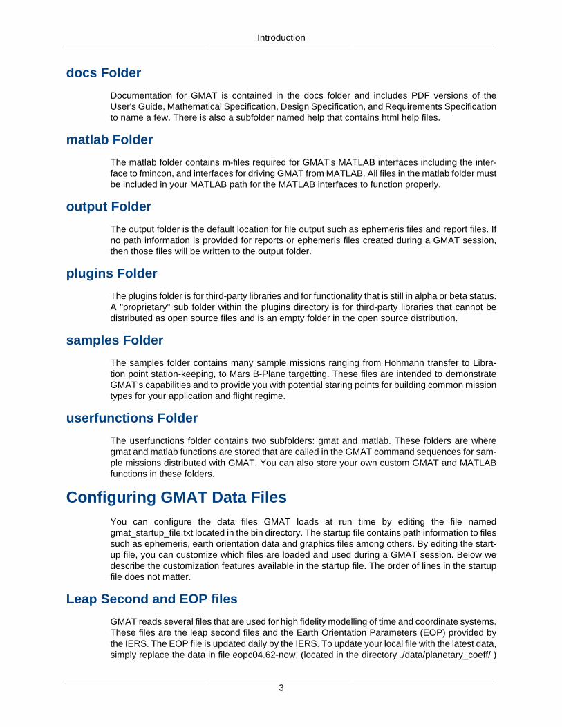
File StructureThe default directory structure for GMAT is shown below and is broken down into eight maindirectories. These directories organize the files and data used to run GMAT including binarylibraries, data files, texture maps, to 3-D models among many others. The only two files in theGMAT root directory are the license.txt file and the README.txt file. A summary of the contentsof each folder is described in further detail in the sections below.
GMAT Directory Structure
Introduction
2
bin Folder
The bin filder contains all binary files required for the core functionality in GMAT (third-party,alpha and beta libraries are placed in the plugins folder). These libraries include the executablefile (GMAT.exe on Windows, GMAT.app on Mac, etc.) and libraries for the GUI. The bin folderalso contains two text files: gmat_startup_file.txt, and gmat.ini. The startup file is discussed indetail in a separate section below. The gmat.ini files is used to configure some GUI panels, setpaths to external web links, and define "tool tip" messages.
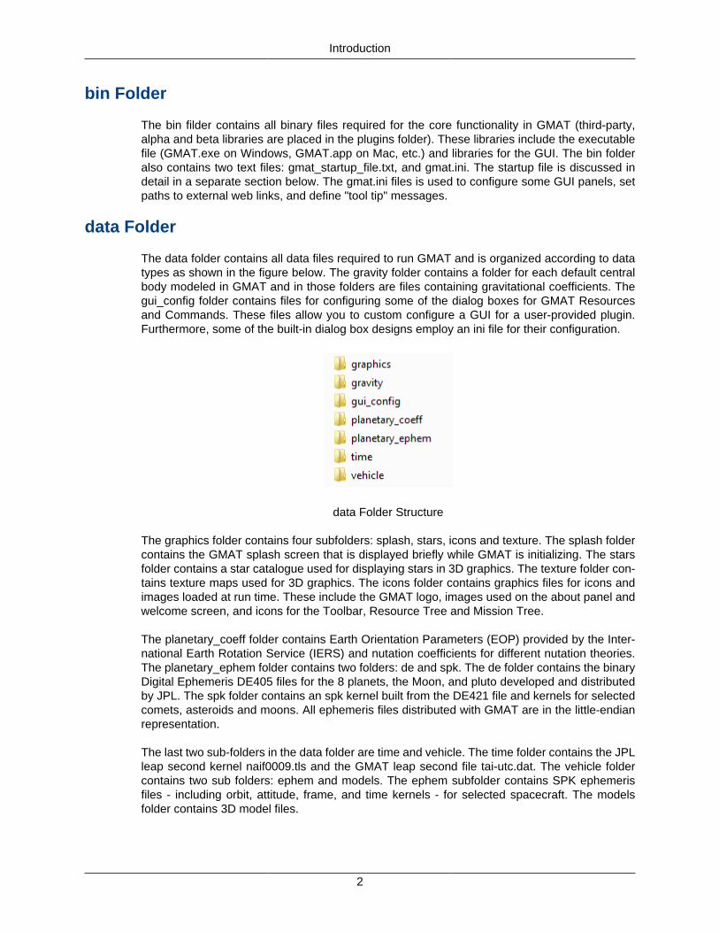
data Folder
The data folder contains all data files required to run GMAT and is organized according to datatypes as shown in the figure below. The gravity folder contains a folder for each default centralbody modeled in GMAT and in those folders are files containing gravitational coefficients. Thegui_config folder contains files for configuring some of the dialog boxes for GMAT Resourcesand Commands. These files allow you to custom configure a GUI for a user-provided plugin.Furthermore, some of the built-in dialog box designs employ an ini file for their configuration.
data Folder Structure
The graphics folder contains four subfolders: splash, stars, icons and texture. The splash foldercontains the GMAT splash screen that is displayed briefly while GMAT is initializing. The starsfolder contains a star catalogue used for displaying stars in 3D graphics. The texture folder con-tains texture maps used for 3D graphics. The icons folder contains graphics files for icons andimages loaded at run time. These include the GMAT logo, images used on the about panel andwelcome screen, and icons for the Toolbar, Resource Tree and Mission Tree.
The planetary_coeff folder contains Earth Orientation Parameters (EOP) provided by the Inter-national Earth Rotation Service (IERS) and nutation coefficients for different nutation theories.The planetary_ephem folder contains two folders: de and spk. The de folder contains the binaryDigital Ephemeris DE405 files for the 8 planets, the Moon, and pluto developed and distributedby JPL. The spk folder contains an spk kernel built from the DE421 file and kernels for selectedcomets, asteroids and moons. All ephemeris files distributed with GMAT are in the little-endianrepresentation.
The last two sub-folders in the data folder are time and vehicle. The time folder contains the JPLleap second kernel naif0009.tls and the GMAT leap second file tai-utc.dat. The vehicle foldercontains two sub folders: ephem and models. The ephem subfolder contains SPK ephemerisfiles - including orbit, attitude, frame, and time kernels - for selected spacecraft. The modelsfolder contains 3D model files.
Introduction
3
docs Folder
Documentation for GMAT is contained in the docs folder and includes PDF versions of theUser's Guide, Mathematical Specification, Design Specification, and Requirements Specificationto name a few. There is also a subfolder named help that contains html help files.
matlab Folder
The matlab folder contains m-files required for GMAT's MATLAB interfaces including the inter-face to fmincon, and interfaces for driving GMAT from MATLAB. All files in the matlab folder mustbe included in your MATLAB path for the MATLAB interfaces to function properly.
output Folder
The output folder is the default location for file output such as ephemeris files and report files. Ifno path information is provided for reports or ephemeris files created during a GMAT session,then those files will be written to the output folder.
plugins Folder
The plugins folder is for third-party libraries and for functionality that is still in alpha or beta status.A "proprietary" sub folder within the plugins directory is for third-party libraries that cannot bedistributed as open source files and is an empty folder in the open source distribution.
samples Folder
The samples folder contains many sample missions ranging from Hohmann transfer to Libra-tion point station-keeping, to Mars B-Plane targetting. These files are intended to demonstrateGMAT's capabilities and to provide you with potential staring points for building common missiontypes for your application and flight regime.
userfunctions Folder
The userfunctions folder contains two subfolders: gmat and matlab. These folders are wheregmat and matlab functions are stored that are called in the GMAT command sequences for sam-ple missions distributed with GMAT. You can also store your own custom GMAT and MATLABfunctions in these folders.
Configuring GMAT Data FilesYou can configure the data files GMAT loads at run time by editing the file namedgmat_startup_file.txt located in the bin directory. The startup file contains path information to filessuch as ephemeris, earth orientation data and graphics files among others. By editing the start-up file, you can customize which files are loaded and used during a GMAT session. Below wedescribe the customization features available in the startup file. The order of lines in the startupfile does not matter.
Leap Second and EOP files
GMAT reads several files that are used for high fidelity modelling of time and coordinate systems.These files are the leap second files and the Earth Orientation Parameters (EOP) provided bythe IERS. The EOP file is updated daily by the IERS. To update your local file with the latest data,simply replace the data in file eopc04.62-now, (located in the directory ./data/planetary_coeff/ )
Introduction
4
with the data provided by the IERS in the link here. There are two leap second files provided withGMAT. The file named naif0009.tls located in the .\data\time folder is used by the JPL SPICElibraries when computing ephemeredes. When a new leap seond is added, you can replace yourold SPICE leap second file with the new file located here here.
GMAT reads the file tai-utc.dat in the .\data\time folder for all time computations requiring leapseconds that are not performed by the SPICE utilities. You can modify this file if a new leapsecond is added by simply duplicating the last row and updating it with the correct informationfor the new leap second. For example, if a new leapsecond were added on 01 Jul 2013, thenyou would add the following line to the tai-utc.dat file:
2013 JUL 1 =JD 2456474.5 TAI-UTC= 35.0 S + (MJD - 41317.) X 0.0
Loading Custom Plugins
Custom plugins are loaded by adding a line to your startup file describing the name and locationof the plugin library. In order for a plugin to work with GMAT, the plugin library must be placedin the folder referenced in the startup file. You specify the path to a plugin using the "PLUGIN"keyword and specify the file by providing its name without the file extension (.dll on Windows). Forexample, to load a Windows plugin named libVF13Optimizer.dll located in the \bin\proprietaryfolder, you add this line to your startup file:
PLUGIN = ./proprietary/libVF13Optimizer
User-defined Function Paths
If you create custom GMAT or MATLAB functions for your application, you can provide the pathto those files and GMAT will locate them at run time. The default startup file is configured soyou can place GMAT files in the ./userfunctions/gmat folder and place MATLAB functions in the /userfunctions/matlab folder GMAT automatically searches those locatations at run time. You canchange the location of the search path to your GMAT or MATLAB functions by changing theselines in your startup file to reflect the location of your files with respect to the GMAT bin folder:
GMAT_FUNCTION_PATH = ../userfunctions/gmat MATLAB_FUNCTION_PATH = ../userfunctions/matlab
If you wish to organize your custom functions in multiple folders, you can add multiple searchpaths to the startup file. For example,
GMAT_FUNCTION_PATH = ../MyFunctions/utils GMAT_FUNCTION_PATH = ../MyFunctions/StateConversion GMAT_FUNCTION_PATH = ../MyFunctions/TimeConversion
Configuring the MATLAB InterfacesGMAT supports several MATLAB interfaces and to use these interfaces the following MATLABfolders must be added to your system path:
MATLAB/bin/win32 MATLAB/bin MATLAB/runtime/win32

Introduction
5
Caution
The above folders are added to your system path during MATLAB installation. How-ever, for some versions of MATLAB (2010a for example), MATLAB and Windowsare distributed with libraries that have the same name. This may cause the Win-dows libraries to load instead of the MATLAB libraries. As a result, you may needto put the folders above at the beginning of your system path.
If you have multilple versions of MATLAB installed, GMAT will use the version that appearsfirst in your system path and that version must be registered as a COM server using the MAT-LAB regserver command. To register the desired version of MATLAB, using a command promptchange directory to the bin folder of the desired MATLAB release and run the following command.
matlab.exe -regserver
Finally you must add to your MATLAB path all files in the matlab directory which is located inthe GMAT root directory.
Support and Resources
6
Release NotesThe General Mission Analysis Tool (GMAT) version R2011a was released April 29, 2011 on thefollowing platforms:
Windows (XP, Vista, 7) Beta
Mac OS X (10.6) Alpha
Linux Alpha
This is the first release since September 2008, and is the 4th public release for the project. Inthis release:
• 100,000 lines of code were added• 798 bugs were opened and 733 were closed• Code was contributed by 9 developers from 4 organizations• 6216 system tests were written and run nightly
New Features
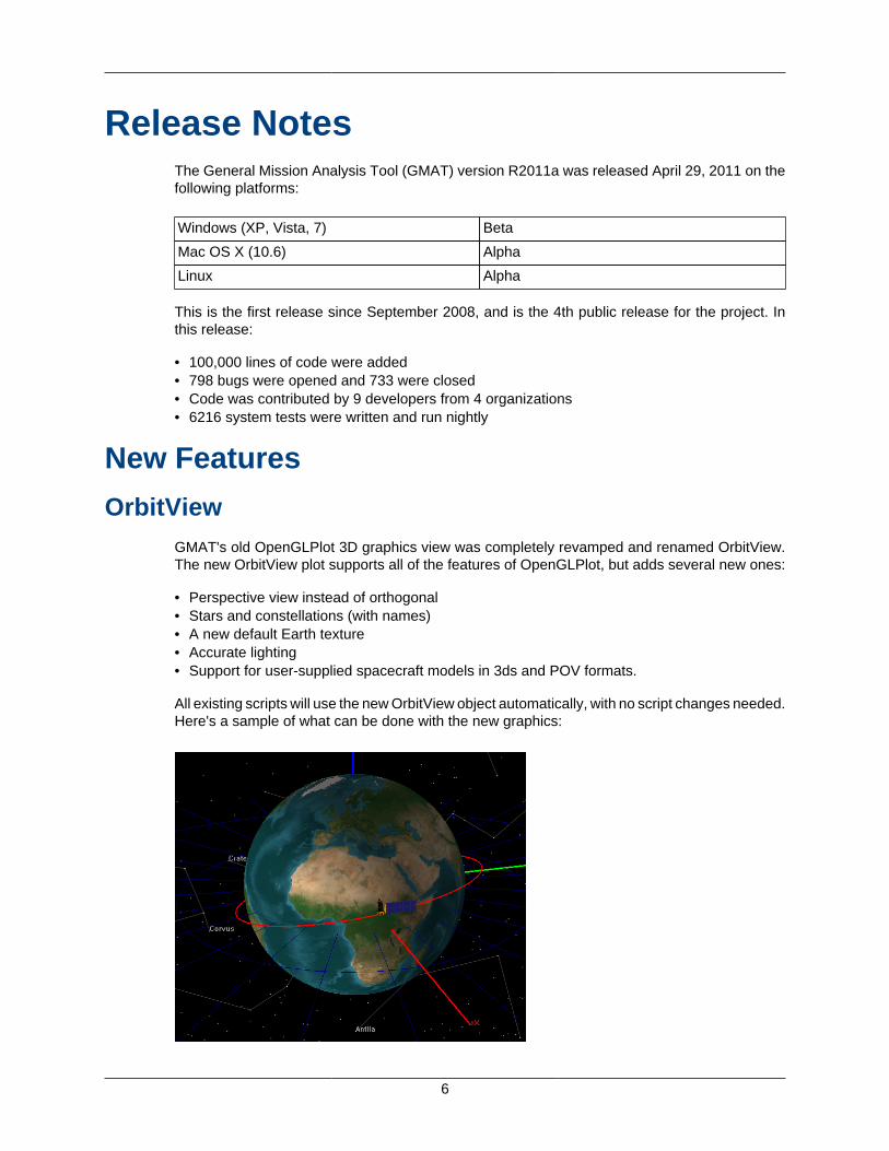
OrbitViewGMAT's old OpenGLPlot 3D graphics view was completely revamped and renamed OrbitView.The new OrbitView plot supports all of the features of OpenGLPlot, but adds several new ones:
• Perspective view instead of orthogonal• Stars and constellations (with names)• A new default Earth texture• Accurate lighting• Support for user-supplied spacecraft models in 3ds and POV formats.
All existing scripts will use the new OrbitView object automatically, with no script changes needed.Here's a sample of what can be done with the new graphics:
Release Notes
7
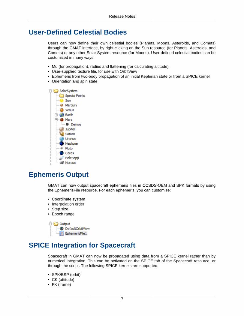
User-Defined Celestial BodiesUsers can now define their own celestial bodies (Planets, Moons, Asteroids, and Comets)through the GMAT interface, by right-clicking on the Sun resource (for Planets, Asteroids, andComets) or any other Solar System resource (for Moons). User-defined celestial bodies can becustomized in many ways:
• Mu (for propagation), radius and flattening (for calculating altitude)• User-supplied texture file, for use with OrbitView• Ephemeris from two-body propagation of an initial Keplerian state or from a SPICE kernel• Orientation and spin state
Ephemeris OutputGMAT can now output spacecraft ephemeris files in CCSDS-OEM and SPK formats by usingthe EphemerisFile resource. For each ephemeris, you can customize:
• Coordinate system• Interpolation order• Step size• Epoch range
SPICE Integration for SpacecraftSpacecraft in GMAT can now be propagated using data from a SPICE kernel rather than bynumerical integration. This can be activated on the SPICE tab of the Spacecraft resource, orthrough the script. The following SPICE kernels are supported:
• SPK/BSP (orbit)• CK (attitude)• FK (frame)
Release Notes
8
• SCLK (spacecraft clock)
PluginsNew features can now be added to GMAT through plugins, rather than being compiled into theGMAT executable itself. The following plugins are included in this release, with their releasestatus indicated:
libMatlabPlugin Beta
libFminconOptimizer (Windows only) Beta
libGmatEstimation Alpha (preview)
Plugins can be enabled or disabled through the startup file (gmat_startup_file.txt), locat-ed in the GMAT bin directory. All plugins are disabled by default.
GUI/Script SynchronizationFor those that work with both the script and the graphical interface, GMAT now makes it explicitlyclear if the two are synchronized, and which script is active (if you have several loaded). Thepossible states are:
• Synchronized (the interface and the script have the same data)• GUI or Script Modified (one of them has been modified with respect to the other)• Unsynchronized (different changes exist in each place)
The only state in which manual intervention is necessary is Unsynchronized, which must bemerged manually (or one set of changes must be discarded). The following status indicatorsare available on Windows and Linux (on Mac, they appear as single characters on the GMATtoolbar).
Estimation [Alpha]GMAT R2011a includes significant new state estimation capabilities in the libGmatEstimationplugin. The included features are:
• Measurement models• Geometric• TDRSS range• USN two-way range
• Estimators• Batch• Extended Kalman
• Resources• GroundStation• Antenna• Transmitter
Release Notes
9
• Receiver• Transponder
Note
This functionality is alpha status, and is included with this release as a previewonly. It has not been rigorously tested.
User DocumentationGMAT’s user documentation has been completely revamped. In place of the old wiki, our formaldocumentation is now implemented in DocBook, with HTML, PDF, and Windows Help formatsshipped with GMAT. Our documentation resources for this release are:
• Help (shipped with GMAT, accessed through the Help > Contents menu item)• Online Help (updated frequently, http://gmat.sourceforge.net/docs/)• Video Tutorials (http://gmat.sourceforge.net/docs/videos.html)• Help Forum (http://gmat.ed-pages.com/forum/)• Wiki (for informal and user-contributed documentation, samples, and tips: http://gmat.ed-
pages.com/wiki/tiki-index.php)
Screenshot ( )GMAT can now export a screenshot of the OrbitView panel to the output folder in PNG format.
Improvements
Automatic MATLAB DetectionMATLAB connectivity is now automatically established through the libMatlabInterface plugin, ifenabled in your gmat_startup_file.txt. We are no longer shipping separate executables with andwithout MATLAB integration. Most recent MATLAB versions are supported, though configurationis necessary.
Dynamics Model NumericsAll included dynamics models have been thoroughly tested against truth software (AGI STK, andA.I. Solutions FreeFlyer, primarily), and all known numeric issues have been corrected.
Release Notes
10
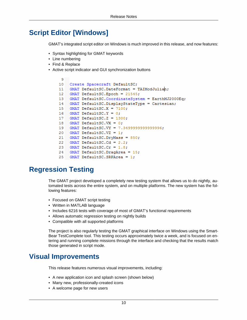
Script Editor [Windows]
GMAT’s integrated script editor on Windows is much improved in this release, and now features:
• Syntax highlighting for GMAT keywords• Line numbering• Find & Replace• Active script indicator and GUI synchronization buttons
Regression Testing
The GMAT project developed a completely new testing system that allows us to do nightly, au-tomated tests across the entire system, and on multiple platforms. The new system has the fol-lowing features:
• Focused on GMAT script testing• Written in MATLAB language• Includes 6216 tests with coverage of most of GMAT’s functional requirements• Allows automatic regression testing on nightly builds• Compatible with all supported platforms
The project is also regularly testing the GMAT graphical interface on Windows using the Smart-Bear TestComplete tool. This testing occurs approximately twice a week, and is focused on en-tering and running complete missions through the interface and checking that the results matchthose generated in script mode.
Visual Improvements
This release features numerous visual improvements, including:
• A new application icon and splash screen (shown below)• Many new, professionally-created icons• A welcome page for new users
Release Notes
11
Compatibility Changes
Platform SupportGMAT supports the following platforms:
• Windows XP• Windows Vista• Windows 7• Mac OS X Snow Leopard (10.6)• Linux (Intel 64-bit)
With the exception of the Linux version, GMAT is a 32-bit application, but will run on 64-bit plat-forms in 32-bit mode. The MATLAB interface was tested with 32-bit MATLAB 2010b on Windows,and is expected to support 32-bit MATLAB versions from R2006b through R2011a.
Mac: MATLAB 2010a was tested, but version coverage is expected to be identical to Windows.
Linux: MATLAB 2009b 64-bit was tested, and 64-bit MATLAB is required. Otherwise, versioncoverage is expected to be identical to Windows.
Script Syntax ChangesThe BeginMissionSequence command will soon be required for all scripts. In this release awarning is generated if this statement is missing.
The following syntax elements are deprecated, and will be removed in a future release:
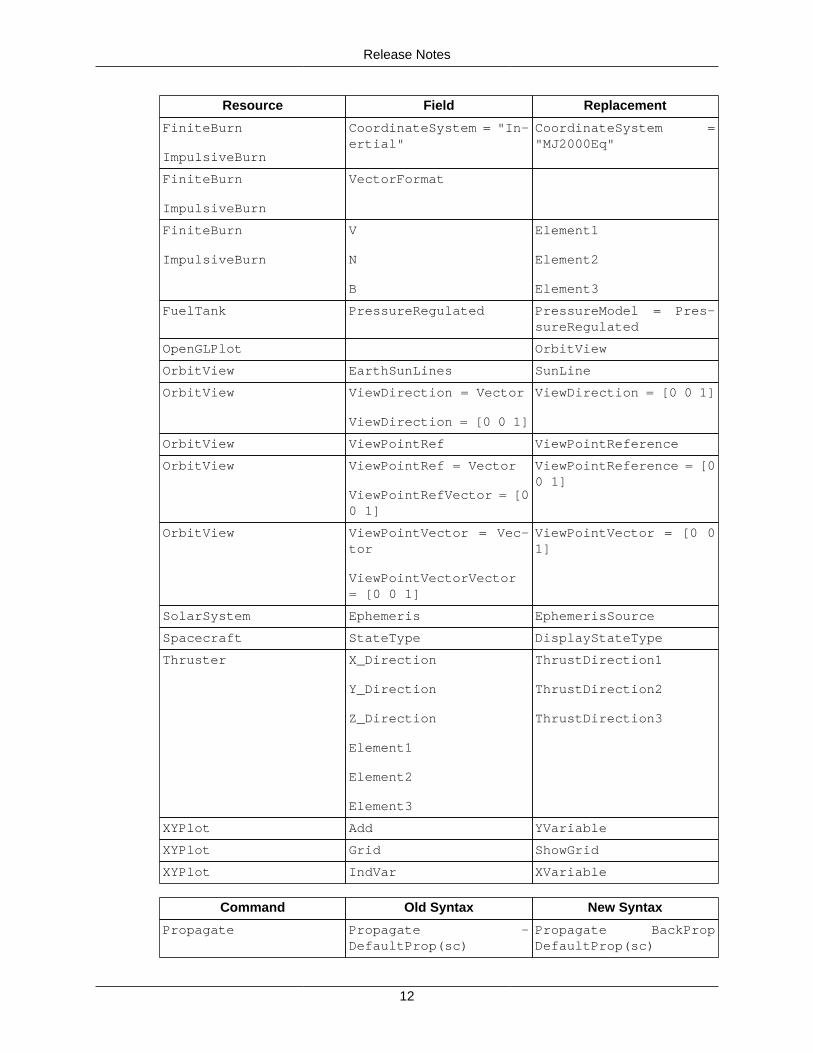
Resource Field Replacement
DifferentialCorrector TargeterTextFile ReportFile
DifferentialCorrector UseCentralDifferences DerivativeMethod ="CentralDifference"
EphemerisFile FileName Filename
FiniteBurn Axes
FiniteBurn BurnScaleFactor
FiniteBurn CoordinateSystem
FiniteBurn Origin
FiniteBurn Tanks
Release Notes
12
Resource Field Replacement
FiniteBurn
ImpulsiveBurn
CoordinateSystem = "In-ertial"
CoordinateSystem ="MJ2000Eq"
FiniteBurn
ImpulsiveBurn
VectorFormat
FiniteBurn
ImpulsiveBurn
V
N
B
Element1
Element2
Element3
FuelTank PressureRegulated PressureModel = Pres-sureRegulated
OpenGLPlot OrbitView
OrbitView EarthSunLines SunLine
OrbitView ViewDirection = Vector
ViewDirection = [0 0 1]
ViewDirection = [0 0 1]
OrbitView ViewPointRef ViewPointReference
OrbitView ViewPointRef = Vector
ViewPointRefVector = [00 1]
ViewPointReference = [00 1]
OrbitView ViewPointVector = Vec-tor
ViewPointVectorVector= [0 0 1]
ViewPointVector = [0 01]
SolarSystem Ephemeris EphemerisSource
Spacecraft StateType DisplayStateType
Thruster X_Direction
Y_Direction
Z_Direction
Element1
Element2
Element3
ThrustDirection1
ThrustDirection2
ThrustDirection3
XYPlot Add YVariable
XYPlot Grid ShowGrid
XYPlot IndVar XVariable
Command Old Syntax New Syntax
Propagate Propagate -DefaultProp(sc)
Propagate BackPropDefaultProp(sc)
Release Notes
13
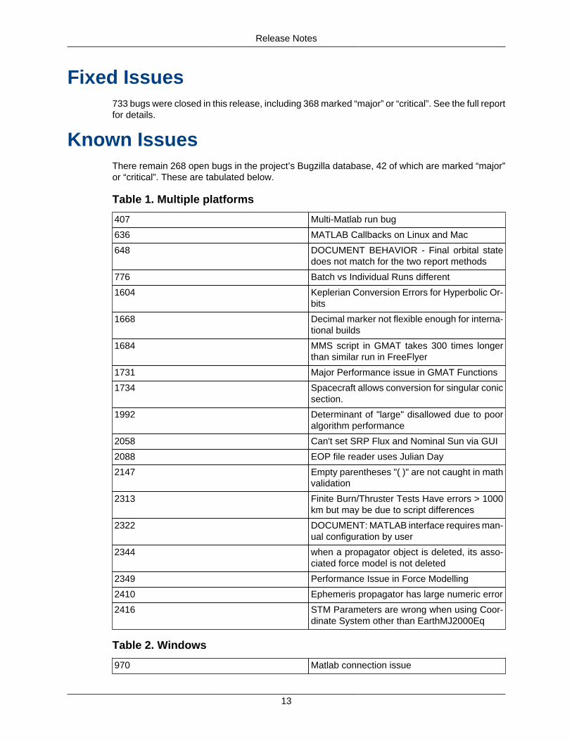
Fixed Issues733 bugs were closed in this release, including 368 marked “major” or “critical”. See the full reportfor details.
Known IssuesThere remain 268 open bugs in the project’s Bugzilla database, 42 of which are marked “major”or “critical”. These are tabulated below.
Table 1. Multiple platforms
407 Multi-Matlab run bug
636 MATLAB Callbacks on Linux and Mac
648 DOCUMENT BEHAVIOR - Final orbital statedoes not match for the two report methods
776 Batch vs Individual Runs different
1604 Keplerian Conversion Errors for Hyperbolic Or-bits
1668 Decimal marker not flexible enough for interna-tional builds
1684 MMS script in GMAT takes 300 times longerthan similar run in FreeFlyer
1731 Major Performance issue in GMAT Functions
1734 Spacecraft allows conversion for singular conicsection.
1992 Determinant of "large" disallowed due to pooralgorithm performance
2058 Can't set SRP Flux and Nominal Sun via GUI
2088 EOP file reader uses Julian Day
2147 Empty parentheses "( )" are not caught in mathvalidation
2313 Finite Burn/Thruster Tests Have errors > 1000km but may be due to script differences
2322 DOCUMENT: MATLAB interface requires man-ual configuration by user
2344 when a propagator object is deleted, its asso-ciated force model is not deleted
2349 Performance Issue in Force Modelling
2410 Ephemeris propagator has large numeric error
2416 STM Parameters are wrong when using Coor-dinate System other than EarthMJ2000Eq
Table 2. Windows
970 Matlab connection issue

Release Notes
14
1012 Quirky Numerical Issues 2 in Batch mode
1128 GMAT incompatible with MATLAB R14 andearlier
1417 Some lines prefixed by "function" are ingored
1436 Potential performance issue using many prop-agate commands
1528 GMAT Function scripts unusable depending onfile ownership/permissions
1580 Spacecraft Attitude Coordinate System Con-version not implemented
1592 Atmosphere Model Setup File Features Not Im-plemented
2056 Reproducibility of script run not guaranteed
2065 Difficult to read low number in Spacecraft Atti-tude GUI
2066 SC Attitude GUI won't accept 0.0:90.0:0.0 as a3-2-1 Euler Angle input
2067 Apply Button Sometimes Not Functional in SCAttitude GUI
2374 Crash when GMAT tries to write to a folder with-out write permissions
2381 TestComplete does not match user inputs toDefaultSC
2382 Point Mass Issue when using Script vs. UserInput
Table 3. Mac OS X
1216 MATLAB->GMAT not working
2081 Texture Maps not showing on Mac for Or-bitView
2092 GMAT crashes when MATLAB engine does notopen
2291 LSK file text ctrl remains visible when sourceset to DE405 or 2Body
2311 Resource Tree - text messed up for objects infolders
2383 Crash running RoutineTests with plots ON
Table 4. Linux
1851 On Linux, STC Editor crashes GMAT on Close
1877 On Linux, Ctrl-C crashes GMAT if no MDIChil-dren are open
15
How To
Reporting mission parameters
Running GMAT Scripts from MATLAB
Overview
GMAT was designed to allow users to run GMAT scripts through MATLAB®. This feature givesthe user greater control and flexibility of GMAT that cannot be done with just the GMAT to MAT-LAB® interface or GMAT alone. For example, if a user would like to dynamically change scriptsand run them, that can currently only be done using the MATLAB® to GMAT interface. A MAT-LAB® script can also be generated to run GMAT scripts that are located in mutliple folders.
If, after running through this tutorial, you still have difficulties with the interfaces between MAT-LAB® and GMAT working, visit our MATLAB Help Forum or our MATLAB<->GMAT InterfaceFAQ forum topic.
Files and Folders to be used
• [rootGMATpath] - folder with the GMAT executable
• Ex_TargetHohmannTransfer.script - Sample Mission script used for running GMAT from Mat-lab
• runMatlabToGMAT.m - MATLAB® script that runs the GMAT script
• runMatlabToGMATsimple.m - simplified MATLAB® script that runs the GMAT script
Procedure
1. Place the downloaded script runMatlabToGMAT.m script into the [rootGMATpath]\matlab\ di-rectory
WARNING! This script clears the MATLAB® workspace. Save your current MATLAB® dataif it's needed
2. Make sure the script Ex_TargetHohmannTransfer.script is in the [rootGMATpath]\input\Sam-pleMissions\ directory
3. Unless it has been done already, open MATLAB® and add [rootGMATpath]\matlab\ directoryand the sub-directories to the MATLAB® path.
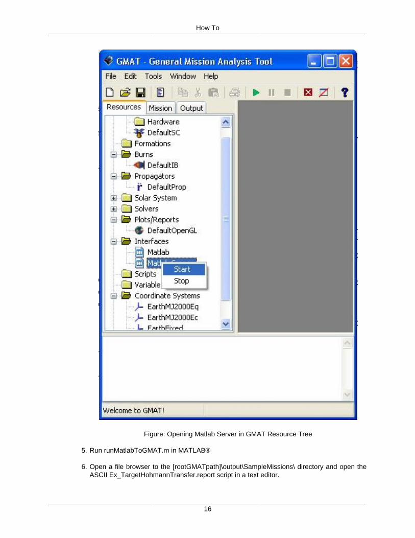
4. Open GMAT and start the Matlab Server.
*The server can be started by navigating in the Resources tree to the Interfaces folder. Rightclick the Matlab Server object and select Start.
How To
16
Figure: Opening Matlab Server in GMAT Resource Tree
5. Run runMatlabToGMAT.m in MATLAB®
6. Open a file browser to the [rootGMATpath]\output\SampleMissions\ directory and open theASCII Ex_TargetHohmannTransfer.report script in a text editor.

How To
17
7. Scroll down to the last few lines, and notice the extra lines indicating that this script was runfrom MATLAB® . If the Ex_TargetHohmannTransfer.script file is run from GMAT, these lineswill not be present.
8. Congratulations - you have finished the main section of this tutorial. Be sure to open therunMatlabToGMAT.m script, to understand how GMAT is controlled by MATLAB® . This MAT-LAB® script is heavily commented to explain what is being done. If you still have questions, feelfree to post them at our GMAT Source Forge forums (http://sourceforge.net/projects/gmat/)
Additional Instructions
The runMatlabToGMAT.m Matlab script might be too complicated for novice MATLAB®users. If so, use a simplified version of the script, runMatlabToGMATsimple.m. For thisscript a .m file is needed, so copy the Ex_TargetHohmannTransfer.script and rename thecopy as Ex_TargetHohmannTransfer.m . Follow the above instructions but first rename therunMatlabToGMAT.m file to runMatlabToGMATsimple.m.
Creating ephemeris files
Creating a Report
Objective and Overview
The objective of this tutorial is to demonstrate how to report parameters out to a file using twodifferent reporting techniques, as well as how to use strings to improve the readability of a reportfile.
Download the script file: ReportFile.script
Prerequisites
• Objects modified (use if you have trouble with this tutorial):
• ReportFile
• Commands modified (use if you have trouble with this tutorial):
• Report Command
• ScriptEvent Command
Mission Description
• Objective: Use the Report Object to output parameters to an ascii file
• Assume: N/A
• Find: N/A

How To
18
Resource, Mission, and Output Trees
Figure: Creating a Report Resource, Mission, and Output Trees
Creating and Configuring the Resource Tree
Objects Required
• Plots/Reports:
• ReportFile - AutoReport, ManualReport, DecoratedReport
• Variables/Arrays/Strings:
• String Variable - StringVar
Creating and Modifying Objects
Add ReportFile Objects
The ReportFile has two features that both allow a user to output data to an ASCII text file. Onefeature of a ReportFile is to output data at every integrator step and the other is to output dataat the user's discretion using Report commands in the Mission Sequence.
How To
19
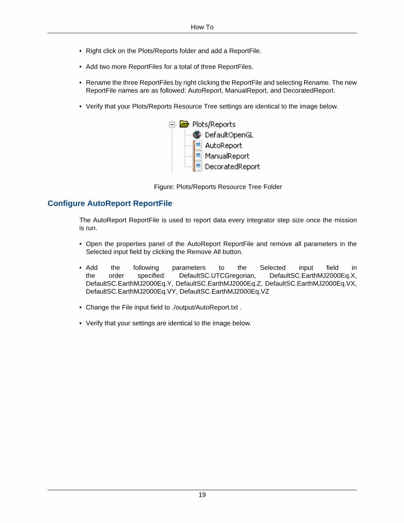
• Right click on the Plots/Reports folder and add a ReportFile.
• Add two more ReportFiles for a total of three ReportFiles.
• Rename the three ReportFiles by right clicking the ReportFile and selecting Rename. The newReportFile names are as followed: AutoReport, ManualReport, and DecoratedReport.
• Verify that your Plots/Reports Resource Tree settings are identical to the image below.
Figure: Plots/Reports Resource Tree Folder
Configure AutoReport ReportFile
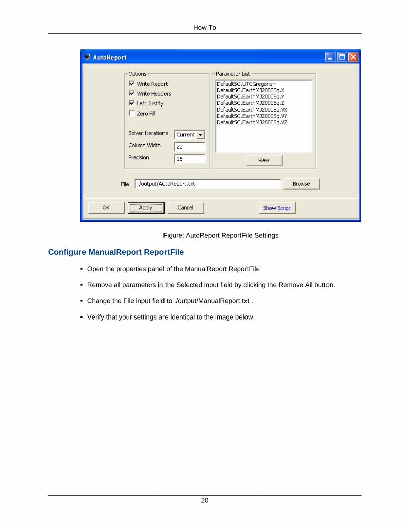
The AutoReport ReportFile is used to report data every integrator step size once the missionis run.
• Open the properties panel of the AutoReport ReportFile and remove all parameters in theSelected input field by clicking the Remove All button.
• Add the following parameters to the Selected input field inthe order specified: DefaultSC.UTCGregorian, DefaultSC.EarthMJ2000Eq.X,DefaultSC.EarthMJ2000Eq.Y, DefaultSC.EarthMJ2000Eq.Z, DefaultSC.EarthMJ2000Eq.VX,DefaultSC.EarthMJ2000Eq.VY, DefaultSC.EarthMJ2000Eq.VZ
• Change the File input field to ./output/AutoReport.txt .
• Verify that your settings are identical to the image below.
How To
20
Figure: AutoReport ReportFile Settings
Configure ManualReport ReportFile
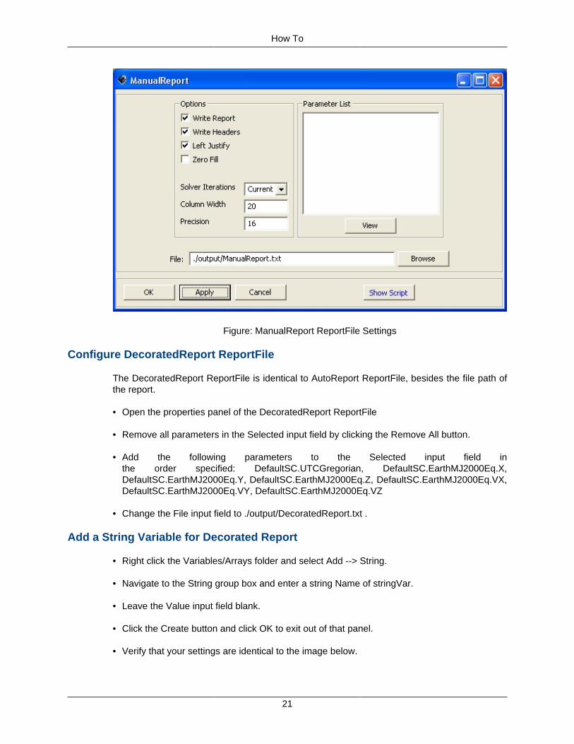
• Open the properties panel of the ManualReport ReportFile
• Remove all parameters in the Selected input field by clicking the Remove All button.
• Change the File input field to ./output/ManualReport.txt .
• Verify that your settings are identical to the image below.
How To
21
Figure: ManualReport ReportFile Settings
Configure DecoratedReport ReportFile
The DecoratedReport ReportFile is identical to AutoReport ReportFile, besides the file path ofthe report.
• Open the properties panel of the DecoratedReport ReportFile
• Remove all parameters in the Selected input field by clicking the Remove All button.
• Add the following parameters to the Selected input field inthe order specified: DefaultSC.UTCGregorian, DefaultSC.EarthMJ2000Eq.X,DefaultSC.EarthMJ2000Eq.Y, DefaultSC.EarthMJ2000Eq.Z, DefaultSC.EarthMJ2000Eq.VX,DefaultSC.EarthMJ2000Eq.VY, DefaultSC.EarthMJ2000Eq.VZ
• Change the File input field to ./output/DecoratedReport.txt .
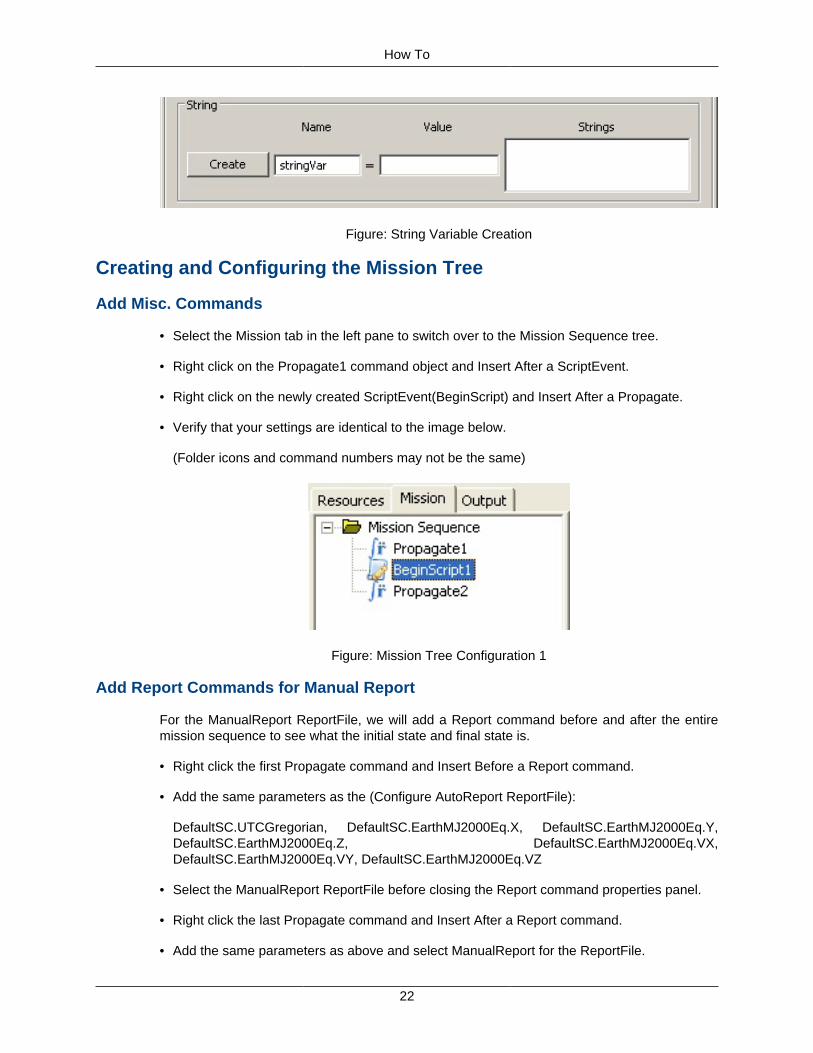
Add a String Variable for Decorated Report
• Right click the Variables/Arrays folder and select Add --> String.
• Navigate to the String group box and enter a string Name of stringVar.
• Leave the Value input field blank.
• Click the Create button and click OK to exit out of that panel.
• Verify that your settings are identical to the image below.
How To
22
Figure: String Variable Creation
Creating and Configuring the Mission Tree
Add Misc. Commands
• Select the Mission tab in the left pane to switch over to the Mission Sequence tree.
• Right click on the Propagate1 command object and Insert After a ScriptEvent.
• Right click on the newly created ScriptEvent(BeginScript) and Insert After a Propagate.
• Verify that your settings are identical to the image below.
(Folder icons and command numbers may not be the same)
Figure: Mission Tree Configuration 1
Add Report Commands for Manual Report
For the ManualReport ReportFile, we will add a Report command before and after the entiremission sequence to see what the initial state and final state is.
• Right click the first Propagate command and Insert Before a Report command.
• Add the same parameters as the (Configure AutoReport ReportFile):
DefaultSC.UTCGregorian, DefaultSC.EarthMJ2000Eq.X, DefaultSC.EarthMJ2000Eq.Y,DefaultSC.EarthMJ2000Eq.Z, DefaultSC.EarthMJ2000Eq.VX,DefaultSC.EarthMJ2000Eq.VY, DefaultSC.EarthMJ2000Eq.VZ
• Select the ManualReport ReportFile before closing the Report command properties panel.
• Right click the last Propagate command and Insert After a Report command.
• Add the same parameters as above and select ManualReport for the ReportFile.
How To
23
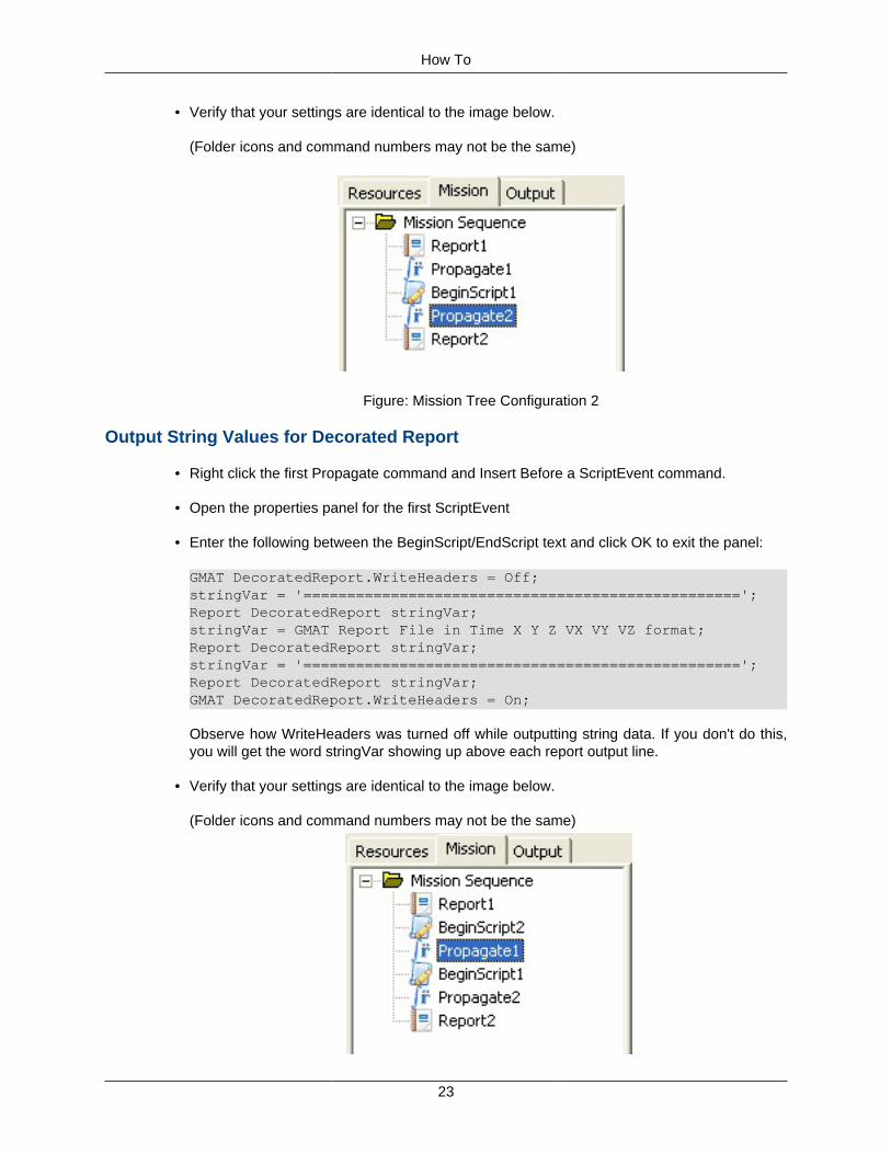
• Verify that your settings are identical to the image below.
(Folder icons and command numbers may not be the same)
Figure: Mission Tree Configuration 2
Output String Values for Decorated Report
• Right click the first Propagate command and Insert Before a ScriptEvent command.
• Open the properties panel for the first ScriptEvent
• Enter the following between the BeginScript/EndScript text and click OK to exit the panel:
GMAT DecoratedReport.WriteHeaders = Off;stringVar = '==================================================';Report DecoratedReport stringVar;stringVar = GMAT Report File in Time X Y Z VX VY VZ format;Report DecoratedReport stringVar;stringVar = '==================================================';Report DecoratedReport stringVar;GMAT DecoratedReport.WriteHeaders = On;
Observe how WriteHeaders was turned off while outputting string data. If you don't do this,you will get the word stringVar showing up above each report output line.
• Verify that your settings are identical to the image below.
(Folder icons and command numbers may not be the same)

How To
24
Figure: Mission Tree Configuration 3
This concludes the configuration of the commands needed for the Mission Sequence.
Running the Mission
Run the mission and navigate to the Output Tab.
AutoReport Output
Open the AutoReport file. The contents are a heading and data associated with the parametersin the heading at each propagator integration step.
The AutoReport output should look like the image below.
Figure: AutoReport Output Results
ManualReport Output
Open the ManualReport file. The contents are a heading followed by the initial spacecraft state,a heading, and the final spacecraft state.
The ManualReport output should look like the image below.
Figure: ManualReport Output Results
DecoratedReport Output
Open the DecoratedReport file. The contents are the custom heading using string variables,followed by the default heading, and data associated with the parameters in the default headingat each propagator integration step.
The DecoratedReport output should look like the image below.

How To
25
Figure: DecoratedReport Output Results
Visualizing a trajectory
26
Samples and TutorialsPropagating a Spacecraft
Objective and OverviewThe objective of this tutorial is to teach you how to create a spacecraft and a propagator, andthen propagate the spacecraft to orbit perigee by following these basic steps:
1. Create a spacecraft and set its epoch and orbital elements.
2. Create and configure a propagator.
3. Modify the default Orbit View to visualize the trajectory.
4. Configure the mission sequence to propagate the spacecraft to periapsis.
Configuring Resources
Creating and Configuring a Spacecraft
In this section, you'll learn how to set a spacecraft's initial epoch and classical orbital elements.You'll need GMAT open with the default mission loaded. The default mission is loaded when anew session of the GMAT executable is started or when the New Mission button in the Toolbaris clicked.
Creating a Spacecraft
Working from the GUI, you can create a new spacecraft by starting at the Resource Tree.
1. Right click on the Spacecraft folder, and select Add Spacecraft
2. Rename the spacecraft by right-clicking on the new spacecraft and selecting Rename fromthe drop down menu. For this tutorial, name the Spacecraft "Sat".
Setting a Spacecraft's Epoch
1. Double left click on the Spacecraft icon for the new spacecraft Sat in the Resource Tree toopen the Spacecraft's dialog box. If it is not already selected, click on the Orbit Tab.
2. Left-click the Epoch Format drop-down menu and select UTCGregorian. You'll see the valuein the Epoch field change to the UTC Gregorian epoch format.
3. Left-click in the Epoch field, and type the desired value of 22 Jul 2014 11:29:10.811 (or youcan cut and paste from the text in this tutorial).
4. Save the changes by left clicking the Apply button at the bottom of the window. In the firstfigure below you see the orbit tab after correctly setting the epoch to the desired value.
Setting a Spacecraft's State
We'll use the Keplerian orbital elements for this tutorial and we'll enter them with respect to Earth'sMJ2000 Equator system.
Samples and Tutorials
27
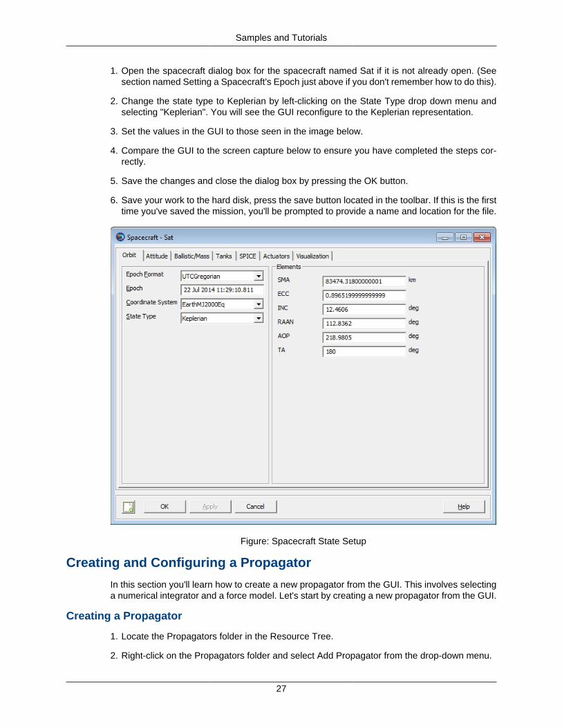
1. Open the spacecraft dialog box for the spacecraft named Sat if it is not already open. (Seesection named Setting a Spacecraft's Epoch just above if you don't remember how to do this).
2. Change the state type to Keplerian by left-clicking on the State Type drop down menu andselecting "Keplerian". You will see the GUI reconfigure to the Keplerian representation.
3. Set the values in the GUI to those seen in the image below.
4. Compare the GUI to the screen capture below to ensure you have completed the steps cor-rectly.
5. Save the changes and close the dialog box by pressing the OK button.
6. Save your work to the hard disk, press the save button located in the toolbar. If this is the firsttime you've saved the mission, you'll be prompted to provide a name and location for the file.
Figure: Spacecraft State Setup
Creating and Configuring a Propagator
In this section you'll learn how to create a new propagator from the GUI. This involves selectinga numerical integrator and a force model. Let's start by creating a new propagator from the GUI.
Creating a Propagator
1. Locate the Propagators folder in the Resource Tree.
2. Right-click on the Propagators folder and select Add Propagator from the drop-down menu.
Samples and Tutorials
28
3. Rename Propagator1 as "LowEarthProp". To do this, right click on the newly created Propa-gator1 and select Rename. In the dialog box that appears, type LowEarthProp and hit OK.
Look at the dialog box for LowEarthProp by double left clicking on its icon under the Propagatorsfolder. On the left side of the propagator dialog box you see where you can select the desirednumerical integrator and configure it for your application. On the right hand side of the panel arecombo boxes and lists that allow the user to set up the force model. Now let's look at how toconfigure a force model.
Configuring a Force Model
For this tutorial we will use an Earth 10x10 non-spherical gravity model, Jacchia-Roberts atmos-pheric model, and point mass perturbations from the Sun and Moon.
1. Open LowEarthProp from the Propagators folder in the Resource tree
2. Locate the Primary Bodies group on the Propagator dialog box. In the Gravity group box,change the degree and order to 10 by left clicking in the text field and typing in the values.
3. Locate the Atmosphere Model pull-down menu in the Drag group.
4. Left click on the pull-down menu and select JacchiaRoberts. (For now we will leave the defaultoptions for Jacchia-Roberts model)
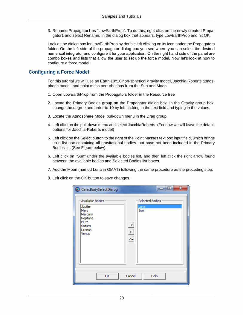
5. Left click on the Select button to the right of the Point Masses text box input field, which bringsup a list box containing all gravitational bodies that have not been included in the PrimaryBodies list (See Figure below).
6. Left click on "Sun" under the available bodies list, and then left click the right arrow foundbetween the available bodies and Selected Bodies list boxes.
7. Add the Moon (named Luna in GMAT) following the same procedure as the preceding step.
8. Left click on the OK button to save changes.

Samples and Tutorials
29
Figure: Force Model Point Mass Configuration
Below is an illustration after correctly configuring the force model according to the instructionsabove.
Figure: Force Model Configuration
Configuring the Default Orbit View Plot
In this section, we'll configure the default Orbit View plot to show the spacecraft we've createdabove. We'll remove DefaultSC from the list of objects to appear in the plot, add Sat, and changethe view point so we can see the entire orbit when we propagate the spacecraft.
1. Locate the Output folder under the Resource Tree and double-left-click on DefaultOrbitViewto open its dialog box.
2. Locate the View Object group, and find the Selected Spacecraft list.
3. Left click on DefaultSC under Selected Spacecraft and then click the left arrow button thatappears to the left of the Selected Spacecraft list. This removes DefaultSC from the plot.
4. Locate the Spacecraft list in the View Object group.
5. Left click on Sat, and then left click on the right-pointing arrow button that appears to the rightof the Spacecraft list.
The orbit for Sat is a highly eccentric orbit, and to view the entire orbit, we need to change thesettings in the View Definition group.
1. Locate the View Point Vector settings in the View Definition group.
2. In the text boxes to the right of the ViewPointVector pull-down menu, enter 30000, -5000, and5000 respectively as shown in illustration below
3. Uncheck the DrawXY Plane box located in the Drawing Options group.
Samples and Tutorials
30
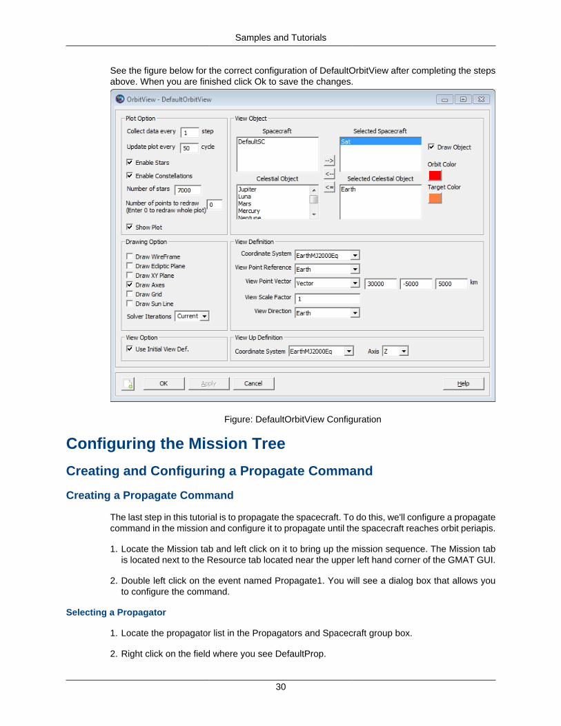
See the figure below for the correct configuration of DefaultOrbitView after completing the stepsabove. When you are finished click Ok to save the changes.
Figure: DefaultOrbitView Configuration
Configuring the Mission Tree
Creating and Configuring a Propagate Command
Creating a Propagate Command
The last step in this tutorial is to propagate the spacecraft. To do this, we'll configure a propagatecommand in the mission and configure it to propagate until the spacecraft reaches orbit periapis.
1. Locate the Mission tab and left click on it to bring up the mission sequence. The Mission tabis located next to the Resource tab located near the upper left hand corner of the GMAT GUI.
2. Double left click on the event named Propagate1. You will see a dialog box that allows youto configure the command.
Selecting a Propagator
1. Locate the propagator list in the Propagators and Spacecraft group box.
2. Right click on the field where you see DefaultProp.
Samples and Tutorials
31
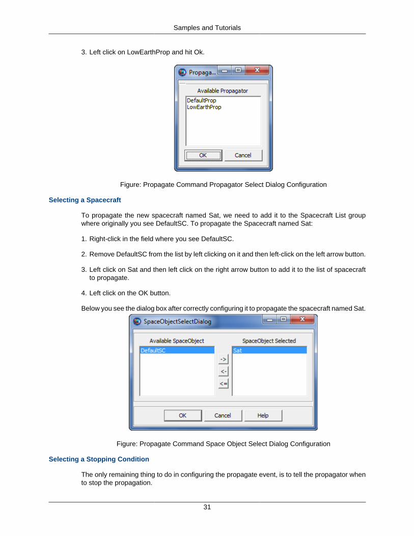
3. Left click on LowEarthProp and hit Ok.
Figure: Propagate Command Propagator Select Dialog Configuration
Selecting a Spacecraft
To propagate the new spacecraft named Sat, we need to add it to the Spacecraft List groupwhere originally you see DefaultSC. To propagate the Spacecraft named Sat:
1. Right-click in the field where you see DefaultSC.
2. Remove DefaultSC from the list by left clicking on it and then left-click on the left arrow button.
3. Left click on Sat and then left click on the right arrow button to add it to the list of spacecraftto propagate.
4. Left click on the OK button.
Below you see the dialog box after correctly configuring it to propagate the spacecraft named Sat.
Figure: Propagate Command Space Object Select Dialog Configuration
Selecting a Stopping Condition
The only remaining thing to do in configuring the propagate event, is to tell the propagator whento stop the propagation.
Samples and Tutorials
32
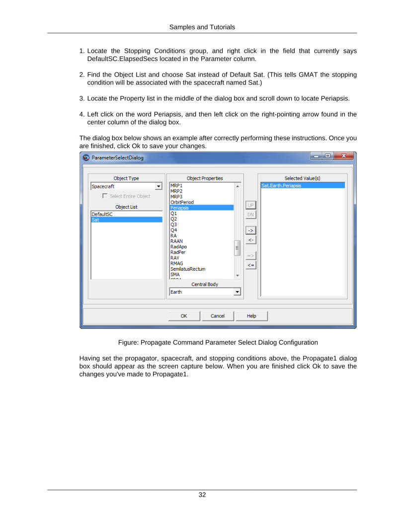
1. Locate the Stopping Conditions group, and right click in the field that currently saysDefaultSC.ElapsedSecs located in the Parameter column.
2. Find the Object List and choose Sat instead of Default Sat. (This tells GMAT the stoppingcondition will be associated with the spacecraft named Sat.)
3. Locate the Property list in the middle of the dialog box and scroll down to locate Periapsis.
4. Left click on the word Periapsis, and then left click on the right-pointing arrow found in thecenter column of the dialog box.
The dialog box below shows an example after correctly performing these instructions. Once youare finished, click Ok to save your changes.
Figure: Propagate Command Parameter Select Dialog Configuration
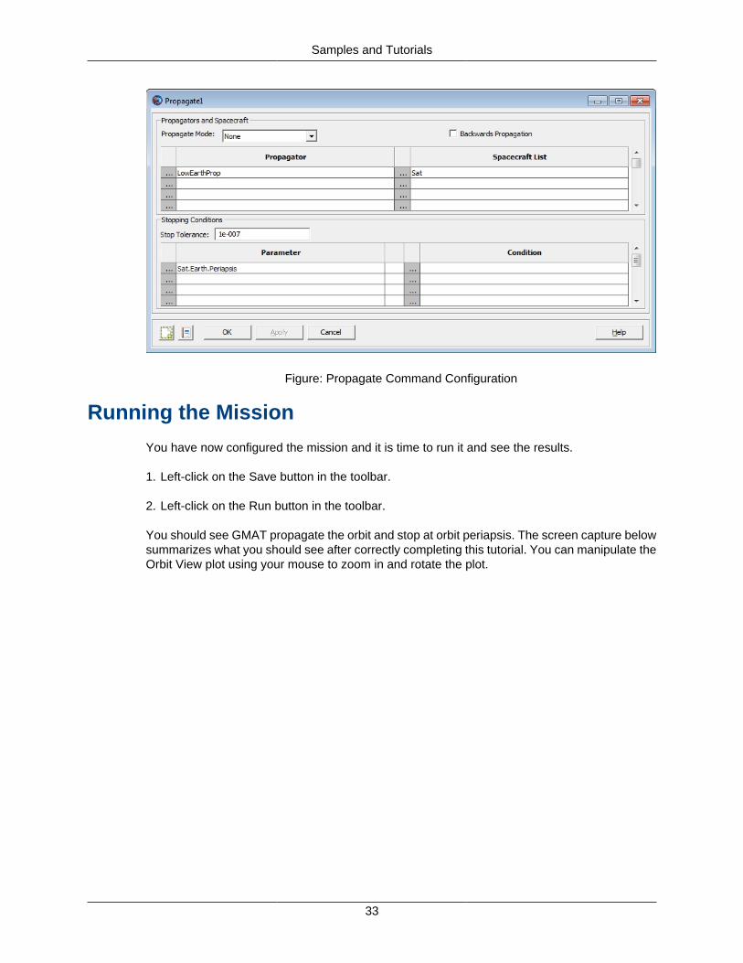
Having set the propagator, spacecraft, and stopping conditions above, the Propagate1 dialogbox should appear as the screen capture below. When you are finished click Ok to save thechanges you've made to Propagate1.
Samples and Tutorials
33
Figure: Propagate Command Configuration
Running the Mission
You have now configured the mission and it is time to run it and see the results.
1. Left-click on the Save button in the toolbar.
2. Left-click on the Run button in the toolbar.
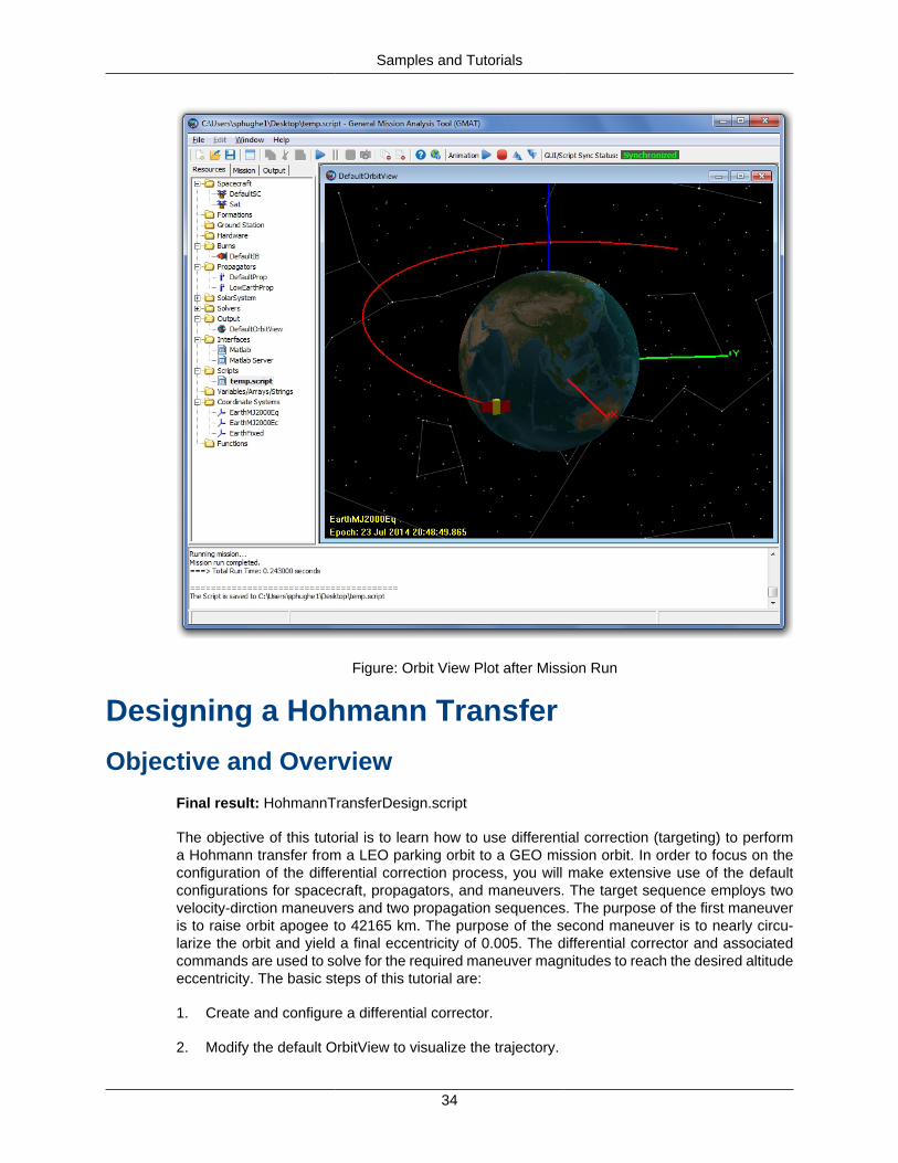
You should see GMAT propagate the orbit and stop at orbit periapsis. The screen capture belowsummarizes what you should see after correctly completing this tutorial. You can manipulate theOrbit View plot using your mouse to zoom in and rotate the plot.
Samples and Tutorials
34
Figure: Orbit View Plot after Mission Run
Designing a Hohmann Transfer
Objective and Overview
Final result: HohmannTransferDesign.script
The objective of this tutorial is to learn how to use differential correction (targeting) to performa Hohmann transfer from a LEO parking orbit to a GEO mission orbit. In order to focus on theconfiguration of the differential correction process, you will make extensive use of the defaultconfigurations for spacecraft, propagators, and maneuvers. The target sequence employs twovelocity-dirction maneuvers and two propagation sequences. The purpose of the first maneuveris to raise orbit apogee to 42165 km. The purpose of the second maneuver is to nearly circu-larize the orbit and yield a final eccentricity of 0.005. The differential corrector and associatedcommands are used to solve for the required maneuver magnitudes to reach the desired altitudeeccentricity. The basic steps of this tutorial are:
1. Create and configure a differential corrector.
2. Modify the default OrbitView to visualize the trajectory.
Samples and Tutorials
35
3. Create two default impulsive maneuvers.
4. Add a target sequence to the mission to raise apogee to GEO altitude and circularize theorbit.
5. Run the mission, save the solution, and rerun the mission using the converged solution.
Creating and Configuring the Resource Tree
Begin by loading the default mission ( click the new mission button in the toolbar) or starting a newGMAT session. For this tutorial, we will use the default configurations for a spaceraft (DefaultSC),a propagator (DefaultProp), and maneuvers. DefaultSC is configured to a near circular orbit andDefaultProp is configured to use Earth as the central body with a gravity model of degree andorder 4. The default impulsive burn model uses the Velocity Normal Binormal (VNB) coordinatesystem. You may want to open the dialog boxes for these objects and inspect them more closelyas we will leave the settings of those objects at their default values.
Creating the Differential Corrector
To create a differential corrector:
1. Locate the Solvers folder in the Resource Tree and expand it if it is minimized.
2. Right-click the Boundary Value Solvers folder, select Add, and then select DifferentialCor-rector.
Modifying the default Orbit View
You need to make minor modifications to default Orbit View so that the entire final orbit will fitin the graphics window.
1. Locate DefaultOrbitView in the Resource Tree, right-click on it, and select Open.
2. Change the SolverIterations input field, located in the Drawing Option group box, to thevalue Current.
3. Change ViewPointVector to 0, 0, 90000 respectively.
4. Change the ViewUpDefinition Axis to X.
5. Verify the configuration against the screen capture below, make any changes necessary,and click Ok on the DefaultOrbitView dialog box.

Samples and Tutorials
36
Modifications to the Default OrbitView
Creating the Maneuvers.
You need two default maneuvers for this tutorial and we will rename the default maneuver andcreate a new maneuver:
1. Locate DefaultIB in the Resource Tree, right-click on it, select Rename, and change thename to dv1.
2. Right-click on the Burns folder, select Add-->ImpulsiveBurn.
3. Right-click on the impulsive burn created in the previous step, select Rename, and changethe name to dv2.
Creating and Configuring the Mission Tree
Below you will create a targeting sequence to raise orbit apogee to GEOsynchronous altitude(~42165km) and then circularize the orbit. You'll begin by modifying the intial propagate com-mand to propagate to periapsis. Next you will create the command structure and finally you willconfigure each command.

Samples and Tutorials
37
Initial Propagate Sequence
To configure the initial propagate sequence to propagate to periapsis, perform the followingsteps:
1. Left-click on the Mission tab to bring up the Mission Tree.
2. Right-click on Propagate1 and select Open from the menu.
3. Locate the Stopping Conditions group box and then right click on the set of ellipses next tothe text "DefaultSC.ElapsedSecs". This will open the Parameter Select Dialog box.
4. Under the Object Properties list on the Parameter Select Dialog box, locate periapsis anddouble-click on it. Click the Ok button to close the Parameter Select Dialog box.
5. Click the Ok button on the Propagate 1 dialog box to save changes and close.
Figure: Propagate1 Command
Creating the Command Sequence
To determine the delta Vs required to raise the orbit apogee to GEO altitude and then circularizethe orbit, you will employ a Targeting loop. Let's begin by creating the commands necessary toperform the targeting sequence. The figure below illustrates the configuration of the mission treeafter you have completed the steps in this section.

Samples and Tutorials
38
Figure: The Mission Tree for a Hohmann Transfer
1. Right-click on Propagate1 in the Mission Tree, select Insert After, and select Target.
2. Right-click on Target1 in the Mission Tree, select Insert After, and select Vary.
3. Right-click on Vary1 in the Mission Tree, select Insert After, and select Manuever.
4. Right-click on Maneuver1 in the Mission Tree, select Insert After, and select Propagate.
5. Right-click on Propagate2 in the Mission Tree, select Insert After, and select Achieve.
6. Right-click on Achieve1 in the Mission Tree, select Insert After, and select Vary.
7. Right-click on Vary2 in the Mission Tree, select Insert After, and select Manuever.
8. Right-click on Maneuver2 in the Mission Tree, select Insert After, and select Propagate.
9. Right-click on Propagate3 in the Mission Tree, select Insert After, and select Achieve.
Let's talk about the function of the command sequence you created above. The Vary commandsdefine the variables the differential corrector can modify to achieve the goals defined in theAchieve commands. Because there are two variables (Vary commands) and two Achieve com-mands (constraints), this is a "square" targeting problem. Below you will configure the Vary com-mands to modify the maneuver values to achieve a final orbit radius of 42165 and an eccentricityof 0.005
Configuring the Command Sequence
Now you will configure the commands you created above to solve for the delta-Vs required toperform a Hohmann transfer.
1. Right-click on Target1 in the Mission Tree and select Open. Locate the ExitMode drop-downmenu and set it to SaveAndContinue. This will save the converged solution of the targetingproblem.
2. When you are finished, click OK to close the Target1 dialog box.

Samples and Tutorials
39
Figure: Target1 Command
3. Right-click on Vary1 in the Mission Tree and select Open. Notice that in the Variable SetUpgroup box, the variable is defined as dv1.Element1. This is the velocity component of dv1in the local VNB system. So we do not need to change the targeter variable.
4. Locate the InitialValue text box and set it to 1.0.
5. Set the MaxStep to 0.5 and then click Ok to close the Vary1 dialog box.
Figure: Vary1 Command
6. Double-click on the Maneuver1 command in the Mission Tree. Notice that the command isset to apply dv1 to DefaultSC so we do not need to change any settings for this command.Click Ok to close the Maneuver1 dialog box.

Samples and Tutorials
40
Figure: Maneuver1 Command
7. Double-click on the Propagate2 dialog box. Use the same procedure shown in the sectionsabove to set the stopping condtion to Apoapsis and then click Ok to close the dialog box.
Figure: Propagate2 Command
8. Double-click on the Achieve1 command in the Mission Tree. Notice that the goal is set toDefaultSC.Earth.RMAG. So we do not need to change any settings for this command. ClickOk to close the dialog box.
Samples and Tutorials
41
Figure: Achieve1 Command
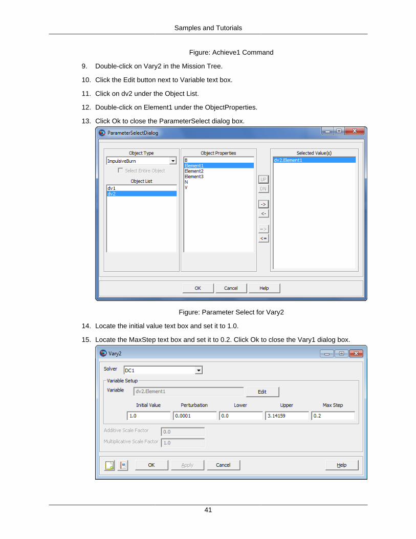
9. Double-click on Vary2 in the Mission Tree.
10. Click the Edit button next to Variable text box.
11. Click on dv2 under the Object List.
12. Double-click on Element1 under the ObjectProperties.
13. Click Ok to close the ParameterSelect dialog box.
Figure: Parameter Select for Vary2
14. Locate the initial value text box and set it to 1.0.
15. Locate the MaxStep text box and set it to 0.2. Click Ok to close the Vary1 dialog box.

Samples and Tutorials
42
Figure: Vary2 Command
16. Double-click on the Maneuver2 command in the Mission Tree.
17. Locate the Burn combo box and change it to dv2. Click OK to close the Maneuver2 dialogbox.
Figure: Maneuver2 Command
18. Double-click on the Propagate3 dialog box. Use the same procedure shown above to setthe stopping condtion to ElapsedDays of 1.0. box.
Figure: Propagate3 Command
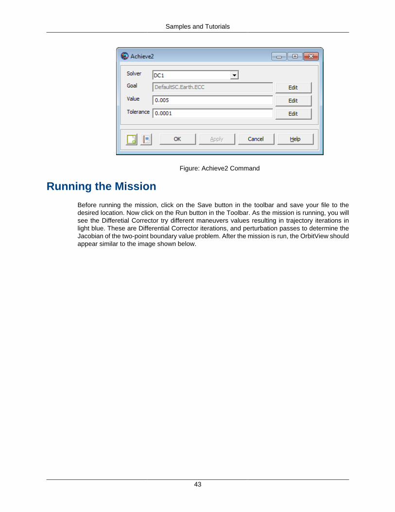
19. Finally, double-click on the Achieve2 command in the Mission Tree.
20. Click on the Edit button next to the Goal text box.
21. Locate ECC in the Object Properties list and double-click on it. Click Ok to close theParameter Select Dialog Box.
22. Change the Value to 0.005.
23. Change the Tolerance to 0.0001
Samples and Tutorials
43
Figure: Achieve2 Command
Running the Mission
Before running the mission, click on the Save button in the toolbar and save your file to thedesired location. Now click on the Run button in the Toolbar. As the mission is running, you willsee the Differetial Corrector try different maneuvers values resulting in trajectory iterations inlight blue. These are Differential Corrector iterations, and perturbation passes to determine theJacobian of the two-point boundary value problem. After the mission is run, the OrbitView shouldappear similar to the image shown below.

Samples and Tutorials
44
Figure: Output After Final Propagate Sequence
You can save the resulting solution so that if you make small changes to the problem and retarget,the initial guess for subsequent runs will use the solution from your work above. .
1. Double-click on Target1 in the Mission Tree.
2. Left-click on Apply Corrections.
3. Rerun the mission by clicking the Run button in the toolbar. If you inspect the results inthe message window you should see that the targetting only took one iteration because itstarted from the solution!
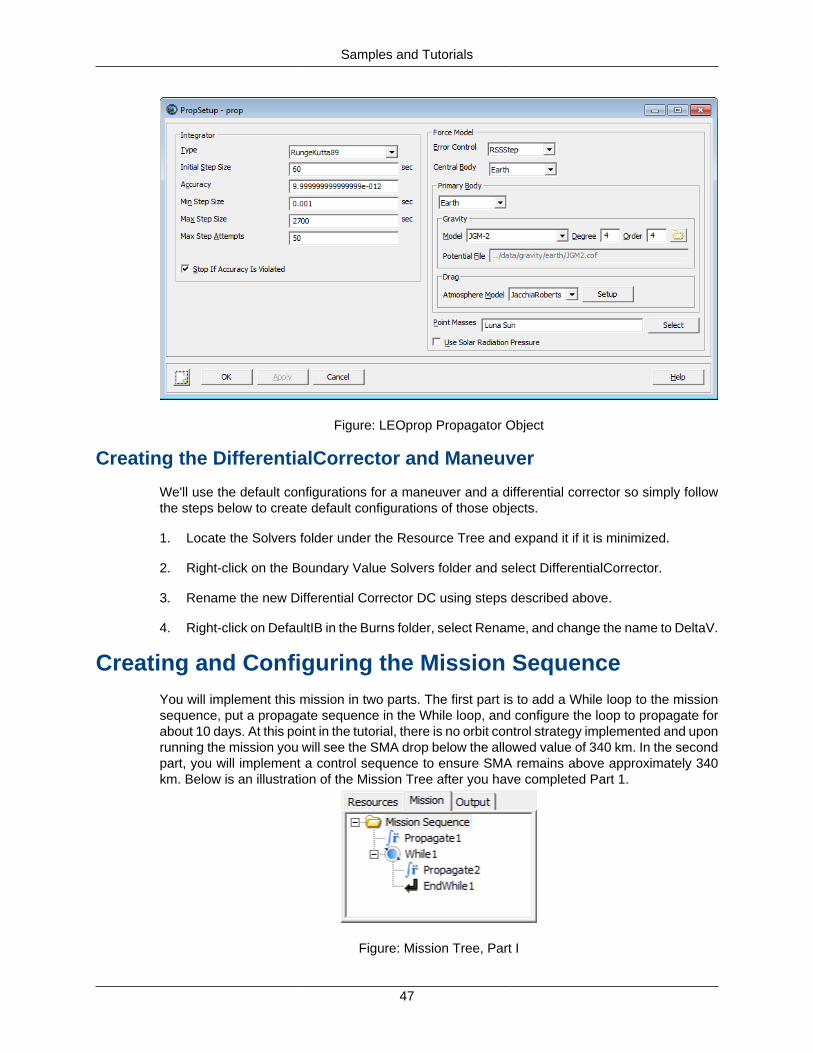
LEO Station Keeping
Objective and OverviewFinal result: HohmannTransferDesign.script
In this tutorial, you will learn how to use control flow and targeting in GMAT to maintain a Low-Earth orbit in the presense of drag. The area-to-mass ratio of the spacecraft is large to cause arapid lowering of the orbit semimajor axis for the sake of simulation time. However, the process
Samples and Tutorials
45
used in this script is useful for generating delta-V estimates for LEO stationkeeping of real-worldmissions. The basic steps of this tutorial are:
1. Create and configure a spacecraft, impulsive maneuver, propagator, XYPlot, and differentialcorrector.
2. Create a conditional loop using a while statement that propagates for 10 days.
3. Run the mission and observe the behavior if there is no orbit control strategy.
4. Create a target sequence nested in an if statement that executes if altitude is below 342 km.
5. Run the mission and observe the behavior of orbit altitude with the control strategy imple-mented in step 4.
Creating and Configuring the Resource Tree
In this section, you will configure a model of a LEO spacecraft, a propopagator , a maneuver,and an XY plot to visualize the SMA during the control sequence developed in the next section.
Creating the Spacecraft
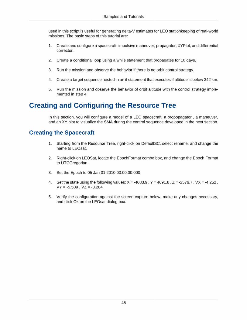
1. Starting from the Resource Tree, right-click on DefaultSC, select rename, and change thename to LEOsat.
2. Right-click on LEOSat, locate the EpochFormat combo box, and change the Epoch Formatto UTCGregorian.
3. Set the Epoch to 05 Jan 01 2010 00:00:00.000
4. Set the state using the following values: X = -4083.9 , Y = 4691.8 , Z = -2576.7 , VX = -4.252 ,VY = -5.509 , VZ = -3.284
5. Verify the configuration against the screen capture below, make any changes necessary,and click Ok on the LEOsat dialog box.
Samples and Tutorials
46
Figure: LEOsat Spacecraft Object
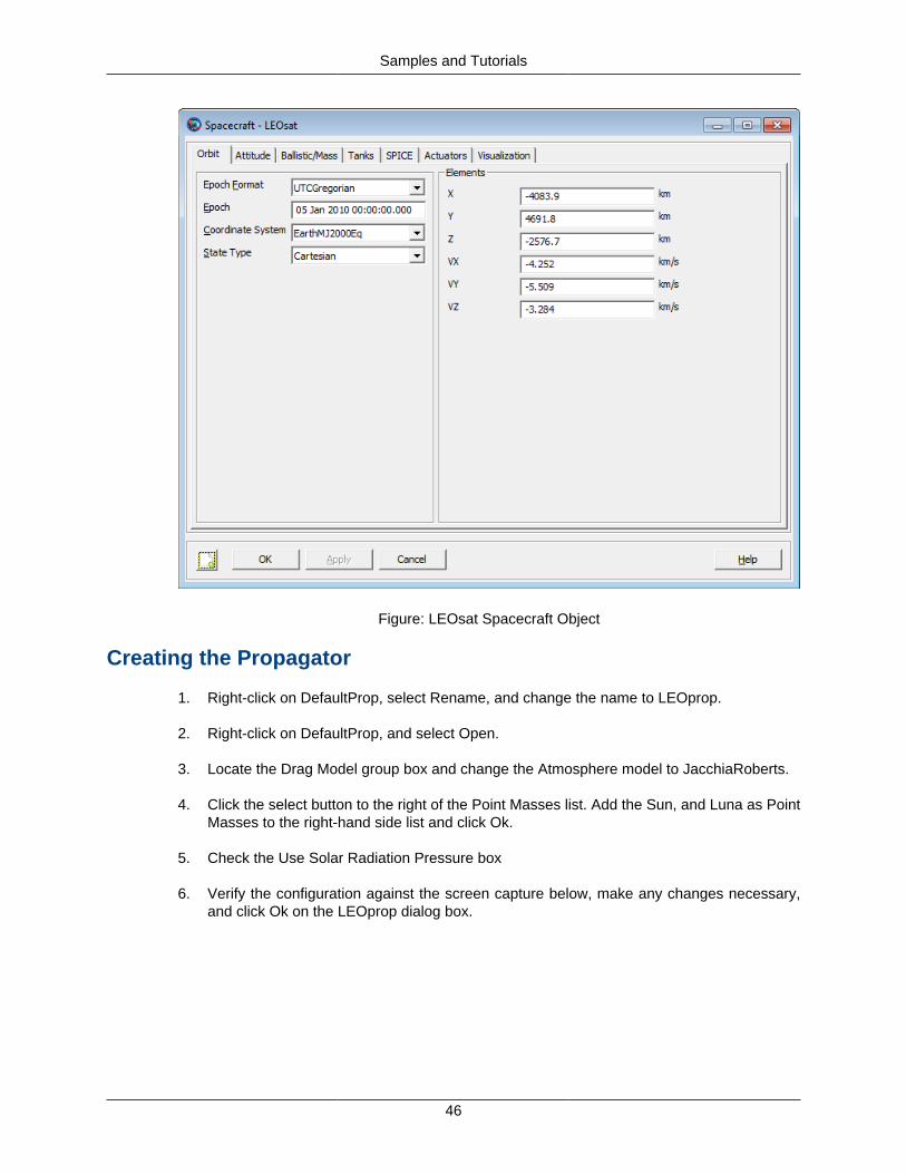
Creating the Propagator
1. Right-click on DefaultProp, select Rename, and change the name to LEOprop.
2. Right-click on DefaultProp, and select Open.
3. Locate the Drag Model group box and change the Atmosphere model to JacchiaRoberts.
4. Click the select button to the right of the Point Masses list. Add the Sun, and Luna as PointMasses to the right-hand side list and click Ok.
5. Check the Use Solar Radiation Pressure box
6. Verify the configuration against the screen capture below, make any changes necessary,and click Ok on the LEOprop dialog box.
Samples and Tutorials
47
Figure: LEOprop Propagator Object
Creating the DifferentialCorrector and Maneuver
We'll use the default configurations for a maneuver and a differential corrector so simply followthe steps below to create default configurations of those objects.
1. Locate the Solvers folder under the Resource Tree and expand it if it is minimized.
2. Right-click on the Boundary Value Solvers folder and select DifferentialCorrector.
3. Rename the new Differential Corrector DC using steps described above.
4. Right-click on DefaultIB in the Burns folder, select Rename, and change the name to DeltaV.
Creating and Configuring the Mission SequenceYou will implement this mission in two parts. The first part is to add a While loop to the missionsequence, put a propagate sequence in the While loop, and configure the loop to propagate forabout 10 days. At this point in the tutorial, there is no orbit control strategy implemented and uponrunning the mission you will see the SMA drop below the allowed value of 340 km. In the secondpart, you will implement a control sequence to ensure SMA remains above approximately 340km. Below is an illustration of the Mission Tree after you have completed Part 1.
Figure: Mission Tree, Part I
Samples and Tutorials
48
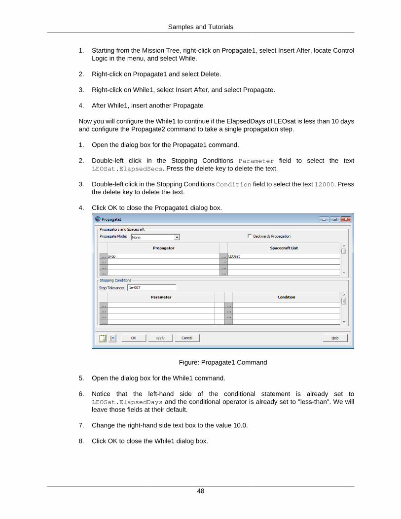
1. Starting from the Mission Tree, right-click on Propagate1, select Insert After, locate ControlLogic in the menu, and select While.
2. Right-click on Propagate1 and select Delete.
3. Right-click on While1, select Insert After, and select Propagate.
4. After While1, insert another Propagate
Now you will configure the While1 to continue if the ElapsedDays of LEOsat is less than 10 daysand configure the Propagate2 command to take a single propagation step.
1. Open the dialog box for the Propagate1 command.
2. Double-left click in the Stopping Conditions Parameter field to select the textLEOSat.ElapsedSecs. Press the delete key to delete the text.
3. Double-left click in the Stopping Conditions Condition field to select the text 12000. Pressthe delete key to delete the text.
4. Click OK to close the Propagate1 dialog box.
Figure: Propagate1 Command
5. Open the dialog box for the While1 command.
6. Notice that the left-hand side of the conditional statement is already set toLEOSat.ElapsedDays and the conditional operator is already set to "less-than". We willleave those fields at their default.
7. Change the right-hand side text box to the value 10.0.
8. Click OK to close the While1 dialog box.

Samples and Tutorials
49
Figure: While1 Command
Now let's run the mission and observe the resulting altitude evolution by clicking Run in theToolbar. You should see a plot that looks similar to the illustration below. Notice that the alttitudedrops below the allowed value of 342 km. In the next part of this tutorial, you will implement acontrol strategy to prohibit altitude from breaking the constraint.
Samples and Tutorials
50
Figure: Output After Part 1
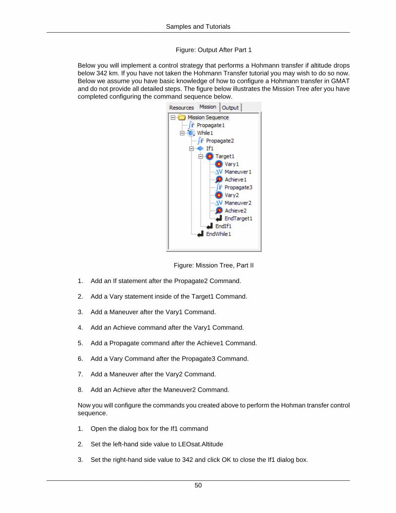
Below you will implement a control strategy that performs a Hohmann transfer if altitude dropsbelow 342 km. If you have not taken the Hohmann Transfer tutorial you may wish to do so now.Below we assume you have basic knowledge of how to configure a Hohmann transfer in GMATand do not provide all detailed steps. The figure below illustrates the Mission Tree afer you havecompleted configuring the command sequence below.
Figure: Mission Tree, Part II
1. Add an If statement after the Propagate2 Command.
2. Add a Vary statement inside of the Target1 Command.
3. Add a Maneuver after the Vary1 Command.
4. Add an Achieve command after the Vary1 Command.
5. Add a Propagate command after the Achieve1 Command.
6. Add a Vary Command after the Propagate3 Command.
7. Add a Maneuver after the Vary2 Command.
8. Add an Achieve after the Maneuver2 Command.
Now you will configure the commands you created above to perform the Hohman transfer controlsequence.
1. Open the dialog box for the If1 command
2. Set the left-hand side value to LEOsat.Altitude
3. Set the right-hand side value to 342 and click OK to close the If1 dialog box.
Samples and Tutorials
51
Figure: If1 Command
4. Open the dialog box for the Vary1 Command.
5. Change the IntialValue field to 0.002 and click OK to close.
Figure: Vary1 Command
6. Open the dialog box for the Achieve1 Command.
7. Change the left hand side value to LEOsat.Earth.SMA.
8. Change the right hand side to 6734 and then click OK to close.

Samples and Tutorials
52
Figure: Achieve1 Command
Running the Mission
The views that you created are good for seeing how well the mission sequence is keeping LEOsatin its orbit. The SMA view shows some thickness to it while the RAAN view shows barely any atall. You may now try and change the mission parameters as outlined in the mission tree sectionto see how the spacecraft's drift is affected.
Figure: Output
Samples and Tutorials
53
Algebraic Optimization
Objective and OverviewThis tutorial finds the minimum value to satisfy a function. This tutorial is intended to show howGMAT's optimizer works. Uses of optimization in a true mission include minimizing the amountof fuel or minimum flight time required to achieve certain characteristics. Learning how to opti-mize a mission sequence also involves learning about optimizers, nonlinear constraints, and theminimize command.
You can download the script file and run it beforehand to see the final results of this tutorial:Ex_AlgebraicOptimization.script
Prerequisites
• Basic Understanding of how to create and propagate a spacecraft, as in Tutorial Creating andPropagating a Spacecraft
Mission Description
• Objective: The goal here is to find values of variables X1 and X2 that minimize a criterionfunction F, with a constraint that X1+X2=8, as follows:
F = ( X1 - 2 )2 + ( X2 - 2 )2
G = X1 + X2
G = 8
• Find: Values X1 and X2
Creating and Configuring the Resource Tree
Objects Required
• Optimizer: SQPfmincon
• Plots/Reports: Report Data
• Variables: X1, X2, F, G
Creating and Modifying Objects
• Variables/Strings/Arrays
• Variable X1 = 0
• Variable X2 = 0
• Variable F = 0
• Variable G = 0

Samples and Tutorials
54
• Solvers
• SQPfmincon Optimizer (Figure below shows the resulting SQPfmincon window)
• Tol Fun = .0001
• Tol Con = .0001
• Tol X = .01
• Max Fun Evals = 1000
• Max Iter = 250
• Diff Min Change = .000001
• Diff Max Change = .01
• Display : Iter
• Diagnostics
Figure: SQPfmincon Boundary Value Solver Object
• Plots/Reports
• Data ReportFile
• Clear Parameter List
• Saved at ./output/SampleMissions/Ex_AlgebraicOptimization.report
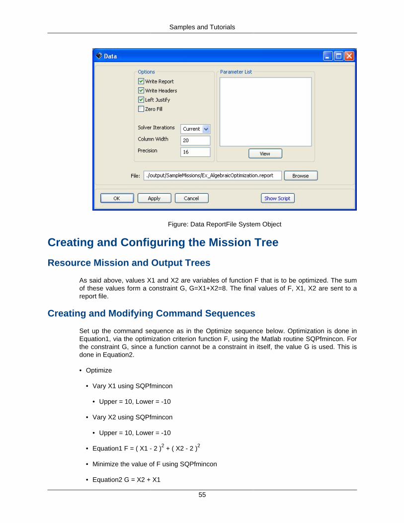
Samples and Tutorials
55
Figure: Data ReportFile System Object
Creating and Configuring the Mission Tree
Resource Mission and Output Trees
As said above, values X1 and X2 are variables of function F that is to be optimized. The sumof these values form a constraint G, G=X1+X2=8. The final values of F, X1, X2 are sent to areport file.
Creating and Modifying Command Sequences
Set up the command sequence as in the Optimize sequence below. Optimization is done inEquation1, via the optimization criterion function F, using the Matlab routine SQPfmincon. Forthe constraint G, since a function cannot be a constraint in itself, the value G is used. This isdone in Equation2.
• Optimize
• Vary X1 using SQPfmincon
• Upper = 10, Lower = -10
• Vary X2 using SQPfmincon
• Upper = 10, Lower = -10
• Equation1 F = ( X1 - 2 )2 + ( X2 - 2 )2
• Minimize the value of F using SQPfmincon
• Equation2 G = X2 + X1
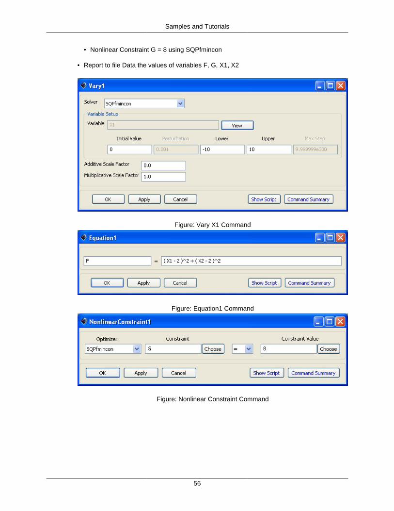
Samples and Tutorials
56
• Nonlinear Constraint G = 8 using SQPfmincon
• Report to file Data the values of variables F, G, X1, X2
Figure: Vary X1 Command
Figure: Equation1 Command
Figure: Nonlinear Constraint Command
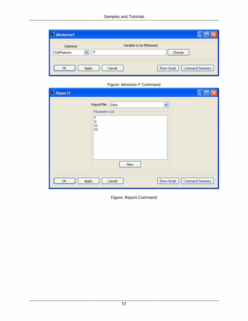
Samples and Tutorials
57
Figure: Minimize F Command
Figure: Report Command
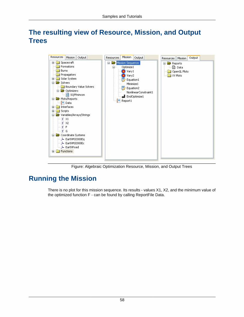
Samples and Tutorials
58
The resulting view of Resource, Mission, and OutputTrees
Figure: Algebraic Optimization Resource, Mission, and Output Trees
Running the Mission
There is no plot for this mission sequence. Its results - values X1, X2, and the minimum value ofthe optimized function F - can be found by calling ReportFile Data.
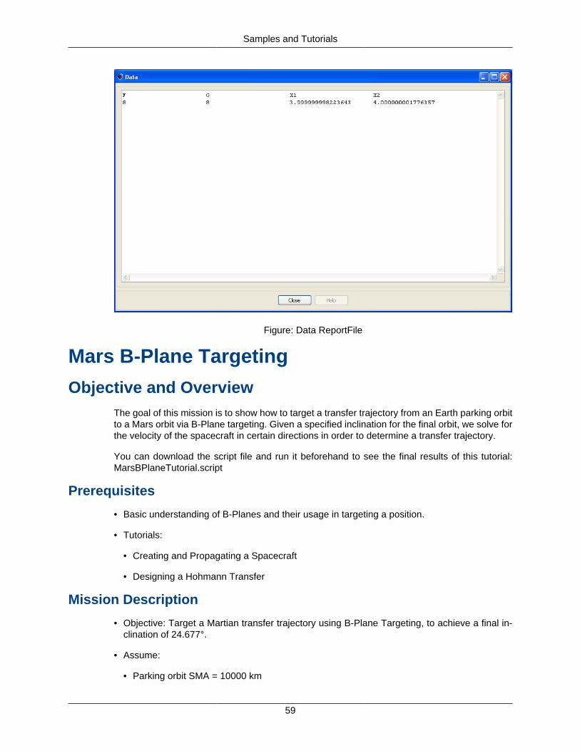
Samples and Tutorials
59
Figure: Data ReportFile
Mars B-Plane Targeting
Objective and OverviewThe goal of this mission is to show how to target a transfer trajectory from an Earth parking orbitto a Mars orbit via B-Plane targeting. Given a specified inclination for the final orbit, we solve forthe velocity of the spacecraft in certain directions in order to determine a transfer trajectory.
You can download the script file and run it beforehand to see the final results of this tutorial:MarsBPlaneTutorial.script
Prerequisites
• Basic understanding of B-Planes and their usage in targeting a position.
• Tutorials:
• Creating and Propagating a Spacecraft
• Designing a Hohmann Transfer
Mission Description
• Objective: Target a Martian transfer trajectory using B-Plane Targeting, to achieve a final in-clination of 24.677°.
• Assume:
• Parking orbit SMA = 10000 km

Samples and Tutorials
60
• Parking orbit ECC = 0.1
• INC = 25.0°
• RAAN = 332.5°
• AOP = 90.0°
• TA = 360°
• Find:
• INC
• BdotT
• BdotR
Creating and Configuring the Resource Tree
For this tutorial, four impulsive burns are used to maneuver a single spacecraft, and three prop-agators are used for different portions of the spacecraft's propagation. The propagators use dif-ferent point masses to account for the dominant gravity fields during the spacecraft's trajectory.Two OpenGL plots are used to track the path at the starting point and ending point of the mission.Finally, four coordinate systems are used to define the spacecraft's position - based, accordingly,on Earth, Mars, the ecliptic, and the equatorial plane of the Earth.
Objects Required
• Spacecraft: MarsSupply
• Impulsive Burns: TOI, MarsMCC, MarsBPlane, and MarsOI
• Propagators: EarthProp, SunProp, and MarsProp
• Differential Corrector: MarsTOIDC
• Plots/Reports: EarthView and MarsView and a data report
• Coordinate Systems: MarsMJ2000Eq, SunMJ2kEc, SunMJ2kEq, and EarthSunRot
Creating and Modifying Objects
• Spacecraft
• Add a spacecraft to the resource tree and rename it MarsSupply
• Set the epoch format to TAIModJulian
• Use an Epoch of 21160
• Set the State Type to Keplerian
• See Assumptions to modify spacecraft element properties

Samples and Tutorials
61
Figure: MarsSupply Spacecraft Object
• Propagators
• Remove all primary bodies and gravity models from all propagators
• EarthProp
• Use an Integrator max step size of 86400 sec
• Include only a Geocentric point mass

Samples and Tutorials
62
Figure: EarthProp Propagator Object
• SunProp
• Set the Integrator max step size to 160000 sec
• Set the Integrator max step attempts to 500
• Include heliocentric, geocentric, and lunar point masses
• MarsProp includes only a martian point mass
• Set the Integrator max step size to 86400 sec
• Set the Integrator max step attempts to 100
• Burns
• Change the TOI vector V to 2.85 km/s
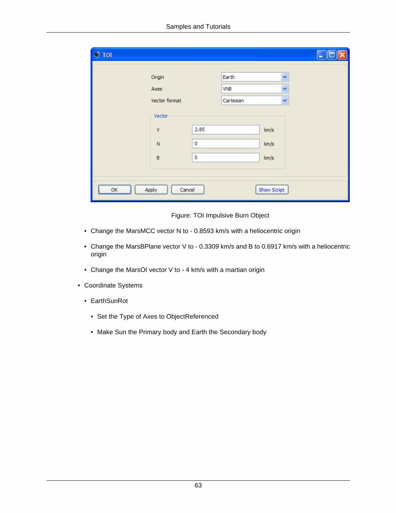
Samples and Tutorials
63
Figure: TOI Impulsive Burn Object
• Change the MarsMCC vector N to - 0.8593 km/s with a heliocentric origin
• Change the MarsBPlane vector V to - 0.3309 km/s and B to 0.6917 km/s with a heliocentricorigin
• Change the MarsOI vector V to - 4 km/s with a martian origin
• Coordinate Systems
• EarthSunRot
• Set the Type of Axes to ObjectReferenced
• Make Sun the Primary body and Earth the Secondary body

Samples and Tutorials
64
Figure: EarthSunCoord Coordinate System Object
• SunMJ2kEc
• Apply a heliocentric origin to the system
• Use MJ2000Ec as the Type of Axes
• SunMJ2kEq
• Apply a heliocentric origin to the system
• Use MJ2000Eq as the Type of Axes
• MarsMJ2000Eq
• Apply a martian origin to the system
• Use MJ2000Eq as the Type of Axes
• Solvers
• Add a differential corrector to the Boundary Value Solvers folder in the Solvers folder underthe resource tree and rename it MarsTOIDC
• Use the Targeter Text File targeter_MarsTOIDC.data
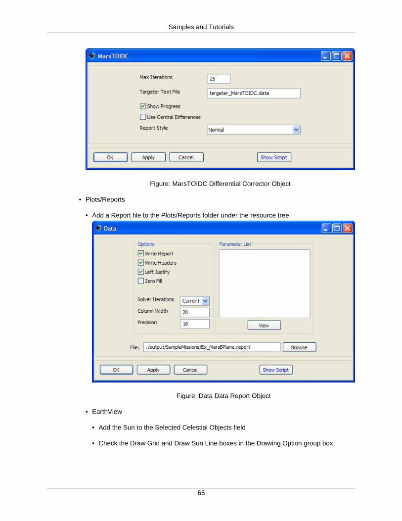
Samples and Tutorials
65
Figure: MarsTOIDC Differential Corrector Object
• Plots/Reports
• Add a Report file to the Plots/Reports folder under the resource tree
Figure: Data Data Report Object
• EarthView
• Add the Sun to the Selected Celestial Objects field
• Check the Draw Grid and Draw Sun Line boxes in the Drawing Option group box

Samples and Tutorials
66
Figure: MarsView OpenGL Plot Object
• MarsView
• Add the Sun and Mars to the Selected Celestial Objects field
• Use MarsMJ2000Eq coordinate system in the View Definition and View Up Definitiongroup boxes
• Use a View Scale Factor of 2
• Check the Draw Grid and Draw Sun Line boxes in the Drawing Option group box
Creating and Configuring the Mission Sequence
This mission begins at the spacecraft orbit's Earth periapsis point, then moves to a Mars transfertrajectory, and ends in an elliptical orbit about Mars. The transfer trajectory calls two targetingsequences, one to obtain an inclination, and the other to obtain a B-Plane position. In the firsttargeting sequence, the inclination is achieved, and is then used when the second sequencetargets a distinct B-Plane parameter. After the second targeting sequence is accomplished, thespacecraft is slowed by a final maneuver that puts it into the elliptical orbit and continues topropagate for another half day. During each Propagate and Maneuver command before and afterthe targeting sequences, reports are added for tracking and analysis purposes, to monitor thespacecraft's Cartesian coordinates and velocity vectors.
• Initial Propagate and Maneuver Sequence
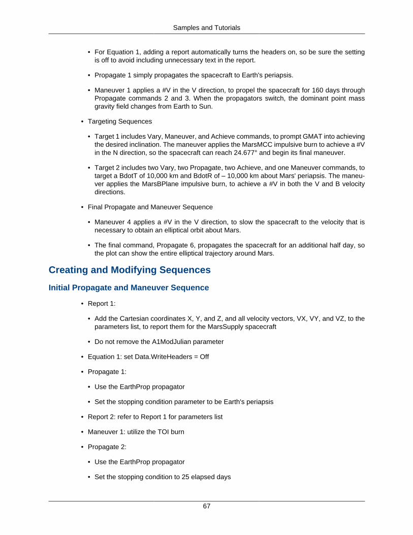
Samples and Tutorials
67
• For Equation 1, adding a report automatically turns the headers on, so be sure the settingis off to avoid including unnecessary text in the report.
• Propagate 1 simply propagates the spacecraft to Earth's periapsis.
• Maneuver 1 applies a #V in the V direction, to propel the spacecraft for 160 days throughPropagate commands 2 and 3. When the propagators switch, the dominant point massgravity field changes from Earth to Sun.
• Targeting Sequences
• Target 1 includes Vary, Maneuver, and Achieve commands, to prompt GMAT into achievingthe desired inclination. The maneuver applies the MarsMCC impulsive burn to achieve a #Vin the N direction, so the spacecraft can reach 24.677° and begin its final maneuver.
• Target 2 includes two Vary, two Propagate, two Achieve, and one Maneuver commands, totarget a BdotT of 10,000 km and BdotR of – 10,000 km about Mars' periapsis. The maneu-ver applies the MarsBPlane impulsive burn, to achieve a #V in both the V and B velocitydirections.
• Final Propagate and Maneuver Sequence
• Maneuver 4 applies a #V in the V direction, to slow the spacecraft to the velocity that isnecessary to obtain an elliptical orbit about Mars.
• The final command, Propagate 6, propagates the spacecraft for an additional half day, sothe plot can show the entire elliptical trajectory around Mars.
Creating and Modifying Sequences
Initial Propagate and Maneuver Sequence
• Report 1:
• Add the Cartesian coordinates X, Y, and Z, and all velocity vectors, VX, VY, and VZ, to theparameters list, to report them for the MarsSupply spacecraft
• Do not remove the A1ModJulian parameter
• Equation 1: set Data.WriteHeaders = Off
• Propagate 1:
• Use the EarthProp propagator
• Set the stopping condition parameter to be Earth's periapsis
• Report 2: refer to Report 1 for parameters list
• Maneuver 1: utilize the TOI burn
• Propagate 2:
• Use the EarthProp propagator
• Set the stopping condition to 25 elapsed days
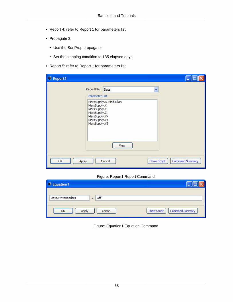
Samples and Tutorials
68
• Report 4: refer to Report 1 for parameters list
• Propagate 3:
• Use the SunProp propagator
• Set the stopping condition to 135 elapsed days
• Report 5: refer to Report 1 for parameters list
Figure: Report1 Report Command
Figure: Equation1 Equation Command
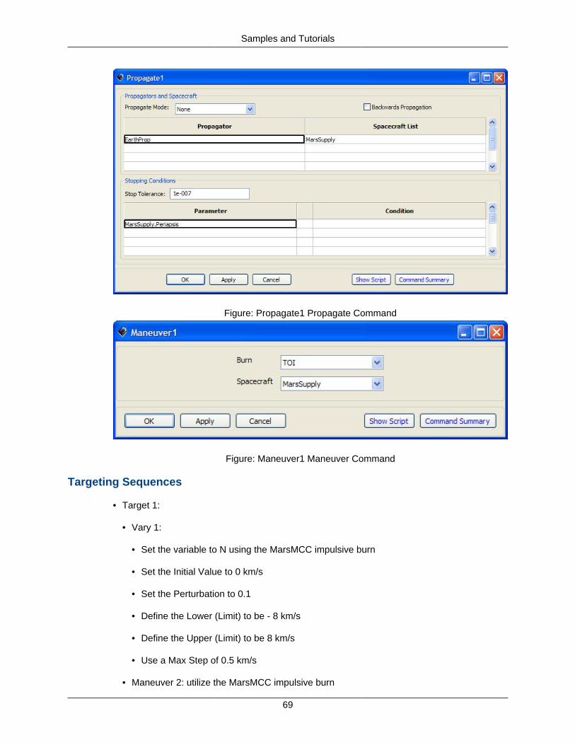
Samples and Tutorials
69
Figure: Propagate1 Propagate Command
Figure: Maneuver1 Maneuver Command
Targeting Sequences
• Target 1:
• Vary 1:
• Set the variable to N using the MarsMCC impulsive burn
• Set the Initial Value to 0 km/s
• Set the Perturbation to 0.1
• Define the Lower (Limit) to be - 8 km/s
• Define the Upper (Limit) to be 8 km/s
• Use a Max Step of 0.5 km/s
• Maneuver 2: utilize the MarsMCC impulsive burn

Samples and Tutorials
70
• Achieve 1:
• Goal:
• Highlight MarsSupply in the Object List menu
• Select the SunMJ2kEq coordinate system from the drop down menu
• Add INC to the Selected Value(s) field
• Set the Value to 24.677°
• Use a Tolerance of 0.001°
• Report 6: refer to Report 1 for parameters list
Figure: Target1 Target Command
Figure: Vary1 Vary Command
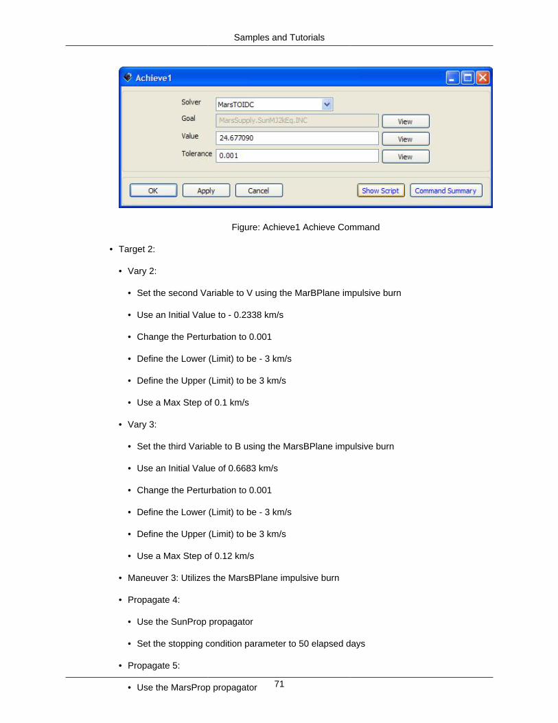
Samples and Tutorials
71
Figure: Achieve1 Achieve Command
• Target 2:
• Vary 2:
• Set the second Variable to V using the MarBPlane impulsive burn
• Use an Initial Value to - 0.2338 km/s
• Change the Perturbation to 0.001
• Define the Lower (Limit) to be - 3 km/s
• Define the Upper (Limit) to be 3 km/s
• Use a Max Step of 0.1 km/s
• Vary 3:
• Set the third Variable to B using the MarsBPlane impulsive burn
• Use an Initial Value of 0.6683 km/s
• Change the Perturbation to 0.001
• Define the Lower (Limit) to be - 3 km/s
• Define the Upper (Limit) to be 3 km/s
• Use a Max Step of 0.12 km/s
• Maneuver 3: Utilizes the MarsBPlane impulsive burn
• Propagate 4:
• Use the SunProp propagator
• Set the stopping condition parameter to 50 elapsed days
• Propagate 5:
• Use the MarsProp propagator
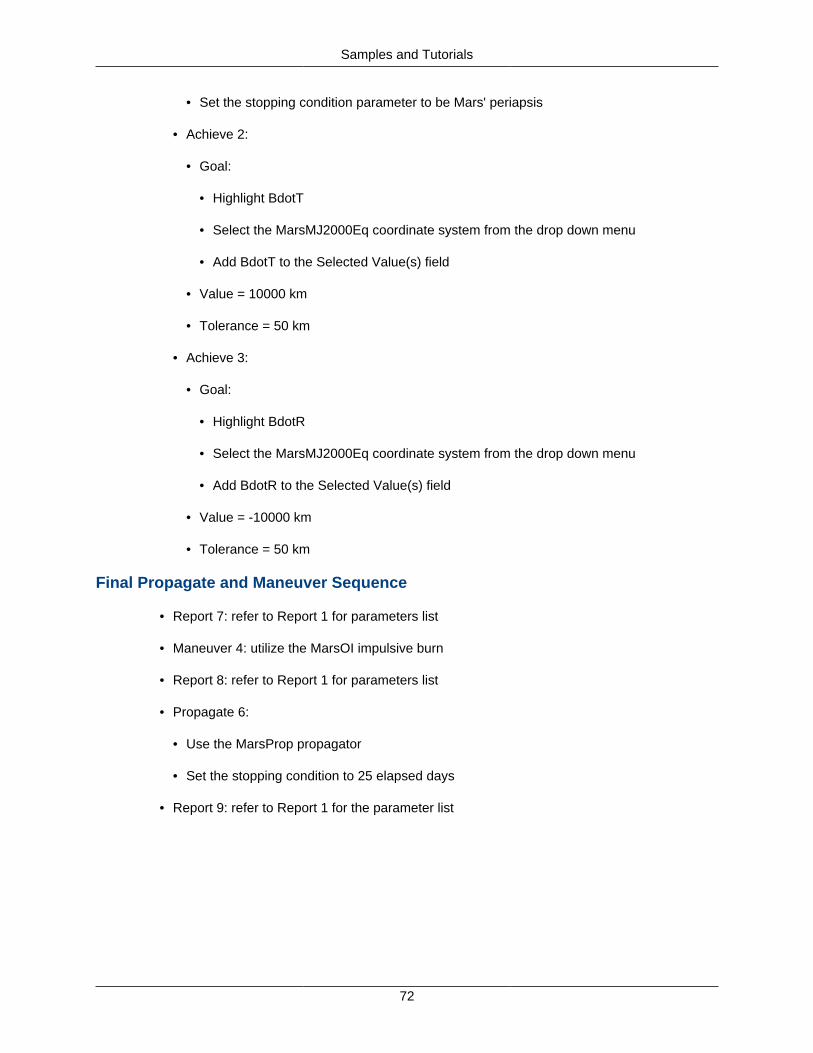
Samples and Tutorials
72
• Set the stopping condition parameter to be Mars' periapsis
• Achieve 2:
• Goal:
• Highlight BdotT
• Select the MarsMJ2000Eq coordinate system from the drop down menu
• Add BdotT to the Selected Value(s) field
• Value = 10000 km
• Tolerance = 50 km
• Achieve 3:
• Goal:
• Highlight BdotR
• Select the MarsMJ2000Eq coordinate system from the drop down menu
• Add BdotR to the Selected Value(s) field
• Value = -10000 km
• Tolerance = 50 km
Final Propagate and Maneuver Sequence
• Report 7: refer to Report 1 for parameters list
• Maneuver 4: utilize the MarsOI impulsive burn
• Report 8: refer to Report 1 for parameters list
• Propagate 6:
• Use the MarsProp propagator
• Set the stopping condition to 25 elapsed days
• Report 9: refer to Report 1 for the parameter list
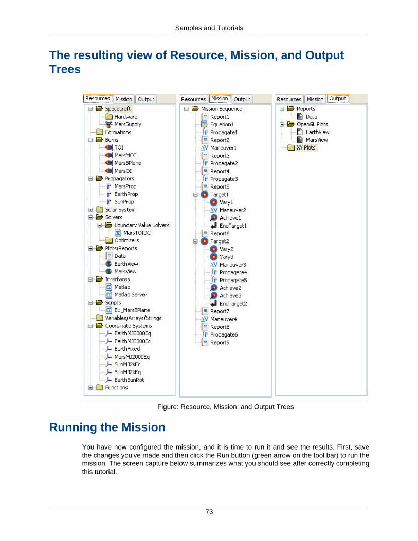
Samples and Tutorials
73
The resulting view of Resource, Mission, and OutputTrees
Figure: Resource, Mission, and Output Trees
Running the Mission
You have now configured the mission, and it is time to run it and see the results. First, savethe changes you've made and then click the Run button (green arrow on the tool bar) to run themission. The screen capture below summarizes what you should see after correctly completingthis tutorial.

Samples and Tutorials
74
Figure: Output

Reference Guide
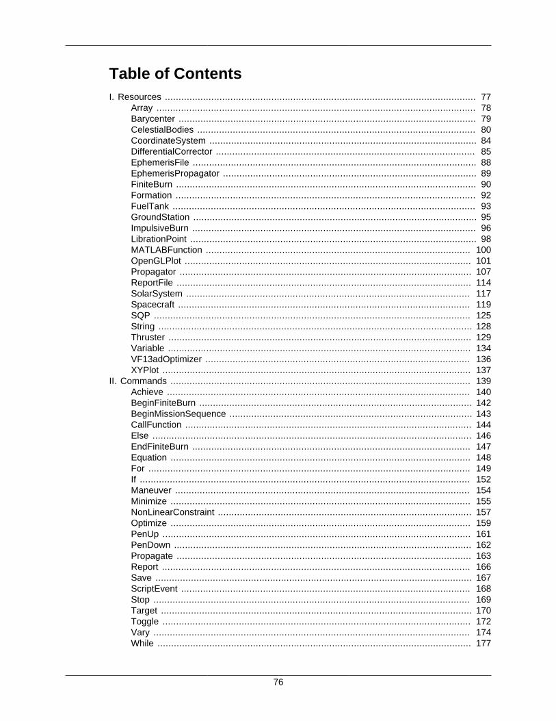
76
Table of ContentsI. Resources .................................................................................................................. 77
Array ..................................................................................................................... 78Barycenter ............................................................................................................. 79CelestialBodies ...................................................................................................... 80CoordinateSystem .................................................................................................. 84DifferentialCorrector ............................................................................................... 85EphemerisFile ........................................................................................................ 88EphemerisPropagator ............................................................................................. 89FiniteBurn .............................................................................................................. 90Formation .............................................................................................................. 92FuelTank ............................................................................................................... 93GroundStation ........................................................................................................ 95ImpulsiveBurn ........................................................................................................ 96LibrationPoint ......................................................................................................... 98MATLABFunction ................................................................................................. 100OpenGLPlot ......................................................................................................... 101Propagator ........................................................................................................... 107ReportFile ............................................................................................................ 114SolarSystem ........................................................................................................ 117Spacecraft ........................................................................................................... 119SQP .................................................................................................................... 125String ................................................................................................................... 128Thruster ............................................................................................................... 129Variable ............................................................................................................... 134VF13adOptimizer ................................................................................................. 136XYPlot ................................................................................................................. 137
II. Commands .............................................................................................................. 139Achieve ............................................................................................................... 140BeginFiniteBurn .................................................................................................... 142BeginMissionSequence ......................................................................................... 143CallFunction ......................................................................................................... 144Else ..................................................................................................................... 146EndFiniteBurn ...................................................................................................... 147Equation .............................................................................................................. 148For ...................................................................................................................... 149If ......................................................................................................................... 152Maneuver ............................................................................................................ 154Minimize .............................................................................................................. 155NonLinearConstraint ............................................................................................. 157Optimize .............................................................................................................. 159PenUp ................................................................................................................. 161PenDown ............................................................................................................. 162Propagate ............................................................................................................ 163Report ................................................................................................................. 166Save .................................................................................................................... 167ScriptEvent .......................................................................................................... 168Stop .................................................................................................................... 169Target .................................................................................................................. 170Toggle ................................................................................................................. 172Vary .................................................................................................................... 174While ................................................................................................................... 177

77
Resources
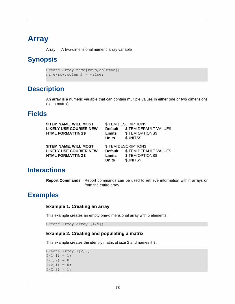
78
ArrayArray — A two-dimensional numeric array variable
SynopsisCreate Array name[rows,columns];name(row,column) = value;…
DescriptionAn array is a numeric variable that can contain multiple values in either one or two dimensions(i.e. a matrix).
Fields$ITEM NAME. WILL MOSTLIKELY USE COURIER NEWHTML FORMATTING$
$ITEM DESCRIPTION$Default $ITEM DEFAULT VALUE$Limits $ITEM OPTIONS$Units $UNITS$
$ITEM NAME. WILL MOSTLIKELY USE COURIER NEWHTML FORMATTING$
$ITEM DESCRIPTION$Default $ITEM DEFAULT VALUE$Limits $ITEM OPTIONS$Units $UNITS$
InteractionsReport Commands Report commands can be used to retrieve information within arrays or
from the entire array.
Examples
Example 1. Creating an array
This example creates an empty one-dimensional array with 5 elements.
Create Array Array1[1,5];
Example 2. Creating and populating a matrix
This example creates the identity matrix of size 2 and names it I:
Create Array I[2,2];I(1,1) = 1;I(1,2) = 0;I(2,1) = 0;I(2,2) = 1;

79
BarycenterBarycenter — A barycenter.
SynopsisCreate Barycenter namename.BodyNames = {bodyName1,bodyName2,...,bodyNameN}
DescriptionA barycenter is the center of mass of one or more celestial bodies and can be used as the origin ofa CoordinateSystem, a reference point in an OrbitView, or as one of the points in a LibrationPoint.
FieldsBody-Names
The BodyNames field is a list that contains the bodies used to define abarycenter. In a script, the list must be surrounded by curly braces. (i.e.BaryCenterName.BodyNames = { Earth, Luna }) Default Earth, LunaLimits Sun, Mercury, Venus, Earth, Luna, Mars, Jupiter, Saturn, Uranus,
Neptune, Pluto, or any user-defined celestial body. At least one bodymust be selected!
Units N/A
InteractionsCoordinate Systems Interacts with the barycenter object selecting it as the origin of the
coordinate system or as a primary or secondary point for defining theaxes.
OpenGL Plot It can be selected as a celestial object to be drawn onto the plot, aView Point Reference, or the View Direction within the dialog box.
ExamplesCreate Barycenter EarthMoonBary;GMAT EarthMoonBary.BodyNames = {Earth, Luna};
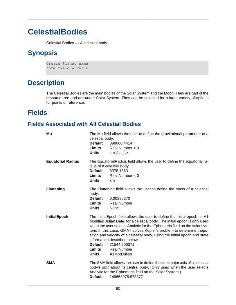
80
CelestialBodiesCelestial Bodies — A celestial body.
SynopsisCreate Planet namename.field = value
DescriptionThe Celestial Bodies are the main bodies of the Solar System and the Moon. They are part of theresource tree and are under Solar System. They can be selected for a large variety of optionsfor points of reference.
Fields
Fields Associated with All Celestial Bodies
Mu The Mu field allows the user to define the gravitational parameter of acelestial body.Default 398600.4414Limits Real Number < 0Units km3/sec2.z
Equatorial Radius The EquatorialRadius field allows the user to define the equatorial ra-dius of a celestial body.Default 6378.1363Limits Real Number < 0Units km
Flattening The Flattening field allows the user to define the mass of a celestialbody.Default 0.00335270Limits Real NumberUnits None
InitialEpoch The InitialEpoch field allows the user to define the initial epoch, in A1Modified Julian Date, for a celestial body. The initial epoch is only usedwhen the user selects Analytic for the Ephemeris field on the solar sys-tem. In this case, GMAT solves Kepler's problem to determine thepo-sition and velocity of a celestial body, using the initial epoch and stateinformation described below.Default 21544.500371Limits Real NumberUnits A1ModJulian
SMA The SMA field allows the user to define the semimajor axis of a celestialbody's orbit about its central body. (Only used when the user selectsAnalytic for the Ephemeris field on the Solar System.)Default 149653978.978377
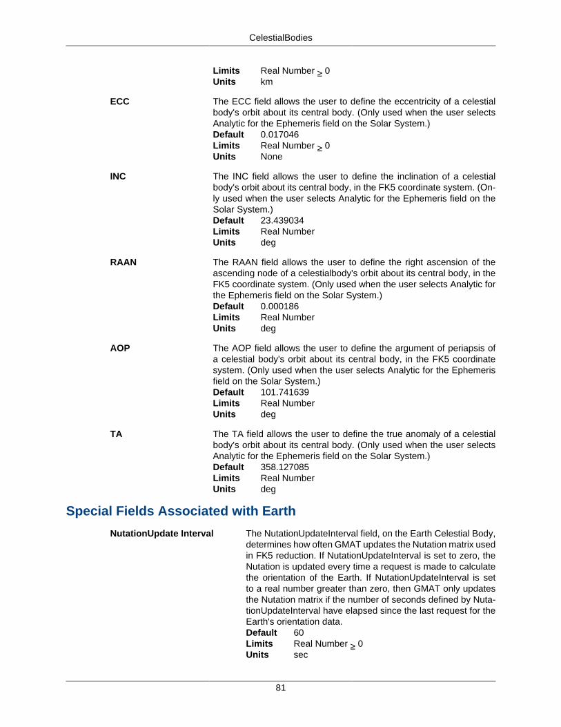
CelestialBodies
81
Limits Real Number ≥ 0Units km
ECC The ECC field allows the user to define the eccentricity of a celestialbody's orbit about its central body. (Only used when the user selectsAnalytic for the Ephemeris field on the Solar System.)Default 0.017046Limits Real Number ≥ 0Units None
INC The INC field allows the user to define the inclination of a celestialbody's orbit about its central body, in the FK5 coordinate system. (On-ly used when the user selects Analytic for the Ephemeris field on theSolar System.)Default 23.439034Limits Real NumberUnits deg
RAAN The RAAN field allows the user to define the right ascension of theascending node of a celestialbody's orbit about its central body, in theFK5 coordinate system. (Only used when the user selects Analytic forthe Ephemeris field on the Solar System.)Default 0.000186Limits Real NumberUnits deg
AOP The AOP field allows the user to define the argument of periapsis ofa celestial body's orbit about its central body, in the FK5 coordinatesystem. (Only used when the user selects Analytic for the Ephemerisfield on the Solar System.)Default 101.741639Limits Real NumberUnits deg
TA The TA field allows the user to define the true anomaly of a celestialbody's orbit about its central body. (Only used when the user selectsAnalytic for the Ephemeris field on the Solar System.)Default 358.127085Limits Real NumberUnits deg
Special Fields Associated with Earth
NutationUpdate Interval The NutationUpdateInterval field, on the Earth Celestial Body,determines how often GMAT updates the Nutation matrix usedin FK5 reduction. If NutationUpdateInterval is set to zero, theNutation is updated every time a request is made to calculatethe orientation of the Earth. If NutationUpdateInterval is setto a real number greater than zero, then GMAT only updatesthe Nutation matrix if the number of seconds defined by Nuta-tionUpdateInterval have elapsed since the last request for theEarth's orientation data.Default 60Limits Real Number ≥ 0Units sec
CelestialBodies
82
Special Fields Associated with Luna
RotationData Source The RotationDataSource, on the Luna Celestial Body, determineswhat source GMAT uses to obtain data describing the orientation ofthe moon with respect to the FK5 system. The RotationDataSourcefield is only used for lunar orientation data when calculating moon-based coordinate systems with the axes types of {Fixed} and {Equa-tor}.Default DE405Limits DE405, IAU2002Units N/A
InteractionsCoordinate System Interacts with the celestial body in that the body can be selected as the
origin of the coordinate system or as a primary or secondary point fordefining the axes.
OpenGL plot Interacts with a celestial body in a number of ways. It can be selected tobe drawn onto the plot, with the color of the orbit an option. A celestialbody can also be selected as the View Point Reference or the ViewDirection.
Propagator Can interact with a celestial body in a number of ways. Under the ForceModel heading, any celestial body can be chosen for use as the centralbody, as the primary bodies, and the secondary bodies.
Bary Center Can interact with celestial bodies in that a bary center is calculatedusing some number of celestial bodies which can be selected.
Libration point Can interact with celestial bodies in that a libration point is calculatedusing two celestial bodies which can be selected.
Spacecraft Interacts with celestial bodies in that for a number of parameters de-scribe how the spacecraft is positioned in relation to a celestial body.This can include the periapsis, apoapsis, and altitude, as well as a greatmany of other parameters.
ExamplesCreate Planet Earth;GMAT Earth.BodyType = 'Planet';GMAT Earth.Mass = 5.973331957140716e+024;GMAT Earth.EquatorialRadius = 6378.1363;GMAT Earth.Flattening = 0.0033527;GMAT Earth.PolarRadius = 6356.75232242699;GMAT Earth.Mu = 398600.4415;GMAT Earth.PosVelSource = 'DE_405';GMAT Earth.State = [ 0 0 0 0 0 0 ];GMAT Earth.StateTime = 0;GMAT Earth.CentralBody = 'Sun';GMAT Earth.BodyNumber = 2;GMAT Earth.RefBodyNumber = 3;GMAT Earth.SourceFilename = './files/planetary_ephem/de/winp1941.405';
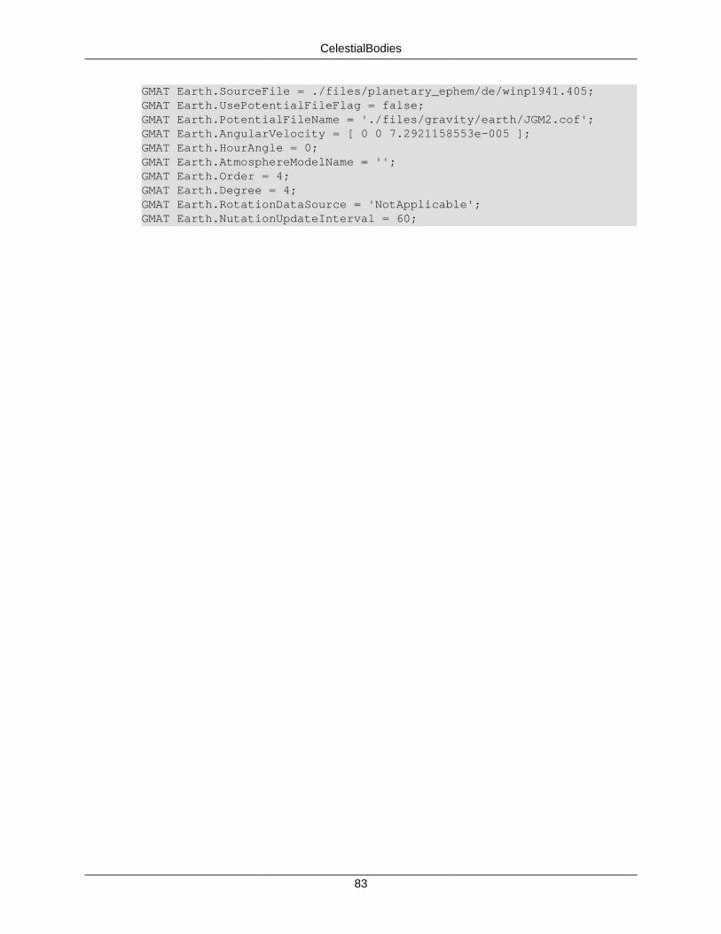
CelestialBodies
83
GMAT Earth.SourceFile = ./files/planetary_ephem/de/winp1941.405;GMAT Earth.UsePotentialFileFlag = false;GMAT Earth.PotentialFileName = './files/gravity/earth/JGM2.cof';GMAT Earth.AngularVelocity = [ 0 0 7.2921158553e-005 ];GMAT Earth.HourAngle = 0;GMAT Earth.AtmosphereModelName = '';GMAT Earth.Order = 4;GMAT Earth.Degree = 4;GMAT Earth.RotationDataSource = 'NotApplicable';GMAT Earth.NutationUpdateInterval = 60;

84
CoordinateSystemCoordinate Systems — A coordinate system.
SynopsisCreate CoordinateSystem namename.field = value
DescriptionCoordinate Systems are critical to GMAT for several reasons. They are what every object rep-resented within the software is referenced to. They are used by GMAT as the basis for which allcalculations are made. They also provide the reference for any OpenGL Plot that is created.
Interactions
Thruster The Thruster object allows you to set a coordinate system asits reference.
Spacecraft In the spacecraft dialog box you may change what coordi-nate system the spacecraft's position is defined in reference,whatever the state type may be set as.
OpenGL Plot Coordinate Systems are very key to the display of OpenGLPlots. They rely on coordinate systems to set how exactly theview of the plot will look using both the View Definition andView Up Definition sections of the OpenGL Plot dialog box.
Parameter Select Dialog Box Whenever you may select a parameter using the parameterselect dialog box, you have the option of selecting certain op-tions such X, Y, Z, and several others that will require to seta coordinate system for them to reference.
ExamplesCreate CoordinateSystem EarthMJ2000Eq;GMAT EarthMJ2000Eq.Origin = Earth;GMAT EarthMJ2000Eq.Axes = MJ2000Eq;GMAT EarthMJ2000Eq.UpdateInterval = 60;GMAT EarthMJ2000Eq.OverrideOriginInterval = false;

85
DifferentialCorrectorDifferential Corrector — A differential corrector.
SynopsisCreate DifferentialCorrector namename.field = value
DescriptionA differential corrector is a numerical solver for solving two-point boundary value problems. TheDC in GMAT uses a simple shooting method where the derivatives are determined using finitedifferencing. In the mission sequence, you use the differential corrector object in a Target se-quence to solve two-point value problems. For example, differential correctors are often usedto determine the maneuver components required to achieve desired orbital conditions, say, B-plane conditions at a planetary flyby.
You must create and configure a differential corrector object according to your application bysetting numerical properties of the solver such as tolerance and maximum iterations. You canalso select among different output options that show increasing levels of information for eachdifferential corrector iteration.
The allowable settings for a differential corrector are shown in the GUI screen shots and referencetable below. You can learn more about how to use a DC in a targeting sequence by reading thehelp files for Target, Vary, and Achieve.
FieldsMaximumIterations The MaximumIterations field allows the user to set the maximum num-
ber of iterations the differential corrector is allowed during the attemptto find a solution. If the maximum iterations is reached, GMAT exitsthe target loop and continues to the next command in the mission se-quence. In this case, the objects retain their states as of the last nom-inal pass through the targeting loop.Default 25Limits Integer >= 1Units N/A
DerivativeMethod The DerivativeMethod field allows the user to choose between one-sided and central differencing for numerically determining the Jacobianmatrix.Default ForwardDifferenceLimits ForwardDifference, BackwardDifference, CentralDiffer-
enceUnits N/A
ShowProgress When the ShowProgress field is set to true, then data illustrating theprogress of the differential correction process are written to the mes-sage window. The message window is updated with information on thecurrent control variable values and the contraint variances for both on

DifferentialCorrector
86
perturbation and iteration passes. When the ShowProgress field is setto false, no information on the progress of the differential correctionprocess is displayed.Default trueLimits true, falseUnits N/A
ReportStyle The ReportStyle field allows the user to control the amount and type ofinformation written to the file defined in the ReportFile field. Currently,the Normal and Concise options contain the same information: the Ja-cobian, the inverse of the Jacobian, the current values of the controlvariables, and achieved and desired values of the constraints. Verbosecontains values of the perturbation variables in addition to the data forNormal and Concise. Debug contains detailed script snippets at eachiteration for objects who have control variables.Default NormalLimits Normal, Concise, Verbose, DebugUnits N/A
ReportFile The ReportFile field allows the user to specify the path and file namefor the differential correction report.Default DifferentialCorrectorDCNameLimits Filename consistent with OSUnits N/A
Object and Command Interactions
The Differential Corrector does not interact directly with any resource objects.
The Differential Corrector is used in the following mission sequence commands:
• Target
• Vary
• Achieve
DifferentialCorrector
87
Examples
Figure: Default Name and Settings for the Differential Corrector Dialog Box
Create DifferentialCorrector DefaultDC;GMAT DefaultDC.ShowProgress = true;GMAT DefaultDC.ReportStyle = 'Normal';GMAT DefaultDC.TargeterTextFile = 'DifferentialCorrectorDefaultDC.data';GMAT DefaultDC.MaximumIterations = 25;GMAT DefaultDC.UseCentralDifferences = false;
88
EphemerisFileEphemerisFile — An ephemeris file.
Synopsis Under Construction.
DescriptionUnder Construction.
FieldsField Name Description....
Type Fill This In.Default Fill This In.Limits Fill This In.Units Fill This In.
Examples
Example 3. Example Script
%
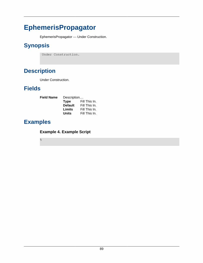
89
EphemerisPropagatorEphemerisPropagator — Under Construction.
Synopsis Under Construction.
DescriptionUnder Construction.
FieldsField Name Description....
Type Fill This In.Default Fill This In.Limits Fill This In.Units Fill This In.
Examples
Example 4. Example Script
%

90
FiniteBurnFinite Burn — A finite burn.
SynopsisCreate FiniteBurn namename.field = value
DescriptionThe Finite Burn object is used when a continuous propulsion is desired. Impulsive burns happeninstantaneously and through a Maneuver command, while finite burns occur until the End FiniteBurn command is reached in the mission sequence and are typically coupled with Propagatecommands.
FieldsOrigin Together the Origin and Axes fields describe the coordinate system in
which a maneuver is applied. The Origin field determines the origin ofthe maneuver coordinate system. The ability to define the coordinate sys-tem locally avoids having to create many coordinate systems, associatedwith specific spacecraft, in order to perform finite maneuvers for multiplespacecraft.Default EarthLimits Any celestial body, libration point, or barycenterUnits N/A
Axes The Axes field, together with the Origin field, describe the coordinate sys-tem in which a finite maneuver is applied. If VNB is chosen for Axes, alocal coordinate system is created such that the x-axis points in the veloc-ity direction of the spacecraft, with respect to the point defined by Origin,the y-axis points in the normal direction of the spacecraft with respect toOrigin, and the z-axis completes the right-handed set.Default VNBLimits VNB, MJ2000EqUnits N/A
Thrusters The Thrusters field allows the selection of which thrusters to usewhen applying a finite maneuver. The user can select more thanone thruster, from the list of thrusters previously created, by includingall thrusters in curly braces. An example is MyFiniteBurn.Thrusters =Thruster1,Thruster2,Thruster3.Default No DefaultLimits Any thruster created by userUnits N/A
BurnScaleFactor The BurnScaleFactor is used to scale the total acceleration before addingthe acceleration due to a finite burn into the sum of the accelerations ofa spacecraft. The scaling is performed by taking the sum of the accelera-tions applied by all thrusters specified under the Thrusters field, and mul-tiplying the total thrust by BurnScaleFactor.

FiniteBurn
91
Default 1.0Limits Real NumberUnits N/A
InteractionsSpacecraft A spacecraft must be created in order to apply any burn.
Thruster Any thruster created in the resource tree can be incorporatedinto a finite burn to be used on the spacecraft.
Begin and End Finite Burncommand
After a finite burn is created, to apply it to the mission se-quence, a Begin and End Finite Burn command must be ap-pended to the mission tree.
Examples
Figure: Default Name and Settings for the Finite Burn Object Dialog Box
Create FiniteBurn FiniteBurn1;GMAT FiniteBurn1.Origin = Earth;GMAT FiniteBurn1.Axes = VNB;GMAT FiniteBurn1.BurnScaleFactor = 1;
92
FormationFormation — An ephemeris file.
Synopsis Under Construction.
DescriptionUnder Construction.
FieldsField Name Description....
Type Fill This In.Default Fill This In.Limits Fill This In.Units Fill This In.
Examples
Example 5. Example Script
%
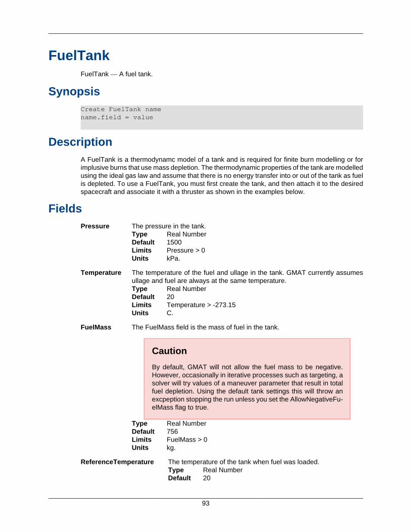
93
FuelTankFuelTank — A fuel tank.
SynopsisCreate FuelTank namename.field = value
DescriptionA FuelTank is a thermodynamc model of a tank and is required for finite burn modelling or forimplusive burns that use mass depletion. The thermodynamic properties of the tank are modelledusing the ideal gas law and assume that there is no energy transfer into or out of the tank as fuelis depleted. To use a FuelTank, you must first create the tank, and then attach it to the desiredspacecraft and associate it with a thruster as shown in the examples below.
FieldsPressure The pressure in the tank.
Type Real NumberDefault 1500Limits Pressure > 0Units kPa.
Temperature The temperature of the fuel and ullage in the tank. GMAT currently assumesullage and fuel are always at the same temperature.Type Real NumberDefault 20Limits Temperature > -273.15Units C.
FuelMass The FuelMass field is the mass of fuel in the tank.
Caution
By default, GMAT will not allow the fuel mass to be negative.However, occasionally in iterative processes such as targeting, asolver will try values of a maneuver parameter that result in totalfuel depletion. Using the default tank settings this will throw anexcpeption stopping the run unless you set the AllowNegativeFu-elMass flag to true.
Type Real NumberDefault 756Limits FuelMass > 0Units kg.
ReferenceTemperature The temperature of the tank when fuel was loaded.Type Real NumberDefault 20
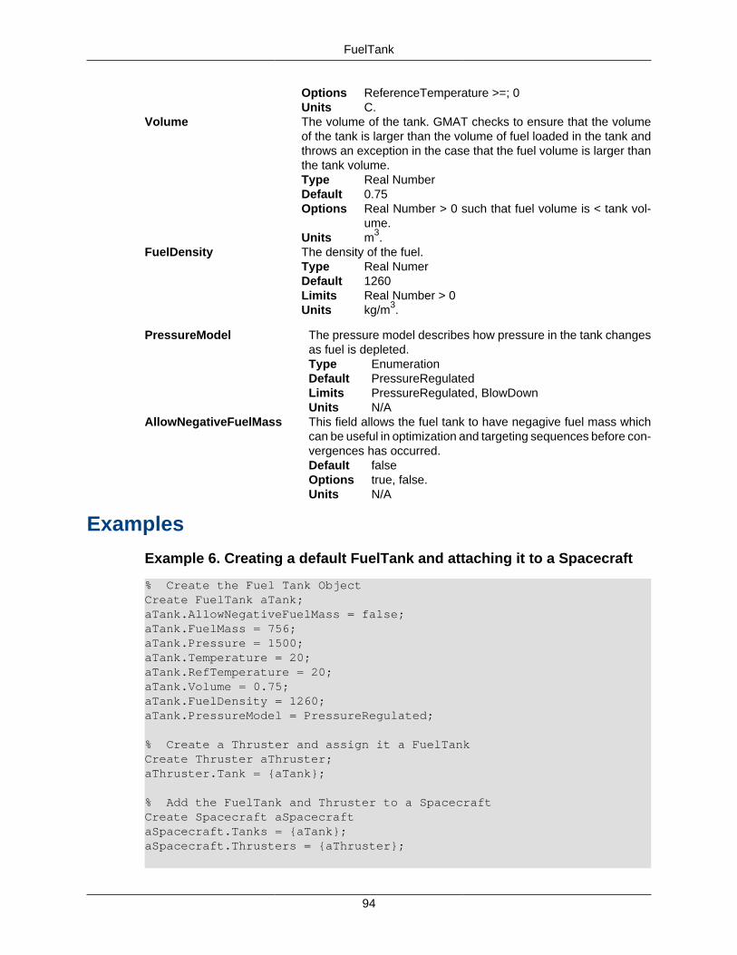
FuelTank
94
Options ReferenceTemperature >=; 0Units C.
Volume The volume of the tank. GMAT checks to ensure that the volumeof the tank is larger than the volume of fuel loaded in the tank andthrows an exception in the case that the fuel volume is larger thanthe tank volume.Type Real NumberDefault 0.75Options Real Number > 0 such that fuel volume is < tank vol-
ume.Units m3.
FuelDensity The density of the fuel.Type Real NumerDefault 1260Limits Real Number > 0Units kg/m3.
PressureModel The pressure model describes how pressure in the tank changesas fuel is depleted.Type EnumerationDefault PressureRegulatedLimits PressureRegulated, BlowDownUnits N/A
AllowNegativeFuelMass This field allows the fuel tank to have negagive fuel mass whichcan be useful in optimization and targeting sequences before con-vergences has occurred.Default falseOptions true, false.Units N/A
Examples
Example 6. Creating a default FuelTank and attaching it to a Spacecraft
% Create the Fuel Tank ObjectCreate FuelTank aTank;aTank.AllowNegativeFuelMass = false;aTank.FuelMass = 756;aTank.Pressure = 1500;aTank.Temperature = 20;aTank.RefTemperature = 20;aTank.Volume = 0.75;aTank.FuelDensity = 1260;aTank.PressureModel = PressureRegulated;
% Create a Thruster and assign it a FuelTankCreate Thruster aThruster;aThruster.Tank = {aTank};
% Add the FuelTank and Thruster to a SpacecraftCreate Spacecraft aSpacecraftaSpacecraft.Tanks = {aTank};aSpacecraft.Thrusters = {aThruster};

95
GroundStationGroundStation — Under Construction.
Synopsis Under Construction.
DescriptionUnder Construction.
FieldsField Name Description....
Type Fill This In.Default Fill This In.Limits Fill This In.Units Fill This In.
Examples
Example 7. Example Script
%

96
ImpulsiveBurnImpulsive Burn — A impulsive burn.
SynopsisCreate ImpulsiveBurn namename.field = value
DescriptionThe impulsive burn object in GMAT allows the spacecraft to undergo an instantaneous #V inup to three dimensions as opposed to a finite burn which is not instantaneous. The user canconfigure the burn by defining its origin, type of axes, vector format, and magnitude of the vectors.Depending on the mission, it will be simpler to use one axes or vector format over the other.
Possible Coupling with Other Objects
Spacecraft Must be created in order to apply any burn. The purpose of the impul-sive burn is to instantaneously propel the spacecraft to either target oroptimize a goal during its mission.
Maneuver com-mand
Must be created to call the burn into the mission sequence because with-out a maneuver, the spacecraft simply propagates around a specifiedtrajectory. If there are several burns that exist, in the Maneuver dialogbox the user can choose which burn to utilize for that part of the missionsequence. In addition, a Propagate command must follow the maneuverto allow the trajectory to unfold after a burn has been applied.
Vary command Required a burn to be specified in the Variable Setup group box. Thepurpose of the Vary command is to apply a burn in order to change aparameter of the spacecraft's trajectory.
FieldsOrigin Together the Origin and Axes fields describe the coordinate system in which
a maneuver is applied. The Origin field determines the origin of the maneuvercoordinatesystem. The ability to define the coordinate system locally avoidshaving to create many coordinate systems, associated with specific space-craft, in order to perform finite maneuvers for multiple spacecraft.Default EarthLimits Any celestial bodyUnits N/A
Axes The Axes field, together with the Origin field, describethe coordinate systemin which an impulsive maneuver is applied. If VNB is chosen for Axes, a localcoordinate system is created such that the x-axis points in the velocity direc-tion of thespacecraft, with respect to the point defined by Origin, the y-axispoints in the normal direction of the spacecraft with respect to Origin, and thez-axis completes the right-handed set.Default VNB
ImpulsiveBurn
97
Limits VNB, MJ2000EqUnits N/A
VectorFormat The VectorFormat field allows the user to define the format of the maneuvervector.Default CartesianLimits CartesianUnits N/A
Element1 The Element1 field allows the user to define the first element of the impulsivemaneuver vector. Element1 is X if VectorFormat is Cartesian.Default 0Limits Real NumberUnits km/sec
Element2 The Element2 field allows the user to define the second element of the impul-sive maneuver vector. Element2 is Y if VectorFormat is Cartesian.Default 0Limits Real NumberUnits km/sec
Element3 The Element3 field allows the user to define the third element of the impulsivemaneuver vector. Element3 is Z if VectorFormat is Cartesian.Default 0Limits Real NumberUnits km/sec
ExamplesCreate ImpulsiveBurn ImpulsiveBurn1;GMAT ImpulsiveBurn1.Origin = Earth;GMAT ImpulsiveBurn1.Axes = VNB;GMAT ImpulsiveBurn1.VectorFormat = Cartesian;GMAT ImpulsiveBurn1.Element1 = 0;GMAT ImpulsiveBurn1.Element2 = 0;GMAT ImpulsiveBurn1.Element3 = 0;
98
LibrationPointLibration Point — A libration point.
SynopsisCreate LibrationPoint namename.field = value
DescriptionA Libration point, also called a Lagrange point, is a point of equilibrium in the restricted three-body problem.
FieldsPrimary The Primary field allows you to define the body treated as the primary in the cal-
culation of the libration point location. (See Math. Spec for more details).Default SunLimits Sun, Mercury, Venus, Earth, Luna, Mars, Jupiter, Saturn, Uranus,
Neptune, Pluto, or any Barycenter. ( The Primary and Secondary bod-ies cannot be the same )
Units N/A
Secondary The Secondary field allows you to define the body treated as the secondary in thecalculation of the libration point location.Default EarthLimits Sun, Mercury, Venus, Earth, Luna, Mars, Jupiter, Saturn, Uranus,
Neptune, Pluto, or any Barycenter. ( The Primary and Secondary bod-ies cannot be the same )
Units N/A
Point The Point field specifies which libration point the object corresponds to.Default L1Limits L1, L2, L3, L4, L5Units N/A
Examples
Script Syntax
Create Libration Point;.Primary = ;.Secondary = ;.Point = <'L1', 'L2', 'L3', 'L4', 'L5'>
Sample Script
Create LibrationPoint Libration1;GMAT Libration1.Primary = Sun;

LibrationPoint
99
GMAT Libration1.Secondary = Earth;GMAT Libration1.Point = 'L1';

100
MATLABFunctionMATLABFunction — Under Construction.
Synopsis Under Construction.
DescriptionUnder Construction.
FieldsField Name Description....
Type Fill This In.Default Fill This In.Limits Fill This In.Units Fill This In.
Examples
Example 8. Example Script
%
101
OpenGLPlotOpenGL Plot — A OpenGL Plot.
SynopsisCreate OpenGLPlot namename.field = value
DescriptionWithout OpenGL Plots, you would have no way of visualizing your spacecraft as it traveled alongits trajectory. OpenGL Plots also have a multitude of options that allow you to customize yourview of the spacecraft. This makes these types of plots very useful and in most cases necessaryto using GMAT.
Fields
Fields Associated with Plot Options
DataCollectFrequency The DataCollectFrequency field allows the user to define howdata is collected for plotting. It is often inefficient to draw everyephemeris point associated with a trajectory. Often, drawing asmaller subset of the data still results in smooth trajectory plots,while executing more quickly. The DataCollectFrequency is an in-teger that represents how often to collect data and store for plot-ting. If DataCollectFrequency is set to 10, then Data is collectedevery 10 integration steps.Default 1Limits Integer ≥ 1Units Integration Steps
UpdatePlotFrequency The UpdatePlotFrequency field allows the user to specify how of-ten to update an OpenGL plot is updated with new data collectedduring the process of propagating spacecraft and running a mis-sion. Data is collected for a plot according the value defined by Dat-aCollectFrequency. An OpenGL plot is updated with the new data,according to the value set in UpdatePlotFrequency. If UpdatePlot-Frequency is set to 10 and DataCollectFrequency is set to 2, thenthe plot is updated with new data every 20 (10*2) integration steps.Default 50Limits Integer ≥ 1Units Integration Steps
NumPointsToRedraw When NumPointsToRedraw is set to zero, all ephemeris points aredrawn. When NumPointsToRedraw is set to a positive integer, say10 for example, only the last 10 collected data points are drawn.See DataCollectFrequency for explanation of how data is collectedfor an OpenGL plot.Default 0Limits Integer ≥ 0
OpenGLPlot
102
Units Integration Steps
ShowPlot The ShowPlot field allows the user to turn off a plot for a particularrun, without deleting the plot object, or removing it from the script.If you select true, then the plot will be shown. If you select false,then the plot will not be shown.Default trueLimits true , falseUnits N/A
Fields Associated with Viewed Objects
Add The Add subfield adds a spacecraft,celestial body, libration point,or barycenter to aplot. When creating a plot the Earth is added as a default body and may be removed byusing the Remove command. The user can add a spacecraft, celestial body, librationpoint, or barycenter to a plot by using the name used to create the object. The GUI'sSelected field is the equivalent of the script's Add field. In the event of no Add commandor no objects in the Selected field, GMAT should run without the OpenGL plot and awarning message displayed in the message window. The following warning messageis sufficient: OpenGL plot will be turned off. No object has been selected for plotting.Default DefaultSC, EarthLimits SpacecraftName CelestialBodyName LibrationPointName Barycenter-
NameUnits N/A
Re-move
The Remove subfield removes a spacecraft,celestial body, libration point, or barycen-ter from a plot. The user can remove any object that has been added to a plot by usingthe name used to add the object.Default No DefaultLimits Any object included in the Add listUnits N/A
Fields Associated with Drawing Options
WireFrame When the WireFrame field is set to On, celestial bodies are drawn usinga wireframe model. When the WireFrame field is set to Off, then celestialbodies are drawn using a full map.Default OffLimits On , OffUnits N/A
EclipticPlane The EclipticPlane field allows the user to tell GMAT to draw a grid rep-resenting the ecliptic plane in an OpenGL plot. Note, the ecliptic planecan currently only be drawn for plots whose coordinate system uses theMJ2000Eq axis system.Default OffLimits On , Off Note: Only allowed for OpenGL plots with Coordi-
nate Systems that use the MJ2000Eq axis systemUnits N/A
XYPlane The XYPlane flag allows the user to tell GMAT to draw a grid represent-ing the XY-plane of the coordinate system selected under the Coordi-nateSystem field of the OpenGL plot.Default OnLimits On , Off
OpenGLPlot
103
Units N/A
Axes The Axis flag allows the user to tell GMAT to draw the Cartesian axissystem associated with the coordinate system selected under the Coor-dinateSystem field of an OpenGL plot.Default OnLimits On , OffUnits N/A
Grid The Grid flag allows the user to tell GMAT to draw a grid representing thelongitude and latitude lines celestial bodies added to an OpenGL plot.Default OnLimits On , OffUnits N/A
EarthSunLines The EarthSunLines allows the user to tell GMAT to draw a line that startsat the center of Earth and points towards the Sun.Default OnLimits On , OffUnits N/A
SolverIterations The SolverIterations field determines whether or not perturbed trajecto-ries are plotted during a solver (Targeter, Optimize) sequence. WhenSolverIterations is set to On, solver iterations are shown on the plot.When SolverIterations is Off, the solver iterations are not shown on theplot.Default OffLimits On , OffUnits N/A
Fields Associated with View Definition
CoordinateSystem The CoordinateSystem field on an OpenGL plot allows the user toselect which coordinate system to use to draw the plot data. A coordi-nate system is defined as an origin and an axis system, and the Co-ordinateSystem field allows the user to determine the origin and axissystem of an OpenGL plot. See the CoordinateSystem object fieldsfor information of defining different types of coordinate systems.Default EarthMJ2000EqLimits Any default or user defined coordinate systemUnits N/A
ViewPointReference The ViewPointReference field is an optional field that allows the userto change the reference point from which ViewPointVector is mea-sured. ViewPointReference} defaults to the origin of the coordinatesystem for the plot. A ViewPointReference can be any spacecraft, ce-lestial body, libration point, or barycenter.Default EarthLimits SpacecraftName, CelestialBodyName, LibrationPoint-
Name, BarycenterName, or a 3-vector of numerical val-ues
Units N/A
ViewPointVector The product of ViewScaleFactor and ViewPointVector field deter-mines the view point location with respect to ViewPointReference.
OpenGLPlot
104
ViewPointVector can be a vector, or any of the following objects:spacecraft,celestial body, libration point,or barycenter. The location ofthe Viewpoint in three-space is defined as the vector addition of View-PointReference, and the vector defined by product of ViewScaleFac-tor and ViewPointVector in the coordinate system chosen by the user.Default [0 0 30000]Limits SpacecraftName, CelestialBodyName, LibrationPoint-
Name, BarycenterName, or a 3-vector of numerical val-ues
Units km or N/A
ViewScaleFactor The ViewScaleFactor field scales ViewPointVector before adding it toViewPointReference. The ViewScaleFactor allows the user to backaway from an object to fit in the field of view.Default 1Limits Real Number ≥ 0Units N/A
ViewDirection The ViewDirection field allows the user to select the direction of viewin an OpenGL plot. The user can specify the view direction by choos-ing an object to point at such as a spacecraft,celestial body, librationpoint,or barycenter. Alternatively, the user can specify a vector of theform [x y z]. If the user specification of ViewDirection, ViewPointRef-erence, and ViewPointVector, results in a zero vector, GMAT uses [00 10000] for ViewDirection.Default EarthLimits SpacecraftName, CelestialBodyName, LibrationPoint-
Name, BarycenterName, or a 3-vector of numerical val-ues
Units km or N/A
Fields Associated with View Options
UseInitialView The UseInitialView field allows the user to control the view of an OpenGLplot between multiple runs of a mission sequence. The first time a specificOpenGL plot is created, GMAT will automatically use the view as definedby the fields associated with View Definition, View Up Direction, and Fieldof View. However, if the user changes the view using the mouse, GMATwill retain this view upon rerunning the mission if UseInitialView is set tofalse. If UseInitialView is set to true, the view for an OpenGL plot will bereturned to the view defined by the initial settings.Default OnLimits On , OffUnits N/A
Fields Associated with View Up Definition
ViewUpCoordinate System The ViewUpCoordinateSystem and ViewUpAxis fields areused to determine which direction appears as up in an OpenGLplot and together with the fields associated the the View Direc-tion, uniquely define the view. The fields associated with theView Definition allow the user to define the point of view in 3-space, and the direction of the line of sight. However, this in-formation alone is not enough to uniquely define the view. We

OpenGLPlot
105
also must provide how the view is oriented about the line ofsight. This is accomplished by defining what direction shouldappear as the up direction in the plot and is configured usingthe ViewUpCoordinateSystem field and the ViewUpAxis field.The ViewUpCoordinateSystem allows the user to select a co-ordinate system to define the up direction. Most of the time thissystem will be the same as the coordinate system chosen un-der the CoordinateSystem field.Default EarthMJ2000EqLimits Any default or user defined coordinate systemUnits N/A
ViewUpAxis The ViewUpAxis allows the user to define which axis of theViewUpCoordinateSystem that will appear as the up directionin an OpenGL plot. See the comments under ViewUpCoordi-nateSystem for more details of fields used to determine the updirection in an OpenGL plot.Default ZLimits X , -X , Y , -Y , Z , -ZUnits N/A
InteractionsSpacecraft Any spacecraft in your mission is available to the OpenGL Plot for
display
Solar System The Sun and all of the Planets may be plotted or referenced in theOpenGL Plot
If you add any Barrycenters or Libration Points, they will also be avail-able for plotting and reference
Coordinate Systems Both View Definition and View Up Definition may use the three defaultor user added coordinate systems
ExamplesCreate OpenGLPlot DefaultOpenGL;GMAT DefaultOpenGL.SolverIterations = Current;GMAT DefaultOpenGL.Add = {DefaultSC, Earth};GMAT DefaultOpenGL.OrbitColor = [ 255 32768 ];GMAT DefaultOpenGL.TargetColor = [ 8421440 0 ];GMAT DefaultOpenGL.CoordinateSystem = EarthMJ2000Eq;GMAT DefaultOpenGL.ViewPointReference = Earth;GMAT DefaultOpenGL.ViewPointVector = [ 0 0 30000 ];GMAT DefaultOpenGL.ViewDirection = Earth;GMAT DefaultOpenGL.ViewScaleFactor = 1;GMAT DefaultOpenGL.ViewUpCoordinateSystem = EarthMJ2000Eq;GMAT DefaultOpenGL.ViewUpAxis = Z;GMAT DefaultOpenGL.CelestialPlane = Off;GMAT DefaultOpenGL.XYPlane = On;GMAT DefaultOpenGL.WireFrame = Off;GMAT DefaultOpenGL.Axes = On;GMAT DefaultOpenGL.Grid = Off;

OpenGLPlot
106
GMAT DefaultOpenGL.SunLine = Off;GMAT DefaultOpenGL.UseInitialView = On;GMAT DefaultOpenGL.DataCollectFrequency = 1;GMAT DefaultOpenGL.UpdatePlotFrequency = 50;GMAT DefaultOpenGL.NumPointsToRedraw = 0;GMAT DefaultOpenGL.ShowPlot = true;
107
PropagatorPropagator — A propagator.
SynopsisCreate Propagator namename.field = value
DescriptionIn GMAT, a Propagator is a combination of an integrator and a force model. Hence, a Propagatorcontains a physical model of the space environment that is used to model the motion of a space-craft as it moves forwards or backwards in time (VOP formulation is not currently supported).You configure a Propagator by selecting among different numerical integrators and environmentmodels to create a Propagator appropriate to the flight regime of your spacecraft during its mis-sion. GMAT supports numerous numerical integrators as well as Force Models like point massand non-spherical gravity, atmospheric drag (Earth), and solar radiation pressure.
To propagate spacecraft in GMAT, you first create and configure a Propagator object in the scriptor in the Resource Tree. Then, in the mission sequence, you create a Propagate command,the topic of another section, and select among previously existing Propagators and Spacecraft.Hence, a Propagator is different from a Propagate command: A Propagator is a resource and isfound in the GUI under the resource tree, and a Propagate Event is configured under the MissionTree and is how you instruct GMAT to propagate spacecraft.
InterfacesThe Propagator dialog box is illustrated below and contains two group boxes: the Integrator groupand the Force Model group. This section discusses the items in each group on the PropagatePanel. It will present how to configure a propagator and discuss all possible user settable fieldsin detail.
Integrator Group
The Integrator group allows you to select and configure a numerical integrator appropriate to yourapplication. You select the type of numerical integrator in the -+Type+- pull-down menu. Afterselecting the integrator type, the fields below the -+Type+- pull-down menu dynamically configureto allow you to set relevant parameters for the selected integrator type. All integrators except forAdams-Bashforth-Moulton (ABM) are configured using the same fields. The ABM integrator hasthe following additional fields: -+MinIntegrationerror+- and -+NomIntegrationerror+-.
Force Model Group
The Force Model group allows you to configure a force model appropriate to the flight regimeof your application. The central body of propagation and error control method are also definedhere. On a Propagator, GMAT classifies all celestial bodies into two mutually exclusive cate-gories: Primary Bodies, and Point Masses. Primary bodies can have a complex force model thatincludes non-spherical gravity, drag, and magnetic field. Point mass bodies only have a point-mass gravitational force.
You can add a Primary Body by clicking the Select button in the Primary Bodies group box. Onceyou have added a Primary Body (or mulitiple bodies in future versions), the pull down menu allows
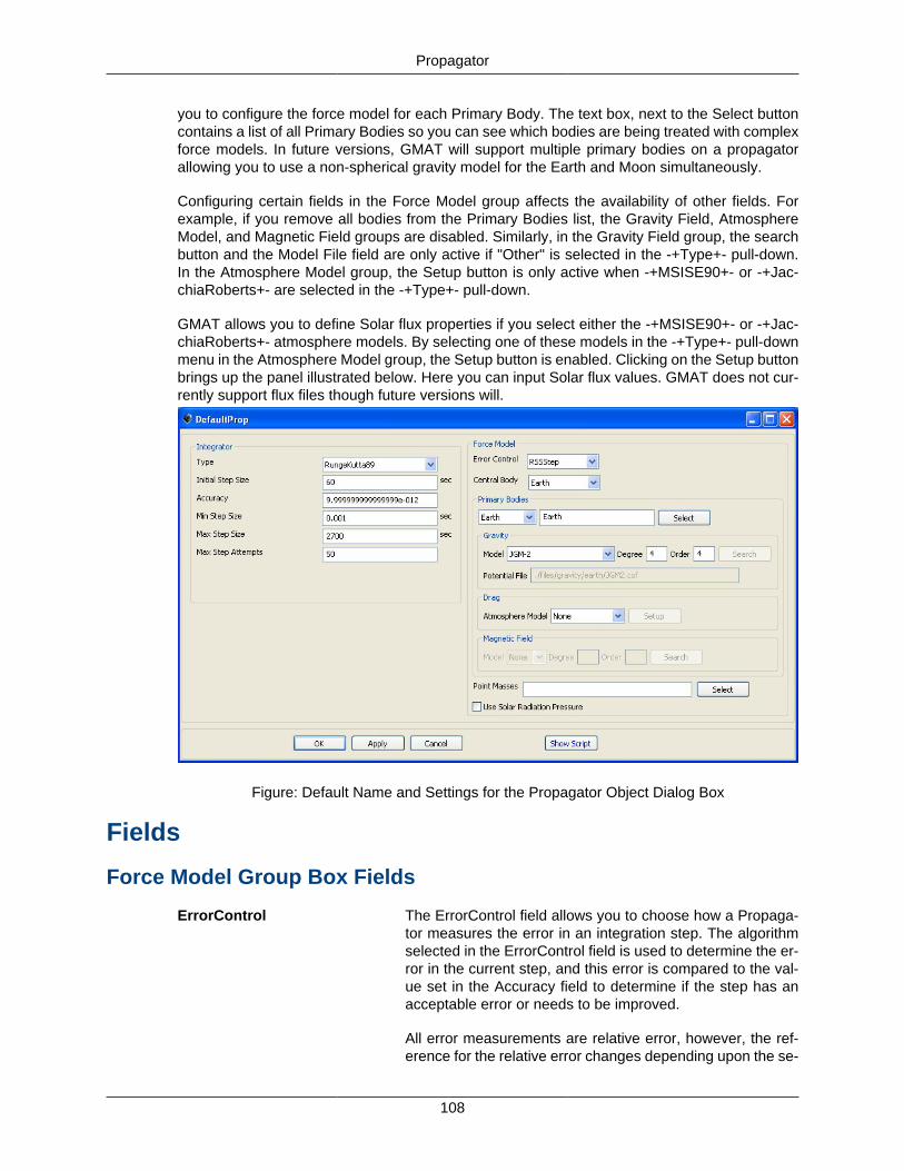
Propagator
108
you to configure the force model for each Primary Body. The text box, next to the Select buttoncontains a list of all Primary Bodies so you can see which bodies are being treated with complexforce models. In future versions, GMAT will support multiple primary bodies on a propagatorallowing you to use a non-spherical gravity model for the Earth and Moon simultaneously.
Configuring certain fields in the Force Model group affects the availability of other fields. Forexample, if you remove all bodies from the Primary Bodies list, the Gravity Field, AtmosphereModel, and Magnetic Field groups are disabled. Similarly, in the Gravity Field group, the searchbutton and the Model File field are only active if "Other" is selected in the -+Type+- pull-down.In the Atmosphere Model group, the Setup button is only active when -+MSISE90+- or -+Jac-chiaRoberts+- are selected in the -+Type+- pull-down.
GMAT allows you to define Solar flux properties if you select either the -+MSISE90+- or -+Jac-chiaRoberts+- atmosphere models. By selecting one of these models in the -+Type+- pull-downmenu in the Atmosphere Model group, the Setup button is enabled. Clicking on the Setup buttonbrings up the panel illustrated below. Here you can input Solar flux values. GMAT does not cur-rently support flux files though future versions will.
Figure: Default Name and Settings for the Propagator Object Dialog Box
Fields
Force Model Group Box Fields
ErrorControl The ErrorControl field allows you to choose how a Propaga-tor measures the error in an integration step. The algorithmselected in the ErrorControl field is used to determine the er-ror in the current step, and this error is compared to the val-ue set in the Accuracy field to determine if the step has anacceptable error or needs to be improved.
All error measurements are relative error, however, the ref-erence for the relative error changes depending upon the se-
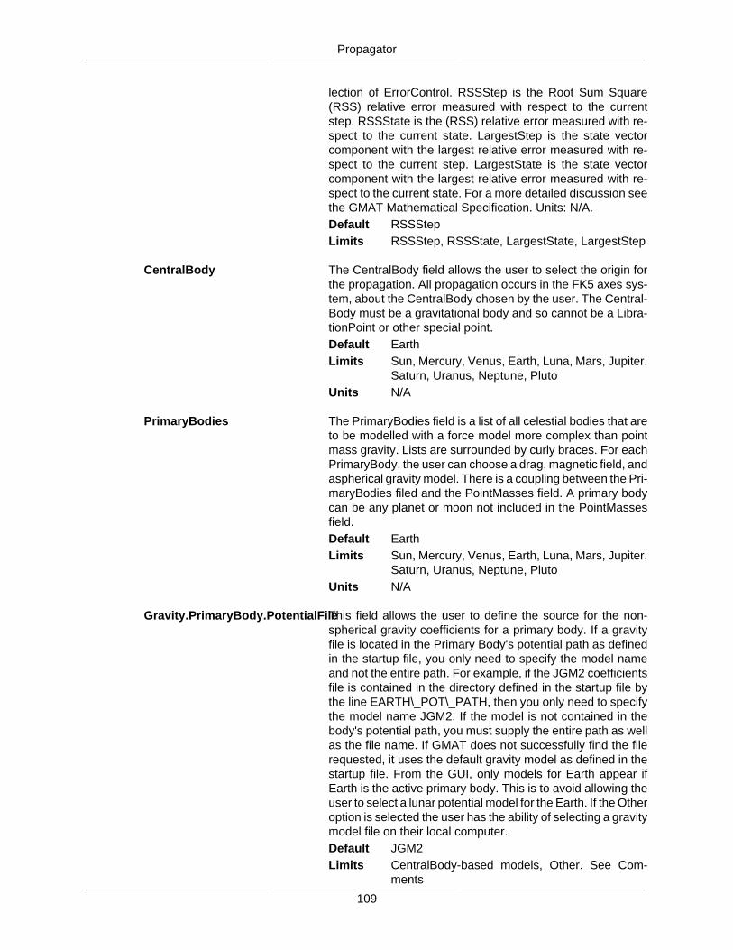
Propagator
109
lection of ErrorControl. RSSStep is the Root Sum Square(RSS) relative error measured with respect to the currentstep. RSSState is the (RSS) relative error measured with re-spect to the current state. LargestStep is the state vectorcomponent with the largest relative error measured with re-spect to the current step. LargestState is the state vectorcomponent with the largest relative error measured with re-spect to the current state. For a more detailed discussion seethe GMAT Mathematical Specification. Units: N/A.Default RSSStepLimits RSSStep, RSSState, LargestState, LargestStep
CentralBody The CentralBody field allows the user to select the origin forthe propagation. All propagation occurs in the FK5 axes sys-tem, about the CentralBody chosen by the user. The Central-Body must be a gravitational body and so cannot be a Libra-tionPoint or other special point.Default EarthLimits Sun, Mercury, Venus, Earth, Luna, Mars, Jupiter,
Saturn, Uranus, Neptune, PlutoUnits N/A
PrimaryBodies The PrimaryBodies field is a list of all celestial bodies that areto be modelled with a force model more complex than pointmass gravity. Lists are surrounded by curly braces. For eachPrimaryBody, the user can choose a drag, magnetic field, andaspherical gravity model. There is a coupling between the Pri-maryBodies filed and the PointMasses field. A primary bodycan be any planet or moon not included in the PointMassesfield.Default EarthLimits Sun, Mercury, Venus, Earth, Luna, Mars, Jupiter,
Saturn, Uranus, Neptune, PlutoUnits N/A
Gravity.PrimaryBody.PotentialFileThis field allows the user to define the source for the non-spherical gravity coefficients for a primary body. If a gravityfile is located in the Primary Body's potential path as definedin the startup file, you only need to specify the model nameand not the entire path. For example, if the JGM2 coefficientsfile is contained in the directory defined in the startup file bythe line EARTH\_POT\_PATH, then you only need to specifythe model name JGM2. If the model is not contained in thebody's potential path, you must supply the entire path as wellas the file name. If GMAT does not successfully find the filerequested, it uses the default gravity model as defined in thestartup file. From the GUI, only models for Earth appear ifEarth is the active primary body. This is to avoid allowing theuser to select a lunar potential model for the Earth. If the Otheroption is selected the user has the ability of selecting a gravitymodel file on their local computer.Default JGM2Limits CentralBody-based models, Other. See Com-
ments
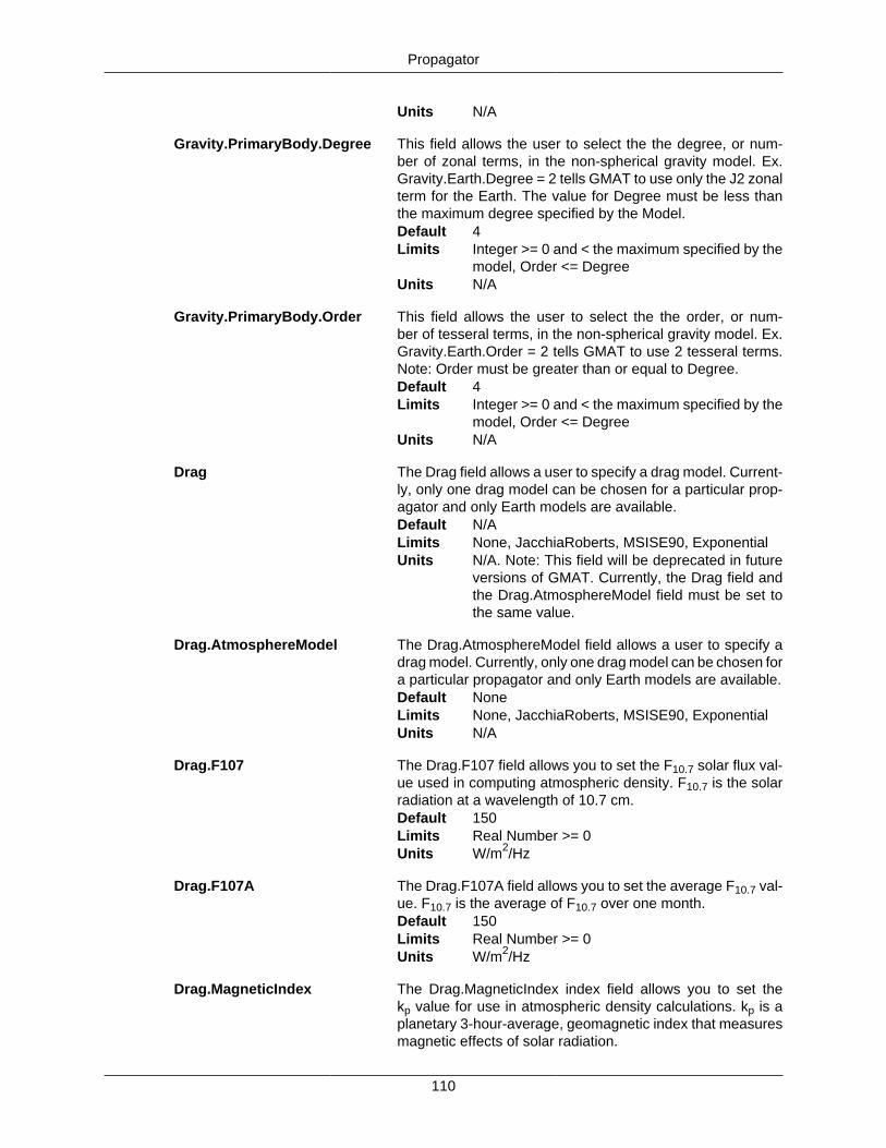
Propagator
110
Units N/A
Gravity.PrimaryBody.Degree This field allows the user to select the the degree, or num-ber of zonal terms, in the non-spherical gravity model. Ex.Gravity.Earth.Degree = 2 tells GMAT to use only the J2 zonalterm for the Earth. The value for Degree must be less thanthe maximum degree specified by the Model.Default 4Limits Integer >= 0 and < the maximum specified by the
model, Order <= DegreeUnits N/A
Gravity.PrimaryBody.Order This field allows the user to select the the order, or num-ber of tesseral terms, in the non-spherical gravity model. Ex.Gravity.Earth.Order = 2 tells GMAT to use 2 tesseral terms.Note: Order must be greater than or equal to Degree.Default 4Limits Integer >= 0 and < the maximum specified by the
model, Order <= DegreeUnits N/A
Drag The Drag field allows a user to specify a drag model. Current-ly, only one drag model can be chosen for a particular prop-agator and only Earth models are available.Default N/ALimits None, JacchiaRoberts, MSISE90, ExponentialUnits N/A. Note: This field will be deprecated in future
versions of GMAT. Currently, the Drag field andthe Drag.AtmosphereModel field must be set tothe same value.
Drag.AtmosphereModel The Drag.AtmosphereModel field allows a user to specify adrag model. Currently, only one drag model can be chosen fora particular propagator and only Earth models are available.Default NoneLimits None, JacchiaRoberts, MSISE90, ExponentialUnits N/A
Drag.F107 The Drag.F107 field allows you to set the F10.7 solar flux val-ue used in computing atmospheric density. F10.7 is the solarradiation at a wavelength of 10.7 cm.Default 150Limits Real Number >= 0Units W/m2/Hz
Drag.F107A The Drag.F107A field allows you to set the average F10.7 val-ue. F10.7 is the average of F10.7 over one month.Default 150Limits Real Number >= 0Units W/m2/Hz
Drag.MagneticIndex The Drag.MagneticIndex index field allows you to set thekp value for use in atmospheric density calculations. kp is aplanetary 3-hour-average, geomagnetic index that measuresmagnetic effects of solar radiation.
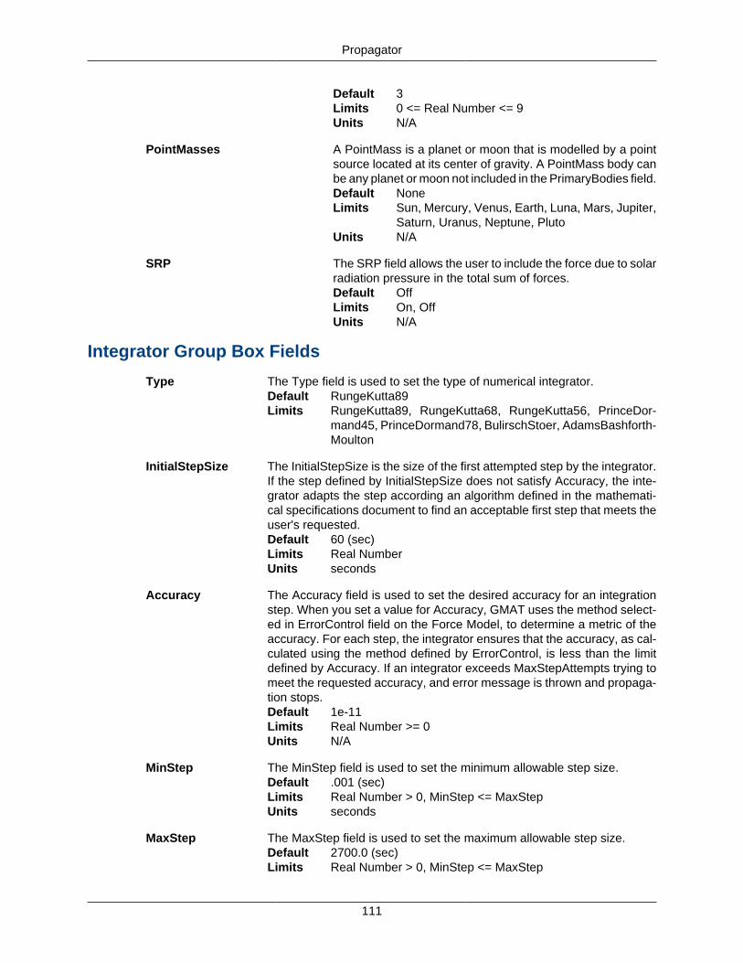
Propagator
111
Default 3Limits 0 <= Real Number <= 9Units N/A
PointMasses A PointMass is a planet or moon that is modelled by a pointsource located at its center of gravity. A PointMass body canbe any planet or moon not included in the PrimaryBodies field.Default NoneLimits Sun, Mercury, Venus, Earth, Luna, Mars, Jupiter,
Saturn, Uranus, Neptune, PlutoUnits N/A
SRP The SRP field allows the user to include the force due to solarradiation pressure in the total sum of forces.Default OffLimits On, OffUnits N/A
Integrator Group Box Fields
Type The Type field is used to set the type of numerical integrator.Default RungeKutta89Limits RungeKutta89, RungeKutta68, RungeKutta56, PrinceDor-
mand45, PrinceDormand78, BulirschStoer, AdamsBashforth-Moulton
InitialStepSize The InitialStepSize is the size of the first attempted step by the integrator.If the step defined by InitialStepSize does not satisfy Accuracy, the inte-grator adapts the step according an algorithm defined in the mathemati-cal specifications document to find an acceptable first step that meets theuser's requested.Default 60 (sec)Limits Real NumberUnits seconds
Accuracy The Accuracy field is used to set the desired accuracy for an integrationstep. When you set a value for Accuracy, GMAT uses the method select-ed in ErrorControl field on the Force Model, to determine a metric of theaccuracy. For each step, the integrator ensures that the accuracy, as cal-culated using the method defined by ErrorControl, is less than the limitdefined by Accuracy. If an integrator exceeds MaxStepAttempts trying tomeet the requested accuracy, and error message is thrown and propaga-tion stops.Default 1e-11Limits Real Number >= 0Units N/A
MinStep The MinStep field is used to set the minimum allowable step size.Default .001 (sec)Limits Real Number > 0, MinStep <= MaxStepUnits seconds
MaxStep The MaxStep field is used to set the maximum allowable step size.Default 2700.0 (sec)Limits Real Number > 0, MinStep <= MaxStep
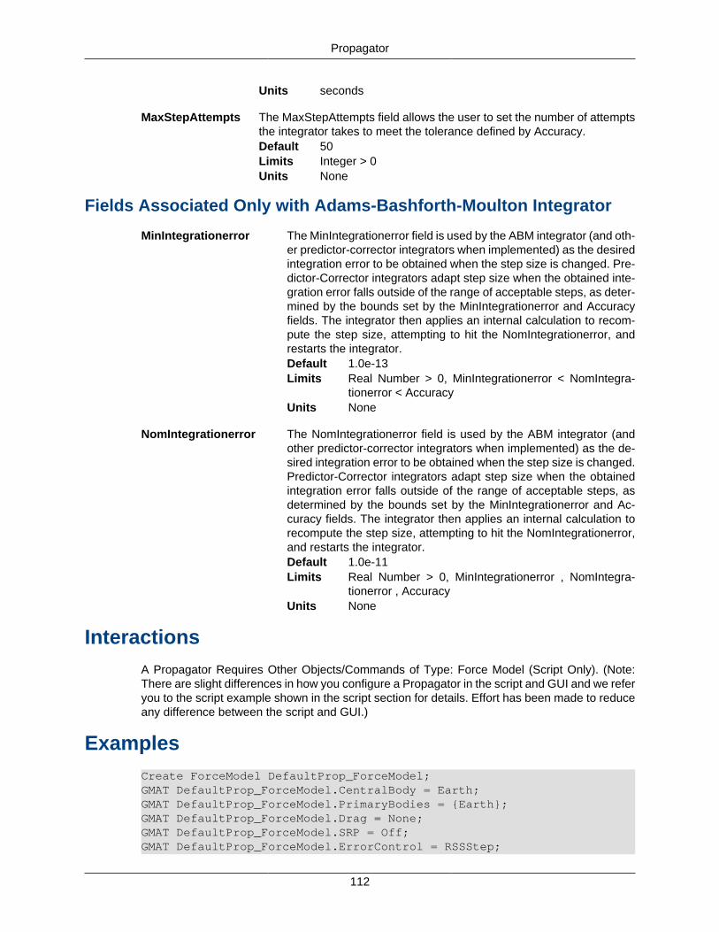
Propagator
112
Units seconds
MaxStepAttempts The MaxStepAttempts field allows the user to set the number of attemptsthe integrator takes to meet the tolerance defined by Accuracy.Default 50Limits Integer > 0Units None
Fields Associated Only with Adams-Bashforth-Moulton Integrator
MinIntegrationerror The MinIntegrationerror field is used by the ABM integrator (and oth-er predictor-corrector integrators when implemented) as the desiredintegration error to be obtained when the step size is changed. Pre-dictor-Corrector integrators adapt step size when the obtained inte-gration error falls outside of the range of acceptable steps, as deter-mined by the bounds set by the MinIntegrationerror and Accuracyfields. The integrator then applies an internal calculation to recom-pute the step size, attempting to hit the NomIntegrationerror, andrestarts the integrator.Default 1.0e-13Limits Real Number > 0, MinIntegrationerror < NomIntegra-
tionerror < AccuracyUnits None
NomIntegrationerror The NomIntegrationerror field is used by the ABM integrator (andother predictor-corrector integrators when implemented) as the de-sired integration error to be obtained when the step size is changed.Predictor-Corrector integrators adapt step size when the obtainedintegration error falls outside of the range of acceptable steps, asdetermined by the bounds set by the MinIntegrationerror and Ac-curacy fields. The integrator then applies an internal calculation torecompute the step size, attempting to hit the NomIntegrationerror,and restarts the integrator.Default 1.0e-11Limits Real Number > 0, MinIntegrationerror , NomIntegra-
tionerror , AccuracyUnits None
InteractionsA Propagator Requires Other Objects/Commands of Type: Force Model (Script Only). (Note:There are slight differences in how you configure a Propagator in the script and GUI and we referyou to the script example shown in the script section for details. Effort has been made to reduceany difference between the script and GUI.)
ExamplesCreate ForceModel DefaultProp_ForceModel;GMAT DefaultProp_ForceModel.CentralBody = Earth;GMAT DefaultProp_ForceModel.PrimaryBodies = {Earth};GMAT DefaultProp_ForceModel.Drag = None;GMAT DefaultProp_ForceModel.SRP = Off;GMAT DefaultProp_ForceModel.ErrorControl = RSSStep;
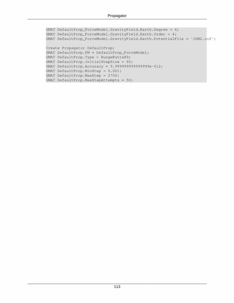
Propagator
113
GMAT DefaultProp_ForceModel.GravityField.Earth.Degree = 4;GMAT DefaultProp_ForceModel.GravityField.Earth.Order = 4;GMAT DefaultProp_ForceModel.GravityField.Earth.PotentialFile = 'JGM2.cof';
Create Propagator DefaultProp;GMAT DefaultProp.FM = DefaultProp_ForceModel;GMAT DefaultProp.Type = RungeKutta89;GMAT DefaultProp.InitialStepSize = 60;GMAT DefaultProp.Accuracy = 9.999999999999999e-012;GMAT DefaultProp.MinStep = 0.001;GMAT DefaultProp.MaxStep = 2700;GMAT DefaultProp.MaxStepAttempts = 50;
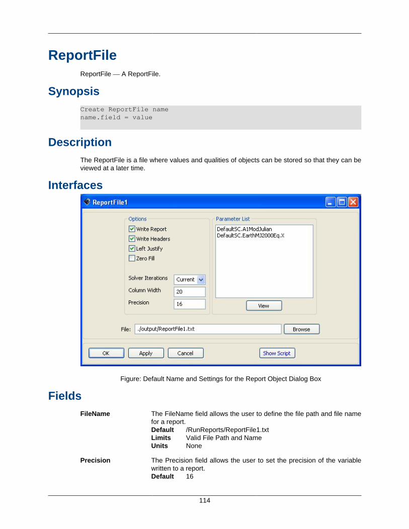
114
ReportFileReportFile — A ReportFile.
SynopsisCreate ReportFile namename.field = value
DescriptionThe ReportFile is a file where values and qualities of objects can be stored so that they can beviewed at a later time.
Interfaces
Figure: Default Name and Settings for the Report Object Dialog Box
FieldsFileName The FileName field allows the user to define the file path and file name
for a report.Default /RunReports/ReportFile1.txtLimits Valid File Path and NameUnits None
Precision The Precision field allows the user to set the precision of the variablewritten to a report.Default 16
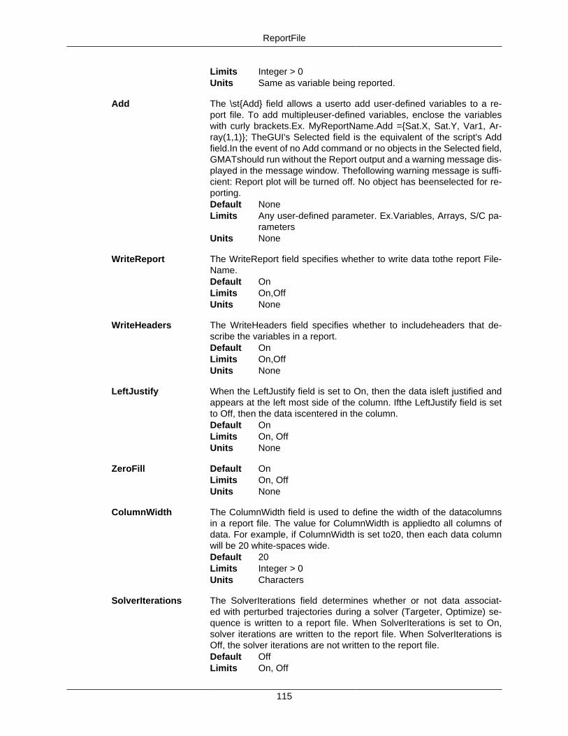
ReportFile
115
Limits Integer > 0Units Same as variable being reported.
Add The \st{Add} field allows a userto add user-defined variables to a re-port file. To add multipleuser-defined variables, enclose the variableswith curly brackets.Ex. MyReportName.Add ={Sat.X, Sat.Y, Var1, Ar-ray(1,1)}; TheGUI's Selected field is the equivalent of the script's Addfield.In the event of no Add command or no objects in the Selected field,GMATshould run without the Report output and a warning message dis-played in the message window. Thefollowing warning message is suffi-cient: Report plot will be turned off. No object has beenselected for re-porting.Default NoneLimits Any user-defined parameter. Ex.Variables, Arrays, S/C pa-
rametersUnits None
WriteReport The WriteReport field specifies whether to write data tothe report File-Name.Default OnLimits On,OffUnits None
WriteHeaders The WriteHeaders field specifies whether to includeheaders that de-scribe the variables in a report.Default OnLimits On,OffUnits None
LeftJustify When the LeftJustify field is set to On, then the data isleft justified andappears at the left most side of the column. Ifthe LeftJustify field is setto Off, then the data iscentered in the column.Default OnLimits On, OffUnits None
ZeroFill Default OnLimits On, OffUnits None
ColumnWidth The ColumnWidth field is used to define the width of the datacolumnsin a report file. The value for ColumnWidth is appliedto all columns ofdata. For example, if ColumnWidth is set to20, then each data columnwill be 20 white-spaces wide.Default 20Limits Integer > 0Units Characters
SolverIterations The SolverIterations field determines whether or not data associat-ed with perturbed trajectories during a solver (Targeter, Optimize) se-quence is written to a report file. When SolverIterations is set to On,solver iterations are written to the report file. When SolverIterations isOff, the solver iterations are not written to the report file.Default OffLimits On, Off
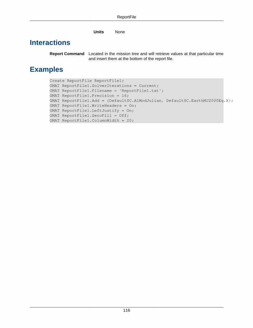
ReportFile
116
Units None
InteractionsReport Command Located in the mission tree and will retrieve values at that particular time
and insert them at the bottom of the report file.
ExamplesCreate ReportFile ReportFile1;GMAT ReportFile1.SolverIterations = Current;GMAT ReportFile1.Filename = 'ReportFile1.txt';GMAT ReportFile1.Precision = 16;GMAT ReportFile1.Add = {DefaultSC.A1ModJulian, DefaultSC.EarthMJ2000Eq.X};GMAT ReportFile1.WriteHeaders = On;GMAT ReportFile1.LeftJustify = On;GMAT ReportFile1.ZeroFill = Off;GMAT ReportFile1.ColumnWidth = 20;

117
SolarSystemSolar System — A solar system.
SynopsisCreate SolarSystem namename.field = value
DescriptionThis folder, found if the Solar System folder itself is double-clicked, enables the user to determinewhere he gets his data on the movements of planets, how often it updates, and how accuratethe data is.
FieldsEphemerisSource The EphemerisSourcefield allows the user to select the
source used for planetaryephemerides. The source is usedglobally whenever planetaryephemeris information is re-quired.Default DE405Limits DE405,DE200, SLP, AnalyticUnits None
Ephemeris UpdateInterval The EphemerisUpdateInterval is used to set howoftenplanetary positions are updated when calculat-ing accelerationsduring propagation. For low-Earthorbits,EphemerisUpdateInterval can be set to around60 for fasternumerical integration with little effecton the accuracy of thepropagation. For deep spacepropagation,EphemerisUpdateInterval should be set to zero.Default 0Limits Real Number ≥ 0Units sec
UseTTForEphemeris GMAT uses time in the TDB system as thedefault time sys-tem in the JPL ephemeris files. However, often itis possibleto use time in the TT time system, without significantdiffer-ence in propagation accuracy. (TT and TDB are within 1mil-lisecond of each other). The advantage to using TT is thatitavoids the transformation from TT to TDB and therefore or-bitpropagation will execute faster. The UseTTForEphemerisfieldallows the user to choose between the default of TDBin theephemeris files (UseTTForEphemeris=false), or TT intheephemeris files (UseTTForEphemeris = true).Default falseLimits true, falseUnits None
EphemerisFile The EphemerisFile field allows the user to specify the locatio-nand name of the file for each type of ephemeris GMAT sup-
SolarSystem
118
ports. Forexample, if Ephemeris is set to DE405, you can setthepath for a DE405 file using SolarSystem.EphemerisFile=c:/MyPath/MyDE405.file.Default Same as startup file.Limits Filepath and file name consistent with operating
systemUnits None
AnalyticModel Default LowFidelityLimits LowFidelityUnits None
InteractionsCelestialBodies, BaryCenter,and Libration Point
The position and data on all these depend on the source ofthe Solar System data and how often it is updated.
Propagator How often the position of the planetary bodies are updatedwill have an impact on how a spacecraft will propagate.
Spacecraft A number of parameters of a spacecraft are based off theposition of the planets

119
SpacecraftSpacecraft — A spacecraft
SynopsisCreate Spacecraft namename.field = value…
Description
A Spacecraft resource contains information about the spacecraft's orbit, its attitude, its physicalparameters (such as mass and drag coefficient), and any attached hardware, including thrustersand fuel tanks. It also contains information about the visual model used to represent it in anOrbitView.
Fields
Epoch
DateFormat The entry format and time system of the Epoch field.
Caution
The definition of the modified Julian date is not the same as othersoftware. Most software uses the Smithsonian Astrophysical Ob-servatory definition of 1957, where JD is the full Julian date:
MJD = JD - 2400000.5
GMAT, however, uses the following definition:
MJD = JD - 2430000.0
Value Description
A1Gregorian A.1 time scale, Gregorian format ("DDMMM YYYY hh:mm:ss.ddd")
A1ModJulian A.1 time scale, modified Julian format
TAIGregorian TAI time scale
TAIModJulian Default
TTGregorian TT time scale
TTModJulian
UTCGregorian UTC time scale
Spacecraft
120
Value Description
UTCModJulian
Epoch The initial epoch of the spacecraft's state and properties.Type stringDefault 21545 (TAIModJulian format)Limits 04 Oct 1957 12:00:00.000 or later in all time systems (6116.0
modified Julian)Units days (modified Julian format only)
Orbit
CoordinateSystem The Coordinate System field allows the user to choose which coordinatesystem with which to define the orbit state vector. The Coordinate Sys-tem field has a dependency upon the State Type field. If the coordinatesystem chosen by the user does not have a gravitational body at the ori-gin, then the state types Keplerian, ModifiedKeplerian, and Equinoctialare not permitted. This is because these state types require a µ value.Type enumerationValues • EarthMJ2000Eq (default)
• EarthMJ2000Ec
• EarthFixed
• any user-defined coordinate system
DisplayStateType The State Type field allows the user to configure the type of state vectorthat they wish to use. The State Type field has a dependency upon theCoordinate System field. If the coordinate system chosen by the userdoes not have a gravitational body at the origin, then the state typesKeplerian, ModifiedKeplerian, and Equinoctial are not permitted. This isbecause these state types require a µ value.Type enumerationValues • Cartesian (default)
• Keplerian
• ModifiedKeplerian
• SphericalAZFPA
• SphericalRADEC
• Equinoctial
Cartesian State
X X is the x-component of the Spacecraft state in the coordinate system chosen in the Space-craft Coordinate System field.Type real numberDefault 7100LimitsUnits km
Y Y is the y-component of the Spacecraft state in the coordinate system chosen in the Space-craft Coordinate System field.Type real numberDefault 0LimitsUnits km
Spacecraft
121
Z Z is the z-component of the Spacecraft state in the coordinate system chosen in the Space-craft Coordinate System field.Type real numberDefault 1300LimitsUnits km
VX VX is the x-component of the Spacecraft velocity in the coordinate system chosen in theSpacecraft Coordinate System field.Type real numberDefault 0LimitsUnits km
VY VY is the y-component of the Spacecraft velocity in the coordinate system chosen in theSpacecraft Coordinate System field.Type real numberDefault 7.35LimitsUnits km
VZ VZ is the z-component of the Spacecraft velocity in the coordinate system chosen in theSpacecraft Coordinate System field.Type real numberDefault 1LimitsUnits km
Keplerian State
SMA The SMA field is the spacecraft orbit's osculating Keplerian semimajor axis in the coor-dinate system chosen in the Spacecraft Coordinate System field. SMA must be strictlygreater than 1 m or less than -1 m to avoid numerical issues in the conversions to otherstate types. For circular and elliptical orbits ( 0 <= ECC < 0.9999999 ) SMA should onlybe greater than 1 m and for hyperbolic orbits (ECC > 1.0000001) SMA should be lessthan -1 m. GMAT does not support the creation of parabolic orbits.Type real numberDefaultLimits |SMA| > 1e-3 kmUnits km
ECC The ECC field is the spacecraft orbit's osculating eccentricity. For circular or elliptic orbits,ECC must be greater than or equal to 0.0, and less than or equal to 0.9999999 to avoidnumerical issues in the conversion to other state types as the Keplerian elements areundefined for parabolic orbits. For hyperbolic orbits ECC must be greater than or equalto 1.0000001. See also the SMA description.Type real numberDefaultLimits 0.0 <= ECC <= 0.9999999 or ECC >= 1.0000001Units none
INC The INC field is the spacecraft orbit's osculating inclination, in degrees, with respect tothe selected coordinate system.Type real number
Spacecraft
122
DefaultLimitsUnits degrees
RAAN The RAAN field is the spacecraft orbit's osculating right ascension of the ascending node,in degrees, with respect to the selected coordinate system.Type real numberDefaultLimitsUnits degrees
AOP The AOP field is the spacecraft orbit's osculating argument of periapsis, in degrees, withrespect to the selected coordinate system.Type real numberDefaultLimitsUnits degrees
TA The TA field is the spacecraft orbit's osculating true anomaly.Type real numberDefaultLimitsUnits degrees
ModifiedKeplerian State
RadPer The RadPer field is the spacecraft orbit's osculating radius of periapsis. RadPer mustbe greater than zero.
Type real number
Default
Limits RadPer > 0
Units km
RadApo The RadApo field is the spacecraft orbit's osculating radius of apoapsis. RadApo mustbe strictly greater than or less than zero. When RadApo is negative, the orbit is hy-perbolic.
Type real number
Default
Limits
Units km
INC See the the section called “Keplerian State” section for a description of this field.
RAAN See the the section called “Keplerian State” section for a description of this field.
AOP See the the section called “Keplerian State” section for a description of this field.
TA See the the section called “Keplerian State” section for a description of this field.
Spacecraft
123
SphericalAZFPA State
RMAG The RMAG field allows the user to set the magnitude of the spacecraft's position vector.
Type real number
Default
Limits
Units km
RA The RA field allows the user to set the spacecraft's right ascension.
Type real number
Default
Limits
Units degrees
DEC The DEC field allows the user to set the spacecraft's declination.
Type real number
Default
Limits
Units degrees
VMAG The VMAG field allows the user to set the magnitude of the spacecraft's velocity.
Type real number
Default
Limits VMAG >= 0
Units
AZI The AZI field allows the user to set the spacecraft's azimuth angle.
Type real number
Default
Limits
Units degrees
FPA The FPA allows the user to set a spacecraft's flight path angle.
Type real number
Default
Limits

Spacecraft
124
Units degrees
Examples
Example 9. Creating a default Spacecraft
Create Spacecraft sc;
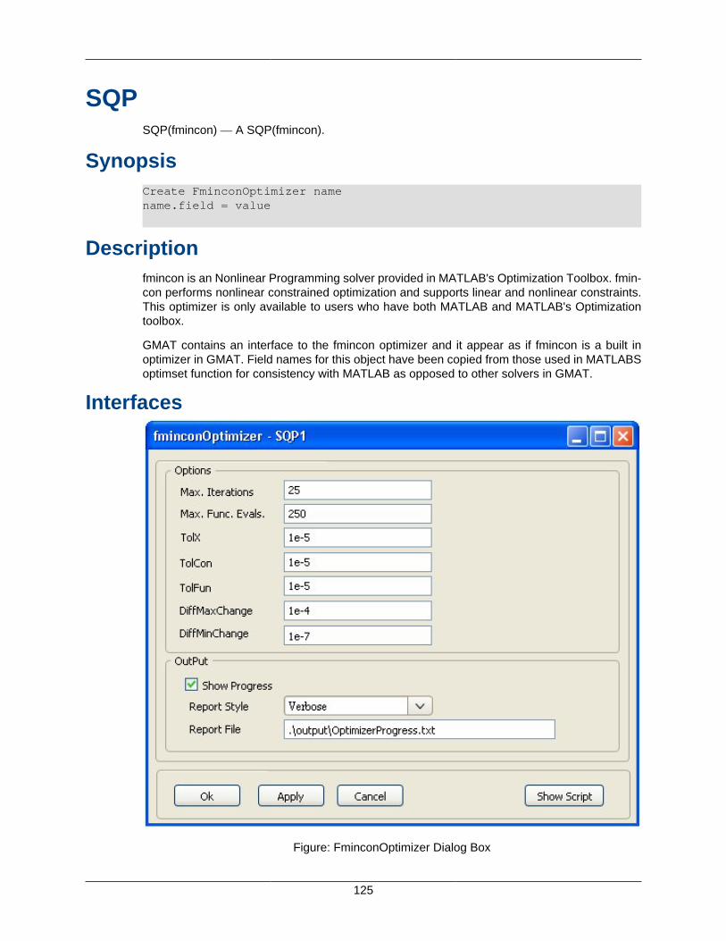
125
SQPSQP(fmincon) — A SQP(fmincon).
SynopsisCreate FminconOptimizer namename.field = value
Descriptionfmincon is an Nonlinear Programming solver provided in MATLAB's Optimization Toolbox. fmin-con performs nonlinear constrained optimization and supports linear and nonlinear constraints.This optimizer is only available to users who have both MATLAB and MATLAB's Optimizationtoolbox.
GMAT contains an interface to the fmincon optimizer and it appear as if fmincon is a built inoptimizer in GMAT. Field names for this object have been copied from those used in MATLABSoptimset function for consistency with MATLAB as opposed to other solvers in GMAT.
Interfaces
Figure: FminconOptimizer Dialog Box
SQP
126
FieldsDiffMax Change The DiffMaxChange parameter is the upper limit on the perturbation used
in MATLAB's finite differencing algorithm. For fmincon, you don't specify asingle perturbation value, but rather give MATLAB a range, and it uses anadaptive algorithm that attempts to find the optimal perturbation.Default 0.1Limits Real Number > 0Units None
DiffMin Change The DiffMinChange parameter is the lower limit on the perturbation usedin MATLAB's finite differencing algorithm. For fmincon, you don't specify asingle perturbation value, but rather give MATLAB a range, and it uses anadaptive algorithm that attempts to find the optimal perturbatin.Default 1e-8Limits Real Number > 0Units None
MaxFunEvals The MaxFunEvals parameter allows the user to set the maximum numberof cost function evaluations in an attempt to find an optimal solution. This isequivalent to setting the maximum number of passes through an optimiza-tion loop in a GMAT script. If a solution is not found before the maximumfunction evaluations, fmincon outputs an ExitFlag of zero, and GMAT con-tinues.Default 1000Limits Integer > 0Units None
MaxIter The MaxIter parameter allows the user to set the maximum allowable num-ber of optimizer iterations. Depending upon the nature of the problem, andwhether gradients are provided, it may take many function evaluations foreach optimizer iteration. The MaxIter parameter allows the user to controlthe maximum function evaluations, and maximum iterations independently.Default 400Limits Integer > 0Units None
TolX The TolX parameter is the termination toler-ance on the vector of indepen-dent variables, and is used only if the user sets a value.Default 1e-4Limits Real Number > 0Units None
TolFun The TolFun parameter is the convergence tolerance on the cost functionvalue.Default 1e-4Limits Real Number > 0Units None
TolCon The TolCon parameter is the convergence tolerance on the constraint func-tions.Default 1e-4Limits Real Number > 0Units None
SQP
127
ShowProgress The ShowProgress field determines whether data pertaining to iterationsof the solver is displayed in the message window. When ShowProgress istrue, the amount of information contained in the message window is con-trolled by the ReportSytle field.Default trueLimits true, falseUnits None
ReportStyle The ReportStyel field determines the amount and type of data written tothe message window for each iteration of the solver (When ShowProgressis true). ADD DESCRIPTIONS OF CONCISE,VERBOSE, ADN NORMAL.I CAN'T RUN THE OPTIMIZER RIGHT NOW SO I CAN'T TELL WHATEACH SETTING DOES.Default NormalLimits Normal, Concise, Verbose, DebugUnits None
ReportFile The ReportFile field contains the path and file name of the report file.Default NormalLimits .\output\OptimizerData.txtUnits None
Using an fminconOptimizer• Optimize Command
• Minimize
• Nonlinear Constraint
ExamplesCreate FminconOptimizer SQP1;GMAT SQP1.MaxIter = 25;GMAT SQP1.MaxFunEvals = 250;GMAT SQP1.TolX = 1e-5;GMAT SQP1.TolFun = 1e-5;GMAT SQP1.TolCon = 1e-5;GMAT SQP1.DiffMaxChange = 1e-4;GMAT SQP1.DiffMinChange = 1e-7;GMAT SQP1.ShowProgress = true;GMAT SQP1.ReportStyle = 'Verbose';GMAT SQP1.ReportFile = '\output\OptimizerProgress.txt';
128
StringString — A string.
SynopsisCreate String namename.field = value
DescriptionThis page will show you how to create and use String objects. Stings are useful for storing char-acters as a set. One possible use of them is to report back a specific message at a set pointin the mission sequence.
InteractionsReportFile You may add a string to the Parameter List in the Report Object dialog box
via the ParameterSelectDialog box.
Report Command Alternatively, you may add a string to the Parameter List in the Report Com-mand dialog box
Using the Script
Script Syntax
GMAT String Name = String;
Script Examples
% The following is an example String declarationGMAT Example = hello world;

129
ThrusterThruster — A thruster.
SynopsisCreate Thruster namename.field = value
DescriptionThe Thruster uses the fuel tank and directs the thrust of the rocket engine while in space. It isused for finite burns.
FieldsCoordinateSystem The CoordinateSystem field for a thrusterdetermines what coordi-
nate system the orientation parametersX_Direction, Y_Direction, andZ_Direction arereferenced to. This is a temporary fix in GMAT.Eventually, theuser will specify the attitude of aspacecraft, and thenX_Direction, Y_Direction, and Z_Direction will be referenced to thespacecraft body frame.Default EarthMJ2000EqLimits EarthMJ2000Eq, EarthMJ2000Ec, EarthMJ2000Eq, or
anyuser defined system
Axis The Axis field allows the user to define a localcoordinate system fora thruster. Note that there is a couplingbetween the Axis parameterand the CoordinateSystemparameter for a thruster. Only one of the twocanbe specified.Default VNBLimits InertialVNBUnits None
Origin The Origin fieldallows the user to define a local origin for a thruster.Note thatthere is a coupling between the Origin parameter and theCo-ordinateSystem parameter for a thruster. Only one of the twocan bespecified.Default EarthLimits Sun, Mercury, Venus, Earth, Luna, Mars,Jupiter, Saturn,
Uranus, Neptune, PlutoUnits None
X_Direction X_Direction, divided by the RSS of the three directioncomponents,forms the x direction of the spacecraft thrust vector direction.Default 1Limits Real Number
Y_Direction Y_Direction, divided by the RSS of the three directioncomponents,forms the y direction of the spacecraft thrust vector direction.Default 0

Thruster
130
Limits Real Number
Z_Direction Z_Direction, divided by the RSS of the three directioncomponents,forms the z direction of the spacecraft thrust vector direction.Default 0Limits Real Number
ThrustScaleFactor ThrustScaleFactor is a scale factor that is multiplied by the thrust vec-tor for a given thruster, before the thrust vector is added into the totalaccleration.Default 1Limits Real Number > 0Units None
Tank The Tank field specifies which tank the thruster draws propellant from.
The constants Ci below are used in the following equation to calculatethrust FT as a function of pressure P and temperature TDefault NoneLimits Tank NameUnits FT(P,T) = {C1+C2P+C3P2+C4PC5+C6PC7+C8PC9
+C10C11C12P}(T/Tref)
1+C13+C14P
C1 Thrust coefficient.Default 500Limits Real NumberUnits N
C2 Thrust coefficient.Default 0Limits Real NumberUnits N/kPa
C3 Thrust coefficient.Default 0Limits Real NumberUnits N/kPa
C4 Thrust coefficient.Default 0Limits Real NumberUnits N/kPaC5
C5 Thrust coefficient.Default 0Limits Real NumberUnits None
C6 Thrust coefficient.Default 0Limits Real NumberUnits N/kPaC7
C7 Thrust coefficient.Default 0Limits Real Number
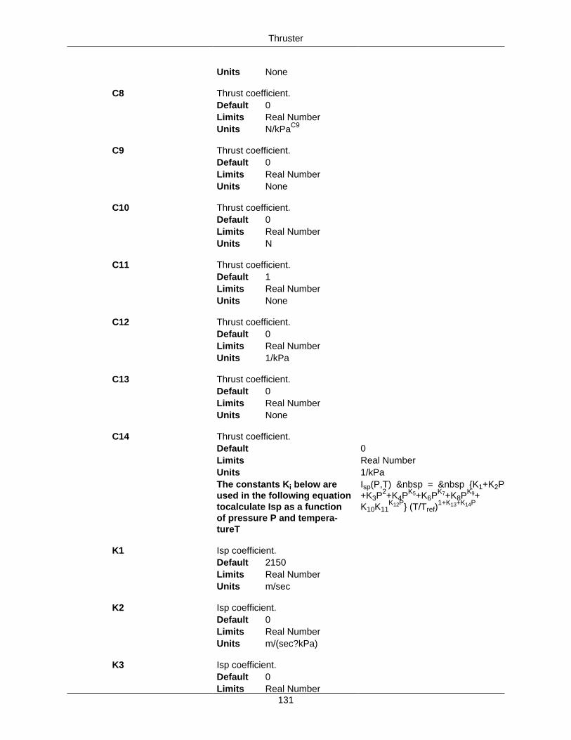
Thruster
131
Units None
C8 Thrust coefficient.Default 0Limits Real NumberUnits N/kPaC9
C9 Thrust coefficient.Default 0Limits Real NumberUnits None
C10 Thrust coefficient.Default 0Limits Real NumberUnits N
C11 Thrust coefficient.Default 1Limits Real NumberUnits None
C12 Thrust coefficient.Default 0Limits Real NumberUnits 1/kPa
C13 Thrust coefficient.Default 0Limits Real NumberUnits None
C14 Thrust coefficient.Default 0Limits Real NumberUnits 1/kPaThe constants Ki below areused in the following equationtocalculate Isp as a functionof pressure P and tempera-tureT
Isp(P,T)   =   {K1+K2P+K3P2+K4PK5+K6PK7+K8PK9+K10K11
K12P} (T/Tref)1+K13+K14P
K1 Isp coefficient.Default 2150Limits Real NumberUnits m/sec
K2 Isp coefficient.Default 0Limits Real NumberUnits m/(sec?kPa)
K3 Isp coefficient.Default 0Limits Real Number
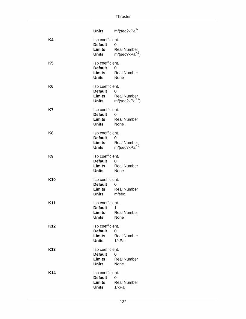
Thruster
132
Units m/(sec?kPa2)
K4 Isp coefficient.Default 0Limits Real NumberUnits m/(sec?kPaK5)
K5 Isp coefficient.Default 0Limits Real NumberUnits None
K6 Isp coefficient.Default 0Limits Real NumberUnits m/(sec?kPaK7)
K7 Isp coefficient.Default 0Limits Real NumberUnits None
K8 Isp coefficient.Default 0Limits Real NumberUnits m/(sec?kPaK9
K9 Isp coefficient.Default 0Limits Real NumberUnits None
K10 Isp coefficient.Default 0Limits Real NumberUnits m/sec
K11 Isp coefficient.Default 1Limits Real NumberUnits None
K12 Isp coefficient.Default 0Limits Real NumberUnits 1/kPa
K13 Isp coefficient.Default 0Limits Real NumberUnits None
K14 Isp coefficient.Default 0Limits Real NumberUnits 1/kPa

Thruster
133
InteractionsBeginFiniteBurn/EndFinite-Burn
These commands use the tank and the thruster to start a finiteburn, where the delta V is not instantaneous.
Fuel Tank This object contains the fuel used to power the thruster andsubsequently the finite burn.
FiniteBurn This takes the parameters of the tank and the thruster andapply it to a coordinate system, with a scaling method avail-able if wanted.
Spacecraft This is the object that the burn is applied to.
Script ExamplesCreate Thruster Thruster1;GMAT Thruster1.Element1 = 1;GMAT Thruster1.Element2 = 0;GMAT Thruster1.Element3 = 0;GMAT Thruster1.C1 = 500;GMAT Thruster1.C2 = 0;GMAT Thruster1.C3 = 0;GMAT Thruster1.C4 = 0;GMAT Thruster1.C5 = 0;GMAT Thruster1.C6 = 0;GMAT Thruster1.C7 = 0;GMAT Thruster1.C8 = 0;GMAT Thruster1.C9 = 0;GMAT Thruster1.C10 = 0;GMAT Thruster1.C11 = 1;GMAT Thruster1.C12 = 0;GMAT Thruster1.C13 = 0;GMAT Thruster1.C14 = 0;GMAT Thruster1.K1 = 2150;GMAT Thruster1.K2 = 0;GMAT Thruster1.K3 = 0;GMAT Thruster1.K4 = 0;GMAT Thruster1.K5 = 0;GMAT Thruster1.K6 = 0;GMAT Thruster1.K7 = 0;GMAT Thruster1.K8 = 0;GMAT Thruster1.K9 = 0;GMAT Thruster1.K10 = 0;GMAT Thruster1.K11 = 1;GMAT Thruster1.K12 = 0;GMAT Thruster1.K13 = 0;GMAT Thruster1.K14 = 0;GMAT Thruster1.CoordinateSystem = 'MJ2000EarthEquator';GMAT Thruster1.ThrustScaleFactor = 1;

134
VariableVariable — A variable.
SynopsisCreate Variable namename = value
DescriptionThe Variable object allows you to create and name a variable and assign to it a real numbervalue. A variable can be used in numerous commands which allows you to customize the mis-sion sequence to your application. In the simplest case, a variable can be defined by a simpleassignment to a numeric literal. In more complex cases, a variable can be defined using an as-signment that contains a complicated mathematical expression.
Interfaces
Figure: Parameter Create Dialog Box
Interactions• Spacecraft Object
• Report Command
• Equation Command
• Vary Command
• Achieve Command
• Minimize Command
ExamplesCreate Variable pi Energy mu SMA
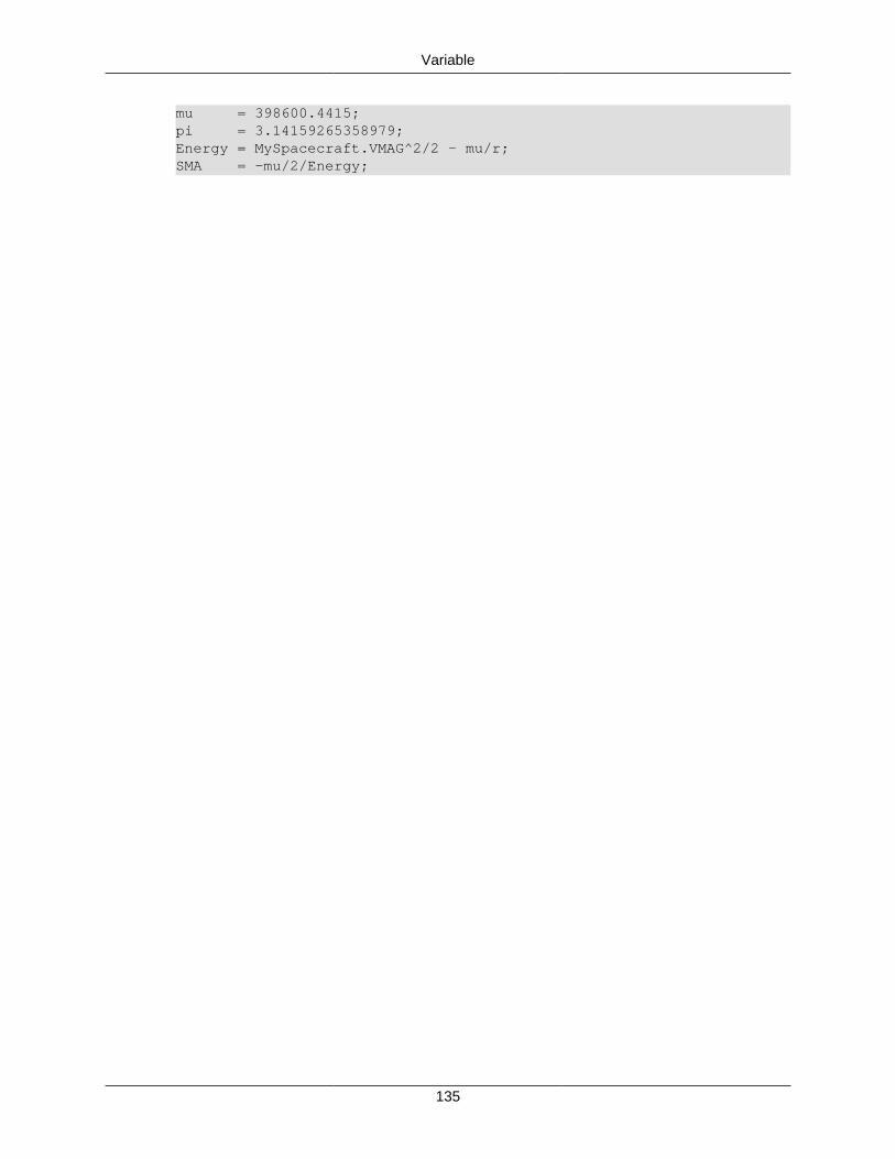
Variable
135
mu = 398600.4415;pi = 3.14159265358979;Energy = MySpacecraft.VMAG^2/2 - mu/r; SMA = -mu/2/Energy;
136
VF13adOptimizerVF13adOptimizer — Under Construction.
Synopsis Under Construction.
DescriptionUnder Construction.
FieldsField Name Description....
Type Fill This In.Default Fill This In.Limits Fill This In.Units Fill This In.
Examples
Example 10. Example Script
%
137
XYPlotXY Plot — A XY Plot.
SynopsisCreate XYPlot namename.field = value
DescriptionThe XY Plot is a graph under the Plots/Reports folder in the resource tree that plots data ontothe X and Y axes of the graph. Any two parameters can be chosen to plot from the ParameterSelect dialog box when the View radio button is clicked. The plot has the capability to be turnedon and/or off throughout the mission if desirable.
InteractionsSpacecraft Spacecraft interact with an XY Plot throughout the entire mission. The data
retrieved from the spacecraft, as it carries out the command, is what getsplotted onto the graph.
Toggle Com-mand
A Toggle can be inserted into the mission sequence to control when the XYPlot is to plot data by subscribing it to the Toggle list. If it is necessary toonly plot data at a certain point during the mission, besides at the beginningor end points, then two Toggle commands can be added to switch it onand off.
FieldsIndVar The IndVar field allows the user to define the independent variable for
an xy-plot. Only one variable can be defined as an independent variable.For example, the line MyXYPlot.IndVar = DefaultSC.A1ModJulian setsthe independent variable to be the epoch of DefaultSC in the A1 timesystem and modified Julian format.Default DefaultSC.A1ModJulianLimits Any user variable, array element, or spacecraft parameterUnits None
Add The Add field allows the user to add dependent variables to an xy-plot. All dependent variables are plotted on the y-axisvs the indepen-dent variable defined by IndVar. To define multiple dependent variables,they should be included in curly braces. For example, MyXYPlot.Add =DefaultSC.EarthMJ2000Eq.Y , DefaultSC.EarthMJ2000Eq.Z. The GUI'sSelected field is the equivalent of the script's Add field. In the event of noAdd command or no objects in the Selected field, GMAT should run with-out the XYPlot and a warning message displayed in the message win-dow. The following warning message is sufficient: XYPlot will be turnedoff. No object has been selected for plotting.Default DefaultSC.EarthMJ2000Eq.XLimits Any user variable, array element, or spacecraft parameter
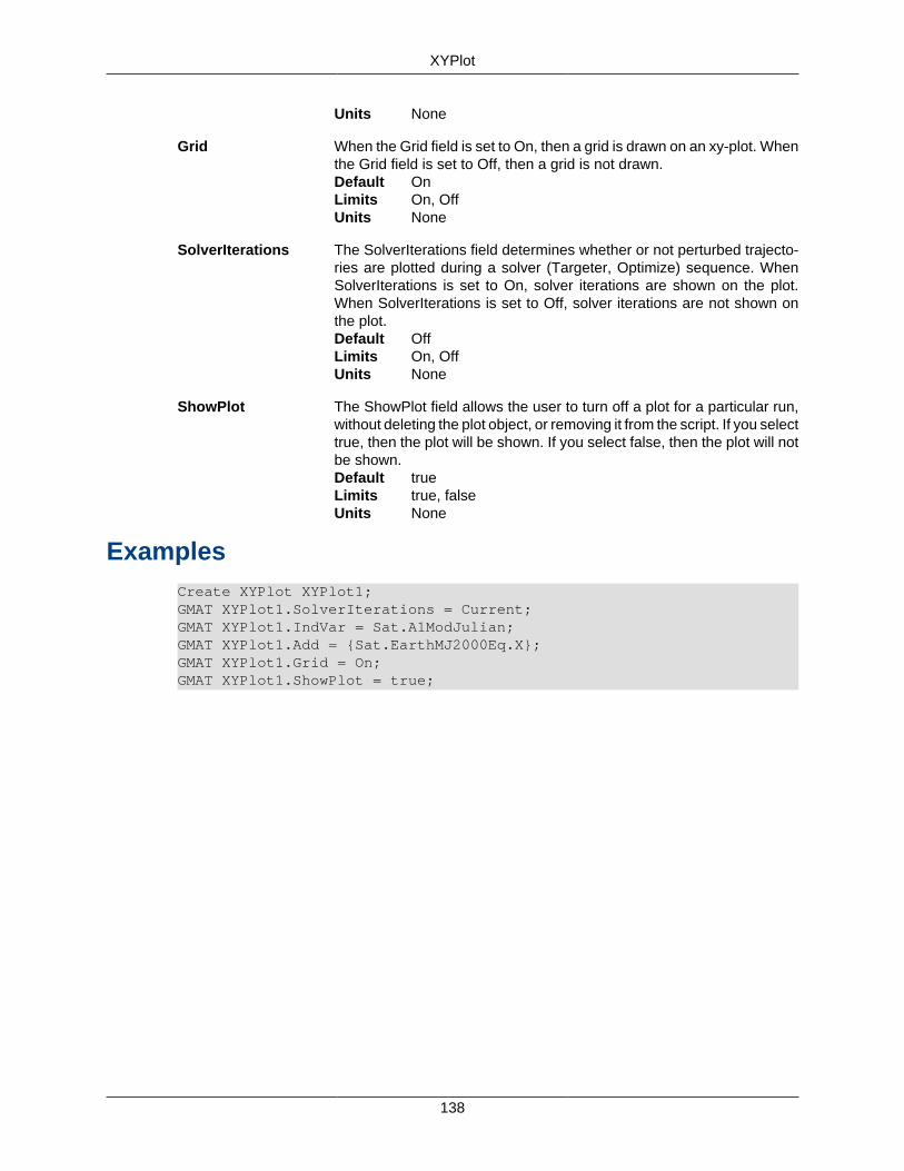
XYPlot
138
Units None
Grid When the Grid field is set to On, then a grid is drawn on an xy-plot. Whenthe Grid field is set to Off, then a grid is not drawn.Default OnLimits On, OffUnits None
SolverIterations The SolverIterations field determines whether or not perturbed trajecto-ries are plotted during a solver (Targeter, Optimize) sequence. WhenSolverIterations is set to On, solver iterations are shown on the plot.When SolverIterations is set to Off, solver iterations are not shown onthe plot.Default OffLimits On, OffUnits None
ShowPlot The ShowPlot field allows the user to turn off a plot for a particular run,without deleting the plot object, or removing it from the script. If you selecttrue, then the plot will be shown. If you select false, then the plot will notbe shown.Default trueLimits true, falseUnits None
ExamplesCreate XYPlot XYPlot1;GMAT XYPlot1.SolverIterations = Current;GMAT XYPlot1.IndVar = Sat.A1ModJulian;GMAT XYPlot1.Add = {Sat.EarthMJ2000Eq.X};GMAT XYPlot1.Grid = On;GMAT XYPlot1.ShowPlot = true;

139
Commands
140
AchieveAchieve — Perform an achieve command
Synopsis
DescriptionThe purpose of the Achieve command is to define a goal for the spacecraft to reach at somepoint in its trajectory. The goal must have a corresponding value and tolerance so the differentialcorrector can solve for the best solution during the spacecraft's flight. To define a goal, a propertymust be chosen out of the Parameter Select dialog box along with the correct components inthe other fields. The command can only be appended within a targeting sequence and must beaccompanied and preceeded by a Vary, Maneuver, and Propagate command.
OptionsGoal The option allows the user to select any single element user defined parameter,
except a number, to Achieve.
Default DefaultSC.Earth.RMAG
Limits Spacecraft parameter, Array element, Variable, or any other singleelement user defined parameter, excluding numbers
Arg1 The Arg1 option is the desired value for after the solver has converged.
Default 42165
Limits Real Number, Array element, Variable, or any user de-fined parameter that obeys the conditions of Chapter~\\ref\{Ch:ObjectsNResources\} for the selected
Units None
Tolerance The Tolerance option sets Arg2. Arg2 is the convergence tolerance for Arg1.
Default 0.1
Limits Real Number, Array element, Variable, or any user defined parame-ter > 0
Units None
SolverName The SolverName option allows the user to choose which solver to assign to theAchieve command.
Default DefaultDC
Limits Any user defined differential corrector
Units None

Achieve
141
ExamplesAchieve SolverName(Goal) = Arg1, Tolerance = Arg2
142
BeginFiniteBurnBeginFiniteBurn — Perform a begin finite burn
Synopsis
DescriptionThe Begin Finite Burn and End Finite Burn commands are very simple. When the Begin FiniteBurn command is entered into the mission sequence it will initiate the thrusters of the spacecraftuntil the End Finite Burn command is reached. After the finite burn is turned off, the spacecraft'sthrusters will shut down.
OptionsManeuverName The ManeuverName option allows the user to choose between any previ-
ously created finite burn. As an example, to maneuver DefaultSC using De-faultFB, the script linewould appear as Manevuer DefaultFB(DefaultSC).
Default DefaultFB
Limits Any finite burn existing in the resource tree or created in thescript
Units None
SpacecraftName The SpacecraftName option allows the user to select which spacecraft tomaneuver using the maneuver selected in the ManeuverName option.
Default DefaultSC
Limits Any spacecraft existing in the resource tree or created in thescript
Units None
ExamplesBeginFiniteBurn ManeuverName (SpacecraftName); EndFiniteBurn DefaultFB(DefaultSC);
143
BeginMissionSequenceBeginMissionSequence — Under construction.
SynopsisUnder construction.
Under construction.Under construction.
Examples
Script Syntax
Under construction.
Script Examples
Under construction.

144
CallFunctionCall Function — Perform a call function
Synopsis
DefinitionGMAT functions are very useful and work nearly the same as they do in most programminglanguages. They may be invoked using the Call Function command covered here.
OptionsOutputList The OutputList option allows the user to set the output of Function to a user
defined parameter.
Default None
Limits Variables, Arrays, S/C, Paramters, any other user-defined parame-ters, or blank. Multiple outputs must be expressed in a comma de-limited list format
Units None
InputList The InputList option allows the user to set the input of Function to a user definedparameter.
Default None
Limits Variables, Arrays, S/C, Paramters, any other user-defined parame-ters, or blank. Multiple inputs must be expressed in a comma delim-ited list format.
Units None
Function The Function option allows the user to set the function that will be called in aspecific location of the mission sequence. The function has to be defined beforeit can be used in the CallFunction Command.
Default None
Limits GMAT of Matlab Function
Units None
Examples
Script Syntax
%Function call with Inputs and OutputsGMAT [OutputList] = Function(InputList)

CallFunction
145
%Function call with Outputs onlyGMAT [OutputList] = Function
%Function call with Inputs onlyGMAT Function(InputList)
Function call with no Inputs or OutputsGMAT Function
Script Examples
% Matlab function call without inputs or outputs
% Syntax 1GMAT clearAll
% Syntax 2GMAT [ ] = clearAll( )

146
ElseElse — Perform an else statement
Synopsis
DescriptionIf-Else statements in GMAT work as they do in other programming languages, especially Matlab.The Else command adds another dimension to an If statement. You use an Else statement whenyou want something to happen when the conditions of an If statement are not met. For example,an If statement who's condition is "x < 5" will only execute the script within its scope when x isindeed less than 5. GMAT would otherwise pass over the If statement's associated script andcontinue. However, having an Else statement after the If will ensure that the lines of script withinthe scope of that Else are executed when x is equal to 5 or greater.
Examples
Script Syntax
If <logical expression>; <Statements>;Else; <Statements>;EndIf;
Script Examples
If DefaultSC.ElapsedDays < 1; Propagate DefaultProp( DefaultSC , { DefaultSC.ElapsedDays = 0.01 });Else; Propagate DefaultProp( DefaultSC , { DefaultSC.ElapsedDays = 0.2 });EndIf;
147
EndFiniteBurnEndFiniteBurn — Under construction.
SynopsisUnder construction.
Under construction.Under construction.
Examples
Script Syntax
Under construction.
Script Examples
Under construction.
148
EquationEquation — Perform an equation command
Synopsis
DescriptionThe Equation command uses the Equation to make one variable equal to some combination ofpreviously defined variables and values. It is highly useful for storing values so that they aren'tlost. Additionally, it is very useful for advanced commands.
OptionsArg1 The Arg1 option allows the user to set Arg1 to Arg2.
Default None
Limits Spacecraft Parameter, Array element, Variable, or any other single elementuser defined parameter
Units None
Arg2 The Arg2 option allows the user to define Arg1.
Default None
Limits Spacecraft Parameter, Array element, Variable, any other single elementuser defined parameter, or a combination of the aforementioned parametersusing math operators
Units None
Examples
Script Syntax
GMAT Arg1 = Arg2;
Script Examples
% Setting a variable to a number GMAT testVar = 24; % Setting a variable to the value of a math statement GMAT testVar = (testVar2 + 50)/2;
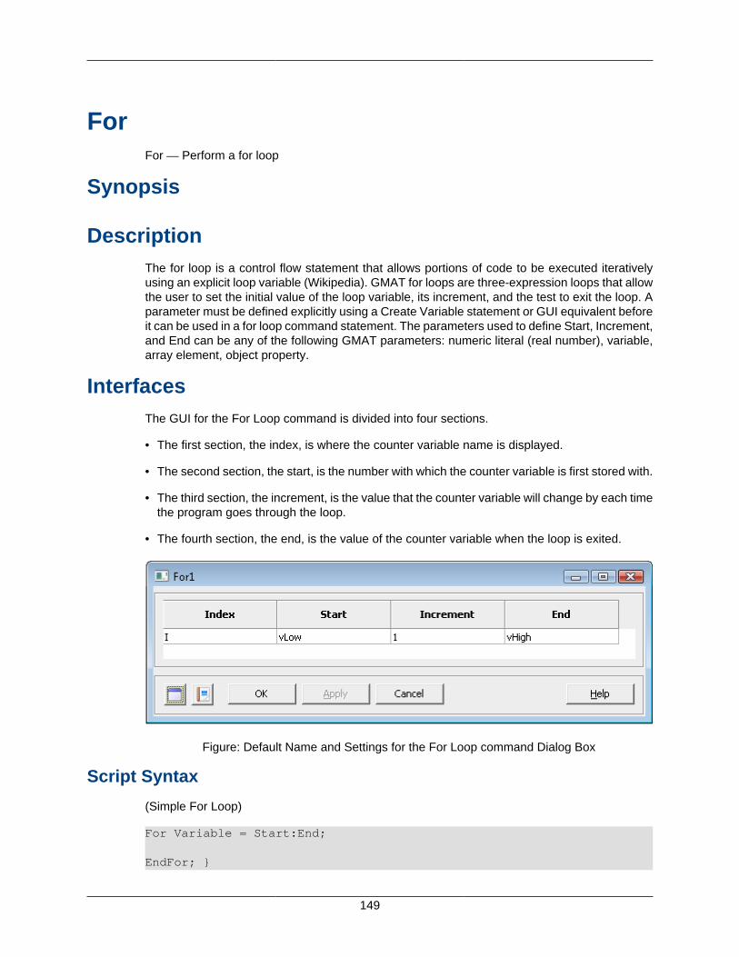
149
ForFor — Perform a for loop
Synopsis
DescriptionThe for loop is a control flow statement that allows portions of code to be executed iterativelyusing an explicit loop variable (Wikipedia). GMAT for loops are three-expression loops that allowthe user to set the initial value of the loop variable, its increment, and the test to exit the loop. Aparameter must be defined explicitly using a Create Variable statement or GUI equivalent beforeit can be used in a for loop command statement. The parameters used to define Start, Increment,and End can be any of the following GMAT parameters: numeric literal (real number), variable,array element, object property.
InterfacesThe GUI for the For Loop command is divided into four sections.
• The first section, the index, is where the counter variable name is displayed.
• The second section, the start, is the number with which the counter variable is first stored with.
• The third section, the increment, is the value that the counter variable will change by each timethe program goes through the loop.
• The fourth section, the end, is the value of the counter variable when the loop is exited.
Figure: Default Name and Settings for the For Loop command Dialog Box
Script Syntax
(Simple For Loop)
For Variable = Start:End;
EndFor; }
For
150
(Expanded For Loop)
For Variable = Start:Increment:End;
EndFor;
Script Examples
% Output the value of the For loop Variable to a fileFor I = 1:1:10;GMAT testVar = I;Report DefaultReportFile I;EndFor;
OptionsVariable The Variable field allows the user to define the variable that to be incremented
during the loop process.
Default None
Limits Variable
Units None
Start The Start option allows the user to set the starting value of the For Loop.
Default 1
Limits Real Number, Array element, Variable, or any user defined parameter
Units None
Increment The Increment option allows the user to set the increment value of the For Loop.When the increment value is not included in a for loop statement, the default valueis used.
Default 1
Limits Real Number, Array element, Variable, or any user defined parameter
Units None
End The End option allows the user to set the ending value of the For Loop.
Default 10
Limits Real Number, Array, Variable, or any user defined parameter
Units None
For Loop BehaviorWhen the Increment option is left out of the script syntax the default value is used. If an Incrementvalue of 0 is used, the For Loop should not execute but GMAT should continue to run. If End>Start

For
151
and Increment<0, then the For Loop should not execute. If Start>End and Increment>0, then theFor Loop should not execute. End can be equal to Start, but the For Loop will not execute.
152
IfIf — Perform an if command
Synopsis
DescriptionThe If command gives you the ability to use a logical statement within GMAT. At some pointduring a mission sequence, when a particular command should only be executed when a certaincondition is met, use of the If command is recommended. The If command also gives you theability to make a command's execution reliant upon multiple conditions.
Options<If Command> Arg1 and Arg2 can be any of the following: Real Number, Array element, Vari-
able, Spacecraft Parameter or any other user defined parameter.
Default DefaultSC.ElapsedDays < 1.0
Limits Arg1 < Arg2 and < can be >, <, >=, <=, ==, ~126~=
Units None
<Statements> Default None
Limits Any script line that can be in the mission sequence
Units None
| The | option allows the user to set an OR operator in between <logicalexpression>s.
Default None
Limits None
Units None
& The & option allows the user to set an AND operator in between <logicalexpression>s
Default None
Limits None
Units None
ExamplesUsing the If command in the script is quite simple. If you have ever programmed before inthe higher level languages such as C, Matlab, or Java, GMAT will be very familiar. The state-
If
153
ment reads like you see it basically: If the given statement after the 'If' is true, then execute thestatement(s) following until the 'EndIf' is reached.
Script Syntax
• Simple If Statement
If <logical expression>; <Statements>;EndIf;
• Compound If statement
If <logical expression> | <logical expression> & <logical expression>; <Statements>;EndIf;
Script Examples
If DefaultSC.ElapsedDays < 1; Propagate DefaultProp( DefaultSC , { DefaultSC.ElapsedDays = 0.01 });EndIf;
If MyVariable < MyArray(1,1); MyArray(1,1) = 5;EndIf;
If DefaultSC.Earth.TA < MyArray(1,2); Propagate DefaultProp( DefaultSC );EndIf;

154
ManeuverManeuver — Perform a maneuver command
Synopsis
DescriptionThe Maneuver command is placed in the mission tree and applies a selected impulsive burn toa selected spacecraft. A finite burn requires something else to be applied.
OptionsBurnName The BurnName field allows the user to choose between any previously cre-
ated impulsive burn. As an example, to maneuver DefaultSC using Default-IB, the script line would appear as Manevuer DefaultIB(DefaultSC).
Default DefaultIB
Limits Any impulsive burn existing in the resource tree or created inthe script
Units None
SpacecraftName The SpacecraftName field allows the user to select which spacecraft tomaneuver using the maneuver selected in the BurnName field.
Default DefaultSC
Limits Any spacecraft existing in the resource tree or created in thescript
Units None
Examples
Script Syntax
Maneuver BurnName (SpacecraftName);
Script Examples
% Impulsive BurnManeuver DefaultIB(DefaultSC);
155
MinimizeMinimize — Perform a minimize command
Synopsis
DescriptionThe minimize command in GMAT allows variables to minimize by using a defined optimizer inoptimize sequence.
Possible Coupling with Other Objects
• fmincon Object
• Must set in order to use Minimize Command.
• Optimize Command
• Must be defined in order to use minimize command in optimize sequence.
OptionsOptimizerName The OptimizerName option allows the user to specify which solver to use to
minimize the cost function.
Default SQP1
Limits Any existing fmincon solver
Units None
Arg The Arg field allows the user to specify the function to be minimized uponconvergence of the solver given by OptimizerName. Arg can be any of thefollowing: Variable, Array element, or Spacecraft Parameter or any other 1x1numeric user defined parameter.
Default DefaultSC.ECC
Limits Variable, Spacecraft parameter, or Array element
Units None
Examples
Script Syntax
Minimize OptimizerName (Arg)
Script Examples
% Minimize the eccentricity of Sat, using fminconSQP

Minimize
156
Minimize fminconSQP(Sat.ECC);
% Minimize the Variable DeltaV, using fminconSQPMinimize fminconSQP(DeltaV);
% Minimize the first component of MyArray, using fminconSQPMinimize fminconSQP(MyArray(1,1));
157
NonLinearConstraintNonLinearConstraint — Apply nonlinear constraint
Synopsis
DescriptionThe nonlinear constraints in GMAT allows spacecraft properties, variable or array to apply con-straint values, and also NonLinearConstraint can be created in optimize sequences. By usingthe fmincon optimizer, users can give various nonlinear constraints.
Possible Coupling with Other Objects
• Optimize Command
• NonLinearConstraints are used in Optimize Command.
• Optimizers (Solvers)
• Must set optimizer in order to apply NonLinearConstraints.
OptionsOptimizeName The OptimizerName option allows the user to specify which solver
to use in satisfying nonlinear constraints.
Default SQP1
Limits Any existing fmincon solver
Units None
{logical expression} The logical expression field allows the user to specify the constraintto be satisfied upon convergence of the solver given by Optimizer-Name. Arg1 and Arg2 can be any of the following: Real Number,a 1-D Array (column vector),Array element, Variable, SpacecraftParameter or any other numeric user defined parameter. If Arg1 isa 1-D Array, then Arg2 must be a 1-D Array with the same dimen-sions and vice-versa.
Default DefaultSC.SMA = 7000
Limits Arg1 <= Arg2 where <= can be >= ; <= ; =
Units None
Examples
Script Syntax
NonLinearConstraint OptimizerName ({logical expression})
NonLinearConstraint
158
Script Examples
% Constrain the SMA of Sat to be 7000 km, using fminconSQPNonLinearConstraint fminconSQP( Sat.SMA = 7000 );
% Constrain the SMA of Sat to be less than or equal to 7000 km, using fminconSQPNonLinearConstraint fminconSQP( Sat.SMA <= 7000 );
% Constrain the SMA of Sat to be greater than or equal to 7000 km, using fminconSQPNonLinearConstraint fminconSQP( Sat.SMA >= 7000a );
159
OptimizeOptimize — Perform an optimize command
Synopsis
DescriptionThe optimize command in GMAT allows variables to optimize by using a solver fmincon object.
Possible Coupling with Other Objects
• fmincon Object
• Must set in order to use Optimize Command.
• Minimize
• Must be defined if you would like to minimize variable in an optimize sequence.
• Vary
• NonLinearConstraint
OptionsSolverName The SolverName field allows the user to choose between any previously cre-
ated optimizer for use in an optimization sequence. For example, to begin aoptimization sequence using DefaultSQP, the script is Optimize DefaultSQP.
Default DefaultSQP
Limits Any existing optimizer
Units None
<Statements>Default None
Limits Any non-targeter and non-optimizer command lines used in themission sequence, as well as the optimizer dependent commandlines Vary, NonLinearConstraint, and Minimize.
Units None
Examples
Script Syntax
Optimize SolverName; <Statements>;
Optimize
160
EndOptimize;
Script Examples
% Beginning and ending syntax for the Optimize commandOptimize DefaultDC;
EndOptimize;
161
PenUpPenUp — Under construction.
SynopsisUnder construction.
Under construction.Under construction.
Examples
Script Syntax
Under construction.
Script Examples
Under construction.

162
PenDownPenDown — Under construction.
SynopsisUnder construction.
Under construction.Under construction.
Examples
Script Syntax
Under construction.
Script Examples
Under construction.

163
PropagatePropagate — Perform a propagate command
Synopsis
Description
The Propagate Command is a very important one and will be covered in this section. Basically,Propagate will take the given spacecraft and, using the Propagat''or'' specified as its guide, makeit travel until the given condition is met whether it be a location or something else such as elapsedtime.
Reference Table
BackProp The BackProp option allows the user to set the flag to enableor disable backwards propagation for all spacecraft in theSatListN option. The Backward Propagation GUI check boxfield stores all the data in BackProp. A check indicates back-ward propagation is enabled and no check indicates forwardpropagation. In the script, BackProp can be the word Back-wards for backward propagation or blank for forward propa-gation.
Default None
Limits Backwards or None
Units None
Mode The Mode option allows the user to set the propagation modefor the propagator that will affect all of the spacecraft addedto the SatListN option. For example, if synchronized is select-ed, all spacecraft are propagated at the same step size. ThePropagate Mode GUI field stores all the data in Mode. In thescript, Mode is left blank for the None option and the text ofthe other options available is used for their respective modes.
Default None
Limits Synchronized or None
Units None
PropagatorName The PropagatorName option allows the user to select a userdefined propagator to use in spacecraft and/or formationpropagation. The Propagator GUI field stores all the data inPropagatorName.
Default DefaultProp
Propagate
164
Limits Default propagator or any user-defined propaga-tor
Units None
SatListN The SatListN option allows the user to enter all the satellitesand/or formations they want to propagate using the Propaga-torName propagator settings. The Spacecraft List GUI fieldstores all the data in SatListN.
Default DefaultSC
Limits Any existing spacecraft or formations, not beingpropagated by another propagator in the samePropagate event. Multiple spacecraft must be ex-pressed in a comma delimited list format.
Units None
StopCondListN / Parameter The StopCondListN option allows the user to enter all the pa-rameters used for the propagator stopping condition. See theStopCondListN/Condition Option/Field for additional detailsto the StopCondListN option.
Default DefaultSC.ElapsedSecs
Limits Any single element user accessible spacecraftparameter followed by an equal sign
Units None
StopCondListN / Condition The StopCondListN option allows the user to enter the prop-agator stopping condition's value for the StopCondListN Pa-rameter field.
Default 8640.0
Limits Real Number, Array element, Variable, space-craft parameter, or any user defined parameter
Units Dependant on the condition selected.
Examples
Script Syntax
Propagate Mode BackProp PropagatorName(SatList1,fStopCondList1g) ...BackPropPropagatorName (SatListN, {StopCondList})
Script Examples
% Single spacecraft propagation with one stopping condition% Syntax #1Propagate DefaultProp(DefaultSC, {DefaultSC.ElapsedSecs = 8640.0});
Propagate
165
% Single spacecraft propagation with one stopping condition% Syntax #2Propagate DefaultProp(DefaultSC) {DefaultSC.ElapsedSecs = 8640.0};
% Single spacecraft propagation by one integration stepPropagate DefaultProp(DefaultSC);
% Multiple spacecraft propagation by one integration stepPropagate DefaultProp(Sat1, Sat2, Sat3);
% Single formation propagation by one integration stepPropagate DefaultProp(DefaultFormation);
% Single spacecraft backwards propagation by one integration stepPropagate Backwards DefaultProp(DefaultSC);
% Two spacecraft synchronized propagation with one stopping conditionPropagate Synchronized DefaultProp(Sat1, Sat2, {DefaultSC.ElapsedSecs = 8640.0});
% Multiple spacecraft propagation with multiple stopping conditions and propagation settings% Syntax #1Propagate Prop1(Sat1,Sat2, {Sat1.ElapsedSecs = 8640.0, Sat2.MA = 90}) ...Prop2(Sat3, {Sat3.TA = 0.0});
% Multiple spacecraft propagation with multiple stopping conditions and propagation settings% Syntax #2Propagate Prop1(Sat1,Sat2) {Sat1.ElapsedSecs = 8640.0, Sat2.MA = 90} ...Prop2(Sat3), {Sat3.TA = 0.0};

166
ReportReport — Output a report
Synopsis
DescriptionThe report command allows the user find parameters of the orbit and the spacecraft at particularmoments in time. This command is inserted into the mission tree at various locations in themission tree. The parameters found by this command are placed into a report file that can beaccessed at a later time.
OptionsReportName The ReportName option allows the user to specift the ReportFile for data output.
Default None
Limits Any ReportFile created
Units None
DataList The DataList option allows the user to output data to the Filename specified bythe ReportName. Multiple objects can be in the DataList when they are separatedby spaces.
Default None
Limits Spacecraft parameter, Array, Variable, String, or any other singleuser defined parameter
Units None
Examples
Script Syntax
Report ReportName DataList
Script Examples
%Report the time and position of DefaultSC
Report DefaultReport DefaultSC.A1ModJulian DefaultSC.X DefaultSC.Y DefaultSC.Z;

167
SaveSave — Under construction.
SynopsisUnder construction.
Under construction.Under construction.
Examples
Script Syntax
Under construction.
Script Examples
Under construction.
168
ScriptEventScriptEvent — Perform a ScriptEvent command
Synopsis
OverviewThe ScriptEvent command allows a user to enter in script within the GUI in the mission sequence.This can be useful in a number of ways if its easier to enter the script than to use the GUIinterface. Also, if multiple things needed to be changed rapidly, this could be useful. Additionally,the ScriptEvent allows a user to have more freedom if the GUI is problematic and won't allowthe user to perform the desired operation.
Options<Statements> Default None
Limits Any valid line of GMAT script
Units None
Examples
Script Syntax
BeginScript <Statements>EndScript;
Script Examples
% Assignment Command inside Script Event
BeginScript GMAT testVar = 24;EndScript;

169
StopStop — Perform a stop command
Synopsis
DescriptionThe Stop command simply ends a mission in GMAT. Whether placed in the script or GUI, Stopwill halt the execution of the mission and have GMAT report back that the Command Sequencewas intentionally interrupted.
Examples
Script Syntax
Stop
Script Examples
% Stop between propagation sequencesPropagate DefaultProp(DefaultSC) DefaultSC.ElapsedSecs = 8640.0;Stop;Propagate DefaultProp(DefaultSC) DefaultSC.ElapsedDays = 10.0;
170
TargetTarget — Perform a targeting sequence
SynopsisTarget SolverName(options) Vary SolverName(Vary arguments); Achieve SolverName(Achieve arguments); [Other Commands;] …EndTarget
DescriptionWhen building a mission, the targeting sequence is one of the most useful tools you have at yourdisposal. It allows you to use the power of a differential corrector to find solutions to complex twoand three-body problems with a limited number of known values and several variables. Target isthe base command that is appended with more commands such as Vary, Maneuver, Propagate,and Achieve in order to meet your goals. This makes it the first part of the sequence to be putinto the Mission tree.
ArgumentsSolverName The SolverName option allows the user to choose between any previously cre-
ated differential correctors for use in a targeting sequence. For example, to begina targeting sequence using DefaultDC, the script is Target DefaultDC.
Type DifferentialCorrector
OptionsSolveMode Tells the targeter state machine how to manage the targeter loop. When running
in the RunInitialGuess mode, the target loop is executed one time using the initialvalues of the targeter variables. No targeting is performed. When running in Solvemode, the targeter searches for a solution satisfying the targeter goals.
Type Enumeration
Values • Solve (default)
• RunInitialGuess
ExitMode Tells the Mission Control Sequence how to proceed after the targeter loop hasfinished running. When running in DiscardAndContinue mode, subsequent callsto the same targeter loop will reset the variables to their initial values. If runningin SaveAndContinue mode, the targeter variables used on a subsequent run startwith the values obtained the last time the targeter loop was run. In Stop mode, themission run halts when the targeter loop completes its work.
Type Enumeration
Target
171
Values • DiscardAndContinue (default)
• SaveAndContinue
• Stop
Examples
Example 11. Targeting geosynchronous orbit using an impulsive burn
Target DefaultDC Vary DefaultDC(DefaultIB.Element1 = 0.5); Maneuver DefaultIB(DefaultSC); Propagate DefaultProp(DefaultSC) {DefaultSC.Earth.Apoapsis}; Achieve DefaultDC(DefaultSC.Earth.RMAG = 42165.0);EndTarget
172
ToggleToggle — Perform a toggle command
Synopsis
DescriptionThe Toggle command is useful in turning on/off certain plots so that they do not become unin-telligible. They are particularly useful if a mission requires multiple sequences to fine-tune theanswer. If this is the case, it might be better to turn off a plot until the final or second-to-last se-quence so that the rougher sequences don't obstruct the view of what is going on in the finessesequences.
OptionsOutputNames The Toggle option allows the user to assign the Plot/Report(s) to be toggled.
When more than one Plot/Report is being toggled they need to be separatedby a space.
Default DefaultOpenGL
Limits Any OpenGL, Report, XYplot, or any other Plot/Report type
Units None
Arg The Arg option allows the user to turn off or on the data output to a Plot/Report.
Default On
Limits On or Off
Units None
Exmaples
Script Syntax
Toggle OutputNames Arg
Script Examples
% Turn off Report file for the first day of propagationToggle ReportFile1 OffPropagate DefaultProp(DefaultSC, {DefaultSC.ElapsedDays = 1});Toggle ReportFile1 OnPropagate DefaultProp(DefaultSC, {DefaultSC.ElapsedDays = 1});
% Turn off XYPlot and Report file for the first day of propagation Toggle XYPlot1 ReportFile1 Off
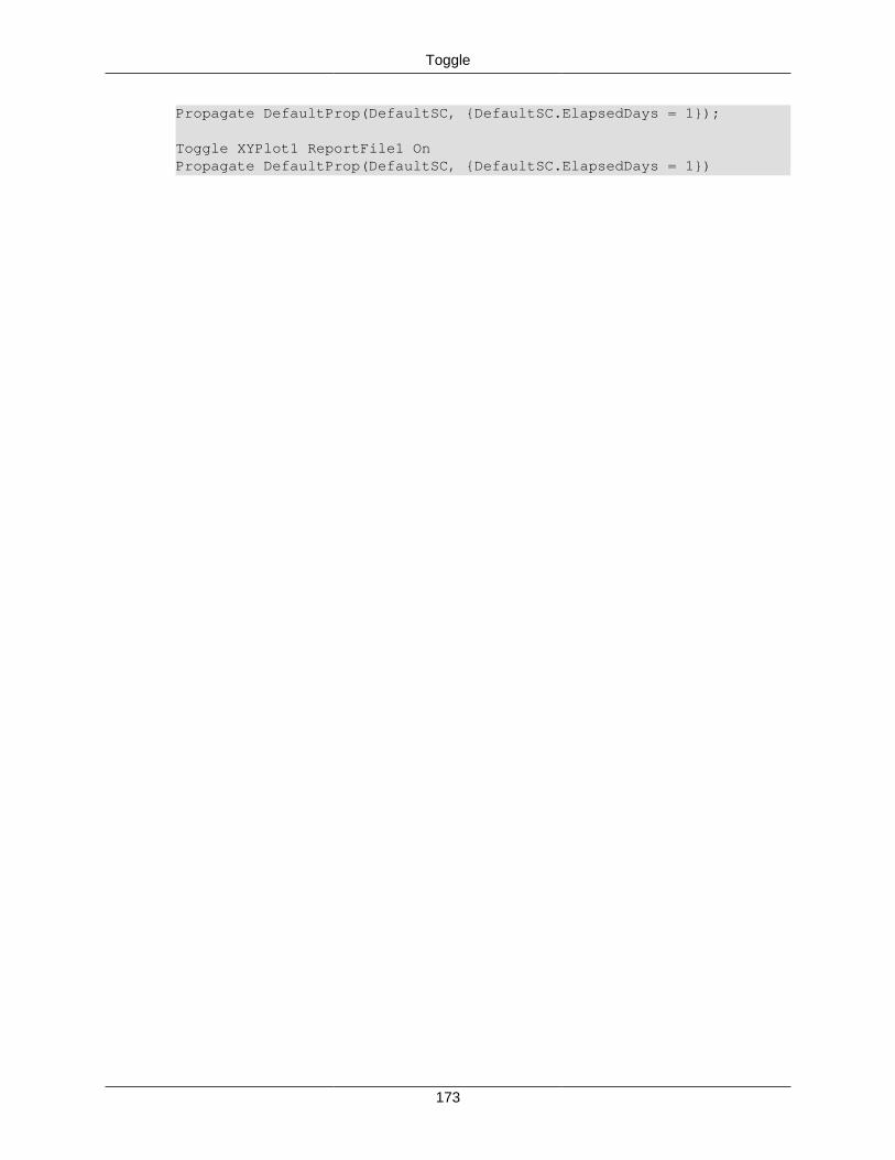
Toggle
173
Propagate DefaultProp(DefaultSC, {DefaultSC.ElapsedDays = 1});
Toggle XYPlot1 ReportFile1 OnPropagate DefaultProp(DefaultSC, {DefaultSC.ElapsedDays = 1})
174
VaryVary — Perform a vary command
Synopsis
DescriptionThe Vary command is used in conjunction with the Target and Optimize Commands. The Varycommand varies a particular parameter within the Target and Optimize Commands until certainconditions are met. It is a highly useful command for creating missions. Multiple Vary commandscan be used within the same targeting or optimizing sequence.
OptionsParameters Associated with All Solvers
SolverName The SolverName option allows the user to choose which solver to assign tothe vary command.
Default DefaultDC
Limits Any user defined solver
Units None
Variable The Variable option allows the user to select any single element user definedparameter, except a number, to vary. For example, DefaultIB.V, DefaultIB.N,DefaultIB.Element1, DefaultSC.TA, Array(1,1), and Variable are all valid val-ues. The three element burn vector or multidimensional Arrays are not validvalues.
Default DefaultIB.V
Limits Spacecrafy paremeter, Array element, Variable, or any other sin-gle element user defined parameter, excluding numbers
Units None
InitialGuess The InitialGuess option allows the user to set the initial guess for the selectedVariable.
Default 0.5
Limits Real Number, Array element, Variable, or any user defined para-meter that obeys the conditions for the selected Variable object
Units km/s
Lower The Lower option allows the user to set Arg3 to the lower bound of the quantitybeing varied.
Default 0.0

Vary
175
Limits Real Number, Array element, Variable, or any user defined para-meter (Upper > Lower )
Units None
Upper The Upper option allows the user to set Arg4 to the upper bound of the quantitybeing varied.
Default 3.14159
Limits Real Number, Array element, Variable, or any user defined para-meter (Upper > Lower )
Units None
Parameters Associated with Differential Corrector
Perturbation The Perturbation option is set by specifying a value for Arg1. The value ofArg1 is the perturbation size in calculating the finite difference derivative.
Default 1e-4
Limits Real Number, Array element, Variable, or any user defined para-meter > 0
Units None
MaxStep The MaxStep option is set by specifying a value for Arg2. The value of Arg2limits the size of the step taken during an interaction of the differential correc-tor.
Default 0.2
Limits Real Number, Array element, Variable, or any user defined para-meter > 0
Units None
Parameters Associated with fmincon Optimizer
Additive Scale Factor The AdditiveScaleFactor Field is used to nondimensionalizethe independent variable. fmincon sees only the nondimen-sional form of the variable. The nondimensionalization is per-formed using the following equation: xn = (xd - a)/m . (xn is thenon-dimensional parameter. xd is the dimensional parameter.a= additive scale factor. m= multiplicative scale factor.)
Default 0
Limits Real Number, Array element, Variable, or anyuser defined parameter
Units None
Multiplicative Scale Factor The MultiplicativeScaleFactor Field is used to nondimension-alize the independent variable. fmincon sees only the nondi-
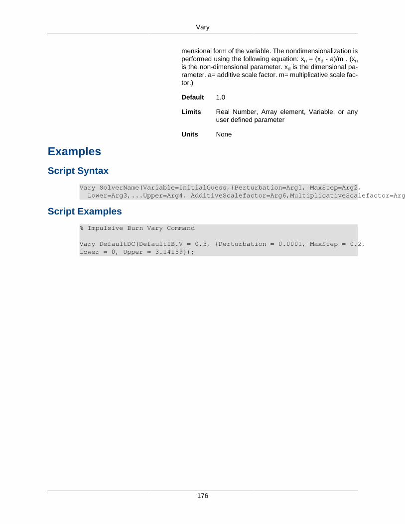
Vary
176
mensional form of the variable. The nondimensionalization isperformed using the following equation: xn = (xd - a)/m . (xnis the non-dimensional parameter. xd is the dimensional pa-rameter. a= additive scale factor. m= multiplicative scale fac-tor.)
Default 1.0
Limits Real Number, Array element, Variable, or anyuser defined parameter
Units None
Examples
Script Syntax
Vary SolverName(Variable=InitialGuess,{Perturbation=Arg1, MaxStep=Arg2, Lower=Arg3,...Upper=Arg4, AdditiveScalefactor=Arg6,MultiplicativeScalefactor=Arg6})
Script Examples
% Impulsive Burn Vary Command
Vary DefaultDC(DefaultIB.V = 0.5, {Perturbation = 0.0001, MaxStep = 0.2, Lower = 0, Upper = 3.14159});
177
WhileWhile — Run a while loop
Synopsis
DescriptionThe while loop is a control logic function that allows GMAT to check the spacecraft's statuson a given parameter while performing a command or another control logic function within themission sequence. When a spacecraft has reached the given property, the while loop will checkits condition and react according to the equation defined in the loop's dialog box.
Options<logical expression> Arg1 and Arg2 can be any of the following: Real Number, Array,
Variable, Spacecraft Parameter or any other user defined parame-ter.
Default DefaultSC.ElapsedDays < 1.0
Limits Arg1 < Arg2 and < can be > , < , >= , <= , == , ~=
Units None
<Statements> Default None
Limits Any script line that can be in the mission sequence
Units None
| The | option allows the user to set an OR operator in between s.
Default None
Limits None
Units None
& The & option allows the user to set an AND operator in between<logical expression>s.
Default None
Limits None
Units None
Examples
Script Syntax
• Simple While Loop

While
178
While <logical expression>; <Statements>;EndWhile;
• Compound While Loop
While <logical expression> | <logical expression> & <logical expression>; <Statements>EndWhile;
Script Examples
While DefaultSC.ElapsedDays < 1;Propagate DefaultProp (DefaultSC , DefaultSC.Elapsed Days = 0.01);EndWhile;
While MyVariable < MyArray(1,1);MyArray(1,1) = 5;EndWhile;
179
IndexAAchieve, 140Array, 78
BBaryCenter, 79BeginFiniteBurn, 142BeginMissionSequence, 143BodyNames, 79
CCallFunction, 144
EElse, 146EndFiniteBurn, 147Equation, 148
FFor, 149
IIf, 152
MManeuver, 154Minimize, 155
NNonLinearConstraint, 157
OOptimize, 159
PPenDown, 162PenUp, 161Propagate, 163
RReport, 166
SSave, 167ScriptEvent, 168Spacecraft, 119Stop, 169
TTarget, 170Toggle, 172
VVary, 174
WWhile, 177