General Equilibrium THIRTEEN CHAPTER and Welfare...General Equilibrium and Welfare The partial...

CHAPTERTHIRTEEN

General Equilibriumand Welfare

The partial equilibrium models of perfect competition that were introduced in Chapter12 are clearly inadequate for describing all the effects that occur when changes in onemarket have repercussions in other markets. Therefore, they are also inadequate formaking general welfare statements about how well market economies perform. Instead,what is needed is an economic model that permits us to view many markets simulta-neously. In this chapter we will develop a few simple versions of such models. TheExtensions to the chapter show how general equilibrium models are applied to the realworld.

Perfectly Competitive Price SystemThe model we will develop in this chapter is primarily an elaboration of the supply–demand mechanism presented in Chapter 12. Here we will assume that all markets are ofthe type described in that chapter and refer to such a set of markets as a perfectly competi-tive price system. The assumption is that there is some large number of homogeneousgoods in this simple economy. Included in this list of goods are not only consumptionitems but also factors of production. Each of these goods has an equilibrium price, estab-lished by the action of supply and demand.1 At this set of prices, every market is clearedin the sense that suppliers are willing to supply the quantity that is demanded and con-sumers will demand the quantity that is supplied. We also assume that there are no trans-action or transportation charges and that both individuals and firms have perfectknowledge of prevailing market prices.

The law of one priceBecause we assume zero transaction cost and perfect information, each good obeys thelaw of one price: A homogeneous good trades at the same price no matter who buys it orwhich firm sells it. If one good traded at two different prices, demanders would rush tobuy the good where it was cheaper, and firms would try to sell all their output where thegood was more expensive. These actions in themselves would tend to equalize the priceof the good. In the perfectly competitive market, each good must have only one price.This is why we may speak unambiguously of the price of a good.

1One aspect of this market interaction should be made clear from the outset. The perfectly competitive market determines onlyrelative (not absolute) prices. In this chapter, we speak only of relative prices. It makes no difference whether the prices ofapples and oranges are $.10 and $.20, respectively, or $10 and $20. The important point in either case is that two apples can beexchanged for one orange in the market. The absolute level of prices is determined mainly by monetary factors—a topic usuallycovered in macroeconomics.

457

Behavioral assumptionsThe perfectly competitive model assumes that people and firms react to prices in specificways.

1. There are assumed to be a large number of people buying any one good. Eachperson takes all prices as given and adjusts his or her behavior to maximize utility,given the prices and his or her budget constraint. People may also be suppliers ofproductive services (e.g., labor), and in such decisions they also regard prices asgiven.2

2. There are assumed to be a large number of firms producing each good, and each firmproduces only a small share of the output of any one good. In making input and out-put choices, firms are assumed to operate to maximize profits. The firms treat allprices as given when making these profit-maximizing decisions.

These various assumptions should be familiar because we have been making themthroughout this book. Our purpose here is to show how an entire economic system oper-ates when all markets work in this way.

A Graphical Model of GeneralEquilibrium with Two GoodsWe begin our analysis with a graphical model of general equilibrium involving only twogoods, which we will call x and y. This model will prove useful because it incorporatesmany of the features of far more complex general equilibrium representations of theeconomy.

General equilibrium demandUltimately, demand patterns in an economy are determined by individuals’ preferences.For our simple model we will assume that all individuals have identical preferences,which can be represented by an indifference curve map3 defined over quantities of thetwo goods, x and y. The benefit of this approach for our purposes is that this indifferencecurve map (which is identical to the ones used in Chapters 3–6) shows how individualsrank consumption bundles containing both goods. These rankings are precisely what wemean by ‘‘demand’’ in a general equilibrium context. Of course, we cannot illustratewhich bundles of commodities will be chosen until we know the budget constraints thatdemanders face. Because incomes are generated as individuals supply labor, capital, andother resources to the production process, we must delay any detailed illustration untilwe have examined the forces of production and supply in our model.

General equilibrium supplyDeveloping a notion of general equilibrium supply in this two-good model is a somewhatmore complex process than describing the demand side of the market because we havenot thus far illustrated production and supply of two goods simultaneously. Our

2Hence, unlike our partial equilibrium models, incomes are endogenously determined in general equilibrium models.3There are some technical problems in using a single indifference curve map to represent the preferences of an entire commu-nity of individuals. In this case the marginal rate of substitution (i.e., the slope of the community indifference curve) will dependon how the available goods are distributed among individuals: The increase in total y required to compensate for a one-unitreduction in x will depend on which specific individual(s) the x is taken from. Although we will not discuss this issue in detailhere, it has been widely examined in the international trade literature.

458 Part 5: Competitive Markets

approach is to use the familiar production possibility curve (see Chapter 1) for this pur-pose. By detailing the way in which this curve is constructed, we can illustrate, in a simplecontext, the ways in which markets for outputs and inputs are related.

Edgeworth box diagram for productionConstruction of the production possibility curve for two outputs (x and y) begins withthe assumption that there are fixed amounts of capital and labor inputs that must be allo-cated to the production of the two goods. The possible allocations of these inputs can beillustrated with an Edgeworth box diagram with dimensions given by the total amountsof capital and labor available.

In Figure 13.1, the length of the box represents total labor-hours, and the height of thebox represents total capital-hours. The lower left corner of the box represents the ‘‘origin’’for measuring capital and labor devoted to production of good x. The upper right cornerof the box represents the origin for resources devoted to y. Using these conventions, anypoint in the box can be regarded as a fully employed allocation of the available resourcesbetween goods x and y. Point A, for example, represents an allocation in which the indi-cated number of labor hours are devoted to x production together with a specified num-ber of hours of capital. Production of good y uses whatever labor and capital are ‘‘leftover.’’ Point A in Figure 13.1, for example, also shows the exact amount of labor and cap-ital used in the production of good y. Any other point in the box has a similar interpreta-tion. Thus, the Edgeworth box shows every possible way the existing capital and labormight be used to produce x and y.

The dimensions of this diagram are given by the total quantities of labor and capital available. Quantitiesof these resources devoted to x production are measured from origin Ox; quantities devoted to y aremeasured from Oy. Any point in the box represents a fully employed allocation of the available resourcesto the two goods.

A

O xTotal labor

Labor for xLabor in y production

Labor for y

Tota

l cap

ital

Cap

ital f

or y

Capitalin yproduction

Labor in x production

Capitalin xproduction

O yC

apita

l for

x

FIGURE 13.1

Construction of anEdgeworth Box Diagramfor Production

Chapter 13: General Equilibrium and Welfare 459

Efficient allocationsMany of the allocations shown in Figure 13.1 are technically inefficient in that it is possi-ble to produce both more x and more y by shifting capital and labor around a bit. In ourmodel we assume that competitive markets will not exhibit such inefficient input choices(for reasons we will explore in more detail later in the chapter). Hence we wish to dis-cover the efficient allocations in Figure 13.1 because these illustrate the production out-comes in this model. To do so, we introduce isoquant maps for good x (using Ox as theorigin) and good y (using Oy as the origin), as shown in Figure 13.2. In this figure it isclear that the arbitrarily chosen allocation A is inefficient. By reallocating capital andlabor, one can produce both more x than x2 and more y than y2.

The efficient allocations in Figure 13.2 are those such as P1, P2, P3, and P4, where theisoquants are tangent to one another. At any other points in the box diagram, the twogoods’ isoquants will intersect, and we can show inefficiency as we did for point A. At thepoints of tangency, however, this kind of unambiguous improvement cannot be made. Ingoing from P2 to P3, for example, more x is being produced, but at the cost of less y beingproduced; therefore, P3 is not ‘‘more efficient’’ than P2—both of the points are efficient.Tangency of the isoquants for good x and good y implies that their slopes are equal. Thatis, the RTS of capital for labor is equal in x and y production. Later we will show howcompetitive input markets will lead firms to make such efficient input choices.

Therefore, the curve joining Ox and Oy that includes all these points of tangency showsall the efficient allocations of capital and labor. Points off this curve are inefficient in thatunambiguous increases in output can be obtained by reshuffling inputs between the twogoods. Points on the curve OxOy are all efficient allocations, however, because more x canbe produced only by cutting back on y production and vice versa.

This diagram adds production isoquants for x and y to Figure 13.1. It then shows technically efficientways to allocate the fixed amounts of k and l between the production of the two outputs. The line joiningOx and Oy is the locus of these efficient points. Along this line, the RTS (of l for k) in the production ofgood x is equal to the RTS in the production of y.

Total l

P1

Totalk

O x

O y

P2

P3

P4

x1

x2

x3

x4

y1y2

y3

y4

A

FIGURE 13.2

Edgeworth Box Diagramof Efficiency inProduction


Production possibility frontierThe efficiency locus in Figure 13.2 shows the maximum output of y that can be producedfor any preassigned output of x.We can use this information to construct a production pos-sibility frontier, which shows the alternative outputs of x and y that can be produced withthe fixed capital and labor inputs. In Figure 13.3 the OxOy locus has been taken from Fig-ure 13.2 and transferred onto a graph with x and y outputs on the axes. At Ox, for example,no resources are devoted to x production; consequently, y output is as large as is possiblewith the existing resources. Similarly, at Oy, the output of x is as large as possible. The otherpoints on the production possibility frontier (say, P1, P2, P3, and P4) are derived from theefficiency locus in an identical way. Hence we have derived the following definition.

Rate of product transformationThe slope of the production possibility frontier shows how x output can be substitutedfor y output when total resources are held constant. For example, for points near Ox on

The production possibility frontier shows the alternative combinations of x and y that can be efficientlyproduced by a firm with fixed resources. The curve can be derived from Figure 13.2 by varying inputsbetween the production of x and y while maintaining the conditions for efficiency. The negative of theslope of the production possibility curve is called the rate of product transformation (RPT).

O yx4

A

P1

P2

P3

P4

x3x2x1

y1

y2

y3

y4

O x

Quantityof x

Quantityof y

D E F I N I T I O N Productionpossibility frontier.The production possibility frontier shows the alternative combinationsof two outputs that can be produced with fixed quantities of inputs if those inputs are employedefficiently.

FIGURE 13.3

Production PossibilityFrontier


the production possibility frontier, the slope is a small negative number—say, !1/4; thisimplies that, by reducing y output by 1 unit, x output could be increased by 4. Near Oy,on the other hand, the slope is a large negative number (say, !5), implying that y outputmust be reduced by 5 units to permit the production of one more x. The slope of the pro-duction possibility frontier clearly shows the possibilities that exist for trading y for x inproduction. The negative of this slope is called the rate of product transformation (RPT).

The RPT records how x can be technically traded for y while continuing to keep the avail-able productive inputs efficiently employed.

Shape of the production possibility frontierThe production possibility frontier illustrated in Figure 13.3 exhibits an increasing RPT.For output levels near Ox, relatively little y must be sacrificed to obtain one more x (–dy/dxis small). Near Oy, on the other hand, additional x may be obtained only by substantialreductions in y output (–dy/dx is large). In this section we will show why this concaveshape might be expected to characterize most production situations.

A first step in that analysis is to recognize that RPT is equal to the ratio of the mar-ginal cost of x (MCx) to the marginal cost of y (MCy). Intuitively, this result is obvious.Suppose, for example, that x and y are produced only with labor. If it takes two laborhours to produce one more x, we might say that MCx is equal to 2. Similarly, if it takesonly one labor hour to produce an extra y, then MCy is equal to 1. But in this situation itis clear that the RPT is 2: two y must be forgone to provide enough labor so that x maybe increased by one unit. Hence the RPT is equal to the ratio of the marginal costs of thetwo goods.

More formally, suppose that the costs (say, in terms of the ‘‘disutility’’ experienced byfactor suppliers) of any output combination are denoted by C(x, y). Along the productionpossibility frontier, C(x, y) will be constant because the inputs are in fixed supply. If wecall this constant level of costs C, we can write C"x, y# ! C $ 0. It is this implicit func-tion that underlies the production possibility frontier. Applying the results from Chapter 2for such a function yields:

RPT $ dydxjC"x, y# ! C$0 $ !

Cx

Cy$ !MCx

MCy: (13:2)

To demonstrate reasons why the RPT might be expected to increase for clockwisemovements along the production possibility frontier, we can proceed by showing why theratio of MCx to MCy should increase as x output expands and y output contracts. We firstpresent two relatively simple arguments that apply only to special cases; then we turn to amore sophisticated general argument.

Diminishing returnsThe most common rationale offered for the concave shape of the production possibilityfrontier is the assumption that both goods are produced under conditions of diminishingreturns. Hence increasing the output of good x will raise its marginal cost, whereas

D E F I N I T I O N Rate of product transformation. The rate of product transformation (RPT) between two outputs isthe negative of the slope of the production possibility frontier for those outputs. Mathematically,

RPT "of x for y# $ !%slope of production possibility frontier&

$ ! dydx"along OxOy#,

(13:1)


decreasing the output of y will reduce its marginal cost. Equation 13.2 then shows thatthe RPT will increase for movements along the production possibility frontier from Ox toOy. A problem with this explanation, of course, is that it applies only to cases in whichboth goods exhibit diminishing returns to scale, and that assumption is at variance withthe theoretical reasons for preferring the assumption of constant or even increasingreturns to scale as mentioned elsewhere in this book.

Specialized inputsIf some inputs were ‘‘more suited’’ for x production than for y production (and viceversa), the concave shape of the production frontier also could be explained. In that case,increases in x output would require drawing progressively less suitable inputs into theproduction of that good. Therefore, marginal costs of x would increase. Marginal costsfor y, on the other hand, would decrease because smaller output levels for y would permitthe use of only those inputs most suited for y production. Such an argument might apply,for example, to a farmer with a variety of types of land under cultivation in differentcrops. In trying to increase the production of any one crop, the farmer would be forcedto grow it on increasingly unsuitable parcels of land. Although this type of specializedinput assumption has considerable importance in explaining a variety of real-world phe-nomena, it is nonetheless at variance with our general assumption of homogeneous fac-tors of production. Hence it cannot serve as a fundamental explanation for concavity.

Differing factor intensitiesEven if inputs are homogeneous and production functions exhibit constant returns toscale, the production possibility frontier will be concave if goods x and y use inputs in dif-ferent proportions.4 In the production box diagram of Figure 13.2, for example, good x iscapital intensive relative to good y. That is, at every point along the OxOy contract curve,the ratio of k to l in x production exceeds the ratio of k to l in y production: The bowedcurve OxOy is always above the main diagonal of the Edgeworth box. If, on the otherhand, good y had been relatively capital intensive, the OxOy contract curve would havebeen bowed downward below the diagonal. Although a formal proof that unequal factorintensities result in a concave production possibility frontier will not be presented here, itis possible to suggest intuitively why that occurs. Consider any two points on the frontierOxOy in Figure 13.3—say, P1 (with coordinates x1, y4) and P3 (with coordinates x3, y2).One way of producing an output combination ‘‘between’’ P1 and P3 would be to producethe combination

x1 ' x32

,y4 ' y2

2:

Because of the constant returns-to-scale assumption, that combination would be feasi-ble and would fully use both factors of production. The combination would lie at the mid-point of a straight-line chord joining points P1 and P3. Although such a point is feasible, itis not efficient, as can be seen by examining points P1 and P3 in the box diagram of Figure13.2. Because of the bowed nature of the contract curve, production at a point midwaybetween P1 and P3 would be off the contract curve: Producing at a point such as P2 wouldprovide more of both goods. Therefore, the production possibility frontier in Figure 13.3must ‘‘bulge out’’ beyond the straight line P1P3. Because such a proof could be constructedfor any two points on OxOy, we have shown that the frontier is concave; that is, the RPTincreases as the output of good X increases. When production is reallocated in a northeast

4If, in addition to homogeneous factors and constant returns to scale, each good also used k and l in the same proportions underoptimal allocations, then the production possibility frontier would be a straight line.


direction along the OxOy contract curve (in Figure 13.3), the capital–labor ratio decreasesin the production of both x and y. Because good x is capital intensive, this changeincreases MCx. On the other hand, because good y is labor intensive, MCy decreases.Hence the relative marginal cost of x (as represented by the RPT) increases.

Opportunity cost and supplyThe production possibility curve demonstrates that there are many possible efficient com-binations of the two goods and that producing more of one good necessitates cutting backon the production of some other good. This is precisely what economists mean by theterm opportunity cost. The cost of producing more x can be most readily measured by thereduction in y output that this entails. Therefore, the cost of one more unit of x is bestmeasured as the RPT (of x for y) at the prevailing point on the production possibilityfrontier. The fact that this cost increases as more x is produced represents the formula-tion of supply in a general equilibrium context.

EXAMPLE 13.1 Concavity of the Production Possibility Frontier

In this example we look at two characteristics of production functions that may cause theproduction possibility frontier to be concave.

Diminishing returns. Suppose that the production of both x and y depends only on laborinput and that the production functions for these goods are

x $ f "lx# $ l 0:5x ,

y $ f "ly# $ l 0:5y :(13:3)

Hence production of each of these goods exhibits diminishing returns to scale. If total laborsupply is limited by

lx ' ly $ 100, (13:4)

then simple substitution shows that the production possibility frontier is given by

x2 ' y2 $ 100 for x, y ( 0: (13:5)

In this case, the frontier is a quarter-circle and is concave. The RPT can now be computeddirectly from the equation for the production possibility frontier (written in implicit form asf "x, y# $ x2 ' y2 ! 100 $ 0):

RPT $ ! dydx$ !"! fx

fy# $ 2x

2y$ x

y, (13:6)

and this slope increases as x output increases. A numerical illustration of concavity starts bynoting that the points (10, 0) and (0, 10) both lie on the frontier. A straight line joining thesetwo points would also include the point (5, 5), but that point lies below the frontier. If equalamounts of labor are devoted to both goods, then production is x $ y $

!!!!!50p

, which yieldsmore of both goods than the midpoint.

Factor intensity. To show how differing factor intensities yield a concave productionpossibility frontier, suppose that the two goods are produced under constant returns to scale butwith different Cobb–Douglas production functions:

x $ f "k, l# $ k0:5x l 0:5x ,

y $ g"k, l# $ k0:25y l 0:75y :(13:7)


Determination of equilibrium pricesGiven these notions of demand and supply in our simple two-good economy, we cannow illustrate how equilibrium prices are determined. Figure 13.4 shows PP, the

Suppose also that total capital and labor are constrained by

kx ' ky $ 100, lx ' ly $ 100: (13:8)

It is easy to show that

RTSx $kxlx$ jx , RTSy $

3kyly$ 3jy , (13:9)

where ki $ ki/li. Being located on the production possibility frontier requires RTSx $ RTSy orkx $ 3ky. That is, no matter how total resources are allocated to production, being on theproduction possibility frontier requires that x be the capital-intensive good (because, in somesense, capital is more productive in x production than in y production). The capital–labor ratiosin the production of the two goods are also constrained by the available resources:

kx ' kylx ' ly

$ kxlx ' ly

'ky

lx ' ly$ ajx ' "1! a#jy $

100100$ 1, (13:10)

where a $ lx/(lx ' ly)—that is, a is the share of total labor devoted to x production. Using thecondition that kx $ 3ky, we can find the input ratios of the two goods in terms of the overallallocation of labor:

jy $1

1' 2a, jx $

31' 2a

: (13:11)

Now we are in a position to phrase the production possibility frontier in terms of the share oflabor devoted to x production:

x $ j0:5x lx $ j0:5

x a"100# $ 100a3

1' 2a

" #0:5

,

y $ j0:25y ly $ j0:25

y "1! a#"100# $ 100"1! a# 11' 2a

" #0:25

:

(13:12)

We could push this algebra even further to eliminate a from these two equations to get anexplicit functional form for the production possibility frontier that involves only x and y, but wecan show concavity with what we already have. First, notice that if a $ 0 (x production gets nolabor or capital inputs), then x $ 0, y $ 100. With a $ 1, we have x $ 100, y $ 0. Hence alinear production possibility frontier would include the point (50, 50). But if a $ 0.39, say, then

x $ 100a3

1' 2a

" #0:5

$ 393

1:78

" #0:5

$ 50:6,

y $ 100"1! a# 11' 2a

" #0:25

$ 611

1:78

" #0:25

$ 52:8,

(13:13)

which shows that the actual frontier is bowed outward beyond a linear frontier. It is worthrepeating that both of the goods in this example are produced under constant returns to scaleand that the two inputs are fully homogeneous. It is only the differing input intensities involvedin the production of the two goods that yields the concave production possibility frontier.

QUERY: How would an increase in the total amount of labor available shift the productionpossibility frontiers in these examples?


production possibility frontier for the economy, and the set of indifference curves rep-resents individuals’ preferences for these goods. First, consider the price ratio px/py. Atthis price ratio, firms will choose to produce the output combination x1, y1. Profit-maximizing firms will choose the more profitable point on PP. At x1, y1 the ratio ofthe two goods’ prices (px/py) is equal to the ratio of the goods’ marginal costs (theRPT); thus, profits are maximized there. On the other hand, given this budget con-straint (line C),5 individuals will demand x01, y

01. Consequently, with these prices, there

is an excess demand for good x (individuals demand more than is being produced) butan excess supply of good y. The workings of the marketplace will cause px to increaseand py to decrease. The price ratio px/py will increase; the price line will take on asteeper slope. Firms will respond to these price changes by moving clockwise along theproduction possibility frontier; that is, they will increase their production of good xand decrease their production of good y. Similarly, individuals will respond to thechanging prices by substituting y for x in their consumption choices. These actions ofboth firms and individuals serve to eliminate the excess demand for x and the excesssupply of y as market prices change.

With a price ratio given by px/py, firms will produce x1, y1; society’s budget constraint will be given byline C. With this budget constraint, individuals demand x01 and y01; that is, there is an excess demand forgood x and an excess supply of good y. The workings of the market will move these prices toward theirequilibrium levels p)x , p

)y . At those prices, society’s budget constraint will be given by line C), and supply

and demand will be in equilibrium. The combination x), y) of goods will be chosen.

Quantityof y

Quantity of x

!px py

Slope = ____

!px

P

py

U1

C*

C*

y*

x*

P C

C U2

y1

x1

U3

Slope = ____E

y1"

x1"

**

5It is important to recognize why the budget constraint has this location. Because px and py are given, the value of total produc-tion is px Æ x1 ' py Æ y1. This is the value of ‘‘GDP’’ in the simple economy pictured in Figure 13.4. It is also, therefore, the totalincome accruing to people in society. Society’s budget constraint therefore passes through x1, y1 and has a slope of –px/py. Thisis precisely the budget constraint labeled C in the figure.

FIGURE 13.4

Determination ofEquilibrium Prices


Equilibrium is reached at x), y) with a price ratio of p)x=p)y . With this price ratio,6 sup-

ply and demand are equilibrated for both good x and good y. Given px and py, firms willproduce x) and y) in maximizing their profits. Similarly, with a budget constraint givenby C), individuals will demand x) and y). The operation of the price system has clearedthe markets for both x and y simultaneously. Therefore, this figure provides a ‘‘generalequilibrium’’ view of the supply–demand process for two markets working together. Forthis reason we will make considerable use of this figure in our subsequent analysis.

Comparative Statics AnalysisAs in our partial equilibrium analysis, the equilibrium price ratio p)x=p

)y illustrated in

Figure 13.4 will tend to persist until either preferences or production technologies change.This competitively determined price ratio reflects these two basic economic forces. If pref-erences were to shift, say, toward good x, then px/py would increase and a new equilibriumwould be established by a clockwise move along the production possibility curve. More xand less y would be produced to meet these changed preferences. Similarly, technical prog-ress in the production of good x would shift the production possibility curve outward, asillustrated in Figure 13.5. This would tend to decrease the relative price of x and increasethe quantity of x consumed (assuming x is a normal good). In the figure the quantity of y

Technical advances that lower marginal costs of x production will shift the production possibilityfrontier. This will generally create income and substitution effects that cause the quantity of x producedto increase (assuming x is a normal good). Effects on the production of y are ambiguous because incomeand substitution effects work in opposite directions.

Quantityof y

Quantityof x

x1 x0

y1y0

E1

E0

U0

U1

6Notice again that competitive markets determine only equilibrium relative prices. Determination of the absolute price levelrequires the introduction of money into this barter model.

FIGURE 13.5

Effects of TechnicalProgress in xProduction


consumed also increases as a result of the income effect arising from the technical advance;however, a slightly different drawing of the figure could have reversed that result if the sub-stitution effect had been dominant. Example 13.2 looks at a few such effects.

EXAMPLE 13.2 Comparative Statics in a General Equilibrium Model

To explore how general equilibrium models work, let’s start with a simple example based on theproduction possibility frontier in Example 13.1. In that example we assumed that production ofboth goods was characterized by decreasing returns x $ l0:5x and y $ l0:5y and also that total laboravailable was given by lx ' ly $ 100. The resulting production possibility frontier was given byx2 ' y2 $ 100, and RPT $ x/y. To complete this model we assume that the typical individual’sutility function is given by U(x, y) $ x0.5y0.5, so the demand functions for the two goods are

x $ x"px , py , I# $0:5Ipx

,

y $ y"px , py , I# $0:5Ipy

:(13:14)

Base-case equilibrium. Profit maximization by firms requires that px/py $ MCx/MCy $ RPT$ x/y, and utility-maximizing demand requires that px/py $ y/x. Thus, equilibrium requires thatx/y $ y/x, or x $ y. Inserting this result into the equation for the production possibility frontiershows that

x) $ y) $!!!!!50p

$ 7:07 andpxpy$ 1: (13:15)

This is the equilibrium for our base case with this model.

The budget constraint. The budget constraint that faces individuals is not especiallytransparent in this illustration; therefore, it may be useful to discuss it explicitly. To bring somedegree of absolute pricing into the model, let’s consider all prices in terms of the wage rate, w.Because total labor supply is 100, it follows that total labor income is 100w. However, becauseof the diminishing returns assumed for production, each firm also earns profits. For firm x, say,the total cost function is C(w, x) $ wlx $ wx2, so px $ MCx $ 2wx $ 2w

!!!!!50p

. Therefore, theprofits for firm x are px $ (px – ACx)x $ (px – wx)x $ wx2 $ 50w. A similar computationshows that profits for firm y are also given by 50w. Because general equilibrium models mustobey the national income identity, we assume that consumers are also shareholders in the twofirms and treat these profits also as part of their spendable incomes. Hence total consumerincome is

total income $ labor income + profits

$ 100w' 2"50w# $ 200w:(13:16)

This income will just permit consumers to spend 100w on each good by buying!!!!!50p

units at aprice of 2w

!!!!!50p

, so the model is internally consistent.

A shift in supply. There are only two ways in which this base-case equilibrium can bedisturbed: (1) by changes in ‘‘supply’’—that is, by changes in the underlying technology of thiseconomy; or (2) by changes in ‘‘demand’’—that is, by changes in preferences. Let’s first considerchanges in technology. Suppose that there is technical improvement in x production so that theproduction function is x $ 2l 0:5x . Now the production possibility frontier is given by x2/4 ' y2 $100, and RPT $ x/4y. Proceeding as before to find the equilibrium in this model:


General Equilibrium Modelingand Factor PricesThis simple general equilibrium model reinforces Marshall’s observations about the im-portance of both supply and demand forces in the price determination process. By pro-viding an explicit connection between the markets for all goods, the general equilibriummodel makes it possible to examine more complex questions about market relationshipsthan is possible by looking at only one market at a time. General equilibrium modelingalso permits an examination of the connections between goods and factor markets; wecan illustrate that with an important historical case.

pxpy$ x

4y"supply#,

pxpy$ y

x"demand#,

(13:17)

so x2 $ 4y2 and the equilibrium is

x) $ 2!!!!!50p

, y) $!!!!!50p

andpxpy$ 1

2: (13:18)

Technical improvements in x production have caused its relative price to decrease and theconsumption of this good to increase. As in many examples with Cobb–Douglas utility, the incomeand substitution effects of this price decrease on y demand are precisely offsetting. Technicalimprovements clearly make consumers better off, however. Whereas utility was previously givenby U"x, y# $ x0:5y0:5 $

!!!!!50p

$ 7:07, now it has increased to U"x, y# $ x0:5y0:5 $ "2!!!!!50p#0:5

"!!!!!50p#0:5 $

!!!2p*!!!!!50p

$ 10. Technical change has increased consumer welfare substantially.

A shift in demand. If consumer preferences were to switch to favor good y as U(x, y) $x0.1y0.9, then demand functions would be given by x $ 0.1I/px and y $ 0.9I/py, and demandequilibrium would require px/py $ y/9x. Returning to the original production possibility frontierto arrive at an overall equilibrium, we have

pxpy$ x

y"supply#,

pxpy$ y

9x"demand#,

(13:19)

so 9x2 $ y2 and the equilibrium is given by

x) $!!!!!10p

, y) $ 3!!!!!10p

andpxpy$ 1

3(13:20)

Hence the decrease in demand for x has significantly reduced its relative price. Observe that inthis case, however, we cannot make a welfare comparison to the previous cases because theutility function has changed.

QUERY: What are the budget constraints in these two alternative scenarios? How is incomedistributed between wages and profits in each case? Explain the differences intuitively.


The Corn Laws debateHigh tariffs on grain imports were imposed by the British government following theNapoleonic wars. Debate over the effects of these Corn Laws dominated the analyticalefforts of economists between the years 1829 and 1845. A principal focus of the debateconcerned the effect that elimination of the tariffs would have on factor prices—a ques-tion that continues to have relevance today, as we will see.

The production possibility frontier in Figure 13.6 shows those combinations of grain(x) and manufactured goods (y) that could be produced by British factors of production.Assuming (somewhat contrary to actuality) that the Corn Laws completely preventedtrade, market equilibrium would be at E with the domestic price ratio given by p)x=p

)y .

Removal of the tariffs would reduce this price ratio to p0x=p0y . Given that new ratio, Britain

would produce combination A and consume combination B. Grain imports wouldamount to xB – xA, and these would be financed by export of manufactured goods equalto yA – yB. Overall utility for the typical British consumer would be increased by theopening of trade. Therefore, use of the production possibility diagram demonstrates theimplications that relaxing the tariffs would have for the production of both goods.

Trade and factor pricesBy referring to the Edgeworth production box diagram (Figure 13.2) that lies behind theproduction possibility frontier (Figure 13.3), it is also possible to analyze the effect of

Reduction of tariff barriers on grain would cause production to be reallocated from point E to point A;consumption would be reallocated from E to B. If grain production is relatively capital intensive, therelative price of capital would decrease as a result of these reallocations.

U2

xA xE

yE

yA

yB

P

xBP

U1

Slope = !px /py

Slope = !p"x /p"y

* *

A

EB

Output of grain (x)

Output ofmanufactured

goods (y)

FIGURE 13.6

Analysis of the CornLaws Debate


tariff reductions on factor prices. The movement from point E to point A in Figure 13.6is similar to a movement from P3 to P1 in Figure 13.2, where production of x is decreasedand production of y is increased.

This figure also records the reallocation of capital and labor made necessary by such amove. If we assume that grain production is relatively capital intensive, then the move-ment from P3 to P1 causes the ratio of k to l to increase in both industries.7 This in turnwill cause the relative price of capital to decrease (and the relative price of labor toincrease). Hence we conclude that repeal of the Corn Laws would be harmful to capitalowners (i.e., landlords) and helpful to laborers. It is not surprising that landed interestsfought repeal of the laws.

Political support for trade policiesThe possibility that trade policies may affect the relative incomes of various factors ofproduction continues to exert a major influence on political debates about such policies.In the United States, for example, exports tend to be intensive in their use of skilled labor,whereas imports tend to be intensive in unskilled labor input. By analogy to our discus-sion of the Corn Laws, it might thus be expected that further movements toward freetrade policies would result in increasing relative wages for skilled workers and in decreas-ing relative wages for unskilled workers. Therefore, it is not surprising that unions repre-senting skilled workers (the machinists or aircraft workers) tend to favor free trade,whereas unions of unskilled workers (those in textiles, shoes, and related businesses) tendto oppose it.8

A Mathematical Modelof ExchangeAlthough the previous graphical model of general equilibrium with two goods is fairlyinstructive, it cannot reflect all the features of general equilibrium modeling with anarbitrary number of goods and productive inputs. In the remainder of this chapter we willillustrate how such a more general model can be constructed, and we will look at some ofthe insights that such a model can provide. For most of our presentation we will lookonly at a model of exchange—quantities of various goods already exist and are merelytraded among individuals. In such a model there is no production. Later in the chapterwe will look briefly at how production can be incorporated into the general model wehave constructed.

Vector notationMost general equilibrium modeling is conducted using vector notation. This providesgreat flexibility in specifying an arbitrary number of goods or individuals in the models.Consequently, this seems to be a good place to offer a brief introduction to such notation.A vector is simply an ordered array of variables (which each may take on specific values).Here we will usually adopt the convention that the vectors we use are column vectors.Hence we will write an n + 1 column vector as:

7In the Corn Laws debate, attention centered on the factors of land and labor.8The finding that the opening of trade will raise the relative price of the abundant factor is called the Stolper–Samuelson theo-rem after the economists who rigorously proved it in the 1950s.


x $

x1x2:::xn

2

6666664

3

7777775, (13:21)

where each xi is a variable that can take on any value. If x and y are two n + 1 columnvectors, then the (vector) sum of them is defined as:

x ' y $

x1x2:::xn

2

6666664

3

7777775'

y1y2:::yn

2

6666664

3

7777775$

x1 ' y1x2 ' y2

:::

xn ' yn

2

6666664

3

7777775: (13:22)

Notice that this sum only is defined if the two vectors are of equal length. In fact, check-ing the length of vectors is one good way of deciding whether one has written a meaning-ful vector equation.

The (dot) product of two vectors is defined as the sum of the component-by-componentproduct of the elements in the two vectors. That is:

xy $ x1y1 ' x2y2 ' * * * ' xnyn: (13:23)

Notice again that this operation is only defined if the vectors are of the same length. Withthese few concepts we are now ready to illustrate the general equilibrium model ofexchange.

Utility, initial endowments, and budget constraintsIn our model of exchange there are assumed to be n goods andm individuals. Each individ-ual gains utility from the vector of goods he or she consumes ui(xi) where i $ 1 . . .m. Indi-viduals also possess initial endowments of the goods given by x i. Individuals are free toexchange their initial endowments with other individuals or to keep some or all the endow-ment for themselves. In their trading individuals are assumed to be price-takers—that is,they face a price vector (p) that specifies the market price for each of the n goods. Eachindividual seeks to maximize utility and is bound by a budget constraint that requires thatthe total amount spent on consumption equals the total value of his or her endowment:

pxi $ pxi: (13:24)

Although this budget constraint has a simple form, it may be worth contemplating it for aminute. The right side of Equation 13.24 is the market value of this individual’s endow-ment (sometimes referred to as his or her full income). He or she could ‘‘afford’’ to con-sume this endowment (and only this endowment) if he or she wished to be self-sufficient.But the endowment can also be spent on some other consumption bundle (which, presum-ably, provides more utility). Because consuming items in one’s own endowment has anopportunity cost, the terms on the left of Equation 13.24 consider the costs of all items thatenter into the final consumption bundle, including endowment goods that are retained.

Demand functions and homogeneityThe utility maximization problem outlined in the previous section is identical to the onewe studied in detail in Part 2 of this book. As we showed in Chapter 4, one outcome of


this process is a set of n individual demand functions (one for each good) in which quan-tities demanded depend on all prices and income. Here we can denote these in vectorform as xi"p, pxi#. These demand functions are continuous, and, as we showed in Chap-ter 4, they are homogeneous of degree 0 in all prices and income. This latter property canbe indicated in vector notation by

xi"tp, tpxi# $ xi"p, pxi# (13:25)

for any t > 0. This property will be useful because it will permit us to adopt a convenientnormalization scheme for prices, which, because it does not alter relative prices, leavesquantities demanded unchanged.

Equilibrium and Walras’ lawEquilibrium in this simple model of exchange requires that the total quantities of eachgood demanded be equal to the total endowment of each good available (remember, thereis no production in this model). Because the model used is similar to the one originallydeveloped by Leon Walras,9 this equilibrium concept is customarily attributed to him.

The n equations in Equation 13.26 state that in equilibrium demand equals supply ineach market. This is the multimarket analog of the single market equilibria examined inthe previous chapter. Because there are n prices to be determined, a simple counting ofequations and unknowns might suggest that the existence of such a set of prices is guar-anteed by the simultaneous equation solution procedures studied in elementary algebra.Such a supposition would be incorrect for two reasons. First, the algebraic theorem aboutsimultaneous equation systems applies only to linear equations. Nothing suggests that thedemand equations in this problem will be linear—in fact, most examples of demandequations we encountered in Part 2 were definitely nonlinear.

A second problem with Equation 13.26 is that the equations are not independent ofone another—they are related by what is known as Walras’ law. Because each individualin this exchange economy is bound by a budget constraint of the form given in Equation13.24, we can sum over all individuals to obtain

Xm

i$1pxi $

Xm

i$1pxi or

Xm

i$1p"xi ! xi# $ 0: (13:27)

In words, Walras’ law states that the value of all quantities demanded must equal thevalue of all endowments. This result holds for any set of prices, not just for equilibrium

D E F I N I T I O N Walrasian equilibrium. Walrasian equilibrium is an allocation of resources and an associated pricevector, p), such that

Xm

i$1xi"p), p)xi# $

Xm

i$1xi, (13:26)

where the summation is taken over the m individuals in this exchange economy.

9The concept is named for the nineteenth century French/Swiss economist Leon Walras, who pioneered the development ofgeneral equilibrium models. Models of the type discussed in this chapter are often referred to as models of Walrasian equilib-rium, primarily because of the price-taking assumptions inherent in them.


prices.10 The general lesson is that the logic of individual budget constraints necessarilycreates a relationship among the prices in any economy. It is this connection that helpsto ensure that a demand–supply equilibrium exists, as we now show.

Existence of equilibrium in the exchange modelThe question of whether all markets can reach equilibrium together has fascinatedeconomists for nearly 200 years. Although intuitive evidence from the real world sug-gests that this must indeed be possible (market prices do not tend to fluctuate wildlyfrom one day to the next), proving the result mathematically proved to be rather dif-ficult. Walras himself thought he had a good proof that relied on evidence from themarket to adjust prices toward equilibrium. The price would increase for any goodfor which demand exceeded supply and decrease when supply exceeded demand.Walras believed that if this process continued long enough, a full set of equilibriumprices would eventually be found. Unfortunately, the pure mathematics of Walras’ so-lution were difficult to state, and ultimately there was no guarantee that a solutionwould be found. But Walras’ idea of adjusting prices toward equilibrium using mar-ket forces provided a starting point for the modern proofs, which were largely devel-oped during the 1950s.

A key aspect of the modern proofs of the existence of equilibrium prices is the choiceof a good normalization rule. Homogeneity of demand functions makes it possible to useany absolute scale for prices, providing that relative prices are unaffected by this choice.Such an especially convenient scale is to normalize prices so that they sum to one. Con-sider an arbitrary set of n non-negative prices p1, p2 . . . pn. We can normalize11 these toform a new set of prices

p0i $piPn

k$1pk: (13:28)

These new prices will have the properties thatPn

k$1p0k $ 1 and that relative price ratios are

maintained:

p0ip0j$ pi=

Ppk

pj$P

pk$ pi

pj: (13:29)

Because this sort of mathematical process can always be done, we will assume, withoutloss of generality, that the price vectors we use (p) have all been normalized in thisway.

Therefore, proving the existence of equilibrium prices in our model of exchangeamounts to showing that there will always exist a price vector p) that achieves equilib-rium in all markets. That is,

Xm

i$1xi"p), p)xi# $

Xm

i$1xi or

Xm

i$1xi"p), p)xi# !

Xm

i$1xi $ 0 or z"p)# $ 0,

(13:30)

where we use z(p) as a shorthand way of recording the ‘‘excess demands’’ for goods at aparticular set of prices. In equilibrium, excess demand is zero in all markets.12

10Walras’ law holds trivially for equilibrium prices as multiplication of Equation 13.26 by p shows.11This is possible only if at least one of the prices is nonzero. Throughout our discussion we will assume that not all equilibriumprices can be zero.12Goods that are in excess supply at equilibrium will have a zero price. We will not be concerned with such ‘‘free goods’’ here.


Now consider the following way of implementing Walras’ idea that goods in excessdemand should have their prices increased, whereas those in excess supply should havetheir prices reduced.13 Starting from any arbitrary set of prices, p0, we define a newset, p1, as

p1 $ f "p0# $ p0 ' k z"p0#, (13:31)

where k is a positive constant. This function will be continuous (because demand func-tions are continuous), and it will map one set of normalized prices into another (becauseof our assumption that all prices are normalized). Hence it will meet the conditions ofthe Brouwer’s fixed point theorem, which states that any continuous function from aclosed compact set onto itself (in the present case, from the ‘‘unit simplex’’ onto itself)will have a ‘‘fixed point’’ such that x $ f (x). The theorem is illustrated for a single dimen-sion in Figure 13.7. There, no matter what shape the function f(x) takes, as long as it iscontinuous, it must somewhere cross the 45! line and at that point x $ f(x).

If we let p) represent the fixed point identified by Brouwer’s theorem for Equation13.31, we have:

p) $ f "p)# $ p) ' k z"p)#: (13:32)

Hence at this point z(p)) $ 0; thus, p) is an equilibrium price vector. The proof thatWalras sought is easily accomplished using an important mathematical result developeda few years after his death. The elegance of the proof may obscure the fact that it uses anumber of assumptions about economic behavior such as: (1) price-taking by all parties;(2) homogeneity of demand functions; (3) continuity of demand functions; and (4) pres-ence of budget constraints and Walras’ law. All these play important roles in showingthat a system of simple markets can indeed achieve a multimarket equilibrium.

Because any continuous function must cross the 45! line somewhere in the unit square, this functionmust have a point for which f (x)) $ x). This point is called a fixed point.

1

0 1 xx*

f (x*)

Fixed point

f (x)

f (x)

45°

13What follows is an extremely simplified version of the proof of the existence of equilibrium prices. In particular, problems offree goods and appropriate normalizations have been largely assumed away. For a mathematically correct proof, see, for example,G. Debreu, Theory of Value (New York: John Wiley & Sons, 1959).

FIGURE 13.7

A Graphical Illustrationof Brouwer’s FixedPoint Theorem


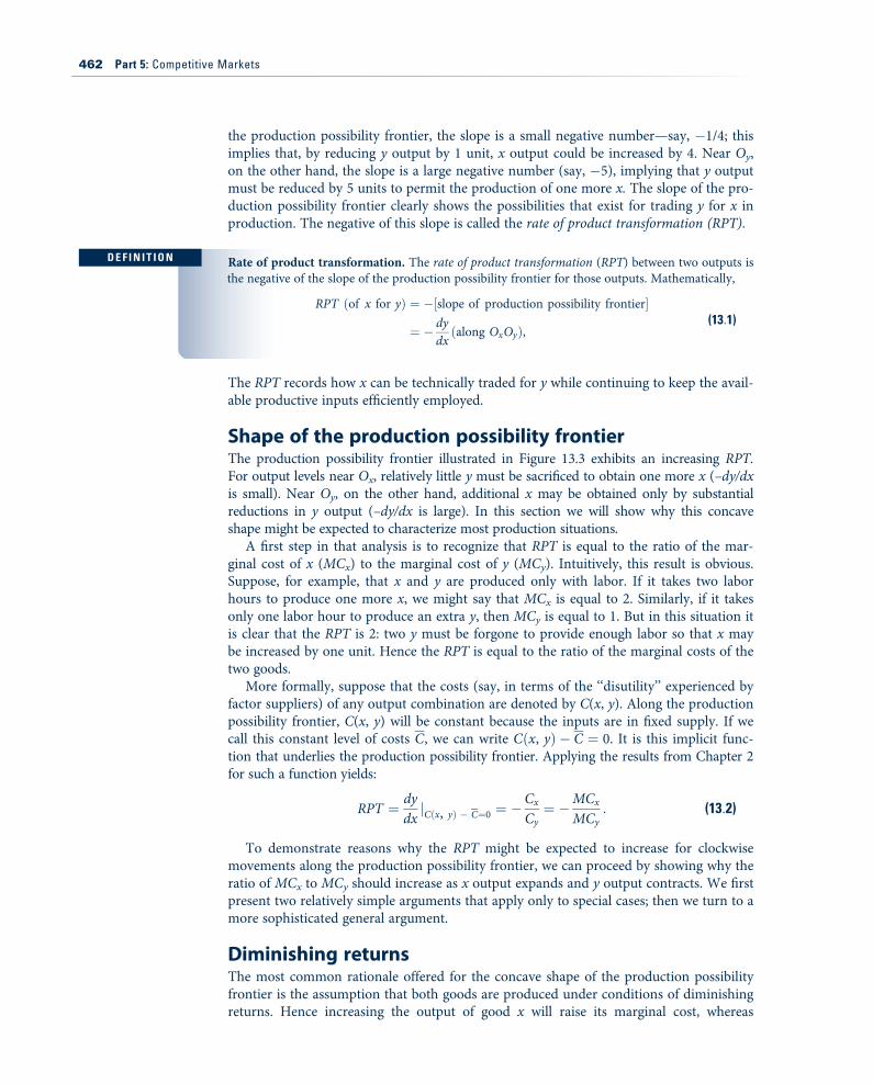
First theorem of welfare economicsGiven that the forces of supply and demand can establish equilibrium prices in the gen-eral equilibrium model of exchange we have developed, it is natural to ask what are thewelfare consequences of this finding. Adam Smith14 hypothesized that market forces pro-vide an ‘‘invisible hand’’ that leads each market participant to ‘‘promote an end [socialwelfare] which was no part of his intention.’’ Modern welfare economics seeks to under-stand the extent to which Smith was correct.

Perhaps the most important welfare result that can be derived from the exchangemodel is that the resulting Walrasian equilibrium is ‘‘efficient’’ in the sense that it is notpossible to devise some alternative allocation of resources in which at least some peopleare better off and no one is worse off. This definition of efficiency was originally devel-oped by Italian economist Vilfredo Pareto in the early 1900s. Understanding the defini-tion is easiest if we consider what an ‘‘inefficient’’ allocation might be. The totalquantities of goods included in initial endowments would be allocated inefficiently if itwere possible, by shifting goods around among individuals, to make at least one personbetter off (i.e., receive a higher utility) and no one worse off. Clearly, if individuals’ pref-erences are to count, such a situation would be undesirable. Hence we have a formaldefinition.

A proof that all Walrasian equilibria are Pareto efficient proceeds indirectly. Supposethat p) generates a Walrasian equilibrium in which the quantity of goods consumed byeach person is denoted by )xk"k $ 1 . . . m#. Now assume that there is some alternativeallocation of the available goods 0xk"k $ 1 . . . m# such that, for at least one person, say,person i, it is that case that 0xi is preferred to )xi. For this person, it must be the case that

p) 0xi > p) )xi (13:33)

because otherwise this person would have bought the preferred bundle in the first place.If all other individuals are to be equally well off under this new proposed allocation, itmust be the case for them that

p) 0xk $ p) )xk k $ 1 . . . m, k 6$ i: (13:34)

If the new bundle were less expensive, such individuals could not have been minimizingexpenditures at p). Finally, to be feasible, the new allocation must obey the quantityconstraints

Xm

i$1

0xi $Xm

i$1xi: (13:35)

Multiplying Equation 13.35 by p)yields

Xm

i$1p) 0xi $

Xm

i$1p) xi, (13:36)

D E F I N I T I O N Pareto efficient allocation. An allocation of the available goods in an exchange economy isefficient if it is not possible to devise an alternative allocation in which at least one person is betteroff and no one is worse off.

14Adam Smith, The Wealth of Nations (New York: Modern Library, 1937) p. 423.


but Equations 13.33 and 13.34 together with Walras’ law applied to the original equilib-rium imply that

Xm

i$1p) 0xi >

Xm

i$1p) )xi $

Xm

i$1p) xi: (13:37)

Hence we have a contradiction and must conclude that no such alternative allocation canexist. Therefore, we can summarize our analysis with the following definition.

The significance of this ‘‘theorem’’ should not be overstated. The theorem does not saythat every Walrasian equilibrium is in some sense socially desirable. Walrasian equilibriacan, for example, exhibit vast inequalities among individuals arising in part from inequal-ities in their initial endowments (see the discussion in the next section). The theorem alsoassumes price-taking behavior and full information about prices—assumptions that neednot hold in other models. Finally, the theorem does not consider possible effects of oneindividual’s consumption on another. In the presence of such externalities even a perfectcompetitive price system may not yield Pareto optimal results (see Chapter 19).

Still, the theorem does show that Smith’s ‘‘invisible hand’’ conjecture has some valid-ity. The simple markets in this exchange world can find equilibrium prices, and at thoseequilibrium prices the resulting allocation of resources will be efficient in the Paretosense. Developing this proof is one of the key achievements of welfare economics.

A graphic illustration of the first theoremIn Figure 13.8 we again use the Edgeworth box diagram, this time to illustrate anexchange economy. In this economy there are only two goods (x and y) and two individ-uals (A and B). The total dimensions of the Edgeworth box are determined by the totalquantities of the two goods available (x and y). Goods allocated to individual A arerecorded using 0A as an origin. Individual B gets those quantities of the two goods thatare ‘‘left over’’ and can be measured using 0B as an origin. Individual A’s indifferencecurve map is drawn in the usual way, whereas individual B’s map is drawn from theperspective of 0B. Point E in the Edgeworth box represents the initial endowments ofthese two individuals. Individual A starts with xA and yA. Individual B starts withxB $ x ! xA and yB $ y ! yA:

The initial endowments provide a utility level of U2A for person A and U2

B for person B.These levels are clearly inefficient in the Pareto sense. For example, we could, by reallo-cating the available goods,15 increase person B’s utility to U3

B while holding person A’sutility constant at U2

A (point B). Or we could increase person A’s utility to U3A while keep-

ing person B on the U2B indifference curve (point A). Allocations A and B are Pareto effi-

cient, however, because at these allocations it is not possible to make either person betteroff without making the other worse off. There are many other efficient allocations in theEdgeworth box diagram. These are identified by the tangencies of the two individuals’indifference curves. The set of all such efficient points is shown by the line joining OA toOB. This line is sometimes called the ‘‘contract curve’’ because it represents all the Pareto-efficient contracts that might be reached by these two individuals. Notice, however, that(assuming that no individual would voluntarily opt for a contract that made him or her

D E F I N I T I O N First theorem of welfare economics. Every Walrasian equilibrium is Pareto efficient.

15This point could in principle be found by solving the following constrained optimization problem: MaximizeUB xB , yB" # subject to the constraintUA xA , yA" # $ U2

A . SeeExample13.3.


worse off ) only contracts between points B and A are viable with initial endowmentsgiven by point E.

The line PP in Figure 13.8 shows the competitively established price ratio that is guar-anteed by our earlier existence proof. The line passes through the initial endowments (E)and shows the terms at which these two individuals can trade away from these initialpositions. Notice that such trading is beneficial to both parties—that is, it allows them toget a higher utility level than is provided by their initial endowments. Such trading willcontinue until all such mutual beneficial trades have been completed. That will occur atallocation E) on the contract curve. Because the individuals’ indifference curves are tan-gent at this point, no further trading would yield gains to both parties. Therefore, thecompetitive allocation E) meets the Pareto criterion for efficiency, as we showed mathe-matically earlier.

Second theorem of welfare economicsThe first theorem of welfare economics shows that a Walrasian equilibrium is Pareto effi-cient, but the social welfare consequences of this result are limited because of the roleplayed by initial endowments in the demonstration. The location of the Walrasian equi-librium at E) in Figure 13.8 was significantly influenced by the designation of E as thestarting point for trading. Points on the contract curve outside the range of AB are notattainable through voluntary transactions, even though these may in fact be more sociallydesirable than E) (perhaps because utilities are more equal). The second theorem of wel-fare economics addresses this issue. It states that for any Pareto optimal allocation ofresources there exists a set of initial endowments and a related price vector such that thisallocation is also a Walrasian equilibrium. Phrased another way, any Pareto optimal allo-cation of resources can also be a Walrasian equilibrium, providing that initial endow-ments are adjusted accordingly.

With initial endowments at point E, individuals trade along the price line PP until they reach point E).This equilibrium is Pareto efficient.

O B

P

A

B

P

U 3B

U 3A

U 2B

U 2A

E

E*

y

O A

y A

y B

x A x B

x

FIGURE 13.8

The First Theorem ofWelfare Economics


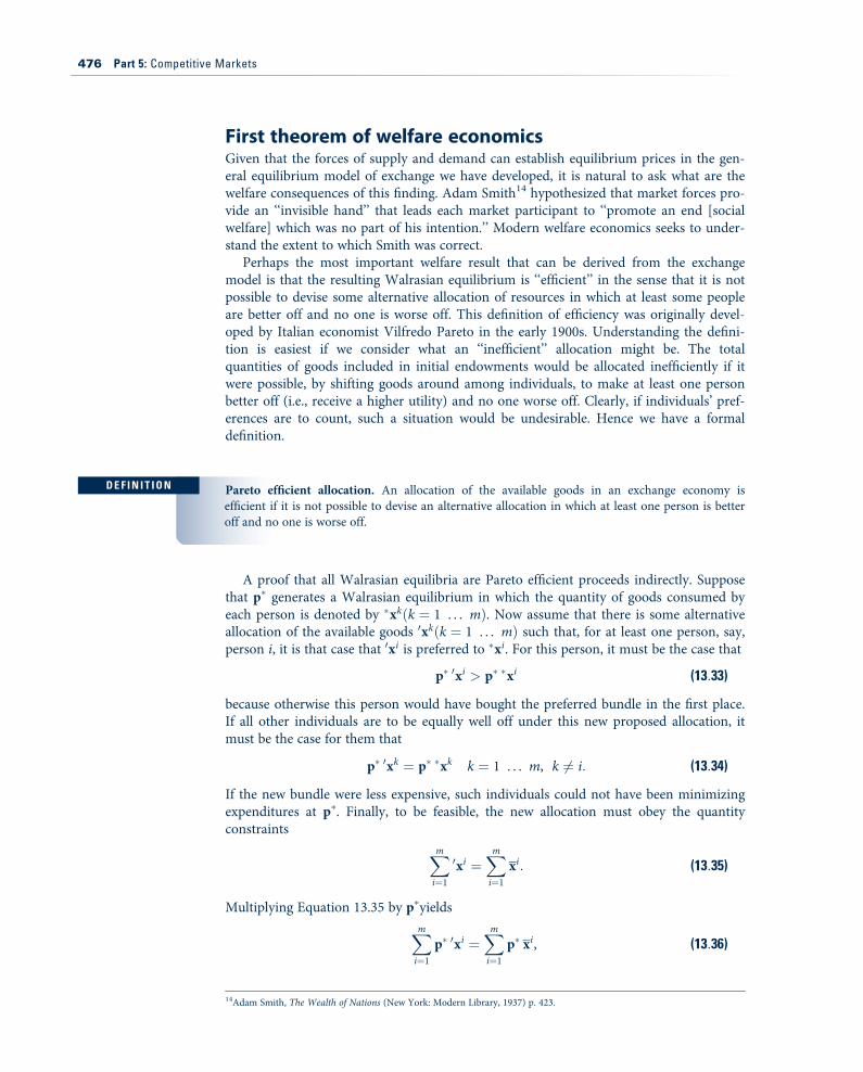
A graphical proof of the second theorem should suffice. Figure 13.9 repeats the keyaspects of the exchange economy pictures in Figure 13.8. Given the initial endowments atpoint E, all voluntary Walrasian equilibrium must lie between points A and B on the con-tract curve. Suppose, however, that these allocations were thought to be undesirable—perhaps because they involve too much inequality of utility. Assume that the Paretooptimal allocation Q) is believed to be socially preferable, but it is not attainable from theinitial endowments at point E. The second theorem states that one can draw a price linethrough Q) that is tangent to both individuals’ respective indifference curves. This line isdenoted by P 0P 0 in Figure 13.9. Because the slope of this line shows potential trades theseindividuals are willing to make, any point on the line can serve as an initial endowmentfrom which trades lead to Q). One such point is denoted by Q. If a benevolent govern-ment wished to ensure that Q) would emerge as a Walrasian equilibrium, it would haveto transfer initial endowments of the goods from E to Q (making person A better off andperson B worse off in the process).

If allocation Q) is regarded as socially optimal, this allocation can be supported by any initialendowments on the price line P0P0 . To move from E to, say, Q would require transfers of initialendowments.

O A

O B

T o ta ly

To ta l x

B

E

AE*

P'

Q*

Q

P'

EXAMPLE 13.3 A Two-Person Exchange Economy

To illustrate these various principles, consider a simple two-person, two-good exchangeeconomy. Suppose that total quantities of the goods are fixed at x $ y $ 1,000. Person A’sutility takes the Cobb–Douglas form:

UA"xA, yA# $ x2=3A y1=3A , (13:38)

and person B’s preferences are given by:

UB"xB, yB# $ x1=3B y2=3B : (13:39)

FIGURE 13.9

The Second Theorem ofWelfare Economics


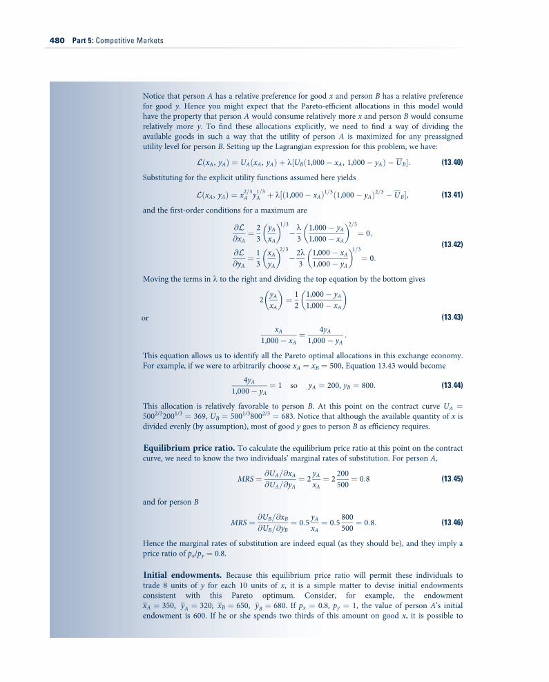
Notice that person A has a relative preference for good x and person B has a relative preferencefor good y. Hence you might expect that the Pareto-efficient allocations in this model wouldhave the property that person A would consume relatively more x and person B would consumerelatively more y. To find these allocations explicitly, we need to find a way of dividing theavailable goods in such a way that the utility of person A is maximized for any preassignedutility level for person B. Setting up the Lagrangian expression for this problem, we have:

L"xA, yA# $ UA"xA, yA# ' k%UB"1,000! xA, 1,000! yA# ! UB&: (13:40)

Substituting for the explicit utility functions assumed here yields

L"xA, yA# $ x2=3A y1=3A ' k%"1,000! xA#1=3"1,000! yA#2=3 ! UB&, (13:41)

and the first-order conditions for a maximum are

@L@xA$ 2

3yAxA

" #1=3!k3

1,000! yA1,000! xA

" #2=3$ 0;

@L@yA$ 1

3xAyA

" #2=3! 2k

31,000! xA1,000! yA

" #1=3$ 0:

(13:42)

Moving the terms in l to the right and dividing the top equation by the bottom gives

2yAxA

" #$ 1

21,000! yA1,000! xA

" #

orxA

1,000! xA$ 4yA

1,000! yA:

(13:43)

This equation allows us to identify all the Pareto optimal allocations in this exchange economy.For example, if we were to arbitrarily choose xA $ xB $ 500, Equation 13.43 would become

4yA1,000! yA

$ 1 so yA $ 200, yB $ 800: (13:44)

This allocation is relatively favorable to person B. At this point on the contract curve UA $5002/32001/3 $ 369, UB $ 5001/38002/3 $ 683. Notice that although the available quantity of x isdivided evenly (by assumption), most of good y goes to person B as efficiency requires.

Equilibrium price ratio. To calculate the equilibrium price ratio at this point on the contractcurve, we need to know the two individuals’ marginal rates of substitution. For person A,

MRS $ @UA=@xA@UA=@yA

$ 2yAxA$ 2

200500$ 0:8 (13:45)

and for person B

MRS $ @UB=@xB@UB=@yB

$ 0:5yAxA$ 0:5

800500$ 0:8: (13:46)

Hence the marginal rates of substitution are indeed equal (as they should be), and they imply aprice ratio of px/py $ 0.8.

Initial endowments. Because this equilibrium price ratio will permit these individuals totrade 8 units of y for each 10 units of x, it is a simple matter to devise initial endowmentsconsistent with this Pareto optimum. Consider, for example, the endowmentxA $ 350, yA $ 320; xB $ 650, yB $ 680. If px $ 0.8, py $ 1, the value of person A’s initialendowment is 600. If he or she spends two thirds of this amount on good x, it is possible to


Social welfare functionsFigure 13.9 shows that there are many Pareto-efficient allocations of the available goods inan exchange economy.We are assured by the second theorem of welfare economics that anyof these can be supported by aWalrasian system of competitively determined prices, provid-ing that initial endowments are adjusted accordingly. Amajor question for welfare econom-ics is how (if at all) to develop criteria for choosing among all these allocations. In thissection we look briefly at one strand of this large topic—the study of social welfare functions.Simply put, a social welfare function is a hypothetical scheme for ranking potential alloca-tions of resources based on the utility they provide to individuals. Inmathematical terms:

Social Welfare $ SW%U1"x1#, U2"x2#, . . . , Um"xm#&: (13:47)

The ‘‘social planner’s’’ goal then is to choose allocations of goods among the m individu-als in the economy in a way that maximizes SW. Of course, this exercise is a purely con-ceptual one—in reality there are no clearly articulated social welfare functions in anyeconomy, and there are serious doubts about whether such a function could ever arisefrom some type of democratic process.16 Still, assuming the existence of such a functioncan help to illuminate many of the thorniest problems in welfare economics.

A first observation that might be made about the social welfare function in Equation13.47 is that any welfare maximum must also be Pareto efficient. If we assume that everyindividual’s utility is to ‘‘count,’’ it seems clear that any allocation that permits furtherPareto improvements (that make one person better off and no one else worse off) cannotbe a welfare maximum. Hence achieving a welfare maximum is a problem in choosingamong Pareto-efficient allocations and their related Walrasian price systems.

We can make further progress in examining the idea of social welfare maximizationby considering the precise functional form that SW might take. Specifically, if we assumeutility is measurable, using the CES form can be particularly instructive:

SW"U1, U2, . . . , Um# $UR1

R' UR

2

R' . . .' UR

m

RR , 1: (13:48)

Because we have used this functional form many times before in this book, its propertiesshould by now be familiar. Specifically, if R $ 1, the function becomes:

SW"U1, U2, . . . , Um# $ U1 ' U2 ' . . . ' Um: (13:49)

purchase 500 units of good x and 200 units of good y. This would increase utility from UA $3502/3 3201/3 $ 340 to 369. Similarly, the value of person B’s endowment is 1,200. If he or shespends one third of this on good x, 500 units can be bought. With the remaining two thirds ofthe value of the endowment being spent on good y, 800 units can be bought. In the process, B’sutility increases from 670 to 683. Thus, trading from the proposed initial endowment to thecontract curve is indeed mutually beneficial (as shown in Figure 13.8).

QUERY: Why did starting with the assumption that good x would be divided equally on thecontract curve result in a situation favoring person B throughout this problem? What point onthe contract curve would provide equal utility to persons A and B? What would the price ratioof the two goods be at this point?

16The ‘‘impossibility’’ of developing a social welfare function from the underlying preferences of people in society was first stud-ied by K. Arrow in Social Choice and Individual Values, 2nd ed. (New York: Wiley, 1963). There is a large body of literaturestemming from Arrow’s initial discovery.


Thus, utility is a simple sum of the utility of every person in the economy. Such a socialwelfare function is sometimes called a utilitarian function. With such a function, socialwelfare is judged by the aggregate sum of utility (or perhaps even income) with no regardfor how utility (income) is distributed among the members of society.

At the other extreme, consider the case R $ !1. In this case, social welfare has a‘‘fixed proportions’’ character and (as we have seen in many other applications),

SW"U1, U2, . . . , Um# $ Min %U1, U2, . . . , Um&: (13:50)

Therefore, this function focuses on the worse-off person in any allocation and choosesthat allocation for which this person has the highest utility. Such a social welfare functionis called a maximin function. It was made popular by the philosopher John Rawls, whoargued that if individuals did not know which position they would ultimately have insociety (i.e., they operate under a ‘‘veil of ignorance’’), they would opt for this sort of socialwelfare function to guard against being the worse-off person.17 Our analysis in Chapter 7suggests that people may not be this risk averse in choosing social arrangements. However,Rawls’ focus on the bottom of the utility distribution is probably a good antidote to think-ing about social welfare in purely utilitarian terms.

It is possible to explore many other potential functional forms for a hypothetical wel-fare function. Problem 13.14 looks at some connections between social welfare functionsand the income distribution, for example. But such illustrations largely miss a crucialpoint if they focus only on an exchange economy. Because the quantities of goods in suchan economy are fixed, issues related to production incentives do not arise when evaluat-ing social welfare alternatives. In actuality, however, any attempt to redistribute income(or utility) through taxes and transfers will necessarily affect production incentives andtherefore affect the size of the Edgeworth box. Therefore, assessing social welfare willinvolve studying the trade-off between achieving distributional goals and maintaining lev-els of production. To examine such possibilities we must introduce production into ourgeneral equilibrium framework.

A Mathematical Model ofProduction and ExchangeAdding production to the model of exchange developed in the previous section is a rela-tively simple process. First, the notion of a ‘‘good’’ needs to be expanded to include fac-tors of production. Therefore, we will assume that our list of n goods now includes inputswhose prices also will be determined within the general equilibrium model. Some inputsfor one firm in a general equilibrium model are produced by other firms. Some of thesegoods may also be consumed by individuals (cars are used by both firms and final con-sumers), and some of these may be used only as intermediate goods (steel sheets are usedonly to make cars and are not bought by consumers). Other inputs may be part of indi-viduals’ initial endowments. Most importantly, this is the way labor supply is treated ingeneral equilibrium models. Individuals are endowed with a certain number of potentiallabor hours. They may sell these to firms by taking jobs at competitively determinedwages, or they may choose to consume the hours themselves in the form of ‘‘leisure,’’In making such choices we continue to assume that individuals maximize utility.18

We will assume that there are r firms involved in production. Each of these firms isbound by a production function that describes the physical constraints on the ways the

17J. Rawls, A Theory of Justice (Cambridge, MA: Harvard University Press, 1971).18A detailed study of labor supply theory is presented in Chapter 16.


firm can turn inputs into outputs. By convention, outputs of the firm take a positive sign,whereas inputs take a negative sign. Using this convention, each firm’s production plan canbe described by an n + 1 column vector, y j( j $ 1 . . . r), which contains both positive andnegative entries. The only vectors that the firm may consider are those that are feasible giventhe current state of technology. Sometimes it is convenient to assume each firm producesonly one output. But that is not necessary for a more general treatment of production.

Firms are assumed to maximize profits. Production functions are assumed to be suffi-ciently convex to ensure a unique profit maximum for any set of output and input prices.This rules out both increasing returns to scale technologies and constant returns becauseneither yields a unique maxima. Many general equilibrium models can handle such possi-bilities, but there is no need to introduce such complexities here. Given these assump-tions, the profits for any firm can be written as:

pj"p# $ py j if pj"p# ( 0 and

y j $ 0 if pj"p# < 0:(13:51)

Hence this model has a ‘‘long run’’ orientation in which firms that lose money (at a par-ticular price configuration) hire no inputs and produce no output. Notice how the con-vention that outputs have a positive sign and inputs a negative sign makes it possible tophrase profits in a compact way.19

Budget constraints and Walras’ lawIn an exchange model, individuals’ purchasing power is determined by the values of theirinitial endowments. Once firms are introduced, we must also consider the income streamthat may flow from ownership of these firms. To do so, we adopt the simplifying assump-

tion that each individual owns a predefined share, si "wherePm

i$1si $ 1 # of the profits

of all firms. That is, each person owns an ‘‘index fund’’ that can claim a proportionateshare of all firms’ profits. We can now rewrite each individual’s budget constraint (fromEquation 13.24) as:

pxi $ siXr

j$1pyj ' pxi i $ 1 . . .m: (13:52)

Of course, if all firms were in long-run equilibrium in perfectly competitive industries, allprofits would be zero and the budget constraint in Equation 13.52 would revert to that inEquation 13.24. But allowing for long-term profits does not greatly complicate our model;therefore, we might as well consider the possibility.

As in the exchange model, the existence of these m budget constraints implies a con-straint of the prices that are possible—a generalization of Walras’ law. Summing thebudget constraints in Equation 13.52 over all individuals yields:

pXm

i$1xi"p# $ p

Xr

j$1y j"p# ' p

Xm

i$1xi, (13:53)

and letting x"p# $P

xi"p#, y"p# $P

yj"p#, x $P

xi provides a simple statement ofWalras’ law:

px"p# $ py"p# ' px: (13:54)

19As we saw in Chapter 11, profit functions are homogeneous of degree 1 in all prices. Hence both output supply functions andinput demand functions are homogeneous of degree 0 in all prices because they are derivatives of the profit function.


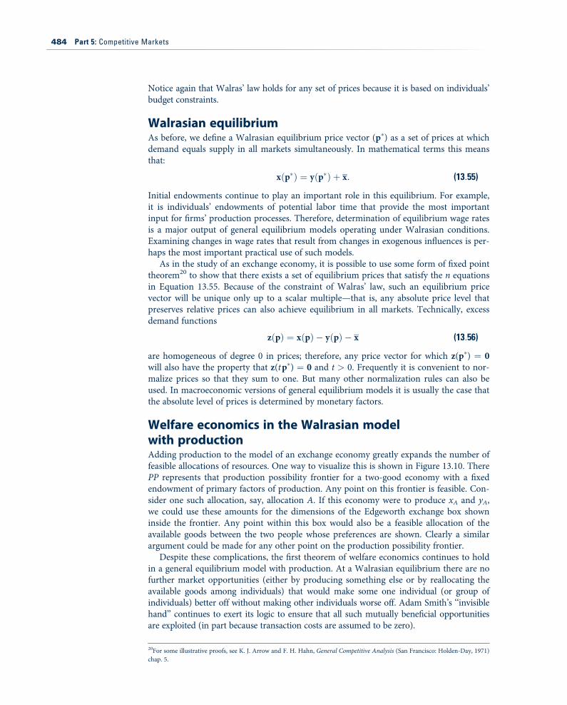
Notice again that Walras’ law holds for any set of prices because it is based on individuals’budget constraints.

Walrasian equilibriumAs before, we define a Walrasian equilibrium price vector (p)) as a set of prices at whichdemand equals supply in all markets simultaneously. In mathematical terms this meansthat:

x"p)# $ y"p)# ' x: (13:55)

Initial endowments continue to play an important role in this equilibrium. For example,it is individuals’ endowments of potential labor time that provide the most importantinput for firms’ production processes. Therefore, determination of equilibrium wage ratesis a major output of general equilibrium models operating under Walrasian conditions.Examining changes in wage rates that result from changes in exogenous influences is per-haps the most important practical use of such models.

As in the study of an exchange economy, it is possible to use some form of fixed pointtheorem20 to show that there exists a set of equilibrium prices that satisfy the n equationsin Equation 13.55. Because of the constraint of Walras’ law, such an equilibrium pricevector will be unique only up to a scalar multiple—that is, any absolute price level thatpreserves relative prices can also achieve equilibrium in all markets. Technically, excessdemand functions

z"p# $ x"p# ! y"p# ! x (13:56)

are homogeneous of degree 0 in prices; therefore, any price vector for which z(p)) $ 0will also have the property that z(tp)) $ 0 and t > 0. Frequently it is convenient to nor-malize prices so that they sum to one. But many other normalization rules can also beused. In macroeconomic versions of general equilibrium models it is usually the case thatthe absolute level of prices is determined by monetary factors.

Welfare economics in the Walrasian modelwith productionAdding production to the model of an exchange economy greatly expands the number offeasible allocations of resources. One way to visualize this is shown in Figure 13.10. TherePP represents that production possibility frontier for a two-good economy with a fixedendowment of primary factors of production. Any point on this frontier is feasible. Con-sider one such allocation, say, allocation A. If this economy were to produce xA and yA,we could use these amounts for the dimensions of the Edgeworth exchange box showninside the frontier. Any point within this box would also be a feasible allocation of theavailable goods between the two people whose preferences are shown. Clearly a similarargument could be made for any other point on the production possibility frontier.

Despite these complications, the first theorem of welfare economics continues to holdin a general equilibrium model with production. At a Walrasian equilibrium there are nofurther market opportunities (either by producing something else or by reallocating theavailable goods among individuals) that would make some one individual (or group ofindividuals) better off without making other individuals worse off. Adam Smith’s ‘‘invisiblehand’’ continues to exert its logic to ensure that all such mutually beneficial opportunitiesare exploited (in part because transaction costs are assumed to be zero).

20For some illustrative proofs, see K. J. Arrow and F. H. Hahn, General Competitive Analysis (San Francisco: Holden-Day, 1971)chap. 5.


Again, the general social welfare implications of the first theorem of welfare economicsare far from clear. There is, of course, a second theorem, which shows that practically anyWalrasian equilibrium can be supported by suitable changes in initial endowments. Onealso could hypothesize a social welfare function to choose among these. But most suchexercises are rather uninformative about actual policy issues.

More interesting is the use of the Walrasian mechanism to judge the hypotheticalimpact of various tax and transfer policies that seek to achieve specific social welfare cri-teria. In this case (as we shall see) the fact that Walrasian models stress interconnectionsamong markets, especially among product and input markets, can yield important andoften surprising results. In the next section we look at a few of these.

Computable General EquilibriumModelsTwo advances have spurred the rapid development of general equilibrium models inrecent years. First, the theory of general equilibrium itself has been expanded to includemany features of real-world markets such as imperfect competition, environmental exter-nalities, and complex tax systems. Models that involve uncertainty and that have adynamic structure also have been devised, most importantly in the field of macroeconom-ics. A second related trend has been the rapid development of computer power and theassociated software for solving general equilibrium models. This has made it possible to

Any point on the production possibility frontier PP can serve as the dimensions of an Edgeworthexchange box.

y A

x A

P

P

A

Quantity of x

Quantity of y

FIGURE 13.10

Production Increasesthe Number of FeasibleAllocations


study models with virtually any number of goods and types of households. In this sectionwe will briefly explore some conceptual aspects of these models.21 The Extensions to thechapter describe a few important applications.

Structure of general equilibrium modelsSpecification of any general equilibrium model begins by defining the number of goodsto be included in the model. These ‘‘goods’’ include not only consumption goods but alsointermediate goods that are used in the production of other goods (e.g., capital equip-ment), productive inputs such as labor or natural resources, and goods that are to be pro-duced by the government (public goods). The goal of the model is then to solve forequilibrium prices for all these goods and to study how these prices change when condi-tions change.

Some of the goods in a general equilibrium model are produced by firms. The technol-ogy of this production must be specified by production functions. The most commonsuch specification is to use the types of CES production functions that we studied inChapters 9 and 10 because these can yield some important insights about the ways inwhich inputs are substituted in the face of changing prices. In general, firms are assumedto maximize their profits given their production functions and given the input and outputprices they face.

Demand is specified in general equilibrium models by defining utility functions forvarious types of households. Utility is treated as a function both of goods that are con-sumed and of inputs that are not supplied to the marketplace (e.g., available labor that isnot supplied to the market is consumed as leisure). Households are assumed to maximizeutility. Their incomes are determined by the amounts of inputs they ‘‘sell’’ in the marketand by the net result of any taxes they pay or transfers they receive.

Finally, a full general equilibrium model must specify how the government operates.If there are taxes in the model, how those taxes are to be spent on transfers or on pub-lic goods (which provide utility to consumers) must be modeled. If government borrow-ing is allowed, the bond market must be explicitly modeled. In short, the model mustfully specify the flow of both sources and uses of income that characterize the economybeing modeled.

Solving general equilibrium modelsOnce technology (supply) and preferences (demand) have been specified, a general equi-librium model must be solved for equilibrium prices and quantities. The proof earlier inthis chapter shows that such a model will generally have such a solution, but actuallyfinding that solution can sometimes be difficult—especially when the number of goodsand households is large. General equilibrium models are usually solved on computers viamodifications of an algorithm originally developed by Herbert Scarf in the 1970s.22

This algorithm (or more modern versions of it) searches for market equilibria by mimick-ing the way markets work. That is, an initial solution is specified and then prices areraised in markets with excess demand and lowered in markets with excess supply until anequilibrium is found in which all excess demands are zero. Sometimes multiple equilibriawill occur, but usually economic models have sufficient curvature in the underlying pro-duction and utility functions that the equilibrium found by the Scarf algorithm will beunique.

21For more detail on the issues discussed here, see W. Nicholson and F. Westhoff, ‘‘General Equilibrium Models: Improving theMicroeconomics Classroom,’’ Journal of Economic Education (Summer 2009): 297–314.22Herbert Scarf with Terje Hansen, On the Computation of Economic Equilibria (New Haven, CT: Yale University Press, 1973).


Economic insights from general equilibrium modelsGeneral equilibrium models provide a number of insights about how economies operatethat cannot be obtained from the types of partial equilibrium models studied in Chapter 12.Some of the most important of these are:

• All prices are endogenous in economic models. The exogenous elements of modelsare preferences and productive technologies.

• All firms and productive inputs are owned by households. All income ultimatelyaccrues to households.

• Any model with a government sector is incomplete if it does not specify how taxreceipts are used.

• The ‘‘bottom line’’ in any policy evaluation is the utility of households. Firms andgovernments are only intermediaries in getting to this final accounting.

• All taxes distort economic decisions along some dimension. The welfare costs of suchdistortions must always be weighed against the benefits of such taxes (in terms ofpublic good production or equity-enhancing transfers).

Some of these insights are illustrated in the next two examples. In later chapters we willreturn to general equilibrium modeling whenever such a perspective seems necessary togain a more complete understanding of the topic being covered.

EXAMPLE 13.4 A Simple General Equilibrium Model

Let’s look at a simple general equilibrium model with only two households, two consumer goods(x and y), and two inputs (capital k and labor l). Each household has an ‘‘endowment’’ of capitaland labor that it can choose to retain or sell in the market. These endowments are denoted byk1, l1 and k2, l2, respectively. Households obtain utility from the amounts of the consumergoods they purchase and from the amount of labor they do not sell into the market (i.e., leisure $li ! li). The households have simple Cobb–Douglas utility functions:

U1 $ x0:51 y0:31 "l1 ! l1#0:2, U2 $ x0:42 y0:42 "l2 ! l2#0:2: (13:57)

Hence household 1 has a relatively greater preference for good x than does household 2. Noticethat capital does not enter into these utility functions directly. Consequently, each householdwill provide its entire endowment of capital to the marketplace. Households will retain somelabor, however, because leisure provides utility directly.

Production of goods x and y is characterized by simple Cobb–Douglas technologies:

x $ k0:2x l 0:8x , y $ k0:8y l 0:2y : (13:58)

Thus, in this example, production of x is relatively labor intensive, whereas production of y isrelatively capital intensive.

To complete this model we must specify initial endowments of capital and labor. Here weassume that

k1 $ 40, l1 $ 24 and k2 $ 10, l2 $ 24: (13:59)

Although the households have equal labor endowments (i.e., 24 ‘‘hours’’), household 1 hassignificantly more capital than does household 2.

Base-case simulation. Equations 13.57–13.59 specify our complete general equilibriummodel in the absence of a government. A solution to this model will consist of four equilibriumprices (for x, y, k, and l ) at which households maximize utility and firms maximize profits.23

23Because firms’ production functions are characterized by constant returns to scale, in equilibrium each earns zero profits;therefore, there is no need to specify firm ownership in this model.


Because any general equilibrium model can compute only relative prices, we are free to impose aprice-normalization scheme. Here we assume that the prices will always sum to unity. That is,

px ' py ' pk ' pl $ 1: (13:60)

Solving24 for these prices yields

px $ 0:363, py $ 0:253, pk $ 0:136, pl $ 0:248: (13:61)

At these prices, total production of x is 23.7 and production of y is 25.1. The utility-maximizingchoices for household 1 are

x1 $ 15:7, y1 $ 8:1; l1 ! l1 $ 24! 14:8 $ 9:2, U1 $ 13:5; (13:62)

for household 2, these choices are

x2 $ 8:1, y2 $ 11:6; l2 ! l2 $ 24! 18:1 $ 5:9, U2 $ 8:75: (13:63)

Observe that household 1 consumes quite a bit of good x but provides less in labor supply thandoes household 2. This reflects the greater capital endowment of household 1 in this base-casesimulation. We will return to this base case in several later simulations.

QUERY: How would you show that each household obeys its budget constraint in thissimulation? Does the budgetary allocation of each household exhibit the budget shares that areimplied by the form of its utility function?

EXAMPLE 13.5 The Excess Burden of a Tax

In Chapter 12 we showed that taxation may impose an excess burden in addition to the taxrevenues collected because of the incentive effects of the tax. With a general equilibrium model wecan show much more about this effect. Specifically, assume that the government in the economyof Example 13.4 imposes an ad valorem tax of 0.4 on good x. This introduces a wedge betweenwhat demanders pay for this good x (px) and what suppliers receive for the good (p0x$ (1 – t)px$0.6px). To complete the model we must specify what happens to the revenues generated by thistax. For simplicity we assume that these revenues are rebated to the households in a 50–50 split.In all other respects the economy remains as described in Example 13.4.

Solving for the new equilibrium prices in this model yields

px = 0.472, py = 0.218, pk = 0.121, pl = 0.188. (13:64)

At these prices, total production of x is 17.9, and total production of y is 28.8. Hence theallocation of resources has shifted significantly toward y production. Even though the relativeprice of x experienced by consumers ($ px/py $ 0.472/0.218 $ 2.17) has increased significantlyfrom its value (of 1.43) in Example 13.4, the price ratio experienced by firms (0.6px/py $ 1.30)has decreased somewhat from this prior value. Therefore, one might expect, based on a partialequilibrium analysis, that consumers would demand less of good x and likewise that firmswould similarly produce less of that good. Partial equilibrium analysis would not, however,allow us to predict the increased production of y (which comes about because the relative price

24The computer program used to find these solutions is accessible at www.amherst.edu/-fwesthoff/compequ/FixedPointsCompEquApplet.html.


www.amherst.edu/~fwesthoff/compequ/FixedPointsCompEquApplet.html

www.amherst.edu/~fwesthoff/compequ/FixedPointsCompEquApplet.html

SUMMARY

This chapter has provided a general exploration of AdamSmith’s conjectures about the efficiency properties of com-petitive markets. We began with a description of how tomodel many competitive markets simultaneously and thenused that model to make a few statements about welfare.Some highlights of this chapter are listed here.

• Preferences and production technologies provide thebuilding blocks on which all general equilibriummodels are based. One particularly simple version ofsuch a model uses individual preferences for two goodstogether with a concave production possibility frontierfor those two goods.

• Competitive markets can establish equilibrium pricesby making marginal adjustments in prices in responseto information about the demand and supply for indi-vidual goods. Walras’ law ties markets together so thatsuch a solution is assured (in most cases).

• General equilibrium models can usually be solved byusing computer algorithms. The resulting solutions

yield many insights about the economy that are notobtainable from partial equilibrium analysis of singlemarkets.

• Competitive prices will result in a Pareto-efficient allo-cation of resources. This is the first theorem of welfareeconomics.

• Factors that interfere with competitive markets’ abil-ities to achieve efficiency include (1) market power,(2) externalities, (3) existence of public goods, and(4) imperfect information. We explore all these issuesin detail in later chapters.

• Competitive markets need not yield equitable distribu-tions of resources, especially when initial endowmentsare highly skewed. In theory, any desired distributioncan be attained through competitive markets accompa-nied by appropriate transfers of initial endowments(the second theorem of welfare economics). But thereare many practical problems in implementing suchtransfers.

of y has decreased for consumers but has increased for firms) nor the reduction in relative inputprices (because there is less being produced overall). A more complete picture of all these effectscan be obtained by looking at the final equilibrium positions of the two households. The post-tax allocation for household 1 is

x1 $ 11:6, y1 $ 15:2, l1 ! l1 $ 11:8, U1 $ 12:7; (13:65)

for household 2,

x2 $ 6.3, y2 $ 13.6, l2 ! l2 $ 7.9, U2 $ 8.96. (13:66)

Hence imposition of the tax has made household 1 considerably worse off: utility decreases from13.5 to 12.7. Household 2 is made slightly better off by this tax and transfer scheme, primarilybecause it receives a relatively large share of the tax proceeds that come mainly from household1. Although total utility has decreased (as predicted by the simple partial equilibrium analysis ofexcess burden), general equilibrium analysis gives a more complete picture of the distributionalconsequences of the tax. Notice also that the total amount of labor supplied decreases as a resultof the tax: total leisure increases from 15.1 (hours) to 19.7. Therefore, imposition of a tax ongood x has had a relatively substantial labor supply effect that is completely invisible in a partialequilibrium model.

QUERY: Would it be possible to make both households better off (relative to Example 13.4) inthis taxation scenario by changing how the tax revenues are redistributed?


General Equilibrium THIRTEEN CHAPTER and Welfare...General Equilibrium and Welfare The partial...

Documents

Transcript of General Equilibrium THIRTEEN CHAPTER and Welfare...General Equilibrium and Welfare The partial...