GENERAL EQUILIBRIUM MODELS:

IMPROVING THE MICROECONOMICS CLASSROOM

Walter Nicholson and Frank Westhoff

Walter Nicholson Frank Westhoff Professor of Economics Professor of Economics Department of Economics Department of Economics Amherst College Amherst College Amherst, MA 01002 Amherst, MA 01002 Tel: 413-542-2191 Tel: 413-542-2190 Fax: 413-542-2090 Fax: 413-542-2090 wenicholson@amherst.edu fwesthoff@amherst.edu

October 19, 2007

The general equilibrium simulation program described in this paper is available at the

following URL:

www.amherst.edu/~fwesthoff/compequ/FixedPointsCompEquApplet.html.

2

Abstract: General equilibrium modeling has come to play an important role in

such fields as international trade, tax policy, environmental regulation, and

economic development. Teaching about these models in intermediate

microeconomics courses has not kept pace with these trends. The typical

microeconomics course devotes only about a week to general equilibrium

issues and microeconomics texts primarily focus on the insights that can be

drawn from the Edgeworth Box diagram for exchange. We believe such

treatment leaves students unprepared for understanding much of the policy-

related literature they will encounter and, more generally, shortchanges their

education in economics. In this paper, we illustrate how computer-based

general equilibrium simulations might improve teaching about these topics in

intermediate microeconomics courses. We provide several illustrations

describing how simulations could be used to make important points about

economic theory, public economics, and environmental regulation.

3

The use of general equilibrium modeling has expanded dramatically in 

recent years.  Such models are now routinely employed to study tax incidence, 

environmental regulation, international trade impacts, and natural disasters.  

Insights provided by these modeling efforts could not have been obtained using 

standard partial equilibrium tools.  Teaching about general equilibrium 

modeling has not generally kept pace with these developments, however.  The 

standard intermediate microeconomics course coverage of general equilibrium 

concepts (if they are covered at all) spends about a week on the topic, mainly by 

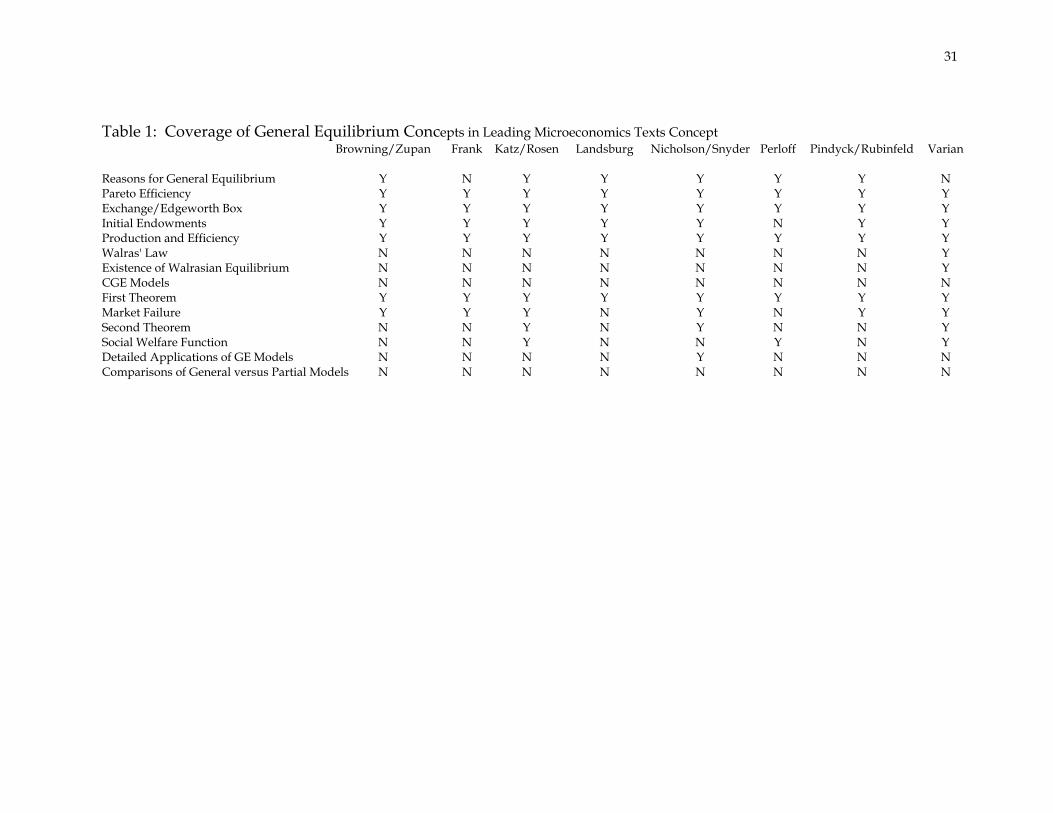
introducing the Edgeworth Box diagram for exchange.  Table 1 illustrates the 

type of coverage given to the central topics in general equilibrium theory in some 

of the leading microeconomics textbooks.  Virtually all of the books discuss 

Pareto optimality, efficiency in production and exchange, and the “first 

fundamental theorem” of welfare economics.  Few, if any, books cover general 

equilibrium modeling as it is practiced today. 

   

We believe that this short‐changing of general equilibrium concepts 

makes students ill prepared for understanding much current research.  More 

generally, we believe that this lack of attention obscures some major economic 

principles that all students of economics should know.  We begin by laying out 

some of the basic principles that we believe would be clarified by greater 

4

attention to general equilibrium models.  We then describe a computer‐based 

general equilibrium simulation program that may prove useful to instructors in 

making these points.  The subsequent sections of the paper present several 

illustrations of how the simulation program works in practice and how it can 

provide insights beyond those obtainable from partial equilibrium analysis. 

We use a “standard” Walrasian general equilibrium model composed of 

utility maximizing households and profit maximizing firms. The simulation uses 

a variant of the Scarf algorithm to find prices that clear each market. The 

underlying analytics of this general equilibrium model can be complex. The 

supply and demand equations for the goods and inputs tend to be complicated 

making it difficult, if not impossible, for even very good undergraduates to “sort 

things out.” We believe that our simulation approach avoids this pitfall by 

utilizing the numerical results. The student can apply the basic qualitative 

microeconomic analysis to appreciate why the equilibrium prices changed as 

they did without delving into the complex general equilibrium analytics. For 

example, students can “see” how a tax on one consumption good affects not only 

the price of that consumption good, but also the price of other consumptions 

goods and inputs. While understanding the workings of the algorithm itself is no 

doubt far beyond reach of the undergraduate, the software allows him/her to use 

the algorithm to illustrate the ramifications of general equilibrium analysis. 

5

 

INSIGHTS FROM GENERAL EQUILIBRIUM MODELS 

The strongest reason for more extensive coverage of general equilibrium 

models in intermediate microeconomics courses is that such inclusion would 

offer many new insights to students about economics.  Among those insights are: 

• Prices (including prices for factors of production) are endogenous in 

market economies.  The exogenous elements are household preferences, 

household endowments, and the productive technologies. 

• Firms and factors of production are owned by individual households, 

either directly or indirectly.  All firm revenue is ultimately claimed by 

some household. 

• Governments are bound by budget constraints.  Any model is incomplete 

if it does not specify how government receipts are used. 

• The “bottom line” in all evaluations of policy options in economics is the 

utility of the individuals in society.  Firms and governments are only 

intermediaries in getting to this final accounting. 

• Lump‐sum taxes have no incentive effects and provide “Pareto efficient” 

transfers. On the other hand, all “realistic” taxes produce incentive effects 

and are distorting, thereby raising important equity‐efficiency 

distributional issues.  

6

• There is a close tie between general equilibrium modeling and cost‐benefit 

accounting.  The general equilibrium approach helps to understand the 

distinction between productive activities and transfers and is necessary to 

get taxation, public good and externality accounting correct. 

 

Unfortunately, many of these insights are either not mentioned or made 

more obscure by the way that general equilibrium is currently taught.  For 

example, we doubt that focusing on how the Edgeworth exchange box is 

constructed helps students grasp how preferences actually affect relative prices.  

Similarly, showing how the production possibility frontier is developed from 

underlying production functions may obscure issues of input ownership and the 

overall budget constraints that characterize any economy.   

A better approach, we believe, would be to introduce students directly to 

computer‐based general equilibrium simulations.  By showing how general 

equilibrium models are structured and by walking students through some 

sample computer simulations, all of the insights listed above should become 

more apparent.  Doing this with existing software for general equilibrium 

modeling, however, may involve far more in set‐up costs than the typical 

instructor wishes to incur.  The computer‐based general equilibrium simulation 

program described below is complex enough to give students a feel for how 

7

general equilibrium models work while at the same time being simple enough 

for students to understand its key elements. 

 COMPUTER‐BASED GENERAL EQUILIBRIUM SIMULATION 

PROGRAM  Our general equilibrium simulation program follows the traditional 

Arrow‐Debreu approach modified to include the possibility of taxes, a public 

good, and an externality. All households and firms act as price‐takers. The 

simulation program has been coded in the Java language to provide a user‐

friendly interface. The program itself is very flexible and can accommodate an 

arbitrary number of goods, households, and firms. While the user can enter all 

the parameters of the economy (household endowments and utility functions; 

firm production functions; etc.), an alternative exists that most may find 

preferable. The user can open one of several existing files which specify the 

parameters for the illustrations that appear below. To reproduce our results, the 

user need only modify a few of the parameters such as the tax rates, the presence 

of a public good or externality, etc. In this way, the time and effort required to 

specify the parameters of the specific model can be minimized. 

 

Households 

8

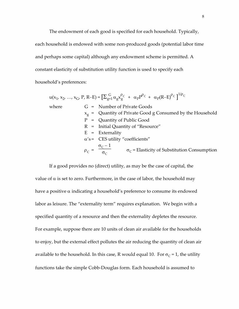
The endowment of each good is specified for each household. Typically, 

each household is endowed with some non‐produced goods (potential labor time 

and perhaps some capital) although any endowment scheme is permitted. A 

constant elasticity of substitution utility function is used to specify each 

household’s preferences: 

u(x1, x2, …, xG, P, R−E) = [Σg=1G αgxg  

ρC   +   αPPρC  +   αP(R−E)

ρC ]1/ρC where  G  =  Number of Private Goods   xg  =  Quantity of Private Good g Consumed by the Household   P  =  Quantity of Public Good   R  =  Initial Quantity of “Resource”   E  =  Externality   α’s =  CES utility “coefficients” 

  ρC  = σC − 1σC

   σC = Elasticity of Substitution Consumption 

 If a good provides no (direct) utility, as may be the case of capital, the 

value of α is set to zero. Furthermore, in the case of labor, the household may 

have a positive α indicating a household’s preference to consume its endowed 

labor as leisure. The “externality term” requires explanation.  We begin with a 

specified quantity of a resource and then the externality depletes the resource. 

For example, suppose there are 10 units of clean air available for the households 

to enjoy, but the external effect pollutes the air reducing the quantity of clean air 

available to the household. In this case, R would equal 10.  For σC = 1, the utility 

functions take the simple Cobb‐Douglas form. Each household is assumed to 

9

maximize its utility subject to a budget constraint that includes both consumer 

goods purchased and endowed resources sold. 

Firms 

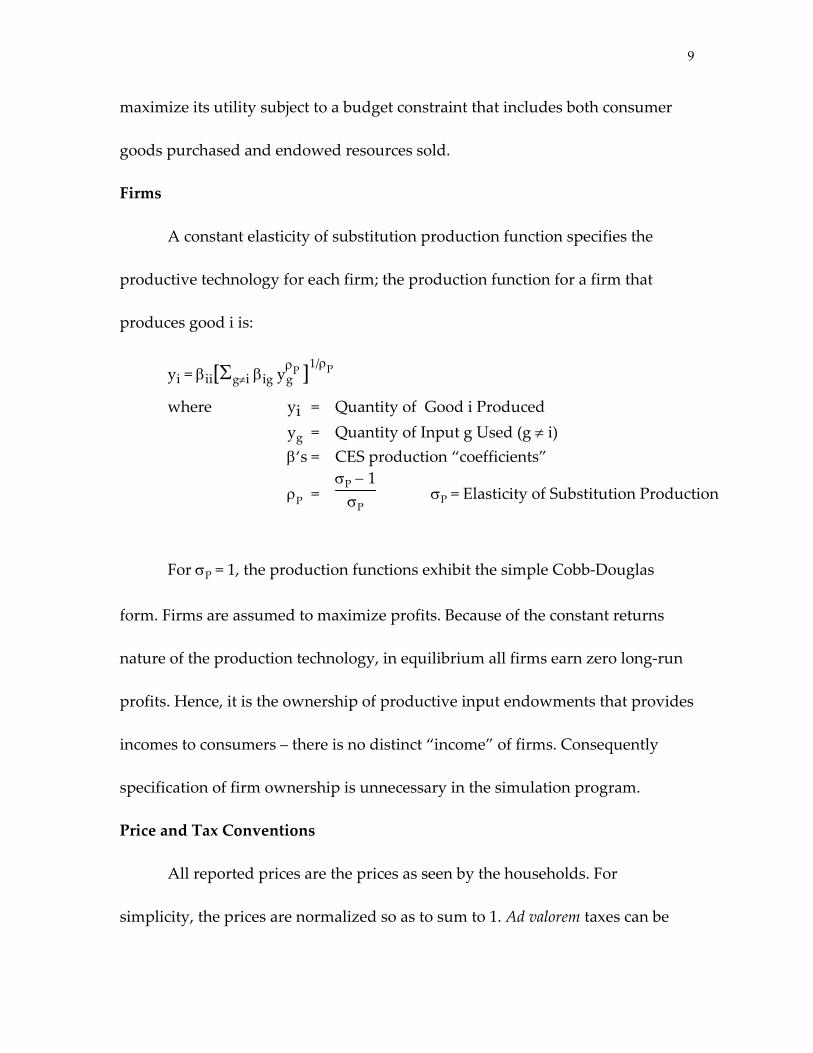
A constant elasticity of substitution production function specifies the 

productive technology for each firm; the production function for a firm that 

produces good i is: 

yi = βii[Σg≠i βig yg  ρP ]1/ρP 

where  yi  =  Quantity of  Good i Produced   yg  =  Quantity of Input g Used (g ≠ i)   β‘s =  CES production “coefficients” 

  ρP  = σP − 1σP

   σP = Elasticity of Substitution Production 

 

For σP = 1, the production functions exhibit the simple Cobb‐Douglas 

form. Firms are assumed to maximize profits. Because of the constant returns 

nature of the production technology, in equilibrium all firms earn zero long‐run 

profits. Hence, it is the ownership of productive input endowments that provides 

incomes to consumers – there is no distinct “income” of firms. Consequently 

specification of firm ownership is unnecessary in the simulation program. 

Price and Tax Conventions 

All reported prices are the prices as seen by the households. For 

simplicity, the prices are normalized so as to sum to 1. Ad valorem taxes can be 

10

placed on any of the goods.1 Because the reported prices are those seen by 

households, it is perhaps easiest to think of taxes as being legally incident on the 

firms even though the legal incidence of the tax is irrelevant. To clarify how taxes 

are modeled, consider two examples.  

Ad valorem tax on an input: Suppose that the price of labor were .40, then 

PL = .40.  Consider imposition of an ad valorem tax of .25 on labor input (tL = .25). 

In this case, each household would receive .40 of income for each unit of labor 

supplied. The firm would be spending .50 for each unit of labor hired. The 

difference would go to the government as tax revenue. More generally, for each 

unit of labor “traded” the: 

• household receives PL of income; 

• firm incurs PL(1 + tL) of costs; 

• government receives PLtL of tax revenue. 

Ad valorem tax on a consumption good: Suppose that the price of 

consumption good X is .50, (PX = .50) and the ad valorem tax on consumption 

good X is .10 (tX = .10). Each household would spend .50 for each unit of 

consumption good X purchased. The firm would receive .45 for each unit of 

1 To allow for the possibility of a tax on the external effect, unit taxes can also be specified in the model. An ad valorem tax on the external effect would have no effect since, in the absence of government intervention, the “price” of the external effect is 0.

11

consumption good X sold. The difference would go the government as tax 

revenue. More generally, for each unit of consumption good X traded the: 

• household pays PX; 

• firm receives PX(1 − tX) of revenues; 

• government receives PXtX of tax revenue. 

Government 

A general equilibrium model allows us to explicitly account for the 

government’s budget constraint. When the government collects tax revenue, 

something must be done with it. Broadly speaking, there are two choices: 

• Redistribute the revenue as transfer payments to households 

• Use the revenue to finance the production of public goods. 

The simulation program allows us to specify “redistribution factors” that 

determines the portion of the government’s tax revenue that is redistributed to 

each households. To satisfy the budget constraint the sum of the redistribution 

factors across households cannot total more than 1. If the sum totals less than 1, 

the portion of the tax revenue not redistributed will be used to finance the 

production of a public good. 

Computational Procedure 

Most consider Walras to be the founding father of general equilibrium 

analysis. It was Walras who proposed a tatonnement process that would lead 

12

each market in an economy to move toward equilibrium based on excess 

demand at any initial price configuration. Unfortunately, a procedure based on 

such a process does did not guarantee convergence; that is, algorithms based on 

tatonnement do not always succeed in finding an equilibrium. The pioneering 

work of Herbert Scarf in the late 1960’s provided the alternative approach, 

however, which allowed the field of applied general equilibrium to develop 

(Scarf, 1967). Scarf’s algorithm finds a vector of prices that are “approximate” 

equilibrium prices – approximate in the sense that at these prices, the market for 

each good is “nearly” in equilibrium: the quantity demanded differs from the 

quantity supplied by a small amount at most (Scarf, 1973). Our simulation 

program computes such equilibrium prices using Merrill’s refinement of Scarf’s 

algorithm (Merrill, 1971). 

  

13

PREVIEW OF ILLUSTRATIONS 

 General equilibrium models allow the illustration of many important 

economic issues. We choose to present five here: 

• Interconnectedness of Markets 

• Equivalence of a General Consumption Tax and General Income Tax 

• Lump Sum versus Distorting Taxes 

• Financing Public Good Production and Efficiency 

• Externalities and Efficiency 

Our first two illustrations are designed to emphasize the fundamental 

general equilibrium principle of market interconnectedness. The first illustrates 

that the impact of a change in one market is not isolated to that particular 

market, but rather it affects other markets also. Second, we present a tax 

equivalence example to emphasize another illustration of market 

interconnectedness, the concept of circular flow. While circular flow is an 

integral part of macroeconomic courses, it is rarely mentioned in 

microeconomics. The third illustration provides a better appreciation of the 

natures of lump sum and distorting taxes by explicitly accounting for what the 

government does with the tax revenue it collects. In doing so, we clearly connect 

the concepts of tax distortions and Pareto optimality. The last two illustrations 

tackle more complicated issues, financing public goods and externalities, to show 

14

how general equilibrium models can provide valuable insights that partial 

equilibrium analysis fails to capture fully. 

In order to simplify our discussion, we include only a small number of 

goods, households, and firms in the specific general equilibrium model that we 

present below. Note that the simulation program itself is not limited in this 

regard. Also, for the sake of simplicity we specify Cobb‐Douglas utility functions 

and Cobb‐Douglas production functions. Specifically, we make the following 

designations: 

Goods 

Our model includes four goods: two consumption goods (X and Y) and 

two inputs (L and K). Throughout, L and K can be thought of as representing 

labor and capital respectively.  

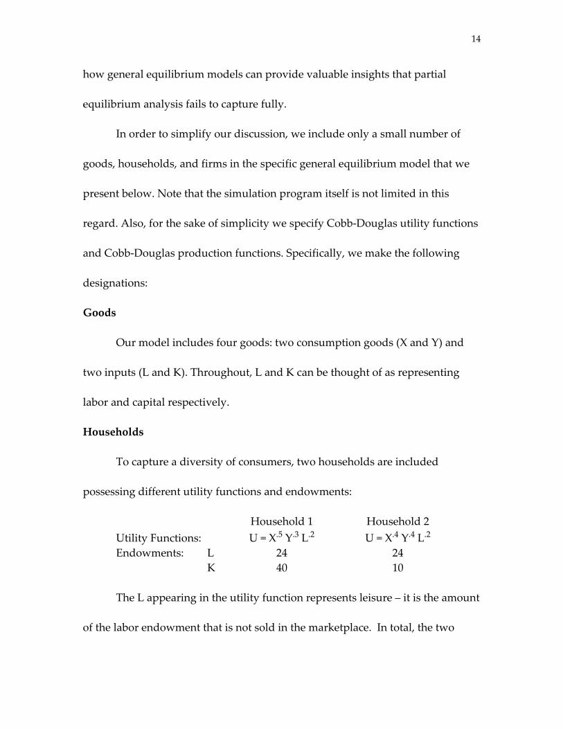
Households 

To capture a diversity of consumers, two households are included 

possessing different utility functions and endowments: 

  Household 1  Household 2 Utility Functions:  U = X.5 Y.3 L.2  U = X.4 Y.4 L.2 Endowments:  L  24  24   K  40  10  The L appearing in the utility function represents leisure – it is the amount 

of the labor endowment that is not sold in the marketplace.  In total, the two 

15

households are (arbitrarily) endowed with a total of 48 units of L, labor, and 50 

units of K, capital. Since L appears in each household’s utility functions, each 

household will “demand” some of its endowed labor to enjoy as leisure. 

Accordingly, there are two sources of demand for a household’s labor, the 

household itself and firms. Note that while the households are endowed with 

identical amounts of labor, household 2 is endowed with more capital. 

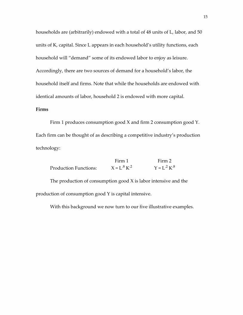
Firms 

Firm 1 produces consumption good X and firm 2 consumption good Y. 

Each firm can be thought of as describing a competitive industry’s production 

technology: 

  Firm 1  Firm 2 Production Functions:  X = L.8 K.2  Y = L.2 K.8  The production of consumption good X is labor intensive and the 

production of consumption good Y is capital intensive. 

With this background we now turn to our five illustrative examples. 

 

16

ILLUSTRATON 1: INTERCONNECTEDNESS OF MARKETS 

General equilibrium models allow us to account for the 

interconnectedness of markets; that is, the models recognize that changes in one 

market affect other markets also. To illustrate this we begin with a no‐tax base 

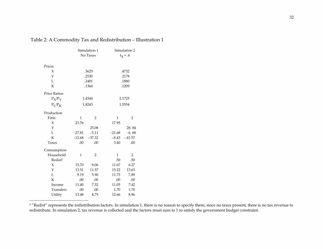
case in Simulation 1 (see Table 2). Then, in Simulation 2, we impose an ad valorem 

tax of .40 on consumption good X. In this simulation, all tax revenue is 

redistributed to households; we have arbitrarily specified that half the tax 

revenue is redistributed to household 1 and half to household 2.2 First, consider 

each simulation separately. In each case, the model has been solved for the 

competitive equilibrium; the quantity demanded equals the quantity supplied 

for all four goods. For example, in Simulation 1, the quantity of consumption 

good X demanded equals 15.70 plus 8.06 or 23.76, which just equals the quantity 

of consumption good X firm 1 produces. Similarly, the quantity of good Y 

demanded equals 13.51 plus 11.57, which just equals the quantity of 

consumption good Y firm 2 produces. 

Now compare the two simulations. Not surprisingly, the X‐Y price ratio 

(as viewed by households) increases from 1.4344 to 2.1725 when consumption 

good X is taxed.  Similarly, the equilibrium quantity of consumption good X falls 

from 23.76 to 17.94. The connections between markets is illustrated first by the 

17

increase in Y consumption from 25.08 to 28.84.  Notice also how the markets for 

the inputs are affected. The wage‐rental rate decreases from 1.8243 to 1.5554. This 

results from the fact that the production of consumption good X is labor 

intensive; the tax on consumption good X depresses the wage rate relative to the 

capital rental rate.  

The two simulations in Table 2 also illustrate the importance of accounting 

for the government’s budget constraint. While the tax decreases the utility of 

household 1, it increases the utility of household 2. This occurs because the 3.40 

of tax revenue is redistributed to the households on a 50‐50 basis. With the 

transfer payment of 1.70, household 2 (who has a somewhat smaller relative 

preference for good X) finds itself better off even though consumption good X is 

now being taxed. Of course, a different set of redistribution factors or of 

preferences would result in different utility consequences for the households.   

The standard partial equilibrium approach to analyzing a tax on a 

consumption good tax relies either on indifference curves and budget lines or on 

demand and supply curves. Neither of these standard approaches captures fully 

the impact of the tax, however. The indifference curve/budget line approach 

implicitly assumes that the prices of the non‐taxed consumption goods and 

inputs (and therefore also income) remain constant; that is, with the exception of 

2 We follow the standard general equilibrium practice of denoting production outputs with

18

the market for the taxed good, all other markets are assumed to be unaffected. 

The simulation shows how the indifference curve/budget line approach fails to 

capture the important consequences of market interconnectedness. Similarly, the 

standard demand/supply approach focuses on the “tax wedge” between the 

price paid by households and the price received by firms; households are hurt 

because they pay more and firms are hurt because they receive less. 

Subsequently, changes in consumer surplus and producer surplus are often 

calculated along with the excess burden. This analysis typically stops there. 

Little, if anything, is said about how changes in one market affect other output 

and input markets nor about how the tax revenues are used. 

General equilibrium models address the deficiencies of the partial 

equilibrium approaches by illustrating how a tax on a single consumption good 

impacts the markets for other consumption goods and the markets for inputs. 

Just as households are affected by what happens in the market for the taxed good 

itself, they are also affected by what happens in these other markets. Also, the 

simulation explicitly shows that the government must do something with the tax 

revenue it collects.  And what it ultimately does also affects household welfare. 

In this simulation, the government redistributes the tax revenue to households as 

transfer payments (in later simulations, we consider the production of public 

positive signs and inputs with negative signs.

19

goods). Firms and the government are intermediaries; ultimately, households 

bear all the ramifications of the tax because households own the firms and the 

factors of production. General equilibrium models allow these important 

principles to be clearly illustrated.  

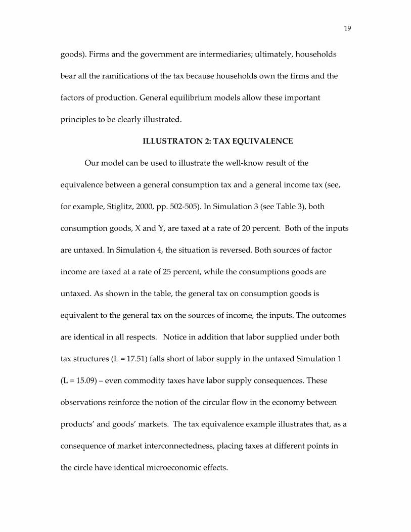
ILLUSTRATON 2: TAX EQUIVALENCE 

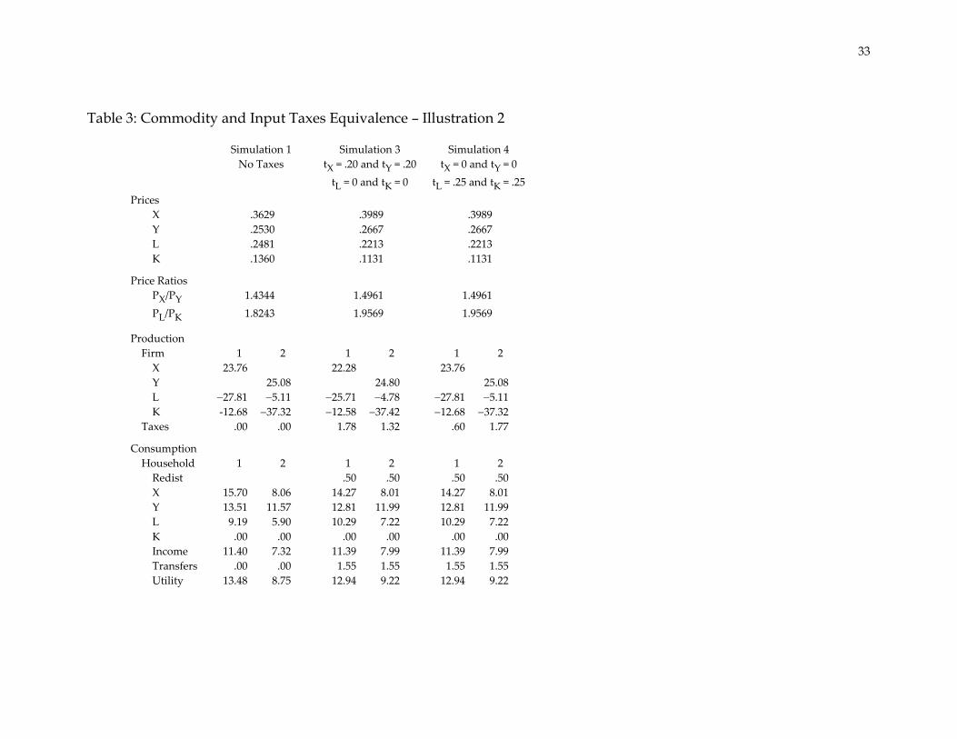
Our model can be used to illustrate the well‐know result of the 

equivalence between a general consumption tax and a general income tax (see, 

for example, Stiglitz, 2000, pp. 502‐505). In Simulation 3 (see Table 3), both 

consumption goods, X and Y, are taxed at a rate of 20 percent.  Both of the inputs 

are untaxed. In Simulation 4, the situation is reversed. Both sources of factor 

income are taxed at a rate of 25 percent, while the consumptions goods are 

untaxed. As shown in the table, the general tax on consumption goods is 

equivalent to the general tax on the sources of income, the inputs. The outcomes 

are identical in all respects.   Notice in addition that labor supplied under both 

tax structures (L = 17.51) falls short of labor supply in the untaxed Simulation 1 

(L = 15.09) – even commodity taxes have labor supply consequences. These 

observations reinforce the notion of the circular flow in the economy between 

products’ and goods’ markets.  The tax equivalence example illustrates that, as a 

consequence of market interconnectedness, placing taxes at different points in 

the circle have identical microeconomic effects. 

20

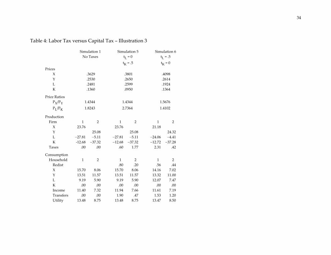
ILLUSTRATON 3: LUMP SUM VERSUS DISTORTING TAXES 

With the exception of a head tax, lump sum taxes are not present in the 

real world; nevertheless, they can provide an instructive base case. However, 

because our simple specification of the economy lacks an inter‐temporal aspect 

and capital does not enter the utility function of the households, the supply of 

capital is completely inelastic. While this is obviously unrealistic, it is useful 

because a tax on capital now provides us with a “lump sum” base case. On the 

other hand, a tax on labor is a “distorting” tax because labor endowments not 

provided to the market (leisure) enter the utility function of the households; 

consequently, the supply curve for labor is not completely inelastic.  

A lump sum tax produces no substitution effects, only income effects. 

Therefore, when a lump‐sum tax imposed, it is possible to redistribute the tax 

revenue back to the households as transfer payments in a way that keeps each 

household equally well‐off. With a distorting tax, it is impossible to do this; even 

when all tax revenue is redistributed back to the households at least one 

household must find itself worse off. Typically, these principles are illustrated 

for the case of a single household by appealing to the standard utility 

maximizing diagram; the budget line is shifted in a parallel fashion for a lump 

sum tax and a non‐parallel fashion for a distorting tax. General equilibrium 

models allow us to illustrate the principles in an alternative way with more than 

21

a single household. Focus attention on Simulations 1 and 5 appearing in Table 4. 

As before, Simulation 1 includes no taxes; on the other hand, Simulation 5 

imposes a 50 percent tax on capital. These simulations confirm the assertion that 

in the context of our specific model, a tax on capital is a lump sum tax; that is, the 

tax on capital leads to no distortions. Such a tax does not affect the allocation of 

resources; each firm’s production decisions are unaffected. The tax does not alter 

the X‐Y price ratio either; hence, the slope of each household’s budget constraint 

is unaffected. The tax on capital raises tax revenues of 2.37.  When 80 percent of 

the revenues are redistributed to household 1 and the remaining 20 percent to 

household 2, both households have their endowments “restored” and are just as 

well off as they were in the no tax situation. This 50 percent general tax on capital 

is therefore a non‐distorting, lump sum tax. 

Comparison of Simulations 1 and 6 illustrate the impact of a distorting tax. 

The 50 percent ad valorem tax on labor in Simulation 6 affects the allocation of 

resources. When the 2.73 of tax revenues is redistributed by giving 56 percent to 

household 1 and 44 percent to household 2, household 1 is (almost) just as well 

off as in the no tax situation, but household 2 is worse off. It is impossible to 

redistribute the tax revenue so as to keep both households equally well‐off. 

Consequently, the tax on labor is a distorting tax that results in a deadweight 

22

loss.  The distribution of this deadweight loss will, however, depend of how the 

tax revenues are redistributed to the households. 

We believe that a simulation including two (or more) households allow 

students to appreciate better the notion of tax distortions and their intimate 

relationship to the Pareto criterion. In the classroom, we typically illustrate a 

lump sum tax as an inward parallel shift in the budget line and then observe that 

that no substitution effect results. Subsequently, by showing that a distorting tax 

leads to a non‐parallel shift, we conclude that it is the substitution effect which 

leads to tax distortions. This analysis is incomplete, however, because it ignores 

the fact that the government must do something with the tax revenue it collects; 

that is, tax revenue does not disappear into a “black hole” as the standard 

diagram suggests. In this illustration, all the tax revenue is redistributed to the 

households for the purpose of illustrating the distinction between lump sum and 

distorting taxes. By doing so, we connect the notion of tax distortions with the 

basic Pareto criterion. In the case of a lump sum tax, each household can be made 

just as well off by redistributing the tax revenue in just the right way. In the case 

of a distorting tax, at least one household is hurt regardless of how the tax 

revenue is redistributed. 

 

23

ILLUSTRATION 4: FINANCING AND THE OPTIMAL LEVEL OF 

PUBLIC GOOD PRODUCTION 

To simplify matters, we have modified our model to study the financing 

of public goods. First, only a single household is included. In this way, it is more 

straightforward to focus on efficiency, as there are no distributional effects. 

Second, we add the public good to the representative household’s utility 

function: 

U = X.5 Y.3 L.2 G.1  where G = Public Good 

The household’s endowments are unchanged, but the tax revenue 

collected is not redistributed; instead, it is used to finance the public good. The 

production functions for the consumption goods, X and Y, are unchanged. The 

production function for the public good takes the simple Cobb‐Douglas form: 

G = L.5 K.5 

 

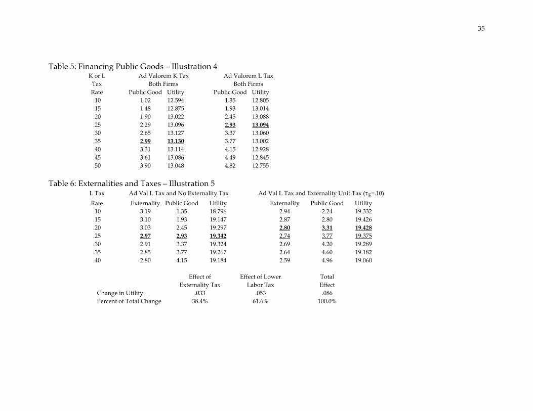
Table 5 reports on two schemes to finance the production of the public 

good. The first uses a tax on capital, a lump sum tax in our model, to finance 

production and the second a tax on labor, a distorting tax. In each case, the 

quantity of the public good financed and the resulting level of household utility 

are reported for selected capital and labor ad valorem tax rates. When the 

production of the public goods is financed with a tax on capital, a lump sum tax, 

24

the optimal level of public good production is 2.99. On the other hand, when a 

tax on labor (a distorting tax) is used the optimal level is lower, 2.93. These 

results illustrate the tradeoff of the benefits of public good production against the 

costs of tax distortions. The optimal level of public good production is lower 

when a distorting tax is used to finance its production than when a non‐

distorting tax is used. 

While this result appears to be intuitive, and arguably is typical (see 

Stiglitz, 2000, pp. 148‐149), it need not be the case. For example, if the taxed good 

is a complement of the public good, the “effective” opportunity cost of 

producing the public good would be reduced below its “physical” opportunity 

cost  because additional public good production stimulates tax revenue as a 

consequence of the complementarity (see Atkinson and Stiglitz, 1980, pp. 490‐

492). Naturally, the demand responsiveness of the taxed good to the tax further 

complicates the analysis. The ultimate effect on the optimal level of public good 

production is ambiguous; it is even possible for the optimal level to increase 

when production is financed by a distorting rather than lump sum tax (see 

Atkinson and Stern, pp. 123‐126).  

While our simulations only illustrate the more intuitive result (moving 

from a non‐distorting to a distorting method of finance reduces the optimal level 

of the public good), they do reinforce the basic lesson general equilibrium 

25

analysis teaches: we cannot just look at one aspect of the economy in isolation. 

The standard public good optimization rule which only considers the benefits 

and costs of producing the public good (the sum of marginal rates of substitution 

equal the rate of product transformation) is not the end of the story. We must 

also account for the impact of the taxes raised to finance the production of the 

public good on other markets.  

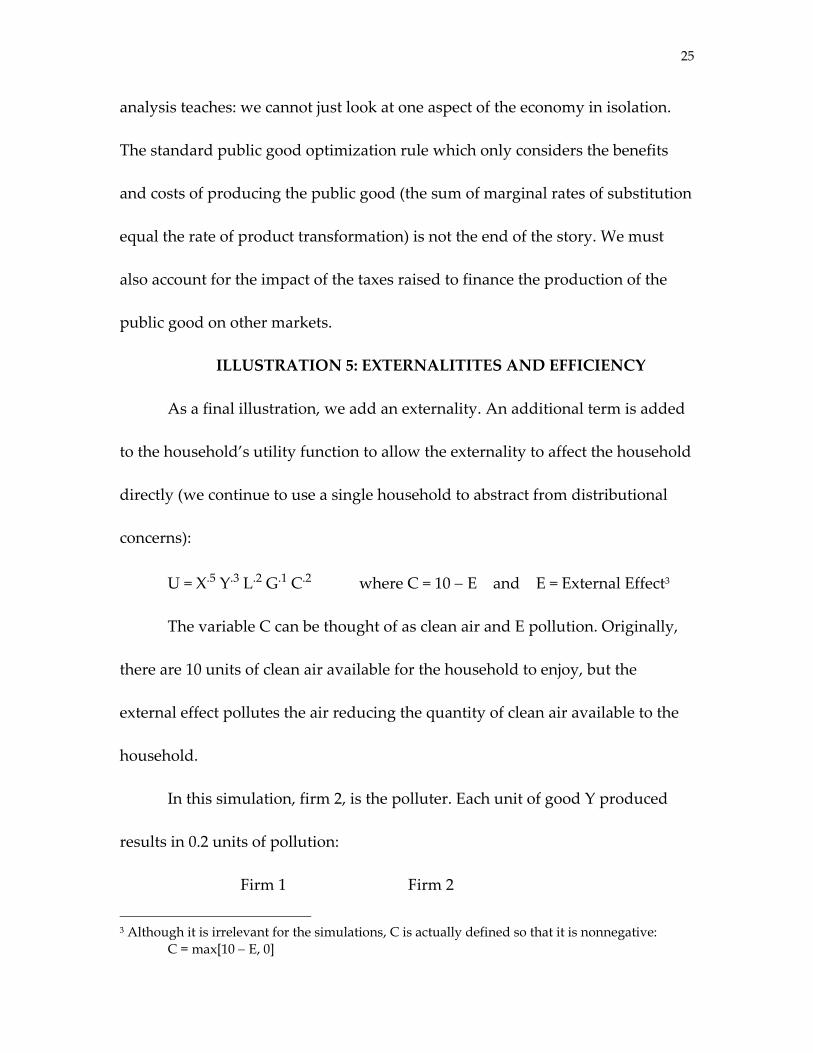
ILLUSTRATION 5: EXTERNALITITES AND EFFICIENCY 

As a final illustration, we add an externality. An additional term is added 

to the household’s utility function to allow the externality to affect the household 

directly (we continue to use a single household to abstract from distributional 

concerns): 

U = X.5 Y.3 L.2 G.1 C.2   where C = 10 − E    and    E = External Effect3 

The variable C can be thought of as clean air and E pollution. Originally, 

there are 10 units of clean air available for the household to enjoy, but the 

external effect pollutes the air reducing the quantity of clean air available to the 

household. 

In this simulation, firm 2, is the polluter. Each unit of good Y produced 

results in 0.2 units of pollution: 

  Firm 1  Firm 2 

3 Although it is irrelevant for the simulations, C is actually defined so that it is nonnegative:

C = max[10 − E, 0]

26

  X = L.8 K.2  Y = L.2 K.8     E = .2Y  Table 6 reports on two scenarios: one in which labor is taxed, but the 

externality is not, and a second in which the labor is taxed and pollution is 

subject to a Pigovian tax of .1 per unit: 4 In the absence of the Pigovian tax, the 

optimal level of public good production is 2.93; in this case, the optimal tax rate 

on labor is 25 percent and 2.97 units of pollution are produced. When the 

Pigovian tax is imposed and the tax rate on labor remains at 25 percent, optimal 

public good production rises because more tax revenue is generated and the 

amount of pollution falls; both of these effects cause utility to increase from 

19.342 to 19.375. Welfare can be improved even more, however, by reducing the 

distorting tax on labor.  A reduction in the labor tax rate from 25 to 20 percent 

increases utility from 19.375 to 19.428. This occurs because the tax revenue 

generated by taxing the externality reduces the need to generate tax revenue 

from the distorting tax on labor. In the addendum to Table 6, we calculate the 

changes in utility arising from each of these two effects thereby illustrating the 

“double dividend” potentially available from environmental taxes. In this case

then, the reduction in the labor tax distortion contributes substantially to the

4 The externality tax is a unit tax of .10 per unit of the external effect when the prices are normalized to sum to 1. Note that an ad valorem tax on the external effect would not make sense since in the absence of government intervention, the “price” of the external effect is 0.

27

increase in utility. One reason that the double dividend is so large here is that

the tax system originally favors good Y, the capital intensive good, which is also

the good producing the pollution. In other situations, the double dividend might

be smaller or even negative (see Salanie, 2003, pp. 200-204). Again, the general

equilibrium models illustrate the importance of considering all of the

ramifications of the fact that markets are interconnected.

 

28

CONCLUSION  The primary reason that students should study general equilibrium theory 

is to learn more about economics generally.  As currently taught in intermediate 

microeconomics courses, general equilibrium theory yields precious few such 

insights.  Other than developing an understanding of Pareto optimality and 

grasping a vague notion that “everything affects everything”, students emerge 

from the typical course thinking that general equilibrium is probably the least 

important part of economic theory for understanding the practical world.  We 

believe that nothing could be further from the truth.  The impacts of most 

important economic policies can only be fully understood in a general 

equilibrium context.  Strengths and limitations of current research in these areas 

can only be understood if someone is familiar with how actual general 

equilibrium models work.  We believe that the general equilibrium approach 

described in this paper provides a relatively simple way for students to begin to 

develop such an understanding. 

REFERENCES 

Arrow, K. J. and Debreu G. “Existence of Equilibrum for a Competitive Economy.” Econometrica 22 (1954). 

 Atkinson, A. B. and Stern, N. H. “Pigou, Taxation and Public Goods”, The Review 

of Economic Studies, 41 (January, 1974).  Atkinson, Anthony B. and Stiglitz, Joseph E., Lectures of Public Economics. New 

York. McGraw‐Hill. 1980. 

29

 Browning, Edgar K. and Mark A. Zupan.  Microeconomic Theory and Applications, 

9th Edition.  Reading (Mass.).  Addison‐Wesley. 2005.  Frank, Robert H.  Microeconomics and Bahavior, 6th Edition.  Boston. Irwin 

McGraw‐Hill.  2006.  Katz, Michael L. and Harvey S. Rosen.  Microeconomics. 3rd Edition.  Boston.  

Irwin McGraw Hill. 1998.  Kehoe, T. M., Srinivasan, T. N., and Whalley, J. Frontiers in Applied General 

Equilibrium Modeling, Cambridge (UK). Cambridge University Press (2005). 

 Landsburg, Steven E.  Price Theory and Applications. 6th Edition. Cincinnati.  South‐

Western. 2004.  McKenzie, L. “On the Existence of General Equilibrium for a Competitive 

Market,” Econometrica 27 (1959).   Merrill, O. H., “Applications and Extensions of an Algorithm that Computes 

Fixed points of Certain Non‐empty Convex Upper Semicontinuous Point to Set Matting,” Technical Report No. 7107, Department of Industrial Engineering, University of Michigan, 1971 

 Nicholson, Walter. and Christopher Snyder.  Intermediate Microeconomics and its 

Application.  10th Edition.  Mason (OH).  Thomson South‐Western.  2007.  Perloff, Jeffrey M.  Microeconomics. 2nd Edition. Boston. Addison‐Wesley. 2001.  Pindyck, Robert S. and Rubinfeld, Daniel L.  Microeconomics. 6th Edition.  Upper 

Saddle River (NJ).  Prentice‐Hall.  2004.  Salanie, Bernard.  The Economics of Taxation.  Cambridge (MA).  MIT Press.  2002.  Scarf, Herbert E. ‘The Approximation of Fixed Points of a Continuous Mappint,” 

SIAM Journal of Applied Mathematics 15 (1967).  Scarf, Herbert E. with Hansen, Terje. On the Computation of Economic Equilibria. 

New Haven. Yale University Press, 1973. 

30

 Stiglitz, Joseph E.  Economics of the Public Sector. 3rd Edition.  New York. W.W. 

Norton.  2000.  Stiglitz, J. E. and Dasgupta, P. “Differential Taxation, Public Goods and 

Economic Efficiency”, Review of Economic Studies,  38 (April 1971).  Varian,  Hal R.  Intermediate Microeconomics: A Modern Approach.  7th Edition.  New 

York.  W.W.Norton.  2006.  

31

Table 1:  Coverage of General Equilibrium Concepts in Leading Microeconomics Texts Concept Browning/Zupan Frank Katz/Rosen Landsburg Nicholson/Snyder Perloff Pindyck/Rubinfeld Varian Reasons for General Equilibrium Y N Y Y Y Y Y N Pareto Efficiency Y Y Y Y Y Y Y Y Exchange/Edgeworth Box Y Y Y Y Y Y Y Y Initial Endowments Y Y Y Y Y N Y Y Production and Efficiency Y Y Y Y Y Y Y Y Walras' Law N N N N N N N Y Existence of Walrasian Equilibrium N N N N N N N Y CGE Models N N N N N N N N First Theorem Y Y Y Y Y Y Y Y Market Failure Y Y Y N Y N Y Y Second Theorem N N Y N Y N N Y Social Welfare Function N N Y N N Y N Y Detailed Applications of GE Models N N N N Y N N N Comparisons of General versus Partial Models N N N N N N N N

32

Table 2: A Commodity Tax and Redistribution – Illustration 1    Simulation 1  Simulation 2   No Taxes  tX = .4      Prices     

X  .3629  .4732 Y  .2530  .2178 L  .2481  .1880 K  .1360  .1209 

Price Ratios PX/PY  1.4344  2.1725 PL/PK  1.8243  1.5554 

Production Firm  1  2  1  2 X  23.76    17.95   Y    25.08    28. 84 L  −27.81  −5.11  −21.68  −6. 68 K  ‐12.68  −37.32  −8.43  −41.57 

Taxes  .00  .00  3.40  .00 

Consumption  Household  1  2  1  2 Redist5      .50  .50 X  15.70  8.06  11.67  6.27 Y  13.51  11.57  15.22  13.63 L  9.19  5.90  11.75  7.89 K  .00  .00  .00  .00 Income  11.40  7.32  11.05  7.42 Transfers  .00  .00  1.70  1.70 Utility  13.48  8.75  12.66  8.96 

5 “Redist” represents the redistribution factors. In simulation 1, there is no reason to specify them; since no taxes present, there is no tax revenue to redistribute. In simulation 2, tax revenue is collected and the factors must sum to 1 to satisfy the government budget constraint.

33

Table 3: Commodity and Input Taxes Equivalence – Illustration 2    Simulation 1  Simulation 3  Simulation 4   No Taxes  tX = .20 and tY = .20  tX = 0 and tY = 0     tL = 0 and tK = 0   tL = .25 and tK = .25 Prices       

X  .3629  .3989  .3989 Y  .2530  .2667  .2667 L  .2481  .2213  .2213 K  .1360  .1131  .1131 

Price Ratios PX/PY  1.4344  1.4961  1.4961 PL/PK  1.8243  1.9569  1.9569 

Production Firm  1  2  1  2  1  2 X  23.76    22.28    23.76   Y    25.08    24.80    25.08 L  −27.81  −5.11  −25.71  −4.78  −27.81  −5.11 K  ‐12.68  −37.32  −12.58  −37.42  −12.68  −37.32 

Taxes  .00  .00  1.78  1.32  .60  1.77 

Consumption  Household  1  2  1  2  1  2 Redist      .50  .50  .50  .50 X  15.70  8.06  14.27  8.01  14.27  8.01 Y  13.51  11.57  12.81  11.99  12.81  11.99 L  9.19  5.90  10.29  7.22  10.29  7.22 K  .00  .00  .00  .00  .00  .00 Income  11.40  7.32  11.39  7.99  11.39  7.99 Transfers  .00  .00  1.55  1.55  1.55  1.55 Utility  13.48  8.75  12.94  9.22  12.94  9.22 

 

34

Table 4: Labor Tax versus Capital Tax – Illustration 3    Simulation 1  Simulation 5  Simulation 6   No Taxes  tL = 0  tL = .5     tK = .5  tK = 0 Prices     

X  .3629  .3801  .4098 Y  .2530  .2650  .2614 L  .2481  .2599  .1924 K  .1360  .0950  .1364 

Price Ratios PX/PY  1.4344  1.4344  1.5676 PL/PK  1.8243  2.7364  1.4102 

Production Firm  1  2  1  2  1  2 X  23.76    23.76    21.18 Y    25.08    25.08    24.32 L  −27.81  −5.11  −27.81  −5.11  −24.06  −4.41 K  ‐12.68  −37.32  −12.68  −37.32  −12.72  −37.28 

Taxes  .00  .00  .60  1.77  2.31  .42 

Consumption  Household  1  2  1  2  1  2 Redist      .80  .20  .56  .44 X  15.70  8.06  15.70  8.06  14.16  7.02 Y  13.51  11.57  13.51  11.57  13.32  11.00 L  9.19  5.90  9.19  5.90  12.07  7.47 K  .00  .00  .00  .00  .00  .00 Income  11.40  7.32  11.94  7.66  11.61  7.19 Transfers  .00  .00  1.90  .47  1.53  1.20 Utility  13.48  8.75  13.48  8.75  13.47  8.50 

35

Table 5: Financing Public Goods – Illustration 4   K or L  Ad Valorem K Tax  Ad Valorem L Tax   Tax  Both Firms  Both Firms   Rate  Public Good   Utility  Public Good  Utility   .10  1.02  12.594  1.35  12.805   .15  1.48  12.875  1.93  13.014   .20  1.90  13.022  2.45  13.088   .25  2.29  13.096  2.93  13.094   .30  2.65  13.127  3.37  13.060   .35  2.99  13.130  3.77  13.002   .40  3.31  13.114  4.15  12.928   .45  3.61  13.086  4.49  12.845   .50  3.90  13.048  4.82  12.755 

 

Table 6: Externalities and Taxes – Illustration 5   L Tax  Ad Val L Tax and No Externality Tax  Ad Val L Tax and Externality Unit Tax (τE=.10)   Rate  Externality  Public Good  Utility   Externality  Public Good  Utility   .10  3.19  1.35  18.796  2.94  2.24  19.332   .15  3.10  1.93  19.147  2.87  2.80  19.426   .20  3.03  2.45  19.297  2.80  3.31  19.428   .25  2.97  2.93  19.342  2.74  3.77  19.375   .30  2.91  3.37  19.324  2.69  4.20  19.289   .35  2.85  3.77  19.267  2.64  4.60  19.182   .40  2.80  4.15  19.184  2.59  4.96  19.060 

   Effect of  Effect of Lower  Total   Externality Tax  Labor Tax  Effect Change in Utility  .033  .053  .086 Percent of Total Change  38.4%  61.6%  100.0% 

 

36