General competitive equilibrium
50
General competitive equilibrium
-
Upload
harlan-sosa -
Category
Documents
-
view
46 -
download
3
description
General competitive equilibrium. General equilibrium: How does an idealized private ownership competitive economy works ?. l goods (indexed by j ) n individuals (households) (indexed by i ) K firms (or technologies) (indexed by k ) - PowerPoint PPT Presentation
Transcript of General competitive equilibrium
General competitive equilibrium

General equilibrium: How does an idealized private ownership
competitive economy works ? l goods (indexed by j) n individuals (households) (indexed by i) K firms (or technologies) (indexed by k) firm k’s technology: a production set Yk l that
is closed, irreversible, convex and satisfies the possibility of inaction, impossibility of free production, and free disposal.
All goods are private (rival and excludable). They are privately owned. i
j 0: quantity of good j initially owned by household i

General equilibrium: How does an idealized private ownership
competitive economy works ? (2)
1 ik 0 : share of firm k owned by
household i Each firm is entirely owned (i i
k = 1 for all k)
Xi l+: Consumption set of household i
(convex and closed) i: preferences of household i (reflexive,
complete, transitive, continous, locally non-satiable and convex binary relation on Xi).

General equilibrium: How does an idealized private ownership
competitive economy works ? (3)
An economy = (Yk,Xi,i,ik,i
j), i =1,…,n, j =1,…,l and k = 1,…K.
Economic problem: finding an allocation of the l goods accross the n individuals.
Some allocations are feasible, some are not.
A(): the set of all allocations of goods that are feasible for the economy .
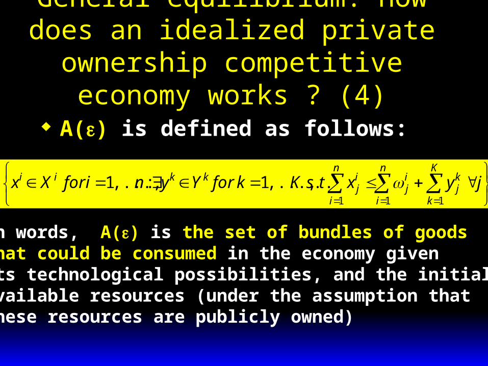
General equilibrium: How does an idealized private ownership
competitive economy works ? (4)
A() is defined as follows:
K
k
kj
n
i
ij
n
i
ij
kkii jyxtsKkforYyniforXx111
..,...,1:,...,1
In words, A() is the set of bundles of goods that could be consumed in the economy given its technological possibilities, and the initial available resources (under the assumption that these resources are publicly owned)

A nice geometrical depiction of the set of feasible allocations: the Edgeworth box Suppose Yk = {0l} for all k (nothing is
produced) Then is an exchange economy. A() in this case can be defined by:
jxniforXxn
i
ij
n
i
ij
ii
11
:,...,1
If l = n=2, we can represent the bundles thatsatisfy this weak inequality at equality on the
following diagram
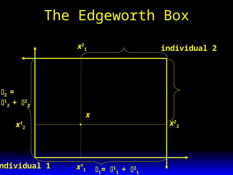
The Edgeworth Box
Individual 1
individual 2
x22
x11
x12
x21
x
2 =1
2 + 22
1= 11 + 2
1
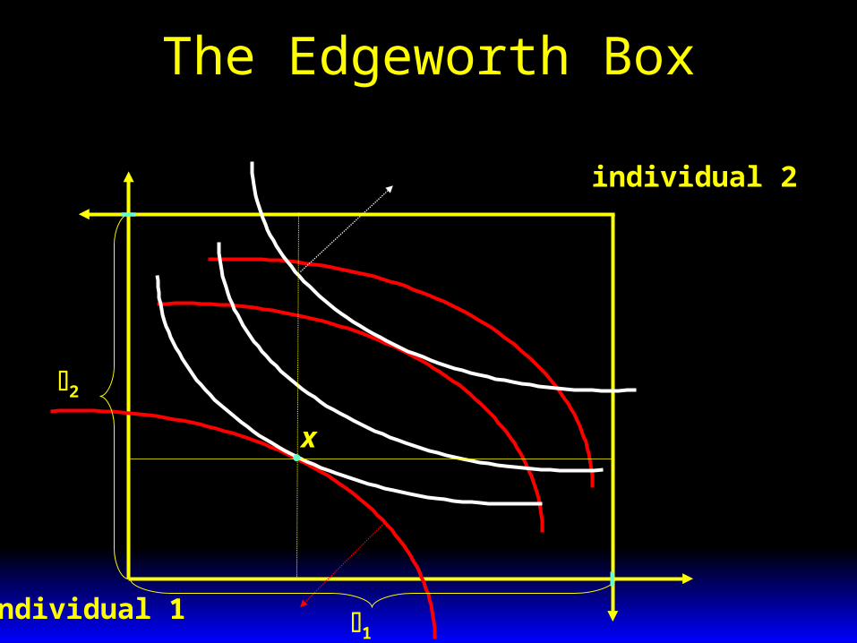
The Edgeworth Box
Individual 1
individual 2
2
1
x

Pareto efficiency
Some feasible allocations of goods involve waste.
Some feasible allocations of goods do not exhaust the existing possibilities of mutual gains (called « win-win » situations in ordinary language)
Some feasible allocations of goods are not Pareto-efficient!
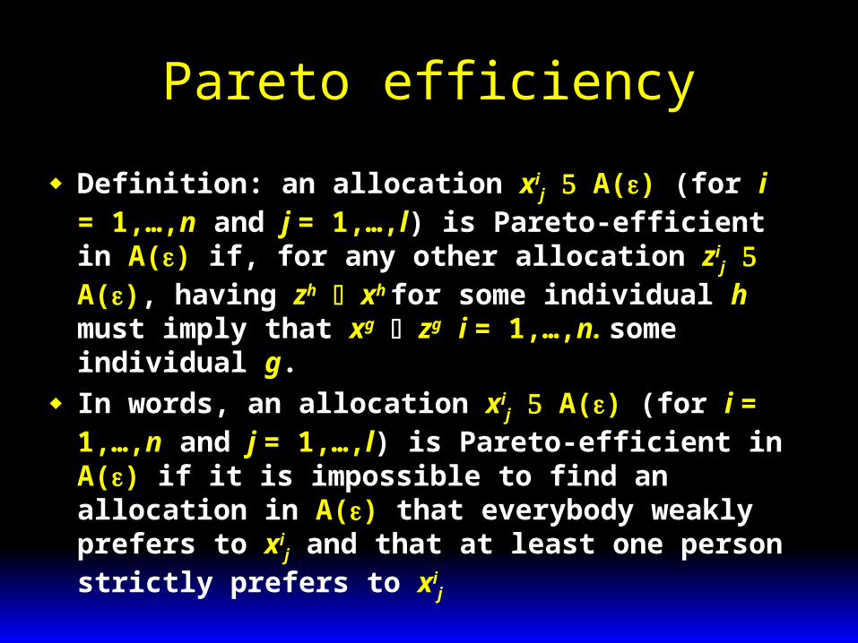
Pareto efficiency
Definition: an allocation xij A() (for i = 1,
…,n and j = 1,…,l) is Pareto-efficient in A() if, for any other allocation zi
j A(), having zh xh for some individual h must imply that xg zg i = 1,…,n. some individual g.
In words, an allocation xij A() (for i = 1,…,n
and j = 1,…,l) is Pareto-efficient in A() if it is impossible to find an allocation in A() that everybody weakly prefers to xi
j and that at least one person strictly prefers to xi
j
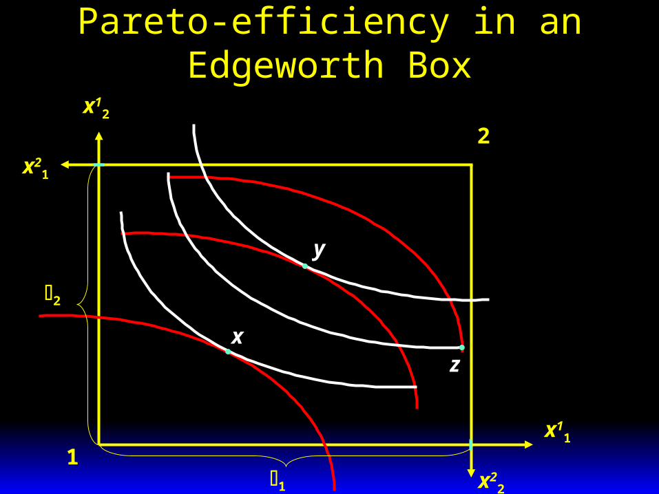
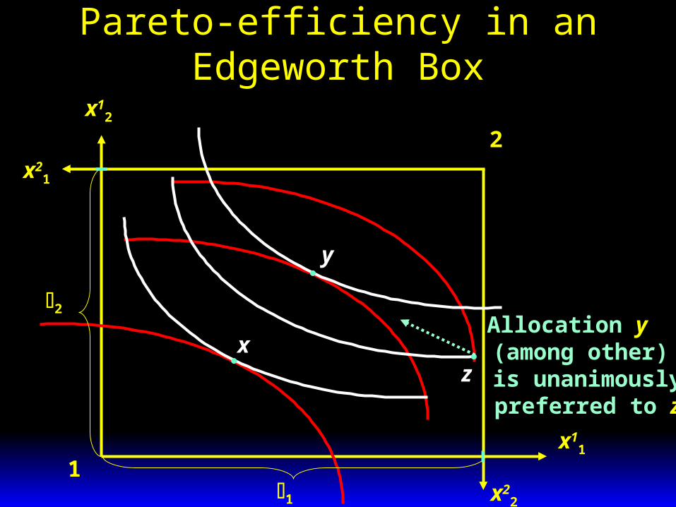
Pareto-efficiency in an Edgeworth Box
1
2
x22
x11
x12
x21
x
y
2
1
z

Pareto-efficiency in an Edgeworth Box
1
2
x22
x11
x12
x21
x
y
z
2
1
z is not Pareto-efficient

Pareto-efficiency in an Edgeworth Box
1
2
x22
x11
x12
x21
x
y
2
1
Allocations in this zone are unanimouslypreferred to z
z
Pareto-efficiency in an Edgeworth Box
1
2
x22
x11
x12
x21
x
y
2
1
Allocation y (among other) is unanimouslypreferred to z
z

Pareto-efficiency in an Edgeworth Box
1
2
x22
x11
x12
x21
x
y
2
1
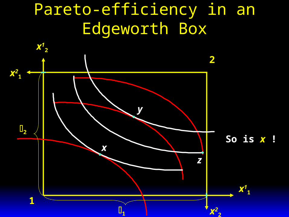
Allocation y is Pareto-efficientz
Pareto-efficiency in an Edgeworth Box
1
2
x22
x11
x12
x21
x
y
2
1
So is x !
z
Pareto-efficiency in an Edgeworth Box
1
2
x22
x11
x12
x21
x
y
2
1
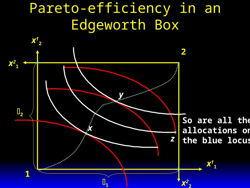
So are all theallocations onthe blue locusz

Pareto efficiency
A minimal normative requirement. An inefficient allocation is unstatisfactory. Yet Pareto-efficiency is hardly a sufficient
requirement. There are many Pareto-efficient allocations,
and some of them may involve significant inequality
As Amartya Sen put it « a society may be Pareto-efficient and perfectly disgusting!

General Competitive equilibrium
What happens when all households and all firms take their decisions individually, taking as given a prevailing set of prices ?
Given prices, each firm chooses a production activity that maximizes its profits.
GIven prices, each household chooses a bundle of l goods that it most prefer.
Prices are such that these choices are mutually consistent (supply equal demand on all markets).

General Competitive equilibrium
Here is a formal definition. A General Competitive Equilibrium (GCE)
for the economy = (Yk,Xi,i,ik,i
j), i =1,…,n, j =1,…,l and k = 1,…K is a list (p*,xi*,yk*) with p* l
+ , xi* Xi for i =1,
…,n, yk* Yk for k =1,…K such that:
)1(),...,,,...,,,...,(
),...,,,...,,,...,(
11**
1*
11**
1*
iK
iil
il
iii
iK
iil
il
ii
ppBzzx
ppBx

General Competitive equilibrium
Here is a formal definition. A General Competitive Equilibrium (GCE)
for the economy = (Yk,Xi,i,ik,i
j), i =1,…,n, j =1,…,l and k = 1,…K is a list (p*,xi*,yk*) with p* l
+ , xi* Xi for i =1,
…,n, yk* Yk for k =1,…K such that:
)2(1
*
1
** kl
jjj
l
j
kjj Yyypyp

General Competitive equilibrium
Here is a formal definition. A General Competitive Equilibrium (GCE)
for the economy = (Yk,Xi,i,ik,i
j), i =1,…,n, j =1,…,l and k = 1,…K is a list (p*,xi*,yk*) with p* l
+ , xi* Xi for i =1,
…,n, yk* Yk for k =1,…K such that:
)2(1
*
1
** kl
jj
kj
l
j
kj
kj Yyypyp
and

General Competitive equilibrium
Here is a formal definition. A General Competitive Equilibrium (GCE)
for the economy = (Yk,Xi,i,ik,i
j), i =1,…,n, j =1,…,l and k = 1,…K is a list (p*,xi*,yk*) with p* l
+ , xi* Xi for i =1,
…,n, yk* Yk for k =1,…K such that:
)3(1 1
*
1
* jyxn
i
K
k
kj
ij
n
i
ij

General Competitive equilibrium
Condition 1) says that given prices, and the budget constraint that these prices define (given initial endowments and ownerships of firms), household i chooses a bundle of goods that it most prefer in its budget set.
Condition 2 says that given prices firm k chooses a production activity in its production set that maximizes its profits.
Condition 3 says that choices made by firms and consumers are all mutually consistent (on every market, the demand for the good is never superior to the amount of good availabe (both as the result of production and initial endowments). prices, each household chooses a bundle of l goods that it most prefer.
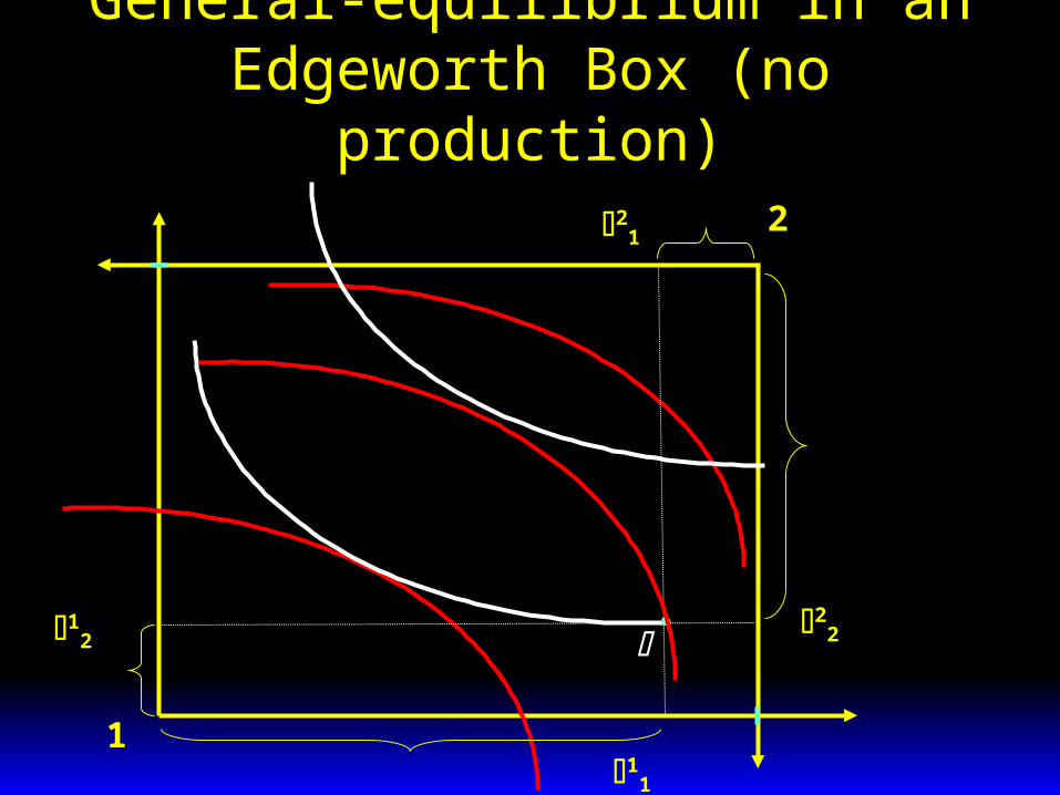
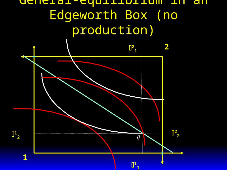
General-equilibrium in an Edgeworth Box (no production)
1
2
12
11
21
22
General-equilibrium in an Edgeworth Box (no production)
1
2
12
11
21
22
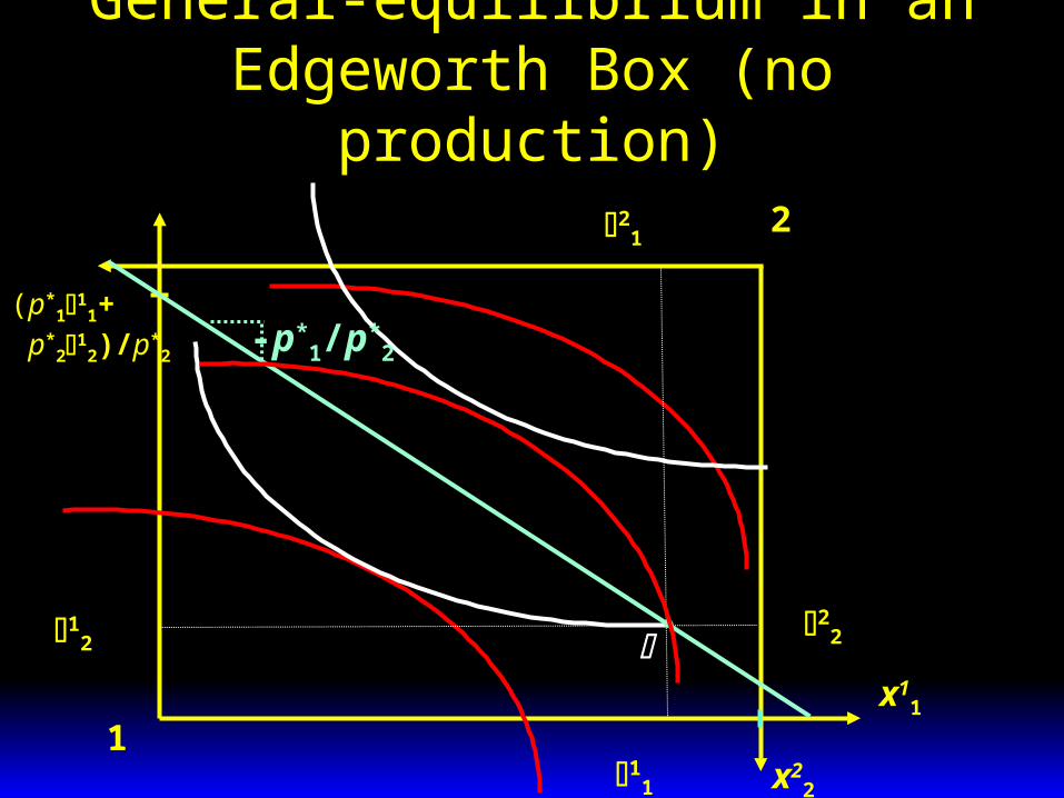
General-equilibrium in an Edgeworth Box (no production)
1
2
x22
x11
12
11
21
22
-p*1/p*
2
(p*11
1+ p*
212)/p*
2
General-equilibrium in an Edgeworth Box (no production)
1
2
x22
x11
12
11
21
22
-p*1/p*
2
(p*11
1+ p*
212)/p*
2

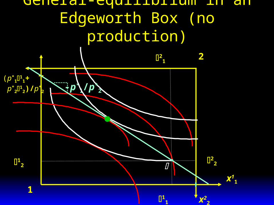
General-equilibrium in an Edgeworth Box (no production)
1
2
x22
x11
12
11
21
22
-p*1/p*
2
(p*11
1+ p*
212)/p*
2
x2*1
x1*1

General-equilibrium in an Edgeworth Box (no production)
1
2
x22
x11
12
11
21
22
-p*1/p*
2
(p*11
1+ p*
212)/p*
2
x2*1
x1*1
x1*2 x2*
2

Excess demand correspondance
Condition 3 defines what is called the « excess demand correspondance » Z: l
+ l. as follows:
jpypxpZn
i
K
k
kj
ij
n
i
Mijj
1 1
*
1
)()()(
Where xjMi(p) is the Marshallian demand of good j by
household i at prices p and yjk*(p) is the net supply of
good j by the firm k at prices p
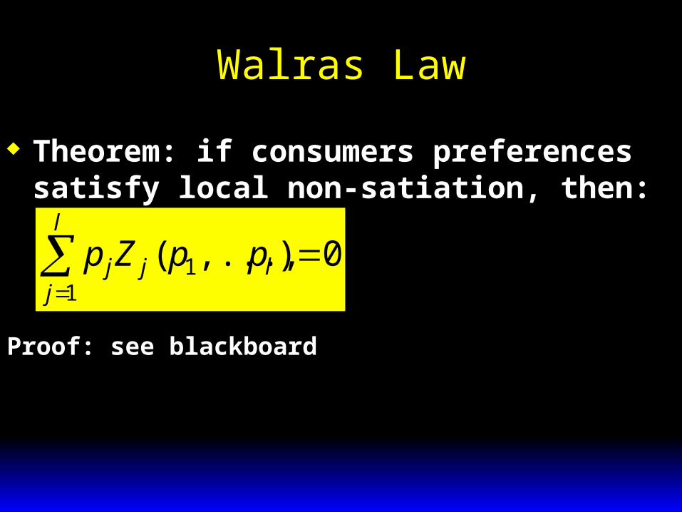
Walras Law
Theorem: if consumers preferences satisfy local non-satiation, then:
l
jljj ppZp
11 0),...,(
Proof: see blackboard
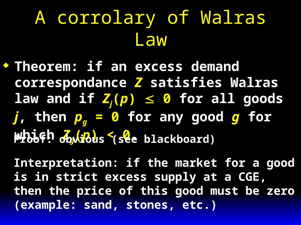
A corrolary of Walras Law
Theorem: if an excess demand correspondance Z satisfies Walras law and if Zj(p) 0 for all goods j, then pg = 0 for any good g for which Zg(p) < 0.
Proof: obvious (see blackboard)
Interpretation: if the market for a good is in strict excess supply at a CGE, then the price of this good must be zero (example: sand, stones, etc.)

Consequence of this corrolary
If (p*,xi*,yk*) is CGE for an economy, then for every good g for which pg > 0 one must have Zg(p) = 0.
We are going to use this to prove the existence of CGE for any economy satisfying our assumptions.
Establishing the existence of CGE has been one of the major achievement of the 20th century mathematical economics (finalized in fifeties through the work of Arrow and Debreu.
Argument is based on the fact that certain functions admit Fixed Points.
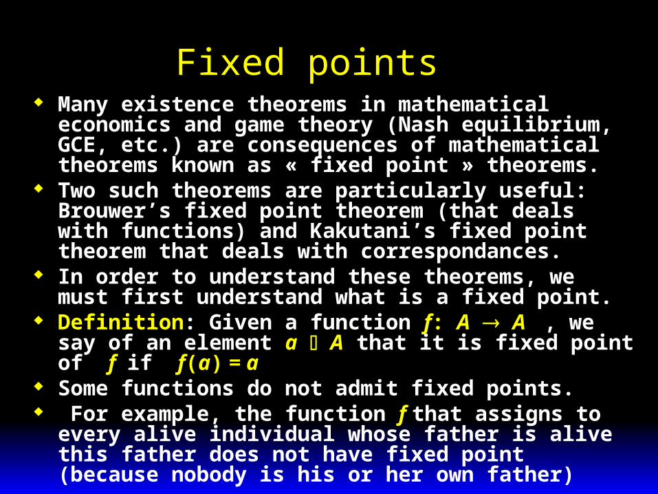
Fixed points Many existence theorems in mathematical economics
and game theory (Nash equilibrium, GCE, etc.) are consequences of mathematical theorems known as « fixed point » theorems.
Two such theorems are particularly useful: Brouwer’s fixed point theorem (that deals with functions) and Kakutani’s fixed point theorem that deals with correspondances.
In order to understand these theorems, we must first understand what is a fixed point.
Definition: Given a function f: A A , we say of an element a A that it is fixed point of f if f(a) = a
Some functions do not admit fixed points. For example, the function f that assigns to every alive
individual whose father is alive this father does not have fixed point (because nobody is his or her own father)

Brouwer’s fixed point theorem The mathematician Brouwer a
established (in 1912) a theorem guaranteeing that a (real-valued) function admits a fixed point.
Brouwer’s fixed point Theorem: Let A be a subset convex and compact of k and let f: A A be a continuous function. Then, there exists an element a A that is a fixed point of f
Let us illustrate the theorem when A is a convex and compact subset (and therefore an interval) of .

Brouwer fixed point theorem
A
A
x
y
y = x
f

Brouwer fixed point theorem
A
A
x
y
y = x
Fixed points
f

Brouwer fixed point Theorem
A
A
x
y
f
The assumptions of Brouwer’s theorem
are all important
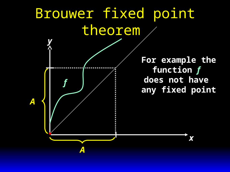
Brouwer fixed point theorem
A
A
x
y
f
For example thefunction f
does not have any fixed point
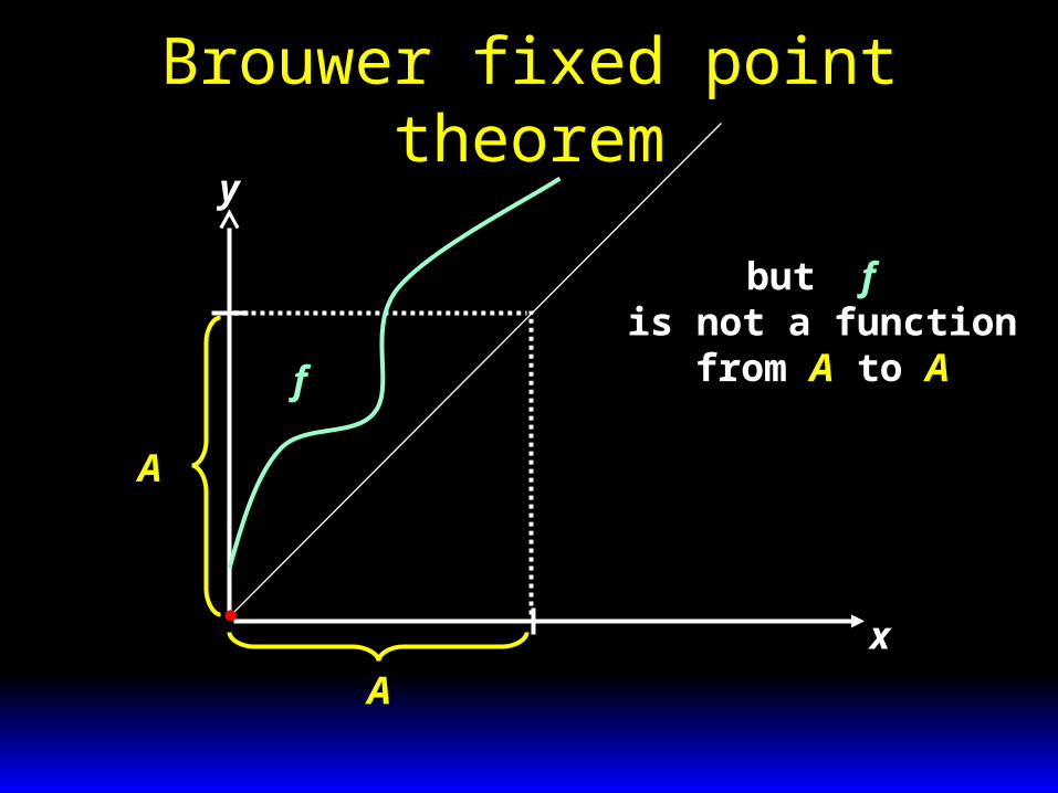
Brouwer fixed point theorem
A
A
x
y
f
but f is not a function
from A to A
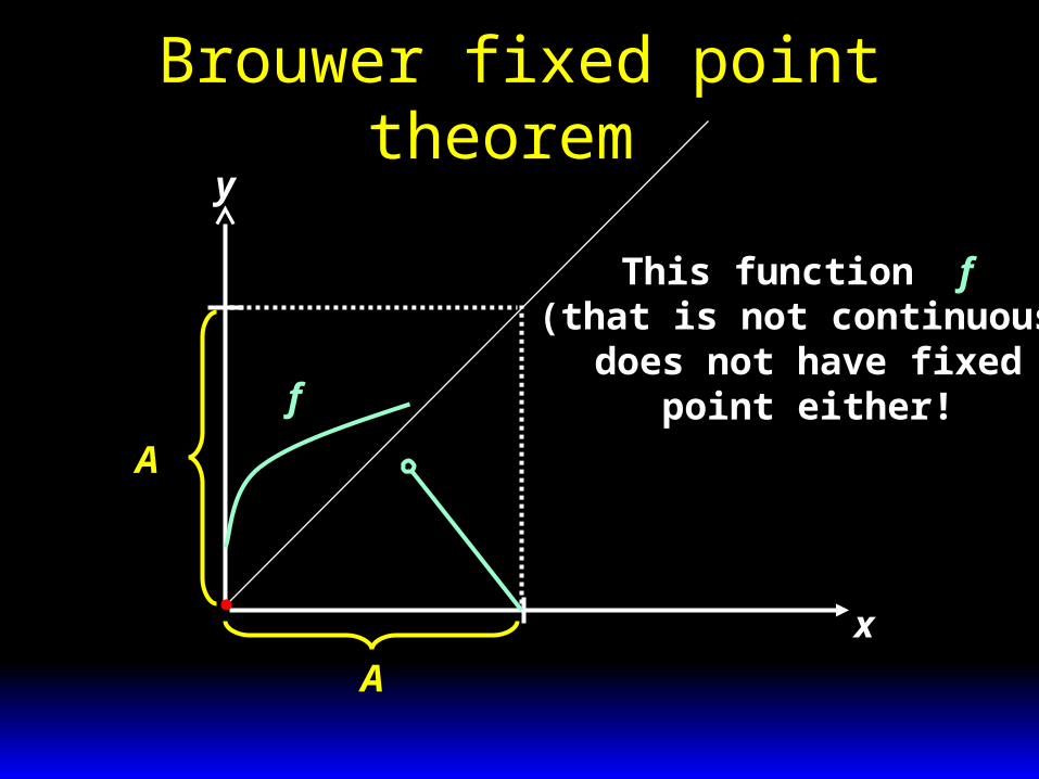
Brouwer fixed point theorem
A
A
x
y
f
This function f (that is not continuous)
does not have fixedpoint either!

Brouwer fixed point theorem
A
A
x
y
f
Similarly, if A isopen above a
continuous function like f does not have
fixed points

Fixed points Brouwer’s fixed point theorem applies to functions. Yet
the CGE can be viewed as the fixed point of a correspondance of price adjustment (based on excess demand).
Kakutani (1941) has generalized Brouwer’s fixed point theorem to correspondances.
Kakutani fixed point theorem: Let A be a convex and compact subset of l and let C: A A be correspondance upper-semi continuous. Then, there exists an element a* A that is a fixed point of C (and that is therefore such that a* C(a*)).
John Nash in 1950 has used this theorem to show the existence of a Nash equilibrium in non-cooperative games.
Debreu (1959) has used it as well in his proof of the existence of CGE.
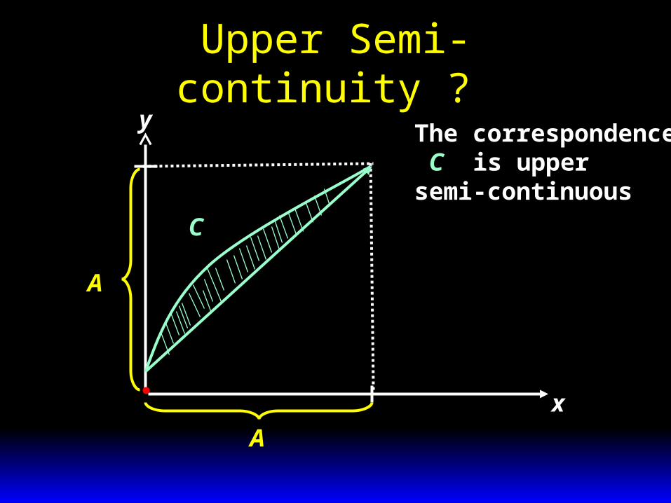
Upper Semi-continuity ?
A
A
x
y
C
The correspondence C is upper semi-continuous

Upper semi-continuity ?
A
A
x
y
C
The correspondence C is upper semi-continuous
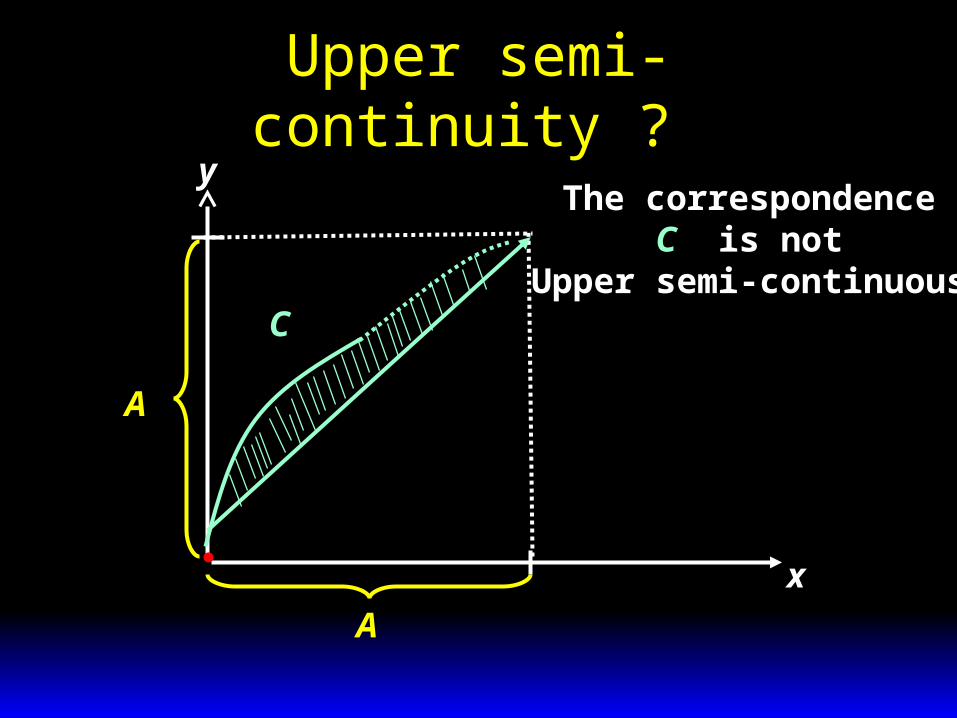
Upper semi-continuity ?
A
A
x
y
C
The correspondence C is not
Upper semi-continuous
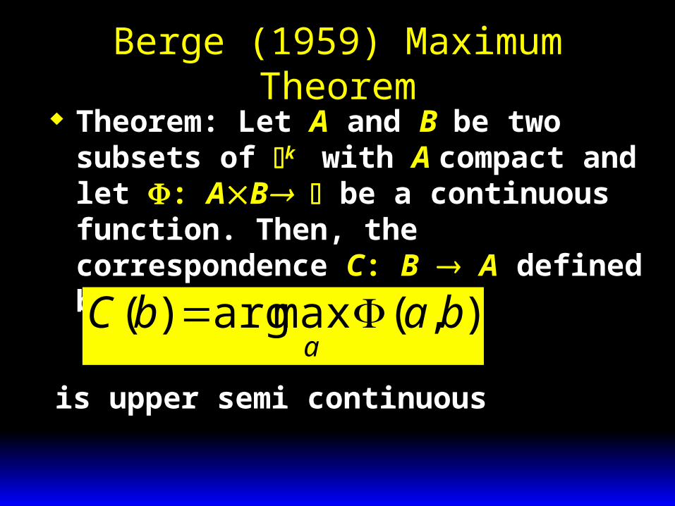
Berge (1959) Maximum Theorem Theorem: Let A and B be two subsets of
k with A compact and let : AB be a continuous function. Then, the correspondence C: B A defined by:
),(maxarg)( babCa
is upper semi continuous
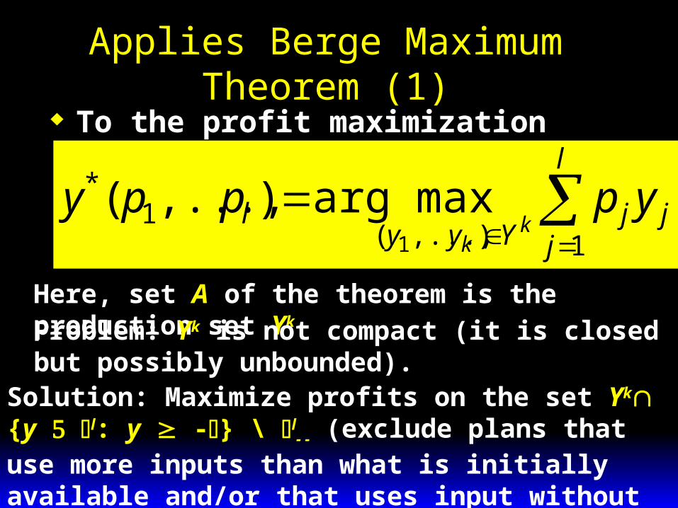
Applies Berge Maximum Theorem (1) To the profit maximization program.
l
jjj
Yyyl ypppy
kk 1),...,(
1*
1
maxarg),...,(
Here, set A of the theorem is the production set Yk
Problem: Yk is not compact (it is closed but possibly unbounded).
Solution: Maximize profits on the set Yk {y l: y -} \ l
- - (exclude plans that use more inputs than what is initially available and/or that uses input without producing any output).

Applies Berge Maximum Theorem (2) To the consumer’s utility maximization
program:
),...,(maxarg),...,( 1),...,,.,...,,,...,(),...,(
11111
li
ppBxxl
M xxUppXik
iil
ill
Here, set A of the theorem is the budget set (that is compact)