Modified: August 25, 2005

General Autoregressive Conditional Heteroscedastic (GARCH) Modeling

Using the SCAB34S-GARCH and SCA WorkBench

Houston H. Stokes Department of Economics

University of Illinois at Chicago

Lon-Mu Liu Department of Information and Decision Sciences

University of Illinois at Chicago

William J. Lattyak Scientific Computing Associates Corp.

Table of Contents 1. GARCH MODELING USING SCAB34S AND WORKBENCH ...................................................................... 2

1.1 ARCH Models.................................................................................................................................................. 3 1.2 GARCH models ............................................................................................................................................... 4 1.3 Integrated GARCH models ............................................................................................................................ 4 1.4 GARCH-M models .......................................................................................................................................... 4 1.5 Non-normal Error Distributions.................................................................................................................... 5

1.5.1 Standardized Student-t Distribution .......................................................................................................... 6 1.5.2 Standard Cauchy Distribution................................................................................................................... 6 1.5.3 General Error Distribution........................................................................................................................ 6

1.6 Asymmetric GARCH models ......................................................................................................................... 7 1.6.1 Glosten-Jagannathan-Runkle (GJR) model............................................................................................... 7 1.6.2 Extended Threshold GARCH model .......................................................................................................... 8 1.6.3 Exponential GARCH model....................................................................................................................... 8 1.6.4 Zakoian Threshold GARCH model............................................................................................................ 9

1.7 Regression plus GARCH models ................................................................................................................... 9 1.8 Bivariate GARCH model.............................................................................................................................. 10

2. ESTIMATION OF GENERALIZED ARCH (GARCH) MODELS................................................................ 11 2.1 Two-Pass Estimation Method Using the SCA Statistical System.............................................................. 11 2.2 The One-Pass Method (Joint Estimation Method) Using SCAB34S......................................................... 12

3. SCA WORKBENCH: A GRAPHICAL USER INTERFACE......................................................................... 12

4. EXAMPLES OF GARCH MODELING USING SCA WORKBENCH ......................................................... 13 4.1 Analysis of the Wholesale Price Index (Enders 1995) ................................................................................ 13

4.1.1 Applying the automatic two-pass method ................................................................................................ 15 4.1.2 Applying the user-directed one-pass method........................................................................................... 18

4.2 GARCH Analysis of the S&P 500 Using the One-Pass Method ................................................................ 22 4.2.1 Considering the student-t distribution (FATTAIL) estimation option...................................................... 25 4.2.2 Considering a GARCH-M model for the S&P 500 monthly returns........................................................ 27

4.3 Regression plus GARCH Models Using IBM returns and S&P 500 Series ............................................. 29 4.3.1 Modeling IBM stock returns and the S&P 500 index using the automatic two-pass method .................. 29 4.2.2 Modeling IBM stock returns and the S&P 500 index using the user-directed one-pass method............. 33

4.4 Bivariate GARCH Models Using IBM returns and S&P 500 Series ........................................................ 35 4.4.1 Bivariate Modeling Approach Assuming Constant Correlations ............................................................ 35 4.4.2 Bivariate Modeling Approach Assuming Time-varying Correlations ..................................................... 39

5. A DETAILED DESCRIPTION OF THE GARCH APPLICATION INTERFACE IN WORKBENCH.... 45 Two-pass Estimation Method: ........................................................................................................................... 45 One-pass Estimation Method: ........................................................................................................................... 45

5.1 Data View for ARCH/GARCH Modeling ................................................................................................... 45 5.2 ARCH/GARCH Modeling Environment..................................................................................................... 48

5.2.1 Automatic two-pass method..................................................................................................................... 49 Regression Components ...................................................................................................................................... 51 5.2.2 User-directed two-pass method ............................................................................................................... 53 5.2.3 User-directed one-pass method ............................................................................................................... 56 Advanced Options/Settings View ......................................................................................................................... 59 MAX LAG in ML Sum ......................................................................................................................................... 61 Bivariate GARCH Model Specification................................................................................................................ 61 5.2.4 Results ..................................................................................................................................................... 63 5.2.5 Graphics .................................................................................................................................................. 65

6. A DETAILED DESCRIPTION OF THE GARCHEST COMMAND IN SCAB34S..................................... 66 Usage: ............................................................................................................................................................... 66

Required subroutine arguments: ....................................................................................................................... 66 Optional keywords and associated arguments: ................................................................................................. 66 Variables created if OPTIONS keyword is specified:........................................................................................ 71

7. A DETAILED DESCRIPTION OF THE GARCHEST COMMAND IN SCAB34S..................................... 73 Usage: ............................................................................................................................................................... 73 Required subroutine arguments: ....................................................................................................................... 73 Optional keywords and associated arguments: ................................................................................................. 74

8. A DETAILED DESCRIPTION OF THE CMAXF2 COMMAND IN SCAB34S .......................................... 77 Usage ..................................................................................................................................................................... 77

9. DESCRIPTION OF CUSTOMIZED SUBROUTINES IN THE GARCH APPLICATION ......................... 80 9.1 DSPGARCH User Subroutine...................................................................................................................... 80

Usage: ............................................................................................................................................................... 81 Required subroutine arguments: ....................................................................................................................... 81 Example:............................................................................................................................................................ 82

9.2 DSPDSCRB User Subroutine....................................................................................................................... 83 Usage: ............................................................................................................................................................... 83 Required subroutine arguments: ....................................................................................................................... 83 Example:............................................................................................................................................................ 83

9.3 DSP_ACF User Subroutine .......................................................................................................................... 84 Usage: ............................................................................................................................................................... 84 Required subroutine arguments: ....................................................................................................................... 84 Example:............................................................................................................................................................ 84

9.4 LAGRANGE User Subroutine..................................................................................................................... 85 Usage: ............................................................................................................................................................... 85 Required subroutine arguments: ....................................................................................................................... 85 Example:............................................................................................................................................................ 85

9.5 GARCHF User Subroutine........................................................................................................................... 86 Usage: ............................................................................................................................................................... 86 Required subroutine arguments: ....................................................................................................................... 86 Example:............................................................................................................................................................ 87

9.6 GRFGARCH User Subroutine..................................................................................................................... 88 Usage: ............................................................................................................................................................... 88 Required subroutine arguments: ....................................................................................................................... 88 Example:............................................................................................................................................................ 88

10. EXAMPLES OF SCAB34S COMMAND FILES FOR GARCH MODELING........................................... 89 10.1 SCA System script for the automatic two-pass example (Section 4.1.1)........................................... 89 10.2 SCAB34S script for the one-pass example (Section 4.1.2) ................................................................. 90 10.3 SCAB34S script for GARCH(1,1) Example (Section 4.2).................................................................. 93 10.4 SCAB34S script for GARCH(1,1) with FAT-TAIL option (Section 4.2.1) ...................................... 96 10.5 SCAB34S script for GARCH-M Model (Section 4.2.2) ..................................................................... 99 10.6 SCA script for Regression +GARCH Using Automatic Two-pass (Section 4.3.1)......................... 102 10.7 SCAB34S script for Regression plus GARCH Using the One-pass (Section 4.3.2) ....................... 103 10.8 SCAB34S script for Bivariate GARCH with Constant Correlations (Section 4.4.1) ................... 106 10.9 SCAB34S script for Bivariate GARCH with Time-varying Correlations (Section 4.4.2)............. 108

11. A DISCUSSION OF THE MCCULLOUGH – RENFRO GARCH BENCHMARK STUDY.......... 110

Coefficients ...................................................................................................................................................... 110 REFERENCES........................................................................................................................................................ 112

General Autoregressive Conditional Heteroscedastic (GARCH) Modeling Using the SCAB34S-GARCH and SCA WorkBench

In this document, we discuss Generalized Autoregressive Conditional Heteroscedastic (GARCH) modeling

and estimation provided by the B34S® ProSeries Econometric System, the SCAB34S applet collection

(GARCH module), and the SCA Statistical System.

The SCAB34S applet collection provides a subset of the capabilities in the B34S® ProSeries Econometric

System. It is organized in modular form and runs conveniently as an integrated component to SCA

WorkBench. The WorkBench product is a companion to the SCA Statistical System and SCAB34S software.

It offers macro management and a graphical user interface for GARCH modeling and other applications.

The SCAB34S product contains a number of procedures to perform common data manipulation tasks,

organizational tasks, and statistical analysis tasks. It also contains a comprehensive matrix programming

language that may be used to address a variety of general nonlinear and optimization problems. No attempt

will be made to cover all features of the SCAB34S product in this document nor the full range of applications

that may be solved using the B34S matrix programming facilities. Instead, we shall exclusively use the

graphical user interface of SCA WorkBench to specify, estimate, and diagnostically test GARCH models in

the SCAB34S and SCA Statistical Systems. WorkBench automatically specifies the program commands used

by SCAB34S based on user menu selections. A command file is then executed in the SCAB34S applet

collection and the results read back into WorkBench in a convenient fashion. For detailed information on the

capabilities of the B34S ProSeries Econometric System, refer to the book by Stokes (1997).

GARCH model specification in SCA WorkBench is intuitive and easy to use. It is also quite flexible,

providing options to estimate a variety of conditional heteroscedastic models including the autoregressive

conditional heteroscedastic (ARCH) model of Engle (1982), the generalized ARCH (GARCH) model of

Bollerslev (1986), the integrated GARCH (IGARCH) model of Nelson (1990, 1991), the GARCH-M model of

Engle, Lilien, and Robins (1987), the GJR-GARCH model of Glosten-Jagannathan-Runkle (1993), the

exponential GARCH (EGARCH) model of Nelson (1991), and a variety of threshold GARCH models.

WorkBench also provides facilities to override starting values for model parameters, adjust constraints on

model parameters, and specify several preferences for nonlinear estimation. This is very important in GARCH

model estimation since the likelihood function tends to be very sensitive especially to starting values.

Two estimation approaches are discussed, a two-pass method and a joint estimation method. We explore

the differences between these two estimation approaches and comment on when one method may be preferred

over the other. The calculation of standard errors for GARCH model parameters is a complex subject that has

2

gained increased research interest. We do not address this subject in detail in this document. However, we do

indicate the computation method for standard errors employed in the SCAB34S product and compare these

numbers to several published works. For an applied and in-depth discussion of GARCH modeling and

methodology, refer to Liu (2005) or Tsay (2002).

1 GARCH MODELING USING SCAB34S AND WORKBENCH

In conventional time series and econometric models, the variance of the disturbance term is assumed to be

constant. However, many economic and financial time series exhibit periods of unusually high volatility

followed by periods of relative tranquility. In such situations, the assumption of a constant variance is

inappropriate. Engle (1982, 1995), Bollerslev (1986), Bollerslev-Ghysels (1996) and others developed a class

of models that address such concerns and also allow for modeling both the level (the first moment) and the

variance (the second moment) of a process.

The first moment equation can be a non-seasonal ARIMA, seasonal ARIMA, or dynamic regression

model. In econometric literature, the dynamic regression model with one explanatory variable is typically

written as

pt 0 i t i j t j t

i 0 j 1Y C X Y (B)a− −

= == + ω + φ + θ∑ ∑

l (1)

where tY is the dependent variable that is differenced to stationarity, t i{X , i 1, ..., }− = l is a lagged variable that

can be expanded to include multiple explanatory variables regressed upon tY , and jφ are the autoregressive

parameters in the first moment model. In econometric literature, the moving average operator (B)θ is

typically expressed as q1 q(B) 1 B Bθ = + θ + ⋅⋅ ⋅ + θ . The SCAB34S software package employs this convention for

expressing (B)θ in (1) for the one-pass (joint) estimation method.

If the regressor variables t iX − ’s are omitted from (1) , the model is simplified to a Box-Jenkins ARIMA

model as

pt 0 j t j t

j 1Y C Y (B)a−

== + φ + θ∑ (2)

or

t 0 t(B)Y C (B)aφ = + θ (3)

where p1 p(B) 1 B Bφ = − φ − ⋅⋅⋅ − φ , and q

1 q(B) 1 B Bθ = + θ + ⋅⋅ ⋅ + θ .

3

In the typical Box-Jenkins framework, the ARIMA model is also expressed as in (3), but (B)θ is defined

as

q1 q(B) 1 B Bθ = − θ − ⋅⋅ ⋅ − θ . (4)

It is important to note that the sign of the moving average operator (B)θ is reversed between these two

formulation conventions. It is equally important to note that in the SCAB34S software package, the ARIMA

formulation for the moving average operator (B)θ in (4) is employed for the two-pass estimation method.

Whereas the two-pass method is not able to use non-normal error distributions, or handle various GARCH

extensions such as asymmetric models or GARCH-M models, the two-pass method using the model form in

(4) is able to handle multiplicative ARIMA models, intervention models, and the generalized form of a transfer

function model.

Now that we have defined the first moment model, the remainder of this document focuses on the second

moment equation that is used to model volatility in financial applications.

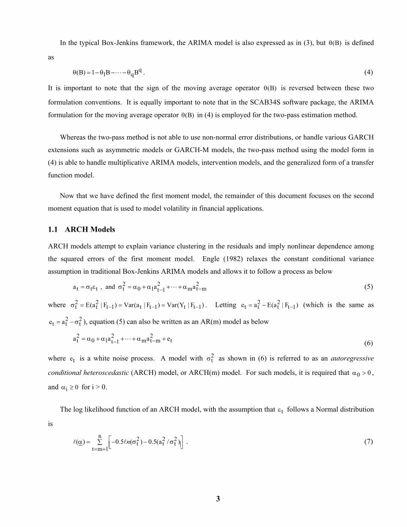
1.1 ARCH Models

ARCH models attempt to explain variance clustering in the residuals and imply nonlinear dependence among

the squared errors of the first moment model. Engle (1982) relaxes the constant conditional variance

assumption in traditional Box-Jenkins ARIMA models and allows it to follow a process as below

2 2 2t t t t 0 1 m t mt 1a , and a a −−= σ ε σ = α +α + ⋅⋅⋅ + α (5)

where 2 2t t t 1 t t 1 t t 1E(a | F ) Var(a | F ) Var(Y | F )− − −σ = = = . Letting 2 2

t t t t 1e a E(a | F )−= − (which is the same as

2 2t t te a= −σ ), equation (5) can also be written as an AR(m) model as below

2 2 2t 0 1 m t m tt 1a a a e−−= α +α + ⋅⋅⋅ + α + (6)

where te is a white noise process. A model with 2tσ as shown in (6) is referred to as an autoregressive

conditional heteroscedastic (ARCH) model, or ARCH(m) model. For such models, it is required that 0 0α > ,

and i 0α ≥ for i > 0.

The log likelihood function of an ARCH model, with the assumption that tε follows a Normal distribution

is n 2 2 2

t t tt m 1

( ) 0.5 ( ) 0.5(a / )= +

α = − σ − σ∑ l ln . (7)

4

In practice, there is substantial evidence showing that the Normality assumption may not always be

satisfactory. Non-normal distributions, such as the Student-t distribution (Bollerslev, 1987), Generalized Error

Distribution (GED) (Nelson, 1991) or standard Cauchy distribution may also be considered. These alternative

error distributions and their modifications to the likelihood functions will be discussed later.

1.2 GARCH Models Although the ARCH model is simple, it restricts the model for the conditional variance 2

tσ (or equivalently

th ) to follow a pure AR process and hence it may require more parameters to adequately represent the

conditional variance process in comparison with other more generalized models. Bollerslev (1986) extends

Engle’s original work by allowing the conditional variance to follow an ARMA process. This model is known

as a generalized ARCH model, or GARCH model. A GARCH(r, m) model can be written as

2 2 2 2 2t t t t 0 1 m t m 1 r t rt 1 t 1a , and a a − −− −= σ ε σ = α +α + ⋅⋅⋅ + α +β σ + ⋅⋅⋅ + β σ (8)

where 0 i j0, 0, 0α > α ≥ β ≥ , and max(m, r)i ii 1 ( ) 1= α +β <∑ . The latter constraint on i iα +β ensures that the

unconditional variance of ta is finite, even though its conditional variance evolves over time. It is easy to see

that model (8) reduces to an ARCH(m) model if r=0. Under the Normality assumption of tε , the log

likelihood function of α for a GARCH(r, m) model is the same as that in (7).

1.3 The Integrated GARCH (IGARCH) model In financial time series, the conditional volatility ( 2

tσ ) is often persistent and therefore may cause a unit root

condition in the model Such a special case of a GARCH model is referred to as the integrated GARCH

(IGARCH) model (Nelson, 1990, 1991). Similar to ARIMA models, the primary characteristic of an

IGARCH model is that the impact of past squared shocks on 2ta is persistent. As an example, an

IGARCH(1,1) model can be written as

2 2 2t t t t 0 1 1t 1 t 1a , and (1 )a − −= σ ε σ = α + −β +β σ (9)

where 0 0α > and 11 0> β > . More complicated restrictions can be estimated using a B34S program to

explicitly specify the model form and a direct call to CMAX2.

1.4 GARCH-M Models In financial markets, the return of a security may be influenced by its volatility. Engle, Lilien, and Robins

(1987) extend the basic GARCH framework to model such a phenomenon. This class of models, called the

5

GARCH-in-mean (GARCH-M) model, is particularly useful in the study of security markets. As an example,

a simple GARCH(1,1)-M model can be written as

t t t t t tY a , a= µ + δσ + = σ ε (10)

2 2 2t 0 1 1t 1 t 1a − −σ = α +α +β σ

where tY represents the return of a security, and µ and δ are constant parameters to be estimated. The

parameter δ is called the risk premium parameter. If δ is positive, it implies that the return is positively

related to its volatility, and vice versa.

The GARCH(1,1)-M model in (10) shows that the mean of first moment model is inferenced upon

conditional standard deviation tσ in the second moment model. The model can alternatively be specified so

that the first moment model is inferenced by the conditional variance 2tσ in the second moment model such

that

2t t tY a= µ + δσ + (11)

Both forms of the GARCH-M model are supported by the GARCH application environment. The same

likelihood function developed earlier under the Normality assumption also applies for the estimation of a

GARCH-M model.

1.5 Non-normal Error Distributions Until now, we have assumed that error distribution of tε for the various symmetric conditional heteroscedastic

models followed a standard Normal distribution. It was further shown that the likelihood function given the

Normalility assumption remained the same for ARCH, GARCH, IGARCH and GARCH-M models. We now

present the possibility of non-normal error distributions. There is substantial evidence showing that the

Normality assumption may not always be satisfactory for GARCH models. When non-normality conditions

are present in the distribution of tε , alternative standardized error distributions such as the Student-t

distribution (Bollerslev, 1987), Generalized Error Distribution (GED) (Nelson, 1991) or standard Cauchy

distribution may be considered. In this section, we shall derive the likelihood function for ARCH, GARCH,

IGARCH and GARCH-M models based on the above assumptions for the distribution of tε . These likelihood

functions can then be used for estimation of model parameters.

6

1.5.1 Standardized Student-t Distribution

In some applications, it is more appropriate to assume that tε follows a heavy-tailed distribution such as a

standardized Student-t distribution (Bollerslev, 1987). This is also known as a fat-tail GARCH model. The

conditional log likelihood function of α with a pre-specified ν degrees of freedom can be expressed as

2n 2tt2t m 1 t

a1 1( ) 1 ( )2 2( 2)= +

ν + α = − + + σ∑ ν − σ

l l ln n . (12)

If we wish to estimate ν jointly with other parameters, then the conditional log likelihood function based on

becomes

[ ] m 1 n( , ) (n m) ( (( 1) / 2)) ( ( / 2)) 0.5 ( 2) ( | a ,..., a )+α ν = − Γ ν + − Γ ν − ν − + αl l l l ln n n (13)

where the second term is given in (12) above.

1.5.2 Standard Cauchy Distribution

We may also employ the standard Cauchy distribution as the underlying distribution for tε . It is important to

note that the mean, variance, skewness, and kurtosis of a Cauchy distribution are undefined, and only the

median and mode of the distribution exist (which are both zero in this case).

The standard Cauchy distribution is equivalent to a Student-t distribution with one degree of freedom.

Compared to the standard Normal distribution, the standard Cauchy distribution is “shorter” and has fatter

(i.e., thicker) tails, thus favoring increased occurrences of extreme values that are associated with high

volatility. Assuming that tε follows the standard Cauchy distribution with median zero, the log likelihood

function for ARCH, GARCH, IGARCH and GARCH-M models can be derived as

n

2 2 2t=m+1 t t t

1( ) [ (a / )]

α = ∑ π σ + σ

l ln . (14)

1.5.3 General Error Distribution

Instead of a Student-t distribution or standard Cauchy distribution, Nelson (1991) employs another commonly

used distribution, the Generalized Error Distribution (GED), as the underlying distribution for tε . The GED

includes the Normal distribution as a special case, along with many other distributions, some more fat tailed

than the Normal (e.g., the double exponential), some more thin tailed (e.g., the uniform).

Assuming that tε follows a standardized GED, the log likelihood function for an ARCH, GARCH,

IGARCH, or GARCH-M model can be derived as

7

n n1 2 tt

tt m 1 t m 1

a( ) (n m)[ ( / ) (1 ) (2) ( (1/ ))] 0.5 ( ) 0.5

ν−

= + = +α = − ν λ − + ν − Γ ν − σ −∑ ∑

λσl l l l ln n n n . (15)

Similar to the Student-t distribution that assumes tε following a fat-tail distribution, the generalized error

distribution allows for tε to follow symmetric long-tail distributions, including the fat-tail, thin-tail as well as

Normal distributions. Consequently, the generalized error distribution is also a means of confirming the error

distribution as Normal or not.

1.6 ASYMMETRIC GARCH MODELS

While ARCH/GARCH models provide a venue for modeling conditional heteroscedastic volatility with a

Normal or Non-normal error distributions, these models assume that positive and negative shocks have the

same effect on volatility because it depends on the square of previous shocks. Therefore the models discussed

in the previous sections are referred to as symmetric ARCH/GARCH models. In practice, the price of

financial assets often reacts more pronouncedly to “bad” news than “good” news. Such a phenomenum leads

to a so called leverage effect, as first noted by Black (1976). The term “leverage” stems from the empirical

observation that the volatility (conditional variance) of a stock tends to increase when its returns are negative.

This effect is particularly important for option markets. Asymmetric GARCH models are designed to capture

leverage effects.

The asymmetric GARCH models discussed in this section include GJR-GARCH models of Glosten,

Jagannathan and Runkle (1993), exponential GARCH (EGARCH) models of Nelson (1991), and some other

threshold GARCH models.

1.6.1 The Glosten-Jagannathan-Runkle (GJR) Model

To capture the leverage effect, Glosten, Jaganathan, and Runkle (1993) show how to allow good news and bad

news to have different effects on volatility by using t 1a − as a threshold. A GJR-GARCH(1,1) model can be

generally expressed as m m r2 2 * 2 2

t 0 i t i i jt i t i t ji 1 i 1 j 1

a (a ) a−− − −= = =

σ = α + α + α + β σ∑ ∑ ∑I (16)

where t i(a ) 1− =I if t ia 0− < and t i(a ) 0− =I if t ia 0− ≥ . It is useful to note that the GJR-GARCH model is a

special case of threshold GARCH (TGARCH) models.

8

1.6.2 Extended Threshold GARCH (ETGARCH) Model

The GJR GARCH model in (16) can be extended to include threshold relationships on 2t j−σ , j=1,2, …, r (Tsay,

2002; page 133) as follows: m m r r2 2 * 2 2 * 2

t 0 i t i i j t j jt i t i t j t ji 1 i 1 j 1 j 1

a (a ) a (a )− −− − − −= = = =

σ = α + α + α + β σ + β σ∑ ∑ ∑ ∑I I (17)

where t i(a ) 1− =I if t ia 0− < , and t i(a ) 0− =I if t ia 0− ≥ . We shall refer to the above model as the extended

threshold GARCH (ETGARCH) model, more specifically, ETGARCH(r,m) model. In the above model, *iα

and *iβ represent the leverage effects associated with t ia − . When m=1 and r=1, we have the ETGARCH(1,1)

model as

2 2 * 2 2 * 2t 0 1 t 1 1 1 t 1 1t 1 t 1 t 1 t 1a (a ) a (a )− −− − − −σ = α +α + α +β σ + β σI I . (18)

In the above ETGARCH model, if it is found that the leverage effect *1β is significant, but *

1α is not, the

ETGARCH(r,m) model in (17) may be simplified to the following model if the term * 2mt i ii 1 t i(a ) a−= −α∑ I is

dropped m r r2 2 2 * 2

t 0 i j t j jt 1 t j t ji 1 j 1 j 1

a (a )−− − −= = =

σ = α + α + β σ + β σ∑ ∑ ∑ I . (19)

In the above simplified ETGARCH model, *jβ represents the leverage effect of t ja − .

1.6.3 The Exponential GARCH (EGARCH) Model

A problem with standard GARCH models is that it is necessary to ensure that all of the estimated coefficients

are positive. Nelson (1991) proposes the exponential GARCH (EGARCH) model that does not require non-

negativity constraints. In addition, the EGARCH model allows for the asymmetric effect of news or shocks on

the conditional volatility. The EGARCH(r, m) model in simplified form is

2 2 2t 0 1 t 1 t 1 m t m t m 1 t 1 r t r( ) (| | ) (| | ) ( ) n( )− − − − − −σ = α +α ε −γ ε + ⋅⋅ ⋅ + α ε −γ ε +β σ + ⋅⋅⋅ + β σl l ln n (20)

The EGARCH model originally proposed by Nelson (1991) was in a more general form than the above. By

using a suitable function g, the EGARCH model of Nelson (1991) can be written as

2 2 2t 0 1 t 1 2 t 2 m t m 1 t 1 r t r( ) g( ) g( ) g( ) ( )− − − − −σ = α +α ε + α ε + ⋅⋅ ⋅ + α ε +β σ + ⋅⋅⋅ + β σl ln n (21)

where t t ta /ε = σ and 1 1α = . Nelson choose the function tg( )ε to be a linear combination of tε and t| |ε such

as

t t t tg( ) [| | E(| |)]ε = δε + λ ε − ε (22)

9

where δ and λ are constant terms to be estimated. In the above function, both tε and t t| | E(| |)ε − ε are i.i.d

variable with zero mean. Also, note that t i tE(| |) E(| |) 2 /−ε = ε = π for all i.

In the SCAB34S package, both the simplified and generalized forms of the EGARCH model may be

specified. For the generalized form in the SCAB34S package, the function t ig( )−ε is defined as

t i t i t i t ig( ) (| | E(| |) , i 1, 2, ...− − − −ε = ε − ε − γ ε = (23)

where the leverage effect γ is equivalent to /−δ λ in (22). Using this formulation, the 1α in (21) is an

estimated coefficient, and the estimates of the 1 m, . . ., α α , 1 r, . . ., β β and γ in (20) and those in (21) are the

same.

1.6.4 The Zakoian Threshold GARCH (ZTGARCH) Model

A threshold GARCH model, proposed by Zakoian (1994), treats the conditional standard deviation as a linear

function of shocks and lagged standard deviations. For an asymmetric ZTGARCH(r,m) model, it takes the

following form: m r

t 0 i t i j t ji t ii 1 j 1

( a a )+ + − −− −−

= =σ = α + α −α + β σ∑ ∑ (24)

where t ta max(a , 0)+ = and t ta min(a , 0)− = are the positive and negative parts of an ta . To meet the needs of

the non-negativity constraints, all the coefficients in (24) are constrained to be positive.

As a special case of (24), if i ii+ −α = α = α for all i , the conditional standard deviation then is simplified to

m rt 0 i t i j t j

i 1 j 1| a |− −

= =σ = α + α + β σ∑ ∑ (25)

which is analogus to the GARCH(r,m) model discussed earlier. The above model is referred to as a symmetric

ZTGARCH(r,m) model and was discussed in Taylor (1986) and Schwert (1989). More detailed discussion on

the properties of the asymmetric ZTGARCH model can be found in Rabemananjara and Zakoian (1993).

1.7 Regression plus GARCH Models

For ARCH/GARCH modeling, the first moment model may be specified in the context of a regression model

with the inclusion of one or more independent variables. The second moment model, for the one-pass

estimation method, may be specified using any of the GARCH functional forms including the GARCH

extensions described in the previous sections. In most econometric literature, the first moment equation is

restricted to the following lag regression model

10

pt 0 i t i j t j t

i 0 j 1Y C X Y (B)a− −

= == + ω + φ + θ∑ ∑

l (26)

or in the case of a GARCH-M model,

pt 0 i t i j t j t t

i 0 j 1Y C X Y (B)a− −

= == + ω + φ + δσ + θ∑ ∑

l, (27)

where (B)θ is typically defined as q1 q(B) 1 ... Bθ = + θ + + θ for the one-pass estimation method. In some

literature, the tσ shown above is replaced by 2tσ . The joint log likelihood function, as defined for a particular

GARCH approach in the previous sections, is maximized.

A regression model with GARCH errors may also be estimated using a two-pass method. The models

allowed for the two-pass method can be more general than that shown in (27).

1.8 Bivariate GARCH Extension

A Bivariate GARCH model is the multivariate form of the generalized univariate volatility model. This

approach allows two series, in essence, to be jointly modeled as a vector ARMA process in both the first

moment and second moment. It is also possible to extend the approach to include more than two series,

however, there are issues related to dimensionality that may introduce some challenges in using higher

dimensioned multivariate volatility models in practical applications. It is also of interest to note that Bivariate

GARCH models can be estimated as a constant correlation model, or they may be estimated with time-varying

correlations. Refer to Tsay (2002) for well organized discussion of multivariate volatility models and their

benefits in financial analysis such as computing the Value at Risk of a financial position involving multiple

assets. The general Bivariate GARCH model is presented below.

( ) ( )

t 1t 11t11 12 1 11 12 11 12

21 22 t 2 21 22 2t 21 22 22t

11 t 1011 12

22 t 2021 22

x e(B) (B) a (B) (B) (B) (B)(B) (B) y a (B) (B) e (B) (B)

B B(B) (B)

σφ φ θ θ µ µ = + + φ φ θ θ µ µ σ

σ αβ β =

σ αβ β

21t11 12221 22 2t

e(B) (B)(B) (B) e

α α + α α

(28)

The Bivariate GARCH model, if estimated with constant correlations is estimated by maximizing the

following likelihood function. The correlations between the second moments is represented by the scalar

parameter, ρ .

11

n 211 t 22 t

t m 1n2 2 2

1 t 11 t 2 t 11 t 1t 2 t 11 t 22 tt m 1

LF .5 ( ( ) ( ) (1 ))

.5 /(1 )( ((e / ) (e / ) 2 e e / ))

= +

= +

= − σ + σ + −ρ∑

− −ρ σ + σ − ρ σ σ∑

ln ln ln (29)

The Bivariate GARCH model, if estimated with time-varying correlations assumes the same model

defined in (28). However, an alternative likelihood function is considered that computes the correlations

between the second moments at time tρ . Therefore, tρ is represented as a vector when time-varying

correlations are considered.

t t

t t

t 0 1 t 1 2 1(t 1) 2(t 1) 11(t 1) 22(t 1)

g gt t

g gt t

n 211t 22 t t

t m 1n 2 2 2

t 1 t 11 t 2 t 11 t t 1 t 2 t 11t 22 tt m 1

g q q q e e /

e /(1 e ) for 0

(e 1) /(1 e ) for 0

LF .5 ( ( ) ( ) (1 ))

.5 / (1 )((e / ) (e / ) 2 e e / )

− − − − −

= +

= +

= + ρ + σ σ

ρ = + ρ >

ρ = − + ρ <

= − σ + σ + −ρ∑

− −ρ σ + σ − ρ σ σ∑

ln ln ln

(30)

2 ESTIMATION OF GENERALIZED ARCH (GARCH) MODELS

Two-pass Estimation Using the SCA Statistical System

The SCA Statistical System provides automatic Box-Jenkins ARIMA modeling capabilities as well as

traditional user-directed modeling capabilities. If a single time series model is entertained, the automatic

modeling capabilities in the SCA System (e.g., IARIMA command) may be employed in a convenient manner

to estimate an ARCH/GARCH model using the two pass estimation method. Here, the SCA IARIMA

command is used to determine the model form, ARCH or GARCH, and estimate the model parameters. If a

model with independent variables is entertained, the SCA System combines the IARIMA and IESTIM

commands to arrive at the first moment model. The respective Box-Jenkins ARIMA models for the first and

second moment equations can also be specified by the user in a traditional manner using the TSMODEL and

ESTIMATE commands in the SCA System.

Note that since the model for the first moment equation in a GARCH-M class of models involves 2tσ , the two-

pass method cannot be employed to estimate such class of models. In addition, the error distribution is

assumed to follow a standard Normal distribution.

12

One-pass Method (Joint Estimation) Using SCAB34S

The SCAB34S product provides joint estimation of GARCH models and their extensions using the

GARCHEST, GARCH, and BGARCH commands. Since SCAB34S also provides comprehensive matrix

programming capabilities, experts can specify any GARCH model variation and call the nonlinear

optimization routines in SCAB34S directly. The later is beyond the scope of this document. For more

information on the capability of the B34S matrix command see Stokes (2002).

The GARCHEST command combines both univariate model specification and estimation in one

command. For all GARCH models and their variations discussed in this document, the GARCHEST

command may be used. If more estimation flexibility is desired, the GARCH command can be used to

calculate the maximum likelihood function inside a B34S user-defined program where the user can use a

number of optimization routines to obtain the answers. While this approach is more complex and slower, the

user is able to fully control the estimation process. The BGARCH command is a hybrid of the GARCHEST

and GARCH commands. The Bivariate GARCH parameters are specified in BGARCH but the estimation is

performed by a direct call to the nonlinear optimization solvers in SCAB34S.

Unlike some other software systems that use general optimizers to solve the system, SCAB34S allows the user

the choice of using a constrained optimizer that can avoid the problem of negative values for the second

moment equation during the estimation process.

3 SCA WorkBench: A Graphical User Interface SCA WorkBench provides a convenient graphical user interface to the SCA Statistical System and SCAB34S

products for GARCH modeling. The WorkBench product builds the data loading steps and GARCH

commands for these statistical engines based on the user’s menu selections. The associated commands are

then organized in either an SCA macro procedure or SCAB34S program file depending on whether the SCA

System (two-pass method) or the SCAB34S GARCH module (one-pass method) is used for estimation.

The ARCH/GARCH modeling environment in WorkBench is organized by tabs.

The Automatic Two-Pass Method tab is used to automatically identify and estimate ARCH/GARCH

models in the SCA System using a two-pass method. The User-directed Two-Pass Method allows the user to

individually specify the first moment and second moment equations and estimate the models in the SCA

System using the two-pass estimation method. The User-Directed One-Pass Method tab is used to specify a

variety of GARCH model approaches and estimate the models in the SCAB34S product . The Results tab

13

displays the output from the model estimation and diagnostics. The Graphs tab displays a variety of high

resolution graphics such as time series plots, residual plots, autocorrelation plots, and others.

Once the SCA macro procedure or SCAB34S program file is created by SCA WorkBench, you may save the

file for future reference or make changes directly to the commands and re-execute the script from SCA

WorkBench.

4 EXAMPLES OF GARCH MODELING USING SCA WORKBENCH This section provides examples of various GARCH modeling approaches using SCA WorkBench and its

interface to the SCA Statistical System and SCAB34S products. The first example analyzes the price data

from Enders (1995) and discusses the differences between the two-pass and one-pass estimation methods. The

remaining examples replicate several of the GARCH analyses found in Tsay, R.S. (2002), Analysis of

Financial Time Series.

The data files used for the examples discussed in this section are installed under the WorkBench

installation folder in a sub-directory named Finance. The command files built by SCA WorkBench for the

illustrated examples are presented later in Section 10 of this document.

4.1 Analysis of the Wholesale Price Index (Enders 1995)

The percent change of the wholesale price index (Enders, 1995) is used to demonstrate the two-pass and one-

pass estimation methods exposed in the SCA WorkBench program. If you are working through this example,

the first step is to set the working directory by selecting the System Profile item under WorkBench’s System

menu. In the Environment tab of the System Profile dialog box, click on the Browse button associated with the

working directory text box. Using the Define Working Directory dialog box, move to the

C:\SCAWORKB\FINANCE directory that contains financial data sets distributed with WorkBench. If

WorkBench is installed under a different directory, the Finance subdirectory is located under the WorkBench

installation directory. An example of the dialog boxes associated with modifying the working directory is

shown below.

14

After the working directory is modified and the new profile is saved, click on the ARCH/GARCH Analysis

item under the Apps menu to enter the graphical user interface for GARCH modeling as demonstrated below.

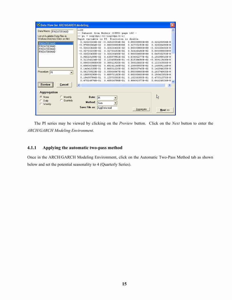
After you click on the ARCH/GARCH Analysis item, it is necessary to select the data to analyze. The Data

View for ARCH/GARCH Modeling dialog box will automatically pop-up and display all SCA data macro files

in the working directory. The wholesale price index data (PI series) is located in the FINDAT01 data macro

file under the PI procedure. Please select this data set as illustrated below.

15

The PI series may be viewed by clicking on the Preview button. Click on the Next button to enter the

ARCH/GARCH Modeling Environment.

4.1.1 Applying the automatic two-pass method

Once in the ARCH/GARCH Modeling Environment, click on the Automatic Two-Pass Method tab as shown

below and set the potential seasonality to 4 (Quarterly Series).

16

By selecting the Show/Create Graphs option, we can later validate if our assumptions are correct by

inspection of various diagnostic graphs.

Click on the Execute button and an expert system approach will be employed to determine the first

moment model and the model for the squared standardized residuals. WorkBench builds a sequence of

commands for the automatic two-pass method that is executed in the SCA System. After the SCA System

determines the appropriate ARIMA model and estimates its parameters based on its IARIMA (expert system

ARIMA modeling) capability, the residuals from the first moment model are stored. The residuals and then

standardized and squared. The IARIMA command is used for a second time to identify an ARIMA model for

the squared standardized residual series. The SCA IARIMA command is quite effective and in most cases

provides an ideal way to proceed.

A portion of the output (first moment model summary) is shown below. The user can scroll through the

output and view full diagnostics for the estimated models, print/save the output, view/edit the command file

used by the SCA engine, or go to the User-directed Two-Pass Method to make modifications to the models

estimated.

17

The table provided below is a summary of the first moment and second moment models that were

automatically identified and estimated for the PI series. For the first moment part of the model, an IMA(1,4)

model was selected with the estimate of 1 0.6178 (t=8.71)=θ and 4 1828 (t=2.05)= −θ . For the second

moment equation, what would be considered an ARCH(4) model was selected.

First Moment Model Summary (Differencing = 1) Parameter Factor Order Value Std.Error t-Value MA 1 1 .6012 .0708 8.49 MA 2 4 -.1828 .0892 -2.05 Second Moment Model Summary Parameter Factor Order Value Std.Error t-Value CNST 1 0 .0001 .00004 3.02 D-AR 1 4 .2131 .0903 2.36 MA 1 1 -.0878 .0885 -.99 MA 2 2 -.1956 .0900 -2.17

Several graphs have been automatically created and may be reviewed by clicking on the Graphs tab, as

shown below. The diagnostic graphs are organized in four sections. The first section provides visual

information about the series analyzed including a time series plot, an autocorrelation plot, and a partial

18

autocorrelation plot. The other sections provide diagnostics for the first moment model and second moment

model.

Note that the two-pass method does not produce standard residuals ( t t tˆ ˆ ˆe a /= σ ) nor does it produce a time plot

of the estimated conditional standard deviation series, Sigma.

4.1.2 Applying the user-directed one-pass method

Enders (1995, page 155) selected an ARIMA(1,0,4) first moment model for the PI series whereas the

automatic ARIMA capability of the SCA System selected a differencing operator instead of an autogressive

term. The equations with parameter estimates presented in Enders’ work is provided below. The standard

errors for the parameter estimates are provided under the coefficients.

1 1 4

21 1

.0013 .7968 .4014 0.2356(.0012) (.1141) (.1585) (.1202)1.5672 5 .2226 .6633(9.34 6) (.1067) (.1515)

− − −

− −

= + + − +

= − + +−

t t t t t

t t t

a a a

h E a hE

π π

19

Since the PI series has already been brought into the ARCH/GARCH Modeling Environment, simply click

on the User-Directed One-Pass Method tab to continue the example. The models can then be defined for the

one-pass method. Since a GARCH model is to be specified, select GARCH under the Model Option frame.

Next, specify the parameters for the first moment and second moment equations as shown below.

The WorkBench program will attempt to determine the number of residuals to drop in the maximum

likelihood estimation based on the maximum autoregressive lag or the expected number of missing residuals.

In some cases, the user must pre-specify the number of beginning residuals to omit in the maximum likelihood

summation when non-linear convergence issues arise. Unfortunately, this is often data driven and therefore

may require some trial and error in deciding the appropriate number of residuals to omit.

To adjust the MAX Lag in ML Sum, click on the Advanced Options/Setting under the View frame and edit

the estimation settings. It is also important to examine the output for warning/error messages that may occur

in estimating the GARCH model. For instance, the messages may indicate that the maximum number of

iterations were exceeded. If you should see messages of this kind, you should increase the default settings. In

the Default Estimation Settings grid, make the changes as follows:

20

Now, to estimate the model and generate various diagnostics, click on the Execute button. When the

SCAB34S engine finishes, you will automatically be placed in the Results tab where you can review the

estimation results. Below is a summary of the GARCH model estimation using the one-pass (joint estimation)

method.

Nonlinear Estimation Summary: GARCH Model ---------------------------------------------------------------------- Number of observations: 129 Number of iterations: 520 Number of Function Evals 530 Number of Gradiant Evals 522 Number of Terms Dropped: 10 Final Functional Value: 487.875 1/Condition of Hessian: 0.26955E-10 AIC (Based on LLF): -1128.63529045 Parameter Order Coefficient Std. Err. t-Value p-Value Comments C1 0 0.00176281 0.00493765 0.36 0.7217 CONS_1 AR 1 0.77451087 0.70309654 1.10 0.2729 AR MA 1 -0.38251331 0.23529208 -1.63 0.1067 MA MA 4 0.25331855 0.13801479 1.84 0.0690 MA C2 0 0.00001426 0.00002692 0.53 0.5974 CONS_2 ARCH 1 0.23291643 0.23712987 0.98 0.3280 GMA GARCH 1 0.66689634 0.29384342 2.27 0.0251 GAR

21

Standardized Error Distn. : Normal Distribution Sum of Squared Residuals : 0.01506806 Volatility of Variance : 0.52111244 Unconditional Variance : 0.00014229 Unconditional Standard Dev: 0.01192857 Diagnostic testing of standardized residuals Number of Cases : 119 Minimum Value : -2.629609 Maximum Value : 4.604357 Mean : 0.083269 Standard Deviation : 1.001289 Skewness : 0.531101 Kurtosis : 2.570206 Cumulant (6th Order): 22.874863 First Quartile : -0.529092 Third Quartile : 0.592427 Sample ACF and PACF for Standardized Residuals ---------------------------------------------------------------- Lag ACF t-Val LB-Q P-Value PACF t-Val 1 0.011 0.12 0.01 0.903 0.011 0.12 2 -0.039 -0.43 0.20 0.903 -0.039 -0.43 3 0.040 0.43 0.40 0.940 0.041 0.44 4 0.084 0.91 1.28 0.864 0.082 0.89 5 -0.146 -1.57 3.97 0.554 -0.146 -1.58 Diagnostic testing of Squared standardized residuals Sample ACF and PACF for Squared Standardized Residuals ---------------------------------------------------------------- Lag ACF t-Val LB-Q P-Value PACF t-Val 1 0.000 0.00 0.00 0.999 0.000 0.00 2 -0.022 -0.24 0.06 0.970 -0.022 -0.24 3 -0.021 -0.23 0.12 0.990 -0.021 -0.23 4 0.179 1.95 4.12 0.390 0.178 1.94 5 -0.027 -0.28 4.21 0.520 -0.029 -0.31 LaGrange Multiplier Tests Variable: Squared Standardized Residuals ---------------------------------------- Lag LM-Value P-Value 1 0.000 0.999 2 0.058 0.972 3 0.116 0.990 4 3.803 0.433 5 3.822 0.575

The results are comparable between the above output and Ender’s estimation results. Slight differences

are acceptable due to non-linear estimation settings and optimization algorithms.

Of some concern is the computational method to arrive at the appropriate standard errors for the model

parameters. The B34S CMAXF2 calculates the standard error of the parameters as the square root of the

absolute value of the diagonal elements of the inverse of the Hessian as calculated by the IMSL routine

22

DBONF. The SE calculation is susceptible to differences in the computational algorithm used to solve the

model. IMSL reports that their Hessian is a BFGS approximation of the Hessian at the solution.

4.2 GARCH Analysis of the S&P 500 Using the One-Pass Method

This example uses the monthly excess returns of the S&P 500 index from 1926-1999 to illustrate a

GARCH(1,1) model specification and estimation. This example was also used in Tsay (2002), Analysis of

Financial Time Series: Example 3.3 – page 97.

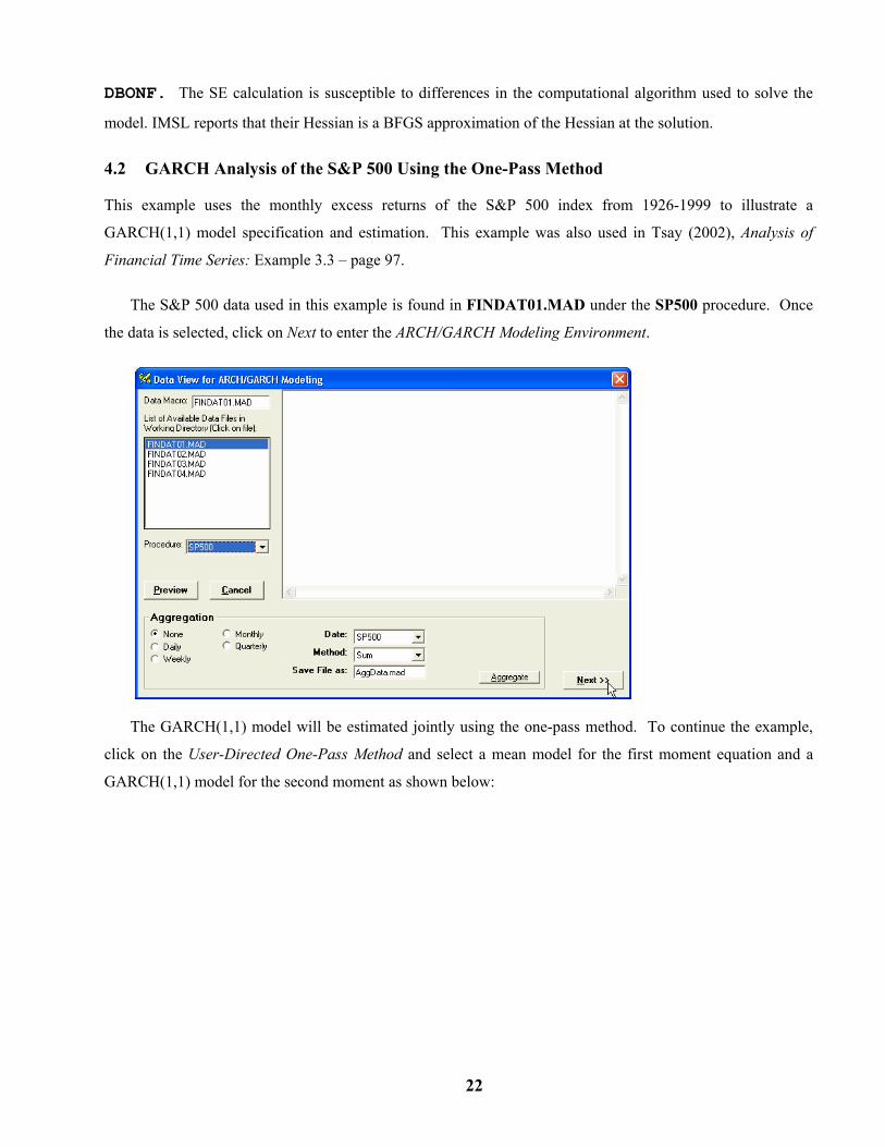
The S&P 500 data used in this example is found in FINDAT01.MAD under the SP500 procedure. Once

the data is selected, click on Next to enter the ARCH/GARCH Modeling Environment.

The GARCH(1,1) model will be estimated jointly using the one-pass method. To continue the example,

click on the User-Directed One-Pass Method and select a mean model for the first moment equation and a

GARCH(1,1) model for the second moment as shown below:

23

In his example, Tsay deletes the first four residuals. To do this in WorkBench, go to the Advanced

Options/Settings view area, and modify the value for the Max Lag in ML Sum under the Default Estimation

Settings grid. The modified setting is shown below:

24

Now, click on the Next button to estimate the model. You may also select the Show/Create Graphs option

for more detailed diagnostics. Once the SCAB34S engine finishes, you will be placed in the Results tab where

you may review the model summary and associated diagnostics. A portion of the output is shown below:

Nonlinear Estimation Summary: GARCH Model ---------------------------------------------------------------------- Number of observations: 792 Number of iterations: 36 Number of Function Evals 51 Number of Gradiant Evals 38 Number of Terms Dropped: 4 Final Functional Value: 1988.600 1/Condition of Hessian: 0.00000025 AIC (Based on LLF): -4486.18247426 Parameter Order Coefficient Std. Err. t-Value p-Value Comments C1 0 0.00766466 0.00151899 5.05 0.0000 CONS_1 C2 0 0.00007859 0.00002594 3.03 0.0025 CONS_2 ARCH 1 0.11846988 0.01860770 6.37 0.0000 GMA GARCH 1 0.85863535 0.01914510 44.85 0.0000 GAR Standardized Error Distn. : Normal Distribution Sum of Squared Residuals : 2.69744855 Volatility of Variance : 0.21642254 Unconditional Variance : 0.00343248 Unconditional Standard Dev: 0.05858735

25

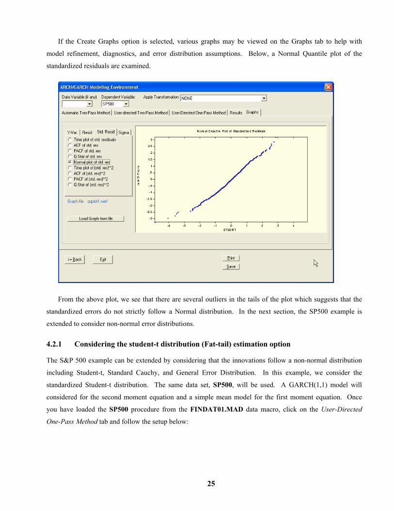
If the Create Graphs option is selected, various graphs may be viewed on the Graphs tab to help with

model refinement, diagnostics, and error distribution assumptions. Below, a Normal Quantile plot of the

standardized residuals are examined.

From the above plot, we see that there are several outliers in the tails of the plot which suggests that the

standardized errors do not strictly follow a Normal distribution. In the next section, the SP500 example is

extended to consider non-normal error distributions.

4.2.1 Considering the student-t distribution (Fat-tail) estimation option

The S&P 500 example can be extended by considering that the innovations follow a non-normal distribution

including Student-t, Standard Cauchy, and General Error Distribution. In this example, we consider the

standardized Student-t distribution. The same data set, SP500, will be used. A GARCH(1,1) model will

considered for the second moment equation and a simple mean model for the first moment equation. Once

you have loaded the SP500 procedure from the FINDAT01.MAD data macro, click on the User-Directed

One-Pass Method tab and follow the setup below:

26

Next, more iterations will be needed to satisfy the convergence criteria. After you have specified the

model above, click on the Advanced Options/Settings view area and make the following modifications to the

Default Estimation Settings grid.

To estimate the GARCH(1,1) model under the assumption that the innovations follow a standardized

Student-t distribution, click on the Execute button. The model estimates and diagnostics will be displayed in

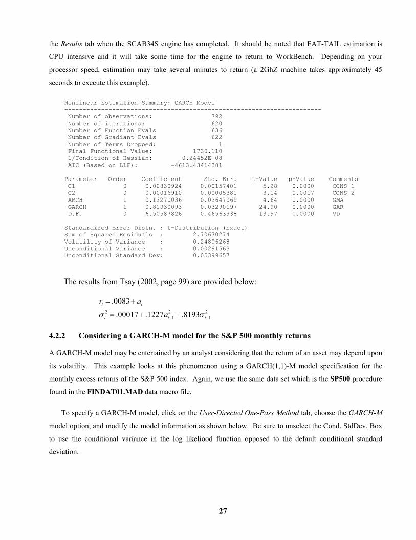
27

the Results tab when the SCAB34S engine has completed. It should be noted that FAT-TAIL estimation is

CPU intensive and it will take some time for the engine to return to WorkBench. Depending on your

processor speed, estimation may take several minutes to return (a 2GhZ machine takes approximately 45

seconds to execute this example).

Nonlinear Estimation Summary: GARCH Model ---------------------------------------------------------------------- Number of observations: 792 Number of iterations: 620 Number of Function Evals 636 Number of Gradiant Evals 622 Number of Terms Dropped: 1 Final Functional Value: 1730.110 1/Condition of Hessian: 0.24452E-08 AIC (Based on LLF): -4613.43414381 Parameter Order Coefficient Std. Err. t-Value p-Value Comments C1 0 0.00830924 0.00157401 5.28 0.0000 CONS_1 C2 0 0.00016910 0.00005381 3.14 0.0017 CONS_2 ARCH 1 0.12270036 0.02647065 4.64 0.0000 GMA GARCH 1 0.81930093 0.03290197 24.90 0.0000 GAR D.F. 0 6.50587826 0.46563938 13.97 0.0000 VD Standardized Error Distn. : t-Distribution (Exact) Sum of Squared Residuals : 2.70670274 Volatility of Variance : 0.24806268 Unconditional Variance : 0.00291563 Unconditional Standard Dev: 0.05399657

The results from Tsay (2002, page 99) are provided below:

2 2 21 1

.0083

.00017 .1227 .8193− −

= +

= + +t t

t t t

r a

aσ σ

4.2.2 Considering a GARCH-M model for the S&P 500 monthly returns

A GARCH-M model may be entertained by an analyst considering that the return of an asset may depend upon

its volatility. This example looks at this phenomenon using a GARCH(1,1)-M model specification for the

monthly excess returns of the S&P 500 index. Again, we use the same data set which is the SP500 procedure

found in the FINDAT01.MAD data macro file.

To specify a GARCH-M model, click on the User-Directed One-Pass Method tab, choose the GARCH-M

model option, and modify the model information as shown below. Be sure to unselect the Cond. StdDev. Box

to use the conditional variance in the log likeliood function opposed to the default conditional standard

deviation.

28

To estimate the GARCH-M model, click on the Execute button. As with the FAT-TAIL option, a

GARCH-M model is CPU intensive and will take some time to complete. This example took approximately

25 seconds on a 2Ghz. Computer. The results are presented below:

Nonlinear Estimation Summary: GARCH-M Model ---------------------------------------------------------------------- Number of observations: 792 Number of iterations: 353 Number of Function Evals 371 Number of Gradiant Evals 355 Number of Terms Dropped: 1 Final Functional Value: 1989.142 1/Condition of Hessian: 0.39470E-09 AIC (Based on LLF): -4547.26382905 Parameter Order Coefficient Std. Err. t-Value p-Value Comments C1 0 0.00259727 0.00223813 1.16 0.2462 CONS_1 Delta 0 1.97279196 0.82937374 2.38 0.0176 MU C2 0 0.00013680 0.00003287 4.16 0.0000 CONS_2 ARCH 1 0.13495986 0.02066926 6.53 0.0000 GMA GARCH 1 0.82188077 0.02125851 38.66 0.0000 GAR Standardized Error Distn. : Normal Distribution Sum of Squared Residuals : 2.72436841 Volatility of Variance : 0.25972847 Unconditional Variance : 0.00316969 Unconditional Standard Dev: 0.05630001

The results from Tsay (2002, page 101) are provided below:

29

2

2 2 21 1

.0028 1.99

.00016 .1328 .8137− −

= + +

= + +t t t

t t t

r a

a

σ

σ σ

4.3 Regression plus GARCH Models Using IBM returns and S&P 500 Series

It is often of interest to examine the behavior of a series based on its relationship to leading indicators or other

stochastic variables. The examples in this section illustrate how to incorporate regression variables in the first

moment model while entertaining a GARCH process in the second moment model. The excess monthly

returns of the IBM stock price is modeled as a function of the S&P 500 index in the first moment model.

4.3.1 Modeling IBM stock returns and the S&P 500 index using the automatic two-pass method

The data for this example is found in the FINDAT01.MAD data macro file under the M_IBMLN2 procedure

name. Once the M_IBMLN2 procedure is selected for the ARCH/GARCH Analysis application, click on the

Automatic Two-Pass Method tab.

The IBMLN series is the monthly returns of the IBM stock price from January 1926 through December

1991. It is contended that the S&P 500 monthly returns is related to the IBM stock price, however we are not

certain at what lags this potential relationship exists. One method that can be used to examine the lag

relationship between the IBMLN and SPLN series is to employ the automatic model identification capabilities

of the SCA System via the automatic two-pass method.

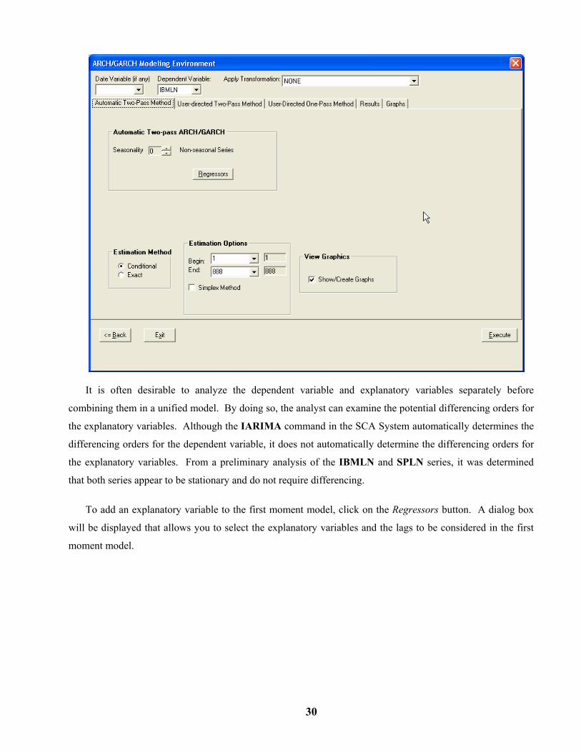
The IBMLN monthly series does not exhibit a seasonal behavior, therefore in the Automatic Two-Pass

Method tab, the series is marked as non-seasonal. If the user is unsure whether seasonality is present, the

dependent series can be marked as a monthly series and the SCA System will consider seasonal terms in the

model. If the seasonal parameters are not significant, the automatic modeling procedure will not include them.

30

It is often desirable to analyze the dependent variable and explanatory variables separately before

combining them in a unified model. By doing so, the analyst can examine the potential differencing orders for

the explanatory variables. Although the IARIMA command in the SCA System automatically determines the

differencing orders for the dependent variable, it does not automatically determine the differencing orders for

the explanatory variables. From a preliminary analysis of the IBMLN and SPLN series, it was determined

that both series appear to be stationary and do not require differencing.

To add an explanatory variable to the first moment model, click on the Regressors button. A dialog box

will be displayed that allows you to select the explanatory variables and the lags to be considered in the first

moment model.

31

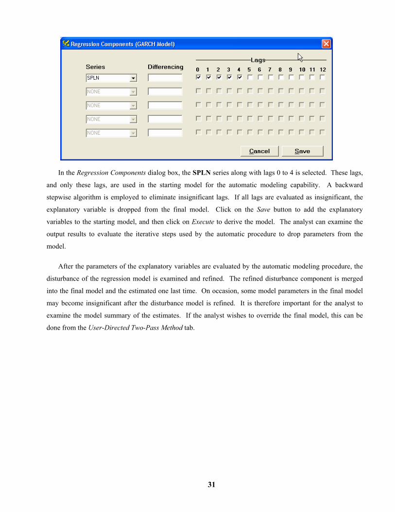
In the Regression Components dialog box, the SPLN series along with lags 0 to 4 is selected. These lags,

and only these lags, are used in the starting model for the automatic modeling capability. A backward

stepwise algorithm is employed to eliminate insignificant lags. If all lags are evaluated as insignificant, the

explanatory variable is dropped from the final model. Click on the Save button to add the explanatory

variables to the starting model, and then click on Execute to derive the model. The analyst can examine the

output results to evaluate the iterative steps used by the automatic procedure to drop parameters from the

model.

After the parameters of the explanatory variables are evaluated by the automatic modeling procedure, the

disturbance of the regression model is examined and refined. The refined disturbance component is merged

into the final model and the estimated one last time. On occasion, some model parameters in the final model

may become insignificant after the disturbance model is refined. It is therefore important for the analyst to

examine the model summary of the estimates. If the analyst wishes to override the final model, this can be

done from the User-Directed Two-Pass Method tab.

32

The final model identified by the automatic two-pass method is displayed in the Results tab. Here, lags 0, 1,

and 2 are retained in the final model. Lags 3 and 4 were deleted. A summary of the parameter estimates for

the first moment and second moment equations is presented below.

First Moment Model Summary (No differencing) Parameter Factor Order Value Std.Error t-Value CNST 1 0 .8384 .1758 4.77 SPLN-0 1 0 0.7517 .0309 24.35 SPLN-1 1 1 0.0684 .0310 2.21 SPLN-2 1 2 -.0646 .0309 -2.09 Second Moment Model Summary Parameter Factor Order Value Std.Error t-Value CNST 1 0 26.7360 1.9848 13.47

33

4.3.2 Modeling IBM stock returns and the S&P 500 index using the user-directed one-pass method

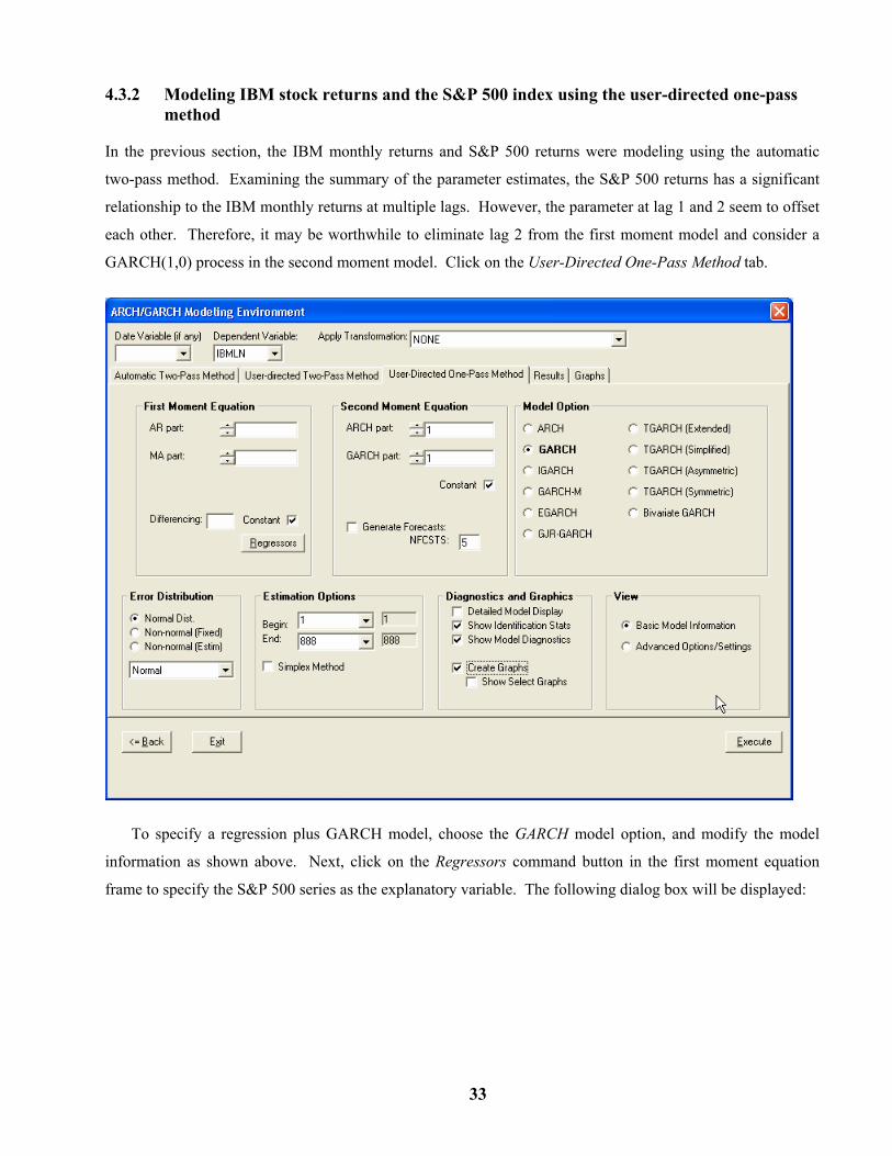
In the previous section, the IBM monthly returns and S&P 500 returns were modeling using the automatic

two-pass method. Examining the summary of the parameter estimates, the S&P 500 returns has a significant

relationship to the IBM monthly returns at multiple lags. However, the parameter at lag 1 and 2 seem to offset

each other. Therefore, it may be worthwhile to eliminate lag 2 from the first moment model and consider a

GARCH(1,0) process in the second moment model. Click on the User-Directed One-Pass Method tab.

To specify a regression plus GARCH model, choose the GARCH model option, and modify the model

information as shown above. Next, click on the Regressors command button in the first moment equation

frame to specify the S&P 500 series as the explanatory variable. The following dialog box will be displayed:

34

Using the dropdown box, select the SPLN series and put checks in the lag 0 box only as shown. To add

the regression component to the first moment equation, click on the Save button. You may add/delete/modify

regression components in the model through this dialog box.

For this example, the default starting values and parameter constraints are fine. The starting values for the

regression parameters are automatically derived using OLS estimation. The starting values and parameter

constraints can be modified by selecting the Advanced Options/Settings option in the View frame. Once the

first moment and second moment equations are specified, click on the Execute button to estimate the model

and generate the model diagnostics. The results are provided below:

Nonlinear Estimation Summary: GARCH Model ---------------------------------------------------------------------- Number of observations: 888 Number of iterations: 32 Number of Function Evals 48 Number of Gradiant Evals 34 Number of Terms Dropped: 1 Final Functional Value: -1888.006 1/Condition of Hessian: 0.00032559 AIC (Based on LLF): 2966.49672120 Parameter Order Coefficient Std. Err. t-Value p-Value Comments C1 0 0.87664543 0.16913978 5.18 0.0000 CONS_1 SPLN 0 0.75020949 0.03100246 24.20 0.0000 INPUT 1 C2 0 2.73574407 0.33594045 8.14 0.0000 CONS_2 ARCH 1 0.07452358 0.01355494 5.50 0.0000 GMA GARCH 1 0.82749572 0.01487442 55.63 0.0000 GAR Standardized Error Distn. : Normal Distribution Sum of Squared Residuals : 23923.58681429 Volatility of Variance : 0.15418985 Unconditional Variance : 27.92125424 Unconditional Standard Dev: 5.28405661

35

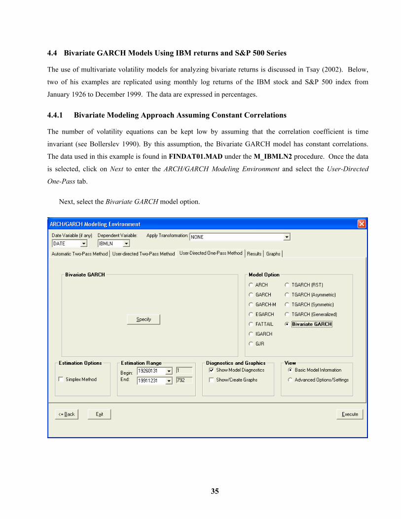
4.4 Bivariate GARCH Models Using IBM returns and S&P 500 Series

The use of multivariate volatility models for analyzing bivariate returns is discussed in Tsay (2002). Below,

two of his examples are replicated using monthly log returns of the IBM stock and S&P 500 index from

January 1926 to December 1999. The data are expressed in percentages.

4.4.1 Bivariate Modeling Approach Assuming Constant Correlations

The number of volatility equations can be kept low by assuming that the correlation coefficient is time

invariant (see Bollerslev 1990). By this assumption, the Bivariate GARCH model has constant correlations.

The data used in this example is found in FINDAT01.MAD under the M_IBMLN2 procedure. Once the data

is selected, click on Next to enter the ARCH/GARCH Modeling Environment and select the User-Directed

One-Pass tab.

Next, select the Bivariate GARCH model option.

36

Click on the Specify button to expose the dialog box to build a Bivariate GARCH model. That dialog box

is slightly more complicated than the univariate GARCH model specification since it involves two equations

for both the first moment and second moment.

Above, Series #1 is set to the IBM monthly returns (IBMLN) and Series #2 is set to the S&P 500 index.

As in the univariate GARCH case, the orders of the parameter are specified in the text boxes provided. Here, a

multivariate GARCH(1,1) model is specified with constant correlations. After the Bivariate GARCH model is

specified, click on Save and you will be returned to the GARCH modeling environment.

Now, select the Advanced Options/Settings option and overwrite the Maxlag in ML Sum so that it equals 3.

The default starting values and constraints will be used.

37

Now, click on Execute to estimate the Bivariate GARCH model. It may take a few minutes to complete

since these types of models are computationally intensive. When estimation has completed, you will be placed

in the Output viewer. The complete output provides diagnostic statistics for both model identification and for

evaluating the fit of the model employed. A portion of the output is displayed below.

38

The SCAB34S GARCH program constrains the ARCH/GARCH parameters to be positive during

estimation since the parameters have a theoretical lower bound of zero. The final functional value obtained

here (3698.99) differs slightly from the RATS results (3691.21) stated in Tsay for this reason. If desired, you

may override the lower bounds of the GAR12_1, GAR21_1 and GMA21_1 model parameters using the

Advanced Options/Settings option. Please note however that you will then allow those model parameters to

enter the inadmissible zone and possibly make the estimation unstable.

First Moment Model Summary (No differencing): Series #1 Parameter Factor Order Value Std.Error t-Value CNST1_1 1 0 1.28139 .20015 6.40 AR11_1 1 1 .072210 .02459 2.94 AR11_2 1 2 .051038 .034804 1.47 AR12_2 1 2 -0.11419 .043722 -2.61 First Moment Model Summary (No differencing): Series #2 CNST1_2 1 0 .68502 .14645 4.68 Second Moment Model Summary: Series #1 Parameter Factor Order Value Std.Error t-Value CNST1_3 1 0 3.2582 .631996 5.16 GMA11_1 1 1 .082307 .0079985 10.29

39

GAR11_1 1 1 .841529 .0079779 105.48 GAR12_1 1 1 0.00 .01182 0.00 Second Moment Model Summary: Series #2 CNST1_4 1 0 .793620 .24928 3.18 GMA21_1 1 1 0.00 .005846 0.00 GMA22_1 1 1 .079812 .017067 4.67 GAR21_1 1 1 0.00 .027117 0.00 GAR22_1 1 1 .8894 .016578 53.65 Constant Correlation Rho 1 1 .60165 .022304 26.97

4.4.2 Bivariate Modeling Approach Assuming Time-varying Correlations

When studying the relationship of two or more assets over an elongated time period, the correlation coefficient

of a multivariate GARCH model may not be constant. This especially true for this example where the

S&P500 index is a weighted average of various stocks. The composition of the index may change over time as

may the individual weighting of the stocks.

To continue the example from the previous section, once again select the M_IBMLN2 from the

FINDAT01.MAD file.

Next, select the Bivariate GARCH model option under the User-Directed One-Pass Method tab and modify

the model as shown:

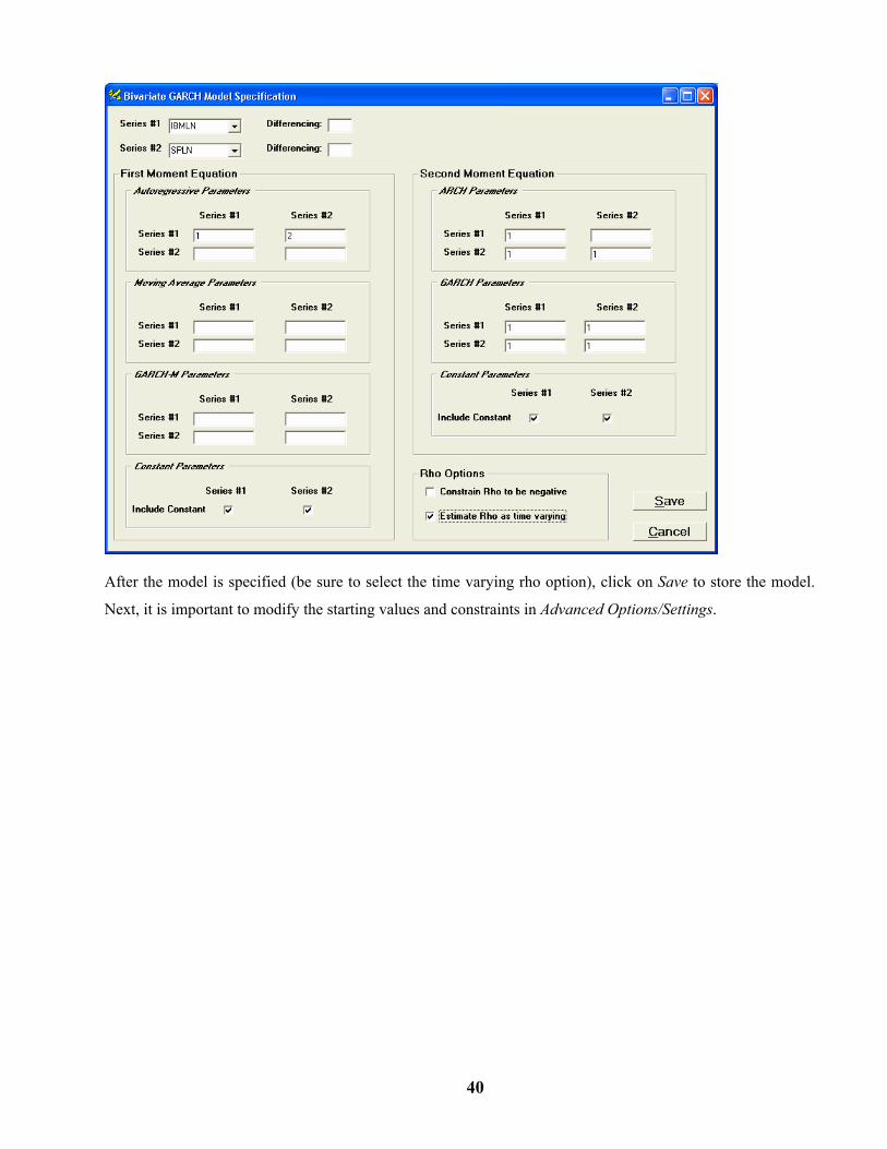
40

After the model is specified (be sure to select the time varying rho option), click on Save to store the model.

Next, it is important to modify the starting values and constraints in Advanced Options/Settings.

41

The starting values of most model parameters need to be changed for estimation purposes. As in the

previous example, the Max Lag in ML Sum value should be set equal to 3. The above form does not show all

parameter starting values and constraints. Therefore, the settings used in this example are provided below for

reference.

Parameter Label LCL UCL Initial Value

AR11_1 -100000.0 100000.0 .08

AR12_2 -100000.0 100000.0 -.07

GAR11_1 0.0 100000.0 .87

GAR12_1 0.0 100000.0 .01

GAR21_1 0.0 100000.0 .01

GAR22_1 0.0 100000.0 .92

GMA11_1 0.0 100000.0 .08

GMA21_1 0.0 100000.0 .04

42

GMA22_1 0.0 100000.0 .05

CNST1_1 -100000.0 100000.0 1.4

CNST1_2 -100000.0 100000.0 0.7

CNST_2_1 -100000.0 100000.0 2.95

CNST2_2 -100000.0 100000.0 2.05

Rho_1 -100000.0 100000.0 -2.0

Rho_2 0.0 100000.0 3.0

Rho_3 0.0 100000.0 0.1

The starting values of Bivariate GARCH models influence estimation greatly. If you employ the time-varying GARCH option, it is recommended that you first estimate the Bivariate GARCH model with constant correlations, and then use those estimates as starting values for the more complex time-varying correlation model.

After setting the initial values for the model parameters, click on Execute to estimate the model. It will

take a minute or two to estimate this model. When it has completed, the output window will be displayed.

43

In reviewing the estimated results, we note that the functional value is (3685.44) which is better than the

constant correlation model (3698.99). We also note that the estimated coefficients of GAR12_1, GAR21_1,

and GMA21_1 are zero. Tsay (2002) allows these parameters to be negative in his example. You may modify

the starting values and lower bounds of these parameters if you wish to replicate the results in Tsay. However,

in general, it is not recommended unless there is valid reasons to allow these parameters to overstep its

theoretical limits.

First Moment Model Summary (No differencing): Series #1 Parameter Factor Order Value Std.Error t-Value CNST1_1 1 0 1.30938 .20899 6.27 AR11_1 1 1 .070150 .027758 2.53 AR12_2 1 2 -0.69000 .031585 -2.18 First Moment Model Summary (No differencing): Series #2 CNST1_2 1 0 .671625 .142150 4.72 Second Moment Model Summary: Series #1 Parameter Factor Order Value Std.Error t-Value CNST1_3 1 0 3.95296 .59568 6.64 GMA11_1 1 1 .100807 .0021885 4.61 GAR11_1 1 1 .80876 .044682 18.10 GAR12_1 1 1 0.00 .044206 0.00

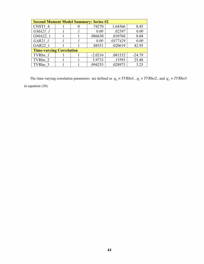
44

Second Moment Model Summary: Series #2 CNST1_4 1 0 .74270 1.64366 0.45 GMA21_1 1 1 0.00 .02597 0.00 GMA22_1 1 1 .086630 .010768 8.04 GAR21_1 1 1 0.00 .0377429 0.00 GAR22_1 1 1 .88551 .020619 42.95 Time-varying Correlation TVRho_1 1 1 -2.0216 .081532 -24.79 TVRho_2 1 1 3.9733 .15593 25.48 TVRho_3 1 1 .094253 .028973 3.25

The time-varying correlation parameters are defined as 0 1q TVRho≡ , 1 2q TVRho≡ , and 2 3q TVRho≡

in equation (30).

45

5 A DETAILED DESCRIPTION OF THE GARCH APPLICATION INTERFACE IN WORKBENCH

SCA WorkBench provides a graphical user interface to the SCA Statistical System, and the SCAB34S Applet

Collection or the B34S ProSeries Econometric System for advanced ARCH and GARCH modeling. Below is

a summary of the forms of ARCH/GARCH models that may be specified through the SCA WorkBench

interface

Two-pass Estimation Method:

Model Form Estimation Source ARCH SCA System (EXPERT) GARCH(*) SCA System (EXPERT)

(*) A GARCH model estimated using the two-pass method is not directly comparable to a GARCH model

estimated using the one-pass (joint) method.

One-pass Estimation Method:

Model Form Estimation Source ARCH SCAB34S Applet Collection (GARCH) or B34S ProSeries GARCH SCAB34S Applet Collection (GARCH) or B34S ProSeries GARCH-M SCAB34S Applet Collection (GARCH) or B34S ProSeries GARCH (Integrated) SCAB34S Applet Collection (GARCH) or B34S ProSeries GARCH (non-normal dist) SCAB34S Applet Collection (GARCH) or B34S ProSeries GARCH (Glosten) SCAB34S Applet Collection (GARCH) or B34S ProSeries GARCH (Exponential) SCAB34S Applet Collection (GARCH) or B34S ProSeries GARCH (Threshold) SCAB34S Applet Collection (GARCH) or B34S ProSeries GARCH (Bivariate) SCAB34S Applet Collection (GARCH) or B34S ProSeries

5.1 Data View for ARCH/GARCH Modeling When you enter the ARCH/GARCH Modeling environment, you must select an SCA data macro (*.MAD) as

a data source. If your data is organized in plain ASCII format, WorkBench will automatically convert it into a

temporary SCA data macro. The temporary file is then accessible from the file list box. To view files with

extensions other than MAD, type the pattern you want to view in the data macro text box. For example, all

DAT files in the working directory can be viewed by typing “*.DAT” in the data macro text box. Once you

select an ASCII data file from the list box, WorkBench will detect that and prompt you as to whether you

would like to create a temporary SCA data macro.

The following dialog box is displayed when you select the ARCH/GARCH Analysis item from the Apps

menu in WorkBench. Here, the “findat01” data macro is selected and its content previewed.

46

This dialog box also provides a utility to aggregate your original data based on a “Date” variable. You

may select various aggregation methods such as sum, mean, median, maximum, minimum, opening price, and

closing price. If you aggregate your data, please be sure to set your Date variable in the dropdown list, specify

the method of aggregation, and provide a name for the new SCA Data Macro that the aggregation results are

saved.

Note that large SCA data macro files may not be fully displayed in the preview area. If the file reaches a certain size, only the comment lines (those lines beginning with “C ” or “—“) are displayed in the preview area. Although complete information may not be displayed, there is no limit to the number of observations in a series analyzed through the ARCH/GARCH environment. Some of the testing data files provided for the GARCH capability contain more than 100,000 observations.

47

The features for the Data Viewer and Selector are summarized below.

Menu Item Description Data Macro This text box allows you to set a filter for the files you want to view

in your working directory. By default, the filter exposes all files with the extension *.mad in your working directory. When you select a file by clicking a file name in the list, that file will be displayed in the Data Macro text box. If your data is in plain ASCII format, WorkBench automatically converts it to an SCA Data Macro with a temporary name. You can then use the temporary SCA data macro to proceed with the ARCH/GARCH Modeling Environment. Simply type the name of your plain ASCII data file in the text box to activate this feature.

List of Available Data Files …

Provides a list of SCA data macro files. You must select a data macro file in order to continue in the ARCH/GARCH modeling environment.

Procedure If your data macro file contains more than one data procedure,

select the appropriate procedure from this drop-down list. Preview Click on the Preview button to view the content of your data file.

Please note that the view box is limited to 64k bytes. In the event your data file exceeds 64k bytes, only a portion of the file will be displayed or only the comment lines in the file will be displayed. This will not cause your data file to be truncated when using the ARCH/GARCH modeling environment. Some testing SCA data macros are over 100,000 observations.

Aggregation You may elect to aggregate your original time series into daily,

weekly, monthly, or quarterly time intervals. A DATE variable must be present in the SCA data macro. It must be in the form YYYYMMDD. If you generated an SCA data macro from a spreadsheet task, WorkBench automatically converts date variables into the YYYYMMDD format.

Method If you aggregate your data series, you must also specify the

method of aggregation you wish to apply from the Method dropdown list. Aggregation methods available are sum, mean, median, maximum, minimum, opening price, and closing price

Save File As If you aggregate your data series, specify the name of the SCA

Data Macro you wish to have the results saved here. The default name is AggData.MAD.

Cancel Exits the ARCH/GARCH Data Viewer. Next After selecting the SCA data macro file and procedure, click on the

Next button to proceed.

48

5.2 ARCH/GARCH Modeling Environment The ARCH/GARCH Modeling Environment contains five tabbed sections. These tabbed sections are:

Automatic Two-Pass Method

– interfaces to the SCA System

User-directed Two-Pass Method – interfaces to the SCA System

User-directed One-Pass Method – interfaces to the SCAB34S GARCH and B34S ProSeries products

Results – displays output files, input commands, and error logs

Graphs – displays various diagnostic graphs (requires SCAB34S or B34S ProSeries products)

49

5.2.1 Automatic two-pass method

This tab allows you to explore whether your data exhibits ARCH/GARCH tendencies using a “quick”

approach. The automatic two-pass method interfaces to the expert system capabilities of the SCA System

(IARIMA) to identify an appropriate Box-Jenkins ARIMA model for the first moment model (dependent

variable) and the squared standardized residuals from the estimated first moment model.

The features of the Automatic Two-Pass method tab are presented below.

Menu Item Description

Date Variable Use this drop-down list to specify the date variable associated with your series. If your SCA Data Macro contains a variable named "DATE", it is automatically assigned by SCA WorkBench. If you have an alternative index variable or date variable, you may select it from the drop-down list. If your SCA Data Macro does not contain a DATE variable, leave the dropdown list empty. WorkBench will then use the observation number as a date index. If your time series is more than 10,000 observations, WorkBench will not use your DATE variable for indexing. Instead, observation number will be used.

50

Dependent Variable

Use this drop-down list to specify the time series that you wish to analyze.

Regressors Click on the Regressors command button to select explanatory variables

to be used in the first moment equation. The regression variables selected in the Regressors dialog box are used in all models (one-pass and two-pass tabs) until the user removes them from the model. It is important to note that the regression variables are their associated lags are used as the starting model for the automatic two-pass modeling method. A backward stepwise algorithm is used to delete insignificant variables and parameters from the model.

Seasonality Specify the potential seasonality of the time series you are analyzing. For

example, if you are analyzing monthly data, set seasonality =12. If you do not specify seasonality, and seasonal patterns exist in your data, the expert system capabilities of the SCA System (IARIMA) may not identify an optimal first moment model.

Estimation method

Use the radio button controls to select the estimation method for Box-Jenkins ARIMA model estimation. The default method is conditional estimation. You may consider using the exact method when the first moment model contains moving average parameters.

Estimation Range

By default, all available data will be used to identify and estimate time series models for the first moment and second moment equations. If you need to select a specific range of data to analyze, you can do so by using the beginning and ending estimation range controls. If your series contains fewer than 10,000 observations, all dates (or observation numbers) will be shown in the dropdown list. If your series contains 10,000 observations or more, you will receive a message indicating that memory is being conserved and short indexing is being used. In this case, only the beginning and ending observation number is provided in the dropdown list. To modify the estimation range, type the range in the dropdown list.

View Graphics If you purchased the SCAB34S Applet Collection, you can generate high-

resolution graphics plots of the original series, residuals, and squared residuals. The graphics plots will be displayed on the screen in an interactive manner until all plots have been created. You must press the Enter-button on your keyboard or click on the graph to step through the graphics tasks. The graphs are also saved in your working directory as Windows Meta Files (*.wmf). You may view these files after they have been created in the Graphs tab.

Back Depending on the tab you are currently working in, clicking on the Back

button will move you one tab to the left. If you are in the left-most tab, Automatic Two-Pass Method tab, you will exit into the ARCH/GARCH Data Viewer dialog box. There, you may choose a new SCA data macro and re-enter the ARCH/GARCH Modeling Environment, or leave the ARCH/GARCH Modeling Environment entirely.

Exit Exits the ARCH/GARCH modeling environment.

51

Execute Executes an automatic two-pass ARCH/GARCH analysis. When completed, you will be automatically positioned in the Results tab.

The actual analyses and modeling tasks are performed in the SCA Statistical System. WorkBench

automatically generates a command file (analysis macro) for the SCA System based on your menu choices.

When you click on Execute, an analysis macro, named GARCH.MAC, is automatically submitted to the SCA

Statistical System. The results are returned to WorkBench for display. This GARCH.MAC file may also be

executed from the System -> Run SCA with Macro menu once it is created from the ARCH/GARCH modeling

environment. However, you may wish to save it under a new name to preserve it for future use. The

GARCH.MAC file is a temporary file used in the ARCH/GARCH modeling environment. It is overwritten by

WorkBench each time a model is executed. An example of the GARCH.MAC analysis macro generated for

the SCA System is presented below:

Regression Components

The Regression Components dialog box is displayed when the user clicks on the Regressors button. It is often

of interest to examine the behavior of a series based on its relationship to leading indicators or other stochastic

variables. The Regression Components dialog box provides a facility for the user to incorporate regression

variables in the first moment model while entertaining a GARCH process in the second moment model.

==ALLMACRO ASSIGN FILE 12. EXTERNAL 'findat01.mad'. CALL D_AA. FILE IS 12. CALL ANALYSIS RETURN ==ANALYSIS SELECT D_AA. SPAN IS (1,2528). IDEN D_AA. IARIMA D_AA. NAME IS MOMENT1. @ HOLD RESID(RES). ACF RES. RES2=RES**2 IDEN RES2. IARIMA RES2. NAME MOMENT2 RETURN

52

The above dialog box is used to add/delete/modify the explanatory variables in the first moment model for

the Automatic Two-Pass Method, User-Directed Two-Pass Method, and User-Directed One-Pass Method tabs.

Since the Regression Components dialog box is a shared among the various methods, the regressor variables

will remain in all models until overwritten by the user.

The explanatory variables and their associated lags specified in the Regression Components dialog box are

used in the starting model under the automatic two-pass method. A backward step-wise algorithm is used to

delete insignificant terms from the model. Regression coefficients that are not specified in the starting model

are not considered in the automatic two-pass method.

For the user-directed methods, the explanatory variables and their associated lags are controlled by the

user. If a regression coefficient is not significant, it will remain in the model.

53

5.2.2 User-directed two-pass method

This tab provides a graphical user interface that you can use to manually specify Box-Jenkins ARIMA models

for both the first moment model and the squared standardized residuals from the first moment estimation. The

SCA System is used to estimate the models based on the two-pass method.

If you use this tab, you typically need to graph the series being modeled and perform some preliminary

identification procedures. It is recommended that you use the Graph -> Run SCAGRAF with Data menu to

plot the series against time, and inspect the ACF and PACF plots for identification purposes.

After you specify a model for the first moment model, click on the Execute button to estimate the model

and generate diagnostic information for the first moment model. The residuals from the first moment model

are automatically standardized and squared. The ACF and PACF plots for the squared standardized residuals

are provided in the output. Based on this information, you may specify the second moment model. If you

have purchased the SCAB34S Applet Collection, you may also automatically generate various presentation

quality graphics and diagnostics by selecting the Show/Create Graphs checkbox.

Menu Item Description

Date Variable Use this drop-down list to specify the date variable associated with your series. If your SCA Data Macro contains a variable named "DATE", it is

54

automatically assigned by SCA WorkBench. If you have an alternative index variable or date variable, you may select it from the drop-down list. If your SCA Data Macro does not contain a DATE variable, leave the dropdown list empty. WorkBench will then use the observation number as a date index. If your time series is more than 10,000 observations, WorkBench will not use your DATE variable for indexing. Instead, observation number will be used.

Dependent Variable

Use this drop-down list to specify the time series that you wish to analyze.

Regressors Click on the Regressors command button to select explanatory variables

to be used in the first moment equation. The regression variables selected in the Regressors dialog box are used in all models (one-pass and two-pass tabs) until the user removes them from the model. Unlike the automatic two-pass method, the user-defined two-pass modeling method does not drop insignificant variables or lags from the model.

First Moment Equation

This frame organizes various controls that you may use to specify a Box-Jenkins ARIMA model for the first moment equation.

Second Moment Equation

This frame organizes various controls that you may use to specify a Box-Jenkins ARIMA model for the second moment equation.

Estimation Method

Use the radio button controls to select the estimation method for Box-Jenkins ARIMA model estimation. The default method is conditional. You may consider using the exact method when you first moment model contains moving average parameters.

Estimation Range

By default, all available data will be used to identify and estimate time series models for the first moment and second moment equations. You may reduce the range of your data by using the beginning and ending estimation range controls. If your series contains fewer than 10,000 observations, all dates (or observation numbers) will be shown in the dropdown list. If your series contains 10,000 observations or more, you will receive a message indicating that memory is being conserved and short indexing is being used. In this case, only the beginning and ending observation number is provided in the dropdown list. To modify the estimation range, type the range in the dropdown list.

View Graphics If you purchased the SCAB34S Applet Collection, you can generate high-

resolution graphics plots of the original series, residuals, and squared residuals. The graphics plots will be displayed on the screen in an interactive manner until all plots have been created. You must press the Enter-button on your keyboard or click on the graph to step through the graphics tasks. The graphs are also saved in your working directory as Windows Meta Files (*.wmf). You may view these files after they have been created in the Graphs tab.

55

Back Depending on the tab you are currently working in, clicking on the Back button will move you one tab to the left.

Exit Exits the ARCH/GARCH modeling environment. Execute Executes an automatic two-pass ARCH/GARCH analysis. When

completed, you will automatically be placed in the Results tab.

Regression Components

The Regression Components dialog box is displayed when the user clicks on the Regressors button. It is often

of interest to examine the behavior of a series based on its relationship to leading indicators or other stochastic

variables. The Regression Components dialog box provides a facility for the user to incorporate regression

variables in the first moment model while entertaining a GARCH process in the second moment model.

The above dialog box is used to add/delete/modify the explanatory variables in the first moment model for

the Automatic Two-Pass Method, User-Directed Two-Pass Method, and User-Directed One-Pass Method tabs.

Since the Regression Components dialog box is a shared among the various methods, the regressor variables

will remain in all models until overwritten by the user.

56

5.2.3 User-directed one-pass method

This tab provides joint estimation of various ARCH/GARCH models. The models supported include ARCH,

GARCH, Integrated GARCH (IGARCH), GARCH-M, Exponential GARCH (EGARCH), Glosten GARCH

(GJR-GARCH), Threshold GARCH (TGARCH), and Bivariate GARCH. In addition, the ARCH, GARCH,

IGARCH, and GARCH-M models may be estimated with a nonnormal error distribution. Supported error

distributions include Gaussian (Normal), Student’s t-distribution, Standard Cauchy, and General Error

Distribution. The asymmetric models of EGARCH, GJR-GARCH, TGARCH, and BGARCH support Normal

error distribution only.

You must have the SCAB34S Applet Collection installed on your computer to invoke capabilities found on this tab.

57

Below is a summary of the features found on the User-Directed One-Pass Method tab.

Menu Item Description

Date Variable Use this drop-down list to specify the date variable associated with your series. If your SCA Data Macro contains a variable named "DATE", it is automatically assigned by SCA WorkBench. If you have an alternative index variable or date variable, you may select it from the drop-down list. If your SCA Data Macro does not contain a DATE variable, leave the dropdown list empty. WorkBench will then use the observation number as a date index. If your time series is more than 10,000 observations, WorkBench will not use your DATE variable for indexing. Instead, observation number will be used.

Dependent Variable

Use this drop-down list to specify the time series that you wish to analyze.

Regressors Click on the Regressors command button to select explanatory variables to

be used in the first moment equation. The regression variables selected in the Regressors dialog box are used in all models (one-pass and two-pass tabs) until the user removes them from the model. Unlike the automatic two-pass method, the user-defined one-pass modeling method does not drop insignificant variables or lags from the model.

First Moment Equation

This frame organizes various controls that you may use to specify a model for the first moment equation. Based on the model option you select, the first moment and second moment frames may show additional options for a particular model.

Second Moment Equation

This frame organizes various controls that you may use to specify a model for the second moment equation. Based on the model option you select, the first moment and second moment frames may show additional options for a particular model.

Model Option The radio buttons in this frame allow you to select the type of model you

want to use. Generate Forecasts

Displays the first moment and second moment forecasts for select models. Set NFCSTS equal to the number of forecasts you wish to compute from the end of the sample. This option is only available for symmetric GARCH models including ARCH, GARCH. IGARCH, and GARCH-M.

Estimation Options

Starting values are very important in nonlinear estimation. If you should experience any problems in estimation (e.g., convergence), you may try using the simplex method option to refine your starting values. You may also override the default starting values, parameter constraints, and estimation settings in Advanced Options/Settings section.

Error Distribution

By default the underlying error distribution is assumed to be Gaussian (Normal). However, return data often follow non-normal error distributions due to increased probability of extreme values for volatility data. You may

58

estimate select GARCH models using an alternative Student t-distribution, Standard Cauchy distribution, or General Error distribution. If the Non-normal (Estim) option is selected, the degrees of freedom is estimated as a parameter in the model.

Estimation Range

By default, all available data will be used to identify and estimate time series models for the first moment and second moment equations. You may select the portion of data to analyze by using the beginning and ending estimation range controls. If your series contains fewer than 2,000 observations, all dates (or observation numbers) will be shown in the dropdown list. If your series contains 2,000 observations or more, you will receive a message indicating that memory is being conserved and short indexing is being used. In this case, only the beginning and ending observation number is provided in the dropdown list. To modify the estimation range, type the range in the dropdown list.

Diagnostics and Graphics Results

If the Detailed Model Display option is selected, the raw output from the SCAB34S product is provided. It is recommended that you do not select the Detailed Model Display unless there is reason to inspect the detailed convergence output or Hessian matrix. This frame also allows you to turn on diagnostics for testing model adequacy and for identifying the first moment and second moment equations. The following diagnostics are available: LaGrange Multiplier ARCH test, ACF, PACF, and Modified Ljung-Box Statistics. If you also select Create Graphs, all graphs will be produced silently and may be viewed on the Graphs tab. If you also select Show Select Graphs, the time plots of the original Y, the residuals, and the conditional standard deviation series will be displayed on screen. These graphs may still be viewed from the Graphs tab.

View The view frame allows you view the basic model information or view

advanced options and settings pertaining to the one-pass ARCH/GARCH modeling tab. Under the advanced options view, you have full control over parameter constraints and estimation settings.

Back Depending on the tab you are currently working in, clicking on the Back

button will move you one tab to the left. If you are in the Automatic Two-Pass Method tab, you will move to the ARCH/GARCH Data Viewer dialog box where you may choose a new SCA data macro or leave the ARCH/GARCH Modeling Environment.

Exit Exits the ARCH/GARCH modeling environment.

Execute Executes ARCH/GARCH model estimation using a one-pass method (i.e., joint estimation). When completed, you will automatically be placed in the Results tab.

SCA WorkBench generates the commands to perform ARCH/GARCH modeling and analysis. The

commands are generated based on your menu choices. When you click on Execute, a command file named

59

“garch.b34” is automatically generated and submitted to the SCAB34S GARCH module. The results are

returned to SCA WorkBench for display.

Once a command file is generated, it also may be executed from the System -> Run SCAB34S Applet Program

File menu item. However, you may wish to save the “garch.b34” file to a new name first. The “garch.b34”

file is temporary and is overwritten by SCA WorkBench each time you execute a GARCH procedure. You

may rename the command file as an option on the Results tab.

Select the type of GARCH model that you want to use by clicking on a radio button in the “Model Type”

frame. The parameters for both the first moment model and the second moment model can be set by using the

spinner buttons next to the parameter text boxes. If multiple orders of a parameter are specified, the orders

must be comma-delimited. This is automatically handled by WorkBench when you use the spinner buttons.

You may also specify models that skip lags. For example, instead of an ARCH(1,2,3,4) model, you can

specify an ARCH(1,4) model. To skip lags in a model, simply delete the unwanted lags directly in the

parameter text box.

Advanced Options/Settings View

The advanced options and settings area allows you to specify alternative starting values, parameter constraints,

estimation options, and lags to use for diagnostic tests.

60

To constrain parameter estimates, make changes directly to the LCL (lower bound) and UCL (upper

bound) cells. To override the starting values for parameters, make changes to the Init. cells. Once you modify

a value in a grid, the Bypass checkbox(es) will indicate that you are overriding the default settings. To reset

the default starting values or constraints, uncheck the Bypass checkbox(es).

Some starting values (constants in the first moment and second moment model, and autoregressive terms

in the first moment model) have numeric values specified. Others indicate MEAN, Var(Res), and OLS

instead. The latter case indicates that the starting estimates are set as the mean of the series, variance of the

standardized residuals, or they will be determined by Ordinary Least Squares estimation (lagged regression) at

run time.

If you make a mistake overriding a cell with run time options (e.g., MEAN), you will not be allowed to re-type

these key words in the cells. Instead, you should uncheck the Bypass checkbox and re-enter your changes.

The parameter labels used in the advanced options/settings are different from the parameter labels in the

SCAB34S GARCH output. The SCAB34S GARCH output provides a comments column in the model

summary for the internal parameter labels (e.g., GMA).

Parameter Order Coefficient Std. Err. t-Value p-Value Comments C1 0 0.00867138 0.00152734 5.68 0.0000 CONS_1 C2 0 0.00012160 0.00004599 2.64 0.0084 CONS_2 ARCH 1 0.10933490 0.02919970 3.74 0.0002 GMA GARCH 1 0.84771253 0.03056573 27.73 0.0000 GAR D.F. 0 6.86151264 1.39810354 4.91 0.0000 VD

Please note these differences when evaluating model results from the GARCH module or changing parameter

settings from WorkBench.

Regression Components

The Regression Components dialog box is displayed when the user clicks on the Regressors button. It is

often of interest to examine the behavior of a series based on its relationship to leading indicators or other

stochastic variables. The Regression Components dialog box provides a facility for the user to incorporate

regression variables in the first moment model while entertaining a GARCH process in the second moment

model.

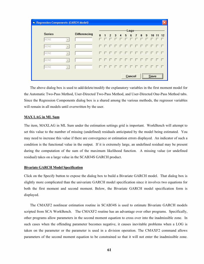
61

The above dialog box is used to add/delete/modify the explanatory variables in the first moment model for

the Automatic Two-Pass Method, User-Directed Two-Pass Method, and User-Directed One-Pass Method tabs.

Since the Regression Components dialog box is a shared among the various methods, the regressor variables

will remain in all models until overwritten by the user.

MAX LAG in ML Sum The item, MAXLAG in ML Sum under the estimation settings grid is important. WorkBench will attempt to

set this value to the number of missing (undefined) residuals anticipated by the model being estimated. You

may need to increase this value if there are convergence or estimation errors displayed. An indicator of such a

condition is the functional value in the output. If it is extremely large, an undefined residual may be present

during the computation of the sum of the maximum likelihood function. A missing value (or undefined

residual) takes on a large value in the SCAB34S GARCH product.

Bivariate GARCH Model Specification

Click on the Specify button to expose the dialog box to build a Bivariate GARCH model. That dialog box is

slightly more complicated than the univariate GARCH model specification since it involves two equations for

both the first moment and second moment. Below, the Bivariate GARCH model specification form is

displayed.

The CMAXF2 nonlinear estimation routine in SCAB34S is used to estimate Bivariate GARCH models

scripted from SCA WorkBench. The CMAXF2 routine has an advantage over other programs. Specifically,

other programs allow parameters in the second moment equation to cross over into the inadmissible zone. In

such cases when the offending parameter becomes negative, it causes inevitable problems when a LOG is

taken on the parameter or the parameter is used in a division operation. The CMAXF2 command allows

parameters of the second moment equation to be constrained so that it will not enter the inadmissible zone.

62

SCA WorkBench sets the constraints to satisfy this condition by default. The user can bypass the default

constraints by changing the LCL and UCL bounds in the Advanced Options/Setting tab

The Bivariate GARCH model that is specified is saved in memory until it is either overwritten by a new

model specification or the ARCH/GARCH Analysis session is ended.

The starting values for Bivariate GARCH models are critical to estimation. It is recommended that careful

thought go into selecting these values. For example, if a time varying correlation model is to be estimated, it is

suggested to first estimate the model with constant correlation and then use the final estimates of that model as

starting values for the time-varying correlation model.

63

5.2.4 Results

The results tab provides a convenient facility to view output from ARCH/GARCH model estimation. It also

allows you to view the input commands for the SCA Statistical System (two-pass methods) or SCAB34S

Applet Collection (one-pass method). If there are errors during the one-pass GARCH estimation, you can

view the log file for a detailed account of all commands executed and error messages.

Menu Item Description

View GARCH Output File

Displays the ARCH/GARCH modeling results and tabulated diagnostics.

View GARCH Input Commands

Displays the input commands submitted to either the SCA System or SCAB34S GARCH module. You can modify the commands directly in this window and submit the modified command file by clicking on the Execute button.

View GARCH Log File

Displays a detailed command and error log for jobs submitted to the SCAB34S Applet Collection: GARCH module.

Print Send information displayed in the viewer to the printer.

64

Save Saves the information in the viewer to a file. You may want to use this feature to save the modeling script with intentions of executing it later from the System -> Run SCA with Macro menu, or the System -> Run SCAB34S Program File menu.

Execute While you are in the Results tab, if you click on Execute, you will send the

information in the viewer to the SCA System or SCAB34S GARCH module for processing.

65

5.2.5 Graphics

The Graphics tab provides a facility to view high-resolution plots that were generated by the SCAB34S Applet

Collection. If you previously selected the Show/Create Graphs option, the individual graphs will initially be

displayed on screen. When you click on the graph, the next generated graph will appear until all graphics have

been created. As the graphs are displayed, they are also being saved as Windows Meta Files using fixed

names such as “yvar.wmf” or “acfy.wmf”.

You can review all created graphic files by selecting the graph from the set of radio buttons provided in

the small tabbed area to the right of the viewer control. In the example below, we are viewing the time plot of

the estimated conditional standard deviation series. The name of the graphic file (sigma.wmf) is displayed for

reference. Since the graphs are saved to fixed file names, they are overwritten each time you generate a new

set of graphs from the ARCH/GARCH modeling environment. If you wish to save the graphic file for future

reference, please use the Save button on this tab to copy the file to a new name. Please do not rename the file

extension because the Save button only renames the file. It does not convert it to a new format. You can view

those renamed files by using the Load Graph from File facility. You may send the graph to the printer by

clicking on the Print command button.

Send the graph to the printer.

Save the current graph to a new file name in Windows Meta File format.

66

6 A DETAILED DESCRIPTION OF THE GARCHEST COMMAND IN SCAB34S

GARCH modeling requires recursive solution of equations. While use of a MATRIX command DO LOOP

would be a possible way to proceed, the resulting complexity and speed loss warranted using the built in

GARCH or GARCHEST commands. For the GARCHEST command, the B34S ordinary least squares

(OLSQ) command is used to get initial values for the AR part of the model and an estimate of the constant is

the second moment equation. A detailed description of the GARCHEST command is listed next and should

be studied prior to any model building.

The GARCHEST subroutine supports a general way to setup and estimate ARCH, GARCH, and GARCH-

M models and avoid the overhead of a DO loop needed for recursive calls. In addition a user program is not

needed. The GARCHEST command works with single series models only. For more complicated models, or

models where computational progress must be monitored, the alternative B34S GARCH command should be

employed.

Usage:

CALL GARCHEST(RES1,RES2,Y,FUNC,MAXLAG,NBAD :OPTIONS);

Required subroutine arguments:

Arguments Intent Comments RES1 Input/Output Residuals for the first moment model. If RES1 is allocated by the user prior

to the GARCHEST call, RES1 will be used as initial values. Otherwise, RES1 initial values are set equal to 0.0

RES2 Input/Output Residuals (ht ) for the second moment model. If RES2 is specified by the user prior to the GARCHEST call, RES2 will be used for initial values. Otherwise, RES2 initial values are set equal to 0.0

Y Input Time series being analyzed in the first moment model FUNC Output The optimized function value MAXLAG Input Maximum lags for purposes of maximum likelihood sum NBAD Output Number of bad data points detected during estimation where

th would have

been negative.

Optional keywords and associated arguments:

Keyword # Args Type(s) Intent Comments :NAR 1 Integer scalar input The maximum AR order (full rank) of the first moment

model. All autoregressive terms up to rank N are estimated.

67

:ARORDER 1 Integer array input This keyword may be used as an alternative to the NAR keyword to restrict (skip lags) the number of AR terms in the first moment model. The NAR keyword is not used in this case.

:ARPARMS 1 Real number array

input The initial values for the AR parameters in the first moment model. Typically, initial values are obtained using the parameter values from a regression model estimated using OLS.

:NMA 1 Integer scalar input The maximum MA order (full rank) of the first moment model. All moving average terms up to rank M are estimated.

:MAORDER 1 Integer array input This keyword may be used as an alternative to the NMA keyword to restrict (skip lags) the number of MA terms in the first moment model. The NMA keyword is not used in this case.

:MAPARMS 1 Real number array

input The initial values for the MA parameters in the first moment model.

:NGAR 1 Integer scalar input The maximum GARCH AR order (full rank) of the second moment model. All autoregressive terms up to rank N are estimated.

:GARORDER 1 Integer array input This keyword may be used as an alternative to the NGAR keyword to restrict (skip lags) the number of GARCH AR terms in the second moment model. The NGAR keyword is ignored in this case.

:GARPARMS 1 Real number array

input The initial values for the GARCH AR parameters in the second moment model. Usually, this option is not required.

:NGMA 1 Integer scalar input The maximum GARCH MA order (full rank) of the second moment model. All moving average terms up to rank M are estimated.

:GMAORDER 1 Integer array input This keyword may be used as an alternative to the NGMA keyword to restrict (skip lags) the number of GARCH MA terms in the second moment model. The NGMA keyword is ignored in this case.

:GMAPARMS 1 Real number array

input The initial values for the GARCH MA parameters in the second moment model. Usually, this option is not required.

:NMU 1 Integer scalar input The number of th terms in the first moment equation. :MUORDER 1 Integer array input This keyword may be used as an alternative to the NMU

keyword to restrict (skip lags) the number of th terms in the first moment model. The NMU keyword is ignored in this case.

:MUPARMS 1 Real number array

input The initial values for the th terms in the second moment model. Usually, this option is not required.

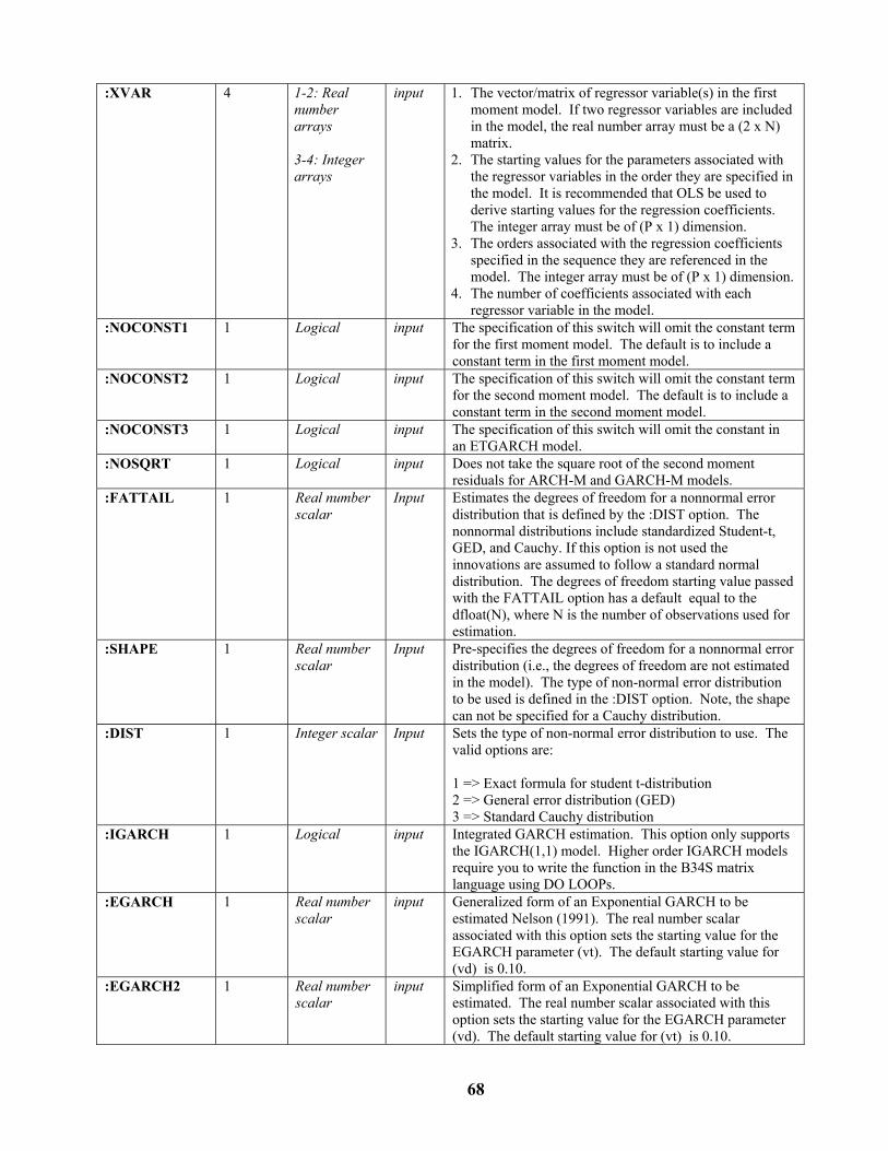
68

:XVAR 4 1-2: Real number arrays 3-4: Integer arrays

input 1. The vector/matrix of regressor variable(s) in the first moment model. If two regressor variables are included in the model, the real number array must be a (2 x N) matrix.

2. The starting values for the parameters associated with the regressor variables in the order they are specified in the model. It is recommended that OLS be used to derive starting values for the regression coefficients. The integer array must be of (P x 1) dimension.

3. The orders associated with the regression coefficients specified in the sequence they are referenced in the model. The integer array must be of (P x 1) dimension.

4. The number of coefficients associated with each regressor variable in the model.

:NOCONST1 1 Logical input The specification of this switch will omit the constant term for the first moment model. The default is to include a constant term in the first moment model.

:NOCONST2 1 Logical input The specification of this switch will omit the constant term for the second moment model. The default is to include a constant term in the second moment model.

:NOCONST3 1 Logical input The specification of this switch will omit the constant in an ETGARCH model.

:NOSQRT 1 Logical input Does not take the square root of the second moment residuals for ARCH-M and GARCH-M models.

:FATTAIL 1 Real number scalar

Input Estimates the degrees of freedom for a nonnormal error distribution that is defined by the :DIST option. The nonnormal distributions include standardized Student-t, GED, and Cauchy. If this option is not used the innovations are assumed to follow a standard normal distribution. The degrees of freedom starting value passed with the FATTAIL option has a default equal to the dfloat(N), where N is the number of observations used for estimation.

:SHAPE 1 Real number scalar

Input Pre-specifies the degrees of freedom for a nonnormal error distribution (i.e., the degrees of freedom are not estimated in the model). The type of non-normal error distribution to be used is defined in the :DIST option. Note, the shape can not be specified for a Cauchy distribution.

:DIST 1 Integer scalar Input Sets the type of non-normal error distribution to use. The valid options are: 1 => Exact formula for student t-distribution 2 => General error distribution (GED) 3 => Standard Cauchy distribution

:IGARCH 1 Logical input Integrated GARCH estimation. This option only supports the IGARCH(1,1) model. Higher order IGARCH models require you to write the function in the B34S matrix language using DO LOOPs.

:EGARCH 1 Real number scalar

input Generalized form of an Exponential GARCH to be estimated Nelson (1991). The real number scalar associated with this option sets the starting value for the EGARCH parameter (vt). The default starting value for (vd) is 0.10.

:EGARCH2 1 Real number scalar

input Simplified form of an Exponential GARCH to be estimated. The real number scalar associated with this option sets the starting value for the EGARCH parameter (vd). The default starting value for (vt) is 0.10.

69

:GJR Real number array

Glosten-Jagannathan-Runkle GARCH estimation. The default starting values associated with the GJR option are set to 0.01. The user can overwrite these default values by passing a real number array. The number of elements in the array must be equal to the number of GARCH (GMA) parameters included in the model.

:TGARCH 1 Real number array

Input Simplified Threshold GARCH model estimation. The real number array associated with this option sets the starting values for the GAR threshold parameters in the model. At least one GAR parameter must be specified in a model with the TGARCH option.

:TGARCH2 1 Real number array

Input ZachoianThreshold GARCH (Asymmetric) model estimation. The real number array associated with this option sets the starting values for the GMA threshold parameters in the model. At least one GMA parameter must be specified in a model with the TGARCH2 option.

:TGARCH3 1 Logical Input Zachoian Threshold GARCH (Symmetric) model estimation. At least one GMA parameter must be specified in a threshold GARCH model using the TGARCH3 option. The GMA threshold parameters in this model are constrained to be the same.

:ETGARCH 1 Real number array

Input Estimates an Extedned Threshold GARCH model. The real number array allows the GAR, GMA and CONST3 starting values to be specified. If the CONST3 constant parameter is to be omitted from the model, the :NOCONST3 option must be specified before the :ETGARCH option. The ETGARCH specification in essence is a combination of the GJR-GARCH and TGARCH models. This form is shown in Tsay (2002) page 168 and discussed on pages 129-133.

:CPARMS 1 Real number array

input Sets initial values for constants. Two elements are passed even if noconst1 or noconst2 are set. If the ETGARCH model option is used, three elements must be passed in the array.

:PRINT 1 Logical input Print estimation results for GARCHEST :PRINT2 1 Logical input Print the simplex estimation results and number of

iterations used for convergence :PRINT3 1 Logical input Displays only the functional form of the model being

estimated. This option is employed by WorkBench since the model summary is formatted using the subroutine DSPGARCH located in “wbsuppl.mac”.

:LOWER 1 Real number array

input Restrict lower bound of parameter values for both the first moment and second moment models. The default lower bound for the ARMA parameters of the first moment model is –1.d+32 and 0.0 for the GARCH parameters in the second moment model. These default settings are appropriate for most purposes.

:UPPER 1 Real number array

input Restrict upper bound of parameter values for both the first moment and second moment models. The default upper bound for the ARMA and GARCH is 1.d+32. These default settings are appropriate for most purposes.

70

:SIMPLEX 1 Logical input Provides access to a nonlinear search procedure that requires only function evaluations, not derivatives. The parameter estimates from the simplex estimation are then used as the starting values for the final one-pass estimation. Also see MAXIT2 option.

:FTOC 1 Real number scalar

Input Sets the relative functional tolerances for simplex estimation. The default is max(1.0d-20,ops**(2/3))

:XSCALE 1 Real number array

input Vector of n elements to scale the coefficient vector. Default = 1.0

:FSCALE 1 Real number scalar

input Functional scaling. Default =1.0

:NGOOD 1 Integer scalar input Sets number of good digits in the function. Default = 5 :MAXIT 1 Integer scalar input Maximum number of iterations. Default =400 :MAXIT2 Integer scalar input Sets the maximum number of iterations for the Simplex

estimation method. It is ignored if the :simplex option is not used.

:MAXFUN 1 Integer scalar input Maximum number of function evaluations. Default=400 :MAXG 1 Integer scalar input Maximum number of gradient evaluations. Default=400 :GRADTOL 1 Real number

scalar input Scaled gradient tolerance.

13Default ε=

:STEPTOL 1 Real number scalar

input Scaled step tolerance. 2

3Default ε=

:RFTOL 1 Real number scalar

input Relative functional tolerance.

( )23maximum 1.0d 20,Default ε= −

:AFTOL 1 Real number scalar

input Absolute functional tolerance

( )23maximum 1.0d 20,Default ε= −

:FCTOL 1 Real number scalar

input False convergence tolerance. 100Default ε= ×

:MAXSTEPS 1 Real number scalar

input Maximum allowable step size. ( )maximum 1, 2 1000, whereDefault TOL TOL= ×

121 ( )

i

i in

TOL XSCALE IVALUE=

= ×∑

1

22 2i

in

TOL XSCALE=

= − ∑

71

Variables created if OPTIONS keyword is specified:

Variable Comments %COEF Real number array; output only

Estimated coefficients in order AR, MA, GAR, GMA, MU, VD, CONST1, CONST2, and CONST3

%SE Real number array; output only Standard errors of coefficients in order AR, MA, GAR, GMA, MU, VD, CONST1, CONST2, and CONST3

%T Real number array; output only t-values of coefficients in order AR, MA, GAR, GMA, MU, VD, CONST1, CONST2, and CONST3

%CNAME Character array; output only Names of coefficients in order AR, MA, GAR, GMA, MU, VD, CONST1, CONST2, and CONST3

%CORDER Integer array; output only Orders of coefficients in order AR, MA, GAR, GMA, MU, VD, CONST1, CONST2, and CONST3

%HESSIAN Real number matrix; output only The Hessian matrix used to compute standard errors of coefficients

%RESOBS Integer array; output only Observation # of residual. First MAXLAG set to missing. First MAXLAG obs of RES1 and RES2 set to missing.

%G Real number array; output only Values of the tg array in an exponential GARCH (EGARCH) estimation,

where (| | / ) (2 / ) ( / )t t t t tg e h v e hπ= − −

%FUNC Real number scalar; output only The final log likelihood functional value obtained in estimation.

%NPARM Integer scalar; output only The number of parameters estimated.

%N_ITER Integer scalar; output only The number of iterations taken for model parameter estimation

%N_FUNC Integer scalar; output only The number of functional evaluations taken for model parameter estimation

%N_GRAD Integer scalar; output only The number of gradient evaluations taken for model parameter estimation

%SG_TOL Real number scalar; output only The scaled gradiant tolerance used in model estimation.

%SS_TOL Real number scalar; output only The scaled step tolerance used in model estimation

%RF_TOL Real number scalar; output only The relative functional tolerance used in model estimation

%FC_TOL Real number scalar; output only The false convergence tolerance used in model estimation

%MAX_SS Real number scalar; output only The maximum allowable step size used in model estimation

%S_TRUST Real number scalar; output only Size of initial trust region used in model estimation

%NT_DROP Integer scalar; output only The number of residuals dropped in model estimation

%H_COND Real number scalar; output only 1/ Condition of Hessian Matrix

%NAR Integer scalar; output only The number of AR terms in the estimated first moment model

72

%NMA Integerscalar; output only The number of MA terms in the estimated first moment model

%NGAR Integer scalar; output only The number of GARCH terms in the second moment model

%NGMA Integer scalar; output only The number of ARCH terms in the second moment model

%NMU Integer scalar; output only The number of MU terms in first moment GARCH-M model

%CON Integer scalar; output only The number of constants in the first and second moment models. 0 = none -1 = first moment model only 1 = second moment model only 2= both

73

7 A DETAILED DESCRIPTION OF THE BGARCH COMMAND IN SCAB34S

The BGARCH command supports a general method for a user to specify a Bivariate GARCH model. Here,

models with constant correlations as well as time-varying correlations are possible. The BGARCH command

works with two series.

Unlike the GARCHEST command, the BGARCH command does not directly estimate the model. It

simply holds the specified model and accompanying likelihood function which can then be maximized using

the CMAXF2 command or the NLPMIN1 command in more complex cases. SCA WorkBench builds the

commands to estimate Bivariate GARCH models exclusively with the CMAXF2 command. The NLPMIN1

command supports nonlinear programming with nonlinear constraints. The latter approach allows nonlinear

restrictions on the parameters but does not give SE's. The user would need to save the B34S program file and

edit the commands if the NLPMIN1 approach is desired.

The CMAXF2 nonlinear estimation routine in SCAB34S has an advantage over other programs such as

RATS. Specifically, other programs have a problem during estimation because these programs allow

parameters in the second moment equation to cross over into the inadmissible zone. In such cases when the

offending parameter goes negative, it causes inevitable problems when a LOG is taken on the parameter or the

parameter is used in a division operation. The CMAXF2 command allows parameters of the second moment

equation to be constrained so that it will not enter the inadmissible zone. SCA WorkBench sets the constraints

to satisfy this condition by default. The user can bypass the default constraints by changing the LCL and UCL

bounds in the Advanced Options/Setting tab.

Usage:

CALL BGARCH(RES1,RES2,ARCH1, ARCH2, Y1,Y2, FUNC,MAXLAG,NBAD :OPTIONS);

Required subroutine arguments:

Arguments Intent Comments RES1 Input/Output Residuals in the first moment model for Series #1. If RES1 is allocated by

the user prior to the CMAXF2 call, RES1 will be used as initial values. Otherwise, RES1 initial values are set equal to 0.0

RES2 Input/Output Residuals in the first moment model for Series #2. If RES2 is allocated by the user prior to the CMAXF2 call, RES2 will be used as initial values. Otherwise, RES2 initial values are set equal to 0.0

ARCH1 Input/Output Residuals (h1t ) in the second moment model for Series #1. If ARCH1 is specified by the user prior to the CMAXF2 call, ARCH1 will be used for

74

initial values. Otherwise, ARCH1 initial values are set equal to 0.0 ARCH2 Residuals (h2t ) in the second moment model for Series #2. If ARCH2 is

specified by the user prior to the CMAXF2 call, ARCH2 will be used for initial values. Otherwise, ARCH2 initial values are set equal to 0.0

Y1 Input Series #1: Time series being analyzed in the first moment model Y2 Input Series #2: Time series being analyzed in the first moment model FUNC Output The optimized function value MAXLAG Input Maximum lags for purposes of maximum likelihood sum NBAD Output Number of bad data points detected during estimation where

th would have

been negative.

Optional keywords and associated arguments:

Keyword # Args

Type(s) Intent Comments

:AR11 2 Char. array, Integer array

input The character array specifies the labels of the autoregressive parameters associated with Series #1 in the first moment model for Series #1. The integer array specifies the orders of the autoregressive parameters. Example, :AR11 array(: p1, p2) index(1, 2)

:AR12 2 Char. array, Integer array

input The character array specifies the labels of the autoregressive parameters associated with Series #2 in the first moment model for Series #1. The integer array specifies the orders of the autoregressive parameters.

:AR21 2 Char. array, Integer array

input The character array specifies the labels of the autoregressive parameters associated with Series #1 in the first moment model for Series #2. The integer array specifies the orders of the autoregressive parameters.

:AR22 2 Char. array, Integer array

input The character array specifies the labels of the autoregressive parameters associated with Series #2 in the first moment model for Series #2. The integer array specifies the orders of the autoregressive parameters.

:MA11 2 Char. array, Integer array

input The character array specifies the labels of the moving average parameters associated with Series #1 in the first moment model for Series #1. The integer array specifies the orders of the moving average parameters. Example, :MA11 array(: q1, q2) index(1, 2)

:MA12 2 Char. array, Integer array

input The character array specifies the labels of the moving average parameters associated with Series #2 in the first moment mode for Series #l. The integer array specifies the orders of the moving average parameters.

75

:MA21 2 Char. array, Integer array

input The character array specifies the labels of the moving average parameters associated with Series #1 in the first moment mode for Series #2. The integer array specifies the orders of the moving average parameters.

:MA22 2 Char. array, Integer array

input The character array specifies the labels of the moving average parameters associated with Series #2 in the first moment mode for Series #2. The integer array specifies the orders of the moving average parameters.

:GAR11 2 Char. array, Integer array

input The character array specifies the labels of the GARCH parameters associated with Series #1 in the second moment model for Series #1. The integer array specifies the orders of the GARCH parameters. Example, :GAR11 array(: g1, g2) index(1, 2)

:GAR12 2 Char. array, Integer array

input The character array specifies the labels of the GARCH parameters associated with Series #2 in the second moment model for Series #1. The integer array specifies the orders of the GARCH parameters.

:GAR21 2 Char. array, Integer array

input The character array specifies the labels of the GARCH parameters associated with Series #1 in the second moment model for Series #2. The integer array specifies the orders of the GARCH parameters.

:GAR22 2 Char. array, Integer array

input The character array specifies the labels of the GARCH parameters associated with Series #2 in the second moment model for Series #2. The integer array specifies the orders of the GARCH parameters.

:GMA11 2 Char. array, Integer array

input The character array specifies the labels of the ARCH parameters associated with Series #1 in the second moment model for Series #1. The integer array specifies the orders of the ARCH parameters. Example, :GMA11 array(: a1, a2) index(1, 2)

:GMA12 2 Char. array, Integer array

input The character array specifies the labels of the ARCH parameters associated with Series #2 in the second moment model for Series #1. The integer array specifies the orders of the ARCH parameters.

:GMA21 2 Char. array, Integer array

input The character array specifies the labels of the ARCH parameters associated with Series #1 in the second moment model for Series #2. The integer array specifies the orders of the ARCH parameters.

:GMA22 2 Char. array, Integer array

input The character array specifies the labels of the ARCH parameters associated with Series #2 in the second moment model for Series #2. The integer array specifies the orders of the ARCH parameters.

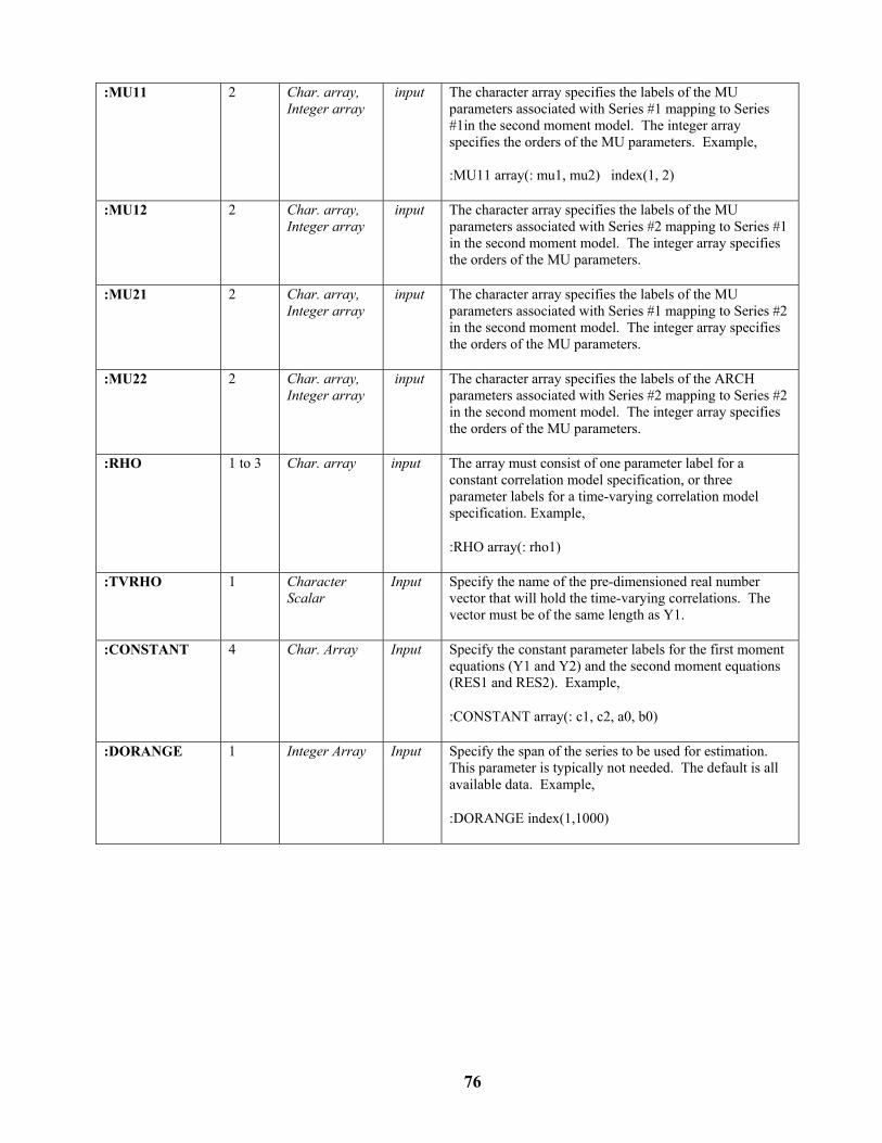
76

:MU11 2 Char. array, Integer array

input The character array specifies the labels of the MU parameters associated with Series #1 mapping to Series #1in the second moment model. The integer array specifies the orders of the MU parameters. Example, :MU11 array(: mu1, mu2) index(1, 2)

:MU12 2 Char. array, Integer array

input The character array specifies the labels of the MU parameters associated with Series #2 mapping to Series #1 in the second moment model. The integer array specifies the orders of the MU parameters.

:MU21 2 Char. array, Integer array

input The character array specifies the labels of the MU parameters associated with Series #1 mapping to Series #2 in the second moment model. The integer array specifies the orders of the MU parameters.

:MU22 2 Char. array, Integer array

input The character array specifies the labels of the ARCH parameters associated with Series #2 mapping to Series #2 in the second moment model. The integer array specifies the orders of the MU parameters.

:RHO 1 to 3 Char. array input The array must consist of one parameter label for a constant correlation model specification, or three parameter labels for a time-varying correlation model specification. Example,

:RHO array(: rho1)

:TVRHO 1 Character Scalar

Input Specify the name of the pre-dimensioned real number vector that will hold the time-varying correlations. The vector must be of the same length as Y1.

:CONSTANT 4 Char. Array Input Specify the constant parameter labels for the first moment equations (Y1 and Y2) and the second moment equations (RES1 and RES2). Example,

:CONSTANT array(: c1, c2, a0, b0)

:DORANGE 1 Integer Array Input Specify the span of the series to be used for estimation. This parameter is typically not needed. The default is all available data. Example,

:DORANGE index(1,1000)

77

8 A DETAILED DESCRIPTION OF THE CMAXF2 COMMAND IN SCAB34S The CMAXF2 command provides a way to maximize a constrained function using the Quasi-Newton Method.

The CMAXF2 command is employed in the scripts built by SCA WorkBench to estimate Bivariate GARCH

models which are specified using the BGARCH command. The CMAXF2 is a general command that can be

used to maximize any defined function. If the functional value is multiplied by -1.0, a minimum can be

obtained.

Usage

CALL CMAXF2(FUNC GRAD :NAME prgnam1 prgnam2 :PARMS var1 var2 … varp :LOWER var :UPPER var :OPTIONS);

Required Arguments:

Argument Type(s) Intent Comments FUNC Function name input The variable name for the final estimated value of the functional

equation GRAD Variable name input Optional. The variable name defining the constraints for the

nonlinear programming model

Required Keywords and Their Associated Arguments:

Keyword # Args

Type(s) Intent Comments

:NAME 1-2 Program name input prgnam1 => The name of the user-specified program defining the functional equation

prgnam2 => Optional. The name of the user-specified program defining the gradient

:PARMS p Variable names

Input Specifies parameters used in the model. The parameters can be set as scalars or as a vector. If a vector is supplied, only one vector can be used. The parameters must be specified in the functional equation of the user-specified program in :NAME that determines FUNC. The keyword :PARMS must be supplied prior to all keywords except :NAME

:LOWER 1 Real number array

Input This (1 x p) array allows the user to specify the lower bounds for the parameters during estimation. Default = -.1d+10

:UPPER 1 Real number array

Input This (1 x p) array allows the user to specify the upper bounds for the parameters during estimation. Default = .1d+10

78

Optional Keywords and Associated Arguments:

Keyword # Args

Type(s) Intent Comments

:PRINT 0 Logical input Print the results :IVALUE 1 Real number

array Input This (1 x p) array allows the user to specify initial values

for the parameters in the nonlinear model. Default = 0.1. :XSCALE 1 Real number

array Input This (1 x p) array allows the user to set scaling for

parameters in the model. Default = 1.0 :FSCALE 1 Real number

array Input This (1 x p) array allows the user to set functional scaling.

Default = 1.0 :NGOOD 1 Integer scalar Input Sets the number of good digits in the function. :MAXIT 1 Integer scalar Input Sets the maximum number of iterations during estimation.

Default = 100 :MAXFUN 1 Integer scalar Input Sets the maximum number of function evaluations.

Default = 400 :MAXG 1 Integer scalar Input Sets the maximum number of gradient evaluations.

Default = 400 :GRADTOL 1 Real number

scalar Input Sets the scaled gradient tolerance.

13Default ε=

:STEPCOL 1 Real number scalar

Input Sets the scaled step tolerance. Default = 2

3Default ε=

:RFTOL 1 Real number scalar

Input Sets the relative functional tolerance.

( )23maximum 1.0d 20,Default ε= −

:AFTOL 1 Real number scalar

Input Sets the absolute functional tolerance.

( )23maximum 1.0d 20,Default ε= −

:FCTOL 1 Real number scalar

Input Sets the false convergence tolerance. 100Default ε= ×

:MAXSTEPS 1 Real number scalar

Input Sets the maximum allowable step size. ( )maximum 1, 2 1000, whereDefault TOL TOL= ×

121 ( )

i

i in

TOL XSCALE IVALUE=

= ×∑

122 2

i

in

TOL XSCALE=

= − ∑

:IHESSIAN 1 Integer scalar Input 0 => The Identify matrix is used for initialization.

otherwise=> max(|f(XGUESS|,FSCALE)*XSCALE(i)

Variables Automatically Created by CMAXF2:

Variable Comments %COEF Real number array; output only

A vector containing the parameter estimates %NPARM Character array; output only

Names of the coefficients %SE Real number array; output only

Standard errors of coefficients %T Real number array; output only

t-values of coefficients %HESSIAN Real number matrix; output only

79

The Hessian matrix %GRAD Real number scalar; output only

Gradient estimate at final iteration

%FUNC Real number scalar; output only Final value of function

80

9 A DETAILED DESCRIPTION OF CUSTOMIZABLE SUBROUTINES USED IN THE GARCH APPLICATION

The ARCH/GARCH application environment of Workbench uses some customized user subroutines that were

developed in the B34S matrix language. These subroutines perform similar to a macro procedure and are

stored in the STAGING.MAC and WBSUPPL.MAC files located in the B34SLM installation folder. Since

these subroutines are loaded and called from the script generated by SCA WorkBench for GARCH modeling,

the user can modify the scripts to handle some specific needs, as long as the nature of the arguments and

calling sequence of the arguments is not changed.

For example, custom subroutines are available to display diagnostic information including ACF, PACF,

and Q-Stats on the dependent variable and the residual series. The expert user familiar with the B34S matrix

language could expand the types of diagnostics available if needed.

It is highly recommended that you make a backup of the original files before attempting to customize the

subroutines.

9.1 DSPGARCH User Subroutine

The DSPGARCH routine customizes the GARCH model summary. It also computes and displays some useful

statistics such as the unconditional variance, volatility of variance, and AIC. An example of the information it

generates is shown below:

Nonlinear Estimation Summary: GARCH Model ---------------------------------------------------------------------- Number of observations: 2528 Number of iterations: 40 Number of Function Evals 80 Number of Gradiant Evals 41 Number of Terms Dropped: 1 Final Functional Value: 8947.610 1/Condition of Hessian: 0.16433E-08 AIC (Based on LLF): -20194.27150134 Parameter Order Coefficient Std. Err. t-Value p-Value Comments C1 0 0.00077068 0.00033882 2.27 0.0230 CONS_1 C2 0 0.00002053 0.00000480 4.27 0.0000 CONS_2 ARCH 1 0.07808543 0.01418957 5.50 0.0000 GMA GARCH 1 0.86123981 0.02476205 34.78 0.0000 GAR Standardized Error Distn. : Normal Distribution Sum of Squared Residuals : 0.83838675 Volatility of Variance : 0.16185477 Unconditional Variance : 0.00033836 Unconditional Standard Dev: 0.01839452

81

Usage: CALL LOAD(DSPGARCH :WBSUPPL); CALL DSPGARCH(ARGUMENTS);

Required subroutine arguments:

Arguments Type(s) Intent Comments MTYPE Integer key input The ID of the GARCH model type.

1 => ARCH 2 => GARCH 3 => IGARCH 4 => GARCH-M 5 => EGARCH 6 => GJR-GARCH 7 => TGARCH (Extended) 8 => TGARCH (Simplified) 9 => TGARCH (Asymmetric) 10 => TGARCH (Symmetric)

DIST Integer key Input The ID of the standardized error distribution that was used for model estimation. -1 => Normal distribution 1 => student-t distribution (exact t) 2 => General error distribution 3 => Cauchy distribution

IDFEST Integer key Input The ID indicator as to whether the degrees of freedom from a non-normal error distribution is pre-specified or estimated in the model. 0 => Normal distribution 1 => Pre-specified degrees of freedom 2 => Estimated degrees of freedom

IOBS Integer scalar Input The number of observations used in model estimation.

NPARMS Integersclar Input The number of parameters in the estimated GARCH model (see %NPARM internal variable created by GARCHEST).

XNAMES Character array

Input The names of variables included as explanatory variables in the first moment model. The order of the array must match the order in which the variables were specified in the model.

RES Real number array

Input The residual series from the estimated GARCH model.

CVAR Real number array

Input The conditional variance series from the estimated GARCH model

COEF Real number array

Input The estimated coefficients of the GARCh model in the expected order as provided by the %COEF internal variable created by the GARCHEST subroutine.

COEFSE Real number array

Input The standard errors of the estimated coefficients of the GARCH model in the expected order as

82

provided by the %COEFSE internal variable created by the GARCHEST subroutine.

TVALS Real number array

Input The t-Values of the estimated coefficients of the GARCH model in the expected order as provided by the %T internal variable created by the GARCHEST subroutine.

CNAMES Character array

Input The names of the parameters in the expected order as provided by the %CNAME internal variable created by the GARCHEST subroutine

CORDER Integer array Input The orders of the coefficents in the expected order

as provided by the %CORDER internal variable created by the GARCHEST subroutine.

NAR Integer scalar Input The number of AR terms in the first moment model (see %NAR internal variable created by GARCHEST)

NMA Integer scalar Input The number of MA terms in the first moment model (see %NMA internal variable created by GARCHEST)

NGAR Integer scalar Input The number of GARCH terms in the second moment model (see %NGAR internal variable created by GARCHEST)

NGMA Integer scalar Input The number of ARCH terms in the second moment model (see %NGMA internal variable created by GARCHEST)

NMU Integer scalar Input The number of MU terms in the first moment GARCH-M model (see %NMU internal variable created by GARCHEST)

CON Integer key Input The integer key to identify the number of constants in the models (see %CON internal variable created by GARCHEST)

FUNC Real number scalar

Input The final log likeihood functional value from model estimation

NITER Integer scalar Input The number of iterations required for model estimation

NFUNC Integer scalar Input The number of function evaluations for model estimation

NGRAD Integer scalar Input The number of gradiant evaluations for model estimation

MLDROP Integer scalar Input The number of residuals deleted in the maximum likelihood sum.

HCOND Real number scalar

Input 1 / Hessian condition

HESS Real number matrix

Input The Hessian matrix

Example: call dspgarch(2,-1,0,norows(D_AA),%nparm,xvnames,res1 res2,%coef,%se,%t,%cname,%corder,%nar,%nma,%ngar,%ngma,%nmu, %con,%func,%n_iter,%n_func,%n_grad,%nt_drop,%h_cond,%hessian);

83

9.2 DSPDSCRB User Subroutine

The DSPDSCRB routine provides descriptive statistics about a variable. This subroutine is called multiple

times in the GARCH program script to show descriptive statistics about the dependent variable and the various

residual series. An example of the information it generates is shown below:

Descriptive Statistics Table - D_AA ------------------------------------------ Number of Cases : 2528 Minimum Value : -0.097300 Maximum Value : 0.140560 Mean : 0.000843 Standard Deviation : 0.018215 Skewness : 0.602421 Kurtosis : 3.636222 Cumulant (6th Order): 92.725149 First Quartile : -0.010695 Third Quartile : 0.010670

Usage: CALL LOAD(DSPDSCRB :WBSUPPL); CALL DSPDSCRB(ARGUMENTS);

Required subroutine arguments:

Arguments Type(s) Intent Comments VNAME Character

string input Specify a description of the variable to be

summarized in single quotes or pass a character string variable presepcified in the B34S matrix language.

Y Real number array

Input The variable to be described

Example:

CALL DSPDSCRB('D_AA',D_AA); Or CALL CHARACTER(_VNTEMP,'Dependent Variable'); CALL DSPDSCRB(_VNTEMP,D_AA);

84

9.3 DSP_ACF User Subroutine

The DSP_ACF routine computes the autocorrelation functions (ACF), partial autocorrelations (PACF), and

Modified Ljung-Box Q Statistics for a specified variable. An example of the information it generates is shown

below:

Sample ACF and PACF for D_AA ---------------------------------------------------------------- Lag ACF t-Val LB-Q P-Value PACF t-Val 1 0.040 2.00 4.01 0.045 0.040 2.00 2 -0.032 -1.59 6.55 0.038 -0.033 -1.67 3 -0.006 -0.32 6.65 0.084 -0.004 -0.19 4 -0.055 -2.74 14.24 0.007 -0.055 -2.78

Usage: CALL LOAD(DSP_ACF :WBSUPPL); CALL DSP_ACF(ARGUMENTS);

Required subroutine arguments:

Arguments Type(s) Intent Comments VNAME Character

string input Specify a description of the variable to be

summarized in single quotes or pass a character string variable presepcified in the B34S matrix language.

Y Real number array

Input The variable to be described

LAGS Integer scalar Input The maximum number of lags to display for the ACF, PACF and LB-Q statistics.

ACFS Real number array

Output The computed ACF values

PACFS Real number array

Output The computed PACF values

STDERRS Real number array

Output The standard errors of the ACF/PACF values

MBLS Real number array

Output The computed Modified Ljung-Box Q Statistics

PROBS Real number array

Output The p-values for the modified Ljung-Box Q Statistics

FUTURE_1 DUMMY NOT USED NOT USED FUTURE_2 DUMMY NOT USED NOT USED FUTURE_3 DUMMY NOT USED NOT USED Example:

CALL DSP_ACF(‘Resids’,RESA,_NLAGS,ACFA,PACFA,SEA,MQA,PMQA,0,0,0); Or CALL CHARACTER(_VNTEMP,'Standardized Residuals'); CALL DSP_ACF(_VNTEMP,RESA,_NLAGS,ACFA,PACFA,SEA,MQA,PMQA,0,0,0);

85

9.4 LAGRANGE User Subroutine

The LAGRANGE routine computes the ARCH LM test for a specified variable. For the GARCH application,

the residuals and standardized residuals are passed to this routine. An example of the information it generates

is shown below:

LaGrange Multiplier Tests Variable: Residuals ----------------------------- Lag LM-Value P-Value 1 10.750 0.001 2 10.769 0.005 3 11.684 0.009 4 11.972 0.018

Usage: CALL LOAD(DSP_ACF :WBSUPPL); CALL LAGRANGE(ARGUMENTS);

Required subroutine arguments:

Arguments Type(s) Intent Comments TBLHEADR Character

string input The table header to de displayed in the output

ZVAR Real number array

Input The variable to be evaluated.

MAXLAG Integer scalar Input The maximum number of lags to compute and display for the ARCH LM test

LMVALUES Real number array

Output The computed ARCH LM test values

PROBS Real number array

Output The p-Values for the ARCH LM tests

ISHOWTBL Integerscalar Input Display the results or compute without showing output 0 => No output 1 => Show output

Example:

call character(tblheadr, 'Residuals'); call lagrange(tblheadr,res1,n,lmvalue,prob,1);

86

9.5 GARCHF User Subroutine

The GARCHF routine computes the forecasts for various symmetric GARCH models. This subroutine must

be called after the GARCHEST subroutine since it uses several internal variables created by GARCHEST. An

example of the information it generates is shown below:

Forecast Table for First Moment and Second Moment ----------------------------------------------------- FCST Y-INDEX LEVEL FCST VOLATILITY FCST ----- ---------- ---------------- ---------------- 0 2528 0.0008 0.00049 1 2529 0.0008 0.00051 2 2530 0.0008 0.00046 3 2531 0.0008 0.00041 4 2532 0.0008 0.00038 5 2533 0.0008 0.00035

Usage: CALL LOAD(GARCHF :STAGING); CALL GARCHF(ARGUMENTS);

Required subroutine arguments:

Arguments Type(s) Intent Comments MTYPE Integerscalar input The ID of the GARCH model type. CURRENTLY

NOT USED.

RES1 Real number array

Input The residuals from estimated GARCH model

RES2 Real number array

Input The estimated conditional variance (or conditional standard deviation series)

Y Real number array

Input The dependent variable

NFORE Integerscalar Input The number of forecasts to generate FORE1 Real number

array Output The first moment forecasts

FORE2 Real number array

Output The conditional variance forecasts

IOBS Integer scalar Output The obervation number for the forecasts NPARM Integersclar Input The number of parameters in the estimated

GARCH model CNAME Character

array Input The names of the parameters in the expected order

as provided by the %CNAME internal variable created by the GARCHEST subroutine

COEF Real number array

Input The estimated coefficients of the GARCh model in the expected order as provided by the %COEF internal variable created by the GARCHEST subroutine.

CORDER Integer array Input The orders of the coefficents in the expected order as provided by the %CORDER internal variable created by the GARCHEST subroutine.

NAR Integer scalar Input The number of AR terms in the first moment model (see %NAR internal variable created by

87

GARCHEST) NMA Integer scalar Input The number of MA terms in the first moment

model (see %NMA internal variable created by GARCHEST)

NGAR Integer scalar Input The number of GARCH terms in the second moment model (see %NGAR internal variable created by GARCHEST)

NGMA Integer scalar Input The number of ARCH terms in the second moment model (see %NGMA internal variable created by GARCHEST)

NMU Integer scalar Input The number of MU terms in the first moment GARCH-M model (see %NMU internal variable created by GARCHEST)

CON Integer key Input The integer key to identify the number of constants in the models (see %CON internal variable created by GARCHEST)

NOSQRT Integer key Input The integer key to specify whether the conditional variance (NOSQRT=1) or conditional standard deviation (NOSQRT=0) is used in the GARCH-M model formula

IPRINTF Integerkey Input Specifies whether to print the forecast table

0 => No print 1 => Unformatted print 2 => Formatted print

Example: call garchf(2, res1, res2, D_AA, 5, fore1, fore2, iobs, %nparm, %cname, %coef, %corder, %nar, %nma, %ngar, %ngma, %nmu, %con, 0, 2);

88

9.6 GRFGARCH User Subroutine

The GRFGARCH creates all GARCH graphics files that are displayed on the Graphs tab of SCA WorkBench

ARCH/GARCH application environment. Below is a listing of the graph types and their associated file names.

Time Series Plots - Y variable yvar.wmf - Residuals resa.wmf - Residuals**2 resa2.wmf - Standardized Residuals sresa.wmf - Standardized Residuals**2 sresa2.wmf - Sigma plot sigma.wmf ACF and PACF plots - Y variable acfy.wmf pacfy.wmf - Residuals acfa.wmf pacfa.wmf - Residuals**2 acfa2.wmf pacfa2.wmf - Standardized Residuals sacfa.wmf spacfa.wmf - Standardized Residuals**2 sacfa2.wmf spacfa2.wmf Modified Ljung-Box Q-Statistic plots - Residuals mqa.wmf - Residuals**2 mqa2.wmf - Standardized Residuals smqa.wmf - Standardized Residuals**2 smqa2.wmf

Usage: CALL LOAD(GRFGARCH :WBSUPPL); CALL GRFGARCH(ARGUMENTS);

Required subroutine arguments:

Arguments Type(s) Intent Comments VNAME Characterstring input The name of the original series, Y, to be graphed

Y Real number array

Input The dependent variable

RES Real number array

Input The residual series

SIGMA Real number array

Input The estimated conditional standard deviation series

LAGS Integerscalar Input The maximum number of lags to show for ACF, PACF, and Ljung Box Q-Stat graphs

ISHOWGRF Integerkey Input 0 => Do not display select graphs on screen 1 => Show select graphs on screen Note that regardless of the ISHOWGRF setting, the hard copy files are always created in the working directory.

Example: call grfgarch('D_AA ',D_AA ,res1,Sigma,_nlags,ishowgrf);

89

10 EXAMPLES OF SCAB34S COMMAND FILES FOR GARCH MODELING SCA WorkBench was used to automatically generate the command files for the SCA Statistical System and

SCAB34S engines for GARCH modeling and estimation. This section presents the command files generated

by WorkBench for the examples used in this document.

10.1 SCA System script for the automatic two-pass example (Section 4.1.1)

==ALLMACRO ASSIGN FILE 12. EXTERNAL 'Findat01.mad'. CALL PI. FILE IS 12. CALL ANALYSIS STOP ==ANALYSIS SELECT PI. SPAN IS (1,129). IDEN PI. IARIMA PI. NAME IS MOMENT1. @ HOLD RESID(RES). @ SEASONALITY 4. ACF RES. RES2=RES**2 IDEN RES2. IARIMA RES2. NAME MOMENT2. SEAS 4. FSAVE PI, RES, RES2. FILE 'GARCHRES.FSV'. @ DATASET DATA. REWIND.. . . The commands related to building graphics in SCAB34S omitted here for brevity. . RETURN

90

10.2 SCAB34S script for the one-pass example (Section 4.1.2)

b34sexec matrix; call echooff; call getsca('Findat01.mad' :mad :member PI); call load(dsp_acf 'C:\b34slm\wbsuppl.mac'); call load(dspgarch 'C:\b34slm\wbsuppl.mac'); call load(grfgarch 'C:\b34slm\wbsuppl.mac'); call load(garchf :staging); call print('-------------------------------------------------------':); call print('Analysis Performed on Variable: PI':); call print('Model: GARCH , Diagnostics: ON, Graphs: ON':); call print('Data Span for Analysis: 1, 129':); call print('-------------------------------------------------------':); /$ **************************************************************$/ /$ Set span for time series: PI /$ **************************************************************$/ iorigins=integers(1, 129); PI = PI(iorigins); xvnames=c1array(1:); xvnames(1)='PI'; _mdliden=1; _tstdiag=1; call dspdscrb('PI',PI); /$ **************************************************************$/ /$ Use OLS to get starting values for parameters in model /$ **************************************************************$/ call olsq(PI PI{1} ); /$ **************************************************************$/ /$ Specify and estimate GARCH model /$ **************************************************************$/ call garchest(res1, res2, PI,func,10,nbad :arorder idint(array(:1)) :cparms array(:%coef(2),%resvar) :arparms array(1: %coef(1)) :maorder idint(array(:1,4)) :garorder idint(array(:1)) :gmaorder idint(array(:1)) :maxfun 1000 :maxg 1000 :maxit 1000 :ngood 15 :print3); idist=-1; iDFEst=0; call dspgarch(2,idist,iDFEst,norows(PI ),%nparm,xvnames,res1 res2,%coef,%se,%t,%cname,%corder,%nar,%nma,%ngar,%ngma,%nmu, %con,%func,%n_iter,%n_func,%n_grad,%nt_drop,%h_cond,%hessian); /$ **************************************************************$/ /$ Make the res1 and res2 even length /$ **************************************************************$/ _sqrmat=array(dmax1(norows(res1),norows(res2)),2:); _sqrmat(,1)=res1; _sqrmat(,2)=res2; _sqrmat =goodrow(_sqrmat); res1=_sqrmat(,1); res2=_sqrmat(,2); call print('** a(t) and sigma(t) saved to _RESVOL.FMT':); call print(' ':); Residual=goodrow(res1); Sigma=goodrow(dsqrt(goodrow(res2))); call makesca(Residual,Sigma :file '_resvol.fmt' :member data1);

91

/$ **************************************************************$/ /$ Set number of lags for ACF/PACF/Q-Stat /$ **************************************************************$/ _nlags=24; if(_mdliden.eq.1)then; /$ **************************************************************$/ /$ Produce ACF,PACF, and Q-Stat statistics for PI /$ **************************************************************$/ call print('-------------------------------------------------------':); call print('Identification Statistics for Dependent Variable: PI':); call print('-------------------------------------------------------':); call dsp_acf('PI',PI,_nlags,acfy,pacfy,sey, mqy,pmqy,1,0,0); endif; if(_tstdiag.eq.1)then; call print('-------------------------------------------------------':); call print('Descriptive Statistics for Residuals':); call print('-------------------------------------------------------':); call character(_vntemp,'Residuals'); call dspdscrb(_vntemp,res1); endif; n=5; if(_mdliden.eq.1)then; /$ **************************************************************$/ /$ Produce ACF,PACF, and Q-Stat statistics for res**2 /$ **************************************************************$/ call print(' ':); call print('-------------------------------------------------------':); call print( 'Identification Statistics for Squared Residuals (res1**2)':); call print('-------------------------------------------------------':); ressqr=res1**2.; call dsp_acf('Squared Residuals',ressqr,_nlags,acfr2,pacfr2,ser2, mqr2,pmqr2,1,0,0); /$ **************************************************************$/ /$ Build LaGrange Multiplier Test for Squared Residuals /$ **************************************************************$/ call character(tblheadr, 'Squared Residuals'); call lagrange(tblheadr,res1,n,lmvalue,prob,1); endif; if(_tstdiag.eq.1)then; /$ **************************************************************$/ /$ Standardize residuals /$ **************************************************************$/ resa=goodrow(goodrow(res1)/Sigma); call print(' ':); call print('-------------------------------------------------------':); call print('Diagnostics of Standardized Residuals':); call print('-------------------------------------------------------':); call character(_vntemp,'Standardized Residuals'); call dspdscrb(_vntemp, resa);

92

/$ **************************************************************$/ /$ Compute ACF, PACF, Q-stats for residuals in 1st moment model /$ **************************************************************$/ call character(_vntemp,'Standardized Residuals'); call dsp_acf(_vntemp,resa,_nlags,acfa,pacfa,sea, mqa,pmqa,1,0,0); /$ **************************************************************$/ /$ Square standardized residuals of 1st moment model /$ **************************************************************$/ resb=resa**2.; call print(' ':); call print('-------------------------------------------------------':); call print('Diagnostics of Squared Standardized Residuals':); call print('-------------------------------------------------------':); /$ **************************************************************$/ /$ Compute ACF, PACF, Q-stats for squared standardized residuals /$ **************************************************************$/ call character(_vntemp,'Squared Standardized Residuals'); call dsp_acf(_vntemp,resb,_nlags,acfb,pacfb,seb,mqb,pmqb,1,0,0); /$ **************************************************************$/ /$ Build LaGrange Multiplier Test /$ **************************************************************$/ call character(tblheadr, 'Squared Standardized Residuals'); call lagrange(tblheadr,resa,n,lmvalue,prob,1); endif; ishowgrf=0; call grfgarch('PI',PI,res1,Sigma,_nlags,ishowgrf); b34srun;

93

10.3 SCAB34S script for GARCH(1,1) Example (Section 4.2)

b34sexec matrix; call echooff; call getsca('Findat01.mad' :mad :member SP500); call load(dsp_acf 'C:\b34slm\wbsuppl.mac'); call load(dspgarch 'C:\b34slm\wbsuppl.mac'); call load(grfgarch 'C:\b34slm\wbsuppl.mac'); call load(garchf :staging); call print('-------------------------------------------------------':); call print('Analysis Performed on Variable: SP500':); call print('Model: GARCH , Diagnostics: ON, Graphs: ON':); call print('Data Span for Analysis: 1, 792':); call print('-------------------------------------------------------':); /$ **************************************************************$/ /$ Set span for time series: SP500 /$ **************************************************************$/ iorigins=integers(1, 792); SP500 = SP500(iorigins); xvnames=c1array(1:); xvnames(1)='SP500 '; _mdliden=1; _tstdiag=1; call dspdscrb('SP500',SP500); /$ **************************************************************$/ /$ Use mean/variance for CONSTANT starting values in model /$ **************************************************************$/ YMean=Mean(SP500); YSigma2=Variance(SP500-YMean); /$ **************************************************************$/ /$ Specify and estimate GARCH model /$ **************************************************************$/ call garchest(res1, res2, SP500,func,4,nbad :cparms array(:YMean, YSigma2) :garorder idint(array(:1)) :gmaorder idint(array(:1)) :maxfun 400 :maxg 400 :maxit 400 :ngood 15 :print3); idist=-1; iDFEst=0; call dspgarch(2,idist,iDFEst,norows(SP500 ),%nparm,xvnames,res1 res2,%coef,%se,%t,%cname,%corder,%nar,%nma,%ngar,%ngma,%nmu, %con,%func,%n_iter,%n_func,%n_grad,%nt_drop,%h_cond,%hessian); /$ **************************************************************$/ /$ Make the res1 and res2 even length /$ **************************************************************$/ _sqrmat=array(dmax1(norows(res1),norows(res2)),2:); _sqrmat(,1)=res1; _sqrmat(,2)=res2; _sqrmat =goodrow(_sqrmat); res1=_sqrmat(,1); res2=_sqrmat(,2); call print('** a(t) and sigma(t) saved to _RESVOL.FMT':); call print(' ':); Residual=goodrow(res1); Sigma=goodrow(dsqrt(goodrow(res2)));

94

call makesca(Residual,Sigma :file '_resvol.fmt' :member data1); /$ **************************************************************$/ /$ Set number of lags for ACF/PACF/Q-Stat /$ **************************************************************$/ _nlags=24; if(_mdliden.eq.1)then; /$ **************************************************************$/ /$ Produce ACF,PACF, and Q-Stat statistics for SP500 /$ **************************************************************$/ call print('-------------------------------------------------------':); call print('Identification Statistics for Dependent Variable: SP500':); call print('-------------------------------------------------------':); call dsp_acf('SP500',SP500,_nlags,acfy,pacfy,sey,mqy,pmqy,1,0,0); endif; if(_tstdiag.eq.1)then; call print('-------------------------------------------------------':); call print('Descriptive Statistics for Residuals':); call print('-------------------------------------------------------':); call character(_vntemp,'Residuals'); call dspdscrb(_vntemp,res1); endif; n=5; if(_mdliden.eq.1)then; /$ **************************************************************$/ /$ Produce ACF,PACF, and Q-Stat statistics for res**2 /$ **************************************************************$/ call print(' ':); call print('-------------------------------------------------------':); call print('Identification Stats for Squared Residuals (res**2)':); call print('-------------------------------------------------------':); ressqr=res1**2.; call dsp_acf('Squared Residuals',ressqr,_nlags,acfr2,pacfr2,ser2, mqr2,pmqr2,1,0,0); /$ **************************************************************$/ /$ Build LaGrange Multiplier Test for Squared Residuals /$ **************************************************************$/ call character(tblheadr, 'Squared Residuals'); call lagrange(tblheadr,res1,n,lmvalue,prob,1); endif; if(_tstdiag.eq.1)then; /$ **************************************************************$/ /$ Standardize residuals /$ **************************************************************$/ resa=goodrow(goodrow(res1)/Sigma); call print(' ':); call print('-------------------------------------------------------':); call print('Diagnostics of Standardized Residuals':); call print('-------------------------------------------------------':); call character(_vntemp,'Standardized Residuals'); call dspdscrb(_vntemp, resa); /$ **************************************************************$/ /$ Compute ACF, PACF, Q-stats for residuals in 1st moment model /$ **************************************************************$/

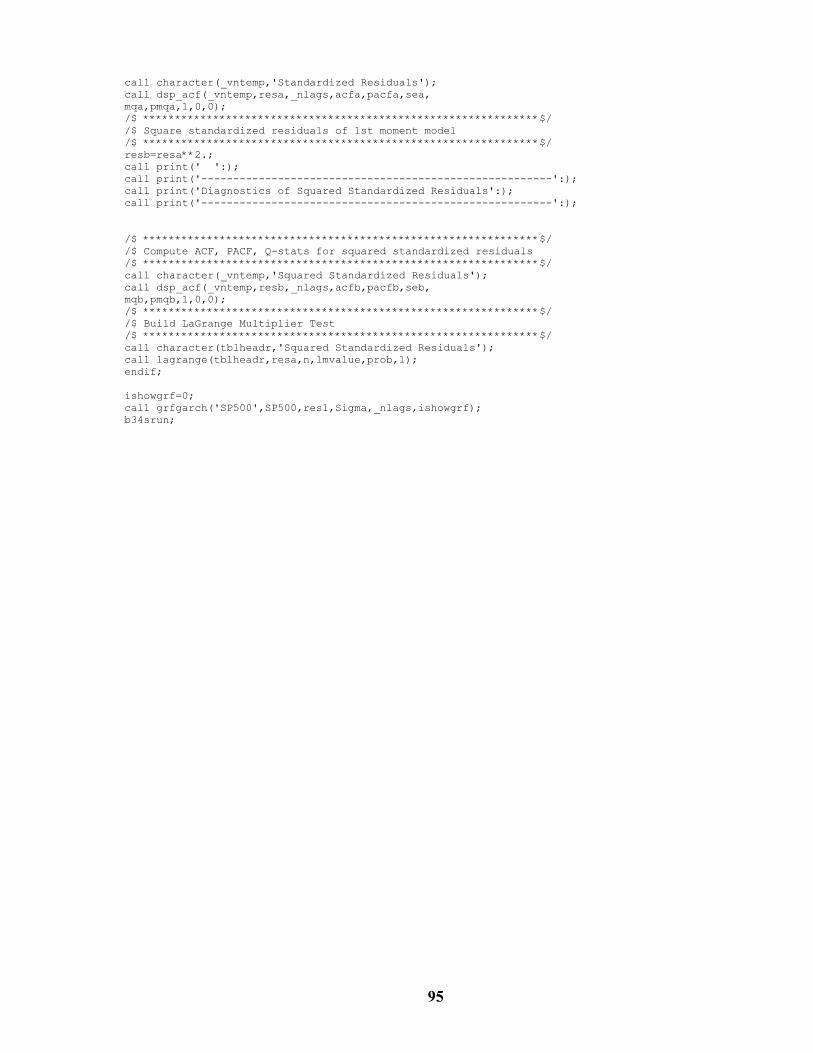
95

call character(_vntemp,'Standardized Residuals'); call dsp_acf(_vntemp,resa,_nlags,acfa,pacfa,sea, mqa,pmqa,1,0,0); /$ **************************************************************$/ /$ Square standardized residuals of 1st moment model /$ **************************************************************$/ resb=resa**2.; call print(' ':); call print('-------------------------------------------------------':); call print('Diagnostics of Squared Standardized Residuals':); call print('-------------------------------------------------------':); /$ **************************************************************$/ /$ Compute ACF, PACF, Q-stats for squared standardized residuals /$ **************************************************************$/ call character(_vntemp,'Squared Standardized Residuals'); call dsp_acf(_vntemp,resb,_nlags,acfb,pacfb,seb, mqb,pmqb,1,0,0); /$ **************************************************************$/ /$ Build LaGrange Multiplier Test /$ **************************************************************$/ call character(tblheadr,'Squared Standardized Residuals'); call lagrange(tblheadr,resa,n,lmvalue,prob,1); endif; ishowgrf=0; call grfgarch('SP500',SP500,res1,Sigma,_nlags,ishowgrf); b34srun;

96

10.4 SCAB34S script for GARCH(1,1) with FAT-TAIL option (Section 4.2.1)

b34sexec matrix; call echooff; call getsca('Findat01.mad' :mad :member SP500); call load(dsp_acf 'C:\b34slm\wbsuppl.mac'); call load(dspgarch 'C:\b34slm\wbsuppl.mac'); call load(grfgarch 'C:\b34slm\wbsuppl.mac'); call load(garchf :staging); call print('-------------------------------------------------------':); call print('Analysis Performed on Variable: SP500':); call print('Model: GARCH , Diagnostics: ON, Graphs: ON':); call print('Data Span for Analysis: 1, 792':); call print('-------------------------------------------------------':); /$ **************************************************************$/ /$ Set span for time series: SP500 /$ **************************************************************$/ iorigins=integers(1, 792); SP500 = SP500(iorigins); xvnames=c1array(1:); xvnames(1)='SP500 '; _mdliden=1; _tstdiag=1; call dspdscrb('SP500',SP500); /$ **************************************************************$/ /$ Use mean/variance for CONSTANT starting values in model /$ **************************************************************$/ YMean=Mean(SP500); YSigma2=Variance(SP500-YMean); /$ **************************************************************$/ /$ Specify and estimate GARCH model /$ **************************************************************$/ call garchest(res1, res2, SP500,func,4,nbad :cparms array(:YMean, YSigma2) :garorder idint(array(:1)) :gmaorder idint(array(:1)) :fattail 5.0 :dist 1 :maxfun 400 :maxg 400 :maxit 400 :ngood 15 :print3); idist=1; iDFEst=2; call dspgarch(2,idist,iDFEst,norows(SP500 ),%nparm,xvnames,res1 res2,%coef,%se,%t,%cname,%corder,%nar,%nma,%ngar,%ngma,%nmu, %con,%func,%n_iter,%n_func,%n_grad,%nt_drop,%h_cond,%hessian); /$ **************************************************************$/ /$ Make the res1 and res2 even length /$ **************************************************************$/ _sqrmat=array(dmax1(norows(res1),norows(res2)),2:); _sqrmat(,1)=res1; _sqrmat(,2)=res2; _sqrmat =goodrow(_sqrmat); res1=_sqrmat(,1); res2=_sqrmat(,2);

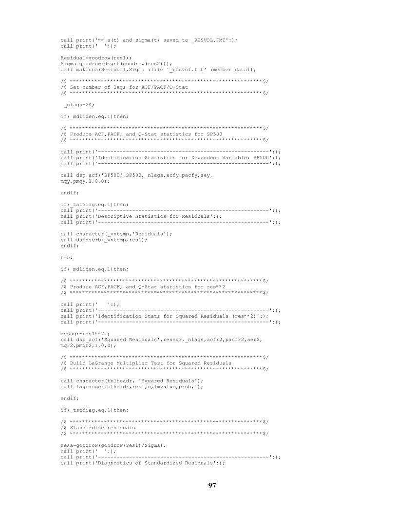
97

call print('** a(t) and sigma(t) saved to _RESVOL.FMT':); call print(' ':); Residual=goodrow(res1); Sigma=goodrow(dsqrt(goodrow(res2))); call makesca(Residual,Sigma :file '_resvol.fmt' :member data1); /$ **************************************************************$/ /$ Set number of lags for ACF/PACF/Q-Stat /$ **************************************************************$/ _nlags=24; if(_mdliden.eq.1)then; /$ **************************************************************$/ /$ Produce ACF,PACF, and Q-Stat statistics for SP500 /$ **************************************************************$/ call print('-------------------------------------------------------':); call print('Identification Statistics for Dependent Variable: SP500':); call print('-------------------------------------------------------':); call dsp_acf('SP500',SP500,_nlags,acfy,pacfy,sey, mqy,pmqy,1,0,0); endif; if(_tstdiag.eq.1)then; call print('-------------------------------------------------------':); call print('Descriptive Statistics for Residuals':); call print('-------------------------------------------------------':); call character(_vntemp,'Residuals'); call dspdscrb(_vntemp,res1); endif; n=5; if(_mdliden.eq.1)then; /$ **************************************************************$/ /$ Produce ACF,PACF, and Q-Stat statistics for res**2 /$ **************************************************************$/ call print(' ':); call print('-------------------------------------------------------':); call print('Identification Stats for Squared Residuals (res**2)':); call print('-------------------------------------------------------':); ressqr=res1**2.; call dsp_acf('Squared Residuals',ressqr,_nlags,acfr2,pacfr2,ser2, mqr2,pmqr2,1,0,0); /$ **************************************************************$/ /$ Build LaGrange Multiplier Test for Squared Residuals /$ **************************************************************$/ call character(tblheadr, 'Squared Residuals'); call lagrange(tblheadr,res1,n,lmvalue,prob,1); endif; if(_tstdiag.eq.1)then; /$ **************************************************************$/ /$ Standardize residuals /$ **************************************************************$/ resa=goodrow(goodrow(res1)/Sigma); call print(' ':); call print('-------------------------------------------------------':); call print('Diagnostics of Standardized Residuals':);

98

call print('-------------------------------------------------------':); call character(_vntemp,'Standardized Residuals'); call dspdscrb(_vntemp, resa); /$ **************************************************************$/ /$ Compute ACF, PACF, Q-stats for residuals in 1st moment model /$ **************************************************************$/ call character(_vntemp,'Standardized Residuals'); call dsp_acf(_vntemp,resa,_nlags,acfa,pacfa,sea, mqa,pmqa,1,0,0); /$ **************************************************************$/ /$ Square standardized residuals of 1st moment model /$ **************************************************************$/ resb=resa**2.; call print(' ':); call print('-------------------------------------------------------':); call print('Diagnostics of Squared Standardized Residuals':); call print('-------------------------------------------------------':); /$ **************************************************************$/ /$ Compute ACF, PACF, Q-stats for squared standardized residuals /$ **************************************************************$/ call character(_vntemp,'Squared Standardized Residuals'); call dsp_acf(_vntemp,resb,_nlags,acfb,pacfb,seb, mqb,pmqb,1,0,0); /$ **************************************************************$/ /$ Build LaGrange Multiplier Test /$ **************************************************************$/ call character(tblheadr,'Squared Standardized Residuals'); call lagrange(tblheadr,resa,n,lmvalue,prob,1); endif; ishowgrf=0; call grfgarch('SP500 ',SP500 ,res1,Sigma,_nlags,ishowgrf); b34srun;

99

10.5 SCAB34S script for GARCH-M Model (Section 4.2.2)

b34sexec matrix; call echooff; call getsca('Findat01.mad' :mad :member SP500); call load(dsp_acf 'C:\b34slm\wbsuppl.mac'); call load(dspgarch 'C:\b34slm\wbsuppl.mac'); call load(grfgarch 'C:\b34slm\wbsuppl.mac'); call load(garchf :staging); call print('-------------------------------------------------------':); call print('Analysis Performed on Variable: SP500':); call print('Model: GARCH-M , Diagnostics: ON, Graphs: ON':); call print('Data Span for Analysis: 1, 792':); call print('-------------------------------------------------------':); /$ **************************************************************$/ /$ Set span for time series: SP500 /$ **************************************************************$/ iorigins=integers(1, 792); SP500 = SP500(iorigins); xvnames=c1array(1:); xvnames(1)='SP500 '; _mdliden=1; _tstdiag=1; call dspdscrb('SP500',SP500); /$ **************************************************************$/ /$ Use mean/variance for CONSTANT starting values in model /$ **************************************************************$/ YMean=Mean(SP500); YSigma2=Variance(SP500-YMean); /$ **************************************************************$/ /$ Specify and estimate GARCH model /$ **************************************************************$/ call garchest(res1, res2, SP500,func,1,nbad :cparms array(:YMean, YSigma2) :garorder idint(array(:1)) :gmaorder idint(array(:1)) :muorder idint(array(:0)) :nosqrt :maxfun 1000 :maxg 1000 :maxit 1000 :ngood 15 :print3); idist=-1; iDFEst=0; call dspgarch(4,idist,iDFEst,norows(SP500 ),%nparm,xvnames,res1 res2,%coef,%se,%t,%cname,%corder,%nar,%nma,%ngar,%ngma,%nmu, %con,%func,%n_iter,%n_func,%n_grad,%nt_drop,%h_cond,%hessian); /$ **************************************************************$/ /$ Make the res1 and res2 even length /$ **************************************************************$/ _sqrmat=array(dmax1(norows(res1),norows(res2)),2:); _sqrmat(,1)=res1; _sqrmat(,2)=res2; _sqrmat =goodrow(_sqrmat); res1=_sqrmat(,1); res2=_sqrmat(,2); call print('** a(t) and sigma(t) saved to _RESVOL.FMT':);

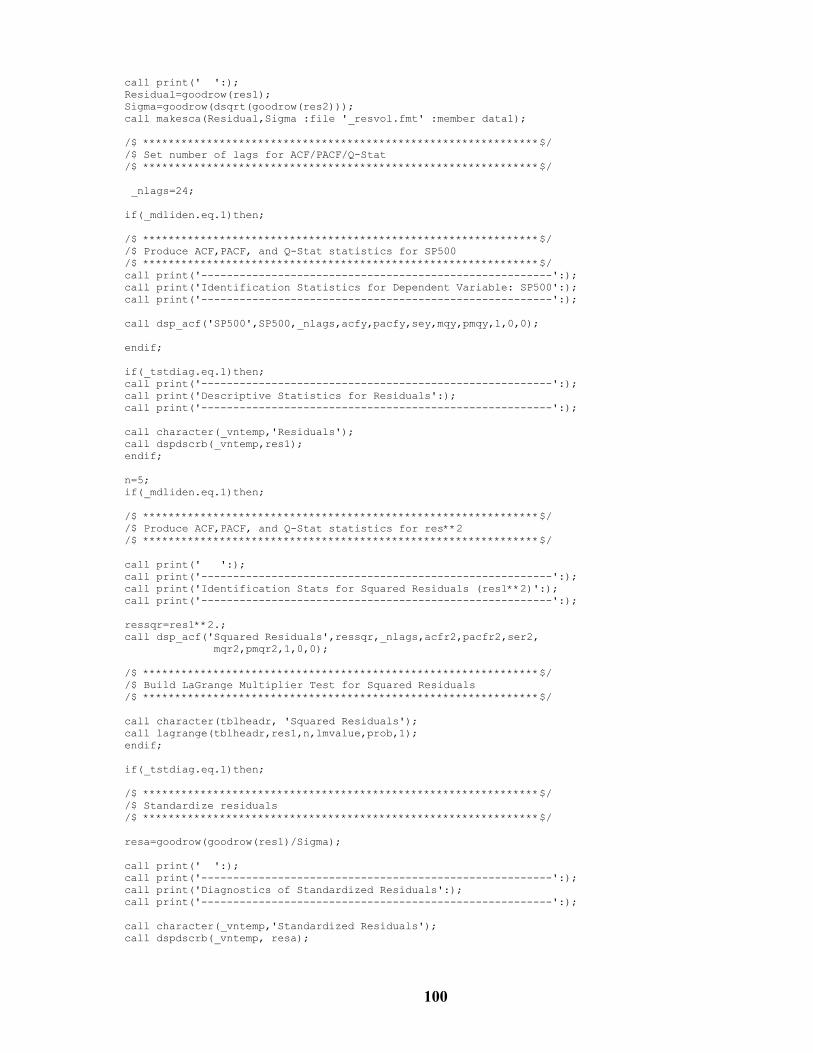
100

call print(' ':); Residual=goodrow(res1); Sigma=goodrow(dsqrt(goodrow(res2))); call makesca(Residual,Sigma :file '_resvol.fmt' :member data1); /$ **************************************************************$/ /$ Set number of lags for ACF/PACF/Q-Stat /$ **************************************************************$/ _nlags=24; if(_mdliden.eq.1)then; /$ **************************************************************$/ /$ Produce ACF,PACF, and Q-Stat statistics for SP500 /$ **************************************************************$/ call print('-------------------------------------------------------':); call print('Identification Statistics for Dependent Variable: SP500':); call print('-------------------------------------------------------':); call dsp_acf('SP500',SP500,_nlags,acfy,pacfy,sey,mqy,pmqy,1,0,0); endif; if(_tstdiag.eq.1)then; call print('-------------------------------------------------------':); call print('Descriptive Statistics for Residuals':); call print('-------------------------------------------------------':); call character(_vntemp,'Residuals'); call dspdscrb(_vntemp,res1); endif; n=5; if(_mdliden.eq.1)then; /$ **************************************************************$/ /$ Produce ACF,PACF, and Q-Stat statistics for res**2 /$ **************************************************************$/ call print(' ':); call print('-------------------------------------------------------':); call print('Identification Stats for Squared Residuals (res1**2)':); call print('-------------------------------------------------------':); ressqr=res1**2.; call dsp_acf('Squared Residuals',ressqr,_nlags,acfr2,pacfr2,ser2, mqr2,pmqr2,1,0,0); /$ **************************************************************$/ /$ Build LaGrange Multiplier Test for Squared Residuals /$ **************************************************************$/ call character(tblheadr, 'Squared Residuals'); call lagrange(tblheadr,res1,n,lmvalue,prob,1); endif; if(_tstdiag.eq.1)then; /$ **************************************************************$/ /$ Standardize residuals /$ **************************************************************$/ resa=goodrow(goodrow(res1)/Sigma); call print(' ':); call print('-------------------------------------------------------':); call print('Diagnostics of Standardized Residuals':); call print('-------------------------------------------------------':); call character(_vntemp,'Standardized Residuals'); call dspdscrb(_vntemp, resa);

101

/$ **************************************************************$/ /$ Compute ACF, PACF, Q-stats for residuals in 1st moment model /$ **************************************************************$/ call character(_vntemp,'Standardized Residuals'); call dsp_acf(_vntemp,resa,_nlags,acfa,pacfa,sea,mqa,pmqa,1,0,0); /$ **************************************************************$/ /$ Square standardized residuals of 1st moment model /$ **************************************************************$/ resb=resa**2.; call print(' ':); call print('-------------------------------------------------------':); call print('Diagnostics of Squared Standardized Residuals':); call print('-------------------------------------------------------':); /$ **************************************************************$/ /$ Compute ACF, PACF, Q-stats for squared standardized residuals /$ **************************************************************$/ call character(_vntemp,'Squared Standardized Residuals'); call dsp_acf(_vntemp,resb,_nlags,acfb,pacfb,seb,mqb,pmqb,1,0,0); /$ **************************************************************$/ /$ Build LaGrange Multiplier Test /$ **************************************************************$/ call character(tblheadr,'Squared Standardized Residuals'); call lagrange(tblheadr,resa,n,lmvalue,prob,1); endif; ishowgrf=0; call grfgarch('SP500 ',SP500 ,res1,Sigma,_nlags,ishowgrf); b34srun;

102

10.6 SCA script for Regression +GARCH Using Automatic Two-pass (Section 4.3.1)

==ALLMACRO ASSIGN FILE 12. EXTERNAL 'Findat01.mad'. CALL M_IBMLN2. FILE IS 12. CALL ANALYSIS STOP ==ANALYSIS SELECT IBMLN. SPAN IS (1,888). IDEN IBMLN. IARIMA IBMLN. NAME IS MOMENT1. @ HOLD RESID(RES). TSMODEL MOMENT1. ADD (0, 1, 2)SPLN . IESTIM MOMENT1. HOLD DIST(NS). PRESERVE ARMA. IARIMA NS. REPLACE MOMENT1. ESTIMATE MOMENT1. HOLD RESID(RES). ACF RES. RES2=RES**2 IDEN RES2. IARIMA RES2. NAME MOMENT2. FSAVE IBMLN, RES, RES2. FILE 'GARCHRES.FSV'. @ DATASET DATA. REWIND. . . . The commands related to building graphics in SCAB34S omitted here for brevity. It is . a common script that will be presented later in this section. . . RETURN

103

10.7 SCAB34S script for Regression plus GARCH Using the One-pass (Section 4.3.2)

b34sexec matrix; call echooff; call getsca('Findat01.mad' :mad :member M_IBMLN2); call load(dsp_acf 'C:\b34slm\wbsuppl.mac'); call load(dspgarch 'C:\b34slm\wbsuppl.mac'); call load(grfgarch 'C:\b34slm\wbsuppl.mac'); call load(garchf :staging); call print('-------------------------------------------------------':); call print('Analysis Performed on Variable: IBMLN':); call print('Model: GARCH , Diagnostics: ON, Graphs: ON':); call print('Data Span for Analysis: 1, 888':); call print('-------------------------------------------------------':); /$ **************************************************************$/ /$ Set span for time series: IBMLN /$ **************************************************************$/ iorigins=integers(1, 888); IBMLN = IBMLN(iorigins); SPLN = SPLN(iorigins); xvnames=c1array(1:); xvnames(1)='SPLN'; _mdliden=1; _tstdiag=1; call dspdscrb('IBMLN',IBMLN); /$ **************************************************************$/ /$ Use OLS to get starting values for parameters in model /$ **************************************************************$/ call olsq(IBMLN SPLN{0} ); /$ **************************************************************$/ /$ Specify and estimate GARCH model /$ **************************************************************$/ call garchest(res1, res2, IBMLN,func,1,nbad :xvar SPLN array(:%coef(1)) idint(array(:0)) idint(array(:1)) :cparms array(:%coef(2),%resvar) :garorder idint(array(:1)) :gmaorder idint(array(:1)) :print3); idist=-1; iDFEst=0; call dspgarch(2,idist,iDFEst,norows(IBMLN ),%nparm,xvnames,res1 res2,%coef,%se,%t,%cname,%corder,%nar,%nma,%ngar,%ngma,%nmu, %con,%func,%n_iter,%n_func,%n_grad,%nt_drop,%h_cond,%hessian); /$ **************************************************************$/ /$ Make the res1 and res2 even length /$ **************************************************************$/ _sqrmat=array(dmax1(norows(res1),norows(res2)),2:); _sqrmat(,1)=res1; _sqrmat(,2)=res2; _sqrmat =goodrow(_sqrmat); res1=_sqrmat(,1); res2=_sqrmat(,2);

104

call print('** a(t) and sigma(t) saved to _RESVOL.FMT':); call print(' ':); Residual=goodrow(res1); Sigma=goodrow(dsqrt(goodrow(res2))); call makesca(Residual,Sigma :file '_resvol.fmt' :member data1); /$ **************************************************************$/ /$ Set number of lags for ACF/PACF/Q-Stat /$ **************************************************************$/ _nlags=24; if(_mdliden.eq.1)then; /$ **************************************************************$/ /$ Produce ACF,PACF, and Q-Stat statistics for IBMLN /$ **************************************************************$/ call print('-------------------------------------------------------':); call print('Identification Statistics for Dependent Variable: IBMLN':); call print('-------------------------------------------------------':); call dsp_acf('IBMLN',IBMLN,_nlags,acfy,pacfy,sey,mqy,pmqy,1,0,0); endif; if(_tstdiag.eq.1)then; call print('-------------------------------------------------------':); call print('Descriptive Statistics for Residuals':); call print('-------------------------------------------------------':); call character(_vntemp,'Residuals'); call dspdscrb(_vntemp,res1); endif; n=5; if(_mdliden.eq.1)then; /$ **************************************************************$/ /$ Produce ACF,PACF, and Q-Stat statistics for res**2 /$ **************************************************************$/ call print(' ':); call print('-------------------------------------------------------':); call print('Identification Stats for Squared Residuals (res1**2)':); call print('-------------------------------------------------------':); ressqr=res1**2.; call dsp_acf('Squared Residuals',ressqr,_nlags,acfr2,pacfr2,ser2, mqr2,pmqr2,1,0,0); /$ **************************************************************$/ /$ Build LaGrange Multiplier Test for Squared Residuals /$ **************************************************************$/ call character(tblheadr, 'Squared Residuals'); call lagrange(tblheadr,res1,n,lmvalue,prob,1); endif; if(_tstdiag.eq.1)then; /$ **************************************************************$/ /$ Standardize residuals /$ **************************************************************$/ resa=goodrow(goodrow(res1)/Sigma); call print(' ':);

105

call print('-------------------------------------------------------':); call print('Diagnostics of Standardized Residuals':); call print('-------------------------------------------------------':); call character(_vntemp,'Standardized Residuals'); call dspdscrb(_vntemp, resa); /$ **************************************************************$/ /$ Compute ACF, PACF, Q-stats for residuals in 1st moment model /$ **************************************************************$/ call character(_vntemp,'Standardized Residuals'); call dsp_acf(_vntemp,resa,_nlags,acfa,pacfa,sea,mqa,pmqa,1,0,0); /$ **************************************************************$/ /$ Square standardized residuals of 1st moment model /$ **************************************************************$/ resb=resa**2.; call print(' ':); call print('-------------------------------------------------------':); call print('Diagnostics of Squared Standardized Residuals':); call print('-------------------------------------------------------':); /$ **************************************************************$/ /$ Compute ACF, PACF, Q-stats for squared standardized residuals /$ **************************************************************$/ call character(_vntemp,'Squared Standardized Residuals'); call dsp_acf(_vntemp,resb,_nlags,acfb,pacfb,seb,mqb,pmqb,1,0,0); /$ **************************************************************$/ /$ Build LaGrange Multiplier Test /$ **************************************************************$/ call character(tblheadr, 'Squared Standardized Residuals'); call lagrange(tblheadr,resa,n,lmvalue,prob,1); endif; ishowgrf=0; call grfgarch('IBMLN ',IBMLN ,res1,Sigma,_nlags,ishowgrf); b34srun;

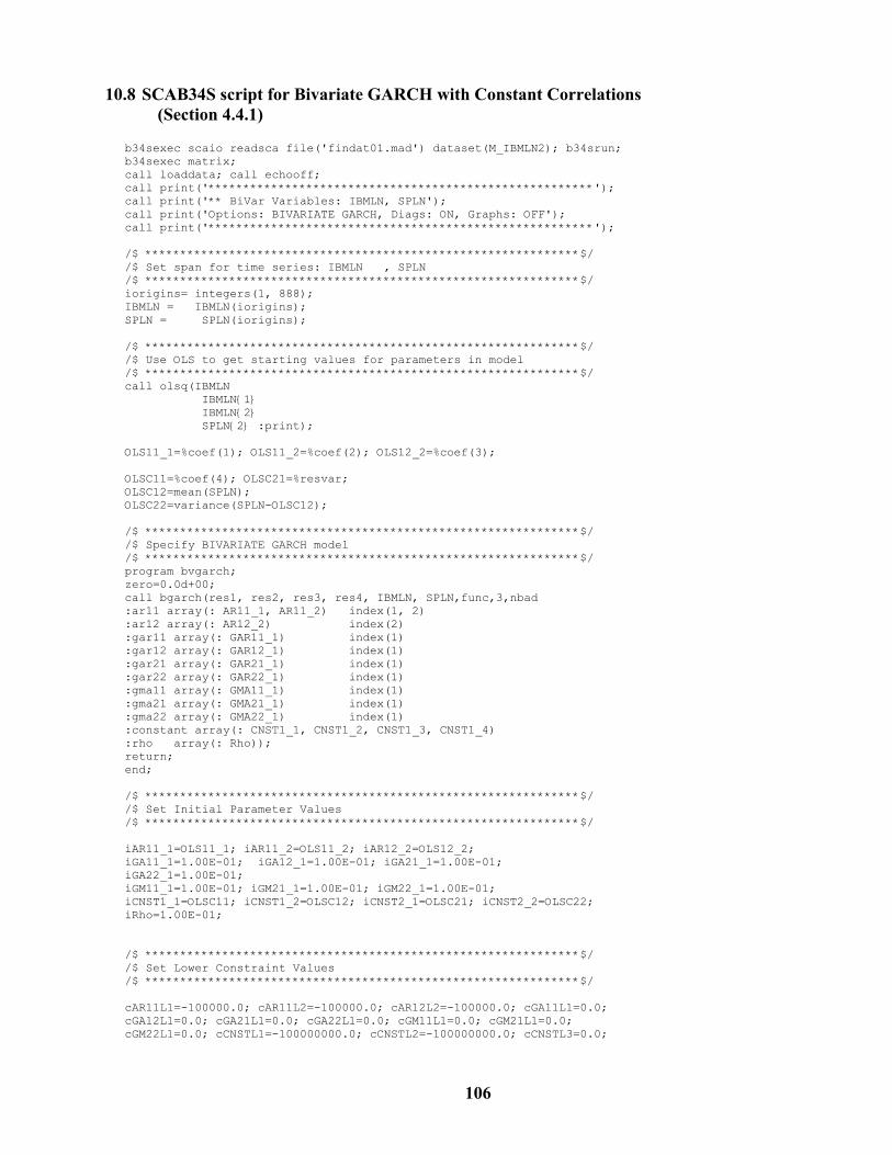
106

10.8 SCAB34S script for Bivariate GARCH with Constant Correlations (Section 4.4.1)

b34sexec scaio readsca file('findat01.mad') dataset(M_IBMLN2); b34srun; b34sexec matrix; call loaddata; call echooff; call print('*******************************************************'); call print('** BiVar Variables: IBMLN, SPLN'); call print('Options: BIVARIATE GARCH, Diags: ON, Graphs: OFF'); call print('*******************************************************'); /$ **************************************************************$/ /$ Set span for time series: IBMLN , SPLN /$ **************************************************************$/ iorigins= integers(1, 888); IBMLN = IBMLN(iorigins); SPLN = SPLN(iorigins); /$ **************************************************************$/ /$ Use OLS to get starting values for parameters in model /$ **************************************************************$/ call olsq(IBMLN IBMLN{1} IBMLN{2} SPLN{2} :print); OLS11_1=%coef(1); OLS11_2=%coef(2); OLS12_2=%coef(3); OLSC11=%coef(4); OLSC21=%resvar; OLSC12=mean(SPLN); OLSC22=variance(SPLN-OLSC12); /$ **************************************************************$/ /$ Specify BIVARIATE GARCH model /$ **************************************************************$/ program bvgarch; zero=0.0d+00; call bgarch(res1, res2, res3, res4, IBMLN, SPLN,func,3,nbad :ar11 array(: AR11_1, AR11_2) index(1, 2) :ar12 array(: AR12_2) index(2) :gar11 array(: GAR11_1) index(1) :gar12 array(: GAR12_1) index(1) :gar21 array(: GAR21_1) index(1) :gar22 array(: GAR22_1) index(1) :gma11 array(: GMA11_1) index(1) :gma21 array(: GMA21_1) index(1) :gma22 array(: GMA22_1) index(1) :constant array(: CNST1_1, CNST1_2, CNST1_3, CNST1_4) :rho array(: Rho)); return; end; /$ **************************************************************$/ /$ Set Initial Parameter Values /$ **************************************************************$/ iAR11_1=OLS11_1; iAR11_2=OLS11_2; iAR12_2=OLS12_2; iGA11_1=1.00E-01; iGA12_1=1.00E-01; iGA21_1=1.00E-01; iGA22_1=1.00E-01; iGM11_1=1.00E-01; iGM21_1=1.00E-01; iGM22_1=1.00E-01; iCNST1_1=OLSC11; iCNST1_2=OLSC12; iCNST2_1=OLSC21; iCNST2_2=OLSC22; iRho=1.00E-01; /$ **************************************************************$/ /$ Set Lower Constraint Values /$ **************************************************************$/ cAR11L1=-100000.0; cAR11L2=-100000.0; cAR12L2=-100000.0; cGA11L1=0.0; cGA12L1=0.0; cGA21L1=0.0; cGA22L1=0.0; cGM11L1=0.0; cGM21L1=0.0; cGM22L1=0.0; cCNSTL1=-100000000.0; cCNSTL2=-100000000.0; cCNSTL3=0.0;

107

cCNSTL4=0.0; cRhoL1=-100000.0; /$ **************************************************************$/ /$ Set Upper Constraint Values /$ **************************************************************$/ cAR11U1=100000.0; cAR11U2=100000.0; cAR12U2=100000.0; cGA11U1=100000.0; cGA12U1=100000.0; cGA21U1=100000.0; cGA22U1=100000.0; cGM11U1=100000.0; cGM21U1=100000.0; cGM22U1=100000.0; cCNSTU1=100000000.0; cCNSTU2=100000000.0; cCNSTU3=100000000.0; cCNSTU4=100000000.0; cRhoU1=100000.0; /$ **************************************************************$/ /$ Call CMAXF2 non-linear solver /$ **************************************************************$/ call cmaxf2(func :name bvgarch :parms AR11_1 AR11_2 AR12_2 GAR11_1 GAR12_1 GAR21_1 GAR22_1 GMA11_1 GMA21_1 GMA22_1 CNST1_1 CNST1_2 CNST1_3 CNST1_4 Rho :ivalue array(:iAR11_1, iAR11_2, iAR12_2, iGA11_1, iGA12_1, iGA21_1, iGA22_1, iGM11_1, iGM21_1, iGM22_1, iCNST1_1, iCNST1_2, iCNST2_1, iCNST2_2, iRho) :lower array(: cAR11L1, cAR11L2, cAR12L2, cGA11L1, cGA12L1, cGA21L1, cGA22L1, cGM11L1, cGM21L1, cGM22L1, cCNSTL1, cCNSTL2, cCNSTL3, cCNSTL4, cRhoL1) :upper array(: cAR11U1, cAR11U2, cAR12U2, cGA11U1, cGA12U1, cGA21U1, cGA22U1, cGM11U1, cGM21U1, cGM22U1, cCNSTU1, cCNSTU2, cCNSTU3, cCNSTU4, cRhoU1) :maxfun 400 :maxg 400 :maxit 400 :ngood 15 :print); b34srun;

108

10.9 SCAB34S script for Bivariate GARCH with Time-varying Correlations (Section 4.4.2)

b34sexec scaio readsca file('findat01.mad') dataset(M_IBMLN2); b34srun; b34sexec matrix; call loaddata; call echooff; call print('*******************************************************'); call print('** BiVar Variables: IBMLN, SPLN'); call print('Options: BIVARIATE GARCH, Diags: ON, Graphs: OFF'); call print('*******************************************************'); /$ **************************************************************$/ /$ Set span for time series: IBMLN , SPLN /$ **************************************************************$/ iorigins=integers(1, 888); IBMLN = IBMLN(iorigins); SPLN = SPLN(iorigins); /$ **************************************************************$/ /$ Use OLS to get starting values for parameters in model /$ **************************************************************$/ call olsq(IBMLN IBMLN{1} SPLN{2} :print); OLS11_1=%coef(1); OLS12_2=%coef(2); OLSC11=%coef(3); OLSC21=%resvar; OLSC12=mean(SPLN); OLSC22=variance(SPLN-OLSC12); /$ **************************************************************$/ /$ Allocate rho array for time varying corr. model /$ **************************************************************$/ rho = array(norows(IBMLN):) + .5 ; /$ **************************************************************$/ /$ Specify BIVARIATE GARCH model /$ **************************************************************$/ program bvgarch; zero=0.0d+00; call bgarch(res1, res2, res3, res4, IBMLN, SPLN,func,3,nbad :ar11 array(: AR11_1) index(1) :ar12 array(: AR12_2) index(2) :gar11 array(: GAR11_1) index(1) :gar12 array(: GAR12_1) index(1) :gar21 array(: GAR21_1) index(1) :gar22 array(: GAR22_1) index(1) :gma11 array(: GMA11_1) index(1) :gma21 array(: GMA21_1) index(1) :gma22 array(: GMA22_1) index(1) :constant array(: CNST1_1, CNST1_2, CNST1_3, CNST1_4) :rho array(: TVRho_1, TVRho_2, TVRho_3) :tvrho rho); return; end; /$ **************************************************************$/ /$ Set Initial Parameter Values /$ **************************************************************$/ iAR11_1=8.00E-02; iAR12_2=-7.00E-02; iGA11_1=8.70E-01; iGA12_1=1.00E-02; iGA21_1=1.00E-02; iGA22_1=9.20E-01; iGM11_1=8.00E-02; iGM21_1=4.00E-02; iGM22_1=5.00E-02; iCNST1_1=1.40E+00; iCNST1_2=7.00E-01; iCNST2_1=2.95E+00; iCNST2_2=2.05E+00; iTVRho_1=-2.00E+00; iTVRho_2=3.00E+00; iTVRho_3=1.00E-01;

109

/$ **************************************************************$/ /$ Set Lower Constraint Values /$ **************************************************************$/ cAR11L1=-100000.0; cAR12L2=-100000.0; cGA11L1=0.0; cGA12L1=0.0; cGA21L1=0.0; cGA22L1=0.0; cGM11L1=0.0; cGM21L1=0.0; cGM22L1=0.0; cCNSTL1=-100000000.0; cCNSTL2=-100000000.0; cCNSTL3=0.0; cCNSTL4=0.0; cRhoL1=-50.0; cRhoL2=0.0; cRhoL3=0.0; /$ **************************************************************$/ /$ Set Upper Constraint Values /$ **************************************************************$/ cAR11U1=100000.0; cAR12U2=100000.0; cGA11U1=100000.0; cGA12U1=100000.0; cGA21U1=100000.0; cGA22U1=100000.0; cGM11U1=100000.0; cGM21U1=100000.0; cGM22U1=100000.0; cCNSTU1=100000000.0; cCNSTU2=100000000.0; cCNSTU3=100000000.0; cCNSTU4=100000000.0; cRhoU1=0.0; cRhoU2=100.0; cRhoU3=1.0; /$ **************************************************************$/ /$ Call CMAXF2 non-linear solver /$ **************************************************************$/ call cmaxf2(func :name bvgarch :parms AR11_1 AR12_2 GAR11_1 GAR12_1 GAR21_1 GAR22_1 GMA11_1 GMA21_1 GMA22_1 CNST1_1 CNST1_2 CNST1_3 CNST1_4 TVRho_1 TVRho_2 TVRho_3 :ivalue array(:iAR11_1, iAR12_2, iGA11_1, iGA12_1, iGA21_1, iGA22_1, iGM11_1, iGM21_1, iGM22_1, iCNST1_1, iCNST1_2, iCNST2_1, iCNST2_2, iTVRho_1, iTVRho_2, iTVRho_3) :lower array(: cAR11L1, cAR12L2, cGA11L1, cGA12L1, cGA21L1, cGA22L1, cGM11L1, cGM21L1, cGM22L1, cCNSTL1, cCNSTL2, cCNSTL3, cCNSTL4, cRhoL1, cRhoL2, cRhoL3) :upper array(: cAR11U1, cAR12U2, cGA11U1, cGA12U1, cGA21U1, cGA22U1, cGM11U1, cGM21U1, cGM22U1, cCNSTU1, cCNSTU2, cCNSTU3, cCNSTU4, cRhoU1, cRhoU2, cRhoU3) :maxfun 400 :maxg 400 :maxit 400 :ngood 15 :print); b34srun;

110

11. A DISCUSSION OF THE MCCULLOUGH – RENFRO GARCH BENCHMARK

STUDY

McCullough - Renfro (1998) used the Bollerslev-Gysel (1996) study of the Deutschemark / British pound

exchange rate as a test case to study a number of unnamed programs. Depending on the setup, there were quite

substantial differences between what answers the programs produced. The model used for the study was:

20 1 1 1 1

t t

t t t

y e

h e h

µ

α α β− −

= +

= + +

We report the McCullough-Renfo (1998) results for Software 1 ~ Software 7 and compare their findings

to our results that are referenced under Package as B34S 1 ~ B34S 4, RATS 1 ~ RATS 2.

GARCH estimates using various programs and starting Values Coefficients t-values Package µ

0α 1α 1β µ 0α 1α 1β Function

Software-1 Software-2 Software-3 Software-4 Software-5 Software-6 Software-7

-.00540 -.00608 -.00624 -.00619 -.00613 -.00919 -.00619

.0096

.0098

.0108

.0108

.0107

.0098

.0108

.142

.144

.153

.152

.153

.144

.153

.821

.818

.806

.806

.806

.818

.806

-0.64 -0.72 -0.74 -0.74 -0.73 -1.08 -0.66

8.01 3.80 8.13 8.15 5.58 8.09 1.66

11.09 5.80

10.95 10.97 7.91

10.77 2.86

53.83 26.34 48.64 48.61 36.96 45.90 11.12

na na na na na na na

B34S-1 B34S-2 B34S-3 B34S-4

-.00552 -.00552 -.00592 -.00621

.0097

.0097

.0133

.0108

.142

.142

.176

.153

.821

.821

.774

.806

-0.70 -0.66 -0.69 -0.72

4.99 4.82 4.18 5.48

7.70 8.71 6.58 8.00

37.56 39.31 22.90 37.02

710.1083 710.1083 702.0017 706.6837

RATS-1 RATS-2

-.00553 -.00553

.0097

.0097 .143 .143

.820

.820 -0.66 -0.66

8.05 3.78

11.09 5.70

53.55 26.07

710.2189 710.2189

The results for Software 1 ~ Software 7 were taken directly from McCullough - Renfro (1998).

0 1 1B34S 1 assumes initialized to zero and , var( ), .01, .5t th x a x xµ α β− = = − = =

0 1 1B34S 2 assumes initialized to zero and .016427, .221130, .35, .5th µ α α β− = − = = =

0 1 1B34S 3 assumes initialized to 1.0 and .016427, .221130, .35, .5th µ α α β− = − = = = 2B34S 4 assumes /t th x N− =∑ 0 1 1and .016427, .221130, .35, .5µ α α β= − = = =

RATS-1 Uses Rats and BHHH method. For detail see code setup below

RATS-2 Uses Rats and BFGS method. For detail see code setup below

The results from B34S-2 differ from B34S-1 only in the fact that the McCullough - Renfro (1998) starting

values are used. While the coefficients and functional value are the same as B34S-1, the t-values are slightly

different. The RATS results from RATS-1 and RATS-2 have the same setup in all respects but uses a different

estimation method. The results from B34S-1, B34S-2, RATS-1 and RATS-2 produce virtually the same

coefficients and functional value. The BHHH method (Berndt, Hall, Hall and Hausman) of estimation

111

produced significant t scores at least two times those found for the BFGS (Broyden, Fletcher, Goldfarb and

Shanno) method. What is striking is the effect of the method of estimation on the estimated t-values.

The results from B34S-3 and B34S-4, while using the same starting values as B34S-2, experiment with

initializing 0.0th = and ht = 2 /tx N∑ respectively. The results from B34S-4 produce coefficients very close

to what was found by Software-3. The results from B34S-3 suggest that initializing 1.0th = is a bad idea

since the initial value of ht or h1 would never change during the estimation process. Consequently, by setting

the initial values to 1.0, the final result may become biased.

Since the results from B34S-1 use computed starting values, excluding the test cases, it is probably the

most appropriate approach. The apparent instability of the estimated coefficient µ is most likely due to the

fact that all estimated models, regardless of software used, indicate that the coefficient µ is not statistically

significant.

To test B34S against the other programs various assumptions were made concerning starting values. The

B34S-1 test run sets ht =0.0 and 0 1 1, var( ), .01, .5tx a x xµ α β= = − = = while test runs RATS-1 and

RATS-2 employ the same problem with RATS using the BHHH (Berndt, Hall, Hall and Hausman) and BFGS

(Broyden, Fletcher, Goldfarb and Shanno) methods respectively.

The basic setup for B34S-1, RATS-1 and RATS-2 is contained in the GARCH6 procedure of the

MATRIX.MAC file (distributed with the SCAB34S product) which provides test problems for all B34S

MATRIX commands.

GARCH modeling has been shown to be a special case of the more general class of maximization models.

While in many cases the models can be estimated using the two pass method, in some cases the models require

joint estimation. Three methods of doing joint estimation were shown with the easiest being the GARCHEST

command. In the next chapter we turn to generalized nonlinear least squares capabilities.

112

REFERENCES

Bollerslev, T "Generalized Autoregressive Conditional Heteroscedasticity," Journal of Econometrics, 31 (1986), 307-327.

Bollerslev, T and E. Ghysels, "Periodic Autoregressive Conditional Heteroscedasticity," Journal of Business

and Economic Statistics, 14 (1996), 139-151. Enders, Walter. Applied Economic Time Series. New York, John Wiley, 1995, 2004. Engle, Robert. “Autoregressive Conditional Heteroscedasticity with Estimates of the Variance of United

Kingdom Inflation.” Econometrica, 55 (July 1982), 987-1007. Engle, Robert. ARCH Selected Readings. U. K. Oxford University Press 1995 Fiorentini, Gabriele and Giorgio Calzolari and Lorenzo Panattoni, "Analytic Derivatives and the Computation

of GARCH Estimates," Journal of Applied Econometrics 11 (1996), 399-417. Glosten, L., R. Jagannathan, and D. Runkle. "On the Relation between the Expected Value and the Volatility

of the Nominal Excess Return on Stocks." Journal of Finance 48 (1993): 1779-1801. Greene, William. Economic Analysis, ed 4., New Jersey, Prentice Hall, 2000. Hanke, John and Arthur Reitsch. Business Forecasting, ed. 6, New Jersey, Prentice Hall, 1998. Judd, Kenneth. Numerical Methods in Economics, MIT Press, Cambridge, MA, 1998. Liu, Lon-Mu Time Series Analysis and Forecasting, Illinois, Scientific Computing Associates Corporation

(2005) McCullough, B. D and Charles Renfro. "Benchmarks and software standards: A case study of GARCH

procedures," Journal of Economic and Social Measurement 25 (1998), 59-71 Nelson, Daniel. "Conditional Heteroskedasticity in Asset Returns: A New Approach." Econometrics 59(2)

(1991): 347-70. Sinai, Allen and Houston H. Stokes, "Real Money Balances: An Omitted Variable From the Production

Function," Review of Economics and Statistics 54, no. 3 (August 1972): 290-296. Sinai, Allen and Houston H. Stokes, "Money and the Production Function: A Reply to Boyes and Kavanaugh,"

Review of Economics and Statistics 63, no. 2 (May 1981): 313-318. Stokes, Houston H. Specifying and Diagnostically Testing Econometric Models, ed. 2. New York, Quorum

Books, 1997 Stokes, Houston H. 'Chapter 16: Programming in the Matrix Command," in Specifying and Diagnostically Testing Econometric Models Volume II. in manuscript form 2002. Tsay, R.S., Analysis of Financial Time Series, New York, John Wiley, 2002.