GENERAL ARTICLE Physics of a Particle on a Rotating Hoop

GENERAL ARTICLE

Physics of a Particle on a Rotating Hoop∗

Experiment and Theory

Kushal Lodha, Anushree Roy and Sayan Kar

Kushal Lodha is a fifth year

undergraduate student in the

Integrated M.Sc. (Physics)

programme at IIT

Kharagpur.

Anushree Roy and Sayan Kar

are faculty members in the

Department of Physics, IIT

Kharagpur.

The simple textbook problem of a particle on a vertical, ro-

tating hoop is analysed both in theory and through exper-

iments. We begin by detailing out a somewhat generalised

theory, where the effect of dry friction as well as the possibil-

ity of a shift in the vertical axis of rotation are incorporated.

The bifurcation curves (plots of the angular position of stabil-

ity versus the angular frequency of rotation) are obtained for

all cases (i.e. with and without friction and a shift of the axis).

Thereafter we present the experimental set-up fabricated by

us and elaborate on the various measurements performed.

Finally, we demonstrate through our experiments how well

the theoretical results on the bifurcation curves tally with the

experimental findings. The match between theory and exper-

iment is found to be reasonably satisfactory. We conclude

by mentioning how various aspects of this simple problem as

well as its generalisations and extensions, are linked with dif-

ferent advanced areas of physics.

1. Introduction

Among the chapter-end problems given in Chapter 2 of the fa-

mous textbook on Classical Mechanics by Goldstein [1] (now by

Goldstein, Poole and Safko) we find the problem of a particle on

a rotating hoop. The same system is also discussed in detail, in

many texts on nonlinear dynamics, for example, in the book by

Strogatz [2]. It is quite amazing how this rather simple problem

has attracted the attention of many students and teachers over the Keywords

Classical mechanics, bifurcation

curves.last several decades. In addition, as we note at the end of our ar-

ticle, this problem and its generalisations can serve as a starting

∗Vol.25, No.9, DOI: https://doi.org/10.1007/s12045-020-1044-5

RESONANCE | September 2020 1261

GENERAL ARTICLE

point to many anWe take a re-look at the

physics of a particle on a

rotating hoop, both

theoretically and

experimentally.

advanced concept in physics.

In this article, we plan to take a re-look at the physics of a particle

on a rotating hoop, both theoretically and experimentally. The

theory is well-known. But actual experiments are few in number.

Moreover, the theory we outline later, is somewhat recent and the

experiment, as well as its comparison with theory has never been

attempted. In that sense, though simple, our results are indeed

new.

One of our primary objectives in this work is to verify experimen-

tally, a general relation between the equilibrium points and a con-

trol parameter of a given system, known as a bifurcation curve.

As the name suggests,One of our primary

objectives in this work is

to verify experimentally,

a general relation

between the equilibrium

points and a control

parameter of a given

system, known as a

bifurcation curve.

a bifurcation curve for a system, through

its nature, would demonstrate a notable, qualitative change in the

location of the equilibrium points, with gradual variation in a cho-

sen control parameter of the system. In addition, we also inves-

tigate the role of other variables and parameters in modifying the

functional nature (qualitative as well as quantitative) of the bifur-

cation curves, particularly in the context of our problem.

In the rest of the article, we have the following section-wise plan.

In the next section, we discuss the physics, the bifurcation dia-

gram and how the presence of dry friction and a shift of the axis

of rotation, can change the known results. Thereafter, in Sec-

tion 3, we discuss the set-up and the measurement techniques. In

Section 4, we look at theory versus experiment. As promised be-

fore, Section 5 looks at the connection of this problem with other

advanced areas of physics. We conclude with some remarks in

Section 6.

2. The Problem and its Physics

Let us begin by briefly recalling the problem. We have a spheri-

cal mass m (assumed a point mass) free to slide on a vertical ring.

Without anything else, this is the same as the problem of a pen-

dulum (not the simple pendulum) or a particle on a circle. We

now set the ring rotating at an angular speed ω about the vertical

axis passing through the centre. This problem of a particle on

1262 RESONANCE | September 2020

GENERAL ARTICLE

a rotating hoop/ring has a bunch of novelties. Firstly, one notes

that there is a critical frequency ω0 =

√

g

R(here g is the accel-

eration due to gravity and R is the radius of the ring). Above

ω0, i.e. for ω > ω0, the effective potential in the problem has a

double-well character. But for ω ≤ ω0, we have the usual single

well. In other words, one expects that for frequencies larger than

ω0, the particle can climb up from its position at the bottom of

the ring and stay put at a θ value which is different from θ = 0.

The various parameters and other details/conventions are shown

in Figure 1. In our work, In our work, we will

incorporate two

additional features: (a)

we will ask what

happens when we shift

the vertical axis of

rotation away from the

centre of the ring, (b) we

will also include the

effect of dry friction.

we will incorporate two additional

features: (a) we will ask what happens when we shift the verti-

cal axis of rotation away from the centre of the ring, (b) we will

also include the effect of dry friction. Including these additional

features, we will introduce the notion of a bifurcation curve for

this problem. Recall that a bifurcation curve in general plots the

equilibrium points versus a control parameter. In our problem,

the equilibrium points are the angles at which the ball is stable

on the rotating hoop, while the chosen control parameter is the

angular frequency of rotation of the hoop. The bifurcation curve

for our system does show a ‘bifurcation’ (more precisely known

as a ‘pitchfork bifurcation’), because the plot is not just a simple

monotonous curve but exhibits a change in nature at or around

a specific value of the angular frequency and beyond. We will

compare the modified bifurcation curves with those without shift

of the axis and/or dry friction.

Let us now move on to describing the mathematical formulation

of the problem.

2.1 Equations of Motion, Effective Potentials

The Lagrangian of the system without shift of the axis (in Figure

1) or dry friction is given as:

L =1

2mR2θ

2 +1

2mR2ω

2 sin2θ + mgR cos θ,

=1

2mR2θ

2 −

[

−mgR cos θ −1

2mR2ω

2 sin2θ

]

, (1)


GENERAL ARTICLE

Figure 1. Ball rotating off

the axis.

where θ is the angle coordinate (see Figure 1), R is the radius

of the hoop, ω the frequency of rotation and g the acceleration

due to gravity. One can extract the effective potential from the

Lagrangian above by simply writing

Ve f f (θ) = −mgR cos θ −1

2mR2ω

2 sin2θ. (2)

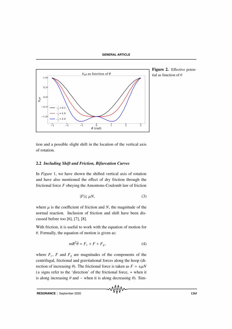
An analysis of the extrema of the effective potential reveals the

interesting fact that they are different for the two cases ω > ω0

and ω ≤ ω0. The graphs for the potentials are shown in Figure 2.

We notice that for ω > ω0 we have a double well, as mentioned

before, while for ω ≤ ω0 we have a single well potential.

To account for the finite size of the spherical mass (ball) m, we

replace the radius (R) by the distance from the centre of the hoop

to the centre of mass of the ball (Rcm).

One can also write down and solve the equations of motion for θ

exactly, in terms of Jacobian elliptic functions [5] but we are not

interested in that here. Instead, we try and see how some realistic

features can be included in the problem by incorporating dry fric-


GENERAL ARTICLE

Figure 2. Effective poten-

tial as function of θ

−3 −2 −1 0 1 2 3θ (rad)

−1.0

−0.5

0.0

0.5

1.0

V eff

Veff as function of θ

ω2

ω20=0.1

ω2

ω20=1.0

ω2

ω20=2.0

tion and a possible slight shift in the location of the vertical axis

of rotation.

2.2 Including Shift and Friction, Bifurcation Curves

In Figure 1, we have shown the shifted vertical axis of rotation

and have also mentioned the effect of dry friction through the

frictional force F obeying the Amontons-Coulomb law of friction

|F|≤ µN, (3)

where µ is the coefficient of friction and N, the magnitude of the

normal reaction. Inclusion of friction and shift have been dis-

cussed before too [6], [7], [8].

With friction, it is useful to work with the equation of motion for

θ. Formally, the equation of motion is given as:

mR2θ = Fc + F + Fg, (4)

where Fc, F and Fg are magnitudes of the components of the

centrifugal, frictional and gravitational forces along the hoop (di-

rection of increasing θ). The frictional force is taken as F = ±µN

(± signs refer to the ‘direction’ of the frictional force, + when it

is along increasing θ and − when it is along decreasing θ). Sim-


GENERAL ARTICLE

plifying the equation of motion we get

θ =

[

ω

2(

sin θ +a

R

)

cos θ

]

−[

ω

20 sin θ

]

±

[

µ

(

ω

20 cos θ + ω2

(

a

R+ sin θ

)

sin θ

)]

, (5)

=

[

ω

2 sin θ cos θ − ω20 sin θ +

(

a

Rω

2 ± µω20

)

cos θ (6)

±µω2 a

Rsin θ ± µω2 sin2

θ

]

.

In the R.H.S of the first equation above, the contributions of the

three terms corresponding to the centrifugal force, the gravita-

tional force and the frictional force are each shown within sepa-

rate square brackets. The effect of shift appears in the replace-

ment of sin θ by sin θ + aR

in all terms related to the centrifugal

force contributions.

θ = 0 corresponds to equilibrium at θ = θc. It leads to the fol-

lowing expression for ω2±, which has been nicely obtained in the

papers by Burov and collaborators [6].

ω

2± = ω

20

∓µ cos θc + sin θc

( aR+ sin θc)(±µ sin θc + cos θc)

. (7)

The above relations yield the bifurcation curves, which are plots

of the equilibrium position θc as a function of ωω0

. Note that these

expressions are not invertible, i.e. one cannot write θc as a func-

tion of ω.

If a < 0, the shift is in the opposite direction by an amount |a|.

One can check from Eqn.(7) and Figure 3, that the a > 0 and

a < 0 bifurcation curves are obtainable from each other through a

reflection about the ωω0

axis. In other words, with a < 0 and θc →

−θc, one finds ω+ → ω− and ω− → ω+. Thus, the functional

form of ω+ in Eqn. (7) (for a > 0) matches with the functional

form of ω− with a < 0 and θc → −θc. Later, when we match with

experiments, we will plot ω+ as a function |θc| (i.e. the magnitude

of θc).

Without friction or a shift of the axis, the bifurcation curve is just


GENERAL ARTICLE

an inverse cosine function ofω

20

ω

2 . It is given as:

ω

20

ω

2= cos θc, (8)

for ω > ω0. The curve demonstrates a ‘bifurcation’ at ω = ω0

–known in nonlinear dynamics as the pitchfork bifurcation. How-

ever, with friction and a = 0 the bifurcation seems to happen near

frequencies smaller in value than the ω0 mentioned above. With

µ and a both non-zero, the bifurcation curve still has differences

with the µ = 0, a 6= 0 curves. We observe some of these features

in our experiments later.

In summary, as stated In summary, as stated

just above, in the

presence of shift and

friction the overall shape

of the bifurcation curve

changes in a quantitative

sense.

just above, in the presence of shift and

friction the overall shape of the bifurcation curve changes in a

quantitative sense. Further, there are now two values for ω, i.e.

ω± and hence two bifurcation curves corresponding to the fric-

tional force being F = +µN and F = −µN. The region between

these two curves is in accordance with the Amontons-Coulomb

friction law which says |F|≤ µN.

Typical bifurcation curves for a 6= 0, µ 6= 0 and for a 6= 0, µ = 0,

a = 0, µ 6= 0, a = 0, µ = 0 are shown in Figure 3. When either µ

or a are non-zero, differences arise which are evident from these

curves.

2.3 What we Hope to See in the Experiments

In our experiment, In our experiment, we

intend to verify the

bifurcation curves

obtained in the previous

section. In particular,

with friction and a shift

of the rotation axis, we

would like to see how

good a match between

theory and experiment (a

result not shown

anywhere yet in the

literature on this

problem) is possible.

we intend to verify the bifurcation curves

obtained in the previous section. In particular, with friction and a

shift of the rotation axis, we would like to see how good a match

between theory and experiment (a result not shown anywhere yet

in the literature on this problem) is possible. We have measured

θc as a function of ω. The ‘upper sign’ (plus) is used while fitting

the bifurcation curves. In other words, we use the expression for

ω

2+ in Eqn. (7).

In addition, we have independently measured the coefficient of

friction µ, in order to verify its fitted value, as obtained from the

analysis of the bifurcation curves.


GENERAL ARTICLE

Figure 3. Theoretical bi-

furcation curves for (a) a =

0 (b) a > 0 (c) a < 0 with

the dotted line representing

the case for µ = 0. For

µ 6= 0, the curve splits into

two branches– the red and

black curves represent these

branches,ω+ andω− respec-

tively.

A video-clip (Link [13]) of our set-up in action is provided along

with this article. The rise of the ball on the rotating hoop, beyond

a certain value of the angular frequency of rotation may easily be

noted while viewing the video. In particular, one also notices that

the rise of the ball seems to begin at a value of ω which is smaller

in value than ω0 =

√

g

R(hear the beep at ω0 while the video

is played). Later, in this article, we will record this fact in our

experiments and show similar results from the related quantitative

measurements (bifurcation curves) we have performed.

3. Experimental set-up and measurements

3.1 Setup

The designed setup is shown in Figure 4. Different parts are

marked by alphabets A-H and are discussed below. The circular

hoop (A), made of aluminum, is of radius ≈ 17.8 ± 0.1 cm with

a U-shaped cross-section of width 2.78 ± 0.01 cm and height of


https://drive.google.com/file/d/1yRkIjniB93Q_GLf5oo-4cuy54oU72LNA/view?usp=sharing

GENERAL ARTICLE

Figure 4. Experimental

setup. All parts, discussed in

the text, are marked.

2.20 ± 0.01 cm. A spherical ball (B) with a low coefficient of

static friction is allowed to roll in the groove of the hoop. The

diameter and mass of the ball are 2.46 ± 0.01 cm and 60 ±1 gm,

respectively. Here we state that the error bars quoted just above

correspond to the least counts of the instruments used for the mea-

surements. For example, a meter scale was used to measure the

diameter of the hoop, a slide caliper to measure the diameter of

the ball and a simple electronic weighing machine to measure the

weight of the ball. The material of the ball is unknown to us

(collected from a Christmas decoration shop). The surface of the

ball appears quite smooth and the ball could roll freely along the

groove of the hoop. For our experimental requirements we mea-

sured the coefficient of static friction between the ball and hoop,

independently. We will discuss this measurement later.

The hoop is connected to an aluminum supporting unit (Figure 4

and in Figure 5 (a) ). To shift the axis of the hoop with respect

to the axis of rotation, the following arrangement has been made.

Holes (M, N, O, P, X and Y) are bored on a plate C1 and block

C2 (see Figure 5(a) and (b)). While C1 can be attached to the


GENERAL ARTICLE

aluminum supporting unit of the hoop using screws and nuts (at

J and K in Figure 5(b)), the lower part C2 is connected to the

axle shaft, which is driven by a 12 Volt DC motor (D in Figure

4 and 5(a)). Both components, C1 and C2, can be assembled in

different settings. When holes M, N, O, P, X and Y of both plates

(see Figure 5 (b)) are set onto each other and fixed, the hoop is

expected to rotate about its axis. The holes on each side of the

center of the plates are separated by ∼ 1 cm. To introduce a shift

of ∼+1, ∼+2 cm between the axis of rotation and the centre of

the hoop, C1 and C2 were fixed keeping the hole O of C1 on

the hole M of C2, and the hole X of the plate C1 on the hole

M of the block C2, respectively. Similarly, the plates could be

adjusted to have a relative shift in the opposite direction. The gear

motor (D) has a gear ratio of 60:1. The whole assembly is placed

on a base, made of a perspex sheet (E in Figure 4 and Figure

5). The base is equipped with levelling screws. These adjustable

screws and a spirit level are used to ensure that the base of the

setup is horizontal. A gear-shaped aluminum disk (F in Figure

4 and also see Figure 5(c)) with 64 cogs is sandwiched between

the motor and the block C2 with screws and nuts. The disk F

rotates between a LED and photo-detector, set in a perpendicular

direction of a plane of the hoop (see Figure 5(c)) and the whole

unit is used as a tachometer.

A 14 MP camera (SJ4000) (H in Figure 4) with a pixel dimension

of 4032×3024 is fitted at the top of the hoop to have an overhead

view of the ball. It is a wireless camera that can record a video

for about an hour at 60 frames per second. A simple stopwatch is

used to synchronize the video time-step with inputs applied at the

frequency controller.

A separate setup (see Figure 5(d)) is used to measure the coef-

ficient of static friction between the ball and the material of the

hoop. It consists of a clamp holder holding a rod (wooden pencil).

One end of two threads are connected to two ends of a wooden

plank and the other ends to two sides of the rod (see Figure 5(d)).

The plank holds a U-shaped aluminium piece (of the same ma-

terial as of the hoop) that allows the free movement of the ball.


GENERAL ARTICLE

Figure 5. (a) Part of the

setup to hold the hoop and

to provide a required shift

between the axis of rotation

and the centre of the hoop.

(b) Arrangement of holes on

the plate C1 and the block

C2. (c) Arrangement to de-

tect the rotational frequency

(d) Set up to measure the co-

efficient of static friction be-

tween the ball and the hoop.

Using clamp holder one can vary the inclination and thus mea-

sure the coefficient of static friction. The measured coefficient of

static friction is 0.04±0.01. The measurement procedure will be

discussed later in Section 3.2.3.

3.2 Measurements

There are three different measurements which we have carried out

in order to obtain the relevant information for plotting the bifurca-

tion curves. These measurements are discussed in the following

subsections.

3.2.1 Measurement of the angular frequency of the hoop

The revolutions per minute (rpm) of the DC motor is controlled

by a motor-driver. The motor driver is driven by an external pulse-

width-modulated signal from an Atmel A89S52 micro-controller

chip. The desired rpm is sent as a digital signal to the chip us-

ing a set-reset key. Recall that the disk F along with a LED and


GENERAL ARTICLE

photo-detector set (G in Figure4 and also see Figure 5 (b)), ar-

ranged in the perpendicular to the plane of the hoop, is used as a

tachometer. When the photo-detector is illuminated by the LED

it converts a light signal to a voltage. As the disc F rotates, the

cogs obstruct the photo-detector at regular intervals. The periodic

light signal, thus produced, is passed through an ADC (Analog to

Digital converter) and yields a digital signal. This signal is fed

to a microprocessor to compute the angular frequency. Since the

disc F has 64 cogs, for N×64 pulses in a minute, the micropro-

cessor measures N rpm. The advantage of this technique is the

following: ideally, one can change the frequency of rotation of

the hoop with a step of 1/64 rpm.

3.2.2 Measurement of the inclination of the ball

The wireless camera, H in Figure 4, placed at the top of the hoop,

is used to measure the position of the ball in the hoop while we

change the frequency of the rotation of the hoop. It records a

video starting from the powering of the motor to switching off

the motor. Thus, the whole video carries the information of the

positions of the ball in the hoop at all frequency steps. The video

is processed using an OpenCV code [3].

The code primarily does two tasks

1. Detects the ball and determines the centre of the ball.

2. Correlates pixel length to the inclination (θ) of the ball with re-

spect to the centre of the hoop.

For the first part, the code splits the full video frame-by-frame

(one of such frames is shown in Figure 6(a)). Each frame is com-

posed of pixels, which have RGB (Red-Green-Blue) attributes.

RGB is a common colour model to quantify colours in colour

photos or in computer display. A bandpass filter is constructed

which allows only a certain range of RGB values correspond-

ing to colour of the ball. Pixels which pass through this filter

are marked as white whereas rejected pixels are marked as black.

This filter converts the frame into a binary image (Figure 6(b)).


GENERAL ARTICLE

Figure 6. Conversion of

RGB image into binary by

means of the bandpass filter.

Application of erosion and dilation filter removes any small blobs

that may be left by the bandpass filter. Using a combination of

Canny Edge detector and Hough Circle Transform, the ball is de-

tected by fitting an equation of a circle, (x−a)2+(y−b)2 = r2, with

parameters a, b and r. These parameters, for each position of the

ball, are saved to files for further processing. It is to be noted that

the coordinates of the ball, thus obtained, are expressed in pixels,

and they do not correspond to physical units. With the change in

inclination of the ball in the hoop, the coordinates of the ball are

displaced by a certain pixel length.

The second task involves correlating the apparent shift in pixels

to physical coordinates by applying triangle similarity rule using

the focal length of the camera lens and the diameter of the hoop.

The measured value of the inclination is quite accurate for a lower

angle of inclination, however it deviates from the true value for

larger angles.


GENERAL ARTICLE

Figure 7. Schematic di-

agram for the principle of

measuring the static friction

between the ball and the

hoop.

3.2.3 Measurement of static coefficient of friction between

the ball and the hoop

The measurement is based on a simple technique, conceptually

thought of by da Vinci and, later furthered by Amontons and

Coulomb.

Our purpose, in doing this experiment, is to check the value of

µ obtained later from the main experiment, using an alternative

route.

If the coefficient of friction between a ball and a plane (refer to

Figure 7) is µ, the magnitude of the maximum force ( fmax) of

friction is given by the equation as fmax = µN, where, N is the

magnitude of the normal force between two bodies. If φ is the an-

gle of tilt of the plane (with respect to the horizontal axis), when

the ball just starts to slide from its rest position, then the coeffi-

cient of friction µ = tan(φ). In contrast, if the ball rolls down (no

sliding) we know the result as µ ≥ 27

tan φ [10], which leads to the

well-known fact that µ for pure rolling is less than that for µ for

pure sliding.

In our experiment, we slowly increase the inclination of the plane

by adjusting the clamp holder and carefully notice when the ball

just starts to move. The inclination is estimated by measuring

the height by which the plank is raised (y) and the length of the

plank (x) using a slide caliper. Thus, if the ball slides down, the


GENERAL ARTICLE

Figure 8. Bifurcation curve

when the hoop rotates about

its axis.

expected value of µ = tan(φ) = y/x=0.04±0.01. If the ball rolls

down, our result from this experiment would then be µ ≥ 0.01 ±

0.01.

Here we would like to mention that we did not make any special

effort to disentangle the effect of rolling friction from that sliding

friction while carrying out the above experiment. The expected

value of µ between the ball and hoop is thus µ ≥ 0.01 or µ =

.04 (for pure sliding). As we shall see later, these values do not

contradict the µ obtained in the main experiment.

4. Theory Versus Experiment

We are now ready to draw the final bifurcation curves. Refer

to Figure 1. We allow the hoop to rotate at a given frequency

(ω) and then measure the inclination (|θc|) of the ball from the

vertical axis. We demonstrate a possible match between theory

and experiment for the various cases with different shifts between

the axis of the hoop and the axis of rotation (a values in Section

2.2).

For calibration of the setup, we begin with ω vs. θ measurements

by keeping the axis of the rotation of the hoop the same as that of

the axis of the hoop, i.e. for one to one correspondence between


GENERAL ARTICLE

all holes in C1 and C2, see Figure 5(b). The data-points in Figure

8 show the measured data for a bifurcation curve.

The best fit (red solid line) to the data points with Eqn. 7 could

be obtained for the values of R= 16.2 ± 0.2 cm, µ=0.042 ± 0.004

and a=0 with the value of χ2 as 0.008. Here the error bars corre-

spond to the standard deviation of the parameters, obtained from

the fitting procedure. We note the following: (i) Recall that the

radius of the hoop is R=17.8±0.1 cm. Taking the correction for

finite size of the ball (i.e. beyond point mass approximation), the

effective radius of the hoop is expected to be Rcm=16.6±0.1 cm,

which is close to the fitted value (16.2±0.2 cm) obtained above.

(ii) The value of µ for the best fit to the data points is close to the

measured value of sliding friction (µ = 0.04 ± 0.01). The blue

dashed line in Figure 8 is the plot for µ=0 in Eqn. 7. Comparing

with the theoretical bifurcation plot in Figure 3, it can be seen

that we have shown the experimental data points in the range of

0.7 < ω/ω0 < 1.1 where ω0 ≈ 7.77 rad/s. In this region the

effect of friction is maximum. Note that both dashed line (with-

out friction) and solid line (fitted to the experimental data points)

nearly merge for higher values of θ. We consider the results ob-

tained from the bifurcation curve in Figure 8 as a calibration of

the setup and use the estimated values of R and µ to study the bi-

furcation curves with a given offset between the axis of rotation

and the axis of the hoop. Here we would also like to mention that

to observe the effect of friction in the dynamics of the ball, we al-

lowed the ball to slide in the U-shaped groove of the hoop, rather

than on the edge, as reported in [7].

The symbols in the bifurcation curves in Figure 9(a) and (b) plot

the data points when the axis of rotation of the hoop and the axle

of the motor is shifted mechanically by +1 cm and -1 cm, re-

spectively. Similarly Figure 9 (c) and (d) plot the same for the

shift between the two by +2 cm and -2 cm. As the holes in the

plates C1 and C2 in Figure 5(b) are hand-drilled, these offset val-

ues (∼ ±1 or ∼ ±2) may not be accurate. Thus, while fitting the

experimental data points using Eqn. 7 we kept a as a free fit-

ting parameter. The values of R and µ are kept fixed to the above


GENERAL ARTICLE

Figure 9. Bifurcation

curves for offset axes. The

shift between the axis of the

hoop and axis of rotation are

(a) a= +1 cm, (b) a= -1 cm,

(c) a= +2 cm and (d) a= -

2 cm in the setup. + (with

closed symbol) and – (with

open symbol) correspond to

right and left offset of the

axis of rotation. The cor-

responding fitted curves are

shown by red and blue solid

lines. The fitted value of

a± (standard deviation), ob-

tained from the fitting pro-

cedure, is mentioned in each

panel. The dashed curves in

each figure is the fitted bifur-

cation curve from Figure 8

for a=0.

mentioned values obtained from the calibration curve in Figure

8. The best fit to the data points are shown by solid lines for (a)

+a=1.21 ±0.05 cm, (b) −a=1.18±0.06 cm, (c) a=2.00 ±0.06 cm

and (d) −a=1.79 ±0.06 cm. The fitted curves match the experi-

mental data points fairly well for 0.15 ≤ θ ≤ 0.65. Here we would

like to mention that as θ is a complicated function of ω, we used

ω as dependent variable to fit data points in Figure 8 and Figure

9 using Eqn. 7. However, to keep the similarity between theoret-

ically and experimentally obtained bifurcation plots, we reversed

the axes in these figures.


GENERAL ARTICLE

5. Connecting the Problem with Other Areas of Physics

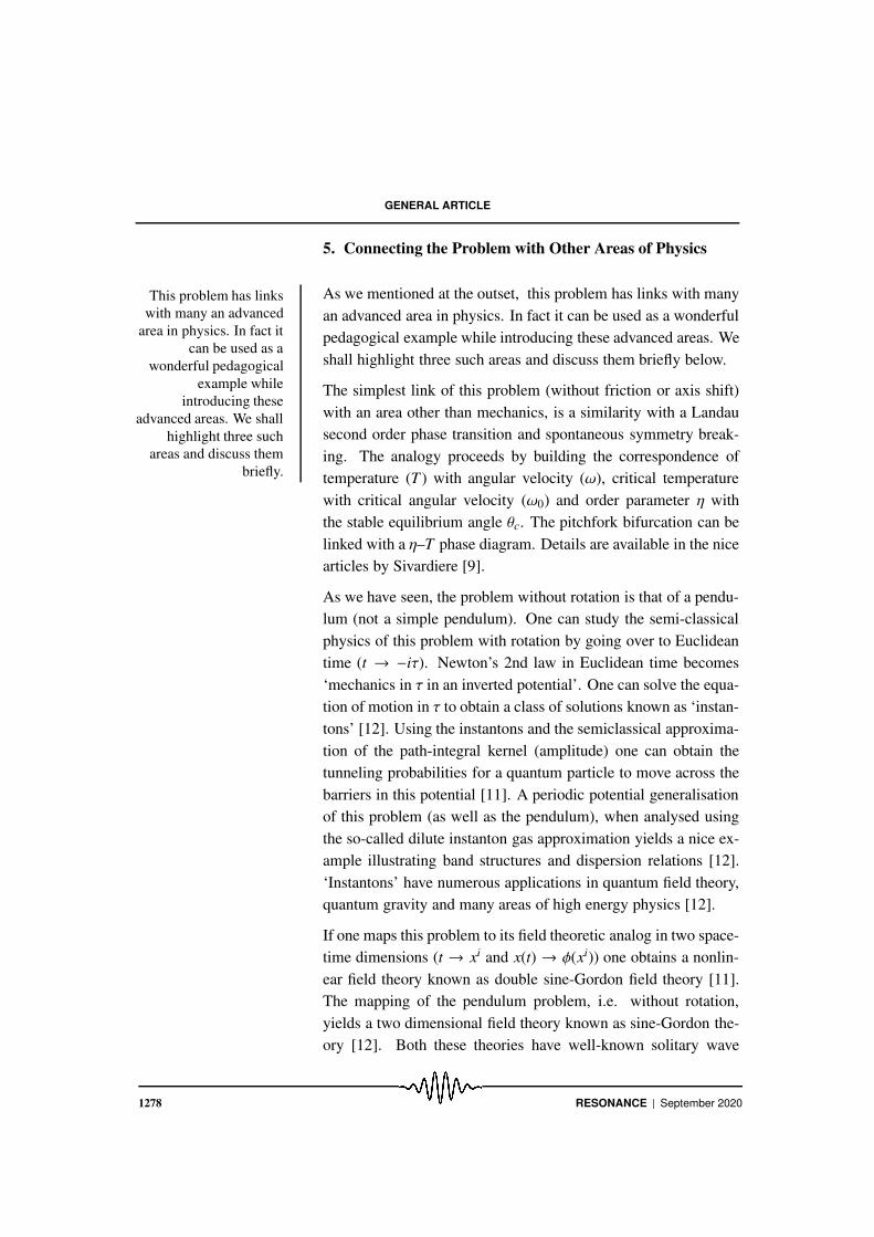
As we mentioned at the outset,This problem has links

with many an advanced

area in physics. In fact it

can be used as a

wonderful pedagogical

example while

introducing these

advanced areas. We shall

highlight three such

areas and discuss them

briefly.

this problem has links with many

an advanced area in physics. In fact it can be used as a wonderful

pedagogical example while introducing these advanced areas. We

shall highlight three such areas and discuss them briefly below.

The simplest link of this problem (without friction or axis shift)

with an area other than mechanics, is a similarity with a Landau

second order phase transition and spontaneous symmetry break-

ing. The analogy proceeds by building the correspondence of

temperature (T ) with angular velocity (ω), critical temperature

with critical angular velocity (ω0) and order parameter η with

the stable equilibrium angle θc. The pitchfork bifurcation can be

linked with a η–T phase diagram. Details are available in the nice

articles by Sivardiere [9].

As we have seen, the problem without rotation is that of a pendu-

lum (not a simple pendulum). One can study the semi-classical

physics of this problem with rotation by going over to Euclidean

time (t → −iτ). Newton’s 2nd law in Euclidean time becomes

‘mechanics in τ in an inverted potential’. One can solve the equa-

tion of motion in τ to obtain a class of solutions known as ‘instan-

tons’ [12]. Using the instantons and the semiclassical approxima-

tion of the path-integral kernel (amplitude) one can obtain the

tunneling probabilities for a quantum particle to move across the

barriers in this potential [11]. A periodic potential generalisation

of this problem (as well as the pendulum), when analysed using

the so-called dilute instanton gas approximation yields a nice ex-

ample illustrating band structures and dispersion relations [12].

‘Instantons’ have numerous applications in quantum field theory,

quantum gravity and many areas of high energy physics [12].

If one maps this problem to its field theoretic analog in two space-

time dimensions (t → xi and x(t) → φ(xi)) one obtains a nonlin-

ear field theory known as double sine-Gordon field theory [11].

The mapping of the pendulum problem, i.e. without rotation,

yields a two dimensional field theory known as sine-Gordon the-

ory [12]. Both these theories have well-known solitary wave


GENERAL ARTICLE

solutions, which represent coherent structures born out of non-

linearity. Such solitary waves behave like ‘particles’ .The more

special dispersion-less propagation happens for ‘solitons’ which

exist in sine-Gordon but not in double sine-Gordon theory. The

sine-Gordon and double sine-Gordon solitons and solitary waves

have been studied quite extensively in theory as well as in exper-

iments over many years and are still of reasonable interest today.

Broadly, solitons are widely used in condensed matter physics

and optics too.

6. Concluding Remarks

We summarize below our results and what we have been able to

show in this work.

We have analysed a simple text-book problem in classical me-

chanics both experimentally and theoretically. The theory has

been around in the literature–we have re-written the essential de-

tails in a simpler way. Subsequently, we have fabricated the set-

up and used it for experiments. The specific details of our set-up

as well as the methodology employed to carry out the observa-

tions have been outlined in full detail in this article. Though a

simple experiment there are many subtleties which need to be

taken into account and we have spelt out our procedures exten-

sively.

Through our experiments, we have We feel that given the

lack of mechanics

experiments in our

undergraduate

curriculum, his

experiment with

appropriate

modifications can

provide a good model

example, worth

introducing to younger

students within their

curriculum or through a

short-term project.

tried to verify the theoretical

findings – in particular the bifurcation curves in the presence of

shift and friction. We have succeeded in verifying the ω versus θc

relations over a reasonable range of ω and θc. This confirms, to

some extent, the validity of the theoretical formulae.

It is a fact that the set-up has many deficiences and our observa-

tion methods can be improved. However, within the limitations,

we believe that we have been able to provide a reasonable match

between theory and experiment in the context of this problem.

We also feel that given the lack of mechanics experiments in our

undergraduate curriculum, this experiment with appropriate mod-

ifications can provide a good model example, worth introducing


GENERAL ARTICLE

to younger students within their curriculum or through a short-

term project.

7. Acknowledgements

The authors thank Bikash Mondal in the Electronic Repair Sec-

tion and Goutam Mondal in the Mechanical Fabrication Section

of CWISS, IIT Kharagpur for their help and support in making

the set-up. They also thank Apoorva Sinha and Harmanjot Singh

Grewal for their participation in the initial stages of this work.

The motivational video attached with this article was recorded

and edited for our purposes by Suman Chatterjee. We thank him

and Anang Kumar Singh for their help in recording the video.

Suggested Reading

[1] H Goldstein, Classical Mechanics, 2nd Edition, Narosa Publishing House, New

Delhi, India (2001).

[2] S H Strogatz, Nonlinear Dynamics and Chaos, Perseus Books Publishing (1994),

p.55, p.61.

[3] A Rosebrock, Ball Tracking with OpenCV, PyImageSearch Blog, 2015.

[4] A Rosebrock, Measuring the size of objects in an image with OpenCV, PyIm-

ageSearch Blog, 2016.

[5] T E Baker and A Bill, Jacobi elliptic functions and a complete solution of the

bead on the hoop problem, American Journal of Physics, Vol.80, 506 2012.

[6] A A Burov, On bifurcations of relative equilibria of a heavy bead sliding with

dry friction on a rotating circle, Acta Mechanica, 212 (3-4), pp.349–354, 2010;

A A Burov and I a Yakushev, Bifurcations of the relative equilibria of a heavy

bead on a rotating hoop with dry friction, Journal of Applied Mathematica and

Mechanics, Vol.78, 460, 2014.

[7] L A Raviola, M E Veliz, H D Salomone, N A Olivieri and E E Rodrıguez, The

bead on a rotating hoop revisited: an unexpected resonance, European Journal

of Physics, Vol.38, p.015005, 2017.

[8] An interesting toy called the ‘Groove Tube’ was used to work on this problem.

Details are in the papers by R. V. Mancuso, A working mechanical model for

first and second order phase transitions and the cusp catastrophe, American

Journal of Physics, Vol.68, 271, 2000; R V Mancuso and G A Schrieber, An im-

proved apparatus for demonstrating first and second order phase transitions,

American Journal of Physics, Vol.73, 366, 2005.

[9] J Sivardiere, A simple mechanical model exhibiting spontaneous symmetry

breaking, American Journal of Physics, Vol.51, 1016, 1983.


https://www.pyimagesearch.com/2015/09/14/ball-tracking-with-opencv/

https://www.pyimagesearch.com/2016/03/28/measuring-size-of-objects-in-an-image-with-opencv/

GENERAL ARTICLE

[10] M Gottlieb and S Chandra, www.feynmanlectures.caltech.edu/info/exercises/

roll without slipping.html

Address for Correspondence

Sayan Kar

Department of Physics and

CTS

Indian Institute of Technology

Kharagpur 721302, India

[email protected]

[11] S Kar, An instanton approach to quantum tunneling for a particle on a rotat-

ing circle, Phys. Letts’., Vol.A 168, 179, 1992; S Kar and A Khare, Classical

and quantum mechanics of a particle on a rotating hoop, American Journal of

Physics, Vol.68, 1128, 2000.

[12] For a good and easy-going introduction to solitons and instantons see Chapters

2, 4 and 10 of R Rajaraman, Solitons and Instantons, North Holland (1987).

[13] https://drive.google.com/file/d/1yRkIjniB93Q GLf5oo-4cuy54oU72LNA/

view?usp=sharing


GENERAL ARTICLE Physics of a Particle on a Rotating Hoop

Documents

Transcript of GENERAL ARTICLE Physics of a Particle on a Rotating Hoop