Gene regulatory network inferencein human pathogenic fungi · flora, it can turn to an...
125
Gene regulatory network inference in human pathogenic fungi Dissertation zur Erlangung des akademischen Grades - doctor rerum naturalium - vorgelegt dem Rat der Biologisch-Pharmazeutischen Fakultät der Friedrich-Schiller-Universität Jena geschrieben von Dipl.-Bioinf. Robert Altwasser geboren am 06.07.1984 in Luckenwalde
-
Upload
vuongquynh -
Category
Documents
-
view
213 -
download
0
Transcript of Gene regulatory network inferencein human pathogenic fungi · flora, it can turn to an...
Gene regulatory network inference inhuman pathogenic fungi
Dissertationzur Erlangung des akademischen Grades
- doctor rerum naturalium -
vorgelegt dem Rat derBiologisch-Pharmazeutischen Fakultät der
Friedrich-Schiller-Universität Jena
geschrieben von Dipl.-Bioinf. Robert Altwassergeboren am 06.07.1984 in Luckenwalde

Diese Doktorarbeit wurde von den folgenden Personen begutachtet:
• Prof. Dr. Reinhard Guthke
• Prof. Dr. Marc Thilo Figge
• Dr. Ronald Westra
Die Dorktorarbeit wurde am 14. Januar 2015 verteidigt.
2

There is a single light of science, andto brighten it anywhere is tobrighten it everywhere.
Isaac Asimov
3


DanksagungIch möchte den Abschluss meiner Doktorarbeit nutzen, um mich bei den Menschen zubedanken, die meine Arbeit möglich gemacht haben. An erster Stelle steht hier Prof.Reinhard Guthke, welcher mir die Stelle angeboten, und mir die Werkzeuge in die Handgegeben hat, die vor mir liegenden Aufgaben zu meistern. Es war leicht ersichtlich dasich bei einem Menschenfreund arbeiten durfte, der sich ehrlich um das Wohlbefindenseiner Mitarbeiter bemüht.
Ich hätte diese Arbeit auch nicht bewältigen können, ohne die umfangreiche Unter-stützung meiner Arbeitsgruppe. Die lockere Arbeitsatmosphäre hat immer zu einemGelingen der Arbeit beigetragen. Insbesondere ist hier natürlich Jörg Linde zu er-wähnen, der mich während dieser Zeit betreut und angeleitet hat, was seine eigene Arbeitsicherlich nicht leichter gemacht hat. Bei Fabian Horn, der mich ein Jahr lang als Zim-merkollegen ertragen hat, möchte ich mich genauso bedanken wie bei Sebastian Vlaic,der mit mir zusammen Florida unsicher gemacht hat. Auch Eugen Fazius, der währendder ersten zwei Jahre um alle Hardware-Probleme gekümmert hat und auch sich auchsonst um eine gute Arbeitsatmosphäre bemüht hat, soll hier nicht unbedankt bleiben.Auch bei Dr. Vito Valiante, der die biologischen Experimente für mich durchgeführthat, möchte ich mich hiermit bedanken. Die anderen aktuellen und vergangen Kollegenwerde ich natürlich auch nicht vergessen, da sie ebenfalls Teil dieses Gesamtprojekts“Doktorarbeit” sind.
Da ich trotz allem Interesse an der Wissenschaft nicht umsonst arbeiten kann, möchteich mich bei der “Jena School for Microbial Communication (JSMC)” bedanken, diesowohl das Geld für mein Gehalt, als auch für meine Auslandseinsätzung und nötigenMaterialien zur Verfügung gestellt haben. Die Jenaer Graduierten-Akademie (JGA) botmir viele Kurse an, die mich sowohl fachlich weiterbrachten, als mir auch den Austauschmit andere Wissenschaftlern ermöglichten.
Natürlich wäre ich nicht hier, ohne meine Freunde und meine Familie, die in Gedankenimmer bei mir waren. Die seelisch-moralische Unterstützung war während der, nichtimmer leichten, Doktorarbeitszeit nötig, und soll hier daher nicht unerwähnt bleiben.
Bei allen Anderen, die in den letzten drei Jahren in mein Leben getreten sind, und michauf dem Weg zum Doktor begleitet haben aber hier noch nicht genannt wurden, möchteich mich nocheinmal bedanken. Diese Dokument ist nicht das Werk eines einzelnen,sondern das Ergebnis der Arbeit vieler.
5


Abstract
Pathogenic fungi are a serious threat to people with impeded immune system, especiallyduring organ transplantation and HIV infections. As the number of treatments thatinclude a weakening of the patients immune system increase, so does the number offungal infections. Often, the infection is opportunistic, meaning the pathogen alreadylives as a commensal in the host and uses the weak immune system to spread out andstarts to colonise different parts of the host. These infections can lead to systemic,life-threatening infections, lowering the survival rate of the often already weakened host.
Two of the most common human pathogens are Candida albicans andAspergillus fumigatus. While C. albicans is a commensal and part of the healthy humanflora, it can turn to an opportunistic pathogen, once the hosts immune system failsto contain it. Conidia of A. fumigatus are inhaled by humans every day and removedagain by the immune system. In a weakened host, A. fumigatus can colonise the lungof the host and spread to other parts of the body, which can lead to fatal results, if notreatment is administered.
The first part of this thesis aims to study the gene regulatory network of C. albicanson a genome-wide level, with a scale-free distribution of node degrees. These networkscan be used to identify genes with central regulatory functions, called hubs, which arepossible drug targets and can be the starting point for future studies. The modelingprocess included a large set of gene expression data measured by microarrays, the use ofprior knowledge and a automatically harvested gold standard for the evaluation of theresults. The final model is used to identify several hubs and is also able to reproducecurrent knowledge.
A focused small-scale gene regulatory network is inferred for A. fumigatus while it istreated with the clinically applied drug caspofungin. The chapter describes the processfrom mapping of the RNA-Seq data over the selection of candidate genes and the harvestof prior knowledge to the application of the NetGenerator tool. A network model of 26genes is tested for robustness against noise and used to identify a so far unknown cross-talk between to key regulators of major drug response pathways in A. fumigatus, whichcould be experimentally verified by the collaboration partner.
Both, the large- and the small-scale network inference are later compared to giveguidance on the correct application depending on the scientific question.
To further study the influence of drug treatment on A. fumigatus caspofungin treat-ment was paired with the use of humidimycin, which does not have antifungal propertieson its own, but seems to enhance the effect of caspofungin. Analysis of differential ex-pression and clustering revealed that the combination of the two drugs lowers the numberof differentially expressed genes in A. fumigatus, giving hints on how the enhancing effectof humidimycin works on the genetic level.
7


Zusammenfassung
Pathogene Pilze stellen eine ernste Bedrohung für Menschen mit geschwächtem Im-munsystem dar. Die betrifft insbesondere Menschen während Organtransplantationenund HIV-Infizierte. Mit der steigenden Anzahl von Behandlungen, bei denen eineSchwächung des Immunsystems einhergeht, steigt auch die Anzahl der Pilzinfektionen.Diese sind häufig opportunistisch, was bedeutet, das der Pathogen bereits als Nutznießerim Wirt lebt und ein geschwächtes Immunsystem nutzt, um sich auszubreiten. Dies kannzu systematischen, lebensbedrohenden Infektionen führen, welche die Überlebenswahr-scheinlichkeit des oft bereits geschwächten Wirts weiter senkt.
Zwei der am weitesten verbreiteten Pathogene sind Candida albicans undAspergillus fumigatus. Während C. albicans gewöhnlich als Teil der gesunden mensch-lichen Flora lebt, ohne Schaden anzurichten, kann es sich zu einem opportunistischemPathogen entwickeln, sobald das Immunsystem des Wirts ihn nicht mehr eindämmenkann. Sporen von A. fumigatus werden von Menschen jeden Tag eingeatmet und vomImmunsystem wieder entfernt. In einem geschwächtem Wirt kann A. fumigatus dieLunge besiedeln und sich auf andere Teile des Körpers ausbreiten. Ohne Behandlungkann dies tödliche Folgen für den Wirt haben.
Der erste Teil dieser Doktorarbeit zielt auf die Untersuchung der genregulatorischenNetzwerke von C. albicans auf genomweiter Ebene ab. Dabei wurden Netzwerke miteiner skalenfreien Verteilung der Kantengrade erzeugt. Diese Netzwerke können dafürverwendet werden, Gene mit zentraler regulatorischer Funktion zu identifizieren. Dieseso genannten Hubs sind mögliche Zielgene für Medikamente und können der Anfangfür zukünftige Studien sein. Die Modellierung enthält die Verwendung von Vorwissenund ein automatisch gesammelter Goldstandard zu Evaluierung der Ergebnisse. Dasendgültige Modell wird benutzt um verschiedene Hubs zu identifizieren und ist auch inder Lage, aktuelles Wissen wiederzugeben.
Darüber hinaus wird ein fokussiertes genregulatorisches Netzwerk für A. fumigatuserstellt, während es mit dem klinischem Medikament Caspofungin behandelt wird. Hierbeschrieben wird der Vorgang von der Kartierung der RNA-Seq-Daten über die Aus-wahl der Kandidatengene und das Sammeln von Vorwissen zu der Anwendung desNetGenerator Programms. Ein Netzwerkmodel aus 26 Genen wird bezüglich seinerRobustheit gegen Rauschen in den Daten und fehlendes Vorwissen getestet. Dabei wirdeine bisher unbekannte Regulation zwischen zwei zentralen Genen gefunden, welche fürdie Stressantwort gegen Medikamente in A. fumigatus verantwortlich sind. Diese Regu-lation konnte experimentell durch Kollaborationspartner bestätigt werden.
Sowohl die genomweite, als auch die fokussierte Netzwerkinfernz werden anschließendverglichen, um Hinweise für ihre korrekte Anwendung zu geben, abhängig von der bio-logischen Fragestellung.
9

Um den Einfluß von Medikamenten auf A. fumigatus weiter zu untersuchen, wurdedie Kombination von Caspofungin mit Humidimycin untersucht. Humidimycin besitztselbst keine antifungielle Wirkung, scheint jedoch die Wirkung von Caspofungin zu ver-stärken. Eine Analyse der differentiell exprimierten Gene und Clustering zeigte, dasdie Kombination beider Medikamente die Anzahl der differentiell exprimierten Gene ge-genüber der Einzelbehandlung mit Caspofungin verringert. Dies gibt Hinweise darauf,wie der verstärkende Effekt von Humidimycin auf Genebene funktioniert.
10

Contents
Abstract 7
Zusammenfassung 10
1 Introduction 171.1 Pathogenic fungi . . . . . . . . . . . . . . . . . . . . . . . . . . . . . . . 17
1.1.1 Candida . . . . . . . . . . . . . . . . . . . . . . . . . . . . . . . . 171.1.2 Aspergillus . . . . . . . . . . . . . . . . . . . . . . . . . . . . . . 19
1.2 Systems biology . . . . . . . . . . . . . . . . . . . . . . . . . . . . . . . . 201.2.1 Prior knowledge . . . . . . . . . . . . . . . . . . . . . . . . . . . . 221.2.2 Scale freeness . . . . . . . . . . . . . . . . . . . . . . . . . . . . . 22
1.3 Network inference . . . . . . . . . . . . . . . . . . . . . . . . . . . . . . . 231.3.1 Linear regression . . . . . . . . . . . . . . . . . . . . . . . . . . . 241.3.2 Mutual information . . . . . . . . . . . . . . . . . . . . . . . . . . 27
1.4 Thesis proposal . . . . . . . . . . . . . . . . . . . . . . . . . . . . . . . . 291.5 Outline of the thesis . . . . . . . . . . . . . . . . . . . . . . . . . . . . . 30
2 Full-genomic network inference on C. albicans 332.1 Introduction . . . . . . . . . . . . . . . . . . . . . . . . . . . . . . . . . . 332.2 Data & Methods . . . . . . . . . . . . . . . . . . . . . . . . . . . . . . . 34
2.2.1 Data . . . . . . . . . . . . . . . . . . . . . . . . . . . . . . . . . . 342.2.2 Methods . . . . . . . . . . . . . . . . . . . . . . . . . . . . . . . . 35
2.3 Results . . . . . . . . . . . . . . . . . . . . . . . . . . . . . . . . . . . . . 362.3.1 Parameter estimation . . . . . . . . . . . . . . . . . . . . . . . . . 362.3.2 Parallelisation . . . . . . . . . . . . . . . . . . . . . . . . . . . . . 46
2.4 Discussion . . . . . . . . . . . . . . . . . . . . . . . . . . . . . . . . . . . 482.4.1 Weighting & evaluating the prior knowledge . . . . . . . . . . . . 482.4.2 Scale-freeness . . . . . . . . . . . . . . . . . . . . . . . . . . . . . 502.4.3 Hubs . . . . . . . . . . . . . . . . . . . . . . . . . . . . . . . . . . 51
2.5 Conclusion . . . . . . . . . . . . . . . . . . . . . . . . . . . . . . . . . . . 52
3 Small-scale network inference on A. fumigatus 553.1 Introduction . . . . . . . . . . . . . . . . . . . . . . . . . . . . . . . . . . 55
3.1.1 Aspergillus fumigatus stress response . . . . . . . . . . . . . . . . 553.2 Material & Methods . . . . . . . . . . . . . . . . . . . . . . . . . . . . . 56
3.2.1 NetGenerator . . . . . . . . . . . . . . . . . . . . . . . . . . . . . 563.2.2 Robustness tests . . . . . . . . . . . . . . . . . . . . . . . . . . . 59
11

Contents
3.2.3 RNA-Seq data . . . . . . . . . . . . . . . . . . . . . . . . . . . . . 593.2.4 Mapping of transcription data . . . . . . . . . . . . . . . . . . . . 603.2.5 Differentially expressed genes . . . . . . . . . . . . . . . . . . . . 603.2.6 Collection of prior knowledge . . . . . . . . . . . . . . . . . . . . 613.2.7 Biological validation . . . . . . . . . . . . . . . . . . . . . . . . . 61
3.3 Results . . . . . . . . . . . . . . . . . . . . . . . . . . . . . . . . . . . . . 633.3.1 Differential expression & clustering . . . . . . . . . . . . . . . . . 633.3.2 Gene selection . . . . . . . . . . . . . . . . . . . . . . . . . . . . . 653.3.3 Comparison wild type & ΔakuB strain . . . . . . . . . . . . . . . 683.3.4 Harvest of prior knowledge . . . . . . . . . . . . . . . . . . . . . . 693.3.5 NetGenerator . . . . . . . . . . . . . . . . . . . . . . . . . . . . . 703.3.6 Model assessment . . . . . . . . . . . . . . . . . . . . . . . . . . . 753.3.7 Network topology . . . . . . . . . . . . . . . . . . . . . . . . . . . 753.3.8 Biological validation . . . . . . . . . . . . . . . . . . . . . . . . . 80
3.4 Discussion . . . . . . . . . . . . . . . . . . . . . . . . . . . . . . . . . . . 833.4.1 Gene Selection . . . . . . . . . . . . . . . . . . . . . . . . . . . . 833.4.2 NetGenerator . . . . . . . . . . . . . . . . . . . . . . . . . . . . . 863.4.3 Robustness . . . . . . . . . . . . . . . . . . . . . . . . . . . . . . 873.4.4 Cross-talk of mpkA & sakA pathways . . . . . . . . . . . . . . . . 873.4.5 New prior knowledge . . . . . . . . . . . . . . . . . . . . . . . . . 893.4.6 Workflow of the RNA-Seq study . . . . . . . . . . . . . . . . . . . 90
4 Comparison with the adaptive LASSO 93
5 Humidimycin 995.1 Introduction . . . . . . . . . . . . . . . . . . . . . . . . . . . . . . . . . . 995.2 Data & Methods . . . . . . . . . . . . . . . . . . . . . . . . . . . . . . . 100
5.2.1 RNASeq data . . . . . . . . . . . . . . . . . . . . . . . . . . . . . 1005.2.2 Differential expression & Clustering . . . . . . . . . . . . . . . . . 100
5.3 Results . . . . . . . . . . . . . . . . . . . . . . . . . . . . . . . . . . . . . 1005.4 Discussion . . . . . . . . . . . . . . . . . . . . . . . . . . . . . . . . . . . 103
6 Conclusion 1056.1 Large-scale network prediction . . . . . . . . . . . . . . . . . . . . . . . . 1056.2 Small-scale network prediction . . . . . . . . . . . . . . . . . . . . . . . . 1066.3 Analysis of expression . . . . . . . . . . . . . . . . . . . . . . . . . . . . 1066.4 Comparison of LASSO & NetGenerator . . . . . . . . . . . . . . . . . . . 1076.5 Final remarks . . . . . . . . . . . . . . . . . . . . . . . . . . . . . . . . . 107
7 Appendix 123
12

List of Tables
2.1 Results of the genome-wide network inference . . . . . . . . . . . . . . . 382.2 Results of the genome-wide network inference with mutual information
methods . . . . . . . . . . . . . . . . . . . . . . . . . . . . . . . . . . . . 422.3 Four hub genes that the gold standard and the network inference with all
prior knowledge have in common . . . . . . . . . . . . . . . . . . . . . . 442.4 16 hubs which are sensitive to antifungal treatment . . . . . . . . . . . . 442.5 Scale-freeness of prior knowledge and gold standard . . . . . . . . . . . . 47
3.1 RNA-Seq data used in this study . . . . . . . . . . . . . . . . . . . . . . 603.2 Mean correlation between the biological replicates of the RNA-Seq data . 633.3 Genes of the model . . . . . . . . . . . . . . . . . . . . . . . . . . . . . . 673.4 List of prior-knowledge used in this work . . . . . . . . . . . . . . . . . . 713.5 Global results for the inferred networks . . . . . . . . . . . . . . . . . . . 733.6 Comparison of different models . . . . . . . . . . . . . . . . . . . . . . . 743.7 Interactions of the simulated network . . . . . . . . . . . . . . . . . . . . 78
5.1 RNASeq data used in this study . . . . . . . . . . . . . . . . . . . . . . . 100
13


List of Figures
2.1 Overlap of prior knowledge with the gold standard . . . . . . . . . . . . . 372.2 Influence of the prior knowledge on the F-measure for a network consisting
of 503 genes . . . . . . . . . . . . . . . . . . . . . . . . . . . . . . . . . . 382.3 Result of the large-scale network inference . . . . . . . . . . . . . . . . . 392.4 Predicted hubs PSA2 and TKL2 . . . . . . . . . . . . . . . . . . . . . . 432.5 Sub-network of GAL-genes . . . . . . . . . . . . . . . . . . . . . . . . . . 462.6 Power law distribution of the nodes in the LASSO model . . . . . . . . . 472.7 Workflow of the Candida study . . . . . . . . . . . . . . . . . . . . . . . 52
3.1 Result of the clustering using all time points . . . . . . . . . . . . . . . . 643.2 Result of the clustering without time point 24 h . . . . . . . . . . . . . . 653.3 Differential expression of genes selected for modeling . . . . . . . . . . . 663.4 Comparison of log2 fold changes for the wild type (wt) and the ΔakuB
mutant strain. . . . . . . . . . . . . . . . . . . . . . . . . . . . . . . . . . 683.5 Comparison of log2 fold changes for the wild type (wt) and the ΔmpkA
and ΔsakA mutant strains . . . . . . . . . . . . . . . . . . . . . . . . . . 693.6 Prior knowledge used in this study . . . . . . . . . . . . . . . . . . . . . 703.7 Simulated gene expression under Caspofungin stress . . . . . . . . . . . . 763.8 Simulated network for Caspofungin stress . . . . . . . . . . . . . . . . . . 773.9 Results of the western blotting . . . . . . . . . . . . . . . . . . . . . . . . 813.10 Results of the qRT-PCR study . . . . . . . . . . . . . . . . . . . . . . . . 823.11 Results of the Rhodamine study . . . . . . . . . . . . . . . . . . . . . . . 843.12 Focused view on the regulatory center of the network . . . . . . . . . . . 883.13 Workflow of this study . . . . . . . . . . . . . . . . . . . . . . . . . . . . 91
4.1 Results of the network inference for different values of c . . . . . . . . . . 944.2 Result of the network inference using adaptive LASSO via ridge regression 954.3 Consensus network between the LASSO-based and NetGenerator-based
approach . . . . . . . . . . . . . . . . . . . . . . . . . . . . . . . . . . . . 96
5.1 Venn diagram of the differentially expressed genes . . . . . . . . . . . . . 1015.2 Cluster analysis for all differentially expressed genes . . . . . . . . . . . . 1025.3 Cluster analysis for all cell wall related genes . . . . . . . . . . . . . . . . 103
15

1 Introduction
1.1 Pathogenic fungiThe advancements in modern medicine offer new hope for formerly terminal ill patients.Complex medical and surgical treatments increase the life expectancy of patients thatsuffer from diseases like organ failure, cancer or HIV-infection. During the treatment, itis often inevitable, and sometimes intended, to weaken the immune system of the patient,or to perforate protective barriers of the body. Those breaches do not go unnoticed topotential pathogens. Every day, the human host is attacked by countless spores ofdifferent fungi. But not all are agents from the outside. Some fungi are constitute partof the human flora. In healthy hosts, they are not able to cause an infection. However,patients that undergo an extensive medical treatment or suffer from a severe illness arehighly susceptible to hospital-acquired (nosocomial) fungal infections [90]. From 1979to 2000, the number of sepsis cases in the USA caused by fungal organisms increased by207% [76]. In 2007 the EPIC II study investigated the infections of 14414 patients in 1265intensive care units (ICUs). It revealed that 19% of pathogens isolated in ICU patientswere fungi [125]. The Candida species was by far the most common fungal pathogen inICU patients, followed by the Aspergillus species. Successful treatment of the infectioncan be hindered by late diagnosis and the development of drug resistances by the fungus.Other risk factors include, but are not limited to: venous catheter or burns that disruptthe human skin and create an entry, or multiple site colonisation. Also advanced age,malnutrition and Diabetes mellitus are risk factors [87]. In European countries, thetrend seems to be ambiguous. Countries like the Netherlands, Iceland and Finlandreported an increase in Candida blood stream infections [8,92,126]. On the other hand,reports from Switzerland, Norway or Germany [74, 77, 100] showed no increase in thenumber of infections. A comprehensive view is still out of reach, since most Europeanstudies are focused on specific groups of patients or selected hospitals. In developingcountries, the HIV epidemic is one of the major factors for invasive fungal infections.Without treatment, over 80% people with HIV-infection contracted an infection by anopportunistic fungus [129].
1.1.1 CandidaThe most common form of nosocomial fungal infection was a bloodstream infectionby the Candida species [87]. It is a well-recognised cause of mortality among ICUpatients. It is difficult to distinguish between a death caused by a fungal infection and theunderlying disease. That is one reason, why the attributed mortality in different studies
17

1 Introduction
varies greatly, ranging from 5 to 71%. However, Candida species is capable of a broadspectrum of diseases, including invasive Candidasis [52,91] and hepatosplenic candidasis[120]. By far the most common representative of the Candida species is Candida albicans.According to estimates, it can be found in half of the worlds population [50]. It is calledan opportunistic pathogen, because most of the time, it lives a harmless commensal aspart of the hosts flora. However, should the conditions change, for example by long-term antibiotic treatment or a compromised immune system, the fungus can switch topathogenic behaviour [132].
Superficial infections on the skin or the mucous membranes can occur also in immun-ocompetent patients [98]. It is recognised that these infections are often chronic andrecurring. As an example, approximately 15% of the population has a fungal infectionon the skin or nails of the feet [20].
An important tool that Candida albicans uses to counter the hosts defences is theability to form hyphae. As a polymorphic fungus, it is able to grow in yeast, hyphal orpseudo-hyphal form [111]. The hyphal form gives C. albicans the ability to enter theblood stream, by penetrating the epithelia and endothelia. Once C. albicans enteredthe bloodstream, it can cause a systemic infection by colonising various organs likebrain and lungs. Other important virulence factors include: adherence to mucosa andbiofilm formation, as it supplies resistance to antifungal therapy [34], iron acquisitionfrom intracellular host sources [112] and the ability to survive in oxygen-limited micro-environments [38]. It is also able to react with hemoglobin [99]. All those virulencefactors require the ability to react on changing environmental conditions. C. albicansfacilitates this via complex pathway, that transmit signal from the surface to cell core.There, the activation of transcription factors lead to altered gene expression as a responseto new condition.
Candida is a yeast belonging to the hemiascomycete group. The most popular rep-resentative of this group is Saccharomyces cerevisiae. One origin of its popularity rootsin the fact that it is used for baking and brewing for thousands of years, giving it thename “baker’s yeast”. Apart from that, it can be very easily manipulated on the geneticlevel. It’s ability to grow haploid makes it comparable easy to create gene knock-outs.Because of this, S. cerevisiae became one of the main model organisms for eukaryoteorganisms in general. It was also the first eukaryote organism to become fully sequencedin 1996 [37]. As an effect, many references for the Candida species root from orthologousgenes of S. cerevisiae. Many tools and procedures used for the study of S. cerevisiae arealso adopted for the use in the investigation of Candida species.
In an attempt to investigate the genetics of C. albicans, the Stanford Genome Tech-nology Center started sequencing its genome [24]. It took ten years before the assemblyof C. albicans’s eight chromosomes were released. The length of the chromosomes variesfrom 0.95 - 3 megabases. In total, C. albicans’s genome consists of 16 megabases [24].The Candida Genome Database [103] makes sequencing data publicly available. Oncethe genome sequence of C. albicans was known, microarrays have been developed toinvestigate its transcriptome.
Despite C. albicans being a model organism among fungal pathogens, it has two specialfeatures that makes genetic investigation difficult. First, C. albicans is a diploid species
18

1.1 Pathogenic fungi
without a sexual cycle including a haploid phase. The creation of knock-out mutantsis therefore difficult and tedious. Another interesting property of C. albicans genomeis that the triplet CUG is translated to serine instead of leucine. This prevents theuse of standard reporter genes. The development of new reporters for C. albicans andother Candida species which share this property is necessary. Instead of a sexual cycle,C. albicans has a parasexual one. The phenotype changes from a white to an opaquestate and is controlled by a mating-type loci. The influence of this parasexual cycle inpathogenesis will need to be further investigated as potential virulence factor.
There are also other Candida species capable of infecting the human host, likeC. glabrata, C. dubliniensis or C. tropicalis [64]. Together with C. albicans and other,non-pathogenic species, comparative studies can unravel the pathogenicity of Candidaspecies [27].
1.1.2 AspergillusThe fungi of the Aspergillus species can be found in various environments all over theworld [14]. It recycles carbon and nitrogen in its ecological niche that consists of soil anddecaying vegetation, which is called a saphorytic lifestyle. The decomposition of organicmatter is an exothermic reaction, which can increase the temperature of the environment.This leads to the development of heat resistance in many saphorytic organisms, whichis beneficial when invading human hosts. A. fumigatus developed the ability to growin temperatures above 30◦C [1]. From its ecological niche, it proliferates using smallconidia get carried away by air. According to estimates, the human body inhales severalhundred of these conidia per day [67]. While these do not pose a threat to humanswith intact immune system, immunocompromised patients can suffer a life-threateningsystemic infection [14]. After the Candida species, Aspergillus moulds are the secondfungal pathogens found most often in ICU patients. Among different pathogens in theAspergillus species, including A. niger, A. flavus and A. terreus, A. fumigatus is by farthe most prominent. It is regarded as the most important airborne fungal pathogen.
Common sources of Aspergillus in the ICU are improperly cleaned ventilation sys-tems, water systems and computer consoles [87]. Clinical symptoms are often not spe-cific, making it difficult to recognise the infection. Sometimes, an autopsy is necessaryto confirm a diagnosis. Depending on the immune status of the patients, different in-fection loci can occur [22]. In immunocompetent patients, mucociliary clearance andphagocytic cells prevent infection [15]. An impaired lung function like asthma can leadto bronchopulmonary aspergillosis. Tuberculosis patients are susceptible to non-invasiveaspergillomas, if they are repeatedly exposed to conidia. Among others, patients whichsuffer from leukemia, organ or stem cell transplantation have a heightened chance ofinvasive aspergillosis, possibly the most severe form of Aspergillus related infections.
2005, Nierman et al. published the complete genome sequence of A. fumigatus strain[84]. In their study, they used the clinical strain Af293. It consists of eight chromosomeswith 29.4 megabases. In their study, Nierman et al. compare the genome with thoseof A. oryzae or A. nidulans. Even though, these fungi are of the same genus, theirevolutionary distance is as far as the one between man and fish [114]. In 2008, Fedorova
19
1 Introduction
et al. published a second A. fumigatus genome sequence, this time on the clinical strainA1163. This was done in an attempt to investigate genetic traits such as sexual cyclesand virulence. One result of the study was that 8.5% of the genes in A. fumigatus arelineage-specific, i.e. genes with limited phylogenetic distribution of orthologous genes inrelated species. Another important step for genetic investigation was the creation ofku70 [63] and ku80 [21] knock-out strains, which did not show a difference in phenotype,but facilitated easy creation of additional knock-outs.
1.2 Systems biologyThe switch from commensal to pathogenic behaviour of C. albicans or the impressiveadaptive capabilities of A. fumigatus, growing in soil and human body alike, are just twoexamples of how organisms are able to adapt to environmental changes. A major goalin biology is to understand the nature of these changes in phenotype and behaviour.
A basic principle of genetic responses in organisms, is that genes usually do not work“on their own”, but interact with each other, forming complex networks of differenttypes. This is necessary to govern the various processes an organism needs to survivein a changing environment. Before the dawn of microarrays and later Next-Generation-Sequencing (NGS), scientists investigated the biology of one gene or protein at a time.From these single information, detailed biomolecular models have been constructed, thatare at the same time accurate and reliable. It soon became obvious that investigatingeach gene one by one is neither practical, nor will it be able to explain the complexityof biological regulation in a cell. The same way, that the whole is greater than the sumof its parts, an organism can not be explained by looking at each part independently.Organisms are complex systems in which all components must be seen in regard to theother components. This is the basic principle of a field in biology called systems biology.To understand the dynamics and structure of whole organisms, even only on the singlecell level, requires extensive knowledge of different fields of science, especially mathem-atics, to cope with probabilities and separate random correlation from significance, andinformatics, whose graph theory is the perfect platform to understand the connectionbetween different parts of cells.
A systematic analysis of multiple regulatory components of a cell, for example genesor proteins, requires huge amounts of data. Depending on which level of regulation is tobe analysed, different data has to be collected. Information on the genome is transcribedinto gene products like RNA and can be translated into proteins. Again, genes do not actalone but influence other genes in their transcription. By studying the expression patternof various genes, these connections can be unraveled. This knowledge can for examplebe used to increase the excretion of desired natural products or to inhibit pathogenictraits.
Technologies like the microarray, and later NGS provide this data. After the genomesequence is known, microarrays can be used to examine the transcriptional activityof genes that forms the basis of gene regulation studies. The first study with 1000human genes was conducted by Schena et al. in 1996 [101]. Two years later, Eisen et al.
20

1.2 Systems biology
published the first genome-wide study of expression patterns [29]. Later, fungi-centeredstudies followed [51, 82]. The invention of different platforms of microarrays lead toa low comparability of results. Experience quickly showed that the use of differentmethodologies concerning sample preparation lowers the comparability of transcriptiondata severely.
2009, Wang et al. developed the RNA-Seq technology [128]. It has several advantagesover microarray technology, for example, the genome sequence does not need to be knownbeforehand. It has also been shown that the comparability of different RNA-Seq studiesis much higher than among microarrays [83]. The sensitivity of RNA-Seq enables it todetect even small changes in expression.
Using measurements of genes, and later proteins, and their expression to describecomplex models is called a “bottom-up” approach. They lead to hypothesis that involvecombination of known subsystems and predict the behaviour of inter- and intracellularprocesses of an organism [31]. The “top-down” approach includes the search for mo-lecular dynamics that can than be verified by new experiments. Due to the limitedamount of data available, only specific problems, like drug-response, can be addressed.The regulatory networks in organisms span over various scales like molecules, cells, or-gan, organism. Some go beyond single organisms in an attempt to model for examplehost–pathogen interactions [49]. In studies of influenza infections [59], it might even bedesirably to integrate knowledge about flight patterns of birds and humans, or transmis-sion efficiency of viruses. As the heterogeneity of the data dramatically increases, it getsmore and more difficult to combine the information. Often, the data is only availablevia supplementary tables of papers. While the data can be visualised using free avail-able tools like Cytoscape [105] or Ondex [61], it can not be combined with orthologousdata. In 2011, Kozhenkov et al. developed a tool to integrate multi-scale data for thatpurpose [62].
Despite new technologies, the amount of data available for regulatory network model-ing is still insufficient. Especially the combination of transcriptome and proteome dateis still difficult [83]. It is clear, that the relation between gene expression and proteinproduction is not a linear one [3]. Because of this, influence networks describe regulationinteractions directly between genes. This reduces the amount of data needed but leadsto a loss of information. Additionally, the use of heuristics and computer simulationsare often necessary among system biological research.
A concept often found in network modeling is that of sparseness [135]. It implies thata regulatory network contains as little connections as possible in order to achieve thenecessary regulation. This property is especially important in network modeling, sincethe number of predictors is usually very high. Selecting only predictors with a highcorrelation to the measured data lessens the probability of including redundant or noisefeatures. The decrease of connections in the network also makes the interpretation ofhigh dimensional data easier.
21

1 Introduction
1.2.1 Prior knowledgeAn approach to increase the amount of available data is to include data from differentsources, so called prior knowledge. It has been successfully applied in network inferencemultiple times [48,133]. Prior knowledge consists of information from other data sourcesthan those directly used in the modeling. This includes regulatory information fromother experiments, literature or data bases. Often, the reliability of these sources remainsunclear. To deal with unreliable data, prior knowledge is often integrated “softly”. Theidea is not to “force” information into the model, but give the algorithm favorableinteractions. To that end, each prior knowledge has a weight, which represents thereliability of the source. If those interactions do not fit the data, the algorithm canstill choose not to implement the prior knowledge. Christley et al. could show thatoffering false prior knowledge to an inference attempt does no decrease the predictivepower [19]. The estimation of the prior knowledge weight remains difficult and addsanother parameter, that has to be estimated in the model.
1.2.2 Scale freenessAnother desired network property is the so called scale freeness. It was described byBarabási and Albert in 1999 [12]. They investigated the topology of various real-worldnetworks such as co-authorship in science, web graphs or genetic regulatory networks.Barabási and Albert soon realised that the connections between nodes were not equallydistributed. Among all nodes were some, that had significantly more connections thanone would expect by chance. To be precise, they found that the probability, that a givennode has a certain number of interactions, follows a power law distribution: P (k) ∼ k−y.P (k) is the probability that a node interacts with k neighbors. This results in networks,were most nodes have a very small number of interactions and only a few are highlyconnected. Those nodes are interpreted as central regulators, called hubs.
The first large scale protein interaction models made it possible to relate the topo-graphic property of a gene or protein with its function [53]. These models were not doneusing reverse-engineering using transcription data, but connecting already verified in-teractions. They also showed the scale freeness and the occurrence of central regulatorygenes. For those so called hubs, Jeong et al. coined the centrality-lethality rule. It statesthat the more connections a gene has, the more essential it is for the organism i.e. themore a deletion of this gene cripples the ability of the organism to grow or proliferate.Jeong realised that this property gives the organism robustness towards mutation, sincea knock-out mutation of a random gene will less likely be fatal. It also increases theadaptability of the organism, since expression change in a few genes are sufficient toalter the phenotype drastically.
Several explanations for this phenomenon have been made, one was based on simplestatistics: If every connection has the same chance of being essential, genes with manyconnections have higher chance of possessing an essential connection [47]. This neglectsthe general topology of the network and focuses on basic statistic. This view was chal-lenged by the theory that hubs increase the connectivity of the network, and mediates
22

1.3 Network inference
between several less connected genes [53]. This can be observed by measuring the net-work diameter before and after deleting central hub genes [2]. This assumes, that theviability of an organism is based on its connectivity between several parts of the genome.
On the other hand, Yu et al. argued against any correlation between centrality andlethality [136]. He presented evidence that he could not observe this relation in hisprotein dataset. Rather, he argued, was the centrality-lethality rule an artifact, causedby an investigation bias towards essential and well-studied proteins, i.e. the more in-formation is available for a protein or gene, the more likely it is to be used in furtherstudies. Following that, [86, 138] argued that there certainly is a correlation betweencentrality and lethality, but with a different explanation that the previously mentioned.They argued that the importance of hubs is not based on connectivity over large parts ofthe network, but because of their role in “essential complex biological molecules”. Thoseare clusters of tightly connected genes that have a similar biological function and someform large multi-protein complexes, like regulation of transcription.
1.3 Network inferenceA general concept of reverse engineering of gene expression is, that the expression patternof a gene is the result of the expression of the other genes in the organism. This is ofcourse a simplified view, since genes do not regulate each other directly, but via complexregulatory pathways, and the connection of different pathways is not always linear.As mentioned before, the available data is often insufficient to generate a multi-layernetwork model. The assumption, that genes with correlated expression pattern aresimilar regulated is a reasonable thought and was already successfully applied to predictgene regulatory networks [48].
There are different mathematical models to simulate the gene expression pattern.One is based on the correlation of expression pattern [110]. The fundamental idea isthat statistical correlation between the expression pattern of two genes, that can not beexplained as artifact of expression profiles of other genes, are assumed to interact. Often,a threshold is applied on the correlation. The higher the correlation is, the more certainthe the prediction. An early limitation was the fact that the networks were alwaysundirected, i.e. there is no way to tell source from target gene of an interaction. Thischanged with the introduction of time–delayed network inference in mutual informationnetworks [137].
Another modelling approach is used by Boolean networks [58]. In a Boolean network,a node can have the state 0 or 1 (e.g. expressed or not expressed). The nodes areconnected by logical Boolean operators like AND, OR or NOT. Since the gene states arealways discrete, the continuous expression data has do be transformed to binary data.This limits their predictive power, since a lot of information is lost in the simplificationof expression. Compared to other models, their predictions are easy to interpret.
A probabilistic approach is the network modeling via Bayesian networks [33]. Theidea is to regard gene expression as random variables, that follow a certain probability
23

1 Introduction
distribution. The connections between the nodes is estimated via Bayes rule1. They arevery well able to deal the randomness and noise that accompanies every gene expressionmeasurement. Bayes rule makes it comparable easy to include prior knowledge. Everymodeling process starts with the selection of a template, for which the network prob-abilities are calculated. Later, different templates and their probabilities are evaluated.The selection of a template is a necessary weak spot in this method. Since the number ofpossible network structures increases exponentially, enumerating all possible templatesis not feasible and heuristics have to be applied.
The simulation via differential equations is a quantitative approach. Here the ex-pression of a gene is described as the direct function of all other genes, plus an outsideperturbation. I want to mention explicitly, that “outside perturbation” in this casemeans outside of the model, not necessarily outside of the cell. It also includes forexample the influence of genes that are not part of the gene regulatory network. Themathematical description of a linear differential equation is:
dxi
dt=
N∑j=1
βi,jxj + biu (1.1)
The expression profile xi is multiplied by βi,j, which is an element of the interactionmatrix B, and describes the influence of predictor xj on xi. Additionally, u refers tothe perturbation and bi its influence on xi. The interaction matrix B later describesthe model and its connections. In practice, there are a lot more genes than measure-ments, which makes the model under-determined. There are infinitely many solutionsfor this system, which makes it ill-posed. To make this system solvable, heuristics andconstraints are applied, for example a threshold on the sum of coefficients or that therelationship between genes is linear.
1.3.1 Linear regressionDifferential equations can be approximated by ordinary difference equations (ODEs).The idea of linear regression is based on these ODEs with the assumption that there isa linear relationship between one gene xi and the expression of all other genes:
xi =N∑
j=1j �=i
βi,jxj (1.2)
where N is the number of examined genes and xj = xj(1), . . . , xj(M) is the expressionof gene j in the experimental condition 1 to M . βi,j is the coefficient matrix, describingthe influence of gene xj on the expression of gene xi. The network is defined via thecoefficient parameters stored in β. Each β �= 0 represents an interaction between twogenes. Positive values are activating, negative values repressing. The restrain on linearmodels is often not enough to find unique solutions to the equation, so often additional
1P (A|B) = P (B|A)P (A)P (B)
24

1.3 Network inference
constrains are applied. One is to have many β = 0, to get sparse networks. Sparsenetworks are generally more reliable, since only predictors with a strong impact in themeasurements are considered for the model. This makes it less susceptible for noise inthe data. Another issue is the so called over-fitting, which occurs when there are a lotof degrees of freedom compared to the measurements. It can happen that the algorithmselects predictors whose high correlation to the target is only coincidence, or have onlya very small impact on the expression of the target.
1.3.1.1 Ridge regression
One of the most common methods to solve ill-posed problems is called “Tikhonov reg-ularisation”, also known as ridge regression [89]. In order to give the ODE a singlesolution, it puts a restriction μ on the L2-norm2 of coefficients:
N∑j=1j �=i
β2i,j ≤ μ (1.3)
The Residual Sum of Squares (RSS) is then minimised:
arg minβ
N∑i=1
(xi −N∑
j=1j �=i
βi,jxj)2 + cN∑
i=1
N∑j=1j �=i
β2i,j (1.4)
the variable λ puts a penalty on the sum of coefficients, which forces the algorithmto shrink them. Since the sum of coefficient is squared before the threshold is applied,it more is preferable to decrease the coefficient with high values. In practice, this oftenleads to networks with all possible predictors having low values. There is no parameterselection, which makes the model difficult to interpret.
1.3.1.2 LASSO
If sparseness of a model is an issue in the network modeling, as it is mostly the case inregulatory network inference, the LASSO may be a more suitable choice. LASSO standsfor Least Absolute Shrinkage and Selection Operator and was introduced by Tibshiraniet al. [116] in 1994. It works very similar to the ridge regression by using a threshold μ tokeep the coefficients small. Here, this threshold is applied on the L1-norm of coefficients
N∑j=1j �=i
| βi,j |≤ μi (1.5)
and minimises:2Lp-norm (x·) = (
∑j |xj |p)1/p
25

1 Introduction
arg minβ
N∑i=1
(xi −N∑
j=1j �=i
βi,jxj)2 + λN∑
i=1
N∑j=1j �=i
| βi,j | (1.6)
The algorithm treats all coefficients equal, disregarding their absolute value, when itcomes to parameter shrinkage. This often leads to smaller coefficients being removedfrom the model first, filtering the parameters to those with the highest influence on themodel. While this is desired in most regulatory network inferences, it can also leadto problems. When correlation among several different predictors is very high, like forexample genes with similar biological mode of action, LASSO tends to select only onegene and omits the others.
This can be problematic, since genes in the same functional cluster often have similarexpression patterns and therefore a high correlation. These clusters may stay be hidden,since LASSO only selects a few of them, unable to uncover the connection.
2006, Zou et al. enhances the algorithm with the weighting parameter ωi,j [139]. Itweights the coefficients in equation 1.5 individually, so the user can influence the para-meter selection
N∑j=1j �=i
ωi,j | βi,j |≤ μi (1.7)
This version is called adaptive LASSO and is used to incorporate prior knowledge.Interactions that the prior knowledge suggests, receive a lower weight and do have lessinfluence on the calculation of the threshold, making it less likely to be omitted fromthe model.
1.3.1.3 LARS
The calculation of a LASSO solution is computationally demanding. In 2004, Efronet al. [117] presented the Least Angle Regression (LARS). It is a less greedy version offorward selection methods. The algorithm starts with selecting the predictor xj with thesmallest angle between the predictor and the response variable xi. Then LARS proceedsin that direction until the angle between xj and the vector of the residual xi − βxj issmaller than the angle between the residuals and other predictors. At the point, whereanother predictor xk enters the model, LARS moves in the direction of the least-squaresfit of (xj, xk) until a third predictor becomes part of the model and so on. Figure showsthe steps LARS takes for an example of two coefficients.
LARS can be modified that it produces similar outputs as LASSO, while being com-putationally less demanding. A reason for this is that, once a predictor entered themodel, LARS keeps it part of the model. This means that the LARS algorithm reachesthe full model after at most m steps, with m being the number of predictors. LASSOon the other hand lets predictors leave and enter the model multiple times. Therefore,calculation of the full model can take more than m steps.
26

1.3 Network inference
1.3.1.4 Combination of ridge regression and adaptive LASSO
One of the most important network properties is its size, i.e. the number of connectionsbetween the genes. It has influence on the network topological properties like scale-freeness and of course sparseness. In the LASSO algorithm, the number of predictors fora target is indirectly regulated by the μi variable in formula 1.7. It is an upper limit tothe absolute sum of coefficients for the target gene xi. As described above, the LASSOalgorithm is very competent at selecting predictors in the model, yet is sometimes togreedy and misses predictors that belong to the same functional cluster. Ridge regressionon the other hand is able to identify these functional clusters and achieve a good fit,but generally selects to much predictors for a model to be considered sparse. In orderto use the advantages of two worlds, Gustafsson et al. combined the algorithms [40,41].Following his approach, I first computed the solution for the ridge regression accordingto formula 1.4. For each gene, I calculated the threshold μridge
i , which is the sum ofcoefficients for a given gene i in the solution:
μridgei =
⎛⎝ N∑
j=1j �=i
(βi,j)2
⎞⎠
12
(1.8)
μridgei represents the calculated influence the predictors should have on the target. It
now serves as an upper limit μlassoi for the LASSO regression to decrease the number
of predictors in formula 1.7. In practice, we found that this upper limit is still to high,as still to many predictors are part of the model. Gustafsson et al. suggested anotherscaling factor c with:
μlassoi = cμridge
i (1.9)
He fixed c to the value of 0.1 and found the results reasonably sparse and changes ofc do not cause large deviations in the results.
1.3.2 Mutual informationA different approach to infer networks are the mutual information networks [78]. Theyderive the network structure by calculating the mutual information of different expres-sion patterns. Mutual information is a non-linear measure of dependency and thereforprovides a natural generalisation. In the information theory, the mutual informationbetween X and Y it is defined as:
I(X; Y ) =∑x∈X
∑y∈Y
p(x, y)log
(p(x, y)
p1(x)p2(y)
)(1.10)
From this, a symmetric Mutual Information Matrix (MIM) can be constructed
MIMi,j = I(xi; xj) (1.11)
27

1 Introduction
Here, the element i, j represents the mutual information between xi and xj. Whenthe mutual information is above a certain threshold, an interaction is assumed. Thisapproach was called relevance network by Butte et al. in 2000 [16]. This method doesnot eliminate indirect interactions between genes. If, for example, gene x1 regulates thegenes the genes x2 and x3, the mutual information between (x1, x2), (x2, x3) and (x1, x3)would be high. Since the algorithm sets edges between nodes with high correlation, itwill create a connection between x2 and x3 as well.
1.3.2.1 ARACNE
In 2006, Margolin et al. presented the Algorithm for the Reconstruction of Accurate Cel-lular Networks (ARACNE) [75]. It is based on the Data Processing Inequality, meaning,if gene x1 interacts with gene x3 through gene x2, then
I(x1; x3) ≤ min(I(x1; x2), I(x2; x3)). (1.12)After assigning an edge between two nodes based on their mutual information, it testseach interaction for statistical significance. If I(xi; xj) < I0, a given threshold, there willno edge be inferred between xi and xj. This approach has been extended by Zoppoliet al. to the Time-Delayed ARACNE [137]. It offers the possibility to include time-series information into the modeling process. By determining the time of initial changeof expression, it is able to detect time-delayed dependencies. The resulting network isdirected, in contrast to the original ARACNE. However, the additional complexity ofthe calculation makes it unsuitable for large scale network inference.
1.3.2.2 CLR
2007, Faith et al. introduced the context likelihood of relatedness (CLR) algorithm [30]as an extension of the relevance network. It derives a score zi,j for each pair of nodes xi
and xj related to the empirical distribution of the mutual information values
zi,j =√
z2i + z2
j (1.13)with
zi = max
(0,
I(xi; xj) − μi
σi
)(1.14)
μi is the sample mean and σi is the standard deviation of the empirical distribution.
1.3.2.3 MRNET
The MRNET by Meyer et al. [78] uses the maximum relevance/minimum redundancyfeature selection method to infer the networks. This method performs filter selectionin supervised learning problems. For a set of input variables V and output Y , themethod ranks V according to the mutual information with Y (maximum relevance)and the average mutual information with the previously ranked variables (minimumredundancy). The idea is that direct interactions have a less redundant informationthan indirect ones and because of this, should be ranked better.
28

1.4 Thesis proposal
1.4 Thesis proposalThe increasing number of drug-resistant strains among pathogenic fungi is a seriousthreat for immunocompromised people all over the world. Developing new treatmentsand enhancing the effectivity of current drugs are keystones in tackling these challenge.To find new drug targets is a major task in systems biology and bioinformatic methodsa valuable assets in this work. We know that in the genetic regulation of organism, somegenes are more important than others. The identification of hubs in gene regulatorynetworks requires to reconstruct the topology of biological network as precise as possible.Two well recognised properties of these biological networks, not only on the geneticlevel, are sparseness and scale-freeness. A robust method to create and evaluate generegulatory networks of pathogenic fungi, that is also able to include current knowledgeinto the modeling process, is necessary for a systematic search of new drug targets.
Often, it is not really understood, how currently applied clinical drugs work on thegenomic level of the pathogen. This is especially dangerous when pathogens start to showunpredictable reactions to the treatment or start to develop resistances. A systemsbiology study not only helps deeper understanding of the genetic effect of a drug tocounter resistances, it also gives valuable hints on how to enhance the effect of the drugaltogether. The emergence of RNA-Seq data allows for a focused and reliable predictionof the regulatory processes in a pathogen during the application of antifungal drugs.Yet it is often not clear what workflow should be followed in order to get results thatare robust and statistically meaningful. Tests in the laboratory are expensive and timeconsuming, so a bioinformatic workflow in the analysis is necessary before biologicaltesting begins.
Network modeling on large- and small-scale often follows different biological questionsand computational requirements and therefore needs different approaches in order toachieve results. The variety of inference methods is hard to keep track of differentdevelopments, increasing the need for standard procedures in the analysis of differentdatasets.
Not always is the amount of data sufficient for network reconstruction when investig-ating the influence of different drugs. And it is also not always necessary, as the analysisof differentially expressed genes can already be of great help when trying to get firstinsight of how drugs work. Humidimycin does not have antifungal properties on its own,but seems to enhance the effect of Caspofungin, a clinically applied drug. Knowledgeabout the global genetic effects the combination of these two drugs can help to increasethe effectivity of the antifungal treatments.
In face of these circumstances, this thesis addresses the following questions:
1. Given transcriptomic data from different experiments, prior knowledge of differentsources and an automatically harvested gold standard, is it possible to infer agene regulatory network that is sparse and follows a scale-free distribution of nodedegrees, in order to identify hub genes?
2. Given RNA-Seq data from a drug study, including knock-out mutants of key reg-ulators, is it possible to extract prior knowledge from the knock-out data, and
29

1 Introduction
infer a focused gene regulatory network that predicts gene regulations that can beverified in the laboratory?
3. What are conceptual differences between large- and small-scale network inferences?
4. Given RNA-Seq data from a study of different drugs and their combination, canbioinformatic analysis give hints on the genetic influence of the treatments?
The first question was investigated for C. albicans while in the second and fourthquestion, A. fumigatus served as model organism. These questions can be posed for anyorganism and the approaches should be able to handle any given organism.
1.5 Outline of the thesisThe first question is addressed in the second chapter of this work. After introducing thequestion of study, data and methods, the results of the modelling is presented. First testswere run on smaller sub-models containing only genes that are part of the gold standardto investigate the influence of the prior knowledge. Next, full-genome networks arepresented with the help of different sources of prior knowledge, the combination of allprior knowledge sources as well as models with no prior knowledge at all. The finalmodel is investigated towards sparseness and scale-freeness and hubs are identified. Theresults are also compared to three different mutual information network inferences. Thiswork is also the subject of publication [4] of 2012.
The second question is the topic of the third chapter. Again, the first third of thechapter is used to introduce the question in more detail, as well as the data and themethods that were used to answer it. The data from a RNA-Seq study of A. fumigatusand different knock-out mutants under Caspofungin treatment is presented. It alsoincludes the methods to extract prior knowledge from knock-out mutants as well asthe literature used to extend the prior knowledge. The second third presents the resultstarting from the investigation of differential expression and clustering of genes. The geneselection is explained in detail as are the candidates for the modeling. After differentmodels are inferred using the NetGenerator tool, the final network is selected usingmodel error and number of implemented prior knowledge. After the interactions in themodel are tested for robustness, hypotheses are extracted and tested in the laboratoryvia western blotting and qRT-PCR. Eventually the results are discussed. To make thiswork public a manuscript has been drafted and is about to be submitted.
The comparison of the large- and small-scale approach is part of chapter four. Thisincludes a repetition of the analysis of the previous chapter with the method presented inchapter two. The results are discussed differences and recommendations for applicationsare given.
The content of the fifth chapter is the comparison of RNA-Seq data from A. fumigatusunder the influence of Humidimycin, Caspofungin and the combination of both. Investig-ation of differentially expression and subsequent clustering is used to show the difference
30

1.5 Outline of the thesis
of global gene expression. Differentially expressed genes are studied using gene enrich-ment analysis. This work is also part of a manuscript that has been drafted and will besubmitted soon.
The last chapter summarises the results of the previous chapters and draws finalconclusions.
31


2 Full-genomic network inference onC. albicans
2.1 Introduction
Since the inference of a full-genome network model requires a lot of data, the first large-scale model inferences were applied on model organisms like S. cerevisiae in 2005 [41]by Gustafsson et al. and Escherichia coli by Faith et al. in 2007 [30]. Gustafsson usedan ODEs-based approach called LASSO (See chapter 1.3.1.2 for details) and proofedits capability to model large-scale biological systems. In his thesis, he himself statedthat the “inferred system contains lots of errors but . . . is more right than wrong” [39].He also mentions the lack of “golden truth” to benchmark the models. Instead, heuses topological properties and biological annotation from data bases to evaluate hisnetworks.
Faith et al. presented an inference method based on mutual information, called CLR.He also stated that the lack of experimentally determined interactions in combinationwith corresponding gene expression data makes it difficult to judge the quality of thenetwork. He was able to find 3216 experimentally determined E. coli interactions and,independent from that, 445 microarrays.
Four years later, non-model organism C. albicans was subject of full-genome stud-ies [69]. It is the first human fungal with a full-genomic network model. Here, the ODEbased adaptive LASSO algorithm was applied (See 1.3.1.2 for details). It is able toimplement prior knowledge into the network. It provided useful insight into the inter-actions of genetic interactions, but it does not follow a power law distribution of nodeconnections (See chapter 1.2.2).
Since all network inference projects have to cope with the problem of how to evaluatethe quality of the network. Along with this comes the question of the strengths andweaknesses of different modeling approaches and how to compare them. To address thisquestions, Stolovitzky et al. started the “Dialogue on Reverse-Engineering Assessmentand Methods” (DREAM) [109]. It contains a conference, specifically addressed to net-work inference assessment, as well as the DREAM challenge, which started in 2007 andwas called DREAM2. In the DREAM challenge, the DREAM team provides expressiondatasets from artificially created networks. The topology of the network is undisclosedand the teams that participate in the challenge are asked to uncover it with the help ofthe expression data provided.
33
2 Full-genomic network inference on C. albicans
2.2 Data & Methods2.2.1 Data2.2.1.1 Microarray data
When collecting data for a large-scale analysis of microarray data, it is often necessary toinclude data from different sources. One of the biggest collection of microarray datasetsfor C. albicans was published by Ihmels et al. in 2005 [51]. It contains the expressiondata of 6167 open reading frames (ORFs) in 244 expression profiles and combines thework seven laboratories. The conditions, under which the samples were taken range fromdrug exposure to application of mating pheromones. Since the set up and conditions ofthe experiments are so diverse, the dataset is not complete. There are 16.7% missingdata points, which have to be imputed, since the applied network inference method cannot handle missing values. I imputed missing data with the remaining values in theexpression profile. 411 ORFs and 46 expression profiles have more than 50% missingdata points. Imputing values on more than 50% missing data is highly unreliable, so Iomitted the respective expression profiles. After the filtering and imputation, I was leftwith 198 expression profiles for 6167 ORFs. I used the Local Least Squares imputation,which is part of the pcaMethods package [106] for the statistic language R [115].
2.2.1.2 Gold standard
We used text mining to harvest as much information about the gene regulation inC. albicans as possible. We call this information gold standard, as it contains inter-action we consider “correct”, in order to evaluate the results of our network inference.We downloaded around 9,000 open access research paper about C. albicans. Buykoet al. applied their JReX [17] algorithm, a high-performance machine-learning relationextraction system. Providing syntactic and semantic information, JReX was able toidentify 1,016 interactions between 509 genes. 503 of them are also part of the expres-sion set and are now called gold genes. The reliability of such an automatically collectedset of interaction is disputable [60], yet there is still no manually curated gold standardavailable for C. albicans and therefore this approach seems justified.
In an attempt to overcome this collection problem and offer a quick and easy way toaccess fungal specific annotation, different databases have been created. Notably FunTFby Shelest et al. [102] and FungiDB by Stajich et al. [107]. The available data containsgenome sequences and annotation for 18 species of several fungal classes as well as cellcycle microarrays and RNA-Seq data. To further assist in in silico studies, it also offersan analysis pipeline.
2.2.1.3 Prior knowledge
The amount of time points we have is still very small compared to the number of pre-dictors we try to estimate. To compensate that, I included four different prior knowledgesources (See chapter 1.2.1), collected by Jörg Linde (HKI, Jena).
34

2.2 Data & Methods
FAC: 249 interactions been 226 genes.From the TRANSFAC database [134], physical transcription factor – target geneinteractions were harvested. This is a human curated database holding regulatoryinteractions for a number of organisms including fungi. We downloaded all fungirelated interactions and blasted the protein sequence of transcription factors andtarget genes against the C. albicans genome. The necessary sequence similaritywas 25% and an E-value had to be smaller than 0.001.
TRANS: 2689 interactions between 1502 genes.Deriving from S. cerevisiae-orthologous genes is a dataset based on transcriptionalrelations. The data was acquired from the work of Balaji [10] who created a regu-latory network based on transcription factors. Again, we mapped the orthologousgenes to C. albicans.
BIND: 6333 interactions between 2288 genes.The Biomolecular Interaction Network Database (BIND) [9] is an archive for bio-molecular interactions and pathways. The data is gathered through individualsubmission, Protein Data Bank (PDB), as well as large-scale network inferences.
PPI: 6674 interactions between 2290 genes.This dataset consisting of protein–protein interactions. It was acquired from or-thologous genes of S. cerevisiae which were taken from the MPACT [44] section ofthe CYGD database at MIPS. For every protein–protein interaction, we identifiedthe corresponding orthologous genes in C. albicans and added the pair of sourcegenes to the prior knowledge.
2.2.2 MethodsFor my investigation of the transcription data, I used the combined approach of ridgeregression and the adaptive LASSO, as presented in chapter 1.3.1.4. First, I calculatedthe coefficients for the ridge regression and used the sum of coefficients for each geneas upper limit for the sum of coefficents for the LASSO solution. A parameter to beestimated is c, which indirectly determins the number of connections in the network.It is a factor multiplied with the solution of the ridge regression, allowing more or lesscoefficients to be included into the model. In order to test different network sizes, Itested 24 different values of c.
The second crucial parameter in the LASSO algorithm (See formula 1.6) is λ, theinfluence the prior knowledge has on the network inference. It lowers the penalty foradding prior knowledge interactions to the model. The smaller the value of λ is, the lesspenalty a prior knowledge interactions receives, which makes it more likely to be selected.If λ = 1, prior knowledge interactions gain no benefit compared to other interaction,which has an equal effect to adding no prior knowledge at all. In order determine a goodlevel of influence, I started a grid search over 10 values ranging from 0.1 to 1. To check
35

2 Full-genomic network inference on C. albicans
the quality of the network, I used the F-measure [94] in search for the best accordanceto the gold standard. The F-measure incorporates two different, often contradicting,aspects of model design. One is the completeness of correct interactions, represented bythe recall1. The second is the ratio of correctly identified interactions compared to allidentified interactions, called precision2:
F = 2 ∗ precision ∗ recall
precision + recall(2.1)
2.3 Results
2.3.1 Parameter estimation2.3.1.1 Prior knowledge
At first, I investigated, how many common interactions can be found among the differentprior knowledge sources. As shown in figure 2.1, the general overlap between the priorknowledge sources is very low. Only BIND and PPI have 4337 common interactions.This is most likely because both data sources investigate very similar properties. Thenext biggest overlap is between TRANS and FAC with only 80 interactions. If the littleoverlap indicate a low compatibility of the data or a widespread use of different sources,remains to be seen.
Since the central measure for the correctness of the network is the gold standard, Icalculated the intersect between it with the prior knowledge sources. The results can alsobe seen in figure 2.1. The overlap is very low. PPI has the most common interactionswith the gold standard, which is not surprising, since it is the biggest source. FAC,being the smallest prior knowledge, has only 14 interactions in common with the goldstandard.
I studied an expression matrix with 6167 genes and 198 experiments and a total of15,945 prior knowledge interactions. In order to investigate how much influence theprior knowledge should get in the network I studied different values of λ. To increasethe accuracy, I limited this test to a subset of the original transcription data, consistingonly of the 503 gold genes (See chapter 2.2.1.2 for details). Testing the 10 possible valuesfor λ on the whole dataset would also be computationally very demanding.
The result of the weighting process is depicted in figure 2.2. It shows that the moreinfluence we give to the prior knowledge, the better the F-measure of the model. Becauseof this, I decided to use λ = 0.1 as weight.
I refrained from giving the prior knowledge higher influence. The information is mainlygathered from orthologous genes of C. albicans, mostly S. cerevisiae. Therefore, I do notconsider the reliability of the dataset very high. Even with a soft integration, incorrectprior knowledge with a high influence can still lead the network into the wrong direction.
1recall = T PT P +F N
2precision = T PT P +F P
36

2.3 Results
1978
2309
2596160
4313
3
74
1 1
BIND
PPI
TRANS
FAC
Gold_standard
92825
8
22
18
6 9
Figure 2.1: Overlap of prior knowledge with the gold standard. Despite BINDand PPI, there is only little overlap between the various prior knowledgesources. No prior knowledge source has many interactions in common withthe gold standard.
2.3.1.2 Network size
I applied the network inference method of combining the ridge regression and the adapt-ive LASSO. An important variable is the scaling factor c. Gustafsson fixed the parameterat 0.1. To further investigate the effects of c, and to have an influence on the networksize, I still performed a grid search over 24 different values. They ranged from 0.00001to 0.5. I used the complete microarray dataset for the investigation and compared thenetwork to the gold standard using the F-measure.
First, I modeled a network using no prior knowledge. The result of the F-measureanalysis can be seen in figure 2.3. The best score was found at a c value of 0.2 by amodel containing 6867 interactions between 6167 genes. The general F-measure is verylow, since I compare the model to the gold standard, which is much smaller than themodel.
Then, I inferred network models for each prior knowledge source individually. Theresults can be seen in table 2.1. The FAC prior knowledge gave results very similarto the one without any prior knowledge, as far as the F-measure is concerned. This isto be expected, since FAC is the smallest prior knowledge (29 interactions) and shouldtherefore have only little influence. Also, it has the smallest total overlap with the goldstandard (14 interactions), so the little improvement is no surprise. The network size isalso close to one without prior knowledge, with 6886 interactions.
With 47 interactions, the overlap between the gold standard and PPI is higher, sincePPI has 6674 interactions. More of a surprise was the high increase in the F-measure.
37

2 Full-genomic network inference on C. albicans
0.1 0.2 0.3 0.4 0.5 0.6 0.7 0.8 0.9 1
0
0.011
0.022
0.033
0.044
0.055
Figure 2.2: Influence of the prior knowledge on the F-measure for a networkconsisting of 503 genes. The lower the value of λ is, the more influencehas the prior knowledge. λ = 1 gives no influence for the prior knowledge. Itshows that the more influence the prior knowledge has (small λ), the betterthe F-measure. Giving no influence to prior knowledge (λ = 1) gives theworst results.
Table 2.1: Results of the genome-wide network inference. The first five columnsshow the results for LASSO and LASSO with different prior knowledgesources. The sixth column shows the LASSO inference with ALL four sourcesof prior knowledge and the column the results when the gold standard is givenas prior knowledge. The last row shows the coefficient of confidence for thefit of the node degree to the power law distribution.
LASSO LASSO LASSO LASSO LASSO LASSO
LASSO +FAC +PPI +TRANS +BIND +ALL +GOLD
F-measure 0.0018 0.0015 0.0053 0.0058 0.0067 0.0064 0.0202
# of interactions 6,867 6,886 6,167 6,167 6,167 6,167 6,167
R2 to power law 0.954 0.945 0.929 0.943 0.933 0.937 0.933
With 0.0053 it is about 4 × higher compared to FAC or no prior knowledge. Close tothis result comes TRANS, which has an F-measure of 0.0058, and BIND, which producesthe best results with 0.0067.
38

2.3 Results
F−measure
0.001
0.0017
0.0024
0.003
0.0037
0.0044
0.0051
0.0058
0.0064
1e−05 0.002 0.004 0.006 0.008 0.01 0.03 0.05 0.07 0.09 0.2 0.4
6100
6336
6572
6808
7044
7281
7517
7753
7989
no pk: Network sizeno pk: F−measureall pk: Network sizeall pk: F−measure
0.1 0.3 0.5
Figure 2.3: Result of the large-scale network inference. This plot shows the resultsfor the network inference using no prior knowledge (no pk) in shades of blueand ALL prior knowledge (all pk) in shades of red. The circles show the F-measure for different values of c while the bars indicate the network size. Themaximum F-measure was achieved at a c value of 0.2 for the model withoutprior knowledge and at 0.00001 for the model with all prior knowledge.
39
2 Full-genomic network inference on C. albicans
I also created a model using all different prior knowledge sources (ALL) to study theircombined effect. The results were close to those of the “big” prior knowledge sources(PPI, TRANS and BIND). The optimal F-measure of 0.0064 was again reached at thesmallest c value, giving it 6167 interactions. Despite the slightly lower F-measure, Ichose this network as the final model for further investigation.
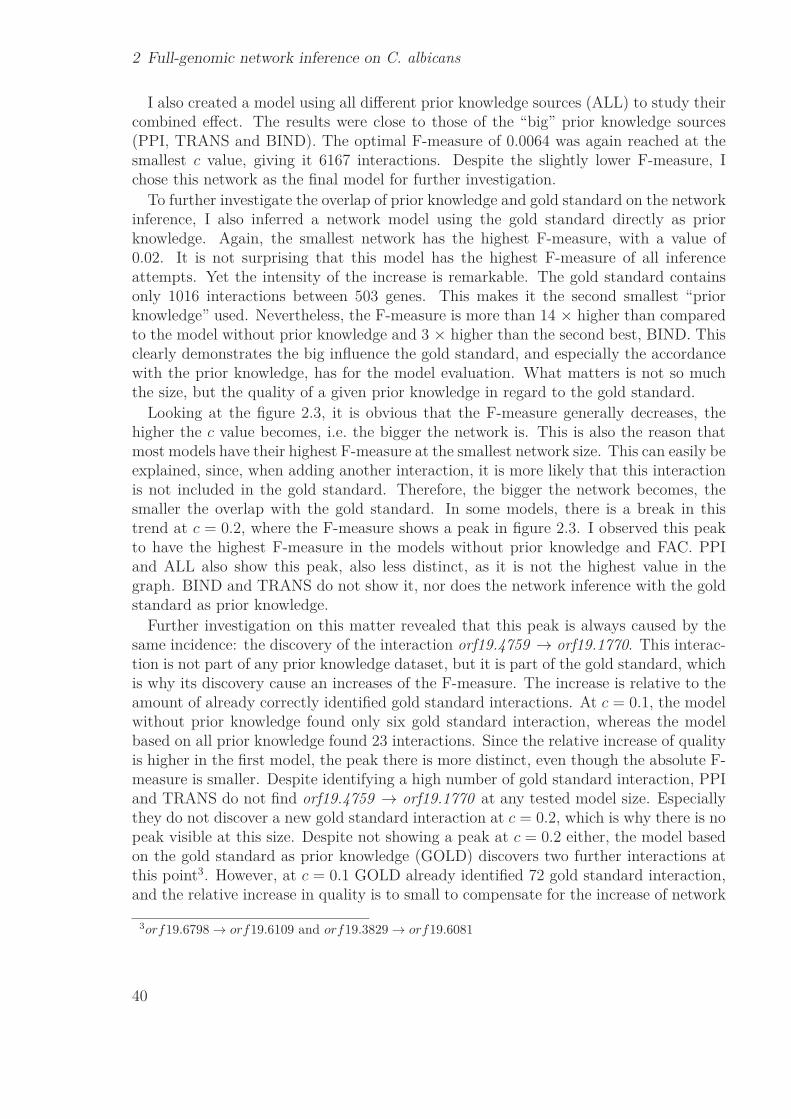
To further investigate the overlap of prior knowledge and gold standard on the networkinference, I also inferred a network model using the gold standard directly as priorknowledge. Again, the smallest network has the highest F-measure, with a value of0.02. It is not surprising that this model has the highest F-measure of all inferenceattempts. Yet the intensity of the increase is remarkable. The gold standard containsonly 1016 interactions between 503 genes. This makes it the second smallest “priorknowledge” used. Nevertheless, the F-measure is more than 14 × higher than comparedto the model without prior knowledge and 3 × higher than the second best, BIND. Thisclearly demonstrates the big influence the gold standard, and especially the accordancewith the prior knowledge, has for the model evaluation. What matters is not so muchthe size, but the quality of a given prior knowledge in regard to the gold standard.
Looking at the figure 2.3, it is obvious that the F-measure generally decreases, thehigher the c value becomes, i.e. the bigger the network is. This is also the reason thatmost models have their highest F-measure at the smallest network size. This can easily beexplained, since, when adding another interaction, it is more likely that this interactionis not included in the gold standard. Therefore, the bigger the network becomes, thesmaller the overlap with the gold standard. In some models, there is a break in thistrend at c = 0.2, where the F-measure shows a peak in figure 2.3. I observed this peakto have the highest F-measure in the models without prior knowledge and FAC. PPIand ALL also show this peak, also less distinct, as it is not the highest value in thegraph. BIND and TRANS do not show it, nor does the network inference with the goldstandard as prior knowledge.
Further investigation on this matter revealed that this peak is always caused by thesame incidence: the discovery of the interaction orf19.4759 → orf19.1770. This interac-tion is not part of any prior knowledge dataset, but it is part of the gold standard, whichis why its discovery cause an increases of the F-measure. The increase is relative to theamount of already correctly identified gold standard interactions. At c = 0.1, the modelwithout prior knowledge found only six gold standard interaction, whereas the modelbased on all prior knowledge found 23 interactions. Since the relative increase of qualityis higher in the first model, the peak there is more distinct, even though the absolute F-measure is smaller. Despite identifying a high number of gold standard interaction, PPIand TRANS do not find orf19.4759 → orf19.1770 at any tested model size. Especiallythey do not discover a new gold standard interaction at c = 0.2, which is why there is nopeak visible at this size. Despite not showing a peak at c = 0.2 either, the model basedon the gold standard as prior knowledge (GOLD) discovers two further interactions atthis point3. However, at c = 0.1 GOLD already identified 72 gold standard interaction,and the relative increase in quality is to small to compensate for the increase of network
3orf19.6798 → orf19.6109 and orf19.3829 → orf19.6081
40
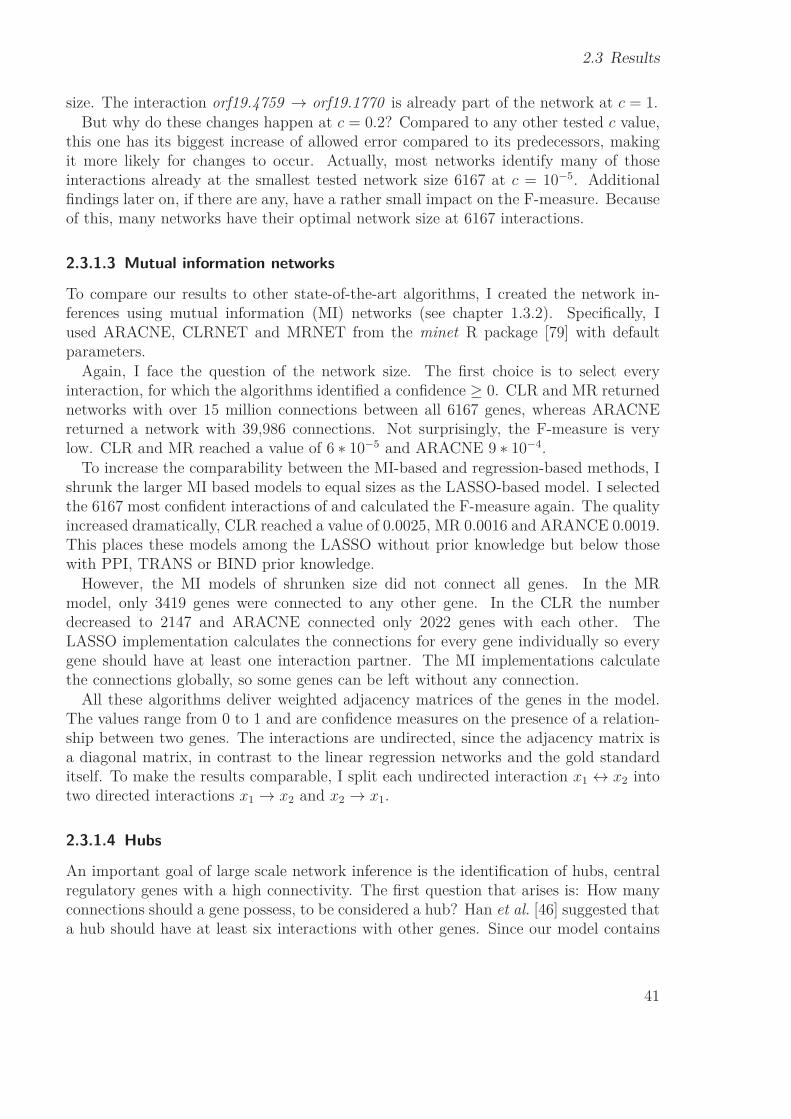
2.3 Results
size. The interaction orf19.4759 → orf19.1770 is already part of the network at c = 1.But why do these changes happen at c = 0.2? Compared to any other tested c value,
this one has its biggest increase of allowed error compared to its predecessors, makingit more likely for changes to occur. Actually, most networks identify many of thoseinteractions already at the smallest tested network size 6167 at c = 10−5. Additionalfindings later on, if there are any, have a rather small impact on the F-measure. Becauseof this, many networks have their optimal network size at 6167 interactions.
2.3.1.3 Mutual information networks
To compare our results to other state-of-the-art algorithms, I created the network in-ferences using mutual information (MI) networks (see chapter 1.3.2). Specifically, Iused ARACNE, CLRNET and MRNET from the minet R package [79] with defaultparameters.
Again, I face the question of the network size. The first choice is to select everyinteraction, for which the algorithms identified a confidence ≥ 0. CLR and MR returnednetworks with over 15 million connections between all 6167 genes, whereas ARACNEreturned a network with 39,986 connections. Not surprisingly, the F-measure is verylow. CLR and MR reached a value of 6 ∗ 10−5 and ARACNE 9 ∗ 10−4.
To increase the comparability between the MI-based and regression-based methods, Ishrunk the larger MI based models to equal sizes as the LASSO-based model. I selectedthe 6167 most confident interactions of and calculated the F-measure again. The qualityincreased dramatically, CLR reached a value of 0.0025, MR 0.0016 and ARANCE 0.0019.This places these models among the LASSO without prior knowledge but below thosewith PPI, TRANS or BIND prior knowledge.
However, the MI models of shrunken size did not connect all genes. In the MRmodel, only 3419 genes were connected to any other gene. In the CLR the numberdecreased to 2147 and ARACNE connected only 2022 genes with each other. TheLASSO implementation calculates the connections for every gene individually so everygene should have at least one interaction partner. The MI implementations calculatethe connections globally, so some genes can be left without any connection.
All these algorithms deliver weighted adjacency matrices of the genes in the model.The values range from 0 to 1 and are confidence measures on the presence of a relation-ship between two genes. The interactions are undirected, since the adjacency matrix isa diagonal matrix, in contrast to the linear regression networks and the gold standarditself. To make the results comparable, I split each undirected interaction x1 ↔ x2 intotwo directed interactions x1 → x2 and x2 → x1.
2.3.1.4 Hubs
An important goal of large scale network inference is the identification of hubs, centralregulatory genes with a high connectivity. The first question that arises is: How manyconnections should a gene possess, to be considered a hub? Han et al. [46] suggested thata hub should have at least six interactions with other genes. Since our model contains
41

2 Full-genomic network inference on C. albicans
Table 2.2: Results of the genome-wide network inference with mutual inform-ation methods. The first three columns show the results for all interactions,for which the algorithms found a correlation. In the last three columns, thenumber of interactions has been reduced to the same number as the LASSOmodel of the inference based methods (6167). This increases the comparabil-ity of results. Reducing the confidence to the 6167 most confident ones leavessome genes disconnected from the network. The last row shows the numberof genes with at least one connection.
CLR MR ARACNE CLR MR ARACNE
small small small
F-measure 0.00006 0.00006 0.0009 0.0025 0.0016 0.0019
# of interactions 15,686,064 15,329,450 39,986 6,167 6,167 6,167
# of genes 6167 6167 6167 2147 3419 2022
more nodes that the one of Han et al. I decided for a minimum of seven, in order toidentify hubs. The use of fixed numbers is of course difficult. The final decision of howmany connections a gene should have to be considered a hub should depend on the totalnumber of genes and the number of connections in the network.
In the LASSO-based network with ALL prior knowledge, I identified 126 genes withan out-degree of seven or more. To annotate them I used the Candida Genome Data-base [104]. Despite ongoing research, only a few genes are annotated, and 31 hub genesI identified do not have a functional description. Often, the annotation originates fromorthologous genes of S. cerevisiae, which makes them less reliable. According to theliterature search, the potential hub genes come from various different functional cat-egories. At least 16 of them are known to susceptible to antimycotica like amphotericinB, azoles or Caspofungin, making them potential drug targets. See table 2.4. Detailsabout Caspofungin can be found in chapter 3.1.1.
The three genes with the highest out-degree are FET31 (29), BNI5 (28), andorf19.1300 (25). The fact, that one of them is only known by its orf -ID demonstratesthe lack of annotation. FET31 [72] is especially interesting, since it is a putative irontransport precursor, which makes it reasonable to assume to have a central regulatoryrole. The fact that it is also susceptible to antifungal drugs makes it an interesting drugtarget. However, heterozygous null mutants remain viable, which lowers its usefulnessas a drug target.
BNI5 is part of the cytokinesis and septin ring assembly, which is about everythinginteresting about it. orf19.1300 is better studied, despite the fact that is misses analias. It is a putative membrane protein and is part of the process controlling filament-ous growth. Homozygous and heterozygous null mutants remain viable, yet homozygousnull mutants have abnormal appearance. Not much more is known about these genes.
42

2.3 Results
Whether they really have central positions in the regulatory processes can only be de-termined by experimental validation.
Figure 2.4 demonstrate how the use of different prior knowledge leads to different in-teractions in the final model. The hub gene PSA2 is responsible for the nucleotidyltrans-ferase activity and biosynthetic processes in C. albicans [104], while TKL1 is involvedin the transketolase activity. The figure shows which interaction was estimated given acertain kind of prior knowledge.
LASSO,ALL,TRANS,FAC,PPI,BIND
LASSO,ALL,TRANS,FAC,PPI,BIND
LASSO,ALL,TRANS,FAC,PPI,BINDLASSO,ALL,FAC
LASSO,ALL,TRANS,FAC,PPI,BIND
LASSO,ALL,FAC
LASSO,ALL,TRANS,FAC,PPI,BIND
LASSO,ALL,FAC
LASSO,ALL,TRANS,FAC,PPI,BIND
LASSO,ALL
ALL,FAC
LASSO,ALL,TRANS,FAC,PPI,BIND
o r f 1 9 . 3 6 1 0
M I R 1
Y m 3 1 5 w
TKL1ADE17
o r f 1 9 . 2 6 3 4
o r f 1 9 . 6 0 5 5
U f d 4
VPS1
STB4
B U D 6
U B A 1
LASSO,ALL,TRANS,FAC,PPI,BIND
LASSO,ALL,BIND
LASSO,ALL,TRANS,FAC,PPI,BIND
LASSO,ALL,TRANS,FAC,PPI,BIND
ALL,TRANS,FAC,PPI,BIND
ALL,BIND
LASSO,ALL,TRANS,FAC,PPI,BIND
LASSO,ALLLASSO,ALL,FAC,PPI
LASSO,ALL,TRANS,FAC,PPI,BIND
LASSO,ALL,TRANS,FAC,PPI,BIND
LASSO,ALL,TRANS,FAC,PPI,BIND
LASSO,ALL,TRANS,FAC,PPI,BIND
LASSO
LASSO,ALL,TRANS,FAC,PPI,BIND
LASSO,ALL,TRANS,FAC,PPI,BIND
TRANS,FAC,PPI
o r f 1 9 . 7 1 8 4
PUT2
o r f 1 9 . 1 1 4 2
SOU2
o r f 1 9 . 4 9 4 6
o r f 1 9 . 4 8 2 4
Y n l 1 9 1 w
RAV1
F M P 4 5
PSA2
FET3
o r f 1 9 . 4 8 1 6
YOL119C
o r f 1 9 . 4 8 8 6
o r f 1 9 . 3 1 8 4
o r f 1 9 . 2 7 3 7
LSP1
o r f 1 9 . 4 9 4 7
Figure 2.4: Predicted hubs PSA2 and TKL2. The labels on the edges show, whichprior knowledge had to be included into the inference algorithm for thatspecific interaction to occur. LASSO means this edge was found withoutany prior knowledge.
I realised that the hubs in the gold standard differ greatly from those in the networks.To determine an appropriate hub size, I calculated the quantiles of the out-degree dis-tribution. The 75% quantile is reached at a value of 3, so I selected an out-degree of 4as the selection criterion, since I want a rather strict hub definition. This lead to 83 hubgenes. From those, only one (WOR1 ) was also identified as hub gene by the networkmodel without prior knowledge. Compared to that, the network model with all priorknowledge has four hub genes in common, see table 2.3.
This shows that there is indeed a significant difference between the gold standard andthe models based on transcriptional analysis, disregarding if they have been inferredwith or without prior knowledge.
43

2 Full-genomic network inference on C. albicans
Table 2.3: Four hub genes that the gold standard and the network inferencewith all prior knowledge have in common. WOR1 was also identifiedby the model without prior knowledge.
name description
ACT1 Actin; transcript regulated by growth phase, starvation
ADE2 role in adenine biosynthesis; required for normal growth and virulence
WOR1 Transcription factor required to establish and maintain the opaque state
BNI1 Formin; role in cytoskeletal organization, cell polarity
Table 2.4: 16 hubs which are sensitive to antifungal treatment. The rows containthe name, the out-degree and the description of the gene. The annotation wastaken from the Candida Genome Database [104]. Susceptibility to antifungalagents are highlighted.
FET31 29 Putative iron transport multicopper oxidase precursor; flucytosineinduced; Caspofungin repressed
SOG2 16 Domain protein of RAM cell wall integrity signalling network; role incell separation, azole sensitivity; required for hyphal growth; lacksorthologs in higher eukaryotes
HIP1 13 Similar to amino acid permeases; alkaline upregulated; flucytosineinduced; fungal-specific (no human or murine homolog)
ARX1 13 Putative ribosomal large subunit biogenesis protein; downregulatedduring core stress response; decreased expression in response toprostaglandins
UTP22 11 Putative U3 snoRNP protein; decreased expression in response toprostaglandins; heterozygous null mutant exhibits resistance toparnafungin
NOG1 11 Putative GTPase; mutation confers hypersensitivity to 5-fluorocytosine, 5-fluorouracil, and tubercidin; decreased expression inresponse to prostaglandins
TYR4 10 Putative zinc finger DNA-binding transcription factor; fluconazole-downregulated; expression regulated during planktonic growth
Continued on next page
44

2.3 Results
Table 2.4 – continued from previous page
APT1 9 Adenine phosphoribosyltransferase; flucytosine induced; repressed bynitric oxide; protein level decreased in stationary phase yeast cultures
Hmg2 8 HMG-CoA reductase; enzyme of sterol pathway; inhibited by lovast-atin; gene not transcriptionally regulated in response to lovastatinand fluconazole
Cor1 8 Putative ubiquinol-cytochrome-c reductase; amphotericin B in-duced; repressed by nitric oxide; protein level decreases in stationaryphase cultures
Taf19 8 Putative TFIID subunit; mutation confers hypersensitivity to ampho-tericin B
OPT8 8 Possible oligopeptide transporter; induced by nitric oxide, ampho-tericin B
Imp4 8 Putative SSU processome component; decreased expression in responseto prostaglandins
ASR1 7 Putative heat shock protein; transcription regulated by cAMP, osmoticstress, ciclopirox olamine, ketoconazole; stationary phase enriched
OPI3 7 Phosphatidylethanolamine N-methyltransferase of phos-phatidylcholine biosynthesis; downregulation correlates with clinicaldevelopment of fluconazole resistance; amphotericin B andCaspofungin repressed
AGP2 7 Amino acid permease; hyphal downregulated; regulated upon white-opaque switching; induced in core Caspofungin response, during cellwall regeneration, or by flucytosine; fungal-specific
2.3.1.5 GAL sub-network
In my network, I was also able to identify a known studied sub-network. The so calledGAL-network has been extensively studied in S. cerevisiae [54,73] and is well conserved inthe yeast clade. It was used to describe transcriptional rewiring between C. albicans andS. cerevisiae [97]. The GAL-network plays a major role in the degradation of galactose.GAL10 transfers β-D-galactose to α-D-galactose. This is converted to α-D-galactose1-phosphate by GAL1. GAL7 then transfers α-D-galactose 1-phosphate to α-D-glucose1-phosphate. The regulatory cascade GAL10 → GAL1 → GAL7 is correctly predictedby the inferred network models from all 6167 genes, as can be seen in Figure 2.5. Thisis especially important, as these interactions are not part of any prior knowledge andonly the interaction GAL1 → GAL7 is part of the gold standard.
45

2 Full-genomic network inference on C. albicans
o r f 1 9 . 3 6 7 1 H A P 4 1
GAL10 GAL7GAL1
Figure 2.5: Sub-network of GAL-genes. Modelled using LASSO and all prior know-ledge. Predicted relations are not part of the prior knowledge. The connec-tion of GAL10, GAL1 and GAL7 is well studied in many yeast forms.
2.3.1.6 Scale-freeness
A desired property of the inference model is scale-freeness (see chapter 1.2.2 for details).To measure this property, I used Cytoscape [105] to fit a power law to the degree distri-bution of the model, and calculate the R2. It is a coefficient of confidence, and describesthe fit between data points and the model. The results can be seen in table 2.1. Thecoefficient for all LASSO based models is above 0.9. A graphical representation can beseen in figure 2.6. The model with no prior knowledge and all prior knowledge have thehighest R2, while the TRANS prior knowledge lead the model to the lowest value. Thisproves that the algorithm is able to infer scale-free network models.
To investigate how much influence the prior knowledge has on the scale-freeness, Icalculated the R2 scores for them as independent networks (see table 2.5 for results).All reached high values, except for TRANS, which had to settle with a score of 0.6.The combination of all available prior knowledge also had a high R2 score of 0.9. BINDand PPI are the biggest prior knowledge networks by far and so already show the scale-freeness of the underlying biological network, since an “investigation bias” is more likelyto occur in networks with a little number of genes.
The gold standard itself has a relative high R2 of 0.87. Every gold gene is part of aninteraction pair, but that does not mean, all gold genes have a relation with each other.This can lead to a scattered and disconnected network. To investigate this, I lookedfor the biggest connected sub-network within the gold standard. In fact, 402 genes aredirectly or indirectly connected with each other. Only 42 genes have only one interactionpartner. This shows that the gold standard is already well connected.
2.3.2 ParallelisationDespite increasing computational power of modern cluster systems, genome-scale net-work inference is still time consuming. It is therefore often advisable to use parallelcomputing if possible. To do so, it is important to identify the time consuming parts
46

2.3 Results
Figure 2.6: Power law distribution of the nodes in the LASSO model. The dotsshow the number of genes with a certain degree. The red line is the fittedpower law distribution. The axises are logarithmic.
Table 2.5: Scale-freeness of prior knowledge and gold standard. The first tworows show the number of genes and interactions in the dataset. The last rowthe value of the R2 score showing the coefficients of confidence that the nodedegree follows a power law distribution.
FAC TRANS BIND PPI ALL GOLD
genes 226 1502 2288 2290 3051 509
interactions 249 2689 6333 6674 11523 1016
R2 0.857 0.615 0.917 0.891 0.908 0.871
of the calculation and extract those parts that are independent from each other. Incase of this study, the calculation of the coefficients for each gene is the most time con-suming part of the calculation. Fortunately, the calculation of the coefficients of one
47
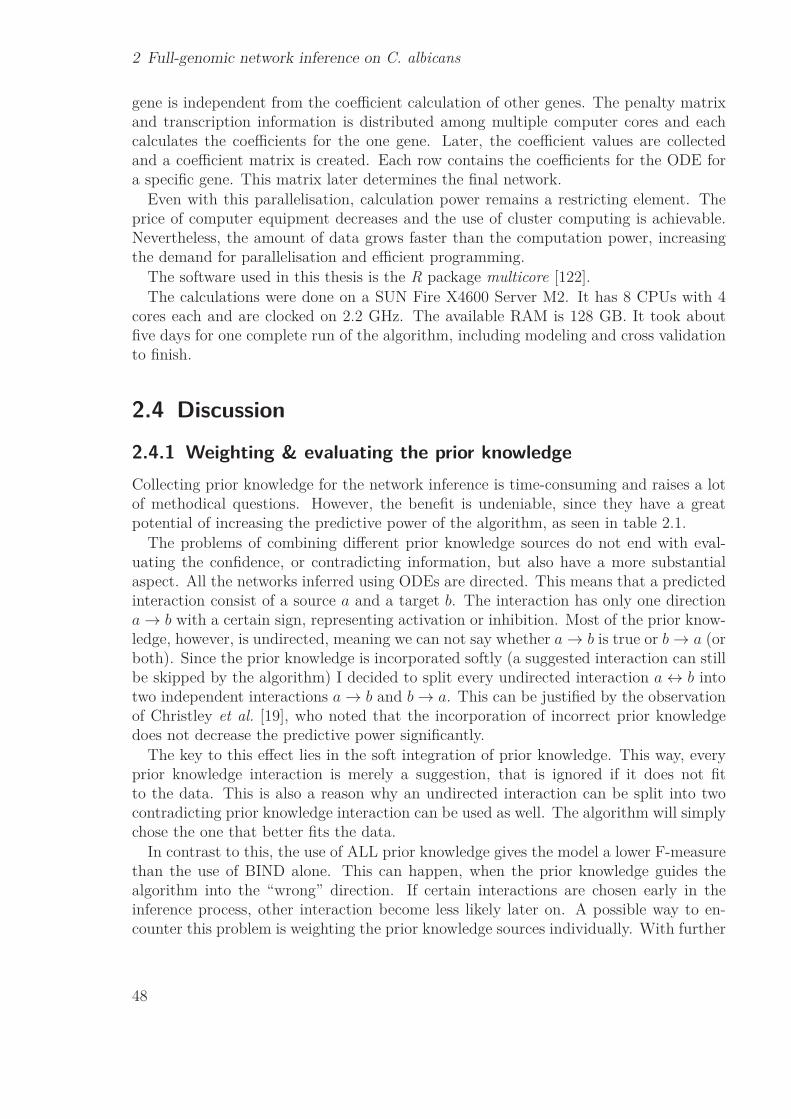
2 Full-genomic network inference on C. albicans
gene is independent from the coefficient calculation of other genes. The penalty matrixand transcription information is distributed among multiple computer cores and eachcalculates the coefficients for the one gene. Later, the coefficient values are collectedand a coefficient matrix is created. Each row contains the coefficients for the ODE fora specific gene. This matrix later determines the final network.
Even with this parallelisation, calculation power remains a restricting element. Theprice of computer equipment decreases and the use of cluster computing is achievable.Nevertheless, the amount of data grows faster than the computation power, increasingthe demand for parallelisation and efficient programming.
The software used in this thesis is the R package multicore [122].The calculations were done on a SUN Fire X4600 Server M2. It has 8 CPUs with 4
cores each and are clocked on 2.2 GHz. The available RAM is 128 GB. It took aboutfive days for one complete run of the algorithm, including modeling and cross validationto finish.
2.4 Discussion
2.4.1 Weighting & evaluating the prior knowledgeCollecting prior knowledge for the network inference is time-consuming and raises a lotof methodical questions. However, the benefit is undeniable, since they have a greatpotential of increasing the predictive power of the algorithm, as seen in table 2.1.
The problems of combining different prior knowledge sources do not end with eval-uating the confidence, or contradicting information, but also have a more substantialaspect. All the networks inferred using ODEs are directed. This means that a predictedinteraction consist of a source a and a target b. The interaction has only one directiona → b with a certain sign, representing activation or inhibition. Most of the prior know-ledge, however, is undirected, meaning we can not say whether a → b is true or b → a (orboth). Since the prior knowledge is incorporated softly (a suggested interaction can stillbe skipped by the algorithm) I decided to split every undirected interaction a ↔ b intotwo independent interactions a → b and b → a. This can be justified by the observationof Christley et al. [19], who noted that the incorporation of incorrect prior knowledgedoes not decrease the predictive power significantly.
The key to this effect lies in the soft integration of prior knowledge. This way, everyprior knowledge interaction is merely a suggestion, that is ignored if it does not fitto the data. This is also a reason why an undirected interaction can be split into twocontradicting prior knowledge interaction can be used as well. The algorithm will simplychose the one that better fits the data.
In contrast to this, the use of ALL prior knowledge gives the model a lower F-measurethan the use of BIND alone. This can happen, when the prior knowledge guides thealgorithm into the “wrong” direction. If certain interactions are chosen early in theinference process, other interaction become less likely later on. A possible way to en-counter this problem is weighting the prior knowledge sources individually. With further
48

2.4 Discussion
investigation of the prior knowledge sources, one may be able fine-tune the influence ofthe prior knowledge. The question remains, how to evaluate this consciously.
The origin of mismatching prior knowledge and gold standard may also be that theprior knowledge mostly comes from S. cerevisiae, whereas the gold standard is basedon C. albicans specific sources. Many interactions are well conserved among these spe-cies. Nevertheless, there are substantial differences in the genetic regulation betweenS. cerevisiae and C. albicans. This is also one reason I did not weight the prior know-ledge more than I did, as it can lead to false conclusions.
2.4.1.1 Gold standard
The results of the modeling with ALL prior knowledge show that the suggested inter-actions sometimes fit well to the transcription data, even though they do not fit to thegold standard. Otherwise they would not have been considered in the first place. Herewe see another possible source of error: What if the gold standard does not fit to thetranscription data? This means, what if the genes, that are connected in the gold stand-ard do not correlate in their transcriptional expression in the dataset? The algorithmwould not be able to identify these interactions, if not guided by prior knowledge. Thehighest F-measure was achieved by a model that has the gold standard itself as input.While some might argue that this does not result in additional knowledge, it can stillbe beneficial. It can present a template of “correct” interactions to guide the inferencealong with it.
As seen in figure 2.2, more influence of prior knowledge increases the predictive power,given an overlap of prior knowledge and gold standard. The predictive power can alsobe increased by selecting smaller networks, which can have multiple reasons. The mostimportant factor is the comparably small gold standard network. With only 1016 inter-actions between 503 genes, the genome-wide networks can never have high F-measureseven if they include every interaction of the gold standard. The current size of the goldstandard is still insufficient to reliably evaluate genome-scale network inferences. How-ever, since new information about interactions and annotations for genes are publishedregularly, the size and quality of the gold standard will grow over time. This showsthe necessity to find automatic and reliable ways to extract these information from theliterature. Databases like FungiDB and the Candida Genome Database are still far fromcomprehensive. Automatic text mining software like JReX offers a mature way to har-vest literature information available. The machine learning algorithm that drives thepattern recognition is still difficult to use and requires lots of work in fine-tuning andproviding the necessary key words. Even though, the false positive and false negativerate remain comparably high.
The gold standard used is a mixture of directed and undirected interactions. Since thegold standard was also compared to mutual information networks, which are undirectedby their nature, I also split every gold standard interaction a ↔ b into two interactionsa → b and b → a. Of course, this approach can lead to false positives, i.e. that I countinteractions as matches even if the gold standard originally had contradicting inform-ation. As mentioned before, in the case of genome-scale network inference, the aim is
49

2 Full-genomic network inference on C. albicans
more about finding hubs and investigating network topology than investigating indi-vidual interactions. Therefore, identifying a connection between two genes is a valuablefeat, even though the direction may be wrong.
2.4.2 Scale-freenessDespite the importance of large scale power law distributed networks, no such networkwas modelled for a pathogenic fungi so far. In my study, I was able to infer a network,whose coefficient of confidence (R2) to the power law distribution was 0.96. This waspossible by combining two algorithms, LASSO and ridge regression.
Since ridge regression does not make a parameter selection, i.e. does not shrink thecoefficients of the model to zero, it always produces fully connected networks, whichmakes it an excellent tool for regularization, but not for model selection. LASSO onthe other hand has a bias for coefficient values becoming zero. The models tend to besmaller, and the coefficient to more significant. This works along with the sparsenesscriterion, which assumes that the number of interactions in a network should be as smallas possible, while still giving a reasonable data fit. Using ridge regression to estimatethe constraint for the LASSO makes it possible to produce scale-free networks.
Using the combined approach of ridge regression and LASSO without prior knowledgecertainly offers a rather unbiased approach on the network structure. By adding priorknowledge to the inference, we most certainly influence the networks structure, which isof course intended. However, Yu and colleagues [136] described the effect that becomesvisible when we start to add prior knowledge. The prior knowledge is not equally dis-tributed among all genes. In fact, the prior knowledge sources themselves follow partlya power law distribution of connections. I took the connections in every source of priorknowledge as an independent network and counted the degrees of every gene. When Icalculated the coefficient of confidence to a fitted power law distribution we observedvery high values. The BIND dataset has a R2 of 0.92, which is the highest value of allprior knowledge. PPI follows with 0.9 and FAC with 0.86. TRANS has the lowest valuewith 0.62. The combination of all prior knowledge sources gave a R2 of 0.91, which isbetter than some prior knowledge sources alone.
One might argue that this reflects the power law distribution of the underlying bio-logical network, instead of following Yu’s argumentation, that there is an investigationbias towards well studied genes. This claim would only hold true if all genes wouldhave equal chance to be investigated, so that an inherent power law distribution wouldshow itself. Despite the fact that the number of investigated genes increases constantly,there is an obvious focus on genes that are presumed to be essential. The general lackof annotation for example is a serious problem when working on regulatory networks.Also, well studied genes are more helpful in understanding the function of a cluster orhub structure, so these are of course more often part of the investigation.
The gold standard R2 score of 0.87 is comparably high. Again, whether this reflectsthe “true” nature of connections, or an investigation bias, can not be told. However,one should consider, that the gold genes are collected from individual, independent datasources, which can lead to a scattered, unconnected network. This may not reflect
50
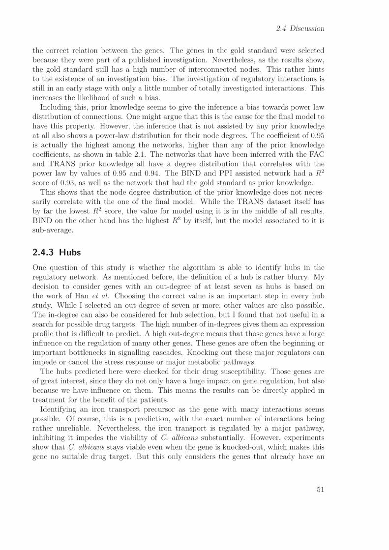
2.4 Discussion
the correct relation between the genes. The genes in the gold standard were selectedbecause they were part of a published investigation. Nevertheless, as the results show,the gold standard still has a high number of interconnected nodes. This rather hintsto the existence of an investigation bias. The investigation of regulatory interactions isstill in an early stage with only a little number of totally investigated interactions. Thisincreases the likelihood of such a bias.
Including this, prior knowledge seems to give the inference a bias towards power lawdistribution of connections. One might argue that this is the cause for the final model tohave this property. However, the inference that is not assisted by any prior knowledgeat all also shows a power-law distribution for their node degrees. The coefficient of 0.95is actually the highest among the networks, higher than any of the prior knowledgecoefficients, as shown in table 2.1. The networks that have been inferred with the FACand TRANS prior knowledge all have a degree distribution that correlates with thepower law by values of 0.95 and 0.94. The BIND and PPI assisted network had a R2
score of 0.93, as well as the network that had the gold standard as prior knowledge.This shows that the node degree distribution of the prior knowledge does not neces-
sarily correlate with the one of the final model. While the TRANS dataset itself hasby far the lowest R2 score, the value for model using it is in the middle of all results.BIND on the other hand has the highest R2 by itself, but the model associated to it issub-average.
2.4.3 HubsOne question of this study is whether the algorithm is able to identify hubs in theregulatory network. As mentioned before, the definition of a hub is rather blurry. Mydecision to consider genes with an out-degree of at least seven as hubs is based onthe work of Han et al. Choosing the correct value is an important step in every hubstudy. While I selected an out-degree of seven or more, other values are also possible.The in-degree can also be considered for hub selection, but I found that not useful in asearch for possible drug targets. The high number of in-degrees gives them an expressionprofile that is difficult to predict. A high out-degree means that those genes have a largeinfluence on the regulation of many other genes. These genes are often the beginning orimportant bottlenecks in signalling cascades. Knocking out these major regulators canimpede or cancel the stress response or major metabolic pathways.
The hubs predicted here were checked for their drug susceptibility. Those genes areof great interest, since they do not only have a huge impact on gene regulation, but alsobecause we have influence on them. This means the results can be directly applied intreatment for the benefit of the patients.
Identifying an iron transport precursor as the gene with many interactions seemspossible. Of course, this is a prediction, with the exact number of interactions beingrather unreliable. Nevertheless, the iron transport is regulated by a major pathway,inhibiting it impedes the viability of C. albicans substantially. However, experimentsshow that C. albicans stays viable even when the gene is knocked-out, which makes thisgene no suitable drug target. But this only considers the genes that already have an
51

2 Full-genomic network inference on C. albicans
Figure 2.7: Workflow of the Candida study. After preprocessing, the expressiondata and the prior knowledge was used to create mathematical models. Thesemodels were evaluated and new hypothesis could be constructed.
annotation, and those are few. After all, looking only at those genes, that are alreadyannotated gives only little insight. More fruitful may be the study of genes withoutannotation, but high number of connections.
As mentioned before, the results of genome-scale network inference should not beconsidered exact. The aim of this inference is rather to point out potential sites of highregulatory activity. Robustly differentiating what is the most important regulator andwhat is the second most important is beyond the scope and capabilities of this approach.The final decision can only be made using experimental validation in the laboratory.Between the genome scale network inference and the experimental validation stands thesmall scale network inference. It takes a closer look into the regulatory interactions,requiring less data and offering a higher reliability of the predictions.
2.5 ConclusionThe rising amount of transcription data available leaves the question of how to analysethem. Often, the data comes from different laboratories, was harvested under multipleconditions or various platforms. Despite many attempts to offer easy and machinereadable access, collecting data compendium often still consists of a lot of manual work.The datasets themselves are often not comprehensive and inhomogeneous. Carefullyand elaborate preprocessing is important in order to combine multiple datasets without
52

2.5 Conclusion
adding a bias. Selecting an adequate approach to model the data may be one of themost important steps in the inference process. Finally, choosing a model and evaluatingit is time consuming and should not be underestimated. There is no unique set ofanswers for these decisions, since it mainly depends on what kind of questions one triesto investigate.
The main question studied here is: Is it possible to create a prior knowledge supportedgenome-scale network inference with a scale-free degree distribution, evaluated by anautomatically harvested gold standard in order to identify central regulatory genes. Thecurrent thesis presents a successful way to tackle this task. The difference equationsystems, used by the adaptive LASSO is able to cope with the lack of data and returnrobust results. The combination of the ridge regression for model fit and the LASSOfor parameter selection proves to be able to create scale free networks. It is challengingto estimate so many interactions of genes using so little data. Using parallelisation andhigh-end server architecture, I was able to solve the equation systems in reasonable time.The general workflow is depicted in figure 2.7.
The incorporation of prior knowledge increased the predictive power of the algorithm.Even small sources of prior knowledge could increase the F-measure in the models. Morecomprehensive prior knowledge was able to increase the quality of the model drastically.Combining all prior knowledge sources to one big set, however, slightly decreased the thequality again. This most likely comes from contradictions inside the different sources.Further investigation on the fine tuning of influence of different prior knowledge sourcesmay not only prevent such decrease in quality, but also improve the predictive power tolevels higher than any source alone.
I found that the bottleneck in the evaluation of the model is the gold standard. Inorder to measure the predictive power, a comprehensive gold standard is necessary. Thegold standard in this study is far from comprehensive. Despite hard work from Buykoet al., only 1016 interactions between 509 genes could be extracted from literature. Thislead to the preference of smaller networks in the model evaluation. Most of the genome-scale networks had their maximum F-measure at their smallest network size, whichconsists of 6167 interactions. These networks found most gold standard interactions atthe beginning and barely any more after that. This fact also leads to the occurrence ofa peak at c = 0.2, since with so few gold standard interactions to find, even one or twonew findings can cause huge changes in the F-measure, as seen in figure 2.3. A largergold standard with more interactions may lead to more sensitivity in the measurements.The small overlap of the gold standard and the prior knowledge is also problematic,since the prior knowledge does not seem to guide the inference in a direction that leadsto a better F-measure. As new publications on fungal pathogens are submitted everyday, the size and quality of a reliable gold standard may increase in the future. Infact, as a consequence of this findings, a new PhD-project will start in autumn 2014,speciffically aiming at improving the quantity and quality of the gold standard and theprior knowledge.
Apart from the gold standard interactions, the algorithm was also able to identify theGAL-sub network. The correct prediction of the regulation cascade GAL10 → GAL1 →GAL7 is a strong sign of the modeling power of this approach. Especially, since no prior
53

2 Full-genomic network inference on C. albicans
knowledge source contain any of these interactions.The scale-freeness of the model enabled me to identify hubs in C. albicans. Studying
the annotation for drug response and viability of knock-out mutants shows that, whilemany are susceptible to drugs, C. albicans is still able to compensate the change or lackof expression. There is more to the importance of a gene as drug target than just a highnumber of connections. Eventually, only experimental validation is able to check theresults of computer modeling. Large-scale networks usually produces a large amount ofhubs with only little reliability. Therefore, it is advisable, to continue the study withsmall scale networks, focusing on the potential hubs and their interactions.
54

3 Small-scale network inference onA. fumigatus
3.1 IntroductionBefore the upcoming microarray technologies, expression changes were seen as linearpathways of causality [113]. With Microarrays, the study of complex regulatory networksbecame possible. The transition from sequential information to functional informationis one important step in the inference process and genome-wide network inference is apowerful tool to identify potential regulators in the genetic network of an organism. Theprecision of the analysis is often not sufficient to get a detailed look at the individualconnections. For a more detailed and robust study of regulatory connections, it isadvisable to focus the investigation on a subset of genes [28].
3.1.1 Aspergillus fumigatus stress responseA. fumigatus is able to colonise various different habitats and in order to survive, ithas to adapt to various changes in environment. A significant change in environmentalconditions occurs for example when the conidia of the fungus colonise the human body.Among other factors, it comes with a change in temperature, pressure and pH-valueand also an activation of the host’s immune response, which poses a serious thread tothe fungus. Inhaled conidia are often trapped in the mucus and transported out of thelung by beating of the cilia [11]. It has been shown, that A. fumigatus is able to releasefactors that can slow the beating of the cilia and damage epithelial cell to create anentrance into the body [5]. Another defense mechanisms of the human body consistsof type I and II pneumocytes. A. fumigatus is capable using the respiratory epitheliumcells as refuge from these phagocytes and may even start germination, as several differentstudies found out [88, 130]. Once the fungus managed to colonise the human host, itmay be discovered and anti-mycotic treatment starts.
In order to overcome all these obstacles, A. fumigatus needs to quickly adapt tothe changing environment. First, A. fumigatus has cell surface proteins that sense theenvironmental conditions. Once these proteins notice a change in the environment, theystart a signalling cascades that eventually lead to activation of transcriptional regulators.These regulators cause a change in the expression of specific target genes and therebyan adaption to the new environmental state by producing (or stop producing) certainproteins. It is important for the survival of the fungus that these cascade mechanismswork quickly and target accurately the correct regulatory interactions. These signalling
55
3 Small-scale network inference on A. fumigatus
cascades and their respective regulatory interactions have been well studied in the lastdecades [45,95]. Not only toward their roles in metabolic regulation, but also concerningdrug adaption. It is important to understand that these cascades are not strictly linearand independent, but are interconnected and complex.
The cell wall of A. fumigatus consists of an unique polysaccharides composition [35].This makes it a suitable target for antifungal drug treatment, since it distinguishes thefungal cells from human cells. Of central importance to this membrane formation isthe protein Fks1, which synthesises β-1,3-D-glucan [18]. These glucans and chitins areessential components of the cell wall in many fungal species. An interesting adaptionmechanism is the capability to compensate for a loss of glucans by inducing a chitinbiosynthesis, and vice versa [108,124,127]. Details of the regulation of this mechanismsare still unclear.
A group of drugs that targets Fks1 and its glucan synthesis is Echinocandins [18].The first clinically applied Echinocandins is Caspofungin [13]. It is used successfullyagainst Candida sp infections, but shows less effectiveness against invasive mycoses, likeaspergillosis. It was not able to decrease the mortality rate of patients suffering frominvasive aspergillosis since it was introduced in clinical trials [56]. This ineffectiveness ismainly caused by two factors: One is the occurrence of resistant strains, the other is a socalled “paradoxical effect”. This paradox effect consists of a lack of effectively, when theconcentration of Caspofungin passes a certain threshold [66, 96]. According to differentstudies, the glucan / chitin ratio in the cell wall may be responsible for this effect. Theglucan / chitin balance itself is regulated by various different signalling pathways, whichoperate on protein kinase C (PKC), calcineurin, HOG and the mitogen activated proteinkinases (MAPKs) [32,80,81,127].
In the A. fumigatus genome, four putative MAPKs have been identified: MpkA,MpkB, MpkC and SakA. MpkA is responsible for the regulation of the cell wall integ-rity (CWI) pathway. It is tightly related to the activity of cell wall acting compoundsand reactive oxygen species [123]. SakA is a putative ortholog of Hog1 in Saccharomy-ces cerevisiae, which governs the high osmolarity glycerol (HOG) response. SakA seemsto regulate the response to oxidative stress and high osmolarity [26]. sakA knock-outmutants show a significant increase in sensitivity to Caspofungin. Both, the CWI as wellas the HOG pathway seem to play a major role in the drug response of A. fumigatus,especially concerning the paradoxical effect. Yet little is known if they interact witheach other, and how they do it.
3.2 Material & Methods
3.2.1 NetGeneratorIn 2005, Guthke et al. [43] presented the basic idea of the NetGenerator heuristic, whichwas implemented in 2007 by Töpfer et al. [119]. NetGenerator uses systems of linearor non-linear differential equations to model dynamic changes of gene expression. Fromdynamic time-resolved data, NetGenerator creates an interaction network that represents
56

3.2 Material & Methods
the most significant interactions between those genes. It determines the coefficients ofthe model via a heuristic, that simulates the dynamic behaviour fitting to the time-resolved gene expression data. It has been successfully applied in modeling human [118]and fungal regulatory networks [42,70,71].
In 2013 Weber et al. published Version 2.0 of the algorithm [131]. The added featuresinclude the capability to work with data from multiple experiments and under multiplestimuli. The way in which prior knowledge is included has also been improved. Intheir publication, Weber et al. explicitly address the occurrence of cross-talk as objectof study, which is a topic in this thesis as well.
The expression change of a gene i at the time-point t is defined as:
xi(t) =N∑
j=1βi,jxj(t) +
M∑j=1
bi,juj(t) (3.1)
βi,j is the influence of a predictor j on the expression of gene i. The second term of theequation describes external influence on the gene expression. uj is the jth of M externalperturbations, multiplied by bi,j, which describes the strength of influence of uj on genei. The sign of the coefficients β determines if the influence is repressing (βi,j ≤ 0) oractivating (βi,j ≥ 0). If βi,j = 0, there is no influence of gene j on gene i. Typically, theexpression of each gene is modeled by one single differential equation. NetGenerator isalso able to model one gene with multiple equations, which is called increase of dynamicorder. It enables NetGenerator to simulate even more complex behaviour, especially atime-delay of interaction.
While determining the network structure, the algorithm applies certain rules to achievesparse networks and avoid over-fitting:
• Addition of a predictor must lead to significantly improved model fit,• Removal of a predictor must not significantly decrease model fit,• The number of predictors in the model must be smaller than the number of time
points in the corresponding time series,• The number of interactions must not exceed a user-set limit
It is difficult to estimate what is a “significant” increase or decrease in model fit. Thedefault parameters consider a change by the factor of 0.2 as significant.
Due to the elaborate nature of calculation, large- or medium-scale modeling is nottractable. In order to find unique solutions for the differential equations, NetGeneratorneeds a minimal “difference” in the expression profiles of the genes. If the similarity ofexpression profiles is to high, the algorithm can not safely decide which gene is respons-ible for a certain regulation. By default, the maximum allowed correlation between twoexpression profiles is 0.95. This limits the maximum number of genes in the network, ifno sufficient number of data points is provided. To increase the amount of data available,NetGenerator is able to interpolate values between data points using cubic splines.
During the determination of network structure, it is also possible to include priorknowledge (see chapter 1.2.1). The algorithm tries to makes all sub model structures
57

3 Small-scale network inference on A. fumigatus
consistent with the offered prior knowledge. The integration of prior knowledge can bedone using two ways: fixed and flexible. Interactions of the fix prior knowledge has tobe part of the final model and can not be ignored by the inference. This should onlybe used with the most reliable of knowledge sources, and the user should be sure thatthe expression data also supports the demanded interaction. Otherwise, NetGeneratoris not able to infer a network with the provided parameters. One should especially checkthe fixed prior knowledge for contradicting information. The flexible prior knowledgeon the other hand is not required to be a part of the final model, as the algorithm canskip it, if it does not fit the data. Each interaction can be individually weighted for itsconfidence and in addition to that, there is also a general parameter defining the overallinfluence of the prior knowledge.
NetGenerator tries to fit the model by minimising the model error i.e. the differencebetween the simulated expression values and the actual measurements:
model_error =T∑
t=1
N∑i=1
(xi(t) − xi(t))2 (3.2)
xi(t) represents the simulated expression of gene i at time point t, which is subtractedfrom the measured value for that gene at that time point (xi(t)).
In general, adding new interactions to the model decreases the model error, at thecost of an increased complexity. This leads to a conflict between modeling power andsparseness (simplicity) of the model. NetGenerator offers a parameter to set the allowedmodel error in the inference process. Since the algorithm stops adding new interactionsonce this allowed error is reached, the parameter serves as an indirect way to influence thenumber of connections in the model: The lower the allowed error, the more interactionsthe final model has. If the model error is set to low, however, NetGenerator may fail tocreate a model that satisfies the given criteria.
3.2.1.1 Parameters
The NetGenerator offers various parameters to optimise the modeling of the network.Three of the main parameters are:
allowedError : The allowed model error compared to the expression data.weightingStruct: The global weight of the prior knowledge.maxDynamicOrder : The dynamic model order.
The parameter allowedError regulates, how well NetGenerator tries to fit the modelto the expression data. While it is of course desirable to fit the data as good as possible,NetGenerator is not always able to achieve the desired fit. This causes the algorithmto crash, giving no results. The model fit generally increases as more connections areincluded into the model. Enforcing a good fit can therefore cause a comparably largenetwork, without the desired sparseness.
In comparison to the individual confidence weighting of the prior knowledge, theweightingStruct parameter influences the global effect of all prior knowledge. This means,
58

3.2 Material & Methods
how much the algorithm insists on including a prior knowledge interaction in favor ofanother interaction, even if the other may yield a better fit. A weightingStruct value of1 does not prefer any prior knowledge, while a value of 0 greatly insists on adding priorknowledge interactions.
The third parameter I estimated is maxDynamicOrder. It determines how manyequations are used to explain the expression of a gene. This allows the sub-model to usea higher order integrator chain, which can be considered hidden states in order to modelmore complex behaviour. A common biological interpretation of this higher order is adelay in the expression.
3.2.2 Robustness testsIt is often difficult to tell how robust an interaction in an inferred network is. Here,robustness describes the likelihood of a certain interaction to appear, even if there aresmall changes in the data. Robustness tests ensure, small alterations in the data andprior knowledge do not lead to completely different models.
I performed two types of robustness tests on the final network. One testing for noiseto the data, since one should always assume a little measurement error. To check howsusceptible a network is to perturbations of the data, I added normal distributed noisewith a mean = 0 and a standard deviation of 0.01 to the pre-processed data. After that,I repeated the inference and counted how many interactions of the original network wereinferred again. I did this 1000 times and considered all interactions, that occur in anleast 50% of the networks, as robust to noise.
I performed a similar test to check the reliability of an interaction on prior knowledge.I repeated the network inference but randomly omitted 10% of the prior knowledge.This test was also repeated 1000 times and an interaction of the original network thatoccurs in at least 50% of the inferences is considered robust to perturbation of the priorknowledge.
At the end, an interaction is considered (truly) robust, if it passed the test againstboth, noise in the gene expression data and missing prior knowledge.
3.2.3 RNA-Seq dataThe RNA-Seq data used in this study comes from the A. fumigatus strain CEA10,also known as A1163. From this strain samples were taken for the wild type (wt) andfor four different knock-out mutants: ΔakuB, ΔmpkA and ΔsakA, as can be seen intable 3.1. The conidiophores were grown for 16 h on a minimal media, and then treatedwith Caspofungin at a dose of 0.1 μg/ml. From the wt and ΔakuB strains, samples weretaken at five different time points after treatment 0.5 h, 1 h, 4 h, 8 h and 24 h. Fromthe ΔsakA and ΔmpkA strains, samples were taken at 4 h after treatment. As control,additional samples of all strains were taken before the administration of Caspofungin.All samples were taken in replicates from three different flasks. The measurements weretaken using an Illumina HiSeq2000 sequencing machine with single end technology.
59

3 Small-scale network inference on A. fumigatus
Table 3.1: RNA-Seq data used in this study. For the wild type (wt) and the ΔakuBmutant, measurements were taken at six time points, whereas for the ΔmpkAand the ΔsakA mutant three time points were taken. All samples were takenin three replicates.
strain wt ΔakuB ΔmpkA ΔsakA
0 hour 3 × 3 × 3 × 3 ×0.5 hours 3 × 3 ×
1 hour 3 × 3 ×4 hours 3 × 3 ×8 hours 3 × 3 ×24 hours 3 × 3 ×
3.2.4 Mapping of transcription data
The reads were provided in FASTA-files. TopHat v1.4.1 [121] was used with a butterflysearch to map the reads to the genome. The reads were mapped to the genome sequenceof the A. fumigatus A1163 strain provided by the CADRE [36] database. A CADREgene transfer format (GTF) file of the same strain was used to annotate the mappedreads. The number of allowed multi-hits was set to 1 to prevent multiple mapping. Afterinvestigating the GTF file, the maximum intron length was set to 2700 bp. The readsthat mapped successfully were sorted and indexed using SAMtools [68].
3.2.5 Differentially expressed genes
The indexed hits were read into R [115] using the easyRNA-Seq package [23]. Thechromosome size was calculated from the CADRE genome sequence file and the readcounts were calculated. BioMart [57] provided exon annotation. The DESeq package [6]was used to normalize the read counts for different library sizes. This is necessary sincesamples with a bigger library size (i. e. sequencing depth) can have more reads for agiven gene then samples with a lower library size, even though the actual expression ofthe gene did not change [25]. The data contains read counts for 10.160 genes.
Differential expression analysis was performed via the “nbinomTest” function of theDESeq package. Genes were considered differentially expressed, with a FDR-adjustedp-value ≤ 0.05. For the wild type and ΔakuB strains, the time points 0.5 h, 1 h, 4 h,8 h and 24 h were compared to the control (0 h). For the ΔsakA and ΔmpkA strainsthe time points 1 h, 4 h were compared to the control.
60

3.2 Material & Methods
3.2.6 Collection of prior knowledgeIn order to implement as much of the currently available information on the A. fumigatuspathway as possible, I followed a knowledge-driven approach. The prior knowledge isused to propose known interactions to the network and guide it. Those interactions aresoftly integrated, which means, the inference algorithm only implements them, if theyfit to the provided expression data. I utilised two types of sources:
3.2.6.1 RNA-Seq data
I investigated the differential expression of the genes in the ΔmpkA and ΔsakA mutantstrains. I compared the expression of the genes in the knock-out mutants with the wildtype at time point 0 h. If a gene x is differentially expressed with an FDR-adjustedp-value ≤ 0.05 in the ΔsakA mutant, a regulatory interaction between x and sakA wasassumed. If x is down regulated in ΔsakA, I assume an activating interaction sakA → x,otherwise a repressing interaction sakA x. The same method was used to identifypotential interactions in the ΔmpkA strain.
3.2.6.2 Literature
In addition to the RNA-Seq data, I also searched in the literature. A valuable source ofprior knowledge is the publication of [95], a review written in 2009 by Rispail et al. Itcompares the MAP kinase and calcium-calcineurin pathway in different pathogenic fungiand plants. It includes orthologous genes for sakA (hog1 ) and mpkA (mpk1 ). While italready is an extensive study of the pathway, the information is not species specific andno cross-talk between sakA and mpkA was investigated. The names of the orthologousof S. cerevisiae were translated to the A. fumigatus naming system.
3.2.7 Biological validation3.2.7.1 Western blot
The phosphorylation of a protein can be measured using western blot analysis. Here,protein samples are placed on a membrane and diffuse through it powered by gel elec-trophoresis. Special antibodies are given to the sample, that bind to the target proteinand stain them for later evaluation. While diffusing through the gel, the proteins in thesample are separated by their molecular weight. The result is a quantitative analysis ofthe target proteins.
In this study, conidia of A. fumigatus were incubated for 18 h and then stressed withCaspofungin. Samples were taken before treatment as well as 0.5 h, 1 h, 2 h, 4 h and 8 hafter treatment. Protein samples were extracted and the phospho-p38 MAPK antibodywas used to detect SakA in its phosphorylated form, while phospho-p44/42 MAPK wasused to detect phosphorylated MpkA.
61

3 Small-scale network inference on A. fumigatus
3.2.7.2 Polymerase chain reaction
A polymerase chain reaction (PCR) is used to determine DNA concentrations in vitro.The PCR uses the DNA-polymerase to amplify the amount of DNA to detectable levels.One cycle of the amplification consists of three major steps:
1. Denaturation: At 95 ◦C, double stranded DNA-helix melts into two.
2. Primer annealing: The temperature is lowered to 50-65 ◦C and the primers,which bind to the part of DNA to be amplified, bind to the DNA-polymerase.
3. Elongation: The DNA-polymerase synthesises the missing strand with free nuc-leotides from the medium, starting form the primer. The primer remains on theDNA-strand, so it can be used again in the next cycle.
The cycle starts again, and is repeated until enough DNA material has been synthes-ised. This is usually after 20-50 cycles. The expression of the genes are then normalisedto housekeeping genes, which are expected to not alter their expression.
An extension to this is the real-time or quantitative PCR (qPCR). Here, a fluorescentdye is given to the medium, which is activated during the elongation process. This allowsto determine the amount of synthesised DNA in real-time.
To determine the activity of specific genes, measuring the RNA of the cell directly in-stead of DNA is advisable. In the reverse-transcriptase PCR (RT-PCR) directly uses theRNA-samples from the data, which are transformed into complementary DNA (cDNA)and then used for the classic PCR.
The results are often shown in Fold difference 2(−ΔΔCt). ΔΔCt is the expression ofthe treated protein minus the experession of the untreated control.
The combination of quantitative and reverse transcription PCR is abbreviated withqRT-PCR.
3.2.7.3 Measurement of Rhodamine-123 uptake
Rhodamine-123 is a fluorescent dye that absorbs light in a spectrum of 505-560 nm.To measure the intracellular permeability of the fungal cell wall, Conidia (106/ml) werecultivated for 16 h in minimal media at 37◦C, 200 rpm. A final concentration of 20μM of Rhodamine-123 was added to the growing mycelia alone or in combination withCaspofungin. Samples were taken at the time of application as well as 0.5 h, 1 h, 2 h,4 h and 8 h. The mycelium was ground with mortar and a pestle using liquid nitrogen.Then cytosolic fraction was extracted and measured using a TECAN microplate readeraccording to the manufacturer’s instructions.
Caspofungin resistant strain Among the strains tested in the Rhodamine-123 studyis also the Caspofungin resistant strain EMFRS678P [96]. The resistance is confered viaa point mutation in fks1, at nucleotide position 2086 (thymin to cytosin).
62
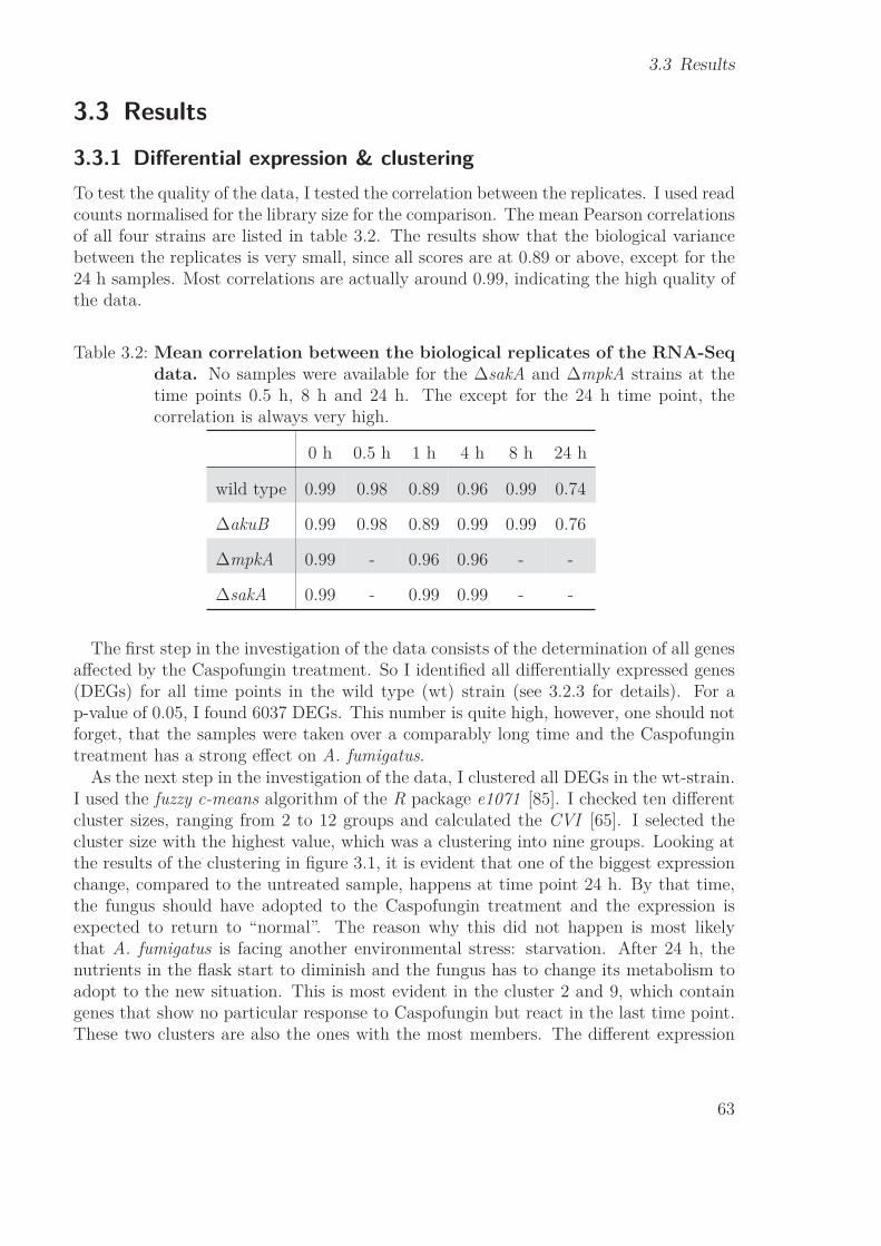
3.3 Results
3.3 Results3.3.1 Differential expression & clusteringTo test the quality of the data, I tested the correlation between the replicates. I used readcounts normalised for the library size for the comparison. The mean Pearson correlationsof all four strains are listed in table 3.2. The results show that the biological variancebetween the replicates is very small, since all scores are at 0.89 or above, except for the24 h samples. Most correlations are actually around 0.99, indicating the high quality ofthe data.
Table 3.2: Mean correlation between the biological replicates of the RNA-Seqdata. No samples were available for the ΔsakA and ΔmpkA strains at thetime points 0.5 h, 8 h and 24 h. The except for the 24 h time point, thecorrelation is always very high.
0 h 0.5 h 1 h 4 h 8 h 24 h
wild type 0.99 0.98 0.89 0.96 0.99 0.74
ΔakuB 0.99 0.98 0.89 0.99 0.99 0.76
ΔmpkA 0.99 - 0.96 0.96 - -
ΔsakA 0.99 - 0.99 0.99 - -
The first step in the investigation of the data consists of the determination of all genesaffected by the Caspofungin treatment. So I identified all differentially expressed genes(DEGs) for all time points in the wild type (wt) strain (see 3.2.3 for details). For ap-value of 0.05, I found 6037 DEGs. This number is quite high, however, one should notforget, that the samples were taken over a comparably long time and the Caspofungintreatment has a strong effect on A. fumigatus.
As the next step in the investigation of the data, I clustered all DEGs in the wt-strain.I used the fuzzy c-means algorithm of the R package e1071 [85]. I checked ten differentcluster sizes, ranging from 2 to 12 groups and calculated the CVI [65]. I selected thecluster size with the highest value, which was a clustering into nine groups. Looking atthe results of the clustering in figure 3.1, it is evident that one of the biggest expressionchange, compared to the untreated sample, happens at time point 24 h. By that time,the fungus should have adopted to the Caspofungin treatment and the expression isexpected to return to “normal”. The reason why this did not happen is most likelythat A. fumigatus is facing another environmental stress: starvation. After 24 h, thenutrients in the flask start to diminish and the fungus has to change its metabolism toadopt to the new situation. This is most evident in the cluster 2 and 9, which containgenes that show no particular response to Caspofungin but react in the last time point.These two clusters are also the ones with the most members. The different expression
63

3 Small-scale network inference on A. fumigatus
profile of time point 24 h can also be seen in the dendrogram for the wild type heat mapin figure 3.3.
−2
−1
01
2
−1
01
2
−2
−1
01
2
−2
−1
01
2
−1
01
2
−2
−1
01
2
−2
−1
01
2
−2
−1
01
2
−2
−1
01
Figure 3.1: Result of the clustering with all time points. Cluster 2 and cluster 9have the most members. In these clusters are mostly genes, that are mainlyinfluenced by the starvation effect.
To investigate the claim that many genes are differentially expressed because of thestarvation effect, I repeated the clustering for all genes that are differentially expressedin any but the last time point. The number of DEGs decreases to 4257. The result ofthe new clustering can be seen in figure 3.2. This time, the optimal CVI was reachedat a cluster size of four. Of special interest here are the clusters one and four, asthey show that at time point 0.5 h there is a distinct reaction to the drug stress, afterwhich the regulation follows the general trend. This early response is most likely tied todrug specific response genes. Their regulation normalises later on, when the drug stressdiminishes to prevent over-expression.
The goal of this study revolves around the study of the Caspofungin stress responseof A. fumigatus, and not the hunger stress. I decided to omit the last time point (24 h)
64

3.3 Results
from the data for the rest of the study, as it would distort the inference. The lowercorrelation of that data point would also weaken the statistical analysis.
−1
.5−
0.5
0.5
1.5
−1
.5−
0.5
0.5
1.5
−1
.5−
0.5
0.5
1.5
−1
.5−
0.5
0.5
1.5
Figure 3.2: Result of the clustering without time point 24 h. Here, the last timepoint (24 h) of the expression data has been omitted. Of special interest isthe time point 0.5 h, which shows an exception of the general trend in theclusters 1 and 4.
3.3.2 Gene selectionSince the 4257 DEGs of the first four time points are much more than the NetGeneratorcan handle, the selection of model genes has to be decreased further. The problem here isthat with only five measurements, many genes will have very similar expression profiles.If two or more genes are potential regulators of another gene, and they all show thesame expression changes over time, NetGenerator can impossibly decide which to chose.Judging from personal experience of colleagues and the maintainers of NetGenerator, Iconsidered a number between 20 and 30 genes as manageable. To find genes connected tothe response to Caspofungin treatment, I performed a Gene Ontology (GO) [7] analysisusing the FungiFun tool [93]. The cut-off for the enrichment was set at a p-value of 0.05.For only 1876 of the genes an annotation was found. I selected genes associated with theterms cell wall and membrane, as well as β-glucosidase and glucan synthase, since theA. fumigatus cell wall is composed of sugars and Caspofungin targets these sugars and
65

3 Small-scale network inference on A. fumigatus
these genes may play a role in its construction and maintenance. As mpkA and sakAare protein-kinases and known to be part of the response, genes with this term werealso considered. Additionally, genes assigned to signaling and transmembrane transportwere selected, since these categories are known to be connected to the drug responseand response to cell wall perforation.
By far the largest group of DEGs belonged to membrane with 323 genes, whereas onlyeight belong to cell wall. 193 genes are assigned to transmembrane transport and 25 tosignal transduction. 86 belong to the protein-kinase group and five response to stress.15 belong to the term glucan synthase or glucosidase. This makes a total of 655 genes,which is still to much for the inference. We took the work of Rispail et al. [95], whoworked on a similar subject, as guideline for further selection. DEGs mentioned in thispublication are involved in the response regulation and were taken as hints for the geneselection. The final decision was done by my colleague Dr. Vito Valiante, who is also aco-author of Rispails publication. The genes that were considered for the modeling arelisted in table 3.3 and figure 3.3 shows the expression profiles for all model genes.
8h4h0.5h 1h 24h
−8 −4 0 2
Color Key
ptc2exg13mae1
hnm1egnE1
rho1mpkA
ypd1rodAssk1cla4sitT
rlmAgel3
ags2mirC
rodBcrf1
sakAmdr4ssk2
exg12exg17
egnE2
fks1ptc2exg13mae1
hnm1egnE1
rho1mpkAypd1rodAssk1cla4sitTrlmAgel3ags2mirC
rodBcrf1sakAmdr4ssk2exg12exg17
egnE2
fks1
Figure 3.3: Differential expression of genes selected for modeling. The expressionof all genes was compared to the untreated wild type strain. The expressionvalues are log2 transformed. For the wild type strain, a dendrogram wascreated, which shows that the time point 24 h has the least similarity to theother time points considering the expression.
66

3.3 ResultsTa
ble
3.3:
Gen
esof
the
mod
el.
The
tabl
epr
esen
tsth
ena
mes
,des
crip
tion
and
GO
-cat
egor
ies.
The
last
colu
mn
indi
cate
s,if
the
gene
was
men
tione
din
Risp
aile
tal.
[95]
Nam
eSy
stem
atic
IDD
escr
iptio
nG
O-c
ateg
ory
Risp
ail
rodA
AFU
B_
0571
30C
onid
ialh
ydro
phob
ince
llwa
llno
rodB
AFU
B_
0166
40C
onid
ialh
ydro
phob
ince
llwa
llno
crf1
AFU
B_
0155
30Ex
trac
ellu
lar
cell
wall
gluc
anas
e/a
llerg
ence
llwa
llno
rlmA
AFU
B_
0405
80C
ellw
allo
rgan
izat
ion,
resp
onse
tost
ress
,Tra
ns.
Fact
orce
llwa
llye
sge
l3A
FUB
_02
8470
1,3-
β-g
luca
nosy
ltran
sfera
sem
embr
ane
norh
o1A
FUB
_07
2830
GT
Pase
;inv
olve
din
radi
algr
owth
and
coni
diat
ion
mem
bran
eye
sex
g13
AFU
B_
0917
20β
-D-g
luco
side
gluc
ohyd
rola
seβ
-glu
cosid
ase
noex
g12
AFU
B_
0061
60β
-glu
cosid
ase
β-g
luco
sidas
eno
exg1
7A
FUB
_00
0280
β-g
luco
sidas
eβ
-glu
cosid
ase
nofk
s1A
FUB
_07
8400
1,3-
β-g
luca
nsy
ntas
e,ta
rget
ofC
aspo
fung
inβ
-glu
cosid
ase
yes
egnE
1A
FUB
_07
9180
Mut
anas
egl
ucan
synt
hase
noeg
nE2
AFU
B_
0814
70M
utan
ase
gluc
ansy
ntha
seno
ags2
AFU
B_
0270
30α
-1,3
-glu
can
synt
hase
gluc
ansy
ntha
seno
mdr
4A
FUB
_01
2160
AB
Cm
ultid
rug
tran
spor
ter
tran
smem
bran
etr
ansp
ort
nohn
m1
AFU
B_
0811
90A
min
oac
idpe
rmea
setr
ansm
embr
ane
tran
spor
tno
mae
1A
FUB
_08
2870
C4-
dica
rbox
ylat
etr
ansp
orte
r/m
alic
acid
tran
spor
tpr
otei
ntr
ansm
embr
ane
tran
spor
tno
mir
CA
FUB
_02
2760
Side
roph
ore
tran
spor
ter
tran
smem
bran
etr
ansp
ort
nosi
tTA
FUB
_04
4820
AB
Cm
ultid
rug
tran
spor
ter
tran
smem
bran
etr
ansp
ort
noss
k1A
FUB
_05
5940
Res
pons
ere
gula
tor,
two-
com
pone
ntsig
nalt
rans
duct
ion
tran
scrip
tion
fact
orye
sss
k2A
FUB
_01
0360
Ort
holo
gha
vero
lece
llula
rre
spon
seto
osm
otic
stre
sspr
otei
nki
nase
activ
ityye
sm
pkA
AFU
B_
0706
30M
APK
;exp
ress
ion
incr
ease
dby
cell
wall
dam
age
prot
ein
kina
seac
tivity
yes
sakA
AFU
B_
0124
20M
AP
kina
sepr
otei
nki
nase
activ
ityye
src
k2A
FUB
_02
0560
Cal
cium
/cal
mod
ulin
-dep
ende
ntpr
otei
nki
nase
prot
ein
kina
seac
tivity
nocl
a4A
FUB
_05
3440
Ort
holo
g(s)
have
prot
ein
serin
e/th
reon
ine
kina
seac
tivity
prot
ein
kina
seac
tivity
yes
ypd1
AFU
B_
0673
90H
istid
ine-
cont
aini
ngph
osph
otra
nsfe
rin
term
edia
tepr
otei
nsig
nalt
rans
duct
ion
yes
ptc2
AFU
B_
1012
70Pr
edic
ted
cata
lytic
activ
ity,p
hosp
hata
seca
taly
ticac
tivity
yes
67

3 Small-scale network inference on A. fumigatus
3.3.3 Comparison wild type & ΔakuB strainThe gene akuB codes for a DNA helicase that is part of the non-homologous end-joiningmachinery in A. fumigatus. This makes the ΔakuB strain much more suitable for ho-mologous deletion [21]. This knock-out is a necessary step to create the sakA and mpkAknock out strains. This raises the question of how much this deletion alter the expressionof other genes, bringing a bias into the data.
To investigate the global effect of the deletion of akuB I compared the expression pro-files of the wild type strain with the expression profile of the ΔakuB strain. I comparedeach of the six time points individually and calculated the Pearson and the Spearmancorrelation of the log2 transformed read counts.
Figure 3.4: Comparison of log2 fold changes for the wild type (wt) and theΔakuB mutant strain. The high correlation indicates that the deletionof the akuB gene does not have significant effects on global Caspofunginresponse.
The results can be seen in figure 3.4. They show that during Caspofungin stressthe wild type and ΔakuB strain have very similar expression patterns, with Spearmancorrelations ranging from 0.93 - 0.99. According to this test, the deletion of akuB doesnot have a significant impact on the global Caspofungin response, and the data fromthe ΔsakA and ΔmpkA mutants, which also contain the akuB deletion, is probably notbiased.
To further investigate the influence of the knock-out mutants, I also calculated the
68

3.3 Results
Figure 3.5: Comparison of log2 fold changes for the wild type (wt) and theΔmpkA and ΔsakA mutant strains. There is a high correlation betweenthe wt and the knock-out mutants.
correlation of the wt with the other knock-out mutants, as seen in figure 3.5. TheSpearman correlation is always quite high, ranging from 0.88 - 0.95 for the comparisonwith the ΔmpkA strain and 0.95 - 0.96 for the ΔsakA strain. Since the deletion of bothgenes should only influence the response pathway, I did not expect global changes inexpression.
3.3.4 Harvest of prior knowledgeAs described in chapter 3.2.3, I used the RNA-Seq data of the ΔmpkA and ΔsakA knock-out mutants to determine the prior knowledge for these genes. The idea is that genes,that are differentially expressed in the knock-out mutants versus wt, must be influencedby the knocked-out gene. The results can be seen in figure 3.6 and table 3.4. By thisanalysis, I identified 14 potential interactions for mpkA, of which 11 are activating,and three are repressing. For sakA, I found 15 of the model genes to be differentiallyexpressed. Nine have an activating regulation from sakA, while five are repressed. Thisleads to a total of 29 RNA-Seq-based prior knowledge interactions.
Additionally, I searched in literature for known interactions between the model genes.The central source here was the publication by Rispail et al. [95]. From this source, Iwas able to harvest a total of seven additional interactions. Six of them are activating,while one is repressing. The literature offered prior knowledge with other sources thansakA and mpkA. Nevertheless, this prior knowledge adds another interaction for sakAand mpkA each. The interaction mpkA → rlmA is the only one that I found in both,literature and RNA-Seq data of the knock-out mutants. This prior knowledge from liter-ature is very important, since it represents current knowledge about the gene regulationin A. fumigatus. It also adds “causal” information, like the connection between the
69

3 Small-scale network inference on A. fumigatus
transcription factor ssk1 and its target ssk2. This information can not be derived purelyfrom the data. The amount of the current knowledge for these model genes, however, isvery small. This is a general problem in network reconstruction.
After collecting all the prior knowledge, I had to decide if I want to weight all priorknowledge interactions equally. This decision is necessary so that the algorithm candeal with ambiguous situations or even contradicting prior knowledge. My set of priorknowledge does not contain contradicting information, yet I still differentiated betweenthe literature knowledge and that extracted from the RNA-Seq data. The literaturedata was tested in the laboratory. This is why I decided to give the prior knowledgeextracted from RNA-Seq data a medium value of 0.5 and a slightly higher value of 0.66to the literature knowledge.
Figure 3.6: Prior knowledge used in this study. The prior knowledge was taken fromtwo different sources, RNA-Seq data (turquoise) and literature (purple) [95].The interaction mpkA → rlmA is the only one that is supported by bothprior knowledge sources (red).
3.3.5 NetGenerator3.3.5.1 Preprocessing
Before application of the NetGenerator, the data has to be prepared for analysis. Asstated in chapter 3.3.1, the 24 h time point is omitted from the data, since the influenceof the starvation effect is to big and creates a bias. I normalised the reads for the differentlibrary sizes with the DESeq package [6] in R.
The NetGenerator assumes that the organisms is in a steady state at the beginningand end of the study. Also, it is important to consider the relative expression changes
70

3.3 Results
Table 3.4: List of prior-knowledge used in this work. The table contains the stand-ard names for the regulators, targets, whether the interaction was activat-ing/inhibiting as well as the confidence score that was assigned to it. Thecolumn “in model” shows if the interaction was found in the final model.Only the interaction mpkA → rlmA was found in prior knowledge based onRNA-Seq data of knock-out data and literature.
source type target confidence source in modelsakA → rlmA 0.66 Rispail et al. [95] yesypd1 → ssk1 0.66 Rispail et al. [95] nossk1 → ssk2 0.66 Rispail et al. [95] yesssk2 → sakA 0.66 Rispail et al. [95] noptc2 sakA 0.66 Rispail et al. [95] yesmirC → cla4 0.66 Rispail et al. [95] yesmpkA → rlmA 0.66 Rispail et al. / ΔmpkA mutant yesmpkA → mdr4 0.5 Diff. expr. in ΔmpkA mutant yesmpkA → sitT 0.5 Diff. expr. in ΔmpkA mutant yesmpkA → ags2 0.5 Diff. expr. in ΔmpkA mutant nompkA → exg13 0.5 Diff. expr. in ΔmpkA mutant nompkA → exg12 0.5 Diff. expr. in ΔmpkA mutant nompkA → exg17 0.5 Diff. expr. in ΔmpkA mutant nompkA → rck2 0.5 Diff. expr. in ΔmpkA mutant nompkA → rodB 0.5 Diff. expr. in ΔmpkA mutant yesmpkA → egnE2 0.5 Diff. expr. in ΔmpkA mutant nompkA → mirC 0.5 Diff. expr. in ΔmpkA mutant nompkA crf1 0.5 Diff. expr. in ΔmpkA mutant yesmpkA hnm1 0.5 Diff. expr. in ΔmpkA mutant yesmpkA gel3 0.5 Diff. expr. in ΔmpkA mutant yessakA → ags2 0.5 Diff. expr. in ΔsakA mutant yessakA → exg13 0.5 Diff. expr. in ΔsakA mutant yessakA → exg12 0.5 Diff. expr. in ΔsakA mutant yessakA → rck2 0.5 Diff. expr. in ΔsakA mutant yessakA → rodA 0.5 Diff. expr. in ΔsakA mutant yessakA → rodB 0.5 Diff. expr. in ΔsakA mutant yessakA → crf1 0.5 Diff. expr. in ΔsakA mutant nosakA → egnE2 0.5 Diff. expr. in ΔsakA mutant yessakA → mirC 0.5 Diff. expr. in ΔsakA mutant yessakA → ypd1 0.5 Diff. expr. in ΔsakA mutant nosakA cla4 0.5 Diff. expr. in ΔsakA mutant yessakA gel3 0.5 Diff. expr. in ΔsakA mutant yessakA sitT 0.5 Diff. expr. in ΔsakA mutant nosakA ssk1 0.5 Diff. expr. in ΔsakA mutant nosakA mae1 0.5 Diff. expr. in ΔsakA mutant yes
71

3 Small-scale network inference on A. fumigatus
during the treatment, and not the absolute ones. When it comes to regulation by geneexpression, even small differences can cause big effects. The preprocessing was done foreach gene and each series of replicates individually.
So I first centered the data by dividing the reads to the expression at time point 0 h.Next, I used log2 transformation so the values revolve around 0. As a last step, thevalues are scaled to fall into the interval [-1, 1] by dividing them trough the maximumof the absolute values. The resulting relative expression values represent the change inexpression starting from 0 (steady state) at time point 0 h and then gives the direction(activation or repression) of the expression change.
A feature of NetGenerator is the ability to work with independent experiment timeseries. In this study, every replicate is considered an individual experiment. TheNetGenerator algorithm will try to optimise the fit over all time series.
To implement the prior knowledge into NetGenerator, two matrices were created, onefor the direction (activating or repressing) and one for the confidence of the explicitinteraction.
3.3.5.2 Parameter estimation
As described in chapter 3.2.1.1, I estimated three different parameters to find a modelthat implements many prior knowledge interactions, finds a good model fit while remainsparse in interactions. The parameters were checked for the following values:
maxDynamicOrder :1, 2weightingStruct:0.000, 0.001, 0.010, 0.050, 0.100, 0.200, 0.300, 0.400, 0.500, 0.600, 0.700, 0.800, 0.900,1.000allowedError :0.001, 0.010, 0.050, 0.100, 0.200, 0.300, 0.400, 0.500, 0.600, 0.700, 0.800, 0.900, 1.000
This leads to 364 different network models. While generating the different networks,the algorithm did not converge a total of 71 times. As mentioned before, some parametercombinations do not lead to a successful modeling. For example when the algorithm isnot able to fit the coefficients enough to meet the allowedError restriction. This is espe-cially difficult, if a high weighting of prior knowledge tries to force many prior knowledgeinteractions into the model. This also indicate that the inference may encounters situ-ations, were the correlation between the expression profiles of potential regulators is tohigh, and the algorithm cannot decide which one to use. As an example, the expressionprofile of ags2 and egne2 are very similar. Comparing the mean expression of all timepoints, these genes have a Pearson correlation of 0.99. NetGenerator does not take themean expression of all time points but each replicate individually, but still, situationscan occur, where this is still not enough.
72

3.3 Results
3.3.5.3 Model selection
Given the number of parameter combinations, minus the number of failed attempts,NetGenerator produced 293 different network model, varying in size (number of con-nection) and topology. Selecting the correct model from this set of possibilities is animportant step towards a reliable network prediction. I considered three different prop-erties of the network for evaluation.
Included prior knowledge:How many prior knowledge interactions were implemented into the model?Model error:How much does the simulation deviate from the expression data?Degree of sparseness:How many interactions were implemented in comparison to the number of nodes?
A small model error and high sparseness of the model are often contradicting goals. Alower model error is achieved by including additional interactions to the network, whichdecreases the sparseness. The number of implemented prior knowledge interactionsdetermines, how close the network is to current knowledge.
To get a global view over the created networks, I calculated the minimal, maximaland average values for the model error, the number of implemented prior knowledge in-teractions and the total number of connections (see table 3.5). Even from these numbersthe results vary greatly. The achieved model error ranges from 1.6 for the best fit 11.2for the worst. The intermediate values are evenly distributed, and it is no surprise, thatthe values grow larger, the higher the allowedError is.
Table 3.5: Global results for the inferred networks. Showing the minimal, aver-age and maximal values for the model error, number of implemented priorknowledge and network size (min / average / max).
model error prior knowledge # of connections
1.6 / 5.5 / 11.2 0 / 5 / 26 0 / 21 / 102
The best fit to data with a model error of 1.6 was reached by a model consisting of 102interactions. It implemented 4 prior knowledge interactions and one model interactioncontradicts the prior knowledge. This leads to a # of prior knowledge
total # of interactions ratio of 0.06. Notonly does this network represent very little of current knowledge, it even contradictsthe exploratory analysis of the RNA-Seq data. In the investigation of the ΔsakA, Ifound a up-regulation of gel3. I therefore assume that gel3 may be repressed by sakA.This network suggests the opposite, which is an activation of gel3 by sakA. While Ido not consider RNA-Seq-based prior knowledge as very confident and do not insist onimplementing it into the network, contradicting this prior knowledge means to ignorethe information we have gained from the knock-out data.
73

3 Small-scale network inference on A. fumigatus
Table 3.6: Comparison of different models. The first column holds the results ofthe mode with the smallest model error and the second column the modelwith the highest number of implemented prior knowledge interactions. Thelast column shows the rerun of the second model without prior knowledgeprovided.
lowestmodel error
mostprior knowledge
started withoutprior knowledge
model error 1.6 2.3 1.6
prior knowledge 4 26 5
# of connections 102 95 100
maxDynamicOrder 1 2 2
weightingStruct 0.01 0.3 -
allowedError 0.001 0.01 0.01
The highest number of implemented prior knowledge interactions by any model is 26.This network has a model error of 2.3 and consists of 95 interactions, which leads to a# of prior knowledge
total # of interactions ratio of 0.37. That means around one third of the model is supportedby an additional data source. The model error is only slightly higher than the bestvalue, while having less connections. In contrast to the model with the lowest error,this network uses second order dynamics, to fit the data. The second order has beenused to simulate the expression of the genes cla4, mirC, ssk1 and gel3. A number of 23of the 26 considered genes have an autoregulation which is always negative. 19 genesare connected to the input, which represents the Caspofungin treatment. Seven of theseconnections are activating and 12 are repressing.
I selected this network as the final model, since it implements most of the currentknowledge and the model error is only slightly higher than the best value.
3.3.5.4 Robustness assessment
To further increase the reliability of the network, I performed robustness tests concerningnoise in the data and dependency to prior knowledge. The technical details can be seenin chapter 3.2.2. As a result, 18 interactions have been found to be not robust. 11of these interactions passed the test for prior knowledge but failed the test for noisydata. The interaction ssk2 rlmA passed the test against noise in the data but was todependent on prior knowledge. Additional six interactions failed both tests.
Among those which failed, is the autoregulation of ssk1 which also looses another out-going and incoming interaction. The autoregulation of the other genes seem to be veryrobust against noise. From the eight interactions of ssk2 (four outgoing, three incoming
74

3.3 Results
and one autoregulation), four fail the robustness test, including the prior knowledgesupported activation of sakA.
ypd1 and cla4 loose their only outgoing connection (except autoregulation), leavingthem without target.
In total, four interactions supported by prior knowledge were found to be not robustagainst noise, while they were still robust against perturbation of the prior knowledge.
All interactions starting at the input proved to be robust. The robust network nowcontains 77 interactions, including autoregulation.
3.3.6 Model assessment3.3.6.1 Simulated expressions
In the gene expression data, some genes show an early response reaction to the Caspo-fungin treatment (see figure 3.2). This early response, which can also be seen in mpkAand sakA in figure 3.7 is quite difficult to model for linear systems. Nevertheless,NetGenerator was able to fit these data points quite well. For some genes like ssk2the use of a second order was necessary to correctly model the expression.
Looking at the simulated gene expression results 3.7, there are several genes like sakA,mpkA or roh1, with small oscillations in their simulated expression. The ripples fade overthe course of the expression, and it is difficult to pinpoint the cause of these phenomenas,since the effected genes form regulatory circles. These oscillations are most likely causedby the attempt of the NetGenerator algorithm to fit the expression in genes where thefirst time point differs greatly from the rest of the measurements. To fit this data, thealgorithm starts the simulation with a strong change in expression and later tries tosmooth the simulation back fit the other measurements.
3.3.7 Network topologyThe results of the network modeling can be seen in figure 3.8 and table 3.7. sakAhas 16 outgoing interactions (including autoregulation), which is the highest numberfor all genes in the network. Except for the autoregulation, all outgoing connectionsare supported by the prior knowledge and none failed the robustness test. Only oneincoming connection did not pass the robustness test. It is the prior knowledge supportedactivation by ssk2. Indirectly, this activation is still included in the model, since ssk2represses ptc2, which is an inhibitor of sakA. sakA then inhibits ssk1, which is thetranscription factor for ssk2, creating an indirect autoregulation.
Since the activation by ssk2 failed the robustness test, only two incoming interactionsreach sakA, one by mpkA and one by ptc2. Since the direct autoregulation of sakA is alsorepressing, this leaves the gene with only inhibiting interactions, which is not sufficientto describe the simulation of expression as seen in figure 3.7. There, little ripples can beseen in the simulated expression. This may indicate a slight over fitting, as these ripplesoccur between two time points, were no data can support such delicate modeling.
75
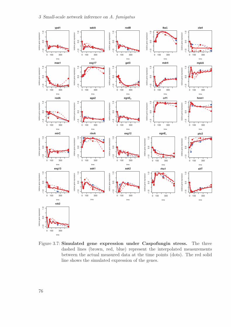
3 Small-scale network inference on A. fumigatus
Figure 3.7: Simulated gene expression under Caspofungin stress. The threedashed lines (brown, red, blue) represent the interpolated measurementsbetween the actual measured data at the time points (dots). The red solidline shows the simulated expression of the genes.
76
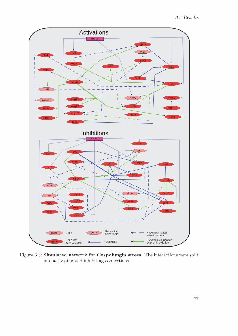
3.3 Results
Figure 3.8: Simulated network for Caspofungin stress. The interactions were splitinto activating and inhibiting connections.
77

3 Small-scale network inference on A. fumigatus
mpkA is the gene with the second highest number of outgoing regulations: six, ex-cluding the autoregulation. Five of them are supported by prior knowledge. Beforethe robustness test, mpkA had three more outgoing interactions, all based on priorknowledge. The only regulation by mpkA, which is not part of the prior knowledgeis a repression of sakA. This so far unreported cross-talk between two major responseregulators is an interesting result of the inference.
mpkA is regulated by fks1, the drug target of Caspofungin in a rather contradictingmanner. First, there is a direct activation, but also an indirect inhibition, since fks1also activates rho1, for which the model predicts a repressing effect on mpkA. This couldhint on some fine tuning of the expression of mpkA. fks1 itself is not connected to theinput, despite the fact that the input represents Caspofungin treatment.
ptc2 is a phosphatase and alterations of phosphorylation states are a well recognisedway of activity regulation in genes. It has inhibiting connections to sakA and fks1,to important regulators in the network, as well as egnE1, a mutanase. Mutanases aresugar-degrading proteins. Since the cell wall of A. fumigatus contains a lot of sugar, itsexpression must be fine tuned in order to react to the cell wall damage.
The Input, which mainly represents the Caspofungin treatment, inhibits all four trans-porters: mirC, mdr4, mae1 and sitT. This hinders A. fumigatus’s ability to decreasethe osmotic stress and part of the antifungal effect of Caspofungin.
From the seven literature based prior knowledge, which I regarded as quite confident,four are part of the final model. The activations mirC → cla3 and ypd1 → ssk1 werenot considered by the inference, while ssk2 → sakA failed the robustness test. Theinteraction mpkA → rlmA, which is supported by both prior knowledge sources, wasimplemented in the network and is robust to noise and perturbation.
Table 3.7: Interactions of the simulated network. Shows the source and targetof every interaction as and if the regulation is activating (→) or repressing(). If the interaction is supported by the prior knowledge can be seen in thecolumn labeled “prior”. The column “robust” shows if the interaction passedthe robustness test.
source type target prior robust source type target prior robustags2 ags2 no yes mpkA → rlmA yes yesags2 hnm1 no no mpkA → mdr4 yes yescla4 cla4 no yes mpkA → sitT yes yescla4 → mpkA no no mpkA gel3 yes nocla4 → mae1 no no mpkA → rodB yes nocrf1 crf1 no yes mpkA → exg17 yes no
egnE1 mdr4 no yes ptc2 sakA yes yesegnE1 sitT no yes ptc2 fks1 no yesegnE1 egnE1 no yes ptc2 egnE1 no yesegnE1 mae1 no yes ptc2 ptc2 no yesegnE1 → hnm1 no yes rck2 rck2 no yes
Continued on next page
78

3.3 Results
Table 3.7 – continued from previous pagesource type target prior robust source type target prior robustegnE2 egnE2 no yes rck2 → rho1 no yesexg12 exg12 no yes rho1 mpkA no yesexg12 rck2 no no rho1 rho1 no yesexg13 exg13 no yes rho1 → ypd1 no yesexg17 exg17 no yes rodA → rodB no nofks1 fks1 no yes rodB rodB no yesfks1 → mpkA no yes rodB mirC no nofks1 → rho1 no yes rodB ssk2 no nogel3 gel3 no yes sakA sakA no yes
hnm1 hnm1 no yes sakA sitT yes yesInput ags2 no yes sakA ssk1 yes yesInput sitT no yes sakA mae1 yes yesInput mirC no yes sakA gel3 yes yesInput mdr4 no yes sakA → rck2 yes yesInput rck2 no yes sakA → rodB yes yesInput ypd1 no yes sakA → egnE2 yes yesInput ssk2 no yes sakA → mirC yes yesInput ssk1 no yes sakA → exg12 yes yesInput mae1 no yes sakA → ags2 yes yesInput egnE1 no yes sakA → rlmA yes yesInput cla4 no yes sakA → exg13 yes yesInput gel3 no yes sakA → ypd1 yes yesInput → mpkA no yes sakA → crf1 yes yesInput → rho1 no yes sakA → rodA yes yesInput → exg17 no yes sitT sitT no yesInput → crf1 no yes sitT fks1 no yesInput → hnm1 no yes sitT ssk1 no noInput → rlmA no yes ssk1 → ssk2 yes yesInput → ptc2 no yes ssk1 ssk1 no nomae1 exg17 no no ssk1 rodA no nomdr4 mdr4 no yes ssk2 ssk2 no yesmirC mirC no yes ssk2 ptc2 no yesmpkA mpkA no yes ssk2 rlmA no nompkA sakA no yes ssk2 → exg17 no nompkA hnm1 yes yes ssk2 → sakA yes nompkA crf1 yes yes ypd1 ypd1 no yesypd1 → mdr4 no no
79

3 Small-scale network inference on A. fumigatus
3.3.7.1 Simulation without prior knowledge
To investigate closer, how many influence the prior knowledge has on the edge selectionprocess, I also studied the network that was not given any advantage by the priorknowledge. I was especially interested, which prior knowledge supported interactionswere still selected. I simulated the network for the same parameters as for the finalmodel, except I did not include any prior knowledge. I also did not perform a robustnessanalysis.
The network inferred without prior knowledge (NoPK ) consists of 100 interactions,including autoregulations, and has a model error of 1.6, similar to the best fitted network(See table 3.6 for details). This model only identified three interactions that are alsopart of the prior knowledge, which are sakA → exg12, sakA → rodB and sakA ssk1.All of them are also part of the network inferred with prior knowledge (table 3.7).
Another significant difference between the model with prior knowledge and NoPK ismpkA and sakA are not hubs without prior knowledge. In NoPK, both mpkA and sakAhave degrees of eight, while the average degree in the network is 6.8. The maximumdegree has sitT with 10 and the minimal degree is five, which was reached by severalgenes. The inhibition of sakA via mpkA is also not part of the NoPK model. Bothmodels shared 50 interactions, mostly autoregulations and interactions starting fromthe Input.
3.3.8 Biological validationMathematical model prediction is a valuable tool in the investigation of gene regulatorynetworks. However, despite careful modeling and robustness testing, final validation(or falsification) of an interaction can only be done in the laboratory. Because of this,selected interactions in the network model were tested with RT-PCR and western blot.The tests were done by my colleagues Dr. Vito Valiante and Clara Baldin.
3.3.8.1 Western blot
The western blot measures the phosphorylation of proteins, which are interpreted asgene expression levels. The phosphorylation levels of MpkA and SakA were taken inthe strain of ΔakuB, Δptc2, ΔmpkA and ΔsakA knock-outs. We saw that the deletionof akuB does not globally alter the gene expression (figure 3.4). This way, the westernblot of the ΔakuB mutant can be used as comparison for the other mutants. The resultscan be seen in figure 3.9. It clearly shows an increase in activation of SakA in theΔmpkA mutant, hinting that there is indeed an inhibition of sakA by mpkA, validatingour hypothesis.
The phosphorylation of SakA is decreased in the Δptc2 mutant. This contradicts themodel prediction, where ptc2 inhibits the expression of sakA.
Looking at the results of the MpkA measurements, it is interesting to see a decreaseof phosphorylation 2 h after treatment. This effect is especially prominent in the ΔsakAmutant. It can be the result of an autoregulatory mechanism to stop the Caspofungin
80

3.3 Results
Figure 3.9: Results of the western blotting. Phosphorylation levels were measuredfor MpkA and SakA in the ΔakuB, Δptc2, ΔsakA and ΔmpkA strains. Thecontrol is the untreated sample of A. fumigatus.
response, after the adaption process is completed. The phosphorylation level in theΔptc2 do not differ from the ones in the ΔakuB mutants. According to the model, ptc2inhibits fks1, an activator of mpkA, so a decrease of activation would be expected in theΔptc2 mutant. However, this effect is shown in figure 3.9 only slightly.
3.3.8.2 qRT-PCR
To further investigate the predicted interactions in the network, a qRT-PCR study wasconducted. The results can be seen figure 3.10. As the western blots, the PCR alsoshow a distinct up-regulation of sakA in the ΔmpkA mutant. This up-regulation canonly be seen 4 h after treatment, not in the 0 h measurement, indicating that it is indeed aresponse to the Caspofungin stress. This validates the prediction of the network. Rispailet al. [95] states and slao the model confirms that ptc2 inhibits sakA under Caspofunginstress. The qRT-PCR shows that in the Δptc2 mutant, sakA is up-regulated beforetreatment, but then down-regulated after the treatment. This could also be a delayeddown-regulation by mpkA, which is still expressed in this mutant.
A similar pattern can be seen for mpkA. It is up-regulated in the Δptc2 mutant at timepoint 0 h, but down-regulated at time point 4 h. Since the model predicted that ptc2inhibits fskA, the activator of mpkA, the initial up-regulation supports the hypothesis.The down-regulation later on should require further study.
According to the model, rodB is activated by mpkA and sakA, with the interactionfrom mpkA failing the robustness test. In the qRT-PCR, rodB is strongly down-regulatedin both mutants, ΔsakA and ΔmpkA. This is in accordance with the model, even if theactivation by mpkA was not part of the final model.
In the model, rlmA is activated by the Input, mpkA and sakA, but up-regulated in
81
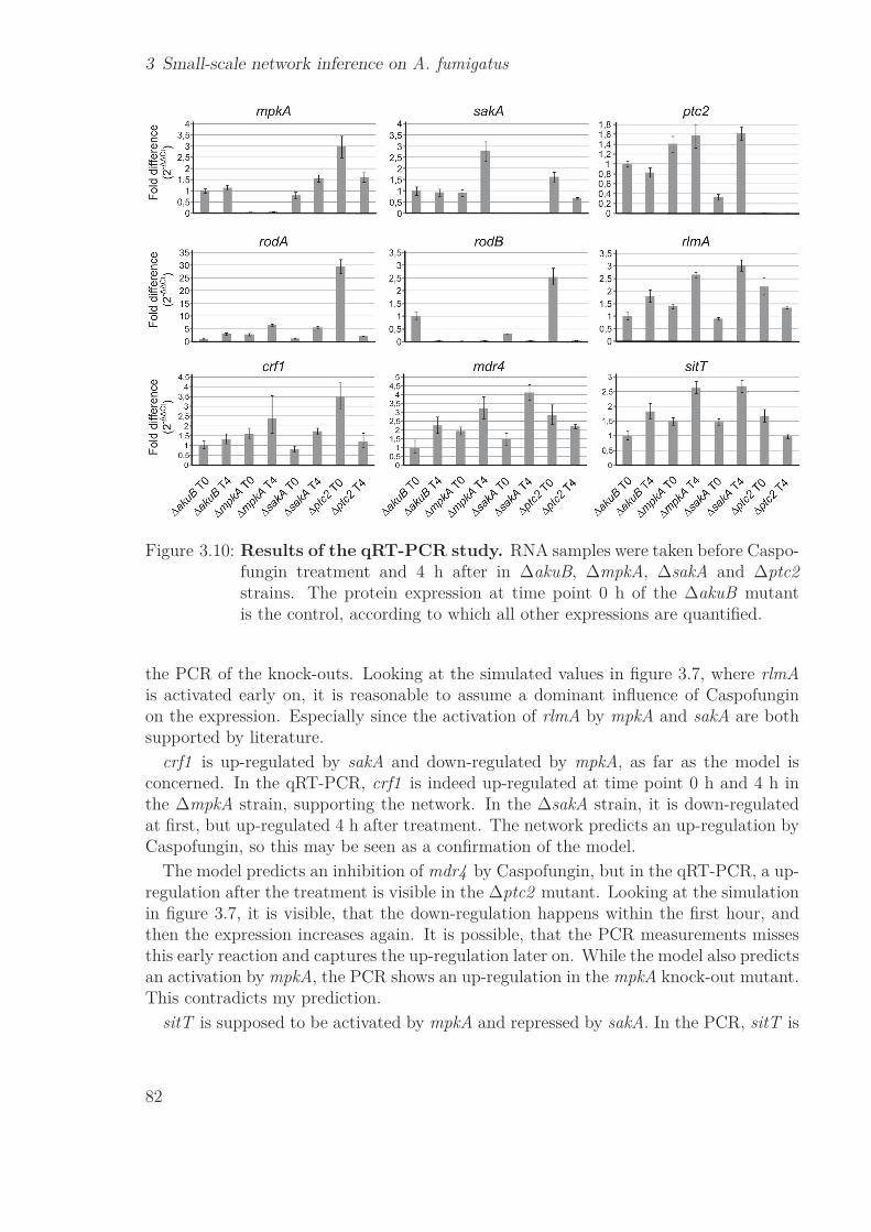
3 Small-scale network inference on A. fumigatus
Figure 3.10: Results of the qRT-PCR study. RNA samples were taken before Caspo-fungin treatment and 4 h after in ΔakuB, ΔmpkA, ΔsakA and Δptc2strains. The protein expression at time point 0 h of the ΔakuB mutantis the control, according to which all other expressions are quantified.
the PCR of the knock-outs. Looking at the simulated values in figure 3.7, where rlmAis activated early on, it is reasonable to assume a dominant influence of Caspofunginon the expression. Especially since the activation of rlmA by mpkA and sakA are bothsupported by literature.
crf1 is up-regulated by sakA and down-regulated by mpkA, as far as the model isconcerned. In the qRT-PCR, crf1 is indeed up-regulated at time point 0 h and 4 h inthe ΔmpkA strain, supporting the network. In the ΔsakA strain, it is down-regulatedat first, but up-regulated 4 h after treatment. The network predicts an up-regulation byCaspofungin, so this may be seen as a confirmation of the model.
The model predicts an inhibition of mdr4 by Caspofungin, but in the qRT-PCR, a up-regulation after the treatment is visible in the Δptc2 mutant. Looking at the simulationin figure 3.7, it is visible, that the down-regulation happens within the first hour, andthen the expression increases again. It is possible, that the PCR measurements missesthis early reaction and captures the up-regulation later on. While the model also predictsan activation by mpkA, the PCR shows an up-regulation in the mpkA knock-out mutant.This contradicts my prediction.
sitT is supposed to be activated by mpkA and repressed by sakA. In the PCR, sitT is
82

3.4 Discussion
up-regulated in both knock-out mutants. This leaves an ambiguous picture, from whichno specific conclusions can be drawn.
We found hints for the correct responses to some of our predictions, especially theinhibition of sakA by mpkA, while some prediction could not be verified and some resultswere inconclusive. It is important not to forget, that in the predicted model, genes areoften regulated by several other genes, while the qRT-PCR was done with single knock-out mutants. This means that the missing stimulus from one knocked-out genes may becompensated by another, without giving us an opportunity to study this.
3.3.8.3 Membrane permeability
The network model suggests, that Caspofungin influences the transport proteins in thecell wall, mirC, mdr4, mae1 and sitT. We reasoned that this hinders A. fumigatus doreact to the osmotic stress, as the fungus is incapable to remove outside agents fromthe cell, without the transporters. In order to investigate the osmotic stress during thetreatment, a Rhodamine-123 was used.
The results can be seen in figure 3.11. They show that after about 4 h, the Rhodamine-123 uptake in the wt is more than two times higher in the samples with a dose of 0.1μg/ml-1 Caspofungin. Similar effects can be seen for the other strains, except for Δptc2.This shows that the cell wall integrity is disrupted from the drug exposure. The ΔsakAshowed an higher absolute Rhodamine-123 uptake than the wt, and the uptake of ΔmpkAstrain was even higher. As for Δptc2, the Rhodamine-123 uptake of the treated sample ishigher during the first four hours, but then normalises at equal level with the untreatedsample. The Caspofungin resistant strain EMFRS678P also showed an increased uptake,even though it can not have been influenced by a Caspofungin induced inhibition of1,3-β-glucan synthase.
The wt was also tested with higher dosages of Caspofungin, which lead to a decreasedRhodamine-123 uptake. This shows the so called paradoxic effect.
3.4 Discussion3.4.1 Gene SelectionOne of the first problems when starting a small-scale network inference is the selectionof genes, that are to be investigated. But in contrast to large-scale models, the expectedprediction accuracy for single interaction is much higher. In our study, we wanted toinvestigate the gene regulatory effect of A. fumigatus on Caspofungin treatment. Thefirst reasonable step was to select all genes that are differentially expressed during theCaspofungin treatment.
The differentially expressed genes (DEGs) are determined using the fold change (oftenlogarithmic), the p-value, which tests for the null hypothesis that there is no expressionchange, or both. It is difficult to observe small changes in expression with the naked eyein semi-quantative methods like western blotting or other biological experiments lateron, which is why often fold changes ≥ 2 are preferred. However, I considered genes to be
83

3 Small-scale network inference on A. fumigatus
Figure 3.11: Results of the Rhodamine study. Measurements of the Rhodamine-123 intake during the with (red line) and without (blue line) Caspofungintreatment for different strains. The knock-out mutant were treated witha sub-lethal dose of Caspofungin (CAS; 0.1 μg ml-1), while the wild type(CEA10) was treated with different dosages. The figures show that withCaspofungin, the Rhodamine-123 uptake is significantly increased after 4 h,proving that Caspofungin increases the permeability of the cell wall.
84

3.4 Discussion
differential expressed if the FDR-adjusted p-value is ≤ 0.05. The reason for this decisioncomes from the good quality of the RNA-Seq data, which can be seen in table 3.2.
Most of the Pearson correlations between the replicates are above 0.96. At timepoint 1 h, the score is “only” 0.89, probably because A. fumigatus is in the middle ofthe Caspofungin adaption, which causes great changes in the gene regulatory network.During that phase, gene regulation is timely regulated, and within a few minutes smallalterations in regulation can occur. The correlation of the samples taken after 24 h isconsiderably lower. The gene-regulation at this time point is mostly influenced by thebeginning starvation.
When the correlation between the three replicates is very high, significant expressionchanges at different time points can be found, even if the absolute expression change israther low. This was one of the reasons I omitted the 24 h time point from the analysis.The mean correlation of 0.74 and 0.76 would weaken the statistical analysis of the data,for example the calculation of the p-value to identify DEGs. It is also more difficult forthe NetGenerator to find a fitting model. Additionally, I figured that the 24 h samplesare largely influenced by starvation than by the Caspofungin treatment. Omitting datafrom the analysis is always a difficult decision, since valuable information can be lost,especially considering the general lack of data we have to face during network inferences.However, during the collection of data, one should always consider the aim of the study.In focused network studies like this one, it is of uttermost importance not to introducebiased or distorted data, as this can quickly lead to false predictions.
Of special interest is also the time point 0.5 h. Several genes showed a strong reaction,a peak or valley, at that time point, which indicates an early response mechanism. TheA. fumigatus wild type strain is able to completely adapt to Caspofungin treatment,and these early responders are a vital part of this adaptation. Important drug stressresponse genes like mpkA, sakA or ssk2 exhibit that strong deviation from the initialstate. The first 30 minutes are of crucial importance when an organism tries to respondto cell surface stress, and the adoption measures vary from the “long term” responses,like modifying the glucan / chitin ratio in the cell wall. Short term responses includeinitialised cell wall repair mechanism and transporter activity, in order to limit thedamage done to the cell.
The second step was functional categorisation of the genes I found. Since Caspofunginis an outside agent that disrupts the cell wall, I knew that investigation of cell wall relatedgenes would be fruitful.
The number of annotated genes for non-model organisms remains low and the littleannotation that can be found often originates from sequence similarity to other modelspecies. Despite the increasing clinical importance of A. fumigatus, there is still littlespecies specific information available. This makes it especially difficult to reliably identifycandidate genes. Despite the very good quality of the data, the quantity limits theinference process to 20-30 genes only. This limitation comes not from the used inferencealgorithm, but caused by a more general issue. When the inference algorithm triesto find a regulator for a certain gene, and two candidates have the same expressionpattern, the algorithm can not decide, which regulator to choose. So even after functionalcategorisation, the final decision on which genes to choose requires expert knowledge,
85

3 Small-scale network inference on A. fumigatus
since the number of candidates was still to high.Transcription data alone is often insufficient to make reliable predictions about genetic
regulation. The amount of data is not enough to find unique solutions for the equationsystems. Most systems are underdetemined, leaving only heuristic approaches. Addi-tionally, transcription data alone gives no information about the semantic informationthat has been discovered over the years. Prior knowledge is the way to include literatureknowledge and therefore the insight gained by other studies. It is also possible to includeadditional data sources and data types in the inference. At present, network inferencewith data from multiple sources is still cumbersome, but as the amount of availabledata increases and standards become more unified, more and more information can becombined.
3.4.2 NetGenerator
The NetGenerator algorithm used in this study is not only able to include prior know-ledge, but also multi stimuli data. This might have been a way to handle the influenceof hunger stress at the 24 h time point and include the data, by considering nutrition adepleting stimulus. But again, this is not the aim of the study and the genes consideredin this network inference are not supposed to directly react to hunger stress.
A general assumption of the NetGenerator algorithm is that the investigated genesare in a steady state at the beginning of the experiment, when an external perturbationcauses a change in expression. After the perturbation subsides, the genes are expectedto return to the steady state. This is another reason, why I excluded the hunger stressin the simulation, as it prevents the fungus to return to “normal” conditions. Whilefigure 3.12 shows that the relative expression of genes like fks1 and roh1 returns to zeroafter 8 h, genes like ptc2 or sakA do not. However, that the expression of the genesreturns to the “normal” state is preferred, but not necessary to get reliable networkpredictions.
The NetGenerator uses many direct autoregulations in the model. Out of 26 genes,23 had an autoregulation, from which one (ssk1 ) is not robust. Mathematically, itprevents the simulation from running out of bounds, i.e. to increase indefinitely. Froma modeling point of view, negative autoregulation is similar to RNA-denaturation. Itstops the uncontrolled accumulation of gene products in a cell.
Genes like mpkA, sakA or ssk1 show a strong reaction in the first time point aftertreatment, showing a early response behaviour, depicted in figure 3.7. Those heavy per-turbation at the 0,5 h time point are difficult to model in ordinary differential equations.On my first attempt, I tried modeling the data using only first-order equations. Theresult was, that some times, the strong response in the first hour threw the model “ofbalance”, e.g. causing huge oscillations, as the model tried to implement the other timepoints. These oscillations can still be seen in figure 3.12, but not as dominant.
86

3.4 Discussion
3.4.3 RobustnessThe robustness tests showed, that 18 of the inferred interactions are not robust. From theseven interactions, that are susceptible to missing prior knowledge, none is actually partof any prior knowledge. This can happen, when a prior knowledge supported interactionsis not inferred due to omitted prior knowledge. This can lead to alternative connectivityin other parts of the network and even cause interactions that are not supported by priorknowledge to disappear.
Modeled networks are often depicted with robust interactions only. I think this rep-resentation is misleading, since these edges are still necessary to explain the expressionof the gene in the simulation. The information, that the interaction is rather fragile isnevertheless important in order to evaluate the reliability of the network. Especiallywhen selecting candidates for biological validation, one should refrain from choosinginteractions, which are not robust.
An alternative way of depicting the results of robustness tests is showing the altern-ative interactions, which came up during the test. During every cycle of the test, theinput data is distorted, and a network is inferred, that may has a different topologythan the original network, lacking certain interactions. These interactions are usuallysubstituted by alternative regulation. It may be interesting to count these alternativeinteractions and show them in the network, revealing alternative pathways. On the otherhand, finding a good visualisation gene regulatory networks including the confidence andalternatives of the infered edges is complicated even for small networks. Showing all al-ternative pathways would increase the complexity of the figure and the evaluation. Onemight also argue, that the alternative networks are done with intentionally distorteddata, and should therefore not be considered in the first place.
3.4.4 Cross-talk of mpkA & sakA pathwaysA goal of this study was the investigation of cross-talk between the high osmolarityglycerol (HOG) pathway, with sakA as a key regulator and the cell wall integrity (CWI)pathway, with mpkA as a key regulator. By investigating the transcriptional activity ofthe genes using the NetGenerator, I found a repressive influence of mpkA on sakA asshown in figures 3.8 and 3.12. This hypothesis was confirmed by western blot, seen infigure 3.9, where the phosphorylation level of SakA is generally increased in the ΔmpkAmutant. Also, the expression of mpkA decreases 2 h after the Caspofungin treatment.This decrease is especially dominant in the ΔsakA mutant, probably because sakA isneeded as a target of the CWI pathway. The decrease may also be the end of the stressresponse of A. fumigatus, as it needs to return to normal gene expression levels, afterthe drug adaption is completed.
However, here, the western blot contradicts the findings of the PCR (figure 3.10).There, the expression of MpkA is increased 4 h after treatment. A possible explanationcould be, that A. fumigatus expresses mpkA, but, as the target protein is missing, doesnot phosphorelate it, rendering it inactive. The qRT-PCR also shows that the expressionof sakA is up to three times higher in the ΔmpkA mutant, but only after the Caspofungin
87

3 Small-scale network inference on A. fumigatus
treatment, confirming the hypothesis of the model. The western blot (figure 3.9) showsthat the phosphorylation of SakA is on equal levels at 0 h and 4 h after treatment,and increased in the next time point at 8 h. This shows that the connection betweenexpression and phosphorylation levels is not always linear and can sometimes lead tocontradicting results. This can partly be explained by the seperation of expression andactivation (via phosphorylation) of a protein.
The model also predicts feed-back loops of mpkA and sakA as seen in figure 3.12. Theindirect regulation loop of sakA is even confirmed by prior knowledge: sakA ssk1 →ssk2 → sakA, although the connection ssk2 → sakA is not robust and alternativelyreplaced via an inhibition of and by ptc2. The other feed-back loop is mpkA → sitT fsk1 → mpkA. Alternatively, fks1 can also activate roh1, which then inhibits mpkA.From the data at hand, I can not tell, under which conditions fks1 acts activatingor inhibiting. Here, only the connection of mpkA and sitT is predicted by the priorknowledge. The prior knowledge also supports the inhibition of sitT by sakA, which isanother way into the feed-back loop of mpkA. Since mpkA also inhibits sakA, it is alsoa feed-back loop mof sakA itself. And there is one big feed-back loop of all genes exceptsitT in figure 3.12.
Figure 3.12: Focused view on the regulatory center of the network.
If the feed-back loop is mediated by post-transcriptional phosphorylation, ptc2 is asuitable candidate as regulator, as it was the only putative phosphatase to be founddifferentially expressed. Prior knowledge already suggested that ptc2 may be respons-ible for the repression of sakA, albeit in another species. The model also predicts thisrepression, but only if this prior knowledge is provided. The western blot on the otherhand did not reflect this hypothesis, as sakA is not up-regulated in the Δptc2 mutant.
88

3.4 Discussion
The qRT-PCR shows an altered protein concentration of sakA and mpkA in the Δptc2mutant, but as an up-regulation. These results show that ptc2 may not be the waympkA regulates sakA, but that there is an additional, hidden regulator.
This also demonstrates the limitations of the western blot and qRT-PCR, as we onlyhave data from single-knock-out mutants, while the model mostly predicts regulation bymultiple sources. If only one of the potential regulators is knocked-out and no change inregulation is detected, it can be because the other regulator compensates for the missingone. Multi-knock-out mutants would be necessary to detect this, but this is extremelycostly.
As mentioned before, A. fumigatus is able to adjust the ratio of chitin and glucan inits cell wall. By increasing the chitin content of the cell wall, it adopts to the Caspo-fungin treatment, since the drug targets the glucan synthesis. The Rhodamine-123experiment of figure 3.11 shows that the Caspofungin resistant strain also shows an in-creased Rhodamine-123 uptake, showing that Caspofungin induces cell wall disruptioneven without an effect of fks1. So Caspofungin attacks via two way: once by inducingcell wall stress, and second by targeting fks1, preventing the glucan synthase and recon-struction of the cell wall. sakA is a key regulator of the HOG pathway and activatedwhen osmotic stress occurs.
As shown in [32,81], the mitogen-activated kinase is responsible for the chitin balancein C. albicans, and most likely also conserved in A. fumigatus. After 2 h, A. fumigatusalso represses the expression of sakA via mpkA, and silences the HOG pathway. Theincrease in chitin in the cell wall, confers the Caspofungin resistance.
A. fumigatus shows a paradoxic effect, which is an increased resistance at a higherdrug dose. The cross-talk between mpkA and sakA can be used to explain this effect,since the treatment with Caspofungin activates mpkA, which then inhibits sakA. Thehigher the Caspofungin dose, the stronger the repression of sakA, and the more chitinis introduced to the cell wall, countering the drug effect. At the dose used in this study,the paradoxic effect did not occur. To further investigate this effect comprehensively,multiple RNA-Seq studies at different Caspofungin concentrations are necessary.
3.4.5 New prior knowledgeThe importance of the prior knowledge was again emphasised by the inference donewithout prior knowledge (see end of chapter 3.3.7.1). mpkA and sakA were not identifiedas hubs and the cross-talk was not found. Transcription data is an important source ofinformation, but still only a small piece of the big picture. Additional data from theoutside is indispensable to get closer to the big picture.
The investigation of the cross-talk does not end with this study. The verified know-ledge gained in these simulations can be used as prior knowledge in future studies. Thisincludes the inhibition of sakA by mpkA, which is predicted by the simulation and val-idated by western blot and qRT-PCR, making it a very reliable piece of information.
There are also several rather ambiguous results of the biological validation, like thepredicted activation of rodB by mpkA and sakA or the regulation of crf1 by mpkA and
89

3 Small-scale network inference on A. fumigatus
sakA. This leads to rather unreliable prior knowledge and if this information is to beused in future studies, it should be done with a small weighting only.
There is knowledge that is hard to acquire and very valuable: negative data. Accordingbiological validations (or rather falsifications), the inhibition of sakA and fks1 by ptc2could not be confirmed, at least not directly. The same is true for the activation ofrlmA by sakA and mpkA. This information can be included as negative prior knowledge,making these interactions less likely to occur in the network, so the algorithm can searchfor alternative regulations. It is unfortunate, that negative data is so hard to come by,even though it is most certainly produced in large quantities.
3.4.6 Workflow of the RNA-Seq studyThe workflow presented here is depicted in figure 3.13. It can serve as a template forRNA-Seq-based small scale network inference. The raw data is mapped and the genesare selected via differential expression, functional categorisation and expert knowledge.One part of the prior knowledge is gained from the same mapped data and an additionalpart is harvested from literature information. The transcription data of the selectedcandidate genes is pre-processed, before the mathematical modeling begins and differentnetworks are created. The final model is selected and its interactions are assessed forrobustness and new hypotheses are crested. These new hypotheses are tested in thelaboratory, where they are verified or falsified. In the end, new knowledge is gained,which can be used as prior knowledge for future investigations.
90
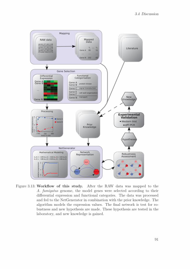
3.4 Discussion
0
−1.0
01.0
−1.0
01.0
Figure 3.13: Workflow of this study. After the RAW data was mapped to theA. fumigatus genome, the model genes were selected according to theirdifferential expression and functional categories. The data was processedand fed to the NetGenerator in combination with the prior knowledge. Thealgorithm models the expression values. The final network is test for ro-bustness and new hypothesis are made. These hypothesis are tested in thelaboratory, and new knowledge is gained.
91


4 Comparison with the adaptiveLASSO
In order to compare the NetGenerator and the adaptive LASSO algorithm, I also cre-ated for the dataset and experimental setup of chapter 3 a network using the methodsdescribed in the chapters 1.3.1 and 2.2.2. Again, I first estimated the best values for λ,which represents the influence of the prior knowledge and c, which determines the net-work size. I performed a grid search over both parameters, checking 13 different valuesranging from 0.001 to 1. This lead to 169 different parameter configuration, which tookabout 5 seconds to calculate on a standard workplace laptop.
Results show that giving more influence on the prior knowledge, by decreasing thevalue of λ, the more prior knowledge became part of the network. Since the imple-mentation of prior knowledge is a main goal of this study, I selected λ = 0.001. Theestimation of c, which is a factor for the results of the ridge regression was more diffi-cult. In contrast to the study on Candida of chapter 2, I did not have a gold standardto compare my results too. In order to get a comparison between the results of the finalnetwork and the NetGenerator approach, I selected the network that is the closest insize. The final network of the NetGenerator had 53 gene-to-gene interactions, excludingautoregulations and Input-to-gene interactions.
Figure 4.1 shows the result of the network inference using different values of c. Thesmallest network at c = 0.001 has 26 gene-to-gene interactions, as do the networks withvalue for c of 0.01 and 0.5. This is the smallest number of connections, the LASSOvia ridge regression can return for a network with 26 genes, since it has to find atleast one regulator for each gene, otherwise, the network reconstruction subroutine willthrow an error and the algorithm stops the calculation. Out of the 26 interactions, 21were supported by prior knowledge, but this may be misleading. The implementationof the algorithm does not allow to differentiate between activating or repressing priorknowledge. It only considers the information about source and target of an interaction.
The network inferred with c = 1 consists of 52 interactions, and is therefore veryclose in size to network inferred by the NetGenerator, promising a good comparison.While it shares 29 interactions with the prior knowledge, 12 of them have a differentsign, meaning they are repressing when the prior knowledge suggests activation andvice versa. With the help of the prior knowledge, sakA and mpkA became hubs again.With 14 interactions for mpkA (12 outgoing and 2 incoming) and 16 interactions forsakA (14 outgoing and 2 incoming). An interesting observation in the network are smallregulatory circles of two genes. One can be seen by the mutual inhibition between exg17and gel3, another between egnE1 and ptc2.
When comparing both networks, one can see that they have 10 interactions in com-
93

4 Comparison with the adaptive LASSO
imp
lem
en
ted
pri
or
kn
ow
led
ge
0.001 0.01 0.05 0.1 0.2 0.3 0.4 0.5 0.6 0.7 0.8 0.9 1
05
10
16
21
26
31
36
42
47
52
03
69
12
14
17
20
23
26
29
c
#o
fin
tera
ctio
ns
network sizeprior knowledge
Figure 4.1: Results of the network inference for different values of c. It is im-portant to notice, that the counting of the prior knowledge only consideredthe correct source and target. Not, if the interaction is repressing or ac-tivating, as the implementation of the adaptive LASSO did not allow thisdistinction.
mon, counting only correct signed interactions of the robust network inferred by theNetGenerator. Figure 4.3 illustrates this with connections in blue. It is little surprisingthat most of them are part of prior knowledge and come or go to sakA and mpkA. Theactivation of roh1 by fks1 is not supported by prior knowledge and was found in bothnetwork predictions, as was the inhibition of egnE1 by ptc2.
In addition to the 10 interactions that are fully in accordance, there are 14 interactions,where the source and target of the interaction is correct, but the sign is wrong. And threeinteractions belong to NetGenerator-network but failed the robustness test: mpkA →exg17, mpkA gel3 and ssk2 → sakA. This may be a reason to reconsider deletingthese edges.
The inhibition of sakA by mpkA was not found in the LASSO-based network inference.Not being able to determine the sign of a prior knowledge interaction in the LASSO-
based gives the algorithm more freedom to decide for it’s own. The point of priorknowledge is, however, to give guidance by more or less verified interactions. It is stillinteresting, that the LASSO algorithm implemented many prior knowledge interactions
94

Figure 4.2: Result of the network inference using adaptive LASSO via ridgeregression. The model consists of 52 interactions, from which 17 are inaccordance with the prior knowledge. 12 interactions have the same sourceand target as the prior knowledge, but a different sign.
with the opposite sign.The adaptive LASSO via ridge regression and the NetGenerator share many features,
like the implementation of prior knowledge and indirectly setting upper limits to the
95

4 Comparison with the adaptive LASSO
Figure 4.3: Consensus network between the LASSO-based and NetGenerator-based approach. 10 interactions are correct in sign and passed the ro-bustness test during the NetGenerator-approach. 14 are in accordance bydirection, but not by sign and additional three failed the robustness test ofthe NetGenerator-approach.
network size. But there are also distinct differences as the NetGenerator has some fea-tures that the adaptive LASSO does not have, like the consideration of external stimulior directed prior knowledge. The inference process is also much more sophisticated, bycreating individual sub models, optimises and assembles them. It is also able to usethe replicates for the modeling, while the LASSO took the averaged values as input,
96

discarding a lot of information. The adaptive LASSO processes the expression data ofeach gene individually without considering the results for other genes. The price for theelaborate way used by NetGenerator creates the networks inference is the increased runtime. The LASSO-based network inference completes the task within seconds, while theNetGenerator needs days. It might therefore be interesting to get first estimates usingthe adaptive LASSO and create the final model with the NetGenerator.
97


5 Humidimycin
5.1 Introduction
The occurrence of drug resistance is an emerging problem in antifungal therapies. Inaddition that, even clinically applied drugs like Caspofungin (see chapter 3.1.1 for de-tails) sometime show unpredicted results, like the so called “paradoxic effect” [66, 96].It describes the observation, that an increase of the drug dosage leads to a decrease ineffectivity. Scientists are continuously on the search for novel antifungal drugs and acomplementary approach is the search for compounds with synergistic or enhancing ef-fects. These are compounds that often have little to no effect on their own, but enhancethe effectivity of other agents. In an attempt to identify potentially enhancing com-pounds, 20,000 microbial natural products were extracted from actinomycetes and fungiand tested in combination with a sub-lethal dosage of Caspofungin in an high-throughputscreening approach. Of these extracts, 0.94% showed the capability to enhance the effectof Caspofungin. The extracts were tested against two A. fumigatus strains, ATCC46645and CEA17ku80, also known as ΔakuB.
From these positively tested extracts, 36.5% showed good dose-response curves andwere chosen for further investigation. Using re-fermentation and fractionation, the com-pounds were obtained and identified. Among them was the peptide Humidimycin, whichwas harvested from fermentation broths of Streptomyces humidus using chromatography.According to mass spectrometry, the molecular formula is C98H132N22O27S4, which givesit a close similarity with siamycin II.
Further studies about the antifungal effect of Humidimycin were done using a con-centration of 8 μg/ml with and without a sub-lethal dose of Caspofungin. Tests were per-formed against Aspergillus fumigatus, Candida albicans, Candida glabrata, Fusarium oxysporum,Cryptococcus neoformans and Saccharomyces cerevisiae. The sub-lethal dose of Caspo-fungin was defined as 1/8 of the minimal effective/inhibitory concentration (MEC/MIC)for that organism, except for F. oxysporum and C. neoformans, where a concentrationof 1 μg/ml was chosen, as they are not susceptible to Caspofungin.
In A. fumigatus, a dose of 1-2 μg/ml Humidimycin caused the MEC to drop from0.12 to 0.015 μg/ml and in C. albicans, the MIC dropped from 0.25 to 0.03 μg/ml. Thisdemonstrated the enhancing effect of Humidimycin in A. fumigatus and C. albicans forCaspofungin, while combined treatment showed no effect in C. glabrata, F. oxysporum,C. neoformans and S. cerevisiae.
99

5 Humidimycin
5.2 Data & Methods5.2.1 RNASeq dataIn order to investigate the mechanism of the enhancement on a genetic level, RNASeqdata was gathered from A. fumigatus conidia stressed with Caspofungin, Humidimycin,both compounds in combination and an unstressed control (see table 5.1). The treatedsamples were taken 4 h after the treatment in order to give A. fumigatus time for aresponse.
Table 5.1: RNASeq data used in this study. The used strain is the ΔakuB mutantand measurements were taken at three different conditions: stressed withCaspofungin, Humidimycin or both in combination. The samples taken at 0hour is the untreated control. All samples were taken in three replicates.
Caspofungin Caspofungin
Humidimycin Humidimycin
0 hour 3 × - -
4 hours 3 × 3 × 3 ×
The RNASeq data was mapped as described in chapter 3.2.3.
5.2.2 Differential expression & ClusteringI considered genes as differentially expressed, if the absolute log2(fold change) is > 2 andthe adjusted p-value < 0.01. Genes of each treatmend were tested against the untreatedcontrol (0 h). Genes were categorised according to GO [7] and KEGG [55] using theenrichment analysis tool FungiFun [93].
I performed the subsequent clustering using the R package e1071 [85], with parametersset to try a maximum number of iteration of 500 and 25 tries to find the best clustering.I searched for an optimal number of clusters between a cluster size of 2 and 8. Insteadof individual replicates, the total number of reads over all replicates was considered.To compare the relative gene expression change compared to the control and not theabsolute values, all gene expressions have been scaled down to fall between [-1, 1].
5.3 ResultsIn the data that includes the Caspofungin treatment only, 668 gene were differentiallyexpressed, 140 in response to the Humidimycin treatment and 571 in response to thecombined approach. In total 833 genes are differentially expressed in any of the samplesand the overlap of DEGs between the samples is quite big, as can be seen in figure 5.1.
100
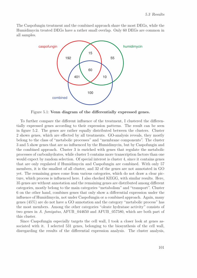
5.3 Results
The Caspofungin treatment and the combined approach share the most DEGs, while theHumidimycin treated DEGs have a rather small overlap. Only 60 DEGs are common inall samples.
192 55
100
15
401 10
60
caspofungin humidimycin
combined
Figure 5.1: Venn diagram of the differentially expressed genes.
To further compare the different influence of the treatment, I clustered the differen-tially expressed genes according to their expression patterns. The result can be seenin figure 5.2. The genes are rather equally distributed between the clusters. Cluster2 shows genes, which are effected by all treatments. GO-analysis reveals, they mostlybelong to the class of “metabolic processes” and “membrane components”. The cluster3 and 5 show genes that are no influenced by the Humidimycin, but by Caspofungin andthe combined approach. Cluster 3 is enriched with genes that regulate the metabolicprocesses of carbonhydrates, while cluster 5 contains more transcription factors than onewould expect by random selection. Of special interest is cluster 4, since it contains genesthat are only regulated if Humidimycin and Caspofungin are combined. With only 57members, it is the smallest of all cluster, and 32 of the genes are not annotated in GOyet. The remaining genes come from various categories, which do not draw a clear pic-ture, which process is influenced here. I also checked KEGG, with similar results. Here,35 genes are without annotation and the remaining genes are distributed among differentcategories, mostly belong to the main categories “metabolism” and “transport”. Cluster6 on the other hand, combines genes that only show a differential expression under theinfluence of Humidimycin, not under Caspofungin or a combined approach. Again, manygenes (45%) are do not have a GO annotation and the category “metabolic process” hasthe most members. Among the other categories “oleate hydratase activity” consists oftwo genes in A. fumigatus, AFUB_044650 and AFUB_057580, which are both part ofthis cluster.
Since Caspofungin especially targets the cell wall, I took a closer look at genes as-sociated with it. I selected 531 genes, belonging to the biosynthesis of the cell wall,disregarding the results of the differential expression analysis. The cluster analysis,
101
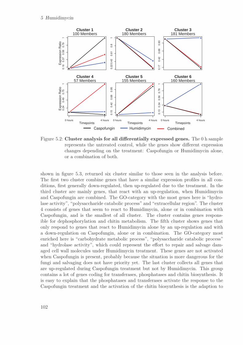
5 Humidimycin
0.2
20.4
20.6
10.8
1
0.1
70
.42
0.6
80
.93
0.2
40.4
90.7
51
0 hours 4 hoursTimepoints
0.1
50
.42
0.6
80
.95
0 hours 4 hoursTimepoints
0.1
60.3
70.5
80.7
91
Expre
ssio
nR
atio
Expre
ssio
nR
atio
0.1
30
.34
0.5
60
.78
1
0 hours 4 hoursTimepoints
Humidimycin CombinedCaspofungin
Figure 5.2: Cluster analysis for all differentially expressed genes. The 0 h samplerepresents the untreated control, while the genes show different expressionchanges depending on the treatment: Caspofungin or Humidimycin alone,or a combination of both.
shown in figure 5.3, returned six cluster similar to those seen in the analysis before.The first two cluster combine genes that have a similar expression profiles in all con-ditions, first generally down-regulated, then up-regulated due to the treatment. In thethird cluster are mainly genes, that react with an up-regulation, when Humidimycinand Caspofungin are combined. The GO-category with the most genes here is “hydro-lase activity”, “polysaccharide catabolic process” and “extracellular region”. The cluster4 consists of genes that seem to react to Humidimycin, alone or in combination withCaspofungin, and is the smallest of all cluster. The cluster contains genes respons-ible for dephosphorylation and chitin metabolism. The fifth cluster shows genes thatonly respond to genes that react to Humidimycin alone by an up-regulation and witha down-regulation on Caspofungin, alone or in combination. The GO-category mostenriched here is “carbohydrate metabolic process”, “polysaccharide catabolic process”and “hydrolase activity”, which could represent the effort to repair and salvage dam-aged cell wall molecules under Humidimycin treatment. These genes are not activatedwhen Caspofungin is present, probably because the situation is more dangerous for thefungi and salvaging does not have priority yet. The last cluster collects all genes thatare up-regulated during Caspofungin treatment but not by Humidimycin. This groupcontains a lot of genes coding for transferases, phosphatases and chitin biosynthesis. Itis easy to explain that the phosphatases and transferases activate the response to theCaspofungin treatment and the activation of the chitin biosynthesis is the adaption to
102

5.4 Discussion
the inhibited glucose synthesis caused by Caspofungin.
0.5
60
.67
0.7
80
.89
1
Exp
ressio
nR
atio
0.6
90
.80
.91
0.6
70
.78
0.8
91
0.6
80
.79
0.9
0 hours 4 hoursTimepoints
0.4
90
.69
0.9
1
0 hours 4 hoursTimepoints
Exp
ressio
nR
atio
0.5
90
.72
0.8
40
.96
0 hours 4 hoursTimepoints
Caspofungin
Figure 5.3: Cluster analysis for all cell wall-related genes. The 0 h sample repres-ents the untreated control, while the genes show different expression changesdepending on the treatment: Caspofungin or Humidimycin alone, or a com-bination of both.
5.4 DiscussionInvestigating the influence different drugs have on each other is not only important tocounter the increasing occurrence of resistance in fungi, but also since they allow thedecrease of the amount of a certain drug to be administered, which can possibly lowerthe degree of side effects. Using different treatments in parallel can also cause new sideeffects and different drugs combined may also block each other out.
Humidimycin seems to enhance the effectiveness of Caspofungin, lowering the neces-sary dosage needed. Looking at figure 5.1, it can be seen, that the number of DEGsdecreases from 668 from the Caspofungin treatment to 571 DEGs in the combined ap-proach. This shows, that Humidimycin, while not damaging the fungus directly, stilllowers the drug response. Further analysis shows that the genes cluster in distinct groupsaccording to their reaction to different treatments. When comparing Caspofungin andthe combined approach, few genes show different expression profiles, and cluster 4 infigure 5.2 contains genes, that only react to the combined treatment. With 57 members,it is the smallest cluster of the test and 32 of them are not annotated in GO yet, which
103

5 Humidimycin
makes investigation difficult. The remaining genes belong to different categories, thatdo draw a clear picture, what sets these genes aside from all others.
The cluster analysis for the cell wall related genes gave a comparable results, eventhough there are more genes that react to Humidimycin than in the previous cluster-ing. Again, cluster 4 is the smallest of all and contains genes that seem to react toHumidimycin alone and in combination with Caspofungin, but not with Caspofunginalone. Interestingly, this cluster contains genes related to dephosphorylation and thechitin metabolism, which is considered as an important part of the Caspofungin drugadaption. In this cluster, these genes are down-regulated, which may be connected to theenhancing effect of the combined drug approach. Cluster 6 on the other hand containsgenes that react to Caspofungin by up-regulation. These are phosphatases and trans-ferases and again chitin biosynthesis, which show the drug response in A. fumigatus.Maybe cluster 4 shows the dampening of the drug response signal in A. fumigatus,caused by Humidimycin, while cluster 6 shows the genes that are nevertheless activatedby the drug Caspofungin.
In conclusion, the only thing that can be safely said is, that Humidimycin lowers thenumber of DEGs when combined with Caspofungin. It also causes the down-regulationof some parts of the chitin metabolism which may also be part of the enhancing effecttowards Caspofungin.
104

6 Conclusion
6.1 Large-scale network prediction
The main goal aim of this study was to investigate the application of network inferencemethods for the study of gene regulation. I started a full-genomic approach to createscale-free gene regulatory networks. The presented approach uses the combination ofdifferent linear regression methods to investigate multi-experiment microarray data, butcan also be used to investigate other high-throughput datasets. I could show that theadditional implementation of multiple sources of prior knowledge is able to increase thepredictive power of the network model. The use of an automatically harvested goldstandard to compare the results of the evaluation was of great help when I had to selectthe final network. Despite careful programming and a constant increase in computationpower, inferring and evaluating large scale networks remain a time consuming task, asseen in the study of chapter 3, where the complete calculation of the final, robust networkof 26 genes took about a week on a computer cluster with 32 cores..
An important property the networks showed is sparseness, which increases reliabilityand interpretability of the networks, by focusing on the most influential network regu-lations and is also a property assumed in biological networks. The scale-freeness allowsthe investigation of topological properties, especially the identification of hubs. Themodel suggested several possible hub genes, which can be drug targets in the future.The experimental testing of drug targets is costly and time consuming, which makescareful computational study beforehand very important, as it can give valuable hints forpromising candidates.
The biggest obstacle in my work is the general lack of a sufficient amount of data.Despite the steady increase of the size of high-throughput data, the available amount isstill insufficient for reliable large scale predictions, especially for non-model organisms.Of special concern is the gold standard that I used to evaluate the final network. Despitethe use of automated text-mining software and scanning of over 6000 full-text researchpapers, the amount of current knowledge is still very low. Additional effort is necessaryto increase the mining output in face of a constantly growing number of publications.Right now, the step from large-scale gene-regulatory networks to the testing of drugtargets in the laboratory should be accompanied by an intermediate step: small-scalenetwork inference.
105

6 Conclusion
6.2 Small-scale network predictionIn order to get a focused view on the gene regulation of genes, small-scale networksare a valuable tool. The critical first decision here is the selection of candidates for theinference. Large-scale models are one way to identify potential hubs, and therefore genesof interest.
I investigated the adaption of A. fumigatus on the clinical drug Caspofungin on agene regulatory level in chapter 3. I used high quality RNA-Seq data and, as no large-scale network models were available, used the combination of differential expression andfunctional categorisation coupled with expert knowledge, to select candidate genes forthe inference. Again, I used prior knowledge to improve the quality of the prediction.The search in literature revealed only little known information about how A. fumigatusregulates the drug adaption. I gained additional knowledge from analysing data of knock-out experiments of known regulators. This additional data is necessary to complementthe little expression data, that is available.
The NetGenerator creates network models of different sizes and the lack of a goldstandard makes it difficult to evaluate their quality. I decided to judge the networksby how close they are to the current knowledge and their modeling error. Furtherrobustness test helped to separate interactions that are robust to noise from those thatare susceptible to noise in the data or changes in the prior knowledge.
From here I derived new hypothesis about the interactions between the regulatorygenes. The most important one is the predicted inhibition of sakA by mpkA, the keyregulators of the two main drug response signalling pathways. Tests in the laboratoryverified this important prediction via western blotting and qRT-PCR. This new interac-tion can explain some critical expects of the A. fumigatus drug adaption, as the genesare known to influence the chitin / glucan balance of the cell wall. Since Caspofunginis known to inhibit the glucan biosynthesis, a shift to chitin synthesis can explain theloss of effectivity. This new knowledge can now used as new input for future studies tounravel even more knowledge about the emergence of resistances in pathogenic fungi.
6.3 Analysis of expressionSometimes, the amount of available data is not sufficient to create gene regulatory net-works, even in small-scale. In chapter 5, I worked with only four data points, each underdifferent conditions. My work was a small part of an extensive study of how Humi-dimycin influences the antifungal properties of Caspofungin, without having antifungalproperties itself. The methods I applied here were also part of the other studies, used ina different context. The identification of differentially expressed genes was used in thesmall-scale study to identify possible candidate genes. Here, it was used in a broadersense of identifying the global influence a treatment has on the genetic activity. Theresults showed that the enhancing effect comes with a decrease in the number of differ-ential expressed genes, which can explain, why A. fumigatus is not hindered in its abilityto adopt to Caspofungin.
106
6.4 Comparison of LASSO & NetGenerator
Further investigation included clustering to sort the differentially expressed genes ac-cording to their reaction to different treatments. This allows further hypothesis of howHumidimycin influences the expression. Detailed examination remained inconclusive, asit is often the case due to a lack of annotated genes. Nevertheless, these study can givevaluable hints which genes might be affected by Humidimycin and Caspofungin.
6.4 Comparison of LASSO & NetGeneratorThe tools available for network inferences are as various as the scientific questions theytry to answer. In my work, I applied mutual information networks, different form oflinear regression models and the NetGenerator tool. The direct comparison of my imple-mentation of the adaptive LASSO via ridge regression and the NetGenerator in chapter 4showed the possibilities and limitations of both approaches.
The LASSO-based approach has one indispensable property, when it comes to large-scale network inference: it is fast. To be precise, this is rather thanks to the LARSimplementation by Efron et al. It made it possible to calculate all LASSO solutions inone run, making the testing for different model sizes tractable. Small-scale modeling thattook days with the NetGenerator was done within seconds using the LASSO. Combiningthe ridge regression for parameter evaluation and the LASSO for parameter selectionseems to be a reasonable way to create network models. Not being to discriminatebetween activating and repressing prior knowledge is certainly a disadvantage, but thisfeature can be added in future implementations. As it is, the LASSO-based approachis a mature way to model large-scale expression data and allows for a quick overview insmall-scale data.
The NetGenerator splits the modeling in several smaller sub-models and optimisesthem individually, before combining them to a bigger network. While this leads tomore accurate results and more implemented prior knowledge, it is also much more timeconsuming. This limits the number of genes expression profiles, that can be modeled,before the computation time becomes limiting. The NetGenerator also offers a lot morepossibilities to influence the modeling results. I focused on the optimisation of threeparameters, but there are much more that can positively influence the results of theinference. Without a proper gold standard, however, it is difficult to evaluate the modeland optimise the results.
6.5 Final remarksEventually, my study revealed the following conclusions: The biggest obstacle to tacklegene regulatory network inference is the lack of high quality data. Often researcherscan not be picky when choosing the data for the modeling. However, one must notforget the aim of the study, which has to be well defined. When using different sourcesof information, it is very easy to include data that introduces a bias in the modeling,since data are always taken under certain conditions, which may not always match your
107

6 Conclusion
question of study. Large-scale studies require the highest amount of data and oftencompendia of different studies from various laboratories are used. These datasets areoften very homogeneous, which must not necessarily be a disadvantage. The aim oflarge-scale studies of often to get an overview of the genetic network. Therefore, havingdata taken under different conditions may be an advantage. One should keep in mindthat not every interaction is active at all times and occur only at certain conditions.Large-scale models usually do not capture these subtleties.
If the study is about specific reactions to fixed conditions, a small-scale analysis isadvisable. While in large-scale models the need for quantity of data exceeds the need forquality (up to a certain extend), small-scale models rely on the quality of the data. Here,the research question is often more specific and includes reactions to fixed treatments.It is often necessary to collect data individually for each study, since it is unlikely tofind a suitable dataset available public.
While each study aims at discovering new knowledge, it is very important to considercurrent knowledge and not only include it into the modeling, but also observe, how muchthe model is able to reflect verified knowledge. A gold standard is therefore an invaluablehelp, since it allows the evaluation of different networks. These gold standards are oftenincomprehensive or completely unavailable, especially for non-model organisms. Themodeling does not return one single network, but an ensemble of networks in differentsizes and structures. Selecting one model as the final one is difficult due to a lack ofindependent measures. Taking the model error only limits the selection process to theexpression data only, ignoring the current knowledge.
The regulation of genes in an organism is a dynamic processes that change over time.The network model is a still frame of the most prominent interactions during the timestudied, and by no means does it capture the full complexity of genetic regulations.This is also a reason why different prior knowledge sources and gold standard sometimeshave contradicting information or do not match the regulatory model. The informationorigins from studies under different conditions, that may lead to different predictions onregulations.
In all, scientific research is always a balancing between current and new knowledge.Putting to much known information into a study and forcing it into the model blocksthe way to new discoveries and returns only the current knowledge. Not offering anyadditional information to the model and not guiding it along current knowledge leadsto highly unreliable results and disregards the work of other scientists. Both extremesblock the path to insight and it is the challenge and responsibility of every scientist tolook at the past and the future.
108

Bibliography[1] A. Abad, J. V. Fernández-Molina, J. Bikandi, A. Ramírez, J. Margareto,
J. Sendino, F. L. Hernando, J. Pontón, J. Garaizar, and A. Rementeria. Whatmakes Aspergillus fumigatus a successful pathogen? genes and molecules involvedin invasive aspergillosis. Rev Iberoam Micol, 27(4):155–182, 2010.
[2] Albert, Jeong, and Barabasi. Error and attack tolerance of complex networks.Nature, 406(6794):378–382, July 2000.
[3] D. Albrecht, R. Guthke, A. A. Brakhage, and O. Kniemeyer. Integrative analysisof the heat shock response in Aspergillus fumigatus. BMC genomics, 11(1):32,2010.
[4] R. Altwasser, J. Linde, and R. Guthke. Genome-wide scale-free network inferencefor Candida albicans. Frontiers in Microbial Immunology, 3:51, 2012.
[5] R. Amitani, G. Taylor, E.-N. Elezis, C. Llewellyn-Jones, J. Mitchell, F. Kuze,P. J. Cole, and R. Wilson. Purification and characterization of factors produced byAspergillus fumigatus which affect human ciliated respiratory epithelium. Infectionand immunity, 63(9):3266–3271, 1995.
[6] S. Anders and W. Huber. Differential expression analysis for sequence count data.Genome Biol, 11(10):R106, 2010.
[7] M. Ashburner, C. A. Ball, J. A. Blake, D. Botstein, H. Butler, J. M. Cherry, A. P.Davis, K. Dolinski, S. S. Dwight, J. T. Eppig, and others. Gene ontology: tool forthe unification of biology. Nature genetics, 25(1):25–29, 2000.
[8] L. R. Asmundsdóttir, H. Erlendsdóttir, and M. Gottfredsson. Increasing incidenceof candidemia: results from a 20-year nationwide study in iceland. J Clin Microbiol,40(9):3489–3492, Sept. 2002.
[9] G. D. Bader. BIND: the biomolecular interaction network database. Nucleic AcidsResearch, 31(1):248–250, Jan. 2003.
[10] S. Balaji, M. M. Babu, L. M. Iyer, N. M. Luscombe, and L. Aravind. Compre-hensive analysis of combinatorial regulation using the transcriptional regulatorynetwork of yeast. Journal of Molecular Biology, 360(1):213–227, June 2006.
[11] V. Balloy and M. Chignard. The innate immune response to Aspergillus fumigatus.Microbes and Infection, 11(12):919–927, Oct. 2009.
109

Bibliography
[12] A. Barabási. Emergence of scaling in random networks. Science, 286(5439):509–512, Oct. 1999.
[13] J. C. Bowman, P. S. Hicks, M. B. Kurtz, H. Rosen, D. M. Schmatz, P. A. Liberator,and C. M. Douglas. The antifungal echinocandin caspofungin acetate kills growingcells of Aspergillus fumigatus in vitro. Antimicrobial Agents and Chemotherapy,46(9):3001–3012, Sept. 2002.
[14] A. Brakhage. Systemic fungal infections caused by aspergillus species: Epi-demiology, infection process and virulence determinants. Current Drug Targets,6(8):875–886, Dec. 2005.
[15] A. A. Brakhage, S. Bruns, A. Thywissen, P. F. Zipfel, and J. Behnsen. Interactionof phagocytes with filamentous fungi. Curr Opin Microbiol, 13(4):409–415, Aug.2010.
[16] A. J. Butte and I. S. Kohane. Mutual information relevance networks: functionalgenomic clustering using pairwise entropy measurements. Pacific Symposium onBiocomputing. Pacific Symposium on Biocomputing, pages 418–429, 2000.
[17] E. Buyko, E. Faessler, J. Wermter, and U. Hahn. Syntactic simplification andsemantic enrichment - trimming dependency graphs for event extraction. Compu-tational Intelligence, 27(4):610–644, 2011.
[18] D. Cappelletty and K. Eiselstein-McKitrick. The echinocandins. Pharmacotherapy,27(3):369–388, Mar. 2007.
[19] S. Christley, Q. Nie, and X. Xie. Incorporating existing network information intogene network inference. PLoS One, 4(8):e6799, 2009.
[20] V. Czaika, P. Nenoff, A. Glöckner, W. Fegeler, K. Becker, and A. F. Schmalreck.Epidemiology and changes in patient-related factors from 1997 to 2009 in clinicalyeast isolates related to dermatology, gynaecology, and paediatrics. Int J Microbiol,2013:703905, 2013.
[21] M. E. da Silva Ferreira, M. R. V. Z. Kress, M. Savoldi, M. H. S. Goldman, A. Hartl,T. Heinekamp, A. A. Brakhage, and G. H. Goldman. The akuBKU80 mutant defi-cient for nonhomologous end joining is a powerful tool for analyzing pathogenicityin Aspergillus fumigatus. Eukaryotic Cell, 5(1):207–211, Jan. 2006.
[22] T. R. T. Dagenais and N. P. Keller. Pathogenesis of Aspergillus fumigatus ininvasive aspergillosis. Clinical Microbiology Reviews, 22(3):447–465, July 2009.
[23] N. Delhomme, I. Padioleau, E. E. Furlong, and L. M. Steinmetz. easyRNASeq: abioconductor package for processing RNA-seq data. Bioinformatics, 28(19):2532–2533, Oct. 2012.
110

Bibliography
[24] C. D’Enfert and B. Hube. Candida: comparative and functional genomics. CaisterAcademic Press. Norfolk,U.K., 2007.
[25] M.-A. Dillies, A. Rau, J. Aubert, C. Hennequet-Antier, M. Jeanmougin, N. Ser-vant, C. Keime, G. Marot, D. Castel, J. Estelle, G. Guernec, B. Jagla, L. Jouneau,D. Laloë, C. L. Gall, B. Schaëffer, S. L. Crom, M. Guedj, and Jaffrézic. A compre-hensive evaluation of normalization methods for illumina high-throughput RNAsequencing data analysis. Brief Bioinform, Sept. 2012.
[26] C. Du, J. Sarfati, J.-P. Latge, and R. Calderone. The role of the sakA (hog1)and tcsB (sln1) genes in the oxidant adaptation of Aspergillus fumigatus. MedicalMycology, 44(3):211–218, Jan. 2006.
[27] B. Dujon, D. Sherman, G. Fischer, P. Durrens, S. Casaregola, I. Lafontaine, J. D.Montigny, C. Marck, C. Neuvéglise, E. Talla, N. Goffard, L. Frangeul, M. Aigle,V. Anthouard, A. Babour, V. Barbe, S. Barnay, S. Blanchin, J.-M. Beckerich,E. Beyne, C. Bleykasten, A. Boisramé, J. Boyer, L. Cattolico, F. Confanioleri,A. D. Daruvar, L. Despons, E. Fabre, C. Fairhead, H. Ferry-Dumazet, A. Groppi,F. Hantraye, C. Hennequin, N. Jauniaux, P. Joyet, R. Kachouri, A. Kerrest,R. Koszul, M. Lemaire, I. Lesur, L. Ma, H. Muller, J.-M. Nicaud, M. Nikol-ski, S. Oztas, O. Ozier-Kalogeropoulos, S. Pellenz, S. Potier, G.-F. Richard, M.-L. Straub, A. Suleau, D. Swennen, F. Tekaia, M. Wésolowski-Louvel, E. West-hof, B. Wirth, M. Zeniou-Meyer, I. Zivanovic, M. Bolotin-Fukuhara, A. Thierry,C. Bouchier, B. Caudron, C. Scarpelli, C. Gaillardin, J. Weissenbach, P. Wincker,and J.-L. Souciet. Genome evolution in yeasts. Nature, 430(6995):35–44, July2004.
[28] P. D’haeseleer, S. Liang, and R. Somogyi. Genetic network inference: from co-expression clustering to reverse engineering. Bioinformatics, 16(8):707–726, Jan.2000.
[29] M. B. Eisen, P. T. Spellman, P. O. Brown, and D. Botstein. Cluster analysis anddisplay of genome-wide expression patterns. Proceedings of the National Academyof Sciences, 95(25):14863–14868, Aug. 1998.
[30] J. J. Faith, B. Hayete, J. T. Thaden, I. Mogno, J. Wierzbowski, G. Cottarel,S. Kasif, J. J. Collins, and T. S. Gardner. Large-scale mapping and validationof escherichia coli transcriptional regulation from a compendium of expressionprofiles. PLoS Biology, 5(1):e8, 2007.
[31] C. V. Forst. Host-pathogen systems biology. Drug discovery today, 11(5-6):220–227, Mar. 2006.
[32] J. R. Fortwendel, P. R. Juvvadi, B. Z. Perfect, L. E. Rogg, J. R. Perfect, andW. J. Steinbach. Transcriptional regulation of chitin synthases by calcineurincontrols paradoxical growth of Aspergillus fumigatus in response to caspofungin.Antimicrobial Agents and Chemotherapy, 54(4):1555–1563, Apr. 2010.
111

Bibliography
[33] N. Friedman, M. Linial, I. Nachman, and D. Pe’er. Using bayesian networks toanalyze expression data. Journal of computational biology, 7(3-4):601–620, 2000.
[34] C. Garcia-Vidal, D. Viasus, and J. Carratalà. Pathogenesis of invasive fungalinfections. Curr Opin Infect Dis, 26(3):270–276, June 2013.
[35] A. Gastebois, C. Clavaud, V. Aimanianda, and J.-P. Latgé. Aspergillus fumigatus:cell wall polysaccharides, their biosynthesis and organization. Future Microbiology,4(5):583–595, June 2009.
[36] J. M. Gilsenan, J. Cooley, and P. Bowyer. CADRE: the Central Aspergillus DataREpository 2012. Nucleic Acids Res, 40(Database issue):D660–D666, Jan. 2012.
[37] A. Goffeau, B. G. Barrell, H. Bussey, R. W. Davis, B. Dujon, H. Feldmann,F. Galibert, J. D. Hoheisel, C. Jacq, M. Johnston, E. J. Louis, H. W. Mewes,Y. Murakami, P. Philippsen, H. Tettelin, and S. G. Oliver. Life with 6000 genes.Science, 274(5287):546–567, Oct. 1996.
[38] N. Grahl, K. M. Shepardson, D. Chung, and R. A. Cramer. Hypoxia and fungalpathogenesis: to air or not to air? Eukaryot Cell, 11(5):560–570, May 2012.
[39] M. Gustafsson. Gene networks from high-throughput data: Reverse engineeringand analysis. 2010.
[40] M. Gustafsson, M. Hörnquist, and A. Lombardi. Large-scale reverse engineeringby the lasso. http://arxiv.org/abs/q-bio/0403012v1, Mar. 2004.
[41] M. Gustafsson, M. Hörnquist, and A. Lombardi. Constructing and analyzing alarge-scale gene-to-gene regulatory network lasso-constrained inference and bio-logical validation. IEEE/ACM transactions on computational biology and bioin-formatics, 2(3):254–261, 2005.
[42] R. Guthke, O. Kniemeyer, D. Albrecht, A. A. Brakhage, and U. Möller. Discoveryof gene regulatory networks in Aspergillus fumigatus. In Knowledge discovery andemergent complexity in bioinformatics, page 22–41. Springer, 2007.
[43] R. Guthke, U. Möller, M. Hoffmann, F. Thies, and S. Töpfer. Dynamic networkreconstruction from gene expression data applied to immune response during bac-terial infection. Bioinformatics, 21(8):1626–1634, Apr. 2005.
[44] U. Güldener, M. Münsterkötter, M. Oesterheld, P. Pagel, A. Ruepp, H.-W. Mewes,and V. Stümpflen. MPact: the MIPS protein interaction resource on yeast. NucleicAcids Research, 34(Database issue):D436–441, Jan. 2006.
[45] L.-P. Hamel, M.-C. Nicole, S. Duplessis, and B. E. Ellis. Mitogen-activated pro-tein kinase signaling in plant-interacting fungi: distinct messages from conservedmessengers. Plant Cell, 24(4):1327–1351, Apr. 2012.
112

Bibliography
[46] J.-D. J. Han, N. Bertin, T. Hao, D. S. Goldberg, G. F. Berriz, L. V. Zhang,D. Dupuy, A. J. M. Walhout, M. E. Cusick, F. P. Roth, and M. Vidal. Evidencefor dynamically organized modularity in the yeast protein–protein interaction net-work. Nature, 430(6995):88–93, July 2004.
[47] X. He and J. Zhang. Why do hubs tend to be essential in protein networks? PLoSGenet, 2(6):e88, June 2006.
[48] M. Hecker, S. Lambeck, S. Toepfer, E. van Someren, and R. Guthke. Gene regulat-ory network inference: Data integration in dynamic models—a review. Biosystems,96(1):86–103, Apr. 2009.
[49] F. Horn, V. Valiante, R. Guthke, and A. A. Brakhage. Data-driven systems bio-logy of fungal infections. In Human Pathogenic Fungi: Molecular Biology andPathogenic Mechanisms. Caister Academic Press, June 2014.
[50] B. Hube. Infection-associated genes of Candida albicans. Future Microbiol,1(2):209–218, Aug. 2006.
[51] J. Ihmels, S. Bergmann, J. Berman, and N. Barkai. Comparative gene expressionanalysis by a differential clustering approach: Application to the Candida albicanstranscription program. PLoS Genet, 1(3):e39, 2005.
[52] W. R. Jarvis. Epidemiology of nosocomial fungal infections, with emphasis oncandida species. Clin Infect Dis, 20(6):1526–1530, June 1995.
[53] H. Jeong, S. P. Mason, A. L. Barabási, and Z. N. Oltvai. Lethality and centralityin protein networks. Nature, 411(6833):41–42, May 2001.
[54] M. Johnston. A model fungal gene regulatory mechanism: the GAL genes ofsaccharomyces cerevisiae. Microbiol Rev, 51(4):458–476, Dec. 1987.
[55] M. Kanehisa, S. Goto, Y. Sato, M. Furumichi, and M. Tanabe. KEGG for integ-ration and interpretation of large-scale molecular data sets. Nucleic Acids Res,40(Database issue):D109–D114, Jan. 2012.
[56] M. Karthaus. Prophylaxis and treatment of invasive aspergillosis withvoriconazole, posaconazole and caspofungin: review of the literature. Europeanjournal of medical research, 16(4):145–152, 2011.
[57] A. Kasprzyk. BioMart: driving a paradigm change in biological data management.Database, 2011(0):bar049–bar049, Nov. 2011.
[58] S. A. Kauffman. Metabolic stability and epigenesis in randomly constructed ge-netic nets. Journal of Theoretical Biology, 22(3):437–467, Mar. 1969.
[59] M. A. Kaufman, G. J. Duke, F. McGain, C. French, C. Aboltins, G. Lane, andG. A. Gutteridge. Life-threatening respiratory failure from h1n1 influenza 09 (hu-man swine influenza). Medical Journal of Australia, 191(3), 2009.
113

Bibliography
[60] J.-D. Kim, T. Ohta, S. Pyysalo, Y. Kano, and J. Tsujii. Extracting bio-molecularevents from literature—the bionlp’09 shared task. Computational Intelligence,27(4):513–540, 2011.
[61] J. Kohler, J. Baumbach, J. Taubert, M. Specht, A. Skusa, A. Ruegg, C. Rawlings,P. Verrier, and S. Philippi. Graph-based analysis and visualization of experimentalresults with ONDEX. Bioinformatics, 22(11):1383–1390, June 2006.
[62] S. Kozhenkov, M. Sedova, Y. Dubinina, A. Gupta, A. Ray, J. Ponomarenko, andM. Baitaluk. BiologicalNetworks-tools enabling the integration of multi-scale datafor the host-pathogen studies. BMC systems biology, 5(1):7, 2011.
[63] S. Krappmann, C. Sasse, and G. H. Braus. Gene targeting in Aspergillus fumigatusby homologous recombination is facilitated in a nonhomologous end- joining-deficient genetic background. Eukaryotic Cell, 5(1):212–215, Jan. 2006.
[64] V. Krcmery and A. J. Barnes. Non-albicans candida spp. causing fungaemia:pathogenicity and antifungal resistance. The Journal of Hospital Infection,50(4):243–260, Apr. 2002.
[65] K. Kryszczuk and P. Hurley. Estimation of the number of clusters using multipleclustering validity indices. In Multiple Classifier Systems, page 114–123. Springer,2010.
[66] F. Lamoth, P. R. Juvvadi, E. J. Soderblom, M. A. Moseley, Y. G. Asfaw, and W. J.Steinbach. Identification of a key lysine residue in heat shock protein 90 required forazole and echinocandin resistance in Aspergillus fumigatus. Antimicrobial Agentsand Chemotherapy, 58(4):1889–1896, Apr. 2014.
[67] J. P. Latgé. Aspergillus fumigatus and aspergillosis. Clin Microbiol Rev,12(2):310–350, Apr. 1999.
[68] H. Li, B. Handsaker, A. Wysoker, T. Fennell, J. Ruan, N. Homer, G. Marth,G. Abecasis, R. Durbin, and 1000 Genome Project Data Processing Subgroup.The sequence alignment/map format and SAMtools. Bioinformatics, 25(16):2078–2079, Aug. 2009.
[69] J. Linde, E. Buyko, R. Altwasser, U. Hahn, and R. Guthke. Full-genomic networkinference for non-model organisms: A case study for the fungal pathogen Candidaalbicans. In Proc. International Conf. on Bioinformatics, Computational Biologyand Biomedical Engineering, ICBCBBE2011, Paris, France, Aug. 2011. WASET.
[70] J. Linde, P. Hortschansky, E. Fazius, A. A. Brakhage, R. Guthke, and H. Haas.Regulatory interactions for iron homeostasis in Aspergillus fumigatus inferred bya systems biology approach. BMC Syst Biol, 6:6, 2012.
114

Bibliography
[71] J. Linde, D. Wilson, B. Hube, and R. Guthke. Regulatory network modelling ofiron acquisition by a fungal pathogen in contact with epithelial cells. BMC SystBiol, 4:148, 2010.
[72] T. T. Liu, R. E. B. Lee, K. S. Barker, R. E. Lee, L. Wei, R. Homayouni, andP. D. Rogers. Genome-wide expression profiling of the response to azole, polyene,echinocandin, and pyrimidine antifungal agents in Candida albicans. AntimicrobialAgents and Chemotherapy, 49(6):2226–2236, June 2005.
[73] D. Lohr, P. Venkov, and J. Zlatanova. Transcriptional regulation in the yeast GALgene family: a complex genetic network. FASEB J, 9(9):777–787, June 1995.
[74] O. Marchetti, J. Bille, U. Fluckiger, P. Eggimann, C. Ruef, J. Garbino,T. Calandra, M.-P. Glauser, M. G. Täuber, D. Pittet, and Fungal Infection Net-work of Switzerland. Epidemiology of candidemia in swiss tertiary care hospitals:secular trends, 1991-2000. Clin Infect Dis, 38(3):311–320, Feb. 2004.
[75] A. A. Margolin, I. Nemenman, K. Basso, C. Wiggins, G. Stolovitzky, R. Favera,and A. Califano. ARACNE: An algorithm for the reconstruction of gene regulatorynetworks in a mammalian cellular context. BMC Bioinformatics, 7(Suppl 1):S7,2006.
[76] G. S. Martin, D. M. Mannino, S. Eaton, and M. Moss. The epidemiology of sepsisin the united states from 1979 through 2000. N Engl J Med, 348(16):1546–1554,Apr. 2003.
[77] E. Meyer, C. Geffers, P. Gastmeier, and F. Schwab. No increase in primary noso-comial candidemia in 682 german intensive care units during 2006 to 2011. EuroSurveill, 18(24), 2013.
[78] P. E. Meyer, K. Kontos, F. Lafitte, and G. Bontempi. Information-theoretic in-ference of large transcriptional regulatory networks. EURASIP Journal on Bioin-formatics and Systems Biology, 2007:1–9, 2007.
[79] P. E. Meyer, F. Lafitte, and G. Bontempi. minet: A R/bioconductor package forinferring large transcriptional networks using mutual information. BMC Bioin-formatics, 9(1):461, 2008.
[80] V. Meyer, R. A. Damveld, M. Arentshorst, U. Stahl, C. A. M. J. J. van den Hondel,and A. F. J. Ram. Survival in the presence of antifungals: Genome-wide expressionprofiling of Aspergillus niger in response to sublethal concentrations of caspofunginand fenpropimorph. Journal of Biological Chemistry, 282(45):32935–32948, Nov.2007.
[81] C. A. Munro, S. Selvaggini, I. de Bruijn, L. Walker, M. D. Lenardon, B. Gerssen,S. Milne, A. J. P. Brown, and N. A. R. Gow. The PKC, HOG and ca2+ signallingpathways co-ordinately regulate chitin synthesis in Candida albicans. MolecularMicrobiology, 63(5):1399–1413, Mar. 2007.
115
Bibliography
[82] A. M. A. Murad, C. d’Enfert, C. Gaillardin, H. Tournu, F. Tekaia, D. Talibi,D. Marechal, V. Marchais, J. Cottin, and A. J. Brown. Transcript profiling inCandida albicans reveals new cellular functions for the transcriptional repressorsCaTup1, CaMig1 and CaNrg1. Molecular microbiology, 42(4):981–993, 2001.
[83] S. Müller, C. Baldin, M. Groth, R. Guthke, O. Kniemeyer, A. A. Brakhage, andV. Valiante. Comparison of transcriptome technologies in the pathogenic fungusAspergillus fumigatus reveals novel insights into the genome and MpkA dependentgene expression. BMC Genomics, 13(1):519, Oct. 2012.
[84] W. C. Nierman, A. Pain, M. J. Anderson, J. R. Wortman, H. S. Kim, J. Ar-royo, M. Berriman, K. Abe, D. B. Archer, C. Bermejo, J. Bennett, P. Bowyer,D. Chen, M. Collins, R. Coulsen, R. Davies, P. S. Dyer, M. Farman, N. Fe-dorova, N. Fedorova, T. V. Feldblyum, R. Fischer, N. Fosker, A. Fraser, J. L.García, M. J. García, A. Goble, G. H. Goldman, K. Gomi, S. Griffith-Jones,R. Gwilliam, B. Haas, H. Haas, D. Harris, H. Horiuchi, J. Huang, S. Hum-phray, J. Jiménez, N. Keller, H. Khouri, K. Kitamoto, T. Kobayashi, S. Konzack,R. Kulkarni, T. Kumagai, A. Lafon, A. Lafton, J.-P. Latgé, W. Li, A. Lord, C. Lu,W. H. Majoros, G. S. May, B. L. Miller, Y. Mohamoud, M. Molina, M. Monod,I. Mouyna, S. Mulligan, L. Murphy, S. O’Neil, I. Paulsen, M. A. Peñalva, M. Per-tea, C. Price, B. L. Pritchard, M. A. Quail, E. Rabbinowitsch, N. Rawlins, M.-A.Rajandream, U. Reichard, H. Renauld, G. D. Robson, S. Rodriguez de Córdoba,J. M. Rodríguez-Peña, C. M. Ronning, S. Rutter, S. L. Salzberg, M. Sanchez,J. C. Sánchez-Ferrero, D. Saunders, K. Seeger, R. Squares, S. Squares, M. Takeu-chi, F. Tekaia, G. Turner, C. R. Vazquez de Aldana, J. Weidman, O. White,J. Woodward, J.-H. Yu, C. Fraser, J. E. Galagan, K. Asai, M. Machida, N. Hall,B. Barrell, and D. W. Denning. Genomic sequence of the pathogenic and aller-genic filamentous fungus Aspergillus fumigatus. Nature, 438(7071):1151–1156, Dec.2005.
[85] N. R. Pal, J. C. Bezdek, and R. J. Hathaway. Sequential competitive learningand the fuzzy c-means clustering algorithms. Neural Networks, 9(5):787–796, July1996.
[86] K. Pang, H. Sheng, and X. Ma. Understanding gene essentiality by finely char-acterizing hubs in the yeast protein interaction network. Biochem Biophys ResCommun, 401(1):112–116, Oct. 2010.
[87] E. Paramythiotou, F. Frantzeskaki, A. Flevari, A. Armaganidis, and G. Dimo-poulos. Invasive fungal infections in the ICU: How to approach, how to treat.Molecules, 19(1):1085–1119, 2014.
[88] S. Paris, E. Boisvieux-Ulrich, B. Crestani, O. Houcine, D. Taramelli, L. Lombardi,and J.-P. Latge. Internalization of Aspergillus fumigatus conidia by epithelial andendothelial cells. Infection and immunity, 65(4):1510–1514, 1997.
116

Bibliography
[89] G. R. Pasha and M. A. Shah. Application of ridge regression to multicollineardata. Journal of research science, 15:97–106, 2004.
[90] J. Perlroth, B. Choi, and B. Spellberg. Nosocomial fungal infections: epidemiology,diagnosis, and treatment. Med Mycol, 45(4):321–346, June 2007.
[91] M. A. Pfaller and D. J. Diekema. Epidemiology of invasive candidiasis: a persistentpublic health problem. Clin Microbiol Rev, 20(1):133–163, Jan. 2007.
[92] E. Poikonen, O. Lyytikäinen, V.-J. Anttila, and P. Ruutu. Candidemia in finland,1995-1999. Emerg Infect Dis, 9(8):985–990, Aug. 2003.
[93] S. Priebe, J. Linde, D. Albrecht, R. Guthke, and A. A. Brakhage. FungiFun: aweb-based application for functional categorization of fungal genes and proteins.Fungal Genet Biol, 48(4):353–358, Apr. 2011.
[94] C. J. V. Rijsbergen. Information Retrieval (2nd ed.), volume 30. London: Butter-worths, Nov. 1979.
[95] N. Rispail, D. M. Soanes, C. Ant, R. Czajkowski, A. Grünler, R. Huguet, E. Perez-Nadales, A. Poli, E. Sartorel, V. Valiante, M. Yang, R. Beffa, A. A. Brakhage,N. A. R. Gow, R. Kahmann, M.-H. Lebrun, H. Lenasi, J. Perez-Martin, N. J.Talbot, J. Wendland, and A. Di Pietro. Comparative genomics of MAP kinaseand calcium-calcineurin signalling components in plant and human pathogenicfungi. Fungal Genet Biol, 46(4):287–298, Apr. 2009.
[96] E. M. F. Rocha, G. Garcia-Effron, S. Park, and D. S. Perlin. A ser678pro substi-tution in fks1p confers resistance to echinocandin drugs in Aspergillus fumigatus.Antimicrobial Agents and Chemotherapy, 51(11):4174–4176, Nov. 2007.
[97] A. Rokas and C. T. Hittinger. Transcriptional rewiring: the proof is in the eating.Curr Biol, 17(16):R626–R628, Aug. 2007.
[98] M. Ruhnke. Epidemiology of Candida albicans infections and role of non-Candida-albicans yeasts. Curr Drug Targets, 7(4):495–504, Apr. 2006.
[99] R. G. R. S. Yan and D. D. Roberts. Hemoglobin-induced binding of candidaalbicans to the cell-binding domain of fibronectin is independent of the arg-gly-asp sequence. Infect. Immun., 66(5):1904–1909, May 1998.
[100] P. Sandven, L. Bevanger, A. Digranes, P. Gaustad, H. H. Haukland, and M. Stein-bakk. Constant low rate of fungemia in norway, 1991 to 1996. The NorwegianYeast Study Group. J Clin Microbiol, 36(12):3455–3459, Dec. 1998.
[101] M. Schena, D. Shalon, R. Heller, A. Chai, P. O. Brown, and R. W. Davis. Parallelhuman genome analysis: microarray-based expression monitoring of 1000 genes.Proceedings of the National Academy of Sciences, 93(20):10614–10619, 1996.
117

Bibliography
[102] E. Shelest and E. Fazius. Database for fungal transcription factors. Jena, Sept.2011.
[103] M. S. Skrzypek, M. B. Arnaud, M. C. Costanzo, D. O. Inglis, P. Shah, G. Binkley,S. R. Miyasato, and G. Sherlock. Candida genome database. Published: Website:http://www.candidagenome.org.
[104] M. S. Skrzypek, M. B. Arnaud, M. C. Costanzo, D. O. Inglis, P. Shah, G. Binkley,S. R. Miyasato, and G. Sherlock. New tools at the candida genome database:biochemical pathways and full-text literature search. Nucleic Acids Research,38(Database):D428–D432, Jan. 2010.
[105] M. E. Smoot, K. Ono, J. Ruscheinski, P.-L. Wang, and T. Ideker. Cytoscape2.8: new features for data integration and network visualization. Bioinformatics,27(3):431–432, Feb. 2011.
[106] W. Stacklies, H. Redestig, M. Scholz, D. Walther, and J. Selbig. pcaMethods abioconductor package providing PCA methods for incomplete data. Bioinformat-ics, 23(9):1164–1167, May 2007.
[107] J. E. Stajich, T. Harris, B. P. Brunk, J. Brestelli, S. Fischer, O. S. Harb, J. C. Kis-singer, W. Li, V. Nayak, D. F. Pinney, C. J. Stoeckert, and D. S. Roos. FungiDB:an integrated functional genomics database for fungi. Nucleic Acids Research,40(D1):D675–D681, Jan. 2012.
[108] D. A. Stevens, M. Ichinomiya, Y. Koshi, and H. Horiuchi. Escape of candidafrom caspofungin inhibition at concentrations above the MIC (paradoxical effect)accomplished by increased cell wall chitin; evidence for beta-1,6-glucan synthesisinhibition by caspofungin. Antimicrob Agents Chemother, 50(9):3160–3161, Sept.2006.
[109] G. Stolovitzky, D. Monroe, and A. Califano. Dialogue on reverse-engineering as-sessment and methods: The DREAM of high-throughput pathway inference. An-nals of the New York Academy of Sciences, 1115(1):1–22, Oct. 2007.
[110] J. M. Stuart. A gene-coexpression network for global discovery of conserved geneticmodules. Science, 302(5643):249–255, Oct. 2003.
[111] P. E. Sudbery. Growth of Candida albicans hyphae. Nat Rev Microbiol,9(10):737–748, Oct. 2011.
[112] R. Sutak, E. Lesuisse, J. Tachezy, and D. R. Richardson. Crusade for iron: iron up-take in unicellular eukaryotes and its significance for virulence. Trends Microbiol,16(6):261–268, June 2008.
[113] Z. Szallasi. Genetic network analysis in light of massively parallel biological dataacquisition. Pacific Symposium on Biocomputing. Pacific Symposium on Biocom-puting, pages 5–16, 1999.
118

Bibliography
[114] J. W. Taylor and M. L. Berbee. Dating divergences in the fungal tree of life: reviewand new analyses. Mycologia, 98(6):838–849, 2006.
[115] R. C. Team. R: A Language and Environment for Statistical Computing. R Found-ation for Statistical Computing, Vienna, Austria, 2013. ISBN 3-900051-07-0.
[116] R. Tibshirani. Regression shrinkage and selection via the Lasso. JOURNAL OFTHE ROYAL STATISTICAL SOCIETY, SERIES B, 58:267—288, 1994.
[117] R. Tibshirani, I. Johnstone, T. Hastie, and B. Efron. Least angle regression. TheAnnals of Statistics, 32(2):407–499, Apr. 2004.
[118] L. Tierney, J. Linde, S. Müller, S. Brunke, J. C. Molina, B. Hube, U. Schöck,R. Guthke, and K. Kuchler. An interspecies regulatory network inferred fromsimultaneous RNA-seq of Candida albicans invading innate immune cells. Frontiersin Microbiology, 3, 2012.
[119] S. Toepfer, R. Guthke, D. Driesch, D. Woetzel, and M. Pfaff. The NetGeneratoralgorithm: Reconstruction of gene regulatory networks. In K. Tuyls, R. Westra,Y. Saeys, and A. Nowé, editors, Knowledge Discovery and Emergent Complexityin Bioinformatics, volume 4366 of Lecture Notes in Computer Science, pages 119–130. Springer Berlin Heidelberg, 2007.
[120] A. Tragiannidis, C. Tsoulas, K. Kerl, and A. H. Groll. Invasive candidiasis: up-date on current pharmacotherapy options and future perspectives. Expert OpinPharmacother, 14(11):1515–1528, Aug. 2013.
[121] C. Trapnell, A. Roberts, L. Goff, G. Pertea, D. Kim, D. R. Kelley, H. Pimentel,S. L. Salzberg, J. L. Rinn, and L. Pachter. Differential gene and transcript ex-pression analysis of RNA-seq experiments with TopHat and Cufflinks. Nat Protoc,7(3):562–578, Mar. 2012.
[122] S. Urbanek. multicore: Parallel processing of R code on machines with multiplecores or CPUs. 2011. R package version 0.1-7.
[123] V. Valiante, R. Jain, T. Heinekamp, and A. A. Brakhage. The MpkA MAPkinase module regulates cell wall integrity signaling and pyomelanin formation inAspergillus fumigatus. Fungal Genetics and Biology, 46(12):909–918, Dec. 2009.
[124] P. E. B. Verwer, M. L. van Duijn, M. Tavakol, I. A. J. M. Bakker-Woudenberg, andW. W. J. van de Sande. Reshuffling of Aspergillus fumigatus cell wall componentschitin and -glucan under the influence of caspofungin or nikkomycin z alone orin combination. Antimicrobial Agents and Chemotherapy, 56(3):1595–1598, Mar.2012.
119

Bibliography
[125] J.-L. Vincent, J. Rello, J. Marshall, E. Silva, A. Anzueto, C. D. Martin, R. Moreno,J. Lipman, C. Gomersall, Y. Sakr, K. Reinhart, and E. P. I. C. I. G. o. Investig-ators. International study of the prevalence and outcomes of infection in intensivecare units. JAMA, 302(21):2323–2329, Dec. 2009.
[126] A. Voss, J. A. Kluytmans, J. G. Koeleman, L. Spanjaard, C. M. Vandenbroucke-Grauls, H. A. Verbrugh, M. C. Vos, A. Y. Weersink, J. A. Hoogkamp-Korstanje,and J. F. Meis. Occurrence of yeast bloodstream infections between 1987 and 1995in five dutch university hospitals. Eur J Clin Microbiol Infect Dis, 15(12):909–912,Dec. 1996.
[127] L. A. Walker, C. A. Munro, I. de Bruijn, M. D. Lenardon, A. McKinnon, andN. A. R. Gow. Stimulation of chitin synthesis rescues Candida albicans fromechinocandins. PLoS Pathogens, 4(4):e1000040, Apr. 2008.
[128] Z. Wang, M. Gerstein, and M. Snyder. RNA-seq: a revolutionary tool for tran-scriptomics. Nature Reviews Genetics, 10(1):57–63, Jan. 2009.
[129] D. W. Warnock. Trends in the epidemiology of invasive fungal infections. NihonIshinkin Gakkai Zasshi, 48(1):1–12, 2007.
[130] J. A. Wasylnka. Aspergillus fumigatus conidia survive and germinate in acidicorganelles of a549 epithelial cells. Journal of Cell Science, 116(8):1579–1587, Apr.2003.
[131] M. Weber, S. G. Henkel, S. Vlaic, R. Guthke, E. J. v. Zoelen, and D. Driesch.Inference of dynamical gene-regulatory networks based on time-resolved multi-stimuli multi-experiment data applying NetGenerator v2.0. BMC Syst Biol, 7:1,2013.
[132] R. P. Wenzel. Nosocomial candidemia: risk factors and attributable mortality.Clinical Infectious Diseases: An Official Publication of the Infectious DiseasesSociety of America, 20(6):1531–1534, June 1995.
[133] A. V. Werhli and D. Husmeier. Reconstructing gene regulatory networks withbayesian networks by combining expression data with multiple sources of priorknowledge. Statistical Applications in Genetics and Molecular Biology, 6(1), Jan.2007.
[134] E. Wingender, P. Dietze, H. Karas, and R. Knüppel. TRANSFAC: a databaseon transcription factors and their DNA binding sites. Nucleic acids research,24(1):238–241, 1996.
[135] M. S. Yeung, J. Tegnér, and J. J. Collins. Reverse engineering gene networks usingsingular value decomposition and robust regression. Proceedings of the NationalAcademy of Sciences, 99(9):6163–6168, 2002.
120

Bibliography
[136] H. Yu, P. Braun, M. A. Yildirim, I. Lemmens, K. Venkatesan, J. Sahalie,T. Hirozane-Kishikawa, F. Gebreab, N. Li, N. Simonis, T. Hao, J.-F. Rual,A. Dricot, A. Vazquez, R. R. Murray, C. Simon, L. Tardivo, S. Tam, N. Svrzikapa,C. Fan, A.-S. d. Smet, A. Motyl, M. E. Hudson, J. Park, X. Xin, M. E. Cusick,T. Moore, C. Boone, M. Snyder, F. P. Roth, A.-L. Barabási, J. Tavernier, D. E.Hill, and M. Vidal. High-quality binary protein interaction map of the yeast in-teractome network. Science, 322(5898):104–110, Oct. 2008.
[137] P. Zoppoli, S. Morganella, and M. Ceccarelli. TimeDelay-ARACNE: Reverse en-gineering of gene networks from time-course data by an information theoretic ap-proach. BMC Bioinformatics, 11(1):154, 2010.
[138] E. Zotenko, J. Mestre, D. P. O’Leary, and T. M. Przytycka. Why do hubs in theyeast protein interaction network tend to be essential: reexamining the connectionbetween the network topology and essentiality. PLoS Comput Biol, 4(8):e1000140,2008.
[139] H. Zou. The adaptive lasso and its oracle properties. Journal of the AmericanStatistical Association, 101:1418–1429, Dec. 2006.
121


7 AppendixThe attached CD contains the data used in this thesis.
The directory “candida” contains the following files:
imputedMatrix.csv: The imputed microarray data, that was used to infer thenetwork in chapter 2.
goldStandard.csv: The result of the automated text mining done by the Buyko et al.This data was used as gold standard to evaluate the network.
pkBind.csv The BIND prior knowledge used in this work.
pkFac.csv The FAC prior knowledge used in this work.
pkPpi.csv The PPI prior knowledge used in this work.
pkTrans.csv The TRANS prior knowledge used in this work.
The directory “aspergillus” contains the following files:
rawCounts.csv: Contains the raw, unnormalised RNASeq-counts of A. fumigatus.Used in the chapters 3, 4 and 5.
prior.knowledge.csv: List with the prior knowledge used in the chapters 3 and4.
123


SelbstständigkeitserklärungHiermit erkläre ich, dass ich die vorliegende Arbeit selbständig und nur unter Verwen-dung der angegebenen Hilfsmittel, persönlichen Mitteilungen und Quellen angefertigthabe. Mir ist die geltende Promotionsordnung bekannt. Ich habe weder die Hilfe einesPromotionsberaters in Anspruch genommen, noch haben Dritte unmittelbare oder mit-telbare geldwerte Leistungen für Arbeit erhalten, die im Zusammenhang mit dem Inhaltder vorgelegten Dissertation stehen.
Die vorgelegte Dissertation wurde bisher nicht als Prüfungsarbeit für eine staatlicheoder andere wissenschaftliche Prüfung eingereicht. Weiterhin habe ich mich mit der vor-liegenden Arbeit an keiner anderen Hochschule um einen akademischen Grad beworbenund weder früher noch gegenwärtig die Eröffnung eines Verfahrens zum Erwerb einesakademischen Grades an einer anderen Hochschule beantragt.
Jena, der 2. Februar 2015Robert Altwasser
125


![(ALDER(GREY, ALMOND, ASPERGILLUS FUMIGATUS, BAHIA … · 2019-11-06 · [ ]adult comprehensive allergy panel (alder(grey, almond, aspergillus fumigatus, bahia grass, bermuda grass,](https://static.fdocuments.in/doc/165x107/5fb12d57752ad135660a561b/aldergrey-almond-aspergillus-fumigatus-bahia-2019-11-06-adult-comprehensive.jpg)