Copyright 0 1983 by the Genetics Society of America

GENE IDENTITY AND GENETIC DIFFERENTIATION OF POPULATIONS IN THE FINITE ISLAND MODEL'

NAOYUKI TAKAHATA

National Institute of Genetics, Mishima, Shizuoka-ken, 411 Japan

Manuscript received August 3, 1982 Revised copy accepted February 9, 1983

ABSTRACT

A formula for the variance of gene identity (homozygosity) was derived for the case of neutral mutations using diffusion approximations for the changes of gene frequencies in a subdivided population. It is shown that when gene flow is extremely small, the variance of gene identity for the entire population at equilibrium is smaller than that of the panmictic population with the same mean gene identity. On the other hand, although a large amount of gene flow makes a subdivided population equivalent to a panmictic population, there is an intermediate range of gene flow in which population subdivision can increase the variance. This increase results from the increased variance between colonies. In such a case, each colony has a predominant allele, but the predominant type may differ from colony to colony. The formula for obtaining the variance allows us to study such statistics as the coefficient of gene differentiation and the correlation of heterozygosity. Computer simulations were conducted to study the distribution of gene identity as well as to check the validity of the analytical formulas. Effects of selection were also studied by simulations.

ATURAL populations are generally subdivided into a number of subpopu- N lations or demes, and there is often significant genetic differentiation among subpopulations. To measure the degree of genetic differentiation of structured populations, WRIGHT (1943) introduced a statistic called the fixation index. NEI (1973) extended it to the case of multiple alleles, proposing an index called the coefficient of gene differentiation. He also proposed a quantity appropritate to measure the genetic distance between two related populations (NEI 1972). For measuring genetic differentiation, there are many other quanti- ties, and the reader may refer to FELSENSTEIN (1976) for them. Although they are diverse, one quantity common to them is gene identity, i.e., the probability of identity of two randomly chosen alleles, which has been intensively studied in relation to geographic distance (WRIGHT 1943, 1946, 1951; MALECOT 1951, 1955; KIMURA and WEISS 1964; WEISS and KIMURA 1965; MARUYAMA l969,197Oa,b,c; and others). However, the theoretical study of gene identity is generally re- stricted to the mean value, except for (1) only two populations (NEI and FELDMAN 1972; LI and NEI 1975, 1977), (2) a finite number of populations that are com- pletely isolated (NEI and CHAKRAVARTI 1977), or (3) diallelic systems without mutation (NEI, CHAKRAVARTI and TATENO 1977).

Contribution no. 1450 from the National Institute of Genetics, Mishima, Shizuoka-ken 411, Japan.

Genetics 104: 497-512 July, 1983.

498 N. TAKAHATA

In this paper I derive a formula for the variance of gene identity for a finite number of incompletely isolated populations and study the variance of the coefficient of gene differentiation and the correlation of heterozygosity. These formulas are derived for neutral mutations at a single locus with K possible allelic states (KIMURA 1968a). Computer simulations have been conducted to check the validity of the formulas and examine the distribution of gene identity. Simulations were also extended to the case of multiallelic mutations with selection.

GENE IDENTITY IN THE ISLAND MODEL

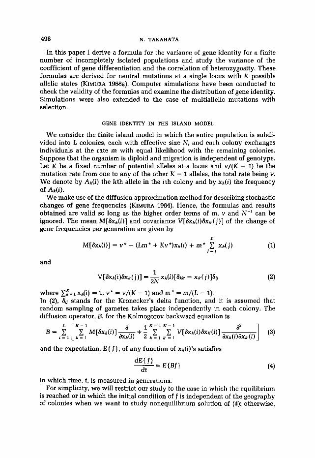
We consider the finite island model in which the entire population is subdi- vided into L colonies, each with effective size N , and each colony exchanges individuals at the rate m with equal likelihood with the remaining colonies. Suppose that the organism is diploid and migration is independent of genotype. Let K be a fixed number of potential alleles at a locus and v/(K - 1) be the mutation rate from one to any of the other K - 1 alleles, the total rate being v. We denote by Ak(i) the kth allele in the ith colony and by x k ( i ) the frequency of Ak(i).

We make use of the diffusion approximation method for describing stochastic changes of gene frequencies (KIMURA 1964). Hence, the formulas and results obtained are valid so long as the higher order terms of m, v and N-’ can be ignored. The mean M [ & x k ( i ) ] and covariance V[6xk(i)6xk,( j)] of the change of gene frequencies per generation are given by

L

M[Sxk(i)] = v* - (Lm* + Kv*)xk(i) + m* C x k ( j ) (1) j = l

and

(2 ) 1

2N V[Sxt(i)6xk,( j ) ] = - xk(i)[& - x d j ) l&

where Zfzl xdi) = 1, v* = v/(K - 1) and m * = m/(L - 1). In (2), 6, stands for the Kronecker’s delta function, and it is assumed that random sampling of gametes takes place independently in each colony. The diffusion operator, B, for the Kolmogorov backward equation is

and the expectation, E { f } , of any function of xk(i)’s satisfies

-- dECf’ - E { B f ) dt (4)

in which time, t, is measured in generations. For simplicity, we will restrict our study to the case in which the equilibrium

is reached or in which the initial condition of f is independent of the geography of colonies when we want to study nonequilibrium solution of (4); otherwise,

GENE DIVERSITY 499

we must formulate an intractable number of moment equations. Twelve mo- ments are required to obtain the variance of gene identity at equilibrium. We define the gene identities within and between colonies, jo and jl,

K I L K

jl = < xk(il)xk(i~) > for i l # iz k - 1

and define the gene identity for the entire population K

jT= y;, yk=<xk(i)> k - 1

Thus, jT

tation taken over the appropriate set of colonies.

jl and in (5) and (6) a symbol e > denotes the expec-

The mean values of jo and jl, denoted by Jo and J1, respectively, satisfies

where the time scale has been changed to a unit of 2N generations (T = t/ZN) and the dot over JO and J1 indicates the differentiation with respect to T . The parameters in (7) are

M * = M/(L - 1) = Nm/(L - l), e* = O/(K - 1) = Nv/(K - l), a1 = 1 + 4K8* + 4M, a2 = 4K8* + 4M *.

Equations in (7) are equivalent to those studied by MAYNARD SMITH (1970) for small values of m and v (see also MARUYAMA 1970a; LATTER 1973; NEI 1975).

The third moments concern identity probabilities for which we choose three genes randomly from one, two and three different colonies,

K

k - 1 K

Ti = E{x%i)}>

T2 = < E{~H(id~k(id}> (9) k - 1

and

where the subscripts of i indicate different colonies. For the fourth moments we must know the quantities concerning identity probabilities when we sample four genes randomly from one, two, three and four different colonies,

500 N. TAKAHATA

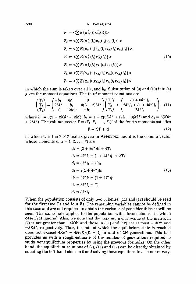
in which the sum is taken over all kl and kz. Substitution of (9) and (10) into (4) gives the moment equations. The third moment equations are

6M 0 (3 + 68*)Jo (;:) = (;:* -b2 4(L - 2)M *) (i:) + (28*Jo + (1 + 48*)Ji i; 0 12M* -b3 68*J1

where bl = 3(1 + 2K8* + ZM), bl = 1 + 2(3K8* + (2L - 3)M*) and b3 = 6(K8* + 2M *). The column vector F = (F1, Fz, . . , , F7)t of the fourth moments satisfies

F = C F + d (12)

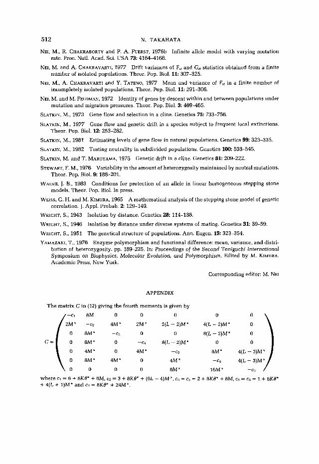
in which C is the 7 x 7 matrix given in APPENDIX, and d is the column vector whose elements di (i = 1, 2, . . . , 7) are

di = (2 + 88")Jo + 4T1

dz = 48*Jo + (1 + 48*)J1 + 2T2

d3 = 88*J1 + 2Tz

d5 = 48*J0 + (1 + 48*)J1

d6 = 88*Jo + T3

d7 = 88*J1.

When the population consists of only two colonies, (11) and (12) should be read for the first two Ts and four Fs. The remaining variables cannot be defined in this case and are not required to obtain the variance of gene identities as will be seen. The same note applies to the population with three colonies, in which case F7 is ignored. Also, we note that the maximum eigenvalue of the matrix in (7) is not greater than -4K8* and those in (11) and (12) are at most -6KB* and -8K8*, respectively. Thus, the rate at which the equilibrium state is reached does not exceed 4K8* = 4NvK/(K - 1) in unit of 2N generations. This fact provides us with a rough estimate of the number of generations required to study nonequilibrium properties by using the previous formulas. On the other hand, the equilibrium solutions of (7), (11) and (12) can be directly obtained by equating the left-hand sides to 0 and solving these equations in a standard way.

GENE DIVERSITY 501

Actual calculation of such equations except for (7) is, however, often tedious so that it was done numerically.

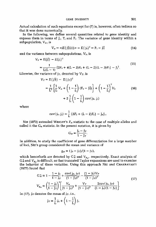
In the following, we define several quantities related to gene identity and express them in terms of Ji, Ti and Fi. The variance of gene identity within a subpopulation, V,, is

V , = <E{ jg(i)}> - E{ io}' = F1- J g (14) and the variance between subpopulations, v b , is

v b = E{j?} - E{jd2 1 (15)

(2F3 + 4(L - 2)Fs + (L - 2)(L - 3)F7} - Ji2. - - L(L - 1)

Likewise, the variance of jT, denoted by VT, is

VT = E{ j$> - E{ jT}2

where 1 L cov( jo, j l ) = - (2Fz + ( L - 2)F5} - JoJI.

NEI (1973) extended WRIGHT'S F,, statistic to the case of multiple alleles and called it the G, statistic. In the present notation, it is given by

In addition, to study the coefficient of gene differentiation for a large number of loci, NEI'S group considered the mean and variance of

gSt = ( j o - jT)/( l - jT) ,

which henceforth are denoted by GZ and V,,, respectively. Exact analysis of G,*t and VgSt is difficult, so that truncated Taylor expansions are used to examine the behavior of these variables. Using this approach NEI and CHAKRAVARTI (1977) found that

1 - JO + cov( jo, jT) (1 - Jo)VT G $ = I - - -

vgs'

(17) 1 - JT (1 - J T ) ~ (1 - J T ) ~

VT - 2cov( jo, jT) (I - (I - J T ) ~ (1 - J o ) ( l - JT)

vw +

In (17), JT denotes the mean of j T , i.e., 1

J T = - J o + L (I-;) Ji

N. TAKAHATA 502

and 1

L2 cov( jo, jT) = - {FI + (L - 1)(2Fz + F4 + (L - 2)Fci)) - JoJT.

It is obvious that (17) is a poor approximation when the amount of polymor- phism in the entire population is low, i.e., for a large value of JT and, thus, (17) should not be used in such a case. As will be discussed later, a more accurate formula particularly for V,, is needed that includes higher moments of jo and

Finally, we define the correlation of heterozygosity between colonies, R, as jT.

R = (F4 - J t ) / v w . (19)

This is equivalent to the correlation of heterozygosities from two randomly chosen colonies among different loci when the mutation rate is the same for all loci. Based on the infinite allele model, LI and NEI (1975) showed that in completely isolated populations R decreases exponentially as time increases and eventually becomes 0. In a subdivided population with gene flow, however, the equilibrium value does not equal 0 even for K = co and takes a value depending heavily on levels of gene flow. Thus, R may be a useful statistic to measure the degree of genetic differentiation of subpopulations.

Before going to the next section, I would like to give some results concerning the equilibrium solution of (7). In particular, when K = CO (KIMURA and CROW 1964) the solution is simple (MAYNARD SMITH 1970; MARUYAMA 1970a; CROW and MARUYAMA 1971; LATTER 1973; NEI 1975). The mean genetic identity for the entire population JT and G , are then given by

and

where, and subsequently, a symbol indicating the equilibrium state is sup- pressed. Formulas in (20) are equivalent to those given in MAYNARD SMITH (1970) and LATTER (1973), provided m, v and N-' are all small. Note that JT = [L(1 + #)I-' and G, = for m = 0 so that the population is very

polymorphic regardless of the value of e(JT < l/L), and that for small 8 the value of GSt is close to 1 because of random genetic drift. On the other hand, when m

1 f- - [ LYl] - l

>> v, JT = [l + 4LBI-l and GSt = [l + 4aM]-', where a = (L - f: l)z. Namely, the \

population can be regarded as panmictic in the sense that JT is equivalent to the mean genetic identity in a panmictic population with effective size NL. Even under the situation, however, Gst is different from 0 if Nm is small and the finiteness of L affects GSt through a. The formula of WRIGHT (1943), Fst = 1/(1 + 4Nm), corresponds to G,, with L = 00.

GENE DIVERSITY 503

COMPUTER SIMULATION

To check the validity of my formula, I conducted computer simulation keeping K finite (K = 4), examining the distribution of gene identity, as well as the mean and variance of gSt. I also examined the effect of selection on these parameters, considering two selection schemes. Both schemes assume that there exists a normal type allele in each colony and that the other alleles are all selectively disadvantageous. One model assumes that the normal type allele varied ran- domly from colony to colony, whereas the other model assumes that the same allele is favored in all colonies. Let 1 - sk(i) be the relative fitness of the kth allele in the ith colony and assume that fitness is multiplicative and that fitnesses do not vary with time.

The mean change of xk(i) per generation due to mutation and migration is given by the right-hand side of (l), and the change due to selection is

Axk(i) = {w(i) - sk(i)}xk(i)/(l - w(i)) (21) where w(i) = CL1 st(i)xl(i). In (21), sk(i) 0 for some k depending on the model used and is a positive constant for all other alleles. For preassigned values of sl(i)’s, v and m, the mean changes of gene frequencies were calculated using (1) and (21), followed by random sampling of gametes using multinomial pseudo- random variables (as described by KIMURA and TAKAHATA 1983).

To establish the equilibrium state, the first v-l generations for each set of parameter values were discarded and, thereafter, 5000 observations were made at every 100 generations. Choosing v as in the simulations, the total of 5 x lo5 generations in each run was used to study the equilibrium properties. Table 1 gives such simulation results for K = 4 and L = 10. Comparison of these results with the theoretical values shows that the formulas except that for V,, provide good approximations. As pointed out by NEI and CHAKRAVARTI (1977), the formula of V,, omits the second- and higher-order terms of jo and jT in the Taylor expansion. Although these terms could not be evaluated analytically, the approximation (17) seems so poor that we cannot use it, particularly for the case of large Nm and small Nv.

MEAN AND VARIANCE OF GENE IDENTITY

Many statistical analyses have been proposed to test the neutrality of poly- morphic genes (KIMURA 1968b), among which methods using the relationship between the mean and variance of heterozygosity (STEWART 1976; LI AND NEI 1975) have received much attention (NEI, CHAKRABORTY and FUERST 1976a,b; FUERST, CHAKRABORTY and NEI 1977; YAMAZAKI 1976; GOJOBORI 1982). However, the theoretical relationships used in these tests are obtained based on the assumption of random mating, so that it is interesting to examine them in the case of a subdivided population. In the following, I will consider only the equilibrium relationships. We keep in mind that the rate at which the equilib- rium state is reached is given approximately by mutation rate when gene flow among colonies seldom occurs.

First, we note from (20) that the total genetic diversity, HT = 1 - J T , increases as m/v decreases, and that the range of HT becomes [l - (W), 11 if m/v is less

504 N. TAKAHATA

TABLE 1

Simulation results for K = 4 and L = 10

Nm 0.01 0.1 I 10

l o exp obs

JI ~ X P obs

IT exp obs

Gst exp obs

GSt* exp obs

l o exp obs

JI ~ X P obs

JT ~ X P obs

GSt exp obs

Gst* exp obs

0.727 (0.0432) 0.726 (0.0434)

0.254 (0.0766) i 0.263 (0.0776)

0.301 (0.0017) r. 0.309 (0.0020)

{::E 0.609 (0.0882) i 0.606 (0.0086)

0.938 (0.0180) 1 0.935 (0.0179)

0.303 (0.1775) i 0.321 (0.1799)

0.366 (0.0081) i 0.381 (0.0079)

0.902 i0.894

0.901 (0.0448) 0.899 (0.0052)

Nv = 0.1

0.644 (0.0403) 0.640 (0.0409)

0.280 (0.0561) 0.277 (0.0549)

0.317 (0.0034) 0.313 (0.0026)

0.479 0.476

0.478 (0.0856) 0.476 (0.0083)

Nv = 0.01

0.840 (0.0361) 0.813 (0.0397)

0.518 (0.1444) 0.434 (0.1386)

0.550 (0.0360) 0.472 (0.0280)

0.644 0.645

0.635 (0.1623) 0.622 (0.0250)

0.452 (0.0190) 0.448 (0.0177)

0.342 (0.0192) 0.339 (0.0162)

0.353 (0.0087) 0.349 (0.0061)

0.153 0.151

0.151 (0.0337) 0.150 (0.0018)

0.756 (0.0476) 0.718 (0.0514)

0.702 (0.0636) 0.657 (0.0669)

0.707 (0.0491) 0.663 (0.0516)

0.167 0.163

0.156 (0.1753) 0.136 (0.0056)

0.379 (0.0123) 0.377 (0.0092)

0.365 (0.0122) 0.366 (0.0087)

0.366 (0.0112) 0.367 (0.0079)

0.196 0.164

0.0193 (0.0044) 0.0164 (0.00002)

0.741 (0.0496) 0.736 (0.0433)

0.735 (0.0509) 0.731 (0.0439)

0.736 (0.0496) 0.732 (0.0429)

0.0198 0.0162

0.183 (0.0312) 0.0148 (6 X

The value of the variance for each quantity is presented in parentheses: exp = theoretical value, obs = observed value in simulation.

than about 0.1. This means that in a small subdivided population with extremely limited migration, different alleles are quasifixed in different colonies, and the total amount of genetic variability can be quite high. Such a situation is theoretically conceivable but does not agree with the observation of 0 5 H T 5 0.3 for most species studied so far (FUERST, CHAKRABORTY and NEI 1977). There are many assumptions that may be responsible for the discrepancy between observed and theoretical values of HT, among which the assumed value of m/v may be important. For the lowest value of HT to be close to 0, say E , the ratio m/v has to be as large as L / E . This indicates that gene flow between colonies should be very high compared with the mutation rate, e.g., if we take E = 0.01, L = 100 and v = the migration rate required is 1% per generation. There is, however, an interesting analysis that reveals low levels of gene flow among colonies. Using the conditional average frequency (the average frequency

GENE DIVERSITY 505

of an allele conditioned on the number of colonies it appears in), SLATKIN (1981, 1982) estimated the level of gene flow in a subdivided population and showed that some species such as salamanders apparently have low levels of gene flow.

STEWART’S formula for the variance of heterozygosity allows us to calculate a theoretical variance, V,, when the population with a given H T is assumed to be panmictic. When K is sufficiently large, we have that

It is important to note that at equilibrium and for sufficiently large K, all variables J i , Ti and Fi (except 10, TI, Fl and F4) are negligibly small when m is much smaller than v and N-’. This indicates that the genetic constitution differs from colony to colony and that v b and cov( io, jl) are greatly reduced. Actually we can show that for m = 0 and K = m, v b = 0, cov( jo, jl) = 0 and

2(1/L - 1 + H T ) ( ~ - H T ) ~ (1/L + 1 - HT)(I/L + 2 - ~ H T )

VT =

for the range of 1 - 1/L I HT I 1. Clearly, V, > VT for L 2 2 and the value of VT decreases at the rate of 1/L2 as L increases. It is interesting to examine whether the whole population of the salamander mentioned before has lower than expected variance of gene diversity.

On the other hand, if m is sufficiently large, population subdivision should not affect the relationship of (22). Therefore, STEWART’S formula (22) is expected to hold for large m. However, there are intermediate values of m for which population subdivision results in a variance larger than expected from that in the panmictic case.

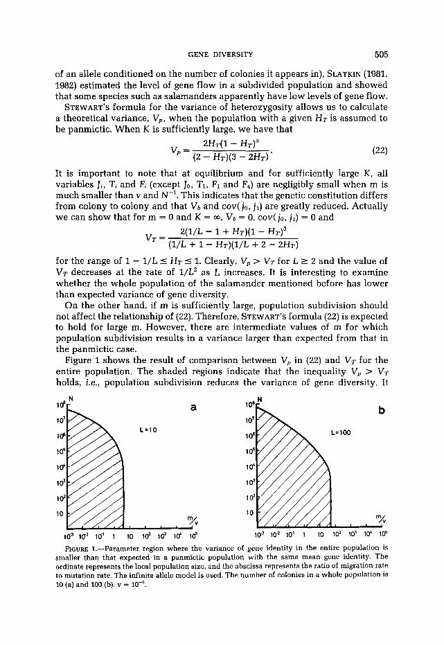
Figure 1 shows the result of comparison between V, in (22) and VT for the entire population. The shaded regions indicate that the inequality V, > VT holds, i.e., population subdivision reduces the variance of gene diversity. It

1ci3 I@ 10’ i io io2 io1 id id FIGURE 1.-Parameter region where the variance of gene identity in the entire population is

smaller than that expected in a panmictic population with the same mean gene identity. The ordinate represents the local population size, and the abscissa represents the ratio of migration rate to mutation rate. The infinite allele model is used. The number of colonies in a whole population is 10 (a) and 100 (b). v =

506

. 0 7 ~ V,

N. TAKAHATA

a

0 .1 .2 . 3 .4 .5 .6 .7 .8 .9 1.0

*071- vT b

0 .1 . 2 . 3 .4 .5 .6 .7 .8 .9 1.0

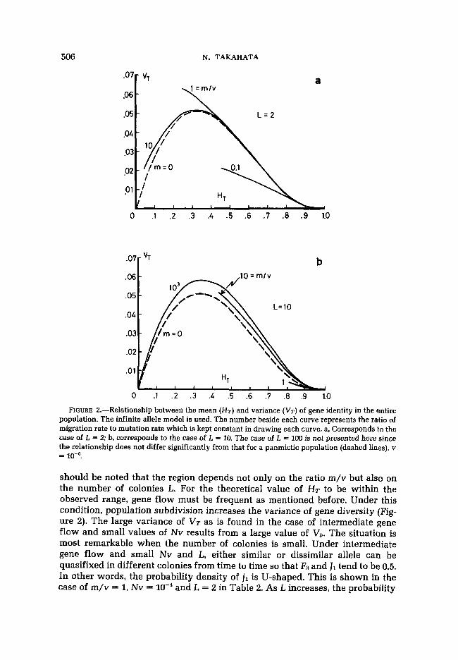
FIGURE 2.-Relationship between the mean (HT) and variance (VT) of gene identity in the entire population. The infinite allele model is used. The number beside each curve represents the ratio of migration rate to mutation rate which is kept constant in drawing each curve. a, Corresponds to the case of L = 2; b, corresponds to the case of L = 10. The case of L = 1oD is not presented here since the relationship does not differ significantly from that for a panmictic population (dashed lines). v =

should be noted that the region depends not only on the ratio m/v but also on the number of colonies L. For the theoretical value of HT to be within the observed range, gene flow must be frequent as mentioned before. Under this condition, population subdivision increases the variance of gene diversity (Fig- ure 2). The large variance of VT as is found in the case of intermediate gene flow and small values of Nv results from a large value of V,. The situation is most remarkable when the number of colonies is small. Under intermediate gene flow and small Nv and L, either similar or dissimilar allele can be quasifixed in different colonies from time to time so that R and J1 tend to be 0.5. In other words, the probability density of jl is U-shaped. This is shown in the case of m/v = 1, Nv = and L = 2 in Table 2. As L increases, the probability

GENE DIVERSITY 507

TABLE 2

Mean and variance (in parentheses) of gene identity; K = m

m/v N~ = N~ = Nv = lo-' Nv = lo-' L = 2 0.1 jo 1.00 (0.Oool) 0.996 (0.0014) 0.958 (0.0129) 0.696 (0.0504)

i l 0.091 (0.0825)* 0.091 (0.0816)* 0.087 (0.0730)* 0.063 (0.0293)* jT 0.545 (0.0207) 0.543 (0.0206) 0.523 (0.0200) 0.380 (0.0144)

1 io 0.999 (0.0002) 0.994 (0.0020) 0.943 (0.0169) 0.625 (0.0486) i l 0.500 (0.2496)* 0.497 (0.2460)* 0.472 (0.2144)' 0.313 (0.0768)* jT 0.750 (0.0625)* 0.746 (0.0622)* 0.708 (0.0599)* 0.469 (0.0373)

10 jo 0.m (0.0003) 0.992 (0.0025) 0.929 (0.0211)* 0.567 (0.0477)* i l 0.908 (0.0825)* 0.902 (0.0812)* 0.845 (0.0753)* 0.515 (0.0524)' jT 0.954 (0.0208)* 0.947 (0.0222)* 0.887 (0.0340)* 0.541 (0.0455)*

L = 10 10 jo 0.998 (0.0008) 0.978 (0.0072) 0.813 (0.0410) 0.304 (0.0164) i l 0.525 (0.0634)' 0.515 (0.0619)* 0.428 (0.0487)* 0.160 (0.0076)* jT 0.572 (0.0514)* 0.561 (0.0506)* 0.467 (0.0419)* 0.174 (0.0074)*

lo2 jo 0.996 (0.0012) 0.964 (0.0115) 0.730 (0.0540)* 0.213 (0.0112)* i l 0.914 (0.0300)* 0.885 (0.0369)* 0.670 (0.0596)* 0.195 (0.0105)* jT 0.922 (0.0245)* 0.893 (0.318)* 0.676 (0.0572)* 0.197 (0.0104)*

I@ jo 0.996 (0.0014) 0.962 (0.0132) 0.716 (0.0569)* 0.201 (0.0109)* il 0.987 (0.0049)* 0.953 (0.0160)* 0.710 (0.0574)* 0.199 (0.0108)* jT 0.988 (0.0043)* 0.954 (0.0154)* 0.710 (0.0571)* 0.200 (0.0108)*

The variance is greater than that expected from STEWART'S formula for a given mean value of gene identity.

that two randomly chosen colonies are genetically identical decreases, reducing the variance of jl but still V, > Va. Thus, large variances of Vb and VT are expected under intermediate gene flow between a small number of colonies. For a subdivided population consisting of a large number of colonies such as L = 100, we cannot expect a large variance of gene identities. This is because under the situation, the probability density of jl tends to be J-shaped, i.e., it is more likely that any pair of colonies is genetically dissimilar.

COEFFICIENT OF GENE DIFFERENTIATION AND CORRELATION OF HETEROZYGOSITY

Table 3 shows some numerical results of the coefficient of gene differentiation GSt (or G2) and the correlation of heterozygosity, R. These two inversely correlated quantities measure the degree of genetic differentiation or similarity between colonies. It is obvious from the table and (20) that large values of m/v and Nv increase the genetic similarity and prevent colonies from local differ- entiation. Although the larger the number of colonies the larger the gene flow required for panmixia of the entire population, it is interesting to examine the L dependence of these statistics keeping m/v constant.

G , is rather insensitive to the change of the number of L and becomes Gst =: 1/(1 + 4N(m + v)) for large K and L. Actually, the value for L = 10 does not differ much from that for L = CO. On the other hand, the value of R depends

508 N. TAKAHATA

TABLE 3

Coefficient of gene differentiation and correlation of heterozygosity; K = m

m/v NV = Nv = IO-” Nv = Nv = IO-’

0.998 0.997 0.0002

0.977 0.969 0.002

0.807 0770 0.018

0.294 0.288 0.103

0.984 0.929 0.005

0.856 0.513 0.049

0.373 0.163 0.309

0.056 0.054 0.694

0.862

0.055 t

0.383

0.353 t

0.059 0.031 0.806

0.006 0.006 0.957

L = 10 10 Gst Gst* R

0.995 0.994 0.001

0.949 0.947 0.012

0.650 0.644 0.086

0.157 0.156 0.249

10’ G, Gst* R

0.953 0.935 0.035

0.667 0.604 0.251

0.167 0.158 0.688

0.020 0.020 0.870

lo3 GSt Gst* R

0.669

0.285 i

0.168

0.766 t

0.020 0.019 0.956

0.002 0.002 0.986

L = 100 10’ G, G*** R

0.960 0.960 0.010

0.708 0.708 0.071

0.195 0.195 0.185

0.024 0.024 0.255

lo3 G , Gst* R

0.710 0.705 0.234

0.197 0.196 0.634

0.024 0.024 0.808

0.002 0.002 0.863

lo4 Gat G,t* R

0.197 0.191 0.725

0.024 0.024 0.940

0.002 0.002 0.977

0.0002 0.0002 0.985

Approximation of (17) is invalid.

markedly on L. For instance, when Nv = 0.01 and Nm = 1, R = 0.688 for L = 10 and equals 0.185 for L = 100. This L dependence of R is caused by a significant change of F4, which in turn depends heavily on L. However, when we want to estimate the degree of local differentiation from observations without knowl- edge of L, a statistic sensitive to L may not give a correct estimate.

DISTRIBUTION OF GENE IDENTITY AND EFFECTS OF SELECTION

The distribution of gene identity and the effect of selection were studied by computer simulation for the case of K = 4 and L = 10. The probability density of jT subject to intermediate gene flow is shown in Figure 3. Let us first examine the case of neutral mutations. When migration occurs rather frequently (Nm =

GENE DIVERSITY

15-

10

5 .

509

-

Nm='

0 .1 .2 .3 .4 .5 .6 .7 .0 .9 1.0 0 .1 2

JT

Nm=l

constant selec

random selection

.4 .5 .6 .7 .0 !

'T FIGURE 3.-Distribution of gene identity in the entire population in the case of K = 4, Nv = 0.01,

Ns = 10 and L = 10. The number of migrants per generation between colonies is 10 (a) and 1 (b). Three curves are plotted in each figure, corresponding to the neutral, random selection and constant selection models. The abscissa is gene identity for the entire population and the ordinate is the corresponding probability density. v = See the text for details.

lo), the pattern of the distribution is qualitatively the same as that for a panmictic population with the same parameters (see STEWART 1976). As Nm decreases, however, the spikes of the distribution at j T = % and ?h become moderate (Figure 3b) and eventually disappear. Instead, a new peak emerges around the mean value of jl due to the similarity between colonies. Note, however, that this does not necessarily mean that the distribution of gene identity between colonies has a peak near its mean value. Actually, when Nm = 0.1 and Nv = 0.01, this distribution is U-shaped with the mean and variance being 0.434 and 0.139, respectively. Under these circumstances, two different colonies can take both genetically similar and dissimilar states to each other as time goes on (because of intermediate gene flow and small K relative to L). The proportion of genetically similar colonies to the total colonies at any given time and it's time average determine the position of a new peak. Thus, in contrast to the distribution of jl, the jT distribution can be unimodal in the intermediate range of jT even though NLv is smaller than 1. This pattern forms a contrast to that in a panmictic population.

The effect of selection on the distribution of jT for the case if K = 4 is conspicuous in both selection models. The random selection model is where the normal type allele in each colony is determined at random, and the constant selection model is where the normal type allele is the same in all colonies. The

510 N. TAKAHATA

distribution in either model has a single sharp peak; the position, however, depends on the selection model used. In the constant selection model, the position is always near 1 because of the high frequency of the common advantageous allele in any colony. On the other hand, in the random selection model, there is the possibility that only a few colonies have a common advan- tageous allele. In the present simulation, the number of combinations of a pair of colonies which have a cdmmon advantageous allele was 10. As the number of all different combinations of two colonies out of L = 10 is 45, the proportion of the combinations was 2/9. And this proportion in turn mainly determines the position of a peak of the distribution. Thus, the position shifts toward 0 as K/L increases. Another interesting feature is the width of the distribution which depends not only on the magnitude of Ns (where s is selection coefficient) but also on Nm. As shown by SLATKIN (1973), a population cannot respond to local selection when gene flow is large relative to the strength of selection (see also SLATKIN and MARUYAMA 1975; FELSENSTEIN 1975; WALSH 1983). In such a case, the distribution will be broad.

We can confirm a well-known effect of random selection on the maintenance of polymorphism (LEVENE 1953 and see pages 258-262 in FELSENSTEIN 1976); in our simulation JT reduces to 0.399 and 0.297 from 0.732 and 0.663, respectively (Figure 3). In fact, the random selection model is an efficient mechanism for maintaining genetic polymorphism. At the same time the variance of jT is greatly decreased, On the other hand, the inbreeding coefficient or the coefficient of gene differentiation G,*t is increased, although the variance V,, is decreased compared with the case of neutral mutations. Our simulation result is that G,*t = 0.812 for Nm = 1 and is 0.117 for Nm = 10 which are 6 and 10 times larger than those for neutral mutations. The increased mean value, GS, comes entirely from the occurrence of genetically similar colonies in a population.

SLATKIN (1977) and MARUYAMA and KIMURA (1980) studied the effect of local extinction and recolonization of colonies on genetic variation and showed that the effective population size is greatly reduced compared with the case of the absence of this effect. As this effect reduces between-colony differentiation, GSt is also reduced. In other words, extinction and subsequent recolonization of colonies is a mechanism equivalent to that of mass migration, counterbalancing the reduction of the effective size. In terms of the variance of gene identity, this process makes not only jl but also j T approach STEWART'S relationship.

I thank BRUCE WALSH, YOSHIO TATENO, MASATOSHI NEI and an anonymous reviewer for their suggestions and comments which greatly improved the manuscript. I am also grateful to MONTGOM- ERY SLATKIN for his critical reading of the manuscript and CURTIS STROBECK for his interest and unpublished paper with G. B. GOLDING.

LITERATURE CITED

CROW, J. F. and T. MARUYAMA, 1971 The number of neutral alleles maintained in a finite,

FELSENSTEIN, J., 1975 Genetic drift in clines which are maintained by migration and natural

FELSENSTEIN, J., 1976 The theoretical population genetics of variable selection and migration.

geographically structured population. Theor. Pop. Biol. 2 437-453.

selection. Genetics 81: 191-207.

Annu. Rev. Genet. 10 253-280.

GENE DIVERSITY 511

FUERST, P. A., R. CHAKRABORTY and M. NEI, 1977 Statistical studies on protein polymorphism in natural populations. I. Distribution of single locus heterozygosity. Genetics 86: 455-483.

GOJOBORI, T., 1982 Means and variances of heterozygosity and protein polymorphism. pp. 137-148. In: Molecular Evolution, Protein Polymorphism and the Neutral Theory, Edited by M. KIMURA. Japan Scientific Societies Press, Tokyo, and Springer-Verlag, Berlin.

KIMURA, M., 1964 Diffusion models in population genetics. J, Appl. Probab. 1 177-232.

KIMURA, M., 1968a Genetic variability maintained in a finite population due to mutational

KIMURA, M., 1968b Evolutionary rate at the molecular level. Nature 217: 624-626. KIMURA, M. and J. F. CROW, 1964 The number of alleles that can be maintained in a finite

population. Genetics 4 9 725-738.

KIMURA, M. and N. TAKAHATA, 1983 Selective constraint in protein polymorphism: study of the effectively neutral mutation model by using an improved pseudosampling method. Proc. Natl. Acad. Sci. USA 8 0 1048-1052.

KIMURA, M. and G. H. WEISS, 1964 The stepping stone model of population structure and the decrease of genetic correlation with distance. Genetics 49: 561-576.

LATTER, B. D. H., 1973 The island model of population differentiation: a general solution. Genetics

LEVENE, H., 1953 Genetic equilibrium when more than one ecological niche is available. Am. Nat.

LI, W.-H. and M. NEI, 1975 Drift variances of heterozygosity and genetic distance in transient

LI, W.-H. and M. NEI, 1977 Persistence of common alleles in two related populations or species.

MALECOT, G., 1951 A stochastic treatment of linear problems (mutation, linkage, migration) in

MALECOT, G., 1955 Remarks on decrease of relationship with distance. Cold Spring Harbor Symp.

MARUYAMA, T., 1969 Genetic correlation in the stepping stone model with non-symmetrical

MARUYAMA, T., 1970a Effective number of alleles in a subdivided population. Theor. Pop. Biol. 1

MARUYAMA, T., 1979b Stepping stone models of finite length. Adv. Appl. Probab. 2: 229-258. MARUYAMA, T., 1979c Analysis of population structure. I. One dimensional stepping stone models

of finite length. Ann. Hum. Genet. 34: 201-219. MARUYAMA, T. and M. KIMURA, 1980 Genetic variability and effective population size when local

extinction and recolonization of subpopulations are frequent. Proc. Natl. Acad. Sci. USA 77: 6710-6714.

MAYNARD SMITH, J., 1970 Population size, polymorphism, and rate of non-Darwinian evolution. Am. Nat. 104: 231-236.

NEI, M., 1972 Genetic distance between populations. Am. Nat. 106 283-292. NEI, M., 1973 Analysis of gene diversity in subdivided populations. Proc. Natl. Acad. Sci. USA 7 0

NEI, M., 1975 Molecular Population Genetics and Evolution. American Elsevier, North Holland,

NEI, M., R. CHAKRABORTY and P. A. FUERST, 1976a Testing the neutral mutation hypothesis by

production of neutral and nearly neutral isoalleles. Genet. Res. 11 247-269.

73 147-157.

87: 331-333.

states. Genet. Res. 2 5 229-248.

Genetics 8 6 901-914.

population genetics. Ann. Univ. Lyon Sci. (Sect. A) 14 79-117.

Quant. Biol. 20: 52-53.

migration rate. J. Appl. Probab. 6 463-477.

273-306.

3321-3323.

New York.

distribution of single locus heterozygosity. Nature 262 491-493.

512 N. TAKAHATA

NEI, M., R. CHAKRABORTY and P. A. FUERST, 197613 Infinite allele model with varying mutation rate. Proc. Natl. Acad. Sci. USA 73: 4164-4168.

NEI, M. and A. CHAKRAVARTI, 1977 Drift variances of F,, and Gat statistics obtained from a finite

NEI, M., A. CHAKRAVARTI and Y. TATENO, 1977 Mean and variance of Fst in a finite number of

NEI, M. and M. FELDMAN, 1972 Identity of genes by descent within and between populations under

SLATKIN, M., 1973 Gene flow and selection in a cline. Genetics 75: 733-756.

SLATKIN, M., 1977 Gene flow and genetic drift in a species subject to frequent local extinctions.

SLATKIN, M., 1981 Estimating levels of gene flow in natural populations. Genetics 9 9 323-335.

SLATKIN, M., 1982 Testing neutrality in subdivided populations. Genetics 100 533-545.

SLATKIN, M. and T. MARUYAMA, 1975

STEWART, F. M., 1976 Variability in the amount of heterozygosity maintained by neutral mutations.

WALSH, J. B., 1983 Conditions for protection of an allele in linear homogeneous stepping stone

WEISS, G. H. and M. KIMURA, 1965 A mathematical analysis of the stepping stone model of genetic

WRIGHT, S., 1943

WRIGHT, S., 1946

WRIGHT, S., 1951

YAMAZAKI, T., 1976

number of isolated populations. Theor. Pop. Biol. 11 307-325.

incompletely isolated populations. Theor. Pop. Biol. 11: 291-306.

mutation and migration pressures. Theor. Pop. Biol. 3: 469-465.

Theor. Pop. Biol. 12: 253-262.

Genetic drift in a cline. Genetics 81 209-222.

Theor. Pop. Biol. 9 188-201.

models. Theor. Pop. Biol. In press.

correlation. J. Appl. Probab. 2 129-149.

Isolation by distance. Genetics 28: 114-138.

Isolation by distance under diverse systems of mating. Genetics 31 39-59.

The genetical structure of populations. Ann. Eugen. 15: 323-354.

Enzyme polymorphism and functional difference: mean, variance, and distri- bution of heterozygosity. pp. 189-225. In: Proceedings of the Second Taniguchi International Symposium on Biophysics, Molecular Evolution, and Polymorphism, Edited by M. KIMURA. Academic Press, New York.

Corresponding editor: M. NEI

APPEND I X

The matrix C in (12) giving the fourth moments is given by

8M 0 0 0 0

- cz 4M* 2M* 2(L - 2)M* 4(L - 2)M*

8M * - c3 0 0 8(L - 2)M * 8M * 0 -cq 8(L - 2)M* 0

4M * 0 4M * -c5 8M *

0 8M* 4M" 0 4M* -c6

0 0 0 8M * 16M *

C =

4(L - 3)M*

4(L - 3)M*

-c7 where CI = 6 + 8K8* + 8M, cz = 3 + 8KB* + (6L - 4)M*, cg = c4 = 2 + 8KB* + 8M, c5 = c6 = 1 + 8K8* + 4(L + l )M * and c7 = 8KB* + 24M *.