GSSPS - Graduate School in Social and Political Sciences

Department of Social and Political Sciences

Sociologia XXVIII ciclo

TESI DI DOTTORATO DI RICERCA

Gender inequalities in medical careers

Settori disciplinari SPS/07, SPS/09

TUTOR Ph.D. CANDIDATE

Prof. Antonio Maria Chiesi Camilla Gaiaschi

2014/2015

© 2016 Camilla Gaiaschi - All Rights Reserved

1

Table of contents

Acknowledgements ……………………………………………………………...

Abstract ………………………………………………………………………….

Introduction ……………………………………………………………………..

Chapter 1. The literature ……………………………………………………….

I. The forms of gender inequalities

II. The reasons of gender inequalities

III. Supply-side explanations

III.1. Human capital characteristics

III.2. Institutional work characteristics: the horizontal segregation

III.3 Family characteristics: Hakim vs Crompton

III.3.1. Do women prefer to care for family?

III.3.2. Work-life balance policies, family arrangements and

gender equality at work.

IV. Theories focusing on the agency of the subject vs theories focusing

on structural constraints: a double shift

V. Demand-side explanations

V.1. Discrimination

V.2. Gender bias or gender schema

V.2.1. The Matthew effect

V.2.2. The Mathilda effect

V.3. Gendered organizations

Chapter 2. The methodology …………………………………………………...

I. The S.T.A.G.E.S. project

II. Field and methods

III. The access to the field: challenges and resistances

IV. The health system in the Lombardy Region

V. The choice of the five hospitals

VI. The data collection

VII. The questionnaire

VIII. The rate of response

IX. Population and email lists: a problem of under-coverage

X. The representativity of respondent data

XI. Recoding the dataset

Chapter 3. The dataset ………………………………………………………….

I. Human capital characteristics

I.1. Age, experience and seniority

p. 3

p. 5

p. 7

p. 13

p. 14

p. 16

p. 18

p. 18

p. 19

p. 21

p. 21

p. 24

p. 28

p. 29

p. 30

p. 31

p. 32

p. 34

p. 34

p. 39

p. 39

p. 40

p. 42

p. 44

p. 45

p. 47

p. 48

p. 51

p. 52

p. 53

p. 56

p. 59

p. 60

p. 60

p. 56

2

I.2. Educational credential and trainings

I.3. Individual work characteristics: mobility, motivational drives

and hours of work

I.3.1. Mobility

I.3.2. Motivational drives

I.3.3. Hours of work

II. Institutional work characteristics

II.1. The type of practice and the type of contract

II.2. The horizontal segregation: institutional characteristics and

specialty

II.3. The vertical segregation: the career steps

II.4. The gender pay gap

III. Family characteristics

III.1. Parental and marital status

III.2. The sexual division of labor

III.3. Work-life conflict

IV. Conclusions

Chapter 4 – Explaining the gender pay gap ……………………………………

I. Measures

II. Hypothesis

III. Interpreting the gap through an OLS multivariate model

IV. Interpreting the pay gap through interaction terms

V. Decomposing the pay gap through the Oaxaca-Blinder decomposition

VI. Conclusions

Chapter 5 – Explaining the vertical segregation ………………………………

I. The gender gap in authority in the literature

II. Research design and hypothesis

III. The model

IV. Measures

V. Results

V.1. The female odds to promotion

V.2. The determinants of the vertical segregation

VI. Conclusions

Conclusions ………………………………………………………………………

References ………………………………………………………………………..

Appendix I ……………………………………………………………………….

Appendix II ……………………………………………………………………....

Appendix III ……………………………………………………………………..

p. 60

p. 64

p. 64

p. 65

p. 68

p. 71

p. 71

p. 74

p. 75

p. 77

p. 79

p. 80

p. 81

p. 83

p. 86

p. 89

p. 89

p. 91

p. 92

p. 95

p. 103

p. 105

p. 109

p. 109

p. 112

p. 114

p. 115

p. 116

p. 117

p. 118

p. 123

p. 125

p. 129

p. 145

p. 163

p. 171

3

Acknowledgments

There are many people to thank for this work. When prof. Maria Luisa Leonini and

prof. Antonio Maria Chiesi asked me to join the project S.T.A.G.E.S. – Structural

Transformation to Achieve Gender Equality in Science (G.A. n°289051) – at the

University of Milan, they gave me the opportunity to be part of a great research team and

I would like to thank them for this. I feel honored to be part of an internationally highly-

recognized research centre such as GENDERS (Gender & Equality in Research and

Science). Prof. Chiesi has supervised this thesis with much interest, providing me with

precious suggestions and insights. I also would like to thank prof. Biolcati and prof.

Ballarino for their methodological advises. Special thanks to Alessandra Caserini, of the

Laboratory of Opinion Polls (LID) at the University of Milan. Alessandra and I have

worked together during the questionnaires’ submission. I know that this has been a huge

work for both of us, as submitting five questionnaires is demanding, as it implies to

multiply the efforts. Without her help this wouldn’t have been done in such a short time.

That is all for the Department of Social and Political Science at the University of

Milan, but not for this work. There are many people in the STAGES research team and

partners of the STAGES project to thank. First of all, dr. Maria Antonietta Banchero of

the Health Department of the Lombardy Region. She “opened the gates” of three out of

five hospitals in which the questionnaire has been submitted. Without her, I would have

never reached such a high number of physicians. Her commitment to the project was one

of the unexpected gift of this journey. Prof. Maria Domenica Cappellini, on one hand,

and prof. Claudia Sorlini and prof. Livio Luzi, on the other, had been fundamental in

opening up the field in the rest of the hospitals: thank you all. In each organisation I have

met very helpful and committed people, some of them they eventually became friends. I

would like to thank them all: dr. Anna Pavan, dr. Matteo Patriarca, dr. Maria Teresa

Bottanelli for the Policlinico Hospital; dr. Carla Dotti, dr. Sergio Castiglioni and Massimo

Colombo for Legnano, dr. Alessandra Farina and dr. Elena Franz for Como; dr. Francesca

4

Ramondetti, and Loredana Esposito for San Donato; dr. Marco Giovanni Stramba-

Badiale and dr. Barbara Garavaglia.

Part of the data analysis has been done during two short visiting periods abroad. Many

thanks to Nick Deschacht of the Faculty of Economics and Business at the University of

Leuven (Brussels campus) for his precious support in getting me start with modelling the

pay gap. I also had the chance to be hosted in the frame of the European project InGRID

– Inclusive Growth Research Infrastructure (GA n°312691) – at the Amsterdam Institute

for Advanced Labour Studies (AIAS) of the University of Amsterdam. During that stay I

have worked with Kea Tijdens and especially with Stephanie Steinmetz, whose help in

the modelling has been very important.

Finally, I would like to thank Dr. Daniela Falcinelli, team leader of the STAGES

project at the University of Milan, for her support. Thank you for reading this research

and provided me with precious suggestions. Her deep understandings of the mechanisms

of female disadvantages throughout their career trajectories has been crucial, as it helped

me to pose the good research questions and look for the most appropriate hypothesis to

test. Moreover, she shared with me her (huge) knowledge of the international literature

on gender work and organization as well as on gender inequalities in scientific careers.

This is an enormous legacy: I hope I will make a good use of it.

5

Abstract

Women have made a significant progress in the medical profession. In 2013, they

accounted for 46.8% of total physicians in OECD countries, a 10% increase from 2003.

In Italy, women account for almost 40% of the medical work-force in 2013 and their

increase has been very strong in years, up to +34% in the decade 2001-2011 and up to

+3% from 2012 to 2013. Notwithstanding the strong feminization of the medical

workforce, gender inequalities still persist. Empirical research has shed light on gender

inequalities in pay, leadership and specialty fields. It is widely acknowledged that women

physicians earn less than men, cluster in less remunerative specialties and progress more

slowly through ranks. Most of these studies have taken place in the United States, where

cross-sectional and longitudinal dataset are available. This research is part of the wider

European project S.T.A.G.E.S. (Structural Transformation to Achieve Gender Equality in

Science) at the University of Milan and it aims to fill the gap in the literature – with

respect to the European context – on gender inequalities in medical careers. Data on more

than one thousand physicians working in five hospitals in the Lombardy Region have

been collected through an online survey with a rate of response of 48.7%. Data have been

analysed through descriptive statistics and through regression analysis. The results point

out that women earn 15% less than men, controlling for human capital, work and family

characteristics, while they are 44.4% less likely to be promoted to the intermediate levels

of the career ladder. Female physicians tend to cluster in medical specialties, while

surgery still remains a male-dominated specialty area. Moreover, they do less private

practice than their male colleagues, which is highly remunerative. Compared to private

institutions, public hospitals seem to guarantee a stronger equality in earnings. The

division of paid and unpaid work appears strongly unbalanced, with women as the main

responsible for the care of children and the elderly. As a consequence, they tend to solve

their work-life conflict by outsourcing care activities while reducing the number of

children or renouncing to motherhood (39% of women in the dataset are childless).

Regression analysis show that mechanisms of gender discrimination take place both in

pay and promotions. Moreover, the same attributes are differently “rewarded” whether

they refer to women or men. Hence, being father significantly increase men’s income and

their likelihood to promotion. The pay penalty for motherhood is significant at 90% level

from the third child, while it negatively affects promotion from the second child. Overall,

the fatherhood premium appears stronger than the motherhood penalty. Being married

positively increases male’s income but it doesn’t have any effect on female colleagues.

Educational credential “pays” more for men than for women in terms of pay, as well as

being a surgeon and a head of a unit. Doing private practice is more rewarding, controlling

for work hours, for men than for women. The amount of time spent at work and the years

of work experience are also differently rewarded in terms of career outcomes, suggesting

that gender inequalities are not only a matter of “being like men are”. Overall, these

results fill a gap in knowledge and argue that structural constraints – preventing female

physicians to earn as much as men do and to have the same chances of career than men

have – are taking place.

6

7

Introduction

Women have made a significant progress in the medical profession. In 2013, they

accounted for 46.8% of total physicians in OECD countries, a 10% increase from 20031.

Their number varies significantly across countries, ranging from the minimum of Japan2

and Korea (where only one out of four physician is a female) and the maximum of the

Baltics, driven by Latvia (74.3% of women physicians), Estonia (69.6) and Lithuania

(61.6%). Between the two extremes, a wide range of industrialized countries stays in the

middle. In the middle, Eastern-European Countries account for the highest rate of female

doctors (ranging from around 50 to 60%) while Western Europe and Anglo-Saxon States

show more moderate rates of female physicians, ranging from around 30% to slightly

more than 50% of the medical population.

The high rate of women in the medical profession in eastern countries finds its

explanation in the earlier process of feminization of the medical profession due to a long

tradition in gender-parity policies which stressed equality in education and favoured the

entrance of women in scientific fields (Glover 2005). On the contrary, the feminization

of the medical profession in western countries occurred only recently. This time gap finds

evidence in the growth rates over time: eastern countries show the smallest variations in

the last years, while western countries register the highest growth of women in medicine

(see Figure 1). In this context, Italy fits in the western model: in 2013 women accounted

for almost 40% of the medical work-force and their increase has been very strong in years,

up to +34% in the decade 2001-2011 and up to +3% from 2012 to 20133.

1 OECD (2015), Health care resources, OECD Health Statistics (database). Data avalaible here:

http://dx.doi.org/10.1787/data-00541-en (Website consulted on February, 28th 2016). 2 Last data available for Japan refers to 2012. 3 No useful data are available for the decade 2003-2013 for Italy a cause of a methodological change in

coverage occurred in 2012.

8

Figure 1

Source: OECD (2015), "Health care resources"4

No matter such a strong feminization of the medical work-force, gender inequalities

still persist. Empirical research has shed light on gender inequalities in pay, leadership,

specialty fields. It is widely acknowledged that women physicians earn less than men

(Hoff 2004, Sasser 2005, Weeks et al. 2009, Jagsi et al. 2012), they are clustered in less

remunerative specialties (Hinze 2000, Sasser 2005, Boulis and Jacobs 2010, Crompton

and Lyonette 2011) and they progress more slowly through ranks (Jagsi et al. 2011, Carnes

et al. 2008).

Most of the studies on gender inequalities in medical careers have taken place in the

United States, where cross-sectional and longitudinal dataset, as the American Medical

Association dataset (AMA) or the Young Physicians’ Survey (YPS), are available (Baker

1996, Sasser 2005, Boulis and Jacobs 2010, Weeks et al. 2015). Studies based on self-

administrated surveys (Hinze 2000, Hoff 2004) as well as qualitative in-sights (Carr et al.

2003, Kass et al. 2006, Levine et al. 2011) into medical organisations are also mostly

American. Only a few researches have been conducted outside the United States and more

4 For Japan, Denmark and Sweden last data available refer to 2012.

0

10

20

30

40

50

60

70

80

% of women physicians in OECD countries in 2013

9

specifically, at my knowledge, in Japan (Nomura and Gohchi 2012), UK (Crompton and

Lyonette 2011), in the Netherlands (Pas et al. 2011) and Sweden (Magnusson 2015). Italy

has a long tradition in the study of the medical profession in a gendered perspective

(Vicarelli 1989, Vicarelli 2003, Vicarelli and Bronzini 2003, Vicarelli 2008, Spina e

Vicarelli 2015). Vicarelli’s studies are mostly concerned with female physicians’

identities, values and career trajectories. Women in the profession are her unit of analysis.

On the contrary, this research takes in consideration both female and male physicians as

it aims to identify, and explain, gender inequalities in the workplaces and within

organisations.

This research is part of the wider European project S.T.A.G.E.S. (Structural

Transformation to Achieve Gender Equality in Science)5 at the University of Milan and

it aims to fill the European gap in the literature on gender inequalities in medical careers.

For the first time in Italy, data on more than one thousand physicians have been collected

through an online survey in five hospitals in the Lombardy Region, where the University

of Milan is located. The submission of the questionnaire took from two to three months

for each hospital and more than one year overall, taking start in June 2014 and ending in

July 2015. The survey aimed to collect information on human capital, work and family

characteristics of the physicians, as well as on work environment. Out of 2205 physicians

receiving the questionnaire, 1074 answered, for a rate of response of 48.7%. Quantitative

data analysis was made using descriptive statistics to identify the forms of gender

inequalities and through regression analysis to identify their causes.

The field was made accessible by the members of the research group of the project

S.T.A.G.E.S. as well as by its partners, and more specifically by the Health Department

of the Region, which played a crucial role in promoting this study. Hospitals were chosen

to be as more representative as possible of the Lombardy health system, which is a quite

peculiar case within the (strongly decentralized) national health system, as it is based on

a mixed logic, where one third of providers are private and two third are public. This has

made the Lombardy health system very competitive and attractive both in terms of

scientific research (Lombardy has the highest concentration of medical schools in Italy)

5 The STAGES project – Structural Transformation to Achieve Gender Equality in Science – GA n° 289051,

has been financed by the DG Research and Innovation of the European Commission within the Seven

Framework Research Programme and it is co-funded by the Italian General Inspectorate for relations with

the European Union of the Ministry of Economy and Finance (IGRUE).

10

and quality of care services (10% of services are provided to patients coming from other

regions with peak concentrations of 50% in some specialties).

Studying gender inequalities in such a competitive and high-quality context has many

advantages. One must objects that, since this study focuses on a very restricted

population, made of high-qualified professionals and more specifically by physicians in

five hospitals organisations, it can’t provide useful insights on the general population.

Statistically speaking, no doubt that this study is made of five quantitative case-studies

which are representative of the five hospitals only. As these hospitals have been chosen

in order to be as more representative as possible of the Lombardy health system, one

could add, at the most, that this study provides information on the Lombardy health

system as well. Is that all? Many reasons suggest that it is not. I argue that this study

doesn’t only provide precious insights on gender inequalities in the medical profession

but in the general population as well. I will explain this concept by quoting Kathleen

Gerson. “Large issues – she says – are often best illuminated by small, well-crafted

studies” (Gerson 1985, p. XVIII). That is, if gender inequalities occur with respect to a

very specific and committed population, it is very reasonable to think that they occur in a

greater extent to the rest of the labour market. In other words, if gender inequalities occur

in a population where women are very similar to men in terms of educational and work

investments (Wajcman 1998), it is likely to think that they occur even more in a

heterogeneous population, where gender differences (in characteristics) are stronger. The

population of this research is restricted twice: with respect to the general population, as it

represents the “slice” made of high-skilled professionals, and with respect to the medical

profession itself, as it represents the very excellence of the health system in Italy and in

Europe. As a consequence, by shedding light on the mechanisms and the reasons of

gender inequalities among physicians in five health organisations in Lombardy, this

research can provide many useful insight on how gender inequalities work in the medical

profession and in the labour market as a whole.

This research is structured in five chapters. The first chapter will provide the review

of the literature on gender inequalities by adopting a multi-disciplinary approach.

Contributions both from the sociological and economical traditions to the study of gender

inequalities will be discussed, with the aim of systematizing the different forms of gender

inequalities and their different explanations identified by international scholars. The

11

second chapter is the methodological chapter. The choice of the methods – in the data

collection and in their analysis - will be discussed, as well as the problematics linked to

the access to the field, challenges and resistances. The questionnaire will be also

illustrated and the representativity of the dataset analyzed. The third chapter will provide

descriptive statistics on the population based on data collected through the survey. The

fourth and fifth chapter will focus on two forms of gender inequalities: the gender pay

gap and the vertical segregation. Both chapters aim to identify the reasons of gender

inequalities in pay (chapter 4) and in authority (chapter 5). In order to do that, a set of

hypothesis, drawn from the literature, will be tested using multiple regression models.

The results will be then discussed at the end of each chapter. In the conclusions, research

outcomes will be summarized, limits and strengths of the study discussed and further

investigations outlined.

12

13

Chapter 1 - The literature

Studies on gender inequalities in the medical profession parallel the wider literature

on gender inequalities in the general population and in non traditional jobs6. Many

scholars have shed light on the obstacles that women face in the world of professions

(Crompton and Sanderson 1990, Beccalli 2004), as managers (Jacobs 1995, Wajcman

1998), in the financial (Roth 2006) and IT (Wright and Jacobs 1995) sector, as well as in

science (Evetts 1996, Glover and Campling 2000, Etzkowitz et al. 2008, Gupta et al.

2004, Smith Doerr 2004).

As for studies on gender inequalities in medical careers, most of the them have been

taken place in the United States, where cross-sectional and longitudinal datasets, as the

American Medical Association dataset (AMA) or the Young Physicians’ Survey (YPS),

are available (Baker 1996, Sasser 2005, Boulis and Jacobs 2010, Weeks et al. 2009).

Studies based on self-administrated surveys (Hinze 2000, Hoff 2004) as well as

qualitative in-sights (Carr et al. 2003, Kass et al. 2006, Jagsi et al. 2011 and 2012, Levine

et al. 2011) into medical organisations are also mostly American. Only a few researches

have been conducted outside the United States and more specifically, at my knowledge,

in Japan (Nomura and Gohchi 2012), UK (Crompton and Lyonette 2011), in the

Netherlands (Pas et al. 2011a and 2011b) and Sweden (Magnusson 2015). Italy has a long

tradition in the study of the medical profession in a gendered perspective based on

Vicarelli’s work (Vicarelli 1989, Vicarelli 2003, Vicarelli and Bronzini 2003, Vicarelli

6 I use the expression “non traditional jobs” or “traditionally male occupations” to mean both male-

dominated occupations (or sex-segregated occupations) and feminized occupations (or mixed-sex

occupations which have recently experienced a process of feminization). In male-dominated (or sex-

segregated) occupations, women account for a minor part of the work-force. Cutting points for defining an

occupation as “sex-segregated” (being either female or male dominated) vary according to scholars: “75%

or 80% one sex, a one-sex majority, or a percentage-point deviation from the sexes’ representation in the

labour force” (Reskin 1993, p. 244). Example of male-dominated occupations are engineering, finance and

the hard-sciences. Male-dominated occupations can experience a process of feminization and can become

mixed-sex occupations. I use this term in the same way used by Roos and Jones (1995), that is to indicate

a growing presence of women within occupations and not to suggest that women have become the

predominant, or even the majority, sex. Examples of feminized occupations are journalism, judiciary and

medicine.

14

2008, Spina e Vicarelli 2015). Her research is mostly concerned with the historical

process of the feminization of the profession on one hand and with female physicians’

identities, values, behaviours and career trajectories on the other. In her studies, women

physicians are the unit of analysis. On the contrary, this Ph.D. thesis takes in consideration

both female and male physicians with the aim of identifying the causes of gender

inequalities in workplaces at within organisations.

I. The forms of gender inequalities

There are different forms or different types of gender inequalities in non traditional

occupations: the horizontal segregation (disparities in sectors/specialties), the vertical

segregation (disparities in rank) and the pay gap (between men and women and between

mothers and childless women).

The horizontal segregation (better known as occupational sex segregation) refers to

the degree to which men and women do different works (Blau 1984, Milkman 1987,

Walby 1988, Reskin and Ross 1990, Reskin 1993, England 1982, England 1992, Jacobs

1989, Jacobs 1995, Charles and Grusky 2004). Men and women can work in different

industries, in different kinds of organisations (public, private, non-profit), in different

occupations. Within the same occupation, they can work in different sectors or specialties,

as it is the case of medicine (Boulis and Jacobs 2010). Once women enter into a male-

dominated profession, mechanisms of re-segregation take place inside the same

occupation (Reskin and Ross 1990). Workplace segregation is usually measured by the

index of dissimilarity, which indicates the proportion of women who would have to move

in order for them to be distributed in the same manner as men (Jacobs 1995). Analytically

speaking, this distribution should not necessarily be a synonym of gender inequality.

Nevertheless, it is well acknowledged that female occupations are usually less well paid

than men’s, provide less on the job-training, promotion opportunities and the

opportunities to exercise authorities (England 1992, Reskin 1993, Jacobs 1995).

Therefore, the occupational sex segregation has some important implications in terms of

gender inequality.

The vertical segregation refers to the female overrepresentation in the lower levels of

the career ladder and the glass ceiling is the most common metaphor to describe it

15

(Federal Glass Ceiling Commission 1995, Baxter and Wright 2000, Cotter et al. 2001,

Liff and Ward 2001). The glass ceiling is defined as an “unseen, yet unbreakable barrier

keeping women from rising to the upper rungs of the corporate ladder, regardless of their

qualifications or achievements” (Federal Glass Ceiling Commission, 1995: 4) and it

emphasises the existence of obstacles at the end of the career ladder. More recently, a

second metaphor has been introduced to offset the limits of the glass ceiling: the sticky

floor (Padavic and Reskin 1994, Britton and William 2000, Booth et al. 2003, Baert et al.

2016). Sticky floors can be described as the pattern that women are, compared to men,

less likely to start climbing the career ladder. In this way, sticky floors complement the

concept of glass ceiling and suggest that barriers can be found also at the beginning of the

career ladder (Baert et al. 2016). The sticky floor is consistent with a third metaphor which

has been mostly used in the literature on scientific careers: the leaky pipeline (Alper 1993,

Blickenstaff 2005). This latter suggest that there is no difference between barriers at the

beginning and barriers at the end of the ladder, as female talents are “dropped” all along

the trajectory, implying the existence of equal obstacles throughout the ladder.

The vertical and the horizontal segregation are two forms of gender inequality. On the

other hand, they are, in themselves, two of the most relevant explanatory factors of a

further form of gender inequality in the workplace: the pay gap. According to Eurostat,

in 2013 women have earned 16.4% less than men in the UE 27 without adjusting for work

hours and other characteristics7. In Italy, the pay gap is “only” 7.3%, mainly because the

female part-time work is less common than in Nordic European Countries. Women earn

less (also) because they are concentrated in female jobs (which are usually worse paid

than male jobs) and (also) because they are stuck in the lower ranks of the job ladder

(Jacobs 1995). Nevertheless, the vertical and horizontal segregation are not the only

causes of wage differentials. Many scholars have shed light on the child penalty for

motherhood (Folbre 1994, Waldfogel 1997, Lundberg and Rose 2000, Buding and

England 2001, England 2005) as well as on employers’ discrimination (Becker 1957, Blau

1984, Reskin and Ross 1990, Gupta et al. 2004). The debate over the explanatory factors

of the gender pay gap is very rich in contributions, both from the economic (Oaxaca 1973,

Blau and Kahn 2000) and the sociological (England 1992, Rubery et al. 2005, Lips 2013)

7 Gender pay gap in unadjusted form in %. Data available at: http://ec.europa.eu/eurostat/data/database.

Accessed on February 25th, 2016.

16

traditions. Both perspectives have been adopted in this research, as they complement each

other: providing the technical tools to calculate the determinants of the gap the former,

correctly interpreting such determinants the latter.

II. The reasons of gender inequalities

Many studies have shed light on the reasons of gender inequalities and a few attempts

to organize the debate have been done. I suggest to clearly distinguish between two levels

of explanation: the level of the explanatory factors (first level) and the level of theoretical

explanations (second level).

Explanatory factors are usually divided between “supply-side” and “demand-side”

(Reskin 1993, Kelly 2012). The former emphasizes workers’ characteristics, the latter

emphasizes employer’s actions (including discrimination) or, more in general,

organisational obstacles. Supply-side explanatory factors are: 1. The human capital

characteristics of workers (educational credentials, work experience and seniority,

training, commitment and productivity); 2. Their institutional work characteristics (the

industrial sector, the kind of organisation, the type of contract); 3. Their family

characteristics (number of children, marital status). Demand-side explanatory factors are:

1. Employers’ discrimination; 2. Gender bias; 3. Gendered organisations.

Supply-side explanatory factors (first level) are, in themselves, neutral, as they can be

“interpreted” in different (even opposite) ways on the base of two different theories

(second level): theories emphasizing the agency of the subject and theories emphasizing

structural constraints8. That’s why it is important to separate the two levels.

8 Many scholars have already attempt to systematize the different contributions on gender inequalities. Jerry

Jacobs (1995) distinguishes between the economic and the sociological perspective, the former

emphasizing the agency of the subject, the latter emphasizing structural conditionings. Nevertheless, not

all economists adopt such a theoretical approach. This is true only for neo-liberal economists. Reskin

distinguishes between the neo-classical or neo-liberal economic perspective and the gender-role

socialization theory (Reskin 1993). This is also partially correct as the socialization theories (Marini and

Brinton 1984, Parsons 1942) are not the only one emphasizing the impact of external factors on individual

agency. Gerson (1985) identifies two main strands sharing a structural approach: theories stressing the

importance of socio-structural coercion (within the Marxist tradition) and theories stressing childhood

socialization (within the psychoanalytic tradition). In order to better comprehend the heterogeneity of

theoretical contributions on both side of the debate, I prefer to distinguish between theories focusing on the

agency of the subject and theories focusing on structural constraints. Indeed, I believe it is a more

comprehensive distinction, including economists and sociologists on both sides of the querelle, as well as,

with respect to the second side only, sociologists and social psychologists. Moreover, I will use the

expression “structural constraints” with a slightly different meaning with respect to Gerson’s (1985). While

17

Theories focusing on the agency of the subjects interpret workers actions in terms of

preferences (Hakim 2000) or rational choices (Becker 1985). According to this

perspective, for example, women would choose “family-friendly” jobs because they

prefer to spend more time in caring their children or because they expect that family

obligations will limit their market work. On the contrary, structuralist theories would shed

light on the social construction of gender (Connell 2002, Risman 2004, Piccone Stella

and Saraceno 1996, Ruspini 2003) shaping women and men’s choices towards specific

occupations (Faulkner 2009, Powell et al. 2009) while determining their structure of

opportunities (Crompton et al. 2005, Crompton and Lyonette 2010).

The two level-approach (explanatory factors vs theoretical interpretation) works for

the supply-side factors only. For one simple reason: supply-side factors concern the

actions of the unit of the analysis of the research (the worker), which can be differently

“interpreted” (as free or constrained action). On the contrary, demand-side factors concern

employers’ actions which, from the point of view of the unit of the analysis (the worker),

are – per se – external constraints as long as they don’t depend on workers’ choice. As

such, they hardly can give place to a theoretical querelle around their nature and they are

usually interpreted by advocating theories stressing structural constraints. In their case,

then, the two levels (factors and interpretation) coincide. The contributions of the

literature will be now explored by shedding light on the explanatory factors of gender

inequalities and their theoretical interpretations.

she reduces structural constraints to socio-economic coercion, I prefer to use the same expression in a more

comprehensive way which is drawn from the structuralist tradition. That is, as an heterogeneous dimension,

including linguistic, psychological, social and economical “conditionings” of human actions.

18

Figure 1. Gender inequalities at work: explanatory factors and theoretical interpretations

III. Supply-side explanations

III.1. Human capital characteristics

The human capital theory in economics (Becker 1985 and 1991) and the preference

theory in the social sciences (Hakim 2000) both argue that differences in individual

characteristics between female and male workers account for gender inequalities.

According to the human capital approach, gender differences in human capital – defined

as the investment that workers make in their skills and commitment through education,

training and work experience – engender inequalities. Since women (or at least married

women) prioritize family over career, they invest less in their (market) human capital and

they reduce their commitment to work. This may reduce women’s productivity either

because they work less hours in order to take care of the children or because they put less

effort par hour relative to men who spend fewer off-job hours on household task. Lower

productivity lead to lower earnings, which explains the gender pay gap, or into the choice

of family-friendly occupations, which explains the occupational segregation.

As one of the foremost exponent of the human capital theory, Gary Becker argues that

married women seek less demanding jobs because of their greater child care and

housework responsibilities (Becker 1985 and 1991). Nevertheless, the way he describes

how and why women “choose” to invest less in paid work doesn’t exclude at all the role

of the “structure” and more in particular of discrimination. In his attempt to explain why

19

women would be less committed to paid work, thus reproducing the sexual division of

labour, he proposes two possible explanations: either they choose it because of their

biological differences or they choose it because they anticipate discrimination. “Whatever

the reason for the traditional division – perhaps discrimination against women or high

fertility – housework responsibilities lower the earnings and affect the jobs of married

women by reducing their time in the labour force and discouraging their investment in

market human capital” (Becker, 1985, p. 55). However, while he doesn’t explain any

further how biological differences affect choices, he is clear on discrimination: since

women have lower returns from their investments in the market human capital than men,

they “choose” not to commit themselves in paid work as much as men do. By

“anticipating” discrimination, they make a perfect rational choice.

Becker’s contribution in explaining gender inequalities has certainly been remarkable

as he has shed light on the relation between family responsibilities and the structure of

opportunities, arguing that un unequal division of non paid work in the household has an

impact on women’s and men’s investments in market human capital. This translate into

lower productivity and, therefore, lower earnings. Nevertheless, studies have shown that

women are not less productive than men even when they reduce their work hours (Sasser

2005). Moreover, gender inequalities occur also for childless and career-oriented women,

that is – given equal level of (market) human capital investments – women earn less than

men (Roth 2006, Wajcman 1998, Falcinelli 2009). In these cases, the human capital

theory appears clearly inadequate in explaining inequalities.

III.2. Institutional work characteristics: the horizontal segregation

As above-mentioned, the occupational sex segregation can be both a form of gender

inequality and, at the same time, an explanatory factor of a further form of gender

inequality: the gender pay gap. In both cases, its interpretation depends upon which

theoretical framework one chooses. The debate on the causes and the consequences of

the horizontal segregation will be briefly illustrated.

The human capital approach to occupational sex segregation holds that women avoid

occupations that demand skills that depreciate while they are out of the labour force

raising their children. Women would choose female-dominated occupations, with

20

relatively high rewards early in life and a low rate of growth in earnings over time. Such

occupations are supposed to be more family-friendly, require less skills than male-

dominated ones, fewer penalties for motherhood and fewer work hours. Therefore,

according to the human capital perspective, the horizontal segregation is the result of

women’s choices. On the contrary, the queuing tradition explains the horizontal

segregation through employer’s discrimination: interpreting the labour queue model in

terms of gender queue9, Reskin and Ross (1990) show that gender stereotypes, customs

and expectations about women performances in male-dominated occupation led

employers to rank men ahead of women, that is to favor male workers over women in

their hiring decisions, no matter equal levels of educational credentials. Hence, the

persistence of male-dominated occupations is the result of barriers at the entrance level,

which in their turn find their justification in stereotypes on women competences and

capacities.

The horizontal segregation is also one of the major causes of the gender pay gap

(Jacobs 1995, Blau and Kahn 2000). Even in this case, two opposite theoretical

approaches can be advocated. According to the neoliberal approach, female-dominated

occupations require lower skills than male-dominated ones and that’s why they are less

rewarded. Analytically speaking, lower levels of (market) human capital explain the

horizontal segregation which in its turn explains the gender pay gap (Polacheck 1987).

Unfortunately, such a position doesn’t fit the facts. First, studies have shown that male

workers have been more successful in enforcing the definition of their jobs as skilled

(Reskin 1993). Second, female-dominated fields pay less than male-dominated fields,

both in the starting salary and in subsequent salary growth and promotions (England 1992,

Roth 2006).

The debate on the “comparable worth” of occupations, which was very popular in the

1990’s, has shown that women’s jobs are not usually less skilled than men’s. Rather,

women’s jobs typically provide less on-the-job training, shorter mobility ladders and less

supervision of others (England 1992). As for the “family-friendly” presumption, many

9 According to this model, which was first theorized by Lester Thurow (1972 and 1975), employers rank

groups of workers (i.e. blacks vs white) in terms of their attractiveness. For example, blacks experience

more unemployment than whites because employers rank them below whites employees in the labour

queue. As a consequence, they are hired only after whites are hired. Reskin and Ross (1990) interpret the

labour queue in terms of gender queues favoring men over women.

21

studies have highlighted that women’s jobs report lower schedule flexibility, fewer

unsupervised break times and less paid sick leaves and vacations (England 1992). Overall,

it appears that female occupations pay less than male jobs occupation not because they

require lower skill levels or because they are more family-friendly, but notwithstanding

similar skill levels and fewer family-friendly arrangements (England 1992, Buding and

England 2001). Evidence abounds that female-dominated jobs have pay levels which are

lower than they would be if the jobs were filled mostly by men (Williams 1992). In other

words, “women’s jobs pay less partly because women do them” (Roth 2006, p. 62). These

facts have led many to argue that women’s jobs suffer from the cultural devaluation of all

activities associated with women or with femininity. Hence, the process of feminization

of a male-dominated occupation parallel its progressive devaluation: women are more

likely to enter male-dominated occupations when their earnings, with respect to all jobs,

are decreasing, and their opportunities for mobility and job autonomy decline (Williams

1989, Reskin and Ross 1990, England 1992, Reskin 1993, Crompton and Sanderson

1990, Cohen and Huffman 2003). In this perspective, the causal relation between the

horizontal segregation and the gender pay gap is nothing for granted or rational, as a

human capital approach would argue by reducing it to differences in skills and efforts. On

the contrary, the pay gap appears to be due to a whole set of cultural and social

assumptions devaluating women’s jobs simply because women do them.

III.3. Family characteristics: Hakim vs Crompton

III.3.1. Do women “prefer” to care for family?

If the human capital theory reduces gender inequalities to differences in investments

in market human capital by at least suspending the judgment on the “nature” of women’s

and men’s choices, the preference theory developed by Catherine Hakim (2000) adds a

further element in the debate: women choose to prioritize career over family on the base

of their preferences. Women – she says – are different from men because of the different

choices they make. Nevertheless, not all women are equal. Hakim argues that there are

three groups of women: home-centred, work-centred and adaptive. Home centred women

give priority to their families and after giving birth to their children either they don’t work

or they work marginally. Work centred women, on the contrary, give priority to their

22

employment careers and they are often childless. Adaptive women – the largest group –

want to combine employment and family without either taking priority for one of the two

aspects and, therefore, they either tend to choose part-time work or they adopt other

strategies to combine full-time work with family life, such as having only one child or

partly outsourcing care-work. In modern societies, and more in particular in liberal and

laissez-faire societies10, adaptive women account for around 60% in the female

population, while home-centred and work-centred women account for one-fifth each.

These three categories can be found also amongst men but with different proportions, as

fewer men are home centred or adaptive. This difference in the proportions of the three

preference categories between men and women is due, according to Hakim, both to social

constraints and to biological factors, such as the difference in testosterone levels which,

in her view, would make men more aggressive and competitive than women in the world

of employment.

Hence, Hakim doesn’t completely deny the role of economic and social structural

factors in influencing “choices”, at least apparently. Citing Bourdieu’s concept of habitus,

she affirms that “preferences do not express themselves in a vacuum, but within the

context of local social and cultural institutions” (Hakim 2000, p. 168) and, therefore, they

“do not predict outcomes with complete certainty” (Hakim 2000, p. 169). On the other

hand, she argues that in modern societies, where “there is no single prescription for the

good life and people have to choose between mutually incompatible values”, structural

constraints are becoming less important and their relative weight declines as the relative

importance of lifestyles preferences steadily grows. The preference theory, she specifies,

simply reinstates preferences as an important determinant of women’s behavior and it

states that they are increasingly important.

As reasonable her theoretical premise – apparently arguing a balance between the

agency and the structure – may appear, her conclusions are rarely consistent with it.

Hakim’s awareness of the impacts of social conditionings is often overshadowed by her

propensity to give priority to biological factors. As Crompton has already pointed out,

10 Liberal and laissez-faire societies are societies where government policy does not actively force women

into accepting only one model of women’s role (Hakim, 2000, p. 157). Britain and the USA provide the

main examples, having social, fiscal and labour policies that are “chaotic, confused and contradictory when

compared to hegemonic modern societies”. In contrast, “many European societies impose more coherent,

consistent and unidirectional policies based on well-defined models of family life, sex-roles and the

standard jobs” (Hakim, 2000, p. 18).

23

this tension often returns in her work (Crompton 2006). For example, with respect to

teenage pregnancies in UK, Hakim admits that given the availability of welfare provisions

in UK for mothers, women without strong professional aspirations may find more

attractive and satisfying to rear their own child than gaining an educational qualification

(Hakim 2000). By confirming what many welfare sociologists have been arguing for the

last twenty years (Orloff 2006 and 2008; Lewis 2002, Lewis et al. 2008; Gornick and

Meyers 2003 and 2006; Naldini and Saraceno 2008), she states that public policies

influence maternity choices. Unfortunately, a few lines after having admitted the role of

welfare provisions on women’s choices, she states exactly the opposite, arguing that the

choice of not aborting, after the contraceptive revolution, “reflects a real choice in most

cases” (Hakim 2000, p. 49) as teenage girls derive pleasure, according to her, from the

ownership of a child.

Another example comes from Hakim’s arguments on the relation between preferences

and social classes. If “preferences do not express themselves in a vacuum”, then the effect

of socio-economic conditions should not be neglected. Unfortunately, it is. In Hakim’s

view, the three types of preferences report the same proportions across social classes,

ethnic groups and educational levels. However, as Crompton has highlighted (2006),

empirical studies show that women in lower-level occupations or with no or lower

qualification are more likely than women in the professions and with high qualifications

to balance work and life by either leaving employment or switching to part-time.

Similarly, the moral commitment towards maternal care lasts longer among working class

women – with lower career opportunities – than among professional women (Crompton

2006). Contrary to Hakim’s arguments, preferences do vary across social classes and

educational levels.

Overall, her “structural” premises à la Bourdieu are not consistent with her essentialist

arguments. Not surprisingly, Hakim states that differences between men and women,

“will never disappear completely” (Hakim 2000, p. 141) and she labels choices as

“genuine” (p. 169). In other words, no matter her references to the habitus and the impacts

of social conditionings, she considers the subjective dimension in terms of a “pure” self,

a transcendent “core” irreducible to any sort of constraints. That’s why her arguments

have found favor in conservative environments and many authors consider her as a

neoliberal gender essentialist (Crompton 2006).

24

Furthermore, her position has also epistemological and methodological implications:

as long as preferences are “genuine”, they can clearly be reported. What women declare

is what women prefer and the social research is called upon to “ask them directly and

explicitly about their preferences” (Hakim 2000, p. 16) without worrying to much about

digging into interviewee’s words and understanding the reasons standing behind

“declared” preferences. However, the task of any social scientist is, on the contrary, to dig

into words and investigate the reasons of human actions. From this point of view, Hakim’s

positivist perspective on knowledge appears quite naïve with respect to the object of her

research: human behaviors and values.

III.3.2. Work-life balance policies, family arrangements and gender equality at

work

If according to the preference theory, most women “choose” to balance work and

family responsibilities thus reducing the hours of work, theories focused on structural

constraints, on the contrary, shed light on the unequal division of paid and unpaid work

between men and women. In this perspective, “female” priority to work-life balance

choices is “shaped” by structural constraints such as cultural expectations on women’s

and men’s roles in society, the lack of adequate welfare services, limited career

opportunities in the organisation, etc. Women “choose”, certainly, but their choices are

taken within a context. The change in the perspective is evident also in the language used

by structuralist scholars: family characteristics are not defined as family-related

preferences but, rather, as family-related obstacles.

Work-life balance issues have been investigated by two different “angles”. On one

hand, scholars in the area of gender, work and organisations11 have analysed how work-

11 I use the term “literature in the area of gender work and organisation” as a general term including two

macro-strands in the sociological literature: studies of (gendered) organisations on one part and studies of

occupations in a gendered perspective on the other. The two strands of literature have different unit of

analysis: the organisation the former, the occupation the latter. The first strand has much develop in the

1990’s upon the theory of gendered organisations (Acker 1990, Britton 2000). The second strand can be

further specified in different traditions whose boundaries often overlap: the study of sex-segregated

occupations (England 1992, Reskin 1993, Jacobs 1995); the study of non traditional jobs (Williams 1989,

Jacobs, 1995, Wajcman 1998, Bagilhole 2002, Crompton 2006, Roth 2006, Boulis and Jacobs 2008),

women and sciences (Evetts 1996, Glover and Campling 2000, Etzkowitz et al. 2008, Gupta et al. 2004,

Schibinger et al. 2008, Smith Doerr 2004), the studies of professions (David and Vicarelli 1994, Sarfatti

Larson 1977), the queueing tradition (Reskin and Ross 1990).

25

life balance obstacles affect female career outcomes and wages in the workplace (Folbre

1994, Wajcman 1998, Buding and England 2001, Sasser 2005, Glauber 2007 and 2008,

Hodges and Budig 2010, Crompton and Lyonette 2006, Crompton 2006). On the other,

welfare scholars have analysed how work-life balance policies affect gender equality both

at the State (Orloff 2006 and 2008; Lewis 2002, Lewis et al. 2008; Gornick and Meyers

2003 and 2006; Saraceno and Naldini 2003, Naldini and Saraceno 2008) and at the

organisational (McDonald et al. 2005, Lewis and Taylor 1996, Lewis 1997, Dex et al.

2001, De Cieri et al. 2005, Straub 2007, Di Santo and Villante 2013, Bombelli and

Lazazzara 2014) level.

Among the scholars who systematically paid attention to both “sides of the coin” is

Rosemary Crompton (1999 and 2006). In her work, she argues that the sexual division of

labour – that is the unequal division of paid and unpaid work between men and women –

is the “major explanation” for gender inequalities in the workplaces and she calls for the

importance of adopting adequate work-life balance and gender equality policies in order

to destructure it.

In her continuum of gender relations (Figure 2), she identifies four “models of family”

or four forms of “gender arrangements”, going from the most to the least traditional with

respect to the division of paid and unpaid work (Crompton 1999 and 2006). The first one

is the male breadwinner-female caregiver model, composed by a full-time male

breadwinner and a full-time housewife. The second one is the male breadwinner-female

part-time earner, which differs from the previous one in the fact that the female partner

works part-time. The third model is the dual earner model, with both members of the

couple working part-time. The fourth model is the dual earner-dual carer model, with both

members of the couple working three quarter of the time and both responsible for unpaid

work.

26

Figure 2 – The continuum of gender relations of Rosemary Crompton

Source: Crompton (2006, p. 193)

The more traditional the gender arrangement it is, the more negative consequences it

has in terms of female occupation and gender equality in the labour market. The

“connection” between gender inequalities at home and gender inequalities in the

workplace finds evidence in the child penalty for motherhood. Many scholars have shown

that motherhood is associated with lower pay and fewer chances of promotion (Folbre

1994, Waldfogel 1997, Lundberg and Rose 2000, Blau-Kahn 2000, Buding and England

2001, England 2005). Comparing childless women with mothers, Buding and England

(2001) finds a 7% of penalty per child in terms of earnings, which is stronger for married

women. On the other hand, several contributions have suggested that fatherhood is

associated with an increase in pay in comparison to childless men (Glabuer 2008, Hodges

and Budig 2010, Kelly 2012). Interesting findings have been also provided by qualitative

studies focusing on the difficulties that women face in combining work and family.

Women professionals and managers experience stronger work-life conflict than working

class women (Wajcman 1998, Hochschild 2001, Wajcman and Martin 2002, Blair-Loy

2009, Crompton 2006, Roth 2006, Gerson 2010). As a consequence, either they delay or

avoid maternity or they outsource care-work as much as they can (Roth 2006). On the

contrary, working class women appear to be more “family-centred”, as their lack of

qualifications and low job experience would make their career progression difficult

(Crompton 2006).

Viceversa, men don’t experience, or experience in a much lower extent, the work-life

conflict, as - by virtue of the sexual division of labour - they have less family

responsibilities than women. Moreover, even if the male breadwinner-female housewife

27

model have become less common in western countries, in some professions men in

traditional family arrangements still report greater career advantages with respect to their

colleagues who are married with a working wife (Roth 2006). Pateman (1988) explains

this mechanism in term of “sexual contract”: marriage, she argues, “frees” men from

family responsibilities and place them in a privileged position to invest in their career.

The less the wife works, the most she can support her husband’s career aspirations. The

work contract, then, requires a sexual contract.

If the literature in the area of gender, work and organisation has paid much attention

on the effects, in terms of gender inequalities, of the sexual division of labour, welfare

scholars have investigated how the sexual division of labour itself can be affected by

work-life balance policies, as long as they “shape” family arrangements. Work-life

balance policies are made of three “core policies” (Gornick and Meyers 2006): family

and parental leaves, early-childhood education and care services, working-time

regulation. The priority given to some pillars rather than others and the way each pillar is

designed has a strong impact in terms of models of family or “gender arrangements”

(Crompton 1999). For example, policies focusing mainly on family leaves and providing

insufficient child-care services encourage women to stay home once they have children

(thus promoting a male breadwinner-female carer model of family). Providing part-time

policies endorse women to balance paid and unpaid work (thus promoting a male

breadwinner-female part-time carer), but with negative consequences in terms of gender

parity, as women are confined to the so called “mummy tracks” (Schwartz 1989) and their

career progression becomes more difficult (Lewis and Taylor 1996, Gornick and Meyers

2003, Crompton 2006, Lewis et al. 2008, Santo e Villante 2013). Anti-discrimination

policies and good childcare services, on the contrary, support female full-time work (thus

promoting a dual earner model of family), as the care of children is outsourced. Flexi-

time policies and paternity leaves promote both a dual earner – dual carer family model,

with both partners working “three quarter of the time” and both having equal family

responsibilities. By challenging traditional gender roles (Fraser 1994), the fourth model

pursues two objectives: gender equality and time for care (Gornick and Meyers 2003).

However, as long as the sexual division of work won’t be deconstructed in favour of new

forms of gender relations (i.e. the dual earner-dual carer couples), gender equality will

remain “unfinished” (Gerson 2010).

28

IV. Theories focusing on the agency of the subject vs theories focusing on

structural constraints: a double shift.

Both the human capital and the preference theory make a causal link between gender

differences (in characteristics) and gender inequalities and do not explore the role of

structural constraints in shaping the former. By doing this, they tend to justify gender

inequalities: women earn less than men, they are clustered in lower-paid occupations and

progress more slowly through ranks because they make different choices with respect to

work and family.

On the contrary, studies focusing on structural constraints adopt a critical approach by

calling gender inequalities into question. They do it through two “steps”. First, by not

taking gender differences (between men and women) for granted. Second, by focusing on

equality (between men and women) rather than difference. These two steps don’t exclude

each other as very often the same author consider them simultaneously.

The first step concerns supply-side factors: if women and men make different choices

with respect to work and family, a structuralist approach investigates what’s “behind”

these choices. Theories focusing on the agency of the subjects explain female choices

either by focusing on expectations (that family will limit their work returns of investments

in market human capital) or by focusing on their “genuine” preferences (for balancing

work and family life). On the contrary, theories focusing on structural constraints adopt a

critical approach. In sociological terms, this means to focus on the sexual division of

labour and the wider context of employment and care, with the aim of identifying the

influence of work-life balance policies and/or socio-cultural assumptions about gender

roles and/or gender bias in shaping women’s choices. In econometric terms, it means to

be aware of the mechanisms of indirect discrimination which encourages women to

“anticipate” discrimination by making different choices which translate in different

characteristics. I’ll come back to this point later.

The second step concerns demand-side factors: if theories focusing on the agency of

the subjects stress differences in choices (or characteristics) between men and women as

a way to justify inequalities, theories focusing on structural constraints focus on equal

choices (or characteristics). What happens indeed to gender inequalities if women and

men make similar choices? If they “show” similar characteristics? If gender inequalities

still persist, then they become hardly justifiable as long as they don’t depend upon

29

workers’ actions or characteristics. Indeed, they must depend merely on the demand-side

factors. That is the reason why studies focusing on structural constraints often investigate

men and women with similar characteristics in order to understand whether (and why)

gender inequalities persist. In sociological terms, this translates into the choice of

focusing, for example, on career-oriented women in high-skilled professions. In

econometric terms, this means, on one hand, to focus on a homogeneous population thus

reducing the bias due to unobservable (or at least hardly measurable) characteristics like

ability and productivity. On the other, it means to “control” for all (observable)

characteristics in order to figure out if direct discrimination occurs (I’ll come back to this

point later).

In this work, I adopt a structural approach in the understanding of gender inequalities

and their explanatory factors. This doesn’t mean to deny the fact that women and men

can make different “choices”. It means, simply, to assume a critical point of view on the

concept of “choices” and investigate what’s behind them, not to take them for granted. In

other words, if women and men show different human capital and work characteristics,

this will be interpreted assuming that “choices” and “preferences” are always embedded

in cultural, social and economic constraints.

V. Demand-side explanations

Many studies have shown that gender inequalities still persist controlling for human

capital, work and family characteristics (Wajcman 1998, Roth 2006). The “part” of gender

inequality which persists no matter similar attributes is considered in the econometric

literature as due to discrimination. If the econometric literature on gender inequalities in

the workplaces has much focused on discrimination and how to “quantify” it (Blau-Kahn

2000), the sociological literature in the area of gender work and organisation has focused

on the mechanisms underneath, shedding light on the reasons of the female disadvantage

in non traditional jobs. Two mechanisms have drawn the attention of social scientists:

gender bias or gender schema from one hand (Valian 1999) and he gendered dimension

of organisations from the other (Acker 1990, Britton 2000).

30

V.1. Discrimination

The econometric literature distinguishes between two “components” of pay

inequalities: the first component is due to differences in observable characteristics (human

capital, subjective and institutional work characteristics, family characteristics); the

second component is due to differences in unobservable characteristics or to (direct)

discrimination. Direct discrimination is defined as the part of the pay gap which occurs

not withstanding equal characteristics between men and women. This distinction reflects

the opposition between supply-side explanatory factors and demand-side explanatory

factors. As above mentioned, neo-liberal economists tend to interpret the first component

(supply-side) as a justification of the pay gap, while the second component (demand-side)

represents the part of the gap due to “discrimination” against women (Fabbri 2001).

Many sociologists have challenged this interpretation by adopting a critical approach.

Olsen and Walby (2004) distinguish between indirect discrimination (concerning

differences in characteristics: first component) and direct discrimination (concerning the

part of inequalities given equal characteristics: second component). Indirect

discrimination is associated with observable characteristics and can affect individuals’

motivations, preferences and attitudes. For example, the expectation of systematic

disadvantage in the labour market encourage women to “anticipate” discrimination,

making family-friendly choices. Therefore, it is incorrect to assume, as neoliberal

economists do, that differences in the pay gap are “legitimate” because they reflect

differences in individual characteristics as long as individual characteristics anticipate

discrimination (Olsen and Walby 2004).

In his study on the pay gap among physicians, Baker (1996) finds that, controlling for

all characteristics, there is no gender difference in pay. That is, regressing all explanatory

variables, being a female doesn’t have a significant impact on pay. In his OLS model,

differences in specialty and practice settings account for the majority of the difference in

hourly earnings between the sexes. Nevertheless, he admits that his study “did not address

the process by which male and female physicians choose – and are chosen for – their

specialties and practice settings”. Such choices involve a variety of considerations: “these

include their preferred practice environments and each physician’s sense of his or her

social role and family responsibilities. Limitations in opportunity, real and perceived, may

also be important”. In other words, social expectations on gender roles in society, which

31

reflects the sexual division of labour, play an important roles in “shaping” choices

opportunities. Therefore, he concludes, “the results of this study should not be interpreted

as the evidence that discrimination is no longer a problem” (Baker 1996, p 963). In short,

if there is no evidence of (direct) discrimination after controlling for individual

characteristics, it doesn’t mean that there is no evidence of (indirect) discrimination at

all.

V.2. Gender bias or gender schema

Employers discriminate women also on the base of their expectations on women’s

performance which in its turn is conditioned by gender bias. One of the foremost

contribution on how gender bias function is Virginia Valian’s Why so slow? The

advancement of women (1999). In the book, Valian sheds light on the reasons of the slow

advancement of women into traditional-male occupations through a literature review of

the studies in the fields of social and cognitive psychology as well as sociology and

economics. Her analysis is centered on two concepts: the gender schema and the

accumulation of advantages (and disadvantages). Gender schema are cognitive

frameworks or hypothesis about sex differences, playing a crucial role in women’s and

men’s professional lives12. They are a set of implicit or unconscious expectations on

female and male’s characteristics and behaviors which belong both to men and women.

In white, western, middle-class societies, “the gender schema for men includes being

capable of independent, autonomous action (agentic, in short), assertive, instrumental,

and task-oriented. Men act. The gender schema for women is different; it includes being

nurturant, expressive, communal and concerned about others” (Valian 1999, p. 13). As

such, these expectations influence the evaluation of women and men’s work and their

performance as professional. Their most important consequence for their professional life

is that men are consistently overrated, while women are underrated. Valian thinks of

professions but her analysis applies to all scientific and traditionally-male dominated

12 Schema are cognitive frameworks or hypothesis about social phenomena. Hence, gender schema are a

particular type of schema, concerning gender differences. The concept of schema differs from the concept

of stereotype. Schema can be accurate or inaccurate, positive, negative or neutral. Moreover, they are a

necessary cognitive framework which enable us to put all the information together and give a sense to the

world around us. On the contrary, stereotypes tend to describe phenomena in a inaccurate and negative

way. Therefore, schema are a more inclusive concept that stereotypes.

32

occupations, where male’s traits and attributes fits with social expectations about the traits

and attributes that people, in those occupations, should have.

Gender schema are acquired from the early childhood and are strongly intertwined

with the sexual division of labour. It’s by observing the unequal divisions of paid and

unpaid work between men and women – both at home and in the wider world - that

children search for an explanation for it and build their gender schema. The most simple

explanation, Valian says, is to make a link between biology and talents, interests,

preferences, attitudes and behaviors. However, biology is not destiny (as neither is the

social environment): “neither determines behavior: both influence it” (Valian 1999, p.

12). This is a very important passage because it clearly makes a link between the sexual

division of labour and gender bias (or, in Valian’s terms, gender schema). That is to say

that the sexual division of labour is not only a material device, assigning greater family

responsibilities to women and thus reducing their time for paid-work. Indeed, it is also a

cultural device, creating gender schema and justifying them by appealing to differences

in nature. For example, to explain and justify the fact that almost all engineers are men

and almost all homemakers are women, “people may say that men have traits and abilities

that fit them to be engineers and cause them to choose engineering over homemaking,

and women have traits and abilities that fit them to be homemakers and cause them to

choose homemaking over engineering” (Valian 1999, p. 13). By assigning different

characteristics and skills to men and women, the sexual division of labour works as a

cultural constraints on people’s choices and evaluations.

V.2.1. The Matthew effect

Gender schema are strictly connected to two other mechanisms which have been used

to describe the obstacles that women face are the Matthew effect (which is in turn strictly

connected to the “self-fulfilling prophecy”) and the Matilda effect.

The Matthew effect has been elaborated by Robert Merton in his study on the

allocation of rewards to scientists and derives its name from the parable of the talents in

the gospel of Matthew, according to which “for unto every one that hath shall be given,

and he shall have abundance: but from him that hath not shall be taken away even that

which he hath” (Merton 1968). According to the Matthew effect, eminent scientists get

33

disproportionately greater credit for their contributions to science while relatively

unknown scientists tend to get disproportionately less credit for comparable

contributions. In other words, there is a pattern of recognition skewed in favor of the

established scientists acquiring further advantages (Merton 1968). Like in interest on

capital, advantages accrue and, like interests on debt, disadvantages accumulate. This

mechanism – cognitive material presented by an outstanding scientist may have greater

stimulus value than roughly the same kind of material presented by an obscure one – give

place to a self-fulfilling prophecy.

Indeed, the material of the outstanding scientists will be read more carefully, “and the

more attention one gives it, the more one is apt to get out of it” (Merton 1968, p. 7). This

becomes a self-confirming process, as the eminent scientist can reinforce his image in the

scientific community, confirming the expectations on him.

Following Merton’s analysis, as women scientists are often outsiders or in

subordinated positions, they are more likely to get disproportionately little credit for their

contribution thus accumulating disadvantages and confirming the expectations that

women don’t fit in science as men do. In this perspective, the occupational disadvantage

of women is the result of mechanisms of accumulation of advantages and disadvantages

at work (Merton 1968, Zuckerman 1975). Virginia Valian reads Merton’s concept in a

gendered perspective: since gender schema affect the evaluation of women’s and men’s

performance, she says, “the long term consequences of small differences in these

evaluations can, as they pile up, result in large disparities in salary, promotion and

prestige” (Valian 1999, p.3). In other words, minor instances of group-based bias add up

to major inequalities. Indeed, expectations on any further performance will be influenced

by our first evaluation, thus giving place to a self-confirmed process. Similarly, attributing

to men and women different characteristics and attitude, we treat them in accordance with

our expectations about those characteristics, thereby confirming hypotheses about the

different natures of males and females. An example can be a work meeting, where often

women talk less than men because they don’t feel recognized in their professional role.

The consequence of a simple “rational” choice (not talking gives a minor disadvantage

than talking without being listened) can provoke a disadvantage in terms of reputational

career (Evetts 1996, Valian 1999).

34

V.2.2. The Mathilda effect

Another interesting mechanism, foremost explored in the studies of women scientists,

is the Mathilda effect. Named after the U.S. women’s rights activist Matilda Joslyn Gage,

who first observed the phenomenon at the end of the 19th century, it was then used by

Margaret Rossiter (1995) to describe the systematic denial of the contribution of women

scientists in research, by attributing their work to their male colleagues. The Mathilda

effect is strongly related to the Matthew effect, as women scientists’ contribution is as

long as male scientists are the ones who often coordinate research groups or held the top

positions in the scientific organisations and therefore enjoy higher visibility, while women

are comparatively unknown. Rossiter provides many examples of the Mathilda effect.

Rosalind Franklin, for example, is now recognized as one of the main contributors to the

discovery of DNA structure but at the time her work was minimized in the distorted

autobiographical account written by two of her male colleagues - Francis Crick and James

Dewey Watson - who actually won the Nobel Prize after her death. Another case of theft

of Nobel credit was Lise Meitner, who worked for decades with Otto Hahn on nuclear

fission. In 1944, Hahn was awarded the Nobel prize for one of the biggest discovery of

the century. An “happy ending” story comes instead from Frieda Robscheit-Robbins, the

associate for thirty years of pathologist George Hoyt Whipple and the co-author of nearly

all of his publications. After having being awarded the Nobel, in 1934, realizing the

indebtedness to her and the injustice of the award, he decided to share the money with her

and two other female assistants (Rossiter 1995).

V.3. Gendered organisations

In explaining the persistence of gender inequalities no matter the absence of normative

(and therefore “visible”) barriers, many authors have focused on the functioning and

characteristics of the organisations. The reasons of inequalities, they argue, must be

searched inside the firms and in the organisation of work.

Within this strand of literature, Kanter’s Men and women of the corporation (1977a)

is still today considered a milestone in the studies of gender and organisations. In her

ethnography in a big selling company, she analyses what happens when women are

“token”, that is when they account for no more than 15% of the workforce. Her works

35

investigates the effects and the dynamics of tokenism: for example, the pressure on

women’s performance (due to their higher visibility when they are few), their isolation in

the organisation and from informal networks (the so called “old boy networks”), and their

entrapment into pre-defined roles. Kanter gets deep into the description of the

mechanisms of the male culture within organisations, arguing that the image of the top

corporate manager include “a masculine ethic” (1977a) and provides a very precise

description of the “role traps” in which women-token are confined in male-dominated

organisations (1977b). However, in Kanter’ view, the dominance of the male culture is

only a matter of numbers: the male culture is stronger as long as men outnumber women

in a significant proportion. That’s why her approach, she says, can be generalized

“beyond male-female relations to persons-of-one-kind and person-of-another-kind

interaction in various contexts” (Kanter 1977b, p. 967). In other words, her models fits

for any minority, for examples black workers in white-dominated occupations or also

male workers in female-dominated occupations. Her implicit assumption is that once

women will have reached the “critical mass”, gender inequalities will disappear.

Many have criticized this “critical-mass” assumption by showing that women’s

exclusion from the top positions occurs also in mix-sex occupations which have recently

went through a process of feminization or by demonstrating the success of men in female-

dominated occupations (Yoder et al. 1996, Williams 1992). The case of medicine itself

contradicts Kanter’s conclusions, where many studies have shown that gender

inequalities persist no matter the feminization of this profession (Baker 1996, Hoff 2004,

Sasser 2005, Carnes et al. 2008, Boulis and Jacobs 2010, Crompton and Lyonette 2011,

Pas et al. 2011a, Magnusson 2015),

No matter her “gender-neutral” approach, Kanter’s work has nevertheless shed light

on many cliché about women at work. Stereotypes like “women are too rigid and

aggressive to be good leaders”, “women don’t help other women”, “women are less

committed to paid work because of their higher commitment to care work” have been

explained by Kanter in terms of opportunities, power and numbers (Falcinelli 2009).

If Kanter has explained stereotypes in terms of “material” constraints (numbers), the

following “generation” of scholars in the study of gender and organisations – mostly post

1980’s – adopted a “cultural” approach, focusing on “gendered” organisations and

gendered identities (Acker 1990, Cockburn 1991, Gherardi 1995, Britton 2000). If, as

36

above mentioned, gender inequalities persist even when women have reached the critical

mass, then Kanter’s “numerical” paradigm is not sufficient. In order to explains the

persistence of this “paradox”, some scholars called into question the “gendered nature”

of workplaces. The idea is that organisations are not gender-neutral but, on the contrary,

they are defined and structured in terms of a distinction between masculinity and

femininity which inevitably will reproduce gender differences (Britton 2000). Gender is

a constitutive element of organisations which not only influences processes and identities

but also reflects and preserves men’s interests. Indeed, organisations promote the idea of

an “abstract worker” which, in reality, is based on male characteristics, with its “body, its

sexuality, minimal responsibility in procreation and conventional control of emotions”

(Acker 1990, p. 152). This idea includes being assertive and decision-maker, but also

working extra hours, while never interrupting its career, for example, by taking parental

leaves (Bombelli 2000). The so called “face-time” culture, evaluating employee’s

performance more on the base of the time spent in the office than on their actual results,

imply that (ideal) workers have no family responsibilities (Pateman 1988, Gherardi 1995,

Wajcman 1998, Blair-Loy 2009). Being the ideal worker doesn’t only imply to be free

from family responsibility: it also can mean to have a nonworking spouse at home who

takes care of the children, of the house, and who support her husband’s career’s aspiration.

The work contract imply a sexual contract, which make fathers and married man more

likely to climb the career ladder than single and childless men (Pateman 1988). In other

words, the gendered nature of organisations is based on, and reinforces, the gendered

division of labour.

Hence, the paid and unpaid division of labour between men and women is deeply

intertwined with the gendered nature of organisations. When Crompton (2006) takes the

distance from the “cultural turn” in the study of organisations, leading, in her opinion, to

a considerable emphasis on the construction of sexual identities, her purpose is not to

reject this kind of contribution, but to refocus the attention on its “material” origin: the

sexual division of labour. There is a sort of “fundamental” priority of the sexual division

of work which explains why the “stigma of motherhood” (Crompton 2006) affect all

women, both mothers and childless women. Indeed, the sexual division of labour is both

a material and a cultural device: as a material device, it reduces working mother’s time

dedicated to paid work, thus negatively impacting their earnings and chances of

37

promotions. As a cultural device, it promotes the idea of an “ideal worker” with male

characteristics, it affects employers’ expectation and evaluations on men and women’s

work, it shapes individual “choices”.

38

39

Chapter 2 – The methodology

Most of the studies on gender inequalities in the medical profession using quantitative

data sources have been taken place in the United States, where federal and national

datasets on physicians are available. Only a few studies have been conducted in Europe,

and more specifically, at my knowledge, in UK (Crompton and Lyonette 2011), the

Netherlands (Pas et al. 2011) and Sweden (Magnusson 2015). This study aims to fulfil

the gap in the European literature by focusing on the Italian labour market.

A dataset on more than a thousand of Italian (male and female) physicians has been

used in order to investigate gender inequalities. An online survey has been sent to 2205

physicians working in five hospitals in the Lombardy Region: the Policlinico Hospital in

Milan, the Civil Hospital in Legnano, the Sant’Anna Hospital in Como, the San Donato

Hospital in San Donato and a fifth hospital in Milan whose general direction asked to

remain anonymous in order to participate. It will be called with a fantasy name: the

Machado Hospital. The survey was sent in order to collect demographic, human capital,

work and family characteristics. A few questions on work environment and the

organisational culture have also been proposed. Out of 2205 physicians, 1074 answered

the questionnaire, for a response rate of 48.7%.

I. The S.T.A.G.E.S project

This research is part of the European project S.T.A.G.E.S. (Structural Transformation

to Achieve Gender Equality) at the University of Milan. Under the coordination of the

Department for Equal Opportunities of the Italian Presidency of Council of Ministers, and

assisted by a research centre specialized in gender and science (ASDO), five research

Institutes/Universities from Italy, Germany, Denmark, Romania and the Netherlands have

been implementing a self-tailored action plan in 3 strategic areas : women-friendly

environment, gender-aware science, women's leadership of science. The project took start

40

in January 2012 and it will end in December 2020. It is made of two phases: the first

phase (January 2012-December 2015) was devoted to the implementation of the action

plan, while the second phase (January 2016-December 2020) will be devoted to ensure

the sustainability of the plan. At the University of Milan, the project has been coordinated

and implemented by the research centre GENDERS (Gender & Equality in Research and

Science)13. The Centre has implemented an integrated set of actions aimed at triggering

structural change processes to foster gender equality and equal opportunities by focusing

on the faculties of agriculture and medicine, but also envisaging actions concerning the

whole University and the territory (for further details on the S.T.A.G.E.S. project see the

guidelines, Cacace et al. 201514). The research on gender inequalities on medical careers

is one of the actions of the project.

II. Field and methods

At the University of Milan (UMIL), gender inequalities in academic-scientific careers

persist throughout all disciplines. At the time when the action plan was drafted, 67% of

the post-doctoral students and almost half of the researchers at the faculty of Medicine

were women, while only 15% of women were full professors (Cacace et al. 2015). Such

unbalance brought the S.T.A.G.E.S team to decide to devote an action of the plan to the

study of the reasons of gender inequalities in medical careers. Since the beginning, the

research was designed with the idea of focusing both on academic and hospital medical

careers as, at UMIL, they are strongly intertwined. Indeed, the University of Milan itself

was founded in 1924 by merging an ancient Academy of arts with the Policlinico

Hospital15, which is the main Hospital in UMIL and the oldest one in town. Today, almost

one third of UMIL employees work in the eight medical departments of the University.

At first, the idea was to focus on a single case study, by entering into the Policlinico

13 The S.T.A.G.E.S project team at the University of Milan (UMIL) is composed by: Dr. Daniela Falcinelli

(Team leader), Prof. Luisa M. Leonini (Scientific Responsible 2014-2015), Prof. Claudia Sorlini (Scientific

Responsible 2012-2014), Prof. Bianca Beccalli, Prof. Maria Domenica Cappellini (head of Department of

Internal Medicine and Medical Specialties at the Policlinico Hospital), Prof. Antonio M. Chiesi (head of

the Department of social and political sciences at UMIL), Dr. Elena Del Giorgio, Camilla Gaiaschi, Prof.

Marisa Porrini, Dr. Patrizia Presbitero. See www.stages.unimi.it Accessed on February 28th, 2016. 14 The guidelines can be downloaded here: http://www.stages.unimi.it/news.php#25. Accessed on February

28th, 2016. 15 For further details on the history of the faculty of Medicine at the Policlinico Hospital:

http://www.lastatale90.it/. Accessed on February 28th, 2016.

41

and conducting an organisational ethnography. This approach would have shed light on

the micro-dynamics and daily practices that produce inequalities. By analyzing the every-

day experiences of people working in the hospital, it would have provided an up-close

understanding of the mechanisms of gender discrimination. Nevertheless, this idea ended

not to be realizable, as renovation works started a few weeks after the launch of the

S.T.A.G.E.S project at UMIL. In a short time, the Policlinico became a giant open-air

construction site whose works haven’t finished yet today. Many operational units were

temporary displaced and physicians were often obliged to work in different buildings.

This event had led the S.T.A.G.E.S team to discard the idea of conducting an

organisational ethnography at the Policlinico. Conducting interviews was then taken in

consideration but it didn’t seem – at least by itself – to adequately balance the loss of the

advantages provided by ethnography and more specifically its in-depth analysis of the

micro organisational dynamics. The team opted then for a (census) survey to sent to the

whole population of the Policlinico with the idea of extending it to other hospitals. If the

advantages of a single-case in-depth analysis would have been lost, the advantages of a

large-scale survey could be at least taken. The research would have lost in details but it

would have gained in representativity. Moreover, the idea of conducting interviews was

not completely abandoned. If the quantitative data collection and analysis have been the

object of the implementation phase of the S.T.A.G.E.S. project, a qualitative investigation

will be realized during the sustainability plan (see conclusions for further details).

After a long phase of contacts and bargains (see next paragraph), five hospitals of the

Lombardy Region have been surveyed and a dataset of more than a thousand physicians

was collected. Investigating gender inequalities in this specific population has its

advantages and its limits. On one hand, it is a homogeneous population which allows to

reduce unobserved heterogeneity as it is composed by very similar individuals in terms

of educational and work investments. On the other hand, for these same reasons, one can

say that it is not representative of the whole labour market as long as female physicians

are not adequately representative of the general female labour force. The latter

comprehends a very large spectrum of female workers, going from residual and part-time

workers to high-skilled professionals working in high-performance jobs (Crompton 2006)

characterized by long hours of work. Considering the two extremes of the spectrum,

female physicians are much closer to the latter than the former.

42

However, as already mentioned in the introduction, if gender inequalities occur with

respect to a very specific and committed population, it is very reasonable to think that

they occur in a greater extent to the rest of the labour market. In other words, if

discrimination occurs no matter if women are very similar to men (in human capital and

work characteristics), it is likely to occur in a greater extent if women are much more

heterogeneous among each-other and difference in work attributes, among women and

with respect to men, are bigger. Moreover, the population of this research doesn’t only

represent a very specific slice of the labour market – the physicians – but, within this

slice, its excellence – the physicians in Lombardy. As a consequence, it is reasonable to

think that if gender inequalities occurs among physicians in Lombardy, it is reasonable to

think that they can occur not only in other similar (high-quality) contexts in Europe, but

also in less efficient health systems in Italy.

III. The access to the field: challenges and resistances

Being part of a EU project has certainly helped in opening the field. The access to the

Policlinico Hospital and to the San Donato hospital was made possible by, respectively,

two members of the S.T.A.G.E.S. research group, that is the head of Department of

Internal Medicine and Medical Specialties at the Policlinico and by the scientific

responsible of the project. The access to the remaining three hospitals – the Legnano

Hospital, the Como Hospital and the Machado Hospital – were made possible by the

Health Department at the Lombardy Region, which is a partner of the project in the

activities on gender medicine16.

The three of them put me in contact with the “gate-keepers” of each organisation: the

general director at the Policlinico, the general director in Legnano, the head of one of the

emergency units in Como and two physicians in S. Donato and Machado who, in their

turn, put me in contact with the vice-director of the Health Department of the former and

the Human Resources team of the latter. The first four organisations (Policlinico,

Legnano, Como, San Donato) were all very committed to gender equality and provided

me with all the support I needed, also in terms of internal human resources (most of the

16 More specifically, the access to the three above-mentioned hospital was made possible by Dr. Maria

Antonietta Banchero of the Health Department of the Lombardy Region.

43

time the IT and/or HR offices), during the research. This is not the case of the fifth

organisation (the Machado hospital): the commitment of the human resource unit whom

I’ve worked with – it is my impression – was only formal, their participation to the

research drawn by the need to please the Health Department of the Region which strongly

promoted it. As a consequence, they put many limitations in the research with respect to

the number of physicians to be contacted and they didn’t provide me with all the

information that I was looking for on the population. As it will explain later, this had an

impact on the of the results.

It is worth to mention that the five above-mentioned hospitals were not the only ones

to be contacted. In total, ten hospitals have been asked to participate and only five

accepted to enter into the research. I didn’t personally carry on the contact-phase at the

very beginning: the STAGES project started in January 2012 but I have entered into the

research group only in October 2013. At that time, the research group had already asked

four hospitals holding an agreement with UMIL – among them the Policlinico – to

participate. The Policlinico was the only one accepting their request. Two of them, at first,

showed interest in entering into a European project but once they realized the aim of the

research – mapping gender inequalities in their organisation – they didn’t go further. The

third hospital actually accepted, the participation to the survey was approved by the board

but the change of the general director stopped the negotiations. In the three cases, the

actors in charge of the negotiations put “implicit resistance” to gender equality (Mergaert

and Lombardo 2014) and no clear explanation was provided to the research group for

their denial. Furthermore, in one of the three hospitals, a private one, such resistance

clearly contradicted its public image of a women-friendly company. This mechanism is

not new, as scholars have highlight the gap existing in many organisations between their

good intents and their real implementation, suggesting that the former are sometimes only

a marketing tool to ameliorate the company’s profile (Bombelli and Lazazzera 2014).

No matter the failure in drawing the three hospitals into the research, the attempt

required an important amount of time. The whole process – which implied choosing the

hospitals, getting in contact with them, having meetings with the persons responsible for

negotiating with the research team and providing all the documents they required in order

to take a decision – started in January 2012. After my arrival, in October 2013, only the

Policlinico hospital had agreed to be part of the research, putting its Equal Opportunity

44

Office and its IT Office at disposal in order to organize the survey. The first of the five

surveys, which was conducted at the Policlinico, would have been sent in June 2014, two

years and a half after the beginning of the project. Once entered into the project, while

preparing the questionnaire I have contacted six further hospitals. Four of them accepted.

Two didn’t. For one of them the denial was not due, at least at that phase of the

negotiation, to any implicit or explicit resistance. On the contrary, the Equal Opportunity

Committee of the Hospital was very interested in the research but it was already

committed on a similar survey regarding employees’ wellbeing and work-life balance.

Therefore, at that time it couldn’t engage its human resources in a second survey. The

second hospital made open resistance. I was introduced to the president of the Equal

Opportunity Committee of the hospital who tried hard to convince the general director to

participate into the research. The director didn’t want to and the reason of his resistance,

as he personally explained to me, was due more to the fear of making public the level of

precarious work in the organisation (which is mostly female in any cases17) than to show

gender inequalities.

Over all, of the ten hospitals contacted, five participated to the survey while five did

not. Among the five hospitals which didn’t participate, four have shown implicit or

explicit resistance with respect to gender equality or, more in general, to social equality.

Among the five hospitals participating, four have proved to be very helpful while one has

in some way hindered the research as its engagement was strictly formal. I will come back

to this point later.

IV. The health system in the Lombardy Region

The Italian National Health System (NHS), established in 1978, is universal and

financed by the government through taxes. Nonetheless, the strong policy of

decentralization, which has been taking place since the early 1990s, has gradually shifted

powers from the state to the twenty-one Italian regions. As a consequence, the state now

17 Data are published in the Equal Opportunity Plan (“Piano di Azione Triennale”) of the organisation which

was provided to me by the president of the Equal Opportunity Committee. The Equal Opportunity Plan is

a document containing information on women and men’s career trajectories as well as a specific plan of

actions to be implemented in order to foster gender equality. It is prescribed by law to all Public

Administrations.

45

retains limited supervisory control and continues to have overall responsibility for the

NHS in order to ensure uniform and essential levels of health services across the country,

while regions have a strong autonomy in structuring and organizing their own health

system (Nuti et al. 2012)

The health system of the Lombardy Region is quite peculiar in the Italian context as it

incorporates the principle of universal coverage and solidarity but, on the other hand, it

promotes the development of a mixed system, made of public and private health care

providers. In Lombardy, private hospitals represent one third of the entire offer. Patients

can access to private providers at the same costs as if they went to public ones as services

are reimbursed by the Region (Pelissero 2010). The promotion of the competition

between public and private providers, alongside with the affordable costs of the latter,

have settled the condition for the development of a very rich – in services and quality –

offer which is able to attract many patients from all over Italy.

According to data provided by the Health Department of the Lombardy Region18, there

are 220 health care providers in Lombardy. Around one third of them are private and two

third are public. Out of the 220 providers, 24 are University hospitals or IRCCS (“Istituti

di Ricovero e Cura a Carattere Scientifico”19). Lombardy has the highest concentration

of medical schools in Italy, as 7 Universities (five public and two private) have a faculty

of medicine and surgery (“Facoltà di medicina e chirurgia”). Out of the 24 IRCCS, four

are public (among which the Policlinico). The whole health system in Lombardy provides

employment for 100.000 workers, while 10% of the services are provided to patients

coming from other regions. In some specialties, as oncology and the cardio-vascular area,

the percentage of patients living outside Lombardy increases to 50%. Half of the stroke

units in Italy are settled in Lombardy.

V. The choice of the five hospitals

The five hospitals were chosen in order to be as more representative as possible of the

hospital system in the Lombardy Region. Out of the five hospitals, three are public

(Policlinico, Legnano, Como) and two are private (S. Donato and Machado). Three are

18 Data were provided by Federica Petraglia, of the Health Department of the Lombardy Region. 19 “Scientific Institutes for hospitalization and care” in Italian.

46

University hospitals or IRSCS (Policlinico, San Donato and Machado) and two are not

(Legnano and Como). Among the three IRCCS, one is public (Policlinico) and two are

private (San Donato and Machado). University hospitals hold an agreement with the

University. This agreement has three main implications. First, some units (or all of them)

are directed by full professors. Second, part of the medical work-force in the hospital

(mainly in the top positions) is made by academic physicians20. Third, because of the

presence of academic physicians and its tight link with the University, the hospital’s

mission is double as it is focused not only on clinics and care but also on research (and

teaching). On the contrary, “regular” hospitals don’t have any agreement with the

University. As a consequence, their medical work-force is made only by hospital

physicians focusing on clinics and referring to one single employer: the hospital.

From a geographical point of view, two hospitals (Policlinico and Machado) are in

Milan. Two hospitals (Legnano and San Donato) are in two small cities outside Milan

which are part of the “metropolitan city”, a recently constituted administrative unit which

has taken the place of the old province. Nevertheless, their location with respect to Milan

is different. San Donato Milanese is 12 km away from downtown Milan and it is

considered part of the bigger urban area, a sort of an annex to the city. It is located within

the ring-road surrounding Milan and it is connected to downtown by the subway.

Legnano, on the contrary, is 31 km away from downtown Milan, it is situated outside the

ring-road and it is not connected with the subway. If the former is felt as being part of the

city, the latter is not. Finally, the Como hospital is in the city of Como, which is not only

another municipality but also another province, 50 km away from Milan, located closed

to the Alps and besides the homonymous lake, near the Swiss border. As such, it

represents the only hospital out of the five ones located in the regional territory.

The five hospitals vary not only in terms of their sector (public vs private), vocation

20 Physicians can be either academic or hospital physician. Academic physicians can be either

“convenzionati” (holding an agreement with the hospital) or “non convenzionati” (not holding an

agreement with the hospital). “Non convenzionati” physicians are “pure” academic physicians. As such,

they are mainly focused on academic research, they follow the academic career track and they refer only to

one employer: the University. “Non convenzionati” physicians are quite rare. Indeed, most of academic

physicians are “convenzionati”, thus holding an agreement with a hospital. As such, their activity is split

between research and clinic and they follow a double career: as professor in their own University and as

physicians at the hospital. As a consequence, they have two employers: the University and the hospital.

Because in Italy academics earn less than physicians, the legislator has decided that academic physicians

who are “convenzionati” must earn as much as their hospital colleagues (law 200/74). Therefore, their base

salary is paid by the University and the rest is paid by the hospital.

47

(scientific or clinic) and geography (city vs province). They also show differences in their

size. The Policlinico is the largest hospital reporting a medical population of 902

physicians, followed by Legnano (721 physicians). Machado and Como are in the middle,

with, respectively, 587 and 524 physicians, while San Donato is the smallest hospital

reporting a medical population of 302 physicians, slightly less than one third of the

Policlinico.

VI. The data collection

A questionnaire has been sent by email to the physicians of the five different hospitals.

The data collection took from two to three months for each hospital and more than one

year overall to be realized, starting in June 2014 and ending in July 2015. The first

organisation in which the survey was realized was the Policlinico hospital, followed by

Legnano, Como, San Donato and, finally, Machado. The physicians received the survey

by email and each hospital contributed to advertise the initiative in its own specific way.

San Donato and Como organized a public meeting with the heads of the units of the

hospital in which the research team presented the survey and invited them to spread the

word among their subordinates. Machado has announced the arrival of the survey in the

letter containing the monthly pay. Policlinico and Legnano advertised the survey on their

Intranet. After the first email containing the web link to the survey, at least three email

recalls in each hospital have been made in order to foster the rate of response.

The survey was conducted by the Laboratory of Opinion Polls (LID) at the University

of Milan21. In two cases (Policlinico and Legnano), the hospital decided to handle the

submission internally: the questionnaire’s link was sent by email by their IT offices and

data were collected afterwards by the LID. In one case (Policlinico), the web link of the

questionnaire was “universal” while in the other four hospitals was “personalized”. The

universal link is the same for all physicians and, as a consequence, respondents can’t be

identified if needed.

21 The Laboratory had the task to computerize the questionnaire through the software IdMonitor V 4.9.2.,

to send the questionnaire’s web link to the physicians by email, to collect data, match them with the dataset

provided by the hospitals (through a numeric code associated to each cases) and deliver it to the research

group on a Spss format. Afterwards, I have transported them into STATA and merged them in one single

file.

48

Indeed, beside the dataset collected through the survey, each hospital provided me with

a dataset containing information on its medical population (or, in the case of Machado,

on part of it, see below). Each dataset contained different information on its physicians,

like for example the type of practice, the gender, the rank, the specialty, etc.. Policlinico

and Legnano provided me with the richest and most detailed datasets, while Machado

was the least generous.

In the cases where the web link of the survey was personalized and the respondents

where, as a consequence, identifiable (Legnano, Como, San Donato and Machado), the

data collected through the questionnaire were “matched” with the dataset provided by the

hospitals through a numeric code associated to each case. This has had an undoubtable

benefit as long as it allowed me to avoid to pose the question (i.e. are you a male or a

female?) when the information (i.e. gender) was already available and, therefore, to

shorten the questionnaire and its time of compilation. Only in the case of the Policlinico

the dataset drawn from the survey couldn’t be matched with the one provided by the

hospital because of their choice to use a universal web link. As already mentioned, the

universal link doesn’t offer the possibility to identify respondents, nor to matched them

to a second dataset. For the same reason, if one day there will be the conditions to repeat

this study in a longitudinal perspective, the Policlinico dataset will be unfortunately

dropped. The Policlinico choice of using a universal link was due to the fact that the Equal

Opportunity Office and IT office – with I’ve worked whom – explicitly asked us to do so

in in order to guarantee the maximum level of privacy of the physicians.

VII. The questionnaire

The questionnaire aimed to collect information on physicians’ demographic, human

capital, work and family characteristics as well as opinions on the work environment and

the organisational culture. Sixty-six questions have been formulated in total, with their

number varying according to the dataset provided by each single hospital, the type of

practice22 and the answers given by the respondent. The questionnaire was written and

22 Many American scholars use the term “practice setting” to refer to the setting of the medical practice,

which can be, for example, a solo practice, a group practice, a practice in hospital, in Hmo - Health

maintenance organisation, at University, in government, etc.. The term practice setting emphasizes the

“place” where a physician practices. On the contrary, I prefer to use the term “type of practice” (or simply

49

submitted in Italian and it can be found in appendix 1. Questions on demographic

characteristics include the gender and the year of birth of the respondent. Questions on

educational credentials include the grade of the medical degree, possible honors, the type

of specialty and further educational titles (second specialty, PhD, masters, etc.). Questions

on work-related human capital characteristics include the number of years of work

experience, the number of years of seniority and the number of weekly work hours. With

respect to work hours, respondents have been asked to specify how many hours they have

worked within the organisation and outside the organisation to control for free-lance

physicians working in more than one hospital. Physicians were also asked to provide the

number of hours of private practice. In order to explore physicians’ propensity for

mobility, they have been asked to provide the number of hospitals in which they have

worked and if they are willing to move to another city in order to be promoted.

Motivational drives have been explored by asking respondents why they have changed

hospital (if they did) and why they work extra-hours (if they do).

Questions on institutional work characteristics include the type of practice, the

contract, the rank within the organisation and pay. The contracts are divided into four

items: open-ended contracts, short-term contracts, contracts of collaborations/grants and

free-lance contracts (in Italian “partita Iva”). Ranks are different between public and

private hospitals (as the former follow the national collective agreement while the latter

don’t) and also between the two private institutions, as each of them has signed its own

specific union contract. Physicians in top positions have been also asked to specify the

year in which they have been promoted. As for the pay, I have asked for the gross annual

income in order to better assess the impact of private practice on total income. Finally,

with respect to the specialty, this could have been assessed either by asking the specialty

school or the operational unit in which the respondent works. The first of the two options

practice) as long as this research refers only to one type of setting or place (the hospital) in which different

types of practice exist. I have operationalized the concept of type of practice in four categories: hospital’s

employees, hospital’s free-lancers, hospital’s collaborators and academic physicians which corresponds to

the items of the variable “practice” as it has been recoded (see paragraph IX). Such classification is based

on the grids used by the hospitals in order to classify their medical working-force. As one can see, the

concept of type of practice include both the type of career (i.e. academics vs hospitalists) and the type of

contract (employees vs freelancers). There is a clear correspondence between the type of practice and the

type of contract. Hospital employees’ are hired either with an open-ended contract or with a short-term

contract. Hospital’s free-lancers have a free-lance contract. Hospital’s collaborators can have a contract of

collaboration (either in the form of a co.co.pro. or co.co.co) or a grants or scholarship. Academic physicians

can have all types of above-mentioned contracts. For all the details on the types of contracts, right and

duties related to each of them, see next chapter, paragraph II.1 and II.2.

50

was preferred as the school classification is common to all the physicians of the five

hospitals while operational units change from hospital to hospital and sometimes are not

comparable.

Many questions have focused on family-related characteristics. Respondents have

been asked to declare whether they have a cohabiting partner or if they are married, if

they are separated or divorced. The number of children was asked, as well as the number

of children under 14 years old and living in the household. A specific set of questions

investigates work-life balance issues. Respondents have been ask whether they

experience a work-life conflict and for which reasons. Who cares for their children when

they are at work and if they can count on a maid and/or a baby-sitter and for how many

hours a week. Whether they do flexi-time or not and which level of time flexibility at

work they can dispose. In order to assess the sexual division of work within the couple,

respondents were asked how many hours a week they spend in nonpaid work, divided by

type of activity (care for children, for the elderly, domestic, etc.). I have repeated the same

question with respect to their cohabiting partner or spouse, asked for his/her occupational

status and how many hours a week he/she works. Respondents were also asked whether

they have a component in their family who is a physician and in which degree of

relationship. A set of questions also relates to the time spent in parental leave (maternity

leaves, paternity leaves and parental leaves).

Most of the questions included in the survey aimed at collecting information on

respondents’ characteristics. The underlying idea was to obtain as much information as

possible in order to control for differences in individual attributes (between men and

women) in the analysis of gender inequalities. In other words, to control for supply-side

factors in order to assess the impact of gender discrimination in pay and career

advancement. As long as it is possible via quantitative data collection, demand-side

characteristics related to the work environment and the culture of the organisation were

explored. Hence, respondents were asked whether they have faced any obstacle at work

and which kind of obstacle among a set of pre-given answers (including sexual

harassment and mobbing); whether they could count on somebody supporting their career,

including possible role models or networks; what’s considered important in the

organisational culture in order to progress the career. Demand-side factors question the

role of structural conditions in producing gender inequalities. Certainly, experimental

51

research and qualitative methods are the most appropriate methods for investigating the

mechanisms of discrimination as well as the functioning of gendered organisations and I

am well aware of the limitations of the questionnaire as a tool to collect information on

these aspects. This doesn’t mean that these aspects should be completely excluded from

surveys as they provide useful suggestions which could be eventually deepen in through

qualitative methodologies afterwards.

VIII. The rate of response

The survey was sent to 2436 email addresses through an email containing the web link

to the questionnaire. In order to calculate the rate of response, the number of emails has

to be corrected by subtracting those individuals who didn’t receive or should never have

received the email. The number of email to subtract is 231 and it includes: wrong email

addresses and full email boxes (77 emails), non medical professionals who were included

in the email list by the hospitals by mistake (biologists, psychologists and dentists: 63 in

total), residents (91)23. After having subtracted these cases to the original email list, the

number of physicians included in the correct email list decreases to 2205. This is the

number from which the rate of response has been calculated. As 1074 physicians

answered the questionnaire, the rate of response is 48.7%.

The rate of response varies significantly from hospital to hospital. Policlinico has a

medical population of 902 physicians but the original email list provided by the hospital

contained only 594 email addresses (see next paragraph). Subtracting wrong email

addresses, full email box, non medical professionals and residents, the correct email list

is reduced to 565 physicians. Out of 565, 249 physicians answered, for a rate of response

of 43.6%. Legnano provided an email list of 759 physicians coinciding with the

population. Subtracting wrong and full email addresses, non medical professionals and

residents, the correct email list is composed by 711 physicians; 403 of them answered,

for a rate of response of 56.68%. Como provided an email list of 533 physicians

23 Legnano, Como and San Donato provided me also with the email addresses of their residents. Machado

and Policlinico didn’t (no matter two residents of the Policlinico were wrongly included in the email list

and I had to take them out). Because of the lack of residents in two out of three email lists, I had to exclude

them all as they wouldn’t have been representative of the whole population, especially considering that

Policlinico has many residents because of its tight connection with UMIL.

52

coinciding with the population. The correct email list is composed by 498 addresses and

239 physicians answered, for a rate of response of 48%. San Donato provided a list of

402 physicians coinciding with the population. Considering the correct email list (288),

the rate of response is 39.2% as 113 physicians answered. Machado has a medical

population of 587 physicians but the email list provided by the hospital was composed

only by 147 physicians (see next paragraph). The correct email list included 143

addresses, 72 physicians answered for a rate of response of 50.3%.

Tab. 1 – The number of respondents by hospital

Frequence Percent

Policlinico 247 23

Legnano 403 37.52

Como 239 22.25

San Donato 113 10.52

Machado 72 6.7

Total 1074 100

IX. Population and email lists: a problem of under-coverage

This research is based on a census survey as the questionnaire was sent to all the

physicians working in each hospital, that is to the whole population without doing any

sampling. Statistically speaking, the survey is representative of that specific population:

the medical population in Policlinico, Legnano, Como, San Donato and Machado.

As it is often the case in census survey, also this survey reports a problem of

undercoverage (Dick 1995). The problem relates to Policlinico and Machado: part of the

population of the two organisations was not recorded in the lists of physicians’ emails

provided by the hospitals in order to send them the questionnaire. In other words, the

elements (or the individuals) in the population didn’t fully correspond to the elements of

the lists who would have been contacted by email. Therefore, a part of the population has

not received the questionnaire, with some consequences in terms of representativity as it

will be discussed in the next paragraph.

As already mentioned, 565 physicians - out of 902 - were included in the Policlinico

53

email lists, while 147 - out of 587 - were included in the Machado email lists. In

percentage term, the 63% of the Policlinico population and the 25% of the Machado

population were “covered” by the survey, that is it was included in the email lists of the

physicians who were contacted. The reasons of such exclusion were different depending

on the hospital. Since the questionnaire was submitted by email, the condition for being

in the email lists was to have an email account. Unfortunately, the Policlinico has a limited

web provider and not all the physicians have a institutional email account, especially the

precarious ones. Moreover, not everybody without an institutional email account has

communicated his/her private email address to the IT office. Therefore, many physicians

couldn’t be included in the list.

A similar problem occurred for Machado, where many free-lance physicians don’t

have an institutional email account. In this case, the HR office decided not to provide me

with private emails evoking privacy reasons. Moreover, this was only one part of the

problem: the HR office put explicit and further limitations in the number of physicians to

be reached by the survey in order to participate, asking for the academics to be excluded.

Privacy reasons were invoked also in this case, as academics refer to two employers: the

hospital and the University. Moreover, the Hr office decided to exclude also physicians

working less than 20 hours per week, supposing that they work in more than one hospital

(as part-time work in the sector is residual) and therefore not considering them as

representative of the organisation. I could made up only for the academics, as out of

thirteen academic physicians working in the hospital (mostly head of units), twelve are

UMIL professors, whose email address could easily found by asking to internal UMIL’s

staff.

X. The representativity of respondent data

In order to test the representativity of the dataset, differences in characteristics –

between respondents and non respondents – should be analysed. To do so, the statistics

drawn from the respondents’ dataset should be compared to the statistics drawn from the

email lists’ dataset, that is the dataset containing the information of the physicians to

whom the questionnaire has been sent by email. In three cases (Legnano, Como, San

Donato), the email lists provided by the hospitals coincided with the population while in

54

two cases (Policlinico and Machado) they did not. For Policlinico and Machado the best

option, in order to test the representativity of respondent data, would have been to make

a double comparison: between respondent data and data based on the email lists and

between respondent data and data based on the population. Unfortunately, this wasn’t

always possible: for Policlinico the comparison was made on the population dataset while

for Machado it was made on the email lists dataset. T-tests have been run in order to

discover self-selection biases24. All descriptive statistics and t-tests are contained in

appendix 2.

With respect to the Policlinico, the statistics based on respondent data could be

compared only with those based on the whole population as the email list of physicians

used by the IT office to submit the survey didn’t contain any useful statistics to compare

with, except for the email address (but without possibility of inferring the gender of the

person). Therefore, no analysis of representativity on the email list of physicians

contacted was possible. On the other hand, the hospital provided a rich dataset on the

medical population which was nonetheless restricted only to 735 employees (out of 902

physicians working at the Policlinico in total)25. Therefore, statistics based on respondent

data could be compared with those based on a restricted population of 735 employees.

The population dataset contained information on gender, rank, age and salary and no

particular differences in the frequencies and means between the respondent data and the

institutional dataset, except for a slight under-representation in the fourth and five step of

the career ladder, have emerged. This problem would be in any case overcome as the

“public” six-steps career scale of the Policlinico would have been merged, in the general

respondent dataset, into a three-step ladder in order to harmonize all the different

hospitals’ classifications (see appendix 2).

As for Machado, the only information regarding the population provided by the

hospital was its composition in terms of type of practice: out of 587 physicians, 376 are

free lance physicians, 98 are (hospital) employees and 13 are academic physicians. The

comparison between respondent data and population data was therefore possible only on

24 One-sample T-tests have been run in order to know, for each hospital, if there are significant differences

in the mean of comparable attributes contained in the two datasets (population/email list dataset versus

respondent dataset). 25 Out of 902 physicians working at the Policlinico, 735 are employees (either with an open-ended or a

short-term contract) and 167 are atypical workers (freelance or collaborators). Atypical workers were not

included in the population dataset provided by the Policlinico.

55

the type of practice. The hospital provided me also with the email list of physicians to be

contacted which was matched with the respondent dataset. Nevertheless, the email list

contained only two useful information: the type of practice (divided in the three above

mentioned categories) and the gender. The comparison between respondent data and

email lists was therefore possible only on the base of two statistics. The comparison

between email list dataset and respondent dataset doesn’t show any particular difference,

while the gender results to be slightly mismatched, with 47% of male respondents versus

51% of male physicians in the email list (see appendix 2)26. Unfortunately, this is not the

case with the population. Because of the choice, by the HR direction of Machado, to

exclude from the email lists those who don’t have an institutional email address, many

free lance physicians were not covered by the survey. Therefore, they are strongly under-

represented in the respondent dataset. If in the population, free-lance physicians account

for 77% of the entire medical work-force (that is 376 physicians out of 587), in the

respondent dataset the free lance-employees ratio turns around completely, with 25% of

respondents being freelance. Such under-representation of freelance physicians in

Machado is due to the above-mentioned problem of under-coverage of the population

(and more in particular of the freelance population) and it can bias the statistics, both

descriptive and analytic. The possibility of weighting the dataset has been taken in

consideration in order to have a better representativity in terms of the type of practice. On

the other hand, the five datasets would have been merged in one single file, thus

smoothing the mismatches between the population and the respondents. Moreover, I

would have been careful in the analysis. Hence, descriptive analysis of the type of practice

and the type of contract (which is linked to the type of practice) in Machado report both

the statistics of the respondent dataset and the statistics of the population (chapter 3) to

provide a better idea of the organisation. The model on the pay gap and the model on the

vertical segregation don’t include neither the type of practice nor the contract among the

explanatory variables (chapter 4), thus excluding those elements that could bias the

results.

As for Legnano, Como and San Donato, the analysis of representativity has proved to

be simpler. The lists of physicians to be contacted by email coincided with the medical

26 One has to consider the low level of total respondents in Machado (72), which makes mismatches of this

sort highly possible.

56

population of each organisation thus avoiding any problem of under-coverage. Legnano

has provided the list of emails physicians including their gender, practice setting,

specialty, rank and seniority. Como email lists contained information on gender, practice

setting and specialty. San Donato email lists contained information on gender, practice

setting, rank, specialty and age. The comparative analysis of statistics has shown a

substantial correspondence between the statistics of the respondent dataset and the

statistics of the population except for a few ones. In Legnano, free-lance physicians are

significantly under-represented (they are 3.9% in the population and 2.2% in the

respondent dataset), while hospital employees are significantly over-represented (97.7%

in the respondent dataset vs 95.5% in the population). As for the specialty, a slight under-

representation of physicians in surgery (28% among respondents vs 32% in the

population) balances a slight over-representation of physicians in diagnostic (24% among

respondents vs 21% in the population). On the other hand, in Como it is the medical area

to be over-represented (50% in the respondent dataset vs 45% in the population), while

surgery is slightly under-represented (24% vs 29%). Also the San Donato respondent

dataset shows a relevant discrepancy with respect to the specialty: the medical area is

over-represented, with 51% of respondents against a rate of 41% in the population. As a

consequence, surgery and diagnostic are under-represented, with respectively the 22%

and 24% of respondents against 28% and 30% in the population. The differences in

distributions with respect to the specialty in the three hospitals are not significant, except

for the over-representation of the medical area in San Donato. For all the comparisons of

statistics and t-tests see appendix 2.

XI. Recoding the dataset

After controlling for the representativity of statistics, the five datasets were merged

into one single file in order to analyse it. A very long work or recodification has proved

to be necessary. Beside the usual and most simple codifications (i.e. transforming strings

containing numbers into numeric variables, transforming multiple choice items in one

single categorical variable, etc.), some challenging tasks had to be solved. First, many

multiple-choice questions offered the possibility, to the respondent, of choosing an empty

item in which he/she could write his/her personal answer. For example, with respect to

57

the question on the specialty, 110 physicians preferred to write his/her own specialty as

they didn’t find theirs in the pre-given list. This was due to the fact that the items were

based on the last ministerial classification of specialty schools (dating back at the end of

the Nineties). Physicians who specialized before that reform may have not found the same

specialty denomination and their answers had to be recode by comparing the different

classifications. The analysis of the free answers related to the specialty also allowed me

to identify those cases who were wrongly included by the hospitals in the email lists

(dentists, psychologists, biologists: 20 in total).

Recoding free items was necessary also with respect to the two questions made in order

to assess the motivational drives (the first one associated with the reasons for changing

hospital and the second one with the reasons for working extra hours): 192 and 154 “free

answers” were recoded on the base of a content analysis. This has meant either to include

the free answer into a pre-given item (if the free answer was very similar in the meaning)

or to create a new item. For example: many physicians declared to have change hospital

to be closer to home and to better commute. I didn’t actually think of that option while I

was building the questionnaire: it was therefore add it ex-post.

Second, many inconsistencies in the answers had to be corrected. Cross-checking the

type of practice and the contract allowed me to discover that some employees have

declared to have a free-lance contract, which is an oxymoron. Some free-lance physicians

declared to have a regular contract, either in an open-ended or in a short-term form, with

the hospital: another oxymoron. There were other single cases of inconsistency between

the type of practice and the contract (i.e. a collaborator declaring an open-ended

contract27). Once again, it was possible to disentangle these problems and recoding these

cases by checking the information of each single physician with the HR offices of the

hospitals.

By cross-checking the contract and the rank, I also realized that a few physicians in

private hospitals chose the wrong item with respect to the contract. For example, a few

heads of a unit in San Donato declared to have a contract of collaboration which, in

general, it is used for younger physicians. Luckily, having at my disposal the institutional

dataset provided by the hospital, I knew that only three physicians in the whole

27 In this case, for example, this physician considered its contractual relationship with the hospital as an

open-ended form of employment as its contract of collaboration was annually renewed. Formally speaking,

it wasn’t.

58

organisation had a contract of collaboration. Therefore, they couldn’t be more than three

respondents, which wasn’t the case. Checking the information by the HR office, I

discovered that many of them, in reality, had a free-lance contract (partita Iva).

Third and last challenge to mention, the answers related to the rank had to be

harmonized. Public hospitals follow a national union contract while private hospitals have

their own union contract which is different between San Donato and Machado. Public

contracts include six steps, while the two private hospitals envisage, respectively, five and

three steps. The only common step to the five hospitals was the last one: the head of the

unit. As a consequence, the ladders of the three public hospitals (six steps) and Machado

(five) had to be merged into the three-steps ladder of San Donato. This was done by

analysing the mean age, experience and income par step and by hospital. Also in this case

the HR offices’ precious collaboration helped me to understand the tasks and the

responsibilities implied in each rank.

Overall, the support of the human resources of the hospitals has certainly been

fundamental. As doubts and problems arose little by little in the recoding phase and

through out the analysis of the dataset, this has meant to contact them many times and

counting on professionals who in some way believed in the project certainly helped. It

wasn’t always the case as, for instance, collecting information and having adequate

support in Machado hasn’t been simple. I had to insist and sometimes renounce to gather

information (as in the case of population statistic, as they provide me only with the type

of practice). Hopefully, this hasn’t had any impact on the recodification of the dataset.

59

Chapter 3 – The dataset

Do men and women differ in human capital, work and family characteristics? Is this

difference relevant? This chapter will answer to these two questions by presenting the

descriptive statistics of physicians in the five health organisations. Coherently with the

theoretical chapter, the findings will be presented distinguishing between human capital,

institutional work and family characteristics. Human capital characteristics are divided

between educational credentials on one hand and individual work characteristics on the

other hand. Individual work characteristics include commitment and productivity and

differ from institutional work characteristics not only because they provide information

on human capital but also because of their subjective dimension28. Some of the

characteristics described in this chapter will be used as explanatory variables for the two

forms of gender inequality which will be discussed in the following chapter: the

differences in pay and the differences in rank.

The frequencies of the characteristics have been distinguished by gender and tested for

significant differences using Chi2 tests for categorical variables and two-sample t tests

for interval ones. Given that, on one hand, the respondent dataset is representative of the

population made by the physicians working in the five hospitals, tests provide information

on the significance of the difference in characteristics between men and women with

respect to that specific population.

As for the structure of this chapter, the above-mentioned three groups of characteristics

– human capital, work and family characteristics – correspond to three different

paragraphs. Each paragraph ends with a summary table presenting the means of the main

characteristics by gender with the results of the difference tests.

28 This is a conventional distinction. Many would use a different classification, arguing, for example, that

the variable “hours of work”, doesn’t properly describe commitment, neither productivity. Sometimes work

hours are not even a subjective “choice”, as it is the case of “forced” part-time work. This is certainly true

and I also adopt this critical approach. However, one must not forget that the human capital is (also) a

function of the hours spent at work and this is the reason why I’ve chosen to place such variable among

individual work characteristics rather than institutional ones.

60

I. Human capital characteristics

I.1. Age, experience and seniority

Out of 1074 physicians, 553 are males (51.5%) and 521 are females (48.5%). Women,

in average, are younger than their male colleagues: the mean age for women is slightly

less than 48 years old, while the mean age for men is slightly more than 52 years old. As

a consequence, women report, in average, a shorter work-experience than men in terms

of years of work (17 years versus 21.6), as well as a shorter seniority, defined as the years

of continuous work within the organisation in which they actually work: 14.1 for females

years versus 16.4 for males (for means and t-test see table 3 at the end of paragraph I).

I.2. Educational credentials and trainings

Women graduate from medical schools with slightly better grades than men (108 vs

107) and, among best-in-class students (that is students obtaining the maximum degree,

which in Italy is 110/110), women tend to obtain special honors slightly more often than

men (47.2% of best-in-class women obtained honors versus 40.8% of men). If women

show better educational credentials up until the University, on the other side men tend to

have more post-graduate titles. For instance, 26% of the male respondents hold two (or

more) specialties against 16% of females (pvalue=0.000), while the difference shrinks

with respect to Ph.D. (6.9% versus 5.2%, pvalue=0.2445).

Results on further educational titles need further insights. The likelihood of having a

second specialization or a Ph.D. changes between different cohorts. In general, older

physicians are more likely to have a second specialty than younger ones, while younger

physicians are more likely to have a Ph.D. than older ones (see table 1 and table 2 in

appendix 3)29. Both phenomena are due to changes in law.

With respect to the second specialty, the reform of specialties schools in 1991 has

strongly decreased the likelihood of having more than one single specialty. The decree

29 The mean age for physicians holding more than one specialty is almost 58 years, while those without a

second specialty are 48 years old in average. The mean age for physicians holding a Ph.D. is 44,5 years

old, while the mean age of those without is 54,5 years. Age significantly increases the likelihood of having

a second specialization (beta=0,1459, p=0.000), while significantly decreases the likelihood of having a

Ph.D (beta=-0,0643; p=0,000). See table 1 and table 2 in appendix 3.

61

law no. 25730 established that specialty schools were a “full-time” and remunerated

activity. Eight years after, with the decree law no. 368/199931, a further element was

introduced: such activity must be regulated by a contract (between the resident and the

hospital) which is renewable each year. In other words, if before the 1990’s physicians

were used to take a second or even a third specialty while working, as a form of permanent

training, the reorganisation of the school system made this option hardly feasible. Today,

if one takes a second specialty he/she will likely “abandon” his/her own career trajectory

and start from the beginning a new one. This has certainly decreased the number of

physicians holding more than one specialty among younger generations.

For similar reasons, but with opposite results, the likelihood of having a Ph.D. has

increased among younger generations. In this case, a reform at University level occurred.

The Ph.D. was introduced in Italy in 1980 with presidential decree no. 38232 and only

recently, it has become, even if informally, a necessary step for climbing the academic

career-ladder. Today, many full professors don’t hold a Ph.D., as it wasn’t required at the

beginning of their career, while both assistant and associate professors, who are much

younger, do. It is interesting to notice that only three academic physicians in the dataset

(out of thirty-three in total) have a Ph.D. Indeed, most of the academic physicians (23)

are heads of units as – at least in University Hospitals – being an academic is a necessary

(even if informal) requirement to reach the top positions in the organisation. Therefore,

their age, as a group, is higher than the average (56,4 the mean age for academics against

49,9 for non academics) and this explains why they rarely hold a Ph.D.

The cohort effect on the likelihood of having a second specialty and a Ph.D. has some

important implications for women. With respect to the second specialty, it is also because

of their late entry in the medical profession and, as a consequence, of their younger age

(in average), that women are less likely than men to hold a second specialty. In other

words, the relation between gender and the likelihood of having a second specialty is

“spurious” and influenced by age (see table 3 and 4 in appendix 3). This is confirmed by

the higher percentage of women holding more than one specialty among younger cohorts.

30 See law at: http://www.normattiva.it/uri-res/N2Ls?urn:nir:stato:decreto.legislativo:1991;257. Accessed

on February 27th, 2016. 31 See law at: http://www.camera.it/parlam/leggi/deleghe/99368dl.htm. Accessed on February 27th, 2016. 32 See law at: http://www.esteri.it/mae/it/normative/normativa_consolare/.../dpr_382_1980.pdf. Accesed

on February 27th, 2016.

62

Considering all cohorts, women are less likely than men to hold a second specialty. But

if one considers only the respondents who are less than 57 years old, they actually are

more likely than men to hold one: up until that age, 9.8% of women against 8.4% of men

hold a second specialty. Considering the respondents who are 57 years old or more, the

percentages overturns: 36% of women against 49.7% of men (p-value never significant)

(see table 5 and 6 in appendix 3). Since most of the physicians holding a second specialty

are concentrated among respondents who are 57 years old or more (70% of them), the

gender gap in the second specialty of the whole population reflects the gender gap in the

older generations.

No matter the two groups (respondents holding a second specialty who are less than

57 years old and respondents holding a second specialty who are 57 years old or more)

are not equally distributed and the differences not significant, their comparison is

nevertheless quite interesting because it provides useful suggestions on the effects of the

above-mentioned 1990s school reform in a gendered perspective. That is, the older group

did not experience the effects of the reform while the younger did. Before the reform men

were more likely to obtain a second or a third specialty while after the reform women

were. Obtaining a second specialty before the reform was more or less equivalent to

follow a permanent training while working already as a physician, without any effect in

terms of the career progression. The lower percentage of women holding a second

specialty among “pre-reform” physicians may therefore be due to their greater family

responsibilities, and/or to lower employer’s investments in female human capital. On the

contrary, obtaining a second specialty after the reform means to start again from the

beginning as a resident in a new specialty thus stopping the career progression. The lower

percentage of men holding a second specialty among “post-reform” physicians may be

due to the fact that, today, they are less likely than women to follow non-linear career

trajectories which are less rewarded in terms of pay and leadership (Jacobs 1989).

With respect to the Ph.D., women are less likely than men to hold a Ph.D. than men:

out of 65 Ph.D. respondents, 27 are female and 38 are male but, as above mentioned, the

difference is not significant. Being a female significantly decreases the likelihood of

holding a Ph.D. only controlling for age (see table 7 and 8 in appendix 3). Analysing

frequencies by cohorts, it appears that this is due to younger generations. Younger

physicians (both female and males) are more likely to hold a Ph.D. because of the

63

relatively recent introduction of the Ph.D.s in Italy and, contrary to older cohorts, show a

significant gender difference. Indeed, the between-group difference in the likelihood of

holding a Ph.D. is significant only considering respondents who are less than 46 years

old: 8.6% of women in this cohort hold a PhD against 15.9% of men (table 9 in appendix

3).

The lower level of women holding a PhD in the five hospitals is inconsistent with

general data on the medical population in the labour market: according to the last She-

Figures report published by the Directorate General for Research and Innovation of the

European Commission, women account for 63% of PhD Italian students in the welfare

and health field of study33. Data from the University of Milan confirm the national trend,

with a percentage of female PhD students in the Health Department at 67.9% (see scissor

diagram of the academic staff in UMIL and in the UMIL’s health sector: figure 1 appendix

3). Hence, no matter a higher female Ph.D. supply in the labour market, hospitals keep

hiring more male Ph.Ds. This finding runs counter neoliberal theories which emphasise

supply-side factors in the explanation of gender inequalities. According to this approach,

lower rate of female employment are due to lower levels of female supply in the labour

market. Data collected in five hospitals in the Lombardy Region suggest the opposite.

Why is there this discrepancy? Why do women Ph.D. are less likely to be working in

hospitals in comparison to men PhDs? From the data collected it is not possible to provide

an answer to this question. Further investigation are required. Two different hypothesis,

paralleling two different theoretical approaches, could be tested. According to the first

hypothesis, women with a Ph.D. may choose to follow the “pure” academic career and

prefer to work in University. Data from the University of Milan showing a majority of

women in the Health sector up until the step of the post doc confirms this possible

explanation (see figure 1 in appendix 3). According to the second hypothesis, employers

may discriminate women with a Ph.D. by favouring men with the same title. If this is the

case, male Ph.Ds would be “ranked” ahead female Ph.Ds by employers, following a

mechanism of “gender queue” (Reskin and Ross 1990).

33 Report available at: http://ec.europa.eu/research/science-society/document_library/pdf_06/she-figures-

2012_en.pdf. Accessed on February 27th, 2016.

64

I.3. Individual work characteristics: mobility, motivational drives and hours of

work

Unlike the general population, physicians represent a quite homogeneous group in

terms of human capital characteristics. Indeed, they all have invested many years in their

education (at least 10, including the specialty) and they all have chosen a profession

requiring long hours of work, as, at least in Italian hospitals, it rarely provides the

possibility of part-time arrangements. No matter such homogeneity, gender differences

still persist.

The descriptive statistics of what many would ascribe as proxies of commitment and

productivity, that are the willingness to move, the motivational drives and the hours spent

at work, will be now presented. A preliminary remark must be done. If it is certainly

important to control for these characteristics (and more specifically work hours) while

modelling the determinants of gender inequalities, one must be aware of their inadequacy

in providing information on commitment and productivity. They are useful tools, but to

handle carefully. Two reasons must be advocated. First, as for any human capital

characteristic, one must not forget the impact of structural constraints (i.e. the sexual

division of work) and indirect discrimination in engendering different levels – if there are

any – of “commitment” and “productivity”. Second, they are what they are: only proxy.

The hours of work can tell us very little about commitment and productivity as one can

reduce the hours of work while being as much (if no more) productive than those who

work longer as Sasser (2005) has shown with respect to women physicians.

I.3.1. Mobility

Having made this clear, one can investigate these characteristics while keeping a

critical approach on them. Hence, studies show that women are less likely to move (Xie

and Schauman 2005, Wacjman and Martin 2003, Falcinelli 2009), but one must not forget

that this may be due, for example, to major family responsibilities. The dataset confirms

the literature: men are more willing than women to move 100 km away in case of a good

professional offer coming from another hospital: 69.5% of males would accept that offer

against 45.1% of females. On the contrary, no strong gender difference is found with

respect to the portfolio career: men have changed, in average, 2.4 hospitals, against 2.2

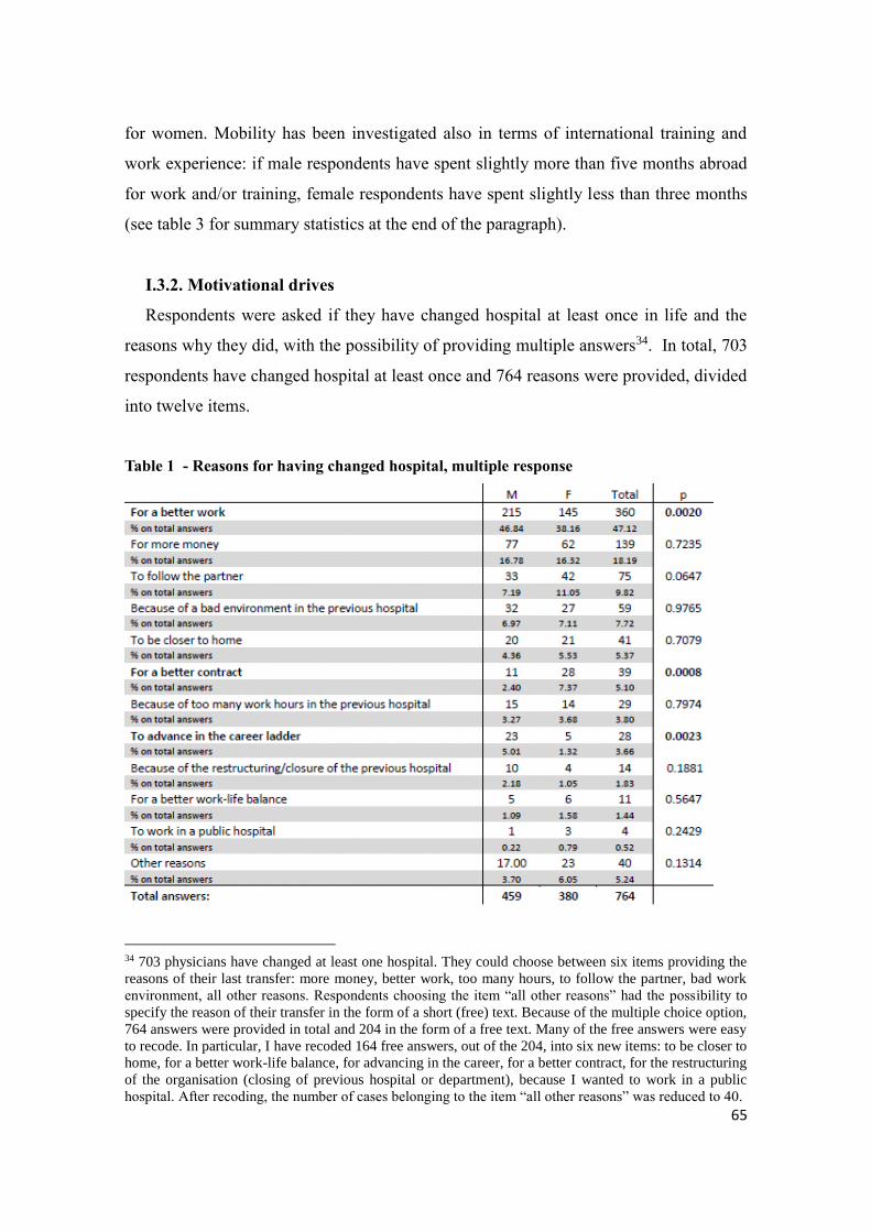
65

for women. Mobility has been investigated also in terms of international training and

work experience: if male respondents have spent slightly more than five months abroad

for work and/or training, female respondents have spent slightly less than three months

(see table 3 for summary statistics at the end of the paragraph).

I.3.2. Motivational drives

Respondents were asked if they have changed hospital at least once in life and the

reasons why they did, with the possibility of providing multiple answers34. In total, 703

respondents have changed hospital at least once and 764 reasons were provided, divided

into twelve items.

Table 1 - Reasons for having changed hospital, multiple response

34 703 physicians have changed at least one hospital. They could choose between six items providing the

reasons of their last transfer: more money, better work, too many hours, to follow the partner, bad work

environment, all other reasons. Respondents choosing the item “all other reasons” had the possibility to

specify the reason of their transfer in the form of a short (free) text. Because of the multiple choice option,

764 answers were provided in total and 204 in the form of a free text. Many of the free answers were easy

to recode. In particular, I have recoded 164 free answers, out of the 204, into six new items: to be closer to

home, for a better work-life balance, for advancing in the career, for a better contract, for the restructuring

of the organisation (closing of previous hospital or department), because I wanted to work in a public

hospital. After recoding, the number of cases belonging to the item “all other reasons” was reduced to 40.

66

Almost half of the physicians (360) have changed hospital to do a better job, that is for

advancing in their research, receiving more training or simply because they were looking

for a more interesting activity. The second most chosen item is the increase in the salary

(139 physicians), followed by the choice of following the partner (75) and the existence

of a bad environment/hostility of colleagues and/or bosses (59). Forty-one respondents

declared they needed to work closer to their house, while only eleven respondents

specified that it was for family reasons: I have decided to distinguish these respondents

in a specific item named “work-life balance reasons”. Worth of mention that 39

respondents declared to have changed hospital in order to have a better contract, which in

most cases was an open-ended contract. As open-ended contracts are rare in private

hospitals, these cases partly coincide with a passage from a private to a public hospital.

Analyzing the answers by gender, only three items show a significant difference

between men and women: men are significantly more likely to change hospital for doing

a better job (p=0.002) and for advancing in the career ladder (p=0.002), while women are

significantly more likely to change hospital for a better contract (p=0.000). As it will be

clear in the next paragraph, women are concentrated in less stable contracts than men and

this certainly explains the higher percentage of female physicians who have changed

hospital for ameliorate their contractual position. Women are more likely to change to

follow the partner while men are more likely to change for money but the differences are

not significant, while women and men are very similar in their answers with respect to

commuting (21 vs 20) and work-life balance (6 vs 5).

Physicians’ motivation has been tested through a second question. Respondents

working extra hours (basically everybody, that is 1051 physicians out of 1074) were asked

why they stay longer at work through a multiple-choice question35. In total, 1911 answers

were provided divided into eight items. No items shows a significant difference between

the two groups (males and females). Only the “advancement-in-career” motivation is

35 Respondents could choose among six items with the multiple choice option: it’s not a choice as it is

required by the organisation/the type of work; to gain more money; to enhance my skills and grow

professionally; to advance in the career ladder; because of a sense of responsibility towards patients; all

other reasons. As for the previous question, respondents choosing the option “all other reasons” had the

possibility to specify the reasons of their working extra-hours in the form of a short text. Eighty-nine

respondents choose to write their own answer. Many of these answers were attributable to the five items

provided in the questionnaire. Others (28) were easy classifiable into two new items: for lack of

colleagues/human resources; for doing research. After recoding, the number of cases belonging to the item

“all other reasons” was reduced to 12.

67

“almost” significant at 90% CI (p=0.0509) with men more likely to choose it but the cases

are too few (19).

Table 2 – Reasons for working extra hours, multiple response

Both questions on motivation – the former being linked to having changed hospital

and the second to working extra hours – don’t follow clear female and male stereotypical

patterns. Within the literature on gender differences in motivations or job “rewards”

(Mottazl 1986, Pelletier et al. 1995, Konrad et al 2000, Rusillo 2004), scholars tend to

distinguish between intrinsic and extrinsic motivations/rewards. The former refers to

inherent satisfaction or pleasure in performing certain activities without expecting any

reward; the latter refers to the tendency to perform activities for external rewards, whether

they are tangible (money, power) or psychological (praise) (Brown 2007). Some studies

have highlighted the existence of gender differences in motivations, thus arguing that

women tend to be more “intrinsically” motivated (Pelletier et al. 2005), while men are

more “extrinsically” motivated (Rusillo 2004). Other studies have contested this idea, by

showing that either there is no significant gender difference in job rewards (Mottazl 1986)

or that differences don’t follow stereotypical patterns (Konrad et al. 2000). This study

68

substantially support this second strand of arguments. Except for the advancement in the

career ladder, which is a significant male characteristic with respect to the reasons for

changing hospital and significant at 90% level with respect to the reasons for working

extra hours, women and men don’t seem to follow the extrinsic-intrinsic schema.

Sometimes they actually reverse it, as men are more likely to have changed hospital for

the job in itself (intrinsic motivation) and women for a better contract (extrinsic

motivation). Significant gender difference, moreover, has not been identified neither with

respect to pay nor with respect to responsibility towards patients or to commuting/work-

life balance.

I.3.3. Hours of work

Women physicians tend to work fewer hours than men after marrying/having children

(Hinze 2000, Jagsi et al. 2012) even though Sasser (2005) highlights that such reduction

in working hours doesn’t lead to a reduction in productivity. She operationalizes

productivity as the hourly wage and finds that, having made significant investments in

human capital, women physicians are able to preserve their hourly earning potential while

working fewer hours (Sasser, 2005).

In the five hospitals analysed, men tend to work slightly more than women, and more

specifically less than three hours a week: 47.78 hours against 44.97 hours in average.

Nevertheless, this difference decreases to 1 hour and 20 minutes if the time spent in doing

private practice is not taken into account (see table 3 at the end of the paragraph I). In

other words, considering only the hours of work spent within and for the hospital, the

difference in work hours between men and women is about 1 hour and twenty minutes

per week. Indeed, men tend to do more private practice, which is more lucrative, than

women: 3.7 hours a week for males against 2 hours for females. Part-time work is residual

among physicians, with no big difference between men and women. Only 13 physicians

– 6 men and 7 women – work less than 20 hours, their number increases up to 34

considering those who work less than 30 hours (22 women and 12 men). These data are

not surprising: unlikely many North-European countries where part-time work is

widespread, in Italy it is not as much. According to Eurostat data, no matter the recent

growth in part-time work, the percentage of part-time workers in Italy is 18.4% in 2014,

slightly less than the EU17 average (22.5%) and much less than countries like the

69

Netherlands (50.4%), Germany (27.6%) and UK (26.8%)36. This is particularly true for

most high-qualified professions, where part-time work is barely absent and long hours of

work are required.

36 EUROSTAT (2015), Persons employed part-time, EUROSTAT Employment Statistics.

http://ec.europa.eu/eurostat/tgm/table.do?tab=table&init=1&language=en&pcode=tps00159&plugin=1

Accessed on February 27th, 2016.

70

Tab 3. Human capital characteristics, mean or percentage37 and difference test

37 The percentage refers to the percentage of women (or men) holding that specific characteristic with

respect the total number of women (or men).

71

II. Institutional work characteristics

II.1. The type of practice and type of contract

Out of 1074 physicians, 36 are academic physicians, that are professors working in the

hospitals, while 1038 are “pure” hospital physicians. Besides the type of practice

(academics vs hospitalists), respondents have been distinguished according to their type

of contract. Indeed, the literature on gender inequalities in medical careers has much

focused on vertical and horizontal segregation (Lorber 1984, Boulis and Jacobs 2010,

Jagsi et al. 2011, Spina and Vicarelli 2015, Kass et al. 2006, Carnes et al. 2008,), as well

as on the pay gap between men and women (Becker 1996, Hinze 2000, Hoff 2004, Sasser

2005, Weeks et al. 2009, Jagsi et al. 2012). Nevertheless, not much attention has been

addressed to gender differences in the types of contracts.

As in many European countries, over the past decades Italy has recorded an increase

in the use of atypical employment. Flexible contracts are particularly widespread among

women and young workers (Barbieri and Schrer 2009), while the traditional “protection

effect” of high education against unemployment and underemployment has recently been

eroded by the economic crisis (Murgia and Poggio 2014). In the health sector, the most

common a-typical employment are: short-term contracts, consultancy (partita Iva),

contracts of collaboration (which takes two forms: the “continuous and coordinated

collaboration” or co.co.co. and the “collaboration on a project” or co.co.pro.), the grant

or scholarship (“borsa di studio”). Short-term contracts are atypical contracts envisaging

a relationship of subordination with one employer, thus providing almost the same

benefits of an open-ended contract in terms of welfare benefits and career progression,

allowing physicians to enter into a sort of “tenure track”. As for the consultancy (“partita

Iva”), it is a form of self-employment regulated either by a contract or not (with the

physician simply issuing an invoice to the hospital). As such, it should not avoid

physicians to work in more than one hospital as a free-lancer. Nevertheless, as in other

professions in Italy (i.e. lawyers or architects), many free-lancers work full-time in one

single hospital, exactly as their colleagues who are officially hired. In these cases, the

free-lance contract becomes a pseudo form of self-employment which implies the same

obligations (but not the same benefits) of a regular contract. The contracts of collaboration

(co.co.co and co.co.pro) are temporary contracts with no relationship of subordination

and very little benefits (even in terms of unemployment schema). Introduced by the

72

reforms on labour market de-regulation of the mid-nineties, the co.co.co. has been

substituted by the co.co.pro. in 2003 through the so-called Biagi law, which forced

employer to link the contract to a specific project. As for the grant, it is a scholarship

provided either by Universities or private Foundations (or both) to young physicians once

they have ended their residency. It often lasts one or two years and it doesn’t provide any

sort of welfare benefits. Considering the duration and the lack of benefits provided, grants

and contracts of collaborations are very similar.

No matter the growing flexibilisation of the labour market in the health sector, the

open-ended contract remains the most common contract in the three public hospitals,

where from 80% to more than 90% of physicians, depending on the hospital, hold a

permanent contract and only a residual part of the workforce (from 1.2% to 5.4%) has a

free-lance contract. In private hospitals, on the contrary, the free-lance contract is the rule.

It accounts for more than 83% of total contracts in San Donato. As for Machado, the

percentage “decreases” to 29% (see tables38). Nevertheless, because of the above-

mentioned discrepancy between the email lists provided by the hospital and the

population, the rate of free-lance contracts in the Machado dataset is not representative

of the population. According to institutional data, free-lance physicians accounts for 77%

of total physicians, while the rest is made of open-ended contracts39.

Hence, public hospitals tend to offer permanent contracts while private ones make a

larger use of atypical employment, especially free-lancers. This difference have some

important implications in terms of career progression. Being a freelancer in a private

hospital is perfectly compatible with the fact of holding top positions. Actually, many

heads of units, either academics or hospitalists, have a free-lance contracts which are very

well paid. On the contrary, in public hospital, except for a few number of retired

physicians who continue to work as consultant, freelancers are often young and out of the

career-ladder, as long as collaborators or grant-fellows. The “meaning” of being a free

lancer is completely different whether one works in public or in private hospitals. Being

38 The frequencies on the type of contract in the respondent dataset are illustrated in tables 10 and 11 in

appendix 3. 39 The frequencies in the type of setting in Machado comparing the population and respondents are

illustrated in table 12 in appendix 3. The comparison has been made on the base of the type of setting since

it is the only data provided by the hospital on the population. The type of setting distinguishes between

academic physicians and hospital physicians. Within hospital physicians, it distinguishes among employees

(who can hold either an open-ended or a short-term contract), freelancers (“partita Iva”) and collaborators

(co.co.co/pro or grants)

73

a freelancer in public institutions means to be an “outsider” who won’t necessarily be part

of the organisation one day, while being a free-lancer in private hospitals doesn’t mean

anything less than being a regular “hired” physician in terms of career progression and

pay (but not in terms of welfare schema). In San Donato being a free-lancer is the rule:

298 physicians out of 302 are freelancers, the rest is made by one open-ended employee

and three collaborators. Out of the three collaborators, two of them are, respectively, vice

and head of unit. Like freelancers, also collaborators in San Donato can hold top positions.

Having made this clear, differences in contract between men and women will be now

investigated. Because of the small number of cases holding a grant or a contract of

collaboration (11), the variable contract has been recoded in three items by merging the

contracts of collaboration and the short-term contracts in one single category as they both

are a form of atypical employment presenting lots of common characteristics, no matter

if the short-term contract is a better contract than the collaboration. They are a form of

precarious employment, often seen as a passage before recruitment much used in public

hospital, where they are offered (mostly) to young people (the mean age is 39.5 for

co.co.pro. vs 40.7 for short-term) and women (10 women out of 11 in co.co.pro and 57

out of 97 in short-term).

Data suggest that women are less likely to hold a stable (and more remunerative)

contract than men are: 74% of women against 78% of men hold an open-ended contract,

while 13% of women against 7% of men hold either a co.co.pro/co, a grant, or a short-

term contract. No much difference persists with respect to free-lance contracts (13% of

females vs 15% of males) (see table at the end of the paragraph II). Worth to mention that

“bad” atypical contracts (co.co.co/pro and grants) are the less remunerative ones, while

“good” ones (free-lance contracts) are the most remunerated ones. And even within each

category, gender differences in pay persist as it shown by the following table:

Table 4 – mean income by gender and contract (n. observations: 1002)

Men Women total

Short-

term/co.co.co/grants 60221 47778 52139

Free-lance 107923 62241 87384

Open-ended 84324 65421 75506

total 85973 62738 74773

74

II.2. The horizontal segregation: institutional characteristics and specialty

Women tend to cluster in less remunerative types of organisations and specialties

(Sasser 2005, Boulis and Jacobs 2010, Crompton and Lyonette 2011). In the dataset, 84%

of women work in a public hospital, against 81.5% of men. There is a slight tendency, for

women, to cluster in public institutions but the difference is not significant. This result is

consistent with Hinze (2000) but not with Jagsi et al. (2012) who finds a higher propensity

for women to work in private organisations. Public institutions offer better schedules and

slightly shorter hours of work: in private hospitals physicians, considering both males and

female, work around 48.7 hours a week, compared to the 46.5 hours worked in public

hospitals, for a difference of two hours.

Gender segregation is evident also in the gender composition of each specialty (Baker

1996, Hinze 2000, Sasser 2005, Magnusson 2005, Boulis and Jacobs 2010, Crompton and

Lyonette 2011, Jagsi et al. 2011 and 2012, Magnusson 2015). The Italian Ministry of

education, universities and research clusters specialties in four areas: medicine, surgery,

diagnostic and public health. In the respondent dataset, more than half of the female

workforce (and precisely the 56%) work in the medical area (against 40% of males) while

only 16% of them is a surgeon, against 35% of men. The diagnostic area appears to be

the most balanced one, with 24% of female physicians working there against 21% of men.

The public health area is made of only 30 cases (17 men and 13 women), which makes it

difficult to draw conclusions. The medical area includes twenty-three specialties like for

instance general medicine, internal medicine, dermatology, haematology, endocrinology,

gastroenterology, neurology, paediatrics, psychiatry, etc.. Some specialties are more

“gendered” than others: in neonatology and rheumatology 80% of physicians are females.

High female rates can also be found in paediatrics (67,5%), radiotherapy (66,7%),

neuropsychiatry (60%), while psychiatry exhibit a lower proportion of women (56,2%).

If women are clustered in the medical area, men are more concentrated in the surgical

one, where, out of ten physicians, seven are males and three are females. The highest level

of segregation occurs in oral and maxilla-facial surgery (91%-9%), orthopaedics (88%-

12%), urology (88%-12%), hearth surgery (83%-17%), general surgery (77%-23%),

vascular surgery and otorhinolaryngology (both at 75%-25%). A traditionally male-

dominated branch – at least in Italy – like genecology has experienced a strong

feminization in the last years: now 49 physicians out of 100 are females. Only two surgical

75

specialties, out of thirteen, appear perfectly gender-balanced: paediatric surgery and

neurosurgery, where the proportion of males and females is 50%-50%. Together, the

medical and the surgical area cover the 74% of the entire medical population. Considering

also the diagnostic area, which is the third most populated area, the three areas represent

up to 96.3% of physicians. The diagnostic area is quite gender balanced, with a slight

majority of women working in (51 out of 100). More than half of the physicians in this

area (58%) and three quarter of physicians concentrated in two specialties: anesthetic and

intensive care, which are both female dominated: 54%-46% is the proportion for the

former and 5%-4% is the proportion for the latter.

II.3. The vertical segregation: the career steps

Studies on medical careers have shown that women physicians concentrate in lower

steps of the career ladder and progress more slowly through steps (Carnes et al. 2008,

Boulis and Jacobs 2010). Data based on the five hospital in Lombardy confirm the

existence of a mechanisms of vertical segregation among physicians. In order to

investigate whether women and men are differently positioned within the organisational

structure, the different career ladders have been harmonized taking in consideration the

differences between public and private hospitals. The former follow the national contract

for physicians in the public sector, made of six formal ranks. The two private hospitals

have their own contract, made of three (for San Donato) and five (for Machado) ranks. I

have re-categorized the steps on the base of a content analysis and through the comparison

of elements such as age and income in order to create one single career ladder.

The result is a ladder made of three ordinal ranks. The first level gather the first two

steps of public hospitals, the first level of San Donato and the first two levels of Machado.

For those physicians who will never be promoted, this level can be at the same time the

first and the last step of their career: one can retire with a “first level” position with her/his

salary being determined by merely seniority or accomplished targets (but not by any

responsibility allowance derived from promotions). The following step – “vice” – is

where promotional mechanisms and responsibilities comes into play. “Vice” gather three

different steps in the public contract, one step in San Donato and two in Machado. The

third and last step – “head” – is the highest level of the ladder and stands for physicians

76

who are responsible for an operational “unit”.

Tab. 5 – The career ladder

Frequencies Percent

1st level 646 60.15

Vice 255 23.74

Head 136 12.66

All others 37 3.45

total 1074 100

The “all others” step gathers three figures which are hard to code in an ordinal scale:

the collaborators or grant fellows of public hospitals, the freelancers of public hospitals

and “pure” academic researchers. Collaborators and freelancers in public institutions are

precarious – often young – workers waiting to be hired. Such (often) temporary positions

are scarcely compatible with a progressive ladder because not everybody passes through

that step. Officially, once the residency is over, one should participate to a public

competition (“concorso”) and, if he/she wins it, be hired as a first level physician (either

with a short-term or open-ended contract). Furthermore, this is true only in public

hospitals: in private ones, where no public competition is needed, precarious contracts are

compatible with any step of the career-ladder. Together with atypical public contracts, the

step “all others” gather four academic physicians “non convenzionati” (without

agreement between the Hospital and the University) whose career progression takes place

only within the University and, therefore, it follows the academic steps40. Because of the

impossibility to “order” into a progressive scale these figures (precarious positions within

the public institutions and academics “non convenzionati”), they have been coded as “all

others” (see table 5). For the same reason, they were excluded from the scissor diagram.

Figure 1 – The scissor diagram: men and women in each rank of the ladder

40 Academic physicians “non convenzionati” (literally: not covered by an agreement between the University

and the Hospital) are paid only by the University, even if part of their activities take place in the hospital.

Their career progression follows only the University “ladder” and that is the reason why I was obliged to

cluster them into the “all others” step of the ladder. On the contrary, academic physicians “convenzionati”

(most of them: that is covered by an agreement between the University and the Hospital) have a double

employer: the University and the Hospital. Their career progression takes place both at the University and

in the Hospital and their salary is much higher than the academics “non convenzionati” because, by law,

must be equal to hospitalists’ pay.

77

The scissor diagram shows the percentage of women and men within each rank. As

one can see, women are the majority of physicians in the lower rank of the ladder (being

56% of first level physicians) while they are the minority both as vices (38%) and heads

(24%). On the contrary, considering the percentage of women and men within each sex

(see table 6 at the end of the paragraph), women are concentrated into the lower ranks,

with 70% of them working as a 1st level physicians (against 50% of men) and 5% as “all

others” (against 2% for men), while they are under-represented both in vice (19% of

women against 29% of men) and in head (6% of women against 19% of men).

II.4. The gender pay gap

In order to have the highest rate of physicians declaring their income, they were given

the opportunity to choose among 21 income classes, going from the lowest one (up to

10.000 euro) to the highest one (more than 400.000 euro). Each class has then been

transformed into its mean when modelling the pay gap. Respondents were asked to

provide the income, and not the salary, in order to account for earnings made in private

practice and all other consultancy activities, if there are any. Moreover, as these earnings,

due to extra work, are taxed once a year through the income tax filling, I have considered

that the gross value would be easier to remember than the net one. Overall, the mean

income of the respondents, considering both sexes, is 74753.5 euro, with a median class

of 65000 euro. Men in the dataset earn, in average, 87973 euro while females earn 62747

43,34

61,96

76,47

56,66

38,04

23,53

0

10

20

30

40

50

60

70

80

90

100

1st level Vice Head

% o

f m

en a

nd

wo

men

in e

ach

ran

k

men

women

78

euro for a earn differential of 23226 euro (number of observations=1004). The

distribution of income, both for men and women, is rather skew with male income

reporting more outliers than the female income. Adopting the Oecd definition of the

gender pay gap41, men earn 26,6% more than women.

Figure 2 – Boxplot of the income by gender

41 The gender wage gap is unadjusted and is defined as the difference between median earnings of men

(75.000 in the dataset) and women (55.000 in the dataset) relative to median earnings of men. Data refer to

full-time employees. See https://data.oecd.org/earnwage/gender-wage-gap.htm. Accessed on February 28th,

2016.

0

100

00

02

00

00

03

00

00

04

00

00

0

male female

inco

me

Graphs by gender

79

Tab 6. Work characteristics, mean or percentage and difference tests

III. Family characteristics

Because of persisting traditional gender roles within the family and the inadequacy of

welfare provisions, women in high-qualified professions face strong challenges in

balancing work and family responsibilities. Many studies have pointed out that marriage

and children have a negative impact on women’s career and income (Lundberg and Rose

2000, Buding and England 2001, Sasser 2005). To avoid such penalties – in rank and pay

– women in non traditional jobs are more likely than men to be single, to reduce the

number of children or to be childless (Wajcman 1998). This is particularly true in Italy,

which is a country traditionally characterized by long hours of work, with inadequate (or

too expensive) care services (especially for early childhood) and where family

80

responsibilities are still a woman’s issue, no matter the growing, and recent, commitment

of Italian fathers in the care of children (Zajczyk and Ruspini 2008, Saraceno and Naldini

2011).

III.1. Parental and marital status

In the dataset, 692 physicians out of 1074 are married. Men are more likely to be

married than women (70.5% of male physicians are married against 58% of female

physicians), while not much gender difference appears in the likelihood of having a

cohabiting partner (15.9 versus 15.7%). As for children, 739 physicians (318 females and

421 males) have at least one children. The percentage of women being mother is lower

than the percentage of men being father: 61% against 76%. On the other hand, 39% of

women are childless, against 24% of men. Among parents, there is a significant gender

difference in the number of children: male physicians have in average 1,51 children

against 1,06 of females physicians (for all the summary statistics see table 9 at the end of

the paragraph).

The debate on the gendered dimension of organisations (Acker 1990, Britton 2000)

has shown how organisations promote the idea of an “abstract worker” which is based on

males’ characteristics. Such ideal worker have very little care responsibilities and,

eventually, can count on a non-working spouse taking care of the children and supporting

him in his work aspirations (Pateman 1988, Wajcman 1998). Descriptive statistics

partially confirm this picture. In the dataset, males physicians are more likely than their

female colleagues to have a non working partner (defined as spouse or cohabiting

partner). The difference is striking: 24% of male physicians have a housewife, while 8.6%

of female physicians are married with a non working partner, which is, nonetheless, a

quite high percentage anyway. Male physicians are more likely to have a partner working

residually or part-time: 12% and 14% of men have partners working, respectively, up to

20 and up to 30 hours, while the percentages shrink to 3% and 5% for women physicians.

Gender parity occurs only when the partner works full time: 32.2% of males and 33.8%

of female physicians exhibit a partner working from 30 up to 40 hours a week. On the

contrary, female physicians are more likely to have a spouse working over-time: almost

50% of women in the dataset have a partner working more than 40 hours, against 18% of

81

men. Gender balance occurs also with respect to homogamy: 24.5% of females and 25.5%

of males are married (or are living together) with a physician.

III.2. The sexual division of labour

Being married and having children have different impacts on women and men’s use of

time devoted to non paid work, defined as both domestic and care work. Respondents had

the choice to report the time devoted to nonpaid work distinguishing between five items:

care for children; care for the elderly, traditionally female domestic activity (cleaning,

laundry, etc.), traditionally male domestic activity (repairing, gardening, etc.), the

coordination of the maid/baby-sitter.

Overall, men and women spend in average, respectively, 15 and a half and 25 and a

half hours per week in non paid activities. This translates into about one and a half hour

a day of gender gap in non-paid activities. The result is not consistent with data on the

general population, which show a much worse picture. According to the National Institute

of Statistics (Istat), Italian men and women spend, respectively, 104 and 315 minutes par

day in non paid activities, which translates into a gap of three and a half hours (211

minutes) par day and sets the country among the worst ones in the OECD area (Gaiaschi

2014). The discrepancy is mostly due to women’s side: translating hours into minutes,

female physicians report 218 minutes of non paid work par day (against 315 minutes in

the general population according to Istat), while male physicians report 133 minutes (104

for Istat).

Part of the reason of such discrepancy could be due to the difference in methods: Istat

uses (daily) diaries, while my data are based on (weekly) estimates (respondent’s

declarations). It is well acknowledged that the former are much more accurate than the

latter, both with respect to paid and nonpaid work (Robinson and Bostrom 1994,

Robinson et al. 2002, Robinson et al. 2011). With respect to nonpaid work in particular,

it has been shown that women tend to underestimate the time spent in non paid activities

(Bonke 2004). One second reason for the discrepancy between my results and national

data on the sexual division of labour could due to the target population. Indeed, general

data account for women working part-time and for women not working at all, while this

research targets a very selected population, composed by high-skilled professionals who

82

have invested a lot in their education and who work long hours of work. As a

consequence, 39% of them are childless while mothers tend to outsource care and

domestic work in order to balance work and family.

Data on outsourcing are quite interesting indeed: women in the dataset have reported

to pay a maid working, in average, almost 7 hours of a week, against 5.4 hours declared

by men. Among women, childless women report having a maid working three hours a

week, exactly as their male childless colleagues, while mothers report having a maid

working nine hours and a half par week, against 6.40 minutes declared by fathers. Hence,

mother physicians tend to reduce their time in nonpaid work by outsourcing domestic

work. Such circumstance, together with the high rate of childless women, reduce the

overall data on women physicians’ nonpaid work activities.

The time devoted to non paid work varies not only according to parenthood but also

according to the parental status. Both single and men with a partner (either a spouse or a

cohabiting partner) devote around 15 hours a week to non paid activities. This means that

marriage doesn’t have any impact on men’s use of time in non paid work. This is not the

case for women: if as single woman spend 19 hours a week in non paid work, as spouse

or cohabiting partner she will spend 28 hours a week. In this case, a change in marital

status parallels a change in women’s use of time in non paid work, enhancing hours in

nonpaid work of almost nine hours a week. Stronger involvements by men occurs when

they become fathers. Childless men devote 10.7 hours a week to unpaid work, which

increases to 17 hours a week with the first child. Nevertheless, the increase is much higher

for women: from 14 hours a week when they are childless to 33 when they are mother.

Indeed, gender inequalities at work reflect gender inequalities at home: it is because

domestic work and the care of children are still a “women issue” that marriage and

children constitute a “penalty” for women’s career (Saraceno 1980, Crompton 2006,

Gerson 2009).

83

Figure 3 – Nonpaid work for women and men (single and in couple)

III.3. Work-life conflict

The problem of work-life balance is strongly felt by women: 46% of female physicians

experience a situation of work-life conflict while 45% experience it sometimes, against,

respectively, 35% and 48% for men.

Tab 7 – Do you have a hard time to balance work and life?

Respondents experiencing a work-life conflict were invited to provide an explanation

for it by choosing among five items: rigid schedule, long hours of work, lack of care

15,3

19

15,6

27,8

0

5

10

15

20

25

30

Men Women

Single

In couple

Pearson chi2(2) = 19.1365 Pr = 0.000

100.00 100.00 100.00

Total 553 521 1,074

35.08 45.87 40.32

Yes 194 239 433

48.82 45.11 47.02

Sometimes 270 235 505

16.09 9.02 12.66

No 89 47 136

onflict male female Total

worklife_c gender

84

services, lack of grandparents caring for children and lack of support by the partner in

sharing care responsibilities. Each item provided a four-point scale (“very”; “slightly”; “a

little”; “not at all”). Women are (significantly) more likely than men to complain for a

rigid schedule, long hours of work, a lack of care services and a lack of support by the

partner in sharing care responsibility. On the contrary, there is no much gender difference

with respect to the lack of grand parents, with the majority of both male (43%) and female

(41%) physicians declaring it doesn’t pose a problem (see figures 2-6 in appendix 3).

Analyzing women’s answers, it’s worth of notice that the lack of care services matters

much more than that the lack of the partner’s support in care responsibilities. Only 24%

of women has indicated the latter as explanation for their work-life conflict (9% of them

have chosen the item “very” and 15% of them have chosen the item “slightly”) while 52%

(divided between 26% as “very” and 24% as “slightly”) has indicate the former. How to

interpret this finding? Either men equally share non paid work with their partners or

women don’t feel it as a problem. Since the unequal division of nonpaid work between

men and women existing among physicians, it seems more reasonable to opt for the

second explanation. In other words, the majority of female respondents facing a work-life

conflict don’t recognize the traditional division of paid and non paid work between the

sexes – which in Italy remains quite strong – as the cause for it (Saraceno 1980, Saraceno

and Naldini 1998, Saraceno and Naldini 2011).

On the other side, the organisation of the time in the workplace is clearly identified by

women as a cause of their work-life conflict: 70% and 84% of them (against 61% and

76% of men) think that, respectively, the rigidity of work schedules and too many hours

of work negatively impact their work-life balance in a “very” or “slightly” manner. The

Person’s Chi2 test is significant in both cases, thus confirming the findings of Lyness et

al. (2003) according to which: 1. Women have less “control” of their schedule than men

do as long as they work in occupations or they are clustered in ranks which don’t provide

enough possibility of flexi-time; 2. Women report working too many hours more often

than men do. The gender difference in the possibility of “controlling” its own schedule

is confirmed by a specific question. Physicians have been asked to explain how their

workday is structured. Four items were proposed from the least to the most flexible

schedule arrangements: no flexibility; flexibility in entry; flexibility both in entry and in

exit, total flexibility. In the table below the results are divided by gender.

85

Tab 8 – Control over worktime

Women are more concentrated in the two first items, which provides less flexibility,

while men in the second two, which provides more flexibility, even if the gender

difference is not significant (p.=0.081).

Pearson chi2(3) = 6.7263 Pr = 0.081

100.00 100.00 100.00

Total 553 521 1,074

21.70 19.00 20.39

Total flexibility 120 99 219

56.24 52.40 54.38

Flexy entry & exit 311 273 584

10.13 11.90 10.99

Fixed entry only 56 62 118

11.93 16.70 14.25

Fixed entry and exit 66 87 153

control male female Total

gender

86

Tab. 9 - Family characteristics

IV. Conclusions

Women and men respondents report many differences in human capital, work and

family characteristics. Women graduate with better grades than men do but once they

have entered in the profession they are less likely to acquire further specializations. Even

if today they are the majority of PhD students at University, it is not the case in hospitals,

87

where more men than women have a post-graduate title. Women physicians tend to have

a smaller portfolio-career than men, they appear less “mobile” and they work fewer hours

than men (mainly because they do less private practice). On the other hand, motivational

drives don’t seem to follow gender stereotypical patterns.

As for the “choice” of specialization, women tend to cluster in medical specialties

while surgery still remains a male-dominated specialty area, with around 70% of

physicians being males. Women are more likely than men to hold an atypical, and less

remunerated, contract. The career ladder still remains harder to climb for them: by

analysing the composition of the medical population, a strong vertical segregation still

persists. Women are the majority of physicians in the lower rank of the ladder but they

are the minority in the upper ranks. Pay differentials are relevant: men earn 26.6% more

than women, which is much greater than the national pay gap (7.3%). Both data are

unadjusted, that is they are not controlled for any work characteristics, but if the former

is based on the income, the latter is based on earnings. Such difference makes the pay gap

found among physicians inclusive of revenues dues to private practice and external

consultancies (if there are any), thus providing a more realistic picture of pay differentials

between men and women.

The analysis of family characteristics has shown a quite traditional picture. Women,

and in particular mothers, are the main responsible for non paid work. In order to face

work-life obstacles they reduce, with respect at least to the general population, the time

devoted to domestic and care activities, either by outsourcing nonpaid work or renouncing

to motherhood and thus confirming the findings of previous research in non traditional

profession (Wajcman 1998, Roth 2006).

One may objects that these disparities are only a “matter of time”, that they will

gradually disappear as long as the level of women entering in the profession will be equal

to all cohorts. Studies on the general labour market have refuted these arguments

(Palomba 2013). If this is the case also with respect to the medical profession, it should

be further investigated: researches on early cohorts of physicians (Jagsi et al. 2012) and

using longitudinal data (Sasser 2005) show that gender inequalities persist among

younger physicians. Yet, further longitudinal data with respect to the European context

are needed to analyse changing conditions across time.

88

89

Chapter 4 – Explaining the gender pay gap

It is well known that women physicians earn less than their male counterparts. Most

of the studies finds that the pay gap persists no matter equal characteristics (Hinze 2000,

Hoff 2004, Sasser 2005, Weeks et al. 2009, Jagsi et al. 2012, Magnusson 2015). On the

contrary, Baker (1996) finds no earning difference after controlling for experience,

specialty, practice setting, family status and other characteristics42. Sasser (2005) focuses

on the child penalty and finds that mothers earn significantly less than childless women

after controlling for all characteristics, with the penalty growing with the number of

children, while fathers with two children earn significantly more than childless men.

In order to examine the determinants of the pay differential, a model for the log annual

income using OLS will be estimated (paragraph II). Afterwards, a model accounting for

interaction terms will be estimated in order to investigate how gender mediates the effects

of characteristics on income (paragraph III). Finally, the pay gap will be composed by

using the Oaxaca-Blinder decomposition (paragraph IV).

I. Measures

The natural logarithm of the annual income is the dependent variable. The type of

hospital is the control variable43. Independent variables include human capital, work and

family characteristics. Human capital characteristics include a four-item variable for

grade and the number of years of work experience. Grade, originally an interval variable,

has been recoded into a multinomial one in order to correct for its distribution as it is

42 Coherently with the theoretical approach of this thesis (see Chapter 1), the results of Baker’s study

“should not be interpreted as evidence that discrimination is no longer a problem” (Baker 1996, p. 963). He

explicitly reminds such concept on his conclusions as he underlines the importance of the structure of

limitations and opportunities in determining the differences in characteristics between men and women

through socialization. 43 In the models of chapter 4 and 5 hospitals are named as following: Public 1 is the Policlinico, Public 2

Legnano, Public 3 Como, Private 1 San Donato and Private 2 Machado.

90

negative skewed, with very few observations on the left tail. Work characteristics include

individual ones, as the number of hours and the number of hours of private practice

worked in a week. Institutional work characteristics include the rank (a three-item

variable divided in first level, vice and head) and the specialty (a four-item variable

divided in medicine, surgery, diagnostic and “all others”44). Family characteristics

include the marital status and the number of children. The marital status is a multinomial

variable accounting for the work status of the partner. It is made by six categories: no

partner, no working partner, partner working residually (from 0 to 20 hours a week),

partner working part-time (from 21 to 30 hours a week), partner working full time (from

31 to 40 hours) and partner working overtime (working more than 40 hours a week). A

dummy variable was also added for having (=1) or not (0) a partner who also works as a

physician to control for homogamous couples. Finally, the number of children is a

categorical variable made on the base of the question on the number of children living at

home45. It is composed by four category: 0 for no children, 1 for 1 children, 2 for 2

children and 3 for more than 2 children. This variable has been transformed into a

categorical variable for two reasons: first, to correct for its distribution. As in the general

population, also with respect to this specific dataset, the right tail of the distribution of

the variable children is not continuous in its extreme values. Second, from a theoretical

point of view, I assume that the impact of children varies importantly across the first steps

(and therefore between 0 children and 1, between 1 and 2, 2 and more than 2), while it

doesn’t so much after the third child (Sasser 2005).

44 The item “all others” of the variable specialty used in the regression includes the specialty of public

health, specialties difficult to recode, physicians with no specialty and missing casses. Cases in these four

groups are very few (44 in total) and, in order to correct for their distribution in the multinomial variable

“specialty”, I had to merge them in one single item. Betas and pvalues for such an item haven’t been taken

then then in consideration as they refer to a very heterogeneous category. 45 I had the possibility to chose between the answers of two different questions. The former regarding the

number of children in general (including the adults one), the second regarding the number of children living

at home. I have chose to add the latter on the base of the literature (Sasser 2005) and because it is the most

coherent with theoretical framework of this work, which emphasizes the sexual division of labour as an

explanatory factor of gender inequalities. Children at home require parents taking care of them (at least

until they are not independent) and thus they impact on the division of paid and unpaid work. This is not

the case, at least in a much lesser extent, for adult children. This is confirmed by the fact that, running the

same regression with the total number of children (instead of the number of children living at home), the

beta decreases (from 2% to 1,4%) and the pvalue increases (from 0.070 to 0.221, in both case not

significant), indicating that children at home have a stronger impact on pay than children in total.

91

II. Hypothesis

I consider five mechanisms by which being a woman physician may negatively affect

pay. First, in anticipation of taking the majority of family responsibilities, women acquire

less human capital (either because they choose it or, alternatively, because employers

provide them with less training) (first hypothesis). In this perspective, women’s lower

pay is attributable to lower levels of human capital (Becker 1981). The human capital

theory is less plausible for a specific and quite homogeneous group as the one composed

only by physicians, as they have chosen a profession requiring many years of education

and long hours of work. On the other hand, descriptive statistics in the previous chapter

show that women report, in average, better grades but lower levels of secondary

specialties, while no relevant gender differences have emerged with respect to the Ph.D..

Moreover, they report fewer years of work experience which may negatively impact the

pay.

Second, women may earn less because they work fewer hours (hypothesis 2) and

because they do less private practice, which is more lucrative, than men (hypothesis 2bis).

The difference in total work hours and in private practice hours may be due to greater

family responsibilities or, in the case of the private practice, to a greater commitment to

the institution.

Third, by anticipating major family responsibilities, women may “choose” family-

friendly specialties like the medical ones which are less paid (hypothesis 3). Medical

specialties are less well paid with respect to surgical ones but they offer better time-

arrangements, with more predictable schedules and shorter hours of work. On the

contrary, surgical specialties implies higher probability of working extra-hours

(especially when complications with patients in the operating rooms occur) and/or facing

emergency situations. This is confirmed by the following table which shows that

physicians in surgical specialties work, in average, two hours more than physicians in the

medical ones. Data include the hours of private practice, which are higher in surgical

specialties.

92

Tab 1. Weekly total hours of work and weekly hours of private practice by specialty

total weekly

work hours

weekly hours of

private practice frequency

Medicine 45.8 2.4 512

Surgery 47.7 4.6 277

Diagnostic 46.2 2 241

all others 46.4 2.9 44

Total 46.4 2.9 1074

Fourth, women may earn less because of their greater family workload. As already

mentioned, the sexual division of labour ensures that women and men are differently

affected by their marital and parental status. Hence, having children may negatively

impact women’s pay while it may enhance men’s pay (hypothesis 4). Moreover, being

married (or living together with) can engender different returns too: positives for men,

negatives for women (hypothesis 4bis).

Fifth, women may earn less because either they are discriminated by their employers

or because of the effect of unobservable characteristics, such as productivity and skills

(hypothesis 5).

III. Interpreting the gap through an OLS multivariate model

In order to test these five hypothesis, a step-wise multivariate regression model using

OLS has been run. Table 1 reports the coefficients on pay for different sets of variables.

Column 1 shows the “gross” effect of gender on income: without no control for

differences in characteristics, women earn 30% less than men. Column 2, 3, 4 and 5

reports the coefficients for different sets of variables, including the control variable

“hospital”. Column 2 controls for human capital characteristics only. Controlling for

grade and years of experience, the penalty decreases to 23.5% but it is still significant.

Column 3 adds for work variables, which includes hours of work, hours of private

practice, the specialty and the rank. Controlling both for human capital and work

variables, the female penalty decreases to 15% thus remaining significant. Column 4

controls for family variables only, while Column 5 reports the full model. Controlling for

93

all characteristics, the female penalty on pay is still significant. Adding family

characteristics doesn’t add to much to the model in terms of explained variance as the

female penalty still lays at 15% in the full model. Such part of pay gap may be due either

to discrimination or to unobservable characteristics.

Over all, table 2 shows that no matter equal (observable) characteristics between men

and women, women earns significantly less. This suggests that, net of unobservable

characteristics, mechanisms of discrimination take place. As for observable

characteristics affecting income, the reduced experience and the reduced hours of work,

both in total and with respect to private practice only, are part of the explanations of the

pay gap. Having obtained honors increases the pay with respect to the reference category

but only at a 90% level of confidence interval. Clearly, being in the top levels of the career

ladder increases income, as it is shown by the significance impact of the “vice” and

“head” ranks with respect to the first level. Working in a surgical specialty with respect

to a medical one significantly increases income, as it does working in diagnostic.

Therefore, the higher concentration of women in the lower ranks of the ladder as well as

in the medical specialties is one of the explanation of the pay gap. All in all, differences

in human capital and work characteristics play a role in engendering a pay differential

between men and women. Nevertheless, they are only part of the whole story, as

controlling for differences in such characteristics, the female penalty on pay persists.

94

Tab. 2. Step-wise multivariate model on income

(1) (2) (3) (4) (5)

Log income Log income Log income Log income Log income

Female -0.305*** -0.232*** -0.149*** -0.279*** -0.150***

(0.000) (0.000) (0.000) (0.000) (0.000)

Hospital: Public 1 0 0 0 0

(.) (.) (.) (.)

Hospital: Public 2 -0.0423 -0.0196 -0.115*** -0.0285

(0.173) (0.489) (0.000) (0.318)

Hospital: Public 3 -0.00575 0.0169 -0.0478 0.0109

(0.871) (0.602) (0.200) (0.740)

Hospital: Private 1 0.180*** 0.0913* 0.0432 0.0948*

(0.000) (0.028) (0.367) (0.023)

Hospital: Private 2 0.234*** 0.176*** 0.207*** 0.173***

(0.000) (0.001) (0.000) (0.001)

Grade: up to 104 0 0 0

(.) (.) (.)

Grade: 105-110 0.0408 0.0314 0.0392

(0.237) (0.315) (0.213)

Grade: honors 0.0542 0.0451 0.0501

(0.100) (0.135) (0.099)

Experience 0.0191*** 0.0122*** 0.0122***

(0.000) (0.000) (0.000)

Work hours 0.00477*** 0.00491***

(0.000) (0.000)

Hours of private practice 0.00881*** 0.00842***

(0.000) (0.000)

Rank: Up to 1st level 0 0

(.) (.)

Rank: Vice 0.193*** 0.184***

(0.000) (0.000)

Rank: Head 0.434*** 0.440***

(0.000) (0.000)

Specialty: Medicine 0 0

(.) (.)

Specialty: Surgery 0.0741** 0.0806**

(0.007) (0.003)

Specialty: Diagnostic 0.149*** 0.149***

(0.000) (0.000)

Specialty: All others 0.0636 0.0570

(0.255) (0.307)

No partner 0 0

(.) (.)

No working partner 0.108* 0.0365

(0.023) (0.365)

Partner working residually 0.0597 -0.0172

(0.331) (0.737)

Partner working part-time 0.0838 0.0791

(0.133) (0.097)

Partner working full-time -0.00287 0.0353

(0.943) (0.303)

Partner working over-time 0.0481 0.0786*

(0.235) (0.022)

95

No children 0 0

(.) (.)

One child 0.0795* 0.0434

(0.017) (0.123)

Two children 0.0658 0.0567*

(0.050) (0.046)

More than two children 0.0633 0.0429

(0.194) (0.297)

Having a physician as

partner

-0.00765 -0.0447

(0.801) (0.079)

Constant 11.27*** 10.81*** 10.51*** 11.22*** 10.45***

(0.000) (0.000) (0.000) (0.000) (0.000)

R-square 0.123 0.362 0.484 0.177 0.494

N 1004 914 914 1004 914

p-values in parentheses * p < 0.05, ** p < 0.01, *** p < 0.001

IV. Interpreting the pay gap through interaction terms

Family variables must be treated carefully. Because of the persistence of the sexual

division of labour assigning major family responsibilities to women, the marital status

and the number of children may affect women’s and men’s pay in different ways. Many

studies have documented the existence of a marital wage premium for men (Korenman

and Neumark 1991, Loh 1996, Hersch and Stratton 2000). Qualitative contributions in

the study of gendered organisations have shed light on the positive effect, on men’s career,

of being married with a non-working spouse (Pateman 1988, Wajcman 1998, Wajcman

and Martin 2001). On the other hand, married women may be penalized in terms of

earnings (Buding and England 2001, Sasser 2005). As for the effect of children on

parent’s wages, many contributions have shed light on the wage penalty for motherhood

(Folbre 1994, Waldfogel 1997, Lundberg and Rose 2000, Buding and England 2001,

England 2005, Sasser 2005) as well as on the fatherhood wage premium (Sasser 2005,

Glabuer 2008, Hodges and Budig 2010, Kelly 2012). In order to account for such

differences in “slopes”, many scholars interact the marital and the parental status with the

gender variable while modelling the pay gap (Tharenou 1999, Sasser 2005, Kelly 2012).

Nevertheless, if the use of interaction terms with respect to family characteristics in

modelling the pay gap is quite common in the literature, it is not with respect to human

capital and work variables. Only a few empirical studies, in the area of gender work and

organisation, go in that direction (Hoff 2004). Yet, that gender moderates the effects of

96

human capital and work characteristics is well known. In the economic literature, the

decomposition methods (i.e. Oaxaca-Blinder) are based on the assumption that the pay

gap is due both to differences (between males and females) in characteristics between

males and females as well as to differences in their returns. Within the sociological

debate, both the queue tradition and the debate on comparable worth (see Chapter 1)

suggest that the “effort” - in education and in employment – are differently “assessed” in

the labour market whether they refer to men or women thus leading to mechanisms of

horizontal segregation and pay inequalities. In multivariate analysis, these differences

could be accounted for by interacting gender with human capital and work characteristics.

In order to investigate the different “slopes” – between men and women – of the same

variables, interaction terms have been added with respect not only to family

characteristics, but also with respect to human capital and work characteristics. The idea

underneath is to investigate whether, for example, women have lower “returns” on their

educational credentials or on the time they spent at work. Whether being a female surgeon

or a female “head” “pay” less than being a male surgeon or a male “head”, controlling for

all other characteristics.

Descriptive statistics suggest that being surgeon or working in a top position is less

rewarding for women than for men, as it is shown in the tables below:

Tab 3. Mean income by specialty and gender

519 485 1004

Total 85973.025 62747.423 74753.486

21 19 40

all other 95238.095 77236.842 86687.5

109 120 229

diagnosti 87568.807 67125 76855.895

183 76 259

surgery 89986.339 61085.526 81505.792

206 270 476

medicine 80618.932 60250 69065.126

specialty male female Total

gender

97

Tab 4. Mean income by rank and gender

Yet the simple crosstabs do not take into account other important differences in human

capital, individual work and family characteristics. In order to do this, one must make use

of an OLS multivariate regression accounting for interactions terms.

Two sets of models have been run. Each set of model shows the full model in the first

column and the model accounting for the interaction terms in the second column.

Preliminary regressions separately for men and women have been run in order to identify

which explanatory variable reported opposite coefficients thus suggesting the need of an

interaction. Afterwards, interaction terms have been added in the full model and

significant interactions up to 90% level have been kept. In the first set of model children

and partner are categorized as dummy variables (1=having children - 0=no children; 1=

having a partner – 0=no partner). In the second set of models both children and partner

are multinomial variables where partner accounts for the hours of work of the partner.

The second set of model reports, in the first column, the same exact full model of table 4

and, in the second column, its version with the interaction terms.

The differences in the use of the children and partner variables make sense as long as

they answer to different research questions. The first set of models reports the effect of

having or not having children and having or not having a partner. The second set of

models – which corresponds exactly to the full model of the previous paragraph – goes

further in details and reports the incremental effect of having children and the effect of

having a working partner, with different degrees of work-schedules, with respect to not

having a partner at all (reference category).

519 485 1004

Total 85973.025 62747.423 74753.486

98 28 126

Head 130765.31 104107.14 124841.27

150 93 243

Vice 88166.667 78010.753 84279.835

271 364 635

up to 1st 68560.886 55666.209 61169.291

rank male female Total

gender

98

As one can see, using a different recodification of the same two variables doesn’t

change much in terms of observations, R squared and F tests, while betas and t statistics

are slightly different but such difference doesn’t modify the interpretation. Each couple

of model presents the full model in the first column and the same model with the

interactions terms in the second column.

99

Table 5. Ols models with interactions

Set 1 Set 2

(1) (2) (1) (2)

Log income Log income Log income Log income

Female -0.141*** 0. 0843 -0.150*** 0.0774

(0.000) (0. 354) (0.000) (0.397)

Hospital: Public 1 0 0 0 0

(.) (.) (.) (.)

Hospital: Public 2 -0.0294 0. 0382 -0.0285 0.0381

(0.301) (0. 348) (0.318) (0.349)

Hospital: Public 3 0.00273 0. 0445 0.0109 0.0454

(0.933) (0. 320) (0.740) (0.318)

Hospital: Private 1 0.0879* 0.201*** 0.0948* 0.213***

(0.034) (0.000) (0.023) (0.000)

Hospital: Private 2 0.170*** 0.238*** 0.173*** 0.247***

(0.001) (0.001) (0.001) (0.000)

Hospital*female: Public 1 0 0

(.) (.)

Hospital*female: Public 2 -0.115* -0.115*

(0.043) (0.045)

Hospital*female: Public 3 -0. 0585 -0.0456

(0. 369) (0.491)

Hospital*female: Private 1 -0. 232** -0.228**

(0.005) (0.006)

Hospital*female: Private 2 -0.102 -0.0923

(0.306) (0.361)

Grade: up to 104 0 0 0 0

(.) (.) (.) (.)

Grade: 105-110 0.0340 0.0437 0.0392 0.0461

(0.275) (0.290) (0.213) (0.269)

Grade: honors 0.0475 0.0937* 0.0501 0.0920*

(0.114) (0.019) (0.099) (0.023)

Grade*female: up to 104 0 0

(.) (.)

Grade*female: 105-110 -0.0276 -0.0221

(0.661) (0.727)

Grade*female: honors -0.0935 -0.0848

(0.123) (0.167)

Experience 0.0120*** 0.0117*** 0.0122*** 0.0121***

(0.000) (0.000) (0.000) (0.000)

Work hours 0.00504*** 0.00476*** 0.00491*** 0.00455***

(0.000) (0.000) (0.000) (0.000)

Hours of private practice 0.00879*** 0.00932** 0.00842*** 0.00872**

(0.000) (0.001) (0.000) (0.003)

Hours of private practice*female -0.00283 -0.00277

(0.557) (0.570)

Rank: Up to 1st level 0 0 0 0

(.) (.) (.) (.)

Rank: Vice 0.183*** 0.145*** 0.184*** 0.143***

(0.000) (0.000) (0.000) (0.000)

Rank: Head 0.437*** 0.398*** 0.440*** 0.399***

(0.000) (0.000) (0.000) (0.000)

Rank*female: Up to 1st level 0 0

100

(.) (.)

Rank*female: Vice 0.0823 0.0864

(0.130) (0.112)

Rank*female: Head 0.159* 0.153

(0.046) (0.060)

Specialty: Medicine 0 0 0 0

(.) (.) (.) (.)

Specialty: Surgery 0.0754** 0.0991** 0.0806** 0.110**

(0.006) (0.004) (0.003) (0.002)

Specialty: Diagnostic 0.145*** 0.145*** 0.149*** 0.150***

(0.000) (0.000) (0.000) (0.000)

Specialty: All others 0.0601 0.199* 0.0570 0.207*

(0.280) (0.014) (0.307) (0.011)

Specialty*female: Medicine 0 0

(.) (.)

Specialty*female: Surgery -0.0295 -0.0328

(0.603) (0.565)

Specialty*female: Diagnostic -0.00548 -0.00462

(0.919) (0.932)

Specialty*female: All others -0.292* -0.298**

(0.010) (0.009)

Partner dummy 0.0511 0.109*

(0.084) (0.021)

Partner dummy*female -0. 0795

(0.182)

Children dummy 0.0501* 0.0659*

(0.033) (0.048)

Children dummy*female -0. 0383

(0.413)

No partner 0 0

(.) (.)

No working partner 0.0365 0.0698

(0.365) (0.204)

Partner working residually -0.0172 0.0774

(0.737) (0.233)

Partner working part-time 0.0791 0.164**

(0.097) (0.009)

Partner working full-time 0.0353 0.0980

(0.303) (0.064)

Partner working over-time 0.0786* 0.155**

(0.022) (0.006)

No partner*female 0

(.)

No working partner*female -0.0315

(0.723)

Partner working residually*female -0.274*

(0.028)

Partner working part-time*female -0.202

(0.063)

Partner working full-time*female -0.0807

(0.250)

Partner working overtime*female -0.0945

(0.187)

No children 0 0

(.) (.)

One child 0.0434 0.0561

(0.123) (0.168)

Two children 0.0567* 0.0691

101

(0.046) (0.077)

More than two children 0.0429 0.117*

(0.297) (0.043)

No children*female 0

(.)

One child*female -0.0313

(0.580)

Two children*female -0.0365

(0.527)

More than two children*female -0.157

(0.059)

Having a physician as partner -0.0401 -0.0493 -0.0447 -0.0683

(0.108) (0.050) (0.079) (0.058)

Having a physician as

partner*female

0.0232

(0.654)

Constant 10.44*** 10.33*** 10.45*** 10.33***

(0.000) (0.000) (0.000) (0.000)

R-square 0.491 0.505 0.494 0.514

N 914 914 914 914

p-values in parentheses * p < 0.05, ** p < 0.01, *** p < 0.001

With respect to family interactions, Column 2 shows that having a partner significantly

grows men’s income while it doesn’t have an effect on women’s income. Column 4

provides further details by reporting that the positive effect on men’s income occurs when

the wife or the cohabiting partner works, and more specifically when she works more

than 40 hours (partner working overtime) or part-time (at 95% level of significance) and

when she works full time (at 90% level of significance). Hence, the analysis of the

working status of the partner rejects previous results of the literature on the positive effect

of housewives on men’s careers (Pateman 1988). Nevertheless, if the male’s partner is a

physician, this seems to have a negative impact on his income at 90% level, while it is

not the case for female physicians (having a physician as partner). This is, apparently, a

contradictory result with respect to the previous findings on the effect of partner’s

working status for men’s pay. The latter suggest that men’s pay is positively affected by

working partners (from 20 to more than 40 hours of work par week). If this partner is a

physician though, the effect is negative. Unfortunately, data on working partners provide

the hours of work but not the type of work that partners do. Certainly, it includes (also)

women working part-time. Moreover, one can assume it includes many different types of

jobs, including typical female-dominated (and low-paid) jobs. Previous studies on

102

aerospace engineers have shown that male scientists have high-educated partners who

either are aerospace engineers as well or, if not, they work in female-dominated and low-

paid sectors (Falcinelli 2009). If this was true also for physicians, it would explain the

different effect of an apparently similar situation. Working wives are a heterogeneous

group (also) including part-time and low-paid workers, while wives working as

physicians represent a very selected group with high income. If this is true, male

physicians with a working partner are more likely to be the breadwinner of the family,

while male physicians in homogamous couples are not, as both members of the couple

are career-oriented. Further investigations though are needed to confirm this

interpretation.

As for children, the “gross” effect of having children (no matter their number) with

respect to not having them at all is positive for men (column 2) while it is not significant

(but worth of notice it is the negative sign of the beta) on women. Analyzing the effects

of each specific number of children, though (column 4), the effect of having more than

two children is significant at 95% level for men (p value 0.043) and at 90% level (p value

0.059) for women. In other words, with the third child a bonus for fatherhood and a

penalty motherhood occur.

Human capital and work characteristics interactions show some interesting results.

Educational credentials “pays” differently by gender: honors (grade) increase men’s

income but not women’s one, no matter if women have, in average, better grades. As for

work variables, the interactions terms show that working in private hospitals is worth for

men, but not for women, as only men’s income increase. On the contrary, working in

Public 2 (Legnano) and Private 1 (San Donato) is disadvantageous for women, as their

income decreases. That is, public institutions seem to guarantee a better gender equality

in terms of revenues, while private don’t. This may be due to the fact that in private

hospitals, unlike in public ones, a substantial part of annual earnings is distributed to

physicians through bonuses. Bonuses depend on employer’s evaluation of physicians’

performances and they can be affected by gender bias (Valian 1999), which explain lower

females’ earnings. These results confirm previous researches on other high-skilled

professions showing that bonuses play a crucial role in determining the gender pay gap

(Roth 2006). As for the choice of the specialty, being in surgery and diagnostic, with

respect of being in medicine, “pays” only for men, while it doesn’t for women. Worth of

103

interest that, while the hours of work don’t behave differently whether they refer to

women or men, it is not the case for the hours of private practice, which increase the

income for men but do not increase the income for women. Finally, there is a positive

effect of being in the top positions for men but not for women, with the “vice” and “head”

position incrementing men’s income.

V. Decomposing the pay gap through the Oaxaca-Blinder decomposition

The idea that the same characteristics can have different effects whether they refer to

women or men is at the base of the Oaxaca-Blinder decomposition (Oaxaca 1973, Blinder

1973, Oaxaca and Ransom 1999). Its formula is based on the assumption that the pay

differential between men and women is due to two components: a component related to

the difference in observable characteristics and a component related to the difference in

returns of these same characteristics. Its formula is the following one:

log(Wm) – log(Wf) = βm (Xm-Xf) + (βm-βf) Xf

where log (W) is the natural logarithm of wage, X are the characteristics and β the

coefficients which refer either to males (m) or females (f). The formula is based on the

linear function of pay46 and indicates that the gender difference in the log wage is equal

to the difference in characteristics of the two groups weighted for the coefficients of the

advantaged group (which is assumed to be men’s group) plus the difference in the returns

of characteristics weighted for the (mean) characteristics of the disadvantaged group

(which is assumed to be women’s group). The first part of the pay difference is the

“explained” part of the gap which economists usually interpret as “fair”, as long as it is

“justified” by a difference in characteristics. The second component, on the contrary, is

the “unexplained” part of the gap and it relates to discrimination, as it is due to the

difference in “values” that employers attribute to women and men’s characteristics.

This interpretation has two limits: on one hand, it doesn’t account for unobservable

characteristics, on the other, it doesn’t account for indirect discrimination. In the light of

46 The above-illustrated formula is the difference in average outputs between two groups (males and

females) : ӯ m – ӯ f. Where the output y (log wage) is the linear function of the covariates X and the error ɛ

is independent of X: y=∑βX + ɛ.

104

this, one should take two precautions in the interpretation of the decomposition. First, the

explained part doesn’t have to be interpreted as the part “justifying” the pay gap as the

difference in characteristics can occur because women “anticipate” discrimination in their

choices. More correctly, the first part should be interpreted as the component accounting

both for the differences in observable characteristics and for indirect discrimination.

Second, the unexplained part also includes the potential effect of unobservable

characteristics which can’t be “controlled” in the model, for example ability and

productivity. As a consequence, it should be correctly interpreted as the component

accounting both for direct discrimination and unobservable characteristics.

An Oaxaca decomposition based on the full OLS model presented in paragraph II

(table 2, column 5) and paragraph III (table 5, set 2, column 1) is shown in the following

table.

Tab 6 – The Oaxaca-Blinder decomposition

Log income

overall

group_1 11.28*** (0.000)

group_2 10.95*** (0.000)

difference 0.326*** (0.000)

explained 0.176*** (0.000)

unexplained 0.150*** (0.000)

explained unexplained

Public 2 0.00183 (0.355) Public 2 0.0428* (0.048)

Public 3 0.000496 (0.741) Public 3 0.00949 (0.497)

Private 1 0.00364 (0.175) Private 1 0.0230* (0.024)

Private 2 -0.000536 (0.843) Private 2 0.00411 (0.471)

Grade: 105-110 -0.000517 (0.691) Grade: 105-110 0.00839 (0.714)

Grade: honors -0.00281 (0.257) Grade: honors 0.0410 (0.215)

Experience 0.0561*** (0.000) Experience -0.0777 (0.107)

Hours of work 0.0156** (0.010) Hours of work -0.215 (0.140)

Private practice 0.0151* (0.027) Private practice 0.0125 (0.494)

Rank: Vice 0.0192*** (0.001) Rank: Vice -0.0104 (0.332)

Rank: Head 0.0597*** (0.000) Rank: Head -0.00600 (0.485)

Specialty: Surgery 0.0148** (0.008) Specialty: Surgery 0.00930 (0.469)

Specialty: Diagnostic -0.00505 (0.232) Specialty: Diagnostic 0.000533 (0.962)

Specialty: All others -0.000246 (0.759) Specialty: All others 0.0114 (0.053)

No working partner 0.00510 (0.382) No working partner 0.00630 (0.564)

Partner working residually -0.00137 (0.753) Partner working residually 0.0130 (0.059)

Partner working part-time 0.00695 (0.112) Partner working part-time 0.0143 (0.059)

Partner working full-time 0.000599 (0.613) Partner working full-time 0.0189 (0.326)

Partner working overtime -0.0157* (0.032) Partner working overtime 0.0174 (0.328)

One child -0.000779 (0.562) One child 0.00894 (0.504)

Two children 0.00382 (0.116) Two children 0.00981 (0.478)

More than two children 0.0000869 (0.914) More than two children 0.0141 (0.063)

Having a physician as partner -0.000367 (0.780) Having a physician as partner -0.00582 (0.659)

Constant 0.199 (0.327)

N 914

p-values in parentheses

* p < 0.05, ** p < 0.01, *** p < 0.001

105

The natural log of the mean income of males (group 1) is 11.28, while the natural log

of the mean income for females (group 2) is 10.95. The natural log of the difference of

the two mean incomes is 0.32. Out of it, 0.17 is the explained part and 0.15 is the

unexplained part. The explained part provides the effects of the difference in

characteristics on the gap: a negative coefficient means that women’s mean value with

respect to a specific characteristic is higher than men’s (Xm-Xf) and it contributes to

decrease the gap of β. On the contrary, a positive coefficient means that women’s mean

value is lower than men’s and it contributes to increase the gap of β. The unexplained part

provides the effects of the difference in returns of the characteristics on the gap. A

negative coefficient means that women’s mean return on a specific characteristic is higher

than men’s and it contributes to decrease the gap of β. A positive coefficient means that

women’s mean return on a specific characteristic is lower than men’s and it contributes

to increase the gap of β.

Among the observable characteristics, the fact that men have, in average, a longer work

experience, work longer hours and do more private practice than women increase the

gender gap. Being more likely than women to be in a “vice” or in a “head” position, as

well as being more likely to work in a surgical specialty, also increase the gender pay gap.

On the other hand, the fact that women are more likely than men to have a partner working

overtime decreases the gap. Looking at the unexplained part, the lower returns, for

women, of working in Public 2 and Private 1 translates into an increase of the total pay

gap, given all other characteristics equals. The lower returns, for women, of having a

partner working residually or part-time also increases the gap at 90% level. Finally, the

“return” on children is higher for men than for women, as all the coefficients regarding

the multinomial variable in the unexplained component report a positive sign but only

having more than two children is significant at 90% level, that is the higher returns, for

men, of having more than two children (with respect to women), increases the pay gap.

VI. Conclusions

The OLS analysis shows that no matter equal (observable) characteristics, women earn

15% less than men. This suggests that, net of unobservable characteristics, mechanisms

of discrimination take place in the five hospitals. These findings challenge the human

106

capital perspective by calling for the role of structural mechanisms in producing

inequalities.

Moreover, adding interaction terms in the model provides useful insights for

understanding the mechanisms of discrimination though the use of interaction terms. The

study confirms previous findings of the literature on the interaction of family

characteristics with gender and more specifically that having a partner and having

children significantly increases men’s income. Nevertheless, it has no effects on women’s

income. Accounting for the incremental number of partner’s working hours and

accounting for the number of children, a significant negative impact for women occurs

with respect to partners working residually or part time and with respect to the third child

at 90% level. Overall, the analysis shows that the “husband” and “fatherhood” premium

for men appear stronger than the “wife” and the “motherhood” penalty for women47.

Further interesting findings have emerged in the analysis of human capital and work

characteristics: the use of interaction terms has shown that honors increase men’s income

but not women’s one. Working in private hospitals increases men’s income but it

decreases, at least in Private 1, women’s. That is, public institutions seem to guarantee

more gender equality in terms of revenues, while private don’t and this may be due to the

fact that in private hospitals, unlike in public ones, a substantial part of annual earnings

is distributed to physicians through bonuses. Different “rewards”, whether they refer to

male or female physicians have been found with respect to the hours of private practice,

the choice of a surgical specialty and working in a top position.

The decomposition partially confirms the results pointed out by the models accounting

for interaction terms. Indeed, if the latter quantify the return of women’s (or men’s)

47 The causal relation between children and men’s income doesn’t have to be interpreted merely as a matter

of (positive, in this case) discrimination. In other words, It is not only because employers discriminate

workers on the base of their gender that, once they have children, they differently “reward” them, by

positively discriminating men and increasing their income. The effect of children on men’s income should

be interpreted also as a matter of “choice”. Once they have children, women and men may choose to

differently invest in their paid work and non paid work activities because, on one part, their earnings are

different, and, on the other, because women may anticipate discrimination. In other words, if on one hand

women earn less than their male’s partner even before becoming mothers and, on the other, they expect to

have greater difficulties in terms of career progression once they will have children, then the choice that

both women and men make within the couple – in terms of splitting responsibilities and time devoted to

paid and non paid activities on the base of the structure of their opportunities - are perfectly rational (Becker

1985). Having considered this, men’s income are positively affected by children not only because

employers reward parenting differently whether it refers to women or men (demand-side: direct

discrimination), but also because of men’s and women’s choices of differently investing in paid activities

once they become parents (supply-side: indirect discrimination).

107

characteristics on women’s (or men’s) income, the former tells if and how this difference

in the returns increases or decreases the difference in pay. The analysis of the explained

part has confirmed the results of the OLS model: the fact that men have a longer work

experience, work longer hours, do more private practice, are clustered in surgical

specialties and in top position increase the pay gap. The analysis of the unexplained part

confirms the role of family interactions in producing inequalities but not the role of human

capital and work interactions. Hence, the higher returns, for men, of having a working

partner and more than two children increases the gap. Women report negative but not

significant betas. Once again, the “husband” and fatherhood bonus seems stronger than

the “wife” and motherhood penalty in determining the pay gap.

108

109

Chapter 5 – Explaining the vertical segregation

I. The gender gap in authority in the literature

The existence of the “vertical segregation” in workplaces is well documented in the

literature (Jacobs 1995, Reskin and Roos 1990, Crompton and Sanderson 1993, Baxter

and Wright 2000, Roth 2006, Crompton 2005). Three main metaphors have been used by

scholars to describe its mechanisms: the “glass ceiling”, the “sticky floors” and the “leaky

pipeline”. The former refers to the existence of an invisible barrier blocking the vertical

mobility of women (Federal Glass Ceiling Commission, 1995), thus suggesting that the

obstacles that women face in promotions are greater at the end of the career ladder than

at the bottom (Baxter and Wright 2000). Sticky floors are complementary to the glass

ceiling and suggest the idea that the obstacles that women face are grater at the beginning

of the career ladder (Baert et al. 2016). The leaky pipeline (Alper 1993, Blickenstaff 2005)

suggests that there is no difference between barriers at the beginning and barriers at the

end of the ladder as female talents are “dropped” all along the career trajectory.

Whether the obstacles are at the beginning, at the end, or all along the career ladder,

the consequence is that women are clustered in the lower ranks of the hierarchies, while

they are under-represented in the middle and in the top positions. While there are several

studies describing the mechanisms of the vertical segregation, very few ones have

addressed the empirical question of the relative probabilities of women and men being

promoted (Baxter and Wright 2000). Even fewer studies apply this question to medical

careers. At my knowledge only Jagsi et al. (2011) have done it with respect to academic

careers, while no study have been conducted with respect to hospital careers yet.

Beyond the more specific debate on medical career, in the more general literature on

the labour market, the study of Baxter and Wright (2000) represents an important

contribution in the study of the vertical segregation as it empirically investigates the

probability of promotion at given steps of the career ladder through logistic regressions.

The idea is to test the existence of the glass ceiling in three labour markets (Us, Sweden

110

and Australia) by calculating the female coefficients of promotion throughout a six-steps

ladder. Baxter and Wright provide two definitions of glass ceiling. In its strict version, it

implies the existence of barriers at the end of the ladder. In its broader version, it implies

the existence of increasing barriers all along the ladder. Considering the two definitions

of glass ceiling, its existence would be confirmed empirically if, on one hand, significant

negative female coefficients to promotion are found at the end of the ladder (strict version)

or if these coefficients worsen throughout the different steps (broader version).

Empirically, the glass ceiling can be tested by running different logit models for each

(adjacent) step of the career. If the female coefficient to promotion at a given level is

worse than at the previous – adjacent – level of the ladder, then one must conclude that

there is a glass ceiling. Their findings don’t confirm the existence of a glass ceiling, as in

all the three countries analysed the female odds ratio to promotion are significant lower

than men’s at the first of the six steps of the ladder, while Sweden and Australia report

significant negative beta also at the third level. Overall, the study shows that in the three

countries analysed, women are less likely to reach the top positions because of the

existence of barriers at the beginning of the career ladder. Moreover, in two out of three

countries, significant obstacles preventing women to climb the hierarchy are identified in

the middle of the ladder. While denying the existence of a glass ceiling, the two authors

are, de facto, confirming the existence of the sticky floors and the leaky pipeline, no

matter if they don’t use such metaphors for describing their results.

Baxter and Wright’s study has given rise to a rich debate. More specifically, their paper

has been the object of two reviews – one by Ferree and Purkayastha (2000) and the other

by Britton and Williams (2000) – shedding light on the critical aspects of their work. Both

reviews contend the definition of glass ceiling provided by Baxter and Wright. According

to the reviewers, the glass ceiling is not the result of increasing female disadvantages. It

is, rather, the result of cumulative disadvantages (thus not necessarily increasing) faced

by women all along their career trajectory. If this is the case – if the glass ceiling is the

effect of tiny, even invisible, disadvantages, not necessarily increasing, throughout all the

steps of the hierarchy – the fact that female coefficients to promotions stay constant or

ameliorate at the top levels (as it is the case of Baxter and Wright’s study), in the critics’

point of view it doesn’t deny the existence of a glass ceiling. In other words, the glass

ceiling is the effect of an accumulation of disadvantages (Merton 1968, Valian 1999).

111

What Britton and Williams suggest is to investigate the glass ceiling otherwise: by

intensive qualitative case studies in order to capture detail information on the whole of

the career trajectory. As for Ferre and Purkayastha (2000), they suggest to calculate the

cumulative odds otherwise: any woman who made it to level 4 of a five-steps ladder has

already survived severe discrimination, they say. Therefore, her odds of promotion to

level 5 are the product of all the relative disadvantages she has gone trough at each step.

If, for example, women have constant relative disadvantage to men, i.e. two thirds the

chance of relative promotion at each level of a four-steps career ladder, the cumulative

odds to promotion for women at level one, compare to their male colleagues at the same

level, will be (2/3)4, that is the relative disadvantage raised to the number of steps (Ferree

and Purkayastha 2000, p. 810).

Both critics, no matter the different “solutions” they propose, insist on the fact that

women face cumulative disadvantages and consider the glass ceiling as the effect of a

leaky pipeline. In other words, they both propose a different definition of glass ceiling

and – on the base of this different definition – they contest Baxter and Wright’s empirical

investigation. This is quite strong in Britton and Williams’s where their critic assumes

theoretical insights. Recalling Reskin and Padavic’s work, the two authors argue that the

glass ceiling and the sticky floors can be the same thing. But whatever language one use,

such critics doesn’t contradicts Baxter and Wright’s empirical findings. It only suggests

how to better interpret them, by taking in consideration the cumulative disadvantages

women experience. By arguing – as Baxter and Wright do – that female odds to promotion

are higher at the lower levels than at the top levels of the ladder simply means to argue

that the problem deals more with sticky floors and leaky pipelines rather than with glass

ceilings. This doesn’t mean to deny that women face cumulative disadvantages, on the

contrary. Nor to deny that they are discriminated. It simply means that early steps of the

career ladder are crucial, even more crucial than later steps, in determining women’s

career outputs and – therefore - their equal representation at the top positions. If they are

crucial, they imply specific policies (i.e. mentoring) which are different from the ones

used for addressing the problem of the glass ceiling (i.e. gender quota). For this reason, it

is important to analytically distinguish the two concepts as it will be do in this chapter.

Denying the existence of the glass ceiling doesn’t mean to deny the existence of the

vertical segregation.

112

The reviewers’ critics appear more appropriate, in terms of empirical consequences,

when they point out the lack of adequate indicators of the horizontal segregation in the

labour market and of the “quality” of employees. If the former of the two problems can

be solved by adding more adequate controls of the occupational segregation, the latter

deals with the well-known problems of the measurability of unobservable characteristics

(i.e. productivity and skills) in regression-based methods. The problem of unobservable

characteristics is even more crucial in the study of the probabilities of promotion as, like

Ferree and Purkayastha (2000) have pointed out, is intertwined with the issue of

accumulated disadvantages. Indeed, since women are subjected to a more stringent

selection process (due to discrimination), they are likely to be increasingly more qualified

than men in the available pool of potential candidates for promotion. Therefore, “even a

constant differential probability of promotion in favor of men would constitute an

intensification of discrimination against women” (Wright and Baxter 2000, p. 817).

Given that characteristics such as ability and skills are very hard to measure, their impact

can be controlled by recurring to very homogeneous population as it is the case of this

research.

In this chapter the mechanism of vertical segregation will be investigated by

replicating Baxter and Wright’s methodology. By adding the variable specialty in the

model, the horizontal segregation will be controlled. Moreover, because of the choice of

investigating one single profession, the problem of unobservable characteristics will be

also reduced.

II. Research design and hypothesis

Drawing from Bexter and Wright’s study, the female odds of promotion will be

calculated through three sets of logistic regressions. The dependent variable is constructed

on a three-step career ladder (first level, vice and head). The first two sets of models are

adjacent-level models calculating the probability of being in level n+1 compared to level

n. The first set of models calculates female coefficients of promotion to “vice” compared

to the first level. The second set of models calculates the female coefficient to promotion

to the “head” level compared to the vice level. If the female odds of becoming head with

respect to vice is worse than the female odds of becoming vice with respect to the 1st level

113

(net of unobservable characteristics), then it means that there is a glass ceiling at the end

of the carrier. On the contrary, if the female odds of becoming vice (with respect to 1st) is

worse than the female odds of becoming head (with respect to head), then it means that

obstacles to women’s career advancement should be identified at the middle of the ladder

and, more specifically, where responsibility (towards a sub-unit and its components) come

into play for the first time48. In addition to the two adjacent level-models, a group-level

model calculates the probability of becoming head compared to both first level and vice

physicians. This set of models allows to relax the assumptions of the first two and it works

as reliability check (I will come back to this point later).

In addition to Baxter and Wright, once having assessed in which step of the ladder

women face greater obstacles than men, I will explore the determinants of these obstacles.

Five mechanisms by which being a woman physician may negatively affect the

probability of career progression will be explored. Women may be less likely to be

promoted because of their lower work experience (hypothesis 1) or because they work

fewer hours (hypothesis 2). Women may be less likely to be promoted because of their

grater family responsibilities. Hence, having children may negatively impact women’s

probability to climb the career ladder while it may enhance men’s one (Hypothesis 3).

Moreover, being married (or living together with) can engender different returns too:

positives for men, negatives for women (Hypothesis 4). Women may be less likely to be

promoted because either they are discriminated by their employers or because of the effect

of unobservable characteristics, such as quality, which are not included in the model.

48 Physicians can very well end their career as 1st level physicians. Being promoted a vice is not automatic,

as it means to be responsible for a sub-unit and for its components. For this reason, it appears more correct

to use the expression “glass ceiling”, rather than “sticky floors”, to refer to the barriers at the vice level.

Unfortunately, I can’t test the sticky floor hypothesis because of the way the career ladder is constructed.

As already mentioned (see chapter 3), each of the five hospitals had its own career ladder. The three public

hospitals have a six-steps career ladder, Machado has a five-steps ladder while San Donato has a three-

steps ladder. In order to harmonize the three models of the ladder and correctly “sets” the physicians of San

Donato (which presents the shortest ladder) in their right rank, I was obliged to create a three-step ladder,

that is to reduce all the ladders to the San Donato model. The first level of the new scale groups two different

ranks of the three public hospitals and Machado. The vice level group three levels of the public hospitals

and two levels of Machado. If, by simplifying the scale, I have certainly gained in robustness, I

unfortunately have lost in details. Such lost is reflected in the analysis of the probability of promotions.

Indeed, I couldn’t analyze in details the probability of promotion through the different middle steps of the

ladder and, most importantly I couldn’t analyze at all the odds of promotion of the early steps of the career.

This analysis would have provided me with information on the existence, or not, of sticky floors. I certainly

can run such analysis by restricting the dataset only to the three public hospitals (with, eventually, Machado)

and excluding San Donato physicians. This will be the object of future researches.

114

III. The model

The position in the career ladder is the dependent variable. According to the way it is

coded, it will be possible to explore the odds of promotion at different levels of the ladder.

In order to do this, three sets of models have been set. The first and the second set of

models are adjacent level models analyzing, respectively, the odds of becoming vice with

respect to the 1st level (vice-versus-1st level: first set) and the odds of becoming head with

respect to the vice level of the career ladder (head-versus-vice: second set). In the first

set, the dataset is restricted to physicians in the first or vice levels, the rank is coded as a

dummy variable where 1=vice and 0=first level. In the second set, the dataset is restricted

to physicians in the vice or head levels, the rank is coded as a dummy variable where

1=head and 0=vice.

The model of the two sets is a logistic regression estimating, for individuals i in a given

level n of the career ladder, the odds ratios of being in the upper level n+1:

Log [Pr(n+1)/Pr(n)]=a)+∑β(n+1)iXi+ ɛ

where Pr(n+1) is the probability of being at level n+1 and Pr(n) is the probability of

being at level n, the subscript n+1 indicates that the coefficients β refers to the probability

of being in the level n+1, X are the covariates, a the intercept and ɛ the error. In the group-

level model, n is a macro-category including both 1st level and vice physicians, while n+1

is the head level.

In addition to the two adjacent level-models, a group-level model calculating the

probability of becoming head compared to both first level and vice physicians is

proposed. To do so, the adjacent levels “1st” and “vice” are collapsed together in a broader

category. In this case, the dependent variable rank is coded as a dummy variable where

1=head and 0=all other levels in order to analyze the probability of becoming head after

a certain cut-point, that is with respect both to the first and the vice levels. The group-

level model is useful for three reasons. First, it allows to increase the sample size as all

the three steps of the ladder are included in the regression. On the contrary, the two

adjacent level models are based on a restricted population. In the head-versus-vice model,

for example, the number of observation is very low (391) as the most populated category

– the 1st level – is excluded. Second, the two adjacent models assumes that the career

115

ladder is somewhat progressive and exclude that a 1st level physician can become head

without passing though the step “vice”49. The group-level model relaxes this assumption.

Third, it works as reliability check. If the results are consistent across the different

codification of the dependent variable, then it provides confidence to the interpretation

(Baxter and Wright, 2000a) 50.

The analysis of the female probability to promotion will be reported in a first table,

while the analysis of the determinants to promotion will be reported in a second table. In

the first table, each sets of models includes two models. The first model reports the

“gross” gender gap in authority without controlling for characteristics (the gender is the

only explanatory variable added in the model). The second model reports the “net” gender

gap controlling for human capital, work and family and characteristics. In the second

table, each sets of models includes two models as well. The first model is the full model

reporting the coefficients of all explanatory variables, the second model is the full model

accounting for interaction terms.

IV. Measures

The dependent variable is a dummy variable indicating the rank in the career ladder.

The type of hospital is the control variable. Independent variables include human capital,

work and family characteristics. Human capital characteristics include educational

credentials and the years of experience. Educational credentials include a categorical

variable with four outcomes for grade and a dummy variable for further titles where

49 “Skipping a step” is rare but not impossible. Certainly, the fact of having merged many different steps

into only three (in order to harmonize the San Donato’s career ladder with the other four ladders) strongly

reduce such probability. 50 Reliability checks have also been done on the two adjacent-level models by running the same analysis

through two multinomial logistic regressions. In this case, the dependent variable is coded as a three-item

multinomial variable where 0=first level; 1=vice and 2=head. The two multinomial logits are run on the

whole population. In the first model, the reference category is the first level. The logit provides two results:

the odds of promotion to the vice level and the odds of promotion to the head level, both with respect to the

reference category 1st level. The first model’s results are kept for doing reliability checks. In the second

model, the reference category is the vice level. The logit provides two results: the odds of promotion to the

head level and the odds of promotion to the 1st level with respect to the reference category vice. The first

model’ results are kept for doing reliability checks. Comparing the four models (odds of promotion to head

through logit and odds of promotion to head through multinomial logit; odds of promotion to vice through

logit and odds of promotion to vice thorough multinomial logit) it emerges that the coefficients of the

covariates, their p values and confidence intervals are very similar. Only the pseudo R2 changes, showing

higher values in the multinomial logit than in the logit. The female coefficients of the multinomial logit

models are reported in table 1 of this chapter.

116

1=having more than one specialty or a Ph.D and 0=having no or one specialty only.

Individual work characteristics include the number of hours and the number of hours of

private practice worked in a week. Institutional work characteristics include the rank (a

three-item variable divided in first level, vice and head) and the specialty (a four-item

variable divided in medicine, surgery, diagnostic and all others).

Family characteristics include the marital status and the number of children. The

marital status is a dummy variable where 1=being married or living together with a

partner and 0=not married nor living together with a partner. The models have been run

also using a multinomial variable for partner instead of the dummy, thus accounting for

the work status of the partner. The multinomial variable is made of six categories: no

partner, no working partner, partner working residually (from 0 to 20 hours a week),

partner working part-time (from 21 to 30 hours a week), partner working full time (from

31 to 40 hours) and workaholic partner (working more than 40 hours a week). The results

of this alternative analysis are provided in the notes. A dummy variable has also been

added for having (=1) or not (0) a partner who also works as a physician to control for

homogamous couples. The number of children is a categorical variable made on the base

of the question on the number of children living at home. It is composed by four category:

0 for no children, 1 for 1 children, 2 for 2 children and 3 for more than 2 children. In order

to account for the sexual division of work, two interval variables were added indicating

the weekly hours of non-paid work and the weekly hours of non-paid work which is

outsourced (through a maid, baby-sitting, etc.). Family networks are controlled through

two dummies: one for having a partner physicians and the one for having a father

physician.

V. Results

Table 1 reports the female coefficient for the gross gender gap and for the net gender

gap for each level of comparison: the vice level against the 1st level (first row); the head

level against the vice level (second row), the head level against the first and vice level

grouped together (third row). The gross gender gap provides the female coefficient

without controlling for differences in characteristics, while the net gender gap provides

the female coefficient controlling for differences in characteristics (in human capital,

117

work and family). Tables from 2 to 4 provide the coefficients for the independent

variables. Column 1 reports the full model, while column 2 reports the full model with

interaction terms. For the second set of models only (vice-versus-head), a further column

has been added reporting a nested model which is very similar to the full model without

interaction except that the variable experience is not included.

V.1. The female odds to promotion

Table 1 reports the gross and net female coefficients to promotion divided by the level

of comparison. As one can see, the coefficients of the binary logit regressions are

consistent with the coefficients of the multinomial logit regressions. The only remarkable

difference is the pseudo R2, which is bigger in the multinomial regressions. The logit only

will be commented. Considering the two adjacent-level models (first and second row),

there is a significant gross gender gap in authority both at the vice (set 1, column1) and

at the head level (set 2, column 1). That is, without controlling for characteristics, first

level female physicians are significantly less likely than men to be promoted to a vice

level and vice female physicians are significantly less likely than men to be promoted to

a head level. Interpreting the results in percentage terms, the odds of a first level woman

being at the vice level are 54.4% smaller than the odds of her male colleagues, and the

odds of a vice women being at the head level are 49.9% smaller than their male

colleagues. The odds in set 2 are slightly better than the odds in set 1, that is the

disadvantages women face (compared to men) at the middle level of the career are bigger

than the disadvantages they face (compared to men) at the upper level. This is true also

in the logit with controls (column 2): female coefficients to promotion to vice (set 1) are

worse than female coefficient to promotion to head (set 2). Interpreting the result in

percentage terms, the odds of a first level woman being at the vice level are 44.4% smaller

than the odds of her male colleagues and the odds of a vice women being at the head level

are 36.2% smaller than their male colleagues, controlling for differences in

characteristics. Nevertheless, if the former are significant, the latter are not. That is,

women experience significant relative disadvantages to promotion (with respect to men)

only at the middle level of the career. As it will be discussed later, this is due to the control

variable “experience”. Hence, after controlling for differences, it appears that the

118

disadvantages that women face have less to do with the existence of a glass ceiling and

more with the existence of obstacles at the middle level of the career.

Considering the grouped-level model (set 3), women are significantly less likely to be

head both without and with controls in characteristics. Interpreting the results in

percentage change, the odds for a woman to be head are 71.7% smaller than men’s odd

without controlling for differences in characteristics and 50.1% smaller controlling for.

Both relative “cumulative” disadvantages are significant.

Tab 1 – Gross and net female gap in authority (logit and mlogit)

Logit Logit M-logit M-logit

(1) (2) (1) (2)

Levels being compared Gross female gap

(no controls)

Net female gap

(with controls)

Gross female gap

(no controls)

Net female gap

(with controls)

Set 1: Vice vs 1st level -0.786*** -0.586** -0.786*** -0.558**

(0.000) (0.005) (0.000) (0.006)

Pseudo R2 0.0255 0.2154 0.0360 0.2991

N 938 853 1074 979

Set 2: Head vs Vice -0.691** -0.449 -0.691** -0.419

(0.004) (0.196) (0.004) (0.195)

Pseudo R2 0.0172 0.2676 0.0360 0.2991

N 391 343 1074 979

Set 3: Head vs all others -1.264*** -0.696*

(0.000) (0.022)

Psuedo R2 0.0501 0.4052

N 1074 979

p-values in parentheses * p < 0.05, ** p < 0.01, *** p < 0.001

V.2. The determinants of the vertical segregation

Table 2 reports the three sets of logit models with controls and explanatory variables.

For each set, the first column (1) reports the full model, while the second column (2)

reports the full model with interaction terms. In Set 2, a further model (0) has been

included: it is a nested one which is very similar to the full model except that the variable

experience is not included.

Overall, 1st level women are significantly less likely to become vice but the

disadvantage is not significant anymore when it’s time, for a vice, to become head,

keeping all characteristics constant. Nevertheless, as the nested model in Set 2 shows

(column 0), without controlling for the years of experience the disadvantage turns

119

significant again. In other words, vice women are less likely to become head because, in

general, they report a lower work experience. Women report a lower work experience

because they are, in average, younger than men, as they have entered into the medical

profession later. At first sight, this means that – considering the adjacent level model –

the glass ceiling at the top level is more a matter of time and cohorts than a matter of

discrimination (net of unobservable characteristics and not considering the cumulative

disadvantage that vice women have already experienced in the earlier steps).

As for the other determinants of the gender gap in authority, table 2 shows that men in

private hospitals are more likely to become head, while it is not the case for women.

Actually, working in Private 2 (Machado) decreases the likelihood of climbing the career

ladder for women, as all the female coefficients in the three sets of model are negative

though significant only in Set 1. Having a second specialty or a Ph.D. increases the

likelihood of becoming vice, both for men and for women, but it increases the likelihood

of becoming head only for men. Work hours increases the likelihood of becoming vice

(set 1) and the cumulative likelihood to become head (set 3) for men, while they don’t

have any positive effect for women. Even increasing years of experience have a different

impact whether they refer to female or male doctors: they increase the likelihood of

climbing the career for men but not for women. Contrary to the model on pay, the private

practice doesn’t increase the likelihood (and the cumulative likelihood) to become head.

As for the promotion to the vice levels, it actually decreases the likelihood for men while

it doesn’t have any effect on women.

As for the rest of the attributes, the hours of non paid work show a negative sign in the

full models but they are not significant. Interacting them with gender proved to be

significant at 90% level only in the cumulative-level model. In this case, they decrease

the likelihood of becoming head for women while they have no effect on men. To

correctly assess the impact of nonpaid work hours a control variable has also been added

in order to account for the hours of nonpaid work outsourced (through a maid or a baby-

sitter).

Contrary to the pay model, the career progression doesn’t seem to depend so much

from the parental and the marital status. Being married (or living together with) doesn’t

have an impact on the likelihood of promotion, nor it does by interacting the variable with

gender. The parental status plays a role only in the likelihood to be promoted to the vice

120

level – as having two children significantly increases the likelihood for men and

significantly decreases the likelihood for women – but not at the very top level. Having a

partner working as a physician doesn’t have any impact, while it does have an impact –

in order to become head – to have a father who is/was a physician. It is true at 90% level

in the adjacent level model of the likelihood to become head and it is true at 95% level in

the group-level model. Interacting the father physician with gender, it appears that having

a father physicians does increase men’s likelihood of becoming head but it doesn’t with

respect to women. This result is worth further analysis. Earlier studies on female

“pioneers” in non traditional jobs have shown that the father’s profession plays a crucial

role in the educational choices of daughters towards traditionally male sectors (Ridgeway

1978, Auster and Auster 1981, Harlan and O’Farrell 1982). More recently, Falcinelli

(2009) finds that having a father who is/was an aerospace engineer significantly increases

female’ earnings. No matter if they refer to different career outcomes, the comparison

between physicians and engineers is quite interesting as it may shed light on how the

different professions work. Indeed, one must consider that the two labour markets – for

engineers and for physicians – are very different in Italy. The latter is strongly intertwined

with social networks and familism, while the former it is not. Different generations of the

same family can work in the same hospital, and fathers can determine the career of their

children. This is particularly true in public institutions and University hospitals, where

academic logics characterized by nepotism (Wenneras and Wold 1997) and familism

(Durante et al. 2011) – come into play. Hence, the different results with respect to the

role of the father should be interpreted considering the differences in the work dynamics.

In a “free” market like engineering, fathers works as role model for female daughters. In

a market like medicine, which is affected by networks and family relations, fathers have

an active role in facilitating their sons’ careers (but not their daughters’).

121

Tab 2 – The determinants of the vertical segregation

Set 1 Set 2 Set 3

Vice vs 1st level Head vs Vice Head vs all others

(1) (2) (0) (1) (2) (1) (2)

Female -0.586** 2.761* -0.743* -0.449 0.396 -0.696* 1.332

(0.005) (0.035) (0.020) (0.196) (0.819) (0.022) (0.568)

Hospital: Public 1 0 0 0 0 0 0 0

(.) (.) (.) (.) (.) (.) (.)

Hospital: Public 2 -0.851*** -0.583 0.773* 0.622 0.217 0.536 0.503

(0.000) (0.090) (0.033) (0.109) (0.650) (0.143) (0.277)

Hospital: Public 3 -0.577* -0.168 1.293** 1.065* 0.827 1.049** 1.249*

(0.036) (0.655) (0.001) (0.014) (0.114) (0.009) (0.013)

Hospital: Private 1 -0.421 -0.128 1.985*** 2.567*** 2.129** 2.391*** 2.252***

(0.266) (0.792) (0.000) (0.000) (0.001) (0.000) (0.000)

Hospital: Private 2 0.613 1.609* 1.292** 1.897*** 2.150** 2.351*** 2.713***

(0.125) (0.016) (0.006) (0.000) (0.003) (0.000) (0.000)

Hospital*female:

Public 1

0 0 0

(.) (.) (.)

Hospital*female:

Public 2

-0.555 1.283 0.387

(0.244) (0.124) (0.617)

Hospital*female:

Public 3

-0.921 0.422 -0.419

(0.092) (0.670) (0.640)

Hospital*female:

Private 1

-0.863 1.361 0.759

(0.301) (0.306) (0.486)

Hospital*female:

Private 2

-1.820* -0.697 -0.904

(0.031) (0.534) (0.401)

Grade: up to 104 0 0 0 0 0 0 0

(.) (.) (.) (.) (.) (.) (.)

Grade: 105-110 -0.0685 -0.0754 0.491 0.256 0.237 0.353 0.382

(0.795) (0.780) (0.227) (0.550) (0.595) (0.360) (0.335)

Grade: honors 0.0896 0.0636 0.711 0.438 0.417 0.531 0.587

(0.732) (0.813) (0.077) (0.307) (0.347) (0.166) (0.137)

Further titles 0.374 0.431* 0.675* 0.202 0.121 0.396 0.713*

(0.078) (0.047) (0.014) (0.501) (0.693) (0.135) (0.029)

Further title*female -0.972

(0.106)

Experience 0.106*** 0.130*** 0.151*** 0.175*** 0.189*** 0.204***

(0.000) (0.000) (0.000) (0.000) (0.000) (0.000)

Experience*female -0.0432 -0.0445 -0.0151

(0.060) (0.409) (0.740)

Work hours 0.0416*** 0.0596*** -

0.00744

0.00855 0.0136 0.0441** 0.0453*

(0.000) (0.000) (0.638) (0.623) (0.459) (0.002) (0.010)

Work hours*female -0.0385 -0.0116

(0.077) (0.719)

Hours of private

practice

-0.0549* -

0.0809**

0.00834 0.000991 0.00263 -0.0461 -0.0430

(0.011) (0.003) (0.804) (0.978) (0.943) (0.082) (0.107)

Hours of private

practice*female

0.0849

122

(0.052)

Specialty: Medicine 0 0 0 0 0 0 0

(.) (.) (.) (.) (.) (.) (.)

Specialty: Surgery 0.113 0.0458 -0.477 -0.139 -0.143 0.0489 -0.0253

(0.632) (0.850) (0.150) (0.703) (0.698) (0.878) (0.939)

Specialty: Diagnostic 0.0922 0.0347 0.393 0.443 0.435 0.274 0.198

(0.697) (0.886) (0.291) (0.267) (0.284) (0.425) (0.570)

Specialty: All others 0.930 1.074* 1.183* 1.704** 1.523* 2.021*** 1.958***

(0.065) (0.035) (0.022) (0.004) (0.013) (0.000) (0.000)

Hours of non-paid

work

-0.00241 -0.00155 -

0.0228*

-0.0124 -0.0109 -0.0135 0.000160

(0.633) (0.762) (0.028) (0.245) (0.322) (0.142) (0.988)

Hours of non-paid

work*female

-0.0363

(0.078)

Outsourced domestic

work (h)

0.00543 0.00864 0.0394** 0.0256 0.0294 0.0286* 0.0324*

(0.607) (0.418) (0.007) (0.106) (0.076) (0.033) (0.020)

No children 0 0 0 0 0 0 0

(.) (.) (.) (.) (.) (.) (.)

One child 0.297 0.231 -0.415 -0.223 -0.218 -0.0284 -0.0434

(0.250) (0.519) (0.211) (0.532) (0.547) (0.927) (0.892)

Two children 0.512* 0.820* -1.085** -0.545 -0.509 -0.301 -0.365

(0.045) (0.013) (0.003) (0.168) (0.211) (0.386) (0.311)

More than two

children

0.596 0.614 -1.226* -0.648 -0.557 -0.576 -0.533

(0.084) (0.182) (0.034) (0.276) (0.353) (0.288) (0.335)

No children*female 0

(.)

One child*female 0.0171

(0.972)

Two children*female -0.967*

(0.049)

More than two

children*female

-0.277

(0.677)

Partner 0.442 0.472 -0.0706 -0.419 -0.529 -0.0359 0.0883

(0.109) (0.092) (0.852) (0.313) (0.215) (0.919) (0.806)

Partner physician -0.404 -0.405 0.228 0.276 0.275 0.0947 0.0331

(0.076) (0.081) (0.453) (0.392) (0.405) (0.746) (0.913)

Father physician 0.229 0.295 0.173 0.591 0.917 0.816* 1.224**

(0.448) (0.343) (0.667) (0.172) (0.069) (0.035) (0.008)

Father

physician*female

-1.824 -1.823

(0.148) (0.117)

Constant -4.970*** -6.671*** -1.256 -6.034*** -

6.693***

-

9.936***

-10.92***

(0.000) (0.000) (0.174) (0.000) (0.000) (0.000) (0.000)

pr2 0.2154 0.2319 0.1623 0.2676 0.2855 0.4052 0.4240

N 853 853 343 343 343 979 979

p-values in parentheses * p < 0.05, ** p < 0.01, *** p < 0.001

123

VI. Conclusions

The adjacent-level models show that the obstacles that women face are stronger in the

middle of the career ladder than at the top. This is confirmed by the fact that the female

relative disadvantage (to men) in the likelihood of becoming head is not significant once

the years of experience are added into the model. Does it mean that what appears to be as

a glass ceiling at the head level is only a matter of time? Yes, but only if one doesn’t

consider the disadvantages that vice female physicians have experienced before arriving

there. In a “cumulative” perspective, being head remains, indeed, significantly more

difficult for women than for men. Interpreting these results at the light of Baxter and

Wright’s critical reviews, the glass ceiling that women physicians face is more the effect

of a leaky pipeline all along the career progression than the effect of existing obstacles at

the end of the ladder.

As for the determinants of the lower female representation at top levels, some work

variables seems to have a different impact whether they refer to women or men: working

in private hospitals helps men but not women, while the hours spent at work and the years

of experience count “more” for men than for women. Family variables don’t play a crucial

role as they did in the pay model, as the second child affect career outcomes (positively

for men and negatively for women) only at the vice level. Rather, having a father

physician helps men, but not women.

Overall, women are significantly penalized when they move from the first level to the

vice level. This is a very important step, as it is the very first step where physicians are

responsible for a sub units and for a team. It is were, actually, the progression of career

starts. As for the reasons why this happens, the child penalty explains only a tiny part of

the problem. Discrimination plays an important role as female disadvantage stands

controlling for all characteristics and equal work attributes produce different outcomes

(work institution, hours, experience).

124

125

Conclusions

This research is an attempt to shed light on the mechanisms and on the causes of gender

inequalities in medical careers. Data on more than a thousand physicians have been

collected through an online survey sent to the medical workforce of five health

organisations in the Lombardy Region. The survey submission lasted for more than a year

and 48.7% of the target population answered to the questionnaire. The research is based

on a very specific population made of high-skilled professionals who strongly invested in

their education and work long hours. This has the advantage of reducing heterogeneity

bias while investigating the reasons of gender inequalities. As it has already argued, if

gender inequalities occur no matter women are similar to men in their human capital and

work characteristics, than it is reasonable to think that they occur in a greater extent in

the rest of the labour market.

Arguing that women and men show similar characteristics doesn’t mean they don’t

show any difference at all. On the contrary, descriptive statistics show that women in the

dataset graduate with better grades than men do but once they have entered in the

profession they are less likely to have further specializations. Even if today they are the

majority of PhD students in the health sector in Italy (and at the University of Milan), it

is not the case in the five hospitals, where more men than women have a post-graduate

title. Women physicians tend to have a smaller portfolio-career than men, they are less

mobile and they work three hours less than men per week, but once the hours of private

practice are not taken into account, the gap decreases to only slightly more than one hour

per week. On the other hand, motivational drives do not seem to follow gender

stereotypical patterns. With respect to the mechanisms of segregation, women tend to

cluster in medical specialties while surgery still remains a male-dominated specialty area.

The career ladder still remains harder to climb for them: women are the majority of

physicians in the lower rank of the ladder but they are the minority in the upper ranks.

Pay differentials are relevant: men earn 26.6% more than women, which is much greater

126

than the national pay gap (7.3%). The analysis of family characteristics has shown a quite

traditional picture, with women, and in particular mothers, remaining the main

responsible for non paid work while reducing, with respect at least to the general

population, the time devoted to domestic and care activities, either by outsourcing

nonpaid work or renouncing to motherhood (39% of women in the dataset are childless),

as other studies on high-skilled professionals have shown (Wajcman 1998, Roth 2006).

Once having “mapped” the population, two forms of gender inequalities have been

explored: the pay gap and the authority gap. The Ols analysis shows that no matter equal

characteristics, women earn 15% less than men. This suggests that, net of unobservable

attributes, mechanisms of discrimination take place in the five hospitals. Adding

interaction terms in the model provides further insights as it allows to investigate the

effect of characteristics by gender. Hence, being married and being father significantly

increases men’s income, while being married and being mother has no effects on

women’s income. Only controlling for the number of children, a negative impact at 90%

for women appears with the third child. In other words, the “husband” and “fatherhood”

premium for men appear stronger than the “wife” and the “motherhood” penalty for

women. This should be interpreted in terms of direct (positive) discrimination towards

fathers (by employers) but also in terms of indirect discrimination, that is in terms of

conditioned choices within the couple, given the structure of opportunities. This is a quite

interesting funding as it may suggest that women’s struggles for emancipation have

reduced employer’s bias against women at work but they haven’t reduced men’s

privilege. Further findings have emerged with respect to human capital and work

characteristics: obtaining honors in medical school is more “rewarding”, in terms of pay,

for men than for women. Similarly, it is more rewarding for men working as a surgeon,

doing private practice or being in a top position (keeping all other characteristics

constant). Working in private hospital is disadvantageous for women while it is

advantageous for men. Overall, public institutions seem to guarantee a greater gender

equality in pay, while private organisations do not and this may be due to the crucial role

played by bonuses – mostly used in private hospitals – in determining revenues (Roth

2006).

The logit models on the likelihood of reaching a top position in the career ladder show

a complementary picture to the one provided by the analysis of the pay gap. Considering

127

the three steps of the career ladder – 1st level, vice and head – women face stronger

obstacles to become “vice” than to become “head”. Metaphorically speaking, the vertical

segregation among physicians seems more a matter of a “leaky pipeline” than a matter of

a “glass ceiling”. Women are significantly less likely than men to become vice and this

may be due to a process of accumulation of disadvantages in the previous steps of the

career. But once they reach that level, it is easier (with respect to the previous steps) to

progress further. As for the determinants of the vertical segregation, family variables don’t

seem to play a crucial role as they do in the pay model except for the second child, who

positively affects the likelihood for men to become vice and negatively affects women’s.

Interaction terms show interesting results. Having a father physicians helps men in

progressing the ladder, but not women, as well as the fact of working in private hospitals.

Work hours and years of experience are also differently “rewarded” in terms of career

outcomes whether they refer to women or men, suggesting once more that gender

inequality is not only a matter of “being like men are” (Wajcman 1998).

These results challenge the human capital approach by arguing that discriminatory

mechanisms, preventing female physicians to earn as much as men do and to have the

same chances of career than men have, are taking place. Structural constraints should be

then advocated to better understand the persistence of gender disparities in medical

careers. This calls for the demand of adopting and implementing equal opportunities and

anti-discriminatory policies in workplaces. Special attention should be devoted to early-

careers, where the risk of loosing women who are likely to become head one day is higher,

as well as to private hospitals, where the pay gap is higher because of the higher

propensity, with respect to public institutions, of rewarding physicians through bonuses.

Gender-aware policies should therefore also be taken in order to reduce the impact of

unconscious gender biases on the bonus policy (Valian 1999). Finally, inequalities in the

distribution of paid and unpaid activities within the couple should also be considered.

Italian women physicians have much invested in their (market) human capital but, at the

same time, they are still most responsible for the care of the children and the elderly. As

a consequence, they “solve” their work-life conflict either by reducing the number of

children or by renouncing to motherhood. Italy lacks of adequate work-life balance

policies (Saraceno and Naldini 1998, Saraceno 2003, Naldini and Saraceno 2008).

Therefore, affordable early-child and elderly care services should be promoted, as well as

128

a stronger sharing in family responsibilities by strengthening paternity and parental

leaves. Italian fathers dispose of only two days of mandatory paternal leaves (plus two

facultative days) and parental leaves are not sufficiently paid (30% of the salary). This is

not enough, as it reinforce traditional gender roles with negative consequences in terms

of women’s occupation and gender equality.

This study has also some limits. First, as it is based on cross-sectional data, it is not

able to provide a solution to the problem of time (or the problem of numbers, if one

prefers) in the study of gender inequalities. Are gender equalities only a matter of time?

Will be they disappear once parity in numbers – between men and women – will be

reached in all cohorts? Recent studies – using either experimental methods (Baert et al.

2016) or longitudinal data (Palomba 2013, Sasser 2005) – argue that they won’t. If this is

the case also with respect to the medical profession, it should be further investigated.

Second, this research is based on quantitative methods, both in the data collection and in

their analysis. This has an advantage – providing information on a large-scale sample –

but it also has a limit, as it sometimes lacks of a deep understanding of the dynamics

which are behind the determinants of gender inequalities. Such understanding could be

provided by in-depth qualitative case studies. Indeed, this was the original idea at the base

of the S.T.A.G.E.S. project, which was eventually discarded for organisational reasons,

as it has been illustrated in the second chapter. Now that the implementation phase of the

project has ended, this idea will be realized during the sustainability phase. In-depth

interviews will be realized to privileged witnesses of the Policlinico Hospital and to

physicians working in the surgical department. The reason of focusing on the surgical

area is motivated by the fact that, unlikely the medical one, surgery is still strongly male-

dominated and its study could provide precious insights on the gender dynamics in “non

traditional” specialties, thus making part of the larger debate on non traditional jobs.

129

References

Online data sources

OECD (2015), Health care resources, OECD Health Statistics (database).

http://dx.doi.org/10.1787/data-00541-en Accessed on February, 28th 2016.

EUROSTAT (2015), Persons employed part-time. Eurostat Employment Statistics.

http://ec.europa.eu/eurostat/tgm/table.do?tab=table&init=1&language=en&pcode=tps00

159&plugin=1 Accessed on February 28th, 2016.

EUROSTAT (2015). Gender pay gap in unadjusted form in % - NACE Rev. 2 (structure

of earnings survey methodology) (earn_gr_gpgr2).

http://ec.europa.eu/eurostat/data/database Accessed on February 25th, 2016.

Literature

A

Acker, J. (1990), Hierarchies, jobs, bodies: A theory of gendered organizations. Gender

& society, 4(2), 139-158.

Alper, J. (1993). The pipeline is leaking women all the way along. Science,260(5106),

409-411.

Auster, C. J., & Auster, D. (1981). Factors influencing women's choice of nontraditional

careers: The role of family, peers, and counselors. Vocational Guidance Quarterly, 29(3),

253-263.

B

Baert, S., De Pauw, A. S., & Deschacht, N. (2016). Do employer preferences contribute

to Sticky Floors?. ILR Review.

Bagilhole, B. (2002). Women in non-traditional occupations. Basingstoke: Palgrave

130

Macmillan.

Barbieri, P., & Scherer, S. (2009). Labour market flexibilization and its consequences in

Italy. European Sociological Review, jcp009.

Baron, R. M., & Kenny, D. A. (1986). The moderator–mediator variable distinction in

social psychological research: Conceptual, strategic, and statistical considerations.

Journal of personality and social psychology, 51(6), 1173.

Baker, L. C. (1996). Differences in earnings between male and female physicians. New

England Journal of Medicine, 334(15), 960-964.

Baxter, J., & Wright, E. O. (2000). The glass ceiling hypothesis a comparative study of

the United States, Sweden, and Australia. Gender & society, 14(2), 275-294.

Beccalli, B. (2004). Questione femminile e azioni positive. Questione giustizia.

Becker G. S. (1957). The economics of discrimination. University of Chicago Press.

Becker, G. S. (1985), Human capital, effort, and the sexual division of labor. Journal of

labor economics, 33-S58.

Becker, G. S. (1991), A treatise on the family, Cambridge, MA: Harvard University Press.

Blair-Loy, M. (2009). Competing devotions: Career and family among women executives.

Harvard University Press.

Blau, F. D. (1984). Occupational segregation and labor market discrimination. Sex

segregation in the workplace: Trends, explanations, remedies, 117-143.

Blau, F. D., & Kahn, L. M. (2000). Gender differences in pay (No. 7732). National bureau

of economic research.

Bleijenbergh, I. L., van Engen, M. L., & Vinkenburg, C. J. (2012). Othering women: fluid

images of the ideal academic. Equality, Diversity and Inclusion: An International

Journal, 32(1), 22-35.

Blickenstaff, J. (2005). Women and science careers: leaky pipeline or gender

filter?. Gender and education, 17(4), 369-386.

Blinder, A. S. (1973). Wage Discrimination: Reduced Form and Structural Estimates.

Journal of Human Resources, 8(4), 436-455.

Blossfeld, H. P., & Drobnic, S. (Eds.). (2001). Careers of couples in contemporary

society: From male breadwinner to dual-earner families. OUP Oxford.

Bombelli, M.C. (2000) (Ed.). Soffitto di vetro e dintorni. Il management al femminile.

Milano: ETAS.

131

Bombelli M.C., & Lazazzara A. (2014). Superare il Diversity Management. Come alcune

terapie rischiano di peggiorare le malattie organizzative. Sociologia del Lavoro, 134, 169-

188

Bonke, J. (2005). Paid work and unpaid work: Diary information versus questionnaire

information. Social Indicators Research, 70(3), 349-368.

Booth, A. L., Francesconi, M., & Frank, J. (2003). A sticky floors model of promotion,

pay, and gender. European Economic Review, 47(2), 295-322.

Boulis, A. K., & Jacobs, J. A. (2010). The changing face of medicine: women doctors and

the evolution of health care in America. Cornell University Press.

Britton, D. M. (2000). The epistemology of the gendered organization. Gender & society,

14(3), 418-434.

Britton, D. M., & Williams (2000). Response to Baxter and Wright. Gender and Society,

14(6), 804-808.

Brown, L. V. (2007). Psychology of motivation. Nova Publishers.

Budig, M. J., & England, P. (2001). The wage penalty for motherhood. American

sociological review, 204-225.

C

Cacace et al. (eds. 2015). Structural transformations to achieve gender equality in

science. Guidelines. S.T.A.G.E.S. project.

Carr, P. L., Szalacha, L., Barnett, R., Caswell, C., & Inui, T. (2003). A" ton of feathers":

Gender discrimination in academic medical careers and how to manage it. Journal of

Women's Health, 12(10), 1009-1018.

Carnes, M., Morrissey, C., & Geller, S. E. (2008). Women's health and women's

leadership in academic medicine: hitting the same glass ceiling?. Journal of Women's

Health, 17(9), 1453-1462.

Charles, M., & Grusky, D. B. (2004). Occupational ghettos: The worldwide segregation

of women and men (Vol. 200). Stanford, CA: Stanford University Press.

Chiesi, A.M. (1989). Sincronismi sociali. Bologna, Il Mulino.

Cockburn, C. (1991). In the way of women: Men's resistance to sex equality in

organizations. Cornell University Press.

Cohen, P. N., & Huffman, M. L. (2003). Individuals, jobs, and labor markets: The

132

devaluation of women's work. American Sociological Review, 443-463.

Cole, J. R., & Zuckerman, H. (1987). Marriage, motherhood and research performance in

science. Scientific American, 256(2), 119-125.

Connell, R. (2002). Gender. Cambridge, Polity Press.

Cotter, D. A., Hermsen, J. M., Ovadia, S., & Vanneman, R. (2001). The glass ceiling

effect. Social forces, 80(2), 655-681.

Crompton, R., & Sanderson, K. (1990). Gendered jobs and social change. Routledge.

Crompton, R. (1999). Restructuring Gender Relations and Employment: the Decline of

the Male Breadwinner, Oxford, Oxford University Press.

Crompton, R., Brockmann, M., & Lyonette, C. (2005). Attitudes, women’s employment

and the domestic division of labour a cross-national analysis in two waves. Work,

Employment & Society, 19(2), 213-233.

Crompton, R. (2006). Employment and the Family: The Reconfiguration of Work and

Family Life in Contemporary Societies. New York, Cambridge University Press.

Crompton, R., & Lyonette, C. (2010). Family, class and gender “strategies” in mothers’

employment and childcare. Gender inequalities in the 21st century: New barriers and

continuing constraints, 174-192.

Crompton, R., & Lyonette, C. (2011). Women's career success and work–life adaptations

in the accountancy and medical professions in Britain. Gender, Work & Organization,

18(2), 231-254.

D

David, P., & Vicarelli, G. (Eds.). (1994). Donne nelle professioni degli uomini (Vol. 21).

Franco Angeli.

De Cieri H., Holmes B., Abbot J. & Pettit T. (2005). Achievements and challenges for

work/life balance strategies in Australian organizations. The International Journal of

Human Resource Management, 16(1), 90-103.

Dex S., Smith C. & Winter S. (2001). Effects of family-friendly policies on business

performance. Working Paper N. 22, Cambridge, University of Cambridge, Judge Institute

of Management.

Dick, P. (1995). Modelling net undercoverage in the 1991 Canadian Census. Survey

Methodology, 21(1), 45-54.

133

Di Santo P., & Villante C. (2013), Genere e responsabilità sociale di impresa, Ediesse.

Durante, R., Labartino, G., & Perotti, R. (2011). Academic dynasties: decentralization

and familism in the Italian academia (No. w17572). National Bureau of Economic

Research.

E

England, P. (1982). The failure of human capital theory to explain occupational sex

segregation. Journal of human resources, 358-370.

England, P. (1992). Comparable worth: theories and evidence. New York: Aldine de

Gruyter.

England, P. (2005). Gender inequality in labor markets: The role of motherhood and

segregation. Social Politics: International Studies in Gender, State & Society, 12(2), 264-

288.

England, P. (2010). The gender revolution uneven and stalled. Gender & Society, 24(2),

149-166.

Esping-Andersen, G. (2009). Incomplete Revolution: Adapting Welfare States to Women's

New Roles. Cambridge, Polity Press.

Etzkowitz, H., Fuchs, S., Gupta, N., Kemelgor, C., & Ranga, M. (2008). The coming

gender revolution in science. The Handbook of Science and Technology Studies, Third

Edition. MIT Press Cambridge, 403-428.

European Commission - Directorate General for Research and Innovation (2013), She

Figures 2012. Gender in research and innovation. Statistics and Indicators.

Evetts, J. (1996). Gender and career in science and engineering (Vol. 2). CRC Press.

F

Fabbri, L. (2001). La discriminazione: evidenza empirica e teoria economica, in: Brucchi

and Luchino (eds.), Manuale di Economia del Lavoro, Il Mulino

Falcinelli, D. (2009). Le carriere delle ingegnere aerospaziali. Doctoral thesis.

Falcinelli, D., & Guglielmi, S. (2010). Donne al lavoro in R&ST. I percorsi le

aspettative e gli ostacoli per le donne impegnate nella ricerca. Un’analisi qualitativa.

Ufficio Consigliera di Parità della Provincia di Milano. AFOL Milano.

Faulkner, W. (2009). Doing gender in engineering workplace cultures. II. Gender

134

in/authenticity and the in/visibility paradox. Engineering Studies, 1(3), 169-189.

Federal Glass Ceiling Commission. (1995). Glass Ceiling Commission-A Solid

Investment: Making Full Use of the Nation's Human Capital. Federal Publications, 120.

Ferree, M. M., & Purkayastha, B. (2000). Equality and cumulative disadvantage:

Response to Baxter and Wright. Gender and Society, 14(6), 809-813.

Folbre, N. (1994). Who pays for the kids?: gender and the structures of constraint (Vol.

4). Taylor & Francis US.

Foschi, M. (2000). Double standards for competence: Theory and research. Annual

Review of Sociology, 21-42.

Fraser, N. (1994). After the Family Wage. Political Theory, 22, 591-618.

G

Gaiaschi, C. (2014). Oltre il modello dual earner-dual carer: dalla conciliazione condivisa

per tutt* alla conciliazione condivisa fra tutt*, AG-About Gender, 3(6)

Gherardi, S. (1995). Gender, symbolism and organizational cultures. Sage.

Gerson, K. (1985). Hard Choices: How Women Decide About Work, Career, and

Motherhood. Berkeley and Los Angeles: University of California Press.

Gerson, K. (2010). The unfinished revolution: How a new generation is reshaping family,

work, and gender in America. New York: Oxford University Press.

Gershuny, J., Bittman, M., & Brice, J. (2005). Exit, Voice, and Suffering: Do Couples

Adapt to Changing Employment Patterns?. Journal of Marriage and Family, 67(3), 656–

665.

Glauber, R. (2008). Race and gender in families and at work the fatherhood wage

premium. Gender & Society, 22(1), 8-30.

Glover, J., & Campling, J. (2000). Women and scientific employment. Basingstoke:

Macmillan.

Glover, J. (2005). Highly Qualified Women in the ‘New Europe’: Territorial Sex

Segregation. European Journal of Industrial Relations, 11(2), 231-245.

Gornick, J.C., & Meyers, M. K. (2003). Families That Work: Policies For Reconciling

Parenthood And Employment, New York, Sage.

Gornick, J.C., & Meyers, M. K. (2006). Welfare Regimes in Relation to Paid Work and

Care. Revue française des affaires sociales, 5, 167-188.

135

Gupta, N., Kemelgor, C., Fuchs, S., & Etzkowitz, H. (2004). The ‘triple burden’: across-

cultural analysis of the consequences of discrimination for women in science. Gender and

Excellence in the Making, 41.

H

Hakim, C. (1979). Occupational segregation: A comparative study of the degree and

pattern of the differentiation between men and women's work in Britain, the United States

and other countries. Leicester University.

Hakim, C. (2000), Work-lifestyle choices in the 21st century. New York, Oxford

University Press.

Harlan, S. L., & O'Farrell, B. (1982). After the Pioneers Prospects for Women in

Nontraditional Blue-Collar Jobs. Work and Occupations, 9(3), 363-386.

Hersch, J., & Stratton, L. S. (2000). Household specialization and the male marriage wage

premium. Industrial & Labor Relations Review, 54(1), 78-94.

Hertz, R. (1988). More equal than others: Women and men in dual-career marriages.

Univ of California Press.

Hinze, S. W. (2000), Inside Medical Marriages The Effect of Gender on Income. Work

and occupations, 27(4), 464-499.

Hodges MJ & Budig MJ (2010). Who gets the daddy bonus? Organizational hegemonic

masculinityand the impact of fatherhood on earnings. Gender & Society 24(6): 717–745.

Hoff, T. J. (2004), Doing the same and earning less: male and female physicians in a new

medical specialty. Inquiry, 301-315.

Hochschild, A. (2001). The time bind, When Work Becomes Home and Home Becomes

Work. New York, Henry Holt and Company.

J

Jacobs, J. A. (1989). Revolving doors: Sex segregation and women's careers. Stanford

University Press.

Jacobs, J. (1995). Gender inequality at work. Thousand Oaks, CA: Sage.

Jagsi, R., DeCastro, R., Griffith, K. A., Rangarajan, S., Churchill, C., Stewart, A., & Ubel,

P. A. (2011). Similarities and differences in the career trajectories of male and female

career development award recipients. Academic Medicine, 86(11), 1415-1421.

136

Jagsi, R., Griffith, K. A., Stewart, A., Sambuco, D., DeCastro, R., & Ubel, P. A. (2012).

Gender differences in salary in a recent cohort of early-career physician-researchers.

Academic medicine: journal of the Association of American Medical Colleges, 88(11),

1689-1699.

Jansen, P. G., & Vinkenburg, C. J. (2006). Predicting management career success from

assessment center data: A longitudinal study. Journal of Vocational Behavior, 68(2), 253-

266.

K

Kanter, R. M. (1977a). Men and Women of the Corporation. New York: Basic books.

Kanter, R. M. (1977b). Some effects of proportions on group life: Skewed sex ratios and

responses to token women. American journal of Sociology, 965-990.

Kass, R. B., Souba, W. W., & Thorndyke, L. E. (2006). Challenges confronting female

surgical leaders: overcoming the barriers. Journal of Surgical Research, 132(2), 179-187.

Kelly, K., & Grant, L. (2012). Penalties and Premiums: The Impact of Gender, Marriage,

and Parenthood, on Faculty Salaries in SEM and non-SEM Fields. Social Studies of

Science, 0306312712457111.

Konrad, A. M., Corrigall, E., Lieb, P., & Ritchie, J. E. (2000). Sex differences in job

attribute preferences among managers and business students. Group & Organization

Management, 25(2), 108-131.

Korenman, S., & Neumark, D. (1991). Does marriage really make men more

productive?. Journal of Human Resources, 282-307.

L

Levine, R. B., Lin, F., Kern, D. E., Wright, S. M., & Carrese, J. (2011). Stories from early-

career women physicians who have left academic medicine: A qualitative study at a single

institution. Academic Medicine, 86(6), 752-758.

Lewis, J. (2002). Gender and Welfare State Change. European Societies, 4(4), 331-57.

Lewis, J., Campbell, M. & Huerta, C. (2008). Patterns of Paid and Unpaid Work in

Western Europe: Gender, Commodification, Preferences and the Implications for Policy.

Journal of European Social Policy, 18(1), 21–37.

Lewis, S. (1997). Family Friendly Employment Policies: a Route to changing

137

Organisational Culture or playing about the Margins?. Gender Work and Organisation,

4(1), 1-23.

Lewis S., & Taylor K (1996). Evaluating the impact of family-friendly employer policies:

a case study, in: Lewis S., & Lewis J. (eds.), The work family challenge: Rethinking

employment, London, Sage.

Liff, S., & Ward, K. (2001). Distorted views through the glass ceiling: the construction of

women's understandings of promotion and senior management positions. Gender, Work

& Organization, 8(1), 19-36.

Lips, H. M. (2013). The gender pay gap: Challenging the rationalizations. Perceived

equity, discrimination, and the limits of human capital models. Sex Roles, 68(3-4), 169-

185.

Loh, E. S. (1996). Productivity differences and the marriage wage premium for white

males. Journal of Human Resources, 566-589.

Lorber, J. (1984). Women physicians: Careers, status, and power. Routledge Kegan &

Paul.

Lucchini, M., Saraceno, C., & Schizzerotto, A. (2007). Dual-earner and dual-career

couples in contemporary Italy. Zeitschrift für Familienforschung-Journal of Family

Research, 19(3).

Lundberg, S., & Rose, E. (2000). Parenthood and the earnings of married men and

women. Labour Economics, 7(6), 689-710.

Lyness K.S., Gornick J.C., Stone P. & Grotto A.R. (2012). It’s all about control worker

control over schedule and hours in cross-national context. American Sociological Review,

77, 1023–49.

M

Magatti, M., & Fullin, G. (2002). Percorsi di lavoro flessibile. Carocci, Roma.

Magnusson, C. (2015). The gender wage gap in highly prestigious occupations: a case

study of Swedish medical doctors. Work, Employment & Society, 0950017015590760.

McDonald P., Brown K. e Bradley L. (2005). Explanations for the provision-utilisation

gap in work-life policy. Women in Management Review», 20(1), 37-55.

Mergaert, L., & Lombardo, E. (2014). Resistance to implementing gender mainstreaming

in EU research policy, in: Weiner, E. & MacRae H. (Eds.). The persistent invisibility of

138

gender in EU policy. European Integration online Papers, Special, (1).

Marini, M. M., & Brinton, M. C. (1984). Sex typing in occupational socialization. Sex

segregation in the workplace: Trends, explanations, remedies, 192-232.

Merton, R. K. (1968). The Matthew effect in science. Science, 159(3810), 56-63.

Milkman, R. (1987). Gender at work: The dynamics of job segregation by sex during

World War II. University of Illinois Press.

MottazI, C. (1986). Gender differences in work satisfaction, work-related rewards and

values, and the determinants of work satisfaction. Human relations, 39(4), 359-377.

Murgia, A., & Poggio, B. (2014). Experiences of precariousness by highly-skilled young

people in Italy, Spain and the UK, in: L. Antonucci, M. Hamilton, S. Roberts (eds.). Young

People and Social Policy in Europe: Dealing with risk, inequality and precariousness in

times of crisis. London, Palgrave, pp. 62-86.

N

Naldini, M., & Saraceno, C. (2008). Social and family policies in Italy: Not totally frozen

but far from structural reforms. Social Policy & Administration, 42(7), 733-748.

Nomura, K., & Gohchi, K. (2012). Impact of gender-based career obstacles on the

working status of women physicians in Japan. Social Science & Medicine, 75(9), 1612-

1616.

Nuti, S., Seghieri, C., Vainieri, M., & Zett, S. (2012). Assessment and improvement of

the Italian healthcare system: first evidence from a pilot national performance evaluation

system. Journal of Healthcare Management, 57(3).

O

Oaxaca, R. (1973). Male-female wage differentials in urban labor markets. International

economic review, 693-709.

Oaxaca, R. L. and M. R. Ransom (1994). On Discrimination and the Decomposition of

Wage Differentials. Journal of Econometrics, 61(1), 5-21.

Olsen, W., & Walby, S. (2004). Modelling gender pay gaps. Manchester: Equal

Opportunities Commission.

Orloff, A.S. (2006). Farewell to Maternalism? State Policies and Mothers’ Employment,

in: Levy J. (ed.), The State after Statism, The state after statism: new state activities in

139

the age of liberalization. Cambridge, MA, Harvard University Press.

Orloff A.S. (2008). Should Feminists Aim for Gender Symmetry? Why a dual earner/dual

caregiver society is not every feminist’s utopia, in: Gornick, J. C., Meyer, M. K., (eds.),

Gender equality. Transforming Family Divisions of Labor, New York, Verso, 129-160.

P

Padavic, I., & Reskin, B. F. (2002). Women and men at work. Pine Forge Press.

Palomba, R. (2013). Sognando parità. Ponte alle Grazie, Milano.

Pas, B., Peters, P., Eisinga, R., Doorewaard, H., & Lagro-Janssen, T. (2011a). Explaining

career motivation among female doctors in the Netherlands: the effects of children, views

on motherhood and work-home cultures. Work, Employment & Society, 25(3), 487-505.

Pas, B., Peters, P., Doorewaard, H., Eisinga, R., & Lagro‐Janssen, T. (2011b).

Feminisation of the medical profession: a strategic HRM dilemma? The effects of family‐

friendly HR practices on female doctors' contracted working hours. Human Resource

Management Journal, 21(3), 285-302.

Parsons, T. (1942). Age and sex in the social structure of the United States. American

sociological review, 604-616.

Pateman, C. (1988). The Sexual Contract. Cambridge: Polity Press.

Piccone-Stella, S., & Saraceno, C. (Eds.). (1996). Genere: la costruzione sociale del

femminile e del maschile. Il mulino.

Pelissero, G. (2010). Health in Lombardy: health system and hospital activity between

2003 and 2008. Franco Angeli.

Pelletier, L. G., Fortier, M. S., Vallerand, R. J., Tuson, K. M., Briere, N. M., & Blais, M.

R. (1995). Toward a new measure of intrinsic motivation, extrinsic motivation, and

amotivation in sports: The Sport Motivation Scale (SMS). Journal of sport and Exercise

Psychology, 17, 35-35.

Polachek, S. W. (1987). Occupational segregation and the gender wage gap. Population

Research and Policy Review, 6(1), 47-67.

Powell, A., Bagilhole, B., & Dainty, A. (2009). How women engineers do and undo

gender: consequences for gender equality. Gender, Work & Organization,16(4), 411-428.

R

140

Padavic, I., & Reskin, B. F. (1994). Women and men at work. Pine Forge Press.

Reskin, B. F., & Roos, P. A. (1990). Job queues, gender queues: Explaining women's

inroads into male occupations (Vol. 868). Philadelphia: Temple University Press

Reskin, B. (1993). Sex segregation in the workplace. Annual review of sociology, 241-

270.

Ridgeway, C. (1978). Parental identification and patterns of career orientation in college

women. Journal of Vocational Behavior, 12(1), 1-11.

Risman, B. J. (2004). Gender as a social structure theory wrestling with activism. Gender

& society, 18(4), 429-450.

Robinson, J. P., & Bostrom, A. (1994). The overestimated workweek? What time diary

measures suggest. Monthly Labor Review, 117(8), 11-23.

Robinson, J. P., Chenu, A., & Alvarez, A. S. (2002). Measuring the complexity of hours

at work: the weekly work grid. Monthly Lab. Rev., 125, 44.

Robinson, J., Martin, S., Glorieux, I., & Minnen, J. (2011). The overestimated workweek

revisited. Monthly Labor Review, 134(6), 43-53.

Ross P.A., & Jones K.W. (1995). Shifting gender boundaries: women’s inroads into

academic sociology, in: Jacobs, J. (ed.), Gender inequalities at work. Thousand Oaks:

Sage Publication.

Rossi, A. S. (1965). Women in science: Why so few? Social and psychological influences

restrict women's choice and pursuit of careers in science. Science,148(3674), 1196-1202.

Rossiter, M. W. (1998). Women scientists in America: Before affirmative action, 1940-

1972 (Vol. 2). JHU Press.

Rosti L. (2004), La teoria del capitale umano e la teoria dei tornei. Un legame tra la

scolarità e i percorsi di carriera delle donne, in: Bevilacqua, J., Franco, M.T. (eds.),

Occupazione femminile, scolarità, congedi parentali, servizi per l'impiego, azioni

positive, mobbing... e altro ancora. FrancoAngeli, 2004

Roth, L. M. (2006). Selling women short: Gender and money on Wall Street. Princeton

University Press.

Rubery, J., Grimshaw, D., & Figueiredo, H. (2005). How to close the gender pay gap in

Europe: towards the gender mainstreaming of pay policy. Industrial Relations

Journal, 36(3), 184-213.

Rusillo, M. T. C., & Arias, P. F. C. (2004). Gender differences in academic motivation of

141

secondary school students. Electronic Journal of Research in Educational Psychology,

2(1), 97-112.

Ruspini, E. (2003). Le identità di genere. Carocci.

Schwartz, F. N. (1989). Management women and the new facts of life. Women in

Management Review, 4(5).

S

Saraceno, C. (Ed.). (1980). Il lavoro mal diviso: ricerca sulla distribuzione dei carichi di

lavoro nelle famiglie (Vol. 56). De Donato.

Saraceno, C., & Naldini, M. (1998). Mutamenti della famiglia e politiche sociali in Italia

(Vol. 408). Mulino.

Saraceno, C. (2003). La conciliazione di responsabilità familiari e attività lavorative in

Italia: paradossi ed equilibri imperfetti. Polis, 17(2), 199-228.

Saraceno, C., & Naldini, M. (2011). Conciliare famiglia e lavoro: Vecchi e nuovi patti tra

sessi e generazioni. Il Mulino, Bologna.

Larson Sarfatti, M. (1977). The rise of professionalism. University of California Press.

Sasser, A. C. (2005). Gender differences in physician pay tradeoffs between career and

family. Journal of human resources, 40(2), 477-504.

Spina, E., & Vicarelli, G. (2015). Are young female doctor breaking through the glass

celing in Italy? Cambio. Rivista sulle trasformazioni sociali, 5(9).

Schiebinger, L. L., Henderson, A. D., & Gilmartin, S. K. (2008). Dual-career academic

couples: What universities need to know. Michelle R. Clayman Institute for Gender

Research, Stanford University.

Semenza, R. (2004). Le trasformazioni del lavoro. Carocci, Roma.

Schizzerotto, A. (ed.). (2002). Vite ineguali: disuguaglianze e corsi di vita nell'Italia

contemporanea (Vol. 497). Il mulino.

Smith-Doerr, L. (2004). Women's work: Gender equality vs. hierarchy in the life sciences.

Lynne Rienner Publishers.

Spina, E., & Vicarelli, G. (2015). Are Young Female Doctors Breaking Through the Glass

Ceiling in Italy?. Cambio, 5(9), 121.

Straub C. (2007). A comparative analysis of the use of work-life balance practices in

Europe: Do practices enhance females’ career advancement?. Women in Management

142

Review, 22(4), 289-304.

T

Tharenou, P. (1999). Is there a link between family structures and women's and men's

managerial career advancement?. Journal of Organizational Behavior, 20(6), 837-863.

Thurow, L. (1972). Education and economic equality. Public Interest 28 (Summer), 66-

81.

Thurow, L. (1975). Generating inequality. New York: Basic Books.

V

Valian, V. (1999). Why so slow?: The advancement of women. MIT press.

Vicarelli, G. (1989). Il medico al femminile. Le donne nello sviluppo della professione

medica in Italia.

Vicarelli, G. (2003). Identità e percorsi professionali delle donne medico in Italia. Polis,

17(1), 93-124.

Vicarelli, G., & Bronzini, M. (2008). Il ruolo delle donne nella medicina generale.

Economia & lavoro, 42(2), 15-0.

Vicarelli, G. (2008). Donne di medicina. Bologna: Il Mulino.

W

Walby, S. (1988). Gender segregation at work. Open University Press.

Walby, S., & Greenwell, J. (1994). Medicine and nursing: professions in a changing

health service. Sage.

Waldfogel, J. (1997). The effect of children on women's wages. American sociological

review, 209-217.

Wajcman, J. (1998). Managing like a man: Women and men in corporate management.

John Wiley & Sons.

Wajcman, J., & Martin, B. (2001). My company or my career: managerial achievement

and loyalty. The British journal of sociology, 52(4), 559-578.

Wajcman, J., & Martin, B. (2002). Narratives of Identity in Modern Management The

Corrosion of Gender Difference?. Sociology, 36(4), 985-1002.

Wenneras, C., & Wold, A. (2001). Nepotism and sexism in peer-review. Women, science,

143

and technology. Routledge, 46-52.

Weeks, W. B., Wallace, T. A., & Wallace, A. E. (2009). How do race and sex affect the

earnings of primary care physicians?. Health Affairs, 28(2), 557-566.

West, C., & Zimmerman, D. H. (1987). Doing gender. Gender & society, 1(2), 125-151.

Williams, C. L. (1989). Gender differences at work: Women and men in non-traditional

occupations. Univ of California Press.

Williams, C. L. (1992). The glass escalator: Hidden advantages for men in the" female"

professions. Social problems, 253-267.

New York: Oxford University Press.

Wright, E. O., & Baxter, J. (2000). The glass ceiling hypothesis: A reply to critics. Gender

and Society, 14(6), 814-821.

Wright, R., & Jacobs, J. (1995). Male flight from computer work: a new look at

occupational resergragation and ghettoization, in: Jacobs, J. (ed.), Gender inequalities at

work. Thousand Oaks: Sage Publication.

X

Xie, Y., & Shauman, K. A. (2005). Women in science: Career processes and outcomes.

Cambridge, MA: Harvard University Press.

Y

Yoder, J. D., Aniakudo, P., & Berendsen, L. (1996). Looking beyond gender: The effects

of racial differences on tokenism perceptions of women. Sex Roles, 35(7-8), 389-400.

Z

Zuckerman, H., & Cole, J. R. (1975). Women in American science. Minerva,13(1), 82-

102.

Zajczyk, F., & Ruspini, E. (2008). Nuovi padri? Mutamenti della paternità in Italia e in

Europa (Vol. 45). Dalai editore.

144

145

Appendix 1

Copy of the questionnaire sent to the Legnano hospital

18 febbraio 2015

Questionario informatizzato Indagine Gender in Medical Careers

Azienda Ospedaliera “Ospedale civile di Legnano”

Nota interna CAMPIONE: 1 -4- 5- 6- 7

Intro

L’Università degli Studi di Milano ha realizzato il presente questionario con l’obiettivo di

mappare i percorsi di carriera del personale medico con attenzione alle differenze di età,

specialità, genere nonché a temi come la qualità dell’ambiente di lavoro, il rapporto con i

colleghi, la precarietà e i meccanismi di promozione.

La ricerca si inserisce nell’ambito del progetto STAGES - Structural Change to Achieve Gender

Equality in Science. La Sua partecipazione al questionario è importante e consentirà di colmare

una lacuna in ambito europeo rispetto alla conoscenza delle carriere mediche.

Non Le occorrerà molto tempo: la compilazione varia infatti da un minimo di 7 a un massimo di

15 minuti.

Le garantiamo che le Sue risposte saranno utilizzate solo in modo aggregato e a fini scientifici,

nel pieno rispetto della normativa a protezione della privacy e dei dati personali (D.L. n. 196 del

30/6/2003).

ISTRUZIONI PER LA COMPILAZIONE DEL QUESTIONARIO:

- Per accedere alle domande: clicchi sulla scritta verde in basso a destra, “procedi

all’indagine”.

- Per modificare/rivedere le sue risposte: clicchi sul bottone in alto a sinistra “Domande

Precedenti” e poi su "correggi".

- Per rivedere l'intero questionario compilato: una volta concluso apparirà il bottone

CORREGGI LE DOMANDE PRECEDENTI .

- AL TERMINE per salvare le sue risposte definitivamente e chiudere il questionario: clicchi

su CONFERMA.

ATTENZIONE: L'inattività per 60 minuti comporta lo scadere della sessione. E'

possibile interrompere la compilazione del questionario e riprendere in seguito dal punto in cui

l'ha lasciata, senza perdere le risposte già inserite --> clicchi su "continua l'indagine in

seguito" e per accedere nuovamente usi il link che le abbiamo inviato.

Può accedere di nuovo a queste istruzioni durante la compilazione cliccando sul tasto .:HELP:.

che trova in alto a destra.

Per ulteriori informazioni puo' scrivere al Laboratorio di Indagini Demoscopiche: lid@unimi.it

Alessandra Caserini

LID- Laboratorio Indagini Demoscopiche

Dipartimento di Scienze Sociali e Politiche

http://www.socpol.unimi.it/lid

______________________________________

000

146

Per cominciare, Lei è:

01 Maschio

02 Femmina

---

001_D Campione =06 e Campione =07

Specifichi quante ore ha lavorato la scorsa settimana...

N. ore tra,0-100

001_D01 /G 001_D per l'Azienda Ospedaliera Ospedale Civile di

Legnano

001_D02 per altra Azienda Ospedaliera

001_D03 per altra attività clinica (ad es. studio privato)

---

001_E Se Campione=06

Lei è:

01 Supplente

02 Titolare

03 Titolare responsabile di branca

77 Altro, specificare ->T

---

002 Se 001=02 OPPURE001=03 Non viene visualizzata a nessuno

Qual è la sua posizione all’interno dell’ Università ?

01 Dottorando/a

02 Borsista (con Borsa per giovani promettenti)

03 Collaboratore (co.co.co)

04 Assegnista di ricerca

05 Ricercatore a tempo determinato

06 Ricercatore a tempo indeterminato

07 Professore Associato

08 Professore Ordinario

77 ALTRO, specificare ____________

---

003 Se 002>01 E 002<06 Non viene visualizzata a nessuno

Potrebbe specificare durata del contratto ?

01 MESI ____________ VALORI ACCETTATI 0-120"

---

004 Se Campione =05 OPPURE Campione =04

Qual è la sua posizione all’interno dell’ OSPEDALE ?

02 Borsista

04 Dirigente con meno di cinque anni di servizio

05 Dirigente con più di cinque anni di servizio

06 Dirigente con incarico professionale

07 Dirigente con incarico di struttura semplice (UOS)

08 Dirigente con incarico di struttura semplice dipartimentale (UOSD)

09 Dirigente con incarico di struttura complessa (UOC)/ PRIMARIO

11 Direttore di dipartimento ->ESCLUDE LE PRECEDENTI

77 ALTRO, specificare (es.: consulente o altro non previsto prima) ____________

---

147

005 Se Campione =01

Qual è la sua area di specializzazione?

01 AREA MEDICA

02 AREA CHIRURGICA

03 AREA SERVIZI CLINICI

04 AREA VETERINARIA

---

006_1 Se 005 =01

Indichi la specializzazione

01 Medicina interna

02 Geriatria

03 Medicina dello sport

04 Medicina termale

05 Oncologia medica

06 Medicina di comunità

07 Allergologia ed Immunologia clinica

08 Dermatologia e Venereologia

09 Ematologia

10 Endocrinologia e malattie del ricambio

11 Gastroenterologia

12 Malattie dell’apparato cardiovascolare

13 Malattie dell’apparato respiratorio

14 Malattie infettive

15 Medicina tropicale

16 Nefrologia

17 Reumatologia

18 Neurofisiopatologia

19 Neurologia

20 Neuropsichiatria infantile

21 Psichiatria

22 Psicologia clinica

23 Pediatria

---

006_2 Se 005 =02

Indichi la specializzazione

01 Chirurgia Generale

02 Chirurgia dell’apparato digerente

03 Chirurgia pediatrica

04 Chirurgia plastica, ricostruttiva ed estetica

05 Ginecologia ed Ostetricia

06 Neurochirurgia

07 Ortopedia e traumatologia

08 Urologia

09 Chirurgia Maxillo-Facciale

10 Oftalmologia

11 Otorinolaringoiatria

12 Cardiochirurgia

13 Chirurgia Toracica

14 Chirurgia Vascolare

77 Altro, Specificare ____________

148

---

006_3 Se 005 =03

Indichi la specializzazione

01 Anatomia Patologica

02 Biochimica Clinica Microbiologia e Virologia

03 Patologia Clinica

04 Radiodiagnostica

05 Radioterapia

06 Medicina nucleare

07 Anestesia Rianimazione e Terapia Intensiva

08 Audiologia e foniatria

09 Medicina fisica e riabilitativa

10 Tossicologia Medica

12 Genetica medica

13 Scienza dell’alimentazione

14 Farmacologia

15 Chirurgia orale

16 Ortognatodonzia

17 Odontoiatria Pediatrica

18 Odontoiatria clinica generale

19 Igiene e Medicina Preventiva

20 Medicina Aeronautica e Spaziale

21 Medicina del Lavoro

22 Medicina Legale

23 Statistica sanitaria

24 Farmacia ospedaliera

25 Fisica Medica

77 Altro, Specificare ____________

---

007 Se 001=03 (non si visualizza mai!)

In Università, qual è il suo settore scientifico-disciplinare?

01 AREA 05 - Scienze biologiche

02 AREA 06 - Scienze Mediche

77 ALTRO Settore, specificare ____________

---

008 Se 007=01 (non viene visualizzata)

Esattamente in quale settore delle SCIENZE BIOLOGICHE?

01 Bio/01 botanica generale

02 Bio/02 botanica sistematica

03 Bio/03 botanica ambientale e applicata

04 Bio/04 fisiologia vegetale

05 Bio/05 zoologia

06 Bio/06 anatomia comparata e citologia

07 Bio/07 ecologia

08 Bio/08 antropologia

09 Bio/09 fisiologia

10 Bio/10 biochimica

11 Bio/11 biologia molecolare

12 Bio/12 biochimica clinica e biologia molecolare clinica

13 Bio/13 biologia applicata

149

14 Bio/14 farmacologia

15 Bio/15 biologia farmaceutica

16 Bio/16 anatomia umana

17 Bio/17 istologia

18 Bio/18 genetica

19 Bio/19 microbiologia generale

77 ALTRO Settore, specificare ____________

---

009 Se 007=02 (non viene visualizzata)

Esattamente in quale settore delle SCIENZE MEDICHE

01 Med/01 statistica medica

02 Med/02 storia della medicina

03 Med/03 genetica medica

04 Med/04 patologia generale

05 Med/05 patologia clinica

06 Med/06 oncologia medica

07 Med/07 microbiologia e microbiologia clinica

08 Med/08 anatomia patologica

09 Med/09 medicina interna

10 Med/10 malattie dell'apparato respiratorio

11 Med/11 malattie dell'apparato cardiovascolare

12 Med/12 gastroenterologia

13 Med/13 endocrinologia

14 Med/14 nefrologia

15 Med/15 malattie del sangue

16 Med/16 reumatologia

17 Med/17 malattie infettive

18 Med/18 chirurgia generale

19 Med/19 chirurgia plastica

20 Med/20 chirurgia pediatrica e infantile

21 Med/21 chirurgia toracica

22 Med/22 chirurgia vascolare

23 Med/23 chirurgia cardiaca

24 Med/24 urologia

25 Med/25 pschiatria

26 Med/26 neurologia

27 Med/27 neurochirurgia

28 Med/28 malattie odontostomatologiche

29 Med/29 chirurgia maxillofacciale

30 Med/30 malattie apparato visivo

31 Med/31 otorinolaringoiatria

32 Med/32 audiologia

33 Med/33 malattie apparato locomotore

34 Med/34 medicina fisica e riabilitativa

35 Med/35 malattie cutanee e veneree

36 Med/36 diagnostica per immagini e radioterapia

37 Med/37 neuroradiologia

38 Med/38 pediatria generale e specialistica

39 Med/39 neuropsichiatria infantile

40 Med/40 ginecologia e ostetricia

41 Med/41 anestesiologia

42 Med/42 igiene generale e applicata

150

43 Med/43 medicina legale

44 Med/44 medicina del lavoro

45 Med/45 scienze infermieristiche generali, cliniche e pediatriche

46 Med/46 scienze tecniche di medicina di laboratorio

47 Med/47 scienze infermieristiche ostetrico-ginecologiche

48 Med/48 scienze infermieristiche e tecniche neuro-psichiatriche e riabilitative

49 Med/49 scienze tecniche dietetiche applicate

50 Med/50 scienze tecniche mediche applicate

77 ALTRO Settore, specificare ____________

---

010 Se Campione=04 OPPURE Campione=05 OPPURE Campione=06 OPPURE

Campione=07

Qual è l'area della sua specializzazione (D.M. 30 gennaio e 31 gennaio 1998)?

01 AREA CHIRURGICA E DELLE SPECIALITA' CHIRURGICHE.

02 AREA DELLA MEDICINA DIAGNOSTICA E DEI SERVIZI.

03 AREA DI ODONTOIATRIA (Specializzazione in ODONTOIATRIA)

04 AREA DI SANITA' PUBBLICA.

05 AREA MEDICA E DELLE SPECIALITA' MEDICHE

06 AREA DELLA SANITA’ ANIMALE

07 AREA DELL’IGIENE DEGLI ALLEVAMENTI E DELLE PRODUZIONI

ZOOTECNICHE (Specializzazione in IGIENE DEGLI ALLEVAMENTI E DELLE

PRODUZIONI ZOOTECNICHE)

77 ALTRO, specificare ____________

---

011_1 Se 010=05

Precisamente, qual è la sua specializzazione?

01 ALLERGOLOGIA ED IMMUNOLOGIA CLINICA

02 ANGIOLOGIA

03 CARDIOLOGIA

04 DERMATOLOGIA E VENEREOLOGIA

05 EMATOLOGIA

06 ENDOCRINOLOGIA

07 GASTROENTEROLOGIA

08 GASTROENTEROLOGIA

09 GERIATRIA

10 MALATTIE DELL'APPARATO RESPIRATORIO

11 MALATTIE INFETTIVE

12 MALATTIE METABOLICHE E DIABETOLOGIA

13 MEDICINA DELLO SPORT

14 MEDICINA E CHIRURGIA D'ACCETTAZIONE E D'URGENZA

15 MEDICINA FISICA E RIABILITAZIONE

16 MEDICINA INTERNA

17 NEFROLOGIA

18 NEONATOLOGIA

19 NEUROLOGIA

20 NEUROPSICHIATRIA INFANTILE

21 ONCOLOGIA

22 PEDIATRIA

23 PSICHIATRIA

24 RADIOTERAPIA

25 REUMATOLOGIA

151

26 SCIENZA DELL'ALIMENTAZIONE E DIETETICA

77 ALTRO, specificare ____________

---

011_02 Se 010=01

Precisamente, qual è la sua specializzazione?

01 CARDIOCHIRURGIA

02 CHIRURGIA GENERALE

03 CHIRURGIA MAXILLO-FACCIALE

04 CHIRURGIA PEDIATRICA

05 CHIRURGIA PLASTICA E RICOSTRUTTIVA

06 CHIRURGIA TORACICA

07 CHIRURGIA VASCOLARE

08 GINECOLOGIA E OSTETRICIA

09 NEUROCHIRURGIA

10 OFTALMOLOGIA

11 ORTOPEDIA E TRAUMATOLOGIA

12 OTORINOLARINGOIATRIA

13 UROLOGIA

77 ALTRO, specificare ____________

---

011_04 Se 010=02

Precisamente, qual è la sua specializzazione?

01 ANATOMIA PATOLOGICA

02 ANESTESIA E RIANIMAZIONE

03 BIOCHIMICA CLINICA

04 FARMACOLOGIA E TOSSICOLOGIA CLINICA

05 LABORATORIO DI GENETICA MEDICA

06 MEDICINA LEGALE

07 MEDICINA NUCLEARE

08 MEDICINA TRASFUSIONALE

09 MlCROBlOLOGIA E VIROLOGIA

10 NEUROFISIOPATOLOGIA

11 NEURORADIOLOGIA

12 PATOLOGIA CLINICA (LABORATORIO DI ANALISI CHIMICO-CLINICHE E

MICROBIOLOGIA)

13 RADIODIAGNOSTICA

77 ALTRO, specificare ____________

---

011_05 Se 010=04

Precisamente, qual è la sua specializzazione?

01 DIREZIONE MEDICA DI PRESIDIO OSPEDALIERO.

02 EPIDEMIOLOGIA

03 IGIENE DEGLI ALIMENTI E DELLA NUTRIZIONE

04 IGIENE EPIDEMIOLOGIA E SANITA' PUBBLICA

05 MEDICINA DEL LAVORO E SICUREZZA DEGLI AMBIENTI DI LAVORO

06 ORGANIZZAZIONE DEI SERVIZI SANITARI DI BASE

77 ALTRO, specificare ____________

---

011_06 Se 010=06

Precisamente, qual è la sua specializzazione?

152

01 AREA DELL’IGIENE DELLA PRODUZIONE, TRASFORMAZIONE,

COMMERCIALIZZAZIONE, CONSERVAZIONE E TRASPORTO DEGLI ALIMENTI DI

ORIGINE ANIMALE E LORO DERIVATI.

77 ALTRO, specificare ____________

---

012 Se Campione=04 OPPURE Campione =05 OPPURE Campione =06

Che tipo di contratto ha?

01 Tempo determinato

02 Tempo indeterminato

03 A progetto/co.co.co

04 A partita Iva

77 ALTRO, specificare ____________

---

013 Se 012=01 OPPURE 012=03

Potrebbe specificare durata del contratto? (in mesi)

01 MESI ____________ VALORI ACCETTATI 0-120"

---

013_01 Se 012 =01

Dalla specialità all'assunzione a tempo determinato quanti anni ha lavorato in una posizione

precaria (es: libera professione, contratto a progetto etc.)?

01 Indica anni ____________ VALORI ACCETTATI 0-30"

---

013_02 Se 012=02

Dalla specialità all'assunzione a tempo indeterminato quanti anni ha lavorato in una posizione

precaria (es: libera professione, contratto a progetto e contratti a tempo determinato etc.)?

01 Indica anni ____________ VALORI ACCETTATI 0-30"

---

014

Ora ricostruiamo la sua carriera a partire dalla laurea. Ci può indicare con quale voto si è

laureata/o?

01 voto ____________ VALORI ACCETTATI 66-110"

02 con lode ->M

99 Non ricordo il voto di laurea

---

015A Se Campione DIVERSO 01 risposta multipla

Quali altri titoli di studio ha conseguito? (possibili più risposte)

01 Dottorato

02 Specializzazione

03 Seconda specializzazione

04 Master

99 Nessuno di questi titoli -> ESCLUDE LE ALTRE

---

015B Se Campione =01 risposta multipla

Esclusa la specializzazione che Lei sta facendo, quali altri titoli di studio ha conseguito?

(possibili più risposte)

153

01 Dottorato

03 Specializzazione

04 Master

99 Nessuno di questi titoli -> ESCLUDE LE ALTRE

---

016

Ha mai fatto esperienze di studio o di lavoro all’estero? Se sì, indichi per quanti mesi

complessivamente?

(se ha avuto più esperienze all'estero faccia la somma totale dei mesi):

01 Sì, di durata inferiore al mese

02 ►Sì, indichi il totale di MESI... ____________ VALORI ACCETTATI 1-200"

03 No, non ho mai fatto esperienze di studio o di lavoro all’estero

---

017 Se Campione DIVERSO 01

In che anno ha iniziato la sua attività lavorativa? Nel caso abbia conseguito una specializzazione

e/o un dottorato post-laurea, ci dica in che anno ha iniziato la sua attività lavorativa una volta

terminata l’eventuale specializzazione e/o dottorato.

01 ANNO ____________ VALORI ACCETTATI 1930-2014"

---

018

In che anno ha cominciato a lavorare nella struttura in cui attualmente lavora? Consideri anche i

contratti precari, i rapporti di collaborazione, ecc.

01 ANNO ____________ VALORI ACCETTATI 1930-2014"

---

019 Se 004=07 OPPURE 004=08 OPPURE 004=09

In che anno è diventato dirigente con incarico di struttura semplice (UOS)?

01 ANNO ____________ VALORI ACCETTATI 1930-2014"

02 Non ho avuto incarichi di UOS

---

020 Se 004=08 OPPURE 004=09

In che anno è diventato dirigente con incarico di struttura semplice dipartimentale (UOSD)?

01 ANNO ____________ VALORI ACCETTATI 1930-2014"

02 Non ho avuto incarichi di UOSD

---

021 Se 004=09

In che anno è diventato dirigente con incarico di struttura complessa (UOC)?

01 ANNO ____________ VALORI ACCETTATI 1930-2014"

---

024 Se Campione DIVERSO 01

In quante strutture ospedaliere ha lavorato nella sua carriera?

(Indichi 1 se ha sempre lavorato presso il medesimo Ospedale)

01 N. OSPEDALI ____________ VALORI ACCETTATI 1-20"

---

025 Se 024>1 risposta multipla

Pensi all’ultimo spostamento: per quale motivo ha cambiato struttura? (possibili più risposte).

154

01 Per migliore offerta economica

02 Per migliorare la mia formazione/ricerca

03 Per ricongiungimento con il mio/la mia partner

04 Perché ero costretto/a a lavorare troppe ore

05 Per conflitto con colleghi/superiori

77 ALTRO, specificare ____________

---

026_01

Parliamo ora della sua situazione lavorativa attuale. Considerando il complesso delle sue

attività, quante ore ha EFFETTIVAMENTE lavorato la settimana scorsa, compresa l'eventuale

libera professione ?

01 N. ore ____________ VALORI ACCETTATI 0-100"

---

026_02

E quante ore sarebbero previste a settimana dal suo contratto?

Se intrattiene rapporti lavorativi con più di un’azienda, faccia la somma delle ore previste in

ciascuno contratto e scriva il totale.

01 N. ore ____________ VALORI ACCETTATI 0-100"

---

027 risposta multipla FINO A MAX 3

Se Le capita di lavorare più di quanto stabilito da contratto, quali sono le principali tre ragioni?(

al massimo 3 risposte)

01 No, non mi capita -> ESCLUDE LE ALTRE

02 Sì, è richiesto dal tipo di lavoro, non è una scelta

03 Sì, per guadagnare di più, arrotondare lo stipendio

04 Sì, per crescita professionale

05 Sì, per fare carriera

06 Sì, per responsabilità nei confronti dei miei pazienti

77 Sì, ALTRA RAGIONE, quale? ____________

---

028

Quale delle affermazioni che seguono descrive meglio la sua situazione?

01 Il mio contratto prevede determinati orari di entrata non modificabili

02 Il mio contratto prevede determinati orari di entrata ed uscita non modificabili.

03 Il mio contratto prevede flessibilità in entrata ed uscita

04 Non ho vincoli di orari di entrata ed uscita

---

029

Pensi al suo lavoro: indicativamente, quanta parte del suo tempo lo dedica a ciascuna delle

seguenti attività? Risponda in percentuale.

01 CLINICA _______________VALORI ACCETTATI 0-100"

02 RICERCA _______________VALORI ACCETTATI 0-100"

77 Altro, specificare (per es. attività di gestione/management): VALORI ACCETTATI 0-100"

---

(warning in caso di errore)

029W se 029_77>1 e 029_77 vuota

ATTENZIONE! E' STATO INSERITO UN VALORE PERCENTUALE SENZA

SPECIFICARE NULLA NEL CAMPO DI TESTO "ALTRO" Clicchi sull'opzione "Correggo

155

la risposta precedente" e su prosegui e compili correttamente il campo SPECIFICA.

01 Correggo la risposta precedente torna a 029

---

(warning in caso di errore)

029W2 Se la somma delle 29 è diversa da 100 (warning in caso di errore)

ATTENZIONE! LA SOMMA DELLE VOCI NON CORRISPONDE al 100%" Clicchi

sull'opzione Correggo la risposta precedente e su prosegui e corregga le cifre.

01 Correggo la risposta precedente torna a 029

---

030 Se Campione diverso da 7

La scorsa settimana per quante ore ha praticato la libera professione ?

01 N. ore ____________ VALORI ACCETTATI 0-100"

02 Non pratico la libera professione

---

032

Se le proponessero un importante avanzamento di carriera o un’interessante occasione

professionale che richiede uno spostamento geografico di oltre 100 km, Lei accetterebbe?

01 Sì

02 No

---

035

Pensi alla sua attività in ospedale. Il suo capo è:

01 Uomo

02 Donna

03 Non ho un capo a cui rispondo direttamente

---

036

Lei ha l’incarico di coordinare il lavoro svolto da altre persone?

01 Sì

02 No

99 Non so/non rispondo

---

037

A suo avviso che cosa conta veramente per poter fare carriera nell’ospedale in cui lavora?

Esprima il suo livello di accordo per ciascuna delle seguente affermazioni:

01 Per

nulla

02

Poco

03

Abbastanza

04

Molto

038_01 Numero di ore lavorate in Ospedale

038_02 Risultati conseguiti/performance

lavorativa

038_03 Anzianità

038_04 Avere un buon network sociale di

conoscenze

038_05 Pubblicazioni

---

039

156

Chi le ha dato maggiore appoggio durante la sua carriera?

01 Partner

02 Un genitore/i genitori

03 Colleghi

04 Capo uomo

05 Capo donna

06 Un mentore (guida, consigliere di fiducia, maestro)

07 Rete di conoscenze/amici/network informali

77 ALTRO, specificare ____________

99 Nessuno

---

040 Se 039 =06

il mentore/la guida è un uomo o una donna?

01 uomo

02 donna

---

041 Se 039 =07

Prevalentemente maschili o femminili?

01 maschili

02 femminili

99 Non so/Non rispondo

---

042

Esprima il suo livello di accordo per ciascuna delle seguenti affermazioni. Nel suo lavoro...

01 Per

nulla

02

Poco

04

Abbastanza

05

Molto

Le mie capacità non sono adeguatamente

valorizzate

Sicurezza e decisione sono le mie doti

Comprensione, condivisione e ascolto sono le mie

doti

E’ fondamentale avere l’appoggio di qualche

collega più anziano

Gli uomini sanno farsi valere meglio delle donne

---

044 Lei ha un/una partner convivente?

01 Sì

02 No

---

045 Se 044=01

Siete sposati?

01 Sì

02 No

---

046 Lei ha figli?, se sì quanti?

01 N. figli - VALORI ACCETTATI DA 1 A 9

157

-09 No, non ho figli

---

047 Se 046>=01

Quanti minori di 14 anni?

01 N. figli minori di 14 anni - VALORI ACCETTATI DA 0 A 9

---

048 Se 046>=01

Quanti convivono con Lei?

01 N. figli coabitanti - VALORI ACCETTATI DA 0 A 9

---

049

Ha mai divorziato o si è mai separato (di fatto o legalmente) ?

01 Sì, ho divorziato

02 Sì, mi sono separato

03 No

---

050 Se 047>=01

Chi si occupa dei figli quando Lei è al lavoro? Attenzione Selezioni in ordine di tempo

trascorso. Sono possibili FINO A due risposte. Es: se i vostri figli trascorrono 6 ore alla scuola

materna e 3 ore con la nonna, cliccare , NELL'ORDINE, PRIMO su “servizi per l’infanzia” e

SECONDO su “nonni”.

01 Primo 02 Secondo 99 Non scelto

Il mio partner/la mia partner

Servizi per l’infanzia (nido-materna) o scuola

Baby sitter

Nonni

ALTRO, specificare...

(warning in caso di errore)

050W se 050_77=01 e 050_77 vuoto OPPURE SE 050_77=02 E 050_77 VUOTO->

ATTENZIONE! E' STATA SCELTA L'OPZIONE ALTRO SENZA SPECIFICARE NULLA

NEL CAMPO DI TESTO "ALTRO" Clicchi sull'opzione, Specifica prosegui e completi il

campo .

01 Specifica -> TORNA ALLA 50

---

051

Ha sperimentato o sperimenta delle difficoltà a conciliare il lavoro con la vita privata?

01 Sì

02 No

03 Qualche volta

---

052 Se 051 =01 OPPURE 051 =03

Indichi quanto ciascuno di questi fattori incide sull’equilibrio vita-lavoro nel suo quotidiano .

Attenzione: qualora l'opzione non fosse applicabile al suo caso perché non ha figli selezioni

"Non sperimentato".

01 Non

sperimentato

02

Per nulla

03

Poco

04

Abbastanza

05

Molto

158

rigidità dell’orario / turni

notturni

giornata lavorativa troppo

lunga

mancanza di servizi per

l’infanzia

mancanza di nonni vicini

mancata condivisione dei

ruoli di cura all’interno

della coppia

Altro, specificare

---

(warning in caso di errore)

052W Se 052_77=02 e 052_77= senza specifica o 052_77=03 e 052_77= senza specifica

oppure 052_77=04 e 052_77= senza specifica , oppure 052_77=05 e 052_77= senza specifica

ATTENZIONE! NON E' STATO SPECIFICATO NULLA NEL CAMPO DI TESTO "ALTRO"

Clicchi su La preghiamo di correggere e su prosegui, poi corregga specificando un fattore che

incide sull’equilibrio vita-lavoro oppure selezionando "NON SPERIMENTATO

1 La preghiamo di correggere ->torna a 052"

---

053 risposta multipla FINO A MAX 2

Nella sua carriera, ha incontrato o sta incontrando qualcuno dei seguenti ostacoli? Quali? Può

indicare fino a 2 risposte

01 nessun ostacolo -> ESCLUDE LE ALTRE

02 mancanza di una guida/di un mentore

03 pregiudizi da parte dei colleghi e/o supervisori

04 ambiente/colleghi ostile/i

05 mobbing

06 difficoltà nell’accedere alle reti informali di conoscenze che contano

07 discriminazione sessuale

77 ALTRO, specificare ____________

---

055

Si avvale di un aiuto domestico retribuito? Se sì, per quante ore la settimana?

01 Sì, indichi il n. di ore settimanali ____________ VALORI ACCETTATI 1-60"

-9 Non ho un aiuto domestico

---

056 Se 044=01

La settimana scorsa, indicativamente, quante ore Lei e il suo/la sua partner avete dedicato alle

seguenti attività? Se non avete svolto queste attività indichi 0

Lei il suo partner

056.01 Cura dei figli minori di 14 anni:

056.02 Cura di genitori/suoceri anziani

056.03 Attività domestiche di pulizia/cucina/bucato ecc:

056.04 Attività come l’amministrazione e la riparazione della casa/dell’auto, il giardinaggio,

ecc:

056.05 Coordinamento della baby sitter / domestica

---

159

057 Se 044=02

La settimana scorsa, indicativamente, quante ore ha dedicato alle seguenti attività? Se non le ha

svolte indichi 0

057.01 Cura dei figli minori di 14 anni:

057.02 Cura di genitori/suoceri anziani

057.03 Attività domestiche di pulizia/cucina/bucato ecc:

057.04 Attività come l’amministrazione e la riparazione della casa/dell’auto, il giardinaggio,

ecc:

057.05 Coordinamento della baby sitter / domestica

---

058 Se 044=01

Indicativamente, per quante ore (retribuite) ha lavorato il suo/la sua partner la settimana scorsa?

01 0 ore

02 da 1 a 10 ore

03 da 10 a 20 ore

04 da 20 a 30 ore

05 da 30 a 40 ore

06 da 40 a 50 ore

07 oltre 50 ore

---

059 (RISPOSTA MULTIPLA)

Ci sono altri medici nella sua famiglia? Specifichi chi, oltre a lei, pratica (o ha praticato prima

del pensionamento) la professione medica. Sono possibili più risposte.

01 Mio padre

02 Mia Madre

03 Il mio/la mia partner

77 Altro familiare? specifichi qui... ____________

99 Nessuno -> ESCLUDE LE ALTRE

---

060 Se 059=03

Qual è posizione suo/ la sua partner?

01 Assegnista

02 Borsista

03 Contrattista/ collaboratore (co.co.co/co.co.pro)

04 Dirigente in formazione con meno di cinque anni di servizio

05 Dirigente con più di cinque anni di servizio

06 Dirigente con incarico professionale

07 Dirigente con incarico di struttura semplice (UOS)

08 Dirigente con incarico di struttura semplice dipartimentale (UOSD)

09 Dirigente con incarico di struttura complessa (UOC)/ PRIMARIO

10 Direttore di area ->M

11 Direttore di dipartimento ->M

77 ALTRO, specificare (es.: consulente o altro non previsto prima) ____________

---

061 Se 046>=01

Ha utilizzato almeno una volta o sta utilizzando i congedi parentali ?Definizione di Congedo

parentale o astensione facoltativa: congedo per entrambi i genitori della durata max di 10 mesi

nei primi 8 anni di vita del bambino remunerato al 30% . (Se è la donna a usufruirne si parla

comunemente di maternità facoltativa)

160

01 No, non ne ho avuto bisogno

02 No, non li ho chiesti: la legge è entrata in vigore quando mio figlio/i miei figli erano già

grandi.

03 No, sono un/una lavoratore/lavoratrice autonomo/a e non ne ho diritto

04 No, li ho chiesti ma non mi sono stati concessi

05 No, li ha utilizzati il mio/la mia partner

06 No, ho preferito non utilizzarli per non compromettere la mia carriera

07 Sì

---

062 Se 061=07

Per quanti giorni complessivamente? Pensi a tutte le volte in cui ne ha usufruito per i suoi figli

01 N. giorni ____________ VALORI ACCETTATI 1-365"

99 Non ricordo

---

063 Se 000==02 E 046>=1

Pensi al/la suo/a primogenito/a: ha usufruito o sta usufruendo dei cosiddetti permessi per

allattamento?

01 No, non ne ho avuto bisogno

02 No, non li ho chiesti: la legge è entrata in vigore quando mio figlio/i miei figli erano già

grandi.

03 No, sono un/una lavoratore/lavoratrice autonomo/a e non ne ho diritto

04 No, li ho chiesti ma non mi sono stati concessi

05 No, li ha utilizzati il mio/la mia partner

06 No, ho preferito non utilizzarli per non compromettere la mia carriera

07 Sì

---

064 Se 000==01 E 046>=1

Ha mai usufruito del congedo di paternità ? In Italia il congedo di paternità è previsto come

diritto autonomo del padre (Legge Fornero) e prevede un giorno di astensione obbligatoria più

due giorni facoltativi entro i 5 mesi dalla nascita del figlio.

01 No, non ne ho avuto bisogno

02 No, non li ho chiesti: la legge è entrata in vigore quando mio figlio/i miei figli erano già

grandi.

03 No, sono un lavoratore autonomo e non ne ho diritto

04 No, li ho chiesti ma non mi è stato concesso

05 No, ho preferito non utilizzarli per non compromettere la mia carriera

06 Sì

---

065F Se 063=07

Fino a che mese di vita del bambino/bambina?

01 MESE ____________ VALORI ACCETTATI 1-12"

---

065M Se 064=06

per quanti giorni complessivamente?

01 N. giorni ____________ VALORI ACCETTATI 1-3"

---

161

066SA

Se Campione =01 OPPURE Campione =04 E 004<04 OPPURE Campione =05

Ultime domande. Qual è la sua retribuzione annuale lorda? Faccia riferimento all’anno passato e

pensi alla retribuzione totale, comprensiva di eventuali indennità, bonus, percentuali sui Drg,

consulenze, libera professione ecc. Pensi in sostanza alla sua dichiarazione dei redditi derivante

da lavoro dipendente e/o autonomo.

01 Fino a 10mila euro

02 Da 10mila a 15mila

03 Da 15mila a 20mila

04 Da 20mila a 25mila

05 Da 25mila a 30mila

06 Da 30 a 40mila

07 da 40 a 50mila

08 Oltre 50mila

99 Non rispondo

---

067 Se Campione =04 E 004=04 OPPURE Campione =04 E 004=05 OPPURE Campione =04

E 004=06 e 026_02<21 )

Ultime domande.

Qual è la sua retribuzione annuale lorda? Faccia riferimento all’anno passato e pensi alla

retribuzione totale, comprensiva di eventuali indennità, bonus, percentuali sui Drg, consulenze,

libera professione ecc. Pensi in sostanza alla sua dichiarazione dei redditi derivante da lavoro

dipendente e/o autonomo.

01 Fino a 25mila

02 Da 25 a 30mila euro

03 Da 30 a 40mila euro

04 Da 40 a 50mila euro

05 Da 50 a 60mila euro

06 Da 60mila a 70mila euro

07 Da 70mila a 80mila euro

08 Da 80mila a 90mila euro

09 Da 90mila a 100mila euro

10 Da 100 a 120mila euro

11 Oltre 120mila euro

99 Non rispondo

---

068 Se (Campione =04 e 004>06) oppure (Campione=4 e 004=06 e 026_02>20)

Ultime domande.

Qual è la sua retribuzione annuale lorda? Faccia riferimento all’anno passato e pensi alla

retribuzione totale, comprensiva di eventuali indennità, bonus, percentuali sui Drg, consulenze,

libera professione ecc. Pensi in sostanza alla sua dichiarazione dei redditi derivante da lavoro

dipendente e/o autonomo.

01 Fino a 50mila

02 Da 50 a 60 mila euro

03 Da 60 a 70mila euro

04 Da 70 a 80mila euro

05 Da 80 a 90mila euro

06 Da 90 a 100mila euro

162

07 Da 100 a 120 mila euro

08 Da 120 a140mila euro

09 Da 140 a 170mila euro

10 Da 170 a 200mila euro

11 Da 200 a 230mila euro

12 Oltre 230mila euro

99 Non rispondo

---

068SLP Se Campione =06 OPPURE Campione =07 (sumaisti e liberi professionisti)

Ultime domande.

Qual è la sua retribuzione annuale lorda? Faccia riferimento all’anno passato e pensi alla

retribuzione totale, comprensiva di eventuali indennità, bonus, bonus, percentuali sui Drg,

consulenze, libera professione ecc. Pensi in sostanza alla sua dichiarazione dei redditi derivante

da lavoro dipendente e/o autonomo.

01 Fino a 20mila euro

02 Da 20 a 30mila euro

03 Da 30 a 40mila euro

04 Da 40 a 50mila euro

05 Da 50 a 60mila euro

06 Da 60mila a 70mila euro

07 Da 70mila a 80mila euro

08 Da 80mila a 90mila euro

09 Da 90mila a 100mila euro

10 Da 100mila a 120mila euro

11 Da 120mila a 140mila euro

12 Da 140mila a 170 mila euro

13 Da 170 mila a 200 mila euro

14 Da 200 a 230 mila

15 Oltre 230 mila

99 Non rispondo

---

069

Per finire, qual è il suo anno di nascita?

01 ANNO ____________ VALORI ACCETTATI 1930-1995"

---

Z77_FINE

Il questionario è terminato, la ringraziamo molto per la sua collaborazione. Se vuole, può

rilasciarci qualche commento o suggerimento.

01 Eventuale commento (facoltativo) ____________

---

163

Appendix 2

Analysis of the representativity of the respondent dataset

1. POLICLINICO51

Gender m f total

Population dataset freq 385 350 735

% 52.38 47.62 100

Respondent dataset freq 126 121 247

% 51.01 48.99 100

p52 0.6680

Rank Population dataset Respondent dataset p

<=IP freq 579 194

% 78.78 78.54 0.1796

Uos freq 93 21

% 12.65 8.5 0.0204

Uosd freq 10 5

% 1.36 2.02 0.0000

Uoc freq 53 27

% 7.21 10.93 0.3876

tot freq 735 247

% 100 100

Year of birth (mean) Population dataset Respondent dataset p

Men 1961.9 1962.7

Women 1065.6 1967.1

Tot 1063.7 1964.8 0.4655

51 For the Policlinico the statistics comparison is made using the population dataset since the email list

dataset doesn’t contain any useful information to compare with. 52 P values greater than 0.05 suggest that there is not a significant difference between the two values. H0:

there is not a significant difference. If p>0.05 the null hypothesis (H0) is accepted.

164

Gross income53 (mean) m f tot

Population dataset 74551 73276 73906

Respondent dataset 85973 62747 74753

2. MACHADO54

Gender m f total

Email list dataset Freq 75 71 146*

% 51.37 48.63 100

Respondent dataset Freq 34 38 72

% 47.22 52.78 100

p 0.4862

Type of practice Email list dataset Respondent dataset p

Academic Freq 12 6

% 8.22 8.33 0.9723

Hospital employees Freq 86 45

% 58.9 62.5 0.5334

Hospital freelancers Freq 48 21

% 32.88 29.17 0.4938

Tot Freq 146 72

% 100 100

53 The income provided by the hospital is the salary. Therefore, it doesn't take account of private practice

and external consultancies. On the contrary, the income in the respondent dataset does. The two data are

therefore not comparable. No matter the impossibility of comparing the two data, this table provides

nonetheless useful insights on the weight of the private practice in producing the gender pay gap. 54 From now on (Machado, Legnano, Como, San Donato), the statistics comparisons are made on the email

list datasets provided by the hospitals which were corrected by excluding residents and non medical

professionals. For Legnano, Como and San Donato the email list dataset corresponds to the population,

while for Machado it corresponds to a sub-population (see chapter 2).

165

3. LEGNANO

Gender m f total

Email list dataset Freq 360 360 720

% 50 50 100

Respondent dataset Freq 191 212 403

% 47.39 52.61 100

p 0.2961

Type of practice Email list dataset Respondent dataset p

Academic Freq 0 0

% 0 0

Hospital employees Freq 688 394

% 95.55 97.77 0.0029

Hospital freelancers Freq 28 9

% 3.89 2.23 0.0252

Hospital collaborators Freq 4 0

% 0.56 0

Tot Freq 720 403

% 100 100

Specialty55 Email list dataset Respondent dataset p

Medicine Freq 324 186

% 45.83 46.5 0.8956

Surgery Freq 225 111

% 31.82 27.75 0.0554

Diagnostic Freq 148 97

% 20.93 24.25 0.1421

Public Health Freq 10 6

% 1.41 1.5 0.9020

Tot Freq 707 400

% 100 100

55 Thirteen cases in the email dataset are missing. Comparison made excluding missing cases. As missing

cases in the email dataset corresponds to cases that in the respondent dataset which are coded either as “all

other specialties” or “missing” (3 in total), both two items have been excluded for comparison in the

respondent dataset.

166

Rank Email list dataset Respondent dataset p

1st level Freq 523 288

% 72.64 71.46 0.6022

Vice Freq 122 71

% 16.94 17.62 0.7232

Head Freq 43 36

% 5.97 8.93 0.0380

All others Freq 32 8

% 4.44 1.99 0.0005

Tot Freq 720 403

% 100 100

Seniority (years,

mean) Email list dataset Respondent dataset p

Men 16.4 17.1

Women 14.2 12.6

Tot 15.3 14.8 0.1603

167

4. COMO

Gender m f total

Email list dataset Freq 305 219 524

% 58.21 41.79 100

Respondent dataset Freq 134 105 239

% 56.07 43.93 100

p 0.5067

Type of practice Email list dataset Respondent dataset p

Hospital employees Freq 491 226

% 93.7 94.56 0.5598

Hospital freelancers Freq 33 13

% 6.3 5.44 0.5598

Tot Freq 524 239

% 100 100

Specialty56 Email list dataset Respondent dataset p

Medicine Freq 184 117

% 44.88 50.21 0.1054

Surgery Freq 117 55

% 28.54 23.61 0.0782

Diagnostic Freq 104 56

% 25.37 24.03 0.6355

Public Health Freq 5 5

% 1.22 2.15 0.3312

Tot Freq 410 233

% 100 100

56 Information provided by the hospital for employees only. The specialty of employee physicians in the

emergency units (81 individuals) can’t be drawn from the email dataset. Comparison made only between

employees and excluding missing cases (which in the respondent dataset are coded either as missing or as

“all other specialties”).

168

5. SAN DONATO

Gender m f total

Email list dataset Freq 176 126 302

% 58.28 41.72 100

Respondent dataset Freq 68 45 113

% 60.18 39.82 100

p 0.6822

Type of practice Email list dataset Respondent dataset p

Academic Freq 17 8

% 5.63 7.08 0.5507

Hospital employees Freq 1 1

% 0.33 0.88 0.5327

Hospital freelancers Freq 281 102

% 93.05 90.27 0.3229

Hospital collaborators Freq 3 2

% 0.99 1.77 0.5344

Tot Freq 302 113

% 100 100

Rank Email list dataset Respondent dataset p

1st level Freq 245 73

% 81.13 64.6

Vice57 Freq 2 15

% 0.66 13.27

1stlevel+Vice Freq 247 88

% 81.79 17.87

Head Freq 55 25

% 18.21 22.12

Total Freq 302 113

% 100 100 0.3207

57 The discrepancy in the vice position between the email dataset and the respondent dataset is due to the

fact that, formally, only two physicians in the whole organization have a vice qualification. Nevertheless,

informally, many 1st level physicians are – de facto – vice, no matter if they don’t report it in their

qualification. This informal step has been reported in the respondent dataset.

169

Specialty58 Email list dataset Respondent dataset p

Medicine Freq 109 58

% 40.98 51.33 0.0305

Surgery Freq 75 25

% 28.2 22.12 0.1244

Diagnostic Freq 79 27

% 29.7 23.89 0.1524

Public Health Freq 3 3

% 1.13 2.65 0.3169

Tot Freq 266 113

% 100 100

Age (years, mean) Email list dataset Respondent dataset p

Men 49.5 49.1

Women 41 42.2

Tot 45.9 46.4 0.6825

58 Thirty-six cases in the email dataset either don’t report the specialty or the specialty is reported but it is

not possible to codify according to the specialty classification used for the respondent dataset. These cases

have been excluded for comparison. The San Donato respondent dataset doesn’t report any missing case

(or “all other specialties” cases).

170

171

Appendix 3

Tables and figures supporting descriptive statistics in Chapter 3

Table 1 –Bivariate analysis on the likelihood of holding a second specialty by age

Table 2 – Bivariate analysis on the likelihood of holding a Ph.D. by age

_cons -9.122819 .6908853 -13.20 0.000 -10.47693 -7.768709

age .1459834 .0122187 11.95 0.000 .1220352 .1699316

second_specialty Coef. Std. Err. z P>|z| [95% Conf. Interval]

Log likelihood = -446.90224 Pseudo R2 = 0.1970

Prob > chi2 = 0.0000

LR chi2(1) = 219.28

Logistic regression Number of obs = 1074

. logit second_specialty age, nolog

_cons .313352 .6326833 0.50 0.620 -.9266844 1.553388

age -.0643219 .0137796 -4.67 0.000 -.0913295 -.0373144

phd Coef. Std. Err. z P>|z| [95% Conf. Interval]

Log likelihood = -233.72244 Pseudo R2 = 0.0472

Prob > chi2 = 0.0000

LR chi2(1) = 23.16

Logistic regression Number of obs = 1074

. logit phd age, nolog

172

Table 3 – Bivariate analysis on the likelihodd of holding a second specialty by gender

Table 4 – Likelihood of holding a second specialty by gender controlling for age

_cons -1.034533 .0966826 -10.70 0.000 -1.224028 -.8450389

gender -.6145829 .1534295 -4.01 0.000 -.9152993 -.3138666

second_specialty Coef. Std. Err. z P>|z| [95% Conf. Interval]

Log likelihood = -548.29593 Pseudo R2 = 0.0148

Prob > chi2 = 0.0000

LR chi2(1) = 16.49

Logistic regression Number of obs = 1074

_cons -8.990215 .721242 -12.46 0.000 -10.40382 -7.576607

age .1443916 .0124563 11.59 0.000 .1199776 .1688055

gender -.1056721 .1728947 -0.61 0.541 -.4445394 .2331953

second_specialty Coef. Std. Err. z P>|z| [95% Conf. Interval]

Log likelihood = -446.71533 Pseudo R2 = 0.1973

Prob > chi2 = 0.0000

LR chi2(2) = 219.65

Logistic regression Number of obs = 1074

. logit second_specialty gender age, nolog

173

Table 5 – Cross-tab between second specialty and gender if age <57

Table 6 – Cross-tab between second specialty and gender if age>56

Pearson chi2(1) = 0.3262 Pr = 0.568

100.00 100.00 100.00

Total 325 407 732

11.38 10.07 10.66

yes 37 41 78

88.62 89.93 89.34

no 288 366 654

specialty male female Total

second gender

Pearson chi2(1) = 2.8697 Pr = 0.090

100.00 100.00 100.00

Total 228 114 342

47.37 37.72 44.15

yes 108 43 151

52.63 62.28 55.85

no 120 71 191

specialty male female Total

second gender

174

Table 7 – Bivariate analysis on the likelihood of holding a Ph.D. by gender

Table 8 – Likelihood of holding a Ph.D. by gender controlling for age

_cons -2.606581 .1680998 -15.51 0.000 -2.93605 -2.277111

gender -.3001179 .2594588 -1.16 0.247 -.8086478 .208412

phd Coef. Std. Err. z P>|z| [95% Conf. Interval]

Log likelihood = -244.62438 Pseudo R2 = 0.0028

Prob > chi2 = 0.2446

LR chi2(1) = 1.35

Logistic regression Number of obs = 1074

. logit phd gender, nolog

_cons .8708749 .6745009 1.29 0.197 -.4511225 2.192872

age -.0703556 .0140027 -5.02 0.000 -.0978004 -.0429108

gender -.5936236 .2682948 -2.21 0.027 -1.119472 -.0677755

phd Coef. Std. Err. z P>|z| [95% Conf. Interval]

Log likelihood = -231.22522 Pseudo R2 = 0.0574

Prob > chi2 = 0.0000

LR chi2(2) = 28.15

Logistic regression Number of obs = 1074

. logit phd gender age, nolog

175

Table 9 - Cross-tab between Ph.D. e gender if age <46 years

Figure 1 – Scissor diagram of academic careers at UMIL, year 2013

Pearson chi2(1) = 4.6166 Pr = 0.032

100.00 100.00 100.00

Total 145 222 367

15.86 8.56 11.44

yes 23 19 42

84.14 91.44 88.56

no 122 203 325

Ph.D male female Total

Holding a gender

40,6 40,244,8

48,7

60,2

72,3

32,3

21

5258,8

72,1

85,1

59,4 59,855,2

51,3

39,8

27,7

67,9

79

4841,2

27,9

14,9

0102030405060708090

Academic careers

% Men UMIL

% Men HEALTH

% Women UMIL

% Women HEALTH

176

Table 10 – Respondents by contract

Frequency Percentage

grants/co.co.co/pro 12 1.12

short-term 92 8.57

free-lance 149 13.87

open-ended 817 76.07

missing 4 0.37

total 1074 100

Table 11 – Respondents by contract and by hospital

Policlinco Legnano Como

San

Donato Machado Total

grants/co.co Freq 10 0 0 2 0 12

% 4.07 0 0 1.79 0 1.12

short-term Freq 6 66 16 0 4 92

% 2.44 16.46 6.69 0 5.56 8.6

free-lance Freq 3 9 13 103 21 149

% 1.22 2.24 5.44 91.96 29.17 13.93

open-ended Freq 227 326 210 7 47 817

% 92.28 81.3 87.87 6.25 65.28 76.36

total Freq 246 401 239 112 72 1070

% 100 100 100 100 100 100

Table 12 – Type of setting in Machado: email list dataset vs respondent dataset

Population Respondents

Academic Freq 13 6

% 2.67 8.33

Hospital employees Freq 98 45

% 20.12 62.5

Hospital freelancers Freq 376 21

% 77.21 29.17

Hospital

collaborators Freq 0 0

% 0 0

177

total Freq 487 72

% 100 100

Figures 2-6: Work-life conflicts explanations

Figure 3 – Long hours of work

answers: 909

p-value for Chi2 test: 0.023

Figure 2 - Rigid schedule

answers: 853

p-value for Chi2 test: 0.004

Figure 3 – Lack of care services

answers: 554

p-value for Chi2 test: 0.000

178

Figure 3 – Lack of care services

answers: 557

p-value for Chi2 test: 0.726

Figure 3 – Lack of care services

answers: 650

p-value for Chi2 test: 0.000