Gear Overview

7/29/2019 Gear Overview

http://slidepdf.com/reader/full/gear-overview 1/22

Acoustic signatures of gear

defects using time-frequency

analyses and a test rig

Test rig



It consists of two gear trains with the same ratio mounted back-to-back to ensure power

recirculation through two separate shafts rotating in opposite directions. Power is

dependent on the rotational speed and a torque precontraint applied to both gears at

standstill in the following way:• loosen one of the semi-flexible gear couplings tapered on one of the shaft while other

couplings are fastened (1)• lock the gear train farthest from the loose coupling in the torque transmission line

(2)• apply a static torque at one end of the loose coupling (3)• fasten the loose coupling back: the two shafts then transmit torques in opposite

directions (1)• finally unlock the gear train (2)

Both gear trains are the driven by a variable-speed ac motor (4) whose powercompensate for mechanical losses of the rig.

Acoustic responses are measured by accelerometers mounted on the casing of the gear

trains next to the (healthy) bearings supporting the gears.

One optical key-way is mounted on both shafts to index meshing gears properly. It is

sensed by Hamatsu photocells generating one TTL pulse/rev for each shaft.

Accelerometers and tops are connected to National Instruments AT or PCI MIO-E 1 dataacquisition card with a special software acquiring acoustic responses of the accelerometers

at equally spaced angular positions of the shafts (corresponding at least at twenty samples

per tooth meshing interval) counted from the optical key-ways.

Main features to watch in gear acoustic signatures:

• Noise generated by sliding tooth profiles. Remember that involute gears roll when

profiles are in contact along the pitch circle and slide otherwise. This particularly

holds true with spur gears that can periodically stop generating high frequency

noise when tooth profile roll on each other at the meshing frequency. Abrasion and

lubrication play a major role in this pattern.

• Sliding may be modulated at the rotational frequencies of shaft when these run

eccentrically like teeth with variable addenda and dedenda could behave. •Pitch,

profile (watch end and tip relief, if any) and helix errors can excite many

frequencies as shocks would do. This can be watched both in time (spikes) and time-

frequency domains (vertical rays showing up at the resonances of casing and

accelerometers).

• If gears are mounted on roller bearings, the cage motion of these bearings can

modulate the transmission path of the acoustic waves to the outboard

accelerometers monitoring the acoustic waves (located after the outer ring)

• Another fault that can generate typical signatures is tooth cracks that can behavesomewhat like a pitch (transmission error).

Beside monitoring gear drives acoustically one could also measure high frequency

variations of torques in almost the same way as one measure transmission errors.



Spur gears

Spur gear train in test rig

The gear ratio for the spur

gear setup is 53/27. Gear

module is 5mm while the

distance between shaft center

is 200 mm.One notices the tooth surface

wear on tooth profiles on one

side.

Helical gearsThe test rig also accommodated a gear train with helical gears, as defined below.

Two trains of back-to-back left- and right-hand

helical gears ensures that no excessive overall axial

thrust occurs when transmitting torques in the

power re-circulation scheme used in the test rig.

Characteristics of the gears are as

follows: gear ratio 41: 37, 5mm

normal module, angle: 20° and

distance between shaft centerlines:

200 mm. It follows that p = 12.839°

(helical angle at pitch diameter), b= 12.052° (ditto for base).

Addendum = 1 X module;

Dedendum= 1.25 X module.

Contact ratio =1.648.

Facewidth = 41.944 mm to ensure

that contact line of constant length

during meshing.

Material : mild steel to easily

introduce surface defects.



Types of defects.

Introducing artificial defects on tooth profiles is rather difficult because the pressure line

extends over tooth dedenda and addenda. Weakening it sufficiently over its whole length

could not be achieved with the simple tooling at our disposal. In real-life wear process

naturally propagates along contact lines.Such an approach is definitely easier with spur gears.

A gallery of artificial defects in helical gears is shown in the table below.

Spalling defects

1

Simulated spalling over partof the face width of the tooth

profile.

One performed spalling on

the active profile of the 33rd

tooth (1st tooth is aligned

with phase reference on

shaft generating one top/revfrom the pickup). Meshing

occurs between 10th and 11th

tooth.

From Tallian: real wearspalling.

2

Deeper spalling over the

same span of face width.

3

Spalling over the whole

tooth face width at the same

distance of shaft center line

In neither one of the threespalling types does one get a

characteristic vibracousticfault response. The reason is

that the contact line

intersects the spalling line at

a certain angle in helical

gears. Spalling in that case

does not significantly

weakens the contact line.

See below vibracousticresponses.



WearInstead of machining spalls on tooth profiles, one may introduce distributed wear as shown

in the table below.

One wears the profile of the 26th tooth counted from tooth 1

which aligned with the rotating phase reference triggering a

photocell pickup generating one top/rev on the 41 teethpinion.

4

Wear on addendum of 26th

tooth of 41 teeth pinion.

No substantial change in

vibracoustic response due,

onec gain to oblique contact

line whose healthy

dedendum portion matches ahealthy addendum on other

pinion.

5

Wear on the neighboring

tooth profile.

Same remark, plus the more

than 1 contact ration

distributes the contact line

amongst two neighboring

tooth profiles.

6

Wear on both addendum and

dedendum of a tooth profile

of the 37 teeth pinion.

Not performing a full

addendum-dedendum wear

on the other pinion would

not guarantee a substantialweakening of the contactline due to the contact ratio

>1.



Experimental results (defect gradation, constant speed, torque)

Undamaged

This is a screen copy of the front panel of the JTFA analysis of a healthy gear train whose

accelerometric responses is gathered over 37 revs of the 41-teeth pinion, thus covering all

meshing combinations of tooth profiles from both pinions. All subsequent results are collected

for larger profile faults under the same conditions at ca 600 rpm (Gabor narrowband 0th crossorder).

The signature is rather uneventful. The accelerometer generates a frequency spectrum at double

the meshing frequency (409 Hz X 2) modulated 41 times, which points to an eccentricity and/orhelix error from the second 37 teeth pinion.

At three times the meshing frequency, one observes a much slower modulation: 4 times over the

whole data acquisition. One can trace back this behavior to joint eccentricity and/or helix errors

of both 41- and 37-teeth pinions. Note that the acceleration overall levels are roughly 1.4 g

peak/peak.

In all the following spectrograms, speed is maintained at 600 rpm, torque at 80 NXM, unless

otherwise mentioned.



Spall1 (case 1 in above Table)

Modulation of the 2X meshing frequency: 41 times and 4 times (small pinion eccentricity and

joint pinions). Distinct joint modulation of both pinions at 5 times the meshing frequency.

Higher g levels.

Spall 2 (case 2)

Joint modulation at 5 times the meshing frequency. Small pinion modulation everywhere else.

More complex spectrogram at 3X the meshing frequency. Somewhat lower g levels!!



Spall 3 (case 3)

Higher g levels. Joint pinion modulation at 3X (rather complex pattern) 4X and 5X the meshingfrequency. Small pinion modulation at 2X, 3X 4X and 5X the meshing frequency.



Wear on one tooth profile on one pinion (case 4 )

Distinct time response pattern with modulation at the rotational frequency of the small pinion (41

times over 37 revs of the 41 teeth pinion). Higher g levels. The JTFA senses this modulation at

5X and 2X the meshing frequency.

Wear on two tooth profiles on pinion 1 and one tooth profile on pinion 2 (case 6)

Torque is reduced from 80 NXM to 40 NXM. Yet higher g levels in time response where themodulation pattern is less visible as in the previous case. Joint pinion and small pinionmodulation clearly appears in spectrogram which becomes complex at 2 X 3X 4X the meshing

frequency. Clear since 41 teeth pinion and joint pinion modulation at 5 times the meshing

frequency.

The meshing frequency shows more clearly in the spectrogram. Even more interesting one

notices a peak at the meshing frequency. It corresponds to meshing both damaged profiles. This

does not show in the time response. More on this in the associated web page.



General comment on the above experimental signatures.

In all the above signatures, the vibro-acoustic response is modulated by the revolutions of the

small 37-teeth pinion. It turned out that this pinion was manufactured with its shaft as a single

solid by a specialized gear manufacturer with up-to-date milling machines and lathes. Afterwardsthe shaft journal of the pinion was re-machined with a somewhat inaccurate workshop. This

introduced some geometrical errors that translate into modulations.

The gear manufacturer did a pretty fine job at indexing gears since no shock was ever noticed in

the accelerometer responses due to indexing errors summing up over a successive profiles at

manufacturing time. In some industrial gearbox, such jumps are clearly noticeable.



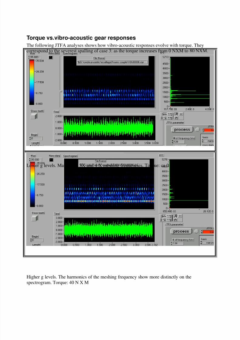
Torque vs.vibro-acoustic gear responses

The following JTFA analyses shows how vibro-acoustic responses evolve with torque. They

correspond to the severest spalling of case 3: as the torque increases from 0 NXM to 80 NXM.

Lower g levels. Mainly 2X 3X and 4 X meshing frequencies. Torque: ca 0 N X M.

Higher g levels. The harmonics of the meshing frequency show more distinctly on the

spectrogram. Torque: 40 N X M



A further increase of torque to 80 N X M does not significantly increase the acceleration levels.

One also observes this type of behavior on the responses of damaged rolling-element bearings

where an increase of the load does not substantially increase levels of acceleration. It seems,

however that there is a shift in the excited frequencies in this particular case.



Rotational frequencies vs. vibro-acoustic responses of gears.

At 600 rpm severest spalling (case 3). Mostly 2X meshing frequency in spectrogram. Meshing

frequency hardly present.

Increasing the rpm increases the g levels and modifies the spectrogram patterns where again the

second harmonic of the meshing frequency dominates but the fundamental is now visible.

Increasing the speed even further would further excite the fundamental. This may be due to the

resonances of the casing on which one mounts the accelerometer.

The above results illustrate that a mere frequency analysis without spectrogram does not help

much in diagnosing faulty gear trains. At times one may miss the meshing frequency, notbecause there is no source of excitation at this frequency, but simply because one measures the

consequences of the excitation at points where resonances may distort the frequency contents.Therefore, spectrograms may better point to gear malfunctions.



Gathering accelerometer signatures in gear trains throughsynchronous sampling

In all the previous analyses, one relies on a single top/rev triggering when on optical strip

(keyway) passes in front of a Hamamatsu infrared photocell. This TTL pulse triggers the start of

the data acquisition. It also connects to the GATE of the MIO data acquisition card to obtain thesuccessive arrival times. Buffered acquisition of the accelerometer responses and these arrivaltime simultaneously start and execute concurrently.

In the front panel, one notices that one requires 1024 samples/rev (It could be any number and issimply the result of some unfounded habit of selecting a power of 2 for the number of samples.

Better would to select a multiple of the number of teeth, here m times 41, m any integer

compatible with the card capabilities).Synchronous sampling then consists of decimating the oversampled data after the buffered

acquisitions (response + arrival times) have elapsed to distribute samples evenly at a rate of 1024

samples/rev for each rev, no matter what the rotating speed may be. This is possible when one

knows the fixed data acquisition oversampling rate rs and the arrival times of the triggers

obtained with the counters fed with the MIO 20 MHz internal clock. Decimation steps is notequal over one rev since rs is generally not a multiple of 1024. To this aim special vi's have been

developed ( [email protected] ).

Such a basic synchronous sampling will do for such applications as vector monitoring of shaft

vibrations because the basic periodicity of vibrations is the shaft revolution. It is partially valid

for analyzing gear signatures.For one thing, this type of data acquisition converts frequency spectra and spectrograms into

order tracking tools. So, when one displays frequencies in Hertz in the above analyses, one

notices that the full frequency range somewhat vary because of minute rotational variations. The

full scale should be expressed in order ratio and then would be fixed at 512 in these cases. This

particular synchronous sampling suppresses frequency modulations in spectrograms which one

often mentions when using them with fixed sampling rate instead of synchronous sampling.It is clearly not enough to analyze vibro-acoustic responses of gear trains, as shown in the

following analyses for the most severe fault (case 6, profiles on both pinions damaged). Thereason is simple: the periodicity of the signatures is not the revolution of either pinion, but the

time it takes to sweep over all combinations of meshing profiles. We'll see later that the periodstarts at a precise instant when two given profiles belonging each to one of the pinion reach a

precise stage of their meshing. That prompted the design of a special data acquisition scheme.



Three successive JTFA analyses of gear train with damaged profiles on both

pinions

Damaged profile pair meshing (white circle) and joint pinion eccentricities and/or helix error at 5times meshing frequency (white arrow)

Same pattern, but shifted in time.



Again similar time-shifted pattern. Sharper signal at the meshing frequency (white circle)



Synchronous sampling for vibro-acoustic gear responses

What does this all tell?

First, the faulty mesh jumps from one position to another one during successive data acquisition.

This is fair enough since the start of the data acquisition is not properly indexed for a pair of pinions and only relies on a single index linked to the 41 teeth pinion.

Second, the faulty mesh does not always show with the same intensity on all spectrograms.

How can one correct this situation in the least obtrusive way in an industrial environment?

• The solution must ensure that the data acquisition starts when two given profiles each

belonging to one pinion mesh.

• The data acquisition must start at precisely the same stage of meshing.

• The data acquisition must encompass all meshing combinations. In other words, it often

corresponds to a number of revs of the larger pinions equal to the number of teeth of the

smaller one. Incidentally, this results in rather long buffers and, therefore, the use of huge

amounts of memory when carrying out JTFA. Fortunately, the advent of inexpensive

RAMs and the PII caches and mother boards accommodating up to 1 Gbyte RAM solvesa problem that hitherto confined JTFA of this style to more powerful computers than

PCs. A good hint when using Labview in this context: if your computer starts swapping,

then select for the vi the Preference 'De-allocate memory as soon as possible".

Then one can period average the successive data acquisition with enough phase-lock precision to

increase the signal-to-noise ratio. This will reinforce the part of the signature that is due to gear

vibro-acoustic responses and progressively attenuate the contribution of asynchronous sources.

Of course, the contributions of the sources that are synchronous with the pinion revs to the

accelerometer responses do not dwindle in the process, like unbalances, eccentricities, helix

errors and the like.One could mount specially designed incremental encoders on one pinion whose pulse train acts

like an external clock driving the data acquisition rate of the data acquisition card. The National

MIO cards, like many others, allow for this. This is much to ask to retrofit such an encoder on an

existing gear drive when performing field diagnoses. This is not even enough, since this does not

solve the problem of starting the data acquisition exactly when a given pair profiles mesh and a

precise stage of meshing. This would require an extremely fine resolution from the encoder to

adapt to each gear ratio.

One opts for another far easier way for field diagnosis, as next shown. The software was

designed by Pierre Fontana ( [email protected] )



Using two phase references

Up to now one relied only upon photocell 1 to phase-lock the data acquisition. From now on, oneuses both photocells 1 and 2 to phase-lock the data acquisition. In the test rig the pinion that

rotate the fastest is pinion 2. Since the reflecting strips have the same width on the shaft of both

pinions, strip 2 will generate a shorter pulse when passing in front of photocell 2 than strip 1 for

photocell 1.

The idea was at first to trigger the data acquisition when both pulses overlap by using a simple

AND TTL gate whose output is directed to the TRIGGER 0 input of a MIO card.. This would

bring us close to start the acquisition of the responses for a given pair of profiles belonging to

both pinions. The following simulations that this was not enough



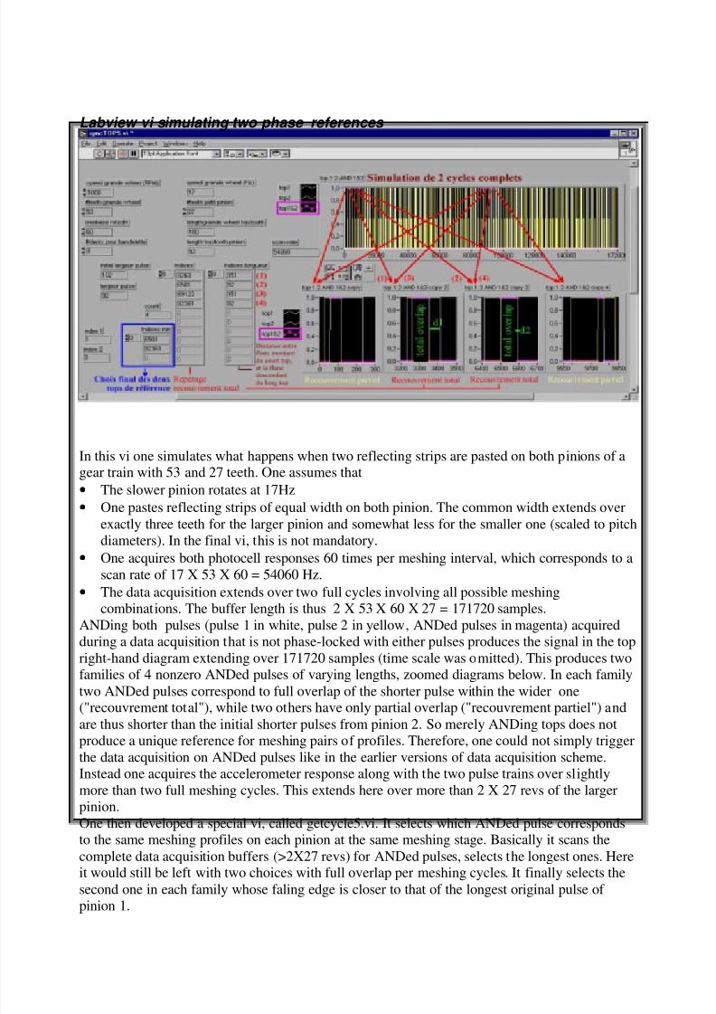
Labview vi simulating two phase references

In this vi one simulates what happens when two reflecting strips are pasted on both pinions of agear train with 53 and 27 teeth. One assumes that

• The slower pinion rotates at 17Hz

• One pastes reflecting strips of equal width on both pinion. The common width extends over

exactly three teeth for the larger pinion and somewhat less for the smaller one (scaled to pitch

diameters). In the final vi, this is not mandatory.

• One acquires both photocell responses 60 times per meshing interval, which corresponds to a

scan rate of 17 X 53 X 60 = 54060 Hz.

• The data acquisition extends over two full cycles involving all possible meshing

combinations. The buffer length is thus 2 X 53 X 60 X 27 = 171720 samples.

ANDing both pulses (pulse 1 in white, pulse 2 in yellow, ANDed pulses in magenta) acquired

during a data acquisition that is not phase-locked with either pulses produces the signal in the top

right-hand diagram extending over 171720 samples (time scale was omitted). This produces two

families of 4 nonzero ANDed pulses of varying lengths, zoomed diagrams below. In each family

two ANDed pulses correspond to full overlap of the shorter pulse within the wider one

("recouvrement total"), while two others have only partial overlap ("recouvrement partiel") andare thus shorter than the initial shorter pulses from pinion 2. So merely ANDing tops does not

produce a unique reference for meshing pairs of profiles. Therefore, one could not simply trigger

the data acquisition on ANDed pulses like in the earlier versions of data acquisition scheme.

Instead one acquires the accelerometer response along with the two pulse trains over slightly

more than two full meshing cycles. This extends here over more than 2 X 27 revs of the larger

pinion.

One then developed a special vi, called getcycle5.vi. It selects which ANDed pulse corresponds

to the same meshing profiles on each pinion at the same meshing stage. Basically it scans the

complete data acquisition buffers (>2X27 revs) for ANDed pulses, selects the longest ones. Hereit would still be left with two choices with full overlap per meshing cycles. It finally selects the

second one in each family whose faling edge is closer to that of the longest original pulse of pinion 1.



Experimental Results

Constant rotational speed

How does getcycle5.vi select the start of a meshing cycle from the data acquisition buffer

extending roughly over two meshing cycles? Meshing cycles correspond to 2 X n2 revolution of

the larger pinion 1, where n2 is the number of teeth of the smaller pinion. Evidently, the

rotational speed of the larger pinion is measured first. Then one selects an appropriate scan rateto acquire both pulses along with the response and finally a buffer length to cover at least two

full meshing cycles.At the end of the acquisition, getcycles5.vi performs the following tasks:

1. It searches the ANDed pulses and cluster them in families of roughly equal lengths. Here it

finds six such pulses.

2. Lengths of the pulses in ticks of data acquisition (scan rate)

3. It scales these lengths to the length of the current longest pulse contributing to the overlap.

4. It holds the position of the rising edges of the ANDed pulses in the data acquisition buffers.

Note that rising edges indices show that these six pulses split into two separate groups each

belonging to distinct meshing cycles separated by a larger index jump.5. It then computes the relative distance d between the falling edge of the ANDed pulse to the

falling edge of the current longest pulse contributing to the ANDed pulse. It finally selectsthe start and end of the meshing cycle, based upon the shortest distance.

6. It uses these indices to extract the full meshing cycle from the acquisition buffer of the

accelerometer responses.



Variable speed

What happens when the gearbox accelerates during the data acquisition?

At first one selected the buffer lengths for data acquisition upon the initial rotational speed. It

may happen that one gathers three instead of two cycles.

For the acceleration of this experiment with the same gear train and reflecting strips, one end up

with a total of nine instead of sic "largest" ANDed pulses. Their absolute lengths in sacn rateticks constantly decrease with the ever increasing rotational speed (2). Scaled to the current

largest pulse contributing to the ANDed pulse, lengths no longer vary (3). Then one proceeds in

the same way as for constant speed. The minimum distance criterion between falling edges of

ANDed pulse to the current longest pulse ends prefers to extract the 3rd cycle as most

representative (5).

With this type of vernier-like selection of meshing cycles, one reaches a very accurate

positioning of meshing cycles. This turns out to be quite valuable when performing JTFA

analyses of gear train vibro-acoustic responses. Labview tremendously helped prototyping such a

scheme.



JTFA analysis of period averaged vibro-acoustic responses of a gearbox with spur gears.

JTFA produces a wealth of information about all what the different "talkers" chatting over the

accelerometer responses. It is outstanding in identify the signatures of all sound sources, and alsoother sources like undesired common mode.

In order to ease the interpretation, one surely wishes to silence sources that are not related to the

gearbox. Period averaging based upon the above scheme allows to zoom upon individual

meshing cycles and then adding them to produce a response that attenuate all sources that do not

"talk" synchronously with the each individual profile meshes.

The following JTFA analyses for a 53:27 5mm module spur gear box make this point clear. They

compare what the JTFA obtained from a period-averaged response (10 responses) with theJTFAs based on two individual responses contributing to this average.

JTFA of vibro-acoustic response of a 53:27 spur gear train. Time response exhibits a dominant

common mode. Using frequency scrollbar, one hides it from the DFT amplitude spectrum andspectrogram. The 547 Hzmeshing frequency is then dominant.

• Some background information on JTFA

• A closer look at JTFA for gear failures (case 6 severe wear)

• Links with uncertainty principle in physics

Gear Overview

Documents

Transcript of Gear Overview