Accepted Manuscript

Gaussian Process Models for Reference ET Estimation from Alternative Mete-orological Data Sources

Daniel Holman, Mohan Sridharan, Prasanna Gowda, Dana Porter, ThomasMarek, Terry Howell, Jerry Moorhead

PII: S0022-1694(14)00355-2DOI: http://dx.doi.org/10.1016/j.jhydrol.2014.05.001Reference: HYDROL 19600

To appear in: Journal of Hydrology

Received Date: 12 October 2012Revised Date: 31 October 2013Accepted Date: 1 May 2014

Please cite this article as: Holman, D., Sridharan, M., Gowda, P., Porter, D., Marek, T., Howell, T., Moorhead, J.,Gaussian Process Models for Reference ET Estimation from Alternative Meteorological Data Sources, Journal ofHydrology (2014), doi: http://dx.doi.org/10.1016/j.jhydrol.2014.05.001

This is a PDF file of an unedited manuscript that has been accepted for publication. As a service to our customerswe are providing this early version of the manuscript. The manuscript will undergo copyediting, typesetting, andreview of the resulting proof before it is published in its final form. Please note that during the production processerrors may be discovered which could affect the content, and all legal disclaimers that apply to the journal pertain.

Gaussian Process Models for Reference ET Estimation1

from Alternative Meteorological Data Sources2

Daniel Holmana,1,∗, Mohan Sridharanb, Prasanna Gowdac, Dana Porterd,b,3

Thomas Mareke, Terry Howellc, Jerry Moorheadc4

aTexas A&M AgriLife Research, Lubbock, TX 79403, USA5

bTexas Tech University, Lubbock, TX 79409, USA6

cUnited States Department of Agriculture - Agricultural Research Service, Bushland, TX7

79012, USA8

dTexas A&M AgriLife Extension Service, Lubbock, TX 79403, USA9

eTexas A&M AgriLife Research, Amarillo, TX 79106, USA10

Abstract11

Accurate estimates of daily crop evapotranspiration (ET) are needed for ef-

ficient irrigation management, especially in arid and semi-arid regions where

crop water demand exceeds rainfall. Daily grass or alfalfa reference ET val-

ues and crop coefficients are widely used to estimate crop water demand.

Inaccurate reference ET estimates can hence have a tremendous impact on

irrigation costs and the demands on U.S. freshwater resources, particularly

within the Ogallala aquifer region. ET networks calculate reference ET using

local meteorological data. With gaps in spatial coverage of existing networks

and the agriculture-based Texas High Plains ET (TXHPET) network in jeop-

ardy due to lack of funding, there is an immediate need for alternative sources

capable of filling data gaps without high maintenance and field-based sup-

port costs. Non-agricultural weather stations located throughout the Texas

High Plains are providing publicly accessible meteorological data. However,

there are concerns that the data may not be suitable for estimating reference

∗Corresponding author. Phone: 806-746-6101 Fax: 806-746-6528Email address: deholman@ag.tamu.edu (Daniel Holman)

Preprint submitted to Journal of Hydrology May 7, 2014

ET due to factors such as weather station siting, fetch requirements, data

formats, parameters recorded, and quality control issues. The goal of the

research reported in this paper is to assess the use of alternative data sources

for reference ET computation. Towards this objective, we train Gaussian

process models, an instance of kernel-based machine learning algorithms, on

data collected from weather stations to estimate reference ET values and

augment the TXHPET database. We show that Gaussian process models

provide much greater accuracy than baseline least square regression models.

Keywords: supervised learning, advanced regression, evapotranspiration,12

Texas High Plains ET Network13

1. Introduction14

Accurate estimates of daily crop evapotranspiration (ET) are valuable15

for irrigation management within arid, semi-arid, and semi-humid regions16

where crop water demand exceeds rainfall. Daily grass/alfalfa reference ET17

(ETo) values are widely used in conjunction with crop coefficients (Kc) to18

estimate crop water demand. Hence, the impact of inaccurate ET estimates19

can hardly be overstated given the increased demands on U.S. freshwater re-20

sources, especially within the central Great Plains underlain by the vast but21

declining Ogallala groundwater aquifer. Reference ET can be estimated using22

the FAO-56 [1] or the recent ASCE Standardized Reference ET Equation [2].23

Areal coverage of ET networks is not universal and there are significant gaps24

in the spatial coverage. It is further complicated by high spatial variation in25

air temperature, wind speed, wind direction and other weather parameters26

due to regional effects such as atmospheric circulation patterns [6, 16] and27

2

local effects such as topography [10], land use [18], elevation [9] and soil prop-28

erties [19]. It is therefore difficult to use one predetermined weather station29

for determining daily reference ET for irrigation management over large re-30

gions. A sufficiently dense network of weather stations can effectively capture31

the spatial variability of parameters for use in computing reference ET. How-32

ever, funding and staffing issues are ongoing concerns of many ET networks,33

making it difficult to expand coverage through additional weather stations.34

Although remote sensing based ET estimates are showing promise of expand-35

ing areal coverage and integration capabilities, accuracy of these methods is36

dependent on accuracy of input (i.e., weather data and/or reference ET).37

There is hence an immediate need for exploring alternative data sources ca-38

pable of filling data gaps without high maintenance and field-based support39

costs. Fortunately, there are other (non-agricultural, non-ET) weather sta-40

tions and data networks, and some of these networks make data publicly41

accessible. However, there are concerns that the data may not be appropri-42

ate for estimating reference ET due to factors such as weather station siting,43

data formats, parameters recorded, and data quality control issues.44

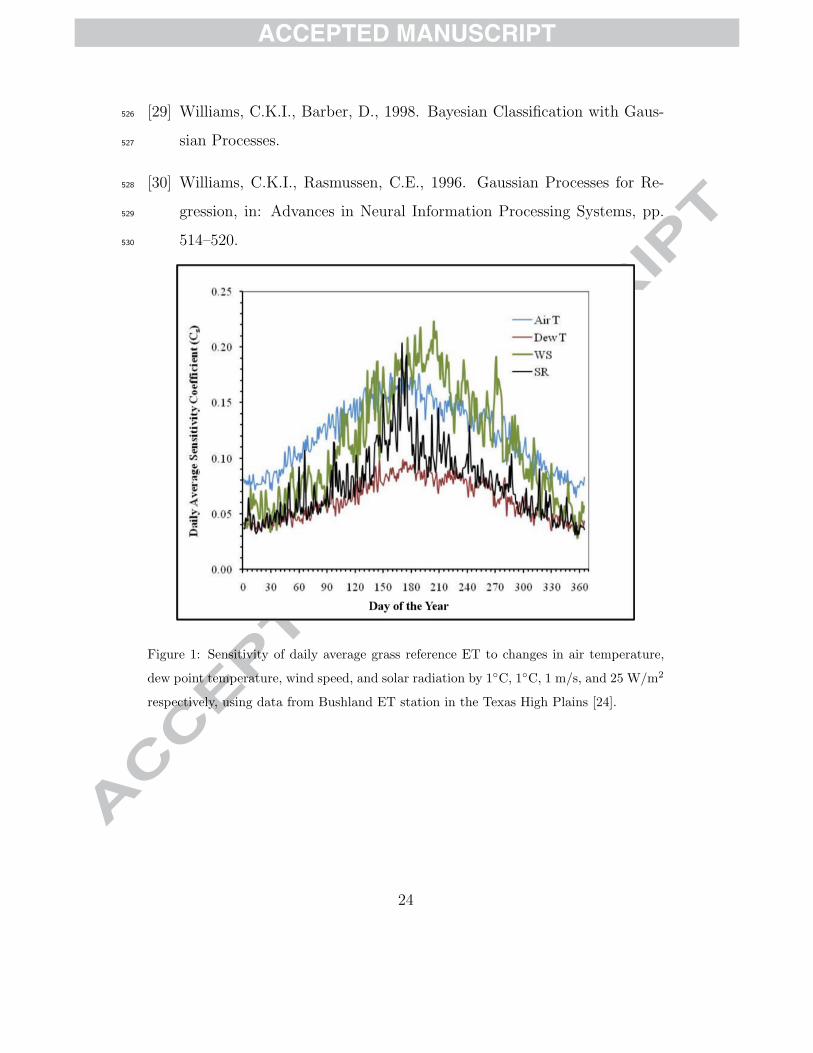
Figure 1 from an article by Porter et al. [24] illustrates the sensitivity of45

average daily grass reference ET to changes in air temperature, dew temper-46

ature, wind speed and solar radiation by 1◦C, 1◦C, 1 m s−1 and 25 W m−247

respectively, using the representative Bushland ET station in the Texas High48

Plains. The authors reported that grass reference ET calculations were most49

sensitive to errors in wind speed and air temperature, and that sensitivity50

was greater during the mid-summer growing season when greater accuracy51

levels are required for irrigation scheduling. For example, a 1◦C error in air52

3

temperature throughout the growing season in the Texas High Plains would53

yield ≈ 25 mm error in the total grass reference ET for the typical corn54

growing season. The cumulative effect of this error over the irrigated corn55

acreage within the Texas High Plains is approximately equivalent to the total56

drinking water consumption by the City of Houston for about 22 days [20].57

Erroneous selection of reference weather station and/or wrong values of ref-58

erence ET rates can thus affect the water use efficiency and producers’ net59

profits, in addition to the loss of mined water of the Ogallala aquifer. This60

illustrative example demonstrates the need for accurate reference ET data61

for irrigation scheduling and irrigation management.62

Most statistical models reported in the literature on irrigation manage-63

ment are based on ordinary least square regression. Popular models used64

in regression include: (1) linear; y = c + bx; (2) exponential; y = aebx;65

(3) power or logarithmic; y = axb; and (4) a quadratic polynomial; y =66

ax2 + bx + c. In these models, y represents the desired output vector (e.g.,67

reference ET values from ET stations) and x is a vector representing input68

values such as rainfall, irrigation amount, weather parameters or reference69

ET estimated at non-agricultural weather stations. Values of coefficients70

a, b (vectors with the same dimension as x) and c are tuned on training71

data such that the computed values of output are as close as possible to the72

given (i.e., known ground truth) output values. The ordinary least squares73

regression formulations tend to fix the basis functions before observing the74

training data, and the number of basis functions grows exponentially with75

the dimensions of input space. Furthermore, the basis functions are not76

adaptable to data and the associated curse of dimensionality makes a strong77

4

case for the use of more sophisticated models [5]. In recent years, numer-78

ous statistical learning algorithms are being developed and used for inference79

and prediction. Examples of such methods include artificial neural network80

(ANN) [3, 4, 7, 8, 14], support vector machine [28] and Gaussian Process81

(GP) models [30]. These methods provide substantial benefits over linear82

(or other) regression models. For instance, ANNs readily adapt to data and83

can be used to model complex functions between input and output param-84

eters. Although different algorithms can be used to learn ANNs based on a85

compromise between computational cost and performance, the most popular86

choice is the back propagation algorithm [26]. However, ANN formulations87

can result in local minima, lead to over-fitting, and become computationally88

expensive in high-dimensional spaces. Further, it is also not easy to extract89

an understandable interpretation of the functions learned.90

Support vector machines (SVMs) have a simple geometric interpreta-91

tion, avoid overfitting and find global solutions. They project input features92

to high dimensions, resulting in sparse representations and robust decision93

boundaries. However, SVMs (and other similar algorithms) require that the94

parametric function that models the relationship between inputs and outputs95

be defined in advance—choosing an appropriate function from the infinite96

space of functions may be difficult in complex problem domains. Gaussian97

Process is a non-parametric kernel-based machine learning algorithm. GP98

models are well-suited for the estimation step of our study and they cap-99

ture the temporal evolution of normally-distributed random variables that100

represent the patterns being tracked. They have been successfully used for101

large-scale estimation problems with high-dimensional features, e.g., nuclear102

5

disasters, climate modeling and sensor placement for surveillance [13, 15, 17].103

To the best of our knowledge, only a few applications of GP models have been104

found in the research field of water resources management, including ground105

water transport [21] and hydrological modeling [27].106

The objective of the study reported in this paper is to identify, evaluate107

and use alternative meteorological data sources for accurately computing108

reference ET values, resulting in efficient irrigation management and water109

resources planning. We trained GP models to estimate reference ET values110

using data from non-ET National Weather Service (NWS) stations. Although111

our study focused on the Texas High Plains, the experimental methodology112

can be used for estimating reference ET from non-agricultural and non-ET113

weather stations elsewhere in the U.S. and the world.114

The remainder of the paper is organized as follows. Section 2 describes115

the geographic locations included in our study, while Section 3 presents an116

overview of the various steps involved in the study. Next, Gaussian processes117

and the underlying mathematical concepts are described in Section 4. The118

experimental setup and results are discussed in Sections 5 and 6 respectively,119

followed by the conclusions in Section 7.120

2. Study Area121

This study covers a 39-county area of the Texas High Plains, as shown122

in Figure 2. Most of this region is semi-arid with highly variable precipi-123

tation (both temporally and spatially), averaging 400 − 560 mm from west124

to east. Most rainfall occurs in scattered thunderstorms—some areas may125

receive 50− 100 mm of daily precipitation while areas a short distance away126

6

may not receive any rainfall. In 2010, the Lubbock weather station recorded127

a total of 672 mm of annual rainfall, while in 2011 the station only recorded128

149 mm. This region is also known to have high evaporative demand (ap-129

proximately 2500 mm/year Class A pan evaporation) due to high solar radi-130

ation, high vapor pressure deficit (VPD), and strong regional advection. The131

grass reference ET data from 15 weather stations managed by the TXHPET132

network [25] (Figure 1) were used to train and evaluate GP models that es-133

timate reference ET values based on meteorological data from non-ET NWS134

stations.135

3. Materials and Methods136

This study was implemented in four steps: (1) identify publicly accessible137

data sources and evaluate whether they provide sufficient data parameters,138

detail and quality for use in computing daily reference ET; (2) determine139

whether missing data can be estimated using other available data, trends and140

associative models and calculate the daily reference ET; (3) assess and vali-141

date the quality of reference ET values determined from these data sources142

compared with valid ET network data sources; and (4) develop and evaluate143

models based on statistical learning methods to calculate reference ET given144

data from non-agricultural, non-ET weather stations or networks. In the re-145

mainder of the paper, we refer to non-agricultural, non-ET weather stations146

as “non-ET stations”.147

The first step involved a thorough assessment of all the weather networks148

in the Texas High Plains for estimating daily reference ET. Selection criteria149

include: (a) timely and real-time availability of data to the public at no cost;150

7

(b) length and continuity of historic records; (c) availability of measurements151

of parameters needed for estimating reference ET; and (d) ability to accu-152

rately estimate parameters that are missing or not measured. Once suitable153

non-ET stations were identified, a map showing the location of these sta-154

tions was used to create a Thiessen polygon map, which (in turn) was used155

to pair these stations with selected agricultural weather stations of the TXH-156

PET network (i.e., the “ET stations”) for model development and evaluation.157

The weather parameters considered include: daily maximum and minimum158

air temperatures, average dew point temperature, average wind speed, aver-159

age relative humidity, barometric measure and solar radiation.160

The second step involved computing missing data using equations pro-161

vided in the 2005 Standardized reference ET methodology [2]. For instance, if162

the solar radiation values were not measured or missing for a non-ET station,163

they were estimated using the complex method equation provided below:164

Rs = λRs

√(Tmax − Tmin)Ra (1)

where Tmax and Tmin are daily maximum and minimum air temperatures,165

Ra is extraterrestrial radiation, λRs is an empirical coefficient for semi-arid166

climates, and Rs is solar radiation. Barometric pressure is calculated using167

the elevation of the corresponding weather station. If the missing data cannot168

be estimated (e.g. wind speed) for a given day, then the data records for169

that day were removed. After verifying the weather dataset and filling the170

missing data, unit conversions of the weather parameters were performed (as171

necessary) to estimate daily reference ET using the ASCE Standardized ET172

equation-based Bushland Reference ET Calculator [11].173

In the third step, statistical relationships were computed between daily174

8

reference ET estimates obtained from the ET stations and the corresponding175

non-ET stations to assess feasibility of using alternative data sources to ex-176

pand (or increase data intensity within) the coverage area of the Texas High177

Plains ET network. Coefficient of determination (R2), slope and intercept178

of the regression line, Nash-Sutcliffe efficiency (NSE) and root mean square179

error (RMSE) were used to compare the reference ET values obtained from180

the ET stations and those obtained from the corresponding non-ET stations.181

The value of R2 describes the proportion of variability in the observed data182

that is explained by the model—R2 ranges from 0 to 1, with a higher value183

indicating a better goodness of fit (model explanation). For instance, R2 = 1184

with an intercept of 0 and slope of 1 indicates a perfect fit between the ob-185

served and modeled data. The NSE is a common efficiency measure that186

compares variance in estimations with the measured data variance. NSE187

ranges between − inf and 1—values closer to 1 are more accurate and an188

NSE of 1 represents an optimal model. Negative NSE values indicate that189

the mean of the observations is more accurate than the model estimation.190

An RMSE of 0 also indicates a perfect fit—it is usually computed as a %191

of the observed mean, e.g., RMSE < 50% is usually considered low. The192

RMSE measure is appropriate for our study because it provides values in the193

same units as the values that are to be estimated (i.e., reference ET). More194

information on performance statistics can be found in Moriasi et al. [22].195

In the fourth step, the Gaussian Process models were trained and evalu-196

ated. These models capture the relationship between the meteorological data197

from non-ET stations and the corresponding reference ET values from the198

ET stations. The trained models can then be used to estimate reference ET199

9

values given new data from the non-ET stations. For evaluating the estima-200

tion ability of GP models, the daily reference ET database was divided into201

two parts. Data corresponding to odd-numbered days of the year were used202

for model development and data from even-numbered days of the year were203

used for validation. Performance statistics (R2, NSE and RMSE) were used204

to evaluate and compare the estimation capabilities of the GP models with205

(baseline) linear regression (LR) models.206

4. Gaussian Processes207

Gaussian processes are sophisticated supervised learning models used for208

regression [30] and classification [29]. Supervised learning approaches infer a209

hypothesis function h(x) based on training data. Training data consists of210

a set of N vectors consisting of inputs: X = {x1, ...,xN} and corresponding211

target outputs: T = {t1, ..., tN}, to generate input-output pairs: {(xi, ti), i =212

1...N}. The supervised learner uses the training data to learn a model that213

approximates h. To evaluate the learned model’s estimation ability, a testing214

dataset consisting of previously unseen inputs and target outputs is defined:215

{(xi, ti), i = 1...N}. The learned model processes input vectors of the testing216

dataset to estimate outputs: y(x), which are compared with ground truth217

(i.e., actual) target outputs. Various statistical error measures can hence be218

used to compute the accuracy of values estimated by the learned model.219

For non-linear regression problems, the unknown function y(x) exists in220

the infinite-dimensional space of possible functions for x, making it difficult221

to decide the range of possible non-linear functions. Standard parametric222

models such as ANNs, linear regression and polynomial regression require223

10

that y(x) have an explicitly defined functional form whose parameters are224

defined in advance—the values of parameters are assigned by learning weights225

W. Choosing this function from the infinite space of function types and226

weights can be a challenge. Gaussian processes address this issue by placing227

a prior P (y(x)) over the space of functions. GP models thus do not need228

an explicit parametric definition of the function y(x), i.e., they are non-229

parametric. Instead, (stochastic) random variables define priors for each230

input vector. Random functions defined over the space of inputs constitute231

the GP prior, as shown in Figure 3. During the training phase, the discrete232

set of inputs are used to modify these functions to pass as close as possible to233

the target outputs, thus approximating the (unknown) underlying function.234

Gaussian processes can be viewed as a natural generalization of a Gaussian235

distribution over a finite vector space to an infinite space of functions. Just as236

a Gaussian distribution is defined by its mean vector and covariance matrix,237

a GP is defined by its mean and covariance functions µ(x) and C(x, x′):238

f ∼ GP (µ(x), C(x,x′)) (2)

where the function f is distributed as a Gaussian process with mean function239

µ(x) and covariance function C(x,x′). In our research, we define the mean240

function as the zero function. The covariance function expresses the expected241

covariance of the values at each pair of points x and x′. Given N input vectors242

in the training data, the covariance function is a N × N covariance matrix243

K : Kij = C(xi,xj). This matrix can be used to estimate output values for244

new inputs. In general, the estimated distribution is Gaussian with mean245

and covariance:246

11

y = kT (x)K−1t (3)

σ2y(x) = C(x,x) − kT (x)K−1k(x)

where x is a new input vector, x(1), ..., x(N) are the training data input247

vectors, k(x) = (C(x,x(1)), ..., C(x,x(N)))T denotes the matrix of covariances248

between the input and training data, K is the covariance matrix for training249

data, and t = (t(1), ..., t(N))T . This algorithm has O(N3) time complexity due250

to the matrix inversion in Equation 3. GP formulations can hence become251

infeasible for data with a large number of samples. Algorithms are being252

developed to enable GP formulations of domains with large datasets [5].253

However, our experiments consist of a few thousand training samples per254

weather station and the time complexity is (currently) not an issue.255

Many different options exist for selecting covariance functions for a Gaus-256

sian process. The main requirement is that the function should generate a257

non-negative definite covariance matrix for any set of inputs (x(1), ...,x(n)).258

Graphically, the goal is to define covariances such that points that are nearby259

in the input space produce similar output estimates. In the research reported260

in this paper, we chose the popular radial basis function (RBF) kernels [23]:261

C(x,x′) = e−γ∗(x−x′)2 (4)

The key advantage of using a non-parametric model such as GP is that262

it does not require any manual parameter tuning. Instead, the covariance263

function contains hyperparameters that are tuned automatically to maximize264

the likelihood of training data. Equation 4 contains a single hyperparameter265

γ. Assigning different values to the hyperparameter results in different GP266

12

models. We randomly initialize a finite set of hyperparameters over the267

space of possible hyperparameter values and compute the estimation error268

of the corresponding GP models on the training data. This training error is269

computed by building a GP model using the training data, and comparing the270

output values estimated by the GP model for the training data inputs with271

the actual outputs included in the training data. The hyperparameter value272

that results in the lowest error, or equivalently the highest accuracy, is chosen273

for subsequent experimental studies. Section 5 illustrates this approach to274

compute a suitable value for the hyperparameter.275

5. Experimental Setup276

The experiments performed for this project were implemented using the277

WEKA open source machine-learning library [12]. WEKA includes Java278

implementations of popular machine-learning algorithms such as GP, SVM,279

linear regression and multi-layer perceptron (ANN). The library also has280

evaluation schemes that can be used to compare performance of different281

algorithms over different datasets. We adapted the existing implementation282

of GP to fit our needs. Our application first reads in the training data and283

trains different GP models corresponding to different values of the hyper-284

parameter (γ). As described in Section 4, γ is selected based on the GP285

model that results in the lowest RMSE between the estimated reference ET286

and actual TXHPET reference ET over the training data. This GP model is287

chosen for further use as it is the most accurate model. The RMSE statistic288

was used because it represents the actual difference in ET in mm. Figure 4289

illustrates this approach to compute the value of γ for the data obtained290

13

from the paired non-ET station and TXHPET station in Lubbock. A linear291

regression (LR) model was also learned from the same training data to serve292

as a baseline for comparison. The estimation accuracy of learned GP models293

was then compared with the estimation accuracy of LR models on separate294

test data for each non-ET station. For instance, Figure 4 also shows that295

the GP models result in significantly lower RMSE in comparison with the296

LR models. It is also possible to automatically select the best value of γ by297

computing error measures over a separate validation set [5].298

To ensure accurate estimates from the learned models, the test data must299

be drawn from the same space as the training data, i.e., the probability dis-300

tributions underlying the datasets must be equivalent. Consider the Lubbock301

datasets over the years 2001 − 2010, and consider the data division scheme302

that uses data from 2001 − 2005 as the training set and data correspond303

to years 2006 − 2010 as the test set. Such a data division scheme will not304

work because the wet and dry years are typically inconsistent—the models305

trained with data corresponding to dry years will result in high errors on306

data corresponding to wet years. We therefore split the data evenly across307

all years by using odd days for training and even days for testing. Although308

such a division of data into training set and testing set makes it difficult to309

run a standard cross-validation analysis, we repeated the experiments after310

swapping the training and test datasets. Overall, we conducted experimental311

trials using data from 15 non-ET (i.e., NWS) weather stations matched with312

the TXHPET stations determined by the Thiessen polygon (Figure 2). We313

used data consisting of daily measurements over a period of 10 years.314

Experimental trials were divided into two groups based on the inputs used315

14

to train GP models. In the first set of experiments, reference ET values were316

computed from non-ET station weather parameters (see Section 3) and used317

as inputs to GP models—each input is thus a single value. The corresponding318

GP models capture the relationship between these reference ET values from319

non-ET stations and the corresponding reference ET values from the paired320

TXHPET station. In the second set of experiments, weather parameters from321

non-ET stations were used as inputs to the GP models—each input is thus a322

vector of weather parameter values. The target outputs were the TXHPET323

reference ET values. We hypothesized that GP models trained in the second324

set of experiments would provide more accurate estimates because they can325

model and account for the uncertainty in computing reference ET from the326

unreliable observations of weather parameters at non-ET stations.327

For each station, the GP model was trained using training data (half the328

values from the total number of years for each station) and various values329

for the hyperparameter γ. Once a suitable GP model is selected for further330

use (as described above), error statistics are computed using the reference331

ET estimates provided by this trained model over the test set and the actual332

reference ET values from the paired TXHPET station(s). Measures used for333

comparison include R2, NSE, and RMSE.334

6. Experimental Results335

Figure 5 summarizes the estimation capabilities of the linear regression336

and Gaussian process models using the R2 measure. Models that provide337

highly accurate estimates will result in points that lie on (or very close to)338

the Y = X line. Figure 5(a) and Figure 5(b) show results (for Lubbock339

15

non-ET and TXHPET stations) with LR models and GP models (respec-340

tively) that used the reference ET computed from non-ET station as inputs.341

Similarly, Figure 5(c) and Figure 5(d) show results with LR models and GP342

models (respectively) that used the weather parameters recorded at the non-343

ET station as inputs. We observed that the estimates were more accurate344

when the weather parameters were used as inputs instead of the reference345

ET computed at the non-ET stations. This observation was true for both346

LR and GP models, and similar plots were obtained for other stations in-347

cluded in the experimental trials. As hypothesized in Section 5, using the348

weather parameters as inputs enables the learned models to account for the349

uncertainty in observations of weather parameters at the non-ET stations.350

In other words, the models were able to capture the correlations in the data351

more accurately. The results reported below therefore correspond to exper-352

iments in which the weather parameter measurements at non-ET stations353

were used as inputs to train and test the models.354

Another key observation based on the results in Figure 5 is that the GP355

models in Figure 5(b) and Figure 5(d) result in much greater accuracy than356

the corresponding LR models. Furthermore, the best performance (i.e., most357

accurate estimates) were obtained using GP models trained using the weather358

parameters as inputs, as shown in Figure 5(d) where most points are along359

the diagonal line. Similar results were obtained using the data from other360

stations included in the study.361

Figure 6 summarizes the results obtained on test data from 15 non-ET362

(NWS) weather stations, using RMSE as the performance measure. We363

observe that GP models provide much lower RMSE in comparison with the364

16

LR models. In other words, the reference ET values estimated by GP models365

are much closer to the reference ET values obtained from the corresponding366

TXHPET stations. This performance improvement is statistically significant367

and GP models show significant promise in enabling the use of alternative368

data sources for accurately computing reference ET values.369

Although the improvement in the accuracy of GP models (compared with370

the LR models) is different at different stations, the improvement is signif-371

icant in all stations considered in our study. Stations such as Lubbock and372

Dalhart produced highly accurate estimates: R2 = 0.98 and 0.98 respec-373

tively and NSE = 0.98 and 0.98, whereas matching the non-ET (NWS)374

station at Lubbock with the Farwell (TXHPET) station obtained R2 = 0.89,375

NSE = 0.89 and RMSE of 0.76 mm for daily reference ET values. This376

represents ≈ 29% error which is still significantly better than the LR mod-377

els that result in an RMSE of 0.84 with a relative error of 33%. Future378

research could consider additional features for input (e.g., elevation) and379

other GIS selection methods for matching non-ET stations with TXHPET380

stations. For instance, although our analysis identifies a good correlation be-381

tween the Farwell TXHPET station and the Lubbock non-ET station based382

on the Thiessen polygon map, including additional features may help identify383

stations that are strongly correlated.384

The GP models provide more accurate estimates of reference ET than385

LR models, and this improvement in accuracy has significant practical value.386

The average difference in RMSE for daily reference ET estimates provided387

by GP and LR models is ≥ 0.2 mm. For a typical cropping season of about388

200 days, this amounts to approximately 40mm or 1.5inches over the season.389

17

Although this difference may seem rather small, one acre-inch of water for390

all the fields of the Texas High Plains results in approximately 24.8 billion391

gallons of wasted water [20], which can be compared to the amount of water392

supplied to the entire city of Houston for about two and a half months!393

Table 1 summarizes the performance of the LR models and GP models at394

each non-ET station included in our study, using the performance measures395

(R2, NSE and RMSE) described in Section 3. With the GP models, each396

station’s R2 and NSE values are closer to 1 with a lower RMSE. The397

results show that GP models provide higher accuracy in estimating reference398

ET than LR models.399

7. Conclusion400

Efficient water resource management represents a pressing need in agri-401

culture. Accurate estimates of crop evapotranspiration (ET) are essential for402

irrigation management, especially in arid and semi-arid regions where crop403

water demands exceed rainfall. Existing ET stations do not provide the re-404

quired areal coverage and also face funding challenges. This paper presented405

the results of a study conducted towards our long-term goal of using data406

from non-ET stations for filling data gaps in the ET networks.407

In the context of data collected in the Texas High Plains, we described408

the use of Gaussian process models, an instance of sophisticated kernel-based409

machine learning, to estimate the daily reference ET values based on the410

corresponding data obtained from National Weather Service stations. Our411

experiments show that GP models result in significantly more accurate esti-412

mates of daily reference ET values than the (popular) linear regression mod-413

18

els. We also observe that using the daily weather parameter measurements414

from the non-ET stations as inputs (instead of the reference ET computed415

from the these measurements) results in more accurate estimates. The im-416

provement (provided by the GP models) in accurately estimating the daily417

reference ET values addresses a critical need and has significant practical418

value. Errors in reference ET estimates can translate to huge costs associ-419

ated with wasteful use of precious water resources (due to over-watering), in420

addition to crop stress and even crop loss (due to under watering).421

Although our study focused on the Texas High Plains, the models and422

experimental methodology can be adapted to regions elsewhere in the world.423

Furthermore, Gaussian process models and other similar stochastic machine424

learning algorithms are generic tools for classification and regression in high-425

dimensional input spaces, with significant potential for addressing key open426

challenges in water resources management and other sub-fields of agriculture.427

USDA EEO Disclaimer428

The U.S. Department of Agriculture (USDA) prohibits discrimination429

in all its programs and activities on the basis of race, color, national ori-430

gin, age, disability, and where applicable, sex, marital status, familial status,431

parental status, religion, sexual orientation, genetic information, political be-432

liefs, reprisal, or because all or part of an individual’s income is derived from433

any public assistance program. (Not all prohibited bases apply to all pro-434

grams.) Persons with disabilities who require alternative means for commu-435

nication of program information (Braille, large print, audiotape, etc.) should436

contact USDA’s TARGET Center at (202) 720-2600 (voice and TDD). To437

19

file a complaint of discrimination, write to USDA, Director, Office of Civil438

Rights, 1400 Independence Avenue, S.W., Washington, D.C. 20250-9410, or439

call (800) 795-3272 (voice) or (202) 720-6382 (TDD). USDA is an equal op-440

portunity provider and employer.441

8. References442

References443

[1] Allen, R.G., Pereira, L.S., Raes, D., Smith, M., 1998. Crop Evapotran-444

spiration - Guidelines for Computing Crop Water Requirements. Techni-445

cal Report 56. Food and Agriculture Organization of the United Nations.446

ROME. URL: http://www.fao.org/docrep/X0490E/X0490E00.htm.447

[2] Allen, R.G., Walter, I.A., Elliot, R., Howell, T.A., 2005. ASCE-EWRI448

Standardization of Reference Evapotranspiration. American Society of449

Civil Engineers - Environmental Water Institute.450

[3] ASCE Task Committee on Applications of Artificial Neural Networks in451

Hydrology, 2000a. Artificial Neural Networks in Hydrology I: Prelimi-452

nary Concepts. Journal of Hydrol. Eng. 5, 115–123.453

[4] ASCE Task Committee on Applications of Artificial Neural Networks in454

Hydrology, 2000b. Artificial Neural Networks in Hydrology II: Hydro-455

logic Applications. Journal of Hydrol. Eng. 5, 124–137.456

[5] Bishop, C.M., 2008. Pattern Recognition and Machine Learning.457

Springer-Verlag, New York.458

20

[6] Buishand, T.A., Brandsma, T., 1997. Comparison of Circulation Clas-459

sification Schemes for Predicting Temperature and Precipitation in the460

Netherlands. International Journal of Climatology 17, 875–889.461

[7] Buscema, M., Sacco, P., 2000. Feedforward Networks in Financial Pre-462

dictions: The Future that Modifies the Present. Expert Systems 17,463

149–169.464

[8] DeRoach, J.N., 1989. Neural Networks: An Artificial Intelligence Ap-465

proach to the Analysis of Clinical Data. Aust. Phys. Eng. Sci. Med. 12,466

100–106.467

[9] Dodson, R., Marks, D., 1997. Daily Air Temperature Interpolated at468

High Spatial Resolution Over a Large Mountainous Region. Climate469

Research 8, 1–20.470

[10] Goovaerts, P., 2000. Geostatistical Approaches for Incorporating Ele-471

vation into the Spatial Interpolation of Rainfall. Journal of Hydrology472

228, 113–129.473

[11] Gowda, P.H., Ennis, J.R., Howell, T.A., Marek, T.H., Porter, D.O.,474

2012. The ASCE Standardized Equation Based Reference ET Calcula-475

tor, in: Proceedings of the World Environmental and Water Resources476

Congress, Albuquerque, NM. pp. 2198–2205.477

[12] Hall, M., Frank, E., Holmes, G., Pfahringer, B., Reutemann, P., Wit-478

ten, I.H., . The WEKA Data Mining Software: An Update. SIGKDD479

Explorations 11.480

21

[13] Higdon, K., Lee, H., Holloman, C., 2003. Markov Chain Monte Carlo-481

based Approaches for Inference in Computationally Intensive Inverse482

Problems, in: Bayesian Statistics, Oxford University Press. pp. 000–483

000.484

[14] Hornik, K., Stinchcombe, M., White, H., 1989. Multilayer Feed Forward485

Network are Universal Approximators. Neural Networks 2, 359–366.486

[15] Kennedy, M., O’Hagan, A., 2001. Bayesian Calibration of Computer487

Models. Journal of Royal Statistical Society B 63(3), 425–464.488

[16] Knapp, P.A., 1992. Correlation of 700-mb Height Data With Seasonal489

Temperature Trends in the Great Basin (Western USA). Climate Re-490

search 2, 65–71.491

[17] Krause, A., Singh, A., Guestrin, C., 2008. Near-Optimal Sensor Place-492

ments in Gaussian Processes: Theory, Efficient Algorithms and Empir-493

ical Studies. Journal of Machine Learning Research 9, 235–284.494

[18] Li, J., Richter, D.D., Mendoza, A., Heine, P., 2010. Effects of Land Use495

History on Soil Spatial Heterogeneity of Macro- and Trace Elements in496

the Southern Piedmont USA. Geoderma 156, 60–73.497

[19] Lopez-Granados, F., M. Jurado-Exposito, J.M.P.n.B., Garcia-Torres, L.,498

2005. Using Geostatistical and Remote Sensing Approaches for Mapping499

Soil Properties. European Journal of Agronomy 23, 279–289.500

[20] Marek, T.H., Porter, D.O., Gowda, P.H., Howell, T.A., Moorhead, J.E.,501

2010. Assessment of Texas Evapotranspiration (ET) Networks.502

22

[21] Marrel, A., Iooss, B., Laurent, B., Roustant, O., 2009. Calculations of503

sobol indices for the gaussian process metamodel. Reliability Engineer-504

ing & System Safety 94, 742–751.505

[22] Moriasi, D.N., Arnold, J.G., Liew, M.W.V., Bingner, R.L., Harmel,506

R.D., Veith, T.L., 2007. Model Evaluation Guidelines for Systematic507

Quantification of Accuracy in Watershed Simulations.508

[23] Musavi, M.T., Ahmed, W., Chan, K.H., Faris, K.B., Hummels, D.M.,509

1992. On the Training of Radial Basis Function Classifiers. Neural510

Networks 5(4), 595–603.511

[24] Porter, D.O., Gowda, P.H., Marek, T.H., Howell, T.A., Moorhead, J.E.,512

Irmak, S., 2012. Sensitivity of Grass and Alfalfa Reference Evapotran-513

spiration to Weather Station Sensor Accuracy. Applied Engineering in514

Agriculture 28(4), 543–549.515

[25] Porter, D.O., Marek, T.H., Howell, T.A., 2005. The Texas High Plains516

Evapotranspiration Network (TXHPET) User Manual.517

[26] Rumelhart, D.E., Hinton, D.E., Williams, R.J., 1986. Learning Internal518

Representations by Error Propagation. MIT Press, Cambridge, MA,519

USA.520

[27] Song, X., Zhan, C., Kong, F., Xia, J., 2011. Advances in the study of521

uncertainty quantification of large-scale hydrological modeling system.522

Journal of Geographical Sciences 21, 801–819.523

[28] Vapnik, V.N., 1995. The Nature of Statistical Learning Theory.524

Springer.525

23

[29] Williams, C.K.I., Barber, D., 1998. Bayesian Classification with Gaus-526

sian Processes.527

[30] Williams, C.K.I., Rasmussen, C.E., 1996. Gaussian Processes for Re-528

gression, in: Advances in Neural Information Processing Systems, pp.529

514–520.530

Figure 1: Sensitivity of daily average grass reference ET to changes in air temperature,

dew point temperature, wind speed, and solar radiation by 1◦C, 1◦C, 1 m/s, and 25 W/m2

respectively, using data from Bushland ET station in the Texas High Plains [24].

24

New Mexico

Oklahoma

JBF

MorseEtter

Lamesa

Lubbock

Halfway

Farwell

Dimmitt

DalhartPerryton

White Deer

WellingtonWT Feedlot

Chillicothe

ARS

Midland

Lubbock

Dalhart

Amarillo

Childress

Santa Rosa, NM

Hutchinson

Witchita Falls

Perryton

Legend

TXHPET Stations

NWS Stations

Thiessen Polygon

TX State Boundary

Figure 2: Locations of 15 weather stations managed by the Texas High Plains ET network

and paired NWS stations in the Texas High Plains.

25

−5 −4 −3 −2 −1 0 1 2 3 4 5−3

−2

−1

0

1

2

3

4

Figure 3: Illustrative (general) example of a Gaussian process prior—three random func-

tions that define outputs as a function of the inputs. GP models use the input values in

the training data to incrementally revise these functions with the objective of minimizing

the error in estimating the corresponding output values.

26

0 0.1 0.2 0.3 0.4 0.5 0.6 0.7 0.8 0.9 10.35

0.4

0.45

0.5

0.55

Hyperparameter Value(Gamma)

Roo

t Mea

n Sq

uare

d Er

ror (

mm

)

Gaussian ProcessLinear Regression

Figure 4: RMSE of GP models trained using data from the paired non-ET station and

TXHPET station in Lubbock for different values of the hyperparameter (γ). GP model

with lowest RMSE can be selected automatically from training data and used to estimate

outputs for the test data. All GP models perform much better than LR models.

27

0 2 4 6 8 10 120

2

4

6

8

10

12

TXHPET Reference ET Value (mm)

Estim

ated

Ref

eren

ce E

T Va

lue

(mm

) R2=0.95

(a) LR estimates using calculated NWS ET

0 2 4 6 8 10 120

2

4

6

8

10

12

TXHPET Reference ET Value (mm)

Estim

ated

Ref

eren

ce E

T Va

lue

(mm

) R2=0.95

(b) GP estimates using calculated NWS ET

0 2 4 6 8 10 120

2

4

6

8

10

12

TXHPET Reference ET Value (mm)

Estim

ated

Ref

eren

ce E

T Va

lue

(mm

) R2=0.94

(c) LR estimates obtained using individual

weather parameters

0 2 4 6 8 10 120

2

4

6

8

10

12

TXHPET Reference ET Value (mm)

Estim

ated

Ref

eren

ce E

T Va

lue

(mm

) R2=0.98

(d) GP estimates obtained using individual

weather parameters

Figure 5: Comparison of estimation capability of GP models and LR models for the two

sets of experiments using Lubbock-NWS and Lubbock TXHPET data.

28

0

0.1

0.2

0.3

0.4

0.5

0.6

0.7

0.8

0.9

1

Amar

illo−B

ushl

and

Amar

illo−D

imm

it

Amar

illo−J

BF

Amar

illo−W

TFee

d

Chi

ldre

ss−C

hillic

othe

Chi

ldre

ss−W

ellin

gton

Dal

hart−

Dal

hart

Dal

hart−

Ette

r

Hut

chin

son−

Mor

se

Hut

chin

son−

Perry

ton

Hut

chin

son−

Whi

teD

eer

Lubb

ock−

Farw

ell

Lubb

ock−

Hal

fway

Lubb

ock−

Lam

esa

Lubb

ock−

Lubb

ock

NWS−TXHPET Stations

Roo

t Mea

n Sq

uare

d Er

ror (

mm

)

Linear RegressionGaussian Process

Figure 6: Comparison of RMSE obtained with the GP models and LR models, with the

results averaged over data from each of the non-ET stations used in the study. The GP

models result in much lower RMSE compared with LR models.

29

Table 1: Performance measures for estimates obtained from the LR models and GP models

at each non-ET station used in this study. The GP models provide higher accuracy than

LR models in estimating reference ET.

NWS - TXHPET StationLinear Regression Gaussian Process

R2 NSE RMSE(mm) R2 NSE RMSE(mm)

Amarillo - Bushland-ARS 0.90 0.89 0.80 0.95 0.95 0.60

Amarillo - Dimmit 0.90 0.88 0.80 0.92 0.92 0.68

Amarillo - Bushland-JBF 0.90 0.89 0.85 0.95 0.95 0.62

Amarillo - West Texas A&M Feedlot 0.90 0.89 0.80 0.95 0.95 0.58

Childress - Chillicothe 0.87 0.85 0.93 0.91 0.91 0.76

Childress - Wellington 0.88 0.87 0.84 0.92 0.92 0.70

Dalhart - Dalhart 0.95 0.95 0.54 0.98 0.98 0.33

Dalhart - Etter 0.92 0.90 0.74 0.95 0.94 0.59

Hutchinson - Morse 0.90 0.89 0.84 0.95 0.95 0.61

Hutchinson - Perryton 0.88 0.87 0.94 0.94 0.94 0.69

Hutchinson - White Deer 0.90 0.89 0.83 0.94 0.94 0.62

Lubbock - Farwell 0.87 0.85 0.84 0.89 0.89 0.76

Lubbock - Halfway 0.91 0.90 0.71 0.94 0.94 0.57

Lubbock - Lamesa 0.91 0.90 0.73 0.94 0.94 0.58

Lubbock - Lubbock 0.94 0.94 0.58 0.98 0.98 0.36

30

• Accurate estimates of daily ref. ET are needed for efficient irrigationmanagement.

• Climate data from non-ET stations can be used to fill ET for sparse ET-based network.

• GP models performed better than OLS regression models for daily ref.ET estimates.

1