GAUSSIAN APPROXIMATION THEOREMS FOR URN MODELS AND …
25
The Annals of Applied Probability 2002, Vol. 12, No. 4, 1149–1173 GAUSSIAN APPROXIMATION THEOREMS FOR URN MODELS AND THEIR APPLICATIONS BY Z. D. BAI , 1 FEIFANG HU 1 AND LI -XIN ZHANG 2 National University of Singapore, University of Virginia and Zhejiang University We consider weak and strong Gaussian approximations for a two-color generalized Friedman’s urn model with homogeneous and nonhomogeneous generating matrices. In particular, the functional central limit theorems and the laws of iterated logarithm are obtained. As an application, we obtain the asymptotic properties for the randomized-play-the-winner rule. Based on the Gaussian approximations, we also get some variance estimators for the urn model. 1. Introduction. Adaptive designs in clinical trials have received consider- able attention in the literature. The goal of adaptive designs is to pursue higher survival rates in a long run of clinical trials while not significantly affecting the ac- curacy of the statistical inferences on all treatments involved in the trials. In these designs, more patients are sequentially to be assigned to better treatments, based on outcomes of previous treatments in clinical trials. A very important class of adap- tive designs is based on the generalized Friedman’s urn (GFU) model [also called the generalized Pólya urn (GPU) in the literature] which has been used in clinical trials, bioassay and psychophysics. For more detailed references, the reader is re- ferred to Flournoy and Rosenberger (1995), Rosenberger (1996), Rosenberger and Grill (1997). Athreya and Karlin (1968) first considered the asymptotic properties of the GFU model with homogeneous generating matrix. Smythe (1996) defined the extended Pólya urn model (EPU) (a special class of GFU) and considered its asymptotic normality. In applications, it is quite often that the generating matri- ces are not homogeneous. Examples can be found in Coad (1991) and Hu and Rosenberger (2000) as well as Bai, Hu and Shen (2002). For the nonhomogeneous case, Bai and Hu (1999) establish strong consistency and asymptotic normality of the GFU model. Statistical inference about adaptive designs is considered in Wei, Smythe, Lin and Park (1990), Rosenberger and Sriram (1997) for the homoge- neous case and Hu, Rosenberger and Zidek (2000) for the nonhomogeneous case. In this paper, we consider a two-color GFU model with W 0 white and W 0 black balls with T 0 = W 0 + W 0 . Balls are drawn at random in succession, their Received November 2000; revised January 2002. 1 Supported in part by National University of Singapore, Grant R-155-000-015-112. 2 Supported in part by National Natural Science Foundation of China Grant 10071072 and a grant from Zhejiang Province, Natural Science Foundation. AMS 2000 subject classifications. Primary 62G10; secondary 60F15, 62E10. Key words and phrases. Gaussian approximation, the law of iterated logarithm, functional central limit theorems, urn model, nonhomogeneous generating matrix, randomized play-the-winner rule. 1149
Transcript of GAUSSIAN APPROXIMATION THEOREMS FOR URN MODELS AND …

The Annals of Applied Probability2002, Vol. 12, No. 4, 1149–1173
GAUSSIAN APPROXIMATION THEOREMS FOR URN MODELSAND THEIR APPLICATIONS
BY Z. D. BAI,1 FEIFANG HU1 AND LI-XIN ZHANG2
National University of Singapore, University of Virginia and Zhejiang University
We consider weak and strong Gaussian approximations for a two-colorgeneralized Friedman’s urn model with homogeneous and nonhomogeneousgenerating matrices. In particular, the functional central limit theorems andthe laws of iterated logarithm are obtained. As an application, we obtain theasymptotic properties for the randomized-play-the-winner rule. Based on theGaussian approximations, we also get some variance estimators for the urnmodel.
1. Introduction. Adaptive designs in clinical trials have received consider-able attention in the literature. The goal of adaptive designs is to pursue highersurvival rates in a long run of clinical trials while not significantly affecting the ac-curacy of the statistical inferences on all treatments involved in the trials. In thesedesigns, more patients are sequentially to be assigned to better treatments, based onoutcomes of previous treatments in clinical trials. A very important class of adap-tive designs is based on the generalized Friedman’s urn (GFU) model [also calledthe generalized Pólya urn (GPU) in the literature] which has been used in clinicaltrials, bioassay and psychophysics. For more detailed references, the reader is re-ferred to Flournoy and Rosenberger (1995), Rosenberger (1996), Rosenberger andGrill (1997). Athreya and Karlin (1968) first considered the asymptotic propertiesof the GFU model with homogeneous generating matrix. Smythe (1996) definedthe extended Pólya urn model (EPU) (a special class of GFU) and considered itsasymptotic normality. In applications, it is quite often that the generating matri-ces are not homogeneous. Examples can be found in Coad (1991) and Hu andRosenberger (2000) as well as Bai, Hu and Shen (2002). For the nonhomogeneouscase, Bai and Hu (1999) establish strong consistency and asymptotic normality ofthe GFU model. Statistical inference about adaptive designs is considered in Wei,Smythe, Lin and Park (1990), Rosenberger and Sriram (1997) for the homoge-neous case and Hu, Rosenberger and Zidek (2000) for the nonhomogeneous case.
In this paper, we consider a two-color GFU model with W0 white and W 0black balls with T0 = W0 +W 0. Balls are drawn at random in succession, their
Received November 2000; revised January 2002.1Supported in part by National University of Singapore, Grant R-155-000-015-112.2Supported in part by National Natural Science Foundation of China Grant 10071072 and a grant
from Zhejiang Province, Natural Science Foundation.AMS 2000 subject classifications. Primary 62G10; secondary 60F15, 62E10.Key words and phrases. Gaussian approximation, the law of iterated logarithm, functional central
limit theorems, urn model, nonhomogeneous generating matrix, randomized play-the-winner rule.
1149

1150 Z. D. BAI, F. HU AND L.-X. ZHANG
color noticed and then replaced in the urn, together with new black and white
balls. Replacements are controlled by a sequence of rule matrices Ri = [Ai BiCi Di
]as
follows: at stage i, if a white ball is drawn, it is returned to the urn with Ai whiteand Bi black balls. Otherwise, when a black is drawn, it is returned with Ci whiteandDi black balls. Negative entries in Ri are allowed and correspond to removals.After n splits and generations, the numbers of white and black balls in the urn aredenoted by Wn and Wn, respectively, and Tn =Wn +Wn is the total number ofballs.
In a two-arm clinical trial, the white and black balls represent treatments 1and 2, respectively. If a white ball is drawn at the ith stage, then the treatment 1 isassigned to the ith patient. The rule Ri is usually a function of ξ(i), a randomvariable associated with the ith stage of the clinical trial, which may includemeasurements on the ith patient and the outcome of the treatment at the ith stage.The sequence of the expectations of the rules
Hi =[
EAi EBiECi EDi
]=:
[ai bici di
]are called generating matrices. The GFU model is called homogeneous if Hi = Hfor all i.
When Ri = [a bc d
]is a deterministic matrix for all i, Gouet (1993) established
the weak invariance principle for the urn process {Wn}. This leads us to show thatthe urn process {Wn} can be weakly and strongly approximated by a Gaussianprocess for both the homogeneous and nonhomogeneous cases. As an application,we establish the weak invariance principle and the law of the iterated logarithm for{Wn}. The technique used here is the Gaussian approximation of a process, whichis different from Gouet (1993) as well as others. Some results of Bai and Hu (1999,2000), if reduced to the two-arm case, can also be obtained as special cases of theresults in the present paper.
The paper is organized as follows. In Section 2, we first describe the modeland some important assumptions. Then some main theorems are presented. Theproofs are given in Section 3. In Section 4, we apply the results to the randomizedplay-the-winner rule [Wei (1979)] to get its asymptotic properties. The asymptoticresults in Section 2 depend on an unknown variance. Based on Wn, we obtain twovariance estimators of the GFU model by using the Gaussian approximation.
2. Main results.
2.1. Notation and assumptions. Suppose that there is a sequence of increasingσ -fields {Fn} and that Wn, An and Cn are three sequences of random variableswhich are adapted to {Fn} and satisfy the following model:
Wn =Wn−1 + InAn+ (1 − In)Cn,(2.1)

APPROXIMATION FOR URN MODELS 1151
where (An,Cn) is the adding rule at the stage n and In is the result of the nth drawwith In = 1 or 0 according to whether a white ball or a black is drawn. We assumethat for each n, (An,Cn) is conditionally independent of In when given Fn−1 andP(In = 1|Fn−1) =Wn−1/Tn−1, where Tn = Wn +Wn is the total number of allballs in the urn at stage n. Write
E(An|Fn−1)= an, E(Cn|Fn−1)= cn,where an and cn are assumed to be nonrandom. The model is called homogeneousif ai = a and ci = c for all i.
We need the following assumptions.
ASSUMPTION 2.1. Tn = ns + β , where β > 0 is the number of the balls inthe initial urn and s is the number of balls added to the urn at each stage. Withoutloss of generality, we assume β = 1 and s = 1.
In some cases, the number of balls added to the urn at each stage is random.Thus, Tn may be a random variable and Assumption 2.1 may not be satisfied. Insuch cases, we shall assume that Tn is not far away from ns+β . And thus in thosecases, we shall make an assumption on the distance of Tn from ns + β instead ofAssumption 2.1. For example, we may assume that T = ns + β + o(√n) in L2when we consider the L2-approximations.
ASSUMPTION 2.2. an → a and cn → c as n→ ∞. Denote ρn = an − cn,ρ = a− c and µ= c/(1 − ρ). Assume ρ ≤ 1/2.
ASSUMPTION 2.3. For some C > 0 and 0< ε ≤ 1, the rule (An,Cn) satisfies
E|An|2+ε ≤ C <∞, E|Cn|2+ε <∞ for all n
and also
Var(An|Fn−1)→ Va a.s., Var(Cn|Fn−1)→ Vc a.s.,
where Va and Vc are nonrandom nonnegative numbers.
ASSUMPTION 2.4. |an− a| + |cn− c| = o((log logn)−1) and |Var(An|Fn−1)
− Va| + |Var(Cn|Fn−1)− Vc| = o((log logn)−1) a.s.
ASSUMPTION 2.5. For some 0< ε ≤ 1, |an− a| + |cn− c| = o((logn)−1−ε)and |Var(An|Fn−1)− Va| + |Var(Cn|Fn−1)− Vc| = o((logn)−1−ε) a.s.
ASSUMPTION 2.6. |an − a| + |cn − c| =O(n−1/2), |Var(An|Fn−1)− Va| +|Var(Cn| Fn−1) −Vc| =O(n−1/2) a.s. and
E|An|4 ≤ C <∞, E|Cn|4 ≤ C <∞ for all n.
1152 Z. D. BAI, F. HU AND L.-X. ZHANG
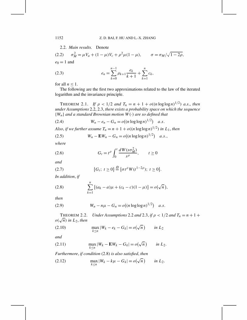
2.2. Main results. Denote
σ 2M =µVa + (1 −µ)Vc + ρ2µ(1 −µ), σ = σM/
√1 − 2ρ,(2.2)
e0 = 1 and
en =n−1∑k=0
ρk+1ek
k + 1+
n∑k=1
ck,(2.3)
for all n≤ 1.The following are the first two approximations related to the law of the iterated
logarithm and the invariance principle.
THEOREM 2.1. If ρ < 1/2 and Tn = n + 1 + o((n log logn)1/2) a.s., thenunder Assumptions 2.2, 2.3, there exists a probability space on which the sequence{Wn} and a standard Brownian motionW(·) are so defined that
Wn− en−Gn = o((n log logn)1/2)a.s.(2.4)
Also, if we further assume Tn = n+ 1 + o((n log logn)1/2) in L1, then
Wn− EWn −Gn = o((n log logn)1/2)a.s.,(2.5)
where
Gt = tρ∫ t
0
dW(sσ 2M)
sρ, t ≥ 0(2.6)
and {Gt; t ≥ 0
} D= {σ tρW(t1−2ρ); t ≥ 0
}.(2.7)
In addition, ifn∑k=1
{(ak − a)µ+ (ck − c)(1 −µ)}= o(√n ),(2.8)
then
Wn− nµ−Gn = o((n log logn)1/2)a.s.(2.9)
THEOREM 2.2. Under Assumptions 2.2 and 2.3, if ρ < 1/2 and Tn = n+ 1 +o(
√n) in L2, then
maxk≤n |Wk − ek −Gk| = o(√n ) in L2(2.10)
and
maxk≤n |Wk − EWk −Gk| = o(√n ) in L2.(2.11)
Furthermore, if condition (2.8) is also satisfied, then
maxk≤n |Wk − kµ−Gk| = o(√n ) in L2.(2.12)

APPROXIMATION FOR URN MODELS 1153
From Theorems 2.1 and 2.2, it is easily seen that
COROLLARY 2.1. Assume ρ < 1/2, and Tn = n + 1 + o(√n) in L2, thenunder Assumptions 2.2, 2.3,
n1/2(W[nt] − EW[nt])�⇒ σ tρW(t1−2ρ);(2.13)
if Tn = n+ 1 + o((n log logn)1/2) a.s. and in L1, then under Assumptions 2.2, 2.3,
lim supn→∞
Wn− EWn√2n log logn
= σ a.s.(2.14)
Furthermore, if condition (2.8) is also satisfied, then EWn can be placed by nµ.
REMARK. (2.13) was first established by Gouet (1993) in the case ofAn = a and Cn = c for all n. Result (2.14) is new. For the random and non-homogeneous Pólya’s urn, Bai and Hu (1999) showed that
n−1/2(Wn − EWn)D→N(0, σ )(2.15)
under the condition∞∑k=1
|ak − a| + |ck − c|k
<∞.(2.16)
Also, the result of Bai and Hu (2000) implies that
n−1/2(Wn− nµ) D→N(0, σ ),
but the following condition is needed:∞∑k=1
|ak − a| + |ck − c|√k
<∞.(2.17)
Obviously, condition (2.17) is stronger than (2.8). But, Bai and Hu (1999, 2000)studied the multicolor urn models.
Assumptions 2.2 and 2.3 used in Theorems 2.1 and 2.2 are very weak andstandard, but the rates of the approximations obtained are slow. The next threetheorems give faster rates for strong approximations.
THEOREM 2.3. If ρ < 1/2 Tn = n + 1 + o(√n) a.s., then under Assump-tions 2.2, 2.3 and 2.4,
Wn − en−Gn = o(√n) a.s.(2.18)
And if also Tn = n+ 1 + o(√n) in L1, then
Wn− EWn −Gn = o(√n) a.s.(2.19)
Furthermore, if (2.8) holds, then
Wn− nµ−Gn = o(√n) a.s.(2.20)

1154 Z. D. BAI, F. HU AND L.-X. ZHANG
THEOREM 2.4. If ρ < 1/2 and Tn = n+ 1 + o(n1/2(logn)−1/2−ε) a.s., thenunder Assumptions 2.2, 2.3 and 2.5,
Wn− en −Gn = o(n1/2(logn)−1/2−ε/3) a.s.
and if also Tn = n+ 1 + o(n1/2(logn)−1/2−ε) in L1, then
Wn − EWn−Gn = o(n1/2(logn)−1/2−ε/3) a.s.
THEOREM 2.5. If ρ < 1/2, then under Assumptions 2.1, 2.2 and 2.6 we have
Wn − en−Gn = o(n1/2−δ) a.s. ∀0< δ < (1/2 − ρ)∧ (1/4)and
Wn− EWn−Gn = o(n1/2−δ) a.s. ∀0< δ < (1/2 − ρ)∧ (1/4),where a ∧ b= min(a, b).
It is known that the best convergence rate of Skorokhod embedding isO(n1/4(logn)1/2(log logn)1/4). Theorem 2.5 gives an approximation close to thisrate. In the remainder of this section, we give a strong approximation in the caseof ρ = 1/2.
THEOREM 2.6. Suppose ρ = 1/2 and Tn = n+ 1 + o(n1/2(logn)1/2−ε) a.s.Then under Assumptions 2.2, 2.3, 2.5 and (2.16) there exists a δ > 0 such that
Wn− en − Gn = o(n1/2(logn)1/2−δ) a.s.(2.21)
Also if Tn = n+ 1 + o(n1/2(logn)1/2−ε) in L1, then
Wn − EWn− Gn = o(n1/2(logn)1/2−δ) a.s.,
where
Gt = t1/2∫ t
1
dW(sσ 2M)
s1/2, t ≥ 0(2.22)
and {Gt; t > 0
} D= {σMt
1/2W(log t); t > 0}.(2.23)
Furthermore, if condition (2.17) is satisfied, then
Wn − nµ− Gn = o(n1/2(logn)1/2−δ) a.s.
The following corollary comes from Theorem 2.6 immediately.

APPROXIMATION FOR URN MODELS 1155
COROLLARY 2.2. Under the conditions in Theorem 2.6, we have
(nt logn)1/2(W[nt ] − EW[nt ]
)�⇒ σMW(t),
and
lim supn→∞
Wn − EWn√2n(logn)(log log logn)
= σM a.s.
Furthermore, if condition (2.17) is satisfied, then EW[nt ] and EWn can be replacedby ntµ and nµ, respectively.
3. Proofs. Recalling (2.1), write
Wn =W0 +n∑k=1
(Ak −Ck)Ik +n∑k=1
Ck
=W0 +n∑k=1
{(Ak −Ck)Ik − E[(Ak −Ck)Ik|Fk−1] + (Ck − ck)}
(3.1)
+n−1∑k=0
ρk+1Wk
Tk+
n∑k=1
ck
=W0 +Mn +n−1∑k=0
ρk+1Wk
k + 1+n−1∑k=0
ρk+1Wk
Tk
(k + 1 − Tkk + 1
)+
n∑k=1
ck,
where
Mn :=n∑k=1
'Mk =n∑k=1
{(Ak −Ck)Ik − E[(Ak −Ck)Ik|Fk−1] + (Ck − ck)}
is a martingale with
E[('Mn)2|Fn−1]
= E[((An −Cn)In +Cn− cn)2|Fn−1
]− ((an − cn)Wn−1
Tn−1
)2
= E[(An −Cn)2In+ 2(An−Cn)(Cn − cn)In + (Cn − cn)2|Fn−1
]−((an − cn)Wn−1
Tn−1
)2
= Wn−1
Tn−1E[(An−Cn)2 + 2(An−Cn)(Cn − cn)|Fn−1
]+ Var(Cn|Fn−1)
−((an − cn)Wn−1
Tn−1
)2

1156 Z. D. BAI, F. HU AND L.-X. ZHANG
= Wn−1
Tn−1Var(An|Fn−1)+
(1 − Wn−1
Tn−1
)Var(Cn|Fn−1)
+ ρ2n
Wn−1
Tn−1
(1 − Wn−1
Tn−1
)(3.2)
=µVar(An|Fn−1)+ (1 −µ)Var(Cn|Fn−1)+ ρ2nµ(1 −µ)
+O(Wn−1
Tn−1−µ
)
=µVa + Vc(1 −µ)+ ρ2µ(1 −µ)+ o(1)+O(Wn−1
Tn−1−µ
)
= σ 2M + o(1)+O
(Wn−1
Tn−1−µ
)a.s.
under Assumptions 2.2 and 2.3.By the Skorokhod embedding theorem [cf. Hall and Heyde (1980)], there exists
an Fn-adapted sequence of nonnegative random variables {τn} and a standardBrownian motionW , such that
E[τn|Fn−1] = E[('Mn)2|Fn−1], E|τn|1+ε/2 ≤ CE|'Mn|2+ε(3.3)
and {W
(n∑i=1
τi
); n= 1,2, . . .
}D= {Mn; n= 1,2, . . .
}.
Without loss of generality, we write
Mn =W(n∑i=1
τi
), n= 1,2, . . . .(3.4)
On the other hand, from (2.3) and (3.1), it follows that
Wn− en =W0 +Mn +n−1∑k=0
ρk+1Wk − ekk + 1
+n−1∑k=0
ρk+1Wk
Tk
(k + 1 − Tkk+ 1
).(3.5)
If Assumption 2.1 is satisfied, that is, Tk = k + 1, then (3.5) becomes
Wn− en =W0 +Mn +n−1∑k=0
ρk+1Wk − ekk + 1
.(3.6)
So it is natural that Wn may be approximated by a Gaussian process, and what weneed to show is how Wn − en can be approximated by a related Gaussian processwhenMn can.
Before proving the theorems, we need some lemmas first. The first two are onthe convergence rates of a real sequence of type (3.6).

APPROXIMATION FOR URN MODELS 1157
LEMMA 3.1. Let ρn and pn be two sequences of real numbers. Define {qn} by
q1 = p1 and qn = pn +n−1∑k=1
ρkqk
k.
Then
qn =n∑k=1
pkrn,k,(3.7)
where rn,n = 1 and
rn,k = ρkk
n−1∏i=k+1
(1 + ρi
i
), k = 1,2, . . . , n− 1, n= 1,2, . . . .
Here we define∏ki=k+1(·)= 1. Furthermore, if ρk → ρ, then for ∀ ε > 0, there is
a constant C > 0 such that
|rn,k| ≤ Ck−1(n/k)ρ+ε, k = 1,2, . . . , n, n= 1,2, . . . .
And if∞∑k=1
|ρk − ρ|/k <∞,(3.8)
then
|rn,k| ≤ Ck−1(n/k)ρ, k = 1,2, . . . , n, n= 1,2, . . . .
PROOF. When n= 1, we have q1 = p1 = r1,1p1. Thus (3.7) is true for n= 1.By induction, we have
qn = pn +n−1∑k=1
ρk
k
k∑j=1
pj rkj = pnrn,n+n−1∑j=1
pj
n−1∑k=j
ρk
krk,j =
n∑j=1
pj rn,j ,
where the last step follows from
n−1∑k=j
ρk
krk,j = ρj
j
(1 +
n−1∑k=j+1
ρk
k
k−1∏i=j+1
(1 + ρi
i
))= rn,j .
The first part of the conclusion is proved. The second part is obvious since
logn−1∏i=k
(1 + ρi
i
)=n−1∑i=k
log(
1 + ρii
)=n−1∑i=k
ρi
i+O(1)
=n−1∑i=k
ρ
i+n−1∑i=k
ρi − ρi
+O(1). �

1158 Z. D. BAI, F. HU AND L.-X. ZHANG
LEMMA 3.2. Let pn, ρn and qn be defined as in Lemma 3.1. If ρn → ρ
and pn = o(nρ+δδn) [or O(nρ+δδn)] where δ > 0 and {δn} is a nondecreasingsequence of positive numbers, then
qn = o(nρ+δδn) [corresp. qn =O(nρ+δδn)].
If (3.8) holds and pn = o(nρδn) [corresp. = O(nρδn)] where δn is a sequence ofpositive numbers, then
qn = o(nρ
n∑k=1
δk/k
) (corresp. qn =O
(nρ
n∑k=1
δk/k
)).
By Lemma 3.1, the proof is easy.The definition of en seems complicated. But, the following two lemmas tell us
that it can be replaced by EWn in most cases, or by nµ in some cases.
LEMMA 3.3. (a) Suppose that Assumptions 2.1 and 2.2 are satisfied. If ρ <1/2, then
EWn− en = o(n1/2−δ) ∀0 ≤ δ < (1/2 − ρ)∧ 1/2.
If ρ = 1/2 and (3.8) holds, then
EWn− en = o(n1/2).
(b) Suppose ρ < 1/2, Assumption 2.2 is true and Tn = n+1+o((n log logn)1/2)in L1. Then
EWn− en = o((n log logn)1/2).
(c) Suppose ρ < 1/2, Assumption 2.2 and Tn = n+ 1 + o(√n) in L1. Then
EWn− en = o(√n ).(d) Suppose Assumption 2.2 and Tn = n+ 1 + o(n1/2(logn)−1/2−ε) in L1 for
some ε > 0. If ρ < 1/2, then
EWn− en = o(n1/2(logn)−1/2−ε).If ρ = 1/2 and (3.8) holds, then
EWn− en = o(n1/2(logn)1/2−ε).PROOF. We give the proof of (a) only. By (3.5),
EWn− en =n−1∑k=0
ρk+1EWk − ekk + 1
+O(1)=n−1∑k=0
ρk+1EWk − ekk+ 1
+ o(n1/2−δ).

APPROXIMATION FOR URN MODELS 1159
By Lemma 3.2, it follows that if ρ < 1/2, then
|EWn− en| = o(n1/2−δ)
since ε =: 1/2 − δ− ρ > 0. If ρ = 1/2 and (3.8) holds, then
|EWn − en| = o(n1/2
n∑k=1
k−1−1/2
)= o(n1/2). �
LEMMA 3.4. Under Assumption 2.2, we have
en
n→µ.
Furthermore, if (2.8) holds and ρ < 1/2, then
en− nµ= o(√n )and if ρ = 1/2 and condition (2.17) is satisfied, then
en− nµ=O(√n ).PROOF. By (2.3),
en− nµ=n−1∑k=0
ρk+1ek − (k + 1)µ
k+ 1+
n∑k=1
{(ak − a)µ+ (ck − c)(1 −µ)}.(3.9)
The first two conclusions follow from Lemma 3.2 easily by taking pn = o(nρ+1−ρ)and pn = o(nρ+1/2−ρ), respectively. Now, assume ρ = 1/2 and (2.17). Takebn = n1/2δn, where
δn =∑nk=1{(ak − a)µ+ (ck − c)(1 −µ)}√
n.
Then, by the second part of Lemma 3.2,
en− nµ=O(n1/2
n∑k=1
δk/k
)
=O(n1/2
n∑k=1
∑ki=1{(ai − a)µ+ (ci − c)(1 −µ)}
k3/2
)
=O(n1/2
n∑i=1
(|ai − a| + |ci − c|)n∑k=ik−3/2
)
=O(n1/2
n∑i=1
|ai − a| + |ci − c|√i
)=O(√n ). �

1160 Z. D. BAI, F. HU AND L.-X. ZHANG
Define
G0 = 0, Gn =W(nσ 2M)+ ρ
n−1∑k=1
Gk
k,(3.10)
where∑0k=1(·) = 0. The next two lemmas tell us how Gn is close to Gn or Gn,
where Gn and Gn are defined in (2.6) and (2.22), respectively.
LEMMA 3.5. If ρ < 1/2, we have for all 0 ≤ δ < 1/2 − ρ,
Gn−Gn = o(n1/2−δ) a.s.(3.11)
and ∥∥∥maxk≤n |Gk −Gk|
∥∥∥2= o(n1/2−δ).(3.12)
PROOF. By the Taylor expansion,
Gn−Gn−1 = nρ∫ nn−1
dW(sσ 2M)
sρ+(
1 + 1
n− 1
)ρGn−1 −Gn−1
= nρ∫ nn−1
dW(sσ 2M)
sρ+ ρGn−1
n− 1+ ρ(ρ − 1)
2(n− 1)2(1 + ξn−1)
ρ−2Gn−1,
where ξn−1 ∈ [0,1] is a real number. It follows that
Gn = ρn−1∑k=1
Gk
k+
n∑k=1
kρ∫ kk−1
dW(sσ 2M)
sρ+ ρ(ρ − 1)
2
n−1∑k=1
(1 + ξk)ρ−2
k2 Gk.
Then,
Gn −Gn = ρn−1∑k=1
Gk −Gkk
+n∑k=1
kρ∫ kk−1
(1
sρ− 1
kρ
)dW(sσ 2
M)
+ ρ(ρ − 1)
2
n−1∑k=1
(1 + ξk)ρ−2
k2 Gk(3.13)
= ρn−1∑k=1
Gk −Gkk
+n∑k=1
Zk + ρ(ρ − 1)
2
n−1∑k=1
(1 + ξk)ρ−2
k2 Gk,
where {Zk; k = 1,2, . . .} is a sequence of independent normal variables withEZk = 0 and
EZ2k = σ 2
Mk2ρ∫ kk−1
(1
sρ− 1
kρ
)2
ds ≤ Ck2ρ 1
k2ρ+2≤ Ck−2.

APPROXIMATION FOR URN MODELS 1161
It follows that∑nk=1Zk = O(1) in L2, and
∑nk=1Zk = O(1) a.s. by the three-
series theorem. Also∣∣∣∣∣ρ(ρ − 1)
2
n−1∑k=1
(1 + ξk)ρ−2
k2 Gk
∣∣∣∣∣≤ |ρ(ρ − 1)|2
n−1∑k=1
|Gk|k2 <∞ a.s. and in L2.
So,
Gn−Gn = ρn−1∑k=1
Gk −Gkk
+O(1)(3.14)
= ρn−1∑k=1
Gk −Gkk
+ o(n1/2−δ) a.s. and in L2.
Hence, from Lemma 3.2 it follows that
Gn−Gn = o(n1/2−δ) a.s. and in L2 ∀0 ≤ δ < 1/2 − ρ.The assertion (3.11) is proved. Finally,
maxm≤n |Gm −Gm| ≤ |ρ|
n−1∑k=1
|Gk −Gk|k
+ maxm≤n
∣∣∣∣∣m∑k=1
Zk
∣∣∣∣∣+ |ρ(ρ − 1)|2
n−1∑k=1
|Gk|k2 .
It follows that∥∥∥∥maxm≤n |Gm−Gm|
∥∥∥∥2≤ |ρ|
n−1∑k=1
‖Gk −Gk‖2
k+∥∥∥∥∥maxm≤n |
m∑k=1
Zk
∥∥∥∥∥2
+ |ρ(ρ − 1)|2
n−1∑k=1
‖Gk‖2
k2
≤ |ρ|n−1∑k=1
o(k1/2−δ−1)+O(1)+n−1∑k=1
O(k1/2−2)= o(n1/2−δ).
The conclusion (3.12) follows. �
LEMMA 3.6. If ρ = 1/2, we have
Gn − Gn = o(n1/2) a.s.
PROOF. Similarly to (3.13),
Gn −Gn = ρn−1∑k=1
Gk −Gkk
+W(σ 2M)+
n∑k=2
Zk + ρ(ρ − 1)
2
n−1∑k=1
(1 + ξk)ρ−2
k2Gk.

1162 Z. D. BAI, F. HU AND L.-X. ZHANG
So, just as in (3.14), we have
Gn −Gn = ρn−1∑k=1
Gk −Gkk
+ o(n1/2−δ) a.s. ∀0< δ < 1/2.
Applying the second part of Lemma 3.2, we conclude that
Gn−Gn = o(n1/2
n∑k=1
k−1−δ)
= o(√n ) a.s. �
Now we are in position to prove the main theorems.
PROOF OF THEOREM 2.1. We first show the two processes are equal in law.Since EGt = 0 and for t ≥ s,
EGsGt = tρsρE(∫ s
0
dW(xσ 2M)
xρ
)2
= tρsρ∫ s
0
σ 2M
x2ρdx = σ 2tρsρs1−2ρ = E
(σ tρW(t1−2ρ)
)(σsρW(s1−2ρ)
).
This shows that the two Gaussian processes have the same mean and covariancefunctions, which implies (2.7).
Note that (2.5) follows from (2.4) and Lemma 3.3(b) whereas (2.9) followsfrom (2.4) and Lemma 3.4. To complete the proof of Theorem 2.1, it suffices toprove (2.4). To this end, we shall first show how Mn can be approximated byW(nσ 2
M). Let τn be defined as in (3.3) and (3.4) through the Skorohod embeddingtheorem. Note that
E|'Mn|2+ε
= E∣∣(An −Cn)In− E[(An −Cn)In|Fn−1] + (Cn − E[Cn|Fn−1])
∣∣2+ε
≤ C(E|An|2+ε + E|Cn|2+ε) < C <∞,where C is a generic notation for positive constants; that is, it may take differentvalues at different appearances.
It then follows that E|τn|1+ε/2 <C <∞. Hence,
∞∑n=1
E∣∣∣∣ τnn1−ε/3
∣∣∣∣1+ε/2<∞.
So, by the law of large numbers for martingales [cf. Theorem 20.11 of Davidson(1994)],
n∑k=1
τk −n∑k=1
E[('Mk)2|Fk−1] =n∑k=1
(τk − E[τk|Fk−1])= o(n1−ε/3) a.s.(3.15)

APPROXIMATION FOR URN MODELS 1163
Obviously, by (3.2),
E[('Mn)2|Fn−1] =O(1) a.s.
Thus,n∑k=1
τk =O(n) a.s.
Then by (3.4) and the law of iterated logarithm of a Brownian motion,
Mn =O((n log logn)1/2)
a.s.
which, together with (3.5) and Lemma 3.2, implies
Wn− en =O((n log logn)1/2)
a.s.(3.16)
By (3.2) and (3.16) and Lemma 3.4, it follows that
E[('Mn)2|Fn−1] = σ 2M + o(1)+O
(Wn−1
Tn−1− en−1
Tn−1
)+O
(en−1
Tn−1−µ
)= σ 2
M + o(1) a.s.
So,n∑k=1
τk = nσ 2M + o(n) a.s.(3.17)
Thus by the properties of a Brownian motion [cf. Theorem 1.2.1 of Csörgo andRévész (1981)], we get the following approximation ofMn:
Mn =W(n∑k=1
τk
)=W(nσ 2
M)+ o((n log logn)1/2
)a.s.(3.18)
Recalling the definition of Gn in (3.10) and noticing (3.11), the proof of (2.4)reduces to showing that
Wn− en−Gn = o((n log logn)1/2)
a.s.(3.19)
Note that
Gn =W(nσ 2M)+ ρ
n−1∑k=1
Gk
k
=W(nσ 2M)+ ρ
n−1∑k=1
Gk
k + 1+ ρ
n−1∑k=1
Gk
k(k + 1)(3.20)
=W(nσ 2M)+
n−1∑k=0
ρk+1Gk
k + 1
+ ρn−1∑k=1
Gk
k(k + 1)+n−1∑k=0
(ρ − ρk+1)Gk
k + 1.

1164 Z. D. BAI, F. HU AND L.-X. ZHANG
Note that by (3.11) and (2.7),
Gn =O((n log logn)1/2)
a.s.
It follows that
Gn =W(nσ 2M)+
n−1∑k=0
ρk+1Gk
k + 1
+ ρn−1∑k=1
o(1)
k + 1+n−1∑k=0
(ρ − ρk+1)O((k log logk)1/2)
k + 1.(3.21)
=W(nσ 2M)+
n−1∑k=0
ρk+1Gk
k + 1+ o((n log logn)1/2
)a.s.
By (3.5), (3.18), (3.21) and
n−1∑k=0
ρk+1Wk
Tk
(k + 1 − Tkk + 1
)= o
(n−1∑k=0
(k log logk)1/2
k + 1
)= o((n log logn)1/2
)a.s.
we conclude that
Wn − en−Gn =n−1∑k=0
ρk+1Wk − ek −Gkk + 1
+ o((n log logn)1/2)
a.s.
Hence by Lemma 3.2, we have proved (3.19). �
PROOF OF THEOREM 2.2. Noticing that (2.11) and (2.12) are consequencesof (2.10) and application of Lemmas 3.3 and 3.4, we need only to show (2.10).Define νn =∑n
k=1 τk − nσ 2M . Then by (3.17),
νn = o(n) a.s.(3.22)
First, we show that
maxk≤n |Mk −W(kσ 2
M)| = o(√n)
in L2.(3.23)
Note that (3.22) implies that maxk≤n |νk|/n→ 0 in probability, and then
E maxk≤n |Mk −W(kσ 2
M)|2
= E maxk≤n |Mk −W(kσ 2
M)|2I{
maxk≤n |νk| ≤ εn
}+ E max
k≤n |Mk −W(kσ 2M)|2I
{maxk≤n |νk|> εn
}≤ E sup
0≤t≤n(1+σ 2M)
sup0≤s≤εn
|W(t + s)−W(t)|2

APPROXIMATION FOR URN MODELS 1165
+ 2E maxk≤n |Mk|2I
{maxk≤n |νk|> εn
}+ 2E max
k≤n |W(kσ 2M)|2I
{maxk≤n |νk|> εn
}≤ nE sup
0≤t≤1+σ 2M
sup0≤s≤ε
|W(t + s)−W(t)|2
+ 2(∥∥∥∥max
k≤n |Mk|∥∥∥∥2
2+ε+∥∥∥∥maxk≤n |W(kσ 2
M)|∥∥∥∥2
2+ε
)
×(
P(
maxk≤n |νk|> εn
))(2+ε)/ε
≤ nE sup0≤t≤1+σ 2
M
sup0≤s≤ε
|W(t + s)−W(t)|2 +Cn(
P(
maxk≤n |νk|> εn
))(2+ε)/ε
= o(n) as n→ ∞ and then ε→ 0.
The assertion (3.23) is proved. Now, let Gn be defined through (3.10). ByLemma 3.5, to prove (2.10), it is enough to show that
maxk≤n |Wk − ek −Gk| = o(√n ) in L2.(3.24)
By (3.5) and (3.20), we have
Wn− en−Gn =W0 +Mn −W(nσ 2M)+
n−1∑k=0
ρk+1Wk − ek −Gkk + 1
+ ρn−1∑k=1
Gk
k(k + 1)+n−1∑k=0
(ρ − ρk+1)Gk
k+ 1(3.25)
+n−1∑k=0
ρk+1Wk
Tk
(k + 1 − Tkk + 1
).
By (3.12) and (2.7), we know that ‖Gn‖2 =O(√n). It follows that∥∥∥∥∥ρn−1∑k=1
Gk
k(k + 1)+n−1∑k=0
(ρ − ρk+1)Gk
k + 1
∥∥∥∥∥2
≤ |ρ|n−1∑k=1
‖Gk‖2
k(k + 1)+n−1∑k=0
|ρ − ρk+1|‖Gk‖2
k+ 1
≤ |ρ|n−1∑k=1
O(√k)
k(k + 1)+n−1∑k=0
|ρ − ρk+1|O(√k)
k + 1= o(√n ),
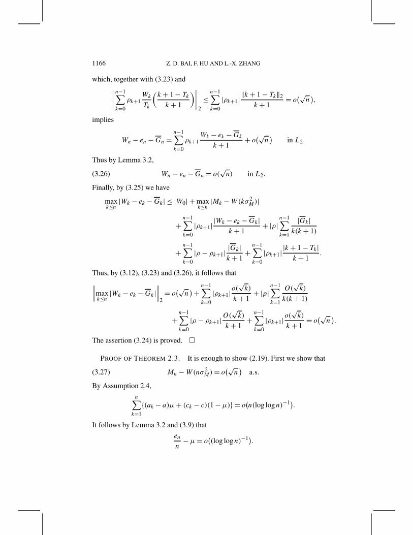
1166 Z. D. BAI, F. HU AND L.-X. ZHANG
which, together with (3.23) and∥∥∥∥∥n−1∑k=0
ρk+1Wk
Tk
(k + 1 − Tkk + 1
)∥∥∥∥∥2
≤n−1∑k=0
|ρk+1|‖k + 1 − Tk‖2
k+ 1= o(√n ),
implies
Wn− en −Gn =n−1∑k=0
ρk+1Wk − ek −Gkk + 1
+ o(√n ) in L2.
Thus by Lemma 3.2,
Wn − en−Gn = o(√n) in L2.(3.26)
Finally, by (3.25) we have
maxk≤n |Wk − ek −Gk| ≤ |W0| + max
k≤n |Mk −W(kσ 2M)|
+n−1∑k=0
|ρk+1| |Wk − ek −Gk|k + 1
+ |ρ|n−1∑k=1
|Gk|k(k + 1)
+n−1∑k=0
|ρ − ρk+1| |Gk|k + 1
+n−1∑k=0
|ρk+1| |k + 1 − Tk|k + 1
.
Thus, by (3.12), (3.23) and (3.26), it follows that∥∥∥∥maxk≤n |Wk − ek −Gk|
∥∥∥∥2= o(√n )+ n−1∑
k=0
|ρk+1|o(√k)
k + 1+ |ρ|
n−1∑k=1
O(√k)
k(k + 1)
+n−1∑k=0
|ρ − ρk+1|O(√k)
k+ 1+n−1∑k=0
|ρk+1|o(√k)
k + 1= o(√n ).
The assertion (3.24) is proved. �
PROOF OF THEOREM 2.3. It is enough to show (2.19). First we show that
Mn−W(nσ 2M)= o
(√n)
a.s.(3.27)
By Assumption 2.4,
n∑k=1
{(ak − a)µ+ (ck − c)(1 −µ)} = o(n(log logn)−1).It follows by Lemma 3.2 and (3.9) that
en
n−µ= o((log logn)−1).

APPROXIMATION FOR URN MODELS 1167
And then by (3.2) and (3.16),
E[('Mn)2|Fn−1] = µVar(An|Fn−1)+ (1 −µ)Var(Cn|Fn−1)+ ρ2nµ(1 −µ)
+O(Wn−1
Tn−1− en−1
n
)+O
(en−1
n−µ
)= σ 2
M + o((log logn)−1) a.s.,
which, together with (3.15), implies
n∑k=1
τk = nσ 2M + o(n(log logn)−1) a.s.
Then by Theorem 1.2.1 of Csörgo and Révész (1981) again,
Mn =W(n∑k=1
τk
)=W(nσ 2
M)+ o((n(log logn)−1)1/2(log logn)1/2
)=W(nσ 2
M)+ o(√n)
a.s.,
from which (3.27) follows. Next, by (3.20),
Gn =W(nσ 2M)+
n−1∑k=0
ρk+1Gk
k + 1
+ ρn−1∑k=1
o(1)
k + 1+n−1∑k=0
o((log log k)−1)O((k log logk)1/2)
k + 1(3.28)
=W(nσ 2M)+
n−1∑k=0
ρk+1Gk
k + 1+ o(√n ) a.s.
Hence by (3.5), (3.27), (3.28) and
n−1∑k=0
ρk+1Wk
Tk
(k + 1 − Tkk+ 1
)= o
(n−1∑k=0
√k
k + 1
)= o(√n ) a.s.,
we conclude that
Wn− en−Gn =n−1∑k=0
ρk+1Wk − ek −Gkk + 1
+ o(√n ) a.s.
By Lemma 3.2, it follows that
Wn− en −Gn = o (√n ) a.s.
The rest of the proof is similar to that of Theorem 2.1. �

1168 Z. D. BAI, F. HU AND L.-X. ZHANG
The proofs of Theorems 2.4 and 2.5 are similar to that of Theorem 2.3, and thedetails are omitted.
PROOF OF THEOREM 2.6. Assertion (2.23) can be easily verified by showingthat the two processes have identical covariance functions. Also, by Lemmas 3.3and 3.4, to prove the theorem, it is enough to show (2.21). Following the lines ofthe proof of Theorem 2.3, one can show that
Mn =W(nσ 2M)+ o
(n1/2(logn)−1/2−ε/3) a.s.
Also, similar to (3.28),
Gn =W(nσ 2M)+
n−1∑k=0
ρk+1Gk
k + 1
+ ρn−1∑k=1
o(1)
k + 1+n−1∑k=0
o((log k)−1−ε)O((k log log k)1/2
k+ 1
=W(nσ 2M)+
n−1∑k=0
ρk+1Gk
k + 1+ o(n1/2(logn)−1−ε/2) a.s.
Hence
Wn− en−Gn =n−1∑k=0
ρk+1Wk − ek −Gkk + 1
+ o(n1/2(logn)−1/2−ε/3) a.s.
By the second part of Lemma 3.2, it follows that
Wn − en−Gn = o(1)n1/2n∑k=1
k−1(log k)−1/2−ε/3 = o(n1/2(logn)1/2−ε/3) a.s.
Finally, by Lemma 3.6,
Gn− Gn = o(√n ) a.s.
The proof is complete. �
4. Some applications.
4.1. Asymptotic properties of the randomized-play-the-winner rule. The ran-domized-play-the-winner (RPW) rule was introduced by Wei and Durham (1978)and it can be formulated as a GFU model [Wei (1979)] as follows: Assume thereare two treatments (say, T1 and T2), with dichotomous response (success andfailure). For the ith patient, if a white ball is drawn, the patient is assigned tothe treatment T1, and otherwise, the patient is assigned to the treatment T2. Theball is then replaced in the urn and the patient response is observed. A success

APPROXIMATION FOR URN MODELS 1169
on treatment T1 or a failure on treatment T2 generates a white ball to the urn;a success on treatment T2 or a failure on treatment T1 generates a black ball to theurn.
Let p1 = P(success|T1), p2 = P(success|T2), q1 = 1 − p1 and q2 = 1 − p2. Itis easy to see that
R =[I (success|T1) 1 − I (success|T1)
1 − I (success|T2) I (success|T2)
]and H =
[p1 q1q2 p2
],
where I is an indicator function. From the results of Section 2, we have thefollowing corollaries.
COROLLARY 4.1. If q1 + q2 > 1/2, then:
(i)
n−1/2(Wn− q2n
q1 + q2
)→N(0, σ 2) in distribution
and further, we have
(ii)
lim supn→∞
Wn− q2n/(q1 + q2)√2n log logn
= σ a.s.,
where σ 2 = q1q2/[(2(q1 + q2)− 1)(q1 + q2)2].
It is easy to see that Tn = n + β and Assumptions 2.2 and 2.3 hold. FromCorollary 2.1, we can obtain both (i) and (ii). The result (i) has been studiedin Smythe and Rosenberger (1995) for the homogeneous case and Bai and Hu(1999) for the nonhomogeneous generating matrices. The result (ii) is new. Whenq1 + q2 = 1/2, the following similar results are true.
COROLLARY 4.2. If q1 + q2 = 1/2, then:
(i)
(n logn)−1/2(Wn− q2n
q1 + q2
)→N(0, σ 2
W) in distribution
and further, we have
(ii)
lim supn→∞
Wn− q2n/(q1 + q2)√2n(logn)(log log logn)
= σW a.s.,
where σ 2W = q1q2/(q1 + q2)
2.

1170 Z. D. BAI, F. HU AND L.-X. ZHANG
4.2. Variance estimation. From Corollary 3.1, we know that under Assump-tions 2.1, 2.2, 2.3 and condition (2.8),
Wn − nµ√nσ
D→N(0,1),(4.1)
where σ is defined as in (2.2). The result (4.1) gives us the limit distribution ofWn/n which is an estimator of µ. But (4.1) is difficult to apply since the valueof σ is unknown. So it is important to find a consistent estimate of σ from thesample {Wn}.
Inspired by Shao (1994), we define two estimators as follows:
σ1,n = 1
logn
n∑i=1
1√i
∣∣∣∣Wii − Wnn
∣∣∣∣ and σ 22,n = 1
logn
n∑i=1
(Wi
i− Wnn
)2
.(4.2)
The following two theorems establish the weak and strong consistency of theestimators, respectively.
THEOREM 4.1. Suppose ρ < 1/2. Under Assumptions 2.2, 2.3, (2.8) and thatTn = n+ 1 + o(√n) in L2, we have
σ1,n→√
2
πσ and σ 2
2,n→ σ 2 in L2.(4.3)
THEOREM 4.2. Suppose ρ < 1/2. Under Assumptions 2.2, 2.3, 2.4, (2.8) andthat Tn = n+ 1 + o(√n) a.s.,
σ1,n→√
2
πσ and σ 2
2,n→ σ 2 a.s.(4.4)
The proofs of Theorems 4.1 and 4.2 are based on the Gaussian approximationsand the following lemma.
LEMMA 4.1. Suppose ρ < 1/2. Let {Gt; t ≥ 0} be as in (2.6), and let
V1,n = 1
logn
n∑i=1
|Gi |i3/2
and V 22,n = 1
logn
n∑i=1
G2i
i2.(4.5)
Then
V1,n→√
2
πσ, V 2
2,n→ σ 2 a.s. as well as in L2.(4.6)
PROOF. Obviously,
EV1,n→√
2
πσ and EV 2
2,n→ σ 2.(4.7)

APPROXIMATION FOR URN MODELS 1171
Also, by (2.6), Cov(Gi/√i,Gj/
√j)= σ 2(i/j)1/2−ρ for all i ≤ j . It follows that
Cov( |Gi |√i,|Gj |√j
)≤ σ 2(i/j)1/2−ρ
and
Cov(G2i
i,G2j
j
)= 2σ 4(i/j)1−2ρ.
Then
Var(V1,n)= 1
(logn)2
{n∑i=1
1
i2Var
( |Gi |√i
)+ 2
n−1∑i=1
n∑j=i+1
1
ijCov
( |Gi|√i,|Gj |√j
)}(4.8)
≤ C 1
(logn)2
n−1∑i=1
n∑j=i
1
ij(i/j)1/2−ρ ≤ C
logn
and
Var(V 21,n)≤ C
1
(logn)2
n−1∑i=1
n∑j=i
1
ij(i/j)1−2ρ ≤ C
logn.(4.9)
The estimates (4.7)–(4.9) directly imply the L2 convergence part of (4.6). By somestandard calculation, the three estimates also imply the a.s. convergence of (4.6)[cf. Shao (1994)]. �
Now we start to prove the main theorems for the consistency of the varianceestimators.
PROOF OF THEOREM 4.1. Let V1,n and V2,n be defined as in (4.5). Since∣∣∣∣∣∣∣∣∣Wii − Wn
n
∣∣∣∣− ∣∣∣∣Gii∣∣∣∣∣∣∣∣∣=
∣∣∣∣∣∣∣∣∣Wi − iµi − Wn − nµ
n
∣∣∣∣− ∣∣∣∣Gii∣∣∣∣∣∣∣∣∣
≤∣∣∣∣Wi − iµi − Wn− nµ
n− Gii
∣∣∣∣≤∣∣∣∣Wi − iµ−Gi
i
∣∣∣∣+ ∣∣∣∣Wn− nµn
∣∣∣∣,we have
‖σ1,n − V1,n‖2 ≤ 1
logn
n∑i=1
1√i
∥∥∥∥Wi − iµ−Gii
∥∥∥∥2+ 1
logn
n∑i=1
1√i
∥∥∥∥Wn− nµn
∥∥∥∥2.

1172 Z. D. BAI, F. HU AND L.-X. ZHANG
Also, if we define ‖ · ‖ to be the Euclidean norm in Rn, and write x = (x1, . . . , xn),y = (y1, . . . , yn) and z = (z1, . . . , zn), where xi = Wi−iµ
i, yi = Wn−nµ
n, zi = Gi
i,
i = 1, . . . , n, then
|σ2,n− V2,n| = 1
(logn)1/2∣∣‖x − y‖ − ‖z‖∣∣≤ 1
(logn)1/2‖x − y − z‖
≤ ‖x − z‖(logn)1/2
+ ‖y‖(logn)1/2
.
So,
‖σ2,n − V2,n‖2 ≤ 1
(logn)1/2∥∥‖x − z‖∥∥2 + 1
(logn)1/2∥∥‖y‖∥∥2
= 1
(logn)1/2
(n∑i=1
E(Wi − iµ−Gi
i
)2)1/2
+ 1
(logn)1/2
(n∑i=1
E(Wn− nµn
)2)1/2
.
From Theorem 2.2 it follows that
‖σ1,n− V1,n‖2 = 1
logn
n∑i=1
1
io(1)+ 1
logn
n∑i=1
1√iO(1/
√n)= o(1)
and
‖σ2,n−V2,n‖2 = 1
(logn)1/2
(n∑i=1
o
(1
i
))1/2
+ 1
(logn)1/2
(n∑i=1
O
(1
n
))1/2
= o(1).
Then, by Lemma 4.1 we have proved the theorem. �
By applying Theorem 2.3 instead of Theorem 2.2, the proof of Theorem 4.2 issimilar to that of Theorem 4.1.
Acknowledgments. Special thanks go to an anonymous referee for construc-tive comments which led to a much improved version of the paper. Professor Huis also affiliated with Department of Statistics and Applied Probability, NationalUniversity of Singapore.
REFERENCES
ATHREYA, K. B. and KARLIN, S. (1968). Embedding of urn schemes into continuous timebranching processes and related limit theorems. Ann. Math. Statist. 39 1801–1817.
BAI, Z. D. and HU, F. (1999). Asymptotic theorem for urn models with nonhomogeneous generatingmatrices. Stochastic Process. Appl. 80 87–101.
APPROXIMATION FOR URN MODELS 1173
BAI, Z. D. and HU, F. (2000). Strong consistency and asymptotic normality for urn models.Unpublished manuscript.
BAI, Z. D., HU, F. and SHEN, L. (2002). An adaptive design for multiarm clinical trials.J. Multivariate Anal. 81 1–18.
COAD, D.S. (1991). Sequential tests for an unstable response variable. Biometrika 78 113–121.CSÖRGO, M. and RÉVÉSZ, P. (1981). Strong Approximations in Probability and Statistics.
Academic Press, New York.DAVIDSON, J. (1994). Stochastic Limit Theory. Oxford Univ. Press.FLOURNOY, N. and ROSENBERGER, W. F., eds. (1995). Adaptive Designs. IMS, Hayward, CA.GOUET, R. (1993). Martingale functional central limit theorems for a generalized Pólya urn. Ann.
Probab. 21 1624–1639.HALL, P. and HEYDE, C. C. (1980). Martingale Limit Theory and Its Applications. Academic Press,
London.HU, F. and ROSENBERGER, W. F. (2000). Analysis of time trends in adaptive designs with
application to a neurophysiology experiment. Statistics in Medicine 19 2067–2075.HU, F., ROSENBERGER, W. F. and ZIDÉK, J. V. (2000). Relevance weighted likelihood for
dependent data. Matrika 51 223–243.ROSENBERGER, W. F. (1996). New directions in adaptive designs. Statist. Sci. 11 137–149.ROSENBERGER, W. F. and GRILL, S. E. (1997). A sequential design for psychophysical
experiments: An application to estimating timing of sensory events. Statistics in Medicine16 2245–2260.
ROSENBERGER, W. F. and SRIRAM, T. N. (1997). Estimation for an adaptive allocation design.J. Statist. Plann. Inference 59 309–319.
SHAO, Q. M. (1994). Self-normalized central limit theorem for sums of weakly dependent randomvariables. J. Theoret. Probab. 7 309–338.
SMYTHE, R. T. (1996). Central limit theorems for urn models. Stochastic Process. Appl. 65 115–137.
SMYTHE, R. T. and ROSENBERGER, W. F. (1995). Play-the-winner designs, generalized Pólyaurns, and Markov branching processes. In Adaptive Designs (N. Flournoy and W. F.Rosenberger, eds.) 13–22. Hayward, CA.
WEI, L. J. (1979). The generalized Pólya’s urn design for sequential medical trials. Ann. Statist. 7291–296.
WEI, L. J. and DURHAM, S. (1978). The randomized pay-the-winner rule in medical trials. J. Amer.Statist. Assoc. 73 840–843.
WEI, L. J., SMYTHE, R. T., LIN, D. Y. and PARK, T. S. (1990). Statistical inference with data-dependent treatment allocation rules. J. Amer. Statist. Assoc. 85 156–162.
Z. D. BAI
DEPARTMENT OF STATISTICS
AND APPLIED PROBABILITY
NATIONAL UNIVERSITY OF SINGAPORE
119260 SINGAPORE
E-MAIL: [email protected]
F. HU
DEPARTMENT OF STATISTICS
UNIVERSITY OF VIRGINIA
HALSEY HALL
CHARLOTTESVILLE, VIRGINIA 22904-4135E-MAIL: [email protected]
L.-X. ZHANG
DEPARTMENT OF MATHEMATICS
ZHEJIANG UNIVERSITY, XIXI CAMPUS
ZHEJIANG, HANGZHOU 310028P.R. CHINA
E-MAIL: [email protected]