
Gauge/Gravity Correspondence and Black Hole Attractors …liweiwei/LiWeithesis.pdf · ·...
211
Gauge/Gravity Correspondence and Black Hole Attractors in Various Dimensions A dissertation presented by Wei Li to The Department of Physics in partial fulfillment of the requirements for the degree of Doctor of Philosophy in the subject of Physics Harvard University Cambridge, Massachusetts June 2008
Transcript of Gauge/Gravity Correspondence and Black Hole Attractors …liweiwei/LiWeithesis.pdf · ·...
Gauge/Gravity Correspondence and Black HoleAttractors in Various Dimensions
A dissertation presented
by
Wei Li
to
The Department of Physics
in partial fulfillment of the requirements
for the degree of
Doctor of Philosophy
in the subject of
Physics
Harvard University
Cambridge, Massachusetts
June 2008

c©2008 - Wei Li
All rights reserved.
Thesis advisor Author
Andrew Strominger Wei Li
Gauge/Gravity Correspondence and Black Hole Attractors in
Various Dimensions
Abstract
This thesis investigates several topics on Gauge/Gravity correspondence and black
hole attractors in various dimensions.
The first chapter contains a brief review and summary of main results. Chapters
2 and 3 aim at a microscopic description of black objects in five dimensions. Chapter
2 studies higher-derivative corrections for 5D black rings and spinning black holes.
It shows that certain R2 terms found in Calabi-Yau compactifications of M-theory
yield macroscopic corrections to the entropies that match the microscopic corrections.
Chapter 3 constructs probe brane configurations that preserve half of the enhanced
near-horizon supersymmetry of 5D spinning black holes, whose near-horizon geometry
is squashed AdS2 × S3. There are supersymmetric zero-brane probes stabilized by
orbital angular momentum on S3 and one-brane probes with momentum and winding
around a U(1)L × U(1)R torus in S3.
Chapter 4 constructs and analyzes generic single-centered and multi-centered
black hole attractor solutions in various four-dimensional models which, after Kaluza-
Klein reduction, admit a description in terms of 3D gravity coupled to a sigma model
whose target space is symmetric coset space. The solutions correspond to certain
iii
Abstract iv
nilpotent generators of the coset algebra. The non-BPS black hole attractors are
found to be drastically different from their BPS counterparts.
Chapter 5 examines three-dimensional topologically massive gravity with negative
cosmological constant in asymptotically AdS3 spacetimes. It proves that the theory
is unitary and stable only at a special value of Chern-Simons coupling, where the
theory becomes chiral. This suggests the existence of a stable, consistent quantum
gravity theory at the chiral point which is dual to a holomorphic boundary CFT2.
Finally, Chapter 6 studies the two-dimensional N = 1 critical string theory with
a linear dilaton background. It constructs time-dependent boundary state solutions
that correspond to D0-branes falling toward the Liouville wall. It also shows that
there exist four types of stable, falling D0-branes (two branes and two anti-branes)
in Type 0A projection and two unstable ones in Type 0B projection.
Contents
Title Page . . . . . . . . . . . . . . . . . . . . . . . . . . . . . . . . . . . . iAbstract . . . . . . . . . . . . . . . . . . . . . . . . . . . . . . . . . . . . . iiiTable of Contents . . . . . . . . . . . . . . . . . . . . . . . . . . . . . . . . vCitations to Previously Published Work . . . . . . . . . . . . . . . . . . . viiiAcknowledgments . . . . . . . . . . . . . . . . . . . . . . . . . . . . . . . . ixDedication . . . . . . . . . . . . . . . . . . . . . . . . . . . . . . . . . . . . xi
1 Introduction and Summary 11.1 Main theme . . . . . . . . . . . . . . . . . . . . . . . . . . . . . . . . 1
1.1.1 Gauge/Gravity Correspondence and its Various Manifestations 11.1.2 Black Hole Attractors . . . . . . . . . . . . . . . . . . . . . . 121.1.3 Outline . . . . . . . . . . . . . . . . . . . . . . . . . . . . . . 17
1.2 Higher Derivative Corrections for Black Objects in Five Dimensions . 191.3 Probe Moduli Space of Rotating Attractors . . . . . . . . . . . . . . . 211.4 Non-Supersymmetric Attractors in String Theory . . . . . . . . . . . 231.5 Chiral gravity in three dimensions . . . . . . . . . . . . . . . . . . . . 261.6 Time-dependent D-brane Solution in 2D Superstring. . . . . . . . . . 30
2 R2 Corrections for 5D Black Holes and Rings 372.1 Introduction . . . . . . . . . . . . . . . . . . . . . . . . . . . . . . . . 372.2 Wald’s Formula in 5D . . . . . . . . . . . . . . . . . . . . . . . . . . 392.3 Black Ring . . . . . . . . . . . . . . . . . . . . . . . . . . . . . . . . . 41
2.3.1 Macroscopic entropy correction . . . . . . . . . . . . . . . . . 412.3.2 Microscopic entropy correction . . . . . . . . . . . . . . . . . . 42
2.4 BMPV Black Hole . . . . . . . . . . . . . . . . . . . . . . . . . . . . 432.5 Summary . . . . . . . . . . . . . . . . . . . . . . . . . . . . . . . . . 45
3 Supersymmetric Probes in a Rotating 5D Attractor 463.1 Introduction . . . . . . . . . . . . . . . . . . . . . . . . . . . . . . . . 463.2 Review of the BMPV Black Hole . . . . . . . . . . . . . . . . . . . . 483.3 Supersymmetric Probe Configurations . . . . . . . . . . . . . . . . . 52
v
Contents vi
3.3.1 Zero-brane probe . . . . . . . . . . . . . . . . . . . . . . . . . 533.3.2 One-brane probe . . . . . . . . . . . . . . . . . . . . . . . . . 60
3.4 Conclusion . . . . . . . . . . . . . . . . . . . . . . . . . . . . . . . . . 65
4 Non-Supersymmetric Attractor Flow in Symmetric Spaces 664.1 Introduction . . . . . . . . . . . . . . . . . . . . . . . . . . . . . . . . 664.2 Framework . . . . . . . . . . . . . . . . . . . . . . . . . . . . . . . . . 70
4.2.1 3D moduli space . . . . . . . . . . . . . . . . . . . . . . . . . 704.2.2 Attractor flow equation . . . . . . . . . . . . . . . . . . . . . . 714.2.3 Models with symmetric moduli space . . . . . . . . . . . . . . 72
4.3 Toroidal Reduction of D-dimensional Pure Gravity . . . . . . . . . 774.3.1 Kaluza-Klein reduction . . . . . . . . . . . . . . . . . . . . . . 774.3.2 Nilpotency . . . . . . . . . . . . . . . . . . . . . . . . . . . . . 804.3.3 A toy example: Hyperkahler Euclidean metrics in 4D . . . . . 804.3.4 Single-centered black holes in pure gravity . . . . . . . . . . . 824.3.5 Multi-centered solutions in pure gravity . . . . . . . . . . . . . 88
4.4 Attractor Flows in G2(2)/(SL(2,R)× SL(2,R)) . . . . . . . . . . . . 904.4.1 The moduli space M3D . . . . . . . . . . . . . . . . . . . . . . 904.4.2 Extracting the coordinates from the coset elements . . . . . . 924.4.3 Nilpotency of the attractor flow generator k. . . . . . . . . . . 974.4.4 Properties of attractor flow . . . . . . . . . . . . . . . . . . . 98
4.5 Flow Generators in the G2(2)/(SL(2,R)× SL(2,R)) Model . . . . . . 1014.5.1 Construction of flow generators . . . . . . . . . . . . . . . . . 1024.5.2 Properties of flow generators . . . . . . . . . . . . . . . . . . . 105
4.6 Single-centered Attractor Flows in G2(2)/(SL(2, R)× SL(2,R)) Model 1094.6.1 BPS attractor flow . . . . . . . . . . . . . . . . . . . . . . . . 1104.6.2 Non-BPS attractor flow . . . . . . . . . . . . . . . . . . . . . 116
4.7 Multi-centered Attractor Flows in G2(2)/(SL(2, R)× SL(2,R)) Model 1224.7.1 BPS multi-centered solutions . . . . . . . . . . . . . . . . . . 1234.7.2 Non-BPS multi-centered solutions. . . . . . . . . . . . . . . . 126
4.8 Conclusion and Discussion . . . . . . . . . . . . . . . . . . . . . . . . 130
5 Chiral Gravity in Three Dimensions 1345.1 Introduction . . . . . . . . . . . . . . . . . . . . . . . . . . . . . . . . 1345.2 Topologically Massive Gravity . . . . . . . . . . . . . . . . . . . . . . 137
5.2.1 Action . . . . . . . . . . . . . . . . . . . . . . . . . . . . . . . 1375.2.2 AdS3 vacuum solution . . . . . . . . . . . . . . . . . . . . . . 1395.2.3 Chiral gravity . . . . . . . . . . . . . . . . . . . . . . . . . . . 140
5.3 Gravitons in AdS3 . . . . . . . . . . . . . . . . . . . . . . . . . . . . 1415.3.1 Equation of motion for gravitons . . . . . . . . . . . . . . . . 1415.3.2 Massless and massive gravitons . . . . . . . . . . . . . . . . . 1425.3.3 Mass of massive gravitons . . . . . . . . . . . . . . . . . . . . 143
Contents vii
5.3.4 Solutions of massless and massive gravitons . . . . . . . . . . 1445.4 Positivity of Energy . . . . . . . . . . . . . . . . . . . . . . . . . . . . 148
5.4.1 BTZ black holes . . . . . . . . . . . . . . . . . . . . . . . . . . 1485.4.2 Gravitons . . . . . . . . . . . . . . . . . . . . . . . . . . . . . 153
5.5 Conclusion and Discussion . . . . . . . . . . . . . . . . . . . . . . . . 155
6 Falling D0-Branes in 2D Superstring Theory 1576.1 Introduction . . . . . . . . . . . . . . . . . . . . . . . . . . . . . . . . 1576.2 N = 1, 2D Superstring Theory and its Boundary States . . . . . . . . 160
6.2.1 cm = 1 N = 1 SLFT . . . . . . . . . . . . . . . . . . . . . . . 1606.2.2 Open/Closed duality: boundary states . . . . . . . . . . . . . 1626.2.3 Ishibashi and Cardy states: the modular bootstrap . . . . . . 1646.2.4 ZZ and FZZT boundary states . . . . . . . . . . . . . . . . . . 1666.2.5 An argument for additional symmetry . . . . . . . . . . . . . 168
6.3 N = 2 SLFT and its Boundary States . . . . . . . . . . . . . . . . . . 1706.3.1 N = 2 SLFT . . . . . . . . . . . . . . . . . . . . . . . . . . . 1706.3.2 N = 2 Ishibashi States and Cardy States . . . . . . . . . . . . 1736.3.3 Falling Euclidean D0-brane in N = 2 SLFT . . . . . . . . . . 1756.3.4 Falling D0-brane in N = 2 SLFT . . . . . . . . . . . . . . . . 177
6.4 Falling D0-brane in N = 1, 2D Superstring Theory . . . . . . . . . . 1786.4.1 Using N = 2 SLFT to study boundary states in 2D superstring 1786.4.2 Number of D0-branes after GSO projection . . . . . . . . . . . 179
6.5 Discussion and Summary . . . . . . . . . . . . . . . . . . . . . . . . . 181
A Derivation of the Moduli Space M3D 183
B Energy-Momentum Pseudotensor 187
Bibliography 190
Citations to Previously Published Work
The results in Chapter 2 were obtained in collaboration with M. Guica, L. Huangand A. Strominger. The text has appeared in the following published work:
“R2 Corrections for 5D Black Holes and Rings”, M. Guica, L. Huang, W.Li and A. Strominger. JHEP 10, 036 (2006), hep-th/0505188;
I would like to thank M. Cyrier, D. Gaiotto and X. Yin for helpful discussions relatedto the material in this chapter.
The results in Chapter 3 were obtained in collaboration with A. Strominger. Theyhas been published in:
“Supersymmetric probes in a rotating 5D attractor”, W. Li and A. Stro-minger. Phys. Lett. B659, 407-415 (2007), hep-th/0605139;
I would also like to acknowledge M. Ernebjerg, D. Gaiotto, L. Huang, J. Lapan andX. Yin for valuable discussions throughout this project.
The results in Chapter 4 were obtained in collaboration with D. Gaiotto and M.Padi. The text has been published in:
“Non-Supersymmetric Attractor Flow in Symmetric Spaces”, D. Gaiotto,W. Li and M. Padi. JHEP 12, 093 (2007), 0710.1638 [hep-th];
I am grateful to A. Neitzke, J. Lapan and A. Strominger for many discussions relatedto this work.
The results in Chapter 5 were obtained in collaboration with W. Song and A.Strominger. They have previously appeared in:
“Chiral Gravity in Three Dimensions”, W. Li, W. Song and A. Strominger.JHEP 04, 082 (2008), arXiv:0801.4566 [hep-th];
I would also like to thank E. Witten and X. Yin for stimulating discussions regardingthis work.
Finally, the results in Chapter 6 were obtained in collaboration with J. Lapan.They have previously appeared in:
“Falling D0-Branes in 2D Superstring Theory”, J. Lapan and W. Li.arXiv:hep-th/0501054;
I would also like to thank A. Strominger and T. Takayanagi for many enlighteningdiscussions regarding this work.
Electronic preprints (shown in typewriter font) are available on the Internet atthe following URL:
http://arXiv.org
viii
Acknowledgments
I would like to express my deepest gratitude to my advisor Andrew Strominger
for his guidance, support and encouragement, to which this thesis owns its existence.
Besides all the physics he taught me, I am immensely grateful for his sharing with
me his passion for physics, his devotion to his students, and his constant reminding
me with his own example that difficulties are irrelevant in the quest for truth.
I am also deeply indebted to my committee members Frederik Denef, Gary Feld-
man and Lubos Motl for their tireless guidance over the years. I must further extend
my profound gratitude to all other members of high energy theory group at Harvard.
In particular, Nima Arkani-Hamed, Shiraz Minwalla, and Cumrun Vafa are always
there to answer questions, offer advice, or simply sprinkle insights. I would also like
to thank post-doctoral fellows Tadashi Takayanagi, Davide Gaiotto, Chris Beasley,
Alessandro Tomasiello, and Mboyo Esole for many stimulating discussions.
It has been truly a great honor and pleasure to work with my collaborators Josh
Lapan, Monica Guica, Lisa Huang, Andrew Strominger, Davide Gaiotto, Megha Padi,
Wei Song and Dionysios Anninos. All the excitement, joy, and even occasional frus-
trations we shared throughout our projects will always remain precious memories.
I also wish to thank my fellow graduate students Matt Baumgart, Michelle Cyrier,
Liam Fitzpatrick, Tom Hartman, Jon Heckman, Lisa Huang, Dan Jafferis, Subhaneil
Lahiri, Joe Marsano, Suvrat Raju, Jihye Seo, and Xi Yin, for all the physics discus-
sions, for their company during those late working nights, and for sharing parts of
their lives with me.
I want to thank Adriana, Dayle, Jean, Nancy, and Sheila for making the depart-
ment feel like home. And I thank my friends outside physics department for all the
ix

Acknowledgments x
wonderful moments we shared during these years. I would mention in particular
Hanli, Rebecca, Saijun, Haidong, Jundai, Dawei, Heather, Qingxia, Jihye, Taolin,
Songsen, Xihong, and Yang Yuntang for bringing warmth and joy, for helping keep
the heart alive and ever hopeful, and for simply being there.

To my parents.
xi
Chapter 1
Introduction and Summary
1.1 Main theme
1.1.1 Gauge/Gravity Correspondence and its Various Man-
ifestations
The conjectured Gauge/Gravity correspondence states that the IR limit of the
world-volume theory on a given D-brane (or M-brane) configuration is equivalent to
the string theory (or M-theory) living in the near-horizon geometry sourced by the
corresponding brane configuration.
The Gauge/Gravity correspondence arises from the two dual descriptions of D-
branes. From the open-string point of view, D-branes are hypersurfaces where open
strings end. Their dynamics is describe by the world-volume theory living on the D-
branes. The string system with a given D-brane configuration can be schematically
1
Chapter 1: Introduction and Summary 2
decomposed into
S = Sbrane + Sbulk + Sinteraction , (1.1)
where Sbrane describes the world-volume theory on the D-branes and Sbulk the bulk
gravity theory; and Sinteraction encodes the interaction between the two.
With certain D-brane configurations (which will be discussed later), Sinteraction →
0 as we take an appropriate low energy limit of the theory. It is called “decoupling
limit” since during which the world-volume theory living on the D-branes is decoupled
from the gravity theory living in the bulk.
From the closed-string point of view, D-branes are non-perturbative states in the
closed-string spectrum. They generate background p-brane geometry with RR-fluxes.
In this context, the above decoupling limit results in two decoupled gravity systems:
one in the near-horizon region and one in the asymptotic region.
Since in both open-string and closed-string formulations, the decoupling limit gives
rise to a pair of two decoupled subsystems with one of them being the gravity theory
living in the asymptotic region, we can identify the remaining subsystems in these
two different formulations. Namely, the low energy limit of the world-volume theory
living on the D-branes is equivalent to the gravity theory living in the near-horizon
geometry sourced by the same D-branes configuration.
Different brane configurations give rise to different manifestations of Gauge/Gravity
correspondence. Among those most studied are following:
AdS/CFT Correspondence. The most prominent example of Gauge/Gravity cor-
respondence is AdS/CFT correspondence. In this duality, the superconformal gauge
theory living on the d-dimensional boundary of a (d + 1)-dimensional anti-de Sitter

Chapter 1: Introduction and Summary 3
space AdSd+1 is conjectured to be equivalent to the string theory living in AdSd+1 ×
M9−d (or M-theory living in AdSd+1×M10−d), where M is a compact manifold [102].1
Consider a D-brane configuration whose near-horizon geometry is AdSd+1 × M .
In the open-string sector, the appropriate decoupling limit is simply the low energy
limit in the world-volume theory on the D-branes. It is equivalent to the limit of
`s → 0 (1.2)
with all dimensionless parameters and the Yang-Mills gauge coupling
g2Y M = 2(2π)d−3gs`
d−4s (1.3)
fixed.
The ten-dimensional and eleven-dimensional gravitational couplings are:2
κ10 ∼ gs`4s ∼ g2
Y M`8−ds ∼ `4
10 , κ11 ∼ (gs`3s)
3/2 ∼ (g2Y M`7−d
s )3/2 ∼ `9/211 . (1.4)
For systems with d ≤ 6, κ10, κ11 → 0 in the above decoupling limit. Therefore, in
the whole coupling region, the gravity theory in the closed string sector is decoupled
from the world-volume theory on the open string sector in this limit.
This limit is effectively a low-energy limit in both open string and closed string
sectors. In the closed string sector, for systems with d ≤ 6, it is translated into the
near-horizon limit: the closed string sector physics reduces into the gravity theory
living in AdSd+1 ×M (with background fluxes given by the D-brane configuration).
1See [1] for a nice review on AdS/CFT correspondence.
2We need to consider κ11 as well since the ten-dimensional string theory transforms into eleven-dimensional M-theory in the strong coupling regime.
Chapter 1: Introduction and Summary 4
In the open string sector, the low-energy limit of the world-volume theory on the D-
branes yields a superconformal gauge theory living on the boundary of AdSd+1. The
conjectured AdS/CFT correspondence then states that the superconformal gauge
theory living on the d-dimensional boundary of AdSd+1 is equivalent to the string
theory living in AdSd+1 ×M .
At energy scale E, the dimensionless effective Yang-Mills coupling is
g2eff ∼ g2
Y MN · Ed−4 . (1.5)
The effective string coupling eφ and the curvature (in string unit) of the AdSd+1
geometry are related to geff as
eφ ∼ (geff )(8−d)/2
N, R`2
s ∼1
geff
. (1.6)
The perturbative Yang-Mills theory is a good approximation when geff ¿ 1. The
supergravity approximation is valid when both eφ ¿ 1 and R`2s ¿ 1, which requires
geff À 1 and N À 1. Therefore, the UV behavior in the open string sector is dual
to the IR behavior of the closed string sector and vice versa.
The AdS/CFT correspondence was initially discovered in the case of N coincident
D3-branes. Its near-horizon geometry is AdS5 × S5, and the low-energy limit of
the world-volume theory is N = 4 super Yang-Mills theory. Thus it produces the
duality between Type IIB string theory in AdS5 × S5 and N = 4 super Yang-Mills
theory on the four-dimensional boundary of AdS5 [102]. Similarly, a stack of N M2-
branes generates a AdS4/CFT3 correspondence, a stack of N M5-branes generates a
AdS7/CFT6 correspondence, and so forth. Gauge/Gravity correspondence can also
be generated by D-brane bound states: for example, the two-dimensional (0, 4) CFT
Chapter 1: Introduction and Summary 5
on the long string created by a triple intersection of three stacks of M5-brane is dual
to M-theory living in AdS3 × S3 ×M created by this M5-brane configuration [104].
As will be shown later, AdS/CFT correspondence is crucial in microscopic de-
scriptions of black holes. In fact, the first microscopic counting of black hole entropy
is in the case of five-dimensional N = 4 supersymmetric black holes created by D1-
D5-P bound states in Type IIB compactification on K3× S1. Taking S1 to be large,
the near-horizon geometry is AdS3 × S3 ×K3. The black hole entropy is then com-
puted by the growth of states in the dual two-dimensional conformal field theory via
Cardy’s formula [140].
MQM/2D string duality This is the earliest example of Gauge/Gravity corre-
spondence. In this duality, the matrix quantum mechanics (MQM) is conjectured
to be equivalent to two-dimensional critical string theory in the linear dilaton back-
ground [107, 143, 57].
The two-dimensional critical string has a linear dilaton field Φ = Q2X1, where X1
is the spatial dimension and Q is tuned such that c = 26 for bosonic string and c = 10
for superstring.
The closed string sector is the two-dimensional world-sheet gravity described by
the Liouville field theory (LFT) coupled to a c = 1 matter field X, which is identified
as the time dimension of the critical string. The space dimension is provided by the
Liouville mode of LFT. To quantize the 2D worldsheet gravity, one first discretize the
2D Riemann surface via a random triangulation:
Z −→ Zdiscrete :∑
h
∫Dg −→
∑
h
∑
triangulations
. (1.7)
Chapter 1: Introduction and Summary 6
The discretized path integral is
Zdiscrete =∑
h
∑
triangulations
g2h−2s e−λ0A
∫ A∏i=1
dXie−∑
<ij>
(Xi−Xj)2
2`2s , (1.8)
where λ0 is the bare world-sheet cosmological constant, and < ij > denotes nearest
neighbors. The area of each triangle is normalized to be 1, so the number of triangles
A gives the total area of the 2D Riemann surface. Exponential of Zdiscrete can be
evaluated as the path integral of the quantum mechanics system of a Hermitian
N ×N matrix M(t):
eZdiscrete =
∫DM(t)e−βSm , (1.9)
where the Euclidean action of MQM is
Sm =
∫ T/2
−T/2
dtTr[1
2(∂tM)2 + V (M)] , (1.10)
with T being the length of the Euclidean time-direction. The coupling constant of
MQM is
k = e−λ0 =
√N
β. (1.11)
One then only needs to find the appropriate continuum limit to bring Zdiscrete back
to the original path integral Z.
On the other hand, in the open string sector of the 2D critical string, there are
D0-branes, defined by the Dirichlet boundary condition in the spatial direction (i.e.
the Liouville direction). The fields living on the one-dimensional world-volume of N
coincident D0-branes include a Hermitian N×N matrix field M(t) and a U(N) gauge
field A(t). The D0-brane world-volume theory has the DBI action:
Sopen = −∫
dtTrV (M(t))√
1− (DtM(t))2 , (1.12)

Chapter 1: Introduction and Summary 7
where DtM = ∂tM + [At,M ]. A(t) can be gauged away and acts merely as a la-
grangian multiplier that projects M(t) onto SU(N) singlets. The potential V (M) =
1/(go`s cosh (M/2)). At low energy, the action of world-volume theory Sopen reduces
to that of MQM in (1.10). The open string coupling go is related to the inverse
temperature β of the MQM system by
go =1
β. (1.13)
The decoupling limit then is simply the appropriate continuum limit that connects
the matrix quantum mechanics with the continuum 2D gravity. Since the physical
states are SU(N) singlets, the system is reduced into a collection of non-interacting
fermions,3 with Hamiltonian
H =N∑
i=1
[− 1
2β2
d2
dm2i
+ V (λi)] , (1.14)
where mi is the ith eigenvalue of M . We see that in this normalization, 1/β (∼ 1/N)
plays the role of Planck constant ~.
The ground state of the fermionic MQM system has N fermions filling the Fermi
sea up to Fermi level µF , which is determined by
∫dm
√2(µF − V ) = π
N
β= πk2 . (1.15)
We define µc as the top of potential V : µc ≡ V (0) = 1go`s
. The renormalized world-
sheet cosmological constant is then λ = π(k2c − k2).
It might appear that the continuum limit is simply N →∞. However, this would
only select the lowest genus surface since the genus-h partition function is weighted
3The degrees-of-freedom of the matrix quantum mechanics becomes fermionic after taking intoaccount the Vandermonde determinant from the path integral.
Chapter 1: Introduction and Summary 8
by N2−2h. Evaluating Zdiscrete shows that it has a critical point at µF = µc, at which
point the length scale diverges. This means that the average area of the Riemann
surface diverges, which is equivalent to shrinking individual triangles to zero size
while keeping the total area fixed — namely the continuum limit. Thus the correct
continuum limit is the one that brings the system to the critical point [30, 75, 120, 78]:4
N →∞ and β →∞ withN
β= k2 → k2
c , (1.16)
with kc defined by (1.15) with µF replaced by the critical value µc, i.e. µF → µc in this
limit. The details of V (x) is lost in this limit since only the immediate neighborhood
around the critical point is relevant.
One can show that in this limit, genus-h partition function is weighted by µ2−2h,
where µ ≡ β(µc − µF ). To include contributions from all topologies, the decoupling
limit should be the double-scaling limit
N →∞ and β →∞ with µ ≡ β(µc − µF ) fixed. (1.17)
Recall that 1/β plays the role of ~, hence gives spacing between energy levels. In the
double-scaling limit, both the energy spacings and the distance between Fermi level
µF and critical level µc vanish, with their ratio kept constant.
In the double-scaling limit, the effective closed string coupling gc emerges as
gc =go
ν, (1.18)
where ν is defined via λ = −ν log ν. Thus the double-scaling limit can also be written
4 Different parameterizations of MQM might lead to different formulations of the decouplinglimit. We follow the conventions of [78].
Chapter 1: Introduction and Summary 9
as
go → 0 and ν → 0 with gc =go
νfixed. (1.19)
The Gauge/Gravity duality generated by N D0-branes in 2D critical string the-
ory states that SU(N) gauged matrix quantum mechanics in the double-scaling limit
(1.19) is equivalent to two-dimensional critical string theory in the linear dilaton back-
ground. The matrix quantum mechanics is an integrable model since its eigenmodes
are non-interacting. Hence many questions of 2D string theory are exactly solvable
once phrased in the language of matrix quantum mechanics.
Matrix theory formulation of M-theory In this duality, the supersymmetric
matrix quantum mechanics with SU(N) gauge symmetry living on N coincident D0-
branes in Type IIA theory in the infinite-momentum frame is conjectured to be dual to
the Discrete Light-Cone Quantization (DLCQ) of M-theory [17, 141, 134]. It provides
a non-perturbative description of M-theory in this background.
In Type IIA string theory, the world-volume theory on a stack of N coincident D0-
branes is the ten-dimensional super Yang-Mills theory dimensionally reduced to 0+1
dimensions, plus higher-order corrections from DBI action. When lifted to M-theory,
the near-horizon geometry sourced by this D0-brane configuration has M-theory circle
R(r) → Rs = gs`s [86, 128]. The N D0-brane bound state corresponds to a graviton
in M-theory, with momentum p10 = N/Rs. The eleven-dimensional Planck length is
`11 = g1/3s `s.
Chapter 1: Introduction and Summary 10
We can boost the M-theory compactified on Rs-circle to a new frame
X0
X10
∼
X0
X10 + 2πRs
=⇒
X0
X10
∼
X0 − 2π R√2
X10 + 2π√
R2
2+ R2
s
with boost parameter
β =1√
1 + 2(Rs
R)2
. (1.20)
The energy and momentum in the new frame are related to those in the old frame by
E
p10
=
1√1−β2
− β√1−β2
− β√1−β2
1√1−β2
E
p10
.
Now consider the limit
Rs → 0 with `11 fixed , (1.21)
which amounts to
gs → 0 `s →∞ with `11 = g1/3s `s fixed. (1.22)
It brings the system into a “infinite momentum frame” since p10 → ∞. The ten-
dimensional Planck length `10 ∼ g1/4s `s = (
`911Rs
)1/8 → ∞ in this limit, so the gravita-
tional back-reaction to D0-branes can be neglected.
In the infinite momentum frame, the energy behaves as
E =√
p210 + E2
10 ≈ p10 +E2
10
2p10
= p10 + ∆E , (1.23)
where E10 is the energy in the ten-dimensional rest frame, and ∆E is the excitation
energy relevant in M-theory and is related to the light-front energy in the new frame
P− (≡ E−p10√2
) by
∆E =
√2√
1− β2
1 + βP− ≈ Rs
RP− =
√Rs`3
11 · (P−
R) · ( 1
`s
) . (1.24)
Chapter 1: Introduction and Summary 11
We can see that in the limit (1.21), although `s →∞, but since ∆E · `s → 0, namely
∆E approaches zero faster than 1/`s does, the limit (1.21) is actually a low-energy
limit. Moreover, it is easy to show that interactions between open-string and closed-
string sectors scale as 1/p10, hence are also suppressed in this limit.
In summary, the limit (1.21) is the decoupling limit in which the world-volume
theory on D0-branes decouples from the closed-string sector and reduces into a su-
persymmetric matrix quantum mechanics with SU(N) gauge symmetry.
In the M-theory side, since β → 1, the boosting is at the speed of light and
the resulting M-theory is compactified on a null circle with radius R, with compact
momentum p10 = NR
. That is, the closed string sector in the decoupling limit (1.21)
gives the sector of M-theory in the Discrete Light-Cone Quantization (DLCQ).
The Gauge/Gravity correspondence then states that the supersymmetric matrix
quantum mechanics with SU(N) gauge symmetry in the infinite-momentum frame is
dual to DLCQ M-theory.
Depending on which of its various facets is emphasized, Gauge/Gravity is also
termed “Boundary/Bulk correspondence” (gauge theory living on the boundary is
dual to Gravity theory living in the bulk), “Open/Closed duality” (the D-brane ex-
citation in the open string sector is dual to the gravity dynamics in the closed string
sector), or “UV-IR correspondence” (the UV behavior in the open string sector is
dual to the IR behavior of the closed string sector and vice versa).
A complete proof of the conjecture is hampered by the lack of a complete definition
of string theory (in fact, it has been proposed that the non-perturbative completion
of string theory should simply be defined by the Gauge/Gravity correspondence).
Chapter 1: Introduction and Summary 12
However, abundant evidence points to its validity, and no falsification of the conjecture
has been found so far. In the present thesis, we will assume the validity of the
conjecture, and examine its various implications and apply it to study the gravity
side of the conjecture.
The present thesis will only consider the first two manifestations of Gauge/Gravity
correspondence, namely, AdS/CFT correspondence and MQM/2D-string duality. In
particular, the first half of Chapter 2 and Chapter 5 apply AdS3/CFT2 correspon-
dence to study black hole solutions with a AdS3 factor in their horizons and gravity
theory living in AdS3; the second half of Chapter 2, Chapter 3 and Chapter 4 are
related to the conjectured AdS2/CFT1 duality; finally, Chapter 6 are connected to
MQM/2D string theory duality.
1.1.2 Black Hole Attractors
Apart from the big bang singularity, the black hole is the object where the tension
between gravity and quantum physics is strongest, hence provides the best stage to
test and unlock the full power of string theory.
Black holes were originally discovered as singular solutions of classical general
relativity. Then it is realized that they obey thermodynamics laws. In particular, the
temperature of a black hole is determined by the surface gravity of its horizon and
its entropy is given by the area law:5
S =A
4Gd~, (1.25)
5The area law receives higher-order correction in the presence of higher derivative terms in theaction.
Chapter 1: Introduction and Summary 13
where A is the area of its event horizon. The finite entropy signifies that a black
hole has quantum states. How to count these micro-states to correctly reproduce
the entropy computed macroscopically is a question all candidates for a theory of
quantum gravity need to answer.
The area law (1.25) asserts that the number of degrees-of-freedom of a black
hole is proportional to its horizon area, instead of its volume as required by all non-
gravitational quantum field theories. This can be generalized to the “holographic
principle” which states that the entropy of any gravitational system is bounded above
as
Smax ≤ A
4Gd~, (1.26)
where A is the horizon area of a black hole with mass M equal to the total mass con-
tained in the system. Hence a quantum field theory coupled to gravity has drastically
fewer degrees-of-freedom than its non-gravitational version.
Another puzzle is the long-standing Information Paradox. The non-zero temper-
ature of a black hole means that it will radiate off its entire mass via the so-called
Hawking radiation. The semi-classical computation of Hawking radiation shows that
it is a thermal radiation [84]. This raised the alarm that the information stored in
the black hole might be lost during its evaporation — thus violating unitarity of
quantum mechanics (barring the very unlikely possibility that the end-point of the
evaporation is a planck-mass remnant that contains all the original information, or
the even more radical one that unitarity of quantum mechanics simply breaks down
in a gravitational system).
The successful microscopic description of black holes by string theory solved all
Chapter 1: Introduction and Summary 14
these puzzles. The crucial element is the AdS/CFT correspondence. For a super-
symmetric black hole with an AdS factor in its horizon geometry, there exists a dual
description via a superconformal gauge theory living on the boundary of the AdS
space. One can count the micro-states in the weak-coupling region of the gauge the-
ory. Supersymmetry then allows us to extrapolate the result to the strong-coupling
region of the gauge theory, which is dual via AdS/CFT correspondence to the weak-
coupling region of the string theory side. This is the region where the supergravity
description is valid, thus one can use the above state-counting result to correctly
reproduce the black hole entropy.
As mentioned earlier, the first microscopic counting of black hole entropy was
performed by A. Strominger and C. Vafa in 1996 in the case of five-dimensional
N = 4 supersymmetric black hole created by D1-D5-P bound states in the Type IIB
compactification on K3 × S1. Taking S1 to be large, its near-horizon geometry is
AdS3 × S3 × K3. Via AdS/CFT correspondence, this gravitational system is dual
to a N = (4, 4) two-dimensional conformal field theory living on the boundary of
AdS3. The black hole entropy is then computed by the growth of states in the dual
two-dimensional conformal field theory via Cardy’s formula [140].
Since then, this success has been generalized to many other types of black holes,
in particular, to small black holes which has vanishing horizon in Einstein gravity but
acquires finite horizon size due to higher-derivative corrections from string theory, and
to some extremal non-supersymmetric black holes and even to near-extremal ones.
The microscopic description of black holes via AdS/CFT correspondence also
explains the “holographic principle” of black holes: the information in the bulk of
Chapter 1: Introduction and Summary 15
a black hole can be viewed as being stored in its horizon surface, since the bulk
gravitational theory has a dual description in terms of a field theory living on the
boundary.
This also simultaneously resolves the black hole information paradox. The dual
description of a quantum gravity system in terms of a non-gravitational quantum
field theory gives the final verdict that unitary must be preserved and no information
will be lost. Hawking radiation as computed in string theory also shows that it is not
thermal but instead contains the information of the black hole.
Black holes in string theory are usually coupled with moduli fields, which carry
continuous values. The entropy of a black hole depends only on properties of its
horizon. Therefore, the entropy of a black hole should depends on the horizon values
of its moduli fields z∗, along with other quantized charges Q:
S = S(Q, z∗) . (1.27)
As one evolves the moduli equation of motion from infinity to horizon, naively, the
horizon values z∗ should depend on the asymptotic values z0, which are continuous.
A zero-temperature (i.e. extremal) black hole is quantum mechanically stable due
to absence of Hawking radiation, and its entropy takes discrete values. This means
that the entropy of an extremal black hole cannot depend on the asymptotic values
of its moduli fields, contrary to the above naive argument.
The puzzle is solved by the black hole “attractor mechanism”: at the horizon of
an extremal black hole, the moduli are completely determined by the charges of the
black hole, independent of their asymptotic values.
z∗ = z∗(Q) −→ Sextremal = S(Q, z∗(Q)) . (1.28)
Chapter 1: Introduction and Summary 16
It was first discovered in 1995 for supersymmetric black holes by S. Ferrara, R. Kallosh
and A. Strominger [63] and then generalized to non-supersymmetric extremal ones in
2005 by A. Sen [135].
The attractor mechanism is a result of the near-horizon geometry of extremal
black holes, rather than supersymmetry. The near-horizon geometry of an extremal
black hole has an infinite throat, whereas the one for a non-extremal black hole only
has a finite throat. As moduli fields evolve towards the horizon, the infinite throat
of an extremal black hole allows them to lose the memory of their initial conditions,
whereas the finite throat of a non-extremal black holes forces them to remember their
initial conditions.
Extremal : z∗ = z∗(Q) ,
Non-extremal : z∗ = z∗(Q, z0) . (1.29)
Both supersymmetric and non-supersymmetric attractors in a given system corre-
spond to critical points of a common black hole potential function.
Most parts of this thesis will consider zero-temperature black holes, namely black
hole attractors, living in a supersymmetric string theory. In particular, the first
half of Chapter 2 studies 5D supersymmetric black ring attractors and the second
half of Chapter 2 and Chapter 3 studies 5D supersymmetric black holes. Chapter
4 constructs both supersymmetric and non-supersymmetric black hole attractors in
four dimensions. The only exception is Chapter 5, which includes finite temperature
BTZ black holes in bosonic gravity.
Chapter 1: Introduction and Summary 17
1.1.3 Outline
The plan of the thesis is as follows. The rest of Chapter 1 presents individual
introduction to each chapter of main contents of the thesis, provides additional back-
grounds to the ensuing discussions, and gives a brief summary of main contents.
Chapter 2 and Chapter 3 aim at a microscopic description of black objects in
five dimensions. Chapter 2 studied the higher derivative corrections for black rings
and spinning black holes in five dimensions. It focuses on certain R2 terms found
in Calabi-Yau compactification of M-theory. In the case of black rings, for which
the microscopic origin of the entropy is generally known, it shows that the higher
order macroscopic correction to the entropy matches a microscopic correction. For
5D spinning black holes in M-theory on a Calabi-Yau three-fold, while the microscopic
origin of the entropy is unknown, the OSV relation allows us to successfully match
the macroscopic correction to the entropy to the one computed from the correction
to the topological string amplitudes.
Chapter 3 constructs probe brane configurations that preserve half of the enhanced
near-horizon supersymmetry of five-dimensional spinning black holes, whose near-
horizon geometry is squashed AdS2×S3. Supersymmetric zero-brane probes stabilized
by orbital angular momentum on the S3 are found and shown to saturate a BPS
bound. We also find supersymmetric one-brane probes which have momentum and
winding around a U(1)L × U(1)R torus in the S3 and in some cases are static with
respect to the global time coordinate of the AdS2. Quantizing the moduli space
of these classical probe solutions can then provide a microscopic description of 5D
rotating black holes.
Chapter 1: Introduction and Summary 18
Chapter 4 constructs and analyzes generic single-centered and multi-centered
black hole attractor solutions in a variety of four-dimensional models which, after
Kaluza-Klein reduction, admit a description in terms of 3D gravity coupled to a
sigma model whose target space is symmetric coset space. The solutions are in cor-
respondence with certain nilpotent generators of the coset algebra. The non-BPS
configurations are found to be drastically different from their BPS counterparts. For
example, in N = 2 supergravity coupled to one vector multiplet, the non-BPS single-
centered attractor constrains all attractor flows with different asymptotic moduli to
flow toward the attractor point along a common tangent direction. The non-BPS
multi-centered attractors in these systems are found to enjoy complete freedom in
the placement of attractor centers but suffer severe constraints on the allowed D-
brane charges, in great contrast to their BPS counterpart,
Chapter 5 studies three dimensional topologically massive gravity (i.e. Einstein
gravity deformed by the addition of a gravitational Chern-Simons term) with a neg-
ative cosmological constant in asymptotically AdS3 spacetimes. It proves that the
theory is unitary and stable only at a special value of Chern-Simons coupling. At this
special point, the theory is found to be chiral: both the boundary CFT and BTZ
black hole becomes right-moving, and the bulk massive graviton degenerates with the
left-moving massless graviton thus can be gauged away. This suggests the existence
of a stable, consistent quantum gravity theory at the chiral point which is dual to a
holomorphic boundary CFT2.
Chapter 6 studies two-dimensional N = 1 critical string theory with a linear
dilaton background. It constructs time-dependent boundary state solutions that cor-
Chapter 1: Introduction and Summary 19
respond to D0-branes falling toward the Liouville wall. It also shows that there exist
four types of stable, falling D0-branes (two branes and two anti-branes) in Type 0A
projection and two unstable ones in Type 0B projection.
1.2 Higher Derivative Corrections for Black Ob-
jects in Five Dimensions
The ten years of spectacular success of string theory in microscopically describ-
ing certain supersymmetric black holes provides strong evidence that we are on the
right track. However, the many unanswered questions are growing increasingly sharp
with time. One such outstanding problem is to find the holographic dual of four-
dimensional supersymmetric black holes with all D-brane charges present, thus es-
tablishing the AdS2/CFT1 correspondence. The two projects summarized in Chapter
2 and Chapter 3 aim at solving this problem. They both focus on five-dimensional
black objects. These 5D black objects share many important features with their
4D cousins via the 4D/5D connection, descending from the IIA/M-theory duality.
Moreover, the 5D spacetime hosts a much richer spectrum of black objects.
In four dimensions, the solution space of supersymmetric black holes is rather
restricted: they all have spherical horizon S2 and zero angular momentum. Moreover,
they obey the “No-hair Theorem” (or “Black Hole Uniqueness Theorem”): a classical
4D black hole is characterized by only a few conserved charges, such as mass and
electric/magnetic charges.
In five dimensions, the solution space of supersymmetric black objects is greatly
Chapter 1: Introduction and Summary 20
enlarged. First of all, there are two independent angular momenta in 5D. In super-
symmetric black hole solutions with a horizon S3, supersymmetry only restricts the
two angular momenta to be equal, in contrast to the 4D case where it restricts the
angular momentum to vanish. Therefore we can have spinning black holes in 5D (i.e.
BMPV black holes) [26]. Secondly, the “No-hair Theorem” breaks down in higher
dimensions. The 5D supersymmetric black ring solution has both a ring-like horizon
S2×S1 and non-conserved dipole charges as its hairs [59]. Finally, one can form even
more exotic solutions by combining these black holes and black rings concentrically
[73]. This thesis will focus on 5D spinning black holes and black rings.
Since the higher derivative corrections are present in almost all string compactifi-
cations, its incorporation is essential to the precise description of black holes. Further-
more, crucial new physics often emerges only after the higher derivative corrections
are included. Chapter 2 studies the higher derivative corrections in the context of the
5D supersymmetric spinning black holes and black rings, from both the supergravity
side and the CFT side.
The area law (1.25) is valid only for Einstein gravity. Gravity theories coming from
the low energy limit of string theory usually contain higher derivative corrections. In
the presence of these higher curvature corrections, the area law needs to be replaced by
Wald’s formula, which computes entropy as a Noether surface charge associated with
the horizon Killing field in all gravitational systems with diffeomorphism invariance
[146]:
SBH = 2π
∫
Hor
dD−2x√
h∂L
∂Rµνρσ
εµνερσ , (1.30)
where εαβ is the binormal to the horizon. The integral is taken over an arbitrary cross
Chapter 1: Introduction and Summary 21
section Σ of the horizon.
We specifically considered the effects of following R2 terms found in Calabi-Yau
compactification of M-theory.
RµνρσRµνρσ − 4RµνR
µν + R2 . (1.31)
In four dimensions, this combination gives the Gauss-Bonnet term
GB4D =1
2εµνµ′ν′ερσρ′σ′RµνρσRµ′ν′ρ′σ′ , (1.32)
which is a total derivative. In five dimensions, they do not form a total derivative,
we will directly evaluate their effects using Wald’s formula.
In the case of black rings, for which the microscopic origin of the entropy is
generally known, we found that the higher order macroscopic correction to the entropy
matches a microscopic correction. For the 5D rotating black holes in M-theory on
a Calabi-Yau three-fold, while the microscopic origin of the entropy is unknown,
the OSV relation allowed us to successfully match the macroscopic correction to the
entropy to the one computed from the correction to the topological string amplitudes.
1.3 Probe Moduli Space of Rotating Attractors
The near-horizon attractor geometry of a BPS black hole has twice as many
supersymmetries as the full asymptotically flat solution. In four dimensions, such
geometries admit BPS probe configurations which preserve half of the enhanced su-
persymmetry of the near-horizon AdS2 × S2 ×CY3 attractor geometry, but break all
of the supersymmetries of the original asymptotically flat solution [137]. The quan-
tization of these classical configurations gives rise to the superconformal quantum
Chapter 1: Introduction and Summary 22
mechanics system which is conjectured to be the holographic dual of the IIA string
theory on AdS2×S2×CY3 [70]. In particular, the supersymmetric black hole ground
states are identified with the chiral primaries of this near-horizon superconformal
quantum mechanics, which form the lowest Landau levels that tile the black hole
horizon [68]. The counting of the degeneracy of the lowest Landau levels reproduces
the Bekenstein-Hawking black hole entropy [69].
Furthermore, a novel feature of these probe brane configurations is that branes
and anti-branes antipodally located on the S2 preserve the same supersymmetries.
In the dilute gas approximation, the black hole partition function is dominated by
the sum over these chiral primary states [71]. An appropriate expansion thus yields
a derivation of the OSV relation [119], with branes and anti-branes contributing to
the holomorphic and anti-holomorphic parts of the partition function.
These interesting 4D phenomena should all have closely related 5D cousins [70].
In five dimensions, the generic supersymmetric black hole is the BMPV rotating
black hole [26]. We are interested in the N = 2 BMPV black hole, which can be
constructed by wrapping M2-branes on the holomorphic two-cycles of the Calabi-Yau
threefold. Unlike the BMPV black hole in N = 4 and N = 8 compactifications,
whose holographic dual have been known for a while, the microscopic description of
the N = 2 BMPV black hole have been eluding our search. For some recent progress
towards this goal, see [79, 87].
Chapter 3 extends the 4D classical BPS probe analysis of [137] to five dimensions.
The 5D problem is considerably enriched by the fact that 5D BMPV BPS black
holes can carry angular momentum J and have a U(1)L×SU(2)R rotational isometry

Chapter 1: Introduction and Summary 23
group [26]. BPS zero-brane probes are constructed by wrapping the M2-brane on the
holomorphic two-cycles of CY3, and are found to orbit the S3 using a κ-symmetry
analysis. Their location in AdS2 depends on the azimuthal angle on S3, the back-
ground rotation J , and the angular momentum of the probe. The BPS one-branes
are constructed by wrapping M5-branes on the holomorphic four-cycles of CY3. We
find BPS configurations with momentum and winding around a torus generated by
a U(1)L × U(1)R rotational subgroup.6 A one-brane in five dimensions can carry the
magnetic charge dual to the electric charge supporting the BMPV black hole. Inter-
estingly, we find that this allows for static BPS “black ring” configurations, where
the angular momentum required for saturation of the BPS bound is carried by the
gauge field.
1.4 Non-Supersymmetric Attractors in String The-
ory
Chapter 4 constructs and analyzes the non-supersymmetric black hole attractors,
both single-centered and multi-centered, in a large class of 4D N = 2 supergravities
coupled to vector-multiplets with cubic prepotentials.
Though more realistic than the supersymmetric (BPS) black holes, the non-
supersymmetric (non-BPS) ones are far less understood microscopically, due to the
absence of the non-renormalization theorem followed from supersymmetry. While the
ultimate goal is to microscopically understand all non-BPS black holes using string
6Inclusion of these states in the partition function of [71] could lead to non-factorizing correctionsto the OSV relation.
Chapter 1: Introduction and Summary 24
theory, our first step would be to tackle the extremal (i.e. zero-temperature) non-
BPS black holes, since they possess the attractor mechanism which allows one to
extrapolate the value of moduli from weak to strong coupling.
The attractor mechanism for supersymmetric (BPS) black holes was discovered in
1995 [63]: at the horizon of a supersymmetric black hole, the moduli are completely
determined by the charges of the black hole, independent of their asymptotic values.
In 2005, Sen showed that all extremal black holes, both supersymmetric and non-
supersymmetric (non-BPS), exhibit attractor behavior [135]: it is a result of the
near-horizon geometry of extremal black holes, rather than supersymmetry. Since
then, non-BPS attractors have been a very active field of research (see for instance [76,
136, 145, 8, 92, 36, 131, 13, 91, 132, 11, 43, 113]). In particular, a microstate counting
for certain non-BPS black holes was proposed in [42]. Moreover, a new extension
of topological string theory was suggested to generalize the Ooguri-Strominger-Vafa
(OSV) formula so that it also applies to non-supersymmetric black holes [133].
Both BPS and non-BPS attractor points are simply determined as the critical
points of the black hole potential VBH [62, 92]. However, it is much easier to solve the
full BPS attractor flow equations than to solve the non-BPS ones: the supersymmetry
condition reduces the second-order equations of motion to first-order ones. Once the
BPS attractor moduli are known in terms of D-brane charges, the full BPS attractor
flow can be generated via a harmonic function procedure, i.e., by replacing the charges
in the attractor moduli with corresponding harmonic functions:
tBPS(~x) = t∗BPS(pI → HI(~x), qI → HI(~x)) . (1.33)
In particular, when the harmonic functions (HI(~x), HI(~x)) are multi-centered, this
Chapter 1: Introduction and Summary 25
procedure generates multi-centered BPS solutions [18].
The existence of multi-centered BPS bound states is crucial in understanding the
microscopic entropy counting of BPS black holes and the exact formulation of OSV
formula [48]. One expects that a similarly important role should be played by multi-
centered non-BPS solutions in understanding non-BPS black holes microscopically.
However, the analytical non-BPS multi-centered black hole solutions with generic
background dependence have been elusive — in contrast to the case of BPS attractor
flows, the difficulty of solving the second-order non-BPS attractor equations makes the
construction of generic non-BPS multi-centered attractor flows a highly non-trivial
problem. In fact, even their existence has been in question.
In the BPS case, the construction of multi-centered attractor solutions is a simple
generalization of the full attractor flows of single-centered black holes: one needs
simply to replace the single-centered harmonic functions in a single-centered BPS
flow with multi-centered harmonic functions. However, the full attractor flow of a
generic single-centered non-BPS black hole has not been constructed analytically,
owing again to the difficulty of solving second-order equations of motion. Ceresole et
al. obtained an equivalent first-order equation for non-BPS attractors in terms of a
“fake superpotential,” but the fake superpotential can only be explicitly constructed
for special charges and asymptotic moduli [34, 98]. Similarly, the harmonic function
procedure was only shown to apply to a special subclass of non-BPS black holes, but
has not been proven for generic cases [91].
Aiming towards the construction of generic black hole attractors with arbitrary
charges and asymptotic moduli, Chapter 4 develops a new framework to encompass
Chapter 1: Introduction and Summary 26
generic black hole attractor solutions, both BPS and non-BPS, single-centered as well
as multi-centered, in all models for which the 3D moduli spaces obtained via c∗-map
are symmetric coset spaces. All attractor solutions in such a 3D moduli space can
be constructed algebraically in a unified way. Then the 3D attractor solutions are
mapped back into four dimensions to give 4D extremal black holes.
The non-BPS configurations are found to be drastically different from their BPS
counterparts. For example, in the particular model that we focused on — N = 2
supergravity coupled to one vector multiplet, the non-BPS single-centered attractor
constrains all attractor flows with different asymptotic moduli to flow toward the
attractor point along a common tangent direction. And in great contrast to the
BPS counterpart, the non-BPS multi-centered attractors in these systems are found
to enjoy complete freedom in the placement of attractor centers but suffer severe
constraints on the allowed D-brane charges. The constraint on the charges is expected
to be released by allowing a coupling between the moduli fields and 3D gravity, thus
generating 4D bound state solutions with non-zero angular momentum.
1.5 Chiral gravity in three dimensions
Chapter 5 concerns three dimensional topologically massive gravity (TMG), namely,
three dimensional Einstein gravity modified by the addition of a gravitational Chern-
Simons action.
Pure Einstein gravity in three dimensions is trivial classically. It has no local
propagating degrees of freedom, as can be seen from a degrees-of-freedom counting.
The degrees-of-freedom counting of Einstein gravity in D-dimensions receives contri-
Chapter 1: Introduction and Summary 27
butions from the spatial part of the metric and the corresponding momenta, minus
the number of constraints from the diffeomorphism symmetry and Bianchi identities:
Spatial metric + Momenta−Diff− Bianchi
=D(D − 1)
2+
D(D − 1)
2−D −D
= D(D − 3) ,
which vanishes at D = 3. Therefore there is no gravitational waves traveling in the
bulk of 3D spacetime in Einstein gravity.
That the 3D pure Einstein gravity is classically trivial also manifests itself in the
fact that 3D Riemann tensor is completely determined by the Ricci tensor:
Rµνρσ = gµρRνσ + gνσRµρ − gνρRµσ − gµσRνρ
−1
2(gµρgνσ − gµσRνρ)R . (1.34)
They both have six degrees of freedom. This means that all solutions of 3D pure
Einstein gravity have constant sectional curvature.
One way to render the 3D pure Einstein gravity non-trivial is to quantize the
theory. In fact, the existence of BTZ black holes [16] in 3D pure Einstein gravity
already signifies that the theory is non-trivial quantum mechanically. In the presence
of a negative cosmological constant Λ, there exist asymptotically AdS3 black hole
solutions [16] as well as massless gravitons which can be viewed as propagating on
the boundary. These BTZ black holes obey the laws of black hole thermodynamics
and have an entropy given by the area law. The microscopic origin of the black hole
entropy in the classically trivial theory can only be understood in the full quantum
version of the theory.
Chapter 1: Introduction and Summary 28
Three dimensional pure gravity can also be rendered non-trivial by adding a gravi-
tational Chern-Simons term. In fact, the Chern-Simons term appears naturally during
renormalization of quantum field theory in a three-dimensional gravitational back-
ground. It also arises in the compactification of string theory down to three dimen-
sions. The resulting theory has one single massive, propagating graviton degree of
freedom at generic Chern-Simons coupling, hence the name “topologically massive
gravity” (TMG).7
All solutions of Einstein gravity are automatically solutions of TMG. Moreover,
with an extra degree of freedom, TMG allows more solutions than its Einstein gravity
counterpart. For example, when Λ = 0, pure Einstein gravity allows only Minkowski
spacetime and no black hole solution, whereas TMG has ACL black holes even at
Λ = 0 [109].8 At Λ < 0, all solutions of Einstein gravity are locally AdS3; they are
AdS3 vacuum and BTZ black holes. In contrast, in addition to AdS3 vacuum and
BTZ black holes, TMG with Λ < 0 also allows Squashed AdS3 solution and “NG/BC”
black holes [116, 82, 24].
In Chapter 5, we will focus on theories with negative cosmological constant, and
consider only asymptotically AdS3 spacetimes. This will allow us to employ the con-
jectured AdS3/CFT2 correspondence to study properties of the bulk theory. Theories
with Λ = 0 is far less interesting than the one with Λ < 0, and theories with Λ > 0 has
dS3 space as its vacuum, which is metastable and does not have a globally conserved
energy, and the conjectured dS3/CFT2 correspondence is not well understood enough
7Note that the naive degrees-of-freedom counting no longer works for 3D TMG since there arenow third-time-derivatives in the action.
8ACL black hole is a type of 3D non-Einstein black hole solution living in TMG with zerocosmological constant.
Chapter 1: Introduction and Summary 29
to be of much use in understanding the bulk theory.
It is conjectured that all asymptotically AdS3 spacetimes are also locally AdS3,
namely, they are AdS3 vacuum solution and BTZ black holes, which belong to Ein-
stein solutions of TMG. Then taking both BTZ black holes and massive gravitons
propagating in the AdS3 vacuum into account, we will show that TMG with Λ < 0
is unstable/inconsistent for generic Chern-Simons coupling:9 either the BTZ black
hole or the massive gravitons would have negative energies. We then showed that
the theory is only unitary and stable when the parameters obey: µ` = 1.10 At this
special point, the theory has several interesting features:
1. The central charges of the dual boundary CFT2 become
cL = 0 , cR =3`
G. (1.35)
2. The conformal weights as well as the wave function of the massive graviton de-
generate with those of the left-moving weight (2, 0) massless boundary graviton.
They are both pure gauge in the bulk, and the gauge transformation parameter
does not vanish at infinity.
3. The mass of the massive graviton vanishes.
4. Both the massive graviton and the left-moving massless graviton have zero
energy.
5. Both BTZ black holes and the right-moving massless graviton have non-negative
energies.
9The Chern-Simons coupling is 1/µ
10Here ` is the radius of the AdS3 vacuum solution.
Chapter 1: Introduction and Summary 30
6. BTZ black holes become right moving, namely, their mass and angular momen-
tum obey
J = `M . (1.36)
This suggests the existence of a stable, consistent quantum gravity theory at
µ` = 1 which is dual to a holomorphic boundary CFT (i.e. containing only right-
moving degrees of freedom) with cR = 3`/G. We conjecture that for a suitable choice
of boundary conditions, the zero-energy left-moving graviton excitations at µ` = 1
can be discarded as pure gauge. We will refer to this theory as 3D chiral gravity. If
such a dual CFT does exist and is unitary, an application of Cardy formula can then
provide a microscopic derivation of the BTZ black hole entropy [139, 95, 96].
1.6 Time-dependent D-brane Solution in 2D Su-
perstring.
The final chaper — chapter 6 — of this thesis discusses the time-dependent D-
brane solutions in two-dimensional superstring theory.
The duality between matrix quantum mechanics and two-dimensional critical
string theory in the linear dilaton background is one of many different manifestations
of Gauge/Graivity correpondence. In this conjecture, the matrix quantum mechanics
is dual to the Liouville field theory (LFT) coupled to the c = 1 matter field, i.e. the
one-dimensional noncritical string theory in flat background. The latter is in turn
equivalent to the two-dimensional critical string theory in the linear dilaton back-
ground once we identify the Liouville mode of LFT with the spatial dimension of the
Chapter 1: Introduction and Summary 31
critical string, and the worldsheet cosmological constant of the former theory with
the amplitude of the tachyon field in the latter one.
In particular, the bosonic Liouville field theory coupled to c = 1 matter is dual to
the matrix model with the inverse harmonic oscillator potential with matrix eigenval-
ues filled at only one side of the potential. In the supersymmetrized version of this
duality, the N = 1 supersymmetric Liouville field theory (SLFT) coupled to c = 1
matter field, which is considered as the c = 1 noncritical Type 0 string theory in the
flat 2D target space, is dual to the matrix model with the same inverse harmonic
oscillator potential but with matrix eigenvalues filled on both sides of the potential.
The purpose of Chapter 6 is to construct and study the time-dependent D0-brane
solutions living in this two-dimensional N = 1, c = 1 noncritical Type 0 string theory.
Below, we will first give a lightening review on the description of D-branes in terms
of boundary states in the closed string sector.
The properties of a D-brane can be described by the boundary condition of the
open string attached to it. According to the string Open/Close duality, the boundary
condition of the open string corresponds to a certain state (boundary state) in the
closed string Hilbert space. This boundary state then serves as a description of the
corresponding D-brane in the closed string sector.
For a state in the closed string Hilbert space to be a boundary state, it must
satisfy two conditions. The most basic constraint that the boundary states must
satisfy comes from the requirement that the corresponding boundary vertex operator
preserve the symmetries of the original theory. In the case of the bosonic Liouville
field theory, this amounts to requiring conformal invariance which, in the language of
Chapter 1: Introduction and Summary 32
boundary states, translates to the constraints
(Lm − L−m)|α〉 = 0 , (1.37)
where |α〉 labels a boundary state, corresponding to a given boundary condition of
open string. Similarly, in the N = 1 cm = 1 supersymmetric Liouville field theory, a
closed string boundary state must satisfy [3],
(Lm − L−m)|α; η, σ〉 = 0 ,
(Gr − iηG−r)|α; η, σ〉 = 0 , (1.38)
where the two additional indices σ = NS − NS, R − R and η = ± label the sector
and spin structure of the boundary states.
More importantly, a boundary state must satisfy constraints coming from
Open/Closed duality of a cylinder diagram. In the open string sector, a cylinder
diagram is interpreted as the open string partition function11
Zαβ(τo) ≡ TrHαβ[qHo
o ] , (1.39)
where qo = e2πiτo and τo denotes the open string modulus. Ho is the open string
Hamiltonian; and the trace is taken over the open string spectrum Hαβ that satisfies
the specified boundary conditions α and β at the two ends of the open string .
In the string Open/Close duality, the same cylinder diagram can also be inter-
preted as a two point function in the closed string sector:
Zαβ(τc) = 〈α|(q1/2c )Hc |β〉 , (1.40)
11Here we will use bosonic string to illustrate the main points. The computations in Chapter 6concern superstring, which is slightly more complicated, with two more indices σ and η to consider.
Chapter 1: Introduction and Summary 33
where qc = e2πiτc with τc denoting the closed string modulus; and Hc is the closed
string Hamiltonian. It computes the evolution of the initial closed string state |β〉
(which corresponds to the right boundary condition β) to the final closed string state
〈α| (which corresponds to the left boundary condition α). The open and closed string
moduli are related through worldsheet duality by a modular transformation:
τc = − 1
τo
. (1.41)
The string Open/Close duality is realized through the modular invariance of the
open string partition function:
Zαβ(τo) = Zαβ(τc) =⇒ TrHαβ[qHo
o ] = 〈α|(q1/2c )Hc|β〉 . (1.42)
The above equation can be considered as the definition of boundary states |α〉 and
|β〉 — the boundary states are the closed string description of the corresponding
D-branes.
Given a set of boundary conditions α and β at the two ends of an open string, we
can use the modular bootstrap to construct the corresponding boundary states |α〉
and |β〉. Now we will review the procedure of modular bootstrap construction.12
First we expand the boundary states with a set of orthonormal states called
Ishibashi states |i〉〉 [89]. They are defined to satisfy the additional constraints
〈〈i|q12Hc
c |j〉〉 = δijTrHi[qHo
c ] = δijχi(τc) , (1.43)
where i, j now label closed string conformal family. Hi is spanned by the conformal
family corresponding to representation i of the constraint algebra. χi(τc) is the char-
12Again, we will focus on bosonic string here. The computation forN = 1, cm = 1 supersymmetricLiouville field theory can be found in Chapter 6.
Chapter 1: Introduction and Summary 34
acter of representation i of Virasoro algebra with closed string modulus τc. Thus a
boundary state |α〉 can be expanded by Ishibashi states:
|α〉 =∑
i
Ψα(i)|i〉〉 , (1.44)
and the problem of finding |α〉 is translated into finding the wave function Ψα(i).
Expand the closed string two point function (1.40) with a set of Ishibashi states
|i〉〉:
Zαβ(τc) = 〈α|(q1/2c )Hc |β〉 =
∑i
Ψ†α(i)Ψβ(i)χi(τc) . (1.45)
On the other hand, it was shown by Cardy in [33] that the trace in the open string
partition function (1.39) may be further rewritten as
Zαβ(τo) = TrHαβ[qHo
o ] =∑
i
niαβχi(τo) , (1.46)
where χi(τo) is the character of representation i of Virasoro algebra with open string
modulus τo. The non-negative integer niαβ counts multiplicty of Hi in Hαβ, and it
depends on the boundary conditions α, β at the two ends of the open string. That it,
the dependence of open string partition function Zαβ(τo) on the boundary conditions
α, β of the open string is only through niαβ.
Expressions (1.45) and (1.46) are equal due to Open/Close duality. Therefore,
using the modular transformation to relate χ(τc) and χ(τo), we can determine the
“wave functions” Ψα(i), after fixing the additional freedom by noting that these
wave functions are one-point functions on the disk and have specific transformation
properties under reflection [65]. This is what is known as the modular bootstrap
construction. As will be shown in Chapter 6 using the supersymmetrized version
of the modular boostrap construction, one can derive boundary state solutions that
Chapter 1: Introduction and Summary 35
correspond to falling D-branes N = 1, 2D superstring theory in the linear dilaton
background.
In the bosonic 2D string in the linear dilaton background with Euclidean time,
Lukyanov, Vitchev, and Zamolodchikov showed the existence of a time-dependent
boundary state, the so-called paperclip brane. This paperclip brane breaks into two
hairpin-shaped branes in the UV region [100]. Under the Wick-rotation from Eu-
clidean time into Minkowski time, the hairpin brane is reinterpreted as the falling
D0-brane.
We will show that in N = 1, 2D superstring theory with a linear dilaton back-
ground — which we will use interchangeably with cm = 1 N = 1 SLFT — there exists
a similar, time-dependent boundary state corresponding to the falling D0-brane. The
naive argument for the existence of the falling D0-brane is as follows. Since the mass
of the D0-brane is inversely related to the string coupling as
m = e−φ , (1.47)
the mass of the D0-brane decreases as it runs along the Liouville direction from the
weak coupling region (φ → −∞) to the strong coupling region (φ → +∞). Thus,
if we set a D0-brane free at the weak coupling region, it will roll along the Liouville
direction towards the strong coupling region until it is reflected back by the boundary
Liouville potential. This is the falling D0-brane solution which can be described by
a time-dependent closed string boundary state of the N = 1, 2D superstring.
In the bosonic case, the hairpin brane satisfies symmetries in addition to those
of the action (conformal symmetry). The additional symmetry is known as the W-
symmetry and is generated by higher spin currents [100]. The hairpin brane is then
Chapter 1: Introduction and Summary 36
constructed from the integral equations that are defined by the W-symmetry. In the
N = 1, 2D superstring, it should be possible to use the supersymmeterized version
of the W-symmetry to go through a similar construction and find a falling D0-brane.
However, we will argue that it can also be obtained by adapting the falling D0-brane
solution in N = 2 SLFT [112, 58], to the N = 1, 2D superstring.
We will also show that there exist four types of stable, falling D0-branes (two
branes and two anti-branes) in the Type 0A projection and two unstable ones in the
Type 0B projection. Type 0, N = 1, 2D superstring theory has a dual description in
the language of matrix models. An interesting question then would be to understand
these falling D0-branes in the context of the dual matrix model.
Chapter 2
R2 Corrections for 5D Black Holes
and Rings
2.1 Introduction
Recently a surprisingly powerful and precise relationship has emerged between
higher dimension F-terms in the 4D effective action for N = 2 string theory (as
captured by the topological string [23]) and the (indexed) BPS black hole degeneracies
[99, 119]. Even more recently [70] a precise relationship has been conjectured between
the 4D and 5D BPS black hole degeneracies. This suggests that there should be a
direct relationship between higher dimension terms in the 5D effective action and 5D
degeneracies which does not employ four dimensions as an intermediate step. Five
dimensions is in many ways simpler than four so such a relation would be of great
interest. It is the purpose of this work to investigate this issue.
The 4D story benefitted from a well understood superspace formulation [108, 45].
37
Chapter 2: R2 Corrections for 5D Black Holes and Rings 38
The relevant supersymmetry-protected terms are integrals of chiral superfields over
half of superspace and can be classified. In 5D the situation is quite different (see e.g.
[22]). There is no superfield formulation and we do not have a general understanding
of the possible supersymmetry-protected terms. In general, the uplift to 5D of most
of the 4D F-terms vanishes. However, the area law cannot be the exact answer for
the black hole entropy (for one thing it doesn’t give integer numbers of microstates!)
so there must be some kind of perturbative supergravity corrections.
As a first step towards a more general understanding, in this work we will study
the leading order entropy correction arising from R2 terms, which are proportional to
the 4D Euler density. Such terms give the one loop corrections in 4D, and — unlike
the higher order terms — do not vanish upon uplift to 5D. They are also of special
interest as descendants of the interesting 11D R4 terms [77, 93]. These terms correct
the entropy of the both the 5D black ring [59] and the 5D BMPV spinning black
hole [26]. We find that the macroscopic black ring correction matches, including the
numerical coefficient, a correction expected from the microscopic analysis of [41]. For
the BMPV black hole, we find the correction matches, to leading order, one expected
from the 4D-5D relation conjectured in [70].
The next section derives the R2 corrections to the 5D entropy as horizon integrals
of curvature components using Wald’s formula. Section 2.3 evaluates this formula for
the black ring, while section 2.4 evaluates it for BMPV. Section 2.5 contains a brief
summary.
Chapter 2: R2 Corrections for 5D Black Holes and Rings 39
2.2 Wald’s Formula in 5D
In this section we will use Wald’s formula to derive an expression for R2 corrections
to the 5D entropy.
The Einstein-frame low energy effective action for the compactification of M-
theory on a Calabi-Yau threefold CY3 down to five dimensions contains the terms
[12]
I0 + ∆I = − 1
32π2
∫d5x
√|g5|R(5)
− 1
29 · 3π2
∫d5x
√|g5|c2AY A(RαβµνR
αβµν − 4RαβRαβ + R2) (2.1)
in units in which G5 = 2π (for compactification on a circle of unit radius, this choice
leads to G4 = 1 and hence facilitates 4D/5D comparisons). Here Y A, A = 1, . . . , nV
are scalar components of vector multiplets. They are proportional to the Kahler
moduli of CY3, normalized so that
DABCY AY BY C = 1 . (2.2)
c2A are the components of the second Chern class of CY3 and DABC the corresponding
intersection numbers. The R2 term in ∆I arises from dimensional reduction of the
much studied R4 term [77, 93] in eleven dimensions. It is also the uplift from four
dimensions of an F term whose coefficient is computed by the N = 2 topological
string on CY3 at one loop order [23].
When we add R2 corrections to the action the entropy is no longer given by the
area law; instead, we need to use the more general formula found by Wald [146]
SBH = 2π
∫
Hor
d3x√
h∂L
∂Rµνρσ
εµνερσ (2.3)
Chapter 2: R2 Corrections for 5D Black Holes and Rings 40
where, εαβ is the binormal to the horizon, defined as the exterior product of two null
vectors normal to the horizon and normalized so that εαβεαβ = −2. We can then
identify two types of first-order corrections implied by this formula:
• modifications to the area law due to the additional terms in the action — these
terms are evaluated using the zeroth order solutions for the metric and the other
fields.
• modification of the area due to the change of the metric on the horizon, which
follows from the fact that adding extra terms to the action may change the
equations of motion.
In 4D, the second type of modification is absent at leading order for this particular
R2 form of ∆I obtained by reduction of (2.1) [104]. This and the 4D-5D agreement
we find to leading order suggest that this may be the case in 5D as well. In order
to understand all R2 corrections to the entropy this should be ascertained by direct
calculation. In the following we consider only the first type of modification.
The corresponding correction to the entropy is then (see also [110])
∆S = −4πc2 · Y29 · 3π2
∫
Hor
d3x√
h ( Rµνρσεµνερσ − 4 Rµρgνσε
µνερσ + Rεµνεµν) , (2.4)
where h is the induced metric on the horizon and the moduli are fixed at their attractor
values. In the following we will evaluate this correction for the spinning black hole
and black ring solutions.
Chapter 2: R2 Corrections for 5D Black Holes and Rings 41
2.3 Black Ring
The black ring solution was discovered in [59] and its entropy understood from a
microscopic perspective in [41]. It represents a supersymmetric solution to 5D super-
gravity coupled to a number of abelian vector (and hyper)multiplets that describes
a charged, rotating black ring. It is characterized by electric charges qA, magnetic
dipole charges pA, and the angular momentum around the ring, Jψ. The macroscopic
entropy formula for the black ring can be written in the suggestive form
SBR = 2π
√cLq0
6(2.5)
where, in terms of the macroscopic charges,
cL = 6D = 6DABCpApBpC , (2.6)
with DABC being (one sixth) the intersection numbers of the Calabi-Yau, and
q0 = −Jψ +1
12DABqAqB +
cL
24, (2.7)
where DAB is the inverse of DAB ≡ DABCpC . The microscopic origin of the entropy
is from the quantum degeneracy of a 2D CFT with central charge cL and left-moving
momentum q0 available for distribution among the oscillators. The last term in (2.7)
is ascribed to the left moving zero point energy.
2.3.1 Macroscopic entropy correction
Now we evaluate the correction to the black ring entropy induced by ∆I. Due to
the 5D attractor mechanism [90] the moduli take the horizon values
Y A =pA
D13
. (2.8)
Chapter 2: R2 Corrections for 5D Black Holes and Rings 42
Next, all we need to do is to find the binormal to the horizon for the black ring metric,
evaluate the relevant curvature terms at the horizon, and integrate. We obtain1
∆SBR =π
6c2 · p
√q0
D. (2.9)
2.3.2 Microscopic entropy correction
The microscopic entropy comes from M5 branes wrapping 4-cycles associated to
pA in CY3. As shown in [104], these are described by a CFT with the left-moving
central charge
cL = 6D + c2 · p . (2.10)
In [41] the leading entropy at large charges was microscopically computed using the
leading approximation (2.6) to cL at large charges. Subleading modifications should
arise from using the exact formula (2.10) in (2.5). This leads to
∆SBR =π
6c2 · p
√q0
D+
π
24c2 · p
√D
q0
+ . . . (2.11)
The first term comes from correcting cL in (2.5), while the second comes from correct-
ing the zero point shift in (2.7). We see that the macroscopic R2 correction matches
1Note that in the following we have employed the following relationships between various quan-tities used in this work, in [59] and in [26]:
Qeemr = (16πG)23 µbmpv =
(4G
π
) 23
q ,
qeemr =(
4G
π
) 13
p ,
J = Jeemr = 16πJbmpv = 4π2µω .
The value of Newton’s constant used in [26] is G5 = (16π)−1, so we needed to rescale their metricby (16πG)
23 in order to get ours. Also recall we are setting G = 2π in the text.
Chapter 2: R2 Corrections for 5D Black Holes and Rings 43
precisely the first term. We do not understand the matching of the second term, but
note that it is subleading in the regime q0 À D where Cardy’s formula is valid.
2.4 BMPV Black Hole
Let us now turn now to BMPV — the charged rotating black hole in 5D character-
ized by electric charges qA and angular momenta J in SU(2)L. Its leading macroscopic
entropy is given by
SBMPV = 2π√
Q3 − J2 (2.12)
where
Q32 = DABCyAyByC (2.13)
where the yA’s are determined from
qA = 3DABCyByC . (2.14)
We find the correction to this entropy following from the application of Wald’s formula
to (2.1) to be
∆SBMPV = − π
24
√Q3 − J2 c2 · Y
(− 3
Q− J2
Q4
)=
π
6A c2 · Y
(1
Q− A2
4Q4
), (2.15)
where we defined A =√
Q3 − J2 and the moduli fields take the horizon values2
Y A =yA
Q12
. (2.16)
In general, the microscopic origin of the entropy for the 5D spinning black holes in
M-theory on CY3 (unlike for black rings) is not known,3 so we will not try herein
2From now on we will take ‘Y A’ to mean the horizon value of the modulus field Y A.
3It is of course known for N = 4 compactifications [140, 26], so it would be interesting to interpretthe macroscopic correction for that case.
Chapter 2: R2 Corrections for 5D Black Holes and Rings 44
to understand the microscopic origin of ∆SBMPV . We will however compare it to
corresponding corrections in 4D and the topological string partition function. As
argued in [70], the exact 5D BMPV entropy is equal to the entropy of the D6-D2-D0
system in 4D, with the same 2-brane charges qA, D6-brane charge p0 = 1, and D0-
brane charge q0 = 2J . In the same paper, the following relationship for the partition
functions of 5D black holes, 4D black holes and consequently of the topological string
— see [119] — was conjectured
Z5D(φA, µ) = Z4D(φA, φ0 =µ
2+ iπ) =
∣∣∣∣Ztop
(gtop =
8π2
µ, tA =
2φA
µ
)∣∣∣∣2
, (2.17)
where φA are the electric potentials conjugate to qA, while φ0 is conjugate to q0 in 4D,
and µ to J in 5D. The absolute value in the last expression is defined by keeping φ0
real. With this in mind, we can start from Ftop — the topological string amplitude —
and compute the entropy of the BMPV (including first order corrections) as follows.
Up to one-loop order Ftop is
Ftop =i(2π)3
g2top
DABCtAtBtC − iπ
12c2AtA (2.18)
=i
π
DABCφAφBφC
µ− iπ
6
c2AφA
µ.
The entropy of the black hole is given by the Legendre transform of
F(φA, Reµ) = ln ZBH = Ftop + Ftop . (2.19)
To first order we have
F = − 1
π2
DABCφAφBφC − π2
6c2AφA
(Reµ2π
)2 + 1, (2.20)
Chapter 2: R2 Corrections for 5D Black Holes and Rings 45
which gives
qA =1
π2
3DABCφBφC − π2
6c2A
(Reµ2π
)2 + 1(2.21)
J = −Reµ
2π4
DABCφAφBφC − π2
6c2AφA
((Reµ
2π)2 + 1
)2
and therefore
S = 2π√
Q3 − J2(1 +1
12
c2AY A
Q+ . . .) (2.22)
where the . . . stand for higher order corrections in |gtop|2 = 16π2A2/Q3.
We see that to the 5D R2 corrections (2.15) to the entropy do not exactly match
the 4D corrections (2.22). This is possible of course because dimensional reduction
of the 5D R2 gives the 4D R2 term plus more terms involving 4D field strengths.
However we also see that the mismatch is subleading in the expansion in gtop, and
we can therefore conclude that the 5D R2 term captures the subleading correction to
the area law.
2.5 Summary
We have shown that higher dimension corrections to the 5D effective action do
give corrections to the black hole/black ring entropy just as in 4D, but that the 5D
situation is currently under much less control than the 4D one. Some leading order
computations were performed and found to give a partial match between macroscopic
and microscopic results. We hope these computations will provide useful data for
finishing the 5D macro/micro story.
Chapter 3
Supersymmetric Probes in a
Rotating 5D Attractor
3.1 Introduction
The near-horizon attractor geometry of a BPS black hole has twice as many
supersymmetries as the full asymptotically flat solution. In four dimensions, such
geometries admit BPS probe configurations which preserve half of the enhanced su-
persymmetry of the near-horizon AdS2 × S2 ×CY3 attractor geometry, but break all
of the supersymmetries of the original asymptotically flat solution [137]. The quan-
tization of these classical configurations gives rise to the superconformal quantum
mechanics system which is conjectured to be the holographic dual of the IIA string
theory on AdS2×S2×CY3 [70]. In particular, the supersymmetric black hole ground
states are identified with the chiral primaries of this near-horizon superconformal
quantum mechanics, which form the lowest Landau levels that tile the black hole
46
Chapter 3: Supersymmetric Probes in a Rotating 5D Attractor 47
horizon [68]. The counting of the degeneracy of the lowest Landau levels reproduces
the Bekenstein-Hawking black hole entropy [69].
Furthermore, a novel feature of these probe brane configurations is that branes
and anti-branes antipodally located on the S2 preserve the same supersymmetries.
In the dilute gas approximation, the black hole partition function is dominated by
the sum over these chiral primary states [71]. An appropriate expansion thus yields
a derivation of the OSV relation [119], with branes and anti-branes contributing to
the holomorphic and anti-holomorphic parts of the partition function.
These interesting 4D phenomena should all have closely related 5D cousins [70].
In five dimensions, the generic supersymmetric black hole is the BMPV rotating
black hole [26]. We are interested in the N = 2 BMPV black hole, which can be
constructed by wrapping M2-branes on the holomorphic two-cycles of the Calabi-Yau
threefold. Unlike the BMPV black hole in N = 4 and N = 8 compactifications,
whose holographic dual has been known for a while, the microscopic description of
the N = 2 BMPV black hole has been eluding our search. For some recent progress
towards this goal, see [79, 87].
The present paper extends the 4D classical BPS probe analysis of [137] to five
dimensions. The 5D problem is considerably enriched by the fact that 5D BMPV BPS
black holes can carry angular momentum J and have a U(1)L × SU(2)R rotational
isometry group [26]. BPS zero-brane probes are constructed by wrapping the M2-
brane on the holomorphic two-cycles of CY3, and are found to orbit the S3 using
a κ-symmetry analysis. Their location in AdS2 depends on the azimuthal angle on
S3, the background rotation J , and the angular momentum of the probe. The BPS

Chapter 3: Supersymmetric Probes in a Rotating 5D Attractor 48
one-branes are constructed by wrapping M5-branes on the holomorphic four-cycles
of CY3. We find BPS configurations with momentum and winding around a torus
generated by a U(1)L × U(1)R rotational subgroup.1 A one-brane in five dimensions
can carry the magnetic charge dual to the electric charge supporting the BMPV black
hole. Interestingly, we find that this allows for static BPS “black ring” configurations,
where the angular momentum required for saturation of the BPS bound is carried by
the gauge field.
3.2 Review of the BMPV Black Hole
The generic five-dimensional N = 2 supersymmetric rotating black hole arises
from M2-branes wrapping holomorphic two-cycles of a Calabi-Yau threefold X. It is
characterized by electric charges qA, A = 1, 2, . . . , b2(X), and the angular momentum
J in SU(2)left. The metric is [26]
ds2 = −(
1 +Q
r2
)−2 [dt +
J
2r2σ3
]2
+
(1 +
Q
r2
) (dr2 + r2dΩ2
3
), (3.1)
dΩ23 =
1
4
[dθ2 + dφ2 + dψ2 + 2 cos θdψdφ
]=
1
4
3∑i=1
(σi)2, (3.2)
where the ranges of the angular parameters are
θ ∈ [0, π], φ ∈ [0, 2π], ψ ∈ [0, 4π]. (3.3)
1Inclusion of these states in the partition function of [71] could lead to non-factorizing correctionsto the OSV relation.
Chapter 3: Supersymmetric Probes in a Rotating 5D Attractor 49
σi are the right-invariant one-forms:2
σ1 = − sin ψdθ + cos ψ sin θdφ ,
σ2 = cos ψdθ + sin ψ sin θdφ , (3.4)
σ3 = dψ + cos θdφ ,
and we choose Planck units l5 = (4G5
π)1/3 = 1. The graviphoton charge Q is deter-
mined via the equations
Q32 = DABCyAyByC , (3.5)
qA = 3DABCyByC , (3.6)
with DABC the intersection form on X.
The near-horizon limit (r → 0) of the metric is
ds2 = −[r2
Qdt +
J
2Qσ3
]2
+ Qdr2
r2+ QdΩ2
3 . (3.7)
Rescaling t to absorb Q, defining sin2 B = J2
Q3 and r2 = 1/σ, we obtain the metric in
Poincare coordinates:
ds2 =Q
4
[−(
dt
σ+ sin Bσ3)
2 +dσ2
σ2+ σ2
1 + σ22 + σ2
3
]. (3.8)
The graviphoton field strength in these coordinates is
F[2] = dA[1] , A[1] =
√Q
2[1
σdt + sin Bσ3] . (3.9)
2The SU(2) rotation matrix is parameterized as:
ei σz2 ψei
σy2 θei σz
2 φ =(
cos θ2ei(ψ+φ)/2 sin θ
2ei(ψ−φ)/2
− sin θ2e−i(ψ−φ)/2 cos θ
2e−i(ψ+φ)/2
).
Chapter 3: Supersymmetric Probes in a Rotating 5D Attractor 50
It was shown in [47] that the black hole entropy is given by the quantum eigenstates
with respect to the global, rather than the Poincare, time of the near horizon AdS2.
Therefore, we will mostly work in the global coordinates (τ, χ, θ, φ, ψ). Using the
coordinate transformation between the global coordinates and Poincare ones:
t =cos B cosh χ sin τ
cosh χ cos τ + sinh χ,
σ =1
cosh χ cos τ + sinh χ,
ψPoincare = ψglobal + 2 tan B tanh−1 (e−χ tanτ
2) ,
we obtain the metric in the global coordinates:
ds2 =Q
4
[− cosh2 χdτ 2 + dχ2 + (sin B sinh χdτ − cos Bσ3)2 + σ2
1 + σ22
], (3.10)
in which
A[1] =
√Q
2[cos B sinh χdτ + sin Bσ3] . (3.11)
The near horizon geometry of the BMPV black hole is a kind of squashed AdS2×
S3. The near-horizon isometry supergroup is SU(1, 1|2)×U(1)left, where the bosonic
subgroup of SU(1, 1|2) is SU(1, 1) × SU(2)right [74]. When J = 0, U(1)left is pro-
moted to SU(2)left and the full SO(4) ∼= SU(2)right×SU(2)left rotational invariance is
restored. The unbroken rotational symmetries for J 6= 0 are generated by the Killing
vectors
ξL3 = ∂ψ , (3.12)
Chapter 3: Supersymmetric Probes in a Rotating 5D Attractor 51
and
ξR1 = sin φ∂θ + cos φ(cot θ∂φ − csc θ∂ψ) ,
ξR2 = cos φ∂θ − sin φ(cot θ∂φ − csc θ∂ψ) , (3.13)
ξR3 = ∂φ .
The supersymmetries arise from Killing spinors ε which are the solutions of the
equation [d +
1
4ωabΓ
ab +i
8
(eaΓbcΓaFbc − 4eaΓbFab
)]ε = 0 . (3.14)
To solve this in global coordinates we choose the vielbein
e0 =
√Q
2[cosh (sin B cos Bψ) cosh χdτ + sinh (sin B cos Bψ)dχ] ,
e1 =
√Q
2[sinh (sin B cos Bψ) cosh χdτ + cosh (sin B cos Bψ)dχ] ,
e2 =
√Q
2[− sin (cos2 Bψ)dθ + cos (cos2 Bψ) sin θdφ] , (3.15)
e3 =
√Q
2[cos (cos2 Bψ)dθ + sin (cos2 Bψ) sin θdφ] ,
e4 =
√Q
2[− sin B sinh χdτ + cos Bσ3] .
The Killing spinors are then [9, 10]
ε = e[−12(sin B cos BΓ01+cos2 BΓ23)ψ]e[+
12(cos BΓ24+i sin BΓ2)θ]e[−
12(cos BΓ34+i sin BΓ3)φ]
e[+12(sin BΓ04−i cos BΓ0)χ]e[−
12(sin BΓ14−i cos BΓ1)τ]ε0
≡ Sε0 , (3.16)
where ε0 is any spinor with constant components in the frame (3.15).
Chapter 3: Supersymmetric Probes in a Rotating 5D Attractor 52
As a comparison, for Poincare coordinates we choose the vielbein
e0 =
√Q
2[dt
σ+ sin Bσ3], e1 =
√Q
2
dσ
σ,
e2 =
√Q
2σ1, e3 =
√Q
2σ2, e4 =
√Q
2σ3. (3.17)
The Killing spinors are [74]
ε+ =1√σ
R(θ, φ, ψ)ε+0 , (3.18)
ε− =
[√σ(1− sin BΓ04)− t√
σΓ01
]R(θ, φ, ψ)ε−0 , (3.19)
where
R(θ, φ, ψ) = e−12Γ23ψe
12Γ24θe−
12Γ23φ ,
iΓ0ε±0 = ±ε±0 , (3.20)
for constant ε±0 .
3.3 Supersymmetric Probe Configurations
In this section, we find classical brane trajectories which preserve some super-
symmetries of the rotating attractor (3.7). The worldvolume action has a local κ-
symmetry (parameterized by κ) as well as a spacetime supersymmetry transformation
(parameterized by ε) which acts nonlinearly. A spacetime supersymmetry is preserved
if its action on the worldvolume fermions Θ can be compensated by a κ transformation
[19, 21]:
δεΘ + δκΘ = ε + (1 + Γ)κ(σ) = 0 , (3.21)
Chapter 3: Supersymmetric Probes in a Rotating 5D Attractor 53
where Γ is given in various cases analyzed below. This gives the condition
(1− Γ)ε = 0, (3.22)
which must be solved for both the Killing spinor and the probe trajectory.
3.3.1 Zero-brane probe
The zero-brane can be obtained by wrapping M2-branes on the holomorphic two-
cycles of the Calabi-Yau threefold X. It carries electric charges vA, A = 1, 2, . . . , b2(X).
For the zero-brane the (bosonic part of the) κ-symmetry projection operator is
Γ =1√h00
Γ0 , (3.23)
where h and Γ0 are the pull-backs of the metric and Dirac matrix onto the worldline
of the zero-brane, respectively:
h00 = ∂0Xµ∂0X
νGµν , (3.24)
Γ0 = ∂0Xµea
µΓa . (3.25)
Global coordinates
First, let’s look at the global coordinates. In the static gauge, where we set the
worldvolume time σ0 equal to the global time τ , the κ-symmetry operator is
Γ =1√h00
dXµ
dτea
µΓa . (3.26)
To solve for the classical trajectory of a supersymmetric zero-brane, we plug the
Killing spinors (3.16) into the κ-symmetry condition (3.22) of the supersymmetric
zero-brane. A zero-brane following a classical trajectory, given by
Chapter 3: Supersymmetric Probes in a Rotating 5D Attractor 54
(χ(τ), θ(τ), φ(τ), ψ(τ)), is supersymmetric if, in the notation of (3.16),
1√h00
dXµ
dτea
µS−1ΓaSε0 = ε0 , (3.27)
for some constant ε0, where S = S(χ, τ, θ, φ, ψ). The explicit prefactors are
S−1ea0ΓaS =
√Q
2[(cosh χ cos τ cos2 B + sin θ cos φ sin2 B)Γ0
+i cosh χ sin τ cos BΓ01 − i cos θ sin BΓ02 − i sin θ sin φ sin BΓ03
+i(cosh χ cos τ − sin θ cos φ) sin B cos BΓ04] ,
S−1ea1ΓaS = (−1)
√Q
2[sin θ cos φ cos τΓ1
− sin τ sin Be12(cos BΓ34+i sin BΓ3)φe−(cos BΓ24+i sin BΓ2)θ
e12(cos BΓ34+i sin BΓ3)φΓ4
−i cos τ cos θ sin BΓ12 − i cos τ sin θ sin φ sin BΓ13
+ie(sin BΓ14−i cos BΓ1)τ sinh χ cos BΓ01
+i(cosh χ− sin θ cos φ cos τ) cos B(sin BΓ14 − i cos BΓ1)] ,
S−1ea2ΓaS = (−1)
√Q
2[cosh χ cos τ cos φΓ3 − cosh χ cos τ sin φ cos BΓ4
+e(cos BΓ34+i sin BΓ3)φ(+i sinh χ cos BΓ03
−i cosh χ sin τ cos BΓ13 + i cos θ sin BΓ23)
+i(cosh χ cos τ cos φ− sin θ) sin B(cos BΓ34 + i sin BΓ3)] ,
S−1ea3ΓaS = (−1)
√Q
2[(cosh χ cos τ cos2 B + sin θ cos φ sin2 B)Γ2
+i sinh χ cos BΓ02 − i cosh χ sin τ cos BΓ12 − i sin θ sin φ sin BΓ23
+i(cosh χ cos τ − sin θ cos φ) sin B cos BΓ24] ,
Chapter 3: Supersymmetric Probes in a Rotating 5D Attractor 55
S−1ea4ΓaS = (−1)
√Q
2cos Be+ 1
2(sin BΓ14−i cos BΓ1)τe−(sin BΓ04−i cos BΓ0)χ
e+ 12(sin BΓ14−i cos BΓ1)τe+ 1
2(cos BΓ34+i sin BΓ3)φe−(cos BΓ24+i sin BΓ2)θ
e+ 12(cos BΓ34+i sin BΓ3)φΓ4 . (3.28)
We first see that a probe static in the global time τ cannot be supersymmetric.
For such a probe we have dχdτ
= dθdτ
= dφdτ
= dψdτ
= 0 and the κ-symmetry condition
reduces to
1√−1− cos2 B sinh2 χ
· [(cosh χ cos τ cos2 B + sin θ cos φ sin2 B)Γ0
+i cosh χ sin τ cos BΓ01 − i cos θ sin BΓ02 − i sin θ sin φ sin BΓ03 (3.29)
+i(cosh χ cos τ − sin θ cos φ) sin B cos BΓ04]ε0 = ε0 .
The terms in this equation proportional to cos τ , sin τ and 1 must all vanish separately,
which is clearly impossible. The lack of such configurations is not surprising, because
angular momentum must be nonzero for a nontrivial BPS configuration.
Now we allow the probe to orbit around the S3. Solving the κ-symmetry condition
(3.22) using (3.28) for Killing spinors obeying
Γ02ε0 = ∓ε0 , (3.30)
we find the supersymmetric trajectory at a generic (χ, θ, ψ) to be
dχ
dτ=
dθ
dτ=
dψ
dτ= 0 ,
dφ
dτ= ±1 . (3.31)
This is a probe orbiting along the φ-direction.
The constraint on the Killing spinor (3.30) projects out half of the components
of ε0, i.e. the orbiting zero-brane probe is a half-BPS configuration. We will show
Chapter 3: Supersymmetric Probes in a Rotating 5D Attractor 56
in the next subsection, using the BPS bound, that this supersymmetric trajectory is
unique up to rotations.
A BPS bound
The worldline action of a zero brane probe, with mass m and the electric charge
q, can be written as
S = −m
∫ √hdσ0 + q
∫A[1] , (3.32)
where A[1] is the 1-form gauge field (3.11). The zero-brane obtained by wrapping M2-
branes on the holomorphic two-cycles of the Calabi-Yau threefold X carries electric
charges vA, A = 1, 2, . . . , b2(X). For the supersymmetric branes we are considering,
m = q = vAyA√Q/2
.
In global coordinates with σ0 = τ , the Lagrangian of the system is
L =
√Q
2−m
√cosh2 χ− χ2 − [sin B sinh χ− cos B(ψ + cos θφ)]2 − θ2 − sin2 θφ2
+m[cos B sinh χ + sin B(ψ + cos θφ)] . (3.33)
The corresponding Hamiltonian is
H = cosh χ
√P 2
χ + P 2θ + (
cos θPφ − Pψ
sin θ)2 + P 2
φ + (sin BPψ −
√Q2
m
cos B)2
+ sinh χ(sin BPψ −
√Q2
m
cos B) , (3.34)
Chapter 3: Supersymmetric Probes in a Rotating 5D Attractor 57
where the momenta are
Pχ =m√
Q
2√
hχ ,
Pθ =m√
Q
2√
hθ ,
Pφ =m√
Q
2[
1√h
(− cos B cos θ[sin B sinh χ− cos B(ψ + cos θφ)] + sin2 θφ
)
+ sin B cos θ] ,
Pψ =m√
Q
2[
1√h
(− cos B[sin B sinh χ− cos B(ψ + cos θφ)]
)+ sin B] , (3.35)
and
h = cosh2 χ− χ2 − [sin B sinh χ− cos B(ψ + cos θφ)]2 − θ2 − sin2 θφ2 . (3.36)
The unbroken rotational symmetries lead to the conserved charges:
J1right = sin φPθ + cos φ(cot θPφ − csc θPψ) ,
J2right = cos φPθ − sin φ(cot θPφ − csc θPψ) ,
J3right = Pφ ,
J3left = Pψ . (3.37)
It is easy to see that there are no static solutions. They would have to minimize
the potential energy according to
0 =∂H
∂χ=
√Q
2m cos B cosh χ(
cos B sinh χ√cos2 B sinh2 χ + 1
− 1) , (3.38)
which has no solutions for finite χ. Physically, the probe is accelerated to χ = ±∞.
Now we allow the probe to orbit. Solutions of this type can be stabilized by the
angular potential. The supersymmetric configuration turns out to be at constant
Chapter 3: Supersymmetric Probes in a Rotating 5D Attractor 58
radius in the AdS2, i.e. Pχ = 0. The Hamiltonian is minimized with respect to χ
when
tanh χ = − 1√P 2
θ + (cos θPφ−Pψ
sin θ)2 + P 2
φ + (sin BPψ−
√Q2
m
cos B)2
(sin BPψ −
√Q2
m
cos B) . (3.39)
The value of H at the minimum is
Hmin =
√P 2
θ + (cos θPφ − Pψ
sin θ)2 + P 2
φ = | ~Jright| , (3.40)
where | ~Jright|2 = (J1right)
2 + (J2right)
2 + (J3right)
2. This implies the BPS bound
H ≥ | ~Jright| (3.41)
for generic χ.
Up to spatial rotations, we may always choose static BPS solutions to satisfy
H = J3right = ±Pφ , J1
right = J2right = 0 . (3.42)
This implies
Pθ = 0 , cos θPφ = Pψ . (3.43)
Hence, the azimuthal angle is determined by the ratio of left and right angular mo-
menta:
cos θ =J3
left
J3right
. (3.44)
We can rewrite φ and ψ in terms of Pφ and Pψ. With χ = θ = 0,
φ =cosh χ(
Pφ−cos θPψ
sin2 θ)√
P 2θ + (
cos θPφ−Pψ
sin θ)2 + P 2
φ + (sin BPψ−
√Q2
m
cos B)2
, (3.45)
ψ =cosh χ[tan B(
sin BPψ−√
Q2
m
cos B)− (
cos θPφ−Pψ
sin2 θ)]√
P 2θ + (
cos θPφ−Pψ
sin θ)2 + P 2
φ + (sin BPψ−
√Q2
m
cos B)2
+ tan B sinh χ . (3.46)
Chapter 3: Supersymmetric Probes in a Rotating 5D Attractor 59
Eliminate χ through (3.39),
φ =1√
P 2θ + (
cos θPφ−Pψ
sin θ)2 + P 2
φ
(Pφ − cos θPψ
sin2 θ) , (3.47)
ψ =1√
P 2θ + (
cos θPφ−Pψ
sin θ)2 + P 2
φ
(Pψ − cos θPφ
sin2 θ) . (3.48)
Plug in (3.43), the solution is
θ = 0 , φ = ±1 , ψ = 0 , (3.49)
for which (Pφ, Pψ) are
Pψ = ±√
Q
2m
cos θ
cos B sinh χ± sin B cos θ, (3.50)
Pφ = ±√
Q
2m
1
cos B sinh χ± sin B cos θ. (3.51)
The energy of the particle following this trajectory is equal to ±Pφ:
H =
√Q
2m
1
cos B sinh χ± sin B cos θ= ±Pφ . (3.52)
We see that the solution with φ = 1 (φ = −1) corresponds to a chiral (anti-chiral)
BPS configuration.
Therefore, we have confirmed that the supersymmetric trajectories (3.31) obtained
by solving the κ-symmetry condition correspond to the BPS states.
Poincare coordinates
In Poincare coordinates and static gauge σ0 = t, the κ-symmetry condition for a
static probe is
1√− 1
σ2
[− 1
σΓ0
]ε = iΓ0ε = ε . (3.53)
Chapter 3: Supersymmetric Probes in a Rotating 5D Attractor 60
This equation is solved by simply taking ε = ε+ = 1√σR(θ, φ, ψ)ε+
0 . Again, we find
a half-supersymmetric solution, although the broken supersymmetries are different
than in the global case. It can be seen that there are no supersymmetric orbiting
trajectories in Poincare time.
3.3.2 One-brane probe
In this subsection, we find some supersymmetric one-brane configurations. The
one-brane probe is constructed by wrapping the M5-brane on a holomorphic 4-cycle
of the CY3. We consider a specific Ansatz with no worldvolume electromagnetic field
and with the one-brane geometry:
τ = σ0 ,
φ = φσ0 + φ′σ1 ,
ψ = ψσ0 + ψ′σ1 , (3.54)
where (σ0, σ1) are worldvolume coordinates, and φ, ψ, φ′ and ψ′ are all taken to be
constant. Note that since (ψ, φ) are the orbits of (J3L, J3
R), they may be viewed as
one-brane momentum-winding modes on the torus generated by (J3L, J3
R). This torus
degenerates to a circle at the loci θ = 0, π. One-branes of the form (3.54) at these
loci are therefore static (up to reparametrizations).
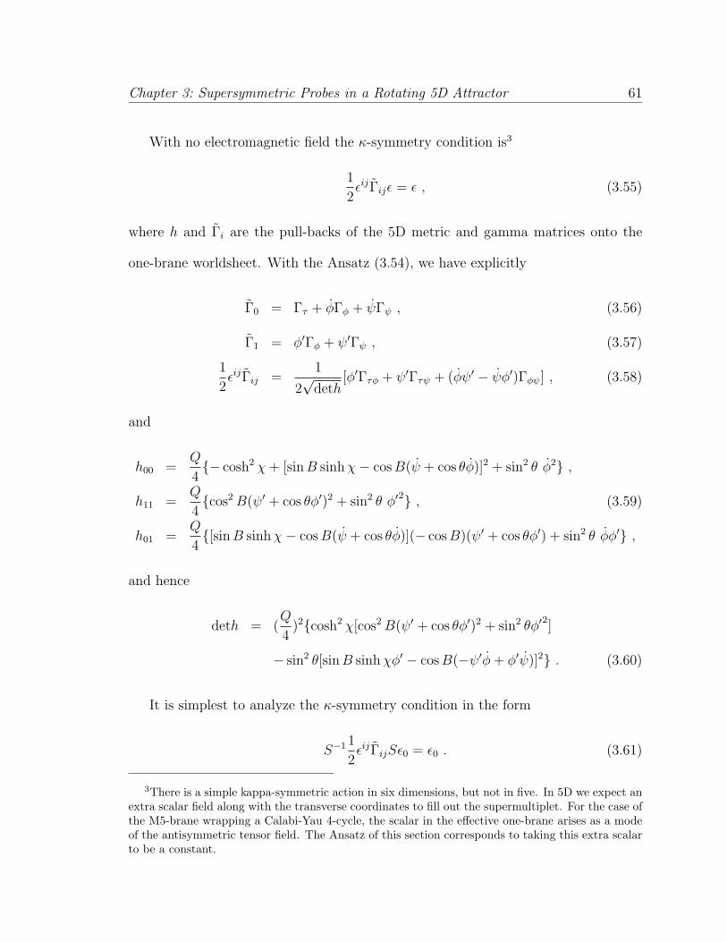
Chapter 3: Supersymmetric Probes in a Rotating 5D Attractor 61
With no electromagnetic field the κ-symmetry condition is3
1
2εijΓijε = ε , (3.55)
where h and Γi are the pull-backs of the 5D metric and gamma matrices onto the
one-brane worldsheet. With the Ansatz (3.54), we have explicitly
Γ0 = Γτ + φΓφ + ψΓψ , (3.56)
Γ1 = φ′Γφ + ψ′Γψ , (3.57)
1
2εijΓij =
1
2√
deth[φ′Γτφ + ψ′Γτψ + (φψ′ − ψφ′)Γφψ] , (3.58)
and
h00 =Q
4− cosh2 χ + [sin B sinh χ− cos B(ψ + cos θφ)]2 + sin2 θ φ2 ,
h11 =Q
4cos2 B(ψ′ + cos θφ′)2 + sin2 θ φ′2 , (3.59)
h01 =Q
4[sin B sinh χ− cos B(ψ + cos θφ)](− cos B)(ψ′ + cos θφ′) + sin2 θ φφ′ ,
and hence
deth = (Q
4)2cosh2 χ[cos2 B(ψ′ + cos θφ′)2 + sin2 θφ′2]
− sin2 θ[sin B sinh χφ′ − cos B(−ψ′φ + φ′ψ)]2 . (3.60)
It is simplest to analyze the κ-symmetry condition in the form
S−1 1
2εijΓijSε0 = ε0 . (3.61)
3There is a simple kappa-symmetric action in six dimensions, but not in five. In 5D we expect anextra scalar field along with the transverse coordinates to fill out the supermultiplet. For the case ofthe M5-brane wrapping a Calabi-Yau 4-cycle, the scalar in the effective one-brane arises as a modeof the antisymmetric tensor field. The Ansatz of this section corresponds to taking this extra scalarto be a constant.
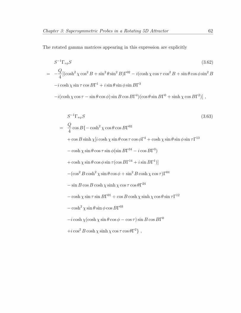
Chapter 3: Supersymmetric Probes in a Rotating 5D Attractor 62
The rotated gamma matrices appearing in this expression are explicitly
S−1ΓτφS (3.62)
= −Q
4[(cosh2 χ cos2 B + sin2 θ sin2 B)Γ02 − i(cosh χ cos τ cos2 B + sin θ cos φ sin2 B
−i cosh χ sin τ cos BΓ1 + i sin θ sin φ sin BΓ3
−i(cosh χ cos τ − sin θ cos φ) sin B cos BΓ4)(cos θ sin BΓ0 + sinh χ cos BΓ2)] ,
S−1ΓτψS (3.63)
=Q
4cos B− cosh2 χ cos θ cos BΓ02
+ cos B sinh χ[i cosh χ sin θ cos τ cos φΓ4 + cosh χ sin θ sin φ sin τΓ13
− cosh χ sin θ cos τ sin φ(sin BΓ34 − i cos BΓ3)
+ cosh χ sin θ cos φ sin τ(cos BΓ14 + i sin BΓ1)]
−(cos2 B cosh2 χ sin θ cos φ + sin2 B cosh χ cos τ)Γ04
− sin B cos B cosh χ sinh χ cos τ cos θΓ24
− cosh χ sin τ sin BΓ01 + cos B cosh χ sinh χ cos θ sin τΓ12
− cosh2 χ sin θ sin φ cos BΓ03
−i cosh χ(cosh χ sin θ cos φ− cos τ) sin B cos BΓ0
+i cos2 B cosh χ sinh χ cos τ cos θΓ2 ,
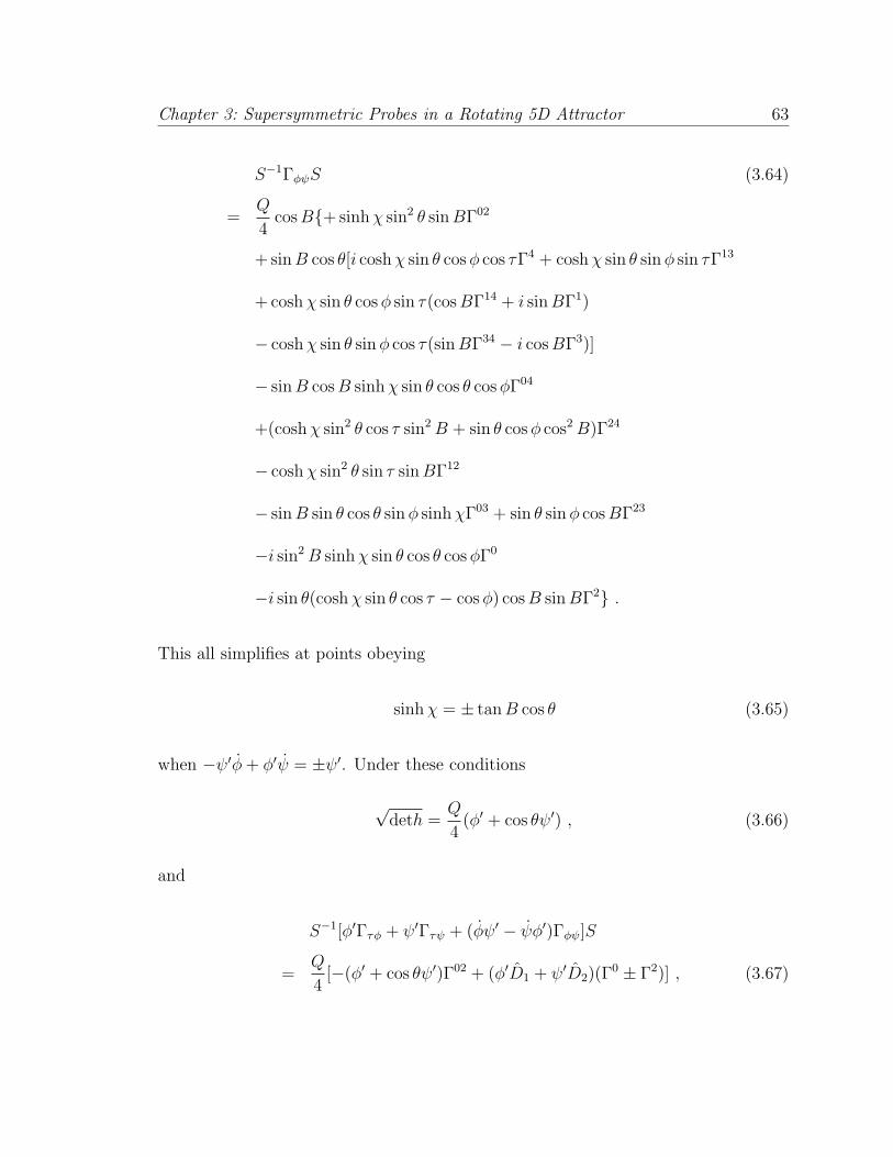
Chapter 3: Supersymmetric Probes in a Rotating 5D Attractor 63
S−1ΓφψS (3.64)
=Q
4cos B+ sinh χ sin2 θ sin BΓ02
+ sin B cos θ[i cosh χ sin θ cos φ cos τΓ4 + cosh χ sin θ sin φ sin τΓ13
+ cosh χ sin θ cos φ sin τ(cos BΓ14 + i sin BΓ1)
− cosh χ sin θ sin φ cos τ(sin BΓ34 − i cos BΓ3)]
− sin B cos B sinh χ sin θ cos θ cos φΓ04
+(cosh χ sin2 θ cos τ sin2 B + sin θ cos φ cos2 B)Γ24
− cosh χ sin2 θ sin τ sin BΓ12
− sin B sin θ cos θ sin φ sinh χΓ03 + sin θ sin φ cos BΓ23
−i sin2 B sinh χ sin θ cos θ cos φΓ0
−i sin θ(cosh χ sin θ cos τ − cos φ) cos B sin BΓ2 .
This all simplifies at points obeying
sinh χ = ± tan B cos θ (3.65)
when −ψ′φ + φ′ψ = ±ψ′. Under these conditions
√deth =
Q
4(φ′ + cos θψ′) , (3.66)
and
S−1[φ′Γτφ + ψ′Γτψ + (φψ′ − ψφ′)Γφψ]S
=Q
4[−(φ′ + cos θψ′)Γ02 + (φ′D1 + ψ′D2)(Γ
0 ± Γ2)] , (3.67)
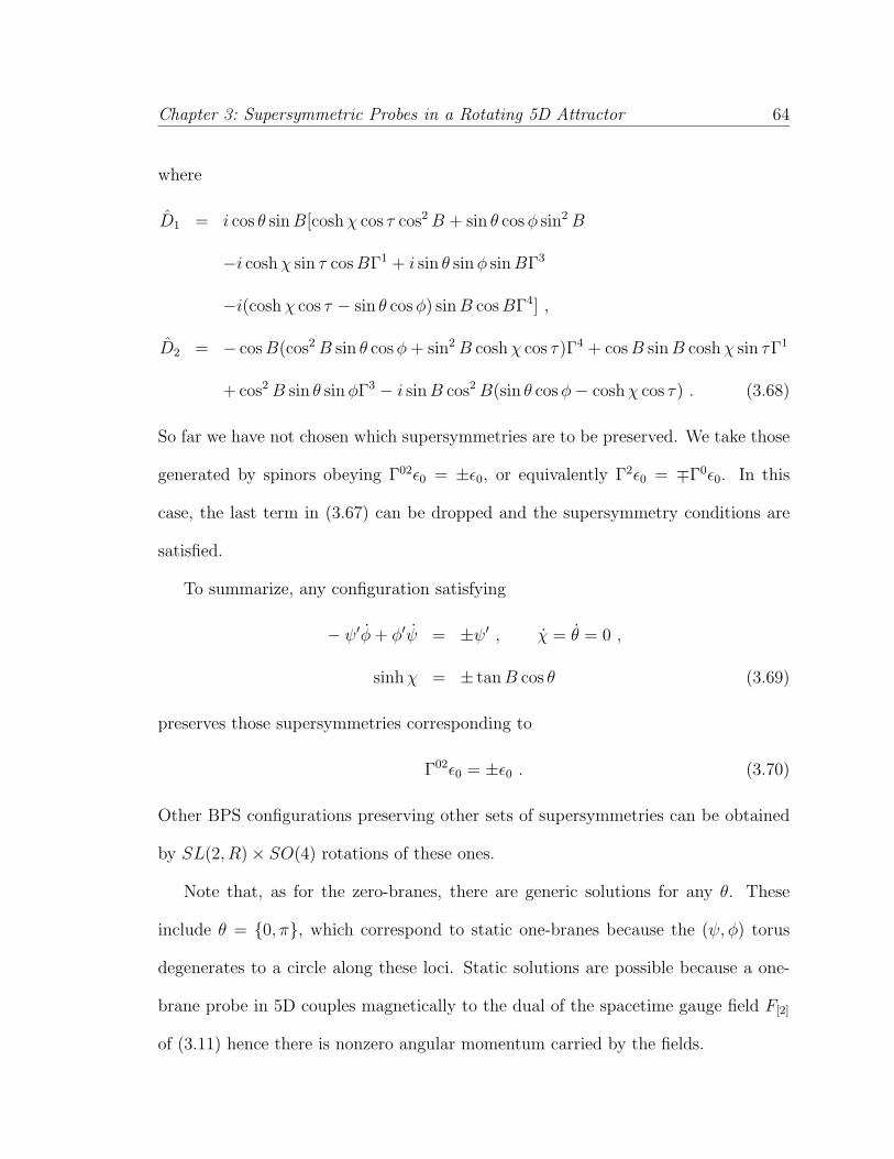
Chapter 3: Supersymmetric Probes in a Rotating 5D Attractor 64
where
D1 = i cos θ sin B[cosh χ cos τ cos2 B + sin θ cos φ sin2 B
−i cosh χ sin τ cos BΓ1 + i sin θ sin φ sin BΓ3
−i(cosh χ cos τ − sin θ cos φ) sin B cos BΓ4] ,
D2 = − cos B(cos2 B sin θ cos φ + sin2 B cosh χ cos τ)Γ4 + cos B sin B cosh χ sin τΓ1
+ cos2 B sin θ sin φΓ3 − i sin B cos2 B(sin θ cos φ− cosh χ cos τ) . (3.68)
So far we have not chosen which supersymmetries are to be preserved. We take those
generated by spinors obeying Γ02ε0 = ±ε0, or equivalently Γ2ε0 = ∓Γ0ε0. In this
case, the last term in (3.67) can be dropped and the supersymmetry conditions are
satisfied.
To summarize, any configuration satisfying
− ψ′φ + φ′ψ = ±ψ′ , χ = θ = 0 ,
sinh χ = ± tan B cos θ (3.69)
preserves those supersymmetries corresponding to
Γ02ε0 = ±ε0 . (3.70)
Other BPS configurations preserving other sets of supersymmetries can be obtained
by SL(2, R)× SO(4) rotations of these ones.
Note that, as for the zero-branes, there are generic solutions for any θ. These
include θ = 0, π, which correspond to static one-branes because the (ψ, φ) torus
degenerates to a circle along these loci. Static solutions are possible because a one-
brane probe in 5D couples magnetically to the dual of the spacetime gauge field F[2]
of (3.11) hence there is nonzero angular momentum carried by the fields.
Chapter 3: Supersymmetric Probes in a Rotating 5D Attractor 65
3.4 Conclusion
In this chapter, we constructed supersymmetric brane probe solutions in the
squashed AdS2 × S3 near-horizon geometry of the BMPV black hole.
We expect that the quantization of the moduli space of these classical configura-
tions will provide a microscopic description of the five-dimensional N = 2 rotating
black holes. This will be carried out in the future work.
Chapter 4
Non-Supersymmetric Attractor
Flow in Symmetric Spaces
4.1 Introduction
Soon after the attractor mechanism was first discovered in supersymmetric (BPS)
black holes [63], it was reformulated in terms of motion on an effective potential for
the moduli [62]. Ferrara et al demonstrated that the critical points of this potential
correspond to the attractor values of the moduli. More recently, several groups used
the effective potential to show that non-supersymmetric (non-BPS) extremal black
holes can also exhibit the attractor mechanism, thereby creating a new and exciting
field of research [92, 76]. Many connections between non-BPS attractors and other
active areas of string theory soon revealed themselves. Andrianopoli et al found that
both BPS and non-BPS black holes embedded in a supergravity with a symmetric
moduli space can be studied using the same formalism, and they uncovered many
66
Chapter 4: Non-Supersymmetric Attractor Flow in Symmetric Spaces 67
intricate relations between the two [11, 43]. Dabholkar, Sen and Trivedi proposed
a microstate counting for non-BPS black holes (albeit subject to certain constraints
[42]). Saraikin and Vafa suggested that a new extension of topological string theory
generalizes the Ooguri-Strominger-Vafa (OSV) formula such that it is also valid for
non-supersymmetric black holes [133]. Studying non-BPS attractors could also give
insight into non-supersymmetric flux vacua. Given all these possible applications, it
is important to characterize non-BPS black holes as fully as possible.
There has been a great deal of progress in understanding the near-horizon region
of these non-BPS attractors. The second derivative of the effective potential at the
critical point determines whether the black hole is an attractor, and the location of
the critical point yields the values of the moduli at the horizon; in this way, one can
compute the stability and attractor moduli for all models with cubic prepotential
[145, 113]. However, the effective potential has only been formulated for the leading-
order terms in the supergravity lagrangian. If one wants to include higher-derivative
corrections, one can instead use Sen’s entropy formalism, which incorporates Wald’s
formula, to characterize the near-horizon geometry in greater generality [135]. Sen’s
method has led to many new results [132, 13, 131, 36, 8, 136]. The tradeoff is that
this method cannot be used to determine any properties of the solution away from
the horizon.
The BPS attractor flow is constructed from the attractor value z∗BPS = z∗BPS(pI , qI)
by simply replacing the D-brane charges with the corresponding harmonic functions:
zBPS(~x) = z∗BPS(pI → HI(~x), qI → HI(~x)) , (4.1)

Chapter 4: Non-Supersymmetric Attractor Flow in Symmetric Spaces 68
where the harmonic functions are
HI(~x)
HI(~x)
=
hI
hI
+
1
|~x|
pI
qI
.
Moreover, this procedure can be applied to construct the multi-centered BPS attrac-
tor flow that describes the supersymmetric black hole bound state [18], where the
harmonic functions are generalized to have multiple centers:
HI(~x)
HI(~x)
=
hI
hI
+
∑i
1
|~x− ~xi|
(pI)i
(qI)i
.
It is conjectured in [91] that the non-BPS flow can be generated in the same fashion,
namely, by replacing the charges in the attractor value with the corresponding har-
monic functions. However, as will be proven in this chapter, this procedure does not
work for systems with generic charge and asymptotic moduli.1
In principle, one could construct the full non-BPS flow (the black hole metric,
together with the attractor flow of the moduli) by solving the equation of motion
derived from the Lagrangian. However, this is a second-order differential equation
and only reduces to a first-order equation upon demanding the preservation of su-
persymmetry. Ceresole et al have written down an equivalent first-order equation in
terms of a “fake superpotential,” but the fake superpotential can only be explicitly
constructed for special charges and asymptotic moduli [34, 98]. The most generic
non-BPS equation of motion is complicated enough that it has not yet been solved.
Similarly, multi-centered non-BPS black holes have not been studied.
Our goal is to construct the full flow for non-BPS stationary black holes in four
dimensions. Instead of directly solving the equation of motion, we reduce the action
1This has also been shown in [98]
Chapter 4: Non-Supersymmetric Attractor Flow in Symmetric Spaces 69
on the timelike isometry and dualize all 4D vectors to scalars. The new moduli space
M3D contains isometries corresponding to all the charges of the black hole, and the
black hole solutions are simply geodesics on M3D. This method was introduced in
[29] and has been used to construct static and rotating black holes in heterotic string
theory [39, 40] and to study the classical BPS single-centered flow and its radial
quantization [81, 114].
In this chapter, we work in two specific theories of gravity, but we expect that this
method can be used for any model whose M3D is symmetric. The basic technique
is reviewed in more detail in Section 4.2. In Section 4.3, we show how this method
works in a simple case: the toroidal compactification of D-dimensional pure gravity.
Section 4.4 serves as an introduction to single-centered attractor flow in N = 2
supergravity coupled to one vector multiplet, and Sections 4.5 and 4.6 are dedicated
to constructing the full flows for both BPS and non-BPS single-centered black holes
with generic charges. We find that they are generated by the action of different classes
of nilpotent elements in the coset algebra. Both types of flows are shown to reach the
correct attractor values at the horizon. In Section 4.7, the procedure is generalized
straightforwardly to construct both BPS and non-BPS multi-centered solutions. We
use a metric ansatz with a flat spatial slice and we are able to recover the BPS bound
states described by Bates and Denef. Using the same ansatz, we are able to build
non-BPS multi-centered solutions. Unfortunately, solutions generated this way turn
out to always have charges at each center which are mutually local. The last section
reviews our conclusions and suggests possibilities for future work.
Chapter 4: Non-Supersymmetric Attractor Flow in Symmetric Spaces 70
4.2 Framework
Here we outline the method we will use to construct black hole solutions. This
method was first described in [29]. We first reduce a general gravity action from four
dimensions down to three, and derive the equation of motion. We then specialize to
certain theories which have a 3D description in terms of a symmetric coset space.
In such situations, we can easily find solutions to the equation of motion. The solu-
tions are geodesics (or generalizations thereof) on the 3D moduli space and they are
generated by elements of the coset algebra.
4.2.1 3D moduli space
We will study stationary solutions in a theory with gravity coupled to scalar and
vector matter. Let the scalars be zi and the vectors be AI . Then the most general
ansatz for a stationary solution in four dimensions is:
ds2 = −e2U(dt + ω)2 + e−2Ugabdxadxb , (4.2)
F I = dAI = d(AI
0(dt + ω) + AI)
, (4.3)
where a, b = 1, 2, 3 label the spatial directions and bold font denotes three-dimensional
fields and operators. Since none of the fields are time-dependent, we can compactify
on the time isometry and reduce to three-dimensional space M3D. This procedure
is called the c∗-map. In three dimensions, a vector is Hodge-dual to a scalar. The
equations of motion for ω and the gauge fields allow us to define the dual scalars φω
and φAI .
Chapter 4: Non-Supersymmetric Attractor Flow in Symmetric Spaces 71
We then obtain the 3D lagrangian in terms of only scalars
L =1
2
√g(−1
κR + ∂aφ
m∂aφngmn) , (4.4)
where φn are the moduli fields
φn = U, zi, z i, φω, AI0, φAI (4.5)
and gab is the space time metric and gmn is the metric of a manifoldM3D. The system
is 3D gravity minimally coupled to a nonlinear sigma model with moduli space M3D.
Next, we will find the equation of motion in this theory.
4.2.2 Attractor flow equation
The equation of motion of 3D gravity is Einstein’s equation:
Rab − 1
2gabR = κTab = κ(∂aφ
m∂bφngmn − 1
2gab∂cφ
m∂cφngmn) , (4.6)
and the equation of motion of the moduli is:
∇a∇aφn + Γnmp∂aφ
m∂aφp = 0 . (4.7)
For simplicity, we consider only the case where the 3D spatial slice is flat (it is guar-
anteed to be flat only for extremal single-centered black holes). Then the dynamics
of the moduli are decoupled from that of the 3D gravity:
Rab = 0 =⇒ ∂aφm∂bφ
ngmn = 0 . (4.8)
In the multi-centered case, we need to solve the full equations for the moduli as
functions of the 3D coordinates ~x. For single-centered solutions, the moduli only
Chapter 4: Non-Supersymmetric Attractor Flow in Symmetric Spaces 72
depend on r; to satisfy the above equations, the motion of the moduli must follow
null geodesics inside M3D.
A generic null geodesic flows to the boundary of the moduli space M3D. A single-
centered attractor flow is defined as a null geodesic that terminates at a point on the
U → −∞ boundary and in the interior region with respect to all other coordinates.
This is guaranteed for the BPS attractor by the constraints imposed by the super-
symmetry. To find the single-centered non-supersymmetric attractor flow, one needs
to find a way to construct null geodesics and a constraint that picks out the ones that
stop at this specific component of the boundary. In the next section, we will show
that we can do this for models with special properties, and the method can be easily
generalized to find the multi-centered attractor solution.
4.2.3 Models with symmetric moduli space
The problem of finding such a constraint in a generic model is not easy. To
simplify, we study any model whose moduli space is a symmetric homogeneous space:
M3D = G/H. When M3D is a homogeneous space, the isometry group G acts
transitively on M3D. H denotes the isotropy group, which is the maximal compact
subgroup of G when one compactifies on a spatial isometry down to (1, 2) space,
or the analytical continuation of the maximal compact subgroup of G when one
compactifies on the time isometry down to (0, 3) space. The Lie algebra g has the
Cartan decomposition: g = h⊕ k where
[h,h] = h , [h,k] = k . (4.9)
Chapter 4: Non-Supersymmetric Attractor Flow in Symmetric Spaces 73
When G is semi-simple, the homogeneous space is symmetric, and
[k,k] = h . (4.10)
The models with symmetric moduli space includes: D-dimensional gravity toroidal-
ly compactified to four dimensions, certain models of 4D N = 2 supergravity coupled
to vector-multiplet, and all 4D N > 2 extended supergravity. The entropy of the
last two classes is U-duality invariant. In the present work, we will only consider the
first two classes, namely, the D-dimensional gravity toroidally compactified to four
dimensions, and the 4D N = 2 supergravity coupled to nV vector-multiplet.
The left-invariant current is
J = M−1dM = Jk + Jh , (4.11)
where M is the coset representative, and Jk is the projection of J onto the coset
algebra k. The lagrangian density of the sigma-model with target space G/H is
given by Jk as:
L = Tr(Jk ∧ ∗3Jk) . (4.12)
The geodesic of the homogeneous space written in terms of the coset representative
is simply
M = M0ekτ/2 with k ∈ k , (4.13)
where M0 parameterizes the initial point, and the 12
is for later convenience. A null
geodesic has zero length:
|k|2 = 0 . (4.14)
Therefore, in a homogeneous space, we can find the null geodesics that end at an
Chapter 4: Non-Supersymmetric Attractor Flow in Symmetric Spaces 74
attractor point by imposing the appropriate constraint on the null elements of the
coset algebra.
Since M is defined up to the action of the isotropy group H, in order to read
off the moduli fields from M in an H-independent way, we construct the symmetric
matrix using the metric signature matrix S0:
S ≡ MS0MT . (4.15)
In all systems considered in the present work, H is the maximal orthogonal subgroup
of G with the correct signature:
HS0HT = S0 for ∀H ∈ H . (4.16)
That is, the isotropy group H preserves the symmetric metric matrix S0. Therefore,
S is invariant under M → MH with H ∈ H. Moreover, as the isotropy group H acts
transitively on the space of of matrices with a given signature, the space of possible
S is the same as the symmetric space G/H. That is, the moduli of G/H can be
combined into the symmetric matrix S. And the current of S is
JS = S−1dS . (4.17)
It is easy to perform the projection onto the coset algebra k. The (generalized)
orthogonality condition of the isotropy group H can be expressed in terms of the
subalgebra element h which is in H = eh as
hS0 + S0hT = 0 ∀h ∈ h . (4.18)
In other words, (hS0) is anti-symmetric: (hS0)T = −(hS0). Thus the coset algebra,
being the compliment of h, can be defined as the k with (kS0) being symmetric:
Chapter 4: Non-Supersymmetric Attractor Flow in Symmetric Spaces 75
(kS0)T = (kS0), i.e.
kT = S−10 kS0 ∀ k ∈ k . (4.19)
Therefore, the projection of an element g in g onto the coset algebra k is:
gk =g + S0g
T S−10
2. (4.20)
For the left-invariant current J = M−1dM , the projection onto k is:
Jk =J + S0J
T S−10
2. (4.21)
It is straightforward to show that the current constructed from S is related to the
projected left-invariant current Jk by:
JS = S−1dS = 2(S0MT )−1Jk(S0M
T ) . (4.22)
The lagrangian in terms of S is thus L = 14Tr(JS ∧ ∗3JS). That is, the lagrangian
density is
L =1
4Tr(S−1∇S · S−1∇S) , (4.23)
which is invariant under the action of the isometry group G:
S → G−1SG where G ∈ G (4.24)
and whose conserved current is:
J = S−1∇S , (4.25)
where we have dropped the subscript S in JS, since we will only be dealing with this
current from now on. The equation of motion is the conservation of the current:
∇ · J = ∇ · (S−1∇S) = 0 . (4.26)
Chapter 4: Non-Supersymmetric Attractor Flow in Symmetric Spaces 76
We now specialize to the single-centered solutions: they correspond to geodesics in
the coset manifold. The spherical symmetry allows the 3D metric to be parameterized
as
ds23 = C(r)2d~x2 . (4.27)
Then the equations of motion involve the operator drr2C(r)dr, and reduce to geodesic
equations in terms of a parameter τ such that
dr
dτ= r2C(r) . (4.28)
The function C(r) is then determined from the equations of motion of 3D gravity.
The equations of motion can be written as
d
dτ(S−1dS
dτ) = 0 . (4.29)
In the extremal limit the geodesics become null, the 3D metric is flat and
τ = −1
r. (4.30)
In the search for multi-centered extremal solutions, where the spherical symmetry
is absent, it is very convenient to restrict to solutions with a flat 3D metric. This is
consistent with the equations of motion as long as the 3D energy momentum tensor
is zero everywhere:
Tab = Tr(JaJb) = 0 . (4.31)
The coupled problem with generic non-flat 3D metric is much harder, and exact
solutions are hard to find unless a second Killing vector is present.
Since different values of the scalars at infinity are easily obtained by a G transfor-
mation, to start with, we will consider the flow starting from M0 = 1, and generalize
Chapter 4: Non-Supersymmetric Attractor Flow in Symmetric Spaces 77
to generic asymptotic moduli later. For a single-centered solution, the flow of M is
M = M0ekτ/2. Since all the coset representatives can be brought into the form eg
with some g ∈ k by an H-action, we can write M0 = eg/2, so M = eg/2ekτ/2. And the
flow of S is
S(τ) = eg/2ekτeg/2S0 . (4.32)
The charges of the solution are read from the conserved currents
J(r) = S−1∇S =S0e
−g/2keg/2S0
r2~r . (4.33)
4.3 Toroidal Reduction of D-dimensional Pure
Gravity
Now we use the method introduced in the previous section to analyze pure gravity
toroidally compactified down to four dimensions. We explain why the attractor flow
generator, k, needs to be nilpotent, and we find the Jordan forms of k2 and k. Using
this information, we construct single-centered attractor flows. We then generalize to
multi-centered black holes in pure gravity and show that these solutions have mutually
local charges and no intrinsic angular momentum.
4.3.1 Kaluza-Klein reduction
The simplest example of a system that admits a 3D description in terms of a
sigma model on a symmetric space is pure gravity in D dimensions, compactified on
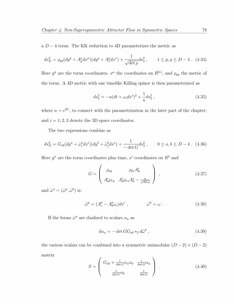
Chapter 4: Non-Supersymmetric Attractor Flow in Symmetric Spaces 78
a D − 4 torus. The KK reduction to 4D parameterizes the metric as
ds2D = ρpq(dyp + Ap
µdxµ)(dyq + Aqνdxν) +
1√det ρ
ds24 , 1 ≤ p, q ≤ D − 4 . (4.34)
Here yp are the torus coordinates, xµ the coordinates on R3,1, and ρpq the metric of
the torus. A 4D metric with one timelike Killing spinor is then parameterized as
ds24 = −u(dt + ωidxi)2 +
1
uds2
3 , (4.35)
where u = e2U , to connect with the parametrization in the later part of the chapter;
and i = 1, 2, 3 denote the 3D space coordinates.
The two expressions combine as
ds2D = Gab(dya + ωa
i dxi)(dyb + ωbjdxj) +
1
− det Gds2
3 , 0 ≤ a, b ≤ D − 4 . (4.36)
Here ya are the torus coordinates plus time, xi coordinates on R3 and
G =
ρpq ρprAr0
Ar0ρrq Ar
0ρrsAs0 − u√
det ρ
, (4.37)
and ωa = (ωp, ω0) is:
ωp = (Api − Ap
0ωi)dxi , ω0 = ω . (4.38)
If the forms ωa are dualized to scalars αa as
dαa = − det GGab ∗3 dωb , (4.39)
the various scalars can be combined into a symmetric unimodular (D− 2)× (D− 2)
matrix
S =
Gab + 1det G
αaαb1
det Gαa
1det G
αb1
det G
. (4.40)
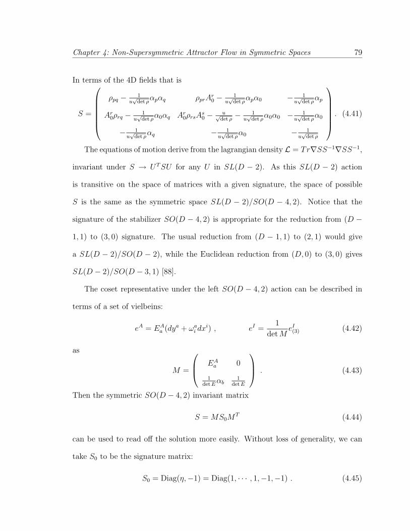
Chapter 4: Non-Supersymmetric Attractor Flow in Symmetric Spaces 79
In terms of the 4D fields that is
S =
ρpq − 1u√
det ραpαq ρprA
r0 − 1
u√
det ραpα0 − 1
u√
det ραp
Ar0ρrq − 1
u√
det ρα0αq Ar
0ρrsAs0 − u√
det ρ− 1
u√
det ρα0α0 − 1
u√
det ρα0
− 1u√
det ραq − 1
u√
det ρα0 − 1
u√
det ρ
. (4.41)
The equations of motion derive from the lagrangian density L = Tr∇SS−1∇SS−1,
invariant under S → UT SU for any U in SL(D − 2). As this SL(D − 2) action
is transitive on the space of matrices with a given signature, the space of possible
S is the same as the symmetric space SL(D − 2)/SO(D − 4, 2). Notice that the
signature of the stabilizer SO(D − 4, 2) is appropriate for the reduction from (D −
1, 1) to (3, 0) signature. The usual reduction from (D − 1, 1) to (2, 1) would give
a SL(D − 2)/SO(D − 2), while the Euclidean reduction from (D, 0) to (3, 0) gives
SL(D − 2)/SO(D − 3, 1) [88].
The coset representative under the left SO(D − 4, 2) action can be described in
terms of a set of vielbeins:
eA = EAa (dya + ωa
i dxi) , eI =1
det MeI(3) (4.42)
as
M =
EAa 0
1det E
αb1
det E
. (4.43)
Then the symmetric SO(D − 4, 2) invariant matrix
S = MS0MT (4.44)
can be used to read off the solution more easily. Without loss of generality, we can
take S0 to be the signature matrix:
S0 = Diag(η,−1) = Diag(1, · · · , 1,−1,−1) . (4.45)
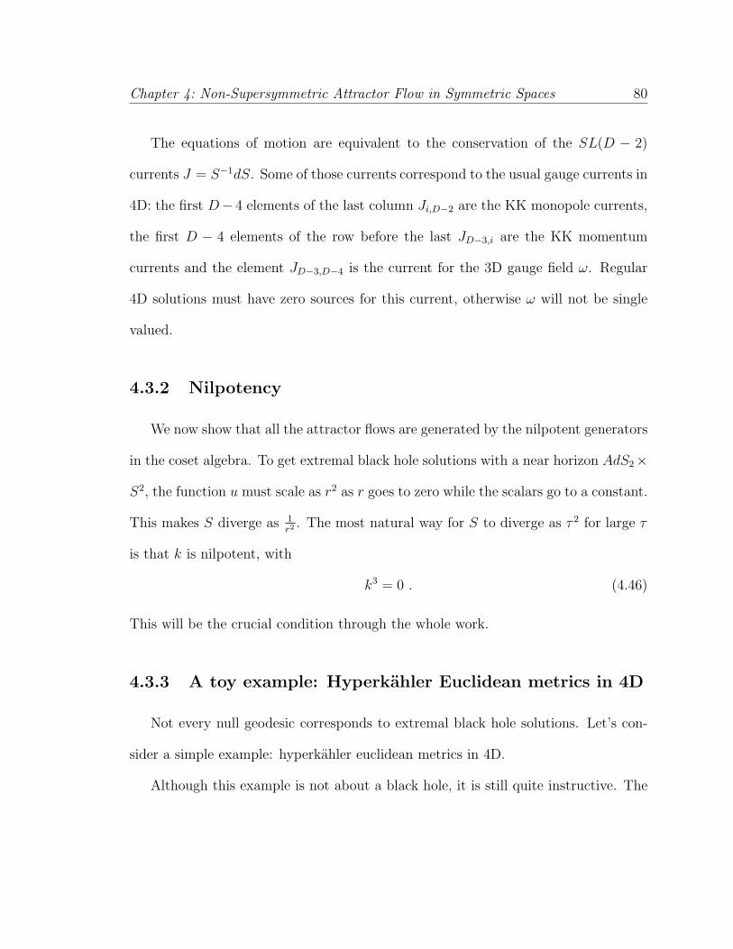
Chapter 4: Non-Supersymmetric Attractor Flow in Symmetric Spaces 80
The equations of motion are equivalent to the conservation of the SL(D − 2)
currents J = S−1dS. Some of those currents correspond to the usual gauge currents in
4D: the first D− 4 elements of the last column Ji,D−2 are the KK monopole currents,
the first D − 4 elements of the row before the last JD−3,i are the KK momentum
currents and the element JD−3,D−4 is the current for the 3D gauge field ω. Regular
4D solutions must have zero sources for this current, otherwise ω will not be single
valued.
4.3.2 Nilpotency
We now show that all the attractor flows are generated by the nilpotent generators
in the coset algebra. To get extremal black hole solutions with a near horizon AdS2×
S2, the function u must scale as r2 as r goes to zero while the scalars go to a constant.
This makes S diverge as 1r2 . The most natural way for S to diverge as τ 2 for large τ
is that k is nilpotent, with
k3 = 0 . (4.46)
This will be the crucial condition through the whole work.
4.3.3 A toy example: Hyperkahler Euclidean metrics in 4D
Not every null geodesic corresponds to extremal black hole solutions. Let’s con-
sider a simple example: hyperkahler euclidean metrics in 4D.
Although this example is not about a black hole, it is still quite instructive. The
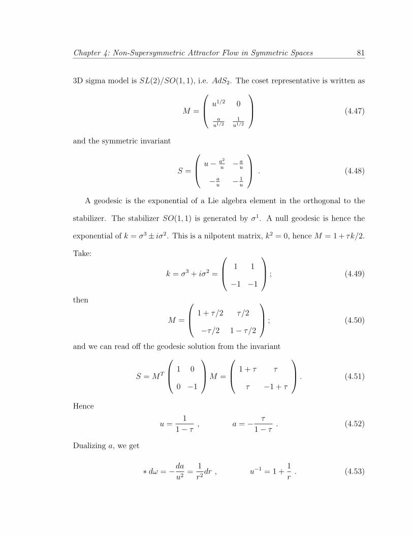
Chapter 4: Non-Supersymmetric Attractor Flow in Symmetric Spaces 81
3D sigma model is SL(2)/SO(1, 1), i.e. AdS2. The coset representative is written as
M =
u1/2 0
au1/2
1u1/2
(4.47)
and the symmetric invariant
S =
u− a2
u− a
u
− au
− 1u
. (4.48)
A geodesic is the exponential of a Lie algebra element in the orthogonal to the
stabilizer. The stabilizer SO(1, 1) is generated by σ1. A null geodesic is hence the
exponential of k = σ3± iσ2. This is a nilpotent matrix, k2 = 0, hence M = 1 + τk/2.
Take:
k = σ3 + iσ2 =
1 1
−1 −1
; (4.49)
then
M =
1 + τ/2 τ/2
−τ/2 1− τ/2
; (4.50)
and we can read off the geodesic solution from the invariant
S = MT
1 0
0 −1
M =
1 + τ τ
τ −1 + τ
. (4.51)
Hence
u =1
1− τ, a = − τ
1− τ. (4.52)
Dualizing a, we get
∗ dω = −da
u2=
1
r2dr , u−1 = 1 +
1
r. (4.53)
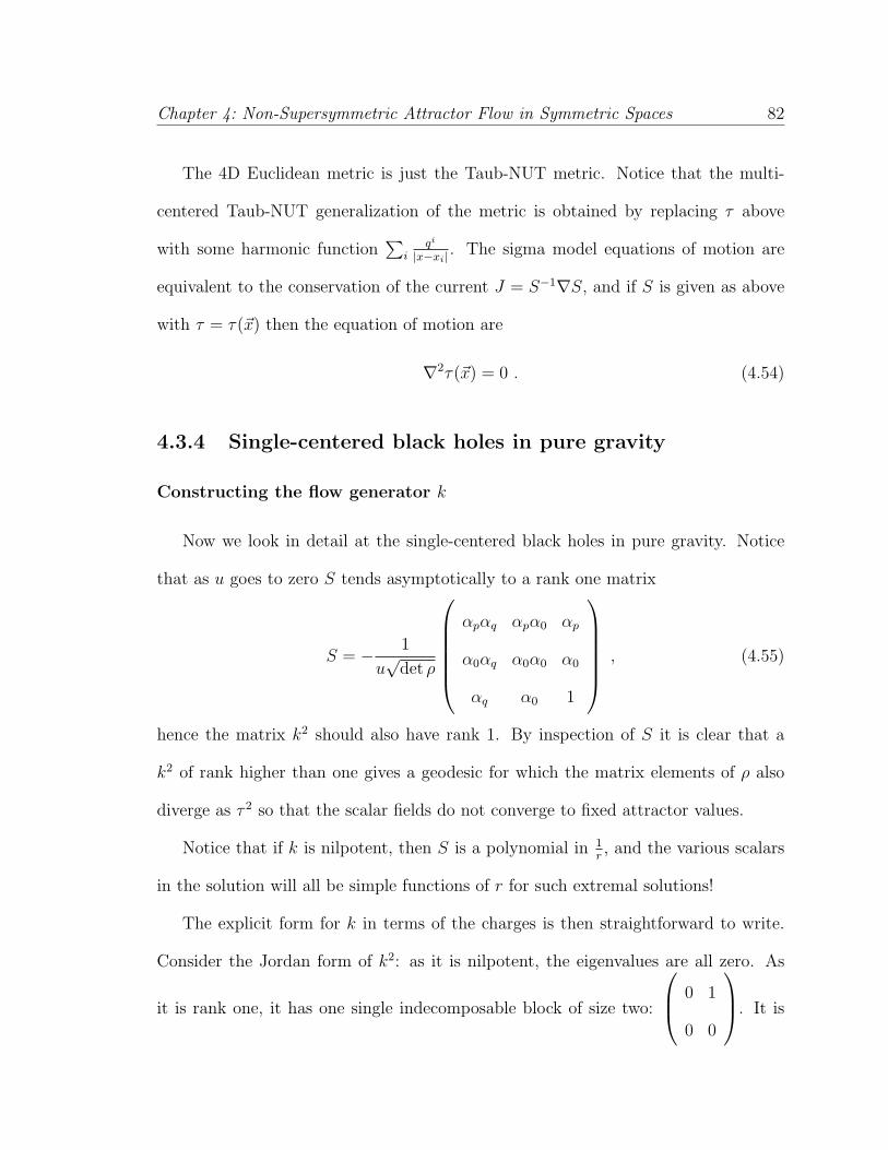
Chapter 4: Non-Supersymmetric Attractor Flow in Symmetric Spaces 82
The 4D Euclidean metric is just the Taub-NUT metric. Notice that the multi-
centered Taub-NUT generalization of the metric is obtained by replacing τ above
with some harmonic function∑
iqi
|x−xi| . The sigma model equations of motion are
equivalent to the conservation of the current J = S−1∇S, and if S is given as above
with τ = τ(~x) then the equation of motion are
∇2τ(~x) = 0 . (4.54)
4.3.4 Single-centered black holes in pure gravity
Constructing the flow generator k
Now we look in detail at the single-centered black holes in pure gravity. Notice
that as u goes to zero S tends asymptotically to a rank one matrix
S = − 1
u√
det ρ
αpαq αpα0 αp
α0αq α0α0 α0
αq α0 1
, (4.55)
hence the matrix k2 should also have rank 1. By inspection of S it is clear that a
k2 of rank higher than one gives a geodesic for which the matrix elements of ρ also
diverge as τ 2 so that the scalar fields do not converge to fixed attractor values.
Notice that if k is nilpotent, then S is a polynomial in 1r, and the various scalars
in the solution will all be simple functions of r for such extremal solutions!
The explicit form for k in terms of the charges is then straightforward to write.
Consider the Jordan form of k2: as it is nilpotent, the eigenvalues are all zero. As
it is rank one, it has one single indecomposable block of size two:
0 1
0 0
. It is
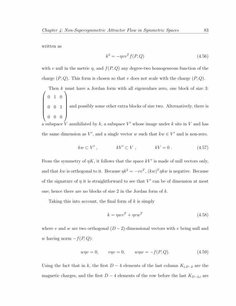
Chapter 4: Non-Supersymmetric Attractor Flow in Symmetric Spaces 83
written as
k2 = −ηvvT f(P,Q) (4.56)
with v null in the metric η, and f(P,Q) any degree-two homogeneous function of the
charge (P,Q). This form is chosen so that v does not scale with the charge (P,Q).
Then k must have a Jordan form with all eigenvalues zero, one block of size 3:
0 1 0
0 0 1
0 0 0
and possibly some other extra blocks of size two. Alternatively, there is
a subspace V annihilated by k, a subspace V ′ whose image under k sits in V and has
the same dimension as V ′, and a single vector w such that kw ∈ V ′ and is non-zero.
kw ⊂ V ′ , kV ′ ⊂ V , kV = 0 . (4.57)
From the symmetry of ηK, it follows that the space kV ′ is made of null vectors only,
and that kw is orthogonal to it. Because ηk2 = −vvT , (kw)T ηkw is negative. Because
of the signature of η it is straightforward to see that V ′ can be of dimension at most
one; hence there are no blocks of size 2 in the Jordan form of k.
Taking this into account, the final form of k is simply
k = ηwvT + ηvwT (4.58)
where v and w are two orthogonal (D− 2)-dimensional vectors with v being null and
w having norm −f(P,Q):
wηv = 0, vηv = 0, wηw = −f(P,Q). (4.59)
Using the fact that in k, the first D − 4 elements of the last column Ki,D−2 are the
magnetic charges, and the first D − 4 elements of the row before the last KD−3,i are
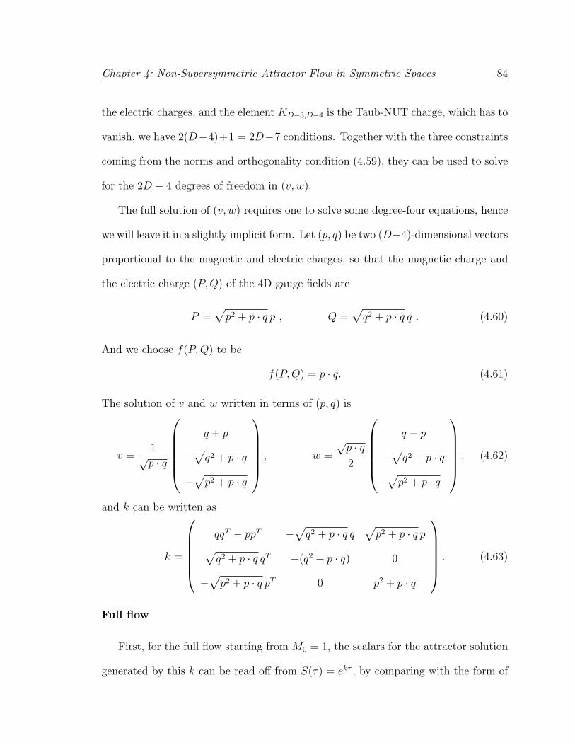
Chapter 4: Non-Supersymmetric Attractor Flow in Symmetric Spaces 84
the electric charges, and the element KD−3,D−4 is the Taub-NUT charge, which has to
vanish, we have 2(D−4)+1 = 2D−7 conditions. Together with the three constraints
coming from the norms and orthogonality condition (4.59), they can be used to solve
for the 2D − 4 degrees of freedom in (v, w).
The full solution of (v, w) requires one to solve some degree-four equations, hence
we will leave it in a slightly implicit form. Let (p, q) be two (D−4)-dimensional vectors
proportional to the magnetic and electric charges, so that the magnetic charge and
the electric charge (P,Q) of the 4D gauge fields are
P =√
p2 + p · q p , Q =√
q2 + p · q q . (4.60)
And we choose f(P,Q) to be
f(P,Q) = p · q. (4.61)
The solution of v and w written in terms of (p, q) is
v =1√p · q
q + p
−√
q2 + p · q
−√
p2 + p · q
, w =
√p · q2
q − p
−√
q2 + p · q√
p2 + p · q
, (4.62)
and k can be written as
k =
qqT − ppT −√
q2 + p · q q√
p2 + p · q p
√q2 + p · q qT −(q2 + p · q) 0
−√
p2 + p · q pT 0 p2 + p · q
. (4.63)
Full flow
First, for the full flow starting from M0 = 1, the scalars for the attractor solution
generated by this k can be read off from S(τ) = ekτ , by comparing with the form of
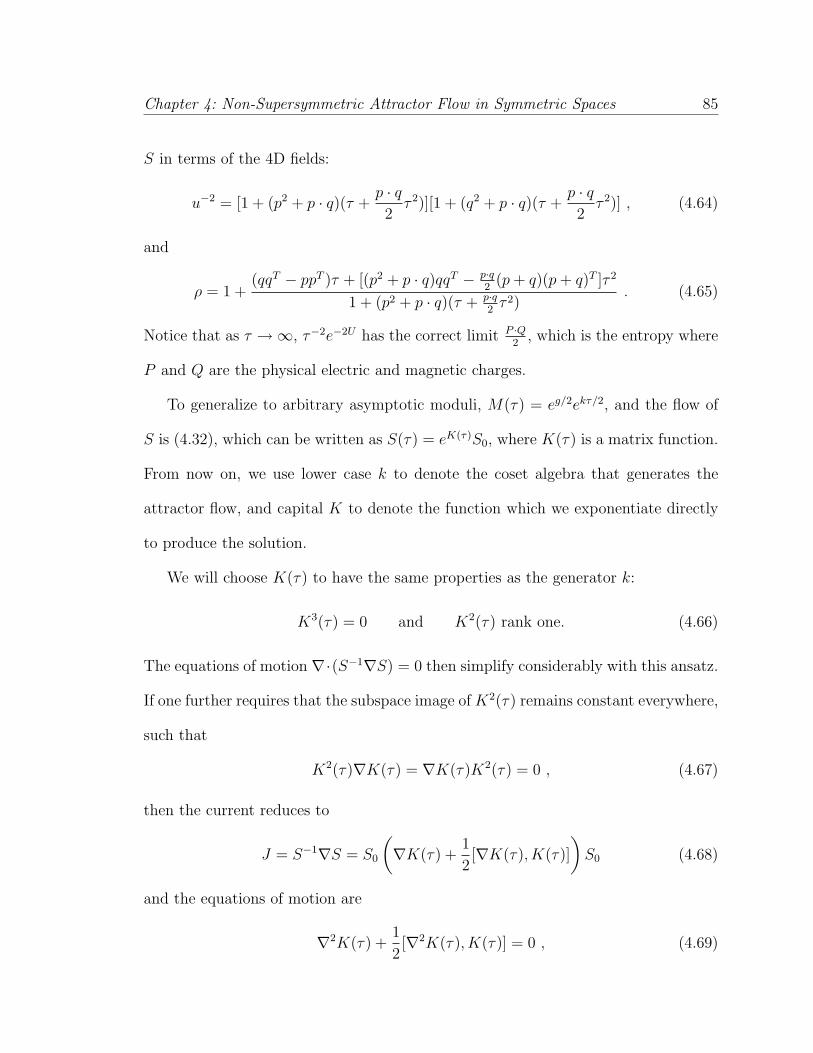
Chapter 4: Non-Supersymmetric Attractor Flow in Symmetric Spaces 85
S in terms of the 4D fields:
u−2 = [1 + (p2 + p · q)(τ +p · q2
τ 2)][1 + (q2 + p · q)(τ +p · q2
τ 2)] , (4.64)
and
ρ = 1 +(qqT − ppT )τ + [(p2 + p · q)qqT − p·q
2(p + q)(p + q)T ]τ 2
1 + (p2 + p · q)(τ + p·q2
τ 2). (4.65)
Notice that as τ →∞, τ−2e−2U has the correct limit P ·Q2
, which is the entropy where
P and Q are the physical electric and magnetic charges.
To generalize to arbitrary asymptotic moduli, M(τ) = eg/2ekτ/2, and the flow of
S is (4.32), which can be written as S(τ) = eK(τ)S0, where K(τ) is a matrix function.
From now on, we use lower case k to denote the coset algebra that generates the
attractor flow, and capital K to denote the function which we exponentiate directly
to produce the solution.
We will choose K(τ) to have the same properties as the generator k:
K3(τ) = 0 and K2(τ) rank one. (4.66)
The equations of motion ∇·(S−1∇S) = 0 then simplify considerably with this ansatz.
If one further requires that the subspace image of K2(τ) remains constant everywhere,
such that
K2(τ)∇K(τ) = ∇K(τ)K2(τ) = 0 , (4.67)
then the current reduces to
J = S−1∇S = S0
(∇K(τ) +
1
2[∇K(τ), K(τ)]
)S0 (4.68)
and the equations of motion are
∇2K(τ) +1
2[∇2K(τ), K(τ)] = 0 , (4.69)
Chapter 4: Non-Supersymmetric Attractor Flow in Symmetric Spaces 86
which is solved by a harmonic K(τ).
It might appear hard to find a K(τ) that is harmonic and satisfies all the required
constraints. However, by remembering that the constraints dictate K(τ) to have the
form:
K(τ) = ηV W T + ηWV T , (4.70)
where V is null and does not scale with the charge (P,Q), and W orthogonal to V
everywhere, one can simply pick a constant null vector V = v′ and a harmonic vector
W (τ) everywhere orthogonal to v′:
W (τ) = w′τ + m with v′ ·W (τ) = 0 . (4.71)
Here m is a (D− 2)-vector and contains the information of asymptotic moduli. Thus
an appropriate K(τ) is built:
K(τ) = k′τ + g (4.72)
where
k′ = ηv′w′T + ηw′v′T , g = ηv′mT + ηmv′T . (4.73)
Now we need to solve for (v′, w′) for the same charge (P,Q) but in the presence
of m. The form of g guaranteed that
[k′, g] = 0 , (4.74)
where we have used the fact that v′ is null and w′ is orthogonal to v′. Therefore,
shifting the starting point of moduli does not change the current as a function of
(v, w):
J(v′, w′) = S0
(k′
r2
)S0 = S0
(ηv′(w′)T + ηw′(v′)T
r2~r
)S0 . (4.75)
Chapter 4: Non-Supersymmetric Attractor Flow in Symmetric Spaces 87
Thus, the solution of (v′, w′) in terms of charges solved from the current does not
change as we vary the starting point of the flow, i.e. they do not depend on the
asymptotic moduli:
v′(Q) = v(Q) w′(Q) = w(Q) . (4.76)
In summary, the flow with arbitrary starting point is simply generated by
K(τ) = ηvW (τ)T + ηW (τ)vT with W = wτ + m , (4.77)
where (v, w) only depend on the charges (P,Q) and m gives the asymptotic moduli.
Example: 5D pure gravity compactified on a circle.
Consider for example the case of extremal black holes in D = 5 pure gravity
compactified on a circle. The 3D sigma model is SL(3)/SO(1, 2). The symmetric
invariant is
Sgr =
ρ− 1u√
ρα1α1 ρA0 − 1
u√
ρα1α0 − 1
u√
ρα1
ρA0 − 1u√
ρα1α0 ρ(A0)
2 − u√ρ− 1
u√
ρα0α0 − 1
u√
ρα0
− 1u√
ρα1 − 1
u√
ρα0 − 1
u√
ρ
. (4.78)
Then we can calculate S = S0ekτ using (4.63) and compare the result to Sgr above
to solve for all the scalars. We find that
e−2U =
√[1 + (q2 + pq)(τ +
pq
2τ 2)][1 + (p2 + pq)(τ +
pq
2τ 2)] (4.79)
ρ =1 + (q2 + pq)(τ + pq
2τ 2)
1 + (p2 + pq)(τ + pq2τ 2)
(4.80)
when starting from the identity. If we allow arbitrary g the flow is too complicated
to write explicitly here, but the attractor value of ρ is the same: q/p.
Chapter 4: Non-Supersymmetric Attractor Flow in Symmetric Spaces 88
4.3.5 Multi-centered solutions in pure gravity
In the context of pure gravity compactified on a torus, we can also give some
examples of multi-centered solutions in the same spirit as the ones for BPS solutions
in N = 2 supergravity, though some important features of the latter are not present
here.
We are interested in solutions given in terms of harmonic functions which can
generalize the single-centered extremal solutions presented above. Similar to the
single-centered case, we exponentiate a matrix function K(~x):
S(~x) = eK(~x)S0 . (4.81)
We will choose K(~x) to have the same properties of the generator k:
K3(~x) = 0 and K2(~x) rank one. (4.82)
Using a similar argument to the single-centered flow, we require that the subspace
image of K2(~x) remains constant everywhere, such that
K2(~x)∇K(~x) = ∇K(~x)K2(~x) = 0 , (4.83)
then the equations of motion are
∇2K(~x) +1
2[∇2K(~x), K(~x)] = 0 , (4.84)
which is solved by a harmonic K(~x).
A multi-centered K(~x) that is harmonic and satisfies all the required constraints
can then be built in the same way as the single-centered one:
K(~x) = ηvW (~x)T + ηW (~x)vT , (4.85)
Chapter 4: Non-Supersymmetric Attractor Flow in Symmetric Spaces 89
where v is the same constant null vector as in k, and W (~x) is the multi-centered
harmonic function:
W (~x) =∑
i
wi
|~x− ~xi| + m , (4.86)
where ~xi is the position of the ith center, and wi is determined by the charges at the ith
center, and m is related to the moduli at infinity. Requiring W (~x) to be orthogonal
to v everywhere gives the following constraints on the wi,m: First, taking ~x to
infinity, it gives
v ·m = 0 . (4.87)
Second, wi are orthogonal to v:
v · wi = 0 . (4.88)
In addition to the constraint from the zero Taub-NUT charge condition −bz−cy = 0,
this makes the space of each possible wi only (D−4)-dimensional. That is, though W
is a (D−2)-vector, one has only (D−4) independent harmonic functions to work with,
because of the orthogonality to v and the requirement of no timelike NUT charges.
This makes the solution relatively boring.
The multi-centered solution in pure gravity does not have the characteristic fea-
tures of the typical BPS multi-centered solution in N = 2 supergravity, where many
centers with relatively non-local charges form bound states which carry intrinsic an-
gular momentum.
The basic reason is that when the ansatz K(~x) = ηvW T (~x) + ηW (~x)vT is used,
the second term of the conserved currents J = S0(∇K + 12[∇K, K])S0 drops out. The
first result is that the charges of the various centers in the solution can be read off
directly from (v, wi), and they do not depend on the positions, charges of the other
Chapter 4: Non-Supersymmetric Attractor Flow in Symmetric Spaces 90
centers. Thus, there is no constraint on the position of each center as in the N = 2
BPS multi-centered solution: centers can be moved around freely.
Moreover, the condition of no timelike Taub-NUT charge is a linear constraint on
the charges at each center which results in a static 4D solution, as ∗dω = 0 leads to
ω = 0. Therefore, no angular momentum is present.
4.4 Attractor Flows in G2(2)/(SL(2,R)× SL(2,R))
We now tackle a more complicated subject: N = 2 supergravity coupled to one
vector multiplet. First, we reduce the theory down to three dimensions and derive the
metric for the resulting moduli space, which is the coset G2(2)/(SL(2,R)×SL(2,R)).2
We then discuss the Cartan and Iwasawa decompositions of the group G2(2), which
we use to construct the coset algebra and translate the flow of coset representative
into the flow of the moduli fields, respectively. We then specify the representation of
G2(2) we will be working with, and describe the form of attractor flow generators in
this representation.
4.4.1 The moduli space M3D
The 3D moduli space for N = 2, d = 4 supergravity coupled to nV vector mul-
tiplets is well-studied, for example in [46, 35, 127]. Some of the main results are
compiled in Appendix A. Here we briefly review the essential points.
2Other work on this coset space has appeared recently, including [25, 37, 80].
Chapter 4: Non-Supersymmetric Attractor Flow in Symmetric Spaces 91
The bosonic part of the action is:
S = − 1
16π
∫d4x
√g(4)
[R− 2gijdzi ∧ ∗4dz j − F I ∧GI
], (4.89)
where I = 0, 1, . . . , nV , and GI = (ReN )IJF J + (ImN )IJ ∗F J . For a model endowed
with a prepotential F (X),
NIJ = FIJ + 2i(ImF ·X)I(ImF ·X)J
X · ImF ·X (4.90)
where FIJ = ∂I∂JF (X). We reduce to three dimensions, dualizing the vectors (ω,AI)
to the scalars (σ,BI), and renaming AI0 as AI . The metric of M∗
3D is then
ds2 = dU · dU +1
4e−4U(dσ + AIdBI −BIdAI) · (dσ + AIdBI −BIdAI)
+gij(z, z)dzi · dz j
+1
2e−2U [(ImN−1)IJ(dBI +NIKdAK) · (dBJ +N JLdAL)] . (4.91)
It is a para-quaternionic-Kahler manifold. Since the holonomy is reduced from
SO(4nV +4)) to Sp(2,R)×Sp(2nV +2,R), the vielbein has two indices (α, A) trans-
forming under Sp(2,R) and Sp(2nV + 2,R), respectively. The para-quaternionic
vielbein is the analytical continuation of the quaternionic vielbein computed in [61].
The explicit form is given in Appendix A.
For nV = 1, XI = (X0, X1). For our purpose, we choose the prepotential
F (X) = −(X1)3
X0. (4.92)
The metric of M∗3D with one-modulus is (4.91) with gzz = 3
4y2 and N and (ImN )−1
being
N =
−(2x− iy)(x + iy)2 3x(x + iy)
3x(x + iy) −3(2x + iy)
, ImN−1 = − 1
y3
1 x
x 3x2 + y2
.
Chapter 4: Non-Supersymmetric Attractor Flow in Symmetric Spaces 92
The isometries of the M∗3D descend from the symmetries of the 4D system. The
gauge symmetries in 4D give shifting isometries of M∗3D, whose associated conserved
charges are:
qIdτ = JAI = PAI−BIPσ, pIdτ = JBI= PBI
+AIPσ, kdτ = Jσ = Pσ
(4.93)
where the momenta Pσ, PAI , PBI are
Pσ =1
2e−4U(dσ + AIdBI −BIdAI) ,
PAI = e−2U [(ImN )IJdAJ + (ReN )IJ(ImN−1)JK(dBK + (ReN )KLdAL)]−BIPσ ,
PBI= e−2U [(ImN−1)IJ(dBJ + (ReN )JKdAK)] + AIPσ . (4.94)
Here τ is the affine parameter defined as dτ ≡ − ∗3 sin θdθdφ. (p0, p1, q1, q0) are the
D6-D4-D2-D0 charges, and k the Taub-NUT charge. A non-zero k gives rise to closed
time-like curves, so we will set k = 0 from now on.
Note that the time translational invariance in 4D gives rise to the conserved current
JU = PU + 2σJσ + AIJAI + BIJBI , (4.95)
where PU = 2dU . The corresponding conserved charge is the ADM mass: 2MADMdτ =
JU .
4.4.2 Extracting the coordinates from the coset elements
The metric (4.91) for the case nV = 1 describes an eight-dimensional manifold
with coordinates φn = u, x, y, σ, A0, A1, B1, B0. This manifold is the coset space
G2(2)/(SL(2,R)×SL(2,R)). The root diagram for the Cartan decomposition of G2(2)
is shown in Figure 4.1.
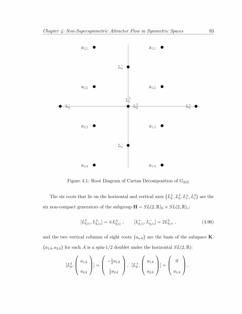
Chapter 4: Non-Supersymmetric Attractor Flow in Symmetric Spaces 93
Lh-
a24
a23
a22
a21
Lv+
Lv3
Lh3
Lv-
a14
a13
a12
a11
Lh+
Figure 4.1: Root Diagram of Cartan Decomposition of G2(2)
The six roots that lie on the horizontal and vertical axes L±h , L3h, L
±v , L3
v are the
six non-compact generators of the subgroup H = SL(2,R)h × SL(2,R)v:
[L3h/v, L
±h/v] = ∓L±h/v , [L+
h/v, L−h/v] = 2L3
h/v , (4.96)
and the two vertical columns of eight roots aαA are the basis of the subspace K.
a1A, a2A for each A is a spin-1/2 doublet under the horizontal SL(2,R):
[L3h,
a1A
a2A
] =
−1
2a1A
12a2A
, [L+
h ,
a1A
a2A
] =
0
a1A
,
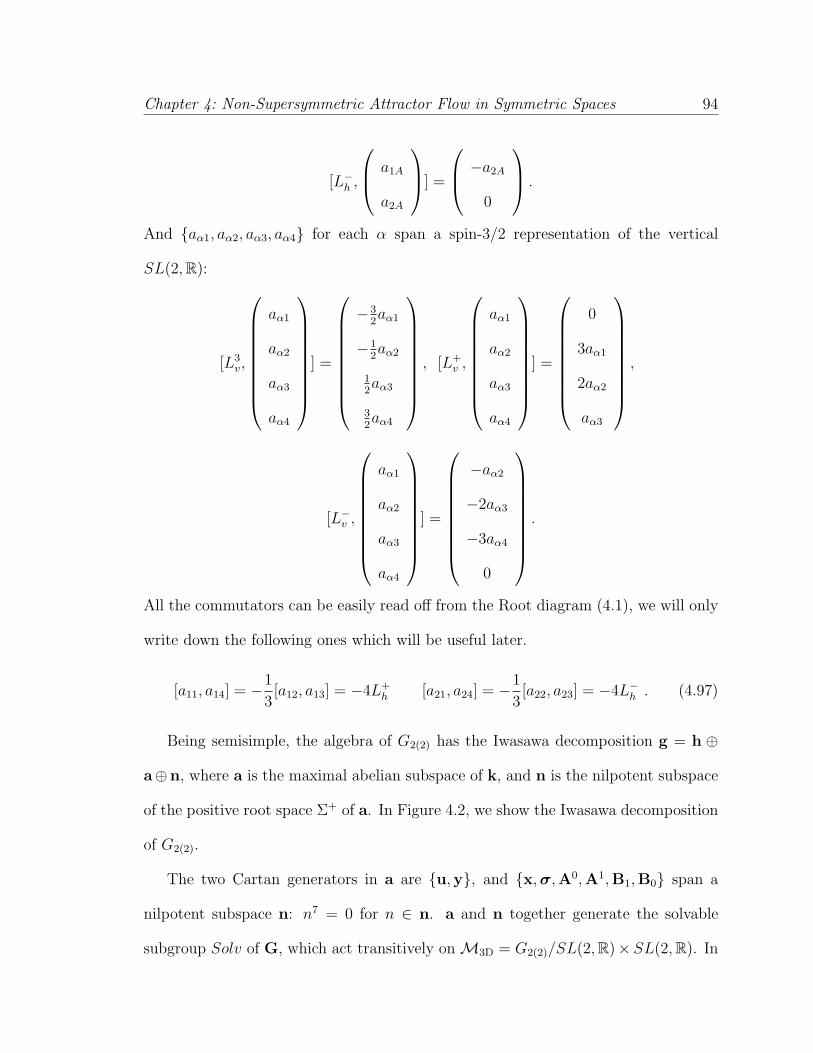
Chapter 4: Non-Supersymmetric Attractor Flow in Symmetric Spaces 94
[L−h ,
a1A
a2A
] =
−a2A
0
.
And aα1, aα2, aα3, aα4 for each α span a spin-3/2 representation of the vertical
SL(2,R):
[L3v,
aα1
aα2
aα3
aα4
] =
−32aα1
−12aα2
12aα3
32aα4
, [L+v ,
aα1
aα2
aα3
aα4
] =
0
3aα1
2aα2
aα3
,
[L−v ,
aα1
aα2
aα3
aα4
] =
−aα2
−2aα3
−3aα4
0
.
All the commutators can be easily read off from the Root diagram (4.1), we will only
write down the following ones which will be useful later.
[a11, a14] = −1
3[a12, a13] = −4L+
h [a21, a24] = −1
3[a22, a23] = −4L−h . (4.97)
Being semisimple, the algebra of G2(2) has the Iwasawa decomposition g = h ⊕
a⊕n, where a is the maximal abelian subspace of k, and n is the nilpotent subspace
of the positive root space Σ+ of a. In Figure 4.2, we show the Iwasawa decomposition
of G2(2).
The two Cartan generators in a are u,y, and x, σ,A0,A1,B1,B0 span a
nilpotent subspace n: n7 = 0 for n ∈ n. a and n together generate the solvable
subgroup Solv of G, which act transitively on M3D = G2(2)/SL(2,R)×SL(2,R). In
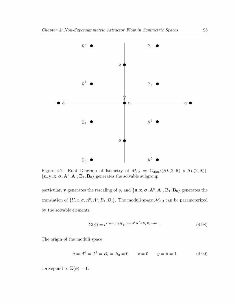
Chapter 4: Non-Supersymmetric Attractor Flow in Symmetric Spaces 95
a`
B`
0
B`
1
A`1
A`0
x
yu
x`
A0
A1
B1
B0
a
Figure 4.2: Root Diagram of Isometry of M3D = G2(2)/(SL(2,R) × SL(2,R)).u,y,x, σ,A0,A1,B1,B0 generates the solvable subgroup.
particular, y generates the rescaling of y, and u,x, σ,A0,A1,B1,B0 generates the
translation of U, x, σ,A0, A1, B1, B0. The moduli space M3D can be parameterized
by the solvable elements:
Σ(φ) = eUu+(ln y)yexx+AIAI+BIBI+σσ . (4.98)
The origin of the moduli space
a = A0 = A1 = B1 = B0 = 0 x = 0 y = u = 1 (4.99)
correspond to Σ(φ) = 1.
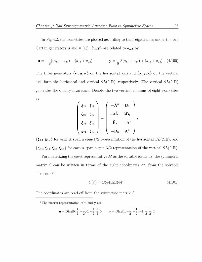
Chapter 4: Non-Supersymmetric Attractor Flow in Symmetric Spaces 96
In Fig 4.2, the isometries are plotted according to their eigenvalues under the two
Cartan generators u and y [46]. u,y are related to aαA by3:
u = −1
8[(a11 + a24)− (a13 + a22)] y =
1
8[3(a11 + a24) + (a13 + a22)]. (4.100)
The three generators σ,u, σ on the horizontal axis and x,y, x on the vertical
axis form the horizontal and vertical SL(2,R), respectively. The vertical SL(2,R)
generates the duality invariance. Denote the two vertical columns of eight isometries
as
ξ21 ξ11
ξ22 ξ12
ξ23 ξ13
ξ24 ξ14
≡
−A0 B0
−3A1 3B1
B1 −A1
−B0 A0
,
ξ1A, ξ2A for each A span a spin-1/2 representation of the horizontal SL(2,R), and
ξα1, ξα2, ξα3, ξα4 for each α span a spin-3/2 representation of the vertical SL(2,R).
Parameterizing the coset representative M as the solvable elements, the symmetric
matrix S can be written in terms of the eight coordinates φn, from the solvable
elements Σ
S(φ) = Σ(φ)S0Σ(φ)T . (4.101)
The coordinates are read off from the symmetric matrix S.
3The matrix representation of u and y are
u = Diag[0,12,−1
2, 0,−1
2,12, 0] y = Diag[1,−1
2,−1
2,−1,
12,12, 0]
Chapter 4: Non-Supersymmetric Attractor Flow in Symmetric Spaces 97
4.4.3 Nilpotency of the attractor flow generator k.
The near-horizon geometry of the 4D attractor is AdS2 × S2, i.e.
e−U →√
VBH |∗τ as τ →∞ . (4.102)
In terms of the variable u ≡ e2U
u → 1
VBH
τ−2 as τ →∞ . (4.103)
The solvable element is
M = eUu+... ∼ u12u . (4.104)
As the flow goes to the near-horizon, u → 0
M(τ) ∼ u−`/2 ∼ τ ` , (4.105)
where −` is the lowest eigenvalue of u. That is, M(τ) is a polynomial function of τ .
On the other hand, since the geodesic flow is generated by k via
M(τ) = M(0)ekτ/2 , (4.106)
i.e., M(τ) is an exponential function of τ . To reconcile the two statements, k must
be nilpotent:
k`+1 = 0 . (4.107)
That is, the element in k that generates the attractor flow is nilpotent. Moreover, by
looking at the weights of the fundamental representation of G2, we see that ` = 2
k3∗ = 0 . (4.108)
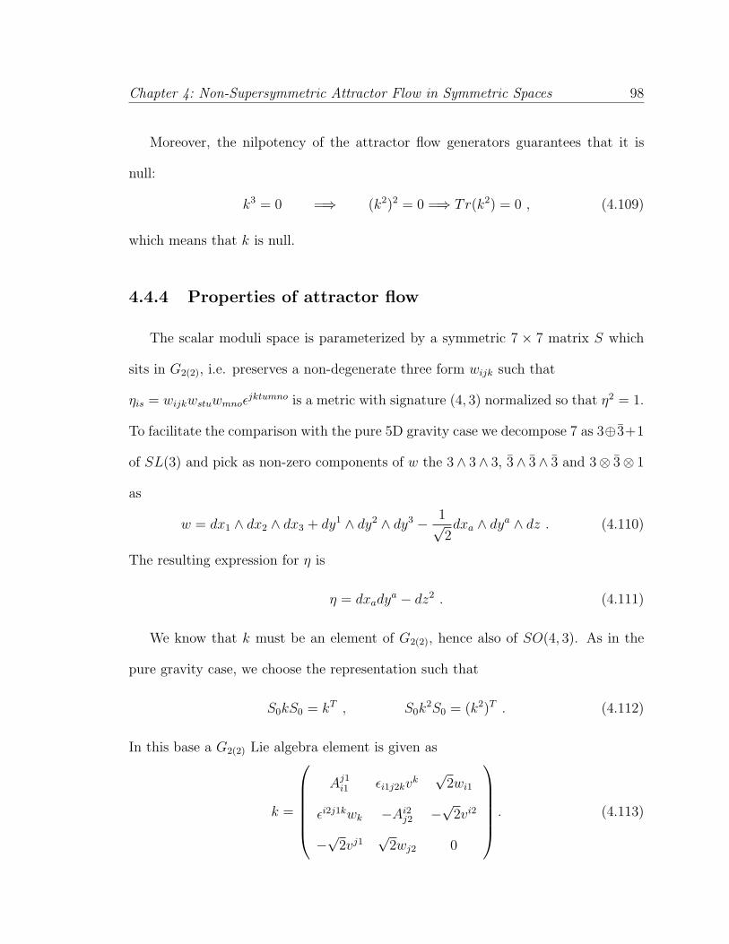
Chapter 4: Non-Supersymmetric Attractor Flow in Symmetric Spaces 98
Moreover, the nilpotency of the attractor flow generators guarantees that it is
null:
k3 = 0 =⇒ (k2)2 = 0 =⇒ Tr(k2) = 0 , (4.109)
which means that k is null.
4.4.4 Properties of attractor flow
The scalar moduli space is parameterized by a symmetric 7 × 7 matrix S which
sits in G2(2), i.e. preserves a non-degenerate three form wijk such that
ηis = wijkwstuwmnoεjktumno is a metric with signature (4, 3) normalized so that η2 = 1.
To facilitate the comparison with the pure 5D gravity case we decompose 7 as 3⊕ 3+1
of SL(3) and pick as non-zero components of w the 3 ∧ 3∧ 3, 3∧ 3∧ 3 and 3⊗ 3⊗ 1
as
w = dx1 ∧ dx2 ∧ dx3 + dy1 ∧ dy2 ∧ dy3 − 1√2dxa ∧ dya ∧ dz . (4.110)
The resulting expression for η is
η = dxadya − dz2 . (4.111)
We know that k must be an element of G2(2), hence also of SO(4, 3). As in the
pure gravity case, we choose the representation such that
S0kS0 = kT , S0k2S0 = (k2)T . (4.112)
In this base a G2(2) Lie algebra element is given as
k =
Aj1i1 εi1j2kv
k√
2wi1
εi2j1kwk −Ai2j2 −√2vi2
−√2vj1√
2wj2 0
. (4.113)
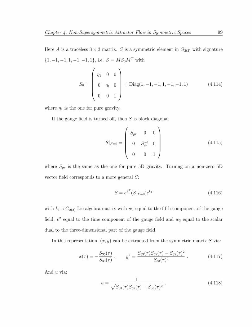
Chapter 4: Non-Supersymmetric Attractor Flow in Symmetric Spaces 99
Here A is a traceless 3× 3 matrix. S is a symmetric element in G2(2) with signature
1,−1,−1, 1,−1,−1, 1, i.e. S = MS0MT with
S0 =
η1 0 0
0 η1 0
0 0 1
= Diag(1,−1,−1, 1,−1,−1, 1) (4.114)
where η1 is the one for pure gravity.
If the gauge field is turned off, then S is block diagonal
S|F=0 =
Sgr 0 0
0 S−1gr 0
0 0 1
(4.115)
where Sgr is the same as the one for pure 5D gravity. Turning on a non-zero 5D
vector field corresponds to a more general S:
S = ekT1 (S|F=0)e
k1 (4.116)
with k1 a G2(2) Lie algebra matrix with w1 equal to the fifth component of the gauge
field, v2 equal to the time component of the gauge field and w3 equal to the scalar
dual to the three-dimensional part of the gauge field.
In this representation, (x, y) can be extracted from the symmetric matrix S via:
x(τ) = −S35(τ)
S33(τ), y2 =
S33(τ)S55(τ)− S35(τ)2
S33(τ)2. (4.117)
And u via:
u =1√
S33(τ)S55(τ)− S35(τ)2. (4.118)
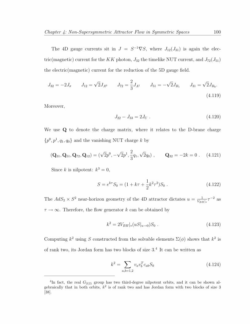
Chapter 4: Non-Supersymmetric Attractor Flow in Symmetric Spaces 100
The 4D gauge currents sit in J = S−1∇S, where J12(J31) is again the elec-
tric(magnetic) current for the KK photon, J32 the timelike NUT current, and J72(J51)
the electric(magnetic) current for the reduction of the 5D gauge field.
J32 = −2Jσ J12 =√
2JA0 J72 =2
3JA1 J51 = −
√2JB1 J31 =
√2JB0 .
(4.119)
Moreover,
J22 − J33 = 2JU . (4.120)
We use Q to denote the charge matrix, where it relates to the D-brane charge
p0, p1, q1, q0 and the vanishing NUT charge k by
(Q31,Q51,Q72,Q12) = (√
2p0,−√
2p1,2
3q1,√
2q0) , Q32 = −2k = 0 . (4.121)
Since k is nilpotent: k3 = 0,
S = ekτS0 = (1 + kτ +1
2k2τ 2)S0 . (4.122)
The AdS2 × S2 near-horizon geometry of the 4D attractor dictates u = 1VBH |∗ τ
−2 as
τ →∞. Therefore, the flow generator k can be obtained by
k2 = 2VBH |∗(uS|u→0)S0 . (4.123)
Computing k2 using S constructed from the solvable elements Σ(φ) shows that k2 is
of rank two, its Jordan form has two blocks of size 3.4 It can be written as
k2 =∑
a,b=1,2
vavTb cabS0 (4.124)
4In fact, the real G2(2) group has two third-degree nilpotent orbits, and it can be shown al-gebraically that in both orbits, k2 is of rank two and has Jordan form with two blocks of size 3[38].

Chapter 4: Non-Supersymmetric Attractor Flow in Symmetric Spaces 101
with va null and orthogonal to each other: va · vb ≡ vTa S0vb = 0, and cab depends on
the particular choice of k. Thus k can be expressed as:
k =∑a=1,2
(vawTa + wav
Ta )S0 (4.125)
where each wa is orthogonal to both va: wa · vb = 0, and wa satisfy
wa · wb = cab . (4.126)
Parallel to the pure gravity case, the single-centered attractor flow is constructed
as S(τ) = eK(τ)S0, where we choose K(τ) to have the same properties as the generator
k:
K3(τ) = 0 and K2(τ) rank two. (4.127)
This determines K(τ) = kτ + g where
k =∑a=1,2
[vawTa + wav
Ta ]S0 and g =
∑a=1,2
[vamTa + mav
Ta ]S0 (4.128)
where the two 7-vectors ma’s are orthogonal to va and contain the information of
asymptotic moduli. Using [[k, g], g] = 0, the current is reduced to
J =S0(k + 1
2[k, g])S0
r2~r (4.129)
from which we obtain va and wa in terms of the charges and the asymptotic moduli.
4.5 Flow Generators in the G2(2)/(SL(2,R)×SL(2,R))
Model
We now explicitly construct the generators of single-centered attractor flows. We
start with the BPS flow which is associated with a specific combination of the coset
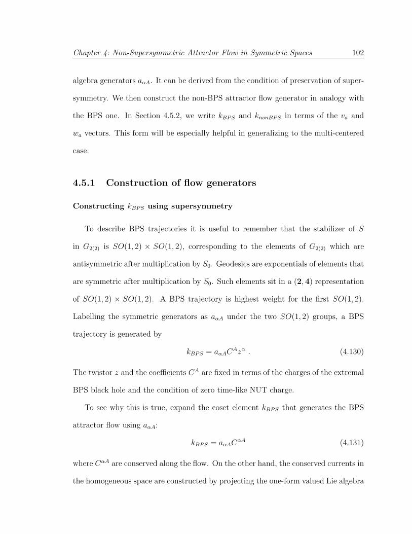
Chapter 4: Non-Supersymmetric Attractor Flow in Symmetric Spaces 102
algebra generators aαA. It can be derived from the condition of preservation of super-
symmetry. We then construct the non-BPS attractor flow generator in analogy with
the BPS one. In Section 4.5.2, we write kBPS and knonBPS in terms of the va and
wa vectors. This form will be especially helpful in generalizing to the multi-centered
case.
4.5.1 Construction of flow generators
Constructing kBPS using supersymmetry
To describe BPS trajectories it is useful to remember that the stabilizer of S
in G2(2) is SO(1, 2) × SO(1, 2), corresponding to the elements of G2(2) which are
antisymmetric after multiplication by S0. Geodesics are exponentials of elements that
are symmetric after multiplication by S0. Such elements sit in a (2,4) representation
of SO(1, 2) × SO(1, 2). A BPS trajectory is highest weight for the first SO(1, 2).
Labelling the symmetric generators as aαA under the two SO(1, 2) groups, a BPS
trajectory is generated by
kBPS = aαACAzα . (4.130)
The twistor z and the coefficients CA are fixed in terms of the charges of the extremal
BPS black hole and the condition of zero time-like NUT charge.
To see why this is true, expand the coset element kBPS that generates the BPS
attractor flow using aαA:
kBPS = aαACαA (4.131)
where CαA are conserved along the flow. On the other hand, the conserved currents in
the homogeneous space are constructed by projecting the one-form valued Lie algebra
Chapter 4: Non-Supersymmetric Attractor Flow in Symmetric Spaces 103
g−1 · dg onto k, which gives the vielbein in the symmetric space:
g−1dg|k = aαAV αA (4.132)
where V αA is conserved:
d
dτ
(V αA
a φa)
= 0 . (4.133)
Therefore, the expansion coefficients of kBPS are
CαA = V αAa φa . (4.134)
In terms of the vielbein, the supersymmetry condition that gives the BPS geodesics
are written as [127]:
V αAzα = 0 . (4.135)
That is:
V αAa φazα = 0 =⇒ CαAzα = 0 . (4.136)
Define zα = εαβzβ,
CαA = CAzα . (4.137)
Therefore, the coset element kBPS is expanded by the coset algebra basis aαA as
kBPS = aαACAzα.
Note that kBPS has five parameters (CA, z) where A = 1, . . . , 4. As will be shown
later, z can actually be determined by (CA) and moduli at infinity. So the geodesic
generated by kBPS is indeed a four-parameter family. It is easy to show that kBPS is
null, but more importantly, it is nilpotent:
k3BPS = 0 . (4.138)
As will be shown later, kBPS indeed gives the correct BPS attractor flow.
Chapter 4: Non-Supersymmetric Attractor Flow in Symmetric Spaces 104
Constructing kNonBPS
To construct the non-BPS attractor flow, one needs to find an element in the coset
algebra distinct from kBPS that satisfies:
k3NonBPS = 0 . (4.139)
The hint again comes from the BPS generator. Note that kBPS = aαAPAzα can be
written as:
kBPS = e−zL−h k0BPSezL−h , (4.140)
where k0BPS spans only the right four coset generators a1A:
k0BPS = a1ACA . (4.141)
That is, kBPS is generated by starting with the element spanning the four generators
annihilated by the horizontal SL(2) raising operator L+h , then conjugating with the
horizontal SL(2) lowering operator L−h . And it is very easy to show that (k0BPS)3 = 0
which proves (kBPS)3 = 0.
In G2(2)/SL(2,R)2, there are two third-degree nilpotent generators in total [38].
And since there are only two SL(2,R)’s inside H, a natural guess for a non-BPS
solution is to look at vectors with fixed properties under the second SL(2,R) group.
An interesting condition is to have positive charge under some rotation of L3v, i.e.
an SL(2,R) rotation of∑
A=1,2 aαACαA. Therefore, this suggests us to start with
the element spanning the four generators annihilated by the square of the vertical
SL(2,R) raising operator (L+v )2 and then conjugate with the vertical SL(2,R) low-
ering operator L−v :
kNonBPS(z) = e−zL−v k0NonBPSezL−v , (4.142)
Chapter 4: Non-Supersymmetric Attractor Flow in Symmetric Spaces 105
where
k0NonBPS = aαaC
αa where α, a = 1, 2. (4.143)
And one can show that: (k0NonBPS)3 = 0 which proves (kNonBPS)3 = 0. Moreover,
(kNonBPS)2 is rank two.
As long as one can pick the coefficients CαA and the twistor z that describes the
SO(1, 2) direction to be such that the time NUT charge is zero, this generator will
give nice non-BPS extremal black holes. All the known non-BPS solutions may be
recovered this way, and more, as this construction gives absolute freedom to pick the
charges and moduli at infinity for the black hole (clearly for certain values of charges
and moduli the solution will crash into a naked singularity, but this is to be expected
from comparison with the BPS case)
4.5.2 Properties of flow generators
Properties of kBPS
We now turn to solving for va and wa in (4.125) in terms of CA and z. First,
from (4.124) we know that the null space of k2 is five-dimensional and the va span the
two-dimensional complement of this null space. For kBPS = aαACAzα the null space
of (kBPS)2 does not depend on CA. Therefore, the va depend only on the twistor
z = z2/z1.
Recall that we are using the basis where k has the form (4.113). From inspection
of k2BPS, we find that (v1, v2) can always be chosen to have the form:5
v1 = (V1,−η1V1, 0) v2 = (−V2, η1V2,√
2) (4.144)
5When solving for (v, w), there are some freedom on the choice of (v1, v2) and (w1, w2): firstly, a
Chapter 4: Non-Supersymmetric Attractor Flow in Symmetric Spaces 106
where η1 is a 3D metric of signature (1,−1,−1), and V1, V2 are two three-vectors with
V1 · V1 = 0, V1 · V2 = 0, V2 · V2 = −1. (4.145)
Since any linear combination of (v1, v2) forms a new set of (v1, v2), this means in
particular that any v2 + cv1 gives a new v2. Looking at the forms of (v1, v2), we see
that V2 is defined up to a shifting of V1 as V2 = V 02 − cV1.
An explicit computation shows that V1 and V2 are given by the twistor z and u as
V1 =
(z1)2 + (z2)2
(z1)2 − (z2)2
2z1z2
, V2 =1
z1u2 − z2u1
z1u1 + z2u2
z1u1 − z2u2
z1u2 + z2u1
, (4.146)
where the twistor u = u2
u1 is related to c by
u = −1 + 2cz
1− 2czz. (4.147)
rotational freedom
(v1, v2) → (v1, v2)(
R11 R12
R21 R22
)and (w1, w2) → (w1, w2)
(R11 R12
R21 R22
)
where R is orthogonal: RRT = 1. Secondly, a rescaling freedom:
va → rva and wa → 1rwa.
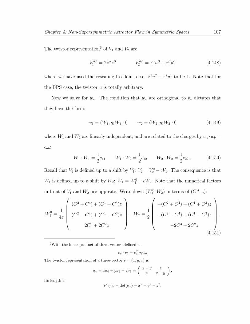
Chapter 4: Non-Supersymmetric Attractor Flow in Symmetric Spaces 107
The twistor representation6 of V1 and V2 are
V αβ1 = 2zαzβ V αβ
2 = zαuβ + zβuα (4.148)
where we have used the rescaling freedom to set z1u2 − z2u1 to be 1. Note that for
the BPS case, the twistor u is totally arbitrary.
Now we solve for wa. The condition that wa are orthogonal to va dictates that
they have the form:
w1 = (W1, η1W1, 0) w2 = (W2, η1W2, 0) (4.149)
where W1 and W2 are linearly independent, and are related to the charges by wa ·wb =
cab:
W1 ·W1 =1
2c11 W1 ·W2 =
1
2c12 W2 ·W2 =
1
2c22 . (4.150)
Recall that V2 is defined up to a shift by V1: V2 = V 02 − cV1. The consequence is that
W1 is defined up to a shift by W2: W1 = W 01 + cW2. Note that the numerical factors
in front of V1 and W2 are opposite. Write down (W 01 ,W2) in terms of (CA, z):
W 01 =
1
4z
(C2 + C4) + (C1 + C3)z
(C2 − C4) + (C1 − C3)z
2C3 + 2C2z
, W2 =1
2
−(C2 + C4) + (C1 + C3)z
−(C2 − C4) + (C1 − C3)z
−2C3 + 2C2z
.
(4.151)
6With the inner product of three-vectors defined as
va · vb = vTa η1vb.
The twistor representation of a three-vector v = (x, y, z) is
σv = xσ0 + yσ3 + zσ1 =(
x + y zz x− y
).
Its length isvT η1v = det(σv) = x2 − y2 − z2.
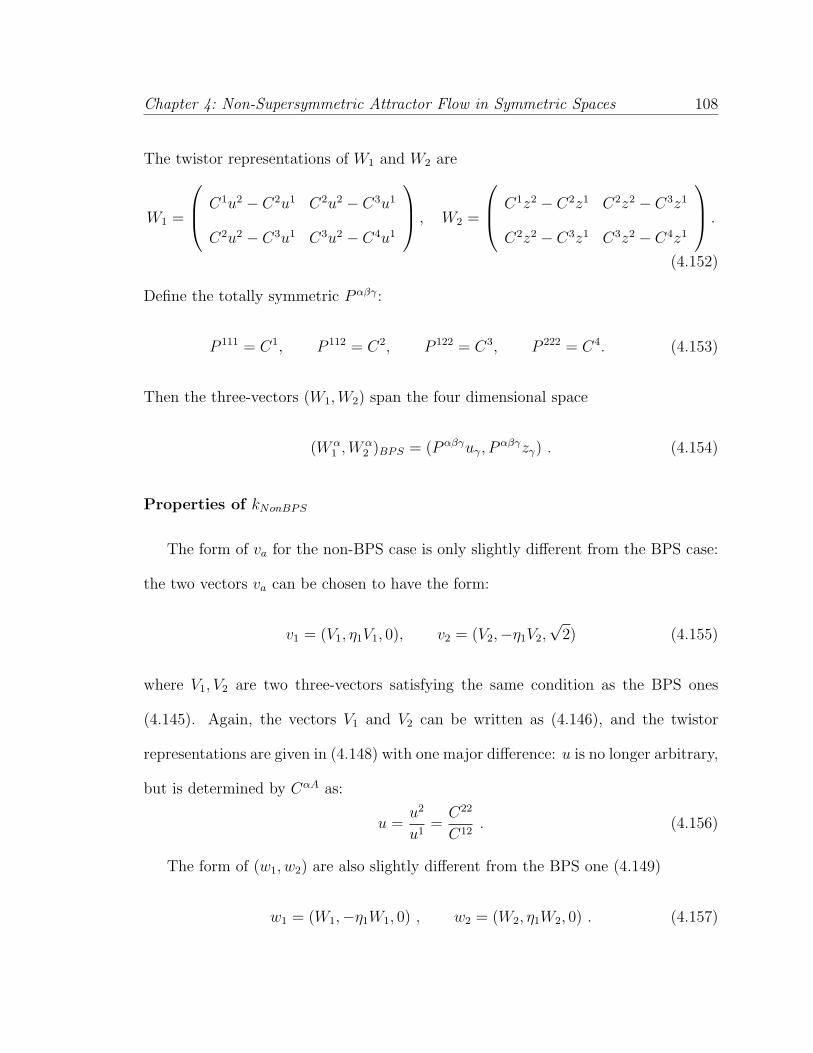
Chapter 4: Non-Supersymmetric Attractor Flow in Symmetric Spaces 108
The twistor representations of W1 and W2 are
W1 =
C1u2 − C2u1 C2u2 − C3u1
C2u2 − C3u1 C3u2 − C4u1
, W2 =
C1z2 − C2z1 C2z2 − C3z1
C2z2 − C3z1 C3z2 − C4z1
.
(4.152)
Define the totally symmetric Pαβγ :
P 111 = C1, P 112 = C2, P 122 = C3, P 222 = C4. (4.153)
Then the three-vectors (W1,W2) span the four dimensional space
(Wα1 ,W α
2 )BPS = (Pαβγuγ, Pαβγzγ) . (4.154)
Properties of kNonBPS
The form of va for the non-BPS case is only slightly different from the BPS case:
the two vectors va can be chosen to have the form:
v1 = (V1, η1V1, 0), v2 = (V2,−η1V2,√
2) (4.155)
where V1, V2 are two three-vectors satisfying the same condition as the BPS ones
(4.145). Again, the vectors V1 and V2 can be written as (4.146), and the twistor
representations are given in (4.148) with one major difference: u is no longer arbitrary,
but is determined by CαA as:
u =u2
u1=
C22
C12. (4.156)
The form of (w1, w2) are also slightly different from the BPS one (4.149)
w1 = (W1,−η1W1, 0) , w2 = (W2, η1W2, 0) . (4.157)
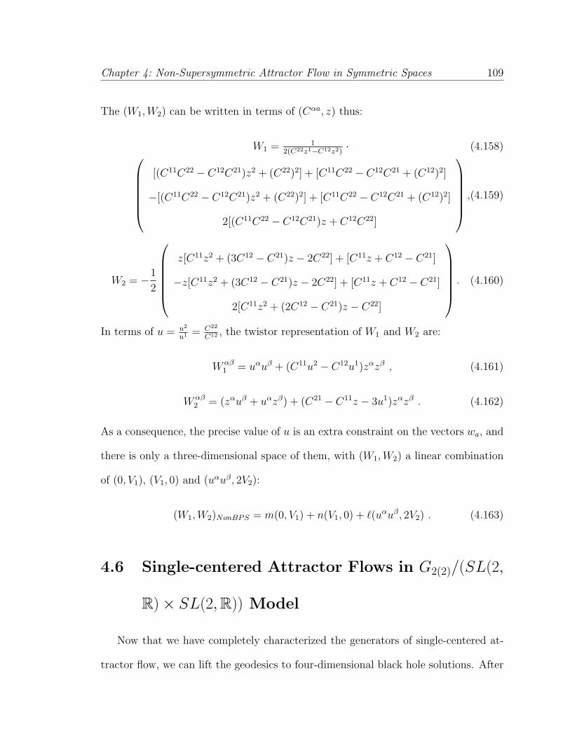
Chapter 4: Non-Supersymmetric Attractor Flow in Symmetric Spaces 109
The (W1,W2) can be written in terms of (Cαa, z) thus:
W1 = 12(C22z1−C12z2)
· (4.158)
[(C11C22 − C12C21)z2 + (C22)2] + [C11C22 − C12C21 + (C12)2]
−[(C11C22 − C12C21)z2 + (C22)2] + [C11C22 − C12C21 + (C12)2]
2[(C11C22 − C12C21)z + C12C22]
,(4.159)
W2 = −1
2
z[C11z2 + (3C12 − C21)z − 2C22] + [C11z + C12 − C21]
−z[C11z2 + (3C12 − C21)z − 2C22] + [C11z + C12 − C21]
2[C11z2 + (2C12 − C21)z − C22]
. (4.160)
In terms of u = u2
u1 = C22
C12 , the twistor representation of W1 and W2 are:
Wαβ1 = uαuβ + (C11u2 − C12u1)zαzβ , (4.161)
Wαβ2 = (zαuβ + uαzβ) + (C21 − C11z − 3u1)zαzβ . (4.162)
As a consequence, the precise value of u is an extra constraint on the vectors wa, and
there is only a three-dimensional space of them, with (W1,W2) a linear combination
of (0, V1), (V1, 0) and (uαuβ, 2V2):
(W1,W2)NonBPS = m(0, V1) + n(V1, 0) + `(uαuβ, 2V2) . (4.163)
4.6 Single-centered Attractor Flows in G2(2)/(SL(2,
R)× SL(2,R)) Model
Now that we have completely characterized the generators of single-centered at-
tractor flow, we can lift the geodesics to four-dimensional black hole solutions. After
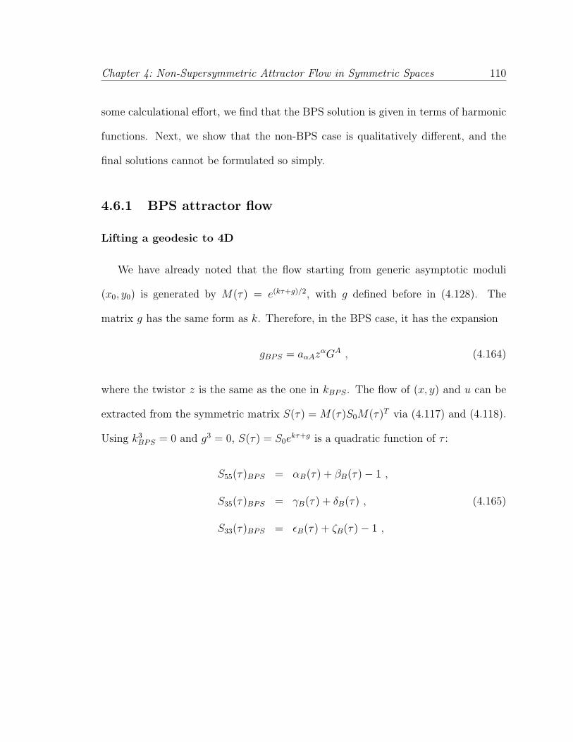
Chapter 4: Non-Supersymmetric Attractor Flow in Symmetric Spaces 110
some calculational effort, we find that the BPS solution is given in terms of harmonic
functions. Next, we show that the non-BPS case is qualitatively different, and the
final solutions cannot be formulated so simply.
4.6.1 BPS attractor flow
Lifting a geodesic to 4D
We have already noted that the flow starting from generic asymptotic moduli
(x0, y0) is generated by M(τ) = e(kτ+g)/2, with g defined before in (4.128). The
matrix g has the same form as k. Therefore, in the BPS case, it has the expansion
gBPS = aαAzαGA , (4.164)
where the twistor z is the same as the one in kBPS. The flow of (x, y) and u can be
extracted from the symmetric matrix S(τ) = M(τ)S0M(τ)T via (4.117) and (4.118).
Using k3BPS = 0 and g3 = 0, S(τ) = S0e
kτ+g is a quadratic function of τ :
S55(τ)BPS = αB(τ) + βB(τ)− 1 ,
S35(τ)BPS = γB(τ) + δB(τ) , (4.165)
S33(τ)BPS = εB(τ) + ζB(τ)− 1 ,

Chapter 4: Non-Supersymmetric Attractor Flow in Symmetric Spaces 111
where αB(τ), γB(τ), εB(τ) are quadratic functions of τ , and βB, δB, ζB are linear
functions of τ :
αB(τ) = z2(H2H4 − (H3)2) + z(H2H3 −H1H4) + (H1H3 − (H2)2) ,
βB(τ) = (H2 −H4)z + (H3 −H1) ,
γB(τ) = −1
2
((H1H4 −H2H3)(z2 − 1) + 2(H2(H2 + H4)−H3(H1 + H3))z
),
δB(τ) = −1
2((H1 + H3)z − (H2 + H4)) ,
εB(τ) = (H1H3 − (H2)2)z2 + (H1H4 −H2H3)z + (H2H4 − (H3)2) ,
ζB(τ) = 2(H2z + H3) , (4.166)
where HA is a linear function of τ defined as HA(τ) ≡ CAτ + GA.
The attractor values are reached when τ →∞ along the geodesic:
x∗BPS = −(k2S0)35
(k2S0)33
, y∗BPS =
√(k2S0)33(k2S0)55 − (k2S0)2
35
(k2S0)33
, (4.167)
and
u∗BPS =1√
(k2S0)33(k2S0)55 − (k2S0)235
. (4.168)
The asymptotic moduli (x0, y0) can be expressed in terms of (GA, z) by extraction
from S = egS0.
Using this technique, one can construct all BPS single-centered black holes. The
charges of each black hole can be read off from the current J using (4.119). One
example is given in Figure 4.3, where we parametrically plot x(τ) and y(τ) for a BPS
black hole with charges (p0, p1, q1, q0) = (5, 2, 7,−3) and attractor point (x∗, y∗) =
(0.329787, 0.788503).7
7The discriminant of the charge (5, 2, 7,−3) is positive, so this is indeed a BPS solution.
Chapter 4: Non-Supersymmetric Attractor Flow in Symmetric Spaces 112
4D solution for given set of charges
To get the solution for a specific set of charges requires more effort. In this section,
we present the analytical result for any set of charges (pI , qI).
The ten parameters in kBPS and g are z, u, CA, GA, among which the twistor u
is arbitrary, corresponding to the freedom of the shift by (v1, w2) in the definition of
(v2, w1): (v2, w1) → (v2+cv1, w1−cw2). The remaining true parameters are enough to
parameterize the four D-brane charges (pI , qI) and the arbitrary asymptotic moduli
(x0, y0) under the condition of vanishing Taub-NUT charge and fixing u0 = 1. We
now solve for kBPS and g for the given D-brane charges and (x0, y0), using the eight
constraints, namely, 4 charges and zero Taub-NUT charge plus 3 asymptotic moduli,
to fix CA and GA, leaving the other twistor z unfixed.8
For the sake of simplicity, we will denote kBPS by k for the rest of this section.
Then the current J(Q) = kT
r2 gives the five coupled equations:
Q = S0(k +1
2[k, g])S0 . (4.169)
In order to show that the BPS flow can be expressed in terms of harmonic functions:
H(τ) = Qτ + h with Q = (pI , qI) and h = (hI , hI) , (4.170)
we will solve g in terms of h instead of (x0, y0). The four h’s relate to the asymptotic
moduli by
x0 = x∗(Q → h) y0 = y∗(Q → h) u0 = u∗(Q → h) , (4.171)
and there is one extra degree of freedom to be fixed later.
8The twistor z can be left unfixed because we will not specify the asymptotic values of the scalarswith translational invariance, namely, (a,AI , BI). Fixing them can fix the twistor z.
Chapter 4: Non-Supersymmetric Attractor Flow in Symmetric Spaces 113
To evaluate [k, g], we first use the commutation relation (4.97) to obtain
[a1ACA, a1BGB] = 〈C, G〉(−4L+h ) , (4.172)
where the product between CA and GA is defined as 〈C, G〉 ≡ C1G4 − 3C2G3 +
3C3G2 − C4G1. Then twisting Eq (4.172) with the twistor z as in (4.140) gives the
commutator of k and g with the same twistor z:
[k, g] = [aαAzαCA, aβBzβGB] = 〈C, G〉Θ , (4.173)
where Θ is defined as Θ ≡ − 41+z2 e
−zL−h L+h ezL−h . On the other hand, using (4.128),
[k, g] = (v2vT1 − v1v
T2 )S0(w2 ·m1 − w1 ·m2) . (4.174)
Θ can also be written as Θ = (v2vT1 − v1v
T2 )S0, and we can check that (w2 ·m1 −w1 ·
m2) = 〈C, G〉.
First, separate from GA the piece which has the same dependence on (h, z) as CA
on (Q, z):
GA = GAh + EA with GA
h ≡ CA(Q → h, z) . (4.175)
That is, g contains two pieces:
g = gh + Λ with gh = aαAzαGAh and Λ = aαAzαEA. (4.176)
We need to solve for EA.
There are three constraints from (4.171). The (x0, y0) and u0 are extracted from
the symmetric matrix S = egS0 via (4.117) and (4.118). On the other hand, requiring
Chapter 4: Non-Supersymmetric Attractor Flow in Symmetric Spaces 114
(4.171) gives (x0, y0, u0) in terms of h:
x0 = −(g2hS0)35
(g2hS0)33
,
y0 =
√(g2
hS0)33(g2hS0)55 − (g2
hS0)235
(g2hS0)33
, (4.177)
u0 =1√
(g2hS0)33(g2
hS0)55 − (g2hS0)2
35
.
Therefore, defining Π ≡ (eg − g2h
2)S0, Π has to satisfy three constaints:
Π33 = Π35 = Π55 = 0 (4.178)
in order for (4.177) to hold for arbitrary h. Using the unfixed degree of freedom in
h’s to set 〈C, Gh〉 = 0, (4.169) becomes
Q = S0(k +1
2[k, Λ])S0 . (4.179)
The zero Taub-NUT charge condition in (4.179) imposes the fourth constraint on Λ:
the (3,2)-element of S0(k + 12[k, Λ])S0 for arbitrary k has to vanish. Combining with
(4.178), we have 4 constraints to fix EA to be:
E1 = −E3 = − 1
1 + z2, E2 = −E4 =
z
1 + z2. (4.180)
The remaining 4 conditions in the coupled equations (4.179) determine CA in the
BPS generator kBPS = aαAzαCA to be
C1 =√
2−q0 − q1z − 3p1z2 + p0z3
(1 + z2)2,
C2 =√
2− q1
3− (2p1 − v0)z + (p0 + 2 q1
3)z2 + p1z3
(1 + z2),
C3 =√
2−p1 + (p0 + 2 q1
3)z + (2p1 − v0)z
2 − q1
3z3
(1 + z2),
C4 =√
2p0 + 3p1z − q1z
2 + q0z3
(1 + z2)2. (4.181)
Chapter 4: Non-Supersymmetric Attractor Flow in Symmetric Spaces 115
The GAh are then determined by GA
h = aαAzACA(Q → h, z). Using the solution of
CA and GAh , we see the product 〈CA, GA
h 〉 is proportional to the symplectic product
of (pI , qI) and (hI , hI):
〈CA, GAh 〉 =
2
1 + z2< Q, h > where < Q, h >≡ p0h0 + p1h1 − q1h
1 − q0h0 .
(4.182)
The condition 〈CA, GAh 〉 = 0 is then the integrability condition on h:
< Q, h >= p0h0 + p1h1 − q1h1 − q0h
0 = 0 . (4.183)
Substituting the expressions of CA and GA in terms of (pI , qI) into (4.165), we
obtain the BPS attractor flow in terms of the charges (pI , qI). In particular, the
attractor values are
x∗BPS = − p0q0 + p1 q1
3
2[(p1)2 + p0 q1
3]
, y∗BPS =
√J4(p0, p1, q1
3, q0)
2[(p1)2 + p0 q1
3]
, (4.184)
where J4(p0, p1, q1, q0) is the quartic E7(7) invariant:
J4(p0, p1, q1, q0) = 3(p1q1)
2 − 6(p0q0)(p1q1)− (p0q0)
2 − 4(p1)3q0 + 4p0(q1)3 , (4.185)
thus J4(p0, p1, q1
3, q0) is the discriminant of charge. The attractor values match those
from the compactification of Type II string theory on diagonal T 6, with q1 → q1
3. The
attractor value of u is
u∗BPS =1√
J4(p0, p1, q1
3, q0)
. (4.186)
The constraint on h from u0 = 1 is then J4(h0, h1, h1
3, h0) = 1.
Now we will show that the geodesic we constructed above indeed reproduces the
attractor flow given by replacing charges by the corresponding harmonic functions in
the attractor moduli. Using the properties of Λ, we have proved that, in terms of

Chapter 4: Non-Supersymmetric Attractor Flow in Symmetric Spaces 116
k and g, the flow of (x, y) can be generated from the attractor value by replacing k
with the harmonic function kτ + gh:
x(τ) = x∗(k → kτ + gh) , y(τ) = y∗(k → kτ + gh) . (4.187)
Since k and gh have the same twistor z, this is equivalent to replacing the CA with
the harmonic function CAτ + GAh while leaving the twistor z fixed:
x(τ) = x∗(CA → CAτ + GAh , z) , y(τ) = y∗(CA → CAτ + GA
h , z) . (4.188)
Since CA is linear in Q and GAh linear in h, and since z drops out after plugging in the
solution of CA in terms of (Q, z) and GAh in terms of (h, z), this proves that the flow of
(x0, y0) is given by replacing the charges in the attractor moduli by the corresponding
harmonic functions:
xBPS(τ) = x∗BPS(Q → Qτ + h) , yBPS(τ) = y∗BPS(Q → Qτ + h) . (4.189)
The integrability condition < Q, h >= 0, in terms of H = Qτ + h, is
< H, dH >= 0 . (4.190)
4.6.2 Non-BPS attractor flow
Lifting a geodesic to 4D
Similar to the BPS attractor flow, the non-BPS flow is generated by M(τ) =
e(kτ+g)/2, and (x, y) can be extracted from the symmetric matrix S(τ) by (4.117) and
the relevant elements of S(τ) are given by (4.165). The only difference is that now
αB, βB, γB, δB, εB, ζB are changed into the non-BPS counterparts
Chapter 4: Non-Supersymmetric Attractor Flow in Symmetric Spaces 117
αNB, βNB, γNB, δNB, εNB, ζNB, which can be written in terms of Hαa ≡ Cαaτ +Gαa
and z:
αNB(τ) = −((H21H12 −H22H11)(z2 − 1)2 + (H22)2z2 − 2zH12H22 + (H12)2) ,
βNB(τ) = (z2 − 1)(H11 −H21z)− 3z2H22 + 2zH12 + H22 ,
γNB(τ) = (z2 − 1)(2z(H11H22 −H12H21) + H22H12) + z((H22)2 − (H12)2) ,
δNB(τ) =1
2(z(1 + z2)H11 + z2(3H12 −H21)− 2H22z + (H12 −H21)) ,
εNB(τ) = (4H11H22 −H12(H12 + 4H21))z2 − 2H12H22z − (H22)2 ,
ζNB(τ) = 2(H11z2 + (2H12 + H21)z + H22) . (4.191)
Note that H22
H12 = u is fixed, independent of τ . The non-BPS flow written in terms
of (Hαa, z) has the same simple form as the BPS flow, i.e. the scalars are rational
functions with both the numerator and denominator being only quadratic. This is due
to the nilpotency of the generator: k3 = 0. Again, the attractor values are reached
when τ → ∞, and the asymptotic moduli can be expressed in terms of (Gαa, z) by
extraction from S = egS0.
Unlike the BPS case, there are only eight parameters in kNonBPS and gNonBPS:
the two twistors (z, u) and (Cαa, Gαa) under the constraints that
u =C22
C12=
G22
G12. (4.192)
Therefore, while kBPS and gBPS can parameterize arbitrary (pI , qI) and (x0, y0) while
leaving (z, u) free, all the parameters in kNonBPS and gNonBPS, including (z, u), will
be fixed.
Chapter 4: Non-Supersymmetric Attractor Flow in Symmetric Spaces 118
The attractor point in terms of Cαa is
x∗NonBPS =γNB(Hαa → Cαa)
εNB(Hαa → Cαa), (4.193)
y∗NonBPS =
√αNB(Hαa → Cαa)εNB(Hαa → Cαa)− γ2
NB(Hαa → Cαa)
εNB(Hαa → Cαa),
with z given by
1
2
(−3C12 − C21 + z((z2 − 3)C11 + 3z(C12 + C21) + 6C22
))= 0 . (4.194)
As in the BPS case, the charges of the black hole are read off from the current J using
(4.119). We have checked that the attractor point is a non-supersymmetric critical
point of the black hole potential VBH = |Z|2 + |DZ|2:
∂VBH = 0 and DZ 6= 0 . (4.195)
It reproduces the results reported in the literature [145]. An example of the non-BPS
attractor flow is shown in Figure 4.4, with (p0, p1, q1, q0) = (5, 2, 7, 3) and attractor
point (x∗, y∗) = (−0.323385, 0.580375). Note that J4(5, 2, 7/3, 3) < 0, so this is indeed
a non-BPS black hole. Unlike the BPS attractor flow, all the non-BPS flows starting
from different asymptotic moduli have the same tangent direction at the attractor
point. The mass matrix of the black-hole potential at a BPS critical point has two
identical eigenvalues, whereas the eigenvalues at a non-BPS critical point are different.
The common tangent direction for the non-BPS flows corresponds to the eigenvector
associated with the smaller mass.
4D solution for given set of charges
We now discuss how to construct the non-BPS black hole solution for a specific
set of charges (pI , qI).
Chapter 4: Non-Supersymmetric Attractor Flow in Symmetric Spaces 119
One major difference between the non-BPS case and the BPS case is that
[kNonBPS, gNonBPS] = 0 (4.196)
automatically, since the forms of (w1, w2) and (m1,m2) guarantee that w1 · m2 =
w2 ·m1 = 0. Thus the charge equation (4.169) becomes simply
QNonBPS = S0(kNonBPS)S0 . (4.197)
These five coupled equations determine the two twistors (z, u) and Cαa in terms of
(pI , qI). Similar to the BPS case, the four equations which determine the D-brane
charge allow us to write Cαa in terms of the charges (p0, p1, q1, q0) and the twistor z
via
C11 =(−2q0 + 6(p1 − q0)z
2 + 4(p0 + q1)z3 − 6p1z4)√
2(1 + z2)3,
C12 =(p0 + q1
3)− 2(2p1 − q0)z − (p0 + 5 q1
3)z2 + 2p1z3
√2(1 + z2)2
,
C21 =(p0 − q1)− 4q1z
2 + 4(3p1 − q0)z3 + (3p0 + q1)z
4
√2(1 + z2)3
,
C22 =2p1 + (p0 + 5 q1
3)z − 2(2p1 − q0)z
2 − (p0 + q1
3)z3
√2(1 + z2)2
. (4.198)
and u = C22
C12 . In contrast to the BPS case, the Gαa do not enter the equations and
therefore cannot be used to eliminate the twistor z. Requiring the Taub-NUT charge
to vanish gives the following degree-six equation for the z:
p0z6 +6p1z5− (3p0 +4q1)z4−4(3p1−2q0)z
3 +(3p0 +4q1)z2 +6p1z−p0 = 0 . (4.199)
The three parameters in gNonBPS, namely, Gαa with the constraint G22
G12 = u are then
fixed by the given asymptotic moduli (x0, y0) and u0 = 1.
Chapter 4: Non-Supersymmetric Attractor Flow in Symmetric Spaces 120
Similar to the BPS flow, the full non-BPS flow can be generated from the attractor
value by replacing Cαa with the harmonic function Hαa(τ) = Cαaτ + Gαa, while
leaving z unchanged as in (4.188). However, there are two major differences. First,
the harmonic functions Hαa have to satisfy the constraint
H22(τ)
H12(τ)= u =
C22
C12=
G22
G12. (4.200)
Note that this does not impose any constraint on the allowed asymptotic moduli since
there are still three degrees of freedom in Gαa to account for (x0, y0, u0). We will see
later that it instead imposes a stringent constraint on the allowed D-brane charges in
the multi-centered non-BPS solution.
Secondly, unlike the BPS flow, replacing Cαa in the attractor moduli by the har-
monic function Hαa(τ) is not equivalent to replacing the charges Q with H = Qτ +h
as in (4.189). The twistor z here is no longer free, but is determined in terms of the
charges as a root of the degree-six equation (4.199), so replacing Q by Qτ + h, for
generic Q and h, would not leave z invariant. Therefore, the generic non-BPS flow
cannot be given by the naive harmonic function procedure, as proposed by Kallosh
et al [91]. Next, we will define the subset of the NonBPS single-centered flow that
can be constructed by the harmonic function procedure.
When the attractor has only D4-D0 charges, namely, Q40 = (0, p1, 0, q0), (4.199)
has a root z = 0, which is independent of the value of charges. If the asymptotic
moduli h is also of the form of h40 = (0, h1, 0, h0), replacing Q40 by Q40τ + h40 would
leave the solution z = 0 invariant. Now we will use the duality symmetry to extend
the subset to a generic charge system with restricted asymptotic moduli.
The one-modulus system can be considered as the STU attractor with the three
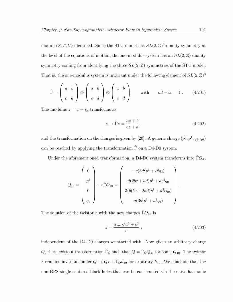
Chapter 4: Non-Supersymmetric Attractor Flow in Symmetric Spaces 121
moduli (S, T, U) identified. Since the STU model has SL(2,Z)3 duality symmetry at
the level of the equations of motion, the one-modulus system has an SL(2,Z) duality
symmetry coming from identifying the three SL(2,Z) symmetries of the STU model.
That is, the one-modulus system is invariant under the following element of SL(2,Z)3
Γ =
a b
c d
⊗
a b
c d
⊗
a b
c d
with ad− bc = 1 . (4.201)
The modulus z = x + iy transforms as
z → Γz =az + b
cz + d, (4.202)
and the transformation on the charges is given by [20]. A generic charge (p0, p1, q1, q0)
can be reached by applying the transformation Γ on a D4-D0 system.
Under the aforementioned transformation, a D4-D0 system transforms into ΓQ40
Q40 =
0
p1
0
q1
→ ΓQ40 =
−c(3d2p1 + c2q0)
d(2bc + ad)p1 + ac2q0
3(b(bc + 2ad)p1 + a2cq0)
a(3b2p1 + a2q0)
.
The solution of the twistor z with the new charges ΓQ40 is
z =a±√a2 + c2
c, (4.203)
independent of the D4-D0 charges we started with. Now given an arbitrary charge
Q, there exists a transformation ΓQ such that Q = ΓQQ40 for some Q40. The twistor
z remains invariant under Q → Qτ + ΓQh40 for arbitrary h40. We conclude that the
non-BPS single-centered black holes that can be constructed via the naive harmonic
Chapter 4: Non-Supersymmetric Attractor Flow in Symmetric Spaces 122
function procedure are only those with (Q, h) being the image of a single transforma-
tion Γ on the (Q40, h40) from a D4-D0 system:
xNB(τ) = x∗NB(ΓQ40 → ΓQ40τ + Γh40) , yNB(τ) = y∗NB(ΓQ40 → ΓQ40τ + Γh40) .
(4.204)
Since we are considering arbitrary charge system, the constraint is on the allowed
values of h.
4.7 Multi-centered Attractor Flows in G2(2)/(SL(2,
R)× SL(2,R)) Model
As proven in the pure gravity system, the multi-centered attractor solutions are
given by exponentiating the matrix harmonic function K(~x):
S(~x) = eK(~x)S0 (4.205)
with K(~x) having the same properties as the generator k:
K3(~x) = 0 and K2(~x) rank two. (4.206)
We now describe how to formulate K(~x) for multi-centered solutions in G2(2).
The K(~x) satisfying all the above constraints is constructed as
K(~x) =∑a=1,2
[vaWa(~x)T + Wa(~x)vTa ]S0 , (4.207)
with va being the same two constant null vectors in k, and the multi-centered harmonic
function
Wa(~x) =∑
i
(wa)i
|~x− ~xi| + ma (4.208)
Chapter 4: Non-Supersymmetric Attractor Flow in Symmetric Spaces 123
is everywhere orthogonal to va. The two 7-vectors (m1,m2) contain the information
of asymptotic moduli and has the same form as (w1, w2). Write K(~x) as K(~x) =
∑i
ki
|~x−~xi| + g where
ki =∑a=1,2
[va(wa)Ti + (wa)iv
Ta ]S0 and g =
∑a=1,2
[vamTa + mav
Ta ]S0 . (4.209)
Since v only depends on the twistor (z, u), and (w1, w2) are linear in CA or Cαa, the
above generating procedure is equivalent to replace CA or Cαa by the multi-centered
harmonic functions while keeping the twistor (z, u) fixed.
Next we discuss the properties of the BPS multi-centered attractor solution and
non-BPS ones separately, since they are very different in character.
4.7.1 BPS multi-centered solutions
In constrast with the multi-centered solutions in pure gravity, now the second
term of the current J = ∇K + 12[∇K, K] does not vanish automatically since
[kBPSi , kBPS
j ] 6= 0 and [kBPSi , gBPS] 6= 0 . (4.210)
Therefore, the centers are no longer free, and we cannot simply read off the charges
from J . Instead, we need to solve for CAi and GA in a set of 5N coupled equations.
The divergence of the current is
∇ · J = 4π∑
i
δ(~x− ~xi)S0(ki +1
2[ki, g] +
1
2
∑j
[ki, kj]
|~xi − ~xj|)S0 . (4.211)
Using Qi to denote the charge matrix which relates to the D-brane charge p0, p1, q1, q0i
as in (4.121), and with Q32 as the vanishing NUT charge, we have 5N coupled equa-
Chapter 4: Non-Supersymmetric Attractor Flow in Symmetric Spaces 124
tions from Qi = 14π
∫i∇ · J :
Qi = S0(ki +1
2[ki, g] +
1
2
∑j
[ki, kj]
|~xi − ~xj|)S0 . (4.212)
The generators of the multi-centered BPS attractor solution ki and g have
4(N + 1) + 2 parameters in total: the two twistors (z, u) and CAi , GA. On the
left hand side of (4.212), there are also 3N − 3 degrees of freedom from the position
of the centers ~xi. On the other hand, a generic N -centered attractor solution has
4N D-brane charges (pI , qI), and three additional constraints from the asymptotic
moduli (x0, y0) and u0 = 1. As we will show, like the single-centered BPS solution,
the three asymptotic moduli, together with the vanishing of the total Taub-NUT
charge, determine the 4 GA inside g. Moreover, as in the single-centered case, we can
solve CAi in terms of the 4D D-brane charges Qi while leaving (z, u) unfixed. The
remaining N − 1 zero Taub-NUT charge conditions at each center will impose N − 1
constraints on the distances between the N -centers ~xi.
First, integrating over the circle at the infinity,∑
i Qi = 14π
∫ ∇ · J gives the sum
of the above N matrix equations:
Qtot =∑
i
Qi = S0(∑
i
ki +1
2[∑
i
ki, g])S0 , (4.213)
which is the same as the one for the single-center attractor with charge Qtot. This
determines g to be g = gh+Λ, same as the one for single-centered attractor in (4.176).
As in the single centered case, h is fixed by the asymptotic moduli (x0, y0) by
x0 = x∗BPS(Q → h) , y0 = y∗BPS(Q → h) , (4.214)
and the two constraints:
< Qtot, h >= 0 , J4(h0, h1,
h1
3, h0) = 1 . (4.215)
Chapter 4: Non-Supersymmetric Attractor Flow in Symmetric Spaces 125
We have used the vanishing of the total Taub-NUT charge to determine Λ. Next,
we will use the remaining coupled 5N − 1 equations to solve for the 4N CAi and
impose N − 1 constraints on the relative positions between the N centers ~xi where
i = 1, . . . , N .
The tentative solutions of CAi are given by (4.181) with (pI , qI) replaced by
(pIi , qI,i). The flow generator of each center ki is then ki = aαAzαCA
i . Substitut-
ing the solution of ki and g = gh + Λ into (4.212), and using
[ki, gh] = 2 < Qi, h > Θ , [ki, kj] = 2 < Qi, Qj > Θ , (4.216)
where all the ki’s and gh have the same value for the twistor z, we get
Qi = S0(ki+ < Qi, h > Θ +1
2[ki, Λ] +
∑j
< Qi, Qj >
|~xi − ~xj| Θ)S0 . (4.217)
Just as in the single-centered case, the solution of ki and the form of Λ guarantee
that
Qi = S0(ki +1
2[ki, Λ])S0 . (4.218)
We see that as long as the following integrability condition is satisfied:
< Qi, h > +∑
j
< Qi, Qj >
|~xi − ~xj| = 0 , (4.219)
the ki and g given above indeed produce the correct multi-centered attractor solution.
Just like in the single-centered case, the multi-centered solution flows to the correct
attractor moduli (x∗i , y∗i ) near each center, independent of the value of z. It also
follows that the multi-centered solution can be generated by replacing the charges
inside the attractor value by the multi-centered harmonic function:
xBPS(~x) = x∗BPS(Q →∑
i
Qi
|~x− ~xi|+h) , yBPS(~x) = y∗BPS(Q →∑
i
Qi
|~x− ~xi|+h) .
(4.220)

Chapter 4: Non-Supersymmetric Attractor Flow in Symmetric Spaces 126
The sum of the N equations in the integrability condition (4.219) reproduces
the constraint on h: < Qtot, h >= 0. Thus the remaining N − 1 equations impose
N − 1 constraints on the relative positions between the N centers ~xi with i =
1, · · · , N . From (A.5) and (4.94), we see that ∗dω is given by J23. Defining the
angular momentum ~J by
ωi = 2εijkJj x
k
r3as r →∞ , (4.221)
we see that there exists a nonzero angular momentum given by
~J =1
2
∑i<j
~xi − ~xj
|~xi − ~xj|〈Qi, Qj〉 . (4.222)
Thus we have shown that our multi-centered BPS attractor solution reproduces the
one found in [18].
4.7.2 Non-BPS multi-centered solutions.
For given (z, u) and Cαai , Gαa, the non-BPS multi-centered solution is the same
as the single-centered one as in (4.191) with Hαa(τ) replaced by the multi-centered
harmonic function Hαa(~x) =∑
iCαa
i
|~x−~xi| + Gαa satisfying the constraint
u =H22
i (~x)
H12i (~x)
=C22
i
C12i
=G22
G12. (4.223)
Accordingly, the attractor values at each center is the same as (4.193) with the cor-
responding Cαas . The asymptotic moduli are obtained by extraction from S = egS0.
The equation of motion for the non-BPS multi-centered solution simplifies a great
deal since
[∇K(~x), K(~x)] = 0 (4.224)
Chapter 4: Non-Supersymmetric Attractor Flow in Symmetric Spaces 127
automatically, following from the fact that for the non-BPS system:
(w1)i ·m2 = (w2)i ·m1 = 0 , (4.225)
which are guaranteed by the forms of NonBPS (w1, w2)i and (m1,m2). Therefore, the
5N equations (4.212) decouple into N sets of 5 coupled equations:
Qi = S0(ki)S0 . (4.226)
Equation (4.226) differs greatly from the BPS counterpart (4.212). Firstly, the
generators of the multi-centered non-BPS attractor solution ki and g have 3(N +
1)+2 parameters: the two twistors (z, u) and Cαai , Gαa with the constraint (4.223).
In constrast to the BPS case, g does not enter the equation. Thus we can simply
use the three asymptotic moduli, without invoking the zero Taub-NUT condition, to
determine the 3 Gαa inside g. Secondly, unlike the BPS multi-centered solution, the
position of the centers ~xi do not appear in the equation, therefore there will be no
constraint imposed on them: the centers are free. Last but not least, the remaining
3N + 2 parameters in (z, u) and Cαa are not enough to parameterize a generic N -
centered attractor solution, which has 4N D-brane charges (pIi , qI,i). Accordingly, the
multi-centered non-BPS attractor generated by this ansatz will not have arbitrary
charges. Combining with the fact that ~xi do not appear in the R.H.S of the equation,
we find that all the N vanishing Taub-NUT charge conditions can only act on the
charges on the L.H.S. We conclude that, in total, there will be 2N − 2 constraints on
the allowed charges.
Now we will show in detail the derivation of the constraints. First, like in the
single-centered NonBPS solution, the absence of the Taub-NUT charge at infinity
Chapter 4: Non-Supersymmetric Attractor Flow in Symmetric Spaces 128
fixes z via∑
i
Qi = S0(∑
i
ki)S0 (4.227)
The solution is the same as the solution to (4.199) with the charges replaced by the
total charges of N centers: z = z(Q → ∑i Qi). Since all the N centers share the same
twistor z, the absence of the NUT charge at each center imposes N − 1 constraints
on the allowed charges Qi: all z(Qi) have to be equal.
The remaining 4N equations in (4.226) determine Cαa in terms of z and Qi. Since
the N -centers decouple, (4.226) for each center is the same as the single-center one
(4.197). Thus the solution of Cαai is given by (4.198) with (pI , qI) replaced by (pI
i , qI,i).
Again, since all the centers share the same twistor u, the condition (4.223) imposes
another N−1 constraints on the allowed charges. Solving these 2N−2 constraints, we
see all the charges Qi are the image of a single transformation Γ on a multi-centered
D4-D0 system Q40,i:
Qi = ΓQ40,i . (4.228)
The charges at different centers are all mutually local
〈Qi, Qj〉 = 0 . (4.229)
Except for the constraint on the charges, the N centers are independent, and there
is no constraint on the position of the centers. A related fact is that the the angular
momentum is zero.
Like the non-BPS single-centered case, though the multi-centered solution can be
generated from the attractor value by replacing Cαa with the multi-centered harmonic
function Hαa(~x) =∑
iCαa
i
|~x−~xi| + Gαa under the constraint (4.223), while leaving z
Chapter 4: Non-Supersymmetric Attractor Flow in Symmetric Spaces 129
unchanged as in (4.188), the generic solution cannot be generated via the harmonic
function procedure used in the BPS case, namely, by replacing the charges inside
the attractor value by the corresponding multi-centered harmonic functions. The
reason is again due to the fact that the twistor z, being a function of charges, does
not remain invariant under this substitution of charges by harmonic functions. The
multi-centered non-BPS solutions that can be generated by the harmonic function
procedure are those with Qi, h being the image of a single Γ on the Q40,i, h40 of
a pure D4-D0 system:
xNB(~x) = x∗NB(ΓQ40 →∑
i
ΓQ40,i
|~x− ~xi| + Γh40) ,
yNB(~x) = y∗NB(ΓQ40 →∑
i
ΓQ40,i
|~x− ~xi| + Γh40) . (4.230)
It appears that the existence of a simple linear ansatz for “superimposing” single
center solutions exists in general only for mutually local extremal black holes, and
only in the supersymmetric case does it extend to mutually non-local centers.
To summarize, the non-BPS multi-centered solution is different from the BPS
case because it imposes no constraints on the position of the centers, but instead
on the allowed charges Qi: the choice of charges at each center are restricted to
a three-dimensional subspace, and they are mutually local. The result is that the
centers can move freely, and there is no angular momentum in the system. It does
not have interesting moduli spaces of centers with mutually non-local charges, so it
is as “boring” as the pure gravity case.
Chapter 4: Non-Supersymmetric Attractor Flow in Symmetric Spaces 130
4.8 Conclusion and Discussion
In this chapter, we find exact single-centered and multi-centered black hole so-
lutions in theories of gravity which have a symmetric 3D moduli space. The BPS
and extremal non-BPS single-centered solutions correspond to certain geodesics in
the moduli space. We construct these geodesics by exponentiating different types of
nilpotent elements in the coset algebra. Using the Jordan form of these nilpotent
elements, we are able to write them down in closed explicit form. Furthermore, we
can use a symmetric matrix parametrization to recover the metric and full flow of the
scalars in four dimensions.
We have also generalized the geodesics to find solutions for non-BPS and BPS
multi-centered black holes. The BPS multi-centered solution reproduces the known
solution of Bates and Denef. Given our assumption that the 3D spatial slice is flat,
we find that a non-BPS multi-centered black hole is very different from its BPS coun-
terpart. It is constrained to have mutually local charges at all of its centers and
therefore carries no intrinsic angular momentum. It is possible that if we dropped
this assumption, we could find more general non-BPS multi-centered solutions. Such
configurations would probably be amenable to exact analysis only in the axially sym-
metric case, using inverse scattering methods.
There are many other avenues for future work. One could explore nilpotent ele-
ments in other symmetric spaces, and see whether non-BPS bound states with nonlo-
cal charges exist. In particular, it would be interesting to study E8(8)/SO∗(16), which
is the 3D moduli space for d = 4,N = 8 supergravity. We would also like to find a
way to modify our method so that we can apply it to non-symmetric homogeneous
Chapter 4: Non-Supersymmetric Attractor Flow in Symmetric Spaces 131
spaces, and eventually to generic moduli spaces. We could then study the much larger
class of non-BPS extremal black holes in generic N = 2 supergravities.
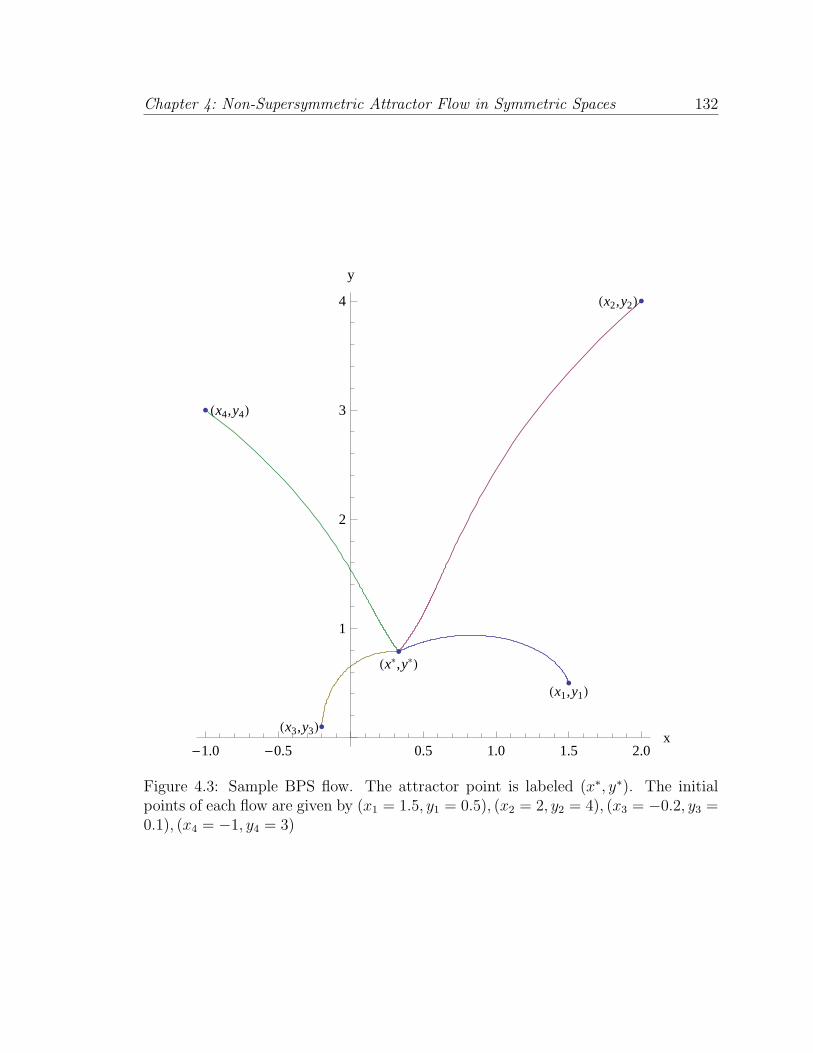
Chapter 4: Non-Supersymmetric Attractor Flow in Symmetric Spaces 132
Hx*,y*L
Hx1,y1L
Hx2,y2L
Hx3,y3L
Hx4,y4L
-1.0 -0.5 0.5 1.0 1.5 2.0x
1
2
3
4
y
Figure 4.3: Sample BPS flow. The attractor point is labeled (x∗, y∗). The initialpoints of each flow are given by (x1 = 1.5, y1 = 0.5), (x2 = 2, y2 = 4), (x3 = −0.2, y3 =0.1), (x4 = −1, y4 = 3)
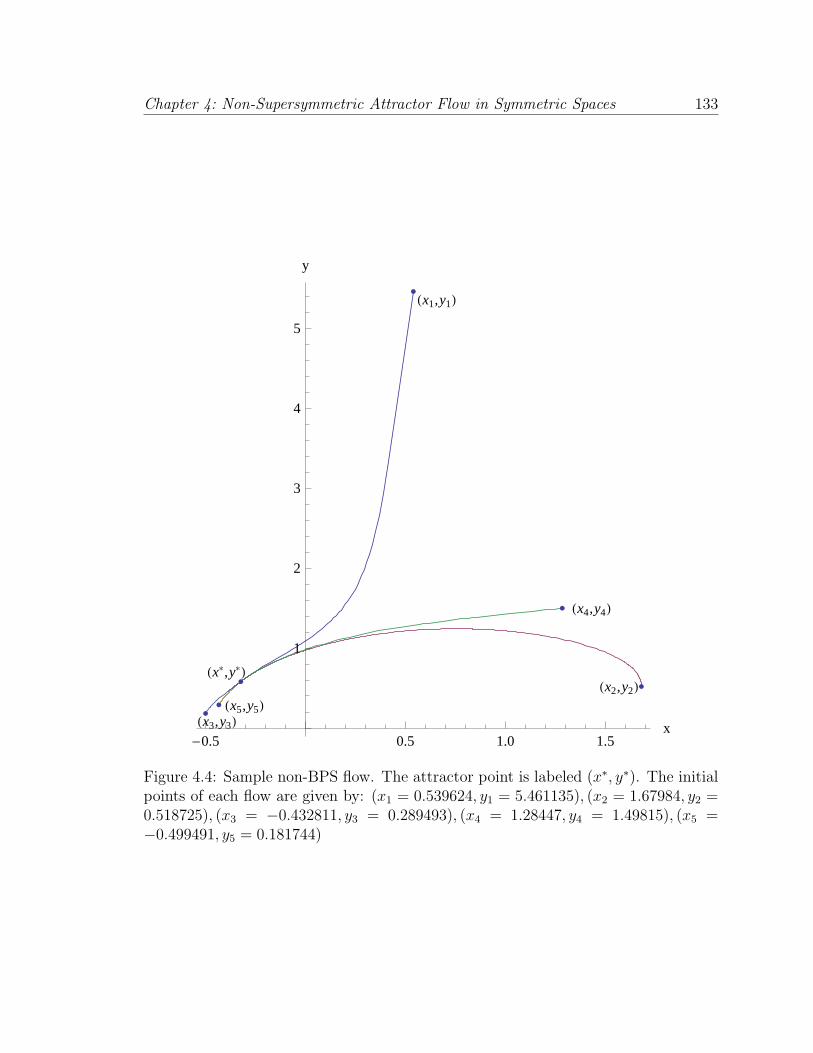
Chapter 4: Non-Supersymmetric Attractor Flow in Symmetric Spaces 133
Hx*,y*L
Hx1,y1L
Hx2,y2L
Hx3,y3L
Hx4,y4L
Hx5,y5L
-0.5 0.5 1.0 1.5x
1
2
3
4
5
y
Figure 4.4: Sample non-BPS flow. The attractor point is labeled (x∗, y∗). The initialpoints of each flow are given by: (x1 = 0.539624, y1 = 5.461135), (x2 = 1.67984, y2 =0.518725), (x3 = −0.432811, y3 = 0.289493), (x4 = 1.28447, y4 = 1.49815), (x5 =−0.499491, y5 = 0.181744)
Chapter 5
Chiral Gravity in Three
Dimensions
5.1 Introduction
In three dimensions, the Riemann and Ricci tensor both have the same num-
ber (six) of independent components. Hence Einstein’s equation, with or without a
cosmological constant Λ, completely constrains the geometry and there are no local
propagating degrees of freedom. At first sight this makes the theory sound too trivial
to be interesting. However in the case of a negative cosmological constant, there are
asymptotically AdS3 black hole solutions [16] as well as massless gravitons which can
be viewed as propagating on the boundary. These black holes obey the laws of black
hole thermodynamics and have an entropy given by one-quarter the horizon area.
This raises the interesting question: what is the microscopic origin of the black hole
entropy in these “trivial” theories?
134
Chapter 5: Chiral Gravity in Three Dimensions 135
In order to address this question one must quantize the theory. One proposal
[147] is to recast it as an SL(2,R)L × SL(2,R)R Chern-Simons gauge theory with
kL = kR. Despite some effort this approach has not given a clear accounting of the
black hole entropy (see however [64] for an interesting attempt). So the situation
remains unsatisfactory.
More might be learned by deforming the theory with the addition of the gravita-
tional Chern-Simons term with coefficient 1µ
[51, 50]. The resulting theory is known
as the topologically massive gravity (TMG) and contains a local, massive propagat-
ing degree of freedom, as well as black holes and massless boundary gravitons. The
addition of the Chern-Simons term leads to more degrees of freedom because it con-
tains three, rather than just two, derivatives of the metric. It is the purpose of this
chapter to study this theory for negative Λ = −1/`2. We will argue that the theory is
unstable/inconsistent for generic µ: either the massive gravitons or BTZ black holes
have negative energy. The exception occurs when the parameters obey µ` = 1, at
which point several interesting phenomena simultaneously arise:
(i) The central charges of the dual boundary CFT become cL = 0, cR = 3`/G.
(ii) The conformal weights as well as the wave function of the massive graviton,
generically 12(3 + µ`,−1 + µ`), degenerate with those of the left-moving weight (2, 0)
massless boundary graviton. They are both pure gauge, but the gauge transformation
parameter does not vanish at infinity.
(iii) BTZ black holes and all gravitons have non-negative masses. Further the
angular momentum is fixed in terms of the mass to be J = M`.
This suggests the possibility of a stable, consistent theory at µ` = 1 which is
Chapter 5: Chiral Gravity in Three Dimensions 136
dual to a holomorphic boundary CFT (i.e. containing only right-moving degrees of
freedom) with cR = 3`/G. The hope — which remains to be investigated — is that
for a suitable choice of boundary conditions the zero-energy left-moving excitations
can be discarded as pure gauge. We will refer to this theory as 3D chiral gravity. As
we will review herein, if such a dual CFT exists, and is unitary, an application of the
Cardy formula gives a microscopic derivation of the black hole entropy [139, 95, 96].
Related recent work [148, 106, 72, 67, 14, 150, 149, 105] has considered an alterna-
tive deformation of pure 3D gravity, locally described by the SL(2,R)L × SL(2,R)R
Chern-Simons gauge theory with kL 6= kR. This is a purely topological theory
with no local degrees of freedom and is not equivalent to TMG. It contains all the
subset of solutions of TMG which are Einstein metrics but not the massive gravi-
tons. It is nevertheless possible that the arguments given in [148] (adapted to the
case kL = 0 as in [106]) which are quite general apply to the chiral gravity dis-
cussed herein. Indeed discrepancies with the semiclassical analysis mentioned in
[148, 106, 72, 67, 14, 150, 149, 105] disappear for the special case kL = 0.1 Moreover
the main assumption of [148] — holomorphic factorization of the partition function
— is simply a consistency requirement for chiral gravity because there are only right
movers.
This chapter is organized as follows. Section 5.2 gives a brief review of the cos-
mological TMG and its AdS3 vacuum solution, and shows that the theory is purely
chiral at the special value of µ = 1/`. Section 5.3 describes the linearized gravitational
excitations around AdS3. Section 5.4 shows how the positivity of energy imposes a
1Although we do not study the Euclidean theory herein the relation M` = J for Lorentzian BTZblack holes in chiral gravity suggests that the saddle point action will be holomorphic.
Chapter 5: Chiral Gravity in Three Dimensions 137
stringent constraint on the allowed value of µ. We end with a short summary and
discussion of future directions.
5.2 Topologically Massive Gravity
5.2.1 Action
The action for topologically massive gravity (TMG) with a negative cosmological
constant Λ is [53]
I =1
16πG
∫d3x
√−g(R− 2Λ) +1
16πGµICS (5.1)
where Ics is the Chern-Simons term
Ics = −1
2
∫d3x
√−gελµνΓρλσ[∂µΓσ
ρν +2
3Γσ
µτΓτνρ] . (5.2)
In this work, we will focus the theory with negative cosmological constant Λ.
We have chosen the sign in front of the Einstein-Hilbert action so that BTZ black
holes have positive energy for large µ, while the massive gravitons will turn out to
have negative energy for this choice. This contrasts with most of the literature which
chooses the opposite sign in order that massive gravitons have positive energy (for
large µ). Note that had we chosen the opposite sign in front of the Einstein action, the
BTZ black holes would have negative masses, which signifies a quantum instability.
Namely, the vacuum would be unstable against decaying into the infinite degeneracy
of zero energy solutions corresponding to negative mass black holes surrounded by
positive energy gravitons.
Chapter 5: Chiral Gravity in Three Dimensions 138
The equation of motion of the theory is
Gµν +1
µCµν = 0 , (5.3)
where Gµν is the cosmological-constant-modified Einstein tensor:
Gµν ≡ Rµν − 1
2gµνR + Λgµν (5.4)
and Cµν is the Cotton tensor
Cµν ≡ εµαβ∇α(Rβν − 1
4gβνR) (5.5)
where ε is Levi-Civita tensor.
Cotton tensor is the three-dimensional analogue of Weyl tensor, which vanishes
identically in 3D. From its definition, it is symmetric, manifestly traceless, and obeys
Bianchi identity.2 Since Cµν is manifestly traceless, its presence does not modify the
value of Ricci scalar solved from the equation of motion. That Cµν obeys Bianchi
identity shows that although the presence of the gravitational Chern-Simons term
manifestly breaks the diffeomorphism invariance of TMG, the equation of motion
of the bulk theory still obeys the diffeomorphism invariance. Finally, the metric
compatibility ensures that Einstein metrics which have Gµν = 0 are a subset of the
general solutions of (5.3).
2The Cotton tensor is symmetric thanks to the Bianchi identity of Gµν :
εαµνCµν = ∇βGαβ = 0 .
Chapter 5: Chiral Gravity in Three Dimensions 139
5.2.2 AdS3 vacuum solution
TMG has an AdS3 solution:
ds2 = gµνdxµdxν = `2(− cosh2 ρdτ 2 + dρ2 + sinh2 ρdφ2) (5.6)
where the radius is related to Λ by
Λ = − 1
`2. (5.7)
The Riemann tensor, Ricci tensor and Ricci scalar of the AdS3 are:
Rµανβ = Λ(gµν gαβ − gµβ gαν) , Rµν = 2Λgµν , R = 6Λ , (5.8)
The metric (5.6) has isometry group SL(2,R)L×SL(2,R)R. The SL(2,R)L generators
are
L0 = i∂u , (5.9)
L−1 = ie−iu
[cosh 2ρ
sinh 2ρ∂u − 1
sinh 2ρ∂v +
i
2∂ρ
], (5.10)
L1 = ieiu
[cosh 2ρ
sinh 2ρ∂u − 1
sinh 2ρ∂v − i
2∂ρ
], (5.11)
where u ≡ τ + φ, v ≡ τ − φ. The SL(2,R)R generators L0, L±1 are given by the
above expressions with u ↔ v. The normalization of the SL(2,R) algebra is
[L0, L±1] = ∓L±1 , [L1, L−1] = 2L0 . (5.12)
The quadratic Casimir of SL(2,R)L is L2 = 12(L1L−1 + L−1L1) − L2
0. When acting
on scalars, L2 + L2 = − `2
2∇2 [103].
Chapter 5: Chiral Gravity in Three Dimensions 140
5.2.3 Chiral gravity
As shown by Brown and Henneaux [31], quantum gravity on asymptotically AdS3
spacetimes with appropriate boundary conditions is described by a 2D CFT which
lives on the boundary. They computed the total central charge of the CFT and found
cL + cR = 3`/G . (5.13)
Simplified calculations were given in [85, 44, 15]. The difference cL − cR corresponds
to the diffeomorphism anomaly. In reference [96, 94] it was shown that
cL − cR = − 3
µG. (5.14)
Combining (5.13) and (5.14), we have
cL =3`
2G(1− 1
µ`) , cR =
3`
2G(1 +
1
µ`) . (5.15)
In order that both central charges are non-negative, we must have, as was also noticed
in [138],
µ` > 1 . (5.16)
An interesting special case is
µ` = 1 , (5.17)
which implies
cL = 0 , cR =3`
G. (5.18)
We will refer to this theory as chiral gravity. If the chiral gravity is unitary it can
have only right-moving excitations.
Chapter 5: Chiral Gravity in Three Dimensions 141
5.3 Gravitons in AdS3
5.3.1 Equation of motion for gravitons
In this section we describe the linearized excitations around background AdS3
metric gµν . Expanding
gµν = gµν + hµν (5.19)
with hµν small, the linearized Ricci tensor and Ricci scalar are [54, 118]:
R(1)µν =
1
2(−∇2hµν − ∇µ∇νh + ∇σ∇νhσµ + ∇σ∇µhσν) , (5.20)
R(1) ≡ (Rµνgµν)(1) = −∇2h + ∇µ∇νh
µν − 2Λh . (5.21)
The leading terms in G and C are
G(1)µν = R(1)
µν −1
2gµνR
(1) − 2Λhµν , (5.22)
C(1)µν = ε αβ
µ ∇α
(R
(1)βν −
1
4gβνR
(1) − 2Λhβν
). (5.23)
We note TrC(1) = 0 and the Bianchi identity implies ∇µG(1)µν = ∇µC
(1)µν = 0 . The
linearized equations of motion are then
G(1)µν +
1
µC(1)
µν = 0 . (5.24)
Tracing this equation yields TrG(1) = −12R(1) = 0. So the equation of motion becomes
G(1)µν +
1
µεµ
αβ∇αG(1)βν = 0 , (5.25)
where in terms of hµν
G(1)µν =
1
2(−∇2hµν − ∇µ∇νh + ∇σ∇νhσµ + ∇σ∇µhσν)− 2Λhµν . (5.26)
Chapter 5: Chiral Gravity in Three Dimensions 142
Now we fix the gauge. We define hµν ≡ hµν−gµνh, which gives h = −2h. Plugging
hµν = hµν − 12gµν h into (5.20) and setting it to zero gives
∇µ∇ν hµν = −Λh . (5.27)
Thus, the gauge
∇µhµν = 0 (5.28)
together with the linearized equation of motion implies tracelessness of hµν : h =
−2h = 0. This gauge is equivalent to the harmonic plus traceless gauge ∇µhµν = h =
0. Noting that
[∇σ, ∇µ]hσν = Rσ
λσµhλν − Rλ
νσµhσλ = 3Λhµν − Λhgµν , (5.29)
and imposing the gauge condition, (5.26) is just
G(1)µν =
1
2(−∇2hµν + 2Λhµν ) . (5.30)
The equation of motion (5.25) thus becomes
(∇2 +2
`2)(hµν +
1
µεµ
αβ∇αhβν) = 0 . (5.31)
5.3.2 Massless and massive gravitons
Define three mutually commuting operators (DL,DR,DM):
(DL/R)µβ ≡ δµ
β ± `εµαβ∇α, and (DM)µ
β ≡ δµβ +
1
µεµ
αβ∇α , (5.32)
where the meaning of superscripts will become clear presently. The equations of
motion (5.25) can then be written as
(DLDRDMh)µν = 0 , (5.33)
Chapter 5: Chiral Gravity in Three Dimensions 143
where we have used the linearized Bianchi identity. Since the three operators commute
equation (5.33) has three branches of solutions. First, the massive gravitons hMµν given
by
(DMhM)µν = hMµν +
1
µεµ
αβ∇αhMβν = 0 (5.34)
are solutions special for TMG. The other two branches are massless gravitons which
are also solutions of Einstein gravity: G(1)µν = 0. The left-mover hL
µν and right-mover
hRµν have different first order equations of motion:
(DLhL)µν = hLµν +`εµ
αβ∇αhLβν = 0 , (DRhR)µν = hR
µν−`εµαβ∇αhR
βν = 0 . (5.35)
Note that the components of (5.34) and (5.35) tangent to the AdS3 boundary relate
those components of hµν to their falloff at infinity. This could be used to directly
infer their conformal weights but we will instead just find the full solutions.
5.3.3 Mass of massive gravitons
At this stage, we can infer the mass of the massive graviton without solving its
full equations of motion. It requires knowing its second order equations of motion.
Define linear operator
(DM)µβ ≡ δµ
β − 1
µεµ
αβ∇α , (5.36)
which commutes with DM defined earlier. Applying DM on (5.25), we obtain the
second order equation of motion,
(DMDMG(1))µν = (DMDMG(1))µν = − 1
µ2[∇2 − (µ2 + 3Λ)]G(1)
µν = 0 (5.37)
where we have used the linearized Bianchi identity. Note that DMG = 0 is just the
linearized gravitational wave equation if we exchange µ for −µ. So solutions of TMG
Chapter 5: Chiral Gravity in Three Dimensions 144
with both signs of µ are solutions of (5.37). It can conversely be shown that all
solutions of (5.37) are solutions of TMG for one sign of µ or the other.
The mass of the massive graviton can be inferred by comparing the second-order
equation of motion of massive gravitons:
[∇2 +2
`2− (µ2 − 1
`2)]hM
µν = 0 (5.38)
with that of massless gravitons:
[∇2 +2
`2]hL/R
µν = 0 . (5.39)
The mass of massive gravitons is thus
m =
√µ2 − 1
`2. (5.40)
At µ` = 1, the massive graviton becomes massless. The mass-squared saturates the
Breitenlohner-Freedman bound m2 = − 1`2
[28, 27] at zero µ.
5.3.4 Solutions of massless and massive gravitons
Next we solve for the three branches of solutions. Rewrite the Laplacian acting
on rank-two tensors in terms of the sum of two SL(2,R) Casimirs:
∇2hµν = −[2
`2(L2 + L2) +
6
`2]hµν . (5.41)
G(1)µν can be written as
G(1)µν = [
1
`2(L2 + L2) +
2
`2]hµν . (5.42)
Thus (5.37) becomes
[− 2
`2(L2 + L2)− 3
`2− µ2][
1
`2(L2 + L2) +
2
`2]hµν = 0 . (5.43)
Chapter 5: Chiral Gravity in Three Dimensions 145
This allows us to use the SL(2,R)L × SL(2,R)R algebra to classify the solutions of
(5.37). Consider states with weight (h, h):
L0|ψµν〉 = h|ψµν〉 , L0|ψµν〉 = h|ψµν〉 . (5.44)
From the explicit form of the generators, we see
ψµν = e−ihu−ihvFµν(ρ) . (5.45)
Now let’s specialize to primary states |ψµν〉 which obey L1|ψµν〉 = L1|ψµν〉 = 0. These
conditions plus the gauge conditions give h− h = ±2 and
Fµν(ρ) = f(ρ)
1 h−h2
isinh(ρ) cosh(ρ)
h−h2
1 i(h−h)2 sinh(ρ) cosh(ρ)
isinh(ρ) cosh(ρ)
i(h−h)2 sinh(ρ) cosh(ρ)
− 1sinh2(ρ) cosh2(ρ)
(5.46)
where
∂ρf(ρ) +(h + h) sinh2 ρ− 2 cosh2 ρ
sinh ρ cosh ρf(ρ) = 0 (5.47)
for the primary states. The solution is
f(ρ) = (cosh ρ)−(h+h) sinh2 ρ . (5.48)
Note that the solution for massive graviton and left and right massless gravitons have
the same form (5.48), with the only difference being their different conformal weights
(h, h).
Now we solve for the conformal weights (h, h) for the massless and massive gravi-
tons. Using
L2|ψµν〉 = −h(h− 1)|ψµν〉 (5.49)
Chapter 5: Chiral Gravity in Three Dimensions 146
for primaries, the weights (h, h) of primary states obey:
[2h(h− 1)+2h(h− 1)− 3−µ2`2][h(h− 1)+ h(h− 1)− 2] = 0, h− h = ±2 . (5.50)
There are two branches of solutions. The first branch has
h(h− 1) + h(h− 1)− 2 = 0 , (5.51)
which gives:
h =3± 1
2, h =
−1± 1
2or h =
−1± 1
2, h =
3± 1
2. (5.52)
These are the solutions for left and right massless gravitons, which already appear in
Einstein gravity. From (5.48), we see that the solutions with the lower sign will blow
up at the infinity, so we will only keep the upper ones corresponding to weights (2, 0)
and (0, 2). We will refer to these as left-moving and right-moving massless gravitons.
The second branch has
2h(h− 1) + 2h(h− 1)− 3− µ2`2 = 0 , (5.53)
which gives:
h =3
2± µ`
2h = −1
2± µ`
2, (5.54)
or h = −1
2± µ`
2h =
3
2± µ`
2. (5.55)
The solution (5.54) are the solutions of (5.25), which is the TMG under consideration.
The solution (5.55) are the solutions of (5.25) with µ replaced by −µ, namely, the
theory with opposite chirality. Moreover, for positive µ, the solutions with negative
signs in (5.54) will blow up at the infinity. Thus we only need to consider the solution
Chapter 5: Chiral Gravity in Three Dimensions 147
with positive signs in (5.54). Hence the relevant solutions corresponding to massive
gravitons are
h =3
2+
µ`
2, h = −1
2+
µ`
2. (5.56)
Descendants are obtained by simply applying L−1 and L−1 on the primary |ψµν〉 .
One immediately sees that the positivity of conformal weights (h, h) also requires
µ` ≥ 1 . (5.57)
Note that for chiral gravity at µ` = 1, with cL = 0, cR = 3lG
, the conformal weights
of the massive graviton (5.56) become those of left-moving massless gravitons:
(h =3
2+
µ`
2h = −1
2+
µ`
2) −→ (h = 2, h = 0) . (5.58)
Recall that the solutions for massive graviton and massless gravitons differ only in
their conformal weights, so the wave function of the massive graviton becomes iden-
tical to that of the left-moving massless graviton at µ` = 1.
The 3D massless graviton are pure gauge in the bulk. In fact, we can explicitly
eliminate the (2, 0) modes with the residual gauge transformation
εt = e−2iu i sinh4(ρ)
6 cosh2(ρ), (5.59)
εφ = e−2iu−i sinh2(ρ)(2 + cosh2(ρ)
)
6 cosh2(ρ), (5.60)
ερ = e−2iu sinh(ρ)(1 + 2 cosh2(ρ)
)
6 cosh3(ρ), (5.61)
which satisfies
∇µεν + ∇νεµ + ψ(2,0)µν = 0 . (5.62)
Chapter 5: Chiral Gravity in Three Dimensions 148
That is, in the chiral gravity with µ` = 1, the 3D massive graviton becomes pure gauge
in the bulk. Note that the above gauge transformation diverges at the boundary, so
whether or not the (2, 0) solution should be regarded as gauge equivalent to the
vacuum depends on the so-far-unspecified boundary conditions.
5.4 Positivity of Energy
5.4.1 BTZ black holes
BTZ black holes in Einstein gravity
BTZ black holes are the only black hole solutions in pure 3D Einstein gravity. Its
metric is
ds2 = −N(r)2dt2 +dr2
N(r)2+ r2(dφ + Nφ(r)dt)2 , (5.63)
where N(r) is the lapse function and Nφ(t) the angular shift:
N(r)2 =(r2 − r2
+)(r2 − r2−)
`2r2, (5.64)
Nφ(r) = ±r+r−`r2
, (5.65)
and r± are the outer and inner horizon. It is locally AdS3 but has different global
topology from AdS3. In fact, BTZ black hole can be constructed as the quotient of
AdS3 space: identifying points in AdS3 along Killing vector ξ at intervals of Killing
parameter 2πn:
P → e2πnξP , (5.66)
where Killing vector ξ mixes between left and right SL(2,R)’s and has positive norm.
Chapter 5: Chiral Gravity in Three Dimensions 149
In pure Einstein gravity, the mass and angular momentum of BTZ black holes are
computed simply as conserved ADM charges:
m =1
8G· r2
+ + r2−
`2, (5.67)
j = ± 1
8G· 2r+r−
`. (5.68)
Inversely, the outer and inner horizons are related to the conserved charges by:
r± = `(4Gm(1±√
1− (j
`m)2))1/2. (5.69)
One immediately sees that there is an upper bound on the angular momentum :
|j| ≤ `m . (5.70)
The “=” sign gives the extremal BTZ black hole, for which the inner and outer
horizons coincide.
The macroscopic entropy of the BTZ black hole in Einstein gravity can be calcu-
lated via Area Law since there is no higher-derivative term in the action:
SBH =π
2G(r+) . (5.71)
It satisfies the first law of black hole thermodynamics:
dm = T+dS + Ω+dj , (5.72)
where T+ is the Hawking temperature on the outer horizon and Ω+ is the angular
velocity of the spacetime at the outer horizon:3
T+ =1
2π`2
r2+ − r2
+
2r+
(5.73)
3 The Hawking temperature can be calculated from the surface gravity:
T± =κ
2π|r=r±
Chapter 5: Chiral Gravity in Three Dimensions 150
and
Ω+ = Nφ(r)|r=r+ =r−`r+
. (5.74)
One can further check that it obeys the microscopic Cardy Formula
SBH =π2cL(µ)TL`
3+
π2cR(µ)TR`
3(5.75)
with the left and right temperatures of the black hole given by
TL/R =r+ ∓ r−
2π`2. (5.76)
BTZ black holes in topologically massive gravity
As all solutions of Einstein gravity are also solutions of TMG, one can also study
the BTZ black holes living in TMG. The metric was the same as given in eq (5.63).
Thus the value of geometric quantities, e.g. inner and outer horizons, surface gravity,
hence the Hawking temperature are unchanged.
However, the values of conserved charges are modified by the addition of the
gravitational Chern-Simons term. The reason is that the addition of the Chern-
Simons term to the bulk action requires additional surface terms, which in turn modify
the definition of conserved charges such as energy and angular momentum [50]. These
surface terms are non-vanishing in general even for those solutions which satisfy the
Einstein’s equation — namely BTZ black holes and massless gravitons. That is,
where the surface gravity is given by
κ =12
d(N2(r))dr
.
The temperature can also be determined from the periodicity of the Euclidean time in the Euclideanaction.
Chapter 5: Chiral Gravity in Three Dimensions 151
same solutions in general have different conserved charges when measured in TMG
compared to the values measured in Einstein gravity.
For Einstein metrics, the mass M(µ) and angular momentum J(µ) at general
coupling µ are related to their values at µ = ∞ by [109, 96]:
`M(µ) = `M(∞) +J(∞)
µ`, (5.77)
J(µ) = J(∞) +M(∞)
µ. (5.78)
Here (M(∞), J(∞)) are just (m, j) computed previously. Note that our conventions
differ from [109] in the orientation, and from [96] in the coefficient before the Chern-
Simons term, which is related by 1µ
= −32πβG3.
For µ` > 1, the bound
`M(∞) ≥ |J(∞)| , (5.79)
ensures positivity of energy for Einstein metrics when µ` > 1. For µ` < 1, the
energy of BTZ black holes becomes negative for sufficiently large rotation (yet within
bound).4 Thus the stability of BTZ black holes in TMG also requires µ` ≥ 1.
Note that for chiral gravity at µ` = 1 we have
`M(1
`) = J(
1
`) . (5.80)
This can be interpreted as the statement that all Einstein geometries are right-moving.
Now let’s compute the macroscopic entropy of BTZ black holes in TMG. The
Area Law no longer applies here due to the presence of the gravitational Chern-
Simons term. Usually, in theories with higher-derivative terms which preserve the
4There are some discussion in the µ` < 1 region in [124, 125, 121, 122, 123], where other signs ofinstability also appear.
Chapter 5: Chiral Gravity in Three Dimensions 152
diffeomorphism invariance, the entropy can be computed via Wald’s formula. The
validity of Wald’s formula requires diffeomorphism invariance in order to compute
the entropy as the conserved surface charge associated with the horizon Killing field.
However, because the gravitational Chern-Simons term breaks the manifest diffeo-
morphism invariance, Wald’s formula in its original form does not apply in TMG
either. Fortunately, since the equation of motion is still diffeomorphism invariant,
it is possible to generalize the Wald’s formula to include the Chern-Simons term, as
done in [142]. One can also reduce to two dimensions and apply Wald’s formula there
[130]. Finally, assuming validity of the first law of black hole thermodynamics, one
can compute the entropy after knowing their conserved mass and angular momentum.
The inner and outer horizons are at
r± =√
2G`(`M(∞) + J(∞))±√
2G`(`M(∞)− J(∞)) (5.81)
and do not depend on µ. In terms of these, the macroscopic formula for the entropy,
including a contribution from the Chern-Simons term, is [138, 130, 125, 142].
SBH(µ) =π
2G(r+ +
1
µ`r−) . (5.82)
The left and right temperatures of the black hole are determined by periodicities
and also do not depend on µ, thus they are unchanged from their Einstein values
(5.76). Assuming the existence of a unitary dual CFT, the microscopic Cardy formula
for the entropy is
SBH(µ) =π2cL(µ)TL`
3+
π2cR(µ)TR`
3. (5.83)
Using formula (5.15) for the central charges one readily finds that this agrees with
the macroscopic result (5.82).
Chapter 5: Chiral Gravity in Three Dimensions 153
5.4.2 Gravitons
For µ` > 1 the weights (h, h) of the massive gravitons are positive. The energy
of the massive gravitons is proportional to these weights but with a possible minus
sign. In particular, if the overall sign of the action is changed, so is the energy, but
the equations of motion and hence the weights are unaffected. In [51, 50, 52], it was
shown that with the sign taken herein but no cosmological constant massive gravitons
have negative energy. In this section we redo this analysis for the case of negative
cosmological constant, by constructing the Hamiltonian [32].
The fluctuation hµν can be decomposed as
hµν = hMµν + hL
µν + hRµν , (5.84)
where we use the subscript M to represent the (3+µ`2
, −1+µ`2
) primary and their descen-
dants, L to represent the (2, 0) primary and their descendants, and R to represent the
(0, 2) primary and their descendants. We will call them massive modes, left-moving
modes and right-moving modes hereafter.
Up to total derivatives, the quadratic action of hµν is
S2 = − 1
32πG
∫d3x
√−ghµν(G(1)µν +
1
µC(1)
µν ) (5.85)
=1
64πG
∫d3x
√−g−∇λhµν∇λhµν +2
`2hµνhµν − 1
µ∇αhµνεµ
αβ(∇2 +2
`2)hβν .
The momentum conjugate to hµν is
Π(1)µν = −√−g
64πG
(∇0(2hµν +
1
µεµα
β∇αhβν)− 1
µεβ
0µ(∇2 +2
`2)hβν
). (5.86)

Chapter 5: Chiral Gravity in Three Dimensions 154
Using the equations of motion we find,
Π(1)µνM =
√−g
64πG(−∇0hµν +
1
µ(µ2 − 1
`2)εβ
0µhβνM ) , (5.87)
Π(1)µνL = −
√−g
64πG(2− 1
µ`)∇0hµν
L , (5.88)
Π(1)µνR = −
√−g
64πG(2 +
1
µ`)∇0hµν
R . (5.89)
Because we have up to three time derivatives in the Lagrangian, using the Os-
trogradskii method we should also introduce Kµν ≡ ∇0hµν as a canonical variable,
whose conjugate momentum is
Π(2)µν =−√−gg00
64πGµεβ
λµ∇λhβν , (5.90)
again using equations of motion we have
Π(2)µνM =
−√−gg00
64πGhµν
M , (5.91)
Π(2)µνR =
−√−gg00
64πGµ`hµν
L , (5.92)
Π(2)µνL =
√−gg00
64πGµ`hµν
R . (5.93)
The Hamiltonian is then
H =
∫d2x
(hµνΠ
(1)µν + KiµΠ(2)iµ − L). (5.94)
Specializing to linearized gravitons, and using their equations of motion, we then have
the energies
EM =1
µ(µ2 − 1
`2)
∫d2x
√−g
64πGεβ
0µhβνM hMµν , (5.95)
EL = (−1 +1
µ`)
∫d2x
√−g
32πG∇0hµν
L hLµν , (5.96)
ER = (−1− 1
µ`)
∫d2x
√−g
32πG∇0hµν
R hRµν . (5.97)

Chapter 5: Chiral Gravity in Three Dimensions 155
All the integrals above are negative, as can be shown by plugging in the solu-
tions (5.45), (5.46), and (5.48) for primaries and by using the SL(2,R) algebra for
descendants. For the massive mode, the energy is negative when µ` > 1 (it becomes
infinitely negative at µ = ∞) and positive when µ` < 1. The energy of left-moving
modes is positive when µ` > 1, and negative when µ` < 1. The energy of right-
moving modes is always positive. µ` = 1 is a critical point, where the energies of
both massive modes and the left-moving modes become zero. Note EL and ER are
consistent with (5.77).
Recall that positivity of central charges requires that µ` ≥ 1, so the only possibility
for avoiding negative energy is to take the chiral gravity theory with µ` = 1. In
that case, we see that massive and left-moving gravitons carry no energy, and might
perhaps be regarded as pure gauge.
5.5 Conclusion and Discussion
In this note, we investigated the cosmological TMG, and found that the theory
can be at most sensible at µ` = 1. At this special point, the theory is completely
chiral. In order to show that the chiral theory is classically sensible asymptotic
boundary conditions which consistently eliminate the infinite degeneracy of zero-
energy excitations must be specified. One must also prove a non-linear positive energy
theorem. Renormalizability must be addressed to define the quantum theory.
At the classical level the chiral structure might enable an exact solution of the
theory. Some exact non-Einstein solutions of TMG with arbitrary µ have been found
in [126, 83, 117, 6, 7, 49, 24]. Should there turn out to also be a consistent quantum

Chapter 5: Chiral Gravity in Three Dimensions 156
theory it would be interesting to find the chiral CFT dual. Towards this end the
approach of [148] may prove useful.
Chapter 6
Falling D0-Branes in 2D
Superstring Theory
6.1 Introduction
In both bosonic and supersymmetric Liouville Field Theory (LFT), there exist
static D0 and D1-branes. In particular, the static D0-branes — the so-called ZZ
branes — sit in the strong coupling region φ → +∞ [60]. In the bosonic system with
Euclidean time, Lukyanov, Vitchev, and Zamolodchikov, showed the existence of a
time-dependent boundary state, the paperclip brane, that breaks into two hairpin-
shaped branes in the UV region [100]. They derived the wave function of the boundary
state from the classical shape of the brane in the spacetime. Under the Wick-rotation
from Euclidean time into Minkowski time, the hairpin brane is reinterpreted as the
falling D0-brane.
The falling D0-brane in the supersymmetric system was first considered by Ku-
157
Chapter 6: Falling D0-Branes in 2D Superstring Theory 158
tasov [97]. He studied the classical dynamics of the falling D0-brane in the vicinity
of a stack of NS5-branes that produce a linear dilaton background. In his treatment,
the radial position (along the Liouville direction) of the D0-brane is a dynamical
field living on its worldvolume, thus the corresponding DBI action gives the classical
trajectory of the D-brane in this background:
e−Qφ2 =
τp
Ecosh
Qt
2, (6.1)
where Q is the background charge of the linear dilaton, and τp and E are the tension
and energy of the D0-brane, respectively.
In [100], they considered free bosonic string theory with a linear dilaton and
boundary conditions on the bosonic fields. As was noted in [112], although [100]
considered no Liouville potential, they required their boundary state to carry the W-
symmetry, which is defined as the operators commuting with two screening charges.
These screening charges are essentially just Liouville potentials. In fact, in [101] it
was shown that the linear dilaton theory with the particular boundary conditions
considered in [100] is dual to a linear dilaton theory with a boundary Liouville poten-
tial. In N = 2 SLFT, which has Euclidean time, a type of time-dependent boundary
state solution was derived in [58]; the Wick-rotation was then carried out in [112] to
study the wave function of the falling D0-brane in the N = 2 SLFT system and was
found to reproduce the trajectory (6.1) in the classical limit.
In the N = 2 case, the W-algebra is then replaced by the N = 2 SCA, leading
to the suggestion that this is the supersymmeterized version of the hairpin brane
[112]. While the hairpin construction was shown to live in a theory with a boundary
Liouville potential [101], their theory contained no bulk Liouville potential. Since
Chapter 6: Falling D0-Branes in 2D Superstring Theory 159
the N = 1 and N = 2 theories typically contain both bulk and boundary Liouville
potentials, to claim a supersymmeterized version of the hairpin brane we will make
a comparison (at the end of section 6.3.3) in the limit that the bulk cosmological
constant is turned off.
We show that in N = 1, 2D superstring theory with a linear dilaton background
— which we will use interchangeably with cm = 1 N = 1 SLFT — there exists a
similar, time-dependent boundary state corresponding to the falling D0-brane. The
naive argument for the existence of the falling D0-brane is as follows. As is well
known, the mass of the D0-brane is inversely related to the string coupling as
m =1
gs
= e−φ , (6.2)
so the mass of the D0-brane decreases as it runs along the Liouville direction from
the weak coupling region (φ → −∞) to the strong coupling region (φ → +∞). Thus,
if we set a D0-brane free at the weak coupling region, it will roll along the Liouville
direction towards the strong coupling region until it is reflected back by the boundary
Liouville potential (this point will be expanded upon at the end of section 6.3.3). This
is the falling D0-brane solution which can be described by a time-dependent closed
string boundary state of the N = 1, 2D superstring.
In the bosonic case, the hairpin brane satisfies symmetries in addition to those
of the action (conformal symmetry). The additional symmetry is known as the W-
symmetry and is generated by higher spin currents [100]. The hairpin brane is then
constructed from the integral equations that are defined by the W-symmetry. In the
N = 1, 2D superstring, it should be possible to use the supersymmetrized version of
the W-symmetry to go through a similar construction and find a falling D0-brane.
Chapter 6: Falling D0-Branes in 2D Superstring Theory 160
However, we will argue that it can also be obtained by adapting the falling D0-brane
solution in N = 2 SLFT [112], [58], to the N = 1, 2D superstring.
In section 6.2, we briefly review properties of N = 1 SLFT, including the con-
struction of boundary states corresponding to ZZ-branes and FZZT-branes using the
modular bootstrap approach. In section 6.3, we review properties of N = 2 SLFT as
well as the construction of the boundary state corresponding to the falling D0-brane.
Finally, in section 6.4 we argue that we may slightly modify the N = 2 SLFT falling
D0-brane boundary state to obtain the solution in N = 1, 2D superstring theory, and
we discuss the number of falling D0-branes in the Type 0A and 0B projections. It
would be interesting to understand these falling D0-branes in the context of matrix
models, but this is beyond the scope of this paper.
6.2 N = 1, 2D Superstring Theory and its Bound-
ary States
6.2.1 cm = 1 N = 1 SLFT
The N = 1 super Liouville theory can be obtained by the quantization of a two
dimensional supergravity theory [129]. After eliminating the auxiliary field by its
equation of motion, adding cm = 1 matter, and setting α′ = 2, the free part of the
action is
S0 =1
2π
∫d2z
[δµν
(∂Xµ∂Xν + ψµ∂ψν + ψµ∂ψν
)+
Q
4RX1
], (6.3)
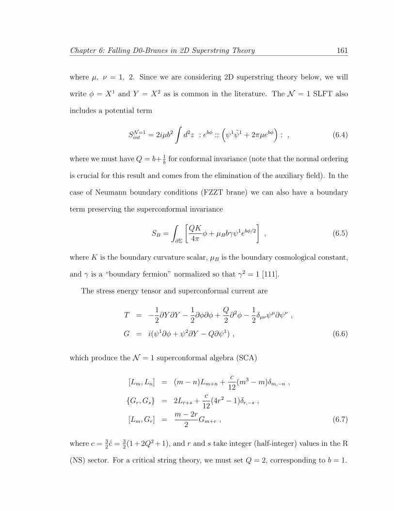
Chapter 6: Falling D0-Branes in 2D Superstring Theory 161
where µ, ν = 1, 2. Since we are considering 2D superstring theory below, we will
write φ = X1 and Y = X2 as is common in the literature. The N = 1 SLFT also
includes a potential term
SN=1int = 2iµb2
∫d2z : ebφ ::
(ψ1ψ1 + 2πµebφ
): , (6.4)
where we must have Q = b+ 1b
for conformal invariance (note that the normal ordering
is crucial for this result and comes from the elimination of the auxiliary field). In the
case of Neumann boundary conditions (FZZT brane) we can also have a boundary
term preserving the superconformal invariance
SB =
∫
∂Σ
[QK
4πφ + µBbγψ1ebφ/2
], (6.5)
where K is the boundary curvature scalar, µB is the boundary cosmological constant,
and γ is a “boundary fermion” normalized so that γ2 = 1 [111].
The stress energy tensor and superconformal current are
T = −1
2∂Y ∂Y − 1
2∂φ∂φ +
Q
2∂2φ− 1
2δµνψ
µ∂ψν ,
G = i(ψ1∂φ + ψ2∂Y −Q∂ψ1) , (6.6)
which produce the N = 1 superconformal algebra (SCA)
[Lm, Ln] = (m− n)Lm+n +c
12(m3 −m)δm,−n ,
Gr, Gs = 2Lr+s +c
12(4r2 − 1)δr,−s ,
[Lm, Gr] =m− 2r
2Gm+r , (6.7)
where c = 32c = 3
2(1+2Q2 +1), and r and s take integer (half-integer) values in the R
(NS) sector. For a critical string theory, we must set Q = 2, corresponding to b = 1.

Chapter 6: Falling D0-Branes in 2D Superstring Theory 162
The primary fields in the NS sector are Np,ω =: e(Q2
+ip)φ+iωY : with weights hNSp,ω =
12(Q2
4+ p2 + ω2), while in the R sector they are R±
p,ω = σ±Np,ω with weights hRp,ω =
hNSp,ω + 1
16. (If we bosonize the complex fermion ψ± = 1√
2(ψ2± iψ1) =: e±iH :, then σ±
is given by σ± =: e±iH/2 :.) The open string character is
χσ,±p,ω (τ) = TrHσ
p,ω[qL0−c/24(±1)F ] , (6.8)
where q ≡ e2πiτ and we trace over the descendants of Np,ω or Rp,ω for σ = NS, R,
respectively. For non-degenerate representations, the open string characters (which
result from a trace over a corresponding primary state and its descendants) are [3,
111],
χNS,+p,ω (τ) = q
12(p2+ω2) θ00(τ, 0)
η(τ)3,
χNS,−p,ω (τ) = q
12(p2+ω2) θ01(τ, 0)
η(τ)3,
χR,+p,ω (τ) = q
12(p2+ω2) θ10(τ, 0)
η(τ)3,
χR,−p,ω (τ) = 0 . (6.9)
6.2.2 Open/Closed duality: boundary states
As is well known, we can realize boundary conditions for an open string as con-
straints on states in the closed string spectrum [56, 55, 66, 115]. For example, Neu-
mann and Dirichlet boundary conditions in the open string are realized classically as
∂X(y)∓ ∂X(y) = 0 and ψ(y)∓ ηψ(y) = 0, where η = ±1, y ∈ R, and we have taken
the boundary to lie along the real axis (the upper sign is for Neumann boundary
conditions and the lower for Dirichlet). To tranform from the open channel to the
closed channel, we must perform the coordinate transformation z → z and z → z−1,
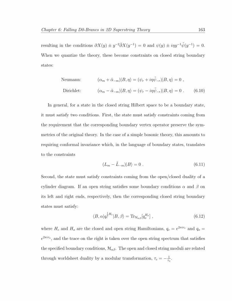
Chapter 6: Falling D0-Branes in 2D Superstring Theory 163
resulting in the conditions ∂X(y) ± y−2∂X(y−1) = 0 and ψ(y) ± iηy−1ψ(y−1) = 0.
When we quantize the theory, these become constraints on closed string boundary
states:
Neumann: (αm + α−m)|B, η〉 = (ψr + iηψ−r)|B, η〉 = 0 ,
Dirichlet: (αm − α−m)|B, η〉 = (ψr − iηψ−r)|B, η〉 = 0 . (6.10)
In general, for a state in the closed string Hilbert space to be a boundary state,
it must satisfy two conditions. First, the state must satisfy constraints coming from
the requirement that the corresponding boundary vertex operator preserve the sym-
metries of the original theory. In the case of a simple bosonic theory, this amounts to
requiring conformal invariance which, in the language of boundary states, translates
to the constraints
(Lm − L−m)|B〉 = 0 . (6.11)
Second, the state must satisfy constraints coming from the open/closed duality of a
cylinder diagram. If an open string satisfies some boundary conditions α and β on
its left and right ends, respectively, then the corresponding closed string boundary
states must satisfy:
〈B, α|q12Hc
c |B, β〉 = TrHαβ[qHo
o ] , (6.12)
where Hc and Ho are the closed and open string Hamiltonians, qc = e2πiτc and qo =
e2πiτo , and the trace on the right is taken over the open string spectrum that satisfies
the specified boundary conditions,Hαβ. The open and closed string moduli are related
through worldsheet duality by a modular transformation, τc = − 1τo
.
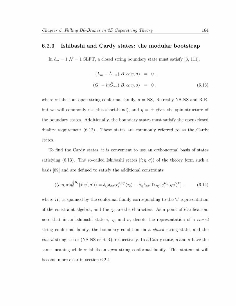
Chapter 6: Falling D0-Branes in 2D Superstring Theory 164
6.2.3 Ishibashi and Cardy states: the modular bootstrap
In cm = 1 N = 1 SLFT, a closed string boundary state must satisfy [3, 111],
(Lm − L−m)|B, α; η, σ〉 = 0 ,
(Gr − iηG−r)|B, α; η, σ〉 = 0 , (6.13)
where α labels an open string conformal family, σ = NS, R (really NS-NS and R-R,
but we will commonly use this short-hand), and η = ± gives the spin structure of
the boundary states. Additionally, the boundary states must satisfy the open/closed
duality requirement (6.12). These states are commonly referred to as the Cardy
states.
To find the Cardy states, it is convenient to use an orthonormal basis of states
satisfying (6.13). The so-called Ishibashi states |i; η, σ〉〉 of the theory form such a
basis [89] and are defined to satisfy the additional constraints
〈〈i; η, σ|q12Hc
c |j; η′, σ′〉〉 = δijδσσ′χσ,ηη′i (τc) ≡ δijδσσ′TrHσ
i[qHo
c (ηη′)F ] , (6.14)
where Hσi is spanned by the conformal family corresponding to the ‘i’ representation
of the constraint algebra, and the χi are the characters. As a point of clarification,
note that in an Ishibashi state i, η, and σ, denote the representation of a closed
string conformal family, the boundary condition on a closed string state, and the
closed string sector (NS-NS or R-R), respectively. In a Cardy state, η and σ have the
same meaning while α labels an open string conformal family. This statement will
become more clear in section 6.2.4.
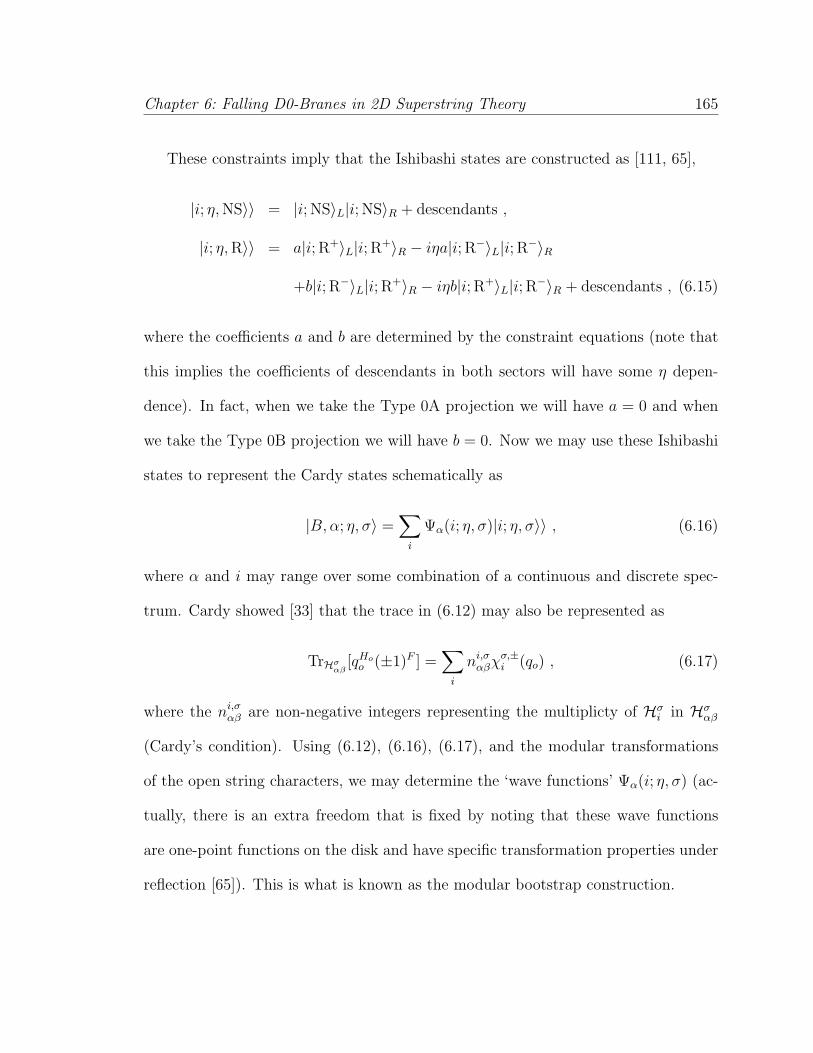
Chapter 6: Falling D0-Branes in 2D Superstring Theory 165
These constraints imply that the Ishibashi states are constructed as [111, 65],
|i; η, NS〉〉 = |i; NS〉L|i; NS〉R + descendants ,
|i; η, R〉〉 = a|i; R+〉L|i; R+〉R − iηa|i; R−〉L|i; R−〉R
+b|i; R−〉L|i; R+〉R − iηb|i; R+〉L|i; R−〉R + descendants , (6.15)
where the coefficients a and b are determined by the constraint equations (note that
this implies the coefficients of descendants in both sectors will have some η depen-
dence). In fact, when we take the Type 0A projection we will have a = 0 and when
we take the Type 0B projection we will have b = 0. Now we may use these Ishibashi
states to represent the Cardy states schematically as
|B, α; η, σ〉 =∑
i
Ψα(i; η, σ)|i; η, σ〉〉 , (6.16)
where α and i may range over some combination of a continuous and discrete spec-
trum. Cardy showed [33] that the trace in (6.12) may also be represented as
TrHσαβ
[qHoo (±1)F ] =
∑i
ni,σαβχσ,±
i (qo) , (6.17)
where the ni,σαβ are non-negative integers representing the multiplicty of Hσ
i in Hσαβ
(Cardy’s condition). Using (6.12), (6.16), (6.17), and the modular transformations
of the open string characters, we may determine the ‘wave functions’ Ψα(i; η, σ) (ac-
tually, there is an extra freedom that is fixed by noting that these wave functions
are one-point functions on the disk and have specific transformation properties under
reflection [65]). This is what is known as the modular bootstrap construction.
Chapter 6: Falling D0-Branes in 2D Superstring Theory 166
6.2.4 ZZ and FZZT boundary states
As an example, let us demonstrate how the modular bootstrap is applied to deter-
mine the boundary states corresponding to the ZZ brane and the FZZT brane. Since
the stress tensor and the superconformal current of the cm = 1 N = 1 SLFT are sim-
ply a sum of the corresponding currents of the cm = 1 theory and the N = 1 SLFT,
the tensor product of an Ishibashi state from each theory will be an Ishibashi state
of the combined theory. The ZZ and FZZT boundary states have been constructed
for the N = 1 SLFT [3, 65], and so a trivial modification allows us to write them in
our theory.
The open string spectrum corresponding to the descendants of the vacuum state
is given by an open string stretching between two vacuum Cardy states, while the
spectrum corresponding to an excited state is given by an open string stretching
between the corresponding excited Cardy state and a vacuum Cardy state:
χσ,ηη′vac (τo) = 〈vac; η, σ|q
12Hc
c |vac; η′, σ〉 ,
χσ,ηη′p,ω (τo) = 〈vac; η, σ|q
12Hc
c |p, ω; η′, σ〉 , (6.18)
where ν(σ) = 12|η − η′|; ν(σ) = 0, 1, corresponds to NS and R, respectively; and
ηη′ = eiπν(σ).
Our goal is to determine the wave function of the Cardy states expressed as a
linear combination of the Ishibashi states, which we denote by
|B, p, ω; η, σ〉 =
∫ ∞
−∞dp′ dω′ Ψp,ω(p′, ω′; η, σ)|p′, ω′; η, σ〉〉 . (6.19)
To apply this to the vacuum, note that the vacuum state has zero weight and so, in
the NS sector, has momentum p = − i2(1
b+ b), ω = 0. Recall that this corresponds to
Chapter 6: Falling D0-Branes in 2D Superstring Theory 167
a (1,1) degenerate representation since every conformal family built from a primary
of momentum p = − i2(m
b+ nb) is degenerate at level mn. This means that the open
string character corresponding to the vacuum representation is
χNS,+vac (τ) = [q−( 1
b+b)2/8 − q−( 1
b−b)2/8]
θ00(τ, 0)
η(τ)3, (6.20)
and the others are obtained similarly. Then by inserting the expansion of the Cardy
states into (6.18) and using the normalization of the Ishibashi states (6.14), the above
open/closed duality equations are rewritten as
χσ,ηη′vac (τo) =
∫ ∞
−∞dp′ dω′ Ψ(σ)∗
vac (p′, ω′; η)Ψ(σ)vac(p
′ω′; η′)χσ,ηη′p′,ω′ (τc) ,
χσ,ηη′p,ω (τo) =
∫ ∞
−∞dp′ dω′ Ψ(σ)∗
vac (p′, ω′; η)Ψ(σ)p,ω(p′ω′; η′)χσ,ηη′
p′,ω′ (τc) . (6.21)
The wave functions of the vacuum boundary states are simply one-point functions
on the disk which must transform in specific ways under reflection [65]. The trans-
formation properties under reflection, combined with the modular transformations
of the open string characters (given by the S-transformation matrix) determine the
wave functions of the vacuum boundary states to be
Ψ(NS)vac (p, ω; η) =
π(µπγ( bQ2
))−ip/b
ipΓ(−ipb)Γ(−ipb)Ψ
(NS),cm=1ω′=0 (ω; η) ,
Ψ(R)vac(p, ω; +) =
π(µπγ( bQ2
))−ip/b
Γ(12− ipb)Γ(1
2− ip
b)Ψ
(R),cm=1ω′=0 (ω; +) , (6.22)
where Ψ(σ),cm=1ω′ denotes the wave function for the cm = 1 matter boundary state whose
properties do not concern us here. (Note that there is no R-sector (1, 1) boundary
state with η = − for the same reason that the open string character in this sector is
zero [65, 57].) These vacuum boundary states, the ZZ branes, correspond to static
Euclidean D0-branes that sit in the strong coupling region, φ → +∞.
Chapter 6: Falling D0-Branes in 2D Superstring Theory 168
The behavior of the Fourier transform of (6.22) is most transparent by utilizing
the product representation of the gamma functions. If this product is cutoff after N
terms, one will be taking the Fourier transform of a function of the form PN(p)eiaN (p),
where PN(p) is a polynomial in p and aN tends to infinity as N tends to infinity.
Such a Fourier transform will give a sum of delta functions and derivatives of delta
functions located at aN . Thus, the Fourier transform of the wave functions in (21)
will be localized at infinity as claimed.
All the excited states are non-degenerate representations with continuous momen-
tum p′. The modular transformation of the open string character of the continuous
representation together with the solution of the ZZ boundary state gives the excited
boundary state (FZZT brane)
Ψ(NS)p′,ω′(p, ω; η) = −cos(2πpp′)
2π
(µπγ
(bQ2
))−ip/bipΓ(ipb)Γ
(ip
b
)Ψ
(NS),cm=1ω′ (ω; η),(6.23)
Ψ(R)p′,ω′(p, ω; +) =
cos(2πpp′)2π
(µπγ
(bQ2
))−ip/bΓ
(12
+ ipb)Γ
(12
+ ipb
)Ψ
(R),cm=1ω′ (ω; +) .
Their pole structures show that they are Euclidean D1-branes, extended in the Liou-
ville direction.
6.2.5 An argument for additional symmetry
As we saw above, the characters for cm = 1 N = 1 SLFT are simply a product of
the individual characters for cm = 1 matter and N = 1 SLFT. This led us to a trivial
modification of the ZZ and FZZT boundary states of N = 1 SLFT that resulted in
static branes, as we saw in section 6.2.4. In fact, we were destined to realize this
result because we restricted ourselves to the subset of cm = 1 N = 1 Ishibashi states
that were simply a tensor product of the Ishibashi states of the separate theories.
Chapter 6: Falling D0-Branes in 2D Superstring Theory 169
We thus implicitly required our boundary states to satisfy an additional symmetry
(namely, that they separately satisfy N = 1 boundary conditions for each direction).
It was because of this additional symmetry we imposed, combined with the fact the
characters decouple, that the wave functions did not mix the two directions.
If we want to find a falling D0-brane, we clearly cannot impose the restrictions
mentioned above. Naturally, the time direction should satisfy ‘Neumann-like’ bound-
ary conditions while the Liouville direction should satisfy ‘Dirichlet-like’ conditions.
However, what conditions to impose are not obvious. In the bosonic case of the
hairpin brane [100], the authors had to impose the W-symmetry to get the time
dependence necessary to obtain a falling D0-brane with the desired trajectory.
It turns out that in the N = 2 SLFT, which has the same matter content as
cm = 1 N = 1 SLFT, there are additional symmetries that naturally follow from the
action. Applying these additional constraints to N = 1 Ishibashi states, one finds
boundary states with trajectories that match that of the falling D0-brane (6.1). We
will show that in N = 1, 2D superstring theory with linear dilaton background (which
is equivalent to cm = 1 N = 1 SLFT), there exists a type of falling D0-brane that has
the additional N = 2 SCA symmetry and can be obtained by a slight modification
of the falling D0-brane solution of the N = 2 SLFT.
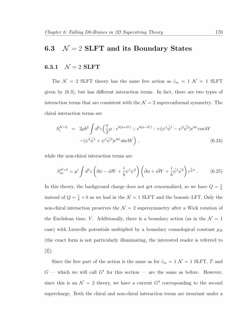
Chapter 6: Falling D0-Branes in 2D Superstring Theory 170
6.3 N = 2 SLFT and its Boundary States
6.3.1 N = 2 SLFT
The N = 2 SLFT theory has the same free action as cm = 1 N = 1 SLFT
given by (6.3), but has different interaction terms. In fact, there are two types of
interaction terms that are consistent with the N = 2 superconformal symmetry. The
chiral interaction terms are
SN=2c = 2µb2
∫d2z
(π
2µ : eb(φ+iY ) :: eb(φ−iY ) : +(ψ1ψ1 − ψ2ψ2)ebφ cos bY
−(ψ2ψ1 + ψ1ψ2)ebφ sin bY)
, (6.24)
while the non-chiral interaction terms are
SN=2nc = µ′
∫d2z
(∂φ− i∂Y +
i
bψ1ψ2
)(∂φ + i∂Y +
i
bψ1ψ2
)e
1bφ . (6.25)
In this theory, the background charge does not get renormalized, so we have Q = 1b
instead of Q = 1b
+ b as we had in the N = 1 SLFT and the bosonic LFT. Only the
non-chiral interaction preserves the N = 2 supersymmetry after a Wick rotation of
the Euclidean time, Y . Additionally, there is a boundary action (as in the N = 1
case) with Liouville potentials multiplied by a boundary cosmological constant µB
(the exact form is not particularly illuminating, the interested reader is referred to
[2]).
Since the free part of the action is the same as for cm = 1 N = 1 SLFT, T and
G — which we will call G1 for this section — are the same as before. However,
since this is an N = 2 theory, we have a current G2 corresponding to the second
supercharge. Both the chiral and non-chiral interaction terms are invariant under a
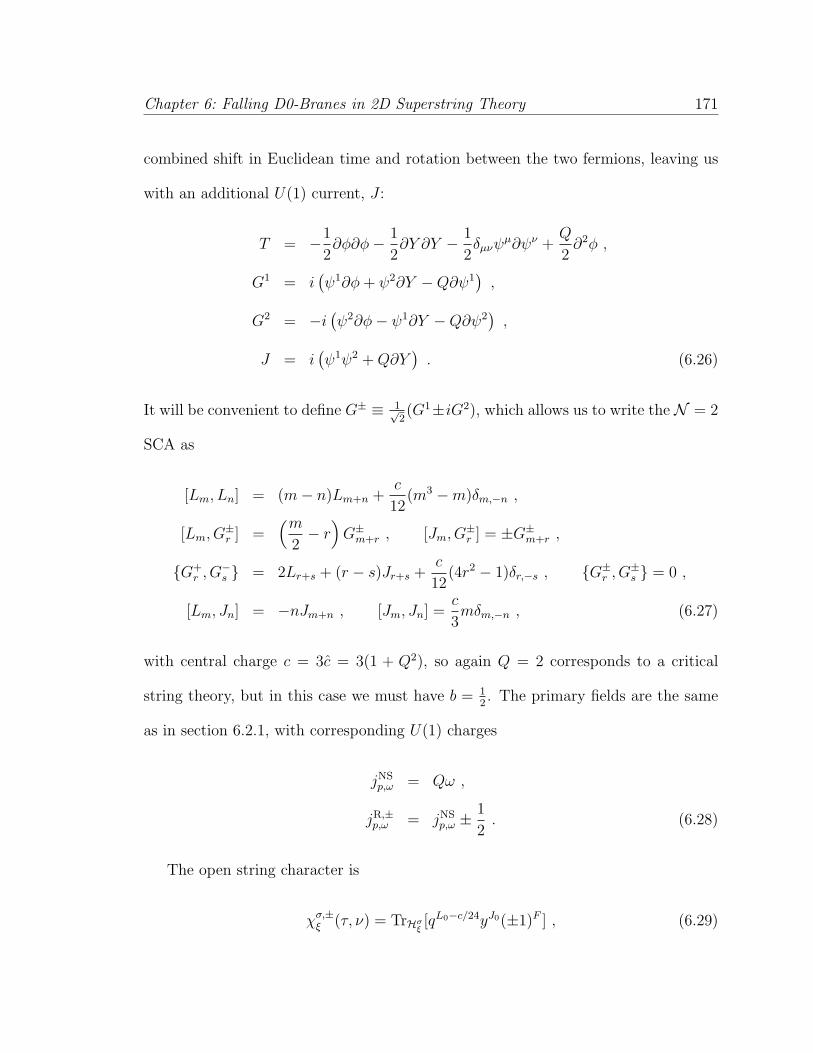
Chapter 6: Falling D0-Branes in 2D Superstring Theory 171
combined shift in Euclidean time and rotation between the two fermions, leaving us
with an additional U(1) current, J :
T = −1
2∂φ∂φ− 1
2∂Y ∂Y − 1
2δµνψ
µ∂ψν +Q
2∂2φ ,
G1 = i(ψ1∂φ + ψ2∂Y −Q∂ψ1
),
G2 = −i(ψ2∂φ− ψ1∂Y −Q∂ψ2
),
J = i(ψ1ψ2 + Q∂Y
). (6.26)
It will be convenient to define G± ≡ 1√2(G1±iG2), which allows us to write the N = 2
SCA as
[Lm, Ln] = (m− n)Lm+n +c
12(m3 −m)δm,−n ,
[Lm, G±r ] =
(m
2− r
)G±
m+r , [Jm, G±r ] = ±G±
m+r ,
G+r , G−
s = 2Lr+s + (r − s)Jr+s +c
12(4r2 − 1)δr,−s , G±
r , G±s = 0 ,
[Lm, Jn] = −nJm+n , [Jm, Jn] =c
3mδm,−n , (6.27)
with central charge c = 3c = 3(1 + Q2), so again Q = 2 corresponds to a critical
string theory, but in this case we must have b = 12. The primary fields are the same
as in section 6.2.1, with corresponding U(1) charges
jNSp,ω = Qω ,
jR,±p,ω = jNS
p,ω ±1
2. (6.28)
The open string character is
χσ,±ξ (τ, ν) = TrHσ
ξ[qL0−c/24yJ0(±1)F ] , (6.29)
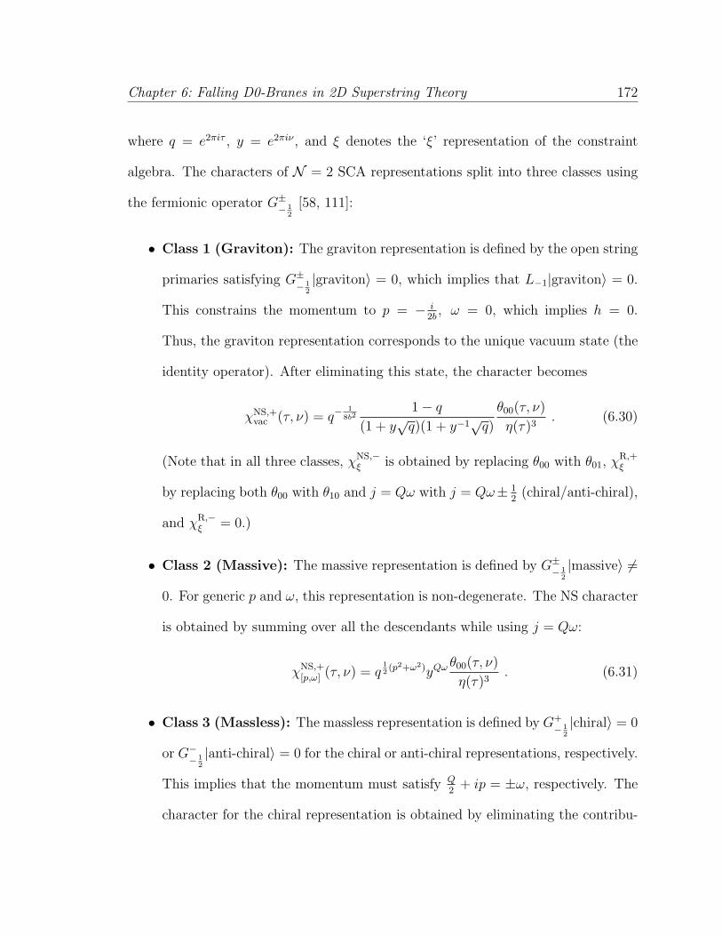
Chapter 6: Falling D0-Branes in 2D Superstring Theory 172
where q = e2πiτ , y = e2πiν , and ξ denotes the ‘ξ’ representation of the constraint
algebra. The characters of N = 2 SCA representations split into three classes using
the fermionic operator G±− 1
2
[58, 111]:
• Class 1 (Graviton): The graviton representation is defined by the open string
primaries satisfying G±− 1
2
|graviton〉 = 0, which implies that L−1|graviton〉 = 0.
This constrains the momentum to p = − i2b
, ω = 0, which implies h = 0.
Thus, the graviton representation corresponds to the unique vacuum state (the
identity operator). After eliminating this state, the character becomes
χNS,+vac (τ, ν) = q−
18b2
1− q
(1 + y√
q)(1 + y−1√
q)
θ00(τ, ν)
η(τ)3. (6.30)
(Note that in all three classes, χNS,−ξ is obtained by replacing θ00 with θ01, χR,+
ξ
by replacing both θ00 with θ10 and j = Qω with j = Qω± 12
(chiral/anti-chiral),
and χR,−ξ = 0.)
• Class 2 (Massive): The massive representation is defined by G±− 1
2
|massive〉 6=
0. For generic p and ω, this representation is non-degenerate. The NS character
is obtained by summing over all the descendants while using j = Qω:
χNS,+[p,ω] (τ, ν) = q
12(p2+ω2)yQω θ00(τ, ν)
η(τ)3. (6.31)
• Class 3 (Massless): The massless representation is defined by G+− 1
2
|chiral〉 = 0
or G−− 1
2
|anti-chiral〉 = 0 for the chiral or anti-chiral representations, respectively.
This implies that the momentum must satisfy Q2
+ ip = ±ω, respectively. The
character for the chiral representation is obtained by eliminating the contribu-
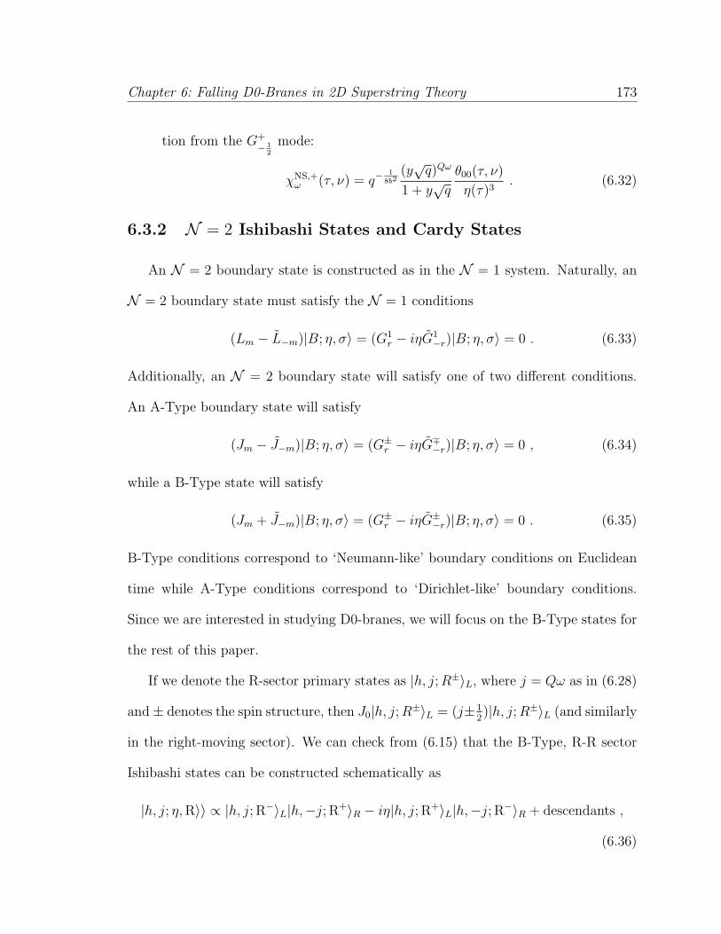
Chapter 6: Falling D0-Branes in 2D Superstring Theory 173
tion from the G+− 1
2
mode:
χNS,+ω (τ, ν) = q−
18b2
(y√
q)Qω
1 + y√
q
θ00(τ, ν)
η(τ)3. (6.32)
6.3.2 N = 2 Ishibashi States and Cardy States
An N = 2 boundary state is constructed as in the N = 1 system. Naturally, an
N = 2 boundary state must satisfy the N = 1 conditions
(Lm − L−m)|B; η, σ〉 = (G1r − iηG1
−r)|B; η, σ〉 = 0 . (6.33)
Additionally, an N = 2 boundary state will satisfy one of two different conditions.
An A-Type boundary state will satisfy
(Jm − J−m)|B; η, σ〉 = (G±r − iηG∓
−r)|B; η, σ〉 = 0 , (6.34)
while a B-Type state will satisfy
(Jm + J−m)|B; η, σ〉 = (G±r − iηG±
−r)|B; η, σ〉 = 0 . (6.35)
B-Type conditions correspond to ‘Neumann-like’ boundary conditions on Euclidean
time while A-Type conditions correspond to ‘Dirichlet-like’ boundary conditions.
Since we are interested in studying D0-branes, we will focus on the B-Type states for
the rest of this paper.
If we denote the R-sector primary states as |h, j; R±〉L, where j = Qω as in (6.28)
and± denotes the spin structure, then J0|h, j; R±〉L = (j± 12)|h, j; R±〉L (and similarly
in the right-moving sector). We can check from (6.15) that the B-Type, R-R sector
Ishibashi states can be constructed schematically as
|h, j; η, R〉〉 ∝ |h, j; R−〉L|h,−j; R+〉R − iη|h, j; R+〉L|h,−j; R−〉R + descendants ,
(6.36)
Chapter 6: Falling D0-Branes in 2D Superstring Theory 174
Since ψ+0 |h, j; R−〉L = |h, j; R+〉L, it is clear that (−1)F+F = −1 on the primary states
in (6.36). Furthermore, from the commutation relations J0, G±0 = ±G±
0 , we can
see that the constraint (J0 + J0) = 0 implies that all descendants in (6.36) must have
an equal number of fermionic raising operators on the left-moving and right-moving
sides, modulo 2. Therefore, B-Type, R-R sector Ishibashi states will be projected out
by the Type 0B GSO projection and so are only present in Type 0A — note that a
similar argument implies that A-Type, R-R sector Ishibashi states are only present in
Type 0B. Thus, B-Type states will yield stable D0-branes in Type 0A and unstable
D0-branes in Type 0B.
B-Type Ishibashi states are constructed to form an orthonormal basis for states
satisfying (6.33) and (6.35), and must also satisfy
Class 1 〈〈vac; η, σ|q12Hc
c y12(J0−J0)
c |vac; η, σ〉〉 = χσ,ηη′vac (τc, νc) ,
Class 2 〈〈p, ω; η, σ|q12Hc
c y12(J0−J0)
c |p′, ω′; η, σ〉〉 = δ(p− p′)δ(ω − ω′)χσ,ηη′[p,ω] (τc, νc) ,
Class 3 〈〈ω; η, σ|q12Hc
c y12(J0−J0)
c |ω′; η, σ〉〉 = δ(ω − ω′)χσ,ηη′ω (τc, νc) , (6.37)
while all other correlators between Ishibashi states vanish. The open and closed
parameters are related by the modular transformation τo = − 1τc
and νo = νc
τc. The
B-Type Cardy states are then constructed as a linear combination of the B-Type
Ishibashi states such that the Cardy states satisfy
〈B, O; η, σ|q12Hc
c y12(J0−J0)
c |B, ξ; η′, σ〉 = eiπcν2o
τo χσ,ηη′ξ (τo, νo) ,
〈B, O; η, σ|q12Hc
c y12(J0−J0)
c |B, O; η′, σ〉 = eiπcν2o
τo χσ,ηη′vac (τo, νo) , (6.38)
where χσ,±ξ (τ, ν) is the open string character of the ξ representation of the constraint
algebra, O represents the graviton state, and σ and ηη′ are defined as in equation
Chapter 6: Falling D0-Branes in 2D Superstring Theory 175
(6.18).
6.3.3 Falling Euclidean D0-brane in N = 2 SLFT
As in cm = 1 N = 1 SLFT, the modular transformation of the Class 1 (Graviton)
representation (identity operator) gives the wave function of the vacuum boundary
state. Then the modular transformation of the Class 2 (Massive) non-degenerate
representation of the open string produces the wave function of the excited boundary
state which corresponds to the FZZT brane (Falling Euclidean D0-brane) solution
[58, 112, 4, 5]:
Ψ[p′,ω′](p, ω; η, σ) (6.39)
=√
2Qµ−ipQe−2πiωω′ cos(2πpp′)Γ(−iQp)Γ
(1− i2p
Q
)
Γ(
12− i p
Q+ ω
Q− ν(σ)
2
)Γ
(12− i p
Q− ω
Q+ ν(σ)
2
) ,
where µ is the renormalized bulk cosmological constant (it is, in fact, proportional
to µ [111] and we will henceforth drop the distinction between the two as it just
corresponds to a finite, constant shift of the dilaton in the position space picture).
Note also that this wave function has no dependence on η.
The Fourier transform of the momentum space wave function into the position
space wave function is
Ψ(NS)[p′,ω′](φ, Y ) ≡
∫ ∞
−∞
dpdω
(2π)2e−ip(φ+Q ln µ)e−iωY Ψ
(NS)[p′,ω′](p, ω) . (6.40)
We can construct solutions where p′ and ω′ are nonzero from the solution in which
they are both zero [112]
Ψ(NS)[0,0] (φ, Y ) =
√2
µπQ(2 cos QY2
)2
Q2 +1· exp
[− φ
Q− e−
φQ
µ(2 cos QY2
)2
Q2
]. (6.41)
Chapter 6: Falling D0-Branes in 2D Superstring Theory 176
Then it is simple to see that
Ψ(NS)[p′,ω′](φ, Y ) =
1
2Ψ
(NS)[0,0] (φ− 2πp′, Y + 2πω′) +
1
2Ψ
(NS)[0,0] (φ + 2πp′, Y + 2πω′) . (6.42)
Actually, p′ is not an independent variable but is instead related to the bulk and
boundary cosmological constants through [4]
(µ2
B +µ2
4Q4µ2B
)=
µ
32πQcosh (2πp′/Q) (6.43)
(at least for ω′ = 0). Since [100] and [101] contain a theory with no bulk cosmological
constant, we should take the limit µ → 0 to make a comparison with the hairpin
brane. In this limit, p′ → ±∞, which is irrelevant since (6.42) contains a sum of both
signs of p′, so let us take p′ → +∞ in which case
e2πp′/Q−→µ→0
64πQµ2B
µ. (6.44)
One then finds
limµ→0
Ψ[p′,0](φ, Y ) =
√2
64π2Q2µ2B(2 cos QY
2)
2Q2 +1
· exp
[− φ
Q− e−
φQ
64πQµ2B(2 cos QY
2)
2Q2
].
(6.45)
The classical shape of this falling Euclidean D0-brane is given by the peak of its wave
function
e−Qφ2 = 128πQµ2
B cosQY
2, (6.46)
reproducing the trajectory of the hairpin brane [100] for appropriate shift of the Liou-
ville direction. This supports the suggestion [97, 112] that this is the supersymmetric
extension of the hairpin brane. Note that if we had instead considered the limit
µB → 0, we would have found that the wave function vanishes. Thus, the boundary
Liouville potential is necessary for the existence of these boundary states.

Chapter 6: Falling D0-Branes in 2D Superstring Theory 177
The wave function Ψ[0,0](φ, Y ) is also peaked along the trajectory
e−Qφ2 = 2 cos
QY
2(6.47)
and we will simply refer to this wave function for the rest of our discussions. Since
we are only interested in bulk one-point functions, limits can always be taken if one
wishes to look at the case with vanishing bulk cosmological constant.
6.3.4 Falling D0-brane in N = 2 SLFT
For the wave function Ψ[0,0](φ, Y ), the Wick-rotation from the Euclidean time
Y into the Minkowski time t, together with a shift in the Liouville direction φ →
φ− 2Q
ln r−Q ln µ, produces the classical trajectory of the falling D0-brane in N = 2
SLFT [112]:
re−Qφ2 = 2 cosh
Qt
2, (6.48)
which matches with (6.1) once we set r = 2Eτp
.
Therefore, the falling D0-brane wave function in position space is [112]
Ψ(NS)[0,0] (φ, t) =
√2
µπQ(2 cosh Qt2
)2
Q2 +1· exp
−
φ− 2Q
ln r
Q− e−
φ− 2Q
ln r
Q
µ(2 cosh Qt2
)2
Q2
. (6.49)
Then the Fourier transform to momentum space yields
Ψ(NS)[0,0] (p, q) =
−i√
2Qµ−ipQei 2pQ
ln r sinh(2πpQ
)
cosh(2πpQ
) + cosh(2πqQ
)·
Γ(−iQp)Γ(1− i2pQ
)
Γ(12− i p
Q+ i q
Q)Γ(1
2− i p
Q− i q
Q)
, (6.50)
and a half spectral flow gives the R-sector wave function
Ψ(R)[0,0](p, q) =
−i√
2Qµ−ipQei 2pQ
ln r sinh(2πpQ
)
cosh(2πpQ
)− cosh(2πqQ
)·
Γ(−iQp)Γ(1− i2pQ
)
Γ(1− i pQ
+ i qQ
)Γ(−i pQ− i q
Q)
. (6.51)
Chapter 6: Falling D0-Branes in 2D Superstring Theory 178
6.4 Falling D0-brane in N = 1, 2D Superstring
Theory
6.4.1 Using N = 2 SLFT to study boundary states in 2D
superstring
We propose that the N = 2 SLFT boundary states may be used to study falling
D0-branes in the N = 1, 2D superstring with linear dilaton background (which is
equivalent to cm = 1 N = 1 SLFT theory). Notice that the field content of both
theories is the same, as are the stress tensor and the first supercharge. Additionally,
as is apparent from the constraints on anN = 2 boundary state, anyN = 2 boundary
state also satisfies the N = 1 constraints (6.13). So an N = 2 SLFT boundary state
is also a boundary state of the N = 1, 2D superstring, with the N = 2 boundary
interaction term.
However, this alone is not enough; if we want to use the N = 2 Ishibashi states,
we must also be able to construct a Cardy state from them that will generate the
cm = 1 N = 1 open string character. In fact, we can do this. In (6.31), ν is the
‘modulus’ of the U(1) charge and appears nontrivially in the functional form of the
character. But if we set ν = 0 (y = 1), the U(1) charge acts trivially on the N = 2
states and we can see that the character of theN = 2 Class 2 (Massive) representation
(6.31) is equivalent to the cm = 1 N = 1 character (6.8). Such a state was found in
[58, 112, 4, 5], and presented in sections 6.3.3 and 6.3.4. The momentum space wave
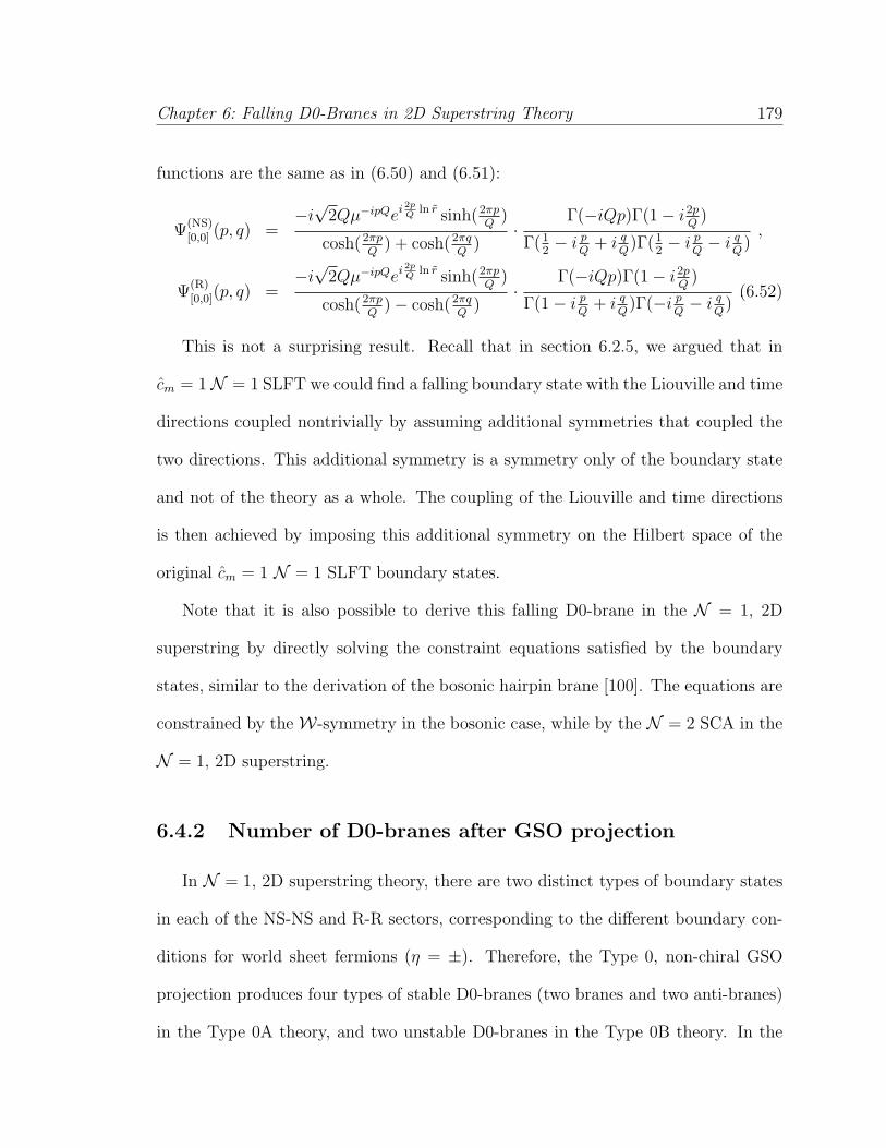
Chapter 6: Falling D0-Branes in 2D Superstring Theory 179
functions are the same as in (6.50) and (6.51):
Ψ(NS)[0,0] (p, q) =
−i√
2Qµ−ipQei 2pQ
ln r sinh(2πpQ
)
cosh(2πpQ
) + cosh(2πqQ
)·
Γ(−iQp)Γ(1− i2pQ
)
Γ(12− i p
Q+ i q
Q)Γ(1
2− i p
Q− i q
Q)
,
Ψ(R)[0,0](p, q) =
−i√
2Qµ−ipQei 2pQ
ln r sinh(2πpQ
)
cosh(2πpQ
)− cosh(2πqQ
)·
Γ(−iQp)Γ(1− i2pQ
)
Γ(1− i pQ
+ i qQ
)Γ(−i pQ− i q
Q)
.(6.52)
This is not a surprising result. Recall that in section 6.2.5, we argued that in
cm = 1N = 1 SLFT we could find a falling boundary state with the Liouville and time
directions coupled nontrivially by assuming additional symmetries that coupled the
two directions. This additional symmetry is a symmetry only of the boundary state
and not of the theory as a whole. The coupling of the Liouville and time directions
is then achieved by imposing this additional symmetry on the Hilbert space of the
original cm = 1 N = 1 SLFT boundary states.
Note that it is also possible to derive this falling D0-brane in the N = 1, 2D
superstring by directly solving the constraint equations satisfied by the boundary
states, similar to the derivation of the bosonic hairpin brane [100]. The equations are
constrained by the W-symmetry in the bosonic case, while by the N = 2 SCA in the
N = 1, 2D superstring.
6.4.2 Number of D0-branes after GSO projection
In N = 1, 2D superstring theory, there are two distinct types of boundary states
in each of the NS-NS and R-R sectors, corresponding to the different boundary con-
ditions for world sheet fermions (η = ±). Therefore, the Type 0, non-chiral GSO
projection produces four types of stable D0-branes (two branes and two anti-branes)
in the Type 0A theory, and two unstable D0-branes in the Type 0B theory. In the

Chapter 6: Falling D0-Branes in 2D Superstring Theory 180
Type 0A theory, the D0±-branes are sourced by two different R-R gauge fields, C(±)1
[144].
The D-brane boundary states in the Type 0A theories are given by the non-chiral
GSO projection 1±(−1)F+F
2, with the upper sign for the NS-NS sector and the lower
sign for the R-R sector. As explained in section 6.3.2, the D0-branes of our theory
correspond to the B-Type boundary states. Since the B-Type, R-R Ishibashi states
survive the Type 0A GSO projection, the D0-branes in Type 0A will be stable. We
can represent them schematically as [66, 144],
|D0; +〉 = |B0; +, NS〉+ |B0; +, R〉 ,
|D0;−〉 = |B0;−, NS〉+ |B0;−, R〉 ,
|D0; +〉 = |B0; +, NS〉 − |B0; +, R〉 ,
|D0;−〉 = |B0;−, NS〉 − |B0;−, R〉 . (6.53)
On the other hand, the D-brane boundary states in the Type 0B theories are given
by the non-chiral GSO projection 1+(−1)F+F
2for both the NS-NS and R-R sectors.
In this case, the B-Type, R-R Ishibashi states are projected out by the Type 0B
projection. This leaves us with two unstable D0-branes represented schematically as
|D0; +〉 = |B0; +, NS〉 ,
|D0;−〉 = |B0;−, NS〉 . (6.54)
Note that the sign, η = ±, really does denote different D0-branes since, by Cardy’s
condition (6.12) and (6.18), these states yield different spectra. It would be interesting
to see how states with different values of η distinguish themselves from each other in
the context of matrix models.
Chapter 6: Falling D0-Branes in 2D Superstring Theory 181
6.5 Discussion and Summary
Recall that in the static case, the D0-brane (ZZ brane) and the D1-brane (FZZT
brane) boundary states were derived from the degenerate and the non-degenerate
representation of the open string character, respectively. So it may seem a little puz-
zling that the falling D0-brane is constructed from the non-degenerate representation
instead of the degenerate one.
In the static case, the difference between the D0-brane and the D1-brane is that
the D0-brane is localized at the same point in the Liouville direction for all time, while
the D1-brane is extended. The open strings ending on this D0-brane can only take
on a fixed (imaginary) value of Liouville momentum, while the open strings ending
on the D1-brane can take on any value of Liouville momentum.
In the case of the falling D0-brane, if we partition the two-dimensional spacetime
into spacelike hypersurfaces, the falling D0-brane is again localized in the Liouville
direction along each hypersurface. However, the Liouville position from one hyper-
surface to the next is not the same (the falling D0-brane is, not surprisingly, moving),
and so open strings ending on the falling D0-brane can take on any value of Liouville
momentum. This is the reason that we must use the non-degenerate representation
of the open string characters to define the falling D0-brane boundary state.
To summarize, we have shown that a falling D0-brane boundary state in N = 1,
2D superstring theory can be obtained by adapting the falling D0-brane boundary
state solution in N = 2 SLFT [112]. In particular, there exist four types of stable,
falling D0-branes (two branes and two anti-branes) in Type 0A theory and two types
of unstable, falling D0-branes in Type 0B theory. As is well known, Type 0, N = 1,
Chapter 6: Falling D0-Branes in 2D Superstring Theory 182
2D superstring theory has a dual description in the language of matrix models. An
interesting question would be to understand these falling D0-branes in the context of
the dual matrix model.

Appendix A
Derivation of the Moduli Space
M3D
Here we briefly review the derivation of the 3d moduli spaceM3D from the c∗-map
of the 4D supergravity coupled to nV vector-multiplets [46] [35] [127].
The bosonic part of the action for the N = 2 supergravity coupled to nV vector-
multiplets is:
S = − 1
16π
∫d4x
√g(4)
[R− 2gijdzi ∧ ∗4dz j − F I ∧GI
](A.1)
where the ranges of the indices are i, j = 1, . . . , nV and I = 0, 1, . . . , nV , and GI =
(ReN )IJF J + (ImN )IJ ∗ F J . The complex symmetric matrix NIJ is defined by
FI = NIJXJ DiFI = N IJDiXJ . (A.2)
For model endowed with a prepotential F (X),
NIJ = FIJ + 2i(ImF ·X)I(ImF ·X)J
X · ImF ·X (A.3)
183
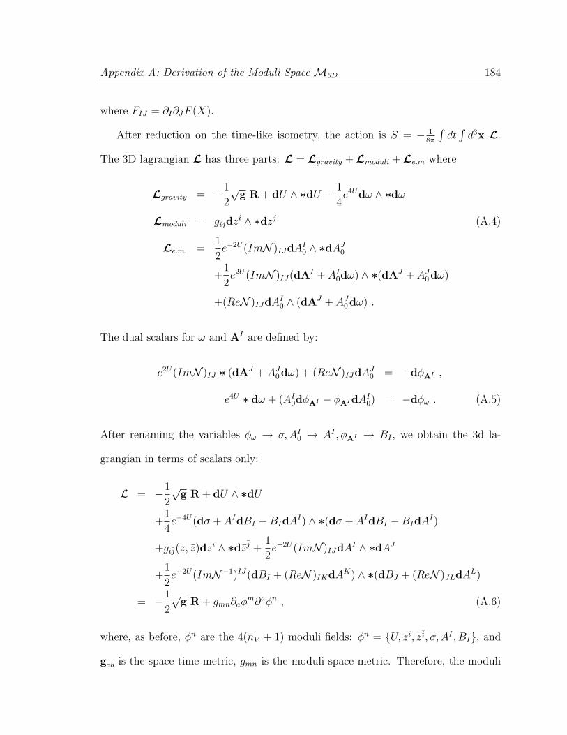
Appendix A: Derivation of the Moduli Space M3D 184
where FIJ = ∂I∂JF (X).
After reduction on the time-like isometry, the action is S = − 18π
∫dt
∫d3x L.
The 3D lagrangian L has three parts: L = Lgravity + Lmoduli + Le.m where
Lgravity = −1
2
√g R + dU ∧ ∗dU − 1
4e4Udω ∧ ∗dω
Lmoduli = gijdzi ∧ ∗dz j (A.4)
Le.m. =1
2e−2U(ImN )IJdAI
0 ∧ ∗dAJ0
+1
2e2U(ImN )IJ(dAI + AI
0dω) ∧ ∗(dAJ + AJ0dω)
+(ReN )IJdAI0 ∧ (dAJ + AJ
0dω) .
The dual scalars for ω and AI are defined by:
e2U(ImN )IJ ∗ (dAJ + AJ0dω) + (ReN )IJdAJ
0 = −dφAI ,
e4U ∗ dω + (AI0dφAI − φAIdAI
0) = −dφω . (A.5)
After renaming the variables φω → σ,AI0 → AI , φAI → BI , we obtain the 3d la-
grangian in terms of scalars only:
L = −1
2
√g R + dU ∧ ∗dU
+1
4e−4U(dσ + AIdBI −BIdAI) ∧ ∗(dσ + AIdBI −BIdAI)
+gij(z, z)dzi ∧ ∗dz j +1
2e−2U(ImN )IJdAI ∧ ∗dAJ
+1
2e−2U(ImN−1)IJ(dBI + (ReN )IKdAK) ∧ ∗(dBJ + (ReN )JLdAL)
= −1
2
√g R + gmn∂aφ
m∂aφn , (A.6)
where, as before, φn are the 4(nV + 1) moduli fields: φn = U, zi, z i, σ, AI , BI, and
gab is the space time metric, gmn is the moduli space metric. Therefore, the moduli
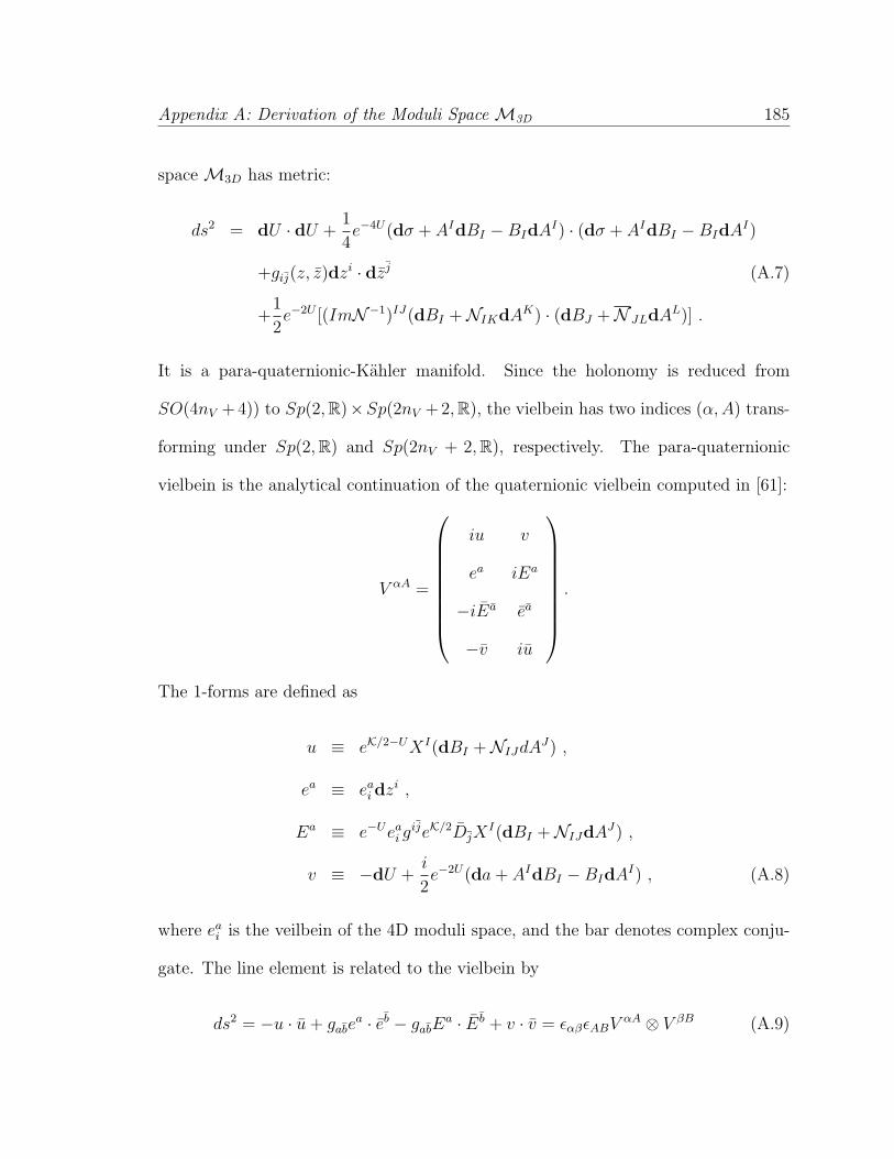
Appendix A: Derivation of the Moduli Space M3D 185
space M3D has metric:
ds2 = dU · dU +1
4e−4U(dσ + AIdBI −BIdAI) · (dσ + AIdBI −BIdAI)
+gij(z, z)dzi · dz j (A.7)
+1
2e−2U [(ImN−1)IJ(dBI +NIKdAK) · (dBJ +N JLdAL)] .
It is a para-quaternionic-Kahler manifold. Since the holonomy is reduced from
SO(4nV +4)) to Sp(2,R)×Sp(2nV +2,R), the vielbein has two indices (α, A) trans-
forming under Sp(2,R) and Sp(2nV + 2,R), respectively. The para-quaternionic
vielbein is the analytical continuation of the quaternionic vielbein computed in [61]:
V αA =
iu v
ea iEa
−iE a ea
−v iu
.
The 1-forms are defined as
u ≡ eK/2−UXI(dBI +NIJdAJ) ,
ea ≡ eai dzi ,
Ea ≡ e−Ueai g
ijeK/2DjXI(dBI +NIJdAJ) ,
v ≡ −dU +i
2e−2U(da + AIdBI −BIdAI) , (A.8)
where eai is the veilbein of the 4D moduli space, and the bar denotes complex conju-
gate. The line element is related to the vielbein by
ds2 = −u · u + gabea · eb − gabE
a · E b + v · v = εαβεABV αA ⊗ V βB (A.9)
Appendix A: Derivation of the Moduli Space M3D 186
where εαβ and εAB are the anti-symmetric tensors invariant under Sp(2,R) ∼= SL(2,R)
and Sp(2nv + 2,R).
The isometries of the M∗3D descends from the symmetry of the 4D system. The
gauge symmetries in 4D gives the shifting isometries of M∗3D:
AI −→ AI + ∆AI ,
BI −→ BI + ∆BI , (A.10)
σ −→ σ + ∆σ + ∆BIAI −∆AIBI .
The conserved currents and charges are given by (4.93) and the discussion thereafter.
Appendix B
Energy-Momentum Pseudotensor
In this appendix we show that the energy defined from the energy momentum
pseudotensor for massive gravitons can be negative. For simplicity we specialize to
Λ = 0: for µ` À 1 the Compton wavelength of the gravitons is much shorter than
the AdS3 radius so the latter can be locally ignored.
Let us first review how the energy-momentum pseudo tensor at quadratic order
is defined without the Chern-Simons term or cosmological constant term. The full
Einstein equation in the presence of matter is
Gµν = 16πGTMµν . (B.1)
Expanding the metric gµν = ηµν + hµν , we have through quadratic order
G(1)µν = −G(2)
µν + 16πGTMµν , (B.2)
where G(1)µν and G
(2)µν are terms linear and quadratic in hµν . The energy momentum
pseudo tensor defined as
tµν = − 1
16πGG(2)
µν , with ∂µtµν = 0 (B.3)
187
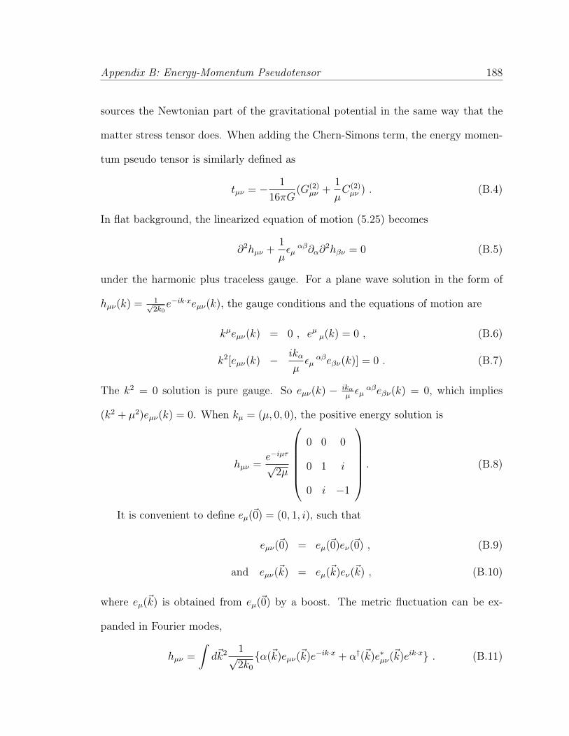
Appendix B: Energy-Momentum Pseudotensor 188
sources the Newtonian part of the gravitational potential in the same way that the
matter stress tensor does. When adding the Chern-Simons term, the energy momen-
tum pseudo tensor is similarly defined as
tµν = − 1
16πG(G(2)
µν +1
µC(2)
µν ) . (B.4)
In flat background, the linearized equation of motion (5.25) becomes
∂2hµν +1
µεµ
αβ∂α∂2hβν = 0 (B.5)
under the harmonic plus traceless gauge. For a plane wave solution in the form of
hµν(k) = 1√2k0
e−ik·xeµν(k), the gauge conditions and the equations of motion are
kµeµν(k) = 0 , eµµ(k) = 0 , (B.6)
k2[eµν(k) − ikα
µεµ
αβeβν(k)] = 0 . (B.7)
The k2 = 0 solution is pure gauge. So eµν(k) − ikα
µεµ
αβeβν(k) = 0, which implies
(k2 + µ2)eµν(k) = 0. When kµ = (µ, 0, 0), the positive energy solution is
hµν =e−iµτ
√2µ
0 0 0
0 1 i
0 i −1
. (B.8)
It is convenient to define eµ(~0) = (0, 1, i), such that
eµν(~0) = eµ(~0)eν(~0) , (B.9)
and eµν(~k) = eµ(~k)eν(~k) , (B.10)
where eµ(~k) is obtained from eµ(~0) by a boost. The metric fluctuation can be ex-
panded in Fourier modes,
hµν =
∫d~k2 1√
2k0
α(~k)eµν(~k)e−ik·x + α†(~k)e∗µν(~k)eik·x . (B.11)
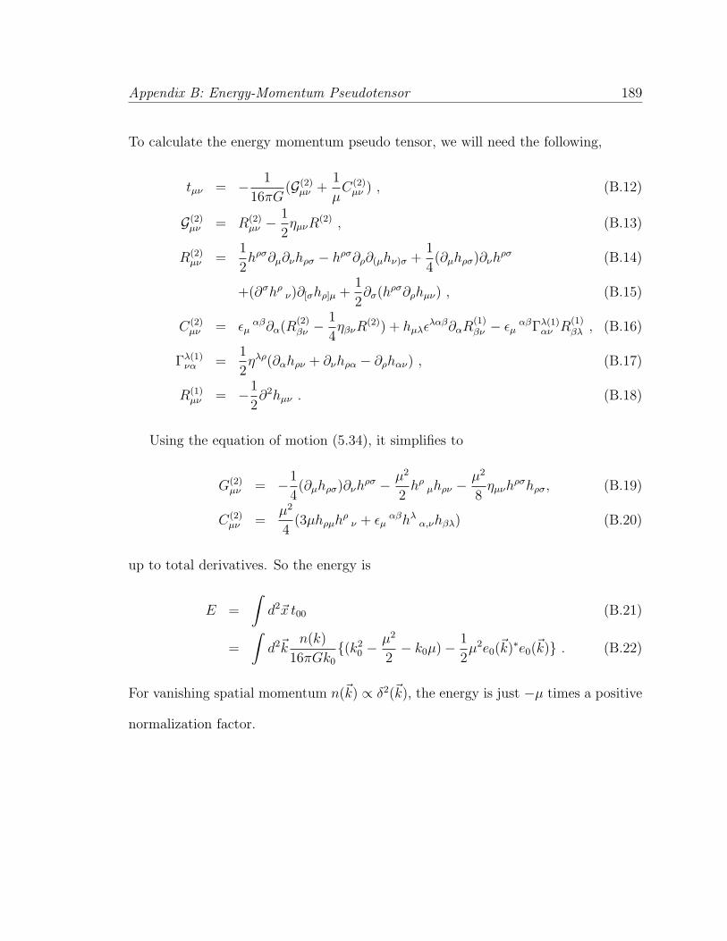
Appendix B: Energy-Momentum Pseudotensor 189
To calculate the energy momentum pseudo tensor, we will need the following,
tµν = − 1
16πG(G(2)
µν +1
µC(2)
µν ) , (B.12)
G(2)µν = R(2)
µν −1
2ηµνR
(2) , (B.13)
R(2)µν =
1
2hρσ∂µ∂νhρσ − hρσ∂ρ∂(µhν)σ +
1
4(∂µhρσ)∂νh
ρσ (B.14)
+(∂σhρν)∂[σhρ]µ +
1
2∂σ(hρσ∂ρhµν) , (B.15)
C(2)µν = εµ
αβ∂α(R(2)βν −
1
4ηβνR
(2)) + hµλελαβ∂αR
(1)βν − εµ
αβΓλ(1)αν R
(1)βλ , (B.16)
Γλ(1)να =
1
2ηλρ(∂αhρν + ∂νhρα − ∂ρhαν) , (B.17)
R(1)µν = −1
2∂2hµν . (B.18)
Using the equation of motion (5.34), it simplifies to
G(2)µν = −1
4(∂µhρσ)∂νh
ρσ − µ2
2hρ
µhρν − µ2
8ηµνh
ρσhρσ, (B.19)
C(2)µν =
µ2
4(3µhρµh
ρν + εµ
αβhλα,νhβλ) (B.20)
up to total derivatives. So the energy is
E =
∫d2~x t00 (B.21)
=
∫d2~k
n(k)
16πGk0
(k20 −
µ2
2− k0µ)− 1
2µ2e0(~k)∗e0(~k) . (B.22)
For vanishing spatial momentum n(~k) ∝ δ2(~k), the energy is just −µ times a positive
normalization factor.
Bibliography
[1] Ofer Aharony, Steven S. Gubser, Juan Martin Maldacena, Hirosi Ooguri, andYaron Oz. Large N field theories, string theory and gravity. Phys. Rept.,323:183–386, 2000, hep-th/9905111.
[2] Chang-rim Ahn and Masayoshi Yamamoto. Boundary action of n = 2 super-liouville theory. Phys. Rev., D69:026007, 2004, hep-th/0310046.
[3] Changrim Ahn, Chaiho Rim, and Marian Stanishkov. Exact one-point functionof N = 1 super-Liouville theory with boundary. Nucl. Phys., B636:497–513,2002, hep-th/0202043.
[4] Changrim Ahn, Marian Stanishkov, and Masayoshi Yamamoto. One-point func-tions of N = 2 super-Liouville theory with boundary. Nucl. Phys., B683:177–195,2004, hep-th/0311169.
[5] Changrim Ahn, Marian Stanishkov, and Masayoshi Yamamoto. ZZ-branes ofN = 2 super-Liouville theory. JHEP, 07:057, 2004, hep-th/0405274.
[6] A. N. Aliev and Y. Nutku. A theorem on topologically massive gravity. Class.Quant. Grav., 13:L29–L32, 1996, gr-qc/9812089.
[7] A. N. Aliev and Y. Nutku. Spinor formulation of topologically massive gravity.1998, gr-qc/9812090.
[8] Mohsen Alishahiha and Hajar Ebrahim. Non-supersymmetric attractors andentropy function. JHEP, 03:003, 2006, hep-th/0601016.
[9] Natxo Alonso-Alberca, Ernesto Lozano-Tellechea, and Tomas Ortin. Geometricconstruction of Killing spinors and supersymmetry algebras in homogeneousspacetimes. Class. Quant. Grav., 19:6009–6024, 2002, hep-th/0208158.
[10] Natxo Alonso-Alberca, Ernesto Lozano-Tellechea, and Tomas Ortin. The near-horizon limit of the extreme rotating d = 5 black hole as a homogeneous space-time. Class. Quant. Grav., 20:423–430, 2003, hep-th/0209069.
190
Bibliography 191
[11] Laura Andrianopoli, Riccardo D’Auria, Sergio Ferrara, and Mario Trigiante.Extremal black holes in supergravity. 2006, hep-th/0611345.
[12] Ignatios Antoniadis, S. Ferrara, R. Minasian, and K. S. Narain. R**4 couplingsin M- and type II theories on Calabi-Yau spaces. Nucl. Phys., B507:571–588,1997, hep-th/9707013.
[13] Dumitru Astefanesei, Kevin Goldstein, Rudra P. Jena, Ashoke Sen, andSandip P. Trivedi. Rotating attractors. JHEP, 10:058, 2006, hep-th/0606244.
[14] Spyros D. Avramis, Alex Kehagias, and Constantina Mattheopoulou. Three-dimensional AdS gravity and extremal CFTs at c=8m. JHEP, 11:022, 2007,arXiv:0708.3386 [hep-th].
[15] Vijay Balasubramanian and Per Kraus. A stress tensor for anti-de Sitter gravity.Commun. Math. Phys., 208:413–428, 1999, hep-th/9902121.
[16] Maximo Banados, Claudio Teitelboim, and Jorge Zanelli. The Black holein three-dimensional space-time. Phys. Rev. Lett., 69:1849–1851, 1992, hep-th/9204099.
[17] Tom Banks, W. Fischler, S. H. Shenker, and Leonard Susskind. M theory as amatrix model: A conjecture. Phys. Rev., D55:5112–5128, 1997, hep-th/9610043.
[18] Brandon Bates and Frederik Denef. Exact solutions for supersymmetric sta-tionary black hole composites. 2003, hep-th/0304094.
[19] Katrin Becker, Melanie Becker, and Andrew Strominger. Five-branes, mem-branes and nonperturbative string theory. Nucl. Phys., B456:130–152, 1995,hep-th/9507158.
[20] Klaus Behrndt, Renata Kallosh, Joachim Rahmfeld, Marina Shmakova, andWing Kai Wong. STU black holes and string triality. Phys. Rev., D54:6293–6301, 1996, hep-th/9608059.
[21] E. Bergshoeff, R. Kallosh, T. Ortin, and G. Papadopoulos. kappa-symmetry,supersymmetry and intersecting branes. Nucl. Phys., B502:149–169, 1997, hep-th/9705040.
[22] Eric Bergshoeff et al. N = 2 supergravity in five dimensions revisited. Class.Quant. Grav., 21:3015–3042, 2004, hep-th/0403045.
[23] M. Bershadsky, S. Cecotti, H. Ooguri, and C. Vafa. Kodaira-Spencer theoryof gravity and exact results for quantum string amplitudes. Commun. Math.Phys., 165:311–428, 1994, hep-th/9309140.
Bibliography 192
[24] Adel Bouchareb and Gerard Clement. Black hole mass and angular momen-tum in topologically massive gravity. Class. Quant. Grav., 24:5581–5594, 2007,arXiv:0706.0263 [gr-qc].
[25] Adel Bouchareb et al. G2 generating technique for minimal D=5 supergravityand black rings. Phys. Rev., D76:104032, 2007, arXiv:0708.2361 [hep-th].
[26] J. C. Breckenridge, Robert C. Myers, A. W. Peet, and C. Vafa. D-branes andspinning black holes. Phys. Lett., B391:93–98, 1997, hep-th/9602065.
[27] Peter Breitenlohner and Daniel Z. Freedman. Positive Energy in anti-De SitterBackgrounds and Gauged Extended Supergravity. Phys. Lett., B115:197, 1982.
[28] Peter Breitenlohner and Daniel Z. Freedman. Stability in Gauged ExtendedSupergravity. Ann. Phys., 144:249, 1982.
[29] Peter Breitenlohner, Dieter Maison, and Gary W. Gibbons. Four-DimensionalBlack Holes from Kaluza-Klein Theories. Commun. Math. Phys., 120:295, 1988.
[30] E. Brezin, V. A. Kazakov, and A. B. Zamolodchikov. Scaling Violation InA Field Theory Of Closed String In One Physical Dimension. Nucl. Phys.,B338:673–688, 1990.
[31] J. David Brown and M. Henneaux. Central Charges in the Canonical Realiza-tion of Asymptotic Symmetries: An Example from Three-Dimensional Gravity.Commun. Math. Phys., 104:207–226, 1986.
[32] I. L. Buchbinder, S. L. Lyahovich, and V. A. Krychtin. Canonical quantizationof topologically massive gravity. Class. Quant. Grav., 10:2083–2090, 1993.
[33] John L. Cardy. Boundary conditions, fusion rules and the Verlinde formula.Nucl. Phys., B324:581, 1989.
[34] Anna Ceresole and Gianguido Dall’Agata. Flow equations for non-BPS extremalblack holes. JHEP, 03:110, 2007, hep-th/0702088.
[35] Anna Ceresole, R. D’Auria, and S. Ferrara. The Symplectic Structure of N=2Supergravity and its Central Extension. Nucl. Phys. Proc. Suppl., 46:67–74,1996, hep-th/9509160.
[36] B. Chandrasekhar, S. Parvizi, A. Tavanfar, and H. Yavartanoo. Non-supersymmetric attractors in R**2 gravities. JHEP, 08:004, 2006, hep-th/0602022.
[37] Gerard Clement. The symmetries of five-dimensional minimal supergravityreduced to three dimensions. 2007, arXiv:0710.1192 [gr-qc].
Bibliography 193
[38] D. H. Collingwood and W. M. McGovern. Nilpotent orbits in semisimple Liealgebras. Van Nostrand Reinhold, New York U.S.A., 1993.
[39] Mirjam Cvetic and Donam Youm. All the Static Spherically Symmetric BlackHoles of Heterotic String on a Six Torus. Nucl. Phys., B472:249–267, 1996,hep-th/9512127.
[40] Mirjam Cvetic and Donam Youm. General Rotating Five Dimensional BlackHoles of Toroidally Compactified Heterotic String. Nucl. Phys., B476:118–132,1996, hep-th/9603100.
[41] Michelle Cyrier, Monica Guica, David Mateos, and Andrew Strominger. Mi-croscopic entropy of the black ring. Phys. Rev. Lett., 94:191601, 2005, hep-th/0411187.
[42] Atish Dabholkar, Ashoke Sen, and Sandip P. Trivedi. Black hole microstatesand attractor without supersymmetry. JHEP, 01:096, 2007, hep-th/0611143.
[43] R. D’Auria, S. Ferrara, and M. Trigiante. Critical points of the black-hole poten-tial for homogeneous special geometries. JHEP, 03:097, 2007, hep-th/0701090.
[44] Sebastian de Haro, Sergey N. Solodukhin, and Kostas Skenderis. Holographicreconstruction of spacetime and renormalization in the AdS/CFT correspon-dence. Commun. Math. Phys., 217:595–622, 2001, hep-th/0002230.
[45] B. de Wit, P. G. Lauwers, and Antoine Van Proeyen. Lagrangians of N=2Supergravity - Matter Systems. Nucl. Phys., B255:569, 1985.
[46] B. de Wit, F. Vanderseypen, and Antoine Van Proeyen. Symmetry structureof special geometries. Nucl. Phys., B400:463–524, 1993, hep-th/9210068.
[47] Frederik Denef, Davide Gaiotto, Andrew Strominger, Dieter Van den Bleeken,and Xi Yin. Black hole deconstruction. 2007, hep-th/0703252.
[48] Frederik Denef and Gregory W. Moore. Split states, entropy enigmas, holesand halos. 2007, hep-th/0702146.
[49] T. Dereli and O. Sarioglu. Topologically massive gravity and black holes inthree dimensions. 2000, gr-qc/0009082.
[50] S. Deser, R. Jackiw, and S. Templeton. Three-Dimensional Massive GaugeTheories. Phys. Rev. Lett., 48:975–978, 1982.
[51] S. Deser, R. Jackiw, and S. Templeton. Topologically massive gauge theories.Ann. Phys., 140:372–411, 1982.
Bibliography 194
[52] S. Deser and J. H. Kay. Topologically Massive Supergravity. Phys. Lett.,B120:97–100, 1983.
[53] S. Deser and Bayram Tekin. Massive, topologically massive, models. Class.Quant. Grav., 19:L97–L100, 2002, hep-th/0203273.
[54] S. Deser and Bayram Tekin. Energy in topologically massive gravity. Class.Quant. Grav., 20:L259, 2003, gr-qc/0307073.
[55] P. Di Vecchia and Antonella Liccardo. D-branes in string theory. II. 1999,hep-th/9912275.
[56] Paolo Di Vecchia and Antonella Liccardo. D branes in string theory. I. NATOAdv. Study Inst. Ser. C. Math. Phys. Sci., 556:1–59, 2000, hep-th/9912161.
[57] M. R. Douglas et al. A new hat for the c = 1 matrix model. 2003, hep-th/0307195.
[58] Tohru Eguchi and Yuji Sugawara. Modular bootstrap for boundary N = 2Liouville theory. JHEP, 01:025, 2004, hep-th/0311141.
[59] Henriette Elvang, Roberto Emparan, David Mateos, and Harvey S. Reall. Su-persymmetric black rings and three-charge supertubes. Phys. Rev., D71:024033,2005, hep-th/0408120.
[60] V. Fateev, Alexander B. Zamolodchikov, and Alexei B. Zamolodchikov. Bound-ary Liouville field theory. I: boundary state and boundary two-point function.2000, hep-th/0001012.
[61] S. Ferrara and S. Sabharwal. Quaternionic Manifolds for Type II SuperstringVacua of Calabi-Yau Spaces. Nucl. Phys., B332:317, 1990.
[62] Sergio Ferrara, Gary W. Gibbons, and Renata Kallosh. Black holes and criticalpoints in moduli space. Nucl. Phys., B500:75–93, 1997, hep-th/9702103.
[63] Sergio Ferrara, Renata Kallosh, and Andrew Strominger. N=2 extremal blackholes. Phys. Rev., D52:5412–5416, 1995, hep-th/9508072.
[64] Jens Fjelstad and Stephen Hwang. Sectors of solutions in three-dimensionalgravity and black holes. Nucl. Phys., B628:331–360, 2002, hep-th/0110235.
[65] Takeshi Fukuda and Kazuo Hosomichi. Super Liouville theory with boundary.Nucl. Phys., B635:215–254, 2002, hep-th/0202032.
[66] Matthias R Gaberdiel. Lectures on non-BPS Dirichlet branes. Class. Quant.Grav., 17:3483–3520, 2000, hep-th/0005029.
Bibliography 195
[67] Matthias R. Gaberdiel. Constraints on extremal self-dual CFTs. JHEP, 11:087,2007, arXiv:0707.4073 [hep-th].
[68] Davide Gaiotto, Aaron Simons, Andrew Strominger, and Xi Yin. D0-branes inblack hole attractors. 2004, hep-th/0412179.
[69] Davide Gaiotto, Andrew Strominger, and Xi Yin. Superconformal black holequantum mechanics. JHEP, 11:017, 2005, hep-th/0412322.
[70] Davide Gaiotto, Andrew Strominger, and Xi Yin. New connections between 4Dand 5D black holes. JHEP, 02:024, 2006, hep-th/0503217.
[71] Davide Gaiotto, Andrew Strominger, and Xi Yin. From AdS(3)/CFT(2) toblack holes / topological strings. JHEP, 09:050, 2007, hep-th/0602046.
[72] Davide Gaiotto and Xi Yin. Genus Two Partition Functions of Extremal Con-formal Field Theories. JHEP, 08:029, 2007, arXiv:0707.3437 [hep-th].
[73] Jerome P. Gauntlett and Jan B. Gutowski. Concentric black rings. Phys. Rev.,D71:025013, 2005, hep-th/0408010.
[74] Jerome P. Gauntlett, Robert C. Myers, and Paul K. Townsend. Black holes ofD = 5 supergravity. Class. Quant. Grav., 16:1–21, 1999, hep-th/9810204.
[75] Paul H. Ginsparg and Jean Zinn-Justin. 2-d Gravity + 1-d Matter. Phys. Lett.,B240:333–340, 1990.
[76] Kevin Goldstein, Norihiro Iizuka, Rudra P. Jena, and Sandip P. Trivedi. Non-supersymmetric attractors. Phys. Rev., D72:124021, 2005, hep-th/0507096.
[77] Michael B. Green and Michael Gutperle. Effects of D-instantons. Nucl. Phys.,B498:195–227, 1997, hep-th/9701093.
[78] David J. Gross and Nikola Miljkovic. A Nonperturbative Solution Of D = 1String Theory. Phys. Lett., B238:217, 1990.
[79] Monica Guica and Andrew Strominger. Wrapped M2/M5 duality. 2007, hep-th/0701011.
[80] Murat Gunaydin, Andrew Neitzke, Oleksandr Pavlyk, and Boris Pioline. Quasi-conformal actions, quaternionic discrete series and twistors: SU(2,1) and G2(2)
. 2007, arXiv:0707.1669 [hep-th].
[81] Murat Gunaydin, Andrew Neitzke, Boris Pioline, and Andrew Waldron. BPSblack holes, quantum attractor flows and automorphic forms. Phys. Rev.,D73:084019, 2006, hep-th/0512296.
Bibliography 196
[82] M. Gurses. Perfect fluid sources in 2+1 dimensions. Class. Quant. Grav.,11:2585–2588, 1994.
[83] G. S. Hall, T. Morgan, and Z. Perjes. Three-Dimensional Space-Times. KFKI-1986-95/B.
[84] S. W. Hawking. Particle Creation by Black Holes. Commun. Math. Phys.,43:199–220, 1975.
[85] M. Henningson and K. Skenderis. The holographic Weyl anomaly. JHEP,07:023, 1998, hep-th/9806087.
[86] Gary T. Horowitz and Andrew Strominger. Black strings and P-branes. Nucl.Phys., B360:197–209, 1991.
[87] Min-xin Huang, Albrecht Klemm, Marcos Marino, and Alireza Tavanfar. BlackHoles and Large Order Quantum Geometry. 2007, arXiv:0704.2440 [hep-th].
[88] C. M. Hull and B. Julia. Duality and moduli spaces for time-like reductions.Nucl. Phys., B534:250–260, 1998, hep-th/9803239.
[89] Nobuyuki Ishibashi. The boundary and crosscap states in conformal field the-ories. Mod. Phys. Lett., A4:251, 1989.
[90] Renata Kallosh, Arvind Rajaraman, and Wing Kai Wong. Supersymmetricrotating black holes and attractors. Phys. Rev., D55:3246–3249, 1997, hep-th/9611094.
[91] Renata Kallosh, Navin Sivanandam, and Masoud Soroush. Exact attractivenon-BPS STU black holes. Phys. Rev., D74:065008, 2006, hep-th/0606263.
[92] Renata Kallosh, Navin Sivanandam, and Masoud Soroush. The non-BPS blackhole attractor equation. JHEP, 03:060, 2006, hep-th/0602005.
[93] Elias Kiritsis and Boris Pioline. On R**4 threshold corrections in type IIBstring theory and (p,q) string instantons. Nucl. Phys., B508:509–534, 1997,hep-th/9707018.
[94] Per Kraus. Lectures on black holes and the AdS(3)/CFT(2) correspondence.2006, hep-th/0609074.
[95] Per Kraus and Finn Larsen. Microscopic black hole entropy in theories withhigher derivatives. JHEP, 09:034, 2005, hep-th/0506176.
[96] Per Kraus and Finn Larsen. Holographic gravitational anomalies. JHEP, 01:022,2006, hep-th/0508218.
Bibliography 197
[97] David Kutasov. D-brane dynamics near NS5-branes. 2004, hep-th/0405058.
[98] Gabriel Lopes Cardoso, Anna Ceresole, Gianguido Dall’Agata, Johannes M.Oberreuter, and Jan Perz. First-order flow equations for extremal black holesin very special geometry. JHEP, 10:063, 2007, arXiv:0706.3373 [hep-th].
[99] Gabriel Lopes Cardoso, Bernard de Wit, and Thomas Mohaupt. Correctionsto macroscopic supersymmetric black-hole entropy. Phys. Lett., B451:309–316,1999, hep-th/9812082.
[100] Sergei L. Lukyanov, E. S. Vitchev, and A. B. Zamolodchikov. Integrable modelof boundary interaction: the paperclip. Nucl. Phys., B683:423–454, 2004, hep-th/0312168.
[101] Sergei L. Lukyanov and Alexander B. Zamolodchikov. Dual form of the paper-clip model. 2005, hep-th/0510145.
[102] Juan Martin Maldacena. The large N limit of superconformal field theories andsupergravity. Adv. Theor. Math. Phys., 2:231–252, 1998, hep-th/9711200.
[103] Juan Martin Maldacena and Andrew Strominger. AdS(3) black holes and astringy exclusion principle. JHEP, 12:005, 1998, hep-th/9804085.
[104] Juan Martin Maldacena, Andrew Strominger, and Edward Witten. Black holeentropy in M-theory. JHEP, 12:002, 1997, hep-th/9711053.
[105] Alexander Maloney and Edward Witten. Quantum Gravity Partition Functionsin Three Dimensions. 2007, arXiv:0712.0155 [hep-th].
[106] Jan Manschot. AdS3 Partition Functions Reconstructed. JHEP, 10:103, 2007,arXiv:0707.1159 [hep-th].
[107] John McGreevy and Herman L. Verlinde. Strings from tachyons: The c = 1matrix reloaded. JHEP, 12:054, 2003, hep-th/0304224.
[108] Thomas Mohaupt. Black hole entropy, special geometry and strings. Fortsch.Phys., 49:3–161, 2001, hep-th/0007195.
[109] Karim Ait Moussa, Gerard Clement, and Cedric Leygnac. The black holes oftopologically massive gravity. Class. Quant. Grav., 20:L277–L283, 2003, gr-qc/0303042.
[110] Robert C. Myers. Black holes in higher curvature gravity. 1998, gr-qc/9811042.
[111] Yu Nakayama. Liouville field theory: a decade after the revolution. Int. J. Mod.Phys., A19:2771–2930, 2004, hep-th/0402009.
Bibliography 198
[112] Yu Nakayama, Yuji Sugawara, and Hiromitsu Takayanagi. Boundary states forthe rolling D-branes in NS5 background. JHEP, 07:020, 2004, hep-th/0406173.
[113] Suresh Nampuri, Prasanta K. Tripathy, and Sandip P. Trivedi. On The Stabil-ity of Non-Supersymmetric Attractors in String Theory. JHEP, 08:054, 2007,arXiv:0705.4554 [hep-th].
[114] Andrew Neitzke, Boris Pioline, and Stefan Vandoren. Twistors and Black Holes.JHEP, 04:038, 2007, hep-th/0701214.
[115] Rafael I. Nepomechie. Consistent superconformal boundary states. J. Phys.,A34:6509–6524, 2001, hep-th/0102010.
[116] Y. Nutku. Exact solutions of topologically massive gravity with a cosmologicalconstant. Class. Quant. Grav., 10:2657–2661, 1993.
[117] Y. Nutku. Harmonic map formulation of colliding electrovac plane waves. 1993,gr-qc/9812030.
[118] Serkay Olmez, Ozgur Sarioglu, and Bayram Tekin. Mass and angular momen-tum of asymptotically AdS or flat solutions in the topologically massive gravity.Class. Quant. Grav., 22:4355–4362, 2005, gr-qc/0507003.
[119] Hirosi Ooguri, Andrew Strominger, and Cumrun Vafa. Black hole attractorsand the topological string. Phys. Rev., D70:106007, 2004, hep-th/0405146.
[120] Giorgio Parisi. String Theory On The One-Dimensional Lattice. Phys. Lett.,B238:213, 1990.
[121] Mu-In Park. BTZ black hole with higher derivatives, the second law of ther-modynamics, and statistical entropy. 2006, hep-th/0609027.
[122] Mu-In Park. Can Hawking temperatures be negative? 2006, hep-th/0610140.
[123] Mu-In Park. Thoughts on the area theorem. 2006, hep-th/0611048.
[124] Mu-In Park. Thermodynamics of exotic black holes, negative temperature, andBekenstein-Hawking entropy. Phys. Lett., B647:472–476, 2007, hep-th/0602114.
[125] Mu-In Park. BTZ black hole with gravitational Chern-Simons: Thermodynam-ics and statistical entropy. Phys. Rev., D77:026011, 2008, hep-th/0608165.
[126] R. Percacci, P. Sodano, and I. Vuorio. Topologically Massive Planar UniversesWith Constant Twist. Ann. Phys., 176:344, 1987.
[127] Boris Pioline. Lectures on on black holes, topological strings and quantumattractors. Class. Quant. Grav., 23:S981, 2006, hep-th/0607227.

Bibliography 199
[128] Joseph Polchinski. M-theory and the light cone. Prog. Theor. Phys. Suppl.,134:158–170, 1999, hep-th/9903165.
[129] Alexander M. Polyakov. Quantum geometry of fermionic strings. Phys. Lett.,B103:211–213, 1981.
[130] Bindusar Sahoo and Ashoke Sen. BTZ black hole with Chern-Simons and higherderivative terms. JHEP, 07:008, 2006, hep-th/0601228.
[131] Bindusar Sahoo and Ashoke Sen. Higher derivative corrections to non-supersymmetric extremal black holes in N = 2 supergravity. JHEP, 09:029,2006, hep-th/0603149.
[132] Bindusar Sahoo and Ashoke Sen. alpha’-Corrections to Extremal Dyonic BlackHoles in Heterotic String Theory. JHEP, 01:010, 2007, hep-th/0608182.
[133] Kirill Saraikin and Cumrun Vafa. Non-supersymmetric Black Holes and Topo-logical Strings. 2007, hep-th/0703214.
[134] Nathan Seiberg. Why is the matrix model correct? Phys. Rev. Lett., 79:3577–3580, 1997, hep-th/9710009.
[135] Ashoke Sen. Black hole entropy function and the attractor mechanism in higherderivative gravity. JHEP, 09:038, 2005, hep-th/0506177.
[136] Ashoke Sen. Entropy function for heterotic black holes. JHEP, 03:008, 2006,hep-th/0508042.
[137] Aaron Simons, Andrew Strominger, David Mattoon Thompson, and Xi Yin.Supersymmetric branes in AdS(2) x S**2 x CY(3). Phys. Rev., D71:066008,2005, hep-th/0406121.
[138] Sergey N. Solodukhin. Holography with gravitational Chern-Simons. Phys.Rev., D74:024015, 2006, hep-th/0509148.
[139] Andrew Strominger. Black hole entropy from near-horizon microstates. JHEP,02:009, 1998, hep-th/9712251.
[140] Andrew Strominger and Cumrun Vafa. Microscopic Origin of the Bekenstein-Hawking Entropy. Phys. Lett., B379:99–104, 1996, hep-th/9601029.
[141] Leonard Susskind. Another conjecture about M(atrix) theory. 1997, hep-th/9704080.
[142] Yuji Tachikawa. Black hole entropy in the presence of Chern-Simons terms.Class. Quant. Grav., 24:737–744, 2007, hep-th/0611141.
Bibliography 200
[143] Tadashi Takayanagi and Nicolaos Toumbas. A matrix model dual of type 0Bstring theory in two dimensions. JHEP, 07:064, 2003, hep-th/0307083.
[144] David Mattoon Thompson. Descent relations in type 0A / 0B. Phys. Rev.,D65:106005, 2002, hep-th/0105314.
[145] Prasanta K. Tripathy and Sandip P. Trivedi. Non-supersymmetric attractorsin string theory. JHEP, 03:022, 2006, hep-th/0511117.
[146] Robert M. Wald. Black hole entropy is the Noether charge. Phys. Rev.,D48:3427–3431, 1993, gr-qc/9307038.
[147] Edward Witten. (2+1)-Dimensional Gravity as an Exactly Soluble System.Nucl. Phys., B311:46, 1988.
[148] Edward Witten. Three-Dimensional Gravity Revisited. 2007, arXiv:0706.3359[hep-th].
[149] Xi Yin. On Non-handlebody Instantons in 3D Gravity. 2007, arXiv:0711.2803[hep-th].
[150] Xi Yin. Partition Functions of Three-Dimensional Pure Gravity. 2007,arXiv:0710.2129 [hep-th].


