Proceedings of the 2012 International Conference on Industrial Engineering and Operations Management Istanbul, Turkey, July 3 – 6, 2012

34

Gauge Imprecision and Process Capability Analysis

Ali Zeinal Hamadani Department of Industrial and Systems Engineering

Isfahan University of Technology Isfahan 84156, Iran

Abstract

Alternative definitions of Process Capability Indices (PCIs), based on different approaches, have been proposed in literature. Most of the research works related to Process Capability Indices assume no gauge measurement errors. However, in industrial applications, despite the use of highly advanced measuring instruments, account needs to be taken of gauge imprecision. The aim of this paper is first to present the state of the art on univariate and multivariate capability indices research, encouraging the use of this important technique for process control and quality improvement and then, to present a review on the recent researches on the effects of measurement errors, showing that measurement errors can alter the results of process capability analysis. Keywords Process capability index, measurement error, gauge imprecision, univariate process capability indices, multivariate process capability Indices 1. Introduction The quality of a product is measured in terms of its characteristics which describe their performance. According to the traditional understanding of quality, the quality characteristic values are not different as long as they are within some specification limits. But today, producing a product that conforms to quality specifications is not sufficient for customers’ satisfaction and keeping the competitive position in the market. After the World War II, a new concept of quality started to arise following the Deming’s philosophy of Continuous Improvement. Previously, the quality control was related to the control of defective products. The items whose quality characteristics lie between the specified limits or the so-called ‘customer tolerance’ are accepted to have a good quality. This approach to quality is named as ‘goal post’ syndrome [1]. In the goal post model no loss is considered unless the quality characteristic of the product is out of specifications. An item which is very close to a limit but within specifications and another one which is at or close to the target are treated in the same way. But, an item which is again very close to a limit but out of specifications is accepted as non-conforming. However, it is recognized that this approach does not make much sense since meeting the specifications of the producer is not enough to meet customer specifications for most of the cases. In fact, the effect of using a product which slightly satisfies and which slightly misses the specifications does not very much differ for a customer. Hence, a product that meets the tolerances may also negatively affect the customer satisfaction and position of the producer in the market. The new understanding of quality takes this important reality into consideration. An important example illustrating for this difference is the Sony television customer preference study [2]. The research shows the fallacy of using number of defective or fraction defective as a quality measure. It is recognized in this research that the customers prefer the television sets produced by Sony-Japan rather than those made by Sony-USA with a reasoning of the difference in their colour density quality. Although both factories use identical designs and specification limits, Sony-Japan is preferred to Sony-USA. The distribution of colour density of television sets produced by Sony- USA had a uniform distribution between the specification limits although the colour density of television sets produced by Sony-Japan had a normal distribution with a mean at the target and a standard deviation of 5/3. Although almost all the sets produced by Sony-USA are within specification limits, and about 0.3 % of the sets produced by Sony-Japan are outside the tolerance limits, the customers use their preferences in favour of the sets produced by Sony-Japan. In this case, the policy used by Sony-USA corresponds to the goal post syndrome of Ross [1]. On the other hand, Sony-Japan factory regards the new philosophy rather than the percent defective.

35

According to the new philosophy, developed by Genichi Taguchi, every product produced imposes a loss to the consumer, even if its quality performance is within the specified limits [2]. This loss can be generally defined as the loss in the product function or properties through its life cycle. The better the quality of a product is, the less it will lose its functionality and properties during its life cycle. Hence, if a product does not perform as it is expected, the consumer senses some loss. So, a quality loss function that can measure the loss of products even when they meet the tolerances should be developed [2]. Taguchi’s quality loss functions express quality as a loss phenomenon. Taguchi assures that a customer is fully satisfied only when the quality characteristic of the product is at the target level. The loss or dissatisfaction of the consumer increases as the quality characteristic deviates from the target. He emphasizes the importance of a quality performance that aims to reach the target value on the average with the minimum deviation from this average value. This can be named as performance consistency [3],[4]. That is why; he focuses more on the process rather than product, regards controlling the location and dispersion of the distribution as well as meeting the specifications and develops a quality measure which is a function of deviation of the process from the target value and the variation in the process. There are several publications on process capability indicating new approaches or formulae to assess process genuine performance. However, there are only a small number of publications discussing the state of the art on this subject. Among which we highlight the works of Pearn et al.[5], Palmer and Tsui [6], Kotz and Johnson [7], and Anis [8]. This article is organized in five sections. Besides this introduction, section two presents a theoretical reference, approaching the main capability indices for univariate and multivariate quality characteristics. Section three presents the idea of gauge imprecision. The comprehensive review of the gauge impression effect on process capability indices are presented in section four, while section five summarizes the main conclusions of this study 2. Process Capability Quantifying the process structure and its development is essential for the success of quality enhancement activities. Thus, capability indices study is an important technique that focuses on the continuous improvement of quality and productivity. It has been observed that although a process can be under statistical control, if it presents high variability when compared to the specification limits, it will be considered not capable, demanding corrective measures in order to regulate the system, in other words, the main objective of studying and interpreting process capability indices is to support decision making, providing a strategic guide to ensure quality leverage. Taguchi and Wu [9], introduced a viewpoint on estimating the loss associated with lack of precision and accuracy in a manufacturing process. The preeminent manufacturing precursor to the viewpoint introduced by Taguchi is the classical “goal-post model” in which the only consideration to production cost is whether the product parameters fall within the process specification limits. Consistent with the goal -post philosophy, the level of process control is typically characterized in terms of what are known as capability indices (CPIs) [10]. Capability indices provide a numerical assessment of the ability of a process in attaining the predefined specifications [10], [11]. A manufacturing process would commonly be described in terms of three parameters: the finite target value (T), an upper specification limit (USL), and a lower specification limit (LSL). All the par ts for which the measured value “x” for a certain specification exceeds the USL or falls below the LSL are rejected. If the process target value for the product characteristic is centred between the USL and LSL, then the tolerances are said to be symmetric. The capability index is of interest to the manufacturing community because it consolidates the details in a complicated multifaceted manufacturing process down to one quantity which can be used to predict the fraction of parts rejected. Typical capability index values can range from 0.7 to 2.0. In the jargon of the community, three sigma process would correspond to a capability index of 1.0 while a much improved six sigma process suggested originally by Motorola would correspond to a capability index of 2.0 [10]. The precision level of a process is related to the standard deviation of the process and the absolute value of the difference between the distribution mean and the process target which is called the target bias is indicative of the process accuracy. According to the Taguchi, it is much easier to adjust the manufacturing process to improve accuracy than to adjust the process to improve the precision [10]. The most commonly assumed probabilistic distribution for a product characteristic with measured value “x” is the normal distribution which can be defined in terms of mean μ, and a standard deviation σ [12]. The primary situation for the application of asymmetric tolerances occurs when the product parameter of interest exhibits a skewed distribution [13]. Historically, capability indices were first applied under the assumption that the mean of the process is on the target [10] or the target bias is at best approximately zero. In some practical cases, it may be necessary to consider the impact of the distribution mean of the product parameter being off target. There have been a variety of target-bias-dependent capability index models introduced. A non-comprehensive but high profile list of such models has been assembled for purposes of this paper.

36

2-1. Univariate process Capability Indices In this section a brief qualitative review of capability indices for univariate quality characteristic is presented. Juran introduced the first study concerning the index Cp in 1974. That study was the base for other indices as Cpk, Cpm, Cpmk. These four indices are represented in equations (1) to (4), respectively, and they are known as the basic univariate process capability indices. They are used when data are normally distributed as well as when the process is in statistical control [7]. (1)

(2)

(3)

= (4)

USL and LSL denote upper and lower specification limits, while process standard deviation, average, and target value are represented, respectively, by σ, μ and T. Cp index represents process potential capability to grant an adequate product, not taking into account the location of the data. In order to solve this issue, Kane (1986) introduced the Cpk index as effective capability index [14]. When used together, Cp & Cpk indices provide a good indication of process capability, assessing average as well as variation performance [15]. However, neither index takes into account process target value. It has been observed that the production of pieces within limits might not be enough, but it might be also necessary to keep process as close to target as possible. Taking that into consideration, the new indices Cpm & Cpmk were proposed, which penalize divergences from the specified target [16],[5]. The Cpm index only reflects the variation allowed within the process (USL, LSL), while the Cpmk index considers the smallest distance between process average and the specification limits. According to the presented indices, it is possible to observe that each one adds an important characteristic from the originally proposed Cp index. As a result, it is interesting to observe that: Cp ≥ Cpk ≥ Cpmk and Cp ≥ Cpm ≥ Cpmk, being the index Cpmk the lowest value on this group, because comprises a more detailed analysis [7]. Also one can see that, if μ = T = M, where M is the mid-point of the specification interval, then, Cp = Cpk = Cpm = Cpmk, i.e., all the indices will have their maximum value equal to the index Cp. The capability index Cp known as short-term index is gauged within a relatively narrow window of time. The long-term capability index, Cpk can be found in the literature to be applied in two ways. It could be applied to extend the short-term capability (days) concept to long-term (months). It is assumed, in this case, that process mean shifts around the target but on the average is “on target.” The concept is that a time-wise shifting around in the short-term process is accounted for with a probability density function (PDF) averaging leading to a higher standard deviation. The long-term precision in the manufacturing process is degraded relative to short-term and, therefore, the long-term capability index is lower than the short-term capability index. On the other hand, Cpk has also found utility as a capability index that can include the impact of target bias. However, as pointed out in [10],[11], this type of usage of Cpk to account for the target bias is questionable. Lastly, a third-measured paradigm for a capability index, Cpm paradigm is also commonly invoked in the community to account for target bias [6],[10],[11]. Because Cpm can be related to Taguchi loss functions [2], it is sometimes referred to as the Taguchi index. One advantage of the Cpm approach is that it is nonparametric, that is, makes no a priori assumptions on the underlying distribution of the specified product parameter distribution. 2-2. Multivariate process capability indices Multivariate capability indices usually produce one number jointly representing capability for two or more quality variables. Alternative definitions of multivariate process capability indices (MPCIs), based on a variety of different approaches, have been proposed in the literature. In general, MPCIs are constructed in one of the following ways: using the ratio of the volume of a tolerance region to the volume of a process region, using the proportion of nonconforming items, or using the principal component analysis (PCA). Taam, Subbaiah, and Liddy[17],

generated

the first multivariate capability index. Chen [18], also proposes a method in order to estimate the multivariate Cp

using a non-conforming proportion approach. Shahriari et al. [19] and Wang et al. [20], proposed a process

capability multivariate vector in order to evaluate the process performance. Braun [21], defined Cp and Cpk as ECp and ECpk, where the both multivariate process region and the multivariate tolerance region are of elliptical shape. Philippe Castagliola and Jose-Victor Castellanos [22],

defined two new capability indices BCp and BCpk dedicated to

two quality characteristics, based on the computation of the theoretical proportion of non-conforming products over

37

convex polygons. For the bivariate case Pal [22], proposed an index. Bothe [23], proposed a method in order to

compute the multivariate Cpk index. Wang and Chen [24], proposed multivariate equivalents for Cp, Cpk, Cpm and Cpmk

based on the PCA (Principal Component Analysis) decomposition. Wang and Du [25], proposed the same indices

and one extension to the non-normal multivariate case. In this section a brief review of the different methods for evaluating the multivariate capability indices are given. 2-2-1. Taam’s Method Taam et al.(1993) defined a multivariate capability index as a ratio of the volume of the modified tolerance region (R1) to the volume of 99.73% process region (R2) [17] MCpm= (5)

If the process data are multivariate normal, then R2 is an elliptical region. The modified tolerance region is the largest ellipsoid completely within the engineering tolerance region and centred at the target. The estimate of MCpm can be calculated as,

pm= (6) Where

And = [1+ ] Here, K is the 99.73% quintile of a χ

2 distribution with v degrees of freedom and v is the number of quality

characteristics. When the process mean vector equals the target vector, and the index has the value 1, then 99.73% of the process values lie within the modified tolerance region. 2-2-2. Chen’s Method Chen (1994) proposed a method, which defines multivariate capability index for rectangular tolerance zone. Firstly a general tolerance zone is defined as [18]:

V = {x (7) Where h(x) is specific positive function with the same scale as x, T∈ is a constant vector and r0 a positive number. Then a rectangular solid tolerance zone is defined by V = {x (8) Where, Ti and ri are specific constants. Another expression for V is V={x (9) Thus, V has the structure, V (x)=max{|xi| ri , i=1,…v } (10) Consequently, the multivariate PCI MCP = 1 r (11) Where r is such that P(max{|Xi – Ti| ri , i=1,…v} r) = 1- (12) Let F be the cumulative distribution function of h(X-T). Then r = F-1(1- ), i.e., the 100(1-α)-th percentile of F. It follows immediately that for any y > 0

38

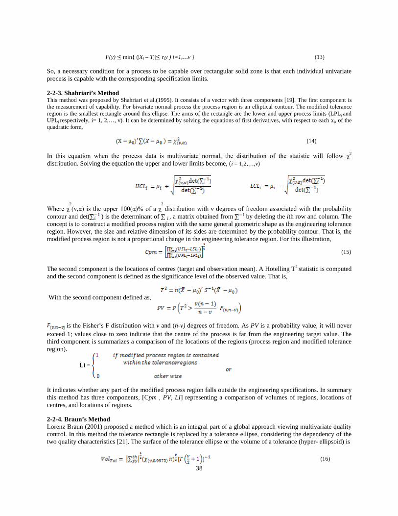
F(y) min{ (|Xi – Ti| riy ) i=1,…v } (13) So, a necessary condition for a process to be capable over rectangular solid zone is that each individual univariate process is capable with the corresponding specification limits. 2-2-3. Shahriari’s Method This method was proposed by Shahriari et al.(1995). It consists of a vector with three components [19]. The first component is the measurement of capability. For bivariate normal process the process region is an elliptical contour. The modified tolerance region is the smallest rectangle around this ellipse. The arms of the rectangle are the lower and upper process limits (LPLi and UPLi respectively, i= 1, 2,…, v). It can be determined by solving the equations of first derivatives, with respect to each xi, of the quadratic form, (14) In this equation when the process data is multivariate normal, the distribution of the statistic will follow χ2

distribution. Solving the equation the upper and lower limits become, (i = 1,2,…,v)

Where χ2(v,α) is the upper 100(α)% of a χ

2 distribution with v degrees of freedom associated with the probability

contour and det( ) is the determinant of , a matrix obtained from by deleting the ith row and column. The concept is to construct a modified process region with the same general geometric shape as the engineering tolerance region. However, the size and relative dimension of its sides are determined by the probability contour. That is, the modified process region is not a proportional change in the engineering tolerance region. For this illustration,

(15)

The second component is the locations of centres (target and observation mean). A Hotelling T2 statistic is computed and the second component is defined as the significance level of the observed value. That is,

With the second component defined as,

is the Fisher’s F distribution with v and (n-v) degrees of freedom. As PV is a probability value, it will never exceed 1; values close to zero indicate that the centre of the process is far from the engineering target value. The third component is summarizes a comparison of the locations of the regions (process region and modified tolerance region).

LI =

It indicates whether any part of the modified process region falls outside the engineering specifications. In summary this method has three components, [Cpm , PV, LI] representing a comparison of volumes of regions, locations of centres, and locations of regions. 2-2-4. Braun’s Method Lorenz Braun (2001) proposed a method which is an integral part of a global approach viewing multivariate quality control. In this method the tolerance rectangle is replaced by a tolerance ellipse, considering the dependency of the two quality characteristics [21]. The surface of the tolerance ellipse or the volume of a tolerance (hyper- ellipsoid) is

(16)

39

Where v is the number of quality characteristics, Γ corresponds to the gamma function and is the 0.9973 percentile of the 𝝌2 distribution with v degrees of freedom. is the hypothetical variance matrix of the quality characteristics, which fits with a given probability of 99.73 percent into the tolerance rectangle or in the tolerance (hyper-cube). The hypothetical variance matrix is calculated using the correlation matrix of the quality characteristics by (17) diag(. . . ) is a matrix, whose elements beside its main diagonal elements are equal to zero and whose main diagonal elements are, corresponding to the 3σ rule, the sixth part of the tolerance intervals of the quality characteristics. A Comparison of this volume with the volume of the process region ( ) is the basic of the elliptical process capability. The basic elliptical process capability ECp compares the 99.73 per cent concentration ellipsoid (elliptical process region) of the vector = ( of the quality characteristics with the tolerance ellipsoid (elliptical tolerance region). That ECp is

(18)

Cp.j thereby corresponds to the univariate basic process capabilities of the m quality characteristics. The basic elliptical process capability is not influenced by the dependency structure of the quality characteristics. This is also meaningful, since otherwise ECp would depend on the degree of multi-collinearity. On the other hand, the deviation between the vector of expected values and the vector of the expected values

must consider the dependency structure of the quality characteristics. The factor of correction of the elliptical process capability KE and the corrected elliptical process capability are

(19)

(20) The numerator in the equation of KE corresponds to an elliptical equation. The denominator is the 0.9973 percentile

of the χ2 distribution with v degrees of freedom. The further the vector of expected values withdraws from the vector

of target values, the larger the counter becomes in relation to the denominator. If a value KE of 1 arises, the vector of expected values lies exactly on the limit (sphere) of the tolerance ellipsoid. If the vector of expected values is situated outside of the tolerance region, the ECpk becomes negative. Thus the ECp and the ECpk must be interpreted similar to the univariate process capabilities Cp and Cpk. 2-2-5. Castagliola’s Method Philippe Castagliola and Jose-Victor Garcia Castellanos proposed a method, in which the MPCI is based on the computation of the theoretical proportion of non-conforming proportion over convex polygons [22]. Assuming the quality of a product depends on two characteristics (X1, X2) and the corresponding tolerance limits are [L1, U1] for

X1 and [L2, U2] for X2. These limits define a rectangular tolerance area called A. Then assuming X = (X1, X2)T

is a

bivariate normal random variable with expectance vector μ = (μ1, μ2)T

and variance-covariance matrix Σ = RVRT

where

and

40

The matrix R is a rotation matrix in which the unit eigenvectors r1 = (r11, r12)T

and r2 = (r21, r22)T

correspond to the main axis of the bivariate normal distribution. Then necessarily r11 = r22 = cos θ and r12 = -r21 = sin θ, where θ is the rotation angle. The diagonal elements of matrix V are the variances on each main axis. In the sequel, it is assumed that L1 < μ1 < U1 and L2 <μ2 < U2. Let D1 and D2 be the straight lines passing through μ and having r1 and r2 as directions. These two lines split the (X1, X2) plane into four regions A1, A2, A3, and A4. Because the bivariate normal distribution is symmetric respectively to the main axis, we necessarily have for i = 1,2,3,4, (21) Let Q1, Q2, Q3, Q4 be the convex polygons defined as the Intersection of regions A1, A2, A3, A4 and the rectangular tolerance area A (i.e. Qi = Ai∩A), and let Pi = Ai – Qi be the complimentary region. Let qi = P(X ∈ Qi) and pi = P (X

Pi) be the probabilities that the random variable X = (X1, X 2)T

is respectively in Qi and Pi. Finally, let q = P(X A) be the probability that the random variable X is in the rectangular tolerance A and p = 1- q be the total proportion of nonconforming products. (22) By definition, we clearly have p = p1 + p2 + p3 + p4 and q = q1 + q2 + q3 + q4. From Equation (22) we can deduce immediately A new bivariate analogy for CPK called BCPK and defined as (23) We have used the following steps to estimate BCPK : 1. Estimating the expectance vector, μ and the variance-covariance matrix Σ from the in-control sample,

= and 2. Computing the eigenvalues (matrix V ) and eigenvectors (matrix ) of , 3. Computing the vertices of the four convex polygons Q1, Q2, Q3 and Q4, 4. Using the method described at the last part of this section computing the proportions . Derive for i = 1,…,4. 5. Computing the estimator for BCPK (24) 2-2-6. MPCIs based on PCA Let X’ = [X1,X2, . . . , Xv] represent the vector of the v quality characteristics of interest with mean vector μ and a positive definite covariance matrix ∑. We assume that the multivariate process data are taken from a multivariate normal distribution. Let us denote the v-vector values of the lower specification limits, upper specification limits and target values as follows: LS = (LSL1,LSL2, . . . ,LSLv) US = (USL1,USL2, . . . ,USLv) = (T1,T2, . . . , Tv) Wang and Chen [20], proposed a procedure for the construction of multivariate capability indices using PCA by the spectral decomposition of the covariance matrix ∑ = UD , where U = (U1,U2, . . . ,Uv) is the matrix of

eigenvectors of ∑ with columns Ui (i = 1, 2, . . . , v), and D = = diag(λ1, . . . , λv) is a diagonal matrix of the eigenvalues. Following PCA, the engineering specifications of the ith principal component (PCi ) and the target value are LSLPCi= LSL USLPCi = USL TPCi= T i = 1, 2, . . . , m (26)

41

Wang and Chen, proposed to assess the multivariate capability considering a subset m (m ≤ v) of principal components. They defined MCp, MCpk, MCpm and MCpmk using the univariate process capability indices of the principal components. The capability index MCp for the multivariate process defined by Wang and Chen is MCp = (27) = (28)

Where, is the univariate measure of capability for the ith principal component, = and m denotes the number of principal components used to assess the capability. Similarly, they defined MCpk, MCpm and MCpmk by replacing Cp;PCi with Cpk;PCi , Cpm;PCi , Cpmk;PCi respectively, for i = 1, 2, . . . , m. This definition of a capability index has the drawback that all the principal components are equally weighted. However, it is widely acknowledged that the first principal components will be more relevant than the last ones. In order to overcome this problem, Xekalaki and Perakis [27], suggested a series of new indices that allow for potential differences in the portion of variance explained by the principal components in question. Account is taken of these differences by assigning unequal weights to the univariate index values corresponding to the principal components employed, in particular in proportion to the percentages of variance explained by them, as determined by their respective eigenvalues. Xekalaki and Perakis [27], specifically proposed the following index MXCp = (29) and offered similar definitions of MXCpk, MXCpm and MXCpmk. Within the framework of a short-run process capability assessment, Wang [27], proposed the use of the weighted geometric mean. The weights in this case are, once again, the eigenvalues λi of each principal component. The index is

MWCp = (30) The author proposed similar definitions for MWCpk, MWCpm and MWCpmk. Further recent works on MPCIs based on PCA have been produced by González and Sánchez [28] and by Shinde and Khadse [29]. 2-2-7. Modification of the existing multivariate process indices Assuming the manufacturing process follows a multivariate normal distribution, the MCp index will be equal to 1 if the manufacturing process region falls completely within an engineering tolerance region. Pan and Lee[30], proved that the calculation of the MCp index proposed by Taam et al.[17] can be simplified to MCp = (31) Where is the correlation matrix of quality characteristics. Equation (31) implies that the value of MCp index maybe greater than one since the value of the determinant of a correlation matrix is between 0 and 1. In other words, the value of MCp index will be greater than 1 if the quality characteristics are not independent, which causes an overestimation of the true process performance. Similarly, the MCpm = index proposed by Taam et al.[17] has the same drawback as the MCp index when the multiple quality characteristics are not independent. Thus, they revised Taam’s modified engineering tolerance region based on the assumption that the correlation of multiple quality characteristics is consistent with the correlation among specifications.To overcome the drawback of overestimation using the MCp and MCpm indices, a revised engineering tolerance region is proposed as ; NMCp = (32)

Where = and the elements of matrix are given by

42

where T is the target vector, represents the correlation coefficient between the ith and jth quality characteristics. The proposed multivariate process capability index is defined as (33)

where and = (34) Cp and Cpm can be considered as a special case of NMCp and NMCpm if v=1. Thus, the NMCp index can be used to evaluate the performance of process precision (i.e. the variability in relationship to the revised engineering tolerance region) and the NMCpm index can be used to evaluate both process precision and accuracy (i.e. the deviation from the target). 5 2-2-8. Comparison of various multivariate process capability indices Pana and Lee [30] have made a comparison between various multivariate process capability indices. In a simulation study they compared the performance of their multivariate process capability indices with the three multivariate process capability indices proposed by Chan et al.[16], Taam et al.[17], and Shahriari et al.[19]. The distinction among the indices proposed by Shahriari et al.[19], Taam et al.[17] and the modified capability indices is:

(1) the comparison regions and (2) the algebraic expression used to compute the indices.

Shahriari.[19] used multiple-dimensional rectangular regions to construct three components. The first component, analogous to Cp in higher dimensions, compares the volumes of the multiple dimensional rectangular regions. The second component measures the distance between the process mean and the process target using the T2 statistic and the third component compares the general location of the two multiple-dimensional rectangular regions. Using ellipsoid-shaped comparison regions (regular ones without taking the correlation among multiple quality characteristics into account), Taam’s two indices, one analogous to Cp and the other analogous to Cpm from the univariate domain, are generated from the underlying multivariate normal distribution. The simulation results show that the NMCp and NMCpm indices are more appropriate than Taam’s MCp and MCpm indices since these indices are robust to the change in the correlation coefficients. Similar to Taam’s MCp and MCpm indices, the proposed NMCp and NMCpm indices can also be viewed as an extension of the univariate process capability indices Cp and Cpm. Thus, the performance of process precision and accuracy for a multivariate manufacturing process can easily be understood by using the proposed modified multivariate process capability indices. Moreover, it is worthy to note that (1) All the multivariate process capability indices including Taam’s MCp and MCpm, Hubele’s Cpm and PV indices

as well as the modified NMCp and NMCpm indices are based on the assumption of multivariate normality for the underlying distribution. Accordingly, any departure from this assumption could lead to erroneous results that include statistical properties, interval estimates and interpretation of process capability indices. Therefore, it is suggested that the multivariate normality assumption be checked by performing a statistical test, such as Shapiro–Wilk test prior to the process capability study.

(2) Engineering tolerance zone or the intersection of the specifications would be a rectangular solid since the specifications for a product generally consist of a collection of individual specifications for each variable.

(3) Although Hubele’s index is also appropriate in evaluating multivariate process capability, it only focuses on computing and interpreting the point estimates of the desired quantity.

Thus, it is subject to statistical fluctuation. In contrast, the proposed NMCp and NMCpm process capability indices and their associated interval estimates, which may lead to sample size determination, can serve as a useful reference for quality practitioners.[30] 3. Gauge Imprecision and Measurement Errors The quality of the products one ships to the customers is limited to how close the readings can get to the ‘true value’ of the characteristic being measured. Measurement Systems are much more than the measuring instruments and

43

Gauges that one uses for measuring. The measurement value that one sees is a result of the measurement process carried out by:

• The Measuring instrument • The person using the measuring instrument (Appraiser) • The Environment under which the reading has been obtained • The Methods used setup and measure the parts • The tooling and fixture that locates and orients the object under measurement • The software that performs intermediate calculations and outputs the result

The reading that is obtained is influenced by each one of the above. The extent to which each of the above parameters affect the reading may vary from one situation to another. However, each one of these influencers can be looked at as factors introducing a variation in the process of measurement. Measurement is a process of evaluating an unknown quantity and expressing it into numbers. The Measurement Process too is subject to all the laws of variation and Statistical Process Control. Measurement Systems Analysis (MSA) is the scientific and statistical Analysis of Variation that is induced into the process of measurement. A measurement system tells us in numerical terms, an important information about the entity that we measure. How sure can we be about the data that the measurement system delivers? Is it the real value of the measure that we obtain out of the measurement process, or is it the measurement system error that we see? Indeed, measurement systems errors can be expensive, and can fog our capability to obtain the true value of what we measure. It is often said that we can be confident about our reading of a parameter only to the extent that our measurement system can allow. To be confident about what the process delivers, it is important to analyse and contain the measurement system variation using the scientific technique of Measurement Systems Analysis. In absence of measurement systems analysis it is common to find, that a product certified as acceptable at the supplier’s end is found rejected at the customer’s end. Variations do also affect decisions across two sets of evaluations in the same organizations. It is a standard practice to periodically calibrate all gauges and measuring instruments used in measurement on the shop floor, and then what is the need of doing MSA once the measuring instruments are calibrated and certified by the calibrating agency. In simple terms, Calibration is a process of matching up the measuring instrument scale against standards of known value, and correcting the difference, if any. Calibration is done under controlled environment and by specially trained personnel. On the shop floor, where these instruments are used, the measurement process is affected by all the factors listed earlier. Factors like method of measurement, appraiser’s influence, environment, and method of locating the work piece do induce variation in the measured value. It is imperative to assess measure and document all the factors affecting the measurement process, and try to minimize their effect on the measurement. The total measurement system variation has to be resolved into components or causes of variation. Each of these components has to be isolated and quantified. Only then, can one start looking for means of reducing the contribution of each one of these error components. 3-1. Measurement System Analysis It is usually assumed that measurement errors are described by a random variable, E ∼ N(0, , where X and E are stochastically independent and additively linked according to: = X + E (35) In this situation X ∼ N(μ, ) represents the unobservable characteristic of the process, while ∼N(μ, ), with

, is the measurable variable. From (35) it follows that the observed variability among the recorded values of a quality characteristic is due to two factors: the first one is the variability of the items produced, the second is the imperfectness of the measurement. Hence, achieving an adequate gauge system capability is one of the aspects that need to be considered in process control and quality improvement studies [31]. There are two fundamental points to be concerned about the measurement system: 1) Accuracy 2) Precision Accuracy: is about the bias between the measured value and the actual value of a quality characteristic. The main idea is that in a measurement system, when an item is measured repeatedly, each observed value will show a difference from the other. However, the average of the measured values should approach to the actual value of the quality characteristic. Hence, accuracy is about the location of the measurement values. When there is an inaccurate measurement system; that is, the measurements are biased, one of the ways to get rid of the bias is calibrating the device used. Instrument calibration is a way to minimize the bias although it is not eliminated totally. And the bias can be ignored if its magnitude is small enough relative to the magnitude of the measurement values [31]. Precision: is about the variation of the measurements. This variation has two components:

44

1) Gauge Repeatability: expresses the variation observed when the measurement device fails to exactly repeat the measurement for the same item. 2) Operator Reproducibility: expresses the variation observed when different operators used in the measurement system fail to exactly reproduce the same measurement for the same parts using the same device. Precision of measurement which is sometimes called the measurement error is defined as: = +

is the variance of measurement error, is the variance of gauge repeatability and is the variance of operator reproducibility. The ratio of 6 to the difference between specification limits is called the precision-to-tolerance ratio and is used to evaluate the measurement system or gauge capability index ( ) [31]. (36) The processes are generally accepted to have a good measurement systems if their “precision to tolerance values” are less than or equal to 10% [31]. 4. The Effect of Measurement Errors on Process Capability Indices Recent studies have given a certain importance to the effects of measurement errors on univariate process capability indices. For example, Mittag [32] evaluated the percentage error in the evaluation of PCIs in the presence of measurement errors, while Bordignon and Scagliarini [33],[34] have studied the statistical properties of certain PCI estimators. Pearn and Liao [35]and Pearn et al. [36] conducted a sensitivity analysis of Cp, Cpk and Cpm in the presence of gauge measurement errors. Scagliarini [37],[38] has examined the joint condition of “autocorrelation and measurement errors” by analyzing the properties of Cp and Cpk estimators for autocorrelated data in the presence of measurement errors. Pearn and Kotz [39] dedicated a chapter of their encyclopaedic work to the issue of “Process capability measures in presence of measurement errors”, while a recent survey paper by Wu et al. [40] contains a subsection on the “gauge measurement error” problem. Other recent papers dealing with the assessment of process performance in the presence of measurement errors, include Villeta et al. [41] and Wu [42]. There are very few studies concerning the effect of measurement errors on multivariate process capability indices. Shishebori and Hamadani [45],[46],[47],[48] have considered the effect of gauge measurement errors and the statistical properties of the multivariate index proposed by Taam et al. and Scagliarini [49] has also proposed a method useful for overcoming the effects of gauge measurement errors on the multivariate process capability indices using the principal components analysis. 4-1. The effect of gauge imprecision on , , and Suppose that represents the relevant quality characteristic of a manufacturing process, and and

measure the true process capability. In practice, the observation variable Y=X+E is measured quality characteristic rather than the true variable X. It is reasonable to assume that X and E are stochastically independent, and E ) so Thus, the empirical process capability and can be obtained by replacing by then the relationship between the true process capability and the empirical process capability can be expressed as:

(37) (38)

(39)

(40) Where , and is called the contamination degree. It is clear from (37), (38) and (39) that the ratios between observable and true PCIs are, in general, decreasing functions of τ (τ ≥ 0), and consequently and , calculated using the observable variable Y, systematically underestimate the true capability of the process. The relation between observable and true PCIs in terms of gauge capability index (λ) is given by:

and

Since the variation of the observed data (with measurement errors) is larger than the variation of the true data (with no measurement errors), the contaminated degree is greater than one , and the true process capability would be

45

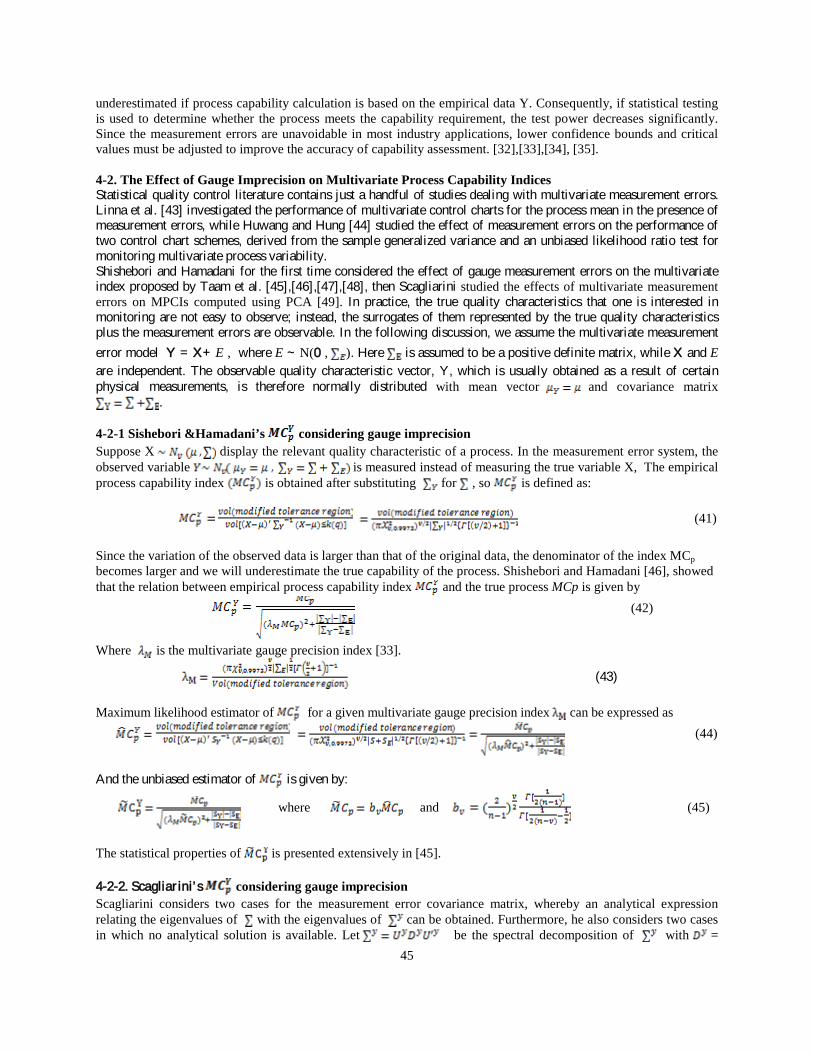
underestimated if process capability calculation is based on the empirical data Y. Consequently, if statistical testing is used to determine whether the process meets the capability requirement, the test power decreases significantly. Since the measurement errors are unavoidable in most industry applications, lower confidence bounds and critical values must be adjusted to improve the accuracy of capability assessment. [32],[33],[34], [35]. 4-2. The Effect of Gauge Imprecision on Multivariate Process Capability Indices Statistical quality control literature contains just a handful of studies dealing with multivariate measurement errors. Linna et al. [43] investigated the performance of multivariate control charts for the process mean in the presence of measurement errors, while Huwang and Hung [44] studied the effect of measurement errors on the performance of two control chart schemes, derived from the sample generalized variance and an unbiased likelihood ratio test for monitoring multivariate process variability. Shishebori and Hamadani for the first time considered the effect of gauge measurement errors on the multivariate index proposed by Taam et al. [45],[46],[47],[48], then Scagliarini studied the effects of multivariate measurement errors on MPCIs computed using PCA [49]. In practice, the true quality characteristics that one is interested in monitoring are not easy to observe; instead, the surrogates of them represented by the true quality characteristics plus the measurement errors are observable. In the following discussion, we assume the multivariate measurement error model Y = X+ E , where E ∼ N(0 , ). Here is assumed to be a positive definite matrix, while X and E are independent. The observable quality characteristic vector, Y, which is usually obtained as a result of certain physical measurements, is therefore normally distributed with mean vector and covariance matrix

. 4-2-1 Sishebori &Hamadani’s considering gauge imprecision Suppose X display the relevant quality characteristic of a process. In the measurement error system, the observed variable is measured instead of measuring the true variable X, The empirical process capability index is obtained after substituting for , so is defined as: (41)

Since the variation of the observed data is larger than that of the original data, the denominator of the index MCp becomes larger and we will underestimate the true capability of the process. Shishebori and Hamadani [46], showed that the relation between empirical process capability index and the true process MCp is given by (42)

Where is the multivariate gauge precision index [33].

(43) Maximum likelihood estimator of for a given multivariate gauge precision index can be expressed as (44)

And the unbiased estimator of is given by:

where and (45)

The statistical properties of is presented extensively in [45]. 4-2-2. Scagliar ini’s considering gauge imprecision Scagliarini considers two cases for the measurement error covariance matrix, whereby an analytical expression relating the eigenvalues of with the eigenvalues of can be obtained. Furthermore, he also considers two cases in which no analytical solution is available. Let be the spectral decomposition of with =

46

diag( , , . . . , ). It is plausible for a real-case scenario that I, since it is likely that the same measurement system can be used to measure all the quality characteristics. From the spectral decomposition of

+ we get the expression; + (46) The eigenvectors remain unchanged, = U, and the eigenvalues can be expressed as = + for i = 1, 2, … , m. The second case is the situation in which the measurement error covariance matrix is proportional to the covariance matrix ∑ . In this situation, which has also been analysed by Huwang and Hung [44] within a process control framework, one can see that

(47) Once again, the eigenvectors remain unchanged, = U, while the eigenvalues can be expressed as = (1 +k) for i = 1, 2, . . . , m. (48) Note that measurement errors lead to an increase in the eigenvalues (46), (47) and consequently according to (27) and (28) the true values of the multivariate process capability indices are underestimated. 4-2-3 Modified Sishebori & Hamadani’s MCp considering gauge imprecision For X as the quality characteristic of a process, suppose that the measured variable

where A is a coefficient matrix that shows the effect of measurement system on the variance-covariance matrix . Using the definition of (Taam et. al., 1993) [17] and the above definition, it has been proved that the relationship between the true process capability and the empirical process capability is: (Hamadani and Ebadi 2011) [48] = (49) Therefore the biased estimator of is given as:

, (50)

Where is the estimator of . One can now use the following steps to estimate the actual process capability index for multivariate case

1. Consider measuring instrument in factory's calibration system and determine its mean and variance. 2. Using by mentioned measuring instrument, collect the required data from manufacturing process. 3. Compute multivariate capability index based on sample data contaminated with the measurement error.

Using the mentioned relationship between the true process capability and the empirical process capability , one can calculate the true process capability. By comparing the modified MCp with previous method, one can see that the calculation of the true process capability by using the empirical process capability and also computing critical value and the power of the process capability testing is simpler than that method [48]. Also we see that the gauge measurement capability has a significant impact on estimating and testing process capability in this situation. In estimating the capability, the estimator using the sample data contaminated with the measurement error severely underestimates the true capability in the presence of measurement error. Acknowledgements The author would like to express his sincere thanks to the Isfahan University of Technology for the support given during the sabbatical leave as well as the School of Engineering and Mathematical Sciences at City University London for hosting me during this period. Also, my special thanks goes to the reviewers for their insightful comments which helped me improve the drafting of this paper. References 1. Ross, P. J. (1996), Taguchi Techniques for Quality Engineering, McGraw-Hill Int., 2nd Edition. 2. Phadke, M.S. (1989), Quality Engineering Using Robust Design, Prentice Hall. 3. Summers, C.S. Donna, (2000), Quality, Prentice Hall, 2nd Edition. 4. DeVor, R.E., Chang, T.-h. and Sutherland, J.W. (1992), Statistical Quality Design and Control, Contemporary

Concepts and Methods. Prentice Hall. 5. Pearn, W.L., Kotz, S. and Johnson, N.L. (1992), Distributional and Inferential Properties of Process Control

Indices”, Journal of Quality Technology, vol. 24, no. 4, 216-231.

47

6. Palmer, K. and Tsui, K.L. (1999), A Review and Interpretations of Process Capability Indices”, Annals of Operations Research, vol. 87, 31-47.

7. Kotz, S. and Johnson, N.L. (2002), Process Capability Indices – A Review, 1992-2000, Journal of Quality Technology, vol. 34, no. 1, 2-19.

8. Anis, M.Z. (2008), Basic process capability indices: an expository review, International Statistical Review, vol. 76, no. 3, 347-367.

9. Taguchi, G. and Wu, Y. (1979), Introduction to Off-Line Quality Control, Central Japan Quality Control Association, Nagoya, Japan.

10. Kotz, S., Pearn, W. L. and Johnson, N. L. (1993), Some process capability indices are more reliable than one might think, Applied Statistics, vol. 42, no. 1, 55–62.

11. Kurekov´, E. (2001), Measurement process capability—trends and approaches, Measurement Science Review, vol. 1, no. 1, pp. 43–46.

12. Boyles, R. A. (1994), Process capability with asymmetric tolerances, Communications in Statistics - Simulation and Computation, vol. 23, no. 3, 615–635.

13. Chen, J. P. and Ding, C. G. (2001), A new process capability index for non-normal distributions, Journal of Quality and Reliability Management, vol. 18, no. 6-7.

14. Kane, V.E. (1986), Process capability indices, Journal of Quality Technology, Vol. 18 No. 1, 41-52. 15. Palmer, K. and Tsui, K.L. (1999), A review and interpretations of process capability indices, Annals of

Operations Research, vol. 87, 31-47. 16. Chan S., Cheng W. and Spring F. A. (1998), A new measure of process capability Cpm, Journal of Quality

Technology, vol. 20, 162–175. 17. Taam, W., Subbiah, P. and W.Liddy, J., (1993), “A Note on Multivariate Capability Indices”, Journal of

Applied Statistics, vol. 20, no. 3, 339-351. 18. Chen, H., (1994), A Multivariate Process Capability Index over a Rectangular Solid Tolerance Zone, Statistica

Sinica, vol. 4, 749-758. 19. Shahriari, H., Hubele, N. F. and Lawrence, F. P., (1995), A Multivariate Process Capability Vector, Proceedings

of the 4th Industrial Engineering Research Conference, 303-308.

20. Wang, F. K. and Chen, J. C., (1998), Capability Index using Principal Components Analysis, Quality Engineering, vol. 11, no. 1, 21-27.

21. Braun, L., (2001), New Methods in Multivariate Statistical Process Control (MSPC), Diskussionsbeiträge des Fachgebietes Unternehmensforschung, 1-12.

22. Castagliola, P. and Castellanos, J. G., (2005), “Capability Indices Dedicated to the Two Quality Characteristics Case”, Quality Tech. and Quantitative Management, vol. 2, no. 2, 201-220.

23. Pal, S., (1999), Performance Evaluation of a Bivariate Normal Process, Quality Engineering, 11(3), 379-386. 24. Bothe, D. R., (1999), Composite Capability Index for Multiple Product Characteristics, Quality Engineering,

vol. 12, no. 2, 253-258. 25. Wang, F. K. and Du, T. C. T., (2000), Using Principal Component Analysis in Process Performance for

Multivariate Data, Omega: The International Journal of Management Science, vol. 28, 185-194. 26. Xekalaki, E. and Perakis, M. (2002), The Use of principal component analysis in the assessment of process

capability indices. In: Proceedings of the Joint Statistical Meetings of the American Statistical Association, The Institute of Mathematical Statistics, The Canadian Statistical Society, New York, 3819–3823.

27. Wang, C.H. (2005), Constructing multivariate process capability indices for short-run production, Int. J. Adv. Manuf. Technol., vol. 26, 1306–1311.

28. González, I. and Sánchez, I. (2009), Capability indices and nonconforming proportion in univariate and multivariate processes. Int. J. Adv. Manuf. Technol., vol. 44, 1036–1050.

29. Shinde, R.L. and Khadse, K.G. (2009), Multivariate process capability using principal component analysis. Qual. Reliab. Eng. Int., vol. 25, 69–77

30. Pan, J.-N. and Lee, C.-Y. (2010), New capability indices for evaluating the performance of multivariate manufacturing processes. Quality and Reliability Eng. Int., 3-15.

31. Montgomery, D. C. and Runger, G. C. (1993), Gauge capability and designed experiments Part I: basic methods. Quality Engineering, vol. 6, no. 1, 115–135.

32. Mittag, H.J. (1997), Measurement error effects on the performance of process capability indices, Lenz, H.J.,Wirlich, P.T. (eds.) Frontiers in Statistical Quality Control, vol. 5, 195–206. Physica-Verlag, Heidelberg.

33. Bordignon, S. and Scagliarini, M. (2002), Statistical analysis of process capability indices with measurement errors.Qual. Reliab. Eng. Int., vol. 18, 321–332.

48

34. Bordignon, S. and Scagliarini, M. (2006), Estimation of Cpm when measurement error is present. Qual. Reliab. Eng. Int., vol. 22, 787–801.

35. Pearn, W.L. and Liao, M.-Y. (2005), Measuring process capability based on Cpk with gauge measurement errors. Microelectron. Reliab., vol. 45, 739–751.

36. Pearn, W.L., Shu, M.H. and Hsu, B. (2005), Testing process capability based on Cpm in the presence of random measurement errors. J. Appl. Stat., vol. 32, 1003–1024.

37. Scagliarini, M. (2002), Estimation of Cp for autocorrelated data and measurement errors. Commun. Stat. A, Theory, vol. 31, 1647–1664.

38. Scagliarini, M. (2010), Inference on Cpk for autocorrelated data in the presence of random measurement errors.J. Appl. Stat., vol. 37, 147–158.

39. Pearn, W.L. and Kotz, S. (2006), Encyclopedia and Handbook of Process Capability Indices. Series on Quality, Reliability and Engineering Statistics, vol. 12. World Scientific, Singapore.

40. Wu, C.-W., Pearn, W.L. and Kotz, S. (2009) An overview of theory and practice on process capability indices for quality assurance. Int. J. Prod. Econ. 117, 338–359.

41. Villeta, M., Rubio, E.M., Sebastián, M.A. and Sanz, A.(2010), New criterion for evaluating the aptitude of measurement systems in process capability determination. Int. J. Adv. Manuf. Technol. Volume 50, Numbers 5-8, 689-697.

42. Wu, C.-W.(2011), Using a novel approach to assess process performance in the presence of measurement errors. Journal of Statistical Computation and Simulation Volume 81, Issue 3, 301-314.

43. Linna, K.W., Woodall, W.H. and Busby, K.L.(2001) The performance of multivariate control chart in the presence of measurement error. J. Qual. Technol. 33, 349–355.

44. Huwang, L. and Hung, Y. (2007), Effect of measurement error on monitoring multivariate process variability. Stat. Sin. 17, 749–760.

45. Shishebori, D. and Hamadani, A.Z. (2009) The effect of gauge measurement capability on MCp and its statistical properties. Int. J. Qual. Reliab. Manag. 26, 564–582.

46. Shishebori, D. and Hamadani, A.Z. (2010) Properties of multivariate process capability in the presence of gauge measurement errors and dependency measure of process variables. J. Manuf. Syst. 29, 10–18.

47. Shishebori, D. and Hamadani,A.Z. (2010) Measurement Capability and Dependency Measure of Process Variables on the MCp, Journal of Industrial and Systems Engineering. Vol. 4, No. 1, 59-76.

48. Hamadani, A.Z. and Ebadi,R. (2011) Modified ( ) in the presence of Measurement Error, Asian journal of quality, Vol. 12 , Issue 3, 269-281.

49. Scagliarini, M (2011) Multivariate process capability using principal component analysis in the presence of measurement errors AStA Adv Stat Anal 95: 113–128.