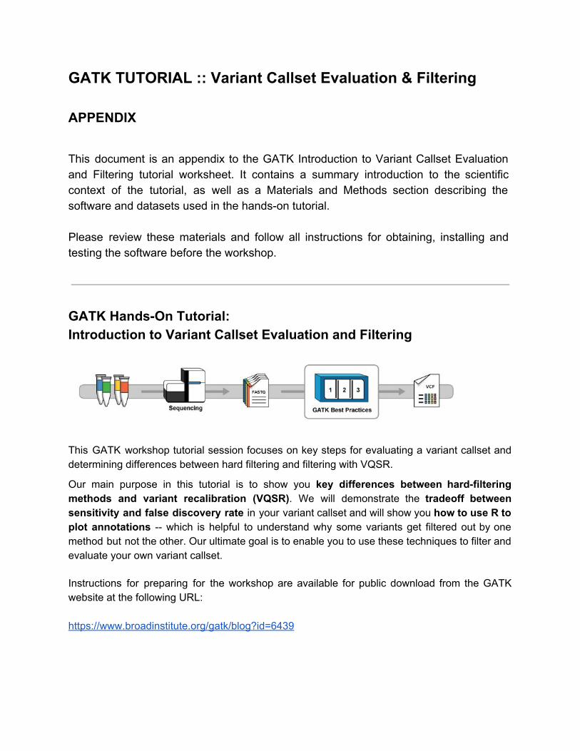
GATK TUTORIAL :: Variant Callset Evaluation & Filtering APPENDIX This document is an appendix to the GATK Introduction to Variant Callset Evaluation and Filtering tutorial worksheet. It contains a summary introduction to the scientific context of the tutorial, as well as a Materials and Methods section describing the software and datasets used in the hands­on tutorial. Please review these materials and follow all instructions for obtaining, installing and testing the software before the workshop.

GATK Hands­On Tutorial: Introduction to Variant Callset Evaluation and Filtering

This GATK workshop tutorial session focuses on key steps for evaluating a variant callset and determining differences between hard filtering and filtering with VQSR.

Our main purpose in this tutorial is to show you key differences between hard­filtering methods and variant recalibration (VQSR). We will demonstrate the tradeoff between sensitivity and false discovery rate in your variant callset and will show you how to use R to plot annotations ­­ which is helpful to understand why some variants get filtered out by one method but not the other. Our ultimate goal is to enable you to use these techniques to filter and evaluate your own variant callset.

Instructions for preparing for the workshop are available for public download from the GATK website at the following URL: https://www.broadinstitute.org/gatk/blog?id=6439

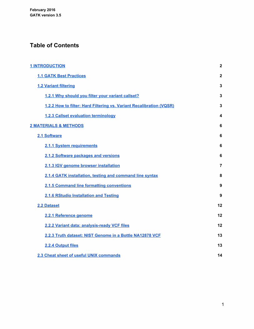
February 2016 GATK version 3.5

Table of Contents

1 INTRODUCTION 2

1.1 GATK Best Practices 2

1.2 Variant filtering 3

1.2.1 Why should you filter your variant callset? 3

1.2.2 How to filter: Hard Filtering vs. Variant Recalibration (VQSR) 3

1.2.3 Callset evaluation terminology 4

2 MATERIALS & METHODS 6

2.1 Software 6

2.1.1 System requirements 6

2.1.2 Software packages and versions 6

2.1.3 IGV genome browser installation 7

2.1.4 GATK installation, testing and command line syntax 8

2.1.5 Command line formatting conventions 9

2.1.6 RStudio Installation and Testing 9

2.2 Dataset 12

2.2.1 Reference genome 12

2.2.2 Variant data: analysis­ready VCF files 12

2.2.3 Truth dataset: NIST Genome in a Bottle NA12878 VCF 13

2.2.4 Output files 13

2.3 Cheat sheet of useful UNIX commands 14

1

February 2016 GATK version 3.5

1 INTRODUCTION

1.1 GATK Best Practices

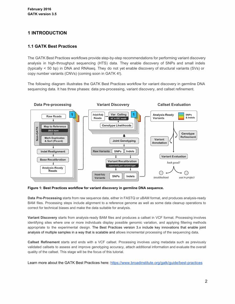
The GATK Best Practices workflows provide step­by­step recommendations for performing variant discovery analysis in high­throughput sequencing (HTS) data. They enable discovery of SNPs and small indels (typically < 50 bp) in DNA and RNAseq. They do not yet enable discovery of structural variants (SVs) or copy number variants (CNVs) (coming soon in GATK 4!). The following diagram illustrates the GATK Best Practices workflow for variant discovery in germline DNA sequencing data. It has three phases: data pre­processing, variant discovery, and callset refinement. Data Pre­processing Variant Discovery Callset Evaluation

Figure 1: Best Practices workflow for variant discovery in germline DNA sequence. Data Pre­Processingstarts from raw sequence data, either in FASTQ or uBAM format, and produces analysis­ready BAM files. Processing steps include alignment to a reference genome as well as some data cleanup operations to correct for technical biases and make the data suitable for analysis. Variant Discovery starts from analysis­ready BAM files and produces a callset in VCF format. Processing involves identifying sites where one or more individuals display possible genomic variation, and applying filtering methods appropriate to the experimental design. The Best Practices version 3.x include key innovations that enable joint analysis of multiple samples in a way that is scalable and allows incremental processing of the sequencing data. Callset Refinement starts and ends with a VCF callset. Processing involves using metadata such as previously validated callsets to assess and improve genotyping accuracy, attach additional information and evaluate the overall quality of the callset. This stage will be the focus of this tutorial. Learn more about the GATK Best Practices here: https://www.broadinstitute.org/gatk/guide/best­practices

2

February 2016 GATK version 3.5

1.2 Variant filtering

In this tutorial module, we are going to focus on the variant filtering steps. To properly show the effects of filtering, we will also do some variant callset evaluation. We’re not going to go over the theory of callset evaluation in detail, but we’ve included some definitions and illustration of terms that we will use in the discussion in case you’re not familiar with them or need a refresher (see section 1.2.3).

1.2.1 Why should you filter your variant callset?

Following variant calling (HaplotypeCaller) and joint genotyping (GenotypeGVCFs), you have a VCF with many variant calls ­­ but they are not necessarily all real (=present in the biological sample). The variant calling tools are designed to maximize sensitivity, i.e. to be very likely to identify all the real variants in your data, at the cost of letting through quite a lot of false positive calls that are just due to artifacts from the sequencing process. This unknown amount of potential false positive calls is a problem because it constitutes noise that can confound downstream analyses. So that’s where filtering comes in ­­ we’re going to try to eliminate as many of these false variants as possible without losing true variants in the process.

1.2.2 How to filter: Hard Filtering vs. Variant Recalibration (VQSR)

Now that we know why we should filter our variant callset, let’s talk about the ways you can filter: either use hard filtering or use Variant Quality Score Recalibration (VQSR). Hard filtering

This method involves removing variants based on whether their annotation values are less than or greater than a set threshold (where annotations are statistics describing various properties of the variants relative to the sequence context). This requires that you determine threshold values for each annotation, either based on previous studies or by trial and error. It is a painstaking process that involves multiple rounds of analysis to do properly. And it is a blunt instrument because it does not take into account the fact that you can have good variants that look bad in some annotation dimensions, purely by chance.

Variant Quality Score Recalibration (VQSR)

This method also involves using annotations to distinguish variant calls that are likely to be real from those that are likely to be false. However, it is very different from hard filtering in that it uses machine learning to identify what are the possible annotation profiles of good vs. bad variants. What’s more, it does so in a way that allows the possibility of non­consecutive ranges of valid annotation values. And it enables analysts to specify filtering parameters based on target sensitivity, without worrying about individual annotation values.

How does it work?

In a nutshell, VQSR first determines how variants that are presumed real based on training data (typically one or more well­validated callsets of variants previously reported in the organism of interest) cluster together along each of the requested annotation dimensions. The program then models the probability of each variant in the full callset being real or false based on how its annotation values relates to the clusters.

3

February 2016 GATK version 3.5

Finally, the program summarizes these probabilities over all requested annotations into a single score (the VQSLOD) for each variant, thereby encapsulating multiple dimensions of the variant properties into a single convenient scale. And because the same model is also applied to a truth set (typically a highly­validated subset of the training data), all that remains to do is to specify a target sensitivity to the truth data (as in “give me the threshold that allows 99% of the sites in the truth set to pass the filter”), which the program then uses to derive the appropriate VQSLOD threshold to apply for filtering.

Admittedly, VQSR may seem scary complicated at first glance ­­ but it is a powerful filtering technique that can make a difficult task surprisingly easier.

That being said, there are two major requirements for using VQSR:

1) You need to have 30 exome samples or more or 1 whole genome sample 2) You need to have some good known variant databases (we provide them for human only)

If you cannot satisfy these two requirements, you may not be able to use VQSR. For example, you might not have enough exomes in your cohort (and can’t follow the workarounds documented in the GATK Guide) or you might be working with a non­model organism that does not have a good set of known variants. Rather than leave your callset unfiltered, you should apply hard filters. We have some recommendations for hard filtering human data that can be used as a starting point:

https://www.broadinstitute.org/gatk/guide/article?id=2806

Finally, you should be aware that all filtering methods involve some tradeoffs between sensitivity and specificity. Whenever you relax your filtering parameters to increase sensitivity (to avoid filtering out true variants), you are bound to let in false positives. Conversely, whenever you tighten up your parameters to remove false positives, you will lose some true positives. VQSR is not immune to that, but it gives you more visibility and control over the tradeoff point ­­ so it’s easier to set the threshold that fits your project objectives.

In this workshop tutorial, we’re going to compare how hard filters and VQSR operate, and how to understand why they filter out some calls and not others.

1.2.3 Callset evaluation terminology

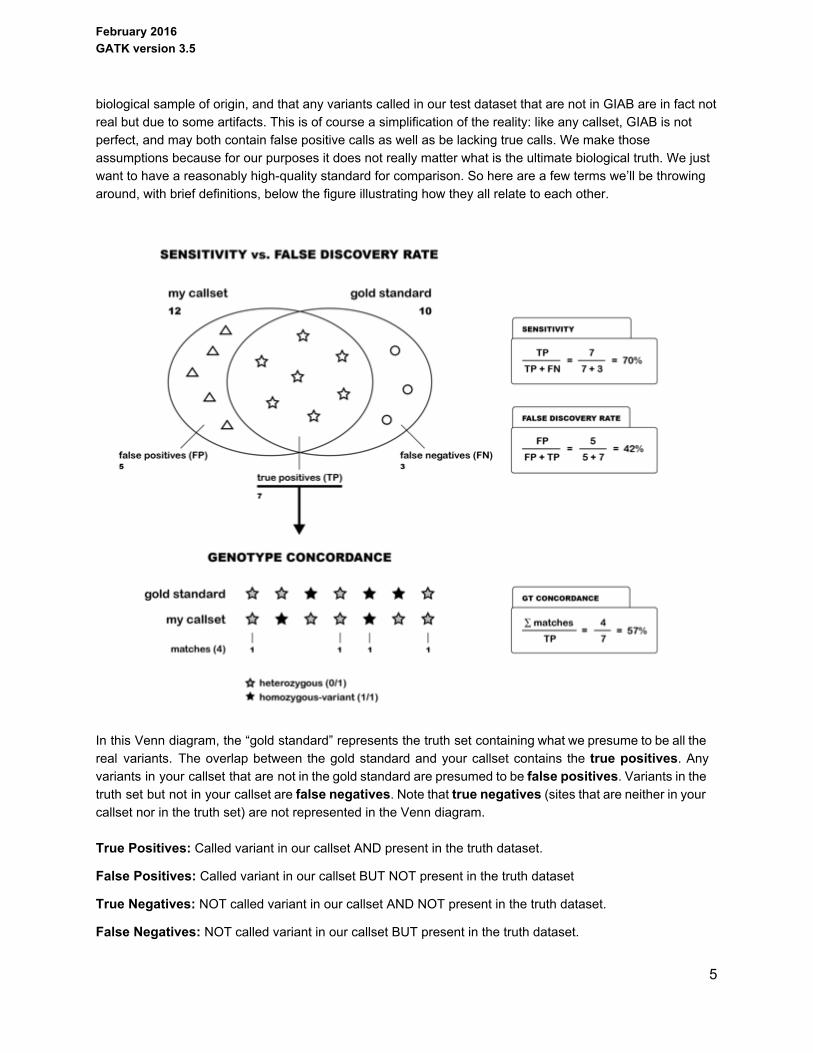
When we talk about evaluating a variant callset in this context, we mean that we want to know how close we have come to identifying all the true variants that are present in the biological sample of interest, and how many calls we made erroneously. Depending on the experimental design, there are several ways to approach this question. See the Callset Evaluation document on https://www.broadinstitute.org/gatk/guide/article?id=6308 for more details on the options and rationale for callset evaluation methods. For the purposes of this tutorial, we are going to keep it fairly simple. We are using our favorite sample, NA12878, which is commonly used as a benchmarking resource (see Material & Methods section for more information on the origin of this sample) so there are truth data resources available for that particular sample. Here we will use the NA12878 dataset Genome in a Bottle (see Material & Methods section also) as our truth set, which means we will assume that all the variants in the GIAB callset are true variants in the

4

February 2016 GATK version 3.5

biological sample of origin, and that any variants called in our test dataset that are not in GIAB are in fact not real but due to some artifacts. This is of course a simplification of the reality: like any callset, GIAB is not perfect, and may both contain false positive calls as well as be lacking true calls. We make those assumptions because for our purposes it does not really matter what is the ultimate biological truth. We just want to have a reasonably high­quality standard for comparison. So here are a few terms we’ll be throwing around, with brief definitions, below the figure illustrating how they all relate to each other.

In this Venn diagram, the “gold standard” represents the truth set containing what we presume to be all the real variants. The overlap between the gold standard and your callset contains the true positives. Any variants in your callset that are not in the gold standard are presumed to befalse positives. Variants in the truth set but not in your callset arefalse negatives. Note thattrue negatives(sites that are neither in your callset nor in the truth set) are not represented in the Venn diagram. True Positives: Called variant in our callset AND present in the truth dataset.

False Positives: Called variant in our callset BUT NOT present in the truth dataset

True Negatives: NOT called variant in our callset AND NOT present in the truth dataset.

False Negatives: NOT called variant in our callset BUT present in the truth dataset.

5

February 2016 GATK version 3.5

Sensitivity = # true positives / # total positives Proportion of true variants (variants present in the truth dataset) that are called variant in our callset. A high sensitivity means you have found many true positives, which is good. However, only having a high sensitivity but a low specificity is not necessarily good, as we will see in the next section. Specificity = # true negatives / # total negatives Proportion of non­variant sites that are correctly identified as non­variant. Having a high specificity value means you do not have many false positives in your variant callset. False Discovery Rate = # false positives / # true positives + # false positives Proportion of false positive calls made per total number of calls made. This can be interpreted as e.g. “for every 100 variants called, 5 are false positives”. False Discovery Rate can be substituted for specificity if you do not have counts for true negatives and false negatives. Genotype Concordance Proportion of true positives for which the correct genotype was identified.

2 MATERIALS & METHODS

2.1 Software

2.1.1 System requirements

This tutorial is intended to be run on either MacOSX, Linux or other flavor of Unix. Microsoft Windows is not supported. You will need at least 500 Mb of free disk space and 2 Gb of available RAM (in addition to whatever you operating system needs to run).

2.1.2 Software packages and versions

This tutorial makes use of the following software. GATK is used from a command line terminal. Basic familiarity with the Unix command line interface will be assumed, but a cheat sheet is provided as part of the supplementary materials at the end of this document.

Java 7 / JRE 1.7 IGV 2.3.60 GATK 3.5 R version 3.2.2 RStudio (any recent version)

You must update to these versions even if you already have a previous version installed, because some arguments and default behaviors may have changed. The functionality presented in this tutorial is very new, so older versions may not even include the necessary components at all.

6

February 2016 GATK version 3.5

All Linux/Unix and MacOS X systems should have a JRE pre­installed, but the version may vary. To test your Java version, run the following command in the terminal:

java ‐version

This should return a message along the lines of ”java version 1.7.0_25” as well as some details on the Runtime Environment (JRE) and Virtual Machine (VM). If you have a version other than 1.7.x, you can install an additional JRE and specify which you want to use at the command­line. To find out how to do so, you should seek help from your systems administrator. Note that GATK will not run at all on Java 6 / JRE 1.6, and is untested on Java 8 / JRE 1.8. Note also that we only support the Sun/Oracle distribution of Java; OpenJDK is not supported.

2.1.3 IGV genome browser installation

IGV is a genome browser originally developed at the Broad Institute. We use it for viewing sequence data and variant calls in context. All the screenshots shown in this tutorial are made with IGV, so we recommend you use IGV to follow along as well even if you are already familiar with another genome browser such as the UCSC browser. You’ll find also that because we work closely with the developers of IGV, some of its features may support GATK output better than other browsers. To install and use IGV, you have several options depending on your operating system, as detailed on the IGV downloads page here: http://www.broadinstitute.org/software/igv/download If you’re on MacOSX, we recommend downloading the full app for best performance. Others will need to either get a webstart version or download the binary distribution and launch it from command line (if this confuses you, choose the webstart version). There are several webstart versions with different memory allocation settings; on platforms running 64­bit Java, be sure to get the 10 Gb (RAM) version. You don’t need to have that much RAM available, but if you have more than 2 Gb, the program will utilize as much as you can spare. The other versions can only allocate up to 2 Gb, which can be limiting for some purposes. For the purposes of our tutorial, 2 Gb should be sufficient. To test that IGV works correctly, simply open it by double­clicking the program file, and familiarize yourself with the interface as described in IGV’s excellent user guide. We especially recommend:

Viewing VCF files (http://www.broadinstitute.org/software/igv/viewing_vcf_files) Viewing Alignments (http://www.broadinstitute.org/software/igv/AlignmentData)

A few additional notes to make your IGV experience more relaxing:

To run the jnlp(webstart) version of IGV, you may need to adjust your system's Java Control Panel settings, e.g. enable Java content in the browser. Also, when first opening thejnlp, overcome Mac OS X's gatekeeper function by right­clicking the saved jnlp and selecting Open with Java Web Start.

7

February 2016 GATK version 3.5

Always load the reference genome before data. For our tutorial data this is a chromosome 20­only version of the Human b37 reference, included in the tutorial data bundle, so you will need to load it from file by going to Genomes > Load as described later in this tutorial.

Before loading data files, you may want to adjust alignment preferences. Go toView>Preferencesand make sure the settings under the Alignments tab allows you to view reads of interest. You can specify e.g. whether or not you want to view duplicate reads. Default settings are tuned to genomic sequence libraries. To restore default preferences, delete or rename the prefs.propertiesfile within your system's igv directory. See http://www.broadinstitute.org/software/igv/prefs.properties for details.

To load data, go to File>Loadfrom and either load alignments fromFileorURL. This is also described in some detail later in this tutorial.

After loading data, adjust viewing modes specific to track type by right­clicking on a track to pop up a menu of options. For alignment tracks, these options are described here.

2.1.4 GATK installation, testing and command line syntax

Hopefully if you're reading this, you're already acquainted with the purpose of the GATK, so go ahead and download the latest version of the software package. In order to access the downloads, you need to register for a free account on theGATK support forum. You will also need to read and accept the license agreement before downloading the GATK software package. Note that if you intend to use the GATK for commercial purposes, you are allowed to use GATK without a license for the duration of the workshop, but if you intend to continue using it after the workshop, you will need to purchase a license. See the licensing page for an overview of the commercial licensing conditions. To install, unpack the file archive you just downloaded by double­clicking it, or in the Terminal by running:

tar xvjf GenomeAnalysisTK‐3.5‐0.tar.bz2

This will produce a directory called GenomeAnalysisTK­3.5 containing the GATK program file, which is called GenomeAnalysisTK.jar, as well as a directory of example files called resources(which you can ignore). GATK tools are distributed as a single pre­compiled Java executable so there is no need to compile them. It's not possible to add the GATK to your path, but you can set up a shortcut to the jar file using environment variables. If you’re not familiar with that, just copy theGenomeAnalysisTK.jarfile to the main directory of the workshop tutorial bundle. This completes the installation process. To test that the GATK program works as expected on your machine, run this command line in the terminal:

java ‐jar GenomeAnalysisTk.jar ‐h

This should print out some version and usage information, as well as a list of the tools included in the GATK. As the Usage line states, commands for GATK always follow the same basic syntax:

java [Java arguments] ‐jar GenomeAnalysisTK.jar ‐T <ToolName> [GATK arguments]

This means that you first invoke Java itself as the main program, then specify that you want to start up the GenomeAnalysisTK.jarprogram in a Java Virtual Machine (JVM). Then you specify which tool you want (such as HaplotypeCaller). Finally you pass whatever other arguments (input files, parameters etc.) are

8

February 2016 GATK version 3.5

needed for the analysis. Any additional java­specific arguments (such as ­Xmx to increase memory allocation) should be inserted between java and ‐jar, like this:

java ‐Xmx4G ‐jar GenomeAnalysisTK.jar [GATK arguments]

We’ll show you some example GATK commands in more detail in the next section. For even more details

about GATK commands, see: https://www.broadinstitute.org/gatk/guide/article?id=4669

2.1.5 Command line formatting conventions

Many command lines in this tutorial are longer than a single line of text, which can be difficult to read and parse even for seasoned users. In the interest of clarity, we represent long command lines on multiple lines. We do this using the backslash character\at the end of each line, which allows us to write the arguments on different lines (which is easier to read than writing them all on the same line) yet still have the terminal recognize that they should be executed as a single command line. This is a single­line command:

samtools view ‐H bams/NA12878_wgs_20_ASHG15.bam | less

This is a multi­line command:

java ‐jar GenomeAnalysisTK.jar \

‐T HaplotypeCaller \

‐R ref/human_g1k_b37_20.fasta \

‐I bams/NA12878_wgs_20.bam \

‐o sandbox/NA12878_wgs_20.vcf

Note the space preceding the backslash. If you do not include the space, it will break your command line. Remember that all command lines are case sensitive and that exact spelling is absolutely required.

2.1.6 RStudio Installation and Testing

We will be using RStudio to plot some annotations to compare which variants VQSR failed and which variants hard filtering failed. Please install the latest version of RStudio from this website: https://www.rstudio.com/ The webpage should automatically detect what platform you are running on and recommend the version most suitable for your system. Binaries are provided for all major platforms; typically they just need to be placed in your Applications (or Programs) directory. We will be working mainly with ggplot. Open RStudio and type the following command in the console window:

install.packages(“ggplot2”)

9

February 2016 GATK version 3.5

This will download and install the ggplot2 library as well as any other library packages that ggplot2 depends on for its operation. Note that some users have reported having to install two additional package themselves, called reshape and gplots. You can install them by typing the following commands in the console window:

install.packages(“reshape”)

install.packages(“gplots”)

To test if you have ggplot installed correctly, try typing the following commands in the console window:

PlantGrowth

PlantGrowth is a dataset that is standard in RStudio. You should see a dataset of plant weight and plant group like this: weight group

1 4.17 ctrl

2 5.58 ctrl

3 5.18 ctrl

4 6.11 ctrl

5 4.50 ctrl

6 4.61 ctrl

7 5.17 ctrl

8 4.53 ctrl

9 5.33 ctrl

10 5.14 ctrl

11 4.81 trt1

12 4.17 trt1

13 4.41 trt1

14 3.59 trt1

15 5.87 trt1

16 3.83 trt1

17 6.03 trt1

18 4.89 trt1

19 4.32 trt1

20 4.69 trt1

21 6.31 trt2

22 5.12 trt2

23 5.54 trt2

24 5.50 trt2

25 5.37 trt2

26 5.29 trt2

27 4.92 trt2

28 6.15 trt2

29 5.80 trt2

30 5.26 trt2

We will plot the two variables next. Now, type:

10

February 2016 GATK version 3.5

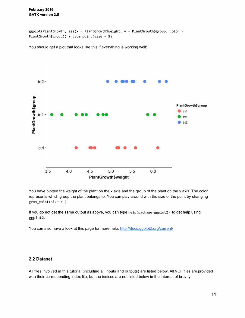
ggplot(PlantGrowth, aes(x = PlantGrowth$weight, y = PlantGrowth$group, color =

PlantGrowth$group)) + geom_point(size = 5) You should get a plot that looks like this if everything is working well:

You have plotted the weight of the plant on the x axis and the group of the plant on the y axis. The color represents which group the plant belongs to. You can play around with the size of the point by changing geom_point(size = )

If you do not get the same output as above, you can type help(package=ggplot2) to get help using ggplot2. You can also have a look at this page for more help: http://docs.ggplot2.org/current/

2.2 Dataset

All files involved in this tutorial (including all inputs and outputs) are listed below. All VCF files are provided with their corresponding index file, but the indices are not listed below in the interest of brevity.

11

February 2016 GATK version 3.5

2.2.1 Reference genome

We are using a version of the b37 human genome reference containing only chromosome 20, which we prepared specially for this tutorial in order to provide a reasonable bundle size for download. It is accompanied by its index and sequence dictionary.

ref/

human_g1k_b37_20.fasta genome reference

human_g1k_b37_20.fai.fasta fasta index

human_g1k_b37_20.dict sequence dictionary

2.2.2 Variant data: analysis­ready VCF files

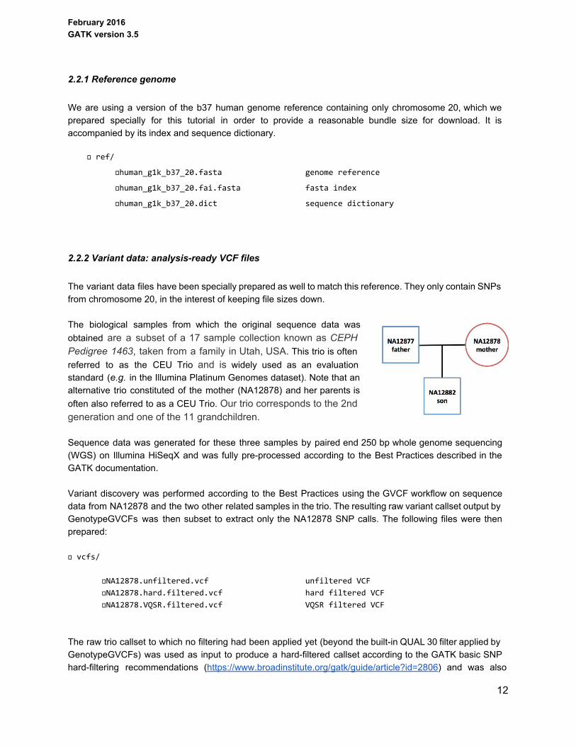
The variant data files have been specially prepared as well to match this reference. They only contain SNPs from chromosome 20, in the interest of keeping file sizes down. The biological samples from which the original sequence data was obtained are a subset of a 17 sample collection known as CEPH Pedigree 1463, taken from a family in Utah, USA. This trio is often referred to as the CEU Trio and is widely used as an evaluation standard (e.g. in the Illumina Platinum Genomes dataset). Note that an alternative trio constituted of the mother (NA12878) and her parents is often also referred to as a CEU Trio. Our trio corresponds to the 2nd generation and one of the 11 grandchildren. Sequence data was generated for these three samples by paired end 250 bp whole genome sequencing (WGS) on Illumina HiSeqX and was fully pre­processed according to the Best Practices described in the GATK documentation. Variant discovery was performed according to the Best Practices using the GVCF workflow on sequence data from NA12878 and the two other related samples in the trio. The resulting raw variant callset output by GenotypeGVCFs was then subset to extract only the NA12878 SNP calls. The following files were then prepared: vcfs/

NA12878.unfiltered.vcf unfiltered VCF

NA12878.hard.filtered.vcf hard filtered VCF

NA12878.VQSR.filtered.vcf VQSR filtered VCF

The raw trio callset to which no filtering had been applied yet (beyond the built­in QUAL 30 filter applied by GenotypeGVCFs) was used as input to produce a hard­filtered callset according to the GATK basic SNP hard­filtering recommendations (https://www.broadinstitute.org/gatk/guide/article?id=2806) and was also

12

February 2016 GATK version 3.5

used as input to produce the VQSR­filtered callset according to GATK Best Practices. All three files were finally subset with SelectVariants (with ‐L 20and‐selectTypeSNP) to contain only the variants on chromosome 20.

2.2.3 Truth dataset: NIST Genome in a Bottle NA12878 VCF

To demonstrate how our VCFs compare to a set of highly validated variants, we provide a truth dataset. This truth dataset comes from the National Institute of Standards and Technology (NIST) Genome in a Bottle Consortium (GIAB). GIAB, among many other things, creates benchmarking data for human genome sequencing. You can read more about the GIAB resources on the GIAB materials webpage at https://sites.stanford.edu/abms/content/giab­reference­materials­and­data. One of the benchmarks it has created is a variant callset generated from NA12878 sequencing data, called using different variant callers. This is what we will use for our truth dataset.

truth_dataset/

NA12878.GIAB.vcf truth dataset

The VCF was downloaded from the NIST database: ftp://ftp­trace.ncbi.nlm.nih.gov/giab/ftp/release/NA12878_HG001/NISTv2.19/ This file was then processed using GATK SelectVariants to retrieve only the SNPs from chromosome 20 (using ‐L20and‐selectTypeSNPin the command). We will compare our differentially filtered NA12878 callsets (described above) to this VCF.

2.2.4 Output files

In case you have trouble executing any of the tutorial commands, we provide a copy of all the output files that are generated over the course of the workshop, so you can skip any obstacles and follow along, and return to the parts you had trouble with later on in your own time. Note that VE stands for VariantEval and FPs stand for false positives in the details below.

output_1/ output files for section 1

Unfiltered.VariantEval.txt VE output from unfiltered VCF

Hard.Filtered.VariantEval.txt VE output from hard‐filtered VCF

VQSR.Filtered.VariantEval.txt VE output from VQSR‐filtered VCF

Unfiltered.FalsePositives.vcf FPs in unfiltered VCF

Hard.Filtered.FalsePositives.vcfFPs in hard filtered VCF

VQSR_Filtered.FalsePositives.vcfFPs in VQSR filtered VCF

Unfiltered.FalsePositives.table FPs from unfiltered VCF (table)

13

February 2016 GATK version 3.5

Hard_Filtered.FalsePositives.table FPs from hard filtered VCF (table)

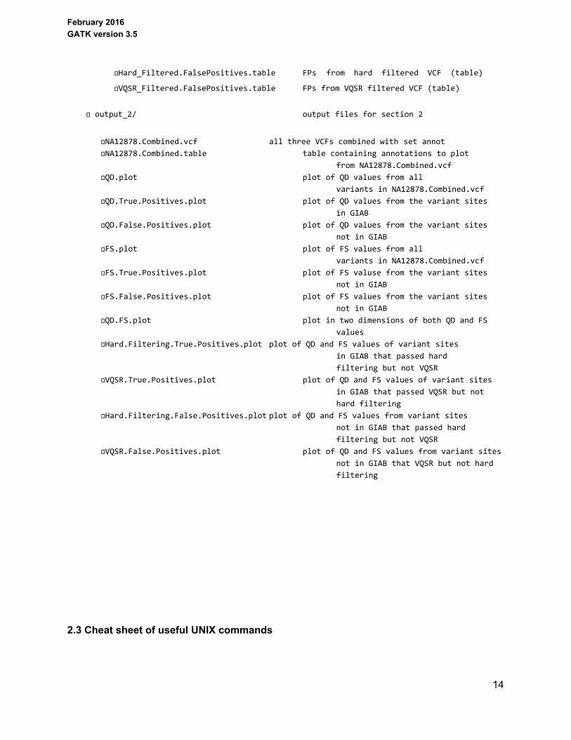
VQSR_Filtered.FalsePositives.table FPs from VQSR filtered VCF (table)

output_2/ output files for section 2

NA12878.Combined.vcf all three VCFs combined with set annot

NA12878.Combined.table table containing annotations to plot

from NA12878.Combined.vcf

QD.plot plot of QD values from all

variants in NA12878.Combined.vcf

QD.True.Positives.plot plot of QD values from the variant sites

in GIAB

QD.False.Positives.plot plot of QD values from the variant sites

not in GIAB

FS.plot plot of FS values from all

variants in NA12878.Combined.vcf

FS.True.Positives.plot plot of FS valuse from the variant sites

not in GIAB

FS.False.Positives.plot plot of FS values from the variant sites

not in GIAB

QD.FS.plot plot in two dimensions of both QD and FS

values

Hard.Filtering.True.Positives.plot plot of QD and FS values of variant sites

in GIAB that passed hard

filtering but not VQSR

VQSR.True.Positives.plot plot of QD and FS values of variant sites

in GIAB that passed VQSR but not

hard filtering

Hard.Filtering.False.Positives.plotplot of QD and FS values from variant sites

not in GIAB that passed hard

filtering but not VQSR

VQSR.False.Positives.plot plot of QD and FS values from variant sites

not in GIAB that VQSR but not hard

filtering

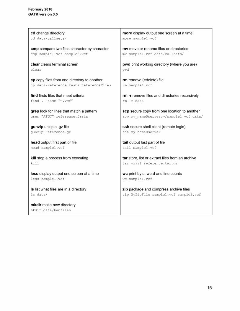
2.3 Cheat sheet of useful UNIX commands

14

February 2016 GATK version 3.5

cd change directory cd data/callsets/

cmp compare two files character by character cmp sample1.vcf sample2.vcf

clear clears terminal screen clear

cp copy files from one directory to another cp data/reference.fasta ReferenceFiles

find finds files that meet criteria find . ­name “*.vcf”

grep look for lines that match a pattern grep “ATGC” reference.fasta

gunzip unzip a .gz file gunzip reference.gz

head output first part of file head sample1.vcf

kill stop a process from executing kill

less display output one screen at a time less sample1.vcf

ls list what files are in a directory ls data/

mkdir make new directory mkdir data/bamfiles

more display output one screen at a time more sample1.vcf

mv move or rename files or directories mv sample1.vcf data/callsets/

pwd print working directory (where you are) pwd

rm remove (=delete) file rm sample1.vcf

rm ­r remove files and directories recursively rm ­r data

scp secure copy from one location to another scp my_name@server:~/sample1.vcf data/

ssh secure shell client (remote login) ssh my_name@server

tail output last part of file tail sample1.vcf

tar store, list or extract files from an archive tar ­xvzf reference.tar.gz

wc print byte, word and line counts wc sample1.vcf

zip package and compress archive files zip MyZipFile sample1.vcf sample2.vcf

15