GATED COMMUNITY PREMIUMS AND AMENITY DIFFERENTIALS...

1

GATED COMMUNITY PREMIUMS AND AMENITY DIFFERENTIALS IN RESIDENTIAL SUBDIVISIONS

Evgeny L. Radetskiy Finance Department

School of Business, La Salle University Philadelphia, PA 19141-1199, USA

Ronald W. Spahr* Department of Finance, Insurance and Real Estate

Fogelman College of Business and Economics, University of Memphis Memphis, TN 38152-3120, USA

[email protected]

Mark A. Sunderman Department of Finance, Insurance and Real Estate

Fogelman College of Business and Economics, University of Memphis Memphis, TN 38152-3120, USA

[email protected]

March 9, 2015 * Corresponding Author.

2


Abstract

We use hedonic models to examine price differences between single family homes in gated communities and a matched sample in non-gated communities in Shelby County, TN. Controlling for idiosyncratic attributes, we find that homes in gated communities carry significant price premiums relative to similar homes in non-gated communities. Price premiums are highest for medium size gated communities. Premiums were also evident in higher priced gated communities before 2008 but vanished after the financial crisis. Gated communities offer homeowners additional attributes but usually have higher infrastructure and service costs. Thus price premiums result from net gated community benefits. Keywords: Housing Values, Gated communities, Hedonic Modeling JEL code: R31

3


1. Introduction

Gated communities are residential developments characterized by physical security

measures such as gates, walls, guards and closed-circuit television cameras. A common feature is

a perimeter wall/fence enclosing the entire development; where, vehicular access is usually

restricted by a gate, controlled by access cards, PIN codes, remote controls or security personnel.

Security within the community is provided by various means, including 24-hour security guard

patrols, ‘back-to-base’ alarm systems and panic buttons, closed-circuit television cameras, guard

dogs, electric fencing, spikes and other forms of anti-intruder perimeter control systems.

Gated communities and residents’ associations are not just an American phenomenon,

gated communities have experienced growth in Argentina, Brazil, Chile, China, France, Russia,

Serbia and the U.K;1 however, approximately 65,700,000 Americans reside in association-

governed communities, including homeowners associations, gated communities, planned unit

developments, condominiums, and cooperatives.2 According to American Housing Survey

(2009), there were 10,759,000 units located in communities whose access is secured with walls,

gates or fences.3 In the United States, gated communities have grown to the point where such

developments now account for roughly 11 per cent of all new housing.4 It is generally concluded

that gated communities transpire out of fear, anxiety, and insecurity of urban inhabitants. Other

factors may include economic restructuring, global terrorism, crime, immigration, the

privatization of public services and a perceived undermining of democratic processes. Thus, to

protect themselves from these perceived risks and uncertainties, homeowners may desire to

create a buffer between themselves and their families and society at large.

4

We temporally examine the existence of price premiums for a sample of single family

homes in private, gated residential communities relative to values in comparable non-gated

communities in Memphis and Shelby County, Tennessee. Each gated community is matched

with a control sample of similar non-gated properties in geographically adjacent or close

proximity communities. Non-gated communities are also matched with gated communities based

on average sale price, total living area, total lot area, and age.

We obtain housing sales data from the Shelby County, TN Assessor’s Office for a sample

period from 2000 through 2012, and apply hedonic modeling similar to that used in a number of

prior studies including Spahr and Sunderman (2009), Sunderman and Spahr (2004, 2006),

Sunderman and Birch (2002), and Asabere and Huffman (1991) consider modifications

suggested by Sirmans, MacPherson, and Zietz (2005).

We posit that our findings may be applicable to other locations in the United States

because of the ethnic, racial and economic diversity of our sample. Our results are consistent

with those obtained by LaCour-Little and Malpezzi (2009) and Helsley and Strange (1999).

We add to the literature in a number of ways. We apply hedonic valuation models to

control for and value unique, distinctive aspects of individual property and community specific

amenities such as club houses, community swimming pools, tennis courts, guard buildings, etc.,

associated with both gated and non-gated communities. While controlling for unique property

attributes, we find that single family homes in gated communities generally command

statistically significant higher prices relative to comparable non-gated communities. Also, we

study the influence of relative gated community size on price premiums, finding that size

impacts average property values. Medium size gated communities appear to carry the highest

price premium as compared to smaller and larger gated communities. We also find that more

5

affluent (higher priced) gated communities command statistically significant, higher gate

premiums than do less affluent (lower priced) gated communities. Gates and access controls

appear to be more highly valued by buyers in more affluent communities.

Additionally, our data period permits us to consider most of the housing cycle from 2000-

2012 allowing us to examine empirically whether gated communities sustained price premiums

before and subsequent to the 2008-2009 subprime crisis. Also, we refine this analysis, using

median sale prices for each year for each community and the median of the median prices, to

classify each gated community and its matching non-gated community into either the higher

priced or lower priced group. We find that higher priced and lower priced gated communities

retained values differently before and after the financial crisis period. Prior to the crisis, higher

priced gated communities carried significant price premiums over comparable non-gated

communities; whereas, evidence of price premiums is mixed for lower priced gated

communities. Subsequent to the crisis, however, we find that neither higher priced nor lower

priced gated communities command statistically significant price premiums over their matching

non-gated counterparts.

Section II describes the review of the literature, Section III presents data and

methodology, Section IV discusses results and robustness tests and Section V concludes.

2. Review of the Literature

Given the relatively recent proliferation of gated communities in Shelby County, TN as

well as in the United States, we study the motivation behind both the increase in gated

communities and whether there are significant economic components associated with them.

LaCour-Little and Malpezzi (2009) find that price premiums associated with properties in

gated communities result from net tradeoffs among positive benefits and higher infrastructure

6

costs. Helsey and Strange (1999), using a microeconomic approach, attribute price premiums to

reduced crime levels in gated communities relative to non-gated communities. In addition to

safety considerations, we use hedonic modeling (a valuation/pricing approach) to quantify net

specific tradeoffs between identified benefits and costs as justification for price premiums.

Homeowners within gated communities typically own undivided interests in streets and

sidewalks in addition to fee simple land ownership on which their homes sit (see LaCour-Little

and Malpezzi, 2009). Homeowners associations generally manage the streets, sidewalks and

common areas, where regular and occasional assessments may be imposed on property owners to

fund maintenance. As compensation for added costs, residents of gated communities gain

control of the streets, thereby restricting access, reducing traffic, noise and possibly crime. Thus,

despite additional costs associated with living in gated communities, the benefits outweigh the

additional ownership costs if value premiums exist.

LaCour-Little and Malpezzi (2009) and Bible and Hsieh (2001) observe security as the

most common cited reason influencing gated community price premiums; however, they also

posit the existence of a number of other reasons for potential premiums.5 The perception that a

gate reduces crime within the community is best explained by the concept of ‘defensible space’

credited to Newman (1973, 1980, 1992, 1995). Newman initially studies the incidence of crime

in gated communities located very near a high crime housing project in St. Louis and finds that

they experienced lower crime and full occupancy throughout the study period. Based on data

from the American Housing Survey for fee-paying gated and non-gated neighborhoods,

Chapman and Lombard (2006) find that neighborhood resident satisfaction levels strongly

depend on the perception of a lack of crime.

Hardin and Cheng (2003) investigate the impact of security and crime protection afforded

7

by gated access and look at the effect on garden apartment rents. They find that rents are

positively related to the presence of gated access constraints. Thus, not only home owners, but

also renters are willing to pay for additional security provided by a gate.

The value of gated property security extends beyond residential properties. Benjamin et

al. (2007), found that gated commercial properties yield rent premiums as compared to non-gated

commercial properties when controlling for other physical characteristics and ownership-

management types.

Wilson-Doenges (2000) studies gated versus non-gated communities in both high income

and low income neighborhoods in Southern California. As may be expected, personal safety and

community safety perceptions per capita are higher in the high income gated versus non-gated

community. However, perceptions of differences in crime rates between gated and non-gated

communities are not statistically significant in both high and low income communities.

Other factors also may affect gated community price premiums. For example, it is

important to consider the impact of additional conveniences such community may offer. Several

previous studies have explored the effects of amenities, other than security, on community real

estate values. Specifically, Benefield (2009) studies packages of amenity offerings and their

impact on property values in neighborhoods. He finds that some amenity packages positively

influence property values.6 Contrary to his study, we conclude that other amenities found within

gated communities negatively impact property values when also controlling for amenities

associated with individual properties, neighborhood size and affluence. We attribute our finding

of negative values for community amenities, such as neighborhood swimming pools, results from

many individual properties duplicating the same amenities.

Regardless of gated community attributes such as crime reduction, perception of

8

increased security and other amenities, gated communities have been the target of criticisms

from academics, the media and the wider community. These criticisms generally focus on the

potential divisions within the community caused by the gated communities. For example,

Kennedy (1995) argues that residential associations (including gated neighborhoods) carry

negative externalities for nonmembers in the form of discrimination on race and class, limiting a

right to travel on private streets (raising a possibility of harassment by security guards or police),

and even reduce free speech rights. If, however, gated communities address the fears and

anxieties of homeowners by enhancing personal safety, the security of material goods, as well as

protecting homes from unwanted intrusions, the value of these attributes may outweigh the

negative externalities and additional costs of such communities, thereby creating a price

premium. Further, the physical design and control of gated neighborhoods may assist in

fostering a sense of community and common purpose among residents (McKenzie, 1994; Lang

and Danielsen, 1997).

The valuation of properties within gated communities is the subject of several previous

studies. Most notably, Bible and Hsieh (2001) use hedonic pricing and find that gated

community properties have price premiums. We refine Bible and Hsieh’s model by controlling

for additional features possibly available within gated communities such as clubhouses,

community swimming pools, tennis courts, basketball courts and small lakes or ponds within the

gated community.

LaCour-Little and Malpezzi (2009) further support value premiums for gated

communities while also controlling for other neighborhood attributes, such as presence of

homeowners associations7 and privately owned streets. They find that price premiums, relative to

non-gated counterparts, range from 7% to 24% for gated neighborhoods in Southern California

9

and 13% for gated neighborhoods in St. Louis.

Pompe (2008), also using a hedonic approach, finds that beach locations are more highly

valuable by residents of gated communities, as compared to similar non-gated communities.

Contrary to our findings, Le Goix (2007), using 1990-2000 data from metropolitan Los Angeles,

California, constructs an index of discontinuity finding that large, high-end gated communities

maintained price premiums and justify higher governance/maintenance costs over time; whereas,

less affluent gated communities (“middle class” gated communities) did not. Also, contrary to

our finding, Le Goix and Vasselinov (2013), using data through 2008, which may not measure

the full impact of the housing crisis period, conclude that properties located within gated

communities are more immune to unexpected decrease in property values during periods of

financial distress as compared to non-gated properties. However, they found some evidence that

price premiums in gated communities had negative price effects on nearby financially distressed

non-gated community properties. They posit that the presence of gated communities within a

financially stressed neighborhood may destabilize prices of nearby non-gated communities. We

find that both higher priced and lower priced gated communities failed to sustain price premiums

subsequent to the 2008-2009 financial crisis.

3. Data and Methodology

Sales data, including descriptions of single family residential properties in Shelby County

from January, 2000 through December, 2012, are obtained from the 2013 Certified Assessment

Roll for Shelby County, Tennessee. The sample includes 11 fully gated communities from

several different areas of Shelby County.8 Data also include sales from 16 comparable

communities, where each gated community is matched with non-gated communities with very

similar locations and property characteristics. The communities deemed to be comparable to

10

gated communities are assessed based on location (proximity to a gated community), total living

area (measured in square feet), sale price, and age of the property. The mean sale price in the

lowest priced gated community is $185,763 and the mean sale price in the highest priced gated

community is $1,315,490.

Exhibit 1 contains summary statistics for both gated and comparable non-gated

communities. Each gated community is matched with at least one comparable non-gated

community based on similar sale prices, total living areas, lot sizes and ages. In some cases, it

was possible to match with more than one comparable non-gated community. For example,

Location 7, a gated community identified as “Gated 7”, is matched with two non-gated

communities identified as “Non-gated 7a” and “Non-gated 7b” all located in relatively close

proximity. These three locations have similar mean sale prices ($392,528, $312,594, and

$314,546 respectively), as well as mean total living areas (4,060 ft2, 3,364 ft2, and 3,225 ft2),

average lot/land areas (15,201 ft2, 18,357 ft2, 18,344 ft2), and average age (20.6 years, 16.7 years,

and 17.4 years).

////////// Insert Exhibit 1 about Here //////////

The final data set contains 4,422 valid observations for the study period – 877 (19.83%)

observations are from the gated communities. To facilitate the homogeneity of our sample, only

single-family residential properties with sizable lots are included in the sample, thus zero-lot line

properties are excluded. Valid sales include those listed as “Land and Buildings” and classified

as “Warranty Deed” (3,927 observations), “Special Warranty Deed” (243 observations), and

“Trustee Deed” (252 observations). All other sale types and instruments of sale types are

excluded from the final sample.9 The mean property sale price in our sample for both gated and

non-gated communities is $340,100.

11

Our sample includes data for a twelve year period from 2000-2012, allowing us to

examine the effects of the boom leading up to, the subprime mortgage crisis housing crash and

the subsequent recovery period. Following the method originally employed by Bryan and

Colwell (1982),10 we control for changing market conditions and prices throughout the study

period by incorporating a time (date of sale) variable. In this method, each date of sale is defined

as a linear combination of the end points of the year in which the sale occurs. Date of sale

variables, B(y), where y designates the year, are the proportional weights assuming that each sale

occurs in the middle of each month. This technique allows the rate of change in prices to be

unique for each year and allows for a monthly price continuum. For example, if a sale occurred

in September 2002, the sale is closer to the beginning of 2003 than to the beginning of 2002;

therefore, more weight is given to B03 than to B02. As a result, the variable B02 is given a

weight of 3.5/12 (or a value of .292), and B03 weighting is 8.5/12 (or a value of .708) and all

other B(y) variables have a value of zero. This technique avoids an annual step function which

would result from the use of annual date of sale variables.

Two additional criteria are used to eliminate outliers in our sales data.11 Sales are deleted

if sale price is greater than three standard errors above or below the predicted price.12 Predictive

errors may result from model misspecification, a lack of sufficiently detailed information

regarding the property and/or incorrect sales data. The second criterion eliminates any sales with

unusually large absolute values for Cook’s distance (>1.00). This indicates that the property has

one or more characteristics that are quite different from other sales, and whose presence has an

unduly large influence on the overall predicted values generated by the model.13 These additional

criteria result in the removal of 68 observations or less than 1.5% of all data.14

The data set includes numerous property characteristics for each property sale used in the

12

analysis. The variables in the models are defined in Exhibit 2 and selected summary statistics for

these variables are shown in Exhibit 3.

////////// Insert Exhibit 2 and Exhibit 3 about Here //////////

Sales price is the dependent or predicted variable in each of our hedonic models. It is

assumed that sale price is a good estimate of true market value and may be explained/predicted

by selected independent-explanatory variables. A number of explanatory variables are generally

employed when multiple regression (hedonic modeling) is used to estimate improved residential

property values. Variables include style of building, wall construction, size, grade of

construction,15 age and other property characteristics. Additionally, we employ variables to

control for other gated community amenities that may affect property values such as presence of

clubhouse, public swimming pool, tennis court, basketball court, pond, and guard building.16

Each gated community and its matched comparable non-gated community(ies) are assigned a

unique location variable of LOCx. These dummy variables control for each of the eleven

different locations. Our general least squares linear regression model is:

Pricei,t = α + b*Gatei,t + c*Xi,j,t + d*Date of Salei + e*Locationi + εi,t (1)

where Pricei,t is the sale price of the property I at time t. Gatei,t is a dichotomous (dummy)

variable indicating if the community of the sale is gated (1) or not (0). Xi,j,t represents a vector of

property attributes/characteristics for property I, attribute j in period t (age, size, number of

bathrooms, etc.). Date of Salei represents linear combinations of the end points of the year in

which sale I occurs, and Locationi indicates each property’s location.

4. Empirical Results for Hedonic Pricing Model

Referring to Exhibit 4, Model 1 represents a good fit with an adjusted R2 of 0.9157.

13

Variance inflation factors (VIF) are run for all variables and are deemed acceptable (VIF

<10.0)17 reducing multicollinearity concerns among independent variables. A dummy variable

controlling for the presence of a gate measures its economic impact on property and amenity

values. Empirical results indicate that the average sale price premium for properties located in

gated communities is $29,996 relative to comparable properties in non-gated communities. The

price premium is statistically significant at the 99 percent confidence level.18


As is the case with gated communities throughout the country, the residents of gated

communities in our study are responsible for upkeep of roads, drainage and other maintenance

that normally would be covered by the municipality for non-gated communities, thus the $29,996

increase in value is the net increase in property values above additional associated costs.

Other notable attributes affecting value are the lot size, where each additional square foot

is worth $0.47, and age of property, where values decline by $2,048.42 per year as properties

age.19 This variable, however, may be somewhat misleading since the average age of properties

studied was 10.9 years and may not be representative of property values in older Shelby County

communities.

Interestingly, multi-story homes sell for less, where a multiple story house sells for

approximately $5,550 less per floor than a single story house. A poured concrete pool has a value

of $80.43 per square foot and pools of other construction have lower values. Houses with

crawlspaces rather than a concrete slab show an increased value of $21,669. Homes with

basements are not common in Shelby County due to high water tables and concerns of flooding.

Also, as expected, waterfront properties carry price premiums of $34,467.20

Compared to General Warranty Deeds, both Special Warranty Deeds and Trustee Deeds

14

result in reduced sale prices of $65,795 and $54,432 respectively. Instruments of sale other than

General Warranty Deeds are considered to be inferior, thus carry a negative sales price premium

(e.g., most Trustee Deeds are associated with forced foreclosure sales).

Properties in communities, whether gated or non-gated, with a golf course sell for

$11,497 more than for communities without a golf course. These findings are consistent with Do

and Grudnitski (1995), Grudnitski (2003), and Shultz and Schmitz (2009).21

Each square foot of living area is worth $44.42 for a house with average quality of

construction. Unsurprisingly, the value of each additional square foot of living area increases

with higher quality construction. The grade of construction varies from average (the base

variable on which each higher quality of construction variable is compared) to good, good plus,

very good minus, very good and best. As expected a “good” construction quality house sells for

an additional $6.88 per square foot when compared to a house with average quality of

construction. Values for good plus, very good minus, very good and best are $15.07, $24.02,

$55.27 and $94.63, respectively. As a result, a home built with the best quality of construction

would be worth $139.05 per square foot.

Annual date of sale variables, B(y), compare market values relative to the base year,

2000. Since Shelby County did not experience the significant run up in market values prior to the

financial crisis that were observed in other parts of the country, except for 2001, market prices

showed price increases till 2007. However, because of the excess supply of houses on the

market and the financial crisis, values began declining from a peak in 2007 ($73,919 above the

price in 2000) to a value in 2010 of only $31,737 above 2000 prices. By the end of 2012 home

prices had rebounded to $41,989 above 2000 prices. To further interpret these results, previously

we indicated that a sale in September 2002 would have a weighted value assigned to B02 of .292

15

and .708 to B03. Multiplying these weights by the coefficients in Model 1 for B02 (6,213.69)

and B03 (9,713.76), the weighted average is $8,691.74. This indicates, holding all else constant,

a house selling in September of 2002 carries a price premium of $8,691.74 above one sold at the

beginning of 2000 and a price appreciation of $2,478.05 since the beginning of 2002. Price

patterns may be seen in Exhibit 7.22

Also, we control for additional amenities provided for residents of gated communities,

including the presence of a clubhouse, community swimming pool, cabana, tennis courts,

basketball courts, small ponds/lakes and for the existence of a guard building in addition to a

gate. Generally, we find that these additional amenities carry highly significant negative values;

where, the presence of additional amenities reduces sale prices by $19,534. Although, at least

superficially, these features seem to have value, we posit that additional maintenance costs

associated with these amenities outweigh their benefits.

Location variables compare and control for price level differences among each of the

other ten gated communities and comparable communities where “Chapel Creek”, the gated

community, and its comparable “Woodchase” (Location 8) are the base communities. See

Exhibit 5 as an example of the location of Chapel Creek relative to it matched community

Woodchase. Location variables range from -$40,849 to $177,958. For example, the variable for

location 1 indicates a value of $40,849 less than Chapel Creek; whereas, the location 10 variable

shows a price level of $177,958 above Chapel Creek.


Other variables (attributes) may be observed in Exhibit 4.23 Overall, the hedonic model

behaves as expected and not surprisingly, the variable of specific interest in this study, Gate,

carries a significant impact on property values. Gated properties sell for $29,996 above similar

16

parcels in non-gated communities.

In Model 2, we introduced three separate dummy variables to capture the impact of

relative size (based on number of homes) for property values in gated communities.24 Results,

shown in Exhibit 4, represent a good fit where the adjusted R2 is 0.9160, VIF values are

acceptable (VIF <10.0), and no major changes relative to Model 1 are observed.

Model 2 finds that medium size communities carry the highest gate premium of $33,775;

whereas, gate premiums for smaller and larger communities are $21,849 and $22,068

respectively. As in Model 1, additional amenities are negatively statistically significant with an

estimate of -$14,372. Results indicate that there may be an optimal gated neighborhood size.

This observation may be relevant for developers considering future real estate property

developments.

We posit that smaller gated communities must spread additional costs (for example

additional costs of maintaining roads, street lighting and the gate), over a lower number of

properties, thus effectively reducing the net benefits of living in a gated community.

Alternatively, larger gated communities may be less convenient requiring residents to travel

further to a gate when entering or exiting the community.25 In addition, larger gated

communities perhaps lack the same cohesiveness and sense of community often found in

medium and smaller communities.

In Model 3, we study the impact of affluence on gated community values. More affluent

gated communities, because of higher real and personal property values, may assign higher

values to gates and fences as compared with less affluent gated communities. Gated communities

in our sample are separated into “Higher Priced” and “Lower Priced” groups. To classify

communities as higher or lower priced, we first determine a median sale price for each gated

17

community over the entire twelve-year study period. Then, we find a median of medians. If

median sale price of a particular gated community is above the overall median of medians, the

gated community is considered a higher priced community and vice versa for lower priced gated

communities. Since we have 11 gated communities in our sample, the median of medians is

equal to one of the gated community’s median price. For that gated community, we determine an

average sale price as well as the median price. If mean sale price is higher than the median sale

price for that community, then it is considered to belong to the higher priced group (and vice

versa for the lower priced group).

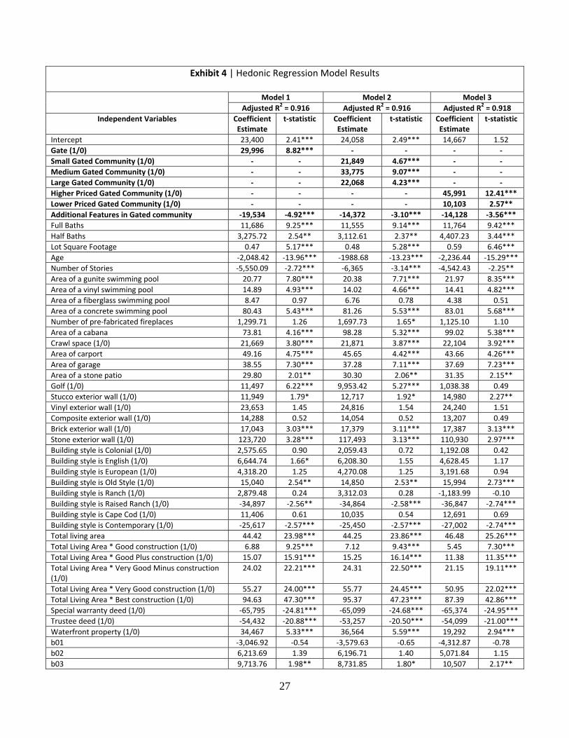
In Model 3 each dummy variable (“higher priced gated community” and “lower priced

gated community”) captures the affluence effect on value of each gated community. Results are

shown in Exhibit 4 (Model 3). Similar to Model 1 and Model 2, Model 3 represents a good fit

with the adjusted R2 equal to 0.9180. Variance inflation factors (VIF) are again tested in this

model and it was found that all variables are highly acceptable (all VIF’s <10.0). There are also

no major changes in the overall model.

Model 3 finds that higher priced, more affluent gated communities carry higher

premiums of $45,991. Whereas, a lower priced gated communities command premiums of

$10,103. All relevant variables in Model 3 are statistically significant.

As in previous models, the additional features of gated communities are statistically

significant with an estimate of -$14,128. For example, people residing in higher priced gated

communities may assign little or no value to a community swimming pool as they may already

have pools on their properties (or tennis and basketball courts). Also, the presence of additional

community amenities appear to have negative values as homeowners may be unwilling to pay for

expenses associated with these benefits.

18

As an alternative to Model 3, we log sale price while holding all independent variables

constant. Results show that higher priced community gate premiums are 14.2% greater than

values for their matched non-gated communities; whereas, gate premiums for properties located

in lower priced communities are only 3.8% higher than for their matched non-gated

communities. These results provide further evidence that more affluent gated communities

command larger price premiums.26

Value premiums for gated communities may vary across time and may be dependent on

the housing market, thus we empirically test the sustainability of gate premiums over different

stages of an economic cycle. Model 4, shown in Exhibit 6, measures relative price patterns

temporally for higher and lower priced gated and non-gated communities. To measure this, we

broke the date of sale variables, B(y), into higher priced gated, HGB(y), higher priced non-gated,

HNGB(y), lower priced gated, LGB(y) and lower priced non-gated, LNGB(y).27 As in Model 3,

we divide our sample into higher priced and lower priced communities based on median sale

prices except, in this situation, classification of gated communities is completed annually. We

then track each date of sale variables across time to determine price patterns for each community

classification. This allows us to measure the effect of the housing crisis on property values and

specifically the temporal sustainability of gate premiums before, during and after the housing

crisis. These date values are graphed in Exhibit 7, and for comparison, the date variables from

Model 1 are also plotted.

////////// Insert Exhibit 6 and Exhibit 7 about Here //////////

As previously discussed, gated communities carry price premiums only if they have a

positive benefit/cost ratio. Exhibit 7 indicates that prior to the subprime crisis (where the crisis

period 2008-2009 is shaded) gated communities carried significant price premiums over non-

19

gated communities. However, beginning in 2008, premiums for higher priced gated

communities declined, and only in 2012 did they appear to trend upward. Although, the lower

priced gated communities typically show a premium over non-gated lower priced communities,

gate premiums were not as great as found in higher priced gated communities. It appears that the

subprime crisis impacted values for all communities in our sample; however, the decline in value

was the largest for the higher priced gated communities.

Date variable differences for each year between higher priced gated and higher priced

non-gated as well as between lower priced gated and lower priced non-gated communities are

tested for statistical significance using an F-test with a null hypothesis (H0) that the difference

between gated and non-gated properties are zero. F-test results are reported in the table under

Exhibit 7. We observe that gated premiums for higher priced gated versus higher priced non-

gated communities were statistically significantly different during eight years (2000-2008);

however, differences were statistically significant in only two (2010 and 2012) out of four years

subsequent to the financial crisis beginning in 2008. Alternatively, differences between lower

priced gated communities and lower priced non-gated communities display a different picture.

Gate premiums were statistically significant in only two (2006 and 2008) out of eight years

leading up to the financial crisis (2000-2008) for lower value communities. Only one statistically

significant difference (gate premium) is observed in 2011 after the crisis period. However, for

both higher priced and lower priced gated communities, even for years when gate premiums

were not shown to be statistically significant, positive premiums indicate a positive benefit/cost

ratio.

Referring back to Le Goix and Vasselinov (2013) who posit that gated communities may

contribute to a local increase in price inequality that destabilizes price patterns at neighborhood

20

levels, a similar pattern may have occurred in the Shelby County prior to the recent financial

crisis. Before 2008, higher price premiums between gated and non-gate communities existed for

more affluent homes. However, as a result of the crisis, a number of businesses in Shelby

County paying high salaries, such as Morgan Keegan and First Tennessee, substantially reduced

their labor forces and forced high earners to sell their homes at substantially reduced prices.

Many of these homes may have been in higher priced gated communities.

We perform several robustness checks finding that our main conclusions associated with

Model 1 remain valid and that all independent variable coefficients carry the same sign and

remain significant. First, we reduce our sample by excluding the most expensive gated

community and its comparable non-gated community (gated community in Location 10 has a

highest average sale price of $1,315,490). The results remain consistent with Model 1, thus

providing assurance that Location 10 is not substantially impacting our results.28

Anselin (1998) and others suggest potential problems with real estate data (such as house

sale prices and neighborhood characteristics) suggesting that real estate data tend to lack

independence among properties and may demonstrate spatial autocorrelation or spatially and

serially clustered residuals, thus results may lead to incorrect conclusions. Moulton (1990)

provides an example showing data units that share the same observable characteristics may also

share unobservable characteristics that would lead to serially correlated residuals and a

downward bias for coefficients within those groups. In order to correct for possibly serially

correlated residuals, Figlio and Lucas (2004) correct standard errors in their regression model

through clustering at both location and time level when dealing with housing sales data. Others

including Genesove and Mayer (2001) use this econometric approach to adjust clustered standard

errors to resolve problems of autocorrelation.29

21

We adjust for possible clustered standard error effects in Model 1 following Petersen

(2009).30 First, we estimate models using clustering by one dimension-neighborhood.31 To

duplicate our initial dataset used in Model 1, we again remove observations if sale price is

greater than three standard errors above or below the predicted price and sales with unusually

large absolute values for Cook's distance (>1.00).32,33 Coefficients for premiums of gated

communities remain stable and strongly significant. All other control variable coefficients

remain consistent in direction and significance. Further, as suggested by Thompson (2011), it

may be appropriate to cluster standard errors by two dimensions in order to deal with serial as

well as spatial correlation. Thus, we cluster standard errors in our model by two dimensions -

neighborhood and time (represented by a variable Year of Sale). Once again, our previous

findings are confirmed with consistent directions and significance of explanatory variable

coefficients. Results for clustered standard errors by one and multiple dimensions are not

reported here but are readily available per request.34

5. Conclusion

This study applies hedonic modeling to assess the value of properties in gated

communities relative to residential real estate values in non-gated communities. Using a data set

of housing sales provided by the Shelby County Tennessee Assessor’s Office, we select a sample

of eleven gated communities and a sample of matched non-gated properties in nearby or adjacent

communities that serve as the control sample. Thus, we formulate a relatively homogeneous

sample of single family residential properties, excluding properties with zero lots, both in gated

communities and control samples. The resulting four hedonic models all had adjusted R2 greater

than 0.90. Also, while controlling for other factors, we find that residential properties in gated

communities command a statistically significant price premium of $29,996. Gated community

22

price premiums most likely result from actual or perceived benefits associated with additional

privacy, home owner associations imposing tighter controls on maintenance, home design and

other externalities and the added assurances against crime and other undesirable activities.

Moreover, since gated communities provide for their own streets, lighting and other services

publically provided to non-gated communities by municipalities, significant gate premiums

result from net benefits versus additional homeownership cost incurred by residents of a gated

community. We also find that the presence of additional amenities within gated communities

reduces sale prices by $19,534. We posit that additional maintenance costs associated with these

amenities outweigh their benefits. It appears that, whereas a gate has value, additional

neighborhood amenities do not.

We further explore gated neighborhood price effects by determining if neighborhood size,

measured by the number of homes, has an impact on value. We find that medium sized

communities have the highest gate premiums relative to either small or large communities. We

also discover that more affluent (higher priced) communities command higher statistically

significant gate premiums, both in monetary and percentage terms, than do less affluent (lower

priced) communities.

Additionally, the time period for our data covers most of the housing cycle from 2000-

2012. We examine whether gated communities sustained gate premiums both before and after

the 2008-2009 subprime crisis. We find that higher priced and lower priced gated communities

retained gate premiums differently before and after the financial crisis period. Prior to the crisis,

higher priced gated communities carried significantly higher price premiums over comparable

non-gated communities; whereas, evidence of price premiums is mixed for lower priced gated

communities. Subsequent to the crisis we find that neither higher priced nor lower priced gated

23

communities command statistically significant gate premiums over their matching non-gated

counterparts. Our finding may change as home values increase subsequent to the crisis period.

24

Exhibit 1 | Descriptive Statistics for Sample Property Sales

Community Sale Price* Total Living Area

(ft2) Land Area (ft2) Age of House

(Years)

Location 1 (loc1)

Gated 1 $229,470 2,860.0 9,287.3 1.8

Non‐gated 1a $205,297 2,888.6 11,216.5 3.4

Non‐gated 1b $293,632 3,668.5 17,734.6 3.1

Location 2 (loc2)

Gated 2 $311,738 3,434.8 12,685.2 13.1

Non‐gated 2 $260,261 2,975.5 16,058.9 13.2

Gated 2.1 $382,673 3,575.9 13,085 6.7

Non‐gated 2.1 $348,976 3,969.6 19,244.2 18.7

Location 3 (loc3)

Gated 3 $476,075 4,087.4 13,984.4 4.1

Non‐gated 3a $401,675 3,930.3 19,456.2 8.7

Non‐gated 3b $501,625 4,326.3 19,349.4 2.7

Location 4 (loc4)

Gated 4 $185,763 2,301.3 7,743.1 9.1

Non‐gated 4a $210,899 2,839.9 10,594.3 8.6

Non‐gated 4b $172,047 2,280.1 10,973.5 6.9

Location 5 (loc5)

Gated 5 $481,832 3,880.9 15,668.2 1.5

Non‐gated 5 $382,947 3,678.4 20,995.5 2.0

Location 6(loc6)

Gated 6 $342,826 3,678.3 23,189.1 2.4

Non‐gated 6 $251,824 3,300.3 20,254.2 32.6

Location 7 (loc7)

Gated 7 $392,528 4,060.7 15,201.5 20.6

Non‐gated 7a $312,594 3,364.9 18,357.3 16.7

Non‐gated 7b $314,546 3,255.4 18,344.3 17.4

Location 8 (loc8)

Gated 8 $494,872 4,930.7 37,979.0 9.8

Non‐gated 8 $284,253 3,708 24,462.4 17.3

Location 9 (loc9)

Gated 9 $240,399 2,350.4 7,531.6 17.8

Non‐gated 9a $362,888 3,457 14,194.7 9.9

Non‐gated 9b $296,223 2,907.7 10,494.3 10.0

Location 10 (loc10)

Gated 10 $1,315,490 6,406.1 20,883.7 4.5

Non‐gated 10 $675,169 5,132.9 31,908.0 22.1

Notes: Values represent means for each neighborhood. Gated communities Gated 2 and Gated 2.1 and respective comparable communities are located in the same proximate location. Age of each house was calculated as the difference between the year of sale and the year house was built. Gated community names are provided by request.

25

Exhibit 2 | Independent Variables Variable Name Description

Gate Dummy Variable: Equals 1 if community Is Gated; 0 otherwise

Small Gated Community Dummy Variable: Equals 1 if gated community has between 38 and 42 houses; 0 otherwise

Medium Gated Community Dummy Variable: Equals 1 if gated community has between 65 and 106 houses; 0 otherwise

Large Gated Community Dummy Variable: Equals 1 if gated community has between 126 and 181 houses; 0 otherwise

Higher Priced Gated Community Dummy Variable: Equals to 1 if gated community is “Higher Priced”; 0 otherwise

Lower Priced Gated Community Dummy Variable: Equals to 1 if gated community is “Lower Priced”; 0 otherwise

Additional Features in Gated community Dummy Variable: Equals 1 if gated community has either clubhouse, swimming pool, cabana, tennis court, basketball court, pond, or guard building; 0 otherwise

Full Baths Number of full baths

Half Baths Number of half baths

Lot Square Footage Total area of the property (ft2)

Age Age of the property; it is calculated as a difference between “Year of Sale” and “Year Built”

Number of Stories Number of stories a property has

Area of a gunite swimming pool Area of a gunite swimming pool (ft2)

Area of a vinyl swimming pool Area of a vinyl swimming pool (ft2)

Area of a fiberglass swimming pool Area of a fiberglass swimming pool (ft2)

Area of a concrete swimming pool Area of a concrete swimming pool (ft2)

Number of pre‐fabricated fireplaces Number of pre‐fabricated fireplaces a property has

Area of a cabana Area of a cabana (ft2)

Crawl space Equals 1 if property has a crawl space; 0 otherwise

Area of carport Area of a carport (ft2)

Area of garage Area of a garage (ft2)

Area of a stone patio Area of a stone patio (ft2)

Golf Dummy Variable: Equals 1 if property has an access to the golf course; 0 otherwise

Stucco exterior wall Dummy Variable: Equals 1 if exterior wall material is stucco; 0 otherwise

Vinyl exterior wall Dummy Variable: Equals 1 if exterior wall material is vinyl; 0 otherwise

Composite exterior wall Dummy Variable: Equals 1 if exterior wall material is composite; 0 otherwise

Brick exterior wall Dummy Variable: Equals 1 if exterior wall material is brick; 0 otherwise

Stone exterior wall Dummy Variable: Equals 1 if exterior wall material is stone; 0 otherwise

Building style is Colonial Dummy Variable: Equals 1 if building style is colonial; 0 otherwise

Building style is English Dummy Variable: Equals 1 if building style is English; 0 otherwise

Building style is European Dummy Variable: Equals 1 if building style is European; 0 otherwise

Building style is Old Style Dummy Variable: Equals 1 if building style is old style; 0 otherwise

Building style is Ranch Dummy Variable: Equals 1 if building style is ranch; 0 otherwise

Building style is Raised Ranch Dummy Variable: Equals 1 if building style is raised ranch; 0 otherwise

Building style is Cape Cod Dummy Variable: Equals 1 if building style is Cape Cod; 0 otherwise

Building style is Contemporary Dummy Variable: Equals 1 if building style is contemporary; 0 otherwise

Total living area Total living area (ft2)

Total Living Area * Good construction Total living area (ft2) multiplied by a dummy variable representing a quality of construction that

was “good”

Total Living Area * Good Plus construction Total living area (ft2) multiplied by a dummy variable representing a quality of construction that

was “good plus”

Total Living Area * Very Good Minus construction

Total living area (ft2) multiplied by a dummy variable representing a quality of construction that

was “very good minus”

Total Living Area * Very Good construction Total living area (ft2) multiplied by a dummy variable representing a quality of construction that

was “very good”

Total Living Area * Best construction Total living area (ft2) multiplied by a dummy variable representing a quality of construction that

was “best”

Special warranty deed Dummy Variable: Equals 1 if sale instrument is special warranty deed; 0 otherwise

Trustee deed Dummy Variable: Equals 1 if sale instrument is trustee deed; 0 otherwise

Waterfront property Dummy Variable: Equals 1 if waterfront property; 0 otherwise

b01‐ b13 Date of sale as a linear combination of the end points of the year in which the sale occurs

hgb01‐ hgb12 Date of sale variables in “Higher Priced” gated community as a linear combination of the end points of the year in which the sale occurs

hngb01‐ hngb12 Date of sale variables in “Higher Priced” non‐ gated community as a linear combination of the end points of the year in which the sale occurs

lgb01‐ lgb12 Date of sale in “Lower Priced” gated community as a linear combination of the end points of the year in which the sale occurs

lngb01‐ lngb12 Date of sale variables in “Lower Priced” non‐ gated community as a linear combination of the end points of the year in which the sale occurs

loc1‐loc10 Dummy variables representing a particular location of a property

26

Exhibit 3 | Descriptive Statistics of the Full Sample

Variable Number of Observations

Mean Median Standard Deviation

Minimum Maximum

Price (USD) 4,422 340,100 322,000 152,287 21,000 2,403,300

Land Area (ft2)

4,422 17,382 15,973 9,836 5,750 328,372

Age (Years) 4,422 10.9 9.0 9.2 1 62

Total Living Area (ft2)

4,422 3,544 3,465 847 1,675 10,860

Number of Sales in Gated Communities Variable Number of Observations Percent of Total Sample

Properties in Gated Communities

877 19.83%

Number of Total Sales (Gated and Non‐gated) by Location

Location 1 533 12.05%

Location 2 472 10.67%

Location 3 1,100 24.86%

Location 4 501 11.33%

Location 5 412 9.32%


Location 7 747 16.89%


Location 9 94 2.13%

Location 10 105 2.38%

27

Exhibit 4 | Hedonic Regression Model Results

Model 1 Model 2 Model 3

Adjusted R2 = 0.916 Adjusted R2 = 0.916 Adjusted R2 = 0.918

Independent Variables Coefficient Estimate

t‐statistic Coefficient Estimate


t‐statistic

Intercept 23,400 2.41*** 24,058 2.49*** 14,667 1.52

Gate (1/0) 29,996 8.82*** ‐ ‐ ‐ ‐

Small Gated Community (1/0) ‐ ‐ 21,849 4.67*** ‐ ‐

Medium Gated Community (1/0) ‐ ‐ 33,775 9.07*** ‐ ‐

Large Gated Community (1/0) ‐ ‐ 22,068 4.23*** ‐ ‐

Higher Priced Gated Community (1/0) ‐ ‐ ‐ ‐ 45,991 12.41***

Lower Priced Gated Community (1/0) ‐ ‐ ‐ ‐ 10,103 2.57**

Additional Features in Gated community ‐19,534 ‐4.92*** ‐14,372 ‐3.10*** ‐14,128 ‐3.56***

Full Baths 11,686 9.25*** 11,555 9.14*** 11,764 9.42***

Half Baths 3,275.72 2.54** 3,112.61 2.37** 4,407.23 3.44***

Lot Square Footage 0.47 5.17*** 0.48 5.28*** 0.59 6.46***

Age ‐2,048.42 ‐13.96*** ‐1988.68 ‐13.23*** ‐2,236.44 ‐15.29***

Number of Stories ‐5,550.09 ‐2.72*** ‐6,365 ‐3.14*** ‐4,542.43 ‐2.25**

Area of a gunite swimming pool 20.77 7.80*** 20.38 7.71*** 21.97 8.35***

Area of a vinyl swimming pool 14.89 4.93*** 14.02 4.66*** 14.41 4.82***

Area of a fiberglass swimming pool 8.47 0.97 6.76 0.78 4.38 0.51

Area of a concrete swimming pool 80.43 5.43*** 81.26 5.53*** 83.01 5.68***

Number of pre‐fabricated fireplaces 1,299.71 1.26 1,697.73 1.65* 1,125.10 1.10

Area of a cabana 73.81 4.16*** 98.28 5.32*** 99.02 5.38***

Crawl space (1/0) 21,669 3.80*** 21,871 3.87*** 22,104 3.92***

Area of carport 49.16 4.75*** 45.65 4.42*** 43.66 4.26***

Area of garage 38.55 7.30*** 37.28 7.11*** 37.69 7.23***

Area of a stone patio 29.80 2.01** 30.30 2.06** 31.35 2.15**

Golf (1/0) 11,497 6.22*** 9,953.42 5.27*** 1,038.38 0.49

Stucco exterior wall (1/0) 11,949 1.79* 12,717 1.92* 14,980 2.27**

Vinyl exterior wall (1/0) 23,653 1.45 24,816 1.54 24,240 1.51

Composite exterior wall (1/0) 14,288 0.52 14,054 0.52 13,207 0.49

Brick exterior wall (1/0) 17,043 3.03*** 17,379 3.11*** 17,387 3.13***

Stone exterior wall (1/0) 123,720 3.28*** 117,493 3.13*** 110,930 2.97***

Building style is Colonial (1/0) 2,575.65 0.90 2,059.43 0.72 1,192.08 0.42

Building style is English (1/0) 6,644.74 1.66* 6,208.30 1.55 4,628.45 1.17

Building style is European (1/0) 4,318.20 1.25 4,270.08 1.25 3,191.68 0.94

Building style is Old Style (1/0) 15,040 2.54** 14,850 2.53** 15,994 2.73***

Building style is Ranch (1/0) 2,879.48 0.24 3,312.03 0.28 ‐1,183.99 ‐0.10

Building style is Raised Ranch (1/0) ‐34,897 ‐2.56** ‐34,864 ‐2.58*** ‐36,847 ‐2.74***

Building style is Cape Cod (1/0) 11,406 0.61 10,035 0.54 12,691 0.69

Building style is Contemporary (1/0) ‐25,617 ‐2.57*** ‐25,450 ‐2.57*** ‐27,002 ‐2.74***

Total living area 44.42 23.98*** 44.25 23.86*** 46.48 25.26***

Total Living Area * Good construction (1/0) 6.88 9.25*** 7.12 9.43*** 5.45 7.30***

Total Living Area * Good Plus construction (1/0) 15.07 15.91*** 15.25 16.14*** 11.38 11.35***

Total Living Area * Very Good Minus construction (1/0)

24.02 22.21*** 24.31 22.50*** 21.15 19.11***

Total Living Area * Very Good construction (1/0) 55.27 24.00*** 55.77 24.45*** 50.95 22.02***

Total Living Area * Best construction (1/0) 94.63 47.30*** 95.37 47.23*** 87.39 42.86***

Special warranty deed (1/0) ‐65,795 ‐24.81*** ‐65,099 ‐24.68*** ‐65,374 ‐24.95***

Trustee deed (1/0) ‐54,432 ‐20.88*** ‐53,257 ‐20.50*** ‐54,099 ‐21.00***

Waterfront property (1/0) 34,467 5.33*** 36,564 5.59*** 19,292 2.94***

b01 ‐3,046.92 ‐0.54 ‐3,579.63 ‐0.65 ‐4,312.87 ‐0.78

b02 6,213.69 1.39 6,196.71 1.40 5,071.84 1.15

b03 9,713.76 1.98** 8,731.85 1.80* 10,507 2.17**

28

Exhibit 4 | (continued)

Model 1 Model 2 Model 3

Independent Variables Coefficient Estimate



t‐statistic

b04 26,510 5.69*** 26,322 5.69*** 26,837 5.83***

b05 39,599 8.34*** 39,079 8.28*** 40,563 8.64***

b06 63,140 13.28*** 62,729 13.28*** 65,119 13.84***

b07 73,919 15.10*** 73,404 15.08*** 74,379 15.37***

b08 66,766 12.96*** 65,791 12.85*** 69,352 13.60***

b09 51,683 9.55*** 50,455 9.37*** 53,098 9.92***

b10 31,737 5.88*** 30,389 5.66*** 34,582 6.47***

b11 34,485 6.25*** 33,459 6.09*** 36,518 6.69***

b12 32,915 5.96*** 31,862 5.79*** 34,698 6.35***

b13 41,989 6.60*** 41,792 6.60*** 45,435 7.22***

Loc1 ‐40,849 ‐10.00*** ‐40,169 ‐9.84*** ‐33,563 ‐8.17***

Loc2 41,397 10.59*** 43,813 10.78*** 48,591 12.33***

Loc3 55,413 14.49*** 56,731 14.84*** 66,452 16.82***

Loc4 ‐26,763 ‐5.79*** ‐23,901 ‐5.07*** ‐13,712 ‐2.87***

Loc5 22,485 5.20*** 24,813 5.66*** 29,532 6.80***

Loc6 36,175 7.67*** 37,899 7.50*** 43,363 9.18***

Loc7 53,354 14.53*** 54,910 14.89*** 56,082 15.40***

Loc9 63,025 11.48*** 65,163 10.86*** 73,832 13.31***

Loc10 177,958 26.39*** 174,029 25.94*** 188,667 27.80*** Notes: The dependent variable is the price of the property. Special Warranty Deeds and Trustee Deeds are compared to General Warranty Deeds; all construction quality variables are compared to average quality of construction; annual date of sale variables (b01‐b13) are compared to the base year, 2000; all siding types variables are compared to wood siding; all house styles are compared to a traditional house style; all locations are compared to location 8. * Significant at the 10% level. ** Significant at the 5% level. *** Significant at the 1% level.

29

Exhibit 5 | Example of Gated and Non‐gated Community Location

Notes: The gated “Chapel Creek” community is outlined in solid black. Comparable community “Woodchase” has a dashed black outline.

30

Exhibit 6 | Property Values in Gated Vs. Non‐gated Communities from 2000‐2012 (Model 4)

Independent Variables Coefficient Estimate t‐statistic

Intercept 16,803 1.85*

hgb01: Property value in “Higher Priced“ gated community 61,797 6.15***

hgb02 ‐‐‐‐‐//‐‐‐‐‐ 9,513.79 1.10

hgb03 ‐‐‐‐‐//‐‐‐‐‐ 44,312 4.03***

hgb04 ‐‐‐‐‐//‐‐‐‐‐ 51,645 5.92***

hgb05 ‐‐‐‐‐//‐‐‐‐‐ 109,996 10.83***

hgb06 ‐‐‐‐‐//‐‐‐‐‐ 140,186 18.95***

hgb07 ‐‐‐‐‐//‐‐‐‐‐ 96,133 12.53***

hgb08 ‐‐‐‐‐//‐‐‐‐‐ 137,054 12.11***

hgb09 ‐‐‐‐‐//‐‐‐‐‐ 73,583 5.47***

hgb10 ‐‐‐‐‐//‐‐‐‐‐ 51,932 4.67***

hgb11 ‐‐‐‐‐//‐‐‐‐‐ 3,539.89 0.32

hgb12 ‐‐‐‐‐//‐‐‐‐‐ 77,195 6.72***

hngb01: Property value in “Higher Priced“ non‐gated community ‐47,206 ‐8.28***

hngb02 ‐‐‐‐‐//‐‐‐‐‐ ‐18,272 ‐4.10***

hngb03 ‐‐‐‐‐//‐‐‐‐‐ ‐8,754.24 ‐1.70*

hngb04 ‐‐‐‐‐//‐‐‐‐‐ 5,290.13 1.26

hngb05 ‐‐‐‐‐//‐‐‐‐‐ 33,790 7.28***

hngb06 ‐‐‐‐‐//‐‐‐‐‐ 47,357 12.03***

hngb07 ‐‐‐‐‐//‐‐‐‐‐ 78,684 17.65***

hngb08 ‐‐‐‐‐//‐‐‐‐‐ 55,047 11.52***

hngb09 ‐‐‐‐‐//‐‐‐‐‐ 50,081 9.16***

hngb10 ‐‐‐‐‐//‐‐‐‐‐ 25,237 4.41***

hngb11 ‐‐‐‐‐//‐‐‐‐‐ 22,270 4.12***

hngb12 ‐‐‐‐‐//‐‐‐‐‐ 29,623 5.86***

lgb01: Property value in “Lower Priced“ gated community ‐13,337 ‐1.32

lgb02 ‐‐‐‐‐//‐‐‐‐‐ 9,390.47 1.23

lgb03 ‐‐‐‐‐//‐‐‐‐‐ ‐3,489.69 ‐0.39

lgb04 ‐‐‐‐‐//‐‐‐‐‐ 26,251 2.82***

lgb05 ‐‐‐‐‐//‐‐‐‐‐ 16,071 2.02**

lgb06 ‐‐‐‐‐//‐‐‐‐‐ 40,577 5.93***

lgb07 ‐‐‐‐‐//‐‐‐‐‐ 28,359 3.35***

lgb08 ‐‐‐‐‐//‐‐‐‐‐ 51,398 6.05***

lgb09 ‐‐‐‐‐//‐‐‐‐‐ 23,328 2.74***

lgb10 ‐‐‐‐‐//‐‐‐‐‐ 8,562.78 1.14

lgb11 ‐‐‐‐‐//‐‐‐‐‐ 20,626 2.28**

lgb12 ‐‐‐‐‐//‐‐‐‐‐ ‐1,155.50 ‐0.11

lngb01: Property value in “Lower Priced“ non‐gated community ‐33,553 ‐6.43***

lngb02 ‐‐‐‐‐//‐‐‐‐‐ ‐6,326.19 ‐0.81

lngb03 ‐‐‐‐‐//‐‐‐‐‐ ‐11,313 ‐2.09**

lngb04 ‐‐‐‐‐//‐‐‐‐‐ 7,240 1.26

lngb05 ‐‐‐‐‐//‐‐‐‐‐ 10,993 2.46**

lngb06 ‐‐‐‐‐//‐‐‐‐‐ 22,834 4.02***

lngb07 ‐‐‐‐‐//‐‐‐‐‐ 32,685 6.84***

lngb08 ‐‐‐‐‐//‐‐‐‐‐ 13,242 2.11**

lngb09 ‐‐‐‐‐//‐‐‐‐‐ 12,896 2.08**

lngb10 ‐‐‐‐‐//‐‐‐‐‐ 175.41 0.03

lngb11 ‐‐‐‐‐//‐‐‐‐‐ ‐4,040.48 ‐0.62

lngb12 ‐‐‐‐‐//‐‐‐‐‐ 387.61 0.06

31

Exhibit 6 | (continued)

Independent Variables Coefficient Estimate t‐statistic

Additional Features in Gated community ‐13,007 ‐3.51***

Full Baths 11,931 9.88***

Half Baths 6,016.36 4.83***

Lot Square Footage 0.66 7.56***

Age ‐1,668.52 ‐12.03***

Number of Stories ‐3,822.72 ‐1.95*

Area of a gunite swimming pool 20.77 8.15***

Area of a vinyl swimming pool 12.30 4.27***

Area of a fiberglass swimming pool ‐0.78 ‐0.09

Area of a concrete swimming pool 76.04 5.36***

Number of pre‐fabricated fireplaces 2,442.98 2.49**

Area of a cabana 71.96 4.24***

Crawl space (1/0) 21,121 3.87***

Area of carport 42.78 4.31***

Area of garage 35.72 7.07***

Area of a stone patio 43.94 3.09***

Golf (1/0) 2,033.48 1.02

Stucco exterior wall (1/0) 8,597.52 1.35

Vinyl exterior wall (1/0) 22,810 1.47

Composite exterior wall (1/0) 9,076.99 0.35

Brick exterior wall (1/0) 14,169 2.63***

Stone exterior wall (1/0) 92,041 2.53**

Building style is Colonial (1/0) ‐622.08 ‐0.23

Building style is English (1/0) 4,767.46 1.23

Building style is European (1/0) 1,008.84 0.31

Building style is Old Style (1/0) 11,559 2.04**

Building style is Ranch (1/0) ‐4,225.24 ‐0.37

Building style is Raised Ranch (1/0) ‐41,459 ‐3.18***

Building style is Cape Cod (1/0) 1,928.52 0.11

Building style is Contemporary (1/0) ‐26,534 ‐2.78***

Total living area 47.24 26.55***

Total Living Area * Good construction (1/0) 4.72 6.55***

Total Living Area * Good Plus construction (1/0) 11.69 12.27***

Total Living Area * Very Good Minus construction (1/0) 20.71 19.51***

Total Living Area * Very Good construction (1/0) 50.17 22.40***

Total Living Area * Best construction (1/0) 86.92 43.99***

Special warranty deed (1/0) ‐56,781 ‐22.01***

Trustee deed (1/0) ‐46,341 ‐18.34***

Waterfront property (1/0) 28,153 4.31***

Loc1 ‐14,935 ‐3.16***

Loc2 68,100 15.86***

Loc3 72,980 19.29***

Loc4 5,856.38 1.12

Loc5 30,959 7.15***

Loc6 44,804 9.07***

Loc7 66,200 17.51***

Loc9 90,492 15.42***

Loc10 184,107 28.11*** Notes: The dependent variable is the price of the property in USD. Adjusted R

2= 0.924. Special Warranty Deeds and Trustee

Deeds are compared to General Warranty Deeds; all construction quality variables are compared to average quality of construction; annual date of sale variables are compared to the base year, 2000; all siding types variables are compared to wood siding; all house styles are compared to a traditional house style; all locations are compared to location 8. * Significant at the 10% level. ** Significant at the 5% level. *** Significant at the 1% level.

32

Exhibit 7 | Annual Property Values in Gated and Non‐gated Communities 2000‐2012

Ho: F‐stat Probability> F 2‐tail Level of Significance Ho: F‐stat Probability> F 2‐tail level of significance

hgb01=hngb01 99.99 0.0001 99% lgb01=lngb01 3.36 0.0668hgb02=hngb02 9.3 0.0023 99% lgb02=lngb02 2.20 0.1382hgb03=hngb03 20.91 0.0001 99% lgb03=lngb03 0.59 0.4436hgb04=hngb04 25.2 0.0001 99% lgb04=lngb04 3.18 0.0747hgb05=hngb05 50.03 0.0001 99% lgb05=lngb05 0.32 0.5694hgb06=hngb06 144.6 0.00001 99% lgb06=lngb06 4.27 0.0388 95%

hgb07=hngb07 4.26 0.039 90% lgb07=lngb07 0.21 0.6471hgb08=hngb08 47.95 0.0001 99% lgb08=lngb08 13.64 0.0002 99%

hgb09=hngb09 2.73 0.0987 lgb09=lngb09 1.02 0.3119hgb10=hngb10 4.94 0.0263 90% lgb10=lngb10 0.76 0.3847hgb11=hngb11 2.39 0.1221 lgb11=lngb11 5.06 0.0245 95%

hgb12=hngb12 16.57 0.0001 99% lgb12=lngb12 0.02 0.8982

Higher Priced Gated Vs. Higher Priced Non‐gated Communities Lower Priced Gated Vs. Lower Priced Non‐gated Communities

Notes: Higher priced and lower priced gated and non‐gated communities date of sale variables are from Model 4, Exhibit 6. Overall trend line is based on date of sale variables from Model 1, Exhibit 4. A statistical significance has been determined using an F‐test with a null hypothesis (H0) that the difference between gated and non‐gated properties is zero.

33

REFERENCES

Anselin, L., GIS Research Infrastructure for Spatial Analysis of Real Estate Markets, Journal of Housing Research, 1998, 9:1, 113–33.

Asabere, P. and F. Huffman, Historic Districts and Land Values, Journal of Real Estate

Research, 1991, 6:1, 1-8. Atkinson, R. and S. Blandy, Introduction: International Perspectives on the New Enclavism and

the Rise of Gated Communities, Housing Studies, 2005, 20:2, 177-86.

Atkinson, R. and J. Flint, Fortress UK? Gated Communities, the Spatial Revolt of the Elites and Time–Space Trajectories of Segregation, Housing Studies, 2004, 19:6, 875-92.

Below, S., E. Beracha and H. Skiba, Land Erosion and Coastal Home Values, Journal of Real

Estate Research, Forthcoming.

Benefield, J., Neighborhood Amenity Packages, Property Price, and Marketing Time, Property Management, 2009, 27:5, 348-70.

Benefield, J., M. Pyles and A. Gleason, Sale Price, Marketing Time, and Limited Service

Listings: The Influence of Home Value and Market Conditions, Journal of Real Estate Research, 2011, 33:4, 531-63.

Benjamin, J., P. Chinloy and W. Hardin, Institutional- Grade Properties: Performance and

Ownership, Journal of Real Estate Research, 2007, 29:3, 219- 40. Bible, D. and C. Hsieh, Gated Communities and Residential Property Values, Appraisal Journal,

2001, 69:2, 140-45. Blakely, E. and M. Snyder, Fortress America: Gated Communities in the United States,

Washington, D.C.: The Brookings Institution, 1997. Blandy, S., D. Lister, R. Atkinson and J. Flint, Gated Communities: A Systematic Review of the

Research Evidence, Bristol: ESRC Centre for Neighbourhood Research, 2003. Blinnikov, M., A. Shanin, N. Sobolev, and L. Volkova, Gated Communities of the Moscow

Green Belt: Newly Segregated Landscapes and the Suburban Russian Environment, GeoJournal, 2006, 66:1-2, 65-81.

Bryan, T. and P. Colwell, Housing Price Indexes, Research in Real Estate, 1982, 2, 57-84. Chapman, D. and J. Lombard, Determinants of Neighborhood Satisfaction in Fee-Based Gated

and Nongated Communities, Urban Affairs Review, 2006, 41:6, 769-99. Do, Q. and G. Grudnitski, Golf Courses and Residential House Prices: An Empirical

Examination, Journal of Real Estate Finance and Economics, 1995, 10:3, 261-70.

34

Dumm, R., S. Sirmans and G. Smersh, Price Variation in Waterfront Properties Over the

Economic Cycle, Journal of Real Estate Research, Forthcoming. Figlio, D. and M. Lucas, What's in a Grade? School Report Cards and the Housing Market,

American Economic Review, 2004, 94:3, 591-604. Genesove, D. and C. Mayer, Loss Aversion and Seller Behavior: Evidence from the Housing

Market, Quarterly Journal of Economics, 2001, 116:4, 1233-60. Gordon, B., D. Winkler, D. Barrett and L. Zumpano, The Effect of Elevation and Corner

Location on Oceanfront Condominium Value, Journal of Real Estate Research, 2013, 35:3, 345-63.

Grudnitski, G., Golf Course Communities: The Effect of Course Type on Housing Prices,

Appraisal Journal, 2003, 71:2, 145–9. Hansz, A. and D. Hayunga, Club Good Influence on Residential Transaction Prices, Journal of

Real Estate Research, 2012, 34:4, 549-76. Hardin, W. and P. Cheng, Apartment Security: A Note on Gated Access and Rental Rates,

Journal of Real Estate Research, 2003, 25:2, 145-58. Helsley, R. and W. Strange, Gated Communities and the Economic Geography of Crime,

Journal of Urban Economics, 1999, 46:1, 80-105. Hirt, S. and M. Petrovic, The Belgrade Wall: The Proliferation of Gated Housing in the Serbian

Capital after Socialism, International Journal of Urban and Regional Research, 2011, 35:4, 753–77.

Hughes, W. and G. Turnbull, Uncertain Neighborhood Effects and Restrictive Covenants,

Journal of Urban Economics, 1996, 39:2, 160-72. Kennedy, D., Residential Associations as State Actors: Regulating the Impact of Gated

Communities on Nonmembers, Yale Law Journal, 1995, 105:3, 761-93. Lang, R. and K. Danielsen, Gated Communities in America: Walling Out the World?, Housing

Policy Debate, 1997, 8:4, 867-77. LaCour-Little, M. and S. Malpezzi, Gated Streets and House Prices, Journal of Housing

Research, 2009, 18:1, 19-44. Le Goix, R., The Impact of Gated Communities on Property Values: Evidences of Changes in

Real Estate Markets- Los Angeles, 1980-2000, Cybergeo: European Journal of Geography, 2007.

35

Le Goix, R. and E. Vesselinov, Gated Communities and Housing Prices: Suburban Change in Southern California, 1980–2008, International Journal of Urban and Regional Research, 2013, 37:6, 2129- 51.

Lin, Z., Y. Liu and V. Yao, Ownership Restriction and Housing Values: Evidence from the

American Housing Survey, Journal of Real Estate Research, 2010, 32:2, 201-20. Maher, L., Most Expensive Gated Communities 2006, Forbes.com, October 10, 2006. McKenzie, E., Privatopia: Homeowner Associations and the Rise of Residential Private

Government, Yale University Press, 1994. Moulton, B., An Illustration of a Pitfall In Estimating the Effects of Aggregate Variables on

Micro Units, The Review of Economics and Statistics, 1990, 72:2, 334-38. Neter, J., W. Wasserman and M. Kutner, Applied Linear Regression Models, Homewood,

Illinois: Richard D. Irwin, Inc., 1983. Newman, O., Defensible Space: Crime Prevention through Urban Design, New York: Collier

books, 1973. Newman, O., Community of Interest, Society, 1980, 18:1, 52-7. Newman, O., Improving the Viability of Two Dayton Communities: Five Oaks and Dunbar

Manor, Great Neck, NY: The Institute for Community Design Analysis, 1992. Newman, O., Defensible Space: A New Physical Planning Tool for Urban Revitalization,

Journal of the American Planning Association, 1995, 61:2, 149–55. Petersen, M., Estimating Standard Errors in Finance Panel Data Sets: Comparing Approaches,

Review of Financial Studies, 2009, 22:1, 435–80. Pompe, J., The Effect of a Gated Community on Property and Beach Amenity Valuation, Land

Economics, 2008, 84:3, 423-33. Rogers, W., The Housing Price Impact of Covenant Restrictions and Other Subdivision

Characteristics, Journal of Real Estate Finance and Economics, 2010, 40:2, 203-20. Sabatini, F. and R. Salcedo, Gated Communities and the Poor in Santiago, Chile, Housing Policy

Debate, 2007, 18:3, 577–606. Shin, W., J. Saginor, and S. Zandt, Evaluating Subdivision Characteristics on Single-Family

Housing Value Using Hierarchical Linear Modeling, Journal of Real Estate Research, 2011, 33:3, 317-48.

36

Shultz, S. and N. Schmitz, Augmenting Housing Sales Data to Improve Hedonic Estimates of Golf Course Frontage, Journal of Real Estate Research, 2009, 31:1, 63-79.

Sirmans, S., D. Macpherson, and E. Zietz, The Composition of Hedonic Pricing Models, Journal

of Real Estate Literature, 2005, 13:1, 1-44. Spahr, R. and M. Sunderman, A Model for Federal Public Land Surface Rights Management,

Journal of Real Estate Research, 2009, 31:2, 119-46. Spahr, R. and M. Sunderman, Property Tax Inequities on Ranch and Farm Properties, Land

Economics, 1998, 74:3, 374-89. Sunderman, M. and J. Birch, Valuation of Land Using Regression Analysis, Real Estate

Valuation: Research Issues in Real Estate, 2002, 8, 325-39. Sunderman, M. and R. Spahr, Management Policy and Estimated Returns on School Trust

Lands, Journal of Real Estate, Finance and Economics, 2006, 33:4, 345-62. Sunderman, M., R. Spahr and S. Runyan, A Relationship of Trust: Are State “School Trust

Lands” Being Prudently Managed for the Beneficiary? Journal of Real Estate Research, 2004, 26:4, 345-70.

Thompson S., Simple Formulas for Standard Errors That Cluster by Both Firm and Time,

Journal of Financial Economics, 2011, 99:1, 1-10. Webster, C., G. Glasze and K. Frantz, The Global Spread of Gated Communities, Environment

and Planning B: Planning and Design, 2002, 29:3, 315–20. Wilson-Doenges, G., An Exploration of Sense of Community and Fear of Crime in Gated

Communities, Environment and Behavior, 2000, 32:5, 597-611. Winson-Geideman, K., D. Jourdan and S. Gao, The Impact of Age on the Value of Historic

Homes in a Nationally Recognized Historic District, Journal of Real Estate Research, 2011, 33:1, 25-47.

Wu, F. and K. Webber, The Rise of “Foreign Gated Communities” in Beijing: Between

Economic Globalization and Local Institutions, Cities, 2004, 21:3, 203-13. Wyman, D., N. Hutchinson and P. Tiwari, Testing the Waters: A Spatial Econometric Pricing

Model of Different Waterfront Views, Journal of Real Estate Research, 2014, 36:3, 363-82.

37

1 See Webster, C., G. Glasze, and K. Frantz (2002), Wu and Webber (2004), Atkinson and Flint (2004), Blinnikov et al. (2006), Maher (2006), Sabatini and Salcedo (2007), and Hirt and Petrovic (2011). 2 Community Association Institute (2013). See also <http://www.cairf.org/research/factbook/2013_statistical_review.pdf> 3 U.S. Census Bureau, Current Housing Reports, Series H150/09, American Housing Survey for the United States: 2009, September 2010. See also <http://www.census.gov/hhes/www/housing/ahs/nationaldata.html>. 4 See, for example, Atkinson and Blandy (2005), Blandy, Lister, Atkinson and Flint, (2003), McKenzie, (1994), and Blakely and Snyder, (1997). 5 Potential benefits cited are a perception of greater safety, reduced traffic, and increased prestige. 6 Also, Hansz and Hayunga (2012) evaluate the presence of a country club as an additional amenity and its influence on the property values. Not so apparent amenities such as sense of arrival, greenway connectivity, and the median length of a cul-de-sac and their positive effects on property values are explored by Shin et al. (2011). 7 Previous study by Hughes and Turnbull (1996) uses hedonic pricing model to find that presence of various deed restrictions imposed by separate subdivisions (possibly HOA’s) is positively capitalized into property values. Rogers (2010) further confirms a positive impact of deed restrictions on housing prices while controlling for other neighborhood characteristics. However, the author indicates that this positive impact disappears with the passage of time if restriction is not timely updated. Lin et al. (2010) argue that a specific covenant of age restrictions on ownership correlates with property values. 8 Our initial sample of gated communities had 38 different communities. We removed gated communities that contained zero-lot line properties since the goal of our study was to compare single-family residential properties with sizable lots. We further reduced our sample by removing gated communities for which we could not identify valid closely matching non-gated communities based on location (either adjusted or in the very close proximity), price, living area, lot land area, and age. Eleven gated communities remained in our study. 9 Given the final sample of eleven gated communities, our initial sample of residential property sales in gated communities contained 5,927 observations. We retained only properties with “Single Family”, “Planned Unit Development”, and “PUD Attached” land use code designations. This resulted in a loss of 60 observations. We further delete observations that indicate sales that are “Multiple Parcels”, “Related Parties”, “Physical Difference”, “Partial Interest/Correction”, “Forced”, “Estate Sale”, and “Non Arms-Length Transaction”, resulting in a loss of 831observations. We felt that these sales may not represent market value. Deeds listed as

38

(number of observations is in parenthesis): Cash Deed (2), Circuit Court Deed (1), Correction Deed (6), Chancery Court Deed (2), Death Notice Deed (2), Marriage Certificate Deed (2), Sheriff Deed (2), Quit Claim Deed (6) were also deleted. Finally, we remove 545 observations with missing data. Our resulting data set has 4,422 observations. 10 In the Bryan and Colwell (1982) approach there is one variable to represent the beginning of each of the years in the analysis period. The two time variables before and after the sale date are assigned values that sum to unity, with the two values being proportionate in each case to the relative closeness of the sale to that year's beginning and end. They take the natural log of each time variable, leading to an estimated price path as a point on a log linear function that moves smoothly from the beginning of each year to the beginning of the next year. Shifts in log linear slope occur only at the beginning of each new year. The system provides more annual flexibility than linear or quadratic movements, being essentially an unconventional piecewise log linear technique, with nodes at each year end within the period analyzed. Alternatively, we apply a similar approach, but retain a linear time variable form allowing for a linear monthly price continuum. 11 This approach was used by Spahr and Sunderman (1998), Sunderman and Birch (2002) and Sunderman and Spahr (2006). 12 In SAS®, we use PROC REG function to determine the studentized residual (RSTUDENT) for each observation to measure the difference between predicted values and the observed values. Observations with absolute value studentized residuals greater than three are removed from the regression. 13 See Neter, Wasserman, and Kutner (1983) for a discussion of this concept. 14 Removing outliers resulted in an increase in adjusted R2 from .8973 to .9157; and all significant variables remained significant. Eliminating sales outliers did not materially change results; however, since the objective of the model is to estimate the value of gated communities, we could argue that deleting the outliers improves the accuracy of the model albeit coefficients may be biased relative to alternative coefficients estimated from the full sample. 15 We have the following categories in Quality of Construction (number of observations are in parenthesis): Average Plus (6), Good Minus (940), Good (1,982), Good Plus (1,181), Very good Minus (259), Very Good (20), Very Good Plus (23), Excellent (11). These measures of quality of construction were provided in data from the 2013 Certified Assessment Roll for Shelby County, Tennessee data. 16 All of the gated and non-gated communities and additional amenities were carefully investigated / matched using Google Maps®. Also, the presence of additional amenities has been verified using the 2013 Certified Assessment Roll for Shelby County, Tennessee data. 17 Variance inflation factors, one for each explanatory variable, measure the extent to which variances of the estimated regression coefficients are inflated as compared to the variance if

39

explanatory variables were not linearly related. The largest factor among the variables is used as the indicator of the severity of multicollinearity. For a discussion of VIF, see Neter et al. (1983). 18 Our main model uses non-logged sale price as the dependent variable. We chose the linear model due to its simplicity for interpretation of results. As a robustness check and check for the presence of possible heteroscedasticity, we test several alternative models. First, we use the natural log of the sale price as the dependent variable without logging any independent variables; second, we use the natural log of the sale price and logged independent variables: age, square footage of land, and square footage of living area; third, we used the non-logged sale and logged age, square footage of land, and square footage of living area. Results of the three alternative models are consistent with our original model: all of the variable coefficients have the same sign and level of statistical significance. Thus, we observe no problems with heteroscedasticity or multicollinearity (as indicated by VIF). However, we find that our original linear-linear model provides the best fit as indicated by adjusted R-Squared. The results from the alternative models are not reported here but are available on request. 19 Age variable effects on value must be carefully evaluated depending on the type of real estate. Winson-Geideman et al. (2011) study the age variable in relation to values of historic properties demonstrating that for historic properties, age variables may turn from negative to positive at some critical point. 20 There are several previous studies that examine effects on values of a proximity to water. Dumm et al. (forthcoming) find that properties on bays, canals, lakes, or rivers provide price protection through the real estate cycle. Below et al. (forthcoming) argue that land erosion negatively affects coastal residential property values. In addition, some studies investigate the effect of waterfront views on real estate valuation. For example, Wyman et al. (2014) study the pricing of waterfront view amenities during different phases of the real estate cycle. They find that prices for lower end waterfront view properties were significantly negatively affected during the real estate downturn. Gordon et al. (2013) argue that certain type of oceanfront condominium units may sell at premiums due to their more scenic views. 21 Do and Grudnitski (1995) find that single-family residential properties that are located adjacent to a golf course carry a sales price premium of 7.6% as compared to houses that are not located on a golf course. Grudnitski (2003) further investigates the value premium by golf course type. Shultz and Schmitz (2009) study the effect of different golf courses classified based on ownership and access characteristics on adjacent property values using GIS. They conclude that golf courses indeed have a positive effect on value of the adjacent single-family houses. 22 The implementation of the annual date of sale variables could be used to develop a transaction- based monthly price index. 23 When compared to wood siding, Model 1 indicates that other siding type relative values are (in $’s): stucco exterior wall +11,940*, vinyl exterior wall +23,653, composite exterior wall +14,288, brick exterior wall +17,043*** and stone exterior wall +123,720***. Also, Model 1 indicates that, when compared to a traditional style house, relative values are (in $’s): colonial

40

+2,576, english +6,645*, european +4,318, old style +15,040**, ranch +2,879, raised ranch -34,2897**, cape cod +11,406 and contemporary -25,617***. Where ***, **, and * indicate significance levels at 99%, 95% and 90% respectively. 24 We divide our gated community sample into three different size groupings. Small Gated Community variable is assigned a value of 1 if gated community has between 38 and 42 houses, and 0 otherwise. Medium Gated Community variable is assigned a value of 1 if gated community has between 65 and 106 houses and 0 otherwise. Large Gated community variable is assigned a value of 1 if gated community has between 126 and 181 houses and 0 otherwise. 25 This observation is based on an anonymous reviewer’s comment. 26 This model is not included but is available upon request. 27 Each observation has only two non-zero time/value coefficients. Each time/value coefficient reflects the proportion of the year before the sale date and the proportion of the year subsequent to the sale date. For example, a sale in June 2008, located in the high property value range and with a gate would be represented by two coefficients – hgb08 ($137,054) and hgb09 ($73,583). These values are plotted in Exhibit 7 for higher priced gated properties along with similar plots of other value properties. 28 This model is not reported but is available upon request. 29 In another application of dealing with possible serial autocorrelation of standard errors, Benefield et al. (2011) use clustering of standard errors on firm level technique in order to determine the impact of the limited service brokerages on selling price and time on the market of the property being sold. They find results similar to the original model used when standard errors were not clustered. 30 Petersen (2009) provides and explains a set of alternative techniques to deal with biased OLS standard errors that arise when panel data is used in finance research. Specifically the author proposes clustering techniques using multiple dimensions in order to produce unbiased standard errors. 31 Clustering by a much larger area - location instead of neighborhood has produced similar and consistent results in our analysis 32 In contrast to “PROC REG” function in SAS® with built-in capabilities of sub-functions automatically removing observations based on standard deviations and Cook’s distance (option “COOKD”), “PROC SURVEYREG” function lacks such capabilities therefore “manual” removal of such observations has been employed. 33 Removing observations of Sale Price at 1% and 99% level has produced similar results - the estimates for explanatory variables were in the same direction and levels of significance have remained consistent.

41

34 Alternatively, “PROC GENMOD” function in SAS® has been used for clustering of errors and produced similar consistent results. Numbers are not reported but are available per request.

GATED COMMUNITY PREMIUMS AND AMENITY DIFFERENTIALS...

Documents

Transcript of GATED COMMUNITY PREMIUMS AND AMENITY DIFFERENTIALS...