Gate Sizing by Lagrangian Relaxation Revisited

Jia Wang, Debasish Das, and Hai ZhouElectrical Engineering and Computer Science

Northwestern UniversityEvanston, Illinois, United States

October 17, 2007

1 / 41

Outline

Introduction to Gate Sizing

Generalized Convex Sizing

The Dual Problems

The DualFD Algorithm

Experiments

Conclusions

2 / 41

Gate Sizing

I A mathematical programming formulation.I Timing constraints: delays, arrival times.I Objective function: clock period, total weighted area, etc.

I Trade off performance and cost.I Optimize performance.I Optimize cost under performance constraint.

3 / 41

Previous Works – General Convex Optimization

TILOS [Fishburn & Dunlop, ’85], [Sapatnekar et al., ’93], etc.

I Transform sizing into a convex programming problem.I Assume convex delays (after variable transformation).I Convexity through geometric programming commonly.

I Apply general convex optimization techniques.I Studied for decades.I High running time.

4 / 41

Previous Works – Lagrangian Relaxation

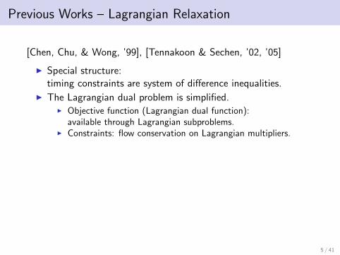
[Chen, Chu, & Wong, ’99], [Tennakoon & Sechen, ’02, ’05]

I Special structure:timing constraints are system of difference inequalities.

I The Lagrangian dual problem is simplified.I Objective function (Lagrangian dual function):

available through Lagrangian subproblems.I Constraints: flow conservation on Lagrangian multipliers.

I Lagrangian dual function is not differentiable in general.Apply subgradient optimizations.

I Difficult to choose good initial solution and step sizes.I Pre-processing can help choosing initial solutions for some

delay models.I No universal pre-processing method for all convex delays.

5 / 41

Previous Works – Lagrangian Relaxation

[Chen, Chu, & Wong, ’99], [Tennakoon & Sechen, ’02, ’05]

I Special structure:timing constraints are system of difference inequalities.

I The Lagrangian dual problem is simplified.I Objective function (Lagrangian dual function):

available through Lagrangian subproblems.I Constraints: flow conservation on Lagrangian multipliers.

I Lagrangian dual function is not differentiable in general.Apply subgradient optimizations.

I Difficult to choose good initial solution and step sizes.I Pre-processing can help choosing initial solutions for some

delay models.I No universal pre-processing method for all convex delays.

5 / 41

Contribution

I Combine gate sizing with sequential optimization.I Revisit Lagrangian relaxation.

I Correct misunderstandings.I Check primal feasibility in dual problems.

I Identify a class of problems with differentiable dual functions.I The DualFD algorithm: use gradient and network flow.

6 / 41

Outline

Introduction to Gate Sizing

Generalized Convex Sizing

The Dual Problems

The DualFD Algorithm

Experiments

Conclusions

7 / 41

Generalized Convex Sizing (GCS)

Minimize C (x)

s.t. ti + di ,j(x)− tj ≤ 0,∀(i , j) ∈ E ,

x ∈ Ω.

I G = (V ,E ): a directed graph, the system structure.

I x: the system parameters belonging to

Ω∆= x : lk ≤ xk ≤ uk ,∀1 ≤ k ≤ n.

I t: (relative) arrival times.

I C (x), di ,j(x): objective function and delays, twicedifferentiable and convex.

8 / 41

The GCS Formulation

I Timing specification in sequential circuits.

Feasible timing ⇔ No positive cycle

I Prefer edge delays to vertex delays for accuracy.I Timing arcs in one gate/cell.I Rise/fall delay and slew.

I Flexibility in choosing x.I Logarithms of sizes (gate, wire, transistor, etc. )for Elmore and

posynomial delays.I Clock skews and clock period.

9 / 41

GCS is Convex

I GCS formulation is convex.I Objective function and feasible set are convex.I Not necessary to establish convexity through geometric

programming.

I Non-convex formulations can be transformed into convexones.

I Properties of convex formulations are not necessarily hold forequivalent non-convex ones.

10 / 41

GCS is Convex

I GCS formulation is convex.I Objective function and feasible set are convex.I Not necessary to establish convexity through geometric

programming.

I Non-convex formulations can be transformed into convexones.

I Properties of convex formulations are not necessarily hold forequivalent non-convex ones.

10 / 41

Proper GCS Problems

DefinitionA GCS is proper iff:

∀x ∈ Ω,∀z 6= 0, z>HC (x)z 6= 0.

I With differentiable dual functions (shown later).I di,j(x) are irrelevant.

I Optimizing total positive weighted area is proper.

11 / 41

Simultaneous Sizing and Clock Skew Optimization

I Minimize total area under performance bound while allowingclock skew optimization.

I Handle long path conditions (setup condition).

I Assume post-processing for repairing of violated short pathconditions (hold condition).

I Not proper: ∂C∂s = 0,∀clock skew variable s.

I Cancel s. Transform to a proper one.

12 / 41

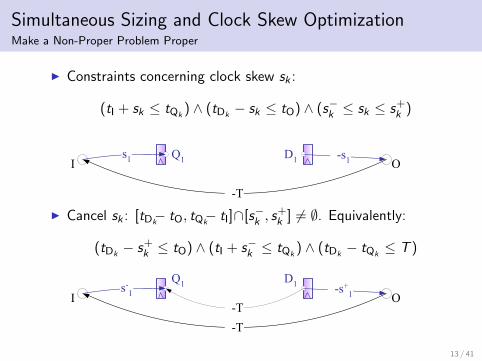
Simultaneous Sizing and Clock Skew OptimizationMake a Non-Proper Problem Proper

I Constraints concerning clock skew sk :

(tI + sk ≤ tQk) ∧ (tDk

− sk ≤ tO) ∧ (s−k ≤ sk ≤ s+k )

I Cancel sk : [tDk− tO, tQk

− tI]∩[s−k , s+k ] 6= ∅. Equivalently:

(tDk− s+

k ≤ tO) ∧ (tI + s−k ≤ tQk) ∧ (tDk

− tQk≤ T )

13 / 41

Outline

Introduction to Gate Sizing

Generalized Convex Sizing

The Dual Problems

The DualFD Algorithm

Experiments

Conclusions

14 / 41

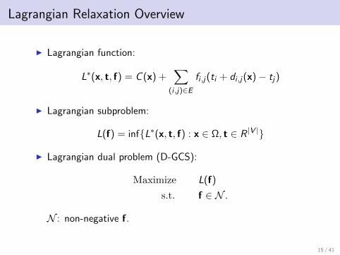
Lagrangian Relaxation Overview

I Lagrangian function:

L∗(x, t, f) = C (x) +∑

(i ,j)∈E

fi ,j(ti + di ,j(x)− tj)

I Lagrangian subproblem:

L(f) = infL∗(x, t, f) : x ∈ Ω, t ∈ R |V |

I Lagrangian dual problem (D-GCS):

Maximize L(f)

s.t. f ∈ N .

N : non-negative f.

15 / 41

Duality Gap

P∆= infC (x) : x ∈ X,D ∆

= supL(f) : f ∈ N.

X : feasible x.

I Zero duality gap is necessary: P = D.

I Establish P = D through Strong Duality Theorem.I Strictly feasible solution ⇒ exists saddle point (x, t, f):

D = L(f) = L∗(x, t, f) = C (x) = P.

I Misunderstanding: previous work applied Strong DualityTheorem to original non-convex formulation (transformationwas necessary for convexity).

I GCS is convex without transformation.

16 / 41

Duality Gap

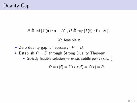
P∆= infC (x) : x ∈ X,D ∆

= supL(f) : f ∈ N.

X : feasible x.

I Zero duality gap is necessary: P = D.I Establish P = D through Strong Duality Theorem.

I Strictly feasible solution ⇒ exists saddle point (x, t, f):

D = L(f) = L∗(x, t, f) = C (x) = P.

I Misunderstanding: previous work applied Strong DualityTheorem to original non-convex formulation (transformationwas necessary for convexity).

I GCS is convex without transformation.

16 / 41

Duality Gap

P∆= infC (x) : x ∈ X,D ∆

= supL(f) : f ∈ N.

X : feasible x.

I Zero duality gap is necessary: P = D.I Establish P = D through Strong Duality Theorem.

I Strictly feasible solution ⇒ exists saddle point (x, t, f):

D = L(f) = L∗(x, t, f) = C (x) = P.

I Misunderstanding: previous work applied Strong DualityTheorem to original non-convex formulation (transformationwas necessary for convexity).

I GCS is convex without transformation.

16 / 41

Duality Gap

I What if there is no strictly feasible solution?

I Regularity condition ⇒ zero duality gap. [Rockafellear 1971]

I More general than Strong Duality Theorem for zero dualitygap.

I No guarantee for saddle points as Strong Duality Theorem.

∀f ∈ N , L(f) < D.

17 / 41

Duality Gap

I What if there is no strictly feasible solution?

I Regularity condition ⇒ zero duality gap. [Rockafellear 1971]

I More general than Strong Duality Theorem for zero dualitygap.

I No guarantee for saddle points as Strong Duality Theorem.

∀f ∈ N , L(f) < D.

17 / 41

Simplify the Dual Problem

I Flow conservation on G :

F ∆= f :

∑(i ,k)∈E

fi ,k =∑

(k,j)∈E

fk,j ,∀k ∈ V .

I L(f) = −∞ for f /∈ F , since

∀f /∈ F ,M ∈ R, x ∈ Ω,∃t ∈ R |V |, L∗(x, t, f) < M.

I Simplify D-GCS into FD-GCS:

Maximize L(f)

s.t. f ∈ F ∩N .

I Misunderstanding: previous works obtained FD-GCS by theKarush-Kuhn-Tucker (KKT) conditions ∂L∗

∂tk= 0. However,

KKT conditions are not necessary conditions.

18 / 41

Simplify the Dual Problem

I Flow conservation on G :

F ∆= f :

∑(i ,k)∈E

fi ,k =∑

(k,j)∈E

fk,j ,∀k ∈ V .

I L(f) = −∞ for f /∈ F , since

∀f /∈ F ,M ∈ R, x ∈ Ω,∃t ∈ R |V |, L∗(x, t, f) < M.

I Simplify D-GCS into FD-GCS:

Maximize L(f)

s.t. f ∈ F ∩N .

I Misunderstanding: previous works obtained FD-GCS by theKarush-Kuhn-Tucker (KKT) conditions ∂L∗

∂tk= 0. However,

KKT conditions are not necessary conditions.

18 / 41

A trivial example that is not trivial.

Will the extreme cases happen for sizing?

I Optimal solutions do NOT satisfy KKT conditions.

I No saddle point.

∀f ∈ F ∩N , L(f) < D.

.

19 / 41

A trivial example that is not trivial.

Optimize a single inverter with size ex and fixed driver/load:

Minimize ex

s.t. t1 + ex ≤ t2, t2 + e−x ≤ t3, t3 ≤ t1 + 2,

− ln 2 ≤ x ≤ ln 2.

I Single feasible solution x = 0.Optimal but not strictly feasible.

I KKT conditions cannot be satisfied by x = 0:

0 =∂L∗

∂x= ex + f1,2e

x − f2,3e−x = 1 + f1,2 − f2,3,

0 =∂L∗

∂t2= f2,3 − f1,2.

20 / 41

A trivial example that is not trivial.

I Since f ∈ F ∩N , assume β = f1,2 = f2,3 = f3,1 ≥ 0.

I Compute L(f):

L(f) = q(β) =

1+β

2 , if 0 ≤ β < 13

2√1+1/β+1

, if β ≥ 13

I q(β) increases from 12 to 1 when β increases from 0 to +∞.

I Therefore,∀f ∈ F ∩N , L(f) < 1 = D.

21 / 41

Further Simplification of the Dual Problem

I Simplify L(f) given f ∈ F :

Pf(x)∆= C (x) +

∑(i ,j)∈E

fi ,jdi ,j(x),

Q(f)∆= infPf(x) : x ∈ Ω.

⇒ L(f) = Q(f),∀f ∈ F .

I SD-GCS:

Maximize Q(f)

s.t. f ∈ F ∩N .

I SD-GCS is different from FD-GCS.

I D-GCS, FD-GCS, SD-GCS are equivalent.

22 / 41

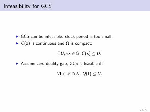
Infeasibility for GCS

I GCS can be infeasible: clock period is too small.

I C (x) is continuous and Ω is compact:

∃U,∀x ∈ Ω,C (x) ≤ U.

I Assume zero duality gap, GCS is feasible iff

∀f ∈ F ∩N ,Q(f) ≤ U.

23 / 41

Outline

Introduction to Gate Sizing

Generalized Convex Sizing

The Dual Problems

The DualFD Algorithm

Experiments

Conclusions

24 / 41

Differentiable Dual Objective Q(f)

I Sufficient condition (from textbook):

∃xf ∈ Ω,∀x ∈ Ω,Q(f) = Pf(xf) < Pf(x).

I Assume the condition is NOT satisfied.

∃x′ 6= x′′ ∈ Ω,Q(f) = Pf(x′) = Pf(x

′′)

⇒ ∀0 ≤ γ ≤ 1,Q(f) = Pf((1− γ)x′ + γx′′)

⇒ (x′′ − x′)>HPf(x′′ + x′

2)(x′′ − x′) = 0

⇒ (x′′ − x′)>HC (x′′ + x′

2)(x′′ − x′) = 0

GCS is NOT proper!I For proper GCS problems, Q(f) is differentiable, and

∂Q(f)

∂fi ,j= di ,j(xf).

25 / 41

Improving Feasible Direction

Method of feasible directions:Find ∆f, an ascent direction that is also feasible (w.r.t. SD-GCS).

∃λ > 0, (Q(f + λ∆f) > Q(f)) ∧ (f + λ∆f ∈ F ∩N ).

How to find?

I d(xf) is the gradient of Q(f):

∆f>d(xf) > 0 ⇒ ∃λ > 0,Q(f + λ∆f) > Q(f).

I Flow conservation:

f +∆f ∈ F ∩N ⇒ ∀0 ≤ λ ≤ min∆fi,j<0

−fi ,j

∆fi ,j, f +λ∆f ∈ F ∩N .

26 / 41

Improving Feasible Direction

Method of feasible directions:Find ∆f, an ascent direction that is also feasible (w.r.t. SD-GCS).

∃λ > 0, (Q(f + λ∆f) > Q(f)) ∧ (f + λ∆f ∈ F ∩N ).

How to find?

I d(xf) is the gradient of Q(f):

∆f>d(xf) > 0 ⇒ ∃λ > 0,Q(f + λ∆f) > Q(f).

I Flow conservation:

f +∆f ∈ F ∩N ⇒ ∀0 ≤ λ ≤ min∆fi,j<0

−fi ,j

∆fi ,j, f +λ∆f ∈ F ∩N .

26 / 41

Improving Feasible Direction

I The direction finding (DF) problem:

Maximize ∆f>d(xf)

s.t. f + ∆f ∈ F ∩N ,

−u ≤ ∆fi ,j ≤ u,∀(i , j) ∈ E .

∆f are decision variables, u is positive constant.

I ∆f>d(xf): first order approx. of Q(f + ∆f)− Q(f).

I DF is a min-cost network flow problem.

I For optimal ∆f, ∆f>d(xf) ≥ 0. And

∆f>d(xf) = 0 ⇒ xf is optimal for GCS.

27 / 41

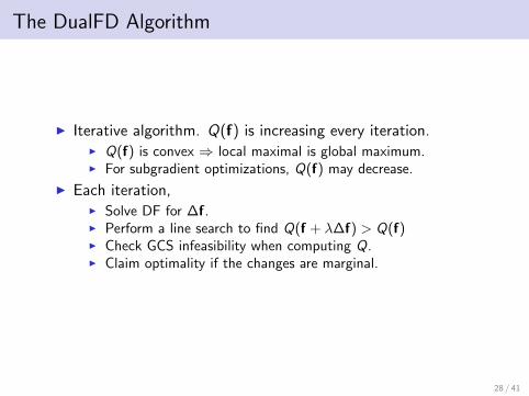
The DualFD Algorithm

I Iterative algorithm. Q(f) is increasing every iteration.I Q(f) is convex ⇒ local maximal is global maximum.I For subgradient optimizations, Q(f) may decrease.

I Each iteration,I Solve DF for ∆f.I Perform a line search to find Q(f + λ∆f) > Q(f)I Check GCS infeasibility when computing Q.I Claim optimality if the changes are marginal.

28 / 41

Outline

Introduction to Gate Sizing

Generalized Convex Sizing

The Dual Problems

The DualFD Algorithm

Experiments

Conclusions

29 / 41

Experimental Setup

I Minimize total area under performance bound with Elmoredelay model.

I ISCAS89 sequential circuits, 29 totally.Largest: ∼55000 vertices, ∼70000 edges, ∼21000 variables.

I Implement DualFD algorithm in C++.

I Use the CS2 min-cost network flow solver for DF. [Goldberg]

I Compare to subgradient optimizations: SubGrad.

30 / 41

Experimental Results

I 15 largest benchmarks.I Clock period achieved T vs. target clock period T0

I s838 is NOT feasible.

31 / 41

Experimental Results

I 15 largest benchmarks.

I Compare area, dual objective, and running time.

DualFD SubGradname area dual t(s) area dual t(s)s832 1060 1074 8.28 493 493 0.11s838 2916 80458 0.07 10189 -257K 51.51s953 776 775 5.92 3449 -80K 55.15s1196 1089 1088 10.90 1642 -14K 54.88s1238 1080 1080 7.80 974 -1823 27.19s1423 1668 1670 1.53 3346 -251K 120.76s1488 2055 2107 28.22 1150 557 31.28s1494 2161 2318 28.33 1140 529 32.02s5378 5856 6083 91.49 9396 -52K 308.39s9234 12935 15508 236.49 11517 -46K 384.86s13207 14608 14608 111.91 15642 -121K 432.81s15850 17766 17766 229.25 20628 -287K 600.10s35932 33522 44344 304.61 80650 -1M 600.34s38417 42176 44551 301.48 49126 -363K 600.35s38584 34973 34973 149.87 35016 -23K 600.19

32 / 41

DualFD vs. SubGrad

I 29 benchmarks totally.

I SubGrad never dominates DualFD.

33 / 41

How far away are we from the optimals?

I Collect feasible solutions to estimate the duality gap.

I 15 out of 29 benchmarks.

34 / 41

Convergence of s38584

35 / 41

Outline

Introduction to Gate Sizing

Generalized Convex Sizing

The Dual Problems

The DualFD Algorithm

Experiments

Conclusions

36 / 41

Conclusions

I Formulate GCS problems to handle sequential optimization.

I Correct misunderstandings when applying Lagrangianrelaxation.

I Show how to detect infeasibility in GCS.

I Prove gradient exists for proposed proper GCS problems.

I Design the DualFD algorithm to solve proper GCS problems.

37 / 41

Q & A

38 / 41

Thank you!

39 / 41

L(f) vs. Q(f)

L(f) = Q(f), ∀f ∈ F ∩N ,

L(f) = −∞, ∀f ∈ N − F ,

Q(f) 6= −∞, ∀f ∈ N − F .

I L(f) is convex but not differentiable for f ∈ N .

I Q(f) is convex and differentiable for f ∈ N .

40 / 41

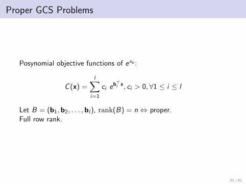
Proper GCS Problems

Posynomial objective functions of exk :

C (x) =l∑

i=1

ci eb>i x, ci > 0,∀1 ≤ i ≤ l

Let B = (b1,b2, . . . ,bl), rank(B) = n ⇔ proper.Full row rank.

41 / 41