
Gas Well Testing Handbook
650
Gas Well Testing Handbook Amanat U. Chaudhry Advanced TWPSOM Petroleum Systems, Inc. Houston, Texas AMSTERDAM • BOSTON • HEIDELBERG • LONDON NEWYORK • OXFORD • PARIS • SANDIEGO SANFRANCISCO • SINGAPORE • SYDNEY • TOKYO Gulf Professional Publishing is an imprint of Elsevier. ELSEVIER
-
Upload
ahmed-al-jishi -
Category
Documents
-
view
640 -
download
3
Transcript of Gas Well Testing Handbook
Gas Well Testing Handbook
Amanat U. Chaudhry
Advanced TWPSOM Petroleum Systems, Inc.Houston, Texas
AMSTERDAM • BOSTON • HEIDELBERG • LONDONNEWYORK • OXFORD • PARIS • SANDIEGO
SANFRANCISCO • SINGAPORE • SYDNEY • TOKYO
Gulf Professional Publishing is an imprint of Elsevier.
ELSEVIER

Gas Well Testing Handbook
Amanat U. Chaudhry
Advanced TWPSOM Petroleum Systems, Inc.Houston, Texas
AMSTERDAM • BOSTON • HEIDELBERG • LONDONNEWYORK • OXFORD • PARIS • SANDIEGO
SANFRANCISCO • SINGAPORE • SYDNEY • TOKYO
Gulf Professional Publishing is an imprint of Elsevier.
ELSEVIER

Gulf Professional Publishing is an imprint of Elsevier Science.
Copyright © 2003 by Elsevier Science. All rights reserved.
No part of this publication may be reproduced, stored in a retrieval system, ortransmitted in any form or by any means, electronic, mechanical, photocopying,recording, or otherwise, without the prior written permission of the publisher.
© Recognizing the importance of preserving what has been written, Elsevier Scienceprints its books on acid-free paper whenever possible.
Library of Congress Cataloging-in-Publication DataChaudhry, Amanat U.
Gas well testing handbook / by Amanat U. Chaudhry.p.cm.
Includes bibliographical references and index.ISBN 0-7506-7705-8 (acid-free paper)
1. Gas wells—Testing—Handbooks, manuals, etc. I. Title.
TN871.C453 2003622'.3385'0287-dc21 2003048310
British Library Cataloguing-in-Publication DataA catalogue record for this book is available from the British Library.
The publisher offers special discounts on bulk orders of this book.For information, please contact:
Manager of Special SalesElsevier Science200 Wheeler RoadBurlington, MA 01803Tel: 781-313-4700Fax:781-313-4882
For information on all Gulf Professional Publishing publications available, contactour World Wide Web home page at: http://www.gulfpp.com
10 9 8 7 6 5 4 3 2 1
Printed in the United States of America

Dedication
This book is dedicated to my son Alhaj U. ChaudhryI am grateful to my parents for providing me with education, inspiration, and
confidence. I am also indebted to my ex-wife, Nuraini Smith, who providedthe encouragement, fortitude, and extraordinary understanding, which enabledme to steal many hours from my family while writing this book.

Foreword
Although elements of gas well testing methods have been practical almost sincegas reservoirs were first recognized, the concept of gas well testing techniqueshas taken form only within the past three decades. Many individual monographsand at least one manual on the subject have been published in the open literature,and it is probable that proprietary presentations of gas well testing conceptsare to be found within the internal libraries of some oil- and gas-producingcompanies. In the present volume, the author presents a treatment of the subjectto be published in book form.
The roots of gas well testing are to be found in reservoir engineering taken inits broadest sense as the technology that deals with the well/reservoir behaviorthrough the measuring and analysis of deliverability test, flow, and transientpressure responses in unfractured and fractured gas wells. The concepts relatedto gas well test data acquisition and interpretation are presented from a practicalviewpoint. These concepts are emphasized throughout the book by means ofexamples and field case studies.
In Gas Well Testing Handbook, the author has presented a comprehensivestudy of the measuring and analysis of deliverability tests, flow, and transientpressure responses in gas wells. The basic principles are reviewed and theapplicability and limitations of the various testing techniques are criticallydiscussed and illustrated with actual field examples. The material is presentedin a form that will allow engineers directly involved in well deliverability,pressure build-up, and flow testing to re-educate themselves on the subject.At the same time, with its up-to-date review of the literature and extensivebibliography, the book will serve as a useful guide and reference to engineersdirectly engaged in well pressure behavior work. The author has accomplishedthe intended objectives of the book in a thorough and excellent manner.
The author has illustrated by field application examples and field case studiesto describe the types of wells and reservoir behavior encountered in modernproduction practice. The source, nature, and precision of the data and studiesupon which the calculations and analysis are based are discussed subordinately.

Numerous examples are provided to help the reader develop an understandingof the principles and limitations of applied gas well testing methods.
The book is essential and important to engineers concerned with evaluatingwell/reservoir systems and the pressure performance of gas wells. The authorhas extensive experience in this field and is most qualified to treat the subject.It is a timely addition to the literature of petroleum technology.
Dilip BorthakerHead of Gas Engineering Department
Gulf Indonesia Resources

Preface
The major purpose of writing this book is to provide a practical referencesource for knowledge regarding state-of-the-art gas well testing technology.The book presents the use of gas well testing techniques and analysis methodsfor evaluation of well conditions and reservoir characteristics. All techniquesand data described in this book are "field-tested" and are published here forthe first time. For example, this book contains new tables and comparisonsof the various methods of well test analysis. Most of these techniques andapplications are clearly illustrated in worked examples of the actual field data.Several actual field example calculations and field case studies are includedfor illustration purposes.
This text is a must for reservoir engineers, simulation engineers, practicingpetroleum engineers, and professional geologists, geophysicists, and technicalmanagers. It helps engineering professors better acquaint their students with"real-life" solution problems. This instructive text includes practical examplesthat readers should find easy to understand and reproduce.
Fundamental concepts related to well test data acquisition and interpretationare presented from a practical viewpoint. Furthermore, a brief summary of theadvances in this area is presented. Emphasis is given to the most commoninterpretation methods used at present. The main emphasis is on practicalsolutions and field application. More than 129 field examples are presentedto illustrate effective gas well testing practices, most analysis techniques, andtheir application.
Many solutions that are presented are based upon the author's experiencedealing with various well testing techniques and interpretation around theworld. I am very thankful to the many companies with whom I had the oppor-tunity to work in well test analysis for many years.
A properly designed, executed, and analyzed well test can provide infor-mation about formation permeability, reservoir initial or average pressure,sand-face condition (well damage or stimulation), volume of drainage area,boundary and discontinuities, reservoir heterogeneity, distance or extension of

the fracture induced, validation of geological model, and system identification(type of reservoir and mathematical model).
Further, it is important to determine the ability of a formation to producereservoir fluids and the underlying reason for a well's productivity. These data,when combined with hydrocarbon production data and with laboratory data onfluid and rock properties, afford the means to estimate the original hydrocarbonin-place and the recovery that may be expected from the reservoir under variousmodes of exploitation. In addition, well test data and IPR well performanceequations, combined with production data, help in designing, analyzing, andoptimizing a total well production system or in production optimization.
The rigorous discussions, practical examples, and easy-to-read mannermake this a valuable addition to every petroleum professional's library. Ourcolleagues' discussions and their suggestions were very valuable in makingthis book useful to a practicing engineer. Most users of this book will findit logically organized and readily applicable to many well testing problemsolutions and field applications.

Acknowledgments
I would also like to thank Dr. Furlow Fulton, Head of the Petroleum Engineer-ing Department at the University of Pittsburgh, for educating me in reservoirengineering. I have also been privileged to work with many professionals inthe oil industry who have taught me many things and helped me grow and de-velop as an engineer. I am also thankful to A.C. Carnes, Jr., General Manager,Integrated Technology Petroleum Consulting Services, Houston, who orientedme in the areas of reservoir simulation and well test analysis during my career.I am also thankful to many companies who were generous in providing thefield histories and data that were used in the book. I am also thankful to AmbarSudiono,* General Manager of State Owned Oil Company of Indonesia, whowas kind enough to read chapters 3, 4, 5, 7, 10 and provided many valuablesuggestions.
Mr. Dilip Borthakur has reviewed the material presented in this book.** Hehas spent hundreds of hours reading, checking, and critically commenting onall aspects of the material and its presentation. There is no doubt that the bookis a much better volume that it would have been without his aid.
Ms. Faiza Azam typed the many versions of the book required to reach thefinal form. Her technical skills and command of the English language haveenabled preparation of this volume to proceed smoothly and on schedule. Shealso prepared all the original illustrations; she redrew many illustrations takenfrom the references to provide a consistent nomenclature and format. Herartist's viewpoint, her skill, and her highly accurate work have added substan-tially to this book. I would also like to acknowledge the support of editorialstaff of Elsevier for their patience and hard work in producing this book. Lastbut not the least, I owe sincere appreciation and thanks to Kyle Sarofeen, PhilCarmical and Christine Kloiber for their contributions to this book.
* Presently General Manager with State Owned Oil Company of Indonesia,Jakarta.
** Presently Head of Gas Engineering Department with Gulf IndonesiaResources.
Amanat Chaudhry

Gulf Professional Publishing is an imprint of Elsevier Science.
Copyright © 2003 by Elsevier Science. All rights reserved.
No part of this publication may be reproduced, stored in a retrieval system, ortransmitted in any form or by any means, electronic, mechanical, photocopying,recording, or otherwise, without the prior written permission of the publisher.
© Recognizing the importance of preserving what has been written, Elsevier Scienceprints its books on acid-free paper whenever possible.
Library of Congress Cataloging-in-Publication DataChaudhry, Amanat U.
Gas well testing handbook / by Amanat U. Chaudhry.p.cm.
Includes bibliographical references and index.ISBN 0-7506-7705-8 (acid-free paper)
1. Gas wells—Testing—Handbooks, manuals, etc. I. Title.
TN871.C453 2003622'.3385'0287-dc21 2003048310
British Library Cataloguing-in-Publication DataA catalogue record for this book is available from the British Library.
The publisher offers special discounts on bulk orders of this book.For information, please contact:
Manager of Special SalesElsevier Science200 Wheeler RoadBurlington, MA 01803Tel: 781-313-4700Fax:781-313-4882
For information on all Gulf Professional Publishing publications available, contactour World Wide Web home page at: http://www.gulfpp.com
10 9 8 7 6 5 4 3 2 1
Printed in the United States of America

Dedication
This book is dedicated to my son Alhaj U. ChaudhryI am grateful to my parents for providing me with education, inspiration, and
confidence. I am also indebted to my ex-wife, Nuraini Smith, who providedthe encouragement, fortitude, and extraordinary understanding, which enabledme to steal many hours from my family while writing this book.
Foreword
Although elements of gas well testing methods have been practical almost sincegas reservoirs were first recognized, the concept of gas well testing techniqueshas taken form only within the past three decades. Many individual monographsand at least one manual on the subject have been published in the open literature,and it is probable that proprietary presentations of gas well testing conceptsare to be found within the internal libraries of some oil- and gas-producingcompanies. In the present volume, the author presents a treatment of the subjectto be published in book form.
The roots of gas well testing are to be found in reservoir engineering taken inits broadest sense as the technology that deals with the well/reservoir behaviorthrough the measuring and analysis of deliverability test, flow, and transientpressure responses in unfractured and fractured gas wells. The concepts relatedto gas well test data acquisition and interpretation are presented from a practicalviewpoint. These concepts are emphasized throughout the book by means ofexamples and field case studies.
In Gas Well Testing Handbook, the author has presented a comprehensivestudy of the measuring and analysis of deliverability tests, flow, and transientpressure responses in gas wells. The basic principles are reviewed and theapplicability and limitations of the various testing techniques are criticallydiscussed and illustrated with actual field examples. The material is presentedin a form that will allow engineers directly involved in well deliverability,pressure build-up, and flow testing to re-educate themselves on the subject.At the same time, with its up-to-date review of the literature and extensivebibliography, the book will serve as a useful guide and reference to engineersdirectly engaged in well pressure behavior work. The author has accomplishedthe intended objectives of the book in a thorough and excellent manner.
The author has illustrated by field application examples and field case studiesto describe the types of wells and reservoir behavior encountered in modernproduction practice. The source, nature, and precision of the data and studiesupon which the calculations and analysis are based are discussed subordinately.

Numerous examples are provided to help the reader develop an understandingof the principles and limitations of applied gas well testing methods.
The book is essential and important to engineers concerned with evaluatingwell/reservoir systems and the pressure performance of gas wells. The authorhas extensive experience in this field and is most qualified to treat the subject.It is a timely addition to the literature of petroleum technology.
Dilip BorthakerHead of Gas Engineering Department
Gulf Indonesia Resources
Preface
The major purpose of writing this book is to provide a practical referencesource for knowledge regarding state-of-the-art gas well testing technology.The book presents the use of gas well testing techniques and analysis methodsfor evaluation of well conditions and reservoir characteristics. All techniquesand data described in this book are "field-tested" and are published here forthe first time. For example, this book contains new tables and comparisonsof the various methods of well test analysis. Most of these techniques andapplications are clearly illustrated in worked examples of the actual field data.Several actual field example calculations and field case studies are includedfor illustration purposes.
This text is a must for reservoir engineers, simulation engineers, practicingpetroleum engineers, and professional geologists, geophysicists, and technicalmanagers. It helps engineering professors better acquaint their students with"real-life" solution problems. This instructive text includes practical examplesthat readers should find easy to understand and reproduce.
Fundamental concepts related to well test data acquisition and interpretationare presented from a practical viewpoint. Furthermore, a brief summary of theadvances in this area is presented. Emphasis is given to the most commoninterpretation methods used at present. The main emphasis is on practicalsolutions and field application. More than 129 field examples are presentedto illustrate effective gas well testing practices, most analysis techniques, andtheir application.
Many solutions that are presented are based upon the author's experiencedealing with various well testing techniques and interpretation around theworld. I am very thankful to the many companies with whom I had the oppor-tunity to work in well test analysis for many years.
A properly designed, executed, and analyzed well test can provide infor-mation about formation permeability, reservoir initial or average pressure,sand-face condition (well damage or stimulation), volume of drainage area,boundary and discontinuities, reservoir heterogeneity, distance or extension of

the fracture induced, validation of geological model, and system identification(type of reservoir and mathematical model).
Further, it is important to determine the ability of a formation to producereservoir fluids and the underlying reason for a well's productivity. These data,when combined with hydrocarbon production data and with laboratory data onfluid and rock properties, afford the means to estimate the original hydrocarbonin-place and the recovery that may be expected from the reservoir under variousmodes of exploitation. In addition, well test data and IPR well performanceequations, combined with production data, help in designing, analyzing, andoptimizing a total well production system or in production optimization.
The rigorous discussions, practical examples, and easy-to-read mannermake this a valuable addition to every petroleum professional's library. Ourcolleagues' discussions and their suggestions were very valuable in makingthis book useful to a practicing engineer. Most users of this book will findit logically organized and readily applicable to many well testing problemsolutions and field applications.
Acknowledgments
I would also like to thank Dr. Furlow Fulton, Head of the Petroleum Engineer-ing Department at the University of Pittsburgh, for educating me in reservoirengineering. I have also been privileged to work with many professionals inthe oil industry who have taught me many things and helped me grow and de-velop as an engineer. I am also thankful to A.C. Carnes, Jr., General Manager,Integrated Technology Petroleum Consulting Services, Houston, who orientedme in the areas of reservoir simulation and well test analysis during my career.I am also thankful to many companies who were generous in providing thefield histories and data that were used in the book. I am also thankful to AmbarSudiono,* General Manager of State Owned Oil Company of Indonesia, whowas kind enough to read chapters 3, 4, 5, 7, 10 and provided many valuablesuggestions.
Mr. Dilip Borthakur has reviewed the material presented in this book.** Hehas spent hundreds of hours reading, checking, and critically commenting onall aspects of the material and its presentation. There is no doubt that the bookis a much better volume that it would have been without his aid.
Ms. Faiza Azam typed the many versions of the book required to reach thefinal form. Her technical skills and command of the English language haveenabled preparation of this volume to proceed smoothly and on schedule. Shealso prepared all the original illustrations; she redrew many illustrations takenfrom the references to provide a consistent nomenclature and format. Herartist's viewpoint, her skill, and her highly accurate work have added substan-tially to this book. I would also like to acknowledge the support of editorialstaff of Elsevier for their patience and hard work in producing this book. Lastbut not the least, I owe sincere appreciation and thanks to Kyle Sarofeen, PhilCarmical and Christine Kloiber for their contributions to this book.
* Presently General Manager with State Owned Oil Company of Indonesia,Jakarta.
** Presently Head of Gas Engineering Department with Gulf IndonesiaResources.
Amanat Chaudhry
vii This page has been reformatted by Knovel to provide easier navigation.
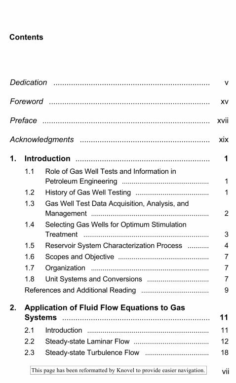
Contents
Dedication ....................................................................... v
Foreword ......................................................................... xv
Preface ............................................................................ xvii
Acknowledgments ........................................................... xix
1. Introduction ............................................................. 1 1.1 Role of Gas Well Tests and Information in
Petroleum Engineering ............................................. 1 1.2 History of Gas Well Testing ...................................... 1 1.3 Gas Well Test Data Acquisition, Analysis, and
Management ............................................................. 2 1.4 Selecting Gas Wells for Optimum Stimulation
Treatment ................................................................. 3 1.5 Reservoir System Characterization Process ........... 4 1.6 Scopes and Objective ............................................... 7 1.7 Organization ............................................................. 7 1.8 Unit Systems and Conversions ................................ 7 References and Additional Reading ................................... 9
2. Application of Fluid Flow Equations to Gas Systems ................................................................... 11 2.1 Introduction ............................................................... 11 2.2 Steady-state Laminar Flow ....................................... 12 2.3 Steady-state Turbulence Flow ................................. 18
viii Contents
This page has been reformatted by Knovel to provide easier navigation.
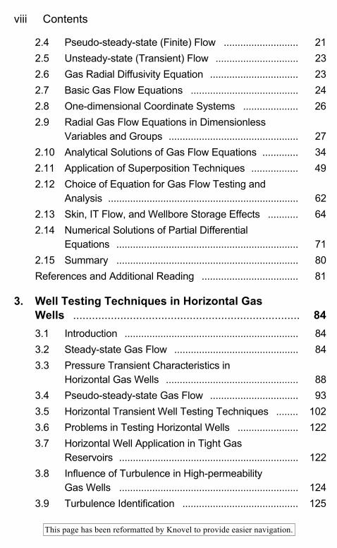
2.4 Pseudo-steady-state (Finite) Flow ........................... 21 2.5 Unsteady-state (Transient) Flow .............................. 23 2.6 Gas Radial Diffusivity Equation ................................ 23 2.7 Basic Gas Flow Equations ....................................... 24 2.8 One-dimensional Coordinate Systems .................... 26 2.9 Radial Gas Flow Equations in Dimensionless
Variables and Groups ............................................... 27 2.10 Analytical Solutions of Gas Flow Equations ............. 34 2.11 Application of Superposition Techniques ................. 49 2.12 Choice of Equation for Gas Flow Testing and
Analysis ..................................................................... 62 2.13 Skin, IT Flow, and Wellbore Storage Effects ........... 64 2.14 Numerical Solutions of Partial Differential
Equations .................................................................. 71 2.15 Summary .................................................................. 80 References and Additional Reading ................................... 81
3. Well Testing Techniques in Horizontal Gas Wells ........................................................................ 84 3.1 Introduction ............................................................... 84 3.2 Steady-state Gas Flow ............................................. 84 3.3 Pressure Transient Characteristics in
Horizontal Gas Wells ................................................ 88 3.4 Pseudo-steady-state Gas Flow ................................ 93 3.5 Horizontal Transient Well Testing Techniques ........ 102 3.6 Problems in Testing Horizontal Wells ...................... 122 3.7 Horizontal Well Application in Tight Gas
Reservoirs ................................................................. 122 3.8 Influence of Turbulence in High-permeability
Gas Wells ................................................................. 124 3.9 Turbulence Identification .......................................... 125
Contents ix
This page has been reformatted by Knovel to provide easier navigation.
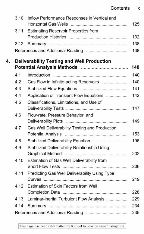
3.10 Inflow Performance Responses in Vertical and Horizontal Gas Wells ................................................ 125
3.11 Estimating Reservoir Properties from Production Histories ................................................. 132
3.12 Summary .................................................................. 138 References and Additional Reading ................................... 138
4. Deliverability Testing and Well Production Potential Analysis Methods ................................... 140 4.1 Introduction ............................................................... 140 4.2 Gas Flow in Infinite-acting Reservoirs ...................... 140 4.3 Stabilized Flow Equations ........................................ 141 4.4 Application of Transient Flow Equations .................. 142 4.5 Classifications, Limitations, and Use of
Deliverability Tests .................................................... 147 4.6 Flow-rate, Pressure Behavior, and
Deliverability Plots .................................................... 149 4.7 Gas Well Deliverability Testing and Production
Potential Analysis ..................................................... 153 4.8 Stabilized Deliverability Equation ............................. 196 4.9 Stabilized Deliverability Relationship Using
Graphical Method ..................................................... 202 4.10 Estimation of Gas Well Deliverability from
Short Flow Tests ....................................................... 206 4.11 Predicting Gas Well Deliverability Using Type
Curves ....................................................................... 219 4.12 Estimation of Skin Factors from Well
Completion Data ....................................................... 228 4.13 Laminar-inertial Turbulent Flow Analysis ................. 229 4.14 Summary .................................................................. 234 References and Additional Reading ................................... 235
x Contents
This page has been reformatted by Knovel to provide easier navigation.
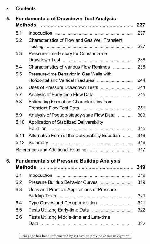
5. Fundamentals of Drawdown Test Analysis Methods ................................................................... 237 5.1 Introduction ............................................................... 237 5.2 Characteristics of Flow and Gas Well Transient
Testing ...................................................................... 237 5.3 Pressure-time History for Constant-rate
Drawdown Test ......................................................... 238 5.4 Characteristics of Various Flow Regimes ................ 238 5.5 Pressure-time Behavior in Gas Wells with
Horizontal and Vertical Fractures ............................. 244 5.6 Uses of Pressure Drawdown Tests .......................... 244 5.7 Analysis of Early-time Flow Data ............................. 245 5.8 Estimating Formation Characteristics from
Transient Flow Test Data ......................................... 251 5.9 Analysis of Pseudo-steady-state Flow Data ............ 309 5.10 Application of Stabilized Deliverability
Equation .................................................................... 315 5.11 Alternative Form of the Deliverability Equation ........ 316 5.12 Summary .................................................................. 316 References and Additional Reading ................................... 317
6. Fundamentals of Pressure Buildup Analysis Methods ................................................................... 319 6.1 Introduction ............................................................... 319 6.2 Pressure Buildup Behavior Curves .......................... 319 6.3 Uses and Practical Applications of Pressure
Buildup Tests ............................................................ 321 6.4 Type Curves and Desuperposition ........................... 321 6.5 Tests Utilizing Early-time Data ................................. 322 6.6 Tests Utilizing Middle-time and Late-time
Data .......................................................................... 322
Contents xi
This page has been reformatted by Knovel to provide easier navigation.
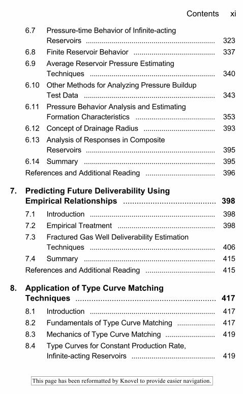
6.7 Pressure-time Behavior of Infinite-acting Reservoirs ................................................................. 323
6.8 Finite Reservoir Behavior ......................................... 337 6.9 Average Reservoir Pressure Estimating
Techniques ............................................................... 340 6.10 Other Methods for Analyzing Pressure Buildup
Test Data .................................................................. 343 6.11 Pressure Behavior Analysis and Estimating
Formation Characteristics ........................................ 353 6.12 Concept of Drainage Radius .................................... 393 6.13 Analysis of Responses in Composite
Reservoirs ................................................................. 395 6.14 Summary .................................................................. 395 References and Additional Reading ................................... 396
7. Predicting Future Deliverability Using Empirical Relationships ......................................... 398 7.1 Introduction ............................................................... 398 7.2 Empirical Treatment ................................................. 398 7.3 Fractured Gas Well Deliverability Estimation
Techniques ............................................................... 406 7.4 Summary .................................................................. 415 References and Additional Reading ................................... 415
8. Application of Type Curve Matching Techniques .............................................................. 417 8.1 Introduction ............................................................... 417 8.2 Fundamentals of Type Curve Matching ................... 417 8.3 Mechanics of Type Curve Matching ......................... 419 8.4 Type Curves for Constant Production Rate,
Infinite-acting Reservoirs .......................................... 419
xii Contents
This page has been reformatted by Knovel to provide easier navigation.
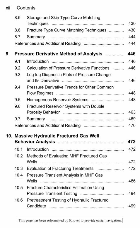
8.5 Storage and Skin Type Curve Matching Techniques ............................................................... 430
8.6 Fracture Type Curve Matching Techniques ............. 430 8.7 Summary .................................................................. 444 References and Additional Reading ................................... 444
9. Pressure Derivative Method of Analysis .............. 446 9.1 Introduction ............................................................... 446 9.2 Calculation of Pressure Derivative Functions .......... 446 9.3 Log-log Diagnostic Plots of Pressure Change
and Its Derivative ...................................................... 446 9.4 Pressure Derivative Trends for Other Common
Flow Regimes ........................................................... 448 9.5 Homogenous Reservoir Systems ............................ 448 9.6 Fractured Reservoir Systems with Double
Porosity Behavior ..................................................... 463 9.7 Summary .................................................................. 469 References and Additional Reading ................................... 470
10. Massive Hydraulic Fractured Gas Well Behavior Analysis ................................................... 472 10.1 Introduction ............................................................... 472 10.2 Methods of Evaluating MHF Fractured Gas
Wells ......................................................................... 472 10.3 Evaluation of Fracturing Treatments ........................ 472 10.4 Pressure Transient Analysis in MHF Gas
Wells ......................................................................... 486 10.5 Fracture Characteristics Estimation Using
Pressure Transient Testing ...................................... 494 10.6 Pretreatment Testing of Hydraulic Fractured
Candidate ................................................................. 499
Contents xiii
This page has been reformatted by Knovel to provide easier navigation.
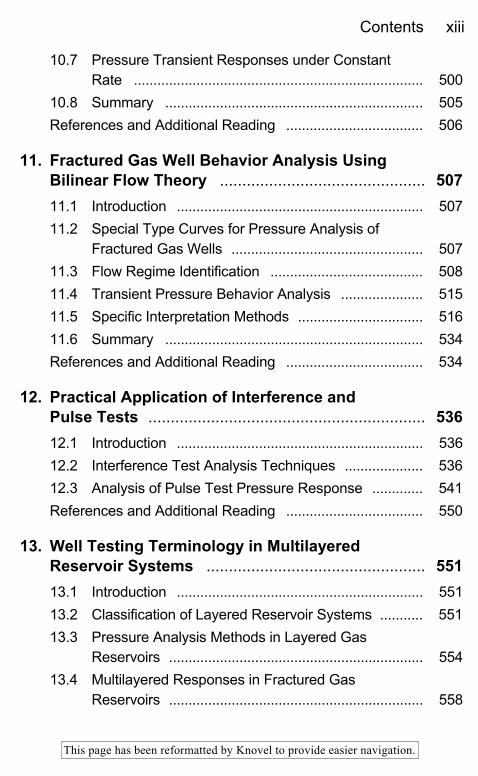
10.7 Pressure Transient Responses under Constant Rate .......................................................................... 500
10.8 Summary .................................................................. 505 References and Additional Reading ................................... 506
11. Fractured Gas Well Behavior Analysis Using Bilinear Flow Theory .............................................. 507 11.1 Introduction ............................................................... 507 11.2 Special Type Curves for Pressure Analysis of
Fractured Gas Wells ................................................. 507 11.3 Flow Regime Identification ....................................... 508 11.4 Transient Pressure Behavior Analysis ..................... 515 11.5 Specific Interpretation Methods ................................ 516 11.6 Summary .................................................................. 534 References and Additional Reading ................................... 534
12. Practical Application of Interference and Pulse Tests .............................................................. 536 12.1 Introduction ............................................................... 536 12.2 Interference Test Analysis Techniques .................... 536 12.3 Analysis of Pulse Test Pressure Response ............. 541 References and Additional Reading ................................... 550
13. Well Testing Terminology in Multilayered Reservoir Systems ................................................. 551 13.1 Introduction ............................................................... 551 13.2 Classification of Layered Reservoir Systems ........... 551 13.3 Pressure Analysis Methods in Layered Gas
Reservoirs ................................................................. 554 13.4 Multilayered Responses in Fractured Gas
Reservoirs ................................................................. 558
xiv Contents
This page has been reformatted by Knovel to provide easier navigation.
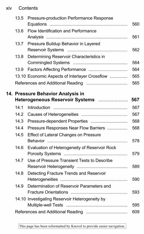
13.5 Pressure-production Performance Response Equations .................................................................. 560
13.6 Flow Identification and Performance Analysis ..................................................................... 561
13.7 Pressure Buildup Behavior in Layered Reservoir Systems ................................................... 562
13.8 Determining Reservoir Characteristics in Commingled Systems .............................................. 564
13.9 Factors Affecting Performance ................................. 564 13.10 Economic Aspects of Interlayer Crossflow ............... 565 References and Additional Reading ................................... 565
14. Pressure Behavior Analysis in Heterogeneous Reservoir Systems ...................... 567 14.1 Introduction ............................................................... 567 14.2 Causes of Heterogeneities ....................................... 567 14.3 Pressure-dependent Properties ............................... 568 14.4 Pressure Responses Near Flow Barriers ................. 568 14.5 Effect of Lateral Changes on Pressure
Behavior .................................................................... 578 14.6 Evaluation of Heterogeneity of Reservoir Rock
Porosity Systems ...................................................... 579 14.7 Use of Pressure Transient Tests to Describe
Reservoir Heterogeneity ........................................... 589 14.8 Detecting Fracture Trends and Reservoir
Heterogeneities ......................................................... 590 14.9 Determination of Reservoir Parameters and
Fracture Orientations ................................................ 593 14.10 Investigating Reservoir Heterogeneity by
Multiple-well Tests .................................................... 595 References and Additional Reading ................................... 609
Contents xv
This page has been reformatted by Knovel to provide easier navigation.
15. Gas Well Testing Field Case Studies .................... 611 15.1 Introduction ............................................................... 611 15.2 Gas Well Test Evaluation Sheet .............................. 611 15.3 Shallow Low-pressure and Highly Productive
Gas Reservoirs ......................................................... 613 15.4 Recommended Form of Rules of Procedure for
Backpressure Tests Required by State Regulatory Bodies .................................................... 614
15.5 Appropriate State Report Forms .............................. 615 15.6 Stimulation Efforts Evaluation, Summary, and
Recommendations .................................................... 616 15.7 Formation Characteristics from Fractured
Carbonate Gas Reservoirs ....................................... 621 15.8 Buildup Interpretations Before and After
Workovers ................................................................. 625 References and Additional Reading ................................... 636
16. Application of Decline Curve Analysis Methods ................................................................... 637 16.1 Introduction ............................................................... 637 16.2 Transient Decline Behavior Analysis ........................ 637 16.3 Pseudo-steady-state Decline ................................... 640 16.4 Characteristics and Classifications of
Production Decline Curves ....................................... 642 16.5 Horizontal Gas Reservoir Performance Using
Production Type Curves ........................................... 654 16.6 Horizontal and Fractured Vertical Gas
Reservoir Production Forecasting ............................ 657 16.7 Estimating in-place Gas Reserves ........................... 660 16.8 Determination of Economic Limit ............................. 663 References and Additional Reading ................................... 663
xvi Contents
This page has been reformatted by Knovel to provide easier navigation.
17. Overall Skin Effects and Impact on Gas Well Performance ............................................................ 664 17.1 Introduction ............................................................... 664 17.2 Rate-dependent Skin Factor .................................... 664 17.3 Skin Factor Due to Partial Penetration ..................... 667 17.4 Skin Factor Due to Perforation ................................. 671 17.5 Skin Factor from Partial Completion and
Slant .......................................................................... 674 17.6 Skin Factor Due to Reduced Crushed-zone
Permeability .............................................................. 675 17.7 Slant Well Damage Skin Effect on Well
Productivity ............................................................... 680 17.8 Horizontal Well Damage Skin Effects ...................... 685 References and Additional Reading ................................... 692
18. Selection of Gas Wells for Production Stimulation .............................................................. 694 18.1 Introduction ............................................................... 694 18.2 Major Causes of Low-productivity Gas Wells .......... 694 18.3 Formation Condition Evaluation Techniques ........... 694 18.4 Relative Indicators of Wellbore Conditions .............. 696 18.5 Skin Factor Concepts, Relationships, and
Equations .................................................................. 696 18.6 Completion Types and Related Skin Factors .......... 699 18.7 Selecting Gas Wells for Fracturing Treatment ......... 700 18.8 Productivity Improvement and Treatment
Variables ................................................................... 700 18.9 IPR Modification to Different Hydraulic
Fracture Designs ...................................................... 702 References and Additional Reading ................................... 703
Contents xvii
This page has been reformatted by Knovel to provide easier navigation.
19. Design Criteria of Flow and Pressure Transient Tests ....................................................... 705 19.1 Introduction ............................................................... 705 19.2 Deliverability Tests .................................................... 705 19.3 Procedures for Conducting Deliverability
Tests ......................................................................... 709 19.4 General Concepts for Designing Transient
Pressure Tests .......................................................... 714 19.5 Test Planning and Data Acquisition ......................... 719 19.6 Guidelines for Gas Well Testing ............................... 719 19.7 Problems in Gas Well Testing .................................. 723 19.8 Reporting Gas Well Test Data .................................. 724 References and Additional Reading ................................... 726
Appendices Appendix A: Use of SI Units in Gas Well Testing
Equations .................................................................. 727 Appendix B: Correlation Tables and Charts for
Dimensionless Functions ......................................... 730 References and Additional Reading ..................... 736
Appendix C: Estimation of Formation Characteristics from Drill-stem Test .................................................. 737 C.1 Normal Routine Drill-stem Test ..................... 737 C.2 Determination of Effective Permeability,
Skin Factor, and Damage Ratio .................... 738 C.3 Initial Reservoir Pressure Estimation
Technique ..................................................... 739 C.4 Radius of Investigation ................................. 740 References and Additional Reading ..................... 740
xviii Contents
This page has been reformatted by Knovel to provide easier navigation.
Appendix D: Gas Flow Rate Measurement Techniques ............................................................... 741 D.1 Gas Flow Rate Calculations ......................... 741 D.2 Determining Orifice Meter Constants
and Factors .................................................. 741 D.3 Critical-flow Prover ....................................... 746 References and Additional Reading ..................... 747
Appendix E: Computing Flowing Bottom-hole Pressure from Wellhead Pressure ........................... 748 E.1 Cullender and Smith Method ........................ 748 References and Additional Reading ..................... 751
Appendix F: Fluid and Rock Property Correlations ............ 752 F.1 Gas Properties and Correlations ................... 753 F.2 Reservoir Rock Properties ............................ 765 F.3 Reservoir PVT Water Properties ................... 766 References and Additional Reading ..................... 783
Appendix G: Substantial Set of Problems without Solutions ................................................................... 785
Nomenclature ................................................................ 803
Bibliography .................................................................. 811
Index ............................................................................... 827
Chapter 1
Introduction
1.1 Role of Gas Well Tests and Informationin Petroleum Engineering
Gas well test analysis is a branch of reservoir engineering. Informationderived from flow and pressure transient tests about in-situ reservoir condi-tions is important in many phases of petroleum engineering. The reservoirengineer must have sufficient information about the reservoir/well conditionand characteristics to adequately analyze reservoir performance and forecastfuture production under various modes of operation. The production engineermust know the condition of production and injection wells to persuade the bestpossible performance from the reservoir.
Pressures are most valuable and useful data in reservoir engineering.Directly or indirectly, they enter into all phases of reservoir engineering cal-culations. Therefore accurate determination of reservoir parameters is veryimportant. In general, gas well test analysis is conducted to meet the followingobjectives:
• To obtain reservoir parameters.• To determine whether all the drilled length of gas well is also a producing
zone.• To estimate skin factor or drilling and completion related damage to a
gas well. Based upon magnitude of the damage a decision regarding wellstimulation can be made.
1.2 History of Gas Well Testing
The first analysis was based on the empirical method applicable to veryporous and permeable reservoirs developed by Schellherdt and Rawlins,1
"Back-Pressure Data on Natural Gas Wells and Their Application to Produc-tion Practices." Monograph 7, U.S.B.M. This method today is known as thefour-point (sometimes as the one-point) method. The [ (p2
R — p^) versus qsc ]square of the average reservoir pressure minus the square of the flowing
sand-face pressure is plotted versus the respective flow rates on log-logpaper. The maximum rate is read at the pressure equal to the average reservoirpressure after a straight line is drawn through test points for four semi-stabilizedflow rates. Later, more practical methods of testing were developed. Theseincluded the isochronal test and the modified isochronal test. Such tests havebeen used extensively by the gas industry.
Most recently flow and pressure transient tests have been developed andused to determine the flow characteristics of gas wells. Development of eventighter gas wells was common during the late 1950s and fracturing with largeamounts of sand was routine. Pressure difference across the drainage areaoften was great. By 1966, a group of engineers working with Russell, ShellOil, published articles using basic flow equations applicable to all gas wells,regardless of the permeability and fractures used by the operators. The stateof the art was summarized in 1967 in "Pressure Buildup and Flow Tests inWells" by Matthews and Russell,2 SPE Monograph 1, Henry L. DohertySeries. Earlougher4 again reviewed the state of the art in 1977 in "Advances inWell Test Analysis" in SPE Monograph 5. One book5 was published in 1975covering different aspects of flow and pressure transient analysis.
The analysis of pressure data for fractured gas wells has deserved specialattention because of the number of wells that have been stimulated by hydraulicfracturing techniques. References 4 through 7 have presented a summary ofthe work done on flow toward fractured wells in 1962 and 1978.
1.3 Gas Well Test Data Acquisition, Analysis,and Management
Throughout the life of a gas well, from exploration to abandonment, enoughwell test data are collected to describe well condition and behavior. It isemphasized that the multidisciplinary professionals need to work as an in-tegrated team to develop and implement well test data management programs.
Efficient Gas Well Test Analysis Programs
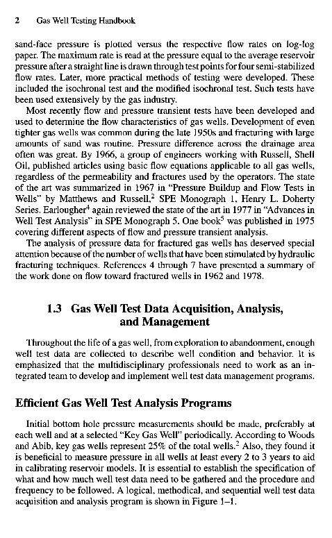
Initial bottom hole pressure measurements should be made, preferably ateach well and at a selected "Key Gas Well" periodically. According to Woodsand Abib, key gas wells represent 25% of the total wells.2 Also, they found itis beneficial to measure pressure in all wells at least every 2 to 3 years to aidin calibrating reservoir models. It is essential to establish the specification ofwhat and how much well test data need to be gathered and the procedure andfrequency to be followed. A logical, methodical, and sequential well test dataacquisition and analysis program is shown in Figure 1-1.
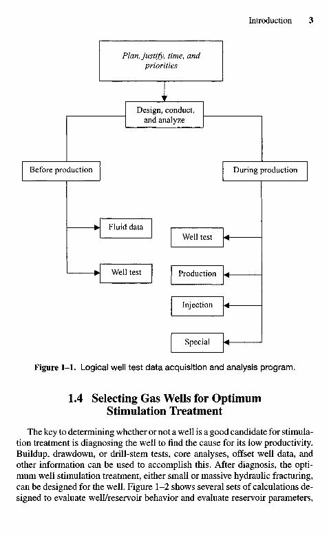
Figure 1-1. Logical well test data acquisition and analysis program.
1.4 Selecting Gas Wells for OptimumStimulation Treatment
The key to determining whether or not a well is a good candidate for stimula-tion treatment is diagnosing the well to find the cause for its low productivity.Buildup, drawdown, or drill-stem tests, core analyses, offset well data, andother information can be used to accomplish this. After diagnosis, the opti-mum well stimulation treatment, either small or massive hydraulic fracturing,can be designed for the well. Figure 1-2 shows several sets of calculations de-signed to evaluate well/reservoir behavior and evaluate reservoir parameters,
Well test
Production
Injection
Special
Fluid data
Well test
Before production During production
Design, conduct,and analyze
Plan, justify, time, andpriorities
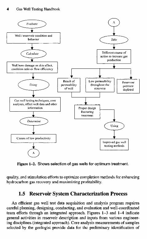
Figure 1-2. Shows selection of gas wells for optimum treatment.
quality, and stimulation efforts to optimize completion methods for enhancinghydrocarbon gas recovery and maximizing profitability.
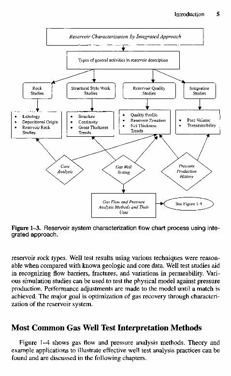
1.5 Reservoir System Characterization Process
An efficient gas well test data acquisition and analysis program requirescareful planning, designing, conducting, and evaluation and well-coordinatedteam efforts through an integrated approach. Figures 1-3 and 1-4 indicategeneral activities in reservoir description and inputs from various engineer-ing disciplines (integrated approach). Core analysis measurements of samplesselected by the geologist provide data for the preliminary identification of
Result ofpermeability
of well
Low permeabilitythroughout the
reservoir
Reservoirpressuredepleted
Improved gas welltesting methods
Using
Proper designfracturingtreatment
Different course ofaction to increase gas
production
Take
AEvaluate
Well / reservoir condition andbehavior
Calculate
Well bore damage or skin effect,condition ratio or flow efficiency
Using
Gas well testing techniques, coreanalyses, offset well data and other
information
Determine
Causes of low productivity
A
LithologyDepositional OriginReservoir RockStudies
StructureContinuityGross ThicknessTrends
Quality ProfileReservoir ZonationNet ThicknessTrends
Pore VolumeTransmissibility
Reservoir Characterization by Integrated Approach
Types of general activities in reservoir description
RockStudies
Structural Style WorkStudies
Reservoir QualityStudies
IntegrationStudies
CoreAnalysis
Gas WellTesting
PressureProduction
History
Gas Flow and PressureAnalysis Methods and Their
Uses
See Figure 1-4
Figure 1-3. Reservoir system characterization flow chart process using inte-grated approach.
reservoir rock types. Well test results using various techniques were reason-able when compared with known geologic and core data. Well test studies aidin recognizing flow barriers, fractures, and variations in permeability. Vari-ous simulation studies can be used to test the physical model against pressureproduction. Performance adjustments are made to the model until a match isachieved. The major goal is optimization of gas recovery through characteri-zation of the reservoir system.
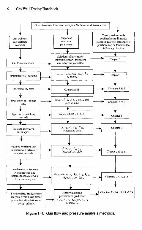
Most Common Gas Well Test Interpretation Methods
Figure 1-4 shows gas flow and pressure analysis methods. Theory andexample applications to illustrate effective well test analysis practices can befound and are discussed in the following chapters.
Gas Flow equations
Horizontal well systems
Deliverability tests
Drawdown & Builduptests
Type curve matchingmethods
Pressure derivativetechniques
Massive hydraulic andfractured well behavior
analysis methods
Interference, pulse testsHomogeneous and
heterogeneous reservoirbehavior analysis
Field studies, decline curveanalysis, overall skin factor,production stimulation and
design criteria.
Solutions of interest forvarious boundary conditions
and reservoir geometry.
l"eh> rev, rVw , Sm , S C A , SCAf , L D
kv and kh
C, n and AOF
kh, S11, s'2, s, D, pR , Apskin and
pore volume
Cs, CSD, k, <j)ct, s \ sf, x f
k , s , k f , C, CD; CDf,m
omega and delta
kfW, Sf, r\v , Xf,
(kfbf)D, rVXf.kfbf
kh/^ , ( j )hc ,k x ,k y ,k x y , km i n ,km
, 0, (J) iC1 v , (J)1, k h t ,
History matching
performance prediction
s , , Sp, s H , S V , s w b , sPf, s c , S0
, ss and Js / Jv
Chapter 2
Chapter 3
Chapters 4 & 7
Chapters 5 & 6
Chapter 8
Chapter 9
Chapters 10 & 11
Chapters 12,13, & 14
Gas well testinterpretation
methods
Importantreservoir
parameters
Chapters 15, 16, 17,18, & 19
Theory and exampleapplications to illustrate
effective gas well test analysispractices can be found in the
following chapters
Gas Flow and Pressure Analysis Methods and Their Uses
Figure 1-4. Gas flow and pressure analysis methods.
1.6 Scopes and Objective
This book is very important to professional petroleum engineers, teachers,graduate students, and those concerned with evaluating reservoir systems andthe pressure performance of gas wells. The data in this book should enablepetroleum professionals to design, conduct, and analyze pressure transienttests to obtain reliable information about reservoir and well conditions.
1.7 Organization
The book presents the following:
• Sound fundamental concepts/methodology related to gas well test dataacquisition and interpretation from a practical viewpoint
• Modern gas well testing methods and pressure transient test analysis tech-niques
• Examples illustrating effective well test analysis techniques• An excellent practical reference source related to pressure transient anal-
ysis techniques and their interpretations• Theory and practices of testing methods and their roles in reservoir engi-
neering management• Practical examples showing step-by-step solutions to problems• Various charts, formulae, and tables included for ready reference and
quick solutions for gas well testing and analyses
This chapter is an overview of gas well testing and analysis techniques. Italso includes a short discussion of unit conversion factors and the SI (metric)unit system. Appendix A provides a list of conversion factors.
Details and supporting materials are presented in the appendices for thebenefit of those who would like to learn more.
1.8 Unit Systems and Conversions
In any book of this nature, it is worthwhile to include a comprehensivelist of unit conversion factors, since data are often reported in units differentfrom those used in the equations. Such factors are presented in Appendix A.Because of the possibility of eventual conversion of engineering calculations toa metric standard, I also include information about the "SI" system of weightsand measures. Finally, I compare some important units and equations in fivedifferent unit systems. The calculation procedure is illustrated in followingexample.
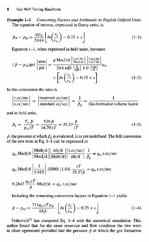
Example 1-1 Converting Factors and Arithmetic to English Oilfield UnitsThe equation of interest, expressed in Darcy units, is
*»-'"=sKs)-a7H (w>Equation 1-1, when expressed in field units, becomes
atm «Mscf/d 1 ^ H J g S(P-ZV)PS1 — - 2nkmD\±\hft\f\ »<
x [/»( — ) -0.75 + s 1 (1-2)
In this conversion the ratio is
r.cc/sec reservoir cc/sec 1 1s.cc/sec standard cc/sec f3g Gas formation volume factor
and in field units,
Tscp 520p pPg = Tp = ,A nri rj, = 3 5 . 3 7 — (1-3)
psczT 14.1OzT zTp, the pressure at which fig is evaluated, is as yet undefined. The full conversionof the rate term in Eq. 1-1 can be expressed as
Mstb/d stb/d s.cc/sec 1#5C Mscf/d — = fe r.cc/sec
Mscf/d Mstb/d stb/d ySg
feMscf/d - i - 110001 |1.84| - ^ - = f e r.cc/secJ .OIJ 35.37/7
9.2647 ^ - Mscf/d = c r.cc/secP
Including the remaining conversion factors in Equation 1-1 yields
Fetkovich11 has compared Eq. \-A with the numerical simulation. Thisauthor found that for the same reservoir and flow condition the two werein close agreement provided that the pressure p at which the gas formation
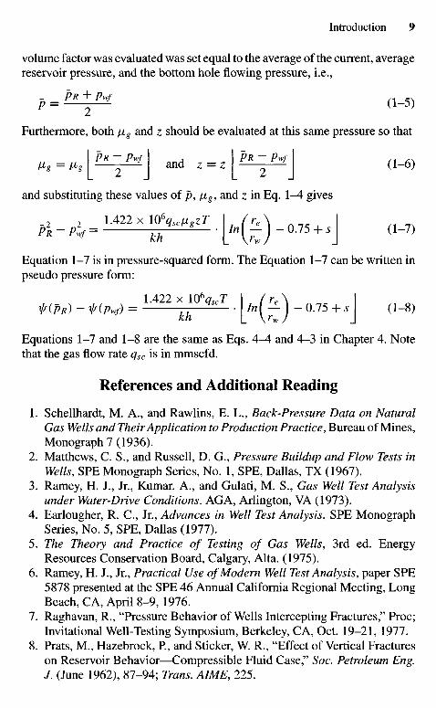
volume factor was evaluated was set equal to the average of the current, averagereservoir pressure, and the bottom hole flowing pressure, i.e.,
P = ± ^ d-5>Furthermore, both /xg and z should be evaluated at this same pressure so that
I PR - Pw/ I , I PR - Pw/ I „ , .Vg = Mg\ Y^ a n d z = z\ Y^ \ ( 1 " 6 )
and substituting these values of p, jng, and z in Eq. \-A gives
Equation 1-7 is in pressure-squared form. The Equation 1-7 can be written inpseudo pressure form:
nM _ , w _ ^ x l O V T - [* ( i ) - 0.75 + ,J ,.-«)
Equations 1-7 and 1-8 are the same as Eqs. 4-4 and 4-3 in Chapter 4. Notethat the gas flow rate qsc is in mmscfd.
References and Additional Reading
1. Schellhardt, M. A., and Rawlins, E. L., Back-Pressure Data on NaturalGas Wells and Their Application to Production Practice, Bureau of Mines,Monograph 7 (1936).
2. Matthews, C. S., and Russell, D. G., Pressure Buildup and Flow Tests inWells, SPE Monograph Series, No. 1, SPE, Dallas, TX (1967).
3. Ramey, H. J., Jr., Kumar, A., and Gulati, M. S., Gas Well Test Analysisunder Water-Drive Conditions. AGA, Arlington, VA (1973).
4. Earlougher, R. C , Jr., Advances in Well Test Analysis, SPE MonographSeries, No. 5, SPE, Dallas (1977).
5. The Theory and Practice of Testing of Gas Wells, 3rd ed. EnergyResources Conservation Board, Calgary, Alta. (1975).
6. Ramey, H. J., Jr., Practical Use of Modern Well Test Analysis, paper SPE5878 presented at the SPE 46 Annual California Regional Meeting, LongBeach, CA, April 8-9, 1976.
7. Raghavan, R., "Pressure Behavior of Wells Intercepting Fractures," Proc;Invitational Well-Testing Symposium, Berkeley, CA, Oct. 19-21, 1977.
8. Prats, M., Hazebrock, P., and Sticker, W. R., "Effect of Vertical Fractureson Reservoir Behavior—Compressible Fluid Case," Soc. Petroleum Eng.J. (June 1962), 87-94; Trans. AIME, 225.

9. Gringarten, A. C, Ramey, H. J., and Raghavan, R., "Applied PressureAnalysis for Fractured Wells,"/ Petroleum Technol. (July 1975), 887-892;Trans. AIME, 259.
10. Cullender, M. H., "The Isochronal Performance Method of Determiningthe Flow Characteristics of Gas Wells," /. Petroleum Technol (Sept. 1953),137.
11. Fetkovich, M. J., "Multipoint Testing of Gas Wells," paper presented atthe SPE-AIME Mid-Continent Section Continuing Education Course onWell Test Analysis (March 1975).
12. Russell, D. G., Goodrich, J., Perry G. E., and Bruskotter, J. R, 1966."Methods of Predicting Gas Well Performance," / Petroleum Technol.(January) 99, 108. Trans. AIME.
Chapter 2
Application of FluidFlow Equations toGas Systems
2.1 Introduction
The aim of this chapter is to develop and present the fundamental equationsfor flow of gases through porous media, along with solutions of interest forvarious boundary conditions and reservoir geometries. These solutions arerequired in the design and interpretation of flow and pressure tests.
To simplify the solutions and application of the solutions, dimensionlessterms are used. Assumptions and approximations necessary for defining thesystem and solving the differential equations are clearly stated. The princi-ple of superposition is applied to solve problems involving interference be-tween wells, variables flow rates, and wells located in noncircular reservoirs.The use of analytical and numerical solutions of the flow equations is alsodiscussed. Formation damage or stimulation, turbulence, and wellbore storageor unloading are given due consideration. This chapter applies in general tolaminar, single, and multiphase flow, but deviations due to inertial and tur-bulent effects are considered. For well testing purposes two-phase flow inthe reservoir is treated analytically by the use of an equivalent single-phasemobility.
The equations of continuity, Darcy's law, and the gas equation of stateare presented and combined to develop a differential equation for flow ofgases through porous media. This equation, in generalized coordinate nota-tion, can be expressed in rectangular, cylindrical, or spherical coordinates andis solved by suitable techniques. The next subsections describe steady-state,pseudo-steady-state, and unsteady-state flow equations including the gas radialdiffusivity equation, basic gas flow equations, solutions, and one-, two-, andthree-dimensional coordinate systems.
2.2 Steady-State Laminar Flow
Darcy's law for flow in a porous medium is
k dp kAdpv = or q=vA = (2-1)
H<g ax /ig ax
where
v = gas viscosity; q = volumetric flow rate; k = effective permeability;/jig = gas viscosity; and ^ = pressure gradient in the direction of flow
For radial flow, Eq. 2-1 becomes
, = ^ ^ * * (2-2)/Xg dx
where r is radial distance and h is reservoir thickness,Equation 2-2 is a differential equation and must be integrated for applica-
tion. Before integration the flow equation must be combined with an equationof state and the continuity equation. The continuity equation is
pxqx = p2 q2 = constant (2-3)
The equation of state for a real gas is
The flow rate of a gas is usually desired at some standard conditions ofpressure and temperature, psc and Tsc. Using these conditions in Eq. 2-3 andcombining Eqs. 2-3 and 2-4, we get
pq = Pscqsc,
or
pM _ pscM
zRT ZscRTsc
Solving for qsc and expressing qsc with Eq. 2-2 gives
pTsc lnrhkdp
psczT /a dr
The variables in this equation are p and r. Separating the variables andintegrating:
P rc
f A qscPscTfigZ f dr
J Tsc2rckh J rPw rw
P2 ~ PJ = qscPscT ill f re\
2 Tsclnkh \rw)
pscTfigz In(^)
In this derivative it was assumed that /Jig and z were independent of pressure.They may be evaluated at reservoir temperature and average pressure in thedrainage area such as
P-P
2
In gasfield units, Eq. 2-5 becomes
OmiOllkhlP2 - Pl)
_ 0 . 0 0 0 3 0 5 ^ ( P 2 - P w2 )
Where qsc = mscf/d; k — permeability in mD; h = formation thickness infeet; pe = reservoir pressure, psi, pw = well bore pressure, psia, T = reservoirtemperature, 0R; re = drainage radius, ft; rw = well bore radius, ft; z = averagecompressibility factor, dimensionless; and jlg = gas viscosity, cP.
This equation incorporates the following values for standard pressure andtemperature:
psc =z 14.7 psia,
Tsc = 600F = 5200R
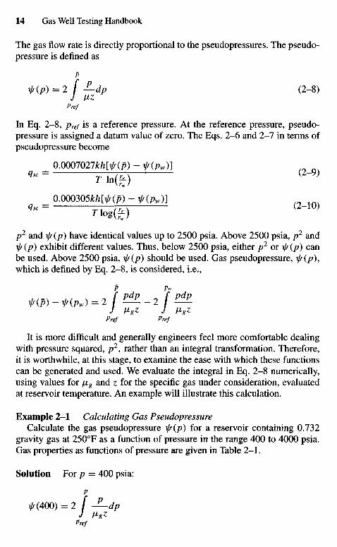
The gas flow rate is directly proportional to the pseudopressures. The pseudo-pressure is defined as
P
^{p) = 2 f JLdp (2-8)J ^z
Pref
In Eq. 2-8, pref is a reference pressure, At the reference pressure, pseudo-pressure is assigned a datum value of zero. The Eqs. 2-6 and 2-7 in terms ofpseudopressure become
_ 0.0007Q27fc/i[^(j>) -js(pw)]
«" " T In(^) ' ( 2 " 9 )
0.000305J/i[«-(/i) -<(•(/>„)]
«« fsgsj <2-"»p2 and is(p) have identical values up to 2500 psia. Above 2500 psia, p2 andif/ (p) exhibit different values. Thus, below 2500 psia, either p2 or ty(p) canbe used. Above 2500 psia, ty{p) should be used. Gas pseudopressure, ^(/?),which is defined by Eq. 2-8, is considered, i.e.,
J /lgz J flgZPref Pref
It is more difficult and generally engineers feel more comfortable dealingwith pressure squared, p2, rather than an integral transformation. Therefore,it is worthwhile, at this stage, to examine the ease with which these functionscan be generated and used. We evaluate the integral in Eq. 2-8 numerically,using values for \xg and z for the specific gas under consideration, evaluatedat reservoir temperature. An example will illustrate this calculation.
Example 2-1 Calculating Gas PseudopressureCalculate the gas pseudopressure %// (p) for a reservoir containing 0.732
gravity gas at 2500F as a function of pressure in the range 400 to 4000 psia.Gas properties as functions of pressure are given in Table 2-1 .
Solution For p = 400 psia:
p
^(400) = 2 f —dpJ VgZ
Pref
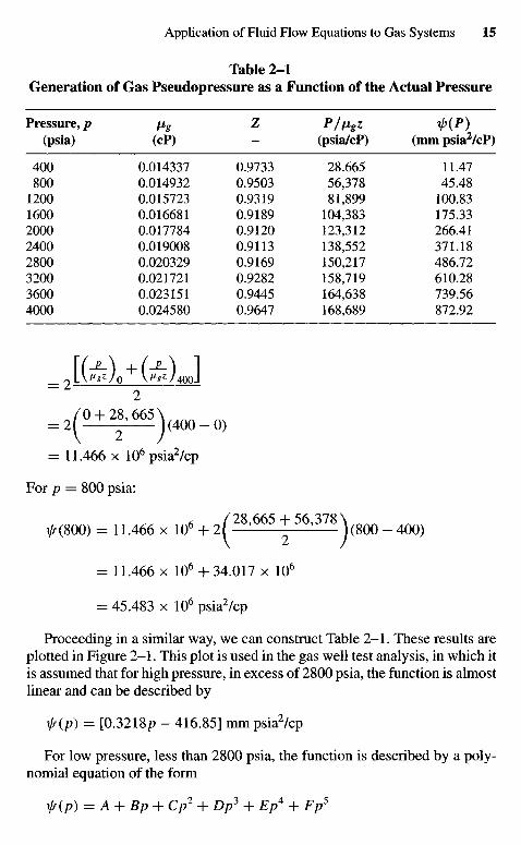
Table 2-1Generation of Gas Pseudopressure as a Function of the Actual Pressure
Pressure,/? /ig Z P/VgZ *1>(P)(psia) (cP) - (psia/cP) (mmpsia2/cP)
400 0.014337 0.9733 28.665 11.47800 0.014932 0.9503 56,378 45.48
1200 0.015723 0.9319 81,899 100.831600 0.016681 0.9189 104,383 175.332000 0.017784 0.9120 123,312 266.412400 0.019008 0.9113 138,552 371.182800 0.020329 0.9169 150,217 486.723200 0.021721 0.9282 158,719 610.283600 0.023151 0.9445 164,638 739.564000 0.024580 0.9647 168,689 872.92
_ 2 LV1Wo V*W4ooJ
= 2^±f^)<400-0>= 11.466 x 10⁶psia2/cp
For p = 800 psia:
VK800) = 11.466 x 10⁶ + 2 ^ 2 ^665 + 56,378^ (80() _ ^
= 11.466 x 10⁶ +34.017 x 106
= 45.483 x 10⁶ psia2/cp
Proceeding in a similar way, we can construct Table 2-1. These results areplotted in Figure 2—1. This plot is used in the gas well test analysis, in which itis assumed that for high pressure, in excess of 2800 psia, the function is almostlinear and can be described by
f(p) = [0.3218/? - 416.85] mmpsia2/cp
For low pressure, less than 2800 psia, the function is described by a poly-nomial equation of the form
^(p) = A +Bp+ Cp2 + Dp3 + Ep4 + Fp5
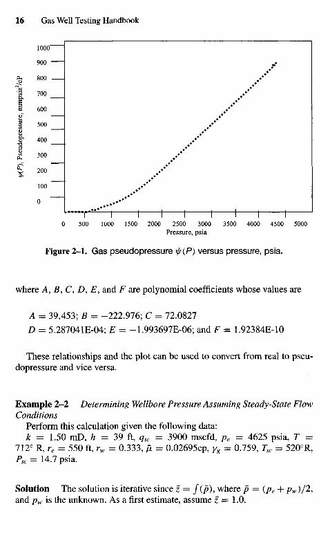
Pressure, psia
Figure 2-1 . Gas pseudopressure XJr(P) versus pressure, psia.
where A, B, C, D, E, and F are polynomial coefficients whose values are
A = 39,453; B = -222.976; C = 72.0827
D = 5.287041E-04; E = -1.993697E-06; and F = 1.92384E-10
These relationships and the plot can be used to convert from real to pseu-dopressure and vice versa.
Example 2-2 Determining Wellbore Pressure Assuming Steady-State FlowConditions
Perform this calculation given the following data:k = 1.50 mD, h = 39 ft, qsc = 3900 mscfd, pe = 4625 psia, T =
712° R, re = 550 ft, rw = 0.333, p, = 0.02695cp, yg = 0.759, Tsc = 5200R,Psc = 14.7 psia.
Solution The solution is iterative since z = f(p), where p = (pe + pw)/2,and pw is the unknown. As a first estimate, assume z = 1.0.
V(P)
, Ps
eudo
pres
sure
, mm
psia
2/cP
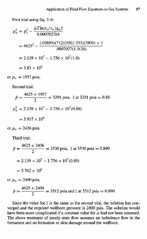
First trial using Eq. 2-6:
2 _ 2 _ fiTln(re/rw)qsczPw-Pe- 0.0007027fc/z
_ 2 (.02695)(712)(550/.333)(3900) x z"~4 .0007027(1.5(30)
= 2.139 x 10⁷ - 1.756 x 10⁷(1.0)
= 3.83 x 10⁶
or pw = 1957 psia.
Second trial:
p = 4 6 2 5 + 1 9 5 7 = 3291 psia, z at 3291 psia = 0.88
pi = 2.139 x 10⁷ - 1.756 x 10⁷(0.88)
= 5.937 x 10⁶
or pw = 2436 psia.
Third trial:
4625 + 2436p = = 3530 psia, z at 3530 psia = 0.890
= 2.139 x 10⁷ - 1.756 x 10⁷(0.89)
= 5.762 x 10⁶
or pw = 2400 psia.
4625 + 2400p = = 3512 psia and z at 3512 psia = 0.890
Since the value for z is the same as for second trial, the solution has con-verged and the required wellbore pressure is 2400 psia. The solution wouldhave been more complicated if a constant value for /x had not been assumed.The above treatment of steady-state flow assumes no turbulence flow in theformation and no formation or skin damage around the wellbore.
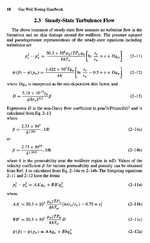
2.3 Steady-State Turbulence Flow
The above treatment of steady-state flow assumes no turbulent flow in theformation and no skin damage around the wellbore. The pressure squaredand pseudopressure representations of the steady-state equations includingturbulence are
2 2 50.3 x 10⁶figZTPscqsc f re 1Pe -Pl = TUT ln 7" + s + Dqsc ( 2"U )
Knlsc [_ 'w J
f(p) - f(pw) = L 4 2 2 *!°3TqSC U - - 0.5 + s + Dqsc] (2-12)
where Dg^ is interpreted as the rate-dependent skin factor, and
Expression D is the non-Darcy flow coefficient in psia2/cP/(mscf/d)2 and iscalculated from Eq. 2-13where
or
973 Y in1 0
where k is the permeability near the wellbore region in mD. Values of thevelocity coefficient /3 for various permeability and porosity can be obtainedfrom Ref. 1 or calculated from Eq. 2-14a or 2-14b. The foregoing equations2-11 and 2-12 have the forms
p2e -pi= AAfqsc + BB'q2
K (2-1 Ia)
where
AA' = 50.3 x 10³ M * z r P j c [In(^ZrH,) - 0.75 + s] (2-1 Ib)khTsc
BB' = 50.3 x 10³ ^zTPscD (2-1 Ic)
khTsc
HP) ~ f(Pw) = AAqsc + Bbql (2-12a)
where
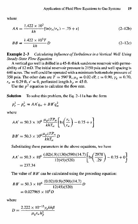
1 422 x 103
AA = —— [ln(re/rw) - .75 + s] (2-12b)kh
BB =>A22X 1037D (2-.2C)kh
Example 2—3 Calculating Influence of Turbulence in a Vertical Well UsingSteady-State Flow Equation
A vertical gas well is drilled in a 45-ft-thick sandstone reservoir with perme-ability of 12 mD. The initial reservoir pressure is 2150 psia and well spacing is640 acres. The well could be operated with a minimum bottomhole pressure of350 psia. The other data are T = 5900R, /xg = 0.02 cP, z = 0.90, yg = 0.70,rw = 0.29 ft, s' = 0, perforated length hp = 45 ft.
Use the p2 equation to calculate the flow rate.
Solution To solve this problem, the Eq. 2-1 Ia has the form
p] -pi= AAfqsc + BB'ql
where
BB' = 50.3 x I O 6 ^ ^ " D
Substituting these parameters in the above equations, we have
= 237.34
The value of BB' can be calculated using the preceding equation:
= 0.027965 x 10⁶D
where
_ 2.222 x \Q-X5ygkhpixgrwh2
p
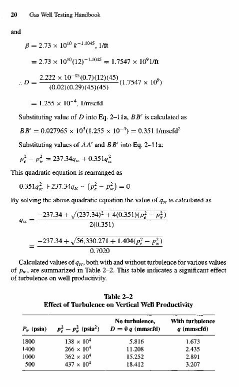
and
p = 2.73 x 10¹⁰ A;-11045, I/ft
= 2.73 x 10¹⁰(12)-11045 = 1.7547 x 10⁹l/ft
2.222 x 10-"(0.7)(12)(45) ^(0.02) (0.29) (45) (45) ^ '
= 1.255 x 10"4, 1/mscfd
Substituting value of D into Eq. 2-1 Ia, BB' is calculated as
BB' = 0.027965 x 10³(1.255 x 10~4) = 0.3511/mscfd2
Substituting values of AA' and BB' into Eq. 2-1 Ia:
p1 -pi= 237.34^c + 0.35\q]c
This quadratic equation is rearranged as
0.351?2 + 237.34?« - (p2e -P
2w)=0
By solving the above quadratic equation the value of qsc is calculated as
_ -237.34 + 7(237.34J2 + 4(0.351)(^g2 - p2
w)qsc " 2(0.351)
_ -237.34 + ^56,330.271 + 1.404(/72 - p2w)
~ 0.7020
Calculated values of qsc, both with and without turbulence for various valuesof pw, are summarized in Table 2-2. This table indicates a significant effectof turbulence on well productivity.
Table 2-2Effect of Turbulence on Vertical Well Productivity
No turbulence, With turbulencePw (psia) pi — p\ (psia2) D = Oq (mmscfd) q (mmscfd)
1800 138 x 104 5.816 1.6731400 266 xlO 4 11.208 2.4351000 362 x 104 15.252 2.891500 437 x 104 18.412 3.207
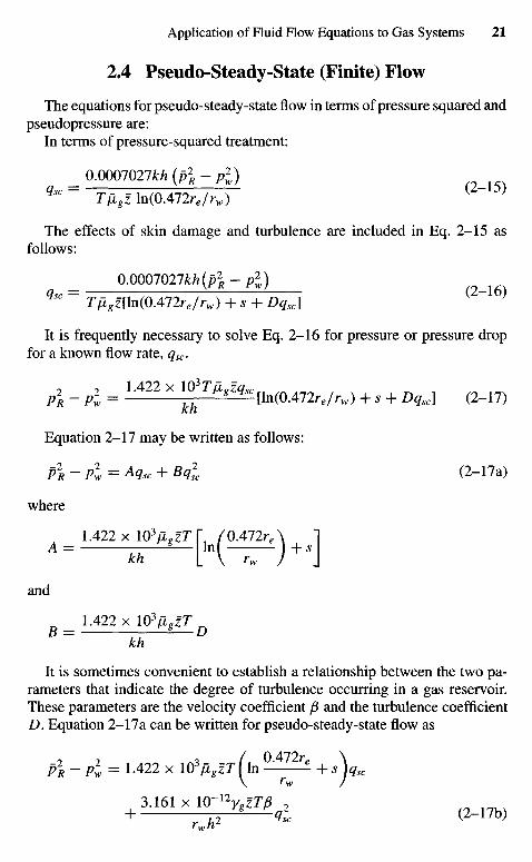
2.4 Pseudo-Steady-State (Finite) Flow
The equations for pseudo-steady-state flow in terms of pressure squared andpseudopressure are:
In terms of pressure-squared treatment:
= 0.0007027*/» (/% -pi)q&c Tp,gz In(OA12re/rw)
The effects of skin damage and turbulence are included in Eq. 2-15 asfollows:
= 0.0007027^(^-/4) (2_mQsc Tflgz[ln(0A72re/rw)+s + Dqsc]
It is frequently necessary to solve Eq. 2-16 for pressure or pressure dropfor a known flow rate, qsc.
P2R-Pl= 1A22Xl^Tllg'Zqsc[ln(0Anre/rw) + s + Dqsc] (2-17)
Equation 2-17 may be written as follows:
P2R-Pl= Msc + Bq2sc (2-17a)
where
A = 1.422 xlO^zT^O^y^
and
B=LU2^10%zlD
kh
It is sometimes convenient to establish a relationship between the two pa-rameters that indicate the degree of turbulence occurring in a gas reservoir.These parameters are the velocity coefficient P and the turbulence coefficientD. Equation 2-17a can be written for pseudo-steady-state flow as
/ Q 472r \p \ -pi = 1.422 x 1 O3PL8ZT f i n ' e +s)qsc
+ 3..«. x . O H ^ < 2 _ n b )
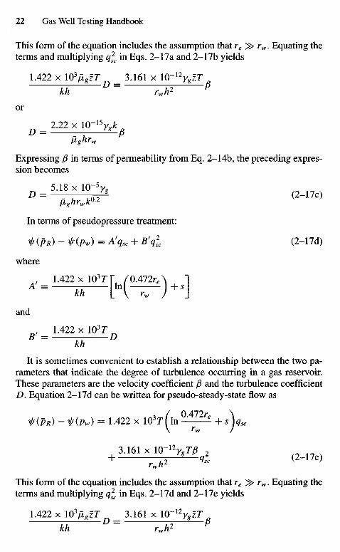
This form of the equation includes the assumption that re > rw. Equating theterms and multiplying qjc in Eqs. 2-17a and 2-17b yields
1.422 x 10³AgZr 3.161 x lO~nygzTVh D = Tjfi p
or
D = 2.22 x IQ-1V^flghrw
Expressing /? in terms of permeability from Eq. 2-14b, the preceding expres-sion becomes
flghrwk02
In terms of pseudopressure treatment:
is(PR) ~ ^(Pw) = A'qsc + B'ql (2-17d)
where
. 1.422 XlO3Tf (QAlIre\ 1
and
^ 1 . 4 2 2 x 1 0 3 7 ^kh
It is sometimes convenient to establish a relationship between the two pa-rameters that indicate the degree of turbulence occurring in a gas reservoir.These parameters are the velocity coefficient P and the turbulence coefficientD. Equation 2-17d can be written for pseudo-steady-state flow as
/ Q 472r \tiPR) ~ Ir(Pw) = 1-422 x 1 0 3 T i I n - — ^ +s\qsc
+ *.m*«r«r.T,d (2_17e)
This form of the equation includes the assumption that re^> rw. Equating theterms and multiplying qjc in Eqs. 2-17d and 2-17e yields
1.422 x W3jjLgzT _ 3.161 x W~nygzT
or
D = 2.22 x I Q - 1 V ^hrw
Expressing /3 in terms of permeability from Eq. 2-14b, the preceding ex-pression becomes
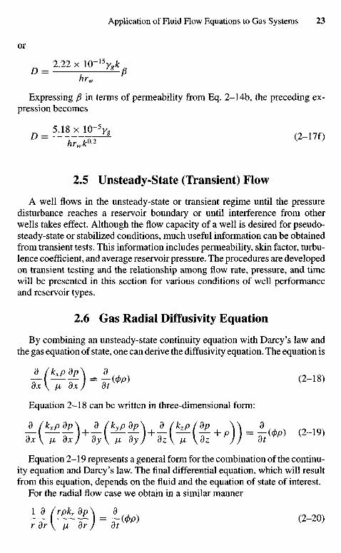
2.5 Unsteady-State (Transient) Flow
A well flows in the unsteady-state or transient regime until the pressuredisturbance reaches a reservoir boundary or until interference from otherwells takes effect. Although the flow capacity of a well is desired for pseudo-steady-state or stabilized conditions, much useful information can be obtainedfrom transient tests. This information includes permeability, skin factor, turbu-lence coefficient, and average reservoir pressure. The procedures are developedon transient testing and the relationship among flow rate, pressure, and timewill be presented in this section for various conditions of well performanceand reservoir types.
2.6 Gas Radial Diffusivity Equation
By combining an unsteady-state continuity equation with Darcy's law andthe gas equation of state, one can derive the diffusivity equation. The equation is
>(±>»J.).±lM (2-1 S ,dx \ ix ox J dt
Equation 2-18 can be written in three-dimensional form:a (kxPdp\ d (kyPdp\ 3 (kzP (dp \ \ a
Equation 2-19 represents a general form for the combination of the continu-ity equation and Darcy's law. The final differential equation, which will resultfrom this equation, depends on the fluid and the equation of state of interest.
For the radial flow case we obtain in a similar manner
ld/rpkrdp\ 3
r Sr \ fi or J dt
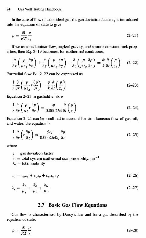
In the case of flow of a nonideal gas, the gas deviation factor zg is introducedinto the equation of state to give
'-iff <2-21)
RT Z8
If we assume laminar flow, neglect gravity, and assume constant rock prop-erties, then Eq. 2-19 becomes, for isothermal conditions,
' ( i .y+ ' (4)+»(±*) .wi) (2-22)dx\fjLzgdxJ dy\fizg oy J dz\/xzg dz/ k dt \zg J
For radial flow Eq. 2-22 can be expressed as
lL(jLr*E\ = ±L(E\ (2-23)rdr\nzg dr/ kdt\zg/
Equation 2-23 in gasfield units is
\L(jLr^E\ = * d (p\ (2-24)rdr\iizrdr) 0.000264 3f \ z /
Equation 2-24 can be modified to account for simultaneous flow of gas, oil,and water; the equation is
rdr\dz) 0.000264A, dt K
where
z = gas deviation factorct = total system isothermal compressibility, psi"1
Xt — total mobility
ct = CgSg + coso + cwswcf (2-26)
Xt = *L + k + bL (2_27)Hg ixo fiw
2.7 Basic Gas Flow Equations
Gas flow is characterized by Darcy's law and for a gas described by theequation of state:
M p
»=Rfl <2-28)
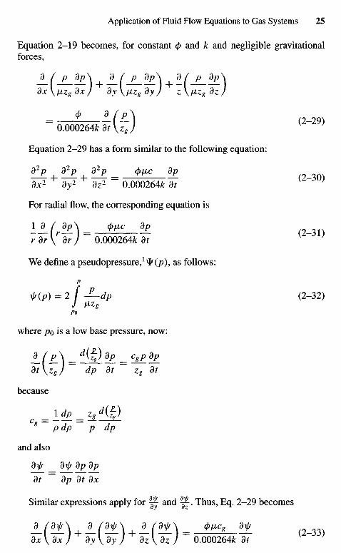
Equation 2-19 becomes, for constant <p and k and negligible gravitationalforces,
JL(JL*E) + L(JL*£\ + 1(JL*£\dx\(iZgdx) dy\nzgdy/ z\I^ZgdzJ
0.000264* 9*Vz«/
Equation 2-29 has a form similar to the following equation:
92p 92p d2p = 4>IMC dp
dx2 dy2 dz2 0.000264fc dt
For radial flow, the corresponding equation is
1 3 / 8p\ _ ^ c dp
rdr\ drj 0.000264fc dt
We define a pseudopressure,J*(/>), as follows:
p
x{r(p) = 2 f -?-dp (2-32)
Po
where po is a low base pressure, now:
d /P\^d(fg)dp ^cgPdp
dt\Zg) dp dt Zg St
because
8 p dp p dp
and also
dx/s _ dx/s dp dp
dt dp dt dx
Similar expressions apply for ^- and -. Thus, Eq. 2-29 becomes
dx \ dx ) dy\dy J dz \ dz ) 0.000264A: dt
For radial flow, the equivalent of Eq. 2-33 is
1 3 / 8 V A _ 0/xcg djr
rdr\ dr J 0.000264A; dt
2.8 One-Dimensional Coordinate Systems
Equation 2-29 may be expressed in terms of rectangular, cylindrical, orspherical coordinates:
V2P = ^ I (2-35)k at
where V2/? is the Laplacian of p. The expression "one-dimensional" refers toa specified coordinate system. For example, one-dimensional flow in the x-direction in rectangular coordinates may be expressed in cylindricalcoordinates.
Linear Flow
Flow lines are parallel, and the cross-sectional area of flow is constant andis represented by Eq. 2-36, which is in the rectangular coordinate system andis the one-dimensional form of Eq. 2-35:
d2p 4>ficdpT-y = —r- — (2-36)dx2 k dt
Fractures often exist naturally in the reservoir, and the flow toward thefracture is linear.
Radial Cylindrical Flow
In petroleum engineering the reservoir is often considered to be circular andof constant thickness h, with a well opened over the entire thickness. The flowtakes place in the radial direction only. The flow lines converge toward a centralpoint in each point, and the cross-sectional area of flow decreases as the centeris approached. Thus flow is directed toward a central line referred to as a line-sink (or line-source in the case of an injection well). In the petroleum literatureit is often simply called radial flow in the cylindrical coordinate system and isgiven by one-dimensional form of Eq. 2-35:
Radial Spherical Flow
If the well is not opened to the entire production formation because of athick reservoir (h is very large), then to measure vertical permeability, theone-dimensional form of Eq. 2-35, in the spherical coordinate system, is ofinterest. It is known as the radial-spherical flow equation and is given by
3 a/ dP\_^cdp
2.9 Radial Gas Flow Equations in DimensionlessVariables and Groups
Equation 2-35 and the relevant boundary conditions in dimensionless termsare:
V2(ApD) = -^-(ApD) (2-39)OtD
where the subscript D means dimensionless, and the dimensionless terms aredefined in the next section for various modes of flow.
Pressure Treatment
The pressure case will be considered along with the boundary and initialconditions. Assuming a well is producing at a constant rate qg from an infinitereservoir, the equation governing flow is
B9_/9p\*?c*Pr dr\ or) k dt
with the following boundary and initial conditions:
Inner Boundary Condition:
Assuming at the wellbore, the flow rate is constant and from Darcy's law,
S- =k-^ for,>0 (2-41)lnrh welI ii dr wdl
That is,
dr well 2 * k h
and in terms of standard conditions,
rdp =q^^Tldr well lnkh pTsc
Outer Boundary Condition:
At all times, the pressure at the outer boundary (radius = infinity) is thesame as the initial pressure, pt, that is,
p —>• pi as r —• o o
for all t.
Initial Condition
Initially, the pressure throughout the reservoir is constant, that is,
p = pi at t = O
for all t.At this stage, the variables which affect the solution of Eq. 2-40 are /?, /?/,
r, rw, qsc, Vg, k, h, 0, c, and t. Let
&P = Pi- Pr
rD = —(dimensionless)rw
APD~~~^~
Then Eq. 2-43 becomes
ro^(AP'D) = -q^Pf_lTsc (2-44)drD
u rD=1 pilnkhp
Let the dimensionless flow rate be
_ qsciiPscTl
Pi27tkhpTsc
Equation 2^44 becomes
9 ^ D L <ID \rD=x
Let the dimensionless pressure drop be
(Apf
D) pi -pApD = =
<7D Pi q D
Then Eq. 2-45 becomes
arD — (ApD) = - 1
3rD rD=\
Equation 2-37 becomes
1 A [ a ( A p D ) l = ^ a ( A p D ) (2^6)?D orD L orD J k dt
Let dimensionless time be
kttD ~ 1 T
Equation 2-37, the radial cylindrical flow equation, may now be expressedin dimensionless terms by
i a r a i a— TT" VD J - ( A?D) = ^ T " ( APD) ( 2 " 4 7 )
with the boundary and initial conditions as follows:
1. rD^(ApD) =-l forfD>0TD = I
2. ApD -> 0 as rD -+ oo for all rD
3. A/?z> = 0 attD =0 for all rz)
The solution of Eq. 2-47, which is the dimensionless form of Eq. 2-40, nowinvolves only ApD, to, and rD. The dimensionless terms in terms of pressuretreatment case are defined in gasfield units as follows:
0.0002637fcftD - . . - 2 (2-48)
Ap D = ?LUL^ (2-49)Pi 9 D
and
= 7.085 x 1 0 V № - ( 2 _ 5 0 )
pkhpi
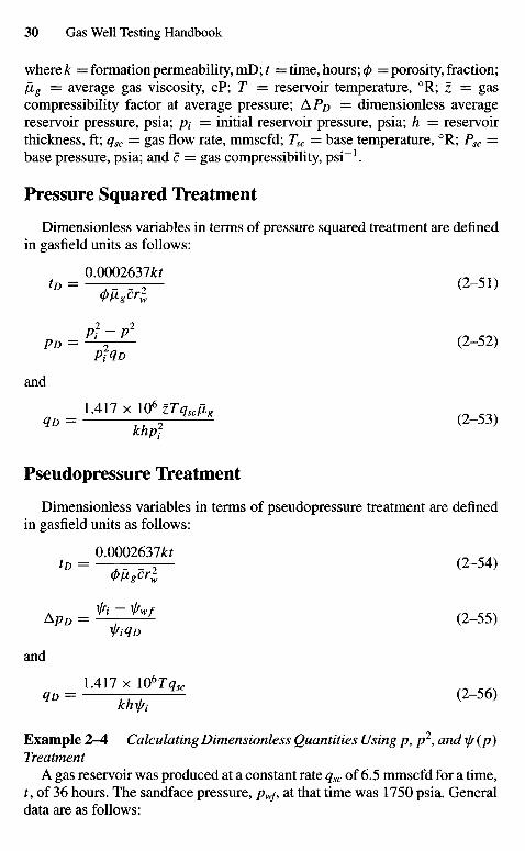
where/: = formation permeability, mD;f = time, hours; 0 = porosity, fraction;flg = average gas viscosity, cP; T = reservoir temperature, 0R; z = gascompressibility factor at average pressure; APD = dimensionless averagereservoir pressure, psia; pi = initial reservoir pressure, psia; h = reservoirthickness, ft; qsc = gas flow rate, mmscfd; Tsc = base temperature, 0R; Psc =base pressure, psia; and c = gas compressibility, psi"1.
Pressure Squared Treatment
Dimensionless variables in terms of pressure squared treatment are definedin gasfield units as follows:
0.0002637**to = . . . 2 (2-51)
PD = ^ V ^ - (2-52)PiQD
and
qD = 77-2 (2-53)khpf
Pseudopressure Treatment
Dimensionless variables in terms of pseudopressure treatment are definedin gasfield units as follows:
0.0002637^to = ^ . _ 2 (2-54)
ApD = — J~ (2-55)№ QD
and
1.417 x lO«Tqsc
<1D = — (2-56)khx//i
Example 2-4 Calculating Dimensionless Quantities Using p, p2, and x/r (p)Treatment
A gas reservoir was produced at a constant rate qsc of 6.5 mmscfd for a time,r, of 36 hours. The sandface pressure, pWf, at that time was 1750 psia. Generaldata are as follows:
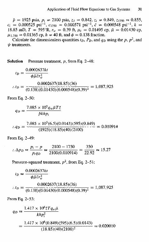
p = 1925 psia, pt = 2100 psia, Zi = 0.842, Zi = 0.849, Zi750 = 0.855,Ct = 0.000525 psi"1, Ci750 = 0.000571 psi"1, c = 0.000548 psi"1, k =18.85 mD, T = 595°R, rw = 0.39 ft, 1- = 0.01495 cp, ft = 0.01430 cp,/X1750 = 0.01365 cp, h = 40 ft, and </> = 0.138 fraction.
Calculate the dimensionless quantities to, PD, and qo using the p, p2, andT/T treatments.
Solution Pressure treatment, /?, from Eq. 2-48:
0.0002637£r
0.0002637(18.85)(36) = Q g ?
" D (0.138)(0.01430)(0.000548)(0.39)2 ' '
From Eq. 2-50:
7.085 x lO5qscflTz
pkhpi
= 7.085 x 10⁵(6.5)(0.0143)(595)(0.849) =Q0lQ9U
"q° (1925)(18.85)(40)(2100)
From Eq. 2-49:
. A = n-P = 2 1 0 ° - 1 7 5 0
= _^_ = 15 27PD piqD 2100(0.010914) 22.92
Pressure-squared treatment, p2, from Eq. 2-51:
0.0002637fcrto = ——3-^—
0.0002637(18.85)(36) = Q g 7
" D (0.138)(0.01430)(0.000548)(0.39)2
From Eq. 2-53:
1.417 x XO6ITqscjlqD — 7T~i
khpf
= 1.417 x 10⁶(0.849)(595)(6.5)(0.0143) =
(18.85)(40)(2100)2
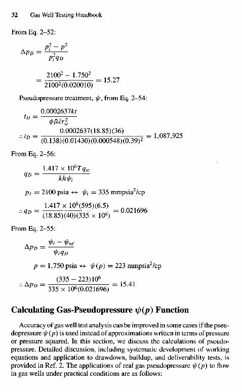
From Eq. 2-52:
^ = ^Pi ID
= 21002 - 1.7502 =
21002(0.020010)
Pseudopressure treatment, \fr, from Eq. 2-54:
0.0002637&ftD = —--rr-2—
0.0002637(18.85)(36) _
" D (0.138)(0.01430)(0.000548)(0.39)2 ' '
From Eq. 2-56:
1.417 x 1 0 6 T ^qD = khfi
Pi = 2100 psia 4> r1- = 335 mmpsia2/cp
From Eq. 2-55:
A ^i ~ irwf&PD = —;
p = 1,750 psia «-> yjf(p) = 223 mmpsia2/cp
(335-223)IQ6
' • A P D = 335 x 10^(0.021696) = 1 5 ' 4 1
Calculating Gas-Pseudopressure t/ (/;) Function
Accuracy of gas well test analysis can be improved in some cases if the pseu-dopressure \/f(p) is used instead of approximations written in terms of pressureor pressure squared. In this section, we discuss the calculations of pseudo-pressure. Detailed discussion, including systematic development of workingequations and application to drawdown, buildup, and deliverability tests, isprovided in Ref. 2. The applications of real gas pseudopressure i//(p) to flowin gas wells under practical conditions are as follows:
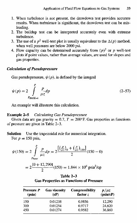
1. When turbulence is not present, the drawdown test provides accurateresults. When turbulence is significant, the drawdown test can be mis-leading.
2. The buildup test can be interpreted accurately even with extremeturbulence.
3. The use of a p2 well-test plot is usually equivalent to the A(p) method,when well pressures are below 2000 psi.
4. Flow capacity can be determined accurately from (p)2 or p well-testplots if point values, rather than average values, are used for slopes andgas properties.
Calculation of Pseudopressure
Gas pseudopressure, i/s(p), is defined by the integral
p
Ir(P) = 2 I ^-dp (2-57)J ^z
pBASE=o
An example will illustrate this calculation.
Example 2-5 Calculating Gas PseudopressureGiven data are gas gravity = 0.7, T = 2000F. Gas properties as functions
of pressure are given in Table 2-3.
Solution Use the trapezoidal rule for numerical integration.For p = 150psia,
*(150) = 2 / ^ ^ 2 [ ( ^ ) o + ^ ) l 5 o ] ( 1 5 O - O )J MZ 2
Phase
= 2 [ Q + 1 2 ? 2 9 0 ] ( 1 5 0 ) = 1.844 x 10⁶ psia2/cp
Table 2-3Gas Properties as Functions of Pressure
Pressure P Gas viscosity Compressibility p/v>z(psia) (cP) factor z (psia/cP)
150 0.01238 0.9856 12,290300 0.01254 0.9717 24,620450 0.01274 0.9582 36,860
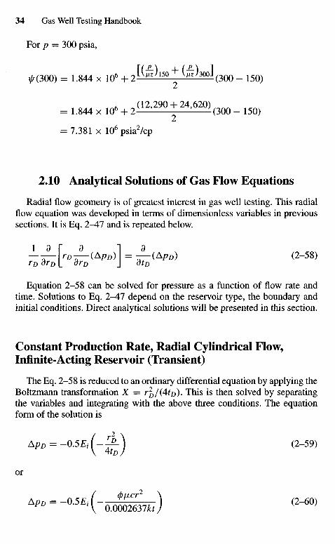
For p = 300 psia,
[YJl) +(*-) 1^(300) = 1.844 x 10⁶ + 2 *z 5 0 — ^ 30° (300 - 150)
-..844XlQO + 2 ' ' 2 ' 2 9 0 + 2 4 '6 2 0 '(300-.5Q
= 7.381 x 10⁶psia2/cp
2.10 Analytical Solutions of Gas Flow Equations
Radial flow geometry is of greatest interest in gas well testing. This radialflow equation was developed in terms of dimensionless variables in previoussections. It is Eq. 2-41 and is repeated below.
i a r a i a—-r- VD j - (A?D) = r (A?D) (2-58)
?D drD L drD J dtD
Equation 2-58 can be solved for pressure as a function of flow rate andtime. Solutions to Eq. 2-47 depend on the reservoir type, the boundary andinitial conditions. Direct analytical solutions will be presented in this section.
Constant Production Rate, Radial Cylindrical Flow,Infinite-Acting Reservoir (Transient)
The Eq. 2-58 is reduced to an ordinary differential equation by applying theBoltzmann transformation X = r^/^to). This is then solved by separatingthe variables and integrating with the above three conditions. The equationform of the solution is
ApD = -0.5Ei(-^-) (2-59)
or
a"° = - a 5 £ ' ( - a = s ) ^
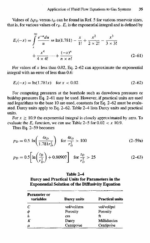
Values of Ap D versus to can be found in Ref. 5 for various reservoir sizes,that is, for various values of rD. Et is the exponential integral and is defined by
OO
/
e~udu x x x
'-^ = ln(1.781) - £ + JL^ _ *u 1! 2 x 2! 3 x 3!
JC
X4 (~x)n
4 x 4 ! n x n\For values of x less than 0.02, Eq. 2-62 can approximate the exponential
integral with an error of less than 0.6:
Ei(-x) = ln(1.78Lc) for* < 0.02 (2-62)
For computing pressures at the borehole such as drawdown pressures orbuildup pressures Eq. 2-61 may be used. However, if practical units are usedand logarithms to the base 10 are used, constants for Eq. 2-62 must be evalu-ated. Darcy units apply to Eq. 2-62. Table 2^- lists Darcy units and practicalunits.
For x > 10.9 the exponential integral is closely approximated by zero. Toevaluate the Ei function, we can use Table 2-5 for 0.02 < x 10.9.
Thus Eq. 2-59 becomes
pD = 0.5 l n f - ^ f y ) for ^ > 100 (2-59a)
pD = 0.5| In(-J 1 + 0.809071 for % > 25 (2-63)L \rD/ J rD
Table 2-4Darcy and Practical Units for Parameters in theExponential Solution of the Diffusivity Equation
Parameter orvariables Darcy units Practical units
C vol/vol/atm vol/vol/psi(f> Porosity Porosityh cm ftK Darcy Millidarcies/x Centipoise Centipoise
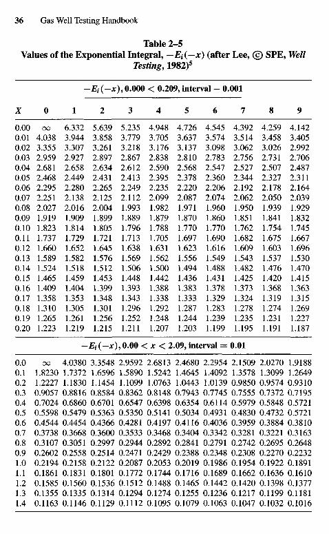
Table 2-5Values of the Exponential Integral, -Et(-x) (after Lee, © SPE, Well
Testing, 1982)5
-Ei(-x), 0.000 < 0.209, interval - 0.001
Z 0 1 2 3 4 5 6 7 8 9
0.00 oo 6.332 5.639 5.235 4.948 4.726 4.545 4.392 4.259 4.1420.01 4.038 3.944 3.858 3.779 3.705 3.637 3.574 3.514 3.458 3.4050.02 3.355 3.307 3.261 3.218 3.176 3.137 3.098 3.062 3.026 2.9920.03 2.959 2.927 2.897 2.867 2.838 2.810 2.783 2.756 2.731 2.7060.04 2.681 2.658 2.634 2.612 2.590 2.568 2.547 2.527 2.507 2.4870.05 2.468 2.449 2.431 2.413 2.395 2.378 2.360 2.344 2.327 2.3110.06 2.295 2.280 2.265 2.249 2.235 2.220 2.206 2.192 2.178 2.1640.07 2.251 2.138 2.125 2.112 2.099 2.087 2.074 2.062 2.050 2.0390.08 2.027 2.016 2.004 1.993 1.982 1.971 1.960 1.950 1.939 1.9290.09 1.919 1.909 1.899 1.889 1.879 1.870 1.860 1.851 1.841 1.8320.10 1.823 1.814 1.805 1.796 1.788 1.770 1.770 1.762 1.754 1.7450.11 1.737 1.729 1.721 1.713 1.705 1.697 1.690 1.682 1.675 1.6670.12 1.660 1.652 1.645 1.638 1.631 1.623 1.616 1.609 1.603 1.6960.13 1.589 1.582 1.576 1.569 1.562 1.556 1.549 1.543 1.537 1.5300.14 1.524 1.518 1.512 1.506 1.500 1.494 1.488 1.482 1.476 1.4700.15 1.465 1.459 1.453 1.448 1.442 1.436 1.431 1.425 1.420 1.4150.16 1.409 1.404 1.399 1.393 1.388 1.383 1.378 1.373 1.368 1.3630.17 1.358 1.353 1.348 1.343 1.338 1.333 1.329 1.324 1.319 1.3150.18 1.310 1.305 1.301 1.296 1.292 1.287 1.283 1.278 1.274 1.2690.19 1.265 1.261 1.256 1.252 1.248 1.244 1.239 1.235 1.231 1.2270.20 1.223 1.219 1.215 1.211 1.207 1.203 1.199 1.195 1.191 1.187
-Et(-x),0.00 < x < 2.09, interval = 0.01
0.0 oo 4.0380 3.3548 2.9592 2.6813 2.4680 2.2954 2.1509 2.0270 1.91880.1 1.8230 1.7372 1.6596 1.5890 1.5242 1.4645 1.4092 1.3578 1.3099 1.26490.2 1.2227 1.1830 1.1454 1.1099 1.0763 1.0443 1.0139 0.9850 0.9574 0.93100.3 0.9057 0.8816 0.8584 0.8362 0.8148 0.7943 0.7745 0.7555 0.7372 0.71950.4 0.7024 0.6860 0.6701 0.6547 0.6398 0.6354 0.6114 0.5979 0.5848 0.57210.5 0.5598 0.5479 0.5363 0.5350 0.5141 0.5034 0.4931 0.4830 0.4732 0.57210.6 0.4544 0.4454 0.4366 0.4281 0.4197 0.4116 0.4036 0.3959 0.3884 0.38100.7 0.3738 0.3668 0.3600 0.3533 0.3468 0.3404 0.3342 0.3281 0.3221 0.31630.8 0.3107 0.3051 0.2997 0.2944 0.2892 0.2841 0.2791 0.2742 0.2695 0.26480.9 0.2602 0.2558 0.2514 0.2471 0.2429 0.2388 0.2348 0.2308 0.2270 0.22321.0 0.2194 0.2158 0.2122 0.2087 0.2053 0.2019 0.1986 0.1954 0.1922 0.18911.1 0.1861 0.1831 0.1801 0.1772 0.1744 0.1716 0.1689 0.1662 0.1636 0.16101.2 0.1585 0.1560 0.1536 0.1512 0.1488 0.1465 0.1442 0.1420 0.1398 0.13771.3 0.1355 0.1335 0.1314 0.1294 0.1274 0.1255 0.1236 0.1217 0.1199 0.11811.4 0.1163 0.1146 0.1129 0.1112 0.1095 0.1079 0.1063 0.1047 0.1032 0.1016
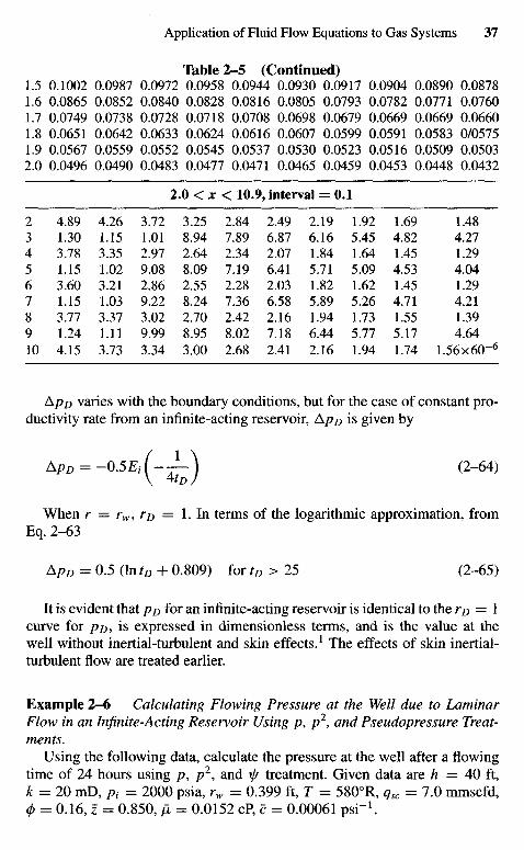
Table 2-5 (Continued)1.5 0.1002 0.0987 0.0972 0.0958 0.0944 0.0930 0.0917 0.0904 0.0890 0.08781.6 0.0865 0.0852 0.0840 0.0828 0.0816 0.0805 0.0793 0.0782 0.0771 0.07601.7 0.0749 0.0738 0.0728 0.0718 0.0708 0.0698 0.0679 0.0669 0.0669 0.06601.8 0.0651 0.0642 0.0633 0.0624 0.0616 0.0607 0.0599 0.0591 0.0583 0/05751.9 0.0567 0.0559 0.0552 0.0545 0.0537 0.0530 0.0523 0.0516 0.0509 0.05032.0 0.0496 0.0490 0.0483 0.0477 0.0471 0.0465 0.0459 0.0453 0.0448 0.0432
2.0 < x < 10.9, interval = 0.1
2 4.89 4.26 3.72 3.25 2.84 2.49 2.19 1.92 1.69 1.483 1.30 1.15 1.01 8.94 7.89 6.87 6.16 5.45 4.82 4.274 3.78 3.35 2.97 2.64 2.34 2.07 1.84 1.64 1.45 1.295 1.15 1.02 9.08 8.09 7.19 6.41 5.71 5.09 4.53 4.046 3.60 3.21 2.86 2.55 2.28 2.03 1.82 1.62 1.45 1.297 1.15 1.03 9.22 8.24 7.36 6.58 5.89 5.26 4.71 4.218 3.77 3.37 3.02 2.70 2.42 2.16 1.94 1.73 1.55 1.399 1.24 1.11 9.99 8.95 8.02 7.18 6.44 5.77 5.17 4.6410 4.15 3.73 3.34 3.00 2.68 2.41 2.16 1.94 1.74 1.56x60"6
ApD varies with the boundary conditions, but for the case of constant pro-ductivity rate from an infinite-acting reservoir, Ap& is given by
ApD = -0.5Ei(-^-\ (2-64)
When r = rw, rD = 1. In terms of the logarithmic approximation, fromEq. 2-63
ApD = 0.5 (In tD + 0.809) for tD > 25 (2-65)
It is evident that pD for an infinite-acting reservoir is identical to the rD = 1curve for po, is expressed in dimensionless terms, and is the value at thewell without inertial-turbulent and skin effects.1 The effects of skin inertial-turbulent flow are treated earlier.
Example 2-6 Calculating Flowing Pressure at the Well due to LaminarFlow in an Infinite-Acting Reservoir Using py p
2, and Pseudopressure Treat-ments.
Using the following data, calculate the pressure at the well after a flowingtime of 24 hours using p, p2, and ty treatment. Given data are h = 40 ft,k — 20 mD, pi = 2000 psia, rw = 0.399 ft, T = 5800R, qsc = 7.0 mmscfd,0 = 0.16, z = 0.850, (I = 0.0152 cP, c = 0.00061 psi"1.
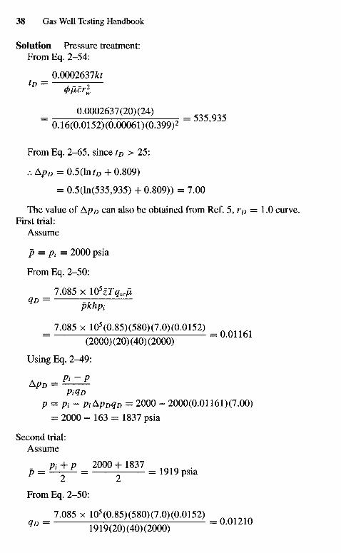
Solution Pressure treatment:From Eq. 2-54:
0.0002637**tD = , - - 9
= 0-0002637(20)(24) =
0.16(0.0152)(0.00061)(0.399)2
From Eq. 2-65, since tD > 25:
:.ApD = 0.5(lnfD+0.809)
= 0.5(ln(535,935) + 0.809)) = 7.00
The value of ApD can also be obtained from Ref. 5, rp = 1.0 curve.First trial:
Assume
p = Pi = 2000 psia
From Eq. 2-50:
7.085 x 10⁵zTqscflQD = —TT
pkhpt^ 7.085 x 10⁵(0.85)(580)(7.0)(0.0152) ^
(2000) (20) (40) (2000)
Using Eq. 2^9:
PiQD
P = Pi- Pi&PDQD == 2000 - 2000(0.01161)(7.00)= 2000- 163 = 1837 psia
Second trial:Assume
„ Pi+p 2000+1837 .P = — y - = 2 = pSia
From Eq. 2-50:
7.085 x 10⁵(0.85)(580)(7.0)(0.0152)H 1919(20)(40)(2000)
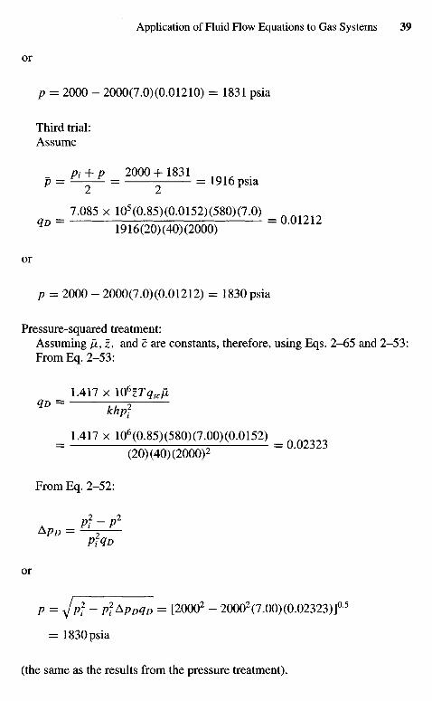
or
p = 2000 - 2000(7.0)(0.01210) = 1831 psia
Third trial:Assume
_ Pi+p 2000+1831 .p = —j- = = 1916 psia
= 7.085 x 10⁵(0.85)(0.0152)(580)(7.0)qD 1916(20)(40)(2000)
or
p = 2000 - 2000(7.0)(0.01212) = 1830 psia
Pressure-squared treatment:Assuming /2, z, and c are constants, therefore, using Eqs. 2-65 and 2-53:From Eq. 2-53:
1.417 x 10⁶zTqscflq° = TTi
khpf
= 1.417 x 10⁶(0.85)(580)(7.00)(0.0152)(20) (40) (2000)2
From Eq. 2-52:
AP. = ^
PiQDor
p = yjpf - pfApDqD = [20002 - 20002(7.00)(0.02323)]a5
= 1830 psia
(the same as the results from the pressure treatment).
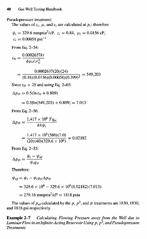
Pseudopressure treatment:The values of z,, /z, and c,- are calculated at pt; therefore
ft = 329.6 mmpsia2/cP, zi = 0.84, /x, = 0.0156 cP,
Ci = 0.00058 psi"1
From Eq. 2-54:
_ 0.0002637^
(frliiCtrl
= 0.0002637(20)(24) =
(0.16)(0.0156)(0.00058)(0.399)2
Since to > 25 and using Eq. 2-65:
Ap D = 0.5 (In f z) +0.809)
= 0.5[ln(549,203) + 0.809] = 7.013
From Eq. 2-56:
1.417 x 10⁶ Tqsc
APD = khtt
= 1.417 x ltf(S8O)C7.O) =
(20) (40) (329.6 x 10⁶)
From Eq. 2-55:
ApD = —: L
^tq D
Therefore:
^wf= ^i - 1^i q D Ap D
= 329.6 x 10⁶ - 329.6 x 10⁶(0.02182)(7.013)
= 279.16 mmpsia2/cP =1818 psia
The values of pwf calculated by the /?, p2, and ^ treatments are 1830,1830,and 1818 psi respectively.
Example 2-7 Calculating Flowing Pressure away from the Well due toLaminar Flow in an Infinite-Acting Reservoir Using p, p2, and PseudopressureTreatments
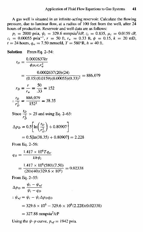
A gas well is situated in an infinite-acting reservoir. Calculate the flowingpressure, due to laminar flow, at a radius of 100 feet from the well, after 24hours of production. Reservoir and well data are as follows:
Pt = 2000 psia, V, = 329.6 mmpsia2/cP, n = 0.835, fit = 0.0159 cP,C1 = 0.00055 psia"1, r = 50 ft, rw = 0.33 ft, 0 = 0.15, k = 20 mD,t = 24 hours, qsc = 7.50 mmscfd, T = 5800R, h = 40 ft.
Solution From Eq. 2-54:
0.0002637JUtD — 1 9
= 0-0002637(20X24)
(0.15)(0.0159)(O.0O055)(0.33)2
rw .33
tD _ 886,079 _
- - " w -38-35
Since -z- > 25 and using Eq. 2-63:
ApD = 0.5[ln( % J + 0.809071
= 0.5[ln(38.35) + 0.80907] = 2.228
From Eq. 2-56:
1.417 x \06TqscqD = TTTi
= 1.417 x ltf(S80)(7.50) =
(20)(40) (329.6 x 10⁶)
From Eq. 2-55:
^PD = ~
.'-fwf= ft -fi&pDqD
= 329.6 x 10⁶ - 329.6 x 10⁶(2.228) (0.02338)
= 327.88 mmpsia2/cP
Using the \(r-p curve, pwf = 19Al psia.
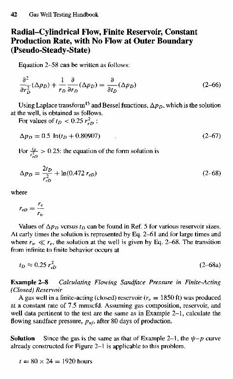
Radial-Cylindrical Flow, Finite Reservoir, ConstantProduction Rate, with No Flow at Outer Boundary(Pseudo-Steady-State)
Equation 2-58 can be written as follows:
d2 Id d—=- (Ap D) + — — (Ap D) = — (Ap D) (2-66)drp rD drD dtD
Using Laplace transform15 and Bessel functions, ApD, which is the solutionat the well, is obtained as follows.
For values of tD < 0.25 r2eD :
ApD = 0.5 Info + 0.80907) (2-67)
For -^- > 0.25: the equation of the form solution is
ApD = -f+ ln(0.472 reD) (2-68)
where
rereD —rw
Values of ApD versus tD can be found in Ref. 5 for various reservoir sizes.At early times the solution is represented by Eq. 2-61 and for large times andwhere rw « r e , the solution at the well is given by Eq. 2-68. The transitionfrom infinite to finite behavior occurs at
tD ^ 0 .25 r2eD (2-68a)
Example 2-8 Calculating Flowing Sandface Pressure in Finite-Acting(Closed) Reservoir
A gas well in a finite-acting (closed) reservoir (re = 1850 ft) was producedat a constant rate of 7.5 mmscfd. Assuming gas composition, reservoir, andwell data pertinent to the test are the same as in Example 2-1 , calculate theflowing sandface pressure, /?w/, after 80 days of production.
Solution Since the gas is the same as that of Example 2-1 , the \js-p curvealready constructed for Figure 2-1 is applicable to this problem.
t = 80 x 24 = 1920 hours
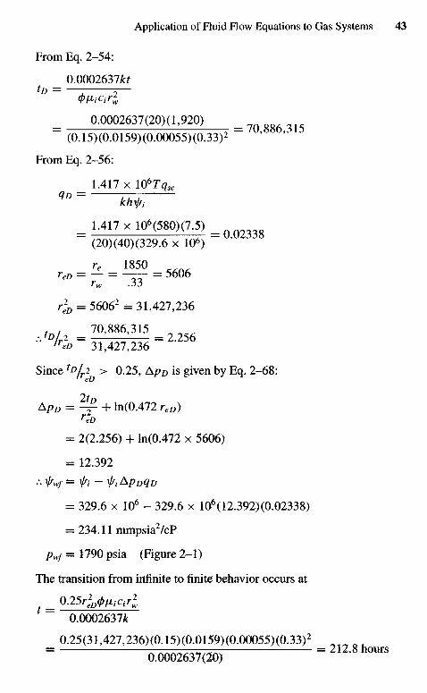
From Eq. 2-54:
0.0002637fo
= 0-0002637(20)(l,920) =
(0.15)(0.0159)(0.00055)(0.33)2
From Eq. 2-56:
1.417 x W6Tqsc
kh\j/i
= 1.417 x 10*(580)(7.5)(20)(40)(329.6 x 10⁶)
re 1850reD = — = —— = 5606
rw .33
r2eD = 56062 = 31,427,236
70,886,315lreD 31,427,236
Since 1^Li > 0.25, A/?/) is given by Eq. 2-68:" eD
ApD = ^- + ln(0.472 reD)
= 2(2.256) + ln(0.472 x 5606)
= 12.392
:.fwf= ft -fiApDqD
= 329.6 x 10⁶ - 329.6 x 10⁶(12.392)(0.02338)
= 234.11 mmpsia2/cP
pwf= 1790 psia (Figure 2-1)
The transition from infinite to finite behavior occurs at
025^/w2,0.0002637)k
0.25(31,427,236)(0.l5)(0.0159)(0.00055)(0.33)2
= 0.0002637(20) ~ = 2U* h°WS
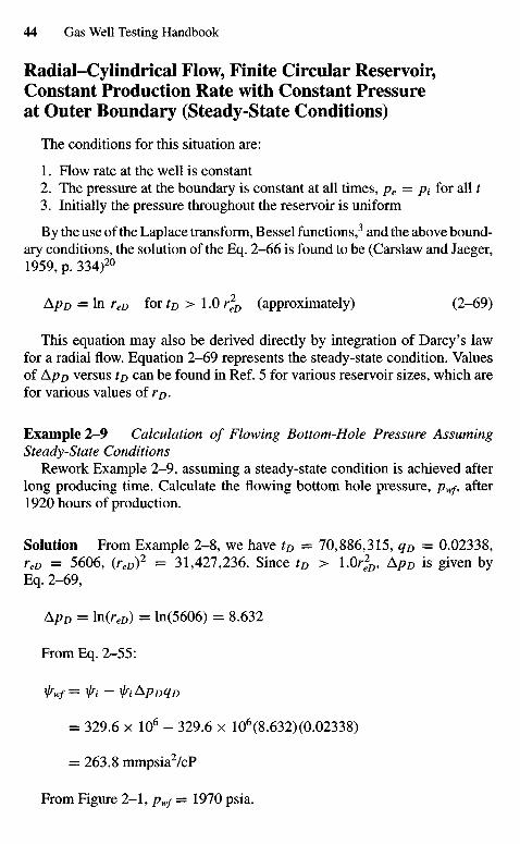
Radial-Cylindrical Flow, Finite Circular Reservoir,Constant Production Rate with Constant Pressureat Outer Boundary (Steady-State Conditions)
The conditions for this situation are:
1. Flow rate at the well is constant2. The pressure at the boundary is constant at all times, pe = pv for all t3. Initially the pressure throughout the reservoir is uniform
By the use of the Laplace transform, Bessel functions,3 and the above bound-ary conditions, the solution of the Eq. 2-66 is found to be (Carslaw and Jaeger,1959, p. 334)20
ApD = In reD fovtD > 1.0 r*D (approximately) (2-69)
This equation may also be derived directly by integration of Darcy's lawfor a radial flow. Equation 2-69 represents the steady-state condition. Valuesof ApD versus to can be found in Ref. 5 for various reservoir sizes, which arefor various values of rr>.
Example 2-9 Calculation of Flowing Bottom-Hole Pressure AssumingSteady-State Conditions
Rework Example 2-9, assuming a steady-state condition is achieved afterlong producing time. Calculate the flowing bottom hole pressure, pwf, after1920 hours of production.
Solution From Example 2-8, we have tD = 70,886,315, qD = 0.02338,reD = 5606, (reD)2 = 31,427,236. Since tD > l.Or^,, ApD is given byEq. 2-69,
ApD = ln(reD) = ln(5606) = 8.632
From Eq. 2-55:
V v = ^i -fi^PDqD
= 329.6 x 10⁶ - 329.6 x 10⁶(8.632)(0.02338)
= 263.8 mmpsia2/cP
From Figure 2-1 , pwf = 1970 psia.
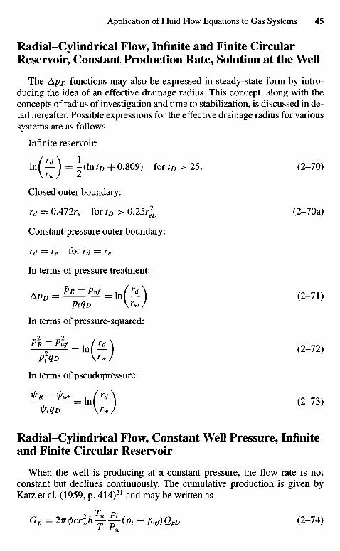
Radial-Cylindrical Flow, Infinite and Finite CircularReservoir, Constant Production Rate, Solution at the Well
The Apr> functions may also be expressed in steady-state form by intro-ducing the idea of an effective drainage radius. This concept, along with theconcepts of radius of investigation and time to stabilization, is discussed in de-tail hereafter. Possible expressions for the effective drainage radius for varioussystems are as follows.
Infinite reservoir:
ln( — ) = -OntD + 0.809) fortD > 25. (2-70)\rw J 2
Closed outer boundary:
rd = 0A72re for tD > 0.25r2eD (2-7Oa)
Constant-pressure outer boundary:
rd = re for rd = re
In terms of pressure treatment:
ApD = ^ ^ = I n ( ^ ) (2-71)Pi q D \rw/
In terms of pressure-squared:
f\Pli = JrA (2-72)pf q D VwJ
In terms of pseudopressure:
±J^l = drA\ (2_73)VtqD VwJ
Radial-Cylindrical Flow, Constant Well Pressure, Infiniteand Finite Circular Reservoir
When the well is producing at a constant pressure, the flow rate is notconstant but declines continuously. The cumulative production is given byKatz et al. (1959, p. 414)21 and may be written as
Gp = 2ncl>crlh^^-(pi - pwf)QpD (2-74)
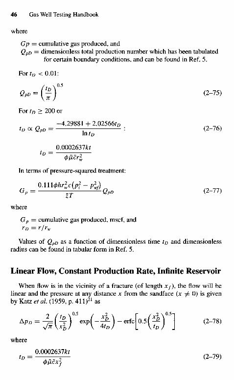
where
Gp = cumulative gas produced, andQpD — dimensionless total production number which has been tabulated
for certain boundary conditions, and can be found in Ref. 5.
For tD < 0.01:
QPD = i f ) (2-75)
For tD > 200 or
-4.29881 + 2.02566rDto oc QpD = ^ : (2-76)mtD
0.0002631kt
In terms of pressure-squared treatment:
O.m<phrlc(pf - plf)P = T ^ QpD (2-77)
where
Gp- cumulative gas produced, mscf, andrD = r/rw
Values of QpD as a function of dimensionless time to and dimensionlessradius can be found in tabular form in Ref. 5.
Linear Flow, Constant Production Rate, Infinite Reservoir
When flow is in the vicinity of a fracture (of length x/), the flow will belinear and the pressure at any distance x from the sandface {x / 0) is givenby Katz et al. (1959, p. 411)21 as
*•- M%T'->(-£)-4K^)I <2-78)where
0.0002637foto = .__ 2 (2-79)
<t>ixcxj
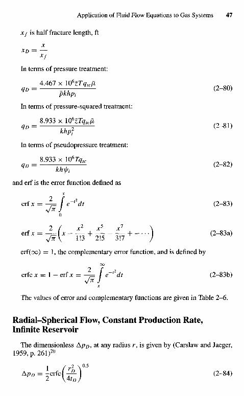
Xf is half fracture length, ft
xxD = —
xf
In terms of pressure treatment:
4.467 x UPzTqxJhqo = — (2-80)
pkhpi
In terms of pressure-squared treatment:
8.933 x l06zTqscfl
<lD = TT—2 (2-81)khpf
In terms of pseudopressure treatment:8.933 x 10⁶Tqsc
qu = — (2-82)khfi
and erf is the error function defined asX
erf X = -^- [ e~t2dt (2-83)V* J
o
erf(oo) = 1, the complementary error function, and is defined by
OO
erfc x = 1 - erf x = -^= f e~{''dt (2-83b)x
The values of error and complementary functions are given in Table 2-6.Radial-Spherical Flow, Constant Production Rate,Infinite Reservoir
The dimensionless ApD, at any radius r, is given by (Carslaw and Jaeger,1959, p. 261)20
1 / r 2 \ a 5
ApD = -erfc(-^\ (2-84)2 \4fD/
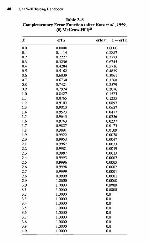
Table 2-6Complementary Error Function (after Katz et al., 1959,
© McGraw-Hill)21
X erf x erfc x = 1 — erf x
0.0 0.0000 1.00000.1 0.1114 0.88870.2 0.2227 0.77730.3 0.3256 0.67450.4 0.4284 0.57160.5 0.5162 0.48390.6 0.6039 0.39610.7 0.6730 0.32680.8 0.7421 0.25790.9 0.7924 0.20761.0 0.8427 0.15731.1 0.8765 0.12351.2 0.9103 0.08971.3 0.9313 0.06871.4 0.9523 0.04771.5 0.9643 0.03561.6 0.9763 0.02371.7 0.9827 0.01731.8 0.9891 0.01091.9 0.9922 0.00782.0 0.9953 0.00472.1 0.9967 0.00332.2 0.9981 0.00192.3 0.9987 0.00132.4 0.9993 0.00072.5 0.9996 0.00052.6 0.9998 0.00022.7 0.9999 0.00012.8 0.9999 0.00012.9 1.0000 0.00003.0 1.0000 0.00003.1 1.0000 0.00003.2 1.0000 0.03.3 1.0000 0.03.4 1.0000 0.03.5 1.0000 0.03.6 1.0000 0.03.7 1.0000 0.03.8 1.0000 0.03.9 1.0000 0.04.0 1.0000 0.0
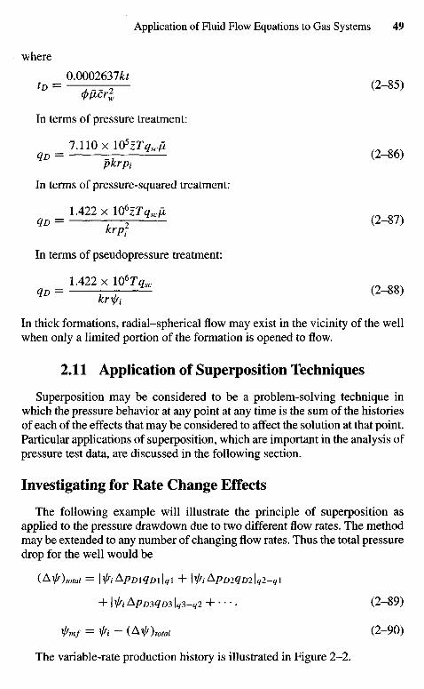
where
0.0002637fr
In terms of pressure treatment:
7.110 XlOPzTqxHqD = — (2-86)
pkrpt
In terms of pressure-squared treatment:
1.422xl06zr^c/2#£> = ;—5 (2-87)
In terms of pseudopressure treatment:
1.422 x IVTq30qD = j — (2-85)
In thick formations, radial-spherical flow may exist in the vicinity of the wellwhen only a limited portion of the formation is opened to flow.
2.11 Application of Superposition Techniques
Superposition may be considered to be a problem-solving technique inwhich the pressure behavior at any point at any time is the sum of the historiesof each of the effects that may be considered to affect the solution at that point.Particular applications of superposition, which are important in the analysis ofpressure test data, are discussed in the following section.
Investigating for Rate Change Effects
The following example will illustrate the principle of superposition asapplied to the pressure drawdown due to two different flow rates. The methodmay be extended to any number of changing flow rates. Thus the total pressuredrop for the well would be
(Axj/)totai = \^iApDiqm\qi + \i/iApD2qD2\q2-qi
+ I x/fi ApD3qD3 \q3.q2 + • • •. (2-89)
fmf = r1. - (Aif)total (2-90)
The variable-rate production history is illustrated in Figure 2-2.
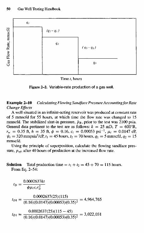
Time t, hours
Figure 2-2. Variable-rate production of a gas well.
Example 2—10 Calculating Flowing Sandface Pressure Accounting for RateChange Effects
A well situated in an infinite-acting reservoir was produced at constant rateof 5 mmscfd for 55 hours, at which time the flow rate was changed to 15mmscfd. The stabilized shut-in pressure, pR, prior to the test was 2100 psia.General data pertinent to the test are as follows: k = 25 mD, T = 6000R,rw = 0.35 ft, h = 35 ft, 0 = 0.16, a = 0.00053 psi"1, /x, = 0.0147 cP,i/ri = 320 mmpsia2/cP, t\ = 45 hours, ^ = 70 hours, q\ = 5 mmscfd, ^2 = 15mmscfd.
Using the principle of superposition, calculate the flowing sandface pres-sure, pwf, after 40 hours of production at the increased flow rate.
Solution Total production time = t\ + ti — 45 + 70 = 115 hours.From Eq. 2-54:
0.0002637JUto = — Y~
_ 0.0002637(25) (115) _tm ~ (0.16)(0.0147)(0.00053)(0.35)2 = ' ' ?
tm = (0.16)(0.0147)(0.00053)(0.35)2 = 3 ' 0 2 2 ' 0 3 1
Gas
Flo
w R
ate,
mm
scfd
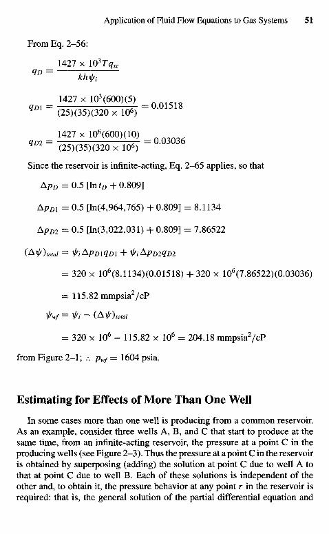
From Eq. 2-56:
1427 x 103r^cqD = —kWt—
qm = (25X35X320 *: 106) = 0 0 1 5 1 8
1427 x 106(600)(10)qm = (25)(35)(320 x 10«) = a O 3 0 3 6
Since the reservoir is infinite-acting, Eq. 2-65 applies, so that
Ap D - 0.5 [lnfD + 0.809]
APDI = 0.5 [ln(4,964,765) + 0.809] = 8.1134
ApD2 = 0.5 [In(3,022,031) + 0.809] = 7.86522
(A\/r) totai = iriApDiqDi + tiApmqm
= 320 x 106(8.1134)(0.01518) + 320 x 106(7.86522)(0.03036)
= 115.82 mmpsia2/cP
ftwf= ^i - (Al//)total
= 320 x 106 - 115.82 x 106 = 204.18 mmpsia2/cP
from Figure 2-1; .-. pwf— 1604 psia.
Estimating for Effects of More Than One Well
In some cases more than one well is producing from a common reservoir.As an example, consider three wells A, B, and C that start to produce at thesame time, from an infinite-acting reservoir, the pressure at a point C in theproducing wells (see Figure 2-3). Thus the pressure at a point C in the reservoiris obtained by superposing (adding) the solution at point C due to well A tothat at point C due to well B. Each of these solutions is independent of theother and, to obtain it, the pressure behavior at any point r in the reservoir isrequired: that is, the general solution of the partial differential equation and
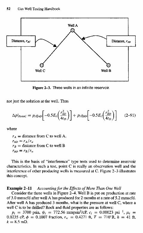
Figure 2-3. Three wells in an infinite reservoir,
not just the solution at the well. Thus
Ap\PointC = A<7AJ-0.5£, ( J f )1 + PiqBD\-0.5Ei ( ^ ) ] (2-91)
where
rA — distance from C to well A.rAD = rA/rw
rB = distance from C to well BrBD = rB/rw
This is the basis of "interference" type tests used to determine reservoircharacteristics. In such a test, point C is really an observation well and theinterference of other producing wells is measured at C. Figure 2-3 illustratesthis concept.
Example 2-11 Accounting for the Effects of More Than One WellConsider the three wells in Figure 2-4. Well B is put on production at rate
of 3.0 mmscfd after well A has produced for 2 months at a rate of 5.2 mmscfd.After well A has produced 3 months, what is the pressure at well C, where awell C is to be drilled? Rock and fluid properties are as follows:
Pi = 3700 psia, 1- = 772.56 mmpsia2/cP, a = 0.00023 psi"1, fit =0.0235 cP, 0 = 0.1007 fraction, rw = 0.4271 ft, T = 7100R, A = 41 ft,k = 8.5 mD.
WeIlC Weil B
Distance, rAB
WeIlA
Distance, rAC
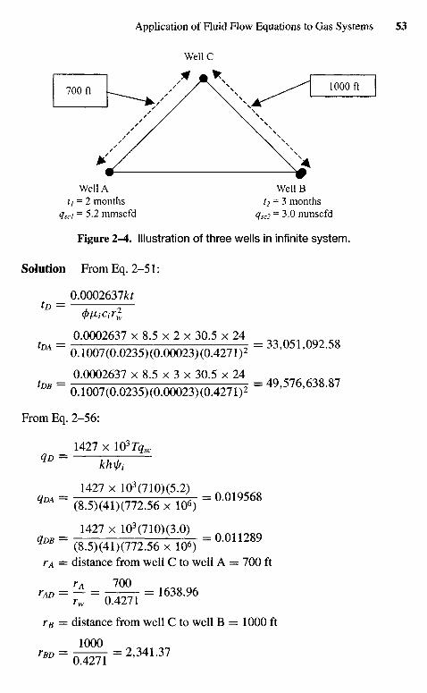
Well A Well BIi = 2 months '2 = 3 months
qsc, = 5.2 mmscfd qsc2 = 3.0 mmscfd
Figure 2-4. Illustration of three wells in infinite system.
Solution From Eq. 2-51:
0.0002637/:?tD = — 5—
- ° - 0 0 0 2 6 3 7 x 8.5 x 2 x 30.5 x 24tDA ~ 0.1007(0.0235) (0.00023) (0.4271 )2 ' ' "
- ° - 0 0 0 2 6 3 7 x 8.5 x 3 x 30.5 x 24tm ~ 0.1007(0.0235)(0.00023)(0.4271)2 ' ' "
From Eq. 2-56:
1427 x 1037tfscqD= kWt
1427 x 103(710)(5.2)qm = (8.5)(41)(772.56 x 10') = ° -° 1 9 5 6 8
1427 x 103(710)(3.0)qm = (8.5)(41)(772.56 x 10«) = °-° 1 1 2 8 9
rA = distance from well C to well A = 700 ft
rA 700' " = ; ; = a427T = 1638-96
rB = distance from well C to well B = 1000 ft
r"> = o ^ r = 2-341-37
WeIlC
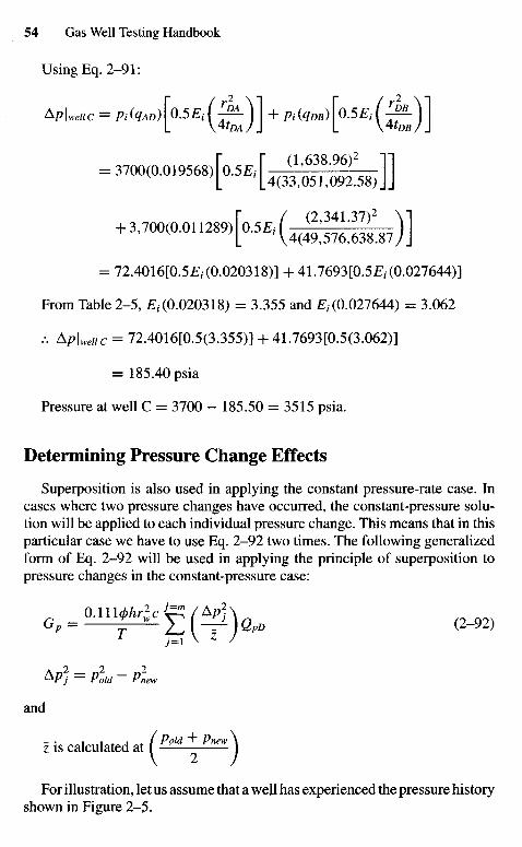
Using Eq. 2-91:
ApLeuc = Pi(qAD)\o.5Ei(^-X\ + p, ( Z>B) fo.5^ ( ^ p - ) l
8370^HHiS]]+ 3,700(0.011289)[0.5£i(^|fl|^)]
= 72.4016[0.5E,-(0.020318)] +41.7693[0.5E1-(0.027644)]
From Table 2-5, E1-(0.020318) = 3.355 and E1-(0.027644) = 3.062
... ApU//c = 72.4016[0.5(3.355)] +41.7693[0.5(3.062)]
= 185.40 psia
Pressure at well C = 3700 - 185.50 = 3515 psia.
Determining Pressure Change Effects
Superposition is also used in applying the constant pressure-rate case. Incases where two pressure changes have occurred, the constant-pressure solu-tion will be applied to each individual pressure change. This means that in thisparticular case we have to use Eq. 2-92 two times. The following generalizedform of Eq. 2-92 will be used in applying the principle of superposition topressure changes in the constant-pressure case:
Gp = -— 2L [ ~^~) Qp° ( 2 " 9 2 )
1 y=i \ z /
AP2j = Pirn - PLw
and
i t x j A / PoId + Pnew \
z is calculated at I — — 1
For illustration, let us assume that a well has experienced the pressure historyshown in Figure 2-5,
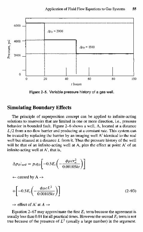
/ hours
Figure 2-5. Variable pressure history of a gas well.
Simulating Boundary Effects
The principle of superposition concept can be applied to infinite-actingsolutions to reservoirs that are limited in one or more direction, i.e., pressurebehavior in bounded fault. Figure 2-6 shows a well, A, located at a distanceL/2 from a no-flow barrier and producing at a constant rate. This system canbe treated by replacing the barrier by an imaging well Ar identical to the realwell but situated at a distance L from it. Thus the pressure history of the wellwill be that of an infinite-acting well at A, plus the effect at point A' of aninfinite-acting well at A', that is,
ApD]-" = PiqD[-°-5Ei(-^iki)]«— caused by A ->
-> effect of A' at A - •
Equation 2-67 may approximate the first Et term because the agreement isusually less than 0.01 for all practical times. However the second Et term is nottrue because of the presence of L2 (usually a large number) in the argument.
Pres
sure
, ps
i
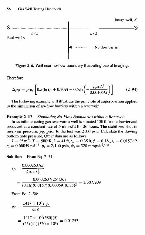
Figure 2-6. Well near no-flow boundary illustrating use of imaging.
Therefore:
*PD = PiqD\o.5(\ntD +0.809) - °-5E<(-Q^Wkt)] (2~94)
The following example will illustrate the principle of superposition appliedto the simulation of no-flow barriers within a reservoir.
Example 2—12 Simulating No-Flow Boundaries within a ReservoirIn an infinite-acting gas reservoir, a well is situated 150 ft from a barrier and
produced at a constant rate of 5 mmscfd for 36 hours. The stabilized shut-inreservoir pressure, /?#, prior to the test was 2100 psia. Calculate the flowingbottom hole pressure. Other data are as follows:
k = 25 mD9 T = 5S0°R,h = 41ft,rw = 0.35 ft, 0 = 0.16, [X1 = 0.0157 cP,Ct = 0.00059 psi"1, pi = 2,100 psia, Vv = 320 mmpsia2/cR
Solution From Eq. 2-51:
0.0002637fcf
= 0-0002637(25)(36) = ^ 3 0 7 3 9
(0.16)(0.0157)(0.00059)(0.35)2
From Eq. 2-56:
1417 x 10 3 r^ eqD = khfi
_ 1417xlQ3(580)(5) _
(25)(41)(320 x 106)
No flow barrier
Image well, A
Real well A
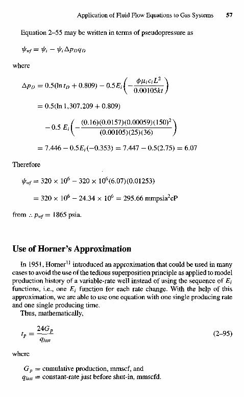
Equation 2-55 may be written in terms of pseudopressure as
^Wf= ti -^i ApDqD
where
ApD = 0.5QntD + 0.809) - 0 . 5 £ , ( - ^ ^ )
= 0.5(ln 1,307,209+ 0.809)
0 5 E ( (0-1 6)(0 '0 1 5 7)( a 0 ( ) Q 5 9)(1 5 Q)2^1V (0.00105)(25)(36) /
= 7.446 - 0.5E1-(-0.353) = 7.447 - 0.5(2.75) = 6.07
Therefore
VV = 320 x 106 - 320 x 106(6.07)(0.01253)
= 320 x 106 - 24.34 x 106 = 295.66 mmpsia2cP
from .-. pWf = 1865 psia.
Use of Horner's Approximation
In 1951, Horner11 introduced an approximation that could be used in manycases to avoid the use of the tedious superposition principle as applied to modelproduction history of a variable-rate well instead of using the sequence of E1-functions, i.e., one Et function for each rate change. With the help of thisapproximation, we are able to use one equation with one single producing rateand one single producing time.
Thus, mathematically,
., - ^ (2-95)tflast
where
Gp = cumulative production, mmscf, andqlast z= constant-rate just before shut-in, mmscfd.
Accounting for Different Reservoir Geometry
Ramey22 has presented models of pseudo-steady-state flow in more generalreservoir shapes. For practical applications, the concept of the shape factor,CA, which depends on the shape of the area and the well position, is quiteuseful. Defining a dimensionless time based on drainage area, A, as
0.0002637A*tD = — — (2-51)
(pficA
tDA = tD
r-f (2-96)
Pi - Pw/ = PiqD\|ln(2'24^AfzMj + 4ntDA - F\ (2-97)
where dimensionless pressure ApD is
A № = > [ l n ( ^ p ) + 4 ^ _ F ] <2_98)and F is the Matthews, Brons, and Hazebroek23 dimensionless pressure func-tion that has been evaluated for various reservoir shapes and well locations. Forsmall values of tDA, that is, the transient region of flow, the well is infinite-actingand
F = 4ntDA (2-99)
and
A P D = 0 . 5 1 n ( 2 - 2 4 5 ^ ) (2-100)
For large values of tDA, when all the boundaries have been felt, that is, atpseudo-steady state,
F = In(C AtDA) (2-101)
and
ApD = 0.5 l n ( 2 ' r
2
2
4 ^ 8 A ) + 2^tDA (2-102)
The late transient between transient and pseudo-steady-state varies witheach situation. During this period, the pressure drop function may be obtainedfrom
APD = 0.5[ln( 2 - 2 4 5 J? A f n 4 ) + Antm - F ] (2-103)
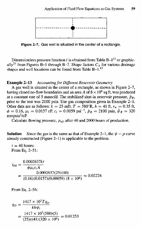
Figure 2-7. Gas well is situated in the center of a rectangle.
Dimensionless pressure function / is obtained from Table B-I23 or graphic-ally23 from Figures B-I through B-7. Shape factors CA for various drainageshapes and well locations can be found from Table B-I.13
Example 2-13 Accounting for Different Reservoir GeometryA gas well is situated in the center of a rectangle, as shown in Figure 2-7,
having closed no-flow boundaries and an area A of 8 x 10⁶ sq ft, was producedat a constant rate of 5 mmscfd. The stabilized shut-in reservoir pressure, /?#,prior to the test was 2100 psia. Use gas composition given in Example 2-1.Other data are as follows: k = 25 mD, T = 5800R, h = 41 ft, rw = 0.35 ft,0 = 0.16, & = 0.0157 cP, Ci = 0.0059 psi"1, pR = 2100 psia, \jrR = 320mmpsia2/cP.
Calculate flowing pressure, pwf, after 40 and 2000 hours of production.
Solution Since the gas is the same as that of Example 2-1, the ^ — P curvealready constructed (Figure 2-1) is applicable to the problem.
t = 40 hours:From Eq. 2-51:
0.0002637£r*DA = —7 :—
= 0-^637(25)(40) =
(0.16)(0.0157)(0.00059) (8 x 10⁶)
From Eq. 2-56:
1417 x 103r^cQD = TT-.
k hyi= "17 x 103(580X5) , a 0 1 2 5 3
(25)((41)(320 x 106)
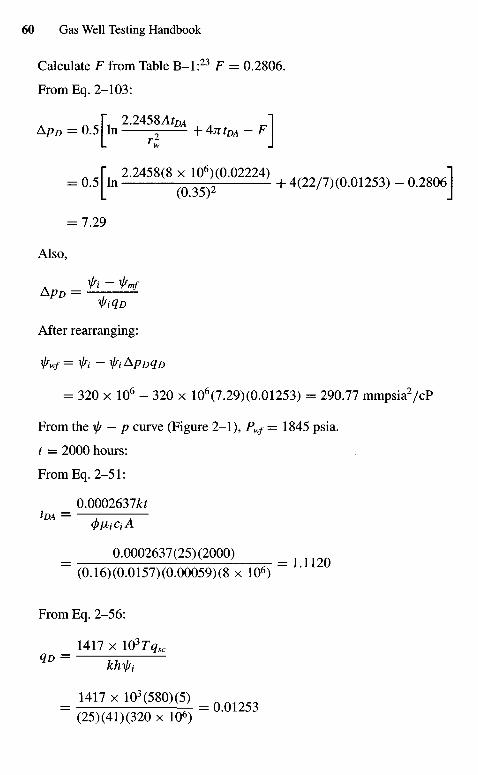
Calculate F from Table B-I:23 F = 0.2806.
From Eq. 2-103:
Apo=0 .5[ln^!^+4^-F]
= 05^ 2.2458(8 x g)(0.02224) + 4(22/7)(0 M253) _ „ 2 g 0 6 ]
= 7.29
Also,
^PD = —:^iq D
After rearranging:
^wf - ft -fiApDqD
= 320 x 106 - 320 x 106(7.29)(0.01253) = 290.77 mmpsia2/cP
From the V - P curve (Figure 2-1), Pwf = 1845 psia.
t = 2000 hours:
From Eq. 2-51:
0.0002637^tDA = 1 A
_ 0.0002637(25) (2000) _~ (0.16)(0.0157)(0.00059)(8 x 10⁶) ~
From Eq. 2-56:
1417 x 103r^c
4° = TTikhy/i
= 1417 x 103(580X5)(25)(41)(320 x 106)
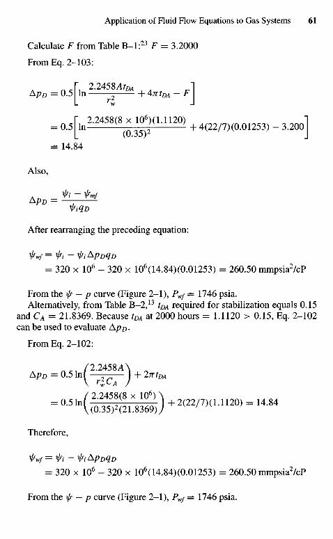
Calculate F from Table B-I:23 F = 3.2000
From Eq. 2-103:
ApD = 0.5 In h 4ntDA - FL ^w J
_ ^TMX9XgHUm +4(22/7)(0.01253) _ 3.200]
= 14.84
Also,
A n in - jfmf^PD = —;
After rearranging the preceding equation:
^Wf= ^i -\lriApDqD
= 320 x 106 - 320 x 106(14.84)(0.01253) = 260.50 mmpsia2/cP
From the x// — p curve (Figure 2-1), Pwf = 1746 psia.Alternatively, from Table B-2,13 tDA required for stabilization equals 0.15
and CA = 21.8369. Because tDA at 2000 hours = 1.1120 > 0.15, Eq. 2-102can be used to evaluate ApD.
From Eq. 2-102:
/2.2458 A \ApD = 0.5 InI 2 c J + 2ntDA
Therefore,
^Wf= fi -fiApDqD
= 320 x 106 - 320 x 106(14.84)(0.01253) = 260.50 mmpsia2/cP
From the x/r - p curve (Figure 2-1), Pwf = 1746 psia.
2.12 Choice of Equation for Gas Flow Testingand Analysis
This section will discuss correlation of the gas flow solutions in terms ofthe pressure; pressure squared, and real-gas pseudopressure approaches. Ananalysis of these approaches has been conducted by Aziz, Mattar, Ko, andBrar.7 They consider the analytical solution at the well for an infinite reservoirgiven by Eq. 2-104:
ApD = -0.5Ei(-^-) (2-104)
Calculate the sandface pressure from this equation, using different ap-proaches.
Pressure Case
For pressure >3000 psi the simpler form is in terms of pressure, p. Thedifferential equation is
±jL(r-\ = 0/XC gg (2-105)
rdr\ drj 0.000263Ik dt v ;
The diffusivity equation in dimensionless variables becomes
i a r a i a— ^-\rD--(ApD) = —(ApD) (2-106)rD drD L drD J dtD
The dimensionless time, , in Eq. 2-106 is defined by
| p = 0.0002637*,/JN
<t>rl \iLcJ
The definition of Ap#, however, is different for this approach. For thepressure case,
kh K p )
Both quantities (^) and (^) in Eqs. 2-107 and 2-108 are evaluated at
(Pi + P) /2.
Pressure-Squared Case
For pressure <2000 psi a simple form in terms of p2 is more generallyapplicable.
a y i dp2
= <t>^c dp2
dr2 r dr 0.0002637/t dt
The diffusivity equation in dimensionless variables becomes
a ^ + 1 3 A ^ adr2
D rD drD dtD
The definition of Ap#, however, is different for this approach. For thepressure-squared case,
^ = M.7xL"Z ) (2-1H)
The quantities ( ^ ) and (fiz) in Eqs. 2-107 and 2-108 are evaluated at p(.
Pseudopressure Case
For both low and high pressures the equation in terms of pseudopressure isbest fitted to this role, is denoted by x/r (p), and is defined by the integral10
p
Ir(P) = 2 f —dp (2-112)J VZ
Phase
The differential equation in terms of this approach is
i a W_ №, w r2_113)
rdr\ dr J 0.0002637A: dt
The diffusivity equation in dimensionless variables becomes
± J L ( , 0 ^ ) = ^ <2_I14)
?D orD \ drD J dtD
The definition of Axj/j) is
The properties are evaluated at initial conditions.
2.13 Skin, IT Flow, and Wellbore Storage Effects
In the derivation of the equations it was assumed that the porous mediumwas homogeneous and isotropic and that flow was single-phase and obeyedDarcy's law. It was also supposed that opening and shut-in of the well wasdone at the sandface. In actual fact these idealizations are not realistic, andderivations from the ideal model are too frequent and important to be ignored.Ways of accounting for skin effects; IT flow, and wellbore storage will betreated in the following sections.
Accounting for Effects of Formation Damage
The permeability of the formation immediately around the well can bedamaged by the well drilling process or improved by fracturing or acidizingthe well on completion. To account for this altered permeability a skin factorwas defined by Van Everdingen8 as
(ApD)skin = s, a constant (2-116)
so that
&PD \weii (including skin) = pD + s (2-117)
This essentially states that there will be an added pressure difference due tothe skin effect given by Eq. 2-117. A position value of s indicates a damagedwell, and a negative value, an improved well. Hawkins9 proposed that the skinbe treated as a region of radius rskin with permeability ksidn, with the skin factorgiven by
s = (-^-l)ln^ (2-118)\ ^ skin / f\v
Equation 2-118 is valid for both positive skin (Jc5Jdn < k) and negative skin(ksktn > k) but there is no unique set of values of kskm and rskin for a particular s.
An alternative treatment of the skin effect is that of an "effective wellboreradius" (Matthews and Russell, 1967, p. 21),15 defined as that radius whichmakes the pressure drop in an ideal reservoir equal to that in an actual reservoirwith skin. Thus:
rw (effective) = rwe~s (2-119)
For positive skin, rw (effective) < rw, that is, the fluid must travel throughadditional formation to cause the observed pressure drop, Ap. For negativeskin, rw (effective) > rw. This is a useful concept in hydraulically fracturedwells.
Accounting for Effects of Turbulence
For gas flow, however, inertial and/or turbulent (IT) flow effects, notaccounted for by Darcy's law, are frequently of significance and should notbe ignored. IT flow is most pronounced near the well and results in an addi-tional pressure drop similar to the skin effect, except that it is not a constantbut varies directly with flow rate.24 Smith25 confirmed with actual test resultsand with numerical solutions that IT flow could be treated as an additional,rate-dependent skin effect.
(ApD)IT = Dqsc (2-120)
Where D — IT flow factor for the system, the pressure at the well is givenby
Apz)U// = PD + s + Dqsc (2-121)
or
s' = (ApD)skin + (&PD)IT = s + Dqsc (2-122)
The following example will show how pressure drop is attributed to laminarflow, skin, and IT flow effects. It assumes negligible effects of viscosity onturbulence.
Example 2-14 Calculating Pressure Drop due to Laminar Skin and IT FlowEffects
In an infinite-acting gas reservoir, a well was produced at a constant rate,qscU of 8 mmscfd for a period of 35 hours. The flowing bottom hole pressure,pwp, at that time was 1550 psia. The same well was produced at a constantrate, qsc2, of 11 mmscfd for a time of 25 hours. The flowing bottom holepressure, p^p, at that time was 1300 psia. The stabilized shut-in pressure, PR,prior to each of the two flowing periods, was 2100 psia. Other data pertinentto the test are given below:
k = 25 mD, rw = 0.35 ft, h = 35 ft, T = 6000R,0 = 0.16, [ii = 0.0147 cP, Ci = .00053 psi"1, f{ = 320.00 mmpsia2/cPt\ = 35 hours, qscl = 8 mmscfd, pWfj = 1550 psiah = 25 hours, qSC2 = 11 mmscfd, pwf2 = 1300 psia
Calculate the skin and IT flow effects, s and D, respectively. Also calculate,for the second flow rate, using the same gas composition given in Example 2-2:
(a) the pressure drop due to the laminar flow effect(b) the pressure drop due to skin effects
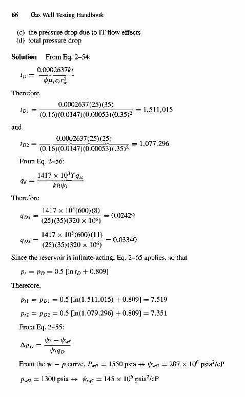
(c) the pressure drop due to IT flow effects(d) total pressure drop
Solution From Eq. 2-54:
0.0002637JfcftD = — —
Therefore
0.0002637(25)(35) _D1 (0.16)(0.0147)(0.00053)(0.35)2 ' '
and
0.0002637(25)(25) _D2 (0.16)(0.0147)(0.00053)(.35)2 ' '
From Eq. 2-56:
1417 x 103Tqsc<ld = —
khx/fi
Therefore
1417 x 103(600)(8)
^ = (25 ) (35 ) (320xm = 0 - ° 2 4 2 9
1417xl03(600)(ll) . „ , . .g D 2 = ( 2 5 ) ( 3 5 ) ( 3 2 0 x l 0 6 )
= ° - 0 3 3 4 0
Since the reservoir is infinite-acting, Eq. 2-65 applies, so that
pt = pD = 0.5 [In tD + 0.809]
Therefore,
pn = Pm = 0.5 [In(1,511,015) + 0.809] = 7.519
Pt2 = Pm = 0.5 [In(1,079,296) + 0.809] = 7.351
From Eq. 2-55:
A fi ~ fwf^PD = — ~
^i q D
From the \/f — p curve, Pwfj = 1550 psia ^> ijrwfi = 207 x 106 psia2/cPpwf2 = 1300 psia «e> x//Wj2 = 145 x 106 psia2/cP
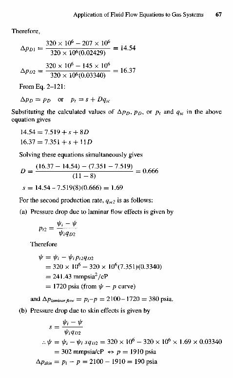
Therefore,
320 x 106 - 207 x 106
APDI = 320 x 106(0.02429) = UM
32Ox 1 0 6 - 1 4 5 x 10⁶
APD2 = 320 x 106(0.03340) = l631
From Eq. 2-121:
^PD = PD or pt=s + Dqsc
Substituting the calculated values of ApD, pD, or pt and qsc in the aboveequation gives
14.54 = 7.519+ J + 8D
16.37 = 7.351+5 + H D
Solving these equations simultaneously gives
^ (16.37 - 14.54) - (7.351 - 7.519) n , _D = ^ - ^ = 0.666
s = 14.54-7.519(8)(0.666) = 1.69
For the second production rate, qsc2 is as follows:
(a) Pressure drop due to laminar flow effects is given by
Pa = —
Therefore
^ = XJf1- fiPaqDi
= 320 x 106 - 320 x 106(7.351)(0.3340)
= 241.43 mmpsia2/cP
= 1720 psia (from x// — p curve)
and Apiaminarfiow = Pi~P = 2100-1720 = 380 psia.
(b) Pressure drop due to skin effects is given by
ttqDi... ilr = \ln- ft sqD2 = 320 x 106 - 320 x 106 x 1.69 x 0.03340
= 302 mmpsia/cP *> p = 1910 psia
kPskin = Pi- P = 2100 - 1910 = 190 psia
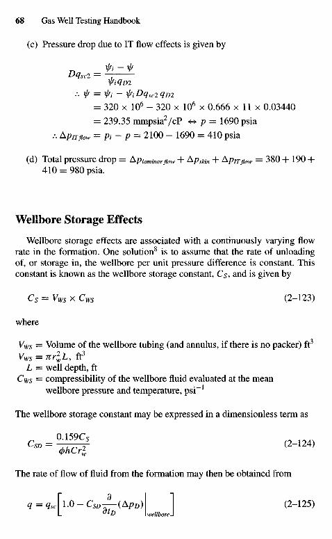
(c) Pressure drop due to IT flow effects is given by
Dqsc2 = —^iq D2
:. xjf = ^ - xj/iDqsc2qD2
= 320 x 106 - 320 x 106 x 0.666 x 11 x 0.03440
= 239.35 mmpsia2/cP op = 1690 psia
... ApITflow = pi - p = 2100 - 1690 = 410 psia
(d) Total pressure drop = Apiaminarflow + Apskin + Ap17 flow = 380 + 190 +410 = 980 psia.
Wellbore Storage Effects
Wellbore storage effects are associated with a continuously varying flowrate in the formation. One solution8 is to assume that the rate of unloadingof, or storage in, the wellbore per unit pressure difference is constant. Thisconstant is known as the wellbore storage constant, Cs, and is given by
C5 = Vws x Cws (2-123)
where
Vws = Volume of the wellbore tubing (and annulus, if there is no packer) ft3
Vws = irrlL, ft3
L = well depth, ftCws = compressibility of the wellbore fluid evaluated at the mean
wellbore pressure and temperature, psi"1
The wellbore storage constant may be expressed in a dimensionless term as
^ - ^ <2- i24>
<t>hCrl
The rate of flow of fluid from the formation may then be obtained from
q = qJl.O - CSD^-(ApD) 1 (2-125)L <™0 wellborn J
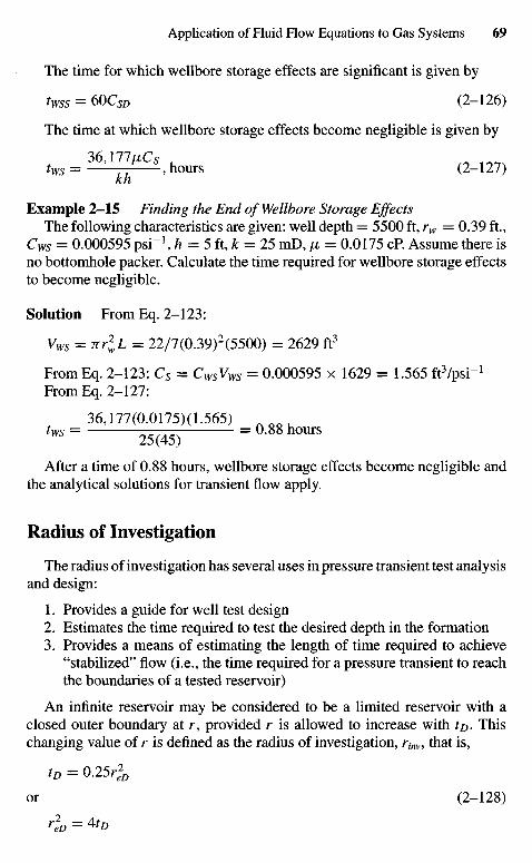
The time for which wellbore storage effects are significant is given by
twss = 60CSD (2-126)
The time at which wellbore storage effects become negligible is given by
36,177MC5 t h o u i g
kh
Example 2-15 Finding the End of Wellbore Storage EffectsThe following characteristics are given: well depth = 5500 ft, rw — 0.39 ft.,
Cws = 0.000595 psi"1, h = 5 ft, k = 25 mD, /x = 0.0175 cR Assume there isno bottomhole packer. Calculate the time required for wellbore storage effectsto become negligible.
Solution From Eq. 2-123:
Vws = nrlL = 22/7(0.39)2(5500) = 2629 ft3
From Eq. 2-123: C5 = CWSVWS = 0.000595 x 1629 = 1.565 ftVpsi"1
From Eq. 2-127:
36,177(0.0175)(1.565)tws = 25(45) = r S
After a time of 0.88 hours, wellbore storage effects become negligible andthe analytical solutions for transient flow apply.
Radius of Investigation
The radius of investigation has several uses in pressure transient test analysisand design:
1. Provides a guide for well test design2. Estimates the time required to test the desired depth in the formation3. Provides a means of estimating the length of time required to achieve
"stabilized" flow (i.e., the time required for a pressure transient to reachthe boundaries of a tested reservoir)
An infinite reservoir may be considered to be a limited reservoir with aclosed outer boundary at r, provided r is allowed to increase with t&. Thischanging value of r is defined as the radius of investigation, rinv, that is,
tD = O.25rjk
or (2-128)
r2eD = 4tD
fa?.\2 = 4tD (2-128a)
/0.00105fcAa5
r™ = —2 ' ft- f o r r'«v < re (2-128b)
If the value of rim obtained from Eq. 2-128a is greater than re, then theradius of investigation is taken to be re.
Time of Stabilization
If a well is centered in a cylindrical drainage area of radius re, then settingrim = re, the time required for stabilization, ts, is defined as follows:
tD = Q25r2eD
or
1. (j)iiCr2e
ts - 4 * 0.0002637fe(2-129)
9480/xCre2 u
= L , hours
Example 2-16 Estimating Radius of InvestigationWe want to conduct a flow test on an exploratory gas well for a long enough
time to ensure that the well will drain a radius of more than 1500 ft. Welland fluid data are as follows: 0 = 0.18 fraction, k = 9.0 mD, rt = 1500 ft,fit = 0.0156 cP, Cti = 2.2 x 10~4 psi"1. What length of flow test appearsadvisable? What flow rate do you suggest?
Solution From Eq. 2-128a, the time required is
/0 .00105i tA a 5 £
rinv = T » f t ' for rinv < re
\ <t>^ct )In principle, any flow rate would sufficient required to achieve a particularradius of investigation is dependent of flow rate.
2J4 Numerical Solutions of Partial DifferentialEquations
Numerical methods must be used for cases where the partial differentialequation and its boundary conditions cannot be linearized, where the reservoirshape is irregular, or when the reservoir is heterogeneous. In some complexsituations, analytical solutions may be so difficult to apply that numerical meth-ods are preferred. In this section a brief discussion of the numerical approachis presented including difference equations.
Three-Dimensional Models
Gas flow equations are different from those for liquid flow in that the equa-tions of state that are used are quite different in functional form from those forliquids. The ideal gas law gives the equation of state for an ideal gas:
m m MPV = -RT and ? = - P = p
where p is the density.In the case of flow of a nonideal gas, the gas deviation factor zg is introduced
into the equation of state to give
If we assume laminar flow, neglect gravity effects, and assume constantrock properties, Eq. 2-130 becomes
*-(j-*L\ + L(^dj\ + A(_£J\ = ±L(L\ n on
dx\nzgdx) ^dy\nzgdy) dz\v.Zg%) kdt\zg)
In field units Eq. 2-131 can be written as
dx\nzgdx) dy\iizgdy) dz\^ZgfJ 0.000264* dt \z J
(2-132)
In terms of pseudopressure, \jf{p), the equation can be written as follows:
p
fip) = 2 I -^- dp (2-133)J HZgPo
where po is a low base pressure. Now,
d (p\^d(f~g) dp ^cgPdp
dt\Zg) dp dt Z8 dt'
because
Co = l dp = Zg ^8 p dp p dp
Also note that
dx/r drfr dp 2p dp
dt dp dt fjLZg dt
and
df _ 2/7 dp
dx fjLZg dx
d\lr dx/fSimilar expressions apply for — and — . Thus Eq. 2-131 becomes
dy dz
d_(djr\ B(W\ + JL(W\ = ^cs W (2_l34)dx\dx J dy\dy) dz\dz) 0.000264fc dt
Equations 2-131 and 2-134 are in three-dimensional form for single-phaseflows and can be used for the study of completely heterogeneous reservoirs.
Radial One-Dimensional Model
For radial flow, the equivalent of Eq. 2-131 is
i_a_(2_rap\ = 4> Z ( P ) ( 2 _ 1 3 5 )
rdr\nzg drj 0.000264k 8t\zg J
In terms of pseudopressure, W(p) is
l d / d * \ _ 0 df
rdr\ dr ) 0.000264it dt
For single-well problems, the use of the cylindrical coordinates providesgreater accuracy than other coordinate systems. For the study of multiwellsystems it is usually necessary to use rectangular coordinates with closelyspaced grid points near the well.
Radial Two-Dimensional Coning Model
Where vertical flow is important, a two-dimensional radial model must beconsidered. The equation to be solved in this case is
rdr\jjizgr dr) dz \^zg dz) 0.000264£ dt \zg)
In terms of pseudopressure, ^(p) is
i d _ ( ty\ a ( W \ = 4>nc8 d/P\rdr\ dr ) dz\dz) 0.000264Jfc dt \zg)
Models of this type can be used to study the effects of anisotropy on thetransient pressure analysis of buildup and drawdown tests.
Areal Two-Dimensional Models
Multiwell problems can be solved through the solution of Eq. 2-139:
The injection or production from different wells is accounted for by theq term. The reservoir shape may be completely arbitrary and there may bedifferent types of boundary conditions such as no-flow or constant pressure.This model can also be used for interference test analysis.
Studies of this type for Darcy's flow have been reported in the literature, forexample, by Carter.12
Multiphase (Gas-Condensate Flow) Model
In this section we outline a detailed derivation of an equation describingradial, and a multiphase mixture of gas, condensate, and water. We assume thata porous medium contains gas condensate and water, and that each phase hassaturation-dependent effective permeability (kg, ko, and kw)\ time-dependentsaturation (Sg, S0, and Sw); and pressure-dependent viscosity (/x^, /JLO, andjiw). When gravitational forces and capillary pressures are negligible, thedifferential equation describing this type of flow is
1A/3VA *,ct 3±
rdr\ dr J 0.000264A, dt
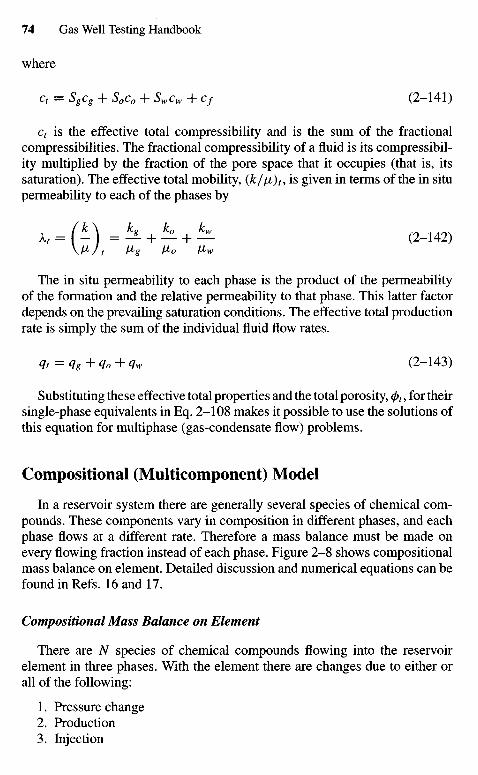
where
ct = Sgcg + S0C0 + Swcw + Cf (2-141)
ct is the effective total compressibility and is the sum of the fractionalcompressibilities. The fractional compressibility of a fluid is its compressibil-ity multiplied by the fraction of the pore space that it occupies (that is, itssaturation). The effective total mobility, (k//ji)t, is given in terms of the in situpermeability to each of the phases by
kt = (-) = ^ - + ^ + — (2-142)
The in situ permeability to each phase is the product of the permeabilityof the formation and the relative permeability to that phase. This latter factordepends on the prevailing saturation conditions. The effective total productionrate is simply the sum of the individual fluid flow rates.
9t=qg+qo + qw (2-143)
Substituting these effective total properties and the total porosity, <j>t, for theirsingle-phase equivalents in Eq. 2-108 makes it possible to use the solutions ofthis equation for multiphase (gas-condensate flow) problems.
Compositional (Multicomponent) Model
In a reservoir system there are generally several species of chemical com-pounds. These components vary in composition in different phases, and eachphase flows at a different rate. Therefore a mass balance must be made onevery flowing fraction instead of each phase. Figure 2-8 shows compositionalmass balance on element. Detailed discussion and numerical equations can befound in Refs. 16 and 17.
Compositional Mass Balance on Element
There are Af species of chemical compounds flowing into the reservoirelement in three phases. With the element there are changes due to either orall of the following:
1. Pressure change2. Production3. Injection
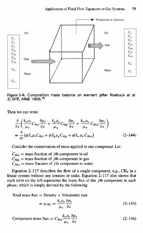
Figure 2-8. Composition mass balance on element (after Roebuck et al.© SPE, AIME 1969).16
Then we can write
° (Kpor °Po kgpg dpg kwpw dpw\
ax \ IJL0 ox fig ox jiw ox )
3= —WSQPOCMOJ + <t>SgPgCMgj + <t>SwpwCMwj) (2-144)
ot
Consider the conservation of mass applied to one compound. Let
CMoj = mass fraction of y'th component in oilCMgj = mass fraction of jth component in gasCMwj = mass fraction of jth component in water
Equation 2-117 describes the flow of a single component, e.g., CH4 in alinear system without any sources or sinks. Equation 2—117 also shows thateach term on the left represents the mass flux of the j th component in eachphase, which is simply derived by the following:
Total mass flux = Density x Volumetric rate
Kpo op 0 / o ....= poqo = — (2-145)
fio dx
Component mass flux = CMoi-^—— — - (2-146)/jio dx
Water
Gas
Oil Oil
Production or injection
Gas
Water
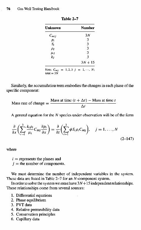
Table 2-7
Unknown Number
Cmij 37VPi 3Si 3Pi 31I1 3*/ 3
3A^+ 15
N o t e : Cmij = 1 , 2 , 3 7 = I , - - - , N;to ta l = 3AT
Similarly, the accumulation term embodies the changes in each phase of thespecific component:
n t Mass at time (t + Ar) - Mass at time tMass rate of change =
A general equation for the Af species under observation will be of the form
T-[ / ^ CMij— = —I }<S>SiPiCMij , J = 1,...,N
(2-147)
where
i = represents the phases andj = the number of components.
We must determine the number of independent variables in the system.These data are listed in Table 2-7 for an AT-component system.
In order to solve the system we must have 3 N+15 independent relationships.These relationships come from several sources:
1. Differential equations2. Phase equilibrium3. PVT data4. Relative permeability data5. Conservation principles6. Capillary data
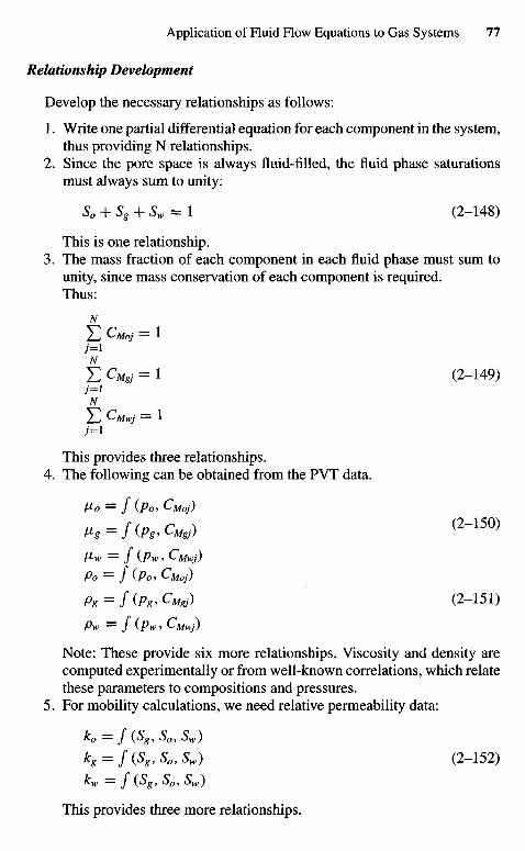
Relationship Development
Develop the necessary relationships as follows:
1. Write one partial differential equation for each component in the system,thus providing N relationships.
2. Since the pore space is always fluid-filled, the fluid phase saturationsmust always sum to unity:
S0 + Sg + Sw = 1 (2-148)
This is one relationship.3. The mass fraction of each component in each fluid phase must sum to
unity, since mass conservation of each component is required.Thus:
N
E CMOJ = 17 = 1
E CMgj = 1 (2-149)7 = 1
z2 CMWJ = i7 = 1
This provides three relationships.4. The following can be obtained from the PVT data.
V>o = J (POXMOJ)
VS = I (PS, CM,) (2-15°)
A6W = / (Pw, CMWJ)
Po= J (Po, CMOJ)
P8 = f(Pg> CM,) (2-151)
Pw = / (Pw> CMWJ)
Note: These provide six more relationships. Viscosity and density arecomputed experimentally or from well-known correlations, which relatethese parameters to compositions and pressures.
5. For mobility calculations, we need relative permeability data:
ko = f(Sg,So,Sw)kg = f (S89 S0, Sw) (2-152)
Kw == J \^g> ^Oi ^w)
This provides three more relationships.
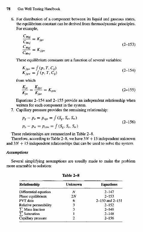
6. For distribution of a component between its liquid and gaseous states,the equilibrium constant can be derived from thermodynamic principles.For example,
CMgj _ v
rm (2-153)
LMgj _r — Ajgw
These equilibrium constants are a function of several variables:
Kjgo = J (Pi T, Ctj) (2-154)
from which
Kj0 Kjgw
— — —— — &gow (Z-IDD)
Equations 2-154 and 2-155 provide an independent relationship whenwritten for each component in the system.
7. Capillary pressure provides the remaining relationship:
Pg ~ Po = Pego — J (Sgi S0, Sw)(2-156)
Po ~ Pw = Pcow — J (SgI S0, Sw)
These relationships are summarized in Table 2-8.Therefore, according to Table 2-8, we have 3 Af + 15 independent unknown
and 3N + 15 independent relationships that can be used to solve the system.
Assumptions
Several simplifying assumptions are usually made to make the problemmore amenable to solution:
Table 2-8
Relationship Unknown Equations
Differential equation N 2-147Phase equilibrium 2N 2-153PVT data 6 2-150 and 2-151Relative permeability 3 2-152J2 Mass fraction 3 2-149J2 Saturation 1 2-148Capillary pressure 2 2-156
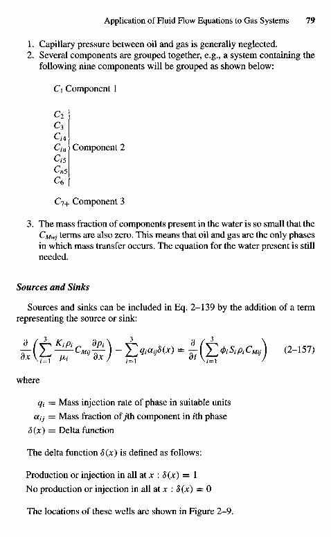
1. Capillary pressure between oil and gas is generally neglected.2. Several components are grouped together, e.g., a system containing the
following nine components will be grouped as shown below:
Ci Component 1
C2
C3
Ci 4Ctn Component 2C15
Cn5
C6
C7 + Component 3
3. The mass fraction of components present in the water is so small that theCMwj terms are also zero. This means that oil and gas are the only phasesin which mass transfer occurs. The equation for the water present is stillneeded.
Sources and Sinks
Sources and sinks can be included in Eq. 2-139 by the addition of a termrepresenting the source or sink:
f ( E ~ C ^ ) - £>**«(*) = £(][>*ACW) (2-157)ox Vf-f № ox ) f-f dt Vfrf /
where
qt = Mass injection rate of phase in suitable units
atj = Mass fraction of jth component in /th phase
8(x) = Delta function
The delta function 8(x) is defined as follows:
Production or injection in all at x : <$(*) = 1
No production or injection in all at x : 8(x) = 0
The locations of these wells are shown in Figure 2-9.
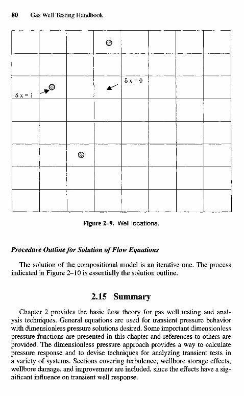
Figure 2-9. Well locations.
Procedure Outline for Solution of Flow Equations
The solution of the compositional model is an iterative one. The processindicated in Figure 2-10 is essentially the solution outline.
2.15 Summary
Chapter 2 provides the basic flow theory for gas well testing and anal-ysis techniques. General equations are used for transient pressure behaviorwith dimensionless pressure solutions desired. Some important dimensionlesspressure functions are presented in this chapter and references to others areprovided. The dimensionless pressure approach provides a way to calculatepressure response and to devise techniques for analyzing transient tests ina variety of systems. Sections covering turbulence, wellbore storage effects,wellbore damage, and improvement are included, since the effects have a sig-nificant influence on transient well response.
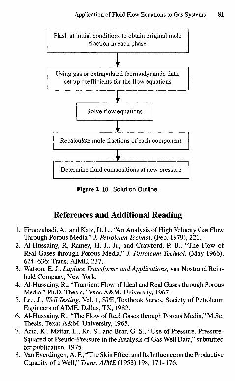
Flash at initial conditions to obtain original molefraction in each phase
Using gas or extrapolated thermodynamic data,set up coefficients for the flow equations
Recalculate mole fractions of each component
Determine fluid compositions at new pressure
Solve flow equations
Figure 2-10. Solution Outline.
References and Additional Reading
1. Firoozabadi, A., and Katz, D. L., "An Analysis of High Velocity Gas FlowThrough Porous Media." /. Petroleum Technol. (Feb. 1979), 221.
2. Al-Hussainy, R, Ramey, H. J., Jr., and Crawford, P. B., "The Flow ofReal Gases through Porous Media," /. Petroleum Technol. (May 1966),624-636; Trans. AIME, 237.
3. Watson, E. J., Laplace Transforms and Applications, van Nostrand Rein-hold Company, New York.
4. Al-Hussainy, R., "Transient Flow of Ideal and Real Gases through PorousMedia," Ph.D. Thesis, Texas A&M. University, 1967.
5. Lee, J., Well Testing, Vol. 1, SPE, Textbook Series, Society of PetroleumEngineers of AIME, Dallas, TX, 1982.
6. Al-Hussainy, R., "The Flow of Real Gases through Porous Media," M.Sc.Thesis, Texas A&M. University, 1965.
7. Aziz, K., Mattar, L., Ko. S., and Brar, G. S., "Use of Pressure, Pressure-Squared or Pseudo-Pressure in the Analysis of Gas Well Data," submittedfor publication, 1975.
8. Van Everdingen, A. F., "The Skin Effect and Its Influence on the ProductiveCapacity of a Well," Trans. AIME (1953) 198, 171-176.
9. Hawkins, M. R, Jr., "A Note on the Skin Effect," Trans. AIME (1956) 207,356-357.
10. Kirchhoff, H., Vorlesungen iiber die Theorie der Warme, Barth, Leipzig,1894.
11. Homer, D. R., "Pressure Buildup in Wells," Proc. Third World PetroleumConference; The Hague, Sec. II, 1951, 503-523.
12. Carter, R. D., "Performance Predictions for Gas Reservoirs Consider-ing Two-Dimensional Unsteady-State Flow," Soc. Petroleum Engineers J.(1966) 6, 35-43.
13. Dietz, D. N., "Determination of Average Reservoir Pressure from BuildupSurveys," /. Petroleum Technol (August 1965), 955-959.
14. Saidikowski, R. M., "Numerical Simulation of the Combined Effects ofWellbore Damage and Partial Penetration," paper SPE 8204, Sept. 23-26,1979.
15. Matthews, C. S., and Russell, D. G., Pressure Buildup and Flow Tests inWells, AIME Monograph, Vol. 1, SPE-AIME, New York, 1967.
16. Roebuck, I. R, Henderson, G. E., Douglas, J., Jr., and Ford, W. T., "TheCompositional Reservoir Simulator: The Linear Model," Trans. AIME(1969)246,115.
17. Abel, W., Jackson, R. R, and Wattenbarger, R. A., "Simulation of a Par-tial Pressure Maintenance Gas Cycling Project with a CompositionalModel, Carson Creek Field, Alberta," /. Petroleum Technol (Jan. 1970)38-46.
18. Van Everdingen, A. R, "The Skin Effect and Its Influence on the ProductiveCapacity of a Well," Trans. AIME (1953) 198, 171-176.
19. Van Poollen, H. K., "Radius of Investigation and Stabilization Time Equa-tions," Oil Gas J. (1964) 63(51), 71-75.
20. Carslaw, H. S., and Jaeger, J. C, Conduction of Heat in Solids, OxfordUniversity Press, London, 1959.
21. Katz, D. L., Cornell, D., Kobayashi, R., Poettmann, R H., Vary, J. A., Elen-baas, J. R., and Weinaug. C. R, Handbook of Natural Gas Engineering,McGraw-Hill, New York, 1959.
22. Ramey, H. J., Jr., "Application of the Line Source Solution to Flow inPorous Media—A Review," Producers Monthly (1967) 31(5), 4-7 and25-27.
23. Matthew, CS., Brons, R, and Hazebroek, P., "A Method for Determinationof Average Pressure in a Bounded Reservoir," Trans. AIME (1954) 201,182-191.
24. Houpeurt, A., "On the Flow of Gases on Porous Media," Revue de UInstitut Francais du Petrole (1959). XIV(Il), 1468-1684.
25. Smith, R. V, "Unsteady-State Gas Flow into Gas Wells," J. PetroleumTechnol (1961) 13, 1151-1159.
26. Bruce, G. H., Peacemen, D. W., Rachford, H. H., Jr., and Rice, J. D.,"Calculation of Unsteady State Gas Flow Through Porous Media," Trans.AIME (1953) 198, 79-92.
27. Carter, R. D., "Solutions of Unsteady-State Radial Gas Flow," /. PetroleumTechnol. (1962) 14, 549-554.
28. Collins, R. E., Flow of Fluids through Porous Materials, Reinhold Pub-lishing Corporation; New York, 1961.
29. De Wiest, R. J. M. (ed.), Flow through Porous Media, Academic Press,New York, 1969.
30. Earlougher, R. C, Jr., Ramey, H. J., Jr., Miller, F. G., and Mueller, T. D.,"Pressure Distributions in Rectangular Reservoirs," /. Petroleum Technol.(1968) 20, 199-208.
31. Derradii, S., "Bessel Functions, Laplace Transforms and Their Applica-tion," M.S. Report, University of Tulsa, Tulsa, OK, 1983.
32. Van Everdingen, A. F, and Hurst, W., "The Application of Laplace Trans-formation to Flow Problems in Reservoirs," Trans. AIME (1949) 186,305-324.
33. Abramowitz, M., and Stegun, I. A. (eds.), Handbook of MathematicalFunctions with Formulas, Graphs and Mathematical Tables, National Bu-reau of Standards Applied Mathematics Series 55 (June 1964) 227-253.
34. Chatas, A. T, "A Practical Treatment of Non-Steady State Flow Problemsin Reservoirs Systems."
35. Watson, G. N., Theory of Bessel Functions, Cambridge University Press,London, 1944.
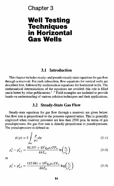
Chapter 3
Well TestingTechniquesin HorizontalGas Wells
3.1 Introduction
This chapter includes steady- and pseudo-steady-state equations for gas flowthrough a reservoir. For each subsection, flow equations for vertical wells aredescribed first, followed by mathematical equations for horizontal wells. Themathematical determinations of the equations are avoided; this role is filledmuch better by other publications.1"5 Field examples are included to providehands-on understanding of various solution techniques and their applications.
3.2 Steady-State Gas Flow
Steady-state equations for gas flow through a reservoir are given below.Gas flow rate is proportional to the pressure-squared terms. This is generallyemployed when reservoir pressures are less than 2500 psia. In terms of gaspseudopressure, the gas flow rate is directly proportional to pseudopressure.The pseudopressure is defined as
p
f{p) = 2 f -E-dp (3-1)J fiz
PRef
pl_plf = 50337x10^7^ JrA (3_2)
KHISC Vw//
or
2 2 115.98IxIO3^ZrP (re\
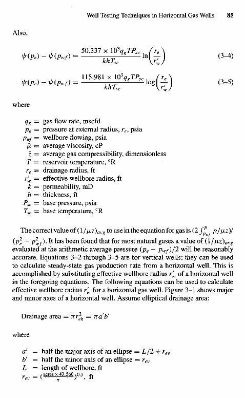
Also,
50.337 x 10³^sTPSC (re\f(Pe) ~ ir(Pwf) = , , - , 8 In -7- (3-*)
. , , . , , 115.981 x l03qgTPsc , (re\+(Pe) ~ fiPwf) = ^ r log(-J (3-5)
where
#g = gas flow rate, mscfdpe = pressure at external radius, re, psia
pwf = wellbore flowing, psiafl = average viscosity, cPz = average gas compressibility, dimensionlessT = reservoir temperature, 0Rre = drainage radius, ft
r'w — effective wellbore radius, ftk = permeability, mDh = thickness, ft
Psc = base pressure, psiaTsc = base temperature, 0R
The correct value of (1 l\xz)avg to use in the equation for gas is (2 fp p/fiz)/
(p2e - pif)> It has been found that for most natural gases a value of (l//xz)avg
evaluated at the arithmetic average pressure (pe — pw/)/2 will be reasonablyaccurate. Equations 3-2 through 3-5 are for vertical wells; they can be usedto calculate steady-state gas production rate from a horizontal well. This isaccomplished by substituting effective wellbore radius rf
w of a horizontal wellin the foregoing equations. The following equations can be used to calculateeffective wellbore radius rf
w for a horizontal gas well. Figure 3-1 shows majorand minor axes of a horizontal well. Assume elliptical drainage area:
Drainage area = itr\h — no!b'
where
a! — half the major axis of an ellipse = L/2 + rev
br — half the minor axis of an ellipse = rev
L = length of wellbore, ft„ _ /acresx43,560\Q.5 ftrev — v J1 ) 1 1 L
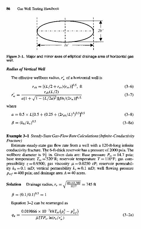
Figure 3-1. Major and minor axes of elliptical drainage area of horizontal gaswell.
Radius of Vertical Well
The effective wellbore radius, r'w of a horizontal well is
reh = [(L/2 + rev)(rev)f\ ft (3-6)
r' = r*«J* (3-7)w a[l + Vl - (L/2a)2][/3h/(2rw)]h/L
where
a = 0.5 x L[0.5 + (0.25 + (2r^/L)4)0'5]0-5 (3-8)
i8 = (W^v)0-5 (3-8a)
Example 3-1 Steady-State Gas-Flow Rate Calculations (Infinite-ConductivityFracture)
Estimate steady-state gas flow rate from a well with a 120-ft-long infiniteconductivity fracture. The 6-ft-thick reservoir has a pressure of 2000 psia. Thewellbore diameter is 9^ in. Given data are: Base pressure Psc = 14.7 psia;base temperature r5C = 520°R; reservoir temperature T = IlO0F; gas com-pressibility z = 0.9500; gas viscosity /JL = 0.0250 cP; reservoir permeabil-ity kh =0.1 mD; vertical permeability kv =0.1 mD; well flowing pressurepwf = 400 psia; and drainage area A = 40 acres.
Solution Drainage radius, re = J40^f0 = 745 ft
P = (O.l/O.l)05 = 1
Equation 3-2 can be rearranged as
_ 0.019866 x lO~3khTsc(p2
e - p2wf)
q* = fizTPscln(reK) ( 3 " 2 a )
For an infinite-conductivity fracture of total length 120 ft, half-length Xf is60 ft. The effective wellbore radius r'w of an infinite-conductivity fracture is
r'w =jc//2 = 60/2 = 30ft
Substituting the value of r'w in Eq. 3-2:
_ 0.019866 x IP"3 x 0.1 x 60 x 520(20002 - 4002)q§ ~ 0.0250 x 0.950 x (110 + 460) x 14.71n(745/60)
= 1196.03/ ln(12.4167) = 1196.03/2.519 = 474.8mscfd
Example 3-2 Calculating Flow Rate for Horizontal Well Assuming Steady -State Conditions
Two horizontal wells are 1000 and 2000 ft long and drain 100 and 150 acres,respectively. AU reservoir properties and drainage areas are the same as thosenoted in Example 3-1.
Solution The steady-state gas flow rate can be calculated using Eq. 3-2:
_ 0.019866 x \Q-3khTsc(p2
e - pi)qg~ flzTPscln(re/rw)
Using the same reservoir properties as Example 3-1, we have
qg = 1196.03/ lnfo/r^), mscfd
For a horizontal gas well, r'w is calculated from Eq. 3-7:
yl = reh(L/2)Tw a[l + Vl - (L/Ia)2Wh/(2rw)f/L
For 100 acres,
Therefore for a 1000-ft-long well from Eq. 3-6:
reh = \\^Y~ + 1177-29 ) (1177.29) 1 = 1405 ft
and from Eq. 3-8:
a = 0.5 x 1000[0.5 + (0.25 + (2 x 1405/1000)4)0-5]0-5
= 500[0.5 + (0.25 + 62.35)a5]a5 = 500[0.5 + 7.92]05 = 1450 ft
Substituting this into Eq. 3-7:
1405(1000/2)
~ 1450[l + y/\ - (1000/(2 x 1450))2][l x 60/0.792]60/1000
702,500
~ 1450[l + Vl - 0.344829] [75.7576]006
= Z 0 ^ = ^ 1 S O O =
1450[l + 0.65517(1.296479)] 2681.651
Therefore
qg = 1196.03/In (-j—) = 1196.03/1.67956 = 712.108 mscfd
For 150 acres,
For a 2000-ft-long well, with 150-acre well spacing, using the procedure shownabove:
a = 1624 ftr'w = 520.20 ftqg = 1173.070 mscfd
Thus, comparing the results of Examples 3-1 and 3-2, one can see that for asteady state, a fractured vertical well with 40-acre spacing can produce at a rateof 475 mscfd. A 2000-ft-long horizontal well at 100-acre spacing can produce712.108 mscfd. A 2000-ft-long horizontal well at 150-acre well spacing canproduce 1173.070 mscfd.
3.3 Pressure Transient Characteristicsin Horizontal Gas Wells
Horizontal wells have high potential in gas reservoirs. They are suitableand applicable in low- as well as high-permeability gas formations. In low-permeability formations, they drain larger volumes than vertical wells andprovide an alternative to achieve long penetration lengths to the formations.They reduce near-wellbore turbulence and enhance well deliverability in high-permeability gas formations. Figure 3-1 a illustrates the character of the log-logplot of the pressure—time data in conjunction with the derivative curve. Thisfigure also shows the effects of wellbore damage associated with the minimum
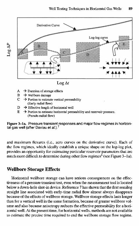
Log At
A -^ Duration of storage effectsB -^ Wellbore damageC -^ Portion to estimate vertical permeability
(Early radial flow)D -> Effective length of horizontal wellE -^ Portion to estimate horizontal permeability and reservoir pressure.
(Pseudo radial flow)
Figure 3-la. Pressure transient responses and major flow regimes in horizon-tal gas well (after Daviau et al.).7
and maximum flexures (i.e., zero curves on the derivative curve). Each ofthe flow regimes, which ideally establish a unique shape on the log-log plot,provides an opportunity for estimating particular reservoir parameters that aremuch more difficult to determine during other flow regimes6 (see Figure 3-la).
Wellbore Storage Effects
Horizontal wellbore storage can have serious consequences on the effec-tiveness of a pressure transient test, even when the measurement tool is locatedbelow a down-hole shut-in device. Reference 7 has shown that the first semilogstraight line associated with early-time radial flow almost always disappearsbecause of the effects of wellbore storage. Wellbore storage effects lasts longerthan for a vertical well in the same formation, because of greater wellbore vol-ume and also because anisotropy reduces the effective permeability for a hori-zontal well. At the present time, for horizontal wells, methods are not availableto estimate the precise time required to end the wellbore storage flow regime.
Derivative Curve
Log-log curve
Log
AP
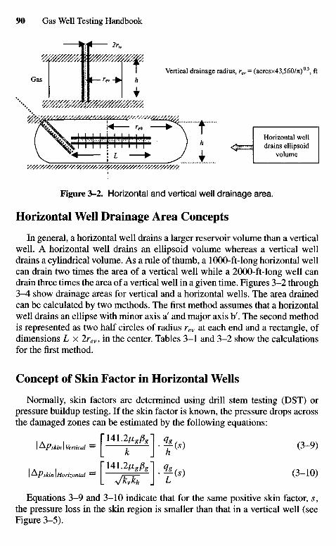
Figure 3-2. Horizontal and vertical well drainage area.
Horizontal Well Drainage Area Concepts
In general, a horizontal well drains a larger reservoir volume than a verticalwell. A horizontal well drains an ellipsoid volume whereas a vertical welldrains a cylindrical volume. As a rule of thumb, a lOOO-ft-long horizontal wellcan drain two times the area of a vertical well while a 2000-ft-long well candrain three times the area of a vertical well in a given time. Figures 3-2 through3-A show drainage areas for vertical and a horizontal wells. The area drainedcan be calculated by two methods. The first method assumes that a horizontalwell drains an ellipse with minor axis a' and major axis b'. The second methodis represented as two half circles of radius rev at each end and a rectangle, ofdimensions L x 2rev, in the center. Tables 3-1 and 3-2 show the calculationsfor the first method.
Concept of Skin Factor in Horizontal Wells
Normally, skin factors are determined using drill stem testing (DST) orpressure buildup testing. If the skin factor is known, the pressure drops acrossthe damaged zones can be estimated by the following equations:
\APskin\Vertical = [ 1 4 1 ^ l . | L ( , ) (3-9)L & \ h
\APskin\Horizontal = [ 1 4 1 J ^ l • (S) (3-10)
Equations 3-9 and 3-10 indicate that for the same positive skin factor, s,the pressure loss in the skin region is smaller than that in a vertical well (seeFigure 3-5).
Vertical drainage radius, rev = (acresx43,560/7i)0'5, ftGas
Horizontal welldrains ellipsoid
volume
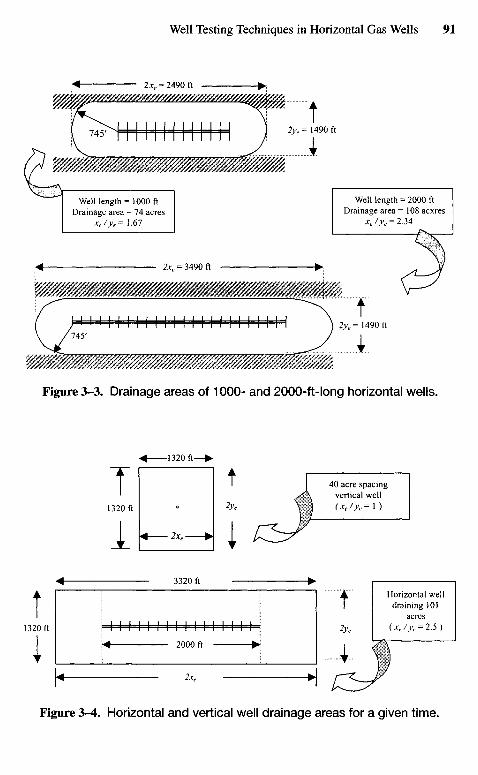
Figure 3-4. Horizontal and vertical well drainage areas for a given time.
Horizontal welldraining 101
acres(xL,/yc = 2.5)
40 acre spacingvertical well(xe/ye=\ )
Figure 3-3. Drainage areas of 1000- and 2000-ft-long horizontal wells.
Well length = 2000 ftDrainage area = 108 acxres
xe/yc, = 234
WeI !length= 1000 ftDrainage area = 74 acres
xe/ye = 1.67
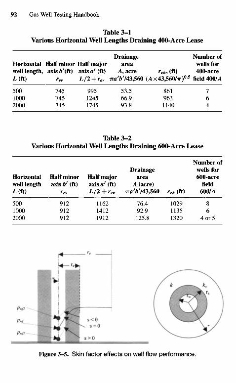
Table 3-1Various Horizontal Well Lengths Draining 400-Acre Lease
Horizontalwell length,L (ft)
50010002000
Half minoraxis b'(ft)
rev
745745745
Half majoraxis a'(ft)L/2 + rev
99512451745
Drainagearea
A, acre7ra'6743,560
53.566.993.8
reh, (ft)(AX43,560/TT)0-5
8619631140
Number ofwells for400-acre
field 400/A
764
Table 3-2Various Horizontal Well Lengths Draining 600-Acre Lease
Horizontalwell lengthL (ft)
50010002000
Half minoraxis b' (ft)
912912912
Half majoraxis a1 (ft)L/2 + rev
116214121912
Drainagearea
A (acre)7^743,560
76.492.9125.8
reh (ft)
102911351320
Number ofwells for600-acre
field600/A
86
4 or 5
Figure 3-5. Skin factor effects on well flow performance.
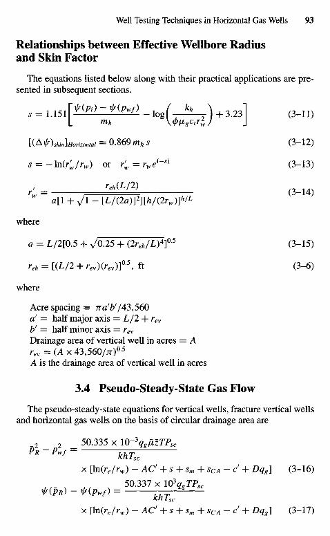
Relationships between Effective Wellbore Radiusand Skin Factor
The equations listed below along with their practical applications are pre-sented in subsequent sections.
s = ll5Jnpd~f(pw/)_lj h U 3 2 3 I (3_H)L mh \4>HgCtrlJ J
[(A\ls)skin]Horizontal = 0.869 mh s (3-12)
s = -\n(r'w/rw) or r'w = rwe(~s) (3-13)
r> = ^ ^ (3-14)w a[l + Vl - [L/(2a)]2][h/(2rw)]h/L
where
a = L/2[0.5 + V0.25 + (2reh/L)4f5 (3-15)
reh = [(L/2 + rev)(rev)f5, ft (3-6)
where
Acre spacing = na'b'/43,560a' = half major axis = L/2 + rev
&' = half minor axis = rev
Drainage area of vertical well in acres = Arev = (A x 43,560/TT)0-5
A is the drainage area of vertical well in acres
3.4 Pseudo-Steady-State Gas Flow
The pseudo-steady-state equations for vertical wells, fracture vertical wellsand horizontal gas wells on the basis of circular drainage area are
_2 2 _ 50.335 x 10~3qgfLzTPsc
x [ln(re/rw) - AC' + s + sm + sCA - c' + Dqg] (3-16)
50.337 x 10\TPsc
IT(PR) - ir(pwf) =Knlsc
x [ln(re/rw) - AC' + s + sm + sCA ~ c' + Dqg] (3-17)
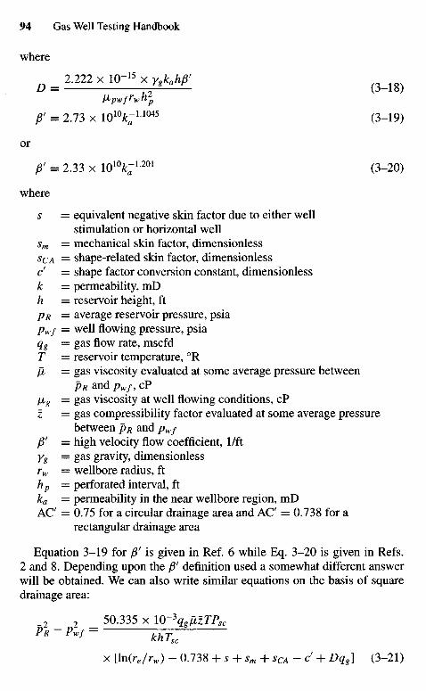
where
D = 2-222 x IQ-" x y g W
VPwfrwh2p
P = 2.73 x 101X1 1 0 4 5 (3-19)
or
ff = 2.33 x 10¹⁰JkJ1-201 (3-20)
where
s — equivalent negative skin factor due to either wellstimulation or horizontal well
sm = mechanical skin factor, dimensionlesssCA = shape-related skin factor, dimensionlessd = shape factor conversion constant, dimensionlessk = permeability, mDh = reservoir height, ftpR = average reservoir pressure, psiapwf — well flowing pressure, psiaqg — gas flow rate, mscfdT = reservoir temperature, 0R/2 = gas viscosity evaluated at some average pressure between
pR and pwf, cPfj,g = gas viscosity at well flowing conditions, cPz = gas compressibility factor evaluated at some average pressure
between pR and pwfft = high velocity flow coefficient, I/ftyg z= gas gravity, dimensionlessrw = wellbore radius, fthp = perforated interval, ftka = permeability in the near wellbore region, mDAC = 0.75 for a circular drainage area and AC = 0.738 for a
rectangular drainage area
Equation 3-19 for ft is given in Ref. 6 while Eq. 3-20 is given in Refs.2 and 8. Depending upon the ft definition used a somewhat different answerwill be obtained. We can also write similar equations on the basis of squaredrainage area:
_2 2 _ 50.335 x 10"3qgjlzTPsc
x [ln(re/rw) - 0.738 + s + sm + sCA ~ c1 + Dq8] (3-21)
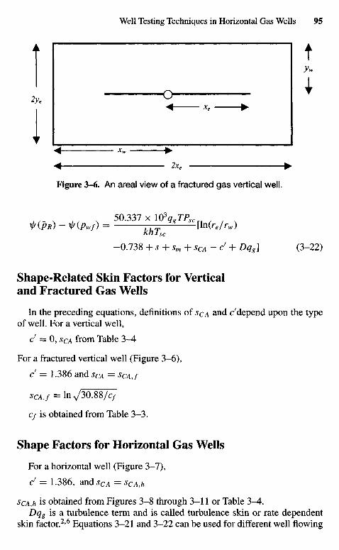
Figure 3-6. An areal view of a fractured gas vertical well.
+ (P*) - *(*,/> = 5 0 3 3 7 ^hlT°3qgTP-[Mre/rw)
Knlsc
-0.738 + s+sm+sCA-cf + Dq8] (3-22)
Shape-Related Skin Factors for Verticaland Fractured Gas Wells
In the preceding equations, definitions of SCA and c'depend upon the typeof well. For a vertical well,
cf = 0, SCA from Table 3-4
For a fractured vertical well (Figure 3-6),
c' = 1.386 and SCA = SCAJ
scA,f = toj30.&S/cf
Cf is obtained from Table 3-3.
Shape Factors for Horizontal Gas Wells
For a horizontal well (Figure 3-7),
d = 1.386, and CA = $CA,h
SCAM i s obtained from Figures 3-8 through 3-11 or Table 3-A.Dqg is a turbulence term and is called turbulence skin or rate dependent
skin factor.2'6 Equations 3-21 and 3-22 can be used for different well flowing
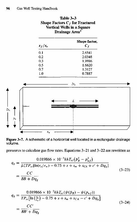
Figure 3-7. A schematic of a horizontal well located in a rectangular drainagevolume.
pressures to calculate gas flow rates. Equations 3-21 and 3-22 are rewritten as
0.019866 x M)-3khTsc(p2
R - p2wf)
qg~ flzTPsc[\n(re/rw) - 0.75 + s + sm + SCA + c* + Dq8]
cc (3"23)
BB + Dq8
0.019866 x lQ-3khTscW(pR) - f{Pwf))qg " TP50[In (^) - 0.75 + s+sm+sCA-C + Dq8]
(3-24)_ CC~ BB' + Dq8
Table 3-3Shape Factors C/ for Fractured
Vertical Wells in a SquareDrainage Area3
Shape factor,Xf/Xe Cf
0.1 2.65410.2 2.03480.3 1.99860.5 1.66200.7 1.31271.0 0.7887
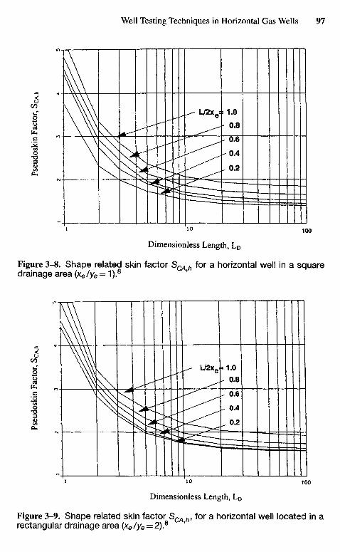
Dimensionless Length, L0
Figure 3-8. Shape related skin factor SCA h for a horizontal well in a squaredrainage area (xe/ye = 1 ).8
Dimensionless Length, LD
Figure 3-9. Shape related skin factor SCA h, for a horizontal well located in arectangular drainage area (xe /ye = 2).8
Pse
ud
osk
in F
acto
r, S
CA.H
Pse
ud
osk
in F
acto
r, S
CA
.h
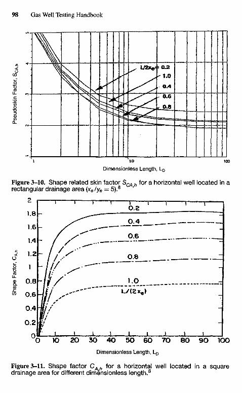
Dimensionless Length, LD
Figure 3-11. Shape factor CAh for a horizontal well located in a squaredrainage area for different dimensionless length.8
Dimensionless Length, LD
Figure 3-10. Shape related skin factor SCA h for a horizontal well located in arectangular drainage area (xe/ye = 5).8
Pse
udos
kin
Fac
tor,
ScA
.hS
hape
Fac
tor,
CA
h
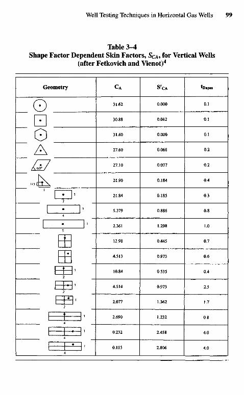
Table 3-4Shape Factor Dependent Skin Factors, SCA> for Vertical Wells
(after Fetkovich and Vienot)4
C A S 'CA tD a p s s
31.62 0.000 0.1
30.88 0.012 0.1
31.60 0.000 0.1
27.60 0.068 0.2
27.10 0.077 0.2
21.90 0.184 0.4
21.84 0.185 0.3
5.379 0.886 0.8
2.361 1.298 1.0
12.98 0.445 0.7
4.513 0.973 0.6
10.84 0.535 0.4
4.514 0.973 2.5
2.077 1.362 1.7
2.690 1.232 0.8
0.232 2.458 4.0
0.115 2.806 4.0
Geometry
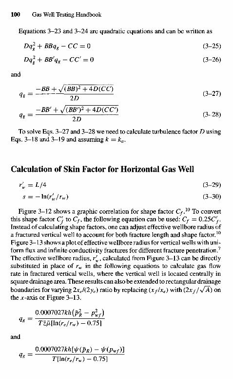
Equations 3-23 and 3-24 are quadratic equations and can be written as
Dq] + BBqg -CC = 0 (3-25)
Dq] + BBrqg - CC' = 0 (3-26)
and
-BB + V(££)2 + 4D(CC)9g = 2D ( 3 " 2 ? )
-BBf + J(BB>)2 + 4D{CC)qg = 2 D
( *
To solve Eqs. 3-27 and 3-28 we need to calculate turbulence factor D usingEqs. 3-18 and 3-19 and assuming k = ka.
Calculation of Skin Factor for Horizontal Gas Well
r'w = L/A (3-29)
s = -\n{rjrw) (3-30)
Figure 3-12 shows a graphic correlation for shape factor C/.10 To convertthis shape factor Cf to C/, the following equation can be used: C/ = 0.25C^.Instead of calculating shape factors, one can adjust effective wellbore radius ofa fractured vertical well to account for both fracture length and shape factor.10
Figure 3-13 shows a plot of effective wellbore radius for vertical wells with uni-form flux and infinite conductivity fractures for different fracture penetration.7
The effective wellbore radius, rfw, calculated from Figure 3-13 can be directly
substituted in place of rw in the following equations to calculate gas flowrate in fractured vertical wells, where the vertical well is located centrally insquare drainage area. These results can also be extended to rectangular drainageboundaries for varying 2xe/(2ye) ratio by replacing (x//xe) with ( 2 J C / / \ / A ) onthe x-axis or Figure 3-13.
0.0007021kh(p2R- plf)
qg= Tz/l[ln(re/rw)-0J5]
and
= 0.0007027^[VrQ)7Q - jr(pwf)]qg T[\n(re/rw) - 0.75]
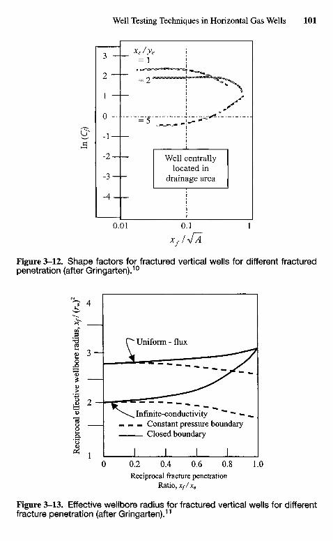
Figure 3-12. Shape factors for fractured vertical wells for different fracturedpenetration (after Gringarten).10
Well centrallylocated in
drainage area
Uniform - flux
Infinite-conductivityConstant pressure boundaryClosed boundary
Reciprocal fracture penetrationRatio, Xf /xe
Figure 3-13. Effective wellbore radius for fractured vertical wells for differentfracture penetration (after Gringarten).11
Rec
ipro
cal
effe
ctiv
e w
ellb
ore
radi
us, X
fI (
r w)2
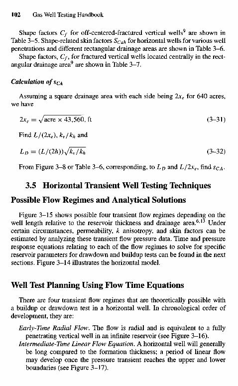
Shape factors Cf for off-centered-fractured vertical wells9 are shown inTable 3-5. Shape-related skin factors Scah f° r horizontal wells for various wellpenetrations and different rectangular drainage areas are shown in Table 3-6.
Shape factors, C/, for fractured vertical wells located centrally in the rect-angular drainage area9 are shown in Table 3-7.
Calculation O/SCA
Assuming a square drainage area with each side being 2xe for 640 acres,we have
2xe = ^/acre x 43,560, ft (3-31)
Find L/(2xe), kv/kh and
LD = (L/(2h))y/kJh (3-32)
From Figure 3-8 or Table 3-6, corresponding, to LD and L/2xe, find SQA-
3.5 Horizontal Transient Well Testing Techniques
Possible Flow Regimes and Analytical Solutions
Figure 3-15 shows possible four transient flow regimes depending on thewell length relative to the reservoir thickness and drainage area.613 Undercertain circumstances, permeability, k anisotropy, and skin factors can beestimated by analyzing these transient flow pressure data. Time and pressureresponse equations relating to each of the flow regimes to solve for specificreservoir parameters for drawdown and buildup tests can be found in the nextsections. Figure 3-14 illustrates the horizontal model.
Well Test Planning Using Flow Time Equations
There are four transient flow regimes that are theoretically possible witha buildup or drawdown test in a horizontal well. In chronological order ofdevelopment, they are:
Early-Time Radial Flow. The flow is radial and is equivalent to a fullypenetrating vertical well in an infinite reservoir (see Figure 3-16).
Intermediate-Time Linear Flow Equation. A horizontal well will generallybe long compared to the formation thickness; a period of linear flowmay develop once the pressure transient reaches the upper and lowerboundaries (see Figure 3-17).
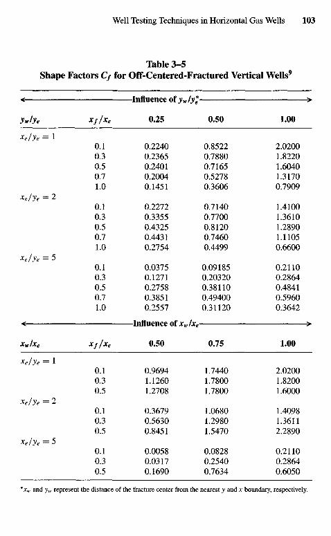
Table 3-5Shape Factors C1 for Off-Centered-Fractured Vertical Wells9
< Influence of yw Iy * >
ywlye XfIx6 0.25 0.50 1.00
xelye = 10.1 0.2240 0.8522 2.02000.3 0.2365 0.7880 1.82200.5 0.2401 0.7165 1.60400.7 0.2004 0.5278 1.31701.0 0.1451 0.3606 0.7909
xelye = 20.1 0.2272 0.7140 1.41000.3 0.3355 0.7700 1.36100.5 0.4325 0.8120 1.28900.7 0.4431 0.7460 1.11051.0 0.2754 0.4499 0.6600
xe/ye = 50.1 0.0375 0.09185 0.21100.3 0.1271 0.20320 0.28640.5 0.2758 0.38110 0.48410.7 0.3851 0.49400 0.59601.0 0.2557 0.31120 0.3642
< Influence of xwlxe >
xwlxe Xf / xe 0.50 0.75 1.00
Xelye = 10.1 0.9694 1.7440 2.02000.3 1.1260 1.7800 1.82000.5 1.2708 1.7800 1.6000
x6/y6 = 20.1 0.3679 1.0680 1.40980.3 0.5630 1.2980 1.36110.5 0.8451 1.5470 2.2890
Xelye = 50.1 0.0058 0.0828 0.21100.3 0.0317 0.2540 0.28640.5 0.1690 0.7634 0.6050
*xw and yw represent the distance of the fracture center from the nearest y and x boundary, respectively.
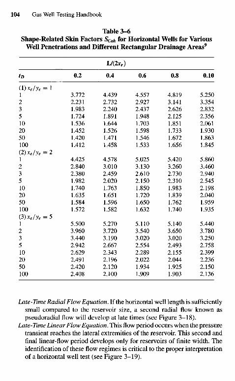
Table 3-6Shape-Related Skin Factors Scah for Horizontal Wells for Various
Well Penetrations and Different Rectangular Drainage Areas9
UQx9)
tD 0.2 0.4 0.6 0.8 0.10
(X) xe I ye = 11 3.772 4.439 4.557 4.819 5.2502 2.231 2.732 2.927 3.141 3.3543 1.983 2.240 2.437 2.626 2.8325 1.724 1.891 1.948 2.125 2.35610 1.536 1.644 1.703 1.851 2.06120 1.452 1.526 1.598 1.733 1.93050 1.420 1.471 1.546 1.672 1.863100 1.412 1.458 1.533 1.656 1.845(2)xe/ye = 21 4.425 4.578 5.025 5.420 5.8602 2.840 3.010 3.130 3.260 3.4603 2.380 2.459 2.610 2.730 2.9405 1.982 2.020 2.150 2.310 2.54510 1.740 1.763 1.850 1.983 2.19820 1.635 1.651 1.720 1.839 2.04050 1.584 1.596 1.650 1.762 1.959100 1.572 1.582 1.632 1.740 1.935(3)xe/ye = 51 5.500 5.270 5.110 5.140 5.4402 3.960 3.720 3.540 3.650 3.7803 3.440 3.190 3.020 3.020 3.2505 2.942 2.667 2.554 2.493 2.75810 2.629 2.343 2.289 2.155 2.39920 2.491 2.196 2.022 2.044 2.23650 2.420 2.120 1.934 1.925 2.150100 2.408 2.100 1.909 1.903 2.136
Late-Time Radial Flow Equation. If the horizontal well length is sufficientlysmall compared to the reservoir size, a second radial flow known aspseudoradial flow will develop at late times (see Figure 3-18).
Late-Time Linear Flow Equation. This flow period occurs when the pressuretransient reaches the lateral extremities of the reservoir. This second andfinal linear-flow period develops only for reservoirs of finite width. Theidentification of these flow regimes is critical to the proper interpretationof a horizontal well test (see Figure 3-19).
Table 3-7Shape Factors, C/, for Fractured Vertical Wells Located
Centrally in a Rectangular Drainage Area
CfXf/xe 1 2 3 5 10 20
0.1 2.020 1.4100 0.751 0.2110 0.0026 0.0000050.3 1.820 1.3611 0.836 0.2860 0.0205 0.0001400.5 1.600 1.2890 0.924 0.6050 0.1179 0.0105500.7 1.320 1.1100 0.880 0.5960 0.3000 0.1226001.0 0.791 0.6662 0.528 0.3640 0.2010 0.106300
Figure 3-14. Horizontal well model.
Flow Time Equations and Solutions
These sets of equations are presented here for estimating for the variousflow regimes based on the concepts of Daviau et al.9 Kuchuk et al., Odehet ah, and Clonts and Ramey respectively.712"14
Method 1: Goode andR. K. M. Thambynayagam's Equations6
Early-Time Radial Flow. The early-time radial flow period ends at
te\ — yj—Dj)
K
Horizontal wellZ or v
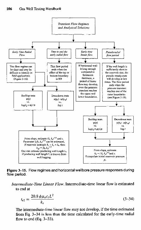
Figure 3-15. Flow regimes and horizontal wellbore pressure responses duringflow period.
Intermediate-Time Linear Flow. Intermediate-time linear flow is estimatedto end at
= 20.8 M,c,L2 ( 3_ 3 4 )
ky
The intermediate-time linear flow may not develop, if the time estimatedfrom Eq. 3-34 is less than the time calculated for the early-time radialflow to end (Eq. 3-33).
Early Time RadialFlow
Time to end theearly radial flow
Early timelinear/low
Pseudoradialflow period
Buildup testsW(p)vs.
\og(tp+At)/At
Drawdown testsW(Pi) - Wfawj)
vs.logt
This flow regime canbe short and may be
difficult to identify infield applications
(Figure 3-16).
This flow periodends when the
effect of the top orbottom boundary
is felt.
Transient Flow Regimesand Analytical Solutions
If horizontal wellis long enoughcompared to
formationthickness, a
period of linearflow may develop,once the pressuretransient reaches
the upper andlower boundaries.
If the well length issufficiently short to
the reservoir size, thepseudo-steady-statewill develop at late
times. The flow periodends when the
pressure transientreaches one of theouter boundaries(see Figure 3-19).
Buildup testsW(P)vs.
\og(tp+At)/At
Drawdown testsW(Pi)~W(pwj)
vs.log/
From slope, estimate (kv ky)05 and s.
Parameter L(kv ky) °'5 can be estimated,
if reservoir isotropic kx = ky = ki,, thenkeff=(khkv)
0-5
One can estimate producing well length L,if producing well length L is known from
well logging.
From slope, estimatekh = (kxky)°-5ands.
Extrapolate initial reservoir pressurePi-
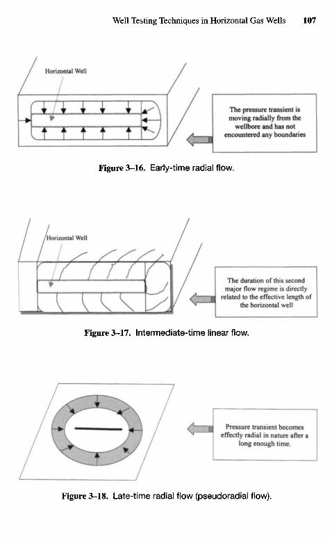
The pressure transient ismoving radially from the
wellbore and has notencountered any boundaries
The duration of this secondmajor flow regime is directly
related to the effective length ofthe horizontal well
Pressure transient becomeseffectly radial in nature after a
long enough time.
Figure 3-18. Late-time radial flow (pseudoradial flow).
Figure 3-17. Intermediate-time linear flow.
Figure 3-16. Early-time radial flow.
Horizontal Well
Horizontal Well
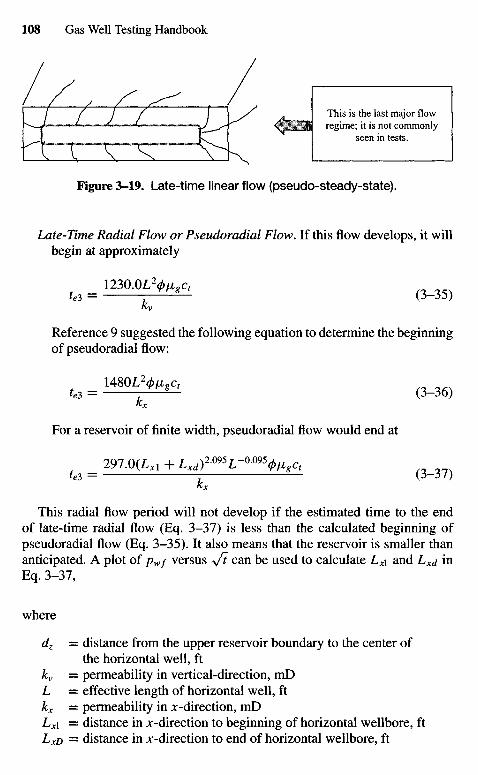
Figure 3-19. Late-time linear flow (pseudo-steady-state).
Late-Time Radial Flow or Pseudoradial Flow. If this flow develops, it willbegin at approximately
12MMHW. (3_35)
Reference 9 suggested the following equation to determine the beginningof pseudoradial flow:
1480LW, ( 3_ 3 6 )
For a reservoir of finite width, pseudoradial flow would end at
, 297.0(L^1+L^)2 Q 9 5L-Q Q 9VM gQUi = : (3-37)
This radial flow period will not develop if the estimated time to the endof late-time radial flow (Eq. 3-37) is less than the calculated beginning ofpseudoradial flow (Eq. 3-35). It also means that the reservoir is smaller thananticipated. A plot of pwf versus +Jt can be used to calculate Lx\ and LXd inEq. 3-37,
where
dz — distance from the upper reservoir boundary to the center ofthe horizontal well, ft
kv = permeability in vertical-direction, mDL = effective length of horizontal well, ftkx = permeability in x -direction, mDLxi = distance in x -direction to beginning of horizontal wellbore, ftLxD = distance in x -direction to end of horizontal wellbore, ft
This is the last major flowregime; it is not commonly
seen in tests.
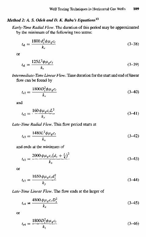
Method2: A. S. Odeh andD. K. Babu's Equations13
Early-Time Radial Flow. The duration of this period may be approximatedby the minimum of the following two terms:
= 180(KW, (3_38)kv
or
U = ^ ^ (3-39)
Intermediate-Time Linear Flow. Time duration for the start and end of linearflow can be found by
= 1800D^c1
and
,* = 160<l>^L2 (3-U)
Late-Time Radial Flow. This flow period starts at
148OL20Mgc,*<?3 = 7 (-3-42)
and ends at the minimum of
2000^0(4+ I)2
r3 _ p- -- ;kx
or1650 (f)^gctd
2y
ky
Late-Time Linear Flow. The flow ends at the larger of
= 4 8 0 0 ^ ^
or
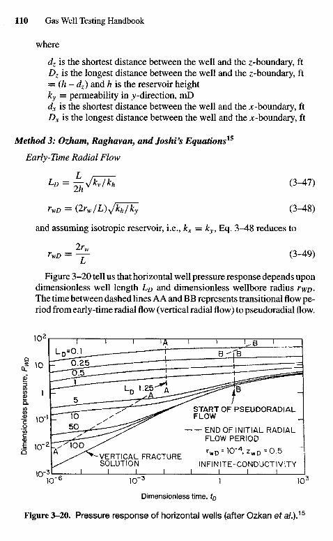
where
dz is the shortest distance between the well and the z-boundary, ftDz is the longest distance between the well and the z-boundary, ft= (h-dz) and h is the reservoir heightky = permeability in y -direction, mDdx is the shortest distance between the well and the x -boundary, ftDx is the longest distance between the well and the x -boundary, ft
Method 3: Ozham, Raghavan, andjoshi's Equations15
Early-Time Radial Flow
LD = ^KIh (3-47)
rwD = (2rw/L)Jkh/ky (3-48)
and assuming isotropic reservoir, i.e., kx — ky, Eq. 3-48 reduces to
rwD = 2^- (3-49)
Figure 3-20 tell us that horizontal well pressure response depends upondimensionless well length Lj) and dimensionless wellbore radius rwD-The time between dashed lines AA and BB represents transitional flow pe-riod from early-time radial flow (vertical radial flow) to pseudoradial flow.
Dimensionless time, tD
Figure 3-20. Pressure response of horizontal wells (after Ozkan et a/.).15
START OF PSEUDORADIALFLOW
•— ENDOFiNITIALRADIALFLOW PERIOD
rwD = KT 4 , z w D = 0.5
INFINITE-CONDUCTIVITYVERTICAL FRACTURESOLUTION
Dim
ensi
onle
ss p
ress
ure,
PW
D
(Note that the intermediate linear flow regime is not included in Figure3-20.) As shown in Figure 3-20, once the pseudoradial flow starts, thehorizontal well solutions for Lo > 10 are practically the same as thevertically fractured well solution. After estimating the value of Lo andrW£>, and using Figure 3-20, one can find to, (dashed line A-A) and theduration of the early-time radial flow, which is given by
tD4>figctLltel = 0.001055** ( 3 " 5 0 )
Late-Time Radial Flow. The start of this radial (pseudoradial) flow can becalculated by using Eqs. 3-47 and 3-48, finding to from Figure 3-20,dashed line B-B, and then using Eq. 3-50,
where:Lo= dimensionless lengthh = reservoir thickness, ftrwD = dimensionless radiusto = dimensionless time
Example 3-3 Calculating the Time Required to End of Early-Time RadialFlow
A horizontal oil well is 2000 ft long and is drilled in a reservoir with the fol-lowing characteristics: h = 120 ft, rw = 0.354 ft, 0 = 15.0%, /xg = 0.02952 cP,Ct = 4.25 x 10"5 psi"1, kh = 0.8 mD (from well test data), kv = 0.2 mD (fromcore data). The well is in the central elevation of the reservoir and the distancefrom the upper reservoir boundary to the center of the horizontal well is 20 ft.Estimate the time required to end initial radial flow.
Solution dz = (120/2 - 20) = 40 ft
Method 1, using Eq. 3-33:
l90.0df095r-0095</>tigcttel = k
/Vy
_ 190.0 x 402095 x 0.354-095 x 0.15 x 0.02952 x 4.25 x 10~5
~ 2= 0.448 hours
Method 2, using Eq. 3-40:
_ 1800 dfyngCttel ~ Jk
1800 x 402x 0.15 x 0.02952 x 4.25 x 10"5 ^ ,= = 2.71 hours
0.2
_ l25L2(/)figct _ 125 x 20002 x 0.15 x 0.02952 x 4.25 x 10~5
hl~ ky " O8
= 117.62 hours
The minimum of these two values is 0.448 hours. Thus, the initial radial flowperiod will end in 0.448 hours.
Method 3, using Figure 3-20:
LD = 2000/(2 x 120)^0.2/0.8 = 4.17 (Eq. 3-47)
Assuming it is an isotropic reservoir, and therefore kx = ky = kh:
rWD = ^yfhlk'y = 2 ^ Q 0 Q 5 4 x 1 = 3.54 x 1(T4 (Eq. 3-48)
With LD, rWD known, the time to the end of the initial radial flow periodis given by dotted line A-A (tD = 1.5 x 10~3), and after rearranging andsubstituting these values in Eq. 3-50,
_ (f)figctL2 _ 0.15 x 0.02952 x 4.25 x 10~5 x 20002
tel = .001055**' tD ~ 0.001055 x 0.8
x (1.5 x 10"3) = 1.34 hours
Therefore the initial time required to end initial radial flow would lastbetween 0.448 and 1.34 hours. The reservoir engineers will have to use down-hole shut-in devices to enhance the chances of measuring the early radial flowregime.
Example 3-4 Calculating the Time to Start and Time to End of Early-TimeLinear Flow
For the well described in Example 3-3, assuming kx = ky = 0.8 mD,calculate the time to start and time to end of early-time linear flow.
Solution The maximum distance of well from either top or bottom boundary
is:
Dz=h-dz = 1 2 0 - 4 0 = 80 ft
From Eq. 3-38:
_ 1800 Dtyfict _ 1800 x 802 x 0.15 x 0.02952 x 4.25 x 10~5
tel ~ kv ~ O2= 10.84 hours
From Eq. 3-41:
_ 16O0/xcrL2 _ 160 x 0.15 x 0.02952 x 4.25 x 10~5 x 20002
te2" Tx " ^= 150.55 hours
From Eq. 3-34:
_ 2O.8 0/xcrL2 _ 20.8 x 0.15 x 0.02952 x 4.25 x IO"5 x 20002
tel " Ix " O8= 19.57 hours
Thus, this flow period will end in about 20 to 150 hours. This indicates thatthe current well is sufficiently long compared to the reservoir height. Therefore,it is possible to analyze pressure data of the flow period.
Example 3-5 Calculating the Time Required to Start a Pseudoradial FlowFor the well/reservoir data given in Example 3-4, calculate time to start and
time to end early-time linear flow.
Solution
Method 1, from Eq. 3-35:
_ 123O0/zc,L2 _ 1230 x 0.15 x 0.02952 x 4.25 x 10"5 x 20002
tel ~ Tx " a s= 1157.4 hours = 38 days
Method 2, from Eq. 3-36:
_ 14800/XQL2 _ 1480 x 0.15 x 0.02952 x 4.25 x 10~5 x 20002
te2~ Tx " O8= 1392.6 hours = 46 days
Method 3, from Figure 3-20 Time to start of pseudoradial flow (dashed lineB-B) is tD = 3.0; thus from Eq. 3-50,
4>fictL2 _ 0.15 x 0.02952 x 4.25 x 10~5 x 20002
tel ~ 0.001055Jfc//D " 0.001055 x 0.8= 2675.7 hours = 88 days
It will take 38 to 88 days to reach pseudoradial flow. It will be economicallydifficult to shut in a well for such a long time. In this case one will have toobtain the necessary information from early-time radial or linear flow periods.
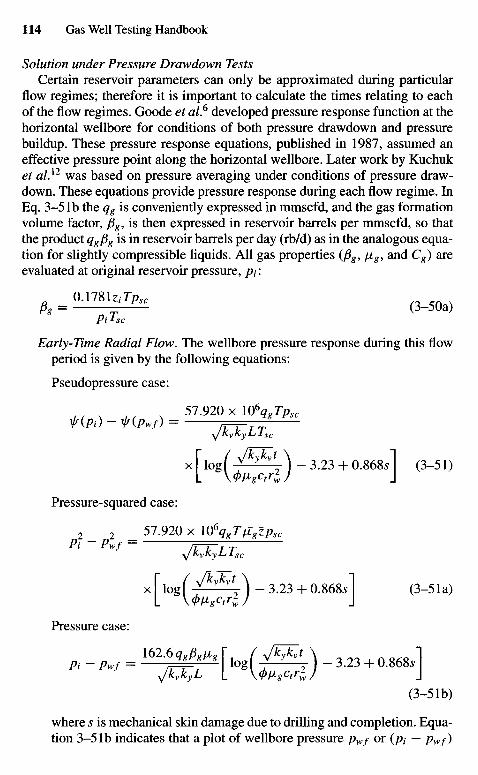
Solution under Pressure Drawdown TestsCertain reservoir parameters can only be approximated during particular
flow regimes; therefore it is important to calculate the times relating to eachof the flow regimes. Goode et al.6 developed pressure response function at thehorizontal wellbore for conditions of both pressure drawdown and pressurebuildup. These pressure response equations, published in 1987, assumed aneffective pressure point along the horizontal wellbore. Later work by Kuchuket al.12 was based on pressure averaging under conditions of pressure draw-down. These equations provide pressure response during each flow regime. InEq. 3-5 Ib the qg is conveniently expressed in mmscfd, and the gas formationvolume factor, fig9 is then expressed in reservoir barrels per mmscfd, so thatthe product qg/3g is in reservoir barrels per day (rb/d) as in the analogous equa-tion for slightly compressible liquids. AU gas properties (/3g, fig, and Cg) areevaluated at original reservoir pressure, /?,-:
ft = ( U T ^ T K ( J _ 5 0 a )
Pi * sc
Early-Time Radial Flow. The wellbore pressure response during this flowperiod is given by the following equations:
Pseudopressure case:
57.920 x l06qgTPscf(Pi) - if(Pwf) = nnriT —
x log ; y . -3 .23 + 0.868s (3-51)
Pressure-squared case:
2 2 _ 57.920 x l06qgTiIgzpscPi ~ Pwf = IkTLT
x log I y . - 3.23 + 0.8685 (3-5Ia)
Pressure case:
_ , ]^Mfi.LJfhL\ _ 3.23 + 0.868s]JETyL L \<l>tigC,rlJ J
(3-5Ib)
where 5 is mechanical skin damage due to drilling and completion. Equa-tion 3-5 Ib indicates that a plot of wellbore pressure pwf or (p, — pwf)

versus log t will exhibit a semilog straight line with slope given by
mx = 1JZpHi?* (3-52)
-»/ /Cy /Cy Ld
The equivalent permeability in a vertical plane around the wellborecan be calculated as
1 6 2 . 6 g ^miL
Extrapolating the semilog straight line to t = 1 hour, the followingequation is obtained:
Pi - Phhr = m\\og( Kky ^) - 3.23 + 0.868*1 (3-54)
where pt is initial reservoir pressure, and p\^r is the pressure obtainedat t = 1 hour. Rearranging Eq. 3-54 gives
s = U51[PLZPl* - U - & +3.23)1 (3-55)
Using Eq. 3-55 one can estimate the skin factor s. If the reservoir isareal isotropic (kx =ky = kh), then using Eq. 3-52, we have
L ^ y = Lkeff=l62'6q^ (3-56)
mi
where keff (= y/khkv) is the effective reservoir permeability. Thus, if keff isknown, one can estimate producing well length Lw. Conversely, if produc-ing well length L is known by well logging, then one can calculate the ef-fective reservoir permeability. As mentioned earlier, this flow regime canbe short in duration and may be difficult to identify in field applications.
Intermediate-Time Linear Flow. Pressure response during this flow periodis given by
p,_p./ = | A / Z I Z + i l l ^ f t f e + s ) (3_57)Lh Y kyCp/jLgCt Ly/kyky
where sz is the pseudoskin factor caused by partial penetration in thevertical direction and is given by9
Sz = l n ( j M + 0 . 2 5 I n ^ ) - l n ( sin } ^ . \ _ L838 (3-58)
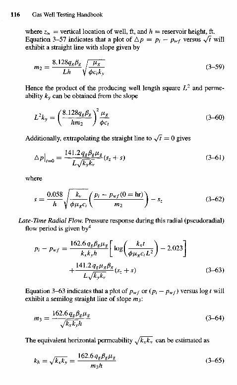
where zw = vertical location of well, ft, and h = reservoir height, ft.Equation 3-57 indicates that a plot of Ap = pi — pwf versus V7 willexhibit a straight line with slope given by
m 2 =!«ra: (3_59)Lh Y (pCfky
Hence the product of the producing well length square L2 and perme-ability ky can be obtained from the slope
= / 8 . 1 2 8 , , M ^ ( 3 _ 6 0 )
V hm2 J 4>Ct
Additionally, extrapolating the straight line to +Ji — 0 gives
A P U = 1 4 1 ; 2 ^ ' f a + J) (3-61)
where
s = O058 [JkT(P1-KfJO = hrA _
Late-Time Radial Flow. Pressure response during this radial (pseudoradial)flow period is given by4
162.6 qgpgng[ ( kxt \ I
t^ht.) (3-63,
Equation 3-63 indicates that a plot of /?wy or {pt — pwf) versus log t willexhibit a semilog straight line of slope my.
The equivalent horizontal permeability y/kxky can be estimated as
^ = JkJT,= 162'6*?'*' (3-65)
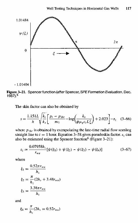
Figure 3-21. Spencer function (after Spencer, SPEFormation Evaluation, Dec.1987).6
The skin factor can also be obtained by
1.151L [kv"f Pi-plhr ( kx \ , ^ ^ ]s = — - — / — log — J + 2.023 -sz (3-66)
h ]f kxl m3 \</>tigctLlJ J
where p\hr is obtained by extrapolating the late-time radial flow semilogstraight line to t = 1 hour. Equation 3-58 gives pseudoskin factor. sz canalso be estimated using the Spencer function6 (Figure 3-21):
sz = a 0 7 9 5 8 f t ' W ( g i ) + № ) - f&) - ^ g 4 ) ] (3-67)F w a
where
0.52jirwa
Ii = ;
2 = ^ ( 2 ^ + 3.48^)
3.38jrrwa
?3 = ;hz
and
h = ?-(2hs=0.52rwa)
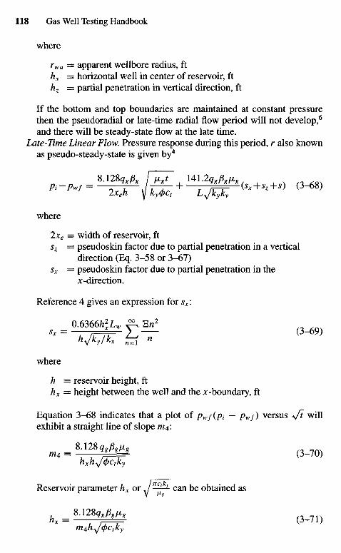
where
rwa = apparent wellbore radius, fths — horizontal well in center of reservoir, fthz = partial penetration in vertical direction, ft
If the bottom and top boundaries are maintained at constant pressurethen the pseudoradial or late-time radial flow period will not develop,6
and there will be steady-state flow at the late time.Late-Time Linear Flow. Pressure response during this period, r also known
as pseudo-steady-state is given by4
8.128^ft, / lint 141.2*7,,PxIIg2xeh y ky(/)ct Ly/kyky
where
2xe = width of reservoir, ftsz = pseudoskin factor due to partial penetration in a vertical
direction (Eq. 3-58 or 3-67)Sx = pseudoskin factor due to partial penetration in the
^-direction.
Reference 4 gives an expression for Sx:
where
h = reservoir height, fthx = height between the well and the x -boundary, ft
Equation 3-68 indicates that a plot of pwf{pt — pwf) versus \ft willexhibit a straight line of slope m^\
m 4 = 8 . 1 2 8 , A % ( 3_7 0 )
hxhyj4>ctky
Reservoir parameter hx or J ^ 1 can be obtained as
hx = 8 - 1 2 8 ^ ( 3 _ ? 1 )
or
\(t)ctky 8.128qg P8[Ig
Y №g m^h^/^Ctky
The skin factor s can be found from
, = « | l t e ) _ {Sx + Sz) (3_72)hhx Y (t>iXgCt \ m4 J
where pw/ (0 hr) is the pressure obtained at t = 0 hour.
Solution under Pressure Buildup Tests
Early-Time Radial Flow. Pressure buildup response during this flow periodis given by the following equations:
Infinite reservoir:
162.6 Qo^o[IA, / % + AA "I ^ , _
"•-"••=^|^ i L i o s ( J ^-) + H <3-73)
where
" = T S I M T ^ T T ) - 2-023l - l0S(f)h\\kx\_ \<p[xgctLlJ J
- logf/^^.) + 3.227 + 0.869s,
Equation 3-73 indicates that a plot of Ap versus l o g ( ^ f
f ) will exhibit
a semilog straight line with slope, m\r, given by
162.6 qgpgligm\r = nrj-j (3-/4)
-t/ ACy »C-y 2-/
The equivalent permeability in the vertical plane can be estimated by
/!62.6,^y (3_?5)
Extrapolating the semilog straight line to t = 1 hour, the following equa-tion is obtained to estimate s:
s = 1 1 5 1 rp^-^/_ l o g /_M^\ + 3 2 3 i (3_76)
Finite (bounded) reservoir:
162.6 qgPgfjLg F1 (U + AA 1pf - Pws = T = T ^ log J L — ~ ) + K2 (3-77)
y/kykyL I \ At J J
where
n _ ^ / ^ - 1 O g ( ^ ) + 3.227 + 0.868fe + «)
Equation 3-76 gives s.Intermediate-Time Linear Flow. Pressure buildup response during this flow
period is given by the following equations:
Infinite reservoir, first linear flow:
8.128 ft & j/jioAt
Pt - P^s = — r r ^ J r V - + w (3-78)
hL y ky(j)ct
where
A plot of Ap versus +/Ki will exhibit a slope given by
mu = SAlS^8 ( 3 _ 7 9 )
ft * / /Cy fv-y
The equivalent permeability in the vertical plane can be calculated by
_ /UMV (3_S0)
The skin factor s is given by
_ 0.058 firi>i f t r-/wl/z Y VgCt L m i / J
Finite (bounded) reservoir:
Pi ~ Pws = — J1 , I V A^ : IhL y ky<pct \ hx J
+ '4 ' ;2^i"S, (3-82,
Using Eq. 3-81 gives sx:Late-Time Radial Flow. Pressure buildup response during this flow period
is given by the following equations:
Infinite reservoir:
p,_p,., = ]^№[, o g (^ ) l ( 3_S3)
A plot of pws versus l o g ( ^ A * ) will exhibit a straight line with slopegiven by
m2r = 1 6 2 " 6 ^ (3-84)fl -\/ /vy »vy
The skin factor s is given by
, , ! ^ & £ » ^ _ loE(-A-,) + 2.023] - S1h y kxl m2r \(/)figctL
2J J
(3-85)
Finite (bounded) reservoir:
Pi - pws = — SJ. log ^ + y4\ (3-86)
where
y4 = A / ^ - l o g f - ^ ) + 2.023 + 0.868,z
Calculate s using Eq. 3-85. Generally, only the initial part of the Hornerplot generated by Eq. 3-86 will be a straight line.
Late-Time Linear Flow. During this flow period the infinite reservoir casedoes not exist (pseudoradial flow) and the pressure buildup response fora finite (bounded) reservoir is given by
_ Pws = *M*^rEftf _ yz7) (3-87)hhX Y Ky(J)Ct
A plot of pws versus (*Ji — fKi) will produce a straight line that willextrapolate to pt while a plot of Ap versus («/t — <sfKi) will exhibit a
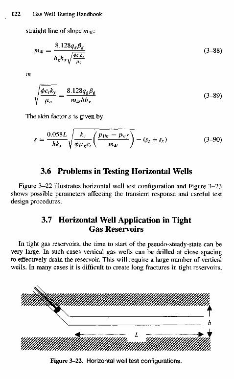
straight line of slope m^:
m4l = ^ = L (3-88)
or
l(/)ctky SA2SqsBsZ±Z = J ^ L ( 3_ 8 9 )Y fio mAihhx
The skin factor s is given by
0.058L [~kv (pxhr - Pw f\s = -rr-J ^ - f )-(Sz + sx) (3-90)
3.6 Problems in Testing Horizontal Wells
Figure 3-22 illustrates horizontal well test configuration and Figure 3-23shows possible parameters affecting the transient response and careful testdesign procedures.
3.7 Horizontal Well Application in TightGas Reservoirs
In tight gas reservoirs, the time to start of the pseudo-steady-state can bevery large. In such cases vertical gas wells can be drilled at close spacingto effectively drain the reservoir. This will require a large number of verticalwells. In many cases it is difficult to create long fractures in tight reservoirs,
Figure 3-22. Horizontal well test configurations.
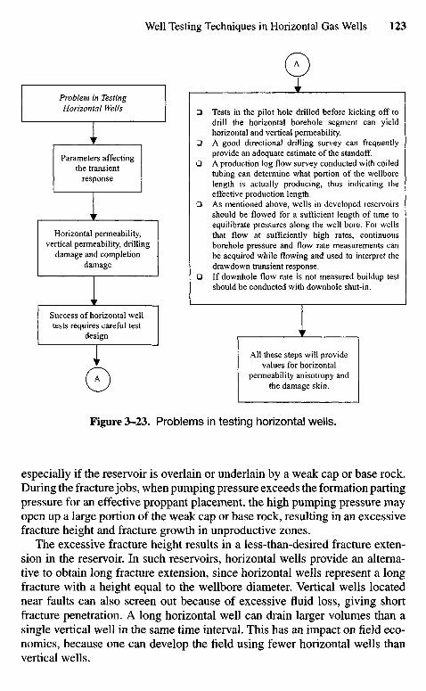
Figure 3-23. Problems in testing horizontal wells.
especially if the reservoir is overlain or underlain by a weak cap or base rock.During the fracture jobs, when pumping pressure exceeds the formation partingpressure for an effective proppant placement, the high pumping pressure mayopen up a large portion of the weak cap or base rock, resulting in an excessivefracture height and fracture growth in unproductive zones.
The excessive fracture height results in a less-than-desired fracture exten-sion in the reservoir. In such reservoirs, horizontal wells provide an alterna-tive to obtain long fracture extension, since horizontal wells represent a longfracture with a height equal to the wellbore diameter. Vertical wells locatednear faults can also screen out because of excessive fluid loss, giving shortfracture penetration. A long horizontal well can drain larger volumes than asingle vertical well in the same time interval. This has an impact on field eco-nomics, because one can develop the field using fewer horizontal wells thanvertical wells.
Problem in TestingHorizontal Wells
Parameters affectingthe transient
response
Horizontal permeability,vertical permeability, drilling
damage and completiondamage
Success of horizontal welltests requires careful test
design
A
Tests in the pilot hole drilled before kicking off todrill the horizontal borehole segment can yieldhorizontal and vertical permeability.A good directional drilling survey can frequentlyprovide an adequate estimate of the standoff.A production log flow survey conducted with coiledtubing can determine what portion of the wellborelength is actually producing, thus indicating theeffective production length.As mentioned above, wells in developed reservoirsshould be flowed for a sufficient length of time toequilibrate pressures along the well bore. For wellsthat flow at sufficiently high rates, continuousborehole pressure and flow rate measurements canbe acquired while flowing and used to interpret thedrawdown transient response.If downhole flow rate is not measured buildup testshould be conducted with downhole shut-in.
All these steps will providevalues for horizontal
permeability anisotropy andthe damage skin.
A
3.8 Influence of Turbulence in High-PermeabilityGas Wells
Horizontal wells are also useful in high-permeability gas wells, especiallyin those wells when near-wellbore turbulence is very high. The near-wellboreturbulence is inversely proportional to the well's perforated interval. By drillinga horizontal well, one can increase productive length and therefore decreasethe near-wellbore turbulence and enhance well productivity.
Turbulent Flow
Darcy's law of flow through porous media is valid only for laminar flowthrough the reservoir:
dp/dr = av (3-91)
where v is velocity, a is a constant, and dp/dr is pressure gradient. Forchheimermodified Darcy's law to account for turbulence effects:
dp/dr =av+ bv2 (3-92)
Equation 3-92 can be rewritten as either:
p2
R-plf=aqg + bq2
g (3-93)
or
fCPR) - ir(Pwf) = a'qg + b'q] (3-94)
where
5 0 3 3 7 x 1 0 ^ 2 7 ^ T (re\ /Ia = — № — r w) ~ °-75+s+SCA -c J (3"95)
^ 5 0 . 3 3 7 x 1 0 3 ^ ^ ^ ( 3 _ % )
khTsc
0 , = 50.337 x •tfrfi.r^x a w + 1 + ^ _ c,1 ( 3 _ 9 7 )
khTsc L VwJ J
v _ 50.337 x ^TP,, D ( 3 _ 9 g )
khTsc
In the foregoing equations, definitions of SQA and d depend upon the typeof the well as defined earlier. D is the turbulence factor in units of 1/mscfdand is defined in Eq. 3-18. Equations 3-93 and 3-94 tell us that the influenceof turbulence is to increase the pressure drop or pressure drawdown required
to produce the given gas production rate. Thus, the presence of turbulencereduces net production from a well. Reducing fluid velocity near the wellborecan minimize the turbulence effect. If there is no turbulence near the wellbore,there will be no turbulence in the reservoir. The fluid velocity near the wellborecan be minimized by increasing perforated producing length hp. A horizontalwell provides a means to significantly enhance perforated interval and reducenear-wellbore turbulence.
3,9 Turbulence Identification
A multirate test can be used to confirm the existence of high-velocity effectsin a well. Flow tests are conducted with different surface pressures. At eachpressure a stabilized gas flow rate qsc is recorded. Based on surface pressureand flow rate, downhole well flowing pressure pwf is estimated. The data arecorrelated as
qsc = C(Pl - p2wf)" (3-99)
where C is a constant and n is a dimensionless constant (1/2 < n < 1).Equation 3-99 is rewritten as
In qsc = In C + ln (p | - p2wf)
n (3-100)
If slope n = l, then there is no turbulence. However, if n < 1, turbulencedoes exist. The lower the value of n, the higher is the turbulence effect, andwhen n = 0.5 turbulence is dominant. It is important to use pseudopressure(is(p) values) when pressure is above 2500 psia.
3.10 Inflow Performance Responses in Verticaland Horizontal Gas Wells
The following example will illustrate the inflow performance responses inboth vertical and horizontal gas wells.
Example 3-6 Inflow Performance Responses for Vertical and HorizontalWells
An engineer suggested drilling a 2000-ft-long horizontal gas well not onlyto reduce near-wellbore turbulence but also to ensure against water coning. De-velop inflow performance curves for vertical and horizontal wells. Assume thatthe gas reservoir is not in communication with the bottom water zone. The fol-lowing reservoir and gas properties are given:
reservoir = sandstone; reservoir temperature = 226°F; depth = 9011 ft;gas gravity (air = 1.0) = 0.681; reservoir pressure = 1660 psia; pseudocrit-ical temperature = 370.0100R; reservoir thickness = 69 ft; pseudocritical
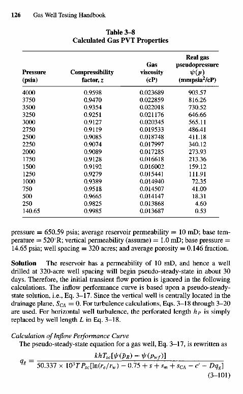
Table 3-8Calculated Gas PVT Properties
Real gasGas pseudopressure
Pressure Compressibility viscosity t/? (p)(psia) factor, z (cP) (mmpsia2/cP)
4000 0.9598 0.023689 903.573750 0.9470 0.022859 816.263500 0.9354 0.022018 730.523250 0.9251 0.021176 646.663000 0.9127 0.020345 565.112750 0.9119 0.019533 486.412500 0.9085 0.018748 411.182250 0.9074 0.017997 340.122000 0.9089 0.017285 273.931750 0.9128 0.016618 213.361500 0.9192 0.016002 159.121250 0.9279 0.015441 111.911000 0.9389 0.014940 72.35750 0.9518 0.014507 41.00500 0.9665 0.014147 18.31250 0.9825 0.013868 4.60140.65 0.9985 0.013687 0.53
pressure = 650.59 psia; average reservoir permeability = 10 mD; base tem-perature = 5200R; vertical permeability (assume) = 1 . 0 mD; base pressure =14.65 psia; well spacing = 320 acres; and average porosity = 0.146 fraction.
Solution The reservoir has a permeability of 10 mD, and hence a welldrilled at 320-acre well spacing will begin pseudo-steady-state in about 30days. Therefore, the initial transient flow portion is ignored in the followingcalculations. The inflow performance curve is based upon a pseudo-steady-state solution, i.e., Eq. 3-17. Since the vertical well is centrally located in thedrainage plane, SCA = 0. For turbulence calculations, Eqs. 3-18 through 3-20are used. For horizontal well turbulence, the perforated length hp is simplyreplaced by well length L in Eq. 3-18.
Calculation of Inflow Performance CurveThe pseudo-steady-state equation for a gas well, Eq. 3-17, is rewritten as
khTsc[\l/(pR) - jr(pwf)]9g ~ 50.337 x 10³TPsc[\n(re/rw) - 0.75 + s + sm + sCA - d - Dqg]
(3-101)
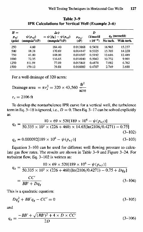
Table 3-9IPR Calculations for Vertical Well (Example 3-6)
H= Aip DPwf *KPwf) = *KPR) ~ 1>(Pwf) /**,, (l/mscfd Qg (mmscfd)
(psia) (mmpsia2/cP) (mmpsia2/cP) (cP) XlO"4) Noturb. Withturb.
250 4.60 184.40 0.013868 0.5431 16.965 15.237500 18.31 170.69 0.014147 0.5325 15.703 14.220750 41.00 148.00 0.014507 0.5192 13.616 12.489
1000 72.35 116.65 0.014940 0.5042 10.732 9.9811250 111.91 77.09 0.015441 0.4878 7.092 6.7621500 159.12 29.88 0.016002 0.4707 2.749 2.688
For a well drainage of 320 acres:
ft2Drainage area = 7tr2
p = 320 x 43,560acre
re = 2106 ft
To develop the nonturbulence IPR curve for a vertical well, the turbulenceterm in Eq. 3-18 is ignored, i.e., Z) -O. Then Eq. 3-17 can be solved explicitlyas
_ 10 x 69 x 520[189 x 106 - f{pwf)19g~ 50.335 x 103 x (226 + 460) x 14.65[ln(2106/0.4271) - 0.75]
(3-102)
qg = 0.000092[189 x 106 - 1r(pwf)] (3-103)
Equation 3-103 can be used for different well flowing pressure to calcu-late gas flow rates. The results are shown in Table 3-9 and Figure 3-24. Forturbulent flow, Eq. 3-102 is written as:
_ 10 x 69 x 520[189 x 106 - t(pwf)\qg~ 50.335 x 103 x (226 + 460)[ln(2106/0.4271) - 0.75 + Dq8]
CC
= WTWx <3-104)
This is a quadratic equation:
Dq] + BB'qg - CC' = 0 (3-105)
and
-2?Z?' + V( i? l?0 2 +4xPxCC 7
Vg = J^ (3-106)
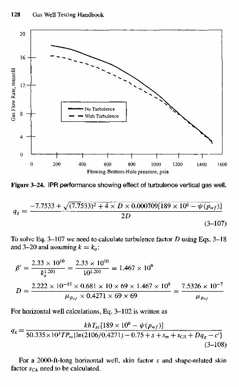
Flowing Bottom-Hole pressure, psia
Figure 3-24. IPR performance showing effect of turbulence vertical gas well.
_ -7.7533 + 7(7.7533)2 + 4 x D x 0.000709[189 x 106 - f(pwf)\qg~ ID
(3-107)
To solve Eq. 3-107 we need to calculate turbulence factor D using Eqs. 3-18and 3-20 and assuming k = ka:
, 2.33 x 10¹⁰ 2.33 x 10¹⁰ 9
P = tL20i = !Qi-201 = L 4 6 7 x 1 0
_ 2.222 x IQ"15 x 0.681 x 10 x 69 x 1.467 x IQ9 _ 7.5326 x 10~7
~ fiPwf x 0.4271 x 69 x 69 ~ ~^f
For horizontal well calculations, Eq. 3-102 is written as
= khTsc[lS9xl06-jf(Pwf)]q* 50.335 x 10377Uln(2106/0.4271) - 0.75 + s + sm + sCA + Dqg - cf]
(3-108)
For a 2000-ft-long horizontal well, skin factor s and shape-related skinfactor SCA need to be calculated.
No TurbulenceWith Turbulence
Gas
Flo
w R
ate,
mm
scfd
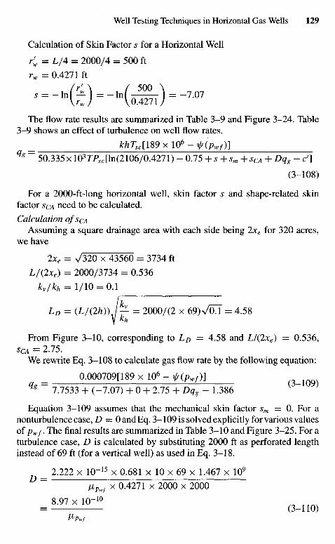
Calculation of Skin Factor s for a Horizontal Well
r'w = L/A = 2000/4 = 500 ft
rw = 0.4271 ft
- ^ ) - K 5 S r ) -The flow rate results are summarized in Table 3-9 and Figure 3-24. Table
3-9 shows an effect of turbulence on well flow rates.
= khTsc[lS9xl06-jr(pwf)]q% 50.335 x 10³rP,c[ln(2106/0.4271) - 0.75 + s + sm + sCA + Dq8 - c']
(3-108)
For a 2000-ft-long horizontal well, skin factor s and shape-related skinfactor SCA need to be calculated.
Calculation of SQAAssuming a square drainage area with each side being 2xe for 320 acres,
we have
2xe = V320 x 43560 = 3734 ft
LI(Ix6) = 2000/3734 = 0.536
kv/kh = 1/10 = 0.1
LD = (L/(2h)) — = 2000/(2 x 69)VaT = 4.58y kh
From Figure 3-10, corresponding to LD = 4.58 and L/(2xe) = 0.536,SCA = 2.75.
We rewrite Eq. 3-108 to calculate gas flow rate by the following equation:
= 0.000709[189 x IQ6 - jf(pwf)]qg 7.7533 + (-7.07) + 0 + 2.75 + Dqg - 1.386
Equation 3-109 assumes that the mechanical skin factor sm — 0. For anonturbulence case, D = O and Eq. 3-109 is solved explicitly for various valuesof pwf. The final results are summarized in Table 3-10 and Figure 3-25. For aturbulence case, D is calculated by substituting 2000 ft as perforated lengthinstead of 69 ft (for a vertical well) as used in Eq. 3-18.
_ 2.222 x 10~15 x 0.681 x 10 x 69 x 1.467 x 109
" /xPwf x 0.4271 x 2000 x 2000
= 8 - 9 7 x K r ' ° 0-110)
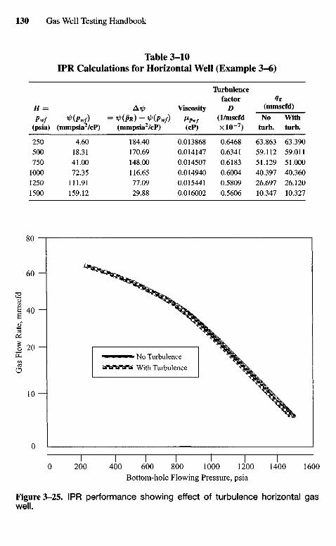
Table 3-10IPR Calculations for Horizontal Well (Example 3-6)
Tlirbiilencefactor Qg
H= AT/> Viscosity D (mmscfd)Pwf 1>(Pwf) = HPR) ~ *l>(Pwf) »pwf (l/mscfd No With
(psia) (mmpsia2/cP) (mmpsia2/cP) (cP) xlO~7) turb. turb.
250 4.60 184.40 0.013868 0.6468 63.863 63.390500 18.31 170.69 0.014147 0.6341 59.112 59.011750 41.00 148.00 0.014507 0.6183 51.129 51.000
1000 72.35 116.65 0.014940 0.6004 40.397 40.360
1250 111.91 77.09 0.015441 0.5809 26.697 26.1201500 159.12 29.88 0.016002 0.5606 10.347 10.327
Bottom-hole Flowing Pressure, psia
Figure 3-25. IPR performance showing effect of turbulence horizontal gaswell.
No Turbulence
With TurbulenceGas
Flo
w R
ate,
mm
scfd
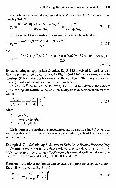
For turbulence calculations, the value of D from Eq. 3-110 is substitutedinto Eq. 3-109:
_ 0.000709[189 x 10 - f(Pwf)] _ CC9g ~ 2Ml+ Dq8 " BB' + Dqg ^ 1 l l )
Equation 3-111 is a quadratic equation, which can be solved as
- ^ + V W 2 + 4xDxCC7
Ig = jo (3-112)
and
-2.047 + >/(2.047)2 + 4 x D x 0.000709(189 x 106 - f(pwf)q* = Tb
(3-113)
By substituting an appropriate D value, Eq. 3-113 is solved for various wellflowing pressure, r/r(pWf), values. In Figure 3-25 inflow performance rela-tionships (IPR curves) for horizontal wells are shown. The plots are for twocases: (1) without turbulence and (2) with turbulence.
Celier et al.16 presented the following Eq. 3-114 to calculate the ratio ofpressure drop due to turbulence, i.e., non-Darcy flow, in horizontal and verticalwells:
(AP>M 2^ \hf (3 114)
<AP)Vf,- ( T + M I Jwhere
h = reservoir height, ftL = well length, ft
It is important to note that the preceding equation assumes that h ft of verticalwell is perforated in an /j-ft-thick reservoir; similarly, L ft of horizontal wellis open to flow.
Example 3-7 Calculating Reduction in Turbulence-Related Pressure DropDetermine reduction in turbulence related pressure drop in a 45-ft-thick,
10.0 mD reservoir by drilling a 2000-ft-long horizontal well. What would bethe pressure drop ratio if kv/kh = 0.01, 0.1, and 1.0?
Solution A ratio of horizontal and vertical well pressure drops due to non-Darcy flow is given in Eq. 3—115:
(Ap)h,t 2P2 Th f
XKp)Z = OTfT)8U8I (3"115)
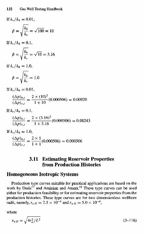
If kv/kh = 0.01,
\ikv/kh =0 .1 ,
If kv/kh = 1.0,
If kv/kh =0.01,
(ApW = 2 x (10)2 ( x ) o s o 6 = Q o o 9 2 o
(Ap)v>, 1 + 10Ifikv/jfc* =0 .1 ,
(ApW = 2x (3 .16 )^ ( o o o o 5 O 6 ) = Q o o 2 4 3
(Ap)VJ 1+3.16
If kv/kh = 1.0,
( A / 7 ) M = 1^1(0.000506) - 0.000506(Ap)v,r 1 + 1
3.11 Estimating Reservoir Propertiesfrom Production Histories
Homogeneous Isotropic Systems
Production type curves suitable for practical applications are based on thework by Duda17 and Aminian and Ameri.18 These type curves can be usedeither for production feasibility or for estimating reservoir properties from theproduction histories. These type curves are for two dimensionless wellboreradii, namely, rwp = 2.5 x 10~4 and rwD = 5.0 x 10~4,
where
rwD = fir*/L* (3-116)
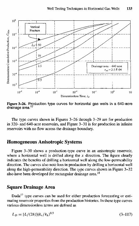
Dimensionless Time, tD
Figure 3-26. Production type curves for horizontal gas wells in a 640-acredrainage area.17
The type curves shown in Figures 3-26 through 3-29 are for productionin 320- and 640-acre reservoirs, and Figure 3-31 is for production in infinitereservoirs with no flow across the drainage boundary.
Homogeneous Anisotropic Systems
Figure 3-30 shows a production-type curve in an anisotropic reservoir,where a horizontal well is drilled along the x direction. The figure clearlyindicates the benefits of drilling a horizontal well along the low-permeabilitydirection. The curves also note loss in production by drilling a horizontal wellalong the high-permeability direction. The type curves shown in Figure 3-32also have been developed for rectangular drainage area.18
Square Drainage Area
Duda17 type curves can be used for either production forecasting or esti-mating reservoir properties from the production histories. In these type curvesvarious dimensionless terms are defined as
LD = [L/(2h)](kv/kh)°-5 (3-117)
Drainage area = 640 acrer w = 2.5E-04
VerticalFracture
Dim
ensi
onle
ss C
umul
ativ
e Pr
oduc
tion,
GPD
A
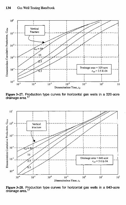
Dimensionless Time, tD
Figure 3-27. Production type curves for horizontal gas wells in a 320-acredrainage area.17
Dimensionless Time, tD
Figure 3-28. Production type curves for horizontal gas wells in a 640-acredrainage area.17
Drainage area = 640 acrerw=5.0E-04
VerticalFracture
Drainage area = 320 acrerwd = 2.5 E-04
VerticalFracture
Dim
ensi
onle
ss C
umul
ativ
e Pr
oduc
tion,
GPD
AD
imen
sion
less
Cum
ulat
ive
Prod
uctio
n, G
p DA
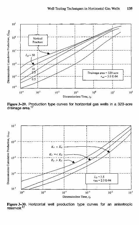
Dimensionless Time, tD
Figure 3-29. Production type curves for horizontal gas wells in a 320-acredrainage area.17
Dimensionless Time, tD
Figure 3-30. Horizontal well production type curves for an anisotropicreservoir.17
Drainage area = 320 acre/W=5.0E-04
VerticalFracture
Dim
ensi
onle
ss C
umul
ativ
e P
rodu
ctio
n, G
PDA
Dim
ensi
onle
ss C
umul
ativ
e P
rodu
ctio
n, G
PD
A

Dimensionless Time, tD
Figure 3-31. Production type curves for horizontal gas wells in an infinitereservoir.17
Dimensionless Time, tDA
Figure 3-32. Production type curve for horizontal gas well in a rectangularreservoir.18
VerticalFracture
Dim
ensi
onle
ss C
umul
ativ
e P
rodu
ctio
n, G
PDA
Dim
ensi
onle
ss c
umul
ativ
e pr
oduc
tion
, G
PD
A
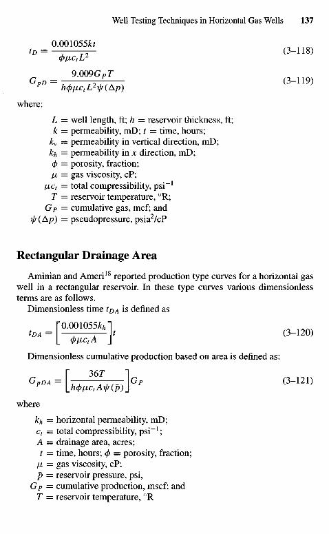
0.001Q55fatD ~ ~~L 7T~ (3-1 lo)
9M9GPTGpD = h^LhHAp) ( 3 " U 9 )
where:
L = well length, ft; h = reservoir thickness, ft;k = permeability, mD; t = time, hours;
kv = permeability in vertical direction, mD;kh = permeability in x direction, mD;0 — porosity, fraction;!A = gas viscosity, cP;
ixct — total compressibility, psi"1
T = reservoir temperature, 0R;Gp= cumulative gas, mcf; and
if (Ap) = pseudopressure, psia2/cP
Rectangular Drainage Area
Aminian and Ameri18 reported production type curves for a horizontal gaswell in a rectangular reservoir. In these type curves various dimensionlessterms are as follows.
Dimensionless time to A is defined as
["0.001055^1tDA = — j± \t (3-120)
Dimensionless cumulative production based on area is defined as:
T- T 7 7 - \Gp (3-121)
where
kh = horizontal permeability, mD;ct = total compressibility, psi"1;A = drainage area, acres;t = time, hours; 0 = porosity, fraction;
/a = gas viscosity, cP;p = reservoir pressure, psi,
Gp= cumulative production, mscf; andT = reservoir temperature, 0R
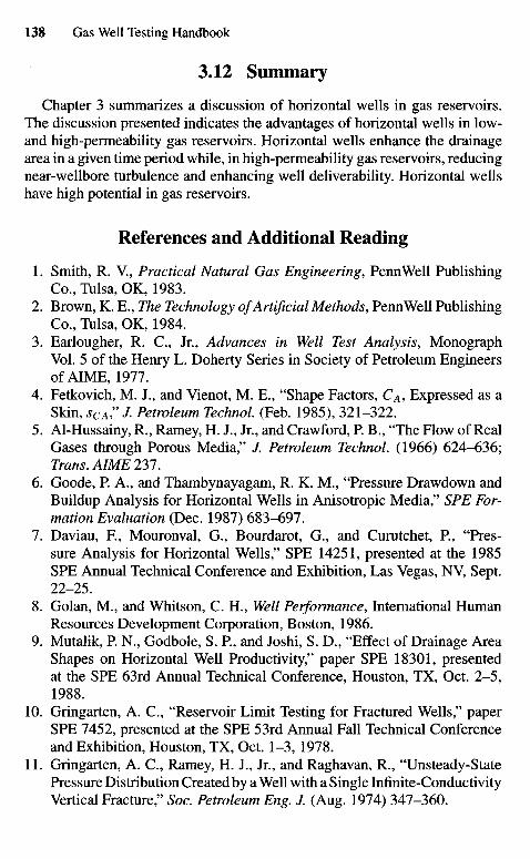
3.12 Summary
Chapter 3 summarizes a discussion of horizontal wells in gas reservoirs.The discussion presented indicates the advantages of horizontal wells in low-and high-permeability gas reservoirs. Horizontal wells enhance the drainagearea in a given time period while, in high-permeability gas reservoirs, reducingnear-wellbore turbulence and enhancing well deliverability. Horizontal wellshave high potential in gas reservoirs.
References and Additional Reading
1. Smith, R. V., Practical Natural Gas Engineering, PennWell PublishingCo., Tulsa, OK, 1983.
2. Brown, K. E., The Technology of Artificial Methods, PennWell PublishingCo., Tulsa, OK, 1984.
3. Earlougher, R. C, Jr., Advances in Well Test Analysis, MonographVol. 5 of the Henry L. Doherty Series in Society of Petroleum EngineersofAIME, 1977.
4. Fetkovich, M. J., and Vienot, M. E., "Shape Factors, CA, Expressed as aSkin, scA" J- Petroleum Technol (Feb. 1985), 321-322.
5. Al-Hussainy, R., Ramey, H. J., Jr., and Crawford, P. B., "The Flow of RealGases through Porous Media," /. Petroleum Technol. (1966) 624-636;Trans. AIME 237.
6. Goode, P. A., and Thambynayagam, R. K. M., "Pressure Drawdown andBuildup Analysis for Horizontal Wells in Anisotropic Media," SPE For-mation Evaluation (Dec. 1987) 683-697.
7. Daviau, F, Mouronval, G., Bourdarot, G., and Curutchet, P., "Pres-sure Analysis for Horizontal Wells," SPE 14251, presented at the 1985SPE Annual Technical Conference and Exhibition, Las Vegas, NV, Sept.22-25.
8. Golan, M., and Whitson, C. H., Well Performance, International HumanResources Development Corporation, Boston, 1986.
9. Mutalik, P. N., Godbole, S. P., and Joshi, S. D., "Effect of Drainage AreaShapes on Horizontal Well Productivity," paper SPE 18301, presentedat the SPE 63rd Annual Technical Conference, Houston, TX, Oct. 2-5,1988.
10. Gringarten, A. C, "Reservoir Limit Testing for Fractured Wells," paperSPE 7452, presented at the SPE 53rd Annual Fall Technical Conferenceand Exhibition, Houston, TX, Oct. 1-3, 1978.
11. Gringarten, A. C, Ramey, H. J., Jr., and Raghavan, R., "Unsteady-StatePressure Distribution Created by a Well with a Single Infinite-ConductivityVertical Fracture," Soc. Petroleum Eng. J. (Aug. 1974) 347-360.
12. Kuchuk, F. J., Goode, P. A., Wilkinson, D. J., and Thambynayagam,R. K. M., "Pressure Transient Behavior of Horizontal Wells with andwithout Gas Cap or Aquifer," paper SPE 17413, presented at the SPECalifornia Regional Meeting, Long Beach, CA, March 23-25, 1988.
13. Odeh, A. S., and Babu, D. K., "Transient Flow Behavior of HorizontalWells Pressure Drawdown and Buildup Analysis," SPE Formation Eval.(March 1990) 7-15.
14. Clonts, M. D., and Ramey, H. J., Jr., "Pressure Transient Analysis forWells with Horizontal Drainageholes," paper SPE 15116, presented at theSPE California Regional Meeting, Oakland, CA, April 2-4, 1986.
15. Ozkan, E., Raghavan, R., and Joshi, S. D., "Horizontal Well PressureAnalysis," SPE Formation Eval (Dec. 1989) 567-575.
16. Celier, G. C. M. R., Jouault, P., de Montigny, O. A. M. C, and Zuidwal,"A Gas Field Development with Horizontal Wells," paper SPE 19826,presented at the SPE 64th Annual Technical Conference and Exhibitionof the Society of Petroleum Engineers, San Antonio, TX, Oct. 8-11,1989.
17. Duda, J. R., "Type Curves for Predicting Production Performance fromHorizontal Wells in Low Permeability Gas Reservoirs," paper SPE 18993,Richardson, TX.
18. Aminian, K, and Ameri, S., "Predicting Horizontal Well Production Per-formance Using Type Curves," paper SPE 19342 presented at the SPEEastern Regional Meeting, Morgantown, WV, Oct. 1989.
Chapter 4
DeliverabilityTesting and WellProductionPotential AnalysisMethods
4.1 Introduction
This chapter discusses basic flow equations expressed in terms of the pseu-dopressure i/r(p) and of approximations to the pseudopressure approach thatare valid at high and low pressures. This is followed by deliverability testsof gas well flow-after-flow, isochronal, and modified isochronal deliverabilitytests including a simplified procedure for gas deliverability calculations usingdimensionless IPR curves. The purpose of this chapter is to provide a completereference work for various deliverability testing techniques. The mathemati-cal determinations of the equations are avoided; this role is filled much betterby other publications.1"2 Field examples are included to provide a hands-onunderstanding of various deliverability testing techniques, their interpretationsand their field applications.
4.2 Gas Flow in Infinite-Acting Reservoirs
References 1 and 3 have shown that gas flow in an infinite-acting reservoircan be expressed by an equation similar to that for flow of slightly compressibleliquids if pseudopressure \j/ (p) is used instead of pressure. The equation in SIunits is
*QV) = +(Pi) + 3.733gfl [l.lSl log (125-3^'C" r-)
-s + D\qg\\
In field units this equation becomes
VK/V) = V(Pi) + 50, 3 0 0 ^ ^J-sc KM
x[ 1 . 1 5Uo g - f a ( 1 ' 6 8 y») - , + Dte|] (4-,)
where the pseudopressure is defined by the integral
p
xlr(p) = 2 f -?-dp (4-2)J Vgz
PB
where /?# is some arbitrary low base pressure. To evaluate i/s(pWf) at somevalue of p, we can evaluate the integral in Eq. 4-2 numerically, using valuesfor /x and z for the specific gas under consideration, evaluated at reservoirtemperature. The term D\qg\ gives a non-Darcy flow pressure drop, i.e., ittakes into account the fact that, at high velocities near the producing well,Darcy's law does not predict correctly the relationship between flow rate andpressure drop. Therefore this additional pressure drop can be added to theDarcy's law pressure drop, just as pressure drop across the altered zone is, andD can be considered constant. The absolute value of qg, \qg\, is used so thatthe term D\qg\, is positive for either production or injection.
4.3 Stabilized Flow Equations
For stabilized3 (r, < re), flow,
xlr(Pwf) = jr(PR) - 1.422 x 1 0 6 ~ \In(y) ~ °'75 + s + D^SA
(4-3)
where PR is any uniform drainage-area pressure. Equations 4-1 and 4-3 pro-vide the basis for analysis of gas well tests. For p > 3000 psia, these equationsassume a simple form (in terms of pressure, p)\ for p < 2000 psia, they as-sume another simple form in terms of p2. Thus we can develop procedures foranalyzing gas well tests with equations in terms of if(p), /?, and p2. In mostof this chapter, equations will be written in terms of \js(p) and p2, not becausep2 is more generally applicable or more accurate (the equations in yj/ best fitthis role), but because the p2 equation illustrate the general method and permiteasier comparison with other methods of gas well test analysis. The stabalized
flow equation in terms of pressure squared is
PIf=P2R ~ 1-422 x i(fSf^Llin(^j -0J5 + s + D\qsc\\ (4-4)
Equations 4-3 and 4-4 are complete deliverability equations. Given a valueof flowing bottom-hole pressure, pwf, corresponding to a given pipeline orbackpressure, we can estimate the flow rate, qsc, at which the well will delivergas. However, certain parameters must be determined before the equations canbe used in this way. The well flows at rate qsc until n > re (stabilized flow). Inthis case, Eq. 4-3 has the form
IT(PR) ~ Ir(pyf) = Aqsc + Bq2sc (4-5)
where
A = 1.422 x 10⁶— \ln( — ) -0 .75 + J (4-6)khl \rwj J
and
B = 1.422 x 10⁶ — D (4-7)kh
Equation 4-4 has the form
P2R-plf=A'qsc + B'qi (4-8)
where
Ar = 1.422 x 1 0 6 ^ - I InI-) - 0.75 + J (4-9)kh L WJ J
B' = 1.422 x 1 0 6 ^ - D (4-10)kh
The constants A, J9, Af, and B' can be determined from flow tests for at leasttwo rates in which qsc and the corresponding value of pwf are measured; PRalso must be known.
4.4 Application of Transient Flow Equations
When rt < re, the flow conditions are said to be transient and for transientflow. In terms of pseudopressure:
t(PR) ~ f(Pwf) = Atqsc + Bq2sc (4-11)
where B has the same meaning as for stabilized flow and where At9 a functionof time, is given by
kh L KtPgiQrlJ J
In terms of pressure squared
p2R-p2
wf=Aftqsc + Bfql (4-13)
A; = 1.422 x 10 6 ^^ [ i / n f -)+s] (4-14)
Br = 1.422 x 1 0 6 ^ - D (4-15)kh
Titrbuleiice or Non-Darcy Effectson Completion Efficiency
Reference 3 can be applied to gas well testing to determine real or presenttime inflow performance relationships. No transient tests are required to eval-uate the completion efficiency, if this method is applied. Reference 3 alsosuggested methods to estimate the improvement in inflow performance whichwould result from re-perforating a well to lengthen the completion interval andpresents guidelines to determine whether the turbulent effects are excessive.Equation 4-13 can be divided by qsc and written as
p2 _ p2- 5 ^ = A' + B'qsc (4-15a)
qsc
where A! and B' are the laminar and turbulent coefficients, respectively, andare defined in Eqs. 4-9 and 4-10. From Eq. 4-15a, it is apparent that a plot of(P\ — P^f)/qsc versus qsc on Cartesian coordinates will yield a line that has aslope of B' and an intercept of Af = A(p2)/qsc as qsc approaches zero. Theseplots apply to both linear and radial flow, but definition of Af and B' woulddepend on the type of flow. In order to have some qualitative measure of theimportance of the turbulence contribution to the total drawdown. Reference3 suggested comparison of the value of A! calculated at the AOF of the well(AA), to the stabilized value of A'. The value of AA can be calculated from
AA = A! + B'(AOF) (4-15b)
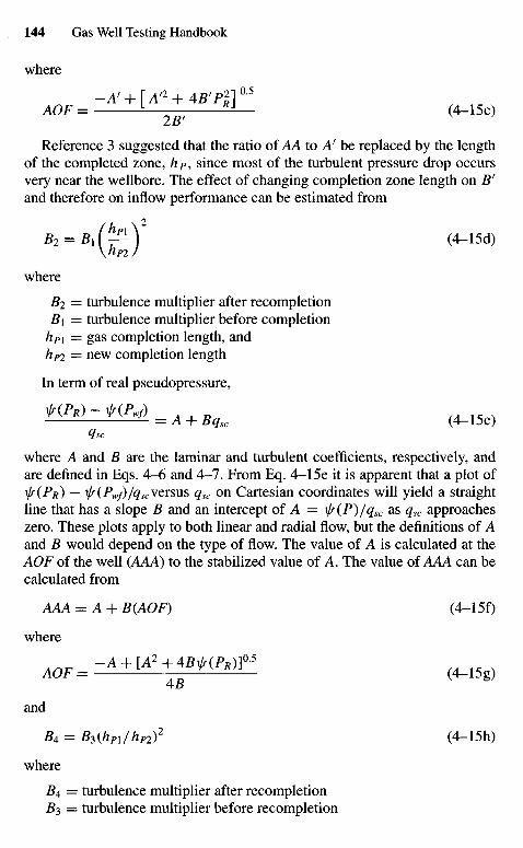
where
-A'+ {A*+4B1P*]0-5
AOF= l—^ ^ - (A-ISc)
Reference 3 suggested that the ratio of AA to A! be replaced by the lengthof the completed zone, /ip, since most of the turbulent pressure drop occursvery near the wellbore. The effect of changing completion zone length on B'and therefore on inflow performance can be estimated from
B2 = B1I-^j (4~15d)
where
B2 = turbulence multiplier after recompletionB\ = turbulence multiplier before completion
hP\ = gas completion length, andhP2 = new completion length
In term of real pseudopressure,
J— = A + Bqsc (4-15e)qsc
where A and B are the laminar and turbulent coefficients, respectively, andare defined in Eqs. 4-6 and 4-7. From Eq. 4-15e it is apparent that a plot of^(PR) — f (Pwf)/qscversus qsc on Cartesian coordinates will yield a straightline that has a slope B and an intercept of A = iff(P)/qsc as qsc approacheszero. These plots apply to both linear and radial flow, but the definitions of Aand B would depend on the type of flow. The value of A is calculated at theAOF of the well (AAA) to the stabilized value of A. The value of AAA can becalculated from
AAA = A + B(AOF) (4-15f)
where
An* - A + [A2+ 4BiA(^)]0 5 (A _ ,
AOF = — (4-15g)
and
B4 = B3(hPl/hP2)2 (4-15h)
whereB4 = turbulence multiplier after recompletion#3 = turbulence multiplier before recompletion
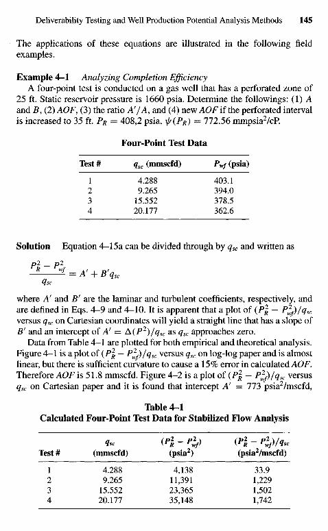
The applications of these equations are illustrated in the following fieldexamples.
Example 4-1 Analyzing Completion EfficiencyA four-point test is conducted on a gas well that has a perforated zone of
25 ft. Static reservoir pressure is 1660 psia. Determine the followings: (1) Aand # , (2) AOF, (3) the ratio A'/A, and (4) new AOF if the perforated intervalis increased to 35 ft. PR = 408,2 psia, ^ (PR) = 772.56 mmpsia2/cP.
Four-Point Test Data
Test # qsc (mmscfd) Pwf (psia)
1 4.288 403.12 9.265 394.03 15.552 378.54 20.177 362.6
Solution Equation 4-15a can be divided through by qsc and written as
^ - ^ = A' + B'qscqsc
where A! and B! are the laminar and turbulent coefficients, respectively, andare defined in Eqs. 4-9 and 4-10. It is apparent that a plot of (P\ — P^f)/qsc
versus qsc on Cartesian coordinates will yield a straight line that has a slope ofB' and an intercept of A! — A(P2)/qsc as qsc approaches zero.
Data from Table 4-1 are plotted for both empirical and theoretical analysis.Figure 4-1 is a plot of ( P | — P^J)/qsc versus qsc on log-log paper and is almostlinear, but there is sufficient curvature to cause a 15% error in calculated AOF.Therefore AOF is 51.8 mmscfd. Figure 4-2 is a plot of (P% — P^)/qsc versusqsc on Cartesian paper and it is found that intercept A! = 773 psia2/mscfd,
Table 4-1Calculated Four-Point Test Data for Stabilized Flow Analysis
Test# (mmscfd) (psia2) (psia2/mscfd)
1 4.288 4,138 33.92 9.265 11,391 1,2293 15.552 23,365 1,5024 20.177 35,148 1,742
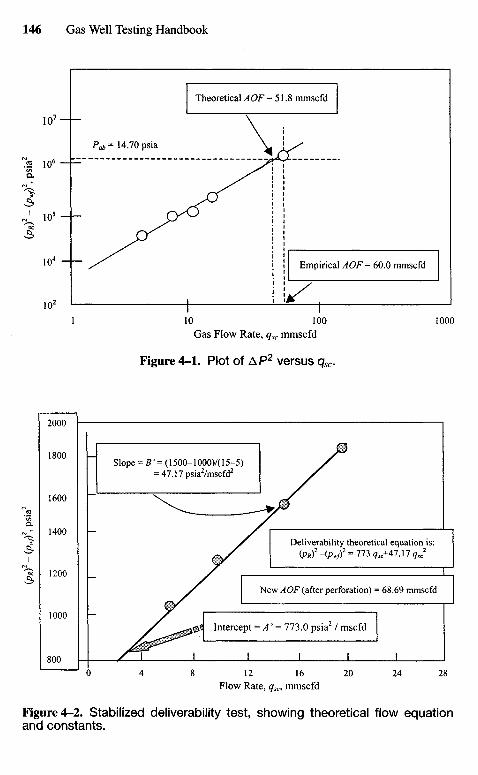
Gas Flow Rate, qsc mmscfd
Figure 4-1. Plot of AP2 versus qsc.
Flow Rate, qsc, mmscfd
Figure 4-2. Stabilized deliverability test, showing theoretical flow equationand constants.
Intercept = A' = 773.0 psia2 / mscfd
New A OF (after perforation) = 68.69 mmscfd
Deliverability theoretical equation is:( P K ) 2 - W ) 2 = 7 7 3 <7~+47.17<7 J C
2
Slope = B' = (1500-1000)/(15-5)= 47.17 psia2/mscfd2
Empirical AOF = 60.0 mmscfd
Theoretical AOF = 51.8 mmscfd
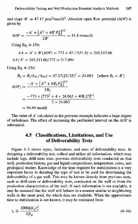
and slope Br = 47.17 psia2/mscfd2. Absolute open flow potential (AOF) isgiven by
-A' + [A'2 + 4B'P*f5
AOF = != ^ - = 51.8 mmscfd2Br
Using Eq. 4-15b:
AA = Af + B'(AOF) = 773 + 47.17(51.8) = 245,113.60
AAIA! = 245,113.60/773 = 317.094
Using Eq. 4-15d:
B2 = Bx(hPX/hp2) = 47.17(25/35)2 = 24.063 [where B1 = B']
-A'+ \Aa+AB2PIf5
_ -113 + [7732 + 4 x 24.063 x 408.22]0-5
~ 2 x 24.063
= 68.69 mscfd
The value of A' calculated in the previous example indicates a large degreeof turbulence. The effect of increasing the perforated interval on the AOF issubstantial.
4.5 Classifications, Limitations, and Useof Deliverability Tests
Figure 4-3 shows types, limitations, and uses of deliverability tests. Indesigning a deliverability test, collect and utilize all information, which mayinclude logs, drill-stem tests, previous deliverability tests conducted on thatwell, production history, gas and liquid compositions, temperature, cores, andgeological studies. Knowledge of the time required for stabilization is a veryimportant factor in deciding the type of test to be used for determining thedeliverability of a gas well. This may be known directly from previous tests,such as drill-stem or deliverability tests, conducted on the well or from theproduction characteristics of the well. If such information is not available, itmay be assumed that the well will behave in a manner similar to neighboringwells in the same pool, for which data are available. When the approximatetime to stabilization is not known, it may be estimated from
10000/x.r,2
ts = Y=-1^ <4"16)kpR
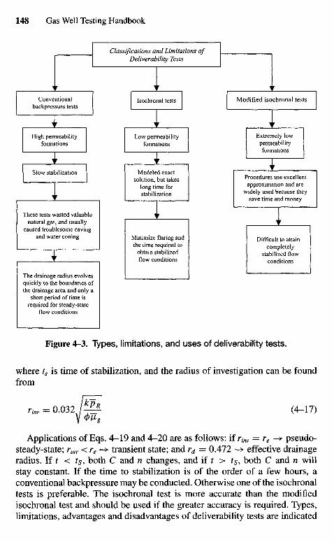
Figure 4-3. Types, limitations, and uses of deliverability tests.
where ts is time of stabilization, and the radius of investigation can be foundfrom
rinv = 0.032 / ^ (4-17)
Applications of Eqs. 4-19 and 4-20 are as follows: if rinv — re^^ pseudo-steady-state; rinv <re-* transient state; and rj = 0.472 -> effective drainageradius. If t < ts, both C and n changes, and if t > ts, both C and n willstay constant. If the time to stabilization is of the order of a few hours, aconventional backpressure may be conducted. Otherwise one of the isochronaltests is preferable. The isochronal test is more accurate than the modifiedisochronal test and should be used if the greater accuracy is required. Types,limitations, advantages and disadvantages of deliverability tests are indicated
Conventionalbackpressure tests
High permeabilityformations
Slow stabilization
These tests wasted valuablenatural gas, and usually
caused troublesome cavingand water coning
The drainage radius evolvesquickly to the boundaries ofthe drainage area and only a
short period of time isrequired for steady-state
flow conditions
Isochronal tests
Low permeabilityformations
Modeled exactsolution, but takes
long time forstabilization
Minimize flaring andthe time required to
obtain stabilizedflow conditions
Modified isochronal tests
Extremely lowpermeabilityformations
Procedures use excellentapproximation and are
widely used because theysave time and money
Difficult to attaincompletely
stabilized flowconditions
Classifications and Limitations ofDeliverability Tests
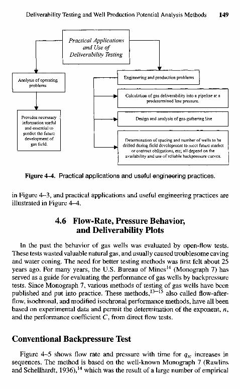
Figure 4-4. Practical applications and useful engineering practices.
in Figure 4-3, and practical applications and useful engineering practices areillustrated in Figure A-A.
4.6 Flow-Rate, Pressure Behavior,and Deliverability Plots
In the past the behavior of gas wells was evaluated by open-flow tests.These tests wasted valuable natural gas, and usually caused troublesome cavingand water coning. The need for better testing methods was first felt about 25years ago. For many years, the U.S. Bureau of Mines14 (Monograph 7) hasserved as a guide for evaluating the performance of gas wells by backpressuretests. Since Monograph 7, various methods of testing of gas wells have beenpublished and put into practice. These methods,13"15 also called flow-after-flow, isochronal, and modified isochronal performance methods, have all beenbased on experimental data and permit the determination of the exponent, n,and the performance coefficient C, from direct flow tests.
Conventional Backpressure Test
Figure 4-5 shows flow rate and pressure with time for qsc increases insequences. The method is based on the well-known Monograph 7 (Rawlinsand Schellhardt, 1936),14 which was the result of a large number of empirical
Engineering and production problems
Calculation of gas deliverability into a pipeline at apredetermined line pressure.
Design and analysis of gas-gathering line
Determination of spacing and number of wells to bedrilled during field development to meet future market
or contract obligations, etc; all depend on theavailability and use of reliable backpressure curves.
Analysis of operatingproblems
Provides necessaryinformation useful
and essential topredict the futuredevelopment of
gas field.
Practical Applicationsand Use of
Deliverability Testing
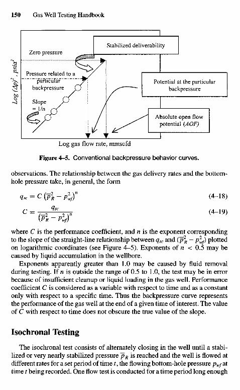
Log gas flow rate, mmscfd
Figure 4-5. Conventional backpressure behavior curves.
observations. The relationship between the gas delivery rates and the bottom-hole pressure take, in general, the form
qsc = C (p2R - p2
wf)n (4-18)
C = 2qsc
n (4-19)(PR ~ Plf)
where C is the performance coefficient, and n is the exponent correspondingto the slope of the straight-line relationship between qsc and (~p2
R — /?L) plottedon logarithmic coordinates (see Figure 4-5). Exponents of n < 0.5 may becaused by liquid accumulation in the wellbore.
Exponents apparently greater than 1.0 may be caused by fluid removalduring testing. If n is outside the range of 0.5 to 1.0, the test may be in errorbecause of insufficient cleanup or liquid loading in the gas well. Performancecoefficient C is considered as a variable with respect to time and as a constantonly with respect to a specific time. Thus the backpressure curve representsthe performance of the gas well at the end of a given time of interest. The valueof C with respect to time does not obscure the true value of the slope.
Isochronal Testing
The isochronal test consists of alternately closing in the well until a stabi-lized or very nearly stabilized pressure ~pR is reached and the well is flowed atdifferent rates for a set period of time t, the flowing bottom-hole pressure pwf attime t being recorded. One flow test is conducted for a time period long enough
Absolute open flowpotential (AOF)
Potential at the particularbackpressure
Stabilized deliverabilityZero pressure
Pressure related to aparticular
backpressure
Slope= 1/n
Log
(A
p)2,
psi
a2
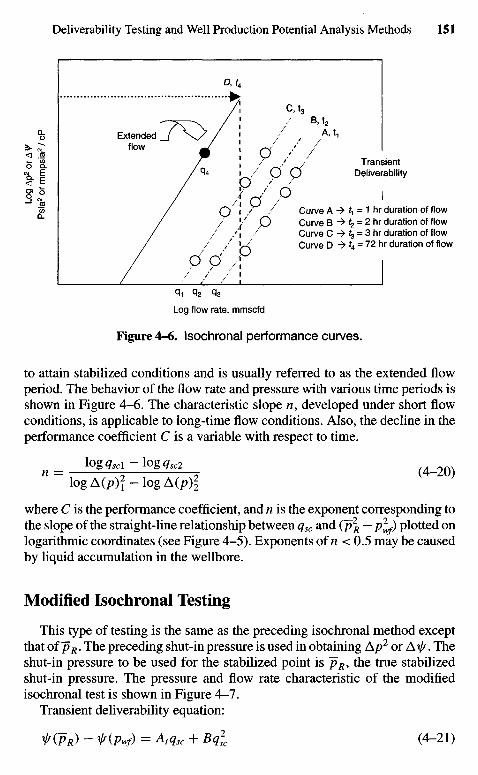
Log flow rate, mmscfd
Figure 4-6. Isochronal performance curves.
to attain stabilized conditions and is usually referred to as the extended flowperiod. The behavior of the flow rate and pressure with various time periods isshown in Figure 4-6. The characteristic slope n, developed under short flowconditions, is applicable to long-time flow conditions. Also, the decline in theperformance coefficient C is a variable with respect to time.
n = 1 O g ^ " 1 O g ^ 2 2 (4-20)
log A(P)? - log A(p)2
where C is the performance coefficient, and n is the exponent corresponding tothe slope of the straight-line relationship between qsc and (~p2
R — pfy plotted onlogarithmic coordinates (see Figure 4-5). Exponents of n < 0.5 may be causedby liquid accumulation in the wellbore.
Modified Isochronal Testing
This type of testing is the same as the preceding isochronal method exceptthat of ~pR. The preceding shut-in pressure is used in obtaining A/?2 or A \j/. Theshut-in pressure to be used for the stabilized point is ~pR, the true stabilizedshut-in pressure. The pressure and flow rate characteristic of the modifiedisochronal test is shown in Figure 4-7.
Transient deliverability equation:
IT(PR) - t(Pwf) = Msc + Bq2sc (4-21)
Curve A -> 1 = 1 hr duration of flowCurve B -> ^ = 2 h r duration of flowCurve C -> t3 = 3 hr duration of flowCurve D -> tA = 72 hr duration of flow
TransientDeliverability
Extendedflow
Log
Ap2
or
AV
Psi
a2 o
r m
mps
ia2 /
cP
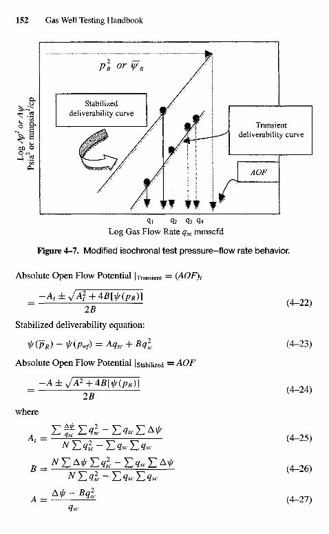
qi q2 q3 q4
Log Gas Flow Rate qsc mmscfd
Figure 4-7. Modified isochronal test pressure-flow rate behavior.
Absolute Open Flow Potential |Transient = (AOF)t
= -At±jAt + 4B№(PR)] ( 4 _ 2 2 )
2,B
Stabilized deliverability equation:
f(PR) ~ ^(/V) = A(lsc + BqI (4-23)
Absolute Open Flow Potential !stabilized = AOF
= -A±JA2 + 4B№(PR)] (4_24)
IB
where
B. "^tuA-j:^* (4_26)
A = A ^ ~~ B9sc (4-27)«5C
/^OF
Transientdeliverability curve
Stabilizeddeliverability curve
Log
Ap2
or
Ay/
Psi
a2 or
mm
psia
2/cp
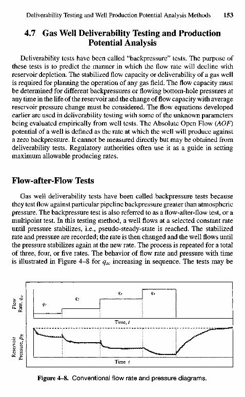
4.7 Gas Well Deliverability Testing and ProductionPotential Analysis
Deliverability tests have been called "backpressure" tests. The purpose ofthese tests is to predict the manner in which the flow rate will decline withreservoir depletion. The stabilized flow capacity or deliverability of a gas wellis required for planning the operation of any gas field. The flow capacity mustbe determined for different backpressures or flowing bottom-hole pressures atany time in the life of the reservoir and the change of flow capacity with averagereservoir pressure change must be considered. The flow equations developedearlier are used in deliverability testing with some of the unknown parametersbeing evaluated empirically from well tests. The Absolute Open Flow (AOF)potential of a well is defined as the rate at which the well will produce againsta zero backpressure. It cannot be measured directly but may be obtained fromdeliverability tests. Regulatory authorities often use it as a guide in settingmaximum allowable producing rates.
Flow-after-Flow Tests
Gas well deliverability tests have been called backpressure tests becausethey test flow against particular pipeline backpressure greater than atmosphericpressure. The backpressure test is also referred to as a flow-after-flow test, or amultipoint test. In this testing method, a well flows at a selected constant rateuntil pressure stabilizes, i.e., pseudo-steady-state is reached. The stabilizedrate and pressure are recorded; the rate is then changed and the well flows untilthe pressure stabilizes again at the new rate. The process is repeated for a totalof three, four, or five rates. The behavior of flow rate and pressure with timeis illustrated in Figure 4-8 for qsc increasing in sequence. The tests may be
Figure 4-8. Conventional flow rate and pressure diagrams.
Time t
Time, t
Flow
Rat
e, q
sc
Res
ervo
irPr
essu
re, P
R
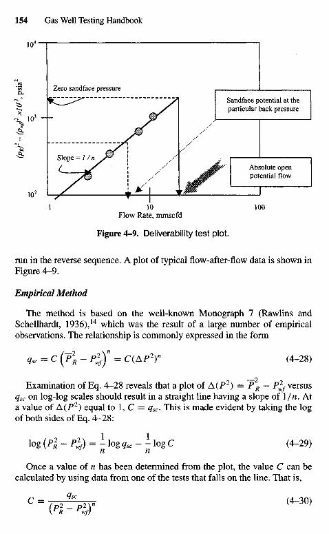
Flow Rate, mmscfd
Figure 4-9. Deliverability test plot.
run in the reverse sequence. A plot of typical flow-after-flow data is shown inFigure 4-9.
Empirical Method
The method is based on the well-known Monograph 7 (Rawlins andSchellhardt, 1936),14 which was the result of a large number of empiricalobservations. The relationship is commonly expressed in the form
qsc = C(J2R- Pl)J1 = C(AP2T (4-28)
Examination of Eq. 4-28 reveals that a plot of A(P2) = P^ — P\ versusqsc on log-log scales should result in a straight line having a slope of l/n. Ata value of A(P2) equal to 1, C — qsc. This is made evident by taking the logof both sides of Eq. 4-28:
log (P2 - Plf) = 1 log qsc " ^ log C (4-29)
Once a value of n has been determined from the plot, the value C can becalculated by using data from one of the tests that falls on the line. That is,
c = ( p 2 ! > r <4-3°)VR 1^Wf)
Absolute openpotential flow
Sandface potential at theparticular back pressure
Zero sandface pressure
Slope = l/n
For wells in which turbulence is important, the value of n approaches 0.5,whereas for wells in which turbulence is negligible, n is obtained from welltests will fall between 0.5 and 1.0. If the values for the flow coefficient C andexponent n can be determined, the flow rate corresponding to any value ofPWf can be calculated and an inflow performance curve can be constructed. Aparameter commonly used to characterize or compare gas wells is the flow ratethat would occur if PWf could be brought to zero. This is called the absoluteopen low potential, or AOF.
Theoretical Methods
The plot of A(P2) versus log qsc that we have discussed so far are based onempirical correlations of field data. Extrapolation of the deliverability curvemuch beyond the range of test data may be required to estimate AOF. An AOFdetermined from such a lengthy extrapolation may be incorrect. The apparentline of the deliverability curve should be slightly concave with unit slope at lowflow rates and somewhat greater slope at high flow rates. The change of slopeis because of increased turbulence near the wellbore and changes in the rate-dependent skin factor as the flow rate increases. Based on this analysis, a plotof AP/qsc, AP2/qSXCi x//(AP)/qsc versus qsc on Cartesian coordinate papershould be a straight line with slope b and intercept a. The AOF determinedusing this curve should be in less error. The deliverability equations9 in thiscase are as follows:
Case 1: Using pressure solution technique:
AP=~PR- Pwf = axqsc + bxq]c (4-31)
Case 2: Using pressure-squared technique:
AP2 = T\ - Plf = a2qsc + b2ql (4-32)
Case 3: Using pseudopressure technique:
V(AP) = V(P*) - ^(Pwf) = a3qsc + b3ql (4-33)
Interpreting Flow Tests
More information, and greater accuracy, can result from the proper conduct-ing and analysis of tests. It will be shown in a later section that the analysisof data from an isochronal type test using the laminar-inertial-turbulent (LIT)flow equation will yield considerable information concerning the reservoir inaddition to providing reliable deliverability data. This may be achieved evenwithout conducting the extended flow test, which is normally associated with
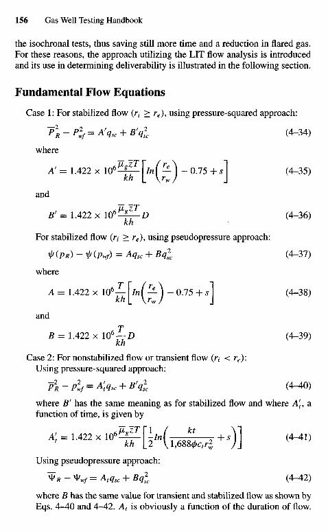
the isochronal tests, thus saving still more time and a reduction in flared gas.For these reasons, the approach utilizing the LIT flow analysis is introducedand its use in determining deliverability is illustrated in the following section.
Fundamental Flow Equations
Case 1: For stabilized flow (r( > re), using pressure-squared approach:
T2R-P*f=A'qsc + B'ql (4-34)
where
A! = 1.422 x 1 0 6 ^ - | / r c ( — J -0.75 + s] (4-35)
and
B' = 1.422 x W6^-D (4-36)kh
For stabilized flow (r,- > re), using pseudopressure approach:
Ir (PR) ~ iK/V) = Msc + BqI (4-37)
where
A = 1.422 x 10⁶^l InI — J -0 .75 + s] (4-38)khl \rwj J
and
B = 1.422 x 10⁶ — D (4-39)kh
Case 2: For nonstabilized flow or transient flow (rt < re):Using pressure-squared approach:
P2R-plf=K<lsc + Bfql (4-40)
where B1 has the same meaning as for stabilized flow and where A!t, afunction of time, is given by
A; = 1.422 x looMiri/nf kt + f Y| (4^i)
Using pseudopressure approach:
* J ? - * l l / = A r f e + B ^ (4-42)
where fi has the same value for transient and stabilized flow as shown byEqs. 4-40 and 4-42. At is obviously a function of the duration of flow.
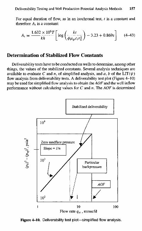
For equal duration of flow, as in an isochronal test, t is a constant andtherefore At is a constant:
Determination of Stabilized Flow Constants
Deliverability tests have to be conducted on wells to determine, among otherthings, the values of the stabilized constants. Several analysis techniques areavailable to evaluate C and n, of simplified analysis, and a, b of the LIT(VOflow analysis from deliverability tests. A deliverability test plot (Figure 4-10)may be used for simplified flow analysis to obtain the AOF and the well inflowperformance without calculating values for C and n. The AOF is determined
Stabilized deliverability
Zero sandface pressure
Slope = 1/n
Particularbackpressure
AOF
Flow rate qsc, mmscfd
Figure 4-10. Deliverability test plot—simplified flow analysis.
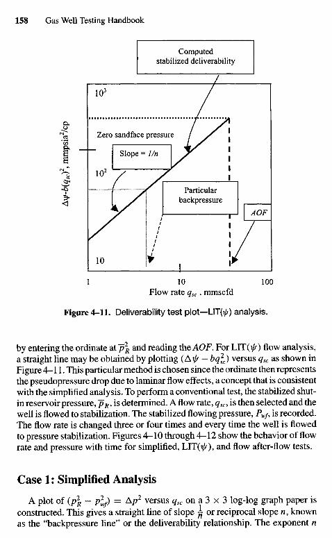
Flow rate qsc, mmscfd
Figure 4-11. Deliverability test plot—LiT(^r) analysis.
by entering the ordinate at ~p\ and reading the AOF. For LIT(VO flow analysis,a straight line may be obtained by plotting ( A ^ - bq2
c) versus qsc as shown inFigure 4-11. This particular method is chosen since the ordinate then representsthe pseudopressure drop due to laminar flow effects, a concept that is consistentwith the simplified analysis. To perform a conventional test, the stabilized shut-in reservoir pressure, ~pR, is determined. A flow rate, qsc, is then selected and thewell is flowed to stabilization. The stabilized flowing pressure, Pwf, is recorded.The flow rate is changed three or four times and every time the well is flowedto pressure stabilization. Figures 4-10 through 4-12 show the behavior of flowrate and pressure with time for simplified, LIT(^), and flow after-flow tests.
Case 1: Simplified Analysis
A plot of (/?! - plf) — Ap2 versus qsc on a 3 x 3 log-log graph paper isconstructed. This gives a straight line of slope ^ or reciprocal slope n, knownas the "backpressure line" or the deliverability relationship. The exponent n
AOF
Particularbackpressure
Slope = 1/n
Zero sandface pressure
Computedstabilized deliverability
A\\j
-b(q
sc)2,
mm
psia
2/cp
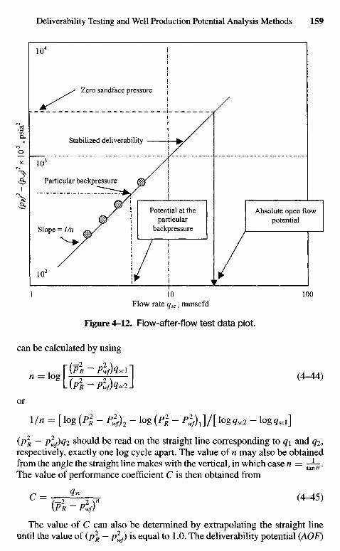
Flow rate qsc, mmscfd
Figure 4-12. Flow-after-flow test data plot.
can be calculated by using
, [(~P2R ~ Plfhsdl AA^
n = \og\ y- f (4^4)L[PR-Pi/Ha]
or\/n = [log (P2
R - P*)2 - log [Pl - Pl^}/[\ogqsc2 - \ogqscl\
(p2R — pl,f)q2 should be read on the straight line corresponding to q\ and #2>
respectively, exactly one log cycle apart. The value of n may also be obtainedfrom the angle the straight line makes with the vertical, in which case n = ^^.The value of performance coefficient C is then obtained from
C = 2qsc
n (4^5)[PR ~ Plf)
The value of C can also be determined by extrapolating the straight lineuntil the value of (p2
R — p^f) is equal to 1.0. The deliverability potential (AOF)
Absolute open flowpotential
Potential at theparticular
backpressureSlope = 1/n
Particular backpressure
Stabilized deliverability
Zero sand face pressure
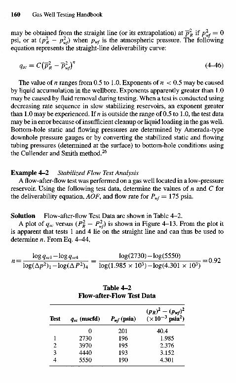
may be obtained from the straight line (or its extrapolation) at p\ if p^f — 0psi, or at (p\ — /?L) when pwf is the atmospheric pressure. The followingequation represents the straight-line deliverability curve:
qsc = C(P2R ~P2Jn (4-46)
The value of n ranges from 0.5 to 1.0. Exponents of n < 0.5 may be causedby liquid accumulation in the wellbore. Exponents apparently greater than 1.0may be caused by fluid removal during testing. When a test is conducted usingdecreasing rate sequence in slow stabilizing reservoirs, an exponent greaterthan 1.0 may be experienced. If n is outside the range of 0.5 to 1.0, the test datamay be in error because of insufficient cleanup or liquid loading in the gas well.Bottom-hole static and flowing pressures are determined by Amerada-typedownhole pressure gauges or by converting the stabilized static and flowingtubing pressures (determined at the surface) to bottom-hole conditions usingthe Cullender and Smith method.26
Example 4-2 Stabilized Flow Test AnalysisA flow-after-flow test was performed on a gas well located in a low-pressure
reservoir. Using the following test data, determine the values of n and C forthe deliverability equation, AOF, and flow rate for Pwf =175 psia.
Solution Flow-after-flow Test Data are shown in Table 4-2.A plot of qsc versus ( P | — P2
f) is shown in Figure 4-13. From the plot itis apparent that tests 1 and 4 lie on the straight line and can thus be used todetermine n. From Eq. A-AA,
l o g ^ c i - l o g ^ c 4 = log(2730)-log(5550)n~log(A/72)i- log(AP2)4 ~ log(1.985 x 10³)-log(4.301 x 10³) " '
Table 4-2Flow-after-Flow Test Data
(PR)2 - (Pwf)2
Test qsc (mscfd) Pwf (psia) (x 10~3 psia2)
0 201 40.41 2730 196 1.9852 3970 195 2.3763 4440 193 3.1524 5550 190 4.301
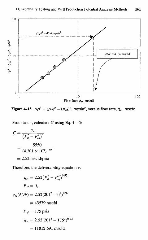
Flow Rate qsc, mscfd
Figure 4-13. Ap2 = (pR)2 - (pwf)2, mpsia2, versus flow rate, qsc, mscfd.
From test 4, calculate C using Eq. 4-45:
r _ qsc
_ 5550
~ (4.301 x IO3)0-92
= 2.52 mscfd/psia
Therefore, the deliverability equation is
qsc — A.z>zyfR rwf)
Pwf=0,
qsc(AOF) = 2.52(2012 - O2)092
= 43579 mscfd
Pwf = 1 7 5 psia
qsc = 2.52(2012 - 1752)092
= 11812.691 mscfd
AOF = 43.57 mscfd
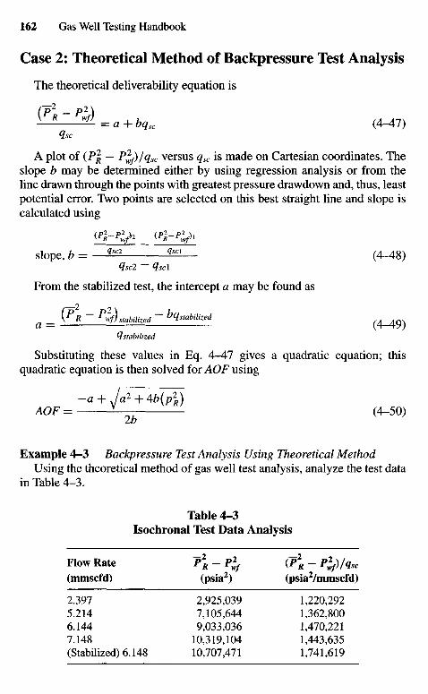
Case 2: Theoretical Method of Backpressure Test Analysis
The theoretical deliverability equation is
J— =a + bqsc (4-47)qsc
A plot of (P\ — Pfy/qsc versus qsc is made on Cartesian coordinates. Theslope b may be determined either by using regression analysis or from theline drawn through the points with greatest pressure drawdown and, thus, leastpotential error. Two points are selected on this best straight line and slope iscalculated using
slope, b = — ^ ^ - (4-48)qSc2 - qsc\
From the stabilized test, the intercept a may be found as
a _ VR ~ PH)stabilized ~ Stabilized (4^9)
^stabilized
Substituting these values in Eq. 4-47 gives a quadratic equation; thisquadratic equation is then solved for AOF using
- f l + / f l2+46(p2)
AOF = y-— (4-50)2b
Example 4-3 Backpressure Test Analysis Using Theoretical MethodUsing the theoretical method of gas well test analysis, analyze the test data
in Table 4-3.
Table 4-3Isochronal Test Data Analysis
Flow Rate T2R - P*f (P2
R - P^f)/qsc
(mmscfd) (psia2) (psia2/mmscfd)
2.397 2,925,039 1,220,2925.214 7,105,644 1,362,8006.144 9,033,036 1,470,2217.148 10,319,104 1,443,635(Stabilized) 6.148 10,707,471 1,741,619
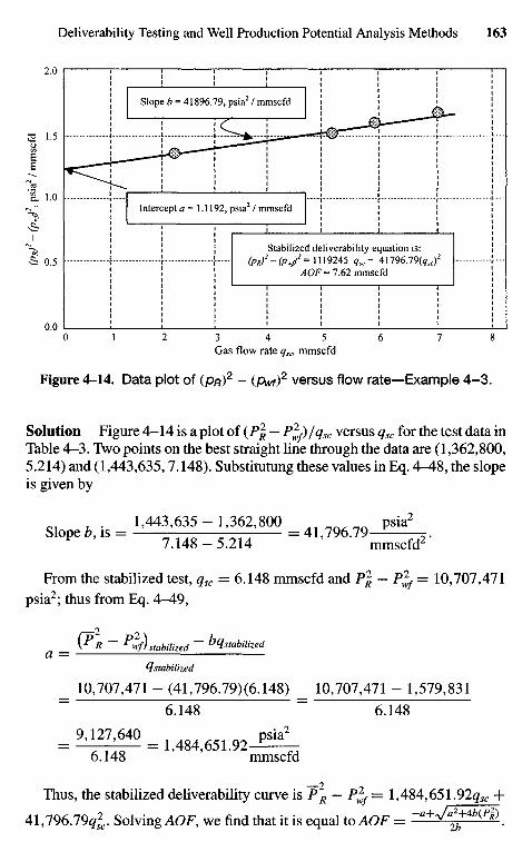
Gas flow rate qsa mmscfd
Figure 4-14. Data plot of (PR)2 - (Pwf)2 versus flow rate—Example 4-3.
Solution Figure 4-14 is a plot of ( P | — Pfy /qsc versus qsc for the test data inTable 4-3. Two points on the best straight line through the data are (1,362,800,5.214) and (1,443,635,7.148). Substitutung these values in Eq. 4 ^ 8 , the slopeis given by
1,443,635-1,362,800 psia2
Slope b, is = - ^ - ^ ^ = 41,796.79— ~.7.148-5.214 mmscfd2
From the stabilized test, qsc — 6.148 mmscfd and P\ - P^ = 10,707,471psia2; thus from Eq. 4-49,
a _ \PR ~ Pwf)stabilized ~ Stabilized
^[stabilized
_ 10,707,471 - (41,796.79)(6.148) _ 10,707,471 - 1,579,831~ 6.148 ~ 6.148
6.148 mmscfd
Thus, the stabilized deliverability curve is T\ - P^ = 1,484,651.92gJC +
41,796.79^2C. Solving AOF, we find that it is equal to AOF = ~^+V^+4^^2
Stabilized deliverability equation is:(PR)2- (pw/= IU9245 qsc+ 41796J9(qsc)
2
AOF =7.62 mmscfd
Intercept a = 1.1192, psia2 / mmscfd
Slope b = 41896.79, psia2 / mmscfd
(PR)
2 ~ (P
wj)2>
psia
2 / m
msc
fd
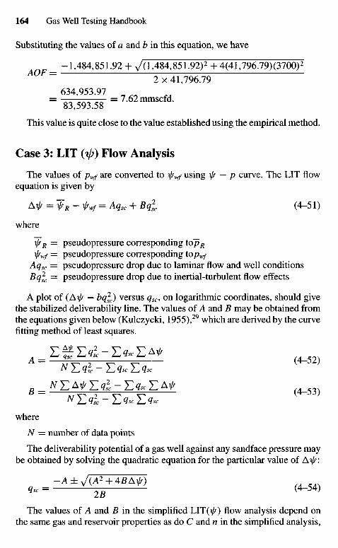
Substituting the values of a and b in this equation, we have
_ -1,484,851.92 + 7(1,484,851.92)2 + 4(41,796.79)(3700)2
2 x 41,796.79634,953.97
= - 8 3 3 1 5 8 " = 7 - 6 2 m m S C f d -
This value is quite close to the value established using the empirical method.
Case 3: LIT (^) Flow Analysis
The values of pwf are converted to W using \jr — p curve. The LIT flowequation is given by
A ^ = f R - VV = Aqsc + Bq]0 (4-51)
where
V^ = pseudopressure corresponding \opR
\/rWf = pseudopressure corresponding to/?w/Aqsc = pseudopressure drop due to laminar flow and well conditionsBq]0 = pseudopressure drop due to inertial-turbulent flow effects
A plot of (A^ - bq]c) versus qsc, on logarithmic coordinates, should givethe stabilized deliverability line. The values of A and B may be obtained fromthe equations given below (Kulczycki, 1955),29 which are derived by the curvefitting method of least squares.
Nz2<isc-z2<isc22qsc
where
N = number of data points
The deliverability potential of a gas well against any sandface pressure maybe obtained by solving the quadratic equation for the particular value of AT^:
LtS
The values of A and B in the simplified LIT(^) flow analysis depend onthe same gas and reservoir properties as do C and n in the simplified analysis,
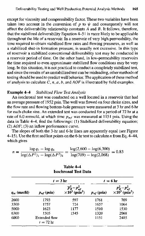
except for viscosity and compressibility factor. These two variables have beentaken into account in the conversion of p to if/ and consequently will notaffect the deliverability relationship constants A and B. It follows, therefore,that the stabilized deliverability Equation 4-51 is more likely to be applicablethroughout the life of a reservoir. In a reservoir of very high permeability, thetime required to obtain stabilized flow rates and flowing pressures, as well asa stabilized shut-in formation pressure, is usually not excessive. In this typeof reservoir a stabilized conventional deliverability test may be conducted ina reservoir period of time. On the other hand, in low-permeability reservoirsthe time required to even approximate stabilized flow conditions may be verylong. In this situation, it is not practical to conduct a completely stabilized test,and since the results of an unstabilized test can be misleading, other methods oftesting should be used to predict well behavior. The application of these methodof analysis to calculate C,n,a,b, and AOF is illustrated by field examples.
Example 4-4 Stabilized Flow Test AnalysisAn isochronal test was conducted on a well located in a reservoir that had
an average pressure of 1952 psia. The well was flowed on four choke sizes, andthe flow rate and flowing bottom-hole pressure were measured at 3 hr and 6 hrfor each choke size. An extended test was conducted for a period of 72 hr at arate of 6.0 mmscfd, at which time pmf was measured at 1151 psia. Using thedata in Table 4-4, find the followings: (1) Stabilized deliverability equation;(2) AOF; (3) an inflow performance curve.
The slopes of both the 3-hr and 6-hr lines are apparently equal (see Figure4-15). Use the first and last points on the 6-hr test to calculate n from Eq. 4-44,which gives
log g l - l og #4 = log(2,600 - log(6,300) = 8 3
log(AP2)! - log(AP2)4 " log(709) - log(2,068) "
Table 4-4Isochronal Test Data
t = 3 hr / = 6 hr
P2R-P2Wf P2R-PIfqsc (mscfd) pwf (psia) X103 (psia2) pwf (psia) X103 (psia2)
2600 1793 597 1761 7093300 1757 724 1657 10645000 1623 1177 1510 15306300 1505 1545 1320 20686000 Extended flow 1151 2485
t = 72 hr
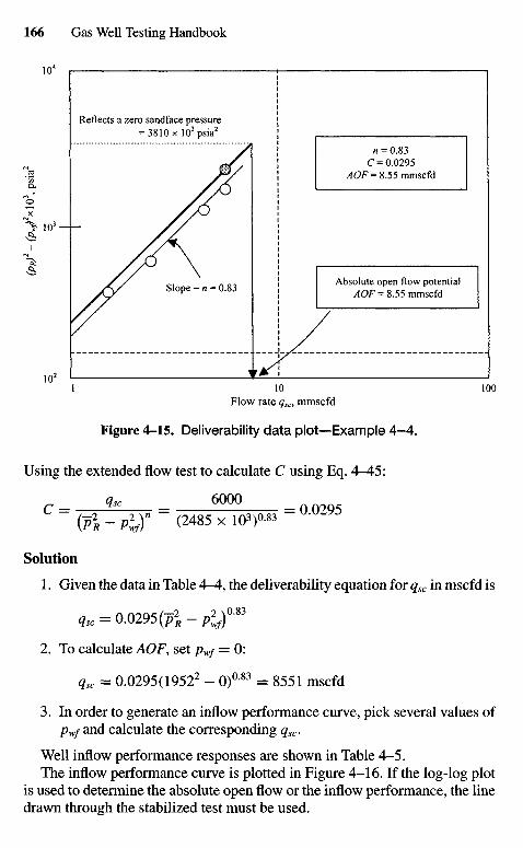
Flow rate qsc, mmscfd
Figure 4-15. Deliverability da ta plot—Example 4 - 4 .
Using the extended flow test to calculate C using Eq. 4 ^ 5 :
C - «££ 6 Q Q 0 _ o 0295
" (Pi ~ P2J ~ <2 4 8 5 X 10³)°-83 "
Solution
1. Given the data in Table 4-4, the deliverability equation for qsc in mscfd is
qsc = 0.0295(p| -P2J™
2. To calculate AOF, set pwf = 0:
qsc = 0.0295(19522 - O)083 = 8551 mscfd
3. In order to generate an inflow performance curve, pick several values ofPwf and calculate the corresponding qsc.
Well inflow performance responses are shown in Table 4-5.The inflow performance curve is plotted in Figure 4-16. If the log-log plot
is used to determine the absolute open flow or the inflow performance, the linedrawn through the stabilized test must be used.
Absolute open flow potentialAOF =8.55 mmscfd
« = 0.83C = 0.0295
AOF-= 8.55 mmscfd
Reflects a zero sandface pressure= 3810 x 103psia2
Slope = n = 0.83
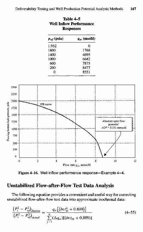
Table 4-5Well Inflow Performance
Responses
pwf (psia) qsc (mscfd)
1.952 01800 17681400 46951000 6642600 7875200 8477
0 8551
Flow rate qsc, mmscfd
Figure 4-16. Well inflow performance response—Example 4-4.
Unstabilized Flow-after-Flow Test Data Analysis
The following equation provides a convenient and useful way for correctingunstabilized flow-after-flow test data into approximate isochronal data:
(Pi ~ P2JDesires _ ^ [ ( / ^ * + 0.809)](p2 _ p2\ ~~ n ^ JJ>\ri rwf)Actual Yl (Afe)[(//I tDj + 0.809)]
7 - 1
Absolute open flowpotential
AOF= 8.551 mmscfd
IPR curve
Flow
ing
botto
m h
ole
pres
sure
, psi
a
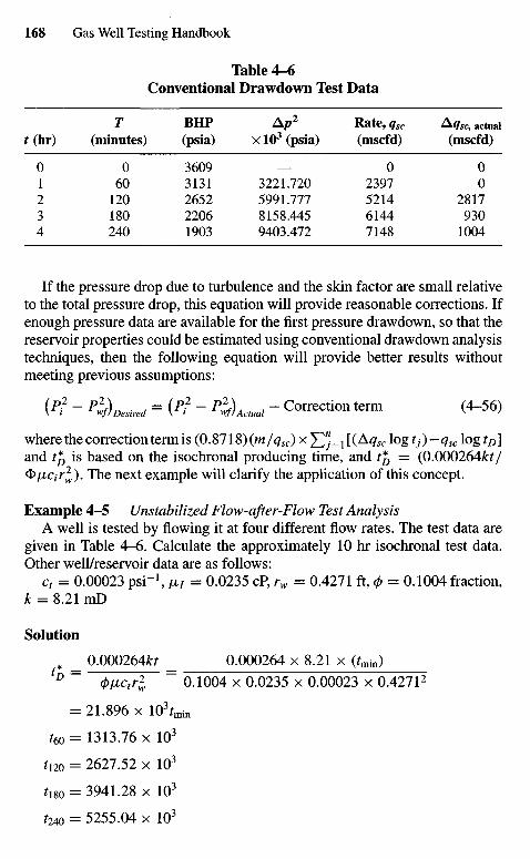
Table 4-6Conventional Drawdown Test Data
T BHP Ap2 Rate,fe Aqsc, actuai
*(hr) (minutes) (psia) xlO3(psia) (mscfd) (mscfd)
0 0 3609 — 0 01 60 3131 3221.720 2397 02 120 2652 5991.777 5214 28173 180 2206 8158.445 6144 9304 240 1903 9403.472 7148 1004
If the pressure drop due to turbulence and the skin factor are small relativeto the total pressure drop, this equation will provide reasonable corrections. Ifenough pressure data are available for the first pressure drawdown, so that thereservoir properties could be estimated using conventional drawdown analysistechniques, then the following equation will provide better results withoutmeeting previous assumptions:
(Pf - F^) (p2 _ p2\ _ correction term (4-56)V i wfj Desired V i wf/Actual v /
where the correction term is (0.8718) (m/qsc) x YTj=\ [(Aqsc log tj)—qsc log tD]and tp is based on the isochronal producing time, and tp = (0.000264&f/OILCiT^). The next example will clarify the application of this concept.
Example 4-5 Unstabilized Flow-after-Flow Test AnalysisA well is tested by flowing it at four different flow rates. The test data are
given in Table 4-6. Calculate the approximately 10 hr isochronal test data.Other well/reservoir data are as follows:
ct = 0.00023 psi"1, M/ = 0.0235 cP, rw = 0.4271 ft, 0 = 0.1004 fraction,k = 8.21 mD
Solution
„ _ 0.000264^ _ 0.000264 x 8.21 x (tmin)
*D ~ <t>iJLctrl ~ 0.1004 x 0.0235 x 0.00023 x 0.42712
- 2 1 . 8 9 6 x 10³rmin
^60 = 1313.76 x 103
fi2o = 2627.52 x 103
/180 = 3941.28 x 103
;24o = 5255.04 x 103
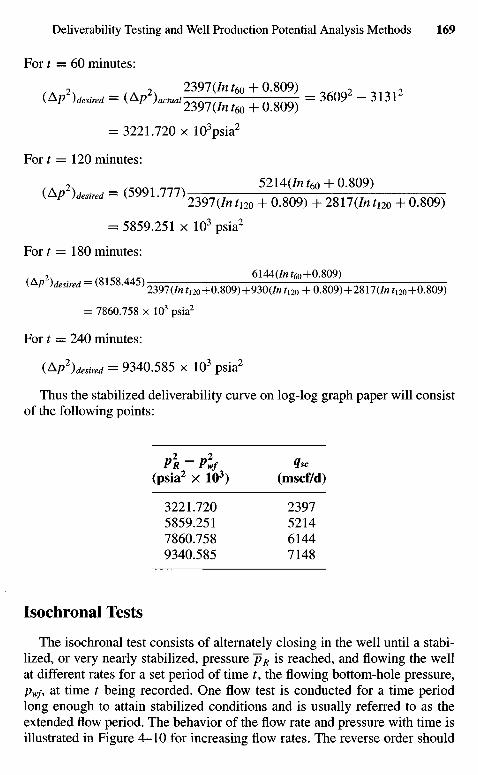
For t = 60 minutes:
= 3221.720 x 103psia2
For t — 120 minutes:
{A 2, _ r S 0 0 1 7 7 7 , 5214(/n ^60 + 0 .809){ P )desired~ VWi'/n>2397(Mr120 + 0.809) + 2SIl(IntUo + 0.809)
= 5859.251 x 103psia2
For £ = 180 minutes:
2 = 6144(/Kf60+0.809)
C P )desired K • ^ 2397 (Z^i20+0.809)+930(7« fi2o + 0.809)+2817(/nfi20+0.809)
= 7860.758 x 103 psia2
For t = 240 minutes:
(Ap2)desired = 9340.585 x 103 psia2
Thus the stabilized deliverability curve on log-log graph paper will consistof the following points:
P2R ~ Plf Isc(psia2 x 103) (mscf/d)
3221.720 23975859.251 52147860.758 61449340.585 7148
Isochronal Tests
The isochronal test consists of alternately closing in the well until a stabi-lized, or very nearly stabilized, pressure ~pR is reached, and flowing the wellat different rates for a set period of time t, the flowing bottom-hole pressure,pwf, at time t being recorded. One flow test is conducted for a time periodlong enough to attain stabilized conditions and is usually referred to as theextended flow period. The behavior of the flow rate and pressure with time isillustrated in Figure 4-10 for increasing flow rates. The reverse order should
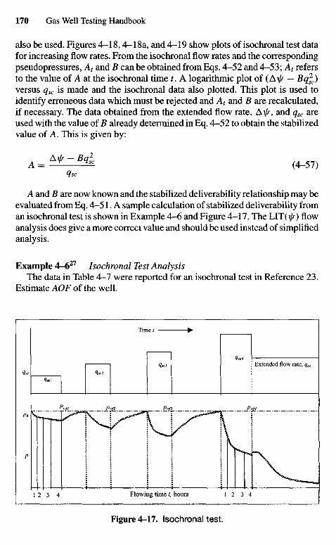
also be used. Figures 4-18,4-18a, and 4-19 show plots of isochronal test datafor increasing flow rates. From the isochronal flow rates and the correspondingpseudopressures, At and B can be obtained from Eqs. 4-52 and 4-53; At refersto the value of A at the isochronal time t. A logarithmic plot of (Axj/ — Bqjc)versus qsc is made and the isochronal data also plotted. This plot is used toidentify erroneous data which must be rejected and At and B are recalculated,if necessary. The data obtained from the extended flow rate, A^, and qsc areused with the value of B already determined in Eq. 4-52 to obtain the stabilizedvalue of A. This is given by:
A = ^ l M (4-57)qsc
A and B are now known and the stabilized deliverability relationship may beevaluated from Eq. 4-51. A sample calculation of stabilized deliverability froman isochronal test is shown in Example 4-6 and Figure 4-17. The LIT(i/0 flowanalysis does give a more correct value and should be used instead of simplifiedanalysis.
Example 4-627 Isochronal Test AnalysisThe data in Table 4-7 were reported for an isochronal test in Reference 23.
Estimate AOF of the well.
Time/
Extended flow rate, qsc
Flowing time t, hours
Figure 4-17. Isochronal test.
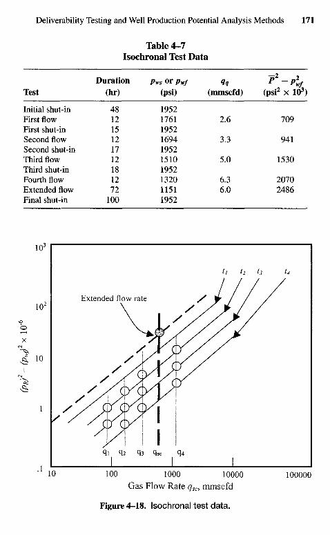
Table 4-7Isochronal Test Data
Duration p w s or pwf qq T - p2wf
Test (hr) (psi) (mmscfd) (psi2 x 103)
Initial shut-in 48 1952First flow 12 1761 2.6 709First shut-in 15 1952Second flow 12 1694 3.3 941Second shut-in 17 1952Third flow 12 1510 5.0 1530Third shut-in 18 1952Fourth flow 12 1320 6.3 2070Extended flow 72 1151 6.0 2486Final shut-in 100 1952
Gas Flow Rate qSC9 mmscfd
Figure 4-18. Isochronal test data.
Extended flow rate
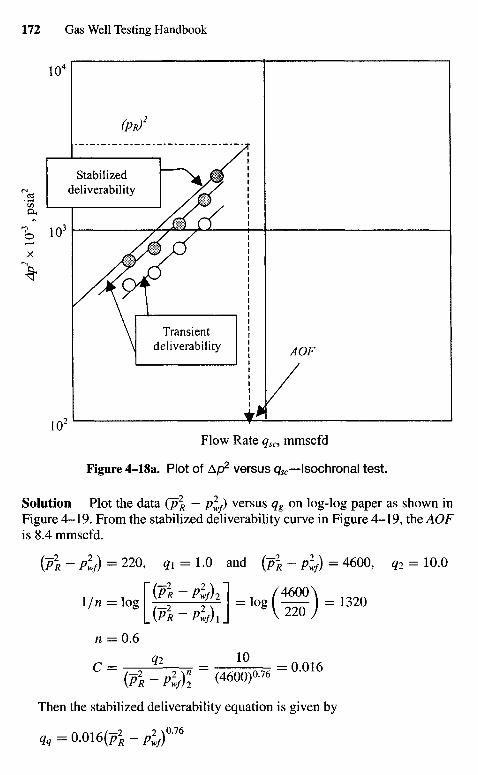
Flow Rate qsc, mmscfd
Figure 4-18a. Plot of Ap2 versus qsc—Isochronal test.
Solution Plot the data (p2R - plf) versus qg on log-log paper as shown in
Figure 4-19. From the stabilized deliverability curve in Figure 4-19, the AOFis 8.4 mmscfd.
[P2R-P2J = 220, <7, = 1.0 and (p\ - p2wf) = 4600, <?2 = 10.0
»/» = .oJj^#l=.ogO = 1320\_\PR-Plf)i\ V 220/
« = 0.6
" (Pl ~ P2J2 ~ (4600)0- " °-°16
Then the stabilized deliverability equation is given by
qq = 0.016(p| - ^ ) 0 7 6
Transientdeliverability
Stabilizeddeliverability
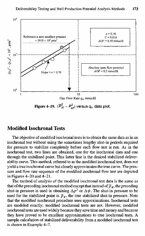
Gas Flow Rate qsc mmscfd
Figure 4-19. (P2R - P*f) versus qsc data plot.
Modified Isochronal Tests
The objective of modified isochronal tests is to obtain the same data as in anisochronal test without using the sometimes lengthy shut-in periods requiredfor pressure to stabilize completely before each flow test is run. As in theisochronal test, two lines are obtained, one for the isochronal data and onethrough the stabilized point. This latter line is the desired stabilized deliver-ability curve. This method, referred to as the modified isochronal test, does notyield a true isochronal curve but closely approximates the true curve. The pres-sure and flow rate sequence of the modified isochronal flow test are depictedin Figures 4-20 and 4-21.
The method of analysis of the modified isochronal test data is the same asthat of the preceding isochronal method except that instead of ~pR, the precedingshut-in pressure is used in obtaining Ap2 or Ai^. The shut-in pressure to beused for the stabilized point is ~pR, the true stabilized shut-in pressure. Notethat the modified isochronal procedure uses approximations. Isochronal testsare modeled exactly; modified isochronal tests are not. However, modifiedisochronal tests are used widely because they save time and money and becausethey have proved to be excellent approximations to true isochronal tests. Asample calculation of stabilized deliverability from a modified isochronal testis shown in Example 4-7.
Slope = n = 0.76
Reference a zero sandface pressure= 3810 x 103psia2
n = 0.76C= 0.016
AOF= 8.50 mmscfd
Absolute open flow potentialAOF =8.5 mmscfd
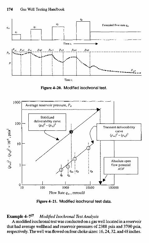
Time t,
Figure 4-20. Modified Isochronal test.
Extended flow rate qsc
Time t,
Average reservoir pressure, PR
Stabilizeddeliverability curve
{pR?-(pWff Transient deliverabilitycurve
(pws)2-(pwf)
2
Absolute openflow potential
AOF
Flow Rate qsc, mmscfd
Figure 4-21. Modified isochronal test data.
Example 4-727 Modified Isochronal Test AnalysisA modified isochronal test was conducted on a gas well located in a reservoir
that had average wellhead and reservoir pressures of 2388 psia and 3700 psia,respectively. The well was flowed on four choke sizes: 16,24,32, and 48 inches.
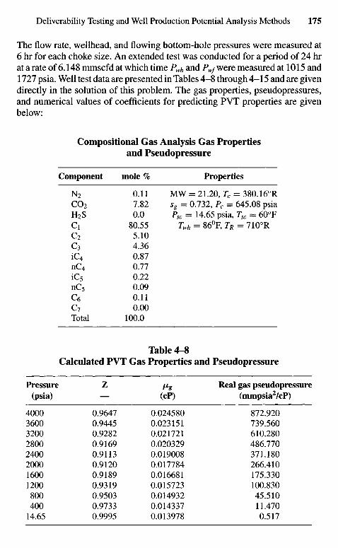
The flow rate, wellhead, and flowing bottom-hole pressures were measured at6 hr for each choke size. An extended test was conducted for a period of 24 hrat a rate of 6.148 mmscfd at which time Pwh and PWf were measured at 1015 and1727 psia. Well test data are presented in Tables 4 - 8 through 4 -15 and are givendirectly in the solution of this problem. The gas properties, pseudopressures,and numerical values of coefficients for predicting PVT properties are givenbelow:
Compositional Gas Analysis Gas Propertiesand Pseudopressure
Component mole % Properties
N2 0.11 MW = 21.20, Tc = 380.16°RCO2 7.82 S8 = 0.732, Pc = 645.08 psiaH2S 0.0 Psc = 14.65 psia, Tsc = 600FCi 80.55 Twh = 860F, TR = 7100RC2 5.10C3 4.36iC4 0.87nC4 0.77iC5 0.22nC5 0.09C6 0.11C7 0.00Total 100.0
Table 4-8Calculated PVT Gas Properties and Pseudopressure
Pressure Z /jbg Real gas pseudopressure(psia) — (cP) (mmpsia2/cP)
4000 0.9647 0.024580 872.9203600 0.9445 0.023151 739.5603200 0.9282 0.021721 610.2802800 0.9169 0.020329 486.7702400 0.9113 0.019008 371.1802000 0.9120 0.017784 266.4101600 0.9189 0.016681 175.3301200 0.9319 0.015723 100.830800 0.9503 0.014932 45.510400 0.9733 0.014337 11.470
14.65 0.9995 0.013978 0.517
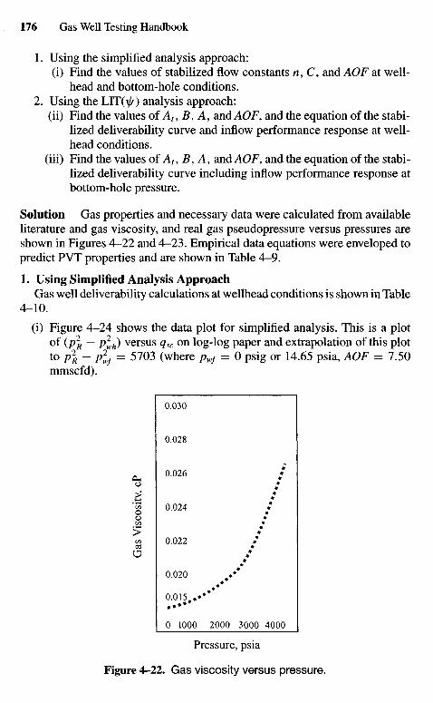
1. Using the simplified analysis approach:(i) Find the values of stabilized flow constants n, C, and AOF at well-
head and bottom-hole conditions.2. Using the LIT(VO analysis approach:
(ii) Find the values of At, B, A, and AOF9 and the equation of the stabi-lized deliverability curve and inflow performance response at well-head conditions.
(iii) Find the values of At, B, A, and AOF, and the equation of the stabi-lized deliverability curve including inflow performance response atbottom-hole pressure.
Solution Gas properties and necessary data were calculated from availableliterature and gas viscosity, and real gas pseudopressure versus pressures areshown in Figures 4-22 and 4-23. Empirical data equations were enveloped topredict PVT properties and are shown in Table 4-9.
1. Using Simplified Analysis ApproachGas well deliverability calculations at wellhead conditions is shown in Table
4-10.
(i) Figure 4-24 shows the data plot for simplified analysis. This is a plotof (p2
R — p^h) versus qsc on log-log paper and extrapolation of this plotto p\ — p^f = 5703 (where pwf = 0 psig or 14.65 psia, AOF — 7.50mmscfd).
Pressure, psia
Figure 4-22. Gas viscosity versus pressure.
Gas
Vis
cosi
ty, c
P
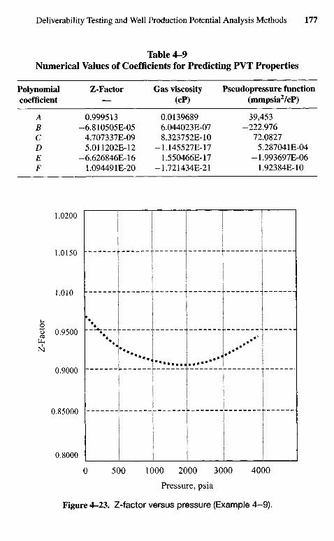
Table 4-9Numerical Values of Coefficients for Predicting PVT Properties
Polynomial Z-Factor Gas viscosity Pseudopressure functioncoefficient — (cP) (mmpsia2/cP)
A 0.999513 0.0139689 39,453B -6.810505E-05 6.044023E-07 -222.976C 4.707337E-09 8.323752E-10 72.0827D 5.011202E-12 -1.145527E-17 5.287041E-04E -6.626846E-16 1.550466E-17 -1.993697E-06F 1.094491E-20 -1.721434E-21 1.92384E-10
Pressure, psia
Figure 4-23. Z-factor versus pressure (Example 4-9).
Z-F
acto
r
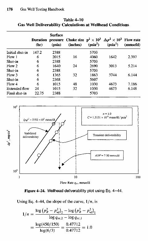
Table 4-10Gas Well Deliverability Calculations at Wellhead Conditions
SurfaceDuration pressure Choke size p2 X 103 Ap2 x 103 Flow rate
(hr) (psia) (inches) (psia2) (psia2) (mmscfd)
Initial shut-in 147.2 2388 5703Flowl 6 2015 16 4060 1642 2.397Shut-in 6 2388 5703Flow 2 6 1640 24 2690 3013 5.214Shut-in 6 2388 5703Flow 3 6 1365 32 1863 3744 6.144Shut-in 6 2368 5607Flow 4 6 1015 48 1030 4673 7.186Extended flow 24 1015 32 1030 4673 6.148Final shut-in 22.75 2388 5703
Flow Rate qsc, mmscfd
Figure 4-24. Wellhead deliverability plot using Eq. 4-44.
Using Eq. 4- 4-4, the slope of the curve, l/n, is
= lQg (P2R ~ PJf)2 ~
lQg (Pi ~ Pi/) il0g^c,2-l0g^c,l
_ log(450/150) _ 0.47712 _log(6/3) ~ 0.47712 ~ '
AOF = 7.50 mmscfd
Transient deliverability
n = 1.0C = 1.3151 x IO'6 mmscfd/psia2
Stabilizeddeliverability
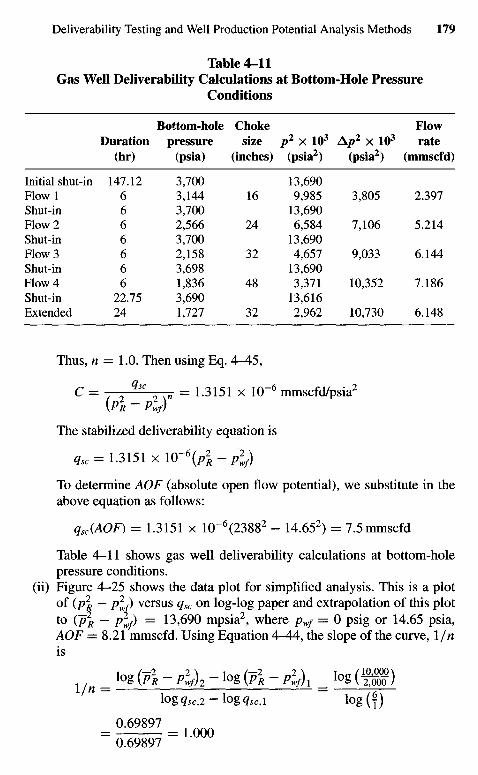
Table 4-11Gas Well Deliverability Calculations at Bottom-Hole Pressure
Conditions
Bottom-hole Choke FlowDuration pressure size p2 X 103 Ap2 x 103 rate
(hr) (psia) (inches) (psia2) (psia2) (mmscfd)
Initial shut-in 147.12 3,700 13,690Flowl 6 3,144 16 9,985 3,805 2.397Shut-in 6 3,700 13,690Flow 2 6 2,566 24 6,584 7,106 5.214Shut-in 6 3,700 13,690Flow 3 6 2,158 32 4,657 9,033 6.144Shut-in 6 3,698 13,690Flow 4 6 1,836 48 3,371 10,352 7.186Shut-in 22.75 3,690 13,616Extended 24 1,727 32 2,962 10,730 6.148
Thus, n = 1.0. Then using Eq. 4-45,
C = . 0 qsc . .n = 1.3151 x 10"6 mmscfd/psia2
(P2R ~ Plf)
The stabilized deliverability equation is
^ = 1.3151 x H T 6 ^ - / ^ )
To determine AOF (absolute open flow potential), we substitute in theabove equation as follows:
qsc(AOF) = 1.3151 x 1(T6(23882 - 14.652) = 7.5 mmscfd
Table 4-11 shows gas well deliverability calculations at bottom-holepressure conditions.
(ii) Figure 4-25 shows the data plot for simplified analysis. This is a plotof (p\ — p\) versus qsc on log-log paper and extrapolation of this plotto (p2
R — plf) = 13,690 mpsia2, where pwf = 0 psig or 14.65 psia,AOF =8.21 mmscfd. Using Equation 4-44, the slope of the curve, \/nis
= log (Pl-P2J2-IQE (Pl -P2J1 = IQg(WlOg<^c,2-log<?5c,l lQg(f)
= 0J^l = !.000
0.69897
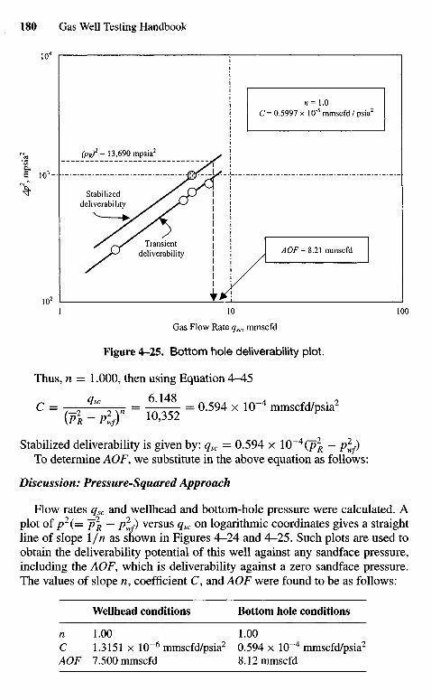
Gas Flow Rate qsc, mmscfd
Figure 4-25. Bottom hole deliverability plot.
Thus, n — 1.000, then using Equation 4-45
C = . 2 qsc
2,n = ^ z = 0.594 x 10⁻⁴ mmscfd/psia2
(PR - Plf) 1 0 ' 3 5 2
Stabilized deliverability is given by: qsc = 0.594 x lO~4(p2R — pfy
To determine AOF, we substitute in the above equation as follows:
Discussion: Pressure-Squared Approach
Flow rates qsc and wellhead and bottom-hole pressure were calculated. Aplot of p2(= ~p\ — P^f) versus qsc on logarithmic coordinates gives a straightline of slope \/n as shown in Figures 4-24 and 4-25. Such plots are used toobtain the deliverability potential of this well against any sandface pressure,including the AOF, which is deliverability against a zero sandface pressure.The values of slope n, coefficient C, and AOF were found to be as follows:
Wellhead conditions Bottom hole conditions
n 1.00 1.00C 1.3151 x 10~6 mmscfd/psia2 0.594 x 10~4 mmscfd/psia2
AOF 7.500 mmscfd 8.12 mmscfd
AOF= 8.21 mmscfd
n=1.0C = 0.5997 x 10'5 mmscfd / psia2
Transientdeliverability
Stabilizeddeliverability
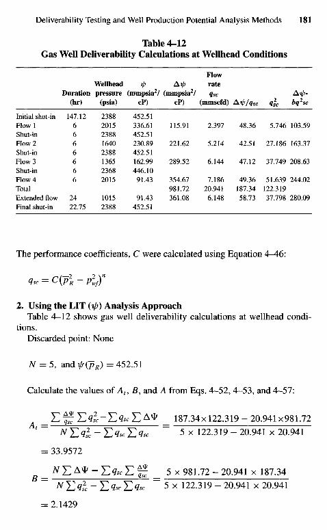
Table 4-12Gas Well Deliverability Calculations at Wellhead Conditions
FlowWellhead \j) Ai/> rate
Duration pressure (mmpsia2/ (mmpsia2/ qsc Aip-(hr) (psia) cP) cP) (mmscfd) Atp/qsc qlc bq2sc
Initial shut-in 147.12 2388 452.51Flowl 6 2015 336.61 115.91 2.397 48.36 5.746 103.59Shut-in 6 2388 452.51Flow 2 6 1640 230.89 221.62 5.214 42.51 27.186 163.37Shut-in 6 2388 452.51Flow 3 6 1365 162.99 289.52 6.144 47.12 37.749 208.63Shut-in 6 2368 446.10Flow 4 6 2015 91.43 354.67 7.186 49.36 51.639 244.02Total 981.72 20.941 187.34 122.319Extended flow 24 1015 91.43 361.08 6.148 58.73 37.798 280.09Final shut-in 22.75 2388 452.51
The performance coefficients, C were calculated using Equation 4-46:
qsc = c(-p2R- plf)
n
2. Using the LIT (t/>) Analysis ApproachTable 4-12 shows gas well deliverability calculations at wellhead condi-
tions.Discarded point: None
N = 5, and (pR) =452.51
Calculate the values of At, B, and A from Eqs. 4-52, 4-53, and 4-57:
_Y,f;Y,<lsc-Y,<lscY,Axi' _ 187.34x122.319-20.941x981.72
' ~ NH<lsc-E 4sc E qsc 5 x 122.319 - 20.941 x 20.941
= 33.9572
_ A ^ E A ^ - E f e E ^ 5 x 981.72 - 20.941 x 187.34
NrZ<ii-EqscEqsc " 5 x 122.319-20.941 x 20.941
= 2.1429
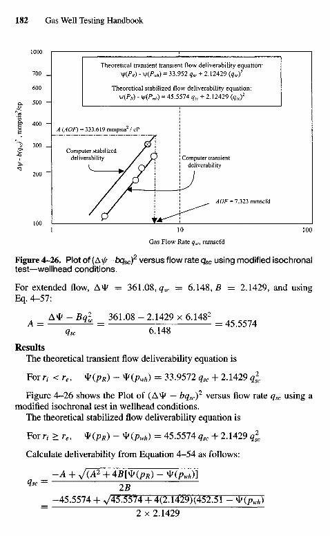
Gas Flow Rate qsc, mmscfd
Figure 4-26. Plot of (Ais-bqsc)2 versus flow rate qsc using modified isochronal
test—wellhead conditions.
For extended flow, AV = 361.08, qsc = 6.148, B = 2.1429, and usingEq. 4-57:
= A * - Bqj = 361.08-2.1429 x 6.1482 =
9«r 6.148
ResultsThe theoretical transient flow deliverability equation is
For n < re, V(pR) - V(pwh) = 33.9572 qsc + 2.1429 q]c
Figure 4-26 shows the Plot of ( A ^ — bqsc)2 versus flow rate qsc using a
modified isochronal test in wellhead conditions.The theoretical stabilized flow deliverability equation is
For n > re, V(pR) - V(pwh) = 45.5574 qsc + 2.1429 q]c
Calculate deliverability from Equation 4-54 as follows:
-A + y/(A2 + 4B[V(PR) - V(pwh)]qsc= IB
_ -45.5574 + V45.5574 + 4(2.1429)(452.51 - V(pwh)~ 2x2.1429
AOF = 7.323 mmscfd
Computer transientdeliverability
Computer stabilizeddeliverability
Theoretical transient transient flow deliverability equation:y{PR) - y(Pwh) = 33.952 qsc + 2.12429 {qscf
Theoretical stabilized flow deliverability equation:\\,{PR) - M/(PVW() = 45.5574 qK + 2.12429 (qsc)
2
Ay/
- b(
q sc)
2, m
mps
ia2/c
p
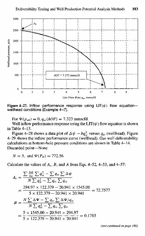
Gas Flow Rate qsc, mmscfd
Figure 4-27. Inflow performance response using LIT(i/r) flow equation-wellhead conditions (Example 4-7).
For V(pwh) = 0, qsc(AOF) = 7.323 mmscfd.Well inflow performance response using the LIT\yfr) flow equation is shown
in Table 4-13.Figure 4-28 shows a data plot of A^ — bqjc versus qsc (wellhead). Figure
4-29 shows the inflow performance curve (wellhead). Gas well deliverabilitycalculations at bottom-hole pressure conditions are shown in Table 4-14.Discarded point—None
Af = 5, and *(P*) = 772.56
Calculate the values of At, B, and A from Eqs. 4-52, 4-53, and 4-57:
_ 294.97 x 122.379 - 20.941 x 1545.00
~ 5 x 122.379 - 20.941 x 20.941 ~ '
B ^N £ A* -lZgscT ^/qsc
_ 5 x 1545.00 - 20.941 x 294.97 _~ 5 x 122.379 - 20.941 x 20.941 ~
(text continued on page 186)
AOF= 7.373 mmscfd
Wel
lhea
d pr
essu
re, p
sia
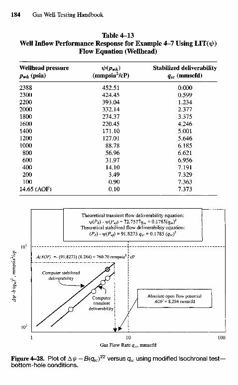
Table 4-13Well Inflow Performance Response for Example 4-7 Using LIT(VO
Flow Equation (Wellhead)
Wellhead pressure ifriPwh) Stabilized deliverabilitypWh (psia) (mmpsia2/cP) qsc (mmscfd)
2388 452.51 0.0002300 424.45 0.5992200 393.04 1.2342000 332.14 2.3771800 274.37 3.3751600 220.45 4.2461400 171.10 5.0011200 127.01 5.6461000 88.78 6.185800 56.96 6.621600 31.97 6.956400 14.10 7.191200 3.49 7.329100 0.90 7.363
14.65(AOF) 0.10 7.373
Gas Flow Rate qsc, mmscfd
Figure 4-28. Plot of A^ - B(qsc)22 versus qsc using modified isochronal test—
bottom-hole conditions.
Absolute open flow potentialAOF= 8.284 mmscfd
Computertransient
deliverability
Computer stabilizeddeliverability
Theoretical transient flow deliverability equation:y(PR) - y(Pwf) = 12.1511 qsc + 0.1785fc)2
Theoretical stabilized flow deliverability equation:(PR) - V)/(/V) = 91.8273 qsc + 0.1785 (qscf
Ay/
-b {
q scf
, m
mps
iaV
cp
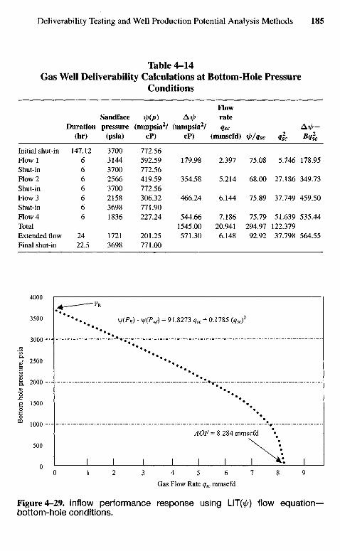
Table 4-14Gas Well Deliverability Calculations at Bottom-Hole Pressure
Conditions
FlowSandface r/>(p) Ai/> rate
Duration pressure (mmpsia2/ (mmpsia2/ qsc Atp—(hr) (psia) cP) cP) (mmscfd) tp/qsc qfc Bq*c
Initial shut-in 147.12 3700 772.56Flowl 6 3144 592.59 179.98 2.397 75.08 5.746 178.95Shut-in 6 3700 772.56Flow 2 6 2566 419.59 354.58 5.214 68.00 27.186 349.73Shut-in 6 3700 772.56Flow 3 6 2158 306.32 466.24 6.144 75.89 37.749 459.50Shut-in 6 3698 771.90Flow 4 6 1836 227.24 544.66 7.186 75.79 51.639 535.44Total 1545.00 20.941 294.97 122.379Extended flow 24 1721 201.25 571.30 6.148 92.92 37.798 564.55Final shut-in 22.5 3698 771.00
Gas Flow Rate qsc mmscfd
Figure 4-29. Inflow performance response using LIT(^) flow equation—bottom-hole conditions.
AOF= 8.284 mmscfd
Bot
tom
hol
e pr
essu
re, p
sia
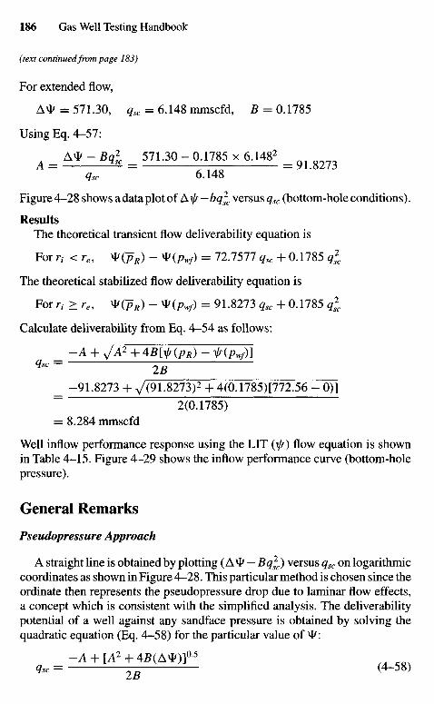
(text continued from page 183)
For extended flow,
A*I> z= 571.30, qsc = 6.148 mmscfd, B = 0.1785
Using Eq. 4-57:
= W-Bqj = 571.30-0.1785 x 6.1482 =
^ 6.148
Figure 4-28 shows a data plot of A \j/—bq^c versus qsc (bottom-hole conditions).
Results
The theoretical transient flow deliverability equation is
For n < re, V(pR) - V(pwf) = 72.7577 qsc + 0.1785 q]c
The theoretical stabilized flow deliverability equation is
For n > re, V(pR) - * ( / v ) = 91.8273 qsc + 0.1785 q]c
Calculate deliverability from Eq. 4-54 as follows:
_ - A + ^A 2 + 4B[jr(pR) - ^ Q y ) ]qsc~ IB
_ -91.8273 + 7(91.8273)2 + 4(0.1785)[772.56 - O)]~ 2(0.1785)= 8.284 mmscfd
Well inflow performance response using the LIT {\jr) flow equation is shownin Table 4-15. Figure 4-29 shows the inflow performance curve (bottom-holepressure).
General Remarks
Pseudopressure Approach
A straight line is obtained by plotting (A^ — Bqjc) versus qsc on logarithmiccoordinates as shown in Figure 4-28. This particular method is chosen since theordinate then represents the pseudopressure drop due to laminar flow effects,a concept which is consistent with the simplified analysis. The deliverabilitypotential of a well against any sandface pressure is obtained by solving thequadratic equation (Eq. 4-58) for the particular value of *I>:
- A + [A2+4B(AvI/)]05
qsc = — (4-58)
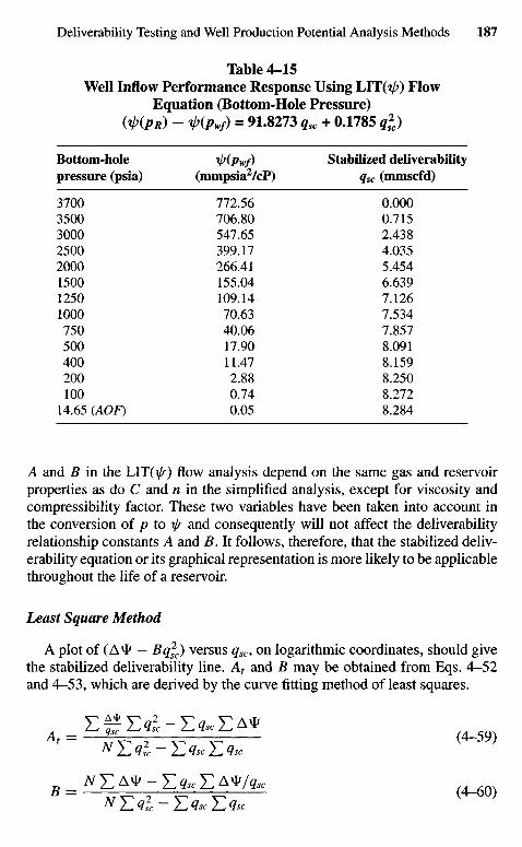
Table 4-15Well Inflow Performance Response Using LIT(t/>) Flow
Equation (Bottom-Hole Pressure)WpR) - i/>(P*f) = 91.8273 qsc + 0.1785 qfc)
Bottom-hole rfiPwf) Stabilized deliverabilitypressure (psia) (mmpsia2/cP) qsc (mmscfd)
3700 772.56 0.0003500 706.80 0.7153000 547.65 2.4382500 399.17 4.0352000 266.41 5.4541500 155.04 6.6391250 109.14 7.1261000 70.63 7.534750 40.06 7.857500 17.90 8.091400 11.47 8.159200 2.88 8.250100 0.74 8.272
14.65 (AOF) 0.05 8.284
A and B in the LIT\x//) flow analysis depend on the same gas and reservoirproperties as do C and n in the simplified analysis, except for viscosity andcompressibility factor. These two variables have been taken into account inthe conversion of p to x/r and consequently will not affect the deliverabilityrelationship constants A and B. It follows, therefore, that the stabilized deliv-erability equation or its graphical representation is more likely to be applicablethroughout the life of a reservoir.
Least Square Method
A plot of ( A ^ — Bq^c) versus qsc, on logarithmic coordinates, should givethe stabilized deliverability line. At and B may be obtained from Eqs. 4-52and 4-53, which are derived by the curve fitting method of least squares.
A1 = E ^ i f C
VE % E (4-59)
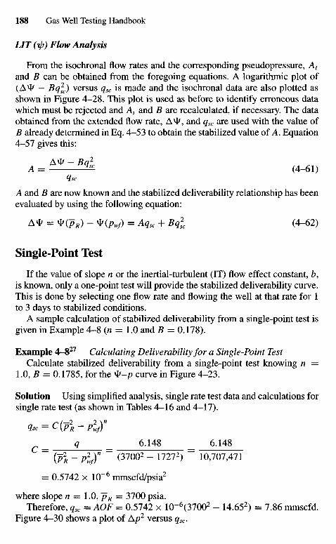
LIT (ip) Flow Analysis
From the isochronal flow rates and the corresponding pseudopressure, At
and B can be obtained from the foregoing equations. A logarithmic plot of(A*I> — Bqjc) versus qsc is made and the isochronal data are also plotted asshown in Figure 4-28. This plot is used as before to identify erroneous datawhich must be rejected and At and B are recalculated, if necessary. The dataobtained from the extended flow rate, A*I>, and qsc are used with the value ofB already determined in Eq. 4-53 to obtain the stabilized value of A. Equation4-57 gives this:
A = A * - B ^ (4-61)
A and B are now known and the stabilized deliverability relationship has beenevaluated by using the following equation:
Avi/ = V(pR) - V(Pwf) = Aqx + Bq2sc (4-62)
Single-Point Test
If the value of slope n or the inertial-turbulent (IT) flow effect constant, b,is known, only a one-point test will provide the stabilized deliverability curve.This is done by selecting one flow rate and flowing the well at that rate for 1to 3 days to stabilized conditions.
A sample calculation of stabilized deliverability from a single-point test isgiven in Example 4-8 (n = 1.0 and B = 0.178).
Example 4-827 Calculating Deliverability for a Single-Point TestCalculate stabilized deliverability from a single-point test knowing n =
1.0,B = 0.1785, for the V-p curve in Figure 4-23.
Solution Using simplified analysis, single rate test data and calculations forsingle rate test (as shown in Tables 4-16 and 4-17).
qsc = c(pi - Pifyq 6.148 _ 6.148
" (p2R - P
2wf)
n " (37002 - 17272) " 10,707,471
= 0.5742 x 10~6 mmscfd/psia2
where slope n = 1.0, ~pR = 3700 psia.Therefore, qsc = AOF = 0.5742 x 10"6(37002 - 14.652) = 7.86 mmscfd.
Figure 4-30 shows a plot of Ap2 versus qsc.
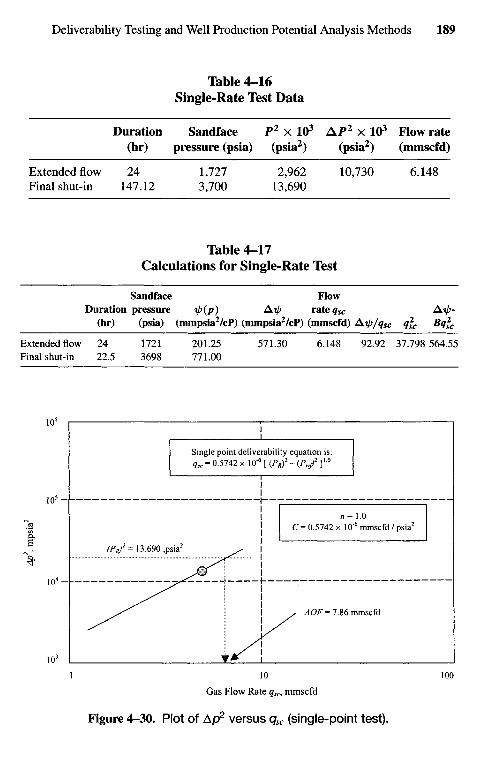
Table 4-16Single-Rate Test Data
Duration Sandface P2 X 103 AP 2 X 10³ Flow rate(hr) pressure (psia) (psia2) (psia2) (mmscfd)
Extended flow 24 1,727 2,962 10,730 6.148Final shut-in 147.12 3,700 13,690
Table 4-17Calculations for Single-Rate Test
Sandface FlowDuration pressure ip(p) A?/> rate qsc A-0-
(hr) (psia) (mmpsia2/cP) (mmpsia2/cP) (mmscfd) Aift/qsc q^c Bqjc
Extended flow 24 1721 201.25 571.30 6.148 92.92 37.798 564.55Final shut-in 22.5 3698 771.00
Gas Flow Rate qsc, mmscfd
Figure 4-30. Plot of Ap2 versus qsc (single-point test).
AOF =7.86 mmscfd
/1= 1.0C = 0.5742 x 10"6 mmscfd / psia2
Single point deliverability equation is:qsc = 0.5742 x 10"6 [(P*)2 - ( P . / ] 1 0
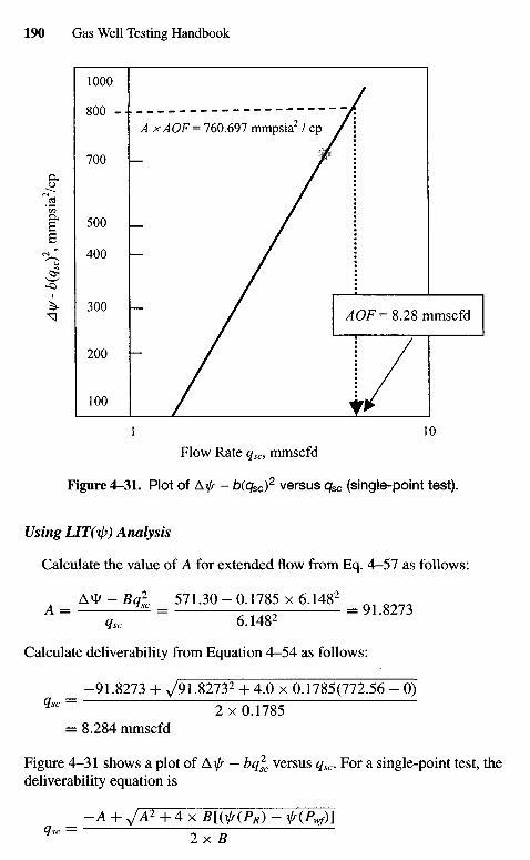
Flow Rate qSCi mmscfd
Figure 4-31. Plot of A^ - b(qsc)2 versus qsc (single-point test).
Using LtT(TJ)) Analysis
Calculate the value of A for extended flow from Eq. 4-57 as follows:
= A * - Bqj = 571.30-0 .1785 x 6.1482 =
qsc 6.1482
Calculate deliverability from Equation 4-54 as follows:
_ -91.8273 + 791.82732 + 4.0 x 0.1785(772.56 - 0)qsc ~ 2x0.1785
= 8.284 mmscfd
Figure 4-31 shows a plot of A^ — bqjc versus qsc. For a single-point test, thedeliverability equation is
_ - A + JA2 + 4 x B[W(PR) - xlf(P^f)]qsc~ 2xB
AOF= 8.28 mmscfdAy/
- b(
q sc)
2, m
mps
ia2/c
p
whereA -91.8273B = 0.1705
qsc = 8.284 mmscfd
Wellhead Deliverability
In practice it is sometime more convenient to measure the pressures at thewellhead. These pressures may be converted to bottom-hole conditions by thecalculation procedure suggested by Cullender and Smith.26 However, in someinstances, the wellhead pressures might be plotted versus flow rate in a mannersimilar to the bottom-hole curves of Figs. 4-25 or 4-28. The relationship thusobtained is known as the wellhead deliverability and is shown in Figures 4-24and 4-27.
On logrithmatic coordinates the slope of the wellhead deliverability plot isnot necessarily equal to that obtained using bottom-hole pressures. A well-head deliverability plot is useful because it relates to a surface situation, forexample, the gathering pipeline backpressure, which is more accessible thanthe reservoir. Because the wellhead deliverability relationship is not constantthroughout the life of a well, different curves are needed to represent the differ-ent average reservoir pressures, as shown in Figures 4-32 and 4-33. A samplecalculation is shown in Example 4-7.
Time to Stabilization
Stabilization is more properly defined in terms of a radius of investigation.By radius of investigation, rinv, we mean the distance that a pressure transienthas moved into a formation following a rate change in a well. As time increases,this radius moves outward into the formation until it reaches the outer boundaryof the reservoir or the no-flow boundary between adjacent flowing wells. Fromthen on, it stays constant, that is, rinv = re, and stabilization is said to have beenattained. This condition is also called the pseudo-steady-state. The pressuredoes not become constant but the rate of pressure decline does. The time tostabilization can be determined approximately by
ts £ 1000-5^ (4-63)kpR
wherets = time of stabilization, hr
JZg = gas viscosity at ~pR, cP0 = gas-filled porosity, fractionk = effective permeability to gas, mD, andre = outer radius of the drainage area, ft
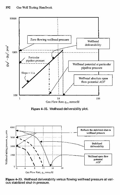
Gas Flow Rate, qc, mmscfd
Figure 4-33. Wellhead deliverability versus flowing wellhead pressure at vari-ous stabilized shut-in pressure.
Stabilizeddeliverability
Wellhead open flowpotential
AOF
Reflects the stabilized shut-inwellhead pressure
Wellhead absolute openflow potential AOF
Wellhead potential at particularpipeline pressure
Wellheaddeliverability
Zero flowing wellhead pressure
Particularpipeline pressure
Gas Flow Rate qsc, mmscfd
Figure 4-32. Wellhead deliverability plot.
Wel
lhea
d tu
bing
pre
ssur
e, p
,f, p
sia
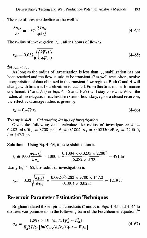
The rate of pressure decline at the well is
*M = _ 3 7 4 !Z% (4_64)
The radius of investigation, rinv, after t hours of flow is
rinv = 0.032 (k-0-\ (4-65)
forrinv < re.As long as the radius of investigation is less than re, stabilization has not
been reached and the flow is said to be transient. Gas well tests often involveinterpretation of data obtained in the transient flow regime. Both C and A willchange with time until stabilization is reached. From this time on, performancecoefficient, C and A (see Eqs. 4-45 and 4-57) will stay constant. When theradius of investigation reaches the exterior boundary, re, of a closed reservoir,the effective drainage radius is given by
rd = 0.472 re (4-66)
Example 4-9 Calculating Radius of InvestigationGiven the following data, calculate the radius of investigation: k =
6.282 mD, ~pR = 3700 psia, 0 = 0.1004, /xg = 0.02350 cP, re = 2200 ft,t = 147.2 hr.
Solution Using Eq. 4-63, time to stabilization is
,, a lmtjvl _ 10Q0 x "• •«» x <"»*> x MW = 491 h,kpR 6.282 x 3700
Using Eq. 4-65, the radius of investigation is
- n r > fif** - 0-Q32V6.282 x 3700 x 147.2 _ 1 o i n ^rinv - U.Jiy ^ - 0.1004x0.0235 " ^ "
Reservoir Parameter Estimation Techniques
Brigham related the empirical constants C and n in Eqs. 4 ^ 5 and 4 ^ 4 tothe reservoir parameters in the following form of the Forchheimer equation:24
L9S7xlO-5khTsc(pl-plf)Qsc — F , (4-67)
H11ZTPx [ln(CAJA/rw)+s + Fqsc]
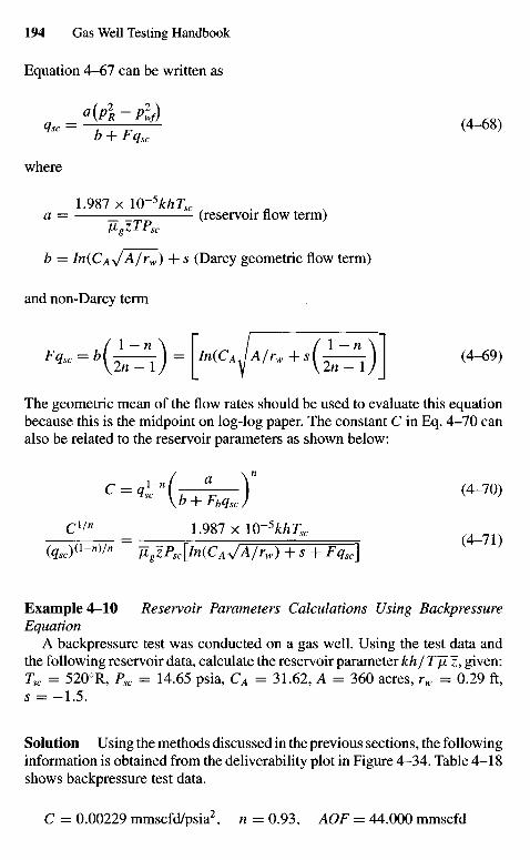
Equation 4-67 can be written as
a(p2R-plf) (A , Q ,
Vsc = , , _, (4-68)b + Fqsc
where
1.987 x 10"5khTsca = zz^ (reservoir flow term)
V>8zTPsc
b = In(CAy/A/rw) + s (Darcy geometric flow term)
and non-Darcy term
Fq"=K^T) = [ / B ( C A / ^ + K ^ T ) ] (4"69)
The geometric mean of the flow rates should be used to evaluate this equationbecause this is the midpoint on log-log paper. The constant C in Eq. 4-70 canalso be related to the reservoir parameters as shown below:
CV" = 1.987 x \Q-5khTsc
(qsc)(1-n)/n jLgzPSc[ln(CAJA/rw) + s + Fqx]
Example 4-10 Reservoir Parameters Calculations Using BackpressureEquation
A backpressure test was conducted on a gas well. Using the test data andthe following reservoir data, calculate the reservoir parameter kh/ TJl z, given:Tsc = 5200R, Psc = 14.65 psia, CA = 31.62, A = 360 acres, rw = 0.29 ft,s = -1 .5 .
Solution Using the methods discussed in the previous sections, the followinginformation is obtained from the deliverability plot in Figure 4-34. Table 4-18shows backpressure test data.
C = 0.00229 mmscfd/psia2, n = 0.93, AOF = 44.000 mmscfd
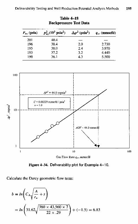
Table 4-18Backpressure Test Data
Pws (psia) pls(103 psia2) Ap2 (psia2) qsc (mmscfd)
201 40.4 — —196 38.4 2.0 2.730195 38.0 2.4 3.970193 37.2 3.2 4.440190 36.1 4.3 5.500
Gas Flow Rate qsc, mmscfd
Figure 4-34. Deliverability plot for Example 4-10.
Calculate the Darcy geometric flow term:
/ /A \b = In [cA —+ s)
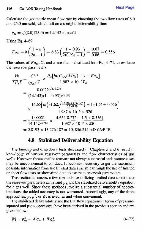
Calculate the geometric mean flow rate by choosing the two flow rates of 8.0and 25.0 mmscfd, which fall on a straight deliverability line:
qsc = 7(8.0) (25.0) = 14.142 mmscfd
Using Eq. 4-69:
The values of Fqsc, C, and n are then substituted into Eq. 4-71, to evaluatethe reservoir parameters:
kh _ Cl'n Psc[ln(CAVAj^) + s + Fqx]7W ~ (qsc)
X L 9 8 7 x 1 0 " 5 r -
0.00229(1/a93)
= (14.142)(l-0.93)/0.93
14.65[//i(31.62y^^p^) + (-1.5) + 0.556]X 1.987 x 10-5 x 520
_ 1.00021 14.65[10.272 - 1.5 + 0.556]~ 14.1420-0753 x 1.987 x 10"5 x 520
= 0.8193 x 13,276.187 = 10, 836.215 mD-ft/cP-°R
4.8 Stabilized Deliverability Equation
The buildup and drawdown tests discussed in Chapters 5 and 6 result inknowledge of various reservoir parameters and flow characteristics of gaswells. However, these detailed tests are not always successful and in some casesmay be uneconomical to conduct. It becomes necessary to get the maximumpossible information from the limited data available through the use of limitedor short flow tests or short-time data to estimate reservoir parameters.
This section discusses a few methods for utilizing limited data to estimatethe reservoir parameters kh, s, and ~p R and the stabilized deliverability equationfor a gas well. Since these methods involve a substantial number of approx-imations, the added accuracy is not warranted. Accordingly, any of the threeapproaches, p, p2, or x/r, is used, as and when convenient.
The stabilized deliverability and the LIT flow equations in terms of pressure-squared and pseudopressure, have been derived in the previous section and aregiven below:
p2R-p2
wf=A'qsc + B'ql (4-72)
Next Page
Chapter 5
Fundamentalsof Drawdown TestAnalysis Methods
5.1 Introduction
Important reservoir parameters can be determined by flowing a well at aconstant rate and measuring flowing wellbore pressure as a function of time.This is called drawdown testing and it can utilize information obtained in boththe transient and pseudo-steady-state flow regimes. If the flow extends to thepseudo-steady state, the test is referred to as a reservoir limit test and can beused to estimate in-place gas and shape of the reservoir. Both single-rate andtwo-rate tests are utilized depending on the information required. The purposeof the drawdown testing is to determine the reservoir characteristics that willaffect flow performance. Some of the important characteristics are the flowcapacity kh, skin factor s, and turbulence coefficient D.
5.2 Characteristics of Flow and GasWell Transient Testing
Much of that information can be obtained from pressure transient tests.Pressure transient testing techniques, such as buildup, drawdown, interfer-ence, and pulse, are an important part of reservoir and production engineering.As the term is used in this book, pressure transient testing includes generat-ing and measuring pressure variations with time in gas wells and subsequently,estimating rock, fluid, and well properties and predicting reservoir/well behav-ior. Practical information obtainable from transient testing includes wellborevolume, damage, and improvement; reservoir pressure; permeability; poros-ity; reserves; reservoir and fluid discontinuities; and other related data. Allthis information can be used to help analyze, improve, and forecast reservoirperformance.
Pressure transient testing and analysis is an important diagnostic tool todefine near-wellbore and interwell conditions as opposed to composite prop-erties that would be indicated by steady-state productivity index data. In othercases, simpler approach is adequate, or a different or combined approach isneeded to solve a problem.
Pressure interference or pulse testing could establish the possible existenceand orientation of vertical fracture of a gas reservoir. However, other informa-tion (such as profile surveys, production logs, stimulation history, well pro-duction tests, packer tests, core descriptions, and other geological data aboutreservoir lithology and continuity) would be useful in distinguishing betweendirectional permeability and fractures or estimating whether the fractures wereinduced or natural. It is generally good practice to run a base pressure transienttest on a producing well shortly after completion or an injection well after asuitable period of injection. This can lead to early recognition and correctionof many problems, of which insufficient stimulation is only the most obvious.Such tests also provide in situ data for reservoir simulation and a base forcomparison with reservoir or well problems as they arise.
5.3 Pressure-Time History for Constant-RateDrawdown Test
Figure 5-1 shows the flow history of an unfractured well and can be dividedinto three periods for analysis:
The transient or early flow period is usually used to analyze flow character-istics
The late transient period is more completeThe semisteady-state flow period is used in reservoir limit tests
As shown in Figure 5-1, radial flow is preceded by a period of linear flow whenwells contain fractures. If the pay interval is partly penetrated or perforated,a spherical-flow-dominated period should be expected between the linear andradial flow times. Also, the first flow unloads the well while accepting a con-tribution from the reservoir. Thus, a group of curves must be constructed toanalyze well tests properly. Flow tests may better represent well performancethan buildup tests since particle movement, turbulence, and capillary constric-tions are then included.
5.4 Characteristics of Various Flow Regimes
The different flow regimes are depicted in Figure 5-1. It is convenient totreat each one separately.
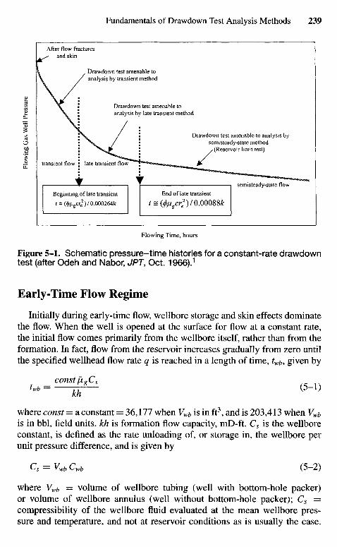
Flowing Time, hours
Figure 5-1. Schematic pressure-time histories for a constant-rate drawdowntest (after Odeh and Nabor, JPT, Oct. 1966).1
Early-Time Flow Regime
Initially during early-time flow, wellbore storage and skin effects dominatethe flow. When the well is opened at the surface for flow at a constant rate,the initial flow comes primarily from the wellbore itself, rather than from theformation. In fact, flow from the reservoir increases gradually from zero untilthe specified wellhead flow rate q is reached in a length of time, twb, given by
_ const Jl8C5t b _ _ (5_1)kh
where const = a constant = 36,177 when Vwb is in ft3, and is 203,413 when Vwb
is in bbl, field units, kh is formation flow capacity, mD-ft. Cs is the wellboreconstant, is defined as the rate unloading of, or storage in, the wellbore perunit pressure difference, and is given by
Cs = VwbCwb (5-2)
where Vwb = volume of wellbore tubing (well with bottom-hole packer)or volume of wellbore annulus (well without bottom-hole packer); Cs =compressibility of the wellbore fluid evaluated at the mean wellbore pres-sure and temperature, and not at reservoir conditions as is usually the case.
Beginning of late transient
t = (<f>ngcre2)/ 0.000264k
End of late transient
t = ((/>jugcre2)/0.00088k
semisteady-state flow
transient flow late transient flow
Drawdown test amenable to analysis bysemisteady-state method
(Reservoir limit test)
Drawdown test amenable toanalysis by late transient method
Drawdown test amenable toanalysis by transient method
After flow fracturesand skin
Flo
win
g G
as W
ell
Pres
sure
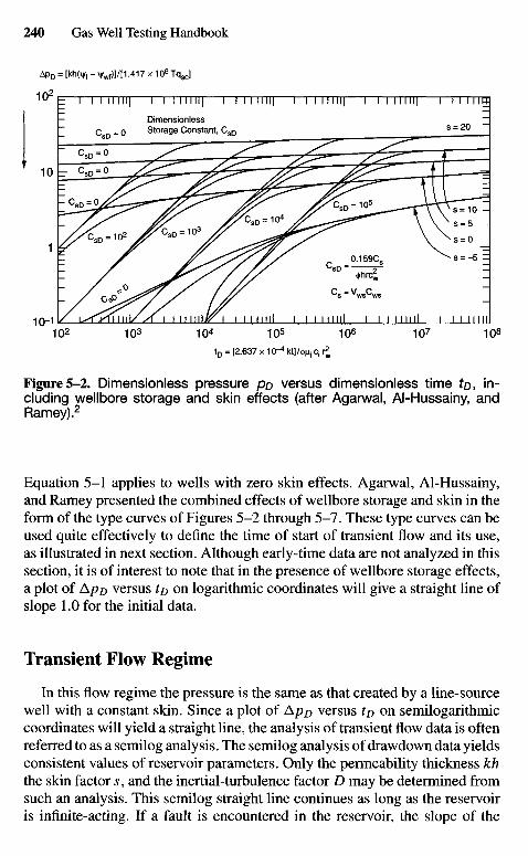
Figure5-2. Dimensionless pressure po versus dimensionless time to, in-cluding wellbore storage and skin effects (after Agarwal, Al-Hussainy, andRamey).2
Equation 5-1 applies to wells with zero skin effects. Agarwal, Al-Hussainy,and Ramey presented the combined effects of wellbore storage and skin in theform of the type curves of Figures 5-2 through 5-7. These type curves can beused quite effectively to define the time of start of transient flow and its use,as illustrated in next section. Although early-time data are not analyzed in thissection, it is of interest to note that in the presence of wellbore storage effects,a plot of ApD versus to on logarithmic coordinates will give a straight line ofslope 1.0 for the initial data.
Transient Flow Regime
In this flow regime the pressure is the same as that created by a line-sourcewell with a constant skin. Since a plot of ApD versus to on semilogarithmiccoordinates will yield a straight line, the analysis of transient flow data is oftenreferred to as a semilog analysis. The semilog analysis of drawdown data yieldsconsistent values of reservoir parameters. Only the permeability thickness khthe skin factor s, and the inertial-turbulence factor D may be determined fromsuch an analysis. This semilog straight line continues as long as the reservoiris infinite-acting. If a fault is encountered in the reservoir, the slope of the
DimensionlessStorage Constant, CsD
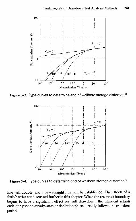
Dimensionless Time, tD
Figure 5-4. Type curves to determine end of wellbore storage distortion.2
line will double, and a new straight line will be established. The effects of afault/barrier are discussed further in this chapter. When the reservoir boundarybegins to have a significant effect on well drawdown, the transient regionends; the pseudo-steady-state or depletion phase directly follows the transientperiod.
Dimensionless Time, tD
Figure 5-3. Type curves to determine end of wellbore storage distortion.2
Dim
ensi
onle
ss P
ress
ure,
PD
Dim
ensi
onle
ss P
ress
ure,
PD
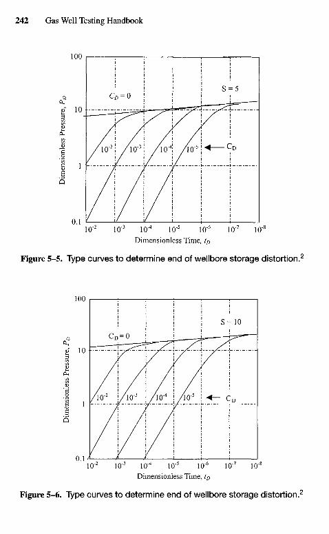
Dimensionless Time, tD
Figure 5-5. Type curves to determine end of wellbore storage distortion.2
Dimensionless Time, tD
Figure 5-6. Type curves to determine end of wellbore storage distortion.2
Dim
ensi
onle
ss P
ress
ure,
PD
Dim
ensi
onle
ss P
ress
ure,
PD
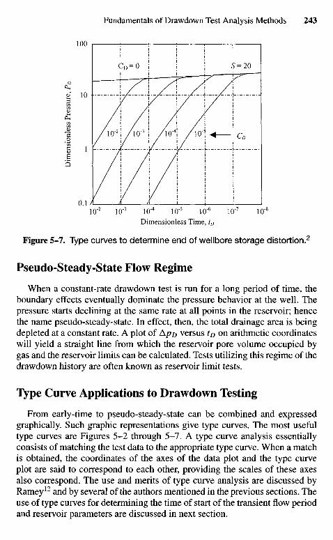
Dimensionless Time, tD
Figure 5-7. Type curves to determine end of wellbore storage distortion.2
Pseudo-Steady-State Flow Regime
When a constant-rate drawdown test is run for a long period of time, theboundary effects eventually dominate the pressure behavior at the well. Thepressure starts declining at the same rate at all points in the reservoir; hencethe name pseudo-steady-state. In effect, then, the total drainage area is beingdepleted at a constant rate. A plot of ApD versus to on arithmetic coordinateswill yield a straight line from which the reservoir pore volume occupied bygas and the reservoir limits can be calculated. Tests utilizing this regime of thedrawdown history are often known as reservoir limit tests.
Type Curve Applications to Drawdown Testing
From early-time to pseudo-steady-state can be combined and expressedgraphically. Such graphic representations give type curves. The most usefultype curves are Figures 5-2 through 5-7. A type curve analysis essentiallyconsists of matching the test data to the appropriate type curve. When a matchis obtained, the coordinates of the axes of the data plot and the type curveplot are said to correspond to each other, providing the scales of these axesalso correspond. The use and merits of type curve analysis are discussed byRamey12 and by several of the authors mentioned in the previous sections. Theuse of type curves for determining the time of start of the transient flow periodand reservoir parameters are discussed in next section.
Dim
ensi
onle
ss P
ress
ure,
PD
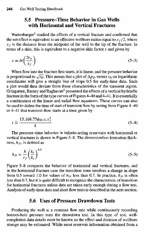
5.5 Pressure-Time Behavior in Gas Wellswith Horizontal and Vertical Fractures
Wattenbarger3 studied the effects of a vertical fracture and confirmed thatthe net effect is equivalent to an effective wellbore radius equal to Jt//2, whereXf is the distance from the midpoint of the well to the tip of the fracture. Interms of a skin, this is equivalent to a negative skin factor s and given by
S=In(^) (5-3)
When flow into the fracture first starts, it is linear, and the pressure behavioris proportional to +Jt^. This means that a plot of ApD versus to on logarithmiccoordinates will give a straight line of slope 0.5 for early-time data. Sucha plot would then deviate from these characteristics of the transient region.Gringarten, Ramey and Raghavan4 presented the effects of a vertical hydraulicfracture in the form of the type curves of Figures 4-40 and 4-41. It is essentiallya combination of the linear and radial flow equations. These curves can alsobe used to define the time of start of transient flow by noting from Figure 4-40or 4-41 that transient flow starts at a time given by
_ 15,168.750/A/QJCJ
The pressure-time behavior in infinite-acting reservoirs with horizontal orvertical fractures is shown in Figure 5-8. The dimensionless formation thick-ness, hD, is defined as
^ = Hf)* <5-5>rf\kzj
Figure 5-8 compares the behavior of horizontal and vertical fractures, andin the horizontal fracture case the transition zone involves a change in slopefrom 0.5 toward 1.0 for values of ho less than 0.7. In practice, ho is oftenless than 0.7, but it is quite difficult to recognize the characteristic of transitionfor horizontal fractures unless data are taken early enough during a flow test.Analysis of early-time data and short flow tests is described in the next section.
5.6 Uses of Pressure Drawdown Tests
Producing the well at a constant flow rate while continuously recordingbottom-hole pressure runs the drawdown test. In this type of test, well-completion data details must be known so the effect and duration of wellborestorage may be estimated. While most reservoir information obtained from a
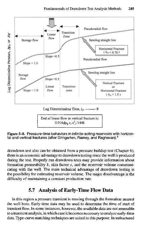
Log Dimensionless Time, tp -^
End of linear flow to vertical fracture is:0.0\6<f>/jgctx
2f/\44k
Figure 5-8. Pressure-time behaviors in infinite-acting reservoirs with horizon-tal and vertical fractures (after Gringarten, Ramey, and Raghavan).4
drawdown test also can be obtained from a pressure buildup test (Chapter 6),there is an economic advantage to drawdown testing since the well is producedduring the test. Properly run drawdown tests may provide information aboutformation permeability k, skin factor s, and the reservoir volume communi-cating with the well. The main technical advantage of drawdown testing isthe possibility for estimating reservoir volume. The major disadvantage is thedifficulty of maintaining a constant production rate.
5.7 Analysis of Early-Time Flow Data
In this region a pressure transient is moving through the formation nearestthe well bore. Early-time data may be used to determine the time of start oftransient flow. In some instances, however, the available data are not amenableto a transient analysis, in which case it becomes necessary to analyze early-timedata. Type-curve matching techniques are suited to this purpose. In unfractured
Log
Dim
ensi
onle
ss P
ress
ure,
Apo
or
A y/
Vertical Fractureor
Horizontal Fracture(hD>\.0)
Semilog straight line
Pseudoradial flow
Horizontal Fracture( hD < 0.70 )
Semilog straight line
Pseudoradial flowTransition
ZoneLinearflow
Storage flow
Slope =0.5
Slope= 1.0
Storageflow Slope =0.5
Slope= 1.0Linearflow
Transitionzone
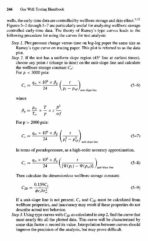
wells, the early-time data are controlled by wellbore storage and skin effect.5'12
Figures 5-2 through 5-7 are particularly useful for analyzing wellbore storagecontrolled early-time data. The theory of Ramey's type curves leads to thefollowing procedure for using the curves for test analysis:
Step 1. Plot pressure change versus time on log-log paper the same size asRamey's type curve on tracing paper. This plot is referred to as the dataplot.
Step 2. If the test has a uniform slope region (45° line at earliest times),choose any point t (change in time) on the unit-slope line and calculatethe wellbore storage constant C8:For p < 3000 psia:
Z 4 \Pi Pwf/ unit siope line
where
a Psc T f?
For p > 2000 psia:
C . ^ ^ 4 ( V T ) №-7)^ \Pi Pwf/unilslopeline
In terms of pseudopressure, as a high-order accuracy approximation,
= qsc x 10* x p, / , \
24 l[%-)-*W]L^to
Then calculate the dimensionless wellbore storage constant:
(j)cthrl
If a unit-slope line is not present, C8 and CSD must be calculated fromwellbore properties, and inaccuracy may result if these properties do notdescribe actual test behavior.
Step 3. Using type curves with CSD as calculated in step 2, find the curve thatmost nearly fits all the plotted data. This curve will be characterized bysome skin factor s; record its value. Interpolation between curves shouldimprove the precision of the analysis, but may prove difficult.
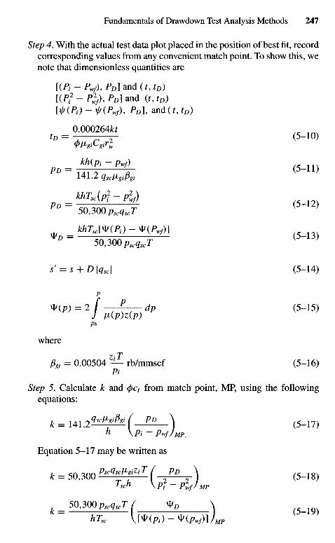
Step 4. With the actual test data plot placed in the position of best fit, recordcorresponding values from any convenient match point. To show this, wenote that dimensionless quantities are
[(P1-Pwf),PD] and (t,tD)
[ ( ^ 2 -P%f)> PD] and (tJD)
Hr(Pi)- ^(/V), PDl and ( M s )
0.000264Jfcfto = . r 2 (5-10)
kh(Pi - pwf)PD =-TTT-Z — P-Il)
141.2 qScligiPgi
khTsc(pf - pjf)PD = -TT-TTT ZT (5-12)
50,300 pscqscT
khTsc[*(Pi)-*(PWf)] r s^D = C A n A P-13)
50,300 pscqScT
s' = s + D\qsc\ (5-14)
p
V(P) = 2 f P dp (5-15)J n(p)z(p)
Pb
where
Pgt = 0.00504 — rb/mmscf (5-16)Pi
Step 5. Calculate k and (/>ct from match point, MP, using the followingequations:
k=14lm2*!^(_PD_\ ( 5 _ 1 7 )
h \Pi~ Pwf/MP,
Equation 5-17 may be written as
k = 50,300 P*«~№T(P°\ ( 5 _ 1 8 )
Tsch \Pt-plfJMp
= 50,300PscqscT / *D \
hTsc \[V(Pi)-y(pwf)])MP
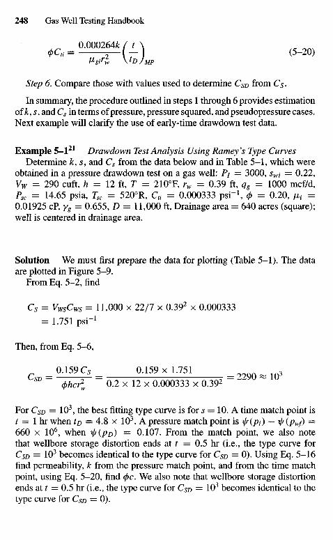
0.000264fc / t \4>cti = 2—1 —I (5"2°)
Step 6. Compare those with values used to determine CSD from Cs-
In summary, the procedure outlined in steps 1 through 6 provides estimationof £, s, and C5 in terms of pressure, pressure squared, and pseudopressure cases.Next example will clarify the use of early-time drawdown test data.
Example 5-12 1 Drawdown Test Analysis Using Ramey 's Type CurvesDetermine k, s, and Cs from the data below and in Table 5-1, which were
obtained in a pressure drawdown test on a gas well: Pj = 3000, sWi = 0.22,Vw = 290 cuft, h = 12 ft, T = 2100F, rw = 0.39 ft, qg = 1000 mcf/d,Psc = 14.65 psia, Tsc = 5200R, Cti = 0.000333 psi"1, 0 = 0.20, /x, =0.01925 cP, yg = 0.655, D = 11,000 ft, Drainage area = 640 acres (square);well is centered in drainage area.
Solution We must first prepare the data for plotting (Table 5-1). The dataare plotted in Figure 5-9.
From Eq. 5-2, find
C5 = VWSCWS = 11,000 x 22/7 x 0.392 x 0.000333
= 1.751 psi"1
Then, from Eq. 5-6,
_ 0 . 1 5 9 C , ^ 0.159x1.751 = ^ 3SD (phcrl 0.2 x 12 x 0.000333 x 0.392
For CSD = 103, the best fitting type curve is for s = 10. A time match point ist = 1 hr when tp = 4.8 x 10³. A pressure match point is i/ript) — ir{pWf) —660 x 106, when II/(PD) = 0.107. From the match point, we also notethat wellbore storage distortion ends at t = 0.5 hr (i.e., the type curve forCSD = 103 becomes identical to the type curve for C ^ = 0). Using Eq. 5-16find permeability, k from the pressure match point, and from the time matchpoint, using Eq. 5-20, find 0c. We also note that wellbore storage distortionends at t = 0.5 hr (i.e., the type curve for CSD = 103 becomes identical to thetype curve for CSD = 0).
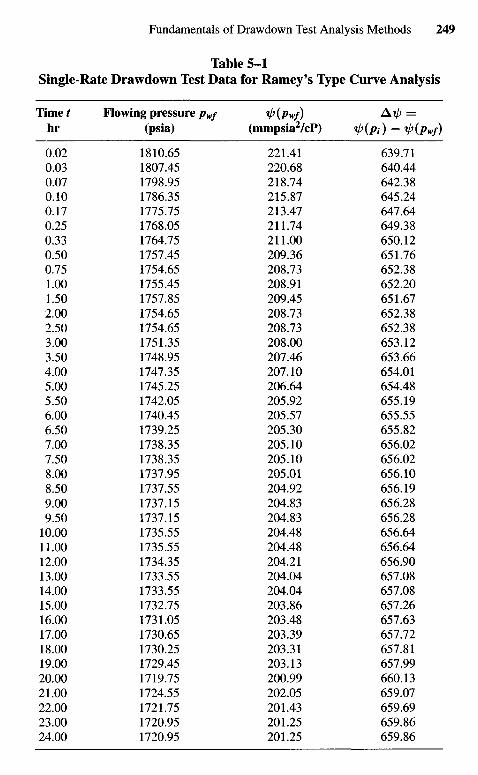
Table 5-1Single-Rate Drawdown Test Data for Ramey's Type Curve Analysis
Time t Flowing pressure pw/ %l){pwf) Ai/? =hr (psia) (mmpsia2/cP) i/>(Pi) — *P(Pwf)
0.02 1810.65 221.41 639.710.03 1807.45 220.68 640.440.07 1798.95 218.74 642.380.10 1786.35 215.87 645.240.17 1775.75 213.47 647.640.25 1768.05 211.74 649.380.33 1764.75 211.00 650.120.50 1757.45 209.36 651.760.75 1754.65 208.73 652.381.00 1755.45 208.91 652.201.50 1757.85 209.45 651.672.00 1754.65 208.73 652.382.50 1754.65 208.73 652.383.00 1751.35 208.00 653.123.50 1748.95 207.46 653.664.00 1747.35 207.10 654.015.00 1745.25 206.64 654.485.50 1742.05 205.92 655.196.00 1740.45 205.57 655.556.50 1739.25 205.30 655.827.00 1738.35 205.10 656.027.50 1738.35 205.10 656.028.00 1737.95 205.01 656.108.50 1737.55 204.92 656.199.00 1737.15 204.83 656.289.50 1737.15 204.83 656.28
10.00 1735.55 204.48 656.6411.00 1735.55 204.48 656.6412.00 1734.35 204.21 656.9013.00 1733.55 204.04 657.0814.00 1733.55 204.04 657.0815.00 1732.75 203.86 657.2616.00 1731.05 203.48 657.6317.00 1730.65 203.39 657.7218.00 1730.25 203.31 657.8119.00 1729.45 203.13 657.9920.00 1719.75 200.99 660.1321.00 1724.55 202.05 659.0722.00 1721.75 201.43 659.6923.00 1720.95 201.25 659.8624.00 1720.95 201.25 659.86
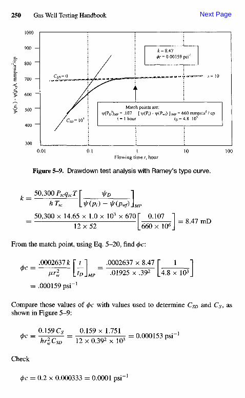
Flowing time t, hour
Figure 5-9. Drawdown test analysis with Ramey's type curve.
k = 50,300 PscgscT T jsD 1
h Tsc If(Pt) - ^(Pwf)jMp
50,300 x 14.65 x 1.0 x 103 x 670 T 0.107 1
= 12^52 L6607K*J = 8-47 m °
From the match point, using Eq. 5-20, find 0c:
_ .0002637 k p i _ .0002637 x 8.47 I" 1 10 C ~ ~^l \JD\MP
= .01925 x .392 L4.8 x 103J
= .000159 psi"1
Compare those values of (j>c with values used to determine CSD and Cs, asshown in Figure 5-9:
0.159C5 0.159 x 1.751 ^ e . ,*C ^ -HC^ - 12x0.39^x103 = a O 0 0 1 5 3 PS 1"
Check
(j)c = 0.2 x 0.000333 = 0.0001 psi"1
xV(P
i)"
y(Pw
d->
mm
psia
"/cp
Match points are:V(PD^MP = -107 [ i}/(Pi) - \|/(Pwf) ] MP = 660 mmpsia2 / cp
t= 1 hour /D = 4.8 103
Next Page
Chapter 6
Fundamentalsof Pressure BuildupAnalysis Methods
6.1 Introduction
This chapter discusses the most frequently used pressure buildup test. It isthe simplest test that can be run on a gas well. If the effects of wellbore storagecan be determined, much useful information can be obtained. This informationincludes permeability k, apparent skin factor s\ and average reservoir pressure~pR. The test consists of flowing the well at a constant rate qsc for a period of timetp, shutting the well in (at At = 0), and measuring wellbore pressure increasewith shut-in time At. Horner developed the test, and this method of analysis isgenerally considered the best. Other conventional methods of analysis includethe Horner plot, the Miller-Dyes-Hutchinson2 plot (often abbreviated as theMDH plot), and the Muskat plot. Horner1 showed that a plot of the shut-inpressure pws versus log (tp + At)/At should result in a straight line for aninfinite-acting reservoir. In the buildup tests, t refers to the drawdown periodprior to a buildup and At refers to the shut-in or buildup time. Matthews,Brons, and Hazebroek,3 abbreviated as MBH, extended the application of theHorner plot to finite reservoirs.
A buildup test is always preceded by a drawdown, and the buildup dataare directly affected by this drawdown. Usually, the drawdown starts from astabilized reservoir condition represented by the stabilized reservoir pressure,Pi. At a time t, the well is shut in and the buildup is continued for a time At.Under these conditions, the behavior of the static sand face pressure, pws, isdepicted in Figure 6-1.
6.2 Pressure Buildup Behavior Curves
Figure 6-2 shows pressure buildup curve shapes. As also shown in thatfigure, the fracture cases and large negative skin cases approach the semilogstraight line from above when wellbore storage is small. That figure also shows
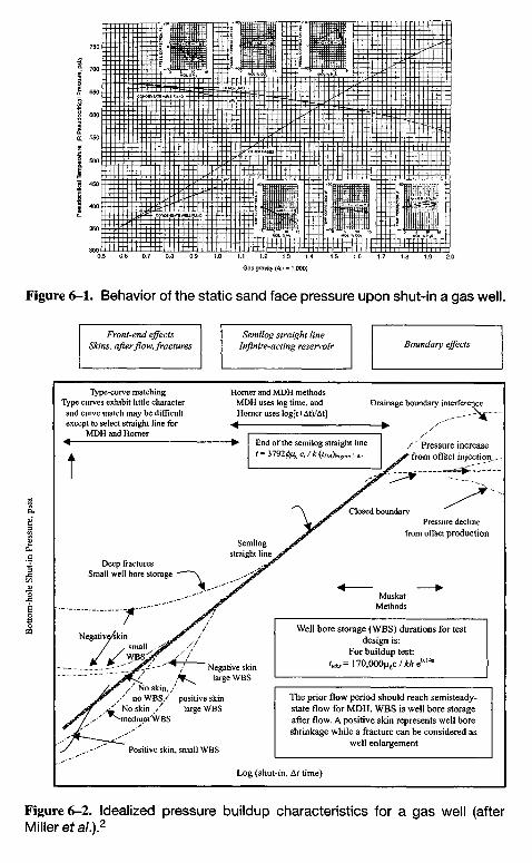
Front-end effectsSkins, after flow, fractures
Semilog straight lineInfinite-acting reservoir Boundary effects
Well bore storage (WBS) durations for testdesign is:
For buildup test:/ ^ = 1 7 0 , 0 0 0 ^ / M e014s
The prior flow period should reach semisteady-state flow for MDH. WBS is well bore storageafter flow. A positive skin represents well boreshrinkage while a fracture can be considered as
well enlargement
Figure 6-2. Idealized pressure buildup characteristics for a gas well (afterMiller ef a/.).2
Drainage boundary interferenceHomer and MDH methods
MDH uses log time, andHorner uses log[t+At)/At]
Type-curve matchingType curves exhibit little character
and curve match may be difficultexcept to select straight line for
MDH and HornerEnd of the semilog straight linet = 3192<pMgct/k(tDA)Figure5.4a
Pressure increasefrom offset injection
Closed boundaryPressure decline
from offset production
MuskatMethods
Semilogstraight line
Deep fracturesSmall well bore storage
Negative/skinsmall
WBS"Negative skin
large WBSNo skin,
no WBS positive skinlarge WBSNo skin
-mediumVBS
Positive skin, small WBS
Log (shut-in, At time)
Gas gravity (Air =1.000)
Figure 6-1. Behavior of the static sand face pressure upon shut-in a gas well.
Pse
udoc
ritic
al T
empe
ratu
re,
jR P
seud
ocrit
ical
Pre
ssur
e, p
sia
Bot
tom
-hol
e Sh
ut-i
n Pr
essu
re, p
sia

that behavior can be hidden by large wellbore storage effects, so the buildupcurve may have the characteristic shape associated with wellbore storage orwith a positive skin. For the figure shown Miller, Dyes, and Hutchinson scales2
are used. The Horner plot is equally useful and is often preferred. Detailsdiscussion can be found in the next sections.
6,3 Uses and Practical Applications of PressureBuildup Tests
Much information can be obtained from pressure transient tests. Pressuretransient testing techniques, such as buildup, drawdown, interference, andpulse, are an important part of reservoir and production engineering. As theterm is used in this book, pressure transient testing includes generating andmeasuring pressure variations with time on gas wells and, subsequently, esti-mating rock, fluid, and well properties and predicting reservoir/well behavior.Practical information obtainable from transient testing includes wellbore vol-ume, damage, and improvements; reservoir pressure; formation permeability;porosity; reserves; reservoir and fluid discontinuities; and other related data.All this information can be used to help analyze, improve, and forecast reser-voir performance.
It is generally good practice to run a base pressure transient test on a pro-ducing well shortly after completion or an injection well after a suitable periodof injection. This can lead to early recognition and correction of many prob-lems, of which insufficient stimulation is only the most obvious. Such testsalso provide in situ data for reservoir simulation and a base for comparisonwith reservoir or well problem as they arise. Figure 6-3 shows types, uses, andpractical applications of buildup tests.
6.4 Type Curves and Desuperposition
Type curves are also applicable to the analysis of buildup tests, thoughtype curve matching techniques are not discussed fully in this section. Typecurve matching provides a simple method for determining the time of startof transient flow during drawdown tests. A similar approach may be used todetermine the time of start of semilog straight-line data in buildup tests withone additional step. Since a buildup is always preceded by a drawdown, thebuildup data must be "desuperposed" before attempting a type curve match. Itmay be noted that desuperposition can also be performed on the second rate ofa two-rate test. Early-time data obtained during a buildup may be desuperposedby assuming i/f (Pw^) to be constant at a value \l/(PWfo).
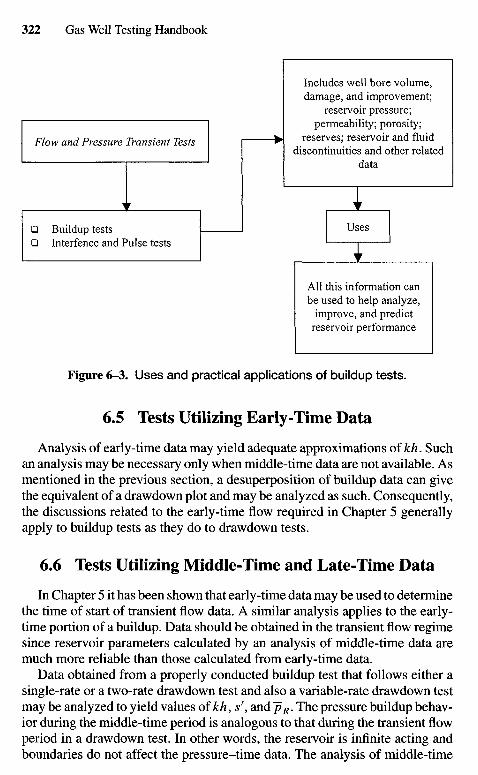
Figure 6-3. Uses and practical applications of buildup tests.
6.5 Tests Utilizing Early-Time Data
Analysis of early-time data may yield adequate approximations of kh. Suchan analysis may be necessary only when middle-time data are not available. Asmentioned in the previous section, a desuperposition of buildup data can givethe equivalent of a drawdown plot and may be analyzed as such. Consequently,the discussions related to the early-time flow required in Chapter 5 generallyapply to buildup tests as they do to drawdown tests.
6.6 Tests Utilizing Middle-Time and Late-Time Data
In Chapter 5 it has been shown that early-time data may be used to determinethe time of start of transient flow data. A similar analysis applies to the early-time portion of a buildup. Data should be obtained in the transient flow regimesince reservoir parameters calculated by an analysis of middle-time data aremuch more reliable than those calculated from early-time data.
Data obtained from a properly conducted buildup test that follows either asingle-rate or a two-rate drawdown test and also a variable-rate drawdown testmay be analyzed to yield values of kh, sf, and ~pR. The pressure buildup behav-ior during the middle-time period is analogous to that during the transient flowperiod in a drawdown test. In other words, the reservoir is infinite acting andboundaries do not affect the pressure-time data. The analysis of middle-time
Flow and Pressure Transient Tests
Buildup testsInterfence and Pulse tests
Includes well bore volume,damage, and improvement;
reservoir pressure;permeability; porosity;
reserves; reservoir and fluiddiscontinuities and other related
data
Uses
AU this information canbe used to help analyze,
improve, and predictreservoir performance
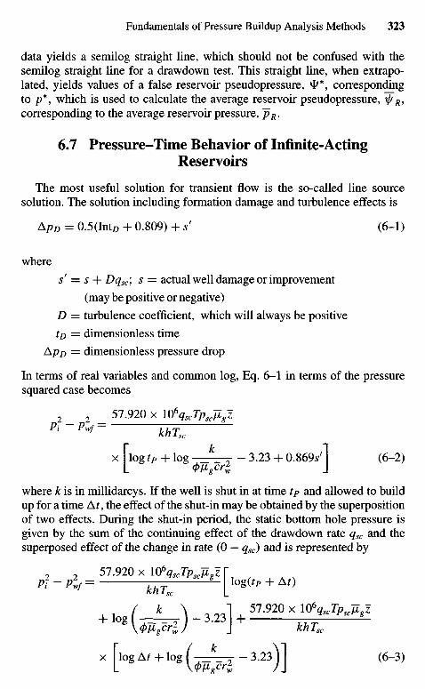
data yields a semilog straight line, which should not be confused with thesemilog straight line for a drawdown test. This straight line, when extrapo-lated, yields values of a false reservoir pseudopressure, **, correspondingto /?*, which is used to calculate the average reservoir pseudopressure, \/fR,corresponding to the average reservoir pressure, ~pR.
6.7 Pressure-Time Behavior of Infinite-ActingReservoirs
The most useful solution for transient flow is the so-called line sourcesolution. The solution including formation damage and turbulence effects is
ApD = 0.5(IntD + 0.809) + s' (6-1)
where
s' = s + Dqsc\ s = actual well damage or improvement(may be positive or negative)
D = turbulence coefficient, which will always be positiveto = dimensionless time
ApD = dimensionless pressure drop
In terms of real variables and common log, Eq. 6-1 in terms of the pressuresquared case becomes
2 2 _ 57.920 x l06gscTpscJ[gzPi P*- khTsc
x I log tP + log _k_ . - 3.23 + 0.869/1 (6-2)
where k is in millidarcys. If the well is shut in at time tP and allowed to buildup for a time Ar, the effect of the shut-in may be obtained by the superpositionof two effects. During the shut-in period, the static bottom hole pressure isgiven by the sum of the continuing effect of the drawdown rate qsc and thesuperposed effect of the change in rate (0 — qsc) and is represented by
0 0 5 7 . 9 2 O x 106 qscTp,IZ gzTPt - Plf = khT
s [ tagto + AO+ - f e ) - ] + 5 7 ' 9 2 0 x ^ w
x [log At + log f — ^ y - 3.23)1 (6-3)
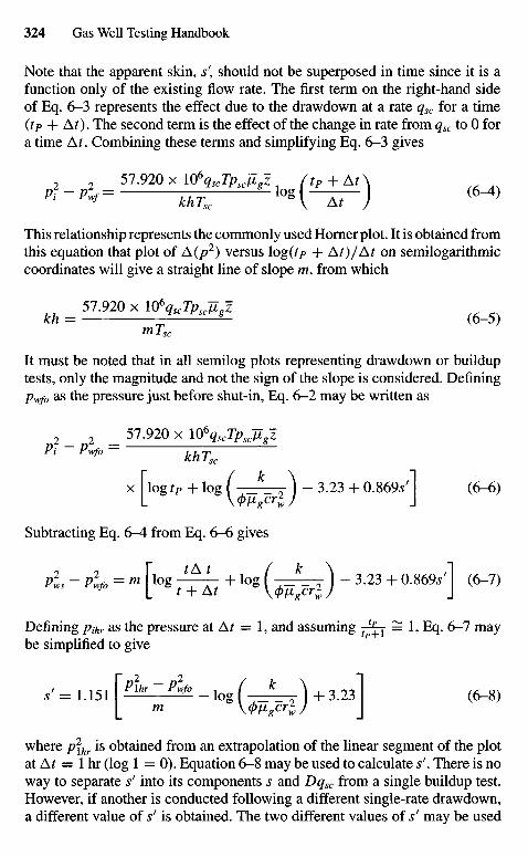
Note that the apparent skin, s\ should not be superposed in time since it is afunction only of the existing flow rate. The first term on the right-hand sideof Eq. 6-3 represents the effect due to the drawdown at a rate qsc for a time(tp + At). The second term is the effect of the change in rate from qsc to 0 fora time At. Combining these terms and simplifying Eq. 6-3 gives
2 2 57.920 x l06qscTPscJZgz (tP + A A^ " ** JS5T log [-X-) (6-4)
This relationship represents the commonly used Horner plot. It is obtained fromthis equation that plot of A(p2) versus \og(tp + At)/At on semilogarithmiccoordinates will give a straight line of slope m, from which
kh = 57.920 x lO%cTpsc]Zgz
mTsc
It must be noted that in all semilog plots representing drawdown or builduptests, only the magnitude and not the sign of the slope is considered. Definingpwf0 as the pressure just before shut-in, Eq. 6-2 may be written as
2 _ 2 57.920 x lO%cTPscJ[gzPi Pwf0 ~ khTsc
x [log tP + log ( * . \ - 3.23 + 0.869s'l (6-6)
Subtracting Eq. 6-4 from Eq. 6-6 gives
A, - J^ = - ['"8 7TS7+ los {WM) ~ " 3 + a 8 6 9 / ] <6"7)
Defining pihr as the pressure at At — 1, and assuming ^ - j - = 1, Eq. 6-7 maybe simplified to give
s, = L151 K r - ^ 4 _ j ( ^ t ) + 3.231 (6-8)
where p\hr is obtained from an extrapolation of the linear segment of the plotat Af = 1 hr (log 1 = 0). Equation 6-8 may be used to calculate sf. There is noway to separate s' into its components s and Dqsc from a single buildup test.However, if another is conducted following a different single-rate drawdown,a different value of sf is obtained. The two different values of sf may be used
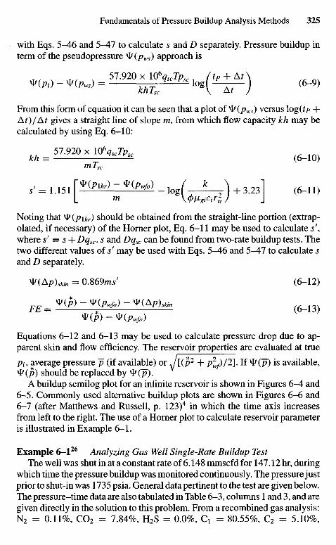
with Eqs. 5-46 and 5-47 to calculate s and D separately. Pressure buildup interm of the pseudopressure W(pws) approach is
khTsc \ At )
From this form of equation it can be seen that a plot of W (pws) versus \og(tp +At)/At gives a straight line of slope m, from which flow capacity kh may becalculated by using Eq. 6-10:
U - 5 7 - 9 2 0 X l ^ « r " « «M0)mTsc
s, = U51 r*^>-*^)_ l ogf_j_)+3 .23l (6_n)
Noting that W{p\hr) should be obtained from the straight-line portion (extrap-olated, if necessary) of the Horner plot, Eq. 6-11 may be used to calculate s\where sf = s + Dqsc. s and Dqsc can be found from two-rate buildup tests. Thetwo different values of sr may be used with Eqs. 5-46 and 5-Al to calculate sand D separately.
W{Ap)skin = 0.869m/ (6-12)
FE = ^(P)-^(PWfo)-^(^P)skin 6 _ 1 3
*(p) - V(Pwfo)
Equations 6-12 and 6-13 may be used to calculate pressure drop due to ap-parent skin and flow efficiency. The reservoir properties are evaluated at true
Pi, average pressure ~p (if available) or J[(p2 + plf)/2], IfW(P) is available,W (p) should be replaced by W (p). V
A buildup semilog plot for an infinite reservoir is shown in Figures 6-4 and6-5. Commonly used alternative buildup plots are shown in Figures 6-6 and6-7 (after Matthews and Russell, p. 123)4 in which the time axis increasesfrom left to the right. The use of a Horner plot to calculate reservoir parameteris illustrated in Example 6-1.
Example 6-126 Analyzing Gas Well Single-Rate Buildup TestThe well was shut in at a constant rate of 6.148 mmscfd for 147.12 hr, during
which time the pressure buildup was monitored continuously. The pressure justprior to shut-in was 1735 psia. General data pertinent to the test are given below.The pressure-time data are also tabulated in Table 6-3, columns 1 and 3, and aregiven directly in the solution to this problem. From a recombined gas analysis:N2 = 0.11%, CO2 = 7.84%, H2S = 0.0%, Cj = 80.55%, C2 = 5.10%,
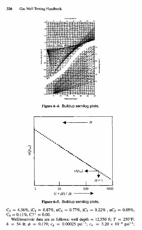
Figure 6-5. Buildup semilog plots.
C3 = 4.36%, IC4 = 0.87%, nC4 = 0.77%, iC5 = 0.22% , nC5 = 0.09%,C6 = 0.11%, C7+ = 0.00.
Well/reservoir data are as follows: well depth = 12,550 ft; T = 2500F;h = 54 ft; 0 = 0.179; cg = 0.00025 psi"1; cw = 3.20 x 10"6 psi"1;
Reduced pressure
Figure 6-4. Buildup semilog plots.
Com
pres
sibi
lity fa
ctor
, Z
Com
pres
sibi
lity fa
ctor
, Z
Reduced pressure
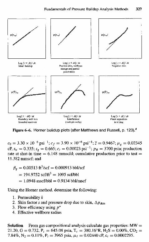
Figure 6-6. Horner buildup plots (after Matthews and Russell, p. 123).4
C0 = 3.30 x ICT6 psi"1; cf = 3.90 x 10~6 psi"1; z = 0.9467; JZg = 0.02345cP, sw = 0.335; sg = 0.665; ct = 0.00023 psi"1; pR = 3700 psia; productionrate at shut-in time = 6.148 mmscfd; cumulative production prior to test =11.382 mmscf; and
P8 = 0.00513 ft3/scf = 0.000913 bbl/scf
= 194.9752 scf/ft3 = 1095 scf/bbl
= 1.0948 mscf/bbl = 0.9134 bbl/mscf
Using the Horner method, determine the following:
1. Permeability k2. Skin factor s and pressure drop due to skin, Aps\^n
3. Flow efficiency using p*4. Effective wellbore radius
Solution From gas compositional analysis calculate gas properties: MW =21.20, G = 0.732, Pc = 645.08 psia, Tc = 380.160R, H2S = 0.00%, CO2 =7.84%, N2 = 0.11%, P1- = 3965 psia, /x7 = 0.02440 cP, c, = 0.0002295.
Log [t + At]I AtBoundary well in abounded reservoir
Log [ / + At]I AtInterference
(multiple wells)
Log [ t + At] I AtPhase separation
in tubing
Log [t + At]I AtIdeal buildup
Log [ t + At] I AtPositive skin, wellbore
storage and partialpenetration
Log [t + At]I AtNegative skin
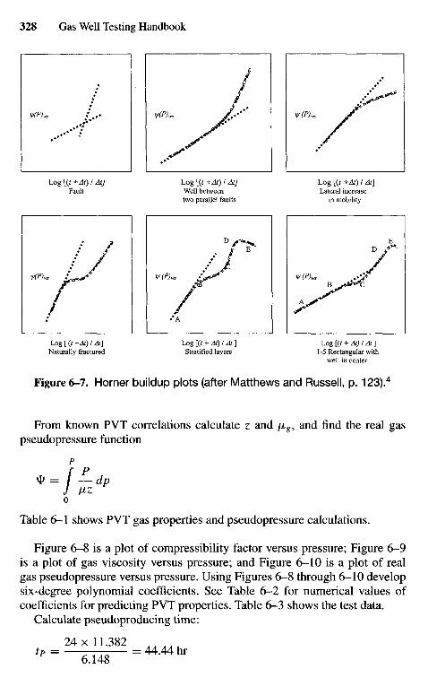
Figure 6-7. Horner buildup plots (after Matthews and Russell, p. 123).4
From known PVT correlations calculate z and /xg, and find the real gaspseudopressure function
pr p
^= — dpJ ^z0
Table 6-1 shows PVT gas properties and pseudopressure calculations.
Figure 6-8 is a plot of compressibility factor versus pressure; Figure 6-9is a plot of gas viscosity versus pressure; and Figure 6-10 is a plot of realgas pseudopressure versus pressure. Using Figures 6-8 through 6-10 developsix-degree polynomial coefficients. See Table 6-2 for numerical values ofcoefficients for predicting PVT properties. Table 6-3 shows the test data.
Calculate pseudoproducing time:
24x11.382tp= 6.148 =UMhr
Log [ (/ +At) I At]Naturally fractured
Log {{t +At)I At]Stratified layers
Log [{t + At) I At ]1-5 Rectangular with
well in center
Log [{t +At) I At]Fault
Log [(t +At) I At]Well betweentwo parallel faults
Log [(t +At) I At]Lateral increase
in mobility
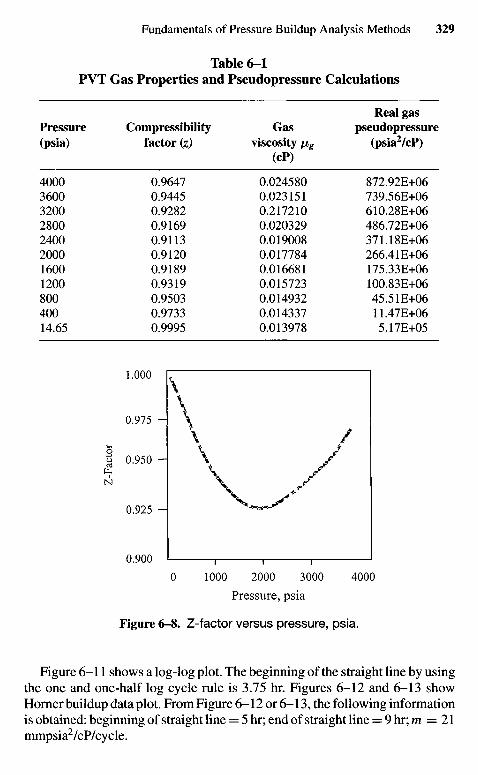
Table 6-1PVT Gas Properties and Pseudopressure Calculations
Real gasPressure Compressibility Gas pseudopressure(psia) factor (z) viscosity \ig (psia2/cP)
(cP)
4000 0.9647 0.024580 872.92E+063600 0.9445 0.023151 739.56E+063200 0.9282 0.217210 610.28E+062800 0.9169 0.020329 486.72E+062400 0.9113 0.019008 371.18E+062000 0.9120 0.017784 266.41E+061600 0.9189 0.016681 175.33E+061200 0.9319 0.015723 100.83E+06800 0.9503 0.014932 45.51E+06400 0.9733 0.014337 11.47E+0614.65 0.9995 0.013978 5.17E+05
Pressure, psia
Figure 6-8. Z-factor versus pressure, psia.
Figure 6-11 shows a log-log plot. The beginning of the straight line by usingthe one and one-half log cycle rule is 3.75 hr. Figures 6-12 and 6-13 showHorner buildup data plot. From Figure 6-12 or 6-13, the following informationis obtained: beginning of straight line = 5 hr; end of straight line = 9 hr; m = 21mmpsia2/cP/cycle.
Z-F
acto
r
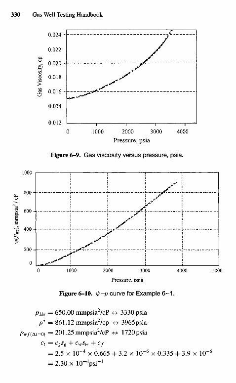
Pressure, psia
Figure 6-9. Gas viscosity versus pressure, psia.
Pressure, psia
Figure 6-10. \[r-p curve for Example 6 - 1 .
plhr = 650.00 mmpsia2/cP <+ 3330 psia
p* — 861.12 mmpsia2/cp «» 3965 psia
Pw/(At=O) = 201.25mmpsia2/cP <-> 1720psia
Cf = CgSg ~r C\v$w ' Cf
= 2.5 x 10"4 x 0.665 + 3.2 x 10~6 x 0.335 + 3.9 x 10~6
= 2.30 x 10"4PSi"1
ty(P
ws)
, m
mps
ia2 /
cP
Gas
Vis
cosi
ty, c
p
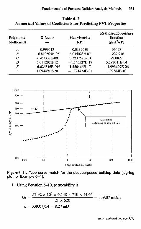
Table 6-2Numerical Values of Coefficients for Predicting PVT Properties
Real pseudopressurePolynomial Z-factor Gas viscosity functioncoefficients — (cP) (psia2/cP)
A 0.999513 0.0139689 39453B -6.810505E-05 6.044023E-07 -222.976C 4.707337E-09 8.323752E-10 72.0827D 5.011202E-12 -1.145527E-17 5.287041E-04E -6.626846E-016 1.550466E-17 -1.993697E-06F 1.094491E-20 -1.721434E-21 1.92384E-10
Shut-in time At, hours
Figure 6-11. Type curve match for the desuperposed buildup data (log-logplot for Example 6-1).
1. Using Equation 6-10, permeability is
_ 57.92 x 1» x 6.H8 x 710 x .4.65
21 x 520
k = 339.07/54 = 8.27 mD
(text continued on page 337)
3.75 hoursBeginning of straight line
V(P
ws)
, m
mps
ia2 /
cP
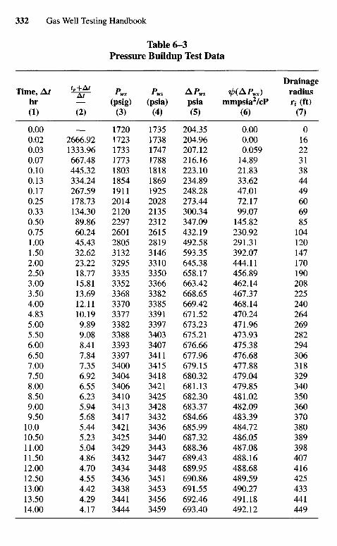
Table 6-3Pressure Buildup Test Data
DrainageTime, At 1^- Pws Pws APWS i/>(APws) radius
hr — (psig) (psia) psia mmpsia2/cP r; (ft)(D (2) (3) (4) (5) (6) (7)
0.00 — 1720 1735 204.35 0.00 00.02 2666.92 1723 1738 204.96 0.00 160.03 1333.96 1733 1747 207.12 0.059 220.07 667.48 1773 1788 216.16 14.89 310.10 445.32 1803 1818 223.10 21.83 380.13 334.24 1854 1869 234.89 33.62 440.17 267.59 1911 1925 248.28 47.01 490.25 178.73 2014 2028 273.44 72.17 600.33 134.30 2120 2135 300.34 99.07 690.50 89.86 2297 2312 347.09 145.82 850.75 60.24 2601 2615 432.19 230.92 1041.00 45.43 2805 2819 492.58 291.31 1201.50 32.62 3132 3146 593.35 392.07 1472.00 23.22 3295 3310 645.38 444.11 1702.50 18.77 3335 3350 658.17 456.89 1903.00 15.81 3352 3366 663.42 462.14 2083.50 13.69 3368 3382 668.65 467.37 2254.00 12.11 3370 3385 669.42 468.14 2404.83 10.19 3377 3391 671.52 470.24 2645.00 9.89 3382 3397 673.23 471.96 2695.50 9.08 3388 3403 675.21 473.93 2826.00 8.41 3393 3407 676.66 475.38 2946.50 7.84 3397 3411 677.96 476.68 3067.00 7.35 3400 3415 679.15 477.88 3187.50 6.92 3404 3418 680.32 479.04 3298.00 6.55 3406 3421 681.13 479.85 3408.50 6.23 3410 3425 682.30 481.02 3509.00 5.94 3413 3428 683.37 482.09 3609.50 5.68 3417 3432 684.66 483.39 37010.0 5.44 3421 3436 685.99 484.72 38010.50 5.23 3425 3440 687.32 486.05 38911.00 5.04 3429 3443 688.36 487.08 39811.50 4.86 3432 3447 689.43 488.16 40712.00 4.70 3434 3448 689.95 488.68 41612.50 4.55 3436 3451 690.86 489.59 42513.00 4.42 3438 3453 691.55 490.27 43313.50 4.29 3441 3456 692.46 491.18 44114.00 4.17 3444 3459 693.40 492.12 449
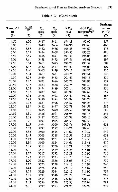
Table 6 -3 (Continued)
DrainageTime, A* ^ ± ^ Pws Pws APWS i/>(APws) radius
hr — (psig) (psia) psia mmpsia2/cP r,- (ft)(1) (2) (3) (4) (5) (6) (7)
14.50 4.06 3447 3461 694.18 492.90 45715.00 3.96 3449 3464 694.96 493.68 46515.50 3.87 3452 3466 695.88 494.62 47316.00 3.78 3454 3468 696.53 495.27 48016.50 3.69 3456 3471 697.31 496.06 48817.00 3.61 3458 3473 697.86 496.61 49517.50 3.54 3461 3475 698.77 497.52 50218.00 3.47 3462 3477 699.29 498.04 50918.50 3.40 3465 3479 700.11 498.85 51619.00 3.34 3467 3481 700.76 499.51 52319.50 3.28 3469 3483 701.41 500.16 53020.00 3.22 3471 3486 702.22 500.97 53720.50 3.17 3473 3488 702.75 501.49 54421.00 3.12 3474 3489 703.14 501.88 55021.50 3.07 3477 3491 703.92 502.67 55722.00 3.02 3478 3493 704.47 503.22 56322.50 2.97 3480 3494 704.99 503.74 57023.00 2.93 3481 3496 705.52 504.26 57623.50 2.89 3482 3497 705.78 504.53 58224.00 2.85 3485 3499 706.59 505.34 58824.50 2.81 3486 3501 706.98 505.73 59425.00 2.78 3487 3502 707.38 506.12 60026.00 2.71 3491 3505 708.58 507.33 61227.00 2.65 3494 3509 709.76 508.51 62428.00 2.59 3497 3512 710.71 509.45 63529.00 2.53 3500 3515 711.62 510.37 64730.00 2.48 3503 3518 712.53 511.28 65831.00 2.43 3506 3521 713.61 512.36 66932.00 2.39 3509 3524 714.66 513.41 67933.00 2.35 3511 3526 715.21 513.96 69034.00 2.31 3514 3529 716.26 515.01 76035.00 2.27 3517 3532 717.21 515.96 71036.00 2.23 3519 3533 717.73 516.48 72037.00 2.20 3522 3536 718.65 517.40 73038.00 2.17 3523 3538 719.17 517.92 74039.00 2.14 3526 3541 720.12 518.87 75040.00 2.22 3529 3544 721.17 519.92 75941.00 2.08 3531 3546 721.72 520.47 76942.00 2.06 3534 3548 722.64 521.39 77843.00 2.03 3536 3550 723.30 522.04 78744.00 2.01 3539 3553 724.25 522.99 797
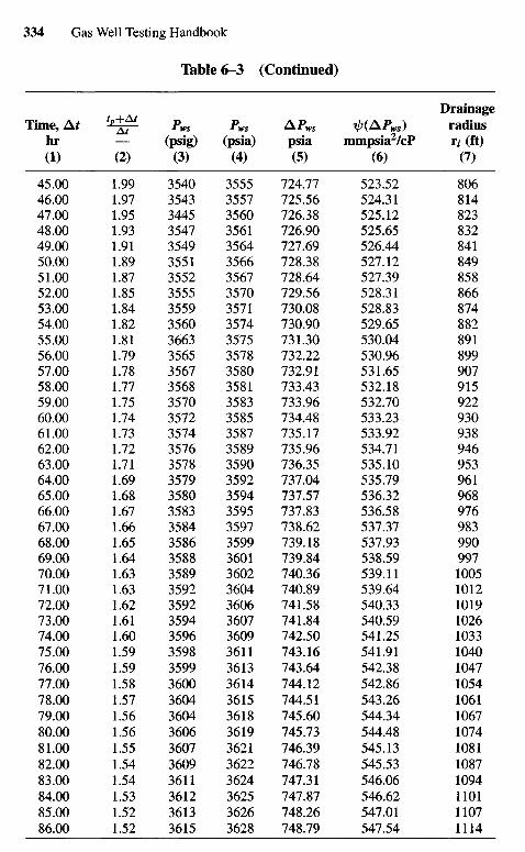
Table 6-3 (Continued)
DrainageTime, At ^ Pws Pws APWS ^(APWS) radius
hr — (psig) (psia) psia mmpsia2/cP r, (ft)(D (2) (3) (4) (5) (6) (7)
45.00 1.99 3540 3555 724.77 523.52 80646.00 1.97 3543 3557 725.56 524.31 81447.00 1.95 3445 3560 726.38 525.12 82348.00 1.93 3547 3561 726.90 525.65 83249.00 1.91 3549 3564 727.69 526.44 84150.00 1.89 3551 3566 728.38 527.12 84951.00 1.87 3552 3567 728.64 527.39 85852.00 1.85 3555 3570 729.56 528.31 86653.00 1.84 3559 3571 730.08 528.83 87454.00 1.82 3560 3574 730.90 529.65 88255.00 1.81 3663 3575 731.30 530.04 89156.00 1.79 3565 3578 732.22 530.96 89957.00 1.78 3567 3580 732.91 531.65 90758.00 1.77 3568 3581 733.43 532.18 91559.00 1.75 3570 3583 733.96 532.70 92260.00 1.74 3572 3585 734.48 533.23 93061.00 1.73 3574 3587 735.17 533.92 93862.00 1.72 3576 3589 735.96 534.71 94663.00 1.71 3578 3590 736.35 535.10 95364.00 1.69 3579 3592 737.04 535.79 96165.00 1.68 3580 3594 737.57 536.32 96866.00 1.67 3583 3595 737.83 536.58 97667.00 1.66 3584 3597 738.62 537.37 98368.00 1.65 3586 3599 739.18 537.93 99069.00 1.64 3588 3601 739.84 538.59 99770.00 1.63 3589 3602 740.36 539.11 100571.00 1.63 3592 3604 740.89 539.64 101272.00 1.62 3592 3606 741.58 540.33 101973.00 1.61 3594 3607 741.84 540.59 102674.00 1.60 3596 3609 742.50 541.25 103375.00 1.59 3598 3611 743.16 541.91 104076.00 1.59 3599 3613 743.64 542.38 104777.00 1.58 3600 3614 744.12 542.86 105478.00 1.57 3604 3615 744.51 543.26 106179.00 1.56 3604 3618 745.60 544.34 106780.00 1.56 3606 3619 745.73 544.48 107481.00 1.55 3607 3621 746.39 545.13 108182.00 1.54 3609 3622 746.78 545.53 108783.00 1.54 3611 3624 747.31 546.06 109484.00 1.53 3612 3625 747.87 546.62 110185.00 1.52 3613 3626 748.26 547.01 110786.00 1.52 3615 3628 748.79 547.54 1114
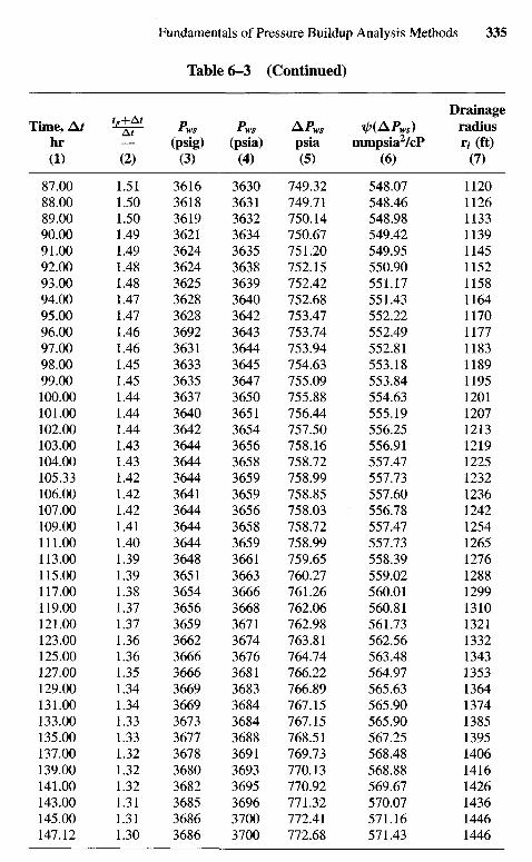
Table 6-3 (Continued)
DrainageTime, A* 1^- Pws Pws APWS ip(APws) radius
hr — (psig) (psia) psia mmpsia2/cP r, (ft)(D (2) (3) (4) (5) (6) (7)
87.00 1.51 3616 3630 749.32 548.07 112088.00 1.50 3618 3631 749.71 548.46 112689.00 1.50 3619 3632 750.14 548.98 113390.00 1.49 3621 3634 750.67 549.42 113991.00 1.49 3624 3635 751.20 549.95 114592.00 1.48 3624 3638 752.15 550.90 115293.00 1.48 3625 3639 752.42 551.17 115894.00 1.47 3628 3640 752.68 551.43 116495.00 1.47 3628 3642 753.47 552.22 117096.00 1.46 3692 3643 753.74 552.49 117797.00 1.46 3631 3644 753.94 552.81 118398.00 1.45 3633 3645 754.63 553.18 118999.00 1.45 3635 3647 755.09 553.84 1195100.00 1.44 3637 3650 755.88 554.63 1201101.00 1.44 3640 3651 756.44 555.19 1207102.00 1.44 3642 3654 757.50 556.25 1213103.00 1.43 3644 3656 758.16 556.91 1219104.00 1.43 3644 3658 758.72 557.47 1225105.33 1.42 3644 3659 758.99 557.73 1232106.00 1.42 3641 3659 758.85 557.60 1236107.00 1.42 3644 3656 758.03 556.78 1242109.00 1.41 3644 3658 758.72 557.47 1254111.00 1.40 3644 3659 758.99 557.73 1265113.00 1.39 3648 3661 759.65 558.39 1276115.00 1.39 3651 3663 760.27 559.02 1288117.00 1.38 3654 3666 761.26 560.01 1299119.00 1.37 3656 3668 762.06 560.81 1310121.00 1.37 3659 3671 762.98 561.73 1321123.00 1.36 3662 3674 763.81 562.56 1332125.00 1.36 3666 3676 764.74 563.48 1343127.00 1.35 3666 3681 766.22 564.97 1353129.00 1.34 3669 3683 766.89 565.63 1364131.00 1.34 3669 3684 767.15 565.90 1374133.00 1.33 3673 3684 767.15 565.90 1385135.00 1.33 3677 3688 768.51 567.25 1395137.00 1.32 3678 3691 769.73 568.48 1406139.00 1.32 3680 3693 770.13 568.88 1416141.00 1.32 3682 3695 770.92 569.67 1426143.00 1.31 3685 3696 771.32 570.07 1436145.00 1.31 3686 3700 772.41 571.16 1446147.12 1.30 3686 3700 772.68 571.43 1446
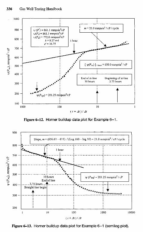
{t + At)I At
Figure 6-12. Horner buildup data plot for Example 6 -1 .
( t + At) I At
Figure 6-13. Horner buildup data plot for Example 6-1 (semilog plot).
Straight line begin.3-75 .hours
10 'hoursEnd!of line
Slope, m
End of st-line Beginning of st-line10 hours 3.75 hours
[ V(Pws) ] i hour = 650.0 mmpsia2 / cP
m = 21.0 mmpsia2 / cP / cycle
\\f(P
ws),
mm
psia
2 / c
PV
C^W
> r
nmps
ia2 /
cP
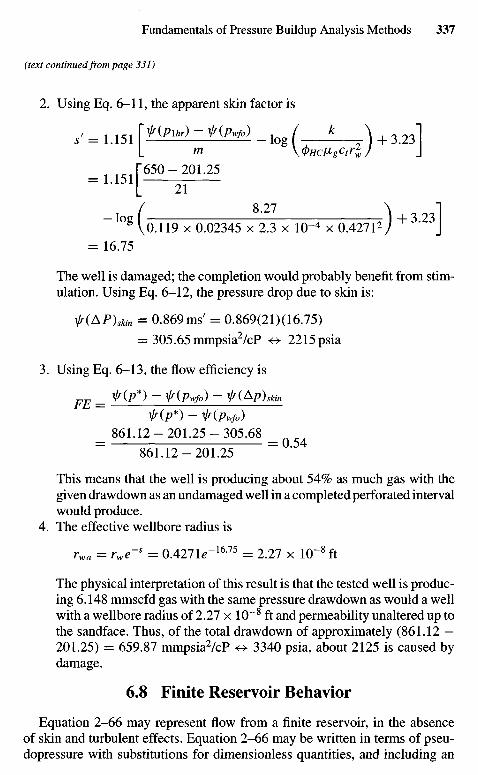
(text continued from page 331)
2. Using Eq. 6-11, the apparent skin factor is
,, = U 5 1 [X/W-VK/W _ / k \ + 3 1
1"65O-201.25L 21
( 8 27 \ ~\
0.119 x 0.02345 x 2.3 x 10~4 x 0.42712J + 3 J= 16.75
The well is damaged; the completion would probably benefit from stim-ulation. Using Eq. 6-12, the pressure drop due to skin is:
is(AP)skin = 0.869 ms' = 0.869(21)(16.75)= 305.65 mmpsia2/cP «» 2215 psia
3. Using Eq. 6-13, the flow efficiency is
J717 ^(P*) ~ ^(Pwfo) ~ if (^p)skinttL —
f(P*) ~ (Pwfo)8 6 1 . 1 2 - 2 0 1 . 2 5 - 3 0 5 . 6 8 ^CA
— — o.54861.12-201.25
This means that the well is producing about 54% as much gas with thegiven drawdown as an undamaged well in a completed perforated intervalwould produce.
4. The effective wellbore radius is
rwa = rwe~s = 0.427Ie"1675 = 2.27 x 10~8ft
The physical interpretation of this result is that the tested well is produc-ing 6.148 mmscfd gas with the same pressure drawdown as would a wellwith a wellbore radius of 2.27 x 10~8 ft and permeability unaltered up tothe sandface. Thus, of the total drawdown of approximately (861.12 —201.25) = 659.87 mmpsia2/cP o 3340 psia, about 2125 is caused bydamage.
6.8 Finite Reservoir Behavior
Equation 2-66 may represent flow from a finite reservoir, in the absenceof skin and turbulent effects. Equation 2-66 may be written in terms of pseu-dopressure with substitutions for dimensionless quantities, and including an
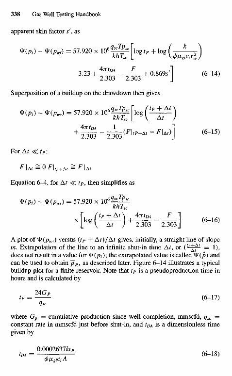
apparent skin factor s\ as
*(/>/) ~ nPwf) = 57.920 x l06^p^\logtP + log f k )khTsc L V</>/V^/
Superposition of a buildup on the drawdown then gives
*(*> -*<„.,) = 57.920 x , 0 ^ [ , o g ( 4 ^ )
+f^-dos^1""'-^] <6-15)
For Ar «; rP;
F | A r = 0F| , p + A r = F | A ,
Equation 6-4, for At <^tP, then simplifies as
* ( # ) - * (p w ) - 57.920 x 1 0 6 ^ ^
f A p + AA 4;rrm F lX r g ("^T-J + 2303 "2303 J (6"16)
A plot of ^(/7WJ) versus (tP + At)/At gives, initially, a straight line of slopem. Extrapolation of the line to an infinite shut-in time Ar, or CP^ = 1),does not result in a value for (/?/); the extrapolated value is called ^(p) andcan be used to obtain ~pR, as described later. Figure 6-14 illustrates a typicalbuildup plot for a finite reservoir. Note that tp is a pseudoproduction time inhours and is calculated by
, , = ™Z (6-17)
where Gp = cumulative production since well completion, mmscfd, qsc =constant rate in mmscfd just before shut-in, and tDA is a dimensionless timegiven by
0.0002637frptDA = — — (6-18)
(pfigiCtA
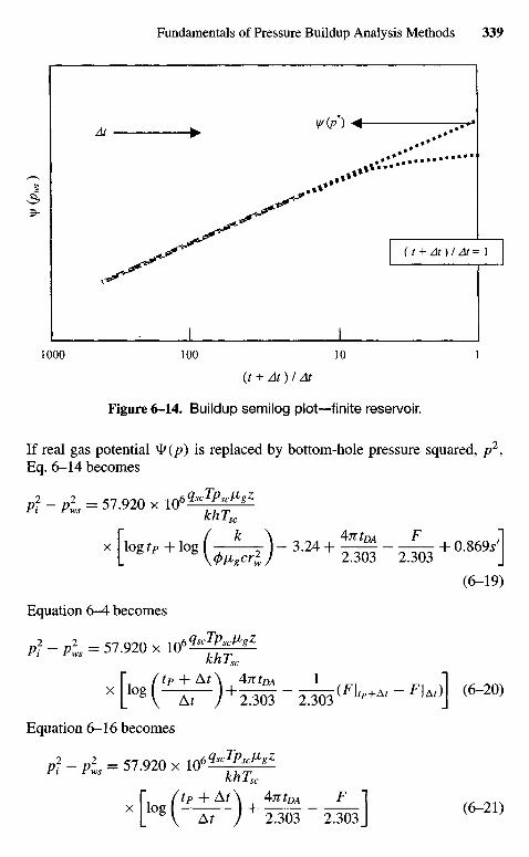
Figure 6-14. Buildup semilog plot—finite reservoir.
If real gas potential ^(p) is replaced by bottom-hole pressure squared, p2,Eq. 6-14 becomes
PI ~ PI, = 57.920 x 1 0 6 f c [ W
(6-19)
Equation 6-4 becomes
p] -pi, = 57.920 x Vfq'lPhff
Equation 6-16 becomes
pf - pi = 57.920 x 1 0 6 ^ g ^Kn 1 sc
XL1Og ( " ^ T - J + 2303 -2303 J (6-21)
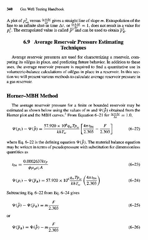
A plot of p\s versus tp^ gives a straight line of slope m. Extrapolation of theline to an infinite shut-in time Af, or tp^' = 1, does not result in a value forpf. The extrapolated value is called p2 and can be used to obtain ~p\.
6.9 Average Reservoir Pressure EstimatingTechniques
Average reservoir pressures are used for characterizing a reservoir, com-puting its oil/gas in place, and predicting future behavior. In addition to theseuses, the average reservoir pressure is required to find a quantitative use involumetric-balance calculations of oil/gas in place in a reservoir. In this sec-tion we will present various methods to calculate average reservoir pressure ina gas reservoir.
Horner-MBH Method
The average reservoir pressure for a finite or bounded reservoir may beestimated as shown below using the values of m and (p) obtained from theHorner plot and the MBH curves.3 From Equation 6-21 for t*^ = 1.0,
»(„)-,<». "-^* " ^ P . [ J ^ - *1 (6-22)khTsc |_ 2.303 2.303 J
where Eq. 6-22 is the defining equation (p). The material balance equationmay be written in terms of pseudopressure with substitution for dimensionlessquantities as
0.0002637foP
toA = — — (6-23)4>V>giCiA
• te)-•(*,_ 57.920x1«.«=^ ( ^ ) (6-24)
Subtracting Eq. 6-22 from Eq. 6-24 gives
*^)-*^)=m2^3 ( 6 " 2 5 )
or
V(PR) = VCP)-M^ (6-26)
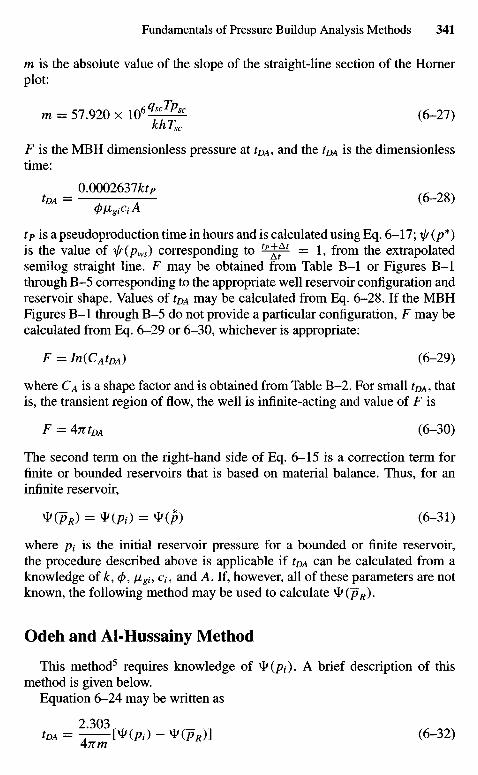
m is the absolute value of the slope of the straight-line section of the Homerplot:
m = 57.920 x i o 6 ^ - ^ (6-27)khTsc
F is the MBH dimensionless pressure at tDA, and the tDA is the dimensionlesstime:
0 .0002637^tDA = — (6-28)
tp is a pseudoproduction time in hours and is calculated using Eq. 6-17; (p*)is the value of x//(pws) corresponding to tp~^ff = 1, from the extrapolatedsemilog straight line. F may be obtained from Table B-I or Figures B-Ithrough B-5 corresponding to the appropriate well reservoir configuration andreservoir shape. Values of tDA may be calculated from Eq. 6-28. If the MBHFigures B-I through B-5 do not provide a particular configuration, F may becalculated from Eq. 6-29 or 6-30, whichever is appropriate:
F = In(CAtDA) (6-29)
where CA is a shape factor and is obtained from Table B-2. For small tDA, thatis, the transient region of flow, the well is infinite-acting and value of F is
F = AntDA (6-30)
The second term on the right-hand side of Eq. 6-15 is a correction term forfinite or bounded reservoirs that is based on material balance. Thus, for aninfinite reservoir,
V(PR) = V(Pi) = V(p) (6-31)
where pt is the initial reservoir pressure for a bounded or finite reservoir,the procedure described above is applicable if tDA can be calculated from aknowledge of k, 0 , /%, Q , and A. If, however, all of these parameters are notknown, the following method may be used to calculate ty(~pR).
Odeh and Al-Hussainy Method
This method5 requires knowledge of ^(pi). A brief description of thismethod is given below.
Equation 6-24 may be written as
tDA = 2^[V(Pt) - V(pR)] (6-32)
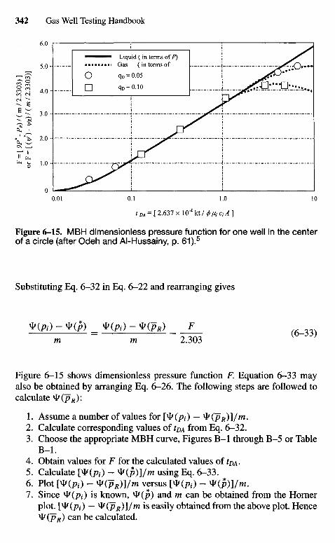
Figure 6-15. MBH dimensionless pressure function for one well in the centerof a circle (after Odeh and Al-Hussainy, p. 61 ).5
Substituting Eq. 6-32 in Eq. 6-22 and rearranging gives
npt) ~ V(P) V(Pi) ~ V(PR) Fm = m B03 ( 6"33)
Figure 6-15 shows dimensionless pressure function F. Equation 6-33 mayalso be obtained by arranging Eq. 6-26. The following steps are followed tocalculate V(pR):
1. Assume a number of values for [^ (pt) — V(pR)]/m.2. Calculate corresponding values of tDA from Eq. 6-32.3. Choose the appropriate MBH curve, Figures B-I through B-5 or Table
B-I.4. Obtain values for F for the calculated values of tDA.5. Calculate [*(#) - V(p)]/m using Eq. 6-33.6. Plot [*(P|.) - V(pR)]/m versus [*(#) - *(p)]/m.7. Since V(pi) is known, W(p) and m can be obtained from the Horner
plot. [V(pi) - ty(pR)]/m is easily obtained from the above plot. HenceV(PR) can be calculated.
Liquid (in terms of F)Gas (in terms of
F =
[9P
*-P
R)/
(m/2
.330
3)
]or
F =
[(y
/)-
y/R)l
(m
/2.3
303)
]
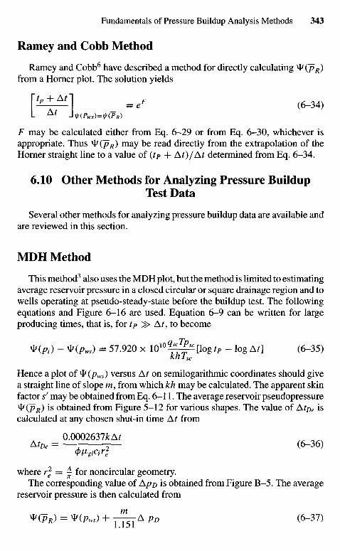
Ramey and Cobb Method
Ramey and Cobb6 have described a method for directly calculating ^(pR)from a Horner plot. The solution yields
№1 -S (M4)
F may be calculated either from Eq. 6-29 or from Eq. 6-30, whichever isappropriate. Thus ^(pR) may be read directly from the extrapolation of theHorner straight line to a value of (tP + At)/At determined from Eq. 6-34.
6.10 Other Methods for Analyzing Pressure BuildupTest Data
Several other methods for analyzing pressure buildup data are available andare reviewed in this section.
MDH Method
This method3 also uses the MDH plot, but the method is limited to estimatingaverage reservoir pressure in a closed circular or square drainage region and towells operating at pseudo-steady-state before the buildup test. The followingequations and Figure 6-16 are used. Equation 6-9 can be written for largeproducing times, that is, for tP ^> At, to become
V(Pi) ~ V(Pws) = 57.920 x 1 0 1 0 ^ ^ [ l o g ^ - log At] (6-35)khTsc
Hence a plot ofV(pws) versus At on semilogarithmic coordinates should givea straight line of slope m, from which kh may be calculated. The apparent skinfactor sr may be obtained from Eq. 6-11. The average reservoir pseudopressure^CPR) is obtained from Figure 5-12 for various shapes. The value of AtDe iscalculated at any chosen shut-in time Ar from
0.0002637fcArAfa, = — — (6-36)
where r* = £ for noncircular geometry.The corresponding value of ApD is obtained from Figure B-5. The average
reservoir pressure is then calculated from
V(pR) = V(Pws) + Y ^ A pD (6-37)
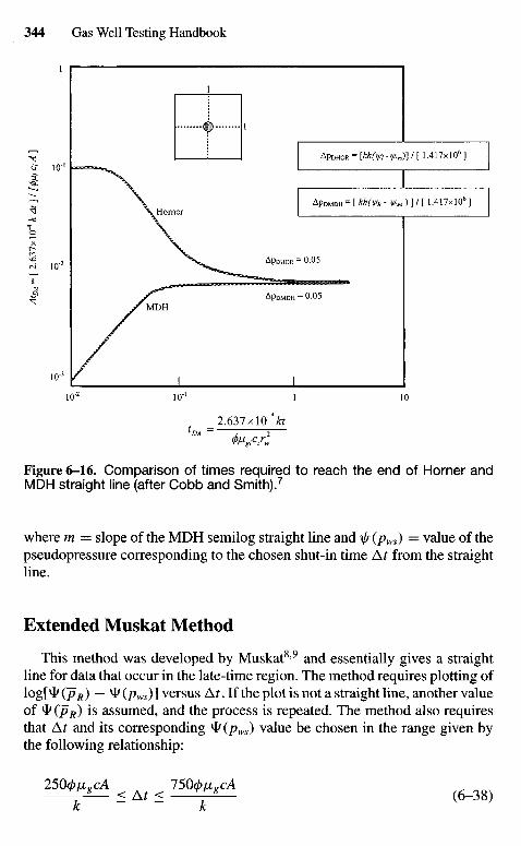
Figure 6-16. Comparison of times required to reach the end of Horner andMDH straight line (after Cobb and Smith).7
where m = slope of the MDH semilog straight line and if(pws) = value of thepseudopressure corresponding to the chosen shut-in time At from the straightline.
Extended Muskat Method
This method was developed by Muskat8'9 and essentially gives a straightline for data that occur in the late-time region. The method requires plotting of\og[fy(pR) — (pws)] versus At. If the plot is not a straight line, another valueof ty(pR) is assumed, and the process is repeated. The method also requiresthat Af and its corresponding V(pws) value be chosen in the range given bythe following relationship:
250(J)IXnCA 7'500 //, »cA^ p _ <At< r ^ l _ (6-38)k k
Horner
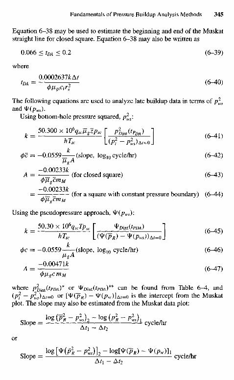
Equation 6-38 may be used to estimate the beginning and end of the Muskatstraight line for closed square. Equation 6-38 may also be written as
0.066 < tDA < 0.2 (6-39)
where
0.0002637£AftDA = — T- (6-40)
The following equations are used to analyze late buildup data in terms of p^s
and*(p w ) .Using bottom-hole pressure squared, p\s\
_ 50.300 x 10%c7ZgzPsc f P2DiJtpDA) 1 (f>.,K — —— —-T — ^o-^-i;
hTsc l(pj-pls)At=o]k
(j)c = -0.0559=:—(slope, log10 cycle/hr) (6-42)
-0.00233fcA = —-—— (for closed square) (6-43)
(j)lxgcmM
—0 00233&_ — j _ _ (for a SqUare with constant pressure boundary) (6-44)
(/>/j,gcmM
Using the pseudopressure approach, ty(pws):
k = 50.30 x l06qscTpsc I" Vpint(tPDA) 1k
(j)c = -0.0559 (slope, log10 cycle/hr) (6-46)fig A
-0.0047 IkA = (6-47)
(p{igcmM
where p2Dmi(tpDA)* or ^DintfezM)** can be found from Table 6-4, and
(pf ~ Pw)At=O or №(~pR) — V(pw)]At=o is the intercept from the Muskatplot. The slope may also be estimated from the Muskat data plot:
Slope = M ^ - K l ) 2 - M P I ~ / qAfi - At2
or
lOg [V {p2R - PJS)]2 ~ IQg[V(PR) ~ V(PW)h 1 _Slope = — — cycle/hr
A^i - Ar2
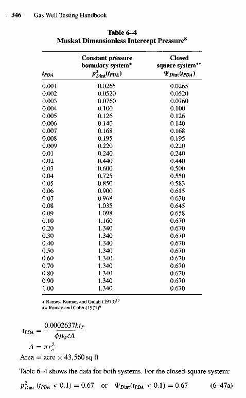
Table 6-4Muskat Dimensionless Intercept Pressure8
Constant pressure Closedboundary system* square system**
tpDA P Dint fPDA ) ^ Dint {tpDA )
0.001 0.0265 0.02650.002 0.0520 0.05200.003 0.0760 0.07600.004 0.100 0.1000.005 0.126 0.1260.006 0.140 0.1400.007 0.168 0.1680.008 0.195 0.1950.009 0.220 0.2200.01 0.240 0.2400.02 0.440 0.4400.03 0.600 0.5000.04 0.725 0.5500.05 0.850 0.5830.06 0.900 0.6150.07 0.968 0.6300.08 1.035 0.6450.09 1.098 0.6580.10 1.160 0.6700.20 1.340 0.6700.30 1.340 0.6700.40 1.340 0.6700.50 1.340 0.6700.60 1.340 0.6700.70 1.340 0.6700.80 1.340 0.6700.90 1.340 0.6701.00 1.340 0.670
* Ramey, Kumar, and Gulati (1973)10
** Ramey and Cobb (1971)6
0.0002637foptl>DA ~ 1 ~A
(J) IJLgCA
A = nr]
Area = acre x 43,560 sq ft
Table 6-4 shows the data for both systems. For the closed-square system:
p2Dint(tpDA< OA) =0.61 or *Dint(frn4< 0.1) =0.67 (6^7a)
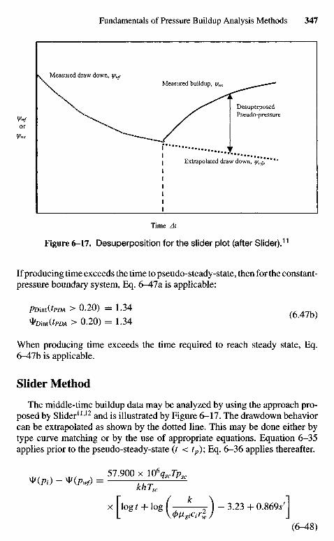
Time At
Figure 6-17. Desuperposition for the slider plot (after Slider).11
If producing time exceeds the time to pseudo-steady-state, then for the constant-pressure boundary system, Eq. 6-Ala. is applicable:
PDintitpDA > 0.20) = 1.34
*Dint(tpDA > 0.20) = 1.34 *
When producing time exceeds the time required to reach steady state, Eq.6-47b is applicable.
Slider Method
The middle-time buildup data may be analyzed by using the approach pro-posed by Slider1112 and is illustrated by Figure 6-17. The drawdown behaviorcan be extrapolated as shown by the dotted line. This may be done either bytype curve matching or by the use of appropriate equations. Equation 6-35applies prior to the pseudo-steady-state (t < tp)\ Eq. 6-36 applies thereafter.
x [log? + log ( 1—-\ - 3.23 + 0.869/1L \<t>iigiCirl) J
(6-48)
Extrapolated draw down, y/wfp
DesuperposedPseudo-pressure
Measured buildup, i//ws
Measured draw down, y/w/
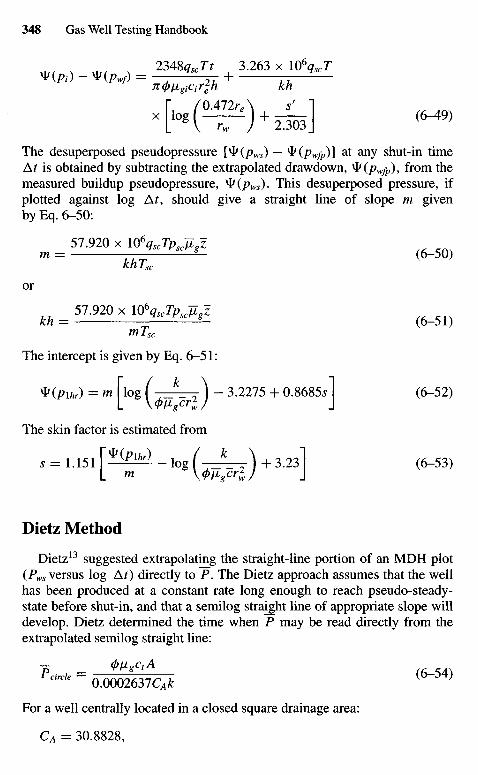
TKp/jigiCir^n kn
The desuperposed pseudopressure №(pws) — (PwJp)] at any shut-in timeAt is obtained by subtracting the extrapolated drawdown, ty(pwjp), from themeasured buildup pseudopressure, ^(pws). This desuperposed pressure, ifplotted against log At9 should give a straight line of slope m givenby Eq. 6-50:
57.920 x \06qscTPscJZgzm = TT^ (6-50)
khTsc
or
57.920 x \06qscTpscJiszkh = * sc g (6-51)m Tsc
The intercept is given by Eq. 6-51:
*(/>i*r) = m [log ( JL_}_ 9 \ - 3.2275 + 0.8685^1 (6-52)
L \<t)ngcrlJ JThe skin factor is estimated from
s = L 1 5 1 r * ^ ) .,ogf * ) +3.23l (6-53)
Dietz Method
Dietz13 suggested extrapolating the straight-line portion of an MDH plot(Pws versus log At) directly to P. The Dietz approach assumes that the wellhas been produced at a constant rate long enough to reach pseudo-steady-state before shut-in, and that a semilog straight line of appropriate slope willdevelop. Dietz determined the time when P may be read directly from theextrapolated semilog straight line:
Pcircle = 0.0002637CA* ( 6 " 5 4 )
For a well centrally located in a closed square drainage area:
CA = 30.8828,
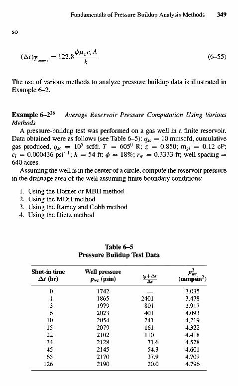
so
(At)7 = 1 2 2 . 8 ^ ^ (6-55)v 7 'square U v /
The use of various methods to analyze pressure buildup data is illustrated inExample 6-2.
Example 6—226 Average Reservoir Pressure Computation Using VariousMethods
A pressure-buildup test was performed on a gas well in a finite reservoir.Data obtained were as follows (see Table 6-5): qsc = 10 mmscfd, cumulativegas produced, qsc = 105 scfd; T = 605° R; z = 0.850; m^ = 0.12 cP;Ci = 0.000436 psi"1; h = 54 ft; 0 = 18%; rw = 0.3333 ft; well spacing =640 acres.
Assuming the well is in the center of a circle, compute the reservoir pressurein the drainage area of the well assuming finite boundary conditions:
1. Using the Horner or MBH method2. Using the MDH method3. Using the Ramey and Cobb method4. Using the Dietz method
Table 6-5Pressure Buildup Test Data
Shut-in time Well pressure p^s
A* (hr) pws (psia) tj^- (mmpsia2)
0 1742 — 3.0351 1865 2401 3.4783 1979 801 3.9176 2023 401 4.09310 2054 241 4.21915 2079 161 4.32222 2102 110 4.41834 2128 71.6 4.52845 2145 54.3 4.60165 2170 37.9 4.709126 2190 20.0 4.796
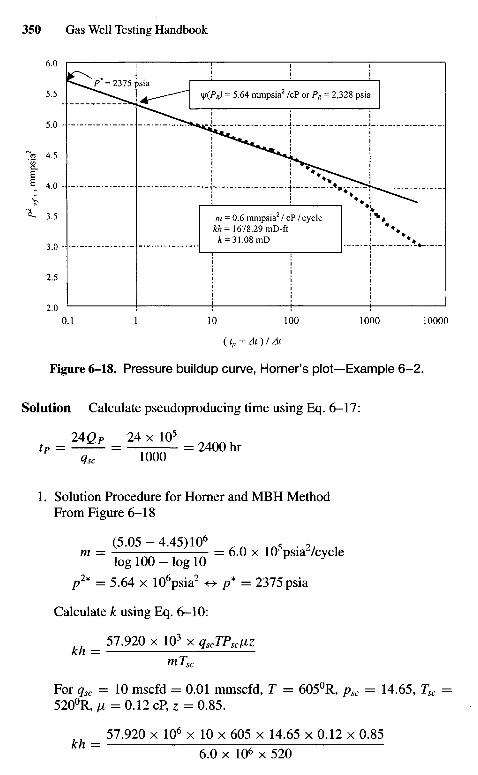
{tp +At)I At
Figure 6-18. Pressure buildup curve, Horner's plot—Example 6-2.
Solution Calculate pseudoproducing time using Eq. 6-17:
2AQP 24 x 105
1. Solution Procedure for Homer and MBH MethodFrom Figure 6-18
( 5 . 0 5 - 4.45) 106 ^ n i n 5 • 2, ,m = = 6.0 x 10 psia /cycle
log 100 - log 10 f J
p2* = 5.64 x 10⁶psia2 +> p* = 2375 psia
Calculate k using Eq. 6-10:
7 57.920 x 10³ x qscTPscfizkh =
mTsc
For qsc = 10 mscfd = 0.01 mmscfd, T = 6050R, psc = 14.65, Tsc =5200R, fi = 0.12 cP, z - 0 . 8 5 .
r 57.920 x 106 x 10 x 605 x 14.65 x 0.12 x 0.85
6.0 x 106 x 520
m = 0.6 mmpsia2 / cP / cyclekh= 1678.29 mD-ft
k = 31.08 mD
\|/(P^ = 5.64 mmpsia2 /cP or / ^ = 2,328 psia
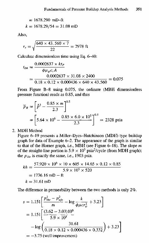
= 1678.290 mD-ft
k = 1678.29/54 = 31.08 mD
Also,
rt = y^74Q6o77=2978f t
Calculate dimensionless time using Eq. 6-40:
0.0002637 x ktPtDA ~ 1 A
0.0002637 x 31.08 x 2400~ 0.18 x 0.12 x 0.000436 x 640 x 43,560 ~ "
From Figure B-8 using 0.075, the ordinate (MBH dimensionlesspressure function) reads as 0.85, and thus
[~*2 0.85 x m "I0'5
P* = [p - - O - J
= [5 .64x I Q ^ - ° - 8 5 X2
63
O x l O 5 ] ° - 5= 2328 psia
2. MDH MethodFigure 6-19 presents a Miller-Dyes-Hutchinson (MDH) type buildupgraph for data of Example 6-2. The appearance of the graph is similarto that of the Horner graph, i.e., MBH (see Figure 6-18). The slope mof the straight-line portion is 5.9 x 10⁵ psia2/cycle (from MDH graph);the p\hr is exactly the same, i.e., 1903 psia.
57.920 x 106 x 10 x 605 x 14.65 x 0.12 x 0.855.9 x 105 x 520
= 1736.16 m D - f t
k = 31.61 mD
The difference in permeability between the two methods is only 2%.
1 ialPlhr~ Pwfo , k , o ^0Is = 1.151 - l o g - + 3.23
L m (t>^crl J_ [(3.62-3.03)IQ6
" L 5.9x10^
" 1 O g \0.18 x 0.12 x 0.000436 x 0.332/ + 3 ' 2 3 J= —3.75 (well improvement)
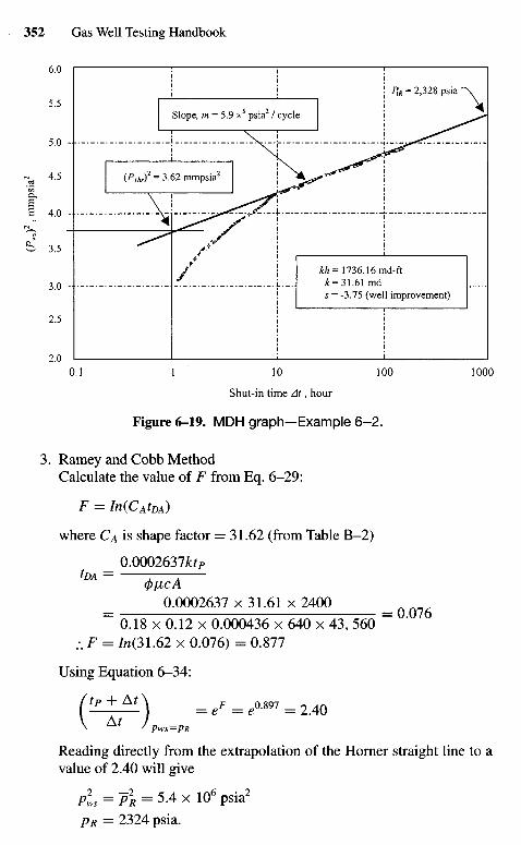
Shut-in time At, hour
Figure 6-19. MDH graph—Example 6-2.
3. Ramey and Cobb MethodCalculate the value of F from Eq. 6-29:
F = In(CAtDA)
where CA is shape factor = 31.62 (from Table B-2)
0.0002637foptDA ~~ 1 A
(P/JLCA
_ 0.0002637 x 31.61 x 2400 _= 0.18 x 0.12 x 0.000436 x 640 x 43, 560 ~ ' ?
;. F = /n(31.62 x 0.076) = 0.877
Using Equation 6-34:
(^±^) = e' = f»» = 2.40^ ' PWS=PR
Reading directly from the extrapolation of the Horner straight line to avalue of 2.40 will give
/ > i = 7 ^ = 5.4xl06psia2
pR = 2324 psia.
kh = 1736.16 md-ft£ = 31.61 md5 = -3.75 (well improvement)
Slope, m = 5.9 x5 psia2 / cycle
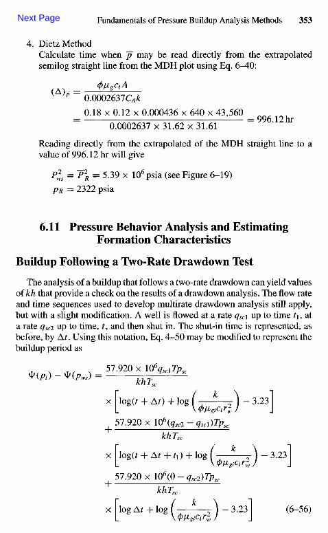
4. Dietz MethodCalculate time when ~p may be read directly from the extrapolatedsemilog straight line from the MDH plot using Eq. 6-AQ\
= 4>ygctAv Jp 0.0002637CA£
_ 0.18 x 0.12 x 0.000436 x 640 x 43,560 _- 0.0002637x31.62x31.61 ~
Reading directly from the extrapolated of the MDH straight line to avalue of 996.12 hr will give
Pls = ~p\ = 5.39 x 10⁶ psia (see Figure 6-19)
pR = 2322 psia
6.11 Pressure Behavior Analysis and EstimatingFormation Characteristics
Buildup Following a Two-Rate Drawdown Test
The analysis of a buildup that follows a two-rate drawdown can yield valuesof kh that provide a check on the results of a drawdown analysis. The flow rateand time sequences used to develop multirate drawdown analysis still apply,but with a slight modification. A well is flowed at a rate qsc\ up to time t\, ata rate qsc2 up to time, t, and then shut in. The shut-in time is represented, asbefore, by At. Using this notation, Eq. 4-50 may be modified to represent thebuildup period as
«(*)-«(^)-"-™»1jV>>-khTsc
x |~log(/ + A?) + log ( * ) - 3.23]
57.920 x 10⁶(frc2 - qsci)Tpsc
khTsc
x LgO + At + h) + log ( * ) - 3.23]
57.920xl06(0-frc2)7>,c
x Tlog At + log ( k \ - 3.23] (6-56)
Next Page
Chapter 7
Predicting FutureDeliverability UsingEmpiricalRelationships
7.1 Introduction
Deliverability testing is a commonly used technique for predicting short-term and long-term behavior of gas wells. Typically, a well is flowed at differentrates, and the pressure-rate-time response is recorded. From analysis of thesedata, information is obtained regarding the deliverability of the well, i.e., itsability to produce against a given backpressure at a given stage of reservoirdepletion. Such forecasting is often required input for designing productionfacilities, planning field development, estimating payout time, setting allow-able rates, etc. Deliverability testing has been done using multipoint flow tests.Empirical equations5'7 to predict current and future gas well deliverability arepresented. Deliverability calculations for both unfractured and fractured gaswells are also briefly discussed in this chapter.
7.2 Empirical Treatment
The basic assumptions are:
1. Homogeneous, isotropic, unfractured reservoir with a closed outerboundary
2. Single, fully penetrating well3. Stabilized conditions prevail, i.e., pseudo-steady-state equations can be
used to describe gas flow in the reservoir4. Turbulent factor D and a rate-dependent skin Dqsc.
Under these assumptions, the drawdown equation, in gas-field units, is
50.300 x l06qscTPsc
Tl / 2.2458 \ 1x -InI — — J + 2ntDA + s + Dqsc (7-1)
After rearranging, Eq. 7-1 becomes
f V(Pi) -*(pwf) 1 1 (A \ 1 /2^458 \
+ 2TUDA + s + D<?5C (7-2)
For a closed drainage volume, material balance gives
r V(P1)-npR) i
L 5 0 . 3 0 0 x l 0 6 ^ c J
Combining Eqs. 7-2 and 7-3, we have
7 Tn = -/»( — + -InI —— + s + Dqsc
L50.300xl06x^|^J 2 V^/ 2 \ CA J(7-4)
This equation can now be rewritten as the familiar quadratic deliverabilityequation:
V(pR) - V(pmf) = aqsc + bql (7-5)
where the coefficients a and b are given by
a = 57.900 x 10⁶- -1" logf 4 ) + logf ^ ) +O.869/I (7-6)khl VlJ \ CA J J
b = 50.300 x 1 0 6 - ^ (7-7)khTsc
Solving Eq. 7-5 and taking the positive root to be qsc,
-a + Ja2 + 4b[V(pR) - V(PmfT] n ^qsc Th (7-8)
and corresponding to a zero sandface pressure, the absolute open flow potential(AOFP) is the theoretical maximum rate (AOF)current\
(AOF)cumnl(nPmf = O)) = - * + > 2 + 4 W ^ ) ] ( 7 _ 9 )
Dividing Eq. 7-8 by Eq. 7-9 we get
f qsc 1 = -a + > 2 + M[V(PR) ~ V(Pmf)]I (AOF ) c u r r e n t J -a + Ja2 + 4b[V(pR)]
which can also be expressed in a form such as
r fa U F 1 № ^ 1 (7_n)
where F l is some functional form. The dimensionless groups [V (pmf)/ V (~pR)]and [qsc/(AOF)current] can be generated for a variety of cases and develop anempirical correlation of the form of Eq. 7-11. This will then be the IPR forcurrent deliverability. To calculate deliverability at future conditions, Eq. 7-9can be rewritten as
(A(Jt ) f u t u r e = — (7-12)
Now dividing Eq. 7-12 by Eq. 7-11, we get
(AOF)future = -a + y/a2 + 4b[V(pR)f]
(AOF)current -a+ a2+ 4b[V(pR)]
This equation can be restated as
[ (A°F)^ ] = F2\^^l] (7-14)L(AOF)current] L V(pR) J
where Fl is some other functional form. The other dimensionless groups[V(pR)f/V(pR)] and [(AOF )future/(AOF )current] can be generated for a vari-ety of cases and develop a second empirical relation, of the form of Eq. 7-14.This will then be the IPR for future deliverability.
Current Deliverability Calculations
Follow these steps:
1. Knowing ^(PR) and ^(Pmf), calculate V(Pmf)/^(FR).2. From the dimensionless IPR for current conditions (test fit curve), esti-
mate [qsc/(AOF)current].
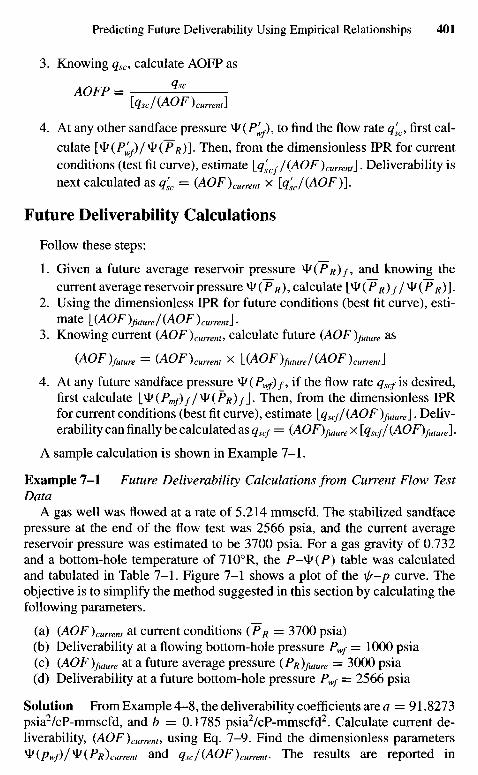
3. Knowing qsc, calculate AOFP as
AOFP = —[qsc/(AOF)current]
4. At any other sandface pressure V(P^)9 to find the flow rate q'sc, first cal-
culate [V (P^)/V (PR)]. Then, from the dimensionless IPR for current
conditions (test fit curve), estimate \_q'scf / (AOF) CUrrent\. Deliverability is
next calculated as qrsc = (A0F)current x [qf
sc/(AOF)].
Future Deliverability Calculations
Follow these steps:
1. Given a future average reservoir pressure V(PR)/, and knowing thecurrent average reservoir pressure V(PR)9 calculate [V(P R) / /V(P R)].
2. Using the dimensionless IPR for future conditions (best fit curve), esti-mate V(AOF )future/(AOF ) c u r r e n t \ .
3. Knowing current (AOF) current, calculate future (AOF)future as
(AOF)future = (AOF)current x [_(AOF)^K/(AOF)current\
4. At any future sandface pressure V(Pwf)f, if the flow rate qSCf is desired,first calculate lV(Pmf)f/V(PR) f\. Then, from the dimensionless IPRfor current conditions (best fit curve), estimate lqScf/(AOF)futurei. Deliv-erability can finally be calculated as qscf = (AOF)futUre x [qscf/ (AOF)future] •
A sample calculation is shown in Example 7-1.
Example 7-1 Future Deliverability Calculations from Current Flow TestData
A gas well was flowed at a rate of 5.214 mmscfd. The stabilized sandfacepressure at the end of the flow test was 2566 psia, and the current averagereservoir pressure was estimated to be 3700 psia. For a gas gravity of 0.732and a bottom-hole temperature of 7100R, the P-V(P) table was calculatedand tabulated in Table 7-1. Figure 7-1 shows a plot of the \jr-p curve. Theobjective is to simplify the method suggested in this section by calculating thefollowing parameters.
(a) (AOF)current at current conditions (PR = 3700 psia)(b) Deliverability at a flowing bottom-hole pressure Pwf — 1000 psia(c) (AOF)future at a future average pressure (PR)future = 3000 psia(d) Deliverability at a future bottom-hole pressure Pwf = 2566 psia
Solution From Example 4-8, the deliverability coefficients are a = 91.8273psia2/cP-mmscfd, and b = 0.1785 psia2/cP-mmscfd2. Calculate current de-liverability, (AOF)current9 using Eq. 7-9. Find the dimensionless parametersV (pwf)/V (PR)CUrrent and qsc/(AOF)current- The results are reported in
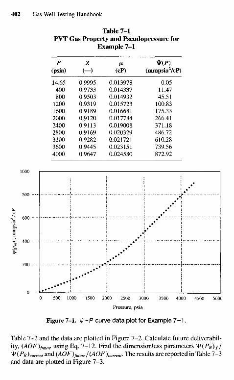
Table 7-1PVT Gas Property and Pseudopressure for
Example 7-1
P Z ft *(P)(psia) (—) (cP) (mmpsia2/cP)
14.65 0.9995 0.013978 0.05400 0.9733 0.014337 11.47800 0.9503 0.014932 45.511200 0.9319 0.015723 100.831600 0.9189 0.016681 175.332000 0.9120 0.017784 266.412400 0.9113 0.019008 371.182800 0.9169 0.020329 486.723200 0.9282 0.021721 610.283600 0.9445 0.023151 739.564000 0.9647 0.024580 872.92
Pressure, psia
Figure 7-1. x/r-P curve data plot for Example 7-1.
Table 7-2 and the data are plotted in Figure 7-2. Calculate future deliverabil-ity, (AOF^ture using Eq. 7-12. Find the dimensionless parameters V(PR)f/^ (PR)current and (AOF )future/(AOF)current- The results are reported in Table 7-3and data are plotted in Figure 7-3.
\y(p
wf),
mm
psia
2 / c
P
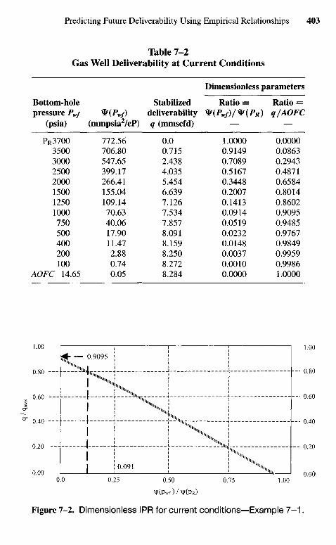
Table 7-2Gas Well Deliverability at Current Conditions
Dimensionless parameters
Bottom-hole Stabilized Ratio = Ratio =pressure Pw/ V(Pwf) deliverability ^F(Pw/)/ V(PR) q/1AOFC
(psia) (mmpsia2/cP) q (mmscfd) — —
PR3700 772.56 0.0 1.0000 0.00003500 706.80 0.715 0.9149 0.08633000 547.65 2.438 0.7089 0.29432500 399.17 4.035 0.5167 0.48712000 266.41 5.454 0.3448 0.65841500 155.04 6.639 0.2007 0.80141250 109.14 7.126 0.1413 0.86021000 70.63 7.534 0.0914 0.9095750 40.06 7.857 0.0519 0.9485500 17.90 8.091 0.0232 0.9767400 11.47 8.159 0.0148 0.9849200 2.88 8.250 0.0037 0.9959100 0.74 8.272 0.0010 0.9986
AOFC 14.65 0.05 8.284 0.0000 1.0000
Figure 7-2. Dimensionless IPR for current conditions—Example 7 -1 .
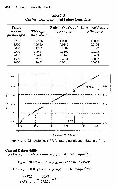
Table 7-3Gas Well Deliverability at Future Conditions
Future Ratio = ^{pidfuture/ Ratio = (AOF)future/reservoir ^(Pldfuture ^iPR)current (AOF)current
pressure (psia) (mmpsia2/cP) — —
3700 772.56 1.0000 1.00003500 706.80 0.9149 0.91563000 547.65 0.7089 0.71222500 399.17 0.5167 0.52032000 266.41 0.3448 0.34891500 155.04 0.2031 0.20071000 70.63 0.0914 0.0927
V(PR) Future / V(PR) Current
Figure 7-3. Dimensionless IPR for future conditions—Example 7 -1 .
Current Deliverability(a) For Pwf = 2566 psia <—> V(Pwf) = 417.59 mmpsia2/cP:
TR = 3700 psia <—> ^ (PR) = 772.56 mmpsia2/cP
(b) Now Pwf = 1000 psia <—> ^(pwf) = 70.63 mmpsia2/cP:
HPjf) = m f f l = o , ( ) 9 1f{PR)currem 772.56
Qm
OX
/Fut
ure
/ Q
max
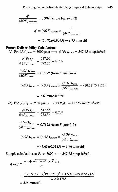
q'——— = 0.9095 (from Figure 7-2)(AOF ) current
qf = (AOF)current x — — | -
[AUr )current
= (10.72) (0.9095) = 9.75 mmscfd
Future Deliverability Calculations(c) For (Pidfuture = 3000 psia <—> ^ (PR)future = 547.65 mmpsia2/cP:
*™f = ^ = 0.7Q9t(PR)current 772.56
unll**" = ° - 7 1 2 2 (fr0m F i § u r e 7-3)(AOF)current
(AOF)future = (AOF)current x ( ^ W e = (10.72)(0.7122)[AUr ) current
= 7.63 mmpsia2/cP
(d) For (Pwf)f = 2566 psia <—> ^(Pwf)f = 417.59 mmpsia2/cP:
f(PR)f = 547,65 =
f{PR)curren, 772.56
^ W g = 0 - 7 1 2 2 ( f r ° m F i § U r e 7-3>( ^ ^ ^ ) current
s A s\n\ / A s^n\ (A(Jr )future(AOF)future = (AOF)current X
(A(yr ) current
= (7.63)(0.5185) = 3.96 mmscfd
Sample calculations at P^ = 3000 <—> 547.65 mmpsia2/cP:
_ -a + Ja2+4b[\l/(PR)f
QrnaxJ — ry,
_ -91.8273 + 7(91.8273)2 + 4 x 0.1785 x 547.65~ 2x0.1785= 5.90 mmscfd
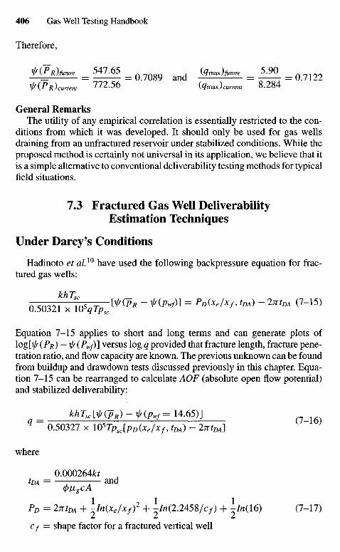
Therefore,
^ ( Z * W = ^ ^ = 0.7089 and ( ^ a x W = ^ - = 0.7122f(PR)current ?72.56 (?max)c,7wif 8.284
General RemarksThe utility of any empirical correlation is essentially restricted to the con-
ditions from which it was developed. It should only be used for gas wellsdraining from an unfractured reservoir under stabilized conditions. While theproposed method is certainly not universal in its application, we believe that itis a simple alternative to conventional deliverability testing methods for typicalfield situations.
13 Fractured Gas Well DeliverabilityEstimation Techniques
Under Darcy's Conditions
Hadinoto et al.10 have used the following backpressure equation for frac-tured gas wells:
khT0 50321 x K)5 T ^ ^ R ~ ^(pw^ = pD(*e/xf, tDA) - 2ntDA (7-15)
Equation 7-15 applies to short and long terms and can generate plots of\og[\l/(PR) - is(Pwf)] versus log q provided that fracture length, fracture pene-tration ratio, and flow capacity are known. The previous unknown can be foundfrom buildup and drawdown tests discussed previously in this chapter. Equa-tion 7-15 can be rearranged to calculate AOF (absolute open flow potential)and stabilized deliverability:
= khTsclif(pR)-if(Pwf=U.65)iq 0.50327 x l05Tpsc[pD(xe/xf, tDA) - 2ntDA\
where
0.000264£ftDA = — 7— and
(p/jigcA
PD = 2ntDA + -In(xe/xf)2 + -In(2.245S/cf) + -Ai(16) (7-17)
Cf = shape factor for a fractured vertical well
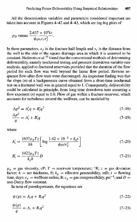
All the dimensionless variables and parameters considered important aretaken into account in Figures 4-42 and 4 ^ 3 , which are log-log plots of
2.637 x l04ktpD versus ~—.
(f)i IXiCiXf
In these parameters, Xf is the fracture half-length and xe is the distance fromthe well to the side of the square drainage area in which it is assumed to beconstant. Hadinoto et al10 found that the conventional methods of determiningdeliverability, namely isochronal testing and pressure drawdown variable-rateanalysis, applied to fractured reservoirs provided that the duration of the flowperiod for each flow was well beyond the linear flow period. Reverse se-quence flow-after-flow tests were discouraged. An important finding was thatthe slope (n) of a backpressure curve obtained from a short-time isochronaltest on a fractured well was in general equal to 1. Consequently, deliverabilitycould be calculated in principle, from long-time drawdown tests assuming aflow exponent (n) equal to 1.0. Flow of gas within a fracture reservoir, whichaccounts for turbulence around the wellbore, can be modeled by
A/72 = A'tq + B[q2 (7-18)
^ - = A; + B[q (7-19)
where
!637^r 1.42 XlO-' x y i ( ? _ 2 0 )
kh L <Pn-crl J
1422^D
kgh
fig = gas viscosity, cP; T = reservoir temperature; 0R; z = gas deviationfactor; h — net thickness, ft; kg = effective permeability, mD; t = flowingtime, days; rw = wellbore radius, ft; cg = gas compressibility, psi"1; and D —non-Darcy flow constant.
In term of pseudopressure, the equations are
f(p) = A,q + Btq2 (7-22)
- ^ ^ = A1 + Btq2 (7-23)
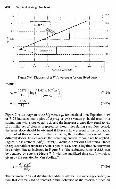
Figure 7-4. Diagram of AP2/q versus q for one fixed time,
where
16377T /1.42 XlO-2JkAIAt = ~TTT\ loS 2 2 ( 7 " 2 4 )
14227Bt = ^^~D (7-25)
Figure 7-4 is a diagram of Ap2/q versus qsc for one fixed time. Equation 7-19or 7-23 indicates that a plot of Ap2/q or \/r(p) versus q should result in astraight line with slope equal to Bx and the intercept at zero flow equal to Ax.If a similar set of plots is prepared for fixed times during each flow period,the same slope should be obtained if Darcy's flow present in the formation.If turbulent flow is present in the formation, the resulting lines would havedifferent slopes. In such a case, the remaining procedure could not be applied.Figure 7-5 is a plot of Ap2/q or \//(p) versus q at various fixed times. UnderDarcy's conditions in the reservoir, a plot of AAA1 versus log time should resultin a straight line as indicated in Figure 7-6. The stabilized value of AAA1 canbe obtained by entering Figure 7-6 with the stabilized time (tstab)> which isgiven by the equation by Van Poollen:14
(p^gcgr2
tstab = A o g 7 — (7-26)
The parameter AAA, at stabilized conditions allows us to write a general equa-tion that can be used to forecast future behavior of the reservoir. Such an
Flow rate q, mmscfd
Intercept = A \
Slope = B',
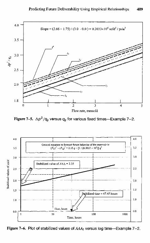
Flow rate, mmscfd
Figure 7-5. Ap2/qg versus qg for various fixed times—Example 7-2.
Slope - (2.66 - 1.75) / (3.0 - 0.0 ) = 0.3033x10⁶ scfd2 / psia2
Figure 7-6. Plot of stabilized values of AAAt versus log time—Example 7-2.
Time, hours
Time, hours
Stabilized time = 47.45 hours
Stabilized value of AAA, = 2.35
General equation to forecast future behavior of the reservoir is:
(PR)2- (/V)2 = 2-35 + H/ (°-3 0 3 3 x lo6)] i2
Stab
ilize
d va
lues
of A
AA
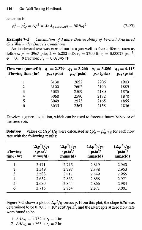
equation is
p? - plf = Ap2 = AAAt(stabilized)q + BBBtq2 (7-27)
Example 7-2 Calculation of Future Deliverability of Vertical FracturedGas Well under Darcy 's Conditions
An isochronal test was carried out in a gas well to four different rates asfollows: pi = 3965 psia; k = 6.282 mD; re = 2200 ft; ct = 0.00023 psi"1;0 = 0.119 fraction; /xg = 0.02345 cP
Flow rate (mmscfd) qt = 2.379 q2 = 3.200 q3 = 3.850 q4 = 4.115Flowing time (hr) pwf (psia) pwf (psia) pwf (psia) pwf (psia)
1 3130 2652 2206 19032 3100 2602 2190 18893 3085 2509 2180 18764 3060 2580 2172 18705 3049 2573 2165 18556 3035 2567 2158 1836
Develop a general equation, which can be used to forecast future behavior ofthe reservoir.
Solution Values of (Ap2)/q were calculated as (p2R — p^S)/q for each flow
rate with the following results:
(Ap2)/qi (Ap2)/q2 (Ap2)/q3 (Ap2)/q4
Flowing (psia2/ (psia2/ (psia2/ (psia2/time(hr) mmscfd) mmscfd) mmscfd) mmscfd)
1 2.471 2.715 2.819 2.9402 2.549 2.797 2.838 2.9533 2.588 2.817 2.849 2.9654 2.652 2.833 2.858 2.9715 2.680 2.844 2.866 2.9846 2.716 2.854 2.871 3.001
Figure 7-5 shows a plot of Ap2/q versus q. From this plot, the slope BBB wasdetermined to be 0.3033 x 10⁶ scfd2/psia2, and the intercepts at zero flow ratewere found to be
1. AAAn = 1.752 at fi = 1 hr2. AAAt2 = 1.863 at t2 = 2 hr
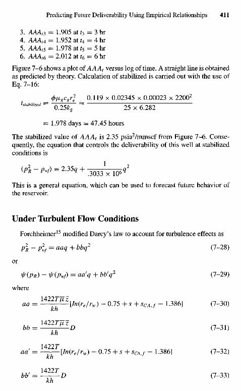
3. AAAt3 = 1.905 at t3 = 3 hr4. AAAt4 = 1.952 at J4 = 4 hr5. AAA,5 = 1.978 at t5 = 5 hr6. A4Ar6 = 2.012 at t6 = 6 hr
Figure 7-6 shows a plot of A A A1 versus log of time. A straight line is obtainedas predicted by theory. Calculation of stabilized is carried out with the use ofEq. 7-16:
_ 0figcgr2
e _ 0.119 x 0.02345 x 0.00023 x 22002
tstabmZed - " 5 ^ - ~ 25 x 6.282
= 1.978 days = 47.45 hours
The stabilized value of AAA1 is 2.35 psia2/mmscf from Figure 7-6. Conse-quently, the equation that controls the deliverability of this well at stabilizedconditions is
This is a general equation, which can be used to forecast future behavior ofthe reservoir.
Under Tlirbulent Flow Conditions
Forchheimer15 modified Darcy's law to account for turbulence effects as
p2R-p2
wf=aaq+bbq2 (7-28)
or
Mp R) ~ tiPvrf) = aa'q + bb'q2 (7-29)
where
aa = U2^1IZ[In(re/rw) - 0.75 + s + sCA / - 1.386] (7-30)
kh
», = ! i ^ D (7_31)kh
\A22Taaf - — — [In(re/rw) ~ 0.75 + s + sCAj - 1.386] (7-32)
KfI
14227
bb' = f±LD (7-33)kh
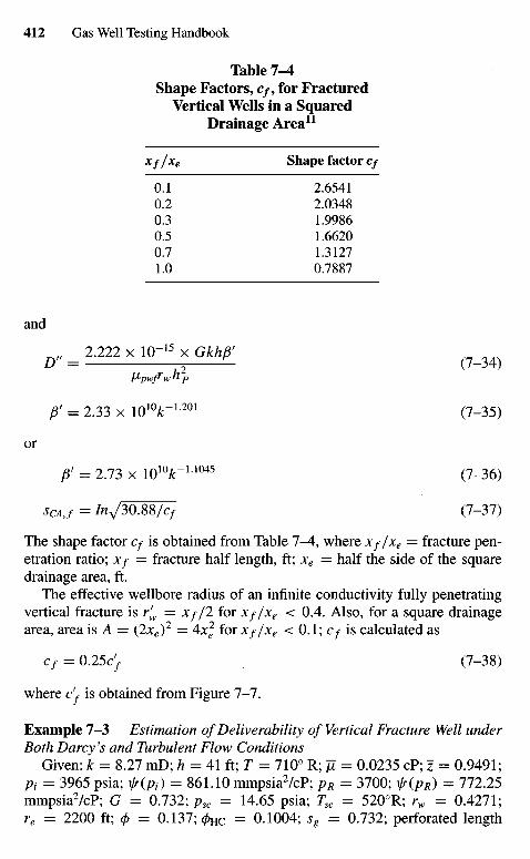
Table 7-4Shape Factors, Cf9 for Fractured
Vertical Wells in a SquaredDrainage Area11
Xf/xe Shape factor c/
0.1 2.65410.2 2.03480.3 1.99860.5 1.66200.7 1.31271.0 0.7887
and
^ - « a x io-» x c«y (7_34)
P' = 2.33 x 10¹⁰yrL201 (7-35)
or
j8; = 2.73 x IO1 0^-1 1 0 4 5 (7-36)
SCAJ = Inj30.SS/cf (7-37)
The shape factor Cf is obtained from Table 7-4, where Xf/xe = fracture pen-etration ratio; Xf = fracture half length, ft; xe = half the side of the squaredrainage area, ft.
The effective wellbore radius of an infinite conductivity fully penetratingvertical fracture is rf
w = Jt//2 for Xf/xe < 0.4. Also, for a square drainagearea, area is A = (2xe)
2 = 4x2 for Xf/xe < 0.1; c/ is calculated as
Cf = 0.25c} (7-38)
where d, is obtained from Figure 7-7.
Example 7-3 Estimation of Deliver ability of Vertical Fracture Well underBoth Darcy 's and Turbulent Flow Conditions
Given: k = 8.27 mD; h = 41 ft; T = 710° R; JI = 0.0235 cP; z = 0.9491;Pi = 3965 psia; V K A ) = 861.10 mmpsia2/cP; pR = 3700; ^(/?/j) = 772.25mmpsia2/cP; G = 0.732; psc = 14.65 psia; Tsc = 5200R; rw = 0.4271;re = 2200 ft; 0 = 0.137; 0Hc = 0.1004; sg = 0.732; perforated length
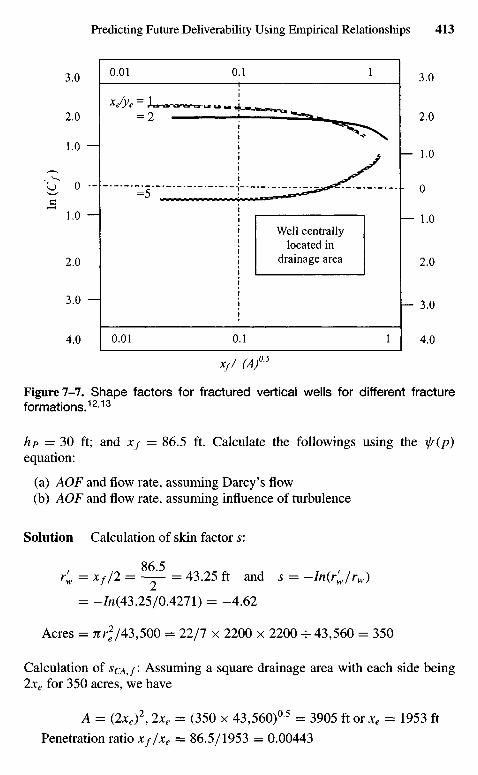
Figure 7-7. Shape factors for fractured vertical wells for different fractureformations.1213
hP = 30 ft; and x/ = 86.5 ft. Calculate the followings using the \j/(p)equation:
(a) AOF and flow rate, assuming Darcy's flow(b) AOF and flow rate, assuming influence of turbulence
Solution Calculation of skin factor s:
r'w = Xf/2 = — ^ = 43.25 ft and s = -In(rjrw)
= -/n(43.25/0.4271) = -4.62
Acres = 7rr^2/43,500 = 22/7 x 2200 x 2200 -=- 43,560 = 350
Calculation of SCAJ'- Assuming a square drainage area with each side being2xe for 350 acres, we have
A = (2xe)2, 2xe = (350 x 43,560)05 = 3905 ft or xe = 1953 ft
Penetration ratio xf/xe = 86.5/1953 = 0.00443
Well centrallylocated in
drainage area
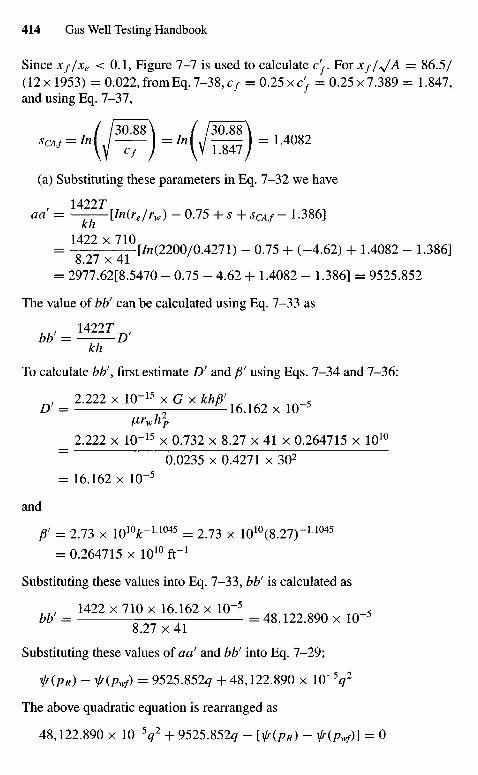
Since x//xe < 0.1, Figure 7-7 is used to calculate c^. For Xf/y/A = 86.5/(12x1953) =0.022, from Eq. 7-38, c/ = 0.25xc'f =0.25x7.389= 1.847,and using Eq. 7-37,
(a) Substituting these parameters in Eq. 7-32 we have
1422Jad = ——[in(re/rw) - 0.75 + s + sCA,f- 1-386]
= - [/n(2200/0.4271) - 0.75 + (-4.62) + 1.4082 - 1.386]8.27 x 41
= 2977.62[8.5470 - 0.75 - 4.62 + 1.4082 - 1.386] = 9525.852
The value of bb' can be calculated using Eq. 7-33 as
kh
To calculate bb', first estimate D' and ft using Eqs. 7-34 and 7-36:
^ 2.222X 1 0 - " X G x ^ 1 6 1 6 2 x iQ_5
HrwhlP
_ 2.222 x K r 1 5 x 0.732 x 8.27 x 41 x 0.264715 x 1010
~ 0.0235 x 0.4271 x 302
= 16.162 x 10~5
and
P' = 2.73 x 10¹⁰JT1-1045 = 2.73 x 10¹⁰(8.27)-11045
= 0.264715 x 1010 ft"1
Substituting these values into Eq. 7-33, bb' is calculated as
= i«2x7ioxi6.uaxir' = 10_5
8.27 x 41
Substituting these values of aa' and bb' into Eq. 7-29;
IT(PR) ~ t(Pwf) = 9525.852# + 48,122.890 x 10~V
The above quadratic equation is rearranged as
48,122.890 x 10"V + 9525.852^ - [f(pR) - <M/v)] = 0
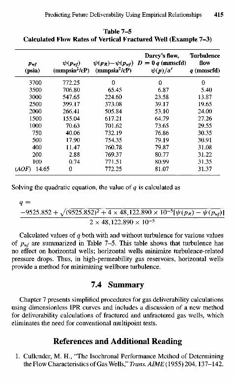
Table 7-5Calculated Flow Rates of Vertical Fractured Well (Example 7-3)
Darcy's flow, TurbulencePwf ip(Pwf) ^(PR)-^(Pwf) D = 0g(mmscfd) flow
(psia) (mmpsia2/cP) (mmpsia2/cP) ip(p)/a' q (mmscfd)
3700 772.25 0 0 03500 706.80 65.45 6.87 5.403000 547.65 224.60 23.58 13.872500 399.17 373.08 39.17 19.652000 266.41 505.84 53.10 24.001500 155.04 617.21 64.79 27.261000 70.63 701.62 73.65 29.55750 40.06 732.19 76.86 30.35500 17.90 754.35 79.19 30.91400 11.47 760.78 79.87 31.08200 2.88 769.37 80.77 31.22100 0.74 771.51 80.99 31.35
(AOF) 14.65 0 772.25 81.07 31.37
Solving the quadratic equation, the value of q is calculated as
q =
-9525.852 + v'(9525.852)2 + 4 x 48,122.890 x K ) - 5 O O * ) - is(pwf)]
2 x 48,122.890 x 10~5
Calculated values of q both with and without turbulence for various valuesof pwf are summarized in Table 7-5. This table shows that turbulence hasno effect on horizontal wells; horizontal wells minimize turbulence-relatedpressure drops. Thus, in high-permeability gas reservoirs, horizontal wellsprovide a method for minimizing wellbore turbulence.
7.4 Summary
Chapter 7 presents simplified procedures for gas deliverability calculationsusing dimensionless IPR curves and includes a discussion of a new methodfor deliverability calculations of fractured and unfractured gas wells, whicheliminates the need for conventional multipoint tests.
References and Additional Reading
1. Cullender, M. H., "The Isochronal Performance Method of Determiningthe Flow Characteristics of Gas Wells," Trans. AIME (1955) 204,137-142.
2. Katz, D. L., Cornell, D., Kobayashi, R., Poettmann, F. H., Vary, J. A.,Elenbaas, J. R., and Weinaug, K, Handbook of Natural Gas Engineering.McGraw-Hill, New York, 1959.
3. Fetkovich, M. J., "Multi-point Testing of Gas Wells," Continuing Educa-tion Course, SPE Mid-Continent Section, March 17, 1975.
4. Lee, A. L., Gonzalez, M. H., and Eakin, B. E., "The Viscosity of NaturalGases," Trans. AIME (1966) 237, 997-1000.
5. Vogel, J. L., "Inflow Performance Relationships for Solution-Gas DriveWells," J. Petroleum Technol. (Jan. 1968) 83-92.
6. Rawlins, E. L., and Schellhardt, M. A., "Back-Pressure Data on NaturalGas Wells and Their Application to Production Practices," Monograph 7,USBM, 1936.
7. Mishra, S., "Deliverability Testing of Gas Wells Using Dimensionless IPRCurves," M.S. Thesis, The University of Texas at Austin, May 1983.
8. Theory and Practice of the Testing of Gas Wells, 3rd ed., Alberta EnergyResources Conservation Board, 1979.
9. Swift, G. W., and Kiel, O. G., "The Prediction of Gas Well PerformanceIncluding the Effect of Non-Darcy Flow," Trans. AIME (1962) 225, 791-798.
10. Hadinoto, N., Raghavan, R., and Thomas, G. W., "Determination of GasWell Deliverability of Vertically Fractured Wells," Paper SPE 6136 pre-sented at the 51st Annual Fall Technical Conference and Exhibition ofSPE ofAIME, New Orleans (October 3-6, 1976).
11. Earlougher, R. C , Jr., "Advances in Well Test Analysis," Monograph Vol. 5of the Henry L. Doherty Series in Society of Petroleum Engineers ofAIME, 1977.
12. Al-Hussainy, R. Ramey, H. J., Jr., and Crawford, P. B., "The Flow of RealGases through Porous Media," / Petroleum Technol. (1966) 624-636;Trans. AIME V 237.
13. Gringarten, A. C , Ramey, H. J., Jr., and Raghavan, R., "UnsteadyState Pressure Distribution Created by a Well with a Single Infinity-Conductivity Vertical Fracture," SPE (Aug. 1974) 347-360.
14. Van Poollen, H. K., "Radius-of-Drainage and Stabilization Time Equa-tions," Oil Gas J. (1964) 62, 138-146.
15. Forchheimer, Ph., "Wasserbewegung durch Boden," Z Ver. Deutsch. Ing.(1901)45,1781-1788.
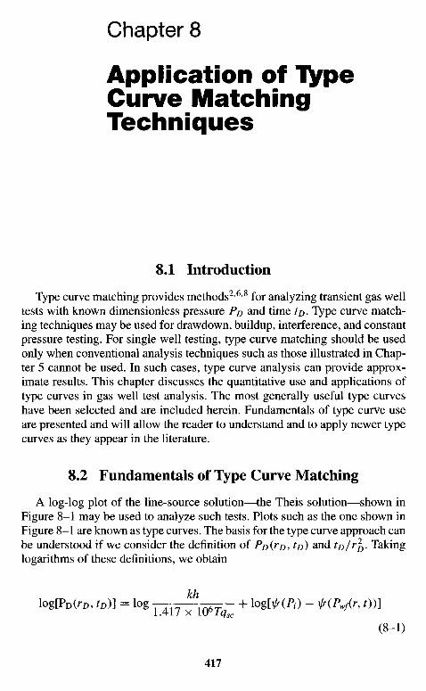
Chapter 8
Application of "typeCurve MatchingTechniques
8.1 Introduction
Type curve matching provides methods2'6'8 for analyzing transient gas welltests with known dimensionless pressure PD and time tp. Type curve match-ing techniques may be used for drawdown, buildup, interference, and constantpressure testing. For single well testing, type curve matching should be usedonly when conventional analysis techniques such as those illustrated in Chap-ter 5 cannot be used. In such cases, type curve analysis can provide approx-imate results. This chapter discusses the quantitative use and applications oftype curves in gas well test analysis. The most generally useful type curveshave been selected and are included herein. Fundamentals of type curve useare presented and will allow the reader to understand and to apply newer typecurves as they appear in the literature.
8.2 Fundamentals of Type Curve Matching
A log-log plot of the line-source solution—the Theis solution—shown inFigure 8-1 may be used to analyze such tests. Plots such as the one shown inFigure 8-1 are known as type curves. The basis for the type curve approach canbe understood if we consider the definition of PD (rD, tD) and tD/r^. Takinglogarithms of these definitions, we obtain
khlog[PD(rz>, tD)] = log i 4 n x i Q 6 r + 1Og[VKP,) - f(Pwf(r, t))]
(8-1)
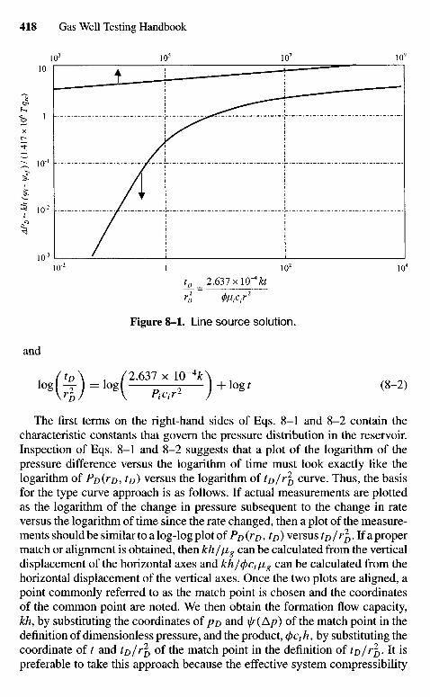
Figure 8-1. Line source solution.
and
(tD\ /2.637 x lO~4k\
' 0 8 ( ^ ) = '°g( r*** ) + log> <8"2)
The first terms on the right-hand sides of Eqs. 8-1 and 8-2 contain thecharacteristic constants that govern the pressure distribution in the reservoir.Inspection of Eqs. 8-1 and 8-2 suggests that a plot of the logarithm of thepressure difference versus the logarithm of time must look exactly like thelogarithm of PD(^D, tD) versus the logarithm of to/r^ curve. Thus, the basisfor the type curve approach is as follows. If actual measurements are plottedas the logarithm of the change in pressure subsequent to the change in rateversus the logarithm of time since the rate changed, then a plot of the measure-ments should be similar to a log-log plot of PD (rD, tD) versus tD / r2
D. If a propermatch or alignment is obtained, then kh/'\ig can be calculated from the verticaldisplacement of the horizontal axes and kh/(/)ctiJLg can be calculated from thehorizontal displacement of the vertical axes. Once the two plots are aligned, apoint commonly referred to as the match point is chosen and the coordinatesof the common point are noted. We then obtain the formation flow capacity,kh, by substituting the coordinates of pD and s(Ap) of the match point in thedefinition of dimensionless pressure, and the product, (/>cth, by substituting thecoordinate of t and to/rjy of the match point in the definition of to/r^. It ispreferable to take this approach because the effective system compressibility
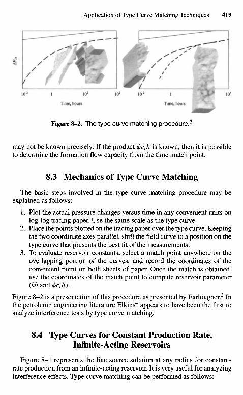
Figure 8-2. The type curve matching procedure.3
may not be known precisely. If the product (j>cth is known, then it is possibleto determine the formation flow capacity from the time match point.
83 Mechanics of Type Curve Matching
The basic steps involved in the type curve matching procedure may beexplained as follows:
1. Plot the actual pressure changes versus time in any convenient units onlog-log tracing paper. Use the same scale as the type curve.
2. Place the points plotted on the tracing paper over the type curve. Keepingthe two coordinate axes parallel, shift the field curve to a position on thetype curve that presents the best fit of the measurements.
3. To evaluate reservoir constants, select a match point anywhere on theoverlapping portion of the curves, and record the coordinates of theconvenient point on both sheets of paper. Once the match is obtained,use the coordinates of the match point to compute reservoir parameter(kh and (pcth).
Figure 8-2 is a presentation of this procedure as presented by Earlougher.3 Inthe petroleum engineering literature Elkins4 appears to have been the first toanalyze interference tests by type curve matching.
8.4 Type Curves for Constant Production Rate,Infinite-Acting Reservoirs
Figure 8-1 represents the line source solution at any radius for constant-rate production from an infinite-acting reservoir. It is very useful for analyzinginterference effects. Type curve matching can be performed as follows:
Time, hoursTime, hours
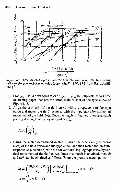
Figure 8-3. Dimensionless pressures for a single well in an infinite system;wellbore storage and skin included (copyright © 1970, SPE, from Trans. AIME,1970).7
1. Plot (iff. — i/rWf) drawdown tests or {\j/ws — \f/Wf) buildup tests versus timeon tracing paper that has the same scale as that of the type curve ofFigure 8-3.
2. Align the Aty axis of the field curve with the Ap D axis of the typecurve and match the field response with the type curve by horizontalmovement of the field plots. Once the match is obtained, choose a matchpoint and record the values of / and tD/r\,.
(OM, (±)VDJM
3. Using the match determined in step 2, align the time axis (horizontalaxes) of the field curve and the type curve, and then match the pressureresponse ( A ^ versus t) with the conventional log-log type curve by ver-tical movement of the field curve. Once this match is obtained, then khand (j)ch can be obtained as follows. From the pressure match point:
th=(n*"*'') rg^>i ,mD.fl\ Tsc J \_fi ~ Wmf\matchpoint
k = — ,mD - ft
LOG CYCLES
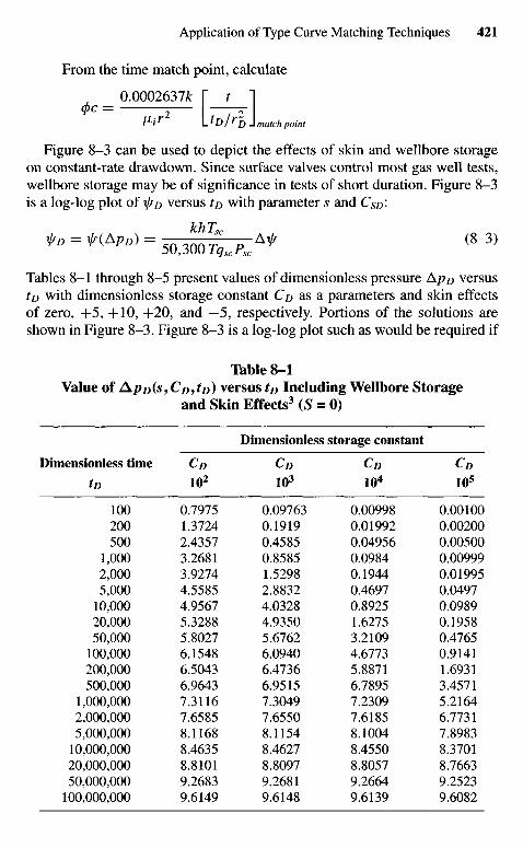
From the time match point, calculate
0.0002637fc T t I
№ir L *D /rD J match point
Figure 8-3 can be used to depict the effects of skin and wellbore storageon constant-rate drawdown. Since surface valves control most gas well tests,wellbore storage may be of significance in tests of short duration. Figure 8-3is a log-log plot of V D versus to with parameter s and CSD'-
khTV D = ^(ApD) = . , . " A ^ ( 8 - 3 )
50,300 TqscPsc
Tables 8-1 through 8-5 present values of dimensionless pressure ApD versustD with dimensionless storage constant CD as a parameters and skin effectsof zero, + 5 , +10, +20, and —5, respectively. Portions of the solutions areshown in Figure 8-3. Figure 8-3 is a log-log plot such as would be required if
Table 8-1Value of ApD(s,CD,tD) versus tD Including Wellbore Storage
and Skin Effects3 (S = 0)
Dimensionless storage constant
Dimensionless time CD CD CD CD
tD 102 103 104 105
100 0.7975 0.09763 0.00998 0.00100200 1.3724 0.1919 0.01992 0.00200500 2.4357 0.4585 0.04956 0.00500
1,000 3.2681 0.8585 0.0984 0.009992,000 3.9274 1.5298 0.1944 0.019955,000 4.5585 2.8832 0.4697 0.0497
10,000 4.9567 4.0328 0.8925 0.098920,000 5.3288 4.9350 1.6275 0.195850,000 5.8027 5.6762 3.2109 0.4765
100,000 6.1548 6.0940 4.6773 0.9141200,000 6.5043 6.4736 5.8871 1.6931500,000 6.9643 6.9515 6.7895 3.4571
1,000,000 7.3116 7.3049 7.2309 5.21642,000,000 7.6585 7.6550 7.6185 6.77315,000,000 8.1168 8.1154 8.1004 7.8983
10,000,000 8.4635 8.4627 8.4550 8.370120,000,000 8.8101 8.8097 8.8057 8.766350,000,000 9.2683 9.2681 9.2664 9.2523
100,000,000 9.6149 9.6148 9.6139 9.6082
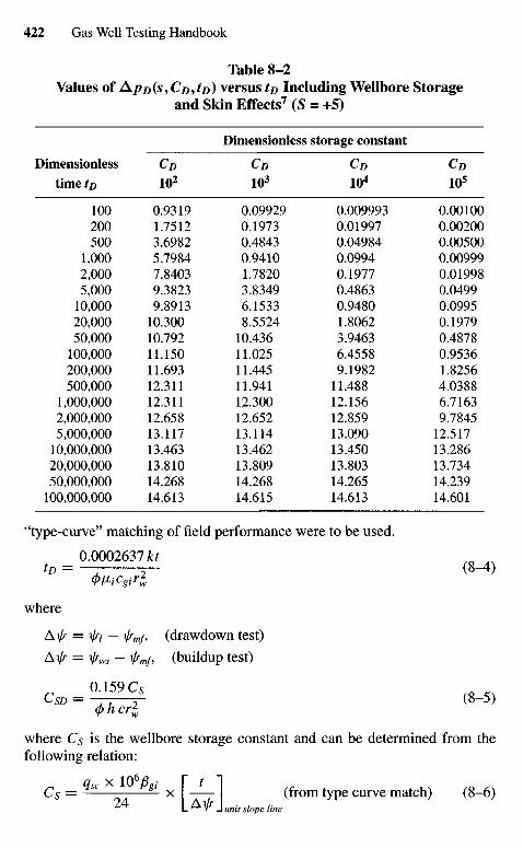
Table 8-2Values of APD(S9CD^D) versus to Including Wellbore Storage
and Skin Effects7 (S = +5)
Dimensionless storage constant
Dimensionless CD CD CD CDtime*/? 102 103 104 105
100 0.9319 0.09929 0.009993 0.00100200 1.7512 0.1973 0.01997 0.00200500 3.6982 0.4843 0.04984 0.00500
1,000 5.7984 0.9410 0.0994 0.009992,000 7.8403 1.7820 0.1977 0.019985,000 9.3823 3.8349 0.4863 0.0499
10,000 9.8913 6.1533 0.9480 0.099520,000 10.300 8.5524 1.8062 0.197950,000 10.792 10.436 3.9463 0.4878
100,000 11.150 11.025 6.4558 0.9536200,000 11.693 11.445 9.1982 1.8256500,000 12.311 11.941 11.488 4.0388
1,000,000 12.311 12.300 12.156 6.71632,000,000 12.658 12.652 12.859 9.78455,000,000 13.117 13.114 13.090 12.517
10,000,000 13.463 13.462 13.450 13.28620,000,000 13.810 13.809 13.803 13.73450,000,000 14.268 14.268 14.265 14.239
100,000,000 14.613 14.615 14.613 14.601
"type-curve" matching of field performance were to be used.
0.0002637 kttD = — T- (8^)
4> iC girlwhere
A\js = if/i — ij/mf, (drawdown test)
A\f/ = i/fws — \/fmf, (buildup test)
r 0 1 5 9 C * r« ^(j)hcrl
where Cs is the wellbore storage constant and can be determined from thefollowing relation:
Cs = - ^ ^ — x — (from type curve match) (8-6)2 4 l^Aunit slope line
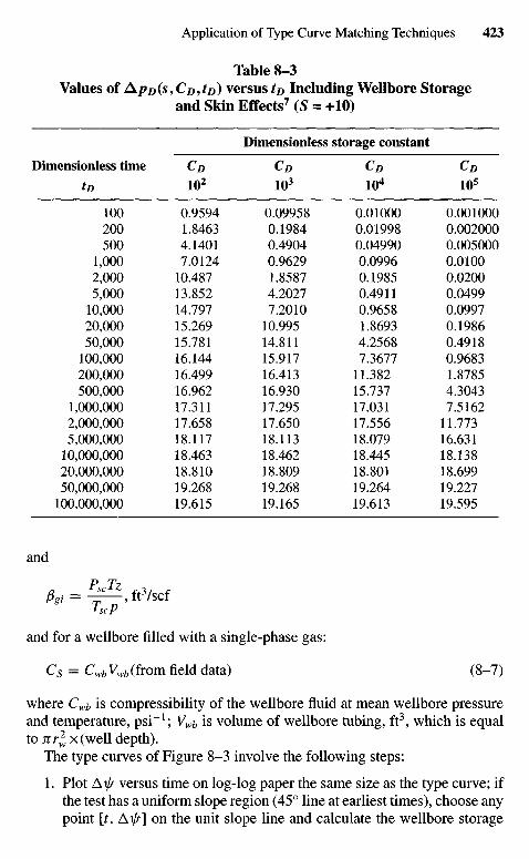
Table 8-3Values of ApD(s, CD^D) versus tD Including Wellbore Storage
and Skin Effects7 (S = +10)
Dimensionless storage constant
Dimensionless time CD CD CD CDtD 102 103 104 105
100 0.9594 0.09958 0.01000 0.001000200 1.8463 0.1984 0.01998 0.002000500 4.1401 0.4904 0.04990 0.005000
1,000 7.0124 0.9629 0.0996 0.01002,000 10.487 1.8587 0.1985 0.02005,000 13.852 4.2027 0.4911 0.0499
10,000 14.797 7.2010 0.9658 0.099720,000 15.269 10.995 1.8693 0.198650,000 15.781 14.811 4.2568 0.4918
100,000 16.144 15.917 7.3677 0.9683200,000 16.499 16.413 11.382 1.8785500,000 16.962 16.930 15.737 4.3043
1,000,000 17.311 17.295 17.031 7.51622,000,000 17.658 17.650 17.556 11.7735,000,000 18.117 18.113 18.079 16.631
10,000,000 18.463 18.462 18.445 18.13820,000,000 18.810 18.809 18.801 18.69950,000,000 19.268 19.268 19.264 19.227
100,000,000 19.615 19.165 19.613 19.595
and
^ = ^ , f t 3 / s c f•*• sc P
and for a wellbore filled with a single-phase gas:
C8 = Cwb Vwb (from field data) (8-7)
where Cwb is compressibility of the wellbore fluid at mean wellbore pressureand temperature, psi"1; Vwb is volume of wellbore tubing, ft3, which is equalto Ttr^ x (well depth).
The type curves of Figure 8-3 involve the following steps:
1. Plot A ^ versus time on log-log paper the same size as the type curve; ifthe test has a uniform slope region (45° line at earliest times), choose anypoint [t, Axf/] on the unit slope line and calculate the wellbore storage
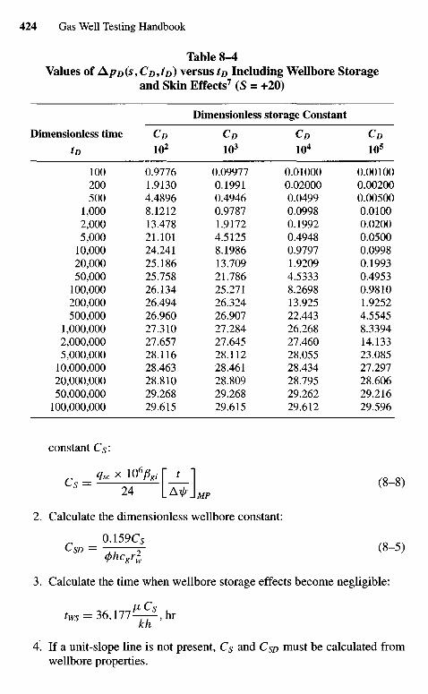
Table 8-4Values of Apo(s,CD,to) versus to Including Wellbore Storage
and Skin Effects7 (S = +20)
Dimensionless storage Constant
Dimensionless time CD CD CD CDtD 102 103 104 105
100 0.9776 0.09977 0.01000 0.00100200 1.9130 0.1991 0.02000 0.00200500 4.4896 0.4946 0.0499 0.00500
1,000 8.1212 0.9787 0.0998 0.01002,000 13.478 1.9172 0.1992 0.02005,000 21.101 4.5125 0.4948 0.0500
10,000 24.241 8.1986 0.9797 0.099820,000 25.186 13.709 1.9209 0.199350,000 25.758 21.786 4.5333 0.4953
100,000 26.134 25.271 8.2698 0.9810200,000 26.494 26.324 13.925 1.9252500,000 26.960 26.907 22.443 4.5545
1,000,000 27.310 27.284 26.268 8.33942,000,000 27.657 27.645 27.460 14.1335,000,000 28.116 28.112 28.055 23.085
10,000,000 28.463 28.461 28.434 27.29720,000,000 28.810 28.809 28.795 28.60650,000,000 29.268 29.268 29.262 29.216
100,000,000 29.615 29.615 29.612 29.596
constant Cs:
C = 4 U 1 (8-8,
2. Calculate the dimensionless wellbore constant:
r 0A59Cs (^ ^4>hcgrl
3. Calculate the time when wellbore storage effects become negligible:
%5 = 3 6 , 1 7 7 ^ , h rkh
4. If a unit-slope line is not present, Cs and Cso must be calculated fromwellbore properties.
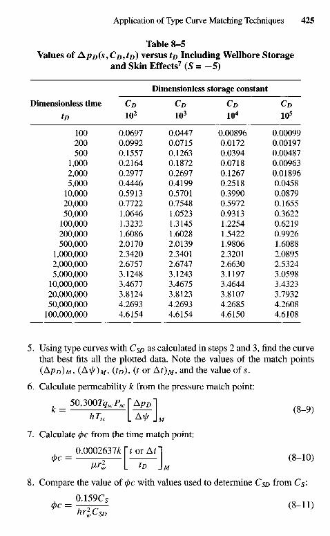
Table 8-5Values of APD(S^CD^D) versus to Including Wellbore Storage
and Skin Effects7 (S = - 5 )
Dimensionless storage constant
Dimensionless time CD CD CD CDtD 102 103 104 105
100 0.0697 0.0447 0.00896 0.00099200 0.0992 0.0715 0.0172 0.00197500 0.1557 0.1263 0.0394 0.00487
1,000 0.2164 0.1872 0.0718 0.009632,000 0.2977 0.2697 0.1267 0.018965,000 0.4446 0.4199 0.2518 0.0458
10,000 0.5913 0.5701 0.3990 0.087920,000 0.7722 0.7548 0.5972 0.165550,000 1.0646 1.0523 0.9313 0.3622
100,000 1.3232 1.3145 1.2254 0.6219200,000 1.6086 1.6028 1.5422 0.9926500,000 2.0170 2.0139 1.9806 1.6088
1,000,000 2.3420 2.3401 2.3201 2.08952,000,000 2.6757 2.6747 2.6630 2.53245,000,000 3.1248 3.1243 3.1197 3.0598
10,000,000 3.4677 3.4675 3.4644 3.432320,000,000 3.8124 3.8123 3.8107 3.793250,000,000 4.2693 4.2693 4.2685 4.2608
100,000,000 4.6154 4.6154 4.6150 4.6108
5. Using type curves with CSD as calculated in steps 2 and 3, find the curvethat best fits all the plotted data. Note the values of the match points(ApD)M9 (Ax//)M, ^D), (t or A O M , and the value of s.
6. Calculate permeability k from the pressure match point:
50,3OQr^P, I-AggihTsc [Af \M
1. Calculate (\>c from the time match point:
0.0002637JkTf or Af]ct>c = - (8-10)
V>rl L tD ] M
8. Compare the value of 0c with values used to determine CSD from C^:
hrlCsD
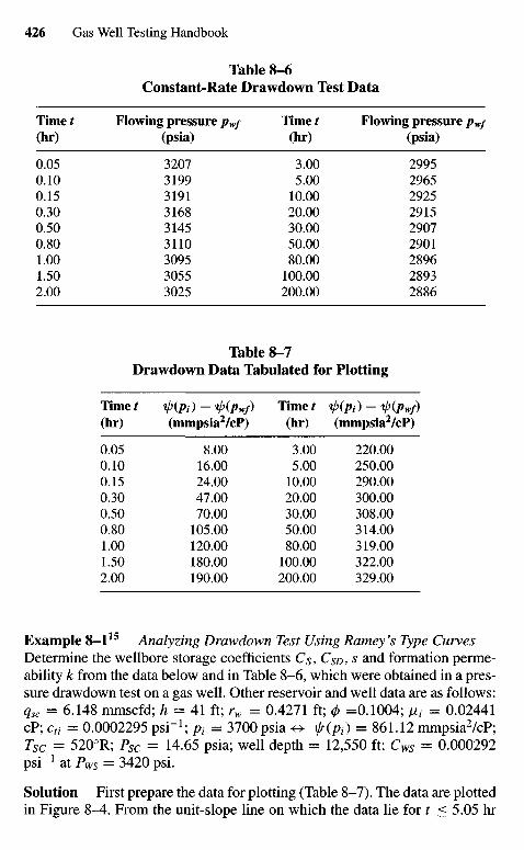
Table 8-6Constant-Rate Drawdown Test Data
Time t Flowing pressure pw/ Time t Flowing pressure pw/(hr) (psia) (hr) (psia)
0.05 3207 3.00 29950.10 3199 5.00 29650.15 3191 10.00 29250.30 3168 20.00 29150.50 3145 30.00 29070.80 3110 50.00 29011.00 3095 80.00 28961.50 3055 100.00 28932.00 3025 200.00 2886
Table 8-7Drawdown Data Tabulated for Plotting
Time t tpipt) - ip(pwf) Time t ^(Pi) - t/>(pwf)(hr) (mmpsia2/cP) (hr) (mmpsia2/cP)
0.05 8.00 3.00 220.000.10 16.00 5.00 250.000.15 24.00 10.00 290.000.30 47.00 20.00 300.000.50 70.00 30.00 308.000.80 105.00 50.00 314.001.00 120.00 80.00 319.001.50 180.00 100.00 322.002.00 190.00 200.00 329.00
Example 8-115 Analyzing Drawdown Test Using Ramey's Type CurvesDetermine the wellbore storage coefficients Cs, CSD, S and formation perme-ability k from the data below and in Table 8-6, which were obtained in a pres-sure drawdown test on a gas well. Other reservoir and well data are as follows:qsc = 6.148 mmscfd; h = 41 ft; rw = 0.4271 ft; 0 =0.1004; ^ = 0.02441cP; cti = 0.0002295 psi"1; pt = 3700 psia <+ i/(pt) = 861.12 mmpsia2/cP;T8C = 5200R; Psc = 14.65 psia; well depth = 12,550 ft; Cws = 0.000292psi"1 at Pws = 3420 psi.
Solution First prepare the data for plotting (Table 8-7). The data are plottedin Figure 8-4. From the unit-slope line on which the data lie for t < 5.05 hr
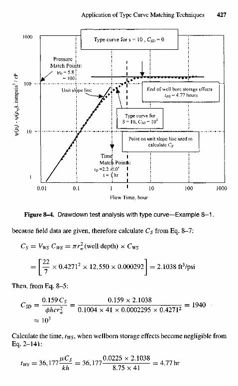
Type curve for s = 10 , CSD = 0
Flow Time, hour
Figure 8-4. Drawdown test analysis with type curve—Example 8 -1 .
because field data are given, therefore calculate Cs from Eq. 8-7:
Cs = Vws Cws = j r r^wel l depth) x Cws
l~22 1= — x 0.42712 x 12,550 x 0.000292 = 2.1038 ft3/psi
Then, from Eq. 8-5:
_ 0.159C5 _ 0.159 x 2.1038 _SD ~ 4>hcrl " 0.1004 x 41 x 0.0002295 x 0.42712 " *
^ 103
Calculate the time, tws> when wellborn storage effects become negligible fromEq. 2-141:
„ - 3 6 . 1 7 7 ^ - 3 6 , 1 7 7 ^ " " ^ - 4 . 7 7 b ,kh 8.75 x 41
Point on unit slope line used tocalculate Cs
Type curve for5=10, C5D=103
End of well bore storage effects(ws = 4.77 hours
Unit slope line
TimdMatct Pointfe:
PressureMatch Poirjts:
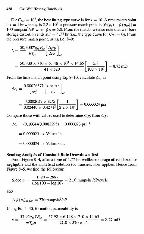
For CSD — 103, the best fitting type curve is for s = 10. A time match pointis t = 1 hr when tD is 2.2 x 10⁴; a pressure match point is [^(pt) - ^/(pWf)] —100 mmpsia2/cP, when yfrD = 5.8. From the match, we also note that wellborestorage distortion ends at t = A.11 hr (i.e., the type curve for CSD = 0). Fromthe pressure match point, using Eq. 8-9:
50,300TqxP5Cr ApDl
hTsc L AiA J M
50,300 x 710 x 6.148 x 103 x 14.65 f 5.8 "I= 4T7520 [l0^A&\ = 8- ? 5 m D
From the time match point using Eq. 8-10, calculate <pct as
0.0002637* ["/or A H
0.0002637 x 8.75 T l ] ,= 0.02440 x 0 . 4 2 7 l 4 ^ T W j = 0^000024P81"
Compare those with values used to determine CSD from Cs :
4>ct = (0.1004) (0.0002295) = 0.000023 psi"1
= 0.000023 -> Values in
= 0.000024 -> Values out.
Semilog Analysis of Constant-Rate Drawdown TestFrom Figure 8-4, after a time of 4.77 hr, wellbore storage effects become
negligible and the analytical solution for transient flow applies. Hence fromFigure 8-5, we find the following:
(320 — 299)Slope m = = 2 1 . 0 mmpsia2/cP/cycleF (log 100 - log 10) F y
and
AyIr(Pi) at \hr = 270 mmpsia2/cP
Using Eq. 5-40, formation permeability is
51.92qscTPsc _ 57.92 x 6.148 x 710 x 14.65 _
mTsch ~ 21.0x520x41 ~ ' m
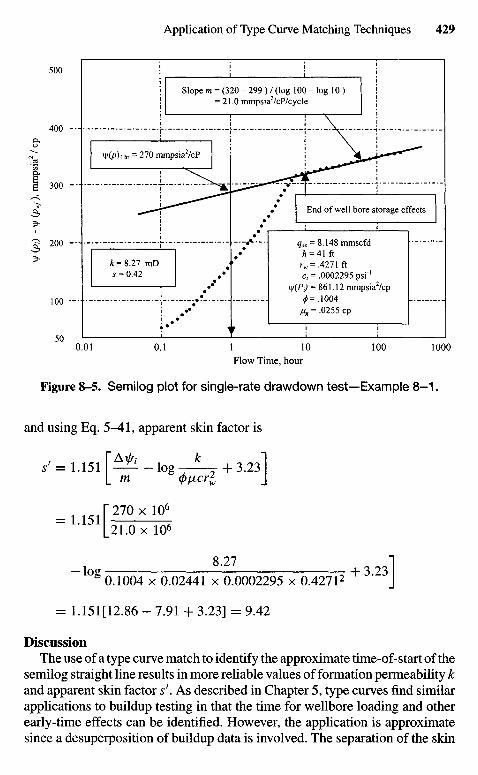
Flow Time, hour
Figure 8-5. Semilog plot for single-rate drawdown test—Example 8-1.
and using Eq. 5-41, apparent skin factor is
y = 1.151 [ ^ - f o g - ^ + 3 . 2 3 1
|_21.0xl06
8.27 1" l 0 g 0.1004 x 0.02441 x 0.0002295 x 0.42712 + 3 J
= 1.151[12.86 - 7.91 + 3.23] = 9.42
DiscussionThe use of a type curve match to identify the approximate time-of-start of the
semilog straight line results in more reliable values of formation permeability kand apparent skin factor sf. As described in Chapter 5, type curves find similarapplications to buildup testing in that the time for wellbore loading and otherearly-time effects can be identified. However, the application is approximatesince a desuperposition of buildup data is involved. The separation of the skin
qsc = 8.148 mmscfdh = 41 ftrw=.4271 ftc, = .0002295 psi"1
\y(Pj) = 861.12 mmpsia2/cp^=.1004
V8 = .0255 cp
End of well bore storage effects
W(p)\ hr = 270 mmpsia2/cP
Slope m = (320 - 299 ) / (log 100 - log 10 )= 21.0 mmpsia2/cP/cycle
and IT flow components of the apparent skin factor simply involves the analysisof another single-rate test by the methods described in this example with theonly additional step being the simultaneous solution of Eqs. 5^-6 and 5^47.
8.5 Storage and Skin Type CurveMatching Techniques
In unfractured gas wells, the early-time data are controlled by wellbore stor-age and skin effects.2'6 Figure 4^0 , developed by Earlougher and Kerch,6 isparticularly useful for analyzing wellbore storage controlled early-time data.The application of this type curve is to estimate kh and s, after it has beenascertained that an analysis of early-time data is desirable. The steps involvedusing this type curve are given in Chapter 4 (section 4.11). The values of khand s, obtained by this type curve matching technique, are not exact and shouldbe compared with values obtained from alternative sources to improve theirreliability. In the absence of any other information, they serve merely as an indi-cation of these parameters and should be treated as such. However, this curve-matching method will give a much more accurate value of kh, if Cs and s areknown from different sources. The use of this type curve (Figure 4-39) to ana-lyze wellbore storage controlled early-time data is illustrated in Example 4-19.
8.6 Fracture Type Curve Matching Techniques5
Infinite Conductivity Vertical Fractured Wells
Figure 4 4-0 represents the condition of constant-rate production for a verti-cally fractured well. It is a combination of the linear and radial flow equations.Its usefulness is readily seen since the majority of wells receive a hydraulicfracture upon completion. Such fractures are generally vertical and have aninfinite conductivity. Figure 4-40 is a log-log plot of i/sp versus tp with variousvalues of parameter xe/x/. Figure 4-40 (see xe/x/ = oo) reveals that the earlyportion of the type curve has a straight-line slope of one-half on a log-log graph,indicating linear flow. The deviation from the half-slope line represents ellip-tical flow or the transient from linear to radial flow response at the well. Thesetype curves are applicable to drawdown, buildup, and fall-off tests in fracturedwells and have been used for many years. Although the ordinate and abscissaof Figures 4-40 and 4-41 are given in terms of \j/, they may be modified quiteeasily for use with either the pressure or pressure square treatment methods byusing appropriate definitions of ApD and to'
and
0.0002637£rto = — T- (8~13)
where
A\fr = xfri — \j/wf - > drawdown test and Axf/ = \j;ws — x//wf, —• buildup test
x / = fracture half-length, ft
After the desirability of an early-time data analysis has been established, thefollowing procedure may be used to estimate the permeability thickness kh,the fracture half-length JC/, and the fracture skin factor s/.
Steps in use of Figure 4^40 or Figure 4-41 as a type curve for well testanalysis include the following:
1. Plot (V^-Vv)' drawdown test, or (^Ws-^wf), buildup test, on 3 x 5 cyclelog-log paper.
2. Select the best match by sliding the actual test data plot both horizontallyand vertically. The most likely curve is that for xe/xf = infinity, exceptwhere the fracture length and the duration of the test are unusually large.
3. Sketch the matched curve onto the data plot, and keep the data plottransfixed on the type curve (Figure 4-40 or Figure 4-41). Pick anyconvenient match point and read the following values:
(Ax/f)M and (OM —>* from data plot
(V^D)M and (^D)M ~> from Figure 4- W) or Figure 4-41
where subscript M refers to a match point.4. Estimate formation permeability from the pressure match point:
k = 50.300 x \06Tqsc PSC x (fD)M
hTsc (\j/i - \jfwf)M
5. Estimate fracture half-length from the time match point:
/0.0002637/: (Q JXf = . (8-15)
Y 0/X/Q (tD)M
6. Estimate the fracture skin factor from
./—*(£) OMW
Figure 4 ^ 1 is more applicable to a vertical fracture (natural fracture). Stepsin the use of Figure 4 ^ 1 as a type curve for well test analysis are the same as for
Figure 4-40. Furthermore, if data are plotted as shown in Figure 4 ^ 0 , insteadof obtaining a single curve, a family of curves will be obtained that depends onfracture flow capacity, formation permeability, and fracture length. However,for infinite fracture flow capacity and a given formation permeability, a uniquecurve exists for each value of xe/xf. Therefore, data from wells with finiteflow-capacity fractures generally cannot be analyzed using the type curvesdeveloped for infinite flow-capacity fractures.
Numerical results, in the form of dimensionless pressure drop versus di-mensionless time, were given for six different fracture penetration ratios,Xf/xe = 0.1,0.2,0.3,0.5,0.7, and 1, respectively, and are shown in Table 8-8.
tD > 0.7 tD + 1.4127 tD + 1.0560 tD + 0.8036 tD + 0.5371 tD
+0.3980 tD + 0.3331
Example 8-215 Analyzing Pressure Drawdown Test Data for Vertical Frac-tured Gas Well Using Type Curve Matching Technique
The reservoir and drawdown data of this gas well with a vertical fractureare presented in Table 8-9. Use type curve matching method to calculatepermeability k and fracture length JC/. Compare your results with the valuescalculated using semilog analysis and the Ax// versus ^/t plot.
Solution To establish the desirability of an early-time data analysis. Preparethe following plots:
1. A log-log plot of \jr(pi) — i/f(Pwf) versus time was prepared on a sheetof tracing paper (data curve). The initial data formed a straight line withunit slope as shown in Figure 8-6. This gave an indication of linear flowand consequently the possible of a fracture. This linear flow period lastedless than 0.6 hr and there were no wellbore storage effects.
2. Prepare a Cartesian coordinate plot of A ^ versus t as shown inFigure 8-7.
3. Prepare a Cartesian plot of A ^ versus +Jt as shown in Figure 8-8. Thisplot shows a straight line, which has slope mvf = 52.50 mmpsia2/cP/hr1/2,and at the end of the linear flow period, {A\j/)ef — 105 mmpsia2/cP.Substituting in the following equation, we get the beginning of thesemilogstraightline: (A\j/)bsi = 2x(A\jr)ef = 2x 105 = 210mmpsia2/cP.
4. Prepare a plot (on tracing paper) for type curve matching. In this exam-ple, the data curve was placed over the type curve for vertical fractures(Figure 4 ^ 0 ) and was displaced until a match was obtained as shown inFigure 8-9. The match obtained was perfect over the entire 4-hr draw-down. In fact, most fracture below 3000 ft tends to be nearly vertical.
(text continued on page 440)
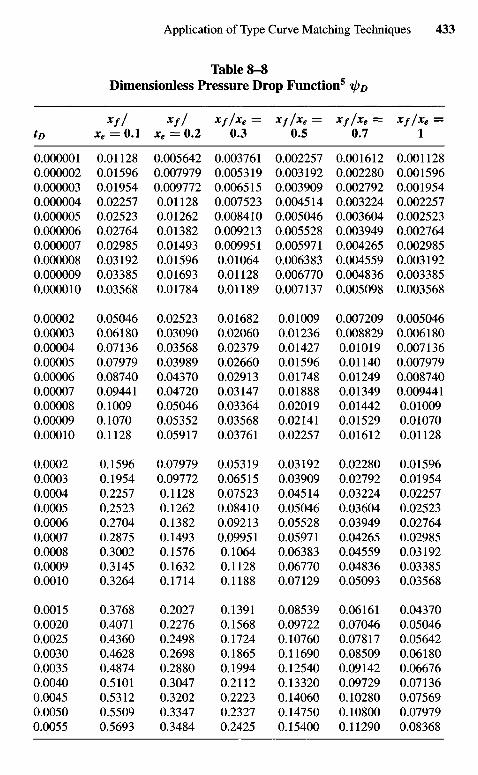
Table 8-8Dimensionless Pressure Drop Function5 t/?/>
xf/ xf/ xf/xe = xf/xe = xf/xe = xf/xe =tD xe = 0.1 xe = 0.2 0.3 0.5 0.7 1
0.000001 0.01128 0.005642 0.003761 0.002257 0.001612 0.0011280.000002 0.01596 0.007979 0.005319 0.003192 0.002280 0.0015960.000003 0.01954 0.009772 0.006515 0.003909 0.002792 0.0019540.000004 0.02257 0.01128 0.007523 0.004514 0.003224 0.0022570.000005 0.02523 0.01262 0.008410 0.005046 0.003604 0.0025230.000006 0.02764 0.01382 0.009213 0.005528 0.003949 0.0027640.000007 0.02985 0.01493 0.009951 0.005971 0.004265 0.0029850.000008 0.03192 0.01596 0.01064 0.006383 0.004559 0.0031920.000009 0.03385 0.01693 0.01128 0.006770 0.004836 0.0033850.000010 0.03568 0.01784 0.01189 0.007137 0.005098 0.003568
0.00002 0.05046 0.02523 0.01682 0.01009 0.007209 0.0050460.00003 0.06180 0.03090 0.02060 0.01236 0.008829 0.0061800.00004 0.07136 0.03568 0.02379 0.01427 0.01019 0.0071360.00005 0.07979 0.03989 0.02660 0.01596 0.01140 0.0079790.00006 0.08740 0.04370 0.02913 0.01748 0.01249 0.0087400.00007 0.09441 0.04720 0.03147 0.01888 0.01349 0.0094410.00008 0.1009 0.05046 0.03364 0.02019 0.01442 0.010090.00009 0.1070 0.05352 0.03568 0.02141 0.01529 0.010700.00010 0.1128 0.05917 0.03761 0.02257 0.01612 0.01128
0.0002 0.1596 0.07979 0.05319 0.03192 0.02280 0.015960.0003 0.1954 0.09772 0.06515 0.03909 0.02792 0.019540.0004 0.2257 0.1128 0.07523 0.04514 0.03224 0.022570.0005 0.2523 0.1262 0.08410 0.05046 0.03604 0.025230.0006 0.2704 0.1382 0.09213 0.05528 0.03949 0.027640.0007 0.2875 0.1493 0.09951 0.05971 0.04265 0.029850.0008 0.3002 0.1576 0.1064 0.06383 0.04559 0.031920.0009 0.3145 0.1632 0.1128 0.06770 0.04836 0.033850.0010 0.3264 0.1714 0.1188 0.07129 0.05093 0.03568
0.0015 0.3768 0.2027 0.1391 0.08539 0.06161 0.043700.0020 0.4071 0.2276 0.1568 0.09722 0.07046 0.050460.0025 0.4360 0.2498 0.1724 0.10760 0.07817 0.056420.0030 0.4628 0.2698 0.1865 0.11690 0.08509 0.061800.0035 0.4874 0.2880 0.1994 0.12540 0.09142 0.066760.0040 0.5101 0.3047 0.2112 0.13320 0.09729 0.071360.0045 0.5312 0.3202 0.2223 0.14060 0.10280 0.075690.0050 0.5509 0.3347 0.2327 0.14750 0.10800 0.079790.0055 0.5693 0.3484 0.2425 0.15400 0.11290 0.08368
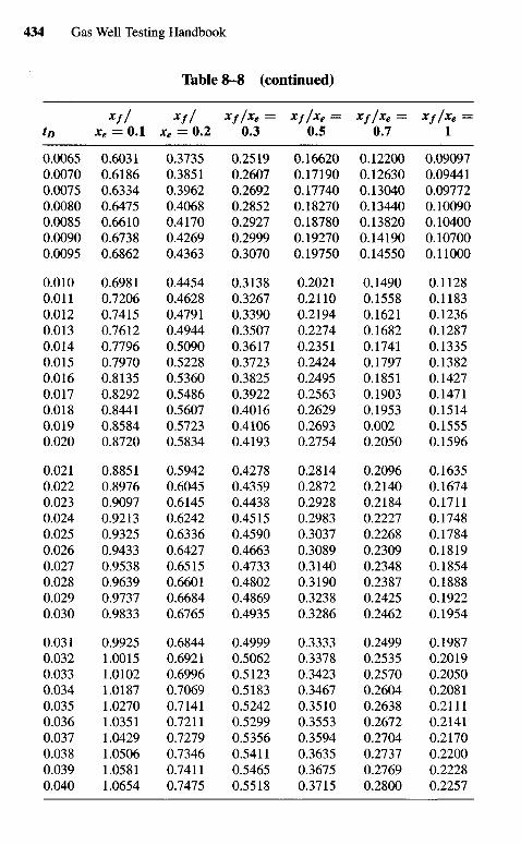
Table 8-8 (continued)
xf/ Xf/ Xf/Xe = XfIx9 = Xf/Xe = Xf/xe =tD xe = 0.1 xe = 0.2 0.3 0.5 0.7 1
0.0065 0.6031 0.3735 0.2519 0.16620 0.12200 0.090970.0070 0.6186 0.3851 0.2607 0.17190 0.12630 0.094410.0075 0.6334 0.3962 0.2692 0.17740 0.13040 0.097720.0080 0.6475 0.4068 0.2852 0.18270 0.13440 0.100900.0085 0.6610 0.4170 0.2927 0.18780 0.13820 0.104000.0090 0.6738 0.4269 0.2999 0.19270 0.14190 0.107000.0095 0.6862 0.4363 0.3070 0.19750 0.14550 0.11000
0.010 0.6981 0.4454 0.3138 0.2021 0.1490 0.11280.011 0.7206 0.4628 0.3267 0.2110 0.1558 0.11830.012 0.7415 0.4791 0.3390 0.2194 0.1621 0.12360.013 0.7612 0.4944 0.3507 0.2274 0.1682 0.12870.014 0.7796 0.5090 0.3617 0.2351 0.1741 0.13350.015 0.7970 0.5228 0.3723 0.2424 0.1797 0.13820.016 0.8135 0.5360 0.3825 0.2495 0.1851 0.14270.017 0.8292 0.5486 0.3922 0.2563 0.1903 0.14710.018 0.8441 0.5607 0.4016 0.2629 0.1953 0.15140.019 0.8584 0.5723 0.4106 0.2693 0.002 0.15550.020 0.8720 0.5834 0.4193 0.2754 0.2050 0.1596
0.021 0.8851 0.5942 0.4278 0.2814 0.2096 0.16350.022 0.8976 0.6045 0.4359 0.2872 0.2140 0.16740.023 0.9097 0.6145 0.4438 0.2928 0.2184 0.17110.024 0.9213 0.6242 0.4515 0.2983 0.2227 0.17480.025 0.9325 0.6336 0.4590 0.3037 0.2268 0.17840.026 0.9433 0.6427 0.4663 0.3089 0.2309 0.18190.027 0.9538 0.6515 0.4733 0.3140 0.2348 0.18540.028 0.9639 0.6601 0.4802 0.3190 0.2387 0.18880.029 0.9737 0.6684 0.4869 0.3238 0.2425 0.19220.030 0.9833 0.6765 0.4935 0.3286 0.2462 0.1954
0.031 0.9925 0.6844 0.4999 0.3333 0.2499 0.19870.032 1.0015 0.6921 0.5062 0.3378 0.2535 0.20190.033 1.0102 0.6996 0.5123 0.3423 0.2570 0.20500.034 1.0187 0.7069 0.5183 0.3467 0.2604 0.20810.035 1.0270 0.7141 0.5242 0.3510 0.2638 0.21110.036 1.0351 0.7211 0.5299 0.3553 0.2672 0.21410.037 1.0429 0.7279 0.5356 0.3594 0.2704 0.21700.038 1.0506 0.7346 0.5411 0.3635 0.2737 0.22000.039 1.0581 0.7411 0.5465 0.3675 0.2769 0.22280.040 1.0654 0.7475 0.5518 0.3715 0.2800 0.2257
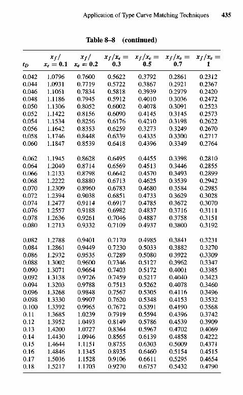
Table 8-8 (continued)
xf/ Xf/ Xf/Xe = Xf/Xe = Xf/X6 = Xf/X6 =tD xe = 0.1 xe = 0.2 0.3 0.5 0.7 1
0.042 1.0796 0.7600 0.5622 0.3792 0.2861 0.2312
0.044 1.0931 0.7719 0.5722 0.3867 0.2921 0.2367
0.046 1.1061 0.7834 0.5818 0.3939 0.2979 0.2420
0.048 1.1186 0.7945 0.5912 0.4010 0.3036 0.2472
0.050 1.1306 0.8052 0.6002 0.4078 0.3091 0.2523
0.052 1.1422 0.8156 0.6090 0.4145 0.3145 0.2573
0.054 1.1534 0.8256 0.6176 0.4210 0.3198 0.2622
0.056 1.1642 0.8353 0.6259 0.3273 0.3249 0.2670
0.058 1.1746 0.8448 0.6339 0.4335 0.3300 0.2717
0.060 1.1847 0.8539 0.6418 0.4396 0.3349 0.2764
0.062 1.1945 0.8628 0.6495 0.4455 0.3398 0.2810
0.064 1.2040 0.8714 0.6569 0.4513 0.3446 0.2855
0.066 1.2133 0.8798 0.6642 0.4570 0.3493 0.2899
0.068 1.2222 0.8880 0.6713 0.4625 0.3539 0.2942
0.070 1.2309 0.8960 0.6783 0.4680 0.3584 0.2985
0.072 1.2394 0.9038 0.6851 0.4733 0.3629 0.3028
0.074 1.2477 0.9114 0.6917 0.4785 0.3672 0.3070
0.076 1.2557 0.9188 0.6982 0.4837 0.3716 0.3111
0.078 1.2636 0.9261 0.7046 0.4887 0.3758 0.3151
0.080 1.2713 0.9332 0.7109 0.4937 0.3800 0.3192
0.082 1.2788 0.9401 0.7170 0.4985 0.3841 0.3231
0.084 1.2861 0.9449 0.7230 0.5033 0.3882 0.3270
0.086 1.2932 0.9535 0.7289 0.5080 0.3922 0.3309
0.088 1.3002 0.9600 0.7346 0.5127 0.3962 0.3347
0.090 1.3071 0.9664 0.7403 0.5172 0.4001 0.3385
0.092 1.3138 0.9726 0.7459 0.5217 0.4040 0.3423
0.094 1.3203 0.9788 0.7513 0.5262 0.4078 0.3460
0.096 1.3268 0.9848 0.7567 0.5305 0.4116 0.3496
0.098 1.3330 0.9907 0.7620 0.5348 0.4153 0.3532
0.100 1.3392 0.9965 0.7672 0.5391 0.4190 0.3568
0.11 1.3685 1.0239 0.7919 0.5594 0.4396 0.3742
0.12 1.3952 1.0493 0.8149 0.5786 0.4539 0.3909
0.13 1.4200 1.0727 0.8364 0.5967 0.4702 0.4069
0.14 1.4430 1.0946 0.8565 0.6139 0.4858 0.4222
0.15 1.4644 1.1151 0.8755 0.6303 0.5009 0.4371
0.16 1.4846 1.1345 0.8935 0.6460 0.5154 0.4515
0.17 1.5036 1.1528 0.9106 0.6611 0.5295 0.4654
0.18 1.5217 1.1703 0.9270 0.6757 0.5432 0.4790
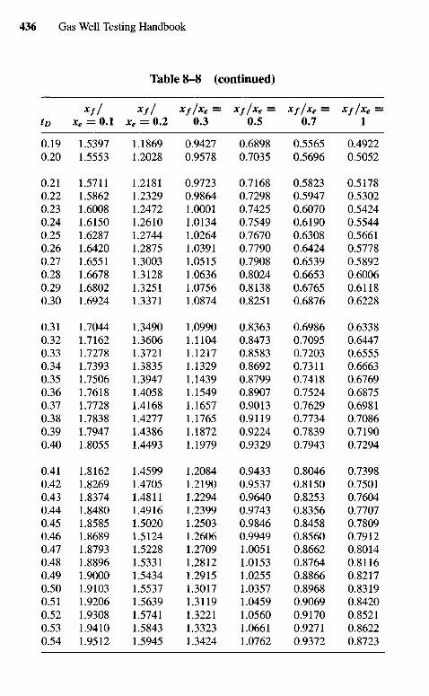
Table 8-8 (continued)
xf/ Xf/ Xf/Xe = XfJX9 = XfIx9 = XfIx9 =tD xe = 0.1 xe = 0.2 0.3 0.5 0.7 1
0.19 1.5397 1.1869 0.9427 0.6898 0.5565 0.49220.20 1.5553 1.2028 0.9578 0.7035 0.5696 0.5052
0.21 1.5711 1.2181 0.9723 0.7168 0.5823 0.51780.22 1.5862 1.2329 0.9864 0.7298 0.5947 0.53020.23 1.6008 1.2472 1.0001 0.7425 0.6070 0.54240.24 1.6150 1.2610 1.0134 0.7549 0.6190 0.55440.25 1.6287 1.2744 1.0264 0.7670 0.6308 0.56610.26 1.6420 1.2875 1.0391 0.7790 0.6424 0.57780.27 1.6551 1.3003 1.0515 0.7908 0.6539 0.58920.28 1.6678 1.3128 1.0636 0.8024 0.6653 0.60060.29 1.6802 1.3251 1.0756 0.8138 0.6765 0.61180.30 1.6924 1.3371 1.0874 0.8251 0.6876 0.6228
0.31 1.7044 1.3490 1.0990 0.8363 0.6986 0.63380.32 1.7162 1.3606 1.1104 0.8473 0.7095 0.64470.33 1.7278 1.3721 1.1217 0.8583 0.7203 0.65550.34 1.7393 1.3835 1.1329 0.8692 0.7311 0.66630.35 1.7506 1.3947 1.1439 0.8799 0.7418 0.67690.36 1.7618 1.4058 1.1549 0.8907 0.7524 0.68750.37 1.7728 1.4168 1.1657 0.9013 0.7629 0.69810.38 1.7838 1.4277 1.1765 0.9119 0.7734 0.70860.39 1.7947 1.4386 1.1872 0.9224 0.7839 0.71900.40 1.8055 1.4493 1.1979 0.9329 0.7943 0.7294
0.41 1.8162 1.4599 1.2084 0.9433 0.8046 0.73980.42 1.8269 1.4705 1.2190 0.9537 0.8150 0.75010.43 1.8374 1.4811 1.2294 0.9640 0.8253 0.76040.44 1.8480 1.4916 1.2399 0.9743 0.8356 0.77070.45 1.8585 1.5020 1.2503 0.9846 0.8458 0.78090.46 1.8689 1.5124 1.2606 0.9949 0.8560 0.79120.47 1.8793 1.5228 1.2709 1.0051 0.8662 0.80140.48 1.8896 1.5331 1.2812 1.0153 0.8764 0.81160.49 1.9000 1.5434 1.2915 1.0255 0.8866 0.82170.50 1.9103 1.5537 1.3017 1.0357 0.8968 0.83190.51 1.9206 1.5639 1.3119 1.0459 0.9069 0.84200.52 1.9308 1.5741 1.3221 1.0560 0.9170 0.85210.53 1.9410 1.5843 1.3323 1.0661 0.9271 0.86220.54 1.9512 1.5945 1.3424 1.0762 0.9372 0.8723
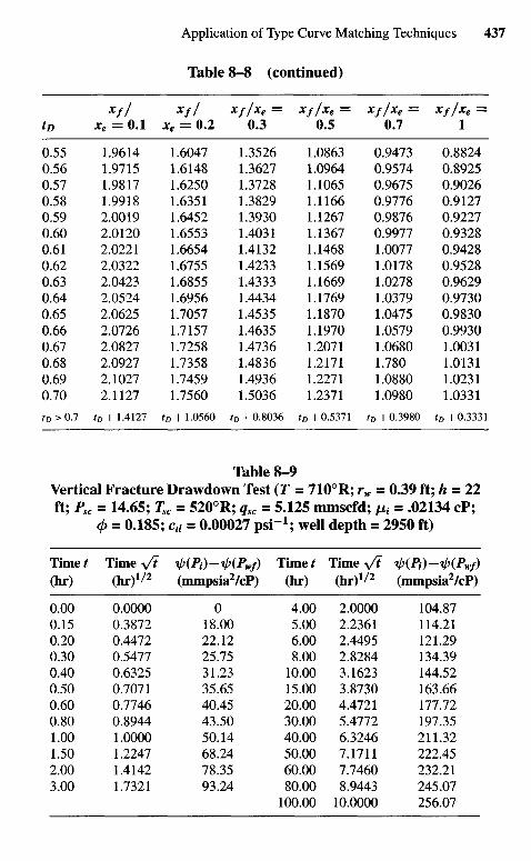
Table 8-8 (continued)
xf/ Xf/ Xf/Xe = XfJX9 = XfIX9 = XfIX9 =tD xe = 0.1 xe = 0.2 0.3 0.5 0.7 1
0.55 1.9614 1.6047 1.3526 1.0863 0.9473 0.88240.56 1.9715 1.6148 1.3627 1.0964 0.9574 0.89250.57 1.9817 1.6250 1.3728 1.1065 0.9675 0.90260.58 1.9918 1.6351 1.3829 1.1166 0.9776 0.91270.59 2.0019 1.6452 1.3930 1.1267 0.9876 0.92270.60 2.0120 1.6553 1.4031 1.1367 0.9977 0.93280.61 2.0221 1.6654 1.4132 1.1468 1.0077 0.94280.62 2.0322 1.6755 1.4233 1.1569 1.0178 0.95280.63 2.0423 1.6855 1.4333 1.1669 1.0278 0.96290.64 2.0524 1.6956 1.4434 1.1769 1.0379 0.97300.65 2.0625 1.7057 1.4535 1.1870 1.0475 0.98300.66 2.0726 1.7157 1.4635 1.1970 1.0579 0.99300.67 2.0827 1.7258 1.4736 1.2071 1.0680 1.00310.68 2.0927 1.7358 1.4836 1.2171 1.780 1.01310.69 2.1027 1.7459 1.4936 1.2271 1.0880 1.02310.70 2.1127 1.7560 1.5036 1.2371 1.0980 1.0331
tD>0.1 tD +1.4127 tD +1.0560 tD +0.8036 tD +0.5371 tD +0.3980 tD +0.3331
Table 8-9Vertical Fracture Drawdown Test (T = 7100R; rw = 0.39 ft; h = 22ft; Psc = 14.65; Tsc = 5200R; qsc = 5.125 mmscfd; /X1 = .02134 cP;
<f> = 0.185; Ca = 0.00027 psi"1; well depth = 2950 ft)
Time/ Time V? ip(Pi)-ip(Pwf) Time/ Time V? tl>(Pi)-ip(Pwf)(hr) (hr)V2 (mmpsia2/cP) (hr) (hr)1/* (mmpsia2/cP)
0.00 0.0000 0 4.00 2.0000 104.870.15 0.3872 18.00 5.00 2.2361 114.210.20 0.4472 22.12 6.00 2.4495 121.290.30 0.5477 25.75 8.00 2.8284 134.390.40 0.6325 31.23 10.00 3.1623 144.520.50 0.7071 35.65 15.00 3.8730 163.660.60 0.7746 40.45 20.00 4.4721 177.720.80 0.8944 43.50 30.00 5.4772 197.351.00 1.0000 50.14 40.00 6.3246 211.321.50 1.2247 68.24 50.00 7.1711 222.452.00 1.4142 78.35 60.00 7.7460 232.213.00 1.7321 93.24 80.00 8.9443 245.07
100.00 10.0000 256.07
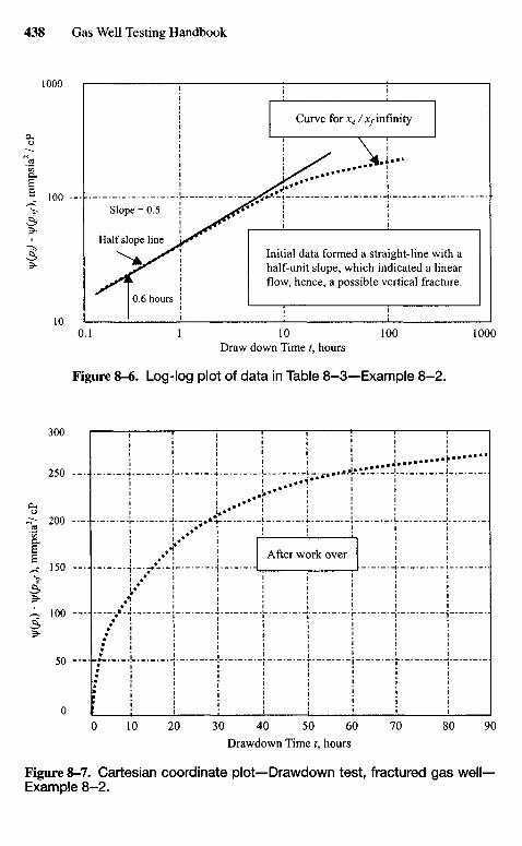
Drawdown Time /, hours
Figure 8-7. Cartesian coordinate plot—Drawdown test, fractured gas we l l -Example 8-2.
After work over
Draw down Time t, hours
Figure 8-6. Log-log plot of data in Table 8-3—Example 8-2.
Initial data formed a straight-line with ahalf-unit slope, which indicated a linearflow, hence, a possible vertical fracture.
Curve for xe / Xf infinity
0.6 hours
Half slope line
Slope = 0.5
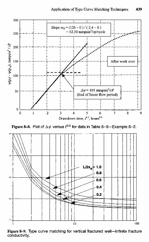
Drawdown time, t°\ hours0 5
Figure 8-8. Plot of A^ versus t05 for data in Table 8-9—Example 8-2.
Figure 8-9. Type curve matching for vertical fractured well—Infinite fractureconductivity.
Ay/= 105 mmpsiaVcP(End of linear flow period)
After work over
Slope mif= (126 - 0 ) / ( 2.4 - 0 )= 52.50 mmpsia2/cp/cycle
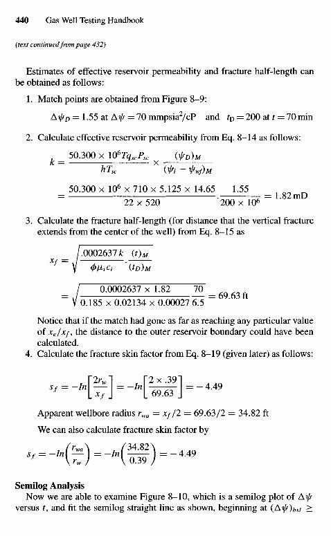
(text continued from page 432)
Estimates of effective reservoir permeability and fracture half-length canbe obtained as follows:
1. Match points are obtained from Figure 8-9:
A fD = 1.55 at A if/ = 70 mmpsia2/cP and tD = 200 at t = 70 min
2. Calculate effective reservoir permeability from Eq. 8-14 as follows:
_ 50.300 x \06TqscPsc {^D)M
k — xhTsc (xf/t - i/wf)M
_ 50.300 x 106 x 710 x 5.125 x 14.65 1.55
~ 22 x 520 '20Ox 106 ~ ' m
3. Calculate the fracture half-length (for distance that the vertical fractureextends from the center of the well) from Eq. 8-15 as
/.0002637k ( 0 MXf = / .
Y <l>tiiCi ' ( t D ) M
= I 0-0002637 x 1 . 8 2 ^ W =
V 0.185 x 0.02134 x 0.00027 6.5
Notice that if the match had gone as far as reaching any particular valueof xe/xf, the distance to the outer reservoir boundary could have beencalculated.
4. Calculate the fracture skin factor from Eq. 8-19 (given later) as follows:
[2rwl [2 x.391
Apparent wellbore radius rwa = xf/2 = 69.63/2 = 34.82 ft
We can also calculate fracture skin factor by
Semilog AnalysisNow we are able to examine Figure 8-10, which is a semilog plot of A\[r
versus t, and fit the semilog straight line as shown, beginning at (A^)^/ >
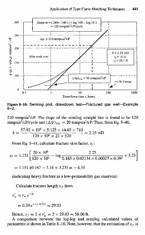
Drawdown time t, hours
Figure 8-10. Semilog plot, drawdown test—Fractured gas well—Example8-2.
210 mmpsia2/cR The slope of the semilog straight line is found to be 120mmpsia2/cP/cycle and (AV0i/ir = 20 mmpsia2/cP. Thus, from Eq. 5^4-0,
57.92 x 106 x 5.125 x 14.65 x 710* = 120 x 10 x 22 x 520 = 2.25 mD
From Eq. 5^4-1, calculate fracture skin factor, s/:
_ r 2Ox IQ6 2^5 "ISf ~ ' [ 120 x 106 ° g 0.185 x 0.02134 x 0.00027 x 0.392 + ' J
= 1.151 [0.167-7.14 + 3.23] = -4.31
(indicating heavy fracture in a low-permeability gas reservoir)
Calculate fracture length x/ from
r' _ r p~sfrw — rw e
= 039e-(-43l) =29.03
Hence, xf = 2 x r'w = 2 x 29.03 = 58.06 ft.A comparison between the log-log and semilog calculated values of
parameters is shown in Table 8-10. Note, however, that the estimation of x/ is
t = 38.5 hours{Ay/)\ hr = 30 mmpsia2/cP
After work over
Ay/ >210mmps ia 2 / cP
Slope m = ( 260-- 140 ) / ( l o g 100 - log 10 )= 120 mmpsia2/cP/cycle
V (
Pi)
" V(
p*yj)
> m
mp
sia2 /
cP
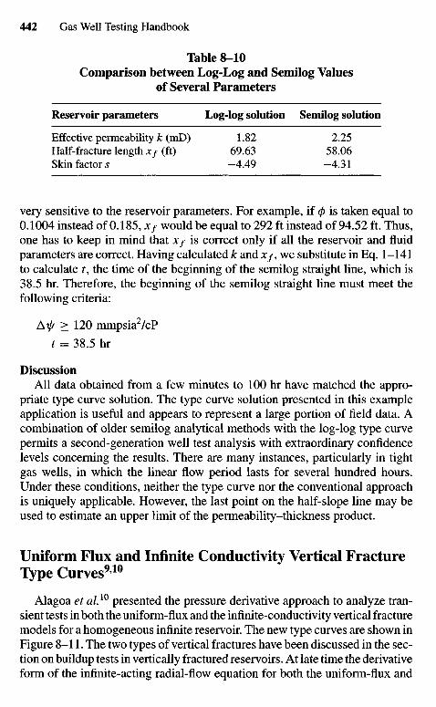
Table 8-10Comparison between Log-Log and Semilog Values
of Several Parameters
Reservoir parameters Log-log solution Semilog solution
Effective permeability k (mD) 1.82 2.25Half-fracture length xf (ft) 69.63 58.06Skin factor s -4.49 -4.31
very sensitive to the reservoir parameters. For example, if (/> is taken equal to0.1004 instead of 0.185, xf would be equal to 292 ft instead of 94.52 ft. Thus,one has to keep in mind that x/ is correct only if all the reservoir and fluidparameters are correct. Having calculated k and Jt/, we substitute in Eq. 1-141to calculate t, the time of the beginning of the semilog straight line, which is38.5 hr. Therefore, the beginning of the semilog straight line must meet thefollowing criteria:
A ^ > 120 mmpsia2/cP
t = 38.5 hr
DiscussionAll data obtained from a few minutes to 100 hr have matched the appro-
priate type curve solution. The type curve solution presented in this exampleapplication is useful and appears to represent a large portion of field data. Acombination of older semilog analytical methods with the log-log type curvepermits a second-generation well test analysis with extraordinary confidencelevels concerning the results. There are many instances, particularly in tightgas wells, in which the linear flow period lasts for several hundred hours.Under these conditions, neither the type curve nor the conventional approachis uniquely applicable. However, the last point on the half-slope line may beused to estimate an upper limit of the permeability-thickness product.
Uniform Flux and Infinite Conductivity Vertical FractureType Curves910
Alagoa et al,10 presented the pressure derivative approach to analyze tran-sient tests in both the uniform-flux and the infinite-conductivity vertical fracturemodels for a homogeneous infinite reservoir. The new type curves are shown inFigure 8-11. The two types of vertical fractures have been discussed in the sec-tion on buildup tests in vertically fractured reservoirs. At late time the derivativeform of the infinite-acting radial-flow equation for both the uniform-flux and
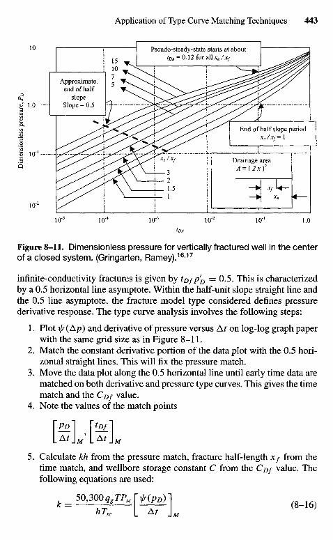
Figure 8-11. Dimensionless pressure for vertically fractured well in the centerof a closed system. (Gringarten, Ramey).16'17
infinite-conductivity fractures is given by tDfPfD = 0.5. This is characterized
by a 0.5 horizontal line asymptote. Within the half-unit slope straight line andthe 0.5 line asymptote, the fracture model type considered defines pressurederivative response. The type curve analysis involves the following steps:
1. Plot xlf(Ap) and derivative of pressure versus At on log-log graph paperwith the same grid size as in Figure 8-11.
2. Match the constant derivative portion of the data plot with the 0.5 hori-zontal straight lines. This will fix the pressure match.
3. Move the data plot along the 0.5 horizontal line until early time data arematched on both derivative and pressure type curves. This gives the timematch and the C Df value.
4. Note the values of the match points
5. Calculate kh from the pressure match, fracture half-length x/ from thetime match, and wellbore storage constant C from the CDf value. Thefollowing equations are used:
k = 50,300qgTPsc h H ^ IhTsc L Af ]M
Drainage area
End of half slope periodXe/Xf~ 1
Pseudo-steady-state starts at abouttDA = 0.12 for all xe /xf
Approximate,end of half
slopeSlope = 0.5
Dim
ensi
onle
ss p
ress
ure,
PD
xf= /o.OOO2637——to] (8-17)
c = k»f (8-I8)No wellbore storage, infinite conductivity fracture (after Gringarten,Ramey, and Raghavan):9'10
s=In(— J (8-19)
Comparing Figures 8-3 and 8-11 shows a striking difference in theslopes at early dimensionless times. The curves for a well with skin andstorage effect (Figure 8-3) start with a unit slope, while the curves forthe vertical fracture (Figure 8-11) start with a slope of one-half. Theone-half slope is caused by linear flow at very short times. A dashed linein Figure 8-11 indicates the end of the half-slope period.
8.7 Summary
Based on the material presented in this chapter, the following remarks arepertinent:
• A new technique is presented to analyze data in the bilinear flow period.It is shown that, during this flow period, a graph of if(pwf) versus /1 / 4
yields a straight line when slope is inversely proportional to hf(k/bf)1^2.• New type curves are now available for pressure analysis of fractured gas
wells, and the problem in the analysis is reduced considerably with theuse of these type curves.
• Prefracture information about the reservoir is necessary to estimate frac-ture parameters.
• The type curve analysis method must be used simultaneously with thespecific analysis methods i//(pwf) versus f1/4, i//(pWf) versus £1/2, andif (Pwf) versus log t to produce reliable results.
References and Additional Reading
1. Ramey, H. J., Jr., "Application of the Line Source Solution to Flow inPorous Media—A Review," Prod. Monthly (May 1967) 4-7, 25-27.
2. Ramey, H. J., Jr., "Short-Time Well Test Data Interpretation in the Presenceof Skin Effect and Wellbore Storage," /. Petroleum Technol. (1970) 22,97-104.
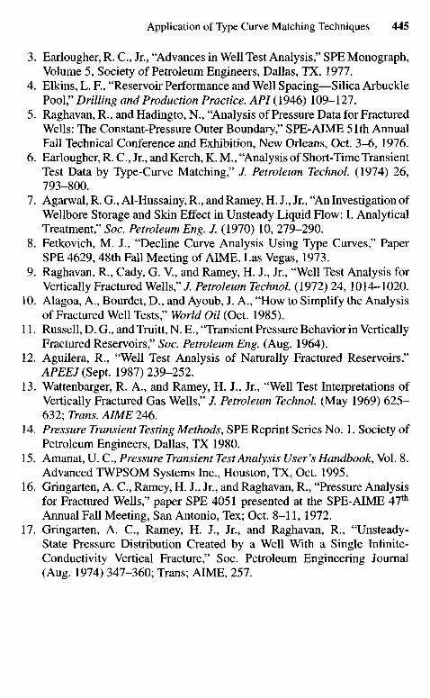
3. Earlougher, R. C, Jr., "Advances in Well Test Analysis," SPE Monograph,Volume 5, Society of Petroleum Engineers, Dallas, TX, 1977.
4. Elkins, L. R, "Reservoir Performance and Well Spacing—Silica ArbucklePool," Drilling and Production Practice, API (1946) 109-127.
5. Raghavan, R., and Hadingto, N., "Analysis of Pressure Data for FracturedWells: The Constant-Pressure Outer Boundary," SPE-AIME 51th AnnualFall Technical Conference and Exhibition, New Orleans, Oct. 3-6, 1976.
6. Earlougher, R. C, Jr., and Kerch, K. M., "Analysis of Short-Time TransientTest Data by Type-Curve Matching," /. Petroleum Technol. (1974) 26,793-800.
7. Agarwal, R. G., Al-Hussainy, R., and Ramey, H. J., Jr., "An Investigation ofWellbore Storage and Skin Effect in Unsteady Liquid Flow: I. AnalyticalTreatment," Soc. Petroleum Eng. J. (1970) 10, 279-290.
8. Fetkovich, M. J., "Decline Curve Analysis Using Type Curves," PaperSPE 4629, 48th Fall Meeting of AIME, Las Vegas, 1973.
9. Raghavan, R., Cady, G. V., and Ramey, H. J., Jr., "Well Test Analysis forVertically Fractured Wells," / Petroleum Technol (1972) 24, 1014-1020.
10. Alagoa, A., Bourdet, D., and Ayoub, J. A., "How to Simplify the Analysisof Fractured Well Tests," World Oil (Oct. 1985).
11. Russell, D. G., and Truitt, N. E., "Transient Pressure Behavior in VerticallyFractured Reservoirs," Soc. Petroleum Eng. (Aug. 1964).
12. Aguilera, R., "Well Test Analysis of Naturally Fractured Reservoirs,"APEE/(Sept. 1987) 239-252.
13. WTattenbarger, R. A., and Ramey, H. J., Jr., "Well Test Interpretations ofVertically Fractured Gas Wells," /. Petroleum Technol. (May 1969) 625-632; Trans. AIME 246.
14. Pressure Transient Testing Methods, SPE Reprint Series No. 1. Society ofPetroleum Engineers, Dallas, TX 1980.
15. Amanat, U. C, Pressure Transient Test Analysis User's Handbook, Vol. 8.Advanced TWPSOM Systems Inc., Houston, TX, Oct. 1995.
16. Gringarten, A. C, Ramey, H. J., Jr., and Raghavan, R., "Pressure Analysisfor Fractured Wells," paper SPE 4051 presented at the SPE-AIME 47th
Annual Fall Meeting, San Antonio, Tex; Oct. 8-11, 1972.17. Gringarten, A. C, Ramey, H. J., Jr., and Raghavan, R., "Unsteady-
State Pressure Distribution Created by a Well With a Single Infinite-Conductivity Vertical Fracture," Soc. Petroleum Engineering Journal(Aug. 1974) 347-360; Trans; AIME, 257.
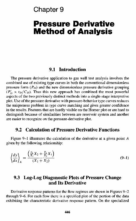
Chapter 9
Pressure DerivativeMethod of Analysis
9.1 Introduction
The pressure derivative application to gas well test analysis involves thecombined use of existing type curves in both the conventional dimensionlesspressure form (PD) and the new dimensionless pressure derivative grouping(PD x ^D/CD)- Thus this new approach has combined the most powerfulaspects of the two previously distinct methods into a single-stage interpretiveplot. Use of the pressure derivative with pressure-behavior type curves reducesthe uniqueness problem in type curve matching and gives greater confidencein the results. Features that are hardly visible on the Horner plot or are hard todistinguish because of similarities between are reservoir system and anotherare easier to recognize on the pressure-derivative plot.
9.2 Calculation of Pressure Derivative Functions
Figure 9-1 illustrates the calculation of the derivative at a given point Agiven by the following relationship:
IfM _ №* + £*•)\dxjA (X1 + X2)
9.3 Log-Log Diagonostic Plots of Pressure Changeand Its Derivative
Derivative response patterns for the flow regimes are shown in Figures 9-2through 9-6. For each flow there is a specified plot of the portion of the dataexhibiting the characteristic derivative response pattern. On the specialized
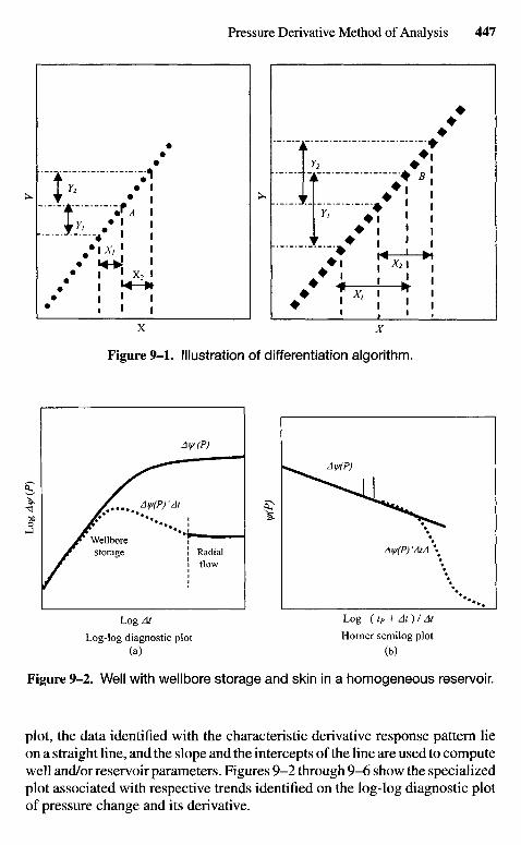
Log At Log (tP + At) / At
Log-log diagnostic plot Horner semilog plot(a) (b)
Figure 9-2. Well with wellbore storage and skin In a homogeneous reservoir.
plot, the data identified with the characteristic derivative response pattern lieon a straight line, and the slope and the intercepts of the line are used to computewell and/or reservoir parameters. Figures 9-2 through 9-6 show the specializedplot associated with respective trends identified on the log-log diagnostic plotof pressure change and its derivative.
Radialflow
Wellborestorage
Figure 9-1. Illustration of differentiation algorithm.
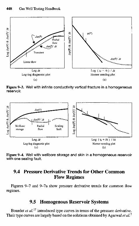
Log At Log (tp + At) /AtLog-log diagnostic plot Homer semilog plot
(a) (b)
Figure 9-4. Well with wellbore storage and skin in a homogeneous reservoirwith one sealing fault.
9.4 Pressure Derivative Trends for Other CommonFlow Regimes
Figures 9-7 and 9-7 a show pressure derivative trends for common flowregimes.
9.5 Homogenous Reservoir Systems
Bourdet et al.xl introduced type curves in terms of the pressure derivative.Their type curves are largely based on the solutions obtained by Agarwal et al?
Wellborestorage
Radialflow
Sealingfault
Log At Log (tp + At) I At
Log-log diagnostic plot Horner semilog plot
(a) (b)
Figure 9-3. Well with infinite conductivity vertical fracture in a homogeneousreservoir.
Linear flow
Transient
Radialflow
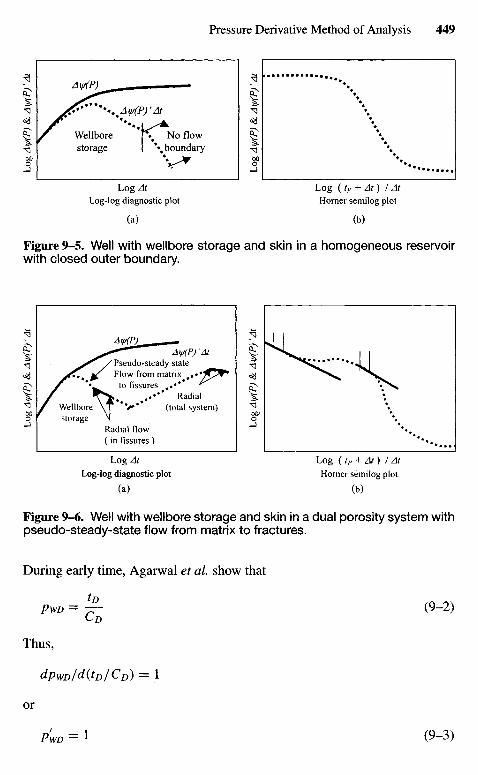
Log At Log ( tP + At) I At
Log-log diagnostic plot Horner semilog plot
(a) (b)
Figure 9-6. Well with wellbore storage and skin in a dual porosity system withpseudo-steady-state flow from matrix to fractures.
During early time, Agarwal et al. show that
PWD = ^- (9-2)
Thus,
dpWD/d(tD/CD) = 1
or
PWD = 1 (9-3)
Radial flow(in fissures)
Wellborestorage
Radial(total system)
Pseudo-steady stateFlow from matrix
to fissures
Log At Log ( tP + At) I AtLog-log diagnostic plot Horner semilog plot
(a) (b)
Figure 9-5. Well with wellbore storage and skin in a homogeneous reservoirwith closed outer boundary.
Wellborestorage
No flowboundary
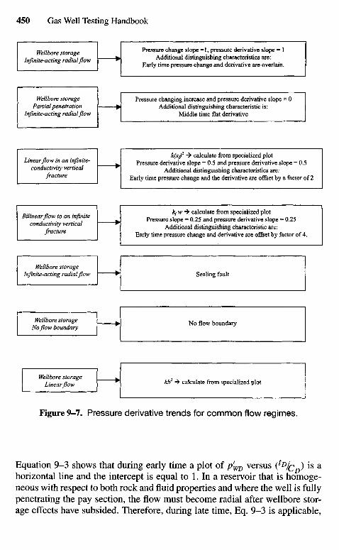
Wellbore storageInfinite-acting radial flow
Wellbore storagePartial penetration
Infinite-acting radial flow
Linear flow in an infinite-conductivity vertical
fracture
Bilinear flow to an infiniteconductivity vertical
fracture
Wellbore storageInfinite-acting radial flow
Wellbore storageNo flow boundary
Wellbore storageLinear flow
Pressure change slope =1, pressure derivative slope = 1Additional distinguishing characteristics are:
Early time pressure change and derivative are overlain.
Pressure changing increase and pressure derivative slope = 0Additional distinguishing characteristic is:
Middle time flat derivative
k(x/ -> calculate from specialized plotPressure derivative slope = 0.5 and pressure derivative slope = 0.5
Additional distinguishing characteristics are:Early time pressure change and the derivative are offset by a factor of 2
kfW -> calculate from specialized plotPressure slope = 0.25 and pressure derivative slope = 0.25
Additional distinguishing characteristic are:Early time pressure change and derivative are offset by factor of 4.
Sealing fault
No flow boundary
kb2 -> calculate from specialized plot
Figure 9-7. Pressure derivative trends for common flow regimes.
Equation 9-3 shows that during early time a plot of p'WD versus ^DIQ ) is ahorizontal line and the intercept is equal to 1. In a reservoir that is homoge-neous with respect to both rock and fluid properties and where the well is fullypenetrating the pay section, the flow must become radial after wellbore stor-age effects have subsided. Therefore, during late time, Eq. 9-3 is applicable,
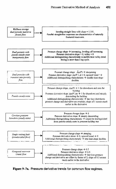
Wellbore storagedual porosity matrix to
fissureflow
Dual porosity withpseodo-steady-state
in terporosity flow
Dual porosity withtransient interporosity
flow
Pseudo-steady-state
Constant pressureboundary (steady-state)
Single sealing fault(pseudoradial flow)
Elongated reservoirLinear flow
Semi log straight lines with slope = 1.151.Parallel straight-line responses are characteristics of naturally
fractured reservoirs.
Pressure change slope -> increasing, leveling off increasingPressure derivative slope = 0, valley = 0
Additional distinguishing characteristic is middle time valley trendduring is more than I log cycle.
Pressure change slope A [//(P) -> steepeningPressure derivative slope A y/(P') At = 0, upward trend = 0
Additional distinguishing characteristic -^ middle time slopedoubles
Pressure change slope, A y/(P) ~^ 1 for drawdown and zero forbuildup
Pressure derivative slope Ay/(P')At -^ 1 for drawdown and steeplydescending for buildup
Additional distinguishing characteristic -> late time drawdownpressure change and derivative are overlain; slope of 1 occurs much
earlier in the derivative.
Pressure change slope -> 0Pressure derivative slope -^ steeply descending
Additional distinguishing characteristic -> cannot be distinguishedfrom pseudo-steady-state in pressure buildup test.
Pressure change slope -> steepingPressure derivative slope -> 0, upward trend -> 0
Additional distinguishing characteristic -> late-time slope doubles
Pressure change slope -> 0.5Pressure derivative slope -> 0.5
Additional distinguishing characteristic -^ late time pressurechange and derivative are offset by factor of 2; slope of 0.5 occurs
much earlier in the derivative
Figure 9-7a. Pressure derivative trends for common flow regimes.
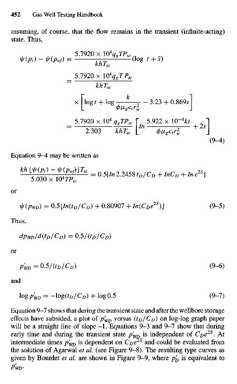
assuming, of course, that the flow remains in the transient (infinite-acting)state. Thus,
5.7920 x ltfqg1?x ,Ir(Pi) ~ VK/V) = Hg "(log t + S)
KnI sc
_ 5.7920 x MfqgTPsc= khl\c
x Hog t + log =- - 3.23 + 0.86951L <t>VgCtrl J
_ 5.7920 x 10⁴ qJPsc I" 5.922 x 10"4^f 1
2 3 0 3 khTsc \_H 4>V>gctrl + J
(9^)
Equation 9-4 may be written as
kh lt£:£%!T' - °-5"" 2-M58 '° / c°+'-c-+*•">or
^T(PTO) - 0.5LMWCz)) + 0.80907 + /rc(CDe25)J (9-5)
Thus,
dpWD/d(tD/CD) = 0 . 5 / ( W C D )
or
p'm = 0.5/(tD/CD) (9-6)
and
log p'm = -log(tD/CD) + log 0.5 (9-7)
Equation 9-7 shows that during the transient state and after the wellbore storageeffects have subsided, a plot of p'WD versus (W CD) on log-log graph paperwill be a straight line of slope - 1 . Equations 9-3 and 9-7 show that duringearly time and during the transient state pf
WD is independent of Coe2S. Atintermediate times p'WD is dependent on Coe2S and could be evaluated fromthe solution of Agarwal et al. (see Figure 9-8). The resulting type curves asgiven by Bourdet et al. are shown in Figure 9-9, where p'D is equivalent to
PWD-
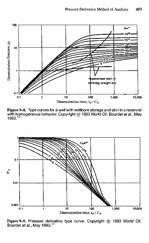
Dimensionless time, tD / CD
Figure 9-9. Pressure derivative type curve. Copyright © 1983 World Oil.Bourdetefa/.,May1983.17
Dimensionless time, tD / CD
Figure 9-8. Type curves for a well with wellbore storage and skin in a reservoirwith homogeneous behavior. Copyright © 1983 World Oil. Bourdet etal., May1983.17
A proximate start < f
s tmi-fog straight Hr e
Dim
ensi
onle
ss P
ress
ure,
pD
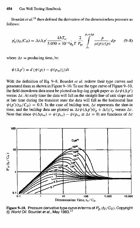
Bourdet et al18 then defined the derivative of the dimensionless pressure asfollows:
Po+Ap
pfD(tD/CD) = AtAp' *kT" 4 _ - | - I , f ( dp (9-8)
5.030 x lO~4qgT Ppc J /x(p)z(p)Po
where At = producing time, hr:
x/f(Ap') = d Hf(Pi) - ^(pwf)\/dt
With the definition of Eq. 9-8, Bourdet et al. redrew their type curves andpresented them as shown in Figure 9-10. To use the type curve of Figure 9-10,the field drawdown data must be plotted on log-log graph paper as At if/ (Ap')versus At. At early time the data will fall on the straight line of unit slope andat late time during the transient state the data will fall as the horizontal lineif(p')(tD/Co) = 0.5. In the case of buildup test, Ar represents the shut-intime, and the buildup data are plotted as AtXJr(Ap')(tp + At)/tp versus At.Note that since xJs(Apws) = xj/(pws) — xj/(pws at At = 0) are functions of At
Dimensionless Time, tD / CD
Figure 9-10. Pressure derivative type curve in terms of P'D (to/CD)- Copyright© World Oil. Bourdet et al., May 1983.17
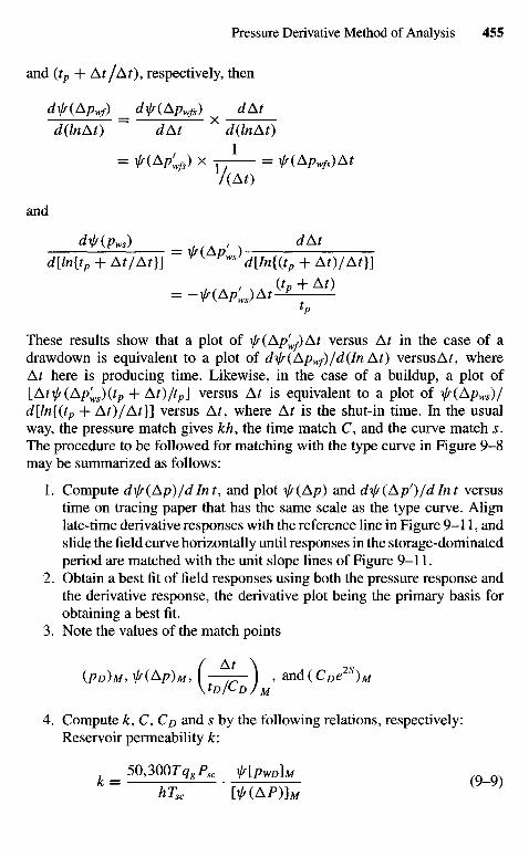
and (tp + At/At)9 respectively, then
df(Apwf) _ djs(Apwfs) dAt
d(lnAt) ~~ dAt * d(lnAt)
= f(Apwfs) x y- = f(Apwfs)At/(AO
and
djr(pws) _ , ^Ar
d[ln{tp + Af/Af}] " ^ ( Pws)d[In{(fp + Af)/Af}]
These results show that a plot of \j/(Apf
wf)At versus AMn the case of adrawdown is equivalent to a plot of dxj/(ApWf)/d(In At) versus At, whereAt here is producing time. Likewise, in the case of a buildup, a plot oflAt\lf(Apf
ws)(tp + At)/tp\ versus At is equivalent to a plot of \js(Apws)/d[ln{(tp + At)/At}] versus At, where At is the shut-in time. In the usualway, the pressure match gives kh, the time match C, and the curve match s.The procedure to be followed for matching with the type curve in Figure 9-8may be summarized as follows:
1. Compute dty(Ap)/dint, and plot \jr(Ap) and d\j/(Ap')/dInt versustime on tracing paper that has the same scale as the type curve. Alignlate-time derivative responses with the reference line in Figure 9-11, andslide the field curve horizontally until responses in the storage-dominatedperiod are matched with the unit slope lines of Figure 9-11.
2. Obtain a best fit of field responses using both the pressure response andthe derivative response, the derivative plot being the primary basis forobtaining a best fit.
3. Note the values of the match points
(pD)M, №P)M, ( - ^ - ) ' a n d ( C D e 2 S ) M
4. Compute k, C, CD and s by the following relations, respectively:Reservoir permeability k\
50,3QOTq8Px fjpwu^M
hTsc ' №(AP)]M
Figure 9-11. Combined and pressure type curves for a well with wellbore stor-age and skin in infinite-acting homogeneous reservoir (courtesy of FlopetrolJohnson Schlumberger).14
Dimensionless pressure and pressure derivative group,P D (WCD)
Dim
ensionless time group, tD/C
D
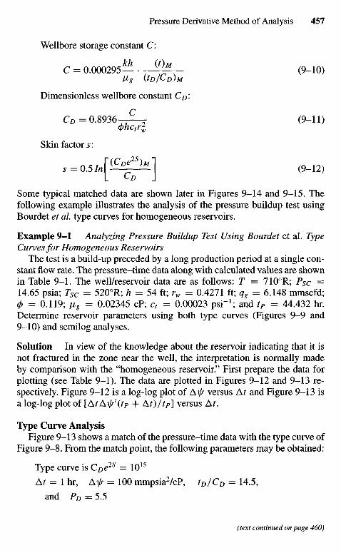
Wellbore storage constant C:
C = 0.000295— • ( / ) M (9-10)V8 (tD/CD)M
Dimensionless wellbore constant C#:
Q> = 0.8936—^-z- (9-11)(j)hctrl
Skin factor s:
s = 0.5In[iC^] (9-12)
Some typical matched data are shown later in Figures 9-14 and 9-15. Thefollowing example illustrates the analysis of the pressure buildup test usingBourdet et ah type curves for homogeneous reservoirs.
Example 9-1 Analyzing Pressure Buildup Test Using Bourdet et al. TypeCurves for Homogeneous Reservoirs
The test is a build-up preceded by a long production period at a single con-stant flow rate. The pressure-time data along with calculated values are shownin Table 9-1. The well/reservoir data are as follows: T = 7100R; Psc =14.65 psia; Tsc = 5200R; h = 54 ft; rw = 0.4271 ft; qg = 6.148 mmscfd;0 = 0.119; /ng = 0.02345 cP; ct = 0.00023 psi"1; and tP = 44.432 hr.Determine reservoir parameters using both type curves (Figures 9-9 and9-10) and semilog analyses.
Solution In view of the knowledge about the reservoir indicating that it isnot fractured in the zone near the well, the interpretation is normally madeby comparison with the "homogeneous reservoir." First prepare the data forplotting (see Table 9-1). The data are plotted in Figures 9-12 and 9-13 re-spectively. Figure 9-12 is a log-log plot of A\j/ versus At and Figure 9-13 isa log-log plot of [AtAi//f(tp + At)/tP] versus At.
Type Curve AnalysisFigure 9-13 shows a match of the pressure-time data with the type curve of
Figure 9-8. From the match point, the following parameters may be obtained:
Type curve is CDe2S = 1015
Ar = 1 hr, Ai^ = 100 mmpsia2/cP, tD/CD = 14.5,and PD = 5.5
(text continued on page 460)
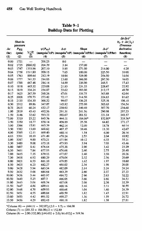
Table 9-1Buildup Data for Plotting
AfAt//Shut-in {tp + At/tp)pressure (Pressure
At Pyys i>(Pws) Ai/) Slope Ai// derivative(hr) (psia) tj^- (mmpsia2/cP) (mmpsia2/cP) (mmpsia2/cP/hr) (mmpsia2/cP/hr) function)(D (2) (3) (4) (5) (6) (7) (8)
0.00 1721 — 201.25 0.0 — — —0.02 1735 2666.92 204.39 3.14 157.00 — —0.03 1747 1333.96 207.10 5.85 271.00 214.00 4.280.04 1758 1111.80 209.15 7.65 180.00 225.50 10.000.05 1763 889.64 212.19 10.94 329.00 254.50 14.040.06 1777 741.53 214.85 13.60 266.00 297.50 16.050.07 1788 667.48 216.14 14.89 226.00 248.5 17.430.10 1818 445.32 223.08 21.83 231.33 228.67 22.920.13 1819 334.24 234.87 33.62 393.00 312.17 40.700.17 1625 267.59 248.26 47.01 334.75 363.88 62.040.25 2028 178.73 273.42 72.17 314.50 324.63 81.620.33 2135 134.30 300.32 99.07 336.25 325.38 108.180.50 2312 89.86 347.07 145.82 275.00 305.63 154.540.75 2615 60.24 432.17 230.92 340.40 307.70 234.681.00 2819 45.43 492.56 291.31 241.56 290.98 297.531.50 3146 32.62 593.33 392.07 201.52 221.54 343.57
*2.00 3310 23.22 645.36 444.11 104.08* 152.80* 319.36*2.50 3350 18.77 658.14 456.89 25.56 64.82 171.173.00 3366 15.81 663.39 462.14 12.00 18.78 60.143.50 3382 13.69 668.62 467.37 10.46 11.30 42.674.00 3385 12.11 669.40 468.14 1.54 6.00 26.164.83 3391 10.19 671.49 470.24 2.53 2.04 10.925.00 3397 9.89 673.21 471.96 10.12 6.33 35.215.50 3403 9.08 675.18 473.93 3.94 7.03 43.466.00 3407 8.41 676.64 475.38 2.90 3.42 23.296.50 3411 7.84 677.93 476.68 2.60 2.75 20.407.00 3415 7.35 679.13 477.87 2.40 2.50 20.267.50 3418 6.92 680.29 479.04 2.32 2.36 20.698.00 3421 6.55 681.10 479.85 1.62 1.97 18.608.50 3425 6.23 682.27 481.02 2.34 1.98 20.059.00 3428 5.94 683.34 482.09 2.14 2.24 24.249.50 3432 5.68 684.64 483.39 2.60 2.37 27.3310.00 3436 5.44 685.97 484.72 2.66 2.63 32.2210.50 3440 5.23 687.3 486.05 2.66 2.66 34.5311.00 3443 5.04 688.34 487.08 2.06 2.36 32.3911.50 3447 4.86 689.41 488.16 2.16 2.11 30.5512.00 3448 4.70 689.93 488.68 1.04 1.60 24.3912.50 3451 4.55 690.84 489.59 1.82 1.43 22.9113.00 3453 4.42 691.52 490.27 1.36 1.59 26.7213.50 3456 4.29 692.43 491.18 1.82 1.58 27.81
*Column (6) -> (444.11 - 392.07)/(2.0 - 1.5) = 104.08Column (7) -» (201.52 + 104.08)/2 = 152.80Column (8) -* 2.00 (152.80) [(44.432 + 2.0)/44.432)] = 319.36
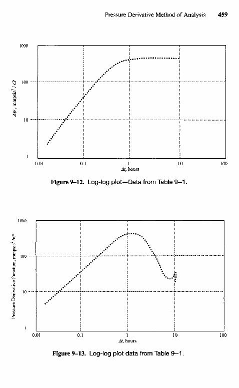
Figure 9-12. Log-log plot—Data from Table 9 -1 .
Figure 9-13. Log-log plot data from Table 9 -1 .
At, hours
At, hours
Pre
ssur
e D
eriv
ativ
e F
unct
ion,
mm
psia
2 /cP
Ay/
, m
mps
ia2 /
cP
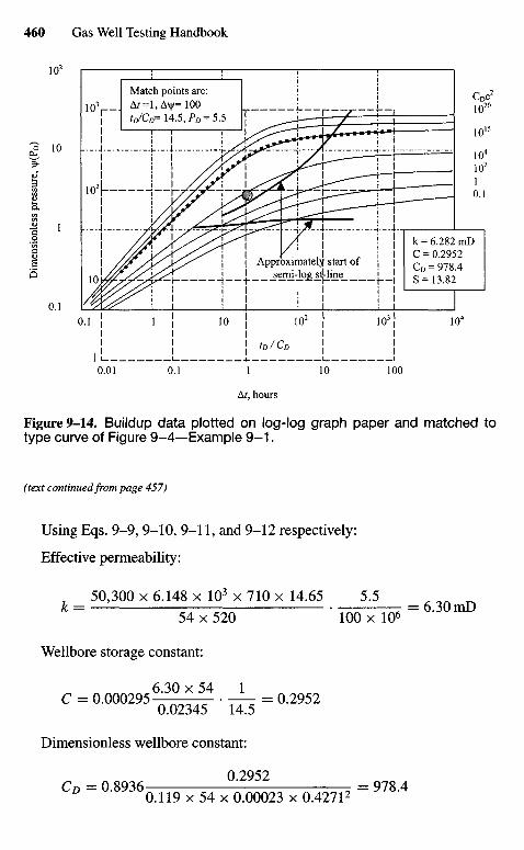
At, hours
Figure 9-14. Buildup data plotted on log-log graph paper and matched totype curve of Figure 9-4—Example 9 -1 .
(text continued from page 457)
Using Eqs. 9-9, 9-10, 9-11, and 9-12 respectively:
Effective permeability:
50,300 x 6.148 x 103 x 710 x 14.65 5.5" = 54^520 T00TW = 6 - 3 0 m D
Wellbore storage constant:
Dimensionless wellbore constant:
CD = ° - 8 9 3 60 U 9 x 5 4 x 0.00023 x 0.42712 = 9 7 8 ' 4
Approximately start ofsemi-log stUine
Match points are:
Dim
ensi
onle
ss p
ress
ure,
VJ/(
PD)
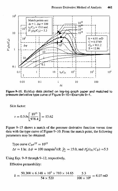
Figure 9-15. Buildup data plotted on log-log graph paper and matched topressure derivative type curve of Figure 9-10—Example 9 -1 .
Skin factor:
Figure 9-15 shows a match of the pressure derivative function versus timedata with the type curve of Figure 9-10. From the match point, the followingparameters may be obtained:
Type curve CDe2S = 1015
At = 1 hr, A^ = 100 mmpsia2/cP, ^- = 15.0, and P^(tD/CD) =5.3
Using Eqs. 9-9 through 9-12, respectively,
Effective permeability:
50,300 x 6.148 x 103 x 710 x 14.65 5.3k = 547520 TooTTo^ 6 'O 7 m D
Match points are:
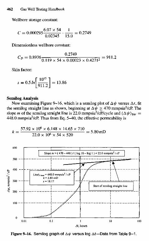
Wellbore storage constant:
c = a o 0 O 2 9 5 1 ^ 5 f IIo=0-2749
Dimensionless wellbore constant:
0.2749CD = a 8 9 3 6 0.119x54x0.00023x0.427P = 9U2
Skin factor:
Semilog AnalysisNow examining Figure 9-16, which is a semilog plot of A^ versus Ar, fit
the semilog straight line as shown, beginning at Ax/r > 470 mmpsia2/cP. Theslope m of the semilog straight line is 22.0 mmpsia2/cP/cycle and {A\j/)ihr =448.0 mmpsia2/cP. Thus from Eq. 5-40, the effective permeability is
57.92 x 106 x 6.148 x 14.65 x 710* = 22.0 x 10» x 54 x 520 = 5MmD
Slope m
Start of semilog straight-line
At9 hours
Figure 9-16. Semilog graph of A^ versus log Af-Data from Table 9 -1 .
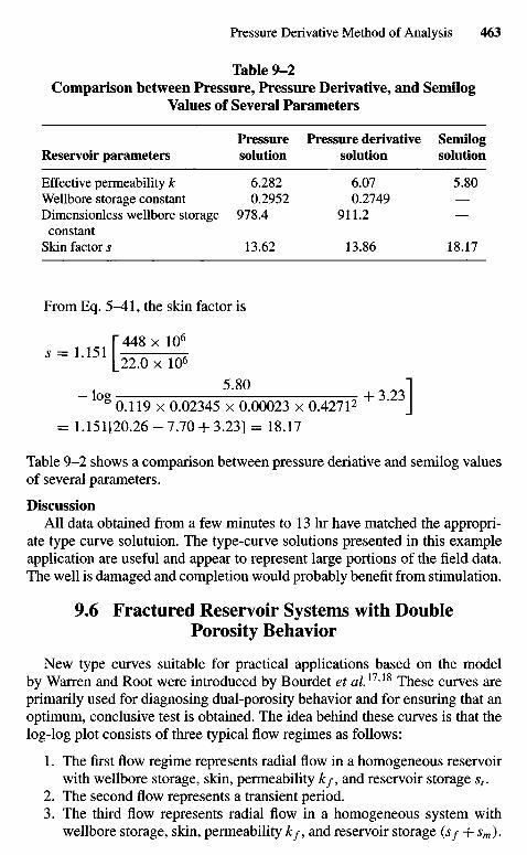
Table 9-2Comparison between Pressure, Pressure Derivative, and Semilog
Values of Several Parameters
Pressure Pressure derivative SemilogReservoir parameters solution solution solution
Effective permeability k 6.282 6.07 5.80Wellbore storage constant 0.2952 0.2749 —Dimensionless wellbore storage 978.4 911.2 —constant
Skin factor s 13.62 13.86 18.17
From Eq. 5-41, the skin factor is
1 1 g i r 4 4 8 x l O 6
5.80 ]
~ ° g 0.119 x 0.02345 x 0.00023 x 0.42712 + ' J= 1.151[20.26 - 7.70 + 3.23] = 18.17
Table 9-2 shows a comparison between pressure deriative and semilog valuesof several parameters.
DiscussionAU data obtained from a few minutes to 13 hr have matched the appropri-
ate type curve solutuion. The type-curve solutions presented in this exampleapplication are useful and appear to represent large portions of the field data.The well is damaged and completion would probably benefit from stimulation.
9.6 Fractured Reservoir Systems with DoublePorosity Behavior
New type curves suitable for practical applications based on the modelby Warren and Root were introduced by Bourdet et a/.1718 These curves areprimarily used for diagnosing dual-porosity behavior and for ensuring that anoptimum, conclusive test is obtained. The idea behind these curves is that thelog-log plot consists of three typical flow regimes as follows:
1. The first flow regime represents radial flow in a homogeneous reservoirwith wellbore storage, skin, permeability kf, and reservoir storage st.
2. The second flow represents a transient period.3. The third flow represents radial flow in a homogeneous system with
wellbore storage, skin, permeability kf, and reservoir storage (Sf + sm).
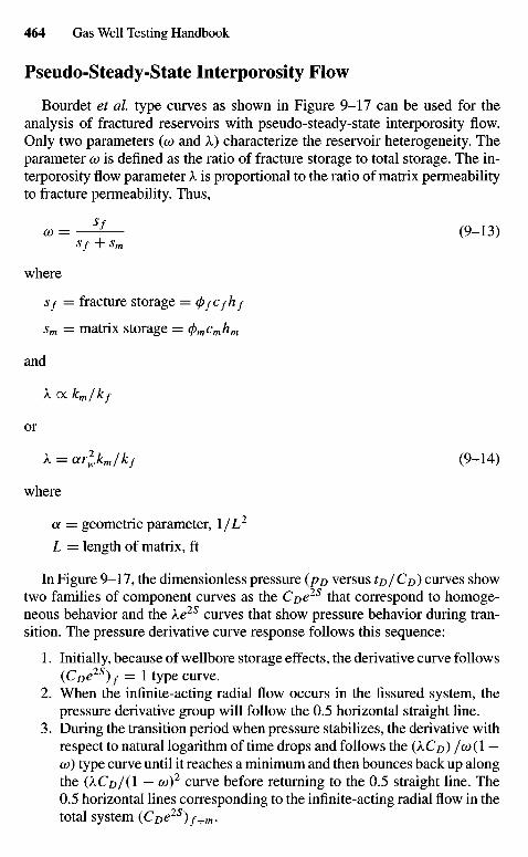
Pseudo-Steady-State Interporosity Flow
Bourdet et al. type curves as shown in Figure 9-17 can be used for theanalysis of fractured reservoirs with pseudo-steady-state interporosity flow.Only two parameters (co and X) characterize the reservoir heterogeneity. Theparameter co is defined as the ratio of fracture storage to total storage. The in-terporosity flow parameter X is proportional to the ratio of matrix permeabilityto fracture permeability. Thus,
co = Sf (9-13)Sf +Sm
where
Sf = fracture storage = cfrfCfhf
sm = matrix storage = (j)mcmhm
and
X ex km/kf
or
X = ar2wkm/kf (9-14)
where
a = geometric parameter, 1/L2
L — length of matrix, ft
In Figure 9-17, the dimensionless pressure (po versus to/Co) curves showtwo families of component curves as the Coe2S that correspond to homoge-neous behavior and the Xe2S curves that show pressure behavior during tran-sition. The pressure derivative curve response follows this sequence:
1. Initially, because of wellbore storage effects, the derivative curve follows(Coels)f — 1 type curve.
2. When the infinite-acting radial flow occurs in the fissured system, thepressure derivative group will follow the 0.5 horizontal straight line.
3. During the transition period when pressure stabilizes, the derivative withrespect to natural logarithm of time drops and follows the (XCo) /co(\ —co) type curve until it reaches a minimum and then bounces back up alongthe (XCo/(l — co)2 curve before returning to the 0.5 straight line. The0.5 horizontal lines corresponding to the infinite-acting radial flow in thetotal system (Coels)f+m.
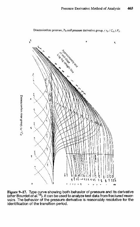
Figure 9-17. Type curve showing both behavior of pressure and its derivative(after Bourdet et a/.18). It can be used to analyze test data from fractured reser-voirs. The behavior of the pressure derivative is reasonably resolutive for theidentification of the transition period.
Dimensionless pressure, PD and pressure derivative group, (tD /' CD) P'D
Dim
ensionless time group, tD / C
D
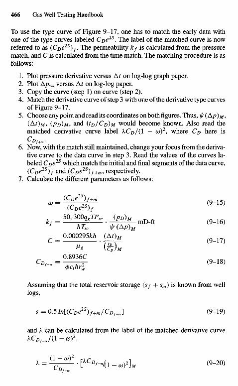
To use the type curve of Figure 9-17, one has to match the early data withone of the type curves labeled Cpe2S. The label of the matched curve is nowreferred to as (Coe2S)f- The permeability k/ is calculated from the pressurematch, and C is calculated from the time match. The matching procedure is asfollows:
1. Plot pressure derivative versus At on log-log graph paper.2. Plot Apws versus A^ on log-log paper.3. Copy the curve (step 1) on curve (step 2).4. Match the derivative curve of step 3 with one of the derivative type curves
of Figure 9-17.5. Choose any point and read its coordinates on both figures. Thus, ^(A/?)M,
(AOM, (PD)M, and {to/C^M would become known. Also read thematched derivative curve label ACD/(1 — co)2, where CD here is
6. Now, with the match still maintained, change your focus from the deriva-tive curve to the data curve in step 3. Read the values of the curves la-beled Coe2S which match the initial and final segments of the data curve,(CDe2S)f and (CDe2S)f+m, respectively.
7. Calculate the different parameters as follows:
-=(Jjf^ (9-15,(CDe2S)f
50,30OggTPsc . J g g ^ ^ f tf hTsc f(Ap)M
0M0295kh (At)M
^ * \CD)M
Assuming that the total reservoir storage (s/ + sm) is known from welllogs,
s = 0.5In[(CDe2S)f+m/CDf+J (9-19)
and k can be calculated from the label of the matched derivative curveXCDf+J(l-eo)2.
x = (l-jof [ ACD / + m / ( 1 _ 2 ] ^ (9_20)
^ Df+m
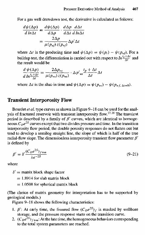
For a gas well drawdown test, the derivative is calculated as follows:
d\ff(Ap) _ di/f(Ap) dAp dAtdin At ~ dAp dAt din At
= 2AP Ap'AtV(Pwf)z(pwf)
where At is the producing time and x/s(Ap) = is(pt) — i/f(pwf)- For abuildup test, the differentiation is carried out with respect to Intp~^t
l andthe result would be
dx/fjAp) = 2Apws , tp + At
dln'-eg- ~ M(Pw.) z(Pws)' Pws At
where At is the shut-in time and ^f(Ap) = is(pws) — i/f(Pwf, A*=O).
Transient Interporosity Flow
Bourdet et al. type curves as shown in Figure 9-18 can be used for the anal-ysis of fractured reservoir with transient interporosity flow.1718 The transientperiod is described by a family of ft curves, which are identical to homoge-neous Cj)els curves except that two divides pressure and time. In the transitioninterporosity flow period, the double porosity responses do not flatten out buttend to develop a semilog straight line, the slope of which is half of the trueradial-flow slope. The dimensionless interporosity transient flow parameter ftis defined by
= s,(CDe2S)f+m ( 9 _ 2 1 )
ke~Zb
where
8' = matrix block shape factor
= 1.8914 for slab matrix block
= 1.0508 for spherical matrix block
(The choice of matrix geometry for interpretation has to be supported bygeological models.)
Figure 9-18 shows the following characteristics:
1. ft: At early time, the fissured flow (CDe2S)f is masked by wellborestorage, and the pressure response starts on the transition curve.
2. (CDe2S)f+m: At the late time, the homogeneous behaviors correspondingto the total system parameters are reached.
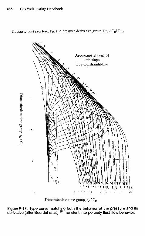
Dimensionless pressure, P0 , and pressure derivative group, [ tD / C0] P 'D
Approximately end ofunit slope
Log-log straight-line
Dimensionless time group, tp / Cp
Figure 9-18. Type curve matching both the behavior of the pressure and itsderivative (after Bourdet et a/.).18 Transient interporosity fluid flow behavior.
Dim
ensionless time group, tD / C
D
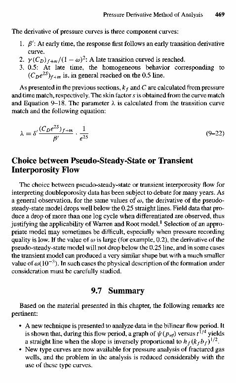
The derivative of pressure curves is three component curves:
1. /3': At early time, the response first follows an early transition derivativecurve.
2. y (C/)) /+ m / ( l — o))1'. A late transition curved is reached.3. 0.5: At late time, the homogeneous behavior corresponding to
{Cue2S)f+m is, in general reached on the 0.5 line.
As presented in the previous sections, kf and C are calculated from pressureand time match, respectively. The skin factor s is obtained from the curve matchand Equation 9-18. The parameter k is calculated from the transition curvematch and the following equation:
k = , ( C o ^ 1 1 . _1_ ( 9 _ 2 2 )
Choice between Pseudo-Steady-State or TransientInterporosity Flow
The choice between pseudo-steady-state or transient interporosity flow forinterpreting doubleporosity data has been subject to debate for many years. Asa general observation, for the same values of co, the derivative of the pseudo-steady-state model drops well below the 0.25 straight lines. Field data that pro-duce a drop of more than one log cycle when differentiated are observed, thusjustifying the applicability of Warren and Root model.1 Selection of an appro-priate model may sometimes be difficult, especially when pressure recordingquality is low. If the value of GO is large (for example, 0.2), the derivative of thepseudo-steady-state model will not drop below the 0.25 line, and in some casesthe transient model can produced a very similar shape but with a much smallervalue of <w(10~3). In such cases the physical description of the formation underconsideration must be carefully studied.
9.7 Summary
Based on the material presented in this chapter, the following remarks arepertinent:
• A new technique is presented to analyze data in the bilinear flow period. Itis shown that, during this flow period, a graph of \[/ (pwf) versus t1/4 yieldsa straight line when the slope is inversely proportional to hf(kfbf)1^2.
• New type curves are now available for pressure analysis of fractured gaswells, and the problem in the analysis is reduced considerably with theuse of these type curves.
• Prefracture information about the reservoir is necessary to estimate frac-ture parameters.
• The type curve analysis method must be used simultaneously with the spe-cific analysis methods ir(pwf) versus tl^4, i/(pwf) versus /1^2, and ir(pWf)versus log t to produce reliable results.
References and Additional Reading
1. Warren, J. E., and Root, P. J., "The Behavior of Naturally Fractured Reser-voirs," Soc. Petroleum Eng. J. (1963) 3, 245-255.
2. Ramey, H. J., Jr., "Short-Time Well Test Data Interpretation in the Presenceof Skin Effect and Wellbore Storage," /. Petroleum TechnoL (1970) 22,97-104.
3. Raghavan, R., Cady, G. V., and Ramey, H. J., Jr., "Well Test Analysis forVertically Fractured Wells,"/ Petroleum TechnoL (1972) 24, 1014-1020.
4. McKinly, R. M. "Wellbore Transmissibility from after Flow-DominatedPressure Buildup Data," Paper SPE 2416, 45th Fall Meeting of AIME,Houston, TX.
5. Gringarten, A. C, Ramey, H. J., Jr., and Raghavan, R., "Applied PressureAnalysis for Fractured Wells," /. Petroleum TechnoL (1975) 17, 887-892.
6. Earlougher, R. C, Jr., and Kerch, K. M., "Analysis of Short-Time TransientTest Data by Type-Curve Matching," /. Petroleum TechnoL (1974) 26,793-800.
7. Agarwal, R. G., Al-Hussainy, R., and Ramey, H. J., Jr., "An Investigationof Wellbore Storage and Skin Effect in Unsteady Liquid Flow: I. Analy-tical Treatment," Soc, Petroleum Eng. J. (1970) 10, 279-290.
8. Fetkovich, M. J., "Decline Curve Analysis Using Type Curves, Paper SPE4629, 48th Fall Meeting of AIME, Las Vegas, 1973.
9. Maer, N. K., Jr., "Type Curves for Analysis of after Flow-DominatedGas Well Build-up Data," Paper SPE 5134, 49th Fall Meeting of AIME,Houston, TX, 1974.
10. Uldrich, D. O., and Ershaghi, L, "A Method for Estimating the Interporos-ity Flow Parameter in Naturally Fractured Reservoirs," Soc. PetroleumEng. J. (Oct. 1979) 324-332.
11. Wattenbarger, R. A., and Ramey, H. J., Jr., "Well Test Interpretations ofVertically Fractured Gas Wells," /. Petroleum TechnoL (May 1969) 625-632; Trans. AIME, 246.
12. Agarwall, R. G., Carter, R. D., and Pollock, C. B., "Evaluation and Predic-tion of Performance of Low-Permeability Gas Wells Stimulated by Mas-sive Hydraulic Fracturing," /. Petroleum (March 1979) 362-372; Trans.AIME 261.
13. Cinco, H., and Samaniego, F., "Effect of Wellbore Storage and Damageon the Transient Pressure Behavior for a Well with a Finite-ConductivityVertical Fracture," Soc. Petroleum Eng. J. (Aug. 1978) 253-264.

14. Flopetrol Johnston Schlumberger, Course Manual, 100 Macco Boulevard,Sugarland, TX 77478.
15. Economides, C. E., "Use of the Pressure Derivative for DiagnosingPressure-Transient Behavior," J. Petroleum TechnoL (Oct. 1988) 1280-1282.
16. Bourdet, D., Whittle, T. M., Douglas, A. A., and Pirard, Y. M., "A NewSet of Type Curves Simplifies Well Test Analysis," World Oil (May 1983).
17. Bourdet, D., Ayoub, J. A., Whittle, T. M., Pirard, Y. M., and Kniazeff, Y,"Interpreting Well Tests in Fractured Reservoirs," World Oil (Oct. 1983).
18. Bourdet, D., Alagoa, A., Ayoub, J. A., and Pirard, Y M., "New Type CurvesAid Analysis of Fissured Zone Well Tests," World Oil (April 1984).
19. Alagoa, A., Bourdet, D., and Ayoub, J. A., "How to Simplify the Analysisof Fractured Well Tests," World Oil (Oct. 1985).
Chapter 10
Massive HydraulicFractured Gas WellBehavior Analysis
10.1 Introduction
References 1 and 2 presented a new set of type curves. These type curveswere specifically needed for massive hydraulic fractured (MHF) wells to handleproduction under constant pressure and constant rate. A fracture is said to havean infinite flow capacity when there is little or no pressure drop along the axisof the fracture. The fracture is said to have a finite flow capacity when there is asignificant pressure drop along its axis. Since the distinction between the defi-nitions of fracture flow capacity and formation flow capacity is often confusing,it may be worthwhile to restate the definition of the formation flow capacity:
Formation flow capacity = kh, mD-ft (10-1)
Fracture flow capacity = k/w, mD-ft (10-2)
10.2 Methods of Evaluating MHF FracturedGas Wells
Figure 10-1 illustrates method of analyzing massive hydraulic fractured gaswells.
10.3 Evaluation of Fracturing Treatments
Constant Wellbore Pressure and Finite FlowCapacity Fracture
Figure 10-2 presents constant wellbore pressure type curves for finiteflow-capacity fractures. These type curves are especially useful when ana-lyzing performance data (production rate versus time) for MHF gas wells that
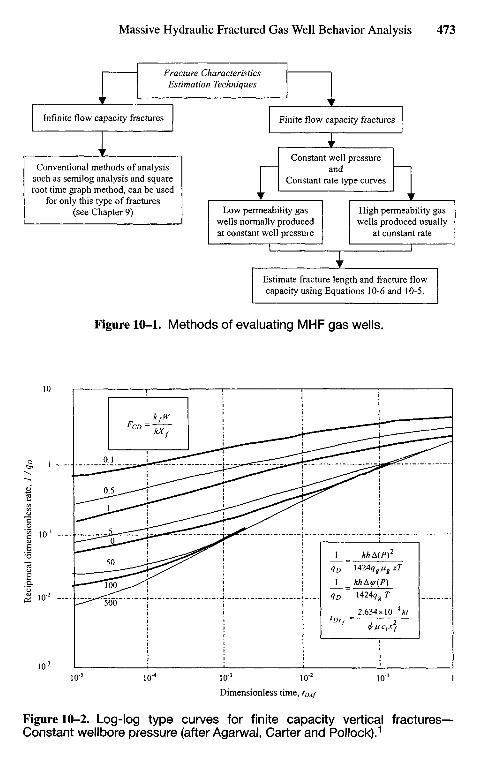
Infinite flow capacity fractures
Conventional methods of analysissuch as semilog analysis and squareroot time graph method, can be used
for only this type of fractures(see Chapter 9)
Finite flow capacity fractures
Constant well pressureand
Constant rate type curves
Low permeability gaswells normally producedat constant well pressure
High permeability gaswells produced usually
at constant rate
Estimate fracture length and fracture flowcapacity using Equations 10-6 and 10-5.
Fracture CharacteristicsEstimation Techniques
Figure 10-1. Methods of evaluating MHF gas wells.
Dimensionless time, tDX/
Figure 10-2. Log-log type curves for finite capacity vertical fractures-Constant wellbore pressure (after Agarwal, Carter and Pollock).1
Rec
ipro
cal
dim
ensi
onle
ss r
ate,
1 /
qo
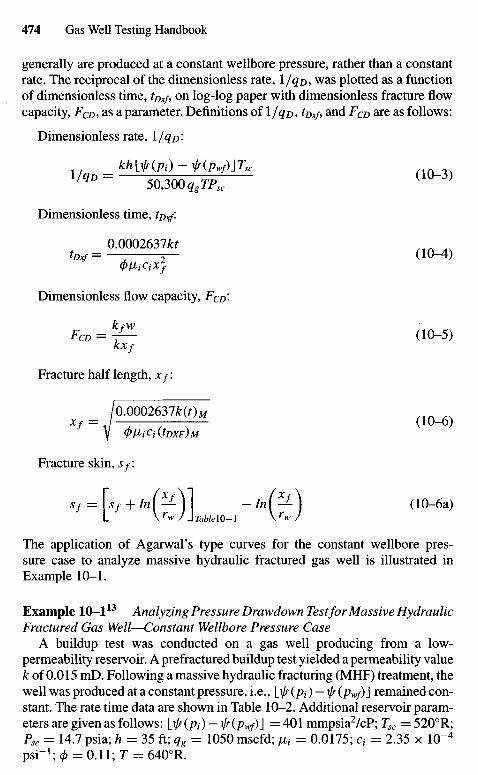
generally are produced at a constant wellbore pressure, rather than a constantrate. The reciprocal of the dimensionless rate, 1/#D> was plotted as a functionof dimensionless time, tDxf, on log-log paper with dimensionless fracture flowcapacity, FCD, as a parameter. Definitions of l/qo, tDxf, and FCD are as follows:
Dimensionless rate, 1/#D-
l / q D = 50,3O0qgTPsc
( 1 ( ^ 3 )
Dimensionless time, tDx/.
0№02631kttDxf=— 2— ( 1 0 ^
0 IXiCiXf
Dimensionless flow capacity, FCD'>
FCD = *fL (10-5)KXf
Fracture half length, x/i
l0.0002631k(t)MXf = . (10-6)Y </}fliCi(tDXF)M
Fracture skin, Sf:
sf = Lf + In(^-)] - In(^.) (10-6a)L V rw / J TablelO-1 V rw /
The application of Agarwal's type curves for the constant wellbore pres-sure case to analyze massive hydraulic fractured gas well is illustrated inExample 10-1.
Example 10-11 3 Analyzing Pressure Drawdown Test for Massive HydraulicFractured Gas Well—Constant Wellbore Pressure Case
A buildup test was conducted on a gas well producing from a low-permeability reservoir. A prefractured buildup test yielded a permeability valuek of 0.015 mD. Following a massive hydraulic fracturing (MHF) treatment, thewell was produced at a constant pressure, i.e., \}jr (/?,-) — r (pwf)\ remained con-stant. The rate time data are shown in Table 10-2. Additional reservoir param-eters are given as follows: LV^(A) — ifiPwf)} = 401 mmpsia2/cP; Tsc = 5200R;Psc = UJ psia; h = 35 ft; qg = 1050 mscfd; /x, = 0.0175; a = 2.35 x 10" 4
psi" 1; 0 = 0.11; T = 6400R.
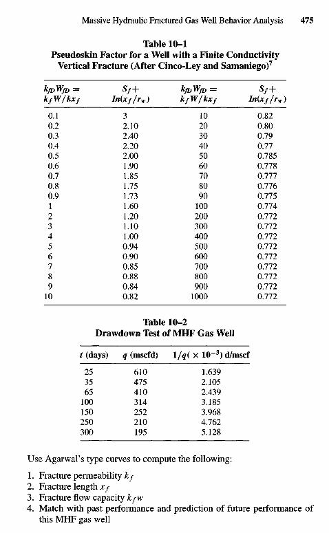
Table 10-1Pseudoskin Factor for a Well with a Finite Conductivity
Vertical Fracture (After Cinco-Ley and Samaniego)7
kflyWfD= Sf+ kfoWjD= Sf+kfW/kxf In(x f/rw) kfW/kxf In(xf/rw)
0.1 3 10 0.820.2 2.10 20 0.800.3 2.40 30 0.790.4 2.20 40 0.770.5 2.00 50 0.7850.6 1.90 60 0.7780.7 1.85 70 0.7770.8 1.75 80 0.7760.9 1.73 90 0.7751 1.60 100 0.7742 1.20 200 0.7723 1.10 300 0.7724 1.00 400 0.7725 0.94 500 0.7726 0.90 600 0.7727 0.85 700 0.7728 0.88 800 0.7729 0.84 900 0.77210 0.82 1000 0.772
Table 10-2Drawdown Test of MHF Gas Well
t (days) q (mscfd) l/q( X 10~3) d/mscf
25 610 1.63935 475 2.10565 410 2.439
100 314 3.185150 252 3.968250 210 4.762300 195 5.128
Use Agarwal's type curves to compute the following:
1. Fracture permeability kf2. Fracture length xf
3. Fracture flow capacity kfw4. Match with past performance and prediction of future performance of
this MHF gas well
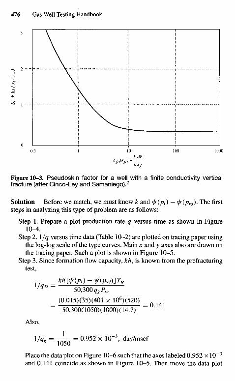
Figure 10-3. Pseudoskin factor for a well with a finite conductivity verticalfracture (after Cinco-Ley and Samaniego).2
Solution Before we match, we must know k and is(pt) — \js(pWf). The firststeps in analyzing this type of problem are as follows:
Step 1. Prepare a plot production rate q versus time as shown in Figure10-4.
Step 2. \/q versus time data (Table 10-2) are plotted on tracing paper usingthe log-log scale of the type curves. Main x and y axes also are drawn onthe tracing paper. Such a plot is shown in Figure 10-5.
Step 3. Since formation flow capacity, kh, is known from the prefracturingtest,
w _khW(Pi) -^{Pwf)\Tscl/qD " 50,300qgPsc
= (0.015)(35)(401 x 106)(520)
50,300(1050)(1000)(14.7)
Also,
\/qg = = 0.952 x 10"3, day/mscf
Place the data plot on Figure 10-6 such that the axes labeled 0.952 x 10~3
and 0.141 coincide as shown in Figure 10-5. Then move the data plot
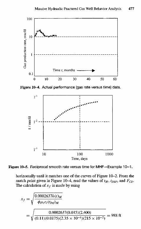
Figure 10-4. Actual performance (gas rate versus time) data.
Time t, months
Time, days
Figure 10-5. Reciprocal smooth rate versus time for MHF-Example 10-1.
horizontally until it matches one of the curves of Figure 10-2. From thematch point given in Figure 10-4, read the values of tM, tDXF, and FCD-The calculation of x/ is made by using
/0.0002637fc(Q^"f y (j)^iCi{tDxf)M
= I 0.0002637(0.015)(2,400) =
Y (0.11)(0.0175)(2.35 x 10~4)(215 x 10"2)
1 /
msc
fdG
as p
rodu
ctio
n ra
te,
msc
fd
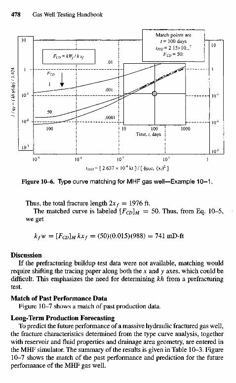
tD X f = [ 2 . 6 3 7 x 1 0 " 4 k t ] / [ Cf)JLi1Ci (x f )2 ]
Figure 10-6. Type curve matching for MHF gas well—Example 10-1.
Thus, the total fracture length 2xf = 1976 ft.The matched curve is labeled [FCD\M = 50. Thus, from Eq. 10-5,
we get
Jk/M; = [FcolAfkxf = (50)(0.015)(988) = 741 mD-ft
DiscussionIf the prefracturing buildup test data were not available, matching would
require shifting the tracing paper along both the x and y axes, which could bedifficult. This emphasizes the need for determining kh from a prefracturingtest.
Match of Past Performance DataFigure 10-7 shows a match of past production data.
Long-Term Production ForecastingTo predict the future performance of a massive hydraulic fractured gas well,
the fracture characteristics determined from the type curve analysis, togetherwith reservoir and fluid properties and drainage area geometry, are entered inthe MHF simulator. The summary of the results is given in Table 10-3. Figure10-7 shows the match of the past performance and prediction for the futureperformance of the MHF gas well.
Match points are/= 100 days
/a v /=2.15xl0_2
FCD = 50:
Time, /, days
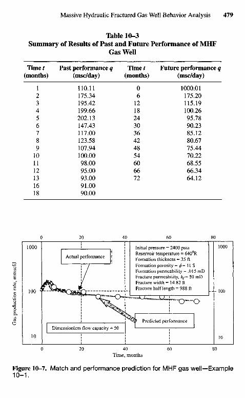
Table 10-3Summary of Results of Past and Future Performance of MHF
Gas Well
Time t Past performance q Time t Future performance q(months) (msc/day) (months) (msc/day)
1 110.11 0 1000.012 175.34 6 175.203 195.42 12 115.194 199.66 18 100.265 202.13 24 95.786 147.43 30 90.237 117.00 36 85.128 123.58 42 80.679 107.94 48 75.4410 100.00 54 70.2211 98.00 60 68.5512 95.00 66 66.3413 93.00 72 64.1216 91.0018 90.00
Time, months
Figure 10-7. Match and performance prediction for MHF gas well—Example10-1.
Dimensionless flow capacity = 50
Predicted performance
Actual performance
Initial pressure = 2400 psiaReservoir temperature = 6400RFormation thickness = 35 ftFormation porosity = 0 = 1 1 $Formation permeability = .015 mDFracture permeability, kf= 50 mDFracture width =14.82 ftFracture half length = 988 ft
Gas
pro
duct
ion
rate
, m
msc
fd
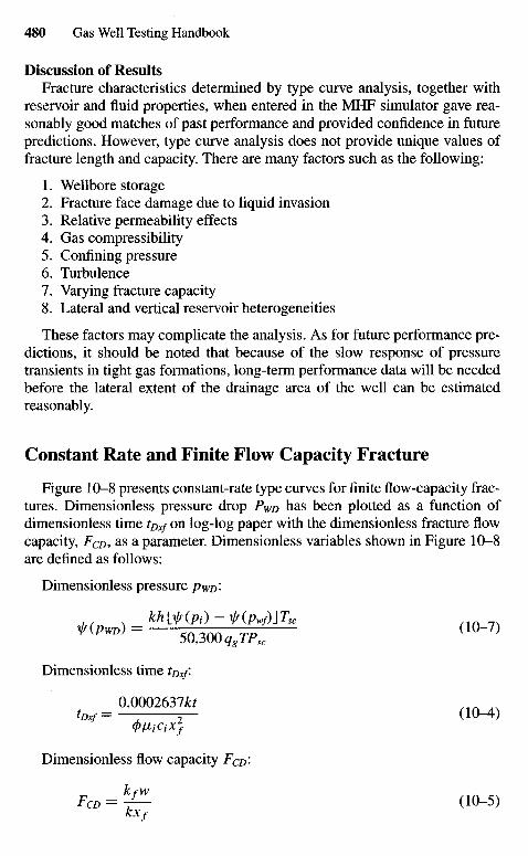
Discussion of ResultsFracture characteristics determined by type curve analysis, together with
reservoir and fluid properties, when entered in the MHF simulator gave rea-sonably good matches of past performance and provided confidence in futurepredictions. However, type curve analysis does not provide unique values offracture length and capacity. There are many factors such as the following:
1. Wellbore storage2. Fracture face damage due to liquid invasion3. Relative permeability effects4. Gas compressibility5. Confining pressure6. Turbulence7. Varying fracture capacity8. Lateral and vertical reservoir heterogeneities
These factors may complicate the analysis. As for future performance pre-dictions, it should be noted that because of the slow response of pressuretransients in tight gas formations, long-term performance data will be neededbefore the lateral extent of the drainage area of the well can be estimatedreasonably.
Constant Rate and Finite Flow Capacity Fracture
Figure 10-8 presents constant-rate type curves for finite flow-capacity frac-tures. Dimensionless pressure drop PWD has been plotted as a function ofdimensionless time tDxf on log-log paper with the dimensionless fracture flowcapacity, FCD, as a parameter. Dimensionless variables shown in Figure 10-8are defined as follows:
Dimensionless pressure pWD:
50,300 qg TPsc
Dimensionless time tDx/.
0.0002631kt
tDxf = — o~" (1 0^>
Dimensionless flow capacity FCD'>
FCD = k-f- (10-5)KXf
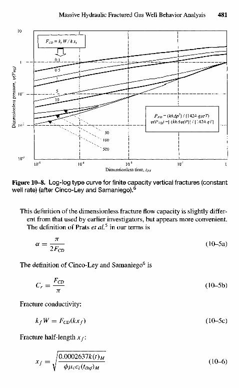
Dimensionless time, tDX
Figure 10-8. Log-log type curve for finite capacity vertical fractures (constantwell rate) (after Cinco-Ley and Samaniego).6
This definition of the dimensionless fracture flow capacity is slightly differ-ent from that used by earlier investigators, but appears more convenient.The definition of Prats et al.5 in our terms is
a =-^- (10-5a)
The definition of Cinco-Ley and Samaniego6 is
Cr = — (10-5b)n
Fracture conductivity:
kfW = FCD(kxf) (10-5c)
Fracture half-length Xf\
/0 .0002637£(OMXf= / (10-6)
Y </>fliCi(tDxf)M
Dim
ensi
onle
ss p
ress
ure,
y/
(Pw
o)
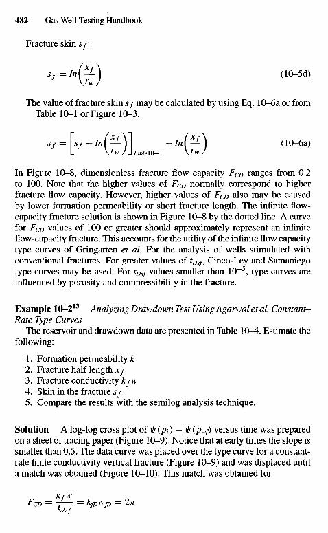
Fracture skin s/:
Sf = /n( — ) (10-5d)
The value of fracture skin s/ may be calculated by using Eq. 10-6a or fromTable 10-1 or Figure 10-3.
sf = L + //if ) I - //if ) (10-6a)L \rw J JTable\0-l \rw /
In Figure 10-8, dimensionless fracture flow capacity FCD ranges from 0.2to 100. Note that the higher values of FCD normally correspond to higherfracture flow capacity. However, higher values of FCD also may be causedby lower formation permeability or short fracture length. The infinite flow-capacity fracture solution is shown in Figure 10-8 by the dotted line. A curvefor FCD values of 100 or greater should approximately represent an infiniteflow-capacity fracture. This accounts for the utility of the infinite flow capacitytype curves of Gringarten et al. For the analysis of wells stimulated withconventional fractures. For greater values of tDxf, Cinco-Ley and Samaniegotype curves may be used. For tDxf values smaller than 10~5, type curves areinfluenced by porosity and compressibility in the fracture.
Example 10-213 Analyzing Drawdown Test Using Agarwal et al Constant-Rate Type Curves
The reservoir and drawdown data are presented in Table 10^4. Estimate thefollowing:
1. Formation permeability k2. Fracture half length Xf3. Fracture conductivity kfW4. Skin in the fracture Sf5. Compare the results with the semilog analysis technique.
Solution A log-log cross plot of\j/(pi) — is(pwf) versus time was preparedon a sheet of tracing paper (Figure 10-9). Notice that at early times the slope issmaller than 0.5. The data curve was placed over the type curve for a constant-rate finite conductivity vertical fracture (Figure 10-9) and was displaced untila match was obtained (Figure 10-10). This match was obtained for
kfWFCD = -j— = kfoWfo — 2n
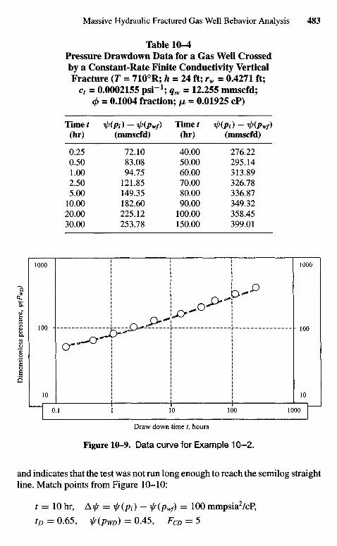
Table 10-4Pressure Drawdown Data for a Gas Well Crossedby a Constant-Rate Finite Conductivity VerticalFracture (T = 7100R; h = 24 ft; rw = 0.4271 ft;
ct = 0.0002155 psi"1; qsc = 12.255 mmscfd;0 = 0.1004 fraction; \x = 0.01925 cP)
Time t </>(#) - ^(pwf) Time t ipipt) - ip(pwf)(hr) (mmscfd) (hr) (mmscfd)
0.25 72.10 40.00 276.220.50 83.08 50.00 295.141.00 94.75 60.00 313.892.50 121.85 70.00 326.785.00 149.35 80.00 336.87
10.00 182.60 90.00 349.3220.00 225.12 100.00 358.4530.00 253.78 150.00 399.01
Draw down time /, hours
Figure 10-9. Data curve for Example 10-2.
and indicates that the test was not run long enough to reach the semilog straightline. Match points from Figure 10-10:
t = 10 hr, Ax// = ir(pi) - i/(pwf) = 100 mmpsia2/cP,
tD = 0.65, f(pwD) = 0.45, FCD = 5
Dim
ensi
onle
ss p
ress
ure,
y/
(Pw
o)
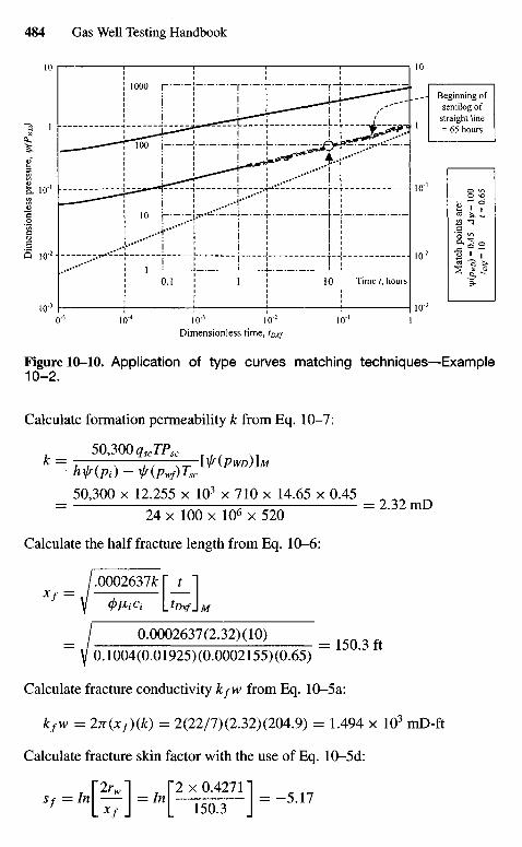
Dimensionless time, tDXf
Figure 10-10. Application of type curves matching techniques—Example10-2.
Calculate formation permeability k from Eq. 10-7:
50,300 qscTPsc
k = y . , . 77—rzri^iPwD^Mh\jf{pt) - ty(pwf)Tsc
_ 50,300 x 12.255 x 103 x 710 x 14.65 x 0.45 _= 24 x 100 x 106 x 520 = 2 ' 3 2 " ^
Calculate the half fracture length from Eq. 10-6:
/.0002637fc|~ t 1f Y (J)IX1Ci L W J M
/ 0.0002637(2.32)(10) = 1 5 0 3 ft
Y 0.1004(0.01925)(0.0002155)(0.65)
Calculate fracture conductivity kfW from Eq. 10-5a:
kfw = 27t(xf)(k) = 2(22/7)(2.32)(204.9) = 1.494 x 10³ mD-ft
Calculate fracture skin factor with the use of Eq. 10-5d:
T[2rwl [ 2 x 0 4 2 7 1 ]sf = In\ — In\ = -5.17
Mat
ch p
oint
s ar
e:
t DX
f=l0
/
= 0
.65
Dim
ensi
onle
ss p
ress
ure,
y/
(Pw
o)
Beginning ofsemilog of
straight line= 65 hours
Time /, hours
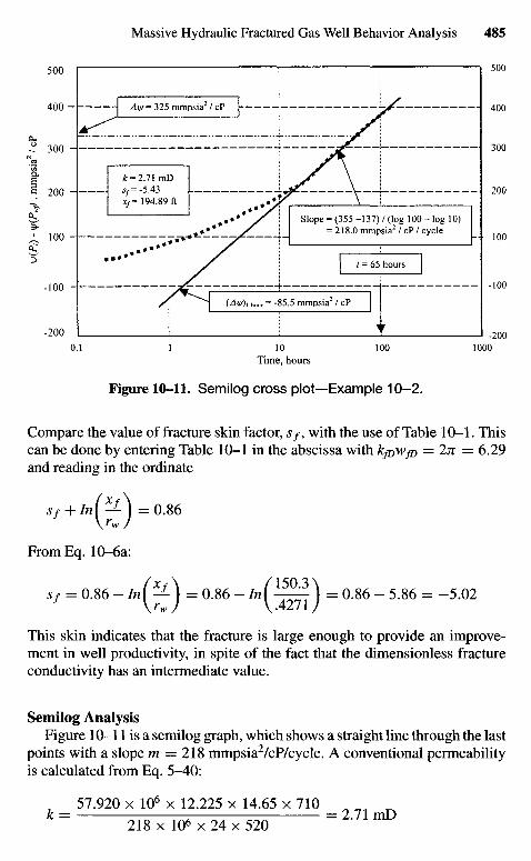
Time, hours
Figure 10-11. Semilog cross plot—Example 10-2.
Compare the value of fracture skin factor, s/, with the use of Table 10-1. Thiscan be done by entering Table 10-1 in the abscissa with Uf0Wf0 = 2n = 6.29and reading in the ordinate
Sf+In(^- ) -0 .86
From Eq. 10-6a:
sf = 0.86 - /H( — ) = 0.86 - In(^—\ = 0.86 - 5.86 = -5.02
This skin indicates that the fracture is large enough to provide an improve-ment in well productivity, in spite of the fact that the dimensionless fractureconductivity has an intermediate value.
Semilog AnalysisFigure 10-11 is a semilog graph, which shows a straight line through the last
points with a slope m = 218 mmpsia2/cP/cycle. A conventional permeabilityis calculated from Eq. 5-40:
7 57.920 x 106 x 12.225 x 14.65 x 710k = 218 x 106 x 24 x 520 =2.11mD
t = 65 hours
Slope = (355 -137) / (log 100 - log 10)= 218.0 mmpsia2 / cP / cycle
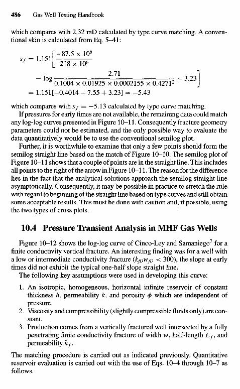
which compares with 2.32 mD calculated by type curve matching. A conven-tional skin is calculated from Eq. 5-41:
11 g 1r-8 7-5 x i°6
Sf = 1 ^ 1 5 1 I 2 I 8 X l O 62.71 ]
" 1Og 0.1004 x 0.01925 x 0.0002155 x 0.42712 + 3*23J= 1.151[-0.4014 - 7.55 + 3.23] = -5.43
which compares with s/ = —5.13 calculated by type curve matching.If pressures for early times are not available, the remaining data could match
any log-log curves presented in Figure 10-11. Consequently fracture geometryparameters could not be estimated, and the only possible way to evaluate thedata quantitatively would be to use the conventional semilog plot.
Further, it is worthwhile to examine that only a few points should form thesemilog straight line based on the match of Figure 10-10. The semilog plot ofFigure 10-11 shows that a couple of points are in the straight line. This includesall points to the right of the arrow in Figure 10-11. The reason for the differencelies in the fact that the analytical solutions approach the semilog straight lineasymptotically. Consequently, it may be possible in practice to stretch the rulewith regard to beginning of the straight line based on type curves and still obtainsome acceptable results. This must be done with caution and, if possible, usingthe two types of cross plots.
10.4 Pressure Transient Analysis in MHF Gas Wells
Figure 10-12 shows the log-log curve of Cinco-Ley and Samaniego7 for afinite conductivity vertical fracture. An interesting finding was for a well witha low or intermediate conductivity fracture (ICJDWJD < 300), the slope at earlytimes did not exhibit the typical one-half slope straight line.
The following key assumptions were used in developing this curve:
1. An isotropic, homogeneous, horizontal infinite reservoir of constantthickness h, permeability k, and porosity 0 which are independent ofpressure.
2. Viscosity and compressibility (slightly compressible fluids only) are con-stant.
3. Production comes from a vertically fractured well intersected by a fullypenetrating finite conductivity fracture of width w, half-length Lf, andpermeability/:/.
The matching procedure is carried out as indicated previously. Quantitativereservoir evaluation is carried out with the use of Eqs. 10-4 through 10-7 asfollows.
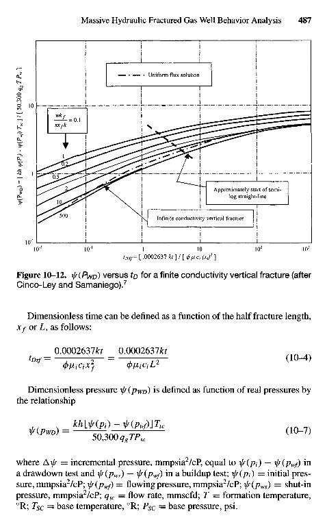
Figure 10-12. ^/{PWD) versus to for a finite conductivity vertical fracture (afterCinco-Ley and Samaniego).7
Dimensionless time can be defined as a function of the half fracture length,Xf or L, as follows:
0.0002637Jfcf 0.0002637fotDxf = — — = — Tj- (10-4)
Dimensionless pressure X//(PWD) is defined as function of real pressures bythe relationship
khli/(pi)-if(pwf)]Tsc
*{Pm) = 50,300qgTPsc ( 1 ° - 7 )
where A ^ = incremental pressure, mmpsia2/cP, equal to yjr(pt) — ir(pwf) ina drawdown test and ^/(pws) — ty(pwf) in a buildup test; i/r(pi) = initial pres-sure, mmpsia2/cP; \j/ (pWf) = flowing pressure, mmpsia2/cP; \//(pws) = shut-inpressure, mmpsia2/cP; qsc = flow rate, mmscfd; T = formation temperature,0R; Tsc = base temperature, 0R; PSc = base pressure, psi.
Infinite conductivity vertical fracture
Approximately start of semi-log straight-line
Uniform flux solution
V(P
WD
) =
[ k
h W
(P1)
- y
(Pw
f) T
sc)/
[ 50.3
00
qg
TP
SC ]
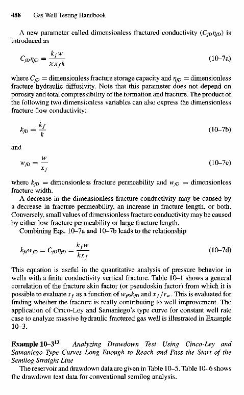
A new parameter called dimensionless fractured conductivity (CfoTjjo) isintroduced as
Cf0T110 = ^ - (10-7a)TCXfk
where Cjo = dimensionless fracture storage capacity and rfjo = dimensionlessfracture hydraulic diffusivity. Note that this parameter does not depend onporosity and total compressibility of the formation and fracture. The product ofthe following two dimensionless variables can also express the dimensionlessfracture flow conductivity:
kJD = Y (10-7b)
and
wwjo = — (10-7c)
xf
where kfo = dimensionless fracture permeability and wjo = dimensionlessfracture width.
A decrease in the dimensionless fracture conductivity may be caused bya decrease in fracture permeability, an increase in fracture length, or both.Conversely, small values of dimensionless fracture conductivity may be causedby either low fracture permeability or large fracture length.
Combining Eqs. 10-7a and 10-7b leads to the relationship
kfdWfo = CfOT11D = / ^ (10-7d)KXf
This equation is useful in the quantitative analysis of pressure behavior inwells with a finite conductivity vertical fracture. Table 10-1 shows a generalcorrelation of the fracture skin factor (or pseudoskin factor) from which it ispossible to evaluate Sf as a function of Wfokfo and x//rw. This is evaluated forfinding whether the fracture is really contributing to well improvement. Theapplication of Cinco-Ley and Samaniego's type curve for constant well ratecase to analyze massive hydraulic fractured gas well is illustrated in Example10-3.
Example 10-313 Analyzing Drawdown Test Using Cinco-Ley andSamaniego Type Curves Long Enough to Reach and Pass the Start of theSemilog Straight Line
The reservoir and drawdown data are given in Table 10-5. Table 10-6 showsthe drawdown text data for conventional semilog analysis.
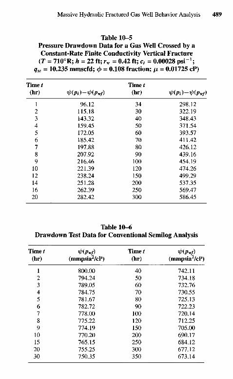
Table 10-5Pressure Drawdown Data for a Gas Well Crossed by aConstant-Rate Finite Conductivity Vertical Fracture
(T = 7100R; h = 22 ft; rw = 0.42 ft; ct = 0.00028 p s i 1 ;qsc = 10.235 mmscfd; </> = 0.108 fraction; ^i = 0.01725 cP)
Time t Time f(hr) i/j(pi)-ip(pwf) (hr) ^(Pi)-^(Pwf)
1 96.12 34 298.122 115.18 30 322.193 143.32 40 348.434 159.45 50 371.545 172.05 60 393.576 185.42 70 411.427 197.88 80 426.128 207.92 90 439.169 216.46 100 454.19
10 221.39 120 474.2612 238.24 150 499.2914 251.28 200 537.3516 262.39 250 569.4720 282.42 300 586.45
Table 10-6Drawdown Test Data for Conventional Semilog Analysis
Timer ^(pwf) Timer ^(Pwf)(hr) (mmpsia2/cP) (hr) (mmpsia2/cP)
1 800.00 40 742.112 794.24 50 734.183 789.05 60 732.764 784.75 70 730.555 781.67 80 725.136 782.72 90 722.237 778.00 100 720.148 775.22 120 712.259 774.19 150 705.0010 770.20 200 690.1715 765.15 250 684.1220 755.25 300 677.1230 750.35 350 673.14
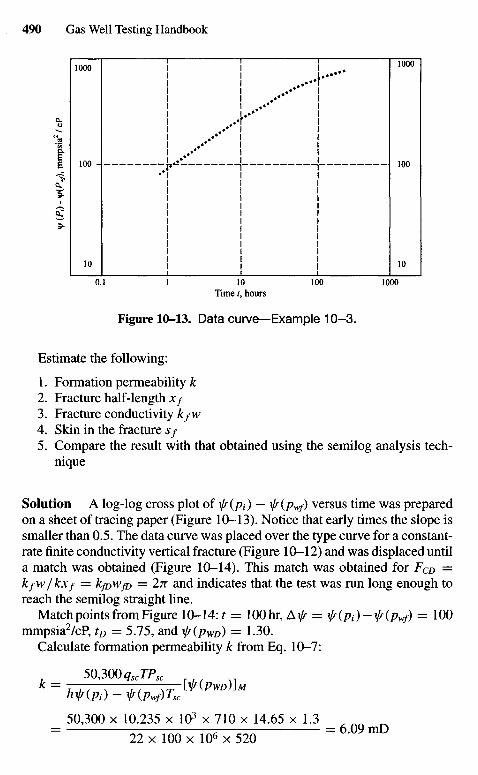
Time /, hours
Figure 10-13. Data curve—Example 10-3.
Estimate the following:
1. Formation permeability A:2. Fracture half-length x/3. Fracture conductivity kfW4. Skin in the fracture s/5. Compare the result with that obtained using the semilog analysis tech-
nique
Solution A log-log cross plot of i/s(pi) — if(pwf) versus time was preparedon a sheet of tracing paper (Figure 10-13). Notice that early times the slope issmaller than 0.5. The data curve was placed over the type curve for a constant-rate finite conductivity vertical fracture (Figure 10-12) and was displaced untila match was obtained (Figure 10-14). This match was obtained for FCD —kf\v/kxf = kfoWjD = 2n and indicates that the test was run long enough toreach the semilog straight line.
MatchpointsfromFigurelO-14:^ = lOOhr, Ax// = f(Pi)-f(pWf) = 100mmpsia2/cP, tD — 5.75, and ^(PWD) = 1-30.
Calculate formation permeability k from Eq. 10-7:
50,300 qsJPsc r | ,k = , , / x TT—7^rW(PwD)]M
W(Pi) - ^(Pwf)Tsc
50,300 x 10.235 x 103 x 710 x 14.65 x 1.3 ,= 22 x 100 x 10 x 520 = 6 ' ° 9 ^
¥ (P
d -
VO
PV),
mm
psia
2 / cP
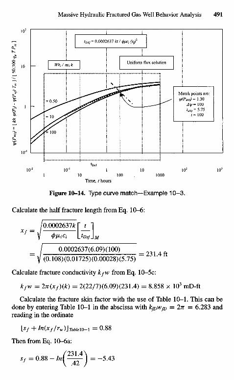
Time, / hours
Figure 10-14. Type curve match-—Example 10-3.
Calculate the half fracture length from Eq. 10-6:
/0.0002637A: |~ t 1
= I 0.0002637(6.09)(100) ~ =
Y (0.108)(0.01725)(0.00028)(5.75)
Calculate fracture conductivity &/w from Eq. 10-5c:
kfw = 2Jt(Xf)Qc) = 2(22/7)(6.09)(231.4) = 8.858 x 10³ mD-ft
Calculate the fracture skin factor with the use of Table 10-1. This can bedone by entering Table 10-1 in the abscissa with kfoWfo = 2n = 6.283 andreading in the ordinate
Is f + In(Xf/rw)}Tabiel0-i = 0.88
Then from Eq. 10-6a:
Sf = 0.88 - ' " ( ^ r ) = -5-43
Match points are:WfTVaJ= 1.30
Ay/= 100toxf= 5.75
/= 100
Uniform flux solution
¥(/W
= [
kh
Y(P
1) -
y/(P
wJ)
Ts
c)/
[ 50
.300
qg
TP
SC}

Flowing time /, hours
Figure 10-15. Conventional semilog drawdown test analysis for fractured gaswell.
This skin indicates that the fracture is large enough to provide an improve-ment in well productivity, in spite of the fact that the dimensionless fractureconductivity has an intermediate value. Figure 10-15 shows a semilog plot oftyiPwf) versus time. From this figure the following information is obtained:
730-810 9Slope m = — — = -90.0 mmpsiaz/cP/cyclev log 100-log 10 F
pihr = 885.00 mmpsia2/cP
Conventional formation permeability calculations using Eq. 5-40:
57.921 x 10"6 x 10.235 x 710 x 14.65
" = 90.0 x 106 x 22 x 520 =5'99mD
A conventional skin calculation using Eq. 5—41:
, , T 8 8 5 . 0 - 8 6 0 . 1J = U 5 1 [ -90.0
( 5-99 A 1° g \0.108 x 0.01725 x 0.00028 x 0.422/ + ' J
= 1.151[-0.277 - 7.81 + 3.23] = -5.59
which compares with Sf = —5.43 calculated by type curve matching.
Slope, /n = [ 730 - 810 ] / [ log 100 - log 10 ] = = 90.0 mmpsia2 / cP/ cycle
Calculate fracture length Xf from the following equation:
r'w = rwe~(S) = 0.42 x e~{-5'59) = 112.45 ft
Hence,
Xf = 2 xr^ = 2(112.54) = 224.90 ft
which compares with xf = 231.4 ft calculated by type curve matching.If pressures for early times are not available, the remaining data could match
any of the curves presented in Figure 10-12. Consequently, fracture geometryparameters could not be estimated, and the only possibility to evaluate the dataquantitatively would be to use the conventional semilog plot.
Final RemarksThe evaluations and prediction of performance of low-permeability gas
wells stimulated by massive hydraulic fracturing warrant the following state-ments:
1. Pressure transient methods (both type-curve and square root graph),based on the concept of infinite flow-capacity fracture, are not adequatefor evaluating MHF gas wells with finite flow capacity fracture.
2. Low-permeability MHF gas wells generally produce at a constantbottom-hole pressure rather than at a constant rate; the constant wellpressure type curves appear more appropriate for analyzing the perfor-mance data. However, where production rates are reasonably constantor vary smoothly with bottom-hole pressure, constant-rate type curvesshould be used.
3. Finite flow-capacity type curves presented here for both the constant-pressure and constant-rate cases are intended for use with drawdowndata. However, they may be used to analyze pressure buildup data, ifproducing time before shut-in is sufficiently long (tp + At & tp) so thatthe buildup data are least affected.
4. In low-permeability MHF wells, testing times may not be long enoughbecause of practical limitations to permit semilog pressure analysis fordetermining formation.
5. The data of Cinco-Ley and Samaniego need to be extended to earliertimes for MHF applications. Square root graphs with log-log type curvesshould be helpful.
6. The use of a mathematical model, such as the MHF simulator, with typecurve analysis can provide a good prediction of well performance.
10.5 Fracture Characteristics Estimation UsingPressure Transient Testing
This section presents theoretical and practical aspects of methods used todetermine formation permeability, fracture length, and fracture conductivityin low-permeability, hydraulically fractured gas reservoirs.
Horner Analysis
Plot buildup test data on a conventional Horner graph; determine the slopem, and thus estimate formation permeability k from
t = 57.92 x ! O V ^ 1 1 1 0
mhTsc
and fracture skin factor s/ from
= Ll5 Jt(EhLZl^A _ log ( - * ) + 3.23] (10-9)
Calculate fracture half-length from
Xf = 2rwe~s' (10-10)
Linear Flow Analysis: High Conductivity Fractures
When linear flow into a fracture dominates (at earliest times), a plot of^s(Ap) versus a square-root-of-time function will result in a straight line withslope mi/, related to fracture half-length and formation permeability:
^ - : J - (10-11)mifh \k(f>ctj
Calculate fracture skin factor s/i
Sf=In(^A (10-i2)V*/ /
The assumptions on which Eq. 10-11 is based limit its applicability in manycases. These limiting assumptions include the following:
1. Formation permeability k must be available, if we wish to estimate x/.2. High fracture conductivity (but not infinite) and FCD is greater than 100.3. Earliest-time data is dominated by linear flow and no wellbore storage
distortion.
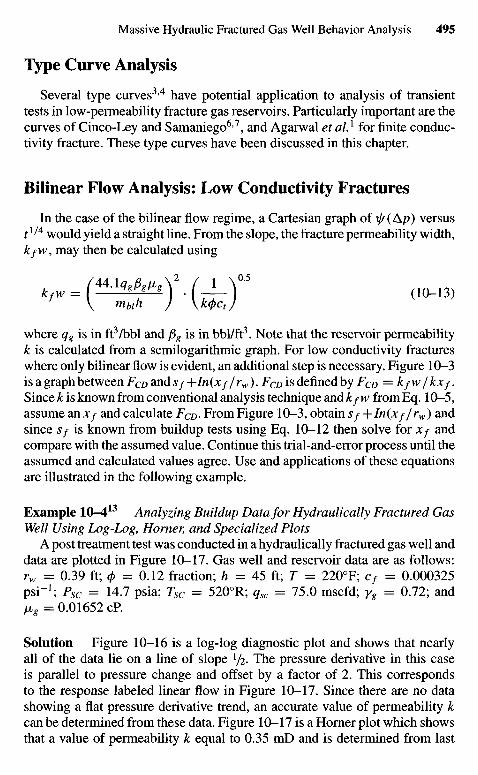
Type Curve Analysis
Several type curves34 have potential application to analysis of transienttests in low-permeability fracture gas reservoirs. Particularly important are thecurves of Cinco-Ley and Samaniego6'7, and Agarwal et all for finite conduc-tivity fracture. These type curves have been discussed in this chapter.
Bilinear Flow Analysis: Low Conductivity Fractures
In the case of the bilinear flow regime, a Cartesian graph of \fr(Ap) versust1/4 would yield a straight line. From the slope, the fracture permeability width,kfW, may then be calculated using
V mbih J \k(/)ctj
where qg is in ft3/bbl and fig is in bbl/ft3. Note that the reservoir permeabilityk is calculated from a semilogarithmic graph. For low conductivity fractureswhere only bilinear flow is evident, an additional step is necessary. Figure 10-3is a graph between FCD and Sf +In(x//rw). FCD is defined by FCD = k/w/ kx/.Since k is known from conventional analysis technique and k/w from Eq. 10-5,assume an Xf and calculate FCD. From Figure 10-3, obtain s/ -\-In(xf/rw) andsince Sf is known from buildup tests using Eq. 10-12 then solve for Xf andcompare with the assumed value. Continue this trial-and-error process until theassumed and calculated values agree. Use and applications of these equationsare illustrated in the following example.
Example 10-413 Analyzing Buildup Data for Hydraulically Fractured GasWell Using Log-Log, Homer, and Specialized Plots
A post treatment test was conducted in a hydraulically fractured gas well anddata are plotted in Figure 10-17. Gas well and reservoir data are as follows:rw = 0.39 ft; 0 = 0.12 fraction; h = 45 ft; T = 2200F; cf = 0.000325psi"1; Psc = 14.7 psia; Tsc = 5200R; qsc = 75.0 mscfd; yg = 0.72; andlig = 0.01652 cP.
Solution Figure 10-16 is a log-log diagnostic plot and shows that nearlyall of the data lie on a line of slope 1^. The pressure derivative in this caseis parallel to pressure change and offset by a factor of 2. This correspondsto the response labeled linear flow in Figure 10-17. Since there are no datashowing a flat pressure derivative trend, an accurate value of permeability kcan be determined from these data. Figure 10-17 is a Horner plot which showsthat a value of permeability k equal to 0.35 mD and is determined from last
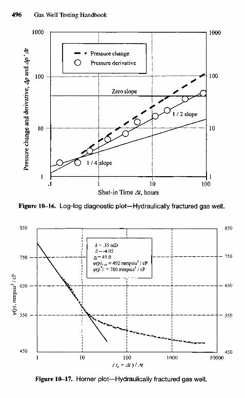
Shut-in Time At, hours
Figure 10-16. Log-log diagnostic plot—Hydraulically fractured gas well.
Figure 10-17. Horner plot—Hydraulically fractured gas well.
£ = . 3 5 m DS =-4.05
xf= 45 ftV(p)i hr= 492 mmpsia2 / cPXIf(P*) = 780 mmpsia2 / cP
Pressure change
Pressure derivative
Zero slope
1 / 4 !slope
1 / 2 slope
Pres
sure
cha
nge
and
deri
vativ
e, A
p an
d A
p 'A
t
y/(p
), m
mps
ia2 /
cP
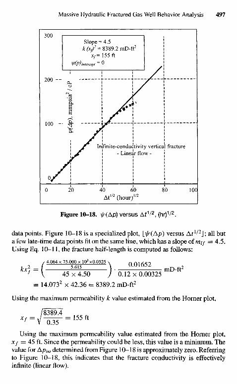
Figure 10-18. ^ (Ap) versus Af1/2, (hr)1/2.
data points. Figure 10-18 is a specialized plot, IrIr(Ap) versus At 1/2J; all buta few late-time data points fit on the same line, which has a slope of m// = 4.5.Using Eq. 10-11, the fracture half-length is computed as follows:
/ 4.064 x 75.000 x IQ3 x0.0525 \ nru^co
"*' - { JFlffeo ) • ft12 x 0.00325 " ^= 14.0732 x 42.36 = 8389.2 mD-ft2
Using the maximum permeability k value estimated from the Homer plot,
/8389.4
* / = v W = 155ft
Using the maximum permeability value estimated from the Horner plot,Xf = 45 ft. Since the permeability could be less, this value is a minimum. Thevalue for Apint determined from Figure 10-18 is approximately zero. Referringto Figure 10-18, this indicates that the fracture conductivity is effectivelyinfinite (linear flow).
hour
Inifinite-conductivity vertical fracture- Linear flow -
Slope = 4.5k (x/ = 8389.2 mD-ft2
xf= 155 ftV(P) Intercept = 0
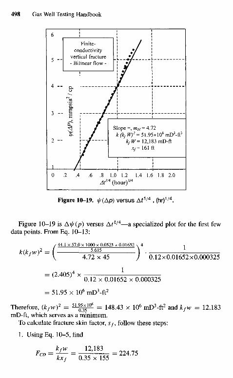
Figure 10-19. ^r(Ap) versus Af1/4 , (hr)1/4.
Figure 10-19 is Ai//(p) versus Af1/4—a specialized plot for the first fewdata points. From Eq. 10-13:
/ 44 .1x 57.0 x 1000 x 0.0525 x 0.01652 \ 4 1
k(kfw)2=( 5J-15 ) 1J V 4.72 x 45 / 0.12x0.01652x0.000325
" 0.12 x 0.01652 x 0.000325
= 51.95 x 10⁶mD3-ft2
Therefore, (kfw)2 = 5 ^ 1 0 " = 148.43 x 10⁶ mD3-ft2 and kfw = 12,183mD-ft, which serves as a minimum.
To calculate fracture skin factor, s/, follow these steps:
1. Using Eq. 10-5, find
kfw 12,183FcD = TTf
= 0.35 x 155 = 2 2 4 - 7 5
hour
Slope=, ^ f = 4.72k (kfW)2 = 51.95x10⁶ mD3-ft3
kfW= 12,183 mD-ftxf= 161 ft
Finite-conductivity
vertical fracture- Bilinear flow -
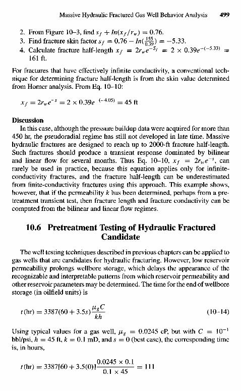
2. From Figure 10-3, find sf + In(xf/rw) = 0.76.3. Find fracture skin factor s/ = 0.76 — In(^) = —5.33.4. Calculate fracture half-length xf = 2rwe~sf = 2 x 039e~(~533) =
161 ft.
For fractures that have effectively infinite conductivity, a conventional tech-nique for determining fracture half-length is from the skin value determinedfrom Horner analysis. From Eq. 10-10:
Xf = 2rwe~s = 2 x 0.39^"(~405) = 45 ft
DiscussionIn this case, although the pressure buildup data were acquired for more than
450 hr, the pseudoradial regime has still not developed in late time. Massivehydraulic fractures are designed to reach up to 2000-ft fracture half-length.Such fractures should produce a transient response dominated by bilinearand linear flow for several months. Thus Eq. 10-10, x/ = 2rwe~\ canrarely be used in practice, because this equation applies only for infinite-conductivity fractures, and the fracture half-length can be underestimatedfrom finite-conductivity fractures using this approach. This example shows,however, that if the permeability k has been determined, perhaps from a pre-treatment transient test, then fracture length and fracture conductivity can becomputed from the bilinear and linear flow regimes.
10.6 Pretreatment Testing of Hydraulic FracturedCandidate
The well testing techniques described in previous chapters can be applied togas wells that are candidates for hydraulic fracturing. However, low reservoirpermeability prolongs wellbore storage, which delays the appearance of therecognizable and interpretable patterns from which reservoir permeability andother reservoir parameters may be determined. The time for the end of wellborestorage (in oilfield units) is
f (hr) = 3387(60 + 3.5s)^*£. (10-14)kh
Using typical values for a gas well, /xg = 0.0245 cP, but with C = 10"1
bbl/psi, h = 45 ft, k = 0.1 mD, and s = 0 (best case), the corresponding timeis, in hours,
f(hr) = 3387[60 + 3 .5 (0 ) ] 0 ^ 4 5 X ° a l = 1110.1 x 45
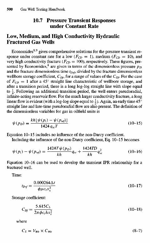
10.7 Pressure Transient Responsesunder Constant Rate
Low, Medium, and High Conductivity HydraulicFractured Gas Wells
Economides8'9 gives comprehensive solutions for the pressure transient re-sponse under constant rate for a low (FCD = 1), medium (FCD = 10), andvery high conductivity fracture (FCD = 100), respectively. These figures, pre-sented by Economides,8 are given in terms of the dimensionless pressure p&and the fracture dimensionless time tDxf, divided by the fracture dimensionlesswellbore storage coefficient, CDf, for a range of values of the CDf. For the caseof FCD = 1 after a 45° straight line characteristic of wellbore storage, andafter a transition period, there is a long log-log straight line with slope equalto | . Following an additional transition period, the well enters pseudoradial,infinite-acting reservoir flow. For the much larger conductivity fracture, a longlinear flow is evident (with a log-log slope equal to ^). Again, an early time 45°straight line and late-time pseudoradial flow are also present. The definition ofthe dimensionless variables for gas in oilfield units is
Equation 10-15 includes no influence of the non-Darcy coefficient.Including the influence of the non-Darcy coefficient, Eq. 10-15 becomes
1424T\/f(pD) 1424TD 7
fiPt) - npwf) = — ] j r ^ q s c + ~~kh~qsc ( 1 0"1 6 )
Equation 10-16 can be used to develop the transient IPR relationship for afractured well.
Time:
0.000264ArtDxf=— — (10-17)
(j>lictx2
x
Storage coefficient:
CDf=^h (10-18)
where
Cs = Vwb x Cwb (8-7)
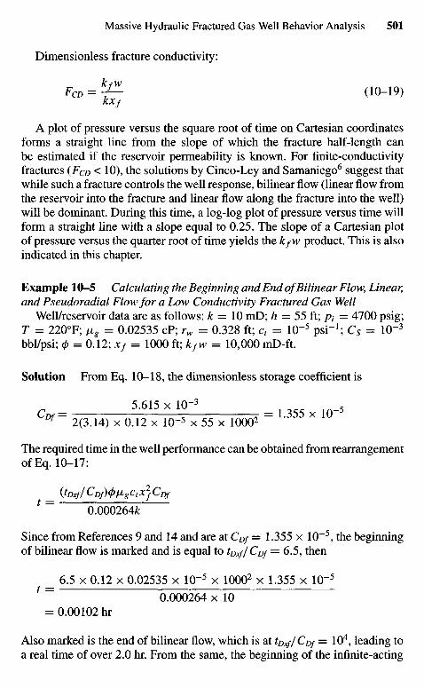
Dimensionless fracture conductivity:
FCD = ^ (10-19)KXf
A plot of pressure versus the square root of time on Cartesian coordinatesforms a straight line from the slope of which the fracture half-length canbe estimated if the reservoir permeability is known. For finite-conductivityfractures (FCD < 10), the solutions by Cinco-Ley and Samaniego6 suggest thatwhile such a fracture controls the well response, bilinear flow (linear flow fromthe reservoir into the fracture and linear flow along the fracture into the well)will be dominant. During this time, a log-log plot of pressure versus time willform a straight line with a slope equal to 0.25. The slope of a Cartesian plotof pressure versus the quarter root of time yields the kfW product. This is alsoindicated in this chapter.
Example 10-5 Calculating the Beginning and End of Bilinear Flow, Linear,and Pseudoradial Flow for a Low Conductivity Fractured Gas Well
Well/reservoir data are as follows: k = 10 mD; h = 55 ft; pt = 4700 psig;T = 2200F; / ^ = 0.02535 cP; rw = 0.328 ft; ct = 10"5 psi"1; C5 = 10"3
bbl/psi; 0 = 0.12; xf = 1000 ft; kfw = 10,000 mD-ft.
Solution From Eq. 10-18, the dimensionless storage coefficient is
5.615 x IQ-3 5
C D / " 2(3.14) x 0.12 x 10-5 x 55 x 10002 " ° 5 5 X 1 0
The required time in the well performance can be obtained from rearrangementofEq. 10-17:
_ {tDxf/CDf)^ixgctx2fCDf
1 = 0.000264&
Since from References 9 and 14 and are at CDf = 1.355 x 10~5, the beginningof bilinear flow is marked and is equal to toxf/Cnf = 6.5, then
_ 6.5 x 0.12 x 0.02535 x 10"5 x 10002 x 1.355 x 10"5
1 " 0.000264 x 10= 0.00102 hr
Also marked is the end of bilinear flow, which is at tDxf/CDf = 104, leading toa real time of over 2.0 hr. From the same, the beginning of the infinite-acting
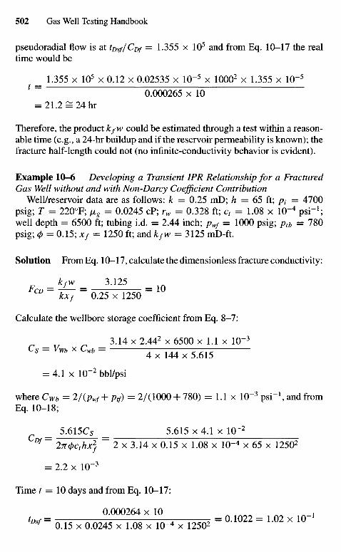
pseudoradial flow is at tDxf/CDf = 1.355 x 10⁵ and from Eq. 10-17 the realtime would be
_ 1.355 x 105 x 0.12 x 0.02535 x 10"5 x 10002 x 1.355 x 10"5
1 ~ 0.000265 x 10= 21.2 = 24hr
Therefore, the product k/w could be estimated through a test within a reason-able time (e.g., a 24-hr buildup and if the reservoir permeability is known); thefracture half-length could not (no infinite-conductivity behavior is evident).
Example 10-6 Developing a Transient IPR Relationship for a FracturedGas Well without and with Non-Darcy Coefficient Contribution
Well/reservoir data are as follows: k = 0.25 mD; h = 65 ft; p( = 4700psig; T = 2200F; /xg = 0.0245 cP; rw = 0.328 ft; ct = 1.08 x 10"4 psi"1;well depth == 6500 ft; tubing i.d. = 2.44 inch; pwf = 1000 psig; ptb = 780psig; 0 = 0.15; xf = 1250 ft; and kfw =3125 mD-ft.
Solution FromEq. 10-17, calculate the dimensionless fracture conductivity:
FCD=k-^= 3 J 2 5 =10c kxf 0.25 x 1250
Calculate the wellbore storage coefficient from Eq. 8-7:
3.14 x 2.442x 6500 x 1.1 x 10"3
Cs — Vwb x Cwb — - — - — c r+c
4 x 144 x 5.615= 4.1 x 10"2bbl/psi
where Cwb = 2/(pwf+ ptf) = 2/(1000 + 780) = 1.1 x 10"3 psi"1, and fromEq. 10-18;
_ 5.615C5 _ 5.615 x 4.1 x 10~2
C°f " 27t(j)cthx2f = 2 x 3.14 x 0.15 x 1.08 x 10"4 x 65 x 12502
= 2.2 x 10"3
Time t = 10 days and from Eq. 10-17:
0.000264 x 10 ,*»= 0.15 x 0.0245 x 1.08 x 1(H x 1250* = ° - 1 0 2 2 = L 0 2 X 1 0
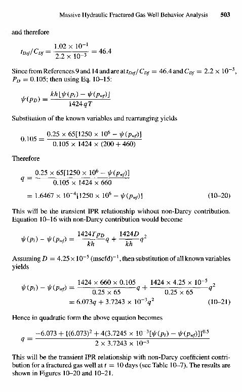
and therefore
1.02 x 1(T1
^ ^ = 2.2x10-3 =46A
Since from References 9 and 14 and are at tDxf/ CD/ = 46.4andCD/ = 2.2 x 10~3
Pz, = 0.105; then using Eq. 10-15:
khlf(Pi)-t(Pwf)\npD) = U24^r
Substitution of the known variables and rearranging yields
Q 1 0 5 = 0.25 x 65[1250x I Q 6 - f Qy)]~ 0.105 x 1424 x (200 + 460)
Therefore
_ 0.25 x 65[1250 x 106 - ^Ov) ]q~ 0.105 x 1424x660
= 1.6467 x 10~4[1250 x 106 - V Ov)] (10-20)
This will be the transient IPR relationship without non-Darcy contribution.Equation 10-16 with non-Darcy contribution would become
U24TpD 1424Z) 7V(Pi) - V(Pwf) = — q + kh q
AssumingD = 4.25xlO~5 (mscfd)"1, then substitution of all known variablesyields
1424 x 660 x 0.105 1424 x 4.25 x 10"5 2
HPi) ~ ^r(ZV) - 5 ^ ^ 9 + 5^7^ 9
= 6.013q + 3.7243 x 10"3^2 (10-21)
Hence in quadratic form the above equation becomes
= -6.073 + {(6.073)2 + 4(3.7245 x IQ-3^(P/) - ^(p^)]}0-5
9 ~ 2 x 3.7243 x 10~3
This will be the transient IPR relationship with non-Darcy coefficient contri-bution for a fractured gas well at t = 10 days (see Table 10-7). The results areshown in Figures 10-20 and 10-21.
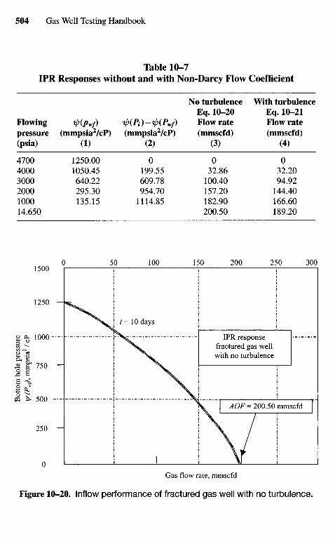
Table 10-7IPR Responses without and with Non-Darcy Flow Coefficient
No turbulence With turbulenceEq. 10-20 Eq. 10-21
Flowing ip(Pwf) ^(Pi)-^(Pwf) Flow rate Flow ratepressure (mmpsia2/cP) (mmpsia2/cP) (mmscfd) (mmscfd)(psia) (1) (2) (3) (4)
4700 1250.00 0 0 04000 1050.45 199.55 32.86 32.203000 640.22 609.78 100.40 94.922000 295.30 954.70 157.20 144.401000 135.15 1114.85 182.90 166.6014.650 200.50 189.20
IPR responsefractured gas wellwith no turbulence
AOF= 200.50 mmscfd
Gas flow rate, mmscfd
Figure 10-20. Inflow performance of fractured gas well with no turbulence.
Bot
tom
hol
e pr
essu
re\j/
(Pwj),
mm
psia
2 / c
P
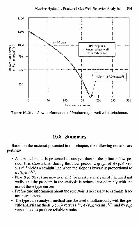
Gas flow rate, mmscfd
Figure 10-21. Inflow performance of fractured gas well with turbulence.
10.8 Summary
Based on the material presented in this chapter, the following remarks arepertinent:
• A new technique is presented to analyze data in the bilinear flow pe-riod. It is shown that, during this flow period, a graph of ^(Pw/) ver-sus r1/4 yields a straight line when the slope is inversely proportional tohf(kfbf)V
2.• New type curves are now available for pressure analysis of fractured gas
wells, and the problem in the analysis is reduced considerably with theuse of these type curves.
• Prefracture information about the reservoir is necessary to estimate frac-ture parameters.
• The type curve analysis method must be used simultaneously with the spe-cific analysis methods is(pwf) versus tl/4, ty(pwf) versus f1/2, and VK/v)versus log t to produce reliable results.
AOF= 189.20mmscfd
IPR responseFractured gas well
with turbulence
Bot
tom
hol
e pr
essu
rey/
(PW
(), m
mps
ia2 /
cP
t = 10 days
References and Additional Reading
1. Agarwal, R. G., Carter, R. D., and Pollock, C. B., "Evaluation and Predic-tion of Performance of Low-Permeability Gas Wells Stimulated by Mas-sive Hydraulic Fracturing," /. Petroleum Technol. (March 1979) 362-372;Trans. AIME 67.
2. Cinco, H., and Samaniego, F. "Effect of Wellbore Storage and Damageon the Transient Pressure Behavior for a Well with a Finite-ConductivityVertical Fracture," Soc. Petroleum Eng. J. (Aug. 1978) 253-264.
3. Pressure Transient Testing Methods, SPE Reprint Series No. 1, Society ofPetroleum Engineers, Dallas, TX, 1980.
4. Advances in Well Test Analysis, SPE Monograph, Vol. 5, Society ofPetroleum Engineers, Dallas, TX, 1977.
5. Prats, M., Hazebrock, P., and Sticker, W. R., "Effect of Vertical Fractureson Reservoir Behavior—Compressible Fluid Case," Soc. Petroleum Eng.J. (June 1962) 87-94; Trans. AIME 225, Vol. 8, Houston, TX, Oct. 1995.
6. Cinco-Ley, H., and Samaniego, F, "Transient Pressure Analysis for Frac-tured Wells," /. Petroleum Technol. (Sept. 1981) 1749-1766.
7. Cinco-Ley, H., and Samaniego, F, "Transient Pressure Analysis for FiniteConductivity Fracture Case versus Damage Fracture Case," SPE Paper10179, 1981.
8. Economides, M. J., "Observations and Recommendations in the Evalua-tion of Tests of Hydraulically Fractured Wells," SPE Paper 16396, 1987.
9. Economides, M. J., and Nolte, K. G., Reservoir Stimulation, 2nd ed.Prentice-Hall, Englewood Cliffs, NJ, 1989.
10. Crawford, G. E., Hagedorn, A. R., and Pierce, A. E., "Analysis of PressureBuild-up Tests in a Naturally Fractured Reservoir," J. Petroleum Technol.(Nov. 1976) 1295-1300.
11. Kazemi, H., Seth, M. S., and Thomas, G. W., "The Interpretation of In-terference Tests in Naturally Fractured Reservoirs with Uniform FractureDistribution " Soc. Petroleum Eng. J. (Dec. 1969) 463-472.
12. Matthews, C. S., and Russel, D. G., Pressure Build-up and Flow Tests inWells, SPE of AIME Monograph, Vol. 1, 25, Henry Doherty Series, 1967.
13. Amanat, U. C, Pressure Transient Test Analysis User's Handbook. Ad-vanced TWPSOM Petroleum Systems Inc., Vol. 8, Houston, TX, Oct.1995.
14. Michael, J. E., Daniel, H. A., and Christine, E. E., "Petroleum ProductionSystems," Prentice-Hall Inc; NJ. (1994). pp. 498-499.
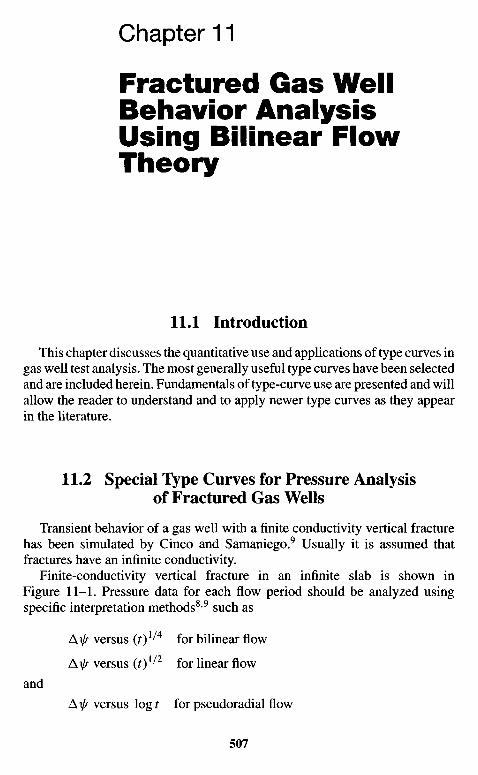
Chapter 11
Fractured Gas WellBehavior AnalysisUsing Bilinear FlowTheory
11.1 Introduction
This chapter discusses the quantitative use and applications of type curves ingas well test analysis. The most generally useful type curves have been selectedand are included herein. Fundamentals of type-curve use are presented and willallow the reader to understand and to apply newer type curves as they appearin the literature.
11.2 Special Type Curves for Pressure Analysisof Fractured Gas Wells
Transient behavior of a gas well with a finite conductivity vertical fracturehas been simulated by Cinco and Samaniego.9 Usually it is assumed thatfractures have an infinite conductivity.
Finite-conductivity vertical fracture in an infinite slab is shown inFigure 11-1. Pressure data for each flow period should be analyzed usingspecific interpretation methods8'9 such as
Axf/ versus (01/ /4 f° r bilinear flow
A\j/ versus (t)l/2 for linear flow
and
Ax// versus log t for pseudoradial flow
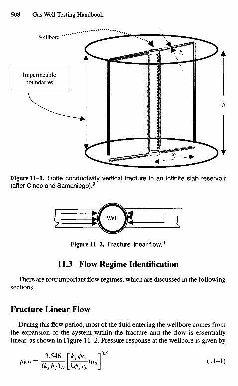
Figure 11-2. Fracture linear flow.9
11.3 Flow Regime Identification
There are four important flow regimes, which are discussed in the followingsections.
Fracture Linear Flow
During this flow period, most of the fluid entering the wellbore comes fromthe expansion of the system within the fracture and the flow is essentiallylinear, as shown in Figure 11-2. Pressure response at the wellbore is given by
3.546 \kf4>ct^ I 0 5
PwD= n , , T^;—tDxf\ (11-1)(kfbf)D VHfCf1
J\
Figure 11-1. Finite conductivity vertical fracture in an infinite slab reservoir(after Cinco and Samaniego).9
Impermeableboundaries
Wellbore
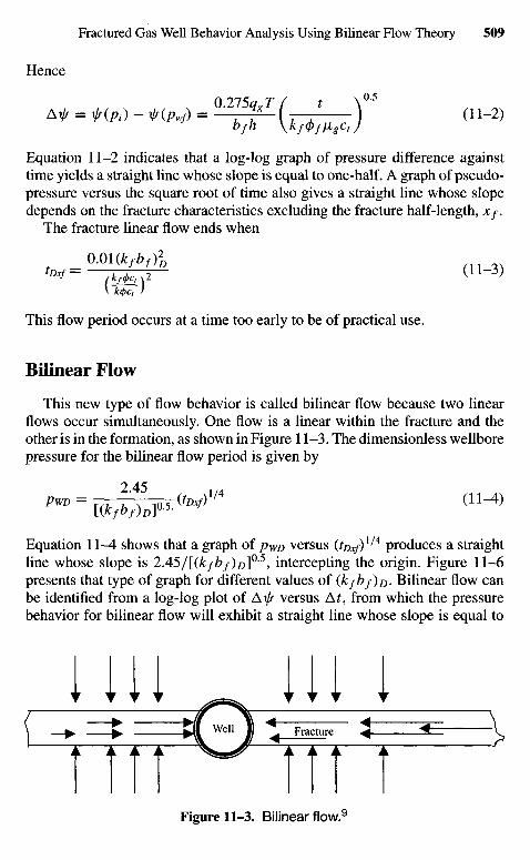
Hence
O 275a T ( t \ °'5AxIf = f{Pi) - i,(pwf) = \ l 8 ( — (11-2)
bfh \kf(j)fixgctj
Equation 11-2 indicates that a log-log graph of pressure difference againsttime yields a straight line whose slope is equal to one-half. A graph of pseudo-pressure versus the square root of time also gives a straight line whose slopedepends on the fracture characteristics excluding the fracture half-length, Xf.
The fracture linear flow ends when
0.Oi (*/*/)!,
V k(t)Ct )
This flow period occurs at a time too early to be of practical use.
Bilinear Flow
This new type of flow behavior is called bilinear flow because two linearflows occur simultaneously. One flow is a linear within the fracture and theother is in the formation, as shown in Figure 11-3. The dimensionless wellborepressure for the bilinear flow period is given by
Equation 11-4 shows that a graph of pWD versus (tDxf)1/4 produces a straight
line whose slope is 2A5/[(kfbf)o]0'5, intercepting the origin. Figure 11-6presents that type of graph for different values of (kfbf)D. Bilinear flow canbe identified from a log-log plot of A\j/ versus Ar, from which the pressurebehavior for bilinear flow will exhibit a straight line whose slope is equal to
Figure 11-3. Bilinear flow.9
FractureWell
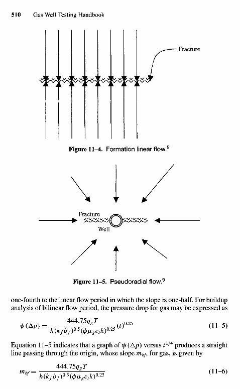
Figure 11-5. Pseudoradial flow.9
one-fourth to the linear flow period in which the slope is one-half. For buildupanalysis of bilinear flow period, the pressure drop for gas may be expressed as
h(kfbf)05^figCtk)025
Equation 11-5 indicates that a graph of ^ (Ap) versus t1^4 produces a straightline passing through the origin, whose slope nib/, for gas, is given by
444.15qgTmbf-hikfbffH^gctk)^ ( 1 1 " 6 )
Well
Fracture
Figure 11-4. Formation linear flow.9
Fracture
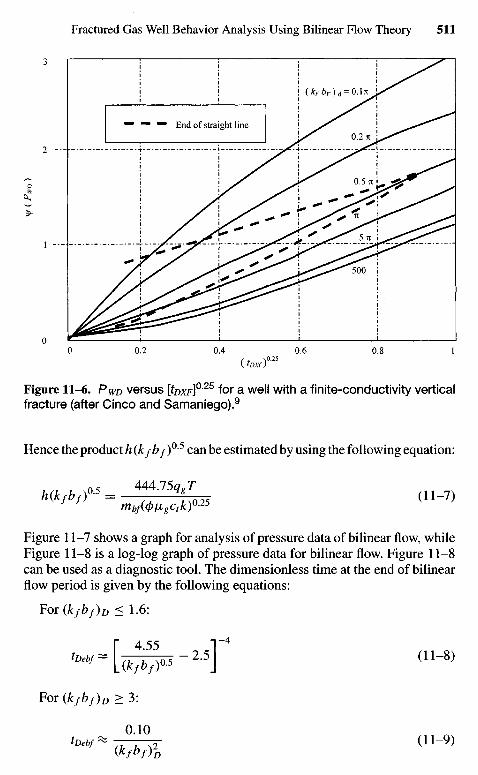
Figure 11-6. PWD versus [toxF]025 for a well with a finite-conductivity verticalfracture (after Cinco and Samaniego).9
Hence the product h (kfbf)0'5 can be estimated by using the following equation:
»» ,» ,?»- ^ 7 5 * * ,11-7)
Figure 11-7 shows a graph for analysis of pressure data of bilinear flow, whileFigure 11-8 is a log-log graph of pressure data for bilinear flow. Figure 11-8can be used as a diagnostic tool. The dimensionless time at the end of bilinearflow period is given by the following equations:
For (kfbf)D < 1.6:
tDebf=h^-Z5Y (11~8)
For (kfbf)D > 3:
0.10tDebf ** TTJT^ (11"9)
(kfbf)D
End of straight line
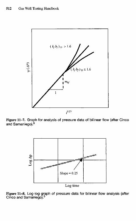
Figure 11-7. Graph for analysis of pressure data of bilinear flow (after Cincoand Samaniego).9
Figure 11-8. Log-log graph of pressure data for bilinear flow analysis (afterCinco and Samaniego).9
Log time
Slope = 0.25
Log
Ap
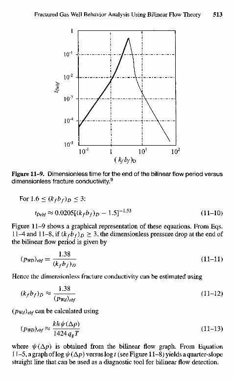
Figure 11-9. Dimensionless time for the end of the bilinear flow period versusdimensionless fracture conductivity.9
For 1.6 < (kfbf)D < 3:
tDebf^0m05[(kfbf)D - 1.5]"L53 (11-10)
Figure 11-9 shows a graphical representation of these equations. From Eqs.11-4 and 11-8, if (kfbf)D > 3, the dimensionless pressure drop at the end ofthe bilinear flow period is given by
(PWD)ebf= , / f 8 (H-Il)
(kfbf)D
Hence the dimensionless fracture conductivity can be estimated using1.38
(kfbf)D™- — (11-12)\Pwd)ebf
(Pwd)ebf can be calculated using
MrJr(Ap)(^*T424^ ( 1 I - 1 3 )
where \jr(Ap) is obtained from the bilinear flow graph. From Equation11-5, a graph of log i// (Ap) versus log t (see Figure 11-8) yields a quarter-slopestraight line that can be used as a diagnostic tool for bilinear flow detection.
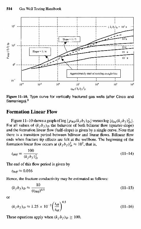
Figure 11-10. Type curve for vertically fractured gas wells (after Cinco andSamaniego).9
Formation Linear Flow
Figure 11-10 shows a graph of log lpwD(kfbf)o} versus log \tDxf(kfbf)2D\.
For all values of (kfbf)D the behavior of both bilinear flow (quarter-slope)and the formation linear flow (half-slope) is given by a single curve. Note thatthere is a transition period between bilinear and linear flows. Bilinear flowends when fracture tip effects are felt at the wellbore. The beginning of theformation linear flow occurs at (k/bf)2
D « 102, that is,
100- ' = ; « a i - i 4 )
The end of this flow period is given by
to,//«0.016
Hence, the fracture conductivity may be estimated as follows:
< w o ~ < ^ < n - i 5 )
or
(t \0"5
(kfbf)D « 1.25 x IO"2/ - ^ ) (11-16)VbIf/
These equations apply when (kfbf)o > 100.
Approximately start of semilog straight-line
Slope = 1 / 4
Slope = 1 / 2
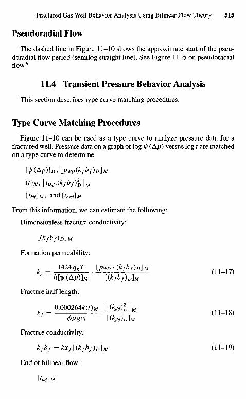
Pseudoradial Flow
The dashed line in Figure 11-10 shows the approximate start of the pseu-doradial flow period (semilog straight line). See Figure 11-5 on pseudoradialflow.9
11.4 Transient Pressure Behavior Analysis
This section describes type curve matching procedures.
Type Curve Matching Procedures
Figure 11-10 can be used as a type curve to analyze pressure data for afractured well. Pressure data on a graph of log \j/(Ap) versus log t are matchedon a type curve to determine
[\jf(Ap)]M, lPWD(kfbf)DjM
(OM, \tDxf.(kfbf)2D\M
[tbif]M, and [WlAf
From this information, we can estimate the following:
Dimensionless fracture conductivity:
l(kfbf)D\M
Formation permeability:
U24qgT lpwD'(kfbf)DjM8 h[ir(Ap)]M [(kfbf)D]M
Fracture half length:
0.000264fc(QAf L(^z)2DJ M m l f i ,Xf = 1 IYf \ 1 (11-15)
Fracture conductivity:
kfbf = kxfl(kfbf)D}M (11-19)
End of bilinear flow:
L%JM
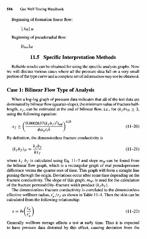
Beginning of formation linear flow:
L hif\ M
Beginning of pseudoradial flow:
[tbsst\M
11.5 Specific Interpretation Methods
Reliable results can be obtained for using the specific analysis graphs. Nowwe will discuss various cases where all the pressure data fall on a very smallportion of the type curve and a complete set of information may not be obtained.
Case 1: Bilinear Flow Type of Analysis
When a log-log graph of pressure data indicates that all of the test data aredominated by bilinear flow (quarter-slope), the minimum value of fracture half-length, Xf, can be estimated at the end of bilinear flow, i.e., for (kfb)o > 3,using the following equation:
> / 0 . O 0 O 2 6 3 7 ( W * , , , A ° *
V (pVgCtk J
By definition, the dimensionless fracture conductivity is
(kfbf)D^~hT (11"21)
where kf b/ is calculated using Eq. 11-7 and slope mbf can be found fromthe bilinear flow graph, which is a rectangular graph of real pseudopressuredifference versus the quarter root of time. This graph will form a straight linepassing through the origin. Deviations occur after some time depending on thefracture conductivity. The slope of this graph, mbf, is used for the calculationof the fracture permeability-fracture width product (kfbf).
The dimensionless fracture conductivity is correlated to the dimensionlesseffective wellbore radius, rf
w/rf as shown in Table 11-1. Then the skin can becalculated from the following relationship:
,=*(£) (H-22)
Generally wellbore storage affects a test at early time. Thus it is expectedto have pressure data distorted by this effect, causing deviation from the
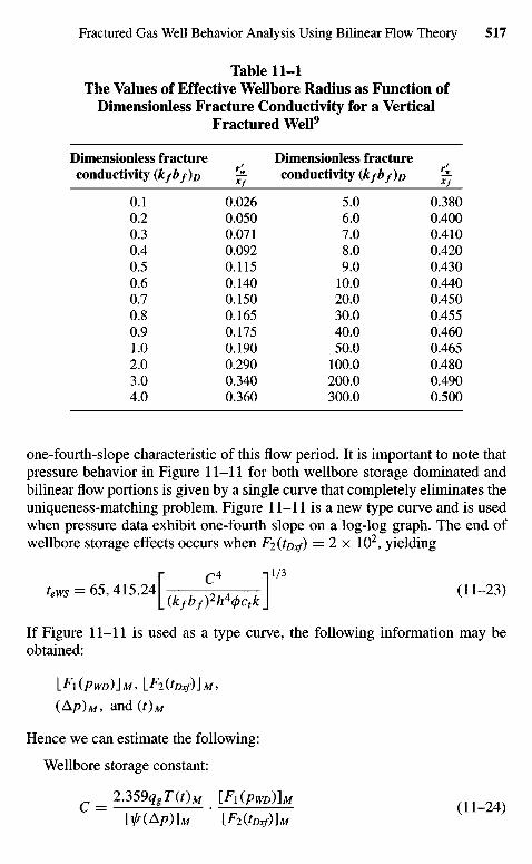
Table 11-1The Values of Effective Wellbore Radius as Function of
Dimensionless Fracture Conductivity for a VerticalFractured Well9
Dimensionless fracture f Dimensionless fractureconductivity (kfbf)o rf- conductivity (kfbf)o rf-
0.1 0.026 5.0 0.3800.2 0.050 6.0 0.4000.3 0.071 7.0 0.4100.4 0.092 8.0 0.4200.5 0.115 9.0 0.4300.6 0.140 10.0 0.4400.7 0.150 20.0 0.4500.8 0.165 30.0 0.4550.9 0.175 40.0 0.4601.0 0.190 50.0 0.4652.0 0.290 100.0 0.4803.0 0.340 200.0 0.4904.0 0.360 300.0 0.500
one-fourth-slope characteristic of this flow period. It is important to note thatpressure behavior in Figure 11-11 for both wellbore storage dominated andbilinear flow portions is given by a single curve that completely eliminates theuniqueness-matching problem. Figure 11-11 is a new type curve and is usedwhen pressure data exhibit one-fourth slope on a log-log graph. The end ofwellbore storage effects occurs when F2{tDxf) = 2 x 10², yielding
r c 4 i1 /3teWS = 65, 415.24 (11-23)
l(kfbf)2h*<l>ctk]
If Figure 11-11 is used as a type curve, the following information may beobtained:
IF\(PWD)\M, YF2(tDxf)\M,
(Ap)M, and (0M
Hence we can estimate the following:
Wellbore storage constant:
= 2 . 3 5 9 ^ 7 ( Q M [ F I ( ^ D ) I M
lf(Ap)]M ' {Fi(tDxf)]M
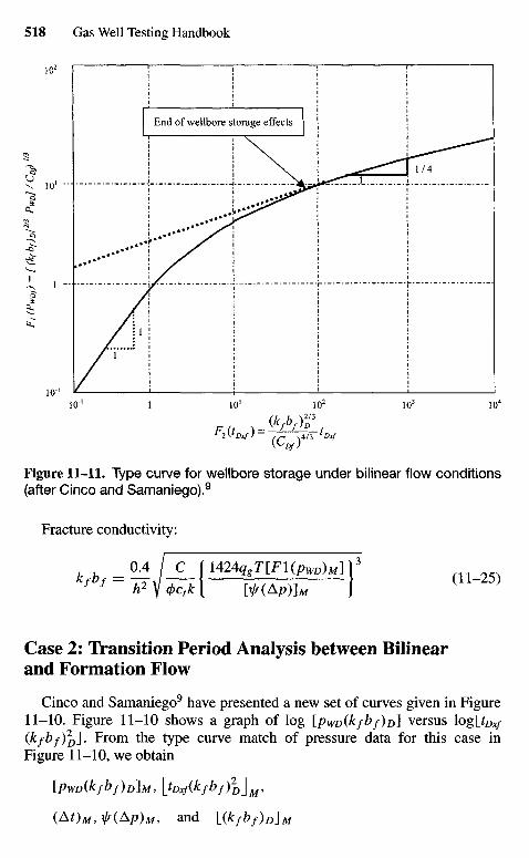
Figure 11-11. Type curve for wellbore storage under bilinear flow conditions(after Cinco and Samaniego).9
Fracture conductivity:
h h 0-4 / C \U24qgT[Fl(pWD)Mn3
k^ = V ^* {—mKpn~M—J (11-25)
Case 2: Transition Period Analysis between Bilinearand Formation Flow
Cinco and Samaniego9 have presented a new set of curves given in Figure11-10. Figure 11-10 shows a graph of log [pwo(kfbf)D] versus log|_fec/(kfbf)2
Dj. From the type curve match of pressure data for this case inFigure 11-10, we obtain
[pwD(kfbf)D]M, [tDxf(kfbf)2D\M,
(At) M ,ir (Ap) M, and V(kfbf)D\M
End of wellbore storage effects
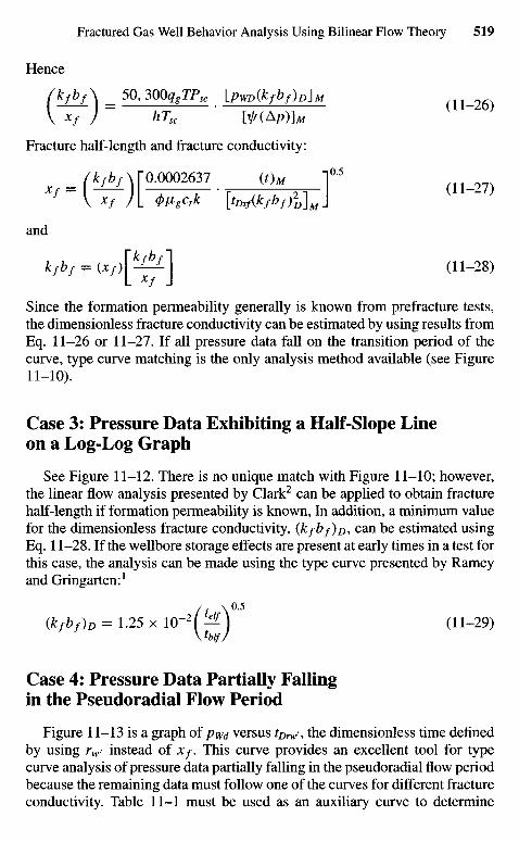
Hence
nfbf\ = 50,3OOqgTPK Ypwp{kfbf)D\uV xf ) hTsc ' [VKAp)]M
Fracture half-length and fracture conductivity:
= nfbf \ f 0.0002637 (O^ I 0 5
V */ /L 0M«C,* [ W * / * / ) D L J
and
*/*/ = (*/) [ ^ ] (11-28)
Since the formation permeability generally is known from prefracture tests,the dimensionless fracture conductivity can be estimated by using results fromEq. 11-26 or 11-27. If all pressure data fall on the transition period of thecurve, type curve matching is the only analysis method available (see Figure11-10).
Case 3: Pressure Data Exhibiting a Half-Slope Lineon a Log-Log Graph
See Figure 11-12. There is no unique match with Figure 11-10; however,the linear flow analysis presented by Clark2 can be applied to obtain fracturehalf-length if formation permeability is known, In addition, a minimum valuefor the dimensionless fracture conductivity, (kfbf)D, can be estimated usingEq. 11-28. If the wellbore storage effects are present at early times in a test forthis case, the analysis can be made using the type curve presented by RameyandGringarten:1
/1 \0'5
(kfbf)D = 1.25 x 10"2I -^ ) (11-29)v«/ /
Case 4: Pressure Data Partially Fallingin the Pseudoradial Flow Period
Figure 11-13 is a graph of pWd versus tDrw>, the dimensionless time definedby using rw> instead of Xf. This curve provides an excellent tool for typecurve analysis of pressure data partially falling in the pseudoradial flow periodbecause the remaining data must follow one of the curves for different fractureconductivity. Table 11-1 must be used as an auxiliary curve to determine
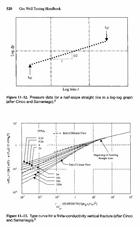
Log time t
Figure 11-12. Pressure data for a half-slope straight line in a log-log graph(after Cinco and Samaniego).9
Figure 11-13. Type curve for a finite-conductivity vertical fracture (after Cincoand Samaniego).9
End of Linear Flow
Beginning of SemilogStraight Line
End of Bilinear Flow
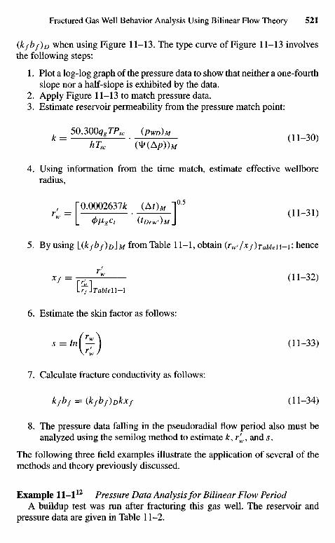
(kfbf)o when using Figure 11-13. The type curve of Figure 11-13 involvesthe following steps:
1. Plot a log-log graph of the pressure data to show that neither a one-fourthslope nor a half-slope is exhibited by the data.
2. Apply Figure 11-13 to match pressure data.3. Estimate reservoir permeability from the pressure match point:
7 _ 50,30Oq8TPx (PWD)Mk~ hTsc '(V(Ap))M ( 1 1 3 U )
4. Using information from the time match, estimate effective wellboreradius,
ro,OOQ2637t ( A Q ^
5. By using L ( ^ / ^ / ) D J M from Table 11-1, obtain (rw>/xf)Tabien-\\ hence
*'=riT*— (11"32)
Lr/ JTable 11-1
6. Estimate the skin factor as follows:
,-*,(£) (11-33,
7. Calculate fracture conductivity as follows:
kfbf = (kfbf)Dkxf (11-34)
8. The pressure data falling in the pseudoradial flow period also must beanalyzed using the semilog method to estimate k, rf
w> and s.
The following three field examples illustrate the application of several of themethods and theory previously discussed.
Example l l - l 1 2 Pressure Data Analysis for Bilinear Flow PeriodA buildup test was run after fracturing this gas well. The reservoir and
pressure data are given in Table 11-2.
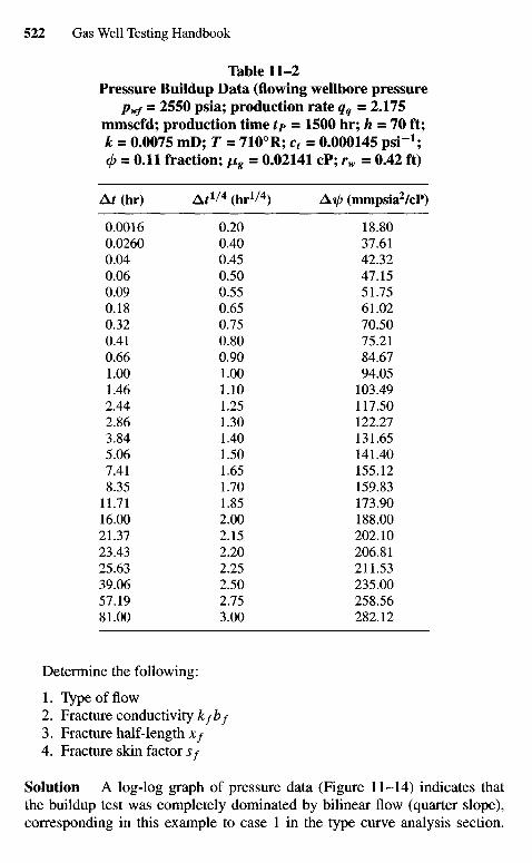
Table 11-2Pressure Buildup Data (flowing wellbore pressure
pwf = 2550 psia; production rate qq = 2.175mmscfd; production time tp = 1500 hr; h = 70 ft;k = 0.0075 mD; T = 7100R; ct = 0.000145 p s i 1 ;</> = 0.11 fraction; /j,g = 0.02141 cP; rw = 0.42 ft)
At (hr) A*1/4 (hr1/4) A ^ (mmpsia2/cP)
0.0016 0.20 18.800.0260 0.40 37.610.04 0.45 42.320.06 0.50 47.150.09 0.55 51.750.18 0.65 61.020.32 0.75 70.500.41 0.80 75.210.66 0.90 84.671.00 1.00 94.051.46 1.10 103.492.44 1.25 117.502.86 1.30 122.273.84 1.40 131.655.06 1.50 141.407.41 1.65 155.128.35 1.70 159.83
11.71 1.85 173.9016.00 2.00 188.0021.37 2.15 202.1023.43 2.20 206.8125.63 2.25 211.5339.06 2.50 235.0057.19 2.75 258.5681.00 3.00 282.12
Determine the following:
1. Type of flow2. Fracture conductivity kfbf3. Fracture half-length x /4. Fracture skin factor Sf
Solution A log-log graph of pressure data (Figure 11-14) indicates thatthe buildup test was completely dominated by bilinear flow (quarter slope),corresponding in this example to case 1 in the type curve analysis section.
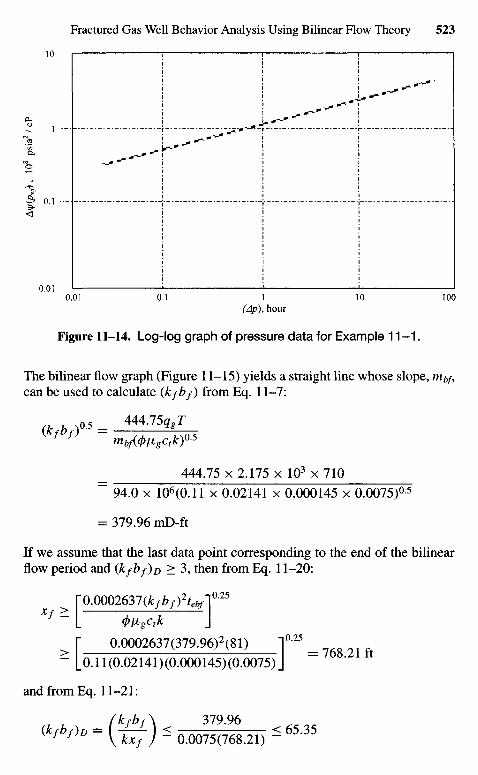
Figure 11-14. Log-log graph of pressure data for Example 11-1.
The bilinear flow graph (Figure 11-15) yields a straight line whose slope, mbf,can be used to calculate (kfbf) from Eq. 11-7:
(t h V>-* _ 444.75ggr
444.75 x 2.175 x IQ3 x 710~ 94.0 x 10⁶(0.11 x 0.02141 x 0.000145 x 0.0075)0-5
= 379.96 mD-ft
If we assume that the last data point corresponding to the end of the bilinearflow period and (kfbf)D > 3, then from Eq. 11-20:
T 0.0002637(A^z)2U/] °'25
L (pligCtk J
> f 0.0002637(379.96)2(81) I 0 2 5
~ L0.11(0.02141)(0.000145)(0.0075)J
and from Eq. 11-21:
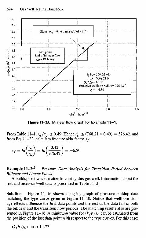
Figure 11-15. Bilinear flow graph for Example 11-1.
From Table 11-1, r'w/xf < 0.49. Hence r'w < (768.21 x 0.49) = 376.42, andfrom Eq. 11-22, calculate fracture skin factor s/i
Example 11-212 Pressure Data Analysis for Transition Period betweenBilinear and Linear Flows
A buildup test was run after fracturing this gas well. Information about thetest and reservoir/well data is presented in Table 11-3.
Solution Figure 11-16 shows a log-log graph of pressure buildup datamatching the type curve given in Figure 11-10. Notice that wellbore stor-age effects influence the first data points and the rest of the data fall in boththe bilinear and the transition flow periods. The matching results also are pre-sented in Figure 11-16. A minimum value for (kfbf)o can be estimated fromthe position of the last data point with respect to the type curves. For this case:
(&/&/)£>min ^ 14.77
/CyA = 379.96 mDXf= 7668.21 ft
(kfbf)D = 65.35Effective wellbore radius = 376.42 ft
Sf= - 6 . 8 0
Last pointEnd of bilinear flow
tet>i = 8 1 hours
Slope, mbf= 94.0 mmpsia2 / cP / hr0 5
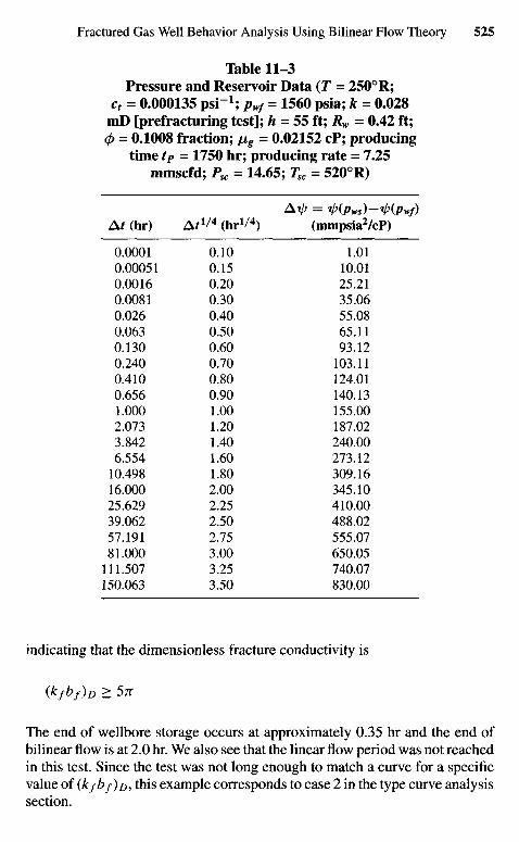
Table 11-3Pressure and Reservoir Data (T = 2500R;
ct = 0.000135 p s i 1 ; pwf = 1560 psia; k = 0.028mD [prefracturing test]; h = 55 ft; Rw = 0.42 ft;(\> = 0.1008 fraction; /j,g = 0.02152 cP; producing
time tP = 1750 hr; producing rate = 7.25mmscfd; Psc = 14.65; Tsc = 5200R)
At/? = i/>(pws)—tl>(Pwf)At (hr) At1/4 (hrx/4) (mmpsia2/cP)
0.0001 0.10 1.010.00051 0.15 10.010.0016 0.20 25.210.0081 0.30 35.060.026 0.40 55.080.063 0.50 65.110.130 0.60 93.120.240 0.70 103.110.410 0.80 124.010.656 0.90 140.131.000 1.00 155.002.073 1.20 187.023.842 1.40 240.006.554 1.60 273.12
10.498 1.80 309.1616.000 2.00 345.1025.629 2.25 410.0039.062 2.50 488.0257.191 2.75 555.0781.000 3.00 650.05
111.507 3.25 740.07150.063 3.50 830.00
indicating that the dimensionless fracture conductivity is
(kfbf)D > 5n
The end of wellbore storage occurs at approximately 0.35 hr and the end ofbilinear flow is at 2.0 hr. We also see that the linear flow period was not reachedin this test. Since the test was not long enough to match a curve for a specificvalue of (kfbf)o, this example corresponds to case 2 in the type curve analysissection.
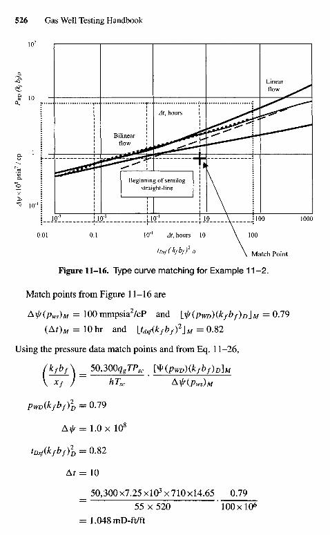
Figure 11-16. Type curve matching for Example 11-2.
Match points from Figure 11-16 are
A\l/(pws)M = 100 mmpsia2/cP and lt(pwD)(kfbf)D\M = 0.79
(AOM = 10 hr and [tdxf{kfbf)2\M = 0.82
Using the pressure data match points and from Eq. 11-26,
/kfbf\ = 5 0 , 3 0 0 ^ ^ mpwp)(kfbf)D]M
V Xf ) hTsc A\l/(pws)M
PwD(kfbf)2D = 0.79
Ax// = 1.0 x 10⁸
tDxf(kfbf)2D = 0.82
At = 10
_ 50,300x7.25 xlO3 x710x14.65 0.79
~" 55 x 520 100 xlO6
= 1.048 mD-ft/ft
Match Point
At, hours
Beginning of semilogstraight-line
Bilinearflow
At, hours
Linearflow
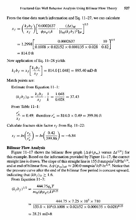
From the time data match information and Eq. 11-27, we can calculate
_ / * / M rO-0002637 (At)M I 0 5
Xf ~~ V Xf )[ <p(igctk [t<kf(kfbf)2]M\
= 1.2998[ °-0 0 0 2 6 3 7 i 0 - ! 0 5
[0.1008 x 0.02152 x 0.000135 x 0.028 0.82 J
= 814.0 ft
Now application of Eq. 11-28 yields
kfbf = xA ^ - \ = 814.0 [1.048] = 895.40mD-ft
Match points are:
Estimate from Equation 11-1:
From Table 11-1:
rf
-^ = 0.49; therefore r'w = 814.0 x 0.49 = 399.86 ftxf
Calculate fracture skin factor s/ from Eq. 11-22:
Bilinear Flow AnalysisFigure 11-17 shows the bilinear flow graph [Ai//(pws) versus Af1^4J for
this example. Based on the information provided by Figure 11-17, the correctstraight line is drawn. The slope of this straight line is 155.0 mmpsia2/cP/hr1/4,and at end of bilinear flow, A\l/(pws)ebi ^ 200.0 mmpsia2/cP-hr1/4. Notice thatthe pressure curve after the end of the bilinear flow period is concave upward,indicating that (kbf)p > 1.6.
From Equation 11-7:
{kfbf) ~ mbA^gctk)025
444.75 x 7.25 x 103 x 710~ 155.0 x 10⁶(0.1008 x 0.02152 x 0.000135 x 0.028)0-25
= 28.21 mD-ft
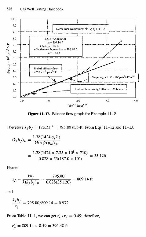
Figure 11-17. Bilinear flow graph for Example 11 - 2 .
Therefore kfbf = (28.21)2 = 795.80 mD-ft. From Eqs. 11-12 and 11-13,
1.38(1424 ftT)(kfbf)D = khAir(Pws)M
_ 1.38(1424 x 7.25 x 103 x 710)0.028 x 55(187.0 x 10⁶) ~ "
Hence
Xf = k(kfbf)D = 0.028(35.126) = 8 ° 9 1 4 ft
and
k-&- = 795.80/809.14 = 0.972xf
From Table 11-1, we can get r'w/xf = 0.49; therefore,
r'w = 809.14 x 0.49 = 396.48 ft
hour
End wellbore storage effects = .35 hours
Slope, mbf= 1.55 xlO8 psia2/cP/hr1/4
End of bilinear flow= 2.0xl08psia2/cP
kfbf= 795.8 md-ftXf= 809.14 ft
(kfbfh = 35.13effective wellbore radius = 396.48 ft
Sy= - 6 . 8 3
Curve concave upwards -> ( kfbf)D > 1.6
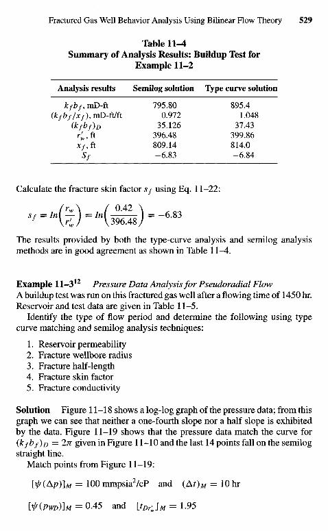
Table 11-4Summary of Analysis Results: Buildup Test for
Example 11-2
Analysis results Semilog solution Type curve solution
kfbf,mD-ft 795.80 895.4(kfbf/xf),mD-fUft 0.972 1.048
(kfbf)D 35.126 37.43r;,ft 396.48 399.86xf, ft 809.14 814.0
Sf -6.83 -6.84
Calculate the fracture skin factor Sf using Eq. 11-22:
The results provided by both the type-curve analysis and semilog analysismethods are in good agreement as shown in Table 11-4.
Example 11-31 2 Pressure Data Analysis for Pseudoradial FlowA buildup test was run on this fractured gas well after a flowing time of 1450 hr.Reservoir and test data are given in Table 11-5.
Identify the type of flow period and determine the following using typecurve matching and semilog analysis techniques:
1. Reservoir permeability2. Fracture wellbore radius3. Fracture half-length4. Fracture skin factor5. Fracture conductivity
Solution Figure 11-18 shows a log-log graph of the pressure data; from thisgraph we can see that neither a one-fourth slope nor a half slope is exhibitedby the data. Figure 11-19 shows that the pressure data match the curve for(kfbf)o = 2TT given in Figure 11-10 and the last 14 points fall on the semilogstraight line.
Match points from Figure 11-19:
[1r(Ap)]M = 100 mmpsia2/cP and ( A O M = 10 hr
№(PWD)]M = 0.45 and U Z ^ J M = 1.95
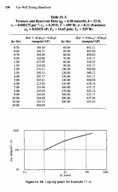
Table 11-5Pressure and Reservoir Data (qg = 6.50 mmscfd; h = 52 ft;
C1 = 0.000175 psi"1; rw = 0.39 ft; T = 6900R; 0 = 0.11 (fraction);fig = 0.02035 cP; Psc = 14.65 psia; Tsc = 5200R)
Alp = ^(Pws)-^(Pwf) Al/? = i/>(pws)-1p(Pwf)At (hr) (mmpsia2/cP) A/ (hr) (mmpsia2/cP)
0.50 105.10 40.00 443.110.60 106.31 50.00 465.000.70 108.05 60.00 490.030.90 120.00 70.00 510.171.00 127.07 80.00 530.221.50 135.02 90.00 545.172.00 150.11 100.00 560.003.50 180.13 120.00 580.174.00 187.17 130.00 592.115.00 205.01 140.00 600.006.00 215.05 150.00 610.187.00 235.00 160.00 615.218.00 245.02 170.00 625.129.00 255.04 180.00 632.11
10.00 264.09 190.00 637.0420.00 355.13 200.00 645.0230.00 400.05
At, hours
Figure 11-18. Log-log graph for Example 11 - 3 .
A y/
, m
mps
ia2 /
cp
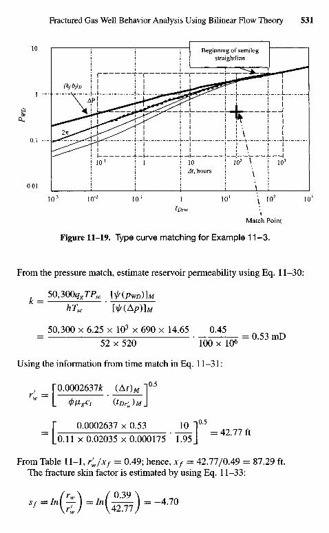
Figure 11-19. Type curve matching for Example 11 - 3 .
From the pressure match, estimate reservoir permeability using Eq. 11-30:
= 50,300qgTPsc [ir(pWD)]M
hTsc ' [Vr(Ap)]M
_ 50,300 x 6.25 x 103 x 690 x 14.65 0.45 _= 52 x 520 100 x 106
Using the information from time match in Eq. 11-31:
, _ r0.0002637fc (AOM I 0 5
= [ 0.0002637 x 0.53 j M ° ' 5 = 4 2 7 7 f t
L 0.11 x 0.02035 x 0.000175 " 1.95 J
From Table 11-1, r'w/xf = 0.49; hence, xf = 42.77/0.49 = 87.29 ft.The fracture skin factor is estimated by using Eq. 11-33:
Match Point
At, hours
Beginning of semilogstraightline
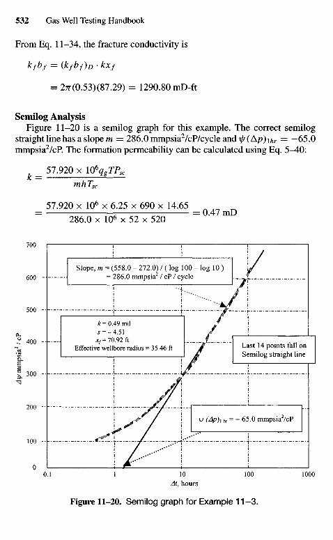
From Eq. 11-34, the fracture conductivity is
k/bf = (kfb/)D - kxf
= 2TT(0.53)(87.29) = 1290.80 mD-ft
Semilog AnalysisFigure 11-20 is a semilog graph for this example. The correct semilog
straight line has a slope m = 286.0mmpsia2/cP/cycleandi/r(A/?)i/ir = —65.0mmpsia2/cP. The formation permeability can be calculated using Eq. 5-40:
_ 57.920 x \06qgTPsc
mhTsc
_ 57.920 x 106 x 6.25 x 690 x 14.65 _~ 286.0 x 106 x 52 x 520 " ' m
Slope, m = (558.0 - 272.0) / ( log 100 - log 10 )= 286.0 mmpsia2 / cP / cycle
£ = 0.49mds = -4 .51
X7= 70.92 ftEffective wellbore radius = 35.46 ft Last 14 points fall on
Semilog straight line
\\J (Ap)i hr = - 65.0 mmpsia2/cP
A \f/
mm
psia
/ c
P
At, hours
Figure 11-20. Semilog graph for Example 11-3.
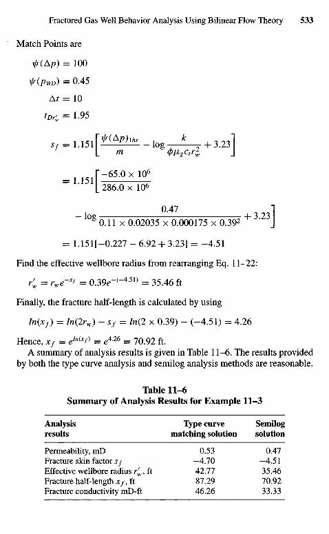
Match Points are
ir (Ap) = 100
Ir (Pm)=O .45
At = 10
tDr'w = 1.95
\xjf(Ap)lhr k , , - o / |Sf = 1.151 log- + 3.23
L m 4>V>gctrl J_ r-65.0xl0^
" L 286.0 xlO6
0.47 "I
~~ 1Og 0.11 x 0.02035 x 0.000175 x 0.392 + 3 J
= 1.151[-0.227 - 6.92 + 3.23] = -4.51
Find the effective wellbore radius from rearranging Eq. 11-22:
r'w = rwe~sf = 0.39^"("4-51) = 35.46 ft
Finally, the fracture half-length is calculated by using
In(xf) = In(2rw) - sf = In(I x 0.39) - (-4.51) = 4.26
Hence, xf = e1"^ = e426 = 70.92 ft.A summary of analysis results is given in Table 11-6. The results provided
by both the type curve analysis and semilog analysis methods are reasonable.
Table 11-6Summary of Analysis Results for Example 11-3
Analysis Type curve Semilogresults matching solution solution
Permeability, mD 0.53 0.47Fracture skin factor Sf -4 .70 -4 .51Effective wellbore radius rr
w, ft 42.77 35.46Fracture half-length JC/, ft 87.29 70.92Fracture conductivity mD-ft 46.26 33.33
From these examples it is demonstrated that type-curve matching analysis,when applied properly, provides an excellent diagnostic tool and a techniqueto estimate both reservoir and fracture parameters.
11.6 Summary
Based on the material presented in this chapter, the following remarks arepertinent:
• A new technique is presented to analyze data in the bilinear flow period.It is shown that, during this flow period, a graph of x//(pwf) versus /1 / 4
yields a straight line when slope is inversely proportional to hf(kfbf)1^2.• New type curves are now available for pressure analysis of fractured gas
wells, and the problems in the analysis are reduced considerably with theuse of these type curves.
• Prefracture information about the reservoir is necessary to estimate frac-ture parameters.
• The type curve analysis method must be used simultaneously with the spe-cific analysis methods ^/(pwf) versus t1^4, \/f(pwf) versus £1/2, and ^(pWf)versus log t to produce reliable results.
References and Additional Reading
1. Ramey, H. J., Jr., and Gringarten, A. C , "Effect of High-Volume VerticalFractures in Geothermal Steam Well Behavior," Proc. Second United Na-tions Symposium on the Use and Development of GeothermaLEnergy, SanFrancisco, May 20-29, 1975.
2. Clark, K. K., "Transient Pressure Testing of Fractured Water InjectionWells," J. Petroleum Technol. (June 1968) 639-643; Trans. AIME 243.
3. Raghavan, R., Cady, G. V, and Ramey, H. J., Jr., "Well Test Analysis forVertically Fractured Wells," / Petroleum Technol. (1972) 24, 1014-1020.
4. Pressure Transient Testing Methods, SPE Reprint Series No. 1, Society ofPetroleum Engineers, Dallas, TX, 1980.
5. Gringarten, A. C , Ramey, H. J., Jr., and Raghavan, R., "Applied PressureAnalysis for Fractured Wells," /. Petroleum Technol. (July 1975) 887-892;Trans. AIME 259.
6. Wattenbarger, R. A., and Ramey, H. J., Jr., "Well Test Interpretations ofVertically Fractured Gas Wells," /. Petroleum Technol (May 1969) 625-633; Trans. AIME 246.
7. Raghavan, R., Cady, G. V, and Ramey, H. J., Jr., "Well Test Analysis forVertically Fractured Wells,"/. Petroleum Technol. (Aug. 1972) 1014-1020;Trans. AIME 253.
8. Scott, J., "The Effect of Vertical Fractures in Transient Pressure Behaviorof Wells,"/. Petroleum Technol. (Dec. 1963) 1365-1369; Trans. AIME 228.
9. Cinco, H., and Samaniego, R, "Effect of Wellbore Storage and Damageon the Transient Pressure Behavior for a Well with a Finite-ConductivityVertical Fracture," Soc. Petroleum Eng. J. (Aug. 1978) 53-264.
10. Gringarten, A. C, Ramey, H. J., Jr., and Raghavan, R., "Applied PressureAnalysis for Fractured Wells," /. Petroleum Technol. (1975) 17, 887-892.
11. Earlougher, R. C, Jr., and Kerch, K. M., "Analysis of Short-Time Tran-sient Test Data by Type-Curve Matching," /. Petroleum Technol. (1974) 26,793-800.
12. Amanat U. C, Pressure Transient Test Analysis User's Handbook, Vol. 8,Advanced TWPSOM Systems Inc., Houston, TX, Oct. 1995.

Chapter 12
PracticalApplication ofInterference andPulse Tests
12.1 Introduction
This chapter discusses two well-testing techniques not yet discussed in thetext: interference tests and pulse tests. This chapter also discusses variouscross plotting techniques, the appearance of common flow regimes, log-logdiagnostic, Horner, and specialized plots, and their field applications. Detailsand supporting materials are also presented in this chapter for the benefit ofthose who would like to learn more.
12.2 Interference Test Analysis Techniques
Interference tests are used to determine whether two or three wells are inpressure communication (i.e., in the same reservoir) and, when communicationexists, to provide estimates of permeability k and porosity/compressibilityproduct cj)ct in the vicinity of the tested well. Convenient analysis techniquesfor interference tests are the use of type curves. Figure 12-1 shows these typecurves, presented by Earlougher,4 which are plot of the logarithm of pD (rD, tD)versus the logarithm of to/r^,. Using the following equations generate thesetype curves:
PD«D, rD) = - 1 £ Y ~ ° ^ S M (12-1)
or
PDHD, rD) = l-[ln(tD/r2D) + 0.80907] (12-2)
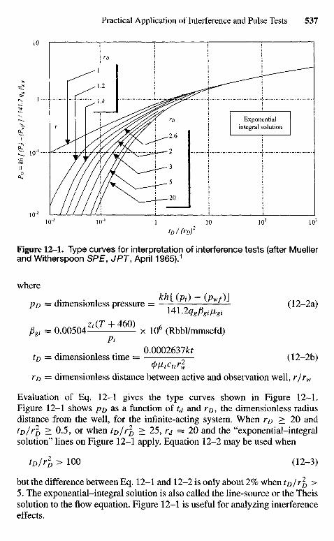
Figure 12-1. Type curves for interpretation of interference tests (after Muellerand Witherspoon SPE, JPT, April 1965).1
where
PD = dimensionless pressure = — — (12-2a)Ul.2qgpgitigi
Pgi = 0 .00504 Z / ( r + 4 6 0 ) x 106 (Rbbl/mmscfd)Pi
. 1 0.0002637**tD = dimensionless time = — (12-2b)
<t>№tirlrD = dimensionless distance between active and observation well, r/rw
Evaluation of Eq. 12-1 gives the type curves shown in Figure 12-1.Figure 12-1 shows pn as a function of td and r/>, the dimensionless radiusdistance from the well, for the infinite-acting system. When rD > 20 andtul^D > 0.5, or when W D > 25, rd = 20 and the "exponential-integralsolution" lines on Figure 12-1 apply. Equation 12-2 may be used when
tD/r2
D > 100 (12-3)
but the difference between Eq. 12-1 and 12-2 is only about 2% when to/r^ >5. The exponential-integral solution is also called the line-source or the Theissolution to the flow equation. Figure 12-1 is useful for analyzing interferenceeffects.
Exponentialintegral solution
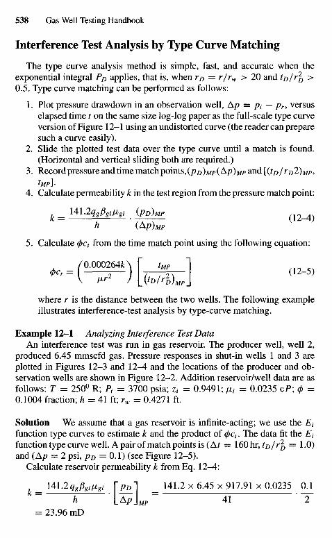
Interference Test Analysis by Type Curve Matching
The type curve analysis method is simple, fast, and accurate when theexponential integral PD applies, that is, when rD = r/rw > 20 and tolr\ >0.5. Type curve matching can be performed as follows:
1. Plot pressure drawdown in an observation well, Ap — pt — pr, versuselapsed time / on the same size log-log paper as the full-scale type curveversion of Figure 12-1 using an undistorted curve (the reader can preparesuch a curve easily).
2. Slide the plotted test data over the type curve until a match is found.(Horizontal and vertical sliding both are required.)
3. Record pressure and time match points,(pD)MP(Ap)Mp and [(tr>/rD2)MP,tMpl
4. Calculate permeability k in the test region from the pressure match point:
k = 141.2gg^g l- (PD)MP
h (Ap)MP
5. Calculate (pct from the time match point using the following equation:
/0.000264*^ [ tMP "I$ct = -— 2 , (12-5)
where r is the distance between the two wells. The following exampleillustrates interference-test analysis by type-curve matching.
Example 12-1 Analyzing Interference Test DataAn interference test was run in gas reservoir. The producer well, well 2,
produced 6.45 mmscfd gas. Pressure responses in shut-in wells 1 and 3 areplotted in Figures 12-3 and 12—4 and the locations of the producer and ob-servation wells are shown in Figure 12-2. Addition reservoir/well data are asfollows: T = 250° R; P1 = 3700 psia; zt = 0.9491; /X1- = 0.0235 cP; 0 =0.1004 fraction; h = 41 ft; rw = 0.4271 ft.
Solution We assume that a gas reservoir is infinite-acting; we use the £,-function type curves to estimate k and the product of (pct. The data fit the Et
function type curve well. A pair of match points is (A^ = 160hr, to/r^ = 1.0)and (Ap = 2 psi, pp = 0.1) (see Figure 12-5).
Calculate reservoir permeability k from Eq. 12-4:
_ U1.2qgpgiiigi \PDI _ 141.2 x 6.45 x 917.91 x 0.0235 0.1= h L PLP = 41 ~2~= 23.96 mD
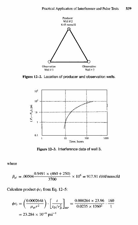
Figure 12-3. Interference data of well 3.
where
figl = Q05040-9491 x (460 + 250) y ^ = ^ 9 1 , ^ -
3/UU
Calculate product 0c, from Eq. 12-5:
__ /0.000264fc\ I" t 1 _ 0.000264 x 23.96 1600 Q " V Hgir2 ) ' L W ^ J M P ~ 0.0235 x 1360^ ' " T
= 23.284 x 10"6 psi~l
Time, hours
Observation ObservationWell # 1 Well # 3
Figure 12-2. Location of producer and observation wells.
ProducerWell # 2
6.45 mmscfd
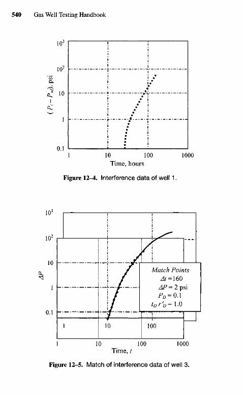
Time, hours
Figure 12-4. Interference data of well 1.
Time, /
Figure 12-5. Match of interference data of well 3.
Match Points4/=160
AP = 2 psiPD = OA
tDr'D= 1.0
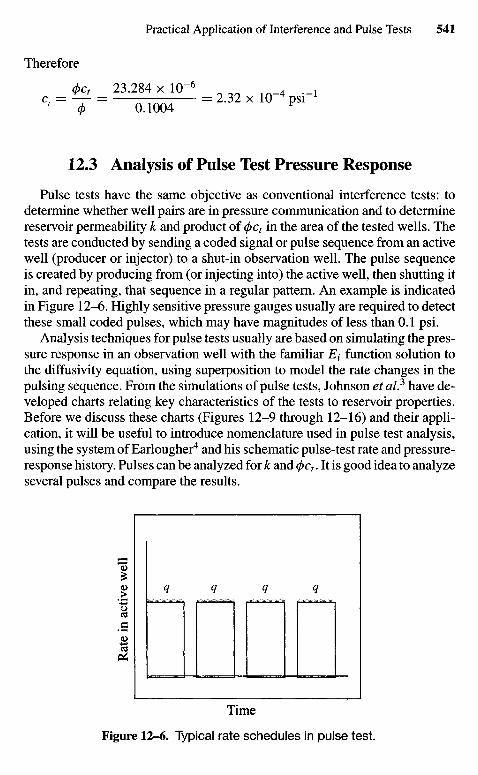
Therefore
0c, 23.284 x 10~6 ^ 4 . ,c = — = = 2.32 x 10"4 psi"1
0 0.1004 F
12.3 Analysis of Pulse Test Pressure Response
Pulse tests have the same objective as conventional interference tests: todetermine whether well pairs are in pressure communication and to determinereservoir permeability k and product of (j)ct in the area of the tested wells. Thetests are conducted by sending a coded signal or pulse sequence from an activewell (producer or injector) to a shut-in observation well. The pulse sequenceis created by producing from (or injecting into) the active well, then shutting itin, and repeating, that sequence in a regular pattern. An example is indicatedin Figure 12-6, Highly sensitive pressure gauges usually are required to detectthese small coded pulses, which may have magnitudes of less than 0.1 psi.
Analysis techniques for pulse tests usually are based on simulating the pres-sure response in an observation well with the familiar E1 function solution tothe diffusivity equation, using superposition to model the rate changes in thepulsing sequence. From the simulations of pulse tests, Johnson et al? have de-veloped charts relating key characteristics of the tests to reservoir properties.Before we discuss these charts (Figures 12-9 through 12-16) and their appli-cation, it will be useful to introduce nomenclature used in pulse test analysis,using the system of Earlougher4 and his schematic pulse-test rate and pressure-response history. Pulses can be analyzed for k and (pct. It is good idea to analyzeseveral pulses and compare the results.
Time
Figure 12-6. Typical rate schedules in pulse test.
Rat
e in
act
ive
wel
l
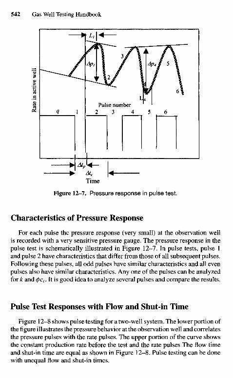
Figure 12-7. Pressure response In pulse test.
Characteristics of Pressure Response
For each pulse the pressure response (very small) at the observation wellis recorded with a very sensitive pressure gauge. The pressure response in thepulse test is schematically illustrated in Figure 12-7. In pulse tests, pulse 1and pulse 2 have characteristics that differ from those of all subsequent pulses.Following these pulses, all odd pulses have similar characteristics and all evenpulses also have similar characteristics. Any one of the pulses can be analyzedfor k and (pct. It is good idea to analyze several pulses and compare the results.
Pulse Test Responses with Flow and Shut-in Time
Figure 12-8 shows pulse testing for a two-well system. The lower portion ofthe figure illustrates the pressure behavior at the observation well and correlatesthe pressure pulses with the rate pulses. The upper portion of the curve showsthe constant production rate before the test and the rate pulses The flow timeand shut-in time are equal as shown in Figure 12-8. Pulse testing can be donewith unequal flow and shut-in times.
Time
Pulse number
Rat
e in
act
ive
wel
l
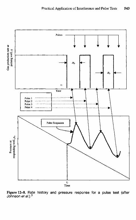
Time
Figure 12-8. Rate history and pressure response for a pulse test (afterJohnson et a/.).3
Pulse Responses
Pulse 1Pulse 2Pulse 3Pulse 4
Pulses
Gas
pro
duct
ion
rat
e at
puls
ing
wel
l, q
Pre
ssur
e at
resp
ondi
ng w
ell,
p w
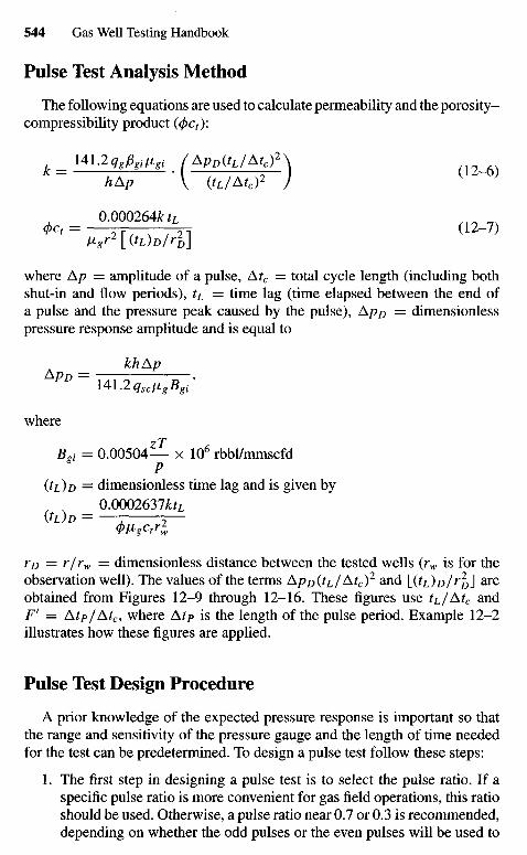
Pulse Test Analysis Method
The following equations are used to calculate permeability and the porosity-compressibility product (0cr):
k = —hETp { fe/AO2 ) (12"6)
0.000264£;L
0 ^ = 2 r 2 1 (12-7)
where A/7 = amplitude of a pulse, Atc = total cycle length (including bothshut-in and flow periods), tL = time lag (time elapsed between the end ofa pulse and the pressure peak caused by the pulse), ApD = dimensionlesspressure response amplitude and is equal to
_ khApAPD " U1.2qscvgBgi'
where
Bgi = 0.00504— x 106 rbbl/mmscfd
OL)D = dimensionless time lag and is given by0.0002637foL
VL)D = T 9
rD = r/rw = dimensionless distance between the tested wells (rw is for theobservation well). The values of the terms ApD(tL/ Atc)
2 and L (^L)D/^ - I ^^obtained from Figures 12-9 through 12-16. These figures use t^lAtc andF' = Atp/ Atc, where A^p is the length of the pulse period. Example 12-2illustrates how these figures are applied.
Pulse Test Design Procedure
A prior knowledge of the expected pressure response is important so thatthe range and sensitivity of the pressure gauge and the length of time neededfor the test can be predetermined. To design a pulse test follow these steps:
1. The first step in designing a pulse test is to select the pulse ratio. If aspecific pulse ratio is more convenient for gas field operations, this ratioshould be used. Otherwise, a pulse ratio near 0.7 or 0.3 is recommended,depending on whether the odd pulses or the even pulses will be used to
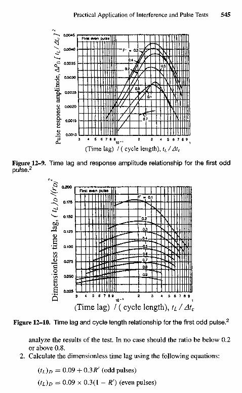
Figure 12-10. Time lag and cycle length relationship for the first odd pulse.2
analyze the results of the test. In no case should the ratio be below 0.2or above 0.8.
2. Calculate the dimensionless time lag using the following equations:
(tL)D = 0.09 + 03Rf (odd pulses)
(tL)D = 0.09 x 0.3(1 - /?') (even pulses)
IU I
(Time lag) / ( cycle length), tL / Atc
Dim
ensi
onle
ss t
ime
lag,
(t
i)oH
rD^
Figure 12-9. Time lag and response amplitude relationship for the first oddpulse.2
(Time lag) / ( cycle length), tL/Atc
Puls
e re
spon
se a
mpl
itude
, A
Pp
[ t L
/ A
t cJ
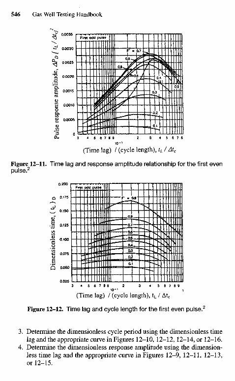
(Time lag) / (cycle length), tL / Atc
Figure 12-12. Time lag and cycle length for the first even pulse.2
3. Determine the dimensionless cycle period using the dimensionless timelag and the appropriate curve in Figures 12-10, 12-12, 12-14, or 12-16.
4. Determine the dimensionless response amplitude using the dimension-less time lag and the appropriate curve in Figures 12-9, 12-11, 12-13,or 12-15.
(Time lag) / (cycle length), tL/Atc
Figure 12-11. Time lag and response amplitude relationship for the first evenpulse.2
Puls
e re
spon
se a
mpl
itud
e, A
PD [
t L/
At c
/D
imen
sion
less
tim
e, (
t L )
D
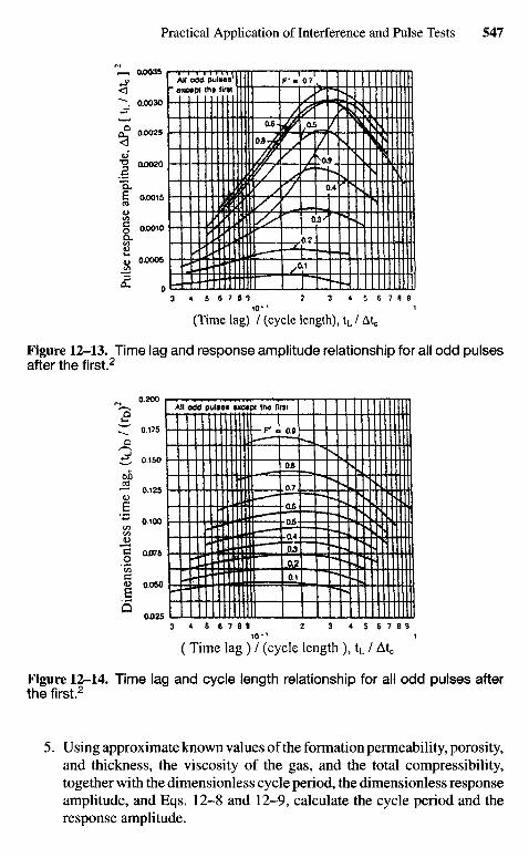
( Time lag ) / (cycle length ), tL / Atc
Figure 12-14. Time lag and cycle length relationship for all odd pulses afterthe first.2
5. Using approximate known values of the formation permeability, porosity,and thickness, the viscosity of the gas, and the total compressibility,together with the dimensionless cycle period, the dimensionless responseamplitude, and Eqs. 12-8 and 12-9, calculate the cycle period and theresponse amplitude.
io-1 i(Time lag) / (cycle length), tL / Atc
Figure 12-13. Time lag and response amplitude relationship for all odd pulsesafter the first.2
Puls
e re
spon
se a
mpl
itud
e, A
P0 [
tL /
At^.
]2
Dim
ensi
onle
ss t
ime
lag
, (t
L) D
/ (r
D)2
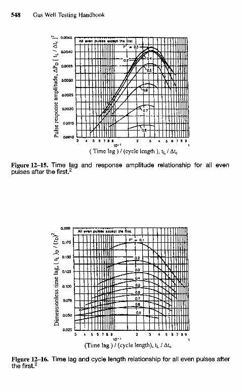
(Time lag ) / (cycle length ), tL / Atc
Figure 12-15. Time lag and response amplitude relationship for all evenpulses after the first.2
(Time lag ) / (cycle length), tL / Atc
Figure 12-16. Time lag and cycle length relationship for all even pulses afterthe first.2
Puls
e re
spon
se a
mpl
itud
e, A
PD [
tL /
At<.
]2
Dim
ensi
onle
ss t
ime
lag,
(t L
)D
/ (r
o)
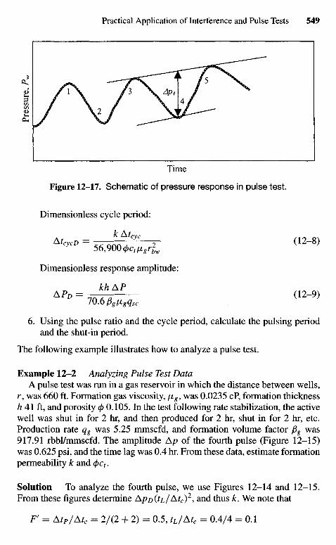
Time
Figure 12-17. Schematic of pressure response in pulse test.
Dimensionless cycle period:
At = k A t ^ ( 12-8)
cycD 56,900<j,ctfigrl
Dimensionless response amplitude:
A f D _ ^ ^ ( 1 M )
70.6pgfigqsc
6. Using the pulse ratio and the cycle period, calculate the pulsing periodand the shut-in period.
The following example illustrates how to analyze a pulse test.
Example 12-2 Analyzing Pulse Test DataA pulse test was run in a gas reservoir in which the distance between wells,
r, was 660 ft. Formation gas viscosity, \±g, was 0.0235 cP, formation thicknessh 41 ft, and porosity (p 0.105. In the test following rate stabilization, the activewell was shut in for 2 hr, and then produced for 2 hr, shut in for 2 hr, etc.Production rate qg was 5.25 mmscfd, and formation volume factor fig was917.91 rbbl/mmscfd. The amplitude Ap of the fourth pulse (Figure 12-15)was 0.625 psi, and the time lag was 0.4 hr. From these data, estimate formationpermeability k and (j>ct.
Solution To analyze the fourth pulse, we use Figures 12-14 and 12-15.From these figures determine ApD(tL/Atc)
2, and thus k. We note that
Fr = Atp/Atc = 2/(2 + 2) = 0.5, tL/Atc = 0.4/4 = 0.1
Pres
sure
, P^
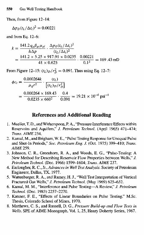
Then, from Figure 12-14:
ApD(tL/Atc)2 = 0.00221
and from Eq. 12-6:
k = U1.2qgpgiiigi ApD(tL/Atc)2
hAp ' (tL/Atc)2
141.2 x 5.25 x 917.91 x 0.0235 0.00221
= ?nro625 o¥~ = mA3mD
From Figure 12-15: (tL)D/r2D = 0.091. Thus using Eq. 12-7:
_ 0.000264fc fa)
0.000264 x 169.43 0.4 fi ,= 0.0235 x 660^ ' OQ9T = 1 9 ' 2 1 X 1 0 PSi
References and Additional Reading
1. Mueller, T. D., and Witherspoon, RA., "Pressure Interference Effects withinReservoirs and Aquifers," J. Petroleum Technol. (April 1965) 471^4-74;Trans. AIME 234.
2. Kamal, M., and Brigham, W. E., "Pulse Testing Response for Unequal Pulseand Shut-In Periods," Soc. Petroleum Eng. J. (Oct. 1975) 399^10; Trans.AIME 259.
3. Johnson, C. R., Greenhorn, R. A., and Woods, E. G., "Pulse-Testing: ANew Method for Describing Reservoir Flow Properties between Wells," J.Petroleum Technol. (Dec. 1966) 1599-1604; Trans. AIME 231.
4. Earlougher, R. C, Jr., Advances in Well Test Analysis. Society of PetroleumEngineers, Dallas, TX, 1977.
5. Wattenbarger, R. A., and Ramey, H. J., "Well Test Interpretation of VerticalFractured Gas Wells " /. Petroleum Technol. (May 1969) 625-632.
6. Kamal, M. M., "Interference and Pulse Testing—A Review," /. PetroleumTechnol (Dec. 1983) 2257-2270.
7. Katsner, F. E., "Effects of Linear Boundaries on Pulse Testing." M.Sc.Thesis, Colorado School of Mines, 1970.
8. Matthews, C. S., and Russell, D. G., Pressure Build-up and Flow Tests inWells. SPE of AIME Monograph, Vol. 1, 25, Henry Doherty Series, 1967.
Chapter 13
Well TestingTerminologyin MultilayeredReservoir Systems
13.1 Introduction
This chapter discusses various types and testing of gas layered reservoirsystems including multilayered responses in fractured reservoirs. It also de-scribes crossflow identification and the nature and degree of communicationbetween layers. Performance equations for cases of constant flowing pres-sure and constant producing rate are presented and discussed. The chapteralso reviews "layer effect" on pressure and/or production behavior includingeconomic aspects of interlayer crossflow.
13.2 Classification of Layered Reservoir Systems
Layered reservoirs can be classified into four groups.
Crossflow Reservoirs
Figure 13-1 shows a crossflow reservoir, which consists of four continu-ous layers that are communicating at the contact planes. These layers are notentirely separated by impervious layers, therefore interlayer crossflow couldoccur during the test. The crossflow would be directed from the layer of lowpermeability to the layer of higher permeability, as shown in the figure. If k\is greater than k^ , then the pressure transients would travel faster in the layerof permeability k\ than in the layer of permeability k^. The duration of thecrossflow periods depends on the storage of each layer. If the storage of thelayer of permeability k\ is negligible when compared to the storage of the layerof permeability fe, then the crossflow will continue throughout the life of the
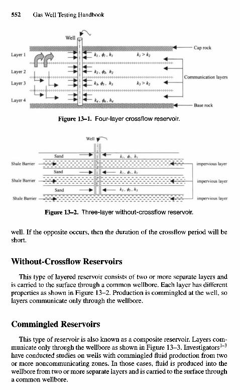
Figure 13-2. Three-layer without-crossflow reservoir.
well. If the opposite occurs, then the duration of the crossflow period will beshort.
Without-Crossflow Reservoirs
This type of layered reservoir consists of two or more separate layers andis carried to the surface through a common wellbore. Each layer has differentproperties as shown in Figure 13-2. Production is commingled at the well, solayers communicate only through the wellbore.
Commingled Reservoirs
This type of reservoir is also known as a composite reservoir. Layers com-municate only through the wellbore as shown in Figure 13-3. Investigators1"3
have conducted studies on wells with commingled fluid production from twoor more noncommunicating zones. In those cases, fluid is produced into thewellbore from two or more separate layers and is carried to the surface througha common wellbore.
impervious layer
impervious layer
impervious layer
Shale Barrier
Shale Barrier
Shale Barrier
Sand
Sand
Sand
Well
Figure 13-1. Four-layer crossflow reservoir.
Base rock
Communication layers
Cap rock
Layer 1
Layer 2
Layer 3
Layer 4
Well
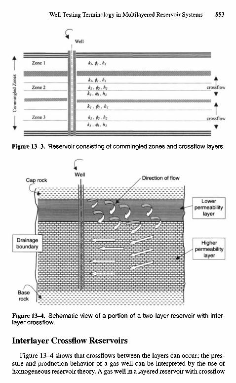
Figure 13-4. Schematic view of a portion of a two-layer reservoir with inter-layer crossflow.
Interlayer Crossflow Reservoirs
Figure 13^4 shows that crossflows between the layers can occur; the pres-sure and production behavior of a gas well can be interpreted by the use ofhomogeneous reservoir theory. A gas well in a layered reservoir with crossflow
Baserock
Drainageboundary
Higherpermeability
layer
Lowerpermeability
layer
Direction of flowWell
Cap rock
Figure 13-3. Reservoir consisting of commingled zones and crossflow layers.
crossflow
crossflow
Well
Zone 1
Zone 2
Zone 3
Com
min
gled
Zon
es
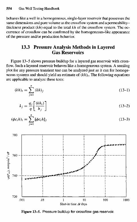
behaves like a well in a homogeneous, single-layer reservoir that possesses thesame dimensions and pore volume as the crossflow system and a permeability-thickness product (kh) equal to the total kh of the crossflow system. The oc-currence of crossflow can be confirmed by the homogeneous-like appearanceof the pressure and/or production behavior.
133 Pressure Analysis Methods in LayeredGas Reservoirs
Figure 13-5 shows pressure buildup for a layered gas reservoir with cross-flow. Such a layered reservoir behaves like a homogeneous system. A semilogplot for any pressure transient test can be analyzed just as it can for homoge-neous systems and should yield an estimate of (kh)t. The following equationsare applicable to analyze these tests:
n
(kh), = J2 Wj (13-Dj=i
n
(4>Cth)t = J2 McMj (13~3)7 = 1
Shut-in time At days
Figure 13-5. Pressure buildup for crossflow gas reservoir.
V(PW
S)J
mm
psi
a2 /
cP
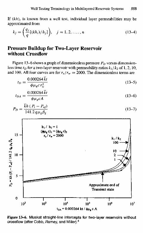
If {kh )t is known from a well test, individual layer permeabilities may beapproximated from
kj = (—[(kht)/hj]\, ./ = l , 2 , . . . . , n (13-4)
Pressure Buildup for Two-Layer Reservoirwithout Crossflow
Figure 13-6 shows a graph of dimensionless pressure Po versus dimension-less time to for a two-layer reservoir with permeability ratios k\ / ki of 1,2,10,and 100. All four curves are for re/rw = 2000. The dimensionless terms are
0.000264**tD = — — (13-5)
0.000264 kttDA = — -r- (13-6)
(frfigcAkh ( Pt - PJ)
p» = 140^7 <13-7)
tDA - 0.000264 kt / ^ c A
Figure 13-6. Muskat straight-line intercepts for two-layer reservoirs withoutcrossflow (after Cobb, Ramey, and Miller).4
Approximate end ofTransient state
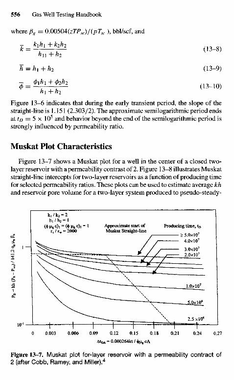
where pg = 0.00504(zTPsc)/(pTsc ), bbl/scf, and
All +/?2
h = hi+ h2 (13-9)
hi +h2
Figure 13-6 indicates that during the early transient period, the slope of thestraight-line is 1.151 (2.303/2). The approximate semilogarithmic period endsat to — 5 x 10⁵ and behavior beyond the end of the semilogarithmic period isstrongly influenced by permeability ratio.
Muskat Plot Characteristics
Figure 13-7 shows a Muskat plot for a well in the center of a closed two-layer reservoir with a permeability contrast of 2. Figure 13-8 illustrates Muskatstraight-line intercepts for two-layer reservoirs as a function of producing timefor selected permeability ratios. These plots can be used to estimate average khand reservoir pore volume for a two-layer system produced to pseudo-steady-
AtDA = 0.000264kt / ^ cA
Figure 13-7. Muskat plot for-layer reservoir with a permeability contract of2 (after Cobb, Ramey, and Miller).4
Producing time, tDApproximate start ofMuskat Straight-line
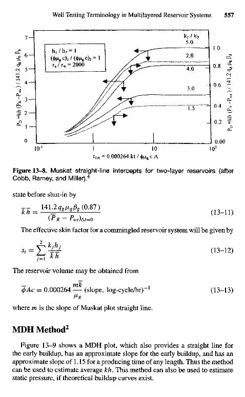
Figure 13-8. Muskat straight-line intercepts for two-layer reservoirs (afterCobb, Ramey, and Miller).4
state before shut-in by
u = HlJ2w.fi, (0-87) ( 1 3 _ n )
(PR ~ Pws)At=o
The effective skin factor for a commingled reservoir system will be given by
The reservoir volume may be obtained from
$Ac = 0.000264 — (slope, log-cycle/hr)"1 (13-13)
where m is the slope of Muskat plot straight line.
MDH Method2
Figure 13-9 shows a MDH plot, which also provides a straight line forthe early buildup, has an approximate slope for the early buildup, and has anapproximate slope of 1.15 for a producing time of any length. Thus the methodcan be used to estimate average kh. This method can also be used to estimatestatic pressure, if theoretical buildup curves exist.
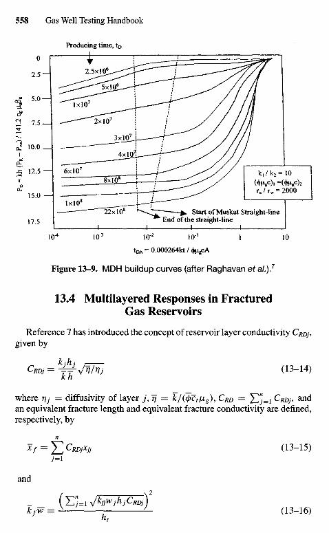
Figure 13-9. MDH buildup curves (after Raghavan et a/.).7
13.4 Multilayered Responses in FracturedGas Reservoirs
Reference 7 has introduced the concept of reservoir layer conductivity CRDJ,given by
Cm = J=-^Nj (13-14)
where r\j = diffusivity of layer j , rj = k/((f)ctiiig), CRD = Y^=I CRDJ, andan equivalent fracture length and equivalent fracture conductivity are defined,respectively, by
n
Xf = ] P CRDjxjj (13-15)
and
kfw = '— (13-16)
Start of Muskat Straight-lineEnd of the straight-line
Producing time, tD
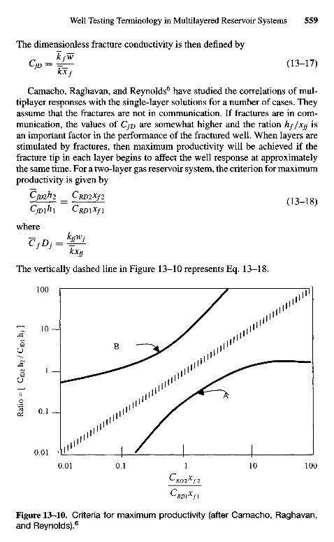
The dimensionless fracture conductivity is then defined by
CfD = & * (13-17)KXf
Camacho, Raghavan, and Reynolds6 have studied the correlations of mul-tiplayer responses with the single-layer solutions for a number of cases. Theyassume that the fractures are not in communication. If fractures are in com-munication, the values of CfD are somewhat higher and the ration hf/xjj isan important factor in the performance of the fractured well. When layers arestimulated by fractures, then maximum productivity will be achieved if thefracture tip in each layer begins to affect the well response at approximatelythe same time. For a two-layer gas reservoir system, the criterion for maximumproductivity is given by
CfQ2H2 _ CRD2Xf2
——— — — ^ o--i o;LfD\n\ tRDiXfi
where
r n - kfjWj
The vertically dashed line in Figure 13-10 represents Eq. 13-18.
Figure 13-10. Criteria for maximum productivity (after Camacho, Raghavan,and Reynolds).6
Rat
io =
[
CfD
2 h 2
/ C
fD1
h, ]
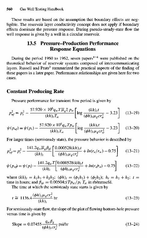
These results are based on the assumption that boundary effects are neg-ligible. The reservoir layer conductivity concept does not apply if boundaryeffects dominate the pressure response. During pseudo-steady-state flow thewell response is given by a well in a circular reservoir.
13.5 Pressure-Production PerformanceResponse Equations
During the period 1960 to 1962, seven papers1"4 were published on thetheoretical behavior of reservoir systems composed of intercommunicatinglayers. Russell and Prats3 summarized the practical aspects of the finding ofthese papers in a later paper. Performance relationships are given here for twocases.
Constant Producing Rate
Pressure performance for transient flow period is given by
2 2 57.920 x lO%cTTZgzPsc^ (kh)tt ]Pwf = Pi TJTV^ l o 3 Z ^ 2 ~ 3 ' 2 3 (13-19)
J (kh)tTsc L (<t>h)tVgcrl Jif ^ if ^ 57.920 x l06qscTpsc f, (kh)tt ]
t(Pwf) = Ir(pi) — — log — - 3.23 (13-20)(kh)tTsc L ((ph)tfigcrl J
For larger times (semisteady state), the pressure behavior is described by
2 2 141.2^c7Zg/^[0.000528(£/z),r , r f ]Pw/= Pi TTT^— ~7IT\ 2~+/«( r g / r w ) -0 .75 (13-21)
J (kh)t L (4>h)tligcrl J
f(pw) = nPi) T7^-I 2 +In(re/rw) ~ 0.75 (13-22)(kh)t L (</>h)tV>gCr* J
where (kh)t = k\h\ +k2h2; ((ph)t = (0iAi) + (^2^2); ht = h\ + h2', t =time in hours; and figt = 0.00504z/r/?5C/p/ Tsc in rb/mmscfd.
The time at which the semisteady state starts is given by
/S1136.4(W^hr (13-23)(kh)t
For semisteady-state flow, the slope of the plot of flowing bottom-hole pressureversus time is given by
Slope = 0 . 0 7 4 5 5 - ^ - r psi/hr (13-24)((/)h)tcrj
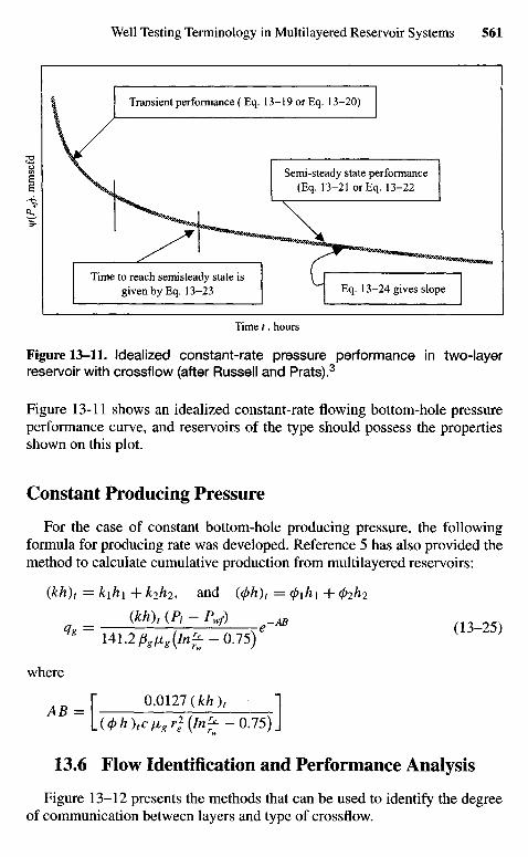
Time / , hours
Figure 13-11. Idealized constant-rate pressure performance in two-layerreservoir with crossflow (after Russell and Prats).3
Figure 13-11 shows an idealized constant-rate flowing bottom-hole pressureperformance curve, and reservoirs of the type should possess the propertiesshown on this plot.
Constant Producing Pressure
For the case of constant bottom-hole producing pressure, the followingformula for producing rate was developed. Reference 5 has also provided themethod to calculate cumulative production from multilayered reservoirs:
(kh)t = k\h\ H- k2h2, and (<f)h)t = $\h\ + (J)2Ii2
_ (M), (P1 - Pwf)q&~ 141.2&/*g(/n£- 0.75)* ( I 3 " 2 5 )
where
AB = \ 0-0127 (fcft), 1lit h)tc^8 r? (In^-0.75)\
13.6 Flow Identification and Performance Analysis
Figure 13-12 presents the methods that can be used to identify the degreeof communication between layers and type of crossflow.
Eq. 13-24 gives slopeTime to reach semisteady state is
given by Eq. 13-23
Semi-steady state performance(Eq. 13-21 or Eq. 13-22
Transient performance ( Eq. 13-19 or Eq. 13-20)
\\j(P
wf).
mm
scfd
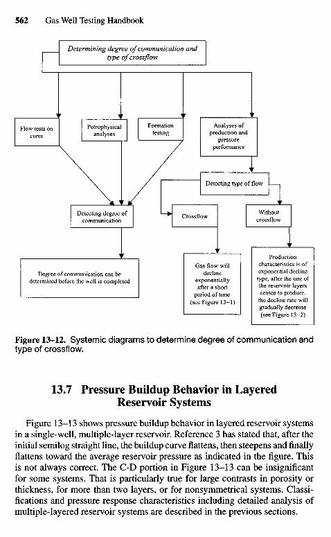
Figure 13-12. Systemic diagrams to determine degree of communication andtype of crossflow.
13.7 Pressure Buildup Behavior in LayeredReservoir Systems
Figure 13-13 shows pressure buildup behavior in layered reservoir systemsin a single-well, multiple-layer reservoir. Reference 3 has stated that, after theinitial semilog straight line, the buildup curve flattens, then steepens and finallyflattens toward the average reservoir pressure as indicated in the figure. Thisis not always correct. The C-D portion in Figure 13-13 can be insignificantfor some systems. That is particularly true for large contrasts in porosity orthickness, for more than two layers, or for nonsymmetrical systems. Classi-fications and pressure response characteristics including detailed analysis ofmultiple-layered reservoir systems are described in the previous sections.
Flow tests oncores
Petrophysicalanalyses
Formationtesting
Analyses ofproduction and
pressureperformance
Detecting degree ofcommunication
CrossflowWithout
crossflow
Gas flow willdecline
exponentiallyafter a short
period of time(see Figure 13-1)
Productioncharacteristics is ofexponential decline
type, after the one ofthe reservoir layersceases to produce,
the decline rate willgradually decrease(see Figure 13-2)
Degree of communication can bedetermined before the well is completed
Detecting type of flow
Determining degree of communication andtype of crossflow
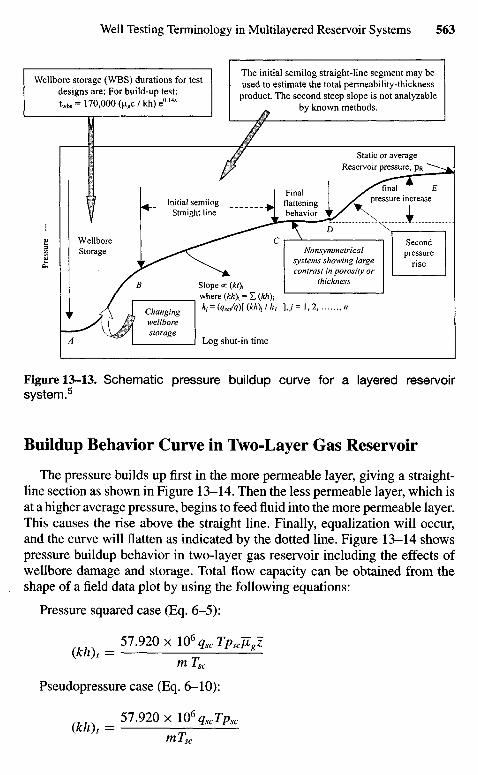
Figure 13-13. Schematic pressure buildup curve for a layered reservoirsystem.5
Buildup Behavior Curve in Two-Layer Gas Reservoir
The pressure builds up first in the more permeable layer, giving a straight-line section as shown in Figure 13-14. Then the less permeable layer, which isat a higher average pressure, begins to feed fluid into the more permeable layer.This causes the rise above the straight line. Finally, equalization will occur,and the curve will flatten as indicated by the dotted line. Figure 13-14 showspressure buildup behavior in two-layer gas reservoir including the effects ofwellbore damage and storage. Total flow capacity can be obtained from theshape of a field data plot by using the following equations:
Pressure squared case (Eq. 6-5):
= 57.920 x IQ6 gscTPscJIgzmTsc
Pseudopressure case (Eq. 6-10):
n^ _ 51.920 x \06qscTpscyKn)t —
mTsc
Wellbore storage (WBS) durations for testdesigns are: For build-up test:twbs= 170,000 (u g c /kh)e 0 1 4 s
The initial semilog straight-line segment may beused to estimate the total permeability-thickness
product. The second steep slope is not analyzableby known methods.
WellboreStorage
Pres
sure
Initial semilogStraight line
Finalflatteningbehavior
Static or averageReservoir pressure, PR
finalpressure increase
Secondpressure
rise
Nonsymmetricalsystems showing largecontrast in porosity or
thickness
Changingwellborestorage
Log shut-in time
Slope oc (*/),where {kh\ = I (kh)-t
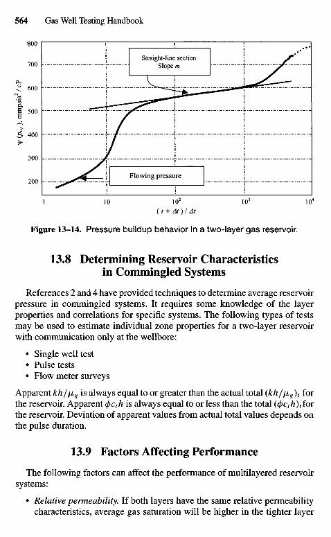
Figure 13-14. Pressure buildup behavior in a two-layer gas reservoir.
13.8 Determining Reservoir Characteristicsin Commingled Systems
References 2 and 4 have provided techniques to determine average reservoirpressure in commingled systems. It requires some knowledge of the layerproperties and correlations for specific systems. The following types of testsmay be used to estimate individual zone properties for a two-layer reservoirwith communication only at the wellbore:
• Single well test• Pulse tests• Flow meter surveys
Apparent kh/fig is always equal to or greater than the actual total (kh/fjig)t forthe reservoir. Apparent (j>cth is always equal to or less than the total ((pcth)tforthe reservoir. Deviation of apparent values from actual total values depends onthe pulse duration.
13.9 Factors Affecting Performance
The following factors can affect the performance of multilayered reservoirsystems:
• Relative permeability. If both layers have the same relative permeabilitycharacteristics, average gas saturation will be higher in the tighter layer
\\f (p
ws)
, m
mp
sia2 /
cP
Flowing pressure
Straight-line sectionSlope m
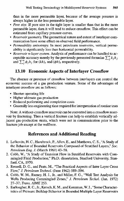
than in the more permeable layer, because of the average pressure isalways higher in the less permeable layer.
• Pore size. If pore size in the tight layer is smaller than that in the morepermeable layer, then it will tend to reduce crossflow. This effect can beestimated from capillary pressure curves.
• Reservoir geometry. The geometrical nature and extent of interlayer com-munication have some effect on observed field performance.
• Permeability anisotropy. In most petroleum reservoirs, vertical perme-ability is significantly less than horizontal permeability.
• Reservoir n-layer system. Analysis of performance can be handled to ac-ceptable accuracy merely by the previously presented formulas YTj kjhjand YTj <t>jhj f° r (kh)t and ((/)h)t respectively.
13.10 Economic Aspects of Interlayer Crossflow
The absence or presence of crossflow between interlayers can control theeconomic success of a gas production venture. Some of the advantages ofinterlayer crossflow are as follows:
• Shorter operating life• Higher ultimate gas production• Reduced perforating and completion costs• Generally less engineering time required for interpretation of routine tests
Note: A without-crossflow reservoir can be converted into a crossflow reser-voir by fracturing. Thus a vertical fracture can help to establish vertically ad-jacent gas-production strata, which were not in communication prior to thefracture job except at the wellbore.
References and Additional Reading
1. Lefkovits, H. C , Hazebrock, P., Allen, E., and Matthews, C S . , "A Study ofthe Behavior of Bounded Reservoirs Composed of Stratified Layers," Soc.Petroleum Eng. J. (March 1961) 43-58.
2. Cobb, W., "A Study of Transient Flow in Stratified Reservoirs with Com-mingled Fluid Production," Ph.D. dissertation, Stanford University, Stan-ford, CA, 1970.
3. Russell, D. G., and Prats, M., "The Practical Aspects of Inter Layer CrossFlow," /. Petroleum Technol. (June 1962) 589-594.
4. Cobb, W. M., Ramey, H. J., Jr., and Miller, F. G., "Well Test Analysis forWells Producing Commingled Zones," /. Petroleum Techol. (Jan. 1972)27-37; Trans. AIME 253.
5. Earlougher, R. C , Jr., Kersch, K. M., andKunzman, W. J., "SomeCharacter-istics of Pressure Buildup Behavior in Bounded Multiple Layer Reservoirs

without Crossflow," /. Petroleum Technol (Oct. 1974) 1178-1186; Trans.AIME 257.
6. Camacho, V., Raghavan, R., and Reynolds, A. C, "Response of WellsProducing Layered Reservoirs, Unequal Fracture Length," SPE FormationEvaluation (Feb. 1987) 9-28.
7. Raghavan, R., Topaloglu, H. N., Cobb, W. M., and Ramey, H. J., Jr., "WellTest A Analysis for Wells Producing from Two Commingled Zones ofUnequal Thickness," J. Petroleum Technol (Sept. 1974) 1035-1043; Trans.AIME 257.

Chapter 14
Pressure BehaviorAnalysis inHeterogeneousReservoir Systems
14.1 Introduction
This chapter discusses the effects of some common reservoir heterogeneitieson pressure transient behavior. It is difficult to delineate specific heterogeneitiesfrom well tests. The difficulty occurs because many different conditions cancause the same or similar well test response. If we have an idea of the type ofheterogeneity, it may be possible to determine some of the properties involvedby pressure transient testing. Some knowledge of geological, seismic, fluidflow, and performance data is necessary before hypotheses are formed aboutthe type and location of the heterogeneities. It may be possible to designa specific transient test to investigate the possibility of a particular type ofheterogeneity. This chapter discusses and classifies reservoir heterogeneities,permeability, and anisotropy and describes how these heterogeneities affecttransient testing. Several types of heterogeneities can cause similar transienttest pressure response, but results should be supported by other data. The nextsection will illustrate a variety of situations such as faults, lateral changesin the hydraulic diffusivity such as occur at fluid contacts, and man-madeheterogeneities.
14.2 Causes of Heterogeneities
Heterogeneities may have the following causes:
• Postdepositional changes in reservoir lithology• Folding and faulting• Changes in fluid type or properties• Variations in rock and fluid properties from one location to another
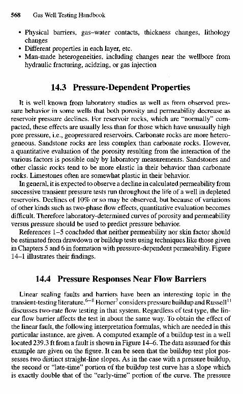
• Physical barriers, gas-water contacts, thickness changes, lithologychanges
• Different properties in each layer, etc.• Man-made heterogeneities, including changes near the wellbore from
hydraulic fracturing, acidzing, or gas injection
14.3 Pressure-Dependent Properties
It is well known from laboratory studies as well as from observed pres-sure behavior in some wells that both porosity and permeability decrease asreservoir pressure declines. For reservoir rocks, which are "normally" com-pacted, these effects are usually less than for those which have unusually highpore pressure, i.e., geopressured reservoirs. Carbonate rocks are more hetero-geneous. Sandstone rocks are less complex than carbonate rocks. However,a quantitative evaluation of the porosity resulting from the interaction of thevarious factors is possible only by laboratory measurements. Sandstones andother classic rocks tend to be more elastic in their behavior than carbonaterocks. Limestones often are somewhat plastic in their behavior.
In general, it is expected to observe a decline in calculated permeability fromsuccessive transient pressure tests run throughout the life of a well in depletedreservoirs. Declines of 10% or so may be observed, but because of variationsof other kinds such as two-phase flow effects, quantitative evaluation becomesdifficult. Therefore laboratory-determined curves of porosity and permeabilityversus pressure should be used to predict pressure behavior.
References 1-5 concluded that neither permeability nor skin factor shouldbe estimated from drawdown or buildup tests using techniques like those givenin Chapters 5 and 6 in formation with pressure-dependent permeability. Figure14-1 illustrates their findings.
14.4 Pressure Responses Near Flow Barriers
Linear sealing faults and barriers have been an interesting topic in thetransient-testing literature.6"8 Horner7 considers pressure buildup and Russell1!
discusses two-rate flow testing in that system. Regardless of test type, the lin-ear flow barrier affects the test in about the same way. To obtain the effect ofthe linear fault, the following interpretation formulas, which are needed in thisparticular instance, are given. A computed example of a buildup test in a welllocated 239.3 ft from a fault is shown in Figure 14-6. The data assumed for thisexample are given on the figure. It can be seen that the buildup test plot pos-sesses two distinct straight-line slopes. As in the case with a pressure buildup,the second or "late-time" portion of the buildup test curve has a slope whichis exactly double that of the "early-time" portion of the curve. The pressure
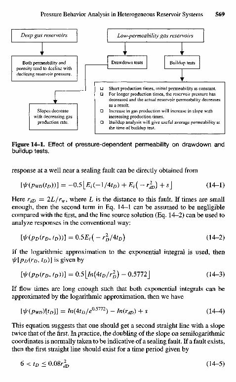
Figure 14-1. Effect of pressure-dependent permeability on drawdown andbuildup tests.
response at a well near a sealing fault can be directly obtained from
W(PWDQD))] = -0.5[Ei(-l/4tD) + Et(- r2
dD) + s\ (14-1)
Here rdD = 2L/rw, where L is the distance to this fault. If times are smallenough, then the second term in Eq. 14-1 can be assumed to be negligiblecompared with the first, and the line source solution (Eq. 14-2) can be used toanalyze responses in the conventional way:
№(PD(rD, tD))] = 0.5Ei(- r2
D/AtD) (14-2)
If the logarithmic approximation to the exponential integral is used, then^[PDQD, tD)]is given by
№(PD(rD, tD))] = 0.5[ln(4tD/rl) - 0.5772J (14-3)
If flow times are long enough such that both exponential integrals can beapproximated by the logarithmic approximation, then we have
№(PwD)[tD]] = In(4tD/e05112) - In(Ta,) + s (14-4)
This equation suggests that one should get a second straight line with a slopetwice that of the first. In practice, the doubling of the slope on semilogarithmiccoordinates is normally taken to be indicative of a sealing fault. If a fault exists,then the first straight line should exist for a time period given by
6 < tD < 0№r2
D (14-5)
Deep gas reservoirs Low-permeability gas reservoirs
Both permeability andporosity tend to decline withdeclining reservoir pressure.
Drawdown tests Buildup tests
Short production times, initial permeability is constant.For longer production times, the reservoir pressure hasdecreased and the actual reservoir permeability decreasesas a result.Increase in gas production will increase in slope withincreasing production times.Buildup analysis will give useful average permeability atthe time of buildup test.
Slopes decreasewith decreasing gas
production rate.
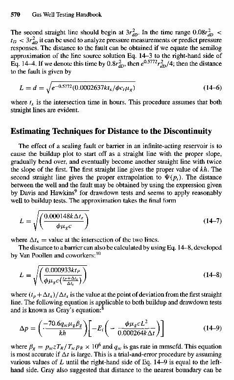
The second straight line should begin at 3r2dD. In the time range 0 . 0 8 ^ <
to < 3r\D it can be used to analyze pressure measurements or predict pressureresponses. The distance to the fault can be obtained if we equate the semilogapproximation of the line source solution Eq. 14-3 to the right-hand side ofEq. 14-4. If we denote this time by 0.8rJD, then e°-57nrjD/4; then the distanceto the fault is given by
L = d = ^-0.5772(0.0002637^/0^/^) (14-6)
where tx is the intersection time in hours. This procedure assumes that bothstraight lines are evident.
Estimating Techniques for Distance to the Discontinuity
The effect of a sealing fault or barrier in an infinite-acting reservoir is tocause the buildup plot to start off as a straight line with the proper slope,gradually bend over, and eventually become another straight line with twicethe slope of the first. The first straight line gives the proper value of kh. Thesecond straight line gives the proper extrapolation to ty(pi). The distancebetween the well and the fault may be obtained by using the expression givenby Davis and Hawkins9 for drawdown tests and seems to apply reasonablywell to buildup tests. The approximation takes the final form
L= ;/0.000148*A,AV V ^ g C J
where Atx = value at the intersection of the two lines.The distance to a barrier can also be calculated by using Eq. 14-8, developed
by Van Poollen and coworkers:10
where (tp +Atx)/Atx is the value at the point of deviation from the first straightline. The following equation is applicable to both buildup and drawdown testsand is known as Gray's equation:8
V kh / L A 0.000264feAfJJ ( }
where fig = psczTR/TscpR x 106 and qsc is gas rate in mmscfd. This equationis most accurate if At is large. This is a trial-and-error procedure by assumingvarious values of L until the right-hand side of Eq. 14-9 is equal to the left-hand side. Gray also suggested that distance to the nearest boundary can be
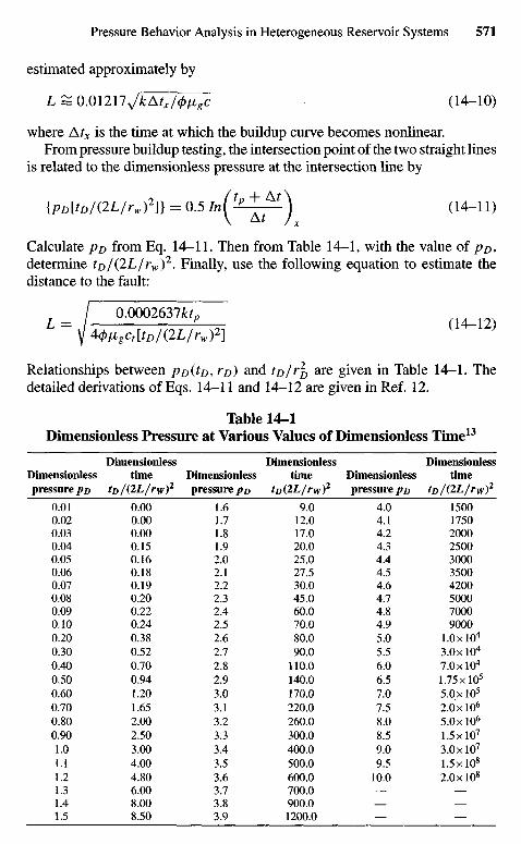
estimated approximately by
L = 0.01217'JkAtx /(/)ijLgc (14-10)
where A x is the time at which the buildup curve becomes nonlinear.From pressure buildup testing, the intersection point of the two straight lines
is related to the dimensionless pressure at the intersection line by
{pD[tD/(2L/rw)2]} = 0.5 I n { ^ ^ - \ (14-11)
Calculate pD from Eq. 14-11. Then from Table 14-1, with the value of pD,determine tD/(2L/rw)2. Finally, use the following equation to estimate thedistance to the fault:
= / 0-0002637^,Y 4^gct[tD/(2L/rw)2]
Relationships between po(to, r^) and tujr^ are given in Table 14-1. Thedetailed derivations of Eqs. 14-11 and 14-12 are given in Ref. 12.
Table 14-1Dimensionless Pressure at Various Values of Dimensionless Time13
Dimensionless Dimensionless DimensionlessDimensionless time Dimensionless time Dimensionless timepressure/?/) to/QL/rw)2 pressure po to(2L/ryy)2 pressure po to/(2L/rw)2
0.01 0.00 1.6 9.0 4.0 15000.02 0.00 1.7 12.0 4.1 17500.03 0.00 1.8 17.0 4.2 20000.04 0.15 1.9 20.0 4.3 25000.05 0.16 2.0 25.0 4.4 30000.06 0.18 2.1 27.5 4.5 35000.07 0.19 2.2 30.0 4.6 42000.08 0.20 2.3 45.0 4.7 50000.09 0.22 2.4 60.0 4.8 70000.10 0.24 2.5 70.0 4.9 90000.20 0.38 2.6 80.0 5.0 1.OxIO4
0.30 0.52 2.7 90.0 5.5 3.OxIO4
0.40 0.70 2.8 110.0 6.0 7.OxIO4
0.50 0.94 2.9 140.0 6.5 1.75xlO5
0.60 1.20 3.0 170.0 7.0 5.0xl05
0.70 1.65 3.1 220.0 7.5 2.OxIO6
0.80 2.00 3.2 260.0 8.0 5.OxIO6
0.90 2.50 3.3 300.0 8.5 1.5xlO7
1.0 3.00 3.4 400.0 9.0 3.0xl07
1.1 4.00 3.5 500.0 9.5 1.5xl08
1.2 4.80 3.6 600.0 10.0 2.OxIO8
1.3 6.00 3.7 700.0 — —1.4 8.00 3.8 900.0 — —1.5 8.50 3.9 1200.0 — —
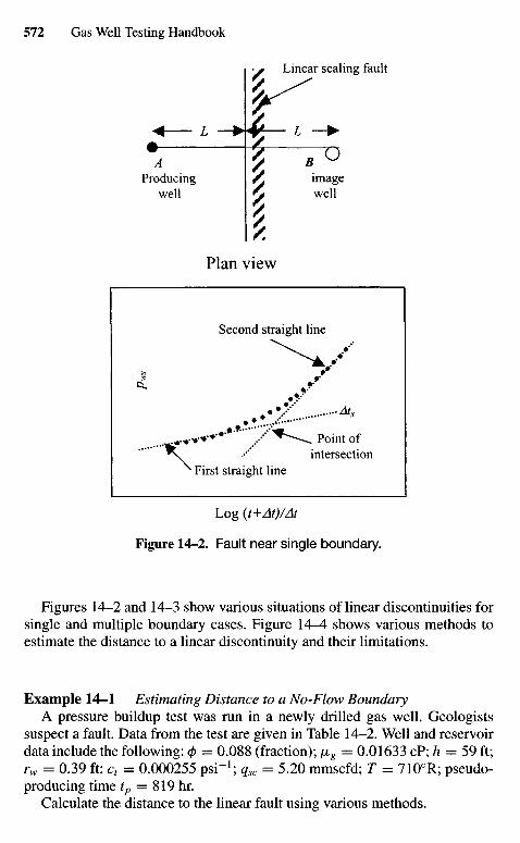
Log (t+At)ZAt
Figure 14-2. Fault near single boundary.
Figures 14-2 and 14-3 show various situations of linear discontinuities forsingle and multiple boundary cases. Figure 1 4 ^ shows various methods toestimate the distance to a linear discontinuity and their limitations.
Example 14—1 Estimating Distance to a No-Flow BoundaryA pressure buildup test was run in a newly drilled gas well. Geologists
suspect a fault. Data from the test are given in Table 14-2. Well and reservoirdata include the following: <j> = 0.088 (fraction); fig = 0.01633 cP; h = 59 ft;rw = 0.39 ft; ct = 0.000255 psi"1; qsc = 5.20 mmscfd; T = 7100R; pseudo-producing time tp = 819 hr.
Calculate the distance to the linear fault using various methods.
First straight line
. Point ofintersection
Second straight line
Plan view
Producingwell
imagewell
Linear sealing fault
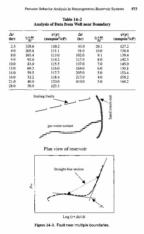
Table 14-2Analysis of Data from Well near Boundary
At f/>(p) At *l>(p)(hr) ^±p (mmpsia2/cP) (hr) ^ ± p (mmpsia2/cP)
2.5 328.6 110.2 43.0 20.1 127.24.0 205.8 111.1 91.0 10.0 138.48.0 103.4 113.0 102.0 9.1 139.49.0 92.0 114.2 117.0 8.0 142.3
10.0 83.0 115.5 137.0 7.0 145.012.0 69.3 116.0 164.0 6.0 150.114.0 59.5 117.7 205.0 5.0 153.416.0 52.2 118.4 213.0 4.0 158.221.0 40.0 120.0 410.0 3.0 164.228.0 30.0 123.3
Sealing Faults
Sand
pin
ch o
ut
gas-water contact
Plan view of reservoir
Straight-line section
Log {t+At)ZAt
Figure 14-3. Fault near multiple boundaries.
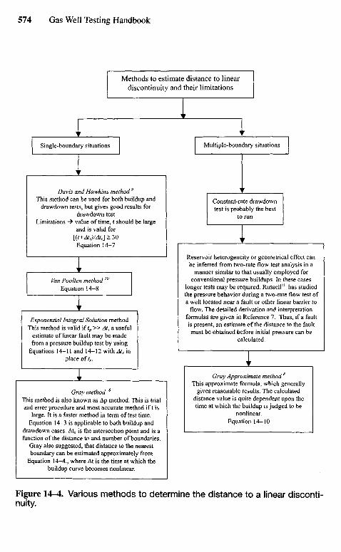
Figure 14-4. Various methods to determine the distance to a linear disconti-nuity.
Single-boundary situations Multiple-boundary situations
Davis and Hawkins method9
This method can be used for both buildup anddrawdown tests, but gives good results for
drawdown testLimitations -> value of time, t should be large
and is valid for[{t+Atx)ZAtx] > 30Equation 14-7
Constant-rate drawdowntest is probably the best
to run
Van Poo Hen method ''
Equation 14-8
Exponential Integral Solution methodThis method is valid if tp » At, a useful
estimate of linear fault may be madefrom a pressure buildup test by using
Equations 14-11 and 14-12 with Atx inplace of tx.
Methods to estimate distance to lineardiscontinuity and their limitations
Reservoir heterogeneity or geometrical effect canbe inferred from two-rate flow test analysis in a
manner similar to that usually employed forconventional pressure buildups. In these cases
longer tests may be required. Russell11 has studiedthe pressure behavior during a two-rate flow test ofa well located near a fault or other linear barrier to
flow. The detailed derivation and interpretationformulas are given in Reference 7. Thus, if a faultis present, an estimate of the distance to the faultmust be obtained before initial pressure can be
calculated.
Gray Approximate method 8
This approximate formula, which generallygives reasonable results. The calculated
distance value is quite dependent upon thetime at which the buildup is judged to be
nonlinear.Equation 14-10
Gray method 8
This method is also known as Ap method. This is trialand error procedure and most accurate method if t is
large. It is a faster method in term of test time.Equation 14-3 is applicable to both buildup and
drawdown cases. Atx is the intersection point and is afunction of the distance to and number of boundaries.
Gray also suggested, that distance to the nearestboundary can be estimated approximately from
Equation 14-4., where At is the time at which thebuildup curve becomes nonlinear.
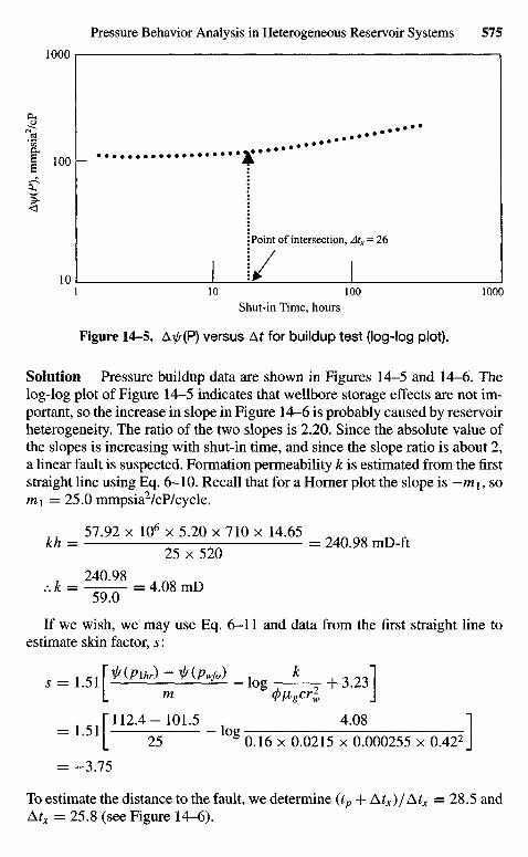
Shut-in Time, hours
Figure 14-5. AI/A(P) versus Af for buildup test (log-log plot).
Solution Pressure buildup data are shown in Figures 14-5 and 14-6. Thelog-log plot of Figure 14-5 indicates that wellbore storage effects are not im-portant, so the increase in slope in Figure 14-6 is probably caused by reservoirheterogeneity. The ratio of the two slopes is 2.20. Since the absolute value ofthe slopes is increasing with shut-in time, and since the slope ratio is about 2,a linear fault is suspected. Formation permeability k is estimated from the firststraight line using Eq. 6-10. Recall that for a Horner plot the slope is — m\, som\ =25.0 mmpsia2/cP/cycle.
, 7 57.92 x 106 x 5.20 x 710 x 14.65
** = ^ 5 2 0 = m 9 8 " ^ "
If we wish, we may use Eq. 6-11 and data from the first straight line toestimate skin factor, s:
t ^\^(P\hr)-^(Pwfo) , k "Is = 1.51 log + 3.23
L m <t>l*gcrl J_ r 112.4-101.5 4.08 "I~ L L 25 ° g 0.16 x 0.0215 x 0.000255 x 0.422J= -3.75
To estimate the distance to the fault, we determine (tp-\- Atx)/Atx =28.5 andAtx = 25.8 (see Figure 14-6).
Point of intersection, Atx = 26
Ay(
P),
mm
psia
2/cP
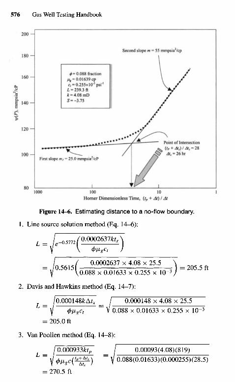
Horner Dimensionless Time, (tp + At) I At
Figure 14-6. Estimating distance to a no-flow boundary.
1. Line source solution method (Eq. 14-6):
V V <$>vgct JI / 0.0002637 x 4.08 x 25.5 \
= f 5 6 1 5 (o .O88 x 0.01633 x 0.255 x 10-3 j = 2 ° 5 - 5 ft
2. Davis and Hawkins method (Eq. 14-7):
/0.000148fcAf7 _ / 0.000148 x 4.08 x 25^5~ Y 4>V>gCt " V 0.088 x 0.01633 x 0.255 x 10~3
= 205.0 ft
3. Van Poollen method (Eq. 14-8):
_ / 0.000933^^ _ / 0.00093(4.08) (819)L = Y <t>figc(tplftx) ~ Y 0.088(0.01633)(0.000255)(28.5)
= 270.5 ft
First slope m, - 25.0 mmpsia2/cP
Point of Intersection(tP + Atx) I Atx = 28Atx = 26 hr
Second slope m = 55 mmpsia2/cp
</)= 0.088 fractionJJ8 = 0.01639 cp^0.255XlO-3PSi"1
L = 239.3 ftk = 4.08 mDS= -3.75
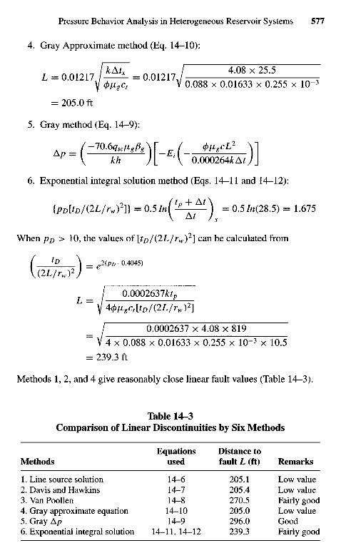
4. Gray Approximate method (Eq. 14-10):
I IcAtx I 4.08 x 25.5L = 0.01217^ ^ - = 0.01217^ 0 0 8 8 x Q - 0 1 6 3 3 x 0 2 5 5 x 10_3
= 205.0 ft
5. Gray method (Eq. 14-9):
/-70.6^AL Et(_ W )]y V kh / L V 0 . 0 0 0 2 6 4 £ A r / J
6. Exponential integral solution method (Eqs. 14-11 and 14-12):
{pD[tD/(2L/rw)2]} = ° ' 5 I n ( t p ^ t ) = 0.5//i(28.5) = 1.675
When pD > 10, the values of j>/)/(2L/rw)2] can be calculated from
( tD \ = e2(PD -0.4045)
V(2L/rw)V
/ 0.0002637**,~y44>ligct[tD/(2L/rw)2]
I 0.0002637 x 4.08 x 819" V 4 x 0.088 x 0.01633 x 0.255 x 10"3 x 10.5= 239.3 ft
Methods 1, 2, and 4 give reasonably close linear fault values (Table 14-3).
Table 14-3Comparison of Linear Discontinuities by Six Methods
Equations Distance toMethods used fault L (ft) Remarks
1. Line source solution 14-6 205.1 Low value2. Davis and Hawkins 14-7 205.4 Low value3. VanPoollen 14-8 270.5 Fairly good4. Gray approximate equation 14-10 205.0 Low value5. Gray Ap 14-9 296.0 Good6. Exponential integral solution 14-11, 14-12 239.3 Fairly good
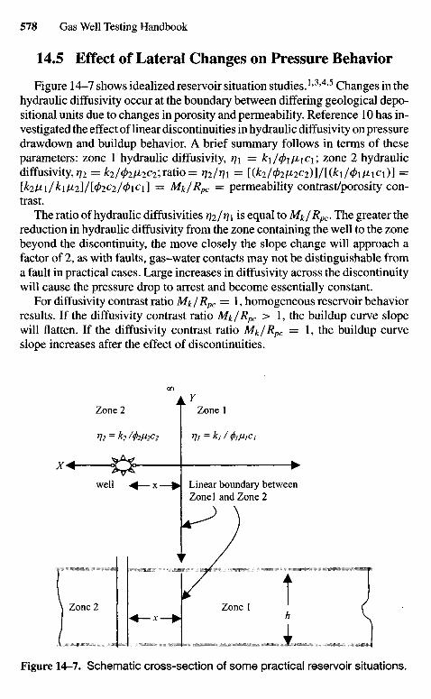
14.5 Effect of Lateral Changes on Pressure Behavior
Figure 14-7 shows idealized reservoir situation studies.1'3'4'5 Changes in thehydraulic diffusivity occur at the boundary between differing geological depo-sitional units due to changes in porosity and permeability. Reference 10 has in-vestigated the effect of linear discontinuities in hydraulic diffusivity on pressuredrawdown and buildup behavior. A brief summary follows in terms of theseparameters: zone 1 hydraulic diffusivity, r\\ — k\/(f>ijbiici; zone 2 hydraulicdiffusivity, T]1 = k2/(J)1IJL2C1', ratio= r)2/rn = [(W02M2C2)]/[(£i/0iMiCi)] =[&2Mi/&iA^]/[02C2/0iCi] = Mk/Rpc = permeability contrast/porosity con-trast.
The ratio of hydraulic diffusivities 772/ 1 is equal to Mk/Rpc. The greater thereduction in hydraulic diffusivity from the zone containing the well to the zonebeyond the discontinuity, the move closely the slope change will approach afactor of 2, as with faults, gas-water contacts may not be distinguishable froma fault in practical cases. Large increases in diffusivity across the discontinuitywill cause the pressure drop to arrest and become essentially constant.
For diffusivity contrast ratio Mk /Rpc — !,homogeneous reservoir behaviorresults. If the diffusivity contrast ratio Mk/Rpc > 1, the buildup curve slopewill flatten. If the diffusivity contrast ratio Mk/Rpc = 1, the buildup curveslope increases after the effect of discontinuities.
Figure 14-7. Schematic cross-section of some practical reservoir situations.
Zone 2 Zone 1
well Linear boundary betweenZonel and Zone 2
Zone 2 Zone 1
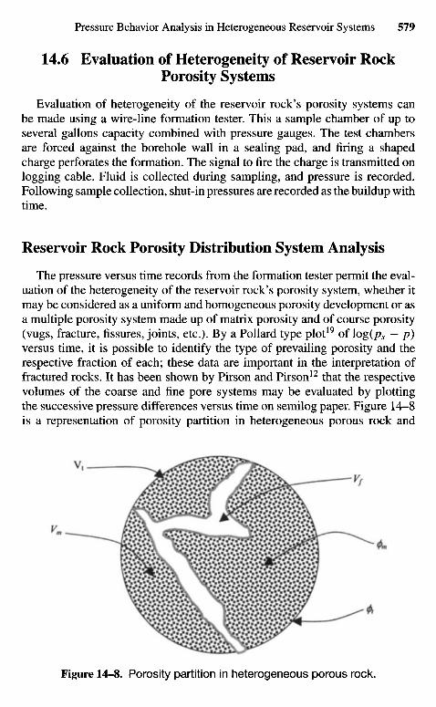
14.6 Evaluation of Heterogeneity of Reservoir RockPorosity Systems
Evaluation of heterogeneity of the reservoir rock's porosity systems canbe made using a wire-line formation tester. This a sample chamber of up toseveral gallons capacity combined with pressure gauges. The test chambersare forced against the borehole wall in a sealing pad, and firing a shapedcharge perforates the formation. The signal to fire the charge is transmitted onlogging cable. Fluid is collected during sampling, and pressure is recorded.Following sample collection, shut-in pressures are recorded as the buildup withtime.
Reservoir Rock Porosity Distribution System Analysis
The pressure versus time records from the formation tester permit the eval-uation of the heterogeneity of the reservoir rock's porosity system, whether itmay be considered as a uniform and homogeneous porosity development or asa multiple porosity system made up of matrix porosity and of course porosity(vugs, fracture, fissures, joints, etc.). By a Pollard type plot19 of log(ps — p)versus time, it is possible to identify the type of prevailing porosity and therespective fraction of each; these data are important in the interpretation offractured rocks. It has been shown by Pirson and Pirson12 that the respectivevolumes of the coarse and fine pore systems may be evaluated by plottingthe successive pressure differences versus time on semilog paper. Figure 14-8is a representation of porosity partition in heterogeneous porous rock and
Figure 14-8. Porosity partition in heterogeneous porous rock.
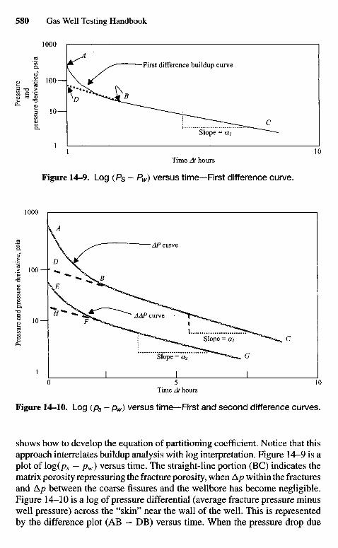
Time At hours
Figure 14-10. Log (ps - Av) versus time—First and second difference curves.
shows how to develop the equation of partitioning coefficient. Notice that thisapproach interrelates buildup analysis with log interpretation. Figure 14-9 is aplot of log(ps — pw) versus time. The straight-line portion (BC) indicates thematrix porosity repressuring the fracture porosity, when Ap within the fracturesand Ap between the coarse fissures and the wellbore has become negligible.Figure 14-10 is a log of pressure differential (average fracture pressure minuswell pressure) across the "skin" near the wall of the well. This is representedby the difference plot (AB — DB) versus time. When the pressure drop due
Slope = CC2
Pres
sure
and
pre
ssur
e de
riva
tive,
psi
aPr
essu
rean
dpr
essu
re d
eriv
atic
e, p
sia
Slope = a,
AAP curve
AP curve
Time At hours
Figure 14-9. Log (Ps — Pw) versus time—First difference curve.
Slope = a i
First difference buildup curve
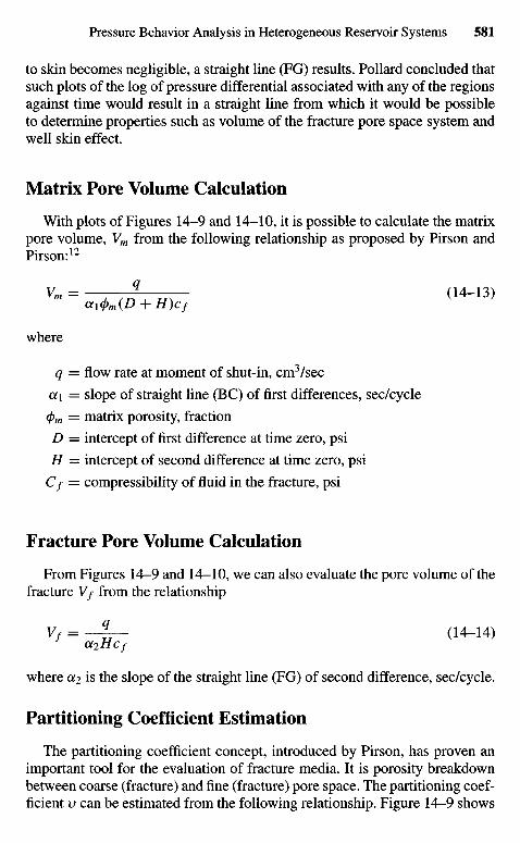
to skin becomes negligible, a straight line (FG) results. Pollard concluded thatsuch plots of the log of pressure differential associated with any of the regionsagainst time would result in a straight line from which it would be possibleto determine properties such as volume of the fracture pore space system andwell skin effect.
Matrix Pore Volume Calculation
With plots of Figures 14-9 and 14-10, it is possible to calculate the matrixpore volume, Vm from the following relationship as proposed by Pirson andPirson:12
Vm = (14-13)ax<t>m(D + H)cf
where
q = flow rate at moment of shut-in, cm3/sec
a\ = slope of straight line (BC) of first differences, sec/cycle
(j)m = matrix porosity, fraction
D = intercept of first difference at time zero, psi
H = intercept of second difference at time zero, psi
Cf = compressibility of fluid in the fracture, psi
Fracture Pore Volume Calculation
From Figures 14-9 and 14-10, we can also evaluate the pore volume of thefracture Vf from the relationship
Vf = — | — (14-14)OL1HCf
where Ot1 is the slope of the straight line (FG) of second difference, sec/cycle.
Partitioning Coefficient Estimation
The partitioning coefficient concept, introduced by Pirson, has proven animportant tool for the evaluation of fracture media. It is porosity breakdownbetween coarse (fracture) and fine (fracture) pore space. The partitioning coef-ficient v can be estimated from the following relationship. Figure 14-9 shows
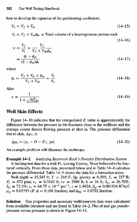
how to develop the equation of the partitioning coefficient.
V0 = Vf + Vm (14-15)
V1 = Vf + Vm<pm — Total volume of a heterogeneous porous rock(14-16)
= Vf = Vfvt vf + vM<pm
= * " * " (14-17)(1 - 0m)&
where
v/ + VM VO
Also
u = i , U (14-!9)
Well Skin Effects
Figure 14-10 indicates that the extrapolated E value is approximately thedifference between the pressure in the fractures close to the wellbore and theaverage coarse fissure flowing pressure at shut-in. The pressure differentialdue to skin, Aps, is
Ap5 = {ps-D- E), psi (14-20)
An example problem will illustrate the technique.
Example 14-2 Analyzing Reservoir Rock's Porosity Distribution SystemA buildup test data for a well #1, Loving County, Texas believed to be frac-
tured vertically. From these data, presented below and in Table 14-4 calculatethe pressure differential. Table 14-5 shows the data for a formation tester.
Well depth = 15,545 ft; T = 245°F; Sp. gravity = 0.595; Tc = 357°R;Pc = 672 psia; rw = 0.3542 ft; re = 2980 ft; h = 16 ft; Swi = 26.70%;Sgt = 73.3%; ct = 64.75 x 10"6 psi"1; z = 1.4924; figi = 0.001934 ft3/scf;lLg = 0.03793 cP; 0 = 0.108 fraction; and (/>HC = 0.0792 fraction.
Solution Gas properties and necessary well/reservoir data were calculatedfrom available literature and are listed in Table 14-2. Plot of real gas pseudo-pressure versus pressure is shown in Figure 14-11.
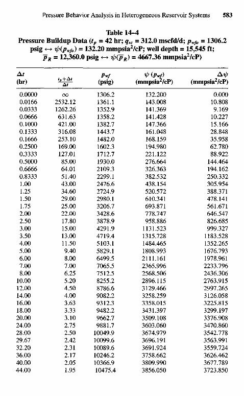
Table 14-4Pressure Buildup Data (tp = 42 hr; qsc = 312.0 mscfd/d; pwfo = 1306.2
psig <-> if>(pWfi,) = 132.20 mmpsiaVcP; well depth = 15,545 ft;pR = 12,360.0 psig <-• V(^*) = 4667.36 mmpsia2/cP)
A* /IH,/ 1/7 (/7H,/) A ^(hr) ^ p (psig) (mmpsia2/cP) (mmpsia2/cP)
0.0000 oo 1306.2 132.200 0.0000.0166 2532.12 1361.1 143.008 10.8080.0333 1262.26 1352.9 141.369 9.1690.0666 631.63 1358.2 141.428 10.2270.1000 421.00 1382.7 147.366 15.1660.1333 316.08 1443.7 161.048 28.8480.1666 253.10 1482.0 168.159 35.9580.2500 169.00 1602.3 194.980 62.7800.3333 127.01 1712.7 221.122 88.9220.5000 85.00 1930.0 276.664 144.4640.6666 64.01 2109.3 326.363 194.1620.8333 51.40 2299.1 382.532 250.3321.00 43.00 2476.6 438.154 305.9541.25 34.60 2724.9 520.572 388.3711.50 29.00 2980.1 610.341 478.1411.75 25.00 3206.7 693.871 561.6712.00 22.00 3428.6 778.747 646.5472.50 17.80 3878.9 958.886 826.6853.00 15.00 4291.9 1131.523 999.3273.50 13.00 4719.4 1315.728 1183.5284.00 11.50 5103.1 1484.465 1352.2655.00 9.40 5829.1 1808.993 1676.7936.00 8.00 6499.5 2111.161 1978.9617.00 7.00 7065.5 2365.996 2233.7968.00 6.25 7512.5 2568.506 2436.30610.00 5.20 8255.2 2896.115 2763.91512.00 4.50 8786.6 3129.466 2997.26514.00 4.00 9082.2 3258.259 3126.05816.00 3.63 9312.3 3358.015 3225.81518.00 3.33 9482.2 3431.397 3299.19720.00 3.10 9662.7 3509.108 3376.90824.00 2.75 9881.7 3603.060 3470.86028.00 2.50 10049.9 3674.979 3542.77829.67 2.42 10099.6 3696.191 3563.99132.20 2.31 10089.6 3691.924 3559.72436.00 2.17 10246.2 3758.662 3626.46240.00 2.05 10366.9 3809.990 3677.78944.00 1.95 10475.4 3856.050 3723.850
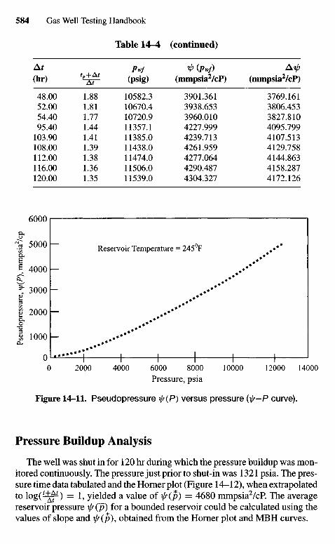
Table 14-4 (continued)
Af pwf Ip(Pw/) Ai/?
(hr) ^±££ (psig) (mmpsia2/cP) (mmpsia2/cP)
48.00 1.88 10582.3 3901.361 3769.16152.00 1.81 10670.4 3938.653 3806.45354.40 1.77 10720.9 3960.010 3827.81095.40 1.44 11357.1 4227.999 4095.799103.90 1.41 11385.0 4239.713 4107.513108.00 1.39 11438.0 4261.959 4129.758112.00 1.38 11474.0 4277.064 4144.863116.00 1.36 11506.0 4290.487 4158.287120.00 1.35 11539.0 4304.327 4172.126
Pseu
dopr
essu
re,
i|/(P
), m
mps
ia2/c
p
Reservoir Temperature = 2450F
Pressure, psia
Figure 14-11. Pseudopressure •ft(P) versus pressure {ft-P curve).
Pressure Buildup Analysis
The well was shut in for 120 hr during which the pressure buildup was mon-itored continuously. The pressure just prior to shut-in was 1321 psia. The pres-sure time data tabulated and the Horner plot (Figure 14-12), when extrapolatedto log (^pO = 1, yielded a value of "ft {pi) = 4680 mmpsia2/cP. The averagereservoir pressure \lr(p) for a bounded reservoir could be calculated using thevalues of slope and \/r(p), obtained from the Horner plot and MBH curves.
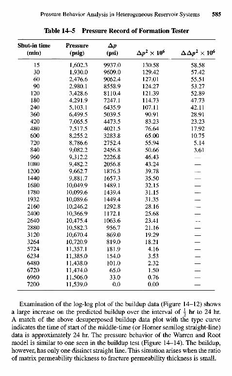
Table 14-5 Pressure Record of Formation Tester
Shut-in time Pressure Ap(min) (psig) (psi) Ap2 X 106 AAp2 X 106
15 1,602.3 9937.0 130.58 58.5830 1,930.0 9609.0 129.42 57.4260 2,476.6 9062.4 127.01 55.5190 2,980.1 8558.9 124.27 53.27
120 3,428.6 8110.4 121.39 52.89180 4,291.9 7247.1 114.73 47.73240 5,103.1 6435.9 107.11 42.11360 6,499.5 5039.5 90.91 28.91420 7,065.5 4473.5 83.23 23.23480 7,517.5 4021.5 76.64 17.92600 8,255.2 3283.8 65.00 10.75720 8,786.6 2752.4 55.94 5.14840 9,082.2 2456.8 50.66 3.61960 9,312.2 2226.8 46.43 —
1080 9,482.2 2056.8 43.24 —1200 9,662.7 1876.3 39.78 —1440 9,881.7 1657.3 35.50 —1680 10,049.9 1489.1 32.15 —1780 10,099.6 1439.4 31.15 —1932 10,089.6 1449.4 31.35 —2160 10,246.2 1292.8 28.16 —2400 10,366.9 1172.1 25.68 —2640 10,475.4 1063.6 23.41 —2880 10,582.3 956.7 21.16 —3120 10,670.4 869.0 19.29 —3264 10,720.9 819.0 18.21 —5724 11,357.1 181.9 4.16 —6234 11,385.0 154.0 3.53 —6480 11,438.0 101.0 2.32 —6720 11,474.0 65.0 1.50 —6960 11,506.0 33.0 0.76 —7200 11,539.0 0.0 0.00 —
Examination of the log-log plot of the buildup data (Figure 14-12) showsa large increase on the predicted buildup over the interval of \ hr to 24 hr.A match of the above desuperposed buildup data plot with the type curveindicates the time of start of the middle-time (or Horner semilog straight-line)data is approximately 24 hr. The pressure behavior of the Warren and Rootmodel is similar to one seen in the buildup test (Figure 14-14). The buildup,however, has only one distinct straight line. This situation arises when the ratioof matrix permeability thickness to fracture permeability thickness is small.
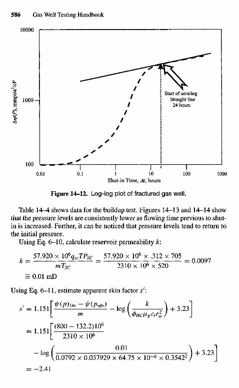
Shut-in Time, At, hours
Figure 14-12. Log-log plot of fractured gas well.
Table 14-4 shows data for the buildup test. Figures 14-13 and 14-14 showthat the pressure levels are consistently lower as flowing time previous to shut-in is increased. Further, it can be noticed that pressure levels tend to return tothe initial pressure.
Using Eq. 6-10, calculate reservoir permeability k:
_ 57.920 x 10⁶^crP5c _ 57.920 x 106 x .312 x 705 _* " rihc = 2310 x 106 x 520 " °* ?
= 0.01 mD
Using Eq. 6-11, estimate apparent skin factor s':
s>=1.15l\f(phhr-*iP»fo)-\og( k \ +3.231
["(800-132.2)106
" [ 231OxIO6
~ 1 O g V0.0792 x 0.037929 x 64.75 x 10~6 x 0.35422/ + 3- J
= -2.41
D1X
l(F),
mm
psi
a2/cP
Start of semilogStraight line
24 hours
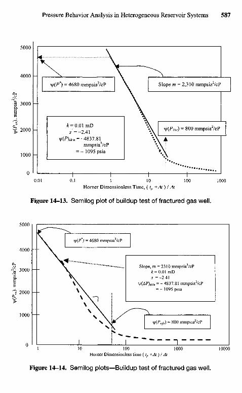
Horner Dimensionless time (tp +At) I At
Figure 14-14. Semilog plots—Buildup test of fractured gas well.
Horner Dimensionless Time, (tp -+At) I At
Figure 14-13. Semilog plot of buildup test of fractured gas well.
W(Pwfo) = 800 mmpsia2/cP
Slope, m = 2310 mmpsia2/cPk = 0.01 mDs' = -2.41
M/(AP)skin = - 4837.81 mmpsia2/cP= - 1095 psia
\\i(P*) = 4680 mmpsia2/cP
it= 0.01 mD5=-2 .41
vWskin = -4837.81mmpsia2/cP
= - 1095 psia
XjZ(P*) = 4680 mmpsia2/cP Slope m = 2,310 mmpsia2/cP
V(Pihr) = 800 mmpsia2/cP
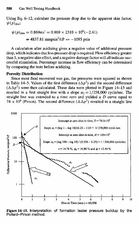
Using Eq. 6-12, calculate the pressure drop due to the apparent skin factor,f{p)skin>
ty(p)skin = 0.869ms' = 0.869 x 2310 x 106(-2.41)
= 4837.81 mmpsia2/cP *± -1095 psia
A calculation after acidizing gives a negative value of additional pressuredrop, which indicates that less pressure drop is required. Flow efficiency greaterthan 1, a negative skin effect, and a negative damage factor will all indicate suc-cessful stimulation. Percentage increase in flow efficiency can be determinedby comparing the tests before acidizing.
Porosity DistributionSince most fluid recovered was gas, the pressures were squared as shown
in Table 14-5. Values of the first difference (Ap2) and the second difference(AAp2) were then calculated. These data were plotted in Figure 14-15 andresulted in a first straight line with a slope a\ = 1/258,000 cycle/sec. Thestraight line was extended to a time zero and yielded a D curve equal to74 x 106 (Pirson). The second difference (AAp2) resulted in a straight line
Intercept at zero shut-in time, D = 74.OxIO6
Slope a, = (log 1 - log 10)/(6.23 - 3.65 = 1/ 258,000 cycle /sec
Intercept at zero shut-in time, H = 16Ox 106
Slope CC2 = (log 100 - log 10) / (0.556 - 0.25) = 1 / 306,000 cycle/sec
v= 14.78 %, (j>m = 10.80 % and $ = 12.44 %
Shut-in Time (sees.) x 60,000
Figure 14-15. Interpretation of formation tester pressure buildup by thePollard-Pirson method.
Dif
fere
ntia
l Pre
ssur
e, m
mps
ia2/c
P
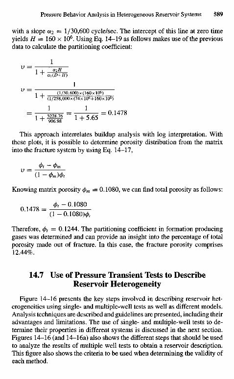
with a slope c*2 = 1/30,600 cycle/sec. The intercept of this line at zero timeyields H = 160 x 106. Using Eq. 14-19 as follows makes use of the previousdata to calculate the partitioning coefficient:
1
1 ^ <*i(D+ff)
_ 1V ~~ i I (1/30,600)x(16Ox IQ6)
1 -*" (l/258,000x(74xl06+160xl06)
= T^mM = TT565 = ( U 4 7 8
1 + 906.98 l t J l U J
This approach interrelates buildup analysis with log interpretation. Withthese plots, it is possible to determine porosity distribution from the matrixinto the fracture system by using Eq. 14-17,
v ~ ( l - 4>m)4>t
Knowing matrix porosity (/>m = 0.1080, we can find total porosity as follows:
0.1478 = * - ° - 1 0 8 0
(1-0.1080)0,
Therefore, <f>t = 0.1244. The partitioning coefficient in formation producinggases was determined and can provide an insight into the percentage of totalporosity made out of fracture. In this case, the fracture porosity comprises12.44%.
14.7 Use of Pressure Transient Tests to DescribeReservoir Heterogeneity
Figure 14-16 presents the key steps involved in describing reservoir het-erogeneities using single- and multiple-well tests as well as different models.Analysis techniques are described and guidelines are presented, including theiradvantages and limitations. The use of single- and multiple-well tests to de-termine their properties in different systems is discussed in the next section.Figures 14-16 (and 14-16a) also shows the different steps that should be usedto analyze the results of multiple well tests to obtain a reservoir description.This figure also shows the criteria to be used when determining the validity ofeach method.
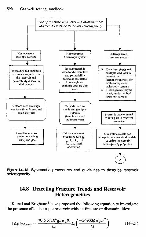
Figure 14-16. Systematic procedures and guidelines to describe reservoirheterogeneity.
14.8 Detecting Fracture Trends and ReservoirHeterogeneities
Kamal and Brigham13 have proposed the following equation to investigatethe presence of an isotropic reservoir without fracture or discontinuities:
70.6 x UPqxP8P8 / -569OO0^cr 2 \L&P !Calculate = TT ^i ( 7 I (14-21)
HomogeneousAnisotropic system
Pressure match issame for different tests
and permeabilityfunctions calculated
from single andmultiple tests are also
same
HomogeneousIsotropic System
If porosity and thicknessare same everywhere in
the reservoir andpermeability is same in
all directions
Heterogeneousreservoir system
Data from single andmultiple well tests failto meet thehomogeneous tests forboth isotropic andanisotropy systemsHeterogeneity may beareal, vertical or bothareal and vertical
System is undeterminedwith respect to reservoir
parameters
Use well tests data andcomputer mathematical models
to estimate reservoirheterogeneity properties
Methods used aresingle and multiple-
well tests(interference andpulse analysis)
Calculate reservoirproperties such as
k Ir Ir h
"Xt > yy ' xy t "*
kmax • Knin andorientation
Methods used are singlewell tests (interference and
pulse analysis)
Calculate reservoirproperties such as
kh//jg and (j)cth
Use of Pressure Transients and MathematicalModels to Describe Reservoir Heterogeneity
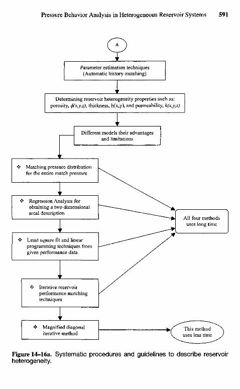
Figure 14-16a. Systematic procedures and guidelines to describe reservoirheterogeneity.
Matching pressure distributionfor the entire match pressure
Regression Analysis forobtaining a two dimensionalareal description
Least square fit and linearprogramming techniques fromgiven performance data
Iterative reservoirperformance matchingtechniques
Magnified diagonaliterative method
All four methodsuses long time
This methoduses less time
Different models their advantagesand limitations
Determining reservoir heterogeneity properties such as:porosity, ^)(x,y,z), thickness, h(x,y), and permeability, k(x,y,z)
Parameter estimation techniques(Automatic history matching)

( c ) Possible sealing fault ( d ) Possible naturally fractured system
Figure 14-17. (a) Location and distance between wells, (b) Possible nonseal-ing faults, (c) Possible sealing fault, (d) Possible naturally fractured system.
where r is the distance between producing and observation well, ft, and t is theflowing time in minutes. Figures 14-17a through 14-17d show general trendsof various reservoir heterogeneutities. Figure 14-18 can be used to confirmcommunication through the reservoir between producer and observation wellor possible to determine general trends or possibilities.
Example 14-3 Detecting Reservoir Heterogeneity or Fracture TrendsTable 14-6 shows the location of six wells. All six wells were shut in until a
stabilized pressure buildup was obtained. The middle well (1) was then placedon production for 110 days. Well/reservoir data are as follows: Pt — 4450 psi;fig = 0.025 cP; rw = 0.550 ft; pg = 6.06 bbl/scf; h = 45 ft; gas injectionrate qg = 5.0 mmscfd; T = 164°F; 0 = 8.5%; ct = 4.45 x 10"3 psi"1; welldepth = 6340 ft.
Substituting the above values in Eq. 14-21 results in the values given inTable 14-7.
Table 14-7 shows as examples the match for well pairs A2-A1, A4-A1,A5-A1, and A6-A1. This will indicate an isotropic reservoir without fractures.
( a ) Location and distance between wells ( b ) Possible nonsealing faults
Producingwell
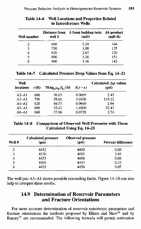
Table 14-6 Well Locations and Properties Relatedto Intereference Wells
Distance from k from buildup tests kh productWell number well 1 (mD) (mD-ft)
2 660 3.24 1463 750 3.00 1354 620 2.67 1205 890 3.36 1516 660 3.16 142
Table 14-7 Calculated Pressure Drop Values from Eq. 14-21
Well Calculated Ap valueslocations r(ft) 70.6qgiJ,g/3g/kh Et{-x) (psi)
A2-A1 660 36.63 0.0669 2.45A3-A1 750 39.61 3.0100 119.22A4-A1 620 44.57 0.0660 2.94A5-A1 890 35.42 1.4800 52.42A6-A1 660 37.66 0.0728 2.74
Table 14-8 Comparison of Observed Well Pressures with ThoseCalculated Using Eq. 14-21
Calculated pressure Observed pressureWell # (psi) (psi) Percent difference
2 4452 4450 0.053 4570 4685 2.454 4453 4456 0.065 4503 4493 0.226 4453 4450 0.07
The well pair A3-A1 shows possible nonsealing faults. Figure 14-18 can alsohelp to interpret these results.
14.9 Determination of Reservoir Parametersand Fracture Orientations
For more accurate determination of reservoir anisotropic parameters andfracture orientations the methods proposed by Elkins and Skov14 and byRamey15 are recommended. The following formula will permit estimation
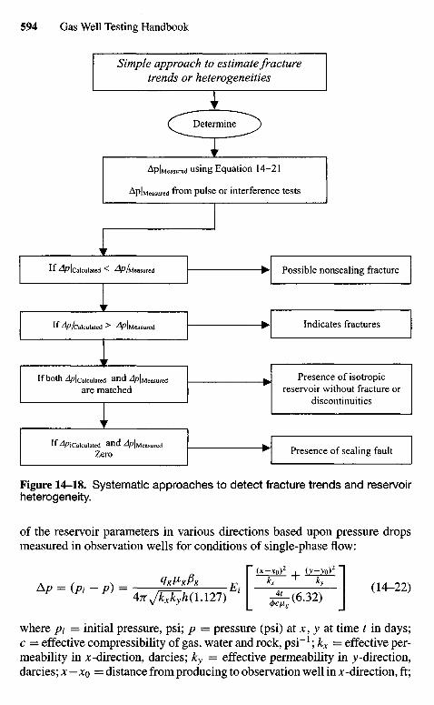
Figure 14-18. Systematic approaches to detect fracture trends and reservoirheterogeneity.
of the reservoir parameters in various directions based upon pressure dropsmeasured in observation wells for conditions of single-phase flow:
Ap = (P, -p) = —M£l E1 [ l ^ l z S l l (14_22)4njkjryh(l.m) [ ^(6-32) J
where pt = initial pressure, psi; p = pressure (psi) at x, y at time t in days;c = effective compressibility of gas, water and rock, psi"1; kx = effective per-meability in *-direction, darcies; ky = effective permeability in j-direction,darcies; x — XQ = distance from producing to observation well in x -direction, ft;
Possible nonsealing fracture
Indicates fractures
Presence of isotropicreservoir without fracture or
discontinuities
Presence of sealing fault
If ^!calculated < 4pAieasured
If 4^/calculated > 4HMeasured
If both 4?|calculated and 4p|Measuredare matched
IfZlplcalcuIated and ^MeasuredZero
Ap|Measured using Equation 14-21
Ap I Measured from pulse or interference tests
Determine
Simple approach to estimate fracturetrends or heterogeneities
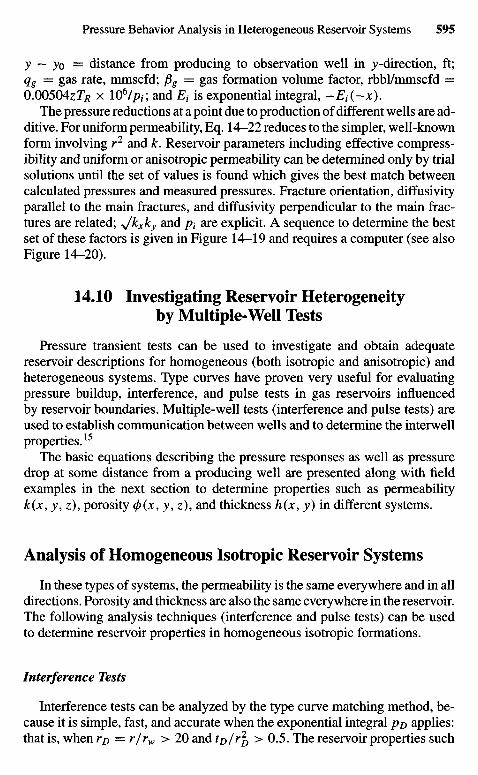
y — y0 = distance from producing to observation well in ^-direction, ft;qg = gas rate, mmscfd; fig = gas formation volume factor, rbbl/mmscfd =0.00504Z^ x lO6/pr, and E1 is exponential integral, -Ei(-x).
The pressure reductions at a point due to production of different wells are ad-ditive. For uniform permeability, Eq. 14-22 reduces to the simpler, well-knownform involving r2 and k. Reservoir parameters including effective compress-ibility and uniform or anisotropic permeability can be determined only by trialsolutions until the set of values is found which gives the best match betweencalculated pressures and measured pressures. Fracture orientation, diffusivityparallel to the main fractures, and diffusivity perpendicular to the main frac-tures are related; *Jkxky and pt are explicit. A sequence to determine the bestset of these factors is given in Figure 14-19 and requires a computer (see alsoFigure 14-20).
14.10 Investigating Reservoir Heterogeneityby Multiple-Well Tests
Pressure transient tests can be used to investigate and obtain adequatereservoir descriptions for homogeneous (both isotropic and anisotropic) andheterogeneous systems. Type curves have proven very useful for evaluatingpressure buildup, interference, and pulse tests in gas reservoirs influencedby reservoir boundaries. Multiple-well tests (interference and pulse tests) areused to establish communication between wells and to determine the interwellproperties.15
The basic equations describing the pressure responses as well as pressuredrop at some distance from a producing well are presented along with fieldexamples in the next section to determine properties such as permeabilityk(x, y, z), porosity (p(x, y, z), and thickness h(x, y) in different systems.
Analysis of Homogeneous Isotropic Reservoir Systems
In these types of systems, the permeability is the same everywhere and in alldirections. Porosity and thickness are also the same everywhere in the reservoir.The following analysis techniques (interference and pulse tests) can be usedto determine reservoir properties in homogeneous isotropic formations.
Interference Tests
Interference tests can be analyzed by the type curve matching method, be-cause it is simple, fast, and accurate when the exponential integral pu applies:that is, when rD = r/rw > 20 and tDlr2
D > 0.5. The reservoir properties such
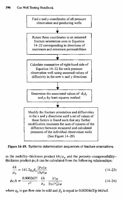
Find x and y coordinates of all pressureobservation and producing wells
Rotate these coordinates to an assumedfracture orientation axes in Equation14-22 corresponding to directions of
maximum and minimum permeabilities
Calculate summation of right-hand side ofEquation 14-22 for each pressure
observation well using assumed values ofdiffusivity in the new x and y directions
Determine the associated values of ^Jkxky
and pi by least-squares method
Modify the fracture orientation and diffusivitiesin the x and y directions until a set of values of
these factors is found such that any furthermodification increases the sum of squares of the
difference between measured and calculatedpressures of the individual observation wells
(See Figure 14-20)
Figure 14-19. Systemic determination sequences of fracture orientations.
as the mobility-thickness product kh//ag and the porosity-compressibility-thickness product (j)cth can be calculated from the following relationships:
f = 1 4 1 . 2 ^ ^ (14-23)
0.0002637 kh \t\M4>cth = -2 " " (14-24)
r2 /xg \tD/r2D\M
where qg is gas flow rate in scfd and pg is equal to 0.00504zT/p bbl/scf.
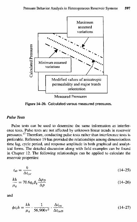
Measured Pressures
Figure 14-20. Calculated versus measured pressures.
Pulse Tests
Pulse tests can be used to determine the same information as interfer-ence tests. Pulse tests are not affected by unknown linear trends in reservoirpressures.17 Therefore, conducting pulse tests rather than interference tests ispreferable. Reference 19 has provided the relationships among dimensionlesstime lag, cycle period, and response amplitude in both graphical and analyt-ical forms. The detailed discussion along with field examples can be foundin Chapter 12. The following relationships can be applied to calculate thereservoir properties:
ttD = - » - (14-25)Atcyc
and
Maximumassumed
variations
Minimum assumedvariations
Modified values of anisotropicpermeability and major trends
orientation
Cal
cula
ted
Pres
sure
s
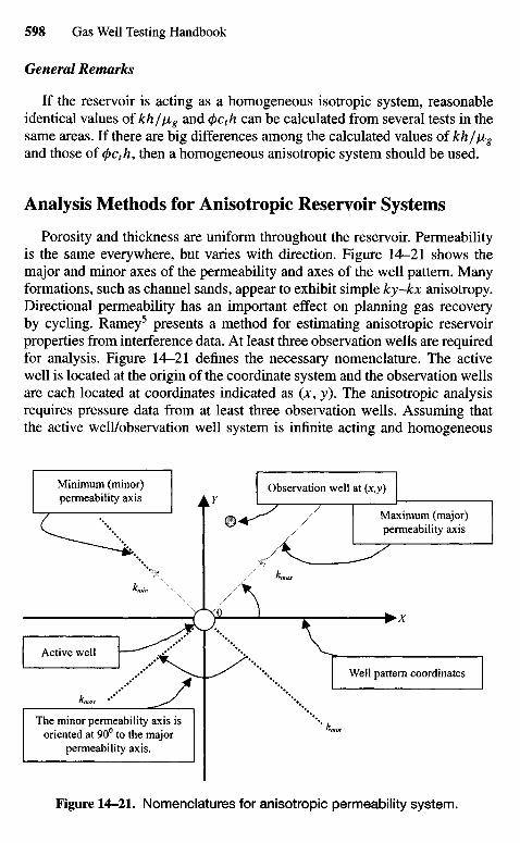
General Remarks
If the reservoir is acting as a homogeneous isotropic system, reasonableidentical values of kh/jjLg and (f>cth can be calculated from several tests in thesame areas. If there are big differences among the calculated values of kh/fig
and those of <j)cth, then a homogeneous anisotropic system should be used.
Analysis Methods for Anisotropic Reservoir Systems
Porosity and thickness are uniform throughout the reservoir. Permeabilityis the same everywhere, but varies with direction. Figure 14-21 shows themajor and minor axes of the permeability and axes of the well pattern. Manyformations, such as channel sands, appear to exhibit simple ky-kx anisotropy.Directional permeability has an important effect on planning gas recoveryby cycling. Ramey5 presents a method for estimating anisotropic reservoirproperties from interference data. At least three observation wells are requiredfor analysis. Figure 14-21 defines the necessary nomenclature. The activewell is located at the origin of the coordinate system and the observation wellsare each located at coordinates indicated as (x, y). The anisotropic analysisrequires pressure data from at least three observation wells. Assuming thatthe active well/observation well system is infinite acting and homogeneous
Minimum (minor)permeability axis
Observation well at (x,y)
Maximum (major)permeability axis
Well pattern coordinates
Active well
The minor permeability axis isoriented at 90° to the major
permeability axis.
Figure 14-21. Nomenclatures for anisotropic permeability system.
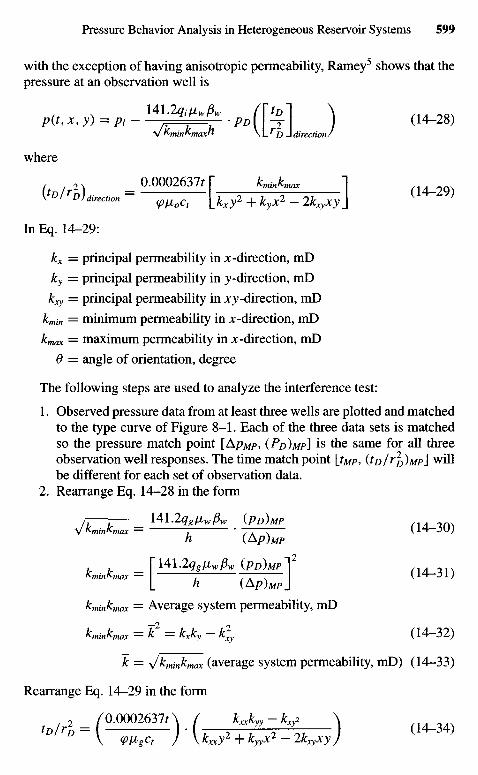
with the exception of having anisotropic permeability, Ramey5 shows that thepressure at an observation well is
p{t,x,y) = Pi . p / ? M _ I (14-28)V fcmin *max "> \ L D J direction /
where
2 _ 0.0002637; T kminkmax 1K<D/rD)direction - ^ ^ [kxy2 + kyX2_2kxyXy\ ( 1 4" 2 9>
In Eq. 14-29:
kx = principal permeability in x -direction, mD
ky = principal permeability in y-direction, mD
kxy = principal permeability in .^-direction, mD
kmin = minimum permeability in x -direction, mD
kmax = maximum permeability in x -direction, mD
6 = angle of orientation, degree
The following steps are used to analyze the interference test:
1. Observed pressure data from at least three wells are plotted and matchedto the type curve of Figure 8-1 . Each of the three data sets is matchedso the pressure match point [ApMP, {PD)MP\ is the same for all threeobservation well responses. The time match point [tMp, (to/r^Mp} willbe different for each set of observation data.
2. Rearrange Eq. 14-28 in the form
/j—r- _ U\2qglxwfiw (pD)MP
h (&P)MP
L h (Ap)Mp J
kminkmax = Average system permeability, mD
kminkmax = & — ^x^y ^xy \1^~*^)
k = y/kminkmax (average system permeability, mD) (14-33)
Rearrange Eq. 14-29 in the form
, B / r , /MOMgTA. / * A - V ) (M_34)V <piigct J \kxxy
2 + kyyX2 - Ik^xy)
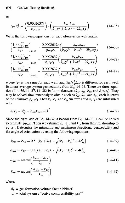
or
2 /0.0002637A / kmaxkmin \tDlY° = [-^r) • [^+ ^-Tk19Xy) (14~35)
Write the following equations for each observation well match:
r(to/ r£Lp] = Q-0002637r / kmaxkmin \L *MP J WeM </>flgCf Vkxxy2 + kyyX2 - 2kxyXy)
r ( W ^ L P 1 = 0.0002637 / kmaxkmin \ ^ ^L fMP J Hfe/C ^ / ^ ^ ^ \ kXXy2 + ^yyX2 - 2 ^ X J /
T ( ^ A D L P 1 = 0-0002637 / kmaxkmin \ (1
L MP JweiB <t>HgCt \kxxy2 + ^ 2 - Ik^xy)
where rM/> is the same for each well, and (to/r^MP is different for each well.Estimate average system permeability from Eq. 14-33. There are three equa-tions (14-36, 14-37, 14-38) in four unknowns (kxx, kyy, kxy, and (pi±oct). Theymay be solved simultaneously to obtain such as kxx, kyy, and k^, each in termsof the unknown (\>\JLgct. Then kx,ky, and k^ (in terms of (/)jJigCt) are substitutedinto
Since the right side of Eq. 14-32 is known from Eq. 14-30, it can be solvedto estimate 0JHOC?. Then we estimate kx,ky, and k^ from their relationship to(/)/uLoct. Determine the minimum and maximum directional permeability andthe angle of orientation by using the following equations:
kmin = kxx = 0.5 [(kx + ky) - y/(kx-ky)2 + 4kl\ (14-39)
kmax = kw = 0.5 [(*, + ky) - J(kx-ky)2 + 4kl\ (14-40)
^ / ^max & XX \ /t A * t\
0max = arctanl j (14-41)
n , {Kmin — kYY\ /1A .^0min = arctan (14-42)
V *xy /where
fig = gas formation volume factor, bbl/scfQ = total system effective compressibility, ps i " 1
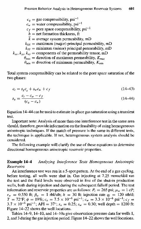
cg = gas compressibility, psi l
cw = water compressibility, psi"1
Cf = pore space compressibility, psi"1
h — net formation thickness, ftk = average system permeability, mD
kxx — maximum (major) principal permeability, mDkyy = minimum (minor) principal permeability, mD
kxx, kyy, kxy = components of the permeability tensor, mD0max = direction of maximum permeability, Kmax
0min = direction of minimum permeability, Kmin
Total system compressibility can be related to the pore space saturation of thetwo phases:
ct = sgcg + swcw + Cf (14-43)
{Cg — Cw)
Equation 14-44 can be used to estimate in-place gas saturation using a transienttest.
Important note: Analysis of more than one interference test in the same areashould, therefore, provide information on the feasibility of using homogeneousanisotropic techniques. If the match of pressure is the same in different tests,the technique is applicable. If not, heterogeneous system analysis should beconsidered.
The following example will clarify the use of these equations to determinedirectional homogeneous anisotropic reservoir properties.
Example 14-4 Analyzing Interference Tests Homogeneous AnisotropicReservoirs
An interference test was run in a 5-spot pattern. At the end of a gas cycling,before testing, all wells were shut in. Gas injecting at 7.25 mmscfd/d ranthe test and the fluid levels were observed in five of the shut-in productionwells, both during injection and during the subsequent falloff period. The testinformation and reservoir properties are as follows: P1- = 265 psi; /JLW = 1 cP;rw = 0.550 ft; fiw = 1 rbl/stb; h = 30 ft; injection rate qt = 120 stb/d;T = 72°F; 0 = 19%; co = 7.5 x 10"6 psi"1; cw = 3.3 x 10"6 psi"1; cf =3.7 x 10~6 psi"1; API = 37°; so = 0.25; sw = 0.30; well depth = 1200 ft:Figure 14-22 shows the well locations.
Tables 14-9, 14-10, and 14-1Oa give observation pressure data for wells 1,2, and 3 during the gas injection period. Figure 14-22 shows the well locations.
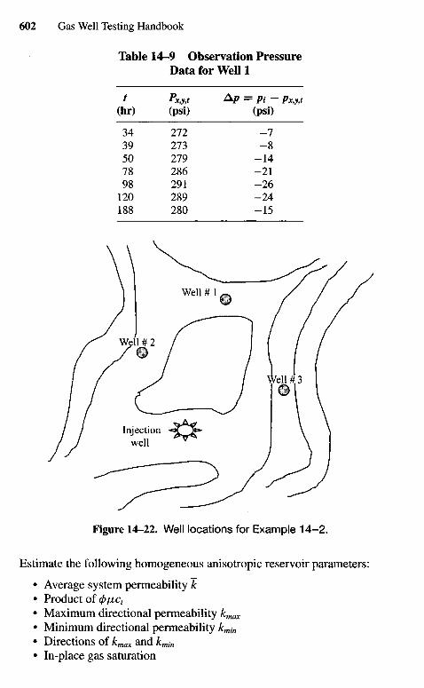
Table 14-9 Observation PressureData for Well 1
t PX>y:( A p = Pi ~ PX>yyt(hr) (psi) (psi)
34 272 -739 273 -850 279 -1478 286 -2198 291 -26120 289 -24188 280 -15
Figure 14-22. Well locations for Example 14-2.
Estimate the following homogeneous anisotropic reservoir parameters:
• Average system permeability k• Product of 0/xcr
• Maximum directional permeability kmax
• Minimum directional permeability kmin
• Directions of kmax and kmin
• In-place gas saturation
Injectionwell
Well # 3
Well # 2
Well # 1
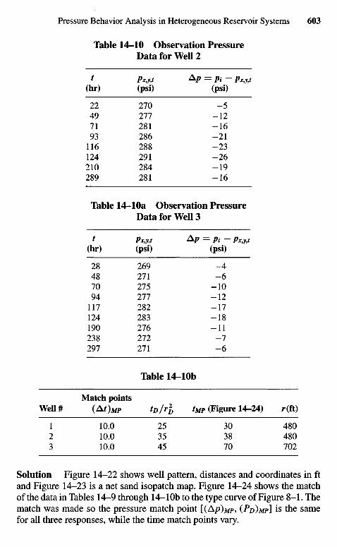
Table 14-10 Observation PressureData for Well 2
t PX)y)t Ap = Pi — PX>yyt
(hr) (psi) (psi)
22 270 -549 277 -1271 281 -1693 286 -21116 288 -23124 291 -26210 284 -19289 281 -16
Table 14-1Oa Observation PressureData for Well 3
t Pxyy,t Ap = Pi — pXyy>t
(hr) (psi) (psi)
28 269 - 448 271 - 670 275 -1094 277 -12
117 282 -17124 283 -18190 276 -11238 272 - 7297 271 - 6
Table 14-1Ob
Match pointsWell # (At)MP tD/r2
D tMP (Figure 14-24) r(ft)
1 10.0 25 30 4802 10.0 35 38 4803 10.0 45 70 702
Solution Figure 14-22 shows well pattern, distances and coordinates in ftand Figure 14-23 is a net sand isopatch map. Figure 14-24 shows the matchof the data in Tables 14-9 through 14-1Ob to the type curve of Figure 8-1. Thematch was made so the pressure match point [(Ap)Mp, (PD)MP\ is the samefor all three responses, while the time match points vary.
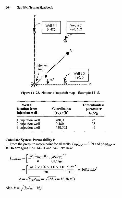
Figure 14-23. Net sand isopatch map—Example 14-2.
Well # Dimentionlesslocation from Coordinates parameterinjection well (x, y) (ft) tD /r£
1, injection well 480,0 252, injection well 0,480 353, injection well 480,702 45
Calculate System Permeability kFrom the pressure match point for all wells, (PD)MP = 0.29 and (Ap)MP =
10. Rearranging Eqs. 14-31 and 14-3, we have
_ \U\.2qniwpw (PD)MP]2
L h (Ap)MP J
[141.2 x 12Ox 1.0 x 1.0 0.29 1 2
* = Vkminkmax = V268.3 = 16.38 mD
Also, k = J(kxxkyy - k^).
Well # 3480,0
Injectionwell
Well # 10,480
Well # 2480, 702
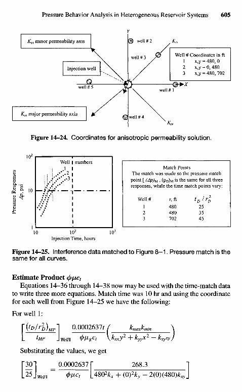
Injection Time, hours
Figure 14-25. Interference data matched to Figure 8 -1 . Pressure match is thesame for all curves.
Estimate Product </>/zc,Equations 14-36 through 14-38 now may be used with the time-match data
to write three more equations. Match time was 10 hr and using the coordinatefor each well from Figure 14-25 we have the following:
For well 1:
[ ( W ^ M P 1 0.0002637; / kmaxkmin \
L fMP \Wein <l>Vgct \kjocy2 + kyyX2 - k^xyj
Substituting the values, we get
pO"j _ 0.00026371" 268.3 1L25 J ^ i = 4>V>ct L4802^ + (0)% - 2(0X480)*^ J
Well numbersMatch Points
The match was made so the pressure matchpoint [ (Ap)M , (PD)M is t n e same for all threeresponses, while the time match points vary:
Well # r, ft tD I rl
1 480 252 480 353 702 45
Pres
sure
Res
pons
esA
p, p
si
Figure 14-24. Coordinates for anisotropic permeability solution.
Well # Coordinates in ft1 x,y = 480, 02 x,y = 0, 4803 x,y = 480, 702
Injection well
KJU major permeability axis
Kyy minor permeability axis
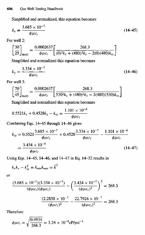
Simplified and normalized, this equation becomes
3.685 x IQ-7
kx = (14-45)
For well 2:
pO"| _ 0.00026371" 268.3 1
l_25_L/2 " 4>№ L(O) 2^ + (4S0)2ky - 2(0)(480)^ J
Simplified and normalized this equation becomes
3.334 x IQ-7
ky = (14-46)(J)JJiCt
For well 3:
1"7Ol _ 0.0002637 T 2683 1
l^lweia ~ 4>№ [5302/:x + (4S0)2ky - 2(480)(530)^ J
Simplified and normalized this equation becomes
0.552U, + 0.4528JL - *« = L 1 0 1 X 1 0
(j)llCt
Combining Eqs. 14-45 through 14-46 gives
r, « „ 3 ' 6 8 5 X 1 0 " 7 ^ , ^ n 3 - 3 3 4 X 1 0 " 7 L 1 0 1 X 1 0 " 6
kxy = 0.5521 + 0.4528<PllCt (J)IlCf (pllCt
= 3-4 3 4 x l°-8 (I«7)(J)IlCf
Using Eqs. 14-45, 14^6, and 14-47 in Eq. 14-32 results in
k k — k2 — k k —1?1^x 1^y 1^ xy — ^min^maX — 1^
or
(3.685 x 10"7)(3.334 x 10~7) /3.434 x 10"7\ 2 _
(0/XQ)(0/XQ) V (0/^Q)2 /
12.2858 x 10"7 22.7924 x 10"7 _
((/)llCt)2 ((l>№t)2
Therefore
/O 4934< ^ c ' = V ^ T = 3 - 2 4 x 10"6cP/psi"'
V ZOo. 5
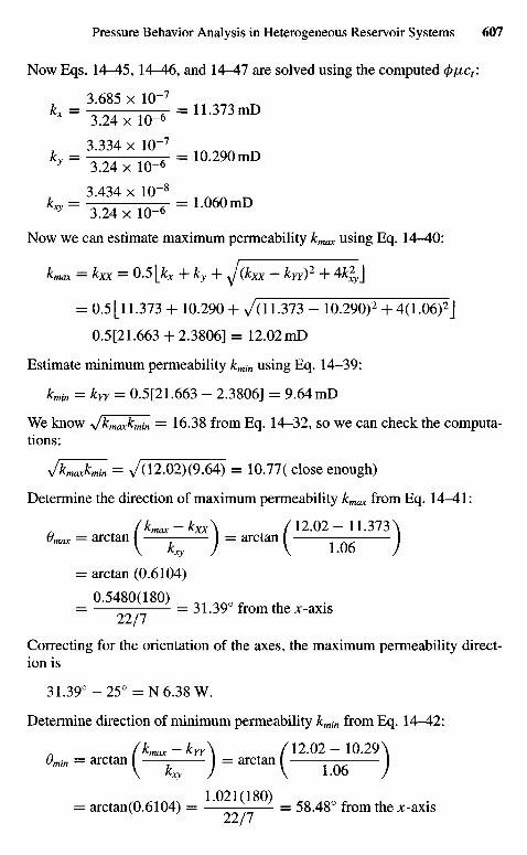
Now Eqs. 14-45, 14-46, and 14-47 are solved using the computed (/>jjict:
3.434 x 10"8
^ = 3.24x10-6 = 1 ° 6 O m D
Now we can estimate maximum permeability kmax using Eq. 14-40:
kmax = kXX = 0.5[kx +ky+ yJikxx-kyY^+Akl]
= 0.5 [11.373 + 10.290 + 7(11373 - 10.290)2 + 4(1.06)2J
0.5[21.663 + 2.3806] = 12.02 mD
Estimate minimum permeability kmin using Eq. 14-39:
kmin =krY = 0.5[21.663 - 2.3806] - 9.64mD
We know \fkmaxkmin = 16.38 from Eq. 14-32, so we can check the computa-tions:
y/kmaxkmin = >/(12.02)(9.64) = 10.77( close enough)
Determine the direction of maximum permeability kmax from Eq. 14^-1:
a f (kmax~kxx\ f ^12.02-11.373^Omax = arctan = arctan - —
V kxy ) \ 1.06 /
= arctan (0.6104)
0.5480(180)= = 31.39 from the x-axis
Correcting for the orientation of the axes, the maximum permeability direct-ion is
31.39°-25° = N 6.38 W.
Determine direction of minimum permeability kmin from Eq. 14-42:
a t (krnax-krA f ^12.02-10.29^emin = arctan = arctan —
V fcxy / V 1.06 /
= arctan(0.6104) = = 58.48° from the x-axis
Correcting for the orientation of the axes, the minimum permeability direct-ion is
58.48° - 25° = N 33.48 W
As shown in Figure 14-23, the jc-axis was chosen as a line through wells 1, 2,and 3. True north lies along the line through wells 2 and 3.
Estimate gas saturation using Eq. 14-44:
_ ct - cw - Cf _ 7.85 x 10~6 - 3.30 x 10~6 - 3.70 x 10"6
S° ~ co-cw "~ 7.40 x 10~6 - 3.30 x 10"6
0.85 x 10"6
= -4i ino^ = 0-21
Hence water saturation is sw = 1 — so — 1 — 0.21 = 0.79.If we check these saturation values with electric log and core data, they are
in good agreement, hence it is possible to make a rough estimate of in-placesaturation using a transient test.
SummaryEquations 14-28 through 14-47, coupled with the log-log type curve pro-
cedure, form a powerful tool for detecting reservoir anisotropy. The injectioninterference test described can be applied widely to aid in planning fluid in-jection programs.
Analysis of Heterogeneous Systems
If the data from multiwell tests fail to meet the homogenity requirementfor both isotropic and anisotropic cases, numerical solutions must be used toanalyze pressure transient data from heterogeneous systems. References 17and 18 have suggested numerical solutions for performing the analysis byparameter estimation techniques to describe reservoir heterogeneities usingpressure transient data. They consider the case of heterogeneous isotropicsystems using the following diffusion equation:
V . (-Vp) = (t>ctd-^ + Q (14-48)
where Q is the diffusion equation source term and p is pressure, psi. In orderto estimate the values of kh(x, y, z) and (j>cth(x, y, z) that minimize E:
Chaventefa/.:17
E = J^f {pf-pffdT (14-49)
Chen et a/.:18
E = Ilil(ptS-PCnf)2 (14-50)W = I J = I
where
£ = sum of the squares of the difference between observed andcalculated pressure, psi2
S = number of observation wells
N = number of observations at well S
p°bs = observed pressure at well S, psi
peak _ c a i c u i a t e ( j pressure at well S, psi
p°b* = observed pressure at well S and data point n
p™lsc = calculated pressure at well S and data point n
References and Additional Reading
1. Vairogs, J., Hearn, C. L., Dareing, D. W., and Rhoades, V. W., "Effectof Rock Stress on Gas Production from Low-Permeability Reservoirs,"J. Petroleum TechnoL (Sept. 1971) 1161-1167; Trans. AIME 251.
2. Thomas, R. D., and Ward, D. C , "Effect of Overburden Pressure andWater Saturation on the Gas Permeability of Tight Sandstone Cores,"J. Petroleum TechnoL (Feb. 1972) 120-124.
3. Vairogs, J., and Rhoades, V. W., " Pressure Transient Tests in FormationsHaving Stress-Sensitive Permeability," /. Petroleum TechnoL (Aug. 1973)965-970; Trans. AIME 255.
4. Raghavan, R., Scorer, J. D. T., and Miller. F. G., "An Investigation byNumerical Methods of the Effect of Pressure Dependent Rock and FluidProperries on Well Flow Tests," Soc. Petroleum Eng. J. (June 1972) 267-275; Trans. AIME 253.
5. Ramey, H. J., Jr., "Non-Darcy Flow and Wellbore Storage Effects in Pres-sure Buildup and Drawdown of Gas Wells," /. Petroleum TechnoL (Feb.1965) 223-233; Trans. AIME 234. Also Reprint Series, No. 9—PressureAnalysis Methods, Society of Petrolem Engineers of AIME, Dallas, TX,1967, pp. 233-243.
6. Matthews, C. S., and Russell, D. G., Pressure Buildup and Flow Testsin Wells. Monograph Series, Society of Petroleum Engineers of AIME,Dallas, TX, 1967.
7. Homer, D. R., "Pressure Build-up in Wells," Proc. Third World Pet. Cong.,The Hague (1951), Sec. II, 503-523. Also Reprint Series, No. 9—Pressure
Analysis Methods, Society of Petroleum Engineers of AIME, Dallas, TX,1967, pp. 25-43.
8. Gray, K. E., "Approximating Well-to-Fault Distance from Pressure Build-up Tests," /. Petroleum Technol (July 1965) 761-767.
9. Davis, E. G., Jr., and Hawkins, M. E, Jr., "Linear Fluid-Barrier Detectionby Well Pressure Measurements,"/. Petroleum Technol (Oct. 1963) 1077-1079.
10. Bixel, H. C, Larkin, B. K., and Van Poollen, H. K., "Effect of Linear Dis-continuities on Pressure Build-Up and Drawdown Behavior," /. PetroleumTechnol (Aug. 1965) 885-895; Trans. AIME 228.
11. Russell, D. G., "Determination of Formation Chracteristics from Two RateFlow Tests," / Petroleum Technol (Dec. 1963) 1347-1355; Trans. AIME228. Also Reprint Series, No. 9—Pressure Analysis Methods. Society ofPetroleum Engineers of AIME, Dallas, TX, 1967, pp. 136-144.
12. Pirson, R. S., and Pirson, S. J., " An Extension of the Pollard AnalysisMethod of Well Pressure Build-up and Drawdown Tests," Paper SPE 101presented at the SPE-AIME 36th Annual Fall Meeting, Dallas, TX, Oct.8-11, 1961.
13. Kamal, M., and Brigham, W. E., "The Effect of Linear Pressure Trendson Interference Tests," /. Petroleum Technol (Nov. 1975) 1383-1384.
14. Elkins, L. R, and Skov, A. M., "Determination of Fracture Orientationfrom Pressure Interference," Trans. AIME (1960) 219, 301-304. AlsoReprint Series, No. 9—Pressure Analysis Methods. Society of PetroleumEngineers of AIME, Dallas, TX, 1967, pp. 97-100.
15. Ramey, H. J., Jr., "Interference Analysis for Anisotropic Formations—ACase History," /. Petroleum Technol. (Oct. 1975) 1290-1298; Trans. AIME259.
16. Brigham, W. E., "Planning and Analysis of Pulse Tests," /. PetroleumTechnol (May 1970) 618-624; Trans. AIME 249.
17. Chavent, C, Dupuy, M., and Lemonier, P., "History Matching by Useof Optimal Control Theory," Soc. Petroleum Eng. J. (Feb. 1975) 74-86;Trans. AIME 259.
18. Chen, W. H., Gavalas, G. R., and Seinfelds, J. H., "A New Alogrithmfor Automatic History Matching," Soc. Petroleum Eng. J. (Dec. 1974)593-608; Trans. AIME 257.
19. Pollard, P., "Evaluation of Acid Treatments from Pressure Build-up Anal-ysis," Trans. AIME (1959) 216, 38^3.

Chapter 15
Gas Well TestingField Case Studies
15.1 Introduction
This chapter presents various field case studies in low, high permeability,and fractured carbonate gas wells including summary, conclusions, and rec-ommendations. It also includes a gas well test evaluation sheet, state reportforms, and various cross plotting techniques before and after workovers.
15.2 Gas Well Test Evaluation Sheet
Well Data and Basic Parameters
Filed name aaaa-~ Well name bbbb
Zone number cccc-Interval feetReservoir datum feet ssEstimated reservoir pressure psiaReservoir temperature 0RNet hydrocarbon thickness feetGas saturation fractionPorosity fractionFluid viscosity cPCompressibility psi"1
Hydrocarbon porosity fractionFluid gradient psi/ftZ-factor —Well radius feetDrainage radius feetCumulative production prior to test mmcf
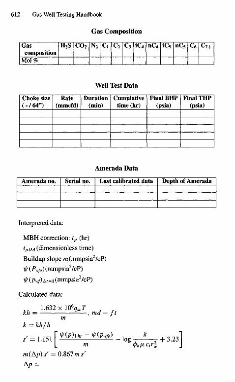
Gas Composition
"Gas IH2SI CO2 IN2 I Ci I C2 I C3 11C4 I nC4 I iC5 I nC5 I C6 I C 7 +
composition
M o I % I I 1 1 1 1 1 1 1 1 1 1
Well Test Data
Choke size I Rate I Duration I Cumulative I Final BHP I Final THP(-/64") (mmcfd) (min) time(hr) (psia) (psia)
Amerada Data
Amerada no. Serial no. Last calibrated data Depth of Amerada
Interpreted data:
MBH correction: tp (hr)
tpDA (dimensionless time)
Buildup slope m(mmpsia2/cP)
if(Pwfo) (mmpsia2/cP)
f (Pwf) At=i (mmpsia2/cP)
Calculated data:
1.632 x 10%cTkh = , md - ft
mk = kh/h
, '= i . i5 i r » ( * > i * - * Q ^ > _ log k
+ 3 .2 31L rn <t>hix ctrl J
m(Ap)j' = 0.867 m /
Ap =
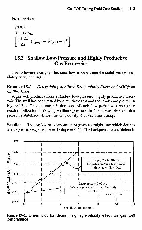
Pressure data:
HPi) =F = 4ntDA
Af is(Pwf) = f(pR) = eF
15.3 Shallow Low-Pressure and Highly ProductiveGas Reservoirs
The following example illustrates how to determine the stabilized deliver-ability curve and AOF.
Example 15-1 Determining Stabilized Deliverability Curve and AOF fromthe Test Data
A gas well produces from a shallow low-pressure, highly productive reser-voir. The well has been tested by a multirate test and the results are plotted inFigure 15-1. One and one-half durations of each flow period was enough toreach stabilization of flowing wellbore pressure. In fact, it was observed thatpressures stabilized almost instantaneously after each rate change.
Solution The log-log backpressure plot gives a straight line which definesa backpressure exponent n = 1 /slope = 0.56. The backpressure coefficient is
Gas flow rate, mmscfd
Figure 15-1. Linear plot for determining high-velocity effect on gas wellperformance.
Intercepts = 0.00145Indicates pressure loss due to steady
state skin s
Slope, B = 0.001607Indicates pressure loss due to
high velocity flow Dqsc
calculated from the curve as
C = 8.0 x 10⁶(ll,200)a56 = 43,204 scf/day/psia2
The backpressure equation then is qsc = 43,204(p| — / ^ ) 0 ' 5 6 and the absoluteopen flow is 45.538 mmscfd. A Cartesian plot of Ap2/qsc versus qsc (Figure15-1) gives a straight line (except for a small deviation and the low rate point).The intercept of the line is A = 0.00145 psia2/scfd/D and the slope is
B = 1.607 x 10⁻³ P d i a 2 / S C M
mmscfd
or, when expressed in scf/d,
* = 1.607xl0-9p S i a 2 / S C f d / d
scfd/d
The low n value and the high B value indicate large rate-dependent skin. Theslope B in Figure 15-1 indicates the significance of the high-velocity effect onthe productivity of the well. A large slope implies large rate-dependent skin.The intercept A is related to steady-state skin factor. If the rate needs to bewritten in terms of flowing pressure, the quadratic equation can be solved asfollows:
^A2+ 4B(pl-p2wf)-A
qsc = YB
^(0.00145)2 +4(1.607 x I O " 9 ) ^ - plf) - 0.00145= 2(1.607 x 10"9)
This equation can be used to calculate the AOF for this example.
15.4 Recommended Form of Rules of Procedurefor Backpressure Tests Required by State
Regulatory Bodies
All backpressure tests required by a state regulatory body shall be conductedin according with the procedures set out by the state regulatory body exceptfor those wells in pools where special testing procedures are applicable.1"3
The calculations shall be made in the manner prescribed in the appropriate testexamples. The observed data and calculations shall be reported on the pre-scribed forms. Gas produced from wells connected to a gas transportationfacility should not be vented to the atmosphere during testing. When an accu-rate test can be obtained only under conditions requiring venting, the volumevented shall be the minimum required to obtain an accurate test. All surface
pressure readings shall be taken with a dead weight gauge. Under special con-ditions where the use of a dead weight gauge is not practical, a properly cali-brated spring gauge may be used when authorized by the state regulatory body.Subsurface pressures determined by the use of a properly calibrated pressurebomb are acceptable. The temperature of the gas column must be accuratelyknown to obtain correct test results; therefore a thermometer well should beinstalled in the wellhead. Under shut-in or low-flow-rate conditions, the ex-ternal temperature may distort the observed wellhead temperatures. Wheneverthis situation exists the mean annual temperature should be used.
15.5 Appropriate State Report Forms
The appropriate state report forms are as follows.
Texas Gas Well12
• Uses tubing pressures• Square root chart entries for gas measurement• GE system dialogue• Answers transferred to G-1 form
New Mexico Gas Well1'2
• Uses tubing pressures• Deviated well• UCS system dialogue• Answers transferred to preprinted state form C-122
Oklahoma Gas Well3
• Uses casing pressures• Single-point test• Case No. 1 assigned to input data• GE system dialogue• Answers presented in report form
Offshore Gas Well Using IOCC Procedure3
• Uses bottom-hole pressures• UCS system dialogue• Answers presented in report form for natural gas Oklahoma
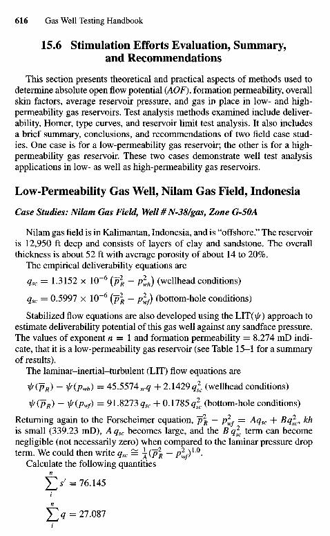
15.6 Stimulation Efforts Evaluation, Summary,and Recommendations
This section presents theoretical and practical aspects of methods used todetermine absolute open flow potential (AOF), formation permeability, overallskin factors, average reservoir pressure, and gas in place in low- and high-permeability gas reservoirs. Test analysis methods examined include deliver-ability, Horner, type curves, and reservoir limit test analysis. It also includesa brief summary, conclusions, and recommendations of two field case stud-ies. One case is for a low-permeability gas reservoir; the other is for a high-permeability gas reservoir. These two cases demonstrate well test analysisapplications in low- as well as high-permeability gas reservoirs.
Low-Permeability Gas Well, Nilam Gas Field, Indonesia
Case Studies: Nilam Gas Field, Well # N-38/gas, Zone GSOA
Nilam gas field is in Kalimantan, Indonesia, and is "offshore." The reservoiris 12,950 ft deep and consists of layers of clay and sandstone. The overallthickness is about 52 ft with average porosity of about 14 to 20%.
The empirical deliverability equations are
qsc = 1.3152 x 10"6 (~p2R - plh) (wellhead conditions)
qsc = 0.5997 x 10~6 (~p2R - plf) (bottom-hole conditions)
Stabilized flow equations are also developed using the LIT(\J/) approach toestimate deliverability potential of this gas well against any sandface pressure.The values of exponent n = 1 and formation permeability = 8.274 mD indi-cate, that it is a low-permeability gas reservoir (see Table 15-1 for a summaryof results).
The laminar-inertial-turbulent (LIT) flow equations are
^(PR) ~ is(Pwh) = 45.5574scq + 2.1429q2c (wellhead conditions)
is(pR) - if(pwf) = 9l.S213qsc + 0.1785 q)c (bottom-hole conditions)
Returning again to the Forscheimer equation, ~p\ — p^ = Aqsc + Bq2c, kh
is small (339.23 mD), A qsc becomes large, and the B q2c term can become
negligible (not necessarily zero) when compared to the laminar pressure dropterm. We could then write qsc = j(~p2
R — P^f)1'0-Calculate the following quantities
n
J2S> = 76.145i
n
Y^q = 27.087
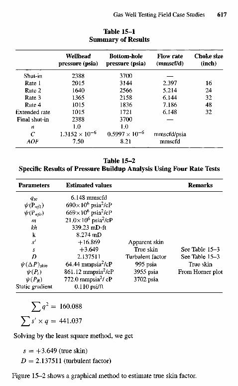
Table 15-1Summary of Results
Wellhead Bottom-hole Flow rate Choke sizepressure (psia) pressure (psia) (mmscf/d) (inch)
Shut-in 2388 3700 —Ratel 2015 3144 2.397 16Rate 2 1640 2566 5.214 24Rate 3 1365 2158 6.144 32Rate 4 1015 1836 7.186 48
Extended rate 1015 1721 6.148 32Final shut-in 2388 3700 —
n 1.0 1.0C 1.3152 x 10"6 0.5997 x 10~6 mmscfd/psia
AOF 7.50 8.21 mmscfd
Table 15-2Specific Results of Pressure Buildup Analysis Using Four Rate Tests
Parameters Estimated values Remarks
qsc 6.148 mmscfdVKPvv/i) 690xl06psia2 /cPxjf(Vwfo) 669xl06psia2/cP
m 21.0x10⁶ psia2/cPkh 339.23 mD-ftk 8.274 mDs' +16.869 Apparent skins +3.649 True skin See Table 15-3D 2.137511 Turbulent factor See Table 15-3
\lr(AP)skin 64.44 mmpsia2/cP 995 psia True skinxjf(Pi) 861.12 mmpsia2/cP 3955 psia From Horner plotxJr(PR) 772.0 mmpsia2/ cP 3702 psia
Static gradient 0.110 psi/ft
J2<12= !60.088
^TY xq = 441.037
Solving by the least square method, we get
s = +3.649 (true skin)
D = 2.137511 (turbulent factor)
Figure 15-2 shows a graphical method to estimate true skin factor.
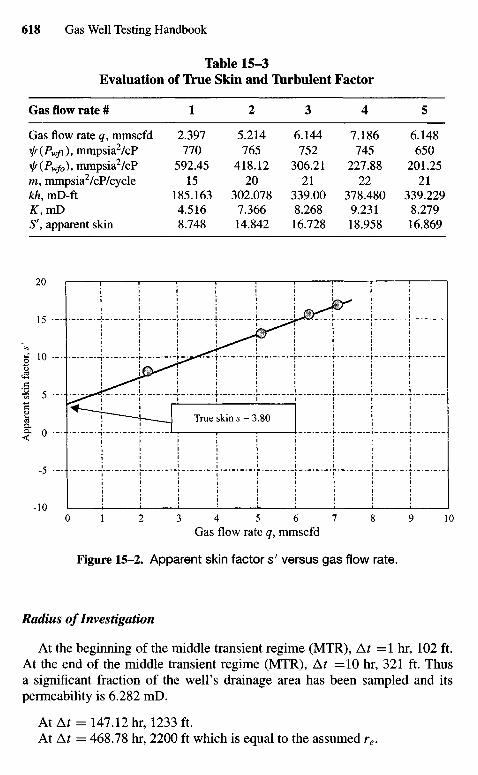
Table 15-3Evaluation of True Skin and TVirbulent Factor
Gas flow rate # 1 2 3 4 5
Gasflowrate^mmscfd 2.397 5.214 6.144 7.186 6.148T/r(Pw/l),mmpsia2/cP 770 765 752 745 650^(Pw/o),mmpsia2/cP 592.45 418.12 306.21 227.88 201.25m, mmpsia2/cP/cycle 15 20 21 22 21Jch,mD-ft 185.163 302.078 339.00 378.480 339.229K,mD 4.516 7.366 8.268 9.231 8.279S', apparent skin 8.748 14.842 16.728 18.958 16.869
Gas flow rate q, mmscfd
Figure 15-2. Apparent skin factor s ' versus gas flow rate.
Radius of Investigation
At the beginning of the middle transient regime (MTR), At =1 hr, 102 ft.At the end of the middle transient regime (MTR), At =10 hr, 321 ft. Thusa significant fraction of the well's drainage area has been sampled and itspermeability is 6.282 mD.
AtAr = 147.12 hr, 1233 ft.At Ar = 468.78 hr, 2200 ft which is equal to the assumed re.
True skin s = 3.80
App
aren
t ski
n fa
ctor
, s'
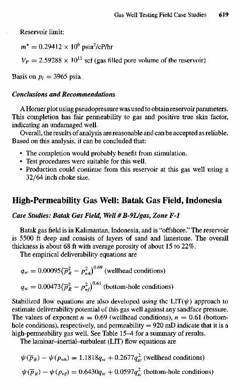
Reservoir limit:
m* = 0.29412 x 10⁶ psia2/cP/hr
Vp = 2.59288 x 10¹¹ scf (gas filled pore volume of the reservoir)
Basis on pt = 3965 psia
Conclusions and Recommendations
A Homer plot using pseudopressure was used to obtain reservoir parameters.This completion has fair permeability to gas and positive true skin factor,indicating an undamaged well.
Overall, the results of analysis are reasonable and can be accepted as reliable.Based on this analysis, it can be concluded that:
• The completion would probably benefit from stimulation.• Test procedures were suitable for this well.• Production could continue from this reservoir at this gas well using a
32/64 inch choke size.
High-Permeability Gas Well: Batak Gas Field, Indonesia
Case Studies: Batak Gas Field, Well # B-9Ugas, Zone F-I
Batak gas field is in Kalimantan, Indonesia, and is "offshore." The reservoiris 5500 ft deep and consists of layers of sand and limestone. The overallthickness is about 68 ft with average porosity of about 15 to 22%.
The empirical deliverability equations are
qsc = 0.00095(~p2R - plh)°'69 (wellhead conditions)
qsc = 0.00473 (~p2R - plf)°
M (bottom-hole conditions)
Stabilized flow equations are also developed using the LIT(VO approach toestimate deliverability potential of this gas well against any sandface pressure.The values of exponent n = 0.69 (wellhead conditions), n = 0.61 (bottom-hole conditions), respectively, and permeability = 920 mD indicate that it is ahigh-permeability gas well. See Table 1 5 ^ for a summary of results.
The laminar-inertial-turbulent (LIT) flow equations are
IT(PR) ~ is(Pwh) = I.lSlSqsc + 0.2677q2sc (wellhead conditions)
^(PR) - f(Pwf) = 0.6430#5C + 0.0597^2c (bottom-hole conditions)
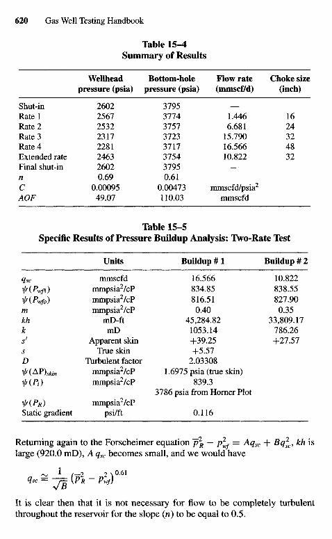
Table 15-4Summary of Results
Wellhead Bottom-hole Flow rate Choke sizepressure (psia) pressure (psia) (mmscf/d) (inch)
Shut-in 2602 3795 —Ratel 2567 3774 1.446 16Rate 2 2532 3757 6.681 24Rate 3 2317 3723 15.790 32Rate 4 2281 3717 16.566 48Extended rate 2463 3754 10.822 32Final shut-in 2602 3795 —n 0.69 0.61C 0.00095 0.00473 mmscfd/psia2
AOF 49.07 110.03 mmscfd
Table 15-5Specific Results of Pressure Buildup Analysis: Two-Rate Test
Units Buildup # 1 Buildup # 2
qsc mmscfd 16.566 10.822ir(Pwfi) mmpsia2/cP 834.85 838.55ir(Pwfo) mmpsia2/cP 816.51 827.90m mmpsia2/cP 0.40 0.35kh mD-ft 45,284.82 33,809.17k mD 1053.14 786.26s' Apparent skin +39.25 +27.57s True skin +5.57D Turbulent factor 2.03308^-(AP)1S^n mmpsia2/cP 1.6975 psia (true skin)\/f (Pi) mmpsia2/cP 839.3
3786 psia from Horner Plotis (PR) mmpsia2/cPStatic gradient psi/ft 0.116
Returning again to the Forscheimer equation ~p\ - p^f = Aqsc + Bqfc, kh islarge (920.0 mD), A qsc becomes small, and we would have
— 1 /—2 2 \ °-61
qsc = V B ^ P R ~ Pwf*It is clear then that it is not necessary for flow to be completely turbulentthroughout the reservoir for the slope (n) to be equal to 0.5.
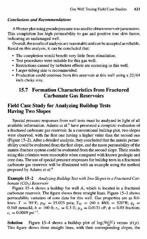
Conclusions and Recommendations
A Horner plot using pseudopressure was used to obtain reservoir parameters.This completion has high permeability to gas and positive true skin factor,indicating an undamaged well.
Overall, the results of analysis are reasonable and can be accepted as reliable.Based on this analysis, it can be concluded that:
• The completion would benefit very little from stimulation.• Test procedures were suitable for this gas well.• Restrictions caused by turbulent effects are occurring in this well.• Larger tubing size is recommended.• Production could continue from this reservoir at this well using a 32/64
inch choke size.
15.7 Formation Characteristics from FracturedCarbonate Gas Reservoirs
Field Case Study for Analyzing Buildup TestsHaving Two Slopes
Special pressure responses from well tests must be analyzed in light of allavailable information. Adams et al.4 have presented a complete evaluation ofa fractured carbonate gas reservoir. In a conventional buildup plot, two slopeswere observed, with the first one having a higher value than the second one(Figure 15-2). After a detailed analysis, they concluded that the matrix perme-ability could be evaluated from the first slope, and the mean permeability of thematrix-fracture system could be evaluated from the second slope. Their resultsusing this criterion were reasonable when compared with known geologic andcore data. The use of special pressure responses for buildup tests in a fracturedcarbonate gas reservoir will be illustrated with an example using the methodproposed by Adams et al.4
Example 15-2 Analyzing Buildup Test with Two Slopes in a Fractured Car-bonate (CO3) Reservoir
Figure 15-4 shows a buildup for well A, which is located in a fracturedcarbonate reservoir. The figure shows three straight lines. Figure 15-3 showspermeability variation of core data for this well. Gas properties are as fol-lows: T = 900F; psc = 15.025 psia; Tsc = (60 + 460) = 5200R; qg =0.548 mmscfd; h = 160 ft; rw = 0.3 ft; \xg = 0.0131 cP; 0 = 0.03 fraction;ct =0.0009psi"1.
Solution Figure 15-4 shows a buildup plot of Xogi^—1) versus x/f(p).This figure shows three straight lines, with their corresponding slopes, the
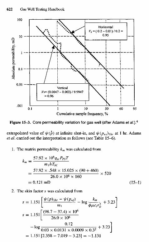
Cumulative sample frequency, %
Figure 15-3. Core permeability variation for gas well (after Adams et a/.).4
extrapolated value of ij/(p) at infinite shut-in, and ty(pws)\hr at 1 hr. Adamset al. carried out the interpretation as follows (see Table 15-6).
1. The matrix permeability km was calculated from
_ 57.92 x l06qscPpST
mihTsc
_ 57.92 x .548 x 15.025 x (90 + 460)
~ 26.0 x 106 x 160 X °= 0.121mD (15-1)
2. The skin factor s was calculated from
s = 1.151 \fiPhhr - fiPwf) - log J ^ , + 3.231
1 ^ 1 [(98.7-37.4) xlO6
^ = 1 1 5 1 L 26.0x10^
0.12 ]
~ ° g 0.03 x 0.0131 x 0.0009 x 0.32 + ' J
= 1.151 [2.358 - 7.019 - 3.23] = -1.131
VerticalFv= (0.0047 - 0.002) / 9.9947
= 0.96
HorizontalFA = ( 0 .2 -0 .01) /0 .2 =
0.95
Abs
olut
e pe
rmea
bili
ty, m
D
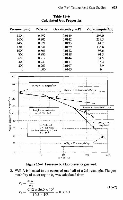
Table 15-6Calculated Gas Properties
Pressure (psia) Z-factor Gas viscosity fj, (cP) il>(p) (mmpsia2/cP)
1800 0.792 0.0149 296.01600 0.805 0.0142 237.51400 0.821 0.0135 184.21200 0.841 0.0129 136.81000 0.861 0.0122 95.6800 0.886 0.0188 61.3600 0.912 0.0144 34.5400 0.949 0.0111 15.4200 0.969 0.0107 3.9
0 1.000 0.0105 0
Pse
udo-
pres
sure
, vj
/(P),
mm
psia
2/cP
V(F*) = 159mmpsia2/cP
Straight-line intersect at(t+At) /At = 26.5
Slope m2 = 10.5 mmpsia2/cP/cycle
Slope m/ = 26 mmpsia2/cP/ cycle
q = 548 mscfd/= 1570 hours
Wellbore radius, rw = 0.3 fth = 160 ft
V(P), hr =-98.7mmpsia2/ cP
i|/(P)Wf= 37.4 mmpsia2/cp
Figure 15-4. Pressure buildup curve for gas well.
3. Well A is located in the center of one-half of a 2:1 rectangle. The per-meability of outer region k2 was calculated from
kxmxk2 =
0.12 x 26.0 x l O 6 U ;
Jc2 = 2 = 0.3 mD10.5 x 106
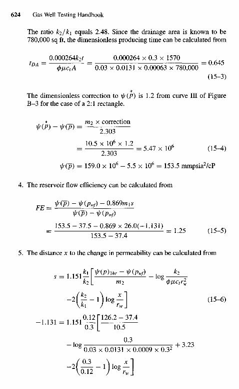
The ratio fe/^i equals 2.48. Since the drainage area is known to be780,000 sq ft, the dimensionless producing time can be calculated from
_ 0.000264Jfc2f _ 0.000264 x 0.3 x 1570 _tDA = (f)iJict A
= 0.03 x 0.0131 x 0.00063 x 780,000 = '(15-3)
*The dimensionless correction to ^r(P) is 1.2 from curve III of FigureB-3 for the case of a 2:1 rectangle.
* _ m,2 x correctionxlr(p) — xl/(p) =^V } ^yy) 2.303
ilr(p) = 159.0 x 10⁶ - 5.5 x 106 = 153.5 mmpsia2/cP
4. The reservoir flow efficiency can be calculated from
xlf(p)-xjf{pwf)-QM9mxs1 1 , = —
f(p) - f{pwf)
_ 153.5 - 37.5 - 0.869 x 26.0(-1.131) _ , o g
~ 153.5 - 37.4 ~ ( }
5. The distance x to the change in permeability can be calculated from
k2 L m2 4>V>ctrl
0.3
~ 1 O g 0.03 x 0.0131 x 0.0009 x 0.32 + 3 ' 2 3
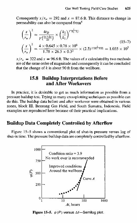
Consequently x/rw = 292 and x = 87.6 ft. This distance to change inpermeability can also be compared from4
/ x \ 2 _ AtD A2V-^-*!)
w ~ HW)x W (i5 7)
JC/rw = 322 and JC = 96.6 ft. The values of x calculated by two methodsare of the same order of magnitude and consequently it can be concludedthat the change of k is about 90 ft from the wellbore.
15.8 Buildup Interpretations Beforeand After Workovers
In practice, it is desirable to get as much information as possible from apressure buildup test. Trying as many crossplotting techniques as possible cando this. The buildup data before and after workover were obtained in variouszones, block III, Benuang Gas Field, and South Sumatra, Indonesia. Fieldexamples are reproduced here because of their practical implications.
Buildup Data Completely Controlled by Afterflow
Figure 15-5 shows a conventional plot of shut-in pressure versus log ofshut-in time. The pressure buildup data are completely controlled by afterflow.
At, hours
Figure 15-5. is(P) versus Af-Semilog plot.
Condition ratio = 3.9No work over is recommended
Improved conditionsAround the wellbore
Curved
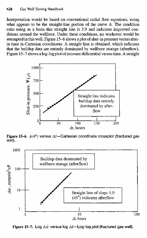
Interpretation would be based on conventional radial flow equations, usingwhat appears to be the straight-line portion of the curve A. The conditionratio using as a basis this straight line is 3.9 and indicates improved con-ditions around the wellbore. Under these conditions, no workover would beattempted in this well. Figure 15-6 shows a plot of shut-in pressure versus shut-in time in Cartesian coordinates. A straight line is obtained, which indicatesthat the buildup data are entirely dominated by wellbore storage (afterflow).Figure 15-7 shows a log-log plot of pressure differential versus time. A straight
Shut
-in
pres
sure
. V
(p)
Ay/
, mm
psia
2/cP
At, hours
Figure 15-6. if (P) versus Af-Cartesian coordinate crossplot (fractured gaswell).
Buildup data dominated bywellbore storage (afterflow)
Straight line of slope 1.0(45°) indicates afterflow
At, hours
Figure 15-7. Log A^ versus log At—Log-log plot (fractured gas well).
Straight line indicatesbuildup data entirelydominated by after-
flow
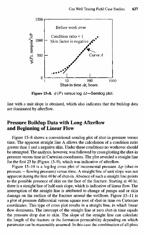
Shut-in time At, hours
Figure 15-8. is(P) versus log Af-Semilog plot.
line with a unit slope is obtained, which also indicates that the buildup dataare dominated by afterflow.
Pressure Buildup Data with Long Afterflowand Beginning of Linear Flow
Figure 15-8 shows a conventional semilog plot of shut-in pressure versustime. The apparent straight line A allows the calculation of a condition ratiogreater than 1 and a negative skin. Under these conditions no workover shouldbe attempted. The analysis, however, was followed by cross plotting the shut-inpressure versus time in Cartesian coordinates. The plot revealed a straight linefor the first 25 hr (Figure 15-9), which was indicative of afterflow.
Figure 15-10 is a log-log cross plot of incremental pressure Ap (shut-inpressure — flowing pressure) versus time. A straight line of unit slope was notapparent during the first 40 hr of shut-in. Absence of such a straight line pointsto the possible presence of skin on the face of the fracture. Starting at 40 hr,there is a straight line of half-unit slope, which is indicative of linear flow. Theinterruption of the straight line is attributed to change of pumps and or skindamage on the surface of the fracture around the wellbore. Figure 15-11 isa plot of pressure differential versus square root of shut-in time on Cartesiancoordinates. This type of cross plot results in a straight line, in which linearflow dominates. The intercept of the straight line at zero shut-in time equalsthe pressure drop due to skin. The slope of the straight line can calculatethe length of the fracture or the formation permeability depending on whichparameter can be reasonably assumed. In this case the combination of all plots
\\j(P
), m
mps
ia2/c
PBefore work over
Condition ratio < 1Skin factor is negative
Curve A
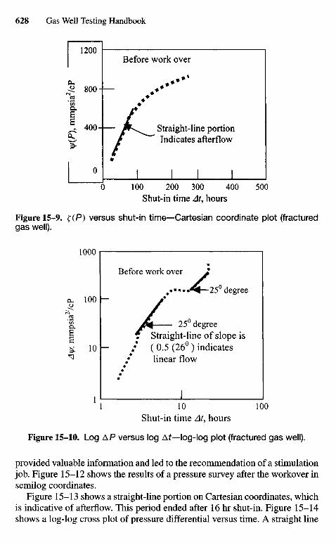
Shut-in time At, hours
Figure 15-10. Log AP versus log Af-log-log plot (fractured gas well).
provided valuable information and led to the recommendation of a stimulationjob. Figure 15-12 shows the results of a pressure survey after the workover insemilog coordinates.
Figure 15-13 shows a straight-line portion on Cartesian coordinates, whichis indicative of afterflow. This period ended after 16 hr shut-in. Figure 15-14shows a log-log cross plot of pressure differential versus time. A straight line
Ay/,
mm
psia
2//c
PVj
Z(P)
, mm
psi
a2/cP
25° degreeStraight-line of slope is( 0.5 (26° ) indicateslinear flow
25° degree
Before work over
Shut-in time At, hours
Figure 15-9. f(P) versus shut-in time—Cartesian coordinate plot (fracturedgas well).
Straight-line portionIndicates afterflow
Before work over
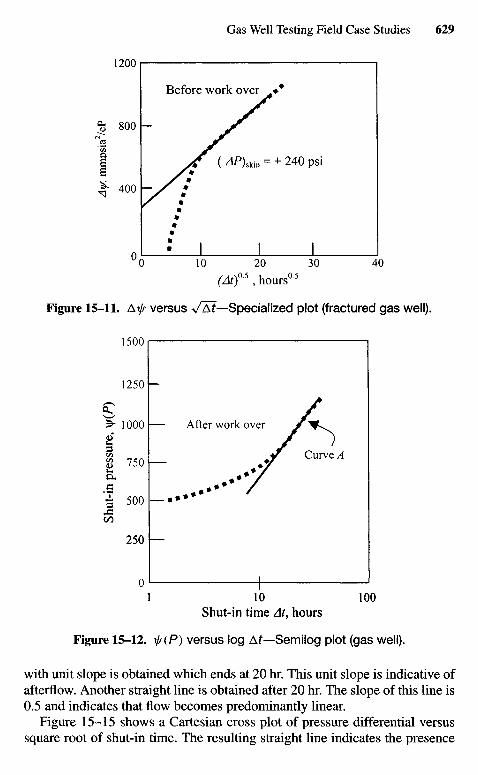
Shut
-in
pre
ssur
e, V
jZ(P
)Ay
/, m
mps
ia2/c
PBefore work over
(At)05, hours05
Figure 15-11. A^ versus V^Af-Specialized plot (fractured gas well).
Shut-in time At, hours
Figure 15-12. \j/(P) versus log Af-Semilog plot (gas well).
with unit slope is obtained which ends at 20 hr. This unit slope is indicative ofafterflow. Another straight line is obtained after 20 hr. The slope of this line is0.5 and indicates that flow becomes predominantly linear.
Figure 15-15 shows a Cartesian cross plot of pressure differential versussquare root of shut-in time. The resulting straight line indicates the presence
After work over
Curved
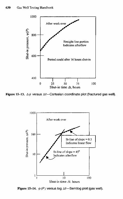
Shut
-in
pres
sure
, \\f
(P)
Shut
-in
pres
sure
, \\f
(P)
After work over
Straight-line portionIndicates afterflow
Period could alter 16 hours shut-in
Shut-in time At, hours
Figure 15-13. A^ versus Af-Cartesian coordinate plot (fractured gas well).
Shut-in time At, hours
Figure 15-14. x/r(P) versus log Af-Semilog plot (gas well).
After work over
St-line of slope = 0.5Indicates linear flow
St-line of slope = 45°Indicates afterflow
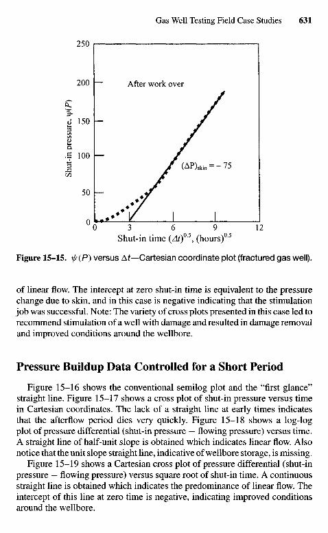
Shut
-in
pres
sure
, i|/(
F)
After work over
Shut-in time (Atf\ (hours)05
Figure 15-15. \/r(P) versus At—Cartesian coordinate plot (fractured gas well).
of linear flow. The intercept at zero shut-in time is equivalent to the pressurechange due to skin, and in this case is negative indicating that the stimulationjob was successful. Note: The variety of cross plots presented in this case led torecommend stimulation of a well with damage and resulted in damage removaland improved conditions around the wellbore.
Pressure Buildup Data Controlled for a Short Period
Figure 15-16 shows the conventional semilog plot and the "first glance"straight line. Figure 15-17 shows a cross plot of shut-in pressure versus timein Cartesian coordinates. The lack of a straight line at early times indicatesthat the afterflow period dies very quickly. Figure 15-18 shows a log-logplot of pressure differential (shut-in pressure — flowing pressure) versus time.A straight line of half-unit slope is obtained which indicates linear flow. Alsonotice that the unit slope straight line, indicative of wellbore storage, is missing.
Figure 15-19 shows a Cartesian cross plot of pressure differential (shut-inpressure — flowing pressure) versus square root of shut-in time. A continuousstraight line is obtained which indicates the predominance of linear flow. Theintercept of this line at zero time is negative, indicating improved conditionsaround the wellbore.
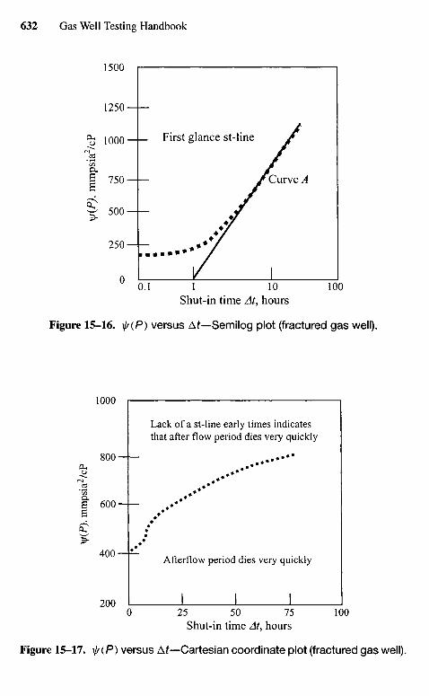
\\f(P
), m
mps
ia2/c
P\j/
(P).
mm
psia
2/cP
First glance st-line
Curved
Shut-in time At, hours
Figure 15-16. is (P) versus Af-Semilog plot (fractured gas well).
Lack of a st-line early times indicatesthat after flow period dies very quickly
Afterflow period dies very quickly
Shut-in time At, hours
Figure 15-17. V(P) versus Af-Cartesian coordinate plot (fractured gas well).
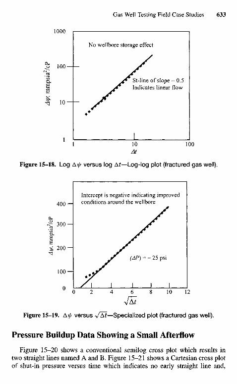
Ay/,
mm
psia
2/cP
A y
/, m
mps
ia2/c
PNo wellbore storage effect
St-line of slope = 0.5Indicates linear flow
Figure 15-18. Log Axj/ versus log At—Log-log plot (fractured gas well).
Intercept is negative indicating improvedconditions around the wellbore
Figure 15-19. A\[r versus +/At—Specialized plot (fractured gas well).
Pressure Buildup Data Showing a Small Afterflow
Figure 15-20 shows a conventional semilog cross plot which results intwo straight lines named A and B. Figure 15-21 shows a Cartesian cross plotof shut-in pressure versus time which indicates no early straight line and,
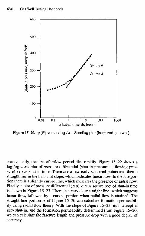
Shut-in time At, hours
Figure 15-20. is(P) versus log Af-Semilog plot (fractured gas well).
consequently, that the afterflow period dies rapidly. Figure 15-22 shows alog-log cross plot of pressure differential (shut-in pressure — flowing pres-sure) versus shut-in time. There are a few early-scattered points and then astraight line in the half-unit slope, which indicates linear flow. In the late por-tion there is a slightly curved line, which indicates the presence of radial flow.Finally, a plot of pressure differential (Ap) versus square root of shut-in timeis shown in Figure 15-23. There is a very clear straight line, which suggestslinear flow, followed by a curved portion when radial flow is attained. Thestraight-line portion A of Figure 15-20 can calculate formation permeabil-ity using radial flow theory. With the slope of Figure 15-23, its intercept atzero shut-in, and the formation permeability determined from Figure 15-20,we can calculate the fracture length and pressure drop with a good degree ofaccuracy.
St-line B
St-line A
Shut
-in
pres
sure
, mm
psia
2/cP
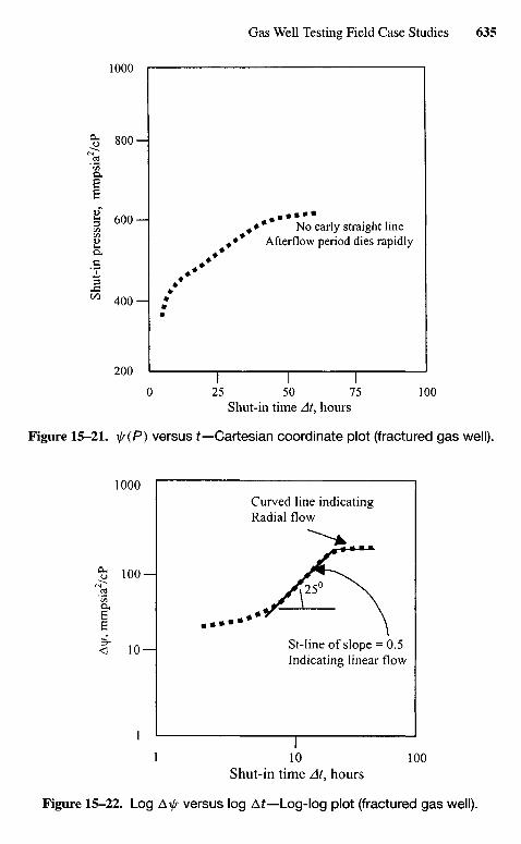
Shu
t-in
pre
ssur
e, m
mps
ia2/c
PAv
j/, m
mps
ia2/c
P
No early straight lineAfterflow period dies rapidly
Shut-in time At, hours
Figure 15-21. f{P) versus t—Cartesian coordinate plot (fractured gas well).
Curved line indicatingRadial flow
St-lineofslope = 0.5Indicating linear flow
Shut-in time At, hours
Figure 15-22. Log Ax/r versus log Af-Log-log plot (fractured gas well).
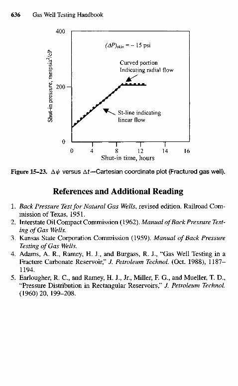
Shut
-in
pres
sure
, m
mps
ia2/c
P(4/>)Skin = - 1 5 p s i
Curved portionIndicating radial flow
St-line indicatinglinear flow
Shut-in time, hours
Figure 15-23. A^ versus At—Cartesian coordinate plot (Fractured gas well).
References and Additional Reading
1. Back Pressure Test for Natural Gas Wells, revised edition. Railroad Com-mission of Texas, 1951.
2. Interstate Oil Compact Commission (1962). Manual of Back Pressure Test-ing of Gas Wells.
3. Kansas State Corporation Commission (1959). Manual of Back PressureTesting of Gas Wells.
4. Adams, A. R., Ramey, H. J., and Burgass, R. J., "Gas Well Testing in aFracture Carbonate Reservoir," /. Petroleum Technol. (Oct. 1988), 1187-1194.
5. Earlougher, R. C, and Ramey, H. J., Jr., Miller, F. G., and Mueller, T. D.,"Pressure Distribution in Rectangular Reservoirs," J. Petroleum Technol.(1960)20, 199-208.
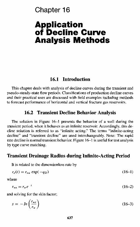
Chapter 16
of Decline CurveAnalysis Methods
16.1 Introduction
This chapter deals with analysis of decline curves during the transient andpseudo-steady-state flow periods. Classifications of production decline curvesand their practical uses are discussed with field examples including methodsto forecast performance of horizontal and vertical fracture gas reservoirs.
16.2 Transient Decline Behavior Analysis
The solution in Figure 16-1 presents the behavior of a well during thetransient period, when it behaves as an infinite reservoir. Accordingly, this de-cline solution is referred to as "infinite acting." The terms "infinite-actingdecline" and "transient decline" are used interchangeably. Note: The rapidrate decline is normal transient behavior. Figure 16-1 is useful for test analysisby type curve matching.
Transient Drainage Radius during Infinite-Acting Period
It is related to the dimensionless rate by
re(f) = rwa exp( -qD) (16-1)
where
rwa = rwe~s (16-2)
and solving for the skin factor;
s= -InI — (16-3)
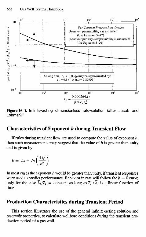
Figure 16-1. Infinite-acting dimensionless rate-solution (after Jacob andLohman).9
Characteristics of Exponent b during Transient Flow
If rules during transient flow are used to compute the value of exponent b,then such measurements may suggest that the value of b is greater than unityand is given by
In most cases the exponent b would be greater than unity, if transient responseswere used to predict performance. Behavior in rate will follow the b = 0 curveonly for the case Xt/ct = constant as long as ct / kt is a linear function oftime.
Production Characteristics during Transient Period
This section illustrates the use of the general infinite-acting solution andreservoir properties, to calculate wellbore conditions during the transient pro-duction period of a gas well.
At long time, tD > 100, qD may be approximated by:qD = 0.5 / [ In (tD) + 0.80907]
For Constant Pressure Rate DeclineReservoir permeability, k is estimated:
(Use Equation 5-17)Reservoir porosity-compressibility is estimated:
(Use Equation 5-20)
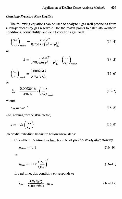
Constant-Pressure Rate Decline
The following equations can be used to analyze a gas well producing froma low-permeability gas reservoir. Use the match points to calculate wellboreconditions, permeability, and skin factor for a gas well:
SqA = H11Z1T
\ijmatch 0.103kh(pj-p2wf)
or
k = ^f1 2 , • (SL) (16-5)
/ f c \ = 0-000264*
\* /match 4> PgICH1Ia
or
i-^-(f) <*-7>4>lHCi \tDjmatch
where
^w« = rwe~s (16-8)
and, solving for the skin factor;
s = _Infr^A (16-9)
To predict rate-time behavior, follow these steps:
1. Calculate dimensionless time for start of pseudo-steady-state flow by
tDApss= 0 . 1 (16-10)
or
top,, = 0.1 n (—) (16-11)\rwa/
In real time, this condition corresponds to
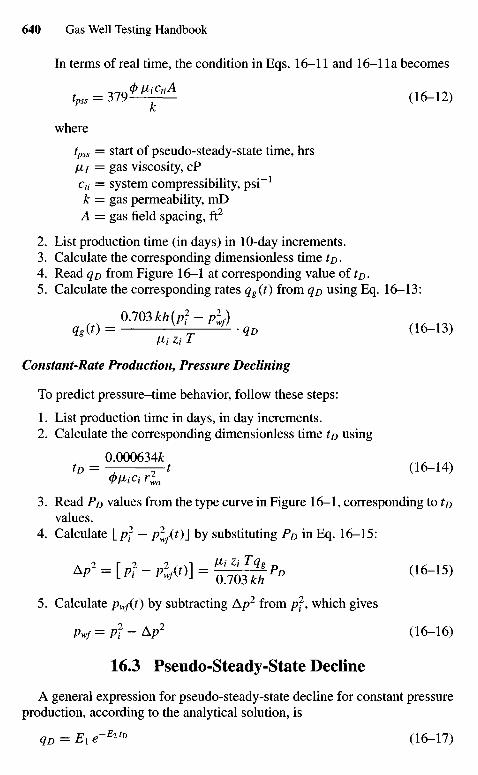
In terms of real time, the condition in Eqs. 16-11 and 16-1 Ia becomes
tpss = 3 7 9 ^ ^ (16-12)
where
tpss = start of pseudo-steady-state time, hrs/JLJ = gas viscosity, cPcti = system compressibility, psi"1
k = gas permeability, mDA = gas field spacing, ft2
2. List production time (in days) in 10-day increments.3. Calculate the corresponding dimensionless time tp.4. Read qD from Figure 16-1 at corresponding value of tD.5. Calculate the corresponding rates qg(t) from qD using Eq. 16-13:
0.103kh(pf-plf)qg(t) =
V V * 9D (16-13)
Constant-Rate Production, Pressure Declining
To predict pressure-time behavior, follow these steps:
1. List production time in days, in day increments.2. Calculate the corresponding dimensionless time to using
0.000634&tD = —t (16-14)
^Wi rla
3. Read PD values from the type curve in Figure 16-1, corresponding to tovalues.
4. Calculate [pf - plf(t)} by substituting PD in Eq. 16-15:
V-[r f -^O)] . ^ f P 0 (16-15)
5. Calculate pw/(t) by subtracting Ap2 from pf, which gives
pwf=pf-Ap2 (16-16)
163 Pseudo-Steady-State Decline
A general expression for pseudo-steady-state decline for constant pressureproduction, according to the analytical solution, is
qD = Eie-E2tD (16-17)
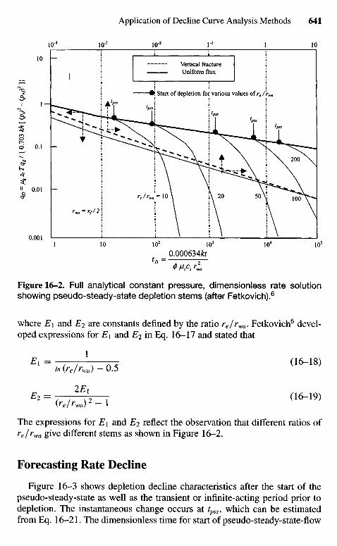
Figure 16-2. Full analytical constant pressure, dimensionless rate solutionshowing pseudo-steady-state depletion stems (after Fetkovich).6
where E\ and E2 are constants defined by the ratio re/rwa. Fetkovich6 devel-oped expressions for E\ and Ei in Eq. 16-17 and stated that
Ei = \ (16-18)in (re/rwa) - 0.5
El = (r/r )2 1 ( 1 6 " 1 9 )
The expressions for E\ and E2 reflect the observation that different ratios ofre/rwa give different stems as shown in Figure 16-2.
Forecasting Rate Decline
Figure 16-3 shows depletion decline characteristics after the start of thepseudo-steady-state as well as the transient or infinite-acting period prior todepletion. The instantaneous change occurs at tpsS9 which can be estimatedfrom Eq. 16-21. The dimensionless time for start of pseudo-steady-state-flow
Start of depletion for various values of re/'rwa
Vertical fractureUniform flux
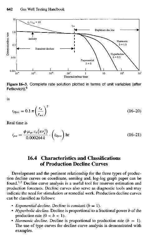
Dimensionless time
Figure 16-3. Complete rate solution plotted in terms of unit variables (afterFetkovich).6
is
tDpss = 0.1 Tt (—) (16-20)
Real time is
16.4 Characteristics and Classificationsof Production Decline Curves
Development and the pertinent relationship for the three types of produc-tion decline curves on coordinate, semilog and, log-log graph paper can befound.1'2 Decline curve analysis is a useful tool for reserves estimation andproduction forecasts. Decline curves also serve as diagnostic tools and mayindicate the need for stimulation or remedial work. Production decline curvescan be classified as follows:
• Exponential decline. Decline is constant (b — V).• Hyperbolic decline. Decline is proportional to a fractional power b of the
production rate (0 < b < 1).• Harmonic decline. Decline is proportional to production rate (b = 1).
The use of type curves for decline curve analysis is demonstrated withexamples.
Dim
ensi
onle
ss r
ate
Transient decline
Infinity
Depletion decline
Harmonic^ 6=1.0
Hyperboloic. 6 = 0.5
Exponential6 = 0
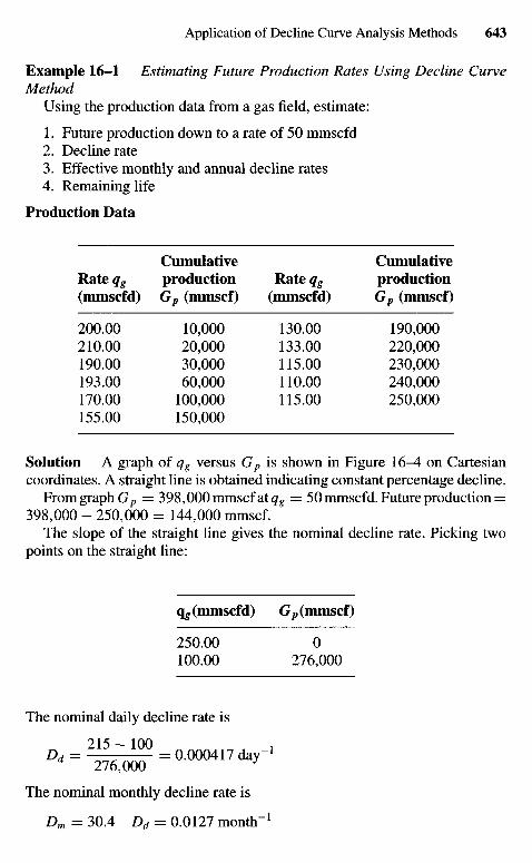
Example 16-1 Estimating Future Production Rates Using Decline CurveMethod
Using the production data from a gas field, estimate:
1. Future production down to a rate of 50 mmscfd2. Decline rate3. Effective monthly and annual decline rates4. Remaining life
Production Data
Cumulative CumulativeRate qg production Rate qg production(mmscfd) Gp (mmscf) (mmscfd) Gp (mmscf)
200.00 10,000 130.00 190,000210.00 20,000 133.00 220,000190.00 30,000 115.00 230,000193.00 60,000 110.00 240,000170.00 100,000 115.00 250,000155.00 150,000
Solution A graph of qg versus Gp is shown in Figure 16-4 on Cartesiancoordinates. A straight line is obtained indicating constant percentage decline.
From graph Gp = 398,000 mmscf at qg = 50 mmscfd. Future production =398,000 - 250,000 = 144,000 mmscf.
The slope of the straight line gives the nominal decline rate. Picking twopoints on the straight line:
(\g (mmscfd) Gp (mmscf)
250.00 0100.00 276,000
The nominal daily decline rate is
The nominal monthly decline rate is
Dm = 30.4 Dd = 0.0127 month"1
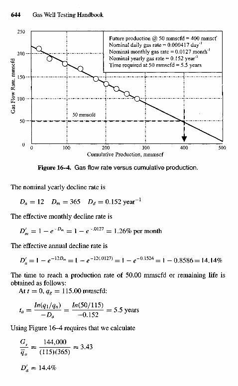
Cumulative Production, mmmscf
Figure 16-4. Gas flow rate versus cumulative production.
The nominal yearly decline rate is
Da = \2 Dm= 365 Dd = 0.152 year"1
The effective monthly decline rate is
D'm = 1 - e~Dm = 1 - e~-0U1 = 1.26% per month
The effective annual decline rate is
D'a = 1 - e-l2D™ = 1 - e-n{m21) = 1 - e"0-1524 = 1 - 0.8586 = U.U%
The time to reach a production rate of 50.00 mmscfd or remaining life isobtained as follows:
At t = 0, qg = 115.00 mmscfd:
In(qi/qn) /n(50/115)
Using Figure 16—4 requires that we calculate
Gg^ 144,000
q0 (115X365) *
Dra = 14.4%
Gas
Flo
w R
ate,
mm
scfd
50 mmscfd
Future production @ 50 mmscfd = 400 mmscfNominal daily gas rate = 0.000417 day'1
Nominal monthly gas rate = 0.0127 month1
Nominal yearly gas rate = 0.152 year"1
Time required at 50 mmscfd = 5.5 years
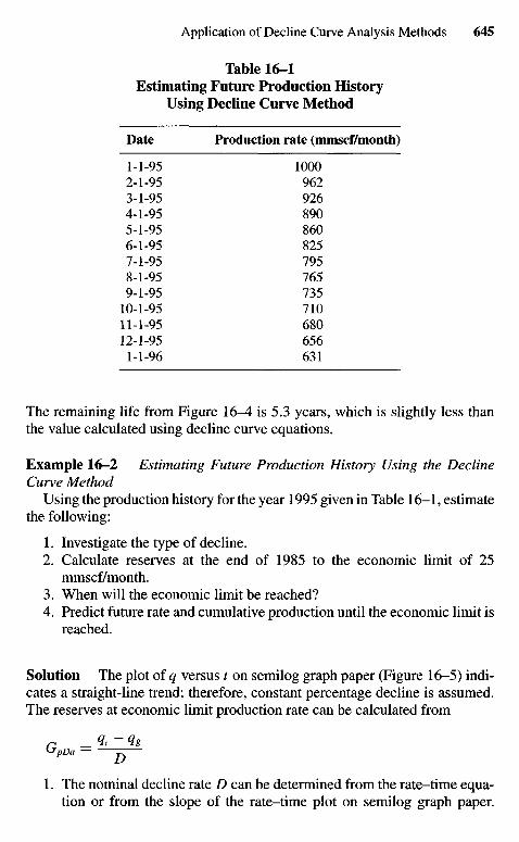
Table 16-1Estimating Future Production History
Using Decline Curve Method
Date Production rate (mmscf/month)
1-1-95 10002-1-95 9623-1-95 9264-1-95 8905-1-95 8606-1-95 8257-1-95 7958-1-95 7659-1-95 735
10-1-95 71011-1-95 68012-1-95 6561-1-96 631
The remaining life from Figure 1 6 ^ is 5.3 years, which is slightly less thanthe value calculated using decline curve equations.
Example 16-2 Estimating Future Production History Using the DeclineCurve Method
Using the production history for the year 1995 given in Table 16-1, estimatethe following:
1. Investigate the type of decline.2. Calculate reserves at the end of 1985 to the economic limit of 25
mmscf/month.3. When will the economic limit be reached?4. Predict future rate and cumulative production until the economic limit is
reached.
Solution The plot of q versus t on semilog graph paper (Figure 16-5) indi-cates a straight-line trend; therefore, constant percentage decline is assumed.The reserves at economic limit production rate can be calculated from
GpDa - - ^ -
1. The nominal decline rate D can be determined from the rate-time equa-tion or from the slope of the rate-time plot on semilog graph paper.
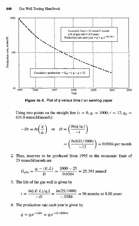
Figure 16-5. Plot of q versus time t on semilog paper.
Using two points on the straight line (t = 0,qt = 1000; t = I2,qg =631.0 mmscfd/month):
-KJ) - "-(^)//n(631/1000) \
= f — J = 0.0384 per month
2. Thus, reserves to be produced from 1995 to the economic limit of25 mmscfd/month are
qt - (E.L) 1000 - 25GpDa = ^ - ^ = ^ ^ = 25,391 mmscf
3. The life of the gas well is given by
InV(E.L)Iq1X 7^(25/1000) ^ AA
t = = ——— = 96 months or 8.00 years
4. The production rate each year is given by
q = qie-nDt = ^*-1 2 ' -0 3 8 4"
Pro
du
ctio
n ra
te,
mm
scfd
Economic limit = 25 mmscf/ monthLift of gas well = 8.0 years
Production rate each year = q = q, e-12(°-384>-'
Cumulative production = GpD = (qt-q) / D
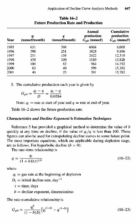
Table 16-2Future Production Rate and Production
Annual Cumulativeqt q production production
Year (mmscf/month) (mmscf/month) GPD (mmscf) GPD (mmscf)
1995 631 398 6068 6,0681996 398 251 3828 9,8961997 251 158 2422 12,3181998 158 100 1510 13,8281999 100 63 964 14,7922000 63 40 599 15,3912001 40 25 391 15,782
5. The cumulative production each year is given by
G = gi - g = g/ - gpD D 0.0384
Note: qi = rate at start of year and q — rate at end of year.
Table 16-2 shows the future production rate.
Characteristics and Decline Exponent b Estimation Techniques
Reference 5 has provided a graphical method to determine the value of bquickly at any time on decline, if the value of qt/q is less than 100. Thesefigures can also be used for extrapolating decline curves to some future point.The most important equations, which are applicable during depletion stage,are as follows. For hyperbolic decline (b > 0):
The rate-time relationship is
* - <!+£.)•/» <16"22)
where
qt = gas rate at the beginning of depletion
Di = initial decline rate, day"1
t = time, days
b = decline exponent, dimensionless
The rate-cumulative relationship is
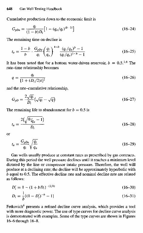
Cumulative production down to the economic limit is
GpDa = ( 1 _ ^ ) A [ 1 - (qa/qi)(b-l)] (16-24)
The remaining time on decline is
, l - b GpDa/qiy-b (qt/qaf-Xta = -r-^rU (*/*)•-*-1 (16"25)
It has been noted that for a bottom water-driven reservoir, b = 0.5.16 Therate-time relationship becomes
«-[i+(£/w (1^26)
and the rate-cumulative relationship,
GpD = ^ ( V * - V ^ ) (16-27)
The remaining life to abandonment for b = 0.5 is
ta = —*—£ (16-28)
or
ta = ^ A / ^ (16-29)
Gas wells usually produce at constant rates as prescribed by gas contracts.During this period the well pressure declines until it reaches a minimum leveldictated by the line or compressor intake pressure. Therefore, the well willproduce at a declining rate; the decline will be approximately hyperbolic withb equal to 0.5. The effective decline rate and nominal decline rate are relatedas follows:
D[ = 1 - (1 + bDi)-(l/b) (16-30)
Di = ^ t ( I - D 1 O - * - ! ] (16-31)
Fetkovich6 presents a refined decline curve analysis, which provides a toolwith more diagnostic power. The use of type curves for decline curve analysisis demonstrated with examples. Some of the type curves are shown in Figures16-6 through 16-8.
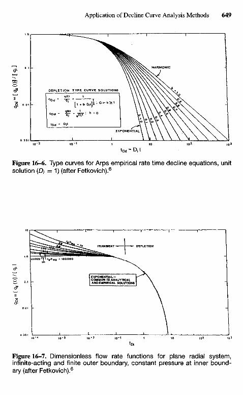
Figure 16-6. Type curves for Arps empirical rate time decline equations, unitsolution (D/ = 1) (after Fetkovich).6
Figure 16-7. Dimensionless flow rate functions for plane radial system,infinite-acting and finite outer boundary, constant pressure at inner bound-ary (after Fetkovich).6
EXPONENTIAL—COMMON TO ANALYTICALANO EMPIRICAL SOLUTIONS
TRANSIENT DEPLETION
EXPONENTIAL
HARMONIC
DEPLETION TYPE CURVE SOLUTIONS
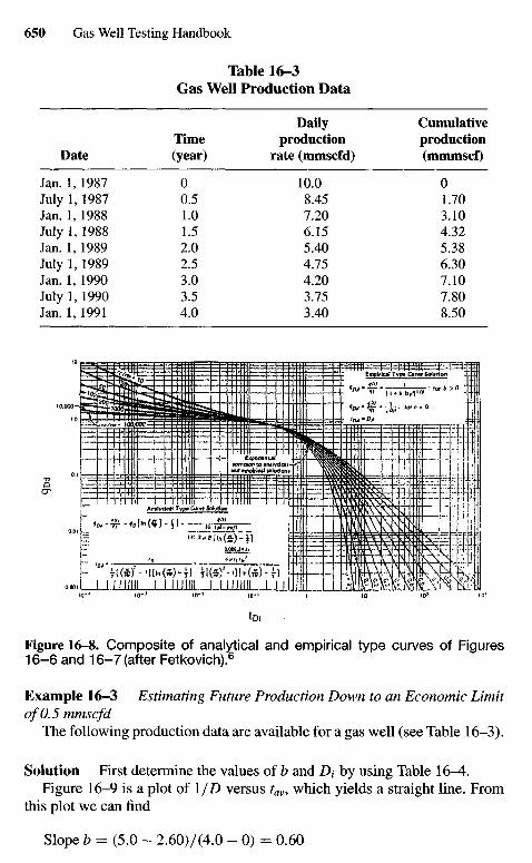
Table 16-3Gas Well Production Data
Daily CumulativeTime production production
Date (year) rate (mmscfd) (mmmscf)
Jan. 1, 1987 0 10.0 0July 1, 1987 0.5 8.45 1.70Jan. 1, 1988 1.0 7.20 3.10July 1, 1988 1.5 6.15 4.32Jan. 1, 1989 2.0 5.40 5.38July 1, 1989 2.5 4.75 6.30Jan. 1, 1990 3.0 4.20 7.10July 1, 1990 3.5 3.75 7.80Jan. 1, 1991 4.0 3.40 8.50
Figure 16-8. Composite of analytical and empirical type curves of Figures16-6 and 16-7 (after Fetkovich).6
Example 16-3 Estimating Future Production Down to an Economic Limitof 0.5 mmscfd
The following production data are available for a gas well (see Table 16-3).
Solution First determine the values of b and Dt by using Table 16-4.Figure 16-9 is a plot of \/D versus tav, which yields a straight line. From
this plot we can find
Slope b = (5.0 - 2.60)/(4.0 - 0) = 0.60
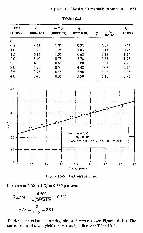
Table 16-4
Time q -Aq qav tav
(years) (mmscfd) (mmscfd) (mmscfd) ^ = ^qfv^t (years)
O 100.5 8.45 1.55 9.23 2.98 0.251.0 7.20 1.25 7.83 3.13 0.751.5 6.15 1.05 6.68 3.18 1.252.0 5.40 0.75 5.78 3.85 1.752.5 4.25 0.65 5.08 3.91 2.253.0 4.20 0.55 4.48 4.07 2.753.5 3.75 0.45 3.98 4.42 3.254.0 3.40 0.35 3.58 5.11 3.75
Intercept = 2.60A = 0.385
Slope b = [5.0 - 2.6] / [4.0 - 0.0] = 0.60
Time t, (years)
Figure 16-9. 1/D versus time.
Intercept = 2.60 and Dt = 0.385 per year.
*<"> = 515 = 2 M
To check the value of linearity, plot q~b versus t (see Figure 16-10). Thecorrect value of b will yield the best straight line. See Table 16-5.
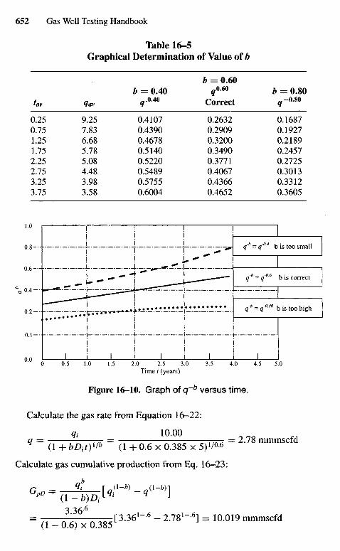
Table 16-5Graphical Determination of Value of b
b = 0.60b = 0.40 q0M b = 0.80
tav qav q*M Correct < r 0 8 0
0.25 9.25 0.4107 0.2632 0.16870.75 7.83 0.4390 0.2909 0.19271.25 6.68 0.4678 0.3200 0.21891.75 5.78 0.5140 0.3490 0.24572.25 5.08 0.5220 0.3771 0.27252.75 4.48 0.5489 0.4067 0.30133.25 3.98 0.5755 0.4366 0.33123.75 3.58 0.6004 0.4652 0.3605
Time t (years)
Figure 16-10. Graph of q~b versus time.
Calculate the gas rate from Equation 16-22:
qt 10.009 = ( l + » A 0 " » = 0+0.6x0.385x5)1/0.6 = 2™ " ^
Calculate gas cumulative production from Eq. 16-23:
GpD~ {\-b)Dt[qi ~q J
= n ™& nooJ 3 - 3 6 1 " ' 6 " 2.781-6] = 10.019 mmmscfd(1 - 0.6) x 0.385
qb = q0M b is too high
qh = q06 b is correct
q'b- q04 b is too small
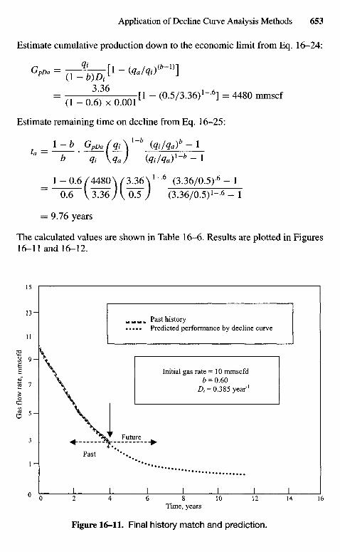
Gas
flo
w r
ate,
mm
scfd
Estimate cumulative production down to the economic limit from Eq. 16-24:
= ( 1 - 0 . " 6 X C O O 1 " - <°-5/3.3«'-«] = 4480 mmscf
Estimate remaining time on decline from Eq. 16-25:
= l-b GpDa/qi\X-b {qi/qa)b-\
b ' q, \qa) (qi/qay-b-\
_ 1-0.6 /4480\ /3.36\ l-6 (3.36/0.5)-6 - 10.6 \336j\0j) (3.36/0.5)1"-6 - 1
= 9.76 years
The calculated values are shown in Table 16-6. Results are plotted in Figures16-11 and 16-12.
Past historyPredicted performance by decline curve
Initial gas rate = 10 mmscfdb = 0.60
A = 0.385 year"1
Future
Past
Time, years
Figure 16-11. Final history match and prediction.
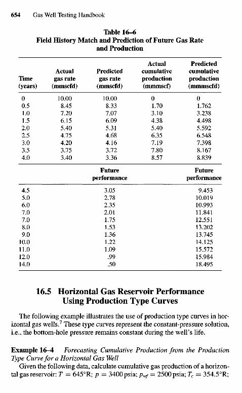
Table 16-6Field History Match and Prediction of Future Gas Rate
and Production
Actual PredictedActual Predicted cumulative cumulative
Time gas rate gas rate production production(years) (mmscfd) (mmscfd) (mmmscf) (mmmscfd)
0 10.00 10.00 0 00.5 8.45 8.33 1.70 1.7621.0 7.20 7.07 3.10 3.2381.5 6.15 6.09 4.38 4.4982.0 5.40 5.31 5.40 5.5922.5 4.75 4.68 6.35 6.5483.0 4.20 4.16 7.19 7.3983.5 3.75 3.72 7.80 8.1674.0 3.40 3.36 8.57 8.839
Future Futureperformance performance
4.5 3.05 9.4535.0 2.78 10.0196.0 2.35 10.9937.0 2.01 11.8417.0 1.75 12.5518.0 1.53 13.2029.0 1.36 13.745
10.0 1.22 14.12511.0 1.09 15.57212.0 .99 15.98414.0 .50 18.495
16.5 Horizontal Gas Reservoir PerformanceUsing Production Type Curves
The following example illustrates the use of production type curves in hor-izontal gas wells.7 These type curves represent the constant-pressure solution,i.e., the bottom-hole pressure remains constant during the well's life.
Example 16-4 Forecasting Cumulative Production from the ProductionType Curve for a Horizontal Gas Well
Given the following data, calculate cumulative gas production of a horizon-tal gas reservoir: T = 645°R; p = 3400 psia; pwf = 2500 psia; Tc = 354.5°R;
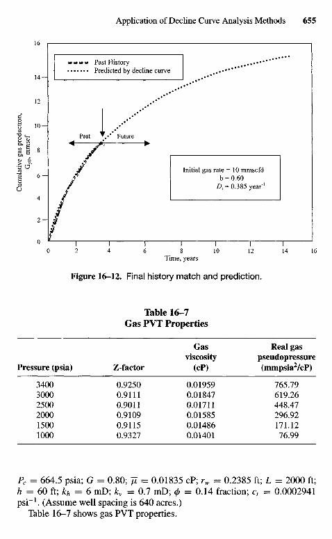
Cum
ulat
ive
gas
prod
ucti
on,
GpD
, mm
scf
Past HistoryPredicted by decline curve
Past Future
Initial gas rate = 10 mmscfdb = 0.60
D1 = 0.385 year1
Time, years
Figure 16-12. Final history match and prediction.
Table 16-7Gas PVT Properties
Gas Real gasviscosity pseudopressure
Pressure (psia) Z-factor (cP) (mmpsia2/cP)
3400 0.9250 0.01959 765.793000 0.9111 0.01847 619.262500 0.9011 0.01711 448.472000 0.9109 0.01585 296.921500 0.9115 0.01486 171.121000 0.9327 0.01401 76.99
Pc = 664.5 psia; G = 0.80; JL = 0.01835 cP; rw = 0.2385 ft; L = 2000 ft;h = 60 ft; kh = 6 mD; kv = 0.7 mD; 0 = 0.14 fraction; ct = 0.0002941psi"1. (Assume well spacing is 640 acres.)
Table 16-7 shows gas PVT properties.
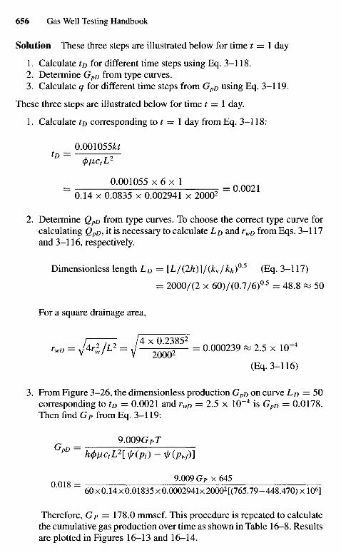
Solution These three steps are illustrated below for time t = 1 day
1. Calculate to for different time steps using Eq. 3-118.2. Determine GpD from type curves.3. Calculate q for different time steps from GpD using Eq. 3-119.
These three steps are illustrated below for time t = 1 day.
1. Calculate to corresponding to t = 1 day from Eq. 3-118:
_ 0.001055^(pjjLCtL
2
= 0 - 0 0 1 0 5 5 x 6 x l = 0.0021
0.14 x 0.0835 x 0.002941 x 20002
2. Determine QpD from type curves. To choose the correct type curve forcalculating QpD, it is necessary to calculate LD and rwD from Eqs. 3-117and 3-116, respectively.
Dimensionless length LD = [L/(2h)]/(kv/kh)05 (Eq. 3-117)
= 2000/(2 x 60)/(0.7/6)05 = 48.8 « 50
For a square drainage area,
rwD = firtjd- = f X2"0
2032852 = 0.000239 * 2.5 x 10"4
(Eq. 3-116)
3. From Figure 3-26, the dimensionless production GpD on curve LQ = 50corresponding to tD = 0.0021 and rwD = 2.5 x 10"4 is GpD = 0.0178.Then find GP from Eq. 3-119:
_ 9.009GPrGpD = h(/>fictL
2[xlf(Pi) - x/f(pwf)]
0 0 1 o 9.Q09GPX645
60 x 0.14 x 0.01835 x 0.0002941x 20002 [(765.79 -448.470) x 106]
Therefore, Gp = 178.0 mmscf. This procedure is repeated to calculatethe cumulative gas production over time as shown in Table 16-8. Resultsare plotted in Figures 16-13 and 16-14.
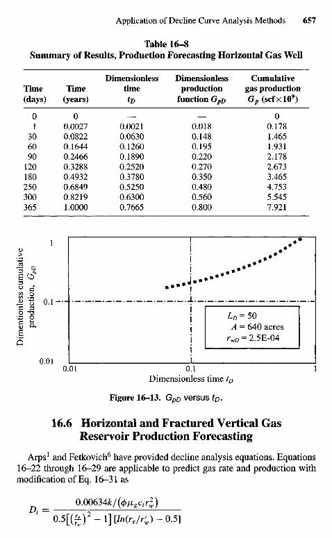
Dim
enti
onle
ss c
umul
ativ
epr
oduc
tion
, G
pD
Table 16-8Summary of Results, Production Forecasting Horizontal Gas Well
Dimensionless Dimensionless CumulativeTime Time time production gas production(days) (years) tD function GpD G^(SCfXlO9)
0 0 — — 01 0.0027 0.0021 0.018 0.178
30 0.0822 0.0630 0.148 1.46560 0.1644 0.1260 0.195 1.93190 0.2466 0.1890 0.220 2.178
120 0.3288 0.2520 0.270 2.673180 0.4932 0.3780 0.350 3.465250 0.6849 0.5250 0.480 4.753300 0.8219 0.6300 0.560 5.545365 1.0000 0.7665 0.800 7.921
LD = 50A = 640 acres
rvvD = 2.5E-04
Dimensionless time tD
Figure 16-13. GPD versus fo.
16.6 Horizontal and Fractured Vertical GasReservoir Production Forecasting
Arps1 and Fetkovich6 have provided decline analysis equations. Equations16-22 through 16-29 are applicable to predict gas rate and production withmodification of Eq. 16-31 as
0.00634&/((j)iJLgctrl)
'~0.5[(^)2-l][/n(r,/r;)-0.5]
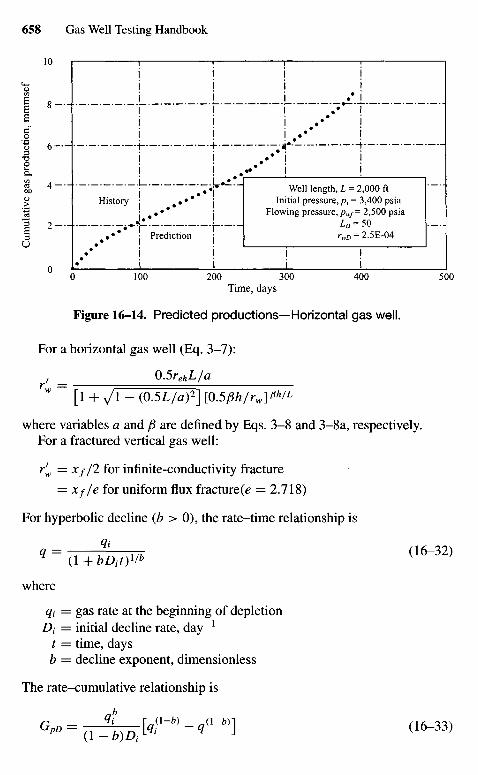
Cu
mu
lati
ve
gas
pro
du
ctio
n,
mm
msc
f
History
Prediction
Well length, L = 2,000 ftInitial pressure, /?, = 3,400 psia
Flowing pressure, pwf— 2,500 psiaLD = 50rvvD = 2.5E-04
Time, days
Figure 16-14. Predicted productions—Horizontal gas well.
For a horizontal gas well (Eq. 3-7):
r , = 0.5rehL/aVw [1 + y/\ - (0.5L/a)2] [0.5ph/rw]Ph/L
where variables a and /J are defined by Eqs. 3-8 and 3-8a, respectively.For a fractured vertical gas well:
r'w = Xf/2 for infinite-conductivity fracture
= Xf/e for uniform flux fracture(e = 2.718)
For hyperbolic decline (b > 0), the rate-time relationship is
q = H + HD1I)W <1 6-3 2)where
qt — gas rate at the beginning of depletionDt = initial decline rate, day"1
t = time, daysb = decline exponent, dimensionless
The rate-cumulative relationship is
G^=^b)oMl~b)-q(l~b)] (16~33)

Example 16-5 Predicting Performance of Horizontal and Fractured Verti-cal Gas Well Using Decline Analysis Equations
Given the following data, calculate performance of a horizontal gas well;A = 100 acres; T = 1100F; pt = 2000 psia; /x = 0.0250 cP; z = 0.95;kh = 0.1; kv = 0.1; qx• = 25.60 mmscfd; rw = 0.396 ft; JC/ = 250 ft; h = 45ft; cr = 0.000375 psi"1; 0 = 0.14; well length L = 2000 ft; b = 0.5.
Solution First calculate the following parameters:
r. _ (Ai£5«) " . ( « « ^ » ) = 1177.29 f,
From Eq. 3-6,
re, = [(L/2 + rev) (rCT)]05 = [(2000/2 + 1177.29) (1177.29)]05
= 1601 ft
From Equation 3-8,
a = 0.5 L [0.5 + 70.25 + (2reh/L)4] °5
= 0.5 x 2000[0.5 + 72(1601/200O)4]0-5 = 1763.95
For a horizontal well, r'w from Eq. 3—7 is
, = 0.5rehL/ar™ ~ [1 + y/\ - (0.5L/a)2][0.5ph/rw]WL
_ 0.5 x 1601 x 2000/1763.95
~ [1 + ^ l _ (0.5 x 2000/1763.95)2] [ 0 ^ p ] ( l x 4 5 / 2 0 0 0 )
= 327.22 ft
For a fractured vertical well,
r'w = Xf/2 = 250/2 = 125 ft
Calculate D, for a horizontal well from Eq. 16-29:
_ 0.00634 x 0.1/ (0.14 x 0.025 x 0.000375 x 0.3962)Di ~ 0.5[(1177.29/0.396)2 - 1] [/«(1177.29/327.22) - 0.5]
= 0.0008933 day"1
= 0.0268 month"1
= 0.3261 year"1
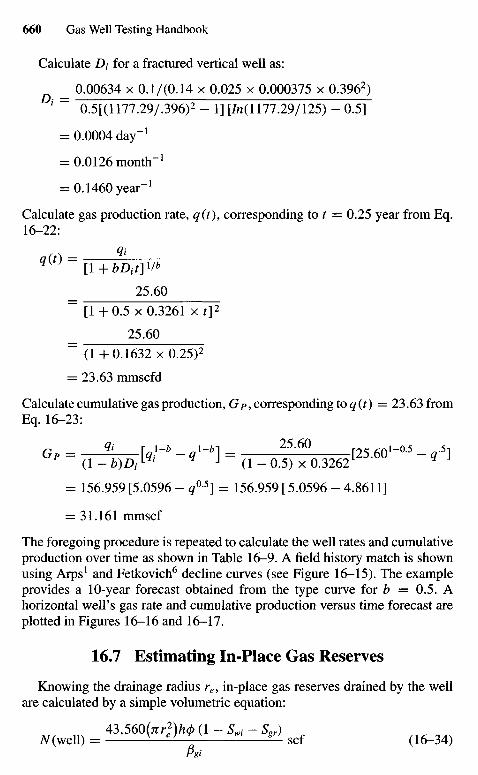
Calculate D1- for a fractured vertical well as:
_ 0.00634 x 0.1/(0.14 x 0.025 x 0.000375 x 0.3962)Di = 0.5[(1177.29/.396)2 - 1] [Zn(1177.29/125) - 0.5]
= 0.0004 day"1
= 0.0126 month"1
= 0.1460 year"1
Calculate gas production rate, q(t), corresponding to t = 0.25 year from Eq.16-22:
q(t) = [l+bDit]Vb
25.60~ [1+0.5x0.3261 x / ] 2
25.60~ (1+ 0.1632 x 0.25)2
= 23.63 mmscfd
Calculate cumulative gas production, Gp, corresponding to q(t) = 23.63 fromEq. 16-23:
n Qi T^l-b ^l-bl 25.60 nl-0.5 .5-1
°P = ( T ^ ) A fo - * J= ( 1 - 0.5) x 0.3262[25'6° " q ]
= 156.959 [5.0596 - q0-5] = 156.959 [ 5.0596 - 4.8611]
= 31.161 mmscfThe foregoing procedure is repeated to calculate the well rates and cumulativeproduction over time as shown in Table 16-9. A field history match is shownusing Arps1 and Fetkovich6 decline curves (see Figure 16-15). The exampleprovides a 10-year forecast obtained from the type curve for b = 0.5. Ahorizontal well's gas rate and cumulative production versus time forecast areplotted in Figures 16-16 and 16-17.
16.7 Estimating In-Place Gas Reserves
Knowing the drainage radius re, in-place gas reserves drained by the wellare calculated by a simple volumetric equation:
43,56O(7rr2)/*0 (1 - Swi - S»r)N (well) = —' V e) *— scf (16-34)
Pgi
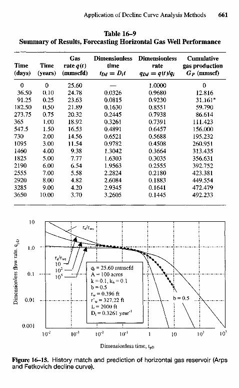
Table 16-9Summary of Results, Forecasting Horizontal Gas Well Performance
Gas Dimensionless Dimensionless CumulativeTime Time rate q(t) time rate gas production(days) (years) (mmscfd) tDd = Dit qDd = q(t)lqi Gp (mmscf)
0 0 25.60 — 1.0000 036.50 0.10 24.78 0.0326 0.9680 12.81691.25 0.25 23.63 0.0815 0.9230 31.161*
182.50 0.50 21.89 0.1630 0.8551 59.790273.75 0.75 20.32 0.2445 0.7938 86.614365 1.00 18.92 0.3261 0.7391 111.423547.5 1.50 16.53 0.4891 0.6457 156.000730 2.00 14.56 0.6521 0.5688 195.2321095 3.00 11.54 0.9782 0.4508 260.9511460 4.00 9.38 1.3042 0.3664 313.4351825 5.00 7.77 1.6303 0.3035 356.6312190 6.00 6.54 1.9563 0.2555 392.7522555 7.00 5.58 2.2824 0.2180 423.3812920 8.00 4.82 2.6084 0.1883 449.5543285 9.00 4.20 2.9345 0.1641 472.4793650 10.00 3.70 3.2605 0.1445 492.233
Dim
ensi
onle
ss f
low
rat
e, q
pD
qt = 25.60 mmscfdA = 100 acresk = 0.1,kh = 0.1b = 0.5rw = 0.396 ftr'w = 327.22 ftL - 2000 ftD1 = 0.3261 year'1
Dimensionless time, tpD
Figure 16-15. History match and prediction of horizontal gas reservoir (Arpsand Fetkovich decline curve).
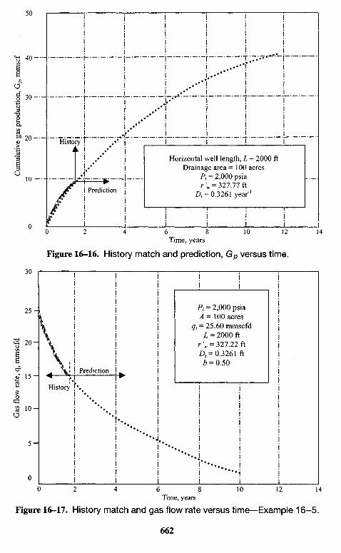
Cum
ulat
ive
gas
prod
ucti
on,
Gp,
mm
scf
Gas
flo
w r
ate,
q,
mm
scfd
History
Prediction
Horizontal well length, L = 2000 ftDrainage area = 100 acres
P1 = 2,000 psiar'w = 327.77 ft
A = 0.3261 year"1
Time, years
Figure 16-16. History match and prediction, Gp versus time.
Pi = 2,000 psiaA= 100 acres
q{~ 25.60 mmscfdL = 2000 ft
r 'w = 327.22 ftD, = 0.3261 ft
6 = 0.50Prediction
History
Time, years
Figure 16-17. History match and gas flow rate versus time—Example 16-5.
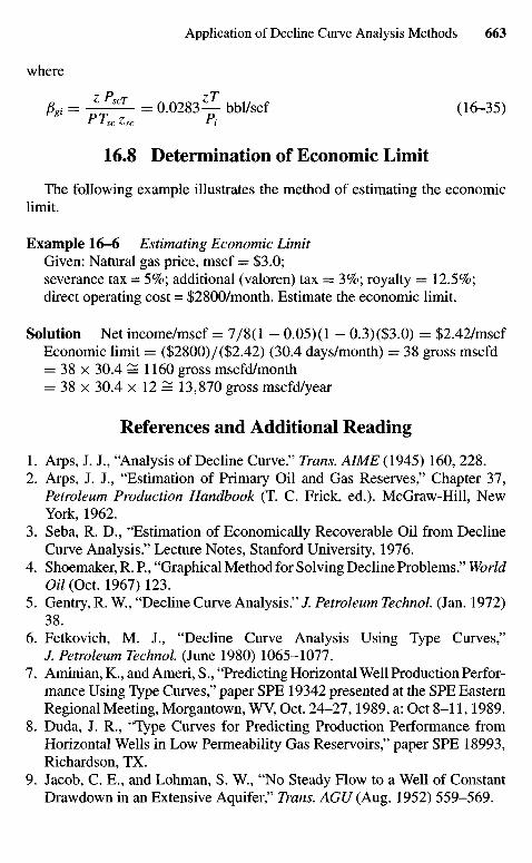
where
pgi = zPscT = 0.0283— bbl/scf (16-35)P Tsc Zsc Pi
16.8 Determination of Economic Limit
The following example illustrates the method of estimating the economiclimit.
Example 16-6 Estimating Economic LimitGiven: Natural gas price, mscf = $3.0;severance tax = 5%; additional (valoren) tax = 3%; royalty = 12.5%;direct operating cost = $2800/month. Estimate the economic limit.
Solution Net income/mscf = 7/8(1 - 0.05)(l - 0.3)($3.0) = $2.42/mscfEconomic limit = ($2800)/($2.42) (30.4 days/month) = 38 gross mscfd= 38 x 30.4 = 1160 gross mscfd/month= 38 x 30.4 x 12 = 13,870 gross mscfd/year
References and Additional Reading
1. Arps, J. J., "Analysis of Decline Curve." Trans. AIME (1945) 160, 228.2. Arps, J. J., "Estimation of Primary Oil and Gas Reserves," Chapter 37,
Petroleum Production Handbook (T. C. Frick, ed.). McGraw-Hill, NewYork, 1962.
3. Seba, R. D., "Estimation of Economically Recoverable Oil from DeclineCurve Analysis." Lecture Notes, Stanford University, 1976.
4. Shoemaker, R. R, "Graphical Method for Solving Decline Problems." WorldOil (Oct. 1967) 123.
5. Gentry, R. W., "Decline Curve Analysis." J. Petroleum Technol (Jan. 1972)38.
6. Fetkovich, M. J., "Decline Curve Analysis Using Type Curves,"/. Petroleum Technol (June 1980) 1065-1077.
7. Aminian, K., and Ameri, S., "Predicting Horizontal Well Production Perfor-mance Using Type Curves," paper SPE 19342 presented at the SPE EasternRegional Meeting, Morgantown, WV, Oct. 24-27,1989, a: Oct 8-11,1989.
8. Duda, J. R., "Type Curves for Predicting Production Performance fromHorizontal Wells in Low Permeability Gas Reservoirs," paper SPE 18993,Richardson, TX.
9. Jacob, C. E., and Lohman, S. W., "No Steady Flow to a Well of ConstantDrawdown in an Extensive Aquifer," Trans. AGU (Aug. 1952) 559-569.
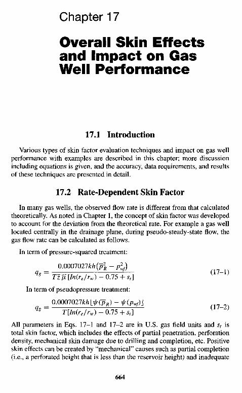
Chapter 17
Overall Skin Effectsand Impact on GasWell Performance
17.1 Introduction
Various types of skin factor evaluation techniques and impact on gas wellperformance with examples are described in this chapter; more discussionincluding equations is given, and the accuracy, data requirements, and resultsof these techniques are presented in detail.
17.2 Rate-Dependent Skin Factor
In many gas wells, the observed flow rate is different from that calculatedtheoretically. As noted in Chapter 1, the concept of skin factor was developedto account for the deviation from the theoretical rate. For example a gas welllocated centrally in the drainage plane, during pseudo-steady-state flow, thegas flow rate can be calculated as follows.
In term of pressure-squared treatment:
= 0.0007027^-^)q* TzJi[In(re/rw) - 0.75 + ^]
In term of pseudopressure treatment:
= 0.0007027khlxlf(pR) - x!f(Pwf)]9* T[In(re/rw)-0.15 + st]
{ )
All parameters in Eqs. 17-1 and 17-2 are in U.S. gas field units and st istotal skin factor, which includes the effects of partial penetration, perforationdensity, mechanical skin damage due to drilling and completion, etc. Positiveskin effects can be created by "mechanical" causes such as partial completion(i.e., a perforated height that is less than the reservoir height) and inadequate
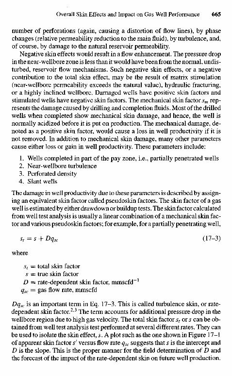
number of perforations (again, causing a distortion of flow lines), by phasechanges (relative permeability reduction to the main fluid), by turbulence, and,of course, by damage to the natural reservoir permeability.
Negative skin effects would result in a flow enhancement. The pressure dropin the near-wellbore zone is less than it would have been from the normal, undis-turbed, reservoir flow mechanisms. Such negative skin effects, or a negativecontribution to the total skin effect, may be the result of matrix stimulation(near-wellbore permeability exceeds the natural value), hydraulic fracturing,or a highly inclined wellbore. Damaged wells have positive skin factors andstimulated wells have negative skin factors. The mechanical skin factor sm rep-resents the damage caused by drilling and completion fluids. Most of the drilledwells when completed show mechanical skin damage, and hence, the well isnormally acidized before it is put on production. The mechanical damage, de-noted as a positive skin factor, would cause a loss in well productivity if it isnot removed. In addition to mechanical skin damage, many other parameterscause either loss or gain in well productivity. These parameters include:
1. Wells completed in part of the pay zone, i.e., partially penetrated wells2. Near-wellbore turbulence3. Perforated density4. Slant wells
The damage in well productivity due to these parameters is described by assign-ing an equivalent skin factor called pseudoskin factors. The skin factor of a gaswell is estimated by either drawdown or buildup tests. The skin factor calculatedfrom well test analysis is usually a linear combination of a mechanical skin fac-tor and various pseudoskin factors; for example, for a partially penetrating well,
st=s + Dqsc (17-3)
where
st = total skin factors = true skin factor
D = rate-dependent skin factor, mmscfd"1
qsc = gas flow rate, mmscfd
Dqsc is an important term in Eq. 17-3. This is called turbulence skin, or rate-dependent skin factor.23 The term accounts for additional pressure drop in thewellbore region due to high gas velocity. The total skin factor st or s can be ob-tained from well test analysis test performed at several different rates. They canbe used to isolate the skin effect, s. A plot such as the one shown in Figure 17-1of apparent skin factor s' versus flow rate qsc suggests that s is the intercept andD is the slope. This is the proper manner for the field determination of D andthe forecast of the impact of the rate-dependent skin on future well production.
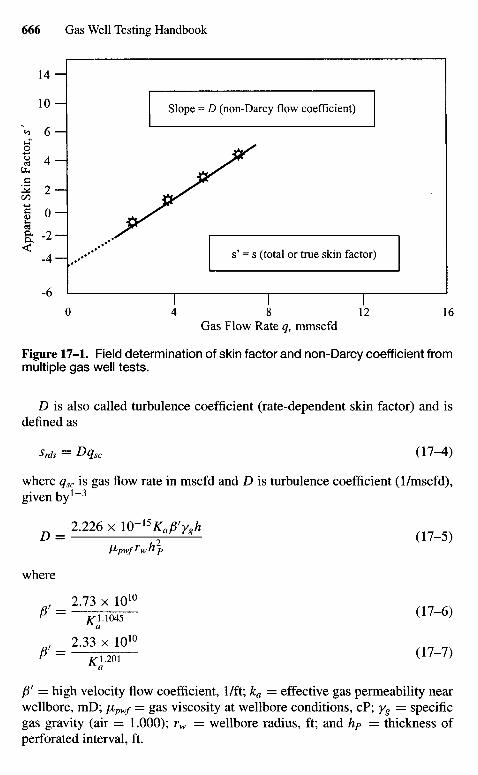
App
aren
t Sk
in F
acto
r, 5
'
Slope = D (non-Darcy flow coefficient)
s' = s (total or true skin factor)
Gas Flow Rate q, mmscfd
Figure 17-1. Field determination of skin factor and non-Darcy coefficient frommultiple gas well tests.
D is also called turbulence coefficient (rate-dependent skin factor) and isdefined as
Srds = Dqsc (17-4)
where qsc is gas flow rate in mscfd and D is turbulence coefficient (1/mscfd),given by 1 " 3
D _ 2.226 x IQ-" W ( ] 7 _ 5 )
№pwf rwh p
where
. 2.73 x 101 0
. 2.33 x 101 0
/3' = high velocity flow coefficient, I/ft; ka = effective gas permeability nearwellbore, mD; /jtpwf = gas viscosity at wellbore conditions, cP; yg = specificgas gravity (air — 1.000); rw — wellbore radius, ft; and hp = thickness ofperforated interval, ft.
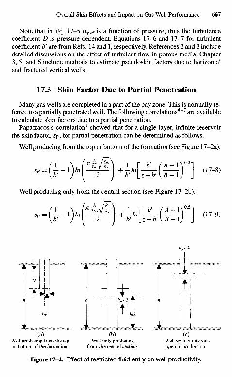
Note that in Eq. 17-5 fipwf is a function of pressure, thus the turbulencecoefficient D is pressure dependent. Equations 17-6 and 17-7 for turbulentcoefficient /3' are from Refs. 14 and 1, respectively. References 2 and 3 includedetailed discussions on the effect of turbulent flow in porous media. Chapter3, 5, and 6 include methods to estimate pseudoskin factors due to horizontaland fractured vertical wells.
17.3 Skin Factor Due to Partial Penetration
Many gas wells are completed in a part of the pay zone. This is normally re-ferred to a partially penetrated well. The following correlations4"7 are availableto calculate skin factors due to a partial penetration.
Papatzacos's correlation4 showed that for a single-layer, infinite reservoirthe skin factor, sP, for partial penetration can be determined as follows.
Well producing from the top or bottom of the formation (see Figure 17-2a):
HH'-(^)+H^(^)1 <™Well producing only from the central section (see Figure 17-2b):
Figure 17-2. Effect of restricted fluid entry on well productivity.
(a)Well producing from the topor bottom of the formation
(b)Well only producing
from the central section
(C)Well with N intervalsopen to production
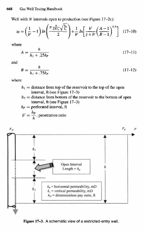
Well with Af intervals open to production (see Figure 17-2c):
where
A = T S v <17-n)
and
B = \ (17-12)h\ + J5hP
where
h\ = distance from top of the reservoir to the top of the openinterval, ft (see Figure 17-3)
h2 = distance from bottom of the reservoir to the bottom of openinterval, ft (see Figure 17-3)
hP = perforated interval, ft
,, hP •b= —, penetration ratio
Figure 17-3. A schematic view of a restricted-entry well.
kft ~ horizontal permeability, tnDkv - vertical permeability, mDho = dimensionless pay zone, ft
Open IntervalLength = hp
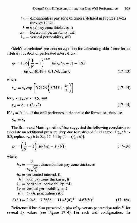
ho = dimensionless pay zone thickness, defined in Figures 17-2athrough 17-2c
h = total pay zone thickness, ftkH = horizontal permeability, mDkv — vertical peimeability, mD
Odeh's correlation5 presents an equation for calculating skin factor for anarbitrary location of perforated interval, hP:
/ , \ 0.825
sP = 1.35^— - I j [In(rwhD + 7) - 1.95
-In(rwe){0A9 + 0.1 In(rwhD}] (17-13)
where
rwc = rw exp | 0.2126 (2.753 + y j1 (17-14)
forO < Zm/h < 0-5, and
Zm=H1 + (ftp/2) (17-15)
If h\ = 0 , i.e., if the well perforates at the top of the formation, then use
The Brons and Marting method6 has suggested the following correlation tocalculate an additional pressure drop due to restricted fluid entry: If zm/h >0.5, replace zm/h in Eq. 17-14 by [1 - (z'Jh)]:
SP = (^- l\ Un(hD) - F (b')] (17-16)
where
ho = p=, dimensionless pay zone thicknessr №•
wy kv
hP = perforated interval, fth = total pay zone thickness, ft
kH = horizontal permeability, mDkv = vertical permeability, mDb' — hp/h, penetration ratio
F(b') = 2.948 - 7.363b' + 11.45(Z/)2 - 4.67(Z/)3 (17-16a)
Reference 6 has also presented a plot of Sp versus penetration ratio V forseveral ho values (see Figure 17-4). For each well configuration, the
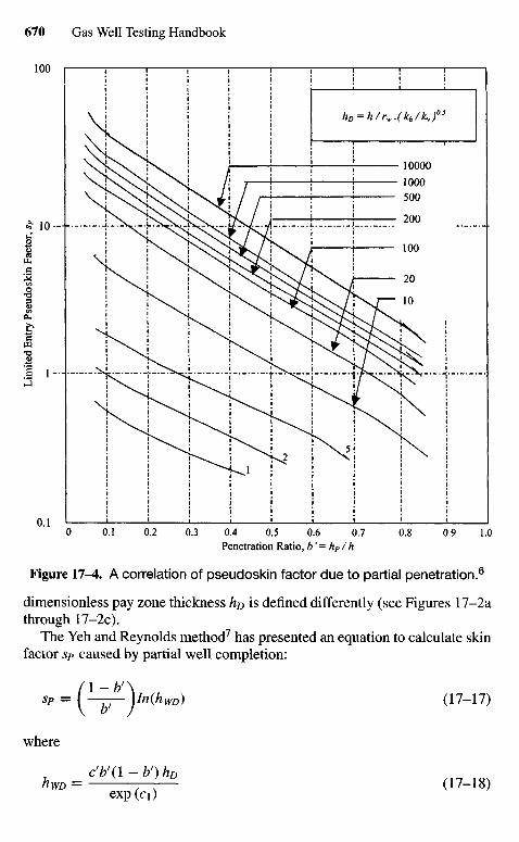
Lim
ited
Ent
ry P
seu
dos
kin
Fac
tor,
sP
Penetration Ratio, b'= hP/h
Figure 17-4. A correlation of pseudoskin factor due to partial penetration.6
dimensionless pay zone thickness hp is defined differently (see Figures 17-2athrough 17-2c).
The Yeh and Reynolds method7 has presented an equation to calculate skinfactor Sp caused by partial well completion:
(\-b'\sp = l —g- Un(hWD) (17-17)
where
hWD = ' (17-18)exp(ci)
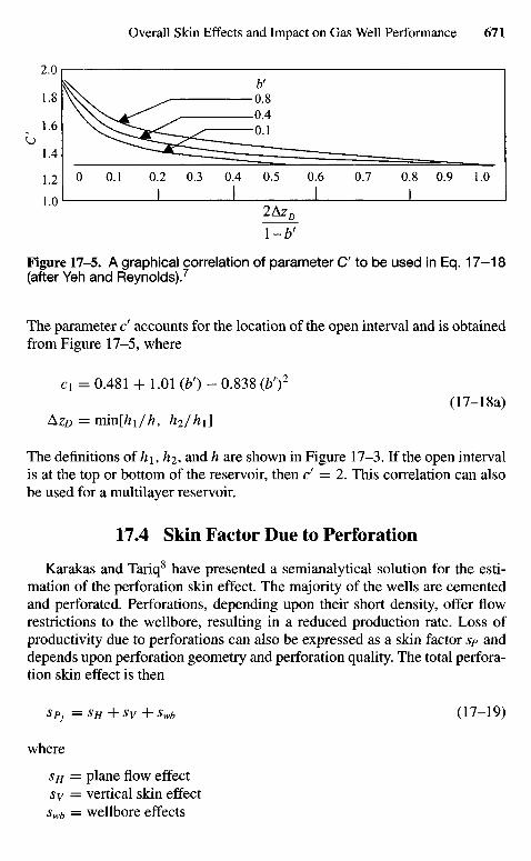
Figure 17-5. A graphical correlation of parameter C to be used in Eq. 17-18(after Yeh and Reynolds).7
The parameter d accounts for the location of the open interval and is obtainedfrom Figure 17-5, where
C1 = 0.481 + 1.01 (bf) - 0.838 (Z/)2
(17-18a)AZD = mm[h\/h, /12/A1]
The definitions of h\, /?2, and h are shown in Figure 17-3. If the open intervalis at the top or bottom of the reservoir, then d = 2. This correlation can alsobe used for a multilayer reservoir.
17.4 Skin Factor Due to Perforation
Karakas and Tariq8 have presented a semianalytical solution for the esti-mation of the perforation skin effect. The majority of the wells are cementedand perforated. Perforations, depending upon their short density, offer flowrestrictions to the wellbore, resulting in a reduced production rate. Loss ofproductivity due to perforations can also be expressed as a skin factor sp anddepends upon perforation geometry and perforation quality. The total perfora-tion skin effect is then
spf =sH+sv + swb (17-19)
where
sH = plane flow effectsv = vertical skin effectswb = wellbore effects
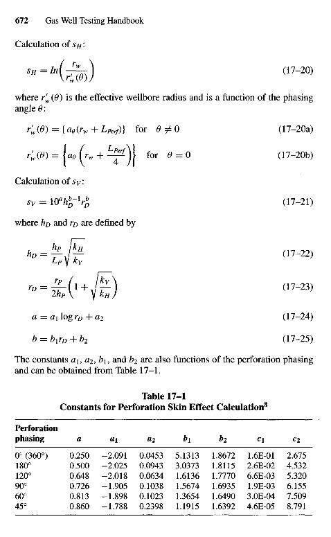
Calculation of sH'.
••-K^) ° 7 - 2 o )
where rrw{9) is the effective wellbore radius and is a function of the phasing
angle (9:
r'w{0) = { a e ( r w + LPerf)} f o r 6 ^ 0 (17-2Oa)
r ; ( 0 ) = L ( V w + ^ ) ) for 0 = 0 (17-2Ob)
Calculation of sv:
sv = Whh-lrhD (17-21)
where hD and rD are defined by
a = ax\ogrD+a2 (17-24)
b = blrD+b2 (17-25)
The constants a\, a2, b\, and b2 are also functions of the perforation phasingand can be obtained from Table 17-1.
Table 17-1Constants for Perforation Skin Effect Calculation8
Perforationphasing a a\ «2 ^i ^i c\ ci
0°(360°) 0.250 -2.091 0.0453 5.1313 1.8672 1.6E-01 2.675180° 0.500 -2.025 0.0943 3.0373 1.8115 2.6E-02 4.532120° 0.648 -2.018 0.0634 1.6136 1.7770 6.6E-03 5.32090° 0.726 -1.905 0.1038 1.5674 1.6935 1.9E-03 6.15560° 0.813 -1.898 0.1023 1.3654 1.6490 3.0E-04 7.50945° 0.860 -1.788 0.2398 1.1915 1.6392 4.6E-05 8.791
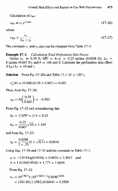
Calculation of sWb'-
swb = C1 e*™> (17-26)
where
rWD = - ^ - (17-27)
The constants c\ and c>i also can be obtained from Table 17-1.
Example 17-1 Calculating Total Perforation Skin FactorGiven: rw = 0.39 ft; SPF = 4; rP = 0.25 inches (0.0208 ft); LP =
8 inches (0.667 ft); and 0 — 168 and 0. Calculate the perforation skin effectifkH/kv = 10 and 1.
Solution From Eq. 17-2Oa and Table 17-1 (0 = 120°),
r'w(0) = (0.648) (0.39 + 0.667) = 0.685
Then, from Eq. 17-20,
*"="• (£§) = - ° - 5 6 3
From Eq. 17-22 and remembering that
hP = 1 /SPF= 1/4 = 0.25
and from Eq. 17-23:
0.0208 ,—rD = - ( I + VoI) = 0.0548
Using Eqs. 17-24 and 17-25 and the constants in Table 17-1,
a = -2.018 log(0.0548) + 0.0634 = 2.4817 and
b = 1.6136(0.0548) + 1.777 = 1.8654
From Eq. 17-21:
sv = 10248171.185(L8654-1)0.0548L8654
= (303.18)(1.1582)(0.0044) = 1.5589
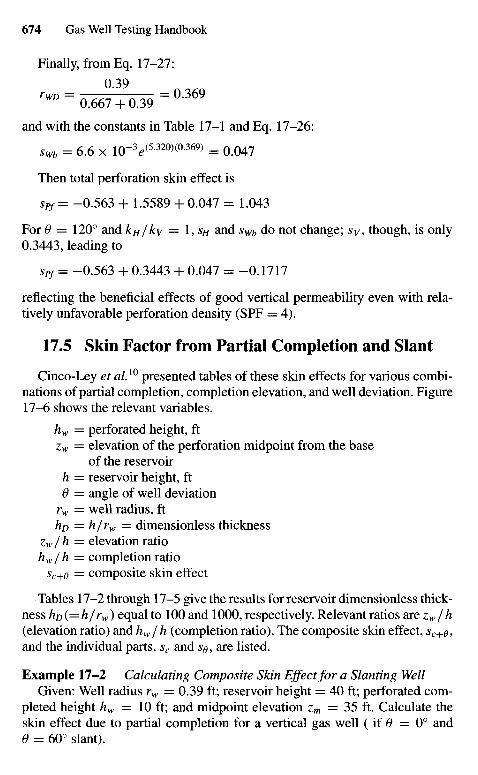
Finally, from Eq. 17-27:
^ = 06Jfo39 = a 3 6 9
and with the constants in Table 17-1 and Eq. 17-26:
sWb = 6.6 x iO-V5-32O)(a369) = 0.047
Then total perforation skin effect is
sPf = -0.563 + 1.5589 + 0.047 - 1.043
For 0 = 120° and kH/ky = 1, % and sWb do not change; sy, though, is only0.3443, leading to
spf = -0.563 + 0.3443 + 0.047 = -0.1717
reflecting the beneficial effects of good vertical permeability even with rela-tively unfavorable perforation density (SPF = 4).
17,5 Skin Factor from Partial Completion and Slant
Cinco-Ley et al.10 presented tables of these skin effects for various combi-nations of partial completion, completion elevation, and well deviation. Figure17-6 shows the relevant variables.
hw = perforated height, ftzw — elevation of the perforation midpoint from the base
of the reservoirh = reservoir height, ft6 = angle of well deviation
rw = well radius, fthD — h/rw = dimensionless thickness
zw/h = elevation ratiohw/h = completion ratio
sc+e = composite skin effect
Tables 17-2 through 17-5 give the results for reservoir dimensionless thick-ness ho(=h/rw) equal to 100 and 1000, respectively. Relevant ratios are zw/h(elevation ratio) and hw/h (completion ratio). The composite skin effect, sc+e,and the individual parts, sc and SQ, are listed.
Example 17-2 Calculating Composite Skin Effect for a Slanting WellGiven: Well radius rw = 0.39 ft; reservoir height = 40 ft; perforated com-
pleted height hw = 10 ft; and midpoint elevation zm = 35 ft. Calculate theskin effect due to partial completion for a vertical gas well ( if 0 = 0° and0 = 60° slant).
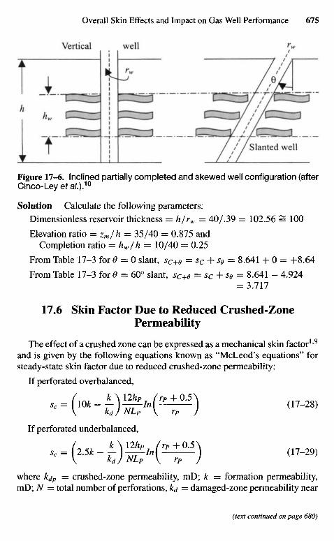
Figure 17-6. Inclined partially completed and skewed well configuration (afterCinco-Leyefa/.).10
Solution Calculate the following parameters:Dimensionless reservoir thickness = h/rw — 40/.39 = 102.56 = 100
Elevation ratio = Zm/h = 35/40 = 0.875 andCompletion ratio = hw/h = 10/40 = 0.25
From Table 17-3 for 0 = 0 slant, sc+e = sc + se = 8.641 + 0 = +8.64
From Table 17-3 for 0 = 60° slant, sc+e = sc + se = 8.641 - 4.924= 3.717
17.6 Skin Factor Due to Reduced Crushed-ZonePermeability
The effect of a crushed zone can be expressed as a mechanical skin factor1'9
and is given by the following equations known as "McLeod's equations" forsteady-state skin factor due to reduced crushed-zone permeability:
If perforated overbalanced,
*_( ,*- *)^fc(!>±W) ( 1 7-28)V kd) NLp \ rP )
If perforated underbalanced,
*_ (2* ')•£*(£ + *») (17-29)V kd) NLp \ rP )
where kdp = crushed-zone permeability, mD; k = formation permeability,mD; N = total number of perforations, kd = damaged-zone permeability near
(text continued on page 680)
Slanted well
Vertical well
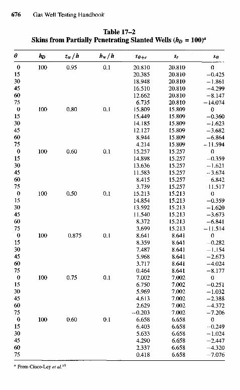
Table 17-2Skins from Partially Penetrating Slanted Wells (hD = 100)a
0 hD Zw/h hw/h SQ+r Sr So
0 100 0.95 0.1 20.810 20.810 015 20.385 20.810 -0.42530 18.948 20.810 -1.86145 16.510 20.810 -4.29960 12.662 20.810 -8.14775 6.735 20.810 -14.0740 100 0.80 0.1 15.809 15.809 015 15.449 15.809 -0.36030 14.185 15.809 -1.62345 12.127 15.809 -3.68260 8.944 15.809 -6.86475 4.214 15.809 -11.5940 100 0.60 0.1 15.257 15.257 015 14.898 15.257 -0.35930 13.636 15.257 -1.62145 11.583 15.257 -3.67460 8.415 15.257 -6.84275 3.739 15.257 -11.5170 100 0.50 0.1 15.213 15.213 015 14.854 15.213 -0.35930 13.592 15.213 -1.62045 11.540 15.213 -3.67360 8.372 15.213 -6.84175 3.699 15.213 -11.5140 100 0.875 0.1 8.641 8.641 015 8.359 8.641 -0.28230 7.487 8.641 -1.15445 5.968 8.641 -2.67360 3.717 8.641 -4.02475 0.464 8.641 -8.1770 100 0.75 0.1 7.002 7.002 015 6.750 7.002 -0.25130 5.969 7.002 -1.03245 4.613 7.002 -2.38860 2.629 7.002 -4.37275 -0.203 7.002 -7.2060 100 0.60 0.1 6.658 6.658 015 6.403 6.658 -0.24930 5.633 6.658 -1.02445 4.290 6.658 -2.44760 2.337 6.658 -4.32075 0.418 6.658 -7.076
a From Cinco-Ley et al.10
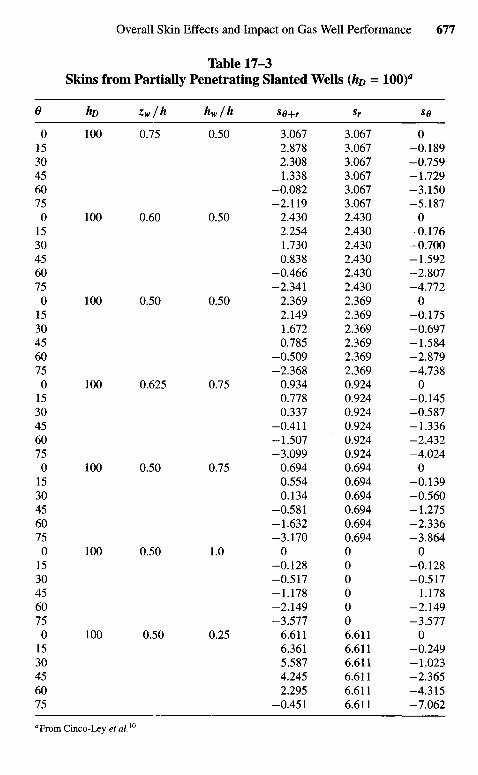
Table 17-3Skins from Partially Penetrating Slanted Wells (hD = 100)"
O hD Zw /h hw/h se+r sr so
0 100 0.75 0.50 3.067 3.067 015 2.878 3.067 -0.18930 2.308 3.067 -0.75945 1.338 3.067 -1.72960 -0.082 3.067 -3.15075 -2.119 3.067 -5.1870 100 0.60 0.50 2.430 2.430 0
15 2.254 2.430 -0.17630 1.730 2.430 -0.70045 0.838 2.430 -1.59260 -0.466 2.430 -2.80775 -2.341 2.430 -4.772
0 100 0.50 0.50 2.369 2.369 015 2.149 2.369 -0.17530 1.672 2.369 -0.69745 0.785 2.369 -1.58460 -0.509 2.369 -2.87975 -2.368 2.369 -4.7380 100 0.625 0.75 0.934 0.924 0
15 0.778 0.924 -0.14530 0.337 0.924 -0.58745 -0.411 0.924 -1.33660 -1.507 0.924 -2.43275 -3.099 0.924 -4.0240 100 0.50 0.75 0.694 0.694 0
15 0.554 0.694 -0.13930 0.134 0.694 -0.56045 -0.581 0.694 -1.27560 -1.632 0.694 -2.33675 -3.170 0.694 -3.864
0 100 0.50 1.0 0 0 015 -0.128 0 -0.12830 -0.517 0 -0.51745 -1.178 0 -1.17860 -2.149 0 -2.14975 -3.577 0 -3.5770 100 0.50 0.25 6.611 6.611 015 6.361 6.611 -0.24930 5.587 6.611 -1.02345 4.245 6.611 -2.36560 2.295 6.611 -4.31575 -0.451 6.611 -7.062
aFrom Cinco-Ley et al.10
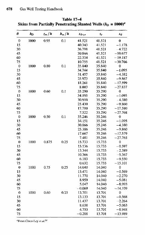
Table 17-4Skins from Partially Penetrating Slanted Wells (hD = 1000)"
0 hD Zw /h hw/h so+r sr se
0 1000 0.95 0.1 41.521 41.521 015 40.343 41.521 -1.17830 36.798 41.521 -4.72245 30.844 41.521 -10.67760 22.334 41.521 -19.18775 10.755 41.521 -30.766
0 1000 0.80 0.1 35.840 35.840 015 34.744 35.840 -1.09530 31.457 35.840 -4.38245 25.973 35.840 -9.86760 18.261 35.840 -17.59975 8.003 35.840 -27.8370 1000 0.60 0.1 35.290 35.290 0
15 34.195 35.290 -1.09530 30.910 35.290 -4.38045 25.430 35.290 -9.86060 17.710 35.290 -17.58075 7.522 35.290 -27.7680 1000 0.50 0.1 35.246 35.246 0
15 34.151 35.246 -1.09530 30.866 35.246 -4.38045 25.386 35.246 -9.86060 17.667 35.246 -17.57975 7.481 35.246 -27.765
0 1000 0.875 0.25 15.733 15.733 015 15.136 15.733 -0.59730 13.344 15.733 -2.38945 10.366 15.733 -5.36760 6.183 15.733 -9.55075 0.632 15.733 -15.101
0 1000 0.75 0.25 14.040 14.040 015 13.471 14.040 -0.56930 11.770 14.040 -2.27045 8.959 14.040 -5.08160 5.047 14.040 -8.99375 -0.069 14.040 -14.109
0 1000 0.60 0.25 13.701 13.701 015 13.133 13.701 -0.56830 11.437 13.701 -2.26445 8.638 13.701 -5.06360 4.753 13.701 -8.94875 -0.288 13.701 -13.989
aFrom Cinco-Ley et al.10
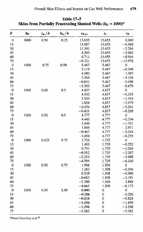
Table 17-5Skins from Partially Penetrating Slanted Wells (hD = 100Of
0 hD Zw /h hw/h So+r Sr S0
0 1000 0.50 0.25 13.655 13.655 0.00015 13.087 13.655 -0.56830 11.391 13.655 -2.26445 8.593 13.655 -5.06360 4.711 13.655 -8.94475 -0.321 13.655 -13.9760 1000 0.75 0.50 5.467 5.467 015 5.119 5.467 -0.34830 4.080 5.467 -1.38745 2.363 5.467 -3.10460 -0.031 5.467 -5.49875 -3.203 5.467 -8.6700 1000 0.60 0.5 4.837 4.837 015 4.502 4.837 -0.33530 3.503 4.837 -1.33445 1.858 4.837 -2.97960 -0.424 4.837 -5.26175 -0.431 4.837 -8.2680 1000 0.50 0.5 4.777 4.777 015 4.443 4.777 -0.33430 3.446 4.777 -1.33145 1.806 4.777 -2.97160 -0.467 4.777 -5.24475 -3.458 4.777 -8.2350 1000 0.625 0.75 1.735 1.735 015 1.483 1.735 -0.25230 0.731 1.735 -1.00445 -0.512 1.735 -2.24760 -2.253 1.735 -3.98875 -4.595 1.735 -6.3300 1000 0.50 0.75 1.508 1.508 015 1.262 1.508 -0.24630 0.528 1.508 -0.98045 -0.683 1.508 -2.19160 -2.380 1.508 -3.88875 -4.665 1.508 -6.1730 1000 0.50 1.00 0.000 0 015 -0.206 0 -0.20630 -0.824 0 -0.82445 -1.850 0 -1.85060 -3.298 0 -3.29875 -5.282 0 -5.282
aFrom Cinco-Ley et al.10

Figure 17-7. Geometry of perforation with crushed zone (after McLeod).9
(text continued from page 675)
the wellbore, mD; rP = perforation radius, ft; rdp = rP + 0.5 = crushed-zoneradius, ft; LP = depth of perforation, ft and hp = perforated interval, ft.
It is believed that these equations are difficult to use with certainty and thusare primarily useful for sensitivity analysis. Figure 17-7 shows the geometryof perforation with a crushed zone.
17/7 Slant Well Damage Skin Effecton Well Productivty
Figure 17-8 shows a schematic diagram of a slant well and Figure 17-9presents pseudoskin factors of slant wells as a function of ho for different slantangles 0. Reference 10 presented an equation to calculate the skin factor dueto a slant well, which depends on the well geometry:
ss = -(0'/4I)2 '06 - (0'/56)L8651Og(WlOQ) (17-30)
Damaged radius
Permeability, kd
Damaged zone
Formation permeability, k
Permeability
Crushed zone
Cen
tral
lin
e of
wel
l
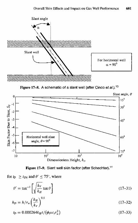
Skin
Fac
tor
Due
to
Slan
t, S 9
For horizontal wella = 90°
Figure 17-8. A schematic of a slant well (after Cinco et a/.).10
Slant angle, 6
Slant well
Slant angle
Dimensionless Height, hD
Figure 17-9. Slant well skin factor (after Schechter).11
for tD > tDX and 9' < 75°, where
0f = tan"1 / — tan# (17-31)LV*ff J(k \0'5
hD = h/rJy-\ (17-32)
tD = 0.000264kHt/((pfictrl) (17-33)
Horizontal well slantangle, 0=90°
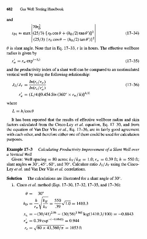
and
7Or*
tm = max (25/3) [ rD cos 9 + (hD/2) tan 0 ')]2 (17-34)
(25/3) [rDcos6> - (hD/2) tan<9')]2
0 is slant angle. Note that in Eq. 17-33, t is in hours. The effective wellboreradius is given by
rfw = rw exp (-^} (17-35)
and the productivity index of a slant well can be compared to an unstimulatedvertical well by using the following relationship:
In(re/rw)Js/Jv = T ( , , . (17-36)
r'w = (L/4)[0.454Sin (360° x rw/h)]h/L
where
L = h/cosO
It has been reported that the results of effective wellbore radius and skinfactors calculated from the Cinco-Ley et al. equation, Eq. 17-30, and fromthe equation of Van Der Vlis et a/., Eq. 17-36, are in fairly good agreementwith each other, and therefore either one of them could be used for calculationpurposes.
Example 17-3 Calculating Productivity Improvement of a Slant Well overa Vertical Well
Given: Well spacing = 80 acres; kv/kH = 1.0; rw = 0.39 ft; h = 550 ft;slant angles = 30°, 45°, 60°, and 70°. Calculate ratio Js/Jv u s i n g the Cinco-Ley et al. and Van Der Vlis et al. correlations.
Solution The calculations are illustrated for a slant angle of 30°.
1. Cinco et al. method (Eqs. 17-30, 17-32, 17-35, and 17-36):
0 = 30°
rw Y kv .39
sSs = - ( 3 0 / 4 I ) 2 0 6 - (30/56)L865log(1410.3/100) = -0.8843
r'w = 0.39exp- ("a8843) = 0.944
re = ^/80 x 43,560/TT = 1053 ft
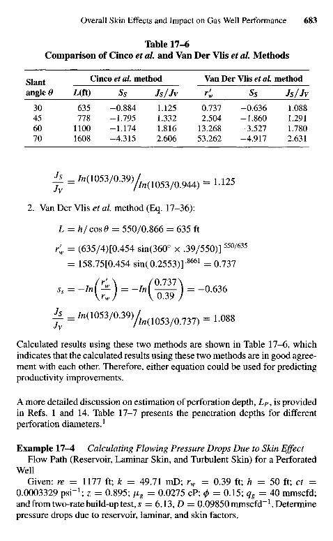
Table 17-6Comparison of Cinco et al. and Van Der Vlis et al. Methods
Slant Cinco et al method Van Der Vlis et al method
angle 0 L(ft) Ss Js/Jv r'w Ss Js/J^
30 635 -0.884 1.125 0.737 -0.636 1.08845 778 -1.795 1.332 2.504 -1.860 1.29160 1100 -1.174 1.816 13.268 -3.527 1.78070 1608 -4.315 2.606 53.262 -4.917 2.631
| = M 1 0 5 3 / 0 . 3 9 ) / / n ( 1 ( ) 5 3 / 0 9 4 4 ) = U 2 5
2. Van Der Vlis et al. method (Eq. 17-36):
L = h/cos0 = 550/0.866 = 635 ft
r'w = (635/4)[0.454 sin(360° x .39/550)] 550/635
= 158.75[0.454 sin( 0.2553)] 8661 =0 .737
—K9 = -'"(w) —A=M(1053/039yfa(1053/()737) = 1.088
Calculated results using these two methods are shown in Table 17-6, whichindicates that the calculated results using these two methods are in good agree-ment with each other. Therefore, either equation could be used for predictingproductivity improvements.
A more detailed discussion on estimation of perforation depth, LP, is providedin Refs. 1 and 14. Table 17-7 presents the penetration depths for differentperforation diameters.1
Example 17-4 Calculating Flowing Pressure Drops Due to Skin EffectFlow Path (Reservoir, Laminar Skin, and Turbulent Skin) for a Perforated
WellGiven: re = 1177 ft; Ic = 49.71 mD; rw = 0.39 ft; h = 50 ft; ct =
0.0003329 psi"1; z = 0.895; fig = 0.0275 cP; 0 = 0.15; qg = 40 mmscfd;and from two-rate build-up test, s = 6.13, D = 0.09850 mmscfd"1. Determinepressure drops due to reservoir, laminar, and skin factors.
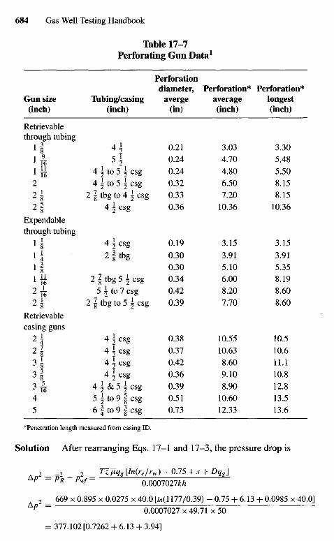
Table 17-7Perforating Gun Data1
Gun size(inch)
Retrievablethrough tubing
ifi£2
Z 82 ^Z 8
Expendablethrough tubing
if
Z 162 8
Retrievablecasing guns
2 *2i3 |
3 |3 ^4
5
TUbing/casing(inch)
5i4 I to 5 I csg
4 ^ to 5 ^ csg
2 I tbg to 4 \ csg
4±csg
4 i csg
2 § tbg
2|tbg5±csg
5 \ to 7 csg
2 I tbg to 5 i csg
4 5 csg
4 ^ csg
4^csg
4 I csg
4 i & 5 i c s g
5 \ to 9 § csg
6 I to 9 § csg
Perforationdiameter,
averge(in)
0.21
0.24
0.24
0.32
0.33
0.36
0.19
0.30
0.30
0.34
0.42
0.39
0.38
0.37
0.42
0.36
0.39
0.51
0.73
Perforation*average(inch)
3.03
4.70
4.80
6.50
7.20
10.36
3.15
3.91
5.10
6.00
8.20
7.70
10.55
10.63
8.60
9.10
8.90
10.60
12.33
Perforation*longest(inch)
3.30
5.48
5.50
8.15
8.15
10.36
3.15
3.91
5.35
8.19
8.60
8.60
10.5
10.6
11.1
10.8
12.8
13.5
13.6
* Penetration length measured from casing ID.
Solution After rearranging Eqs. 17-1 and 17-3, the pressure drop is
2 _ -2 2 _ Fz/Zffg \In(re/rw) - 0.75 + s + Dqg\AP -pR~pM- O.OOOlOUkh
2 _ 669 x 0.895 x 0.0275 x 40.0 [/«(1177/0.39) - 0.75 + 6.13 + 0.0985 x 40.0]AP = 0.0007027x49.71x50
= 377.102 [0.7262 4- 6.13 4- 3.94]
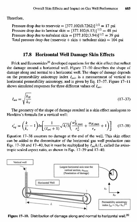
Therefore,
Pressure drop due to reservoir = [377.102(0.7262)] 1Z2 = 17 psiPressure drop due to laminar skin = [377.102(6.13)]1/2 = 48 psiPressure drop due to turbulent skin = [377.102(3.94)] 1Z2 = 39 psiTotal pressure drop due (reservoir + skin + turbulent skin) =104 psi
17.8 Horizontal Well Damage Skin Effects
Frick and Economides20 developed equations for the skin effect that reflectthe damage around a horizontal well. Figure 17-10 describes the shape ofdamage along and normal to a horizontal well. The shape of damage dependson the permeability anisotropy index /am, is a measurement of vertical tohorizontal permeability anisotropy, and is given by Eq. 17-37. Figure 17-11shows simulated responses for three different values of Iani.
lam = J ^r- (17-37)
The geometry of the shape of damage resulted in a skin effect analogous toHawkins's formula for a vertical well:
s'eq = (h- - i W ^ ^ V W ^ + ?*=« + iYI (17-38)
Equation 17-38 assumes no damage at the end of the well. This skin effectcan be added to the denominator of the horizontal gas well production rateEqs. 17-39 and 17^+0, but it must be multiplied by Ianih/L, called the aniso-tropic scaled aspect ratio, as shown in Eqs. 17-39 and 17-40.
Vertical well
Largest horizontal axis near thevertical section, oiH,max
(Penetration of damage)
Horizontal Well
Permeability anisotropyindex Iani=(kH/kvf-
5
Figure 17-10. Distribution of damage along and normal to horizontal well.20
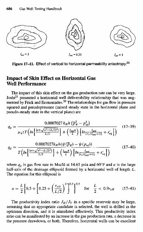
Figure 17-11. Effect of vertical to horizontal permeability anisotropy.20
Impact of Skin Effect on Horizontal GasWell Performance
The impact of this skin effect on the gas production rate can be very large.Joshi21 presented a horizontal well deliverability relationship that was aug-mented by Frick and Economides.20 The relationships for gas flow in pressuresquared and pseudopressure (mixed steady state in the horizontal plane andpseudo-steady state in the vertical plane) are
0.0007027 ifcHA (p2R -P2J
qg = , K——^ (17-39)
^8Z1 \ln\ L/2 } + V L ) I [^(W+Dl ±Seq\)
= 0.0001027kHh(xlf(pR) - jf(pwf))98 / I [ .+V^MZT^I / W A I Iani | \
1 \ m \ L/2 } ^ V L ) I [^(/oni+1)] ^ S*4\)
where qg is gas flow rate in Mscfd at 14.65 psia and 600F and a is the largehalf-axis of the drainage ellipsoid formed by a horizontal well of length L.The equation for this ellipsoid is
a = - (0.5 + [0.25 + ( ^ ) J } for - < 0.9^ (17-41)
The productivity index ratio JH/ Jv in a specific reservoir may be large,assuming that an appropriate candidate is selected, the well is drilled in theoptimum direction, and it is stimulated effectively. This productivity indexratio can be manifested by an increase in the gas production rate, a decrease inthe pressure drawdown, or both. Therefore, horizontal wells can be excellent
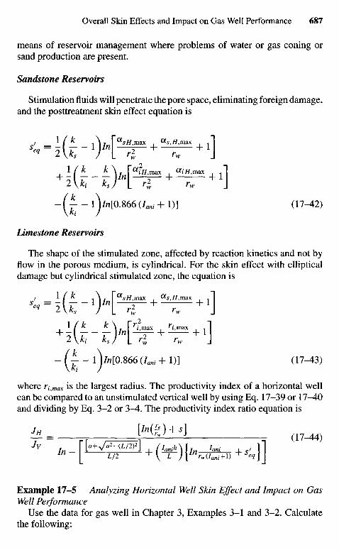
means of reservoir management where problems of water or gas coning orsand production are present.
Sandstone Reservoirs
Stimulation fluids will penetrate the pore space, eliminating foreign damage,and the posttreatment skin effect equation is
+ I f * - - k V n [ ^ m a x + aiH>™x + l l2 Ui ksj I rI rw J
-(^- lWo.866(Iani + I)] (17-42)
Limestone Reservoirs
The shape of the stimulated zone, affected by reaction kinetics and not byflow in the porous medium, is cylindrical. For the skin effect with ellipticaldamage but cylindrical stimulated zone, the equation is
'-- K£ -1H2T+ 2 1T+ 1]+ K H H I f + ^ + 1 ]- (^- - 1 Wo.866 (Iani + I)] (17-43)
where r\imax is the largest radius. The productivity index of a horizontal wellcan be compared to an unstimulated vertical well by using Eq. 17-39 or 17-40and dividing by Eq. 3-2 or 3-A. The productivity index ratio equation is
ft- „ , №4 , (.7^4,
Example 17-5 Analyzing Horizontal Well Skin Effect and Impact on GasWell Performance
Use the data for gas well in Chapter 3, Examples 3-1 and 3-2. Calculatethe following:
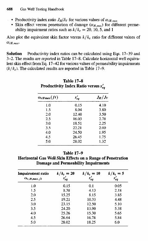
• Productivity index ratio JH/Jv for various values of aiH,max• Skin effect versus penetration of damage (piH,max) f° r different perme-
ability impairment ratios such as k/ks = 20, 10, 5, and 1
Also plot the equivalent skin factor versus k/ks ratio for different values of&iH,max'
Solution Productivity index ratios can be calculated using Eqs. 17-39 and3-2. The results are reported in Table 17-8. Calculate horizontal well equiva-lent skin effect from Eq. 17-42 for various values of permeability impairments(k/ks). The calculated results are reported in Table 17-9.
Table 17-8Productivity Index Ratio versus s'eq
<XsHmax(ft) s'eq JH/JV
1.0 0.15 4.101.5 8.04 3.802.0 12.40 3.502.5 16.03 2.783.0 18.51 2.253.5 22.21 2.004.0 24.50 1.954.5 26.45 1.755.0 28.02 1.32
Table 17-9Horizontal Gas Well Skin Effects on a Range of Penetration
Damage and Permeability Impairments
Impairement ratio k/ks = 20 k/ks = 1 0 k/ks = 5&s,Hjnax,ft Seq $eq Seq
1.0 0.15 0.1 0.051.5 8.38 4.13 2.182.0 15.25 8.15 3.852.5 19.21 10.33 4.483.0 23.15 12.50 5.103.5 24.20 13.90 5.384.0 25.26 15.30 5.654.5 26.64 16.78 5.845.0 28.02 18.25 6.0
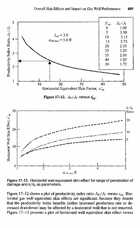
Prod
ucti
vity
Ind
ex R
atio
, J H
/Jv
Hor
izon
tal W
ell
Skin
Eff
ect,
s \ q
Horizontal Equivalent Skin Factor, s 'eq
Figure 17-12. JH/Jv versus SQQ.
S'eq JH? Jv0 1.005 3.50
10 3.1515 2.7520 2.3525 2.2035 2.0040 1.8550 1.72
Figure 17-13. Horizontal well equivalent skin effect for range of penetration ofdamage and k/ks as parameters.
Figure 17-12 shows a plot of productivity index ratio JH/Jv versus seq. Hor-izontal gas well equivalent skin effects are significant, because they denotethat the productivity index benefits (either increased production rate or de-creased drawdown) may be affected by a horizontal well that is not removed.Figure 17-13 presents a plot of horizontal well equivalent skin effect versus
Ratio
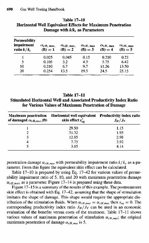
Table 17-10Horizontal Well Equivalent Effects for Maximum Penetration
Damage with k/ks as Parameters
Permeabilityi m p a i r m e n t OLsH,max, CXsH, max, OLsH,max OLsH, max OC8H, max
ratio k/ ks (ft) = 1 (ft) = 2 (ft) = 3 (ft) = 4 (ft) = 5
1 0.025 0.045 0.15 0.210 0.235 0.105 3.2 4.3 5.75 6.42
10 0.210 6.7 9.7 11.26 13.5020 0.254 13.5 19.5 24.5 25.15
Table 17-11Stimulated Horizontal Well and Associated Productivity Index Ratio
for Various Values of Maximum Penetration of Damage
Maximum penetration Horizontal well equivalent Productivity index ratioof damaged a,-H,max,(ft) skin effect s'eq JH/JV
1 29.50 1.152 31.32 1.953 12.85 2.984 7.75 3.925 3.65 4.14
penetration damage asH,max with permeability impairment ratio k/ks as a pa-rameter. From this figure the equivalent skin effect can be calculated.
Table 17-10 is prepared by using Eq. 17-42 for various values of perme-ability impairment ratio of 5, 10, and 20 with maximum penetration damageas H,max a s a parameter. Figure 17-14 is prepared using these data.
Figure 17-15 is a summary of the results of this example. The posttreatmentskin effect is obtained with Eq. 17-42, assuming that the shape of stimulationimitates the shape of damage. This shape would require the appropriate dis-tribution of the stimulation fluids. When aiH,max = aSH,max then seq = 0. Thecorresponding productivity index ratio JH/Jv c a n be used in an economicevaluation of the benefits versus costs of the treatment. Table 17-11 showsvarious values of maximum penetration of stimulation af-H,max', the originalmaximum penetration of damage aSH,max is 5.
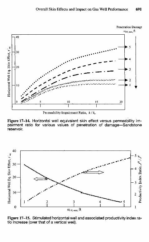
Permeability Impairment Ratio, k / ks
Figure 17-14. Horizontal well equivalent skin effect versus permeability im-pairment ratio for various values of penetration of damage—Sandstonereservoir.
Hor
izon
tal
Wel
l E
q. S
kin
Eff
ect,
s \ q
Hor
izon
tal
Wel
l E
q. S
kin
Eff
ect,
s\q
Prod
uctiv
ity I
ndex
Rat
io, j
" /
f
Penetration Damage
Figure 17-15. Stimulated horizontal well and associated productivity index ra-tio increase (over that of a vertical well).
References and Additional Reading
1. Brown, K. E., The Technology of Artificial Lift Methods, Vol. 4. Penn WellPublishing Co., Tulsa, OK, 1984.
2. Wittenberg, R. A., and Ramey, H. J., Jr., "Gas Well Testing with Turbu-lence," /. Petroleum Technol. (Jan. 1983) 31-39.
3. Ding, W., "Gas Well Test Analysis," M.S. Thesis, University of Tulsa,Tulsa, OK, 1986.
4. Papatzacos, P., "Approximate Partial-Penetration Pseudo-Skin for Infinite-Conductivity Wells," SPE Reservoir Eng. (May 1988) 227-234; Trans.AIME 283.
5. Odeh, A.S., "An Equation for Calculating Skin Factor Due to Restricted-Entry," /. Petroleum Technol (June 1980) 964-965.
6. Brons, R, and Mailing, V. E., "The Effect of Restricted Fluid Entry onWell Productivity," /. Petroleum Technol (Feb. 1961) 172-174.
7. Yeh, N. S., and Reynolds, A. C, "Computation of the Pseudo-Skin Causedby a Restricted-Entry Well Completed in a Multilayer Reservoir," SPEFormation Eval (June 1989) 253-263.
8. Karakas, M., and Tariq, S., "Semi-Analytical Production Model for Per-forated Completion," SPE Paper 18247, 1988.
9. McLeod, H. O., Jr., "The Effect of Perforating Conditions on Well Perfor-mance," /. Petroleum Technol (Jan. 1983) 31-39.
10. Cinco-Ley, H., Ramey, H. J., Jr., and Miller, F. G., "Pseudo-Skin Factors forPartially Penetrating Directionally Drilled Wells," SPE paper 5589, 1975.
11. Schechter, R. S., Oil Well Stimulation. Prentice-Hall, Englewood Cliffs,NJ, 1982.
12. Schechter, R. S., and Gidley, J. L., "The Change in Pore Size Distributionfrom Surface Reactions in Porous Media," AICHEJ (May 1969) 339-350.
13. Tyler, T. N., Metzger, R. R., and Twyford, L. R., "Analysis and Treatmentof Formation Damage at Prudhoe Bay, AK," SPE Paper 12471, 1984.
14. Golan, M., and Whitson, C. H., Well Performance. International HumanResources Corporation, Boston, 1986.
15. Cinco, H., Miller, F. G., and Ramey, H. J., Jr., "Unsteady-State Pres-sure Distribution Created by a Directionally Drilled Well," /. PetroleumTechnol (Nov. 1975) 1392-1402.
16. Jones, L. G., Blount, E. A., and Glaze, O. H., "Use of Short-Term Multiple-Rate Flow Tests to Predict Performance of Wells Having Turbulence,"Paper SPE 6144 presented at the SPE Annual Technical Conference andExhibition, New Orleans, Oct. 3-6, 1976.
17. Mach, J., Proano, E., and Brown, K. F, "Application of Production SystemsAnalysis to Determine Completion Sensitivity on Gas Well Completion,"Paper 8113 presented at the ASME Energy Sources Technical Conference,Houston, Jan. 18-22, 1981.

18. Klotz, J. A., Krueger, R. R, and PyIe, H., "Effect of Perforation Damage onWell Productivity," /. Petroleum Technol. (Nov. 1974) 1303-1314; Trans.AIME 251.
19. Firoozabadii, A., and Katz, D. L., "An Analysis of High-Velocity GasFlow through Porous Media." /. Petroleum Technol. (Feb. 1979) 211-216.
20. Frick, T. P., and Economides, M. J., "Horizontal Well Damage Character-ization and Removal," SPE Paper 21795, 1991.
21. Joshi, S. D., "A Review of Horizontal Well and Drainhole Technology,"Paper SPE 16868, presented at the 1987 Annual Technical Conference,Dallas, TX. A revised version was presented at the SPE Rocky MountainRegional Meeting, Casper, WY, May 1988.
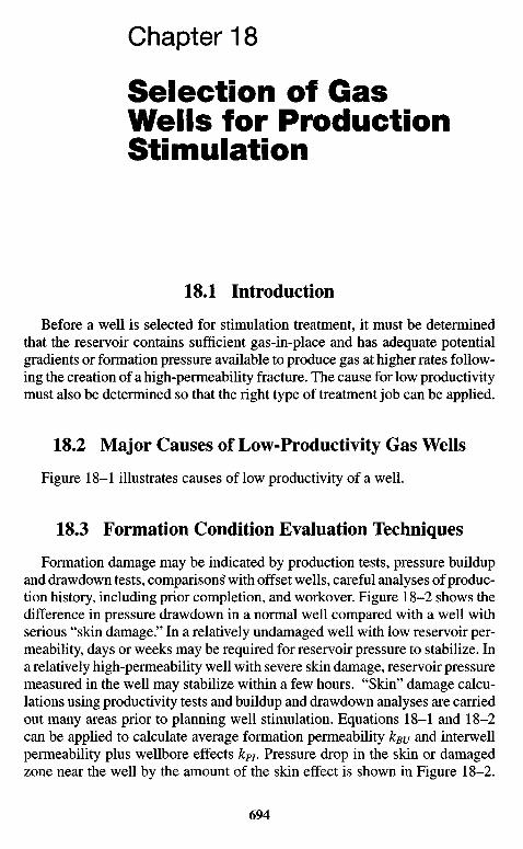
Chapter 18
Selection of GasWells for ProductionStimulation
18.1 Introduction
Before a well is selected for stimulation treatment, it must be determinedthat the reservoir contains sufficient gas-in-place and has adequate potentialgradients or formation pressure available to produce gas at higher rates follow-ing the creation of a high-permeability fracture. The cause for low productivitymust also be determined so that the right type of treatment job can be applied.
18.2 Major Causes of Low-Productivity Gas Wells
Figure 18-1 illustrates causes of low productivity of a well.
18.3 Formation Condition Evaluation Techniques
Formation damage may be indicated by production tests, pressure buildupand drawdown tests, comparisons'with offset wells, careful analyses of produc-tion history, including prior completion, and workover. Figure 18-2 shows thedifference in pressure drawdown in a normal well compared with a well withserious "skin damage." In a relatively undamaged well with low reservoir per-meability, days or weeks may be required for reservoir pressure to stabilize. Ina relatively high-permeability well with severe skin damage, reservoir pressuremeasured in the well may stabilize within a few hours. "Skin" damage calcu-lations using productivity tests and buildup and drawdown analyses are carriedout many areas prior to planning well stimulation. Equations 18-1 and 18-2can be applied to calculate average formation permeability kBu and interwellpermeability plus wellbore effects kPI. Pressure drop in the skin or damagedzone near the well by the amount of the skin effect is shown in Figure 18-2.
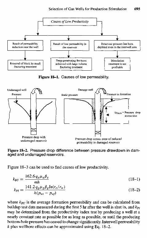
Figure 18-2. Pressure drop difference between pressure drawdown In dam-aged and undamaged reservoirs.
Figure 18-3 can be used to find causes of low productivity.
kBU = 1 6 2 - < W ' (18-1)mn
U1.2qgligpgln(re/rw)Kp1 = — (lo-2)
nyPws - Pwf)where kBu is the average formation permeability and can be calculated frombuildup test data measured during the first 5 hr after the well is shut in, and kPI
may be determined from the productivity index test by producing a well at anearly constant rate as possible for as long as possible, or until the producingbottom-hole pressure has ceased to change significantly. Interwell permeabilityk plus wellbore effects can be approximated using Eq. 18-2.
Pressure drop across zone of reducedpermeability in damaged reservoir
Pressure drop withundamaged reservoir
APSKIN = Pressure dropacross skin
Pressure in formation
Damage well
Static pressure
Undamaged well
Pressure
Result of permeabilityreduction near the well
Result of low permeability inthe reservoir
Reservoir pressure has beendepleted even in the interwell area
Removal of block by smallfracturing treatment
Deep-penetrating fracturesachieved with large volume
fracturing treatment
Stimulationtreatment is not
profitable
Figure 18-1. Causes of low permeability.
Causes of Low Productivity
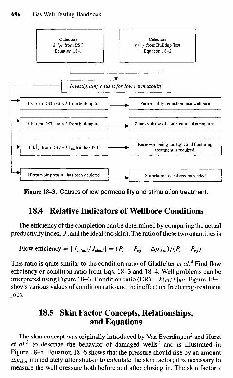
If k from DST test < k from buildup test
If k from DST test > k from buildup test
If k I p, from DST = k \ Bu buildup Test
If reservoir pressure has been depleted
Permeability reduction near wellbore
Small volume of acid treatment is required
Reservoir being too tight and fracturingtreatment is required.
Stimulation is not recommended
Calculatek I PI from DSTEquation 18-1
Calculatek I BU from Buildup Test
Equation 18-2
Investigating causes for low permeability
Figure 18-3. Causes of low permeability and stimulation treatment.
18.4 Relative Indicators of Wellbore Conditions
The efficiency of the completion can be determined by comparing the actualproductivity index, / , and the ideal (no skin). The ratio of these two quantities is
FlOW efficiency = [Jactual/Jideal] = (Pi - Pwf- Apskin)/(Pi - Pwf)
This ratio is quite similar to the condition ratio of Gladfelter et al.4 Find flowefficiency or condition ratio from Eqs. 18-3 and 18-4. Well problems can beinterpreted using Figure 18-3. Condition ratio (CR) = k\PI/k\Bu- Figure 18-4shows various values of condition ratio and their effect on fracturing treatmentjobs.
18.5 Skin Factor Concepts, Relationships,and Equations
The skin concept was originally introduced by Van Everdingen2 and Hurstet al? to describe the behavior of damaged wells2 and is illustrated inFigure 18-5. Equation 18-6 shows that the pressure should rise by an amountApskin immediately after shut-in to calculate the skin factor; it is necessary tomeasure the well pressure both before and after closing in. The skin factor s
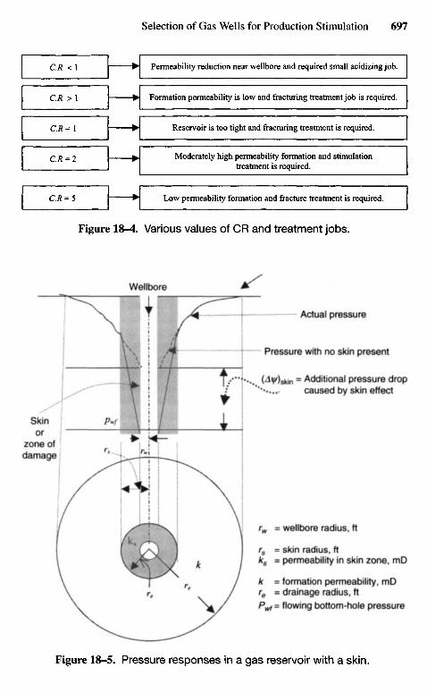
Permeability reduction near wellbore and required small acidizing job.
Formation permeability is low and fracturing treatment job is required.
Reservoir is too tight and fracturing treatment is required.
Moderately high permeability formation and stimulationtreatment is required.
Low permeability formation and fracture treatment is required.
Figure 18-4. Various values of CR and treatment jobs.
Actual pressure
Wellbore
Pressure with no skin present
(4y)skin = Additional pressure dropcaused by skin effect
rw = wellbore radius, ft
rs = skin radius, ftks = permeability in skin zone, mD
k = formation permeability, mDre = drainage radius, ftPw1= flowing bottom-hole pressure
Figure 18-5. Pressure responses in a gas reservoir with a skin.
Skinor
zone ofdamage
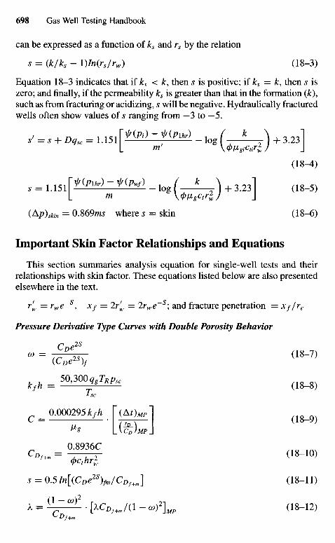
can be expressed as a function of ks and rs by the relation
s = (k/ks - l)In(rs/rw) (18-3)
Equation 18-3 indicates that if ks < k, then s is positive; if ks = k, then s iszero; and finally, if the permeability ks is greater than that in the formation (&),such as from fracturing or acidizing, s will be negative. Hydraulically fracturedwells often show values of s ranging from —3 to —5.
s =s + Dqsc = 1.151 ; log 1+3.23
(18-4)
s = ll5l^(Pur)-nPwf) _ ( ^ \ + 3 2J (18_5)
(Ap)skin = O.S69ms where s — skin (18-6)
Important Skin Factor Relationships and Equations
This section summaries analysis equation for single-well tests and theirrelationships with skin factor. These equations listed below are also presentedelsewhere in the text.
r'w = rwe~s, x/ = 2rfw = 2rwe~s; and fracture penetration = x//re
Pressure Derivative Type Curves with Double Porosity Behavior
°> - 7 § ^ <>8-7)(CDe2S)f
kfh = 5O'300*'^* (18-8)
r 0-000295 kfh [(AfW]u ' \ (tD \ \^g L\CZ)MP]
C ° - 8 9 3 6 C r1R 10
CD'~ = -^Ml (18~10)
s = 0.5/4(CZyC^] (18-n)
k = {±Z^L . [xCDf+J(l - co)2]Mp (18-12)
C Df+m
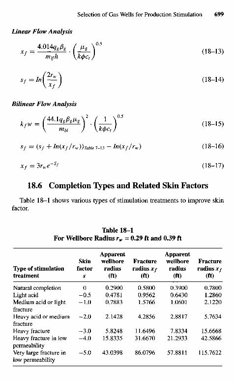
Linear Flow Analysis
« x > ! « a / W £ \ " (18_13)
mlfh \k</>ctj
Sf=In(—\ (18-14)
Bilinear Flow Analysis
,^.(*!!te)'.(>f M\ mu J \k<t)ctj
Sf = (sf + In(xf/rw))Tabie7_i3 - In(x//rw) (18-16)Jc7 = 3rw<Ts' (18-17)
18.6 Completion Types and Related Skin Factors
Table 18-1 shows various types of stimulation treatments to improve skinfactor.
Table 18-1For Wellbore Radius rw = 0.29 ft and 0.39 ft
Apparent ApparentSkin wellbore Fracture wellbore Fracture
Type of stimulation factor radius radius x/ radius radius x/treatment s (ft) (ft) (ft) (ft)
Natural completion 0 0.2900 0.5800 0.3900 0.7800Light acid -0.5 0.4781 0.9562 0.6430 1.2860Medium acid or light -1.0 0.7883 1.5766 1.0601 2.1220fractureHeavy acid or medium -2.0 2.1428 4.2856 2.8817 5.7634fractureHeavy fracture -3.0 5.8248 11.6496 7.8334 15.6668Heavy fracture in low -4.0 15.8335 31.6670 21.2933 42.5866permeabilityVery large fracture in -5.0 43.0398 86.0796 57.8811 115.7622low permeability
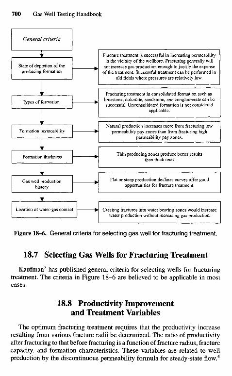
General criteria
State of depletion of theproducing formation
Types of formation
Formation permeability
Formation thickness
Gas well productionhistory
Location of water-gas contact
Fracture treatment is successful in increasing permeabilityin the vicinity of the wellbore. Fracturing generally will
not increase gas production enough to justify the expenseof the treatment. Successful treatment can be performed in
old fields where pressures are relatively low.
Fracturing treatment in consolidated formation such aslimestone, dolomite, sandstone, and conglomerate can besuccessful. Unconsolidated formation is not considered
applicable.
Natural production increases more from fracturing lowpermeability pay zones than from fracturing high
permeability pay zones.
Thin producing zones produce better resultsthan thick ones.
Flat or steep production declines curves offer goodopportunities for fracture treatment.
Creating fractures into water bearing zones would increasewater production without increasing gas production.
Figure 18-6. General criteria for selecting gas well for fracturing treatment.
18.7 Selecting Gas Wells for Fracturing Treatment
Kaufman7 has published general criteria for selecting wells for fracturingtreatment. The criteria in Figure 18-6 are believed to be applicable in mostcases.
18.8 Productivity Improvementand Treatment Variables
The optimum fracturing treatment requires that the productivity increaseresulting from various fracture radii be determined. The ratio of productivityafter fracturing to that before fracturing is a function of fracture radius, fracturecapacity, and formation characteristics. These variables are related to wellproduction by the discontinuous permeability formula for steady-state flow.4
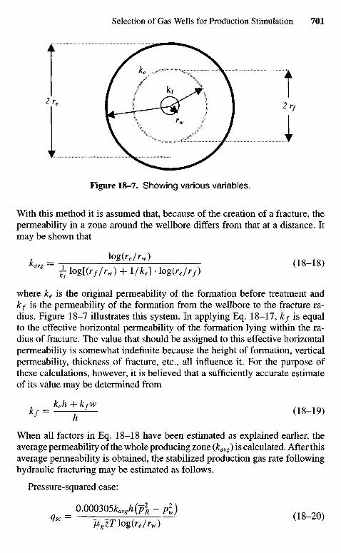
Figure 18-7. Showing various variables.
With this method it is assumed that, because of the creation of a fracture, thepermeability in a zone around the wellbore differs from that at a distance. Itmay be shown that
kavg = 1 ^ ^ ^ (18-18)Tf log[(r//rw) + l/ke] • logfo/r,)
where ke is the original permeability of the formation before treatment andkf is the permeability of the formation from the wellbore to the fracture ra-dius. Figure 18-7 illustrates this system. In applying Eq. 18-17, kf is equalto the effective horizontal permeability of the formation lying within the ra-dius of fracture. The value that should be assigned to this effective horizontalpermeability is somewhat indefinite because the height of formation, verticalpermeability, thickness of fracture, etc., all influence it. For the purpose ofthese calculations, however, it is believed that a sufficiently accurate estimateof its value may be determined from
*/ = ^ ^ (18-19)
When all factors in Eq. 18-18 have been estimated as explained earlier, theaverage permeability of the whole producing zone (kavg) is calculated. After thisaverage permeability is obtained, the stabilized production gas rate followinghydraulic fracturing may be estimated as follows.
Pressure-squared case:
0.000305kavghCp2R -pi)
qsc = ~-T7 < , / (18"20)
figzTlog(re/rw)
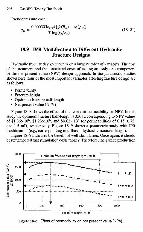
Pseudopressure case:
0.000305kavgh№(pR)- jr(pw)iqsC = riog(r./rw) ( 1 8 " 2 1 )
18.9 IPR Modification to Different HydraulicFracture Designs
Hydraulic fracture design depends on a large number of variables. The costof the treatment and the associated costs of testing are only one componentof the net present value (NPV) design approach. In the parametric studiesshown here, four of the most important variables affecting fracture design areas follows.
• Permeability• Fracture height• Optimum fracture half-length• Net present value (NPV)
Figure 18-8 shows the effect of the reservoir permeability on NPV. In thisstudy the optimum fracture half-length is 350 ft, corresponding to NPV valuesof $1.86xlO6, $1.28xlO6, and $0.62xl06 for permeabilities of 0.15, 0.75,and 1.5 mD, respectively. Figure 18-9 shows a parametric study with IPRmodification (e.g., corresponding to different hydraulic fracture design).
Figure 18-9 indicates the benefit of well stimulation. Once again, it shouldbe remembered that stimulation costs money. Therefore, the gain in production
Optimum fracture half-length Xf- 330 ft
k= 1.5 mD
& = 0.75mD
* = 0.15mDNet
pre
sen
t va
lue
(NP
V),
($ 1
000)
Fracture length, Xf, ft
Figure 18-8. Effect of permeability on net present value (NPV).
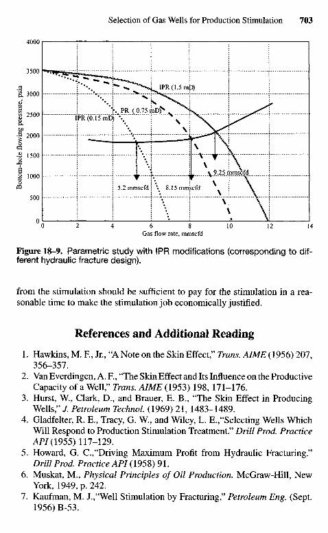
Bot
tom
-hol
e fl
owin
g pr
essu
re,
psia
Gas flow rate, mmscfd
Figure 18-9. Parametric study with IPR modifications (corresponding to dif-ferent hydraulic fracture design).
from the stimulation should be sufficient to pay for the stimulation in a rea-sonable time to make the stimulation job economically justified.
References and Additional Reading
1. Hawkins, M. R, Jr., "A Note on the Skin Effect," Trans. AIME (1956) 207,356-357.
2. Van Everdingen, A. R, "The Skin Effect and Its Influence on the ProductiveCapacity of a Well," Trans. AIME (1953) 198, 171-176.
3. Hurst, W., Clark, D., and Brauer, E. B., "The Skin Effect in ProducingWells," /. Petroleum TechnoL (1969) 21, 1483-1489.
4. Gladfelter, R. E., Tracy, G. W., and Wiley, L. E.,"Selecting Wells WhichWill Respond to Production Stimulation Treatment," Drill Prod. PracticeAPI (1955) 117-129.
5. Howard, G. C.,"Driving Maximum Profit from Hydraulic Fracturing"Drill Prod. Practice API (1958) 91.
6. Muskat, M., Physical Principles of Oil Production. McGraw-Hill, NewYork, 1949, p. 242.
7. Kaufman, M. J.,"Well Stimulation by Fracturing," Petroleum Eng. (Sept.1956) B-53.

8. Clark, J. B., Fast, C. R., and Howard, G. C, "A Multiple-Fracturing Processfor Increasing Productivity of Wells," Drill Prod. Practice API (1952) 104.
9. MaIy, J. W., and Morton, T. E., "Selection and Evaluation of Wells forHydrafrac Treatment," Oil Gas J. (May 1951) 52, 126.
10. Clark, R. F, Freedman, H. G., Bolstead, J. H., and Coffer, H. F, "Applica-tion of Hydraulic Fracturing to the Stimulation of Oil and Gas Production,"Drill Prod. Practice API (1953) 113.
Chapter 19
Design Criteria ofFlow and PressureTransient Tests
19.1 Introduction
Specific test data are required for each transient test analysis technique;adequate data are essential for satisfactory transient test results. Thus, an im-portant part of preparation for a transient well test is deciding which data areneeded and how they will be obtained. This chapter discusses the design ofdeliverability and transient tests and data required and describes characteristicsof suitable equipment.1
19.2 Deliverability Tests
The accuracy of the results calculated depends on the accuracy of data used.Obtaining accurate field data can be accomplished only if the field personnelfollow established procedures for data collection. Detailed procedures can befound in Refs. 1-3. Brief procedures are summarized below.
Equipment and Procedure for Field Tests
The wells were shut in preparatory to running the initial drawdown test. InAppendix D, Figure D-I shows the equipment used for these tests. A bottom-hole pressure bomb recorded bottom-hole pressures. A dead-weight testerperiodically measured surface pressures. For all tests, the bomb was loweredon a wire line to the same pressure datum.
The initial flow rate was selected with the aid of well capacity informationmade available from the AOF data, considering that two or three added flowrates were to be used within the span of the well's indicated capacity. Once therate was selected, the pressure controller was set to provide a constant pressure
downstream of the choke, thus maintaining a constant rate throughout the test.The specific rate was obtained by using the appropriate orifice plate and criticalflow proper pressure.
The bomb was pulled after a period of 24 to 72 hr, depending on the clockused. Pressures and flow rates were determined immediately. Plots were pre-pared. By flowing pressure performance it could be determined whether thetest should be continued or terminated. Rerunning the pressure bomb did notaffect flow rate or pressure data.
Guidelines for Designing Deliverability Tests
In designing a deliverability test, collect and utilize all information, whichmay include logs, drill-stem tests, previous deliverability tests conducted onthat well, production history, fluid composition and temperature, cores, andgeological studies. Knowledge of the time required for stabilization is a veryimportant factor in deciding the type of test to be used for determining thedeliverability of a well. This may be known directly from previous tests, such asdrill-stem or deliverability tests, conducted on the well or from the productioncharacteristics of the well. If such information is not available, it may beassumed that the well will behave in a manner similar to neighboring wellsin the same pool, for which the data are available. When the approximatetime to stabilization is not known, it may be estimated from Eq. 19-3. If thetime to stabilization is of the order of a few hours, a conventional test may beconducted. Otherwise one of the isochronal tests is preferable. The isochronaltest is more accurate than the modified isochronal test and should be used ifthe greater accuracy is required. A single-point test is appropriate when thedeliverability relationship of the well is known from previous tests, and onlyupdating of this relationship is desired.
Some of the factors affecting the choice of equipment are the expectedflow rates and pressures and the composition of gas and liquid. The possibilityand location of hydrate formation must be investigated. Production of liquid,water or condensate, causes fluctuations in the rate and pressure measurements.Long flow times of at least 6 to 8 hr are needed before the liquid-to-gas ratiostabilizes.
Some idea of the flow rates at which a well is capable of flowing maybe obtained from the drill-stem test or from the preliminary well cleanupflows. In the absence of any data whatsoever, the AOF may be estimated fromthe equation given below by assuming stabilized, purely laminar flow in thereservoir.
AOF = p —'- =- (19-1)3.274 x 1O6J [log(0.472^j + ^ J
or
AOF = * * * « - * « = O) (19_2)
1.422 x 1067^In(0.472^J +sj
s may be estimated from similar stimulation treatment performed on approxi-mately similar wells in the formation. The duration of the isochronal periodsis determined by two considerations, namely, (a) wellbore storage time and (b)the radius of investigation.
The wellbore storage time tws is the approximate time required for thewellbore storage effects to become negligible. This can be calculated by
_ 36MlTZgVwsCwstws - Ih ( 9 ~ 3 )
where
Vws = volume of the wellbore tubing (and annulus, if there is no packer)Cws = compressibility of the wellbore fluid evaluated at the wellbore at the
mean wellbore pressure and temperature
For wells with no damage or improvement an approximate time to investigate100 ft is obtained from Eq. 19-4:
tm = 107^S (IiM)kP R
Equations 19-3 and 19^4 give the minimum duration of flow that will yield datarepresentative of the bulk formation rather than the wellbore area. Durationequal to about four times this value is recommended for the isochronal periods.In conducting a multipoint test, the minimum flow rate used should be at leastequal to that required lifting the liquids, if any, from the well. It should also besufficient to maintain a wellhead temperature above the hydrate point. Whenthese considerations do not apply, the minimum and maximum flow rates arechosen, whenever practical such that the pressure drops cause at the well areapproximately 10%, respectively of the shut-in pressure. Alternatively, theymay be taken to be about 10%, respectively, of the AOF.
Designing Suitable Deliverability Tests
The following example illustrates how to design a suitable deliverabilitytest.
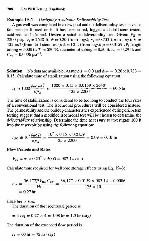
Example 19-1 Designing a Suitable Deliverability TestA gas well was completed in a new pool and no deliverability tests have, so
far, been performed on it. It has been cored, logged and drill-stem tested,acidized, and cleaned. Design a suitable deliverability test. Given: PR =2200 psig; re = 2640 ft; 0 = 0.20 (from logs); sg =0.733 (from logs); k =125 m£> (from drill-stem tests); h = 10 ft (from logs); [i — 0.0159 cP; lengthtubing = 5000 ft; T = 5800R; diameter of tubing = 0.50 ft; rw = 0.29 ft; andCws = 0.0006psi~1.
Solution No data are available. Assume s = 0.0 and (pHC = 0.20 x 0.733 =0.15. Calculate time of stabilization using the following equation:
ts = 1 0 0 0 ^ i = 1000 x 0.15 x 0.0159 x 264Q2 =b kpR 125 x 2200
The time of stabilization is considered to be too long to conduct the four ratesof a conventional test. The isochronal procedures will be considered instead.The permeability and the buildup characteristics experienced during drill-stemtesting suggest that a modified isochronal test will be chosen to determine thedeliverability relationship. Determine the time necessary to investigate 100 ftinto the reservoir by using the following equation:
_ ^1(J)HCTL 1 0 7 X 0.15 x 0.0159 n n o n i n u10O = 10 = = 0.09 = 0.10 hr
Kp R 125x2200
Flow Periods and Rates
Vws = n x 0.252 x 5000 = 982.14 cu ft
Calculate time required for wellbore storage effects using Eq. 19-3:
_ 36,1777ZVVs Cws _ 36,177 x 0.0159 x 982.14 x 0.0006tws" kh " 125 x 10
= 0.27hr
since tws > fioo-
The duration of the isochronal period is
= 4 tws = 0.27 x 4 = 1.08 hr = 1.5 hr (say)
The duration of the extended flow period is
ts = 60 hr = 72 hr (say)
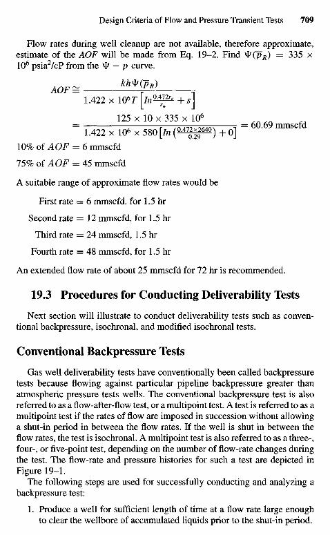
Flow rates during well cleanup are not available, therefore approximate,estimate of the AOF will be made from Eq. 19-2. Find W(PR) = 335 x106 psia2/cP from the *I> - p curve.
AOF = ^ =•
1.422 x 10⁶r[/>i^^+sJ125 x 10 x 335 x 106
= F—,HAT, ^ A ^ =r = 60.69 mmscfd1.422 x 106 x 580 [in (°-47
02*9
2640) + 0]10% of AOF = 6 mmscfd
75% of AOF = 45 mmscfd
A suitable range of approximate flow rates would be
First rate = 6 mmscfd, for 1.5 hr
Second rate = 1 2 mmscfd, for 1.5 hr
Third rate = 24 mmscfd, 1.5 hr
Fourth rate = 48 mmscfd, for 1.5 hr
An extended flow rate of about 25 mmscfd for 72 hr is recommended.
19.3 Procedures for Conducting Deliverability Tests
Next section will illustrate to conduct deliverability tests such as conven-tional backpressure, isochronal, and modified isochronal tests.
Conventional Backpressure Tests
Gas well deliverability tests have conventionally been called backpressuretests because flowing against particular pipeline backpressure greater thanatmospheric pressure tests wells. The conventional backpressure test is alsoreferred to as a flow-after-flow test, or a multipoint test. A test is referred to as amultipoint test if the rates of flow are imposed in succession without allowinga shut-in period in between the flow rates. If the well is shut in between theflow rates, the test is isochronal. A multipoint test is also referred to as a three-,four-, or five-point test, depending on the number of flow-rate changes duringthe test. The flow-rate and pressure histories for such a test are depicted inFigure 19-1.
The following steps are used for successfully conducting and analyzing abackpressure test:
1. Produce a well for sufficient length of time at a flow rate large enoughto clear the wellbore of accumulated liquids prior to the shut-in period.
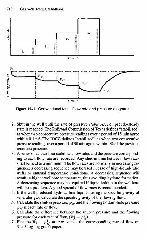
Gas
rat
eF
low
ing
pres
sure
Time, t
Figure 19-1. Conventional test—Flow rate and pressure diagrams.
2. Shut in the well until the rate of pressure stabilizes, i.e., pseudo-steadystate is reached. The Railroad Commission of Texas defines "stabilized"as when two consecutive pressure readings over a period of 15 min agreewithin 0.1 psi. The IOCC defines "stabilized" as when two consecutivepressure readings over a period of 30 min agree within 1 % of the previousrecorded pressure.
3. A series of at least four stabilized flow rates and the pressure correspond-ing to each flow rate are recorded. Any shut-in time between flow ratesshall be held to a minimum. The flow rates are normally in increasing se-quence; a decreasing sequence may be used in case of high-liquid-ratiowells or unusual temperature conditions. A decreasing sequence willresult in higher wellbore temperature, thus avoiding hydrate formation.A decreasing sequence may be required if liquid holdup in the wellborewill be a problem. A good spread of flow rates is recommended.
4. If the well produced hydrocarbon liquids, using the specific gravity ofseparator gas, calculate the specific gravity of the flowing fluid.
5. Calculate the shut-in pressure, ~pR, and the flowing bottom-hole pressurepwf at each rate of flow.
6. Calculate the difference between the shut-in pressure and the flowingpressure for each rate of flow, (p2
R - plf).7. Plot the ~p\ — p^f = Ap2 versus the corresponding rate of flow on
3 x 3 log-log graph paper.
Time, t
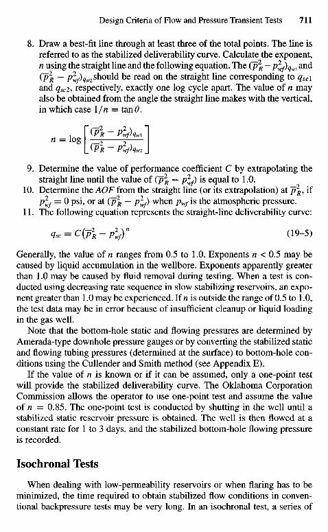
8. Draw a best-fit line through at least three of the total points. The line isreferred to as the stabilized deliverability curve. Calculate the exponent,n using the straight line and the following equation. The (~p2
R — plf)qscl and(P2R ~ ptf)qSC2 should be read on the straight line corresponding to qsc\and qSC2, respectively, exactly one log cycle apart. The value of n mayalso be obtained from the angle the straight line makes with the vertical,in which case l/n = tanO.
, \ (PR ~ Plf)q~i~\n = log — {
1(PR-Plf)qsc2]9. Determine the value of performance coefficient C by extrapolating the
straight line until the value of (~p2R — p^) is equal to 1.0.
10. Determine the AOF from the straight line (or its extrapolation) at ~p\, ifp^ = 0 psi, or at (~p2
R — p^f) when pwf is the atmospheric pressure.11. The following equation represents the straight-line deliverability curve:
qsc = C(p2R-p2
wf)n (19-5)
Generally, the value of n ranges from 0.5 to 1.0. Exponents n < 0.5 may becaused by liquid accumulation in the wellbore. Exponents apparently greaterthan 1.0 may be caused by fluid removal during testing. When a test is con-ducted using decreasing rate sequence in slow stabilizing reservoirs, an expo-nent greater than 1.0 may be experienced. If n is outside the range of 0.5 to 1.0,the test data may be in error because of insufficient cleanup or liquid loadingin the gas well.
Note that the bottom-hole static and flowing pressures are determined byAmerada-type downhole pressure gauges or by converting the stabilized staticand flowing tubing pressures (determined at the surface) to bottom-hole con-ditions using the Cullender and Smith method (see Appendix E).
If the value of n is known or if it can be assumed, only a one-point testwill provide the stabilized deliverability curve. The Oklahoma CorporationCommission allows the operator to use one-point test and assume the valueof n = 0.85. The one-point test is conducted by shutting in the well until astabilized static reservoir pressure is obtained. The well is then flowed at aconstant rate for 1 to 3 days, and the stabilized bottom-hole flowing pressureis recorded.
Isochronal Tests
When dealing with low-permeability reservoirs or when flaring has to beminimized, the time required to obtain stabilized flow conditions in conven-tional backpressure tests may be very long. In an isochronal test, a series of
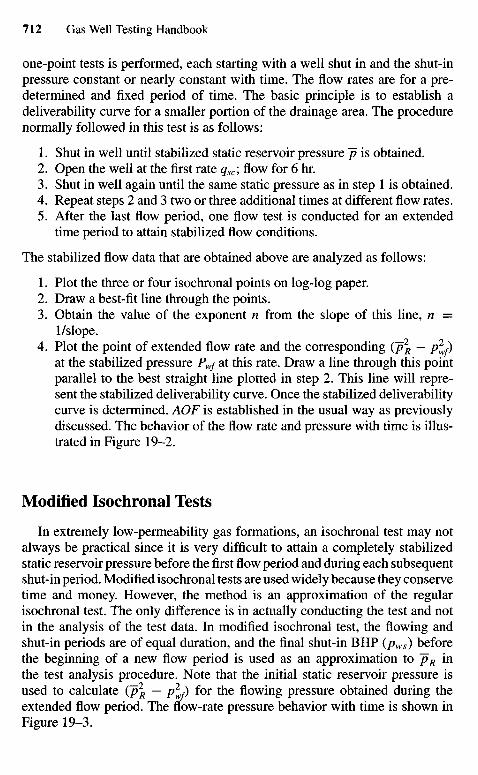
one-point tests is performed, each starting with a well shut in and the shut-inpressure constant or nearly constant with time. The flow rates are for a pre-determined and fixed period of time. The basic principle is to establish adeliverability curve for a smaller portion of the drainage area. The procedurenormally followed in this test is as follows:
1. Shut in well until stabilized static reservoir pressure ~p is obtained.2. Open the well at the first rate qsc\ flow for 6 hr.3. Shut in well again until the same static pressure as in step 1 is obtained.4. Repeat steps 2 and 3 two or three additional times at different flow rates.5. After the last flow period, one flow test is conducted for an extended
time period to attain stabilized flow conditions.
The stabilized flow data that are obtained above are analyzed as follows:
1. Plot the three or four isochronal points on log-log paper.2. Draw a best-fit line through the points.3. Obtain the value of the exponent n from the slope of this line, n =
1/slope.4. Plot the point of extended flow rate and the corresponding (p2
R — p\)at the stabilized pressure PWf at this rate. Draw a line through this pointparallel to the best straight line plotted in step 2. This line will repre-sent the stabilized deliverability curve. Once the stabilized deliverabilitycurve is determined. AOF is established in the usual way as previouslydiscussed. The behavior of the flow rate and pressure with time is illus-trated in Figure 19-2.
Modified Isochronal Tests
In extremely low-permeability gas formations, an isochronal test may notalways be practical since it is very difficult to attain a completely stabilizedstatic reservoir pressure before the first flow period and during each subsequentshut-in period. Modified isochronal tests are used widely because they conservetime and money. However, the method is an approximation of the regularisochronal test. The only difference is in actually conducting the test and notin the analysis of the test data. In modified isochronal test, the flowing andshut-in periods are of equal duration, and the final shut-in BHP (pws) beforethe beginning of a new flow period is used as an approximation to ~pR inthe test analysis procedure. Note that the initial static reservoir pressure isused to calculate (~p2
R — p^f) for the flowing pressure obtained during theextended flow period. The flow-rate pressure behavior with time is shown inFigure 19-3.
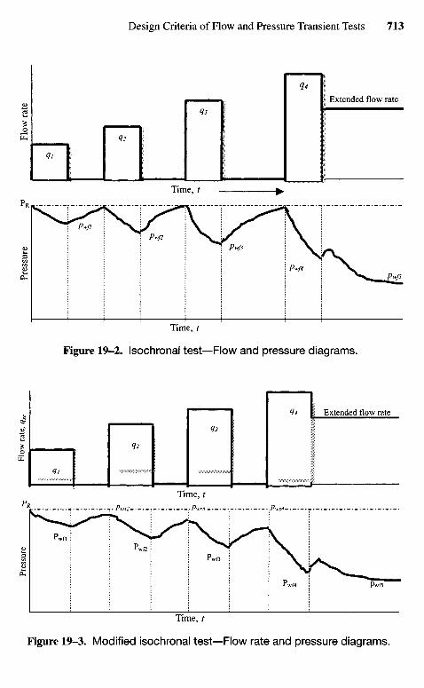
Flo
w r
ate
Pre
ssur
eF
low
rat
e, q
scP
ress
ure
Extended flow rate
Time, t
Time, t
Figure 19-2. Isochronal test—Flow and pressure diagrams.
Extended flow rate
Time, t
Time, t
Figure 19-3. Modified isochronal test—Flow rate and pressure diagrams.
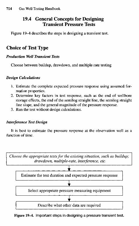
19.4 General Concepts for DesigningTransient Pressure Tests
Figure 19-4 describes the steps in designing a transient test.
Choice of Test Type
Production Well Transient Tests
Choose between buildup, drawdown, and multiple rate testing
Design Calculations
1. Estimate the complete expected pressure response using assumed for-mation properties.
2. Determine key factors in test response, such as the end of wellborestorage effects, the end of the semilog straight line, the semilog straightline slope, and the general magnitude of the pressure response.
3. Run the test without design calculations.
Interference Test Design
It is best to estimate the pressure response at the observation well as afunction of time.
Choose the appropriate tests for the existing situation, such as buildup;drawdown, multiple-rate, interference, etc.
Estimate the test duration and expected pressure response
Select appropriate pressure measuring equipment
Describe what other data are required
Figure 19-4. Important steps in designing a pressure transient test.

Pulse Test Design
Reference 2 has developed a method of interference determination by pulsetesting. In this method a production well near the observation well is alternatelyproduced and then closed in to give series of pressure pulses. These pressurepulses are detected at the observation well by a very accurate (0.001 psi)pressure gauge. Use of this gauge allows the interference pressure pulses to bedetected much more rapidly.
Design of Flow and Buildup Tests
Test design should include the following:
1. A set of calculations are performed similar to those made during analysisof results using likely assumed values, so that the flow rates and time arechosen properly.
2. Be certain that test results can be adequately analyzed before spendingthe time and money, including risk in the field.
Guidelines for Designing Drawdown Tests
1. Wells that have not been produced or wells that have been shut in longenough to permit pressure stabilization are good candidate for drawdowntesting and analysis.
2. In the isochronal deliverability tests discussed in the previous section, aseries of shut-in periods is required to attain pressure stabilization; in theconventional deliverability tests, each flow period must be continued topressure stabilization. In either case, the time required for stabilizationmay be very large and will limit the application of such tests.
3. A drawdown test may prove to be particularly attractive, since such atest minimizes the loss of production associated with a shut-in.
4. Drawdown tests may also be conducted to supplement information ob-tained from other tests such as buildup or deliverability tests.
5. When it is difficult to achieve constant flow rates because of slugging ofthe well, a drawdown test is not recommended.
6. Tests utilizing early-time data and their interpretations are only recom-mended, if, after testing, it is found that they are the only data amenableto analysis.
7. Tests utilizing transient flow data are recommended when an accurateknowledge of reservoir characteristics and skin effects is desired.
8. A single-rate test is acceptable when IT flow effects are negligible; oth-erwise two single-rate tests should be conducted to evaluate the skin andIT flow components of the apparent skin factor.
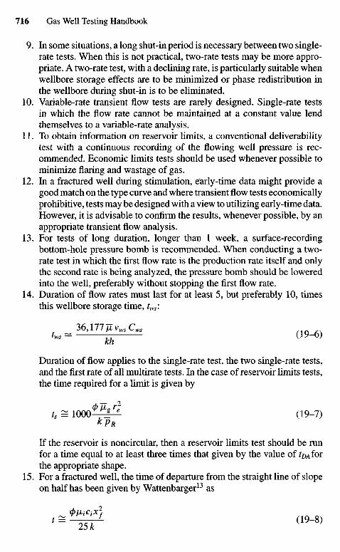
9. In some situations, a long shut-in period is necessary between two single-rate tests. When this is not practical, two-rate tests may be more appro-priate. A two-rate test, with a declining rate, is particularly suitable whenwellbore storage effects are to be minimized or phase redistribution inthe wellbore during shut-in is to be eliminated.
10. Variable-rate transient flow tests are rarely designed. Single-rate testsin which the flow rate cannot be maintained at a constant value lendthemselves to a variable-rate analysis.
11. To obtain information on reservoir limits, a conventional deliverabilitytest with a continuous recording of the flowing well pressure is rec-ommended. Economic limits tests should be used whenever possible tominimize flaring and wastage of gas.
12. In a fractured well during stimulation, early-time data might provide agood match on the type curve and where transient flow tests economicallyprohibitive, tests may be designed with a view to utilizing early-time data.However, it is advisable to confirm the results, whenever possible, by anappropriate transient flow analysis.
13. For tests of long duration, longer than 1 week, a surface-recordingbottom-hole pressure bomb is recommended. When conducting a two-rate test in which the first flow rate is the production rate itself and onlythe second rate is being analyzed, the pressure bomb should be loweredinto the well, preferably without stopping the first flow rate.
14. Duration of flow rates must last for at least 5, but preferably 10, timesthis wellbore storage time, tws:
= 36,177MV-C. .
kh
Duration of flow applies to the single-rate test, the two single-rate tests,and the first rate of all multirate tests. In the case of reservoir limits tests,the time required for a limit is given by
ts = 1000 1Ve (19-7)kpR
If the reservoir is noncircular, then a reservoir limits test should be runfor a time equal to at least three times that given by the value of tDAforthe appropriate shape.
15. For a fractured well, the time of departure from the straight line of slopeon half has been given by Wattenbarger13 as
Xf)JJLjCiXl
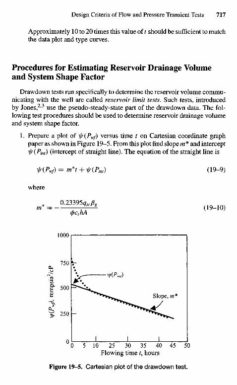
Approximately 10 to 20 times this value of t should be sufficient to matchthe data plot and type curves.
Procedures for Estimating Reservoir Drainage Volumeand System Shape Factor
Drawdown tests run specifically to determine the reservoir volume commu-nicating with the well are called reservoir limit tests. Such tests, introducedby Jones,2'3 use the pseudo-steady-state part of the drawdown data. The fol-lowing test procedures should be used to determine reservoir drainage volumeand system shape factor.
1. Prepare a plot of i/s(PWf) versus time t on Cartesian coordinate graphpaper as shown in Figure 19-5. From this plot find slope m* and intercepti* (Pint) (intercept of straight line). The equation of the straight line is
x/f(Pwf)= m*t +Ir(Pn) (19-9)
where
^•-"•y 09-10,<pcthA
\\f(P
wj),
m
mps
ia2/c
P
Slope, m*
Flowing time t, hours
Figure 19-5. Cartesian plot of the drawdown test.
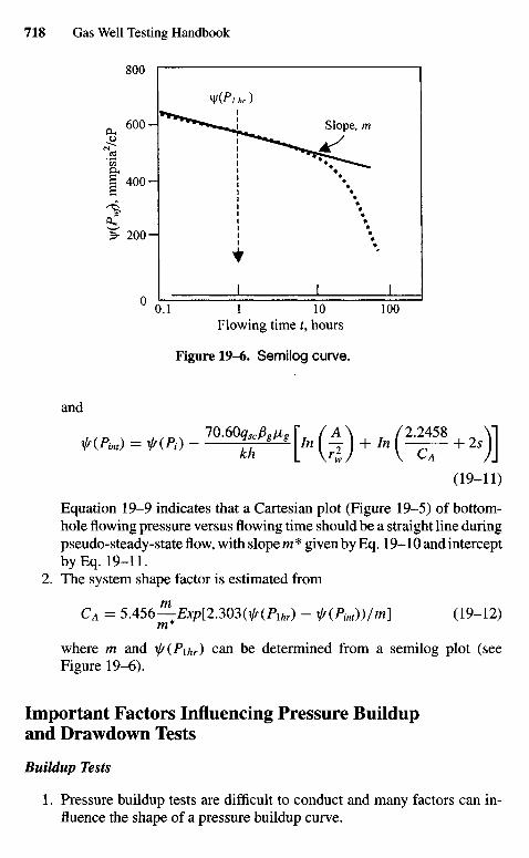
\y(P
J),
mm
psia
2/cP
Flowing time t, hours
Figure 19-6. Semilog curve.
and
(19-11)
Equation 19-9 indicates that a Cartesian plot (Figure 19-5) of bottom-hole flowing pressure versus flowing time should be a straight line duringpseudo-steady-state flow, with slope m * given by Eq. 19-10 and interceptby Eq. 19-11.
2. The system shape factor is estimated from
CA = 5A56^-Exp[2303(xlf(Plhr) - f{Pint))/m] (19-12)m*
where m and ty{P\hr) can be determined from a semilog plot (seeFigure 19-6).
Important Factors Influencing Pressure Buildupand Drawdown Tests
Buildup Tests
1. Pressure buildup tests are difficult to conduct and many factors can in-fluence the shape of a pressure buildup curve.
Slope, m
2. In addition to wellbore storage effects, hydraulic fractures, particularlyin low-permeability formations, can have a major effect on buildup curveshape and analysis. Chapter 6 gives a more detailed discussion of boththese factors.
Drawdown Tests
1. The test may be hard to control since it is a flowing gas well.2. The early part of the drawdown data is influenced by wellbore storage.
Sometimes it is possible to draw a straight line through the semilog plotof data taken during this time. The slope of that line gives incorrect valuesof permeability and skin. A log-log data plot of the drawdown data mustbe made to select the correct semilog straight line.
19,5 Test Planning and Data Acquisition
The important parts of test operation and planning include the following:
1. Good and complete rate stabilization2. Placement of the pressure instrument before the test begins3. Careful documentation of what happens during the test, both at the test
well and at nearby operating wells
The general data checklist in Figure 19-7 is an aid to complete data acquisition.
19.6 Guidelines for Gas Well Testing
Accurate field data can be obtained if the field personnel follow establishedprocedures for data collection.
Choice of Testing Equipment
It depends upon the nature of the produced fluids and the type of test beingconducted. Various wellhead-testing facilities are necessitated by the presenceof condensate, water, or acid gases in the natural gas being produced.
Sweet Dry Gas
Figure 19-8 may be used. As shown in this figure, if valve A is closedgradually while valve B is being opened, maintaining a constant pressure inthe flow string, the flow rate being measured by the flow prover will be thesame as the production rate. The deliverability of constant flow rates duringtests is very important. Figure 19-9 illustrates the wellhead rigging that mayprovide constant flow rates. Flow downstream from the flow prover is usually
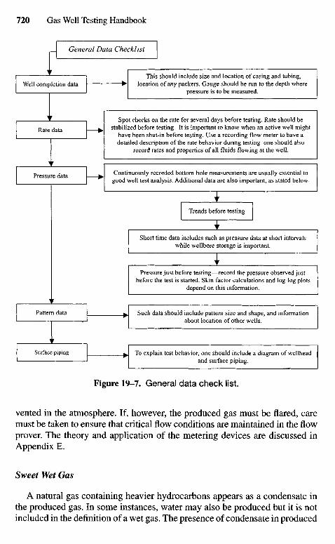
Short time data includes such as pressure data at short intervalswhile wellbore storage is important.
Pressure just before testing—record the pressure observed justbefore the test is started. Skin factor calculations and log-log plots
depend on this information.
Such data should include pattern size and shape, and informationabout location of other wells.
To explain test behavior, one should include a diagram of wellheadand surface piping.
Spot checks on the rate for several days before testing. Rate should bestabilized before testing. It is important to know when an active well might
have been shut-in before testing. Use a recording flow meter to have adetailed description of the rate behavior during testing one should also
record rates and properties of all fluids flowing at the well.
Continuously recorded bottom-hole measurements are usually essential togood well test analysis. Additional data are also important, as stated below.
Trends before testing
This should include size and location of casing and tubing,location of any packers. Gauge should be run to the depth where
pressure is to be measured.
General Data Checklist
Well completion data
Rate data
Pressure data
Pattern data
Surface piping
Figure 19-7. General data check list.
vented in the atmosphere. If, however, the produced gas must be flared, caremust be taken to ensure that critical flow conditions are maintained in the flowprover. The theory and application of the metering devices are discussed inAppendix E.
Sweet Wet Gas
A natural gas containing heavier hydrocarbons appears as a condensate inthe produced gas. In some instances, water may also be produced but it is notincluded in the definition of a wet gas. The presence of condensate in produced
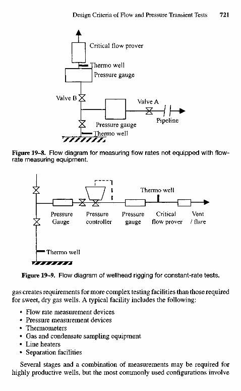
Figure 19-9. Flow diagram of wellhead rigging for constant-rate tests.
gas creates requirements for more complex testing facilities than those requiredfor sweet, dry gas wells. A typical facility includes the following:
• Flow rate measurement devices• Pressure measurement devices• Thermometers• Gas and condensate sampling equipment• Line heaters• Separation facilities
Several stages and a combination of measurements may be required forhighly productive wells, but the most commonly used configurations involve
Thermo well
PressureGauge
Pressurecontroller
Pressuregauge
Criticalflow prover
Vent/flare
Thermo well
Figure 19-8. Flow diagram for measuring flow rates not equipped with flow-rate measuring equipment.
Pressure gaugeThermo well
Pipeline
Valve AValve B
Thermo well
Pressure gauge
Critical flow prover
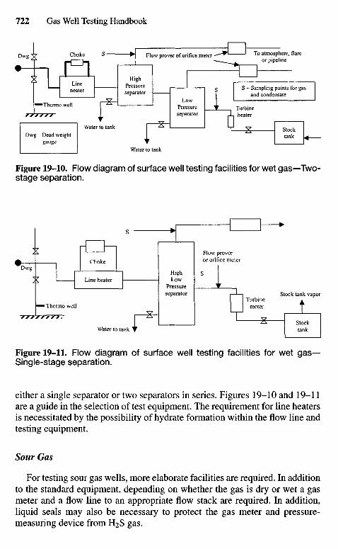
Figure 19-11. Flow diagram of surface well testing facilities for wet gas -Single-stage separation.
either a single separator or two separators in series. Figures 19-10 and 19-11are a guide in the selection of test equipment. The requirement for line heatersis necessitated by the possibility of hydrate formation within the flow line andtesting equipment.
Sour Gas
For testing sour gas wells, more elaborate facilities are required. In additionto the standard equipment, depending on whether the gas is dry or wet a gasmeter and a flow line to an appropriate flow stack are required. In addition,liquid seals may also be necessary to protect the gas meter and pressure-measuring device from H2S gas.
Stocktank
Turbinemeter
Stock tank vapor
Flow proveror orifice meter
HighLow
Pressureseparator
Water to tank
Thermo well
Line heater
Choke
Figure 19-10. Flow diagram of surface well testing facilities for wet gas—Two-stage separation.
Stocktank
Turbineheater
S - Sampling points for gasand condensate
To atmosphere, flareor pipeline
LowPressureseparator
Flow prover of orifice meter
HighPressureseparator
Water to tank
Water to tankDwg - Dead weight
gauge
Thermo well
Lineheater
Choke
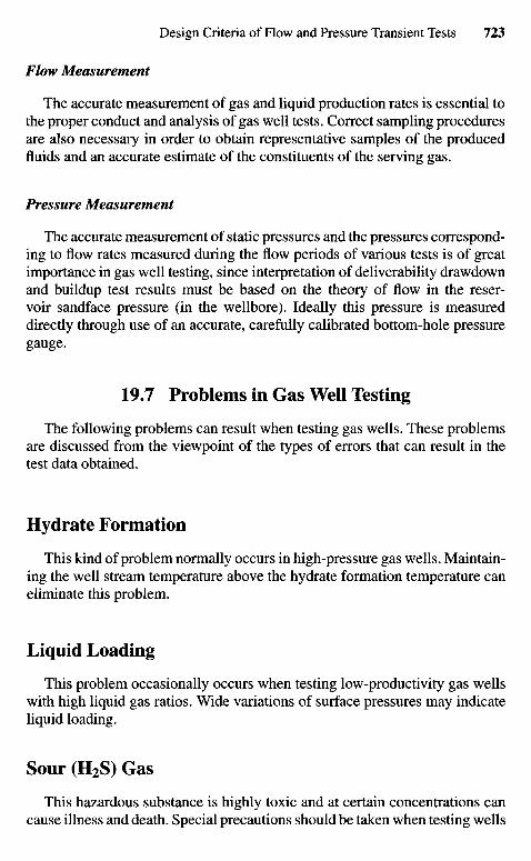
Flow Measurement
The accurate measurement of gas and liquid production rates is essential tothe proper conduct and analysis of gas well tests. Correct sampling proceduresare also necessary in order to obtain representative samples of the producedfluids and an accurate estimate of the constituents of the serving gas.
Pressure Measurement
The accurate measurement of static pressures and the pressures correspond-ing to flow rates measured during the flow periods of various tests is of greatimportance in gas well testing, since interpretation of deliverability drawdownand buildup test results must be based on the theory of flow in the reser-voir sandface pressure (in the wellbore). Ideally this pressure is measureddirectly through use of an accurate, carefully calibrated bottom-hole pressuregauge.
19.7 Problems in Gas Well Testing
The following problems can result when testing gas wells. These problemsare discussed from the viewpoint of the types of errors that can result in thetest data obtained.
Hydrate Formation
This kind of problem normally occurs in high-pressure gas wells. Maintain-ing the well stream temperature above the hydrate formation temperature caneliminate this problem.
Liquid Loading
This problem occasionally occurs when testing low-productivity gas wellswith high liquid gas ratios. Wide variations of surface pressures may indicateliquid loading.
Sour (H2S) Gas
This hazardous substance is highly toxic and at certain concentrations cancause illness and death. Special precautions should be taken when testing wells
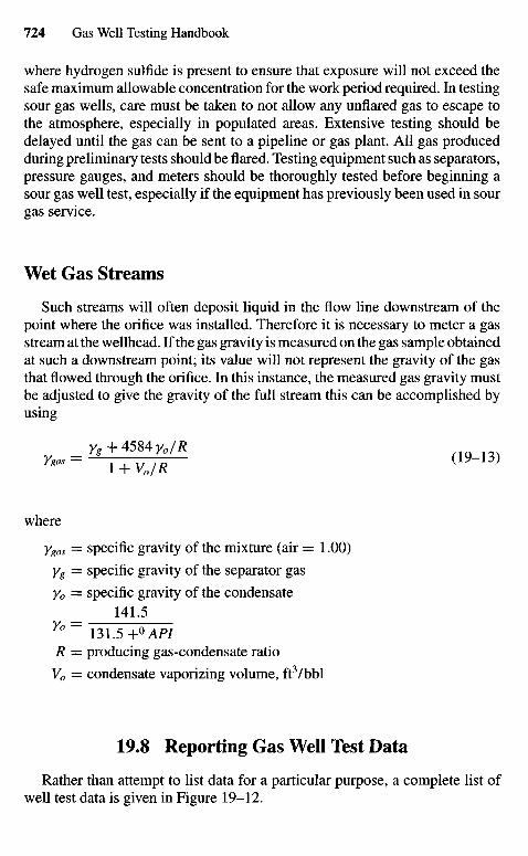
where hydrogen sulfide is present to ensure that exposure will not exceed thesafe maximum allowable concentration for the work period required. In testingsour gas wells, care must be taken to not allow any unflared gas to escape tothe atmosphere, especially in populated areas. Extensive testing should bedelayed until the gas can be sent to a pipeline or gas plant. AU gas producedduring preliminary tests should be flared. Testing equipment such as separators,pressure gauges, and meters should be thoroughly tested before beginning asour gas well test, especially if the equipment has previously been used in sourgas service.
Wet Gas Streams
Such streams will often deposit liquid in the flow line downstream of thepoint where the orifice was installed. Therefore it is necessary to meter a gasstream at the wellhead. If the gas gravity is measured on the gas sample obtainedat such a downstream point; its value will not represent the gravity of the gasthat flowed through the orifice. In this instance, the measured gas gravity mustbe adjusted to give the gravity of the full stream this can be accomplished byusing
yg+A5UYo/RYgas ~ 1 + V0/R
( i y '
where
ygas = specific gravity of the mixture (air — 1.00)Yg = specific gravity of the separator gasyo = specific gravity of the condensate
_ 141.5Yo ~ 131.5+0AP/R = producing gas-condensate ratioV0 = condensate vaporizing volume, ft3/bbl
19.8 Reporting Gas Well Test Data
Rather than attempt to list data for a particular purpose, a complete list ofwell test data is given in Figure 19-12.
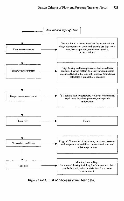
Gas rate for all streams, mscf per day or mmscf perday; condensate rate, stock tank barrels per day; water
rate, barrels per day; condensate gravity,API (at 60° F).
Psig: flowing wellhead pressure; shut-in wellheadpressure; flowing bottom-hole pressure (sometimescalculated) shut-in bottom-hole pressure (sometimes
calculated); atmospheric pressure.
0F : bottom-hole temperature; wellhead temperature;stock-tank liquid temperature; atmospheric
temperature.
Inches
Psig and 0F: number of separators; separator pressuresand temperatures; stabilized pressure and inlet and
outlet temperatures.
Minutes, Hours, Days:Duration of flowing test; length of time on test choke
size before test period; shut-in time for pressuremeasurement.
Flow measurements
Pressure measurement
Temperature measurement
Choke size
Separation conditions
Time data
Amount and Type of Data
Figure 19-12. List of necessary well test data.
References and Additional Reading
1. The Theory and Practice of Testing of Gas Wells, 3rd ed. Energy ResourcesConservation Board, Calgary, Alta. 1975.
2. Jones, R, "Reservoir Limit Test," Oil Gas J. (June 1956) 184-196.3. Jones, R, "Drawdown Exploration Reservoir Limit, Well and Formation
Evaluation," Paper 824-G presented at the SPE, AIME, Midland, TX, April18-19, 1957.
4. Dale Beggs H., Gas Production Operations. Oil and Gas ConsultantsInternational Inc., Tulsa, OK, 1975.
5. Shiu, K. C , and Beggs, H. D., "Predicting Temperature in Flowing Wells,"J. Energy Res. Technol. (March 1980), Trans. AIME.
6. Field Handling of Natural Gas, Petroleum Extension Service, Universityof Texas at Austin, TX, 1972.
7. Engineering Data Book, 9th ed. Natural Gas Processors Associations,Tulsa, OK, 1972.
8. Campbell, L. M., Gas Conditioning and Processing. Campbell PetroleumSeries, Norman, OK, 1976.
9. Manual of Back Pressure Testing of Gas Wells. Interstate Oil CompactCommission, 1962.
10. Manual of Back Pressure Testing of Gas Wells. Kansas State CorporationCommission, 1959.
11. Back Pressure Test for Natural Gas Wells. Railroad Commission of Texas,1950. Revised edition, 1951.
12. Rawlins, E. L., and Schellhardt, M. A., Backpressure Data on NaturalGas Wells and Their Application to Production Practices. U.S. Bureau ofMines, Monograph 7, 1936.
13. Wattenbarger, R. A., and Ramey, H. J., Jr., "Gas Well Testing with Turbu-lence, Damage and Wellbore Storage," /. Petroleum Technol. (Aug. 1968)877-877., Trans., AIME, 243.
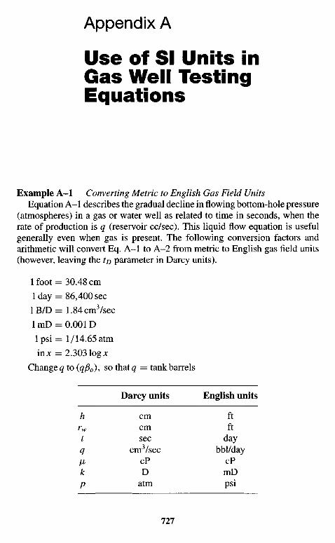
Appendix A
Use of SI Units inGas Well TestingEquations
Example A-I Converting Metric to English Gas Field UnitsEquation A-I describes the gradual decline in flowing bottom-hole pressure
(atmospheres) in a gas or water well as related to time in seconds, when therate of production is q (reservoir cc/sec). This liquid flow equation is usefulgenerally even when gas is present. The following conversion factors andarithmetic will convert Eq. A-I to A-2 from metric to English gas field units(however, leaving the tjy parameter in Darcy units).
1 foot = 30.48 cmlday = 86,400 sec1B/D = 1.84cm3/sec1 mD = 0.001 Dlpsi = 1/14.65 atm
in x = 2.303 log x
Change g to (#$,), so that q = tank barrels
Darcy units English units
h cm ftrw cm ftt sec dayq cmVsec bbl/day/JL CP CP
k D mDp atm psi
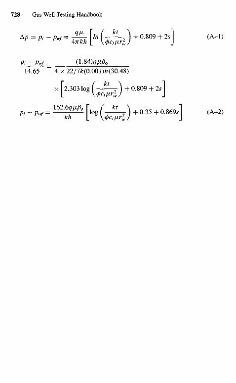
Pi - Pw/ (1.84)gjLtj80
14.65 ~ 4 x 22/7&(0.001)/*(30.48)
x [2.303 log { ± kt .\ + 0.809 + 2s\
_ = 1 6 2 | ^ r / fo\ + 0 35 + 0 869 1
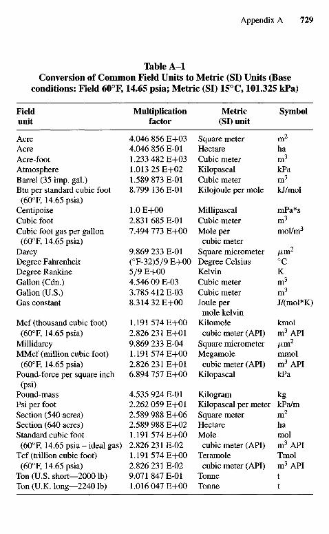
Table A-IConversion of Common Field Units to Metric (SI) Units (Base
conditions: Field 6O0F, 14.65 psia; Metric (SI) 15°C, 101.325 kPa)
Fieldunit
AcreAcreAcre-footAtmosphereBarrel (35 imp. gal.)Btu per standard cubic foot
(600F, 14.65 psia)CentipoiseCubic footCubic foot gas per gallon
(600F, 14.65 psia)DarcyDegree FahrenheitDegree RankineGallon (Cdn.)Gallon (U.S.)Gas constant
Mcf (thousand cubic foot)(600F, 14.65 psia)
MillidarcyMMcf (million cubic foot)
(600F, 14.65 psia)Pound-force per square inch
(psi)Pound-massPsi per footSection (540 acres)Section (640 acres)Standard cubic foot(600F, 14.65 psia - ideal gas)
Tcf (trillion cubic foot)(600F, 14.65 psia)
Ton (U.S. short—2000 Ib)Ton (U.K. long—2240 Ib)
Multiplicationfactor
4.046 856 E+034.046 856 E-Ol1.233 482 E+031.013 25 E+021.589 873 E-Ol8.799 136 E-Ol
1.0E+002.831 685 E-Ol7.494 773 E+00
9.869 233 E-Ol(°F-32)5/9 E+005/9 E+004.546 09 E-033.785 412 E-038.314 32 E+00
1.191 574 E+002.826 231 E+019.869 233 E-041.191 574 E+002.826 231 E+016.894 757 E+00
4.535 924 E-Ol2.262 059 E+012.589 988 E+062.589 988 E+021.191 574 E+002.826 231 E-021.191 574 E+002.826 231 E-029.071 847 E-Ol1.016 047 E+00
Metric(SI) unit
Square meterHectareCubic meterKilopascalCubic meterKilojoule per mole
MillipascalCubic meterMole percubic meter
Square micrometerDegree CelsiusKelvinCubic meterCubic meterJoule permole kelvin
Kilomolecubic meter (API)
Square micrometerMegamolecubic meter (API)
Kilopascal
KilogramKilopascal per meterSquare meterHectareMolecubic meter (API)
Teramolecubic meter (API)
TonneTonne
Symbol
m2
ham3
kPam3
kJ/mol
mPa*sm3
mol/m3
/xm2
0CKm3
m3
J/(mol*K)
kmolm3 APIfim2
mmolm3 APIkPa
kgkPa/mm2
hamolm3 APITmolm3 APItt
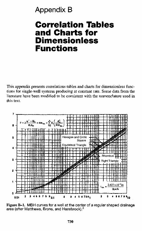
Appendix B
Correlation Tablesand Charts forDimensionlessFunctions
This appendix presents correlations tables and charts for dimensionless func-tions for single-well systems producing at constant rate. Some data from theliterature have been modified to be consistent with the nomenclature used inthis text.
Figure B-I. MBH curves for a well at the center of a regular shaped drainagearea (after Matthews, Brons, and Hazebrock).3
Hexagon and CircleSquare
Equilateral Triangle
Rhombus
Right Triangle
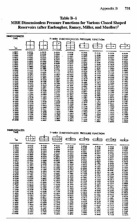
Table B-IMBH Dimensionless Pressure Functions for Various Closed Shaped
Reservoirs (after Earlougher, Ramey, Miller, and Mueller)1
DIMENSIONLESSTIME F=MBH DIMENStONlESS PRESSURE FUNCTION
DIMENSIONIESSTIME F=MBH DIMENSIONLESS PRESSUREFUNCTION
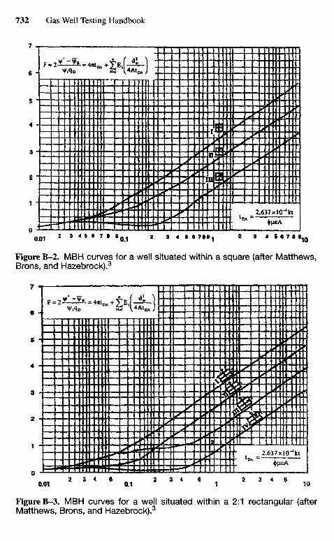
Figure B-2. MBH curves for a well situated within a square (after Matthews,Brons, and Hazebrock).3
Figure B-3. MBH curves for a well situated within a 2:1 rectangular (afterMatthews, Brons, and Hazebrock).3
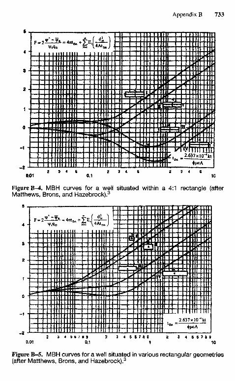
Figure B-4. MBH curves for a well situated within a 4:1 rectangle (afterMatthews, Brons, and Hazebrock).3
Figure B-5. MBH curves for a well situated in various rectangular geometries(after Matthews, Brons, and Hazebrock).3
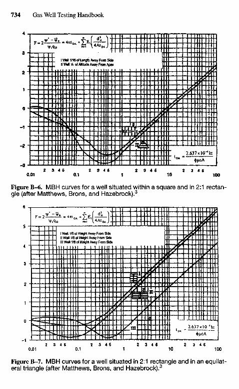
Figure B-6. MBH curves for a well situated within a square and in 2:1 rectan-gle (after Matthews, Brons, and Hazebrock).3
Figure B-7. MBH curves for a well situated in 2:1 rectangle and in an equilat-eral triangle (after Matthews, Brons, and Hazebrock).3
I Wd11/6 of Height Away From SideII Weil 1/8 of Height Away From SideHi Weil 1/8 of Height Away From Side
IWM1/16 of Leng» Away From Side!I WBH VS of AWludB Away Front Apex
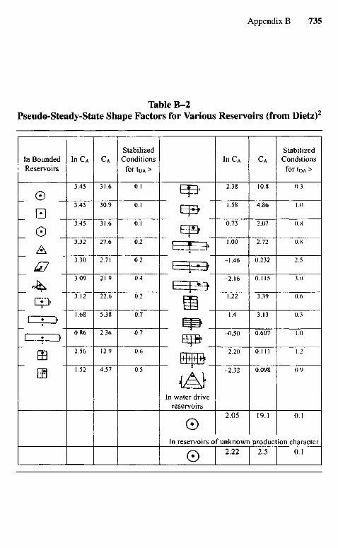
Table B-2Pseudo-Steady-State Shape Factors for Various Reservoirs (from Dietz)2
Stabilized StabilizedIn Bounded In CA CA Conditions In CA CA ConditionsReservoirs for tDA > for tDA >
In water drivereservoirs
In reservoirs of unknown production character
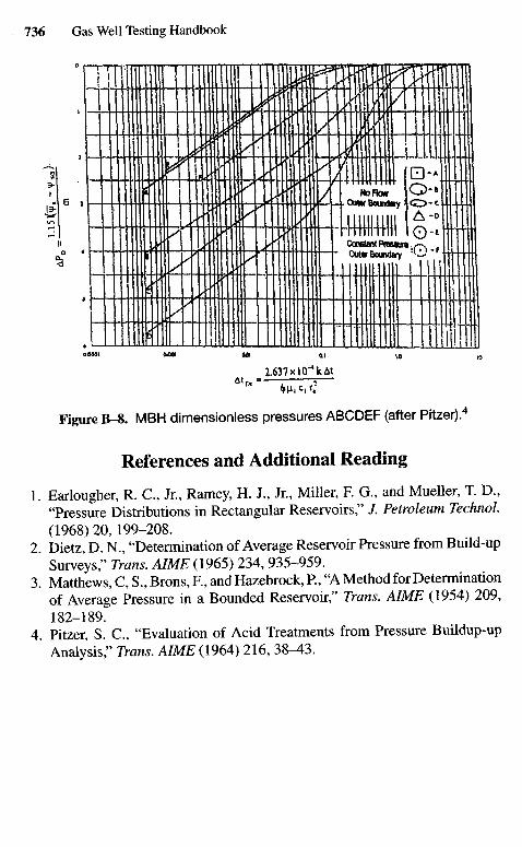
Figure B-8. MBH dimension less pressures ABCDEF (after Pitzer).4
References and Additional Reading
1. Earlougher, R. C, Jr., Ramey, H. J., Jr., Miller, F. G., and Mueller, T. D.,"Pressure Distributions in Rectangular Reservoirs," /. Petroleum Technol.(1968) 20, 199-208.
2. Dietz, D. N., "Determination of Average Reservoir Pressure from Build-upSurveys," Trans. AIME (1965) 234, 935-959.
3. Matthews, C, S., Brons, R, and Hazebrock, P., "A Method for Determinationof Average Pressure in a Bounded Reservoir," Trans. AIME (1954) 209,182-189.
4. Pitzer, S. C, "Evaluation of Acid Treatments from Pressure Buildup-upAnalysis," Trans. AIME (1964) 216, 38^*3.
Appendix C
Estimation ofFormationCharacteristicsfrom Drill-Stem Test
The normal Homer and/or Miller, Dyes, and Hutchinson methods are applica-ble to drill-stem tests. At times, shortcut methods as used by service companiesin field analysis are reliable. The drill-stem test often uses two bombs, and oneor more flow and shut-in sequences are recorded, as illustrated in Figures C-Iand C-2. To illustrate how a typical DST is performed, we will examine aschematic chart (Figure C-I) of pressure versus time from a test with two flowperiods and two shut-in periods.
Point A: Tool is lowered into the hole.Point B: Tool is on bottom.Point C: Packers are set, the mud column is compressed, and a still higher
pressure is recorded.Point D: Tool is opened for an initial flow period and the pressure drop as
shown.Point E to point F: Fluid accumulates in the drill stem above the pressure
gauge, the well is shut in, and pressure rises to point F.Point G to point H: After a suitable shut-in period, the well is reopened for
a second final flow period from point G to point H.Point H to point I: Final shut-in period.Point J to point K: Packers are then released; the testing device is then
removed from the hole.
C l Normal Routine Drill-Stem Test
The first flow is very short and is designed to remove any excess pres-sure, which may have resulted from setting the packers. The first buildup israther long since a reliable value for the initial reservoir pressure is desired.
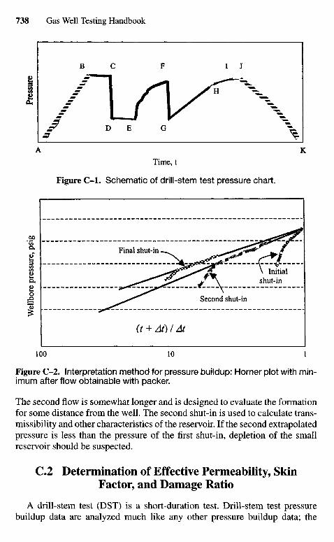
Figure C-2. Interpretation method for pressure buildup: Horner plot with min-imum after flow obtainable with packer.
The second flow is somewhat longer and is designed to evaluate the formationfor some distance from the well. The second shut-in is used to calculate trans-missibility and other characteristics of the reservoir. If the second extrapolatedpressure is less than the pressure of the first shut-in, depletion of the smallreservoir should be suspected.
C.2 Determination of Effective Permeability, SkinFactor, and Damage Ratio
A drill-stem test (DST) is a short-duration test. Drill-stem test pressurebuildup data are analyzed much like any other pressure buildup data; the
Second shut-in
Initialshut-in
Final shut-in
Time, t
Figure C-I. Schematic of drill-stem test pressure chart.
Pre
ssur
eW
ellb
ore
pres
sure
, ps
ig
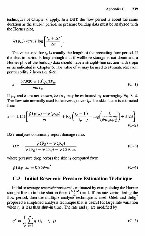
techniques of Chapter 6 apply. In a DST, the flow period is about the sameduration as the shut-in period, so pressure buildup data must be analyzed withthe Horner plot,
y(Pws) versus log -1— L
The value used for tp is usually the length of the preceding flow period. Ifthe shut-in period is long enough and if wellbore storage is not dominant, aHorner plot of the buildup data should have a straight-line section with slopem, as indicated in Chapter 6. The value of m may be used to estimate reservoirpermeability k from Eq. 6-5:
_ 57.920 x \0%cTPsc
mhTsc
If iig and h are not known, kh/fig may be estimated by rearranging Eq. 8-4.The flow rate normally used is the average over tp. The skin factor is estimatedfrom
L m \ tp J \(p{j,giCir2 J J
(C-2)
DST analyses commonly report damage ratio:
DR = ^(P*) ~ ^(/V) ( C _ 3 )
f (PR) ~ f(Pwf) ~ Ir(Ap)skin
where pressure drop across the skin is computed from
is(Ap)skin = 0.869ms' (C-A)
C3 Initial Reservoir Pressure Estimation Technique
Initial or average reservoir pressure is estimated by extrapolating the Hornerstraight line to infinite shut-in time, (tp~^ff) = 1. If the rate varies during theflow period, then the multiple analysis technique is used. Odeh and Selig2
proposed a simplified analysis technique that is useful for large rate variationwhen tp is less than shut-in time. The rate and tp are modified by
<?* = iZ>^-0-i) (C-5)1P j=\
and
C.4 Radius of Investigation
The modified values t* and q* are used in the Horner plot. For practicalpurpose, the radius of investigation during DST is equivalent to the radius ofdrainage given by
/ kAtmax
1 ~ }j 94S4>n8ct ( °
References and Additional Reading
1. Van Poollen, H. K., "Status of Drill-Stem Testing Techniques and Anal-ysis." /. Petroleum Technol (April 1961) 333-339. Also Reprint Series,No. 9—Pressure Analysis Methods, Society of Petroleum Engineers ofAIME, Dallas, TX, 1967, pp. 104-110.
2. Odeh, A. S. and Selig, R, "Pressure Buildup Analysis Variable-Rate Case,"/. Petroleum Tech. (July 1963) 790-794. Trans. AIME, 228. Also ReprintSeries, No. 9—Pressure Analysis Methods, Society of Petroleum EngineersofAIME, Dallas, TX, 1967, pp. 131-135.
Appendix D
Gas Flow RateMeasurementTechniques
D.I Gas Flow Rate Calculations
The natural gas is measured by volume in standard cubic feet at an operatingpressure and temperature and is corrected to some reference or base pressureand temperature, generally 600F and atmospheric pressure. The two most com-monly used gas measurement devices are the orifice meters and critical flowprovers.
D.2 Determining Orifice Meter Constantsand Factors
Orifice Meters
An orifice meter is utilized for gas measurement if environmental constraintsprohibit gas venting to the atmosphere. A typical closed-orifice metering sys-tem consists of orifice plates, meter tubes, flange taps, and pipe taps. The gasflow rate through a closed-orifice metering system is determined using
qsc = Cy/K pf (D-I)
where
C = FbFPbFtbFgFtfFrFPvFmY (D-2)
The term C is known as the orifice constant, the value of which dependsprimarily on the basic orifice factor, Fb. Values for most of these constants aretabulated for various orifice sizes and flowing conditions in Tables D-I andD-2. The FhFPbFtbFgFtfFrFPvFm Y factors are determined empirically and areperiodically updated by the AGA.
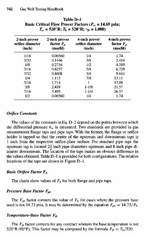
Table D-IBasic Critical Flow Prover Factors (Psc = 14.65 psia;
Tsc = 5200R; Tb = 5200R; <yb = 1.000)
2-inch prover 2-inch prover 4-inch prover 4-inch proverorifice diameter factor Fp orifice diameter factor Fp
(inch) (mscfd) (inch) (mscfd)
1/16 0.06560 1/4 1.743/32 0.1446 3/8 2.4141/8 0.2716 1/2 4.319
3/16 0.6237 5/8 6.7297/32 0.8608 3/4 9.6431/4 1.115 7/8 13.11
5/16 1.714 1 17.083/8 2.439 1-1/8 21.577/16 3.495 1-1/4 26.571/2 0.06560 1/4 1.74
Orifice Constants
The values of the constants in Eq. D-2 depend on the points between whichthe differential pressure hw is measured. Two standards are provided in gasmeasurement flange taps and pipe taps. With the former, the flange or orificeholder is tapped so that the center of the upstream and downstream taps is1 inch from the respective orifice-plate surface. For standard pipe taps theupstream tap is located i\ inch pipe diameters upstream and 8-inch pipe di-ameter downstream. The location of the taps makes an obvious difference inthe values obtained. Table D-I is provided for both configurations. The relativelocations of the taps are shown in Figure D-I .
Basic Orifice Factor Ff,
The charts show values of Fb for both flange and pipe taps.
Pressure Base Factor Fpb
The Fpb factor corrects the value of Fb for cases where the pressure baseused is not 14.73 psia. It may be determined by the equation Fpb = 14.73/Pb.
Temperature-Base Factor Ftb
The Ftb factor corrects for any contract wherein the base temperature is not5200R (6O0F). This factor may be computed by the formula Ftb — Tb/520.
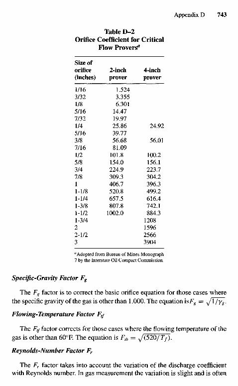
Table D-2Orifice Coefficient for Critical
Flow Provers"
Size oforifice 2-inch 4-inch(inches) prover prover
1/16 1.5243/32 3.3551/8 6.3015/16 14.477/32 19.971/4 25.86 24.925/16 39.773/8 56.68 56.017/16 81.091/2 101.8 100.25/8 154.0 156.13/4 224.9 223.77/8 309.3 304.21 406.7 396.31-1/8 520.8 499.21-1/4 657.5 616.41-3/8 807.8 742.11-1/2 1002.0 884.31-3/4 12082 15962-1/2 25663 3904
a Adopted from Bureau of Mines Monograph7 by the Interstate Oil Compact Commission.
Specific-Gravity Factor Fg
The Fg factor is to correct the basic orifice equation for those cases wherethe specific gravity of the gas is other than 1.000. The equation isFg = y/l/yg.
Flowing-Temperature Factor Ftf
The Ftf factor corrects for those cases where the flowing temperature of thegas is other than 600F. The equation is Ftb = ^ (520 / 7 » .
Reynolds-Number Factor Fr
The Fr factor takes into account the variation of the discharge coefficientwith Reynolds number. In gas measurement the variation is slight and is often
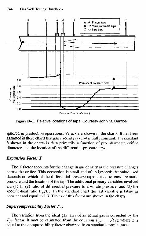
Pressure Profile (Orifice)
Figure D-I. Relative locations of taps. Courtesy John M. Cambell.
ignored in production operations. Values are shown in the charts. It has beenassumed in these charts that gas viscosity is substantially constant. The constantb shown in the charts is then primarily a function of pipe diameter, orificediameter, and the location of the differential-pressure taps.
Expansion Factor Y
The Y factor accounts for the change in gas density as the pressure changesacross the orifice. This correction is small and often ignored; the value useddepends on which of the differential-pressure taps is used to measure staticpressure and the location of the tap. The additional primary variables involvedare (1) /3, (2) ratio of differential pressure to absolute pressure, and (3) thespecific-heat ratio Cp/Cv. In the standard chart the last variable is taken asconstant and equal to 1.3. Tables of this factor are shown in the charts.
Supercompressibility Factor Fpv
The variation from the ideal gas laws of an actual gas is corrected by theFpv factor. It may be estimated from the equation Fpv = ^/TJz where z isequal to the compressibility factor obtained from standard correlations.
Permanent Pressure Loss
A -> Flange tapsB -> Vena contracta tapsC -> Pipe taps
Cha
nge
inS
tati
c pr
essu
re
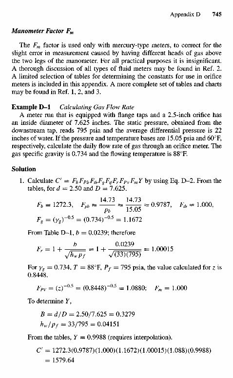
Manometer Factor Fm
The Fm factor is used only with mercury-type meters, to correct for theslight error in measurement caused by having different heads of gas abovethe two legs of the manometer. For all practical purposes it is insignificant.A thorough discussion of all types of fluid meters may be found in Ref. 2.A limited selection of tables for determining the constants for use in orificemeters is included in this appendix. A more complete set of tables and chartsmay be found in Ref. 1, 2, and 3.
Example D-I Calculating Gas Flow RateA meter run that is equipped with flange taps and a 2.5-inch orifice has
an inside diameter of 7.625 inches. The static pressure, obtained from thedownstream tap, reads 795 psia and the average differential pressure is 22inches of water. If the pressure and temperature bases are 15.05 psia and 600F,respectively, calculate the daily flow rate of gas through an orifice meter. Thegas specific gravity is 0.734 and the flowing temperature is 88°F.
Solution
1. Calculate C — FbFpbFtbFgFtfFrFpvFmY by using Eq. D-2. From thetables, for d = 2.50 and D = 7.625,
Fb = 1272.3, Fpb = 1 ^ - = 1 ^ - = 0.9787, Ftb = 1.000,pb 15.05
Fg = (K^)"05 = (0.734) -°-5 = 1.1672
From Table D-I , b = 0.0239; therefore
Fr = l+ , b = 1 + /a ° 2 3 9 = 1.00015
Jh~^s V(33)(795)
For Yg = 0.734, T = 88°F, Pf = 795 psia, the value calculated for z is0.8448.
FPy = (z)-° 5 = (0.8448)"05 = 1.0880; Fm = 1.000
To determine Y,
B = d/D = 2.50/7.625 = 0.3279
hw/pf = 33/795 = 0.04151
From the tables, Y = 0.9988 (requires interpolation).
C = 1272.3(0.9787)(1.000)(1.1672)(1.00015)(1.088)(0.9988)
= 1579.64
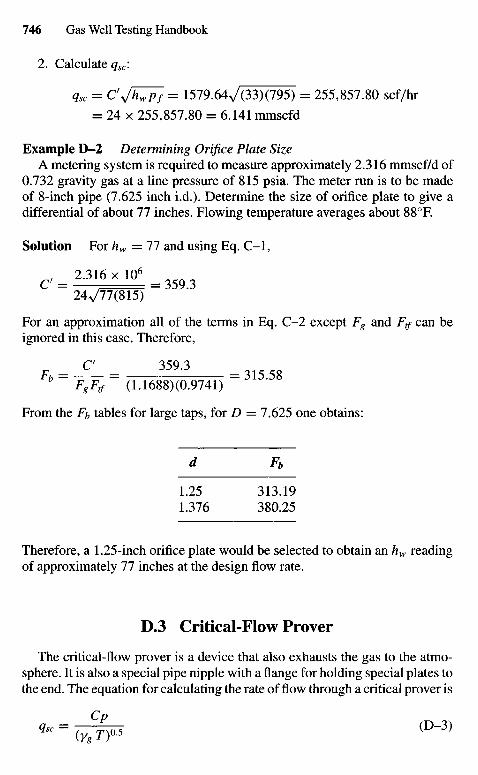
2. Calculate qsc:
qsc = C'JKp} = 1579.64v/(33)(795) = 255,857.80 scf/hr
= 24 x 255,857.80 = 6.141 mmscfd
Example D-2 Determining Orifice Plate SizeA metering system is required to measure approximately 2.316 mmscf/d of
0.732 gravity gas at a line pressure of 815 psia. The meter run is to be madeof 8-inch pipe (7.625 inch i.d.). Determine the size of orifice plate to give adifferential of about 77 inches. Flowing temperature averages about 88°F.
Solution For hw = 77 and using Eq. C-I ,
" "'6x'°' —24^/77(815)
For an approximation all of the terms in Eq. C-2 except Fg and Ftf can beignored in this case. Therefore,
C 359.3Fb = FgFtf = (1.1688)(0.9741) = 3 1 5 ' 5 8
From the Fb tables for large taps, for D = 7.625 one obtains:
d Fb
1.25 313.191.376 380.25
Therefore, a 1.25-inch orifice plate would be selected to obtain an hw readingof approximately 77 inches at the design flow rate.
D.3 Critical-Flow Prover
The critical-flow prover is a device that also exhausts the gas to the atmo-sphere. It is also a special pipe nipple with a flange for holding special plates tothe end. The equation for calculating the rate of flow through a critical prover is
q~= ( ^ ( D - 3 )
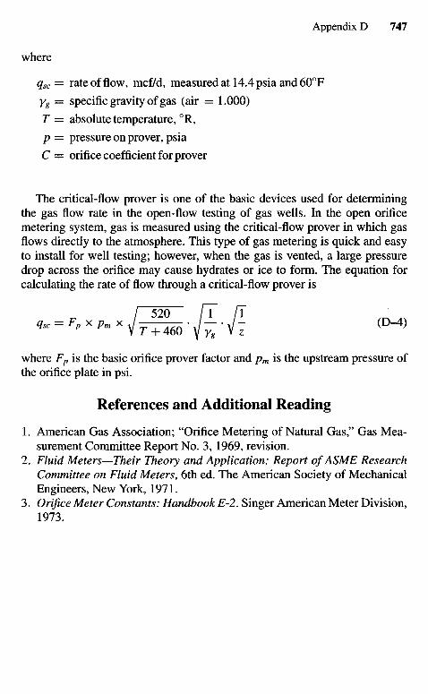
where
qsc = rate of flow, mcf/d, measured at 14.4psiaand60°Fyg = specific gravity of gas (air = 1.000)T = absolute temperature, 0R,p = pressure on prover, psiaC = orifice coefficient for prover
The critical-flow prover is one of the basic devices used for determiningthe gas flow rate in the open-flow testing of gas wells. In the open orificemetering system, gas is measured using the critical-flow prover in which gasflows directly to the atmosphere. This type of gas metering is quick and easyto install for well testing; however, when the gas is vented, a large pressuredrop across the orifice may cause hydrates or ice to form. The equation forcalculating the rate of flow through a critical-flow prover is
/ 520 [T [Tqsc = F?xp™xiT^m^7g'i-z
a>4)
where Fp is the basic orifice prover factor and pm is the upstream pressure ofthe orifice plate in psi.
References and Additional Reading
1. American Gas Association; "Orifice Metering of Natural Gas," Gas Mea-surement Committee Report No. 3, 1969, revision.
2. Fluid Meters—Their Theory and Application: Report of ASME ResearchCommittee on Fluid Meters, 6th ed. The American Society of MechanicalEngineers, New York, 1971.
3. Orifice Meter Constants: Handbook E-2. Singer American Meter Division,1973.
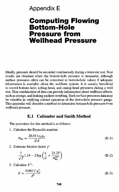
Appendix E
Computing FlowingBottom-HolePressure fromWellhead Pressure
Ideally, pressure should be recorded continuously during a transient test. Bestresults are obtained when the bottom-hole pressure is measured, althoughsurface pressures often can be converted to bottom-hole values if adequateinformation is available about the wellbore system. It is usually beneficialto record bottom-hole, tubing-head, and casing-head pressures during a welltest. That combination of data can provide information about wellbore effects,such as storage, and leaking packers or tubing. Such surface pressures data maybe valuable in verifying correct operation of the down-hole pressure gauge.This appendix will describe a method to determine bottom-hole pressure fromwellhead pressure.
E.I Cullender and Smith Method
The procedure for this method is as follows:
1. Calculate the Reynolds number:
20,0nygqsc^VRe = Z=T-, (Ii-I)
{id
2. Estimate friction factor / :
3. Calculate F2:
F=<^pi <E-3)
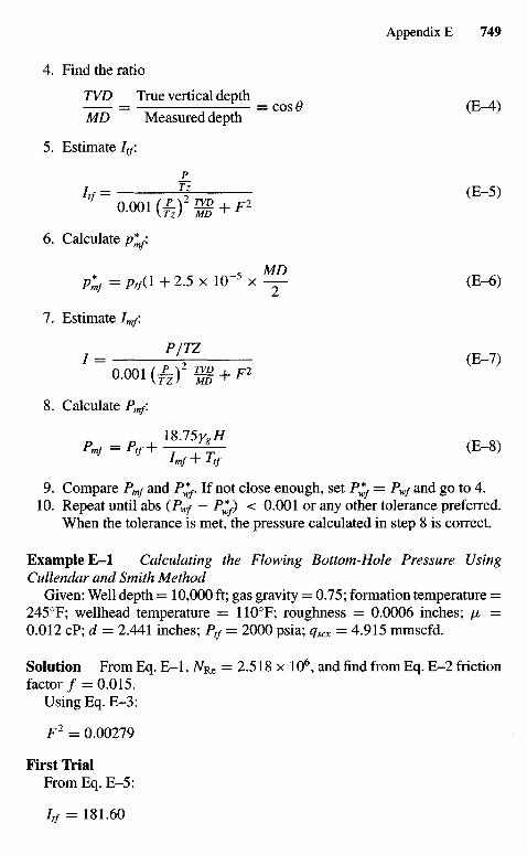
4. Find the ratio
TVD True vertical depth= — = cos6> (E-4)
MD Measured depth
5. Estimate It/.
_p_
ltf = T (E"5)
0.001 (0%§ + F*6. Calculate p*;.
p*mf = / v ( * + 2 - 5 x 1 0 ~ 5 x ^ r <&•*>
7. Estimate / m /
P/7Z/ = S (E-7)
o-ooi (£ ) 2 ^ +1*
8. Calculate Pm/:
P«-Pt+¥&L (E-S)
9. Compare Pmf and P1^. If not close enough, set P*f = Pwf and go to 4.10. Repeat until abs (PWf — P^) < 0.001 or any other tolerance preferred.
When the tolerance is met, the pressure calculated in step 8 is correct.
Example E-I Calculating the Flowing Bottom-Hole Pressure UsingCullendar and Smith Method
Given: Well depth = 10,000 ft; gas gravity = 0.75; formation temperature =245°F; wellhead temperature = 1100F; roughness = 0.0006 inches; /x =0.012 cP; d = 2.441 inches; Ptf = 2000 psia; qscx = 4.915 mmscfd.
Solution From Eq. E-I , NRe = 2.518 x 10⁶, and find from Eq. E-2 frictionfactor / = 0.015.
Using Eq. E-3:
F2 = 0.00279
First TrialFrom Eq. E-5:
ltf = 181.60
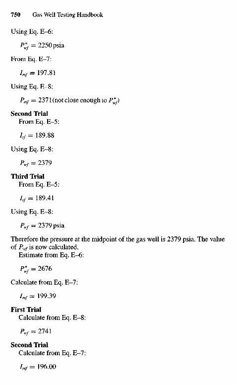
Using Eq. E-6:
P ^ = 2250 psia
From Eq. E-7:
Imf= 197.81
Using Eq. E-8:
Pmf = 2371 (not close enough to P*f)
Second Trial
From Eq. E-5:
Itf= 189.88
Using Eq. E-8:
Pwf = 2379
Third Trial
From Eq. E-5:
Itf= 189.41
Using Eq. E-8:
Pwf = 2379 psiaTherefore the pressure at the midpoint of the gas well is 2379 psia. The valueof Pwf is now calculated.
Estimate from Eq. E-6:
P1^ = 2676
Calculate from Eq. E-7:
Imf = 199.39
First Trial
Calculate from Eq. E-8:
Pwf = 2741
Second TrialCalculate from Eq. E-7:Imf = 196.00
Calculate from Eq. E-8:
Pwf = 2744 psia
This is close enough to the previously calculated value of 2741 psia. Therefore,the flowing bottom-hole pressure is 2744 psia.
References and Additional Reading
1. Cullender, M. H., and Smith, R. V., "Practical Solution of Gas Flow Equa-tion for Wells and Pipelines with Large Temperature Gradients," Trans.AIME (1956) 207.
Next Page
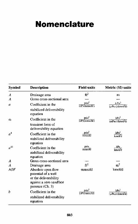
Symbol
AA
a
at
a1
au
AAAOF
b
Description
Drainage areaGross cross-sectional areaCoefficient in thestabilized deliverabilityequationCoefficient in thetransient form ofdeliverability equation
Coefficient in thestabilized deliverabilityequationCoefficient in thestabilized deliverabilityequationGross cross-sectional areaDrainage areaAbsolute open flowpotential of a wellor the deliverabilityagainst a zero sandfacepressure (Ch. 3)
Coefficient in thestabilized deliverabilityequation
Field units
ft2
psia2
(cP)(mmscfd)
psia2
(cP)(mmscfd)
psia2
mmscfd
mmscfd
ft2
mmscfd
psia2
(cP) (mmscfd)
Metric (SI) units
m
kPa2
(/xPa.s)(kmol/d)
kPa2
(mPay) (kmol/d)
kPa2
kmol/d
kPakmol/d
m2
kmol/d
kPa2
(jtPa.s) (kmol/d)
Nomenclature
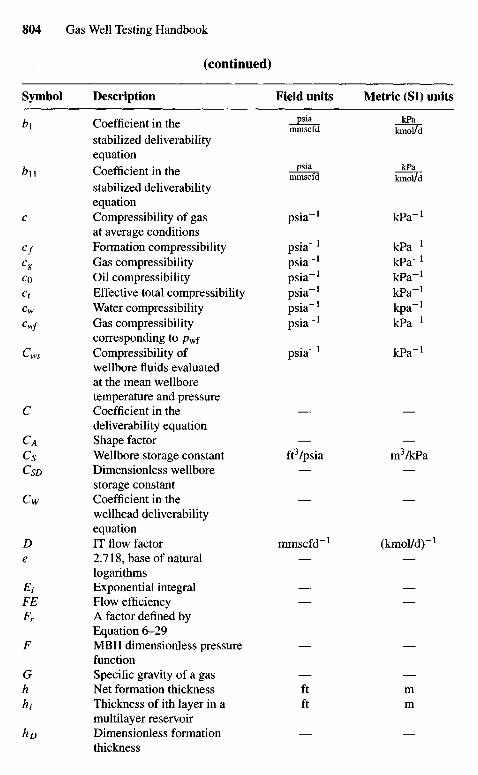
Symbol
bx
bn
C
cfcg
CO
Ctcw
Cwf
("ws
C
CA
CsCSD
Cw
De
EtFEFr
F
Ghhi
hD
(continued)
Description
Coefficient in thestabilized deliverabilityequationCoefficient in thestabilized deliverabilityequationCompressibility of gasat average conditionsFormation compressibilityGas compressibilityOil compressibilityEffective total compressibilityWater compressibilityGas compressibilitycorresponding to /?wfCompressibility ofwellbore fluids evaluatedat the mean wellboretemperature and pressureCoefficient in thedeliverability equationShape factorWellbore storage constantDimensionless wellborestorage constantCoefficient in thewellhead deliverabilityequationIT flow factor2.718, base of naturallogarithmsExponential integralFlow efficiencyA factor defined byEquation 6-29MBH dimensionless pressurefunctionSpecific gravity of a gasNet formation thicknessThickness of ith layer in amultilayer reservoirDimensionless formationthickness
Field units
psiammscfd
psiammscfd
psia"1
psia"1
psia"1
psia"1
psia"1
psia"1
psia"1
psia"1
ft3/psia
mmscfd"1
ftft
Metric (SI) units
kPakmol/d
kPakmol/d
kPa"1
kPa"1
kPa"1
kPa"1
kPa"1
kpa"1
kPa"1
kPa"1
m3/kPa
(kmoyd)-1
mm
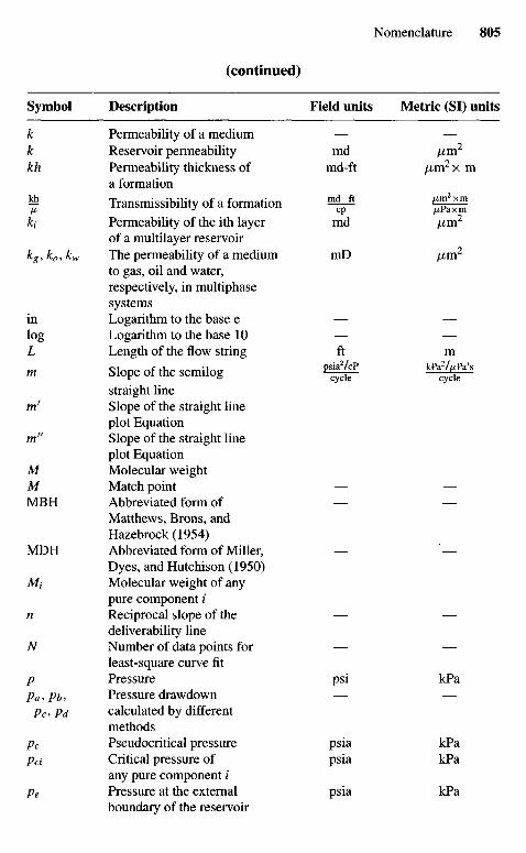
Symbol
kkkh
kh
ki
k k k1^g, KO, KW
inlogL
m
mf
m"
MMMBH
MDH
M1
n
N
P
Pa, Pb,
Pc, Pd
Pc
Pci
Pe
(continued)
Description
Permeability of a mediumReservoir permeabilityPermeability thickness ofa formationTransmissibility of a formationPermeability of the ith layerof a multilayer reservoirThe permeability of a mediumto gas, oil and water,respectively, in multiphasesystemsLogarithm to the base eLogarithm to the base 10Length of the flow string
Slope of the semilogstraight lineSlope of the straight lineplot EquationSlope of the straight lineplot EquationMolecular weightMatch pointAbbreviated form ofMatthews, Brons, andHazebrock (1954)Abbreviated form of Miller,Dyes, and Hutchison (1950)Molecular weight of anypure component iReciprocal slope of thedeliverability lineNumber of data points forleast-square curve fitPressurePressure drawdowncalculated by differentmethodsPseudocritical pressureCritical pressure ofany pure component iPressure at the externalboundary of the reservoir
Field units
mdmd-ft
md-ftcp
md
mD
ftpsiaVcP
cycle
psi
psiapsia
psia
Metric (SI) units
/xm2
/xm2x m
/xm2xm/^Pa x m
fim2
m
kPaV/xPa'scycle
kPa
kPakPa
kPa
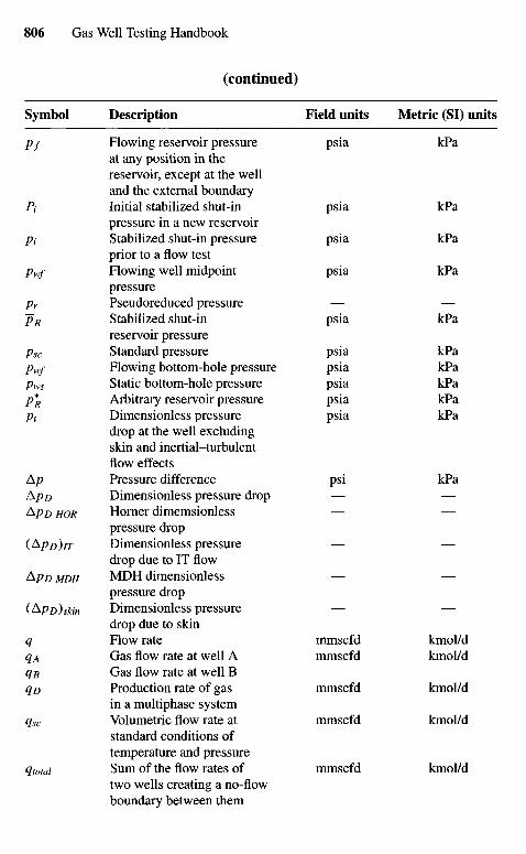
Symbol
Pf
Pi
Pi
Pwf
Pr
PR
PscPwfPws
PR
Pt
Ap
ApD
Ap D HOR
(ApD)IT
Ap D MDH
(ApD)skin
q
qD
qsc
qtotal
(continued)
Description
Flowing reservoir pressureat any position in thereservoir, except at the welland the external boundaryInitial stabilized shut-inpressure in a new reservoirStabilized shut-in pressureprior to a flow testFlowing well midpointpressurePseudoreduced pressureStabilized shut-inreservoir pressureStandard pressureFlowing bottom-hole pressureStatic bottom-hole pressureArbitrary reservoir pressureDimensionless pressuredrop at the well excludingskin and inertial-turbulentflow effectsPressure differenceDimensionless pressure dropHorner dimemsionlesspressure dropDimensionless pressuredrop due to IT flowMDH dimensionlesspressure dropDimensionless pressuredrop due to skinFlow rateGas flow rate at well AGas flow rate at well BProduction rate of gasin a multiphase systemVolumetric flow rate atstandard conditions oftemperature and pressureSum of the flow rates oftwo wells creating a no-flowboundary between them
Field units
psia
psia
psia
psia
psia
psiapsiapsiapsiapsia
psi
mmscfdmmscfd
mmscfd
mmscfd
mmscfd
Metric (SI) units
kPa
kPa
kPa
kPa
kPa
kPakPakPakPakPa
kPa
kmol/dkmol/d
kmol/d
kmol/d
kmol/d
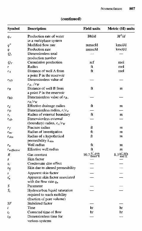
Symbol
q*qQ,
QTr
rA
rAD
rB
rdrDre
reD
rfFiriV
Vskin
rw
t"weffective
RS
Sc
SK
S
SSc
SFt
tctD
(continued)
Description
Production rate of waterin a multiphase systemModified flow rateProduction rateDimensionless totalproduction numberCumulative productionRadiusDistance of well A froma point P in the reservoirDimensionless value of^A,/rwDistance of well B froma point P in the reservoirDimensionless value of r#,rB/rwEffective drainage radiusDimensionless radius, r/rw
Radius of external boundaryDimensionless external(boundary) radius, re/r\yFracture radiusRadius of investigationRadius of a hypotheticalpermeability ksidn
Well radiusEffective well radius
Gas constantSkin factorCondensate skin effectSkin due to altered permeabilityApparent skin factorApparent skin factor associatedwith the flow rate qn
ParameterHydrocarbon liquid saturationrequired to reach mobility(fraction of pore volume)Stabilized factorTimeCorrected time of flowDimensionless time forvarious systems
Field units
BbVd
mmscfdmmscfd
scfftft
ft
ft
ft
ftftft
ftft
hrhr
Metric (SI) units
M3Id
kmol/dkmol/d
molmolmol
m
m
m
mmm
mm
hrhr
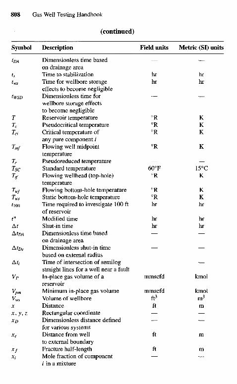
Symbol
tDA
ts
tws
tWSD
T
Tc
Ta
Tmf
Tr
TscT<f
TwfT
^100
At
AfDA
AtDe
Af1-
VP
VpmT/
X
x, y,z
XD
Xe
XfXi
(continued)
Description
Dimensionless time basedon drainage areaTime to stabilizationTime for wellbore storageeffects to become negligibleDimensionless time forwellbore storage effectsto become negligibleReservoir temperaturePseudocritical temperatureCritical temperature ofany pure component /Flowing well midpointtemperaturePseudoreduced temperatureStandard temperatureFlowing wellhead (top-hole)temperatureFlowing bottom-hole temperatureStatic bottom-hole temperatureTime required to investigate 100 ftof reservoirModified timeShut-in timeDimensionless time basedon drainage areaDimensionless shut-in timebased on external radiusTime of intersection of semilogstraight lines for a well near a faultIn-place gas volume of areservoirMinimum in-place gas volumeVolume of wellboreDistanceRectangular coordinateDimensionless distance definedfor various systemsDistance from wellto external boundaryFracture half-lengthMole fraction of componenti in a mixture
Field units
hrhr
0R0R0R0R
600F0R
0R0Rhr
hrhr
mmscfd
mmscfdft3
ft
ft
ft
Metric (SI) units
hrhr
K
K
K
K
15°CK
KKhr
hrhr
kmol
kmolm3
m
m
m
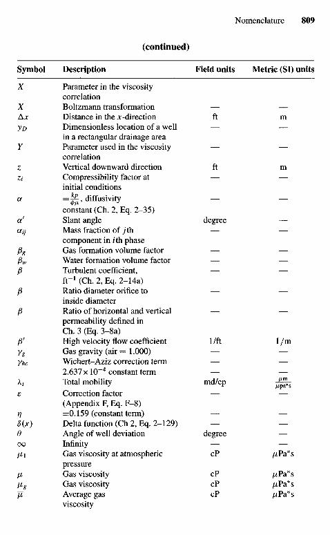
Symbol
X
XAxyD
Y
Z
Zi
a
a'ay
PgPw
P
P
P
P'YgYhc
£
8 (x)0OO
Ml
H
VgM
(continued)
Description
Parameter in the viscositycorrelationBoltzmann transformationDistance in the x -directionDimensionless location of a wellin a rectangular drainage areaParameter used in the viscositycorrelationVertical downward directionCompressibility factor atinitial conditions-^ ,d i f fus iv i tyconstant (Ch. 2, Eq. 2-35)Slant angleMass fraction of jthcomponent in /th phaseGas formation volume factorWater formation volume factorTurbulent coefficient,ft"1 (Ch. 2, Eq. 2-14a)Ratio diameter orifice toinside diameterRatio of horizontal and verticalpermeability defined inCh. 3 (Eq. 3-8a)High velocity flow coefficientGas gravity (air = 1.000)Wichert-Aziz correction term2.637 x 10"4 constant termTotal mobilityCorrection factor(Appendix F, Eq. F-8)=0.159 (constant term)Delta function (Ch 2, Eq. 2-129)Angle of well deviationInfinityGas viscosity at atmosphericpressureGas viscosityGas viscosityAverage gasviscosity
Field units
ft
ft
degree
I/ft
md/cp
degree
cP
cPcPcP
Metric (SI) units
m
m
1/m
/xm/xpa*s
//,Pa* s/x Pa* s/xPa*s/xPa*s
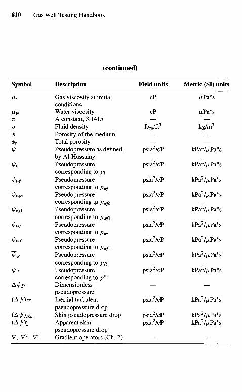
Symbol
fit
7V
P
<t><t>t
f
fwf
tywfo
fwf\
fws
\/f*
Ax/rD
(AlIf)1T
(Air) Skin
(AxIrY5
V, V2, V;
(continued)
Description
Gas viscosity at initialconditionsWater viscosityA constant, 3.1415Fluid densityPorosity of the mediumTotal porosityPseudopressure as definedby Al-HussainyPseudopressurecorresponding to piPseudopressurecorresponding to pwfPseudopressurecorresponding tp pwfo
Pseudopressurecorresponding to pwf\Pseudopressurecorresponding to pws
Pseudopressurecorresponding to pw/\Pseudopressurecorresponding to PRPseudopressurecorresponding to /7*DimensionlesspseudopressureInertial turbulentpseudopressure dropSkin pseudopressure dropApparent skinpseudopressure dropGradient operators (Ch. 2)
Field units
cP
cP
lbm/ft3
psia2/cP
psia2/cP
psia2/cP
psia2/cP
psia2/cP
psia2/cP
psia2/cP
psia2/cP
psia2/cP
psia2/cP
psia2/cPpsia2/cP
Metric (SI) units
/xPa*s
/xPa*s
kg/m3
kPa2//xPa*s
kPa2//xPa*s
kPa2//xPa*s
kPa2//xPa*s
kPa2//xPa*s
kPa2//iPa*s
kPa2//xPa*s
kPa2//xPa*s
kPa2//xPa*s
kPa2//xPa*s
kPa2//xPa*skPa2//xPa*s

Bibliography
Abel, W., R. F. Jackson, and R. A. Wattenbarger. "Simulation of a PartialPressure Maintenance Gas Cycling Project with a Compositional Model,Carson Creek Field, Alberta," /. Petroleum Technol (Jan. 1970), 3 8 ^ 6 .
Abramowitz, M., and I. A. Stegun (ed.). Handbook of MathematicalFunctions with Formulas, Graphs and Mathematical Tables, NationalBureau of Standards Applied Mathematics Series-55 (June 1964) 227-253.
Adams, A. R., H. J. Ramey, and R. J. Burgess, "Gas Well Testing in a FractureCarbonate Reservoir," /. of Petroleum Technol, October 1968, 1187-1194.
Agarwal, R. G., R. Al-Hussainy, and H. J. Ramey, Jr. "The Importance of WaterFlux in Gas Reservoirs," Trans, AIME, v. 234, p. 1336, 1965.
Agarwal, R. G., R. Al-Hussainy, and H. J. Ramey, Jr. (1970). An Investigationof Wellbore Storage and Skin Effect in Unsteady Liquid Flow: I. AnalyticalTreatment, Society of Petroleum Eng. J; 10, 279-290.
Agarwall, R. G., R. D. Carter, and C. B. Pollock. "Evaluation and Predictionof Performance of Low-Permeability Gas Wells Stimulated by MassiveHydraulic Fracturing," J. Petroleum Technol. (March 1979) 362-372; Trans;AIME, 267.
Aguilera, R. "Well Test Analysis of Naturally Fractured Reservoirs," APEEJ,Sept. 1987, pp. 239-252.
Aguilera, R. and M. C. Ng. "Transient Pressure Analysis of Horizontal Wells inAnisotropic Naturally Fractured Reservoirs," paper SPE 19002, presentedat the SPE Joint Rocky Mountain Regional/Low Permeability ReservoirsSymposium and Exhibition, Denver, Colorado, March 6-8, 1989.
Al-Hussainy, R. (1967). Transient Flow of Ideal and Real Gases ThroughPorous Media, Ph. D. Thesis, Texas A. and M. University.
Al-Hussainy, R., and H. J. Ramey, Jr. (1966). "Application of Real Gas FlowTheory to Well Testing and Deliverability Forecasting," /. of PetroleumTechnol. pp. 18, 637-642.
Al-Hussainy, R., H. J. Ramey, Jr., and P. B. Crawford. "The Flow of RealGases Through Porous Media," /. of Petroleum Technol. (May 1966), pp.624-636; Trans; AIME; 237.
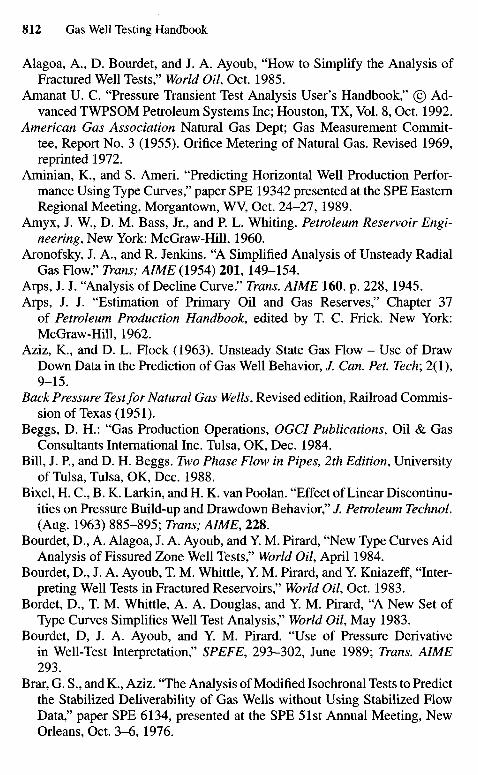
Alagoa, A., D. Bourdet, and J. A. Ayoub, "How to Simplify the Analysis ofFractured Well Tests," World Oil, Oct. 1985.
Amanat U. C. "Pressure Transient Test Analysis User's Handbook," © Ad-vanced TWPSOM Petroleum Systems Inc; Houston, TX, Vol. 8, Oct. 1992.
American Gas Association Natural Gas Dept; Gas Measurement Commit-tee, Report No. 3 (1955). Orifice Metering of Natural Gas. Revised 1969,reprinted 1972.
Aminian, K., and S. Ameri. "Predicting Horizontal Well Production Perfor-mance Using Type Curves," paper SPE 19342 presented at the SPE EasternRegional Meeting, Morgantown, WV, Oct. 24-27, 1989.
Amyx, J. W., D. M. Bass, Jr., and P. L. Whiting. Petroleum Reservoir Engi-neering, New York: McGraw-Hill, 1960.
Aronofsky, J. A., and R. Jenkins. "A Simplified Analysis of Unsteady RadialGas Flow," Trans; AIME (1954) 201, 149-154.
Arps, J. J. "Analysis of Decline Curve." Trans. AIME160. p. 228, 1945.Arps, J. J. "Estimation of Primary Oil and Gas Reserves," Chapter 37
of Petroleum Production Handbook, edited by T. C. Frick. New York:McGraw-Hill, 1962.
Aziz, K., and D. L. Flock (1963). Unsteady State Gas Flow - Use of DrawDown Data in the Prediction of Gas Well Behavior, /. Can. Pet. Tech; 2(1),9-15.
BackPressure Test for Natural Gas Wells, Revised edition, Railroad Commis-sion of Texas (1951).
Beggs, D. H.: "Gas Production Operations, OGCI Publications, Oil & GasConsultants International Inc. Tulsa, OK, Dec. 1984.
Bill, J. P., and D. H. Beggs. Two Phase Flow in Pipes, 2th Edition, Universityof Tulsa, Tulsa, OK, Dec. 1988.
Bixel, H. C, B. K. Larkin, and H. K. van Poolan. "Effect of Linear Discontinu-ities on Pressure Build-up and Drawdown Behavior," /. Petroleum Technol.(Aug. 1963) 885-895; Trans; AIME, 228.
Bourdet, D., A. Alagoa, J. A. Ayoub, and Y. M. Pirard, "New Type Curves AidAnalysis of Fissured Zone Well Tests," World Oil, April 1984.
Bourdet, D., J. A. Ayoub, T. M. Whittle, Y. M. Pirard, and Y. Kniazeff, "Inter-preting Well Tests in Fractured Reservoirs," World Oil, Oct. 1983.
Bordet, D., T. M. Whittle, A. A. Douglas, and Y. M. Pirard, "A New Set ofType Curves Simplifies Well Test Analysis," World Oil, May 1983.
Bourdet, D, J. A. Ayoub, and Y. M. Pirard. "Use of Pressure Derivativein Well-Test Interpretation," SPEFE, 293-302, June 1989; Trans. AIME293.
Brar, G. S., and K., Aziz. "The Analysis of Modified Isochronal Tests to Predictthe Stabilized Deliverability of Gas Wells without Using Stabilized FlowData," paper SPE 6134, presented at the SPE 51st Annual Meeting, NewOrleans, Oct. 3-6, 1976.
Brauser, E. B. (1965). Simplification of the Superposition Principle for PressureAnalysis at Variable Rates, paper SPE 1184, 40th Fall Meeting of AIME,Denver, CO.
Brigham, W. E. "Estimating Reservoir Parameters From the Gas backpressureEquation," SPE Reservoir Engineers, May 1988, pp. 649-650.
Brons, R, and V. E. Mailing. "The Effect of Restricted Fluid Entry on WellProductivity," /. of Petroleum Technol, pp. 172-174, February 1961.
Brown, G. G., D. L. Katz, C. G. Oberfell, and R. C. Alden. "Natural Gasolineand the Volatile Hydrocarbons;' NGAA, Tulsa, OK, 1948.
Brown, K. E. The Technology of Artificial Methods, Tulsa, OK, PennWellPublishing Co; 1984.
Bruce, G. H., D. W. Peaceman, A. A. Rachford, Jr., and J. D. Rice. "Calculationsof Unsteady-State Gas Flow Through Porous Media:" Trans. AIME. VoI 198,1953, pp 79-92.
Burns, William A., Jr.: "New Single Well Test for Determining Vertical Per-meability," /. Petroleum Technol. (June 1969) 743-752; Trans; AIME, 246.
Cannon, J. R., and A. H. Dogru. "Estimation of Permeability and Porosityfrom Well Test Data," paper SPE 5345 presented at the SPE. AIME 45thAnnual California Regional Meeting, Ventura, April 2-4, 1975.
Carr, N. L., R. Kobayashi, and D. B. Burrows. "Viscosity of HydrocarbonGases Under Pressure," Trans. AIME. 201, 264-272, 1954.
Carroll, J. A., Ill, and R. N. Home. "Multivariate Optimization of ProductionSystems," /. Petroleum Technol, pp. 782-789, July 1992.
Carter, R. D. (1962). Solutions of Unsteady-State Radial Gas Flow, /. PetroleumTechnol, 14,549-554.
Carter, R. D. (1966). Performance Predictions for Gas Reservoirs ConsideringTwo-Dimensional Unsteady-State Flow, Society of Petroleum EngineersJournal, 6, 35-43.
Carter, R. D., S. C. Millers, Jr., and H. G. Riley. "Determination of StabilizedGas Well Performance from Short Flow Tests," /. Petroleum Technology(June 1963) 651-653.
Celier, G. C. M. R., P. Jouault, O. A. M. C. de Montigny. "Zuidwal: A GasField Development with Horizontal Wells," paper SPE 19826, presented atthe SPE 64th Annual Technical Conference and Exhibition of the Society ofPetroleum Engineers, San Antonio, TX, Oct. 8-11, 1989.
Chatas, Angelos T. "A Practical Treatment of Non-Steady State Flow Problemsin Reservoirs Systems,"
Cinco, H., F. G. Miller, and H. J. Ramey, Jr. "Unsteady-State Pressure Distri-bution Created by a Directionally Drilled Well," /. Petroleum Technol, pp.1392-1402, November 1975.
Cinco, H., and F. Samaniego. "Effect of Wellbore Storage and Damage on theTransient Pressure Behavior for a Well with a Finite-Conductivity VerticalFracture," Soc. Pet. Eng. J. (Aug. 1978) 253-264.
Cinco-Ley, H., H. J. Ramey, Jr., and F. G., Miller. "Pseudo-skin Factors forPartially Penetrating Directionally Drilled Wells," SPE paper 5589, 1975.
Cinco-Ley, H., and F. Samaniego. "Transient Pressure Analysis for Finite Con-ductivity Fracture Case versus Damage Fracture Case," SPE Paper 10179,1981b.
Cobb, W. M., H. J. Ramey, Jr., and F. G. Miller (1972). Well-Test Analysis forWells Producing Commingled Zones, /. Petroleum Technol. 29, 28-37.
Collins, R. E. (1961). Flow of Fluids Through Porous Materials, ReinholdPublishing Corporation, New York.
Compressed Air and Gas Data, Ingersoll-Rand Co; Woodcliff Lake, NJ.Conversion of Operational and Process Measurement Units to the Metric (SI)
System, Manual of Petroleum Measurement Standards, Pub. API 2564, API(March 1974) Chap. 15, Sec. 2.
Cornell, D. "How to Determine Gas Well Interference Graphically" World Oil,Nov. 1952, p. 187-188.
Cornell, D., and D. L. Katz. "Pressure Gradients in Natural Gas Reservoirs"Trans. AIME, vol. 198, 1953, pp. 61-70.
Cornelson, D. W. "Analytical Prediction of Natural Gas Reservoir RecoveryFactors." /. Can. Petroleum Technology (1974) 13 (4), 17024.
Cornett, J. E. (1961). How to Locate Reservoir Limits, Pet. Eng. J; 33, B19-B24.
Craft, B. C, and M. F. Hawkins. "Applied Petroleum Reservoir Engineering"Prentice-Hall. Inc; 1959, Chapter 6.
Crafton, J. W., and C. D. Harris. "Direct Finite Difference Simulation of a GasWell with a Finite Capacity Vertical Fracture." Paper SPE 5736 presentedat the 4th Symposium of Numerical Simulation of Reservoir Performance,SPE ofAIME, Los Angeles (February 19-20, 1979).
Crawford, G. E., A. R. Hagedorn, and A. E. Pierce (1973). Analysis of PressureBuildup Tests in a Naturally Fractured Reservoir, Paper SPE 4558,48th FallMeeting ofAIME, Las Vegas, NV.
Cregg, M. W. (1968). The Flow of Real Gases in Porous Media, Paper SPE2091, 43rd Fall Meeting of AIME, Houston, Texas.
Cullender, M. H. "The Isochronal Performance Method of Determiningthe Flow Characteristics of Gas Wells," Trans. AIME (1955) 204, 137-142.
Cullender, M. H., and R. V. Smith (1956). Practical Solution of Gas-FlowEquations for Well and Pipelines with Large Temperature Gradients, Trans.AIME, 207, 281-287.
Culbertson, O. L., and J. J. Mcketta. "Solubility of Methane in Water at Pres-sures to 10,000 psia," Trans. AIME (1951), 223.
Dake, L. P. Fundamentals of Reservoir Engineering, Elsevier Scientific Pub.Co. (1978).
De Swaan, A. O. "Analytical Solutions for Determining Naturally FracturedReservoirs Properties by Well Testing." Society of Petroleum EngineersJournal, June 1976, 117-122.
De Wiest, R. J. M. ed. (1969). Flow Through Porous Media, Academic Press,Inc., New York.
Deaton, W. M., and E. M. Frost. "Gas Hydrates," USBM Monograph(1946) 8.
Denson, A. H., J. T. Smith, and W. M. Cobb. "Determining Well DrainagePore Volume and Porosity from Pressure Build-up Tests," Soc. Pet. Eng. J.(Aug. 1976) 209-216; Trans. AlME, 261.
Derradii S. Bessel Functions, Laplace Transforms and Their Application, M.S.Report, University of Tulsa, Tulsa, OK, (1983).
Dietz, D. N. "Determination of Average Reservoir Pressure from Build-UpSurveys," (1965) Trans. AIME.
Ding, W. Gas Well Test Analysis, MS Thesis, University of Tulsa, Tulsa, OK,1986.
Dodson, C. R., and M. B. Standing. "Pressure-Volume-Temperature and Sol-ubility Relations for Natural-Gas-Water Mixtures," Drill and Prod. Prac;API (1944) 173-179.
Dranchuk, P. M., and J. G. Flores (1973). Non-Darcy Transient Radial GasFlow Through Porous Media, Paper SPE 4595.48th Fall Meeting of AIME,Las Vegas, NV.
Duda, J. R. "Type Curves for Predicting Production Performance from Hor-izontal Wells in Low Permeability Gas Reservoirs," paper SPE 18993,Richardson, TX.
Dykstra, H. (1961). Calculated Pressure Buildup for a Low-Permeability Gas-Condensate Well, J. Petroleum Technol, 13, 1131-1134.
Earlougher, R. C, Jr. (1971). Estimating Drainage Shapes from ReservoirLimit Tests, J. Petroleum Technol., 23, 1266-1268.
Earlougher, Robert C, Jr.: "Variable Flow Rate Reservoir Limit Testing," /Petroleum Technol. (Dec. 1972) 1423-1429.
Earlougher, R. C, Jr., Advances in Well Test Analysis," Monograph Vol. 5 ofthe Henry L. Doherty Series in Society of Petroleum Engineers of AIME,1977.
Earlougher, R. C, Jr., and K. M. Kerch (1974). Analysis of Short-Time Tran-sient Test Data by Type-Curve Matching, /. Petroleum Technol., 26, 793-800.
Earlougher, R. C, Jr., and H. J. Ramey, Jr. (1968). The Use of Interpolationto Obtain Shape Factors for Pressure Buildup Calculations, J. PetroleumTechnol., 20, 449-450.
Earlougher, R. C, Jr., and H. J. Ramey, Jr. (1973). Interference Analysis inBounded Systems, / Can. Pet. Tech., 12(4), 33-45.
Earlougher, R. C , Jr., H. J. Ramey, Jr., F. G. Miller, and T. D. Mueller (1968).Pressure Distributions in Rectangular Reservoirs, /. Petroleum Technol., 20,199-208.
Economides, C. E. "Use of the Pressure Derivative for Diagnosing Pressure-Transient Behavior," /. Petroleum Technol, Oct. 1988, pp. 1280-1282.
Economides, M. J. "Observations and Recommendations in the Evaluation ofTests of Hydraulically Fractured Wells." SPE Paper 16396, 1987.
Economodes, M. J. et al. Petroleum Production Systems, Prentice-Hall,Englewood Cliffs, NJ, 1994.
Economides, M. J., and K. G. Nolte. Reservoir Stimulation, 2nd ed; Prentice-Hall, Englewood Cliffs, NJ, 1989.
Edwards, A. G., and R. H. Winn. "A Summary of Modern Tools and TechniquesUsed in Drillstem Testing," Pub. T-4069, Halliburton Co; Duncan, OK (Sept.1973).
Eilerts, C. K. "Methods for Estimating Deliverability After Massive FractureCompletions in Tight Formations," paper SPE 5112 presented at the SPE-AIME Deep Drilling and Production Symposium, Amarillo, TX; Sept. 8-10,1974.
Energy Resources Conservation Board (1974). Guide for the Planning, Con-ducting and Reporting of Subsurface Pressure Tests.
Engineering Data Book, 9th ed; Gas Processors Suppliers Association; Tulsa,OK (1972) Sec. 1.
Fetkovich, M. J. (1973). Decline Curve Analysis Using Type Curves, PaperSPE 4629, 48th Fall Meeting of AIME, Las Vegas, NV.
Fetkovich, M. J., and M. E. Vienot. "Shape Factors, CA, Expressed as a Skin,SCA " J' Petroleum Technol, pp. 321-322, February 1985.
Fetkovich, M. J. "Multi-point Testing of Gas Wells," Continuing EducationCourse, SPE Mid-Continent Section, March 17, 1975.
Firoozabadii. A., and D. L. Katz. "An Analysis of High-Velocity Gas FlowThrough Porous Media. /. Petroleum Technol (Feb. 1979) 211-16.
Flopetrol Johnston Schlumberger, Course Manual, 100 Macco Boulevard, Sug-arland, TX 77478.
Fluid Meters—Their Theory and Application: Report of ASME Research Com-mittee on Fluid Meters, 6th edition, The American Society of MechanicalEngineers, New York (1971).
Gas Processors Suppliers Association, Engineering Data Book. 9th edition1972, Revised 1974.
Gas Technology, VoI 1, SPE Reprint Series No. 13, Society of PetroleumEngineers of AIME, Dallas, TX, 1977 Edition.
Gentry, R. W. "Decline Curve Analysis." /. Petroleum Technol, p. 38, January1972.
Gilbert. W. E. "Flowing and Gas-Lift Well Performance," Drilling and Prod.Prac; API (1954) 16-43.
Golan, M., and C. H. Whitson. Well Performance International Human Re-sources Corporation, Boston, MA, 1986.
Goode R A., and R. K. M. Thambynayagam. "Pressure Drawdown and BuildupAnalysis for Horizontal Wells in Anisotropic Media," SPE Formation Eval-uation, pp. 683-697, December 1987.
Govier. G. W. (1961). Interpretation of the Results of Back Pressure Testingof Gas Wells, Trans. AIME, LXIV, 511-514.
Govier, G. W. Theory and Practice of the Testing of Gas Wells, Energy Re-sources Conservation Board, Calgary, Alberta, Canada, 1975.
Govier. G. W., and M. Forgarasi (1975). Pressure Drop in Wells Producing Gasand Condensate, Paper Presented at 26th Technical Meeting of Petroleum.Soc. of CIM, Banff, Alta.
Gray, H. E. "Vertical Flow Correlation in Gas Wells," User Manual for API14B. Subsurface Controlled Safety Vales String Computer Program. App.B. API, Dallas, TX (June 1974).
Gray, K. E. (1965). "Approximating Well-to-Fault Distance from PressureBuild-Up Tests," /. Petroleum Technol, 17, 761-767.
Gringarten, A. C. "Reservoir Limit Testing for Fractured Wells," paper SPE7452, presented at the SPE 53rd Annual Fall Technical Conference andExhibition, Houston, TX, Oct. 1-3, 1978.
Gringarten, A. C, H. J., Ramey, Jr., and R. Raghavan. "Unsteady-State PressureDistribution Created by a Well with a Single Infinite-Conductivity VerticalFracture," Society of Petroleum Engineer's Journal, pp. 347-360, August1974.
Gringarten, A. C, H. J. Ramey, Jr., and R. Raghvan (1975). AppliedPressure Analysis for Fractured Wells, /. Petroleum TechnoL, 17, 887-892.
Hadinoto, N., R. Raghavan, and G.W. Thomas. "Determination of Gas WellDeliverability of Vertically Fractured Wells." Paper SPE 6136 presented atthe 51 st Annual Fall Technical Conference and Exhibition of SPE of AIME,New Orleans (October 3-6, 1976).
Hall, H. N. "Compressibility of Reservoir Rocks," Trans. AIME, Vol. 198,1953, pp. 309-311.
Hammerschmidt, E. G. "Formation of Gas Hydrates in Natural Gas Transmis-sion Lines," Ind. And Eng. Chem. (1934) 26, 851.
Hankinson, R. W., L. K. Thomas, and K. A. Phillips. "Predict Natural GasProperties," Hydrocarbon Processing, pp. 106-108, April 1969.
Havlena, D., and A. S. Odeh. "The Material Balance as an Equation of StraightLine " /. Petroleum Technol. (August 1963): 896-900.
Havlena, D., and A. S. Odeh. "The Material Balance as an Equation of StraightLine - Part II, Field Cases," /. Petroleum Technol. (July 1964): 815-822.
Homer, D. R. (1951). Pressure Build-Up in Wells, Proceedings, Third WorldPet. Congress—Sect. II, 503-521.
Houpeurt, A.: "Analog Study of Radial Circular Transient Flow of Gas inporous media," Revue IFP (1953) 8. 129, 193, 248 (in French).
Hurst, W., J. D. Clark, and E. B. Brauer (1969). The Skin Effect in ProducingWells, J. Petroleum TechnoL, 21, 1483-1489.
Hurst, W., W. C. Goodson, and R. E. Leeser (1963). Aspects of Gas Deliver-ability, J. Petroleum TechnoL, 15, 568-676.
Interstate Oil Compact Commission (1962). Manual of Back Pressure Testingof Gas Wells.
Ishteiwy, A. A., and H. K. Van Poolen (1967). Radius-of-Drainage Equation forPressure Buildup, Paper Presented at Libyan Assoc. of Pet. Technologies'Meeting, Tripoli, Libya, Jan. 25-26.
Jacoby, R. H., R. C. Koeller, and V. J. Berry, Jr. "Effect of Compositionand Temperature on Phase Behavior and Depletion Performance of Gas-Condensate Systems," Paper presented before SPE of AIME, Houston, TX,Oct. 5-8, 1958.
Jahnke, E., and F. Emde (1945). Tables of Functions with Formulae and Curves,4th edition, Dover Publications, New York.
Janicek, J., and D. L. Katz (1955). Applications of Unsteady-State Gas FlowCalculations, Preprint, University. Of Michigan Publishing Services, AnnArbor, MI.
Johnson, C. R., R. A. Greenhorn, and E. G. Woods. "Pulse-Testing: A NewMethod for Describing Reservoir Flow Properties Between Wells," J.Petroleum TechnoL (Dec. 1966) 1599-1604; Trans. AIME, 237.
Jones, L. G. (1961). "An Approximate Method for Computing Non-steady-State Flow of Gases in Porous Media," Society of Petroleum Engineers J.1,264-276.
Jones, L. G., E. M. Blount, and O. H. Glaze, "Use of Short Term Multiple RateFlow Tests to Predict Performance of Wells Having Turbulence," paper SPE6133 presented at the SPE 51st Annual Meeting, New Orleans, Oct. 3-6,1976.
Jones, P. (1963). Reservoir Limits Test on Gas Wells, J. Petroleum TechnoL,14, 613-619.
Joshi, S. D. "A Review of Horizontal Well and Drain Hole Technology," Pa-per No. SPE 16868, SPE Annual Technical Conference, Dallas, 1987, andrevised version SPE Rocky Mountain Regional Meeting, Casper, WY, May1988.
Joshi, S. D. "Horizontal Well Technology," PennWell Books, Tulsa, OK, 1991.Kamal, M. M. "Interference and Pulse Testing—A Review, J. Petroleum Tech-
noL, 2257-2270, Dec, 1983.Kansas State Corporation Commission (1959). Manual of Back Pressure Test-
ing of Gas Wells.Karakas, M., and S. Tariq. "Semi-Analytical Production Model for Perforated
Completion," SPE Paper 18247, 1988.
Katsner, F. E. "Effects of Linear Boundaries on Pulse Testing." M. Sc. Thesis,Colorado School of Mines, 1970.
Katz, D. L., D. Cornell, R. Kobayashi, F. H. Poettmann, J. A. Vary, J. R.Elenbaas, and C. F. Weinaug (1959). Handbook of Natural Gas Engineering,McGraw-Hill, New York.
Kazemi, H. (1969). "Pressure Transient Analysis of Naturally FracturedReservoirs with Uniform Fracture Distribution," Soc. Pet. Eng. J; 69,451-462.
Kazemi, H. (1974). "Determining Average Reservoir Pressure from PressureBuildup Tests," Soc. Pet. Eng. J; 14, 55-62.
Kazemi. H., M. S. Seth, and G. W. Thomas. "The Interpretation of InterferenceTests in Naturally Fractured Reservoirs with Uniform Fracture Distribu-tion." Society of Petroleum Engineers Journal, Dec. 1969, 463-472.
Klotz. J. A., R. F. Krueger, and H. PyIe, "Effect of Perforation Damage on WellProductivity," /. Petroleum Technol. (Nov. 1974) 1303-14; Trans; AIME.257.
Kulczycki, W. (1955). "New Method of Determination of the Output and theAbsolute Open-Flow of Gas Wells," Nafta, 11(10), 233-237.
Larson, V. C. (1963). Understanding the Muskat Method of Analyzing PressureBuild-Up Curves, /. Can. Pet. Tech., 2(3), 136-141.
Lee, A., M. H. Gonzales, and B. E. Eakin (August, 1966). "The Viscosity ofNatural Gases," /. Petroleum Technol, 18, 997-1000.
Lee, W. J. "Wellbore Storage: How It Effects Pressure Build-up and PressureDrawdown Tests," paper Presented at the SPWLA 12th Annual LoggingSymposium, Dallas, TX, May 2-5, 1971.
Lee. W. J. "Well Testing," vol. 1. SPE, Textbook Series, Society of PetroleumEngineers of AIME, Dallas, TX, 1982.
Lee, W. J., R. R. Harrell, and W. D. McCain, Jr. (1972). "Evaluation of a GasWell Testing Method," paper SPE 3872, N. Plains Sect, Regional Meetingof AIME, Omaha, NE.
Lee, W. J., Jr. "Analysis of Hydraulically Fractured Wells with Pressure Build-up Tests," paper SPE 1820 Presented at the SPE-AIME 42nd Annual FallMeeting, Houston, TX, Oct. 1-4, 1967.
Letkeman, J. P., and R. L. Ridings (1970). "A Numerical Coning Model,"Trans. AIME, 249, 418^24.
Livak, B. I. Texaco E & P Technology Department: Personal Contact.Mach. J., E. Proano, and K. F. Brown. "Application of Production Systems
Analysis to Determine Completion Sensitivity on Gas Well Completion,"paper 8113 presented at the ASME Energy Sources Technical Conference,Houston, TX, Jan. 18-22, 1981.
Maer, N. K., Jr. (1974). "Type Curves for Analysis of Afterflow-DominatedGas Well Build-up Data," Paper SPE 5134, 49th Fall Meeting of AIME,Houston, TX.
Martin, J. C. (1959). Simplified Equations of Flow in Gas Drive Reservoirsand the Theoretical Foundation of Multiphase Pressure Buildup Analyses,Trans. AIME, 216, 309-311.
Mathews, C. S., F. Brons, and P. Hazebrock. "A Method for Determination ofAverage Pressure in a Bounded Reservoir," (1954) Trans. AIME.
Mathews, C. S., and D. G. Russell (1967). Pressure Buildup and Flow Testsin Wells, AIME, Monograph.
Mattews, L., G. S. F. Brons, and P. Hazebroek (1954). "A Method for Deter-mination of Average Pressure in a Bounded Reservoir," Trans. AIME, 201,182-191.
McCain W. D., Jr. The Properties of Petroleum Fluids, Petroleum PublishingCo. Tulsa, OK (1990).
McKinley, R. M. (1970). Wellbore Transmissibility from Afterflow-Dominated Pressure Buildup Data, Paper SPE 2416, 45th Fall Meetingof AIME, Houston, TX.
McKinley, R. M. (1974). Estimating Flow Efficiency from Afterflow-DistortedPressure Buildup Data, / . Petroleum TechnoL, 26(6), 696-697.
McLeod, H. O. "The Effect of Perforating Conditions on Well Performance,"J. Petroleum TechnoL (Jan. 1983).
McMahon, J. J. (1961). "Determination of Gas Well Stabilization Factors fromSurface Flow Tests and Build-Up Tests," Paper SPE 114, 36th Fall MeetingofAIME, Dallas, TX.
Meng. H. Z. et al. "Production Systems Analysis of Vertically Fractured Wells,"paper SPE/DOE 10842 presented at the SPE/DOE Unconventional GasRecovery Symposium, Pittsburgh, PA, May 16-18, 1982.
Mishra, S. "Deliverability Testing of Gas Wells Using Dimensionless IPRCurves," M.S. Thesis, The University of Texas at Austin, May 1983.
Mueller, T. D., and Paul A. Witherspoon. "Pressure Interference Effects WithinReservoirs and Aquifers," /. Petroleum TechnoL (April 1965) 471-474;Trans. AIME, 234.
Muskat, M. (1936). Use of Data on the Build-Up of Bottom-Hole Pressures,Paper presented Fort Worth Meeting, Fort Worth, TX, Oct. 1966.
Muskat, M. The Flow of Homogeneous Fluids Through Porous Media,McGraw-Hill, New York. (1973).
Mutalik, P. N., S. P. Godbole, and S. D. Joshi. "Effect of Drainage Area Shapeson Horizontal Well Productivity," paper SPE 18301, presented in the SPE63rd Annual Technical Conference, Houston, TX, Oct. 2-5, 1988.
Najurieta, H. L. "A Theory for the Pressure Transient Analysis in NaturallyFractured Reservoirs," Paper SPE 6017 presented at the SPE-AIME 51stAnnual Fall Technical Conference and Exhibition, New Orleans, Oct. 3-6,1976.
Nemeth, L. K., and H. T. Kennedy, "A Correlation of Dew Point Pressure withFluid Composition and Temperature," J. Petroleum TechnoL, June 1967,p. 99.
NGPSA Data Book, 9th ed., Tulsa, OK (1972).Nisle, R. G. (1956). "The Effect of a Short Term Shut-in on a Subsequent
Pressure Build-up Test on an Oil Well," Trans. AIME, 207, 320-321.Odeh, A. S. (1965). Unsteady-State Behavior of Naturally Fractured Reser-
voirs, Soc. Pet. Eng. J., 5, 60-66.Odeh, A. S. (1969). "Flow Test Analysis for a well with Radial Discontinuity,"
J. Petroleum Technol. 21, 207-210.Odeh, A. S. "An Equation for Calculating Skin Factor Due to Restricted-Entry,"
/ Petroleum Technol., pp. 964-965, June 1980.Odeh, A. S., and R. Al-Hussainy (1971). "A Method for Determining the Static
Pressure of a Well from Build-up Data," / Petroleum Technol., 23,621-624.Odeh, A. S., and D. K. Babu. "Transient Flow Behavior of Horizontal Wells,
Pressure Drawdown and Buildup Analysis," SPE Formation Evaluation, pp.7-15, March 1990.
Odeh, A. S., and L. G. Jones (1965). "Pressure Drawdown Analysis Variable-Rate Case," /. Petroleum Technol., 17, 960-964.
Odeh, A. S., and G. W. Nabor (1966). "The Effect of Production History onDetermination of Formation Characteristics from Flow Tests," / PetroleumTechnol., 18, 1343-1350.
Odeh, A. S., and F. Selig (1963). "Pressure Buildup Analysis, Variable-RateCase," /. Petroleum Technol, 15, 790-794.
Omana, R., C. Houssiere, K. E. Jt. Brown, J. O. Brill, and R. E. Thompson."Multiphase Flow Through Chokes," SPE Paper 2682, 1969.
Orifice Meter Constants: Handbook E-2, Singer American Meter Division(1973).
Overbey, W. K., Jr., A. B. Yost II, and D. A. Wilkins. "Inducing MultipleHydraulic Fractures from a Horizontal Wellbore," paper SPE 18249, pre-sented at the SPE 63rd Technical Conference and Exhibit Annual Meeting,Houston, TX, Oct. 2-5, 1988.
Ozkan, E. "Performance of Horizontal Wells," Ph.D. Dissertation, The Uni-versity of Tulsa, Tulsa, OK, 1988.
Ozkan, E., R. Raghavan, and S. D. Joshi. "Horizontal Well Pressure Analysis,"SPE Formation Evaluation, pp. 567-575, Dec. 1989.
Papatzacos, P. "Approximate Partial-Penetration Pseudo-Skin for Infinite-Conductivity Wells," SPE Reservoir Engineering, pp. 227-234, May 1988,Trans. AIME, vol. 283.
Perrine, R. L. (1956). "Analysis of Pressure-Buildup Curves," API Drill, andProd. Practice, 482.
Pierce, H. R., and E. L. Rawlins (1929). The Study of a Fundamental Basisfor Controlling and Gauging Natural-Gas Wells, U.S. Dept. of Commerce-Bureau of Mines, Series 2929.
Pirson, R. S., and S. J. Pirson (1961). "An Extension of the Pollard AnalysisMethod of Well Pressure Build-up and Drawdown Tests," paper SPE 101,36th Fall Meeting of AIME, Dallas, TX.
Pitzer, S. C. (1964). "Uses of Transient Pressure Tests," API Drill and Prod.Practice', 115-130.
Pollard, P. (1959). "Evaluation of Acid Treatments from Pressure Build-upAnalysis," Trans. AIME9 216, 38-43.
Prasad, R. K. (1973). "Pressure Transient Analysis in the Presence of TwoIntersecting Boundaries," paper SPE 4560,48th Fall Meeting of AIME, LasVegas, NV.
Quon, D., P. M. Dranchuk, S. R. Allada, and P. K. Leung (1966). "Applicationof the Alternating Directional Explicit Procedure to Two-Dimensional Nat-ural Gas Reservoirs," Soc. Pet. Eng. J\ 6, 137-142.
Raghavan, R., G. V. Cady, and H. J. Ramey, Jr. (1972). "Well Test Analysisfor Vertically Fractured Wells," /. Petroleum TechnoL, 24, 1014-1020.
Railroad Commission of Texas (1950). Back Pressure Test for Natural GasWells. Revised Edition, 1951.
Ramey, H. J., Jr. "Non-Darcy Flow and Wellbore Storage Effects in PressureBuild-up and Drawdown of Gas Wells." /. Petroleum TechnoL, (1965) 223-233.
Ramey H. J., Jr. (1967). "Application of the Line Source Solution to Flowin Porous Media—A Review," Producers Monthly, 31 (5), 4-7 and25-27.
Ramey, H. J., Jr. (1970). "Short-Time Well Test Data Interpretation in thePresence of Skin Effect and Wellbore Storage," /. Petroleum TechnoL, 22,97-104.
Ramey, H. J., Jr. A. Kumar, and M. S. Gulati (1973). Gas Well Test AnalysisUnder Water-Drive Conditions, American Gas Association; VA.
Ramey, H. J., Jr. A. Kumar, and M. Gulati. Gas Well Test Analysis Under WaterDrive Conditions, Monograph, American Gas Association Project 61-51(1975).
Rawlins, E. L., and M. A. Schellhardt. "Back-Pressure Data on Natural GasWells and their Application To Production Practices," Monograph 7. USBM,1936.
Roebuck, I. F, G. E. Henderson, J. Douglas, Jr., and W. T. Ford, "The Com-positional Reservoir Simulator: The Linear Model," Trans. AIME (1969),246,115.
Russell, D. G. (1963). "Determination of Formation Characteristics from Two-Rate Flow Tests," J. Petroleum TechnoL, 15, 1317-1355.
Russell, D. G. (1966). "Extensions of Pressure Build-up Analysis Methods,"/. Petroleum TechnoL, 18, 1624-1636.
Russell, D. G., J. H. Goodrich, G. E. Perry, and J. F Bruskotter. "Methodsfor Predicting Gas Well Performance," /. Petroleum TechnoL, (Jan. 1966)99-108.
Russell, D. G., and N. E. Truitt. "Transient Pressure Behavior in VerticallyFractured Reservoirs," Society of Petroleum Engineers, August 1964.
Saidikowski, R. M. "Numerical Simulation of the Combined Effects ofWellbore Damage and Partial Penetration," paper SPE 8204, Sept. 23-26,1979.
Schechter, R. S. Oil Well Stimulation, Prentice-Hall, Englewood Cliffs, NJ,1982.
Schechter, R. S., and J. L. Gidley. "The Change in Pore Size Distributionfrom Surface Reactions in Porous Media." AICHEJ; May 1969, 339-350.
Schlumberger Educational Services, repeat Formation Tester, SMP-9070,Houston, TX, 1986b.
Seba, R. D. "Estimation of Economically Recoverable Oil from Decline CurveAnalysis," Lecture Notes, Stanford University, 1976.
Shoemaker, R. P. "Graphical Method for Solving Decline Problems." WorldOil, p. 123, October 1967.
Slider, H. C. "Application of Pseudo-Steady-State Flow to Pressure Build-upAnalysis," paper SPE 1403 Presented at the SPE-AIME Regional Sympo-sium, Amarillo, TX, Oct. 27-28, 1966.
Slider, H. C. (1971). "A Simplified Method of Pressure Analysis for a StabilizedWell," /. Petroleum TechnoL, 23, 1155-11160.
Smith, R. V. (1961). "Unsteady-State Gas Flow into Gas Wells," /. PetroleumTechnoL, 13, 1151-1159.
Smith, R.V. Practical Natural Gas Engineering, Tulsa, OK, Penn-WellPublishing Co; 1983.
Smolen, J. J., and L. R. Litsey. "Formation Evaluation Using Wireline Forma-tion Tester Pressure Data," /. Petroleum TechnoL, (Jan. 1979) 25-32.
Standing, M. B. Volumetric and Phase Behavior of Oil Field HydrocarbonSystems, Reinhold Publishing Corp; New York (1952).
Standing, M. B. "Concerning the Calculation of Inflow Performance of WellsProducing Solution Gas Drive Reservoirs," /. Petroleum TechnoL (Sept.1971) 1141-1142.
Standing, M. B., and C. R. Dodson. "Pressure-Volume-Temperature and Sol-ubility Relations for Natural Gas Water Mixtures," Drill. And Prod. Proc;API (1944), 1973.
Standing, M. B., and D. L. Katz. "Density of Natural Gases," Trans. AIME(1942) 146, 140-149.
Strobel, C. J., M. S. Gulati, H. J. Ramey, Jr. "Reservoir Limit Tests in aNaturallyFractured Reservoir—A Field Case Study Using Type Curves," J. PetroleumTechnoL, Sept. 1976, pp. 1097-1106.
Swift, G. W., and O. G. Kiel (1962). "The Prediction of Gas Well PerformanceIncluding the Effect of Non-Darcy Flow," /. Petroleum TechnoL, 14, 791-798.
Szilas, A. P. Production and Transport of Oil and Gas, Elevier, Amstrdam,1975.
Theory and Practice of the Testing of Gas Wells, Energy Resources Conserva-tion Board, Calgary, Alberta, Canada, 1975.
Tiab, D., and A. Kumar. "Application of po Function to Interference Analysis,"paper SPE 6053 Presented at the SPE-AIME 51st Annual Fall TechnicalConference and Exhibition, New Orleans, Oct. 3-6, 1976.
Timmerman, E. H., and H. K. van Poolen. "Practical Use of Drill-Stem Tests,"/ Cdn Pet. Tech. (April-June 1972) 31-41.
Trube, A. S. "Compressibility of Natural Gases," Trans. AIME (1957) 210,355-357.
Trube, A. S. etal "Compressibility of Under-saturated Hydrocarbon ReservoirFluids," Trans. AIME (1957), 341.
Tyler, T. N., R. R. Metzger, and L. R. Twyford. "Analysis and Treatment ofFormation Damage at Prudhoe Bay, AK," SPE Paper 12471, 1984.
U.S. Bureau of Mines, Monograph 7 (1936). Backpressure Data on NaturalGas Wells and Their Application to Production Practices.
Uldrich, D. O., and I. Ershaghi. "A Method for Estimating the InterporosityFlow Parameter in Naturally Fractured Reservoirs," Society of PetroleumEng, J; Oct. 1979, pp. 324-332.
Van Everdingen, A. F. (1953). "The Skin Effect and Its Influence on the Pro-ductive Capacity of a Well," Trans. AIME, 198, 171-176.
Van Everdingen, A. F , and W. Hurst (1949). "The Application of the LaplaceTransformation to Flow Problems in Reservoirs," Trans. AIME, 179, 305-324.
Van Everdingen, A. F., I. Meyer, and L. Joffre. "Analysis of Buildup CurvesObtained After Well Treatment," /. Petroleum Technoi, (April 1971) 513-524; Trans. AIME, 251.
Van Poollen, H. K. (1964). "Radius-of-Drainage and Stabilization-Time Equa-tions," Oil and Gas J; 62, 138-146.
Van Poollen, H. K., H. C. Bixel, and J. R. Jargon. "Reservoir Modeling—4:Explicit Finite-Difference Technique," OilandGasJ. (Nov. 3,1969) 81-87.
Van Poollen, H. K., H. C. Bixel, and J. R. Jargon. "Reservoir Modeling—5:Implicit Finite-Difference Technique," Oil and Gas J. (Jan. 3,1970) 88-92.
Van Poollen, H. K., H. C. Bixel, and J. R. Jargon. "Reservoir Modeling—8:Single-Phase Gas Flow," Oil and Gas J. (March 30, 1970) 106-107.
Van Poollen, H. K., H. C. Bixel, and J. R. Jargon. "Reservoir Modeling—9:Here Are Fundamental Equations for Multiphase Fluid Flow," Oil and GasJ. (May 11, 1970)72-78.
Vogel, J. L. "Inflow Performance Relationships for Solution-Gas Drive Wells,"J. Petroleum Technol. (Jan. 1968) 83-92.
Wang, B., and T. S. Teasdale. "GASWAT-PC: A Microcomputer Program forGas Material Balance with Water Influx." SPE Paper 16484, PetroleumIndustry Applications of Microcomputer, Del Lago on Lake Conroe, TX,June 23-26, 1987.
Warren, J. E., and J. H. Hartsock. "Well Interference," Trans. AIME (1960)218,89-91.
Warren, J. E., and P. J. Root (1963). "The Behavior of Naturally FracturedReservoirs," Soc. Pet. Eng. J; 3, 245-255.
Warren, J. E., and P. J. Root. "Discussion of Unsteady-State Behavior of Nat-urally Fractured Reservoirs," Soc. Pet. Eng. J. (March 1965) 64-65; Trans.AIME, 234.
Watson, E. J. Laplace Transforms and Applications, van Nostrand ReinholdCompany, New York (1981) 89.
Watson, G. N. Theory of Bessel Functions, Cambridge University Press,London(1944) 44.
Wattenbarger, R. A. (1967). Effects of Turbulence, Wellbore Damage, WellboreStorage and Vertical Fractures on Gas Well Testing, Ph.D. Thesis, StanfordUniversity; Stanford, CA.
Wattenbarger, R. A., and H. J. Ramey, Jr. "Gas Well Testing with TurbulenceDamage, and Wellbore Storage," J. Petroleum Technol. (Aug. 1968) 877-887; Trans. AIME, 243.
Wattenbarger, R. A., and H. J. Ramey, Jr. "Well Test Interpretations of VerticallyFractured Gas Wells " / Petroleum Technol. (May 1969) 625-632; Trans.AIME, 246.
Weber, J. H. "Predicting Properties of Gas Mixtures," Chemical Eng. (May19, 1980).
Wichert, E., and K. Aziz. "Calculation of Z's for Sour Gases," HydrocarbonProcessing, 51 (5), 1972.
Willis, R. B.: "How to Simply Gas-Well Test Analysis," Petroleum TechnologyJ. (1965) 37, 95-98.
Yarborough, L., and K. R. Hall. "How to Solve Equation of State for z-factors,"Oil and Gas J. (Feb. 18 1974) 86-88.
Yeh, N. S., and A. C. Reynolds. "Computation of the Pseudo-Skin Caused bya Restricted-Entry Well Completed in a Multilayer Reservoir," SPE Forma-tion Evaluation, pp. 253-263, June 1989.
Yost II, A. B., W. K. Overbey, Jr., D. A. Wilkens, and C. D. Locke. "HydraulicFracturing of a Horizontal Well in a Naturally Fractured Reservoir: CaseStudy for Multiple-Fracture Design," paper SPE 17759, presented at theSPE Gas Technology Symposium, Dallas, TX, June 13-15, 1988.
Zana, E. T, and G. W. Thomas (1970). "Some Effects of Contaminants onReal Gas Flow," J. Petroleum Technol., 22(9), 1157-1168.