Gas-Surface Interaction Models in Hypersonic Flows · Gas-Surface Interaction Models in Hypersonic...
104
Gas-Surface Interaction Models in Hypersonic Flows Carlos Manuel da Cunha Teixeira Thesis to obtain the Master of Science Degree in Aerospace Engineering Supervisors: Prof. Mário António Prazeres Lino da Silva Dr. Bruno Eduardo Lopez Examination Committee Chairperson: Prof. Filipe Szolnoky Ramos Pinto Cunha Supervisor: Dr. Bruno Eduardo Lopez Member of the Committee: Prof. Vasco António Dinis Leitão Guerra December 2015
Transcript of Gas-Surface Interaction Models in Hypersonic Flows · Gas-Surface Interaction Models in Hypersonic...
Gas-Surface Interaction Models in Hypersonic Flows
Carlos Manuel da Cunha Teixeira
Thesis to obtain the Master of Science Degree in
Aerospace Engineering
Supervisors: Prof. Mário António Prazeres Lino da SilvaDr. Bruno Eduardo Lopez
Examination Committee
Chairperson: Prof. Filipe Szolnoky Ramos Pinto CunhaSupervisor: Dr. Bruno Eduardo Lopez
Member of the Committee: Prof. Vasco António Dinis Leitão Guerra
December 2015

ii

Acknowledgments
Firstly I recommend to the novice two great books to serve as foundations to the field. Anderson [1] has
a very good, down-to-earth pedagogical approach that stimulates the student. Vicenti and Kruger [2]
prime for their succinct and yet highly detailed explanations.
I thank IPFN for having welcomed me in the past months and presenting me with unique and interest-
ing opportunities. I thank Prof. Mario Lino for having introduced me to this fascinating field of high-
temperature gas-dynamics, for his enthusiasm towards the subject and for his flexibility and support as
supervisor. I thank him further for the financial support provided.
I congratulate Dr. Bruno Lopez for his elaborate work on SPARK. I acknowledge the imposing task of
being the sole developer of the code. I thank him for his devote tutoring and insightful inputs.
I thank my colleagues Joao Vargas, Daniel and Carolina for the enjoyable breaks from work. They
helped me relax from the strains of the thesis and face my tasks with renewed energy.
Lastly I thank my parents for the support in all forms on this past years, and always keeping sure I had
everything I needed, and my sister for her interest in my achievements.
iii

iv
Resumo
Esta tese consiste na introducao do fenomeno de catalicidade no SPARK.
O SPARK e um codigo de aerotermodinamica que resolve numericamente as equacoes de Navier-
Stokes reactivas. Ele e usado para simular o escoamento de reentrada atmosferica de naves espaciais.
O SPARK foi desenvolvido e e mantido pelo IPFN.
Ate entao o SPARK negligenciava reaccoes heterogeneas (reaccoes fluido/parede) atraves das quais 2
atomos, mediados pela superfıcie, recombinam, libertando energia para o veıculo, apesar desta funcao
estar disponıvel em grande parte de codigos semelhantes. A catalicidade tem um efeito na composicao
quımica do escoamento, e um forte impacto no fluxo de calor para a nave. Foi introduzido um modelo
de catalicidade que modela o fenomeno de forma macroscopica. Neste modelo a recombinacao na
parede de especies quımicas dissociadas e caracterizado por um unico parametro que e constante ou
que dependente da temperatura (da parede). Para tal foi necessario modificar as equacoes de balanco
de massa e energia na fronteira entre o escoamento e a parede. Os resultados de varias simulacoes
foram comparados com outros codigos numericos e dados experimentais.
Para alem disso, iniciou-se a implementacao de um modelo mais avancado, denominado FRSC, que
permite prever fenomenos de ablacao e pirolise. Foi elaborada a formulacao inicial que descreve com
grande detalhe reaccoes quımicas heterogeneas no caso de nao haver escoamento. Esta formulacao
serve de base para a implementacao final num escoamento governado pelas equacoes de Navier-
Stokes reactivas.
Palavras-chave: TPS, catalicidade, SPARK, escoamento hipersonico, aerotermodinamica
v

vi

Abstract
This thesis consists on the implementation of catalycity in SPARK.
SPARK is an aerothermodynamics code that solves the reacting Navier-Stokes equations. It is used to
simulate re-entry flows of space vehicles. SPARK is developed and maintained at IPFN.
Until then SPARK neglected heterogeneous reactions (fluid/solid interaction) through which 2 atoms,
mediated by the surface, recombine, releasing energy into the vehicle. However, this capability is stan-
dard in similar codes. Catalyticy has an effect on the composition of the flow and plays a pivotal role
on the heat flux into the space-ship. A model that describes catalycity macroscopically has been intro-
duced. In this model the recombination at the wall of two dissociated species is characterized by a single
parameter that can be either constant of temperature dependent. That required a suitable improvement
of the mass and energy balance equations between the fluid flow and the wall. The results from various
simulations were compared with other numerical codes and experimental data.
Furthermore, the first stage of the implementation of a more advanced model, termed FRSC, that takes
into account ablation and pyrolysis phenomenon has been achieved. This initial formulation describes
microscopically, and in great detail, the heterogeneous chemical reactions on the particular case of no
gas flow; and serves as the foundation for the final implementation of the FRSC on a flow governed by
the full reacting Navier-Stokes equations.
Keywords: TPS, catalycity, SPARK, hypersonic flow, aerothermodynamics
vii

viii

Contents
Acknowledgments . . . . . . . . . . . . . . . . . . . . . . . . . . . . . . . . . . . . . . . . . . . iii
Resumo . . . . . . . . . . . . . . . . . . . . . . . . . . . . . . . . . . . . . . . . . . . . . . . . . v
Abstract . . . . . . . . . . . . . . . . . . . . . . . . . . . . . . . . . . . . . . . . . . . . . . . . . vii
List of Tables . . . . . . . . . . . . . . . . . . . . . . . . . . . . . . . . . . . . . . . . . . . . . . xi
List of Figures . . . . . . . . . . . . . . . . . . . . . . . . . . . . . . . . . . . . . . . . . . . . . xiii
Nomenclature . . . . . . . . . . . . . . . . . . . . . . . . . . . . . . . . . . . . . . . . . . . . . . xvii
Glossary . . . . . . . . . . . . . . . . . . . . . . . . . . . . . . . . . . . . . . . . . . . . . . . . xxi
1 Introduction 1
1.1 Topic Overview . . . . . . . . . . . . . . . . . . . . . . . . . . . . . . . . . . . . . . . . . . 1
1.2 Ground Testing and CFD Modeling for re-entry problems . . . . . . . . . . . . . . . . . . . 4
1.3 Objectives . . . . . . . . . . . . . . . . . . . . . . . . . . . . . . . . . . . . . . . . . . . . . 5
1.4 Thesis Outline . . . . . . . . . . . . . . . . . . . . . . . . . . . . . . . . . . . . . . . . . . 6
2 Physical Models 9
2.1 Governing Equations . . . . . . . . . . . . . . . . . . . . . . . . . . . . . . . . . . . . . . . 10
2.2 Thermodynamic Relations . . . . . . . . . . . . . . . . . . . . . . . . . . . . . . . . . . . . 11
2.3 Transport Properties . . . . . . . . . . . . . . . . . . . . . . . . . . . . . . . . . . . . . . . 13
2.4 Nonequilibrium Processes . . . . . . . . . . . . . . . . . . . . . . . . . . . . . . . . . . . . 13
2.5 Gas-Surface Interactions . . . . . . . . . . . . . . . . . . . . . . . . . . . . . . . . . . . . 15
2.5.1 Species Mass Balance . . . . . . . . . . . . . . . . . . . . . . . . . . . . . . . . . . 15
2.5.2 Surface Energy Balance . . . . . . . . . . . . . . . . . . . . . . . . . . . . . . . . . 21
3 Numerical Method and Implementation Aspects 23
3.1 Redesign of the Boundary Condition Structure . . . . . . . . . . . . . . . . . . . . . . . . 23
3.2 Ghost Cell Concept . . . . . . . . . . . . . . . . . . . . . . . . . . . . . . . . . . . . . . . 24
3.3 Implementation of the species mass balance . . . . . . . . . . . . . . . . . . . . . . . . . 26
3.4 Implementation of the surface energy balance . . . . . . . . . . . . . . . . . . . . . . . . . 29
4 Results for the Specified Reaction Efficiency (SRE) model 31
4.1 Sharp Cones . . . . . . . . . . . . . . . . . . . . . . . . . . . . . . . . . . . . . . . . . . . 31
4.1.1 Semi-Angle = 100, Tw = 1200 [K] . . . . . . . . . . . . . . . . . . . . . . . . . . . . 32
ix
4.1.2 Semi-Angle = 100, SEB . . . . . . . . . . . . . . . . . . . . . . . . . . . . . . . . . 35
4.1.3 Semi-Angle = 200, SEB . . . . . . . . . . . . . . . . . . . . . . . . . . . . . . . . . 37
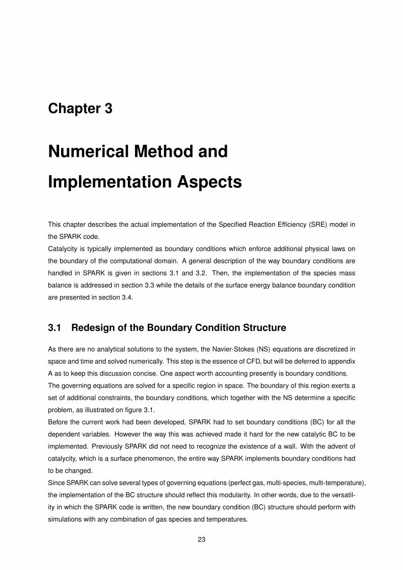
4.1.4 Mesh convergence study and computational cost . . . . . . . . . . . . . . . . . . . 39
4.2 Electre Probe . . . . . . . . . . . . . . . . . . . . . . . . . . . . . . . . . . . . . . . . . . . 41
4.2.1 Viviani et al. . . . . . . . . . . . . . . . . . . . . . . . . . . . . . . . . . . . . . . . . 42
4.2.2 Muylaert et al. . . . . . . . . . . . . . . . . . . . . . . . . . . . . . . . . . . . . . . 42
4.2.3 Barbato et al. . . . . . . . . . . . . . . . . . . . . . . . . . . . . . . . . . . . . . . . 43
4.2.4 Mesh, convergence study and computational cost . . . . . . . . . . . . . . . . . . 47
4.3 Temperature varying SRE, γ = γ(T ) . . . . . . . . . . . . . . . . . . . . . . . . . . . . . . 48
4.4 Self assessment of the implementation . . . . . . . . . . . . . . . . . . . . . . . . . . . . . 52
5 The Finite Rate Surface Chemistry (FRSC) model 55
5.1 Theoretical Overview . . . . . . . . . . . . . . . . . . . . . . . . . . . . . . . . . . . . . . . 55
5.2 Implementation of the FRSC model on SPARK . . . . . . . . . . . . . . . . . . . . . . . . 58
5.3 Stand Alone Code . . . . . . . . . . . . . . . . . . . . . . . . . . . . . . . . . . . . . . . . 59
5.3.1 Equilibrium constants to compute surface reaction rates . . . . . . . . . . . . . . . 60
5.4 Results of the Stand Alone Code . . . . . . . . . . . . . . . . . . . . . . . . . . . . . . . . 62
5.4.1 Fixed Gas Phase of Dissociated Oxygen . . . . . . . . . . . . . . . . . . . . . . . 62
5.4.2 Silica Sublimation . . . . . . . . . . . . . . . . . . . . . . . . . . . . . . . . . . . . 64
6 Conclusions 67
6.1 Achievements . . . . . . . . . . . . . . . . . . . . . . . . . . . . . . . . . . . . . . . . . . . 67
6.2 Future Work . . . . . . . . . . . . . . . . . . . . . . . . . . . . . . . . . . . . . . . . . . . . 68
Bibliography 69
A Discretization of the Navier-Stokes equations 73
A.1 Transformation of Variables . . . . . . . . . . . . . . . . . . . . . . . . . . . . . . . . . . . 73
A.2 Finite-Volume Discretization . . . . . . . . . . . . . . . . . . . . . . . . . . . . . . . . . . . 74
A.2.1 Explicit Time Integration . . . . . . . . . . . . . . . . . . . . . . . . . . . . . . . . . 75
A.2.2 Spacial Discretization of the Fluxes . . . . . . . . . . . . . . . . . . . . . . . . . . . 76
B Other Computational Results 77
B.1 Sharp Cones . . . . . . . . . . . . . . . . . . . . . . . . . . . . . . . . . . . . . . . . . . . 77
B.2 Electre Probe . . . . . . . . . . . . . . . . . . . . . . . . . . . . . . . . . . . . . . . . . . . 79
B.3 Temperature varying SRE, γ = γ(T ) . . . . . . . . . . . . . . . . . . . . . . . . . . . . . . 80
B.4 FRSC - Finite Rate Surface Chemistry . . . . . . . . . . . . . . . . . . . . . . . . . . . . . 81
x

List of Tables
1.1 Energy necessary to vaporize some typical materials. . . . . . . . . . . . . . . . . . . . . 1
4.1 Upstream conditions for all the simulations over sharp cones. . . . . . . . . . . . . . . . . 32
4.2 Computational cost of the main simulations carried out for sharp cones. . . . . . . . . . . 40
4.3 Upstream conditions for the 3 test cases from different authors over the Electre probe. . . 41
4.4 Computational cost of the main simulations carried out for the Electre probe. . . . . . . . 48
5.1 Forward reaction rates. . . . . . . . . . . . . . . . . . . . . . . . . . . . . . . . . . . . . . 57
5.2 Summary of the data of the problem. Fixed gas phase of dissociated oxygen. . . . . . . . 62
5.3 Summary of the data of the problem. Silica Sublimation. . . . . . . . . . . . . . . . . . . . 64
5.4 Concentration of gas ( mol m−3 ) and surface ( mol m−2 ) species in steady-state(equilibrium)
enabled by different sets of catalytic reactions at constant volume and constant tempera-
ture T = 2500K. Silica sublimation case. . . . . . . . . . . . . . . . . . . . . . . . . . . . . 65
xi

xii

List of Figures
1.1 Suitability of reusable and ablative TPS for different mission types. Concerns flight regimes
in the particular case of Earth’s atmosphere. . . . . . . . . . . . . . . . . . . . . . . . . . 2
1.2 Energy accommodation of TPS materials. . . . . . . . . . . . . . . . . . . . . . . . . . . . 4
1.3 RoadMap for the thesis report. . . . . . . . . . . . . . . . . . . . . . . . . . . . . . . . . . 6
2.1 Modes of molecular energy. . . . . . . . . . . . . . . . . . . . . . . . . . . . . . . . . . . . 11
2.2 Mass fraction profile of species i normal to the wall. . . . . . . . . . . . . . . . . . . . . . 16
2.3 Mass wall balance of species i at the wall. . . . . . . . . . . . . . . . . . . . . . . . . . . . 16
2.4 Specified reaction efficiency (SRE) recombination Model. . . . . . . . . . . . . . . . . . . 17
2.5 Most used models for the recombination coefficient or reaction efficiency γ. . . . . . . . . 19
2.6 Wall energy balance. Heat fluxes over the catalytic surface. . . . . . . . . . . . . . . . . . 21
3.1 The domain governed by the Navier-Stokes equations and its boundary where boundary
conditions must be specified. . . . . . . . . . . . . . . . . . . . . . . . . . . . . . . . . . . 24
3.2 Actual mesh used on this thesis for a SPARK simulation over a sharp cone. The inflow
comes from the W face. The mesh has only one block. . . . . . . . . . . . . . . . . . . . . 24
3.3 The extension of the domain with 2 rows of ghost cells. i and j are indexes. . . . . . . . . 25
3.4 Finite volume cells at the Wall. . . . . . . . . . . . . . . . . . . . . . . . . . . . . . . . . . 26
3.5 Algorithm of the explicit approach implemented on SPARK to deal with surfaces in radia-
tive equilibrium, where Tw is not known a priori. . . . . . . . . . . . . . . . . . . . . . . . . 30
4.1 RoadMap for the chapter. . . . . . . . . . . . . . . . . . . . . . . . . . . . . . . . . . . . . 31
4.2 Test cases from Miller et al., 1994 reproduced on this thesis. . . . . . . . . . . . . . . . . 32
4.3 Cone Geometric Shape and Computational Mesh . . . . . . . . . . . . . . . . . . . . . . . 32
4.4 Temperature Profile normal to cone surface at x = 0.5[m].(θ = 10o, Isothermal Wall,
Tw = 1200[K]) . . . . . . . . . . . . . . . . . . . . . . . . . . . . . . . . . . . . . . . . . . 33
4.5 Mass fraction comparison (Miller et al. vs. SPARK) of profiles normal to cone surface at
x = 0.5[m].(θ = 10o, Isothermal Wall, Tw = 1200[K]) . . . . . . . . . . . . . . . . . . . . . 33
4.6 Comparison of the specific enthalpy as a function of temperature for each species. . . . . 34
4.7 Temperature Profile normal to cone surface at x = 0.5[m].(θ = 10o, SEB) . . . . . . . . . 35
4.8 O mass fraction profiles normal to cone surface at x = 0.5[m].(θ = 10o, SEB) . . . . . . . 36
4.9 NO mass fraction profiles normal to cone surface at x = 0.5[m].(θ = 10o, SEB) . . . . . . 37
xiii

4.10 Comparison of the specific heat cpi , non-dimensionalized by the individual gas constant
Ri, as a function of temperature for each species. . . . . . . . . . . . . . . . . . . . . . . 37
4.11 Temperature Profile normal to cone surface at x = 0.5[m].(θ = 20o, SEB) . . . . . . . . . 38
4.12 Mass fraction comparison (Miller et al. vs. SPARK) of profiles normal to cone surface at
x = 0.5[m].(θ = 20o, SEB) . . . . . . . . . . . . . . . . . . . . . . . . . . . . . . . . . . . 39
4.13 Illustration of the difference in the height of the first cell at the cone surface between the
mesh used Miller et al., and the mesh of the SPARK simulations. . . . . . . . . . . . . . . 39
4.14 RoadMap for the Electre test cases. . . . . . . . . . . . . . . . . . . . . . . . . . . . . . . 41
4.15 Electre Probe’s model and Computational Mesh . . . . . . . . . . . . . . . . . . . . . . . 41
4.16 Comparison between available results from Viviani et al., 2009 and corresponding SPARK
simulations. Heat flux and pressure coefficient as a function of the nondimensionalized
length along the axis of Electre. The ”shots” correspond to experimental data. . . . . . . . 42
4.17 Comparison between available results from Muylaert et al., 1998 and corresponding
SPARK simulations. Heat flux and pressure coefficient as a function of the length along
the axis of Electre. DLR, CIRA and ESTEC are independent CFD codes. . . . . . . . . . 43
4.18 Temperature and N2 and N mass fractions along the normal to Electre’s wall at x = 0.1m
for Tw = 343K. Comparison of current results under SPARK with Barbato et al., 1994.
Equ. on the legend stands for equilibrium wall boundary condition. . . . . . . . . . . . . . 44
4.19 Mass fractions of species O2, O and NO along the normal to Electre’s wall at x = 0.1m for
Tw = 343K. Comparison of current results under SPARK with Barbato et al., 1994. Equ.
on the legend stands for equilibrium wall boundary condition. . . . . . . . . . . . . . . . . 45
4.20 Comparison between available results from Barbato et al., 1994 and corresponding SPARK
simulations for Tw = 800K. Heat flux as a function of the length along the axis of Electre. . 46
4.21 Illustration of the formation of a shock wave in front of Electre, and the outer limits of two
computational meshes that follow the shock’s shape. . . . . . . . . . . . . . . . . . . . . . 47
4.22 Recombination coefficients/reaction efficiency (γ) on the surface of the cone as a function
of its axial length for the 3 models implemented in SPARK applied on the same case:
Sharp Cone, Semi-angle=20o, SEB.. The temperature is the same for all plots. Ranges
of left hand y-axis are not the same. . . . . . . . . . . . . . . . . . . . . . . . . . . . . . . 49
4.23 Mass fraction of the dissociated species N, O and NO on the surface of the cone as a
function of its axial length for several models applied on the same case: Sharp Cone,
Semi-angle=20o, SEB. Ranges of y-axis are not the same. γN = γO = γ. . . . . . . . . . . 51
5.1 Road Map for the chapter. . . . . . . . . . . . . . . . . . . . . . . . . . . . . . . . . . . . . 55
5.2 Practice to compute thermodynamic variables for surface species. . . . . . . . . . . . . . 61
5.3 Comparison between the current results and results from MacLean et al., 2011. Percent-
age of sites containing O(s) as a function of temperature for 200, 2000 and 20000 Pa.
Case: 10% O - 90% O2. . . . . . . . . . . . . . . . . . . . . . . . . . . . . . . . . . . . . . 63
xiv

5.4 Comparison between the current results and results from MacLean et al., 2011. Loss
efficiency as a function of temperature for 200, 2000 and 20000 Pa. Case: 10% O - 90%
O2. . . . . . . . . . . . . . . . . . . . . . . . . . . . . . . . . . . . . . . . . . . . . . . . . . 63
A.1 A typical control volume cell and its neighbours along with the surface frontiers S and the
remaining notation used. . . . . . . . . . . . . . . . . . . . . . . . . . . . . . . . . . . . . . 75
B.1 SPARK results for mass fraction of profiles normal to cone surface at x = 0.5m.(θ = 10,
SEB) using kinetics from Park, 2001 vs. Blottner, 1971. . . . . . . . . . . . . . . . . . . . 77
B.2 SPARK mesh convergence study for the 3 test cases of sharp cones reproduced by
SPARK. The variable examined is the temperature profile normal to the cone surface
at x=0.5[m]. . . . . . . . . . . . . . . . . . . . . . . . . . . . . . . . . . . . . . . . . . . . . 78
B.3 SPARK mesh convergence study for the scenarios concerning the Electre probe. The
quantity examined is the heat flux into Electre. . . . . . . . . . . . . . . . . . . . . . . . . 79
B.4 Temperature along the normal to Electre’s wall at x = 0.1m for Tw = 343K. Comparison
of current results under SPARK for two catalytic recombination coefficients γ = 1 and γ =
0.01 to examine their effect on temperature. Upstream conditions correspond to Barbato
et al. . . . . . . . . . . . . . . . . . . . . . . . . . . . . . . . . . . . . . . . . . . . . . . . . 79
B.5 Mesh used on the simulations for verification of the temperature dependent recombination
efficiency models implemented on SPARK. Details: θ = 20, 40X50 cells. The discrete
black points represent the location of the profiles(temperature and mass fractions). The
cone starts at x=0. . . . . . . . . . . . . . . . . . . . . . . . . . . . . . . . . . . . . . . . . 80
B.6 2-dimensional plot of temperature for SPARK simulation case: Sharp Cone, Semi-angle
= 20, SEB. Catalytic model not relevant as temperature was grossly insensitive to it. . . . 80
B.7 Mass fraction of species N2 and O2 on the surface of the cone as a function of its axial
length for several models applied on the same case: Sharp Cone, Semi-angle = 20, SEB.
Ranges of y-axis are not the same. γN = γO = γ. . . . . . . . . . . . . . . . . . . . . . . . 80
B.8 Transient evolution of the species concentrations (mol m−3 or mol m−2) from an initial
condition consisting of only bulk silica, argon and free sites. The temperature is 2500 K
and the initial pressure is 10000 Pa. All surface reactions included. Silica sublimation case. 81
xv

xvi

.
xvii

Nomenclature
Greek symbols
[τ ] Viscous stress tensor, N m−2
χi Mole fraction of species i on a bulk environment.
ε Emissivity of the surface.
γ Catalytic recombination coefficient, also known as reaction efficiency. When accompanied with
an index γi is concerns a particular catalytic reaction for which species i is the reactant, dimen-
sionless
ν Fundamental vibrational frequency of a molecule.
νgr Stoichiometric coefficient that runs only over gas species:∑i
(ν′′
ir − ν′
ir
)ν′
ir, ν′′
ir Stoichiometric coefficients of species i on reactant and product sides of a chemical equation r,
respectively.
Φs Active site density, mol m−2.
Φns,i Concentration of gas species i on surface phase ns. The index ns may be omitted if only one
surface phase exists, mol m−2.
ρ Density, kg m−3.
σ Stefan-Boltzmann constant.
Roman symbols
ci Mass fraction of species i.
ci,w Mass fraction of species i at the wall.
Ci Concentration of species i, i.e., number of moles of species i per unit volume of mixture, mol m−3.
Ri Specific gas constant of species i, J kg−1 K−1.
Ru Universal gas constant, J mol−1 K−1.
R Specific gas constant of a mixture, J kg−1 K−1.
xviii

Xi Generalized concentration of species i. Has a different symbol and units if it concerns a gas,
surface of bulk species.
∆n Distance from the internal cell to the wall.
ωir Production rate of species i due to reaction r. Due to convenience the units are kg m−2 s−1 for
the SRE model and mol m−2 s−1 for the FRSC model.
ωi Production rate of species i due to all reactions. Due to convenience the units are kg m−2 s−1 for
the SRE model and mol m−2 s−1 for the FRSC model.
~u Mean flow velocity, m s−1
Cp Specific heat at constant pressure, J kg−1 K−1
Cv Specific heat at constant volume, J kg−1 K−1
D Diffusion coefficient, m2 s−1.
E Total energy, J
G0i Gibbs energy of species i, J mol−1.
h Specific enthalpy kJ kg−1 or Plack’s constant
H0i Enthalpy of species i, J mol−1.
k Thermal conductivity, J s−1 m−1 K−1
kfr, kbr Forward and backward reaction rates for reaction r, units vary.
M↓ Impinging mass flux, kg m−2 s−1.
Ns Number of species.
p Pressure, Pa.
S0i Entropy of species i, J mol−1 K−1.
T Temperature, K
Subscripts
∞ Free-stream value.
g Gas species.
i Species index. When in a different font i represents an internal cell, namely the first internal cell
after the ghost cells.
j Species index, although the most common subscript for the species index is i.
r Index of a reaction.
xix

s Surface species
g Evaluated at the ghost cell. On the FRSC model it may also mean gas species.
ref Reference condition.
w Evaluated at the wall.
xx

Glossary
CFD Computational Fluid Dynamics is a branch of
fluid mechanics that uses numerical methods
and algorithms to solve problems that involve
fluid flows.
DPLR Data Parallel Line Relaxation is a CFD code
employed by NASA Ames Research Center
for re-entry flow calculations. It is a struc-
tured, finite volume code that solves the react-
ing Navier-Stokes equations.
ER The Eley-Rideal mechanism describes the sur-
face reaction between a reactant molecule from
a gas phase and one that is absorbed on the
surface.
FRSC Finite Rate Surface Chemistry is a state-of-art
formulation to deal with catalycity. In contrast
with the SRE method, it takes into account the
microscopic processes through which surface
reactions occur.
IPFN Instituto de Plasmas e Fusao Nuclear is a re-
search unit of Instituto Superior Tecnico from
the University of Lisbon.
LAURA Langley Aerothermodynamic Upwind Relax-
ation Algorithm is a structured, finite volume
CFD code that solves the reacting Navier-
Stokes equations.
LH The Langmuir–Hinshelwood mechanism de-
scribes the surface reaction between two ad-
sorbed species that undergo a bimolecular re-
action.
xxi

LeMANS (Le) Michigan Aerothermodynamics Navier-
Stokes is a CFD code developed at the Uni-
versity of Michigan. It is an unstructured, finite
volume code that solves the reacting Navier-
Stokes equations.
NV Navier-Stokes, as in Navier-Stokes equations,
is a set of equations that governs fluid flow.
ODE Ordinary Differential Equation.
SEB The Surface Energy Balance constitutes a
boundary condition that assumes that the wall
is in radiative equilibrium. There is no conduc-
tion loss through the wall, and the incoming en-
ergy is balanced by the emissivity of the wall.
SPARK Software Package for Aerothermodynamics,
Radiation and Kinetics is a multiphysics code
developed and maintained at IPFN. It is struc-
tured, finite-volume code that solves the react-
ing Navier-Stokes equations.
SRE Specified Reaction Efficiency is formulation
used by CFD codes to deal with catalycity in
which a surface efficiency, or surface recombi-
nation coefficient, often denoted γ, is specified
as a constant or as a function of temperature.
The value determines the ratio of consumption
of a given atomic species that impinges on the
wall.
TPS A Thermal Protection System is a barrier to pro-
tect a space vehicle from the intense heat flux
experienced during atmospheric re-entry.
V&V Verification and Validation is a set of processes
to assess the credibility and reliability of com-
puter simulations.
xxii

Chapter 1
Introduction
1.1 Topic Overview
Space vehicles enter a planetary (Earth or other planet) atmosphere at near orbital (V∞ = 7.9 kms for
Earth) and super-orbital speeds, relative to the atmosphere [3]. In this hypersonic flow regime a strong
shock-wave is formed upstream of the spacecraft, wherein the flow slows down to subsonic speeds. The
total energy associated with such high velocities (≈ 12mV
2) is partially converted into internal energy of
the gas giving rise to various physical processes like dissociation, ionization occurring between the
shock and the vehicle. As a first approximation if we assume that all this energy is absorbed by the
vehicle [4], few materials could withstand this level without disintegrating:
Q =1
2mV 2 ⇔ Q
m=V 2
2
Earth re-entry V∞ ≈ 7.9kms
:Q
m= 31 401
kJkg
(1.1)
Where Q is the total (kinetic) energy, m is the mass of the spaceship and V its velocity. Table 1.1 shows
that only parts made of graphite would resist and that there is 3.5 × the energy needed to vaporize
Titanium.
Material Energy to Vaporize [kJ/kg] Melting Temperature [K]Tungsten 4350 3611Titanium 8990 2056
Beryllium Oxide 31168 1611Graphite 66756 3778
Table 1.1: Energy necessary to vaporize some typical materials, adapted from [4]
Moreover, if we make a quick estimate for the stagnation temperature on the nose of the vehicle [4] with
1

the help of the steady one-dimensional heat equation [5, pp. 51-52]:
h∞ +V 2∞2
= h0 +V 2
0
2︸︷︷︸=0(Stagnation)
⇔
CpT∞ +V 2∞2
= CpTo ⇔
Using the approximation T0 T∞ : T0 =V 2∞
2Cp
Earth re-entry V∞ ≈ 7.9kms
: T0 = 31 245K
Where h is the enthalpy, Cp is the specific heat constant taken to be 1.005 kJkg K , T is the temperature,
and the subscripts 0 and ∞ refer to stagnation and free-stream respectively.
Again, from table 1.1, this temperature value is more than most materials can endure. Admittedly this is
a crude analysis, and not all the energy is absorbed by the vehicle. However these concise calculations
help evidencing why heat loading is both a key parameter and a challenge for the design of entry space-
craft. Effectively, the surface of such vehicles must be equipped with a Thermal Protection System (TPS)
designed to sustain heat loads of this magnitude withtout endangering the underlying structure [6]. De-
pending heating on the heating levels, there are two TPS classes that can be employed: Reusable TPS
and ablative TPS [7]. The corresponding range of applicability is illustrated on figure 1.1.
Figure 1.1: Suitability of reusable and ablative TPS for different mission types, reproduced from [8].Concerns flight regimes in the particular case of Earth’s atmosphere.
• Reusable TPS
Reusable TPS are characterized by not promoting property changes or mass loss of the TPS ma-
terials. In other words, they retain structural integrity and their physical properties up to a critical
point. Catalytic reactions occur at the surface but do not involve the surface materials. Such reac-
tions consist on the recombination of the incoming dissociated environment gas. As recombination
increases the heat carried to the vehicle, it is desirable to have a surface with low catalycity . Also,
2

the surface may irradiate some energy, as a function of its black-body temperature, and therefore
net radiation is an important mechanism of heat transfer. The surface coating should have a high
emissivity to carry as much heat away as possible [7].
The Space Shuttle program was the responsible for a great emphasis on reusable TPS research (
at the cost of ceasing ablative TPS) [8], and hence is the source of much of the experimental data
and theoretical models known [9, 10].
A disadvantage of reusable TPS is that they are systems limited for operation in relatively mild
aerothermal re-entry conditions.
• Ablative TPS
Ablative TPS can handle higher heating rates by allowing material property changes and also
sacrificing TPS material/mass. There are two ways through which this mass loss occurs:
– Pyrolyzing/charring ablating TPS
Pyrolysis is the decomposition of the internal solid material and occurs when the material is
exposed to high temperatures. It produces gaseous products that end up being injected in the
boundary-layer due to the gas pressure inside the pyrolysis zone [6]. As the pyrolysis gases
ascend to the boundary layer, they absorb some of the energy from the solid material. On the
surface itself, a char layer is formed that recedes due to chemical or mechanical action.
These TPS are composites of polymer resins with some other reinforcement material (gener-
ally carbon, glass or organic polymers) [11].
– Non-pyrolyzing/non-charring ablating TPS
In contrast, non-charring materials don’t undergo in-depth decomposition. Instead, the ex-
posed surface chemically reacts with the gas environment resulting in sublimation and vapor-
ization (endothermic) and oxidation and nitration (exothermic). The corresponding reaction
products are diffused into the boundary-layer promoting its cooling and reducing the heat flux
into the wall. This phenomenon is referred as ”blowing”. Such mechanisms yield a specific
surface consumption rate and have a great impact on the net energy to the surface [7].
In contrast with charring ablative TPS, noncharring ablative TPS are usually made of car-
bon or silica. They are denser and structurally stronger than charring ablators, and can also
withstand higher shearing stresses [12].
Furthermore, and as can be seen on figure 1.2, radiation is also a relevant energy transfer mecha-
nism for ablative TPS. Again it is desirable to have a high emittance surface to promote re-radiation
[13], specially when the temperatures are higher.
In short, ablative TPS burn away in a controlled manner so as to dissipative heat. The physical
and chemical processes involved are, when compared with reusable TPS, more varied and much
more complex.
3

(a) Reusable TPS (b) Ablative - charring and non-charring - TPS
Figure 1.2: Energy accommodation of TPS materials [7].
1.2 Ground Testing and CFD Modeling for re-entry problems
Because experimental data is very rare, owing to prohibitive costs of on-board experiments ( atmo-
spheric re-entry ), this field depends greatly on ground testing and CFD. Ground tests are widely used
but present certain limitations in simulating turbulent flow, high shear, high pressure gradients and com-
bined convective and radiative heating [8]. The types of existing ground testing facilities are arc jets,
inductively coupled plasma facilities, energy laser facilities, shock tubes and arc heaters. The first two
are the most common [11]. However, none of these single facilities is able to replicate all actual re-entry
flight conditions simultaneously, which is why ground testing is usually delegated to development and
selection of TPS materials and validation of the CFD simulations on a segmented way [14]. That is, each
facility is used for validation within the specific test conditions it is able to reproduce.
Aero-thermodynamics is a multidisciplinary topic. CFD in non-equilibrium flow is thus particularly com-
plex. There have been many improvements on the past decades, namely in the numerical solvers and
the non-equilibrium thermodynamic models. Despite this, the improvements that directly concern TPS
design have been, until recently, overlooked. In fact, most codes model surface conditions with a con-
stant temperature or a constant heat flux, and neglect mass transfer altogether. This is incompatible with
the complex chemical and physical interactions between the surface and the gas occurring on ablative
TPS. Even on reusable TPS, a fixed temperature or constant heat flux along the entire surface is too
simplistic.
More recently, a few codes have implemented the modelling of fluid/surface interaction, i.e., the ap-
propriate coupling of the homogeneous flow with the vehicle’s surface behaviour. The most known and
complete are LeMANS from the University of Michigan [15], DPLR from the NASA Ames research center
[16, 17] and the 2008 LAURA update from NASA Langley [18]. They represent the current state-of-the-
art, specially in TPS modelling, and are capable of dealing with non-charring ablation as well as charring
ablation.
Most of the remaining codes can just be expected to model reusable TPS. Because the heating rates
are not high, the CFD implementation just needs to take into account certain catalytic reactions at the
4

surface, namely recombination reactions, and not the surface participating reactions like sublimation,
characteristic of ablation. For air environments, normally the recombination of O and N is modelled:
N + N −−→ N2
O + O −−→ O2
N + O −−→ NO
(1.2)
These reactions need to be taken into account on both the energy and mass balance boundary con-
ditions. To model recombination effects, it is customary to define a parameter γ that macroscopically
expresses the ratio between the number of incoming atoms from the dissociated gas, and the number
of those atoms that recombine through 1.2. The more recombination exists, the higher the heat transfer
to the vehicle as determined by the energy balance equation. Often some CFD codes just assume a
worst case scenario that results in the highest possible heat transfer, in order to avoid the modelling just
described. On the other hand, more sophisticated codes discard this macroscopic approach and take
into account the microscopic pathways through which these reactions occur.
Obviously there is a certain division on the capabilities of the various CFD programs that follow the de-
mands of each TPS classes previously discussed. In other words, certain codes can just model reusable
TPS while others can fully model ablative TPS [19].
1.3 Objectives
This works aims at improving the capabilities of the SPARK code.
SPARK - Software Package for Aerothermodynamics, Radiation and Kinetics - is a multiphysics code
capable of hypersonic re-entry simulations. It has been developed and is maintained at IPFN - Instituto
Superior Tecnico, by Bruno Lopez. SPARK is a 2-dimensional, structured, finite-volume, reactive Navier-
Stokes equations solver, that takes into account finite-rate chemistry and vibrational non-equilibrium
effects. It is written in Fortran 03/08 language via oriented object programming.
Before the present work, SPARK was unable to deal with the most basic form of catalycity. The first
objective consisted in implementing in SPARK a versatile capability of catalycity that was at the level of
reusable TPS. Versatility means a code that adapts, without further changes, to different simulations;
that is, a code that is not hard-coded.
The general approach followed is not much different from the one many other codes have implemented
in the past. This is because the model (in the analytical sense) that describes reusable TPS is fairly
straightforward and is more or less closed to any improvements. The differences are therefore on the
numerical implementation itself that depend to a large extent on computational scheme each code uses
to discretize and solve the Navier-Stokes equations. Furthermore, for clarity, this model shall be referred
to as the SRE - Specified Reaction Efficiency - model, or simply the ”constant γ” model. On the literature
there is no universal naming convention for it.
The second objective consisted in a preliminary formulation of the Finite-Rate Surface Chemistry (FRSC)
5

model. The FRSC model serves 2 purposes. On one hand it is able to model catalytic reactions more
rigorously than the SRE model. It is more rigorous because the SRE model is phenomenological while
the FRSC follows the physics of the surface reactions. On the other hand the FRSC approach is able
to completely model surface altering reactions (e.g., sublimation) that lead to surface consumption and
are the basis for non-charring ablation. The FRSC model was developed by MacLean et al. [17, 20] for
the DPLR code of NASA Ames, but has also been implemented in LeMANS by Alkandry et al. [21] and
used by Abhilasha Anna [11]. There is a vast gap - from both a theoretical and CFD implementation
point of view - between the SRE and FRSC models. As such, the objective regarding the FRSC model
consisted in developing a code external to SPARK that permits to verify surface reactions decoupled
from the flow field. This stand alone code is a preliminary step before a full implementation of the FRSC
onto SPARK.
1.4 Thesis Outline
The natural way to divide this thesis is between the SRE and FRSC model because they are very distinct
and were developed independently. The thesis presents both topics separately, meaning that there is
a theoretical introduction, implementation and results section for each one individually and in different
parts of this document. The bulk of the work of this thesis was devoted to the SRE model, and thus it
makes up most of this report, namely chapters 2, 3 and 4. In contrast, everything related with the FRSC
model is presented in chapter 5. It is important to note that there are a lot of similarities between an
SRE implementation and a FRSC implementation on a CFD code but for the limited functionalities of the
FRSC developed in this thesis, the FRSC model is independent on the SRE model.
Figure 1.3: RoadMap for the thesis report.
The second chapter begins with an overall account of the relevant aspects of re-entry simulations. Then
it describes the approaches commonly used to model catalycity, followed by a detailed discussion of the
6

role of the mass and energy balances.
On the third chapter the techniques used by SPARK to deal with boundary conditions are introduced.
This is followed by the numerical discretization of the analytical boundary conditions derived on chapter
2 and their implementation on SPARK.
The fourth chapter presents various CFD simulations using SPARK and the results are compared with
experimental data and other numerical codes. The goal here is to judge whether the objectives were
met, that is, if catalycity was correctly implemented in SPARK. When discrepancies are found between
the results, informed discussions often requiring topics introduced on the background chapter, ensue.
Lastly, chapter five is entirely devoted to the FRSC model. On its sections, the original formulation on
surface chemistry is presented, followed by a rationale on how to fully implement the model in SPARK
in the near future and ending with a comparison of the results with MacLean et al. [17, 20].
7

8

Chapter 2
Physical Models
Adding new catalytic features to SPARK can not be done disregarding the rest of SPARK itself. In other
words, the catalytic module cannot be developed in a black-box approach, in which the implementation
would receive input data from the main code, process it, and return output. Because catalycity depends
on the flow-field it is intertwined with other phenomenon particular to aerothermodynamics, such as high-
temperature thermodynamic properties, non-equilibrium effects, and transport properties. Adding to this,
catalycity directly effects the flow field (particularly the flow field near the wall) which becomes evident
during the post-processing of the results. For this reasons it is necessary to study certain aspects of
aerothermodynamics as a background for the correct implementation of catalycity and also the correct
interpretation and post-processing of the results. This aspects are discussed on the following sections.
Other theoretical considerations are delegated to the appendices.
This chapter describes the underlying physical models along with the governing equations that have
been used in this work. As stated in the introduction, the current work has been performed using
the Spark code which includes a large set of physical models related to thermodynamics, transport
properties, chemical kinetics and energy exchange processes. Although a detailed description of all
these models is out of the scope of this work, these models are strongly coupled to the gas-surface
models which have been implemented within this master thesis. Therefore, the various physical models
involved in the gas-surface processes are briefly presented here for completeness. This chapter starts
by presenting the set of governing equations in section 2.1 for a multi-species, multi-temperature gas.
Then, the thermodynamic relations used to described the state of a gas in high temperature conditions
are given in section 2.2. The modelling of thermo-chemical non-equilibrium processes is presented in
section 2.4. The last section, section 2.5, addresses the modelling of gas-surface interactions, and
represent to main contribution of the current work.
9
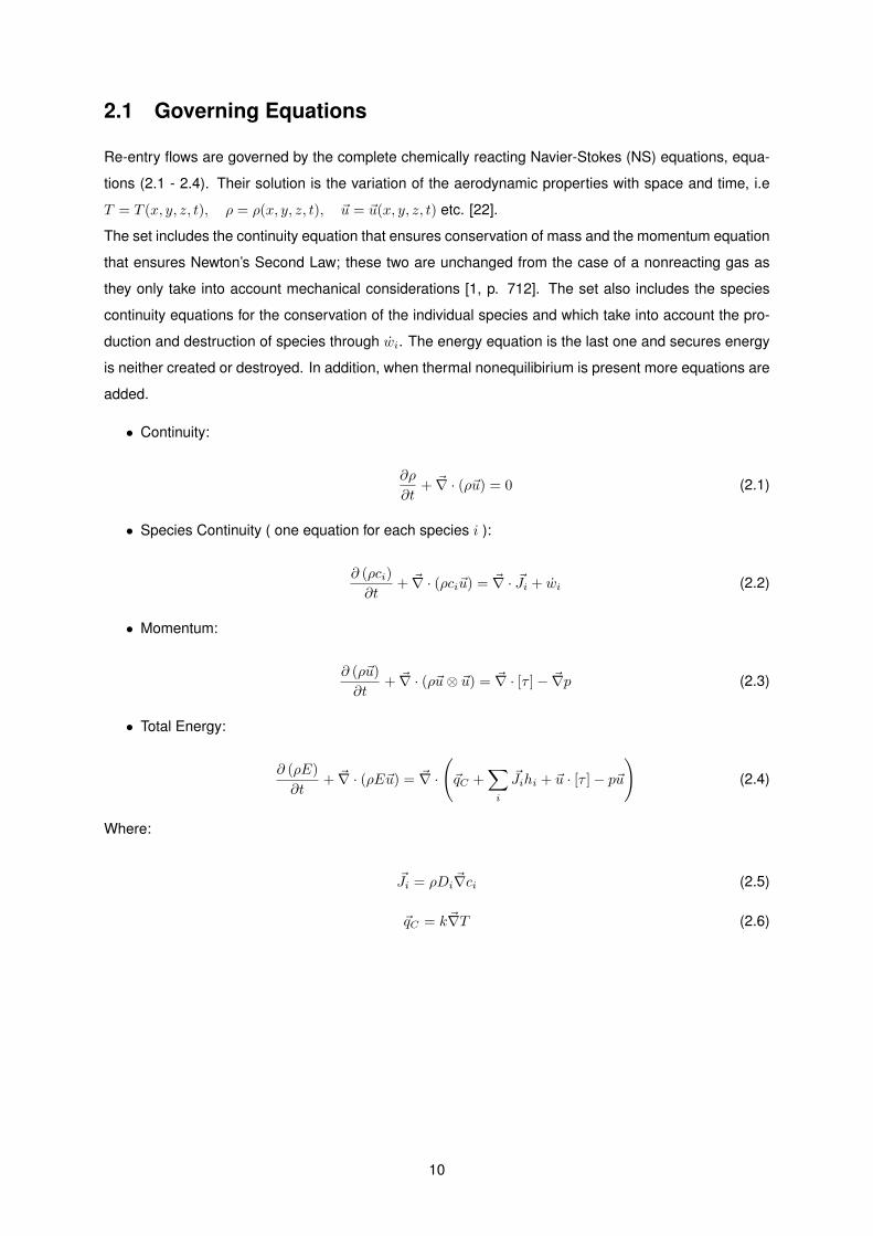
2.1 Governing Equations
Re-entry flows are governed by the complete chemically reacting Navier-Stokes (NS) equations, equa-
tions (2.1 - 2.4). Their solution is the variation of the aerodynamic properties with space and time, i.e
T = T (x, y, z, t), ρ = ρ(x, y, z, t), ~u = ~u(x, y, z, t) etc. [22].
The set includes the continuity equation that ensures conservation of mass and the momentum equation
that ensures Newton’s Second Law; these two are unchanged from the case of a nonreacting gas as
they only take into account mechanical considerations [1, p. 712]. The set also includes the species
continuity equations for the conservation of the individual species and which take into account the pro-
duction and destruction of species through wi. The energy equation is the last one and secures energy
is neither created or destroyed. In addition, when thermal nonequilibirium is present more equations are
added.
• Continuity:
∂ρ
∂t+ ~∇ · (ρ~u) = 0 (2.1)
• Species Continuity ( one equation for each species i ):
∂ (ρci)
∂t+ ~∇ · (ρci~u) = ~∇ · ~Ji + wi (2.2)
• Momentum:
∂ (ρ~u)
∂t+ ~∇ · (ρ~u⊗ ~u) = ~∇ · [τ ]− ~∇p (2.3)
• Total Energy:
∂ (ρE)
∂t+ ~∇ · (ρE~u) = ~∇ ·
(~qC +
∑i
~Jihi + ~u · [τ ]− p~u
)(2.4)
Where:
~Ji = ρDi~∇ci (2.5)
~qC = k~∇T (2.6)
10

2.2 Thermodynamic Relations
Aerothermodynamics requires a microscopic description of the gas. The gas is assumed to be made
of a large number of molecules and atoms. These molecules have four modes of energy which are
illustrated on figure 2.1. The total energy of a molecule is the sum of the energies of the 4 modes,
namely translation, rotational, vibrational and electronic energies:
ε = εtrans + εrot + εvib + εel + ε0 (2.7)
Due to conventions [2, p. 129] ε0, representing the zero point energy, which is equal to the energy of
the molecule at absolute zero [1, p. 507] has to be added. This means that εtrans, εrot, εvib and εel are
energies above the zero-point energy at T = 0K. A Boltzmann distribution is assumed, which means the
Figure 2.1: Modes of molecular energy. Reproduced from [23].
thermodynamic properties are computed assuming statistical thermodynamics. Assuming a Boltzmann
distribution is common practice in all the CFD codes in existence. This is mainly because of the compu-
tational cost of not assuming a Boltzmann distributions, i.e the State-to-State approaches, is currently
too high to be practically considered other than in simplified time relaxation or steady-state models.
Accordingly, from statistical thermodynamics, the internal energy per unit mass of a pure chemical
species i is:
etrans =3
2RiT
erot = RiT
evib =hν/kT
ehν/kT − 1RiT
eel = eel
(2.8)
11
ei =3
2RiT +RiT +
hν/kT
ehν/kT − 1RiT + eel + (∆hf )
0i (2.9)
Where Ri is the specific gas constant and ν is the vibrational frequency of the molecule.
The previous is for a single chemical gas species. The first 4 energies are measured above the zero-
point energy while ei is the absolute energy. (∆hf )0i is heat of formation of species i per unit mass, and
embodies an effective zero point energy [1, pp. 245, 557].
For a mixture of such gases, the internal energy per unit mass of mixture is:
e =∑i
ciei (2.10)
Where e includes the zero-point energy through ei, and ci is the mass fraction of species i.
The specific enthalpy for a single gas species and for a mixture is given by equations (2.11) and (2.12)
respectively:
hi ≡(e+
p
ρ
)i
= ei +RiT (2.11)
h =∑i
cihi (2.12)
Furthermore, the specific heat at constant volume, Cv, and the specific heat at constant pressure, Cp,
are defined as:
Cv ≡(∂e
∂T
)v
and Cp ≡(∂h
∂T
)p
(2.13)
Introducing (2.10) and (2.12) into expressions (2.13):
Cv =
∑i
(ci∂ei∂T
+ ei∂ci∂T
)Cp =
∑i
(ci∂hi∂T
+ hi∂ci∂T
) (2.14)
For CFD applications, the thermodynamic properties previously discussed - namely energy, enthalpy and
specific heats - need to be obtained for use during the calculations. Using the aforementioned expres-
sions for their computation at running time is the most obvious approach. This means expressions (2.9
- 2.14) are explicitly evaluated as the code runs. However, due to convenience, two other approaches
have been frequently used by CFD codes to access the properties when the mixture is air. There are
several tables with the thermodynamic properties of an air mixture and/or of the species present in it
(e.g., N2, O2 etc.) [24]. These tables can be incorporated on the CFD code which interpolates between
its discrete entries when necessary or, in alternative, the data of these tables can be correlated through
polynomial expressions, and these used directly by the code.
12

2.3 Transport Properties
There are 3 transport coefficients to account for dissipative effects: Viscosity, thermal conductivity and
the diffusion coefficient. For catalycity only the diffusion coefficient Di is relevant.
There are various models to compute the diffusion coefficient, which vary in terms of ”exactness” and
computational expensiveness. For all the simulations performed under the current work in SPARK, only
the most simple approach for Di was used. It consists in assuming a constant Lewis number Le, and
evaluating the expression:
Di =Le k
ρCp(2.15)
Where Cp is the total specific heat at constant pressure and k is the thermal conductivity.
The model (2.15) is not derived from any physical considerations but for Le values ranging between
1 and 1.4, it gives good estimates for the diffusion coefficient. It is thus a straightforward, computa-
tional inexpensive approximation that has a practical advantage over more advanced models in which
Di = f(ci, p, T ) and that are more expensive.
The Lewis number on the SPARK simulations was changed according to the value used in the results
being emulated. By default SPARK uses Le = 1.2.
2.4 Nonequilibrium Processes
Let us imagine the flow of an element of fluid through a continuously changing steady state field. When
equilibrium is assumed, this fluid element is supposed to instantaneously adapt, as it moves through
the flow, to the local p and T. However, this is never the case because this adaptation occurs through
molecular collisions, that take time and are thus not instantaneous [1, 2]. The question then arises of
when is thermodynamic equilibrium a valid approximation to describe this fluid element. If the character-
istic time of the collisional processes τc to achieve equilibrium is of the same order as the characteristic
time of the gas flow τf (∼ lV∞
where l is a characteristic length) then equilibrium is not at all suitable
and nonequilibirum must be taken into account [2, p. 197]. If, on the contrary, the characteristic time
for collisions is negligible when compared with the characteristic flow time as on described in (2.16),
thermodynamic equilibrium is a very practical and applicable approximation.
Nonequilibrium :τf ∼ τc
Equilibrium :τf τc
(2.16)
For the case of a re-entry vehicle, a bow shock wave will be formed ahead of the vehicle [1, 3]. Generally,
across this shock wave, the p and T change in such a abrupt manner, that the fluid element will not be
able to keep up1. Thus, a certain amount of time will be needed, after the shock, for the molecular
collisions to enforce equilibrium conditions. For that reason, chemical reactions are needed to describe
1This actually depends on the density and velocity of re-entry [1, p. 647]
13

this flow.
The general chemical equation for the homogeneous reaction r is:
∑i=1
ν′
irXi ∑i=1
ν′′
irXi (2.17)
Where ν are stoichiometric coefficients.
It is an observable fact that the rate of formation of the various species i involved in an elementary
reaction r can be expressed by:
(d [Xi]
dt
)r
= (ν′′
ir − ν′
ir)
kf,r
∏i=1
Xν′iri − kb,r
∏i=1
Xν′′iri
[molm3 s
](2.18)
Where kf,r and kb,r are the forward and backward reaction rates respectively, and depend only on
temperature.
Remembering the discussion at the beginning of the chapter, it is now appropriate to emphasize certain
aspects of this topic that are specially important further down the thesis and which are generally know
as the ”kinetic scheme”. There are 2 considerations. On one hand, 1) the number of reactions one uses
to describe a specific flow is not universally fixed and may depend to some extent on the judgement of
the researcher. In a gas flow we have to ascertain the species present, then nonequilibium is outlined
by all the reactions possible between those species. Despite this, only a subset of those species and
reactions might be sufficient for gas-dynamic calculations. Obviously, the outcome of choosing a wrong
subset is an incorrect result, but various sub-sets might correctly model the nonequilibrium. Taking the
example of air, below 8000 K the only species expected to exist in significant amounts are N2, O2, N, O
and NO [2, p. 230]. The reactions taken to be sufficient are r = 1 - 6 below, but reaction 7 is often added
in which case species NO+ and e– should be added to the subset of relevant species.
r = 1 : O2 + M −−−− 2 O + M
r = 3 : NO + M −−−− N + O + M
r = 5 : N2 + O −−−− NO + N
r = 7 : N + O −−−− NO+ + e−
r = 2 : N2 + M −−−− 2 N + M
r = 4 : NO + O −−−− O2 + N
r = 6 : N2 + O2−−−− 2 NO
Where M is any of the other species.
On the other hand, 2) the chemical rates kf,r and kb,r are generally measured by experiments whose
results are correlated in an expression called the Arrhenius equation:
k = AT−ne−ΘR/kT (2.19)
Where A, n and ΘR are fitted from experiments.
Because this rates are difficult to measure experimentally there is always some uncertainty on the data
available [1, 2]. Besides, the rate data is constantly being updated by new models and experiments,
such that the rates kf,r and kb,r, for a specific elementary reaction, change over the years.
14

2.5 Gas-Surface Interactions
2.5.1 Species Mass Balance
When a reactive gas is considered, a boundary condition must by specified to model the species mass
fractions at the wall. These models are often referred as wall catalycity. Several different approaches
can be used to describe wall catalycity:
Non-catalytic model: In this model the surface behaves as being indifferent to the gas flow. The im-
pinging atoms on the vehicle wall do not recombine. No diffusion occurs. Note this was the only
BC model implemented in SPARK at the start of this master thesis.
Fully catalytic model: This model assumes all the incoming atoms recombine into molecules releasing
heat into the surface thus providing an upper bound for the heat flux into the vehicle.
Partially catalytic model: This model assumes that only a fraction of the incoming atoms recombines
at the wall. The first two models are therefore particular cases. This was the model implemented
on SPARK. On this thesis it is referred as the Specified Reaction Efficiency (SRE) model.
Super catalytic model: This model imposes the composition at the wall to be equal to the free-stream
composition.
The equilibrium wall model: This model assumes that the wall composition is the equilibrium compo-
sition at the wall pressure and temperature.
Finite-rate model: This model accounts for the actual chemical processes occurring on the surface. It
is a very advanced model based on the actual microscopic steps involved in a surface reaction.
On this thesis it is referred as the FRSC model.
Note that the fully catalytic model is physically consistent in the sense that it represents the overall
efficiency of all microscopic reactions concerning a particular species i. On the other hand, the super-
catalytic and the equilibrium wall models have no physical significance because there is no mechanism
to impose, for example, the wall and free-stream compositions to be equal. They are used in some CFD
codes because for Earth re-entry they provide results similar to the fully-catalytic model and because
they are easier to implement.
Species boundary condition
All the expressions which define boundary conditions follow from one or several physical principles. On
a catalytic wall these principles are the mass balance of species i at the energy conservation at the wall.
We know, by Fick’s Law of diffusion, that when in a given mixture there is a gradient of mass fraction of a
given species i , there will be a mass motion of this species in the direction opposite of the gradient. For
a gas with more than two species, the flux ji of this particles is approximately given by equation (2.20)
15

where the minus sign requires the flux to be opposite to the gradient.
ji = −ρDi∇ci (2.20)
Where Di is the diffusion coefficient of species i and ρ is the density of the mixture.
Given the direction n, normal to the surface on figure 2.2, the mass flux into the wall is given by (2.21).
If the slope at the wall is positive, as in curve (2), there is a positive flux of species from the fluid to the
wall. On the other hand, in curve (1) the slope is negative and the wall is diffusing species i into the flow.
Figure 2.2: Mass fraction profile of species i normal to the wall.
(ji)w, into the wall =
(ρDi
∂ci∂n
)w
(2.21)
We are now in a position to derive the boundary condition. Referring to illustration 2.3, if we imagine a
control volume that envelops the flow/surface interface, in steady state, the net rate of diffusion of species
i to the surface must be balanced to the rate at which species i is being destroyed due to catalycity.
Figure 2.3: Mass wall balance of species i at the wall.
It is important to address a misnomer supported by some authors [25, 26]. The physical principle at play
here is not the mass conservation of species i which does not occur since each species is literally being
destroyed or created but rather a steady-state mass balance. There is however a mass (or number)
conservation of chemical elements independent of their molecular configuration (i.e. 2 O atoms in a O2
molecule). This physical principle is used further down the implementation.
For this purpose, let ωi,w be the production of species i (mass of species i per second per unit area).
Henceforth, at the wall, the rate at which species i diffuses into the wall must be balanced by the surface
amount of its destruction, which given the definition above, is (−ωi,w):
(ji)w, into the wall = (−ωi,w)⇔
−(ρDi
∂ci∂n
)w
= (ωi,w)(2.22)
16

Modelling the Source Terms ωi,w
The specified reaction efficiency (SRE) model follows when one looks at the flow near a wall from a
macroscopic point of view. That is, we realize that near a wall there are some atoms impinging on it.
Thus, it is natural to assume from that amount of atoms only a portion will recombine into molecules,
while the other part will be reflected. Such mechanism is illustrated in figure 2.4. The fraction of incident
atoms impinging on the surface that recombine is referred as recombination coefficient of reaction effi-
ciency and defined as γ :
γi ≡|Mi||M↓i |
(2.23)
Where |M↓i | is the mass flux of atoms towards the surface, and |Mi| is the mass flux of actual recombin-
ing atoms.
As there can’t be more atoms recombining that those arriving at the surface, it is physically inconsistent
to have γi > 1. The limiting case γi = 1, translates to say that all the incoming atoms recombine. On the
other extreme, when γi = 0 all the atoms are reflected. The later is designated as the non catalytic case
and former as the fully catalytic. For values in between, the wall is named partially catalytic as already
referred.
Figure 2.4: Specified reaction efficiency (SRE) recombination Model. Adapted from [27].
What is ultimately desired is an expression modelling the production term ωi,w, which should have units
of mass of species i per second per unit area. Notice that the production term is in fact |Mi| both from its
description and units. Hence we need |M↓i | so that ωi,w = γi|M↓i |. In turns out that the expression for the
mass flux of atoms impinging on the surface, |M↓i |, follows from kinetic theory [28]. More specifically it is
the result of the integration of the mass fluxes over the distribution functions. Such derivation is outside
the scope of this thesis and is explained by Scott [29]. One form of the final result states:
M↓i = ci,wρw
√RiTw
2π,[kg m−2 s−1
](2.24)
17

Catalycity in SPARK was implemented for air environments for which there are 3 reactions of interest
[19]:
N + N −−→ N2
O + O −−→ O2
N + O −−→ NO
(2.25)
Amongst these, recombination of nitrogen oxide is less important than the other two [19, 30] and was
thus ignored. Given the definition for γ and also (2.24) and (2.25) the production terms for incoming
atoms are:
ωN,w = −γNcN,wρw
√RNTw
2π
[kg m−2 s−1
]ωO,w = −γOcO,wρw
√ROTw
2π
[kg m−2 s−1
] (2.26)
Where the minus sign was inserted for agreement with the previous definition of ωi,w, positive for pro-
duction.
The production terms for the products N2 and O2 follow from (2.26) and the principle of element conser-
vation [28, pp. 3-4]. The net number of atoms produced regardless of their molecular arrangement must
equal 0. For the 2 reactions considered this states, in terms of mass:
ωN2,w + ωN,w = 0⇔ ωN2,w = γNcN,wρw
√RNTw
2π
ωO2,w + ωO,w = 0⇔ ωO2,w = γOcO,wρw
√ROTw
2π
(2.27)
The above expressions have not been hard-coded into SPARK. Instead SPARK has been incorporated
with a versatile stratagem to compute the production rates ωi,w of reactants and products involved in a
reaction. The stratagem was influenced by [31] and is versatile because it allows for extension to other
environments (e.g., CO2 in Mars) and reactions with little effort:
ωi,w = M↓i γi∑r
ν(i, r)−∑j
∑r
γjM↓j µ(j, i, r) (2.28)
Where ν(i, r) = 1 if species i is destroyed during reaction r and 0 otherwise; and µ(j, i, r) = 1 if when
species j is destroyed during reaction r it produces i and 0 otherwise.
Nonetheless, for the air environment considered, SPARK indeed defaults to expressions (2.26) and
(2.27). The productions terms for all other species, including NO, are ωi,w = 0.
The recombination coefficient, γ
The recombination coefficient represents an overall efficiency and is not based on a single chemical
process like the rates for the homogeneous reactions; hence for the same reaction on the same surface
there can be different values for γ depending on the temperature, pressure and gas composition. That
is the price for modelling catalycity from such a macroscopic point of view.
18

There are two approaches for the reaction efficiency γ: either it is given as a constant or temperature
dependent γ = γ(T ).
It is often the approach of several authors to use constant values for the recombination coefficient without
any associated model (e.g., γ = 0, 0.01, 0.5, 1 ). Such capability has been implemented assuming the
same coefficient for the recombination of N2 and O2, γO = γN, as is the standard procedure in the
literature, namely on [30] and [32], later used for code verification.
On the other hand, temperature dependent reaction efficiencies are obtained from experiments. There
are several models in existence. The most used on the literature are from Kolodzieg and Stewart [33],
Zoby et al. [10] and Scott [9] . All have been incorporated into SPARK and are reported on (2.29) and
figure 2.5:
Scott
γN = 0.0714e−2219Tw 950 < Tw < 1670[K]
γO = 16.0e−2219Tw 1400 < Tw < 1650[K]
Zoby
γN = 0.0714e−2219Tw 950 < Tw < 1670[K]
γO = 0.00941e−658.9Tw 800 < Tw < 1400[K]
Stewart
γN = 6.1E − 2e−2480Tw 1410 < Tw < 1640[K]
γN = 6.1E − 4e5090Tw 1640 < Tw < 1905[K]
γO = 40e−11440Tw 1435 < Tw < 1580[K]
γO = 39E − 9e21410Tw 1580 < Tw < 1845[K]
(2.29)
0
0.01
0.02
0.03
0.04
0.05
0.06
800 1000 1200 1400 1600 1800 2000
Reco
mbin
ati
on C
oeffi
cient,γ
[-]
Wall Temperature, TW [K]
Scott - γΝScott - γΟ
(a) Scott Model
0
0.01
0.02
0.03
0.04
0.05
0.06
800 1000 1200 1400 1600 1800 2000
Reco
mbin
ati
on C
oeffi
cient,γ
[-]
Wall Temperature, TW [K]
Zoby - γΝZoby - γΟ
(b) Zoby et al. Model
0
0.01
0.02
0.03
0.04
0.05
0.06
800 1000 1200 1400 1600 1800 2000
Reco
mbin
ati
on C
oeffi
cient,γ
[-]
Wall Temperature, TW [K]
Stewart - γΝStewart - γΟ
(c) Stewart et al. Model
Figure 2.5: Most used models for the recombination coefficient or reaction efficiency γ.
Given the various models available for the recombination coefficient, it is relevant to ask under what con-
ditions to use one over another. The answer is not straightforward since the recombination coefficient is
highly dependent on external properties of the flow. All the 3 models were developed to predict the heat-
ing rates for the Space-Shuttle which consists of high temperature reusable surface insulation (HRSI)
coated with reaction-cured borosilicate glass (RCG) with a high silica content. Since the coating of the
Space-Shuttle seeks to inhibit recombination, the coefficients of all models over their validity ranges are
very low as seen on figure 2.5.
19

On the other hand, SPARK extrapolates for wall temperatures outside the ranges of validity of each given
model as is common practice on other CFD codes. The recombination coefficient for O on Scott’s model
has no upper bound with increasing wall temperature as shown by equation (2.29). For this and similar
cases SPARK imposes γmax = 1, that is, it overrules the model to guarantee no physical inconsistent
extrapolations are made.
Using any of the models with a isothermal wall boundary condition Tw = cte is equivalent to setting a
constant value of γ since the recombination coefficient depends only on Tw which is constant over the
entire surface. On the other hand, when the wall temperature is allowed to vary over the surface through
the SEB boundary condition, there will have a different γ value on each wall cell depending on the local
temperature. In this latter case, the situation could not be reproduced using a constant value for recom-
bination coefficient γ.
20

2.5.2 Surface Energy Balance
Like mass fractions, temperature is also a dependent variable and thus requires appropriate boundary
conditions. It is often assumed that the vehicle surface can maintain a constant temperature Tw, but rare
are the situations this is a valid assumption. In alternative the temperature is allowed to vary along the
surface but is dictated by an energy balance at the wall. As illustrated on figure 2.6, energy arrives at the
Figure 2.6: Wall energy balance. Heat fluxes over the catalytic surface.
surface via different mechanisms. Convection, qconv originates from temperature gradients, and it may
involve one or two terms, depending on the number of temperatures used in the simulation. Due to the
gradients of mass of each species, diffusion contributes with as many terms as the Ns different species
in the gas. The term qrad-out accounts for the re-radiation by the surface assuming a constant emissivity
ε. In SPARK the value was hard-coded to ε = 0.85 to conform with the literature [30] whose results are
latter used for code verification. Energy is also carried away to the solid interior in the form of conduction
qcond. This term and the radiation received from the gas are harder to model and often dropped out.
At (2.31) the surface is then said to be at radiative equilibrium. This was the approach implemented in
SPARK which can, in alternative, use a constant wall temperature Tw.
(k∂T
∂n
)w︸ ︷︷ ︸
qconv
+
(Ns∑i=1
hiρDi∂ci∂n
)w︸ ︷︷ ︸
qdiff
+qrad-in = εσT 4w︸ ︷︷ ︸
qrad-out
+qcond (2.30)
(k∂T
∂n
)w
+
(Ns∑i=1
hiρDi∂ci∂n
)w
= εσT 4w (2.31)
The term qcond, dropped out for the surface at radiative equilibrium can be modelled correctly only if
conduction is numerically solved inside the solid or by semi-analytical correlations [6]. Moreover, further
terms must be account for in the case of ablation and surface recession [17, 6].
21

22
Chapter 3
Numerical Method and
Implementation Aspects
This chapter describes the actual implementation of the Specified Reaction Efficiency (SRE) model in
the SPARK code.
Catalycity is typically implemented as boundary conditions which enforce additional physical laws on
the boundary of the computational domain. A general description of the way boundary conditions are
handled in SPARK is given in sections 3.1 and 3.2. Then, the implementation of the species mass
balance is addressed in section 3.3 while the details of the surface energy balance boundary condition
are presented in section 3.4.
3.1 Redesign of the Boundary Condition Structure
As there are no analytical solutions to the system, the Navier-Stokes (NS) equations are discretized in
space and time and solved numerically. This step is the essence of CFD, but will be deferred to appendix
A as to keep this discussion concise. One aspect worth accounting presently is boundary conditions.
The governing equations are solved for a specific region in space. The boundary of this region exerts a
set of additional constraints, the boundary conditions, which together with the NS determine a specific
problem, as illustrated on figure 3.1.
Before the current work had been developed, SPARK had to set boundary conditions (BC) for all the
dependent variables. However the way this was achieved made it hard for the new catalytic BC to be
implemented. Previously SPARK did not need to recognize the existence of a wall. With the advent of
catalycity, which is a surface phenomenon, the entire way SPARK implements boundary conditions had
to be changed.
Since SPARK can solve several types of governing equations (perfect gas, multi-species, multi-temperature),
the implementation of the BC structure should reflect this modularity. In other words, due to the versatil-
ity in which the SPARK code is written, the new boundary condition (BC) structure should perform with
simulations with any combination of gas species and temperatures.
23

Figure 3.1: The domain governed by the Navier-Stokes equations and its boundary where boundaryconditions must be specified.
The new implementation makes use of modern Fortran language using object-oriented programming
(OOP) techniques:
SPARK uses block structured meshes. This means that the computational domain, i.e., the mesh, can
be split in several blocks, each block being composed of four faces. Then, each face can be composed
of several patches to account for different types of BC. The concept of a wall is introduced on this patch
by virtue of allowing the patch to have a structure named STATE that saves all the flow variables of the
patch. In other words the patch, which is defined on a boundary, has now the capability to store and
operate with variables that characterize the boundary. The rationale is exemplified on figure 3.2 where
Figure 3.2: Actual mesh used on this thesis for a SPARK simulation over a sharp cone. The inflowcomes from the W face. The mesh has only one block.
N, S, E, W are the four faces of the block, and face S has two patches, the second patch correspond-
ing to an actual wall. Therefore this patch is provided with a structure named STATE which stores flow
variables like mass fraction ci of each species i, the various temperatures present in the model T , Tv ,
etc., the density ρ and all the other flow variables. This variables are distinguished with the subscript w,
for example ci,w or Tw . This wall variables are then used on the implementation of catalytic boundary
conditions, as will become apparent on the next section.
3.2 Ghost Cell Concept
Enforcing boundary conditions (BC) on a CFD code can be done in a number of ways. In the case of
SPARK and other codes [26], the computational domain is extended beyond the region governed by the
24

NS equations with two ghost cells as exemplified on figure 3.3. Then, at each iteration, the information
(i.e the flow variables ρ, T, p, etc) at this ghost cells is imposed as to conform with the boundary con-
ditions. While the ultimate objective is to update the ghost cells, this is done by first applying a given
boundary condition at the wall, obtaining as a consequence new wall variables, and only then is the
ghost cell value imposed. As an example, we can imagine a specified temperature flux into the wall in
figure 3.3: (∂T
∂y
)wall
= qspecified (3.1)
Discretizing the derivative at the wall:
Ti,j − Tw
∆n= qspecified ⇔ (3.2)
⇔ Tw = Ti,j − qspecified∆n (3.3)
Where i and j are the indexes of the cells on the figure and ∆n is the distance between the first cell and
the wall.
Then the temperature at the ghost cell is set by a linear extrapolation of the value at the wall and the first
internal cell:
Ti,j−1 = 2Tw − Ti,j (3.4)
In this case: Ti,j−1 = Ti,j − 2∆nqspecified (3.5)
Figure 3.3: The extension of the domain with 2 rows of ghost cells. i and j are indexes. Adapted from[23].
The advantage of this approach to deal with the boundary conditions is that the cells near the outer
bounds of the domain, i.e., the first cells after a boundary, can be discretized exactly like the remaining
25

internal/real cells. For example, the discretization of the internal cell (i, j + 2) (not shown on figure
3.3), depends on the surrounding cells including cells (i, j + 1) and (i, j). On the same grounds, the
discretization of a cell near the boundary, say cell (i, j), can be made just as easily by the existence of
the ghost cells. If these did not exist, the discretization of that cell would require a different approach,
that would result in a different mindset for the discretization of the internal real cells and the border real
cells.
3.3 Implementation of the species mass balance
Expression (2.22) is the analytical boundary condition resulting from the wall mass balance.
−(ρDi
∂ci∂n
)w
= (ωi,w) (2.22 revisited)
For the numerical implementation, we proceed with a 1st order approximation of the gradient as given
by: ∂ci∂n
w
=(ci)i − (ci)w
∆n(3.6)
where (ci)i and (ci)w are the mass fractions at the internal cell closest to the wall and the wall respec-
tively, and ∆n is the distance between the cell and the wall as figure 3.4 illustrates.
Figure 3.4: Finite volume cells at the Wall.
Inserting (3.6) into (2.22), and noting that (2.22) is valid for every instant in time:
cni,w = cni,i + ωni,w ·
∆n
ρwDi,w
n
(3.7)
where the superscript n indicates a discretized time instant.
The unknown of the above equation is the wall mass fraction of i, ci,w. Following from the discussion on
ghost cells the final objective is to update the value at the ghost cell. Thus once the value at the wall is
26

known, the ghost cell value is linearly extrapolated according with:
ci,g = 2ci,w − ci,i. (3.8)
This being said, the derivation will continue with ci,w as the unknown.
Due to the numerical implementation of the overall CFD code, when the mass fractions at the wall are
computed, there is already the information on the mass fractions of the internal cell, cni,i, at the same
instant of time n. However, to calculate cni,w, the 2nd term of the r.h.s of equation (3.7) is also needed.
The difficulty then arises that the production term ωni,w, in general depends not only on the mass fraction
of cni,w but also on other species mass fractions cnk,w, as equation (3.9) exposes.
ωni,w = f(cnk,w); k = 1, ..., Ns; where Ns is the number of species.⇔
ωni,w = f(cn1,w, cn2,w, ..., c
ni,w, ..., c
nNs,w)
(3.9)
Equation (3.9) prevents equation (3.7) from being evaluated explicitly. For example, if we were to eval-
uate cn1,w using (3.7), we might need cn3,w to calculate ωn1,w. However, cn3,w is also an unknown. The
stalemate can be solved by 2 main approaches:
1. Explicit
It consists in calculating cni,w using for the calculation of ωni,w the values of the mass fractions from
the previous iteration, cn−1i,w , which area available and are not unknowns. If for instance there are
3 species and ωn1,w = f(cn1,w, cn2,w, c
n3,w), then to compute cn1,w the function f is explicitly evaluated
with the variables from the previous CFD iteration, ωn1,w = f(cn−11,w , cn−1
2,w , cn−13,w ). This was not the
solution chosen, as it may originate stability issues.
2. Implicit
This more robust approach requires the Taylor series expansion of the production terms ωni,w rel-
ative to the wall mass fractions of all species at time level n, cnk,w. The implementation takes into
account the intertwined dependencies between all the unknowns. All the unknowns are solved
simultaneously in a linear system.
Hence, following the implicit approach, the production terms ωni,w are discretized with a Taylor expansion
of 1st order on the wall mass fractions around the previous time interval n− 1. Because the function has
several variables, namely Ns variables:
ωni,w = ωn−1i,w +
NS∑j=1
∂ωi,w∂cj,w
n−1
·(cni,w − cn−1
i,w
)(3.10)
Where the derivatives of the mass source terms with respect to the species mass fractions ∂ωi,w/∂cj,w
need to be computed analytically what requires the expressions for ωi,w. Inserting (3.10) in (3.7) leads
27

to:
cni,w = cni,i +
ωn−1i,w +
NS∑j=1
∂ωi,w∂cj,w
n−1 (cnj,w − cn−1
j,w
) · ∆n
ρwDi,w
n
Moving the unknowns, namely the wall mass fractions cnj,w, to the left-hand-side, this equation can, after
some algebraic manipulation be arranged as:
NS∑j=1
δij − αn−1i
∂ωi,w∂cj,w
n−1 cnj,w = cni,i +
ωn−1i,w −
NS∑j=1
cn−1j,w ·
∂ωi,w∂cj,w
n−1 (αi)
n−1 (3.11)
where the term
αn−1i =
∆n
ρwDi,w
n−1
has been introduced purely for convenience in the derivation and δij is the Kronecker delta function.
As expected, the implicitation of the boundary condition led to a system of algebraic equations, which
can be recognized in equation (3.11) by giving all the possible values for i, which will originate Ns
equations. This equations can be recognized as a linear system of the form:
A ·X = b (3.12)
with
Aij = δij − αn−1i
∂ωi,w∂cj,w
n−1
b = cni,i +
ωn−1i,w −
NS∑j=1
cn−1i,w ·
∂ωi,w∂cj,w
n−1 (αi)
n−1
X = cnj,w
In summary, on a given iteration n, we want to compute the wall mass fractions of all the Ns species. The
information available at that time is all the unknowns at the previous time n− 1, as well as the variables
(including the mass fractions) on all internal cells, ci,i. For a 3 species gas, this systems of equations
corresponds to:
28

1 + α1
∂ω1,w
∂c1,w
α1
∂ω1,w
∂c2,w
α1
∂ω1,w
∂c3,w
α2
∂ω2,w
∂c1,w
1 + α2
∂ω2,w
∂c2,w
α2
∂ω2,w
∂c3,w
α3
∂ω3,w
∂c1,w
α3
∂ω3,w
∂c2,w
1 + α3
∂ω3,w
∂c3,w
·
cn1,w
cn2,w
cn3,w
=
c1,i − α1
ω1,w −NS∑j=1
cn−1j,w
∂ω1,w
∂cj,w
c2,i − α2
ω2,w −NS∑j=1
cn−1j,w
∂ω2,w
∂cj,w
c3,i − α3
ω3,w −NS∑j=1
cn−1j,w
∂ω3,w
∂cj,w
3.4 Implementation of the surface energy balance
On equation (3.9), it was assumed that the production terms ωi,w depend only on the mass fractions. As
seen previously they in fact also depend on temperature as emphasized on (3.13). For an isothermal
wall case, this dependence does not need to be taken into account on the implicitation since Tw is
prescribed along the entire surface and at all time instants.
ωni,w = f(cnk,w, Tnw ); k = 1, ..., Ns; (3.13)
(k∂T
∂n
)w
+
(Ns∑i=1
hiρDi∂ci∂n
)w
= εσT 4w (2.31 revisited)
For the surface energy balance (SEB) the temperature at the wall Tw is evaluated via (2.31) but the
diffusion terms require the derivative of the mass fractions at the wall to be already known. Since the
production terms depend on Tw and they are needed to find the mass fractions at the wall this gives rise
to another impasse. The most elegant solution would be to incorporate Tw on the Taylor expansion of
the productions terms ωi,w, discretize the surface energy balance (SEB) equation (2.31) and the mass
balance equation and solved them simultaneously. The outcome would be a full implicit implementation
in SPARK.
Instead for the cases in which the wall temperature is not provided, SPARK deals with this coupling
explicitly. The algorithm implement is exposed on figure 3.5.
After a particular CFD iteration n all the variables in all the cells are known. In particular the temperature
Tni and the mass fraction of each species cni,w are known at the first internal cell i. Also available are
the wall values of this quantities from the previous iteration n − 1: Tn−1w and cn−1
i,w . The first step is
to compute the new mass fractions at the wall cni,w by solving (3.12) previously discussed; for that it is
initially assumed the temperature at the wall to be Tn−1w .
[A] ·cni,w
= b (3.12 revisited)
29

Figure 3.5: Algorithm of the explicit approach implemented on SPARK to deal with surfaces in radiativeequilibrium, where Tw is not known a priori.
After the previous step, all mass fractions at the wall of all species at time level n are provisionally known.
The second step consists in extracting a new Tnw by solving the surface energy balance (2.31). Because
the equation is non-linear, it requires a Newton iterative procedure. This temperature is then compared
with the temperature initially used to solving for the mass fractions cni,w. If the results didn’t converge, the
new Tnw is fed back to the linear system and the loop continues until the convergence criterion is met.
30

Chapter 4
Results for the Specified Reaction
Efficiency (SRE) model
After incorporating catalycity in SPARK, it is crucial to assess the credibility of the implementation. That
is the purpose of this chapter and to this end, SPARK is compared with experimental results and other
computational simulations involving Specified Reaction Efficiency (SRE) catalycity from several different
sources involving flows over different bodies and different free stream conditions. The last section tries
to assess if catalycity has been correctly implemented.
The benchmark simulations and reference results chosen are illustrated on the road map of figure 4.1
below.
Figure 4.1: RoadMap for the chapter.
4.1 Sharp Cones
This first set of test cases from Miller et al., 1994 [30] consists in computational studies of hypersonic
laminar flows over sharp cones. Their objective was to study the flow effects on walls with finite catalycity.
The test cases reproduced are illustrated on the road map of figure 4.2. As seen on figure 4.3, a sharp
cone is uniquely defined by its length and the aperture angle. All the cones are 0.5m in length and have
either 10 or 20 semi-aperture angles. Furthermore, the boundary conditions, either isothermal wall or
SEB, with various catalytic efficiencies γ, are numerically explored.
The upstream and initial conditions for all the simulations are indicated on table 4.1. Furthermore, flows
over cones at zero degree angle of attack are axisymmetrical, which means the variation of properties
around its perimeter at each constant station are zero; this in turn allows the computational mesh in
31

Length = 0.5 [m]
Semi Angle = 10o
Semi Angle = 20o
Isothermal WallTw = 1200 [K]
Surface Energy Balance
Surface Energy Balance
Figure 4.2: Test cases from reference [30] reproduced on this thesis.
figure 4.3 to represent solely the upper part of the cone.
Two other important notes on the computational mesh in figure 4.3 are: 1) the mesh is denser (i.e has
more points) near the cone surface in order to effectively capture the greater gradients expected there
and 2) the profile plots presented and analysed in the following pages concern the last internal cells of
the mesh as illustrated by the discrete black points in the figure.
(a) 3D representation of Sharp Cone and corre-sponding Shock-Wave. Adapted from [1]
(b) Mesh for SPARK simulations. Example for θ = 10, 16X50 Cells. Thediscrete black points represent the location of the profiles(temperature andmass fractions) of all the test cases presented next.
Figure 4.3: Cone Geometric Shape and Computational Mesh
V∞ [m/s] T∞ [K] P∞ [Pa] cN2[-] cO2
[-] Species considered8071 252.6 20.35 0.7371 0.2629 N2, O2, N, O, NO
Table 4.1: Upstream conditions for all the simulations over sharp cones. Refer to [30]
4.1.1 Semi-Angle = 100, Tw = 1200 [K]
Figure 4.4 compares the temperature profile between the results from reference [30] and the current
results using the SPARK code. The profiles are nearly identical except at the shock region between
0.019 < ynormal [m] < 0.026. Of greater importance is to note that under Millers’, the same temperature
profile shown was obtained for both fully-catalytic (γ = 1) and non-catalytic (γ = 0) regimes. By other
words, the temperature profile is independent on the mass fractions boundary condition for this particular
case. The same conclusion was drawn from the SPARK simulations. This is convenient as it allows one
to focus the comparison on the mass fractions alone. For example, if the temperature varied greatly
32

Figure 4.4: Temperature Profile normal to cone surface at x = 0.5[m].(θ = 10o, Isothermal Wall, Tw =1200[K])
with the catalytic efficiency and mass fractions, a disagreement between SPARK and Miller’s results
could come from the implementation of catalycity, the SPARK code itself or from both. Figure 4.5 allows
(a) O Mass Fractions (b) NO Mass Fractions
Figure 4.5: Mass fraction comparison (Miller et al. vs. SPARK) of profiles normal to cone surface atx = 0.5[m].(θ = 10o, Isothermal Wall, Tw = 1200[K])
the comparison of the mass fractions of O and NO between the SPARK runs and the computational
results obtained by Miller et al. [30]. On both, the results are qualitatively and quantitatively similar.
33

SPARK tends to overestimate the mass fractions along the entire boundary layer. The error is greatest
for Non catalytic conditions at the wall for both cO and cNO, where it reaches differences of 10% and
18% respectively. This mismatch albeit small might be explained by:
• A different enthalpy computation procedure
• Results for non catalytic condition
Firstly, although there was an effort to emulate the conditions under which Miller et al. conducted their
simulations, as for example, using the same reaction kinetics and the same technique to compute the
diffusion coefficients, there are certain aspects in which the codes differ. The one that may mostly effect
the mass fractions is the procedure used to calculate the enthalpy which is taken into account on the
energy equation of the NS set, equation (2.4). Miller et al. [30, p. 3] used a table lookup procedure
using the data from Blottner, 1971 [34] to compute the specific enthalpy of all the species involved, while
SPARK computes the enthalpy of each species directly from analytical expressions. The discrepancy
between the two approaches is evidenced on figure 4.6. For the maximum temperature on the profile
of figure 4.4, around 7000 K (∼ 27×252.6 K) , the enthalpy differences are about 70%∼80% for N2 and
O2, and 13%∼20% for N and O. Because there is low dissociation, the discrepancy on the molecular
species (N2 and O2) has a greater effect.
Secondly, these errors are found for the Non-Catalytic case. However, for this particular case of isother-
mal wall, when γ = 0, the catalytic implementation effectively defaults to the native SPARK capabilities.
That is, SPARK is in practice running its standard non catalytic condition, which reinforces the conclusion
that the discrepancies are due to the gas-phase portion of the code and not this works’ implementation.
Figure 4.6: Comparison of the specific enthalpy as a function of temperature for the species shown, asdetermined from the data from Blottner [34] ( which is used by Miller et al.) and SPARK.
34

4.1.2 Semi-Angle = 100, SEB
For the radiative equilibrium boundary condition, figure 4.7 shows the temperature profiles to be very
similar. There is only a subtle under-prediction of the maximum temperature by SPARK at around
ynormal = 0.005m. Again, for both codes, it is verified that the catalytic boundary condition has little to
no influence on the temperature profile. For this reason only a single profile is represented, valid for
an arbitrary γ. This is surprising since the Surface Energy Balance (SEB) boundary condition directly
couples the mass fractions and temperature at the wall, through equation (2.31).
Figure 4.7: Temperature Profile normal to cone surface at x = 0.5[m].(θ = 10o, SEB)
This case is the only for which Miller et al. [30] present results for finite rate catalycity (i.e γ′s other than 0
or 1). The mass profiles of figures 4.8 and 4.9 show a good qualitative agreement but higher quantitative
differences than the previous case.
On the qualitative side, by analysing sub-figures a) and b) independently, both the non catalytic and
fully catalytic conditions constitute the upper and lower limits for the mass fractions respectively, with
the intermediate catalycity efficiencies having, at every constant ynormal station, a value greater than the
immediately higher catalytic γ value, which means there are no cross overs between the profiles of each
different γ. Moreover, the O mass fraction slopes at the wall of figure 4.8 are positive which through
equation (2.22) means that there is only destruction and never production of O at the wall. This is
physically consistent with the catalytic model implemented that allows the forward reaction O+O −−→ O2
but never its inverse which produces O. Similarly, the slopes of mass fraction for O2 (profiles for O2 not
shown),∂cO2
∂n , are negative since O2 can be created at the wall, but never destroyed.
On the quantitative side, the discrepancies are more apparent than for the isothermal case. There are
now differences up to 100% at the wall for cO when γ = 0.1 and 85% at the wall for cNO when γ =
0.01. Again, some explanation of the discrepancies is possible. The discussion about enthalpy for the
35

isothermal case remains valid, and is in fact more pertinent due to the direct inclusion of the species
enthalpy (hi) on the SEB boundary condition, equation (2.31).
(k∂T
∂n
)w
+
(Ns∑i=1
hiρDi∂ci∂n
)w
= εσT 4w (2.31 revisited)
Additional differences in the results can be explained via1:
• Different Cp computation procedures
• Low levels of dissociation which increase the effect of discrepancies
Because the heat capacity, Cp, enters the expression for the diffusion coefficients through equation
(2.15) and because these coefficients are inputs in the SEB, equation (2.31), a small difference on the
Cp value may have a great impact on the flow field composition near the wall. Miller et al. used a look-up
procedure from the data of Blottner [34] to evaluate the specific heat of the species. The differences to
the values of Cp used by SPARK are present on figure 4.10, reaching 10% for cpO2at 7000 K.
Furthermore, Miller et al. [30] assume the Lewis to be Le = 0.4 while SPARK uses a default value of 1.2.
The Lewis number as a linear influence on the diffusion:
Di =Lek
ρCp(2.15 revisited)
(a) Results by Miller et al. [30] (b) Current results under SPARK (c) Comparison
Figure 4.8: O mass fraction profiles normal to cone surface at x = 0.5[m].(θ = 10o, SEB)
At around 2% for O and 0.4% for NO the mass fraction values are very low. Accordingly, the percentual
differences indicated between the SPARK results and the results from Miller et al., 85%∼100%, cor-
respond to very small, <1%, absolute differences. For such a small extent of dissociation, the mass
fractions’ results are sensitive to changes and more disposed to potentiate discrepancies. For example,
a slight discrepancy on the temperature profile may, through the corresponding change in the kinetic
rates, have a disproportionate effect on the mass fractions. The next case, for the 20 semi-angle, with1This next topics are also valid for the discussion of the results of the isothermal case.
36

(a) Results by Miller et al. [30] (b) Current results under SPARK (c) Comparison
Figure 4.9: NO mass fraction profiles normal to cone surface at x = 0.5[m].(θ = 10o, SEB)
Figure 4.10: Comparison of the specific heat cpi , non-dimensionalized by the individual gas constant Ri,as a function of temperature for the species shown, as determined by the data from Blottner [34] ( whichis used by Miller et al.) and SPARK.
far more dissociation, might be useful for this argument. In the meantime, it is possible to verify the
sensibility at these low levels of dissociation, of the mass fractions to the kinetic rates by referring to
figure B.1 of the Appendix. This figure shows the current simulation but with a different kinetic scheme,
namely from Park, 2001 [35]. The differences surpass 200%. Although one may argue that a small
difference in temperature on the same kinetic scheme has a much lower effect than having different
schemes altogether, these results undoubtedly show the sensitivity of the mass fractions to the kinetic
rates, for such low dissociation degree.
4.1.3 Semi-Angle = 200, SEB
According with the theory of inviscid non-reactive flow over sharp cones [5] , everything else being
constant, an increase on the cone aperture angle will result on a stronger shock. Hence, the temperature
37

after the shock will be greater than for the previous case. Higher temperatures will in turn promote greater
dissociation.
The temperature profiles are presented in figure 4.11, and follow the trends of the other cases. There
is a good agreement with Miller’s work. The differences are greater at around 0.02 < ynormal [m] < 0.03
which models the shock discontinuity. These disagreements are expected since the shock is a strong
discontinuity highly dependent on discretization scheme used. The result is a slight change on shock
position which carries little consequence to our catalytic considerations. More important would be the
slight underestimation of the temperature occurring at ynormal = 0.01m.
Figure 4.11: Temperature Profile normal to cone surface at x = 0.5[m].(θ = 20o, SEB)
Figure 4.12 shows that the increase in temperature did indeed for allow more dissociation, increasing it
ten fold. For the mass fraction results, there is a good qualitative and quantitative agreement. There is a
maximum difference of 20% for the NO mass fraction and 10% for O at the wall, both for the non-catalytic
case. The differences have decreased, which supports the argument that the differences for the θ = 10
case were due to sensitivity at low dissociation.
For this test case, Miller et al. used a mesh size at the wall of hMiller et al. = 5× 10⁻⁶ m, while in SPARK
the height of the first cell for this and all other test cases was hSPARK = 5× 10⁻⁵ m (see the illustration on
figure 4.13). All the attempts to use a smaller height were unsuccessful, as the simulations would either
develop stability issues and crash, or take non-practicable amounts of time to converge. Obviously, a
mesh has to be fine enough to capture the phenomenon of the flow, and at the wall, the presence of
the boundary layer is characterized by large gradients, which require a very small cell height. However,
below a certain height there is no crucial importance of decreasing it further. This being said, because
the SPARK simulations can capture all the aspects of the flow, since they follow the profiles of Miller et
al., it is unreasonable to conclude the mesh was the source of relevant errors.
38
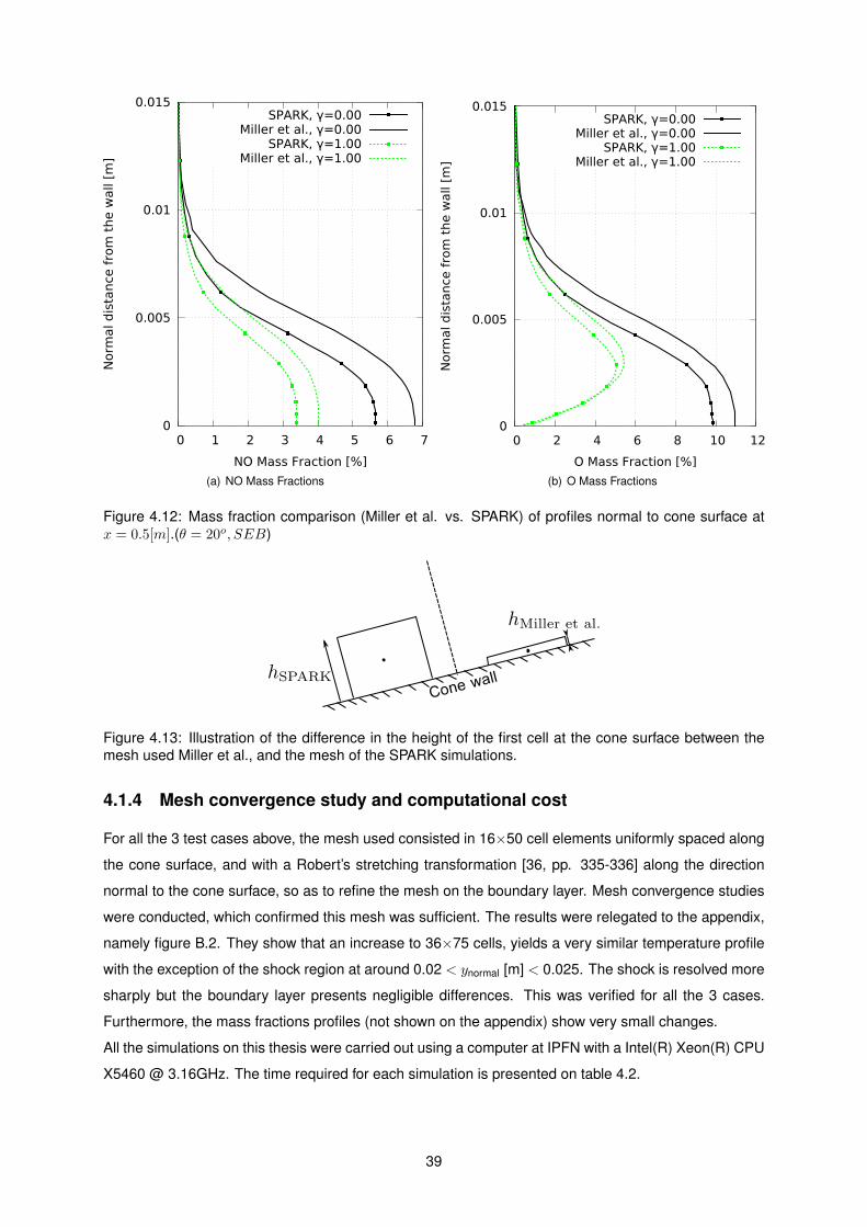
(a) NO Mass Fractions (b) O Mass Fractions
Figure 4.12: Mass fraction comparison (Miller et al. vs. SPARK) of profiles normal to cone surface atx = 0.5[m].(θ = 20o, SEB)
Figure 4.13: Illustration of the difference in the height of the first cell at the cone surface between themesh used Miller et al., and the mesh of the SPARK simulations.
4.1.4 Mesh convergence study and computational cost
For all the 3 test cases above, the mesh used consisted in 16×50 cell elements uniformly spaced along
the cone surface, and with a Robert’s stretching transformation [36, pp. 335-336] along the direction
normal to the cone surface, so as to refine the mesh on the boundary layer. Mesh convergence studies
were conducted, which confirmed this mesh was sufficient. The results were relegated to the appendix,
namely figure B.2. They show that an increase to 36×75 cells, yields a very similar temperature profile
with the exception of the shock region at around 0.02 < ynormal [m] < 0.025. The shock is resolved more
sharply but the boundary layer presents negligible differences. This was verified for all the 3 cases.
Furthermore, the mass fractions profiles (not shown on the appendix) show very small changes.
All the simulations on this thesis were carried out using a computer at IPFN with a Intel(R) Xeon(R) CPU
X5460 @ 3.16GHz. The time required for each simulation is presented on table 4.2.
39

Isothermal Wall SEB, 100 SEB, 200
16×50 cells 3 hrs 3 hrs 7 hrs36×75 cells 10 hrs 10.5 hrs 24 hrs
Table 4.2: Computational cost of the main simulations carried out for sharp cones.
40
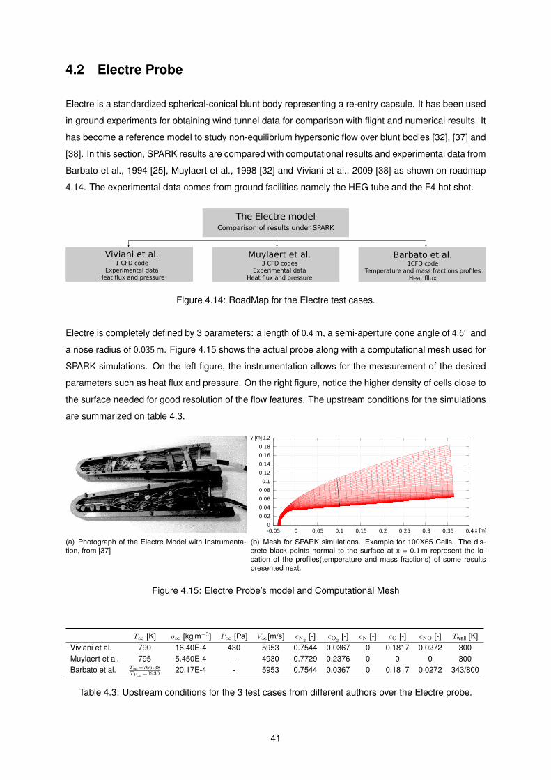
4.2 Electre Probe
Electre is a standardized spherical-conical blunt body representing a re-entry capsule. It has been used
in ground experiments for obtaining wind tunnel data for comparison with flight and numerical results. It
has become a reference model to study non-equilibrium hypersonic flow over blunt bodies [32], [37] and
[38]. In this section, SPARK results are compared with computational results and experimental data from
Barbato et al., 1994 [25], Muylaert et al., 1998 [32] and Viviani et al., 2009 [38] as shown on roadmap
4.14. The experimental data comes from ground facilities namely the HEG tube and the F4 hot shot.
Figure 4.14: RoadMap for the Electre test cases.
Electre is completely defined by 3 parameters: a length of 0.4m, a semi-aperture cone angle of 4.6 and
a nose radius of 0.035m. Figure 4.15 shows the actual probe along with a computational mesh used for
SPARK simulations. On the left figure, the instrumentation allows for the measurement of the desired
parameters such as heat flux and pressure. On the right figure, notice the higher density of cells close to
the surface needed for good resolution of the flow features. The upstream conditions for the simulations
are summarized on table 4.3.
(a) Photograph of the Electre Model with Instrumenta-tion, from [37]
(b) Mesh for SPARK simulations. Example for 100X65 Cells. The dis-crete black points normal to the surface at x = 0.1m represent the lo-cation of the profiles(temperature and mass fractions) of some resultspresented next.
Figure 4.15: Electre Probe’s model and Computational Mesh
T∞ [K] ρ∞ [kg m−3] P∞ [Pa] V∞[m/s] cN2[-] cO2
[-] cN [-] cO [-] cNO [-] Twall [K]Viviani et al. 790 16.40E-4 430 5953 0.7544 0.0367 0 0.1817 0.0272 300Muylaert et al. 795 5.450E-4 - 4930 0.7729 0.2376 0 0 0 300Barbato et al. T∞=766.38
TV∞=3930 20.17E-4 - 5953 0.7544 0.0367 0 0.1817 0.0272 343/800
Table 4.3: Upstream conditions for the 3 test cases from different authors over the Electre probe.
41

4.2.1 Viviani et al.
The analysis of figures 4.16 show that SPARK underpredicts the heat flux for both the non catalytic
and fully catalytic simulations. Because on the noncatalytic case there is no diffusion, the discrepancy
cannot be attributed to the catalytic model implemented. This difference reaches 40% at the nose of
Electre and over 42% at xL = 1.
For the fully catalytic simulations the heat flux increases on both curves but the errors rise to 90% at
the nose and roughly 50% at the back, evidencing an additional error introduced due to the catalytic
model implemented on SPARK. Only the break-up of the total heat flux onto its constituent terms (i.e.,
convective(translational) and diffusive fluxes) would allow proving this. Furthermore, the experimental
data shows that SPARK predicts relatively well the heat flux on the spherical portion of Electre but not
along its slope. Despite to this, the results have a very good qualitative agreement as they appear to
just being shifted from one to another.
On the other hand the SPARK simulations were ran with thermal equilibrium while Viviani at al. assumed
a two-temperature model. Also different was the procedure to compute the diffusion coefficient of all
species Di. However, it is believed the results would not have suffered any noticeable difference had the
models been the same.
It is relevant to analyse the pressure coefficient on the surface. There is a perfect match with the
computational results of Viviani et al. and the experimental data. The fact that the pressure matches
perfectly but not the heat flux is not contradictory because the fluid flow pressure is a variable which is
predominantly governed by the momentum equation and only slightly affected by thermodynamics [1, p.
607]. The result thus verifies the ”correctness” of SPARK on this regard.
(a) Total Heat Flux onto Electre - FullyCatalytic
(b) Total Heat Flux onto Electre - Non Cat-alytic
(c) Pressure coefficient on the surface ofElectre. Cp = p−p∞
12ρ∞V 2
∞
Figure 4.16: Comparison between available results from Viviani et al. [38] and corresponding SPARKsimulations. Heat flux and pressure coefficient as a function of the nondimensionalized length along theaxis of Electre. The ”shots” correspond to experimental data.
4.2.2 Muylaert et al.
In this case Muylaert et al. [32] presents results from 3 different CFD codes. Some of the features
employed by each of these codes are different; they use different chemical schemes, different methods
42

to compute the diffusion coefficient Di and even the overall CFD Navier-Stokes (NS) scheme is not the
same. It will suffice to say that the one closest to SPARK in these simulations is CIRA.
Despite this diversity, all the 3 codes agree to a large extent for the full catalytic simulation, figure 4.17,
while SPARK underpredicts those curves along the entire surface. At x = 0.4m the difference to the CIRA
curve is about 50%. For the non-catalytic case there is less agreement between CIRA and ESTEC but
still SPARK shows a heat flux clearly lower than these two. The difference to the CIRA heat flux is
again roughly 50% at x = 0.4m. In either case the SPARK results are closest to the CIRA curves which
conforms with both codes sharing most of their features (i.e., they share the NS scheme, the chemical
scheme and more).
From figure (c), the agreement of the pressure coefficient is even more pronounced as the curves are
almost indistinguishable from each other and the experimental results. Obviously the previous comment
applies here.
(a) Total Heat Flux onto Electre - FullyCatalytic
(b) Total Heat Flux onto Electre - Non Cat-alytic
(c) Pressure coefficient on the surface ofElectre. Cp = p−p∞
12ρ∞V 2
∞
Figure 4.17: Comparison between available results from Muylaert et al. [32] and corresponding SPARKsimulations. Heat flux and pressure coefficient as a function of the length along the axis of Electre. DLR,CIRA and ESTEC are independent CFD codes.
4.2.3 Barbato et al.
Two different cases concerning two wall temperatures, namely Tw = 343K and Tw = 800K are reproduced
after Barbato et al., 1994 [25]. The upstream conditions are on table 4.3.
There was an effort to run the SPARK simulations on the same grounds as the results that are being
reproduced. The same chemical set (Blottner [34]) and chemical vibrational coupling model are used.
There was no reference to the evaluation of thermodynamic properties or the diffusion coefficient model.
However, the approach followed by Barbato et al. to model catalycity is the equilibrium wall approxima-
tion which is different from the implementation on SPARK. The importance of this is addressed when
relevant.
Case: Tw = 343K
For the simulation with Tw = 343K as boundary condition, the compared results are the temperature
profile and the mass fraction profiles of all species along the normal to the Electre wall at x = 0.1m.
43

The discrete black points on figure 4.15 illustrate the location of these profiles. For all profiles the Bar-
bato et al. figures (in digital format) from which the results were extracted had low quality. Hence it
is possible that some curves are presented with some corruption. Furthermore, it was not possible to
obtain temperature and mass fraction points on the absolute proximity of the wall, also because of this
poor digital quality.
From a broad perspective, by inspecting figures 4.18 and 4.19 we may immediately find that there is
a good qualitative agreement and a decent quantitative agreement between the current SPARK and
Barbato et al. results. For temperature, SPARK captures the same ”S” like shape near the wall but
overpredicts that local maximum by 8%. The profile seems to be shifted to the right. The low quality of
the figures from which this data was extracted might have introduced this error. Furthermore, in contrast
with the temperature profiles normal to the sharp-cones ( as analysed previously on section 4.1 ) the
current temperature along the normal of Electre depends on the catalycity (i.e., on γ) of the surface, as
shown on figure B.4 of the appendix. For γ = 0.01 the ”S” shape fades due to the decrease of the local
maximum near the wall. This shows that the curves on (a) have already embedded on them the effects
of wall catalycity.
The discrepancies for ynormal > 2 cm are considered not to be born out of the catalytic model.
(a) Temperature Profile (b) Mass Fraction of species N2 and N.
Figure 4.18: Temperature and N2 and N mass fractions along the normal to Electre’s wall at x = 0.1m forTw = 343K. Comparison of current results under SPARK with Barbato et al. [25]. Equ. on the legendstands for equilibrium wall boundary condition.
For the mass fraction results, the agreement is very good with the exception of NO. Notice however that
there are no data points for the profiles under Barbato et al. at the immediate vicinity at the wall because
of the low quality of the digital figures from which the data was extracted. A comparison near the wall,
would be most relevant, as the slope of the mass fraction there determines the heat into Electre. Still
the slopes seem to be identical for N2, N, O2 and O.
The discrepancies are the greatest for NO, specially near the wall where the two curves have opposite
trends. The explanation is guaranteed to come from the equilibrium wall boundary condition employed
by Barbato et al.
As discussed on section 2.5.1, the equilibrium wall model consists in simply setting the composition at
44

the wall to the equilibrium composition that would exist at the temperature and pressure of that point on
the wall:
ci,w = ci,w(pw, Tw)
In practice it works quite well for air environments and provides very similar results compared with the
full catalytic (implemented in SPARK) approach [39, p. 132]; so similar indeed that the terms equilibrium
wall and fully catalytic are often used interchangeably [27, p. 181]. Thus using the results of Barbato et
al. for the verification of SPARK’s implementation is a valid approach.
Despite this, the NO profiles don’t match near the wall because in SPARK there is no NO production or
consumption (ωNO,w = 0). Thus the slope of NO mass fraction on the wall is always zero2, ωNO,w = 0
⇒(∂cNO
∂n
)w = 0. The surface can be regarded as being indifferent to NO allowing the value cNO,w to be
decided by the gas flow. In contrast the equilibrium wall condition used by Barbato et al. explicitly sets
cNO,w = cNO(pw, Tw) which requires the cNO profile to accommodate to the equilibrium value dictated
by the wall temperature and local pressure. In this case the value is lower than would otherwise be if
the surface didn’t interfere in the composition of NO directly, as happened for the fully catalytic case in
SPARK.
The intention of the previous discussion was to demonstrate that the differences on the NO profiles were
expected and not the evidence of an incorrect implementation of catalycity in SPARK.
(a) Mass fraction of O2 (b) Mass fraction of O (c) Mass fraction of NO
Figure 4.19: Mass fractions of species O2, O and NO along the normal to Electre’s wall at x = 0.1m forTw = 343K. Comparison of current results under SPARK with Barbato et al. [25]. Equ. on the legendstands for equilibrium wall boundary condition.
Case: Tw = 800K
For the second simulation where Tw = 800K, the various forms of heat flux along the Electre surface
are compared on the 5 graphs of figure 4.20. Overall, the agreement of the results is equivalent to the
previous cases for Viviani et al. and Muyalert et al. on figures 4.16 and 4.17 respectively. Unlike those
cases however, the various contributions of the heat flux are presently discriminated for the full-catalycity
simulation.
The non-catalytic simulation (only the total heat flux is shown) for which no heat through diffusion occurs,
already exhibits a disagreement, but both curves are well within the same order of magnitude. SPARK
2This is not clear from figure 4.19 but it becomes evident when zooming in near the wall.
45

again seems to underpredict Barbato’s results. In the nose the heat flux is 40% lower and at x = 0.4m
48% lower.
As expected the heat flux increases, on both curves, for the full catalytic simulation. This is almost
entirely due to the emergence of gradients of the mass fractions of the various species, which trough
diffusion contribute with heat by an amount similar to the heat flux coming from temperature gradients
(i.e., translational flux). Furthermore, vibrational heat flux is one order of magnitude lower than the other
modes, not because of the gradient of vibrational temperature, but due to the very low conductive coef-
ficient for vibration kvib, about 1 order of magnitude lower than ktrans for this temperatures [40].
There is a greater mismatch for the diffusive fluxes in figure (e) than for the translation heat fluxes at
(c). The translational heat flux under SPARK is 25% lower at the nose and 31% lower at x = 0.4m while
the difference for the diffusion fluxes is also of 25% at the nose but exceeds 50% at x = 0.4m. This
difference between the curves increases along the surface of Electre and may in part be explained by
Barbato et al. using the equilibrium wall and not the full catalytic conditions. As seen for Tw = 343K, the
profiles of cNO are opposite in direction near the wall. SPARK results have zero slope and thus there is
no diffusion heat flux from NO. In contrast there is a positive gradient of NO molecules at the wall for the
curve under Barbato et al. which results in an additional term of heat flux:
qdiffNO=
(hNOρDNO
∂cNO
∂n
)w
(4.1)
(a) Non catalytic - Total heat flux (b) Full catalytic - Total heat flux
(c) Full catalytic - Translational flux (d) Full catalytic - Vibrational flux (e) Full catalytic - Diffusive flux
Figure 4.20: Comparison between available results from Barbato et al. [25] and corresponding SPARKsimulations for Tw = 800K. Heat flux as a function of the length along the axis of Electre.
46

4.2.4 Mesh, convergence study and computational cost
While not particularly relevant for the study of catalycity, it remains important to comment some aspects
of the CFD simulations.
Because the mesh represents the discretized space where the Navier-Stokes(NS) equations are solved,
it must be big enough to capture the shock wave, otherwise we would be setting a non-physical simula-
tion whereby the space dimensions where the NS equations are being solved is incompatible with the
dimensions of the phenomenon which it produces.
Because the position and shape of the shock-wave are not known a priori but only after the simulation
has ran its course, the mesh dimensions could be overestimated to ensure the inclusion of the shock-
wave as in figure 4.21 by the red solid line. Although that would be effective it would not be efficient
because would inevitably result in higher computational cost due to more cells being needed to cover
the area before the shock, or less accuracy by using the same cells to cover a greater area.
The workaround consisted in using the results of Billig [41], who presents correlations for the shape of
shock waves around blunt-bodies. These correlations were based on experimental data, but have a very
good agreement with numerical calculations [42], at least for non-reactive flows. Billig presents equation
(4.2), giving the shape as a function of the bodies’ dimensions and the incoming Mach Number M∞. For
Electre the dimensions were the nose radius (R = 0.035m) and the semi aperture cone angle (θ = 4.6).
Also, on correlation (4.2) variables x and y represent the coordinates of the shock-wave, and the rest of
the nomenclature is illustrated on figure 4.21.
x = R+ δ −Rc cot2 θ
[(1 +
y2 tan2 θ
R2c
)1/2
− 1
]Where δ, Rc = f(M∞, R)
(4.2)
Figure 4.21: Illustration of the formation of a shock wave in front of Electre, and the outer limits of twocomputational meshes that follow the shock’s shape.
Hence the mesh for Electre used in SPARK allows for a very judicious use of computational power. Re-
47

visiting the computational mesh of figure 4.15, Billig’s model allows finding out how short can the mesh
dimensions be at the nose (y = 0m) and how lengthy, in terms of normal distance from the surface, it
needs to be at the ”rear”. Lastly, similar to the cone case, the cells height grows with the distance from
the wall of the probe via the Robert’s stretching [36, pp. 335-336].
The convergence studies performed to access the independence of the results from the mesh are
present on figure B.3 of the appendix. The corresponding computational times are given on table 4.4:
50X35 cells 70X50 cells 90X65 cells 100X65 cellsViviani et al. 19 hrs 44 hrsMuylaert et al. 27 hrs 45 hrs 92 hrsBarbato et al. 24 hrs 120 hrs
Table 4.4: Computational cost of the main simulations carried out for the Electre probe.
4.3 Temperature varying SRE, γ = γ(T )
The objective of the present section is to verify the implementation of the temperature dependent re-
combination coefficients, γ = γ(T ). In contrast with the other V&V sections considered above, SPARK
results will not be compared with other codes. From the 2 studies found on SRE catalicity using the
same models, Godart et al., 1996 [43] does not present the free-stream conditions which prevents the
reproduction of results and Barbato et al., 1994 [25] runs the simulations for an isothermal case of Twall
= 1500K, which caps the purpose of temperature dependent recombination coefficient models.
Consequently, the models from Scott, Zoby et al. and Stewart et al. presented on section 2.5.1 were
tested for the sharp cone, SEB, semi-angle = 20 case, where the free-stream conditions remained the
same3. A SEB condition was chosen so as to allow for the wall temperature to vary along the surface;
on contrary for an isothermal wall, the models would result on a fixed γ along the surface evaluated
at the given temperature. The particular case of semi-angle = 20 was preferred because the greater
dissociation levels allows richer results.
A code-to-code comparison is desirable, but not indispensable as there are other procedures used to
verify the code ”correctness” [44, ch. 5]; in this case, without benchmark solutions, the discussion will
be centred around the consistency of the results.
The results analysed are the mass fractions on the surface of the cone presented on figure 4.23. The
reader is referred to figures B.5 and B.6 of the appendix for a better appreciation of the results that
follow. The black dots on figure B.5 illustrate the location where temperature, mass fraction and reaction
efficiency are accessed.
Figure 4.23 shows the mass fractions of N, O and NO on the surface of the cone as a function of its
axial length. The results for N2 and O2 are on the appendix B.3. For each species there are 5 curves: 3
for the models after Scott, 1980 [9] Zoby et al., 1984 [10] and Stewart et al., 1987 [33] and the other 2
3The mesh used was, however, finer. It had 40 cells, instead of 14, along the surface of the cone, since in this case the interestwere plots along the surface of the cone. The mesh can be seen on figure B.5 of the appendix.
48
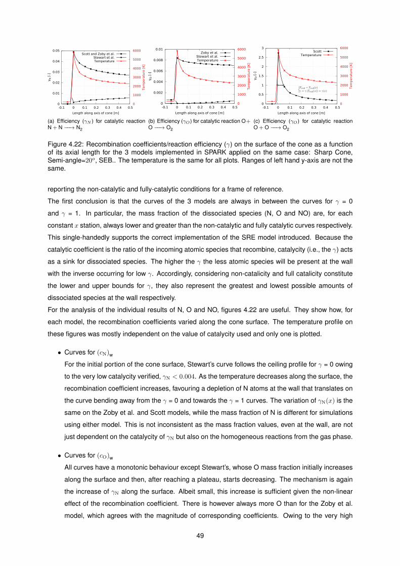
(a) Efficiency (γN ) for catalytic reactionN + N −−→ N2
(b) Efficiency (γO) for catalytic reaction O+O −−→ O2
(c) Efficiency (γO) for catalytic reactionO + O −−→ O2
Figure 4.22: Recombination coefficients/reaction efficiency (γ) on the surface of the cone as a functionof its axial length for the 3 models implemented in SPARK applied on the same case: Sharp Cone,Semi-angle=20o, SEB.. The temperature is the same for all plots. Ranges of left hand y-axis are not thesame.
reporting the non-catalytic and fully-catalytic conditions for a frame of reference.
The first conclusion is that the curves of the 3 models are always in between the curves for γ = 0
and γ = 1. In particular, the mass fraction of the dissociated species (N, O and NO) are, for each
constant x station, always lower and greater than the non-catalytic and fully catalytic curves respectively.
This single-handedly supports the correct implementation of the SRE model introduced. Because the
catalytic coefficient is the ratio of the incoming atomic species that recombine, catalycity (i.e., the γ) acts
as a sink for dissociated species. The higher the γ the less atomic species will be present at the wall
with the inverse occurring for low γ. Accordingly, considering non-catalicity and full catalicity constitute
the lower and upper bounds for γ, they also represent the greatest and lowest possible amounts of
dissociated species at the wall respectively.
For the analysis of the individual results of N, O and NO, figures 4.22 are useful. They show how, for
each model, the recombination coefficients varied along the cone surface. The temperature profile on
these figures was mostly independent on the value of catalycity used and only one is plotted.
• Curves for (cN)w
For the initial portion of the cone surface, Stewart’s curve follows the ceiling profile for γ = 0 owing
to the very low catalycity verified, γN < 0.004. As the temperature decreases along the surface, the
recombination coefficient increases, favouring a depletion of N atoms at the wall that translates on
the curve bending away from the γ = 0 and towards the γ = 1 curves. The variation of γN(x) is the
same on the Zoby et al. and Scott models, while the mass fraction of N is different for simulations
using either model. This is not inconsistent as the mass fraction values, even at the wall, are not
just dependent on the catalycity of γN but also on the homogeneous reactions from the gas phase.
• Curves for (cO)w
All curves have a monotonic behaviour except Stewart’s, whose O mass fraction initially increases
along the surface and then, after reaching a plateau, starts decreasing. The mechanism is again
the increase of γN along the surface. Albeit small, this increase is sufficient given the non-linear
effect of the recombination coefficient. There is however always more O than for the Zoby et al.
model, which agrees with the magnitude of corresponding coefficients. Owing to the very high
49

recombination coefficient along the cone wall, Scott’s model results in much less amount of O, with
the profile approaching the fully-catalytic case. In particular, we can notice on the initial portion
corresponding to x < 0.005m that the recombination efficiency is extrapolated from the model to
be as high as γO = 2.7. As discussed on the introductory chapters, this is non-physical and SPARK
overrides the value to γO = 1.
• Curves for (cNO)w
Lastly for NO, all the profiles vary linearly along the cone surface. Remember that there is no
production of NO directly from catalycity, i.e the reaction N + O −−→ NO is not modelled. The
coefficient on the legend of figures 4.23 refers merely to γN = γO = γ. This means the values for
(cNO)w are an effect of the gas-phase reactions, most likely linked with the homogeneous reaction
O2 + N ←−→ NO + O. This explains the small amounts of N (for all models), as this species
is consumed for the creation of NO. Furthermore, Scott’s model results in much less NO, which
conforms with the already seen lower quantity of N and O, essential for the creation of NO.
50

(a) N mass fraction on the surface of the cone, (cN)w (b) O mass fraction on the surface of the cone, (cO)w
(c) NO mass fraction on the surface of the cone, (cNO)w
Figure 4.23: Mass fraction of the dissociated species N, O and NO on the surface of the cone as afunction of its axial length for several models applied on the same case: Sharp Cone, Semi-angle=20o,SEB. Ranges of y-axis are not the same. γN = γO = γ.
51

4.4 Self assessment of the implementation
In the present chapter a great number of computational results under SPARK have been compared with
other CFD codes and experimental data. The original purpose was to verify the ”correctness” of the
implementation of catalycity in SPARK. Is SPARK now able to credibly model re-entry Earth flows where
catalycity is expected to play a role?
Overall, it is clear that on the qualitative level the results have a very good agreement. They present the
same trends with the same slopes often just shifted. On the quantitative side however the differences to
the other results are in some cases only just slightly beyond reasonable doubt.
The author believes a likely explanation can simply be the evaluation of ∆n which from chapter 3 corre-
sponds to the distance between the first cell node and the wall:
The metric terms of the transformation
As presented on appendix A, the discretization of the Navier-Stokes (NS) by SPARK includes a trans-
formation of coordinates from the physical plane (x, y) to a computational domain (ξ, η):
x = x(ξ, η), y = y(ξ, η)
Transforming the equations has certain advantages but effectively changes their nature and must now
include metric terms as described on the appendix.
The boundary conditions also change because of this transformation. The equations are the same but
expressed in different coordinates. For example, on Fick’s law of diffusion of (2.20) the gradient can no
longer be described in terms of (x, y) because the Navier-Stokes are being solved in another domain.
ji = −ρDi∇ci (2.20 revisited)
⇔ ji = −ρDi∇ci = −ρDi
HH
HHHH
(∂ci∂x
,∂ci∂y
)Transforming the wall mass balance to the new computational coordinates begins with:
ji,into the wall = −ρDi∇ci · ~n = −ρDi
(∂ci∂x
,∂ci∂y
)· (nx, ny) = −ρDi
(∂ci∂x
nx +∂ci∂y
ny
)(4.3)
Where ~n is a vector normal to the wall and nx, ny are its components.
Through the transformation, the derivatives with respect to x and y are converted to ξ, η, via the relations
[45, ch. 5]:∂ci∂x
=1
J
[∂ci∂ξ
yη −∂ci∂η
yξ
]∂ci∂y
=1
J
[∂ci∂η
xξ −∂ci∂ξ
xη
] (4.4)
Where the ξx, ξy, ηx and ηy are known as metric terms with the subscripts corresponding to differentia-
tion and J is the Jacobian of the transformation.
52

Introducing (4.4) into (4.3) the mass flux can be expressed as:
ji,into the wall = −ρDi1
J
[∂ci∂ξ
(yηnx − xηny) +∂ci∂η
(xξny − yξnx)
](4.5)
Now the mass flux is expressed in terms of the computational variables ξ and η.
The next step is to specify the wall normal ~n in terms of the computational variables. Without loss of
generality it is assumed that the wall corresponds to a constant ξ line on the computational domain. In
that case the wall normal is given by:
nx =−yη√x2η + y2
η
ny =xη√x2η + y2
η
(4.6)
Inserting (4.6) into (4.5) eventually leads to 4:
ji,into the wall =
ρDi∂ci∂ξ
1
J
y2η√
x2η + y2
η
+x2η√
x2η + y2
η
w
(4.7)
In contrast, the original wall mass balance equation was developed into (2.21):
(ji)w, into the wall = − (ji)w =
(ρDi
∂ci∂n
)w
(2.21 revisited)
The expressions are similar. While n was the coordinate normal to the wall, now ξ is the coordinate
normal to the wall. However, the boundary condition must now incorporate the boxed term embodying
the effects of the coordinate transformation.
From the point of view of the implementation onto SPARK the discretization originally given by (3.6) has
in fact a more complex nature given by (4.8).
∂ci∂n
w
=(ci)i − (ci)w
∆n(3.6 revisited)
∂ci∂ξ
w
=(ci)i − (ci)w
∆ξ
1
J
y2η√
x2η + y2
η
+x2η√
x2η + y2
η
w
⇔
(∂ci∂ξ
)w
=(ci)i − (ci)w
(∆ξ)′ Where:
[(∆ξ)
′]−1=
1
∆ξ
1
J
y2η√
x2η + y2
η
+x2η√
x2η + y2
η
w
(4.8)
Where (∆ξ)′ can be viewed as an effective distance to the wall.
The implementation into SPARK does indeed take the metric terms into consideration, i.e., it evaluates
the ”effective” ∆n through an expression similar to (4.8). The objective with this derivations and this
section is then to ask whether or not the term is correctly implemented in SPARK, as the author feels that
4This is actually a particular case, but which is most useful to illustrate the point. It corresponds to an orthogonal transformation.
53

a complete understanding of the matter is paramount to increase the confidence on the implementation.
This can be accomplished by running certain very simple test cases that evidence this ∆n aspect or
more importantly by analysing and comparing the theoretical derivations in other aerothermodynamics
CFD codes that discretize the Navier-Stokes with a coordinate transformation.
54

Chapter 5
The Finite Rate Surface Chemistry
(FRSC) model
As illustrated on figure 5.1, this chapter has 3 sections. The first section consists in a brief overview
of the theoretical formulation of the FRSC model; as commented along the text, this formulation was
developed by Marschall and MacLean, 2011 [20] and is used by several codes [11, 21]. The second
section is a concise description on how to readily update SPARK from the SRE to the FRSC model.
As noted before, this thesis work did not actually include this update and only the strategy to do it is
described. Lastly, the third section concerns the stand alone code, which can be regarded as a pre-
requisite for a future full implementation of the FRSC model in SPARK; the results are matched with the
implementation by MacLean et al. [20].
Figure 5.1: Road Map for the chapter.
5.1 Theoretical Overview
The next step towards a state-of-the-art modelling of catalycity is a general finite-rate surface chemistry
(FRSC) model. The improvement consists in abandoning the imposed surface efficiency γ, that attempts
to macroscopically model catalycity and start taking into account the microscopic processes responsi-
ble, on a more basic level, for catalycity thus providing a physically justified model.
In short, a finite-rate surface chemistry model (FRSC) tries to emulate for the heterogeneous reactions
the mechanisms and procedures used for homogeneous gas phase reactions. This is done by firstly
recognizing pseudo-species specific to a surface that enable fundamental pathways involved and sec-
ondly by allowing competing kinetic reactions taking place within this surface relating both the gas phase
55
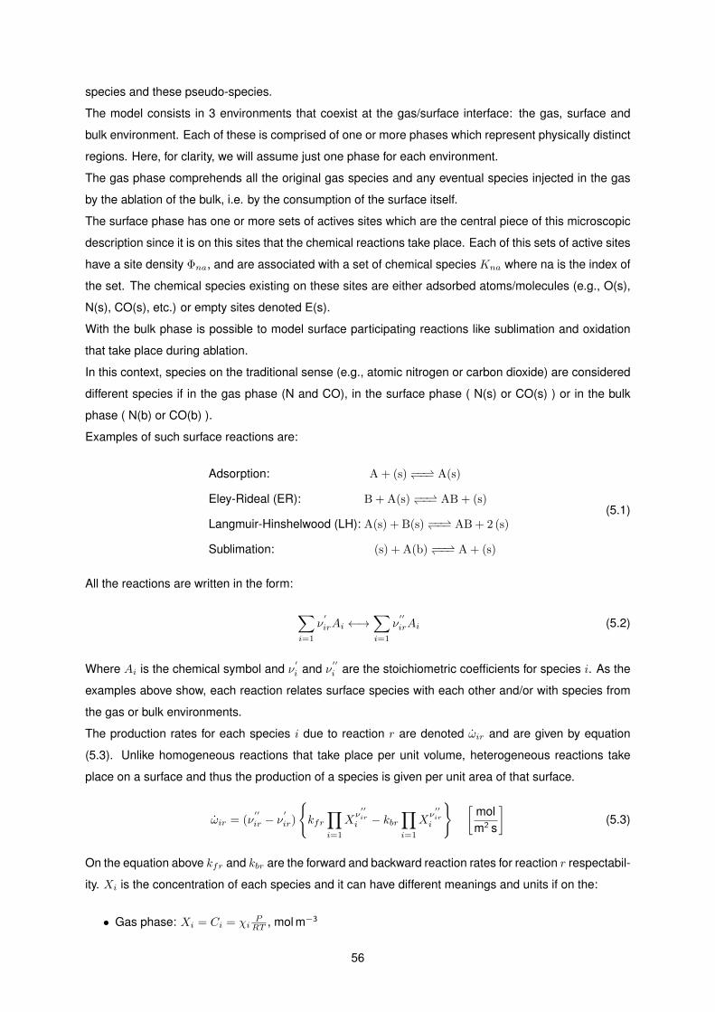
species and these pseudo-species.
The model consists in 3 environments that coexist at the gas/surface interface: the gas, surface and
bulk environment. Each of these is comprised of one or more phases which represent physically distinct
regions. Here, for clarity, we will assume just one phase for each environment.
The gas phase comprehends all the original gas species and any eventual species injected in the gas
by the ablation of the bulk, i.e. by the consumption of the surface itself.
The surface phase has one or more sets of actives sites which are the central piece of this microscopic
description since it is on this sites that the chemical reactions take place. Each of this sets of active sites
have a site density Φna, and are associated with a set of chemical species Kna where na is the index of
the set. The chemical species existing on these sites are either adsorbed atoms/molecules (e.g., O(s),
N(s), CO(s), etc.) or empty sites denoted E(s).
With the bulk phase is possible to model surface participating reactions like sublimation and oxidation
that take place during ablation.
In this context, species on the traditional sense (e.g., atomic nitrogen or carbon dioxide) are considered
different species if in the gas phase (N and CO), in the surface phase ( N(s) or CO(s) ) or in the bulk
phase ( N(b) or CO(b) ).
Examples of such surface reactions are:
Adsorption: A + (s) −−−− A(s)
Eley-Rideal (ER): B + A(s) −−−− AB + (s)
Langmuir-Hinshelwood (LH): A(s) + B(s) −−−− AB + 2 (s)
Sublimation: (s) + A(b) −−−− A + (s)
(5.1)
All the reactions are written in the form:
∑i=1
ν′
irAi ←→∑i=1
ν′′
irAi (5.2)
Where Ai is the chemical symbol and ν′
i and ν′′
i are the stoichiometric coefficients for species i. As the
examples above show, each reaction relates surface species with each other and/or with species from
the gas or bulk environments.
The production rates for each species i due to reaction r are denoted ωir and are given by equation
(5.3). Unlike homogeneous reactions that take place per unit volume, heterogeneous reactions take
place on a surface and thus the production of a species is given per unit area of that surface.
ωir = (ν′′
ir − ν′
ir)
kfr
∏i=1
Xν′′iri − kbr
∏i=1
Xν′′iri
[molm2 s
](5.3)
On the equation above kfr and kbr are the forward and backward reaction rates for reaction r respectabil-
ity. Xi is the concentration of each species and it can have different meanings and units if on the:
• Gas phase: Xi = Ci = χiPRT , mol m−3
56

• Surface phase: Xi = φns,i, mol m−2
• Bulk phase: Xi = χnb,i, adim
While this is expected, since it wouldn’t be reasonable to have the surface species, that by definition exist
only on the surface, be defined per unit volume or gas species defined per unit area, it is in contrast with
the homogeneous reactions where the concentrations of the species all have the same units, namelymolm3 . The units of kfr and kbr take this into account and adjust in order to ultimately have mol
m2 sfor the
production terms on equation (5.3).
The forward reaction rates can and are often specified by general Arrhenius type expressions. Other
times the rates are specified by the expressions 1 to 4 on table 5.1. The difference is that the parameters
of the Arrhenius expressions (A, β, E) are sometimes difficult to relate to the physical and chemical
processes that constitutes the surface reaction. This new expressions are able to break down this
parameters, namely the A coefficient, into sub-parameters that are more insightful.
Reaction Type Rate Formula Specified Parameters
0: Arrhenius kf = AT βexp(− ERT
)A, β, E
1: Adsorption kf =[
v4Φνss
]S0T
βexp(−EadRT
)S0, β, Ead
2: Eley-Rideal (ER) kf =[
v4Φνss
]γ0T
βexp(−EerRT
)γ0, β, Ead
3: Langmuir-Hinshelwood (LH) kf =[v2DΦ
(1.5−νs)s
√Av
]ClhT
βexp(−ElhRT
)Clh, β, Elh
4: Sublimation kf =[
v4Φνss RT
]γsubT
βexp(−EsubRT
)γsub, β, Esub
Table 5.1: Forward reaction rates. Table reproduced from [20].
At times, the backward reactions can be neglected. When they need to be taken into account, the
backward rates need to be computed. Similar to the case for the homogeneous reactions, the backward
rates for surface reactions can be directly given or determined through equilibrium constants. The latter
situation requires the concentration-based equilibrium constant Kcr:
kbr =kfrKcr
(5.4)
The concentration-based equilibrium constant can either be directly specified or computed through the
activity-based equilibrium constant Kar:
Kcr = Kar
(PrefRT
)νgr(5.5)
Where Pref = 1× 10⁵ Pa, and νgr is a stoichiometric coefficient.
In turn the activity-based equilibrium constant can be calculated from changes in the Gibbs energy of
formation at temperature T in going from the reactants to products (see [20] for details):
Kar = exp
[−∆G0
r(T )
RT
]= exp
[−
K∑i=1
νirG0i (T )
RT
]= exp
[−
K∑i=1
νir
(H0i (T )
RT− S0
i (T )
R
)](5.6)
57

This approach requires the thermodynamic functions to be known for all species participating in the
specific reaction r. Although data for gas phase and bulk phase species is usually accessible, there is
rarely information on surface phase species.
5.2 Implementation of the FRSC model on SPARK
When discussing the implementation of catalycity into SPARK in chapter 3, the first step was to develop
the mass boundary condition at the wall, which states that the diffusion of each species into the wall is
balanced by the consumption of that species:
(ji)w, into the wall = (−ωi,w)⇔
−(ρDi
∂ci∂n
)w
= (ωi,w)(2.22 revisited)
Afterwards, under the approach of the simple SRE model, expressions for the production terms were
presented:
ωi,w = −γici,wρw
√RiTw
2π
[kg
m2 s
](2.26 revisited)
For the more advanced FRSC model, the mass balance on equation (2.22) remains unchanged but the
production terms ωi,w are not as straightforward as they are given by:
ωi,w =∑r=1
(ν′′
ir − ν′
ir)
kfr
K∏i=1
Xν′′iri − kbr
K∏i=1
Xν′′iri
[molm2 s
](5.3 revisited)
The time accurate implicit discretization of equation (2.22) with the FRSC production terms is challenging
but was developed and implemented into the DPLR code by MacLean et al. [17] making the code the
state-of-the-art in the field. In contrast, some other authors [21], [46] follow an explicit approach which
is easier. It is easier because it maybe done without altering the original CFD code, although that has
downsides as decreasing numerical stability. This approach can be readily implemented onto SPARK:
First, after each CFD iteration, the steady-state concentration of surface species is computed by solving
Ks − 1 equations of the form (5.7) together with equation (5.8).
dΦns,idt
= 0 (5.7)
Φs =∑i
Φns,i (5.8)
Where Φs is the total active site density and Φns,i is the concentration of surface species i.
After this step, all the surface species concentrations are known which allow for the evaluation of the
production terms of the gas species using equation (5.3). Finally, recovering expression (3.7), the new
value of each species mass fraction at the wall is computed allowing for the next CFD iteration to take
58

place.
cni,w = cni,i + ωni,w ·
∆n
ρwDi,w
n
(3.7 revisited)
5.3 Stand Alone Code
The upgrade provided by the FRSC model affects only the production terms wi,w since the physical
principles behind the boundary conditions remain as being the conservation of mass and energy at
the flow/surface interface. In this regard, the stand alone code can be viewed as a tool to verify the
consistency of the production terms and the steady state surface coverage, equation (5.7), under various
settings. The idea is for the code to exist independently of SPARK, decoupling the surface chemistry
from the flow phenomena occurring on the nearby gas, such as diffusion, convection, heat transfer and
gas phase reactions. In other others, there is no flow, only surface reactions that take a system from a
initial condition to a steady-state condition. This takes the form of 0D simulations (differential equations
in time).
There are 2 types of simulations. In all of them only surface-kinetics and never homogeneous reactions
are allowed to occur:
1. Fixed Gas Phase Composition
Here we admit the gas phase has a given composition that is fixed. The temperature and pres-
sure are also prescribed. The surface phase species concentration on the other hand are free
to adjust to such composition, via the allowed surface kinetics, from a initial condition. The prob-
lems amounts to solving one equation of type (5.9) for each surface species. It’s concentration will
progress over time until, if correctly posed, the problem will reach a steady-state solution.
d[X]sdt
= [w]s (5.9)
2. Constant Volume
In this case, we eliminate the restrain of constant gas phase composition and allow it to to vary from
an initial condition. As a consequence of the changing gas phase composition and the volume and
temperature being constant, the pressure will also evolve. It’s final value can be computed by the
perfect gas law, equation (5.10), where obviously only the gas phase species matter. In addition
to the set (5.9) it is now necessary to solve for the unknowns, time changing concentrations of gas
phase species, equations (5.11).
p = ρRT Where R =∑i
ciRi (5.10)
d[X]gdt
= [ω]g (5.11)
59

Both types constitute a system of coupled ordinary differential equations (ODE) in time. They are solved
using a standardized ODE solver named DVODE. This solver package is the same used by the bulk of
SPARK in other contexts.
5.3.1 Equilibrium constants to compute surface reaction rates
One important peculiarity of the formulation developed by MacLean et al. is the computation of the
backward rates kbi from the equilibrium constants Kci and Kai. As explained previously, this requires
the Gibbs energy of formation of all species involved on the particular reaction, but there is no data
on the thermodynamic properties of surface species; for example, on the equilibrium constants Kai of
the generic ER and LH reactions, equations (5.13)-(5.14), the terms G0A(s)(T ) and G0
(s)(T ) are unknown.
The workaround consists in specifying both the forward and backward reaction rates for each adsorption
reaction. In doing so it is possible to evaluate the activity base equilibrium constant Ka,ads and then
extract the term(G0
A(s)(T )
RT − G0(s)(T )
RT
)by inverting equation (5.12). This process is illustrated on figure
5.2.
Ka,ads = exp
[G0
A(T )
RT−
(G0
A(s)(T )
RT−G0
(s)(T )
RT
)](5.12)
Ka,ER = exp
[−(G0
AB(T )
RT− G0
B(T )
RT
)+
(G0
A(s)(T )
RT−G0
(s)(T )
RT
)](5.13)
Ka,LH = exp
[−G
0AB(T )
RT+
(G0
A(s)(T )
RT−G0
(s)(T )
RT
)+
(G0
B(s)(T )
RT−G0
(s)(T )
RT
)](5.14)
The Gibbs energies for the gas phase species, A and AB, should be readily available from the literature.
SPARK obtains the thermodynamic data from the NASA Glenn compilation of thermodynamic properties
[47].
This manoeuvre is widely employed by our source paper of MacLean et al. [20]. In essence it consists
in shifting the uncertainty from prescribing equilibrium constants directly for the ER and LH reactions
or finding the thermodynamic functions of the surface species to the uncertainty of specifying backward
rates for adsorption reactions. The advantage is, according with the reference, that the backward rate
for adsorption can be derived from simple statistical thermodynamics and kinetic theory.
60

Figure 5.2: Practice to compute thermodynamic variables for surface species.
61

5.4 Results of the Stand Alone Code
On this section, the current results are matched with MacLean et al. [20]. There are only available for
comparison steady-state solutions but on section B.4 of the appendix there are some transient results
from the current stand alone code as a reference.
There are 2 cases. On the first the gas phase composition is fixed and only the surface species equations
(5.9) are solved for 3 different pressures and a wide spectrum of temperatures. On the second case,
the gas phase composition is allowed to vary by adding equations (5.11) and solving them for the same
temperature and initial pressure but assuming different sets of surface reactions.
5.4.1 Fixed Gas Phase of Dissociated Oxygen
The first case studied concerned a gas composed of partially dissociated oxygen. The species taken
into account were O2 and O for the gas phase, adsorbed oxygen O(s) and free-sites E(s) for the surface
phase and no bulk phase. Only 3 reactions were simulated as to allow for recombination: One adsorption
reaction for O atoms to stick to the surface and 2 recombination reactions (1 Eley-Rideal(ER) and 1
Langmuir-Hinshelwood(LH)) to form O2. The information is summarized in table 5.2.
Phases Species Initial ConditionGas O2, O CO2
=0.9, CO=0.1Surface O(s), E(s) Φ1,O(s) = 0, Φ1,(s) = 7.5E-6 mol/m2
Reaction Form ParametersForward Reaction Backward Reaction
Adsorption R1: O + (s)↔ O(s)S0 = 0.05 , β = 0 Ades = 1,ν = 1.0E12 s−1
Ead = 0 β = 0, Edes = 350000 J mol−1
ER R2: O + O(s)↔ O2 + (s)γer = 0.001 , β = 0,
-Eer = 9000 J mol−1
LH R3: O(s) + O(s)↔ O2 + 2(s)Clh = 0.1 , β = 0
-Elh = 300000 J mol−1
Table 5.2: Summary of the data of the problem. Fixed gas phase of dissociated oxygen.
The parameters for the backward reaction of the adsorption reaction concern expression (5.15)
kb = kdes = AdesTβνexp
(−EdesRT
)(5.15)
On both figures 5.3 and 5.4, and for clarity of the presentation, there is only on thick black line repre-
senting all MacLean et al. cases for which there also exists results for the current implementation. For
both the surface coverage of O-atoms ( O(s) ) and the loss efficiency of O and O2 the current results are
indistinguishable from those of MacLean at al.
The main cause of an eventual disagreement between the results is not knowing how MacLean et al.
computes the Gibbs energy for the gas phase species. However, given the match of the results, either
they also use the NASA polynomials [47], or the difference of the methods is insignificant.
Passing now to the physical analysis of the results, the first comment is that every point on both figures,
62

Figure 5.3: Comparison between the current results and results from MacLean et al. [20]. Percentageof sites containing O(s) as a function of temperature for 200, 2000 and 20000 Pa. Case: 10% O - 90%O2.
Figure 5.4: Comparison between the current results and results from MacLean et al. [20]. Loss efficiencyas a function of temperature for 200, 2000 and 20000 Pa. Case: 10% O - 90% O2.
despite representing a steady-state solution, doesn’t constitute a thermodynamic equilibrium state. This
is because, in general, the fixed gas phase composition (90 % O2 - 10% O) is not compatible with the
steady-state achieved by the surface species and should actually be changing in order to conciliate with
the steady-state. By other words, the results contradict the assumptions. To see this we first develop the
production term for the O specie:
dCO
dt= ωO = −kf1COΦ(s) + kb1ΦO(s) − kf2COΦO(s) + kb2CO2
Φ1,(s) (5.16)
We then take a random point from figure 5.3, say (P = 20 000Pa, T = 3000K) where there is a 40% cov-
erage of O-atoms. As the total distribution of sites, empty or with O, is Φs = 7.5× 10⁻⁶ molm2 , then we have
Φ1,O(s) = 3× 10⁻⁶ molm2 and Φ1,(s) = 4.5× 10⁻⁶ mol
m2 . With this, and assuming the said constant composition
for the gas phase of CO = 0.1 PRT = 0.008 mol
m3 and CO2= 0.9 P
RT = 0.0721 molm3 , we get dCO
dt = 1.354 molm3 when
it should equal zero, thus showing a changing gas phase composition.
63

This could also have been showed by simply noting that, on figure 5.4, there is an active loss of O2
molecules for the same state (P = 2000Pa, T = 3000K).
This apparent inconsistency stems from just solving the equations (5.9) for the surface species and
ignoring the equations (5.11) for the gas phase species. Given the above analysis, this case is repre-
sentative of an actual CFD simulation where the gas flow near the catalytic wall is such that it is instantly
providing/absorving the necessary/excess O and O2 so that in practice the gas phase composition re-
mains the same.
5.4.2 Silica Sublimation
This second study concerns silica sublimation, a typical compound of many TPS as reported on the
introduction 1. In contrast with the previous case, the gas phase composition is not fixed but allowed to
vary with the surface species and thus the steady-state reached is an equilibrium solution.
Initially the system is composed of Argon at 10 000Pa in the gas phase and bulk Silica on the bulk phase.
The temperature is fixed at 2500K but the pressure varies according with this fixed temperature, the fixed
volume, and the composition.
The details of the problem are on table 5.3. There are 5 reactions: Sublimation allows for the bulk silica
to vaporize into the gas phase with mediation by the surface sites (s1). The participation of surface sites
(s1) is an artifice to describe the reaction on the same grounds as catalytic reactions. Furthermore,
there is adsorption of oxygen atoms onto to the surface and 3 ER reactions concerning the absorbed
O(s1) species and species O, SiO and Si from the gas phase.
Notice that the appearance of gas species other than Argon depends directly on the catalytic reactions.
For example, without the first ER reaction O2 could never be created. Following the description of
MacLean et al. [20, pp. 26-29] table 5.4 presents the equilibrium compositions when considering subsets
of the 5 reactions.
Phases Species Initial ConditionGas O2, O, Ar, SiO2, SiO, Si Only ArgonSurface E(s1), E(s2), O(s2) Φ1,E(s1 ) = Φ1,E(s2 ) = 3.75× 10⁻⁶ mol m−2
Bulk Bulk silica - SiO2(b1) χSiO2(b1 )=cte=1
Reaction Form ParametersForward Reaction Backward Reaction
Sublimation RC1: (s1) + SiO2(b1)↔ SiO2 + (s1)γsub=3.5E13, β=0 -Esub = 565352
Adsorption RC2: O + (s2)↔ O(s2) -
ERRC3: O + O(s2)↔ O2 + (s2) -RC4: SiO + O(s2)↔ SiO2 + (s2) -RC5: Si + O(s2)↔ SiO + (s2) -
Table 5.3: Summary of the data of the problem. Silica Sublimation. The parameters for the adsorptionand all 3 ER reactions are the same as the parameters for the adsorption and ER reactions present ontable 5.2 respectively.
64

The first subset consists in just sublimation of silica, i.e reaction RC1. Naturally only SiO2 is present at
steady-state as no mechanism can form the other species. This simple case is equivalent to equating
equation (5.17) to zero, where the backward rate kb1 is computed using the equilibrium constant Kc1.
Because the active sites (s1) appear as reactants and products, there is no need to know the Gibbs
energy of formation of that species as shown on equations (5.18).
dCSiO2
dt= kf1χSiO2(b1 )Φ(s1 ) − kb1CSiO2
ΦO(s) (5.17)
Ka1 = exp
[−
(G0
SiO2(T )
RT+G0
(s1 )(T )
RT−G0
(s1 )(T )
RT−G0
SiO2(b1 )(T )
RT
)]⇔
Ka1 = exp
[G0
SiO2(b1 )(T )
RT−G0
SiO2(T )
RT
] (5.18)
On the second set RC2 and RC4 are added. The backward mechanism of reaction RC4 dissociates
the previously sublimated silica into SiO and ensures the adsorption of O atoms on the surface, while
reaction RC2 promotes the desorption of this surface specie O(s2) for the creation of O.
On the third subset RC3 is added allowing the formation of O2, with the set being completed by the
inclusion of reaction RC5 which allocates a trace amount of Si.
For all the entries in table 5.4 there is a great match between MacLean et al. and the current results,
with the difference no higher than 0.5%.
Notice further that the active sites (s1) and (s2) are conserved. The sum of the concentration of surface
species O(s2) and E(s2) always equals the concentration of active (s2) sites, 3.75× 10⁻⁶ molm2 .
Species O2 O SiO2 SiO Si E(s1) E(s2) O(s2) Pressure [Pa]
Initial 0 0 0 0 0 3.75E-6 3.75E-6 0 10000
RC1 0 0 2.9841E-3 0 0 3.75E-6 3.75E-6 0 0
RC1 (MacLean) 0 0 2.9970E-3 0 0 3.75E-6 3.75E-6 0 10062
RC124 0 8.6193E-3 2.9881E-3 8.6206E-3 0 3.75E-6 2.4401E-6 1.3099E-6 0
RC124 (MacLean) 0 8.6199E-3 2.9970E-3 8.6212E-3 0 3.75E-6 2.4401E-6 1.3099E-6 10421
RC1234 1.0065E-2 3.1867E-3 0 2.3317E-2 0 3.75E-6 3.129E-6 6.2102E-7 0
RC1234 (MacLean) 1.0066E-2 3.1868E-3 2.9970E-3 2.3319E-2 0 3.75E-6 3.129E-6 6.2098E-7 10822
RC12345 1.0065E-2 3.1867E-3 2.9882E-3 2.3317E-2 3.8531E-9 3.75E-6 3.129E-6 6.2102E-7 0
RC12345 (MacLean) 1.0066E-2 3.1868E-3 2.9970E-3 2.3319E-2 3.8645E-9 3.75E-6 3.129E-6 6.2098E-7 10822
Table 5.4: Concentration of gas ( mol m−3 ) and surface ( mol m−2 ) species in steady-state(equilibrium)enabled by different sets of catalytic reactions at constant volume and constant temperature T = 2500K.Comparison between current results and results from MacLean et al. [20]. Silica sublimation case.
65

66

Chapter 6
Conclusions
6.1 Achievements
Before the current work, SPARK did not have the capability to account for catalycity in re-entry simula-
tions. It neglected the phenomenon by assuming the wall of a re-entry vehicle is indifferent to surface
reactions. This limited the application of SPARK to simulations where catalycity was not expected to
play a significant role. When catalycity is relevant, it primarily affects the heat flux into the vehicle and
the gas composition near the surface.
The current work implemented catalycity in SPARK for Earth re-entry following a phenomenological ap-
proach. Through it, two catalytic reactions are accounted for: N2 and O2 recombination. Modelling them
consists in recognizing a parameter, the reaction efficiency γ, that quantifies the ratio of the incoming N
and O atoms that achieve recombination. The reaction efficiency γ is introduced by the user, which can
also select pre-defined models. By choosing γ = 1 the model defaults to the worst case scenario in terms
of the quantity of heat flux entering the vehicle and thus equips SPARK the ability to define an upper
bound on heat flux for a particular re-entry simulation. The account of surface reactions at the surface
also required a mass and energy balance at the wall which was not done before in SPARK. From the
energy balance point of view two alternatives were implemented. One for constant wall temperature Tw,
and the other for radiative equilibrium where it is assume that all the incoming energy flux due to tem-
perature gradients and catalycity is re-radiated by the surface. To verify and validate the implementation
a battery of simulations were ran and the results compared with several other computational codes and
experimental data. Given the results, doubts remain on whether the implementation was successful.
Further analysis is needed.
Another achievement was the formulation of a more advanced approach named FRSC model. Due to
the added complexity this alternative required the previous development of a stand-alone code in which
the surface catalycity is detached from the Navier-Stokes (NS) equations. This stand-alone code serves
as the antechamber for a posterior full implementation in SPARK. The results were compared with other
codes.
67

6.2 Future Work
The order of things to be done can be categorized in two areas. Firstly it should be concluded whether
or not the current implementation is completely correct and if not so, correct it. After this there a number
of improvements possible for the SRE approach: the recombination of nitrogen oxide (N + O −−→
NO) could be implemented, the SEB boundary condition could be updated to allow conduction to the
wall or conduction could be modelled in the solid and coupled to the SEB condition. Reactions for
CO2 recombination can be introduced to allow simulating a Mars re-entry. However all this sub steps
would ultimately be limited by the simplicity of the SRE model. Thus, the second step is to improve the
modelling of catalycity with the FRSC model which is more versatile:
• 1st: Guarantee the correct implementation so far
Following the discussion on section 4.4, this would require analysing the theoretical implementation
of boundary conditions in other aerothermodynamics CFD codes that discretize the NS equations
on the same way as SPARK. The LAURA and DPLR are examples of such codes. In parallel
simple simulations over simple geometries as flat plates would be useful because one could focus
on the effects of the metric terms originating from the transformation.
• 2nd: Incorporate the finite-rate chemistry model (FRSC)
Following the discussion on section 5.2 this can be promptly achieved by and explicit approach. To
this aid, the stand-alone code serves as foundation. This is not the most competent approach albeit
in practice it works quite well. So the next step, after the explicit approach has been achieved, is to
implicitize the FRSC model. In the end SPARK would be equipped with a state-of-the-art catalycity
module capable of predicting ablation and pyrolysis.
68

Bibliography
[1] J. D. Anderson Jr. Hypersonic And High-Temperature Gas Dynamics. AIAA, 2nd edition, 2006.
[2] W. G. Vincenti and C. H. Kruger. Introduction to Physical Gas Dynamics. Krieger Publishing
Company, Reprint of the 1967 ed. published by Wiley, New York.
[3] P. A. Gnoffo. Planetary-entry gas dynamics. Annual Review of Fluid Mechanics, 31:459–494, 1999.
[4] W. L. Hankey. Re-entry Aerodynamics. AIAA Educational Series, 1988.
[5] J. D. Anderson Jr. Modern Compressible Flow with Historical Perspective. McGraw-Hill, Inc, 2nd
edition, 1990.
[6] D. Bianchi. Modeling of ablation phenomena in space applications. PhD thesis, Universita degli
Studi di Roma ”La Sapienza”, Dipartimento di Meccanica e Aeronautica, 2006/2007.
[7] B. Laub and E. Venkatapathy. Thermal protection system technology and facility needs for demand-
ing future planetary missions. In Workshop on Planetary Probe Atmospheric Entry and Descent
Trajectory Analysis and Science, Lisbon, Portugal, October 2003.
[8] S. M. Jonhson. Approach to tps development for hypersonic applications at nasa ames research
center. Proceedings 5th European Workshop on Thermal Protection Systems and Hot Structures,
Noordwijk, The Netherlands, 2006.
[9] C. D. Scott. Catalytic recombination of nitrogen and oxygen on high-temperature reusable sur-
face insulation. In AIAA 15th Thermophysics Conference, July 14-16, 1980/Snowmass, Colorado,
number AIAA-80-1477.
[10] E. Zoby, R. Gupta, and A. Simmonds. Temperature-dependent reaction-rate expression for oxygen
recombination at shuttle entry conditions. In AIAA 22nd Aerospace Sciences Meeting, January 9-12,
1984/Reno, Nevada, number AIAA-84-0224.
[11] A. Abhilasha. Numerical Modeling of Surface Chemistry Processes for Hypersonic Entry Environ-
ments. PhD thesis, The University of Michigan, 2013.
[12] H. Molavi, A. Hakkaki-Fard, I. Pourshaban, I. Mahbubi Fard, and R. K. Rahmanis. Estimation of
temperature-dependent thermophysical properties of noncharring ablators. Journal of Thermo-
physics and Heat Transfer, 23(1), January-March 2009.
69

[13] R. Beck. Ablative thermal protection systems fundamentals. In International Planetary Probe Work-
shop 10, San Jose, California, June 15-16, 2013.
[14] J. H. Grinstead, D. A. Stewart, and C. A. Smith. High enthalpy test methodologies for thermal
protection systems development at nasa ames research center. AIAA 2005-3326.
[15] A. Martin, L. C. Scalabrin, and I. D. Boyd. High performance modeling of atmospheric re-entry
vehicles. Journal of Physics: Conference Series 341, (012002), 2012.
[16] M. J. Wright, G. V. Candler, and D. Bose. Data-parallel line relaxation method for the navier-stokes
equations. AIAA Journal, 36(9), September 1998.
[17] M. MacLean, J. Marschall, and D. M. Driver. Finite-rate surface chemistry model, ii: Coupling to
viscous navier-stokes code. AIAA 2011-3784.
[18] R. A. Thompson and P. A. Gnoffo. Implementation of a blowing boundary condition in the laura
code. AIAA 2008-1243.
[19] F. S. Milos and D. J. Rasky. Review of numerical procedures for computational surface thermo-
chemistry. Journal of Thermophysics and Heat Transfer, 8(1), January-March 1994.
[20] J. Marschall and M. MacLean. Finite-rate surface chemistry model, i: Formulation and reaction
system examples. AIAA 2011-3783.
[21] H. Alkandry, E. D. Farbar, and I. D. Boyd. Evaluation of finite-rate surface chemistry models for
simulation of the stardust reentry capsule. AIAA 2012-2874.
[22] J. D. Anderson. Fundamentals of Aerodynamics. McGraw-Hill, 4th edition, 2007. International
Edition.
[23] B. Lopez. Simulation Des Ecoulements De Plasma Hypersonique Hors Equilibre Thermochimique.
PhD thesis, Universite D’ Orleans, 2010.
[24] R. N. Gupta, J. M. Yos, R. A. Thompson, and K.-P. Lee. A review of reaction rates and thermody-
namic and transport properties for an 11-species air model for chemical and thermal nonequilibrium
calculations to 30 000 k. Technical Report RP-1232, NASA Langley Research Center, August 1990.
[25] M. Barbato, D. Giordano, and C. Bruno. Comparison between finite rate and other catalytic bound-
ary conditions for hypersonic flows. AIAA 94-2074, 1994. 6th AIAA/ASME Joint Thermophysics and
Heat Transfer Conference, June 20-23, 1994/Colorado Springs, CO.
[26] L. M. F. M. Walpot. Development and Application of a Hypersonic Flow Solver. PhD thesis, Tech-
nische Universiteit Delft, 2002.
[27] C. D. Scott. Wall catalytic recombination and boundary conditions in nonequilibrium hypersonic
flows - with applications. In Advances in Hypersonics, volume 8/9, chapter Modeling Hypersonic
Flows, pages 176–250. Birkhauser Boston, 1992.
70

[28] J. Marschall. Laboratory determination of thermal protection system materials surface catalytic
properties. In TRO-EN-AVT-142, Paper 11.
[29] C. D. Scott. Wall boundary equations with slip and catalysis for multicomponent nonequilibrium gas
flows. NASA TM X-58111, December 1973.
[30] J. H. Miller, J. C. Tannehill, G. Wadawadigi, T. A. Edwards, and S. L. Lawrence. Computation
of hypersonic flows with finite-catalytic walls. In 25th AIAA Fluid Dynamics Conference, June 20-
23/1994 Colorado Springs, CO, number AIAA 94-2354.
[31] O. Chazot. An integrated experimental and computational study of heating due to surface catalysis
under hypersonic conditions. Technical Report EOARD Grant 11-3066, Institut Von Karman De
Dynamique Des Fluids, August 2012.
[32] J. Muylaert, L. Walpot, M. Spel, P. Sagnier, K. Hannemann, and H. Olivier. A review of european
code validation studies in high enthalpy flow. American Institute of Aeronautics and Astronautics,
Inc., (98-2769), 1998.
[33] P. Kolodziej and D. A. Stewart. Nitrogen recombination on high-temperature reusable surface insu-
lation and the analysis of its effect on surface catalysis. In AIAA 22nd Thermophysics Conference,
June 8-10, 1987/Honolulu, Hawaii, number AIAA-87-1637.
[34] F. G. Blottner, M. Jonhson, and M. Ellis. Chemically reacting viscous flow program for multi-
component gas mixtures. Technical report, Sandia Laboratories, Albuquerque, New Mexico, De-
cember 1971. Report SC-RR-70-754.
[35] C. Park, R. Jaffe, and H. Partridge. Chemical kinetics parameters of hyperbolic earth entry. Journal
of Thermophysics and Heat Transfer, 15(1), 2001.
[36] J. C. Tannehill, D. A. Anderson, and R. H. Pletcher. Computational Fluid Mechanics and Heat
Transfer. 2nd edition, 1997.
[37] B. Rousset and P. Adam. Electre experiments in t5. Technical report, Graduate Aeronautical
Laboratories California Institute of Technology, Pasadena, California, September 1993.
[38] A. Viviani and G. Pezzella. Nonequilibrium aerothermodynamics for a capsule reentry vehicle. In
Engineering Applications of Computational Fluid Mechanics, volume 3, pages 543–561. 2009.
[39] E. H. Hirschel. Basics of Aerothermodynamics. Springer, second, revised edition edition, 2015.
[40] D. Loureiro. High-temperature modeling of transport properties in hypersonic flows. Master’s thesis,
Instituto Superior Tecnico, November 2015.
[41] F. S. Billig. Shock-wave shapes around spherical- and cylindrical-nosed bodies. Journal of Space-
craft and Rockets, 4(6):822–833, June 1967.
71

[42] J. D. Anderson, L. M. Albacete, and A. E. Winkelmann. Comment on shock-wave shapes around
spherical- and cylindrical-nosed bodies. Journal of Spacecraft and Rockets, 5(10):1247–1248,
October 1968.
[43] C. Godart, M. V. Salvetti, and J. A. Desideri. Numerical comparison of wall catalysis models for
hypersonic reactive air flows. 3rd Workshop on Modelling of Chemical Reactions Systems, July
24-26, 1996, Heidelberg, Germany.
[44] W. L. Oberkampf and C. J. Roy. Verification and Validation in Scientific Computing. Cambridge
University Presss, New York, 2010.
[45] J. D. Anderson. Computational Fluid Dynamics The Basics with Applications. McGraw-Hill, 1995.
[46] C. Sorensen, P. Valentini, and T. E. Schwartzentruber. Uncertainty analysis of reaction rates in a
finite-rate surface-catalysis model. Journal of Thermophysics and Heat Transfer, 26(3):407–416,
2012.
[47] B. J. McBride, M. J. Zehe, and S. Gordon. Nasa glenn coefficients for calculating thermodynamic
properties of individual species. Technical Report NASA/TP - 2002-211556, Glenn Research Cen-
ter, Cleveland, Ohio, September 2002.
[48] J. H. Ferziger and M. Peric. Computational Methods for Fluid Dynamics. Springer, 3rd edition, 2002.
72
Appendix A
Discretization of the Navier-Stokes
equations
The purpose of the following derivations is to give a general but accurate overview of the process trough
which SPARK discretizes and solves the Navier-Stokes equations. For a complete study the reader
should consult the work of Lopez, 2010 [23] that serves the foundation of SPARK and that of Walpot,
2002 [26] whose hypersonic code is similar to SPARK.
A.1 Transformation of Variables
It is convenient to cast the Navier-Stokes (NS) equations in vectorial form. For a 2-dimension flow the
NS equations (2.1 - 2.4) are written as:
~Qt + ~Ex + ~Fy = ~Ω, (A.1)
where the subscripts correspond to differentiation and ~Q and ~Ω are the vectores of the conservative
variables and the source terms, respectively:
~Q = (ρi, ρu, ρv, ρE)T
~Ω = (ωi, 0, 0, 0)T
(A.2)
Also, the flux vectors ~E and ~F in the x-, and y- direction are given by:
~E =
ρiu− ρiDicix
ρuu− σxxρvu− σxy
(e− σxx)u− σxyv − qTx − qdx
~F =
ρiv − ρiDiciy
ρuv − σyxρvv − σyy
(e− σyy)v − σyxu− qTy − qdy
(A.3)
73
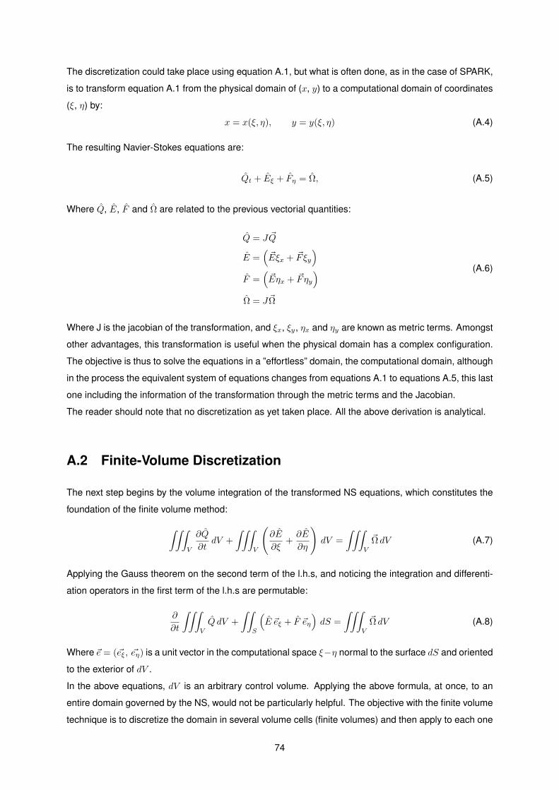
The discretization could take place using equation A.1, but what is often done, as in the case of SPARK,
is to transform equation A.1 from the physical domain of (x, y) to a computational domain of coordinates
(ξ, η) by:
x = x(ξ, η), y = y(ξ, η) (A.4)
The resulting Navier-Stokes equations are:
Qt + Eξ + Fη = Ω, (A.5)
Where Q, E, F and Ω are related to the previous vectorial quantities:
Q = J ~Q
E =(~Eξx + ~Fξy
)F =
(~Eηx + ~Fηy
)Ω = J~Ω
(A.6)
Where J is the jacobian of the transformation, and ξx, ξy, ηx and ηy are known as metric terms. Amongst
other advantages, this transformation is useful when the physical domain has a complex configuration.
The objective is thus to solve the equations in a ”effortless” domain, the computational domain, although
in the process the equivalent system of equations changes from equations A.1 to equations A.5, this last
one including the information of the transformation through the metric terms and the Jacobian.
The reader should note that no discretization as yet taken place. All the above derivation is analytical.
A.2 Finite-Volume Discretization
The next step begins by the volume integration of the transformed NS equations, which constitutes the
foundation of the finite volume method:
∫∫∫V
∂Q
∂tdV +
∫∫∫V
(∂E
∂ξ+∂E
∂η
)dV =
∫∫∫V
~Ω dV (A.7)
Applying the Gauss theorem on the second term of the l.h.s, and noticing the integration and differenti-
ation operators in the first term of the l.h.s are permutable:
∂
∂t
∫∫∫V
Q dV +
∫∫S
(E ~eξ + F ~eη
)dS =
∫∫∫V
~Ω dV (A.8)
Where ~e = (~eξ, ~eη) is a unit vector in the computational space ξ−η normal to the surface dS and oriented
to the exterior of dV .
In the above equations, dV is an arbitrary control volume. Applying the above formula, at once, to an
entire domain governed by the NS, would not be particularly helpful. The objective with the finite volume
technique is to discretize the domain in several volume cells (finite volumes) and then apply to each one
74

equation A.8. Using the nomenclature of figure A.1 we apply it to one such finite cell:
∂
∂t
∫∫∫V
Q dξ dη+
∫∫Si+1
2,j
E dη −∫∫
Si− 1
2,j
E dη
+
∫∫Si,j+1
2
F dξ −∫∫
Si,j+1
2
F dξ
=
∫∫∫V
~Ω dξ dη
(A.9)
Up until now, every derivation was exact and no discretization formally took place. Now, because the
integrands in the volume and surface integrals are not known, i.e it is not know how Q and Ω vary
within the volume and is not know how E and F vary across the boundaries S, approximations must be
introduced [48, ch. 4]. To that end, Q and Ω are assumed constant over each volume Vi,j whose value
is located at the cell centres. Similarly, the flux vectors E and F are assumed to be constant over the
cell faces Si,j . The integrals can then be evaluated, leading to:
∂Qi,j∂t
+Ei+ 1
2 ,j− Ei− 1
2 ,j
∆ξ+Fi,j+ 1
2− Fi,j− 1
2
∆η= Ωi,j (A.10)
Figure A.1: A typical control volume cell and its neighbours along with the surface frontiers S and theremaining notation used.
A.2.1 Explicit Time Integration
The discretization in space has been partially done above and will be completed on the next section.
In the meantime, it is required to discretize the time dependence on the first term of equation A.10,
resulting in the equations being solved for a finite number of intervals [tn, tn+1].
There are two types of time discretization: implicit and explicit . SPARK has both approaches available,
but the catalytic capabilities implemented assumed a explicit discretization. An explicit approach is
by definition one where equation A.10 for each volume cell (i, j) contains a single unknown term in
75

time tn+1 = tn + ∆t, while others are known terms in the current time step tn [45, ch. 4]. With the
above definition, the time derivative is first discretized by a first-order approximation which then leads to
equation A.12.∂Q
∂t=Qn+1i,j − Qni,j
∆t(A.11)
Qn+1i,j − Qni,j
∆t= Ωni,j −
Eni+ 12 ,j− En
i− 12 ,j
∆ξ+Fni,j+ 1
2
− Fni,j− 1
2
∆η
⇔Qn+1i,j = Qni,j + ∆t
Ωni,j −
Eni+ 12 ,j− En
i− 12 ,j
∆ξ+Fni,j+ 1
2
− Fni,j− 1
2
∆η
(A.12)
A.2.2 Spacial Discretization of the Fluxes
From equation A.10 and figure A.1 it can be noticed that the fluxes E and F are evaluated at the cell
faces (e.g Eni+ 1
2 ,jon face Si+ 1
2 ,j) but in the finite volume method all the information is stored on the cell
centres. Therefore the last step consists in expressing the cell faced values of the fluxes in terms of
the cell centres. The methodology followed by SPARK is lengthy . Here just the diffusive fluxes will be
covered. Again the reader is referred to references [23] and [26].
If φ represents any given variable inside the fluxes E and F then:
φi+ 12 ,j
=1
2(φi,j + φi+1,j) (A.13)(
∂φ
∂ξ
)i+ 1
2 ,j
=1
∆ξ(φi+1,j − φi,j) (A.14)
Notice that this procedure effectively couples the equations for all the finite volume cells.
76

Appendix B
Other Computational Results
B.1 Sharp Cones
0
0.005
0.01
0.015
0.02
0 0.5 1 1.5 2 2.5 3
Norm
al dis
tance
fro
m t
he w
all
[m]
O Mass Fraction [%]
Blottner, 1971 - γ=0.00Park, 2001 - γ=0.00
γ=0.01γ=1.00
(a) O Mass Fraction
0
0.005
0.01
0.015
0.02
0 0.1 0.2 0.3 0.4 0.5
Norm
al dis
tance
fro
m t
he w
all
[m]
NO Mass Fraction [%]
Blottner, 1971 - γ=0.00Park, 2001 - γ=0.00
γ=0.01γ=1.00
(b) NO Mass Fraction
Figure B.1: SPARK results for mass fraction of profiles normal to cone surface at x = 0.5m.(θ = 10,SEB) using kinetics from Park, 2001 [35] vs. Blottner, 1971 [34].
77

(a) Isothermal wall, Tw=1200 K, Semi-Angle = 100. (b) SEB, Semi-Angle = 100.
(c) SEB, Semi-Angle = 200.
Figure B.2: SPARK mesh convergence study for the 3 test cases of sharp cones reproduced by SPARK.The variable examined is the temperature profile normal to the cone surface at x=0.5[m].
78

B.2 Electre Probe
(a) Test case corresponding to Vivani et al., [38] (b) Test case corresponding to Muylaert et al., [32]
Figure B.3: SPARK mesh convergence study for the scenarios concerning the Electre probe. Thequantity examined is the heat flux into Electre.
(a) Temperature profile normal to surface of Electre at x = 0.1m
Figure B.4: Temperature along the normal to Electre’s wall at x = 0.1m for Tw = 343K. Comparison ofcurrent results under SPARK for two catalytic recombination coefficients γ = 1 and γ = 0.01 to examinetheir effect on temperature. Upstream conditions correspond to Barbato et al.
79

B.3 Temperature varying SRE, γ = γ(T )
Figure B.5: Mesh used on the simulations for verification of the temperature dependent recombinationefficiency models implemented on SPARK. Details: θ = 20, 40X50 cells. The discrete black pointsrepresent the location of the profiles(temperature and mass fractions). The cone starts at x=0.
Figure B.6: 2-dimensional plot of temperature for SPARK simulation case: Sharp Cone, Semi-angle =20, SEB. Catalytic model not relevant as temperature was grossly insensitive to it.
(a) N2 mass fraction on the surface of the cone,(cN2
)w (b) O2 mass fraction on the surface of the cone,
(cO2
)w
Figure B.7: Mass fraction of species N2 and O2 on the surface of the cone as a function of its axial lengthfor several models applied on the same case: Sharp Cone, Semi-angle = 20, SEB. Ranges of y-axisare not the same. γN = γO = γ.
80

B.4 FRSC - Finite Rate Surface Chemistry
(a) First range of time. (b) Second range of time.
Figure B.8: Transient evolution of the species concentrations (mol m−3 or mol m−2) from an initial condi-tion consisting of only bulk silica, argon and free sites. The temperature is 2500 K and the initial pressureis 10000 Pa. All surface reactions included. Silica sublimation case.
81

82