Gas Pipelines Corrosion Data Analysis and Related Topics de... · 2017-07-03 · Abstract Gas...
155
Gas Pipelines Corrosion Data Analysis and Related Topics by Daniel Lewandowski A thesis submitted to the Delft University of Technology in conformity with the requirements for the degree of Master of Science. Delft, The Netherlands Copyright c 2002 by Daniel Lewandowski, All rights reserved.
Transcript of Gas Pipelines Corrosion Data Analysis and Related Topics de... · 2017-07-03 · Abstract Gas...
Gas Pipelines Corrosion Data Analysis and
Related Topics
by
Daniel Lewandowski
A thesis submitted to the Delft University of Technology in conformity with
the requirements for the degree of Master of Science.
Delft, The Netherlands
Copyright c©2002 by Daniel Lewandowski,
All rights reserved.

Abstract
Gas Pipelines Corrosion Data Analysisand Related Topics
by Daniel Lewandowski
Chairperson of Graduate Committee: Prof. dr Roger M. CookeDepartment of Mathematics
Graduate Committee: Prof. dr Roger M. CookeIr. Eric JagerDrs. Robert KuikDr Dorota KurowickaProf. dr Thomas A. Mazzuchi
In The Netherlands the grid of gas pipelines consists of over 11, 000 km
of steel pipes, most of the them laid in ’60s. A large percentage of the grid
reaches the age when corrosion of the pipelines is becoming increasingly impor-
tant. Recently N.V. Nederlandse Gasunie, the leading Dutch gas company, has
performed inspections of few of their pipelines. This thesis describes and ana-
lyzes with details the corrosion data collected during the inspection. The data
includes information on percentage of metal loss and positions of the corrosion
spots along the pipe. The preliminary analysis brings closer some statistical
characteristics of the occurrence of corrosion and tries to find patterns in the
data. Furthermore, there exists a Monte Carlo model which predicts failure
frequency of gas pipelines given full characteristic of a pipe. Part of the thesis
compares the results obtained by running the model with the actual data.

Acknowledgements
The author wishes to express sincere appreciation to the Delft University of
Technology, where he has had the opportunity to work with Roger M. Cooke,
il miglior fabbro, Dorota Kurowicka and Thomas A. Mazzuchi. Thanks to Eric
Jager and Gerard Stallenberg from N.V. Nederlandse Gasunie for proposing
the subject of this thesis, providing data and helpful explanations of issues
related to the maintenance of gas pipelines. The author would also like to
acknowledge Kasia, Pawe l and Cornel for being good friends during these two
years spent in Delft.
Last but not least, the author would like to acknowledge his parents and
sister for their continuous support.
Contents
List of tables iii
List of figures iv
List of symbols vii
Introduction xi
1 Gas pipelines safety regulations 11.1 Gas safety guidelines and recommendations . . . . . . . . . . . . 11.2 Risk assessment . . . . . . . . . . . . . . . . . . . . . . . . . . . 21.3 Location classification . . . . . . . . . . . . . . . . . . . . . . . 41.4 Other risk minimizing factors . . . . . . . . . . . . . . . . . . . 61.5 Inspection, reporting and maintenance policy . . . . . . . . . . . 71.6 Future initiatives . . . . . . . . . . . . . . . . . . . . . . . . . . 9
2 Description of the Gasunie data 112.1 MFL-pig . . . . . . . . . . . . . . . . . . . . . . . . . . . . . . . 112.2 Overview of the Gasunie data . . . . . . . . . . . . . . . . . . . 12
3 Description of the UNICORN model 173.1 Introduction . . . . . . . . . . . . . . . . . . . . . . . . . . . . . 173.2 Modelling pipeline failures . . . . . . . . . . . . . . . . . . . . . 19
3.2.1 Example of modelling approach . . . . . . . . . . . . . . 213.2.2 Overall modelling approach . . . . . . . . . . . . . . . . 23
3.3 Third party interference . . . . . . . . . . . . . . . . . . . . . . 243.4 Damage due to environment . . . . . . . . . . . . . . . . . . . . 293.5 Failure due to corrosion . . . . . . . . . . . . . . . . . . . . . . 30
3.5.1 Modelling corrosion induced failures . . . . . . . . . . . . 303.5.2 Pit corrosion rate . . . . . . . . . . . . . . . . . . . . . . 33
3.6 Results for ranking . . . . . . . . . . . . . . . . . . . . . . . . . 353.6.1 Case-wise comparisons . . . . . . . . . . . . . . . . . . . 35
i
3.6.2 Importance in specific case . . . . . . . . . . . . . . . . . 373.7 Conclusions . . . . . . . . . . . . . . . . . . . . . . . . . . . . . 403.8 Implementation . . . . . . . . . . . . . . . . . . . . . . . . . . . 413.9 UNICORN frontend for the model . . . . . . . . . . . . . . . . . 42
4 Bayesian sensitivity analysis 454.1 Introduction . . . . . . . . . . . . . . . . . . . . . . . . . . . . . 454.2 Sensitivity in hierarchical models . . . . . . . . . . . . . . . . . 46
4.2.1 Which parameters are sensitive to the data? . . . . . . . 464.2.2 Which parameters are sensitive for a given parameter? . 474.2.3 A more general notion of sensitivity. . . . . . . . . . . . 474.2.4 Can the computations be done efficiently? . . . . . . . . 49
4.3 Example, the SKI model . . . . . . . . . . . . . . . . . . . . . . 524.4 Sensitivity results . . . . . . . . . . . . . . . . . . . . . . . . . . 564.5 Conclusions . . . . . . . . . . . . . . . . . . . . . . . . . . . . . 60
5 Sensitivity analysis of the UNICORN model factors 635.1 Sensitivities in modelling of damage due to 3rd party digs . . . . 645.2 Sensitivities in modelling environmental factors . . . . . . . . . 675.3 Sensitivities in modelling the overall failure frequency in sand . 705.4 Sensitivities in modelling the overall failure frequency in clay . . 75
6 Analysis of the corrosion data 816.1 Analysis of pipeline A data . . . . . . . . . . . . . . . . . . . . . 816.2 Analysis of pipelines B, C, D and E data . . . . . . . . . . . . . 846.3 Comparison of the UNICORN output with the actual data . . . 86
7 Corrosion rate 97
8 Conclusions 101
Bibliography 107
A Help file for GasUnicorn 111
B Unicorn model implementation 117
C MatLab code performing preliminary analysis 124
ii

List of tables
1.1 Location classification. . . . . . . . . . . . . . . . . . . . . . . . 41.2 Proximity and survey distances in meters. . . . . . . . . . . . . 5
2.1 Accuracy of sizing depth of metal loss. . . . . . . . . . . . . . . 112.2 General characteristics of the inspected pipelines. . . . . . . . . 14
3.1 Marks for 3rd party digs. . . . . . . . . . . . . . . . . . . . . . . 253.2 Factors influencing failure due to corrosion. . . . . . . . . . . . . 30
4.1 Swedish nuclear plant centrifugal pump data. . . . . . . . . . . 554.2 Results for λ15. . . . . . . . . . . . . . . . . . . . . . . . . . . . 554.3 Correlation ratios for λ15. . . . . . . . . . . . . . . . . . . . . . 57
5.1 Correlation ratios for outputs of HITPIP submodel. . . . . . . . 655.2 Influence of environmental characteristics on the corrosion rate
in sand. . . . . . . . . . . . . . . . . . . . . . . . . . . . . . . . 675.3 Influence of environmental characteristics on the corrosion rate
in clay. . . . . . . . . . . . . . . . . . . . . . . . . . . . . . . . . 705.4 Influence of the corrosion rate on the failure frequency due to
corrosion in sand. . . . . . . . . . . . . . . . . . . . . . . . . . . 725.5 Influence of some variables on the failure frequency due to cor-
rosion in sand. . . . . . . . . . . . . . . . . . . . . . . . . . . . . 725.6 Influence of the corrosion rate on the failure frequency due to
corrosion in clay. . . . . . . . . . . . . . . . . . . . . . . . . . . 775.7 Influence of some variables on the failure frequency due to cor-
rosion in clay. . . . . . . . . . . . . . . . . . . . . . . . . . . . . 77
6.1 Two characteristics of sand applied to the UNICORN model. . . 92
iii
List of figures
1.1 Example of incident scenarios for flammable media. . . . . . . . 2
1.2 Hypothetical safety evaluation path. . . . . . . . . . . . . . . . 3
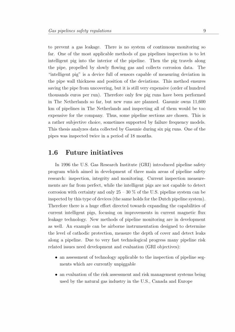
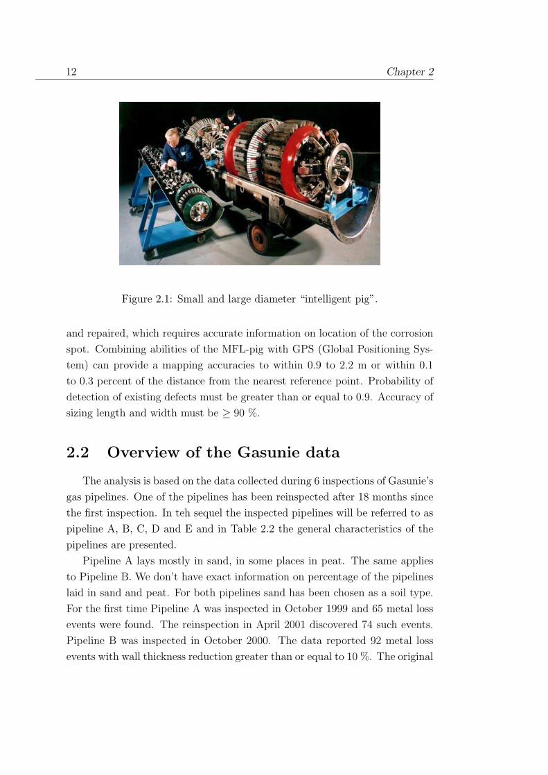
2.1 Small and large diameter “intelligent pig”. . . . . . . . . . . . . 12
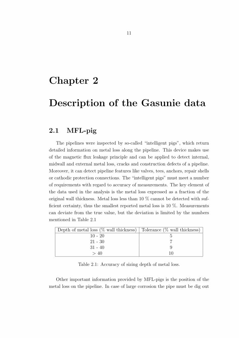
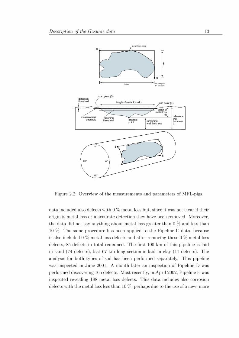
2.2 Overview of the measurements and parameters of MFL-pigs. . . 13
2.3 Sample of the data collected during inspection of Pipeline E. . . 14
3.1 Fault tree for gas pipeline failure. . . . . . . . . . . . . . . . . . 23
3.2 Digs as marked point process. . . . . . . . . . . . . . . . . . . . 24
3.3 Overview of cathodic protection system. . . . . . . . . . . . . . 31
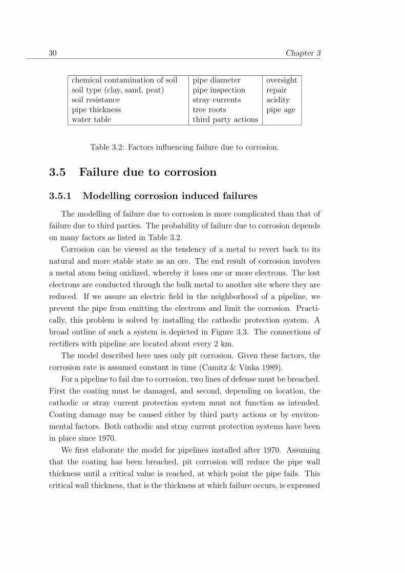
3.4 Effective lives and critical years for three damage types for fixedcorrosion rate. . . . . . . . . . . . . . . . . . . . . . . . . . . . . 32
3.5 Uncertainty distributions for three cases. . . . . . . . . . . . . . 36
3.6 Unconditional cobweb plot. . . . . . . . . . . . . . . . . . . . . 38
3.7 Cobweb plot conditional on high values of corlk. . . . . . . . . . 39
3.8 Cobweb plot conditional on low values of corlk. . . . . . . . . . 40
3.9 Main window of GasUnicorn, new interface for UNICORN. . . . 41
3.10 Report created by GasUnicorn based on the results of last sim-ulation. . . . . . . . . . . . . . . . . . . . . . . . . . . . . . . . 42
4.1 Density approximation with 5 observations. . . . . . . . . . . . 49
4.2 Entropy, 1000 standard normals, 20 iterations. . . . . . . . . . . 51
4.3 I(X|Y ) 1000 samples, 20 iterations, X=N(0,1), Y = N(5,3). . . 52
4.4 Cumulative distribution function of λ15. . . . . . . . . . . . . . 54
4.5 Variance of pi compared to correlation ratio between λ15 and pi. 58
4.6 The MTTF of the plant i compared to the inverse of expectationof λ15 (MTTF of λ15) and the correlation between λ15 and pi. . 58
4.7 Dependence between E(λ15|α) and α compared to E(λ15) . . . . 59
4.8 Dependence between E(λ15|β) and β compared to E(λ15) . . . . 59
4.9 Dependence between E(λ15|c) and c compared to E(λ15) . . . . 60
5.1 Cobweb plots of the variables of HITPIP submodel. . . . . . . . 64
iv
5.2 Conditional expectation E(cd3rn|roon). . . . . . . . . . . . . . 66
5.3 Influence of depth cover on frequency of damages due to 3rd
party digs. . . . . . . . . . . . . . . . . . . . . . . . . . . . . . . 66
5.4 Correlation ratio between udfb and udfp and input factors. . . . 68
5.5 Mean frequency of coating damages due to environment. . . . . 69
5.6 Effective life of the pipeline given partially working cathodicprotection system. . . . . . . . . . . . . . . . . . . . . . . . . . 73
5.7 Effective life of the pipeline given partially working cathodicprotection system for small values of crp. . . . . . . . . . . . . . 74
5.8 Cobweb plot of corlk and other variables conditionalized on highvalues of corlk, 31 year old pipeline laid in sand in 1967. . . . . 75
5.9 Cobweb plot of corlk and other variables conditionalized on lowvalues of corlk, 31 year old pipeline laid in sand in 1967. . . . . 76
5.10 Cobweb plot of corlk and other variables conditionalized on highvalues of corlk, 22 year old pipeline laid in sand in 1975. . . . . 76
5.11 Cobweb plot of corlk and other variables conditionalized on highvalues of corlk, 31 year old pipeline laid in clay in 1967. . . . . . 78
5.12 Cobweb plot of corlk and other variables conditionalized on lowvalues of corlk, 31 year old pipeline laid in clay in 1967. . . . . . 78
5.13 Cobweb plot of corlk and other variables, 31 year old pipelinelaid in clay in 1967. . . . . . . . . . . . . . . . . . . . . . . . . . 79
6.1 Total number of corrosion spots in Pipeline A and A1 data sets. 82
6.2 Quantile-quantile plot of Pipeline A and A1 data sets. . . . . . . 82
6.3 Empirical distribution functions of metal loss for Pipeline A andA1 corrosion data. . . . . . . . . . . . . . . . . . . . . . . . . . 83
6.4 Histograms of corrosion events found during inspections in 1999(pipeA) and 2001 (pipeA1). . . . . . . . . . . . . . . . . . . . . 83
6.5 Vertical positions of the metal loss events on the surface ofpipeline A. . . . . . . . . . . . . . . . . . . . . . . . . . . . . . . 84
6.6 Total number of corrosion spots in pipeline B, C, D and E datasets. . . . . . . . . . . . . . . . . . . . . . . . . . . . . . . . . . 85
6.7 Histograms of corrosion events found during inspections of pipelinesB, C, D and E. . . . . . . . . . . . . . . . . . . . . . . . . . . . 86
6.8 Vertical positions of the metal loss events on the surface ofpipelines B, C, D and E. . . . . . . . . . . . . . . . . . . . . . . 87
6.9 Comparison of the UNICORN output with the Pipeline A datainspected in 1999. . . . . . . . . . . . . . . . . . . . . . . . . . . 88
6.10 Comparison of the UNICORN output with the Pipeline A datainspected in 2001. . . . . . . . . . . . . . . . . . . . . . . . . . . 89
6.11 Comparison of the UNICORN output with the Pipeline B data. 89
v
6.12 Comparison of the UNICORN output with the Pipeline C data(first 100 km of the pipeline laid in sand). . . . . . . . . . . . . 91
6.13 Comparison of the UNICORN output with the Pipeline C data(last 67 km of the pipeline laid in clay). . . . . . . . . . . . . . . 91
6.14 Comparison of the UNICORN output with the Pipeline D data. 936.15 Comparison of the UNICORN output with the Pipeline E data. 936.16 Influence of values of the parameters on frequency of exceeding
25 % of metal loss. . . . . . . . . . . . . . . . . . . . . . . . . . 94
7.1 Location of the corrosion spots. . . . . . . . . . . . . . . . . . . 987.2 Manual searching for the corresponding spots. . . . . . . . . . . 987.3 Cumulative distribution functions of free and partial corrosion
rate returned by the Unicorn model for Pipeline A characteristics. 99
8.1 Cobweb plot of corlk, crf and crp. . . . . . . . . . . . . . . . . . 1028.2 Cobweb plot of corlk, crf and crp conditionalized on 30th per-
centile of corlk. . . . . . . . . . . . . . . . . . . . . . . . . . . . 1038.3 Histograms of the selected samples of crf and crp. . . . . . . . . 104
A.1 Structural organization of the model. . . . . . . . . . . . . . . . 112A.2 Report generated by GasUnicorn. . . . . . . . . . . . . . . . . . 115
vi
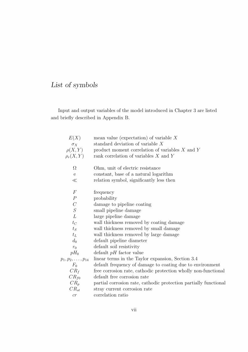
List of symbols
Input and output variables of the model introduced in Chapter 3 are listed
and briefly described in Appendix B.
E(X) mean value (expectation) of variable XσX standard deviation of variable X
ρ(X,Y ) product moment correlation of variables X and Yρr(X,Y ) rank correlation of variables X and Y
Ω Ohm, unit of electric resistancee constant, base of a natural logarithm relation symbol, significantly less then
F frequencyP probabilityC damage to pipeline coatingS small pipeline damageL large pipeline damagetC wall thickness removed by coating damagetS wall thickness removed by small damagetL wall thickness removed by large damaged0 default pipeline diameterr0 default soil resistivitypH0 default pH factor value
p1, p2, . . . , p14 linear terms in the Taylor expansion, Section 3.4F0 default frequency of damage to coating due to environmentCRf free corrosion rate, cathodic protection wholly non-functionalCRf0 default free corrosion rateCRp partial corrosion rate, cathodic protection partially functionalCRst stray current corrosion ratecr correlation ratio
vii
List of abbreviations
Ω.cm Ohm centimeterkm.yr kilometer yearFCL frequency of closed digs per km.yrFOP frequency of open digs per km.yrMFL magnetic flux leakageLNG liquified natural gasCDE coating damage due to environmentCP cathodic protection systemSP stray current protection system
MTTF mean time to failure
Glossary of terms
%bit %km with bitumen coating%ebe % of coating damages due to ground movement, root growth or
chemical contamination; bitumen%epe % of coating damages due to ground movement, root growth or
chemical contamination; polyethyleneb birthyearbs %1km pipe near bond sitech %km with heavy industrial contaminationcps year of cathodic protection (CP) installmentcrf free corrosion ratecrfz default free corrosion ratecrp corrosion rate when CP partially functionalcrpe pit corrosion rate if the pipe ground potential is -700 mVcrse corrosion rate if there are unprotected stray currentsdia diameterdl prob. of direct leak from 3rd parties
dpth depth [m]fcl frequency of closed digs per km.yrfclz freq. of closed digs per km.yr; 0th orderfop frequency of open digs per km.yrfopz freq. of open digs per km.yr; 0th order
viii
grb rate of occurrence of bitumen defects (per 100 km)grp rate occurrence of polyethylene defects (per 100 km)
hcone freq. of hitting per km.yr; closed dig, no oversighthconz freq. of hitting per km.yr; closed dig, no oversight, 0th orderhcoye freq. of hitting per km.yr; closed dig, oversighthcoyz freq. of hitting per km.yr; closed dig, oversight, 0th orderhoone freq. of hitting per km.yr; open dig, no oversighthoonz freq. of hitting per km.yr; open dig, no oversight, 0thhooye freq. of hitting per km.yr; open dig, oversightorderhooyz freq. of hitting per km.yr; open dig, oversight, 0th orderpcen prob. of coating damage from environmentpcpfe prob. that CP fails completelypcppe prob. that CP fails partiallypc3 prob. of coating damage from 3rd partiesph pH valuepl prob. of large pipe damageps prob. of small pipe damage
pspe prob. that stray current protection fails at bond siter resistivity
rcon perc. of repaired damages due to hits during closed digs withoutoversight
rcoy perc. of repaired damages due to hits during closed digs withoversight
roon perc. of repaired damages due to hits during open digs withoutoversight
rooy perc. of repaired damages due to hits during open digs withoversight
rt %km with heavy roots growthrup54 perc. of direct leak which will be ruptures per km.yr; 5.4 mm wtrup71 perc. of direct leak which will be ruptures per km.yr; 7.1 mm wt
t pipe wall thickness [mm]tl material removed by large line damage [mm]ts material removed by small line damage [mm]wf %km with fluctuation under and above water tablewu % km under water table
xbche #defects per 100 km if chemical contamination; bitumenxbde #defects per 100 km if diameter = 36”; bitumenxbrte #defects per 100 km if heavy root growth; bitumenxbwfe #defects per 100 km if water table fluctuates; bitumenxpche #defects per 100 km if chemical contamination; polyethylene
xc critical thickness fraction; coating damage
ix

xl critical thickness fraction; large damagexpde #defects per 100 km if diameter = 36”; polyethylenexphe pit corrosion rate if pH is raised by 2.3xprte #defects per 100 km if heavy root growth; polyethylenexpwfe #defects per 100 km if water table fluctuates; polyethylene
xre pit corrosion rate if resistivity is a factor 10 lowerxs critical thickness fraction; small damage
xwfe pit corrosion rate if water table fluctuatesxwue pit corrosion rate if water table is above pipe lines
yb begin year for cumulative frequency of corrosionye end year for cumulative frequency of corrosion
x

Introduction
Nature of industrial hazard
Industrialization and technological development are irreversible processes,
which significantly influence human life and its quality. Aside from good and
desirable consequences of these processes, there are also some visible side ef-
fects, like emission of toxical materials, noise, as well as hidden threats - indus-
trial constructions are very complex and may involve seides of high emergency.
All these dangers have been perceived and now there is a significant effort con-
centrated on eliminating or minimizing industrial risks. One of the sources of
risk is transmission of hazardous substances, like oil or gas, in pipelines. Steel
gas pipelines are exposed to many factors supporting growth of the corrosion.
To be able to prevent this growth, many methods and techniques have been
developed. These include passive prevention like bitumen or polyethylene coat-
ing, as well as active methods involving change of electrostatic characteristic
of the pipe.
Goals of the research
This thesis concentrates on analysis of the corrosion data obtained by in-
specting gas pipelines owned by N.V. Nederlandse Gasunie, Dutch gas com-
pany. Using MFL-pigs1 (Magnetic Flux Leakage), also called “intelligent pigs”,
five pipelines were inspected. One of the pipelines have been reinspected and
this data is also available. The data contains information on the wall thickness
reduction, assumed to be caused by 3rd party digs or corrosion. The goal of
this thesis is to bring closer a wide spectrum of safety and maintenance issues
the gas industry, the Dutch gas industry in particular, must deal with. These
1For more detailed specification of MFL-pigs please refer to Chapter 2.
xi

issues will be presented from a mathematical point of view. Firstly, Chapter 1
describes the safety regulations to which the gas pipelines operators are subject.
The implication of those regulations is the requirement for appropriate main-
tenance of pipelines, including their inspections. Chapter 2 contains a small
sample of the data collected during one of the inspections and general overview
of all of the data sets provided by Gasunie. The actual data will be compared
with the outputs of a probabilistic model of failure frequency of gas pipelines.
The model was developed using a software program for uncertainty analysis
with correlations written at Delft University of Technology, UNICORN, and is
introduced with details in Chapter 3. Since the model is rather complicated, it
might be interesting to study dependencies between input and output variables
of the model. This will be done by sensitivity analysis. A general tool for this
type of analysis is introduced in Chapter 4 and its application to UNICORN
model is described in Chapter 5. Afterwards begins the actual analysis of the
Gasunie’s corrosion data. In Chapter 6 the data is visualized and compared
to the model output, which allows us to evaluate performance of the model
and eventually to recommend some future extensions of the model. Chapter 7
deals with determining the corrosion rate based on the data, since this is a hot
topic now. Besides this, some additional tasks have been performed including
writing a software application on the basis of UNICORN. The new front end is
designed to run only the model introduced in Chapter 3. It will be presented
with screen shots in the same chapter. Appendix A contains the help file for
this front end and in Appendix B the reader will find the implementation of the
model in UNICORN, with descriptions and definitions of input parameters and
output formulas. Appendix C contains the MatLab code used in preliminary
analysis of the data (Chapter 6).
The provided data proved to be very useful. Direct comparison with the
UNICORN model outputs showed very good performance of the later in terms
of predicting the failure frequency. Basically, for all of the inspected cases the
actual data corresponded to 20th – 80th percentile of the distributions of failure
frequency per km.yr. However, in most cases the results varied even less and
were between 20th and 45th percentile of the distributions, what suggests a
small tendency of the model to overestimate the frequency of failures.
The data sets reveal dissimilarities between the inspected pipelines. Pipeline
A, A1 and B data report defects mostly located at the bottom of the pipelines,
xii

whereas in case of Pipeline C, D and E data the defects are spread more
uniformly, regardless if it is the top or the bottom of the pipeline. The
Kolmogorov-Smirnov test allowed to distinct three groups of the pipelines.
Data from pipelines in each of the groups can be regarded as drawn from the
same underlying distribution. The first group are pipelines A, A1 and B, in
the second one are Pipeline C and D. The last group consists of only Pipeline
E.
Dutch gas industry
The first gas deposits in The Netherlands were discovered long before the
Second World War. In 1933, the Batavian Petroleum Company (BPM, a sub-
sidiary of Shell), decided to acquire rights for exclusive exploration of gas-rich
fields in provinces of Groningen, Friesland, Drenthe, Overijssel and Gelder-
land. On 19 September 1947 the Dutch Petroleum Company (NAM) was set
up, with BPM and Standard Oil Company (New Jersey), i.e. Esso, each taking
a 50% share. At this time the whole natural gas production was located in the
eastern part of The Netherlands. In 1962 the official natural gas supply by the
NAM was one million cubic meters per day. On 18 October 1960 the NAM in-
formed that the reserves in the Groningen gas field were greater than foreseen.
A team from Esso proposed that the gas should initially be sold in the small
users’ market, in the public supply. Three gas companies - State Mines, Shell
and Esso, signed a partnership which would sell the gas extracted to a limited
company yet to be set up. This company would be responsible for purchasing,
transporting and selling Dutch natural gas (and also other gases). The charter
of the N.V. Nederlandse Gasunie was signed in the Old Wassenaar Castle on
6 April 1963. Shortly after that, Gasunie started to develop their network of
large diameter natural gas pipelines.
xiii

1
Chapter 1
Gas pipelines safety regulations
In general, pipelines are recognized as a safe way to transport dangerous
substances. However, pipelines accidents have occurred in Europe and world-
wide, indicating that pipelines should be included within scope of the Seveso II
Directive. This legislation regulates safety requirements imposed on companies
dealing with hazardous materials. There was no general agreement on this
issue, noweven, and pipes were excluded from the directive. Currently the
European Council is discussing about introducing a separate legislation for
pipeline transport. Basically, safety of the transport of dangerous substances
in pipelines is regulated by national legislation and regulations, which can
vary significantly even among the member states of EU. All major incidents
related to gas pipelines in The Netherlands are investigated by a independent
governmental body, the Dutch Transport Safety Board.
1.1 Gas safety guidelines and recommendations
Gas pipeline safety assessment and management concentrates on the release
of the transported medium (leakage, rupture) from a pipeline. There are four
well-known books describing methods and recommendations in designing and
maintaining gas pipelines. Methods for determining and processing probabili-
ties are described in the Red Book (CPR 12E). The study of the physical effects
from releases of hazardous materials is described in Yellow Book (CPR 14E).
The Green Book (CPR 16E) contains methods of determining the possible
damage to people. Finally, risks due to transport of hazardous substances via
2 Chapter 1
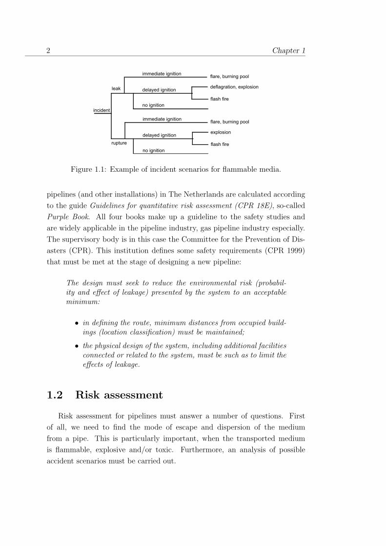
incident
leak
immediate ignition
delayed ignition
no ignition
flare, burning pool
deflagration, explosion
flash fire
immediate ignition
delayed ignition
no ignition
flare, burning pool
explosion
flash firerupture
Figure 1.1: Example of incident scenarios for flammable media.
pipelines (and other installations) in The Netherlands are calculated according
to the guide Guidelines for quantitative risk assessment (CPR 18E), so-called
Purple Book. All four books make up a guideline to the safety studies and
are widely applicable in the pipeline industry, gas pipeline industry especially.
The supervisory body is in this case the Committee for the Prevention of Dis-
asters (CPR). This institution defines some safety requirements (CPR 1999)
that must be met at the stage of designing a new pipeline:
The design must seek to reduce the environmental risk (probabil-ity and effect of leakage) presented by the system to an acceptableminimum:
• in defining the route, minimum distances from occupied build-ings (location classification) must be maintained;
• the physical design of the system, including additional facilitiesconnected or related to the system, must be such as to limit theeffects of leakage.
1.2 Risk assessment
Risk assessment for pipelines must answer a number of questions. First
of all, we need to find the mode of escape and dispersion of the medium
from a pipe. This is particularly important, when the transported medium
is flammable, explosive and/or toxic. Furthermore, an analysis of possible
accident scenarios must be carried out.
Gas pipelines safety regulations 3
preliminary choice of route
nature of medium
mode of escape and
dispersion
incidents scenarios
effect calculationfailure probability analysis
individual iso-risk contours,
proximity distance, survey
distance
location classification
choice of route/safety distances
(location classification) +
identification of infringments
risk reducing measures:
- reducing failure probability
- mitigating effects
- management systems
definitive route, pipeline design
and management system
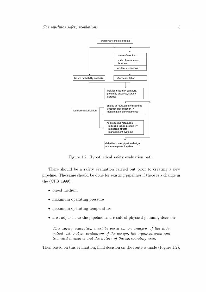
Figure 1.2: Hypothetical safety evaluation path.
There should be a safety evaluation carried out prior to creating a new
pipeline. The same should be done for existing pipelines if there is a change in
the (CPR 1999):
• piped medium
• maximum operating pressure
• maximum operating temperature
• area adjacent to the pipeline as a result of physical planning decisions
This safety evaluation must be based on an analysis of the indi-vidual risk and an evaluation of the design, the organizational andtechnical measures and the nature of the surrounding area.
Then based on this evaluation, final decision on the route is made (Figure 1.2).

4 Chapter 1
Area LocationClassification
scattered residential housing orno residential housing
1
less important special premises 2residential areas, recreational ar-eas or industrial areas
3
apartment building or importantspecial premises
4
Table 1.1: Location classification.
1.3 Location classification
We can see that, as with other potentially hazardous structures, the land-
use planning must be performed in case of pipelines. Location classification is
performed in order to be able to distinguish (CPR 1999):
• population density
• building density
• presence of sensitive sites which are centers of human activity
• level of industry activity and the economic value
All structures and installments in neighborhood of a pipeline must be clas-
sified into four categories mentioned in Table 1.1. The higher the location
classification, the smaller acceptable risk.
The individual risk is the probability that a person will die by accident when
he is at a certain location for a year. The iso-contour of the individual risk
connects points with equal individual risk and is called the risk contour. The
minimum acceptable distances are derived from analysis of the risk contours.
There are two basic concepts applied to determine the acceptability of the
assumed road for a pipeline:
proximity distance - the shortest distance between the center of the pipeline
and residential buildings or special structures; coincides with the 10−6
iso-risk contour (max. permissible individual risk)

Gas pipelines safety regulations 5
Nominaldiameter
Proximity distances [m] Survey distances [m]
inch 20-50bars
50-80bars
80-110bars
20-50bars
50-80bars
80-110bars
2 4 5 5 20 20 204 4 5 7 20 20 256 4 5 7 20 25 308 7 8 10 20 30 4010 9 10 14 25 35 4512 14 17 20 30 40 5014 17 20 25 35 50 6016 20 20 25 40 55 7518 ∗ 20 25 45 60 7024 ∗ 25 25 60 80 9530 ∗ 30 35 75 95 12036 ∗ 35 45 90 115 14042 ∗ 45 55 105 130 16048 ∗ 50 60 120 150 180
∗ - distance to be determined in consultation between the parties involved in
the project
Table 1.2: Proximity and survey distances in meters.
survey distance - the distance measured on both sides from the center of
the pipeline within a survey is made to identify the presence of residen-
tial buildings, special structures and recreational and industrial areas;
coincides with the 10−8 iso-risk contour.
Research has shown that calculation of the iso-risk contours can be dispensed
with gas pipelines if the values given in Table 1.2 are used for the proximity
distance and the survey distance from buildings. Currently these values are
under review. It is expected that these will change in the near future.
Gasunie has purchased population density data of The Netherlands, to
be able to carry out quantitative risk assessment concerning influence of the
population density on frequency of pipelines failures. Moreover, locations of
new pipelines are consulted with the regional authorities using their population
data.
6 Chapter 1
For transport pipelines the minimum separation distance from the nearest
installation must be at least equal to the survey distance. However, some
departures from this requirement are allowed. This is the case, when shorter
distance is justified on planning, technical or economic grounds, but it cannot
be less then the proximity distance. For locations where the individual risk
induced by the presence of a pipeline is between 10−6 and 10−8 per year, a
careful assessment must be carried out of all of the interests involved. This
includes primary effects of release of the medium transported by the pipeline
like:
• environmental pollution
• combustion/explosion following ignition
• physical explosion
• toxicity
Secondary consequential damages caused by one of the above mentioned
incidents must be taken into account as well. This can be for example flood,
erosion, blockage of shipping routes.
1.4 Other risk minimizing factors
There are also some restrictions concerning depth cover of pipelines. Obvi-
ously, the deeper a given pipe is laid, the smaller probability of hitting during
3rd party digs. The minimum depth cover must have 80 cm and must be
increased if there is a likelihood of:
• deep ploughing or deep excavation
• grading works
or lays beneath road surfaces. If providing the required depth of cover is
difficult, then the pipe must be protected with a cover, mainly concrete one.
In places where the pipe crosses ditches or watercourses, it must be laid to a
depth of at least 60 cm, unless a concrete cover is applied.
Many regulations concern pipe wall thickness to protect against mechanical
damage and corrosion (CPR 1999):
Gas pipelines safety regulations 7
The specified minimum yield strength divided by the circumferentialstress at design pressure must be equal to or greater than the wallthickness allowances for mechanical damage.
1.5 Inspection, reporting and maintenance pol-
icy
Risk contours are calculated based on the probability of a pipeline failure.
Therefore it is very important to maintain a well-designed failure database,
since the failure analysis is based on historical data. The data is collected by
inspecting the pipelines.
Failure data shows that the most important factors causing pipelines dam-
ages are third party activities. This can be for example laying telecommunica-
tion cables, pitting foundations etc. It must be ensured that the underground
gas pipelines are marked and gas supplier employee supervise earthworks, es-
pecially those using heavy machines.
Australian gas regulations (Gas Safety (Safety Case) Regulations 1999)
states, that safety management system must specify a number of issues regard-
ing gas pipelines. Among other things they are:
• technical standards used in the design, construction, installation and op-
eration of the facility
• clear definition of organizational structure and responsibilities
• control systems like alarm systems, temperature and pressure measure
systems, emergency shut-down systems
• machinery and equipment must be specified to ensure that the equipment
is fit for the purpose
• specification of the response plans designed to address all reasonably
foreseeable emergencies
• emergency communication system adequate to communicate within fa-
cility and with the relevant fire authorities and emergency service
8 Chapter 1
• internal monitoring, auditing and reviewing to ensure appropriate imple-
mentation of safety policies, objectives and procedures specified in SMS
• gas incidents recording, investigation and reviewing
• training to ensure that all employees have proper skill, knowledge and
experience
Other national legislation concerning risk management of the gas facilities is
more or less constructed with the same pattern. For example, English national
regulations specify detailed procedures of acting in case of incidents involving
gas (Health and Safety: The Gas Safety (Installation and Use) Regulations
1998). If escape of gas from a pipe occurs, a gas supplier must within 12 hours
of being so informed of the escape, prevent the gas escaping.
In 1998 the U.S. Research and Special Programs Administration published a
proposal replacing most LNG (Liquefied Natural Gas) requirements for siting,
design, construction, equipment and fire protection. It also proposed some
minor amendments to operation and maintenance requirements for new and
significantly altered facilities. Those changes were proposed in order to more
accurately reflect current technology and practices in the LNG industry and
replace the regulations from 1979.
Recently in the U.S. the Department of Transportation of the Office of
Pipeline Safety prepared amendments to some safety regulations. In January
2000 new safety standards for the repair of corroded or damaged steel pipe in
gas or hazardous liquid pipelines have been introduced. Another legislation act
is making changes to the reporting requirements for hazardous liquid pipeline
accidents. The rule lowers the current reporting threshold of 50 barrels to a
new threshold of 5 gallons, and makes changes to the accident report form. The
changes are necessary, because the existing reporting threshold and reporting
form have been recognized as not sufficiently informative for efficient safety
analysis. This rule is effective since 1 January 2002.
One of the main factors having great impact on frequency of gas pipelines
failures is corrosion. Progressing corrosion reduces the pipe wall thickness,
causing a strength to stress to drop significantly. Since the gas in a pipe is
under heavy pressure, pipe failure is a direct implication of the weak strength.
It is extremely important to have a system of inspecting pipelines in order
Gas pipelines safety regulations 9
to prevent a gas leakage. There is no system of continuous monitoring so
far. One of the most applicable methods of gas pipelines inspection is to let
intelligent pig into the interior of the pipeline. Then the pig travels along
the pipe, propelled by slowly flowing gas and collects corrosion data. The
“intelligent pig” is a device full of sensors capable of measuring deviation in
the pipe wall thickness and position of the deviations. This method ensures
saving the pipe from uncovering, but it is still very expensive (order of hundred
thousands euros per run). Therefore only few pig runs have been performed
in The Netherlands so far, but new runs are planned. Gasunie owns 11,600
km of pipelines in The Netherlands and inspecting all of them would be too
expensive for the company. Thus, some pipeline sections are chosen. This is
a rather subjective choice, sometimes supported by failure frequency models.
This thesis analyzes data collected by Gasunie during six pig runs. One of the
pipes was inspected twice in a period of 18 months.
1.6 Future initiatives
In 1996 the U.S. Gas Research Institute (GRI) introduced pipeline safety
program which aimed in development of three main areas of pipeline safety
research: inspection, integrity and monitoring. Current inspection measure-
ments are far from perfect, while the intelligent pigs are not capable to detect
corrosion with certainty and only 25 – 30 % of the U.S. pipeline system can be
inspected by this type of devices (the same holds for the Dutch pipeline system).
Therefore there is a huge effort directed towards expanding the capabilities of
current intelligent pigs, focusing on improvements in current magnetic flux
leakage technology. New methods of pipeline monitoring are in development
as well. An example can be airborne instrumentation designed to determine
the level of cathodic protection, measure the depth of cover and detect leaks
along a pipeline. Due to very fast technological progress many pipeline risk
related issues need development and evaluation (GRI objectives):
• an assessment of technology applicable to the inspection of pipeline seg-
ments which are currently unpiggable
• an evaluation of the risk assessment and risk management systems being
used by the natural gas industry in the U.S., Canada and Europe

10 Chapter 1
• an analysis of promising near-term pipeline monitoring technologies
• development of a national damage prevention/one-call system and anatom-
ical mapping standard
• development of risk management as an alternative to current prescriptive
regulations
It seems to be likely, that the development of safety standards in Europe will
go in the same way.
The United States have a very good pipelines risk management system.
The first priority of the U.S. pipeline industry is the Office of Pipeline Safety,
which develops regulations and other approaches to risk management to assure
safety in design, construction, maintenance and emergency response of pipeline
facilities. In The Netherlands the gas sector has a rather significant freedom in
establishing safety regulations. Basically, the largest Dutch gas company, N.V.
Nederlandse Gasunie, must meet the requirements imposed by the Dutch gov-
ernment, but they are consulted before the regulations take effect. Nowadays,
Gasunie is working on a proposal of new regulations concerning safety of gas
facilities.
Risk assessment of natural gas transmission systems can be simplified and
accelerated by using computer programs. A very well-known example of such
a software is PIPESAFE, which is a result of joint work of many international
gas companies, including N.V. Nederlandse Gasunie.
11
Chapter 2
Description of the Gasunie data
2.1 MFL-pig
The pipelines were inspected by so-called “intelligent pigs”, which return
detailed information on metal loss along the pipeline. This device makes use
of the magnetic flux leakage principle and can be applied to detect internal,
midwall and external metal loss, cracks and construction defects of a pipeline.
Moreover, it can detect pipeline features like valves, tees, anchors, repair shells
or cathodic protection connections. The “intelligent pigs” must meet a number
of requirements with regard to accuracy of measurements. The key element of
the data used in the analysis is the metal loss expressed as a fraction of the
original wall thickness. Metal loss less than 10 % cannot be detected with suf-
ficient certainty, thus the smallest reported metal loss is 10 %. Measurements
can deviate from the true value, but the deviation is limited by the numbers
mentioned in Table 2.1
Depth of metal loss (% wall thickness) Tolerance (% wall thickness)10 - 20 521 - 30 731 - 40 9> 40 10
Table 2.1: Accuracy of sizing depth of metal loss.
Other important information provided by MFL-pigs is the position of the
metal loss on the pipeline. In case of large corrosion the pipe must be dig out
12 Chapter 2
Figure 2.1: Small and large diameter “intelligent pig”.
and repaired, which requires accurate information on location of the corrosion
spot. Combining abilities of the MFL-pig with GPS (Global Positioning Sys-
tem) can provide a mapping accuracies to within 0.9 to 2.2 m or within 0.1
to 0.3 percent of the distance from the nearest reference point. Probability of
detection of existing defects must be greater than or equal to 0.9. Accuracy of
sizing length and width must be ≥ 90 %.
2.2 Overview of the Gasunie data
The analysis is based on the data collected during 6 inspections of Gasunie’s
gas pipelines. One of the pipelines has been reinspected after 18 months since
the first inspection. In teh sequel the inspected pipelines will be referred to as
pipeline A, B, C, D and E and in Table 2.2 the general characteristics of the
pipelines are presented.
Pipeline A lays mostly in sand, in some places in peat. The same applies
to Pipeline B. We don’t have exact information on percentage of the pipelines
laid in sand and peat. For both pipelines sand has been chosen as a soil type.
For the first time Pipeline A was inspected in October 1999 and 65 metal loss
events were found. The reinspection in April 2001 discovered 74 such events.
Pipeline B was inspected in October 2000. The data reported 92 metal loss
events with wall thickness reduction greater than or equal to 10 %. The original
Description of the Gasunie data 13
metal loss area
S
E
length
S = star t point
E = end point
S
E
0 °
90 ° 270 °
180 °
d e e p e s t p o i n t
r e f e r e n c e w a l l t h i c k n e s s ( t )
r e m a i n i n g w a l l t h i c k n e s s
d e p t h o f m e t a l l o s s
( d ) m e a s u r e m e n t
t h r e s h o l d
d e t e c t i o n t h r e s h o l d
r e p o r t i n g t h r e s h o l d
l e n g t h o f m e t a l l o s s ( L ) e n d p o i n t ( E )
s t a r t p o i n t ( S )
Figure 2.2: Overview of the measurements and parameters of MFL-pigs.
data included also defects with 0 % metal loss but, since it was not clear if their
origin is metal loss or inaccurate detection they have been removed. Moreover,
the data did not say anything about metal loss greater than 0 % and less than
10 %. The same procedure has been applied to the Pipeline C data, because
it also included 0 % metal loss defects and after removing these 0 % metal loss
defects, 85 defects in total remained. The first 100 km of this pipeline is laid
in sand (74 defects), last 67 km long section is laid in clay (11 defects). The
analysis for both types of soil has been performed separately. This pipeline
was inspected in June 2001. A month later an inspection of Pipeline D was
performed discovering 165 defects. Most recently, in April 2002, Pipeline E was
inspected revealing 188 metal loss defects. This data includes also corrosion
defects with the metal loss less than 10 %, perhaps due to the use of a new, more

14 Chapter 2
Pipeline Length [km] Averageyear ofinstallment
Diameter[inch]
Averagewallthickness[mm]
Averagedepthcover [m]
A 69 1967 36 12.25 1.77B 86 1965 36 11.77 1.9C 168 1967 36 12.6 1.56D 139 1966 24 7.87 1.45E 50 1967 18 5.95 1.65
Table 2.2: General characteristics of the inspected pipelines.
Year of
construction
Length of
pipeline
section with
corresponding
wall thickness
Wall
thicknes
Distance from
reference
location
Position Metal loss Length WidthWall
thickness
calendar
yearm m hour % mm mm mm
1965 262.00 5.59 427.87 4:40 8 9 14 5.59
1965 558.80 5.59 686.35 7:50 11 16 14 5.59
1965 649.90 5.59 1031.57 10:00 24 14 21 5.59
1965 569.90 5.59 1993.63 8:40 9 9 15 5.59
1965 598.50 5.59 1993.71 8:00 24 19 14 5.59
1965 596.10 5.59 2113.07 12:50 19 9 20 5.59
1965 652.00 5.59 2255.3 1:10 8 9 14 5.59
1965 619.80 5.59 2263.26 9:50 7 21 22 5.59
1965 607.50 5.59 2397.59 11:50 16 18 16 5.59
1966 639.90 5.59 2571.41 3:30 3 84 76 5.59
1966 662.20 5.59 3299.71 9:50 10 21 14 5.59
Figure 2.3: Sample of the data collected during inspection of Pipeline E.
accurate MFL-pig. Those defects were not removed. The last two pipelines
are laid in sand.
Each of the pipelines consists of a number of joined sections. During uti-
lization of the pipe some of the sections have been replaced. Hence hardly any
of the pipes preserves the same birth year (year of last inspection) and wall
thickness of all of the sections. This fact holds for the inspected pipelines. For
further analysis weighted average birth year, weighted average wall thickness
and weighted average depth cover has been calculated and used in the analy-
sis. Weights were calculated as the percentage of the pipeline length with given
birth year, wall thickness and depth cover respectively. It must be noted that
taking the average depth of cover is a quite significant simplification, since the
frequency of damages to coating is not linear in the depth.
The data was provided in the form of MS Excel sheets. Figure 2.3 depicts

Description of the Gasunie data 15
small sample of the data collected during the inspection of Pipeline E. The
left part of the figure gives information on length of individual sections of the
pipe with corresponding wall thickness. The right part describes places with
reduced wall thickness. The spots can be easily located thanks to given distance
from the reference location (location where the MFL-pig has been let into the
interior of the pipeline) and position on the surface expressed as an hour (0:00
is top and 6:00 is bottom of the pipe). Furthermore, the data includes length
and width of the spots, what help to orientate in their area.

16 Chapter 2
17
Chapter 3
Description of the UNICORN
model
This chapter is mostly based on the article “The Failure Frequency of Un-
derground Gas Pipelines: A Model Based on Field Data and Expert Judgement”
by D. Lewandowski & R.M. Cooke & E. Jager, to be published in “Case Stud-
ies in Reliability and Maintenance” by W.R. Blischke & D.N.P. Murthy (eds)
(Lewandowski, Cooke & Jager 2002)
3.1 Introduction
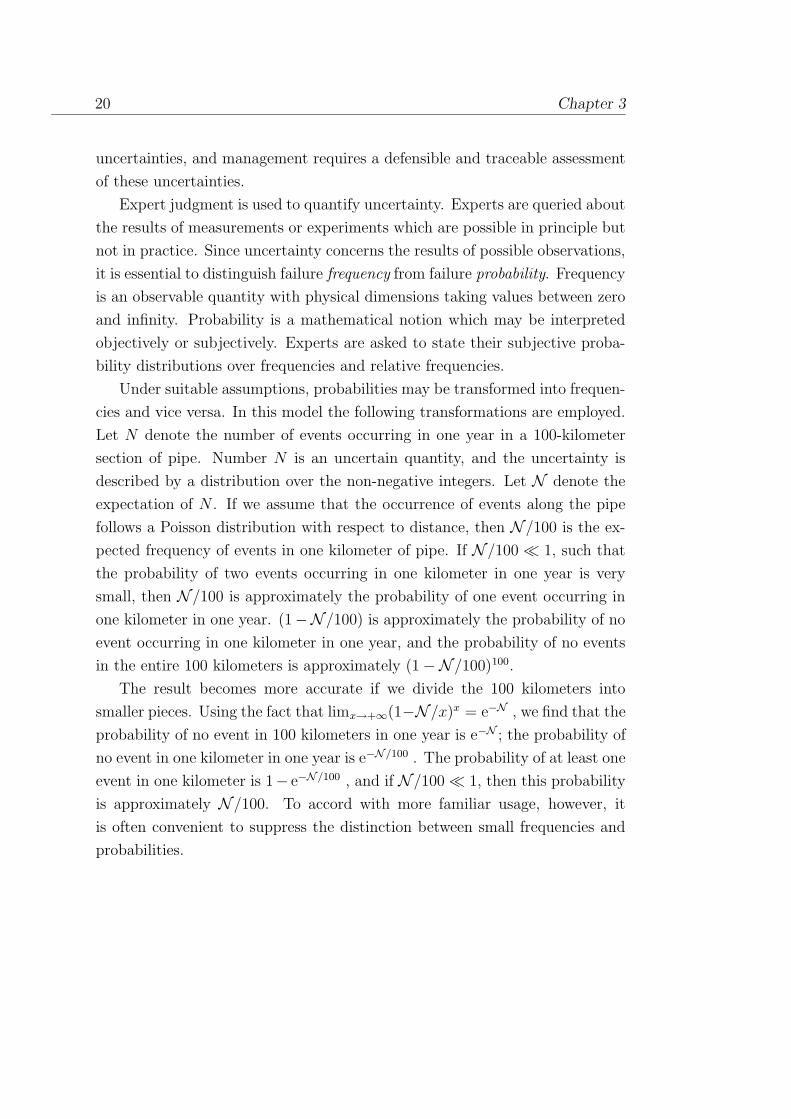
This chapter presents a model predicting with uncertainty failure frequency
of gas pipelines. It was developed by R.M. Cooke and E. Jager as a cooperative
work of Delft University of Technology and N.V. Nederlandse Gasunie in 1995.
Previous studies (see for example Kiefner, Vieth & Feder 1990) focused on
developing ranking tools which provide qualitative indicators for prioritizing
inspection and maintenance activities. Such tools perform well in some situa-
tions. In The Netherlands, however, qualitative ranking tools have not yielded
sufficient discrimination to support inspection and maintenance decisions. The
population of gas pipelines in The Netherlands is too homogeneous. Moreover,
as the status of current pipes and knowledge of effectiveness of current tech-
nologies is uncertain, it was felt that uncertainty should be taken into account
when deciding which pipelines to inspect and maintain.
We therefore desire a quantitative model of the uncertainty in the failure

18 Chapter 3
frequency of gas pipelines. This uncertainty is modelled as a function of ob-
servable pipeline and environmental characteristics. The following pipe and
environmental characteristics were chosen to characterize a kilometer year of
a pipeline (Basalo (1992), Lukezich, Hancock & Yen (1992), Chaker & (eds)
(1989)):
Pipe Characteristics Environmental Characteristics1. pipe wall thickness 1. frequency of construction activity2. pipe diameter 2. frequency of drainage, pile driving, deep plow-
ing, placing dam walls3. ground cover 3. percent of pipe under water table4. coating (bitumen orpolyethylene)
4. percent of pipe exposed to fluctuating watertable
5. age of pipe (since lastinspection)
5. percent of pipe exposed to heavy root growth
6. percent of pipe exposed to chemical contami-nation7. soil type (sand, clay, peat)8. pH value of soil9. resistivity of soil10. presence of cathodic protection11. number of rectifiers12. frequency of inspection of rectifiers13. number of bond sites
Although extensive failure data is available, the data is not sufficient to
quantify all parameters in the model. Indeed, the data yield significant es-
timates only when aggregated over large populations, whereas maintenance
decisions must be taken with regard to specific pipe segments. Hence, the ef-
fects of combinations of pipe and environmental characteristics on the failure
frequency is uncertain and is assessed with expert judgment. The expert judg-
ment method is discussed in “Expert Judgment in the Uncertainty Analysis of
Dike Ring Failure Frequency” (Cooke and Slijkhuis). Fifteen experts partici-
pated in this study, from The Netherlands, Germany, Belgium, Denmark, The
United Kingdom, Italy, France and Canada.
When values for the pipe and environmental characteristics are specified,
the model yields an uncertainty distribution over the failure frequency per
kilometer year. Thus the model provides answers to questions like:
• Given a 9 inch diameter pipe with 7 mm wall laid in sandy soil in 1960
Description of the UNICORN model 19
with bitumen coating etc., what is the probability that the failure fre-
quency per year due to corrosion will exceed the yearly failure frequency
due to 3rd party interference?
• Given a 9 inch pipe with 7 mm walls laid in 1970 in sand, with heavy
root growth, chemical contamination and fluctuating water table, how is
the uncertainty in failure frequency affected by the type of coating?
• Given a clay soil with pH = 4.3, resistivity 4, 000 Ω.cm and a pipe exposed
to fluctuating water table, which factors or combinations of factors are
associated with high values of the free corrosion rate?
In carrying out this work three problems had to be solved:
• How should the failure frequency be modelled as a function of the above
physical and environmental variables, so as to use existing data to the
maximal extent?
• How should existing data be supplemented with structured expert judg-
ment?
• How can information about complex interdependencies be communicated
easily to decision makers?
In spite of the fact that the uncertainties in the failure frequency of gas
pipelines are large, we can nonetheless obtain clear answers to questions like
those formulated above.
3.2 Modelling pipeline failures
The failure of gas pipelines is a complex affair depending on physical pro-
cesses, pipe characteristics, inspection and maintenance policies and actions of
third parties. A great deal of historical material has been collected and a great
deal is known about relevant physical processes. However, this knowledge is
not sufficient to predict failure frequencies under all relevant circumstances.
This is due to lack of knowledge of physical conditions and processes and lack
of data. Hence, predictions of failure frequencies are associated with significant
20 Chapter 3
uncertainties, and management requires a defensible and traceable assessment
of these uncertainties.
Expert judgment is used to quantify uncertainty. Experts are queried about
the results of measurements or experiments which are possible in principle but
not in practice. Since uncertainty concerns the results of possible observations,
it is essential to distinguish failure frequency from failure probability. Frequency
is an observable quantity with physical dimensions taking values between zero
and infinity. Probability is a mathematical notion which may be interpreted
objectively or subjectively. Experts are asked to state their subjective proba-
bility distributions over frequencies and relative frequencies.
Under suitable assumptions, probabilities may be transformed into frequen-
cies and vice versa. In this model the following transformations are employed.
Let N denote the number of events occurring in one year in a 100-kilometer
section of pipe. Number N is an uncertain quantity, and the uncertainty is
described by a distribution over the non-negative integers. Let N denote the
expectation of N . If we assume that the occurrence of events along the pipe
follows a Poisson distribution with respect to distance, then N /100 is the ex-
pected frequency of events in one kilometer of pipe. If N /100 1, such that
the probability of two events occurring in one kilometer in one year is very
small, then N /100 is approximately the probability of one event occurring in
one kilometer in one year. (1−N /100) is approximately the probability of no
event occurring in one kilometer in one year, and the probability of no events
in the entire 100 kilometers is approximately (1 −N /100)100.
The result becomes more accurate if we divide the 100 kilometers into
smaller pieces. Using the fact that limx→+∞(1−N /x)x = e−N , we find that the
probability of no event in 100 kilometers in one year is e−N ; the probability of
no event in one kilometer in one year is e−N/100 . The probability of at least one
event in one kilometer is 1− e−N/100 , and if N /100 1, then this probability
is approximately N /100. To accord with more familiar usage, however, it
is often convenient to suppress the distinction between small frequencies and
probabilities.
Description of the UNICORN model 21
3.2.1 Example of modelling approach
The notation in this section is similar to, but a bit simpler than that used
in the sequel.
Suppose we are interested in the frequency per kilometer per year that a gas
pipeline is hit (H) during third party actions at which an overseer from Gasunie
has marked the lines (O). Third party actions are distinguished according to
whether the digging is closed (CL; drilling, pile driving, deep plowing, drainage,
inserting dam walls, etc) and open (OP ; e.g. construction). Letting F denote
frequency and P probability, we could write
FrequencyHit and Oversight present per km.yr = F (H ∩O/km.yr)
= F (CL/km.yr)P (H ∩O|CL) + F (OP/km.yr)P (H ∩O|OP ). (3.1)
This expression seems to give the functional dependence of F (H ∩ O) on
F (CL) and F (OP ), the frequencies of closed and open digs respectively. How-
ever, eq. (3.1) assumes that the conditional probabilities of hitting with over-
sight given closed or open digs does not depend on the frequency of closed and
open digs. This may not be realistic; an area where the frequency of 3rd party
digging is twice the population average may not experience twice as many in-
cidents of hitting a pipe. One may anticipate that regions with more 3rd party
activity, people are more aware of the risks of hitting underground pipelines
and take appropriate precautions. This was indeed confirmed by the experts.
It is therefore illustrative to look at this dependence in another way. Think
of F (H ∩ O) as a function of two continuous variables, FCL = frequency of
closed digs per kilometer year, and FOP = frequency of open digs per kilometer
year. Write the Taylor expansion about observed frequencies FCL0 and FOP0.
Retaining only the linear terms one can obtain
F (H ∩O/km.yr) = F (FCL, FOP ) =
F (FCL0, FOP0) + p1(FCL− FCL0) + p2(FOP − FOP0) (3.2)
If P (H ∩ O|CL) and P (H ∩ O|OP ) do not depend on FCL and FOP then
eq. (3.2) is approximately equivalent to eq. (3.1). Indeed, put p1 = P (H ∩O|CL);
p2 = P (H ∩O|OP ), and note that F (FCL0, FOP0) = p1FCL0 + p2FOP0.
The Taylor approach conveniently expresses the dependence on FCL and
FOP , in a manner familiar to physical scientists and engineers. Of course it

22 Chapter 3
can be extended to include higher order terms. If we take the “zero-order term”
F (FCL0, FOP0) equal to the total number of times gas lines are hit while an
overseer has marked the lines, divided by the number of kilometer years in The
Netherlands, then we can estimate this term from data. Frequencies FCL0 and
FOP0 are the overall frequencies of closed and open digs. Probabilities p1 and
p2 could be estimated from data if we could estimate F (FCL, FOP ) for other
values of FCL and FOP , but there are not enough hittings in the data base to
support this. As a result these terms must be assessed with expert judgment,
yielding uncertainty distributions over p1 and p2. Experts are queried over
their subjective uncertainty regarding measurable quantities; thus they may
be asked:
Taking account of the overall frequency F (FCL0, FOP0) of hitting a pipe
line while overseer has marked the lines, what are the 5, 50 and 95 percent
quantiles of your subjective probability distribution for:
The frequency of hitting a pipeline while overseer has marked the lines if
frequency of closed digs increases from FCL0 to FCL, and other factors re-
maining the same.
In answering this question the expert conditionalizes his uncertainty on
everything he knows, in particular the overall frequency F (FCL0, FOP0). We
configure the elicitation such that the “zero order terms” can be determined
from historical data, whenever possible.
How do we use these distributions? Of course if we are only interested in
the average situation in the Netherlands, then we needn’t use them at all, since
this frequency is estimated from data. However, it is known that the frequency
of third party activity (with and without oversight) varies significantly from
region to region. If we wish to estimate the frequency of hitting with oversight
where FCL 6= FCL0 and FOP 6= FOP0, then we substitute these values into
eq. (3.2), and obtain an uncertainty distribution for F (H ∩O), conditional on
the zero-order estimate and conditional on the values FCL, FOP . This is pure
expert subjective uncertainty. If we wish, we may also include uncertainty due
to sampling fluctuations in the zero-order estimate.
Description of the UNICORN model 23
Failure pipeline ingiven year andgiven kilometer
OR
Other causes (sabotage,stress, corrosioncracking, etc.)
Direct leak Failure due to corrosion
AND
(Partial) failure ofcathodic protection
system
Damage to coating
OR
Damage from 3rdparty interference
Damage from environment
Figure 3.1: Fault tree for gas pipeline failure.
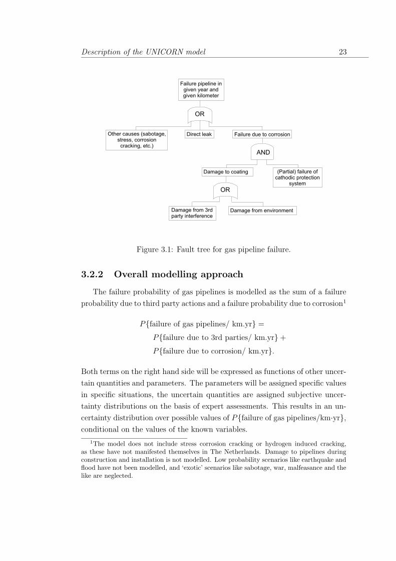
3.2.2 Overall modelling approach
The failure probability of gas pipelines is modelled as the sum of a failure
probability due to third party actions and a failure probability due to corrosion1
Pfailure of gas pipelines/ km.yr =
Pfailure due to 3rd parties/ km.yr +
Pfailure due to corrosion/ km.yr.
Both terms on the right hand side will be expressed as functions of other uncer-
tain quantities and parameters. The parameters will be assigned specific values
in specific situations, the uncertain quantities are assigned subjective uncer-
tainty distributions on the basis of expert assessments. This results in an un-
certainty distribution over possible values of Pfailure of gas pipelines/km·yr,
conditional on the values of the known variables.
1The model does not include stress corrosion cracking or hydrogen induced cracking,as these have not manifested themselves in The Netherlands. Damage to pipelines duringconstruction and installation is not modelled. Low probability scenarios like earthquake andflood have not been modelled, and ‘exotic’ scenarios like sabotage, war, malfeasance and thelike are neglected.
24 Chapter 3
dig nr 1
H = hyO = onR = rnD = dlG = cl
H = hnO = onR = rnD = nG = op
H = hyO = oyR = ryD = ldsG = op
dig nr 2 dig nr 3
Time
Figure 3.2: Digs as marked point process.
Failure due to corrosion requires damage to the pipe coating material, and
(partial) failure of the cathodic and stray current protection systems. Dam-
age to coating may come either from third parties or from the environment
(Lukezich et al. 1992). The overall model may be put in the form of a fault
tree as shown in Figure 3.1.
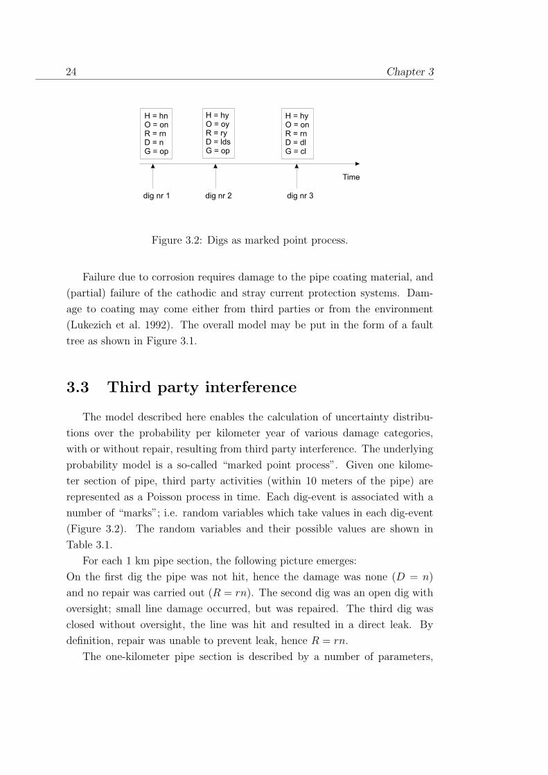
3.3 Third party interference
The model described here enables the calculation of uncertainty distribu-
tions over the probability per kilometer year of various damage categories,
with or without repair, resulting from third party interference. The underlying
probability model is a so-called “marked point process”. Given one kilome-
ter section of pipe, third party activities (within 10 meters of the pipe) are
represented as a Poisson process in time. Each dig-event is associated with a
number of “marks”; i.e. random variables which take values in each dig-event
(Figure 3.2). The random variables and their possible values are shown in
Table 3.1.
For each 1 km pipe section, the following picture emerges:
On the first dig the pipe was not hit, hence the damage was none (D = n)
and no repair was carried out (R = rn). The second dig was an open dig with
oversight; small line damage occurred, but was repaired. The third dig was
closed without oversight, the line was hit and resulted in a direct leak. By
definition, repair was unable to prevent leak, hence R = rn.
The one-kilometer pipe section is described by a number of parameters,

Description of the UNICORN model 25
Variable Meaning Values InterpretationH Pipe hit? hy, hn hityes, hitnoO Overseer notified? oy, on overtsightyes,
oversightnoR Repair carried out? ry, rn repairyes, re-
pairnoD Damage? n, cd3, lds, ldl, dl none, coating
damage, smallline damage,large line dam-age, direct leak
G Dig type? op, cl open dig, closeddig
Table 3.1: Marks for 3rd party digs.
which are assumed to be constant along this section:
• t: pipe wall thickness
• gc: depth of (ground) cover
• f = (FOP, FCL): frequency of open and closed digs within 10 m of pipe
The values of these parameters will influence the distributions of the random
variables in Table 3.1. Hence, we regard these as random variables, and their
influence on other random variables is described by conditionalization. In
any one-kilometer section the values for these variables can be retrieved from
Gasunie data, and the distributions of other variables can be conditionalized on
these values. From a preliminary study (Geervliet 1994) it emerged that pipe
diameter and coating type were not of influence on the probability of hitting a
pipe.
The damage types indicated in Table 3.1 are defined more precisely as:
• dl: direct leak (puncture or rupture)
• ldl: line damage large (at least 1 mm of pipe material removed, no leak)
• lds: line damage small (less than 1 mm of pipe material removed)
26 Chapter 3
• cd3: coating damage without line damage due to 3rd parties
Every time a gas pipeline is hit, we assume that one and only one of these
damage categories is realized. Hence, D = n if and only if H = hn. By
definition, if D = dl, then repair prior to failure is impossible.
We wish to calculate uncertainty distributions over the probability of un-
repaired damage
P (D = z ∩R = rn|t, gc, f); z ∈ cd3, lds, ldl, dl.
Letting∑
HOG denote summation over the possible values of H, O, G, we have
P (D = z ∩R = rn|t, gc, f) = (3.3)∑
HOG
P (D = z ∩R = rn|H,O,G, t, gc, f)P (H,O,G|t, gc, f) =
∑
OG
P (D = z ∩R = rn|H = hy,O,G, t, gc, f)P (H = hy,O,G|t, gc, f),
since third party damage can only occur if the pipe is hit.
For each of the four damage types, there are four conditional probabilities to
consider, each conditional on four continuous valued random variables. To keep
the model tractable it is necessary to identify plausible simplifying assumptions.
These are listed and discussed below. The expressions “X depends only on Y”
and “X influences only Y” mean that given Y, X is independent of every other
random variable.
1. D depends only on (H,G, t)
2. R depends only on (H,G,OandD ∈ cd3, lds, ldl)
3. gc influences only H
4. gc is independent of f
5. G is independent of f
6. (H,O,G) is independent of t given (gc, f).
Assumptions 1, 3, 4 and 5 speak more or less for themselves. Assumption
2 says the following: if the pipe is hit and the damage is repairable (D 6= dl)

Description of the UNICORN model 27
then the probability of repair depends only on the type of dig and the presence
of oversight; it does not depend on the type of repairable damage inflicted.
Assumptions 1 and 2 entail that D and R depend only on (H,G,O, t,D ∈
cd3, lds, ldl).
To appreciate assumption 5, suppose the uncertainty over f = (FOP, FCL)
is described by an uncertainty distribution, and consider the expression
P (FOP, FCL|G = cl). Would knowing the type of dig in a given 3rd party
event tell us anything about the frequencies of open and closed digs? It might.
Suppose that either all digs were open or all digs were closed, each possibil-
ity having probability 1/2 initially. Now we learn that one dig was closed;
conditional on this knowledge, only closed digs are possible. Barring extreme
correlations between the uncertainty over values for FOP and FCL, knowing
G = cl can tell us very little about the values of FCL and FOP . Assumption
5 says that it tells us nothing at all.
To illustrate how these assumptions simplify the calculations, we consider
the event (D = cd3 ∩ R = rn); which we abbreviate as (cd3 ∩ rn). We can
show that eq. (3.3) is now equal to
P (cd3 ∩ rn|t, gc, f) =∑
OG
P (rn|hy,O,G)P (cd3|hy,G, t)P (O, hy|G, f)P (G)P (gc|hy)/P (gc).
Proof.
Using elementary probability manipulations and assumptions 1 and 2
P (cd3 ∩ rn|hy,O,G, t, gc, f)P (hy,O,G|t, gc, f) =
P (cd3 ∩ rn|hy,O,G, t)P (hy,O,G|t, gc, f) =
P (cd3|rn, hy,O,G, t)P (rn|hy,O,G, t)P (hy,O,G|t, gc, f) =
P (cd3|hy,G, t)P (rn|hy,O,G)P (hy,O,G|t, gc, f).
Reasoning similarly with assumptions 3, 4, 5 and 6, and using Bayes’ theorem
P (hy,O,G|t, gc, f) = P (hy,O,G|gc, f)
= P (gc, O,G|hy, f)P (hy|f)/P (gc|f) =
= P (gc|O,G, hy, f)P (O,G|hy, f)P (hy|f)/P (gc|f) = (?)
28 Chapter 3
(?) = P (gc|hy)P (O,G|hy, f)P (hy|f)/P (gc)
= P (gc|hy)P (O, hy|G, f)P (G|f)/P (gc)
= P (gc|hy)P (O, hy|G, f)P (G)/P (gc).
Similar expressions hold for damage types lds and ldl. For dl, the term
P (rn|hy,O,G) equals one as repair is not possible in this case. The terms
P (cd3|hy,G, t), P (G|hy), P (G), P (gc|hy) and P (gc)
can be estimated from data; the other terms are assessed (with uncertainty)
using expert judgment. The uncertainty in the data estimates derives from
sampling fluctuations and can be added later, although this will be small rel-
ative to uncertainty from expert judgment. The term
P (gc|hy)/P (gc) = P (H = hy|gc)/P (H = hy)
is called the “depth factor”; it is estimated by dividing the proportion of hits
at depth gc by the total proportion of pipe at depth gc. P (G = cl|hy, cd3) is
estimated as the percentage of coating damages from third parties caused by
closed digs; P (G = cl|hy) is the percentage of hits caused by closed digs, and
P (G) is the probability per kilometer year of a closed dig. This probability is
estimated as the frequency of closed digs per kilometer year, if this frequency
is much less than 1 (which it is).
The term P (rn|hy,O,G) is assessed by experts directly when the terms
P (O, hy|G, f) are assessed using the Taylor approach described in section 3.
To assess the probability (with uncertainty) of ruptures due to third parties,
experts assess, for two different wall thickness, the percentages of direct leaks
which will be ruptures. Let RUP71 and RUP54 denote random variables whose
distributions reflect the uncertainty in these percentages for thickness 7.1 and
5.4 mm respectively. We assume that RUP71 and RUP54 are comonotonic2.
Putting
RUP54 = RUP71 + r(7.1 − 5.4),
we can solve for the the linear factor r, and for some other thickness t.
RUPt = RUP71 + r(7.1 − t)
2That is, their rank correlations are equal to one.
Description of the UNICORN model 29
gives an assessment of the uncertainty in the probability of rupture, given
direct leak, for thickness t. This produces reasonable results for t near 7.1. For
t > 10 mm it is generally agreed that rupture from third parties is not possible
(Hopkins, Corder & Corbin 1992).
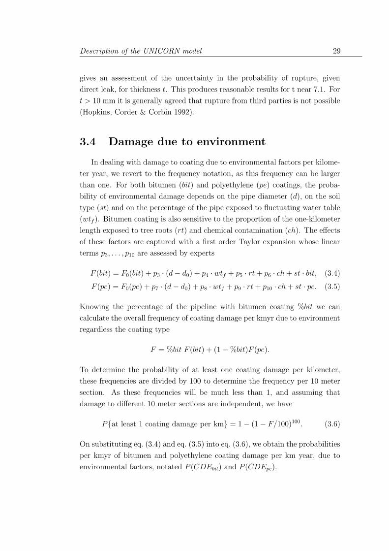
3.4 Damage due to environment
In dealing with damage to coating due to environmental factors per kilome-
ter year, we revert to the frequency notation, as this frequency can be larger
than one. For both bitumen (bit) and polyethylene (pe) coatings, the proba-
bility of environmental damage depends on the pipe diameter (d), on the soil
type (st) and on the percentage of the pipe exposed to fluctuating water table
(wtf ). Bitumen coating is also sensitive to the proportion of the one-kilometer
length exposed to tree roots (rt) and chemical contamination (ch). The effects
of these factors are captured with a first order Taylor expansion whose linear
terms p3, . . . , p10 are assessed by experts
F (bit) = F0(bit) + p3 · (d− d0) + p4 · wtf + p5 · rt+ p6 · ch+ st · bit, (3.4)
F (pe) = F0(pe) + p7 · (d− d0) + p8 · wtf + p9 · rt+ p10 · ch+ st · pe. (3.5)
Knowing the percentage of the pipeline with bitumen coating %bit we can
calculate the overall frequency of coating damage per kmyr due to environment
regardless the coating type
F = %bit F (bit) + (1 − %bit)F (pe).
To determine the probability of at least one coating damage per kilometer,
these frequencies are divided by 100 to determine the frequency per 10 meter
section. As these frequencies will be much less than 1, and assuming that
damage to different 10 meter sections are independent, we have
Pat least 1 coating damage per km = 1 − (1 − F/100)100. (3.6)
On substituting eq. (3.4) and eq. (3.5) into eq. (3.6), we obtain the probabilities
per kmyr of bitumen and polyethylene coating damage per km year, due to
environmental factors, notated P (CDEbit) and P (CDEpe).
30 Chapter 3
chemical contamination of soil pipe diameter oversightsoil type (clay, sand, peat) pipe inspection repairsoil resistance stray currents aciditypipe thickness tree roots pipe agewater table third party actions
Table 3.2: Factors influencing failure due to corrosion.
3.5 Failure due to corrosion
3.5.1 Modelling corrosion induced failures
The modelling of failure due to corrosion is more complicated than that of
failure due to third parties. The probability of failure due to corrosion depends
on many factors as listed in Table 3.2.
Corrosion can be viewed as the tendency of a metal to revert back to its
natural and more stable state as an ore. The end result of corrosion involves
a metal atom being oxidized, whereby it loses one or more electrons. The lost
electrons are conducted through the bulk metal to another site where they are
reduced. If we assure an electric field in the neighborhood of a pipeline, we
prevent the pipe from emitting the electrons and limit the corrosion. Practi-
cally, this problem is solved by installing the cathodic protection system. A
broad outline of such a system is depicted in Figure 3.3. The connections of
rectifiers with pipeline are located about every 2 km.
The model described here uses only pit corrosion. Given these factors, the
corrosion rate is assumed constant in time (Camitz & Vinka 1989).
For a pipeline to fail due to corrosion, two lines of defense must be breached.
First the coating must be damaged, and second, depending on location, the
cathodic or stray current protection system must not function as intended.
Coating damage may be caused either by third party actions or by environ-
mental factors. Both cathodic and stray current protection systems have been
in place since 1970.
We first elaborate the model for pipelines installed after 1970. Assuming
that the coating has been breached, pit corrosion will reduce the pipe wall
thickness until a critical value is reached, at which point the pipe fails. This
critical wall thickness, that is the thickness at which failure occurs, is expressed

Description of the UNICORN model 31
Figure 3.3: Overview of cathodic protection system.
as a fraction x of the original wall thickness minus the pipe material removed
during the damage event. The fraction x depends on the pressure of the gas in
the pipeline, and on the geometry of the pipe damage, and this relationship has
been established by experiment. In this model, x is introduced as a parameter
whose value depends only on the damage type, thus we distinguish xC , xS
and xL for (only) coating damage, small and large pipe damage respectively.
Coating damage is either caused by 3rd parties (cd3) or by the environment
(cde).
A length of pipe can be inspected for corrosion, and if corrosion is found,
the pipe is uncovered and repaired. Hence, after such inspection the pipe is as
good as new. The effective birthday (eb) of a pipe section is the calendar year
of the last inspection.
Given a corrosion rate (CR) and a damage type, we define the effective life
of a pipe section as the time required for the corrosion to reduce wall thickness
to the critical wall thickness. Letting t denote the original pipe wall thickness,
and tC = 0, tS = 0.5 mm, tL = 2 mm denote the pipe wall thickness removed
by damage type i, i ∈ C, S, L:
EL(CR, i) = xi(t− ti)/CR. (3.7)
In this equation, CR is uncertain and xi, ti are parameters with uncertain
indices. EL(CR, i) is the time a pipe survives given corrosion rate CR after
sustaining damage type i, i ∈ C, S, L.
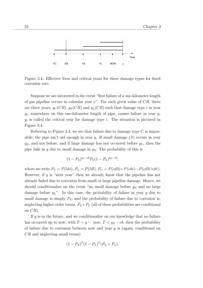
32 Chapter 3
YC EB
Time
YS yYL NOW
Figure 3.4: Effective lives and critical years for three damage types for fixedcorrosion rate.
Suppose we are interested in the event “first failure of a one-kilometer length
of gas pipeline occurs in calendar year y”. For each given value of CR, there
are three years, yC(CR), yS(CR) and yL(CR) such that damage type i in year
yi, somewhere on this one-kilometer length of pipe, causes failure in year y.
yi is called the critical year for damage type i. The situation is pictured in
Figure 3.4.
Referring to Figure 3.4, we see that failure due to damage type C is impos-
sible; the pipe isn’t old enough in year y. If small damage (S) occurs in year
yS, and not before, and if large damage has not occurred before yL, then the
pipe fails in y due to small damage in yS. The probability of this is
(1 − PS)yS−ebPS(1 − PL)yL−eb,
where we write PS = P (lds), PL = P (ldl), PC = P (cd3)+P (cde)−P (cd3∩cde).
However, if y is “next year” then we already know that the pipeline has not
already failed due to corrosion from small or large pipeline damage. Hence, we
should conditionalize on the event “no small damage before yS and no large
damage before yL”. In this case, the probability of failure in year y due to
small damage is simply PS, and the probability of failure due to corrosion is,
neglecting higher order terms, PS+PL (all of these probabilities are conditional
on CR).
If y is in the future, and we conditionalize on our knowledge that no failure
has occurred up to now, with T = y− now, T < yS − eb, then the probability
of failure due to corrosion between now and year y is (again, conditional on
CR and neglecting small terms)
(1 − PS)T (1 − PL)T (PS + PL).

Description of the UNICORN model 33
In general, let
qi(eb, y, now , CR) = min(yi(CR) − eb), (y − 1 − now)
denote the number of years between y and now in which a failure due to damage
type i could have caused failure between now and year y − 1, conditional on
CR, and let
1i =
1, if yi(CR) > eb
0, otherwise
then (sum and product are over i ∈ C, S, L)
Pf |cr(CR, eb, y, now, PC , PS, PL, t, xC , xS, xL) =∏
(1 − Pi)qi
∑
1iPi (3.8)
is approximately the probability of failure in year y due to corrosion, given CR.
Pf |CR is an uncertain quantity since the arguments written in capital letters
represent uncertain quantities.
3.5.2 Pit corrosion rate
The free rate of pit corrosion CRf [mm/yr] is modelled to depend on the
soil type (clay, sand, peat), the soil resistance (r), the acidity (pH) and the pro-
portion of pipeline under the water table, and fluctuating under and above the
water table (wtu, wtf ). CRf is the rate of corrosion which would be obtained
if the cathodic protection were not present. Using a zero-order corrosion rate
with arguments r0, pH0, wtu0 = wtf0 = 0; we apply the linear approximation
(supported by experiment)
CRf = CRf0 + p11(r − ro) + p12(pH − pH0) + p13 · wtf + p14 · wtu. (3.9)
The linear terms p11, . . . p14 are assessed with expert judgment. All of the terms
in eq. (3.9) depend on soil type.
We distinguish three states of the cathodic protection system:
• CPf : wholly non-functional, CR = CRf
• CPp: partially functional (pipe-soil potential outside prescribed range),
CR = CRp

34 Chapter 3
• CPok: wholly functional as prescribed; CR ∼ 0.
Before the cathodic protection system was installed in 1970, only state
CPf was available. CRp is determined via expert judgment as a fraction of
CRf . P (CPi) is the fraction of one-kilometer pipe length for which cathodic
protection is in state i, i ∈ f , p, ok. Since the factors affecting the cathodic
protection do not change from year to year, we assume that the states CPf
and CPp affect the same portions of pipe each year.
Stray currents can induce corrosion against which cathodic protection is
ineffective. In 1970 a protection system of bonds was installed to drain off
strong stray currents in locations where these are known to occur. Each bond
is inspected once a month hence if a bond has failed the stray current corro-
sion rate CRst has been operative on the average for one half month. In the
neighborhood of a bond, the corrosion rate before 1970 due to stray currents is
CRst, and after 1970 it is assumed to be CRst/24. If bs is the proportion of a
one-kilometer length of pipe in the neighborhood of a bond sites and P (SP ) is
the probability that the stray current protection system fails at one site, then
bs · P (SP ) is the probability that CRst (before 1970) or CRst/24 (after 1970)
obtains, given that damage has occurred somewhere in the pipe section.
Unconditionalizing equation (3.9) on CR, we obtain the probability of fail-
ure per kilometer year due to corrosion for pipe installed after 1970
Pcor>70 =
Pf |cr(CRf )P (CPf ) + Pf |cr(CRp)P (CPp) + Pf |cr(CRst/24)bsP (SP ).(3.10)
This is an uncertain quantity whose distribution is the uncertainty distribution
for the failure frequency for a one-kilometer length of gas pipeline with specified
pipe and environment parameter values.
For pipelines whose effective birthday is before 1970,
xi(t− ti) − (y − 1970) · CR
is the thickness of pipe wall, under damage type i, exposed to corrosion at the
rate obtaining before protection systems were installed. Let
1i,CR =
1, if y − xi(t− ti)/CR > 1970
0, otherwise

Description of the UNICORN model 35
If 1i,CR = 1, then yi > 1970; if yi < 1970 then we must account for the absence
of protection systems. We compute the effective life as follows
EL(CRf , i) = xi(t− ti)/CRf ,
EL(CRp, i) = 1i,CRpxi(t− ti)/CRp,
+ (1 − 1i,CRp)(xi(t− ti) − (y − 1970)CRp)/CRf ,
EL(CRst, i) = 1i,CRstxi(t− ti)24/CRst (3.11)
+ (1 − 1i,CRst)(xi(t− ti) − (y − 1970)CRst/24)/CRst.
The probability Pcor<70 is obtained by using eq. (3.11) instead of eq. (3.7) in
eq. (3.8).
3.6 Results for ranking
3.6.1 Case-wise comparisons
Two types of results can be obtained with the model. First, we can perform
case-wise comparisons. By specifying parameter values for two or more types
of kilometer-year sections of pipelines, the uncertainty distributions for the
frequency of failure can be compared. In Figure 3.5 compares three cases,
namely
• bitumen coated pipe laid in 1975 in sand
• bitumen coated pipe laid in 1975 in clay
• polyethylene coated pipe laid in 1975 in sand
Percentiles of the subjective uncertainty distribution are shown horizon-
tally; the logarithm of the failure frequency per kilometer year is plotted ver-
tically (the absolute values are proprietary). Other parameters are the same
in all cases, and those describing the frequency of 3rd party intervention are
chosen in accord with the generic values retrievable from the Dutch data. Each
graph plots the frequency per kilometer year of failure against the percentiles
of the uncertainty distribution for the failure frequency. Each graph shows
three curves, a curve corresponding to failure due to corrosion (corlk), a curve
corresponding to failure due to 3rd party interference (3leak), and a curve cor-
responding to the sum of these two (leak).
36 Chapter 3
Figure 3.5: Uncertainty distributions for three cases.
Because of the choice of 3rd party interference frequencies, the curves for
failure due to 3rd party interference are constant - this means that there is
no uncertainty regarding this failure frequency. The curves for failure due to
corrosion are not constant. In the first graph (bitumen in sand), we see that
the 66th percentile of the uncertainty distribution for failure due to corrosion
corresponds to the same failure frequency as 3rd party intervention. In other
words, there is a 0.66 probability that the frequency of failure due to corrosion
will be lower than that due to 3rd party intervention.
In the second graph (bitumen in clay) we find a probability of 0.85 that the
frequency of failure due to corrosion will be lower than that due to 3rd party
intervention. In the third graph (polyethylene in sand), we find a probability of
0.77 that the frequency of failure due to corrosion will be lower than that due
to 3rd party intervention. In the second graph, note that the failure frequency
curve for corrosion drops off more rapidly than in the third graph. This means
that very low values are more likely for bitumen coated pipe in clay than for
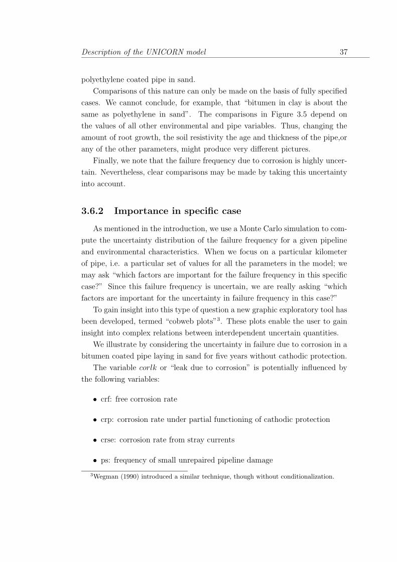
Description of the UNICORN model 37
polyethylene coated pipe in sand.
Comparisons of this nature can only be made on the basis of fully specified
cases. We cannot conclude, for example, that “bitumen in clay is about the
same as polyethylene in sand”. The comparisons in Figure 3.5 depend on
the values of all other environmental and pipe variables. Thus, changing the
amount of root growth, the soil resistivity the age and thickness of the pipe,or
any of the other parameters, might produce very different pictures.
Finally, we note that the failure frequency due to corrosion is highly uncer-
tain. Nevertheless, clear comparisons may be made by taking this uncertainty
into account.
3.6.2 Importance in specific case
As mentioned in the introduction, we use a Monte Carlo simulation to com-
pute the uncertainty distribution of the failure frequency for a given pipeline
and environmental characteristics. When we focus on a particular kilometer
of pipe, i.e. a particular set of values for all the parameters in the model; we
may ask “which factors are important for the failure frequency in this specific
case?” Since this failure frequency is uncertain, we are really asking “which
factors are important for the uncertainty in failure frequency in this case?”
To gain insight into this type of question a new graphic exploratory tool has
been developed, termed “cobweb plots”3. These plots enable the user to gain
insight into complex relations between interdependent uncertain quantities.
We illustrate by considering the uncertainty in failure due to corrosion in a
bitumen coated pipe laying in sand for five years without cathodic protection.
The variable corlk or “leak due to corrosion” is potentially influenced by
the following variables:
• crf: free corrosion rate
• crp: corrosion rate under partial functioning of cathodic protection
• crse: corrosion rate from stray currents
• ps: frequency of small unrepaired pipeline damage
3Wegman (1990) introduced a similar technique, though without conditionalization.
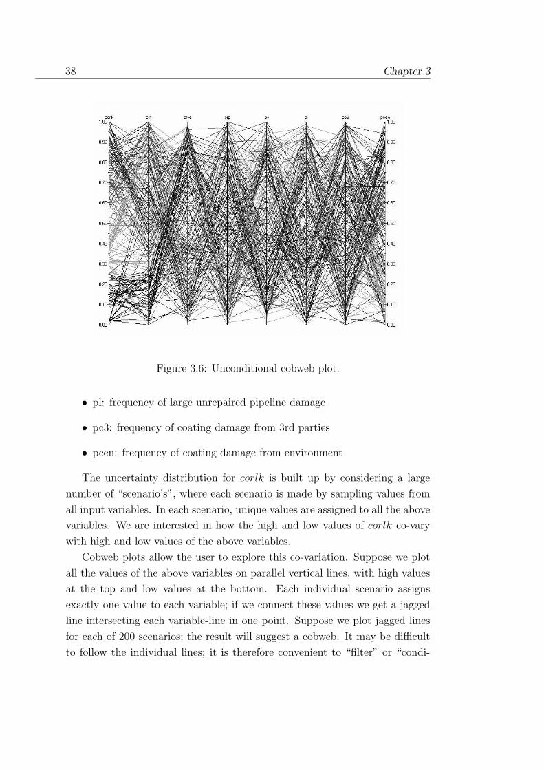
38 Chapter 3
Figure 3.6: Unconditional cobweb plot.
• pl: frequency of large unrepaired pipeline damage
• pc3: frequency of coating damage from 3rd parties
• pcen: frequency of coating damage from environment
The uncertainty distribution for corlk is built up by considering a large
number of “scenario’s”, where each scenario is made by sampling values from
all input variables. In each scenario, unique values are assigned to all the above
variables. We are interested in how the high and low values of corlk co-vary
with high and low values of the above variables.
Cobweb plots allow the user to explore this co-variation. Suppose we plot
all the values of the above variables on parallel vertical lines, with high values
at the top and low values at the bottom. Each individual scenario assigns
exactly one value to each variable; if we connect these values we get a jagged
line intersecting each variable-line in one point. Suppose we plot jagged lines
for each of 200 scenarios; the result will suggest a cobweb. It may be difficult
to follow the individual lines; it is therefore convenient to “filter” or “condi-
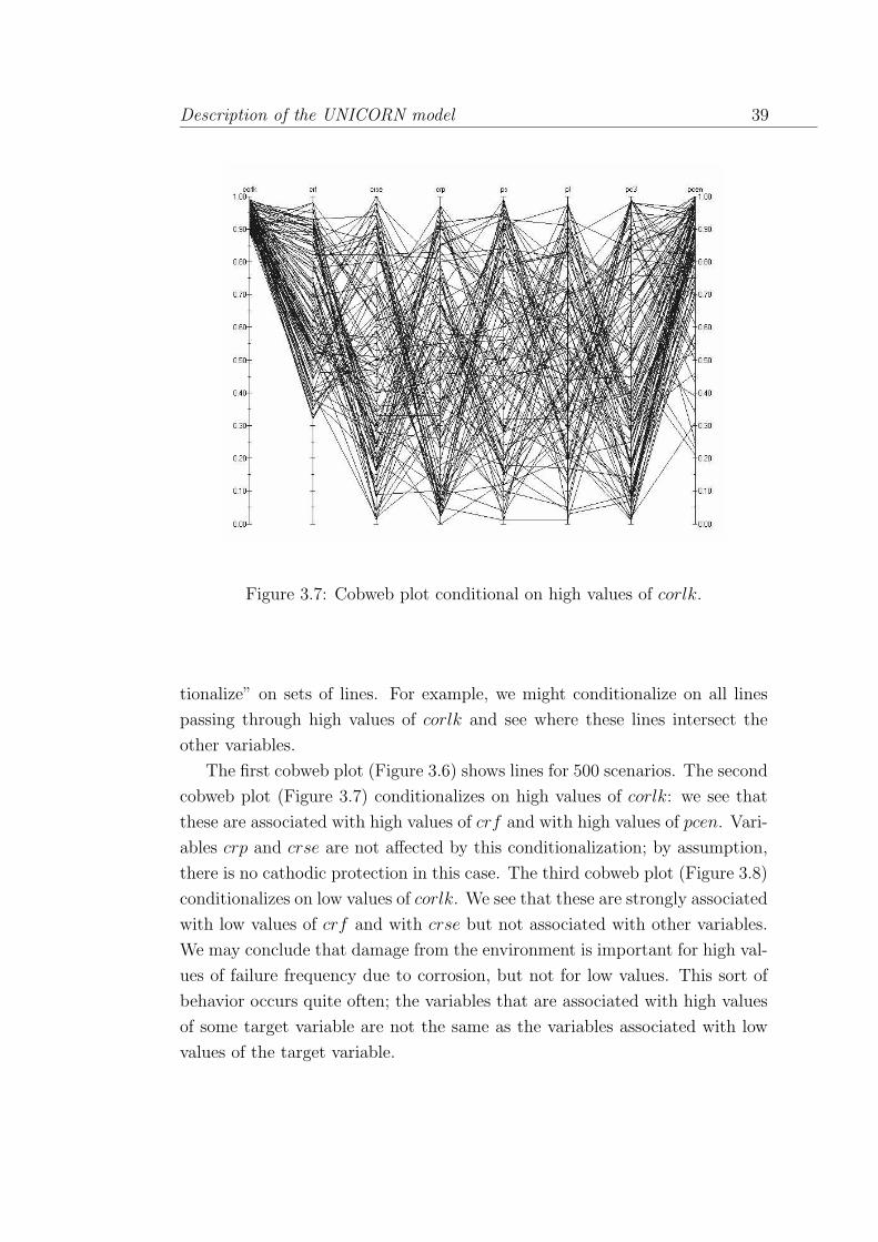
Description of the UNICORN model 39
Figure 3.7: Cobweb plot conditional on high values of corlk.
tionalize” on sets of lines. For example, we might conditionalize on all lines
passing through high values of corlk and see where these lines intersect the
other variables.
The first cobweb plot (Figure 3.6) shows lines for 500 scenarios. The second
cobweb plot (Figure 3.7) conditionalizes on high values of corlk: we see that
these are associated with high values of crf and with high values of pcen. Vari-
ables crp and crse are not affected by this conditionalization; by assumption,
there is no cathodic protection in this case. The third cobweb plot (Figure 3.8)
conditionalizes on low values of corlk. We see that these are strongly associated
with low values of crf and with crse but not associated with other variables.
We may conclude that damage from the environment is important for high val-
ues of failure frequency due to corrosion, but not for low values. This sort of
behavior occurs quite often; the variables that are associated with high values
of some target variable are not the same as the variables associated with low
values of the target variable.
40 Chapter 3
Figure 3.8: Cobweb plot conditional on low values of corlk.
3.7 Conclusions
We collect a number of conclusions.
• A ranking tool has been developed which uses failure data and structured
judgment.
• The tool characterizes pipe sections according to some 20 pipe charac-
teristics and environmental characteristics
• The tool predicts failure frequencies per kilometer year, and gives uncer-
tainty bounds
• These predictions allow distinctions to be made between pipe sections
with different characteristics, and these distinctions are not swamped by
uncertainties, despite the fact that the uncertainties are large
• For most pipes, the risk due to corrosion is significantly less than the risk
due to 3rd party interference

Description of the UNICORN model 41
Figure 3.9: Main window of GasUnicorn, new interface for UNICORN.
• The depth of ground cover is of significant influence for the frequency
and severity of 3rd party damage.
More detailed sensitivity analysis will be described in chapters 4 and 5.
3.8 Implementation
The whole theory presented in this chapter has been implemented in UNI-
CORN, software package developed at Delft University of Technology. This
program uses Monte Carlo methods for dealing with uncertainties and gives a
possibility to incorporate dependencies between input variables.
For convenience, the model has been split into three submodels, each of
them forming a separate section. First, we calculate the probability of coating
damage, small damage, large damage and direct leak caused by 3rd party inter-
ference (we call this submodel HITPIP), then we calculate the probability of
coating damage due to corrosion and corrosion rate (ENVSAND, ENVCLAY
or ENVPEAT, depends on soil type). Outputs of these two submodels are used
by the third submodel (CORRSAND, CORRCLAY or CORRPEAT) to deter-
mine overall failure frequency of gas pipelines. Definitions of input parameters
and functions are available in Appendix B.
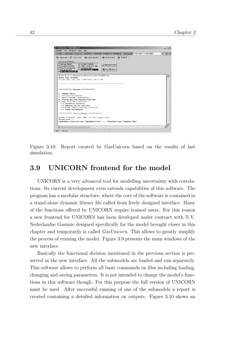
42 Chapter 3
Figure 3.10: Report created by GasUnicorn based on the results of lastsimulation.
3.9 UNICORN frontend for the model
UNICORN is a very advanced tool for modelling uncertainty with correla-
tions. Its current development even extends capabilities of this software. The
program has a modular structure, where the core of the software is contained in
a stand-alone dynamic library file called from freely designed interface. Many
of the functions offered by UNICORN require trained users. For this reason
a new frontend for UNICORN has been developed under contract with N.V.
Nederlandse Gasunie designed specifically for the model brought closer in this
chapter and temporarily is called GasUnicorn. This allows to greatly simplify
the process of running the model. Figure 3.9 presents the main windows of the
new interface.
Basically the functional division mentioned in the previous section is pre-
served in the new interface. All the submodels are loaded and run separately.
This software allows to perform all basic commands on files including loading,
changing and saving parameters. It is not intended to change the model’s func-
tions in this software though. For this purpose the full version of UNICORN
must be used. After successful running of one of the submodels a report is
created containing a detailed information on outputs. Figure 3.10 shows an

Description of the UNICORN model 43
example of such a report. All samples can be saved into a file. This allows
to produce so-called cobweb plots, representation of high dimensional distri-
butions4. New feature introduced in this software is a capability to export the
report to a MS Excel file.
Appendix A describes running UNICORN with the new interface.
4See section 3.6.2 for details.

44 Chapter 3
45
Chapter 4
Bayesian sensitivity analysis
This chapter is based on the article “Bayesian Sensitivity Analysis” by D.
Lewandowski & R.M. Cooke (Lewandowski & Cooke 2001)
4.1 Introduction
As Bayesian models become more popular and more complex, it issues of
appraising model performance, and identifying important parameters receive
more attention.
Classically, a parameter is identifiable if there is a function of the data which
converges almost surely to the value of this parameter. A distinctive feature of
Bayesian methods is that we can easily learn from data about parameters which
in a classical sense are not identifiable. In particular, the posterior distribution
can differ from the prior, without having a Dirac distribution as its limit. This
simple remark means that sensitivity, sensitivity to data, and the consequences
of sensitivity must be rethought from a Bayesian perspective.
In this chapter we discuss a number of issues that arise in Bayesian model
criticism and sensitivity analysis. Methods are suggested for identifying impor-
tant parameters and for analysing the impact of data versus prior information.
These ideas are illustrated with an analysis of the two stage hierarchical
model used the Swedish Nuclear Inspectorate’s data processing (Porn 1990)1.
This model is designed to utilize failure data from similar plants to update
1Prof. R.E. Barlow was instrumental in the development of this model and served on thePhD thesis committee
46 Chapter 4
failure rates at a given plant. Relevant questions concern the sensitivity to
hyperparameters, the sensitivity to data, and the impact of information from
other plants.
4.2 Sensitivity in hierarchical models
We are interested in characterizing the sensitivity of aspects of a model
to the data. Loosely, if a parameter “does not listen to the data” then it is
weakly identifiable in a Bayesian sense. This is relevant for model criticism for
two reasons. First, if other quantities of interest depend on weakly identifiable
parameters, then this might be a cause of concern as these quantities would re-
main strongly dependent on the prior distribution. Second, weakly identifiable
parameters might be eliminated in a more parsimonious model.
We consider a generic two stage model with parameter vector λ = (λ1, ..., λn),
hyperparameter vector θ = (α, β, γ, . . . ), data matrix X = Xij with row i as-
sociated with λi, and some distribution g over θ containing constants K. In
general it is assumed that the components of λ are independent given θ, and
that given λi the data Xi,· is independent of (θ,Xj,·), j 6= i.
Among the questions of interest are:
• Which parameters are sensitive to the data?
• Which parameters are sensitive for a given parameter?
• Can the computation of sensitivities be done efficiently?
4.2.1 Which parameters are sensitive to the data?
This question can be answered by computing the relative information of a
parameter’s posterior with respect to its prior. Letting (λi|X) denote a random
variable with distribution equal to the conditional distribution of λi given X,
and assuming densities exist, we could compute
I((λi|X);λi) =
∫
f(λi|X) ln
(
f(λi|X)
f(λi)
)
dλi. (4.1)
Note that if λi follows the improper prior dλi, then
−I((λi|X);λi) = H(λi|X) = −
∫
f(λi|X) ln f(λi|X) dλi. (4.2)
Bayesian sensitivity analysis 47
where H denotes the entropy.
4.2.2 Which parameters are sensitive for a given param-
eter?
Having determined the sensitivity of parameters to data, we now examine
the sensitivity of parameters to each other. There are many ways of doing this
and the best method will depend on the specific case at hand. The simplest idea
is to regress the parameter of interest, say λi onto other parameters, indexed
as ψ
λi =∑
ψ
ρ(λi, ψ)σλi
σψψ + Error. (4.3)
In many cases the relationship between λi and ψ is exponential rather than
linear and eq. (4.3) might be replaced by log linear regression
ln(λi) =∑
ψ
ρ(ln(λi), ψ)σln(λi)
σψψ + Error, (4.4)
or by rank regression
Fi(λi) =∑
ψ
ρ(Fi(λi), Fψ(ψ))Fψ(ψ) + Error, (4.5)
where F∗ denotes the cumulative distribution function of its argument. Equa-
tion (4.5) regresses the quantile function of λi on the quantile functions of the
ψ’s. The quantile function of a continuous random variable is of course uni-
form on [0, 1] with variance 1/12. The rank correlation ρ(Fi(λi), Fψ(ψ)) is also
denoted ρr(λi, ψ).
The expressions (4.3), (4.4) and (4.5) can be evaluated either in the prior or
in the posterior joint distributions. The former two can be evaluated on-the-fly,
as their computation involves only moments. The rank regression coefficients
cannot be evaluated on-the-fly as we must first determine the cumulative dis-
tribution function, and this is typically known only at the end of a simulation.
4.2.3 A more general notion of sensitivity.
We consider a function G = G(X,Y ) of random vectors X and Y with
σ2G < ∞. In analogy with the above, we may ask for which function f(X)
48 Chapter 4
with σ2f(X) <∞ is ρ2(G, f(X)) maximal? The answer is given in the following
proposition.
Proposition 4.2.1. Let G = G(X,Y ) with σ2G <∞; then
(i) Cov(G,E(G|X)) = σ2E(G|X),
(ii) maxf ; σ2f(X)
<∞ ρ2(G, f(X)) = ρ2(G,E(G|X)) =σ2
E(G|X)
σ2G
.
Proof.
(i) Cov(G,E(G|X)) = E(E(GE(G|X)|X))−EGE(E(G|X)) = E(E2(G|X))−
E2(E(G|X)).
(ii) Let δ(X) be any function with finite variance. Put A = σ2E(G|X), B =
Cov(E(G|X), δ(X)), C = σ2G, and D = σ2
δ . Then
ρ2(G,E(G|X) + δ(X)) =(A+B)2
C(A+D + 2B),
σ2E(G|X)
σ2G
=A
C,
(A+B)2
C(A+D + 2B)≤A
C⇐⇒ B2 ≤ AD.
The latter inequality follows from the Cauchy-Schwarz inequality. This is sim-
ilar to a result by Whittle (1992).
The quantityσ2
E(G|X)
σ2G
is called the correlation ratio, and may be taken as the
general sensitivity of G to X. Note that the correlation ratio is always positive,
and hence gives no information regarding the direction of the influence. If we
take f(X) = X then we will notice, that according to Proposition 4.2.1, the
product moment correlation ρ2(G,X) ≤ ρ2(G,E(G|X)), but in case of a strong
nonlinearity this is not a good estimation. The more the relation between X
and E(G|X) (thus implicitly between X i G) is nonlinear, the greater the
difference between ρ2(G,X) and ρ2(G,E(G|X)). It is easy to show that
0 ≤ρ2(G,X)
ρ2(G,E(G|X))≤ 1,
and this fraction is equal to 1 if E(G|X) = k ·X, where k is a constant. Thus
it can be regarded as a sort of a measure of nonlinearity.
The following propositions explore some properties of the correlation ratio.
The first is straightforward, the second uses Proposition 4.2.1.
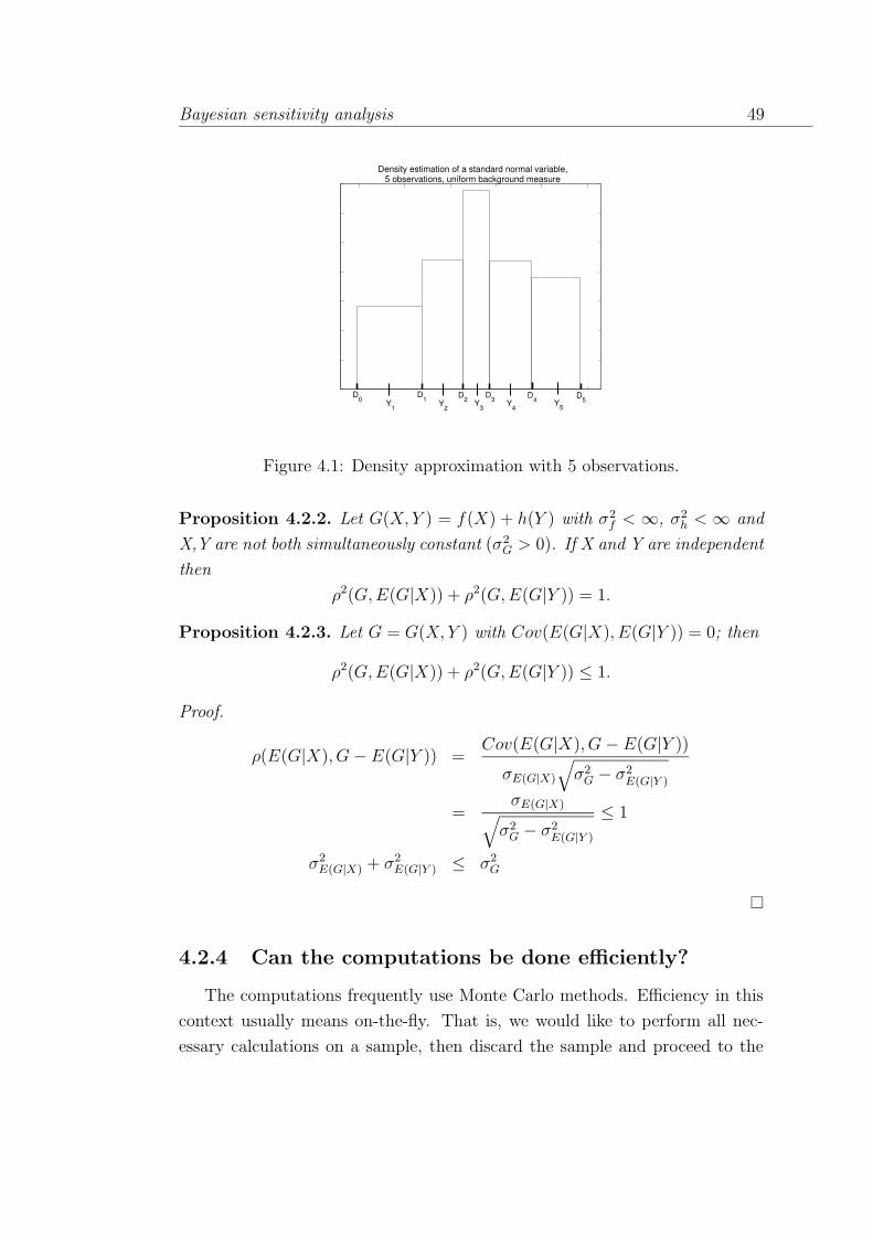
Bayesian sensitivity analysis 49
Density estimation of a standard normal variable,5 observations, uniform background measure
Y1 Y
3 Y
4 Y
5 Y
2
D5 D
4 D
0 D
3 D
2 D
1
Figure 4.1: Density approximation with 5 observations.
Proposition 4.2.2. Let G(X,Y ) = f(X) + h(Y ) with σ2f < ∞, σ2
h < ∞ and
X,Y are not both simultaneously constant (σ2G > 0). If X and Y are independent
then
ρ2(G,E(G|X)) + ρ2(G,E(G|Y )) = 1.
Proposition 4.2.3. Let G = G(X,Y ) with Cov(E(G|X), E(G|Y )) = 0; then
ρ2(G,E(G|X)) + ρ2(G,E(G|Y )) ≤ 1.
Proof.
ρ(E(G|X), G− E(G|Y )) =Cov(E(G|X), G− E(G|Y ))
σE(G|X)
√
σ2G − σ2
E(G|Y )
=σE(G|X)
√
σ2G − σ2
E(G|Y )
≤ 1
σ2E(G|X) + σ2
E(G|Y ) ≤ σ2G
4.2.4 Can the computations be done efficiently?
The computations frequently use Monte Carlo methods. Efficiency in this
context usually means on-the-fly. That is, we would like to perform all nec-
essary calculations on a sample, then discard the sample and proceed to the

50 Chapter 4
next sample. A computation which involves operations on the entire sample is
not efficient.
For reasons of simplicity we first discuss an on-the-fly method of computing
the entropy as defined in (4.2). Values for λi are generated by simulation and
are plotted on the real line as Y1 . . . YN (see Figure 4.1)2. We approximate the
density as a step function whose steps occur at the midpoints Di between Yi,
and Yi+1. We set D0 = Y1 − (Y2 − Y1)/2, and DN = YN + (YN − YN−1)/2.
Each point has equal probability, namely 1/N . The density above the point
Yi is therefore estimated as
Pi =1
N(Di −Di−1).
The entropy is then computed as
H ≈ (−1/N)N
∑
i=1
ln
(
1
N(Di −Di−1)
)
.
The relative information (4.1) is computed in a similar fashion. The prior
density of λi is approximated as a step function with value f(Yi) between points
Di−1, Di, where f is the prior density
I((λi|X);λi) ≈ (1/N)N
∑
i=1
ln
(
1
N(Di −Di−1)f(Yi)
)
. (4.6)
These quantities can be computed on-the-fly. If the computation has been
done for N samples, adding one additional sample requires only a local ad-
justment. We can also group the samples, such that we consider k adja-
cent samples and estimate the density over such a k-tuple starting with Yi
as k/(N(Di+k − Di−1)). Grouping the samples in this way a larger “local
adjustment” in (4.6), but gives better results.
To illustrate, the entropy of 1000 samples from the standard normal distri-
bution has been computed on 20 iterations. The results are shown as computed
above, and also after grouping the data points by 2’s, by 5’s and by 10’s (see
Figure 4.2). The Entropy of the standard normal is 1.419. If we truncate the
standard normal to [−3.3] corresponding roughly the above density approxi-
mation with 1000 samples, the entropy integral is 1.4056.
2Although we must retain the ordered sample in memory, we do not perform operationson the whole sample; in this sense we are still on-the-fly.

Bayesian sensitivity analysis 51
2 4 6 8 10 12 14 16 18 200.9
1
1.1
1.2
1.3
1.4
Entropy on−the−fly, 1000 standard normal samples with grouping, 20 iterations, theoretical value 1.419
Iteration nr
Ent
ropy
ungroupedgrouped by 2’sgrouped by 5’sgrouped by 10’s
Figure 4.2: Entropy, 1000 standard normals, 20 iterations.
We see that the results are stable, though the ungrouped data tend to be
a bit jittery, thus producing a lower entropy value than the theoretical value.
The same pattern emerges in computing the relative information on the fly.
Figure 4.3 shows 20 iterations of 1000 samples for calculating I(X|Y ), where
X is standard normal, and Y is normal with mean 5 and standard deviation 3.
The distribution of X is treated as the posterior in (4.6). The theoretical value
is 2.043. Again, the estimator with ungrouped data is stable but overestimates
the relative information due to sample jitter.
A. O’Hagan (personal communication) has recently proved that the bias in
computing entropy with ungrouped data is asymptotically equal to γ−1+ln(2),
where γ is Euler’s constant. Thus, for a sufficiently large sample, we can remove
this bias and obtain better results.
Computing correlation ratio cr may be difficult in some cases. However,
if we can sample Y ′ from the conditional distribution (Y |X) independently of
Y , and if the evaluation of G is not too expensive, then the following simple
algorithm may be applied (Homma 1990):
1. Sample (x, y) from (X,Y ),
2. Compute G(x, y),
3. Sample y′ from (Y |X = x) independent of Y = y,
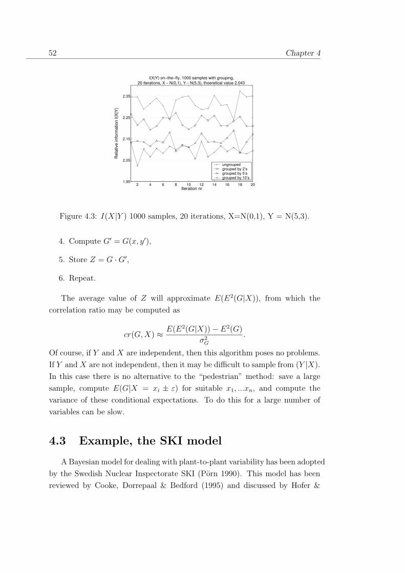
52 Chapter 4
2 4 6 8 10 12 14 16 18 201.95
2.05
2.15
2.25
2.35
I(X|Y) on−the−fly, 1000 samples with grouping,20 iterations, X ∼ N(0,1), Y ∼ N(5,3), thoeretical value 2.043
Iteration nr
Rel
ativ
e in
form
atio
n I(X
|Y)
ungroupedgrouped by 2’sgrouped by 5’sgrouped by 10’s
Figure 4.3: I(X|Y ) 1000 samples, 20 iterations, X=N(0,1), Y = N(5,3).
4. Compute G′ = G(x, y′),
5. Store Z = G ·G′,
6. Repeat.
The average value of Z will approximate E(E2(G|X)), from which the
correlation ratio may be computed as
cr(G,X) ≈E(E2(G|X)) − E2(G)
σ2G
.
Of course, if Y and X are independent, then this algorithm poses no problems.
If Y and X are not independent, then it may be difficult to sample from (Y |X).
In this case there is no alternative to the “pedestrian” method: save a large
sample, compute E(G|X = xi ± ε) for suitable x1, ...xn, and compute the
variance of these conditional expectations. To do this for a large number of
variables can be slow.
4.3 Example, the SKI model
A Bayesian model for dealing with plant-to-plant variability has been adopted
by the Swedish Nuclear Inspectorate SKI (Porn 1990). This model has been
reviewed by Cooke, Dorrepaal & Bedford (1995) and discussed by Hofer &

Bayesian sensitivity analysis 53
Peschke (1999) and Meyer & Hennings (1999). Hora & Iman (1990) describe a
similar model. We consider a collection of classes of components (plants). Each
class consists of components which are considered identical for the purposes of
lifetime estimation, and which are used in a specific plant under plant-specific
conditions. Different plant specific conditions lead to different Rate of Occur-
rence of Failure (ROCOF). Since we would like to use data from given plants to
make inference about the ROCOF in another plant, we have to assume some-
thing about the underlying relationship between the ROCOF’s of the various
plants. In Porn’s model, these ROCOF’s are treated as independent realisa-
tions of random quantities with the same distribution.
Specifically:
1. The pattern of failures at each plant is supposed to follow a Poisson
process. At plant i, we have xi failures in an operating time of Ti. The
plant specific ROCOF is λi, which is a realisation of the random variable
Λ.
2. Λ follows a mixed gamma distribution
P (λi|θ) = G(λi|α, β)(1 − c) +G(λi|1/2, 1)c.
α and β are unknown shape and scale parameters, and c is a random
variable taking values in [0, 1]. According to (Porn 1990), c is a con-
tamination parameter mixing G(λi|α, β) with a relatively vague gamma
to “add a pinch of uncertainty”. The uncertainty over values of θ is
modelled by assuming that θ is a random vector.
3. λ1, . . . , λn are independent realizations of Λ.
4. Given (λ1, . . . , λn), (x1, . . . , xn) are independent.
5. Given λi, xi and (θ, λ1, . . . λi−1, λi+1, . . . , λn) are independent.
A consequence of the dependence structure here is that data (xi, Ti) from
plant i can only influence our beliefs on the value of λj (j 6= i) through its
influence on our beliefs on the value of θ.
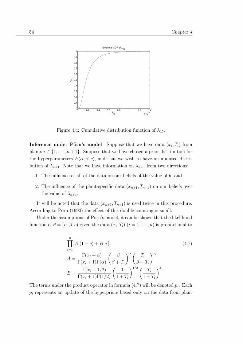
54 Chapter 4
0 0.2 0.4 0.6 0.8 1 1.2 1.4
x 10−3
0
0.1
0.2
0.3
0.4
0.5
0.6
0.7
0.8
0.9
1
λ15
F(x)
Empirical CDF of λ15
Figure 4.4: Cumulative distribution function of λ15.
Inference under Porn’s model Suppose that we have data (xi, Ti) from
plants i ∈ 1, . . . , n+ 1. Suppose that we have chosen a prior distribution for
the hyperparameters P (α, β, c), and that we wish to have an updated distri-
bution of λn+1. Note that we have information on λn+1 from two directions:
1. The influence of all of the data on our beliefs of the value of θ, and
2. The influence of the plant-specific data (xn+1, Tn+1) on our beliefs over
the value of λn+1.
It will be noted that the data (xn+1, Tn+1) is used twice in this procedure.
According to Porn (1990) the effect of this double counting is small.
Under the assumptions of Porn’s model, it can be shown that the likelihood
function of θ = (α, β, c) given the data (xi, Ti) (i = 1, . . . , n) is proportional to
n∏
i=1
[A (1 − c) +B c ] (4.7)
A =Γ(xi + α)
Γ(xi + 1)Γ(α)
(
β
β + Ti
)α (
Tiβ + Ti
)xi
B =Γ(xi + 1/2)
Γ(xi + 1)Γ(1/2)
(
1
1 + Ti
)1/2 (
Ti1 + Ti
)xi
The terms under the product operator in formula (4.7) will be denoted pi. Each
pi represents an update of the hyperpriors based only on the data from plant
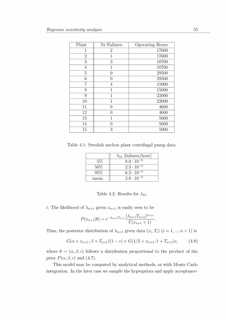
Bayesian sensitivity analysis 55
Plant Nr Failures Operating Hours1 2 176002 1 176003 3 107004 1 107005 0 295006 0 295007 4 150008 1 150009 1 22000
10 1 2200011 0 460012 0 460013 1 560014 0 560015 3 5000
Table 4.1: Swedish nuclear plant centrifugal pump data.
λ15 [failures/hour]5% 8.0 · 10−5
50% 2.3 · 10−4
95% 6.3 · 10−4
mean 2.8 · 10−4
Table 4.2: Results for λ15.
i. The likelihood of λn+1 given xn+1 is easily seen to be
P (xn+1|θ) = e−λn+1Tn+1(λn+1Tn+1)
xn+1
Γ(xn+1 + 1).
Thus, the posterior distribution of λn+1 given data (xi, Ti) (i = 1, ..., n+ 1) is
G(α + xn+1, β + Tn+1)(1 − c) +G(1/2 + xn+1, 1 + Tn+1)c, (4.8)
where θ = (α, β, c) follows a distribution proportional to the product of the
prior P (α, β, c) and (4.7).
This model may be computed by analytical methods, or with Monte Carlo
integration. In the later case we sample the hyperpriors and apply acceptance-
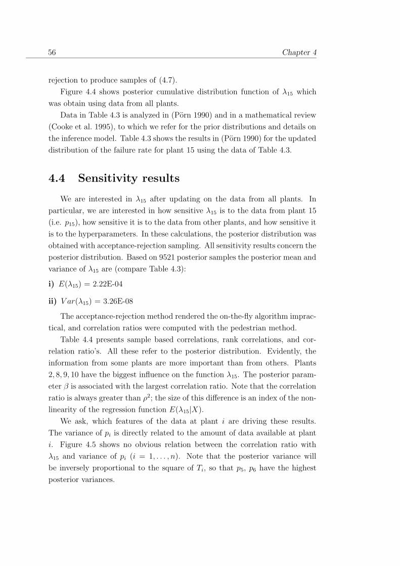
56 Chapter 4
rejection to produce samples of (4.7).
Figure 4.4 shows posterior cumulative distribution function of λ15 which
was obtain using data from all plants.
Data in Table 4.3 is analyzed in (Porn 1990) and in a mathematical review
(Cooke et al. 1995), to which we refer for the prior distributions and details on
the inference model. Table 4.3 shows the results in (Porn 1990) for the updated
distribution of the failure rate for plant 15 using the data of Table 4.3.
4.4 Sensitivity results
We are interested in λ15 after updating on the data from all plants. In
particular, we are interested in how sensitive λ15 is to the data from plant 15
(i.e. p15), how sensitive it is to the data from other plants, and how sensitive it
is to the hyperparameters. In these calculations, the posterior distribution was
obtained with acceptance-rejection sampling. All sensitivity results concern the
posterior distribution. Based on 9521 posterior samples the posterior mean and
variance of λ15 are (compare Table 4.3):
i) E(λ15) = 2.22E-04
ii) V ar(λ15) = 3.26E-08
The acceptance-rejection method rendered the on-the-fly algorithm imprac-
tical, and correlation ratios were computed with the pedestrian method.
Table 4.4 presents sample based correlations, rank correlations, and cor-
relation ratio’s. All these refer to the posterior distribution. Evidently, the
information from some plants are more important than from others. Plants
2, 8, 9, 10 have the biggest influence on the function λ15. The posterior param-
eter β is associated with the largest correlation ratio. Note that the correlation
ratio is always greater than ρ2; the size of this difference is an index of the non-
linearity of the regression function E(λ15|X).
We ask, which features of the data at plant i are driving these results.
The variance of pi is directly related to the amount of data available at plant
i. Figure 4.5 shows no obvious relation between the correlation ratio with
λ15 and variance of pi (i = 1, . . . , n). Note that the posterior variance will
be inversely proportional to the square of Ti, so that p5, p6 have the highest
posterior variances.

Bayesian sensitivity analysis 57
X ρ(λ15, X) ρr(λ15, X) ρ2(λ15, X) ρ2r(λ15, X) ρ2(λ15, E(λ15|X))
p1 -0.19 -0.14 0.0361 0.0196 0.0558p2 -0.47 -0.55 0.2209 0.3025 0.234p3 0.28 0.44 0.0784 0.1936 0.113p4 -0.33 -0.31 0.1089 0.0961 0.119p5 0.02 -0.04 0.0004 0.0016 0.0185p6 0.02 -0.04 0.0004 0.0016 0.0185p7 0.29 0.46 0.0841 0.2116 0.123p8 -0.44 -0.50 0.01936 0.25 0.208p9 -0.48 -0.59 0.2304 0.3481 0.247p10 -0.48 -0.59 0.2304 0.3481 0.247p11 -0.29 -0.36 0.0841 0.1296 0.102p12 -0.29 -0.36 0.0841 0.1296 0.102p13 -0.04 0.05 0.0016 0.0025 0.0162p14 -0.27 -0.35 0.0729 0.1225 0.1415α -0.33 -0.45 0.1089 0.2025 0.153β -0.39 -0.59 0.1521 0.3481 0.251c 0.09 0.03 0.0081 0.0009 0.0207
Table 4.3: Correlation ratios for λ15.
The key to understanding the sensitivities of Table 4.4 is given in Figure 4.6.
The “mean time to failure” MTTF of a plant i is the operating time Ti divided
by the number of failures xi. If this time is bigger than the inverse expectation
of λ15 (4444) then the function pi is strongly negatively correlated with λ15.
The greater this difference the greater is the absolute value of the correlation
(both product moment correlation and rank correlation). Notice, that if plant
i has a MTTF smaller than MTTF of λ15 then the correlation is positive.
Although the mean lifetime at plant 3 is only a little smaller than 4444, p3 and
λ15 are quite strongly correlated. We know that ρ2(λ15, pi) ≤ ρ2(λ15, E(λ15|pi))
(Proposition 4.2.1). Thus if a MTTF of a plant i is much different from the
inverse of the expectation of λ15 then pi has greater influence on λ15. Note the
effect of the sign of the correlation.
Variables α, β and c are hyperparameters. We use data from the plants to
update our belief in these variables. In the posterior distribution, we see that
β is the most important parameter, and α is more important than 10 of the
14 plants. This indicates that the final result is still strongly driven by the

58 Chapter 4
Variance compare to correlation ratio
0
0.05
0.1
0.15
0.2
0.25
0.3
p1 p2 p3 p4 p5 p6 p7 p8 p9 p10 p11 p12 p13 p14
Plant
Va
ria
nce
0
0.002
0.004
0.006
0.008
0.01
0.012
0.014
Co
rre
latio
nra
tio
correlation ratiovariance
Figure 4.5: Variance of pi compared to correlation ratio between λ15 and pi.
MTTF of plants and correlation with 15
0
5000
10000
15000
20000
25000
p3 p7 p13 p1 p4 p8 p2 p9 p10
Plant
MT
TF
[h]
0.28 0.29- 0.04
- 0.19
- 0.48
- 0.47
- 0.44
- 0.33
- 0.48
MTTF( 15)
Figure 4.6: The MTTF of the plant i compared to the inverse of expectationof λ15 (MTTF of λ15) and the correlation between λ15 and pi.
hyperparameters. It must be noted that the distributions of the pi also depend
on the hyperparameters; however we should hope that their influence dies off
rapidly as the data from all plants is gathered. After all, the data represents a
total of 188,600 operating hours. The parameter c, on the other hand, does not
play a significant role. The persistence of hyperparameters α and β observed
here confirms the conclusion of Cooke et al. (1995), obtained with a much more
laborious analysis.
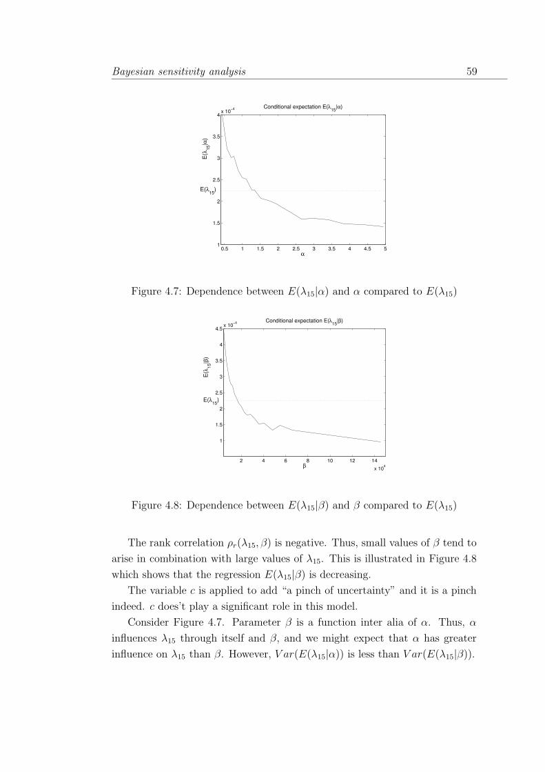
Bayesian sensitivity analysis 59
0.5 1 1.5 2 2.5 3 3.5 4 4.5 51
1.5
2
2.5
3
3.5
4x 10
−4 Conditional expectation E(λ15
|α)
α
E(λ
15|α
)
E(λ15
)
Figure 4.7: Dependence between E(λ15|α) and α compared to E(λ15)
2 4 6 8 10 12 14
x 104
1
1.5
2
2.5
3
3.5
4
4.5x 10
−4 Conditional expectation E(λ15
|β)
β
E(λ
15|β
)
E(λ15
)
Figure 4.8: Dependence between E(λ15|β) and β compared to E(λ15)
The rank correlation ρr(λ15, β) is negative. Thus, small values of β tend to
arise in combination with large values of λ15. This is illustrated in Figure 4.8
which shows that the regression E(λ15|β) is decreasing.
The variable c is applied to add “a pinch of uncertainty” and it is a pinch
indeed. c does’t play a significant role in this model.
Consider Figure 4.7. Parameter β is a function inter alia of α. Thus, α
influences λ15 through itself and β, and we might expect that α has greater
influence on λ15 than β. However, V ar(E(λ15|α)) is less than V ar(E(λ15|β)).

60 Chapter 4
0 0.05 0.1 0.15 0.2 0.25 0.3 0.351
2
3
4x 10
−4 Conditional expectation E(λ15
|c)
c
E(λ
15|c
)
E(λ15
)
Figure 4.9: Dependence between E(λ15|c) and c compared to E(λ15)
Figures 4.7 and 4.8 show that the regression of λ15 on α and β is not linear.
This recommends the use of the correlation ratio as a measure of dependence.
The relative unimportance of c is illustrated in Figure 4.9, where we see that
the conditional expectation of λ15 given c does not differ greatly from the
unconditional expectation of λ15.
4.5 Conclusions
Sensitivity analysis and model criticism are active topics at the moment.
The Bayesian approach allows these issues to be raised and analysed in a
natural way. By analysing the sensitivity of a parameter of interest to data and
to prior parameters, we can judge the relative importance of prior assumptions.
There are many ways to quantify sensitivity using entropy based concepts
or regression based concepts. We have argued that the correlation ratio is
particularly attractive in this regard, although it cannot always be computed
on-the-fly, and may be difficult to compute analytically.
The SKI two stage Hierarchical Bayes model is a very interesting case be-
cause, (i) it is an important application (ii) it has been studied and reviewed
extensively, and (iii) it is complicated enough that quantitative measures of
sensitivity greatly contribute to understanding the model. The main conclu-
sions regarding the persistence of hyperparameters α and β reached by Cooke

Bayesian sensitivity analysis 61
et al. (1995) by laborious re-computations, are obtained quite simply in Ta-
ble 4.4. Moreover, we also gain insight into the features of the data which drive
the parameter of interest (Figure 4.5).

62 Chapter 4

63
Chapter 5
Sensitivity analysis of the
UNICORN model factors
The previous chapter presented a commonly used measure of sensitivity
of output results to input parameters. This measure is called the correlation
ratio and denoted by cr. It will be applied to the Unicorn model that has
been studied in Chapter 3. The correlation ratio does not have a property
of symmetry (cr(G,X) 6= cr(X,G)). Since we want to know how the input
variable changes values of its function, we take G as the conditioned function
and X as the conditioning variable. Thus we calculate cr(G,X).
The model consists of 3 submodels and dependencies in each submodel will
be analyzed separately. This analysis is not the easy task though. The problem
described by the model has so many dimensions, that checking impact of all of
the parameters on the output is simply a very time-consuming task. Therefore
we concentrate on some chosen in advance parameters, which will describe
a hypothetical family of gas pipelines. For instance, we can be interested
in answering the following question - To what extent the inputs influence the
frequency of leakage per kmyr of a pipe laid in sand in 1965? The pipeline has
a bitumen coating and 36 inch diameter. This is a part of the specification
of Pipeline A. Taking also values of the rest of the parameters derived from
characteristics of this pipeline, allows to replace the above question with this
one - Which factors drives the failure frequency of Pipeline A and which ones
have the greatest influence on this frequency?. We no longer regard a non-
existing pipeline. Now the number of the defects indicated in the Pipeline

64 Chapter 5
Figure 5.1: Cobweb plots of the variables of HITPIP submodel.
A data is rather a sample from the distribution of the number of defects of
a virtual pipeline having the same characteristics as Pipeline A. This makes
the sensitivity analysis even more important. The best documented is the
information on pipelines A and B, which includes full characteristics of the
soil type in which the pipelines were laid. Since those two pipelines are very
similar as regards physical dimensions and environmental characteristics, we
shall concentrate on the sensitivity analysis for model with specification of
pipeline A. For comparison, the soil type will be replaced with clay with typical
values of some parameters like pH factor and resistivity.
5.1 Sensitivities in modelling of damage due
to 3rd party digs
The submodel HITPIP evaluates the probability of coating damage cd3rn,
small damage ldsrn and large damage ldlrn, as well as the probability of a direct
leak dl. Two main user selected parameters are thickness and depth of the
pipeline. Consider a set of parameters given in Appendix B for this submodel.

Sensitivity analysis of the UNICORN model factors 65
Conditioning Conditioned variablevariable cd3rn ldsrn ldlrn
roon 0.84 0.85 0.84rcon 0.06 0.06 0.06rooy 0.13 0.14 0.13rcoy 0.03 0.03 0.04
Table 5.1: Correlation ratios for outputs of HITPIP submodel.
Inputs hooye, hcoye, hoone and hcone representing experts’ assessment of the
frequency of hitting a pipeline do not contribute in the model, because this
particular set of values takes into account only the zero order terms while
calculating outputs. Notice that fop and fopz are equal, similarly fcl and
fclz (Appendix B describes the abbreviations used in this chapter). From the
remaining inputs important are percentages of the hits of the pipeline that are
repaired rooy, rcoy, roon and rcon. The source for these variables were experts.
Table 5.1 contains the correlation ratios of the output (conditioned) variables
given conditioning variables. The probability of a direct leak is not analyzed
here, since in this case it explicitly depends on depth and frequency of ruptures
and is not uncertain.
The most influencial input variable is the percentage of hits during open
digs without oversight roon, regardless the output variable. The formulas of
cd3rn, ldsrn and ldlrn do not differ significantly from each other and there
is no surprise in almost equality of the correlation ratios. Figure 5.1 agrees
with the numbers in Table 5.1. It clearly shows a strong negative correlation
between cd3rn and roon. Intuitively, the greater the percentage of repaired
damages, the lower the frequency of damages that can initiate corrosion. The
mean value of roon is not very big (0.461) and is less than the mean value of
rooy which is equal to 0.84. Nevertheless, the great impact of variable roon on
the models outputs can be explained by large value of the associated constant
hoonz, frequency of hitting per kmyr during open digs with no oversight. This
frequency is at least twice as large as the other frequencies - hooyz, hcoyz
and hconz. Remarkable is the fact that ρ2(cd3rn, roon) ≈ cr(cd3rn, roon).
According to proposition eq. (4.2.1), this means, that the relation between
cd3rn and roon is almost fully linear and this is also depicted in Figure 5.2.
We see that the conditional expectation E(cd3rn|roon) is almost linear in roon.
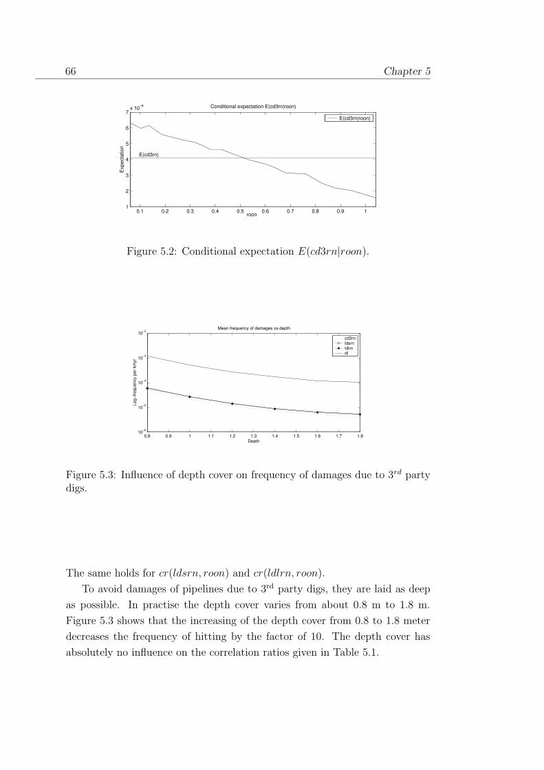
66 Chapter 5
0.1 0.2 0.3 0.4 0.5 0.6 0.7 0.8 0.9 11
2
3
4
5
6
7x 10⁻⁶ Conditional expectation E(cd3rn|roon)
roon
Exp
ecta
tion
E(cd3rn|roon)
E(cd3rn)
Figure 5.2: Conditional expectation E(cd3rn|roon).
0.8 0.9 1 1.1 1.2 1.3 1.4 1.5 1.6 1.7 1.810−6
10−5
10−4
10−3
10−2
Depth
Log−
frequ
ency
per
km
yr
Mean frequency of damages vs depth
cd3rnldsrnldlrndl
Figure 5.3: Influence of depth cover on frequency of damages due to 3rd partydigs.
The same holds for cr(ldsrn, roon) and cr(ldlrn, roon).
To avoid damages of pipelines due to 3rd party digs, they are laid as deep
as possible. In practise the depth cover varies from about 0.8 m to 1.8 m.
Figure 5.3 shows that the increasing of the depth cover from 0.8 to 1.8 meter
decreases the frequency of hitting by the factor of 10. The depth cover has
absolutely no influence on the correlation ratios given in Table 5.1.
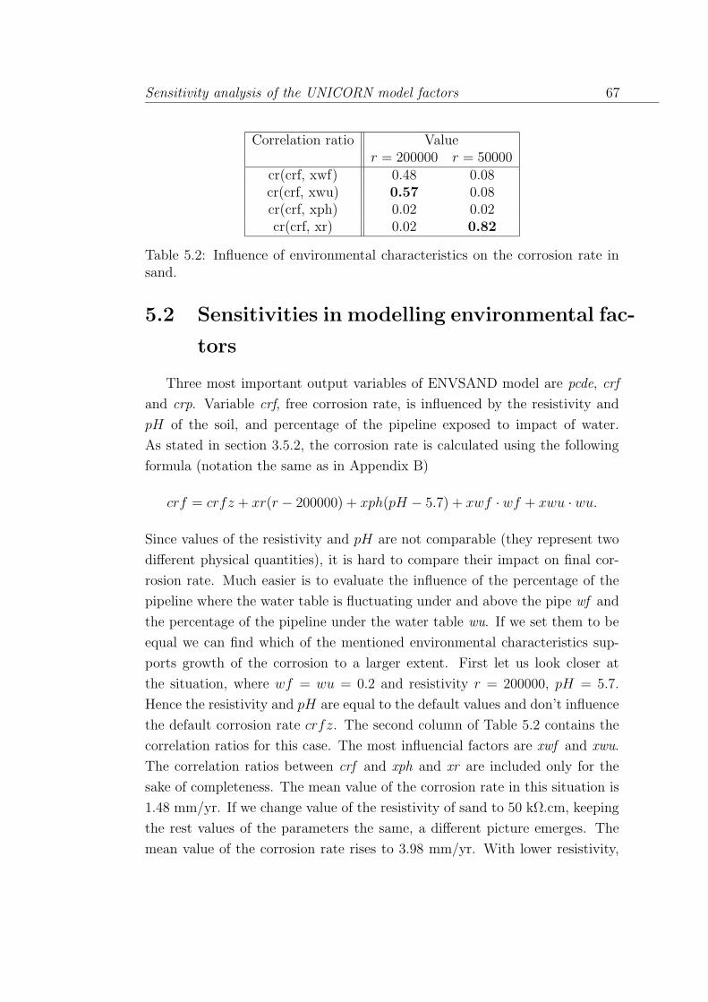
Sensitivity analysis of the UNICORN model factors 67
Correlation ratio Valuer = 200000 r = 50000
cr(crf, xwf) 0.48 0.08cr(crf, xwu) 0.57 0.08cr(crf, xph) 0.02 0.02cr(crf, xr) 0.02 0.82
Table 5.2: Influence of environmental characteristics on the corrosion rate insand.
5.2 Sensitivities in modelling environmental fac-
tors
Three most important output variables of ENVSAND model are pcde, crf
and crp. Variable crf, free corrosion rate, is influenced by the resistivity and
pH of the soil, and percentage of the pipeline exposed to impact of water.
As stated in section 3.5.2, the corrosion rate is calculated using the following
formula (notation the same as in Appendix B)
crf = crfz + xr(r − 200000) + xph(pH − 5.7) + xwf · wf + xwu · wu.
Since values of the resistivity and pH are not comparable (they represent two
different physical quantities), it is hard to compare their impact on final cor-
rosion rate. Much easier is to evaluate the influence of the percentage of the
pipeline where the water table is fluctuating under and above the pipe wf and
the percentage of the pipeline under the water table wu. If we set them to be
equal we can find which of the mentioned environmental characteristics sup-
ports growth of the corrosion to a larger extent. First let us look closer at
the situation, where wf = wu = 0.2 and resistivity r = 200000, pH = 5.7.
Hence the resistivity and pH are equal to the default values and don’t influence
the default corrosion rate crfz. The second column of Table 5.2 contains the
correlation ratios for this case. The most influencial factors are xwf and xwu.
The correlation ratios between crf and xph and xr are included only for the
sake of completeness. The mean value of the corrosion rate in this situation is
1.48 mm/yr. If we change value of the resistivity of sand to 50 kΩ.cm, keeping
the rest values of the parameters the same, a different picture emerges. The
mean value of the corrosion rate rises to 3.98 mm/yr. With lower resistivity,
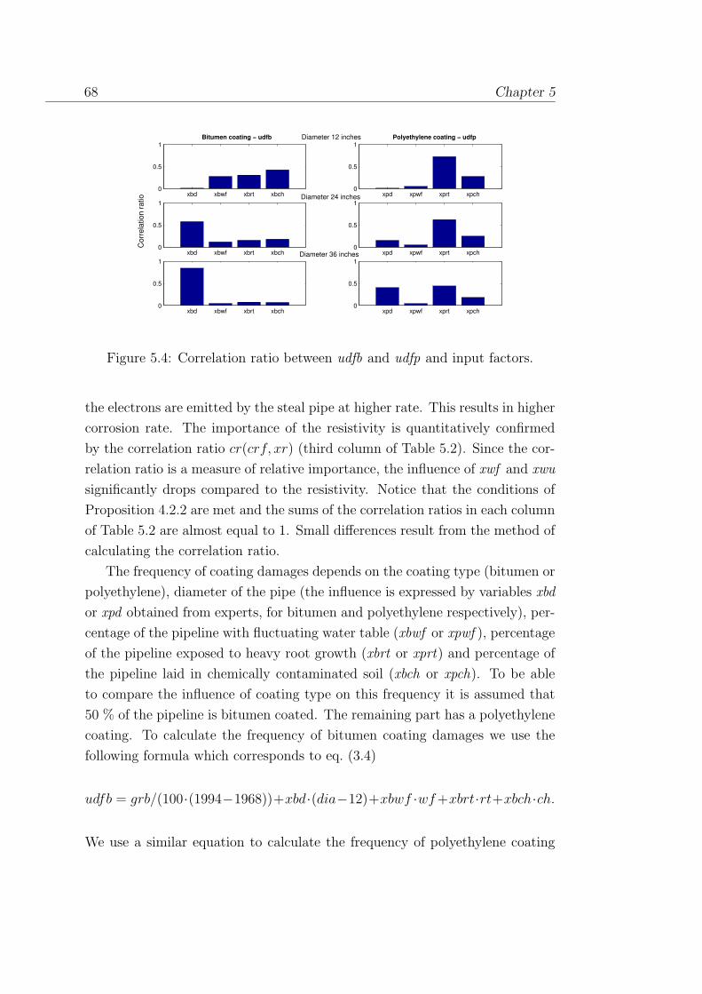
68 Chapter 5
xbd xbwf xbrt xbch0
0.5
1
xpd xpwf xprt xpch0
0.5
1
xbd xbwf xbrt xbch0
0.5
1
xpd xpwf xprt xpch0
0.5
1
xbd xbwf xbrt xbch0
0.5
1
xpd xpwf xprt xpch0
0.5
1
Diameter 12 inches
Diameter 24 inches
Diameter 36 inches
Bitumen coating − udfb Polyethylene coating − udfpC
orre
latio
n ra
tio
Figure 5.4: Correlation ratio between udfb and udfp and input factors.
the electrons are emitted by the steal pipe at higher rate. This results in higher
corrosion rate. The importance of the resistivity is quantitatively confirmed
by the correlation ratio cr(crf, xr) (third column of Table 5.2). Since the cor-
relation ratio is a measure of relative importance, the influence of xwf and xwu
significantly drops compared to the resistivity. Notice that the conditions of
Proposition 4.2.2 are met and the sums of the correlation ratios in each column
of Table 5.2 are almost equal to 1. Small differences result from the method of
calculating the correlation ratio.
The frequency of coating damages depends on the coating type (bitumen or
polyethylene), diameter of the pipe (the influence is expressed by variables xbd
or xpd obtained from experts, for bitumen and polyethylene respectively), per-
centage of the pipeline with fluctuating water table (xbwf or xpwf ), percentage
of the pipeline exposed to heavy root growth (xbrt or xprt) and percentage of
the pipeline laid in chemically contaminated soil (xbch or xpch). To be able
to compare the influence of coating type on this frequency it is assumed that
50 % of the pipeline is bitumen coated. The remaining part has a polyethylene
coating. To calculate the frequency of bitumen coating damages we use the
following formula which corresponds to eq. (3.4)
udfb = grb/(100·(1994−1968))+xbd·(dia−12)+xbwf ·wf+xbrt·rt+xbch·ch.
We use a similar equation to calculate the frequency of polyethylene coating

Sensitivity analysis of the UNICORN model factors 69
10 15 20 25 30 35 400.05
0.1
0.15
0.2
0.25
0.3
0.35
0.4
0.45
0.5
0.55
Diameter
Freq
uenc
y pe
r km
yr
Mean frequency of damages due to environment
udfbudfpfcde
Figure 5.5: Mean frequency of coating damages due to environment.
damages
udfp = grp/(100·(1994−1968))+xpd·(dia−12)+xpwf ·wf+xprt·rt+xpch·ch.
Given these two quantities we find the overall frequency of coating damages as
follows
fcde = %bit · udfb+ (1 − %bit) · udfp,
where %bit denotes the percentage of the pipeline with bitumen coating. As it
has been stated above, in this analysis %bit = 0.5.
Figure 5.4 depicts the correlation ratios between udfb and xbd, xbwf, xbrt,
xbch in case of bitumen coating (left column). The column on the right hand
side contain the same information but for polyethylene type of coating. Simul-
taneously, the six plots present influence of the diameter of the pipeline on the
correlation ratios. In case of a 12 inches diameter pipeline, the most impor-
tant factor appears to be the chemical contamination of the soil (bitumen) and
root growth (polyethylene). Diameter does not affect the frequency of coating
damages, because it is equal to the default value used in the formula of udfb
and udfp. The more we increase the diameter, the more important becomes
this factor at the cost of the others. But this is easily seen from the above
formulas. We can see also that bitumen is more sensitive to fluctuating water
table than polyethylene.
The frequency of coating damages due to environment increases with the
increase of the diameter. Figure 5.5 shows this relationship. For larger per-
centage of bitumen coating this frequency would be closer to the upper line
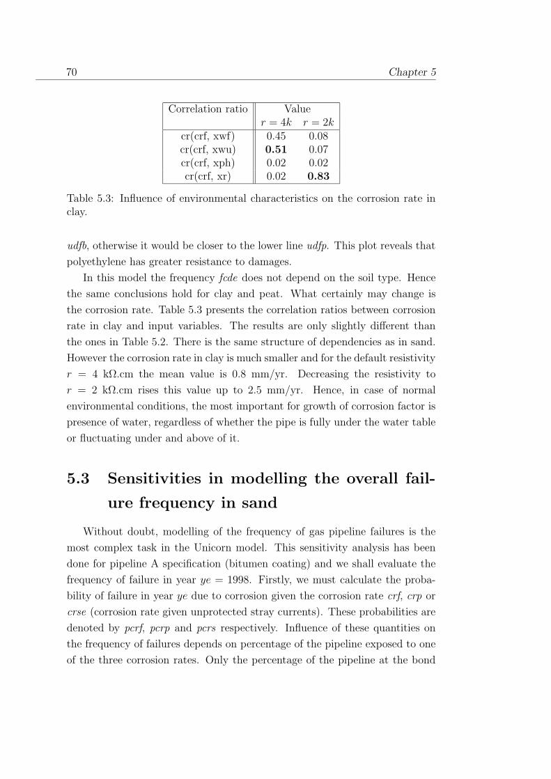
70 Chapter 5
Correlation ratio Valuer = 4k r = 2k
cr(crf, xwf) 0.45 0.08cr(crf, xwu) 0.51 0.07cr(crf, xph) 0.02 0.02cr(crf, xr) 0.02 0.83
Table 5.3: Influence of environmental characteristics on the corrosion rate inclay.
udfb, otherwise it would be closer to the lower line udfp. This plot reveals that
polyethylene has greater resistance to damages.
In this model the frequency fcde does not depend on the soil type. Hence
the same conclusions hold for clay and peat. What certainly may change is
the corrosion rate. Table 5.3 presents the correlation ratios between corrosion
rate in clay and input variables. The results are only slightly different than
the ones in Table 5.2. There is the same structure of dependencies as in sand.
However the corrosion rate in clay is much smaller and for the default resistivity
r = 4 kΩ.cm the mean value is 0.8 mm/yr. Decreasing the resistivity to
r = 2 kΩ.cm rises this value up to 2.5 mm/yr. Hence, in case of normal
environmental conditions, the most important for growth of corrosion factor is
presence of water, regardless of whether the pipe is fully under the water table
or fluctuating under and above of it.
5.3 Sensitivities in modelling the overall fail-
ure frequency in sand
Without doubt, modelling of the frequency of gas pipeline failures is the
most complex task in the Unicorn model. This sensitivity analysis has been
done for pipeline A specification (bitumen coating) and we shall evaluate the
frequency of failure in year ye = 1998. Firstly, we must calculate the proba-
bility of failure in year ye due to corrosion given the corrosion rate crf, crp or
crse (corrosion rate given unprotected stray currents). These probabilities are
denoted by pcrf, pcrp and pcrs respectively. Influence of these quantities on
the frequency of failures depends on percentage of the pipeline exposed to one
of the three corrosion rates. Only the percentage of the pipeline at the bond

Sensitivity analysis of the UNICORN model factors 71
sites bs can be selected by the user. Thus implicitly, the user can influence
the probability of the pipeline failure due to corrosion induced by the stray
currents. To account that fact we consider two situations, where bs = 0.8 and
bs = 0.2. Moreover, very important for the overall failure frequency is the birth
year b, since the pipelines laid before 1970 were subjected to intense corrosion
rate (cathodic protection was installed in 1970). Hence in total, we have 4
scenarios and the results of the analysis are in Table 5.4. For the pipeline laid
in 1975 the most important factor is the probability of failure due to free corro-
sion rate. Only this corrosion rate is able to remove enough wall thickness and
cause a leak within 23 years. The effective life of the pipeline given partially
working cathodic protection or failure of the stray currents protection system is
simply to long to cause a failure in 1998 (minimum is 29 years). Furthermore,
the results are completely insensitive to bs. The mean of corlk is 0.0024 per
km.yr.
For the pipeline laid in 1967 this number increases to 0.0164 per km.yr
for bs = 0.2 and 0.0679 per km.yr if bs = 0.8. Because of the very complex
interactions between the input variables, the sensitivity analysis gets very com-
plicated. The probability of failure given fully non-working cathodic protection
system pcrf is slightly higher than in the former case. But now the probabil-
ity of the pipeline failure given partially working cathodic protection system
pcrp is greater than zero, because 31 years is about the 30th percentile of the
distribution of the effective life. The probability of pipeline failure given stray
currents protection system failure pcrs behaves similarly. Variable pcrp has a
little bit larger values than pcrf. The probability of the failure of the stray
currents protection system pcrs is constant and in 54 % of the scenarios higher
than the probability of full failure of the cathodic protection. If we add, that
in this specific case the percentage of the pipe in the neighborhood of bond
sites is 20 to 80 times greater than the percentage of the pipeline exposed to
free corrosion rate, we can understand why pcrs have became so important in
this case.
Indirectly corlk may be influenced by the following variables:
pcen frequency of coating damage from environment
pc3 frequency of coating damage from 3rd parties
ps frequency of small unrepaired pipeline damage
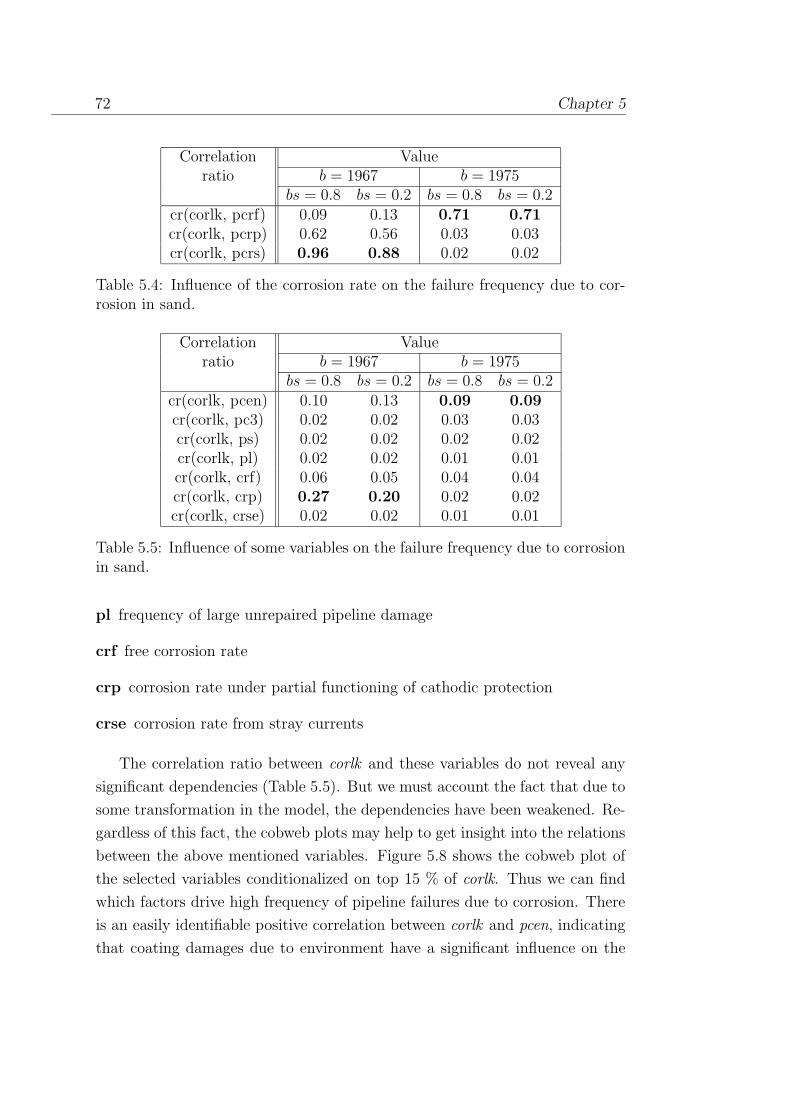
72 Chapter 5
Correlation Valueratio b = 1967 b = 1975
bs = 0.8 bs = 0.2 bs = 0.8 bs = 0.2cr(corlk, pcrf) 0.09 0.13 0.71 0.71cr(corlk, pcrp) 0.62 0.56 0.03 0.03cr(corlk, pcrs) 0.96 0.88 0.02 0.02
Table 5.4: Influence of the corrosion rate on the failure frequency due to cor-rosion in sand.
Correlation Valueratio b = 1967 b = 1975
bs = 0.8 bs = 0.2 bs = 0.8 bs = 0.2cr(corlk, pcen) 0.10 0.13 0.09 0.09cr(corlk, pc3) 0.02 0.02 0.03 0.03cr(corlk, ps) 0.02 0.02 0.02 0.02cr(corlk, pl) 0.02 0.02 0.01 0.01cr(corlk, crf) 0.06 0.05 0.04 0.04cr(corlk, crp) 0.27 0.20 0.02 0.02cr(corlk, crse) 0.02 0.02 0.01 0.01
Table 5.5: Influence of some variables on the failure frequency due to corrosionin sand.
pl frequency of large unrepaired pipeline damage
crf free corrosion rate
crp corrosion rate under partial functioning of cathodic protection
crse corrosion rate from stray currents
The correlation ratio between corlk and these variables do not reveal any
significant dependencies (Table 5.5). But we must account the fact that due to
some transformation in the model, the dependencies have been weakened. Re-
gardless of this fact, the cobweb plots may help to get insight into the relations
between the above mentioned variables. Figure 5.8 shows the cobweb plot of
the selected variables conditionalized on top 15 % of corlk. Thus we can find
which factors drive high frequency of pipeline failures due to corrosion. There
is an easily identifiable positive correlation between corlk and pcen, indicating
that coating damages due to environment have a significant influence on the

Sensitivity analysis of the UNICORN model factors 73
0 1 2 3 4 5 6 7 8 9
102
103
crp
Effe
ctiv
e lif
e
Effective life given crp and coating damage, small and large damage
elcpelspellp
Figure 5.6: Effective life of the pipeline given partially working cathodic pro-tection system.
high failure frequency. Variable crp has even greater impact on corlk. Al-
though, there is a few percent of the scenarios from the top of the distribution
of crp selected, the majority of them are in lower 26 % of the distribution. This
is an interesting feature while low crp should increase the effective life of the
pipeline, resulting in a lower frequency of the pipeline failures. The relation-
ship between crp and effective life given coating damage elcp, small damage
elsp and ellp is pictured in Figure 5.6. We can see that for small values of crp
there is a large uncertainty involved. For larger values of crp we observe an
expected decrease of the effective life.
Let us zoom to the area of the plot where the effective life has very large
variance (Figure 5.7). This time the x-axis is labelled by index of the ordered
statistics of crp instead of their values. We consider 300 out of 1000 ordered
samples of crp and corresponding values of elcp. To make the picture more
clearer elsp and ellp have not been plotted, but keep in mind that they act in
exactly the same manner as elcp. There are very high peaks visible in the plot,
48 out of 266 values of elcp are larger than 57.3 years. This number of years
corresponds to the value of eclp at 267th ordered point of crp from which elcp
starts to be smooth and decreasing in crp. Hence for the rest of these selected
scenarios (exactly 218) the effective life elcp is about 30 years, meaning that
the pipe reaches the age when the failure due to partial failure of the cathodic
protection becomes highly likely. Note that 267th ordered sample of crp is
about its 26th percentile and this agrees with the cobweb plot in Figure 5.8.

74 Chapter 5
0 50 100 150 200 250 30025
100
1000
Index
Log
effe
ctiv
e lif
e [y
ears
]Effective life given crp
Figure 5.7: Effective life of the pipeline given partially working cathodic pro-tection system for small values of crp.
Where does this unexpected feature come from? The effective life of the
pipeline given partially working cathodic protection and coating damage is
calculated with the following formula
elcp = (xc · t− (j − 1970) · crp)/crf + j − 1970
for pipeline which effective birthyear is before 1970 and
elcp = (xc · t)/crp+ j − 1970 (5.1)
otherwise, where xc = 0.9 is the critical thickness fraction, t = 12.26 is the pipe
wall thickness and j = ye = 1999 is year of inspection. We see that only two
uncertain quantities appear in this equation, crp and crf. Samples of crp have
been ordered, hence the only quantity which could cause those peaks is crf.
If crp is less than or equal to 0.38 mm/year, then the effective live is so long
that the pipe must have been placed in the ground before 1970 and then hence
the pipeline was exposed to crf for years between effective birthyear and 1970.
The 267th ordered sample of crp is equal to 0.39 mm/year and that is why for
this value and greater elcp is calculated using equation (5.1) where crf does
not appear. Further analysis of the sample files created by Unicorn revealed
that for those 267 scenarios, crf have very small values (less than 0.1 mm/yr)
and this cause the observed peaks of elcp.
Coming back to Figure 5.8, the small amount of samples at the top of the
distribution of crp is a result of the short effective life elcp, elsp and ellp for
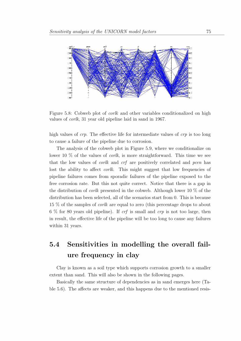
Sensitivity analysis of the UNICORN model factors 75
Figure 5.8: Cobweb plot of corlk and other variables conditionalized on highvalues of corlk, 31 year old pipeline laid in sand in 1967.
high values of crp. The effective life for intermediate values of crp is too long
to cause a failure of the pipeline due to corrosion.
The analysis of the cobweb plot in Figure 5.9, where we conditionalize on
lower 10 % of the values of corlk, is more straightforward. This time we see
that the low values of corlk and crf are positively correlated and pcen has
lost the ability to affect corlk. This might suggest that low frequencies of
pipeline failures comes from sporadic failures of the pipeline exposed to the
free corrosion rate. But this not quite correct. Notice that there is a gap in
the distribution of corlk presented in the cobweb. Although lower 10 % of the
distribution has been selected, all of the scenarios start from 0. This is because
15 % of the samples of corlk are equal to zero (this percentage drops to about
6 % for 80 years old pipeline). If crf is small and crp is not too large, then
in result, the effective life of the pipeline will be too long to cause any failures
within 31 years.
5.4 Sensitivities in modelling the overall fail-
ure frequency in clay
Clay is known as a soil type which supports corrosion growth to a smaller
extent than sand. This will also be shown in the following pages.
Basically the same structure of dependencies as in sand emerges here (Ta-
ble 5.6). The affects are weaker, and this happens due to the mentioned resis-
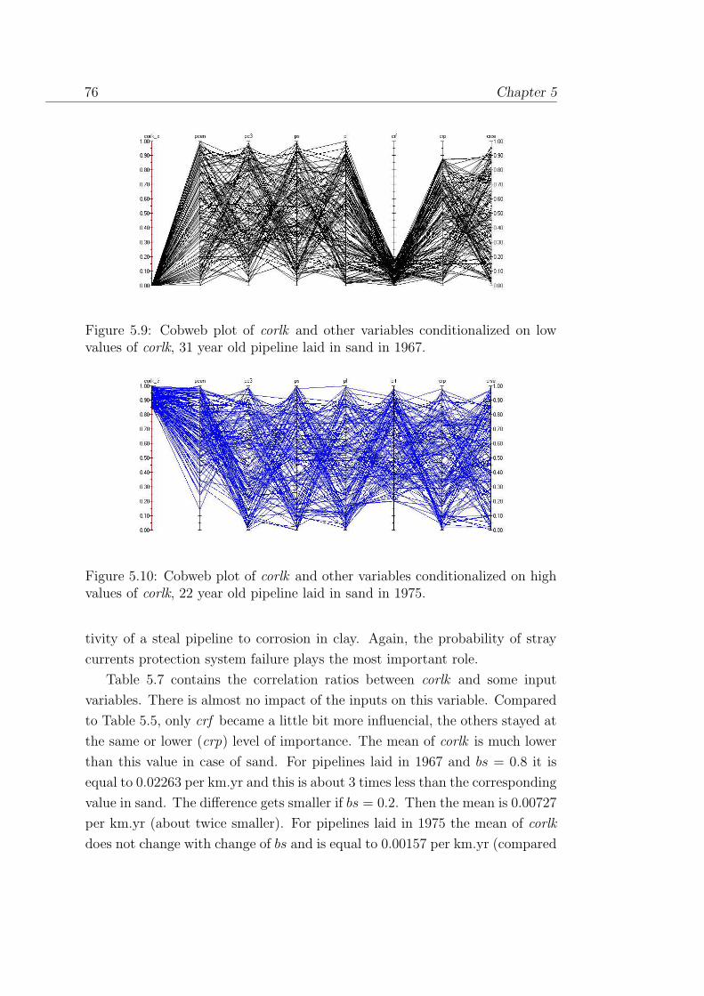
76 Chapter 5
Figure 5.9: Cobweb plot of corlk and other variables conditionalized on lowvalues of corlk, 31 year old pipeline laid in sand in 1967.
Figure 5.10: Cobweb plot of corlk and other variables conditionalized on highvalues of corlk, 22 year old pipeline laid in sand in 1975.
tivity of a steal pipeline to corrosion in clay. Again, the probability of stray
currents protection system failure plays the most important role.
Table 5.7 contains the correlation ratios between corlk and some input
variables. There is almost no impact of the inputs on this variable. Compared
to Table 5.5, only crf became a little bit more influencial, the others stayed at
the same or lower (crp) level of importance. The mean of corlk is much lower
than this value in case of sand. For pipelines laid in 1967 and bs = 0.8 it is
equal to 0.02263 per km.yr and this is about 3 times less than the corresponding
value in sand. The difference gets smaller if bs = 0.2. Then the mean is 0.00727
per km.yr (about twice smaller). For pipelines laid in 1975 the mean of corlk
does not change with change of bs and is equal to 0.00157 per km.yr (compared
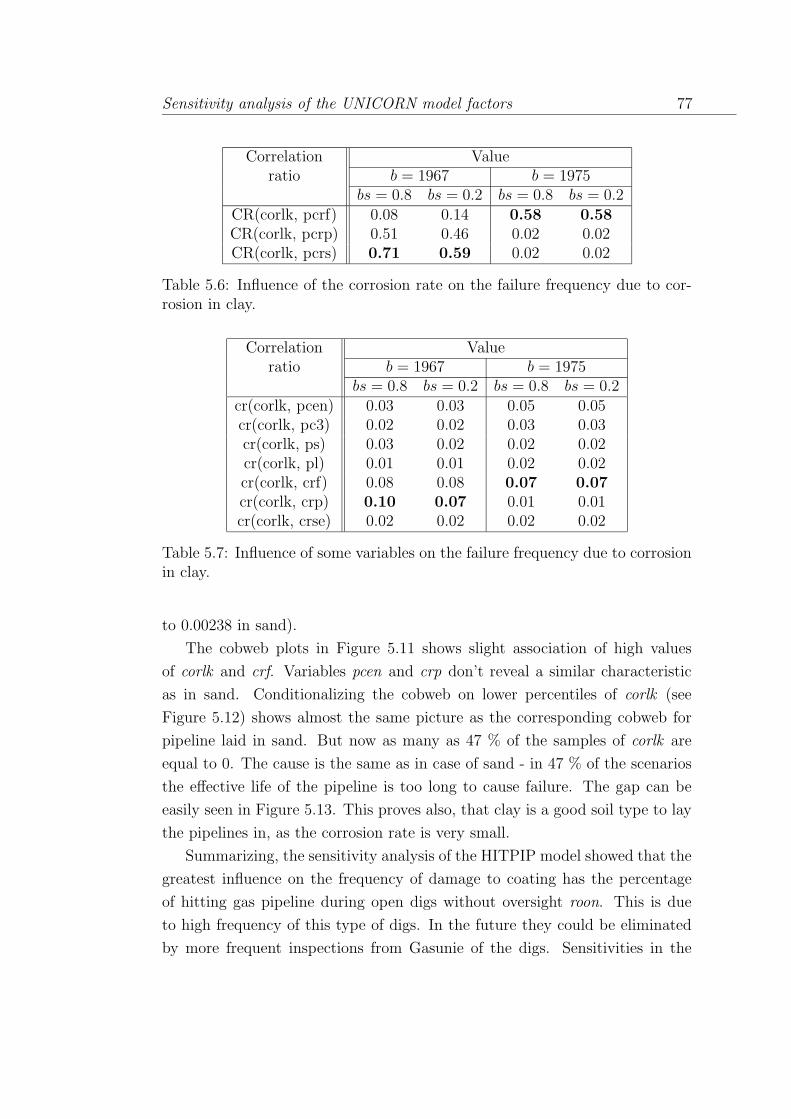
Sensitivity analysis of the UNICORN model factors 77
Correlation Valueratio b = 1967 b = 1975
bs = 0.8 bs = 0.2 bs = 0.8 bs = 0.2CR(corlk, pcrf) 0.08 0.14 0.58 0.58CR(corlk, pcrp) 0.51 0.46 0.02 0.02CR(corlk, pcrs) 0.71 0.59 0.02 0.02
Table 5.6: Influence of the corrosion rate on the failure frequency due to cor-rosion in clay.
Correlation Valueratio b = 1967 b = 1975
bs = 0.8 bs = 0.2 bs = 0.8 bs = 0.2cr(corlk, pcen) 0.03 0.03 0.05 0.05cr(corlk, pc3) 0.02 0.02 0.03 0.03cr(corlk, ps) 0.03 0.02 0.02 0.02cr(corlk, pl) 0.01 0.01 0.02 0.02cr(corlk, crf) 0.08 0.08 0.07 0.07cr(corlk, crp) 0.10 0.07 0.01 0.01cr(corlk, crse) 0.02 0.02 0.02 0.02
Table 5.7: Influence of some variables on the failure frequency due to corrosionin clay.
to 0.00238 in sand).
The cobweb plots in Figure 5.11 shows slight association of high values
of corlk and crf. Variables pcen and crp don’t reveal a similar characteristic
as in sand. Conditionalizing the cobweb on lower percentiles of corlk (see
Figure 5.12) shows almost the same picture as the corresponding cobweb for
pipeline laid in sand. But now as many as 47 % of the samples of corlk are
equal to 0. The cause is the same as in case of sand - in 47 % of the scenarios
the effective life of the pipeline is too long to cause failure. The gap can be
easily seen in Figure 5.13. This proves also, that clay is a good soil type to lay
the pipelines in, as the corrosion rate is very small.
Summarizing, the sensitivity analysis of the HITPIP model showed that the
greatest influence on the frequency of damage to coating has the percentage
of hitting gas pipeline during open digs without oversight roon. This is due
to high frequency of this type of digs. In the future they could be eliminated
by more frequent inspections from Gasunie of the digs. Sensitivities in the

78 Chapter 5
Figure 5.11: Cobweb plot of corlk and other variables conditionalized on highvalues of corlk, 31 year old pipeline laid in clay in 1967.
Figure 5.12: Cobweb plot of corlk and other variables conditionalized on lowvalues of corlk, 31 year old pipeline laid in clay in 1967.
environmental part of the model must be analyzed individually for a specific
set of input variables, because of the very complex interactions occurring there.
The same holds for the analysis of the overall failure frequency. For sure,
polyethylene is a much better coating material than bitumen. As regards these
two types of materials, they both are sensitive to different damage initiating
events. This should be taken into account when a new pipeline is designed.

Sensitivity analysis of the UNICORN model factors 79
Figure 5.13: Cobweb plot of corlk and other variables, 31 year old pipeline laidin clay in 1967.

80 Chapter 5

81
Chapter 6
Analysis of the corrosion data
This chapter studies information on inspected pipelines by visualizing the
data. This will help to form a clearer picture of specific aspects of the corrosion
problem the gas industry is dealing with. Pipeline A data will be analyzed
separately, since this pipeline was inspected twice in course of 18 months.
The analysis methods have been implemented in MatLab. The code of the
function is available in Appendix C.
6.1 Analysis of pipeline A data
The first inspection of Pipeline A was performed in October 1999, after 32
years since laying in the ground. In April 2001 the pipeline was reinspected.
Figure 6.1 presents two step functions constructed by plotting the total
number of corrosion spots against distance from the reference location. This
kind of plots allow to discover locations where the occurrence of metal loss is
more likely than elsewhere. Line representing the number of corrosion spots
found during reinspection in 2001 (Pipeline A1) is above the line representing
the same number for inspection from 1999 (Pipeline A). This is correct, since
the pipeline A1 data include the metal loss locations from the pipeline A data
plus additional spots that have had appeared in time period of 18 months
between the inspections. This plot shows also that many of the spots appear
as clusters (high jumps of the lines).
The quantile-quantile plot shows almost linear relationship between the
both data sets. There is only a difference in tails of the distributions (Fig-

82 Chapter 6
0 1 2 3 4 5 6 7
x 104
0
10
20
30
40
50
60
70
80pipeA1
pipeA
Total number of corrosions vs distance from the starting point
Distance [m]
Tota
l num
ber o
f cor
rosi
ons
Figure 6.1: Total number of corrosion spots in Pipeline A and A1 data sets.
10 15 20 25 30 35 40 45 50 5510
15
20
25
30
35
40
45
50
55
60
pipeA1 data quantiles
pipe
A d
ata
quan
tiles
Quantile−quantile plot of both corrosion data sets
Figure 6.2: Quantile-quantile plot of Pipeline A and A1 data sets.
ure 6.2), because maximum metal loss in the pipeline A data is 44 %, whereas
in 2001 the maximum is 55 %. The empirical distribution function plotted in
Figure 6.3 also depicts that fact.
Figure 6.4 presents histograms of the corrosion data. During inspection in
2001 many new, small metal loss events have been observed. There were 5
such events in 1999 and this number increased to 20 in 2001. Assuming, that
the MFL-pigs used for the inspections were accurate, 15 new corrosion spots
have appeared within 18 months. This might seem to be a lot, since within 32
years since “birth year” only 66 corrosion events developed and suddenly after
18 month we have 15 new ones. But we must remember that only corrosion
events with greater than 10 % of metal loss are reported. It could be that

Analysis of the corrosion data 83
5 10 15 20 25 30 35 40 45 50 55 600
0.2
0.4
0.6
0.8
1
Metal loss [%]
CD
F
Empirical distribution functions
pipeApipeA1
Figure 6.3: Empirical distribution functions of metal loss for Pipeline A andA1 corrosion data.
10 15 20 25 30 35 40 450
5
10
15Histogram of the pipeA data
Metal loss [%]
Num
ber o
f cor
rosi
on e
vent
s
10 15 20 25 30 35 40 45 50 550
5
10
15
20Histogram of the pipeA1 data
Metal loss [%]
Num
ber o
f cor
rosi
on e
vent
s
Figure 6.4: Histograms of corrosion events found during inspections in 1999(pipeA) and 2001 (pipeA1).
in 1999 there were many small corrosion spots with the metal loss close to
10 % but not exceeding this value. A period of 18 months is enough time for
corrosion to remove a few percent of the wall thickness what makes corrosion
spots detectable.
Figure 6.5 presents histograms of the vertical positions of the metal loss
events in polar coordinates. This allows to visualize the positions in a very
intuitive way, where 0 and 180 labels represent top and bottom of the pipe
respectively. According to Figure 6.5, the metal loss spots are located mainly
at the bottom of the pipeline. This excludes 3rd party digs as a cause of the

84 Chapter 6
0o
90o
180o
270o
15 metal loss events
0o
90o
180o
270o
18 metal loss events
First inspection Second inpection
Figure 6.5: Vertical positions of the metal loss events on the surface of pipelineA.
metal loss. Very likely corrosion could start because of the damage of the
coating during laying the pipe in the ground. Very curious is the fact, that in
1999 most of the spots were located between 180 and 270 degrees, whereas in
2001 it appeared to be 145–210 degrees. It might be an indication of not very
accurate locating the metal loss locations by the MFL-pig.
6.2 Analysis of pipelines B, C, D and E data
This section analyzes the data from pipelines B, C, D and E. Similarly to
the previous section let us start with plotting the total number of the metal
loss events against the distance from the reference point. Pipelines B and C
have the same diameter and wall thickness. They both are high pressure, large
diameter pipelines. Pipelines D and E have smaller diameter and wall thickness
(see Table 2.2 for details). Especially pipelines D and E reveal no sensitivity to
location, what supports the assumption of the UNICORN model, saying that
the distance between two successive corrosion spots is exponentially distributed
and hence, the number of the spots in a segment of pipeline with given length
follows a homogeneous Poisson process. In case of pipelines B and C we can
again observe high jumps indicating clusters of corrosion spots.

Analysis of the corrosion data 85
0 2 4 6 8 10 12 14 16 18
x 104
0
20
40
60
80
100pipeB
pipeC
Total number of corrosions vs distance from the starting point
Distance [m]
Tota
l num
ber o
f cor
rosi
ons
0 2 4 6 8 10 12 14
x 104
0
50
100
150
200
pipeD
pipeE
Total number of corrosions vs distance from the starting point
Distance [m]
Tota
l num
ber o
f cor
rosi
ons
Figure 6.6: Total number of corrosion spots in pipeline B, C, D and E datasets.
Pipelines B, C and D corrosion data is left-truncated (see Figure 6.7). Only
Pipeline E data provides information on corrosion events with less than 10 % of
the wall thickness metal loss. This pipeline has been inspected most recently.
Pipelines D and E definitely reveal different characteristics (susceptibility to
corrosion) than the others. First of all, there is twice as many of the detected
defects as in the other data sets. The reason for that could be smaller wall
thickness of these pipes. If pipe E has the wall thickness equal to 5.95 mm,
than 10 % of the metal loss is 0.595 mm. In case of pipe A 10 % of metal loss is
1.225 mm. Since the corrosion rate (metal loss due to corrosion in millimeters
per km per year) is independent of the wall thickness, corrosion of pipe E will
be detectable sooner than that one occurring in pipe A. The second factor
making them distinctive is an almost complete lack of clusters of defects.
Figure 6.8 visualizes information on positions of corrosion spots on the
surface of pipelines B, C, D and E. Pipeline B data reveals the same pattern as
Pipeline A data. Most of the spots are located at the bottom of the pipelines.
A completely different picture emerges from Pipeline C, D and E data. In
these cases the spots are spread out almost uniformly regardless if it is the top

86 Chapter 6
10 15 20 25 30 35 40 45 50 55 600
10
20
30Histogram of the pipeB data
Metal loss [%]
Num
ber o
f cor
rosi
on e
vent
s
10 15 20 25 30 35 400
10
20
30
40Histogram of the pipeC data
Metal loss [%]
Num
ber o
f cor
rosi
on e
vent
s
11 13 15 17 19 21 23 25 27 29 31 33 35 37 390
50
100Histogram of the pipeD data
Metal loss [%]
Num
ber o
f cor
rosi
on e
vent
s
0 5 10 15 20 25 30 35 40 45 500
20
40
60
80Histogram of the pipeE data
Metal loss [%]
Num
ber o
f cor
rosi
on e
vent
s
Figure 6.7: Histograms of corrosion events found during inspections of pipelinesB, C, D and E.
or bottom of the pipeline. It might be that pipelines C, D and E are crossing
highly urbanized areas and part of the defects could be initiated by 3rd party
digs, but we don’t have this kind of information. Further analysis did not
reveal any particular dependency between distance from the reference point
and vertical positions of the corrosion spots on surface of the pipelines.
6.3 Comparison of the UNICORN output with
the actual data
One of the main purposes of this study is evaluation of the UNICORN
model presented in Chapter 3. This model predicts, with uncertainty, failure
frequency of gas pipelines. It has been designed specifically to the Dutch

Analysis of the corrosion data 87
0o
90o
180o
270o
36 metal loss events
Pipeline B 0o
90o
180o
270o
12 metal loss events
Pipeline C
0o
90o
180o
270o
18 metal loss events
Pipeline D0o
90o
180o
270o
18 metal loss events
Pipeline E
Figure 6.8: Vertical positions of the metal loss events on the surface of pipelinesB, C, D and E.
conditions. One can ask how can we compare output of the model with the
data, since there is no failure in the data! However what the model returns is,
in fact, the frequency of exceeding a certain level of metal loss. This level is set
by three parameters xc, xs and xl which are critical thickness fraction given
that there was a coating damage (C), small damage (S, 0.5 mm of removed wall
thickness) or large damage (L, 2 mm of removed wall thickness) respectively.
By default xc = 0.9, xs = 0.7 and xl = 0.6. For instance, assume that there
was a small damage in past; a telecommunication company laid their cables and
scratched the pipeline. The parameter xs says that 70 % of the remaining wall

88 Chapter 6
10−12 10−10 10−8 10−6 10−4 10−2 1000
10
20
30
40
50
60
70
80
90
100
Frequency corrosion per kmyr
Per
cent
iles
Frequency of exceeding a certain percentage of corrosion based on pipe A data.
10% 15%
20% 25%
30% 35%
40%
Squares mark data from pipeline A inspected in 1999
Figure 6.9: Comparison of the UNICORN output with the Pipeline A datainspected in 1999.
thickness (the initial thickness minus 0.5 mm) must be removed by corrosion in
order to cause a leak. The values of xc = 0.9, xs = 0.7 and xl = 0.6 have been
determined experimentally. We see that the UNICORN model output is simply
the frequency of exceeding 90 %, 70 % and 60 % of metal loss. By manipulating
these parameters, we could obtain frequency of exceeding any other percentage
of metal loss, like 10 % to 40 %. And this frequency is implicitly given in the
inspection data. The data includes total length of the pipelines and their age.
We can determine the number of defects where the percentage of metal loss
exceeds, say 20 %. In case of Pipeline A this number is 21. Dividing 21 by
the length of Pipeline A (69 km) and its age (32 years) we obtain frequency
of exceeding 20 % of metal loss per km.year. There is nothing simpler than
plotting this frequency and distribution of the frequency of exceeding 20 % of
metal loss from the UNICORN model together.
To obtain the corresponding distribution from UNICORN, we must set xc,
xs and xl such that for each of the initiative events (coating damage, small
damage and large damage) sum of the wall thickness removed by this event
and later corrosion is equal to 20 %. Obviously xc = 0.2, since the pipe wall
was untouched. Values of xs and xl will depend on the initial wall thickness,
because 0.5 mm removed by small damage is about 4 % and 8 % of the initial
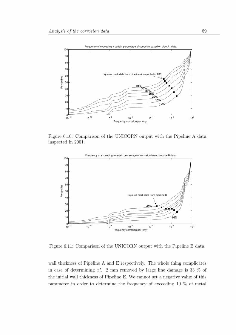
Analysis of the corrosion data 89
10−12 10−10 10−8 10−6 10−4 10−2 1000
10
20
30
40
50
60
70
80
90
100
Frequency corrosion per kmyr
Per
cent
iles
Frequency of exceeding a certain percentage of corrosion based on pipe A1 data.
10% 15%
20% 25%
30% 35%
40%
Squares mark data from pipeline A inspected in 2001
Figure 6.10: Comparison of the UNICORN output with the Pipeline A datainspected in 2001.
10−12 10−10 10−8 10−6 10−4 10−2 1000
10
20
30
40
50
60
70
80
90
100
Frequency corrosion per kmyr
Per
cent
iles
Frequency of exceeding a certain percentage of corrosion based on pipe B data.
10%
40%
Squares mark data from pipeline B
Figure 6.11: Comparison of the UNICORN output with the Pipeline B data.
wall thickness of Pipeline A and E respectively. The whole thing complicates
in case of determining xl. 2 mm removed by large line damage is 33 % of
the initial wall thickness of Pipeline E. We cannot set a negative value of this
parameter in order to determine the frequency of exceeding 10 % of metal

90 Chapter 6
loss. In such cases xl is set to be equal 0 and this is easily distinguishable, for
instance in Figure 6.13, where the lines representing the frequency of exceeding
10 % and 15 % of metal loss starts from 10−8 on x-axis in contrast to the rest
of the frequencies.
Figure 6.9 depicts results obtained by implementing the above reasoning.
First the characteristics of Pipeline A have been incorporated into the UNI-
CORN model. The resulting seven output distributions depicted in the figure
corresponds to exceeding 10 % to 40 % of metal loss with step 5 %. The black
squares mark the frequencies derived from the data. The data vary from 30th
to 56th percentile of the UNICORN’s output. This is a satisfactory result,
since the data is in the range predicted by the model and very close to medi-
ans, which are ones of the main quantitative characteristics of a probabilistic
distribution.
The same conclusion holds for the data from reinspection of Pipeline A
in 2001 (Figure 6.10). There are 11 more defects compare to inspection from
1999, but the UNICORN model took this fact into account. A different picture
emerges from Figure 6.11, where the model’s predictions are overestimated
compare to the data. This could be a problem of the model or the information
on soil characteristics, like pH or resistivity might not be correct. However,
even this result cannot disqualify the whole model.
The analysis of pipeline C data was more time-consuming and complicated
because of the fact that first 100 km was laid in sand and the second part
(last 67 km) was laid in clay. The two sections have been analyzed separately.
The average weighted birth year of the first section is 1965. In case of the
second section it is 1969 (this part was repaired many times in the past).
Moreover the characteristics of the soil, in which the pipe was laid is unknown.
Therefore the analysis was performed for two different characteristics of the
soil. Nevertheless, it is still dangerous to draw some strong conclusions from
this analysis, since the real characteristic of the soil may be completely different
from those assumed.
First let’s concentrate on analysis of the first 100 km of pipeline C. Fig-
ure 6.12 contains plots of the distributions returned by the model assuming
two different characteristics of sand. The first set of values comes from the
information we have on Pipeline A and B. Set 2 was used during development
of the model in 1995. The values of the individual parameters are in Table 6.1.

Analysis of the corrosion data 91
10−12 10−10 10−8 10−6 10−4 10−2 1000
10
20
30
40
50
60
70
80
90
100
Frequency corrosion per kmyr
Per
cent
iles
Frequency of exceeding a certain percentage of corrosion based on pipe C, sand, set1 data.
Squares mark the data from the pipelines
10%
40% 35%
30% 25%
20% 15%
10−12 10−10 10−8 10−6 10−4 10−2 1000
20
40
60
80
100
Frequency corrosion per kmyr
Per
cent
iles
Frequency of exceeding a certain percentage of corrosion based on pipe C, sand, set2 data.
Squares mark the data from the pipelines
10%
40% 35% 30% 25% 20%
15%
Figure 6.12: Comparison of the UNICORN output with the Pipeline C data(first 100 km of the pipeline laid in sand).
10−12 10−10 10−8 10−6 10−4 10−2 1000
20
40
60
80
100
Frequency corrosion per kmyr
Per
cent
iles
Frequency of exceeding a certain percentage of corrosion based on pipe C, clay, set1 data.
Squares mark the data from the pipelines
10%
40% 35% 30% 25%
20%
15%
10−12 10−10 10−8 10−6 10−4 10−2 1000
20
40
60
80
100
Frequency corrosion per kmyr
Per
cent
iles
Frequency of exceeding a certain percentage of corrosion based on pipe C, clay, set2 data.
Squares mark the data from the pipelines
10%
40%
20%
15%
Figure 6.13: Comparison of the UNICORN output with the Pipeline C data(last 67 km of the pipeline laid in clay).
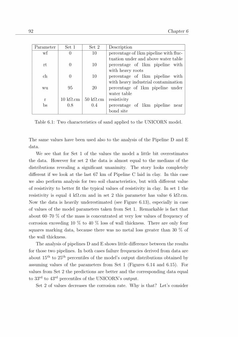
92 Chapter 6
Parameter Set 1 Set 2 Descriptionwf 0 10 percentage of 1km pipeline with fluc-
tuation under and above water tablert 0 10 percentage of 1km pipeline with
with heavy rootsch 0 10 percentage of 1km pipeline with
with heavy industrial contaminationwu 95 20 percentage of 1km pipeline under
water tabler 10 kΩ.cm 50 kΩ.cm resistivity
bs 0.8 0.4 percentage of 1km pipeline nearbond site
Table 6.1: Two characteristics of sand applied to the UNICORN model.
The same values have been used also to the analysis of the Pipeline D and E
data.
We see that for Set 1 of the values the model a little bit overestimates
the data. However for set 2 the data is almost equal to the medians of the
distributions revealing a significant unanimity. The story looks completely
different if we look at the last 67 km of Pipeline C laid in clay. In this case
we also perform analysis for two soil characteristics, but with different value
of resistivity to better fit the typical values of resistivity in clay. In set 1 the
resistivity is equal 4 kΩ.cm and in set 2 this parameter has value 6 kΩ.cm.
Now the data is heavily underestimated (see Figure 6.13), especially in case
of values of the model parameters taken from Set 1. Remarkable is fact that
about 60–70 % of the mass is concentrated at very low values of frequency of
corrosion exceeding 10 % to 40 % loss of wall thickness. There are only four
squares marking data, because there was no metal loss greater than 30 % of
the wall thickness.
The analysis of pipelines D and E shows little difference between the results
for those two pipelines. In both cases failure frequencies derived from data are
about 15th to 25th percentiles of the model’s output distributions obtained by
assuming values of the parameters from Set 1 (Figures 6.14 and 6.15). For
values from Set 2 the predictions are better and the corresponding data equal
to 33rd to 43rd percentiles of the UNICORN’s output.
Set 2 of values decreases the corrosion rate. Why is that? Let’s consider

Analysis of the corrosion data 93
10−12 10−10 10−8 10−6 10−4 10−2 1000
10
20
30
40
50
60
70
80
90
100
Frequency corrosion per kmyr
Per
cent
iles
Frequency of exceeding a certain percentage of corrosion based on pipe D, set1 data.
Squares mark the data from the pipelines10%15%20%25%30%35%40%
10%
40%
10−12 10−10 10−8 10−6 10−4 10−2 1000
10
20
30
40
50
60
70
80
90
100
Frequency corrosion per kmyr
Per
cent
iles
Frequency of exceeding a certain percentage of corrosion based on pipe D, set2 data.
Squares mark the data from the pipelines
10%
40%
Figure 6.14: Comparison of the UNICORN output with the Pipeline D data.
10−12 10−10 10−8 10−6 10−4 10−2 1000
10
20
30
40
50
60
70
80
90
100
Frequency corrosion per kmyr
Per
cent
iles
Frequency of exceeding a certain percentage of corrosion based on pipe E, set1 data.
Squares mark the data from the pipelines10%15%20%25%30%35%40%
10%
40%
10−12 10−10 10−8 10−6 10−4 10−2 1000
10
20
30
40
50
60
70
80
90
100
Frequency corrosion per kmyr
Per
cent
iles
Frequency of exceeding a certain percentage of corrosion based on pipe E, set2 data.
Squares mark the data from the pipelines
10%
40%
Figure 6.15: Comparison of the UNICORN output with the Pipeline E data.

94 Chapter 6
0 0.1 0.2 0.3 0.4 0.5 0.6 0.7 0.8 0.90
10
20
30
40
50
60
70
80
90
100Influence of values of the parameters on frequency of exceeding 35% of metal loss
Frequency/ kmyr
Per
cent
ile
CH=0.4 WF=0.4 RT=0.4
Set 1 R=50k
WU=0.2 BS=0.4
Figure 6.16: Influence of values of the parameters on frequency of exceeding25 % of metal loss.
the following situation. First we perform a run of the UNICORN model using
values from Set 1. The rest of the parameter values correspond to the spec-
ification of pipeline D. Setting xc = 0.35,xs = 0.3 and xl = 0.06 causes the
output distribution to represent the frequency of exceeding 35 % of the metal
loss due to corrosion. Now change one value of a parameter at time, for exam-
ple increase wf from 0 to 0.4 and keeping the rest of the parameters as in set
1, perform another run. Figure 6.16 depict results obtained by changing values
of the parameters to bs = wf = rt = ch = 0.4, wu = 0.2 and r = 50 kΩ.cm, of
course each of them separately. The x-axis has a linear scale in contrast to Fig-
ures 6.9–6.15. Increasing percentage of the pipe length fluctuating under and
above water table (wf) and exposed to heavy root growth (rt) and chemical
contamination (ch) causes the corrosion rate to increase implying higher fre-
quency of defects. Among these three parameters ch influences the frequency
to the largest extent (the distribution has a longer tail, than the one obtained
with the standard values of the parameters taken from Set 1). Resistivity does
not seem to influence significantly the frequency. Decreasing the percentage
of the pipeline under the water table from 95 % to 20 % decreases also the
failure frequency. This clearly shows that presence of the water supports the
growth of the corrosion. Bond sites are particulary open to corrosion, because

Analysis of the corrosion data 95
of stray currents that may occur in such places. In 1970 a system preventing
occurrence of strong stray currents but the probability that this system will
fail is very high (0.95). Hence the larger portion of the pipe is in the neigh-
borhood of the bond sites, the higher corrosion rate and frequency of failure.
In the model this portion is set by value of the parameter bs. The model’s
predictions show here proper behavior. The frequency distribution obtained
for bs = 40 % is concentrated on lower values than the one obtained for bs =
80 % (see Figure 6.16).
The analysis in this chapter showed that in some aspects the data reveal sig-
nificant dissimilarities between the inspected pipelines. First of all, the Pipeline
A and B data report only defects located at the bottom of the pipelines, whereas
in the Pipeline C, D and E data the metal loss defects are located also at the
top of the pipelines. It seems that Pipeline D and E data are the most accurate
ones. They both have smaller diameter and thickness than the other pipelines
and this makes the defects easier to detect. Together they provide information
on over 350 metal loss events and give information justifying the assumptions
of the UNICORN model (the occurrence of events along the pipe follows the
Poisson distribution with respect to distance). The Kolmogorov-Smirnov test
tests whether two data sets differ significantly. This test proved that there is
no sufficient grounds for rejecting the hypothesis that the Pipeline A and B
corrosion data come from the same underlying distribution. We can include
also Pipeline A1 data in this group. However, any of these data sets differ
significantly from Pipeline C, D and E data. The test for lack of a significant
difference between the Pipeline C and D data returned p− value = 0.996 indi-
cating that the empirical distribution functions of the percentage of metal loss
reported by these data sets are almost identical. This is a very strong evidence
of a similarity of these two data sets. Pipeline E differs significantly from the
rest of the data, because it is the only data set that includes the metal loss
events with less than 10 % of removed material. Comparison of the data with
the UNICORN output showed a rather good performance of the model. In
case of the modelling of the frequency of failures of a pipeline laid in sand it
overestimates the results a little bit, but this doesn’t disqualify the model.

96 Chapter 6
97
Chapter 7
Corrosion rate
Determining the corrosion growth rate of steel pipelines is a hot topic now.
Until now there was no corrosion data available. Nowadays, there exists a
technology capable to collect this kind of data. Mainly we have the MFL-pigs
in mind here. This device have been used by Gasunie to inspect their pipelines.
Pipeline A data might be particularly useful in determining the corrosion rate.
This pipeline was inspected for the first time in 1999. Eighteen months later
the pipeline has been reinspected. We shall name the data collected during the
reinspection as Pipeline A1.
Ideally, to find the distribution of the corrosion rate per km.yr, we would
have to determine the same corrosion spots in both data sets and then check
the difference between the metal losses. This difference would be the corrosion
rate per kilometer per 18 months, which can be easily transformed to corrosion
rate per km.yr. Thus, the first task is to determine the same corrosion spots.
Figure 7.1 visualizes locations of the corrosion spots reported in both data
sets. We can clearly see locations of the new spots like at 5.5th km or 24th km of
the pipeline. Puzzling is the fact, that some of the spots observed in 1999 were
not report in 2001 (for instance at 5th km or 60th km of the pipeline). Likely,
this is caused by inaccurate locations of the spots given by the MFL-pig. To
have perfect distinction of the corresponding spots 3 measurements must agree
- two reported defects must be at the same location and position and the metal
loss reported in the 1999 data must be at most equal to the metal loss detected
in the 2001 data. These three conditions are not met simultaneously by the
provided data.

98 Chapter 7
0 10 20 30 40 50 60 70
1999
2001
Distance at which corrosions were observed
Distance [km]
Insp
ectio
n ye
ar [c
alen
dar y
ear]
Figure 7.1: Location of the corrosion spots.
Figure 7.2: Manual searching for the corresponding spots.
Both “intelligent pig” runs were started from the same place but unfortu-
nately, here we encounter the first problem. For none of the spots in Pipeline
A data we can find the corresponding spot in Pipeline A1 data, such that the
distance between them is zero (or at least close to zero). Arduous searching for
any pattern in the data failed, similarly as the automated attempt performed
by a MatLab function searching for the corresponding spots in the data. Fig-
ure 7.2 shows a small sample of the data which could depict related defects.
First of all the difference between the locations of the defects reported in 1999
and 2001 is almost constant and equal to 120.2 m (only for this selected group
of defects). This may suggest that the reference location is shifted by 120.2
m. But for a different group of defects this difference changes. Moreover, the
difference between the positions is about 30 (1 hour) in this case. Now starts
a long procedure of assigning the defects from both data sets. But certainly,
the result is nothing that we could rely on. For example, the maximum metal
loss detected in 2001 is 54 %. With very high probability, the same defect
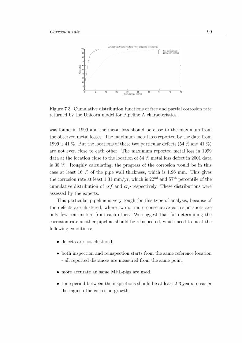
Corrosion rate 99
0 5 10 15 20 25 30 35 40 450
10
20
30
40
50
60
70
80
90
100
Corrosion rate [mm/yr]
Per
cent
iles
Cumulative distribution functions of free and partial corrosion rate
free corrosion ratepartial corrosion rate
Figure 7.3: Cumulative distribution functions of free and partial corrosion ratereturned by the Unicorn model for Pipeline A characteristics.
was found in 1999 and the metal loss should be close to the maximum from
the observed metal losses. The maximum metal loss reported by the data from
1999 is 41 %. But the locations of these two particular defects (54 % and 41 %)
are not even close to each other. The maximum reported metal loss in 1999
data at the location close to the location of 54 % metal loss defect in 2001 data
is 38 %. Roughly calculating, the progress of the corrosion would be in this
case at least 16 % of the pipe wall thickness, which is 1.96 mm. This gives
the corrosion rate at least 1.31 mm/yr, which is 22nd and 57th percentile of the
cumulative distribution of crf and crp respectively. These distributions were
assessed by the experts.
This particular pipeline is very tough for this type of analysis, because of
the defects are clustered, where two or more consecutive corrosion spots are
only few centimeters from each other. We suggest that for determining the
corrosion rate another pipeline should be reinspected, which need to meet the
following conditions:
• defects are not clustered,
• both inspection and reinspection starts from the same reference location
- all reported distances are measured from the same point,
• more accurate an same MFL-pigs are used,
• time period between the inspections should be at least 2-3 years to easier
distinguish the corrosion growth

100 Chapter 7
• data includes characteristics of the soil at the defects’ locations (soil type,
pH, resistivity),
• data includes the information on state of the cathodic protection at the
defects’ locations,
• data includes defects with metal loss than 0%, in contrast to the currently
used 10% threshold.
The third and fourth conditions would be used to determine is we calculate crf
or crp and to see the impact of the environmental factors on the corrosion rate.
The last condition allows to use all information from the reinspection. Suppose
there are defects with 10 % metal loss collected during the reinspection, which
were not detected during the first inspection. Pipeline A data has this feature.
Since we don’t know what was the metal loss for these defects before the
reinspection, we cannot use them to find the distribution of the corrosion rate.
If we took only three first conditions into account we would recommend to
reinspect pipelines D and E, especially as there is a lot of defects reported by
the pipeline D and E data sets.

101
Chapter 8
Conclusions
Collecting corrosion data with MFL-pigs is still not a very reliable way of
inspecting gas pipelines. There is an intensive development of these devices,
though. The data presented and analyzed in this thesis confirm this remark.
First of all, measuring the metal loss due to external corrosion is rather in-
accurate and the deviation from the real value of removed wall thickness can
be even more than 15 %. Currently, only excavation of the inspected pipeline
allows to evaluate the quality of the measurements. Some intelligent pigs may
overestimate or underestimate the metal loss. Therefore, if a pipeline is rein-
spected, it is very important to do this with the same device. Otherwise the
results will be very hard to compare and analyze. For instance, metal loss
reported during the reinspection might be less than the one collected during
the previous inspection. This is the case with Pipeline A, which was inspected
twice in a period of 18 months, but with two different MFL-pigs. As Gasunie
stated recently, the defects with the largest metal losses found during the first
inspection of Pipeline A in 1999 were repaired. Another important issue re-
lated to the MFL-pigs based inspection is accuracy of positioning of the defects.
The positions we can find in the presented data are returned directly by the
intelligent pig. However, before this information is used, Gasunie processes
the data comparing it with the information they have on construction of the
pipeline’s sections. As a result, they obtain a very accurate positioning of the
defects and usually, if an excavation is made for repairing a defect, they don’t
miss the point they are looking for. Currently, one of the pipelines owned by
Gasunie is being inspected 3 times, each inspection with a different intelligent

102 Chapter 8
Figure 8.1: Cobweb plot of corlk, crf and crp.
pig. The resulting data will be very interesting obviously, since it will allow to
compare the performance of the used pigs and obtain more reliable corrosion
data. If, in addition, Gasunie will perform a number of excavations at some
randomly chosen locations of the discovered corrosion spots in order to confirm
the information provided by the pigs with the reality, then we could obtain a
very nice study of the currently used inspection technology.
One possible extension of the technology applied nowadays is improving the
MFL-pig by lowering the detection threshold. The data we have is reporting
only the defects with metal loss more than 10 %. The exception is Pipeline E
data, where the smallest metal loss defects have 5 % of removed wall thickness.
However, if one look at the histogram of the data from this pipeline (Figure 6.7),
he/she will immediately notice, that the number of the defects with metal loss
between 5 % and 10 % is not realistic. As the metal loss approaches 0 %,
the number of defects with the corresponding metal loss should converge to
infinity. This is not the case here. The most likely, the data has been filtered
out. To assess the number of defects with metal loss less than 10 % we can try
to fit a parametric model to the corrosion data and extrapolate the information
that we have on the metal losses. Under the assumption, that the data is right
censored, we can find the overall distribution of the percentage of metal loss.
Pipeline D data could be particularly helpful for this task, because this data
set gives information on a large number of defects. Hence, the uncertainty
associated with the number of defects with a given percentage of metal loss

Conclusions 103
Figure 8.2: Cobweb plot of corlk, crf and crp conditionalized on 30th percentileof corlk.
should be the smallest among the data sets we present in this thesis. This is
reflected by the histogram of this data in Figure 6.7, which depicts the most
regular shape. Similarly, Pipeline E data could be used as well, but after
removing the defects with metal loss less than 10 %.
Determination of the corrosion rate is a particularly tough task. Since we
don’t know the year in which a given corrosion spot has started to grow, the
information on the percentage of metal loss gives no indication of the corrosion
rate. We see that one inspection of a pipeline does not give sufficient grounds
for calculation of the corrosion rate.
As it has been stated in the previous chapter, if one wants to determine the
corrosion rate from the data given a twice inspected pipeline (like Pipeline A)
few conditions must be met in order to have a reliable information on metal loss
due to corrosion. First of all, the period of time between the inspections must
be long enough such that the effect of growing corrosion is easier to detect.
Moreover, the intelligent pigs used during the inspections should be accurate
and, preferably, the same. A different approach to this problem involves using
the UNICORN model and samples exploring tool, UNIGRAPH. Suppose, we
observe a frequency of exceeding 10 % of the metal loss as equal to 0.03 per
km.yr (Pipeline A data). Now we set the UNICORN model’s parameters, such
that the model returns the distribution of the exceeding 10 % of metal loss
due to corrosion, like it has been described in Section 6.3 where we produced
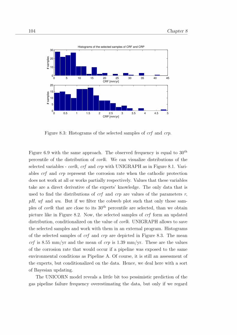
104 Chapter 8
0 5 10 15 20 25 30 35 40 450
10
20
30
CRF [mm/yr]
# sa
mpl
esHistograms of the selected samples of CRF and CRP
0 0.5 1 1.5 2 2.5 3 3.5 4 4.5 50
5
10
15
20
CRP [mm/yr]
# sa
mpl
es
Figure 8.3: Histograms of the selected samples of crf and crp.
Figure 6.9 with the same approach. The observed frequency is equal to 30th
percentile of the distribution of corlk. We can visualize distributions of the
selected variables - corlk, crf and crp with UNIGRAPH as in Figure 8.1. Vari-
ables crf and crp represent the corrosion rate when the cathodic protection
does not work at all or works partially respectively. Values that these variables
take are a direct derivative of the experts’ knowledge. The only data that is
used to find the distributions of crf and crp are values of the parameters r,
pH, wf and wu. But if we filter the cobweb plot such that only those sam-
ples of corlk that are close to its 30th percentile are selected, than we obtain
picture like in Figure 8.2. Now, the selected samples of crf form an updated
distribution, conditionalized on the value of corlk. UNIGRAPH allows to save
the selected samples and work with them in an external program. Histograms
of the selected samples of crf and crp are depicted in Figure 8.3. The mean
crf is 8.55 mm/yr and the mean of crp is 1.39 mm/yr. These are the values
of the corrosion rate that would occur if a pipeline was exposed to the same
environmental conditions as Pipeline A. Of course, it is still an assessment of
the experts, but conditionalized on the data. Hence, we deal here with a sort
of Bayesian updating.
The UNICORN model reveals a little bit too pessimistic prediction of the
gas pipeline failure frequency overestimating the data, but only if we regard
Conclusions 105
pipelines laid in sand. The situations changes completely in case of the data
collected from the pipelines laid in clay. Then the model is too conservative
and heavily underestimates the frequencies. Certainly, there are many factors
influencing the failure frequencies not covered by the model, that could be
incorporated into the model. Under some circumstances, biological organism
(microbes) may influence corrosion. This influence often results in extremely
accelerated rate of corrosion, but this cause of corrosion is not taken into
account by the model. Peat is particularly susceptible to microbal corrosion.
This soil type very often is mixed with clay. The microbal corrosion occurs
mostly at the bottom of pipeline. From the existing model’s parameters the
critical wall thickness is relatively easy to update. The default values which
are now in use might need a small adjustment based on the analysis of the
experiments that many laboratories have performed. These values will change
depending, for instance, on diameter of a pipeline or type of damage to pipe
initiating corrosion.
The technology used in the gas industry is getting more and more sophis-
ticated, and this is also applicable to the inspection devices such as MFL-pigs.
However, data collected during inspections of gas pipelines still must be treated
with caution since the measurement may vary from the true values. Using com-
puter programs for predicting the failure frequency in combination with data
will result in larger reliability of future pipelines, since this will allow to deter-
mine the factors that are the most dangerous for safe transport of liquid natural
gas. UNICORN and the model introduced in this thesis are examples of a sta-
tistical tool and its application. Combination of those two with UNIGRAPH
gives a system which helps to explore the statistical aspects of maintaining
gas pipelines, which cannot be neglected as the information provided by un-
certainty and sensitivity analysis may allow to find factors minimizing risk of
failure.

106 Chapter 8

107
Bibliography
Basalo, C. (1992), ‘Water and gas mains corrosion, degradation and protection’.
Ellis Horwood, New York.
Camitz, G. & Vinka, T. (1989), ‘Corrosion of steel and metal-coated steel in
swedish soils - effects of soil parameters’. Effects of Soil Characteristics
on Corrosion ASTM STP 1013.
Chaker, V. & (eds), J. P. (1989), ‘Effects of soil characteristics on corrosion’.
ASTM STP 1013.
Cooke, R. (1991), ‘Experts in uncertainty’. Oxford University Press, Oxford,
UK.
Cooke, R., Dorrepaal, J. & Bedford, T. (1995), ‘Review of ski data processing
methodology, ski report 95:2’.
CPR (1999), Guidelines for quantitative risk assessment (CPR 18E), Guide-
line, Committee for the Prevention of Disasters, The Hague, The Nether-
lands.
Gas Safety (Safety Case) Regulations (1999). S.R. No. 5/1999, Victoria State,
Australia.
Geervliet, S. (1994), ‘Modellering van de faalkans van ondergronds transportlei-
dingen’. Report for Two Year Post Graduate Program, Department of
Mathematics and Informatics, performed under contract with the Nether-
lands Gasunie, Delft University of Technology, Delft.
Health and Safety: The Gas Safety (Installation and Use) Regulations (1998).
Statutory Instrument 1994 No. 1886, UK.
108 Bibliography
Hofer, E. & Peschke, J. (1999), ‘Bayesian modeling of failure rates and initiat-
ing event frequencies’, Safety and Reliability pp. 887–887.
Homma, T. I. T. (1990), ‘An importance quantification technique in uncer-
tainty analysis for computer models’, Proceedings of the ISUMA ’90 First
International Symposium on Uncertianty Modelling and Analysis pp. 398–
403.
Hopkins, P., Corder, I. & Corbin, P. (1992), ‘The resistance of gas transmission
pipelines to mechanical damage’. European Pipeline Research Group.
Hora, S. & Iman, R. (1990), ‘Bayesian modelling of initiating event frequencies
at nuclear power plants’, Risk Analysis 10(1), 102–109.
Kiefner, J., Vieth, P. & Feder, P. (1990), ‘Methods for prioritizing pipeline
maintenance and rehabilitation’. American Gas Association, Washington.
Lewandowski, D. & Cooke, R. (2001), ‘Bayesian sensitivity analysis’, System
and bayesian reliability - Essays in honor of professor Richard E. Barlow
on his 70th birthday 19, 315–331.
Lewandowski, D., Cooke, R. & Jager, E. (2002), ‘The failure frequency of un-
derground gas pipelines: A model based on field data and expert judge-
ment’. to be published in Case Studies in Reliability and Maintenance by
W.R. Blischke and D.N.P. Murthy (eds).
Lukezich, S., Hancock, J. & Yen, B. (1992), ‘State-of-the-art for the use of
anti-corrosion coatings on buried pipelines in the natural gas industry’.
topical report 06-3699, Gas Research Institute.
Meyer, W. & Hennings, W. (1999), ‘Prior distributions in two-stage bayesian
estimation of failure rates’, Safety and Reliability pp. 893–899.
Porn, K. (1990), ‘On empirical bayesian inference applied to poisson probability
models’, Linkoping Studies in Science and Technology (Dissertation No.
234).
Wegman, E. (1990), ‘Hyperdimensional data analysis using parallel coordi-
nates’, Journal of the American Statistical Analysis 90(411).

Bibliography 109
Whittle, P. (1992), ‘Probability via expectation’, Springer Verlag .

110 Bibliography
111
Appendix A
Help file for GasUnicorn
GasUnicorn
Authors: Valery Kritchallo - core, Daniel Lewandowski - interface
Overview
The full model consists of 3 submodels:
• 3rd Party - HITPIP
• Environment
– ENVSAND - for sand
– ENVCLAY - for clay
– ENVPEAT - for peat
• Corrosion
– CORRSAND - for sand
– CORRCLAY - for clay
– CORRPEAT - for peat
Environment and Corrosion use different experts’ distributions for different
soil type. Corrosion submodel uses outputs of 3rd Party and Environment
models as input variables (see figure A.1). It is advisable to run the whole
model in one of the following orders:
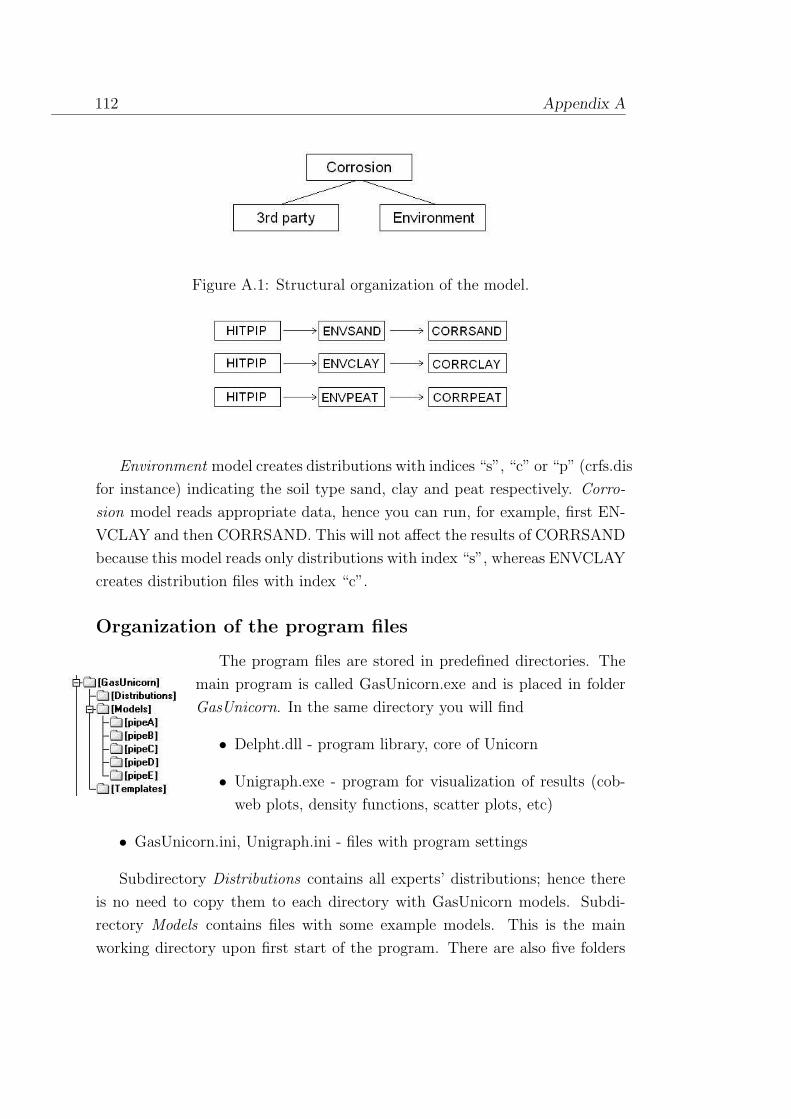
112 Appendix A
Figure A.1: Structural organization of the model.
Environment model creates distributions with indices “s”, “c” or “p” (crfs.dis
for instance) indicating the soil type sand, clay and peat respectively. Corro-
sion model reads appropriate data, hence you can run, for example, first EN-
VCLAY and then CORRSAND. This will not affect the results of CORRSAND
because this model reads only distributions with index “s”, whereas ENVCLAY
creates distribution files with index “c”.
Organization of the program files
The program files are stored in predefined directories. The
main program is called GasUnicorn.exe and is placed in folder
GasUnicorn. In the same directory you will find
• Delpht.dll - program library, core of Unicorn
• Unigraph.exe - program for visualization of results (cob-
web plots, density functions, scatter plots, etc)
• GasUnicorn.ini, Unigraph.ini - files with program settings
Subdirectory Distributions contains all experts’ distributions; hence there
is no need to copy them to each directory with GasUnicorn models. Subdi-
rectory Models contains files with some example models. This is the main
working directory upon first start of the program. There are also five folders

Help file for GasUnicorn 113
PipeA,. . . ,PipeE containing models with parameters corresponding to charac-
teristics of the inspected pipelines. Running a submodel will result in creating
a distribution files (extension .dis) of output variables which will be used in
the next submodel. Only those distribution files that are required at the next
stage of the simulation process are produced. Files Cdc.dis, Cdo.dis, Dlc.dis,
Dlo.dis, Ldlc.dis, Ldlo.dis, Ldsc.dis, Ldso.dis must be copied to all directories
with files containing parameters for 3rd Party (HITPIP) submodel. Folder
Templates stores ExcelTemplate.xlt - template file used during exporting the
report to Excel, and files with default values of parameters for all submodels.
The working directory can be changed. It is strongly recommended to
work only with files from directories added from within the program. This will
assure removing by the program all of the intermediate files produced during
the simulation.
Running the model
After the application has been started, you can load a file with models’
parameters. The file can be load either by clicking one of the buttons in
Assign files to submodels frame or appropriate menu entry.
Content of the file is displayed in 3rd Party
tab. Parameters can be changed. Click Val-
idate parameters to perform simple validation
of the parameters (not required). This action
checks whether the filled numbers and experts’
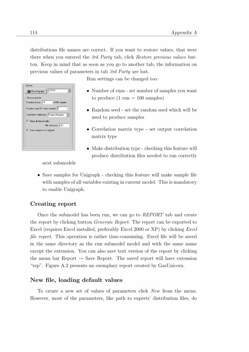
114 Appendix A
distributions file names are correct. If you want to restore values, that were
there when you entered the 3rd Party tab, click Restore previous values but-
ton. Keep in mind that as soon as you go to another tab, the information on
previous values of parameters in tab 3rd Party are lost.
Run settings can be changed too:
• Number of runs - set number of samples you want
to produce (1 run = 100 samples)
• Random seed - set the random seed which will be
used to produce samples
• Correlation matrix type - set output correlation
matrix type
• Make distribution type - checking this feature will
produce distribution files needed to run correctly
next submodels
• Save samples for Unigraph - checking this feature will make sample file
with samples of all variables existing in current model. This is mandatory
to enable Unigraph.
Creating report
Once the submodel has been run, we can go to REPORT tab and create
the report by clicking button Generate Report. The report can be exported to
Excel (requires Excel installed, preferably Excel 2000 or XP) by clicking Excel
file report. This operation is rather time-consuming. Excel file will be saved
in the same directory as the run submodel model and with the same name
except the extension. You can also save text version of the report by clicking
the menu bar Report → Save Report. The saved report will have extension
“rep”. Figure A.2 presents an exemplary report created by GasUnicorn.
New file, loading default values
To create a new set of values of parameters click New from the menu.
However, most of the parameters, like path to experts’ distribution files, do

Help file for GasUnicorn 115
Figure A.2: Report generated by GasUnicorn.
not have to be changed. Hence it may be useful to load default values of the
parameters and adjust only the most important ones. For each submodel there
exists a file with default values for parameters. The names are:
• NF3RD.unc
• NFENVSAND.unc
• NFENVCLAY.unc
• NFENVPEAT.unc
• NFCORRSAND.unc
• NFCORRCLAY.unc
• NFCORRPEAT.unc

116 Appendix A
You can load these files, change values of the parameters and save. To load
default values click Load default values from the menu.
The same approach holds for the rest of the submodels.
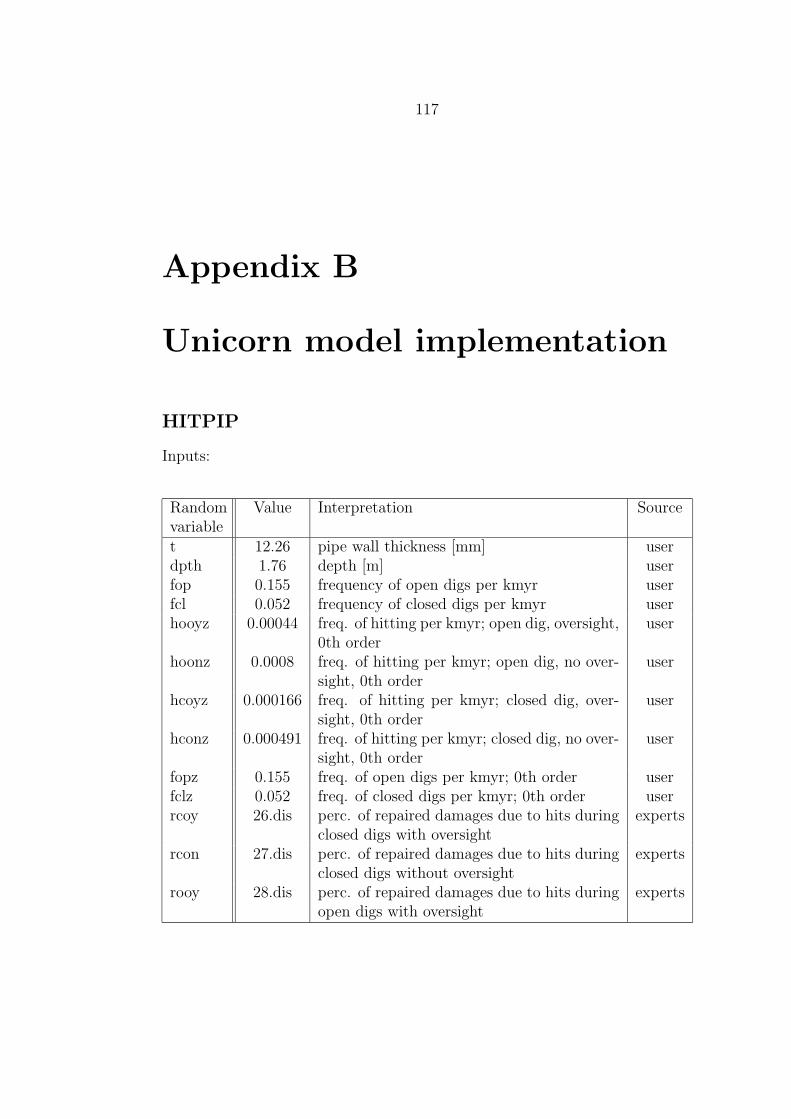
117
Appendix B
Unicorn model implementation
HITPIP
Inputs:
Randomvariable
Value Interpretation Source
t 12.26 pipe wall thickness [mm] userdpth 1.76 depth [m] userfop 0.155 frequency of open digs per kmyr userfcl 0.052 frequency of closed digs per kmyr userhooyz 0.00044 freq. of hitting per kmyr; open dig, oversight,
0th orderuser
hoonz 0.0008 freq. of hitting per kmyr; open dig, no over-sight, 0th order
user
hcoyz 0.000166 freq. of hitting per kmyr; closed dig, over-sight, 0th order
user
hconz 0.000491 freq. of hitting per kmyr; closed dig, no over-sight, 0th order
user
fopz 0.155 freq. of open digs per kmyr; 0th order userfclz 0.052 freq. of closed digs per kmyr; 0th order userrcoy 26.dis perc. of repaired damages due to hits during
closed digs with oversightexperts
rcon 27.dis perc. of repaired damages due to hits duringclosed digs without oversight
experts
rooy 28.dis perc. of repaired damages due to hits duringopen digs with oversight
experts

118 Appendix B
Randomvariable
Value Interpretation Source
roon 29.dis perc. of repaired damages due to hits duringopen digs without oversight
experts
rup71 24.dis perc. of direct leak which will be ruptures perkmyr; 7.1 mm wt
experts
rup54 23.dis perc. of direct leak which will be ruptures perkmyr; 5.4 mm wt
experts
hooye 01.dis freq. of hitting per kmyr; open dig, oversight expertshoone 02.dis freq. of hitting per kmyr; open dig, no oversight expertshcoye 03.dis freq. of hitting per kmyr; closed dig, oversight expertshcone 04.dis freq. of hitting per kmyr; closed dig, no over-
sightexperts
Outputs:
Formulaname
Formula
thick tdf exp(5.43-7.31*dpth+1.88*dpthˆ2)ufo fop*((1-rooy)*(hooyz+(fop-fopz)*(hooye/11000-hooyz)/fopz)+
(1-roon)*(hoonz+(fop-fopz)*(hoone/11000-hoonz)/fopz))ufc fcl*((1-rcoy)*(hcoyz+(fcl-fclz)*(hcoye/11000-hcoyz)/fclz)+
(1-rcon)*(hconz+(fcl-fclz)*(hcone/11000-hconz)/fclz))cd3rn df*(ufo*cdo(t)+ufc*cdc(t))ldsrn df*(ufo*ldso(t)+ufc*ldsc(t))ldlrn df*(ufo*ldlo(t)+ufc*ldlc(t))dl (dlo(t)*(hooyz+(fop-fopz)*(hooye/11000-hooyz)/fopz+hoonz+
(fop-fopz)*(hoone/11000-hoonz)/fopz)+dlc(t)*(hcoyz+(fcl-fclz)*(hcoye/11000-hcoyz)/fclz+hconz+(fcl-fclz)*(hcone/11000-hconz)/fclz))*df
rup dl*(rup71+(rup71-rup54)*(t-7.1)/1.7)*i10.00000000001,dl*(rup71+(rup71-rup54)*(t-7.1)/1.7),1

Unicorn model implementation 119
ENVSAND
Inputs:
Randomvariable
Value Interpretation Source
%bit 1 %km with bitumen coating userdia 36 diameter userwf 0 %km with fluctuation under and above water
tableuser
rt 0 %km with heavy roots growth userch 0 %km with heavy industrial contamination userph 5.7 pH value userwu 0.95 % km under water table usercrfz 0.13 default free corrosion rate userr 10000 resistivity usergrb 255 rate of occurrence of bitumen defects (per 100
km)user
grp 33 rate occurrence of polyethylene defects (per 100km)
user
%ebe 33.dis % of coating damages due to ground movement,root growth or chemical contamination; bitu-men
experts
%epe 34.dis % of coating damages due to ground move-ment, root growth or chemical contamination;polyethylene
experts
xbde 37.dis #defects per 100 km if diameter = 36”; bitumen expertsxbwfe 39.dis #defects per 100 km if water table fluctuates;
bitumenexperts
xbrte 41.dis #defects per 100 km if heavy root growth; bi-tumen
experts
xbche 43.dis #defects per 100 km if chemical contamination;bitumen
experts
xpde 38.dis #defects per 100 km if diameter = 36”;polyethylene
experts
xpwfe 40.dis #defects per 100 km if water table fluctuates;polyethylene
experts
xprte 42.dis #defects per 100 km if heavy root growth;polyethylene
experts
xpche 44.dis #defects per 100 km if chemical contamination;polyethylene
experts

120 Appendix B
Randomvariable
Value Interpretation Source
xre 51.dis pit corrosion rate if resistivity is a factor 10lower
experts
xphe 69.dis pit corrosion rate if pH is raised by 2.3 expertsxwfe 63.dis pit corrosion rate if water table fluctuates expertsxwue 57.dis pit corrosion rate if water table is above pipe
linesexperts
crpe 0.0256 pit corrosion rate if the pipe ground potentialis -700 mV
experts
Outputs:
Formulaname
Formula
crp crf*crpe/crfzxbd (xbde-grb)/(2400*(1994-1968))xbwf (xbwfe-grb)/(100*(1994-1968))xbrt (xbrte-grb)/(100*(1994-1968))xbch (xbche-grb)/(100*(1994-1968))xpd (xpde-grb)/(2400*(1994-1973))xpwf (xpwfe-grb)/(100*(1994-1973))xprt (xprte-grb)/(100*(1994-1973))xpch (xpche-grb)/(100*(1994-1973))xr (crfz-xr)/18000xph (xphe-crfz)/2.3xwu (xwue-crfz)udfb grb/(100*(1994-1968))+xbd*(dia-12)+xbwf*wf+xbrt*rt+xbch*chudfp grp/(100*(1994-1973))+xpd*(dia-12)+xpwf*wf+xprt*rt+xpch*chfcde %bit*udfb+(1-%bit)*udfppcde 1-exp(-fcde)xwf xwfe-crfzcrf crfz+xr*(r-200000)+xph*(pH-5,7)+xwf*wf+xwu*wucondition i10,00001,crf,>>

Unicorn model implementation 121
CORRSAND
Inputs:
Randomvariable
Value Interpretation Source
b 1967 birthyear useryb 1998 begin year for cumulative frequency of cor-
rosionuser
ye 1999 end year for cumulative frequency of cor-rosion
user
cps 1970 year of cathodic protection (CP) install-ment
user
ts 0.5 material removed by small line damage[mm]
user
tl 2 material removed by large line damage[mm]
user
t thick.dis pipe wall thickness [mm] userxc 0.9 critical thickness fraction; coating damage userxs 0.7 critical thickness fraction; small damage userxl 0.6 critical thickness fraction; large damage usercrse 87.dis corrosion rate if there are unprotected
stray currentsexperts
bs 0.8 %1km pipe near bond site userpspe 0.93 prob. that stray current protection fails
at bond siteexperts
pcpfe 91.dis prob. that CP fails completely expertspcppe 96.dis prob. that CP fails partially expertspc3 cd3rn.dis prob. of coating damage from 3rd parties cd3rn.disps ldsrn.dis prob. of small pipe damage ldsrn.displ ldlrn.dis prob. of large pipe damage ldlrn.disdl dl.dis prob. of direct leak from 3rd parties dl.discrf crf s.dis free corrosion rate crf.dispcen pcde s.dis prob. of coating damage from environ-
mentpcde.dis
crp crp s.dis corrosion rate when CP partially func-tional
crp.dis

122 Appendix B
Outputs:
Formulaname
Formula
leak 3leak+corlk-3leak*corlkpsp pspe/600pcpf pcpfe/150000pcpp pcppe/150000pc minpc3+pcen,.999j varyyb+1,ye+0.5,1elcf xc*t/crfleak 3leak+corlk-3leak*corlkelsf xs*(t-ts)/crfellf xl*(t-tl)/crfelcp i11970,j-xc*t/crp,>>*xc*t/crp+(1-i11970,j-
xc*t/crp,>>)*(xc*t-(j-1970)*crp)/crf+j-1970elsp i11970,j-xs*(t-ts)/crp,>>*xs*(t-ts)/crp+(1-i11970,j-xs*(t-
ts)/crp,>>)*(xs*(t-ts)-(j-1970)*crp)/crf+j-1970ellp i11970,j-xl*(t-tl)/crp,>>*xl*(t-tl)/crp+(1-i11970,j-xl*(t-
tl)/crp,>>)*(xl*(t-tl)-(j-1970)*crp)/crf+j-1970elcs i11970,j-xc*t*24/crse,>>*xc*t*24/crse+(1-i11970,,j-
xc*t*24/crse,>>)*(xc*t-(j-1970)*crse/24)/crse+ j-1970elss i11970,j-xs*(t-ts)*24/crse,>>*xs*(t-ts)*24/crse+(1-i11970,,j-
xs*(t-ts)*24/crse,>>)*(xs*(t-ts)-(j-1970)*crse/24)/crse+j-1970ells i11970,j-xl*(t-tl)*24/crse,>>*xs*(t-tl)*24/crse+(1-i11970,,j-
xl*(t-tl)*24/crse,>>)*(xl*(t-tl)-(j-1970)*crse/24)/crse+j-1970qcf minmaxj-elcf-b, .00009, y-ybqsf minmaxj-elsf-b, .00009, y-ybqlf minmaxj-ellf-b, .00009, y-ybqcp minmaxj-elcp-b, .00009, y-ybqsp minmaxj-elsp-b, .00009, y-ybqlp minmaxj-ellp-b, .00009, y-ybqcs minmaxj-elcs-b, .00009, y-ybqss minmaxj-elss-b, .00009, y-ybqls minmaxj-ells-b, .00009, y-ybpcrf sum((1-pcˆ2)ˆmaxqcf-1,0*(1-ps)ˆqsf*(1-
pl)ˆqlf*i11,qcf,>>*(1-(1-pcpf)ˆ(-ln(1-pc)))+((1-pc)ˆqcf*(1-ps)ˆmaxqsf-1,0*(1-pl)ˆqlf*ps*i11,qsf,>>+(1-pc)ˆqcf*(1-ps)ˆqsf*(1-pl)ˆmaxqlf-1,0*pl*i11,qlf,>>)*pcpf)

Unicorn model implementation 123
Formulaname
Formula
pcrp sum((1-pcˆ2)ˆmaxqcp-1,0*(1-ps)ˆqsp*(1-pl)ˆqlp*i11,qcp,>>*(1-(1-pcpp)ˆ(-ln(1-pc)))+((1-pc)ˆqcp*(1-ps)ˆmaxqsp-1,0*(1-pl)ˆqlp*ps*i11,qsp,>>+(1-pc)ˆqcp*(1-ps)ˆqsp*(1-pl)ˆmaxqlp-1,0*pl*i11,qlp,>>)*pcpp)
pcrs sum((1-pcˆ2)ˆmaxqcs-1,0*(1-ps)ˆqss*(1-pl)ˆqls*i11,qcp,>>*(1-(1-bs)ˆ(-ln(1-pc)))+((1-pc)ˆqcs*(1-ps)ˆmaxqss-1,0*(1-pl)ˆqls*ps*i11,qss,>>+(1-pc)ˆqcs*(1-ps)ˆqss*(1-pl)ˆmaxqls-1,0*pl*i11,qls,>>)*psp)
3leak sum((1-dl)ˆ(j-yb-1)*dl)corlk pcrf+pcrp+pcrs-pcrf*pcrp-pcrf*pcrs*pcrp*pcrs+pcrf*pcrp*pcrp
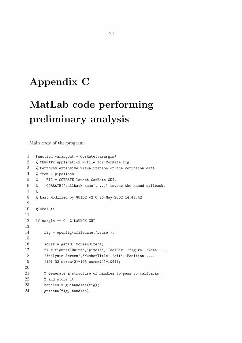
124
Appendix C
MatLab code performing
preliminary analysis
Main code of the program.
1 function varargout = CorRate(varargin)
2 % CORRATE Application M-file for CorRate.fig
3 % Performs extensive visualization of the corrosion data
4 % from 4 pipelines.
5 % FIG = CORRATE launch CorRate GUI.
6 % CORRATE(’callback_name’, ...) invoke the named callback.
7 %
8 % Last Modified by GUIDE v2.0 26-May-2002 14:42:42
9
10 global fi
11
12 if nargin == 0 % LAUNCH GUI
13
14 fig = openfig(mfilename,’reuse’);
15
16 scrsz = get(0,’ScreenSize’);
17 fi = figure(’Units’,’pixels’,’ToolBar’,’figure’,’Name’,...
18 ’Analysis Screen’,’NumberTitle’,’off’,’Position’,...
19 [191 32 scrsz(3)-193 scrsz(4)-104]);
20
21 % Generate a structure of handles to pass to callbacks,
22 % and store it.
23 handles = guihandles(fig);
24 guidata(fig, handles);

MatLab code performing preliminary analysis 125
25
26 pop = 0;
27
28 if nargout > 0
29 varargout1 = fig;
30 end
31
32 elseif ischar(varargin1) % INVOKE NAMED SUBFUNCTION OR CALLBACK
33
34 try
35 [varargout1:nargout] = feval(varargin:); % FEVAL switchyard
36 catch
37 disp(lasterr);
38 end
39
40 end
Total number of corrosions vs distance from the starting point.
41 % -----------------------------------------------------------------
42 function varargout = pushbutton1_Callback(h, eventdata, handles,...
43 varargin)
44 % Stub for Callback of the uicontrol handles.pushbutton1.
45 global fi
46
47 subplot(1,1,1);
48 [p1, p2, name1, name2] = determine_data(handles);
49 set(fi,’Name’,’TOTAL NUMBER OF OBSERVED CORROSIONS’);
50 if ~isempty(name1)
51 stairs(p1.stationary, [1:length(p1.stationary)]);
52 text(max(p1.stationary)*.95,length(p1.stationary)+1.5,name1);
53 hold on;
54 end
55 if ~isempty(name2)
56 stairs(p2.stationary, [1:length(p2.stationary)],’r’);
57 text(max(p2.stationary)*.95,length(p2.stationary)+1.5,name2);
58 end
59
60 hold off;
61 title(’Total number of corrosions vs distance from the starting point’);
62 xlabel(’Distance [m]’);
63 ylabel(’Total number of corrosions’);
64

126 Appendix C
65 if isequal(name1,’pipeA’) & isequal(name2,’pipeA1’)
66 legend(’October 1999’,’August 2001’,4);
67 set(handles.text1,’Visible’,’on’,’String’,...
68 [’ OBSERVATIONS:’;’Length of the pipeline - 66 km’;...
69 ’October 1999 - 65 events’;’August 2001 - 74 events’;]);
70 end
Quantile-quantile plot of both corrosion data sets.
71 % -----------------------------------------------------------------
72 function varargout = pushbutton2_Callback(h, eventdata, handles,...
73 varargin)
74 % Stub for Callback of the uicontrol handles.pushbutton2.
75 global fi
76
77 subplot(1,1,1);
78 [p1, p2, name1, name2] = determine_data(handles);
79 set(fi,’Name’,’QUANTILE-QUANTILE PLOT OF BOTH DATA SETS’);
80 subplot(1,1,1);
81 qqplot(p1.ml,p2.ml);
82 title(’Quantile-quantile plot of both corrosion data sets’);
83 xlabel([name1,’ data quantiles’]);
84 ylabel([name2,’ data quantiles’]);
Empirical distribution functions.
85 % -----------------------------------------------------------------
86 function varargout = pushbutton3_Callback(h, eventdata, handles,...
87 varargin)
88 % Stub for Callback of the uicontrol handles.pushbutton3.
89 global fi
90
91 [p1, p2, name1, name2] = determine_data(handles);
92 set(fi,’Name’,’EMPIRICAL CDF’);
93 subplot(1,1,1);
94 if ~isempty(name1)
95 cdfplot(p1.ml);
96 hold on;
97 end
98 if ~isempty(name2)
99 hand = cdfplot(p2.ml);
100 set(hand,’Color’,’r’);
101 end
102 hold off;
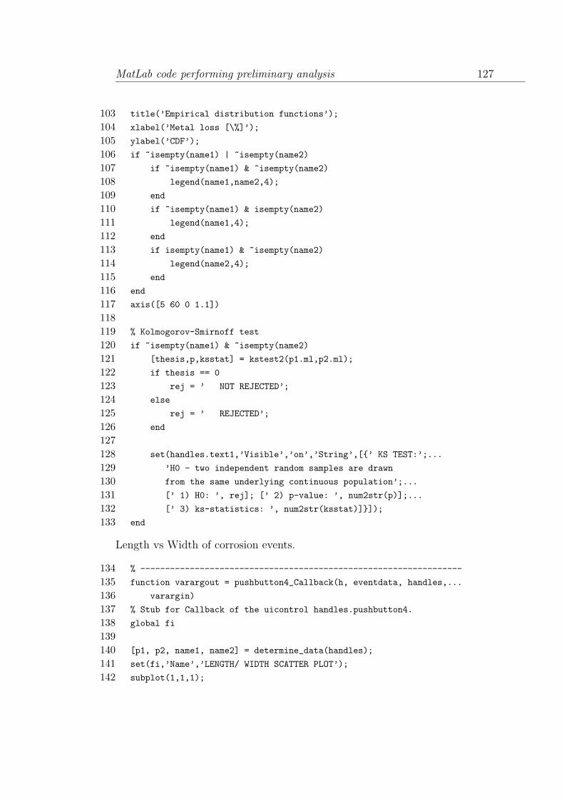
MatLab code performing preliminary analysis 127
103 title(’Empirical distribution functions’);
104 xlabel(’Metal loss [\%]’);
105 ylabel(’CDF’);
106 if ~isempty(name1) | ~isempty(name2)
107 if ~isempty(name1) & ~isempty(name2)
108 legend(name1,name2,4);
109 end
110 if ~isempty(name1) & isempty(name2)
111 legend(name1,4);
112 end
113 if isempty(name1) & ~isempty(name2)
114 legend(name2,4);
115 end
116 end
117 axis([5 60 0 1.1])
118
119 % Kolmogorov-Smirnoff test
120 if ~isempty(name1) & ~isempty(name2)
121 [thesis,p,ksstat] = kstest2(p1.ml,p2.ml);
122 if thesis == 0
123 rej = ’ NOT REJECTED’;
124 else
125 rej = ’ REJECTED’;
126 end
127
128 set(handles.text1,’Visible’,’on’,’String’,[’ KS TEST:’;...
129 ’H0 - two independent random samples are drawn
130 from the same underlying continuous population’;...
131 [’ 1) H0: ’, rej]; [’ 2) p-value: ’, num2str(p)];...
132 [’ 3) ks-statistics: ’, num2str(ksstat)]]);
133 end
Length vs Width of corrosion events.
134 % -----------------------------------------------------------------
135 function varargout = pushbutton4_Callback(h, eventdata, handles,...
136 varargin)
137 % Stub for Callback of the uicontrol handles.pushbutton4.
138 global fi
139
140 [p1, p2, name1, name2] = determine_data(handles);
141 set(fi,’Name’,’LENGTH/ WIDTH SCATTER PLOT’);
142 subplot(1,1,1);
128 Appendix C
143 if ~isempty(name1)
144 loglog(p1.length,p1.width,’o’,’MarkerEdgeColor’,’b’,...
145 ’MarkerFaceColor’,’b’,’MarkerSize’,5)
146 hold on;
147 end
148 if ~isempty(name2)
149 loglog(p2.length,p2.width,’o’,’MarkerEdgeColor’,’m’,...
150 ’MarkerFaceColor’,’m’,’MarkerSize’,5)
151 end
152 hold off;
153 title(’Length vs Width of corrosion events’);
154 xlabel(’Length [mm]’);
155 ylabel(’Width [mm]’);
156 if ~isempty(name1) | ~isempty(name2)
157 if ~isempty(name1) & ~isempty(name2)
158 legend(name1,name2,4);
159 end
160 if ~isempty(name1) & isempty(name2)
161 legend(name1,4);
162 end
163 if isempty(name1) & ~isempty(name2)
164 legend(name2,4);
165 end
166 end
Distance at which corrosion was observed.
167 % -----------------------------------------------------------------
168 function varargout = pushbutton5_Callback(h, eventdata, handles,...
169 varargin)
170 % Stub for Callback of the uicontrol handles.pushbutton5.
171 global fi
172
173 load pipeA;
174 load pipeA1;
175 subplot(1,1,1);
176 set(fi,’Name’,’DISTANCE’);
177 subplot(1,1,1);
178 plot(pipeA.stationary,ones(length(pipeA.stationary)),...
179 ’o’,’MarkerEdgeColor’,’b’,’MarkerFaceColor’,’b’,’MarkerSize’,5);
180 hold on;
181 plot(pipeA1.stationary,ones(length(pipeA1.stationary))*2,...
182 ’o’,’MarkerEdgeColor’,’b’,’MarkerFaceColor’,’b’,’MarkerSize’,5);

MatLab code performing preliminary analysis 129
183 hold off;
184 set(gca,’YLim’,[-1,4]);
185 set(gca,’YTick’,[1:2],’YTickLabel’,’1999’,’2001’);
186 set(gca,’XGrid’,’on’);
187
188 title(’Distance at which corrosion was observed’);
189 xlabel(’Distance [m]’);
190 ylabel(’Inspection year [calendar year]’);
Histogram of the corrosion data.
191 % -----------------------------------------------------------------
192 function varargout = pushbutton6_Callback(h, eventdata, handles,...
193 varargin)
194 % Stub for Callback of the uicontrol handles.pushbutton6.
195 global fi
196
197 [p1, p2, name1, name2] = determine_data(handles);
198 set(fi,’Name’,’HISTOGRAMS’);
199 if ~isempty(name1) | ~isempty(name2)
200 if ~isempty(name1) & ~isempty(name2)
201 subplot(2,1,1);
202 hist(p1.ml,15);
203 title([’Histogram of the ’, name1, ’ data’]);
204 xlabel(’Metal loss [%]’);
205 ylabel(’Number of corrosion events’);
206
207 subplot(2,1,2);
208 hist(p2.ml,15);
209 title([’Histogram of the ’, name2, ’ data’]);
210 xlabel(’Metal loss [%]’);
211 ylabel(’Number of corrosion events’);
212 else if ~isempty(name1)
213 subplot(1,1,1);
214 hist(p1.ml,15);
215 title([’Histogram of the ’, name1, ’ data’]);
216 xlabel(’Metal loss [%]’);
217 ylabel(’Number of corrosion events’);
218 else
219 subplot(1,1,1);
220 hist(p2.ml,15);
221 title([’Histogram of the ’, name2, ’ data’]);
222 xlabel(’Metal loss [%]’);
130 Appendix C
223 ylabel(’Number of corrosion events’);
224 end
225 end
226 end
Destroy figure and quit program.
227 % -----------------------------------------------------------------
228 function varargout = figure1_DeleteFcn(h, eventdata, handles,...
229 varargin)
230 % Stub for DeleteFcn of the figure handles.figure1.
231 global fi
232
233 delete(fi);
Minimum distance between corrosion events given by both data sets.
234 % -----------------------------------------------------------------
235 function varargout = popupmenu1_Callback(h, eventdata, handles,...
236 varargin)
237 % Stub for Callback of the uicontrol handles.popupmenu1.
238 global fi
239
240 load pipeA;
241 load pipeA1;
242 set(fi,’Name’,’1:1 PROJECTION’);
243 subplot(1,1,1);
244
245 g = zeros(length(pipeA.stationary));
246
247 for i=1:length(pipeA.stationary)
248 g(i) = min(abs(pipeA1.stationary-pipeA.stationary(i)));
249 end
250
251 for i=1:length(pipeA.stationary)
252 d(i).ind = find(pipeA1.stationary-pipeA.stationary(i)==g(i));
253 end
254
255 switch get(handles.popupmenu1,’Value’)
256 case 2
257 stem(pipeA.stationary,g);
258 xlabel(’Distance [m]’);
259 case 3
260 stem(g);

MatLab code performing preliminary analysis 131
261 xlabel(’Index of the corrosion event in the pipeA data’);
262 end
263 hold off;
264 title(’Minimum distance between corrosion events...
265 given by both data sets’);
266 ylabel(’Minimum distance [m]’);
Positions of the corrosion spots on the surface of pipelines.
267 % -----------------------------------------------------------------
268 function varargout = popupmenu2_Callback(h, eventdata, handles,...
269 varargin)
270 % Stub for Callback of the uicontrol handles.popupmenu2.
271 global fi
272
273 set(fi,’Name’,’POSITIONS’);
274 switch get(handles.popupmenu2,’Value’)
275 case 2
276 load pipeA;
277 MyData = pipeA;
278 case 3
279 load pipeA1;
280 MyData = pipeA1;
281 case 4
282 load pipeB;
283 MyData = pipeB;
284 clear pipeB;
285 case 5
286 load pipeC;
287 MyData = pipeC;
288 clear pipeC;
289 case 6
290 load pipeD;
291 MyData = pipeD;
292 clear pipeD;
293 case 7
294 load pipeE;
295 MyData = pipeE;
296 clear pipeE;
297 end subplot(1,1,1);
298 if get(handles.popupmenu2,’Value’)>1
299 i = [0:0.025:0.5];
300 N = histc(MyData.position,i);
132 Appendix C
301 [XX,YY] = stairs(i,N);
302 XX = XX * 4 * pi;
303 N = N/sum(N);
304 XX = 2*pi - XX;
305 max(YY)
306 YY = YY/sum(YY);
307 YY = YY*0.1957/max(YY);
308 area(max(YY)*2*cos([0:0.01:2*pi]),...
309 max(YY)*2*sin([0:0.01:2*pi]),’FaceColor’,’red’,...
310 ’LineStyle’,’none’);
311 hold on;
312 area((max(YY)*2 - YY).*cos(XX+pi/2),...
313 (max(YY)*2-YY).*sin(XX+pi/2),’FaceColor’,’white’,...
314 ’LineStyle’,’none’);
315 plot(max(YY)*cos([0:0.01:2*pi]),max(YY)*sin([0:0.01:2*pi]),...
316 ’LineStyle’,’:’);
317 axis([-max(YY)*2 max(YY)*2 -max(YY)*2 max(YY)*2]);
318 hold on;
319 pbaspect([1 1 1]);
320 text(0,max(YY)*2 + 0.02,’0^o’);
321 text(max(YY)*2 + 0.01,0,’90^o’);
322 text(0,-(max(YY)*2+0.02),’180^o’);
323 text(-(max(YY)*2+0.05),0,’270^o’);
324 set(gca,’YTick’,[]);
325 set(gca,’XTick’,[])
326 hold off;
327 end
Determine data set to load.
328 % -----------------------------------------------------------------
329 function [p1, p2, name1, name2] = determine_data(handles)
330
331 name1 = ’’;
332 name2 = ’’;
333
334 switch get(handles.popupmenu3,’Value’) case 1
335 load pipeA;
336 p1 = pipeA;
337 clear pipeA;
338 case 2
339 load pipeA;
340 p1 = pipeA;
MatLab code performing preliminary analysis 133
341 clear pipeA;
342 name1 = ’pipeA’;
343 case 3
344 load pipeA1;
345 p1 = pipeA1;
346 clear pipeA1;
347 name1 = ’pipeA1’;
348 case 4
349 load pipeB;
350 p1 = pipeB;
351 clear pipeB;
352 name1 = ’pipeB’;
353 case 5
354 load pipeC;
355 p1 = pipeC;
356 clear pipeC;
357 name1 = ’pipeC’;
358 case 6
359 load pipeD;
360 p1 = pipeD;
361 clear pipeD;
362 name1 = ’pipeD’;
363 case 7
364 load pipeE;
365 p1 = pipeE;
366 clear pipeE;
367 name1 = ’pipeE’;
368 end
369
370 switch get(handles.popupmenu4,’Value’) case 1
371 p2check = 0;
372 load pipeA;
373 p2 = pipeA;
374 clear pipeA;
375 case 2
376 load pipeA;
377 p2 = pipeA;
378 clear pipeA;
379 name2 = ’pipeA’;
380 case 3
381 load pipeA1;
382 p2 = pipeA1;

134 Appendix C
383 clear pipeA1;
384 name2 = ’pipeA1’;
385 case 4
386 load pipeB;
387 p2 = pipeB;
388 clear pipeB;
389 name2 = ’pipeB’;
390 case 5
391 load pipeC;
392 p2 = pipeC;
393 clear pipeC;
394 name2 = ’pipeC’;
395 case 6
396 load pipeD;
397 p2 = pipeD;
398 clear pipeD;
399 name2 = ’pipeD’;
400 case 7
401 load pipeE;
402 p2 = pipeE;
403 clear pipeE;
404 name2 = ’pipeE’;
405 end
Display comparison of the data with the model output.
406 % -----------------------------------------------------------------
407 function varargout = popupmenu5_Callback(h, eventdata, handles,...
408 varargin)
409 % Stub for Callback of the uicontrol handles.popupmenu5.
410 global fi
411
412 MyData = 0;
413 x = [0.25 1:99 99.75];
414 set(fi,’Name’,’UNICORN’’s DATA’);
415 switch get(handles.popupmenu5,’Value’)
416 case 2
417 load pipeAunc;
418 MyData = pipeAunc;
419 clear pipeAunc;
420 name = ’A’;
421 case 3
422 load pipeA1unc;

MatLab code performing preliminary analysis 135
423 MyData = pipeA1unc;
424 clear pipeA1unc;
425 name = ’A1’;
426 case 4
427 load pipeBunc;
428 MyData = pipeBunc;
429 clear pipeBunc;
430 name = ’B’;
431 end
432 subplot(1,1,1);
433 semilogx(MyData.d10,x,’b’);
434 hold on;
435 semilogx(MyData.d15,x,’r’);
436 semilogx(MyData.d20,x,’k’);
437 semilogx(MyData.d25,x,’g’);
438 semilogx(MyData.d30,x,’y’);
439 semilogx(MyData.d35,x,’m’);
440 semilogx(MyData.d40,x,’c’);
441 perc = find(abs(MyData.d10 - MyData.unic(1)) == ...
442 min(abs(MyData.d10 - MyData.unic(1))));
443 semilogx(MyData.d10(perc),x(perc),’s’,’MarkerEdgeColor’,...
444 ’b’,’MarkerFaceColor’,’b’,’MarkerSize’,5);
445 perc = find(abs(MyData.d15 - MyData.unic(2)) == ...
446 min(abs(MyData.d15 - MyData.unic(2))));
447 semilogx(MyData.d15(perc),x(perc),’s’,’MarkerEdgeColor’,...
448 ’r’,’MarkerFaceColor’,’r’,’MarkerSize’,5);
449 perc = find(abs(MyData.d20 - MyData.unic(3)) == ...
450 min(abs(MyData.d20 - MyData.unic(3))));
451 semilogx(MyData.d20(perc),x(perc),’s’,’MarkerEdgeColor’,...
452 ’k’,’MarkerFaceColor’,’k’,’MarkerSize’,5);
453 perc = find(abs(MyData.d25- MyData.unic(4)) == ...
454 min(abs(MyData.d25 - MyData.unic(4))));
455 semilogx(MyData.d25(perc),x(perc),’s’,’MarkerEdgeColor’,...
456 ’g’,’MarkerFaceColor’,’g’,’MarkerSize’,5);
457 perc = find(abs(MyData.d30 - MyData.unic(5)) == ...
458 min(abs(MyData.d30 - MyData.unic(5))));
459 semilogx(MyData.d30(perc),x(perc),’s’,’MarkerEdgeColor’,...
460 ’y’,’MarkerFaceColor’,’y’,’MarkerSize’,5);
461 perc = find(abs(MyData.d35 - MyData.unic(6)) == ...
462 min(abs(MyData.d35 - MyData.unic(6))));
463 semilogx(MyData.d35(perc),x(perc),’s’,’MarkerEdgeColor’,...
464 ’m’,’MarkerFaceColor’,’m’,’MarkerSize’,5);

136 Appendix C
465 perc = find(abs(MyData.d40 - MyData.unic(7)) == ...
466 min(abs(MyData.d40 - MyData.unic(7))));
467 semilogx(MyData.d40(perc),x(perc),’s’,’MarkerEdgeColor’,...
468 ’c’,’MarkerFaceColor’,’c’,’MarkerSize’,5);
469 hold off;
470 axis([10^(-12) 10^0 0 100]);
471 legend(’10\%’,’15\%’,’20\%’,’25\%’,’30\%’,’35\%’,’40\%’,2);
472 xlabel(’Frequency corrosion per kmyr’);
473 ylabel(’Percentiles’);
474 title([’Frequency of exceeding a certain percentage of ...
475 corrosion based on pipe ’, name, ’ data.’]);
476 text(10^(-10), 95, ’Squares mark the data from the pipelines’);

Vita
Daniel Lewandowski was born in Poland in 1977. In 1997 he began mathemat-
ical studies at the Technical University of Zielona Gora, Poland. During the
studies he completed a course in Risk and Uncertainty Analysis at the Delft
University of Technology and in 2000 he became a regular MSc student at this
university.