GARLI manual (10-06) Derrick J. Zwickl zwickl@nescent.org

GARLI manual (version 0.95) Short serial algorithm description ....................................................................................... 2 A quick guide to running the program................................................................................. 3 Serial FAQ ......................................................................................................................... 4 Descriptions of serial GARLI settings................................................................................. 9

General settings .............................................................................................................. 9 Model specification settings:......................................................................................... 12 Population Settings ....................................................................................................... 13 Branch-length optimization settings: ............................................................................. 14 Settings controlling the proportions of the mutation types: ............................................ 15 Settings controlling mutation details: ............................................................................ 17 Miscellaneous options:.................................................................................................. 18

The parallel GARLI algorithm.......................................................................................... 18 Parallel FAQ:.................................................................................................................... 20 Descriptions of parallel GARLI setttings .......................................................................... 21

New in version 0.95 Numerous changes have been made behind the scenes. Portions of the manual that are

new in version 0.95 appear underlined. The practical differences are as follows:

1. The ability to perform constrained tree searches

2. The ability to specify a variety of common nucleotide substitution models and rate

heterogeneity models

3. The ability to write automatic run checkpoints, allowing runs to be easily restarted if

terminated

4. The ability to take advantage of multiple processors within the same system (dual-core or

dual-processor machines) on some computer architectures (currently requires compiling

the code yourself)

5. The ability to monitor which branch-swaps have already been tried and to bias mutations

toward swaps that have not yet been attempted

6. Automatic logging of all program screen output to a file (<ofprefix>.screen.log)

New in version 0.94 The primary differences in version 0.94 were increased speed and the ability to obtain

nonparametric bootstrap confidence estimates.

GARLI manual (10-06) Derrick J. Zwickl zwickl@nescent.org Short serial algorithm description

GARLI performs phylogenetic searches on aligned nucleotide datasets using the

maximum likelihood criterion. Available models of nucleotide substitution include the General

Time Reversible (GTR) model and its more common submodels. Gamma distributed rate

heterogeneity (with a specified number of rate categories) and estimation of the proportion of

invariable sites is also included. The implementation of these models is exactly equivalent to

that is PAUP*, making the log likelihood (lnL) scores obtained directly comparable. All model

parameters may be estimated or fixed.

GARLI is loosely based on the program GAML, by Paul O. Lewis. It uses a genetic

algorithm approach to simultaneously find the topology, branch lengths and model parameters

that maximize the lnL. This involves the evolution of a population of solutions termed

individuals, with each individual encoding a tree topology, a set of branch lengths and a set of

model parameters. Each individual is assigned a fitness based on its lnL score. Each generation

random mutations are applied to some of the components of the individuals, and their fitnesses

are recalculated. The individuals are then chosen to be the parents of the individuals of the next

generation, in proportion to their fitnesses. This process is repeated many times, and the

population of individuals evolves toward higher fitness solutions. Note that the highest fitness

individual is automatically maintained in the population, ensuring that it is not lost due to chance

(genetic drift).

The mutation types used by GARLI are divided into three types: topological mutations,

model parameter mutations and branch-length mutations. Topological mutations consist of the

standard NNI and SPR rearrangement types, as well as a localized form of SPR in which the

pruned subtree may only be reattached to branches within a certain radius of its former location.

Topological mutations are followed by some degree of rough branch-length optimization. Model

mutations simply choose one of the model parameters and multiply it by a gamma-distributed

variable with mean 1.0. When branch-length mutations are performed, a number of branches are

chosen and each has its current length multiplied by a different gamma-distributed variable.

GARLI manual (10-06) Derrick J. Zwickl zwickl@nescent.org A quick guide to running the program Step 1: Get your dataset ready

GARLI can read either Phylip or Nexus formatted datasets, but only if they are NOT

interleaved. This means that the entire sequence for each taxon needs to be on a single line.

Also, any columns of the alignment that you want excluded from the analysis must be removed

from the dataset before it is given to GARLI. If you have access to PAUP* and can get the

dataset executed, you can easily make a dataset that GARLI will be able to read. Simply

execute your dataset in PAUP*, exclude any characters (if necessary), and then export the data

to a new file, either in Nexus or Phylip format. Ideally, put your dataset in the same directory

as the executable and configuration file.

Step 2: Tell GARLI what you want it to do

Graphical OS X version – Double click on the icon to start the program. On the File menu,

choose Open and select your dataset. You will now see an interface with several tabs that you

can use to tell GARLI what to output and how to run. Default values will already be entered,

and they typically work well (at least for an initial exploratory run). The rest of this manual

gives details on what the settings mean, which you might want to alter, and why.

All other versions – Most GARLI versions have no interface at all. All directions to the

program are provided through a text-based configuration file, which by default is named

garli.conf. You will need to open this file in a text editor (Textedit, BBedit, TextWrangler,

Notepad, vi, emacs, etc) to make changes. In the file you will see a series of fairly cryptically

named options. The only thing that must be changed in the file is to enter your dataset name as

the datafname. You should also change the ofprefix setting to give the program a prefix to be

added to the beginning of output files. The default values for most settings should work well, at

least for an initial exploratory run. The rest of this manual gives details on what the settings

mean, which you might want to alter, and why. Make sure that you save the configuration file

after making any changes.

Step 3: Run the program

Graphical OS X version – Simply press the Run button. The program can be terminated

prematurely, but should ideally be allowed to decide when to stop on its own.

GARLI manual (10-06) Derrick J. Zwickl zwickl@nescent.org

Windows version – Double-click on the executable to start it. It will automatically read the

garli.conf file and start. (If you like, you may also start the windows version from the

command line, which allows for executing batch scripts. See the FAQ.)

All other versions – Linux and non-graphical OS X versions must be started from the

command line. From a terminal or shell window, get to the directory containing the executable

and your dataset. Type “./Garli0.95” (or whatever the executable you have is named). The “./”

is important, and tells the computer to look for the executable in the current directory. If you

know what you are doing, you may of course put the executable somewhere in your path and

omit the “./”. (See the FAQ for details on performing multiple runs in batch.)

Step 4: Interpret results

The best solution found by GARLI will be saved in the file <ofprefix>.best.tre. This file

contains the best tree found by the program, with optimized branch lengths, in Nexus format.

If you open the file in a text editor you can also see the optimized model parameters. This file

can be opened in programs that read Nexus trees, such as PAUP*, Treeview, Mesquite, etc.

Most importantly, you should note the log likelihood value of the best solution. You should do

more runs to verify the result you just obtained. First change the ofprefix setting in the config

file (or the “Prefix for output files” in the GUI version) so that you don’t overwrite your

previous results. The search algorithm of GARLI is stochastic, so it is entirely possible that

another run with the same settings could give a different result (although hopefully not). You

may also try specifying a starting tree or changing other settings. Look through the FAQ for

more info.

Serial FAQ How many generations/seconds should I run for? This is dataset specific, and there is no way

to tell in advance. It is recommended to set the maximum generations and seconds to very

large values (>1x106) and use the automated stopping criterion (see enforcetermconditions in

the settings list below). Note that the program can be stopped gracefully at any point by

pressing Ctrl-C.

How many runs should I do? That somewhat depends on how much time/computational

resources you have. It is recommended to ALWAYS do multiple runs. If you perform a few

runs and get very similar trees/lnL scores, that may suggest that you don’t need to do many

more. If there is a lot of variation between runs, try using a variety of starting topologies

GARLI manual (10-06) Derrick J. Zwickl zwickl@nescent.org

(including random ones) and choose the best result that you obtain. Note that the program is

stochastic, and runs performed with exactly the same starting conditions and settings (but

different random number seeds) may give different results.

Should I specify a starting topology or use a random one? For datasets consisting of up to

several hundred taxa, using a random starting tree is a viable option, and on some datasets

results in better final scores (although slightly longer runtimes) than those obtained when a

starting tree is specified. It is recommended to perform runs with both random and user-

specified starting trees when possible. For datasets of larger than about 500 taxa, random

starting trees sometimes perform quite poorly, so specifying a tree is highly recommended.

How should I obtain a starting topology? Note that currently GARLI can only generate

random starting topologies. A program such as PAUP* will need to be used to obtain other

starting topologies. It does not appear to make much of a difference how these topologies are

obtained. Fast methods such as Neighbor Joining or Stepwise Addition using the parsimony

criterion seem to work fine. Using a number of different starting trees is a good idea. Note

that GARLI requires strictly bifurcating start tree topologies (i.e., no polytomies). Under

certain conditions PAUP* collapses branches during searches under all optimality criteria, so

you will want to tell it not to do that before you search. The commands are “pset collapse=no”

(parsimony), “lset lcollapse=no” (likelihood) and “dset dcollapse=no” (distance).

What is the proper format for specifying a starting topology? The tree must be specified in

standard Newick format (parenthetical notation) and terminated with a semicolon. Note that

the tree description may contain either the taxon numbers (corresponding to the order of the

taxa in the dataset), or the taxon names. This is easy to get from PAUP* by saving a NEXUS

treefile and deleting everything but the tree description. See the ranastart.tre file for an

example starting condition file.

Should I specify a starting topology with branch lengths? It doesn’t appear to make much of

a difference, so I would suggest not doing so. Note that it is probably NOT a good idea to

provide starting branch lengths estimated under a different likelihood model or by Neighbor

Joining. When in doubt, leave out branch lengths.

Should I specify a starting model? If you do not intend to fix the model parameters, specifying

a starting model is generally of little help. If you do intend to fix the parameters at values

obtained elsewhere, then you obviously must include a starting model.

GARLI manual (10-06) Derrick J. Zwickl zwickl@nescent.org How do I fix model parameters? New in version 0.95, it is now possible to fix all parameters or

to fix some and estimate others. See the new settings below that govern model specification

(ratematrix, statefrequencies, invariantsites, ratehetmodel). You will not be allowed to fix

parameters without specifying them.

Should I fix the model parameters? The main reason one would fix parameters is to increase

speed. Fixing model parameters results in a huge speed increase in PAUP*, but not very much

in GARLI (approx. 10%). Unless you have good model estimates (under exactly the same

model), do not fix them. One other reason that you might fix parameters would be to use a

model of substitution that is not available in GARLI, although all of the most common

substitution models are now available (see the next question).

Can I use models other than GTR with gamma rate heterogeneity and a proportion of

invariable sites? Yes, in version 0.95 it is now much easier to specify a variety of substitution

models. The model is specified by the new configuration file entries ratematrix,

statefrequencies, invariantsites, ratehetmodel and numratecats. For example, the

statefrequencies may be set to equal, empirical, estimate or fixed. It is also now possible to

perform runs with a variable number of gamma distributed rate categories, and to remove rate

heterogeneity from the model entirely.

Do I need to perform model testing when using GARLI? Yes! Just as when doing an ML

search in PAUP* or a Bayesian analysis in MrBayes, you should pick a model that is

statistically justified given your data. You may use something like MODELTEST by Posada

and Crandall to do the testing. However, most large datasets (which is what GARLI is

designed to analyze) do support the use of GTR with gamma and invariants, which is the

default in GARLI. Most of the models examined by MODELTEST can now be estimated in

GARLI, excepting some of the more obscure ones (TrN and TrY). These models can be used

by estimating and fixing the substitution rate matrix.

Is the score that GARLI reports at the end of a run equivalent to what PAUP* would

calculate after fully optimizing model parameters and branch lengths on the final

topology? It depends. In general it should be quite close, although PAUP* is better at doing

the optimization. If you’ve run for sufficiently long and not played with the optimization

settings, the score will probably be within a few tenths of a log-likelihood unit from the score

one would get optimizing in PAUP*. On very large trees it may be somewhat more. On some

GARLI manual (10-06) Derrick J. Zwickl zwickl@nescent.org

very rare conditions the score given by GARLI is better than that given by PAUP* after

optimization, which appears to be due to PAUP* getting trapped in local branch-length optima.

This should not be cause for concern. If you want to be absolutely sure of the score of the final

tree, optimize it in PAUP*.

Is the score that GARLI reports at the end of a run equivalent to what other ML programs

would calculate after fully optimizing model parameters and branch lengths on the final

topology? In general, NO! You cannot assume the that scores reported by most programs will

be equivalent to those reported by GARLI, even if they use the same model. To truly know

which program has given a better result you will need to score and optimize the resulting trees

using a single program, under the same model. Also see the previous question.

Which GARLI settings should I play around with? Besides specifying your own dataset,

most settings don’t need to be tinkered with, although you are free to do so if you understand

what they do. Settings that SHOULD be set by the user are ofprefix, availablememory,

stopgen, stoptime and genthreshfortopoterm. If you want to tinker, you might try changing

uniqueswapbias, distanceswapbias, nindiv, selectionintensity, limsprrange startoptprec,

minoptprec and numberofprecisionreductions. In general, using a different starting

topology tends to have more of an effect on the results than any of these settings do.

Can I specify columns of my data matrix to be excluded? Currently, no. If you have access

to PAUP* it is very easy to remove the columns that you don’t want. Simply execute your

dataset in PAUP*, exclude the characters that you don’t want, and then export the file to a new

name. It will then only include the columns you want. If you don’t have access to PAUP*,

you’ll probably have to delete columns manually in an alignment viewing program.

How do I specify a topological constraint? In short, this requires deciding which branches (or

bipartitions) you would like to constrain, specifying those branches in a file and telling GARLI

where to find that file. See the constraintfile option below for details on constraint formats.

Why might I want to specify a topological constraint? There are two main reasons: to reduce

the search space or to perform hypothesis testing (such as parametric bootstrapping). For large

datasets in which you are certain of some groupings, it may be helpful to constrain a few major

groups. Note that if constraints are specified without a starting tree, GARLI will create a

random tree that is compatible with those constraints. This may be an easy way of improving

searching without the potential bias of using a starting tree. A discussion of parametric

GARLI manual (10-06) Derrick J. Zwickl zwickl@nescent.org

bootstrapping (sometimes called the SOWH test) is out of the scope of this manual. It is a

method of testing topological null hypotheses with a given dataset through simulation. See

Huelsenbeck et. al, 1996. A likelihood ratio test of monophyly. Systematic Biology 45(4):546-

558.

How do I perform a non-parametric bootstrap in GARLI? Set up the config file as normal,

and set the bootstrapreps setting to the number of reps you want. The program will perform

searches on that number of bootstrap reweighted datasets, and store the best tree found for each

dataset in a single file called <ofprefix>.boot.tre. This file will need to be read into a program

such as PAUP* to do a majority-rule consensus and obtain your bootstrap support values. See

the bootstrapreps setting below for more info.

How do I use checkpointing (i.e., stop and later restart a run)? Set the writecheckpoints

option to ‘1’ before doing a run. If the run is stopped for some reason, it can be restarted by

changing the restart option to ‘1’ in the config file and executing the program. DO NOT

make any other changes to the config file before attempting a restart, or bad things may

happen. See the writecheckpoints and restart options below.

What are the differences between the Graphical (GUI) OS X version and other versions?

The main differences are in how the user interacts with the program. The GUI version changes

the cryptic option names below into normal English. If you hold your mouse pointer over an

option in the GUI it will give you a description of what that option is (generally taken directly

from this manual). There may be some options that are not available in the GUI. Currently

this includes constrained searches and checkpointing.

Can I use GARLI to do batches of runs, one after another? Yes, any of the non-GUI

versions can do this. First create a different config file for each run you need to do, and name

them something like run1.conf run2.conf, etc. You may then make a shell script that runs each

config file through the program like this:

./Garli0.95 –b run1.conf

./Garli0.95 –b run2.conf

etc.

The –b tells the program to use batch mode and to not expect user input before terminating.

The details of making a shell script are beyond the scope of this manual, but you can find help

online or ask your nearest Unix guru.

GARLI manual (10-06) Derrick J. Zwickl zwickl@nescent.org Descriptions of serial GARLI settings General settings datafname - Name of the file containing the dataset, in non-interleaved PHYLIP or NEXUS

format. Note that the program can’t read anything but the most simple, vanilla nexus file. If

you have problems getting a nexus file to read, try executing it in paup and then exporting it

to another filename. To save time on subsequent runs, you may also specify the

“compressed” .comp file that GARLI outputs after executing the dataset for the first time.

constraintfile – The file containing any topology constraint specifications, or “none” if there are

no constraints. The easiest way to explain the format is by example. Consider a dataset of 8

taxa, in which your constraint consists of grouping taxa 1, 3 and 5. You may specify either

positive constraints (inferred tree MUST contain constrained group) or negative constraints

(also called converse constraints, inferred tree CANNOT contain constrained group). These

are specified with either a ‘+’ or a ‘-‘ at the beginning of the constraint specification, for

positive and negative constraints, respectively.

For a positive constraint on a grouping of taxa 1, 3 and 5:

+((1,3,5), 2, 4, 6, 7, 8);

For a negative constraint on a grouping on taxa 1, 3 and 5:

-((1,3,5), 2, 4, 6, 7, 8);

(Note that there are many other equivalent parenthetical representations of this constraint.)

GARLI also accepts another constraint format that may be easier to use in some cases. This

involves specifying a single branch to be constrained with a string of ‘*’ (asterisk) and ‘.’

(period) characters, with one character per taxon. Each taxon specified with a ‘*’ falls on

one side of the constrained branch, and all those specified with a ‘.’ fall on the other. This

should be familiar to anyone who has looked at PAUP* bootstrap output.

With this format, a positive constraint on a grouping of taxa 1, 3 and 5 would look like this:

+*.*.*…

or alternatively like this:

+.*.*.***

With this format each line only designates a single branch, so multiple constrained branches

may be specified as multiple lines in the file.

GARLI manual (10-06) Derrick J. Zwickl zwickl@nescent.org streefname – Specify either “random” (to use a random start tree and default model parameters)

or the name of the file containing the population starting conditions. Starting model

parameters and/or a starting topology may be specified. If both model and topology are

specified, the model must come first, and both must appear on the same line of the file. Each

model parameter is specified by a letter representing the parameter type, followed by the

value or values assigned. Thus

r 1.4 3.4 0.55 1.09 4.94 b 0.297 0.185 0.213 0.305 a 0.66 p 0.43 ((((((140:……etc specifies

starting values for the rate matrix (in the order AC, AG, AT, CG, CT), base frequencies (in

the order A, C, G, T), alpha shape of the gamma rate-heterogeneity distribution and the

proportion of invariable sites, and is followed by the starting tree. If starting parameters are

not specified, the base frequencies begin at their empirical values, the proportion of

invariable sites begins at 20% of the observed proportion of invariants sites, alpha starts at

0.5 and the rate matrix starts at values equivalent to a kappa value of 5.0. If included, the tree

specification should appear in Newick format (parenthetical notation), with the taxa

represented by either their name or their number in the data matrix (starting at 1). Starting

branch lengths on the tree are optional. The sample dataset included with the program comes

with an example of a starting model/tree file.

In version 0.95, various models may be specified and various parameter values fixed. Any

model parameters that appear in the starting condition file must correspond to the model

chosen in the config file. In addition, any parameters specified as fixed in the config file

must have their values specified here.

ofprefix - Prefix of various output filenames, such as log, treelog, etc.

randseed – The random number seed used by the random number generator. Specify –1 to have

a seed chosen for you. Specifying the same seed number in multiple runs will result in

exactly identical runs, if all other parameters are also identical.

availablememeory – Typically this is the amount of available physical memory on the system,

in megabytes. This lets GARLI determine how much system memory it may be able to use

to store computations for reuse. The program will use up to about 80% of this value,

although large amounts of memory are only needed on very large datasets. If other programs

must be open or used when GARLI is running, you may need to reduce this value. This

setting can also have a significant effect on performance (speed), but more is not always

GARLI manual (10-06) Derrick J. Zwickl zwickl@nescent.org

better. It may be helpful to reduce this value, especially on large datasets. When a run is

started, GARLI will output the amount of memory necessary for a particular dataset to

achieve each of the “memory levels”, numbered 0-3. Lower memory levels are generally

better because more calculations are stored and can be reused, but when the amount of

memory needed for memlevel 0 becomes greater than about 512 megabytes or so,

performance can be slowed because the operating system has difficulty swapping in and out

that much memory. In general, chose an amount of memory that allows level 0 when this is

less than 512 megs, and reduce the amount of memory into level 1 or 2 as necessary. Avoid

level 3 whenever possible.

logevery (1 to infinity, 10) - The frequency with which the best score is written to the log file

saveevery (1 to infinity, 100)- The frequency with which the best tree and parameter estimates

are written in nexus format to the <ofprefix>.best.tre file.

refinestart (0 or 1, 1) – Specifies whether some initial rough optimization is performed on the

starting branch lengths and alpha parameter. This is always recommended.

outputeachbettertopology (0 or 1, 1) – If true, each new topology encountered with a better

score than the previous best is written to file. In some cases this can result in really big files

though, especially for random starting topologies on large datasets. Note that this file is

interesting to get an idea of how the searches progressed, but the collection of trees should

NOT be interpreted in any meaningful way.

enforcetermconditions (0 or 1, 1) – Specifies whether the automatic termination conditions will

be used. The conditions specified by both of the following two parameters must be met. See

the following two parameters for their definitions. If this is false, the run will continue until

it reaches the time (stoptime) or generation (stopgen) limit. It is highly recommended that

this option is used!

genthreshfortopoterm (0 to infinity, 10,000) – This specifies the first part of the termination

condition. When no new significantly better scoring topology (see significanttopochange

below) has been encountered in greater than this number of generations, this condition is met.

Increasing this parameter may improve the lnL scores obtained (especially on large datasets),

but will also increase runtimes.

scorethreshforterm (0 to infinity, 0.05) – The second part of the termination condition. When

the total improvement in score over the last intervallength x intervalstostore generations

GARLI manual (10-06) Derrick J. Zwickl zwickl@nescent.org

(see below) is less than this value, this condition is met. This does not usually need to be

changed.

significanttopochange (0 to infinity, 0.01) – The lnL increase required for a new topology to be

considered significant as far as the termination condition is concerned. This was fixed at

0.01 in version 0.93, but is now controllable. It probably doesn’t need to be played with, but

you might try increasing it slightly if your runs reach a stable score and then take a very long

time to terminate due to very minor changes in topology.

outputphyliptree (0 or 1, 0) – Whether a phylip formatted tree file will be output in addition to

the default nexus file for the best solution.

outputmostlyuselessfiles (0 or 1, 0) – Whether to output three files of little general interest: the

“fate”, “problog” and “swap” files.

writecheckpoints (0 or 1, 0) - Whether to write three files to disk containing all information

about the current state of the population. These files can be used to restart a run at the last

checkpoint written by setting the restart option. Checkpoints are output every

intervallength x intervalstostore generations, and each successive checkpoint overwrites

the previous one.

restart (0 or 1, 0) – Whether to restart at a previously saved checkpoint. To use this option the

writecheckpoints option must have been on during a previous run. The program will look

for checkpoint files that are named based on the ofprefix of the previous run. If you intend

to restart a run, NOTHING should be changed in the config file except setting restart to 1.

Model specification settings: ratematrix (1rate, 2rate, 6rate, fixed) – The number of relative substitution rates estimated.

Equivalent to the “nst” setting in PAUP* and MrBayes. 1rate assumes that substitutions

between all pairs of nucleotides occur at the same rate, 2rate allows different rates for

transitions and transversions, and 6rate allows a different rate between each nucleotide pair.

These rates are estimated unless the fixed option is chosen.

statefrequencies (equal, empirical, estimate, fixed) – Specifies how the equilibrium state

frequencies (of A, C, G and T) are treated. The empirical setting fixes the frequencies at

their observed proportions, and the other options should be self-explanatory.

GARLI manual (10-06) Derrick J. Zwickl zwickl@nescent.org invariantsites (none, estimate, fixed) – Specifies whether a parameter representing the

proportion of sites that are unable to change will be included. (note that this option replaces

the previous dontinferproportioninvariant option of version 0.94)

ratehetmodel (none, gamma, gammafixed) – The model of rate heterogeneity assumed.

gammafixed requires that the alpha shape parameter is provided, and gamma estimates it.

numratecats (1 to 20, 4) – The number of categories of variable rates (does not include the

invariant site class, if included). Must be set to 1 if ratehetmodel is set to none. Note that

runtimes and memory usage scale linearly with this setting.

Population Settings nindivs (2 to 100, 4)- The number of individuals in the population. This may be increased, but

generally seems to slow the rate of score increase.

holdover (1 to nindivs-1, 1)- The number of times the best individual is copied to the next

generation with no chance of mutation. It is best not to mess with this.

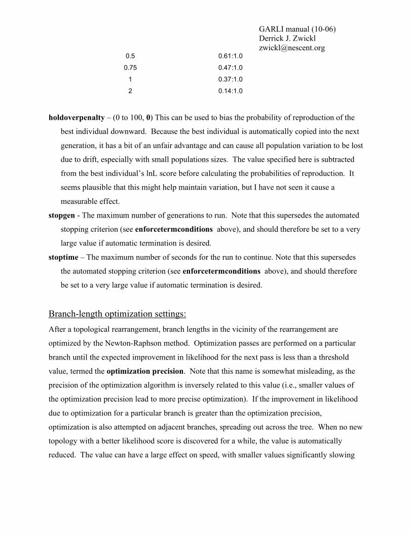
selectionintensity (0.01 to 5.0, 0.5)- Controls the strength of selection, with larger numbers

denoting stronger selection. The relative probability of reproduction of two individuals

depends on the difference in their log likelihoods (ΔlnL) and is formulated very similarly to

the procedure of calculating Akaike weights. The relative probability of reproduction of the

less fit individual is equal to:

eLntensityselectionI ln*)( !"

In

general this setting does not seem to have much of an effect on the progress of a run. In

theory higher values should cause scores to increase more quickly, but make the search more

likely to be entrapped in a local optimum. The following table gives the relative probabilities

of reproduction for different values of the selection intensity when the difference in log

likelihood is 1.0

Selection intensity Ratio of probabilities of reproduction

0.05 0.95:1.0

0.1 0.90:1.0

0.25 0.78:1.0

GARLI manual (10-06) Derrick J. Zwickl zwickl@nescent.org

0.5 0.61:1.0

0.75 0.47:1.0

1 0.37:1.0

2 0.14:1.0

holdoverpenalty – (0 to 100, 0) This can be used to bias the probability of reproduction of the

best individual downward. Because the best individual is automatically copied into the next

generation, it has a bit of an unfair advantage and can cause all population variation to be lost

due to drift, especially with small populations sizes. The value specified here is subtracted

from the best individual’s lnL score before calculating the probabilities of reproduction. It

seems plausible that this might help maintain variation, but I have not seen it cause a

measurable effect.

stopgen - The maximum number of generations to run. Note that this supersedes the automated

stopping criterion (see enforcetermconditions above), and should therefore be set to a very

large value if automatic termination is desired.

stoptime – The maximum number of seconds for the run to continue. Note that this supersedes

the automated stopping criterion (see enforcetermconditions above), and should therefore

be set to a very large value if automatic termination is desired.

Branch-length optimization settings: After a topological rearrangement, branch lengths in the vicinity of the rearrangement are

optimized by the Newton-Raphson method. Optimization passes are performed on a particular

branch until the expected improvement in likelihood for the next pass is less than a threshold

value, termed the optimization precision. Note that this name is somewhat misleading, as the

precision of the optimization algorithm is inversely related to this value (i.e., smaller values of

the optimization precision lead to more precise optimization). If the improvement in likelihood

due to optimization for a particular branch is greater than the optimization precision,

optimization is also attempted on adjacent branches, spreading out across the tree. When no new

topology with a better likelihood score is discovered for a while, the value is automatically

reduced. The value can have a large effect on speed, with smaller values significantly slowing

GARLI manual (10-06) Derrick J. Zwickl zwickl@nescent.org down the algorithm. The value of the optimization precision and how it changes over the course

of a run are determined by the following three parameters.

startoptprec (0.005 to 5.0, 0.5)- The beginning optimization precision.

minoptprec (0.001 to startoptprec, 0.01)- The minimum allowed value of the optimization

precision.

numberofprecreductions (0 to 100, 40) – Specify the number of steps that it will take for the

optimization precision to decrease from startoptprec to minoptprec. In version 0.95, the

reduction from startoptprec to minoptprec is now linear, rather than geometric.

treerejectionthreshold (0 to 500, 50) – This setting controls which trees have more extensive

branch-length optimization applied to them. All trees created by a branch swap receive

optimization on a few branches that directly took part in the rearrangement. If the difference

in score between the partially optimized tree and the best known tree is greater than

treerejectionthreshold, no further optimization is applied to the branches of that tree.

Reducing this value can significantly reduce runtimes, often with little or no effect on results.

However, it is possible that a better tree could be missed if this is set too low. I recommend a

fairly conservative (large) value.

Settings controlling the proportions of the mutation types: Each mutation type is assigned a prior weight . These values determine the expected

proportions of the various mutation types that are performed. The primary mutation categories

are topology (t), model (m) and branch length (b). Each are assigned a prior weight (Pi) in the

config file. Each time that a new best likelihood score is attained, the amount of the increase in

score is credited to the mutation type responsible, with the sum of the increases (Si) maintained

over the last intervallength x intervalstostore generations. The number of times that each

mutation is performed (Ni) is also tallied. The total weight of a mutation type is Wi = Pi +

(Si/Ni). The proportion of mutations of type i out of all mutations is then

!=

bmt

j

j

i

W

WiP

,,)(

GARLI manual (10-06) Derrick J. Zwickl zwickl@nescent.org

The proportion of each mutation is thus related to its prior weight and the average increase in

score that it has caused over recent generations. The prior weights can be used to control the

expected (and starting) proportions of the mutation types, as well as how sensitive the

proportions are to the course of events in a run. It is generally a good idea to make the topology

prior much larger than the others so that when no mutations are improving the score many

topology mutations are still attempted. You can look at the “problog” file to determine what the

proportions of the mutations actually were over the course of a run.

topoweight (0 to infinity, 1.0) The prior weight assigned to the class of topology mutations

(NNI, SPR and limSPR).

modweight (0 to infinity, 0.05) The prior weight assigned to the class of model mutations. Note

that setting this at 0.0 fixes the model during the run.

brlenweight ((0 to infinity, 0.2) The prior weight assigned to branch-length mutations.

The same procedure used above to determine the proportion of Topology:Model:Branch-Length

mutations is also used to determine the relative proportions of the three types of topological

mutations (NNI:SPR:limSPR), controlled by the following three weights. Note that the

proportion of mutations applied to each of the model parameters is not user controlled.

randnniweight (0 to infinity, 0.1) - The prior weight assigned to NNI mutations.

randsprweight (0 to infinity, 0.3) - The prior weight assigned to random SPR mutations. For

very large datasets it is often best to set this to 0.0, as random SPR mutations essentially

never result in score increases.

limsprweight (0 to infinity, 0.6) - The prior weight assigned to SPR mutations with the

reconnection branch limited to being a maximum of limsprrange branches away from where

the branch was detached.

intervallength (10 to 1000, 100) – The number of generations in each interval during which the

number and benefit of each mutation type are stored.

intervalstostore = (1 to 10, 5) – The number of intervals to be stored. Thus, records of

mutations are kept for the last (intervallength x intervalstostore) generations. Every

GARLI manual (10-06) Derrick J. Zwickl zwickl@nescent.org

intervallength generations the probabilities of the mutation types are updated by the scheme

described above.

Settings controlling mutation details: limsprrange (0 to infinity, 6) – The maximum number of branches away from its original

location that a branch may be reattached during a limited SPR move. Setting this too high (>

10) can seriously degrade performance.

meanbrlenmuts (1 to # taxa, 5) - The mean of the binomial distribution from which the number

of branch lengths mutated is drawn during a branch length mutation.

gammashapebrlen (50 to 2000, 1000) - The shape parameter of the gamma distribution (with a

mean of 1.0) from which the branch-length multipliers are drawn for branch-length

mutations. Larger numbers cause smaller changes in branch lengths. (Note that this has

nothing to do with gamma rate heterogeneity.)

gammashapemodel (50 to 2000, 1000) - The shape parameter of the gamma distribution (with a

mean of 1.0) from which the model mutation multipliers are drawn for model parameters

mutations. Larger numbers cause smaller changes in model parameters. (Note that this has

nothing to do with gamma rate heterogeneity.)

uniqueswapbias (0.01 to 1.0, 0.1) – In version 0.95, GARLI now keeps track of which branch

swaps it has attempted on the current best tree. Because swaps are applied randomly, it is

possible that some swaps are tried twice before others are tried at all. This option allows the

program to bias the swaps applied toward those that have not yet been attempted. Each swap

is assigned a relative weight depending on the number of times that it has been attempted on

the current best tree. This weight is equal to (uniqueswapbias) raised to the (# times swap

attempted) power. In other words, a value of 0.5 means that swaps that have already been

tried once will be half as likely as those not yet attempted, swaps attempted twice will be ¼

as likely, etc. A value of 1.0 means no biasing. If this value is not equal to 1.0 and the

outputmostlyuseless files option is on, a file called <ofprefix>.swap.log is output. This file

shows the total number rearrangements tried and the number of unique ones over the course

of a run. Note that this bias is only applied to NNI and limSPR rearrangements. Use of this

option may allow the use of somewhat larger values of limsprrange.

GARLI manual (10-06) Derrick J. Zwickl zwickl@nescent.org distanceswapbias (0.1 to 10, 1.0) – This option is similar to uniqueswapbias, except that it

biases toward certain swaps based on the topological distance between the initial and

rearranged trees. The distance is measured as in the limsprrange, and is half the the

Robinson-Foulds distance between the trees. As with uniqueswapbias, distanceswapbias

assigns a relative weight to each potential swap. In this case the weight is

(distanceswapbias) raised to the (reconnection distance - 1) power. Thus, given a value of

0.5, the weight of an NNI is 1.0, the weight of an SPR with distance 2 is 0.5, with distance 3

is 0.25, etc. Note that values less than 1.0 bias toward more localized swaps, while values

greater than 1.0 bias toward more extreme swaps. Also note that this bias is only applied to

limSPR rearrangements. Be careful in setting this, as extreme values can have a very large

effect.

Miscellaneous options: bootstrapreps (0 to infinity, 0) - The number of bootstrap reps to perform. If this is greater than

0, normal searching will not be performed. The resulting bootstrap trees (one per rep) will be

output to a file named <ofprefix>.boot.tre. To obtain the bootstrap proportions they will then

need to be read into PAUP* or a similar program to obtain a majority rule consensus. Note

that it is probably safe to reduce the strictness of the termination conditions during

bootstrapping (perhaps halve genthreshfortopoterm), which will greatly speed up the

bootstrapping process with negligible effects on the results.

inferinternalstateprobs = (0 or 1, 0) – Specify 1 to have GARLI infer the marginal posterior

probability of each character at each internal node. This is done at the very end of the run,

just before termination. The results are output to a file named <ofprefix>.internalstates.log.

The parallel GARLI algorithm (NOTE: As of the release of serial version 0.95, I have not yet verified that the parallel code

will work with changes to the GARLI core algorithm. I am sure that adjustment will be

needed. For now the parallel version of the previous release, v0.942, is the newest parallel

version. I will get version 0.95 working in parallel as soon as I have time. 10-17-06)

The parallel GARLI algorithm, for use on computer clusters implementing MPI, creates a

separate evolving population on each processor. One “master” population communicates with

GARLI manual (10-06) Derrick J. Zwickl zwickl@nescent.org all the other “remote” populations, which do not communicate directly with one another. All of

the settings discussed above pertaining to population, optimization and mutation details

discussed above may be set independently for the master and remote populations. The primary

benefit of the parallel version is that larger amounts of variation can be maintained across the

populations than would be possible in a single population. Note that this does not necessarily

result in a huge increase in speed relative to the serial algorithm, but for very larger datasets it

often results in higher scoring solutions.

The master population is able to perform recombination between the topologies found by the

remotes, resulting in better recombinant solutions. Recombination is performed by choosing two

trees and finding a bipartition (i.e., a subtree containing the same taxa) that is shared between

then. This subtree is detached from one topology and substituted for the corresponding subtree

on the other topology.

Besides the settings controlling the specifics of the algorithm within the master and remote

populations, a number of other settings may be changed to control the way that the master

interacts with the remote populations. Every sendinterval seconds the remotes send a copy of

their best individual to the master. At all times the master population retains a copy of the most

recent individual received from each remote (in addition to its normal set of individuals), with no

chance of mutation or of loosing these individuals due to selection. This ensures that the master

population always has access to plenty of variation in solutions. These “shielded” individuals

may be the parents of offspring or create new individuals by recombination.

The behavior of the parallel algorithm is largely dependent on the updatethreshold

parameter. When the master population receives an individual from a remote population, it

calculates the difference in lnL score between that individual and the best individual yet

encountered across all of the populations. If that score difference is greater than the

updatethreshold, the master reseeds that remote population with a copy of the best individual

yet encountered. The updatethreshold value may be optionally reduced over the course of the

run, much like the branch optimization parameter. A number of distinct parallel strategies may

be applied by specifying different values for the settings controlling the updatethreshold.

General strategies type follow:

Independent search – The remote populations are infrequently (or never) sent the best-known

individual. This allows maximum independence and variation among the populations, and

GARLI manual (10-06) Derrick J. Zwickl zwickl@nescent.org

recombination by the master proves quite beneficial. Set startupdatethresh and

minupdatethresh to the same large value (102 to 106). If using random starting topologies

this value should be very large so that the populations are not immediately homogenized at

the outset of the run.

Tightly coordinated search – All of the remote populations are frequently sent the best-known

individual found by any of them. This can result in a faster increase in likelihood score, but

entrapment in local optima is much more likely. Set starupdatethresh and

minupdatethresh to the same small value (1.0 to 20.0). The smaller the number, the less

freedom the remote populations have to explore on their own. Little benefit comes from

recombination with this strategy because there is little variation.

Hybrid search – This strategy utilizes both the independent and coordinated search strategies at

different points during the run. Initially the updatethreshold is large, allowing a lot of

independence during the early part of the run. This can be helpful as the search finds the

most promising general area of the search-space. The way this works has been changed

(simplified) in version 0.94. The updatereductionfactor and parallelinterval settings have

been removed. Now you simply specify a startupdatethresh and a minupdatethresh and

the program will decrease the value of the updatethresh during the course of the run, at the

same times that it reduce the optimization precision (see above in the serial section). The

update thresh will be reduced geometrically from its starting to minimum values, and the

number of steps necessary to do so will be the same as the number of steps necessary to

change from the startoptprecision to the minoptprecision. Values of

startupdatethresh=5000.0 and minupdatethresh=5.0 seem to work fairly well.

Parallel FAQ: How do I know what is going on with my parallel search? Looking at the node output files

should give you some idea what is going on. The node00.log file records all interactions that

the master has with the remotes. Each of the remotes also has its own file detailing its

interaction with the master (node01.log, node02.log, etc). You could also plot the log files of

each population (log00.log, log01.log, etc), which would give you some idea of how the

scores of the remotes compare to those of the master.

How many processors should I use? Because there is only one master population, the parallel

algorithm does not scale well to very large numbers of processors. Something in the 4 to 32

GARLI manual (10-06) Derrick J. Zwickl zwickl@nescent.org

processor range is reasonable, but you might not see much benefit in increasing past 8 or 10

processors except on very large trees (thousands of taxa).

Is there a parallel automated termination condition? Yes. It is the same as the serial version

(specified by enforcetermconditions, genhreshfortopoterm and scorethreshforterm),

except that the master includes individuals that it receives from the remotes in determining if

the genhreshfortopoterm and scorethreshforterm conditions have been met.

How do I run the parallel version? Where do I specify how many processors to use? etc.

Good questions, but beyond the scope of this document. You will need to compile the source

using a specific compiler script (often mpiCC), and the details of setting up and submitting

the parallel settings will be very specific to your cluster. Hopefully you have some kind of

systems administrator to answer these questions. If not, feel free to contact me with

questions or difficulties and I’ll see what I can do.

Will the parallel program run on a multiprocessor Mac? In theory I think that it should work

with Pooch, but I have not tried it (nor do I have access to Pooch). If someone gets this

working, I’d be interested to hear about it.

Descriptions of parallel GARLI setttings startupdatethresh (see strategies above)– The initial value of the updatethreshold.

minupdatethresh (see strategies above)– The minimum value of the updatethreshold.

maxrecomindivs (0 to nindivs minus holdover, 1)– The number of individuals that the master

will attempt to generate each generation by recombining topologies obtained from remote

populations.

sendinterval (5 to 600, 30) - The interval (in seconds) at which the remote populations send a

copy of their best individual to the master population. This can be set lower for smaller

datasets, but setting it too low may result in a speed reduction due to the overhead of sending

MPI messages over the network. Something in the range of 5 to 10 seconds per 50 taxa in

the dataset is reasonable.