Document downloaded from:

This paper must be cited as:

The final publication is available at

Copyright

http://dx.doi.org/10.1007/s11235-011-9568-3

http://hdl.handle.net/10251/45030

Springer Verlag (Germany)

García Pineda, M.; Sendra Compte, S.; Lloret, J.; Canovas Solbes, A. (2013). SavingEnergy and Improving Communications using Cooperative Group-based Wireless SensorNetworks. Telecommunication Systems. 52(4):2489-2502. doi:10.1007/s11235-011-9568-3.

1

Saving Energy and Improving Communications using Cooperative Group-

based Wireless Sensor Networks

Miguel Garcia, Sandra Sendra, Jaime Lloret, and Alejandro Canovas

Research Institute for Integrated Management of Coastal Areas.

Universitat Politècnica de Valéncia. Camino de Vera s/n, 46015 Valencia, Spain. migarpi@posgrado.upv.es, sansenco@posgrado.upv.es, jlloret@dcom.upv.es, alcasol@posgrado.upv.es

Abstract - Wireless Sensor Networks (WSNs) can be used in many real applications

(environmental monitoring, habitat monitoring, health, etc.). The energy consumption of each

sensor should be as lower as possible, and methods for grouping nodes can improve the network

performance. In this work, we show how organizing sensors in cooperative groups can reduce the

global energy consumption of the WSN. We will also show that a cooperative group-based

network reduces the number of the messages transmitted inside the WSNs, which implieasa

reduction of energy consumed by the whole network, and, consequently, an increase of the

network lifetime. The simulations will show how the number of groups improves the network

performance.

Keywords - Wireless Sensor Networks, Cooperative Group-based network, Saving

Energy, Efficient communications.

Introduction

A WSN can be defined as a network of small embedded devices strategically

located in a physical environment that are able to gather data from it. This type of

structure usually consists of sensor nodes that take measurements from the

environment and send the information to the base station that usually has greater

processing capacity and storage [1]. The base station is considered the gateway

between the sensor network and the data network. WSNs offer many good

features for the users such as easy to deploy, mobility, flexibility, cost reduction

and scalability [2]. The improvements in the wireless technology and the lower

cost of the sensors have helped the WSN market growth.

There are many applications where the WSN could be used. Some examples are: a

monitoring system for fire detection [3], for habitat monitoring [4], a fish farm

monitoring and control [5], etc.

2

However, when we want to cover large extensions and areas with difficult access,

there are certain technical limitations that require an exhaustive network design,

and study, to choose the appropriate communication algorithm and a good

network topology. One of the main concerns of the researchers and developers is

the whole network power consumption because devices are powered with

batteries, and low maintenance is desired.

In order to reduce the power consumption, the hardware design is very important.

Some of the techniques employed are related to knowing when the device must be

in one mode (active mode, sleep mode or idle mode) or in another [6], thereby

achieving to reduce unnecessary power consumption. But it also ensures

minimum levels of quality of information flowing through the network. There are

many systems, architectures, and protocols that can be used for WSN [7], but in

our previous works, we have demonstrated that wireless sensors group-based

topologies and networks improve the performance and the efficiency of the whole

network [8][9]. Group-based topologies allow the sensor to operate more flexibly,

efficiently and less energy consuming than regular network topologies [10].

Moreover, in one of our previous works we propose a group-based protocol for

large wireless ad hoc and sensor networks [11].

In this paper, we demonstrate that cooperative group-based networks have very

good features to be used in WSNs. Cooperative networks improve WSNs by

saving energy and providing efficient communications to the WSNs.

The rest of this paper is organized as follows. Section 2 shows others architectures

for saving energy in WSNs. The features of cooperative group-based networks

and the differences between the regular networks are explained in Section 3.

Section 4 describes our cooperative group-based architecture. A mathematical

analysis to prove that cooperative group-based networks save more energy is

provided in Section 5. Section 6 describes our proposal using the graph theory,

and shows the number of messages needed for cooperative group-based networks.

A simulation test using a network simulator is presented in Section 7. This

performance test let us improve the analytical results shown in previous sections.

Finally, Section 8 shows the conclusion and future work.

3

Related Work

No one of the papers found in the related literature analyze the power

consumption and the communications using the group-based strategy (except the

in a paper from the same authors [12], where we introduce these ideas). On one

hand, some works show that organizing the sensors into groups provide greater

benefits than doing otherwise. On the other hand, some works are focused on

network architectures to decrease the energy consumption, but without forgetting

the communications efficiency.

The paper with reference [13] shows that grouping nodes in WSN gives better

performance to the group and to the global system, because the system avoids

unnecessary message forwarding and additional overhead. In this paper, we can

see the efficiency of MANET routing protocols when the nodes are organized in

groups. To do this, the authors simulate several protocols such as DSR, AODV

and OLSR and study the advantages of grouping the individual nodes in each

protocol for fixed and mobile networks (mobile nodes with a random behavior).

Grouping nodes increase the productivity and the network performance providing

low overhead and low traffic. Therefore, good scalability can be achieved in

group-based networks.

J. Lloret et al. propose a new group-based protocol for WSN in [14]. First, they

compare some wireless technologies (IEEE 802.11a/b/g, Bluetooth and Zigbee)

for their use in WSNs. Then, they estimate the number of sensor nodes that would

be needed to cover a large area and propose an analytical model comparing the

energy consumed by each device over time. Finally, they compare their new

group-based protocol with other protocols such as DSDV, AODV and DSR. The

simulations show that the proposed protocol sends less number of packets to the

network and consequently there is less energy consumption. Following these

works, we see that the use of group-based networks provide benefits such as

traffic, delay, etc. in networks.

There are also several published works related with the analysis of energy

consumption and energy saving mechanisms in WLANs. These types of analysis

may help us know some power saving issues when they are used in WSNs.

The paper in reference [15] describes several techniques to reduce the dynamic

energy consumption in WLAN IEEE 802.11n standard systems in order to

increase the battery life in mobile systems. They propose to reduce the devices

4

consumption from their initial design by building smaller devices because they

consume less energy.

V. Raghunathan et al. describe in [16] some considerations about the architecture

and protocols to be considered in order to make an energy-efficient design of a

sensor node in a WSN. The paper shows an analysis of the energy consumption

characteristics of a node, using multihop architectures. Moreover, they identify

the key factors that can affect the life of the global system. They show the sensor

energy consumption, the power-aware computing, the energy-aware software, the

power management of wireless communication, the energy-aware packet

forwarding and traffic distribution, among others. This work is important to know

what the most important factors are, in order to take them into account when a

system is developed.

In paper [17], the authors discuss the required key technologies for low-energy

distributed microsensors and present a power aware Application Programming

Interface (API) to calibrate the energy efficiency of various parts of the

application. They took care of the power aware computation/communication

component technology, low-energy signaling and networking, system partitioning

considering computation and communication trade-offs, and a power aware

software infrastructure. This work also shows some analytical models of the

device behavior and the results of applying different parameters, such as the

number of sensors, type of protocol used to communicate the sensors, the system

power consumption by controlling when they should enter a sleep mode and

applying dynamic voltage scaling. These models will help us to develop our

models.

Reference [18] shows the relationship between the power usage and the number of

neighbors in a WSN. They state that many of the topologies proposed for wired

networks cannot be used for wireless networks because wireless networks depend

on the physical neighborhood and the transmission power while in a wired

network depends on the physical connections among nodes. A. Salhieh et al.

analyze various 2D and 3D structures with different numbers of nodes. They

measured the network performance for different network topologies and the

node's power dissipation in order to determine what the best topology is for a

WSN. But, they assume that they control the placement of these sensors and the

sensor locations are fixed respect to each other. Moreover, the authors do not

5

consider the effects of communication with a base station. They conclude that the

best power efficiency in 2D topologies is achieved with four neighbors, and

although 3D topology is better, it may not be feasible for some applications.

The energy consumption must not deteriorate the communications quality. We

have found some works that attempt to improve the efficiency of the

communications in WSNs, but trying to reduce energy consumption. Many of

them are related with the development of protocols at the MAC layer. Here, we

present some works.

In [19], S. Jayashree et al. present a MAC protocol that takes into account the

state of the battery and improves its efficiency. The main objectives of this

protocol are to reduce energy consumption, to extend the battery life and to have

higher performance. They present the BAMAC model battery that is based on

Markov chain process. Each node contains a table with the information of the

battery charge of each neighbor that is from a jump. The information in the table

organizes battery charges in descending order. RTS, CTS, Data and ACK packets

carry information of the remaining battery charge of the node that originated the

packet. A node that listens one of these packets, collects and stores the

information in its table. The simulation results, of this work, show that the battery

life is prolonged in about 70% and reduces the nominal battery consumption for

packet transmission by 21% compared with IEEE 802.11 MAC protocols DWOP.

In [20], the authors present sensor-MAC (S-MAC), a new MAC protocol

designed for WSN. First, the authors identify the main causes of energy

consumption: (1) when a transmitted packet is corrupted and it has to be discarded

because retransmissions increase the energy consumption, (2) the overhearing (a

node picks up packets that are destined to other nodes), (3) the control packets due

to the repetitive sending and receiving, and (4) being listening because

measurements have shown that this functional mode consumes around 50–100%

of the energy required for receiving. The main goal of this MAC protocol is to

reduce the energy consumption by taking care of these main causes, while

supporting good scalability and collision avoidance. The authors show that their

protocol achieves a reduction of the 30% in the device consumption and the

protocol has the ability to make trade-offs between energy.

C. Ching and C. Schindelhauer, presented in [21] a proposal that takes into

account the power consumption of both the motion and the radio communications

6

because they are the primary energy consumers. In order to achieve their goal,

they used a scenario with a series of robots and several antennas that

communicate among themselves. Each robot is assigned to different tasks

(searching, exploring, sensing, foraging, etc.). The authors reduce the energy

consumption in mobile receivers within a WSN considering a hybrid wireless

network formed by two scenarios: a single autonomous mobile node

communicating with multiple static relays through single hop, and secondly, a

single mobile node communicating with a static base station via a mobile relay.

The mobile node interacts with the relays within its vicinity by continuously

transmitting high-bandwidth data. The authors introduce Radio-Energy-Aware

(REA) path computation strategy and propose a novel energy-aware that finds the

best paths. The energy consumption for both mobility and communications is

minimized for mobile receivers and for the devices that keep communications in

all mobile nodes. They compare their method REA with Motion-Energy-Aware

(MEA) method. The simulation results show that their proposed strategy improves

the energy efficiency of mobile nodes.

The paper with reference [22], authored by Q. Gao et al., show the relationship

between optimal radio range and traffic. The authors adjust the communication

systems properties, according to some optimum strategies, in order to save the

average power. They carry out different approaches and mathematical

developments in order to adjust the maximum performance of a sensor node

model. The formulae used are made taking into account factors such as: the

network size, and the distance between nodes and between the nodes and the base

station. The authors proved that a good design and node's positioning choice

inside the WSN could lead to double the network lifetime because of the

significant reduction of the energy consumption.

In [23], the authors analyze the broadcast routing according to the energy cost. In

this case, the energy cost is defined as the sum of each individual node energy

cost that transmits broadcast messages. So, in order to solve this problem, the

authors try to minimize the number of broadcast messages. They use three

centralized heuristic methods to minimize it. According to their simulations, we

can see that there are some algorithms better than others. But the main problem of

these solutions is that all of them are based on centralized solutions and nowadays

the architectures are evolving to decentralized solutions.

7

Tiago Camilo et al. present in [24] a new routing protocol specially designed to

maximize the life time of the sensor nodes in WSNs. This protocol is based on

Ant Colony Optimization (ACO) metaheuristic method. In this protocol, the

communication with the next network node is selected according to a probability

(which is function of the node energy and the number of nodes of the path). In

order to check the truthfulness of their proposal, they present some simulations

that compare their protocol with other ant-routing protocols. The main drawback

of this type of protocols is the management of the ants (the backbone of routing

protocol).

In [25], the authors show that the cluster-based sensor networks have a better

energetic behavior than regular sensor networks. They present a routing protocol

for managing the sensor network with the main objective of extending the life of

the sensors in a particular cluster. Their proposal uses a gateway node which acts

as a cluster-based centralized network manager that sets routes for sensor data,

monitors latency throughout the cluster, and arbitrates medium access among

sensors. Finally they present some simulations that show the benefits of their

algorithm.

Another type of sensor lifetime extension mechanism is the one based on

deployment strategies. In [26], the authors explore these strategies. They propose

a general framework for the analysis of the network lifetime for several network

deployment strategies, and the authors consider the extra costs associated with

each deployment strategy to determine the best overall strategy for a given

scenario. This is an important work because it shows several issues that influence

the node's lifetime, and demonstrates and disagrees some intuitions.

Finally, another work where the authors present an energy-efficient deployment

algorithm based on Voronoi diagrams is [27]. Three different deployment

methods are proposed by the authors. The first one is a deployment algorithm for

mobile nodes where each node is equally important and a peer-based structure is

obtained. The second one uses the clustering idea to increase the amount of local

control. The third one uses the algorithm based on Voronoi diagrams to provide

an estimation of the lifetime of each node in a distributed fashion. They simulate

their algorithm and check its benefits, but the main problem of this research is that

it is only based on one-hope architecture and nowadays almost all networks are

multi-hop networks.

8

None of the previous works have used cooperative group-based sensor network

strategies in order to save energy or improve the communications in the WSN. For

this reason, we presented a main idea in [12]. In this paper, we show the analytical

model and its simulations which describe the improvement of cooperative group-

based systems versus regular architectures.

Differences between Regular WSNs, Group-based WSNs and Cooperative Group-based WSNs

In this section we review the main differences between regular WSNs and

cooperative group-based WSNs.

Regular WSNs are networks where all nodes have the same function from the

point of view of the network level. Each node measures a parameter, then, it is

processed and, finally, the information is sent to its neighbors. Its neighbors will

send the sensed information to their neighbors in order to reach the base station or

the sink.

Passive WSNs are those ones whose sensors sense the environment and send the

information to a sink without taking any other action. In an active WSN, when an

event occurs, it is notified to the sink and/or to the manage center (MC). Then, the

MC sends the necessary information to all nodes (or to some selected nodes) of

the network in order to take the appropriate action (send the information to other

nodes, sense more variables, etc.).

Currently passive WSN are not useful because in many environments an

intelligent WSN is required. Sometimes, when an event occurs inside the WSN

certain tasks should be carried out to perform a specific reply. For example, if we

build a WSN to detect fire, the sensors should be able to sense different variables

in order to verify the fire and even to monitor it (temperature, CO2, humidity,

wind direction, etc.). In this case, sensors may collect these variables and, after

some data processing, send the necessary information to a higher processing

capacity node in order to activate the appropriate fire fighting mechanisms.

Figure 1 shows the differences between passive and active WSNs. Red arrows

indicate the messages from sensor nodes to the MC and the blue arrows indicate

the communication from the MC to the sensor nodes in order to take the

appropriate actions. Blue arrows only exist in active WSNs.

9

Figure 1. Passive WSN vs. Active WSN

Cooperative group-based sensor networks do not work in the same way. First,

they are group-based networks, so the network is logically divided into several

small networks (groups). A group is defined as a small number of interdependent

nodes with complementary operations that interact in order to share resources or

computation time, or to acquire content or data and produce joint results. In a

wireless group-based architecture, a group consists of a set of nodes that are close

to each other (in terms of geographical location, coverage area or round trip time)

and neighboring groups could be connected if a node of a group is close to a node

of another group. In [12], we can see that the group-based WSNs provide many

benefits. Moreover, cluster-based networks could be considered as a subset of the

group-based networks, because every cluster could be a group [28][11]. But, a

group-based network is capable of having any type of topology inside the group,

not only clusters. Furthermore, in a group-based network, each group could use a

different type of routing protocol. A cluster-based network is made of a CH,

Gateways, and Cluster Members (CM). In a cluster, CH nodes fully control the

cluster, while in group-based networks, no node controls the group.

Cooperative group-based sensor networks imply cooperation between nodes from

the same group and cooperation between nodes from different groups. Thus, the

information may be shared only between the most appropriate nodes (from the

same groups or from different groups). An event produced by a sensor will imply

the exchange of information between different nodes in order to take a final

decision and produce an action in the same place or in other location of the

network. Moreover, in a cooperative WSN only those parameters that can affect

Passive WSN Active WSN

10

the final decision, i.e. the information coming from the neighboring groups of the

group that generated the alert, are considered. Following the example of the WSN

deployment for fire detection, when a sensor detects a fire, the alert message is

sent to all nodes in its group, and, after processing the information, and taking into

account other parameters such as wind direction, the alert is sent to the affected

neighboring groups. Affected neighboring groups will perform the appropriate

actions that other groups will not have to do.

From the point of view of the network messages and energy consumed, in a

regular WSN, when a node registers an alert, it transmits the alert to all its

neighbors, these neighbors transmits the alert to their neighbors and so on, the

alert is spread to the entire WSN without control. Moreover, a node could receive

several times the alert message from different neighbors (see Figure 2a). This

situation leads to excessive energy consumption. A collaborative group-based

WSN is built based on defined areas or as a function of the nodes’ features.

Moreover, each group is formed by nodes that interact to share resources or to

acquire data to produce joint results [29]. In this case, when a sensor detects a new

event, this sensor sends the information to all the members of the group and,

depending on the case, the neighboring groups could share this information in

order to reach all sensors of the WSN or just some groups. Only the closest

sensors to the edge of the group will transmit the information to the sensors of

other groups (see Figure 2b). This fact avoids raising considerably the global

energy consumption of the WSN, which is very important to enlarge the lifetime

of the WSN.

Figure 2. Regular WSN vs. Cooperative group-based WSN.

a) b)

11

Although we are mainly talking about collaborative group-based WSN with fixed

sensors, they could be mobile sensors. In our study we will consider group-based

WSNs where mobile sensors move only inside the boundaries of the groups.

Failures could happen in each group. In this case, the mobility will affect in the

same manner as in a non-group-based WSN.

In [11] we presented an example of cooperative group-based sensor network. The

WSN formation is performed in the same manner of a group-based network but

introducing cooperation issues. In addition, each group selects the best connection

between sensor nodes taking into account the proximity and the nodes’ capacity

[30]. In order to have an efficient group-based wireless sensor network, the groups

have to communicate with their neighboring groups. When a node detects an

event, it warns the alert, jointly with the parameters measured, to the nodes of its

groups and, routing the information, to its neighboring groups (not to all groups)

based on the location of each group or any other parameter. The location of the

sensors could be entered manually or using GPS [31], and a position-based

routing algorithm [32] could be used to send the message to the appropriate

situation. Neighboring groups could reply to the group that firstly sent the alert if

any of the parameters that caused the alert is changed, in order to take the

appropriate actions. Cooperation with other groups could change the direction of

the alert propagation and the level of the alert.

Figure 3 a) shows a group-based topology example. In a group-based WSN, all

groups will be aware of an event produced inside the Group 1. The network

efficiency would be yet higher than in a regular topology [10]. But, in cooperative

group-based networks this efficiency is greater, because the decision is taken

based on the information shared and only the neighboring groups will be aware of

it. The other groups could be in sleep mode. Sleep groups will be saving energy

and they would not transmit unnecessary information. Figure 3 b) shows that the

neighboring cooperative groups of group 1 are group 2 and 5. In this case they are

the physical neighbors. An example is explained in more detailed in [29].

12

Figure 3. Comparison of group-based WSN and cooperative group-based WSN.

Energy Analysis

This section analyzes the energy needed to transmit packets in a cooperative

group-based WSNs architecture and we compare it with a regular WSN

architecture.

The notation used in our analysis is shown in table 1. ϕ11, ϕ12 and ϕ2 are constant

radio parameters, typical values are ϕ11=50 nJ/bit, ϕ12= 50 nJ/bit, ϕ2 = 10

pJ/bit/m2 (when n = 2) or 0.0013 pJ/bit/m4 (when n = 4).

Table 1. Notation and definition.

Parameter Definition Parameter Definition

ϕ11 Power required to turn on the transmitter r Bit rate (bits per second)

ϕ12 Power required to turn on the receiver R Average area radius of a WSN

ϕ1 ϕ11 + ϕ12 Ri Average area radius of the

groupi

ϕ2 Power required to transmit s # of sensors in the WSN

d Distance between 2 communicating

sensors

Si # of sensors in the groupi

dopt Optimum distance between 2 sensors Jm # of cooperative groups

n Path loss exponent (typical values: 2 or 4) J # of groups, m Є [1,J]

We follow the model presented in [33]. The energy consumed by a sensor to

transmit and receive a data packet between two nodes is given by (1).

P = ϕ11 + ϕ12( )⋅ r + ϕ2 ⋅ (d n )⋅ r (1)

Where d is the distance between both nodes.

Group 1

Group 2

Group 3

Group 4

Group 5 event

a) Group-based WSN

Group 1

Group 2

Group 3

Group 4

Group 5 event

b) Cooperative Group-based WSN

Cooperativegroups

13

Let be D the distance between the sending node of a group and the closest node

from other group. Thus, P(D) ≥ P opt (D), being P opt (D) the minimum power to

transmit a data packet from the node to the other group. Popt (D) is equal to (2) if

and only if D is multiple integer of ( )nopt n

d1·2

1

−=

ϕϕ , as we can see in [34].

P opt D( ) = ϕ1 ⋅n

n − 1⋅

Dd opt

− ϕ12

⎛

⎝ ⎜ ⎜

⎞

⎠ ⎟ ⎟ ⋅ r (2)

P opt (D) is the lower bound of energy consumption in the flat scheme without data

aggregation, which indicates an ideal case where the per-hop distance for

transmission is dopt meters. According to the energy model in [33] and the

previous assumptions, the expected energy consumption per second of a group is

given by (3).

( ) ( ) rDrn

RSP nn

ii ⋅⋅++⋅⎟⎟

⎠

⎞⎜⎜⎝

⎛+⋅

⋅+⋅−= 21121 221 ϕϕϕϕ (3)

We assume that there are J groups in the network and each regular node only

needs to transmit its data packet to the central node or to the border node of its

group. The average radius of each m group can regard it as mJR , and the

expected energy consumption per second in all regular nodes will be given by (4).

( ) rJ

Rn

JsPn

mrn ⋅⎥⎥⎦

⎤

⎢⎢⎣

⎡⎟⎠

⎞⎜⎝

⎛⋅

+⋅+−=

22· 211 ϕϕ (4)

The energy consumption for all border nodes is given by (5).

( ) rJ

RJrJsPn

mmbor ⋅⎥⎥⎦

⎤

⎢⎢⎣

⎡⎟⎟⎠

⎞⎜⎜⎝

⎛⋅+⋅+⋅⋅−= 21112 ϕϕϕ (5)

In order to evaluate the energy consumed in a network without cooperative

groups, we consider (4) and (5) for a single group (J=1), and only one sink node.

Then, we obtain the equations (6) and (7) respectively.

( ) rRn

sP nrn ⋅⎥⎦

⎤⎢⎣⎡ ⋅

+⋅+⋅=

22

211 ϕϕ (6)

rnRsPbor ⋅⎥⎦⎤

⎢⎣⎡ ⋅++⋅= 21112 ϕϕϕ (7)

14

The global energy consumption in both cases cooperative network and a network

without cooperative groups is given by equation (8).

borrnT PPP += (8)

Another important issue that we have noticed is the importance of the number of

group nodes (high J) than the number of cooperative groups (Jm). If the number of

cooperative groups is greater, the consumption will be lower, but this

consumption decreases more quickly if we create more groups.

Analytical comparison

In order to observe the energy-saving improvements provided by a cooperative

group-based WSN compared to regular WSN, we have taken into account

equation 8 for both cases (regular WSN and cooperative group-based WSN).

Following the typical values of the constants that appear at the beginning of this

section (ϕ11=50 nJ/bit, ϕ12= 50 nJ/bit, ϕ2 = 10 pJ/bit/m2), we have used n=2

because it is the most appropriate value for outdoor communications.

Furthermore, we have chosen m=2, our network has 100 nodes (s=100) and the

network radius equals to 200 meters (R=200). We have programed the above

equations and varying analytically the number of groups and bitrate we obtain the

Figure 4. Figure 4 shows the global energy consumption for different values of Jm.

When Jm=1, we talk about just one group (the whole WSN), so we can see that the

energy consumption is higher than in any other value of Jm (higher values of Jm

imply more groups). By increasing Jm we see that consumption decreases, but

each time the difference of the slope is lower.

0,00

0,20

0,40

0,60

0,80

1,00

1,20

1,40

1,60

0 10000 20000 30000 40000 50000

Total energy (J)

r (bps)

1 510 1520 2530

15

Figure 4. Energy of the cooperative group-based WSN.

Communication Analysis

In a cooperative group-based WSN all nodes are alike from of the point of view of

network level and may be mobile. There are not base stations, sinks or

management nodes. For this reason, all nodes can make decisions of their

connections according to an algorithm. In our case the algorithm is defined in

[29]. Moreover, all communications between the sensor nodes are done by

wireless links.

As usual, we can model a WSN using the graph theory, where a WSN is defined

as ( )ESG ,= , where S is the set of sensor nodes ( sS = ) and e = i, j( )∈ E

represents a wireless link between the nodes i and j only if they are in their

communication range.

Any two nodes that are connected by an edge are neighbors to each other. Nodes

in G can send (and receive) messages to (from) their neighbors. Every node Sv ∈

has a unique identity ID(v). Each node initially knows its own identity and the

identities of its neighbors in one jump inside G.

The size of a group is the number of nodes belonging to it. According to the

definition of our WSN, there are three types of nodes: central, intermediate and

border nodes [10]. For example, the central node of the group k is defined as ( )kC .

The number of border nodes in the group is B, where B is smaller than n.

Other parameters that are used for defining communications in sensor networks is

the distance between two nodes, d i, j( ), it is the Euclidean distance between the

nodes i and j. As it is a group-based network, each group will be defined as ( )kG ,

in this case this is the group k.

From the graph theory textbook [35] we will denote Γk i( ) the k-neighborhood of a

node i, e.g., ( ) ( ){ }kjidSvik ≤<∈=Γ ,0 and we will denoteδk i( ) = Γk i( ) .

Besides, we will denote e i /G( ) = maxv∈G(i) d i, j( )( ) the eccentricity of a node i

inside its group. Thus the diameter of a group will be D G i( )( )= maxv∈G( i) e v /G( )( ). Once the definition of a group-based WSN has been done, we analyze the number

of messages sent inside the network when an event occurs and this information

has to be sent to other nodes. According to [36], in the worst situation, the number

16

of messages in a regular network when there is an alert is ( )sO , while in a

cooperative group-based network the number of messages is O m +1( )B2( ), where

m is the average number of cooperative groups in the network.

If sB << we can affirm that the number of messages in a group-based network

will be less than in regular networks, for this reason ( )( ) ( )sOBmO <<+ 21 .

Analytical comparison

In order to validate this analysis, we performed a simulation test. There were s

nodes distributed in a square area of length l units. The nodes are randomly

placed. The average density of nodes per unit length is 2/ ls . In this model, the

nodes have a link with another node if and only if they are within a distance d

units of each other. Consequently, a node will have an average of ( ) 1/ 22 −lsdπ

neighbors. This leads to an edge probability of ( ) ( )1/1/ 22 −− slsdπ which is the

probability that two nodes chosen at random in the network are connected by a

link. In particular, for a large value of s, the edge probability is approximately

equal to πd2 /l2.

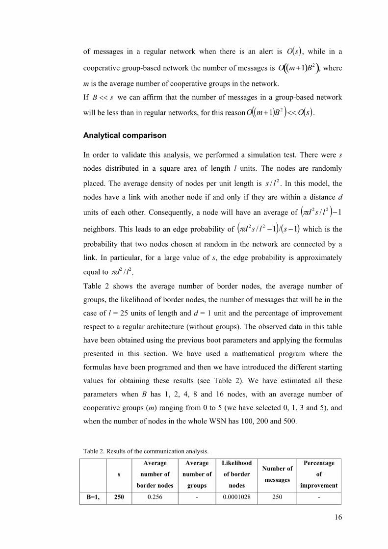
Table 2 shows the average number of border nodes, the average number of

groups, the likelihood of border nodes, the number of messages that will be in the

case of l = 25 units of length and d = 1 unit and the percentage of improvement

respect to a regular architecture (without groups). The observed data in this table

have been obtained using the previous boot parameters and applying the formulas

presented in this section. We have used a mathematical program where the

formulas have been programed and then we have introduced the different starting

values for obtaining these results (see Table 2). We have estimated all these

parameters when B has 1, 2, 4, 8 and 16 nodes, with an average number of

cooperative groups (m) ranging from 0 to 5 (we have selected 0, 1, 3 and 5), and

when the number of nodes in the whole WSN has 100, 200 and 500.

Table 2. Results of the communication analysis.

s

Average

number of

border nodes

Average

number of

groups

Likelihood

of border

nodes

Number of

messages

Percentage

of

improvement

B=1, 250 0.256 - 0.0001028 250 -

17

m=0 500 1.512 - 0.00303 500 -

1000 4.024 - 0.00403 1000 -

B=2,

m=1

250 0.256 125 0.0001028 8 96.8 %

500 1.512 250 0.00303 8 98.4 %

1000 4.024 500 0.00403 8 99.2 %

B=4,

m=3

250 0.256 62.5 0.0001028 64 74.4 %

500 1.512 125 0.00303 64 87.2 %

1000 4.024 250 0.00403 64 93.6 %

B=8,

m=3

250 0.256 31.25 0.0001028 256 No

improvement

500 1.512 62.5 0.00303 256 48.8 %

1000 4.024 125 0.00403 256 74.4 %

B=16,

m=5

250 0.256 15.625 0.0001028 1536 No

Improvement

500 1.512 31.25 0.00303 1536 No

improvement

1000 4.024 62.5 0.00403 1536 No

improvement

According to the results shown in Table 2, when we have a cooperative group-

based WSN with B=4 and m=3 or B=8 and m=3, the average number of nodes is

adequate, but when there are many border nodes the efficiency of the

collaborative group-based WSN is low (in red in table 2, e.g. B=16 and m=5).

This happens because when the groups are large, B ↑↑, so the WSN becomes a

regular WSN and moreover the architecture needs more control messages to

manage the collaborative group-based architecture. There is a tradeoff between

the number of network nodes and the appropriate number of groups, so a group-

based network is better than the regular network.

Figure 5 shows the maximum number of broadcasting messages needed when we

have several sizes of groups and several average cooperative groups. In this case

the number of nodes s was 1000 and l was 25 units. In this figure we can observe

that increasing the group size (B) and the number of cooperative groups, it

increases the number of messages in the WSN. The simulation shows that when a

high number of messages is expected in the WSN, it is better a group-based WSN

with a low B and with few cooperative groups. This happens with the

broadcasting messages, but if we look the management messages, when we have

small groups there are a lot control messages to create and manage the groups. For

18

this reason, there has to be a compromise between the group size, the number of

cooperative groups and the number of broadcasting messages. Seeing the figure 5,

the best solution could be a group size between 4 and 6 and an average number of

cooperative groups between 3 and 5.

Figure 5. Maximum number of broadcasting messages for different group size and varying the

average number of cooperative groups.

Cooperative group-based network test with mobility

In order to evaluate the system proposed in this paper. We have simulated several

scenarios using the OPNET Modeler network simulator [37]. In next simulations

we are going to see the behavior of the cooperative group-based WSN according

to the number of groups in network. The test scenario has 100 sensor nodes placed

in 500x500 meters. We have increased the number of groups in each simulation.

We have chosen DSR as routing protocol because in [14] we saw that this

protocol has the worst behavior. We select the worst routing protocol because we

want to show the positive aspects of our system, even using poor conditions.

Instead of a standard structure we have chosen a random topology. The nodes can

move randomly during the simulation. The physical topology does not follow any

known pattern. The obtained data neither depend on the initial topology of the

nodes nor on their movement pattern because all of it has been fortuitous.

The sensor nodes have a 40MHz processor, 512KB RAM memory, a radio

channel bandwidth of 1Mbps and their working frequency is 2.4GHz. Their

maximum coverage radius is 50 meters. This is a conservative value because

050100150200250300350400450500550

0 1 2 3 4 5 6 7 8

# of broadcasting messages

m

B=2 B=3 B=4 B=5

B=6 B=7 B=8

19

usually the nodes in sensor networks have larger coverage radius, but we

preferred to have lower transmitting power for the sensor devices in order to

enlarge their lifetime.

The traffic load used in the simulations is MANET traffic generated by OPNET.

We inject this traffic 100 seconds after the beginning. The traffic follows a

Poisson distribution (for the arrivals) with a mean time between arrivals of 30

seconds. The packet size follows an exponential distribution with a mean value of

1024 bits. The injected traffic has a random destination address, obtaining a

simulation that does not depend on the traffic direction. In Figure 6 we see that the

traffic injected into the simulation follows the same pattern for all scenarios. The

average traffic is 100 Kbps (an adequate traffic for WSNs).

Figure 6. Injected traffic comparison.

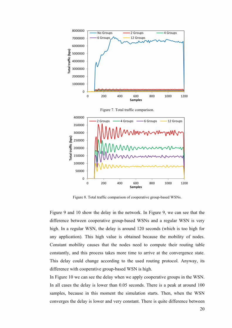
Figure 7 and 8 show the total traffic in the WSN. In figure 7, the total traffic in the

network is too high compared with the topology that uses collaborative groups.

When the network does not have collaborative groups, the average total traffic is

around 6500 Kbps, when we have 2 cooperative groups it decreases 95%. In

figure 8, we only see the cooperative group-based topologies in order to show

better the results. The total traffic decreases when the number of groups increases.

As we can see in Figure 8, when we have 2 groups the average total traffic is

around 310 Kbps, but when we have more groups (e.g. 6 groups), the total traffic

decreases down to 140 Kbps. This demonstrates that collaborative group-based

WSNs have lower traffic.

0

20000

40000

60000

80000

100000

120000

140000

0 200 400 600 800 1000 1200

Traffic in

jected

 (bps)

Samples

No Groups 2 Groups 4 Groups

6 Groups 12 Groups

20

Figure 7. Total traffic comparison.

Figure 8. Total traffic comparison of cooperative group-based WSNs.

Figure 9 and 10 show the delay in the network. In Figure 9, we can see that the

difference between cooperative group-based WSNs and a regular WSN is very

high. In a regular WSN, the delay is around 120 seconds (which is too high for

any application). This high value is obtained because the mobility of nodes.

Constant mobility causes that the nodes need to compute their routing table

constantly, and this process takes more time to arrive at the convergence state.

This delay could change according to the used routing protocol. Anyway, its

difference with cooperative group-based WSN is high.

In Figure 10 we can see the delay when we apply cooperative groups in the WSN.

In all cases the delay is lower than 0.05 seconds. There is a peak at around 100

samples, because in this moment the simulation starts. Then, when the WSN

converges the delay is lower and very constant. There is quite difference between

0

1000000

2000000

3000000

4000000

5000000

6000000

7000000

8000000

0 200 400 600 800 1000 1200

Total traffic (b

ps)

Samples

No Groups 2 Groups 4 Groups6 Groups 12 Groups

0

50000

100000

150000

200000

250000

300000

350000

400000

0 200 400 600 800 1000 1200

Total traffic (b

ps)

Samples

2 Groups 4 Groups 6 Groups 12 Groups

21

cooperative group-based WSN and regular WSN. When there are not

collaborative groups, the nodes are not segmented, and, for this reason, we need

more resources to manage the network. When the WSN is divided into

cooperative groups, the management process is also divided, for this reason we

need less resources.

Figure 9. Delay comparison.

Figure 10. Delay comparison of cooperative group-based WSNs.

In Figure 11, we show the average number of hops needed to arrive to a

destination when we are using groups and when we are not. As we can see, when

we have a regular WSN, the average number of hops is around 6, so we need to

cross 6 nodes to arrive to the destination. When we have collaborative groups in

the network, the average number of hops is the half. We need 3 hops to arrive to

the destination when we use collaborative group-based topologies.

0

20

40

60

80

100

120

140

160

0 200 400 600 800 1000 1200

Delay (s)

Samples

No Groups 2 Groups 4 Groups

6 Groups 8 Groups

0

0,05

0,1

0,15

0,2

0,25

0 200 400 600 800 1000 1200

Delay (s)

Samples

2 Groups 4 Groups 6 Groups 8 Groups

22

Figure 11. Hops per route needed to arrive to the destination.

In figure 12 and 13 we analyze the number of ACKs sent in regular and group-

based WSNs. In these cases we observe the same behavior as in previous figures.

The regular architecture needs more ACKs (2400) than the cooperative group-

based architectures (see Figure 12). This is because regular WSNs need more

messages to manage the architecture.

In order to better see the total number of ACKs sent in cooperative group-based

WSNs, we show figure 13. In this figure we can see that the number of ACKs sent

follow the same pattern for all topologies independently of the number of groups,

although each topology inserts more or less ACKs. When we have 2 groups,

where each group manages 50 sensor nodes, the average total ACKs sent is

around 400. This number drops to half when the number of groups is equal to 4.

But, figure 13 shows that although we increase the number of groups, the total

ACKs sent will not be less than a certain value. In this case, for a topology with 6

or 12 groups, the total number of ACK sent approximately equals 75.

0

1

2

3

4

5

6

7

0 200 400 600 800 1000 1200

Hop

s pe

r route

Samples

No Groups 2 Groups 4 Groups 6 Groups 12 Groups

23

Figure 12. Total number of ACKs sent.

Figure 13. Total number of ACKs sent in cooperative group-based WSNs.

Figures 14 and 15 show the retransmission attempts for all cases aforementioned.

In figure 14 we see that the regular WSN needs approximately 1.5 retransmission

packets to guarantee the correct running of the system. But this retransmission is

not needed when our system is based on collaborative groups, because the

required management is done by cooperative group-based WSN.

When we increase the number of groups we need less number of retransmissions.

When we have two groups, the average number of retransmissions is less than 0.1

packets, so it is negligible (see Figure 15). We can notice that when the number of

groups is less than 4, the retransmission packets could be zero. Observing these

simulations (Figure 14 and 15) we can affirm that when we use cooperative

0

5000

10000

15000

20000

25000

30000

0 200 400 600 800 1000 1200

Total A

CK sen

t

Samples

No Groups 2 Groups 4 Groups

6 Groups 12 Groups

0

50

100

150

200

250

300

350

400

450

500

0 200 400 600 800 1000 1200

Total A

CK sen

t

Samples

2 Groups 4 Groups 6 Groups 12 Groups

24

groups in our WSNs, we needs less retransmissions, even they could be zero,

depending of the system.

Figure 14. Retransmission Attempts.

Figure 15. Retransmission Attempts in cooperative group-based WSNs.

Finally, in Figure 16, we present the load processed by a collaborative group. In

this figure we only focus on the group-based WSNs, because, as we have seen in

the previous figures, the regular WSN has worse performance. In this figure we

see that when we have 2 groups in our network, the load is around 150 Kbps, this

load decreases down to 60 Kbps when we have 4 groups, 25 Kbps for 6 groups,

and less than 10 kbps for 12 groups. This happens because when we have more

collaborative groups, the number of nodes managed per group is lower. When we

have a lot of collaborative groups in the WSN, we need more control information

to manage it correctly. For this reason, when we select the number of groups, we

0

0,2

0,4

0,6

0,8

1

1,2

1,4

1,6

1,8

2

0 200 400 600 800 1000 1200

Retran

smission

 Attem

pts (packets)

Samples

No Groups 2 Groups 4 Groups

6 Groups 12 Groups

0

0,05

0,1

0,15

0,2

0,25

0,3

0,35

0,4

0,45

0,5

0 200 400 600 800 1000 1200

Retran

smission

 Attem

pts (packets)

Samples

2 Groups 4 Groups

6 Groups 12 Groups

25

should think several issues: to take into account the efficiency at network level,

and take care of the management information needed to create and manage each

collaborative group.

Figure 16. Load processed by a group.

Conclusion and Future Work

In this paper we have analyzed cooperative group-based WSNs. In this type of

WSNs when a sensor detects a new event, the alert is sent to its group and it is

distributed to an appropriate neighboring groups based on the information shared

between sensors. Cooperation between groups could be used to change the

direction of the alert propagation and the level of the alert in order to take the

appropriate actions.

Using several analytical analyses we have proved that the cooperative group-

based WSNs save energy and improve the efficiency of the WSN

communications. Moreover, we have seen that there are some WSN topologies

that have better results than others. For this reason, our future work is based on

this issue. We will analyze the best collaborative group-based WSN topology.

Moreover, in future works we will study the energy issues related with mobile

sensors and the communication procedures of joining and leaving the groups.

References

[1] Akyildiz, I.F., Su, W., Sankarasubramaniam, Y., Cayirci, E. (2002). Wireless sensor networks:

a survey Journal of Computer Networks, 38 (4) 393–422.

0

20000

40000

60000

80000

100000

120000

140000

160000

180000

200000

0 200 400 600 800 1000 1200

Group

 Loa

d (bps)

Samples

2 Groups 4 Groups 6 Groups 12 Groups

26

[2] Miguel Garcia, Diana Bri, Sandra Sendra, Jaime Lloret, Practical Deployments of Wireless

Sensor Networks: a Survey, Journal On Advances in Networks and Services. Vol. 3 Issue 1&2. Pp.

1-16. 2010.

[3] Lloret J., Garcia M., Bri D., Sendra S. (2009) A Wireless Sensor Network Deployment for

Rural and Forest Fire Detection and Verification. Sensors. 9 11 8722-8747.

[4] Mainwaring, A., Polastre, J., Szewczyk, R., Culler, D. (2002). Wireless sensor networks for

habitat monitoring. In ACM Workshop on Sensor Networks and Applications (WSNA’02),

Atlanta, GA, USA, September.

[5] Miguel Garcia, Sandra Sendra, Gines Lloret, Jaime Lloret, Monitoring and Control Sensor

System for Fish Feeding in Marine Fish Farms. IET Communications. 2010. In press.

[6] Sinha, A., Chandrakasan, A. (2001). Dynamic power management in wireless sensor networks.

IEEE Design and Test of Computers, 18 (2) 62-74.

[7] Garcia, M., Coll, H., Bri, D., Lloret, J. (2008). Using MANET protocols in Wireless Sensor

and Actor Networks. The Second International Conference on Sensor Technologies and

Applications (SENSORCOMM 2008). Cap Esterel, Costa Azul (Francia). 25-31 August.

[8] Lloret, J., García, M., Boronat, F., Tomás, J. (2008). Chapter 13: MANET protocols

performance in group-based Networks. Wireless and Mobile Networking. Springer Berlin

Heidelberg Boston. Vol.284, Pp. 161-172.

[9] Lloret, J., García, M., Tomás, J. (2008). Improving Mobile and Ad-Hoc Networks Performance

using Group-based topologies. Wireless Sensor and Actor Networks 2008 (WSAN 2008). Springer

Berlin Heidelberg New York. Ottawa (Canada). 14-15 July.

[10] Lloret, J., Palau, C., Boronat, F., Tomas, J. (2008). Improving Networks Using Group-based

Topologies. Journal of Computer Communications. Elsevier B. V. 31 (14) 3438-3450 .

[11] Lloret, J., Garcia, M., Tomás,J., Boronat, F. (2008). GBP-WAHSN: A Group-Based Protocol

for Large Wireless Ad Hoc and Sensor Networks. Journal of Computer Science and Technology.

23 (3) 461-480.

[12] Lloret, J., García, M., Boronat, F., Tomás, J. (2008). MANET protocols performance in

group-based Networks. 10th IFIP International Conference on Mobile and Wireless

Communications Networks (MWCN 2008). Toulouse (France). 30 September – 2 October.

[13] Garcia, M., Sendra, S., Lloret, J., Lacuesta, R. (2010) Saving energy with cooperative group-

based wireless sensor networks. Cooperative Design, Visualization, and Engineering: CDVE 2010.

LNCS. Vol. 6240. Pp. 231-238. September 2010.

[14] Lloret, J., Sendra, S., Coll, H., García, M. (2010). Saving Energy in Wireless Local Area

Sensor Networks. The Computer Journal (2010) 53(10): 1658-1673. Oxford University Press.

[15] Meiyappan, S. S., Frederiks, G., Hahn, S. (2006). Dynamic Power Save Techniques for Next

Generation WLAN Systems. Proceedings of the 38th Southeastern Symposium on System Theory

(SSST), Cookeville, Tennessee, USA, 5-7 March.

[16] Raghunathan, V., Schurgers, C., Park, S., Srivastava, M. (2002). Energy aware wireless

microsensor networks. IEEE Signal Processing Magazine, 19 (2) 40-50.

27

[17] Rex Min, Manish Bhardwaj, Seong-Hwan Cho, Eugene Shih, Amit Sinha, Alice Wang,

Anantha Chandrakasan, (2001). Low power wireless sensor networks. Proceedings of International

Conference on VLSI Design, Bangalore, India, 3-7 January.

[18] Salhieh, A., Weinmann, J., Kochha, M., Schwiebert,L. (2001). Power efficient topologies for

wireless sensor networks. Procedimgs of the IEEE International Conference on Parallel

Processing. Pp 156-163. 3-7 September

[19] Jayashree, S., Manoj, B. S., Murthy, C.S. R. (2004) A battery aware medium access control

(BAMAC) protocol for Ad-hoc wireless network, Proceedings of the 15th IEEE International

Symposium on Personal, Indoor and Mobile Radio Communications (PIMRC 2004). Barcelona

(Spain), 5-8 September, Vol. 2, Pp. 995-999.

[20] Ye, W., Heidemann, J., Estrin. D. (2002) An energy-efficient MAC protocol for wireless

sensor networks. Proceedings IEEE INFOCOM 2002, The 21st Annual Joint Conference of the

IEEE Computer and Communications Societies, New York, USA, 23-27June.

[21] Ching, C., Schindelhauer, C. (2010) Utilizing detours for energy conservation in mobile

wireless networks. Journal of Telecommunication Systems. Springer Netherlands. (DOI

10.1007/s11235-009-9188-3)

[22] Gao, Q., Blow, K., Holding, D., Marshall, I., Peng, X. (2004) Radio range adjustment for

energy efficient wireless sensor networks, Journal of Ad Hoc Networks. 4 (1) 75-82.

[23] Deying Li, Xiaohua Jia, and Hai Liu. (2004). Energy Efficient Broadcast Routing in Static Ad

Hoc Wireless Networks. IEEE Transactions on Mobile Computing, Vol. 3, No. 1, pp. 1-8.

January-March 2004.

[24] Camilo, Tiago and Carreto, Carlos and Silva, Jorge and Boavida, Fernando. (2006). An

Energy-Efficient Ant-Based Routing Algorithm for Wireless Sensor Networks. Lecture Notes in

Computer Science, Ant Colony Optimization and Swarm Intelligence, vol. 4150, pp. 49-59.

[25] M. Younis, M. Youssef, and K. Arisha. (2002). Energy-Aware Routing in Cluster-Based

Sensor Networks. In Proceedings of the 10th IEEE International Symposium on Modeling,

Analysis, and Simulation of Computer and Telecommunications Systems (MASCOTS '02). IEEE

Computer Society, Washington, DC, USA, pp. 129-136.

[26] Zhao Cheng, Mark Perillo, and Wendi B. Heinzelman. (2008). General Network Lifetime and

Cost Models for Evaluating Sensor Network Deployment Strategies. IEEE TRANSACTIONS ON

MOBILE COMPUTING, VOL. 7, NO. 4, pp. 484-497. April 2008.

[27] Nojeong Heo and Pramod K. Varshney. (2005).Energy-Efficient Deployment of Intelligent

Mobile Sensor Networks. IEEE Transactions on Systems, Man, and Cybernetics—Part A: Systems

And Humans, Vol. 35, No. 1, pp. 78-92. January 2005.

[28] Vlajic, N., Xia, D. (2006) Wireless sensor networks: to cluster or not to cluster?. International

Symposium on a World of Wireless, Mobile and Multimedia Networks, 2006. WoWMoM 2006.

[29] Garcia, M. and Lloret, J. (2009) A Cooperative Group-Based Sensor Network for

Environmental Monitoring. Cooperative Design, Visualization, and Engineering: CDVE 2009.

LNCS 5738, pp. 276–279.

28

[30] Garcia, M., Bri, D., Boronat, F., Lloret, J. (2008) A New Neighbour Selection Strategy for

Group-Based Wireless Sensor Networks. In: 4th Int. Conf. on Networking and Services, ICNS

2008, March 16-21, pp. 109–114

[31] Kaplan, E.D. (1996) Understanding GPS: Principles and Applications. Artech House, Boston.

[32] Stojmenovic, I. (2002) Position based routing in ad hoc networks. IEEE Communications

Magazine 40(7), 128–134.

[33] Heinzelman, W.B., Chandrakasan, A.P., Balakrishnan H. (2002) An application-specific

protocol architecture for wireless microsensor networks, IEEE Trans. on Wireless

Communications 1 (4) 660–670.

[34] Bhardwaj, M., Garnett, T., Chandrakasan, A.P. (2001) Upper bounds on the lifetime of sensor

networks. International Conference on Communications (ICC’01), June 2001, pp. 785–790.

[35] A. Gibbons. (1985) Algorithmic graph theory. Cambridge University Press, 1985.

[36] Fraigniaud, P., Pelc, A., Peleg, D., Perennes, S. (2000) Assigning labels in unknown

anonymous networks. Proceedings of the 19th Annual ACM SIGACT-SIGOPS Symposium on

Principles of Distributed Computing, Portland, OR, USA, July 2000, vol. 1, pp. 101–111.

[37] OPNET Modeler® Wireless Suite network simulator, available at

http://www.opnet.com/solutions/network_rd/modeler_wireless.html