Games of School Choice under the Boston Mechanism∗

Haluk Ergin

Department of Economics, MIT, 50 Memorial Drive, MA 02142

and

Tayfun Sonmez

Department of Economics, Koc University, 34450, Istanbul, Turkey, and

Harvard Business School, Mellon D2-4, Boston MA, 02163.

Abstract

Many school districts in the U.S. use a student assignment mechanism that we refer to asthe Boston mechanism. Under this mechanism a student loses his priority at a school unlesshis parents rank it as their first choice. Therefore parents are given incentives to rank high ontheir list the schools where the student has a good chance of getting in. We characterize theNash equilibria of the induced preference revelation game. An important policy implicationof our result is that a transition from the Boston mechanism to the student-optimal stablemechanism would lead to unambiguous efficiency gains. (JEL C78, D61, D78, I20)

∗We thank Chris Avery, Glenn Ellison, Sergei Izmalkov, Parag Pathak, Alvin Roth, Utku Unver, seminar par-ticipants at CORE, Duke, HBS (NOM), UCL, LSE, Spring 2003 NSF/NBER/CEME Decentralization Conference(Purdue University), Spring 2003 Wallis Institute Mini Conference (University of Rochester), GAMES 2004 (Mar-seille), ESSET 2004 (Gerzensee) and three anonymous referees for their insightful comments. Sonmez gratefullyacknowledges the research support of KocBank via the KocBank scholar program and Turkish Academy of Sciencesin the framework of the Young Scientist Award Program via grant TS/TUBA-GEBIP/2002-1-19. Any errors areour own responsibility.

1

1 Introduction

In the U.S., many school choice programs that assign children to public schools rely on the

centralized student assignment mechanism that is currently used in Boston. Other major school

districts that use versions of this mechanism include Cambridge,Charlotte, Denver, Minnesota,

Seattle and St.Petersburg-Tampa. Under the Boston mechanism a student who is not assigned

to his top ranked school A is considered for his second choice B only after the students who have

top-ranked B. Therefore a student loses his priority at a school unless his family ranks it as

their first choice. In particular it is typically not in the best interest of parents to reveal their

true preferences.1 Such preference manipulation is often advocated in local press. Consider the

following statement from the Seattle Press:2

The method the school district uses to sort the school choice requests gives first priority

to students who are already enrolled at that school. Next in line come those students

with siblings at the school. Both of these factors are beyond your control. These

students are sure things. Enrollment at these schools is theirs for the asking. No

amount of strategizing, short of polling all existing students to determine how many

have younger siblings about to enter the school, can help you here. Third in line, and

the first effect of any real choice, are those students who live in the school’s reference

area. This is why you have such an excellent chance of getting into your reference

school if you make it your top choice. Choosing another neighborhood’s reference

school, however, puts a lot of kids in line ahead of yours. That reduces your chances

of getting in, particularly if the school has small classes.

To see how such preference misrepresentation may lead to an efficiency loss, consider three

schools A, B, and C each having 100 students in its reference area and a class size 100. Let us

assume for simplicity that the only priority taken into account is proximity, that is, students in

a given school’s reference area are given priority for that school; and a lottery number is used to

break ties. Suppose that school C is the least desired school from the perspective of every family

and in each reference area, 50 families prefer A over B and the other 50 prefer B over A.

Consider a student i from the reference area A whose parents prefer school B to school A. If

they rank B as their first choice then she loses her priority at A, hence it becomes difficult for i

to get a seat at her reference area school A if she can not get a seat at school B. Hence by top

ranking their true favorite B, i’s parents risk their child to be assigned to their least preferred

1Chen and Sonmez [2003] report an experiment in which about 80 percent of the subjects mis-represent theirpreferences under the Boston mechanism. In their experimental setting the mis-representation rate increases amongsubjects who think there will be stiff competition for their first choice.

2Charles Mas, Navigating the School Choice Maze, The Seattle Press, December 30, 1998,http://www.seattlepress.com/article-483.html, accessed 02/10/2004.

2

school C . Alternatively i’s parents may adopt the safer strategy and ensure i a seat at school A

by ranking A as their first choice.

As more students from the B area submit B as their first choice, it becomes more difficult for i

to get a seat at B when her parents rank B as their first choice, hence the safer strategy becomes

more attractive. The situation is completely symmetric for a student j from the reference area B

whose parents prefer school A to school B. The safer strategy for j’s parents is to rank B as their

top choice, and this strategy becomes more attractive as more students from the A area top rank

A. As a result, it is an equilibrium under the Boston mechanism for each family to play their safe

strategy and top rank the school in their reference area.3 Under this equilibrium, every student is

assigned to his/her reference area school. Note that it is feasible under the given level of resources,

to assign all the students from the reference area of A who prefer B to A, to school B; and all the

students from the reference area of B who prefer A to B, to school A. Such a reallocation of seats

would improve the welfare of 100 families without affecting the others, illustrating the aggregate

efficiency loss under the Boston mechanism.

In this paper, we characterize the extent of the efficiency loss suggested by the above example

and identify the part of the inefficiency that can be recovered without violating the priorities.

To understand how families choose to distort their rankings in equilibrium, we will identify the

Nash equilibria of the preference revelation game induced by the Boston mechanism. In order

to describe the set of Nash equilibrium outcomes, we shall connect school choice with an impor-

tant model which has played a prominent role in the mechanism design literature. The school

choice model (Abdulkadiroglu and Sonmez [2003]) is closely related to the well-known two-sided

matching markets (Gale and Shapley [1962]). The key difference between the two models is that

in the former schools are indivisible objects which shall be assigned to students based on student

preferences and school priorities whereas in the latter parties in both sides of the market are

agents who have preferences over the other side and whose welfare are taken into consideration.

While school priorities are determined by the school district based on state/local laws (and/or

education policies) and do not necessarily represent school tastes, one can formally treat school

priorities as school preferences and hence obtain a two-sided matching market for each school

choice problem (see Abdulkadiroglu and Sonmez [2003], Balinski and Sonmez [1999], and Ergin

[2002]). Consequently concepts/findings in two-sided matching have their counterparts in school

choice.

The central notion in two-sided matching is stability . Importance of this concept does not

diminish in the context of school choice because if a matching is not stable then there is a student-

school pair (i, s) such that (1) student i prefers school s to his assignment and (2) either school s

has some empty seats or student i has higher priority than another student who is assigned a seat

at school s. In either case student i can seek legal action against the school district for not assigning

3Note that this is one of many equilibria.

3

him a seat at school s. It is well-known that there exists a stable matching and furthermore there

exists a stable matching which is preferred by any student to any other stable matching (Gale

and Shapley [1962]). This matching is known as the student-optimal stable matching and it has

played a key role in the re-design of U.S. hospital-intern market in 1998 (see Roth [2002], Roth

and Peranson [1999]). The student-optimal stable matching can be obtained in several steps with

the following student-proposing deferred acceptance algorithm: At Step 1 each student “proposes”

to her first choice and each school tentatively assigns its seats to its proposers one at a time in

their priority order. Any remaining proposers are rejected at the end of Step 1. In each of the

following steps (a) each student who was rejected in the previous step proposes to her next choice

if one remains, and (b) each school considers the students it has been holding together with its new

proposers, tentatively assigns its seats to these students one at a time in priority order and rejects

the remaining proposers. The algorithm terminates when no student proposal is rejected, and each

student is assigned her final tentative assignment. Besides the fact that it is the most efficient

stable mechanism, another desirable feature of the student-optimal stable mechanism is that under

this mechanism it is a dominant strategy for student families to state their true rankings of the

schools (Dubins and Freedman [1981], Roth [1982]).

While the student-optimal stable mechanism is well analyzed, not much is known about the

Boston mechanism despite its widespread use at many school districts. In our main result we

describe the Nash equilibrium outcomes of the preference revelation game induced by the Boston

mechanism: The set of Nash equilibrium outcomes is equal to the set of stable matchings under

the true preferences. This result allows us to make welfare comparison between the student-

optimal stable mechanism and the Boston mechanism: The preference revelation game induced

by the student-optimal stable mechanism has a dominant strategy equilibrium (which is truthful-

revelation) and its outcome is either equal to or Pareto dominates the Nash equilibrium outcomes

of the Boston mechanism. In that sense the outcome of the student-optimal stable mechanism

is the best one can hope for under the Boston mechanism. An important policy implication is

that a transition to student-optimal stable mechanism may result in significant efficiency gains in

Boston, Cambridge, Charlotte, Denver, Minneapolis, Seattle, St. Petersburg-Tampa, and other

districts which rely on variants of the Boston mechanism.4 Our main result is fairly robust in a

number of directions and our characterization extends:

1. to the case with strategic schools when Nash equilibria in undominated strategies is consid-

ered,

4After the first version of this paper was written, officials at the Boston Public Schools have authorized a studyconcerning an empirical analysis of the Boston mechanism and a possible transition to the student-optimal stablemechanism (Abdulkadiroglu, Pathak, Roth and Sonmez [2005]). Roughly around the same time New York CityDepartment of Education adopted a version of the student-optimal stable mechanism for the assignment of morethan 90,000 eighth graders to public highschools (Abdulkadiroglu, Pathak and Roth [2005]).

4

2. to the the case where there are capacity constraints on various types of students, and

3. to the more general class of priority matching mechanisms (Roth [1991]) when students are

allowed to veto any subset of schools.

In addition to its policy implications, our paper also contributes to the theory of implemen-

tation in matching markets.5 There are a number of papers that analyze equilibria induced by

various mechanisms in the context of marriage problems (i.e. two-sided matching markets where

each agent has only one slot.) One important negative result in this context is that preference

revelation games induced by stable mechanisms may have Nash equilibria with unstable outcomes

(Alcalde [1996]), and indeed given any Pareto efficient and individually rational mechanism the set

of Nash equilibrium outcomes of the induced preference revelation game is the set of individually

rational matchings (Sonmez [1997]). If, however, a refinement of Nash equilibria that allows pairs

(one from each side of the market) is considered as the underlying equilibrium concept, then the

set of equilibrium outcomes of these games is the set of stable matchings (Ma [1995], Shin and

Suh [1996], Sonmez [1997]).6 Our main result shows that the negative result mentioned above is

avoided when only one side of the market is strategic: There exists a Pareto efficient and individ-

ually rational mechanism (the Boston mechanism) where the set of Nash equilibrium outcomes of

the induced preference game is the set of stable matchings.

The fact that student families have incentives to misrepresent their preferences under the

Boston mechanism was first brought into the attention of economists by Abdulkadiroglu and

Sonmez [2003]. They also noted that the outcome of the Boston mechanism may be unstable

under the stated preferences and is therefore vulnerable to legal action by unsatisfied students and

their parents. Our result shows that although the Boston mechanism is not stable, its equilibrium

outcomes are stable with respect to true preferences. In particular, in equilibrium no family can

ensure their child a seat in a more preferred school through legal action, hence do not have any

incentives to initiate a lawsuit.

2 School Choice and Two-Sided Matching

In a school choice problem (Abdulkadiroglu and Sonmez [2003]) there are a number of students

each of whom should be assigned a seat at one of a number of schools. Each student has strict

5We can restate our result using implementation theory jargon as follows: The Boston mechanism implementsthe stable correspondence in Nash equilibria.

6See also Alcalde and Romero-Medina [2000], Kara and Sonmez [1996, 1997], Konishi and Unver [2003], Shinot-suka and Takamiya [2003], Sotomayor [2003], Tadenuma and Toda [1998], Teo, Sethuraman and Tan [2001] foradditional results on implementation in two-sided matching markets and Jackson [2001] for a recent and compre-hensive survey on implementation theory.

5

preferences over all schools and each school has a strict priority ranking of all students. Each

school has a maximum capacity but there is no shortage of the total number of seats.

Formally a school choice problem consists of:

1. a set of students I = {i1, . . . , in},

2. a set of schools S = {s1, . . . , sm},

3. a capacity vector q = (qs1 , . . . , qsm),

4. a list of strict student preferences PI = (Pi1 , . . . , Pin), and

5. a list of strict school priorities f = (fs1 , . . . , fsm).

Here sPis′ means that student i strictly prefers school s to school s′, qs denotes the capacity of

school s where Σs∈S qs ≥ |I |, and fs denotes the strict priority ordering of students at school s.

The school choice problem is closely related to the well-known two-sided matching markets

(Gale and Shapley [1962]).7 Two-sided matching markets have been extensively studied and

successfully applied in the American and British entry-level labor markets (see Roth [1984, 1991]).

The key difference between the two models is that in school choice schools are “objects” to be

consumed by the students whereas in two-sided matching participants in both sides of the market

are agents who have preferences over the other side.

Formally a two-sided matching market consists of:

1. a set of students I = {i1, . . . , in},

2. a set of schools S = {s1, . . . , sm},

3. a capacity vector q = (qs1 , . . . , qsm),

4. a list of strict student preferences PI = (Pi1 , . . . , Pin), and

5. a list of strict school preferences PS = (Ps1 , . . . , Psm).

Here Ps denotes the strict preference relation of school s over all students.

The two-sided matching theory have immediate implications on school choice. That is because,

school priorities in the context of school choice can be interpreted as school preferences in the

context of college admissions (see Abdulkadiroglu and Sonmez [2003], Balinski and Sonmez [1999],

Ehlers and Klaus [2004], Ergin [2002], and Kesten [2004]).

The outcome of both school choice problems and two-sided matching markets is known as a

matching. Formally a matching µ : I −→ S is a function from the set of students to the set of

7Throughout the paper we consider the many-to-one version of two-sided matching markets. These problemsare also knows as college admissions problems.

6

schools such that no school is assigned to more students than its capacity. Let µ(i) denote the

assignment of student i under matching µ. Note that µ−1(s) is the set of students each of whom

is matched to school s under matching µ.

In the two-sided matching context, a student-school pair (i, s) is said to block a matching µ if

either (1) student i prefers school s to its assignment µ(i) and school s has empty seats under µ,

or (2) student i prefers school s to its assignment µ(i) and school s prefers student i to at least one

of the students in µ−1(s). A matching is stable if and only if there is no student-school pair that

blocks it. Stability has been central to the two-sided matching literature. It is by now well known

that not only the set of stable matchings is non-empty for each two-sided matching market, but

also there exists a stable matching which is at least as good as any stable matching for any student

(Gale and Shapley [1962]). This matching is known as the student-optimal stable matching.

Given a school choice problem we refer to a matching to be stable whenever it is stable for

the induced two-sided matching market that is obtained by interpreting school priorities as school

preferences. We refer to the mechanism that selects the student-optimal stable matching for each

school choice problem as the student-optimal stable mechanism. By definition the student-

optimal stable mechanism always yields a matching that is at least as good as any stable matching

for any student. Moreover it is strategy-proof, that is truthful-preference revelation is always in

students’ best interest (Dubins and Freedman [1981], Roth [1982]).

3 The Boston Student Assignment Mechanism

A student assignment mechanism is a systematic procedure that selects a matching for each

school choice problem. The following mechanism is the most widely used student assignment

mechanism in real-life applications of school choice problems.8

The Boston Mechanism: For each school a strict priority ordering of students is determined,

each student submits a preference ranking of the schools, and the key phase is the choice of a

matching based on fixed priorities and submitted preferences.

Round 1 : In Round 1 only the first choices of the students are considered. For each school,

consider the students who have listed it as their first choice and assign seats of the school to these

students one at a time following their priority order until either there are no seats left or there is

no student left who has listed it as his first choice.

Round 2: Consider the remaining students. In Round 2 only the 2nd choices of these students

are considered. For each school with still available seats, consider the students who have listed it

as their 2nd choice and assign the remaining seats to these students one at a time following their

8See Introducing the Boston Public Schools 2002 , http://boston.k12.ma.us/teach/assign.asp, accessed02/10/2004.

7

priority order until either there are no seats left or there is no student left who has listed it as his

2nd choice.

In general, at

Round k: Consider the remaining students. In Round k only the kth choices of these students

are considered. For each school with still available seats, consider the students who have listed it

as their kth choice and assign the remaining seats to these students one at a time following their

priority order until either there are no seats left or there is no student left who has listed it as his

kth choice.

The procedure terminates when each student is assigned a seat at a school.

We next present a simple example which illustrates the working of the Boston mechanism.

Example 1: Let I = {i1, i2, i3, i4, i5, i6} be the set of students, S = {a, b, c, d} be the set of

schools, and q = (2, 2, 1, 1) be the school capacity vector. Student priorities at schools as well as

their preferences are as follows:

fa : i5 − i1 − i2 − i3 . . .

fb : i5 − i6 − i3 . . .

fc : i4 − i5 − i6 . . .

fd : i5 − i6 . . .

Pi1 : a . . .

Pi2 : a . . .

Pi3 : a − b . . .

Pi4 : c . . .

Pi5 : c − a − b − d

Pi6 : c − a − b − d

Round 1 : Only the first choices of students are considered and those with higher priorities are

accomodated. Each of students i1 and i2 is assigned a seat at school a; i4 is assigned a seat at

school c. At the end of Round 1, b has 2 and d has 1 seat available; students i3, i5, and i6 are

unassigned.

Round 2 : Remaining students are considered for their second choices. There is no seat left at

school a so students i5, i6 will not be accomodated in this round (too bad for student i5 who lost

the highest priority at school a) and student i3 is assigned at seat at school b. Therefore at the

end of Round 2, each of schools b, d has 1 seat available and students i5, i6 are unassigned.

Round 3 : Remaining students are considered for their third choices and student i5 is assigned a

seat at school b. At the end of Round 3, school d has 1 seat available and student i6 is unassigned.

Round 4 : The only remaining student i6 is assigned a seat at his forth choice school d.

Therefore the outcome of the Boston mechanism is:⎛⎝ i1 i2 i3 i4 i5 i6

a a b c b d

⎞⎠ .

8

The Boston mechanism is a special case of a priority matching mechanism (Roth [1991])

versions of which had been used to match medical school graduates (interns) to supervising con-

sultants in several regions of UK starting with late 1960’s. Each of these priority matching mech-

anisms were subsequently abandoned from the UK hospital-intern markets. Consider a school

choice problem with n students and m schools. Under the Boston mechanism any student-school

pair that rank each other first has the highest match priority. Roth [1991] refers to any such

match as a (1, 1) match. Similarly define a (k, �) match to be a match between a pair such

that the student ranks the school kth in his preferences and he has the �th priority at the school.

The Boston mechanism first forms any feasible (1, 1) match, next any feasible (1, 2) match, . . .,

next any feasible (1, n) match, next any feasible (2, 1) match, next any feasible (2, 2) match, . . .,

next any feasible (2, n) match, next any feasible (3, 1) match, . . ., and last in hierarchy is any

feasible (m, n) match. A priority matching mechanism is a generalization of this idea but it can

differ in the match priority hierarchy. Note that the match priority is lexicographic under the

Boston mechanism: It first considers the student preferences and only then the school priorities.

A similar lexicographic priority matching mechanism was used in Edinburgh in 1967 and 1968.

Roth [1991] shows that no priority matching mechanism is stable and the Boston mechanism

is no exception. In particular a student may lose his priority at a school unless he ranks it as

his first choice and hence truthful preference revelation may not be in students’ best interest.9

Students and their families are forced to play a preference revelation game that we will analyze in

the next section. As field evidence, preference manipulation is often advocated by the local press.

In addition to the Seattle Press story quoted in the Introduction, consider the following statement

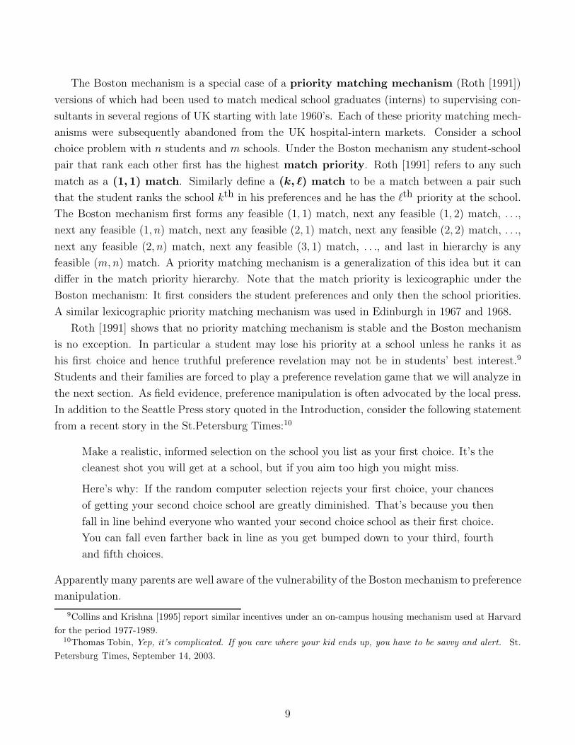
from a recent story in the St.Petersburg Times:10

Make a realistic, informed selection on the school you list as your first choice. It’s the

cleanest shot you will get at a school, but if you aim too high you might miss.

Here’s why: If the random computer selection rejects your first choice, your chances

of getting your second choice school are greatly diminished. That’s because you then

fall in line behind everyone who wanted your second choice school as their first choice.

You can fall even farther back in line as you get bumped down to your third, fourth

and fifth choices.

Apparently many parents are well aware of the vulnerability of the Boston mechanism to preference

manipulation.

9Collins and Krishna [1995] report similar incentives under an on-campus housing mechanism used at Harvardfor the period 1977-1989.

10Thomas Tobin, Yep, it’s complicated. If you care where your kid ends up, you have to be savvy and alert. St.Petersburg Times, September 14, 2003.

9

4 Nash Equilibria under the Boston Mechanism

In school districts that rely on the Boston mechanism, the students and their parents play a non-

trivial preference revelation game. Under this game, the strategies of the students are preferences

over schools and the outcome is determined by the Boston mechanism. The choice of their stated

preferences and especially their stated top choices play a key role in determining the schools they

will be assigned. In our main result we characterize the set of Nash equilibrium outcomes of the

preference revelation game induced by the Boston mechanism. Before we present our main result,

we give a detailed example which illustrates the preference revelation game induced by the Boston

mechanism and highlights some of the key points.

Example 2: There are three students i1, i2, i3 and three schools a, b, c each of which has one

seat. The utilities of the students as well as their priorities are as follows:

a b c

Ui1 2 1 0

Ui2 1 2 0

Ui3 0 2 1

fa : i3 − i2 − i1

fb : i1 − i3 − i2

fc : i2 − i1 − i3

Each student can submit one of the preferences abc, acb, bac, bca, cab, cba and therefore under

the Boston mechanism the following 6 × 6 × 6 simultaneous game is induced:

[Figure 1 about here]

In the resulting game the payoff vectors (2, 2, 1), (2, 0, 2), (1, 1, 1), (1, 0, 0), (0, 1, 2), and (0, 2, 0)

correspond to the matchings

µ1 =

⎛⎝ i1 i2 i3

a b c

⎞⎠ , µ2 =

⎛⎝ i1 i2 i3

a c b

⎞⎠ , µ3 =

⎛⎝ i1 i2 i3

b a c

⎞⎠ ,

µ4 =

⎛⎝ i1 i2 i3

b c a

⎞⎠ , µ5 =

⎛⎝ i1 i2 i3

c a b

⎞⎠ , and µ6 =

⎛⎝ i1 i2 i3

c b a

⎞⎠ respectively.

In the resulting game the boldface payoff vectors correspond to Nash equilibria. We have two key

observations about the Nash equilibria:

1. The strategy profile which corresponds to truthful preference revelation, (abc, bac, bca), is

NOT a Nash equilibrium of the induced preference revelation game.

2. The payoff vector in Nash equilibria is either (1, 1, 1) which is the payoff for matching µ3,

or (1, 0, 0) which is the payoff for matching µ4. The significance of matchings µ3 and µ4 is

that they constitute the set of stable matchings under true preferences.11

11The matching µ1 is blocked by the student-school pair (i3, b), the matching µ2 is blocked by the student-schoolpair (i2, a), the matching µ5 is blocked by the student-school pair (i1, b), and the matching µ6 is blocked by thestudent-school pair (i1, b).

10

The matching µ3 is the student optimal stable matching for the true preferences. Note that

the unstable matching µ1 Pareto dominates the student optimal stable matching µ3 which in turn

Pareto dominates the other stable matching µ4. The reason that neither of the stable matchings

is Pareto efficient is because stability and Pareto efficiency are not compatible in the context of

school choice.12 That is, the efficiency loss going from µ1 to µ3 is due to this incompatibility,

therefore it can not be recovered given that we are required to respect the legally determined

priorities. However the efficiency loss going from µ3 to µ4 would be caused by student families

being stuck in a bad equilibrium. This additional efficiency loss can be recovered by employing the

student optimal stable mechanism instead of the Boston mechanism.

We are now ready to present our main result which shows that these observations are not

specific to the above example. The key to this result is the similarity between participation of a

student in blocking of an unstable matching and profitable deviation by a student in the game

induced by the Boston mechanism.

Theorem 1 Let PI be the list of true student preferences and consider the preference revelation

game induced by the Boston mechanism. The set of Nash equilibrium outcomes of this game is

equal to the set of stable matchings under the true preferences PI .

Proof : Let Q = (Q1, . . . , Qn) be an arbitrary strategy profile and let µ be the resulting outcome

of the Boston mechanism. Suppose µ is not stable under the true preferences. Then there is a

student-school pair (i, s) such that student i prefers school s to his assignment µ(i) and either

school s has an empty seat under µ, or student i has higher priority at school s than another

student who is assigned a seat at school s. This implies that under the stated preference Qi

student i does not rank school s as his first choice for otherwise he would be assigned a seat

at school s. Let Q′i be any strategy where student i ranks school s as his first choice. Student

i is assigned a seat at school s under the profile (Q−i, Q′i) and therefore neither Q is a Nash

equilibrium profile nor µ is a Nash equilibrium outcome. Hence any Nash equilibrium outcome

should be stable under the true preferences.

Conversely let µ be a stable matching under the true preferences. Consider a preference profile

Q = (Q1, . . . , Qn) where each student i ranks school µ(i) as his top choice under his stated

preferences Qi. Under the preference profile Q, the Boston mechanism terminates at Round 1

and each student is assigned a seat at his first choice based on the stated preferences. Hence µ

is the resulting outcome for the strategy profile Q. Next we show that Q is a Nash equilibrium

profile. Consider a student i and a school s such that student i prefers school s to his assignment

µ(i). Since µ is stable, not only all seats of school s are filled under µ but also each student who

12Ergin [2002] identifies a condition on the list of priority orderings that is both necessary and sufficient for thecompatibility of Pareto efficiency and stability. In contrast, any stable matching is Pareto efficient in the contextof two-sided matching markets where the welfare of both sides of the market are taken into account.

11

is assigned a seat at school s under µ has higher priority than student i for school s. Moreover

each such student j ranks school s as his first choice under Qj. Therefore given Q−i, there is no

way student i can secure a seat at school s even if he ranks it as his first choice. Therefore Q

is a Nash equilibrium strategy profile and µ is a Nash equilibrium outcome. Hence any stable

matching under the true preferences is a Nash equilibrium outcome. ♦Even though the Boston mechanism itself is not stable, by Theorem 1 all Nash equilibrium

outcomes of the preference revelation game induced by the Boston mechanism are stable. The

outcome of the Boston mechanism is Pareto efficient, provided that students truthfully reveal

their preferences. However truthful preference revelation is rarely in the best interest of students,

and efficiency loss is expected. Theorem 1 clarifies the nature of this efficiency loss: Since all

equilibrium outcomes are stable, part of the inefficiency is due to the incompatibility of efficiency

and stability. However out of all equilibrium outcomes there is one, the student-optimal stable

matching, which Pareto dominates any other. Therefore in all equilibrium outcomes with the

exception of the student-optimal stable matching there is additional efficiency loss.

Researchers in education tend to evaluate the Boston mechanism and its variants based on the

stated preferences of students. For example Glenn [1991] argues that in 1991, 74 percent of sixth

graders at Boston were assigned to their first choice school. He also states

As an example of how school selections change, analysis of first-place preferences in

Boston for sixth-grade enrollment in 1989 (the first year of controlled choice in Boston)

and 1990 shows that the number of relatively popular schools doubled in only the

second year of controlled choice. The strong lead of few schools was reduced as others

“tried harder.”

Given the incentives under the Boston mechanism, this conclusion is overly optimistic. A more

plausible scenario is, the first time the mechanism was implemented most families did not un-

derstand the details of the mechanism and naively revealed their preferences truthfully; by the

second year of implementation the incentives offered by the mechanism was understood and most

families stated their preferences strategically. Along similar lines Glazerman and Meyer [1994]

argue that in 1993-94 more than 80 percent of students at Minneapolis were assigned to their first

choice school and they conclude

These numbers imply that student preferences in Minneapolis are quite diverse and

that students perceive that there are significant differences in school characteristics. If

this were not the case, we might expect most students to apply to a very limited set

of schools. As a result, very few students would have been assigned to their preferred

school.

Once again, this conclusion is inadequate. The Boston mechanism gives each student an incentive

to state a preference in which he top ranks the best possible school that he can be assigned to, given

12

the submitted preferences of other students. However this best possible school is not necessarily the

true top choice. It is interesting to note that, under the Nash equilibrium strategies we constructed,

each students is assigned to his/her first choice school based on the stated preferences. Whether

intentional or not, school districts that use the Boston mechanism are misleading policy-makers by

giving the impression that they are able to accommodate most students’ top choices and ironically

the Boston mechanism is the perfect tool to create this impression.

5 The Two-Sided Case: Strategic Schools

In some cities such as the New York City, schools determine their priority rankings subject to

certain regulatory restrictions. In this case it is natural to expect that schools will behave strate-

gically when submitting their priorities. Since both sides of the market are strategic we will call

this the two-sided case. We will show that given the Boston mechanism and under suitable as-

sumptions, it is a dominant strategy for schools to submit their true preferences over students as

their priority rankings. As a corollary, our main result extends to the two-sided case when schools

play undominated strategies.

Let PS = (Ps)s∈S denote the list of strict school preferences over subsets of students where

each subset corresponds to an incoming class. We assume that for any school s, for any subset

of students J and any two students i, j /∈ J , iPsj implies (J ∪ i) Ps (J ∪ j). This property is

known as responsiveness (Roth [1985]) and it is a consistency condition between preferences

over individual students and over sets of students. Two priority rankings fs and f ′s of school s are

outcome equivalent if for any list of student preferences PI and any list of priority rankings of

the remaining schools f−s, the Boston mechanism yields the same matching for (PI , f−s, fs) and

(PI , f−s, f′s).

Theorem 2 In the two-sided version of the Boston mechanism, it is a dominant strategy for any

school s to rank students based on its true preferences Ps. Moreover any other dominant strategy

of school s is outcome equivalent to truthfully ranking students based on Ps.

Proof : Let f∗s rank students based on Ps. Let QI be a list of student preferences and f−s be a list

of school priorities for all schools but school s. Let fs be an arbitrary priority order and consider

the outcome of the Boston mechanism for (QI, f−s, fs). If school s does not fill its capacity under

the resulting matching then the algorithm does not depend on fs, hence it would yield the same

matching for any priority order. If on the other hand s fills its capacity, then let k∗ be the round

where the last seat in s is assigned. Note that the assignments in rounds earlier than k∗ do not

depend on fs. At the beginning of round k∗, let J be the set of students who are already assigned

a seat at s, K be the set of unassigned students who rank s as their k∗th choice, r be the number

of remaining seats at s, and L be the set of top r individual students in K based on Ps. By

13

responsiveness (J ∪ L) Rs (J ∪ L′) for any r student subset L′ of K and indifference occurs only

when L = L′. Given QI and f−s, if s submits f∗s its remaining seats are assigned to L, and if s

submits any other priority order fs �= f∗s its seats are assigned to L′ for some r student subset L′

of K. Therefore s is weakly better-off submitting f∗s than submitting fs, and indifferent only if

L = L′, when (QI, f−s, fs) and (QI , f−s, f∗s ) yield the same matching.

Since the initial choice of QI and f−s was arbitrary, we conclude that it is a dominant strategy

for s to submit f∗s and that any other dominant strategy fs must be outcome equivalent to f∗

s . ♦

Corollary 1 In the two-sided version of the Boston mechanism, the set of Nash equilibrium out-

comes in undominated strategies is equal to the set of stable matchings under the true preferences.

Remark 1: Consider a two-sided matching market where each participant has a capacity of one

and refer the two sides of the market as men and women. Consider the preference revelation game

induced by the man-optimal stable mechanism. The combination of a result by Roth [1984b] and

another by Gale and Sotomayor [1985] in this context is analogous to Corollary 1: Under the

man-optimal stable mechanism the set of Nash equilibrium outcomes in undominated strategies

is equal to the set of stable matchings under the true preferences.

6 Controlled Choice

One of the major concerns about the implementation of school choice programs is that they

may result in racial and ethnic segregation at schools. Because of these concerns, school choice

programs in some districts are limited by court-ordered desegregation guidelines. This version of

school choice is known as controlled choice. In Minneapolis, controlled choice constraints are

implemented by imposing type-specific quotas. Under this practice students are partitioned into

different groups based on their type (which often depends on their ethnic/racial background) and

for each school, type-specific quotas are determined in additional to the capacity of the school.

These quotas may be rigid or they may be flexible. For example, in Minneapolis the district is

allowed to go above or below the district-wide average enrollment rates by up to 15 percent points

in determining the ethnic/racial quotas. Currently in Minneapolis and for ten years until 1999 in

Boston the following variant of the Boston mechanism is used to assign students to public schools.

The Boston Mechanism with Type-Specific Quotas: The students are partitioned based on

their types and for each school, in addition to the capacity of the school, type-specific quotas are

determined. For each school a strict priority ordering of the students is determined, each student

submits a preference ranking of the schools, and based on type-specific quotas, student priorities,

and submitted preferences, the student assignment is determined in several rounds.

Round 1 : In Round 1 only the first choices of the students are considered. For each school,

consider the students who have listed it as their first choice and assign seats of the school to these

14

students one at a time following their priority order unless the quota of a type is full. When that

happens, remaining students of that type are rejected and the process continues with the students

of other types until either there are no seats left or there is no student left who has listed it as his

first choice.

In general, at

Round k: Consider the remaining students. In Round k only the kth choices of these students

are considered. For each school with still available seats, consider the students who have listed it

as their kth choice and assign the remaining seats to these students one at a time following their

priority order unless the quota of a type is full. When that happens, remaining students of that

type are rejected and the process continues with the students of other types until either there are

no seats left or there is no student left who has listed it as his kth choice.

The procedure terminates when each student is assigned a seat at a school.

As in the case of the Boston mechanism, this modified version also induces a non-trivial

preference revelation game. We need an additional definition in order to characterize the set of

Nash equilibrium outcomes of this game.

Given a controlled choice problem, we call a matching µ weakly stable if it does not violate

the type-specific quotas, and there is no student-school pair (i, s) such that student i prefers school

s to his assignment µ(i) and either (a) school s has not filled its quota for the type of student i

and it has an empty seat, or (b) school s has not filled the quota for the type of student i and

student i has higher priority than another student (of any type) who is assigned a seat at school s,

or (c) school s has filled its quota for the type of student i but student i has higher priority than

another student of his own type who is assigned a seat at school s. Following Kelso and Crawford

[1982] and Roth [1991], Abdulkadiroglu [2002] shows that the set of weakly stable matchings is

non-empty. We are ready to characterize the set of Nash equilibrium outcomes of the preference

revelation game induced by the Boston mechanism with type-specific quotas.

Theorem 3 Let PI be the list of true student preferences and consider the preference revelation

game induced by the Boston mechanism with type-specific quotas. The set of Nash equilibrium

outcomes of this game is equal to the set of weakly stable matchings under the true preferences PI .

Proof : Similar to the proof of Theorem 1.

Many of the key properties on the structure of stable matchings carry over to the set of

weakly stable matchings provided that types of students form a partition of the students (see

Abdulkadiroglu [2002]). Most notably, given a controlled choice problem, there exists a weakly

stable matching which is at least as good as any other weakly stable matching for any student

(Kelso and Crawford [1982], Roth [1991], Abdulkadiroglu [2002]). Theorem 3 shows that policy

implications of our main result carry over to the controlled choice model. Most notably, transition

15

to the controlled choice version of the student-optimal stable mechanism is likely to result in Pareto

improvements in school districts that currently rely on the Boston mechanism with type-specific

quotas.13

7 Nash Equilibria Under Priority Matching Mechanisms

As we have already indicated, the Boston mechanism is a special case of priority matching mecha-

nisms. A natural question is whether our characterization result extends to other priority matching

mechanisms. The following example shows that the answer is negative. Indeed there is a priority

matching mechanism and a school choice problem where the set of stable matchings and the set

of Nash equilibrium outcomes of the induced preference revelation game are two distinct sets.

Example 3: Let I = {i1, i2} be the set of students, S = {a, b} be the set of schools, and q = (2, 2)

be the school capacity vector. Student priorities at schools and their preferences are as follows:

fa : i1 − i2

fb : i2 − i1

Pi1 : b − a

Pi2 : a − b

Note that the unique stable matching for this problem is:

µ1 =

⎛⎝ i1 i2

b a

⎞⎠ .

Next consider the priority matching mechanism which first considers school priorities and only

then the student preferences. This mechanism

• first forms any feasible (1,1) match,

• next forms any feasible (2,1) match,

• next forms any feasible (1,2) match,

• and finally forms any feasible (2,2) match

when there are two students and two schools. Observe that given the above priorities at schools,

the outcome of this mechanism is

µ2 =

⎛⎝ i1 i2

a b

⎞⎠

regardless of the stated student preferences. Hence any preference profile is a Nash equilibrium

with an outcome of µ2.

13Roth [1991] reports that a similar transition had been carried out in Edinburgh hospital-intern market in 1969where a priority matching mechanism was replaced with the controlled choice version of a stable mechanism.

16

While the above example is discouraging, a minor modification in the school choice model

allows us to generalize our characterization result to priority matching mechanisms. In the original

model each student ranks all schools and she does not have the ability to “veto” any school. In

practice, however, students often have outside options (such as private schools) and they are

allowed to consider any subset of schools. We next modify the school choice model to allow for

this possibility.

In this richer model each student i has strict preferences Pi over S ∪ {i} where i denotes the

option of remaining unmatched. Let Ri denote the weak preference relation induced by Pi. School

s is acceptable to student i if and only if sRii.

A matching in this modified model is a function µ : I → S ∪ I such that

(i) µ(i) ∈ S ∪ {i} for all i ∈ I , and

(ii) |µ−1(s)| ≤ qs for all s ∈ S

and it is stable if and only if

(a) µ(i)Rii for any student i,

(b1) there is no student-school pair (i, s) and another student j with µ(j) = s such that sPiµ(i)

and fs(i) < fs(j), and

(b2) there is no student-school pair (i, s) such that sPiµ(i) and |µ−1(s)| < qs.

A priority matching mechanism is defined similarly as in the original model with the exception

that students are only admitted to acceptable schools. Recall that a (k, l) match is defined to be

a match between a student-school pair such that the student ranks the school kth in his preferences

and he has the lth priority at the school. Given a modified problem with n students and m schools,

a match priority is a one-to-one function

π : {1, . . . , n} × {1, . . . , m} → {1, . . . , nm}

and the resulting priority matching mechanism determines its outcome in nm steps with the

following priority matching algorithm:

Step 1 : Form any feasible and acceptable π−1(1) match.

Step 2 : Form any feasible and acceptable π−1(2) match....

...

Step nm : Form any feasible and acceptable π−1(nm) match.

Each student who remains unmatched at the end of nm steps is matched to herself.

For example under the special case of the Boston mechanism any feasible and acceptable

π−1(1)=(1,1) match is formed at Step 1, any feasible and acceptable π−1(2)=(1,2) match is formed

17

at Step 2, etc. Note that the first n steps under this description correspond to Round 1 of the

original description of the Boston mechanism, the next n steps correspond to Round 2, and so on.

A match priority π is monotonic if (k, l) ≤ (k′, l′) implies π(k, l) ≤ π(k′, l′). A priority

matching mechanism is monotonic if it is induced by a monotonic match priority.

We are now ready to present our final result.

Theorem 4 Consider the modified school choice model where each student can consider any subset

of the schools. Let P be a list of student preferences and consider the preference revelation game

induced by any monotonic priority matching mechanism. The set of Nash equilibrium outcomes

of this game is equal to the set of stable matchings under the true preferences P .

Proof : Fix a modified problem where P denotes the list of student preferences. Fix a monotonic

match priority π and let Π denote the resulting priority matching mechanism. Consider the

induced preference revelation game.

“⊃”: First suppose that µ is a stable matching under P . For each student i with µ(i) = i, let

Pi be a preference ranking with no acceptable school. For each student i with µ(i) = s, let Pi be

a preference ranking where s is the only acceptable school. Clearly Π(P ) = µ.

We next show that P is a Nash equilibrium. Suppose towards a contradiction that there is a

student i, a preference ranking P ′i , and a school s such that Πi(P−i, P

′i ) = s and sPiµ(i). Since µ

is stable, there are qs students j1, . . . , jqs each of whom is assigned a seat at school s under µ and

also has a higher priority for school s than student i. Consider the priority matching algorithm

under (P−i, P′i ). School s is the only acceptable school for each student j ∈ {j1, . . . , jqs} under Pj

and by monotonicity of the match priority π, the match of each such student j and school s has

higher match priority than the match of student i and school s. Therefore the seats of school s are

exhausted before the match of i and s is considered, achieving the desired contradiction. Hence

P is a Nash equilibrium and µ is a Nash equilibrium outcome.

“⊂”: Let P be a strategy profile that yields the unstable matching µ under the priority

matching mechanism Π. We will show that P is not a Nash equilibrium for each of the following

three cases:

(a) there is a student i∗ such that i∗Pi∗µ(i∗),

(b1) there is a student-school pair (i∗, s∗) and another student j∗ with µ(j∗) = s∗ such that

s∗Pi∗µ(i∗) and fs∗(i∗) < fs∗(j

∗), and

(b2) there is no student-school pair (i∗, s∗) such that s∗Pi∗µ(i∗) and |µ−1(s∗)| < qs∗ .

(a) Let P ′i∗ be a preference ranking where no school is acceptable. The priority matching

mechanism Π leaves student i unmatched under the profile (P−i∗ , P′i∗) and hence P ′

i∗ is a profitable

deviation.

18

(b) Let P ′i∗ be a preference ranking where the only acceptable school is s∗. Let l denote the

priority ranking of student i∗ at school s∗ (i.e. l = fs∗(i∗)) and let r∗ denote the step at which all

feasible and acceptable (1,l) matches are formed by the priority matching algorithm for the match

priority π (i.e. r∗ := π(1, l)). We will show by induction that:

Claim. Consider the priority matching algorithm for the match priority π. At the beginning

of each round r (1 ≤ r ≤ r∗):

1. For each student i �= i∗, if i is already matched under P , then he is also already matched

under (P−i∗ , P′i∗).

2. For each school s, there are at least as many unassigned seats under (P−i∗ , P′i∗) as under P .

Proof of the Claim : Since the priority matching algorithm starts with each student unmatched,

the Claim holds for r = 1. Suppose the Claim holds for r where 1 ≤ r < r∗. We will show that it

holds for (r + 1) as well.

1. Take any student i �= i∗ who gets matched to a school, say school s, at Step r under P .

We will show that student i is matched to a school by the end of Step r under (P−i∗ , P′i∗).

School s has at least one available seat at the beginning of Step r under P and therefore by

part 2 of the inductive assumption it has at least one available seat at the beginning of Step

r under (P−i∗ , P′i∗) as well. Suppose student i is still unmatched at the beginning of Step r

under (P−i∗ , P′i∗). Since i �= i∗, student i and school s form a π−1(r) match under (P−i∗ , P

′i∗)

and hence student i gets matched by the end of Step r under (P−i∗ , P′i∗).

2. Take any school s and consider any student i who is matched with school s at Step r under

(P−i∗ , P′i∗). We will show that either student i is matched with school s at Step r under P

or there are no seats left at school s at the beginning of Step r under P . Recall that under

P ′i∗ the only acceptable school is s∗, and by assumption i∗ and s∗ can only be matched at

Step r∗ (in case a seat is still available at s∗). Therefore i �= i∗. By assumption student

i is unmatched at the beginning of Step r under (P−i∗ , P′i∗) and therefore by part 1 of the

inductive assumption student i is unmatched at the beginning of Step r under P as well.

Hence if s has any seats left at the beginning of Step r under P , then student i and school

s form a π−1(r) match and get matched at Step r.

This completes the proof of the claim. �Recall that by assumption student i∗ is unmatched at the beginning of Step r∗ under (P−i∗ , P

′i∗).

Suppose (b1) holds and student j∗ and school s∗ form a (k, l′) match under P for some l < l′.

By monotonicity of the priority matching mechanism Π a (1, l) match will be considered before

a (k, l′) match for any k, and hence school s∗ has an empty seat at the beginning of Step r∗

(i.e. when (1, l) matches are considered) under P . If on the other hand (b2) holds, then again

19

school s∗ has an empty seat at the beginning of Step r∗ (and indeed throughout the algorithm)

under P . Therefore by the above Claim, school s∗ has an empty seat at the beginning of Step r∗

under (P−i∗ , P′i∗) whether (b1) or (b2) holds and student i∗ and school s∗ are matched at Step r∗

under (P−i∗ , P′i∗). Hence P ′

i∗ is a profitable deviation for student i∗ showing that P is not a Nash

equilibrium. ♦

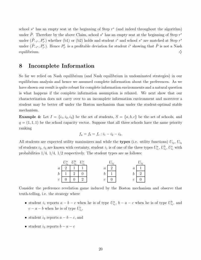
8 Incomplete Information

So far we relied on Nash equilibrium (and Nash equilibrium in undominated strategies) in our

equilibrium analysis and hence we assumed complete information about the preferences. As we

have shown our result is quite robust for complete information environments and a natural question

is what happens if the complete information assumption is relaxed. We next show that our

characterization does not carry over to an incomplete information environment and moreover a

student may be better off under the Boston mechanism than under the student-optimal stable

mechanism.

Example 4: Let I = {i1, i2, i3} be the set of students, S = {a, b, c} be the set of schools, and

q = (1, 1, 1) be the school capacity vector. Suppose that all three schools have the same priority

ranking

fa = fb = fc : i1 − i2 − i3.

All students are expected utility maximizers and while the types (i.e. utility functions) Ui2, Ui3

of students i2, i3 are known with certainty, student i1 is of one of the three types Uai1, U b

i1, U c

i1with

probabilities 1/4, 1/4, 1/2 respectively. The student types are as follows:

Uai1

U bi1

U ci1

a 2 1 1

b 1 2 0

c 0 0 2

Ui2

a 2

b 1

c 0

Ui3

a 1

b 2

c 0

Consider the preference revelation game induced by the Boston mechanism and observe that

truth-telling, i.e. the strategy where

• student i1 reports a − b − c when he is of type Uai1, b − a − c when he is of type U b

i1, and

c − a − b when he is of type U ci1,

• student i2 reports a − b − c, and

• student i3 reports b − a − c

20

is a Bayesian Nash equilibrium with an expected payoff vector of (2, 32, 3

2).14 The outcome of this

equilibrium is a lottery but not all matchings in its support are stable. In particular, when the

realized type profile is (Uai1, Ui2, Ui3), truth-telling yields

⎛⎝ i1 i2 i3

a c b

⎞⎠

which is an unstable matching.

The following table compares the expected payoffs of the dominant-strategy equilibrium of

the student-optimal stable mechanism and the above described Bayesian Nash equilibrium of the

Boston mechanism:

Uai1

U bi1

U ci1

Ui2 Ui3

Student-Optimal Stable Mechanism 2 2 2 74

1

The Boston Mechanism 2 2 2 32

32

Note that the Bayesian Nash equilibrium described above benefits the low-priority student i3 at

the expense of the intermediate priority student i2.

9 Conclusion

In this paper we presented an equilibrium analysis of the Boston mechanism, an assignment

mechanism that is in use at several U.S. school districts including Boston, Cambridge, Charlotte,

Minnesota, Seattle, and St. Petersburg-Tampa. Our results suggest that a transition to an

alternative mechanism, the student-optimal stable mechanism, is likely to result in potentially

significant welfare gains. Such a transition will also eliminate the need for strategizing because

truthful preference revelation is a dominant strategy under the student-optimal stable mechanism.

In contrast, as we present, the Boston mechanism induces a complicated coordination game with

multiple equilibria among large numbers of parents. Unlike in complete information environments,

some students may benefit from the Boston mechanism in incomplete information environments

due to coordination failures of other students. As it is recently argued by the Boston Public

Schools Strategic Planning Manager,15 “assignment becomes a high-stakes gamble for families”

14Since student i1 has the highest priority at each school, truthful preference revelation yields him his top choiceregardless of his type. It is also clear that no student can profit from improving the ranking of his last choice school.That leaves b− a− c as the only potentially profitable deviation for student i2 and a− b− c as the only potentiallyprofitable deviation for student i3. However using strategy b− a− c reduces the expected utility of student i2 to 5

4

and using strategy a− b− c reduces the expected utility of student i3 to 1 showing that truth-telling is a BayesianNash equilibrium.

15Valerie Edwards, “Understanding the Options for a New BPS Assignment Method,” presented at the October13, 2004 dated Boston Public Schools school committee meeting.

21

under the Boston mechanism. One important direction for future research is a thorough analysis

of equilibria in incomplete information environments for it will enhance our understanding of this

high stakes gamble.

References

[1] A. Abdulkadiroglu, “College Admissions with Affirmative Action,” mimeo, Columbia Uni-

versity, 2002.

[2] A. Abdulkadiroglu, P.A. Pathak and A.E. Roth, “The New York City High School Match,”

mimeo, Harvard Business School, 2005, forthcoming in American Economic Review, Papers

and Proceedings .

[3] A. Abdulkadiroglu, P.A. Pathak, A.E. Roth, and T. Sonmez , “The Boston Public School

Match,” mimeo, Harvard Business School, 2005, forthcoming in American Economic Review,

Papers and Proceedings .

[4] A. Abdulkadiroglu and T. Sonmez, “School Choice: A Mechanism Design Approach,” Amer-

ican Economic Review 93, 729-747, 2003.

[5] J. Alcalde, “Implementation of Stable Solutions to Marriage Problems,” Journal of Eco-

nomic Theory 69, 240-254, 1996.

[6] J. Alcalde and A. Romero-Medina, “Simple Mechanisms to Implement the Core of College

Admissions Problems,” Games and Economic Behavior 31, 294-302, 2000.

[7] M. Balinski and T. Sonmez, “A Tale of Two Mechanisms: Student Placement,” Journal of

Economic Theory 84, 73-94, 1999.

[8] Y. Chen and T. Sonmez, “School Choice: An Experimental Study,” mimeo, University of

Michigan and Koc University, 2003, forthcoming in Journal of Economic Theory .

[9] S. Collins and K. Krishna, The Harvard Housing Lottery: Rationality and Reform, mimeo,

Georgetown University and Penn State University, 1995.

[10] L. E. Dubins and D.A. Freedman, “Machiavelli and the Gale-Shapley Algorithm.” American

Mathematical Monthly 88, 485-494, 1981.

[11] L. Ehlers and B. Klaus, “Efficient Priority Rules,” mimeo, University of Montreal and

Universitat Autonoma Barcelona, 2004.

[12] H. Ergin, “Efficient Resource Allocation on the Basis of Priorities,” Econometrica 70, 2489-

2497, 2002.

22

[13] D. Gale and L. Shapley, “College admissions and the stability of marriage,” American Math-

ematical Monthly 69, 9-15, 1962.

[14] D. Gale and M. Sotomayor, “Ms Machievelli and the stable matching problem,” American

Mathematical Monthly 92, 261-268, 1985.

[15] S. Glazerman and R. H. Meyer, “Public School Choice in Minneapolis, Midwest Approaches

to School Reform,” Proceedings of a Conference Held at the Federal Reserve Bank of Chicago,

October 26-27, 1994.

[16] C. L. Glenn, “Controlled choice in Massachusetts public schools,” Public Interest 103, 88-105,

Spring 1991.

[17] M. O. Jackson, “A crash course in implementation theory,” Social Choice and Welfare 18,

655-708, 2001.

[18] T. Kara and T. Sonmez, “Nash Implementation of Matching Rules,” Journal of Economic

Theory 68, 425-439, 1996.

[19] T. Kara and T. Sonmez, “Implementation of College Admission Rules,” Economic Theory

9, 197-218, 1997.

[20] A. S. Kelso and V. P. Crawford, “Job Matching, Coalition Formation, and Gross Substi-

tutes,” Econometrica 50, 1483-1504, 1982.

[21] O. Kesten, “Student placement to public schools in the US: Two new solutions,” mimeo,

University of Rochester, 2004.

[22] H. Konishi and M. U. Unver, “Games of Capacity Manipulation in Hospital-Intern Markets,”

mimeo, Boston College and Koc University, 2002, forthcoming in Social Choice and Welfare.

[23] J. Ma, “Stable Matchings and Rematching-Proof Equilibria in a Two-Sided Matching Mar-

ket,” Journal of Economic Theory 66, 352-369, 1995.

[24] A. E. Roth, “The Economics of Matching: Stability and Incentives,” Mathematics of Oper-

ations Research 7, 617-628, 1982.

[25] A. E. Roth, “The evolution of labor market for medical interns and residents: A case study

in game theory,” Journal of Political Economy 92, 991-1016, 1984.

[26] A. E. Roth, “Misrepresentation and stability in the marriage problem,” Journal of Economic

Theory 34, 383-387, 1984.

23

[27] A. E. Roth, “The college admissions problem is not equivalent to the marriage problem,”

Journal of Economic Theory 36, 277-288, 1985.

[28] A. E. Roth, “A natural experiment in the organization of entry-level labor markets: Regional

markets for new physicians amd surgeons in U.K.,” American Economic Review 81, 441-464,

1991.

[29] A. E. Roth, “The Economist as Engineer: Game Theory, Experimentation, and Computation

as Tools for Design Economics,” Econometrica 70, 1341-1378, 2002.

[30] A. E. Roth and E. Peranson, “The Redesign of the Matching Market for American Physi-

cians: Some Engineering Aspects of Economic Design,” American Economic Review 89,

748-780, 1999.

[31] S. Shin and S. Suh, “A Mechanism Implementing the Stable Rule in Marriage Problems,”

Economics Letters 51-2, 185-189, 1996.

[32] T. Shinotsuka and K. Takamiya, “The Weak Core of Simple Games with Ordinal Preferences:

Implementation in Nash Equilibrium,” Games and Economic Behavior 44, 379-389, 2003.

[33] T. Sonmez, “Games of Manipulation in Marriage Problems,” Games and Economic Behavior

20, 169-176, 1997.

[34] M. Sotomayor, “Reaching the Core of the Marriage Market Through a Non-Revelation

Matching Mechanism,” International Journal of Game Theory, 32-2, 241-251, 2003.

[35] K. Tadenuma and M. Toda, “Implementable Stable Solutions to Pure Matching Problems,”

Mathematical Scocial Sciences 35, 121-132, 1998.

[36] C.-P. Teo, J. Sethuraman and W.-P. Tan, “Gale-Shapley Stable Marriage Problem Revisited:

Strategic Issues and Applications,” Management Science 47-8, 1252-1267, 2001.

24

abc

abc acb bac bca cab cba

abc 1,0,0 1,0,0 0,2,0 0,2,0 1,0,0 1,0,0acb 0,2,0 0,2,0 0,2,0 0,2,0 1,0,0 1,0,0bac 1,0,0 1,0,0 1,0,0 1,0,0 1,0,0 1,0,0

bca 1,0,0 1,0,0 1,0,0 1,0,0 1,0,0 1,0,0

cab 0,2,0 0,2,0 0,2,0 0,2,0 1,0,0 1,0,0cba 0,2,0 0,2,0 0,2,0 0,2,0 1,0,0 1,0,0

acb

abc acb bac bca cab cba

abc 1,0,0 1,0,0 0,2,0 0,2,0 1,0,0 1,0,0acb 0,2,0 0,2,0 0,2,0 0,2,0 1,0,0 1,0,0bac 1,0,0 1,0,0 1,0,0 1,0,0 1,0,0 1,0,0

bca 1,0,0 1,0,0 1,0,0 1,0,0 1,0,0 1,0,0

cab 0,2,0 0,2,0 0,2,0 0,2,0 1,0,0 1,0,0cba 0,2,0 0,2,0 0,2,0 0,2,0 1,0,0 1,0,0

bac

abc acb bac bca cab cba

abc 0,1,2 0,1,2 2,0,2 2,0,2 2,0,2 2,0,2acb 0,1,2 0,1,2 2,0,2 2,0,2 2,0,2 2,0,2bac 1,1,1 1,1,1 1,0,0 1,0,0 1,0,0 1,0,0bca 1,1,1 1,1,1 1,0,0 1,0,0 1,0,0 1,0,0cab 0,1,2 0,1,2 0,1,2 0,1,2 2,0,2 2,0,2cba 0,1,2 0,1,2 0,1,2 0,1,2 2,0,2 2,0,2

bca

abc acb bac bca cab cba

abc 0,1,2 0,1,2 2,0,2 2,0,2 2,0,2 2,0,2acb 0,1,2 0,1,2 2,0,2 2,0,2 2,0,2 2,0,2bac 1,1,1 1,1,1 1,1,1 1,0,0 1,0,0 1,0,0bca 1,1,1 1,1,1 1,1,1 1,0,0 1,0,0 1,0,0cab 0,1,2 0,1,2 0,1,2 0,1,2 2,0,2 2,0,2cba 0,1,2 0,1,2 0,1,2 0,1,2 2,0,2 2,0,2

cab

abc acb bac bca cab cba

abc 1,1,1 1,1,1 2,2,1 2,2,1 2,0,2 2,0,2acb 1,1,1 1,1,1 2,2,1 2,2,1 2,0,2 2,0,2bac 1,1,1 1,1,1 1,1,1 1,1,1 1,0,0 1,0,0bca 1,1,1 1,1,1 1,1,1 1,1,1 1,0,0 1,0,0cab 0,1,2 0,1,2 0,1,2 0,1,2 1,0,0 1,0,0cba 0,1,2 0,1,2 0,1,2 0,1,2 1,0,0 1,0,0

cba

abc acb bac bca cab cba

abc 1,1,1 1,1,1 2,2,1 2,2,1 2,0,2 2,0,2acb 1,1,1 1,1,1 2,2,1 2,2,1 2,0,2 2,0,2bac 1,1,1 1,1,1 1,1,1 1,1,1 1,0,0 1,0,0bca 1,1,1 1,1,1 1,1,1 1,1,1 1,0,0 1,0,0cab 0,1,2 0,1,2 0,1,2 0,1,2 2,0,2 2,0,2cba 0,1,2 0,1,2 0,1,2 0,1,2 1,0,0 1,0,0

Figure 1: The simultaneous game induced by the Boston mechanism for the school choice problem

in Example 1. In this game i1 is the row player, i2 is the column player and i3 is the matrix player.

25