GALOIS THEORY IN GENERAL CATEGORIES · Coverings in classical Galois theory 17. Covering spaces in...
66
1 GALOIS THEORY IN GENERAL CATEGORIES George Janelidze, University of Cape Town, 31 May 2009 Introduction This chapter describes a purely-categorical approach to Galois theory whose first version was proposed in [25] as a generalization of A. R. Magid’s Galois theory of commutative rings [46]. It is, however, important to note here that: Magid’s approach is itself on the one hand a generalization of the commutative-ring “reduction” of A. Grothendieck’s Galois–Poincaré theory [24] and on the other hand a generalization of Galois theory of commutative rings due to S. U. Chase, D. K. Harrison, and A. Rosenberg [16]. A reasonable historical overview would also require at least mentioning [1], [2], [17], [43], [47], and [48]. The approach of [25] was presented slightly differently in [26] and then extended in [28] and again in [30]. Further developments in various directions include [7]-[9], [12]-[15], [18]- [23], [27], [29], [31], and [33]-[42]; some of them are briefly described in [6], [20], and [32] (see also references there). Apart from the commutative-ring-theoretic motivation, categorical Galois theory has an important topos-theoretic motivation (based on the geometric/topological motivation), provided by [3]-[5], which itself generalizes A. Grothendieck’s and C. Chevalley’s approach. Giving details here would require mentioning many books and articles devoted to covering maps and the fundamental group. The same can be said about the algebraic-geometric side of the story involving étale coverings of schemes and the étale fundamental group. There are many investigations of other kinds of abstract Galois theories, especially in topos theory, still to be compared with what we describe (see e.g. [39] and [40], and what they say about A. Joyal’s and M. Tierney’s Galois theory [44] and about the Tannaka duality respectively). Some topos-theoretic comparison results are contained in [10] and [11]. This chapter consists of the following sections: 1. How do categories appear in modern mathematics? 2. Isomorphism and equivalence of categories 3. Yoneda lemma and Yoneda embedding 4. Representable functors and discrete fibrations 5. Adjoint functors 6. Monoidal categories 7. Monads and algebras 8. More on adjoint functors and category equivalences 9. Remarks on coequalizers 10. Monadicity 11. Internal precategory actions 12. Descent via monadicity and internal actions 13. Galois structures and admissibility 14. Monadic extensions and coverings 15. Categories of abstract families 16. Coverings in classical Galois theory 17. Covering spaces in algebraic topology 18. Central extensions of groups
Transcript of GALOIS THEORY IN GENERAL CATEGORIES · Coverings in classical Galois theory 17. Covering spaces in...

1
GALOIS THEORY IN GENERAL CATEGORIES George Janelidze, University of Cape Town, 31 May 2009
Introduction
This chapter describes a purely-categorical approach to Galois theory whose first version was
proposed in [25] as a generalization of A. R. Magid’s Galois theory of commutative rings
[46]. It is, however, important to note here that:
Magid’s approach is itself on the one hand a generalization of the commutative-ring
“reduction” of A. Grothendieck’s Galois–Poincaré theory [24] and on the other hand a
generalization of Galois theory of commutative rings due to S. U. Chase, D. K. Harrison, and
A. Rosenberg [16]. A reasonable historical overview would also require at least mentioning
[1], [2], [17], [43], [47], and [48].
The approach of [25] was presented slightly differently in [26] and then extended in [28]
and again in [30]. Further developments in various directions include [7]-[9], [12]-[15], [18]-
[23], [27], [29], [31], and [33]-[42]; some of them are briefly described in [6], [20], and [32]
(see also references there).
Apart from the commutative-ring-theoretic motivation, categorical Galois theory has an
important topos-theoretic motivation (based on the geometric/topological motivation),
provided by [3]-[5], which itself generalizes A. Grothendieck’s and C. Chevalley’s approach.
Giving details here would require mentioning many books and articles devoted to covering
maps and the fundamental group. The same can be said about the algebraic-geometric side of
the story involving étale coverings of schemes and the étale fundamental group.
There are many investigations of other kinds of abstract Galois theories, especially in topos
theory, still to be compared with what we describe (see e.g. [39] and [40], and what they say
about A. Joyal’s and M. Tierney’s Galois theory [44] and about the Tannaka duality
respectively). Some topos-theoretic comparison results are contained in [10] and [11].
This chapter consists of the following sections:
1. How do categories appear in modern mathematics?
2. Isomorphism and equivalence of categories
3. Yoneda lemma and Yoneda embedding
4. Representable functors and discrete fibrations
5. Adjoint functors
6. Monoidal categories
7. Monads and algebras
8. More on adjoint functors and category equivalences
9. Remarks on coequalizers
10. Monadicity
11. Internal precategory actions
12. Descent via monadicity and internal actions
13. Galois structures and admissibility
14. Monadic extensions and coverings
15. Categories of abstract families
16. Coverings in classical Galois theory
17. Covering spaces in algebraic topology
18. Central extensions of groups

2
19. The fundamental theorem of Galois theory
20. Back to the classical cases
A1. Remarks on functors and natural transformations
A2. Limits and colimits
A3. Galois connections
Section 1 can simply be omitted by those readers who have no doubts about the importance of
category theory; however, it should be useful to others – as it presents an important
motivation – well known but not mentioned in many textbooks. Sections 2-10 will tell almost
nothing new to those readers who are familiar with the corresponding material from
S. Mac Lane’s book [45]. Sections 11 and 12 also present material well known to category-
theorists, even though it is not present in [45]. Sections 13-14 and 19 describe the main
notions and the main result (“fundamental theorem”) of categorical Galois theory
respectively, while the intermediate Sections 15-18 describe the main examples. And Section
20 shows what does that fundamental theorem give in what should be considered as (the)
classical cases. Sections A1-A3 (“Appendix”) attempt to make this chapter self-contained.
References
1. M. Auslander and O. Goldman, The Brauer group of a commutative ring, Trans. AMS 97,
1960, 367-409
2. M. Auslander and D. Buchsbaum, On ramification theory in Noetherian rings, American
J. of Math. 81 (1959) 749-764
3. M. Barr, Abstract Galois theory, Journal of Pure and Applied Algebra 19, 1980, 21-42
4. M. Barr, Abstract Galois theory II, Journal of Pure and Applied Algebra 25, 1982, 227-
247
5. M. Barr and R. Diaconescu, On locally simply connected toposes and their fundamental
groups, Cahiers de Topologie et Geométrie Différentielle Catégoriques 22-3, 1980, 301-
314
6. F. Borceux and G. Janelidze, Galois Theories, Cambridge Studies in Advanced
Mathematics 72, Cambridge University Press, 2001
7. R. Brown and G. Janelidze, Van Kampen theorems for categories of covering morphisms
in lextensive categories, Journal of Pure and Applied Algebra 119, 1997, 255-263
8. R. Brown and G. Janelidze, Galois theory of second order covering maps of simplicial
sets, Journal of Pure and Applied Algebra 135, 1999, 23-31
9. R. Brown and G. Janelidze, Galois theory and a new homotopy double groupoid of a map
of spaces, Applied Categorical Structures 12, 2004, 63-80
10. M. Bunge, Galois groupoids and covering morphisms in topos theory, Fields Institute
Communications 43, 2004, 131-161
11. M. Bunge and S. Lack, Van Kampen Theorems for Toposes, Advances in Mathematics
179/2, 2003, 291-317
12. A. Carboni and G. Janelidze, Decidable (=separable) objects and morphisms in lextensive
categories, Journal of Pure and Applied Algebra 110, 1996, 219-240
13. A. Carboni and G. Janelidze, Boolean Galois theories, Georgian Mathematical Journal 9,
4, 2002, 645-658
14. A. Carboni, G. Janelidze, G. M. Kelly, and R. Paré, On localization and stabilization of
factorization systems, Applied Categorical Structures 5, 1997, 1-58
15. A. Carboni, G. Janelidze, and A. R. Magid, A note on Galois correspondence for
commutative rings, Journal of Algebra 183, 1996, 266-272

3
16. S. U. Chase, D. K. Harrison, and A. Rosenberg, Galois theory and cohomology of
commutative rings, Mem. AMS 52, 1965, 15-33
17. S. U. Chase and M. E. Sweedler, Hopf algebras and Galois theory, Lecture Notes in
Mathematics 97, Springer 1969
18. T. Everaert, An approach to non-abelian homology based on Categorical Galois Theory,
PhD Thesis, Free University of Brussels, Brussels, 2007
19. T. Everaert, M. Gran, and T. Van der Linden, Higher Hopf formulae for homology via
Galois theory, Advances in Mathematics 217, 2008, 2231-2267
20. M. Gran, Applications of categorical Galois theory in universal algebra, Fields Institute
Communications 43, 2004, 243-280
21. M. Gran, Structures galoisiennes dans les categories algébriques et homologiques,
Habilitation Thesis, Littoral University, Calais, 2007
22. M. Gran and V. Rossi, Torsion theories and Galois coverings of topological groups, J.
Pure Appl. Algebra 208, 2007, 135-151
23. M. Grandis and G. Janelidze, Galois theory of simplicial complexes, Topology and its
Applications 132, 3, 2003, 281-289
24. A. Grothendieck, Revêtements étales et groupe fondamental, SGA 1, exposé V, Lecture
Notes in Mathematics 224, Springer 1971
25. G. Janelidze, Magid’s theorem in categories, Bull. Georgian Acad. Sci. 114, 3, 1984, 497-
500 (in Russian)
26. G. Janelidze, The fundamental theorem of Galois theory, Math. USSR Sbornik 64 (2),
1989, 359-384
27. G. Janelidze, Galois theory in categories: the new example of differential fields, Proc.
Conf. Categorical Topology in Prague 1988, World Scientific 1989, 369-380
28. G. Janelidze, Pure Galois theory in categories, Journal of Algebra 132, 1990, 270-286
29. G. Janelidze, What is a double central extension? (the question was asked by Ronald
Brown), Cahiers de Topologie et Geometrie Differentielle Categorique XXXII-3, 1991,
191-202
30. G. Janelidze, Precategories and Galois theory, Lecture Notes in Mathematics 1488,
Springer, 1991, 157-173
31. G. Janelidze, A note on Barr-Diaconescu covering theory, Contemporary Mathematics
131, 3, 1992, 121-124
32. G. Janelidze, Categorical Galois theory: revision and some recent developments, Galois
Connections and Applications, Kluwer Academic Publishers B.V., 2004,139-171
33. G. Janelidze, Galois groups, abstract commutators, and Hopf formula, Applied
Categorical Structures 16, 6, 2008, 653-761
34. G. Janelidze and G. M. Kelly, Galois theory and a general notion of a central extension,
Journal of Pure and Applied Algebra 97, 1994, 135-161
35. G. Janelidze and G. M. Kelly, The reflectiveness of covering morphisms in algebra and
geometry, Theory and Applications of Categories 3, 1997, 132-159
36. G. Janelidze and G. M. Kelly, Central extensions in universal algebra: a unification of
three notions, Algebra Universalis 44, 2000, 123-128
37. G. Janelidze and G. M. Kelly, Central extensions in Mal’tsev varieties, Theory and
Applications of Categories 7, 10, 2000, 219-226
38. G. Janelidze, L. Márki, and W. Tholen, Locally semisimple coverings, Journal of Pure and
Applied Algebra 128, 1998, 281-289
39. G. Janelidze, D. Schumacher, and R. H. Street, Galois theory in variable categories,
Applied Categorical Structures 1, 1993, 103-110
40. G. Janelidze and R. H. Street, Galois theory in symmetric monoidal categories, Journal of
Algebra 220, 1999, 174-187

4
41. G. Janelidze and W. Tholen, Functorial factorization, well-pointedness and separability,
Journal of Pure and Applied Algebra 142, 1999, 99-130
42. G. Janelidze and W. Tholen, Extended Galois theory and dissonant morphisms, Journal of
Pure and Applied Algebra 143, 1999, 231-253
43. G. J. Janusz, Separable algebras over commutative rings, Trans. AMS 122, 1966, 461-479
44. A. Joyal and M. Tierney, An extension of the Galois theory of Grothendieck, Mem. AMS
309, 1984
45. S. Mac Lane, Categories for the Working Mathematician, Springer 1971; 2nd
Edition 1998
46. A. R. Magid, The separable Galois theory of commutative rings, Marcel Dekker, 1974
47. O. Villamayor and D. Zelinsky, Galois theory for rings with finitely many idempotents,
Nagoya Math. Journal 27, 1966, 721-731
48. O. Villamayor and D. Zelinsky, Galois theory with infinitely many idempotents, Nagoya
Math. Journal 35, 1969, 83-98
1. How do categories appear in modern mathematics?
The question “How do categories appear in modern mathematics?” has many answers; this
section is devoted to only one of them, far away from the original answer visible in the joint
work of S. Eilenberg and S. Mac Lane, and our presentation is very brief of course…
First, thinking of mathematics as the study of abstract mathematical structures, such as
groups, rings, topological spaces, etc., we ask: what is a mathematical structure in general?
And, having Bourbaki structures in mind, we might answer:
We begin with two finite collections of sets: constant sets E1, … , Em and variable sets
X1, … , Xn.
We build a scale, which is a sequence of sets obtained from the sets above by taking finite
products and power sets, and by iterating these operations.
A type is a uniformly defined subset T(X1,…,Xn) of a set in such a scale, and a structure of
that type on the sets X1, … , Xn is an element s in T(X1,…,Xn); one then also says that
(X1,…,Xn,s) is a structure of the type T. Making the term “uniformly” precise would be a long
story, which we omit; let us only mention that considering various structures of a given type
T, we will fix the sets E1, … , Em, but not the sets X1, … , Xn – which explains why we write
T(X1,…,Xn) and not T(E1,…,Em,X1,…,Xn).
For the readers not familiar with Bourbaki structures it might be helpful to consider the
following simple examples, where, as for most basic mathematical structures, we have m = 0
and n = 1:
Example 1.1. (a) A topology on a set X is an element of the set
T = T(X) = { PP(X) is closed under arbitrary unions and finite intersections},
where P(X) denotes the power set of X;
(b) a binary operation on a set X is an element of the set
T = T(X) = {m P(XXX) m determines a map XX X}.
It turns out that every mathematical structure ever considered in mathematics can indeed be
presented an (X1,…,Xn,s) above, and moreover, using the fact that arbitrary bijections

5
f1 : X1 X '1, … , fn : Xn X 'n induce a bijection T(f1,…,fn) : T(X1,…,Xn) T(X '1,…, X 'n), it is
easy to define a general notion of an isomorphism for structures of the same type:
Definition 1.2. Let (X1,…,Xn,s) and (X '1,…, X 'n,s') be mathematical structures of the same type
T; an isomorphism
(f1,…,fn) : (X1,…,Xn,s) (X '1,…, X 'n,s'),
is a family of bijections f1 : X1 X '1, … , fn : Xn X 'n with T(f1,…,fn)(s) = s'.
However, we are not able to define structure preserving maps (=homomorphisms) in general.
The best we can do, is:
Definition 1.3. Let T be a type. For structures (X1,…,Xn,s) and (X '1,…, X 'n,s') of the same type
T, a map
(f1,…,fn) : (X1,…,Xn,s) (X '1,…, X 'n,s'),
is a family of maps f1 : X1 X '1, … , fn : Xn X 'n. A class M of such maps is said to be a
class of morphisms, if it satisfies the following conditions:
(a) If (f1,…,fn) : (X1,…,Xn,s) (X '1,…, X 'n,s') and (f '1,…,f 'n) : (X '1,…, X 'n,s') (X ''1,…, X '''n,s'')
are in M, then so is (f '1f1,…,f 'nfn) : (X1,…,Xn,s) (X ''1,…, X '''n,s'');
(b) the class of invertible morphisms in M coincides with the class of isomorphisms in the
sense of Definition 1.2.
Accordingly, our study of the structures of a given type T will depend on the chosen class M
of morphisms – suggesting that it is a study of a new structure whose “elements” are
structures of the type T and the elements of M. And such a new structure is first of all a
category of course, but is it merely a category? Would not replacing our T and M with an
abstract category trivialize our study? In other words, is abstract category theory powerful
enough to express deep properties of classical mathematical structures and simple enough to
clarify those properties and to help proving them? Answering these questions seriously, and
especially saying well-motivated “yes” to the last one, is not what we can do in a few page
section of these notes. But the following definition, of one of the oldest categorical concepts,
due to S. Mac Lane, should give some initial indication of the remarkable power of the
categorical approach:
Definition 1.4. The product of two objects A and B in a category C is an object AB in C
together with two morphisms 1 : AB A and 2 : AB B, such that for every object C
and morphisms f : C A and g : C B, there exists a unique morphism h : C AB
making the diagram
C
f h g (1.1)
A AB B 1 2
6
commute, i.e. satisfying 1h = f and 2h = g.
This so simple definition is equivalent to the familiar ones in essentially all important
categories of interest in algebra and geometry/topology, and the same is true for its dual,
which is:
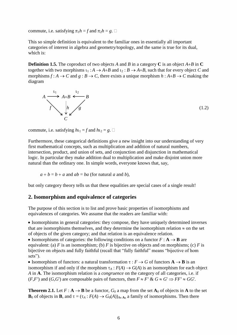
Definition 1.5. The coproduct of two objects A and B in a category C is an object AB in C
together with two morphisms 1 : A AB and 2 : B AB, such that for every object C and
morphisms f : A C and g : B C, there exists a unique morphism h : AB C making the
diagram
1 2
A AB B
f h g (1.2)
C
commute, i.e. satisfying h1 = f and h2 = g.
Furthermore, these categorical definitions give a new insight into our understanding of very
first mathematical concepts, such as multiplication and addition of natural numbers,
intersection, product, and union of sets, and conjunction and disjunction in mathematical
logic. In particular they make addition dual to multiplication and make disjoint union more
natural than the ordinary one. In simple words, everyone knows that, say,
a b = b a and ab = ba (for natural a and b),
but only category theory tells us that these equalities are special cases of a single result!
2. Isomorphism and equivalence of categories
The purpose of this section is to list and prove basic properties of isomorphisms and
equivalences of categories. We assume that the readers are familiar with:
Isomorphisms in general categories: they compose, they have uniquely determined inverses
that are isomorphisms themselves, and they determine the isomorphism relation on the set
of objects of the given category; and that relation is an equivalence relation.
Isomorphisms of categories: the following conditions on a functor F : A B are
equivalent: (a) F is an isomorphism; (b) F is bijective on objects and on morphisms; (c) F is
bijective on objects and fully faithful (recall that “fully faithful” means “bijective of hom
sets”).
Isomorphism of functors: a natural transformation : F G of functors A B is an
isomorphism if and only if the morphism A : F(A) G(A) is an isomorphism for each object
A in A. The isomorphism relation is a congruence on the category of all categories, i.e. if
(F,F ') and (G,G') are composable pairs of functors, then F F ' & G G' FF ' GG'.
Theorem 2.1. Let F : A B be a functor, G0 a map from the set A0 of objects in A to the set
B0 of objects in B, and = (A : F(A) G0(A))AA0 a family of isomorphisms. Then there

7
exists a unique functor G : A B, for which G0 is the object function and : F G is an
(iso)morphism.
Proof. On the one hand : F G is an isomorphism if and only if for each morphism
: A A' in A, we have G() = A'F()A1
, and on the other hand it is easy to check that
sending : A A' to A'F()A1
determines a functor A B whose object function is G0.
Remark 2.2. (a) Since G0 above is completely determined by the family = (A)AA0, the
assumptions of Theorem 2.1 should be understood as “given F : A B and, for each object A
in A, an isomorphism A from F(A) to somewhere”.
(b) Theorem 2.1 has an interesting application: Starting from an arbitrary isomorphism
: X Y in a category A, we apply this theorem to B = A, F = 1A, and
: X Y, if A = X;
A = 1
: Y X, if A = Y; (2.1)
1A : A A, if X A Y;
it is easy to see that the resulting functor G : A A is an isomorphism (for, use Theorem
2.3(c) below, and the fact that a functor is an isomorphism if and only it is bijective on objects
and fully faithful). This in fact explains how to interchange isomorphic objects in any
categorical construction.
Given a functor F : A B and objects A and A' in A, let us write
FA,A' : homA(A,A') homB(F(A),F(A')) (2.2)
for the induced map between the hom sets homA(A,A') and homB(F(A),F(A')). As in fact
already observed in the proof of Theorem 2.1, given an isomorphism : F G, the diagram
homB(F(A),F(A'))
FA,A'
homA(A,A') f A'fA1
g A'1
gA (2.3)
GA,A'
homB(G(A),G(A'))
commutes. Since its vertical arrows are bijections, we obtain:
Theorem 2.3. If F and G are isomorphic functors, then:
(a) F is faithful (=all FA,A'’s above are injective) if and only if so is G;
(b) F is full (=all FA,A'’s above are surjective) if and only if so is G;
(c) F is fully faithful (=all FA,A'’s above are bijective) if and only if so is G.
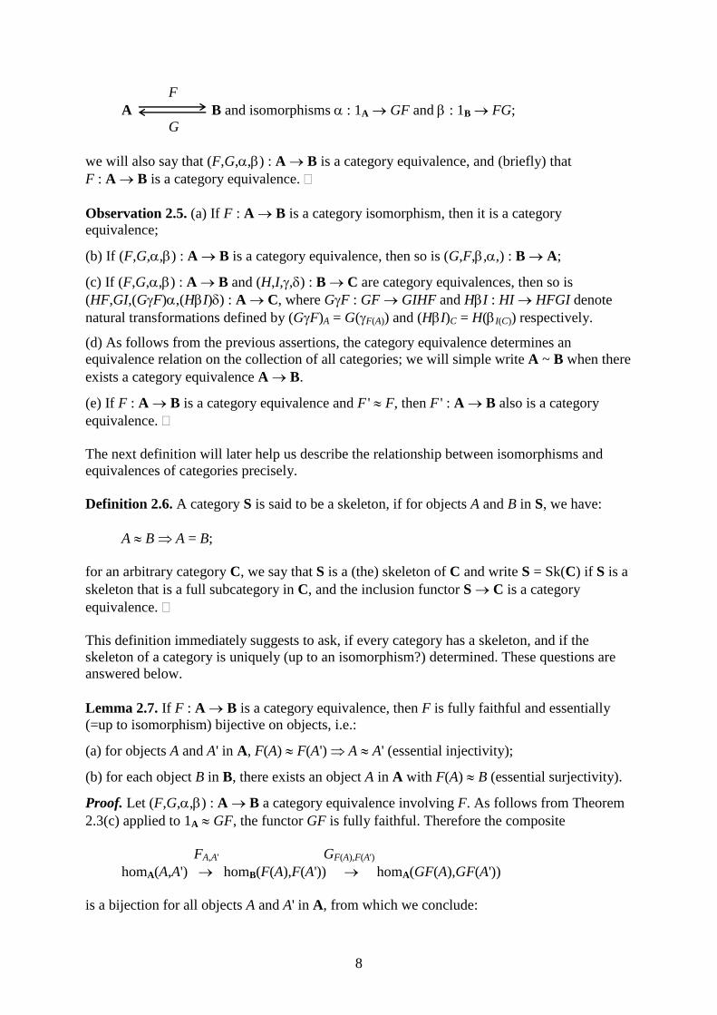
Definition 2.4. An equivalence of categories A and B is a system consisting of functors
8
F
A B and isomorphisms : 1A GF and : 1B FG;
G
we will also say that (F,G,,) : A B is a category equivalence, and (briefly) that
F : A B is a category equivalence.
Observation 2.5. (a) If F : A B is a category isomorphism, then it is a category
equivalence;
(b) If (F,G,,) : A B is a category equivalence, then so is (G,F,,,) : B A;
(c) If (F,G,,) : A B and (H,I,,) : B C are category equivalences, then so is
(HF,GI,(GF),(HI)) : A C, where GF : GF GIHF and HI : HI HFGI denote
natural transformations defined by (GF)A = G(F(A)) and (HI)C = H(I(C)) respectively.
(d) As follows from the previous assertions, the category equivalence determines an
equivalence relation on the collection of all categories; we will simple write A ~ B when there
exists a category equivalence A B.
(e) If F : A B is a category equivalence and F ' F, then F ' : A B also is a category
equivalence.
The next definition will later help us describe the relationship between isomorphisms and
equivalences of categories precisely.
Definition 2.6. A category S is said to be a skeleton, if for objects A and B in S, we have:
A B A = B;
for an arbitrary category C, we say that S is a (the) skeleton of C and write S = Sk(C) if S is a
skeleton that is a full subcategory in C, and the inclusion functor S C is a category
equivalence.
This definition immediately suggests to ask, if every category has a skeleton, and if the
skeleton of a category is uniquely (up to an isomorphism?) determined. These questions are
answered below.
Lemma 2.7. If F : A B is a category equivalence, then F is fully faithful and essentially
(=up to isomorphism) bijective on objects, i.e.:
(a) for objects A and A' in A, F(A) F(A') A A' (essential injectivity);
(b) for each object B in B, there exists an object A in A with F(A) B (essential surjectivity).
Proof. Let (F,G,,) : A B a category equivalence involving F. As follows from Theorem
2.3(c) applied to 1A GF, the functor GF is fully faithful. Therefore the composite
FA,A' GF(A),F(A')
homA(A,A') homB(F(A),F(A')) homA(GF(A),GF(A'))
is a bijection for all objects A and A' in A, from which we conclude:

9
F is faithful;
since F is always faithful in such a situation, G is also faithful by 2.5(b);
since G is faithful, GF(A),F(A') is always injective;
since FA,A' and GF(A),F(A') are injective and their composite is bijective, FA,A' is bijective too.
That is, F is fully faithful. Essential bijectivity on objects is obvious:
F(A) F(A') A GF(A) GF(A') A' and F(A) B for A = G(B).
Remark 2.8. (a) In fact the crucial properties here are fully faithful-ness and essential
surjectivity, since it is easy to show that a fully faithful functor is always essentially injective
on objects. Indeed, if F : A B is fully faithful, and : F(A) F(A') is an isomorphism in
B, then we can choose : A A' with F() = and ' : A' A with F(') = 1
– and these
chosen morphisms will be inverse to each other since so are their images under F.
(b) Proving essential injectivity of the functor F in (a) we in fact also proved another
important property of a fully faithful functor, which is reflection of isomorphisms. It says: if
F() is an isomorphism, then so is .
From Observation 2.5(a), Lemma 2.7, and Remark 2.8 we obtain:
Lemma 2.9. The following conditions on a functor F between skeletons are equivalent:
(a) F is a category equivalence;
(b) F is fully faithful and essentially bijective on objects;
(c) F is fully faithful and essentially surjective on objects;
(d) F is an isomorphism.
Remark 2.10. (a) It is not, however, true of course that G = F1
for any equivalence
(F,G,,) : A B between skeletons.
(b) As follows from 2.5(d) and 2.9(a)(d), skeletons of equivalent categories are always
isomorphic. In particular so are every two skeletons of the same category.
Theorem 2.11. Every category has a skeleton.
Proof. Given a category A, we choose:
an object in each isomorphism class of objects in A, and for any object A in A, the chosen
object isomorphic to A will be denoted by (A);
an isomorphism A : A (A), assuming for simplicity that (A) = 1(A);
: A A to be the functor obtained from the identity functor of A and the family (A)AA0
as in Theorem 2.1 (see also Remark 2.2(a)), making : 1A an isomorphism;
S to be the full subcategory in A with object all (A) (A A0);
F : S A to be the inclusion functor;
G : A S defined by FG = (which indeed defines a functor since the image of is
inside S), making GF = 1S, since (A) = 1(A) for all objects A in A0.
Here S is a skeleton and (F,G,11S,) : S A is a category equivalence.
Theorem 2.12. (a) A functor is a category equivalence if and only if it is fully faithful and
essentially surjective on objects.

10
(b) Two categories are equivalent if and only if they have isomorphic skeletons.
Proof. (a): Suppose F : A B is fully faithful and essentially surjective on objects. Consider
the diagram
F
A B
K L M N (2.4)
NFK
Sk(A) Sk(B)
(NFK)1
in which:
the vertical arrows determine equivalences A ~ Sk(A) and B ~ Sk(B), which exist by
Theorem 2.11.
the composite NFK is fully faithful and essentially surjective on objects, because so are N,
F, and K; therefore NFK is an isomorphism by Lemma 2.9(c)(d).
Using Observation 2.5 we conclude that MNFKL is a category equivalence, and then that
since MNFKL 1BF1A = F, so is F.
The “only if” part is Lemma 2.7.
(b): Again, just use Observation 2.5, Lemma 2.9, and the square diagram above (although the
“only if” part has already been proved: see Remark 2.10(b)).
3. Yoneda lemma and Yoneda embedding
The purpose of this section is to describe fully faithful functors
Y G
C SetsCop
(CatC), (3.1)
where C is an arbitrary category, SetsCop
is the category of functors Cop
Sets, and (CatC)
is the comma category of the category Cat of all categories over the category C (i.e. the
category of pairs (D,P), where D is a category and P : D C a functor. As we will see, the
fully faithful-ness of Y will follow from
Theorem 3.1(“Yoneda lemma”). For any functor T : Cop
Sets and any object C in C, the
map
Nat(homC(,C),T) T(C), C(1C) (3.2)
from the set Nat(homC(,C),T), of natural transformations from homC(,C) to T, to the set
T(C) is bijective.
Proof. Let us denote the map above by and define a map : T(C) Nat(homC(,C),T) by
(t)A(f) = T(f)(t) – for a t T(C) and a morphism f : A C in C.

11
We are going to show that and are inverse to each other. We have
(t) = (t)C(1C) = T(1C)(t) = t for each t T(C),
proving that is the identity map of T(C). On the other hand, for : homC(,C) T and
f : A C, we have
()A(f) = T(f)(()) = T(f)(C(1C)) = A(homC(f,C)(1C)) = A(f),
where the last equality is visible in the naturality square
C
homC(C,C) T(C)
homC(f,C) T(f)
homC(A,C) T(A),
A
and the equality ()A(f) = A(f) (for all f) implies that is the identity map of
Nat(homC(,C),T).
Consider the special case of this theorem in which the functor T is of the form T = homC(,C')
for some C' in C. Then the bijection of Theorem 3.1 together with its inverse become
C(1C)
Nat(homC(,C),homC(,C')) homC(C,C'), (3.3)
(f tf) t
where (f tf) t means that t : C C' is sent to the natural transformation
: homC(,C) homC(,C') defined by A(f) = tf.
However this map homC(C,C') Nat(homC(,C),homC(,C')) is the same as YC,C', where
Y : C SetsCop
is the functor defined by Y(C) = homC(,C),
i.e. the functor corresponding to the functor hom : CopC Sets via the canonical category
isomorphism
homCat(CopC,Sets) homCat(C,Sets
Cop
). (3.4)
Therefore Theorem 3.1 gives
Corollary 3.2. The functor
Y : C SetsCop
defined by Y(C) = homC(,C) (3.5)
is fully faithful.
12
The functor Y above is usually called the Yoneda embedding (for C), while the functor
G : SetsCop
(CatC) we are going to introduce now has no name; a somewhat artificial
name would be “the discrete form of Grothendieck construction”.
For a functor T : Cop
Sets, the category El(T) is defined as the category of pairs (A,a),
where A is an object in C and a is an element T(A); in this category, a morphism
f : (A,a) (B,b) is a morphism f : A B in C with T(f)(b) = a.
We define the functor
G : SetsCop
(CatC) by G(T) = (El(T),PT),
where PT : El(T) C is the forgetful functor, sending f : (A,a) (B,b) to f : A B. In order
to see how exactly is G defined on morphisms, let us describe morphisms in (CatC) of the
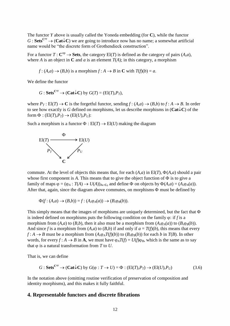
form : (El(T),PT) (El(U),PU):
Such a morphism is a functor : El(T) El(U) making the diagram
El(T) El(U)
PT PU
C
commute. At the level of objects this means that, for each (A,a) in El(T), (A,a) should a pair
whose first component is A. This means that to give the object function of is to give a
family of maps = (A : T(A) U(A))AC0 and define on objects by (A,a) = (A,A(a)).
After that, again, since the diagram above commutes, on morphisms must be defined by
(f : (A,a) (B,b)) = f : (A,A(a)) (B,B(b)).
This simply means that the images of morphisms are uniquely determined, but the fact that
is indeed defined on morphisms puts the following condition on the family : if f is a
morphism from (A,a) to (B,b), then it also must be a morphism from (A,A(a)) to (B,B(b)).
And since f is a morphism from (A,a) to (B,b) if and only if a = T(f)(b), this means that every
f : A B must be a morphism from (A,AT(f)(b)) to (B,B(b)) for each b in T(B). In other
words, for every f : A B in A, we must have AT(f) = U(f)B, which is the same as to say
that is a natural transformation from T to U.
That is, we can define
G : SetsCop
(CatC) by G( : T U) = : (El(T),PT) (El(U),PU) (3.6)
In the notation above (omitting routine verification of preservation of composition and
identity morphisms), and this makes it fully faithful.
4. Representable functors and discrete fibrations

13
Definition 4.1. (a) A functor T : Cop
Sets is said to be representable if it is isomorphic to a
functor of the form Y(C) = homC(,C) for some object C in C.
(b) A functor P : D C is said to be a discrete fibration, if the diagram
D1 D0
P1 P0 (4.1)
C1 C0,
in which the horizontal arrows are the codomain maps of D and C, and the vertical arrows are
the morphism function and the object function of P respectively, is a pullback.
This section is devoted to the following two theorems:
Theorem 4.2. A functor T : Cop
Sets is representable if and only if the category El(T) has a
terminal object. Moreover, a natural transformation : homC(,C) T is an isomorphism if
and only if the pair (C,t), in which t is the image of under the map (3.2), is a terminal object
in El(T).
Proof. For the assertions (a) – (f) below we obviously have (a)(b)(c)(d)(e)(f):
(a) : homC(,C) T is an isomorphism;
(b) A : homC(A,C) T(A) is a bijection for each object A in C;
(c) for every object A in C and every a T(A) there exists a unique morphism f : A C with
A(f) = a;
(d) for every object A in C and every a T(A) there exists a unique morphism f : A C with
T(f)C(1C) = a;
(e) for every object (A,a) in El(T) there exists a unique morphism from (A,a) to (C,C(1C));
(f) (C,C(1C)) is a terminal object in El(T).
And since (C,C(1C)) is exactly the image of under the map (3.2), this completes the proof.
Theorem 4.3. A functor P : D C is a discrete fibration, if and only if the object (D,P) of
(CatC) is isomorphic to G(T) = (El(T),PT), for some functor T : Cop
Sets.
Proof. “If”: We have to prove that (El(T),PT) is always a discrete fibration. This means to
prove that for every morphism f : A B in C and every b T(B), there exists a unique a
T(A) for which f is a morphism from (A,a) to (B,b). However this is trivial since f is a
morphism from (A,a) to (B,b) if and only if a = T(f)(b).
“Only if”: Assuming that P : D C is a discrete fibration, we define a functor T : Cop
Sets
as follows:
For an object C in C, we take T(C) to be the set of objects D in D with P(D) = C.
For a morphism f : A B in C, and an element b in T(B), which in fact an object in D with
P(b) = B, we take g to be the morphism g in D, with P(g) = f and codomain of g equal to b.
The existence and uniqueness of such a g follows from the fact that the diagram (4.1) is a
pullback. We then take T(f)(b) to be the domain of g.

14
Accordingly the procedure of defining T(f)’s (for all f) displays as
D
T(f)(b) b
–
(4.2)
C
A B
and it is easy to see that it indeed defines a functor T : Cop
Sets in such a way that
(El(T),PT) becomes isomorphic to (D,P).
5. Adjoint functors
Adjoint functors will be defined at the end of this section via several equivalent kinds of data
that will be described before.
Definition 5.1. Let U : A X be a functor and X an object in X. A universal arrow X U is
a pair (F(X),X) in which F(X) is an object in A and X : X UF(X) a morphism in X with
the following universal property: for every object A in A and every morphism u : X U(A) in
X there exists a unique morphism f : F(X) A making the diagram
UF(X) U(f)
U(A)
X (5.1)
u
X
commute.
Theorem 5.2. Let U : A X be a functor and ((F(X),X))XX0 a family of universal arrows
X U given for each object X in X. Then there exists a unique functor F : X A for which
the family ((F(X),X))XX0 determines a natural transformation : 1X UF.
Proof. Given a morphism h : X Y in X, we can define F(h) : F(X) F(Y) as the unique
morphism making the diagram (5.1) commute for A = F(Y) and u = Yh. Since the
commutativity of (5.1) in this case is equivalent to the commutativity of the naturality square

15
UF(h)
UF(X) UF(Y)
X Y (5.2)
X Y,
h
this proves the theorem.
Observation 5.3. (a) The universal property given in Definition 5.1 can be equivalently
reformulated as: the map
X,A : homA(F(X),A) homX(X,U(A)), defined by X,A(f) = U(f)X, (5.3)
is a bijection for each object A in A. Moreover, since this map is obviously natural in A, that
universal property can also be reformulated as: the natural transformation
X, : homA(F(X),) homX(X,U()), defined by X,A(f) = U(f)X, (5.4)
is an isomorphism. Furthermore, let
X, : homA(F(X),) homX(X,U()) (5.5)
be an arbitrary isomorphism. Then, for any f : F(X) A, using the naturality square
X,F(X)
homA(F(X),F(X)) homX(X,U(F(X)))
homA(F(X),f) homX(X,U(f)) (5.6)
homA(F(X),A) homX(X,U(A)),
X,A
we obtain X,A(f) = X,AhomA(F(X),f)(1F(X)) = homX(X,U(f))X,F(X)(1F(X)) = U(f)X,F(X)(1F(X)).
Therefore we have one more reformulation of the universal property given in Definition 5.1,
namely: there exists an isomorphism (5.5); and with this reformulation X and X, determine
each other by
X,A(f) = U(f)X and X = X,F(X)(1F(X)). (5.7)
(b) The relationship between X and X, can be seen of course as a special case of the
statement dual to Theorem 4.2, but we omit details here.
(c) Suppose X, or, equivalently, X, is given for every object X in X. Then, by Theorem 5.2,
there is a unique way to make F a functor X A, so that the family ((F(X),X))XX0
determines a natural transformation : 1X UF. And it is easy to check that this will also
make X, natural in X, yielding a natural isomorphism
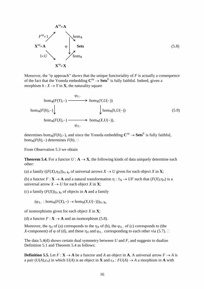
16
AopA
Fop1 homA
XopA Sets (5.8)
1U homX
XopX
Moreover, the “ approach” shows that the unique functoriality of F is actually a consequence
of the fact that the Yoneda embedding Cop
SetsC is fully faithful. Indeed, given a
morphism h : X Y in X, the naturality square
Y,
homA(F(Y),) homX(Y,U())
homA(F(h),) homX(h,U()) (5.9)
homA(F(X),) homX(X,U()),
X,
determines homA(F(h),), and since the Yoneda embedding Cop
SetsC is fully faithful,
homA(F(h),) determines F(h).
From Observation 5.3 we obtain
Theorem 5.4. For a functor U : A X, the following kinds of data uniquely determine each
other:
(a) a family ((F(X),X))XX0 of universal arrows X U given for each object X in X;
(b) a functor F : X A and a natural transformation : 1X UF such that (F(X),X) is a
universal arrow X U for each object X in X;
(c) a family (F(X))XX0 of objects in A and a family
(X, : homA(F(X),) homX(X,U()))XX0
of isomorphisms given for each object X in X;
(d) a functor F : X A and an isomorphism (5.8).
Moreover, the X of (a) corresponds to the X of (b), the X, of (c) corresponds to (the
X-component) of of (d), and these X and X, corresponding to each other via (5.7).
The data 5.4(d) shows certain dual symmetry between U and F, and suggests to dualize
Definition 5.1 and Theorem 5.4 as follows:
Definition 5.5. Let F : X A be a functor and A an object in A. A universal arrow F A is
a pair (U(A),A) in which U(A) is an object in X and A : FU(A) A a morphism in A with

17
the following universal property: for every object X in X and every morphism f : F(X) A in
A there exists a unique morphism u : X U(A) making the diagram
FU(A) F(u)
F(X)
A (5.10)
f
A
commute.
Theorem 5.6. For a functor F : X A, the following kinds of data uniquely determine each
other:
(a) a family ((U(A),A))AA0 of universal arrows F A given for each object A in A;
(b) a functor U : A X and a natural transformation : FU 1A such that (U(A),A) is a
universal arrow F A for each object A in A;
(c) a family (U(A))AA0 of objects in X and a family
(,A : homX(,U(A)) homA(F(),A))AA0
of isomorphisms given for each object A in A;
(d) a functor U : A X and an isomorphism
AopA
Fop1 homA
XopA Sets (5.11)
1U homX
XopX
Moreover, the A of (a) corresponds to the A of (b), the ,A of (c) corresponds to (the
A-component) of of (d), and these A and ,A corresponding to each other via
X,A(u) = AF(u) and A = U(A),A(1U(A)). (5.12)
Remark 5.7. The data described in Theorem 5.4(d) is obviously identical to the data
described in Theorem 5.6(d): just take and inverse to each other. Therefore these two
theorems actually describe eight equivalent kinds of data.
Remark 5.7 is not the end of this story: although eight is a large number, it is good to add at
least one more, which is purely equational. For, we observe:
18
Having functors U : A X and F : X A, and merely natural transformations
: 1X UF and : FU 1A, we can still define natural transformations and as in (5.8)
and in (5.11) respectively.
Under no conditions on and , those and will also be merely natural transformations
independent from each other. But requiring them to be each other’s inverses and
reformulating this requirement in terms of and will give us a new equivalent form of the
desired data, which is purely equational.
Requiring and to be each other’s inverses means to require X,AX,A(f) = f and
X,AX,A(u) = u for each f : F(X) A in A and each u : X U(A) in X. But then Yoneda
lemma (Theorem 3.1) tells us that it suffices to have these equalities for
f = 1F(X) : F(X) F(X) and u = 1U(A) : U(A) U(A).
Thus, we are interested in X,F(X)X,F(X)(1F(X)) = 1F(X) and U(A),AU(A),A(1U(A)) = 1U(A).
Translated into the language of and , these equations become
F(X)F(X) = 1F(X) and U(A)U(A) = 1U(A), (5.13)
and we obtain:
Theorem 5.8. Let U : A X and F : X A be functors and : 1X UF and : FU 1A
natural transformations. The following conditions are equivalent:
(a) (F(X),X) is a universal arrow X U for each object X in X, and is the corresponding
family of morphisms, i.e. U(A)U(A) = 1U(A) for every object A in A;
(b) (U(A),A) is a universal arrow F A for each object A in A, and is the corresponding
family of morphisms, i.e. F(X)F(X) = 1F(X) for every object X in X;
(c) the equalities F(X)F(X) = 1F(X) and U(A)U(A) = 1U(A) hold for every object X in X and
every object A in A.
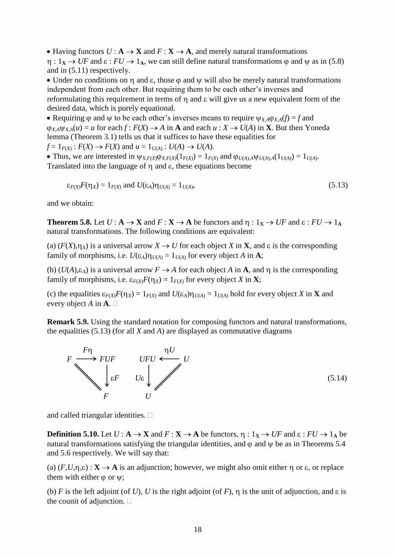
Remark 5.9. Using the standard notation for composing functors and natural transformations,
the equalities (5.13) (for all X and A) are displayed as commutative diagrams
F U
F FUF UFU U
F U (5.14)
F U
and called triangular identities.
Definition 5.10. Let U : A X and F : X A be functors, : 1X UF and : FU 1A be
natural transformations satisfying the triangular identities, and and be as in Theorems 5.4
and 5.6 respectively. We will say that:
(a) (F,U,,) : X A is an adjunction; however, we might also omit either or , or replace
them with either or ;
(b) F is the left adjoint (of U), U is the right adjoint (of F), is the unit of adjunction, and is
the counit of adjunction.
19
6. Monoidal categories
In this section we introduce monoidal categories with some examples and related concepts.
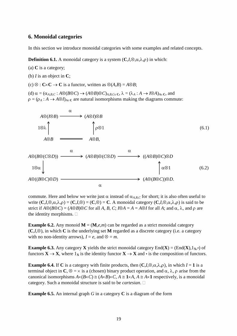
Definition 6.1. A monoidal category is a system (C,I,,,,) in which:
(a) C is a category;
(b) I is an object in C;
(c) : CC C is a functor, written as (A,B) = AB;
(d) = (A,B,C : A(BC) (AB)C)A,B,CC, = (A : A IA)AC, and
= (A : A AI)AC are natural isomorphisms making the diagrams commute:
A(IB) (AI)B
1 1 (6.1)
AB AB,
A(B(CD)) (AB)(CD) ((AB)C)D
1 1 (6.2)
A((BC)D) (A(BC))D.
commute. Here and below we write just instead of A,B,C for short; it is also often useful to
write (C,I,,,,) = (C,I,) = (C,) = C. A monoidal category (C,I,,,,) is said to be
strict if A(BC) = (AB)C for all A, B, C; IA = A = AI for all A; and , , and are
the identity morphisms.
Example 6.2. Any monoid M = (M,e,m) can be regarded as a strict monoidal category
(C,I,), in which C is the underlying set M regarded as a discrete category (i.e. a category
with no non-identity arrows), I = e, and = m.
Example 6.3. Any category X yields the strict monoidal category End(X) = (End(X),1X,•) of
functors X X, where 1X is the identity functor X X and • is the composition of functors.
Example 6.4. If C is a category with finite products, then (C,I,,,,), in which I = 1 is a
terminal object in C, = is a (chosen) binary product operation, and , , arise from the
canonical isomorphisms A(BC) (AB)C, A 1A, A A1 respectively, is a monoidal
category. Such a monoidal structure is said to be cartesian.
Example 6.5. An internal graph G in a category C is a diagram of the form

20
dG
G1 G0
cG
in C. For a fixed object O, the internal graphs G in C with G0 = O are called internal O-graphs
in C, and their category will be denoted by Graphs(C,O); a morphism f : G H in
Graphs(C,O) is a morphism f : G1 H1 in C with dHf = dG and cHf = cG. When C has chosen
pullbacks, this category becomes a monoidal category (Graphs(C,O),I,,,,) as follows:
I has I0 = I1 = O and dI = cI = 1O;
is defined as the span composition, i.e. for G and H in Graphs(C,O), GH is defined by
(GH)1 = G1OH1, dGH = dH2, and cGH = cG1 via the diagram
G1OH1
1 2
G1 H1 (6.3)
cG dG cH dH
O O O,
in which diamond part is the chosen pullback of the pair (dG,cG).
, , and arise from the appropriate canonical isomorphisms.
In the special case in which O = 1 is a terminal object in C, the pullbacks we need become
binary products, and the monoidal category we obtain coincides with the one from Example
6.4.
Example 6.6. Dualizing Example 6.4, if C is a category with finite coproducts, then
(C,I,,,,), in which I = 0 is an initial object in C, = + is a (chosen) binary coproduct
operation, and , , arise from the canonical isomorphisms A+(B+C) (A+B)+C, A 0+A,
A A+0 respectively, is a monoidal category.
Example 6.7. Let R be a commutative ring, and C the category of R-modules. Then
(C,I,,,,), in which I = R, the usual tensor product over R, and , , the usual natural
isomorphisms, forms a monoidal category.
Definition 6.8. Let C = (C,I,,,,) and C' = (C',I,,,,) be monoidal categories (we use
the prime sign ' only for C, although the I, , etc. in C and in C' are not, of course, supposed
to be the same). A monoidal functor F = (F,,) : C C' consists of
(a) an ordinary functor F : C C';
(b) a morphism : I F(I) in C';
(c) a natural transformation = (A,B : F(A)F(B) F(AB))A,BC making the diagrams

21
F(A)(F(B)F(C)) (F(A)F(B))F(C)
1 1
F(A)(F(BC)) (F(AB))F(C) (6.4)
F(A(BC)) F((AB)C),
F()
IF(A) F(A)
1 F() (6.5)
F(I)F(A) F(IA),
F(A)I F(A)
1 F() (6.6)
F(A)F(I) F(AI),
commute. A monoidal functor F = (F,,) is said to be strong if and are isomorphisms,
and strict if moreover F(I) = I, F(A)F(B) = F(AB) for all A and B, and and are the
identity morphisms.
Definition 6.9. Let Fi = (Fi,i,i) : C C' (i = 1,2) be monoidal functors. A monoidal natural
transformation : F1 F2 is an ordinary natural transformation : F1 F2 such that the
diagrams
1
I F1(I)
(6.7)
I F2(I), 2
22
1
F1(A)F1(B) F1(AB)
(6.8)
F2(A)F2(B) F2(AB) 2
commute.
Several examples of monoidal functors are used as definitions of important concepts. Two of
them will be given here with further cases considered in the next sections.
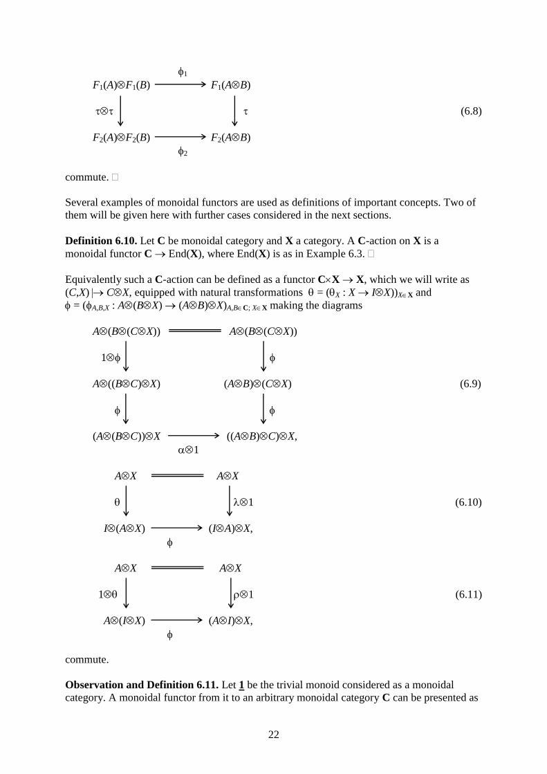
Definition 6.10. Let C be monoidal category and X a category. A C-action on X is a
monoidal functor C End(X), where End(X) is as in Example 6.3.
Equivalently such a C-action can be defined as a functor CX X, which we will write as
(C,X) CX, equipped with natural transformations = (X : X IX))XX and
= (A,B,X : A(BX) (AB)X)A,BC; XX making the diagrams
A(B(CX)) A(B(CX))
1
A((BC)X) (AB)(CX) (6.9)
(A(BC))X ((AB)C)X,
1
AX AX
1 (6.10)
I(AX) (IA)X, AX AX
1 1 (6.11)
A(IX) (AI)X,
commute.
Observation and Definition 6.11. Let 1 be the trivial monoid considered as a monoidal
category. A monoidal functor from it to an arbitrary monoidal category C can be presented as

23
a triple M = (M,e,m), in which M is an object in C and e : I M and m : MM M
morphisms in C making the diagram
m1 (e1)
M(MM) (MM)M MM M
1m m (1e) (6.12)
MM M MM
m m
commute. Such a triple is called a monoid in C.
Moreover, a monoidal natural transformation : (M1,e1,m1) (M2,e2,m2) being a morphism
: M1 M2 in C with e1 = e2 and m1 = m2(), is nothing but a monoid homomorphism
in C. So, the monoids in C form a category Mon(C), which is the category MonCat(1,C) of
monoidal functors 1 C. In particular this immediately tells us that every monoidal functor
F = (F,,) : C C' induces a functor Mon(F) : Mon(C) Mon(C'), which sends (M,e,m) to
the composite
(M,e,m) (F,,)
1 C C'
considered as a monoid in C'.
7. Monads and algebras
In this section we introduce monads, algebras over monads, and free algebras; we also
introduce a very general notion of a monoid action as a “general example”.
Definition 7.1. A monad on a category X is a monoid in the monoidal category End(X) of
Example 6.3. Explicitly, a monad on X is a triple T = (T,,), in which T : X X is a functor
and : 1X T and : T2 T natural transformations making the diagram
T T
T3 T
2 T
T T (7.1)
T2 T T
2
commute.
Definition 7.2. Let T = (T,,) be a monad on a category X. A T-algebra (or an algebra over
T) is a pair (X,), in which X is an object in X and : T(X) X a morphism making the
diagram

24
X X
T2(X) T(X) X
T() (7.2)
T(X) X
commute. A morphism h : (X,) (X ',') of T-algebras is a morphism h : X X ' making the
diagram
T(h)
T(X) T(X ')
' (7.3)
X X '
h
commute. The category of T-algebras will be denoted by XT.
Theorem 7.3. Let T = (T,,) be a monad on a category X, and let UT : X
T X be the
forgetful functor defined by UT(X,) = X. Then:
(a) for each object X in X, the pair (T(X),X) is a T-algebra;
(b) the functor FT : X X
T, defined by F
T(X) = (T(X),X) is a left adjoint of U
T. The unit and
counit of the adjunction are, respectively, : 1X T = UTF
T and : F
TU
T 1XT defined by
(T(X),X) = X.
Proof. (a): We have to prove the commutativity of
T(X) T(X)
T3(X) T
2(X) T(X)
T(X) X (7.4)
T2(X) T(X)
X
but it follows from the commutativity of (7.1).
(b): The square part of (7.4) insures that putting
(T(X),X) = X
determines a natural transformation : FTU
T 1XT, and it is easy to see that and satisfy
the triangular identities.
Example 7.4. Let X be a category equipped with an action of a monoidal category C.
According to Definition 6.10, such an action is simply a monoidal functor F : C End(X),

25
and, like every monoidal functor, it induces a functor Mon(F) : Mon(C) Mon(End(X)).
Therefore every monoid M = (M,e,m) in C determines a monad on X; the algebras over that
monad are called M-actions, and their category is denoted by XM
. Explicitly, such an M-action
is a pair (X,), in which : MX X is a morphism in X making the diagram
m1 (e1)
M(MX) (MM)X MX X
1
MX X
commute. Here and are as in (6.9)–(6.11).
Remark 7.5. (a) According to G. M. Kelly, an “M-action” is the right name not for a pair
(X,) above, but just for its structure morphism .
(b) Example 7.4 is at the same time a “generalization”. Indeed, starting from an arbitrary
monad T on X, we can consider T-algebras as T-actions in the sense of Example 7.4, putting
C = End(X) and considering the identity momoidal functor End(X) End(X) as the action of
End(X) on X.
8. More on adjoint functors and category equivalences
This section contains additional observations on adjoint functors and category equivalence;
some them will be explicitly used later, while others simply help to understand the concepts
involved. We begin with
Observation 8.1. (a) It is easy to see that (F,U,,) : X A is an adjunction if and only if so
is (Uop
,Fop
,op
,op
) : Xop
Aop
(in the obvious notation). Therefore every general property of
adjoint functors has its dual, where the left and the right adjoints exchange their roles (see e.g.
Theorems 8.5 and 8.6 below).
(b) Since in an adjunction (F,U,,) : X A, X : X UF(X) is a universal arrow X U for
each object X in X, the functor U alone determines such an adjunction uniquely up to an
isomorphism; dually, the same is true for F.
(c) It is easy to see that adjunctions compose: if (F,U,,) : X A and (G,V,,) : Y X are
adjunctions, then so is (FG,VU,(VG),(FU)) : Y A (cf. 2.5(c)).
(d) Let
K
A B
M
K' M ' N L (8.1)
N '
B' C
L'
26
a diagram of functors in which M, M ', N, and N ' are the left adjoints of K, K', L, and L'
respectively. Then, as easily follows from (b) and (c), we have LK L'K' MN M 'N '.
Lemma 8.2. Every fully faithful functor reflects isomorphisms, i.e. under such a functor only
isomorphisms are sent to isomorphisms.
Proof. Let U : A X be a fully faithful functor with U(f : A B) being an isomorphism.
Since U is full, U(f)1
= U(g) for some g : B A in A. Then since U(gf) = 1U(A), U(fg) = 1U(B),
and U is faithful, we obtain gf = 1A and fg = 1B, which shows that f : A B is an
isomorphism.
Definition 8.3. An adjunction (F,U,,) : X A is said to be an adjoint equivalence if and
are isomorphisms.
Theorem 8.4. Let U : A X be a category equivalence, F0 a map from the set X0 of objects
in X to the set A0 of objects in A, and = (X : X UF0(X))XX0 a family of isomorphisms.
Then there exists a unique functor F : X A and a unique natural transformation
: FU 1A, for which F0 is the object function of F and (F,U,,) : X A is an adjunction.
Moreover, that adjunction is always an adjoint equivalence.
Proof. Since U is fully faithful (by Lemma 2.7) and each X : X UF0(X) is an isomorphism,
it is easy to see that X : X UF0(X) is a universal arrow X U for each object X in X. After
that the first assertion of the theorem follows from Remark 5.7 (see also Definition 5.10).
Next, since X’s are isomorphisms, so are U(A)’s (by the second identity in (5.13)), and by
Lemma 8.2 this implies that is an isomorphism.
Theorem 8.5. Let (F,U,,) : X A be an adjunction. Then:
(a) U is faithful if and only if is an epimorphism;
(b) U is full if and only if is a split monomorphism;
(c) and therefore U is fully faithful if and only if is an isomorphism.
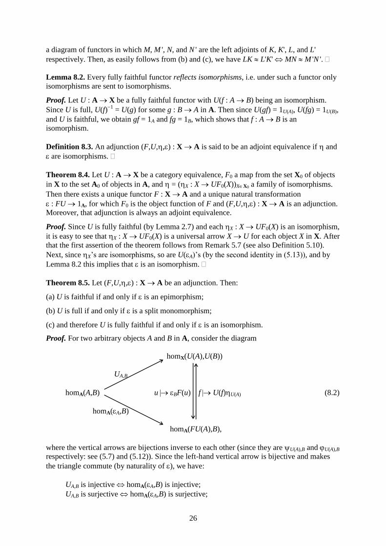
Proof. For two arbitrary objects A and B in A, consider the diagram
homX(U(A),U(B))
UA,B
homA(A,B) u BF(u) f U(f)U(A) (8.2)
homA(A,B)
homA(FU(A),B),
where the vertical arrows are bijections inverse to each other (since they are U(A),B and U(A),B
respectively: see (5.7) and (5.12)). Since the left-hand vertical arrow is bijective and makes
the triangle commute (by naturality of ), we have:
UA,B is injective homA(A,B) is injective;
UA,B is surjective homA(A,B) is surjective;

27
UA,B is bijective homA(A,B) is bijective.
Since homA(A,B) is injective, surjective, or bijective if and only if A is an epimorphism, split
monomorphism, or isomorphism respectively, this completes the proof.
Dually, we obtain:
Theorem 8.6. Let (F,U,,) : X A be an adjunction. Then:
(a) F is faithful if and only if is a monomorphism;
(b) F is full if and only if is a split epimorphism;
(c) and therefore F is fully faithful if and only if is an isomorphism.
– which helps to prove the following:
Theorem 8.7. The following conditions on an adjunction (F,U,,) : X A are equivalent:
(a) (F,U,,) : X A is an adjoint equvalence;
(b) F and U are fully faithful;
(c) F is fully faithful and U reflects isomorphisms;
(d) is an isomorphism and U reflects isomorphisms;
(e) U is fully faithful and F reflects isomorphisms;
(f) is an isomorphism and F reflects isomorphisms.
Proof. (a)(b), (c)(d), and (e)(f) follow from 8.6(a)(c) and 8.5(a)(c). (b)(c) and
(b)(e) follow from Lemma 8.2. Therefore it suffices to prove the implications (d)(a) and
(f)(a). Moreover, since these implications are dual to each other, it suffices to prove only
one of them, say, (d)(a). For, consider the second identity U(A)U(A) = 1U(A) in (5.13).
Assuming that is an isomorphism, we conclude that so is U(A) for each A, and, when U
reflects isomorphisms, this implies that is an isomorphism, as desired.
9. Remarks on coequalizers
The remarks on coequalizers we make in this section are presented as a definition and an
example:
Definition 9.1. (a) A coequalizer diagram in a given category is a diagram in of the form
f
A B h
C (9.1)
g
in which hf = hg, and for every morphism h' : B C' with h'f = h'g, there exists a unique
morphism k : C C' with kh = h'. We will then also say that h is the coequalizer of the pair
(f,g).

28
(b) A morphism that occurs in a coequalizer diagram as the morphism h occurs in (9.1) is
called a regular epimorphism.
(c) A coequalizer diagram is said to be absolute, if it is preserved by any functor, i.e. if its
image under any functor is a coequalizer diagram.
Example 9.2. (a) Consider a split fork, i.e. a diagram of the form
j i
f
A B h
C (9.2)
g
in which hf = hg, hi = 1C, fj = 1B, and gj = ih. In each such diagram f, g, and h form a
coequalizer diagram. Indeed, given h' : B C' with h'f = h'g, it is easy to see that there is a
unique morphism k : C C' with kh = h': just take k = h'i, which gives
kh = h'ih = h'gj = h'fj = h',
and the uniqueness follows from the fact that h is a split epimorphism. Since the conditions
imposed on the diagram (9.2) were purely equational and therefore are “preserved” by every
functor, this also proves that f, g, and h form an absolute coequalizer diagram.
(b) An arbitrary split epimorphism h : B C can be involved in a split fork, namely in
1B i
1B
B B h
C (9.3)
ih
where i is a splitting, i.e. a morphism from C to B with hi = 1C. Therefore every split
epimorphism is a regular epimorphism.
(c) For a monad T = (T,,) on a category X, any T-algebra (X,) determines the following
split fork in X:
T(X) X
X
T2(X) T(X)
X (9.4)
T()
10. Monadicity
In this section we discuss the relationship between adjunctions and monad.
Theorem 10.1. For every adjunction (F,U,,) : X A, the triple T = (T,,) defined by

29
T = UF,
of (T,,) is the same as of (F,U,,),
= UF, i.e. = (X : T2(X) T(X))XX0 is defined by X = U(F(X)),
is a monad on X.
Proof. For the triple above, and any object X in X, the X-component of the diagram (7.1)
becomes
U(FUF(X)) UF(X)
UFUFUF(X) UFUF(X) UF(X)
UFU(F(X)) U(F(X)) UF(X) (10.1)
UFUF(X) UF(X) UFUF(X)
U(F(X)) U(F(X))
and its left-hand square commutes by the naturality of while the triangles commute by the
triangular identities (5.13).
Example 10.2. (a) Starting from an arbitrary monad T = (T,,) on a category X, we obtain
the forgetful-free adjunction (FT,U
T,
T,
T) : X X
T described in Theorem 7.3. It is easy to
see that the corresponding monad on X is the same as the original monad T = (T,,). This
tells us that every monad can be obtained from an adjunction as in Theorem 10.1. Since this
result is originally due to S. Eilenberg and J. Moore, the category XT is often called the
Eilenberg-Moore category (of algebras over T). Note also, that using only free T-algebras, i.e.
the T-algebras of the form FT(X) = (T(X),X) we could also obtain an adjunction whose
corresponding monad is T = (T,,). Furthermore, since such an algebra (T(X),X) is fully
determined by its underlying object X, the full subcategory in XT with objects all free
T-algebras can be described as the so-called Kleisli category of T, whose objects are the same
as the objects in X. In detail:
The category Kleisli(T) is defined as the category with the same objects as the in X, and a
morphism f : X Y being a morphism f : X T(Y) in X; the composite of morphisms
f : X Y and g : Y Z in Kleisli(T) is the composite
f T(g) Z
X T(Y) T2(Z) T (Z)
in X.
The forgetful functor U : Kleisli(T) X is defined by U(f : X Y) = ZT(f) : T(X) T(Y),
and free functor F : X Kleisli(T) is defined by F(f : X Y) = Yf : X T(Y), considered as
a morphism from X to Y in Kleisli(T).
And the monad obtained from adjunction as in Theorem 10.1 is again the same as the
original monad T = (T,,) (a result due to H. Kleisli).
It is now natural ask, to what extend is it possible to recover the adjunction
(F,U,,) : X A from the monad T = (T,,) in the situation of Theorem 10.1? In order to
formulate this question properly, we need:

30
Theorem 10.3. (F,U,,) : X A and T = (T,,) be as in Theorem 10.1. Then there exists a
unique functor K : A XT with U
TK = U and KF = F
T.
Proof. Existence: Simply define K by
K(A) = (U(A),U(A)). (10.2)
To prove that (U(A),U(A)) is indeed a T-algebra is to prove that the diagram
U(FU(A)) U(A)
UFUFU(A) UFU(A) U(A)
UFU(A) U(A) (10.3)
UFU(A) U(A)
U(A)
commutes, which, for the left-hand square, follows from the naturality of , and, for the
triangle, follows from the second identity in (5.13) (cf. (10.1)). Defining K by (10.2), we also
obviously have UTK = U, and KF = F
T since KF(X) = (UF(X),U(F(X))) = (T(X),X) = F
T(X).
Uniqueness: Let H : A XT be a functor satisfying U
TH = U and HF = F
T. Since U
TH = U,
such a functor must be given by H(A) = (U(A),A) for some natural transformation
: UFU U. On the other hand, since HF = FT, we must have F(X) = X = U(F(X)). After
that, comparing the naturality square from (10.3) with the naturality square
U(FU(A)) = FU(A)
UFUFU(A) UFU(A)
UFU(A) U(A)
UFU(A) U(A)
A
we obtain AUFU(A) = U(A)UFU(A), which implies A = U(A), since UFU(A) is a split
epimorphism by the second identity in (5.13).
Definition 10.4. Let (F,U,,) : X A and T = (T,,) be as in Theorems 10.1 and 10.3.
Then:
(a) the functor K : A XT as in Theorem 10.3 is called the comparison functor;
(b) the functor U : A X is said to be monadic if the functor K : A XT above is a category
equivalence.
Accordingly, saying that an adjunction (F,U,,) : X A can be recovered from the
corresponding monad T = (T,,) on X should be understood as saying that the functor U is
monadic. In order to formulate some of the monadicity results, we will need the following
construction containing long calculations:

31
Construction 10.5. Let (F,U,,) : X A and T = (T,,) be as above, and suppose that for
every T-algebra (X,), the pair (F(X),F()) has a coequalizer in A. Then the comparison
functor K : A XT has a left adjoint forming an adjunction (L,K,ή,έ) : X
T A that can be
described as follows:
(a) For a T-algebra (X,), the object L(X,) is defined via the coequalizer diagram
F(X)
FUF(X) F(X) (X,) L(X,) (10.4)
F()
(b) For a morphism h : (X,) (X ',') of T-algebras, we form the diagram
F(X)
FUF(X) F(X) (X,) L(X,)
F()
FUF(h) F(h) L(h) (10.5)
F(X ')
FUF(X ') F(X ') (X ',') L(X ',')
F(')
of solid arrows, in which
(X ',')F(h)F(X) = (X ',')F(X ')FUF(h) = (X ',')F(')FUF(h) = (X ',')F(h)F()
implies the existence and uniqueness of the dotted arrow making the right-hand square
commute. This determines a functor L : XT A.
(c) We then define ή(X,) : (X,) KL(X,) = (UL(X,),U(L(X,))) as the composite U((X,))X,
which we can do since the diagram
UF(X) UFU((X,))
UF(X) UFUF(X) UFUL(X,)
U(L(X,)) (10.6)
X UF(X) UL(X,)
X U((X,))
commutes. Indeed, we have
U(L(X,))UFU((X,))UF(X) = U(L(X,)FU((X,))F(X)) (by functoriality of U)
= U((X,)F(X)F(X)) (by naturality of )
= U((X,)) (by the first identity in (5.13))
= U((X,))U(F(X))UF(X) (by the second identity in (5.13) applied to A = F(X))
= U((X,)F(X))UF(X) (by functoriality of U)
= U((X,)F())UF(X) (since (10.4) is a coequalizer diagram)

32
= U((X,))UF()UF(X) (by functoriality of U)
= U((X,))X (by naturality of ).
(d) To show that ή(X,) is a universal arrow (X,) K is to show that for every morphism
k : (X,) (U(A),U(A)) there exists a unique morphism l : L(X,) A with
U(l)U((X,))X = k.
Since U(l)U((X,)) = U(l(X,)) and (F,U,,) is an adjunction, this is the same as to show that
there exists a unique morphism l : L(X,) A with l(X,) = AF(k). Since (10.4) is a
coequalizer diagram this simply means to show that
AF(k)F(X) = AF(k)F(). (10.7)
For, we have
AF(k)F() = AF(k) (by functoriality of F)
= AF(U(A)UF(k)) (since k : (X,) (U(A),U(A)) is a morphism of T-algebras)
= AFU(AF(k)) (by functoriality of U)
= AF(k)F(X) (by naturality of ),
as desired.
(e) In particular, for an object A in A, the morphism έA : LK(A) A is the unique morphism
L((U(A),U(A)) A making the diagram
FU(A)
FUFU(A) FU(A) (U(A),A)
L((U(A),U(A))
FU(A) (10.8)
A έA
A
commute.
Remark 10.6. As an intermediate result of the calculation in 10.5(c), we have
U((X,))X = U((X,)) (10.9)
for every T-algebra (T(X),). Since ή(X,) : (X,) KL(X,) was defined (in 10.5(c)) as
U((X,))X, this equality together with Example 9.2 tell us that ή(X,) considered as a morphism
in X is the unique morphism making the diagram

33
U(F(X)) = X
UFUF(X) UF(X)
X
UF() = T() (10.10)
U((X,)) ή(X,) = U((X,))X
UL(X,)
commute.
Theorem 10.7. For (F,U,,) : X A and T = (T,,) as above the following conditions are
equivalent:
(a) the functor U : A X is monadic;
(b) the functor U preserves the coequalizer diagram (10.4) for every T-algebra (X,), and, for
every object A in A, the morphism A is the coequalizer of the pair (FU(A),FU(A));
(c) the functor U reflects isomorphisms and preserves the coequalizer diagram (10.4) for
every T-algebra (X,);
(d) the functor U reflects isomorphisms, and every pair (f,g) of parallel morphisms in A, for
which the pair (U(f),U(g)) has an absolute coequalizer, has a coequalizer preserved by U.
Proof. We observe:
Since UTK = U, and U
T : X
T X obviously reflects isomorphisms, U reflects isomorphisms
if and only if K does.
As follows from Remark 10.6 and the fact that the top part of the diagram (10.10) is a
coequalizer diagram (see Example 9.2), the functor U preserves the coequalizer diagram
(10.4) if and only if ή(X,) : (X,) KL(X,) is an isomorphism.
As follows from 10.5(e), the morphism A is the coequalizer of the pair (FU(A),FU(A)) if
and only if έA : LK(A) A is an isomorphism.
This proves (a)(b) and makes (b)(c) a consequence of Theorem 8.7 (in fact a
consequence of the last argument in its proof).
Since the pair (U(F(X)),UF()) = (X,T()) involved in (10.10) is a part of a split fork (9.4),
(d) implies (c).
After this all we need to prove is that if (f,g) of parallel morphisms in XT, for which the pair
(f,g) has an absolute coequalizer in X, then (f,g) has a coequalizer in XT preserved by U
T. For,
consider the diagram
T(f)
T(X) T(Y) T(h)
T(Z)
T(g)
(10.11)
f
X Y h
Z
g
where: h is the coequalizer of (f,g) in X; the left-hand and the middle vertical arrows are the
domain and the codomain of f (and of g) respectively in the category XT; and the dotted arrow
is determined by the fact that the top row in (10.11) is a coequalizer diagram (since h is the

34
absolute coequalizer of (f,g) in X). Using the fact that not only T but also T2 preserves the
equalizer of (f,g), it is easy to check that the dotted arrow determines a T-algebra structure on
Z and then makes h is the coequalizer of (f,g) in XT – and this coequalizer is trivially
preserved by UT.
Remark 10.8. (a) Condition 10.7(d) can modified by asking the pair (U(f),U(g)) to be a split
coequalizer (i.e. to be a part of a split fork) instead of an absolute one. As one can see from
the argument proving (d)(c) of Theorem 10.7, this follows from the fact that the diagram
(9.4) is a split fork.
(b) The pair (F(X),F()) involved in (10.4) is reflexive, which means that F(X) and F() are
split epimorphisms with a common splitting – which is F(X). Therefore using the same
arguments as in the proof of Theorem 10.7, we can prove the following: if a functor admits a
left adjoint, reflects isomorphisms, and preserves coequalizers of reflexive pairs, then it is
monadic.
11. Internal precategory actions
This section presents generalized versions of very first concepts of internal category theory
need for the purposes of categorical Galois theory.
Definition 11.1. An internal precategory in a category X is a diagram
P = (P0,P1,P2,d,c,e,m) =
p d
P2 m
P1 e
P0 (11.1)
q c
in X with de = 1 = ce, dp = cq, dm = dq, and cm = cp. An internal precategory in Sets is
simply called a precategory.
Example 11.2. Any (small) category C can be regarded as a precategory; it is then to be
displayed as
p d
C2 m
C1 e
C0 (11.2)
q c
where:
C0 is the set of objects in C;
C1 is the set of morphisms in C;
d and c are the domain map and the codomain map respectively, i.e. d(f) = x and
c(f) = y if and only if f is a morphism from x to y;
C2 = {(g,f)d(g) = c(f)} is the set of composable pairs of morphisms in C;

35
p and q are the projection maps, i.e. p(g,f) = g and q(g,f) = f.
Example 11.2 suggests:
Definition 11.3. An internal category in a category X with pullbacks is an internal
precategory C in X, in which the diagram formed by d, c, p, q is a pullback (yielding C2 =
C1(d,c)C1) and the diagram
1m ec,1
C1(d,c)C1(d,c)C1 C1(d,c)C1 C1
m1 m 1,ed (11.3)
C1(d,c)C1 C1 C1(d,c)C1
m m
commutes.
Observation 11.4. (a) Comparing diagrams (11.3) and (6.12) makes clear that an internal
category C in X is nothing but a monoid in the monoidal category (Graphs(X,O),I,,,,),
described in Example 6.5, for O = C0.
(b) An internal category in Sets is of course the same as an ordinary (small) category.
The readers familiar with simplicial sets might prefer to consider precategories as truncated
simplicial sets, and present Example 11.2 via the notion of nerve of a category. According to
this approach, but also independently of it, given a precategory P, it is convenient to use
displays like
x h z
t x e(x) (11.4)
f
y
g
for t in P2, g = p(t), f = q(t), h = m(t), x = d(f) = d(h), y = d(g) = c(f), and z = c(g) = c(h). Note
that these displays “remember” all identities required in Definition 11.1.
Thinking of internal precategories as generalized categories, we are going now to generalize
functors. In fact there are several concepts to be introduced, and the first obvious step is to
define precategory morphisms as the corresponding diagram morphisms, which brings us to
Definition 11.5. Let P and P' be internal precategories in X. A morphism : P P' is a
diagram in X of the form

36
p d
( P2 m
P1 e
P0 ) = P
q c
2 1 0 (11.5)
p' d '
( P'2 m'
P'1 e'
P'0 ) = P'
q' c'
which reasonably commutes, i.e. has 0d = d '1, 0c = c'1, 1e = e'0, 1p = p'2, 1q = q'2,
and 1m = m'2. A morphism : P P' above is said to be
(a) a discrete fibration if the squares 0c = c'1 and 1p = p'2 in (11.5) are pullbacks;
(b) a discrete opfibration if the squares 0d = d '1 and 1q = q'2 in (11.5) are pullbacks.
Remark 11.6. It is easy to show that if : P P' is a discrete fibration and P' is an internal
category, then P also is an internal category. On the other hand, if P and P' were internal
categories, then : P P' is a discrete fibration whenever just the square 0c = c'1 in (11.5)
is a pullback. Therefore discrete fibrations of internal categories in Sets are the same as
ordinary ones defined in 4.1(b).
Next, we need “functors” P X, and since this concept is less obvious, let us begin with the
case X = Sets:
Definition 11.7. Let P be a precategory. Then:
(a) For a category C, a prefunctor P C is a precategory morphism P C, where C is
regarded as a precategory in the same way as in Example 11.2.
(b) A P-action is a diagram A = (A0,,) =
P1P0A0 A0
P0, (11.6)
where P1P0A0 = P1(d,)A0 is the pullback of d and , is written as (f,a) = fa, and
(fa) = c(f), e(x)a = a, ha = g(fa) (11.7)
in the situation (11.4) whenever (a) = x.
Remark 11.8. (a) When P is a category (see Example 11.2), the equalities (11.7) are to be
rewritten as
(fa) = c(f), 1xa = a, (gf)a = g(fa). (11.8)

37
That is, when P is a category, a P-action is nothing but a functor from P to Sets. To be
absolutely precise, we should say that in that case there is a canonical equivalence between
the category of P-actions and the category of functors from P to Sets.
(b) The general case reduces to the case of categories. Indeed: Let
L : Precategories Categories (11.9)
be the left adjoint of the inclusion functor from the category of categories to the category of
precategories. Explicitly, for a precategory P = (P0,P1,P2,d,c,e,m), the category L(P) is the
quotient category Pa(G)/, where:
Pa(G) is the free category (“the category of paths”) on the underlying graph
G = (P0,P1,d,c) of P; that is, the objects of Pa(G) are the elements of P0, and a morphism
x y is a finite (possibly empty) sequence (f0,…,fn), in which d(fn) = x, c(fi) = d(fi1) (for
i = 1,…,n), and c(f0) = y.
is the smallest congruence on Pa(G), for which e(x) 1x and m(t) p(t)q(t) for each x in
P0 and t in P2.
Requiring m(t) p(t)q(t) here is of course the same to require h gf in the situation (11.4),
and the category of P-actions can be identified with the category of L(P)-actions.
(c) The category of P-actions is canonically equivalent to the category of prefunctors
P Sets. This can be either shown directly, or deduced from (a) and (b), since the category
of prefunctors P Sets is obviously canonically isomorphic to the category of functors
L(P) Sets.
Internalizing now Definition 11.7(b) we arrive at:
Definition 11.9. Let P = (P0,P1,P2,d,c,e,m) be an internal precategory in a category X with
pullbacks. A P-action is a diagram A = (A0,,) =
P1P0A0 A0
P0, (11.10)
where P1P0A0 = P1(d,)A0 is the pullback of d and , and the diagram
p,q1 1 e,1
P2(dq,)A0 P1(d,c)P1(d,)A0 P1(d,)A0 A0
m1
P1(d,)A0 A0 (11.11)
proj1
P1 P0
c
commutes. The category of P-actions will be denoted by XP.

38
Remark 11.10. When P is an internal category, the diagram (11.11) becomes
1 e,1
P1(d,c)P1(d,)A0 P1(d,)A0 A0
m1
P1(d,)A0 A0 (11.12)
proj1
P1 P0
c
This makes a P-action a special case of an M-action in the sense of Example 7.4. Specifically:
we take the monoidal category C of Example 7.4 to be (Graphs(X,P0),I,,,,);
the role of X in Example 7.4 will be played by the comma category (XP0) (of pairs
A = (A0,), where : A0 P0 is a morphism in X);
the C-action on (Graphs(X,P0),I,,,,) is defined in the obvious way using
PA = (P1(d,)A0,c(proj1)) defined via
P1(d,)A0
proj1 proj2
P1 A0 (11.13)
c d
P0 P0;
then since P becomes a monoid in (Graphs(X,P0),I,,,,), we have the category (XP0)P
of P-actions in the sense of Example 7.4, and it coincides with the category XP of P-actions in
the sense of Definition 11.9.
We end this section with a natural (dual) internal-precategorical version of the results of
Section 4 concerning discrete fibrations:
Theorem 11.11. Let P = (P0,P1,P2,d,c,e,m) be an internal precategory in a category X with
pullbacks and A = (A0,,) a P-action. Then the diagram

39
(1)(p,q1) proj2
P2(dq,)A0 m1
P1(d,)A0 e,1
A0
q1
proj1 proj1 (11.14)
p d
P2 m
P1 e
P0
q c
is a discrete opfibration. Moreover, sending A to the so defined opfibration determines an
equivalence between the category XP of P-actions and the category DisOpfib(P) of discrete
opfibrations over P (i.e. the category of discrete opfibrations ? P considered as a full
subcategory of the comma category ((Precategories in X)P)).
Proof is a routine calculation.
12. Descent via monadicity and internal actions
In this section we develop a simplified approach to Grothendieck descent theory suitable for
our purposes.
Let p : E B be a fixed morphism in a category C with pullbacks. Consider the diagram
K
(CB) (CE)T
p* F
p! U (12.1)
(CE)
in which:
p! is defined as the composition with p, i.e. by p!(D,) = (D,p);
p* is the pullback-along-p (change-of-base functor determined by p), and we will write
p*(A,) = (E(p,)A,proj1) = (EBA,proj1);
it is to see that p! is the left adjoint p*, and T denotes the corresponding monad on (CE);
(CE)T is the category of T-algebras and U, F, and K the corresponding forgetful functor,
free functor, and comparison functor respectively.
Explicitly:
a T-algebra is a diagram (D,,) =
E(p, p)D
D E, (12.2)
for which the diagram

40
1 ,1
E(p,p)E(p,p)D E(p,p)D D
proj1,proj3
E(p,p)D D (12.3)
proj1
E
commutes;
the functor U is defined by U(D,,) = (D,);
the functor F is defined by F(D,) = (E(p,p)D,proj1,proj1,proj3), where (here and below)
proji (i = 1, 2, 3) are suitable projections;
the functor K is defined by K(A,) = (E(p,)A,proj1,proj1,proj3).
The diagrams (12.2) and (12.3) look almost similar to the diagrams (11.10) and (11.11) (see
also (11.12)), and in fact they are special cases of those. For, let us take (X = C and) P to be
the internal category Eq(p) =
proj1,proj2 proj2
EBEBE proj1,proj3 EBE
1,1 E (12.4)
proj2,proj3 proj1
E(p,p)E(p,p)E E(p,p)E
and write (D,) instead of (A0,) in (11.10) and (11.11). Then (11.10) becomes
(E(p,p)E)(proj2,)D D
E, (12.5)
and a straightforward calculation proves:
Theorem 12.1. For an object (D,) in (CE), the morphism
= proj1,proj3 : (E(p,p)E)(proj2,)D E(p,p)D (12.6)
is an isomorphism and (D,,) is a T-algebra if and only if (D,,) is an Eq(p)-action.
Moreover, sending (D,,) to (D,,) determines a category isomorphism
(CE)T C
Eq(p). (12.7)

41
Remark 12.2. (a) As the notation obviously suggests, Eq(p) is nothing but the right internal
version of the equivalence on E determined by p. Moreover, of course there are suitable
notions of an internal groupoid, an internal preorder, an internal equivalence relation, and the
opposite internal category to a given one, for which:
every internal groupoid is isomorphic to its opposite internal groupoid;
a morphism of internal groupoids is a discrete fibration if and only it is a discrete
opfibration;
an internal preorder is the same as an internal category whose domain morphism and
codomain morphism are jointly monic;
an internal equivalence relation is the same as an internal groupoid that is an internal
preorder.
In particular we do not need to be too careful in distinguishing Eq(p) from its opposite
internal equivalence relation.
(b) Every morphism : P P' of internal precategories in C obviously determines an
induced functor C : C
P' C
P, and this determines a pseudofunctor (where “pseudo” refers
to preservation of composition and identities only up to “good” isomorphisms; omitting
details let us just mention that this is similar to “preservation” of by monoidal functors)
C? : Precat(C)
op Cat, (12.8)
where Precat(C) and Cat denote the category of internal precategories in C and the category
of categories respectively. In particular applying this pseudofunctor to the commutative
diagram
p
Eq(1E) = E B = Eq(1B)
(12.9)
Eq(p),
(in the obvious notation) and identifying CEq(1E)
and CEq(1B)
with (CE) and (CB)
respectively, we obtain a diagram
(CB) (CE)
(12.10)
CEq(p)
that can be identified with

42
p*
(CB) (CE)
K U (12.11)
(CE)T
via the isomorphism (12.7).
Definition 12.3. A morphism p : E B in a category C with pullbacks is said to be:
(a) a descent morphism if the comparison functor K : (CB) (CE)T is fully faithful;
(b) an effective descent morphism if the functor p* is monadic, i.e. if K is an equivalence of
categories; in this and in the more general situation considered in later sections we will also
say that p : E B is a monadic extension.
13. Galois structures and admissibility
Admissible Galois structures introduced in this section are the basic categorical structures for
Galois theory in general categories.
Definition 13.1. A Galois structure is a system (C,X,I,H,,,F,), in which
(I,H,,) : C X (13.1)
is an adjunction, and F and class of morphisms in C and in X respectively, satisfying the
following conditions:
(a) I(F) and H() F.
(b) The category C admits pullbacks along morphisms from F, and the class F is pullback
stable; similarly, the category X admits pullbacks along morphisms from , and the class is
pullback stable. Furthermore, the classes F and contain all isomorphisms in C and X
respectively.
Given a Galois structure = (C,X,I,H,,,F,) and an object B in C, there is an induced
adjunction
(IB,H
B,
B,
B) : F(B) (I(B)), (13.2)
in which:
F(B) is the full subcategory in (CB) with objects all pairs (A,) with : A B in F;
similarly (I(B)) is the full subcategory in (XI(B)) with objects all pairs (X,) with
: X I(B) in ;
IB(A,) = (I(A),I());
HB(X,) = (BHI(B)H(X),proj1) is defined via the pullback
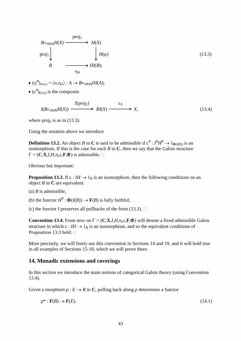
43
proj2
BHI(B)H(X) H(X)
proj1 H() (13.3)
B HI(B);
B
(B)(A,) = ,A : A BHI(B)HI(A);
(B)(X,) is the composite
I(proj2) X
I(BHI(B)H(X)) IH(X) X, (13.4)
where proj2 is as in (13.3).
Using the notation above we introduce
Definition 13.2. An object B in C is said to be admissible if B : I
BH
B 1(I(B)) is an
isomorphism. If this is the case for each B in C, then we say that the Galois structure
= (C,X,I,H,,,F,) is admissible.
Obvious but important:
Proposition 13.3. If : IH 1X is an isomorphism, then the following conditions on an
object B in C are equivalent:
(a) B is admissible;
(b) the functor HB : (I(B)) F(B) is fully faithful;
(c) the functor I preserves all pullbacks of the form (13.3).
Convention 13.4. From now on = (C,X,I,H,,,F,) will denote a fixed admissible Galois
structure in which : IH 1X is an isomorphism, and so the equivalent conditions of
Proposition 13.3 hold.
More precisely, we will freely use this convention in Sections 14 and 19, and it will hold true
in all examples of Sections 15-18, which we will prove there.
14. Monadic extensions and coverings
In this section we introduce the main notions of categorical Galois theory (using Convention
13.4).
Given a morphism p : E B in C, pulling back along p determines a functor
p* : F(B) F(E), (14.1)

44
and the composition with p determines a functor
p! : F(E) F(B), (14.2)
which is the left adjoint of p*.
Definition 14.1. A pair (E,p), in which p : E B is morphism in C, or a morphism p : E B
itself, is said to be a monadic extension of B if the following conditions hold:
(a) If (D,) is in F(E), then (D,p) is in F(B);
(b) the functor p* : F(B) F(E) is monadic.
We are now ready to introduce our main definition:
Definition 14.2. (a) An object (A,) in F(B) is said to be a trivial covering (of B) if the
morphism (B)(A,) : (A,) H
BIB(A,) is an isomorphism, or, equivalently, the diagram
A
A HI(A)
HI() (14.3)
B HI(B)
B
is a pullback.
(b) An object (A,) in F(B) is said to be split over a monadic extension (E,p) of B if p*(A,) is
a trivial covering.
(c) An object (A,) in F(B) is said to be a covering of B if there exists a monadic extension
(E,p) of B such that (A,) is split over (E,p). We will then also say that : A B is a
covering morphism.
According to this definition we have
TrivCov(B) = Spl(B,1B) Cov(B) = (E,p)
Spl(E,p) F(B), (14.4)
where:
TrivCov(B) is the full subcategory in F(B) with objects all trivial coverings of B;
Spl(E,p) is the full subcategory in F(B) of all objects split over (E,p);
Cov(B) is the full subcategory in F(B) with objects all coverings of B;
the union of Spl(E,p)’s in (6.4) is taken over all monadic extensions (E,p) of B.
Remark 14.3. The following simple properties of coverings are useful:
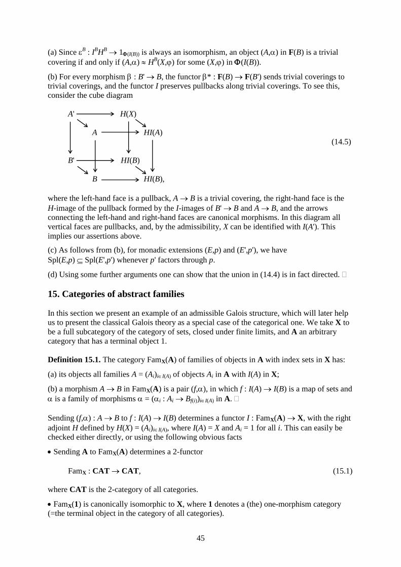
45
(a) Since B : I
BH
B 1(I(B)) is always an isomorphism, an object (A,) in F(B) is a trivial
covering if and only if (A,) HB(X,) for some (X,) in (I(B)).
(b) For every morphism : B' B, the functor * : F(B) F(B') sends trivial coverings to
trivial coverings, and the functor I preserves pullbacks along trivial coverings. To see this,
consider the cube diagram
A' H(X)
A HI(A)
(14.5)
B' HI(B)
B HI(B),
where the left-hand face is a pullback, A B is a trivial covering, the right-hand face is the
H-image of the pullback formed by the I-images of B' B and A B, and the arrows
connecting the left-hand and right-hand faces are canonical morphisms. In this diagram all
vertical faces are pullbacks, and, by the admissibility, X can be identified with I(A'). This
implies our assertions above.
(c) As follows from (b), for monadic extensions (E,p) and (E',p'), we have
Spl(E,p) Spl(E',p') whenever p' factors through p.
(d) Using some further arguments one can show that the union in (14.4) is in fact directed.
15. Categories of abstract families
In this section we present an example of an admissible Galois structure, which will later help
us to present the classical Galois theory as a special case of the categorical one. We take X to
be a full subcategory of the category of sets, closed under finite limits, and A an arbitrary
category that has a terminal object 1.
Definition 15.1. The category FamX(A) of families of objects in A with index sets in X has:
(a) its objects all families A = (Ai)iI(A) of objects Ai in A with I(A) in X;
(b) a morphism A B in FamX(A) is a pair (f,), in which f : I(A) I(B) is a map of sets and
is a family of morphisms = (i : Ai Bf(i))iI(A) in A.
Sending (f,) : A B to f : I(A) I(B) determines a functor I : FamX(A) X, with the right
adjoint H defined by H(X) = (Ai)iI(A), where I(A) = X and Ai = 1 for all i. This can easily be
checked either directly, or using the following obvious facts
Sending A to FamX(A) determines a 2-functor
FamX : CAT CAT, (15.1)
where CAT is the 2-category of all categories.
FamX(1) is canonically isomorphic to X, where 1 denotes a (the) one-morphism category
(=the terminal object in the category of all categories).

46
The unique functor A 1 has the right adjoint sending the unique object of 1 to the
terminal 1 object in A, and the functor I : FamX(A) X above is nothing but the composite
FamX(A) FamX(1) X.
It is then easy to prove:
Theorem 15.2. Let = (FamX(A),X,I,H,,,F,) be a Galois structure, in which
I : FamX(A) X and H : X FamX(A) are as above, with suitable and , the class of all
morphisms in X, and F an arbitrary class of morphisms in FamX(A) containing H() and
satisfying 5.1(b). Then : IH 1X is an isomorphism and is admissible.
Theorem 15.3. Let = (FamX(A),X,I,H,,,F,) be as in Theorem 7.2, and (f,) : A B be
in F. Then (A,(f,)) is a trivial covering of B if and only if i : Ai Bf(i) is an isomorphism for
each i I(A).
16. Coverings in classical Galois theory
In this section we describe the relationship between the separable/Galois extensions in
classical Galois theory and covering morphisms of categorical Galois theory.
Here, K denotes a field, C the opposite category of commutative unitary K-algebras that are
finite-dimensional as K-vector spaces, and X the category of finite sets. We define here
I : C X by
I(A) = the set of minimal (non-zero) idempotents in A; (16.1)
that is I(A) consists of all e A such that e2 = e 0 and e'
2 = e' 0 ee' implies ee' = e.
Sending A to the family (Ae)eI(A) determines a category equivalence
C FamX(A), (16.2)
where A is the full subcategory in C with objects all (commutative unitary) K-algebras with
no non-trivial idempotents, i.e. no elements e with e2 = e and 0 e 1. Moreover, the functor
I : C X above is a special case of the one defined in the previous section up to the
equivalence (16.2). Using this fact and Theorem 15.2 we obtain:
Theorem 16.1. Let I : C X be as above, H : X C the right adjoint of I defined therefore
by
H(X) = K … K = the K-algebra of all maps from X to K, (16.3)
coproduct
in C of K
with itself
“X-times”
and the unit and counit of adjunction, and F and the classes of all morphisms in C and
in X respectively. Then : IH 1X is an isomorphism and = (C,X,I,H,,,F,) is an
admissible Galois structure.

47
Next, using Theorem 10.7, we easily prove:
Theorem 16.2. A morphism p : E B in C, in which B is a field, is a monadic extension if
and only if E is a non-zero ring. In particular this is the case whenever E is a field.
Proof. The functor p* : F(B) F(E), whose monadicity we have to prove for a non-zero E, is
the same as the functor
EB() : (Commutative unitary B-algebras)op
(Commutative unitary E-algebras)op
. (16.4)
According to Theorem 10.7 it suffices to prove that this functor reflects isomorphisms and
preserves coequalizers. Moreover, since the coequalizers in the categories involved are the
same as equalizers of algebras, and since those are calculated via the corresponding equalizers
of underlying modules, we only need to prove that the functor
EB() : B-modules E-modules (16.5)
reflects isomorphisms and is (left) exact, which is obvious since B is a field.
Now we are ready to prove:
Theorem 16.3. Let K B E be finite (=finite-dimensional over B) field extensions and A =
(A,) a B-algebra (in particular : B A is a ring homomorphism and B acts on A via ba =
(b)a). Out of the following three conditions, the first two are always equivalent, and the third
always follows from them and implies them when B E is a Galois extension:
(a) (A,) belongs to Spl(E,p) (where Spl(E,p) is defined with respect to the Galois structure
described in Theorem 16.1) with p being the inclusion map B E considered as a morphism
E B in C;
(b) EBA E…E (a finite product of K-algebras = a finite coproduct in C);
(c) A E1…En for some natural n (0 is not excluded), where B Ei E (i = 1,…,n) (and
therefore E1,…,En are field extensions of B).
Proof. (a)(b) easily follows, using the equivalence (16.2), from Theorem 16.3 and the fact
that EBA considered as an object in C is the same as p*(A,).
(b)(c) ((b)(c) always, and (b)(c) when B E is a Galois extension) is well known in
classical algebra, and we only sketch the proof here:
(b)(c): (b) implies that A has no nilpotent elements. Therefore A E1…En as B-algebras,
for some field extensions E1,…,En of B, say, by the Wedderburn Theorem. After that in order
to show that E1,…,En can be chosen among the subextensions of B E, it suffices to show
that each of E1,…,En admits a B-algebra homomorphism into E. This, however, immediately
follows from EBA E…E and A E1…En.
(c)(b) when B E is a Galois extension: Since a finite product of B-algebras satisfying (b)
itself obviously satisfies (b), we can assume from the beginning that A is a B-subalgebra in E.
Moreover, since B E is a Galois extension, there is a polynomial u B[x] that splits into
linear factors u = mi=1(x ai) with ai = aj i = j, and has B[x]/uB[x]. Therefore
48
EBA EB(B[x]/uB[x]) E[x]/uE[x] E[x]/(mi=1(x ai))
mi=1(E[x]/(x ai)E[x]) E…E (m times),
as desired.
In fact the connection with classical Galois theory goes much further, and provides
categorical proofs for many of its results. Let us mention just two of them that are “almost
corollaries” of Theorem 8.3:
Theorem 16.4. Let K B E be finite field extensions and p the inclusion map B E
considered as a morphism E B in C. Then the following conditions are equivalent:
(a) (E,p) belongs to Spl(E,p);
(b) B E is a Galois extension.
Theorem 16.5. Let K B be a finite field extensions and A = (A,) a B-algebra as above.
Then the following conditions are equivalent:
(a) (A,) is a covering of B;
(b) there exists a finite field extension B E, such that (A,) belongs to Spl(E,p), where
Spl(E,p) is as in Theorem 8.3;
(c) there exists a finite Galois field extension B E, such that (A,) belongs to Spl(E,p),
where Spl(E,p) is as in Theorem 8.3;
(d) A = (A,) is a commutative separable B-algebra;
(e) A = (A,) is a finite product of finite separable field extensions of B.
17. Covering spaces in algebraic topology
The purpose of this section is to present classical covering maps of locally connected
topological spaces as covering morphisms in the sence of categorical Galois theory.
Therefore we take here C to be the category of locally connected topological spaces and X the
category of sets. And we define the functor I : C X by
I(A) = 0(A) the set of connected components of A. (17.1)
Sending spaces to the families of their connected components determines a category
equivalence
C FamX(A), (17.2)
where A is the category of connected locally connected topological spaces. Moreover, the
functor I : C X above is a special case of the one defined in Section 15. Using this fact and
Theorem 15.2 we easily obtain:
Theorem 17.1. Let I : C X be as above, H : X C the inclusion functor, and the unit
and counit of adjunction, F = Étale the class of local homeomorphisms (=étale maps) of

49
locally connected topological spaces, and the class of all morphisms in X. Then
: IH 1X is an isomorphism and = (C,X,I,H,,,F,) is an admissible Galois structure.
A brief story of monadic extensions and coverings with respect to this Galois structure is:
Theorem 17.2. A morphism p : E B in C is a monadic extension if and only if it is a
surjective local homeomorphism.
Proof. “If”: Assuming that p : E B is a surjective local homeomorphism, we have to prove
that the functor (6.1), which we write here as
p* : Étale(B) Étale(E), (17.3)
is monadic. We observe:
(i) Since the class of local homeomorphisms is closed under composition the functor (17.3)
has a left adjoint.
(ii) A morphism f : (A,) (A',') in Étale(B) is an isomorphism if and only if the map
f : A A' is bijective; this easily implies that, for a surjective p, the functor (17.3) reflects
isomorphisms.
(iii) When : A B is a local homeomorphism, the local connectedness of B implies the
local connectedness of A. Therefore Étale(B) can be identified, up to a category equivalence,
with the topos of sheaves (of sets) over the space B. The same is true for E, and the functor
(17.3) can be identified with the inverse image functor
p* : Shv(B) Shv(E) (17.4)
between the toposes of sheaves. Since the functor (17.4) has a (well-known) right adjoint,
namely the direct image functor
p*
: Shv(E) Shv(B), (17.5)
we conclude that it preserves all coequalizers. Indeed, it is easy to show that any left adjoint
functor preserves all colimits, and in particular all coequalizers.
(iv) The desired monadicity follows from (i), (ii), (iii), and Theorem 10.7.
“Only if”: When (E,p) is a monadic extension, p must be a local homeomorphism by
Definition 6.1(a) (applied to = 1E). Therefore we only need to prove that p is surjective. For,
consider the objects (B,1B) and (p(E), inclusion) in F(B) = Étale(B); note that (p(E), inclusion)
is indeed in F(B) since p is open. Since the functor p* reflects isomorphisms and sends the
canonical map (p(E), inclusion) (B,1B) to an isomorphism, we must have p(E) = B, as
desired.
Lemma 17.3. Suppose B (in C) is connected. Then the following conditions on an object
(A,) in F(B) = Étale(B) are equivalent:
(a) (A,) is a trivial covering of B (in the sense of Definition 14.2(a));
(b) A is a disjoint union of open subsets, each of which is mapped homeomorphically on B by
.

50
Proof. This is an easy corollary of Theorem 15.3.
Theorem 17.4. The following conditions on an object (A,) in F(B) = Étale(B) are
equivalent:
(a) (A,) is a covering of B (in the sense of Definition 14.2(c));
(b) every element b in B has an open neighbourhood U for which the pair
(1
(U), the map 1
(U) U induced by ) (17.6)
is a trivial covering of U (in the sense of Definition 14.2(a));
(c) the same as (b), but with U required to be connected;
(d) (A,) is a covering space over B in the classical sense, i.e. every element in B has an open
neighbourhood whose inverse image is a disjoint union of open subsets, each of which is
mapped homeomorphically on it by .
Proof. (a)(b) easily follows from the “only if” part of Theorem 17.2, and (b)(a) can easily
be deduced from the same theorem and the following simple observation:
For each b in B, let Ub be a chosen open neighbourhood of b, let E be the topological
coproduct of all these neighbourhoods, and let p : E B be the map induced by the family of
inclusion maps Ub B (for all b in B). Then p is a local homeomorphism.
(b)(c) follows from the local connectedness of B and (c)(b) is trivial.
(c)(d) follows from the local connectedness of B and Lemma 17.3.
18. Central extensions of groups
The purpose of this section is to present central extensions of groups as covering morphisms
in the sence of categorical Galois theory.
Accordinly C will denote now the category of groups, X the category of abelian groups, and
I : C X the left adjoint of the inclusion X C, which will plays the role of H. That is:
From the viewpoint of universal algebra I is the abelianization functor sending groups to
their quotients determined by the identity xy = yx, we could write
I(A) = A/R, where R is the congruence generated by {(a,b) AA ab = ba}. (18.1)
From the viewpoint of group theory I is to be defined by
I(A) = A/[A,A], (18.2)
where [A,A] is the commutator of A with itself.
From the viewpoint of homological algebra I is to be defined by
I(A) = H1(A,Z), (18.3)
where H1(A,Z) is the first homology group of A with coefficients in the additive group of
integers, on which A acts trivially.

51
The Galois structure = (C,X,I,H,,,F,) that we fix in this section will have C, X, I, H as
above, with the canonical and , and F and being the classes of surjective
homomorphisms of groups and of abelian groups respectively. The morphism : IH 1X is
obviously an isomorphism here, but the admissibility needs a little proof:
Theorem 18.1. = (C,X,I,H,,,F,) is admissible.
Proof. Consider the pullback (13.3), which now becomes
proj2
BB/[B,B]X X
proj1 (18.4)
B B/[B,B].
B
We need to prove that proj2 : BB/[B,B]X X has the universal property of the abelianization of
BB/[B,B]X, or, equivalently, that the kernel Ker(proj2) of this morphism is contained in
[BB/[B,B]X,BB/[B,B]X]. We observe that any element k in Ker(proj2) is of the form k = (b,1),
where b is in [B,B], and so we can present it as
k = ([b1,b'1]…[bn,b'n],1) = ([b1,b'1],1)…([bn,b'n],1). (18.5)
Since is surjective, there exist x1,…,xn,x'1,…,x'n in X with (x1) = b1[B,B], …,
(xn) = bn[B,B], (x'1) = b'1[B,B], …, (x'n) = b'n[B,B]; and since X is abelian, we have [x1,x'1]
=…= [xn,x'n] = 1. Therefore
k = ([b1,b'1],[x1,x'1])…([bn,b'n],[xn,x'n]) = [(b1,x1),(b'1,x'1)]…[(bn,xn),(b'n,x'n)], (18.6)
which shows that k is in [BB/[B,B]X, BB/[B,B]X], as desired.
Remark 18.2. The surjectivity of played a crucial role in the proof of Theorem 10.1.
Indeed, taking X = 0 in (10.4), we would obtain Ker(proj2) [B,B], but at the same time
[BB/[B,B]X, BB/[B,B]X] [[B,B],[B,B]] (canonically).
Next, the monadic extensions:
Theorem 18.3. A morphism p : E B in C is a monadic extension if and only if it is
surjective.
Proof. “If”: According to Remark 10.8(b), it suffices to prove that, for a surjective p, the
functor p* : F(B) F(E) reflects isomorphisms and preserves coequalizers of reflexive pairs.
However, it is an easy exercise to show that the coequalizers of reflexive pairs of group
homomorphisms are calculated as in the category of sets – which reduces the problem to the
case of sets, where the proof becomes another easy exercise.
The “only if” part follows from Definition 14.1(a) (applied to = 1E).
In order to characterize coverings we will also need the following almost obvious fact:

52
Lemma 18.4. For a pullback diagram
u
D A
(18.7)
E B
v
with and surjective, the conditions (a) and (b) below are related as follows: (a) always
implies (b), and (b) implies (a) whenever v is surjective.
(a) (A,) is a central extension of B (i.e. ka = ak for all k in Ker() and all a in A);
(b) (D,) is a central extension of E.
– after which we are ready to prove
Theorem 18.5. The following conditions on an object (A,) in F(B) are equivalent:
(a) (A,) is a covering of B;
(b) (A,) is a central extension of B.
Proof. (a)(b) follows from (the “only if” part of) Theorem 18.3 and Lemma 18.4.
(b)(a): As follows from the “if” part of Theorem 18.3, (A,) is a monadic extension of B.
Consider the object
*(A,) = (ABA,proj1) (18.8)
in F(A). It has Ker(proj1) canonically isomorphic to Ker(), and proj1 is a split epimorphism.
Being central by Lemma 18.4(a)(b), it is therefore isomorphic to
*(A,) = (AKer(), the first projection), (18.9)
after which we only need to observe:
The object (18.9) is a trivial covering of A since (Ker(), Ker() 0) is a trivial covering of
0, and the class of trivial coverings is pullback stable by Remark 14.3(b).
19. The fundamental theorem of Galois theory
In this section we formulate and prove the fundamental theorem of categorical Galois theory.
Let = (C,X,I,H,,,F,) be a fixed abstract Galois structure satisfying Convention 5.4. We
begin by considering various induced adjunctions:
We can obviously look at the category of internal precategories in C as the functor category
C, where is the free category determined by the graph
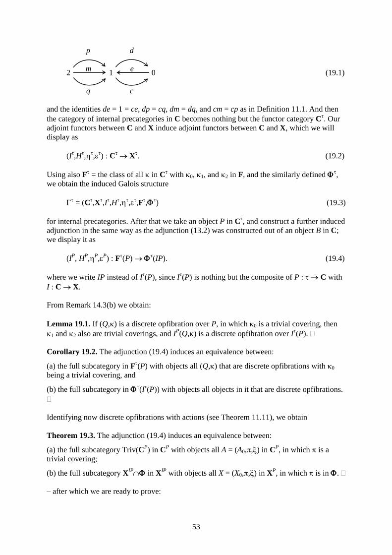
53
p d
2 m
1 e
0 (19.1)
q c
and the identities de = 1 = ce, dp = cq, dm = dq, and cm = cp as in Definition 11.1. And then
the category of internal precategories in C becomes nothing but the functor category C. Our
adjoint functors between C and X induce adjoint functors between C and X, which we will
display as
(I,H
,
,) : C
X
. (19.2)
Using also F = the class of all in C
with 0, 1, and 2 in F, and the similarly defined
,
we obtain the induced Galois structure
= (C
,X
,I,H
,
,,F
,
) (19.3)
for internal precategories. After that we take an object P in C, and construct a further induced
adjunction in the same way as the adjunction (13.2) was constructed out of an object B in C;
we display it as
(IP, H
P,
P,
P) : F
(P)
(IP). (19.4)
where we write IP instead of I(P), since I
(P) is nothing but the composite of P : C with
I : C X.
From Remark 14.3(b) we obtain:
Lemma 19.1. If (Q,) is a discrete opfibration over P, in which 0 is a trivial covering, then
1 and 2 also are trivial coverings, and IP(Q,) is a discrete opfibration over I
(P).
Corollary 19.2. The adjunction (19.4) induces an equivalence between:
(a) the full subcategory in F(P) with objects all (Q,) that are discrete opfibrations with 0
being a trivial covering, and
(b) the full subcategory in (I(P)) with objects all objects in it that are discrete opfibrations.
Identifying now discrete opfibrations with actions (see Theorem 11.11), we obtain
Theorem 19.3. The adjunction (19.4) induces an equivalence between:
(a) the full subcategory Triv(CP) in C
P with objects all A = (A0,,) in C
P, in which is a
trivial covering;
(b) the full subcategory XIP in X
IP with objects all X = (X0,,) in X
P, in which is in .
– after which we are ready to prove:

54
Theorem 19.4. (“The fundamental theorem of Galois theory”) Let = (C,X,I,H,,,F,)
be a fixed abstract Galois structure satisfying Convention 5.4 as above, and let (E,p) be a
monadic extension of an object B in C. Then sending an object (A,) in Spl(E,p) to the triple
(I(EBA),I(proj1),I(proj1)I(proj2)), determines a category equivalence
Spl(E,p) XI(Eq(p))
(19.5)
(denoting by proji (i = 1, 2) suitable projections, in particular using proj1 for both EBA E
and EBE E, and using the notation of Theorem 19.3 for P = Eq(p)).
Proof. All we need is to consider the diagram
F(B) F(E)T C
Eq(p)F
(19.6)
Spl(E,p) Triv(CEq(p)
) XI(Eq(p))
,
in which:
(i) T is the monad determined by the monadic functor p* : F(B) F(E), and
F(B) F(E)T is the comparison functor, which is a category equivalence since p* is monadic.
(ii) F(E)T C
Eq(p)F is the isomorphism established in the same way as the isomorphism
(12.7) in Theorem 2.1. It therefore sends a T-algebra (D,,) to the triple (D,,), where =
proj1,proj3 : (E(p,p)E)(proj2,)D E(p,p)D as in Theorem 12.1.
(iii) Calculating the composite F(B) F(E)T C
Eq(p)F we easily conclude that it sends an
object (A,) to the triple (EBA,proj1,proj1proj2), where proji (i = 1, 2) are the same as in the
formulation of the theorem.
(iv) The vertical arrows are the inclusion functors.
(v) (A,) belongs to Spl(E,p) exactly when (EBA,proj1) is a trivial covering. Therefore (iii)
tells us that the composite F(B) F(E)T C
Eq(p)F determines the dotted arrow in (11.4),
and that that arrow is an equivalence of categories.
(vi) Triv(CEq(p)
) XI(Eq(p))
is the equivalence described in Theorem 11.3 (for P = Eq(p)).
(vii) The desired equivalence is the composite of the equivalences Spl(E,p) Triv(CEq(p)
) and
Triv(CEq(p)
) XI(Eq(p))
.
Remark 19.5. (a) According to this theorem it is good to write
Gal(E,p) = I(Eq(p)), (19.7)
and call this internal precategory the Galois pregroupoid of the monadic extension (E,p). Here
“pregroupoid” (rather than “precategory”) refers to a certain extra structure, that makes
I(Eq(p)) a groupoid whenever it is a category. And in fact it is a groupoid whenever (E,p) is
normal, which means that (E,p) belongs to Spl(E,p). Other reasonable synonyms of “normal”
are Galois covering and regular covering. Furthermore, for a normal (E,p), I(Eq(p)) is a group
if and only if E is connected, i.e. I(E) is a terminal object in X.
55
(b) There is also a reasonable way to define fundamental groupoids as “the largest” Galois
groupoids.
20. Back to the classical cases
In this section we consider the simplest applications the fundamental theorem of categorical
Galois theory.
The classical form of the fundamental theorem of Galois theory is usually formulated as
follows:
Theorem 20.1. Let B E be a finite Galois field extension, and AutB(E) its Galois group.
Then:
(a) The correspondences
F AutF(E) and H EH = {x E g H g(x) = x} (20.1)
determine inverse to each other and inclusion reversing bijections between the lattice
Sub(E/B) of field subextensions of B E, and the lattice Sub(AutB(E)) of subgroups in
AutB(E).
(b) If B F is a field subextension of B E, then every B-algebra homomorphism from F to
E extends to a B-algebra automorphism of E.
(c) A field subextension B F of B E is a Galois extension if and only if its corresponding
subgroup AutF(E) is a normal subgroup in AutB(E). In this case every B-algebra
automorphism of E restricts to a B-algebra automorphism of F, yielding a short exact
sequence
0 AutF(E) AutB(E) AutB(F) 0 (20.2)
of groups.
How does this theorem follow from Theorem 19.4?
Answering this question requires a number of simple observations:
(i) Every statement of Theorem 20.1 is a statement about purely-categorical properties of the
category Sub(E/B) of subextensions of the field extension B E. The only thing that needs an
explanation here, is that E itself can be defined categorically as a special object in Sub(E/B).
For, just observe that it is the only weak terminal object (i.e. the only object that admits
morphisms from all other objects into it).
(ii) Moreover, it turns out that the category Sub(E/B)op
is equivalent to the category of
transitive (=one-orbit) AutB(E)-sets – which is known as Grothendieck’s form of the
fundamental theorem of Galois theory – and every statement of Theorem 20.1 follows from
this fact.
(iii) Furthermore, it is sufficient to know that Sub(E/B)op
is equivalent to the category of
transitive G-sets for some monoid G, because this fact itself implies that G is isomorphic to
AutB(E). Indeed:

56
We know that Sub(E/B) has a unique weakly terminal object, namely E, and that the
endomorphism monoid of this object is AutB(E).
On the other hand G acts on itself via its multiplication, and this object is weakly initial in
the category of transitive G-sets; and its endomorphism monoid is isomorphic to G.
Therefore the equivalence of Sub(E/B)op
to the category of transitive G-sets implies that G is
isomorphic to AutB(E).
(iv) Let us now apply Theorem 19.4 to the situation considered in Section 16. As follows
from the equivalence (a)(c) in Theorem 16.3, which assumes that B E is a Galois
extension and p : E B is the inclusion map B E, in that situation we have
Spl(E,p) FamX(Sub(E/B)op
). (20.3)
At the same time Theorem 19.4 tells us that the category Spl(E,p) is equivalent to the category
of finite G-sets for some finite monoid G – namely for G = L(I(Eq(p))), where L is the functor
(11.9), and L(I(Eq(p))) is indeed a monoid since I(E) has only one element.
(v) As follows from (iv), Sub(E/B)op
must be equivalent to the category of transitive
G-sets, as desired. Therefore Theorem 20.1 indeed follows from Theorem 19.4.
The situation with covering spaces is very similar: many standard text books in algebraic
topology show how the connected covering spaces of a “good” space B are “classified” via
subgroups of the fundamental group of B by proving a theorem similar to Theorem 12.1,
usually not showing the categorical result behind, which is:
Theorem 20.2. Let B be a connected locally connected topological space, admitting a
universal covering space (E,p) over it. Then the category of covering spaces over B is
equivalent to the category of Aut(E,p)-sets.
– and this theorem can easily be obtained as a corollary of Theorem 19.4, using the results of
Section 17. Recall, however, that what is called a universal covering space of B is in fact a
weakly initial object in the category of non-empty covering spaces over B, and that
“weakness” can be avoided by using pointed spaces.
Applying Theorem 19.4 to the situation considered in Section 18, we obtain, in particular, a
description of the category Centr(B) of central extension of an arbitrary group B. The full
explanation would involve some homological algebra and internal category theory (in “nice”
categories), which would take us too far. Therefore let us just mention that it becomes
especially simple when B is perfect, i.e. when [B,B] = B: in this case
Centr(B) ((Abelian groups)H2(A,Z)), (20.4)
which presents the second homology group H2(A,Z) as a certain “Galois group”, and implies
the well-known result saying that every perfect group has a universal central extension.
Finally, let us mention one less familiar examples of Galois theories very briefly; being less
familiar it was, however, the original motivating example for categorical Galois theory:
Example 20.3. The system (C,X,I,H,,,F,) described below is an admissible Galois
structure in which is an isomorphism:

57
C is the opposite category of commutative unitary rings;
X is the opposite category of (unitary) Boolean rings, or, equivalently, the opposite category
of Boolean algebras; up to a category equivalence we can identify X with the category of
Stone spaces (=profinite topological spaces = compact totally disconnected Hausdorff spaces
= compact 0-dimensional Hausdorff spaces = compact topological spaces in which every two
points can be separated by a closed-and-open subset);
I : C X is sending rings to the Boolean rings of their idempotents, or, considering X as
the category of Stone spaces, I is defined by
I(A) = Boolean spectrum of A = Stone space of the Boolean algebra of
idempotents in A = the space of connected components of the Zariski (20.5)
spectrum of A;
H : X C is defined by
H(X) = hom(X,Z), (20.6)
where X is any object in X considered as a topological space, Z is the ring of integers
equipped with the discrete topology, and hom(X,Z) is set of continuous maps X Z with the
ring structure induced by the ring structure of Z;
and are defined accordingly, and F and are the classes of all morphisms in C and X
respectively.
The covering morphisms with respect to this Galois structure are the same as what A. R.
Magid calls componentially locally strongy separable algebras; they are defined as follows:
(a) a commutative (unitary) algebra S over a commutative (unitary) ring R is said to be
separable if it is projective as an SRS-module;
(b) a commutative separable R-algebra S is said to be strongly separable if it is projective as
an R-module;
(c) an R-algebra S is said to be locally strongly separable if every finite subset in it is
contained in a strongly separable R-subalgebra;
(d) a commutative R-algebra S is said to be componentially locally strongy separable if its all
Boolean localizations Sx are locally strongly separable Rx-algebras; here, for a maximal ideal x
of the Boolean ring of idempotents in R, the Boolean localizations Sx is defined as the quotient
algebra S/Sx.
And these componentially locally strongy separable algebras were the most general algebras
involved in Magid’s separable Galois theory of commutative rings. For a field extension
B E we have:
E is a separable B-algebra E is a strongly separable B-algebra
E is a finite separable extension of B. (20.7)
A1. Remarks on functors and natural transformations
A1.1. Natural transformations can be composed vercally and horizontally, and these
operations agree via the middle interchange law. For, consider the diagram
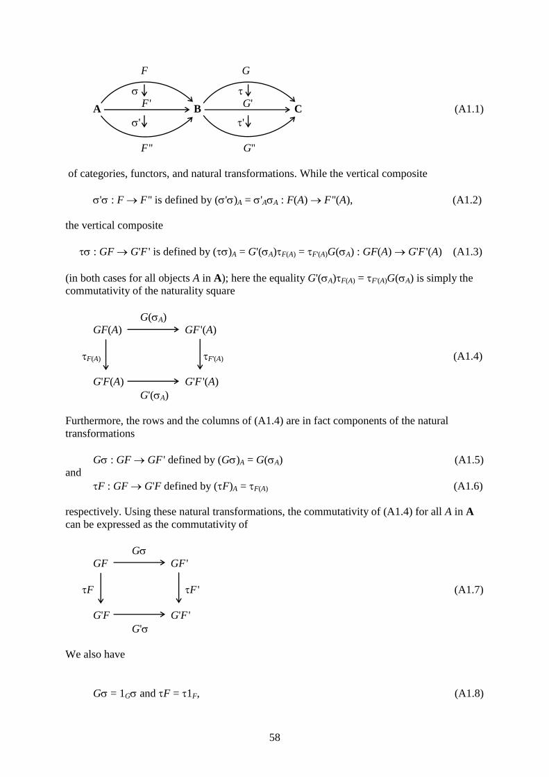
58
F G
A F '
B G'
C (A1.1)
' '
F '' G''
of categories, functors, and natural transformations. While the vertical composite
' : F F '' is defined by (')A = 'AA : F(A) F ''(A), (A1.2)
the vertical composite
: GF G'F ' is defined by ()A = G'(A)F(A) = F '(A)G(A) : GF(A) G'F '(A) (A1.3)
(in both cases for all objects A in A); here the equality G'(A)F(A) = F '(A)G(A) is simply the
commutativity of the naturality square
G(A)
GF(A) GF '(A)
F(A) F '(A) (A1.4)
G'F(A) G'F '(A)
G'(A)
Furthermore, the rows and the columns of (A1.4) are in fact components of the natural
transformations
G : GF GF ' defined by (G)A = G(A) (A1.5)
and
F : GF G'F defined by (F)A = F(A) (A1.6)
respectively. Using these natural transformations, the commutativity of (A1.4) for all A in A
can be expressed as the commutativity of
G
GF GF '
F F ' (A1.7)
G'F G'F '
G'
We also have
G = 1G and F = 1F, (A1.8)

59
and the commutativity of (A1.7), written as the equality
(1G')(1F) = (1F ')(1G), (A1.9)
can be deduced from the middle interchange law
(')(') = ('')(), (A1.10)
written here for the situation (A1.1). Indeed, applying (A1.10) to
F G
1F
A F
B G'
C
1G'
F ' G' and
F G
1G
A F '
B G
C
1F '
F ' G'
we obtain
(1G')(1F) = (1G')(1F) and (1G)(1F ') = (1F ')(1G) (A1.11)
respectively, which gives
(1G')(1F) = (1G')(1F) = = (1G)(1F ') = (1F ')(1G) (A1.12)
On the other hand the middle interchange law (A1.10) can itself be obtained using the
appropriate commutative diagrams of the form (A1.7), which is easy to show using the
diagram
G G'
GF GF ' GF ''
F F ' F ''
G'F G'F ' G'F '' (A1.13)
G' G''
'F 'F ' 'F ''
G''F G''F ' G''F ''
G'' G'''
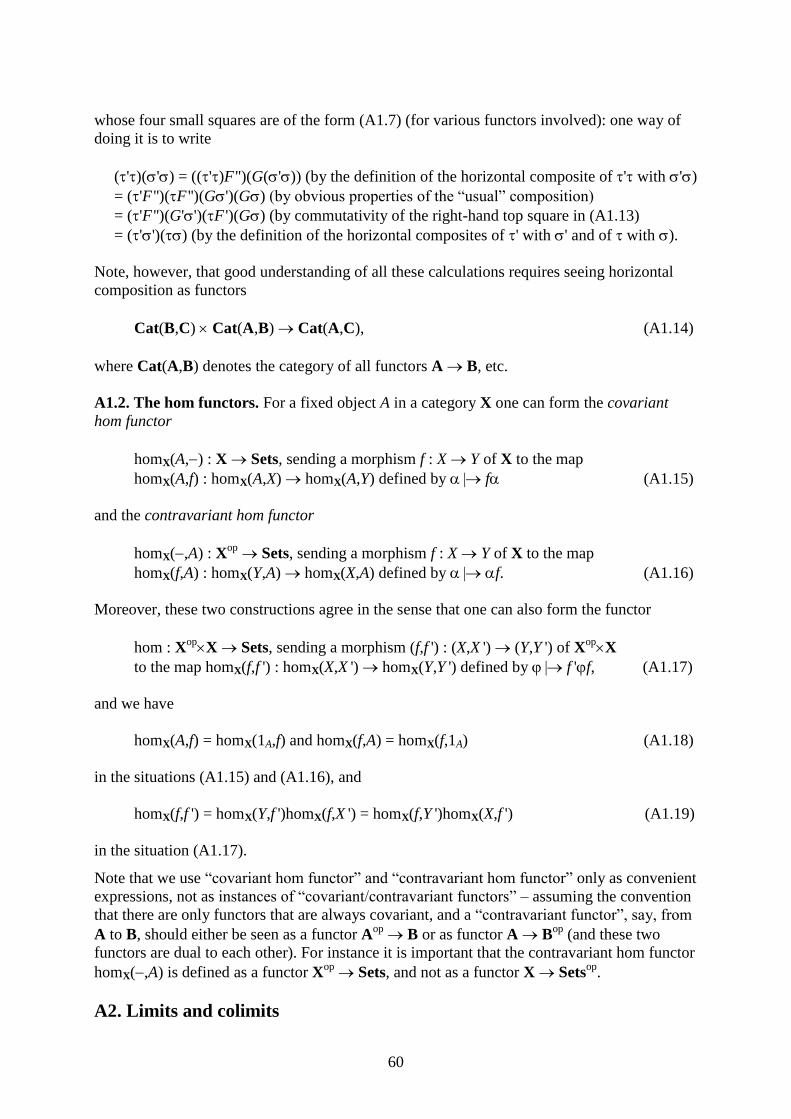
60
whose four small squares are of the form (A1.7) (for various functors involved): one way of
doing it is to write
(')(') = ((')F '')(G(')) (by the definition of the horizontal composite of ' with ')
= ('F '')(F '')(G')(G) (by obvious properties of the “usual” composition)
= ('F '')(G'')(F ')(G) (by commutativity of the right-hand top square in (A1.13)
= ('')() (by the definition of the horizontal composites of ' with ' and of with ).
Note, however, that good understanding of all these calculations requires seeing horizontal
composition as functors
Cat(B,C) Cat(A,B) Cat(A,C), (A1.14)
where Cat(A,B) denotes the category of all functors A B, etc.
A1.2. The hom functors. For a fixed object A in a category X one can form the covariant
hom functor
homX(A,) : X Sets, sending a morphism f : X Y of X to the map
homX(A,f) : homX(A,X) homX(A,Y) defined by f (A1.15)
and the contravariant hom functor
homX(,A) : Xop
Sets, sending a morphism f : X Y of X to the map
homX(f,A) : homX(Y,A) homX(X,A) defined by f. (A1.16)
Moreover, these two constructions agree in the sense that one can also form the functor
hom : XopX Sets, sending a morphism (f,f ') : (X,X ') (Y,Y ') of X
opX
to the map homX(f,f ') : homX(X,X ') homX(Y,Y ') defined by f 'f, (A1.17)
and we have
homX(A,f) = homX(1A,f) and homX(f,A) = homX(f,1A) (A1.18)
in the situations (A1.15) and (A1.16), and
homX(f,f ') = homX(Y,f ')homX(f,X ') = homX(f,Y ')homX(X,f ') (A1.19)
in the situation (A1.17).
Note that we use “covariant hom functor” and “contravariant hom functor” only as convenient
expressions, not as instances of “covariant/contravariant functors” – assuming the convention
that there are only functors that are always covariant, and a “contravariant functor”, say, from
A to B, should either be seen as a functor Aop
B or as functor A Bop
(and these two
functors are dual to each other). For instance it is important that the contravariant hom functor
homX(,A) is defined as a functor Xop
Sets, and not as a functor X Setsop
.
A2. Limits and colimits
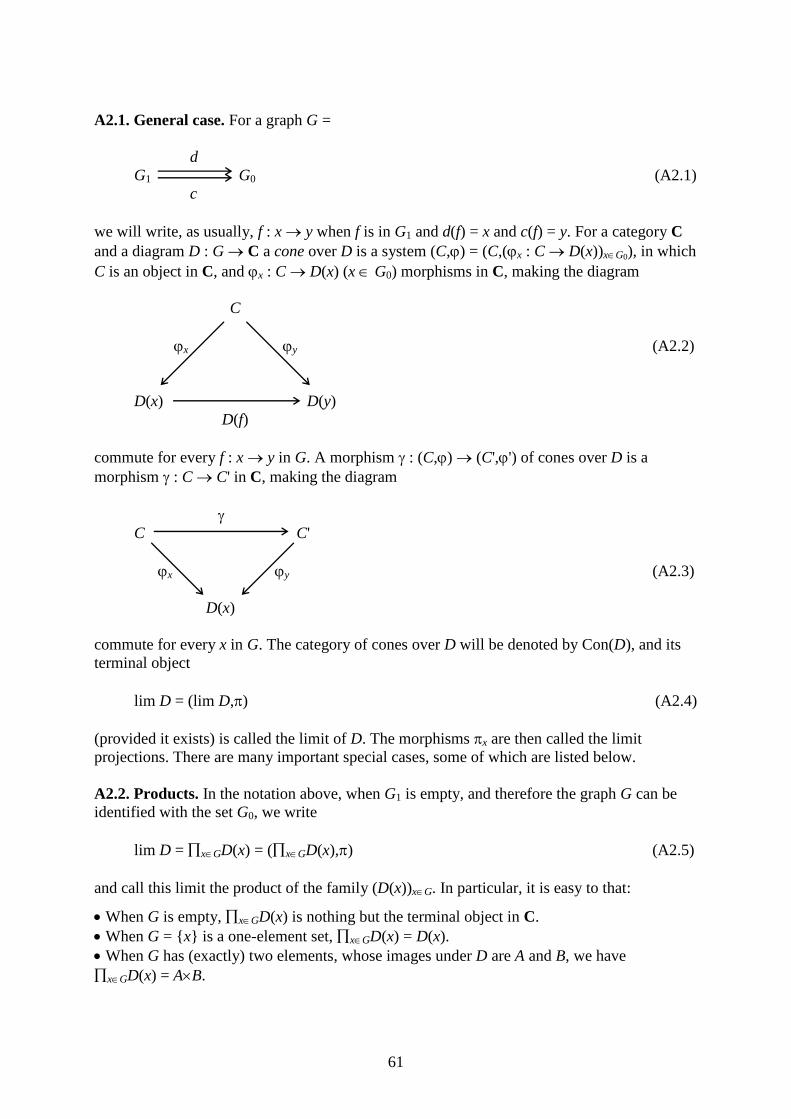
61
A2.1. General case. For a graph G =
d
G1 G0 (A2.1)
c
we will write, as usually, f : x y when f is in G1 and d(f) = x and c(f) = y. For a category C
and a diagram D : G C a cone over D is a system (C,) = (C,(x : C D(x))xG0), in which
C is an object in C, and x : C D(x) (x G0) morphisms in C, making the diagram
C
x y (A2.2)
D(x) D(y)
D(f)
commute for every f : x y in G. A morphism : (C,) (C',') of cones over D is a
morphism : C C' in C, making the diagram
C C'
x y (A2.3)
D(x)
commute for every x in G. The category of cones over D will be denoted by Con(D), and its
terminal object
lim D = (lim D,) (A2.4)
(provided it exists) is called the limit of D. The morphisms x are then called the limit
projections. There are many important special cases, some of which are listed below.
A2.2. Products. In the notation above, when G1 is empty, and therefore the graph G can be
identified with the set G0, we write
lim D = xGD(x) = (xGD(x),) (A2.5)
and call this limit the product of the family (D(x))xG. In particular, it is easy to that:
When G is empty, xGD(x) is nothing but the terminal object in C.
When G = {x} is a one-element set, xGD(x) = D(x).
When G has (exactly) two elements, whose images under D are A and B, we have
xGD(x) = AB.

62
And more generally, when G has n elements, whose images under D are A1, …, An, it is
convenient to write xGD(x) = A1…An.
A2.3. Infima. If C is an ordered set considered as a category, then for every
D : G C we have
lim D = xG0D(x) = xG0D(x) = inf{D(x) x G0}, (A2.6)
i.e. lim D is the infimum of the set {D(x) x G0} in C.
A2.4. Equalizers. Let G be a graph that has two objects x and y, and two morphisms from x to
y, and let D be the diagram sending those two morphisms to
f
A B (A2.7)
g
Then to give a cone over D is to give a morphism h : X A with fh = gh. Therefore the limit
of D can be identified with a pair (E,e), in which e : E A is a morphism in C such that:
(a) fe = ge;
(b) if fh = gh as above, then there exists a unique morphism u : X E with eu = h.
Such a pair (E,e) is called the equalizer of the pair (f,g).
A2.5. Pullbacks. Let G be a graph that has three objects x, y, and z, one morphism from x to z,
and one morphism from y to z, and let D be the diagram sending those two morphisms to
B
g (A2.8)
A C
f
Then to give a cone over D is to give a morphisms h : X A and k : X B with fh = gk.
Therefore the limit of D can be identified with a triple (P,p,q), in which p : P A and
q : P B are morphisms in C such that:
(a) fp = gq;
(b) if fh = gk as above, then there exists a unique morphism u : X P with pu = h and qu = k.
As suggested by the display

63
X k
u
P B
h q
p g (A2.9)
A C,
f
the limit of D is called the pullback of f and g. One also says that:
the square formed by f, g, p, q is a pullback square, or a cartesian square;
p is a pullback of g along f, and q is a pullback of f along g;
P is a fibred product of (A,f) and (B,g) (since indeed, (P,fp) = (P,gq) is the product of (A,f)
and (B,g) in the category (CC); another good reason is that, say, for C = Sets, it turnes out
that the fibres of fp = gq are the products of the corresponding fibres of f and g). One also
writes P = A(f,g)B = ACB.
A2.6. Examples of limits. In many concrete categories, including Sets, all varieties of
universal algebras, and the category of topological spaces, limits can be constructed as
follows: the products are the same as the usual cartesian products, and then
lim D = {(ax)xG0 xG0D(x) D(f)(ax) = ay for each f : x y in G}, (A2.10)
in the notation above, with x : lim D D(x) being induced by the corresponding usual
product projection for each x in G0. In particular the equalizer of a pair (A2.7) of parallel
morphisms in C can be identified with
{a A f(a) = g(a)}, (A2.11)
and for the pullback in (A2.9) we can write
A(f,g)B = {(a,b) AB f(a) = g(b)} (A2.12)
A2.7. Colimits. The colimit of a diagram D : G C is the same as the limit of the dual
diagram Dop
: Gop
Cop
. That is, the notion of colimit is simply dual to the notion of limit.
And all special limits above have their dual versions: coproducts are dual to products,
coequalizers to equalizers, and pushouts to pullbacks. The standard notation is:
colim D – for the colimit of a diagram D;
xGD(x), or ∐xGD(x) – for the coproduct of the family (D(x))xG;
AB = A∐B for the coproduct of A and B, and accordingly for pushouts.
However the constructions of colimits in familiar categories are usually more complicated
than those of limits. When we say that limits in varieties of universal algebras and in the
category of topological spaces are “constructed in the same way as in the category of sets”, it
first of all means that the forgetful functors from all these categories to sets preserve limits (in
the obvious sense). This, however, is usually not the case for colimits. Say, for a variety C of
universal algebras, the colimit of a diagram D : G C can be constructed in several steps as
follows:

64
we take A to the free algebra on the disjoint union of all D(x) (x G0);
define the congruence ~ on A as the smallest congruence E for which the composite of the
canonical maps D(x) A and A A/E is a homomorphism of algebras;
then one can show that A/~ becomes the colimit of D.
A3. Galois connections
A Galois connection between ordered sets L and M is a pair of maps
L M, both written as x x*, (A3.1)
and satisfying the following conditions:
x y y* x* for all x and y in L and for all x and y in M; (A3.2)
x x** for all x in L and for all x in M. (A3.3)
That is, a Galois connection between L and M is nothing but an adjunction L Mop
, or,
equivalently, an adjunction M Lop
. And just as any adjunction X A determines a monad
on X, any Galois connection above determines closure operators on L and on M, both given
by
c(x) = x**. (A3.4)
Let us recall here that in general a closure operator on ordered sets is unary operation c
satisfying the following conditions:
x y c(x) c(y);
x c(x); (A3.5)
cc(x) = c(x).
And if c is defined via a Galois connection as above, then the conditions (A3.5) easily follow
from (A3.2) and (A3.3) of course; the crucial observation is the equality
x*** = x*, (A3.6)
in which x* x*** by (A3.3) applied to x*, and x*** x* by (A3.2) applied to (A3.3).
As usually, an element x is called closed (under a given closure operator c) if c(x) = x. From
the equality (A3.6) we easily conclude:
Theorem A3.1. Any Galois connection (A3.1) induces inverse to each other bijections
between the set of closed elements in L and the set of closed elements in M.
When L and M are power sets ordered by inclusion, the Galois connections between L and M
are nothing but binary relations between the ground sets. More precisely, we have:
Theorem A3.2. Let X and Y be arbitrary sets and P(X) and P(Y) their power sets. Then:
(a) For any Galois connection between P(X) and P(Y), and x in X and y in Y, we have:
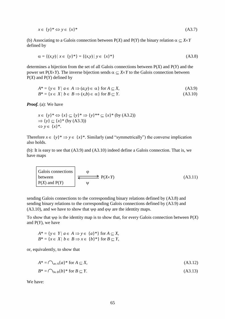
65
x {y}* y {x}* (A3.7)
(b) Associating to a Galois connection between P(X) and P(Y) the binary relation XY
defined by
= {(x,y) x {y}*} = {(x,y) y {x}*} (A3.8)
determines a bijection from the set of all Galois connections between P(X) and P(Y) and the
power set P(XY). The inverse bijection sends XY to the Galois connection between
P(X) and P(Y) defined by
A* = {y Y a A (a,y) } for A X, (A3.9)
B* = {x X b B (x,b) } for B Y. (A3.10)
Proof. (a): We have
x {y}* {x} {y}* {y}** {x}* (by (A3.2))
{y} {x}* (by (A3.3))
y {x}*.
Therefore x {y}* y {x}*. Similarly (and “symmetrically”) the converse implication
also holds.
(b): It is easy to see that (A3.9) and (A3.10) indeed define a Galois connection. That is, we
have maps
Galois connections
between P(XY) (A3.11)
P(X) and P(Y)
sending Galois connections to the corresponding binary relations defined by (A3.8) and
sending binary relations to the corresponding Galois connections defined by (A3.9) and
(A3.10), and we have to show that and are the identity maps.
To show that is the identity map is to show that, for every Galois connection between P(X)
and P(Y), we have
A* = {y Y a A y {a}*} for A X,
B* = {x X b B x {b}*} for B Y,
or, equivalently, to show that
A* = aA{a}* for A X, (A3.12)
B* = bB{b}* for B Y. (A3.13)
We have:

66
y A* aA((a,y) ) aA(y {a}*) y aA{a}*,
which proves (A3.12), and (A3.13) can be proved similarly.
To show that is the identity map is (according to (A3.8)) to show that, for every binary
relation XY, we have
= {(x,y) x {y}*}, where {y}* = {x X (x,y) },
i.e.
= {(x,y) (x,y) },
which is trivial.
Remark A3.3. To construct a closure operator out of a Galois connection via (A3.4) is a
special case of constructing a monad out of an adjunction. But are there also general theorems
about adjoint functors that would give Theorems A3.1 and A3.2 as special cases? Yes, but
they are far more sophisticated and we shall not need them here.