
GallagherFinalReport
11
Numerical Simulation of Arc-Jet Experiments using the Data- Parallel Line Relaxation Method Jason Gallagher, Graduate Student, Stanford University Sponsor: David M. Driver, Senior Research Scientist, Experimental Aerophysics Branch NASA Organization: APS June 14, 2004 – September 24, 2004 Abstract A computational fluid dynamics analysis has been performed on various simple geometries using the Data-Parallel Line Relaxation (DPLR) method. Results were obtained for arc-jet simulations of a twenty-degree half wedge, a flat-faced puck, a spherical calorimeter, and also a perfect air calculation for the nose of the shuttle in a simplified re-entry environment. The results obtained will be compared to actual test and/or flight data to validate future CFD models and their accuracy. Introduction The focus of this study was to obtain numerical solutions of arc-jet experiments and compare them with actual test data. The arc-jet is designed to provide ground-based hyperthermal and hypervelocity environments in support of NASA activities in thermal protection materials, aero- thermodynamics, vehicle structures, and hypersonic propulsion and flight. Current arc-jet experiments are being implemented in order to test proposed repair materials for the leading edge of the space shuttle wing in a re-entry environment. The types of models being tested include a twenty-degree half wedge and a flat-faced puck. Developing CFD models that can reproduce the arc-jet environment is important for future tests. If CFD models can be produced yielding trustworthy results, many more test configurations can be processed numerically without having to suffer the cost associated with arc-jet facility usage. To better understand the process of developing reliable CFD models, time was spent modeling various geometries that have been tested in the arc-jet in recent months. Three main geometries were analyzed throughout this study. The first was a twenty-degree half wedge. The second model was a flat-faced puck. Last, was a spherical geometry. All of the studies were performed in two-dimensions using DPLR-2D. Methods and Materials The Data-Parallel Line Relaxation (DPLR) method in two-dimensions was used to perform the CFD calculations. The DPLR method was chosen because it has shown particularly good convergence properties and reaches a steady-state solution in less time than other methods 1 . Also, because of its high parallel efficiency, it is very capable of modeling viscous flows in a reasonable time 1 , especially for smaller scale applications such as the geometries being studied. In addition to the numerical solution performed by DPLR-2D, grids were generated using Gridgen software. Learning the basics of Gridgen was relatively simple. It utilizes a “bottom-
-
Upload
jason-gallagher -
Category
Documents
-
view
108 -
download
0
Transcript of GallagherFinalReport

Numerical Simulation of Arc-Jet Experiments using the Data-
Parallel Line Relaxation Method
Jason Gallagher, Graduate Student, Stanford University
Sponsor: David M. Driver, Senior Research Scientist, Experimental Aerophysics Branch
NASA Organization: APS
June 14, 2004 – September 24, 2004
Abstract
A computational fluid dynamics analysis
has been performed on various simple
geometries using the Data-Parallel Line
Relaxation (DPLR) method. Results
were obtained for arc-jet simulations of a
twenty-degree half wedge, a flat-faced
puck, a spherical calorimeter, and also a
perfect air calculation for the nose of the
shuttle in a simplified re-entry
environment. The results obtained will
be compared to actual test and/or flight
data to validate future CFD models and
their accuracy.
Introduction
The focus of this study was to obtain
numerical solutions of arc-jet
experiments and compare them with
actual test data. The arc-jet is designed
to provide ground-based hyperthermal
and hypervelocity environments in
support of NASA activities in thermal
protection materials, aero-
thermodynamics, vehicle structures, and
hypersonic propulsion and flight.
Current arc-jet experiments are being
implemented in order to test proposed
repair materials for the leading edge of
the space shuttle wing in a re-entry
environment. The types of models being
tested include a twenty-degree half
wedge and a flat-faced puck.
Developing CFD models that can
reproduce the arc-jet environment is
important for future tests. If CFD models
can be produced yielding trustworthy
results, many more test configurations
can be processed numerically without
having to suffer the cost associated with
arc-jet facility usage. To better
understand the process of developing
reliable CFD models, time was spent
modeling various geometries that have
been tested in the arc-jet in recent
months.
Three main geometries were analyzed
throughout this study. The first was a
twenty-degree half wedge. The second
model was a flat-faced puck. Last, was a
spherical geometry. All of the studies
were performed in two-dimensions using
DPLR-2D.
Methods and Materials
The Data-Parallel Line Relaxation
(DPLR) method in two-dimensions was
used to perform the CFD calculations.
The DPLR method was chosen because
it has shown particularly good
convergence properties and reaches a
steady-state solution in less time than
other methods1. Also, because of its high
parallel efficiency, it is very capable of
modeling viscous flows in a reasonable
time1, especially for smaller scale
applications such as the geometries
being studied.
In addition to the numerical solution
performed by DPLR-2D, grids were
generated using Gridgen software.
Learning the basics of Gridgen was
relatively simple. It utilizes a “bottom-

up” technique in which curves are
created first, followed by surfaces, then
volumes. Also, Gridgen allows for the
grids to be exported in the native format
of many CFD applications, which made
it easy to use with DPLR-2D.
In addition to Gridgen, another meshing
software known as the Self Adaptive
Grid codE (SAGE), was used in order to
adapt the grids to the flow field solutions
calculated using DPLR. Essentially, this
software was used mainly to adapt the
grid to the outer contour of the shock by
moving the outer boundary. This
allowed for much more efficient use of
the grid domain. Also, this software was
used to change wall spacing, which
helps resolve flow quantities near the
wall.
Twenty-Degree Half-Angle Wedge
The first grid generated in Gridgen was
for the twenty-degree half-angle wedge.
Creating the surface of the wedge and
extruding hyperbolically from the wedge
surface to create the grid produced this
computational domain (Figure 1). After
adapting the grid to the first flow
solution using SAGE, one can see the
difference in the outer boundaries of the
grid (Figure 2).
Figure 1: Original Wedge Grid (123 x
51)
Figure 2: Final SAGEd Wedge Grid
This verification case involved the
computation of a hypersonic flow field
past a wedge with a half-angle of
twenty-degrees and at a ten-degree angle
of attack. The flow field past the shock
is uniform. The leading edge of the
wedge is located at coordinates
(x=0,y=0) and is assumed to extend
indefinitely in the z-coordinate. The
half-angle of the wedge is 20 degrees
measured from the x-axis, but the flow
sees a thirty-degree inclination due to the
additional ten-degree angle-of-attack.
The computational domain was not
chosen along an axis of symmetry due to
the ten-degree angle of attack. The
inflow boundary is located at a non-
arbitrary length to the left of the wedge.
The outflow boundary is located at the
end of the wedge. The far field boundary
was placed at a distance large enough to
place it well above the oblique shock.
The surface of the wedge contained two
different materials, represented by two
different blocks in the grid. The first
block began on the underneath portion of
the wedge, traveled around the nose of
the wedge, and ended a third of the way
up the incline. This is actually a copper

surface, which was modeled as fully
catalytic with a constant wall
temperature of 300K. The latter half of
the wedge was modeled as RCG using
the catalysis model from Stewart. The
incoming flow was simulated using a 6
species (N2 O2 NO N O Ar) air model.
The freestream conditions for this
condition were:
Mach 4.85
Pressure (Pa) 987
Temperature (K) 2078
Angle-of-Attack (deg) 10
Angle-of-Sideslip (deg) 0
Table 1: Arc-Jet Freestream
Conditions
Flat Faced Puck
The analysis of the puck involves the
computation of a hypersonic flow field
with a freestream Mach number of 4.85
and the same conditions as shown in
Table 1.
The geometry of the puck is simple. The
origin is located at the center of the
puck. The flat surface extends two
inches in the vertical direction before the
corner is reached. The puck then extends
horizontally. The puck is assumed to
extend infinitely in the z-direction. The
computational domain was chosen along
an axis of symmetry since a zero degree
angle of attack was approaching the
puck. The inflow and outflow
boundaries were originally placed well
beyond the location where the shock will
form. One particular area of interest is
the puck corner. Because of the sharp
radius of curvature it is important to
refine the mesh here. For this reason,
more grid points were clustered in this
region. For the puck analysis, two main
corner radii were analyzed, 0.25 and
0.0625 inches.
Due to the fact that the CFD solution is
very sensitive to the geometry of the grid
being used, two main grids were
analyzed. The first was a grid generated
by Danesh Prabhu. This grid was
generated using Gridpro software and
can be seen in Figure 3. The second grid
was generated using Gridgen software
(Figure 4) and subsequently SAGEd to
fit the flow field features (Figure 5).
Figure 3: Puck grid using Gridpro (65
x 97)
Figure 4: Original Puck grid using
Gridgen (65 x 84)

Figure 5: Final SAGEd Puck Grid
from Gridgen
The puck itself was modeled as a surface
with a catalytic, radiative equilibrium
wall using the RCG model from Stewart.
Spherical Calorimeter
The analysis of the spherical calorimeter
was the last simulation ran using arc-jet
conditions (Table 1). The goal of the
calorimeter validation is to measure the
predicted quantity of heat exchanged to
the surface of the calorimeter and
compare it to actual heat exchange data
obtained from placing a calorimeter into
the flow of the arc-jet. This involves a
very simple model.
Figure 6: Original Sphere Grid (60 x
60)
In two-dimensions, the sphere is
modeled as a half circle. The
computational domain was made by
hyperbolically extruding from the
surface of the sphere (Figure 6). After
adapting the grid to the flow field using
SAGE, the grid was much more compact
and aligned with the flow field
characteristics (Figure 7).
Figure 7: Final SAGEd Sphere Grid
Spherical Shuttle Nose
The goal of simulating the shuttle nose
in a flight environment was to compare
the results to actual flight data. By doing
this, confidence could be built by
producing results similar to what is
recorded in flight. The shuttle nose was
chosen because of its simple geometry
and because there is sufficient flight data
that is obtained and recorded for each
flight.
The geometry of the shuttle nose is the
same as the calorimeter (Figure 6),
except that the radius is 24 inches
instead of 1.5. However, the freestream
flight conditions and surface properties
are different. The surface of the shuttle
nose was modeled as a catalytic,
radiative equilibrium wall using the
RCG model from Stewart. The
freestream conditions were modeled

using a single-species perfect air model
and were as follows: Mach 23
Pressure (Pa) 9
Temperature (K) 200
Angle-of-Attack (deg) 0
Angle-of-Sideslip (deg) 0
Table 2: Shuttle Nose Freestream
Conditions
Results
Twenty-Degree Half-Angle Wedge
Figure 7 shows the main features of the
flow field for the half-angle wedge. As
the flow meets the leading edge of the
wedge, an oblique shock is formed as the
flow turns to become tangent with the
wedge surface. The flow field past the
shock is uniform. While the results
obtained for the wedge were not
explicitly compared to experimental
data, they were in agreement with
similar wedge flow solutions obtained
by CFD specialists. The following plots
represent the final solutions obtained for
the twenty-degree half-wedge at a ten-
degree angle of attack.
Figure 8: Mach Contours for Wedge
The surface temperature distribution
across the wedge is shown in Figure 8.
The surface temperature distribution
indicates the “cold wall” boundary
condition for the first block with a
dashed line. At the material transition,
the temperature rises quickly to reach a
maximum of approximately 2050 K
(3230 F) and then retains a temperature
of roughly 1960 K (3070 F) to the end of
the wedge.
Figure 9: Surface Temperature
Distribution
Figure 10: Surface Heat transfer
Distribution for Wedge
Figure 11: Surface Pressure
Distribution for Wedge

The surface pressure and heat transfer
plots both show relatively constant
trends across the RCG material surface.
The heat transfer remains approximately
88 W/cm2 while the pressure remains
approximately 13000 Pa.
Flat-Faced Puck
As the flow approaches the surface of
the puck, a bow shock is formed in front
of the puck. Along the centerline, the
flow travels through a normal shock and
subsequently enters a large subsonic
flow region. As the flow travels around
the edge of the puck, the shock becomes
more oblique and the downstream Mach
number increases behind the shock. The
flow field past the shock is uniform.
Computationally, the puck was the
hardest solution to obtain. Due to
problems that have not currently been
resolved, the puck with a corner radius
of 0.0625 inches will not be presented.
Two solutions for the 0.25-inch corner
radius will be presented and compared
with one another. The first is the solution
obtained from the grid produced in
Gridpro (Figure 3), and the second will
be the results from the grid produced in
Gridgen (Figure 5). It is important to
note that the dimensions of the grid from
Gridpro are 65 x 97 and the grid from
Gridgen is 65 x 83. The initial wall
spacing chosen for each grid was 1e-4
before applying SAGE to the grid.
Figure 12: Mach Contours from
Gridpro Grid
Figure 13: Mach Contours from
Gridgen Grid
The Mach contours from the Gridpro
grid extend further towards the end of
the puck than the Gridgen grid. For
example, the Mach 2 contour extends to
0.02 meters in the x-direction in Figure
11 but not as far in Figure 12.

Figure 14: Surface Temperature
Distribution (Gridpro grid)
Figure 15: Surface Temperature
Distribution (Gridgen grid)
The surface temperature distributions
indicate different trends, particularly
along the centerline. However, the
centerline and peak values are within
reasonable error limits. For instance, the
centerline temperatures for the Gridpro
and Gridgen grids are 2540 K and 2620
K, respectively. This indicates an
approximate error of 3%. Similarly, the
maximum temperatures are within
approximately 3% error of one another.
Whether or not either one of them is an
acceptable solution is the more
important matter. This will be clearer
when the results are compared to
experimental data.
Figure 16: Surface Heat Transfer
Distribution (Gridpro grid)
Figure 17: Surface Heat Transfer
Distribution (Gridgen grid)
An observation of the heat transfer
distributions for the two different grids
show dissimilarity in trend as well as in
quantity. One can see that the centerline
trend is much different for the Gridpro
grid. The noticeable difference leads to
the question of what in the grid causes
the solution to act accordingly, and how

one might fix it. It is likely that the
subsonic region just behind the shock is
responsible for a large amount of the
numerical differences. Ways in which
this may be resolved is by reclustering
the grid around the shock or increasing
the number of grid points in the i-
direction. The quantitative difference in
centerline and maximum heat transfer is
15% and 13%, respectively. This is
expected due to the fact that heat transfer
is proportional to the temperature to the
fourth power. In percentages, this would
equate to a factor of 4, which is
approximately what we see. This is a
significant amount of disagreement
between grid solutions and needs to be
explored further.
Figure 18: Surface Pressure
Distribution (Gridpro grid)
Figure 19: Surface Pressure
Distribution (Gridgen grid)
Both of the surface pressure distributions
are in close agreement with one another.
Their distributions follow similar trends
along the entire puck surface and
quantitatively are less then 3% in error
from one another.
Spherical Calorimeter
Using the grid presented in Figure 7 the
analysis of the calorimeter was
performed. The resulting flow field
Mach contours can be seen below:
Figure 20: Mach Contours for
Calorimeter
At this high Mach number the bow
shock wave is forced close to the front of
the body. The flow is subsonic behind
the part of the bow wave that is ahead of
the sphere and over its surface back to
about 45 degrees. The flow is
completely symmetric about the x –axis
of the sphere, which is expected. One
can see slight waves in the shock front
near the end of the sphere. This is due to
the fact that at this point the shock is in
between two adjacent grid cells. As it
moves from one cell to the other, a jump
is seen in the shock. This does not affect
the surface quantities on the sphere due
to the fact that the region of influence
downstream of that point is not a part of
the computed flow field.
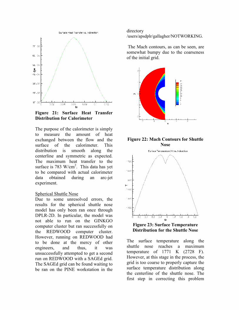
Figure 21: Surface Heat Transfer
Distribution for Calorimeter
The purpose of the calorimeter is simply
to measure the amount of heat
exchanged between the flow and the
surface of the calorimeter. This
distribution is smooth along the
centerline and symmetric as expected.
The maximum heat transfer to the
surface is 783 W/cm2. This data has yet
to be compared with actual calorimeter
data obtained during an arc-jet
experiment.
Spherical Shuttle Nose
Due to some unresolved errors, the
results for the spherical shuttle nose
model has only been ran once through
DPLR-2D. In particular, the model was
not able to run on the GINKGO
computer cluster but ran successfully on
the REDWOOD computer cluster.
However, running on REDWOOD had
to be done at the mercy of other
engineers, and thus, it was
unsuccessfully attempted to get a second
run on REDWOOD with a SAGEd grid.
The SAGEd grid can be found waiting to
be ran on the PINE workstation in the
directory /users/apsdplr/gallagher/NOTWORKING.
The Mach contours, as can be seen, are
somewhat bumpy due to the coarseness
of the initial grid.
Figure 22: Mach Contours for Shuttle
Nose
Figure 23: Surface Temperature
Distribution for the Shuttle Nose
The surface temperature along the
shuttle nose reaches a maximum
temperature of 1771 K (2728 F).
However, at this stage in the process, the
grid is too coarse to properly capture the
surface temperature distribution along
the centerline of the shuttle nose. The
first step in correcting this problem

would be to rerun the SAGEd grid
through DPLR-2D to see whether that
corrects the temperature distribution or
not.
Since the heat transfer is directly
proportional to the temperature raised to
the fourth power, one would expect to
see a similar distribution for the heat
transfer.
Figure 24: Surface Heat Transfer
Distribution for Shuttle Nose
Last, the surface pressure distribution
was calculated for the shuttle nose.
Figure 25: Surface Pressure
Distribution for Shuttle Nose
Summary
The validations of the two-dimensional
CFD models have not yet been
completed. The results for the wedge
and calorimeter models seem to be
numerically valid, while the puck and
shuttle nose models are somewhat
questionable. Inconsistencies in
numerical solutions were most apparent
in the quarter-inch radius puck
geometries. Of the two grids that were
analyzed, the temperature and heat
transfer distributions varied the most.
The quantitative results for each of the
four models can be seen in Table 3: Twenty-Degree Half-Angle Wedge RCG
Maximum Surface Quantities
Temperature (K,F) 2050, 32230
Heat Transfer (W/cm^2) 88.2
Pressure (Pa) 13030
Puck from Gridpro Surface Quantities
Centerline Temperature (K,F) 2540
Maximum Temperature (K,F) 2600
Centerline Heat Transfer (W/cm^2) 206
Maximum Heat Transfer (W/cm^2) 230
Centerline Pressure (Pa) 33775
Puck from Gridgen Surface Quantities
Centerline Temperature (K,F) 2620, 4256
Maximum Temperature (K,F) 2683, 4370
Centerline Heat Transfer (W/cm^2) 238
Maximum Heat Transfer (W/cm^2) 261
Centerline Pressure (Pa) 32864
Spherical Calorimeter Maximum Surface Quantities
Temperature (K) 300
Heat Transfer (W/cm^2) 783
Pressure (Pa) 33300
Spherical Shuttle Nose Maximum Surface Quantities
Temperature (K, F) 1771, 2728
Heat Transfer (W/cm^2) 49.68
Pressure (Pa) 5890
Table 3: Results Summary
Throughout the course of this project,
many different grids were generated and
ran using DPLR-2D. Solutions were
often surprising and sometimes led to
questions about the robustness of the
DPLR method. It was soon discovered,

after many trial runs, that CFD codes, in
general, are only as good as the grids
that are being used to run them on. This
placed an extreme importance on mesh
quality throughout the course of these
simulations.
Mesh quality is where the CFD analyst
has the largest impact on solution. A
high quality mesh increases the accuracy
of the CFD solution and improves
convergence relative to a poor quality
mesh. Therefore, it's important for a
mesher to have tools for obtaining and
improving a mesh. This area in
particular likely requires a great deal of
intuition, which is developed over many
years of CFD analysis. Due to lack of
intuition and experience on the meshers
part, the grids developed in this project
may be one of the primary sources for
discrepancies in numerical solutions.
Thus, they should be one of the first
objects scrutinized in determining why a
solution does not meet the expected
values or trends.
In particular, there was a significant
amount of disagreement between grid
solutions for the puck geometry. If time
permitted, this would be explored
further. However, the results themselves
will be clearer when compared to
experimental data.
In the end, it was not trivial to develop
models with the given geometries and
replicate arc-jet experimental data. To
date, there is work left to be done on the
puck and shuttle nose models in order to
obtain valid solutions and further
validate the DPLR method for these
particular flow fields.
Acknowledgements
The author would like to thank David
Driver for the opportunity to work on
this project at NASA Ames. In addition,
to all the people who helped with
various technicalities: Jack Atchison,
George Raiche, Dean Kontinos, Mike
Wright, Ryan McDaniel, Jeff Brown,
Tahir Gokcen, and Danesh Prabhu.
References
1. Wright, M.J., Candler, G.V., and
Bose, D., “A Data-Parallel Line
Relaxation Method for the Navier-
Stokes Equations,” AIAA Journal,
AIAA Paper No. 97-2046, June 1997.


