Astronomy & Astrophysics manuscript no. Robin2012 © ESO 2018June 4, 2018

Gaia Universe Model SnapshotA statistical analysis of the expected contents of the Gaia catalogue

A.C. Robin1, X. Luri2, C. Reylé1, Y. Isasi2, E. Grux1, S. Blanco-Cuaresma2, F. Arenou3, C. Babusiaux3, M. Belcheva4,R. Drimmel5, C. Jordi2, A. Krone-Martins7, E. Masana2, J.C. Mauduit8, F. Mignard8, N. Mowlavi6, B.

Rocca-Volmerange9, P. Sartoretti3, E. Slezak8, and A. Sozzetti5

1 Institut Utinam, CNRS UMR6213, Université de Franche-Comté, Observatoire de Besançon, Besançon, Francee-mail: annie.robin@obs-besancon.fr

2 Dept. Astronomia i Meteorologia ICCUB-IEEC, Martí i Franquès 1, Barcelona, Spaine-mail: xluri@am.ub.es

3 GEPI, Observatoire de Paris, CNRS, Université Paris Diderot ; 5 Place Jules Janssen, 92190 Meudon, France4 Department of Astrophysics Astronomy & Mechanics, Faculty of Physics, University of Athens, Athens, Greece5 OAT, Torino, Italy6 Observatoire de Genève, Sauverny, Switzerland7 SIM, Faculdade de Ciências, Universidade de Lisboa, Portugal8 Observatoire de la Côte d’Azur, Nice, France9 Institut d’Astrophysique de Paris, France

Abstract

Context. This study has been developed in the framework of the computational simulations executed for the preparation of the ESAGaia astrometric mission.Aims. We focus on describing the objects and characteristics that Gaia will potentially observe without taking into considerationinstrumental effects (detection efficiency, observing errors).Methods. The theoretical Universe Model prepared for the Gaia simulation has been statistically analyzed at a given time. Ingredientsof the model are described, giving most attention to the stellar content, the double and multiple stars, and variability.Results. In this simulation the errors have not been included yet. Hence we estimate the number of objects and their theoreticalphotometric, astrometric and spectroscopic characteristics in the case that they are perfectly detected. We show that Gaia will be ableto potentially observe 1.1 billion of stars (single or part of multiple star systems) of which about 2% are variable stars, 3% have oneor two exoplanets. At the extragalactic level, observations will be potentially composed by several millions of galaxies, half millionto 1 million of quasars and about 50,000 supernovas that will occur during the 5 years of mission. The simulated catalogue will bemade publicly available by the DPAC on the Gaia portal of the ESA web site http://www.rssd.esa.int/gaia/

Key words. Stars:statistics, Galaxy:stellar content, Galaxy:structure, Galaxies:statistics, Methods: data analysis, Catalogs

1. Introduction

The ESA Gaia astrometric mission has been designed for solvingone of the most difficult yet deeply fundamental challengesin modern astronomy: to create an extraordinarily precise 3Dmap of about a billion stars throughout our Galaxy and beyond(Perryman et al. 2001).

The survey aims to reach completeness at Vlim∼ 20−25 magdepending on the color of the object, with astrometric accuraciesof about 10µas at V=15. In the process, it will map stellarmotions and provide detailed physical properties of each starobserved: characterizing their luminosity, temperature, gravityand elemental composition. Additionally, it will perform thedetection and orbital classification of tens of thousands of extra-solar planetary systems, and a comprehensive survey of some105− 106 minor bodies in our solar system, as well as galaxiesin the nearby Universe and distant quasars.

This massive stellar census will provide the basicobservational data to tackle important questions related to the

Send offprint requests to: A.C. Robin

origin, structure and evolutionary history of our Galaxy and newtests of general relativity and cosmology.

It is clear that the Gaia data analysis will be an enormoustask in terms of expertise, effort and dedicated computing power.In that sense, the Data Processing and Analysis Consortium(DPAC) is a large pan-European team of expert scientists andsoftware developers which are officially responsible for Gaiadata processing and analysis1. The consortium is divided intospecialized units with a unique set of processing tasks known asCoordination Units (CUs). More precisely, the CU2 is the taskforce in charge of the simulation needs for the work of otherCUs, ensuring that reliable data simulations are available for thevarious stages of the data processing and analysis development.One key piece of the simulation software developed by CU2for Gaia is the Universe Model that generates the astronomicalsources.

The main goal of the present paper is to analyze the contentof a full sky snapshot (for a given moment in time) of the

1 http://www.rssd.esa.int/gaia/dpac

1

arX

iv:1

202.

0132

v2 [

astr

o-ph

.GA

] 2

Feb

201

2

A.C. Robin et al.: Gaia Universe Model Snapshot

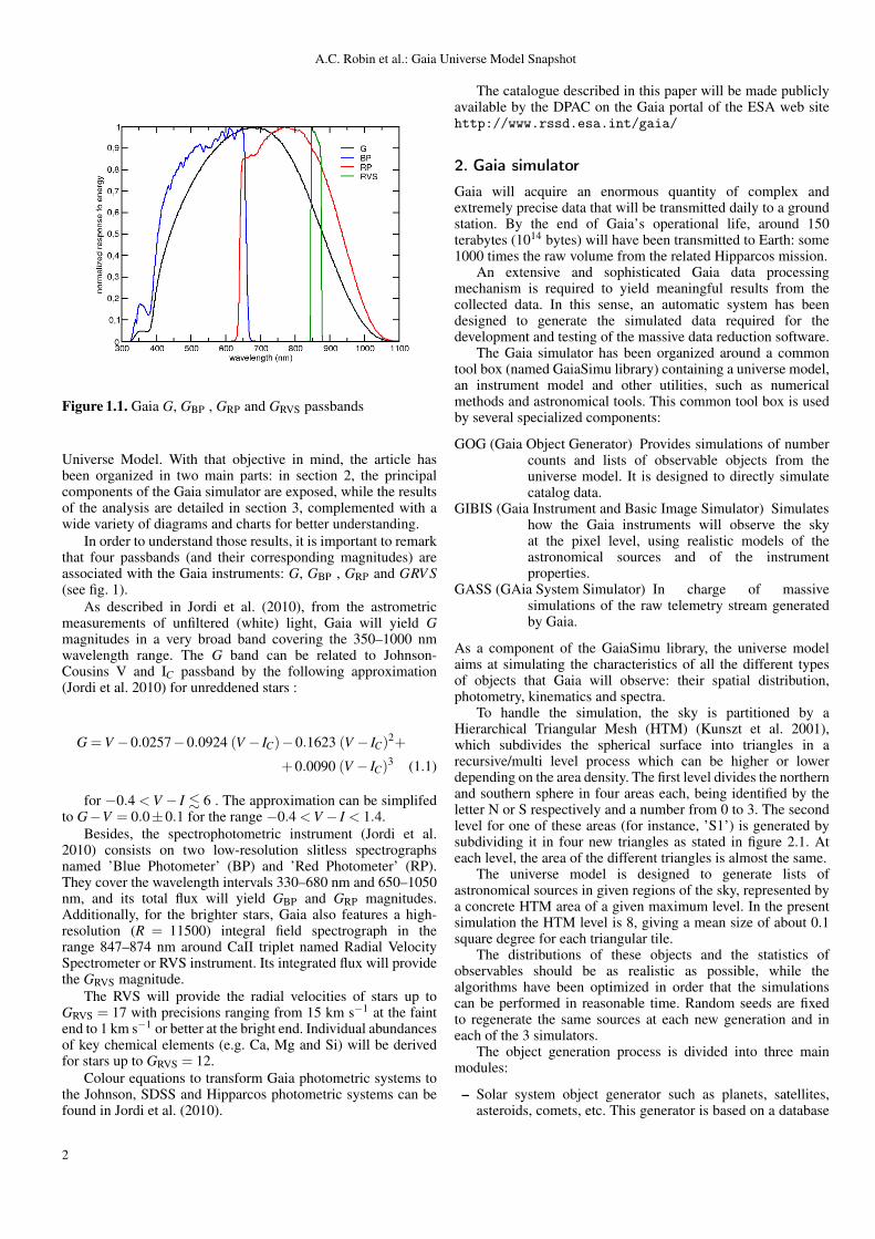
Figure 1.1. Gaia G, GBP , GRP and GRVS passbands

Universe Model. With that objective in mind, the article hasbeen organized in two main parts: in section 2, the principalcomponents of the Gaia simulator are exposed, while the resultsof the analysis are detailed in section 3, complemented with awide variety of diagrams and charts for better understanding.

In order to understand those results, it is important to remarkthat four passbands (and their corresponding magnitudes) areassociated with the Gaia instruments: G, GBP , GRP and GRV S(see fig. 1).

As described in Jordi et al. (2010), from the astrometricmeasurements of unfiltered (white) light, Gaia will yield Gmagnitudes in a very broad band covering the 350–1000 nmwavelength range. The G band can be related to Johnson-Cousins V and IC passband by the following approximation(Jordi et al. 2010) for unreddened stars :

G =V −0.0257−0.0924 (V − IC)−0.1623 (V − IC)2+

+0.0090 (V − IC)3 (1.1)

for −0.4 < V − I . 6 . The approximation can be simplifedto G−V = 0.0±0.1 for the range −0.4 <V − I < 1.4.

Besides, the spectrophotometric instrument (Jordi et al.2010) consists on two low-resolution slitless spectrographsnamed ’Blue Photometer’ (BP) and ’Red Photometer’ (RP).They cover the wavelength intervals 330–680 nm and 650–1050nm, and its total flux will yield GBP and GRP magnitudes.Additionally, for the brighter stars, Gaia also features a high-resolution (R = 11500) integral field spectrograph in therange 847–874 nm around CaII triplet named Radial VelocitySpectrometer or RVS instrument. Its integrated flux will providethe GRVS magnitude.

The RVS will provide the radial velocities of stars up toGRVS = 17 with precisions ranging from 15 km s−1 at the faintend to 1 km s−1 or better at the bright end. Individual abundancesof key chemical elements (e.g. Ca, Mg and Si) will be derivedfor stars up to GRVS = 12.

Colour equations to transform Gaia photometric systems tothe Johnson, SDSS and Hipparcos photometric systems can befound in Jordi et al. (2010).

The catalogue described in this paper will be made publiclyavailable by the DPAC on the Gaia portal of the ESA web sitehttp://www.rssd.esa.int/gaia/

2. Gaia simulator

Gaia will acquire an enormous quantity of complex andextremely precise data that will be transmitted daily to a groundstation. By the end of Gaia’s operational life, around 150terabytes (1014 bytes) will have been transmitted to Earth: some1000 times the raw volume from the related Hipparcos mission.

An extensive and sophisticated Gaia data processingmechanism is required to yield meaningful results from thecollected data. In this sense, an automatic system has beendesigned to generate the simulated data required for thedevelopment and testing of the massive data reduction software.

The Gaia simulator has been organized around a commontool box (named GaiaSimu library) containing a universe model,an instrument model and other utilities, such as numericalmethods and astronomical tools. This common tool box is usedby several specialized components:

GOG (Gaia Object Generator) Provides simulations of numbercounts and lists of observable objects from theuniverse model. It is designed to directly simulatecatalog data.

GIBIS (Gaia Instrument and Basic Image Simulator) Simulateshow the Gaia instruments will observe the skyat the pixel level, using realistic models of theastronomical sources and of the instrumentproperties.

GASS (GAia System Simulator) In charge of massivesimulations of the raw telemetry stream generatedby Gaia.

As a component of the GaiaSimu library, the universe modelaims at simulating the characteristics of all the different typesof objects that Gaia will observe: their spatial distribution,photometry, kinematics and spectra.

To handle the simulation, the sky is partitioned by aHierarchical Triangular Mesh (HTM) (Kunszt et al. 2001),which subdivides the spherical surface into triangles in arecursive/multi level process which can be higher or lowerdepending on the area density. The first level divides the northernand southern sphere in four areas each, being identified by theletter N or S respectively and a number from 0 to 3. The secondlevel for one of these areas (for instance, ’S1’) is generated bysubdividing it in four new triangles as stated in figure 2.1. Ateach level, the area of the different triangles is almost the same.

The universe model is designed to generate lists ofastronomical sources in given regions of the sky, represented bya concrete HTM area of a given maximum level. In the presentsimulation the HTM level is 8, giving a mean size of about 0.1square degree for each triangular tile.

The distributions of these objects and the statistics ofobservables should be as realistic as possible, while thealgorithms have been optimized in order that the simulationscan be performed in reasonable time. Random seeds are fixedto regenerate the same sources at each new generation and ineach of the 3 simulators.

The object generation process is divided into three mainmodules:

– Solar system object generator such as planets, satellites,asteroids, comets, etc. This generator is based on a database

2

A.C. Robin et al.: Gaia Universe Model Snapshot

Figure 2.1. Hierarchical Triangular Mesh subdivisions scheme:Each triangle has three vertices labeled 0, 1 and 2. When thearea is subdivided in 4 new triangles, the opposite midpointsare labeled 0’, 1’ and 2’, respectively, and the central triangleis suffixed with a 3.

of known objects and has not been activated in the presentstatistical analysisTanga (2011).

– Galactic object generator based on the Besançon Galaxymodel (BGM from now on). It creates stellar sources takinginto account extinction, star variability, existence of binarysystems and exoplanets.

– Extragalactic objects generator such as unresolved galaxies,QSO and supernovas.

In the following subsections, the generation of the different typesof objects and the computation of their relevant characteristicsare described.

2.1. Galactic objects

Galactic objects are generated from a model based on BGM(Robin et al. 2003) which provides the distribution of thestars, their intrinsic parameters and their motions. The stellarpopulation synthesis combines:

– Theoretical considerations such as stellar evolution, galacticevolution and dynamics.

– Observational facts such as the local luminosity function, theage-velocity dispersion relation, the age-metallicity relation.

The result is a comprehensive description of the stellarcomponents of the Galaxy with their physical characteristics(e.g. temperature, mass, gravity, chemical composition andmotions).

The Galaxy model is formed by four stellar populationsconstructed with different model parameters. For eachpopulation the stellar content is defined by the Hess diagramaccording to the age and metallicity characteristics. Thepopulations considered here are:

– The thin disc: young stars with solar metallicity in the mean.It is additionally divided in seven isothermal components ofages varying from 0–0.15 Gyr for the youngest to 7–10 Gyrfor the oldest.

– The thick disc: in terms of metallicity, age and kinematics,stars are intermediate between the thin disc and the stellarhalo.

– The stellar halo (spheroid): old and metal poor stars.– The outer bulge: old stars with metallicities similar to the

ones in the thin disc.

The simulations are done using the equation of stellarstatistics. Specifying a direction and a distance rmax, the modelgenerates a star catalog using the following equation:

Table 2.1. Local mass density ρ0 for different populations. Axisratio ε are given as a function of age for the disc population andthe spheroid.

Population Age (Gyr) Local density(Mpc−3) ε

Disc 0–0.15 4.0×10−3 0.01400.15–1 7.9×10−3 0.0268

1–2 6.2×10−3 0.03752–3 4.0×10−3 0.05513–5 4.0×10−3 0.06965–7 4.9×10−3 0.0785

7–10 6.6×10−3 0.0791WD 3.96×10−3 -

Thick disc 11 1.34×10−3 -WD 3.04×10−4 -

Spheroid 14 9.32×10−6 0.76

N =∫ rmax

0

n

∑i=1

ρi (R,θ ,z,Age)×Φ(MV ,Teff,Age)ωr2dr (2.1)

where ρ (R,θ ,z,Age) is the stellar density law withgalactocentric coordinates (R,θ ,z), also described in table 2.1,Φ(MV ,Teff,Age) is the number of stars per square parsec in agiven cell of the HR Diagram (MV ,Teff,Age) for a given agerange near the sun, ω is the solid angle and r the distance to thesun.

The functions ρ (R,θ ,z,Age) (density laws) andΦ(MV ,Teff,Age) (Hess diagrams) are specific for eachpopulation, and established using theoretical and empiricalconstraints, as described below.

In a given volume element having an expected densityof N, ≈ N stars are generated using a Poisson distribution.After generating the corresponding number of stars, each staris assigned its intrinsic attributes (age, effective temperature,bolometric magnitude, U,V,W velocities, distance) andcorresponding observational parameters (apparent magnitudes,colors, proper motions, radial velocities, etc) and finally affectedby the implemented 3D extinction model from Drimmel et al.(2003).

2.1.1. Density laws

Density laws allow to extrapolate what is observed in the solarneighbourhood (i.e. local densities) to the rest of the Galaxy.The density law of each population has been described in Robinet al. (2003). However the disc and bulge density have beenslightly changed. Revised density laws are given in table 2.3.It is worth noting that the local density assigned to the sevensub-populations of the thin disc and its scale height z hasbeen defined by a dynamically self-consistent process usingthe Galactic potential and Boltzman equations (Bienayme et al.1987). In this table for simplicity the density formulae do notinclude the warp and flare, which are added as a modification ofthe position and thickness of the mid-plane.

The flare is the increase of the thickness of the disc withgalactocentric distance:

kflare = 1.+gflare× (R−Rflare) (2.2)

with gflare = 0.545×10−6 pc−1 and Rflare = 9500 pc. The warpis modeled as a symmetrical S-shape warp with a linear slope of

3

A.C. Robin et al.: Gaia Universe Model Snapshot

Table 2.2. Parameters of the 2 arms of the spiral structure.

Parameter 1st arm 2nd armInternal radius in kpc 3.426 3.426Pitch angle in radian 4.027 3.426

Phase angle of start in radian 0.188 2.677Amplitude 1.823 2.013

Thickness in the plane 4.804 4.964

Table 2.4. IMF and SFR for each population for primary stars.

Age (Gyr) IMF SRF

Disc 0-10

f (m) =dndm

∝ m−α

α = 1.1,0.07 < m < 0.6Mα = 1.6,0.6 < m < 1M

α = 3.0,m > 1M

constant

Thick disc 11 f (m) = dndm ∝ m−0.5 one burst

Stellar halo 14 f (m) = dndm ∝ m−0.5 one burst

Bulge 10 f (m) = dndm ∝ m−2.35

for m > 0.7Mone burst

0.09 starting at galactocentric distance of 8400 pc (Reylé et al.2009). Moreover a spiral structure has been added with 2 arms,as determined in a preliminary study by De Amores & Robin (inprep.). The parameters of the arms are given in table 2.2.

2.1.2. Magnitude - Temperature - Age distribution

The distribution of stars in the HR diagram Φ(MV ,Teff) is basedon the Initial Mass Function (IMF) and Star Formation Rate(SFR) observed in the solar neighbourhood (see table 2.4). Foreach population, the SFR determines how much stellar mass iscreated at a given formation epoch, while the IMF distributesthis mass into stars of different sizes. Then, the model bringsevery star created in each formation epoch to the present dayconsidering evolutionary tracks and the population age.

For the thin disc, the distribution in the Hess diagram splitsinto several age bins. It is obtained from an evolutionary modelwhich starts with a mass of gas, generates stars of differentmasses assuming an IMF and a SFR history, and makes thesestars evolve along evolutionary tracks. The evolution modelis described in Haywood et al. (1997a,b). It produces a filedescribing the distribution of stars per element volume in thespace (MV , Teff, Age). Similar Hess diagrams are also producedfor the bulge, the thick disc and the spheroid populations,assuming a single burst of star formation and ages of 10 Gyr,11 Gyr and 14 Gyr respectively using Bergbush & VandenBerg(1992) isochrones.

The stellar luminosity function is the one of primarystars (single stars, or primary stars in multiple systems)and is normalized to the luminosity functions in the solarneighbourhood (Reid et al. 2002).

A summary of age and metallicities, star formation historyand IMF for each population is given in tables 2.4 and 2.5.

White dwarfs are taken into account using the Wood (1992)luminosity function for the disc and Chabrier (1999) for thehalo. Bulge white dwarfs are not considered. Additionally, somerare objects such as Be stars, peculiar metallicity stars and WolfRayet stars have also been added (see section 2.1.6).

Table 2.5. Age, metallicity and radial metallicity gradients.

Age(Gyr)

<[Fe/H]> (dex) d[Fe/H]dR

(dex/kpc)Disc 0–0.15

0.15–11–22–33–55–7

7–10

0.01±0.0100.00±0.11−0.02±0.12−0.03±0.125−0.05±0.135−0.09±0.16−0.12±0.18

−0.07

Thick disc 11 −0.50±0.30 0.00Stellar Halo 14 −1.5±0.50 0.00

Bulge 10 0.00±0.20 0.00

Table 2.7. Velocity dispersions, asymmetric drift Vad at the solarposition and velocity dispersion gradient. W axis is pointing thenorth galactic pole, U the galactic center and V is tangential to

the rotational motion. It is worth noting thatd ln(σ2

U)dR = 0.2 for

the disc.

Age(Gyr)

σU(kms−1) σV(

kms−1) σW(kms−1) Vad(

kms−1)Disc 0–0.15 16.7 10.8 6 3.5

0.15–1 19.8 12.8 8 3.11–2 27.2 17.6 10 5.82–3 30.2 19.5 13.2 7.33–5 36.7 23.7 15.8 10.85–7 43.1 27.8 17.4 14.8

7–10 43.1 27.8 17.5 14.8Thick disc 11 67 51 42 53Spheroid 14 131 106 85 226

Bulge 10 113 115 100 79

2.1.3. Metallicity

Contrarily to Robin et al. (2003) metallicities [Fe/H] arecomputed through an empirical age-metallicity relationψ (Z,Age) from Haywood (2008). The mean thick disc andspheroid metallicities have also been revised. For each age andpopulation component the metallicity is drawn from a gaussian,with a mean and a dispersion as given in table 2.5. One alsoaccounts for radial metallicity gradient for the thin disc, −0.7dex/kpc, but no vertical metallicity gradient.

2.1.4. Alpha elements - Metallicity relation

Alpha element abundances are computed as a function of thepopulation and the metallicity. For the halo, the abundance inalpha element is drawn from a random around a mean value,while for the thin disc, thick disc, and bulge populations itdepends on [Fe/H]. Formulas are given in table 2.6.

2.1.5. Age - velocity dispersion

Age-velocity dispersion relation is obtained from Gomez et al.(1997) for the thin disc, while Ojha et al. (1996); Ojha et al.(1999) determined the velocity ellipsoid of the thick disc, whichhas been used in the model (see table 2.7).

4

A.C. Robin et al.: Gaia Universe Model Snapshot

Table 2.3. Density laws where ρ0 is the local mass density, d0 a normalization factor to have a density of 1 at the solar position, kflare

the flare factor and a =

√R2 +

( zε

)2 in kpc with ε being the axis ratio and (R,z) the cylindrical galactic coordinates. Local densityρ0 and axial ratio ε can be found in table 2.1. For simplicity the disc density law is given here without the warp and flare (see textfor their characteristics). For the bulge, x,y,z are in the bulge reference frame and values of N, x0, y0, z0, Rc as well as angles fromthe main axis to the Galaxy reference frame are given in Robin et al. (2003), table 5.

Population Density laws

Disc ρ0/d0/kflare×

e−(

ahR+

)2

− e−(

ahR−

)2with hR+ = 5000 pc and hR− = 3000 pc

if age ≤ 0.15 Gyr

ρ0/d0/kflare×

e−

(0.25+ a2

h2R+

) 12

− e−

(0.25+ a2

h2R−

) 12

with hR+ = 2530 pc and hR− = 1320 pc

if age > 0.15 Gyr

Thick disc ρ0/d0/kflare× e−R−R

hR ×(

1− 1/hzxl×(2.+xl/hz)

× z2)

if |z| ≤ xl ,xl = 72 pc

ρ0× e−R−R

hR × exl /hz

1+xl/2hze−

|z|hz

with hR = 4000 pc and hz = 1200 pcif |z|> xl ,xl = 72 pc

Spheroid ρ0/d0×(

acR

)−2.44if a≤ ac, ac = 500 pc

ρ0×(

aR

)−2.44if a > ac, ac = 500 pc

Bulge N× e−0.5×r2s

√x2 + y2 < Rc

N× e−0.5×r2s × e

−0.5(√

x2+y20.5

)2

with r2s =

√[(xx0

)2+(

yy0

)2]2

+(

zz0

)4

√x2 + y2 > Rc

Table 2.6. Alpha element abundances and metallicity relation estimated from Bensby & Feltzing (2009) for the thin and thick disc,and Gonzales et al (2011) for the bulge.

<[α/Fe]> (dex) Dispersion

Disc 0.01043−0.13× [Fe/H]+0.197∗ [Fe/H]2 +0.1882∗ [Fe/H]3 0.02Thick disc 0.392− e1.19375×[Fe/H]−1.3038 0.05

Stellar Halo 0.4 0.05Bulge −0.334× [Fe/H]+0.134 0.05

2.1.6. Stellar rotation

The rotation of each star is simulated following specificationsfrom Cox et al. (2000). The rotation velocity is computed as afunction of luminosity and spectral type. Then vsini is computedfor random values of the inclination of the star’s rotation axis.

2.1.7. Rare objects

For the needs of the simulator, some rare objects have beenadded to the BGM Hess diagram:

Be stars: this is a transient state of B-type stars with agaseous disc that is formed of material ejected from the star(Be stars are typically variable). Prominent emission lines ofhydrogen are found in its spectrum because of re-processingstellar ultraviolet light in the gaseous disc. Additionally, infraredexcess and polarization is detected as a result from the scatteringof stellar light in the disc.

Oe and Be stars are simulated as a proportion of 29% ofO7-B4 stars, 20% of B5-B7 stars and 3% of B8-B9 stars(Jaschek et al. 1988; Zorec & Briot 1997). For these objects,the ratio between the envelope radius and the stellar radius is

linked with the line strength in order to be able to determinetheir spectrum. Over the time, this ratio changes between 1.2and 6.9 to simulate the variation of the emission lines.

Two types of peculiar metallicity stars are simulated,following Kurtz (1982); Kochukhov (2007); Stift & Alecian(2009), for A and B stars that have a much slower rotation thannormal:

– Am stars have strong and often variable absorption lines ofmetals such as zinc, strontium, zirconium, and barium, anddeficiencies of others, such as calcium and scandium. Theseanomalies with respect to A-type stars are due to the factthat the elements that absorb more light are pushed towardsthe surface, while others sink under the force of gravity.

In the model, 12% of A stars on the main sequence inthe Teff range 7400 K - 10200 K are set to be Am stars. 70%of these Am stars belong to a binary system with periodfrom 2.5 to 100 days. They are forced to be slow rotators:67% have a projection of rotation velocity vsin i < 50 km/sand 23% have 50 < vsin i < 100 km/s.

5

A.C. Robin et al.: Gaia Universe Model Snapshot

– Ap/Bp stars present overabundances of some metals, suchas strontium, chromium, europium, praseodymium andneodymium, which might be connected to the presentstronger magnetic fields than classical A or B type star.

In the simulation, 8% of A and B stars on the mainsequence in the Teff range 8000 K – 15000 K are set to beAp or Bp stars. They are forced to have a smaller rotation :vsin i < 120 km/s.

Wolf Rayet (WR) stars are hot and massive stars witha high rate of mass loss by means of a very strong stellarwind. There are 3 classes based on their spectra: the WN stars(nitrogen dominant, some carbon), WC stars (carbon dominant,no nitrogen) and the rare WO stars with C/O < 1.

WR densities are computed following the observed statisticsfrom the VIIth catalogue of Galactic Wolf-Rayet stars of vander Hucht (2001). The local column density of WR stars is2.9 × 10−6pc−2 or volume density 2.37 × 10−8pc−3. Amongthem, 50% are WN, 46% are WC and 3.6% are WO. Theabsolute magnitude, colors, effective temperature, gravity andmass have been estimated from the literature. The masses andeffective temperature vary considerably from one author toanother. As a conservative value, it is assumed that the WR starshave masses of 10 M in the mean, an absolute V magnitude of-4, a gravity of -0.5, and an effective temperature of 50,000 K.

2.1.8. Binary systems

The BGM model produces only single stars which densities havebeen normalized to follow the luminosity function (LF) of singlestars and primaries in the solar neighbourhood (Reid et al. 2002).The IMF, inferred from the LF and the mass-luminosity relation,goes down to the hydrogen burning limit, and include disc starsdown to MV = 24. It corresponds to spectral types down to aboutL5.

In the Gaia simulation multiple star systems are generatedwith some probability (Arenou 2011) increasing with the massof the primary star obtained from the BGM model.

The mass of the companion is then obtained through a givenstatistical relation q = M2

M1= f (M1) which depends on period

and mass ranges, ensuring that the total number of stars andtheir distribution is compatible with the statistical observationsand checking that the pairing is realistic. The mass and age ofsecondary determine physical parameters computed using theHess diagram distribution in the Besançon model. Although, forthe case of PMS stars, it appears that pairing has been done issome cases with main sequence stars due to the resolution inage which is not good enough to distinguish them. It will beimproved in further simulations.

It is worth noting that while, observationally, the primaryof a system is conventionally the brighter, the model uses herethe other convention, i.e. the primary is the one with the largestmass, and consequently the generated mass ratio is constrainedto be 0 < q≤ 1.

The separation of the components (AU) is chosen with aGaussian probability with different mean values depending onthe stars’ masses (a smaller average separation for low massstars). Through Kepler’s third law, the separation and massesthen give the orbital period. The average orbital eccentricity (aperfect circular orbit corresponds to e= 0) depends on the periodby the following relation:

E [e] = a(

b− e−c log(P))

(2.3)

where a,b,c are constant with different values depending on thestar’s spectral type (values can be found in table 1 of Arenou(2010))

To describe the orientation of the orbit, three angles arechosen randomly:

– The argument of the periastron ω2 uniformly in [0, 2π[,– The position angle of the node Ω uniformly in [0, 2π[– The inclination i uniformly random in cos(i).

The moment at which stars are closest together (the periastrondate T ) is also chosen uniformly between 0 and the period P.

A large effort has been put at trying to ensure that simulatedmultiple stars numbers are in accordance with latest fractionsknown from available observations. A more detailed descriptioncan be found in Arenou (2011).

Although the present paper describes the content of theUniverse Model at a fixed moment in time, it should be remindedthat the model is being used to simulate the Gaia observations.Thus, obviously, the astrometric, photometric and spectroscopicobservables of a multiple system vary in time according to theorbital properties. This means that e.g. the apparent path ofthe photocentre of an unresolved binary will reflect the orbitalmotion through positional and radial velocity changes, or thatthe light curve of an eclipsing binary will vary in each band.

2.1.9. Variable stars

– Regular and semi-regular variables

Depending on their position in the HR Diagram, the generatedstars have a probability of being one of the six types of regularand semi-regular variable stars considered in the simulator:

Cepheids: Supergiant stars which undergo pulsations with veryregular periods on the order of days to months. Theirluminosity is directly related to their period of variation.

δScuti: Similar to Cepheids but rather fainter, and with shorterperiods.

RR Lyrae: Much more common than Cepheids, but also muchless luminous. Their period is shorter, typically less than oneday. They are classified intoRRab: Asymmetric light curves (they are the majority type).RRc: Nearly symmetric light curves (sometimes

sinusoidal).Gamma Doradus: Display variations in luminosity due to non-

radial pulsations of their surface. Periods of the order of oneday.

RoAp: Rapidly oscillating Ap stars are a subtype of the Apstar class (see section 2.1.7) that exhibits short-timescalerapid photometric or radial velocity variations. Periods onthe order of minutes.

ZZceti: Pulsating white dwarf with hydrogen atmosphere.These stars have periods between seconds to minutes.

Miras: Cool red supergiants, which are undergoing very largepulsations (order of months).

Semiregular: Usually red giants or supergiants that show adefinite period on occasion, but also go through periods ofirregular variation. Periods lie in the range from 20 to morethan 2000 days.

ACV (α Canes Venaticorum): Stars with strong magnetic fieldswhose variability is caused by axial rotation with respect tothe observer.

6

A.C. Robin et al.: Gaia Universe Model Snapshot

Table 2.8. Characteristics of the variable types. Localization inthe (spectral type, luminosity class) diagram, probability of a starto be variable in this region, stellar population and metallicityrange which are concerned.

Type Spec. Lum. Proba Pop [Fe/H]δ Scuti (a) A0:F2 III 0.3 all allδ Scuti (b) A1:F3 IV:V 0.3 all allACV (a) B5:B9 V 0.016 thin disc -1 to 1ACV (b) A0:A8 IV:V 0.01 thin disc -1 to 1Cepheid F5:G0 I:III 0.3 thin disc -1 to 1

RRab A8:F5 III 0.4 spheroid allRRc A8:F5 III 0.1 spheroid all

RoAp A0:A9 V 0.001 thin disc -1 to 1SemiReg (a) K5:K9 III 0.5 all allSemiReg (b) M0:M9 III 0.9 all all

Miras M0:M9 I:III 1.0 all allZZCeti White dwarf - 1.0 all all

GammaDor F0:F5 V 0.3 all all

A summary of the variable type characteristics is given in table2.8 and the description of their light curve is given in table 2.9

Period and amplitude are taken randomly from a 2Ddistribution defined for each variability type (Eyer et al. 2005).For Cepheids, a period-luminosity relation is also includedlog(P)=(−MV + 1.42)/2.78 (Molinaro et al. 2011). For Mirasthe relation is log(P)=(−MBol + 2.06)/2.54 (Feast et al. 1989).The different light curve models for each variability type aredescribed in Reylé et al. (2007).

The variation of the radius and radial velocity are computedaccordingly to the light variation, for stars with radial pulsations(RRab, RRc, Cepheids, δ Scuti, SemiRegular, and Miras).

– Dwarf and classical novae

Dwarf novae and Classical novae are cataclysmic variable starsconsisting of close binary star systems in which one of thecomponents is a white dwarf that accretes matter from itscompanion.

Classical novae result from the fusion and detonation ofaccreted hydrogen, while current theory suggests that dwarfnovae result from instability in the accretion disc that leadsto releases of large amounts of gravitational potential energy.Luminosity of dwarf novae is lower than classical ones andit increases with the recurrence interval as well as the orbitalperiod.

The model simulates half of the white dwarfs in close binarysystems with period smaller than 14 hours as dwarf novae.The light curve is simulated by a linear increase followedby an exponential decrease. The time between two bursts,the amplitude, the rising time and the decay time are drawnfrom gaussian distributions derived from OGLE observations(Wyrzykowski & Skowron, private communication).

The other half of white dwarfs in such systems is simulatedas a Classical novae.

– M-dwarf flares

Flares are due to magnetic reconnection in the stellaratmospheres. These events can produce dramatic increases inbrightness when they take place in M dwarfs and brown dwarfs.

The statistics used in the model for M-dwarf flares aremainly based on Kowalski et al. (2009) and their study on SDSSdata: 0.1% of M0-M1 dwarfs, 0.6% of M2-M3 dwarfs, and 5.6%

of M4-M6 dwarfs are flaring. The light curve for magnitude mis described as follows:

f = 1+ e−(t−t0)/τ t > t0f = 1 t < t0 (2.4)

m = m0−1.32877×A×2.5× log( f )

where t0 is the time of the maximum, τ is the decay time (in days,random between 1 and 15 minutes), m0 is the baseline magnitudeof the source star, A is the amplitude in magnitudes (drawn froma gaussian gaussian distribution with σ = 1 and x0 = 1.2).

– Eclipsing binaries

Eclipsing binaries, while being variables, are treated as binariesand the eclipses are computed from the orbits of the components.See section 2.1.8.

– Microlensing events

Gravitational microlensing is an astronomical phenomenon dueto the gravitational lens effect, where distribution of matterbetween a distant source and an observer is capable of bending(lensing) the light from the source. The magnification effectpermits the observation of faint objects such as brown dwarfs.

In the model, microlensing effects are generated assuming amap of event rates as a function of Galactic coordinates (l,b).The probabilities of lensing over the sky are drawn from thestudy of Han (2008). This probabilistic treatment is not basedon the real existence of a modelled lens close to the line of sightof the source, it simply uses the lensing probability to randomlygenerate microlensing events for a given source during the fiveyear observing period.

The Einstein crossing time is also a function of the directionof observation in the bulge, obtained from the same paper. TheEinstein time of the simulated events are drawn from a gaussiandistribution centered on the mean Einstein time. The impactparameter follows a flat distribution from 0 to 1. The time ofmaximum is uniformely distributed and completely random,from the beginning to the end of the mission. The Paczynskiformula (Paczynski 1986) is used to compute the light curve.

2.1.10. Exoplanets

One or two extra-solar planets are generated with distributionsin true mass Mp and orbital period P resembling thoseof Tabachnik & Tremaine (2002) which constitutes quite areasonable approximation to the observed distributions as oftoday, and extrapolated down to the masses close to the massof Earth. A detailed description can be found in Sozzetti et al.(2009).

Semi-major axes are derived given the star mass, planetmass, and period. Eccentricities are drawn from a power-law-type distribution, where full circular orbits (e= 0.0) are assumedfor periods below 6 days. All orbital angles (i, ω and Ω)are drawn from uniform distributions. Observed correlationsbetween different parameters (e.g, P and Mp ) are reproduced.

Simple prescriptions for the radius (assuming a mass-radius relationship from available structural models, see e.g.Baraffe et al. (2003)), effective temperature, phase, and albedo(assuming toy models for the atmospheres, such as a Lambertsphere) are provided, based on the present-day observationalevidence.

For every dwarf star generated of spectral type between Fand mid-K, the likelihood that it harbours a planet of given mass

7

A.C. Robin et al.: Gaia Universe Model Snapshot

Table 2.9. Light curves of the regular or semi-regular variable stars where ω t = 2πtP +φ (P is the period, φ is the phase)

Type Light curve

CepheidS =0.148sin(ω t −20.76)+0.1419sin(2ω t −63.76)

+0.0664sin(3ω t −91.57)+0.0354sin(4ω t −112.62)+0.020sin(5ω t −129.47)

δ Scuti, RoAp, RRc, Miras S = 0.5sin(ω t)

ACV S =−0.5cos(2ω t)1− f×cos(ω t )

1+ f/2 where f is a random number in [0;1]SemiReg Inverse Fourier Transform of a gaussian in frequency space

and period depends on its metal abundance according to theFischer & Valenti (2005) and Sozzetti et al. (2009) prescriptions.M dwarfs, giant stars, white dwarfs, and young stars do notinclude simulated planets for the time being, as well as doubleand multiple systems.

The astrometric displacement, spectroscopic radial velocityamplitude, and photometric dimming (when transiting) inducedby a planet on the parent star, and their evolution in time, arepresently computed from orbital components similarly to doublestellar systems.

2.2. Extragalactic objects

2.2.1. Resolved galaxies

In order to simulate the Magellanic clouds, catalogues of starsand their characteristics (magnitudes B, V , I, Teff, log(g),spectral type) have been obtained from the literature (Belchevaet al., private communication).

For the astrometry, since star by star distance is missing,a single proper motion and radial velocity for all stars of bothclouds is assumed. Chemical abundances are also guessed fromthe mean abundance taken from the literature. The resultingvalues and their references are given in table 2.10. For simulatingthe depth of the clouds a gaussian distribution is assumed alongthe line of sight with a sigma given in the table.

Stellar masses are estimated for each star from polynomialfits of the mass as a function of B − V colour, for severalranges of log(g), based on Padova isochrones for a metallicityof z = 0.003 for the LMC and z = 0.0013 for the SMC. Thegravities have been estimated from the effective temperatureand luminosity class but is very difficult to assert from theavailable observables. Hence the resulting HR diagrams for theMagellanic clouds are not as well defined and reliable as theywould be from theoretical isochrones.

2.2.2. Unresolved galaxies

Most galaxies observable by Gaia will not be resolved intheir individual stars. These unresolved galaxies are simulatedusing the Stuff (catalog generation) and Skymaker (shape/imagesimulation) codes from Bertin (2009), adapted to Gaia by Dollet(2004) and (Krone-Martins et al. 2008).

This simulator generates a catalog of galaxies with a 2Duniform distribution and a number density distribution in eachHubble type sampled from Schechter’s luminosity function(Fioc & Rocca-Volmerange 1999). Parameters of the luminosityfunction for each Hubble type are given in table 2.11. Eachgalaxy is assembled as a sum of a disc and a spheroid, theyare located at their redshift and luminosity and K correctionsare applied. The algorithm returns for each galaxy its position,

Table 2.11. Parameters defining the luminosity function fordifferent galaxy types at z = 0, from Fioc & Rocca-Volmerange(1999). The LF follows a shape from Schechter (1976). M* (Bj)is the magnitude in the Bj filter in the Schechter formalism.

Type φ* (Mpc−3) M* (Bj) Alpha Bulge/Total

E2 1.91×10−3 −20.02 −1 1.0E-SO 1.91×10−3 −20.02 −1 0.9

Sa 2.18×10−3 −19.62 −1 0.57Sb 2.18×10−3 −19.62 −1 0.32Sbc 2.18×10−3 −19.62 −1 0.32Sc 4.82×10−3 −18.86 −1 0.016Sd 9.65×10−3 −18.86 −1 0.049Im 9.65×10−3 −18.86 −1 0.0

QSFG 1.03×10−2 −16.99 −1.73 0.0

magnitude, B/T relation, disc size, bulge size, bulge flatness,redshift, position angles, and V − I.

The adopted library of synthetic spectra at low resolutionhas been created Tsalmantza et al. (2009) based on Pegase-2 code (Fioc & Rocca-Volmerange 1997)(http://www2.iap.fr/pegase). 9 Hubble types are available (including QuenchedStar Forming Galaxies or QSFG) Tsalmantza et al. (2009), with5 different inclinations (0.00, 22.5, 45.0, 67.5, 90.0) for non-elliptical galaxies, and at 11 redshifts (from 0. to 2. by step of0.2). For all inclinations, Pegase-2 spectra are computed withinternal extinction by transfer model with two geometries eitherslab or spheroid depending on type.

It should be noted that the resulting percentages per type,given in Table 3.13, reflect the numbers expected withoutapplying the Gaia source detection and prioritization algorithms.De facto, the detection efficiency will be better for unresolvedgalaxies having a prominent bulge and for nucleated galaxies,hence the effective Gaia catalog will have different percentagesthan the ones given in the table.

2.2.3. Quasars

QSOs are simulated from the scheme proposed in Slezak &Mignard (2007). To summarize, lists of sources have beengenerated with similar statistical properties as the SDSS, butextrapolated to G = 20.5 (the SDSS sample being complete toi = 19.1) and taking into account the flatter slope expected at thefaint-end of the QSO luminosity distribution. The space densityper bin of magnitude and the luminosity function should bevery close to the actual sky distribution. Since bright quasarsare saturated in the SDSS, the catalogue is complemented by theVéron-Cetty & Véron (2006) catalogue of nearby QSOs.

The equatorial coordinates have been generated from auniform drawing on the sphere in each of the sub-populationsdefined by its redshift. No screening has been applied in the

8

A.C. Robin et al.: Gaia Universe Model Snapshot

Table 2.10. Assumed parameters of the Magellanic clouds.

Parameter Units LMC SMC ReferenceDistance kpc 48.1 60.6 LMC: Macri et al. (2006)

SMC: Hilditch et al. (2005)Depth kpc 0.75 1.48 LMC: Sakai et al. (2000)

SMC: Subramanian (2009)µα cos(δ ) mas/yr 1.95 0.95 Costa et al. (2009)

µδ mas/yr 0.43 -1.14 Costa et al. (2009)Vlos km/s 283 158 SIMBAD (CDS)

[Fe/H] dex -0.75±0.5 -1.2±0.2 Kontizas et al, (2011)[α/Fe] dex 0.00±0.2 0.00±0.5 Kontizas et al, (2011)

Table 2.12. Predictions of SNII and SNIa numbers explodingper century for M* (Bj) galaxies defined in table 2.11.

Hubble type SNII /century SNI /centuryE2 0.0 0.05

E-S0 0.0 0.05Sa 0.4 0.11Sb 0.62 0.13Sbc 1.07 0.16Sc 0.16 0.07Sd 0.049 0.07Im 0.60 0.05

QSFG 0.0 0.05

vicinity of the Galactic plane since this will result directly fromthe application of the absorption and reddening model at a laterstage. Distance indicators can be derived for each object fromits redshift value by specifying a cosmological model. Eachof these sources lying at cosmological distances, a nearly zero(10−6mas) parallax has been assigned to all of them (equivalentto an Euclidean distance of about 1 Gpc ) in order to avoidpossible overflow/underflow problems in the simulation.

In principle, distant sources are assumed to be co-movingwith the general expansion of the distant Universe and haveno transverse motion. However, the observer is not at rest withrespect to the distant Universe and the accelerated motion aroundthe Galactic center, or more generally, that of the Local grouptoward the Virgo cluster is the source of a spurious propermotion with a systematic pattern. This has been discussed inmany places (Kovalevsky 2003; Mignard 2005). Eventually theeffect of the acceleration (centripetal acceleration of the solarsystem) will show up as a small proper motion of the quasars,or stated differently we will see the motion of the quasars on atiny fraction of the aberration ellipse whose period is 250 millionyears. This effect is simulated directly in the quasar catalogue,and equations given in Slezak & Mignard (2007). This explainstheir not null proper motions in the output catalogue.

2.2.4. Supernovae

A set of supernovae (SN) are generated associated with galaxies,with a proportion for each Hubble type, as given in table 2.12.Numbers of SNIIs are computed from the local star formationrate at 13Gyrs (z=0) and IMF for M*(Bj) galaxy types aspredicted by the code PEGASE.2. Theoretical SNIa numbersfollow the SNII/SNIa ratios from Greggio & Renzini (1983). Inthis case, the SN is situated at a distance randomly selected atless than a disc radius from the parent galaxy, accounting for theinclination.

Table 2.13. Parameters for each supernova type taken fromBelokurov & Evans (2003). The probability is given for eachtype, as well as the absolute magnitude and a dispersion aboutthis magnitude corresponding to the cosmic variance.

Type Probability MG SigmaIa 0.6663 -18.99 0.76

Ib/Ic 0.0999 -17.75 1.29II-L 0.1978 -17.63 0.88II-P 0.0387 -16.44 1.23

Another set of SN are generated randomly on the sky tosimulate SN on host galaxies which are too faint in surfacebrightness to be detected by Gaia.

Four SN types are available with a total probability ofoccuring determined to give at the end 6366 SN per steradianduring the 5 year mission (from estimations by Belokurov &Evans (2003)). For each SN generated a type is attributedfrom the associated probability, and the absolute magnitude iscomputed from a Gaussian drawing centered on the absolutemagnitude and the dispersion of the type corresponding tothe cosmic scatter. These parameters are given in table 2.13.Supernova light curves are from Peter Nugent2. It is assumedthat the SN varies the same way at each wavelength and the lightcurve in V has been taken as reference.

2.3. Extinction model

The extinction model, applied to Galactic and extragalaticobjects, is based on the dust distribution model of Drimmel et al.(2003). This full 3D extinction model is a strong improvementover previous generations of extinction models as it includesboth a smooth diffuse absorption distribution for a disc andthe spiral structure and smaller scale corrections based on theintegrated dust emission measured from the far infrared (FIR).The extinction law is from Cardelli et al. (1989).

3. Gaia Universe Model Snapshot (GUMS)

The Gaia Universe Model Snapshot (GUMS) is part of the GOGcomponent of the Gaia simulator. It has been used to generatea synthetic catalogue of objects from the universe model for agiven static time t0 simulating the real environment where Gaiawill observe (down to G = 20).

It is worth noting that this snapshot is what Gaia willbe able to potentially observe but not what it will reallydetect, since satellite instrument specifications and the available

2 http://supernova.lbl.gov/~nugent/nugent_templates.html

9

A.C. Robin et al.: Gaia Universe Model Snapshot

error models are not taken into account in the presentstatistical analysis. Gaia performances and error models aredescribed at http://www.rssd.esa.int/index.php?page=Science_Performance&project=GAIA.

The generated universe model snapshot has been analyzedby using the Gog Analysis Tool (GAT) statistics framework,which produces all types of diagnostic statistics allowingits scientific validation (e.g. star density distributions, HRdiagrams, distributions of the properties of the stars). The visualrepresentation of the most interesting results exposed in thisarticle have been generated using Python, Healpy and Matplotlib(Hunter 2007).

The simulation was performed with MareNostrum, oneof the most powerful supercomputers in Europe managed bythe Barcelona Supercomputing Center. The execution took20.000 hours (equivalent to 28 months) of computation timedistributed in 20 jobs, each one using between 16 and 128 CPUs.MareNostrum runs a SUSE Linux Enterprise Server 10SP2 andits 2,560 nodes are powered by 2 dual-core IBM 64-bit PowerPC970MP processors running at 2.3 GHz.

3.1. Galactic objects overview

– G less than 20 mag

In general terms, the universe model has generated a totalnumber of 1,000,000,000 galactic objects of which ~49% aresingle stars and ~51% stellar systems formed by stars withplanets and binary/multiple stars.

Individually, the model has created 1,600,000,000 starswhere about 32% of them are single stars with magnitude G lessthan 20 (potentially observable by Gaia) and 68% correspondto stars in multiple systems (see table 3.1). This last group isformed by stars that have magnitude G less than 20 as a systembut, in some cases, the isolated components can have magnitudeG superior to 20 and won’t be individually detectable by Gaia.

Only taking into consideration the magnitude limit in G andignoring the angular separation of multiple systems, Gaia couldbe able to individually observe up to 1,100,000,000 stars (69%)in single and multiple systems.

– GRVS less than 17 mag

For GRVS magnitudes limited to 17, the model has generated370,000,000 galactic objects of which ~43% are single starsand ~57% stellar systems formed by stars with planets andbinary/multiple stars.

Concretely, the RVS instrument could potentially provideradial velocities for up to 390,000,000 stars in single andmultiple systems if the limit in angular separation and resolutionpower are ignored (see table 3.1).

– GRVS less than 12 mag

The model has generated 13,100,000 galactic objects with GRVSless than 12, of which ~27% are single stars and ~73% stellarsystems formed by stars with planets and binary/multiple stars.

Again, if the limits in angular separation and resolutionpower are ignored, the RVS instrument could measure individualabundances of key chemical elements (metallicities) for~13,000,000 stars (see table 3.1).

3.2. Star distribution

The distribution of stars in the sky has been plotted using aHierarchical Equal Area isoLatitude Pixelisation, also known as

Table 3.1. Overview of the number of single stars and multiplesystem generated by the universe model. Percentages have beencalculated over the total stars.

Stars G < 20 mag Grvs < 17 mag Grvs < 12 mag

Single stars 31.59% 25.82% 12.91%Stars in multiple systems 68.41% 74.18% 87.09%⇒ In binary systems 52.25% 51.55% 40.24%⇒ Others (ternary, etc.) 16.16% 22.63% 46.85%

Total stars 1,600,000,000 600,000,000 28,000,000Individually observable 1,100,000,000 390,000,000 13,000,000

⇒ Variable 1.78% 3.06% 8.37%⇒ With planets 1.75% 1.44% 0.66%

Healpix projection. Unlike the HTM internal representation ofthe sky explained in section 2, Healpix provide areas of identicalsize which are useful for comparison.

G < 20 mag

Grvs < 17 mag

Grvs < 12 mag

0.0

0.5

1.0

1.5

2.0

2.5

3.0

3.5

4.0

4.5

5.0

5.5

6.0

Figure 3.1. Total sky distribution of stars for differentmagnitudes. Top down: G < 20, GRVS < 17 and GRVS < 12.Color scale indicates the log10 of the number of stars per squaredegree.

The number of stars on every region of the sky variessignificantly depending on the band (figure 3.1) and thepopulation (figure 3.2). In this last case, it is clear how thegalactic center is concentrated in the middle of the galaxy withonly 10% of stars, while the thin disc is the densest region (67%)as stated in table 3.2.

The effects of the extinction model due to the interstellarmaterial of the Galaxy, predominantly atomic and molecular

10

A.C. Robin et al.: Gaia Universe Model Snapshot

hydrogen and significant amounts of dust, is clearly visible inthese representations of the sky.

Table 3.2. Stars by population. Percentages have been calculatedover the total number of stars for each respective column.

Population G < 20 mag Grvs < 17 mag Grvs < 12 mag

disc 66.59% 76.82% 76.21%Thick disc 21.88% 14.39% 8.75%Spheroid 1.25% 0.58% 0.19%

Bulge 10.28% 8.22% 14.85%

Total 1,100,000,000 390,000,000 13,000,000

A projected representation in heliocentric-galacticcoordinates of the stellar distribution shows how the majorityof the generated stars are denser near the sun position, locatedat the origin of the XYZ coordinate system, and the bulge at8.5 kpc away (figure 3.3). Specially from a top perspective (XYview), it is appreciable the extinction effect which produceswindows where farther stars can be observed. One also noticethe sudden density drop towards the anticenter which is due tothe edge of the disc, assumed to be at a galactocentric distanceof 14 kpc, following Robin et al. (1992).

The distribution of stars according to the G magnitude variesdepending on the stellar population, being specially different forthe bulge (figure 3.4).

5 6 7 8 9 10 11 12 13 14 15 16 17 18 19 20G [mag]

0

1

2

3

4

5

6

7

8

Coun

t [log] Disk

Thick diskSpheroidBulge

Figure 3.4. G distribution split by stellar population. It is worthnoting that the bump for the bulge is due to the red clump, whichis seen at I=15 in Baade’s window.

3.3. Star classification

As expected, the most abundant group of stars belong to the mainsequence class (69%), followed by sub-giants (15%) and giants(14%). The complete star luminosity classification is given intable 3.3.

The star distribution as a function of G can be found infigure 3.5. Main sequence stars present the biggest exponentialincrease, relatively similar to sub giants. The population of white

Table 3.3. Luminosity class of generated stars. Percentages havebeen calculated over the total number of stars for each respectivecolumn.

Luminosity class G < 20 mag Grvs < 17 mag Grvs < 12 mag

supergiant 0.00% 0.01% 0.07%Bright giant 0.81% 2.18% 11.01%

Giant 14.47% 28.38% 62.71%Sub-giant 15.08% 14.38% 10.32%

Main sequence 69.40% 54.82% 15.76%Pre-main sequence 0.18% 0.20% 0.08%

White dwarf 0.05% 0.01% 0.03%Others 0.01% 0.02% 0.02%

Total 1,100,000,000 390,000,000 13,000,000

5 6 7 8 9 10 11 12 13 14 15 16 17 18 19 20G [mag]

0

1

2

3

4

5

6

7

8

Coun

t [log]

Super giantBright giantGiantSub giantMain sequencePre-Main sequenceWhite dwarfOther

Figure 3.5. Star distribution split by luminosity class for G< 20.

Table 3.4. Spectral types of generated stars. Percentages havebeen calculated over the total number of stars for each respectivecolumn.

Spectral type G < 20 mag Grvs < 17 mag Grvs < 12 mag

O <0.01% <0.01% <0.01%B 0.26% 0.50% 0.88%A 1.85% 3.30% 4.84%F 23.13% 22.94% 13.83%G 38.28% 31.58% 15.46%K 27.68% 32.23% 41.75%M 7.75% 6.78% 11.38%L <0.01% <0.01% <0.01%

WR <0.01% <0.01% 0.01%AGB 0.91% 2.50% 11.37%Other 0.09% 0.07% 0.33%

Total 1,100,000,000 390,000,000 13,000,000

dwarfs increases significantly starting at magnitude G = 14. Itis also interesting how supergiants decrease in number becausethey are intrinsically so bright and the peak that bright giantspresent at G = 14.5. For both of them, the decrease correspondsmainly to the distance of the edge of the disc in the Galacticplane.

The spectral classification of stars (table 3.4) shows that Gtypes are the most numerous (38%), followed by K types (28%)and F types (23%).

11

A.C. Robin et al.: Gaia Universe Model Snapshot

Disk Thick disk

Spheroid Bulge

0.0 0.5 1.0 1.5 2.0 2.5 3.0 3.5 4.0 4.5 5.0 5.5 6.0

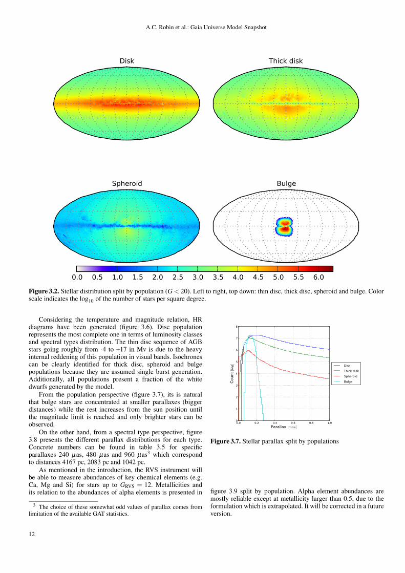
Figure 3.2. Stellar distribution split by population (G < 20). Left to right, top down: thin disc, thick disc, spheroid and bulge. Colorscale indicates the log10 of the number of stars per square degree.

Considering the temperature and magnitude relation, HRdiagrams have been generated (figure 3.6). Disc populationrepresents the most complete one in terms of luminosity classesand spectral types distribution. The thin disc sequence of AGBstars going roughly from -4 to +17 in Mv is due to the heavyinternal reddening of this population in visual bands. Isochronescan be clearly identified for thick disc, spheroid and bulgepopulations because they are assumed single burst generation.Additionally, all populations present a fraction of the whitedwarfs generated by the model.

From the population perspective (figure 3.7), its is naturalthat bulge stars are concentrated at smaller parallaxes (biggerdistances) while the rest increases from the sun position untilthe magnitude limit is reached and only brighter stars can beobserved.

On the other hand, from a spectral type perspective, figure3.8 presents the different parallax distributions for each type.Concrete numbers can be found in table 3.5 for specificparallaxes 240 µas, 480 µas and 960 µas3 which correspondto distances 4167 pc, 2083 pc and 1042 pc.

As mentioned in the introduction, the RVS instrument willbe able to measure abundances of key chemical elements (e.g.Ca, Mg and Si) for stars up to GRVS = 12. Metallicities andits relation to the abundances of alpha elements is presented in

3 The choice of these somewhat odd values of parallax comes fromlimitation of the available GAT statistics.

0.0 0.2 0.4 0.6 0.8 1.0Parallax [mas]

0

1

2

3

4

5

6

7

8

Coun

t [log] Disk

Thick diskSpheroidBulge

Figure 3.7. Stellar parallax split by populations

figure 3.9 split by population. Alpha element abundances aremostly reliable except at metallicity larger than 0.5, due to theformulation which is extrapolated. It will be corrected in a futureversion.

12

A.C. Robin et al.: Gaia Universe Model Snapshot

-9000 -4500 0 4500 9000

x [pc]

-9000

-6000

-3000

0

3000

6000

9000

y [pc]

G < 20 mag

-9000 -4500 0 4500 9000

x [pc]

-9000

-6000

-3000

0

3000

6000

9000

z [pc]

-9000 -4500 0 4500 9000

y [pc]

-9000

-6000

-3000

0

3000

6000

9000

z [pc]

-9000 -4500 0 4500 9000

x [pc]

-9000

-6000

-3000

0

3000

6000

9000

y [pc]

Grvs < 17 mag

-9000 -4500 0 4500 9000

x [pc]

-9000

-6000

-3000

0

3000

6000

9000z

[pc]

-9000 -4500 0 4500 9000

y [pc]

-9000

-6000

-3000

0

3000

6000

9000

z [pc]

-9000 -4500 0 4500 9000

x [pc]

-9000

-6000

-3000

0

3000

6000

9000

y [pc]

Grvs < 12 mag

-9000 -4500 0 4500 9000

x [pc]

-9000

-6000

-3000

0

3000

6000

9000

z [pc]

-9000 -4500 0 4500 9000

y [pc]

-9000

-6000

-3000

0

3000

6000

9000

z [pc]

−4.0

−3.2

−2.4

−1.6

−0.8

0.0

0.8

1.6

Figure 3.3. Distribution of star in heliocentric Cartesian coordinates (G < 20): top (XY), side (XZ) and front (YZ) perspectives.Color scale indicates the log10 of the number of stars per square parsec.

3.4. Kinematics

Proper motion of stars and radial velocity are represented infigure 3.10. Means are located at µα cos(δ ) = −1.95 mas/yearand µδ = −2.78 mas/year, which are affected by the motion ofthe solar local standard of rest.

Older stars, which present poorest metallicities, tend to havelowest velocities on the V axis compared to the solar localstandard of rest (figure 3.11) following the so-called asymmetricdrift. The approximate mean V velocities are -48 km s−1 for thethin disc, -98 km s−1 for the thick disc, -243 km s−1 for thespheroid and -116 km s−1 for the bulge.

3.5. Variable stars

From the total amount of 1,600,000,000 individual starsgenerated by the model, ~1.8% are variable stars (of the variabletypes included in the Universe Model). They are composed

by 6,800,000 single stars (~25% over total variable stars)with magnitude G less than 20 (observable by Gaia if theirmaximum magnitude is reached at least once during the mission)and 21,000,000 stars in multiple system (~75%). However, asexplained in section 3.1, this last group is formed by stars thathave magnitude G less than 20 as a system but, in some cases,its isolated components can have magnitude G superior to 20 andwon’t be individually detectable by Gaia.

Again, only taking into consideration magnitude G andignoring the angular separation of multiple systems, Gaia couldbe able to observe up to 21,500,000 variable stars in single andmultiple systems (~2% over total individually observable starsexposed in section 3.1).

Regarding radial velocities, they will be measurable for16,000,000 variable stars with GRVS < 17, while metallicitieswill be available for 2,000,000 variable stars (~1%) with GRVS <12 (see table 3.6).

13

A.C. Robin et al.: Gaia Universe Model Snapshot

3.03.54.04.55.0

-5.0

0.0

5.0

10.0

15.0

20.0

25.0

Mv

[mag]

Disk

3.03.54.04.55.0

-5.0

0.0

5.0

10.0

15.0

20.0

25.0

Thick disk

3.03.54.04.55.0Teff [log(K)]

-5.0

0.0

5.0

10.0

15.0

20.0

25.0

Mv

[mag]

Spheroid

3.03.54.04.55.0Teff [log(K)]

-5.0

0.0

5.0

10.0

15.0

20.0

25.0

Bulge

0.0

0.5

1.0

1.5

2.0

2.5

3.0

3.5

4.0

4.5

5.0

5.5

6.0

6.5

7.0

7.5

Figure 3.6. HR Diagram of stars split by population (left to right, top down): thin disc, thick disc, spheroid and bulge. Color scaleindicates the log10 of the number of stars per 0.025 log(K) and 0.37 mag.

0 5 10 15 20 25Parallax [mas]

0

1

2

3

4

5

6

7

8

9

Coun

t [log]

OBAFGKMLAGBWROther

Figure 3.8. Stellar parallax split by spectral type

By variability type, δ scuti are the most abundantrepresenting the 49% of the variable stars, followed bysemiregulars (42%) and microlenses (4.3%) as seen in table 3.7.However, microlenses are highly related to denser regions of thegalaxy as shown in figure 3.12, and they can involve stars of any

Table 3.5. Number of stars for each spectral type at differentparallaxes. Percentages have been calculated over totals perspectral type, which can be deduced from table 3.4.

Spectral type π > 240µas π > 480µas π > 960µasO 30.25% 1.54% 0.31%B 38.38% 4.69% 0.99%A 45.61% 9.87% 2.33%F 35.06% 8.07% 1.74%G 44.52% 11.48% 2.46%K 70.61% 34.28% 7.94%M 92.75% 90.50% 62.09%L 0.00% 0.00% 0.00%

WR 27.98% 1.89% 0.23%AGB 0.05% 0.01% <0.01%Other 71.56% 64.73% 57.53%Total 570,000,000 250,000,000 90,000,000

kind. The rest of variability types are strongly related to differentlocations in the HR diagram (figure 3.13).

3.6. Binary stars

As seen in section 3.1, the model has generated 410,000,000binary systems. Therefore about 820,000,000 stars have been

14

A.C. Robin et al.: Gaia Universe Model Snapshot

4 3 2 1 0 10.6

0.4

0.2

0.0

0.2

0.4

0.6Al

pha

elem

ents

[α/Fe]

3 6Count [log]

0246

Coun

t [log]

Disk

4 3 2 1 0 10.6

0.4

0.2

0.0

0.2

0.4

0.6

0 3 6Count [log]

012345

Coun

t [log]

Thick disk

4 3 2 1 0 1Metallicity [Fe/H]

0.6

0.4

0.2

0.0

0.2

0.4

0.6

Alph

a el

emen

ts [α/Fe]

2 4Count [log]

0123

Coun

t [log]

Spheroid

4 3 2 1 0 1Metallicity [Fe/H]

0.6

0.4

0.2

0.0

0.2

0.4

0.6

0 3 6Count [log]

0123456

Coun

t [log]

Bulge

0.0

0.5

1.0

1.5

2.0

2.5

3.0

3.5

4.0

4.5

5.0

5.5

Figure 3.9. Metallicity - alpha elements relation for GRVS < 12. Color scale indicates the log10 of the number of stars per 0.05[Fe/H] and 0.04 [α/Fe].

−150−100−50 0 50 100 150

µα cos(δ)

4

6

8

10

12

14

16

18

20

G [mag]

3 6 9

Count [log]

3

4

5

6

7

8

9

Count [log

]

−150−100−50 0 50 100 150µδ

4

6

8

10

12

14

16

18

20

3 6 9

Count [log]

4

6

8

Count [log

]

−150−100−50 0 50 100 150

Radial velocity [km/s]

4

6

8

10

12

14

16

18

20

3 6 9

Count [log]

5

6

7

8

Count [log

]

0.00

0.50

1.00

1.50

2.00

2.50

3.00

3.50

4.00

4.50

5.00

5.50

6.00

6.50

7.00

7.50

8.00

Figure 3.10. Proper motion of stars µα cosδ , µδ and radial velocity VR. Color scale indicates the log10 of the number of stars per 2.4mas/year (km/s in case of VR) and 1.0 mag.

15

A.C. Robin et al.: Gaia Universe Model Snapshot

−4 −3 −2 −1 0 1−500

−400

−300

−200

−100

0

100

V V

elo

city

[km/s]

0 4 8

Count [log]

0

2

4

6

8

Count

[log

]

Disk

−4 −3 −2 −1 0 1−500

−400

−300

−200

−100

0

100

3 6

Count [log]

0

2

4

6

8

Count

[log

]

Thick disk

−4 −3 −2 −1 0 1

Metallicity [Fe/H]

−500

−400

−300

−200

−100

0

100

V V

elo

city

[km/s]

4 5

Count [log]

0

2

4

6

Count

[log

]

Spheroid

−4 −3 −2 −1 0 1

Metallicity [Fe/H]

−500

−400

−300

−200

−100

0

100

4 6

Count [log]

0

2

4

6

8

Count

[log

]

Bulge

0.00

0.50

1.00

1.50

2.00

2.50

3.00

3.50

4.00

4.50

5.00

5.50

6.00

6.50

Figure 3.11. Metallicity and V axis velocity relation split by population (left to right, top down): thin disc, thick disc, spheroid andbulge. Color scale indicates the log10 of the number of stars per 0.05 [Fe/H] and 6 km/s.

Table 3.6. Overview of variable stars. Percentages have beencalculated over the total variable stars.

Stars G < 20 mag Grvs < 17 mag Grvs < 12 mag

Single variable stars 24.52% 25.79% 28.39%Variable stars in multiple systems 75.48% 74.21% 71.61%⇒ In binary systems 55.74% 52.65% 38.49%⇒ Others (ternary, etc.) 19.73% 21.55% 33.12%

Total variable stars 28,000,000 19,000,000 2,700,000Individually observable 21,500,000 16,000,000 2,000,000

With planets 2.09% 2.64% 2.09%

generated but it is important to remark that not all of them willbe individually observable by Gaia. Some systems may havecomponents with magnitude G fainter than 20 (although theintegrated magnitude is brighter) and others may be so closetogether that they cannot be resolved (although they can bedetected by other means).

The majority of the primary stars are from the main sequence(67%), being the most popular combination a double mainsequence star system (62%). Sub-giants and giants as primarycoupled with a main sequence star are the second and third most

Table 3.7. Stars distribution by variability type.

Variability type G < 20 mag Grvs < 17 mag Grvs < 12 mag

ACV 0.61% 0.52% 0.18%Flaring 1.46% 0.49% 0.01%RRab 0.37% 0.34% 0.02%RRc 0.09% 0.09% 0.01%

ZZceti 0.12% <0.01% <0.01%Be 2.15% 2.02% 0.87%

Cepheids 0.03% 0.04% 0.11%Classical novae 0.05% 0.06% 0.19%

δ scuti 48.57% 41.01% 14.11%Dwarf novae <0.01% <0.01% 0.00%Gammador 0.09% 0.01% <0.01%Microlens 4.27% 1.87% 0.91%

Mira 0.19% 0.24% 0.91%ρ Ap 0.05% 0.04% 0.01%

Semiregular 41.94% 53.27% 82.6%

Total 21,500,000 16,000,000 2,000,000

probable systems (16% and 14% respectively). In general terms,the distribution is coherent with star formation and evolution

16

A.C. Robin et al.: Gaia Universe Model Snapshot

Table 3.8. Binary stars classified depending on the luminosity class combination (only binary systems whose integrated magnitudeis G<20). Values are in percentage.

Supe

rgia

nt

Bri

ghtG

iant

Gia

nt

Sub-

gian

t

Mai

nse

quen

ce

Whi

tedw

arf

Oth

ers

Tota

lper

prim

ary

Supergiant 0.0000 0.0001 0.0001 0.0004 0.0021 0.0000 0.0000 0.0028Bright giant 0.0000 0.0022 0.0140 0.0154 0.1487 0.0015 0.0000 0.1819Giant 0.0000 0.2933 0.5933 0.4997 12.7477 0.7229 0.0072 14.8641Sub-giant 0.0001 0.5135 0.6916 0.5429 16.1521 0.0000 0.0100 17.9101Main sequence 0.0001 0.4990 1.1328 0.0657 63.0344 1.8421 0.0000 66.5743White dwarf 0.0000 0.0019 0.0059 0.0043 0.4258 0.0280 0.0000 0.4659Others 0.0000 0.0001 0.0001 0.0000 0.0009 0.0001 0.0000 0.0011Total per secondary 0.0002 1.3101 2.4378 1.1283 92.5118 2.5946 0.0172

0.0 0.5 1.0 1.5 2.0 2.5 3.0

Figure 3.12. Sky distribution of microlenses that could takeplace during the 5 years of the mission. Color scale indicatesthe log10 of the number of microlenses per square degree.

theories (e.g. supergiants are not accompanied by white dwarfs),see table 3.8.

The magnitude difference versus angular separation betweencomponents is shown in figure 3.14. While main sequencepairs should produce only negative magnitude differences,the presence of white dwarf primaries with small red dwarfcompanions produce the asymmetrical shape of the figure(recalling that "primary" here means the more massive). To givea hint of the angular resolution capabilities of Gaia, we canassume it at first step as nearly diffraction-limited and correctlysampled with pixel size ≈ 59 mas. Figure 3.14 thus showsthat a small fraction only of binaries with moderate magnitudedifferences will be resolved.

The mean separation of binary systems is 30 AU and theypresent a mean orbital period of about 250 years (figure 3.15).While only pairs with periods smaller than a decade may havetheir orbit determined by Gaia, a significative fraction of binarieswill be detected through the astrometric “acceleration” of theirmotion.

3.7. Stars with planets

A total number of 34,000,000 planets have been generatedand associated to 27,500,000 single stars (~2.6% over totalindividually observable stars exposed in section 3.1), implyingthat 25% of the stars have been generated with two planets (table3.9). No exoplanets are associated to multiple systems in thisversion of the model.

3.03.54.04.55.0Teff [log(K)]

5

0

5

10

15

20

25

Mv

[mag]

Classical novae

ACV

be

CepheidDelta scuti

Flaring

SemiregularZZceti

Mira

3.03.54.04.55.0Teff [log(K)]

5

0

5

10

15

20

25

Mv

[mag]

Gammador

roAp

Dwarf novae

RRab / RRc

Figure 3.13. HR diagram split by variability type.

The majority of star with planets belong to the mainsequence (66%), followed by giants (17%) and sub-giants(16.8%) as shown in table 3.10. Only 8% of stars have a planetthat produces eclipses.

On the other hand, stars with solar or higher metallicitiespresent a bigger probability of having a planet than stars poorerin metals (figure 3.16).

Finally, 77% of stars with planets belong to the thin discpopulation, while 11% are in the bulge, 11% in the thick discand 0.4% in the spheroid (figure 3.17).

17

A.C. Robin et al.: Gaia Universe Model Snapshot

−15 −10 −5 0 5 10

G difference

−4

−2

0

2

4

6

Max. angula

r se

para

tion [log(mas)

]

3 6

Count [log]

4

5

6

7C

ount

[log

]

0.00

0.50

1.00

1.50

2.00

2.50

3.00

3.50

4.00

4.50

5.00

5.50

Figure 3.14. G difference and angular separation relation forbinaries. Color scale indicates the log10 of the number of binariesper 0.25 difference in magnitude and 6 log(mas).

4 2 0 2 4 6 8 10Period [log(days)]

0.0

0.2

0.4

0.6

0.8

1.0

Ecce

ntric

ity

7Count [log]

0

2

4

6

Coun

t [log]

0.00

0.50

1.00

1.50

2.00

2.50

3.00

3.50

4.00

4.50

5.00

5.50

Figure 3.15. Period - Eccentricity relation for binaries. Colorscale indicates the log10 of the number of binaries per 0.01difference in eccentricity and 0.13log(days).

Table 3.9. Overview of stars with planets

Stars G < 20 mag Grvs < 17 mag Grvs < 12 mag

Total stars with planets 27,500,000 9,000,000 182,000

⇒ Stars with one planet 75.00% 74.99% 74.93%⇒ Stars with two planets 25.00% 25.01% 25.07%

Total number of planets 34,000,000 11,000,000 228,000

3.8. Extragalactic objects

Apart from the stars presented in the previous sections, themodel generates 8,800,000 additional stars that belong to theMagellanic Clouds. Again, the most abundant spectral typeare G stars (46%), followed by K types (33%) and A types

Table 3.10. Luminosity class of stars with planets

Luminosity class G < 20 mag Grvs < 17 mag Grvs < 12 mag

Supergiant <0.01% 0.01% 0.14%Bright giant 0.18% 0.46% 2.50%

Giant 17.04% 34.05% 65.01%Sub-giant 16.81% 14.07% 11.91%

Main sequence 65.72% 51.19% 20.36%Pre-main sequence 0.20% 0.22% 0.08%

White dwarf 0.03% <0.01% <0.01%Others <0.01% <0.01% <0.01%

Total 27,500,000 9,000,000 182,000

4 3 2 1 0 1Metallicity [Fe/H]

0

1

2

3

4

5

6

7

8

Coun

t [log]

StarsStars with planets

Figure 3.16. Metallicity distribution of stars with planets.

4 6 8 10 12 14 16 18 20G [mag]

0

1

2

3

4

5

6

7

Coun

t [log] Disk

Thick diskSpheroidBulge

Figure 3.17. G distribution of stars having planets split bypopulation.

(17%). There are no F type stars reachable by Gaia, because themagnitude cut at the cloud distance selects only the upper partof the HR diagram including massive stars on the blue side, andlate type giants and supergiants on the red side.

Regarding unresolved galaxies, 38,000,000 have beengenerated. However due to the on board thresholding algorithmoptimized for point sources, a significant fraction of thesegalaxies will not have their data transfered to Earth. Gaia willbe able to measure radial velocities for only 8% and metalabundances for 0.01% of them. The most frequent galaxy typeare spirals (58% considering Sa, Sb, Sc, Sd, Sbc), followed by

18

A.C. Robin et al.: Gaia Universe Model Snapshot

Table 3.11. Overview of extragalactic objects

Stars G < 20 mag Grvs < 17 mag Grvs < 12 mag

Stars in LMC 7,550,000 1,039,000 5,600Stars in SMC 1,250,000 161,000 950Unresolved galaxies 38,000,000 3,000,000 4,320QSO 1,000,000 5,200 11Supernovae 50,000 - -

Table 3.12. Spectral types of stars from LMC/SMC

Spectral type G < 20 mag Grvs < 17 mag Grvs < 12 mag

O 0.25% 0.17% 0.39%B 3.24% 3.40% 1.85%A 17.20% 5.01% 4.83%F 0.00% 0.00% 0.00%G 45.98% 23.16% 55.19%K 32.62% 64.82% 35.33%M 0.71% 3.44% 2.41%

Total 8,800,000 1,200,000 6,600

Table 3.13. Galaxies by type. Percentages calculated over totalgalaxies (table 3.11).

Galaxies G < 20 mag Grvs < 17 mag Grvs < 12 mag

E2 6.36% 10.24% 10.51%E-S0 7.03% 11.67% 12.85%Sa 7.51% 10.55% 10.05%Sb 9.21% 12.39% 13.70%Sc 10.21% 8.50% 8.08%Sd 22.08% 17.08% 15.00%Sbc 9.21% 12.35% 13.73%Im 24.77% 15.46% 14.44%QSFG 3.61% 1.76% 1.64%

Table 3.14. Supernovae types. Percentages calculated over50,000 supernovas.

Supernovae types

Ia 76.74%Ib/c 7.36%II-L 14.24%II-P 1.65%

irregulars (25%) and ellipticals (13% adding E2 and E-S0) asseen in table 3.13.

Additionally, 1,000,000 quasars have been generated and themodel predicts 50,000 supernovas that will occur during the 5years of mission, being 77% of them from Ia type (table 3.14).

The sky distribution of these three types of objects is shownin figure 3.18.

Regarding redshifts, galaxies go up to z ∼ 0.75, while themost distant quasars are at z ∼ 5. Magnitudes also present adifferent pattern depending on the type of object as shown infigure 3.19.

4. Conclusions

Gaia will be able to provide a much more precise and completeview of the Galaxy than its predecessor Hipparcos, representinga large increase in the total number of stars (table 4.1) and thesolar neighbourhood (table 4.2).

Galaxies

QSOs

Supernovae

0.0

0.5

1.0

1.5

2.0

2.5

3.0

Figure 3.18. Total sky distribution of unresolved galaxies,quasars and supernovae. Color scale indicates the log10 of thenumber of objects per square degree.

Table 4.1. Comparison of Hipparcos and Gaia characteristicsand the predicted number of stars, variables and binariespresented in this study.* Includes stars which may not be resolved due to its angular separation and Gaia resolution

power.

Hipparcos Gaia

Number of stars 118,218 1,100,000,000∗

Mean sky density (per square degree) ~ 3 ~ 30.425Limiting magnitude V ~ 12.4 mag V ~ 20 – 25 mag

Median astrometric precision 0.97 mas (V<9) ~ 10µ as (V=15)Possibly variable 11,597 21,500,000∗

Suspected double systems 23,882 410,000,000∗

The Gaia Universe Model, and other population synthesismodels in general, can be useful tools for survey preparation. Inthis particular case, it has been possible to obtain a general ideaof the numbers, percentages and distribution of different objectsand characteristics of the environment that Gaia can potentiallyobserve and measure.

Additionally, the analysis of the snapshot has facilitated thedetection of several aspects to be improved. Therefore, it hasbeen a quite fruitful quality assurance process from a scientificpoint of view.

Looking forward, the next reasonable step would be toreproduce the same analysis but taking into consideration theinstrument specifications and the available error models. Byconvolving it with the idealized universe model presented inthis paper, it will be possible to evaluate the impact of the

19

A.C. Robin et al.: Gaia Universe Model Snapshot

2 4 6 8 10 12 14 16 18 200.0

0.1

0.2

0.3

0.4

0.5

0.6

0.7

0.8

Redshift z

0 3 6

Count [log]

0

2

4

6

Count

[log

]

Galaxies

15 16 17 18 19 20

G [mag]

0

1

2

3

4

5

Redshift z

0 2 4

Count [log]

012345

Count

[log

]

QSOs

0.0

0.6

1.2

1.8

2.4

3.0

3.6

4.2

4.8

Figure 3.19. Redshift and G relation for galaxies and QSOs.Color scale indicates the log10 of the number of objects per 0.05mag and 0.05 redshift difference.

Table 4.2. Number of nearby stars (within 25 pc) detected byHipparcos compared with the predicted number of stars in theuniverse model

Distance (pc) StarsMin. Max. Hipparcos (V < 9) Gaia (G < 20)

20 25 1,126 4,56310 20 1,552 1,7845 10 257 9270 5 61 7060 25 2,996 7,980

instrumental effects on the actual composition of the Gaiacatalogue. In the mean time the simulated catalogue presentedin this paper will be publicly available through the ESA GaiaPortal at http://www.rssd.esa.int/gaia/.

Acknowledgements. The development of the Universe Model and of the GOGsimulator used here have been possible thanks to contributions from manypeople. We warmly acknowledge the contributions from Mary Kontizas, LaurentEyer, Guillaume Debouzy, Oscar Martínez, Raul Borrachero, Jordi Peralta, andClaire Dollet.

This work has been possible thanks to the European Science Foundation(ESF) and its funding for the activity entitled ’Gaia Research for EuropeanAstronomy Training’, as well as the infrastructure used for the computation inthe Barcelona Supercomputing Center (MareNostrum).

This work was supported by the MICINN (Spanish Ministry ofScience and Innovation) - FEDER through grant AYA2009-14648-C02-01 andCONSOLIDER CSD2007-00050.

NOTE: Internal referred documents from the Gaia mission can be found at http: // www.rssd. esa. int/ index. php? project= GAIA&page= Library_ Livelink

ReferencesArenou, F. 2010, The simulated multiple stars, Tech. rep., Observatoire de Paris-

Meudon, GAIA-C2-SP-OPM-FA-054Arenou, F. 2011, in American Institute of Physics Conference Series, Vol. 1346,

International Workshop Double and Multiple Stars: Dynamics, Physics, andInstrumentation, ed. J. A. Docobo, V. S. Tamazian, & Y. Y. Balega, 107–121

Baraffe, I., Chabrier, G., Barman, T. S., Allard, F., & Hauschildt, P. H. 2003, aap,402, 701

Belokurov, V. A. & Evans, N. W. 2003, mnras, 341, 569Bergbush, P. & VandenBerg, D. 1992, ApJS, 81, 163Bertin, E. 2009, memsai, 80, 422Bienayme, O., Robin, A. C., & Crézé, M. 1987, Astronomy and Astrophysics

(ISSN 0004-6361), 180, 94Cardelli, J. A., Clayton, G. C., & Mathis, J. S. 1989, ApJ, 345, 245Chabrier, G. 1999, ApJ, 513, L103Cox, A. N., Becker, S. A., & Pesnell, W. D. 2000, Theoretical Stellar Evolution,

ed. Cox, A. N., 499Dollet, C. 2004, PhD Thesis, Tech. rep., Université de NiceDrimmel, R., Cabrera-Lavers, A., & Lopez-Corredoira, M. 2003,

Astron.Astrophys., 409:205-216,2003Eyer, L., Robin, A., Evans, D. W., & Reylé, C. 2005, Implementation of variable

stars in the Galactic model. I. General concept, Tech. rep., Observatoire deGenève, VSWG-LE-002

Feast, M. W., Glass, I. S., Whitelock, P. A., & Catchpole, R. M. 1989, mnras,241, 375

Fioc, M. & Rocca-Volmerange, B. 1997, A&A, 326, 950Fioc, M. & Rocca-Volmerange, B. 1999, A&A, 344, 393Fischer, D. A. & Valenti, J. 2005, apj, 622, 1102Gomez, A. E., Grenier, S., Udry, S., et al. 1997, in ESA Special Publication, Vol.

402, ESA Special Publication, 621–624Greggio, L. & Renzini, A. 1983, A&A, 118, 217Han, C. 2008, apj, 681, 806Haywood, M. 2008, MNRAS, 388, 1175Haywood, M., Robin, A. C., & Crézé, M. 1997a, Astronomy and Astrophysics

(ISSN 0004-6361), 320, 428Haywood, M., Robin, A. C., & Crézé, M. 1997b, Astronomy and Astrophysics

(ISSN 0004-6361), 320, 440Hunter, J. D. 2007, Computing In Science & Engineering, 9, 90Jaschek, C., Jaschek, M., Egret, D., & Andrillat, Y. 1988, A&A, 192, 285Jordi, C., Gebran, M., Carrasco, J. M., et al. 2010, A&A, 523, A48+Kochukhov, O. 2007, Communications in Asteroseismology, 150, 39Kovalevsky, J. 2003, aap, 404, 743Kowalski, A. F., Hawley, S. L., Hilton, E. J., et al. 2009, aj, 138, 633Krone-Martins, A. G. O., Ducourant, C., Teixeira, R., & Luri, X. 2008, in

IAU Symposium, Vol. 248, IAU Symposium, ed. W. J. Jin, I. Platais, &M. A. C. Perryman, 276–277

Kunszt, P. Z., Szalay, A. S., & Thakar, A. R. 2001, in Mining the Sky, ed.A. J. Banday, S. Zaroubi, & M. Bartelmann, 631–+

Kurtz, D. W. 1982, mnras, 200, 807Mignard, F. 2005, in ESA Special Publication, Vol. 576, The Three-Dimensional

Universe with Gaia, ed. C. Turon, K. S. O’Flaherty, & M. A. C. Perryman,5–+

Molinaro, R., Ripepi, V., Marconi, M., et al. 2011, MNRAS, 413, 942Ojha, D., Bienayme, O., Robin, A., Crézé, M., & Mohan, V. 1996, A&A, 311,

456Ojha, D. K., Bienaymé, O., Mohan, V., & Robin, A. C. 1999, A&A, 351, 945Paczynski, B. 1986, ApJ, 304, 1Perryman, M. A. C., de Boer, K. S., Gilmore, G., et al. 2001, Astron.Astrophys.,

369:339-363,2001Reid, I. N., Gizis, J. E., & Hawley, S. L. 2002, aj, 124, 2721Reylé, C., Marshall, D. J., Robin, A. C., & Schultheis, M. 2009, aap, 495, 819Reylé, C., Robin, A., Arenou, F., & Grux, E. 2007, Universe Model Interface

Control Document, Tech. rep., Obs. de Besançon, Obs. de Paris-Meudon,GAIA-C2-SP-LAOB-CR-001

Robin, A. C., Crézé, M., & Mohan, V. 1992, ApJ, 400, L25Robin, A. C., Reylé, C., Derriére, S., & Picaud, S. 2003, Astronomy and

Astrophysics (ISSN 0004-6361), 409, 523Schechter, P. 1976, apj, 203, 297Slezak, E. & Mignard, F. 2007, A realistic QSO Catalogue for the Gaia Universe

Model, Tech. rep., Observatoire de la Côte d’Azur, GAIA-C2-TN-OCA-ES-001-1

Sozzetti, A., Torres, G., Latham, D. W., et al. 2009, apj, 697, 544Stift, M. J. & Alecian, G. 2009, mnras, 394, 1503Tabachnik, S. & Tremaine, S. 2002, mnras, 335, 151Tanga, P. 2011, in EAS Publications Series, Vol. 45, EAS Publications Series,

225–230

20

A.C. Robin et al.: Gaia Universe Model Snapshot

Tsalmantza, P., Kontizas, M., Rocca-Volmerange, B., et al. 2009, A&A, 504,1071

van der Hucht, K. A. 2001, New Astronomy Review, 45, 135Véron-Cetty, M.-P. & Véron, P. 2006, aap, 455, 773Wood, M. A. 1992, ApJ, 386, 539Zorec, J. & Briot, D. 1997, A&A, 318, 443

21