Gabrieli Lab. McGovern Institute for Brain Research http ... · Gabrieli Lab. McGovern Institute...

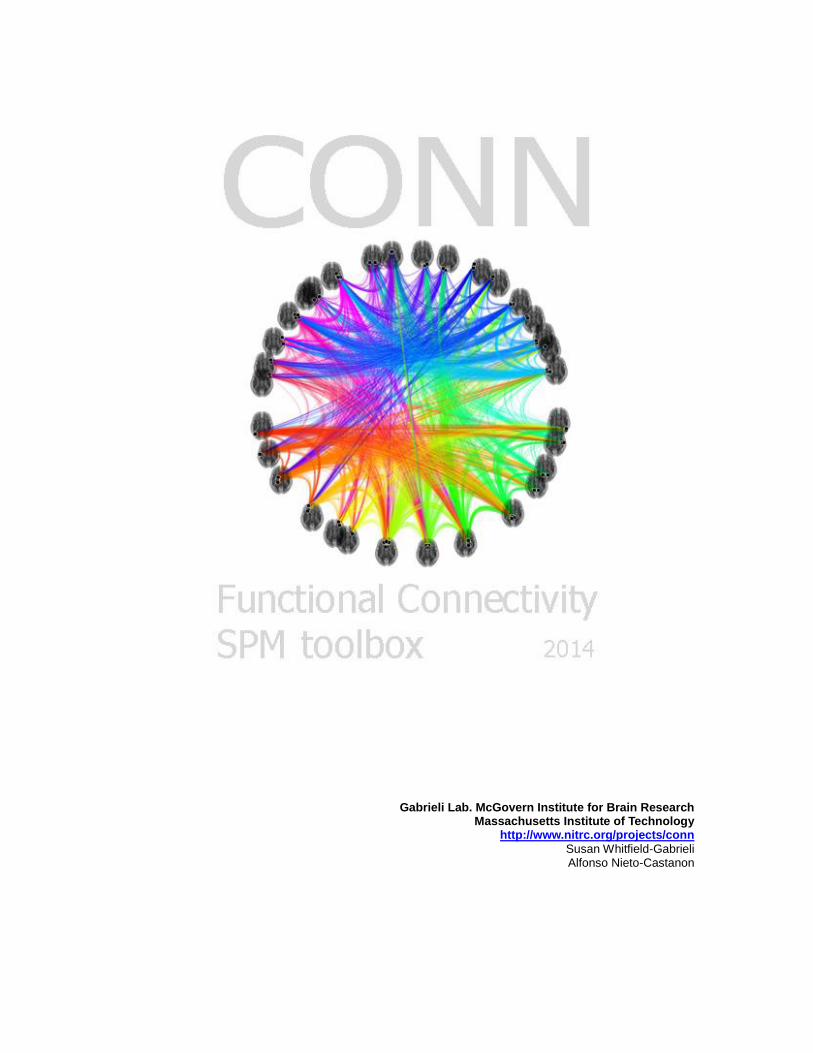
Gabrieli Lab. McGovern Institute for Brain Research Massachusetts Institute of Technology

http://www.nitrc.org/projects/conn

Susan Whitfield-Gabrieli Alfonso Nieto-Castanon


(2) conn - fMRI Functional connectivity toolbox v14

Overview

CONN is a Matlab-based cross-platform software for the computation, display, and analysis of functional

connectivity in fMRI (fcMRI). Connectivity measures include seed-to-voxel connectivity maps, ROI-to-

ROI connectivity matrices, graph properties of connectivity networks, and voxel-to-voxel measures

(intrinsic connectivity, local correlation maps, and others).

CONN is available for resting state data (rsfMRI) as well as task-related designs. It covers the entire

pipeline from raw fMRI data to hypothesis testing. The toolbox implements aCompCor strategy for

physiological (and other) noise source reduction, first-level General Linear Model for correlation and

regression connectivity estimation, and second-level random-effect analyses.

Installing the toolbox:

download and unzip conn*.zip, and add the resulting ./conn/ directory to

the matlab path (in Matlab’s File-Set path)

Requirements:

SPM5 or above

Matlab R2008b or above (no additional toolboxes required)

To start the toolbox:

On the Matlab command window, type : conn

(make sure your matlab path includes the path to the connectivity toolbox)

Updating to latest version:

On the CONN gui click on Help->Update


General

In order to perform connectivity analyses using this toolbox you will need:

a) Functional data. Either resting-state or block designs can be analyzed.

b) Structural data. One anatomical volume for each subject (this is used for plotting purposes and to

derive the gray/white/CSF masks used in the aCompCor confound removal method)

c) ROI definitions. A series of files defining seeds of interest. ROIs can be defined from mask

images, text files defining a list of MNI positions, or multiple-label images. The toolbox is also provided

with a series of pre-defined regions of interest that that will be loaded automatically (these include a series

of seed areas useful for investigating default network connectivity –FOX_*.img-, as well as a complete list

of Brodmann areas obtained from the Talairach Daemon atlas –TD.img-; see the utils/otherrois/ folder for

additional roi files).

The toolbox operation is divided in four sequential steps:

1. Setup: Defines basic experiment information, data locations, regions of interest (seeds), temporal

covariates, and second-level models.

2. Preprocessing: Define, explore, and remove possible confounds in the BOLD signal

3. Analyses: Perform first-level analyses. Define the seeds of interest and explore the functional

connectivity of different sources separately for each subject

4. Results: Perform second-level analyses. Define and explore within- and between- subject

contrasts of interest

Each of these steps can be defined interactively using the toolbox gui or by scripting using the conn_batch

functionality. The following sections describe the steps when using the gui in more detail (see the conn

batch manual for additional information).


Step one: Setup (Defines experiment information, file sources for functional data, structural data,

regions of interest, and other covariates)

Click on the SETUP tab

Click on the New button to start a new project. The toolbox will offer the option to spatially preprocess

your data (segmentation, slicetiming, realignment, coregistration, normalization, and smoothing) at this

time using a wizard. This wizard will also initialize some of the basic setup information (you can skip the

Basic, Functional and Structural steps below). If your data is already spatially preprocess simply skip this

step and continue with the steps below1.

Click on the Basic button on the left side, enter experiment information (Number of subjects, TR, number

of sessions per subject, and acquisition type)

Click on the Structural button on the left side to load the structural images. Click sequentially on each

subject and select the associated anatomical image. These images should be coregistered to the functional

and ROI volumes for each subject (e.g. if using normalized functional volumes you should enter here the

normalized anatomical volume).

GUI tip 1: The “Find” in the “Select functional data files” window can be used to search for all files within

the target folder recursively. Change the “Filter” window to narrow the search.

1 Keep in mind that the toolbox assumes that the functional, structural, and ROI volumes are: 1)

coregistered to each other (see check-registration in SPM to verify this); and 2) roughly realigned to a

standard template (roughly centered and in the same orientation; see check-registration to compare them to

a canonical image). In addition if you want to perform second-level analyses the functional images should

be normalized and resliced to the same dimensions/voxel-size.


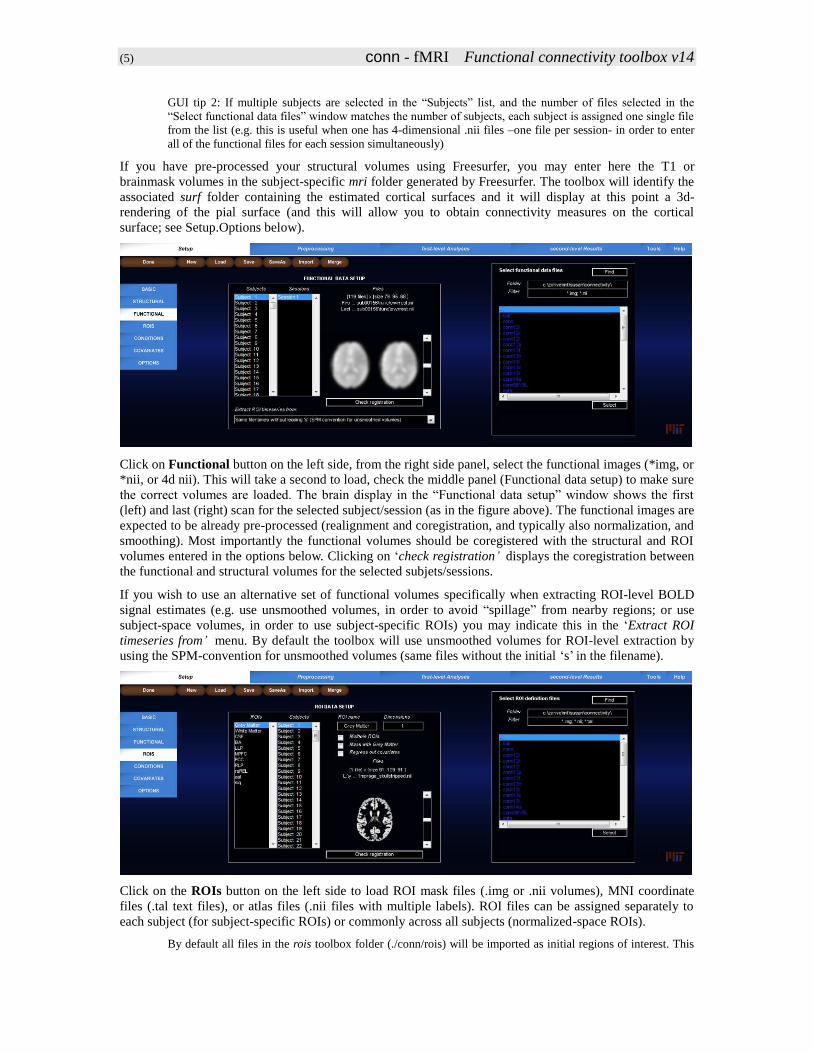
GUI tip 2: If multiple subjects are selected in the “Subjects” list, and the number of files selected in the

“Select functional data files” window matches the number of subjects, each subject is assigned one single file

from the list (e.g. this is useful when one has 4-dimensional .nii files –one file per session- in order to enter

all of the functional files for each session simultaneously)

If you have pre-processed your structural volumes using Freesurfer, you may enter here the T1 or

brainmask volumes in the subject-specific mri folder generated by Freesurfer. The toolbox will identify the

associated surf folder containing the estimated cortical surfaces and it will display at this point a 3d-

rendering of the pial surface (and this will allow you to obtain connectivity measures on the cortical

surface; see Setup.Options below).

Click on Functional button on the left side, from the right side panel, select the functional images (*img, or

*nii, or 4d nii). This will take a second to load, check the middle panel (Functional data setup) to make sure

the correct volumes are loaded. The brain display in the “Functional data setup” window shows the first

(left) and last (right) scan for the selected subject/session (as in the figure above). The functional images are

expected to be already pre-processed (realignment and coregistration, and typically also normalization, and

smoothing). Most importantly the functional volumes should be coregistered with the structural and ROI

volumes entered in the options below. Clicking on ‘check registration’ displays the coregistration between

the functional and structural volumes for the selected subjets/sessions.

If you wish to use an alternative set of functional volumes specifically when extracting ROI-level BOLD

signal estimates (e.g. use unsmoothed volumes, in order to avoid “spillage” from nearby regions; or use

subject-space volumes, in order to use subject-specific ROIs) you may indicate this in the ‘Extract ROI

timeseries from’ menu. By default the toolbox will use unsmoothed volumes for ROI-level extraction by

using the SPM-convention for unsmoothed volumes (same files without the initial ‘s’ in the filename).

Click on the ROIs button on the left side to load ROI mask files (.img or .nii volumes), MNI coordinate

files (.tal text files), or atlas files (.nii files with multiple labels). ROI files can be assigned separately to

each subject (for subject-specific ROIs) or commonly across all subjects (normalized-space ROIs).

By default all files in the rois toolbox folder (./conn/rois) will be imported as initial regions of interest. This


folder includes by default four Fox ROIs and all the Brodmann areas (defined from the Talairach daemon

atlas). To import new ROIs, click below the last ROI listed and enter the appropriate information. To remove

an existing ROI from this list right-click on an ROI and select “remove”. When importing subject-specific

ROIs click sequentially on each subject and select the corresponding ROI file. When importing subject-

independent ROI files, select all subjects simultaneously and then select the corresponding ROI file.

Load the grey matter, white matter and CSF mask for each subject if they already exist (if left blank, the

toolbox will generate these masks by performing segmentation on the structural image for each subject)

ROI files should be coregistered to the provided structural and functional volumes of this subject (they could

be defined in normalized space, or they could be defined in subject-space). Click on check registration to

display the coregistration between the selected ROI(s) and the structural volumes.

The default dimensions (number of PCA components to be extracted) for each ROI can be changed here. In

the following steps (preprocessing, analyses), you can later select the number of components among the

extracted ones you wish to use in the connectivity analyses. If one dimensions is chosen for a ROI the time-

series of interest is defined as the average BOLD activation within the ROI voxels. If more than one

dimension is chosen for a ROI the time-series of interest are defined as the principal eigenvariates of the

time-series within the ROI voxels (note: PCA decomposition is performed after removal of task-effects and

first-level covariates).

Select “mask with grey matter” on selected ROIs to further restrict these ROIs’ voxels to those voxels within

the estimated grey matter mask for each subject.

Select “multiple ROIs” if the ROI file contains multiple labels (e.g. atlas file TD.img provided in roi folder),

or multiple disconnected sets (e.g. functionally-defined ROI composed of multiple clusters, and you wish to

use each cluster as a separate seed).

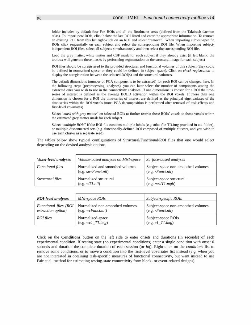
The tables below show typical configurations of Structural/Functional/ROI files that one would select

depending on the desired analysis options

Voxel-level analyses Volume-based analyses on MNI-space Surface-based analyses

Functional files Normalized and smoothed volumes

(e.g. swrFunct.nii)

Subject-space non-smoothed volumes

(e.g. rFunct.nii)

Structural files Normalized structural

(e.g. wT1.nii)

Subject-space structural

(e.g. mri/T1.mgh)

ROI-level analyses MNI-space ROIs Subject-specific ROIs

Functional files (ROI

extraction option)

Normalized non-smoothed volumes

(e.g. wrFunct.nii)

Subject-space non-smoothed volumes

(e.g. rFunct.nii)

ROI files Normalized-space

(e.g. wc1_T1.img)

Subject-space ROIs

(e.g. c1_T1.img)

Click on the Conditions button on the left side to enter onsets and durations (in seconds) of each

experimental condition. If resting state (no experimental conditions) enter a single condition with onset 0

seconds and duration the complete duration of each session (or inf). Right-click on the conditions list to

remove some conditions, or to move a condition into the first-level covariates list instead (e.g. when you

are not interested in obtaining task-specific measures of functional connectivity, but want instead to use

Fair et al. method for estimating resting-state connectivity from block- or event-related designs)


Click on the Covariates:First-level button to define first level covariates such as realignment parameters

to be used in the first-level BOLD model. For each covariate select a .txt or .mat file (for each subject and

session) containing the covariate time series (e.g. select the realignment parameters file rp_*.txt to include

the movement parameters as covariates).

When importing .txt files they should contain as many rows of number as scans for any given subject/session,

and an arbitrary number of columns (columns are separated by spaces). When importing .mat files they

should contain a single variable (arbitrarily named) consisting of a matrix with as many rows as scans for any

given subject/session and arbitrary number of columns.

If you want to obtain aggregated subject-level measures of some of your first-level covariates (e.g. to

compute the maximum amount of movement for each subject) you may do so at this point by selecting each

first-level measure in the covariates list and clicking on the subject-level aggreagate button below.

Click on the Covariates:Second-level button to define groups and subject-level regressors (e.g. behavioral

measures). Use 1/0 to define subject groups, or continuous values to perform between-subject regression

models). Click on the empty space below “All” to add a variable.

e.g. patients: 1 1 1 1 0 0 0 0

controls: 0 0 0 0 1 1 1 1

performance : 1 2 3 2 3 4 5 6

Note: Second-level covariates can be defined at any time in the analyses (changes to any of other “Setup”

options requires rerunning all the analyses steps, while changes to the second-level covariates do not as they

only affect the second-level analyses in the “Results” window)

Right-click on the covariates list to delete some of your covariates, or use the orthogonalize covariate

button to orthogonalize some of your covariates (e.g. you may ‘center’ a between-subjects variable by

orthogonalizing it with respect of the constant –all subjects- term)

GUI tip: Use Tools->Calculator on the main CONN gui to visualize and analyze your current 2nd-level

covariates (e.g. look at potential between-group differences in subject movement, levels of association

between your different subject-level measures, etc.). The way to define 2nd-level analyses in the calculator is

the same as that of the main CONN gui 2nd-level results view (see Step 4 below)

Click on the Options button on the left side for additional analysis options. Select the type of analyses that

you wish to perform (ROI-to-ROI, seed-to-voxel, and/or voxel-to-voxel analyses). For voxel-based

analyses define the desired analysis space (by default volume-based analyses using isotropic 2mm voxels;


you may indicate surface-based analyses only if you have selected Freesurfer generated structural volumes

for all of your subjects) as well as the type of analysis mask to be used (by default a gray matter template

mask). Last select if you wish optional/additional output files to be created by the toolbox.

When finished defining the experiment data press Done. This will import the functional data. If the

gray/white/CSF ROIs have not been defined before, this step will also perform segmentation of the

structural data in order to define these masks (in this case, after this process is finished come back to Setup

to inspect the resulting ROIs for possible inconsistencies). Last it will extract the ROIs time-series

(performing PCA on the within-ROI activations when appropriate). A .mat file and a folder of the same

name will be created for the project.

Save / Save as button will save the setup configurations in a .mat file, which can be loaded later (Load

button). The .mat file will be updated each time the “Done” button is pressed

Note 1: If the data has initially been defined in SPM you can skip many of the above steps by clicking the

Import button (right after entering the number of subjects in the Basic setup) and specify one SPM.mat file

for each subject. The program will extract the location of the functional data, the number of conditions per

subject, the onset/length of the conditions of interest, and any specified first-level covariates from these

SPM.mat files.


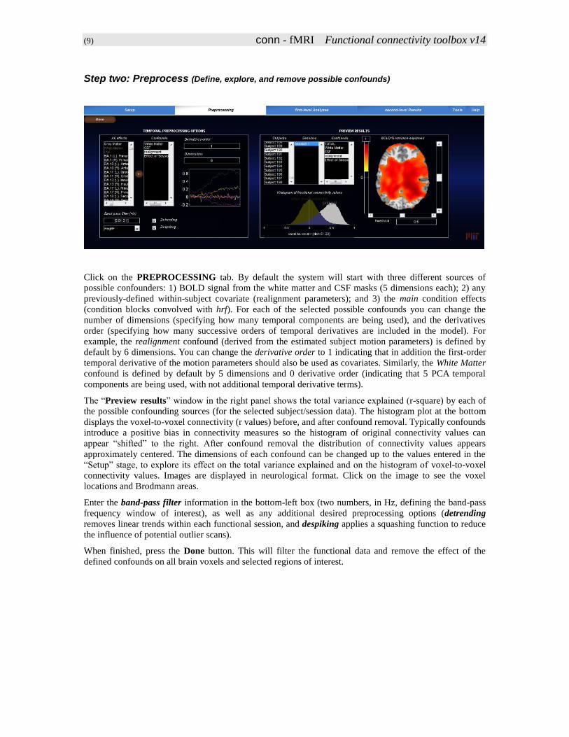
Step two: Preprocess (Define, explore, and remove possible confounds)

Click on the PREPROCESSING tab. By default the system will start with three different sources of

possible confounders: 1) BOLD signal from the white matter and CSF masks (5 dimensions each); 2) any

previously-defined within-subject covariate (realignment parameters); and 3) the main condition effects

(condition blocks convolved with hrf). For each of the selected possible confounds you can change the

number of dimensions (specifying how many temporal components are being used), and the derivatives

order (specifying how many successive orders of temporal derivatives are included in the model). For

example, the realignment confound (derived from the estimated subject motion parameters) is defined by

default by 6 dimensions. You can change the derivative order to 1 indicating that in addition the first-order

temporal derivative of the motion parameters should also be used as covariates. Similarly, the White Matter

confound is defined by default by 5 dimensions and 0 derivative order (indicating that 5 PCA temporal

components are being used, with not additional temporal derivative terms).

The “Preview results” window in the right panel shows the total variance explained (r-square) by each of

the possible confounding sources (for the selected subject/session data). The histogram plot at the bottom

displays the voxel-to-voxel connectivity (r values) before, and after confound removal. Typically confounds

introduce a positive bias in connectivity measures so the histogram of original connectivity values can

appear “shifted” to the right. After confound removal the distribution of connectivity values appears

approximately centered. The dimensions of each confound can be changed up to the values entered in the

“Setup” stage, to explore its effect on the total variance explained and on the histogram of voxel-to-voxel

connectivity values. Images are displayed in neurological format. Click on the image to see the voxel

locations and Brodmann areas.

Enter the band-pass filter information in the bottom-left box (two numbers, in Hz, defining the band-pass

frequency window of interest), as well as any additional desired preprocessing options (detrending

removes linear trends within each functional session, and despiking applies a squashing function to reduce

the influence of potential outlier scans).

When finished, press the Done button. This will filter the functional data and remove the effect of the

defined confounds on all brain voxels and selected regions of interest.


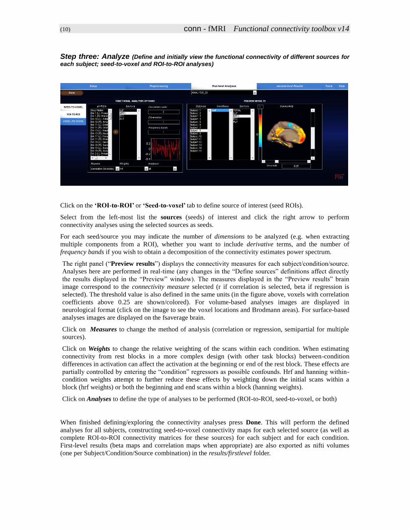
Step three: Analyze (Define and initially view the functional connectivity of different sources for

each subject; seed-to-voxel and ROI-to-ROI analyses)

Click on the ‘ROI-to-ROI’ or ‘Seed-to-voxel’ tab to define source of interest (seed ROIs).

Select from the left-most list the sources (seeds) of interest and click the right arrow to perform

connectivity analyses using the selected sources as seeds.

For each seed/source you may indicate the number of dimensions to be analyzed (e.g. when extracting

multiple components from a ROI), whether you want to include derivative terms, and the number of

frequency bands if you wish to obtain a decomposition of the connectivity estimates power spectrum.

The right panel (“Preview results”) displays the connectivity measures for each subject/condition/source.

Analyses here are performed in real-time (any changes in the “Define sources” definitions affect directly

the results displayed in the “Preview” window). The measures displayed in the “Preview results” brain

image correspond to the connectivity measure selected (r if correlation is selected, beta if regression is

selected). The threshold value is also defined in the same units (in the figure above, voxels with correlation

coefficients above 0.25 are shown/colored). For volume-based analyses images are displayed in

neurological format (click on the image to see the voxel locations and Brodmann areas). For surface-based

analyses images are displayed on the fsaverage brain.

Click on Measures to change the method of analysis (correlation or regression, semipartial for multiple

sources).

Click on Weights to change the relative weighting of the scans within each condition. When estimating

connectivity from rest blocks in a more complex design (with other task blocks) between-condition

differences in activation can affect the activation at the beginning or end of the rest block. These effects are

partially controlled by entering the “condition” regressors as possible confounds. Hrf and hanning within-

condition weights attempt to further reduce these effects by weighting down the initial scans within a

block (hrf weights) or both the beginning and end scans within a block (hanning weights).

Click on Analyses to define the type of analyses to be performed (ROI-to-ROI, seed-to-voxel, or both)

When finished defining/exploring the connectivity analyses press Done. This will perform the defined

analyses for all subjects, constructing seed-to-voxel connectivity maps for each selected source (as well as

complete ROI-to-ROI connectivity matrices for these sources) for each subject and for each condition.

First-level results (beta maps and correlation maps when appropriate) are also exported as nifti volumes

(one per Subject/Condition/Source combination) in the results/firstlevel folder.


Step three: Analyze (Define and initially view voxel-level connectome-wise measures for each

subject; voxel-to-voxel analyses)

If you wish to perform voxel-to-voxel analyses, click on the ‘voxel-to-voxel’ tab at the left of the figure.

Voxel-to-voxel analyses are analyses that take into account the entire matrix of voxel-to-voxel connectivity

values. These are useful when you do not want to restrict your analyses to one or several a priori

seeds/ROIs and rather want to investigate possible connectivity differences across the entire brain. The

implemented analyses/measures are:

Connectome-MPVA: These analyses create, separately for each voxel, a low-dimensional

multivariate representation characterizing the connectivity pattern between this voxel and the rest

of the brain (this representation is defined by performing separately for each voxel a Principal

Component Analysis of the variability in connectivity patterns between this voxel and the rest of

the brain across all subjects and conditions). The resulting representation optimally characterizes

the observed variability in connectivity patterns across subjects/conditions, and it allows you to

investigate connectivity differences across subjects directly using second-level multivariate

analyses. Edit the 2nd

-level dimensions field to modify the number of dimensions/components kept

in this multivariate representation, and the 1st-level dimensionality field to modify the degree of

dimensionality reduction used to characterize the voxel-to-voxel connectivity matrix for each

subject (number of subject-specific SVD components retained when characterizing this matrix; set

to inf for no dimensionality reduction).

Indexes: These analyses create, separately for each voxel, specific indexes/measures each

characterizing a different aspect of the connectivity pattern between this voxel and the rest of the

brain. Integrated Local Correlation (ILC, Deshpande et al. 2007) characterizes the average local

connectivity between each voxel and its neighbors (a single number for each voxel). Radial

Correlation Contrast (RCC, Goelman, 2004) characterizes the spatial asymmetry of the local

connectivity pattern between each voxel and its neighbors (a 3d vector for each voxel). Intrinsic

Connectivity Contrast (ICC, Martuzzi et al. 2011) characterizes the strength of the global

connectivity pattern between each voxel and the rest of the brain (a single number for each voxel).

Radial Similarity Contrast characterizes the global similarity (Kim et al. 2010) between the

connectivity patterns of neighboring voxels (a 3d vector for each voxel). You can also edit each

measure properties. The measure type field specifies whether the local or global connectivity

patterns for each voxel are considered (see table below); the kernel shape and kernel size fields

define the shape and size, respectively, of the convolution filter h; and the 1st-level dimensionality

field specifies the degree of dimensionality reduction used to characterize the voxel-to-voxel

connectivity matrix r (number of subject-specific SVD components retained when characterizing

this matrix).


Local measures (ILC,RCC)

y

yxyx ),()( rh

Global measures (ICC,RSC)

y

yxx2

),()(1

rh

Select from the left-most list the measures of interest and click the right arrow to add these

analyses/measures to the list of voxel-to-voxel analyses.

The right panel (“Preview results”) displays the resulting f(x) maps separately for each subject/session.

Analyses here are performed in real-time (any changes in the “Define measure” definitions affect directly

the results displayed in the “Preview” window, except for connectome-MVAP analyses for which the

preview display is not available). For volume-based analyses images are displayed in neurological format

(click on the image to see the voxel locations and Brodmann areas). For surface-based analyses images are

displayed on the fsaverage brain.

When finished defining/exploring the connectivity analyses press Done. This will perform the defined

analyses for all subjects, estimating the resulting maps from the voxel-to-voxel connectivity matrix for each

subject and for each condition. First-level results (beta maps) are also exported as nifti volumes (one per

Subject/Condition/Measure combination) in the results/firstlevel folder.


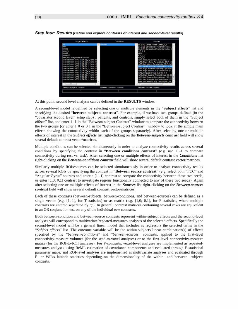
Step four: Results (Define and explore contrasts of interest and second-level results)

At this point, second level analysis can be defined in the RESULTS window.

A second-level model is defined by selecting one or multiple elements in the “Subject effects” list and

specifying the desired “between-subjects contrast”. For example, if we have two groups defined (in the

“covariates:second level” setup step) : patients, and controls, simply select both of them in the “Subject

effects” list, and enter 1 -1 in the “Between-subject Contrast” window to compare the connectivity between

the two groups (or enter 1 0 or 0 1 in the “Between-subject Contrast” window to look at the simple main

effects showing the connectivity within each of the groups separately). After selecting one or multiple

effects of interest in the Subject effects list right-clicking on the Between-subjects contrast field will show

several default contrast vector/matrices.

Multiple conditions can be selected simultaneously in order to analyze connectivity results across several

conditions by specifying the contrast in “Between conditions contrast” (e.g. use 1 -1 to compare

connectivity during rest vs. task). After selecting one or multiple effects of interest in the Conditions list

right-clicking on the Between-conditions contrast field will show several default contrast vector/matrices.

Similarly multiple ROIs/sources can be selected simultaneously in order to analyze connectivity results

across several ROIs by specifying the contrast in “Between source contrast” (e.g. select both “PCC” and

“Angular Gyrus” sources and enter a [1 -1] contrast to compare the connectivity between these two seeds,

or enter [1,0; 0,1] contrast to investigate regions functionally connected to any of these two seeds). Again

after selecting one or multiple effects of interest in the Sources list right-clicking on the Between-sources

contrast field will show several default contrast vector/matrices.

Each of these contrasts (between-subjects, between-conditions, and between-sources) can be defined as a

single vector (e.g. [1,-1], for T-statistics) or as matrix (e.g. [1,0; 0,1], for F-statistics, where multiple

contrasts are entered separated by ‘;’). In general, contrast matrices containing several rows are equivalent

to an OR conjunction test on any of the individual row contrasts.

Both between-condition and between-source contrasts represent within-subject effects and the second-level

analyses will correspond to multivariate/repeated-measures analyses of the selected effects. Specifically the

second-level model will be a general linear model that includes as regressors the selected terms in the

“Subject effects” list. The outcome variable will be the within-subjects linear combination(s) of effects

specified by the “between-conditions” and ”between-sources” contrasts, applied to the first-level

connectivity-measure volumes (for the seed-to-voxel analyses) or to the first-level connectivity-measure

matrix (for the ROI-to-ROI analyses). For F-contrasts, voxel-level analyses are implemented as repeated-

measures analyses using ReML estimation of covariance components and evaluated through F-statistical

parameter maps, and ROI-level analyses are implemented as multivariate analyses and evaluated through

F- or Wilks lambda statistics depending on the dimensionality of the within- and between- subjects

contrasts.


Step four: ROI-to-ROI results (analyze ROI-to-ROI functional connectivity matrices)

When selecting Roi-to-Roi analyses (from the leftmost tab in the figure), the brain display at the right

shows an axial view of the roi-to-roi second-level analysis results estimated in real time. These results can

be thresholded at the desired p-value threshold, using uncorrected p-values or FDR-corrected p-values, and

for one- or two-sided inferences. Right-click on the image to view a 3d display of these results. The

dropdown menu above this figure allows you to modify the list of target ROIs being displayed (this choice

affects the FDR-corrected p-values of the results; FDR correction is applied over the set of target ROIs

chosen). Images are displayed in neurological format. For each target ROI the list at the bottom of the

figure displays the connectivity contrast effect sizes (between the selected source –or linear combination of

sources- and each target), as well as T/F/X- values, uncorrected p-values, and FDR-corrected p- values for

the specified second-level analysis. Right-clicking on this table allows you to export this table to a .txt, .csv,

or .mat file. It also allows you to import the estimated ROI-to-ROI connectivity values for each subject

between any pair of ROIs as a new second-level covariate into the CONN toolbox. Last, right-clicking on

the image display allows you to view a 3d-rendered display of the supra-threshold ROI-level results.

In addition by clicking ROI-to-ROI results explorer a graphical display of all of the ROI-to-ROI

connectivity measures (for the selected between-subjects and between-condition contrasts) is shown. The

define connectivity matrix field allows you to define the specific ROIs to be included in the ROI-to-ROI

connectivity matrix analyses. You can then select one or multiple seed ROIs in the select seed ROIs field,

and the bottom-right table will display the ROI-to-ROI connectivity values between the selected source(s)

and all of the other ROIs. Right-clicking on this table allows you to export the table or sort it by different


criteria. The statistical results can be thresholded using a combination of a connection-level threshold (e.g.

uncorrected or FDR-corrected p- values on the individual ROI-to-ROI connections) and a seed- or network-

level thresholds (e.g. F-test on the multivariate connectivity strength for each seed ROI; or network-based

statistics (NBS) on the number or strength of individual connections in each connected subnetwork of

ROIs). In order to use any of the network-based statistic measures you need to first enable permutation

tests (NBS measures are obtained using permutation tests which may take a few minutes to run, depending

on the complexity of your between-subjects and between-conditions contrasts).

Right-clicking on the brain display shows additional display options, including connectome,

axial/coronal/saggital, or 3d-rendered views of the results (note: the connectome view displays all of the

ROIs on a circle, with individual suprathreshold connectivity lines between them; you may sort the ROIs

on this ring using several criteria by right-clicking on the figure and selecting one of the ROI display order

options)

Last by clicking graph-theory results explorer a graphical display is shown allowing the users to test (for

the selected between-subjects and between-condition contrasts) measures of efficiency, centrality, and

cost/degree, associated with an ROI-to-ROI connectivity network. Click on ‘Network nodes’ to limit the

ROI-to-ROI network analyzed to that defined by a subset of ROIs. The ‘Network edges’ option allows the

definition of the connectivity threshold above

which two ROIs are considered connected, and it

can be defined based on correlation scores, z-

scores, or cost values. For each ROI the list at the

bottom of the figure displays the corresponding

measure effect size (global efficiency, local

effiency, or cost), as well as T- values, uncorrected

p-values, and FDR-corrected p- values for the

specified second-level analysis. The graphical

display and second-level results can be thresholded

using either uncorrected or FDR-corrected p-

values, and it can be set to display one-sided or

two-sided results. Right-clicking on the brain

display shows additional display options, including

3d-rendered views of the analyzed network of

connectivity.


Step four: seed-to-voxel or voxel-to-voxel results (analyze voxel-level functional

connectivity measures)

When selecting Seed-to-Voxel analyses (from the leftmost tab in the figure), the brain display at the right

allows you to explore the seed-to-voxel results explorer for the specified second-level analysis estimated

in real time. These results can be thresholded using a voxel-level uncorrected p-value threshold (e.g.

p<.001 uncorrected in the gui image above; see below for additional thresholding options). For volume-

based analyses images are displayed in neurological format, while for surface-based analyses images are

displayed on the fsaverage surface.

Clicking on Seed-to-Voxel results explorer button launches a graphical display showing the results of

these second-level analyses using a MIP view of supra-threshold voxels for the entire brain, and allowing

you additional thresholding and analysis options. This display can be thresholded by a combination of

height (voxel-level) and extent (cluster-level) thresholds. Clusters are listed below together with their peak-

voxel location (in mm), number of voxels (k), uncorrected, FWE-corrected (Guassian fields theory, Friston

et al. 94), and FDR-corrected cluster-level p- values, and uncorrected and FDR-corrected peak-level p-

values (topological FDR, Chumbley et al., peak voxel within each cluster). Statistics are one-sided, select

“negative contrast” in the dropdown menu at the top right to view

the results for the reverse directionality of the contrast, or “two-

sided” to perform two-sided analyses. From this graphical display

you can also export the results as a text file containing the supra-

threshold clusters and their statistics by right-clicking on the stats

table, or as a .nii mask file defining supra-threshold voxels (export

mask button). These mask files can be re-entered directly in the

toolbox as ROI files (e.g. for post hoc analyses using suprathreshold

clusters as seeds/ROIs). In addition you may click on import values

to directly import the average connectivity values for each subject


within each supra-threshold cluster as a new second-level covariate into the CONN toolbox. Last, the

surface display, and volume display options allow you to access different 3d-rendered views of the results,

and the SPM display option allows you to load these results in the standard SPM results viewer.

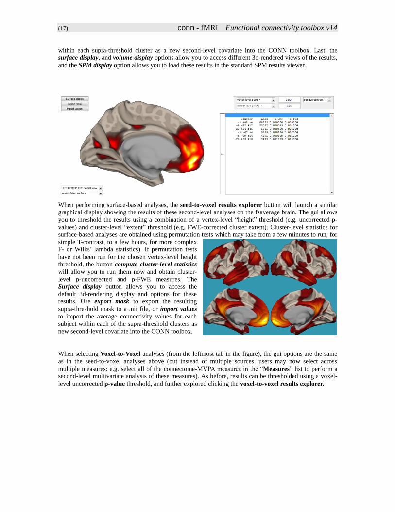
When performing surface-based analyses, the seed-to-voxel results explorer button will launch a similar

graphical display showing the results of these second-level analyses on the fsaverage brain. The gui allows

you to threshold the results using a combination of a vertex-level “height” threshold (e.g. uncorrected p-

values) and cluster-level “extent” threshold (e.g. FWE-corrected cluster extent). Cluster-level statistics for

surface-based analyses are obtained using permutation tests which may take from a few minutes to run, for

simple T-contrast, to a few hours, for more complex

F- or Wilks’ lambda statistics). If permutation tests

have not been run for the chosen vertex-level height

threshold, the button compute cluster-level statistics

will allow you to run them now and obtain cluster-

level p-uncorrected and p-FWE measures. The

Surface display button allows you to access the

default 3d-rendering display and options for these

results. Use export mask to export the resulting

supra-threshold mask to a .nii file, or import values

to import the average connectivity values for each

subject within each of the supra-threshold clusters as

new second-level covariate into the CONN toolbox.

When selecting Voxel-to-Voxel analyses (from the leftmost tab in the figure), the gui options are the same

as in the seed-to-voxel analyses above (but instead of multiple sources, users may now select across

multiple measures; e.g. select all of the connectome-MVPA measures in the “Measures” list to perform a

second-level multivariate analysis of these measures). As before, results can be thresholded using a voxel-

level uncorrected p-value threshold, and further explored clicking the voxel-to-voxel results explorer.


For more information about the CONN toolbox visit:

NITRC conn site: http://www.nitrc.org/projects/conn

Help forum: http://www.nitrc.org/forum/forum.php?forum_id=1144

FAQ: http://www.alfnie.com/software/conn


http://www.nitrc.org/forum/forum.php?forum_id=1144

http://www.alfnie.com/software/conn

Gabrieli Lab. McGovern Institute for Brain Research http ... · Gabrieli Lab. McGovern Institute...

Documents

Transcript of Gabrieli Lab. McGovern Institute for Brain Research http ... · Gabrieli Lab. McGovern Institute...