Gabriel Kreiman - Harvard...

565

Computational Models of Visual Object Recognition

Gabriel Kreiman

Visual object recognition constitutes a prime example of a cognitive task that seems to be almost instantaneous and effortless for humans, yet involves formidable challenges for computers. We open our eyes and by shifting our gaze we can, under most circumstances, easily identify the people around us, navigate through the environment, and recognize a large number of objects. The intricate neuronal circuitry behind this process is intensely studied using a combination of neurophysiologi-cal recordings and computational models. Here, we summarize some of the initial steps toward a theoretical understanding of the computational principles behind transformation-invariant visual recognition in the primate cortex.

29.1 Defining the Problem

We start by defining what needs to be explained and the necessary constraints to solve the problem. A theory of visual object recognition, implemented by a computational model, should be able to explain the following phenomena and have the following characteristics:

1. Selectivity. The primate visual system shows a remarkable degree of selectivity in that it can differentiate among shapes that appear to be very similar at the pixel level (e.g., arbi-trary three-dimensional (3D) shapes created from paperclips, different faces). Critical to successful object recognition, a model should be able to discriminate among physically similar but distinct shapes.

2. Transformation tolerance. A trivial solution to achieve high selectivity would be to memo-rize all the pixels in the object. The problem with this type of template-matching algorithm is that it would not tolerate any changes in the object’s image. An object can cast an infinite number of projections onto the retina. These different projections arise due to changes in object position with respect to fixation, object scale, plane or depth rotation, changes in contrast or illumination, color, occlusion, and others. The importance of combining selectivity and tolerance has been emphasized by many investigators (e.g., Rolls, 1991;

29

Contents

29.1 Defining the Problem ............................................................................................................ 56529.2 Brief Description of the Primate Visual Cortex ................................................................... 56729.3 Modeling the Ventral Visual Stream: Common Themes ..................................................... 56929.4 Panoply of Models ................................................................................................................ 57029.5 Bottom-Up Hierarchical Models of the Ventral Visual Stream ........................................... 57129.6 Top-Down Signals in Visual Recognition ............................................................................ 57429.7 Road Ahead .......................................................................................................................... 575References ...................................................................................................................................... 576

K12460_C029.indd 565 10/13/2012 11:55:42 AM

566 Principles of Neural Coding

Olshausen et al., 1993; Logothetis and Sheinberg, 1996; Riesenhuber and Poggio, 1999; Deco and Rolls, 2004a; Serre et al., 2007b, among others).

3. Speed. Visual recognition is very fast, as emphasized by many psychophysical investi-gations (Potter and Levy, 1969; Kirchner and Thorpe, 2006; Serre et al., 2007a), scalp electroencephalography (EEG) measurements (Thorpe et al., 1996), and invasive neuro-physiological recordings in humans (Liu et al., 2009) and monkeys (e.g., Richmond et al., 1983; Keysers et al., 2001; Hung et al., 2005). This speed imposes an important constraint on the number of computational steps that the visual system can use for pattern recognition (Rolls, 1991; Serre et al., 2007b).

4. Generic shape recognition. We can recognize a large variety of objects and shapes. Estimates about the exact number of objects or object categories that primates can discrim-inate vary widely depending on several assumptions and extrapolations (e.g., Standing, 1973; Biederman, 1987; Abbott et al., 1996; Brady et al., 2008). Certain types of shapes may be particularly interesting, may have more cortical real estate associated with them, and may be processed faster, and their recognition could be impaired independently of other shapes. For example, there has been extensive discussion in the literature about faces, their representation, and how they can be different from other visual stimuli (for review, see Tsao and Livingstone, 2008). Yet, independently of precise figures about the number of shapes that primates can discriminate and independently also of whether natural objects and faces are special or not, it is clear that there exists a generic recognition machinery capable of discriminating among multiple arbitrary shapes. For simplicity and generality, here, we focus first on this generic shape recognition problem. Face recognition, or spe-cialization for natural objects versus other shapes, constitutes interesting and important specific instantiations and subproblems of the general one that we try to address here.

5. Implementable in a computational algorithm. A successful theory of visual object recog-nition needs to be described in sufficient detail to be implemented through computational algorithms. This requirement is important because the computational instantiation allows us to run simulations and hence to quantitatively compare the performance of the model against behavioral metrics. The computational simulations also lend themselves to a direct comparison between the model’s computational steps and neurophysiological responses at different stages of the visual processing circuitry. The algorithmic implementation forces us to rigorously state the assumptions and formalize the computational steps; in this way, computational models can be more readily compared than “armchair” theories and “word/descriptive” models. The implementation can also help us debug the theory by discovering hidden assumptions, bottlenecks, and challenges that the algorithms cannot solve or where the algorithms’ performance is poor. There are multiple fascinating ideas and theories about visual object recognition that have not been implemented through computational algorithms. These ideas can be extremely useful and helpful for the field and can inspire the development of computational models. Yet, we emphasize that we cannot easily com-pare theories that can be and have been implemented against other theories that have not.

6. Focused on primates. Here, we restrict the discussion to object recognition in primates. There are strong similarities in visual object recognition at the behavioral and neurophysi-ological levels between macaque monkeys (one of the prime species for neurophysiological studies) and humans (e.g., Myerson et al., 1981; Logothetis and Sheinberg, 1996; Orban, 2004; Nielsen et al., 2006; Kriegeskorte et al., 2008; Liu et al., 2009). While other spe-cies (e.g., cats, rodents, and pigeons) also display strong visual recognition abilities, at this stage, we know less about the neuronal circuits and computational principles involved in some of these other animal models.

7. Biophysically plausible. There are multiple computational approaches to visual object rec-ognition. Here, we restrict the discussion to models that are biophysically plausible. In doing so, we ignore a vast literature in computer vision, where investigators are trying to

Q1

K12460_C029.indd 566 10/13/2012 11:55:42 AM

567Computational Models of Visual Object Recognition

solve similar problems without direct reference to the cortical circuitry. These engineering approaches are extremely interesting and useful from a practical viewpoint. Ultimately, in the same way that computers can become quite successful at playing chess without any direct connection to the way in which humans play the game, computer vision approaches can achieve high performance without mimicking neuronal circuits. Here, we focus on biophysically plausible theories and algorithms.

8. Restricted to the visual system. The visual system is not isolated from the rest of the brain and there are plenty of connections between the visual cortex and other sensory cortices, between the visual cortex and memory systems in the medial temporal lobe, and between the visual cortex and the frontal cortex. It is likely that these connections also play an important role in the process of visual recognition, particularly through feedback signals that incorporate expectations (e.g., the probability that there is a lion in an office setting is very small), prior knowledge and experience (e.g., the object appears similar to another object that we are familiar with), and cross-modal information (e.g., the object is likely to be a musical instrument because of its harmonious sound). To begin with and to simplify the problem, we restrict the discussion to the visual system.

In a nutshell, in this chapter, we consider a scenario where an arbitrary image is flashed for a brief period of time, say 50 ms, and we need to identify its contents. We emphasize that visual rec-ognition is far more complex than the identification of specific objects. Under natural viewing con-ditions, objects are embedded in complex scenes and need to be separated from their background. How this segmentation occurs constitutes an important challenge in itself. Segmentation depends on a variety of cues including sharp edges, texture changes, and object motion among others. Some object recognition models assume that segmentation must occur prior to recognition. There is no clear biological evidence for segmentation prior to recognition. We do not discuss segmentation here (see Borenstein et al., 2004; Sharon et al., 2006 for recent examples of segmentation algorithms).

Another simplification that we consider here (as in many computational models) is to ignore color and focus on grayscale image. While colors can significantly enhance and enrich visual experience, it is clear that we can recognize shapes in grayscale images and we therefore restrict the discussion to this stripped down version of the shape recognition problem.

Most object recognition models are based on studying static images. Under natural viewing con-ditions, there are important cues that depend on temporal correlations and temporal integration of information. These dynamic cues can significantly enhance recognition. Yet, it is clear that we can recognize objects in briefly flashed static images. Therefore, many computational models aim to solve the reduced (and more difficult) version, the pattern recognition problem, ignoring dynamical information. In this chapter, we follow this trend and focus on the analysis of static images.

We can perform a variety of complex tasks that rely on visual information that are different from identification. For example, we can put together images of snakes, lions, and dolphins, and cat-egorize them as animals. Categorization is a very important problem in vision research and it also constitutes a formidable challenge for computer-based approaches. Here, we focus on the question of object identification.

29.2 brief DesCriPtion of the Primate Visual Cortex

We succinctly summarize here some aspects of the neuroanatomy and neurophysiology of the pri-mate visual system. The account does not aim to be exhaustive. We need to define some of the key brain areas and neuronal circuits to be discussed and modeled in the following sections. For fur-ther reading, see Felleman and Van Essen (1991), Logothetis and Sheinberg (1996), Tanaka (1996), Connor et al. (2007), and Blumberg and Kreiman (2010).

Visual information processing starts at the retina where incoming photons are transduced into an electrical signal. The intricate computational circuitry in the retina is far more sophisticated than

K12460_C029.indd 567 10/13/2012 11:55:42 AM


modern digital cameras and already performs a number of important computations on the image (much more so than often credited for in visual recognition models). Before arriving at retinal gan-glion cells, information is processed through a cascade of transformations from the photoreceptors to bipolar cells, horizontal cells, and amacrine cells. The main pathway for visual recognition con-veys information from retinal ganglion cells to the dorsal part of the thalamus, the lateral geniculate nucleus (LGN). Neurons in the retina and LGN display a center–surround receptive field structure, responding most strongly to visual input in the center of a specific location of the visual field and being inhibited by visual input in the surround. This is a common theme throughout the neocortex; neurons respond most strongly to differences (in this case, between the illumination at the center and surround) rather than uniform stimulation. This center–surround receptive field structure is typically described as a difference of Gaussians operator. Assuming independence between the spa-tial and temporal aspects of the receptive field, the filter describing the center–surround structure at position x, y (when the center is at x = 0, y = 0) can be written as

F x y

x y B( , ) exp exp= − +

−12 2 22

2 2

2 2πσ σ σcenter center surround

−− +

x y2 2

22σsurround (29.1)

where σcenter and σsurround denote the extent of the center and surround regions, respectively and B controls the relative strength of the center and surround (Wandell, 1995; Dayan and Abbott, 2001).

Neurons in the LGN project to the primary visual cortex (area V1), located at the back of our brains. Neurons in the primary visual cortex show more sophisticated receptive fields and respond vigorously to oriented bars within their receptive fields (Hubel and Wiesel, 1962). Neurons are tuned to the orientation of the bar; this preference is often described by a Gabor function:

F x yx y

kxx y x y

( , ) exp cos( )= − −

−12 2 22 2πσ σ σ σ

φ

(29.2)

where σx and σy determine the spatial extent in x and y, k is the preferred spatial frequency, and ϕ indicates the preferred spatial phase. Convolving an image with a Gabor filter is one way of enhanc-ing the spatial edges (Horn, 1986). Equations 29.1 and 29.2 typically describe the initial processing of an input image by multiple computational models of visual recognition. As noted, this is only an approximation and the biological pathway from the retina to the primary visual cortex provides a more sophisticated transformation, including nonlinearities in the contrast response, responses to different colors, temporal adaptation, and responses to motion among others (Dowling, 1987; Wandell, 1995; Smirnakis et al., 1997; Lennie and Movshon, 2005; Kohn, 2007).

Two main types of cells have been characterized in the primary visual cortex based on their functional responses to the oriented bars: simple cells and complex cells. The key distinction is that complex cells show a significant degree of tolerance to the exact position of the oriented bar within the receptive field. We can think of these two types of responses as providing initial steps toward satisfying the first two constraints for the visual recognition problem: selectivity and invariance. The first step (simple cells) is to extract selective information (edges) relevant for recognition. The second step (complex cells) is to ensure that this edge extraction process can tolerate small shifts in position. This distinction between simple and complex cells plays an important role in many com-putational models as emphasized below.

We can distinguish two main pathways emerging from V1 (Ungerleider and Mishkin, 1982; Haxby et al., 1991). The dorsal pathway is often referred to as the “where” or “action” pathway and involves projections to areas V2, MT, and MST. Neurons along this pathway are sensitive to motion direction and depth information. The ventral pathway is often referred to as the “what” pathway and involves projections to area V2, V4, and the inferior temporal cortex (Felleman and Van Essen,

K12460_C029.indd 568 10/13/2012 11:55:43 AM


1991). The inferior temporal cortex is a large and poorly studied region of the cortex that has also been divided into multiple subregions (Tanaka, 1996).

The ventral pathway seems to be the main pathway involved in the process of shape recognition. To a reasonable first approximation, the ventral visual cortex is often thought of as a hierarchical cascade of signal processing steps (Felleman and Van Essen, 1991). Ascending through this hierar-chy, there is a progressive increase in the size of receptive fields, in the degree of selectivity to “com-plex” shapes, and in the degree of tolerance to object transformations (Rolls, 1991; Connor et al., 2007). There is also a progressive increase in the latency of neurophysiological responses to the visual stimuli with an increase of about 15 ms per step in the hierarchy (Schmolesky et al., 1998).

In spite of significant work studying the responses of neurons along the ventral visual stream, there have been more studies of the retina to V1 path than on the rest of the visual cortex combined. Our understanding of the visual preferences of neurons beyond the primary visual cortex is quite primitive (Connor et al., 2007; DiCarlo et al., 2012). Investigators have used a variety of shapes to interrogate the selectivity of neurons, including gratings, angles, lines with parameterized curvatures, shapes defined by Fourier descriptors, paperclips, abstract shapes, natural objects, and many more (Miyashita and Chang, 1988; Logothetis et al., 1995; Brincat and Connor, 2004; Hung et al., 2005; Hegde and Van Essen, 2007). We are still far from a systematic understanding of the shape preferences along the ventral stream that can be condensed into expressions such as Equations 29.1 and 29.2 above.

29.3 moDeling the Ventral Visual stream: Common themes

Several investigators have proposed computational models that aim to capture some of the essential principles behind the transformations along the primate ventral visual stream. Before discussing some of those models in more detail, we start by providing some common themes that are shared by many of these models.

The input to the models is typically an image, defined by a matrix that contains the grayscale value of each pixel. Object shapes can be discriminated quite well in grayscale images and, there-fore, most models ignore the added complexities of color processing (but eventually it will also be informative and important to add color to these models). Because the focus is often on the compu-tational properties of the ventral visual cortex, several investigators often ignore the complexities of modeling the computations in the retina and LGN: the pixels themselves or the pixels convolved with the center–surround receptive field structure described by Equation 29.1 are used to coarsely represent the output of retinal ganglion cells and LGN cells. As noted above, this is one of the many oversimplifications in several computation models. This pixel-like input is then typically convolved with a filter such as the one defined by Equation 29.2 to emphasize image edges and mimic the initial processing in V1 simple cells.

Most models have a hierarchical and deep structure that aims to mimic the approximately hier-archical architecture of the ventral visual cortex (Felleman and Van Essen, 1991; Maunsell, 1995). The properties of deep networks have received considerable attention in the computational world, even if the mathematics underlying learning in deep networks that include nonlinear responses is far less understood than the mathematics of shallow networks (Poggio and Smale, 2003; Hinton and Salakhutdinov, 2006; Bengio et al., 2007). To a first approximation, it seems that the neocortex and computer modelers have adopted a divide and conquer strategy whereby a complex problem is divided into many simpler tasks.

Most computational models assume, explicitly or implicitly, that cortex is cortex, and hence that there exist canonical microcircuits and computations that are repeated over and over throughout the hierarchy (Riesenhuber and Poggio, 1999; Douglas and Martin, 2004; Serre et al., 2007b).

As we ascend through the hierarchical structure of the model, units in higher levels typically have larger receptive fields, respond to more complex visual features, and show an increased degree of tolerance to transformations of their preferred features (Rolls, 1991; Riesenhuber and Poggio, 1999). The details matter and models differ in how exactly these properties are implemented.

K12460_C029.indd 569 10/13/2012 11:55:43 AM


29.4 PanoPly of moDels

We summarize now a few important ideas that have been developed to describe visual object rec-ognition. The presentation here is neither an exhaustive list nor a thorough discussion of each of these approaches. For a more detailed discussion of several of these approaches, see Marr (1982), Hummel and Biederman (1992), Olshausen et al. (1993), Bulthoff et al. (1995), Ullman (1996), Edelman and Duvdevani-Bar (1997), Mel (1997), Wallis and Rolls (1997), LeCun et al. (1998), Amit and Mascaro (2002), Riesenhuber and Poggio (2002), Kersten and Yuille (2003), Lee and Mumford (2003), Deco and Rolls (2004b), Rao (2005), and Serre et al. (2005b).

Straightforward template matching does not work for pattern recognition. Even shifting a pat-tern by one pixel would pose significant challenges for an algorithm that merely compares the input with a stored pattern on a pixel-by-pixel fashion. As noted at the beginning of this chapter, a key challenge to recognition is that an object can lead to an infinite number of retinal images depending on its size, position, illumination, and so on. If all objects were always presented in a standardized position, scale, rotation, and illumination, recognition would be considerably easier (DiCarlo and Cox, 2007; Serre et al., 2007b). On the basis of this notion, several approaches are based on try-ing to transform an incoming object into a canonical prototypical format by shifting, scaling, and rotating objects (e.g., Ullman, 1996). The type of transformations required is usually rather com-plex, particularly for nonaffine transformations. While some of these problems can be overcome by ingenious computational strategies, it is not entirely clear (yet) how the brain would implement such complex calculations, nor is there currently any clear link to the type of neurophysiological responses observed in the ventral visual cortex.

A number of approaches are based on decomposing an object into its component parts and their interactions. The idea behind this notion is that there could be a small dictionary of object parts and a small set of possible interactions that act as building blocks of all objects. Several of these ideas can be traced back to the prominent work of David Marr (Marr and Nishihara, 1978; Marr, 1982), where those constituent parts were based on generalized cone shapes. The artificial intelligence community also embraced the notion of structural descriptions (Winston, 1975). In the same way that a mathematical function can be decomposed into a sum over a certain basis set (e.g., polynomi-als or sine and cosine functions), the idea of thinking about objects as a sum over parts is attractive because it may be possible and easier to detect these parts in a transformation-invariant manner (Biederman, 1987; Mel, 1997). In the simplest instantiations, these models are based on detecting a conjunction of object parts, an approach that suffers from the fact that part rearrangements would not impair recognition but they should (e.g., consider a house with a garage on the roof and the chimney on the floor). More elaborate versions include part interactions and relative positions. Yet, this approach seems to convert the problem of object recognition to the problem of object part rec-ognition plus the problem of object part interaction recognition. It is not entirely obvious that object part recognition would be a trivial problem in itself nor is it obvious that any object can be uniquely and succinctly described by a universal and small dictionary of simpler parts (of course, any object can ultimately be described by pixels but this is not useful). To be useful, an object and its myriad transformed versions should be described by a small and unique set of parts and interactions in the same way that a rich universe of words can be formed by simple combinations of a handful of let-ters. It is not entirely trivial how the recognition of complex shapes (e.g., consider discriminating between two faces) can be easily described in terms of a structural description of parts and their interactions. Computational implementations of these structural descriptions have been sparse (see however Hummel and Biederman, 1992). More importantly, it is not entirely apparent how these structural descriptions relate to the neurophysiology of the ventral visual cortex (see however Vogels et al., 2001).

A series of computational algorithms, typically rooted in the neural network literature (Hinton, 1992), attempts to build deep structures where inputs can be reconstructed at each stage (for a recent version of this idea, see, e.g., Hinton and Salakhutdinov, 2006). In an extreme version of

K12460_C029.indd 570 10/13/2012 11:55:43 AM


this approach, there is no information loss along the deep hierarchy and backward signals carry information capable of recreating arbitrary inputs in lower visual areas. There are a number of interesting applications for such “auto-encoder” deep networks such as the possibility of performing dimensionality reduction. From a neurophysiological viewpoint, however, it seems that the purpose of the cortex is precisely the opposite, namely, to lose information in biologically interesting ways. As emphasized at the beginning of this chapter, it seems that a key goal of the ventral visual cortex is to be able to extract biologically relevant information (e.g., object identity) in spite of changes in the input at the pixel level.

Particularly within the neurophysiology community, there exist several approaches where inves-tigators attempt to parametrically define a space of shapes and then record the activity of neurons along the ventral visual stream in response to these shapes (Tanaka, 1996; Brincat and Connor, 2004; Connor et al., 2007). This dictionary of shapes can be more or less quantitatively defined. For example, in some cases, investigators start by presenting different shapes in search of a stimulus that elicits strong responses. Subsequently, they manipulate the “preferred” stimulus by removing or changing different parts and evaluating how the neuronal responses are modified by these trans-formations. While interesting, these approaches suffer from the difficulties inherent in considering arbitrary shapes that may or may not constitute the truly “preferred” stimuli. Additionally, in some cases, the transformations examined only reveal anthropomorphic biases about what features could be relevant (e.g., the distance between the two eyes for face recognition). A more systematic and less anthropomorphic approach is to define shapes parametrically according to certain functions loosely inspired by neurophysiological data. For example, Brincat and colleagues considered a family of shapes with different types of curvatures and modeled responses in a six-dimensional space defined by a sum of Gaussians with parameters given by the curvature, orientation, relative position, and absolute position of the contour elements in the display. This approach is intriguing because it has the attractive property of allowing investigators to plot “tuning curves” similar to the ones used to represent the activity of units in the earlier visual areas. Yet, it also makes strong assumptions about the type of shapes preferred by the units.

Expanding on these ideas, investigators have tried to start from generic shapes and use genetic algorithms whose trajectories are guided by the neuronal preferences (Yamane et al., 2008). What is particularly interesting about this approach is that it seems to be less biased than the former two approaches. A key limitation in these approaches is the recording time, which limits the investiga-tors possibilities to sample the stimulus space. Further, genetic algorithms, particularly with small data sets, may converge onto the local minima or even may not converge at all. Genetic algorithms can be more thoroughly examined in the computational domain. For example, investigators can examine a huge variety of computational models and let them “compete” with each other through evolutionary mechanisms (Pinto et al., 2009). To guide the evolutionary paths, it is necessary to define a cost function; for example, evolution can be constrained by rewarding models that achieve better performance in certain recognition tasks. This type of approach can lead to models with high performance (although it also suffers from difficulties related to the local minima). Unfortunately, it is not obvious that better performance necessarily implies any better approximation to the way in which the cortex solves the visual recognition problem.

29.5 bottom-uP hierarChiCal moDels of the Ventral Visual stream

A hierarchical network model can be described by a series of layers i = 0,1,. . .,N. Each layer con-tains n(i) × n(i) units arranged in a matrix. The activity of each unit in each layer can be represented by the matrix xi (xi

n i n i∈ ×� ( ) ( )). In several models, xi (j,k) (i.e., the activity of the unit at position j,k in layer i) is a scalar value interpreted as the firing rate of the unit. The initial layer is defined as the input image; x0 represents the (grayscale) values of the pixels of a given image. Dynamical models include a time variable: xi(t).

Q2

K12460_C029.indd 571 10/13/2012 11:55:43 AM


Equations 29.1 and 29.2 constitute the initial steps for many object recognition models and capi-talize on the more studied parts of the visual system, the pathway from the retina to the primary visual cortex. The output of Equation 29.2, after convolving the activity of center–surround recep-tive fields with a Gabor function, can be thought of as a first-order approximation to extracting the edges in the image. As noted above, our understanding of the ventral visual cortex beyond V1 is far more primitive and it is therefore not surprising that this is where most models diverge. In a first-order simplification, we can generically describe the transformations along the ventral visual stream as

x xi i if+ =1 ( ) (29.3)

This assumes that the activity in a given layer only depends on the activity pattern in the previous layer. This assumption implies that at least three types of connections are ignored: (i) connections that “skip” a layer in the hierarchy (e.g., direct synapses from the LGN to V4 skipping V1 and V2), (ii) top-down connections (e.g., synapses from V2 to V1 (Virga, 1989)), and (iii) connections within a layer (e.g., horizontal connections between neurons with similar preferences in V1 (Callaway, 1998)).

The subindex i in the function f indicates that the transformation from one layer to another is not necessarily the same across layers. It is often assumed, explicitly or tacitly, that there exist general rules, often summarized in the epithet “cortex is cortex,” such that only a few such transforma-tions are allowed (Fukushima, 1980; Douglas and Martin, 2004; Serre et al., 2007b; DiCarlo et al., 2012). Therefore, while the exact parameters can be distinct in different layers, the functions fi are restricted to a few canonical forms.

A simple form that f could take is a linear function:

x W xi i i+ =1 (29.4)

where the matrix Wi represents the linear weights that transform activity in layer i into activity in layer i + 1. Not all neurons in layer i need to be connected to all neurons in layer i + 1; in other words, many entries in W can be 0. Equation 29.4 may seem to be oversimplistic and it is. Yet, in some cases, there is some empirical evidence that the activity of some neurons can be approximately described by a linear filtering operation on the activity of the input neurons. For example, Hubel and Wiesel proposed that the oriented filters in the primary visual cortex could arise from a linear sum-mation of the activity of neurons in the LGN with appropriately aligned center–surround receptive fields (Hubel and Wiesel, 1962). In addition, this type of linear processing is a simple formulation that has been assumed in multiple theoretical studies and computational simulations (Hertz et al., 1991; Dayan and Abbott, 2001). Unfortunately, neurons are far more intricate devices and nonlin-earities abound in their response properties. For example, Hubel and Wiesel also described the activity of the so-called complex cells that are also orientation tuned but show a nonlinear response as a function of spatial frequency or bar length. An interesting discussion of the extent and limits of linear summation and nonlinear models to describe the activity of neurons in early vision is presented in Carandini et al. (2005). It should also be noted that a cascade of linear operations can be described as a single linear operation and therefore nonlinearities constitute a key piece of the “divide and conquer” strategy advocated above. Furthermore, the ability to achieve tolerance to object transformations seems to depend on the existence of nonlinear operations.

One of the early models that aimed to describe object recognition, inspired by the neurophysi-ological findings of Hubel and Wiesel, was the Neocognitron (Fukushima, 1980) (see also earlier theoretical ideas in Sutherland, 1968). This model had two possible operations, a linear tuning function that could be described by Equation 29.4 (performed by “simple” cells) and a nonlinear OR operation (performed by “complex” cells). These two operations were alternated and repeated through the multiple layers in the hierarchy. This model demonstrated the feasibility to achieve

Q3

Q4

K12460_C029.indd 572 10/13/2012 11:55:44 AM


scale and position tolerance in a letter recognition task for these linear/nonlinear cascades of opera-tions. Several subsequent efforts (Olshausen et al., 1993; Wallis and Rolls, 1997; LeCun et al., 1998; Riesenhuber and Poggio, 1999; Amit and Mascaro, 2003; Deco and Rolls, 2004a) were inspired by the Neocognitron architecture.

Several studies have considered alternating stages of linear and nonlinear processing (sometimes generically defined as “LN models”) (Heeger et al., 1996; Carandini et al., 1997, 2005; Keat et al., 2001; Rust et al., 2006). Typically, nonlinearities in such models include rectification (such that fir-ing rates do not take negative values and are bounded by a maximum rate) and a local nonselective divisive normalization operation. Most of these types of models have so far been aimed toward describing the responses in early visual areas, including the LGN, V1, and even MT, although recently some of these ideas have also been extended to examine visual recognition tasks (Pinto et al., 2009).

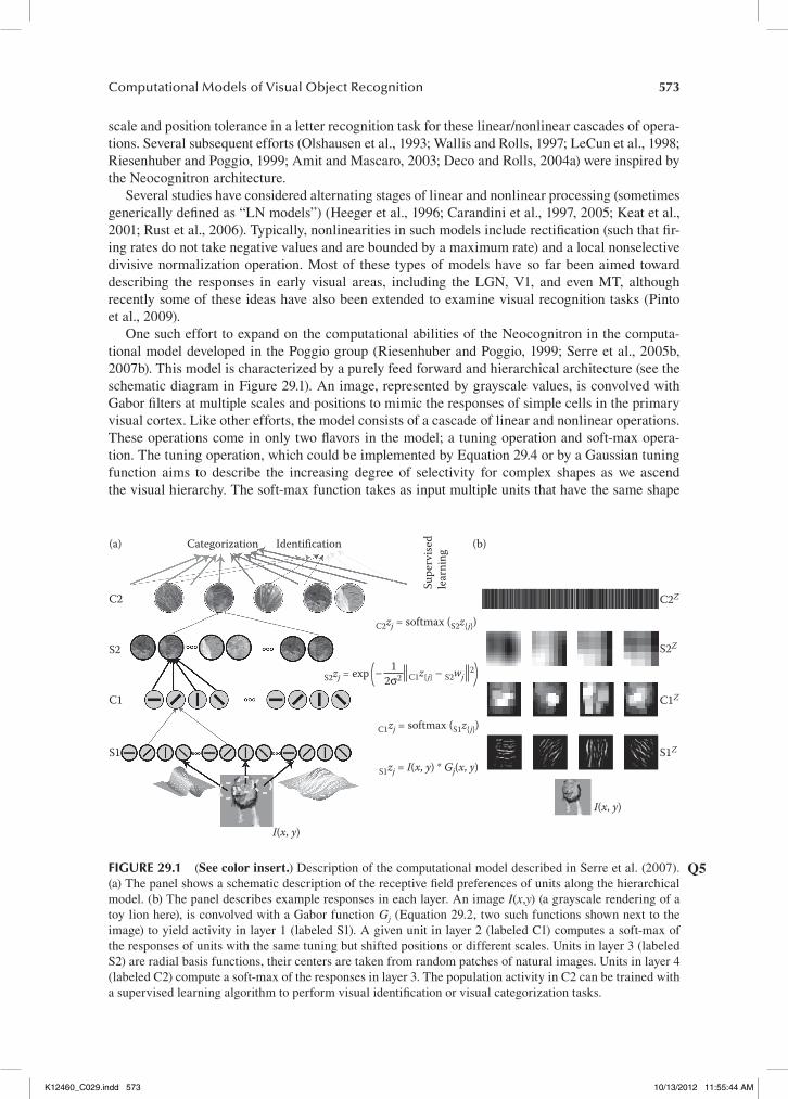
One such effort to expand on the computational abilities of the Neocognitron in the computa-tional model developed in the Poggio group (Riesenhuber and Poggio, 1999; Serre et al., 2005b, 2007b). This model is characterized by a purely feed forward and hierarchical architecture (see the schematic diagram in Figure 29.1). An image, represented by grayscale values, is convolved with Gabor filters at multiple scales and positions to mimic the responses of simple cells in the primary visual cortex. Like other efforts, the model consists of a cascade of linear and nonlinear operations. These operations come in only two flavors in the model; a tuning operation and soft-max opera-tion. The tuning operation, which could be implemented by Equation 29.4 or by a Gaussian tuning function aims to describe the increasing degree of selectivity for complex shapes as we ascend the visual hierarchy. The soft-max function takes as input multiple units that have the same shape

C2

(a) (b)

S2

C1

S1

C2Z

S2Z

C1Z

S1Z

I(x, y)

Categorization Identification

2σ2– 1

Supe

rvis

edle

arni

ng

I(x, y)

S1zj = I(x, y) * Gj(x, y)

C1zj = softmax (S1z{ j})

C1z{ j} – S2wj 2

S2zj = exp

C2zj = softmax (S2z{ j})

figure 29.1 (See color insert.) Description of the computational model described in Serre et al. (2007). (a) The panel shows a schematic description of the receptive field preferences of units along the hierarchical model. (b) The panel describes example responses in each layer. An image I(x,y) (a grayscale rendering of a toy lion here), is convolved with a Gabor function Gj (Equation 29.2, two such functions shown next to the image) to yield activity in layer 1 (labeled S1). A given unit in layer 2 (labeled C1) computes a soft-max of the responses of units with the same tuning but shifted positions or different scales. Units in layer 3 (labeled S2) are radial basis functions, their centers are taken from random patches of natural images. Units in layer 4 (labeled C2) compute a soft-max of the responses in layer 3. The population activity in C2 can be trained with a supervised learning algorithm to perform visual identification or visual categorization tasks.

Q5

K12460_C029.indd 573 10/13/2012 11:55:44 AM


preferences but different receptive field properties (e.g., shifted or scaled versions) and the max operation (winner-take-all) yields tolerance to transformation (e.g., position or scale). Both opera-tions can be expressed in the following form:

x k g

w j k x j

x j

i

ip

j

n

iq

j

nr+

=

=

=

+

∑

∑1

1

1

[ ]

[ , ] [ ]

[ ]α

(29.5)

where xi+1[k] represents the activity of unit k in layer i + 1, w[j,k] represents the connection weight between unit j in layer i and unit k in layer i + 1, p, q, r are integer constants, α is a normalization constant, and g is a nonlinear function (e.g., sigmoid). Depending on the values of p, q, and r, differ-ent interesting behaviors can be obtained. In particular, taking r = 1/2, p = 1, q = 2, leads to a tuning operation where the numerator is a dot product similar to the one described by Equation 29.4 and the denominator provides a normalization operation: x k g w j k j xx ji ij

ni j

n+ = == ∑ + ∑( )1

21 1[ ] [ , ] [ ] .[ ]/α

The responses of the unit are controlled by the weights w (e.g., from C1 to S2 in the scheme in Figure 29.1). As emphasized above, tuning is a central aspect of any computational model of visual recognition, allowing units along the hierarchy to respond to increasingly more elaborate fea-tures. Taking w = 1, p = q + 1, r = 1, leads to a soft-max operation, particularly for large values of q x k g j xx ji i

qjn

iq

jn: /+ =

+== ∑ + ∑( )1 1

11[ ] [ ] [ ]α (e.g., from S1 to C1 or from S2 to C2 in Figure 29.1).

When the exponent q is large, the ratio in the parenthesis is dominated by max(xi). In the scheme in Figure 29.1, the units j that form the input to this equation (xi[j]) have the same shape preferences but slightly shifted or scaled receptive fields. Under these conditions, the unit with response xi+1[k] will have the same response tuning to the units with response xi[j] for j = 1,. . .,n. Yet, the higher-level unit i + 1 will show a stronger degree of tolerance to those aspects of the response that differentiate the j units in layer i (e.g., scale and position).

The different operations that can arise from Equation 29.5 (e.g., the tuning and soft-max opera-tion just described) can be implemented by a relatively simple and biophysically plausible circuit (Kouh and Poggio, 2004). These types of circuits are reminiscent of the LN cascades that have been used successfully to describe responses in the LGN and the primary visual cortex (Heeger et al., 1996; Carandini et al., 1997).

This and similar architectures have been subjected to several tests, including comparison with psychophysical measurements (e.g., Serre et al., 2007a), comparison with neurophysiological responses (e.g., Deco and Rolls, 2004a; Lampl et al., 2004; Hung et al., 2005; Serre et al., 2005b; Cadieu et al., 2007), and quantitative evaluation of performance in computer vision recognition tasks (e.g., LeCun et al., 1998; Serre et al., 2005a; Mutch and Lowe, 2006; Pinto et al., 2009).

29.6 toP-Down signals in Visual reCognition

In spite of the multiple simplifications, the success of bottom-up architectures in describing a large number of visual recognition phenomena suggest that they may not be a bad first cut (Poggio, 2011; DiCarlo et al., 2012). As emphasized above, bottom-up architectures constitute only an approxi-mation to the complexities and wonders of neocortical computation. One of the several simpli-fications in bottom-up models is the lack of top-down signals. We know that there are abundant backprojections in the neocortex (e.g., Felleman and Van Essen, 1991; Callaway, 2004; Douglas and Martin, 2004). The functions of top-down connections have been less studied at the neuro-physiological level but there is no shortage of computational models illustrating the rich array of computations that emerge with such connectivity. Several models have used top-down connections

Q4

K12460_C029.indd 574 10/13/2012 11:55:46 AM


to guide attention to specific locations or specific features within the image (e.g., Tsotsos, 1990; Olshausen et al., 1993; Itti and Koch, 2001; Deco and Rolls, 2005; Rao, 2005; Compte and Wang, 2006; Chikkerur et al., 2009). The allocation of attention to the specific parts of an image can sig-nificantly enhance the recognition performance by alleviating the problems associated with image segmentation and clutter.

Top-down signals can also play an important role in the recognition of occluded objects. When only partial object information is available, the system must be able to perform object completion and interpret the image based on prior knowledge. Attractor networks (with all-to-all connectivity) have been shown to be able to retrieve the identity of stored memories from partial information (e.g., Hopfield, 1982). Some computational models have combined bottom-up architectures with attractor networks at the top of the hierarchy (e.g., Deco and Rolls, 2004a). During object completion, top-down signals could play an important role by providing prior stored information that influences the bottom-up sensory responses.

Several proposals have argued that visual recognition can be formulated as a Bayesian infer-ence problem (Mumford, 1992; Rao et al., 2002; Lee and Mumford, 2003; Rao, 2004; Yuille and Kersten, 2006; Chikkerur et al., 2009). Considering three layers of the visual cascade (e.g., LGN, V1, and higher areas), and denoting activity in those layers as x0, x1, and xh, respectively, then the probability of obtaining a given response pattern in V1 depends both on the sensory input and the feedback from higher areas:

P

P PPh

h h

h

( , )( , ) ( )

( )x x x

x x x x xx x1 0

0 1 1

0

|| |

|=

(29.6)

where P h( )x x1| represents the feedback biases conveying prior information (Lee and Mumford, 2003). An intriguing idea proposed by Rao and Ballard argues that top-down connections provide predictive signals whereas bottom-up signals convey the difference between the sensory input and the top-down predictions (Rao and Ballard, 1999). Particularly at the psychophysics level, there have been multiple studies illustrating how top-down signals can help explain human recognition performance in a variety of tasks (for a review, see Kersten and Yuille, 2003).

29.7 roaD aheaD

Significant progress has been made toward describing visual object recognition in a principled and theoretically sound fashion. Yet, the lacunas in our understanding of the functional and computa-tional architecture of the ventral visual cortex are not small. The preliminary steps have distilled important principles of neocortical computation, including deep networks that can divide and con-quer complex tasks, bottom-up circuits that perform rapid computations, gradual increases in selec-tivity, and tolerance to object transformation.

In stark contrast with the pathway from the retina to the primary visual cortex, we do not have a quantitative description of the feature preferences of neurons along the ventral visual pathway. In addition, several computational models do not make clear, concrete, and testable predictions toward systematically characterizing the ventral visual cortex at the physiological levels. Computational models can perform several complex recognition tasks and compete against nonbiological computer vision approaches. Yet, for the vast majority of recognition tasks, they still fall significantly below human performance.

The next several years are likely to bring many new surprises in the field. We will be able to characterize the system at unprecedented resolution at the experimental level and we will be able to evaluate sophisticated and computationally intensive theories in realistic times. In the same way that the younger generations are not surprised by machines that can play chess competitively, the next generation may not be surprised by intelligent devices that can “see” like we do or even better.

K12460_C029.indd 575 10/13/2012 11:55:46 AM


referenCes

Abbott LF, Rolls ET, Tovee MJ. 1996. Representational capacity of face coding in monkeys. Cerebral Cortex 6:498–505.

Amit Y, Mascaro M. 2002. An integrated network for invariant visual detection and recognition. Vision Research 43:14.

Amit Y, Mascaro M. 2003. An integrated network for invariant visual detection and recognition. Vision Research 43:2073–2088.

Bengio Y, Lamblin P, Popovici D, Larochelle H. 2007. Greedy layer-wise training of deep networks. In: Advances in Neural Information Processing Systems.

Biederman I. 1987. Recognition-by-components: A theory of human image understanding. Psychological Review 24:115–147.

Blumberg J, Kreiman G. 2010. How cortical neurons help us see: Visual recognition in the human brain. Journal of Clinical Investigation 120:3054–3063.

Borenstein E, Sharon E, Ullman S. 2004. Combining top-down and bottom-up segmentation. In: IEEE Conference on Computer Vision and Pattern Recognition.

Brady TF, Konkle T, Alvarez GA, Oliva A. 2008. Visual long-term memory has a massive storage capacity for object details. Proceedings of the National Academy of Science of the United States of America 105:14325–14329.

Brincat SL, Connor CE. 2004. Underlying principles of visual shape selectivity in posterior inferotemporal cortex. Nature Neuroscience 7:880–886.

Bulthoff HH, Edelman SY, Tarr MJ. 1995. How are three-dimensional objects represented in the brain? Cerebral Cortex 5:247–260.

Cadieu C, Kouh M, Pasupathy A, Connor C, Riesenhuber M, Poggio T. 2007. A model of V4 shape selectivity and invariance. Journal of Neurophysiology 98:1733–1750.

Callaway EM. 1998. Local circuits in primary visual cortex of the macaque monkey. Annual Review of Neuroscience 21:47–74.

Callaway EM. 2004. Feedforward, feedback and inhibitory connections in primate visual cortex. Neural Network 17:625–632.

Carandini M, Demb JB, Mante V, Tolhurst DJ, Dan Y, Olshausen BA, Gallant JL, Rust NC. 2005. Do we know what the early visual system does? Journal of Neuroscience 25:10577–10597.

Carandini M, Heeger DJ, Movshon JA. 1997. Linearity and normalization in simple cells of the macaque primary visual cortex. Journal of Neuroscience 17:8621–8644.

Chikkerur S, Serre T, Poggio T. 2009. A Bayesian inference theory of attention: Neuroscience and algorithms. In: (MIT-CSAIL-TR, ed), Cambridge: MIT.

Compte A, Wang XJ. 2006. Tuning curve shift by attention modulation in cortical neurons: A computational study of its mechanisms. Cerebral Cortex 16:761–778.

Connor CE, Brincat SL, Pasupathy A. 2007. Transformation of shape information in the ventral pathway. Current Opinion in Neurobiology 17:140–147.

Dayan P, Abbott L. 2001. Theoretical Neuroscience. Cambridge: MIT Press.Deco G, Rolls ET. 2004a. A neurodynamical cortical model of visual attention and invariant object recognition.

Vision Research 44:621–642.Deco G, Rolls ET. 2004b. Computational Neuroscience of Vision. Oxford University Press.Deco G, Rolls ET. 2005. Attention, short-term memory, and action selection: A unifying theory. Progress in

Neurobiology 76:236–256.DiCarlo JJ, Cox DD. 2007. Untangling invariant object recognition. Trends in Cognitive Science 11:333–341.DiCarlo JJ, Zoccolan D, Rust NC. 2012. How does the brain solve visual object recognition? Neuron

73:415–434.Douglas RJ, Martin KA. 2004. Neuronal circuits of the neocortex. Annual Review in Neuroscience

27:419–451.Dowling J. 1987. The Retina. An Approachable Part of the Brain. Belknap Press.Edelman S, Duvdevani-Bar S. 1997. A model of visual recognition and categorization. Philosophy of

Transaction Royal Society of London B: Biological Science 352:1191–1202.Felleman DJ, Van Essen DC. 1991. Distributed hierarchical processing in the primate cerebral cortex. Cerebral

Cortex 1:1–47.Fukushima K. 1980. Neocognitron: A self organizing neural network model for a mechanism of pattern recog-

nition unaffected by shift in position. Biological Cybernetics 36:193–202.

Q6

Q7

Q8

Q9

Q9

K12460_C029.indd 576 10/13/2012 11:55:46 AM


Haxby J, Grady C, Horwitz B, Ungerleider L, Mishkin M, Carson R, Herscovitch P, Schapiro M, Rapoport S. 1991. Dissociation of object and spatial visual processing pathways in human extrastriate cortex. Proceedings of the National Academy of Sciences 88:1621–1625.

Heeger DJ, Simoncelli EP, Movshon JA. 1996. Computational models of cortical visual processing. Proceedings of the National Academy of Sciences of the United States of America 93:623–627.

Hegde J, Van Essen DC. 2007. A comparative study of shape representation in macaque visual areas v2 and v4. Cerebral Cortex 17:1100–1116.

Hertz J, Krogh A, Palmer R. 1991. Introduction to the Theory of Neural Computation. Santa Fe: Santa Fe Institute Studies in the Sciences of Complexity.

Hinton G. 1992. How neural networks learn from experience. Scientific American 267:145–151.Hinton GE, Salakhutdinov RR. 2006. Reducing the dimensionality of data with neural networks. Science

313:504–507.Hopfield JJ. 1982. Neural networks and physical systems with emergent collective computational abilities.

Proceedings of the National Academy of Sciences 79:2554–2558.Horn B. 1986. Robot Vision. Cambridge: MIT Press.Hubel DH, Wiesel TN. 1962. Receptive fields, binocular interaction and functional architecture in the cat’s

visual cortex. Journal of Physiology 160:106–154.Hummel JE, Biederman I. 1992. Dynamic binding in a neural network for shape recognition. Psychological

Review 99:480–517.Hung C, Kreiman G, Poggio T, DiCarlo J. 2005. Fast read-out of object identity from macaque inferior tempo-

ral cortex. Science 310:863–866.Itti L, Koch C. 2001. Computational modeling of visual attention. National Review of Neuroscience 2:194–203.Keat J, Reinagel P, Reid RC, Meister M. 2001. Predicting every spike: A model for the responses of visual

neurons. Neuron 30:803–817.Kersten D, Yuille A. 2003. Bayesian models of object perception. Current Opinion in Neurobiology 13:150–158.Keysers C, Xiao DK, Foldiak P, Perret DI. 2001. The speed of sight. Journal of Cognitive Neuroscience

13:90–101.Kirchner H, Thorpe SJ. 2006. Ultra-rapid object detection with saccadic eye movements: Visual processing

speed revisited. Vision Research 46:1762–1776.Kohn A. 2007. Visual adaptation: Physiology, mechanisms, and functional benefits. Journal of Neurophysiology

97:3155–3164.Kouh M, Poggio T. 2004. A general mechanism for tuning: Gain control circuits and synapses underlie tuning

of cortical neurons. In: (Memo MA, ed). Cambridge: MIT.Kriegeskorte N, Mur M, Ruff DA, Kiani R, Bodurka J, Esteky H, Tanaka K, Bandettini PA. 2008.

Matching categorical object representations in inferior temporal cortex of man and monkey. Neuron 60:1126–1141.

Lampl I, Ferster D, Poggio T, Riesenhuber M. 2004. Intracellular measurements of spatial integration and the MAX operation in complex cells of the cat primary visual cortex. Journal of Neurophysiology 92:2704–2713.

LeCun Y, Bottou L, Bengio Y, Haffner P. 1998. Gradient-based learning applied to document recognition. Proceedings of the IEEE 86:2278–2324.

Lee TS, Mumford D. 2003. Hierarchical Bayesian inference in the visual cortex. Journal of the Optical Society of America A, Optics of Image Science Vision 20:1434–1448.

Lennie P, Movshon JA. 2005. Coding of color and form in the geniculostriate visual pathway (invited review). Journal of the Optical Society of America A, Optics of Image Science Vision 22:2013–2033.

Liu H, Agam Y, Madsen JR, Kreiman G. 2009. Timing, timing, timing: Fast decoding of object information from intracranial field potentials in human visual cortex. Neuron 62:281–290.

Logothetis NK, Sheinberg DL. 1996. Visual object recognition. Annual Review of Neuroscience 19:577–621.Logothetis NK, Pauls J, Poggio T. 1995. Shape representation in the inferior temporal cortex of monkeys.

Current Biology 5:552–563.Marr D. 1982. Vision. Freeman Publishers.Marr D, Nishihara HK. 1978. Representation and recognition of the spatial organization of three-dimensional

shapes. Proceedings of the Royal Society of London B: Biological Science 200:269–294.Maunsell JHR. 1995. The brain’s visual world: Representatioin of visual targets in cerebral cortex. Science

270:764–769.Meister M. 1996. Multineuronal codes in retinal signaling. Proceedings of the National Academy of Science

93:609–614.

Q8

Q9

Q10

K12460_C029.indd 577 10/13/2012 11:55:46 AM


Mel B. 1997. SEEMORE: Combining color, shape and texture histogramming in a neurally inspired approach to visual object recognition. Neural Computation 9:777.

Miyashita Y, Chang HS. 1988. Neuronal correlate of pictorial short-term memory in the primate temporal cortex. Nature 331:68–71.

Mumford D. 1992. On the computational architecture of the neocortex. II. The role of cortico-cortical loops. Biology of Cybernetics 66:241–251.

Mutch J, Lowe D. 2006. Multiclass object recognition with sparse, localized features. In: CVPR, pp 11–18. New York.

Myerson J, Miezin F, Allman J. 1981. Binocular rivalry in macaque monkeys and humans: A comparative study in perception. Behavioral Analysis Letters 1:149–159.

Nielsen KJ, Logothetis NK, Rainer G. 2006. Discrimination strategies of humans and rhesus monkeys for complex visual displays. Current Biology 16:814–820.

Olshausen BA, Anderson CH, Van Essen DC. 1993. A neurobiological model of visual attention and invariant pattern recognition based on dynamic routing of information. Journal of Neuroscience 13:4700–4719.

Orban GA, Van Essen, D., Vanduffel, W. 2004. Comparative mapping of higher visual areas in monkeys and humans. Trends in Cognitive Sciences 8:315–324.

Pinto N, Doukhan D, DiCarlo JJ, Cox DD. 2009. A high-throughput screening approach to discovering good forms of biologically inspired visual representation. PLoS Compution in Biology 5:e1000579.

Poggio T. 2011. The computational magic of the ventral steam: Towards a theory. Nature Proceedings.Poggio T, Smale S. 2003. The mathematics of learning: Dealing with data. Notices of the American Mathematical

Society 50:537–544.Potter M, Levy E. 1969. Recognition memory for a rapid sequence of pictures. Journal of Experimental

Psychology 81:10–15.Rao RP. 2004. Bayesian computation in recurrent neural circuits. Neural Computation 16:1–38.Rao RP. 2005. Bayesian inference and attentional modulation in the visual cortex. Neuroreport 16:1843–1848.Rao RP, Ballard DH. 1999. Predictive coding in the visual cortex: A functional interpretation of some extra-

classical receptive-field effects. Nature Neuroscience 2:79–87.Rao RPN, Olshausen BA, Lewicki MS, eds. 2002. Probabilistic Models of the Brain: Perception and Neural

Function. Cambridge: MIT Press.Richmond B, Wurtz R, Sato T. 1983. Visual responses in inferior temporal neurons in awake Rhesus monkey.

Journal of Neurophysiology 50:1415–1432.Riesenhuber M, Poggio T. 1999. Hierarchical models of object recognition in cortex. Nature Neuroscience

2:1019–1025.Riesenhuber M, Poggio T. 2002. Neural mechanisms of object recognition. Current Opinion in Neurobiology

12:162–168.Rolls E. 1991. Neural organization of higher visual functions. Current Opinion in Neurobiology 1:274–278.Rust NC, Mante V, Simoncelli EP, Movshon JA. 2006. How MT cells analyze the motion of visual patterns.

Nature Neuroscience 9:1421–1431.Schmolesky M, Wang Y, Hanes D, Thompson K, Leutgeb S, Schall J, Leventhal A. 1998. Signal timing across

the macaque visual system. Journal of Neurophysiology 79:3272–3278.Serre T, Wolf L, Poggio T. 2005a. Object recognition with features inspired by visual cortex. In: CVPR.Serre T, Oliva A, Poggio T. 2007a. Feedforward theories of visual cortex account for human performance in

rapid categorization. Proceedings of the National Academy of Science 104:6424–6429.Serre T, Kouh M, Cadieu C, Knoblich U, Kreiman G, Poggio T. 2005b. A theory of object recognition:

Computations and circuits in the feedforward path of the ventral stream in primate visual cortex. In: pp CBCL Paper #259/AI Memo #2005-2036. Boston: MIT.

Serre T, Kreiman G, Kouh M, Cadieu C, Knoblich U, Poggio T. 2007b. A quantitative theory of immediate visual recognition. Progress in Brain Research 165C:33–56.

Sharon E, Galun M, Sharon D, Basri R, Brandt A. 2006. Hierarchy and adaptivity in segmenting visual scenes. Nature 442:810–813.

Smirnakis SM, Berry MJ, Warland DK, Bialek W, Meister M. 1997. Adaptation of retinal processing to image contrast and spatial scale. Nature 386:69–73.

Standing L. 1973. Learning 10,000 pictures. Quarterly Journal of Experimental Psychology 25:207–222.Sutherland NS. 1968. Outlines of a theory of visual pattern recognition in animals and man. Proceedings of the

Royal Society of London B: Biological Science 171:297–317.Tanaka K. 1996. Inferotemporal cortex and object vision. Annual Review of Neuroscience 19:109–139.Thorpe S, Fize D, Marlot C. 1996. Speed of processing in the human visual system. Nature 381:520–522.Tsao DY, Livingstone MS. 2008. Mechanisms of face perception. The Annual Review of Neuroscience 31:26.

Q9

Q9

K12460_C029.indd 578 10/13/2012 11:55:46 AM


Tsotsos J. 1990. Analyzing vision at the complexity level. Behavioral and Brain Sciences 13–30:423–445.Ullman S. 1996. High-Level Vision. Cambridge, MA: The MIT Press.Ungerleider L, Mishkin M. 1982. Two cortical visual systems. In: Analysis of Visual Behavior (Ingle D,

Goodale M, Mansfield R, eds). Cambridge: MIT Press.Virga A, Rockland, KS. 1989. Terminal arbors of individual “feedback” axons projecting from area V2 to V1

in the macaque monkey: A study using immunohistochemistry of anterogradely transported phaseolus vulgaris-leucoagglutinin. The Journal of Comparative Neurology 285:54–72.

Vogels R, Biederman I, Bar M, Lorincz A. 2001. Inferior temporal neurons show greater sensitivity to nonac-cidental than to metric shape differences. Journal of Cognitive Neuroscience 13:444–453.

Wallis G, Rolls ET. 1997. Invariant face and object recognition in the visual system. Progress in Neurobiology 51:167–194.

Wandell BA. 1995. Foundations of Vision. Sunderland: Sinauer Associates Inc.Winston P. 1975. Learning structural descriptions from examples. In: The Psychology of Computer Vision

(Winston P, ed), pp 157–209: McGraw-Hill.Yamane Y, Carlson ET, Bowman KC, Wang Z, Connor CE. 2008. A neural code for three-dimensional object

shape in macaque inferotemporal cortex. Nature Neuroscience 11:1352–1360.Yuille A, Kersten D. 2006. Vision as Bayesian inference: Analysis by synthesis? Trends in Cognitive Science

10:301–308.

Q9

K12460_C029.indd 579 10/13/2012 11:55:46 AM

K12460_C029.indd 580 10/13/2012 11:55:46 AM

Cat#: K12460 Chapter: 029

TO: CORRESPONDING AUTHOR

AUTHOR QUERIES - TO BE ANSWERED BY THE AUTHOR

The following queries have arisen during the typesetting of your manuscript. Please answer these queries by marking the required corrections at the appropriate point in the

text.

Query No.

Query Response

Q1 Is it Orban, 2004 or Orban et al., 2004? Please confirm.

Q2 Is “values of the pixels of a given image” OK here as changed?

Q3 Is it Virga, 1989 or Virga and Rockland, 1989? Please confirm.

Q4 Please define the following terms OR, LN.

Q5 Is it Serre et al. 2007a or Serre et al. 2007b? Please confirm.

Q6 Please provide the publisher name and place of publication in Bengio et al., 2007.

Q7 Please provide the venue of the conference in Borenstein et al., 2004.

Q8 Please clarify the book title for the following References: Chikkerur et al. 2009, Kouh et al. 2004.

Q9 Please provide the place of publication for the following References:Deco and Rolls, 2004b, Dowling, 1987, Marr, 1982, Poggio, 2011, Serre et al., 2005a, Winston, 1975.

Q10 Meister, 1996 is not cited. Please suggest a suitable place for its citation in the text.

Gabriel Kreiman - Harvard...

Documents

Transcript of Gabriel Kreiman - Harvard...