Department of Economics and Finance

Working Paper No. 14-09

http://www.brunel.ac.uk/economics

Eco

nom

ics

and F

inance

Work

ing P

aper

Series

Guglielmo Maria Caporale, Luis Gil-Alana, Alex Plastun and Inna Makarenko

The Weekend Effect: A Trading Robot and Fractional Integration Analysis

June 2014

1

THE WEEKEND EFFECT:

A TRADING ROBOT

AND FRACTIONAL INTEGRATION ANALYSIS

Guglielmo Maria Caporale*

Brunel University, London, CESifo and DIW Berlin

Luis Gil-Alana

University of Navarra

Alex Plastun

Ukrainian Academy of Banking

Inna Makarenko

Ukrainian Academy of Banking

May 2014

Abstract

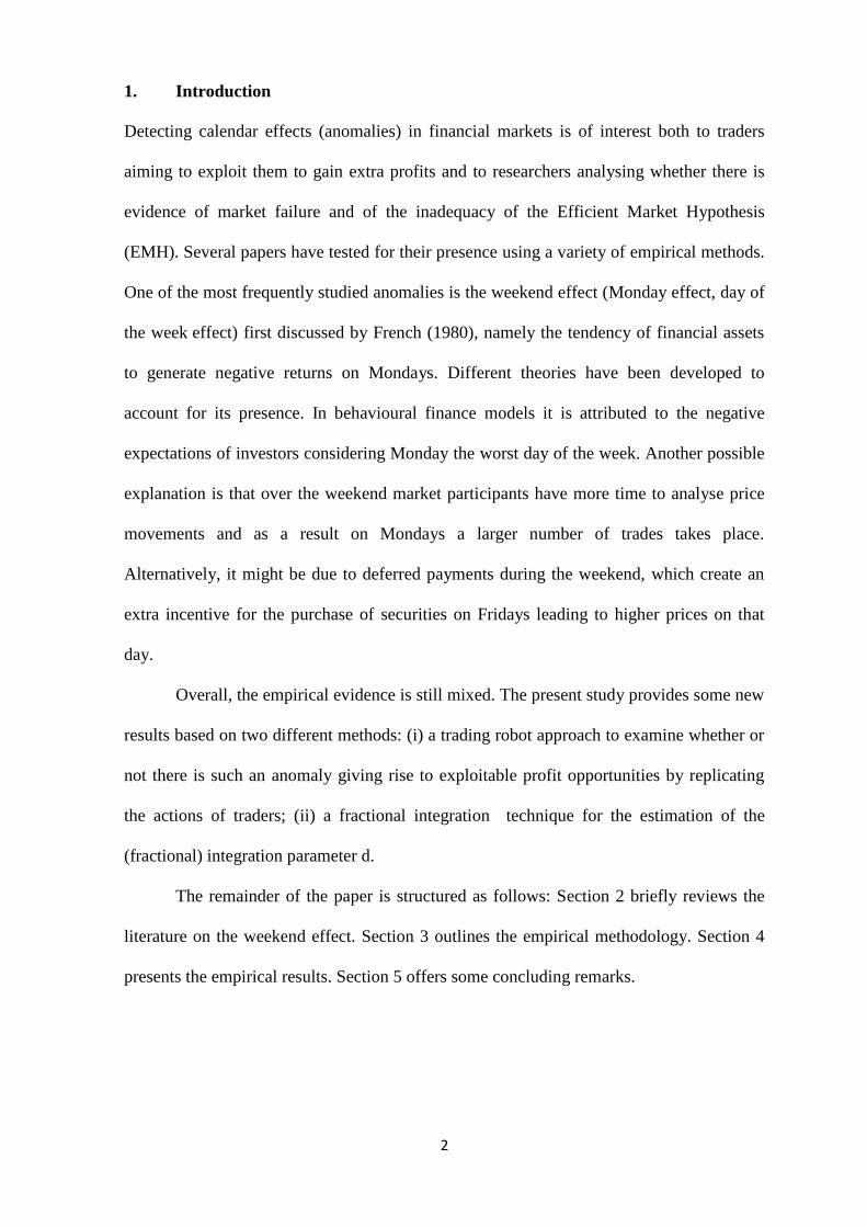
This paper provides some new empirical evidence on the weekend effect, one

of the most recognized anomalies in financial markets. Two different methods

are used: (i) a trading robot approach to examine whether or not there is

such an anomaly giving rise to exploitable profit opportunities by replicating

the actions of traders; (ii) a fractional integration technique for the

estimation of the (fractional) integration parameter d. The results suggest that

trading strategies aimed at exploiting the weekend effect can generate extra

profits but only in a minority of cases in the gold and stock markets, whist

they appear to be profitable in most cases in the FOREX. Further, the lowest

orders of integration are generally found on Mondays, which can be seen as

additional evidence for a weekend effect.

Keywords: Efficient Market Hypothesis; weekend effect; trading strategy.

JEL classification: G12, C63

*Corresponding author. Department of Economics and Finance, Brunel

University, London, UB8 3PH.

Email: Guglielmo-Maria.Caporale@brunel.ac.uk

2

1. Introduction

Detecting calendar effects (anomalies) in financial markets is of interest both to traders

aiming to exploit them to gain extra profits and to researchers analysing whether there is

evidence of market failure and of the inadequacy of the Efficient Market Hypothesis

(EMH). Several papers have tested for their presence using a variety of empirical methods.

One of the most frequently studied anomalies is the weekend effect (Monday effect, day of

the week effect) first discussed by French (1980), namely the tendency of financial assets

to generate negative returns on Mondays. Different theories have been developed to

account for its presence. In behavioural finance models it is attributed to the negative

expectations of investors considering Monday the worst day of the week. Another possible

explanation is that over the weekend market participants have more time to analyse price

movements and as a result on Mondays a larger number of trades takes place.

Alternatively, it might be due to deferred payments during the weekend, which create an

extra incentive for the purchase of securities on Fridays leading to higher prices on that

day.

Overall, the empirical evidence is still mixed. The present study provides some new

results based on two different methods: (i) a trading robot approach to examine whether or

not there is such an anomaly giving rise to exploitable profit opportunities by replicating

the actions of traders; (ii) a fractional integration technique for the estimation of the

(fractional) integration parameter d.

The remainder of the paper is structured as follows: Section 2 briefly reviews the

literature on the weekend effect. Section 3 outlines the empirical methodology. Section 4

presents the empirical results. Section 5 offers some concluding remarks.

3

2. Literature Review

Fields (1931) suggested that the best trading day of the week is Saturday. Another

important study on the weekend effect is that by Cross (1973), who analysed the Friday-

Monday data for the Standard & Poor's Composite Stock Index from January 1953 to

December 1970 and found an increase on Fridays and a decrease on Mondays.French

(1980) extended the analysis to 1977 and also reported negative returns on Mondays.

Further contributions by Gibbons and Hess (1981), Keim and Stambaugh (1984), Rogalski

(1984), and Smirlock and Starks (1986) also found the positive-Friday / negative-Monday

pattern. Connolly (1999) also allowed for heteroscedasticity but still detected a Monday

effect from the mid- 1970s.Rystrom and Benson (1989) explained the presence of the day-

of-the-week effect on the basis of the psychology of investors who believe that Monday is

a “difficult” day of the week and have a more positive perception of Friday. Ariel (1990)

argued against a connection between the weekend and the Monday effect. Agrawal and

Tandon (1994) examined 19 equity markets around the world, and found the day-of-the -

week effect in most developed markets. Sias and Starks (1995) associate the weekend

effect with stocks in large portfolios of institutional investors. Research conducted in

Fortune (1998, 1999) shows that it has a tendency to disappear and is a phenomenon with

two components: the first is the “weekend drift effect”, i.e. stock prices tend to decline

over weekends but rise during the trading week; the second is the “weekend volatility

effect”, i.e. the volatility of returns during weekends is less per day than that over

contiguous trading days.

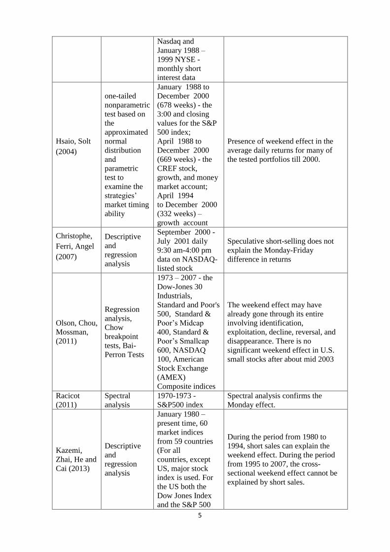
As for the role of short-selling, Kazemi, Zhai, He and Cai (2013) and Chen and

Singal (2003) explain the weekend effect as resulting from the closing of speculative

positions on Fridays and the establishing of new short positions on Mondays by traders.

However, the results of the study by Christophe, Ferri and Angel (2007) do not support this

conclusion. Further evidence is provided by Singal and Tayal (2014) for the futures

4

market, Olson, Chou, Mossman (2011) who carry out various breakpoint and stability tests,

and Racicot (2011) who uses spectral analysis. The findings from other relevant studies are

summarised in Table 1.

Table 1 Weekend effect: an overview of recent researches

Author Type of

analysis

Object of analysis

(time period,

market, index)

Results

Sias, Starks

(1995)

Hypothesis

testing (t-test

and F-test)

1977-1991 market

equity

capitalization,

institutional

holdings, daily

returns and volume

of 1500

institutional

investors on the

NYSE

The weekend effect is driven

primarily by institutional investor

trading patterns

Fortune

(1998)

Jump

diffusion

model of

stock returns

January 1980 -June

1998 - daily close-

to-close data for the

S&P

500

The negative weekend drift appears

to have disappeared although

weekends continue to have low

volatility

Fortune

(1999)

January 1980 -

January 1999

daily close-to-close

data of the Dow

30, the S&P 500,

the Wilshire 5000,

the Nasdaq

Composite,

and the Russell

2000

The weekend drift effect is a

financial anomaly that will

ultimately correct itself.

Schwert

(2003)

Correlation

analysis

1885–1927 - the

Dow Jones indexes

portfolio; 1928–

2002 - the S&P

composite portfolio

The weekend effect seems to have

disappeared since the 1980-s

Chen, Singal

(2003)

Descriptive

and

regression

analysis

July 1962 -

December 1999 -

New York Stock

(NYSE); December

1972 - December

1999 - Nasdaq -

daily returns for

stocks;

June 1988 -

December 1999

Speculative short sales can explain

the weekend effect.

5

Nasdaq and

January 1988 –

1999 NYSE -

monthly short

interest data

Hsaio, Solt

(2004)

one-tailed

nonparametric

test based on

the

approximated

normal

distribution

аnd

parametric

test to

examine the

strategies’

market timing

ability

January 1988 to

December 2000

(678 weeks) - the

3:00 and closing

values for the S&P

500 index;

April 1988 to

December 2000

(669 weeks) - the

CREF stock,

growth, and money

market account;

April 1994

to December 2000

(332 weeks) –

growth account

Presence of weekend effect in the

average daily returns for many of

the tested portfolios till 2000.

Christophe,

Ferri, Angel

(2007)

Descriptive

and

regression

analysis

September 2000 -

July 2001 daily

9:30 am-4:00 pm

data on NASDAQ-

listed stock

Speculative short-selling does not

explain the Monday-Friday

difference in returns

Olson, Chou,

Mossman,

(2011)

Regression

analysis,

Chow

breakpoint

tests, Bai-

Perron Tests

1973 – 2007 - the

Dow-Jones 30

Industrials,

Standard and Poor's

500, Standard &

Poor’s Midcap

400, Standard &

Poor’s Smallcap

600, NASDAQ

100, American

Stock Exchange

(AMEX)

Composite indices

The weekend effect may have

already gone through its entire

involving identification,

exploitation, decline, reversal, and

disappearance. There is no

significant weekend effect in U.S.

small stocks after about mid 2003

Racicot

(2011)

Spectral

analysis

1970-1973 -

S&P500 index

Spectral analysis confirms the

Monday effect.

Kazemi,

Zhai, He and

Cai (2013)

Descriptive

and

regression

analysis

January 1980 –

present time, 60

market indices

from 59 countries

(For all

countries, except

US, major stock

index is used. For

the US both the

Dow Jones Index

and the S&P 500

During the period from 1980 to

1994, short sales can explain the

weekend effect. During the period

from 1995 to 2007, the cross-

sectional weekend effect cannot be

explained by short sales.

6

were used)

Singal and

Tayal (2014)

Descriptive

and

regression

analysis

1990 – 2012, eight

futures: Crude oil,

Heating Oil,

Soybeans, Sugar,

S&P 500 Index,

British Pound,

10-Year Treasury

Note, and Gold

Evidence of the weekend effect in

futures markets shows that security

prices will generally be biased

upwards, with greater overvaluation

for more volatile securities.

Unconstrained short selling is not a

sufficient condition for unbiased

prices

3. Data and Methodology

We use daily data for 35 US companies included in the Dow Jones index and 8 Blue-chip

Russian companies. The sample period for the US and Russian stock markets covers the

period from January 2005 and 2008 respectively till the end of April 2014. We also analyse

the FOREX using data on the six most liquid currency pairs (EURUSD, GBPUSD,

USDJPY, USDCHF, AUDUSD, USDCAD) and gold prices over the period from January

2000 and 2005 respectively till the end of April 2014.

Our first (trading-bot) approach considers the weekend effect from the trader’s

viewpoint, namely whether it is possible to make abnormal profits by exploiting it.

Specifically, we programme a trading robot which simulates the actions of a trader

according to an algorithm (trading strategy). To test it with historical data we use a

MetaTrader trading platform which provides tools for replicating price dynamics and

trades according to the adopted strategy.

We examine two trading strategies:

- Strategy 1: Sell on Friday close. Close position on Monday close.

- Strategy 2: Sell on Monday open. Close position on Monday close.

If a strategy results in the number of profitable trades > 50% and/or total profits from

trading are > 0, then we conclude that there is a market anomaly.

7

Our second approach is based on estimating the degree of integration of the series

for different days of the week. Specifically, we use the Whittle function in the frequency

domain, as in following model:

,)1(; tt

d

tt uxLxty (*)

where yt is the observed time series; α and β are the intercept and the coefficient on the

linear trend respectively, xt is assumed to be an I(d) process where d can be any real

number, and ut is assumed to be weakly autocorrelated. However, instead of specifying a

parametric ARMA model, we follow the non-parametric approach of Bloomfield (1973),

which also produces autocorrelations decaying exponentially as in the AR case. If the

estimated order of integration for a particular day, specifically Monday, is significantly

different from that for the other days of the week, then it can be argued that there is

evidence of a weekend effect.

4. Empirical Results

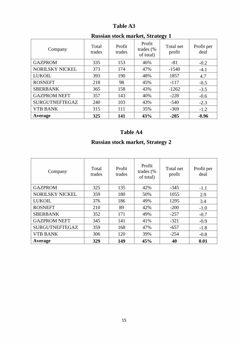
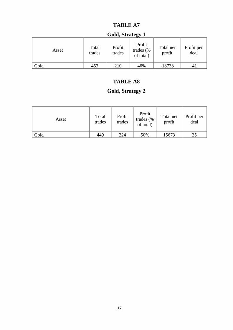
Detailed results are presented in the Appendix. Table 1 summarises those for Strategy 1.

Table 1a: Summary of testing results for Strategy 1

Type of a

market Totaltrades Profittrades

Profittrades

% oftotal Totalnetprofit

Profittrades

%>50, %

Profit>0,

%

US stock

market 434 201 46% -1334 14% 26%

Russian

stock

market

325 141 43% -285 0% 13%

FOREX 724 357 49% 7726 50% 50%

GOLD 453 210 46% -18733 0% 0%

In general this strategy is unprofitable in the stock markets (both US and Russian)

and in gold market but can generate profits in the FOREX. However, in the latter case, the

number of profitable trades is less than 50%, and only for 3 of the 6 currencies analysed

can profits be made. Overall, the EMH is not contradicted.

8

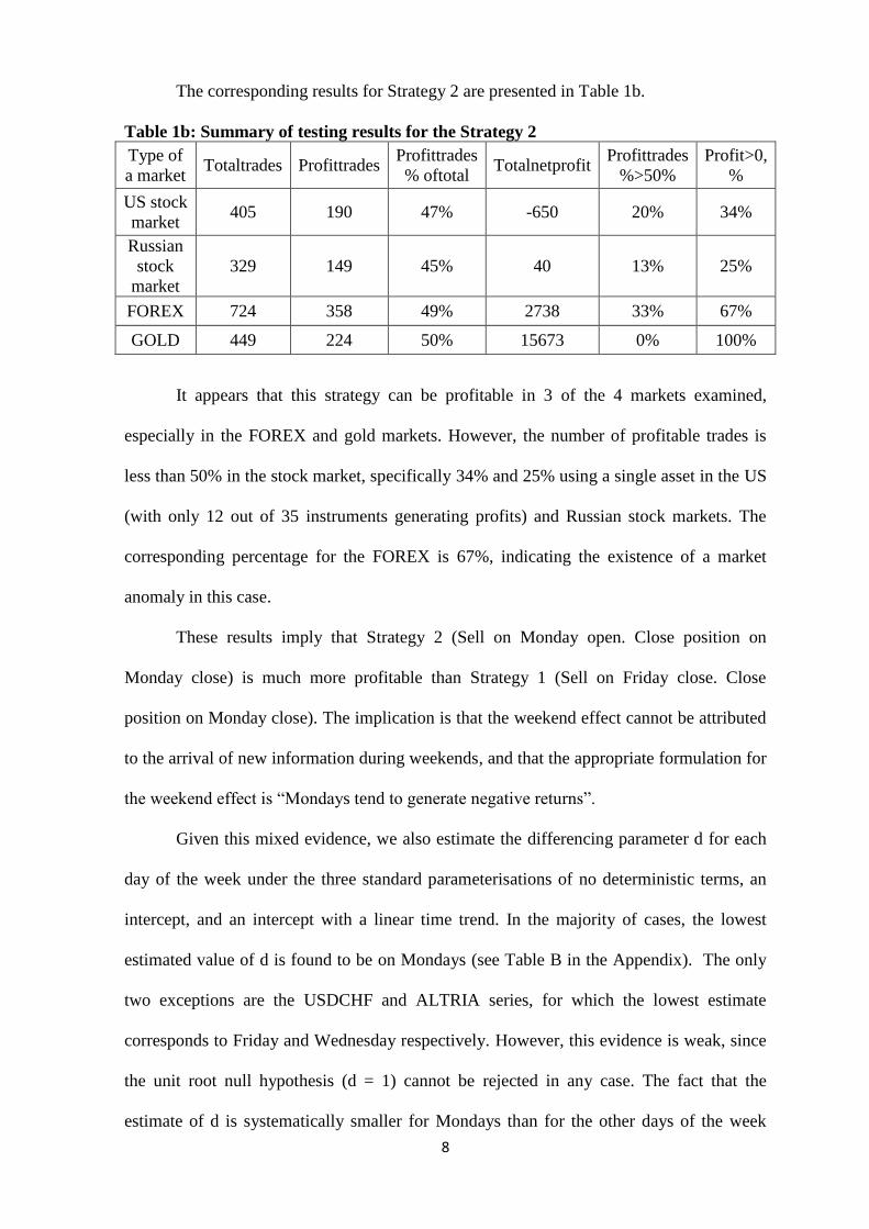
The corresponding results for Strategy 2 are presented in Table 1b.

Table 1b: Summary of testing results for the Strategy 2

Type of

a market Totaltrades Profittrades

Profittrades

% oftotal Totalnetprofit

Profittrades

%>50%

Profit>0,

%

US stock

market 405 190 47% -650 20% 34%

Russian

stock

market

329 149 45% 40 13% 25%

FOREX 724 358 49% 2738 33% 67%

GOLD 449 224 50% 15673 0% 100%

It appears that this strategy can be profitable in 3 of the 4 markets examined,

especially in the FOREX and gold markets. However, the number of profitable trades is

less than 50% in the stock market, specifically 34% and 25% using a single asset in the US

(with only 12 out of 35 instruments generating profits) and Russian stock markets. The

corresponding percentage for the FOREX is 67%, indicating the existence of a market

anomaly in this case.

These results imply that Strategy 2 (Sell on Monday open. Close position on

Monday close) is much more profitable than Strategy 1 (Sell on Friday close. Close

position on Monday close). The implication is that the weekend effect cannot be attributed

to the arrival of new information during weekends, and that the appropriate formulation for

the weekend effect is “Mondays tend to generate negative returns”.

Given this mixed evidence, we also estimate the differencing parameter d for each

day of the week under the three standard parameterisations of no deterministic terms, an

intercept, and an intercept with a linear time trend. In the majority of cases, the lowest

estimated value of d is found to be on Mondays (see Table B in the Appendix). The only

two exceptions are the USDCHF and ALTRIA series, for which the lowest estimate

corresponds to Friday and Wednesday respectively. However, this evidence is weak, since

the unit root null hypothesis (d = 1) cannot be rejected in any case. The fact that the

estimate of d is systematically smaller for Mondays than for the other days of the week

9

suggests abnormal behaviour on this day. An estimated value of d significantly smaller

than 1 would imply that it is possible to make systematic profits on this day of the week

using historical data. However, as can be seen in the Appendix, the confidence intervals

are relatively wide in all cases, and therefore the unit root null hypothesis cannot be

rejected for any day of the week, which implies weak support for a weekend effect.

5. Conclusions

This paper examines one of the most recognized anomalies, i.e. the weekend effect, in

various financial markets (US and Russian stock markets, FOREX, gold) applying two

different methods to daily data. The first, the trading-bot approach, uses a trading robot to

simulate the behaviour of traders according to a given algorithm (in our case trading on the

weekend effect) and considering two alternative strategies. The second analyses the

stochastic properties of the series on different days of the week by estimating their

fractional integration parameter, testing if this value differs depending on the day of the

week.

The results can be summarised as follows. Strategy 1 (Sell on Friday close. Close

position on Monday close) is unprofitable in most cases. The only possible “weekend

effect” formulation is “negative returns on Mondays”. This is confirmed by the results for

Strategy 2 (Sell on Monday open. Close position on Monday close): in this case it is

possible to make profits, although the number of profitable deals is less than 50% and

therefore it cannot be concluded that there is a market anomaly according to our criterion.

The estimates of the fractional parameter d are lowest on Mondays in most cases, which is

evidence in favour of the weekend effect, although the wide confidence intervals mean that

this evidence is rather weak. Finally, exploitable profit opportunities based on the weekend

effect are found mainly in the FOREX market.

10

References

Agrawal, A., Tandon, K., 1994, Anomalies or Illusions? Evidence from Stock Markets in

Eighteen Countries. Journal of international Money and Finance, №13, 83-106.

Ariel, R., 1990, High Stock Returns Before Holidays: Existence and Evidence on Possible

Causes. Journal of Finance, (December), 1611-1626.

Bloomfield, P. (1973).An exponential model in the spectrum of a scalar time series,

Biometrika 60, 217-226.

Chen, H. and Singal, V., 2003, Role of Speculative Short Sales in Price Formation: The

Case of the Weekend Effect. Journal of Finance. LVIII, 2.

Christophe, S., Ferri, M. and Angel, J., 2007, Short-selling and the Weekend Effect in

Stock Returns

http://www.efmaefm.org/0EFMAMEETINGS/EFMA%20ANNUAL%20MEETINGS/

2007-Vienna/Papers/0260.pdf.

Connolly, R., 1989, An Examination of the Robustness of the Weekend Effect. Journal of

Financial and Quantitative Analysis, 24, 2,133-169.

Cross, F., 1973, The Behavior of Stock Prices on Fridays and Mondays. Financial Analysts

Journal, November - December, 67-69.

Fields, M., 1931, Stock Prices: A Problem in Verification. Journal of Business. October.

415-418.

Fortune, P., 1998, Weekends Can Be Rough : Revisiting the Weekend Effect in Stock

Prices. Federal Reserve Bank of Boston. Working Paper No. 98-6.

Fortune, P., 1999, Are stock returns different over weekends? а jump diffusion analysis of

the «weekend effect». New England Economic Review.3-19

11

French, K., 1980, Stock Returns and the Weekend Effect. Journal of Financial Economics.

8, 1, 55-69.

Gibbons, M. and Hess, P., 1981, Day Effects and Asset Returns. Journal of Business, 54,

no, 4, 579-596.

Hsaio, P., Solt, M., 2004, Is the Weekend Effect Exploitable? Investment Management and

Financial Innovations, 1, 53.

Kazemi, H. S., Zhai, W., He, J. and Cai, J., 2013, Stock Market Volatility, Speculative

Short Sellers and Weekend Effect: International Evidence. Journal of Financial Risk

Management. Vol.2 , No. 3. 47-54.

Keim, D. B. and R. F. Stambaugh, 1984, A Further Investigation of the Weekend Effect in

Stock Returns, Journal of Finance, Vol. 39 (July), 819-835.

Olson, D., Chou, N. T., & Mossman, C., 2011, Stages in the Life of the Weekend Effect

http://louisville.edu/research/for-faculty-staff/reference-search/1999-references/2011-

business/olson-et-al-2011-stages-in-the-life-of-the-weekend-effect.

Racicot, F-É., 2011, Low-frequency components and the Weekend effect revisited:

Evidence from Spectral Analysis. International Journal of Finance, 2, 2-19.

Rogalski, R. J., 1984, New Findings Regarding Day-of-the-Week Returns over Trading

and Non-Trading Periods: A Note, Journal of Finance, Vol. 39, (December), 1603-1614.

Rystrom, D.S. and Benson, E., 1989, Investor psychology and the day-of-the-week effect.

Financial Analysts Journal (September/October), 75-78.

Schwert, G. W., 2003, Anomalies and Market Efficiency. Handbook of the Economics of

Finance. Elsevier Science B.V., Ch.5, 937-972.

Sias, R. W., Starks, L. T., 1995, The day-of-the week anomaly: the role of institutional

investors. Financial Analyst Journal. May – June.58-67.

12

Singal, V. and Tayal, J. (2014) Does Unconstrained Short Selling Result in Unbiased

Security Prices? Evidence from the Weekend Effect in Futures Markets (May 5, 2014).

Available at SSRN: http://ssrn.com/abstract=2433233

Smirlock, M. and Starks, L., 1986, Day-of-the-Week and Intraday Effects in Stock

Returns, Journal of Financial Economics, Vol. 17, 197-210.

13

APPENDIX

Table A1

US stock market, Strategy 1

Company Total

trades

Profit

trades

Profit

trades (%

of total)

Total net

profit

Profit per

deal

Alcoa 442 206 47% -379 -0.9

AltriaGroup 444 177 40% -2518 -5.7

American Express Company 442 224 51% 747 1.7

AmericanInternationalGroupInc 444 205 46% -1003 -2.3

ATT Inc 441 184 42% -2253 -5.1

BankofAmerica 409 201 49% 1881 4.6

Boeing 444 212 48% -2324 -5.2

CaterpillarInc 408 185 45% -5631 -13.8

CISCO 409 187 46% -1478 -3.6

Coca-Cola 445 184 41% 1009 2.3

DuPont 445 215 48% -670 -1.5

ExxonMobilCorporation 445 200 45% -3803 -8.5

Freeport-McMoRan

Copper&GoldInc 409 207 51% 3711

9.1

Hewlett-Packard Company 412 194 47% 417 1.0

HomeDepotCorp 445 223 50% -755 -1.7

HoneywellInternationalInc 445 218 49% -685 -1.5

IntelCorporation 444 190 43% -1778 -4.0

InternationalPaperCompany 445 213 48% -832 -1.9

Johnson&Johnson 445 201 45% -3261 -7.3

JP MorganChase 445 220 49% 2016 4.5

KraftFoods 410 166 40% -2781 -6.8

McDonaldsCorporation 445 190 43% -5021 -11.3

MerckCoInc 445 205 46% -3812 -8.6

Microsoft 445 198 44% -1365 -3.1

MMM Company 445 201 45% -2364 -5.3

Pfizer 445 202 45% -1409 -3.2

ProcterGambleCompany 445 198 44% -3563 -8.0

QUALCOMM Inc 409 230 56% 2824 6.9

Travelers 409 189 46% 27,8 0.1

UnitedParcelServiceInc 409 175 43% -4776 -11.7

United Technologies Corporation 445 209 47% -4521 -10.2

VerizonCommunicationsInc 449 203 45% -1059 -2.4

Wal-Mart StoresInc 445 200 45% -3445 -7.7

WaltDisney 445 213 48% -824 -1.9

Yahoo! Inc 406 215 53% 2977 7.3

Average 434 201 46% -1334 -3

14

Table A2

US stock market, Strategy 2

Company Total

trades

Profit

trades

Profit

trades (%

of total)

Total net

profit

Profit per

deal

Alcoa 412 204 50% 594 1.4

AltriaGroup 413 184 45% -1389 -3.4

American Express Company 412 218 53% 1194 2.9

AmericanInternationalGroupInc 413 231 56% 1227 3.0

ATT Inc 410 182 44% -1179 -2.9

BankofAmerica 384 204 53% 2840 7.4

Boeing 413 190 46% -851 -2.1

CaterpillarInc 385 188 49% 78 0.2

CISCO 384 173 45% -1091 -2.8

Coca-Cola 413 175 42% -2691 -6.5

DuPont 413 180 44% -594 -1.4

ExxonMobilCorporation 413 180 44% -4024 -9.7

Freeport-McMoRan

Copper&GoldInc 384 202 53% 7284

19.0

Hewlett-Packard Company 383 163 43% -2305 -6.0

HomeDepotCorp 413 197 48% -679 -1.6

HoneywellInternationalInc 413 200 48% -190 -0.5

IntelCorporation 413 187 45% -1137 -2.8

InternationalPaperCompany 413 206 50% 61 0.1

Johnson&Johnson 413 180 44% -2377 -5.8

JP MorganChase 413 197 48% 2259 5.5

KraftFoods 382 174 46% -1374 -3.6

McDonaldsCorporation 413 179 43% -3537 -8.6

MerckCoInc 413 181 44% -2268 -5.5

Microsoft 413 197 48% -1165 -2.8

MMM Company 413 172 42% -1977 -4.8

Pfizer 413 178 43% -1185 -2.9

ProcterGambleCompany 413 173 42% -3806 -9.2

QUALCOMM Inc 384 197 51% 1693 4.4

Travelers 384 185 48% 320 0.8

UnitedParcelServiceInc 384 161 42% -3972 -10.3

United Technologies

Corporation 413 201 49% -2158

-5.2

VerizonCommunicationsInc 416 207 50% 140 0.3

Wal-Mart StoresInc 413 189 46% -2782 -6.7

WaltDisney 413 208 50% -5 0.0

Yahoo! Inc 383 211 55% 2311 6.0

Average 405 190 47% -650 -2

15

Table A3

Russian stock market, Strategy 1

Company Total

trades

Profit

trades

Profit

trades (%

of total)

Total net

profit

Profit per

deal

GAZPROM 335 153 46% -81 -0.2

NORILSKY NICKEL 373 174 47% -1540 -4.1

LUKOIL 393 190 48% 1857 4.7

ROSNEFT 218 98 45% -117 -0.5

SBERBANK 365 158 43% -1262 -3.5

GAZPROM NEFT 357 143 40% -228 -0.6

SURGUTNEFTEGAZ 240 103 43% -540 -2.3

VTB BANK 315 111 35% -369 -1.2

Average 325 141 43% -285 -0.96

Table A4

Russian stock market, Strategy 2

Company Total

trades

Profit

trades

Profit

trades (%

of total)

Total net

profit

Profit per

deal

GAZPROM 325 135 42% -345 -1.1

NORILSKY NICKEL 359 180 50% 1055 2.9

LUKOIL 376 186 49% 1295 3.4

ROSNEFT 210 89 42% -200 -1.0

SBERBANK 352 171 49% -257 -0.7

GAZPROM NEFT 345 141 41% -321 -0.9

SURGUTNEFTEGAZ 359 168 47% -657 -1.8

VTB BANK 306 120 39% -254 -0.8

Average 329 149 45% 40 0.01

16

Table A5

FOREX, Strategy 1

Asset Total

trades

Profit

trades

Profit

trades (%

of total)

Total net

profit

Profit per

deal

EURUSD 724 367 51% 25948 36

GBPUSD 724 364 50% 48839 67

USDCHF 724 334 46% -17523 -24

USDJPY 724 370 51% 9807 14

AUDUSD 724 358 49% -4671 -6

USDCAD 724 349 48% -16044 -22

Average 724 357 49% 7726 11

TABLE A6

FOREX, Strategy 2

Asset Total

trades

Profit

trades

Profit

trades (%

of total)

Total net

profit

Profit per

deal

EURUSD 724 363 50% 18640 26

GBPUSD 724 360 50% 20576 28

USDCHF 724 355 49% -16479 -23

USDJPY 724 377 52% 6281 9

AUDUSD 724 337 47% 554 1

USDCAD 724 357 49% -13142 -18

Average 724 358 49% 2738 4

17

TABLE A7

Gold, Strategy 1

Asset Total

trades

Profit

trades

Profit

trades (%

of total)

Total net

profit

Profit per

deal

Gold 453 210 46% -18733 -41

TABLE A8

Gold, Strategy 2

Asset Total

trades

Profit

trades

Profit

trades (%

of total)

Total net

profit

Profit per

deal

Gold 449 224 50% 15673 35

18

Estimates of d in a model with autocorrelated errors

Table B1: Estimates of d in a model with autocorrelated errors: GOLD

Day of the week No regressors An intercept A linear time trend

Monday 0.930 (0.855, 1.064) 0.939 (0.866, 1.032) 0.939 (0.865, 1.035)

Tuesday 0.930 (0.854, 1.047) 0.942 (0.871, 1.044) 0.942 (0.877, 1.042)

Wednesday 0.938 (0.841, 1.064) 0.949 (0.872, 1.062) 0.950 (0.876, 1.068)

Thursday 0.937 (0.843, 1.055) 0.946 (0.866, 1.053) 0.946 (0.864, 1.057)

Friday 0.936 (0.840, 1.060) 0.943 (0.865, 1.054) 0.943 (0.863, 1.057)

Table B2: Estimates of d in a model with autocorrelated errors: EURUSD

Day of the week No regressors An intercept A linear time trend

Monday 0.954 (0.877, 1.044) 0.963 (0.885, 1.066) 0.963 (0.885, 1.063)

Tuesday 0.958 (0.884, 1.037) 0.991 (0.900, 1.092) 0.992 (0.902, 1.092)

Wednesday 0.961 (0.886, 1.055) 1.010 (0.921, 1.107) 1.010 (0.924, 1.107)

Thursday 0.964 (0.876, 1.045) 1.008 (0.936, 1.106) 1.008 (0.935, 1.106)

Friday 0.972 (0.890, 1.050) 1.003 (0.914, 1.104) 1.003 (0.914, 1.098)

Table B3: Estimates of d in a model with autocorrelated errors: USDCHF

Day of the week No regressors An intercept A linear time trend

Monday 1.008 (0.940, 1.104) 0.936 (0.856, 1.042) 0.936 (0.856, 1.045)

Tuesday 1.016 (0.945, 1.117) 0.937 (0.857, 1.044) 0.936 (0.857, 1.042)

Wednesday 1.012 (0.941, 1.113) 0.929 (0.853, 1.030) 0.929 (0.842, 1.032)

Thursday 1.015 (0.931, 1.098) 0.930 (0.843, 1.013) 0.930 (0.846, 1.012)

Friday 1.002 (0.920, 1.089) 0.928 (0.850, 1.034) 0.928 (0.843, 1.034)

19

Table B4: Estimates of d in a model with autocorrelated errors: LUKOIL

Day of the week No regressors An intercept A linear time trend

Monday 0.987 (0.888, 1.118) 0.858 (0.736, 1.035) 0.858 (0.734, 1.035)

Tuesday 0.989 (0.882, 1.155) 0.859 (0.739, 0.978) 0.859 (0.739, 0.977)

Wednesday 0.934 (0.837, 1.059) 0.868 (0.752, 1.024) 0.868 (0.752, 1.019)

Thursday 1.007 (0.883, 1.143) 0.927 (0.793, 1.073) 0.921 (0.802, 1.075)

Friday 1.002 (0.905, 1.136) 0.898 (0.767, 1.057) 0.898 (0.776, 1.055)

Table B5: Estimates of d in a model with autocorrelated errors: GAZPROM

Day of the week No regressors An intercept A linear time trend

Monday 0.939 (0.820, 1.184) 0.963 (0.836, 1.102) 0.963 (0.836, 1.102)

Tuesday 0.962 (0.845, 1.107) 0.992 (0.857, 1.144) 0.992 (0.855, 1.142)

Wednesday 0.954 (0.841, 1.100) 0.982 (0.863, 1.130) 0.982 (0.863, 1.132)

Thursday 0.962 (0.831, 1.118) 0.997 (0.863, 1.155) 0.997 (0.862, 1.155)

Friday 0.939 (0.877, 1.089) 0.987 (0.860, 1.131) 0.988 (0.861, 1.132)

Table B6: Estimates of d in a model with autocorrelated errors: ALTRIA

Day of the week No regressors An intercept A linear time trend

Monday 1.005 (0.910, 1.122) 1.008 (0.916, 1.132) 1.007 (0.915, 1.133)

Tuesday 0.993 (0.925, 1.097) 0.992 (0.907, 1.094) 0.992 (0.907, 1.096)

Wednesday 0.986 (0.911, 1.090) 0.971 (0.883, 1.076) 0.971 (0.883, 1.076)

Thursday 0.986 (0.913, 1.103) 0.979 (0.903, 1.085) 0.979 (0.903, 1.086)

Friday 1.001 (0.917, 1.093) 0.991 (0.900, 1.091) 0.994 (0.900, 1.091)

Table B7: Estimates of d in a model with autocorrelated errors: FREEPORT

Day of the week No regressors An intercept A linear time trend

Monday 1.042 (0.944, 1.183) 1.047 (0.944, 1.183) 1.047 (0.943, 1.190)

Tuesday 1.096 (0.984, 1.232) 1.050 (0.990, 1.255) 1.064 (0.990, 1.255)

Wednesday 1.074 (0.960, 1.210) 1.073 (0.962, 1.204) 1.072 (0.960, 1.204)

Thursday 1.044 (0.943, 1.199) 1.044 (0.943, 1.179) 1.049 (0.943, 1.179)

Friday 1.067 (0.967, 1.221) 1.088 (0.962, 1.224) 1.088 (0.962, 1.225)