G. A. Matthews - Pesticide Application Methods, 3rd ...

4 Spray droplets

Importance of droplet size in pest management

The aim must be to optimise the amount of pesticide deposited on the intended target with minimal losses elsewhere. Unfortunately, most sprays contain a large number of droplets that vary in size, so some contain too much pesticide, while others may be too small and are particularly prone to movement outside a treated area - the spray drift that needs to be avoided wherever possible. Pesticide sprays are generally classified according to droplet size with particular reference to volume median diameter (VMD) in micrometres (Table 4.1). In the UK, spray quality is based on the assessment of the droplet size spectrum measured using a laser system (see below) rather than just the VMD shown in Table 4.1 (Doble et al., 1985). This system was updated by Southcombe et al. (1997), as its use had been taken up by other countries. Reference nozzles were used to demarcate the separation between the

Table 4.1 Classification of spraysa according to droplet size

Volume median diameter (pm) Size classification

< 25 26-50 ] fogb 1 very fine spray Fine aerosol

Coarse aerosol 51-100 Mist" I

101-200 Fine spray Medium spra

< 300 Coarse spray J 201-300

a Standards for spray quality classification use specified reference nozzles to demarcate the boundary between different spray qualities. This table is a guide for those unable to do a full assessment of spray quality.

The term 'fog' is used in the UK for treatments with a VMD < 50 pm and with more than 10% by volume below 30 Fm Mist treatments must have less than 10% by volume i 30 pm.

'In the USA, an additional extra coarse spray is used.

74


different spray qualities because the various measuring instruments can give different numerical results. Womac et al. (1999) report on the differences in droplet sizes obtained from nozzles produced by different manufacturers and indicated that a dedicated set of reference nozzles would improve the overall uniformity in classification thresholds. Womac (2000) evaluated over a hun- dred nozzles for use as reference nozzles to support an ASAE standard (X- 572) which is the American equivalent of the BCPC nozzle classification system.

As indicated earlier, the original studies were made with standard fan nozzles, so now data from operating the nozzles in a wind tunnel are also considered as a measure of the drift potential of the nozzle (Miller et al., 1993; Herbst and Ganzelmeier, 2000). This was necessary to accommodate rotary atomisers as well as air inclusion and twin fluid nozzles that produce droplets containing air bubbles. Instead of quoting a droplet size, the terms ‘very fine’, ‘fine’, ‘medium’, ‘coarse’ and ‘very coarse’ are used to indicate the spectrum produced by a nozzle at a given operating pressure. Such information will increasingly be included on pesticide labels (Hewitt and Valcore, 1999).

Space treatments require very small droplets that remain airborne, so fogs (see Chapter l l ) , also referred to as aerosols, are used. Mists are considered ideal for treating foliage with very-low or ultralow volumes of spray liquid. The droplets in the 50-1001m range can move downwind, but are small enough to be transported within a crop canopy by air turbulence and be deposited on leaves. When drift must be minimised a ‘medium’ or ‘coarse’ spray is required, irrespective of the volume applied. However, even when a coarse spray is applied, with most standard hydraulic nozzles there will be a proportion of the spray volume emitted as very small droplets that can drift. The proportion of small droplets has been decreased with certain new nozzle designs described in Chapter 5. Although more prone to downwind drift, especially in hot weather with thermal upcurrents, a fine spray may be required where good coverage of foliage is required, especially on the more vertical leaves of cereal crops. An electrostatic charge on the droplets can improve deposition on exposed leaves, but deposition will be poor on the lower leaves unless there is sufficient air turbulence to improve penetration of the crop canopy. Where a fine spray is required drift can be reduced by also using a downwardly directed air flow.

The most widely used parameter of droplet size is the volume median diameter (VMD) measured in micrometres (pm). A representative sample of droplets of a spray is divided into two equal parts by volume, so that one half of the volume contains droplets smaller than a droplet whose diameter is the VMD and the other half of the volume contains larger droplets (Fig. 4.1). A few large droplets can account for a large proportion of the spray and so can increase the value of the VMD. The number median diameter (NMD) is when the droplets are divided into two equal parts by number without reference to their volume, thus emphasising the small droplets. The ratio between the VMD and NMD will give an indication of the range in sizes of droplets within a spray. If a spray was produced with a VMD/NMD ratio of unity, then all the

75

Spray droplets

Fig. 4.1 Diagrammatic representation of the VMD - half of the volume of spray contains droplets larger than the VMD, while the other half has smaller droplets.

droplets would be of the same size. Table 4.2 indicates droplet parameters for a range of different nozzles. NMD is more difficult to measure, so the range of droplet size is more often referred to by the ‘span’. This is the difference in diameter for 90 and 10 per cent of the spray by volume divided by the VMD.

D0.9 - D0.l

D0.5 Span =

Bateman (1993) and Maas (1971) favour the volume average diameter (VAD), which is the diameter of the droplets representing the total volume of spray divided by the number of droplets. The VAD can also be expressed as the average droplet volume (ADV) in picolitres. Dividing 10l2 by the ADV will give the estimated number of droplets of uniform size that can be obtained from a litre of liquid. Lefebvre (1989) describes other measures of droplet size used mainly in relation to studies of combustion and other industrial uses of spray nozzles. Butler Ellis and Tuck (2000) preferred to use Sauter mean diameter for aerated droplets produced by air induction nozzles, due to the variation in amount of air within droplets.

When choosing a given droplet size for a particular target, consideration must be given to the movement of spray droplets or particles from the application equipment towards the target. The magnitude of the effects of gravitational, meteorological and electrostatic forces on the movement of droplets is influenced by their size. The size of individual droplets has not always been considered in the past, as most nozzles produce a range of droplet sizes. When a high volume of spray is applied, droplets coalesce to provide a continuous film of liquid on the surfaces which are wetted. As indicated

76


Table 4.2 Some examples of spray droplet size data for different nozzlesa

Nozzle Flow rate Spray liquids r.p.m. or VMD NMD used pressure

Vortical 35 ml/min Deodorised 0.2 bar 12 kerosene

Electrodynamic 6 mlimin

Spinning cup 30 mllmin 52 mm dia.

Standard fan 80" 200 ml/min

Standard fan 80" 800 ml/min

Cone D4/25 1.47 Vmin

Air inclusionb 0.96 l/min

Spinning disc 60 ml/min 90 mm dia.

ED blank 25 kV 48 46

ULV 15 000 r.p.m. 70 42

Water + wetting 300 kPa 99 22 agent



agent

Water + wetting 2000r.p.m. 260 agent

Water + wetting 200 kPa 500

Airshear 50 ml/min Risella oil 85 m l s " 132 25

Airshear 400 ml/min Water + wetting 85 m /s 282 35 agent

agent Airshear 480ml/min Water + wetting 100mls 90 24

a See subsequent chapters for description of different nozzles. Performance of air inclusion fan nozzles varies between manufacturers. Air velocity at nozzle.

earlier, there is greater concern about effects of pesticides reaching non-target organisms, so it is imperative where possible to select a droplet size, or at least as narrow a range of sizes as possible, to increase the proportion of spray that is deposited on its intended target.

The theoretical droplet density obtained if uniform droplets were dis- tributed evenly over a flat surface is given Table 4.3. The number of droplets available from a specified volume of liquid is inversely related to the cube of the diameter; thus the mean number falling on a square centimetre n of a flat surface is calculated from

n = - ( d ) 60 100 Q 7r

where d is the droplet diameter in micrometres and Q is the volume is spray (litres applied) per hectare.

Volumes of 50-100 litredha will become more accepted as growers increasingly relate application to the amount of foliage that needs protection.

77

Spray droplets

Table 4.3 Theoretical droplet density when spraying 1 litre evenly over 1 ha

Droplet diameter (mm) Number of droplets/cm2

10 20 50

100 200 400

1000

19099 2387

153 19 2.4 0.298 0.019

In the UK, growers can increase the concentration of a.i. in a spray by up to ten times that specified on the label if not specifically prohibited to do so and provided the maximum dose rate is not exceeded, but the grower must accept responsibility for using any variation of the label recommendations such as a reduced dosage.

Movement of droplets

Effect of gravity

A droplet released into still air will accelerate downwards under the force of gravity until the gravitational force is counterbalanced by aerodynamic drag forces, when the fall will continue as a constant terminal velocity. Terminal velocity is normally reached in less than 25mm by droplets smaller than 100 pm diameter, and in 70 cm for 500 pm droplets. The size, density of the contents of the droplet, and the shape of the droplet, together with the density and viscosity of the air, all affect terminal velocity. Thus,

where V, is the terminal velocity (m/s), d is the diameter of the droplet (m), Q d

is the droplet of density (kg/m2), g is gravitational acceleration (m/s2), q is the viscosity of air in newton seconds per square metre (1 N s/m2 = 10 P (poise)) equal to 181 pP at 20°C. This equation is usually referred to as Stokes’ law.

The most important factor affecting terminal velocity is droplet size. The terminal velocity for a range of sizes of spheres is given in Table 4.4, and is approximately the same for liquid droplets within this range, but droplets may be deformed due to aerodynamic forces so the diameter is reduced and terminal velocity is less than calculated for a sphere. Owing to their low terminal velocities, droplets of less than diameter 20 pm will take several minutes or longer to fall in still air. Examples of the time to fall to ground level when released from a height of 3 m are shown in Table 4.4. Small droplets are thus exposed to the influence of air mwement over a longer period. In a light

78


Table 4.4 Terminal velocity ( d s ) of spheres and fall time in still air

Droplet diameter (pm) Specific gravity Fall time from 3 m (sp.gr = 1)

1.0 2.5

1 10 20 50

100 200 500

0.00003 0.000085 28.1 h 0.003 0.0076 16.9 min 0.012 0.031 4.2 min 0.075 0.192 40.5 s 0.279 0.549 10.9 s 0.721 1.40 4.2 s 2.139 3.81 1.65 s

breeze, for example a constant wind velocity of 1.3 m/s parallel to the ground, a 1 pm droplet released from 3 m can theoretically travel over 150 km downwind before settling out. In contrast a 200pm droplet can settle less than 6m downwind if the droplet remains the same size.

If air moved smoothly over a flat surface (laminar flow), the distance S that droplets travel downwind could be predicted from the equation

where H is the height of release U is the wind speed and V, is the terminal velocity of droplets.

The Porton method of spraying described by G u m et al. (1948) utilised this principle to spray by aircraft, by adjusting spray height within practical limits inversely with wind speed to deposit spray with droplets of a given size at a fixed distance downwind of the source. This technique is still the basis for drift spraying against locusts where droplets of 70-90 pm are released so that they move downwind and are collected on the vegetation on which locusts are feeding (Courshee, 1959).

In practice, airflow is not laminar. Surface friction affects the flow of air, even over a flat surface, so that wind speed is zero at ground level. The topography of the land will also influence air movement. However, the presence of a crop will cause crop friction and significantly affect the flow of air. On large fields with a crop of uniform height, e.g. wheat, there will be less crop friction than in an intercrop with a tall and low crop, such as grounduts with maize.

Large droplets (> 200 pm) will be deposited rapidly by sedimentation, so spray drift will not be a problem. Thus, in areas immediately adjacent to an ecologically sensitive area such as a water course, a buffer zone is needed unless a coarse spray is applied to reduce drift. However, large droplets in a coarse spray will follow a vertical path and will be collected on predominently on horizontal surfaces. If not collected on foliage, such droplets will fall to the soil surface. Smaller droplets will give better coverage of foliage as their trajectory will be increasingly affected by air flows, and thus their path from

79

Spray droplets

the nozzle will change direction. Droplets moving in a more horizontal plane can be impacted on the more vertical parts of crops, i.e. the stems and petioles as well as the more vertical leaves of monocotyledon crops. Small droplets released above a flat field can travel long distances, but foliage of a crop can filter out most of the droplets (Payne and Shaefer, 1986). Few droplets will be deposited on the undersides of leaves unless the nozzle is positioned to spray upwards and/or there is air turbulence moving the leaves or an upwardly directed airflow (see Chapter 10).

Effect of meteorological factors

The proportion of spray which reaches the target is greatly influenced by local climatic conditions, so an understanding of the meteorological factors affecting the movement of droplets necessitates information on the climate close to the ground. The basic factors are temperature, wind velocity, wind direction and relative humidity.

Air temperature is affected by atmospheric pressure which decreases with height above the ground, so that if a mass of air rises without adding or removing heat, it expands and cools. A decrease in temperature of approximately 1°C for every 100m in dry air is referred to as the adiabatic lapse rate. If the temperature decreases more rapidly, a super-adiabatic lapse rate exists. Under these conditions, a mass of air which is close to the ground, warmed by radiation from the sun, will start to rise and continue to do so while it remains hotter and lighter than surrounding air. These convective movements of air result in an unstable atmosphere, and thus turbulent conditions, such as those associated with the formation of thunderstorms when large changes in wind speed and direction often occur (Fig. 4.2). Turbulence can occur at night under monsoonal conditions.

(a) Gain

energy flux Net ; ,/ Time 12.00 24.00

Sunset 0 Sunrise

Loss ; I I

Fig. 4.2 Schematic representation of diurnal variations in (a) net energy flux; (b) sensible heat flow

80


ce 19

Free atmosphere (d) I

inversion (stable boundary layer)

I I I I I 06.00 12.00 18.00 24.00 06.00

Time (h)

Fig. 4.2 (c) air temperature profiles and (d) boundary layer structure for a period of fine weather with clear skies (from Bache & Johnstone, 1992).

A temperature decrease less than the adiabatic lapse rate inhibits upward movement of air so the atmosphere is stable. When the ground loses heat by radiation and cools more rapidly than the air above it, air temperature increases with height and an inversion condition exists (Fig. 4.2d). Inversions typically occur in the evening when there is a clear sky following a hot day, and may persist until after dawn and until the sun heats up the ground.

Fog or early morning mist occurs during inversion conditons, when wind velocity is low and air flow approaches a smooth laminar state, so

81

Spray droplets

there is little turbulence (Fig. 4.3a). Irregularities in the ground surface cause masses of air to be mixed by friction, so eddies develop. These can cause rapidly fluctuating gusts, lulls and changes in wind direction to occur. This mixing of air may destroy an inversion or it may persist at a higher level. Therefore the stability of the atmosphere is affected by the movement of masses of air from convection caused by thermal gradients and surface friction determined by local topography. Roughness of vegetation, causing resistance to air flow, is one of the factors influencing surface friction (Fig. 4.4). Bache and Johnstone (1992) discuss in greater detail the dispersion of spray in relation to the microclimate associated with crops. Earlier accounts are given by Sutton (1953), Pasquill (1974) and Oke (1978).

Measurements of air turbulence include the dimensionless Richardson number (Richardson, 1920) and stability ratio SR (Coutts and Yates, 1968).

(a) Low turbulence

3

c

G G c

c

c

Fig. 4.3 (a) Stable inversion conditions. (b) Air turbulence caused by surface heating - super adiabatic lapse rate conditions.

82


Airflow

Windspeed

Fig. 4.4 Air turbulence caused by surface friction.

where T2 and TI are the temperatures ("C) at 10 and 2.5 m above ground level and U is the wind velocity (cm/s) at 5 m. The gustiness of a wind is not taken into account.

A positive SR value indicates temperature inversion conditions, which are ideal for applying a cold or thermal fog to control mosquitoes. This fortunately often coincides with mosquito activity in the evening or early morning. A negative stability ratio occurs when there is turbulent mixing. Normal lapse rate and mild mixing conditions prevail if the SR is at or near zero. Convection is usually less on cloudy days.

A multidirectional anemometer may be used to record variations in wind speed within crop canopies, especially in orchards, to assess the impact of an air assisted sprayer on spray distribution. Mini-meteorological stations are also available for growers to use and can be used in conjunction with computer models to optimise timing of an application in relation to a pest or disease (Fig. 4.5) (Leonard et al., 2000).

Effect of evaporation

The surface area of the spray liquid is increased very significantly when dis- persed as small droplets, especially when the diameter of the droplet is less than 50 pm (Fig. 4.6). A droplet will lose any volatile liquid over this surface area. The rate of evaporation decreases as the evaporation from a droplet saturates the surrounding air, but as droplets move further apart, this effect is diluted. Changes in concentration of the components of the spray liquid due to non-volatile components may depress the vapour pressure of any solvent within the formulation. Many of the older emulsifiable concentrate formulations contained highly volatile organic solvents. The main concern is that the

83

Spray droplets

HI it, metres 2,o

1 3

Radiation Leaf wetness Wind speed

Air humidity Temperature

Fig. 4.5 Mini-meteorological station.

most widely used diluent of pesticidal sprays is water, which is volatile. Thus evaporation of diluent during the flight of droplets will cause droplets to shrink in size and become more vulnerable to movement by air flows.

Spillman (1984) indicated that the diameter of freely falling water droplets (> 150 pm) decreased linearly with time, but below 150 pm the rate at which the diameter decreased increased by about 27 per cent. This change seems to be associated with the fall in Reynolds number, such that at values greater than four a toroidal vortex of trapped air becomes saturated and reduces the rate of evaporation from part of the surface (Fig. 4.7). Batchelor (1967) had shown that the liquid within a falling droplet would follow certain streamlines (Fig. 4.8) from which Spillman postulated that because volatile liquid evapo-

84


% . 6oooo

- 5 % 6000

>o 600 I .- C

? m 60

L P 1 10 100 1000 10000

2 m al 6 L - $ Droplet diameter ( r m )

10 200 300 400 500

Droplet diameter (,urn)

Fig. 4.6 Rate of increase of specific surface or reduction of droplet diameter (after Fraser, 1958).

rated from the surface, the concentration of any involatile component will increase. If the involatile component has a higher viscosity, the surface velocity will decrease, and this can result in a more rigid skin of involatile material over the surface. Studies suggested that if 20-30 per cent molasses is added to a spray, the thickness of the skin was 1.5-3 pm for 70-100 pm droplets. Similar effects have been noted when an oil adjuvant is mixed with the spray. ,

a5

Spray droplets

R = 100

Fig. 4.7 Development of the rear toroidal vortex behind a sphere as Reynolds number increases (Spillman, 1984).

y _ _-

Droplet falling in this direction

1

Y

Fig. 4.8 Streamlines of the flow induced by surface friction on a falling droplet (from Batchelor, 1967).

86


The interaction between the water within a droplet and moisture in the surrounding air is very complex, but a simple equation indicates the lifetime t of a water droplet measured in seconds (Amsden, 1962)

d2 t=-- 80A T

where d is the droplet diameter (pm); ATis the difference in temperature ("C) between wet and dry thermometers (i.e. a measurement of relative humidity).

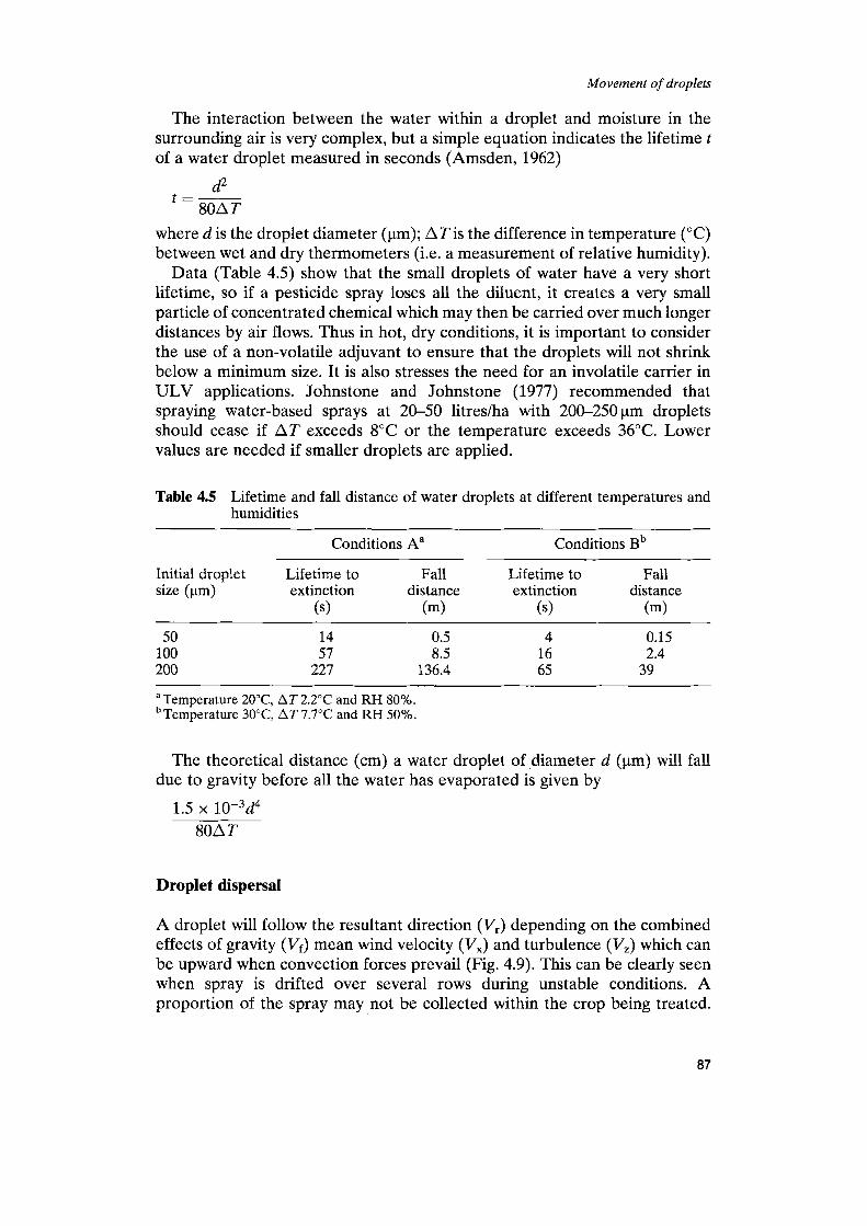
Data (Table 4.5) show that the small droplets of water have a very short lifetime, so if a pesticide spray loses all the diluent, it creates a very small particle of concentrated chemical which may then be carried over much longer distances by air flows. Thus in hot, dry conditions, it is important to consider the use of a non-volatile adjuvant to ensure that the droplets will not shrink below a minimum size. It is also stresses the need for an involatile carrier in ULV applications. Johnstone and Johnstone (1977) recommended that spraying water-based sprays at 20-50 litredha with 200-250 pn droplets should cease if AT exceeds 8°C or the temperature exceeds 36°C. Lower values are needed if smaller droplets are applied.

Table 4.5 Lifetime and fall distance of water droplets at different temperatures and humidities

Conditions A" Conditions Bb

Initial droplet Lifetime to Fall Lifetime to Fall size (pm) extinction distance extinction distance

(s) (m) (s) (m)

50 14 0.5 4 0.15 100 57 8.5 16 2.4 200 227 136.4 65 39

"Temperature 2 0 T , AT 2.2"C and RH 80%. bTemperature 30°C , AT 7.7"C and RH 50%.

The theoretical distance (cm) a water droplet of .diameter d (pm) will fall due to gravity before all the water has evaporated is given by

1.5 x 10-3d4 80A T

Droplet dispersal

A droplet will follow the resultant direction (Vr) depending on the combined effects of gravity (Vf) mean wind velocity (Vx) and turbulence (Vz) which can be upward when convection forces prevail (Fig. 4.9). This can be clearly seen when spray is drifted over several rows during unstable conditions. A proportion of the spray may not be collected within the crop being treated.

87

Spray droplets

(up or down) v z

Fig. 4.9 Resultant direction of a droplet (Vr) depending on the magnitude of effects of gravity, wind and convective air movement (after Johnstone et ul.,, 1974).

Bache and Sayer (1975) found that peak deposition of small droplets downwind was proportional to the height of the nozzle and inversely proportional to the intensity of turbulence, whereas larger droplets are relatively unaffected by turbulence and sediment according to the HUIV, relationship. Upward movement of small droplets (< 60 pm) is counterbalanced by downdraughts which return the droplets elsewhere; thus when relatively small areas are involved (hectares rather than square kilometres) the downdraughts may deposit droplets on a totally different area, contaminating other crops or pastures.

Evidence of this has been clearly demonstrated when an untreated crop, susceptible to a particular pesticide, shows distinctive symptoms of damage. A good example of this is when cotton has 'strap leaf' due to 2,4-D herbicide, which may be detected considerable distances from the site of application. Early morning is often considered the best time to apply herbicides (Skuterud e t al., 1998), provided there are no small droplets. If an inversion persists, such small airborne droplets could disperse in any direction.

Studies on droplet dispersal under field conditions are not easy due to variations in meteorological conditions, variations in droplet size, and the complexity of sampling. Many different techniques have been used to sample spray droplets downwind. Flat sheets have been widely used to measure fallout of the larger droplets, but smaller targets have been used for airborne spray to increase the capture efficiency. Bui et al. (1998) evaluated a number of different samplers and Amin et al. (1999) report studies with air samples for aerosol and gaseous pesticides. Hewitt e t al. (2000) included field studies with

88

Spray distribution

a range of hydraulic nozzles, while similar studies have been made in several countries. However, as results in the field are quite variable due to changes in wind speed and direction, most attention to the quantification of spray drift is being given to wind tunnel studies. Using a single nozzle and 2 mm diameter polythene lines as collectors in a wind tunnel, Phillips and Miller (1999) and Walklate et al. (2000a) then employed a model to relate laboratory measurements to field data. This system has been used to classify drift from boom sprayers in relation to determining buffer zones.

Some comparisons in the field have been made by spraying simultaneously with different machines, each applying a different tracer (Johnstone and Huntington, 1977). Similarly Sanderson et al. (1997) reported using an aircraft with a separate spray system for each wing so the two different dyes simula- taneously traced the distribution of different formulations of a herbicide. Parkin et al. (1985) used two food dyes - red erythrosine and water blue, while Cayley et al. (1987) suggested using a series of chlorinated esters as tracers. Babcock et al. (1990) used the ninhydrin reaction to quantify deposits of an amino acid. Cross and Berrie (1995) used fluorescent tracers Tinopal CBS-X or Uvitex OB (with 10% Helios per litre) to assess orchard sprayers and photographed deposits on leaves under UV light for analysis with a computer image analyser. Payne (1994) used a fluorescent tracer suspended in tripro- pylene glycol monomethyl ether to aerial sprays applied in different wind conditions. Background fluorescence on some leaves can be a problem in assessing deposits. An alternative is the use of chelated metal salts; thus Cross et al. (2000) used manganese, zinc, copper and cobalt salts to compare different spray treatments on strawberries. Choice of tracer is particularly important when assessing spray distribution on food crops.

A more complex approach was made in Canada to examine the dispersion of a spray cloud from an aircraft. Mickle (1990) used a light detection and range (LIDAR) laser beam to scan the spray cloud and sample 1 m3 of cloud at distances of 1 km. Similar studies showed that movement of airborne droplets was primarily dependent on the stability of the atmosphere, and that wide- spread dispersal of a small amount of pesticide is inevitable (Miller and Stoughton, 2000). A LIDAR technique has also been used to assess the structure of orchard crops to assist development of improved spraying techniques (Fig. 10.18) (Walklate et al., 2000b)

The biological effect of downwind drift of insecticides was assessed by bioassays using two day old Pieris brassicae larvae on potted plants (Davis et al., 1994). Similarly, herbicide drift was examined on young seedlings of rag- ged-robin (Lychnis flos-cuculi) in conjunction with deposition of fluorescein on various sampling receptors (Davis et al., 1993)

Spray distribution

Fluorescent tracers are also used more generally to demonstrate differences in the distribution of deposits on plants (Patterson, 1963). Insoluble micrqnised

89

Spray droplets

powders such as Lunar Yellow or Lumogen have been widely used (Fig. 4.10), but require careful mixing with a suitable surfactant before being diluted with water to the correct volume. A pre-formulated fluorescent dye suspension is available in some countries. A fluoresence spectrophotometer can be used to assess leaf surface deposits (Furness and Newton, 1988). Uvitex 2B has also been widely used, as it retains sensitivity at low concentration (Hunt and Baker, 1987). Downer et al. (1997) examined the effect of several water soluble fluorescent tracers on the droplet spectra produced by a fan nozzle. They showed that addition of a tracer can increase the proportion of small droplets produced; thus care needs to be taken in matching the spray quality with a pesticide spray when using a tracer to study downwind drift.

Fig. 4.10 Fluorescent spray deposit on cotton leaf (photo: ICI Agrochemicals, now Zeneca).

Samples of the target, often leaves, are collected and examined under UV light. Care must be taken to avoid looking directly at the UV light. Samples are usually sorted into arbitrary categories depending on the amount of cover obtained (Staniland, 1959). Courshee and Ireson (1961) and Matthews and Johnstone (1968) did chemical analysis of a sub-sample of leaves from each of the arbitrary categories to relate actual deposits with coverage. This allowed examination of a very large sample of leaves but limited the need for chemical analyses. Quantitative analysis of deposits is possible with light stable soluble tracers that are easily removed from the surface and measured with a fluoresence spectrometer. Murray et al. (2000) have also used ranked set sampling in spray deposit assessment and introduced an image analysis system

90

Determination of spray droplet size

that enables images to be stored. Carlton (1992) developed a method of washing deposits from both the upper and lower leaf surfaces.

The behaviour of individual droplets landing on leaf surfaces was studied using a videographic system (Reichard et al., 1998; Brazee et al., 1999). Similar studies have been reported by Webb et al. (2000) who investigated the impact of droplets on pea leaves. The aim of such studies has been to develop a model to predict retention or loss of pesticide droplets from leaf surfaces. With a single droplet generator the reflection height of droplets rebounding from a leaf surface could be determined. The effect of different surfactants on aqueous spray droplets landing on an adaxial leaf surface was also quantified. Another model examining deposition within a cereal crop canopy has analysed the crop architecture, aiming to use crop height as the main parameter in the model (Jagers op Akkerhuis et al., 1998).

Studies of droplets on leaf surfaces are also possible using scanning electron microscopy and cathodoluminescence (Fig. 4.11) (Hart, 1979; Hart and Young, 1987). Detailed spatial distribution can be provided by elemental mapping with a scanning electron microscope with energy dispersive X-ray (EDX) analysis. Fluorescence microscopy and autoradiography have also been used to trace deposits (Hunt and Baker, 1987), while Dobson et al. (1983) used neutron activation analysis to determine the amount of dysprosium in spray deposits in a crop and up to 100m downwind. Salyani and Serdynski (1989) reported experimenting with a sensor to provide an electrical signal proportional to the amount of spray deposit.

Variations in spray coverage in farmers’ crops are now usually demonstrated by clipping pieces of water sensitive paper to various parts of the crop. Stapling a folded paper to a leaf will show differences between upper and lower surface deposits. The papers can be made by treating glossy paper with a water sensitive dye such as bromophenol blue. The paper is yellow when dry, but aqueous droplets produce blue stains of the ionised dye (Turner and Huntington, 1970). Suitable papers are commercially available, but need to used carefully as the whole surface can turn blue in humid conditions and unless held on the edge, the surface readily shows blue fingerprints. Plain Kromekote cards have also been used when spraying a dye (e.g. Sundaram et al., 1991).


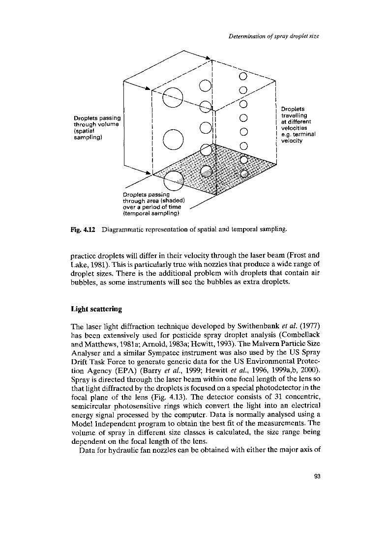
Measurement of spray droplets in flight is now done using one of several instruments that have a laser light beam through which droplets are projected. Sampling is either spatial (measuring droplets simultaneously within a defined space, within a section of the laser beam, i.e. number/m3) or temporal (measuring droplet flux passing through a defined sampling volume over a set time, i.e. number per m3 per second) (Fig. 4.12). In one type of instrument, the sampling volume is defined by the intersection of two laser beams. If all the droplets travel at the same speed both methods would be equivalent, but in

91

Spray droplets

(4

Fig. 4.11 Cathodoluminescence image of ‘Ulvapron’ oil containing ‘Uvitex OB’ and Brilliant Yellow R (photo: ICI Agrochemicals, now Zeneca). Spray droplets on tsetse fly: (a) arista; (b) near compound eye.

92


Droplets passing through volume (spatial sampling)

Droplets travelling at different velocities e.g. terminal velocity

over a period of time (temporal sampling)

/

Fig. 4.l2 Diagrammatic representation of spatial and temporal sampling.

practice droplets will differ in their velocity through the laser beam (Frost and Lake, 1981). This is particularly true with nozzles that produce a wide range of droplet sizes. There is the additional problem with droplets that contain air bubbles, as some instruments will see the bubbles as extra droplets.

Light scattering

The laser light diffraction technique developed by Swithenbank et al. (1977) has been extensively used for pesticide spray droplet analysis (Combellack and Matthews, 1981a; Arnold, 1983a; Hewitt, 1993). The Malvern Particle Size Analyser and a similar Sympatec instrument was also used by the US Spray Drift Task Force to generate generic data for the US Environmental Protec- tion Agency (EPA) (Barry et al., 1999; Hewitt et al., 1996, 1999a,b, 2000). Spray is directed through the laser beam within one focal length of the lens so that light diffracted by the droplets is focused on a special photodetector in the focal plane of the lens (Fig. 4.13). The detector consists of 31 concentric, semicircular photosensitive rings which convert the light into an electrical energy signal processed by the computer. Data is normally analysed using a Model Independent program to obtain the best fit of the measurements. The volume of spray in different size classes is calculated, the size range being dependent on the focal length of the lens.

Data for hydraulic fan nozzles can be obtained with either the major axis of

93

Spray droplets

(a)

Receiver cut-off Measured zone

Analyser beam

Spray nozzle

I I

I I

n 0 - -

Printer Computer

Ib) Detector measures

integral scattering of all

scatter at high angles I

Fig. 4.W (a) Layout of a Malvern light diffraction particle size analyser. (b) Dif- fraction of two different sized droplets. (c) Photo detector. (d) Transform property of receiver lens.

the fan in line with the laser beam, or alternatively individual parts of the spray can be examined with the fan perpendicular to the beam (Arnold, A.C., 1983). Cone nozzles need to be assessed more carefully as the droplet sizes will be affected by the part of the cone sampled (Combellack and Matthews, 1981a). In the USA, a Malvern mounted in a high speed wind tunnel measured droplets from nozzles used on aircraft (Hewitt et al., 1994a,b). Apart from comparisons between different types of nozzles, flow rates and operating pressures, effects of formulation on droplet spectra have been measured

94


I X

Each detector element is an annular ring collecting light scattered between two solid angles of scatter w 1 and w,

(dl

Fourier transform property of receiver lens

Optical transformation (thus almost instant)

A ll rays-incident at angle 'w'

Strike detector at 'w' from axis

(Combellack and Matthews, 1981b). The instrument can also be used to measure small particles in suspension in a glass cell mounted in the laser beam to check the formulation of a biopesticide (Bateman and Chapple, 2000).

Arnold (1987) and Teske et al. (2000) have compared the Malvern with another light scattering instrument, the Particle Measuring System (PMS) (Knollenberg, (1976) developed to measure particles in clouds. In this system of temporal sampling, droplets passing through a focused laser beam form a shadow on a photodiode array (Fig. 4.14). Droplet size is a function of the number of elements obscured by the passage of a droplet. Any droplet which is

95

Spray droplets

2.0 mW He-Ne Laser Sampling ' . volume .

- 0 0 0

L ,

0. J4 4

_ _ *4--- .

Spray .- f- . .

Collimated light beam

I

0 d /Mirror 0 - 0 Secondary Objective

Viewing volume

An intermediate

volume

Fig. 4.14 (a) Optical system of optical array spectrometer. (b) Three dimensional diagram to show shadow effect on detector.

not in the correct plane produces an out-of-focus pattern, so the computer is programmed to accept or reject data depending on the shadow produced. As the sampling volume is small, most nozzles have to be moved on an x-y grid to obtain a representative sample of a spray (Lake and Dix, 1985). The PMS has been used in wind tunnels (Parkin et al., 1980) to assess orchard sprayers (Reichard et al., 1977) and on aircraft .(Yates et al., 1982).

96


Laser Doppler droplet sampling

In this system (Aerometrics and Dantec equipment) a beamsplitter and lenses are used with a continuous laser to provide two intersecting beams, where interference fringes are produced (Bachalo et al., 1987; Lading and Andersen, 1989). A droplet passing through the intersection of the two beams produces modulated scattered light (a Doppler burst signal), the spatial frequency of which has to be measured to size the droplets (Fig. 4.15). Also, droplet velocity is measured, as it is proportional to the temporal frequency of the modulation. A forward light scattering angle of 30" is usually used. Three detectors are used to detect the phase shifts and avoid ambiguity in measurements. As there is a greater probability of larger droplets crossing the edge of the sample volume and producing an inadequate signal, the computer program adjusts for variation of sample volume. The droplet size range is dependent on the optics, but is usually with 50 class sizes. The total range can cover droplet diameters from 1 to 8000 pm. An on-line computer system provides real-time displays of droplet spectra. Using this type of equipment with an x-y grid, Western et al. (1989) compared hydraulic nozzles with a twin fluid nozzle.

Measurement

Yume Laser

I Beam splitter

Fig. 4.15 Principle of phase Doppler droplet sizing.

When Tuck et al. (1997) compared the Doppler particle analyser with a two- dimensional imaging probe (PMS), they showed that each instrument produced different droplet size and velocity distributions, but both instruments were useful provided their limitations were recognised.

Other techniques

A new system involves a pulsed laser to capture an image of the spray which can be subsequently analysed. By using a double flash of the laser, each

97

Spray droplets

droplet is recorded twice so that droplet velocity is also calculated. The system also enables the behaviour of droplets to be observed as they impinge on leaf surfaces (Fig. 4.16).

Fig. 4.16 Laser Visisizing of droplets (Oxford Lasers).

In-line holography was used to measure droplets in flight (Dunn and Walls, 1978), but the reconstruction of the holograms and their analysis is very slow compared with the newer laser techniques. Another technique has used hot- wire anemometry to assess the size of droplets, particularly small aerosol droplets (Mahler and Magnus, 1986) (Fig. 4.17). Using a portable instrument, this technique was used to measure droplets in a crop canopy (Adams et al., 1989).

Despite the capability of measuring droplets in flight, it is also important to measure droplets that have landed on a surface. Himel (1969a) pointed out that, ideally, the actual leaf surface should be used, and by spraying a known concentration of fluorescent particles (FPs) he estimated droplet size based on the number of individual particles deposited as discrete droplets on leaves. The method is most suitable for droplets in the range 20-70pm if the spray contains a uniform suspension of 2 x 10' FPs/ml, but counting individual particles is very tedious as a doubling of droplet diameter increases the number of particles per droplet eightfold (Fig. 4.18). Some sampling methods indicate the presence of spray but are not suitable for droplet sizing. One example is the use of a yarn of acrylic and nylon fibres with many fine hairs

98


Sensor utilises a 5pm heated platinum wire

Fig. 4.17 Hot-wire droplet sensor.

100- 90 80 - 70 - 60 - 50 -

-

Number of fluorescent particles per droplet

Fig. 4.18 Number of fluorescent particles (FPs) in droplets of different size according to the concentration of FPs in the spray (after Himel, 1969a).

which will collect small droplets very efficiently for chemical or fluorometric analysis (Cooper et al., 1996). The ‘harp’ with extemely fine tungsten wires was proposed for measuring small droplets, but is only suitable for an involatile spray liquid (McDaniel and Himel, 1977).

Sampling surface Sampling droplets in the field requires their collection on a suitable surface on which a mark, crater or stain is left by their impact. A standard surface is magnesium oxide, obtained by burning two strips of magnesium ribbon, each lOcm in length, below a glass slide so that only the central area is coated

99

Spray droplets

uniformly. The slide should be in contact with a metal stand to prevent unequal heating of the glass. On impact with the magnesium oxide a droplet (20-200 pm diameter) forms a crater which is 1.15 times larger than the true droplet size (May, 1950). The difference in size between the crater and the true size is the spread factor. The reciprocal of the spread factor is used to convert the measurements of craters (or stains) to the true size; thus for magnesium oxide the factor is is 0.86. The factor is reduced to 0.8 and 0.75 for measuring droplets between 15 and 20 pm and 10 and 15 pm, respectively. The magnesium oxide surface is less satisfactory for smaller droplets, and those above 200pm may shatter on impact. Droplets below below 100pm may bounce unless they impinge at greater than terminal velocity. If using water, the addition of a colour dye will facilitate seeing the droplets on the white surface. Glass slides coated with Teflon have been used to assess droplets of relatively involatile insecticides applied in mosquito control (Carroll and Bourg, 1979). The water sensitive paper mentioned previously has also been used to collect droplets for sizing, but as the stains can increase in diameter with time, its use to indicate percentage area covered is preferred (Salyani and Fox, 1999). However, treatment with ethyl acetate can be used to make the stains more permanent. In addition, the spread factor will vary according to the formulation and droplet size (Thacker and Hall, 1991). Plain glossy white card, such as Kromekote card, can be used if a water soluble colour dye (e.g. lis- samine scarlet or nigrosine) or oil-soluble (e.g. waxoline red) dye is added to the spray, depending on the type of liquid being used. Paper sensitive to oils and especially certain solvents can also be used. Salyani (1999) used acetone vapour to stabilise the stains caused by the droplets.

Water droplets can be collected on a grease matrix, but the droplets must be covered with oil to prevent evaporation reducing their size. A suitable matrix has one part of petroleum jelly and two parts of a light oil (risella oil or medicinal paraffin). No spread factor is needed as the droplets resume their original shape on the surface of the matrix.

Sampling technique

Although widely used, the technique of waving a slide through a spray cloud is not a very efficient way of sampling. Droplets less than 40 mm in diameter are not collected as efficiently as larger droplets. Sampling of airborne aerosol droplets is either with a cascade impactor which requires a vacuum pump (May, 1945) or by using a battery operated electric motor to rotate the slides (Cooper et al., 1996) or preferably narrower rods (Lee, 1974). Alternatively, sampling surfaces can be placed in a horizontal position within a settling chamber and sufficient time allowed for the smallest droplets to sediment on them.

Measurement of droplets

One method is to view the sample of droplets with a microscope fitted with a

100


graticule such as a Porton G12 graticule (Fig. 4.19). The microscope must have a mechanical stage to line up the stains or craters on the sampling surface with a series of lines on the graticule. The distance between these lines from the baseline Z increases by a fi progression. A stage micrometer is needed to calibrate the graticule. Use of the graticule is laborious if large numbers of samples require measurement, and alternative methods have been devised to increase speed and accuracy. Automatic scanning of samples using an image- analysing computer is much more rapid, provided the image of droplets is sharply contrasted against the background (Jepson et al., 1987; Last et al., 1987). Wolf et al. (1999) used Dropletscan software to measure droplets collected on water sensitive cards.

New Porton G12 Root two progression

Fig. 4.19 Porton G12 Graticule (courtesy: Graticules Ltd.).

Calculation of number and volume median diameter

A computer program (Cooper, 1991) can be used to calculate these parameters, but the following notes provide an example of the calculation shown in Table 4.6. The graticule is calibrated by measuring the distance between the Z line and one of the outer lines, e.g. 13; the true size is then calculated on the basis of the spread factor, and then the distance between 2 and each of the other lines calculated on the fi progression. The mean size is the average size of the limits of each class size. The number of droplets measured in each class size is recorded in column N . The percentage of droplets is then calculated, and the cumulative percentage plotted on log probability paper against the mean diameter (Fig. 4.20). As the volume of a sphere is 7cd3/6 and 7c/6 is a common factor, the cube of the mean diameter is calculated and multiplied by

101

Spray droplets

Table 4.6 An example of the calculations required to determine the NMD and VMD (from Matthews, 1975)

Graticule Upper True size Mean Number N Z N dm3 Ndm3 Ndm3 Z no. class upper size in class (YO) (YO) (%) Ndm3

size limit ( d ) (d,) ( N ) ("/I (D)

4 5 6 7 8 9

10 11 12 13

13.2 18.8 26.5 37.5 53 75

106 150 212

780 300

16 33 6.5 6.5 4096 135168 0.3 0.3 22.6 97 19.1 25.6 11543 1119671 2.3 2.6 32 150 29.6 55.2 32768 4915200 10.0 12.6 45.25 143 28.3 83.5 92652 13249236 26.9 39.5 64 66 13.0 96.5 262144 17301504 35.1 74.6 90.5 17 3.3 99.8 741217 12600689 25.5 100.1

128 181 256 Total: 506 Total: 49321468

Cumulative percentage

Fig. 4.20 Graph of cumulative percentage against mean droplet size to calculate the volume (solid curve) and number (broken curve) median diameter of the spray.

the number of droplets in that class (Ndm3). These figures are then expressed as percentages of the total volume of the sample, and the cumulative percentages plotted on the same graph (Fig. 4.20). The NMD and VMD are then read at the 50% intersect.

102

G. A. Matthews - Pesticide Application Methods, 3rd ...

Documents

Transcript of G. A. Matthews - Pesticide Application Methods, 3rd ...