FUZZY LOGIC CONTROLLER FOR POWER SYSTEM STABILIZER 

   

 

This thesis is submitted In partial Fulfillment of the Requirements for the degree of master of power system 

 

 

BY: 

WALEED ABD ALRAHIM MOHAMMED ISHAG 

 

Supervised by: 

Dr. Mirghani Fath Elrahman 

 

 

FACULTY OF ENGINEERING  

 

October 2009 

 

 

 

 

 

TABLE OF CONTENTS 

Acknowledgement                …………………………………………………………………………………………i 

Abstract    (English)               …………………………………………………………………………………….….ii 

Abstract    (Arabic)                 ……………………………………………………………………………………… iii 

 

Chapter 1 Introduc on

1.1Introduc on……………………………………………………………………………………………..…(1) 

1.2 Power System Stability…………………………………………………..………………………..…(1) 

1.3 Power system stabilizers(PSS)……………………………………………..…………………..…(3) 

1.4 Fuzzy Logic PSS……………………………………………………………………….………………....(4) 

1.5 Mo va on and Objec ves……………………………………………………….……………..…(5) 

1.6 Scope of the thesis…………………………………………………………………….……………….(6) 

 

Chapter 2 Literature Review 

2.1 Introduc on…………………………………………………………………………………..…..…....(7) 

2.1 Fuzzy Logic Control …………………………………………………………………………….…….(7) 

2.3 Stability Methods……………………………………………………………………………….....…(9) 

2.4 Power system stabilizers………………………………………………………………..…….….(10) 

2.5 fuzzy Control to Power Applica on……………………………………………..…………..(11) 

2.6 Fuzzy Power system Stabilizer………………………………………………………….…......(13) 

 

Chapter 3 Fuzzy Logic and Fuzzy Control 

3.1 Introduc on…………………………………………………………………………………….……...(16) 

3.2 Fuzzy Logic Control…………………………………………………………………………………..(17) 

 

 

3.3Fuzzy Logic Theory………………………………………………………………………………….…(19) 

3.3.1 Fuzzy Set versus Crisp Sets……………………………………………………………….…...(19) 

3.3.2Fuzzy Set Opera ons……………………………………………………………….…………..…(21) 

3.3.3Linguis c Variables …………………………………………………………………………………(23) 

3.3.4Membership Func ons……………………………………………………………………………(24) 

3.4 IF Then   Rule……………………………….……………………………………………………………(26) 

3.5 fuzzy Inference and defuzzifica on …………………………………………………..………(28) 

3.5 Scaling Factor………………………………………………………………………………………….…(31) 

3.6 Example……………………………………………………………………………………………….……(34) 

Chapter 4 Power system Model 

4.1 Introduction …………………………………………………………………………………………..…(38) 

4.2 Generator Represented by the Classical Model……………………………………….…(39) 

4.3 Block diagram of the system including Field circuit……………………………......…(42) 

4.3.1 Effect of flux linage varia on on system stability………………………………..….(43) 

4.4 Block diagram  of the system including Excitation system…………………………(44) 

4.4.1 Effect of AVR on synchronizing and damping torque componenets  ……..(45) 

4.5 Power system stabilizer………………………………………………………………….………...(46) 

Chapter 5 Simulation and results 

6.1Fuzzy PSS for Single Machine Infinite Bus…………………………………………………...(50) 

6‐2 Simula on Results……………………………………………………………………………………..(55) 

 

Chapter  6 Conclusion and further research 

6‐3 Conclusion……………………………………………………………………………………………….…(58) 

Further Research………………………………………………………………………………………………(59) 

Reference…………………………………………………………………………………………………………(60) 

Appendix  A( K constants equa ons)…………………………………………………………………(62) 

Appendix  B (system parameters).……………………………….……………………………………(64) 

Appendix  C (CPSS parameters).…………………………..……………………………………………(64) 

 

 

 

 

 

 

 

Acknowledgements 

                I  would  like  to  express  my  sincere  to  my  supervisor,  Dr. 

Mirghani  Fath  Elrahman,  and  Dr.  Abd  alrahman  karar  for  thier 

constant guidance, encouragement and support thr oughout my thesis. 

                I am  thankful  to Dr. Awad alla  tayfour, Sudan University,  for 

taking out  time  from his busy  schedule  to explain me  the  concept of 

programming fuzzy logic with matlab. 

        thanks  to  my  parents,  brothers  and  sisters  for  their  tireless  , support and encouragement . 

 

 

 

 

 

 

 

 

 

 

Abstract  

 

        Fuzzy logic controller has been designed as power system stabilizer (PSS) for

power system stability enhancement. The application of fuzzy logic controller is

investigated by means of simulation studies on a model of single machine infinite

bus (SMIB) using mat-lab program.

In this thesis the structure of a fuzzy logic controller is presented. A close

loop control strategy is taken as a knowledge base for the fuzzy controller design.

Speed deviation (∆ω) and acceleration (dω/dt ) of the synchronous machine are

chosen as the input signals to the fuzzy controller in order to achieve a good

dynamic performance. The complete range for the variation of each of the two

controller inputs is represented by a 7×7 decision table, i.e. 49 rules using

Proportional derivative like fuzzy controller. To tune the proposed controller we

increased the gain using trial and error method. The response of the SMIB with

fuzzy controller is compared against the model with conventional controller for

ten seconds in one graph.

The simulation results of the proposed fuzzy logic controller on SMIB gave a

better dynamic response, decreased the over shoot and the settling time when

proposed controller is compared with conventional PSS. The simulation results

proved the superior performance of the proposed controller.

 

 

 

خالصة

لقد تم فى هذا البحث تصميم متحكم مبنى على اساس المنطق الغامض لتحسين اتزان

تم تطبيق ودراسة المتحكم المقترح على نموذج ماآينة مفردة . أنظمة القوى الكهربائية

 .باستحدام برنامج المات الب

واختيرت استراتيجية ، مضنائي للمتحكم ذو المنطق الغتم في هذا البحث شرح الترآيب الب

تم اختيار السرعة والتسارع للمولد آما ، التحكم ذات الدوائر المغلقة آقاعدة بيانات فى التصميم

آما تم تمثيل مدى اشارات الدخل بجدول .امضالمولد المتزامن آاشارات دخل لمتحكم المنطق الغ

لموالفة المتحكم تمت زيادة .على اساس المشتق النسبى قاعدة مبنية 49على وى تيح 7×7قرار

استجابة نموذج الماآينة المفردة بوجود المتحكم . الكسب بطريقة الكسب بطريقة التجربة والخطاء

ذو المنطق الغامض تمت مقارنتها مع استجابة النظام بوجود المتحكم التقليدى فى مخطط واحد

.لمدة عشرة ثوانى

المتحكم المقترح على نموذج الماآينة المفردة اداء ديناميكى أفضل عند محاآاةاعطت نتائج

مقارنتها مع نتائج المتحكم التقليدى من حيث تقليل زمن الذروة وزمن االستقرار وبذلك ثبتت

.فاعلية وأفضلية المتحكم المقترح

 

 

 

Chapter 1 Introduction

   1.1 Introduction

 Modern  power  systems  are  highly  sensitive  to  large  disturbances which 

can propagate  through  the  large  network of  interconnection  in  the  absence  of 

adequate  safeguards.  In  order  to  have  reliable  generation  and  transmission,  a 

power system should be stable. Most present day power generators are equipped 

with  power  system  stabilizer  (PSS)  for  controlling  slowing  oscillating  type 

instability.  

1.2 Power System Stability  

   Power  system  stability  refers  to  the  ability  of  the  synchronous machines  to 

remain  in  synchronism while delivering power at normal voltage and  frequency 

[1] .Depending on the type of disturbance, power system stability is classified into 

the following[1]: 

 

• Steady state stability. • Transient stability. • Oscillating stability. 

 

              Steady  state  stability  involves  slow  or  gradual  changes  in  power without 

loss of stability or synchronism of machine. Steady state stability studies ensure that 

 

 

phase angles across  transmission  lines are not  too  large, bus voltages are  close  to 

nominal  values  and  that  generator,  transmission  lines,  transformers,  and  other 

equipments are not over loaded. 

               Oscillating  stability    is  ability  of  a  system  to  maintain  stability  when 

subjected  to  small  disturbances  such  as  small  changes  in mechanical  torque.  The 

action  of  turbine  governor,  excitation  systems,  tap  changer  transformers  and 

controls from a power system dispatch center can interact to stabilize or destabilize 

a  power  system  several  minutes  after  a  disturbance  has  occurred.  Control  of 

excitation,  static  var  control  (SVC)  and  fast  valving  are  some  of  methods  for 

controlling slowly changing oscillations. 

               Transient stability  involves major disturbances such as  loss of generators, 

line  switching  operations.  Faults  and  sudden  load  changes.  The  objective  of  a 

transient stability study  is  to determine whether or not  the machine will  return  to 

synchronous  frequency with new steady state power angles. Usually  the regulating 

devices are not fast enough to function during transient period .the system May loss 

its  stability  at  first  swing  unless  an  effective  counter  is  taken  such  as  dynamic 

resistances braking, or load shedding.  

1.3 Power System Stabilizers    Excitation  control  involves  feeding  an  extra  stabilizing  control  with  the 

automatic  voltage  regulator  (AVR).this  generally  is  derived  from  a  power  system 

stabilizer  (PSS).  How  much  an  excitation  control  signal  affects  the  stabilization 

 

 

process of  the machine depends upon  the  response of excitation system, available 

field energy, and maximum and minimum allowable  limits of excitation voltage. On 

occurrence of  the  fault  on  a  system,  the  voltage  at  all buses  is  reduced, which  is 

sensed by the AVR. The AVR then acts to restore the generator terminal voltage. The 

general  effect  of  excitation  system  is  to  reduce  the  initial  rotor  angles  swing 

following the fault. This  is done by boosting the field voltage  .The  increased air gap 

flux  exerts  a  restraining  torque  on  the  rotor which  tend  to  slow  down  the  rotor 

motion. This method is more effective for smaller disturbances. 

           The use of PSS  to  improve  the dynamic performance of power systems has 

increased  steadily  since  the  sixties  when  they  were  first  presented.  Since  then, 

extensive  research  has  been  carried  out  in  this  area.  Conventional  types  are 

designed with fixed structure and constant parameters tuned for optimal operating 

conditions. Since the operating point of a power system changes nonlinearly as loads 

and  generating  units  are  connected\disconnected,  and  since  unpredictable  faults 

occur, the performance of a fixed structure PSS varies greatly. It is desirable to adapt 

the  stabilizer  parameters  in  real  time  based  on  line  measurements  in  order  to 

maintain good dynamic performance over a wide range of operating conditions. This 

motivated the development of a self tuning stabilizer .Although the self tuning PSS, it 

suffers  from  a  major  drawback  of  requiring  model  identification  in  real  time 

consuming,  especially  for  a microcomputer with  limited  computational  capability. 

Some  of  the  artificial  intelligence  based  alternatives  of  designing  PSS which  have 

been reported in the literature are: 

1. Rule based. 2. Neural Network. 3. Fuzzy Logic. 

 

 

1.4 Fuzzy Logic PSS  

    Fuzzy  logic  control  (FLC)  has  found  its  application  in  power  industry  in 

recent  years.  Several  reporting  have  been made  about  design  of  PSS  involving 

fuzzy  control  theory.  Its  simplicity  and  performance  makes  it  attractive  for 

implementation. 

     The fuzzy PSS has four components in it. These are 

1. Fuzzifier. 2. Knowledge base. 3. Inference Engine. 4. Defuzzifier. 

     The  inputs  to  PSS  which  normally  are  speed,  acceleration,  power  etc.  are 

converted to fuzzy signals through the fuzzifier. 

    The  expert  Knowledge  about  the  PSS  control  strategy  is      normally  stored  in 

knowledge base. It consists of data base and rule base guide us about the decision‐

making  logic,  i.e.  set of  rules  and  from  the data  base we  know  about  thresholds, 

shape and number of membership functions. 

     The  fuzzy  logic  inference  engine  infers  the  proper  control  action  based  on 

available fuzzy rules. 

           Since  the  input  to  the excitation  system  is  crisp.  The  fuzzy  signal obtained 

through the above procedure is defuzzified and fed to the AVR. 

 

 

 

 

1.5  Motivation and objectives    

           Conventional  PSS  (CPSS)  is widely  used  in  existing  power  systems  and  has 

made a contribution in enhancing power system stability. The parameter of CPSS are 

determined  based  on  a  linearized  model  of  power  system  around  a  nominal             

operating point where they can provide good performance. Since power system are 

highly  non‐linear  systems,  with  configurations  and  parameters  that  change  with 

time,  the  CPSS  design  based  on  the  linearised  model  of  power  system  cannot 

quarantee its performance in a practical operating environment. 

      Since the design of fuzzy  logic controller, unlike most conventional methods, a 

mathematical model  is not required to describe the system under study.  It  is based 

on the implementation of fuzzy logic technique to PSS to improve damping.   

    The objective of this thesis  is to use  fuzzy  logic controller to simulate the small 

signal stability of  the system consist of  four machines connected  to a  large system 

through a double  circuit  transmission  lines. The  simulation  is about a  steady  state 

operating condition following a loss of one circuit.   

 

 

1.6 Scope of the Thesis 

 

         Chapter  2  of  the  thesis  presents  a  literature  review  on  stability methods, 

power system stabilizers, fuzzy  logic control and application of fuzzy  logic control. 

Chapter  3  gives  a  brief  theory  on  fuzzy  logic  control.  Chapter  4  presents  single 

 

 

machine  infinite bus model. Chapter 5 presents PD  like  fuzzy  logic controller and 

chapter 6 includes simulation results, conclusions and recommendations.   

 

 

 

 

 

 

 

 

 

 

 

 

 

 

Chapter 2

Literature Review

2.1 Introduc on 

  

 

 

     A great deal of work has been reported on the  issue of power system stability 

and control. In this chapter, we present a review of the fuzzy logic control ,stability 

methods,  power  system  stabilizers,  fuzzy  logic  to  power  system  application.  The 

last section is devoted to fuzzy power system stabilizer. 

 

2.2 Fuzzy Logic Control 

         The concept of Fuzzy Logic (FL) was conceived by Lotfi Zadeh, a professor

at the University of California at Berkley, and presented not as a control

methodology, but as a way of processing data by allowing partial set membership

rather than crisp set membership. This approach to set theory was not applied to

control systems until the 70's due to insufficient small-computer capability prior to

that time. Professor Zadeh reasoned that people do not require precise, numerical

information input, and yet they are capable of highly adaptive control. If feedback

controllers could be programmed to accept noisy, imprecise input, they would be

much more effective and perhaps easier to implement. Unfortunately, U.S.

manufacturers have not been so quick to embrace this technology while the

Europeans and Japanese have been aggressively building real products around it.

FL is a problem-solving control system methodology that lends itself to

implementation in systems ranging from simple, small, embedded micro-

controllers to large, networked, multi-channel PC or workstation-based data

acquisition and control systems. It can be implemented in hardware, software, or a

combination of both. FL provides a simple way to arrive at a definite conclusion

based upon vague, ambiguous, imprecise, noisy, or missing input information. FL's

 

 

approach to control problems mimics how a person would make decisions, only

much faster.

FL incorporates a simple, rule-based IF X AND Y THEN Z approach to a

solving control problem rather than attempting to model a system mathematically.

The FL model is empirically-based, relying on an operator's experience rather than

their technical understanding of the system. For example, rather than dealing with

temperature control in terms such as "210C <TEMP <220C", terms like "IF

(process is too cool) AND (process is getting colder) THEN (add heat to the

process)" or "IF (process is too hot) AND (process is heating rapidly) THEN (cool

the process quickly)" are used. These terms are imprecise and yet very descriptive

of what must actually happen. Consider what you do in the shower if the

temperature is too cold: you will make the water comfortable very quickly with

little trouble. FL is capable of mimicking this type of behavior but at very high

rate.

FL requires some numerical parameters in order to operate such as what is

considered significant error and significant rate-of-change-of-error, but exact

values of these numbers are usually not critical unless very responsive performance

is required in which case empirical tuning would determine them. For example, a

simple temperature control system could use a single temperature feedback sensor

whose data is subtracted from the command signal to compute "error" and then

time-differentiated to yield the error slope or rate-of-change-of-error.

FL was conceived as a better method for sorting and handling data but has

proven to be a excellent choice for many control system applications since it

mimics human control logic. It can be built into anything from small, hand-held

products to large computerized process control systems. It uses an imprecise but

 

 

very descriptive language to deal with input data more like a human operator. It is

very robust and forgiving of operator and data input and often works when first

implemented with little or no tuning.

 

2.3 Stability Methods 

 

    A  reliable  power  system  should  be  able  to  restore  itself  to  nominal  operating 

conditions following a disturbance. This can be done only if the system is equipped 

with  effective  control  tools. Research on  improvement of power  system  stability 

can  be  categorized  into  two  types.  Transmission  side modification &  generation 

side modification[1] . 

 

The transmission side modification can be subdivided as: 

     

1. High speed fault clearing. 2. Reduction of transmission line reactance. 3. Dynamic braking resistor. 4. Independent pole operation of circuit breaker. 5. Regulated shunt compensation. 6. Parallel usage of AC and DC systems. 7. Controlled system separation and load shedding.

  

 

The generation side modification can be subdivided as: 

 

 

 

1. Turbine Valve control. 2. Excitation  Control. 

 

 

 

 

2.4 power system stabilizers 

 

         Different types of power system stabilizer have been designed and reported 

in the literature in an effort to improve the system performance under smaller and 

larger disturbances. Some of the related literature on the topic is presented. 

            Schlief  showed  that  damping  and  stability  are  greatly  improved  by 

supplementary  control with  a  specially  derived  function  of  frequency  deviation  , 

established  understanding  of  stabilizing  requirements,  and  included  the  voltage 

regulator gain parameters and transfer function characteristics for a machine speed 

derived  signal  superposed  on  the  voltage  regulator  gain  reference  for  providing 

damping  of  machine  oscillation.  And  then  addressed  the  problem  of  the  most 

effective  selection  of  generating  unit  to  be  equipped  with  excitation  system 

stabilizer in multimachine system[3]. 

          Chin   & Hsu present the performance objective of   PSS    in terms of types of 

oscillations  and  operating  conditions  and  developed  relationship  between  phase 

 

 

compensation  tuning  and  root  locus  analysis.  designed  an  optimal  variable 

structure stabilizer by increasing the damping torque of synchronous machine. 

            C.    M.  Lim  present  a  method  of  designing  decentralized  stabilizer  in 

multimachine power  system. Propotional  Integral   PSS was  first  reported by Hsu. 

He  used  two  approaches,  the  root  locus  method  &  the  suboptimal  requlator 

method[4].  

  

     So far as self tuning stabilizers are concerned, a significant amount of work has 

been done and these were the center of attention of power system researches  in 

late  eighties. 

      chen  &  Hsu  designed  an  adaptive  output  feedback  PSS  using  local  signal 

generator e‐g. Speed or power and give adaptive pole shi ing self tuning PSS [5]. 

 

    Wu & Hsu  designed a self tuning PID PSS for multi machine  power system. The 

proposed  stabilizer  had  a  decentralized  structure  and  only  local measurements 

within  each  generating  unit  was  required.  S.Lefbvre  proposed  an  approach  of 

simultaneously selecting the parameter of all the stabilizers in multi machine power 

system.  He  formulated  the  parameter    optimization  problem  into  eigen  value 

assignment problem and developed algorithm enabling exact assignment of system 

modes[6]. 

            Recently,  some work  is  reported  in  the  literature  on  rule  baseand  neural 

networkin  an  effort  to  get  rid  of  model  dependence  and  in  turn  reduce  the 

calculation time of control. 

 

 

 

2.5 Fuzzy Control to Power Applica ons 

One of the earliest applications of fuzzy  logic  in power system and nuclear 

control was in 1988. Later, the fuzzy technique was applied in almost all the power 

related areas, such as, planning, scheduling, reliability, contingency analysis, (VAR) 

Voltage control,  stability evaluation,  load  forecasting,  load management, decision 

making  support,  monitoring  &  control,  unit  commitment,  state  estimation, 

transformer diagnosis, machine diagnoses and fault analysis[7].

Fuzzy  logic  has  been  applied  in  power  system  expansion  planning.  The  decision 

making  process  in  power  system  expansion  planning  is,  to  a  large  extent, 

qualitative and can be described more flexibly and intuitively by fuzzy set concepts. 

Power  system  long/mid  term  scheduling  problems  such  as  yearly  maintenance 

scheduling, seasonal fuel and mid term operation mode studies are usually solved 

by  various optimal and heuristic methods but  it  is more  reasonable  to  represent 

constraints  in  fuzzy  expressions.  The  combination  of  conventional methods with 

fuzzy sets may constitute an effective approach to solve these problems [8].

The present practice  in dynamic  security assessment  (DSA)  is  to perform off‐  line 

studies for a. wide range of Likely system conditions and network configurations. In 

on‐line applications  the operators are allowed  to rely on  their own  judgment and 

knowledge acquired  in off‐line  studies and experience gathered during  long  time 

operation.  Fuzzy  set  theory may  be  useful  in  building  an  expert  system  for DSA 

based on the operator’s empirical knowledge [9].

 

 

Power  system  load  demand  is  influenced  by  many  factors  such  as  weather, 

economic &  social  activities  and different  load  component  (residential,  industrial 

and  commercial  etc.).  Fuzzy  logic  approach  has  shown  advantages  over 

conventional methods.  The  numerical  aspects  and  uncertainties  of  this  problem 

appear suitable methodologies [10].

Human  experts  play  central  role  in  trouble  shooting  or  fault  analysis.  In  power 

systems, it is required to diagnose equipment malfunctions as well as disturbances. 

Equipment malfunctions are caused by many  factors and  information available  to 

perform diagnoses is incomplete. In addition, the conditions that induce faults may 

change  with  time.  Subjective  conjectures  based  on  experience  are  necessary. 

Accordingly,  the expert  systems  approach has  to be useful. As  stated previously, 

fuzzy  set  concepts  can  lend  itself  to  the  representation  of  knowledge  and  the 

building of an expert system [11].

In  traditional  controller  design.  a  system  model  needs  to  be  constructed  and 

control  laws  are  derived  from  the  analysis  of  the model.  Because  of  the  non‐

linearity  it  is nearly always necessary  to Linearize  the system model and  then  the 

linear controllers are used to control the non‐linear system. Fuzzy  logic controllers 

have  received  much  attention  in  recent  years,  since  they  are  more  model‐

independent,  show  high  robustness,  and  can  adapt.  Fuzzy  Logic  controllers  are 

mainly used for power system excitation and converter controls .  

T.Hiyama  and  his  colleagues  presented  an  application  of  a  fuzzy  logic  control 

scheme  for  switched  series  capacitor  modules  to  enhance  overall  stability  of 

electrical power system [12]. Desh presented a new approach to the design of PLC 

for  HVDC  transmission  Link  using  fuzzy  logic[13].  The  fuzzy  controller  relates 

 

 

variables like speed & acceleration of generator to a control signal for the rectifier 

current regulator loop using fuzzy membership functions. 

 

 

2.6 Fuzzy Power System Stabilizer 

 

One of the earliest articles which present a PSS other than the conventional 

design, was from Takashi Hiyama in 1989[14]. He presented a rule based stabilizing 

controller to electrical power system. The control scheme utilized was a bang bang 

strategy  for a  single machine  infinite bus model. The  input  signal considered was 

speed deviation and acceleration. Later he modified the strategy by considering the 

weighted  acceleration.  He  extended  his  work  on  rule  based  fuzzy  control  to 

multimachine system  and refined his work through several other publications.

                Hassan  [15]  improved  Hiyama’s  work  by  changing  the  shape  of  the 

membership  functions.  Standard  non‐linear  continuous  membership  functions, 

which are more  suitable  for  synchronous machine. He  later, also proposed a  self 

tuned PSS, and implemented the controller in the laboratory.  Hsu also reproduced 

Hiyama’s work[14], by changing the shape of membership functions.

              One of the first articles which reported a PSS design, based entirely on fuzzy 

logic control was from Hsu  in 1.990[16]. He used the concepts of fuzzification and 

defuzzification  in  the  PSS  design  and  compared  the  results  with  conventional 

stabilizer.  A  number  of  membership  functions  were  employed  making  the 

computation complicated. 

 

 

              Sharaf presented a hybrid of conventional and fuzzy PSS design for damping 

electromechanical modes of oscillations and enhancing power system stability [17]. 

Kitauchi developed  a  fuzzy  excitation  control  scheme,  for  the purpose of  further 

improving the stability to large disturbances[18]. His fuzzy stabilizer was multi‐input 

multi‐output (MIMO) type and consists of two subcontrollers using basic concept of 

AVR & PSS. The inputs to the fuzzy AVR were change in terminal voltage and its rate 

of  change while  the  input  to  FPSS were  change  in  electrical  power  and  rate  of 

change  in  electrical  power.  Finally  the  two  output  signals were  added.  Iskandar, 

Ortmeyer  reported  hybrid  PSS’s  which  take  care  of  small  as  well  as  large 

disturbances  [90].  In  order  to  get  rid  of measurement  noise  in  speed  signal  at 

smaller  disturbances,  two  stabilizers  were  designed  ‐one  speed  deviation  input 

fuzzy controller and other electrical power deviation input analog‐type PSS.A fuzzy 

judgment mechanism was suggested which help select one of  two controllers  for 

large and small disturbances, respectively.

           Hariri’s  adaptive network based  stabilizer  [19]  combines  the  advantages of 

artificial neural network and fuzzy logic control together. Fuzzy PSS having learning 

ability  is  trained directly  from  the  input and output of  the generating unit. Park’s 

self  organizing  power  system  stabilizer  (SOPSS)  use  the  fuzzy  Auto  Regressive 

model  [93].  The  control  rules  and  the  membership  functions  of  the  proposed 

controller  are  generated  automatically  without  using  any  plant  model.  The 

generated  rules  are  stored  in  the  fuzzy  rule  space  and updated on‐line by  a  self 

organizing procedure.

P.K.Desh designed an anticipatory  fuzzy control PSS which differs  from  traditional 

fuzzy  control  in  that, once  the  fuzzy  control  rules have been used  to  generate  a 

 

 

control value, a prediction routine built into the controller is called for  Anticipating 

its effect on the system out put and hence updating the rule base or input out put 

membership functions in the event of unsatisfactory performance. 

 

 

 

 

 

 

 

 

 

 

 

 

 

 

 

Chapter 3

Fuzzy logic and Fuzzy Control

 

 

 

 

3.1 Introduction  

   Fuzzy logic system (FLS) is a convenient way to map input space into 

output space. this means for the given conditions or sample inputs of the system,  

the designed fuzzy logic system would lead to the crisp output, no matter how 

non‐linear or stochastic in nature the system is. In order to understand the 

working properly, it should be noted that FLS is not the only way of solving 

problems. If it were replace with the black box , there may be a number of things 

in that box solving the problem, such as linear systems, expert system, neural 

network, differential equations, interpolating multidimensional look up tables, 

etc. Now the equation arises to what sort of problems fuzzy logic should be 

applied and to which problem it’s not beneficial. The answer is, when the problem 

is simple enough and a crisp mathematical expression solves the problem more 

effectively, fuzzy logic should be avoided. When problem is very complex, 

ambiguous and information available is imprecise, fuzzy reasoning provides away 

to understand system behavior by allowing interpolation between input and 

output situations. 

 

 

 

3.2  Fuzzy Logic Control 

     A layout of a general fuzzy logic system is given in Figure 3.1  

 

 

         

 

              FLC comprises of four principal components. These are: a fuzzification 

interface, a knowledge base (NB), decision making logic, and difuzzification 

interface. 

 

KNOWLEDGE 

DECISION 

MAKING

CONTROLLED 

SYSTEM 

DEFUZZIFICATIONFUZZIFICATION 

Fuzzy  Fuzzy 

Process Output & state 

Actual Control Non Fuzzy 

Figure 3.1 The Basic Configura on of a FLC. 

 

 

 

1\ the fuzzification interface involves the following functions: 

 

- Measures the values of input variables (Process output). 

- Performs  a  scale  mapping  that  transfers  the  range  of  values  of  input 

variables into corresponding universe of discourse. 

- Performs  the  function  of  fuzzification  that  converts  data  into  suitable 

linguistic values which may be viewed as labels of fuzzy set. 

 

2/ the knowledge base comprises of knowledge of the          application domain 

and the attendant control goals. It consists of a “data base” and a “linguistic 

(fuzzy) control rule base:” 

 

- The  database  provides  necessary  definitions,  which  are  used  to  define 

linguistic control rules and fuzzy data manipulation in FLC. 

- The rule base characterizes the control goals by means of a set of linguistic 

control rules. 

 

3/  the decision making logic is the kernel of an FLC, it has the capability of 

simulating human decision making based on fuzzy concepts and of inferring fuzzy 

control actions employing fuzzy implication and the rules of inference in fuzzy 

logic. 

 

 

 

4/ the deffuzzification interface perform the following functions: 

 

- a scale mapping, which converts the range of value of output variables into 

corresponding universes of discourse, 

- defuzzification, which  yields  a  nonfuzzy  control  action  from  an  inferred 

fuzzy control action. 

 

         Before we proceed with the application of FLC to the power system stability, 

a brief background on the fuzzy control theory, the fuzzification and 

difuzzification procedure, etc. is given in the following sections. 

3.3 Fuzzy Logic Theory  

       3.3.1 Fuzzy Set versus Crisp Sets 

 

          The classical mathematical set theory is known as theory of crisp sets. The 

crisp set has some well defined boundaries, i.e., there is no uncertainty in the 

prescription or location of boundaries of the set. Any element of the universe of 

discourse is either in that crisp set or not. So the membership value of any is 

either one or zero. It can describe by its characteristics function as follows: 

 

                 0,1 3.1  

 

 

                      

 

         The characteristic function   is called the membership function. Let us 

denote temperature 25°C or greater as “hot”. Any temperature less than 25°C is 

then not hot. Then the membership function of crisp set “hot” can be shown as in 

Fig. 3.2 

 

 

  

     

 

 

              In contrast to crisp set, fuzzy set does not have well defined boundaries’ 

rather it is prescribed by vague or somewhat ambiguous boundaries. A fuzzy set 

then is a set containing element that has varying degrees of membership in the 

set.  

 

 

T 

Figure 3.2 The Characteris c Func on   

1 

25 0 

 

 

      The definition of a fuzzy set is given by the characteristics function 

 

                                            0 … .1 3.2  

    

  

             If  now the characteristics function of   is considered one can express 

the human opinion, being for example that 24 degrees is still fairly hot and 26 

degrees is hot but not as 30 degrees higher. This results in gradual transition from 

full membership (1) to non‐membership (0). Fig. 3.3 shows an example of 

membership function   of the fuzzy set   .the membership function; 

however, every individual can construct a different transition according to his 

own opinion. 

 

 

 

 

 

 

 Figure 3.3 The Membership Function   

1 

25 0  20  30 

 

 

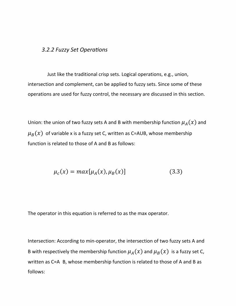
 3.2.2 Fuzzy Set Opera ons 

 

              Just like the traditional crisp sets. Logical operations, e.g., union, 

intersection and complement, can be applied to fuzzy sets. Since some of these 

operations are used for fuzzy control, the necessary are discussed in this section. 

 

Union: the union of two fuzzy sets A and B with membership function   and 

  of variable x is a fuzzy set C, written as C=AUB, whose membership 

function is related to those of A and B as follows:  

 

, 3.3  

 

 

The operator in this equation is referred to as the max operator. 

 

Intersection: According to min‐operator, the intersection of two fuzzy sets A and 

B with respectively the membership function   and    is a fuzzy set C, 

written as C=A�B, whose membership function is related to those of A and B as 

follows: 

 

 

 

, 3.4  

 

Both the intersection and the union operations are explained by Figure 3.4 

 

 

 

 

Complement: The complement of a fuzzy set denoted Ā as with a membership 

function defined as 

 

 

 

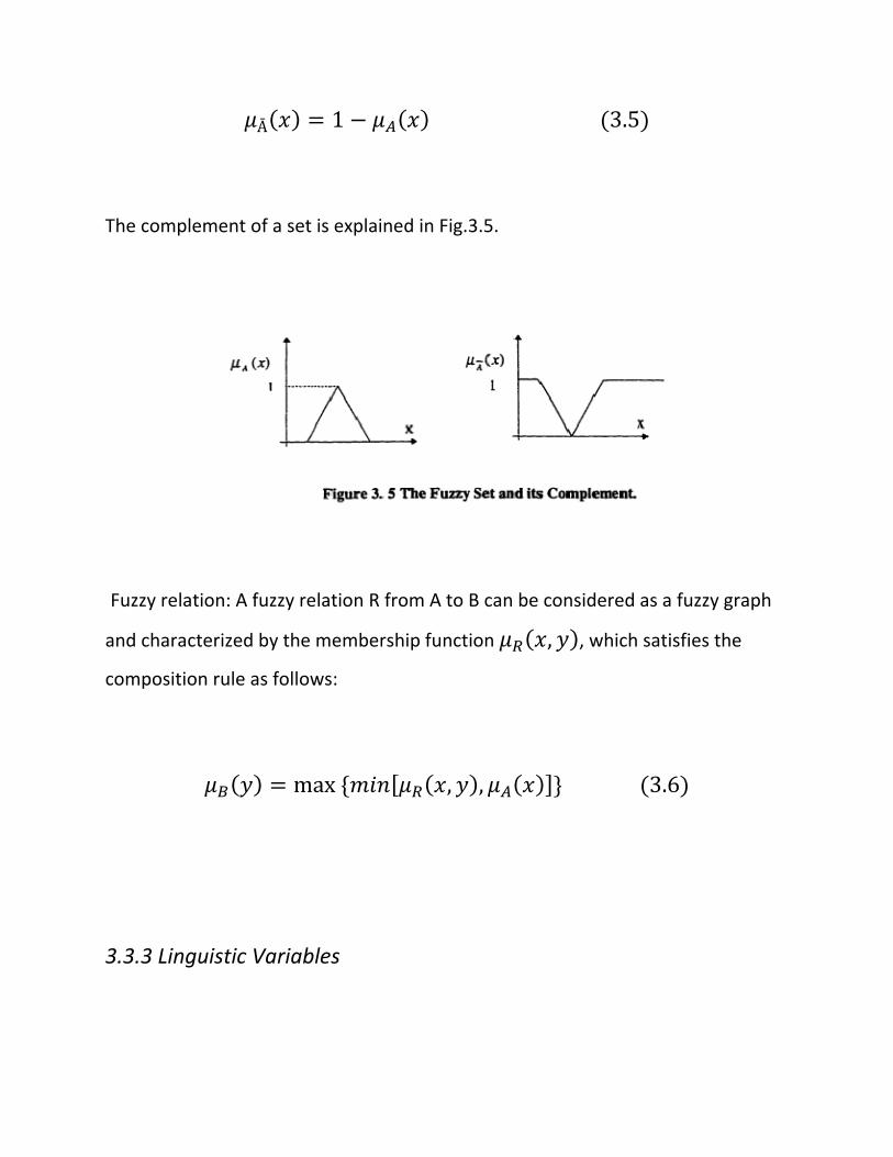
Ā 1 3.5  

 

The complement of a set is explained in Fig.3.5. 

 

 

 

 Fuzzy relation: A fuzzy relation R from A to B can be considered as a fuzzy graph 

and characterized by the membership function  , , which satisfies the 

composition rule as follows: 

 

max , , 3.6  

 

 

3.3.3 Linguistic Variables 

 

 

 

            Variable whose values are not numbers but words or sentences are called 

linguistic variables. The motivation of the use of words or sentences rather than 

numbers is that linguistic characterizations are, in general, less specific than 

numerical ones. 

           A linguistic variable is usually decomposed into a set of terms which cover 

its universe of discourse. For example, a control variable can be represented as: 

 

U(control variable)={Large positive, Medium positive, Small positive, Very small, 

small negative, Medium negative, Large negative} 

 

Where each term in U is characterized as a fuzzy set. 

Similarly, we can construct an example of pressure (P). The universe of discourse 

is 

 

 P= [100psi‐2300psi]. 

 

It can decompose into the following set of terms. 

 

P (pressure) :{ Very low, low, medium ,high, Very high} 

 

 

 

It might be interpreted as 

 

Very low a pressure below 200 psi 

Low as a pressure close to 700 psi 

Medium as a pressure close to 1050 psi 

High as a pressure close to 1500 psi 

Very high as a pressure above 2200 psi 

 

3.3.4 Membership Functions 

 

         The characteristic function of a fuzzy set is called the membership 

function, as it gives the degree of membership for each element of the universe 

of discourse. The x‐axis of membership function shows thresholds of linguistic 

variables and y‐axis show the membership value for that linguistic variable. 

       The most commonly used shapes for membership functions are monotonic, 

triangle, trapezoidal or bell shaped, etc., as shown in Fig. 3.6 Membership 

functions are chosen by the users, based on the users experiences, prospective, 

cultures, etc., hence, the membership functions for two users could be quite 

different for the same problem. 

 

 

 

       

 

            How many membership functions should be used to represent a certain 

variable depend upon the user. Greater resolution is achieved by using more 

memberships at the price of greater computational complexity. 

Membership functions do not overlap in crisp set theory but one of greater 

strength of fuzzy logic is that membership functions can be made to overlap. 

 

          In most control systems, the input variables of a FLC are error signals and 

their derivatives or their integral. These variable can be supported by terms like 

Large Negative (LN), Medium Negative (MN),Small Negative(SN) ,Zero(Z),Small 

Positive(SP) ,Medium Positive(MP),Large Positive(LP). In figure 3.7 a set of 

triangular shaped membership functions are given to describe the above linguistic 

variables and these are equally distributed over the universe of discourse. Using 

other membership function shapes can change the behavior of the FLC 

 

 

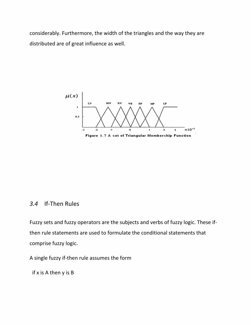
considerably. Furthermore, the width of the triangles and the way they are 

distributed are of great influence as well. 

 

  

  

3.4 If‐Then Rules  

Fuzzy sets and fuzzy operators are the subjects and verbs of fuzzy logic. These if‐

then rule statements are used to formulate the conditional statements that 

comprise fuzzy logic. 

A single fuzzy if‐then rule assumes the form 

  if x is A then y is B 

 

 

where A and B are linguistic values defined by fuzzy sets on the ranges (universes 

of discourse) X and Y, respectively. The if‐part of the rule "x is A" is called the 

antecedent, while the then‐part of the rule "y is B" is called the consequent or 

conclusion.  

      In general, the input to an if‐then rule is the current value for the input 

variable and the output is an entire fuzzy set. This set will later be defuzzified, 

assigning one value to the output. The concept of defuzzification is described in 

the next section. 

          Interpreting an if‐then rule involves distinct parts: first evaluating the 

antecedent (which involves fuzzifying the input and applying any necessary fuzzy 

operators) and second applying that result to the consequent (known as 

implication). In the case of two‐valued or binary logic, if‐then rules don't present 

much difficulty. If the antecedent is true, then the conclusion is true. If we relax 

the restrictions of two‐valued logic and let the antecedent be a fuzzy statement, 

how does this reflect on the conclusion? The answer is a simple one. if the 

antecedent is true to some degree of membership, then the consequent is also 

true to that same degree.  

 

The antecedent of a rule can have multiple parts. if sky is gray and wind is strong 

and barometer is falling, then ... 

in which case all parts of the antecedent are calculated simultaneously and 

resolved to a single number using the logical operators described in the preceding 

section.  

 

 

The consequent of a rule can also have multiple parts. 

if temperature is cold then hot water valve is open and cold water valve is shut 

in which case all consequents are affected equally by the result of the antecedent. 

How  is  the consequent affected by  the antecedent? The consequent  specifies a 

fuzzy set be assigned to the output. The  implication  function then modifies that 

fuzzy set to the degree specified by the antecedent. The most common ways to 

modify the output fuzzy set are truncation using the min function or scaling using 

the prod function. 

 

 

 

 

3.5 Fuzzy inference and defuzzification  

        Fuzzy inference is the process of formulating the mapping from a given input 

to an output using fuzzy logic. The mapping then provides a basis from which 

decisions can be made. The process of fuzzy inference involves all of the pieces 

that are described in the previous sections: membership functions, fuzzy logic 

operators, and if‐then rules. There are two types of fuzzy inference systems that 

can be implemented in the Fuzzy Logic: Mamdani‐type and Sugeno‐type. These 

two types of inference systems vary somewhat in the way outputs are 

determined.  

 

 

             Mamdani‐type inference, as we have defined it for the Fuzzy Logic, 

expects the output membership functions to be fuzzy sets. After the aggregation 

process, there is a fuzzy set for each output variable that needs defuzzification. it 

is possible, and in many cases much more efficient, to use a single spike as the 

output membership function rather than a distributed fuzzy set. This is sometimes 

known as a singleton output membership function, and it can be thought of as a 

pre‐defuzzified fuzzy set. It enhances the efficiency of the defuzzification process 

because it greatly simplifies the computation required by the more general 

Mamdani method, which finds the centroid of a two‐dimensional function. Rather 

than integrating across the two‐dimensional function to find the centroid, we use 

the weighted average of a few data points. Sugeno‐type systems support this type 

of model. In general, Sugeno‐type systems can be used to model any inference 

system in which the output membership functions are either linear or constant. 

        In the Fuzzy Logic, there are five parts of the fuzzy inference process: 

fuzzification of the input variables, application of the fuzzy operator (AND or OR) 

in the antecedent, implication from the antecedent to the consequent, 

aggregation of the consequents across the rules, and defuzzification. These 

sometimes cryptic and odd names have very specific meaning that we will define 

carefully as we step through each of them in more detail below.  

 

Step 1. Fuzzify Inputs 

   The first step is to take the inputs and determine the degree to which they 

belong to each of the appropriate fuzzy sets via membership functions. In the 

 

 

Fuzzy Logic, the input is always a crisp numerical value limited to the universe of 

discourse of the input variable (in this case the interval between 0 and 10) and 

the output is a fuzzy degree of membership in the qualifying linguistic set (always 

the interval between 0 and 1). Fuzzification of the input amounts to either a table 

lookup or a function evaluation. 

 

Step 2. Apply Fuzzy Operator 

             Once the inputs have been fuzzified, we know the degree to which each 

part of the antecedent has been satisfied for each rule. If the antecedent of a 

given rule has more than one part, the fuzzy operator is applied to obtain one 

number that represents the result of the antecedent for that rule. This number 

will then be applied to the output function. The input to the fuzzy operator is two 

or more membership values from fuzzified input variables. The output is a single 

truth value. 

Step 3. Apply Implica on Method 

         Before applying the implication method, we must take care of the rule's 

weight. Every rule has a weight (a number between 0 and 1),  

Once proper weighting has been assigned to each rule, the implication method is 

implemented. A consequent is a fuzzy set represented by a membership function, 

which weights appropriately the linguistic characteristics that are attributed to it. 

The consequent is reshaped using a function associated with the antecedent (a 

single number). The input for the implication process is a single number given by 

 

 

the antecedent, and the output is a fuzzy set. Implication is implemented for each 

rule. Two methods are supported, and they are the same functions that are used 

by the AND method: min (minimum), which truncates the output fuzzy set, and 

prod (product), which scales the output fuzzy set.  

 

Step 4. Aggregate All Outputs 

Since decisions are based on the testing of all of the rules in an FIS, the rules must 

be combined in some manner in order to make a decision. Aggregation is the 

process by which the fuzzy sets that represent the outputs of each rule are 

combined into a single fuzzy set. Aggregation only occurs once for each output 

variable, just prior to the fifth and final step, defuzzification. The input of the 

aggregation process is the list of truncated output functions returned by the 

implication process for each rule. The output of the aggregation process is one 

fuzzy set for each output variable.  

Notice that as long as the aggregation method is commutative (which it always 

should be), then the order in which the rules are executed is unimportant. Three 

methods are supported: max (maximum), probor (probabilistic OR), and sum 

(simply the sum of each rule's output set). 

 

 

 

 

 

Step 5. Defuzzification  

          The input for the defuzzification process is a fuzzy set (the aggregate output 

fuzzy set) and the output is a single number. As much as fuzziness helps the rule 

evaluation during the intermediate steps, the final desired output for each 

variable is generally a single number. However, the aggregate of a fuzzy set 

encompasses a range of output values, and so must be defuzzified in order to 

resolve a single output value from the set.  

Perhaps  the most popular defuzzification method  is  the centroid calculation,  

which  returns  the  center  of  area  under  the  curve.  There  are  five methods 

supported:  centroid,  bisector,  middle  of  maximum  (the  average  of  the 

maximum  value  of  the  output  set),  largest  of  maximum,  and  smallest  of 

maximum. 

 

3.5 Scaling factors 

To choose membership functions, first of all one needs to consider the

universe of discourse for all the linguistic variables, applied to the rules

formulation. To specify the universe of discourse, one must firstly

determine the applicable range for a characteristic variable in the context of

the system designed. The range you select should be carefully considered.

For example, if you specify a range which is too small, regularly occurring

data will be off the scale, that may impact on an overall system

performance. Conversely, if the universe for the input is too large, a

 

 

temptation will often be to have wide membership functions on the right or

left to capture the extreme input values.

It  is usually desirable and often necessary to scale, or normalize, the   

universe  of  discourse  of  an  input/output  variable.  Normalization means 

applying  the  standard  range of  [–1,+1]  for  the universe of discourse both 

for the  inputs and the outputs.  In the case of the normalized universe, an 

appropriate choice of  specific operating areas  requires  scaling  factors. An 

input scaling factor transforms a crisp input into a normalized input in order 

to keep  its value within  the universe. An output  scaling  factor provides a 

transformation  of  the  defuzzified  crisp  output  from  the  normalized 

universe of the controller output into an actual physical output. The role of 

a right choice of  input scaling factors  is evidently shown by the fact that  if 

your  choice  is  bad,  the  actual  operating  area  of  the  inputs  will  be 

transformed into a very narrow subset of the normalized universe or some 

values of the inputs will be saturated. 

One can see when the output is scaled, the gain factor of the controller

is scaled. The choice of the output scaling factor affects the closed loop

gain, which as any control engineer knows, influences the system stability.

The behaviour of the system controlled depends on the choice of the

normalised transfer characteristics (control surface) of the controller. In the

case of a predefined rules table, the control surface is determined by the

shape and location of the input and output membership functions.

      

 

 

 

 

To start tuning recommends the following priority list[2]: 

 

● The output denormalisation factor has the most influence on stability and

oscillation tendency. Because of its strong impact on stability, this factor is

assigned to the first priority in the design process.

● Input scaling factors have the most influence on basic sensitivity of the

controller with respect to the optimal choice of the operating areas of the

input signals. Therefore, input scaling factors are assigned the second

priority.

● The shape and location of input and output membership functions may

influence positively or negatively the behavior of the controlled system in

different areas of the state space provided that the operating areas of the

signals are optimally chosen. Therefore, this aspect is the third priority.

 

 

 

 

 

 

 

 

 

 

 

 

 

3.6 Example 

 suppose we want to design a simple proportional temperature controller with an 

electric heating element and a variable‐speed cooling fan. A positive signal output 

calls for 0‐100 percent heat while a negative signal output calls for 0‐100 percent 

cooling. Control is achieved through proper balance and control of these two 

active devices. 

  

the linguistic variables in the matrix. For this example, the following will be used:  

"N" = "negative" error or error‐dot input level  

"Z" = "zero" error or error‐dot input level  

"P" = "positive" error or error‐dot input level  

"H" = "Heat" output response  

"‐" = "No Change" to current output  

"C" = "Cool" output response  

 

 

 

‐ Rule matrix 

                                           Table No.3.1 

 

 

 

 

 

 

 

 

 

- The input membership function in Fig.(3.8)

   X2  X1 

P  Z  N 

P  C  H  H 

Z  C  NC  H 

N  C  C  H 

 

 

                 

Fig.(3.8) input membership functions 

‐In Fig(3.9), consider an “error” of ‐1.0 and an”error‐dot” of +2.5. 

Input Degree of membership 

‐The degree of membership for input 

"error" = ‐1.0: "negative" = 0.5 and "zero" = 0.5  

"error‐dot" = +2.5: "zero" = 0.5 and "positive" = 0.5  

 

 

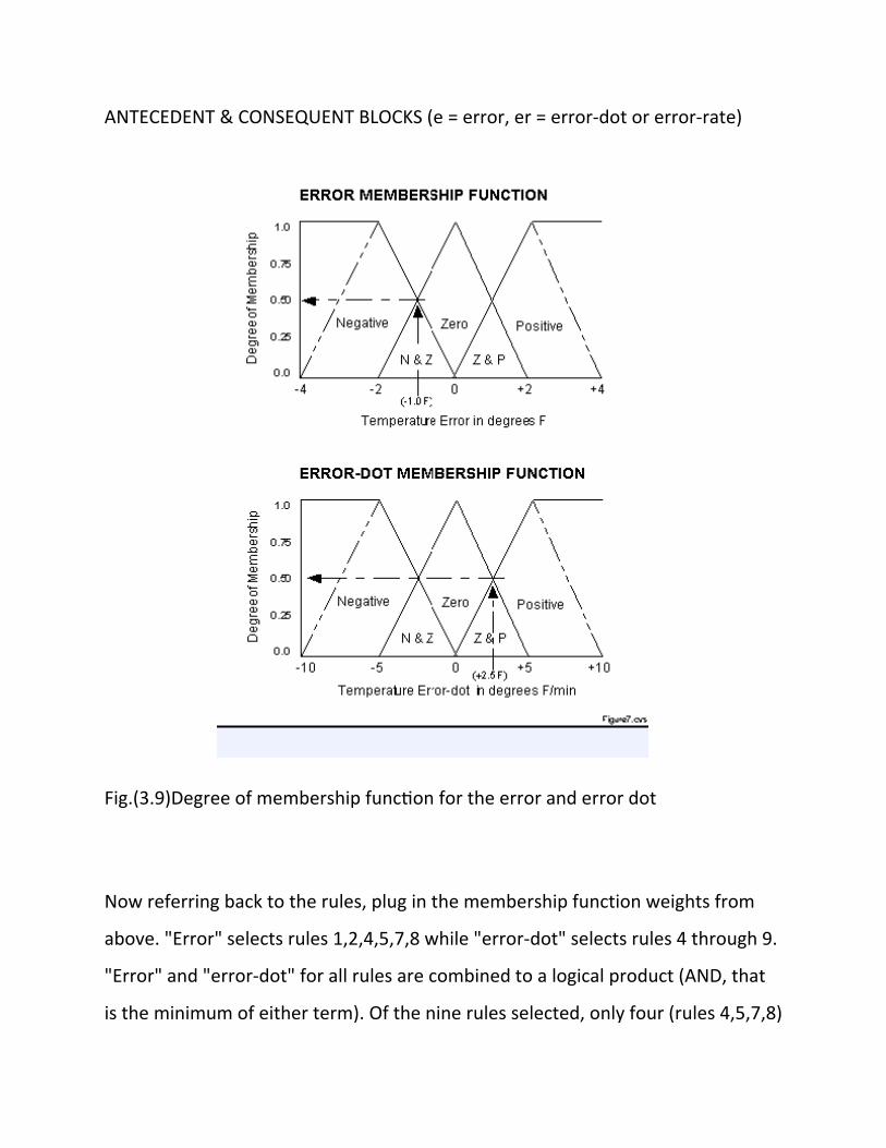
ANTECEDENT & CONSEQUENT BLOCKS (e = error, er = error‐dot or error‐rate)  

                          

Fig.(3.9)Degree of membership function for the error and error dot  

 

Now referring back to the rules, plug in the membership function weights from 

above. "Error" selects rules 1,2,4,5,7,8 while "error‐dot" selects rules 4 through 9. 

"Error" and "error‐dot" for all rules are combined to a logical product (AND, that 

is the minimum of either term). Of the nine rules selected, only four (rules 4,5,7,8) 

 

 

fire or have non‐zero results. This leaves fuzzy output response magnitudes for 

only "Cooling" and "No_Change" which must be inferred, combined, and 

defuzzified to return the actual crisp output. In the rule list below, the following 

definitions apply: (e)=error, (er)=error‐dot. 

R1. If (e < 0) AND (er < 0) then Cool 0.5 & 0.0 = 0.0  

R2. If (e = 0) AND (er < 0) then Heat 0.5 & 0.0 = 0.0  

R3. If (e > 0) AND (er < 0) then Heat 0.0 & 0.0 = 0.0  

R4. If (e < 0) AND (er = 0) then Cool 0.5 & 0.5 = 0.5  

R5. If (e = 0) AND (er = 0) then No_Chng 0.5 & 0.5 = 0.5  

R6. If (e > 0) AND (er = 0) then Heat 0.0 & 0.5 = 0.0  

R7. If (e < 0) AND (er > 0) then Cool 0.5 & 0.5 = 0.5  

R8. If (e = 0) AND (er > 0) then Cool 0.5 & 0.5 = 0.5  

R9. If (e > 0) AND (er > 0) then Heat 0.0 & 0.5 = 0.0  

 

‐The Root Sum Squire method was chosen to include all contributing rules since 

there are so few member functions associated with the inputs and outputs. For 

the ongoing example, an error of ‐1.0 and an error‐dot of +2.5 selects regions of 

the "negative" and "zero" output membership functions. The respective output 

membership function strengths (range: 0‐1) from the possible rules (R1‐R9) are: 

 

 

"negative" = (R1^2 + R4^2 + R7^2 + R8^2) (Cooling) = (0.00^2 + 0.50^2 + 0.50^2 + 

0.50^2)^.5 = 0.866  

"zero" = (R5^2)^.5 = (0.50^2)^.5 (No Change) = 0.500  

"positive" = (R2^2 + R3^2 + R6^2 + R9^2) (Heating) = (0.00^2 + 0.00^2 + 0.00^2 + 

0.00^2)^.5 = 0.000  

 

‐The defuzzification of the data into a crisp output is accomplished by combining 

the results of the inference process and then computing the "fuzzy centroid" of 

the area. 

 

 

(neg_center * neg_strength + zero_center * zero_strength + pos_center * pos_strength) =  

(neg_strength + zero_strength + pos_strength)  

output 

   

(‐100 * 0.866 + 0 * 0.500 + 100 * 0.000) = 63.4%  

(0.866 + 0.500 + 0.000)  

  

 

 

 

                                 

      Fig.(3.10)The horizontal coordinate  of the centroid is taken as the crisp output 

 

 

 

 

 

 

 

 

 

 

 

 

 

 

 

 

 

Chapter 4 

Power system model 

 4.1  Introduction  

         In  this  chapter we will  study  the  small  signal  performance  of  a  single 

machine connected to a large system through transmission lines [1]. A general 

system  configuration  is  shown  in  Fig.  4.1.aAnalysis  of  system  having  such 

simple  configurations  is extremely useful  in understanding basic effects and 

concepts. 

        First we analyze a generator by the classical model and then present the 

model gradually by accounting the effects of the dynamics of field circuit and 

excitation  system.  Additionally,  we  present  the  basic  function  of  power 

system stabilizer and its components. 

               

 

 

 

 

 

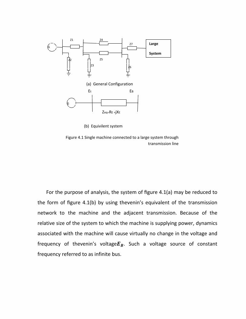
      For the purpose of analysis, the system of figure 4.1(a) may be reduced to 

the  form of figure 4.1(b) by using  thevenin’s equivalent of  the  transmission 

network  to  the  machine  and  the  adjacent  transmission.  Because  of  the 

relative size of the system to which the machine is supplying power, dynamics 

associated with the machine will cause virtually no change in the voltage and 

frequency  of  thevenin’s  voltage .  Such  a  voltage  source  of  constant 

frequency referred to as infinite bus. 

Large   

System

Z1 

Z2 

Z3  Z6

Z7Z4

Z5

G 

(a)  General Configuration 

Et  EB 

Zeq=RE +jXE 

(b)  Equivilent system 

Figure 4.1 Single machine connected to a large system through transmission line 

G 

 

 

   In  this  representation,  the  dynamic  characteristics  of  the  system  are 

expressed  in  terms  of  so‐called  k  constants  defined  in  appendix  A,  which 

depend on system parameters. 

 

 

4.1.1 Generator Represented by the Classical Model 

 

    The  generator  is  represented  by  the  classical model  and  all  resistances 

neglected, the system representation is shown in figure 4.2. 

       Here  E   is  the  voltage  behind  X .its magnitude  is  assumed  to  remain 

constant at pre‐disturbance value. Let δ be  the angle by which E   leads  the 

infinite bus voltageE . As the rotor oscillates during a disturbance, δ changes. 

    With  E   is as reference phasor, 

 

 

 

 

        

… … … … … … … … … … … … 4.1  

 

The complex power behind  X  is given by 

 

         , … . 4.2  

 

With  the  stator  resistance neglected,  the  air‐gap power  (P )  is equal  to  the 

terminal  power  (P).  in  per  unit,  the  air‐gap  torque  is  equal  to  the  air  gap 

power.  

Hence, 

                           … … … … … … … … … … . 4.3  

  

  

  

Figure 4‐2

 

 

 

Linearizing about an initial operating condition represented by δ δ  yields  

 

                        Δ Δ   cos Δ … … … … … … . 4.4      

 

The equation of motion in per unit is [1] 

 

                         Δω T T K Δω … … … … … … 4.5  

                          

                        δ ω Δω ……………………………………(4.6) 

 

 Where Δω is the per unit speed deviation, δ is rotor angle in electrical radian, ω  

is  the base rotor electrical speed  in  radians per second, and P  is  the differential 

operator       with the t in seconds. 

 

Linearizing equation 4.5 and substituting for  Δ  given by equation 4.4 we obtain  

                           

                         Δω T K Δ K Δω …………..(4.7) 

 

 

 

Where K  is the synchronizing torque coefficient given by   

                                K cos … … … … … … … … … … … 4.8    

  

Linearizing equation 4.6 , we have 

                            

                                 Δδ ω Δω … … … … … … … … … … … … 4.9  

 

Writing Equations 4.8 and 4.9 in the vector matrix form, we obtain 

ΔωΔδ 2 2

ω 0

ΔωΔδ Δ … … … … … … … . 4.10  

 This is of form  . The elements of the state matrix A are seen to be dependent on the system parameters  ,H, X  and the initial operating condition represented by the values of   and  . The block diagram representation shown in Figure4.3 can be used to describe the small signal stability performance. 

 

 

 

 

 

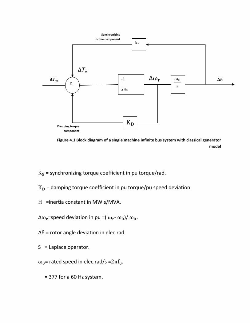
K  = synchronizing torque coefficient in pu torque/rad. 

K  = damping torque coefficient in pu torque/pu speed deviation. 

H   =inertia constant in MW.s/MVA. 

Δω =speed deviation in pu =( ω ‐ ω )/ ω . 

Δδ = rotor angle deviation in elec.rad. 

S   = Laplace operator. 

ω = rated speed in elec.rad/s =2πf . 

     = 377 for a 60 Hz system. 

Figure 4.3 Block diagram of a single machine infinite bus system with classical generator model 

ks

‐1    

2Hs   

K  

  ∑     

Δ   

Δω  

Damping torque component 

Synchronizing torque component 

 

 

 

4.1.2Block diagram of the system including Field circuit 

 

   Figure  4.4  presents  the  block  diagram  of  the  system  representing  the 

synchronous machine and accounting the dynamic effects of the field circuit. 

   

  From figure above we may express the change in air‐gap torque as a

function of rotor angle ∆δ and field flux variation ∆ψ as follows: 

 

                    ∆ ∆ ∆ … … … … … … … … … . 4.11   

Where

Figure 4.3 Block diagram representation with constant   

Δ

K

  

K

  ∑

ΔΔδΔω  

   K∑    ∑∆   

Field  circuit 

∆ 0  

 

 

 K ∆∆

with constant ∆ψ  

 

        K ∆

∆ with constant rotor angle δ 

 

                The component for and are given by K ∆δ is in phase with ∆δ and

hence represents a synchronizing torque component.

The component of torque resulting from variations in field flux linkage

is given by K ∆ψ . 

 

          The variation of ∆ψ is determined by the field circuit dynamic

equation: 

              

                  ∆ ∆ ∆ … … … … … … … … 4.12

 

Effect of field flux linkage variation on system stability

 

 

With constant field voltage ∆E 0 , the ield lux variations are caused

only by feedback of ∆ through coefficient . This represents the

demagnetizing effect of armature reaction. The change in air‐gap torque

due field flux variations caused by rotor angle change is given by

∆∆

Ι ∆ … … … … … … … … … 4.13

         

The constants , , are usually positive. The contribution of

∆ψ to synchronizing and damping torque components depends on the

oscillating frequency. 

 

 

4.1.3Block diagram  of the system including Excita on system 

 

Figure 4.5 shows the block diagram obtained by extending igure 4.4 to

include the voltage transducer and AVR/Exciter blocks. 

 

 

 

 

 

The representation is applicable to any type of exciter, with G s

representing the transfer function of the AVR and exciter. For a thyristor

exciter,

G s K … … … … … … … … … … … . . 4.14

Figure 4.5 Block diagram representation with exciter and AVR 

  

  

 ∑Δω  

  ∑   ∆

K∆

Field  circuit

  

 

Exciter 

Voltage  transducer 

∑

∑   ∆     

 

 

The terminal voltage error signal, which forms the input to the voltage

transducer block, is given by equation 4.15

∆E K ∆δ K ∆ψ … … … … … … … … 4.15

The coefficient K is always positive, whereas K can be either positive or

negative, depending on the operating condition and external network

impedance . The value of K has a significant bearing on the

influence of the AVR on the damping of the system oscillations.

Effect of AVR on synchronizing and damping torque component

With automatic voltage regulator action, the field flux variations are

cause by the field voltage variations, in addition to armature reaction.

From diagram of figure 4.5 we see that

∆ ∆δ ∆δ ∆ … … . 4.16

By grouping terms involving ∆ and rearranging,

∆

∆δ … … … … … … … . 4.17

 

 

The range in air‐gap torque due to change in field flux linkage is

∆ ∆

As noted before, the constants , , are usually positive;

however, may take either positive or negative values. The effect of the

AVR on damping and synchronizing torque components is therefore

primarily influenced by and G s .

For high values of external system reactance and high generator out

put K is negative . In practice, the situation where K is negative are

commonly encountered. For such cases, a high response exciter is

beneficial in increasing synchronizing torque. However, in so doing it

introduces negative damping. we thus have conflicting requirements with

regard to exciter response. One possible recourse is to strike a

compromise and set the exciter response so that it results in sufficient

synchronizing and damping components for the expected range of system

operating conditions. This may not always be possible. It may necessary to

use a high response exciter to provide the required synchronizing torque

and transient stability performance. With a very high external system

reactance, even with low exciter response the net damping torque

coefficient may be negative.

 

 

An effective way to meet the conflicting exciter performance

requirements with regard to system stability is to provide a power system

stabilizer.

 

4.1.4 Power system stabilizer 

 

The basic function of a power system stabilizer PSS is to add

damping to the generator rotor oscillations by controlling its excitation

using auxiliary stabilizing signal. To provide damping, the stabilizer must

produce a component of electrical torque in phase with the rotor speed

deviations.

The theoretical basis for a PSS may be illustrated with the aid of the

block diagram of igure 4.6. This is an extension of block diagram of igure

4.5 and includes the effect of a PSS.

Since the purpose of a PSS is to introduce a damping torque

component, a logical signal to use for controlling generator excitation is

the speed deviation ∆ω .

 

 

If the exciter transfer function G s and the generator transfer

function between ∆E and ∆T were pure gains, a direct feedback of ∆ω

would result in a damping torque component. However, in practice both

the generator and the exciter depending on its type exhibit frequency

dependent gain and phase characteristics. Therefore, the PSS transfer

function, G s , should have appropriate phase compensation circuits to

compensate for the phase lag between the exciter input and the electrical

torque. In ideal case, with the phase characteristic of G s being an

exact inverse of the exciter and generator phase characteristics to be

compensated, the PSS would result in a pure damping torque at all

oscillating frequencies.

Figure 4.6 Block diagram representation with exciter and AVR

  

  

  ∑Δω

  ∑    ∑∆

K∆

Field  circuit

  

 

Exciter 

Voltage  transducer 

∑

∑   ∆   

 

 

The PSS representation in igure 4.7 consists of three blocks: a phase

compensation block, a signal washout block, and a gain block.

The phase compensation block provides the appreciate phase –lead

characteristic to compensate for the phase lag between the exciter input

and the generator electrical air‐gap torque. The figure shows a single

first‐order block. In practice, two or more first‐order block may be used to

achieve the desired compensation. In some cases, second‐order blocks

with complex roots have been used.

  

Phase compensation Wash out Gain 

Figure 4.7 Power System Stabilizer

  Δω      

 

 

Stabilizing Signal Washout block serve as high pass filter with the time

constant T high enough to allow signals associated with oscillations in

ω to pass unchanged. Without it, steady change in speed would modify

the terminal voltage. It allows the PSS to respond to the changes in speed.

From the viewpoint of washout function, the value of T is not critical and

may be in the range of 1 to 20 seconds. The main consideration is that it be

long enough to pass stabilizing signals at the frequencies of interest

unchanged.

The stabilizer gain K determines the amount of damping introduced by

the PSS. Ideally, the gain should be set at a value corresponding to

maximum damping; however, it is often limited by other considerations.

 

 

 

 

 

 

 

 

 

 

 

 

 

Chapter5

PD‐like fuzzy controller

 

5.1 Fuzzy controllers as a part of a feedback system 

It is not easy to design an exact PD controller, but one can construct a PD‐

like  fuzzy controller. To do  it we need  to choose  the  input and output variables 

and the rules of the controller properly.  If one has made a choice of designing a  

PD      like  fuzzy  controller,  this  already  implies  the  choice  of  process  state  and 

control output variables, as well as  the  content of  the  rule‐antecedent and  the 

rule‐consequent parts for each rule. The process state variables representing the 

contents of the rule‐antecedent (if‐part of a rule) are selected among[20]: 

 

● error signal, denoted by e; 

● change‐of‐error, denoted by  e; 

 

 

The  control output  (process  input) variables  representing  the  contents of 

the rule‐consequent (then‐part of the rule) are selected among: 

 

� change‐of‐control output, denoted by  u; 

 

 

� control output, denoted by u. 

 

      The error is the difference between the desired output of the object or 

process under control or  the set‐point and  the actual output. This  is one of  the 

basic milestones  in conventional feedback control. Furthermore, by analogy with 

a conventional controller, we have: 

 

� e(t) =   – y(t); 

�  e (t) = e(t) – e(t – 1); 

�  u (t) = u(t) – u(t – 1). 

In the above expressions, y  stands for the desired process output or the 

set‐point,  y  is  the  process  output  variable  (control  variable);  k  determines  the 

current time. 

      

     The deviation  can be  considered as an error and  the  turn as a  control 

output.  Then  this  table  represents  a  choice  of  the  control  output  roughly 

proportional to the error. It means that we have designed a P‐like controller. 

 

5.2 PD‐like fuzzy controller 

 

 

 

      The equation giving a conventional PD‐controller is 

 

u(k) =K .e(t) +K .� e(t)……………………….(5.1) 

 

where K  and K  are the proportional and the differential gain factors. 

        Let us consider  the above equation. The PD controller  for any pair of 

the values of error (e) and change‐of‐error ( e) calculates the control signal (u). 

The fuzzy controller should do the same thing. For any pair of error and change‐

of‐error,  it  should work  out  the  control  signal.  Then  a  PD‐like  fuzzy  controller 

consists of rules, and a symbolic description of each rule is given as 

 

 

Change of error 

+ 

‐ 

Fig. 5.1 A block diagram of a PD‐like fuzzy controller

 

 

if  e(t)  is  <property  symbol>  and  e(t)  is  <property  symbol>  then  u(t)  is 

<property symbol>, where <property symbol> is the symbolic name of a linguistic 

value. 

 

The natural language equivalent of the above symbolic description reads as 

follows. For each sampling time t: 

 

if  the value of error is <linguistic value> and the value of change of‐error is 

<linguistic value> then the value of control output is <linguistic value>. 

 

      We will omit the explicit reference to sampling time t, since such a rule 

expresses  a  casual  relationship  between  the  process  state  and  control  output 

variables, which holds for any sampling time t. 

 So the rules of the PD controller can be like: 

if error is Positive Big and change‐of‐error is Negative Big then control is 

Negative Small 

 

5.2.1 Positive and negative values 

 

 

 

  We need to describe an error signal. Because the actual process output y 

can be higher than the desired one as well as lower, the error can be negative as 

well as positive. Values of error (e) with a Negative  sign mean that the current 

process output y(t) has a value above the set‐point   since e(t) =   – y(t) > 0. 

A positve value describes the magnitude of the difference y  – y. On the other 

hand, linguistic values of e with a Positive  sign mean that the current value of y is 

below  the set‐point. The magnitude of such a positve value is the magnitude of 

the difference   – y.     

The change‐of‐error ( e) with a negative sign means that the current 

process output y (t) has increased when compared with its previous value y(t–1), 

since  e(t) = e(t) – e(t – 1) = –y(t) + y(t –1) < 0. The magnitude of this negative 

value is given by the magnitude of this increase. Linguistic values of  e(t) with a 

positive sign mean that y(t) has decreased its value when compared to y(t – 1). 

The magnitude of this value is the magnitude of the decrease.  

Linguistic values of e with a negative sign mean that the current process 

output y has a value above the set‐point   since e(t) =   – y(t) < 0. The 

magnitude of a negative value describes the magnitude of the difference   – y. 

On the other hand, linguistic values of e with a positive sign mean that the current 

value of y is below the set‐point. The magnitude of such a positive value is the 

magnitude of the difference   – y. 

       Linguistic  values  of  e  with  a  negative  sign  mean  that  the  current 

process output y(t) has increased when compared with its previous value y(t – 1) 

 

 

since  e(t) = – y(t) + y(t – 1) < 0. The magnitude of such a negative value is given 

by  the magnitude of  this  increase. Linguistic values of  e(t) with a positive sign 

mean 

That  y  (t)  has  decreased  its  value  when  compared  to  y(t  –  1).  The 

magnitude of such a value is the magnitude of the decrease. 

        A linguistic value of ‘zero’ for e means that the current process output 

is about the set‐point. A ‘zero’ for  e means that the current process output has 

not changed significantly from its previous value, i.e. – (y(t) – y(t – 1)) = 0. The sign 

and the magnitude for u constitute the value of the control signal. 

 

5.3 Rules table nota on 

 

  A convenient form to write down rules when we have two inputs and one 

output  is  table  (5.1). On  the  top  side of  the  table we  should write  the possible 

linguistic values  for  the change‐of‐error  ( e) and on  the  left  side,  the error  (e). 

The cell of the table at the intersection of the row and the column will contain the 

linguistic value for the output corresponding to the value of the first input written 

at the beginning of  the row and to the value of the second input written on the 

top of the column. 

         Let  us  consider  both  inputs  and  an  output  have  a  set  of  possible 

linguistic values {NB, NM, NS,Z, PS, PM, PB} where NB stands for Negative Big, NM 

stands for Negative Medium, NS stands for Negative Small, Z stands for Zero, PS 

 

 

stands  for  Positive  Small,  PM  stands  for  Positive  Medium  and  PB  stands  for 

Positive Big (Table 5.1). 

 

Table(5.1)

e ∆e 

PB  PM  PS  Z NS NM NB

PB  NB  NB  NB  NB NM NS ZPM  NB  NB  NB  NM NS Z PMPS  NB  NB  NM  NS Z PS PBZ  NB  NM  NS  Z PS PM PBNS  NM  NS  Z  PS PM PB PBNM  NS  Z  PS  PM PB PB PBNB  Z  PS  PM  PB PB PB PB

 

         

 The cell defined by  the  intersection of  the  first  row and  the  first column 

represents a rule such as: 

if e(t) is NB and  e(t) is NB then u(t) is NB 

 

This  table  includes 49  rules. We are  taking  into account now not  just  the 

error but  the change‐of‐error as well.  It allows  to describe  the dynamics of  the 

controller. To explain how this rules set works and how to choose the rules, let us 

divide the set of all rules into the following five groups: 

  GR0

  GR1

  GR2

  GR3

  GR4

 

 

Group  0:  In  this  group  of  rules  both  e  and  e  are  (positive  or  negative) 

small or zero. This means that the current value of the process output variable y 

has deviated from the desired level (the set‐point) but  is still close to it. Because 

of  this closeness  the control  signal  should be  zero or  small  in magnitude and  is 

intended  to  correct  small deviations  from  the  set‐point. Therefore,  the  rules  in 

this group are related to the steady‐state behavior of the process. The change‐of‐

error, when it is Negative Small or Positive Small, shifts the output to negative or 

positive  region, because  in  this case,  for example, when e(t) and  e(t) are both 

Negative Small the error  is already negative and, due to the negative change‐of‐

error,  tends  to  become  more  negative.  To  prevent  this  trend,  one  needs  to 

increase the magnitude of the control output. 

      Group  1:  For  this  group of  rules  e(t)  is  Positive Big or Medium which 

implies that y(t) is significantly below  the set‐point. At the same time since  e(t) 

is negative, this means that y is moving towards the set‐point. The control signal is 

intended  to  either  speed  up  or  slow  down  the  approach  to  the  set‐point.  For 

example,  if y(t)  is much below the set‐point (e(t)  is Positive Big) and  it  is moving 

towards  the  set‐point  with  a  small  step  ( e(t)  is  Negative  Small)  then  the 

magnitude of this step has to be significantly increased (u(t) is Negative Medium). 

However, when y(t) is still much below the set‐point (e(t) is Positive Big) but it is 

moving  towards  the set‐point very  fast  ( e(t)  is Negative Big) no control action 

can be recommended because the error will be compensated due to the current 

trend. 

 

 

       Group 2: For this group of rules y(t) is either close to the set‐point (e(t) 

is Positive Small, Zero, Negative Small) or significantly above it (Negative Medium, 

Negative Big). At the same time, since  e(t) is negative, y(t) is moving away from 

the  set‐point. The control here  is  intended  to  reverse  this  trend and make y(t), 

instead of moving away from the set‐point, start moving towards  it. So here the 

main  reason  for  the  control  action  choice  is  not  just  the  current  error but  the 

trend in its change. 

       Group 3: For this group of rules e(t)  is Negative Medium or Big, which 

means that y(t) is significantly above the set‐point. At the same time, since  e(t) 

is positive, y(t) is moving towards the set‐point. The control is intended to either 

speed up or slow down the approach to the set‐point. For example, if y(t) is much 

above  the set‐point  (e(t)  is Negative Big) and  it  is moving  towards  the set‐point 

with a  somewhat  large  step  ( e(t)  is Positive Medium),  then  the magnitude of 

this step has to be only slightly enlarged (u(t) is Negative Small) 

       Group 4: The situation here is similar to the Group 2 in some sense. For 

this  group  of  rules  e(t)  is  either  close  to  the  set‐point(Positive  Small,  Zero, 

Negative  Small) or  significantly below  it  (Positive Medium,  Positive Big). At  the 

same  time  since  e(t)  is  positive  y(t)  is moving  away  from  the  set‐point.  This 

control signal  is  intended  to  reverse  this  trend and make y(t)  instead of moving 

away from the set‐point start moving towards it. 

 

 

 

 

 

 

Chapter6 

Simulation and results 

 

 6‐1 FPSS for single machine infinite bus 

 Figure 6.1  shows a  schematic diagram of  the  test  system with CPSS and FLPSS. 

Since  the  goal  of  this  application  is  to  stabilize  and  improve  the  damping  of 

synchronous  machine  rotor  speed  deviation  and  acceleration  of  rotor  speed 

deviation (∆ω,∆ώ) have been selected as controller inputs. The controller output 

is then injected into AVR summing point. 

 

 

 

 

             We  use  the  system  model  presented  in  chapter  4  Fig.4  the  model 

parameters are shown in appendix B. The conventional power system stabilizer is 

designed  using  a  linearized  model  [1].  Therefore,  this  provides  optimum 

performance for a nominal operating condition and fixed system parameters. the 

CPSS parameters are shown in appendix C. 

         Designing  of  FPSS  using  matlab  toolbox  constitutes  construction  of  the 

following: 

 

1. The input membership functions. 

2. The output membership functions. 

3. The decision table. 

4. Deffuzification strategy. 

 

 

 

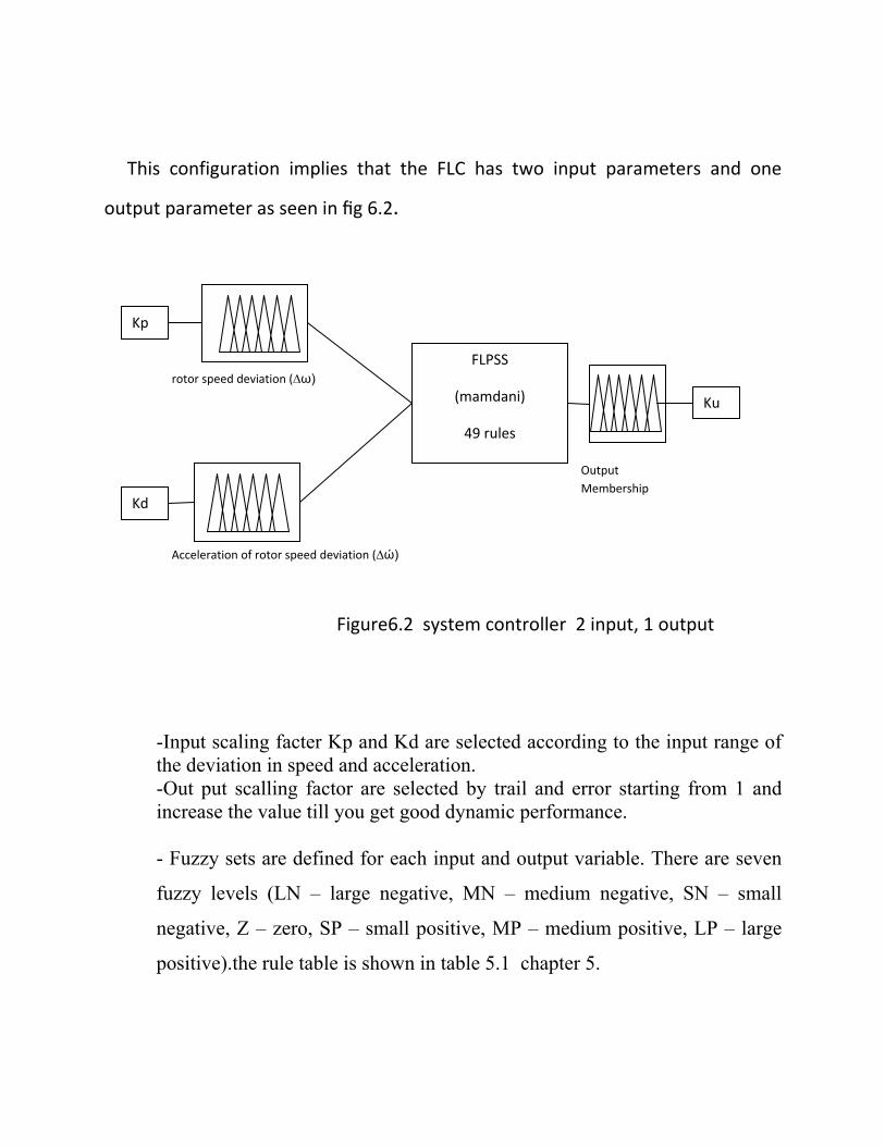
     This  configuration  implies  that  the  FLC  has  two  input  parameters  and  one 

output parameter as seen in fig 6.2.  

 

 

-Input scaling facter Kp and Kd are selected according to the input range of the deviation in speed and acceleration. -Out put scalling factor are selected by trail and error starting from 1 and increase the value till you get good dynamic performance. - Fuzzy sets are defined for each input and output variable. There are seven

fuzzy levels (LN – large negative, MN – medium negative, SN – small

negative, Z – zero, SP – small positive, MP – medium positive, LP – large

positive).the rule table is shown in table 5.1 chapter 5.

Figure6.2  system controller  2 input, 1 output

rotor speed deviation (∆ω) 

Acceleration of rotor speed deviation (∆ώ) 

FLPSS 

(mamdani) 

49 rules 

 

 

 Output Membership 

Kp 

Kd 

Ku 

 

 

‐  The membership functions for input and output variable are triangular and

used the normalized universe [-1, 1]. As shown in figure (6.3).

 

     Using Fuzzy Logic Toolbox and Simulink drawing diagram shown in

figure 6.3. The parameters of FLPSS structure is choose fuzzy mamdani

type, AndMethod using ‘min’, OrMethod using ‘max’, ImpMethod using

‘min’, AggMethod using ‘max’,and DeffuzzMethod using ‘centroid’.

-we select the input scaling factors by trail and error increasing Kp and

degreasing Kd will degrese the rise time and increasing Ku will increase the

controller gain and damp system oscillation. 

 

 

Figure (6, 3) Normalized membership func ons for 2 inputs and 1 output.

0‐1  1 

NB  ZNM  NS  PS  PM  PB 

 

 

6‐2 Simula on Results          The model of the system shown in Fig 6.1 is tested for step response with no

feedback control and give oscillatory response with time as shown in Fig.6.4.

Fig 6.5 ---Fig.6.7 give a comparison results of the system response with CPSS and

with FLPSS and demonstrate how the response is improved when we increased the

output scaling factor showing that a good performance for FLPSS than

conventional control in terms of over shoot and settling time. 

 

                       

Figure 6.4 System response without PSS 

 

 

 

          Figure 6.5 Deviation in speed  

 a)with CPSS.            b)with FLPSS for Ku=1 

           

 

 

Figure 6.6 Deviation in speed 

 a)with CPSS.                   b)with FLPSS for Ku=16. 

 

 

 

 

 

 

 

Figure 6.7 Deviation in speed 

 a)with CPSS.                   b)with FLPSS for Ku=16. 

 

 6‐3 Conclusion 

The thesis presents fuzzy  logic based PSS design for oscillation damping.  It 

systematically  explains  the  steps  involved  in  fuzzy  logic  control  design  for 

oscillation damping for single machine infinite bus.  

            A  comparison  between  the  FLPSS  and  the  CPSS  shows  that  the  FLPSS 

provides  better  performance  than  CPSS.  The  results  show  that  the  proposed 

FLPSS provides good damping and improves the dynamics. 

            Unlike the classical design approach which requires a deep understanding 

of the system, exact mathematical models, and precise numerical values, a basic 

feature of the fuzzy logic controller is that the process can be controlled without 

the knowledge of  its underlying dynamics. The control strategy  learned  through 

experience  can  be  expressed  by  set  of  rules  that  describe  the  behavior  of  the 

controller  using  linguistic  terms.  Thus,  fuzzy  logic  controllers  are  suitable  for 

 

 

nonlinear, dynamic processes for which an exact mathematical model may not be 

available. 

             Using  the  principle  of  fuzzy  logic  control,  a  PSS  has  been  designed  to 

enhance  the  operation  and  stability  of  single machine  infinite  bus  .  Results  of 

simulation studies look promising. 

 

 

 

 

Further Research 

   In  the  following,  some  recommendations are  given  for  future  research  in  the area 

 

1. The fuzzy logic controller developed in this work, should also be implemented in the laboratory to evaluate its real time performance.

2. In this study, only min-max technique of fuzzy logic was used, max-dot technique can also be tried to see if it can help to improve the results.

3. Different defuzzification technique can be tried to find out which is most suitable to the power system applications.

4. Shapes other triangular functions such as bell shapes, etc... Can also be tried to find out which function suits speed and acceleration of machines.

5. Fuzzy logic controller can be tried for multi machine system. 6. Fuzzy logic controller can also be used for other dynamic security

assessment technique such as a) Dynamic breaking. b) Static var compensators. c) HVDC links.

 

 

 

References: 

[1]   Kundur.” Power System Stability and Control”. McGraw Hill, New York, Ch.12. pp.817‐822. (1994) 

[2]FRANCISCO P. DEMELLO, senior member,IEEE, and CHARLES CONCORDIA, FELLOW,IEEE 

“Concept of Synchronous Machine Stability as Affected by Excitation Control”. 

  [3]   F.P.De Mello and Charles Concordia, “Concepts of synchronous machine stability as effected by  

[4] Y.Y.Hsu & C.Y.Hsu. “Design of a propotional‐integral power system stabilizer, “IEEE Trans. On Power apparatus and systems, 

vol. 1,May 1986,pp.46‐53. 

[5] C.L.Chen & Y.Y.Hsu. “Coordinated synthesis of multi‐machine power systm stabilizer using an efficient decentralized modal 

control (DMC) algorithm.”IEEE Trans. On power Apparatus and systems, vol. 2 ,August 1987, pp.543‐551. 

[6]  “Tuning  of  stabilizer  in multimachine  power  systems”  IEEE  Trans.  On  power  apparatus  and  systems,  vol.  102,  no.5, 

1986,pp.290‐299. 

 [7]  J.A.Month &  K.Tomsov,  “Overview  and  literature  survey  of  fuzzy  set  theory  in  power  systems,”IEEE  Trans. On  power 

systems, vol.10 no.3 August 1995, pp.1676‐1690. 

 [8] Z.J.Hu, “power system planning with programming,”1993 Expert system application to power systems, Melbourne, January 

1993 1993, pp.107‐1111. 

 [9]  A.V.Machias,  J.L.Souflis  &  E.N.Dialynas,  “A  fuzzy  transient  Index  in  power  system  security  evalution,”  IEEE  Trans.  On 

Automatic Control, vol.34, no.6,june 1989,pp. 662‐666. 

[10]  G.L.Torres,  etal,  “A  fuzzy  Knowledge  base  for  load  forecasting,”1991  Expert  system  applications  to  power 

systems.Tokyo/kobe,April 1991, pp.439‐446. 

 [11]  H.E.D.Dijk,  “Exformer:  An  expert  system  stabilizer  for  transformer  fault  diagnosis,”  Proc.  Of  9th  power  system 

computation conference, Lisbon, September 1987, pp.715‐721. 

 [12] Takashi Hiyama, M.Mishiro, H.Kihara,“Coordinated  fuzzy  logic control  for series capacitor modules and PSS to enhance 

stability of power stability of power system,”IEEE Trans. On power system Delivery, vol.10, no.2, Sep. 1995, pp.1098‐

1104. 

[13] P.K.Dash, A.Routary, S.Rahman, “An adaptive fuzzy logic controller for AC‐DC power systems, ”Proc. Of 2nd Int. forum on 

applications of neural network to power systems.ANNPS, pp.218‐223. 

 

 

[14] T.Hiyama &C.M.Lim, “Application of fuzzy logic control scheme for stability enhancement of a power system,” IFAC power 

systems and power plant control, Seoul, Korea,1989,pp.313‐316. 

[15] M.A.M.Hassan, O.PMalik,   G.S.Hope, “A Fuzzy  logic based stabilizer for a synchronous machine, ”  IEEE Trans. On Energy 

Conversion, vol.6,no.3,Dec.1991,pp.407‐413. 

 

[16] Y.Y.Hsu, C.H.Cheng, “Design of fuzzy system stabilizers for multi machine power systems,”IEE Proc. Vol.137, Pt. C, no.3, 

May 1990, pp233‐238. 

 [17] A.M.Sharaf,T.T.Lie,  “Ahybrid nero‐fuzzy power  system  stabilizer,” proc. Of 3rd    IEEE Conf. on  fuzzy  systems,  July 1994, 

pp.1608‐1613. 

[18] Yashihiro Kitauchar & Haruhito Taniguchi,  “Development of  fuzzy excitation  control  system,  ”Electrical Engg.  in  Japan, 

vol.114, no.3, 1994,pp.47‐57. 

 [19] A.Hiriri, O.P.Malik, “Adaptive network based Fuzzy logic power system stabilizer,”IEEE WESCANEX Proceedings 95, pp.11 

1‐1 16. 

[20] LEDNID REZNIK,”fuzzy controller”,Victoria University, Australia,puplished 1997. 

 

 

 

 

 

 

 

 

 

 

 

 

 

 

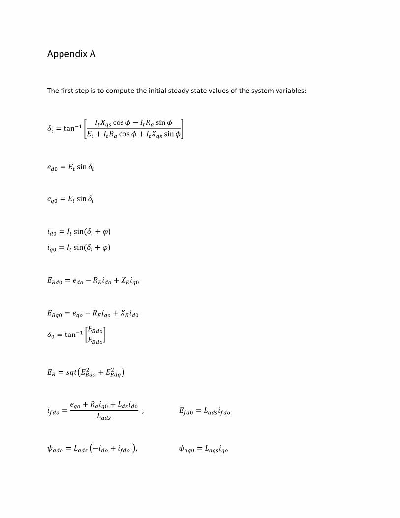
Appendix A 

 

The first step is to compute the initial steady state values of the system variables: 

 

tancos sin

cos sin  

 

sin  

 

sin  

 

sin ) 

sin ) 

 

 

 

 

tan  

 

 

 

,  

 

,  

 

 

 

 

 

         

 

∆ ∆ ∆  

 

∆∆

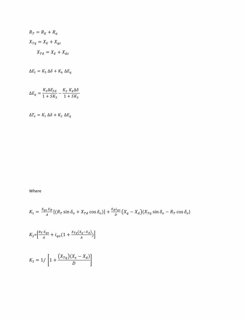
1 ∆

1 

 

∆ ∆ ∆  

 

 

 

 

 

 

 

Where 

 

sin cos sin cos ) 

 

= 1  

 

1/ 1  

 

 

 

/ 1  

 

sin cos ) 

 

sin E cos cos E sin 

1  

 

+  

 

 

 

, , . 

, , . 

. 

. 

. 

. 

. 

. 

. 

 

Subscript 0 means steady state value. 

Prefix ∆ indicate small change. 

 

 

 

APPENDEX B :    

System parameters 

. , . , 36, . 0, . , / .  

, . , . , , . 

K‐constants 

.  

.  

.  

.  

.  

.  

. s 

 

 

 

APPENDEX C :  PSS Parameters  

 

 

.  

.  

9.5s