
Infrastructure Demand Quantitative Analysis for Scenarios ...

California Water Plan Update 2018 Supporting Document
Future Scenarios of Water Supply and Demand in Central Valley, California
through 2100
Impacts of Climate Change and Urban Growth
June 2019
CALIFORNIA DEPARTMENT OF WATER RESOURCES
Division of Statewide Integrated Water Management
Kamyar Guivetchi, Division Chief
Integrated Data and Analysis Branch
Chris McCready, Branch Chief
Water Budgets and Analysis Section
Abdul Khan, Section Chief
This report was prepared by:
Mohammad Rayej, Senior Water Resources Engineer
With assistance from:
Salma Kibrya, Research Program Specialist II (Demography)
Paul Shipman, Water Resources Engineer
Matthew Correa, Senior Water Resources Engineer

Contents
i
Contents
Acronyms and Abbreviations Page xv
Executive Summary Page ES-1
1. Introduction Page 1
2. Development of Future Scenarios Page 3
2.1 Planning Horizon Page 3
2.2 Scenario Factors Page 3
2.2.1 Climate Change Page 3
2.2.2 Urban Growth Page 5
3. Analytical Tool: Central Valley Planning Area Model Page 9
3.1 WEAP-CVPA Model Description Page 9
3.2 Model Calibration-Validation Page 11
3.3 Model Geographic Coverage Page 11
3.3.1 Sacramento River HR Planning Areas Page 11
3.3.2 San Joaquin River HR Planning Areas Page 12
3.3.3 Tulare Lake HR Planning Areas Page 13
4. WEAP-CVPA Model Results: Future Water Conditions Page 15
4.1 Sacramento River Hydrologic Region Page 15
4.1.1 Agriculture Page 15
4.1.2 Urban Indoor Page 25
4.1.3 Urban Outdoor Page 29
4.1.4 Future Water Shortages: Vulnerability Analysis- Vulnerabilities and Likelihoods Page 35
4.2 San Joaquin River Hydrologic Region Page 41
4.2.1 Agriculture Page 41
4.2.2 Urban Indoor Page 49
4.2.3 Urban Outdoor Page 53
4.2.4 Future Water Shortages: Vulnerability Analysis- Vulnerabilities and Likelihoods Page 58
4.3 Tulare Lake Hydrologic Region Page 66

Future Scenarios of Water Supply and Demand in Central Valley
ii
4.3.1 Agriculture Page 66
4.3.2 Urban Indoor Page 74
4.3.3 Urban Outdoor Page 79
4.3.4 Future Water Shortages: Vulnerability Analysis — Vulnerabilities and Likelihoods Page 84
4.4 Future Water Storage Conditions Page 92
4.4.1 Surface Storage Page 92
4.4.2 Groundwater Storage Page 97
5. Conclusions and Recommendations Page 101
6. References Page 105
Appendix A. Validation of the Central Valley Planning Area and Water Evaluation and Planning Model Page 107
1. Scope of Work Page 109
2. Selection of Climate Projections for Validation of Important System Variables Page 109
3. Model Runs and Analysis Page 111
4. Model Validation Page 111
4.1 Summary of Selected Climate Projections Page 111
4.2 Model Outputs: Hydrology and Water Availability Page 115
4.3 Water Deliveries Page 118
4.4 Delta Flows Page 120
5. Conclusions Page 122
Tables Table A-1 Summary Statistics of Chosen Climate Projections, Annual Precipitation by Global Climate Model, Water Years 2020–2099 (in millimeters) Page 112
Table A-2 Summary Statistics of Chosen Climate Projections, Annual Average Temperature by Global Climate Model, Water Years 2020–2099 (in °C) Page 112
Table A-3 Precipitation Projections Summary, Water Years 2020–2069 (in millimeters) Page 114

Future Scenarios of Water Supply and Demand in Central Valley
iii
Table A-4 Precipitation Projections Summary, Water Years 2070–2099 (in millimeters) Page 115
Table A-5 Temperature Projections Summary, Water Years 2020–2069 (in °C) Page 115
Table A-6 Temperature Projections Summary, Water Years 2070–2099 (in °C) Page 115
Table A-7 Important Flow and Storage Outputs, Averages for Water Years 2070–2099 Page 117
Table A-8 Surface Water and Groundwater Deliveries, Annual Averages Water Years 2070–2099 Page 120
Table A-9 Annual Average of Maximum Groundwater Withdrawals, Water Years 2070–2099 (for select aquifers) Page 120
Table A-10 Delta Inflows, Outflows and Exports, Annual Average, Water Years 2070–2099 Page 121
Table A-11 Delta Exports from California Aqueduct and Delta-Mendota Canal, Water Years 2070–2099 Page 122
Table A-12 Favorites Used for this Validation Exercise Page 123
Figures Figure ES-1 Urban Sector Vulnerability in the Three Hydrologic Regions under 95 Percent Demand Threshold (5 Percent Demand Reduction Plan) for Climate scenario ACCESS_1.0_4.5 and Urban Growth Scenario CTP-CTD Page 3
Figure ES-2 Agricultural Sector Vulnerability in the Three Hydrologic Regions under 95 Percent Demand Threshold (5 Percent Demand Reduction Plan) for Climate Scenario ACCESS_1.0_4.5 and Urban Growth Scenario CTP-CTD Page 4
Figure ES-3 Agricultural Sector Vulnerability in the Three Hydrologic Regions under 90 Percent Demand Threshold (10 Percent Demand Reduction Plan) for Climate Scenario ACCESS_1.0_4.5 and Urban Growth Scenario CTP-CTD Page 4
Figure 1 Future Projections of Temperatures (°C), Sacramento River Hydrologic Region, 2000–2100 Page 4

Future Scenarios of Water Supply and Demand in Central Valley
iv
Figure 2 Future Projections of Precipitation (millimeters), Sacramento Hydrologic Region, 2000–2100 Page 4
Figure 3 Future Statewide Projections of Population, 2010–2100 Page 6
Figure 4 Schematic Representation of Water Evaluation and Planning-Central Valley Planning Area Model Page 10
Figure 5 Sacramento River Hydrologic Region Planning Areas Page 12
Figure 6 San Joaquin River Hydrologic Region Planning Areas Page 13
Figure 7 Tulare Lake Hydrologic Region Planning Areas Page 14
Figure 8 Future Projections of Agricultural Acreage, Sacramento River Hydrologic Region, 2006–2100 Page 16
Figure 9 Future Projections of Temperature (°C) under 20 Global Climate Model Scenarios, Sacramento River Hydrologic Region, 2006–2100 Page 17
Figure 10 Future Projections of Precipitation (millimeters) under 20 Global Climate Model Scenarios, Sacramento River Hydrologic Region, 2006–2100 Page 17
Figure 11 Future Projections of Agricultural Water Demand, Sacramento River Hydrologic Region, Single Urban Growth Scenario CTP-CTD, 20 Climate Scenarios, 2006–2100 Page 18
Figure 12 Future Projections of Agricultural Water Demand, Sacramento River Hydrologic Region, Single Urban Growth Scenario HIP-LOD, 20 Climate Scenarios, 2006–2100 Page 19
Figure 13 Future Projections of Agricultural Water Demand, Sacramento River Hydrologic Region, Single Climate Scenario ACCESS1.0-4.5, Five Urban Growth Scenarios, 2006–2100 Page 20
Figure 14 Future Projections of Agricultural Water Supply Deliveries (million acre-feet), Sacramento River Hydrologic Region, Single Urban Growth Scenario CTP-CTD, 20 Climate Scenarios, 2006–2100 Page 21
Figure 15 Future Projections of Agricultural Water Supply Delivery, Sacramento River Hydrologic Region, Single Urban Growth Scenario HIP-LOD, 20 Climate Scenarios, 2006–2100 Page 21

Future Scenarios of Water Supply and Demand in Central Valley
v
Figure 16 Future Projections of Agricultural Water Supply Delivery, Sacramento River Hydrologic Region, Single Climate Scenario ACCESS1.0-4.5, Five Urban Growth Scenarios, 2006–2100 Page 22
Figure 17 Future Projections of Agricultural Unmet Water Demand, Sacramento River Hydrologic Region, Single Urban Growth Scenario CTP-CTD, 20 Climate Scenarios, 2006–2100 Page 23
Figure 18 Future Projections of Agricultural Unmet Water Demand, Sacramento River Hydrologic Region, Single Urban Growth Scenario HIP-LOD, 20 Climate Scenarios, 2006–2100 Page 24
Figure 19 Future Projections of Agricultural Unmet Water Demand, Sacramento River Hydrologic Region, Single Climate Scenario HADGEM2_CC_8.5, 5 Urban Growth Scenarios, 2006–2100 Page 24
Figure 20 Future Projections of Population Growth, Sacramento River Hydrologic Region, 2006–2100 Page 25
Figure 21 Future Projections of Urban Indoor Water Demand, Sacramento River Hydrologic Region, Five Urban Growth Scenarios, 2006–2100 Page 27
Figure 22 Future Projections of Urban Indoor Water Supply Delivery, Sacramento River Hydrologic Region, Five Urban Growth Scenarios, 2006–2100 Page 27
Figure 23 Future Projections of Urban Indoor Unmet Water Demand, Sacramento River Hydrologic Region, Single Urban Growth Scenario CTP-CTD, 20 Climate Scenarios, 2006–2100 Page 28
Figure 24 Future Projections of Urban Indoor Unmet Water Demand, Sacramento River Hydrologic Region, Single Urban Growth Scenario HIP-LOD, 20 Climate Scenarios, 2006–2100 Page 29
Figure 25 Future Projections of Urban Outdoor Water Demand, Sacramento River Hydrologic Region, Single Urban Growth Scenario CTP-CTD, 20 Climate Scenarios, 2006–2100 Page 30
Figure 26 Future Projections of Urban Outdoor Water Demand, Sacramento River Hydrologic Region, Single Urban Growth Scenario HIP-LOD, 20 Climate Scenarios, 2006–2100 Page 30
Figure 27 Future Projections of Urban Outdoor Water Demand, Sacramento River Hydrologic Region, Single Climate Scenario ACCESS1.0-4.5, Five Urban Multi-Growth Scenarios, 2006–2100 Page 31
Future Scenarios of Water Supply and Demand in Central Valley
vi
Figure 28 Future Projections of Urban Outdoor Water Supply Delivery, Sacramento River Hydrologic Region, Single Urban Growth Scenario CTP-CTD, 20 Climate Scenarios, 2006–2100 Page 32
Figure 29 Future Projections of Urban Outdoor Water Supply Delivery, Sacramento River Hydrologic Region, Single Urban Growth Scenario HIP-LOD, 20 Climate Scenarios, 2006–2100 Page 32
Figure 30 Future Projections of Urban Outdoor Supply Delivery, Sacramento River Hydrologic Region, Single Climate Scenario ACCESS1.0-4.5, Five Urban Growth Scenarios, 2006–2100 Page 33
Figure 31 Future Projections of Urban Outdoor Unmet Water Demand, Sacramento River Hydrologic Region, Single Urban Growth Scenario CTP-CTD, 20 Climate Scenarios, 2006–2100 Page 34
Figure 32 Future Projections of Urban Outdoor Unmet Water Demand, Sacramento River Hydrologic Region, Single Urban Growth Scenario HIP-LOD, 20 Climate Scenarios, 2006–2100 Page 34
Figure 33 Vulnerability Map Agricultural Water Shortages at 100 Percent and 95 Percent Demand Threshold, Sacramento River Hydrologic Region Page 36
Figure 34 Vulnerability Map, Planning Area Level, Agricultural Water Shortages at 100 Percent and 95 Percent Demand Threshold, Sacramento River Hydrologic Region Page 37
Figure 35 Vulnerability Map, Urban Indoor Water Shortages at 100 Percent and 95 Percent Demand Threshold, Sacramento River Hydrologic Region Page 38
Figure 36 Vulnerability Map, Planning Area Level, Urban Indoor Water Shortages at 100 Percent and 95 Percent Demand Threshold, Sacramento River Hydrologic Region Page 39
Figure 37 Vulnerability Map, Urban Outdoor Water Shortages at 100 Percent and 95 Percent Demand Threshold, Sacramento River Hydrologic Region Page 40
Figure 38 Vulnerability Map, Planning Area Level, Urban Outdoor Water Shortages at 100 Percent and 95 Percent Demand Threshold, Sacramento River Hydrologic Region Page 40
Figure 39 Future Projections of Agricultural Acreage, San Joaquin River Hydrologic Region, 2006–2100 Page 41

Future Scenarios of Water Supply and Demand in Central Valley
vii
Figure 40 Future Projections of Temperature, San Joaquin River Hydrologic Region, 2006–2100 Page 42
Figure 41 Future Projections of Precipitation, San Joaquin River Hydrologic Region, 2006–2100 Page 42
Figure 42 Future Projections of Agricultural Water Demand, San Joaquin River Hydrologic Region, Single Urban Growth Scenario CTP-CTD, 20 Climate Scenarios, 2006–2100 Page 43
Figure 43 Future Projections of Agricultural Water Demand, San Joaquin River Hydrologic Region, Single Urban Growth Scenario HIP-LOD, 20 Climate Scenarios, 2006–2100 Page 44
Figure 44 Future Projections of Agricultural Water Demand, San Joaquin River Hydrologic Region, Single Climate Scenario ACCESS1.0-4.5, Five Urban Growth Scenarios, 2006–2100 Page 44
Figure 45 Future Projections of Agricultural Water Supply Delivery, San Joaquin River Hydrologic Region, Single Urban Growth Scenario CTP-CTD, 20 Climate Scenarios, 2006–2100 Page 45
Figure 46 Future Projections of Agricultural Water Supply Delivery, San Joaquin River Hydrologic Region, Single Urban Growth Scenario HIP-LOD, 20 Climate Scenarios, 2006–2100 Page 46
Figure 47 Future Projections of Agricultural Water Supply Delivery, San Joaquin River Hydrologic Region, Single Climate Scenario ACCESS1.0-4.5, Five Urban Growth Scenarios, 2006–2100 Page 47
Figure 48 Future Projections of Agricultural Unmet Water Demand, San Joaquin River Hydrologic Region, Single Urban Growth Scenario CTP-CTD, 20 Climate Scenarios, 2006–2100 Page 48
Figure 49 Future Projections of Agricultural Unmet Water Demand, San Joaquin River Hydrologic Region, Single Urban Growth Scenario HIP-LOD, 20 Climate Scenarios, 2006–2100 Page 49
Figure 50 Future Projections of Agricultural Unmet Water Demand, San Joaquin River Hydrologic Region, Single Climate Scenario HADGEM2_CC_8.5, Five Urban Growth Scenarios, 2006–2100 Page 49
Figure 51 Future Projections of Population Growth, San Joaquin River Hydrologic Region, 2006–2100 Page 50
Future Scenarios of Water Supply and Demand in Central Valley
viii
Figure 52 Future Projections of Urban Indoor Water Demand, San Joaquin River Hydrologic Region, Single Climate Scenarios ACCESS1.0_4.5, Five Urban Growth Scenarios, 2006–2100 Page 51
Figure 53 Future Projections of Urban Indoor Water Supply Delivery, San Joaquin River Hydrologic Region, Five Urban Growth Scenarios, 2006–2100 Page 52
Figure 54 Future Projections of Urban Indoor Unmet Water Demand, San Joaquin River Hydrologic Region, Single Urban Growth Scenario CTP-CTD, 2006–2100 Page 53
Figure 55 Future Projections of Urban Outdoor Water Demand, San Joaquin River Hydrologic Region, Single Urban Growth Scenario CTP-CTD, 20 Climate Scenarios, 2006–2100 Page 54
Figure 56 Future Projections of Urban Outdoor Water Demand, San Joaquin River Hydrologic Region, Single Urban Growth Scenario HIP-LOD, 20 Multi-Climate Scenarios, 2006–2100 Page 54
Figure 57 Future Projections of Urban Outdoor Water Demand, San Joaquin River Hydrologic Region, Single Climate Scenario ACCESS1.0-4.5, Five Urban Growth Scenarios, 2006–2100 Page 55
Figure 58 Future Projections of Urban Outdoor Water Supply Delivery, San Joaquin River Hydrologic Region, Single Urban Growth Scenario CTP-CTD, 20 Climate Scenarios, 2006–2100 Page 56
Figure 59 Future Projections of Urban Outdoor Water Supply Delivery, San Joaquin River Hydrologic Region, Single Urban Growth Scenario HIP-LOD, 20 Climate Scenarios, 2006–2100 Page 56
Figure 60 Future Projections of Urban Outdoor Supply Delivery, San Joaquin River Hydrologic Region, Single Climate Scenario ACCESS1.0-4.5, Five Urban Growth Scenarios, 2006–2100 Page 57
Figure 61 Future Projections of Urban Outdoor Unmet Water Demand, San Joaquin River Hydrologic Region, Single Urban Growth Scenario CTP-CTD, 20 Climate Scenarios, 2006–2100 Page 58
Figure 62 Future Projections of Urban Outdoor Unmet Water Demand, San Joaquin River Hydrologic Region, Single Urban Growth Scenario HIP-LOD, 20 Climate Scenarios, 2006–2100 Page 58
Figure 63 Vulnerability Map, Agricultural Water Shortages at 100 Percent and 95 Percent Demand Threshold, San Joaquin River Hydrologic Region Page 60
Future Scenarios of Water Supply and Demand in Central Valley
ix
Figure 64 Vulnerability Map, Planning Area Level, Agricultural Water Shortages at 100 percent and 95 percent Demand Threshold, San Joaquin River Hydrologic Region Page 61
Figure 65 Vulnerability Map, Urban Indoor Water Shortages at 100 Percent and 95 Percent Demand Threshold, San Joaquin River Hydrologic Region Page 62
Figure 66 Vulnerability Map, Planning Area Level, Urban Indoor Water Shortages at 100 Percent and 95 Percent Demand Threshold, San Joaquin River Hydrologic Region Page 63
Figure 67 Vulnerability Map, Urban Outdoor Water Shortages at 100 Percent and 95 Percent Demand Threshold, San Joaquin River Hydrologic Region Page 64
Figure 68 Vulnerability Map, Planning Area Level, Urban Outdoor Water Shortages at 100 Percent and 95 Percent Demand Threshold, San Joaquin River Hydrologic Region Page 65
Figure 69 Future Projections of Agricultural Acreage, Tulare Lake Hydrologic Region, 2006–2100 Page 66
Figure 70 Future Projections of Temperature, Tulare Lake Hydrologic Region, 2006–2100 Page 67
Figure 71 Future Projections of Precipitation, Tulare Lake Hydrologic Region, 2006–2100 Page 67
Figure 72 Future Projections of Agricultural Water Demand, Tulare Lake Hydrologic Region, Single Urban Growth Scenario CTP-CTD, 20 Climate Scenarios, 2006–2100 Page 68
Figure 73 Future Projections of Agricultural Water Demand, Tulare Lake Hydrologic Region, Single Urban Growth Scenario HIP-LOD, 20 Climate Scenarios, 2006–2100 Page 69
Figure 74 Future Projections of Agricultural Water Demand, Tulare Lake Hydrologic Region, Single Climate Scenario ACCESS1.0-4.5, Five Urban Growth Scenarios, 2006–2100 Page 69
Figure 75 Future Projections of Agricultural Water Supply Delivery, Tulare Lake Hydrologic Region, Single Urban Growth Scenario CTP-CTD, 20 Climate Scenarios, 2006–2100 Page 70
Figure 76 Future Projections of Agricultural Water Supply Delivery, Tulare Lake Hydrologic Region, Single Urban Growth Scenario HIP-LOD, 20 Climate Scenarios, 2006–2100 Page 71

Future Scenarios of Water Supply and Demand in Central Valley
x
Figure 77 Future Projections of Agricultural Water Supply Delivery, Tulare Lake Hydrologic Region, Single Climate Scenario ACCESS1.0-4.5, Five Urban Growth Scenarios, 2006–2100 Page 72
Figure 78 Future Projections of Agricultural Unmet Water Demand, Tulare Lake Hydrologic Region, Single Urban Growth Scenario CTP-CTD, 20 Climate Scenarios, 2006–2100 Page 73
Figure 79 Future Projections of Agricultural Unmet Water Demand, Tulare Lake Hydrologic Region, Single Urban Growth Scenario HIP-LOD, 20 Climate Scenarios, 2006–2100 Page 73
Figure 80 Future Projections of Agricultural Unmet Water Demand, Tulare Lake Hydrologic Region, Single Climate Scenario ACCESS1.0_4.5, Five Urban Growth Scenarios, 2006–2100 Page 74
Figure 81 Future Projections of Population Growth, Tulare Lake Hydrologic Region, 2006–2100 Page 75
Figure 82 Future Projections of Urban Indoor Water Demand, Tulare Lake Hydrologic Region, Five Urban Growth Scenarios, 2006–2100 Page 76
Figure 83 Future Projections of Urban Indoor Water Supply Delivery, Tulare Lake Hydrologic Region, Five Urban Growth Scenarios, 2006–2100 Page 77
Figure 84 Future Projections of Urban Indoor Unmet Water Demand, Tulare Lake Hydrologic Region, Single Urban Growth Scenario CTP-CTD, 2006–2100 Page 78
Figure 85 Future Projections of Urban Indoor Unmet Water Demand, Tulare Lake Hydrologic Region, Single Urban Growth Scenario HIP-LOD, 2006–2100 Page 79
Figure 86 Future Projections of Urban Outdoor Water Demand, Tulare Lake Hydrologic Region, Single Urban Growth Scenario CTP-CTD, 20 Climate Scenarios, 2006–2100 Page 80
Figure 87 Future Projections of Urban Outdoor Water Demand, Tulare Lake Hydrologic Region, Single Urban Growth Scenario HIP-LOD, 20 Climate Scenarios, 2006–2100 Page 80
Figure 88 Future Projections of Urban Outdoor Water Demand, Tulare Lake Hydrologic Region, Single Climate Scenario ACCESS1.0-4.5, Five Urban Growth Scenarios, 2006–2100 Page 81
Future Scenarios of Water Supply and Demand in Central Valley
xi
Figure 89 Future Projections of Urban Outdoor Water Supply Delivery, Tulare Lake Hydrologic Region, Single Urban Growth Scenario CTP-CTD, 20 Climate Scenarios, 2006–2100 Page 82
Figure 90 Future Projections of Urban Outdoor Water Supply Delivery, Tulare Lake Hydrologic Region, Single Urban Growth Scenario HIP-LOD, 20 Climate Scenarios, 2006–2100 Page 82
Figure 91 Future Projections of Urban Outdoor Supply Delivery, Tulare Lake Hydrologic Region, Single Climate Scenario ACCESS1.0-4.5, Five Urban Growth Scenarios, 2006–2100 Page 83
Figure 92 Future Projections of Urban Outdoor Unmet Water Demand, Tulare Lake Hydrologic Region, Single Urban Growth Scenario CTP-CTD, 20 Climate Scenarios, 2006–2100 Page 84
Figure 93 Future Projections of Urban Outdoor Unmet Water Demand, Tulare Lake Hydrologic Region, Single Urban Growth Scenario HIP-LOD, 20 Climate Scenarios, 2006–2100 Page 84
Figure 94 Vulnerability Map, Agricultural Water Shortages at 100 Percent and 95 Percent Demand Threshold, Tulare Lake Hydrologic Region Page 86
Figure 95 Vulnerability Map, Planning Area (PA) Level, Agricultural Water Shortages at 100 Percent and 95 Percent Demand Threshold, Tulare Lake Hydrologic Region Page 87
Figure 96 Vulnerability Map, Urban Indoor Water Shortages at 100 Percent and 95 Percent Demand Threshold, Tulare Lake Hydrologic Region Page 88
Figure 97 Vulnerability Map, Planning Area Level, Urban Indoor Water Shortages at 100 Percent and 95 Percent Demand Threshold, Tulare Lake Hydrologic Region Page 89
Figure 98 Vulnerability Map, Urban Outdoor Water Shortages at 100 Percent and 95 Percent Demand Threshold, Tulare Lake Hydrologic Region Page 90
Figure 99 Vulnerability Map, Planning Area Level, Urban Outdoor Water Shortages at 100 Percent and 95 Percent Demand Threshold, Tulare Lake Hydrologic Region Page 91
Figure 100 Future Projections of Monthly Storages in Shasta Reservoir, Single Urban Growth Scenario CTP-CTD, 20 Climate Scenarios, 2006–2100 Page 93

Future Scenarios of Water Supply and Demand in Central Valley
xii
Figure 101 Future Projections of Monthly Storages in Oroville Reservoir, Single Urban Growth Scenario CTP-CTD, 20 Climate Scenarios, 2006–2100 Page 93
Figure 102 Future Projections of Monthly Storages in Folsom Reservoir, Single Urban Growth Scenario CTP-CTD, 20 Climate Scenarios, 2006–2100 Page 94
Figure 103 Future Projections of Monthly Storages in San Luis Reservoir, Single Urban Growth Scenario CTP-CTD, 20 Climate Scenarios, 2006–2100 Page 94
Figure 104 Future Projections of Monthly Storages in Don Pedro Reservoir, Single Urban Growth Scenario CTP-CTD, 20 Climate Scenarios, 2006–2100 Page 95
Figure 105 Future Projections of Monthly Storages in New Melones Reservoir, Single Urban Growth Scenario CTP-CTD, 20 Climate Scenarios, 2006–2100 Page 95
Figure 106 Future Projections of Monthly Storages in New Hogan Reservoir, Single Urban Growth Scenario CTP-CTD, 20 Climate Scenarios, 2006–2100 Page 96
Figure 107 Future Projections of Monthly Storages in New Bullards Reservoir, Single Urban Growth Scenario CTP-CTD, 20 Climate Scenarios, 2006–2100 Page 96
Figure 108 Future Projections of Monthly Storages in Millerton Reservoir, Single Urban Growth Scenario CTP-CTD, 20 Climate Scenarios, 2006–2100 Page 97
Figure 109 Future Projections of Annual (end of year) Groundwater Storages in Sacramento River Hydrologic Region, Single Urban Growth Scenario CTP-CTD, Climate Scenario ACCESS 1.0-4.5, 2006–2100 Page 98
Figure 110 Future Projections of Annual (end-of-year) Groundwater Storages in San Joaquin River Hydrologic Region, Single Urban Growth Scenario CTP-CTD, Climate Scenario ACCESS 1.0-4.5, 2006–2100 Page 99
Figure 111 Future Projections of Annual (end-of-year) Groundwater Storages in Tulare Lake River Hydrologic Region, Single Urban Growth Scenario CTP-CTD, Climate Scenario ACCESS 1.0-4.5, 2006–2100 Page 99
Figure A-1 Climate Projections Compared Page 110

Future Scenarios of Water Supply and Demand in Central Valley
xiii
Figure A-2 Precipitation and Temperature Time Series of Selected Climate Projections Page 113
Figure A-3 Boxplots of Precipitation and Temperature of the Selected Climate Projections, Water Years 2020–2099 Page 113
Figure A-4 Monthly Average Rimflows, Water Years 2070–2099 Page 117
Figure A-5 Annual Average Deliveries of Surface Water and Groundwater, Water Years 2070–2099 Page 119

Future Scenarios of Water Supply and Demand in Central Valley
xiv

Acronyms and Abbreviations
xv
Acronyms and Abbreviations af acre-feet
CAT Climate Action Team
CCTAG Climate Change Technical Advisory Group
CTD current-trend density
CTP current-trend population
CVPA Central Valley Planning Area
CWP California Water Plan
GCM global climate model
GHG greenhouse gas
HID high density
HIP high population
LOD low density
LOP low population
maf million acre-feet
mm millimeters
PA planning area
RCP representative concentration pathways
SGMA Sustainable Groundwater Management Act
taf thousand acre-feet
Future Scenarios of Water Supply and Demand in Central Valley
xvi
Update 2013 California Water Plan Update 2013
Update 2018 California Water Plan Update 2018
w/m2 watts per square meter
WEAP Water Evaluation and Planning

Executive Summary
ES-1
Executive Summary A fully integrated water supply and demand model based on the Water Evaluation and Planning (WEAP) analytical tool was used to project future water conditions in the California’s Central Valley in support of the California Water Plan Update 2018. The projections are based on a combination of five urban growth and 20 updated climate scenarios recommended by the California Department of Water Resources’ (DWR’s) Climate Change Technical Advisory Group (CCTAG). The combination of urban growth and climate change scenarios resulted in 100 scenarios of alternative futures, accounting for uncertainties in population growth, urbanization, land use pattern, and climate factors. The projections provide annual variations of water demand, supply deliveries, and the gap between the demand and the delivered supplies starting from the base year of 2006 through the end of the century (2100).
This technical report describes the approach, methodologies, and results of applying WEAP Central Valley Planning Area integrated model to quantify future water demands in urban and agricultural sectors, as well as supply deliveries to meet those demands. Factors considered affecting future water demand in urban and agricultural sectors include population growth and urbanization, as well as loss of agricultural lands because of urban encroachment. These factors were coupled with climate factors affecting urban outdoor landscape and agricultural crop consumptive demand. Climatic factors (temperature, precipitation, and relative humidity) not only affect the demand side of the water balance, they also affect the supply side which includes stream flows and snowmelt runoff. Use of a fully integrated water and supply model facilitated the analysis intended for this study.
The five urban growth scenarios used in this study include:
• A low-population growth coupled with high-density housing to bracket the low end of urban water use.
• A high-population growth coupled with low-density housing to bracket the high end of urban water use.
• A medium current-trend population (CTP) growth scenario coupled with three housing densities (low, medium, and high) to give three medium urban water-use scenarios.

Future Scenarios of Water Supply and Demand in Central Valley
ES-2
These combinations resulted in five urban growth scenarios. The 20 updated future climate scenarios of temperature and precipitation projections, recommended by DWR CCTAG, are based on the results of
10 global climate models coupled with two representative concentration pathways greenhouse gas emission scenarios. The emission scenarios reflect the increase in atmospheric entrapments of solar radiative forcing of +4.5 watts per square meter (w/m2) and +8.5 w/m2 by 2100 relative to 2000. The combinations resulting from five urban growth scenarios and 20 climate scenarios resulted in 100 future scenarios.
The results include long-term projections of monthly and annual future water demand, supply deliveries, and unmet demand in urban (indoor and outdoor) and agricultural sectors over the span of approximately 100 years at planning area scale of the three hydrologic regions (HRs) (Sacramento River, San Joaquin River, Tulare Lake) in the Central Valley. The results generally indicate that future urban indoor and outdoor demands will increase over time in all three hydrologic regions under the scenarios of population and urbanization studied. Urban outdoor demand was further influenced by climate factors including precipitation and temperature affecting outdoor landscape consumptive demand resulting in inter-annual variations over the projection period. Also included are the results of vulnerability analysis and vulnerability maps developed based on statistical frequencies to quantify future likelihoods of unmet demands (supply shortfalls) in urban sector. Vulnerability is defined as the percentage of the time that a certain level of demand (demand threshold) is not met. Results of the vulnerability analysis show future likelihoods and risks of supply shortages can be managed when some levels of demand reduction are adopted.
For example, under a 95 percent demand threshold, which assumes adoption of a 5 percent demand reduction, vulnerability in Sacramento River HR under an example set of climate and urbanization scenario (climate scenario ACCESS_10.0_4.5 and urban growth scenario current trend population-current trend density [CTP_CTD]) is 0 percent, as shown in Figure ES-1. This indicates a positive response to demand reduction because of resilient available supplies in the region. San Joaquin River HR shows a similar response. In contrast, vulnerability of the Tulare Lake HR is approximately 6 percent, indicating a persistent vulnerability resulting from

Future Scenarios of Water Supply and Demand in Central Valley
ES-3
lack of reliable supplies in the region. This should not be deemed conclusive across all 100 sets of future scenarios because results may vary under different sets of conditions. The online Tableau Dashboard (https://tableau.cnra.ca.gov/t/DWR_Planning/views/WEAP_Scenarios/DemandSupplyMultiClimate?iframeSizedToWindow=true&:embed=y&:showAppBanner=false&:display_count=no&:showVizHome=no) provides more information on the vulnerabilities under various conditions.
Figure ES-1 Urban Sector Vulnerability in the Three Hydrologic Regions under 95 Percent Demand Threshold (5 Percent Demand Reduction Plan) for Climate scenario ACCESS_1.0_4.5 and Urban Growth Scenario CTP-CTD
Note: CTP-CTD = current trend population-current trend density, SJ = San Joaquin River Hydrologic Region, SR = Sacramento River Hydrologic Region, TL = Tulare Lake Hydrologic Region
The agricultural sector shows an overall downward trend in water demand because of loss of irrigated lands resulting from urbanization in the three hydrologic regions of the Central Valley. Vulnerability maps in this sector show, even with downward trend in future agricultural water demand, all three regions had high vulnerabilities when compared with those in the urban sector. This is because the agricultural sector was given lower priority in water supply allocation for meeting demands in the current application of the WEAP model.
Under a 95 percent demand threshold (adoption of a 5 percent demand reduction), vulnerability in the Sacramento River Hydrologic Region is approximately 10 percent, as opposed to a much higher vulnerability of 32 percent in the San Joaquin HR and 49 percent in the Tulare Lake HR (Figure ES-2). This again indicates more reliable sources of supplies in Sacramento River HR than those in San Joaquin River and Tulare Lake HRs. When demand threshold is reduced to 90 percent (adoption of 10 percent

Future Scenarios of Water Supply and Demand in Central Valley
ES-4
demand reduction), vulnerability in the Sacramento River HR is reduced to 0 percent (Figure ES-3). In San Joaquin River HR vulnerability drops to about 9 percent, while in Tulare Lake it remains high at 33 percent. These results demonstrate that vulnerability in the agricultural sector would persist in southern parts of Central Valley even with a 10 percent demand reduction.
Figure ES-2 Agricultural Sector Vulnerability in the Three Hydrologic Regions under 95 Percent Demand Threshold (5 Percent Demand Reduction Plan) for Climate Scenario ACCESS_1.0_4.5 and Urban Growth Scenario CTP-CTD
Note: CTP-CTD = current trend population-current trend density, SJ = San Joaquin River Hydrologic Region, SR = Sacramento River Hydrologic Region, TL = Tulare Lake Hydrologic Region
Figure ES-3 Agricultural Sector Vulnerability in the Three Hydrologic Regions under 90 Percent Demand Threshold (10 Percent Demand Reduction Plan) for Climate Scenario ACCESS_1.0_4.5 and Urban Growth Scenario CTP-CTD
Note: CTP-CTD = current trend population-current trend density, SJ = San Joaquin River Hydrologic Region, SR = Sacramento River Hydrologic Region, TL = Tulare Lake Hydrologic Region

1.Introduction
1
1. Introduction On January 27, 2014, Governor Brown released the California Water Action Plan to provide a roadmap to improve the reliability of water supply in an uncertain future. Water managers and planners acknowledge that planning for an uncertain future is a challenge given the fact that the only “constant” in the future is the “change” that will continue to occur. To address the risk to water supply because of potential changes that may occur, water planners and managers must consider and quantify uncertainty, risk, and sustainability.
Although, it is not possible to know for certain how population growth, land use decisions, water demand patterns, environmental conditions, climate, and many other factors may change over time, a series of plausible alternative futures could be envisioned in evaluating future water conditions. The California Water Plan (CWP) considers a multitude of alternative future scenarios as an integral part of its analytical approach to evaluate future water conditions under a range of population and urban growth scenarios, land use, and climate uncertainties.
The focus of previous CWP updates, including updates in 2005 (California Department of Water Resources 2019a) and 2009 (California Department of Water Resources 2019b), has been the projection and quantification of future water demand in the 10 hydrologic regions of California through mid-century (2050). It also includes evaluation of selected demand management strategies at the regional level. But in California Water Plan Update 2013 (Update 2013) (California Department of Water Resources 2019c), in addition to regional quantification of future water demands, a separate effort was made to quantify the supply side of the water balance on a much finer scale of planning areas in the three hydrologic regions of the Central Valley. This approach gave a more complete picture of the future water conditions including demand, supply deliveries, and quantities of unmet demand (supply shortfalls). California Water Plan Update 2018 (Update 2018) applies the same integrated water supply-demand approach and extends the projections further into the future through the end of the century (2100) under an updated set of climate scenarios based on representative concentration pathways (RCP) CO2 emissions.

Future Scenarios of Water Supply and Demand in Central Valley
2
This technical report describes the approach, methodologies and results of applying the Water Evaluation and Planning (WEAP) model at planning area (PA) scale to quantify future water supply and demand conditions in the Central Valley in support of Update 2018. The results include long-term future trends of monthly and annual water demand, supply deliveries, and unmet demand (supply shortfalls) over a span of approximately 100 years (2006 through 2100) in the three hydrologic regions (Sacramento River, San Joaquin River, Tulare Lake) of the Central Valley. Also included are vulnerability maps developed based on statistical frequencies to quantify likelihoods and magnitudes of future unmet water demands and supply shortfalls. The analyses and maps can help identify vulnerable regions and areas prone to long-term water shortages.
2. Development of Future Scenarios
3
2. Development of Future Scenarios 2.1 Planning Horizon In Update 2013, the planning horizon of future projections was set at midcentury (2050). But in Update 2018, the planning horizon is extended to the end of the century (2100) to provide longer-term projections. This would provide a longer-term assessment of risks, uncertainties, and vulnerabilities associated with future water supply, demand, and shortages.
2.2 Scenario Factors Scenario factors are major parameters that affect future water conditions of water supply and demand in a given region. The major scenario factors considered in Update 2018 are climate change and urban growth.
2.2.1 Climate Change A significant improvement in recent CWP updates, starting with Update 2013, was to quantify future water conditions under the uncertainties of future climate. In Update 2013, 12 future climate scenarios, recommended by the Climate Action Team (CAT), were selected based on six global climate models (GCMs) and two greenhouse gas (GHG) emission scenarios (A2, B1). In Update 2018, 20 updated climate scenarios were used which include 10 GCMs and two representative concentration pathways (RCP) GHG emissions (4.5 watts per square meter [w/m2] and 8.5 w/m2). The new updates of climate scenarios were based on guidance from the California Department of Water Resources’ (DWR’s) Climate Change Technical Advisory Group (CCTAG).
Figures 1 shows the future temperature projections (monthly) of all 20 climate scenarios at a sample location in Sacramento River Hydrologic Region from 2000 to 2100. The temperature graphs from the
20 climate scenarios show a clear trend of rise in temperature by the end of the century (2100). But, the precipitation graph in Figure 2, other than showing the monthly and inter-annual variations, does not exhibit any significant overall future trend.

Future Scenarios of Water Supply and Demand in Central Valley
4
Figure 1 Future Projections of Temperatures (°C), Sacramento River Hydrologic Region, 2000–2100
Figure 2 Future Projections of Precipitation (millimeters), Sacramento Hydrologic Region, 2000–2100
2.2.1.1 Global Climate Models
The 10 GCMs used in Update 2018 are those recommended by DWR’s CCTAG for California water resources planning. They are the results of rigorous evaluation and assessment process undertaken by CCTAG. The 10 selected models are:
• access-1.0.
Future Scenarios of Water Supply and Demand in Central Valley
5
• canesm2.
• ccesm4.
• cesm1-bgc.
• cmcc-cms.
• cnrm-cm5.
• gfdl-cm3.
• hadgem2-cc.
• hadgem2-es.
• miroc5.
For additional information on the models and the process, refer to the CCTAG report, “Perspective and Guidance for Climate Change Analysis” (https://water.ca.gov/-/media/DWR-Website/Web-Pages/Programs/All-Programs/Climate-Change-Program/Files/Perspectives_Guidance_Climate_Change_Analysis.pdf)
2.2.1.2 RCP GHG Emission Scenarios
The GHG emission scenarios used in Update 2018 are based on two RCPs (+4.5 w/m2 and +8.5 w/m2). These represent the amounts of increase in entrapment of incoming solar radiative energy in atmospheric layers in 2100 relative to 2000 as a result of increase in atmospheric GHG concentrations.
2.2.2 Urban Growth Future water demand is affected by several growth and land use factors, such as population growth, planting decisions by farmers, and size and type of urban landscapes. The CWP quantifies several factors that together provide a description of future growth and how growth could affect water demand for urban, agricultural, and environmental sectors. Growth factors are varied among the scenarios to capture some of the uncertainties that may be encountered by water managers.
2.2.2.1 Population Growth
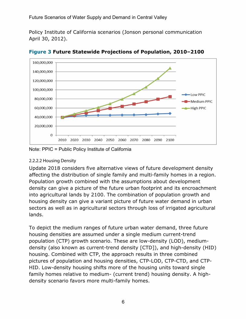
It is impossible to predict future population growth accurately, so the CWP uses three different, but plausible, population-growth estimates when determining future urban water demands. Figure 3 shows the future projection of statewide population from 2010 to 2100 under three Public
Future Scenarios of Water Supply and Demand in Central Valley
6
Policy Institute of California scenarios (Jonson personal communication April 30, 2012).
Figure 3 Future Statewide Projections of Population, 2010–2100
Note: PPIC = Public Policy Institute of California
2.2.2.2 Housing Density
Update 2018 considers five alternative views of future development density affecting the distribution of single family and multi-family homes in a region. Population growth combined with the assumptions about development density can give a picture of the future urban footprint and its encroachment into agricultural lands by 2100. The combination of population growth and housing density can give a variant picture of future water demand in urban sectors as well as in agricultural sectors through loss of irrigated agricultural lands.
To depict the medium ranges of future urban water demand, three future housing densities are assumed under a single medium current-trend population (CTP) growth scenario. These are low-density (LOD), medium-density (also known as current-trend density [CTD]), and high-density (HID) housing. Combined with CTP, the approach results in three combined pictures of population and housing densities, CTP-LOD, CTP-CTD, and CTP-HID. Low-density housing shifts more of the housing units toward single family homes relative to medium- (current trend) housing density. A high-density scenario favors more multi-family homes.

Future Scenarios of Water Supply and Demand in Central Valley
7
To bracket a higher future water demand, a fourth housing density with higher ratios of low-density single-family homes was considered under the high population (HIP) growth scenario, HIP-LOD.
To bracket the low end of the future water demand, a fifth housing density was assumed favoring higher ratios of high-density multi-family homes under low population (LOP) growth scenarios, LOP-HID.

Future Scenarios of Water Supply and Demand in Central Valley
8

3. Analytical Tool: Central Valley Planning Area Model
9
3. Analytical Tool: Central Valley Planning Area Model 3.1 WEAP-CVPA Model Description The CWP supported the development of a model of the Central Valley by using the WEAP system (www.weap21.org), called WEAP-Central Valley Planning Area (CVPA) model. The WEAP system is a comprehensive, fully integrated river basin analysis tool. It is a simulation model that includes a robust and flexible representation of water demands from different sectors and the ability to include operating rules for infrastructure elements such as reservoirs, canals, and hydropower projects.
It also has watershed rainfall-runoff modeling capabilities that allow the water infrastructure and demand to be dynamically nested within the underlying hydrological processes. This functionality allows the analyses of how specific configurations of infrastructure, operating rules, and operational priorities will affect water uses as diverse as instream flows, irrigated agriculture, and municipal water supply under hydrological input data and physical watershed conditions. This integration of watershed hydrology with a water-systems planning model makes WEAP ideally suited to study the potential effects of various uncertainties, including climate change.
In WEAP, water-demand sites receive supply deliveries based on the volumes of computed demand and a system of user-defined “demand priorities.” The highest priority demand sites will receive their supply deliveries first. If any water is left in the system, it will be delivered to the next demand sites down the priority list. If there is not enough water is left in the system, the demands in lower priority sites will not get their full demand met, resulting in unmet demands.
On the supply side, the requested supplies are delivered to demand sites based on “supply preferences” imposed by water users on their supply options. This combination of demand priorities and supply preferences form a hierarchical matrix of supply allocation “order” for supply deliveries. WEAP uses a linear programming optimization solver to solve the matrix of allocation order in the objective function. The objective function is to maximize percentage of demand met (i.e., demand coverage) at each

Future Scenarios of Water Supply and Demand in Central Valley
10
demand site, subject to system constraints including storage and conveyance capacity limitations as well as contractual, environmental, institutional and legal constraints. The major demand sectors in the current WEAP CVPA model application are agricultural, urban indoor, urban outdoor, and environmental flows. Major supply sources to meet the requested demands are from stream diversions, surface reservoirs, groundwater aquifers, and return flows.
Figure 4 shows a schematic representation of Central Valley planning areas (PAs) in the WEAP-CVPA model.
Figure 4 Schematic Representation of Water Evaluation and Planning-Central Valley Planning Area Model

Future Scenarios of Water Supply and Demand in Central Valley
11
3.2 Model Calibration-Validation Update 2013 describes the calibration process of the WEAP-CVPA model; it will not be repeated here. To test the model performance under the extreme conditions of the 20 newly updated climate scenarios, a model validation was performed using five climate scenarios ranging from cool-wet to warm-dry conditions. The climate scenarios selected were:
cnrm_cm5_4.5 (cool-wet, also selected by Sustainable Groundwater Management Act [SGMA] climate guidance).
• miroc5_4.5 (cool-dry).
• canesm2_8.5 (warm-wet).
• hadgem2_ES (warm-dry, also selected by SGMA climate guidance).
• ccsm4_8.5 (central tendency).
The urban growth scenario selected for this model validation was based on CTP-CTD. For more detailed information on selection of climate and urban growth scenarios and validation results, see the validation report prepared by Stockholm Environment Institute included in Appendix A.
3.3 Model Geographic Coverage The WEAP-CVPA model covers three hydrologic regions (HRs) in the Central Valley (Sacramento River, San Joaquin River, and Tulare Lake) and performs detailed water supply and demand computations at the PA level for each hydrologic region.
3.3.1 Sacramento River HR Planning Areas Sacramento River HR consists of 11 PAs as shown in Figure 5.
1. PA 501 (Shasta-Pit).
2. PA 502 (Upper NW Valley).
3. PA 503 (Lower NW Valley).
4. PA 504 (NE Valley).
5. PA 505 (Southwest).
6. PA 506 (Colusa Basin).
7. PA 507 (Butte-Sutter-Yuba).
Future Scenarios of Water Supply and Demand in Central Valley
12
8. PA 508 (Southeast).
9. PA 509 (Central Basin-West).
10. PA 510 (Sacramento-San Joaquin Delta).
11. PA 511 (Central Basin- East).
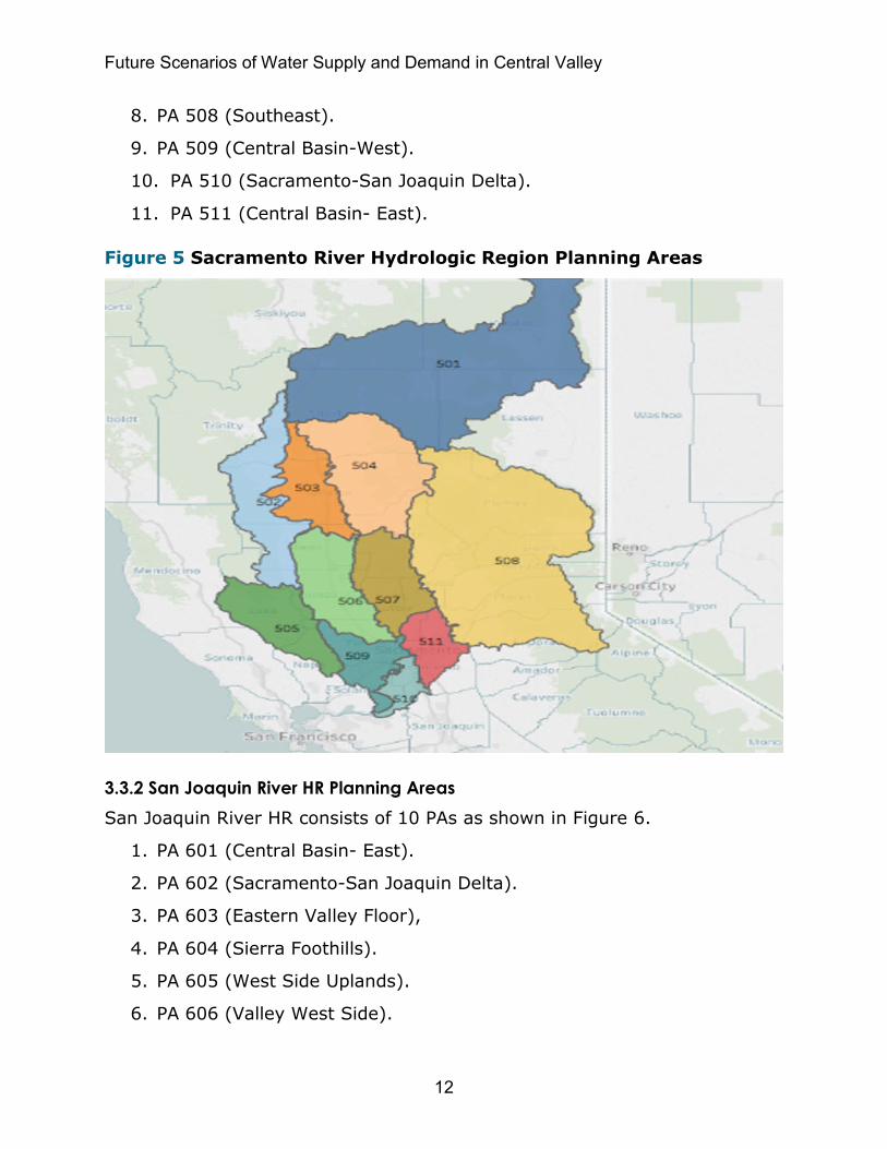
Figure 5 Sacramento River Hydrologic Region Planning Areas
3.3.2 San Joaquin River HR Planning Areas San Joaquin River HR consists of 10 PAs as shown in Figure 6.
1. PA 601 (Central Basin- East).
2. PA 602 (Sacramento-San Joaquin Delta).
3. PA 603 (Eastern Valley Floor),
4. PA 604 (Sierra Foothills).
5. PA 605 (West Side Uplands).
6. PA 606 (Valley West Side).

Future Scenarios of Water Supply and Demand in Central Valley
13
7. PA 607 (Upper Valley East Side).
8. PA 608 (Middle Valley East Side).
9. PA 609 (Lower Valley East Side).
10. PA 610 (East Side Uplands).
Figure 6 San Joaquin River Hydrologic Region Planning Areas
3.3.3 Tulare Lake HR Planning Areas Tulare Lake HR consists of 10 PAs as shown in Figure 7.
1. PA 701 (Western Uplands).
2. PA 702 (San Luis Side).
3. PA 703 (Lower Kings- Tulare).
4. PA 704 (Fresno Academy).
5. PA 705 (Alta-Orange Cove).
6. PA 706 (Kaweah Delta).

Future Scenarios of Water Supply and Demand in Central Valley
14
7. PA 707 (Uplands).
8. PA 708 (Semitropic).
9. PA 709 (Kern Valley Floor).
10. PA 710 (Kern Delta).
Figure 7 Tulare Lake Hydrologic Region Planning Areas
4.Weap-CVPA Model Results: Future Water Conditions
15
4. WEAP-CVPA Model Results: Future Water Conditions This section presents the modeling results of future projections of water conditions including water demands, supply deliveries, unmet demands (water shortages), and storages in surface reservoirs and ground aquifers. It includes the results in the three hydrologic regions (HRs) of the Central Valley under the five urban growth patterns and 20 climate scenarios from 2006 to 2100. WEAP computes the information at monthly time-step and at PA level but they are scaled up to annual and aggregated up to HR level.
NOTE: The modeling results presented herein are based on a key future water resource management strategy envisioned in Update 2013, Volume 3, Chapter 16, “Groundwater/Aquifer Remediation.” It recommended a limitation of groundwater pumping to prevent future overdraft. As a result, aquifer withdrawals and pumping were constrained in current model applications to prevent groundwater levels from dropping below historical minimums. Should this limitation in groundwater pumping be removed, the results would be expected to be different.
Because most of the results presented in this report are aggregated to hydrologic region scale, more detailed information on future water conditions at PA level within each of the three hydrologic regions in Central Valley is available on the interactive Tableau Dashboard (California Department of Water Resources 2019d).
4.1 Sacramento River Hydrologic Region
4.1.1 Agriculture
4.1.1.1 Agricultural Water Demand
Agricultural water demand calculations in the WEAP Central Valley model are based on two major sets of input parameters and driving factors, (1) irrigated agriculture acreages and climate factors affecting evapotranspiration and, (2) crop consumptive use such as temperature, precipitation, relative humidity and wind speed. Descriptions of future projections of irrigated agriculture acreages in the Sacramento River HR, as

Future Scenarios of Water Supply and Demand in Central Valley
16
well as future trends of climate factors including temperature and precipitation at sample locations, are provided below.
Agricultural Acreage: Figure 8 shows three projections of future agriculture acreages in the Sacramento River HR under three future urban growth scenarios. Results are based on UPLAN model studies of future urbanization and loss of irrigated lands described in Update 2013. As shown in Figure 8, irrigated acreages decline because of urbanization and urban encroachment into agricultural lands. As expected, agricultural land reduction is more pronounced under the HIP-LOD urban scenario (depicted by the red line) — decreasing from approximately 1.6 million acres in 2006 to approximately 1.3 million acres in 2100.
Figure 8 Future Projections of Agricultural Acreage, Sacramento River Hydrologic Region, 2006–2100
Note: CTP-CTD = current trend population-current trend density scenario, HIP-LOD = high population-low density scenario, LOP-HID = low population-high density scenario
Climatic Conditions: Agricultural water demand is also affected by climate factors. Figures 9 and 10 show the future projections of monthly temperature and precipitation, respectively, under the 20 GCM climate scenarios at a sample location in the Sacramento River HR from 2006 to 2100. As shown in Figure 9, the general trend in temperature shows a gradual rise from approximately 15 °C in 2006 to approximately 18 °C by

Future Scenarios of Water Supply and Demand in Central Valley
17
the end of the century (2100). As shown in Figure 10, total precipitation does not show a trend, either increasing or decreasing, over the same period.
Figure 9 Future Projections of Temperature (°C) under 20 Global Climate Model Scenarios, Sacramento River Hydrologic Region, 2006–2100
Figure 10 Future Projections of Precipitation (millimeters) under 20 Global Climate Model Scenarios, Sacramento River Hydrologic Region, 2006–2100
Note: mm = millimeters

Future Scenarios of Water Supply and Demand in Central Valley
18
Future Agricultural Water Demand: Figure 11 shows the result of the WEAP-CVPA model projection of future annual agricultural demand in million acre-feet (maf) in the Sacramento River HR under the collective 20 climate scenarios for CTP-CTD urban growth scenario from 2006 to 2100. Fluctuations in annual agricultural water demand, as shown in the figure, is the result of inter-annual variability of climatic conditions. Future agricultural demand shows an overall declining trend under the CTP-CTD urban growth scenario. More detailed results at the PA level, and for the other four urban growth scenarios, are available on the online Tableau Dashboard.
Agricultural water demand, on average, under this moderate CTP-CTD urban growth scenario and under the 20 climate scenarios, declined from approximately 8.8 maf in 2006 to approximately 7.9 maf in 2100.
Figure 11 Future Projections of Agricultural Water Demand, Sacramento River Hydrologic Region, Single Urban Growth Scenario CTP-CTD, 20 Climate Scenarios, 2006–2100
Note: CTP-CTD = current-trend population–current-trend density
The decline in agricultural demand was more pronounced under the HIP-LOD scenario. As shown in Figure 12, on average, agricultural demand declined from 8.8 maf in 2006 to approximately 7.2 maf in 2100.

Future Scenarios of Water Supply and Demand in Central Valley
19
Figure 12 Future Projections of Agricultural Water Demand, Sacramento River Hydrologic Region, Single Urban Growth Scenario HIP-LOD, 20 Climate Scenarios, 2006–2100
Note: HIP-LOD = high population-low density
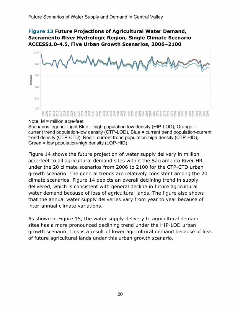
Figure 13 illustrates relative impacts of the five urban growth scenarios on future agricultural demand in the Sacramento River HR under a single climate scenario, ACCESS1.0_4.5. All five urban growth scenarios have similar impacts on agricultural demand at the beginning. But as time progresses toward the end of the century, the impacts of urbanization and encroachments into agricultural lands become more pronounced. As expected, the HIP-LOD (light blue line) scenario shows more pronounced decline in future agricultural demand because of a greater loss of agricultural lands relative to the other four urban growth scenarios.
4.1.1.2 Agricultural Water Supply Delivery
In WEAP, the amount of water supply deliveries from supply sources, (e.g., surface water, groundwater aquifers, and return flows to demand sites) are based on requested “demand volumes” and supply preferences imposed by water users on their supply options, and on their system conveyance capacity or other physical or institutional constraints. Future projections of volumes of water supply deliveries to demand sites are computed at each PA level but are aggregated up to hydrologic region scale for presenting a more summarized information. More detailed analysis and visualization of future trend under each individual climate and individual urban growth scenarios at each PA, is available on the Tableau Dashboard.
Future Scenarios of Water Supply and Demand in Central Valley
20
Figure 13 Future Projections of Agricultural Water Demand, Sacramento River Hydrologic Region, Single Climate Scenario ACCESS1.0-4.5, Five Urban Growth Scenarios, 2006–2100
Note: M = million acre-feet Scenarios legend: Light Blue = high population-low density (HIP-LOD), Orange = current trend population-low density (CTP-LOD), Blue = current trend population-current trend density (CTP-CTD), Red = current trend population-high density (CTP-HID), Green = low population-high density (LOP-HID)
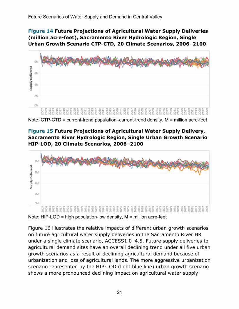
Figure 14 shows the future projection of water supply delivery in million acre-feet to all agricultural demand sites within the Sacramento River HR under the 20 climate scenarios from 2006 to 2100 for the CTP-CTD urban growth scenario. The general trends are relatively consistent among the 20 climate scenarios. Figure 14 depicts an overall declining trend in supply delivered, which is consistent with general decline in future agricultural water demand because of loss of agricultural lands. The figure also shows that the annual water supply deliveries vary from year to year because of inter-annual climate variations.
As shown in Figure 15, the water supply delivery to agricultural demand sites has a more pronounced declining trend under the HIP-LOD urban growth scenario. This is a result of lower agricultural demand because of loss of future agricultural lands under this urban growth scenario.
Future Scenarios of Water Supply and Demand in Central Valley
21
Figure 14 Future Projections of Agricultural Water Supply Deliveries (million acre-feet), Sacramento River Hydrologic Region, Single Urban Growth Scenario CTP-CTD, 20 Climate Scenarios, 2006–2100
Note: CTP-CTD = current-trend population–current-trend density, M = million acre-feet
Figure 15 Future Projections of Agricultural Water Supply Delivery, Sacramento River Hydrologic Region, Single Urban Growth Scenario HIP-LOD, 20 Climate Scenarios, 2006–2100
Note: HIP-LOD = high population-low density, M = million acre-feet
Figure 16 illustrates the relative impacts of different urban growth scenarios on future agricultural water supply deliveries in the Sacramento River HR under a single climate scenario, ACCESS1.0_4.5. Future supply deliveries to agricultural demand sites have an overall declining trend under all five urban growth scenarios as a result of declining agricultural demand because of urbanization and loss of agricultural lands. The more aggressive urbanization scenario represented by the HIP-LOD (light blue line) urban growth scenario shows a more pronounced declining impact on agricultural water supply

Future Scenarios of Water Supply and Demand in Central Valley
22
deliveries relative to the other four urban growth scenarios. To understand the impacts of urbanization on future agricultural water supply deliveries under the other 19 individual climate scenarios, information is available on the Tableau Dashboard.
Figure 16 Future Projections of Agricultural Water Supply Delivery, Sacramento River Hydrologic Region, Single Climate Scenario ACCESS1.0-4.5, Five Urban Growth Scenarios, 2006–2100
Note: M = million acre-feet Scenarios legend: Light Blue = high population-low density (HIP-LOD), Orange = current trend population-low density (CTP-LOD), Blue = current trend population-current trend density (CTP-CTD), Red = current trend population-high density (CTP-HID), Green = low population-high density (LOP-HID)
4.1.1.3 Agricultural Unmet Water Demand (Shortages)
Unmet water demand calculations in WEAP model are based on the difference between the requested demand for water and the amount of supplies delivered. Depending on supply availability, as well as physical, contractual, and legal constraints on water delivery system, the demand node may not receive all the requested water (i.e., it may not meet 100 percent of its demand), resulting in an “unmet” demand (shortage) situation.
Figure 17 shows the projected annual unmet demand in acre-feet (af) for the agricultural sector within the Sacramento River HR from 2006 to 2100 under the 20 climate scenarios for CTP-CTD urban growth scenario. As shown in Figure 17, the amount and occurrences of the shortages generally increases as time progresses toward the end of the century.

Future Scenarios of Water Supply and Demand in Central Valley
23
More detailed information at PA level, and for the other four urban growth scenarios, is available on the companion Tableau Dashboard. Also, a more rigorous vulnerability analysis to identify areas in agricultural sector within the Sacramento River HR prone to long-term water shortages are provided in Section 4.1.2.3, “Urban Indoor Unmet Water Demands (Shortages).”
Figure 17 Future Projections of Agricultural Unmet Water Demand, Sacramento River Hydrologic Region, Single Urban Growth Scenario CTP-CTD, 20 Climate Scenarios, 2006–2100
Note: CTP-CTD = current-trend population–current-trend density, K = thousand acre-feet
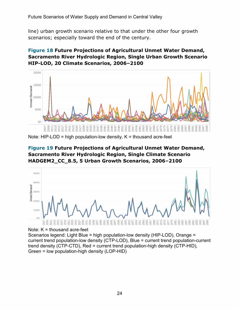
Figure 18 shows the amount and occurrences of unmet water demand in the agricultural sector of the Sacramento River HR for the HIP-LOD housing scenario. As shown in Figure 18, the magnitudes and occurrences of shortages become more pronounced toward the end of the century under the more aggressive HIP-LOD urban growth scenario relative to that of the more moderate CTP-CTD urban scenario. Even though the agricultural demand declines even more under the aggressive high-population scenario because of higher loss of agricultural lands, urban demand is given a higher “priority” in supply allocation order relative to agricultural sector in the WEAP-CVPA model, giving much of available supplies to the urban sector. The result is higher shortages in the agricultural sector as time progresses toward the end of the century.
Figure 19 illustrates the relative impacts of different urban growth scenarios on future unmet agricultural water demand under a single climate scenario, HADGEM2_CC_8.5. At the beginning, all five growth scenarios show similar impacts. But as time progresses, the amount of impacts on unmet demand becomes more pronounced under the more aggressive HIP-LOD (light blue
Future Scenarios of Water Supply and Demand in Central Valley
24
line) urban growth scenario relative to that under the other four growth scenarios; especially toward the end of the century.
Figure 18 Future Projections of Agricultural Unmet Water Demand, Sacramento River Hydrologic Region, Single Urban Growth Scenario HIP-LOD, 20 Climate Scenarios, 2006–2100
Note: HIP-LOD = high population-low density, K = thousand acre-feet
Figure 19 Future Projections of Agricultural Unmet Water Demand, Sacramento River Hydrologic Region, Single Climate Scenario HADGEM2_CC_8.5, 5 Urban Growth Scenarios, 2006–2100
Note: K = thousand acre-feet Scenarios legend: Light Blue = high population-low density (HIP-LOD), Orange = current trend population-low density (CTP-LOD), Blue = current trend population-current trend density (CTP-CTD), Red = current trend population-high density (CTP-HID), Green = low population-high density (LOP-HID)

Future Scenarios of Water Supply and Demand in Central Valley
25
4.1.2 Urban Indoor
4.1.2.1 Urban Indoor Water Demand
Urban indoor water demand calculations in the WEAP-CVPA model are primarily based on population and housing densities. Indoor water use includes consumptions in single family and multi-family residentials, as well as in commercial and industrial sectors. It is assumed indoor water use is not affected by climate conditions.
Population: Figure 20 shows three projections of future population in the Sacramento River HR from 2006 to 2100. The blue line represents the current trend projections, under which, population grows from approximately 3 million in 2006 to approximately 6 million in 2100. The low-projection scenario (green line) estimates population to be slightly more than 4 million, the high-projection scenario estimates population to be slightly more than 12 million by 2100.
Figure 20 Future Projections of Population Growth, Sacramento River Hydrologic Region, 2006–2100
Future Urban Indoor Water Demand: Urban water demand in current application of WEAP-CVPA model is not only a function of population but also a function of housing density. To capture a range of future urban water demands, three future housing density scenarios were assumed under the medium current-trend population growth CTP scenario. These are LOD housing, with more single-family homes; CTD housing; and HID housing, which favors more multi-family homes. This resulted in three combinations
Future Scenarios of Water Supply and Demand in Central Valley
26
of population and housing density: CTP-CTD, CTP-LOD, and CTP-HID. Additionally, to bracket the low and high ends of urban water demand, a HID scenario was assumed under the low-population growth (LOP), and a LOD scenario was assumed under HIP growth. This resulted in two additional urban growth scenarios: LOP-HID and HIP-LOD. This provided a total of five future urban growth scenarios affecting future urban water demands.
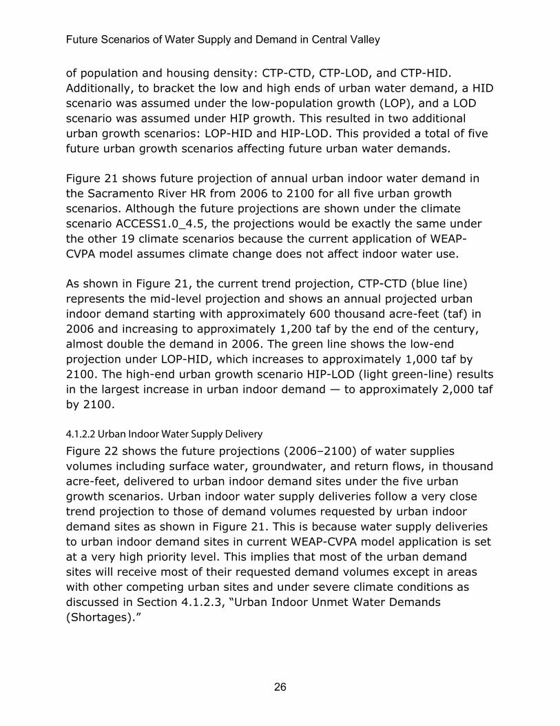
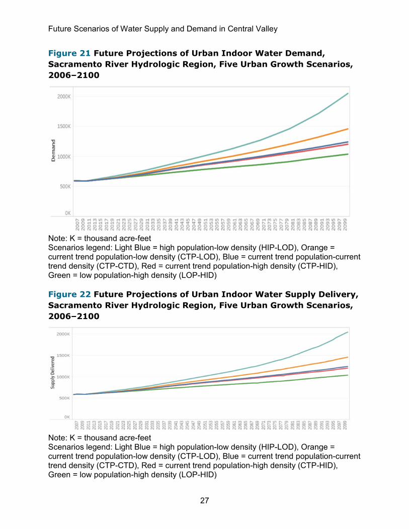
Figure 21 shows future projection of annual urban indoor water demand in the Sacramento River HR from 2006 to 2100 for all five urban growth scenarios. Although the future projections are shown under the climate scenario ACCESS1.0_4.5, the projections would be exactly the same under the other 19 climate scenarios because the current application of WEAP-CVPA model assumes climate change does not affect indoor water use.
As shown in Figure 21, the current trend projection, CTP-CTD (blue line) represents the mid-level projection and shows an annual projected urban indoor demand starting with approximately 600 thousand acre-feet (taf) in 2006 and increasing to approximately 1,200 taf by the end of the century, almost double the demand in 2006. The green line shows the low-end projection under LOP-HID, which increases to approximately 1,000 taf by 2100. The high-end urban growth scenario HIP-LOD (light green-line) results in the largest increase in urban indoor demand — to approximately 2,000 taf by 2100.
4.1.2.2 Urban Indoor Water Supply Delivery
Figure 22 shows the future projections (2006–2100) of water supplies volumes including surface water, groundwater, and return flows, in thousand acre-feet, delivered to urban indoor demand sites under the five urban growth scenarios. Urban indoor water supply deliveries follow a very close trend projection to those of demand volumes requested by urban indoor demand sites as shown in Figure 21. This is because water supply deliveries to urban indoor demand sites in current WEAP-CVPA model application is set at a very high priority level. This implies that most of the urban demand sites will receive most of their requested demand volumes except in areas with other competing urban sites and under severe climate conditions as discussed in Section 4.1.2.3, “Urban Indoor Unmet Water Demands (Shortages).”
Future Scenarios of Water Supply and Demand in Central Valley
27
Figure 21 Future Projections of Urban Indoor Water Demand, Sacramento River Hydrologic Region, Five Urban Growth Scenarios, 2006–2100
Note: K = thousand acre-feet Scenarios legend: Light Blue = high population-low density (HIP-LOD), Orange = current trend population-low density (CTP-LOD), Blue = current trend population-current trend density (CTP-CTD), Red = current trend population-high density (CTP-HID), Green = low population-high density (LOP-HID)
Figure 22 Future Projections of Urban Indoor Water Supply Delivery, Sacramento River Hydrologic Region, Five Urban Growth Scenarios, 2006–2100
Note: K = thousand acre-feet Scenarios legend: Light Blue = high population-low density (HIP-LOD), Orange = current trend population-low density (CTP-LOD), Blue = current trend population-current trend density (CTP-CTD), Red = current trend population-high density (CTP-HID), Green = low population-high density (LOP-HID)

Future Scenarios of Water Supply and Demand in Central Valley
28
4.1.2.3 Urban Indoor Unmet Water Demands (Shortages)
Figure 23 shows the future projections of annual unmet demand in the urban indoor sector in thousand acre-feet within the Sacramento River HR from 2006 to 2100 for the moderate CTP-CTD urban growth scenario under the 20 climate scenarios. As time progresses toward the end of the century the magnitude of unmet demand becomes larger and occurs more frequently depending on the severity of hydrologic and climatic conditions. The maximum unmet volume peaks at approximately 15 taf under the climate scenario CCSM4_8.5 in 2097.
Figure 23 Future Projections of Urban Indoor Unmet Water Demand, Sacramento River Hydrologic Region, Single Urban Growth Scenario CTP-CTD, 20 Climate Scenarios, 2006–2100
Note: CTP-CTD = current-trend population–current-trend density, K = thousand acre-feet
As shown in Figure 24, under a more aggressive high-population urban growth scenario, HIP-LOD, the future unmet demand in the urban indoor sector becomes even more severe and more frequent toward the end of the century. The unmet demand peaks around 2097 at approximately 30 taf, double the amount under the moderate CTP-CTD scenario, and under the same climate scenario, CCSM4_8.5. A more rigorous vulnerability analysis to identify areas in urban sector within the Sacramento River HR prone to long-term water shortages are provided in Section 4.1.4.2, “Urban Water Shortages.”

Future Scenarios of Water Supply and Demand in Central Valley
29
Figure 24 Future Projections of Urban Indoor Unmet Water Demand, Sacramento River Hydrologic Region, Single Urban Growth Scenario HIP-LOD, 20 Climate Scenarios, 2006–2100
Note: HIP-LOD = high population-low density, K = thousand acre-feet
4.1.3 Urban Outdoor
4.1.3.1 Urban Outdoor Water Demand
Unlike urban indoor water demand, which was assumed to not be a function of climate change in the WEAP-CVPA model application, the urban outdoor water demand in residential, commercial, and large landscapes varies from year to year as a function of climatic conditions under different climate scenarios. The urban outdoor demand, in addition to being a function of urban expansion, is a function of climatic conditions which can vary seasonally, annually, and between climate scenarios.
Figure 25 shows future projections of the annual urban outdoor demand in thousand acre-feet under the 20 climate scenarios for the moderate CTP-CTD urban growth scenario from 2006 to 2100. Urban outdoor demand increases over time in response to urban expansion under all 20 climate scenarios. On average, the increase is from approximately 350 taf in 2006 to approximately 400 taf by 2100.

Future Scenarios of Water Supply and Demand in Central Valley
30
Figure 25 Future Projections of Urban Outdoor Water Demand, Sacramento River Hydrologic Region, Single Urban Growth Scenario CTP-CTD, 20 Climate Scenarios, 2006–2100
Note: CTP-CTD = current-trend population–current-trend density, K = thousand acre-feet
But under a more aggressive urban expansion scenario, HIP-LOD, represented by high population and low-density housing (e.g., more single-family homes), the increase in future projection of water demand is even more steep, as shown in Figure 26. On average, over the 20 climate scenarios, water demand increases from 300 taf in 2006 to approximately 500 taf by 2100.
Figure 26 Future Projections of Urban Outdoor Water Demand, Sacramento River Hydrologic Region, Single Urban Growth Scenario HIP-LOD, 20 Climate Scenarios, 2006–2100
Note: HIP-LOD = high population-low density, K = thousand acre-feet

Future Scenarios of Water Supply and Demand in Central Valley
31
Figure 27 shows the relative impacts of the five urban growth scenarios on urban outdoor water demand for climate scenario ACCESS1.0_4.5 from 2006 to 2100. The more aggressive urban expansion high population-low density scenario, HIP-LOD, represented by the light blue line, has the greatest effect, especially toward the end of the century. The water demand increased from approximately 350 taf in 2006 to approximately 500 taf around 2100. As expected, the least expansive scenario, LOP-HID, represented by green line, has the least effect. The water demand increased to a moderate 360 taf toward the end of the century. Figure 27 also shows the annual fluctuation in outdoor water demand caused by inter-annual climate variations affecting outdoor landscape consumptive uses, under all five urban growth scenarios.
Figure 27 Future Projections of Urban Outdoor Water Demand, Sacramento River Hydrologic Region, Single Climate Scenario ACCESS1.0-4.5, Five Urban Multi-Growth Scenarios, 2006–2100
Note: K = thousand acre-feet Scenarios legend: Light Blue = high population-low density (HIP-LOD), Red = current trend population-low density (CTP-LOD), Blue = current trend population-current trend density (CTP-CTD), Orange = current trend population-high density (CTP-HID), Green = low population-high density (LOP-HID)
4.1.3.2 Urban Outdoor Water Supply Delivery
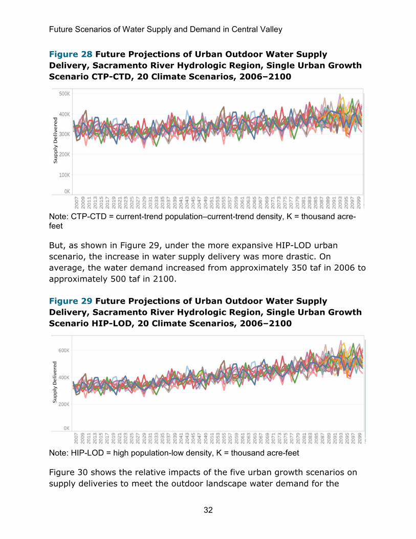
Figure 28 shows supplies in thousand acre-feet including surface water, groundwater, and return flows delivered to meet the water demand of all outdoor landscape sites within the Sacramento River HR under the 20 climate scenarios for the moderate urban expansion scenario CTP-CTD from 2006 to 2100. On average, the supply deliveries increased from approximately 350 taf in 2006 to approximately 380 taf by 2100 under CTP-CTD.
Future Scenarios of Water Supply and Demand in Central Valley
32
Figure 28 Future Projections of Urban Outdoor Water Supply Delivery, Sacramento River Hydrologic Region, Single Urban Growth Scenario CTP-CTD, 20 Climate Scenarios, 2006–2100
Note: CTP-CTD = current-trend population–current-trend density, K = thousand acre-feet
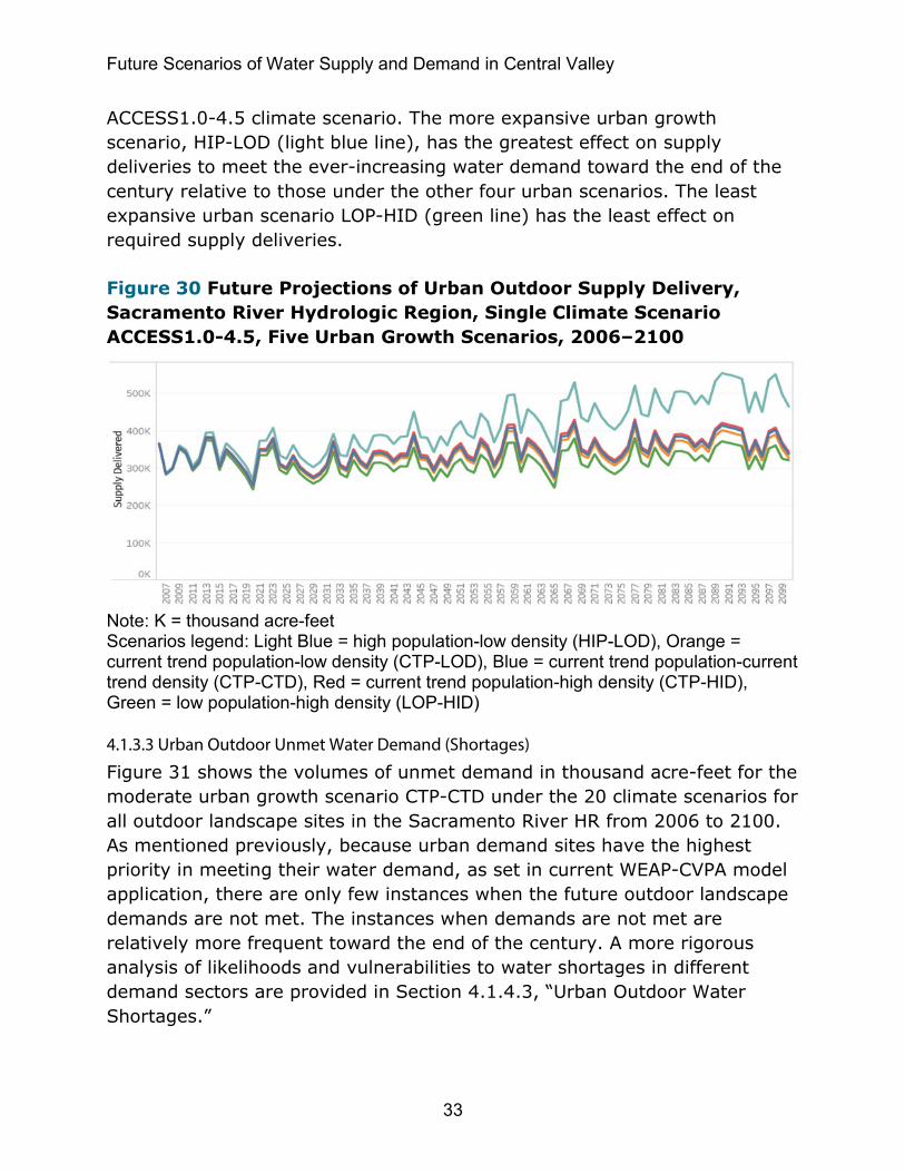
But, as shown in Figure 29, under the more expansive HIP-LOD urban scenario, the increase in water supply delivery was more drastic. On average, the water demand increased from approximately 350 taf in 2006 to approximately 500 taf in 2100.
Figure 29 Future Projections of Urban Outdoor Water Supply Delivery, Sacramento River Hydrologic Region, Single Urban Growth Scenario HIP-LOD, 20 Climate Scenarios, 2006–2100
Note: HIP-LOD = high population-low density, K = thousand acre-feet
Figure 30 shows the relative impacts of the five urban growth scenarios on supply deliveries to meet the outdoor landscape water demand for the
Future Scenarios of Water Supply and Demand in Central Valley
33
ACCESS1.0-4.5 climate scenario. The more expansive urban growth scenario, HIP-LOD (light blue line), has the greatest effect on supply deliveries to meet the ever-increasing water demand toward the end of the century relative to those under the other four urban scenarios. The least expansive urban scenario LOP-HID (green line) has the least effect on required supply deliveries.
Figure 30 Future Projections of Urban Outdoor Supply Delivery, Sacramento River Hydrologic Region, Single Climate Scenario ACCESS1.0-4.5, Five Urban Growth Scenarios, 2006–2100
Note: K = thousand acre-feet Scenarios legend: Light Blue = high population-low density (HIP-LOD), Orange = current trend population-low density (CTP-LOD), Blue = current trend population-current trend density (CTP-CTD), Red = current trend population-high density (CTP-HID), Green = low population-high density (LOP-HID)
4.1.3.3 Urban Outdoor Unmet Water Demand (Shortages)
Figure 31 shows the volumes of unmet demand in thousand acre-feet for the moderate urban growth scenario CTP-CTD under the 20 climate scenarios for all outdoor landscape sites in the Sacramento River HR from 2006 to 2100. As mentioned previously, because urban demand sites have the highest priority in meeting their water demand, as set in current WEAP-CVPA model application, there are only few instances when the future outdoor landscape demands are not met. The instances when demands are not met are relatively more frequent toward the end of the century. A more rigorous analysis of likelihoods and vulnerabilities to water shortages in different demand sectors are provided in Section 4.1.4.3, “Urban Outdoor Water Shortages.”

Future Scenarios of Water Supply and Demand in Central Valley
34
More detailed information on climate scenarios that result in more frequent occurrences of large quantities of unmet demands are available in the companion Tableau Dashboard.
Figure 31 Future Projections of Urban Outdoor Unmet Water Demand, Sacramento River Hydrologic Region, Single Urban Growth Scenario CTP-CTD, 20 Climate Scenarios, 2006–2100
Note: CTP-CTD = current-trend population–current-trend density, K = thousand acre-feet
As shown in Figure 32, under the more expansive HIP-LOD urban scenario, the instances of unmet demands are more frequent as time progresses toward the end of the century.
Figure 32 Future Projections of Urban Outdoor Unmet Water Demand, Sacramento River Hydrologic Region, Single Urban Growth Scenario HIP-LOD, 20 Climate Scenarios, 2006–2100
Note: HIP-LOD = high population-low density, K = thousand acre-feet

Future Scenarios of Water Supply and Demand in Central Valley
35
4.1.4 Future Water Shortages: Vulnerability Analysis- Vulnerabilities and Likelihoods Water shortage (unmet demand) is the difference between the requested demand and supplies delivered to a demand sector in a region. When supplies are not sufficient to meet the total requested demand over an extended period of time, when only a portion of the demand is met, then the region may be deemed vulnerable and prone to extended water shortages. Some regions may reduce their demand as part of their mandatory best management practices and water management strategies, or as a voluntary measure to accept some level of water shortages. This reduced level of demand is termed “demand threshold.” By changing demand thresholds, the likelihood of water shortages can change too. For example, reducing the demand threshold can result in lowering the likelihood of water shortages because available supplies can more frequently meet the reduced demands characterized by the demand threshold.
Through vulnerability analysis, the likelihood of future water shortages over an extended period of time can be quantified; regions prone to long-term water shortages can be identified. This can help guide the planning and allocation of future investments to reduce vulnerabilities and risks to water shortages.
Vulnerability maps were developed to show the long-term likelihood of water shortages at regional HR level, as well as at PA level. Regional-level vulnerabilities may mask vulnerabilities at smaller scales. As a result, quantifying and assessing vulnerabilities at PA level will help identify areas exhibiting more severe vulnerabilities. Vulnerability analyses described in the following section are provided as examples under selected urban growth and climate scenarios. More detailed information on vulnerability analyses under other future scenarios, is provided in the companion Tableau Dashboard.
4.1.4.1 Agricultural Water Shortages
Figure 33 (a and b) shows the long-term future vulnerability of agricultural sectors at the regional level in the Sacramento River HR to water shortages under the CTP-CTD urban growth and ACCESS1.0_4.5 climate scenario. The 100 percent demand threshold (no demand reduction) on the left (a), and 95 percent demand threshold (5 percent demand reduction) on the right (b). Figure 33a shows that when no demand reduction is adopted, the likelihood of water shortages will be approximately 98.9 percent. This implies there is
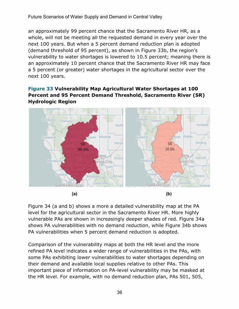
Future Scenarios of Water Supply and Demand in Central Valley
36
an approximately 99 percent chance that the Sacramento River HR, as a whole, will not be meeting all the requested demand in every year over the next 100 years. But when a 5 percent demand reduction plan is adopted (demand threshold of 95 percent), as shown in Figure 33b, the region’s vulnerability to water shortages is lowered to 10.5 percent; meaning there is an approximately 10 percent chance that the Sacramento River HR may face a 5 percent (or greater) water shortages in the agricultural sector over the next 100 years.
Figure 33 Vulnerability Map Agricultural Water Shortages at 100 Percent and 95 Percent Demand Threshold, Sacramento River (SR) Hydrologic Region
Figure 34 (a and b) shows a more a detailed vulnerability map at the PA level for the agricultural sector in the Sacramento River HR. More highly vulnerable PAs are shown in increasingly deeper shades of red. Figure 34a shows PA vulnerabilities with no demand reduction, while Figure 34b shows PA vulnerabilities when 5 percent demand reduction is adopted.
Comparison of the vulnerability maps at both the HR level and the more refined PA level indicates a wider range of vulnerabilities in the PAs, with some PAs exhibiting lower vulnerabilities to water shortages depending on their demand and available local supplies relative to other PAs. This important piece of information on PA-level vulnerability may be masked at the HR level. For example, with no demand reduction plan, PAs 501, 505,

Future Scenarios of Water Supply and Demand in Central Valley
37
and 509 show the highest vulnerability to water shortages at 97.9 percent, 57.9 percent, and 25.3 percent, respectively. But other PAs in the hydrologic region shows a much lower level of vulnerability, ranging from 2.1 percent in PA 508 to 7.4 percent in PA 502.The same general pattern is also observed when a 5 percent demand reduction is adopted, as a comparison of Figure 33b and Figure 34b demonstrates.
Figure 34 Vulnerability Map, Planning Area (PA) Level, Agricultural Water Shortages at 100 Percent and 95 Percent Demand Threshold, Sacramento River Hydrologic Region
4.1.4.2 Urban Indoor Water Shortages
Figure 35 (a and b) shows the likelihood of water shortages in the urban indoor sector of the Sacramento River HR at 100 percent demand threshold (Figure 35a) and at 95 percent demand threshold (Figure 35b) under the CTP-CTD urban growth and ACCESS1.0_4.5 climate scenario. Figure 35a shows that when no demand reduction is adopted, the region faces water shortages about 25.3 percent of time over the next 100 years. But, at 5 percent demand reduction, the likelihood to have shortages of 5 percent (or more) diminishes to almost zero, as shown in Figure 35b.

Future Scenarios of Water Supply and Demand in Central Valley
38
As expected, the urban sector shows a much lower likelihood of water shortages (less vulnerable) relative to the agricultural sector as discussed previously, because urban sector was given a higher demand priority in the current application of WEAP Central Valley model.
Figure 35 Vulnerability Map, Urban Indoor Water Shortages at 100 Percent and 95 Percent Demand Threshold, Sacramento River (SR) Hydrologic Region
Figure 36 (a and b) shows the same urban indoor water vulnerability map, but at a more detailed PA level. As shown in Figure 36a, most parts of the region exhibit very little vulnerability to water shortages. The exception is PA 505 which may face a 25.3 percent chance of water shortages when no demand reduction is adopted. But, when a 5 percent demand reduction (95 percent demand threshold) is adopted, the same PA may face a lower chance (approximately 25 percent) of having a water shortage of 5 percent (or greater).

Future Scenarios of Water Supply and Demand in Central Valley
39
Figure 36 Vulnerability Map, Planning Area (PA) Level, Urban Indoor Water Shortages at 100 Percent and 95 Percent Demand Threshold, Sacramento River Hydrologic Region
4.1.4.3 Urban Outdoor Water Shortages
Figure 37 (a and b) shows vulnerabilities of urban outdoor sector to water shortages in the Sacramento River region at HR level over the next 100 years for the CTP-CTD urban growth and ACCESS1.0_4.5 climate scenarios.
Figure 37a shows that the likelihood of water shortages, when no demand reduction is adopted, is very low at approximately 1.1 percent. This implies there is only 1.1 percent chance that over the next 100 years the outdoor urban sector at HR level will face water shortages when all 100 percent demand is requested. Again, this very low likelihood occurs because urban sectors in the current Central Valley WEAP model have highest demand priorities. When 5 percent demand reduction is adopted (95 percent demand threshold), the likelihood of water shortages reduces to zero (Figure 35b), implying available supplies will be sufficient to meet the reduced levels of demand.

Future Scenarios of Water Supply and Demand in Central Valley
40
Figure 37 Vulnerability Map, Urban Outdoor Water Shortages at 100 Percent and 95 Percent Demand Threshold, Sacramento River (SR) Hydrologic Region
Figure 38 (a and b) shows the same urban outdoor vulnerability map, but at a more detailed PA level. As Figure 38a shows, most of the PAs exhibit very little or no vulnerability, consistent with that at the regional level. In this case, regional level vulnerability properly captured what was occurring at the PA level. On Figure 38b, the previous conclusion also holds for urban demand at 95 percent demand threshold.
Figure 38 Vulnerability Map, Planning Area (PA) Level, Urban Outdoor Water Shortages at 100 Percent and 95 Percent Demand Threshold, Sacramento River Hydrologic Region

Future Scenarios of Water Supply and Demand in Central Valley
41
4.2 San Joaquin River Hydrologic Region 4.2.1 Agriculture 4.2.1.1 Agricultural Water Demand
As mentioned in Section 4.1.1.1, agricultural water demand calculations in the WEAP Central Valley model are based on two major sets of input parameters and driving factors, (1) irrigated agricultural acreages and climate factors affecting evapotranspiration and, (2) crop consumptive use, such as temperature, precipitation, relative humidity, and wind speed. A description of future projections of irrigated agricultural acreages in the San Joaquin River HR, as well as future trends of climate factors, including temperature and precipitation at a sample location, are given below.
Agricultural Acreage: Figure 39 shows three projections of future agricultural acreages in the San Joaquin River HR under three future urban growth scenarios. Results are based on UPLAN model studies of future urbanization and loss of irrigated agricultural lands as explained in Update 2013. As shown in Figure 39, agricultural acreages decline because of urbanization and urban encroachment into agricultural lands. As expected, agricultural land reduction is more pronounced under the HIP-LOD urban scenario (red-line). It decreases from approximately 2.0 million acres in 2006 to approximately 1.5 million acres in 2100.
Figure 39 Future Projections of Agricultural Acreage, San Joaquin River Hydrologic Region, 2006–2100
Note: CTP-CTD = current-trend population–current-trend density, HIP-LOD = high population-low density, LOP-HID = low population-high density
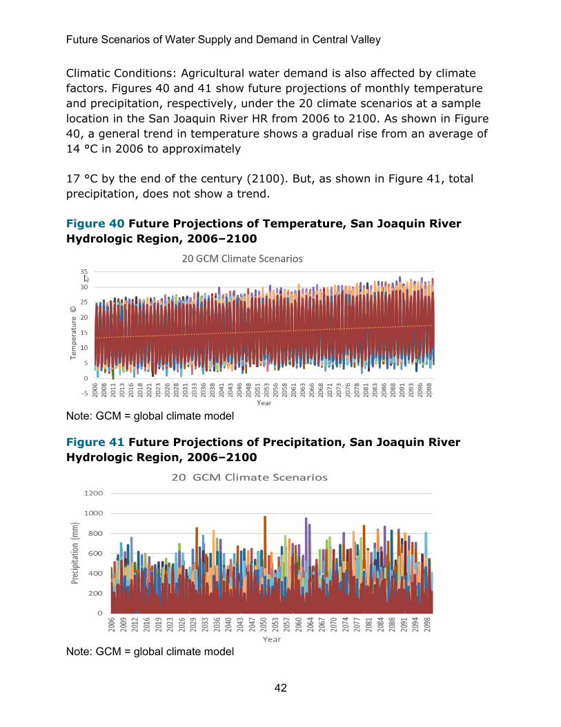
Future Scenarios of Water Supply and Demand in Central Valley
42
Climatic Conditions: Agricultural water demand is also affected by climate factors. Figures 40 and 41 show future projections of monthly temperature and precipitation, respectively, under the 20 climate scenarios at a sample location in the San Joaquin River HR from 2006 to 2100. As shown in Figure 40, a general trend in temperature shows a gradual rise from an average of 14 °C in 2006 to approximately
17 °C by the end of the century (2100). But, as shown in Figure 41, total precipitation, does not show a trend.
Figure 40 Future Projections of Temperature, San Joaquin River Hydrologic Region, 2006–2100
Note: GCM = global climate model
Figure 41 Future Projections of Precipitation, San Joaquin River Hydrologic Region, 2006–2100
Note: GCM = global climate model

Future Scenarios of Water Supply and Demand in Central Valley
43
Future Agricultural Water Demand: Figure 42 shows the result of a WEAP-CVPA model projection of future annual agricultural demand in million acre-feet in the San Joaquin River HR under the collective 20 climate scenarios for CTP-CTD urban scenario from 2006 to 2100. Fluctuations in annual agricultural water demand, as shown in the figure, is because of inter-annual variability of climatic conditions. The model gives the results at the PA level, but they were aggregated up to give regional total for the purpose of this report. Future agricultural demand shows an overall declining trend under the CTP-CTD urban scenario. As shown in the figure, agricultural water demand, on average, under the moderate CTP-CTD urban scenario, declined from approximately 7.5 maf in 2006 to approximately 5.8 maf in 2100.
More detailed results at the PA level and for the other four urban scenarios are available on the online Tableau Dashboard.
Figure 42 Future Projections of Agricultural Water Demand, San Joaquin River Hydrologic Region, Single Urban Growth Scenario CTP-CTD, 20 Climate Scenarios, 2006–2100
Note: CTP-CTD = current-trend population–current-trend density, M = million acre-feet
The decline in agricultural demand was even more pronounced under the HIP-LOD scenario, as shown in Figure 43. On average, it declined from 7.3 maf in 2006 to approximately 5.1 maf in 2100.
Figure 44 illustrates relative impacts of the five urban growth scenarios on future agricultural demand in the San Joaquin River HR under a single climate scenario, ACCESS1.0_4.5. All five urban scenarios have similar effect on agricultural demand at the beginning. But as time progresses toward the

Future Scenarios of Water Supply and Demand in Central Valley
44
end of the century, the impacts of urbanization and encroachments into agricultural lands become more pronounced. As expected, the HIP-LOD (light blue line) shows more pronounced decline in future agricultural demand because of a greater loss of agricultural lands relative to the other four urban scenarios.
Figure 43 Future Projections of Agricultural Water Demand, San Joaquin River Hydrologic Region, Single Urban Growth Scenario HIP-LOD, 20 Climate Scenarios, 2006–2100
Note: HIP-LOD = high population-low density, M = million acre-feet
Figure 44 Future Projections of Agricultural Water Demand, San Joaquin River Hydrologic Region, Single Climate Scenario ACCESS1.0-4.5, Five Urban Growth Scenarios, 2006–2100
Note: M = million acre-feet Scenarios legend: Light Blue = high population (HIP-LOD), Orange = current trend population-low density (CTP-LOD), Blue = current trend population-current trend density (CTP-CTD), Red = current trend population-high density (CTP-HID), Green = low population-high density (LOP-HID)
4.2.1.2 Agricultural Water Supply Delivery
As previously mentioned, computation of water supply deliveries in WEAP from different supply sources, including surface water, groundwater aquifers,

Future Scenarios of Water Supply and Demand in Central Valley
45
and return flows to demand sites are based on requested demand volumes as well as supply preferences imposed by water users on their supply options. They are also based on their system conveyance capacity or other physical or institutional constraints. Even though future projections of water supply deliveries to demand sites are computed at each PA level, they are aggregated up to HR scale for presenting more summarized information. More detailed analysis and visualization of future trends under each individual scenario of climate and urban growth at each PA are available on the companion Tableau Dashboard.
Figure 45 shows future projection of water supply delivery in million acre-feet to all agricultural demand sites within the San Joaquin River HR under the 20 climate scenarios from 2006 to 2100 for the CTP-CTD urban growth scenario. The general trends are relatively consistent among the 20 climate scenarios. It also shows an overall declining trend consistent with general decline in future agricultural water demand because of loss of agricultural lands. The figure also shows the annual water supply deliveries vary from year to year because of inter-annual climate variations.
Figure 45 Future Projections of Agricultural Water Supply Delivery, San Joaquin River Hydrologic Region, Single Urban Growth Scenario CTP-CTD, 20 Climate Scenarios, 2006–2100
Note: CTP-CTD = current-trend population–current-trend density, M = million acre-feet
As shown in Figure 46, water supply deliveries to agricultural demand sites have a more pronounced declining trend under the HIP-LOD scenario. This was expected because of lower agricultural water demand resulting from the loss of future agricultural lands under this expansive urban growth scenario.

Future Scenarios of Water Supply and Demand in Central Valley
46
Figure 46 Future Projections of Agricultural Water Supply Delivery, San Joaquin River Hydrologic Region, Single Urban Growth Scenario HIP-LOD, 20 Climate Scenarios, 2006–2100
Note: HIP-LOD = high population-low density, M = million acre-feet
Figure 47 illustrates the relative impacts of different urban growth scenarios on future agricultural water supply deliveries in the San Joaquin River HR under a single climate scenario, ACCESS1.0_4.5. It shows future supply deliveries to agricultural demand sites has an overall declining trend under all five urban growth scenarios as a result of declining agricultural demand because of urbanization and loss of agricultural lands. But the more aggressive urbanization scenario represented by the HIP-LOD (light blue line) scenario shows a more pronounced declining effect on agricultural water supply delivery when compared with the other four urban scenarios. To understand the impacts of urbanization on future agricultural water supply deliveries under the other 19 individual climate scenarios, more information is provided in the Tableau Dashboard.

Future Scenarios of Water Supply and Demand in Central Valley
47
Figure 47 Future Projections of Agricultural Water Supply Delivery, San Joaquin River Hydrologic Region, Single Climate Scenario ACCESS1.0-4.5, Five Urban Growth Scenarios, 2006–2100
Note: M = million acre-feet Scenarios legend: Light Blue = high population-low density (HIP-LOD), Orange = current trend population-low density (CTP-LOD), Blue = current trend population-current trend density (CTP-CTD), Red = current trend population-high density (CTP-HID), Green = low population-high density (LOP-HID)
4.2.1.3 Agricultural Unmet Water Demand (Shortages)
Unmet water demand calculation in the WEAP model is based on the difference between the requested demand for water and the amount of supplies delivered. Depending on supply availability as well as physical, contractual, and legal constraints on water delivery systems, the demand sector may not receive all the requested water. When less than 100 percent of the demand is met it results in an unmet water demand (shortage) situation.
Figure 48 shows the projected annual unmet demand in acre-feet for the agricultural sector within the San Joaquin River HR from 2006 to 2100 under the 20 climate scenarios for CTP-CTD urban growth scenario. As shown in Figure 48, with few instances of high unmet demand early on, the amount and occurrences of water shortages are generally more concentrated toward the end of the century.
More detailed information at the PA level, and for the other four urban scenarios, is available from the companion Tableau Dashboard. In addition, a more rigorous vulnerability analysis to identify areas in the agricultural sector within San Joaquin River HR prone to long-term water shortages are provided in Section 4.2.4.1, “Agricultural Water Shortages.”
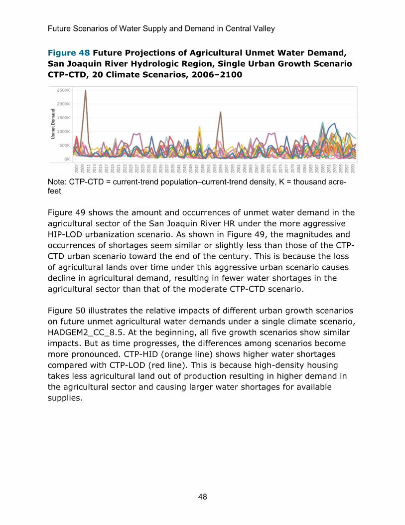
Future Scenarios of Water Supply and Demand in Central Valley
48
Figure 48 Future Projections of Agricultural Unmet Water Demand, San Joaquin River Hydrologic Region, Single Urban Growth Scenario CTP-CTD, 20 Climate Scenarios, 2006–2100
Note: CTP-CTD = current-trend population–current-trend density, K = thousand acre-feet
Figure 49 shows the amount and occurrences of unmet water demand in the agricultural sector of the San Joaquin River HR under the more aggressive HIP-LOD urbanization scenario. As shown in Figure 49, the magnitudes and occurrences of shortages seem similar or slightly less than those of the CTP-CTD urban scenario toward the end of the century. This is because the loss of agricultural lands over time under this aggressive urban scenario causes decline in agricultural demand, resulting in fewer water shortages in the agricultural sector than that of the moderate CTP-CTD scenario.
Figure 50 illustrates the relative impacts of different urban growth scenarios on future unmet agricultural water demands under a single climate scenario, HADGEM2_CC_8.5. At the beginning, all five growth scenarios show similar impacts. But as time progresses, the differences among scenarios become more pronounced. CTP-HID (orange line) shows higher water shortages compared with CTP-LOD (red line). This is because high-density housing takes less agricultural land out of production resulting in higher demand in the agricultural sector and causing larger water shortages for available supplies.

Future Scenarios of Water Supply and Demand in Central Valley
49
Figure 49 Future Projections of Agricultural Unmet Water Demand, San Joaquin River Hydrologic Region, Single Urban Growth Scenario HIP-LOD, 20 Climate Scenarios, 2006–2100
Note: HIP-LOD = high population-low density, K = thousand acre-feet
Figure 50 Future Projections of Agricultural Unmet Water Demand, San Joaquin River Hydrologic Region, Single Climate Scenario HADGEM2_CC_8.5, Five Urban Growth Scenarios, 2006–2100
Note: K = thousand acre-feet Scenarios legend: Light Blue = high population-low density (HIP-LOD), Red = current trend population-low density (CTP-LOD), Blue = current trend population-current trend density (CTP-CTD), Orange = current trend population-high density (CTP-HID), Green = low population-high density (LOP-HID)
4.2.2 Urban Indoor
4.2.2.1 Urban Indoor Water Demand
Urban indoor water demand calculations in the WEAP-CVPA model are primarily based on population and housing densities. The indoor water use includes consumptions in single family and multi-family residentials as well as in commercial and industrial sectors. It is assumed the indoor water use is not affected by climate conditions.

Future Scenarios of Water Supply and Demand in Central Valley
50
Population: Figure 51 shows three projections of future population in the San Joaquin River HR from 2006 to 2100. The blue line represents the current trend projections of the population growing from approximately 2.0 million in 2006, to approximately 5.4 million by 2100. The low-projection scenario (green line) shows a population of approximately 4.8 million. The high-projection scenario (red line) estimates the population at slightly more than 10.8 million by the 2100 in the San Joaquin HR.
Figure 51 Future Projections of Population Growth, San Joaquin River Hydrologic Region, 2006–2100
Future Urban Indoor Water Demand: Urban water demand in current application of the WEAP-CVPA model is not only a function of population but also a function of housing density. To capture the medium ranges of future water demand, three future housing density scenarios were assumed under the single medium current-trend population growth CTP scenario. These are LOD housing, with more single-family homes; CTD housing; and HID housing, which favors more multi-family homes. This gives three combinations of population and housing density, CTP-CTD, CTP-LOD and CTP-HID. Additionally, to bracket the low and high end of urban water demand, an HID scenario was assumed under the low-population growth (LOP), and a LOD housing scenario was assumed under the HIP scenario. This creates two additional urban growth scenarios, LOP-HID and HIP-LOD, and provides a total of five future urban growth scenarios affecting the future urban water demand.
Figure 52 shows future projections of annual urban indoor water demand in the San Joaquin River HR from 2006 to 2100 for all five urban growth

Future Scenarios of Water Supply and Demand in Central Valley
51
scenarios. Although the projections are shown under climate scenario ACCESS1.0_4.5, they would exactly be the same under the other 19 climate scenarios because the current application of the WEAP-CVPA model assumes climatic conditions do not affect indoor water use.
As shown in Figure 52, the current trend projection, CTP-CTD (green line) shows the mid-level projection starting at approximately 400 taf in 2006 and increasing to approximately 1,500 taf by the end of the century. The red line shows the low-end projection under LOP-HID which increases to approximately 1,000 taf by 2100. As expected, the high-end urban growth scenario HIP-LOD (light blue line) resulted in the highest increase, approximately 1,900 taf, by 2100. This high-end urban growth scenario, with expansive LOD single-family homes initially gave similar projection to another low-density scenario, CTP-LOD, shown by the orange line in Figure 52, but it was the HIP-LOD scenario (light blue line) that finally took over and resulted in the highest indoor demand toward the end of the century.
Figure 52 Future Projections of Urban Indoor Water Demand, San Joaquin River Hydrologic Region, Single Climate Scenarios ACCESS1.0_4.5, Five Urban Growth Scenarios, 2006–2100
Note K = thousand acre-feet Scenarios legend: Light Blue = high population-low density (HIP-LOD), Orange = current trend population-low density (CTP-LOD), Green = current trend population-current trend density (CTP-CTD), Blue = current trend population-high density (CTP-HID), Red = low population-high density (LOP-HID)

Future Scenarios of Water Supply and Demand in Central Valley
52
4.2.2.2 Urban Indoor Water Supply Delivery
Figure 53 shows the future projections (2006–2100) of water supply volumes including surface water, groundwater, and return flows, in thousand acre-feet, delivered to urban indoor demand sites under the five urban growth scenarios. Urban indoor water supply deliveries follow a very close trend projection to those of demand volumes requested by urban indoor demand sites as shown in demand projections in Figure 52. This is because water supply deliveries to urban indoor demand sites in the current WEAP-CVPA model application is set at a high-priority level. This implies most of urban demand sites will receive most of their requested demand volumes, except in some areas with other competing urban sites and under some severe climate conditions as discussed in Section 4.2.2.3, “Urban Indoor Unmet Water Demand (Shortages).”
Figure 53 Future Projections of Urban Indoor Water Supply Delivery, San Joaquin River Hydrologic Region, Five Urban Growth Scenarios, 2006–2100
Note: K = thousand acre-feet Scenarios legend: Light Blue = high population-low density (HIP-LOD), Red = current trend population-low density (CTP-LOD), Blue = current trend population-current trend density (CTP-CTD), Orange = current trend population-high density (CTP-HID), Green = low population-high density (LOP-HID)
4.2.2.3 Urban Indoor Unmet Water Demands (Shortages)
Figure 54 shows future projections of annual unmet demand in urban indoor sector in thousand acre-feet (taf) within the San Joaquin River HR from 2006 to 2100 for the moderate CTP-CTD urban growth scenario. As shown in Figure 54, except in few instances, initially there is no unmet demand in urban indoor sector. But, toward the end of the century, the magnitude of unmet demand becomes larger and occurs more frequently, depending on

Future Scenarios of Water Supply and Demand in Central Valley
53
severity of hydrologic and climatic conditions caused by type of climate scenario. The maximum unmet volume peaks at approximately 5 taf under climate scenario CMCC_CMS_8.5 around 2095.
Figure 54 Future Projections of Urban Indoor Unmet Water Demand, San Joaquin River Hydrologic Region, Single Urban Growth Scenario CTP-CTD, 2006–2100
Note: CTP-CTD = current-trend population–current-trend density, K = thousand acre-feet Scenarios legend: Light Blue = high population-low density (HIP-LOD), Red = current trend population-low density (CTP-LOD), Blue = current trend population-current trend density (CTP-CTD), Orange = current trend population-high density (CTP-HID), Green = low population-high density (LOP-HID)
4.2.3 Urban Outdoor
4.2.3.1 Urban Outdoor Water Demand
Unlike urban indoor demand, which was assumed to not be a function of climate change in the current WEAP-CVPA model application, the urban outdoor demand in residential, commercial, and large landscapes varies from year to year as a function of climatic conditions under different climate scenarios. The urban outdoor demand is not only a function of urban expansion, but also a function of climatic conditions which can vary seasonally, annually, and between climate scenarios.
Figure 55 shows future projections of the annual urban outdoor demand in thousand acre-feet under the 20 climate scenarios for the moderate CTP-CTD urban scenario from 2006 to 2100. Urban outdoor demand increases over time in response to urban expansion under all 20 climate scenarios. On average, the increase is from approximately 280 taf in 2006 to approximately 450 taf by 2100.

Future Scenarios of Water Supply and Demand in Central Valley
54
But under a more aggressive urban expansion scenario, HIP-LOD, represented by high population and low-density housing (i.e., more single-family homes), the increase in future projection of water demand becomes even more pronounced as shown in Figure 56. On average, over the 20 climate scenarios, water demand increases from 280 taf in 2006 to approximately 650 taf by 2100.
Figure 55 Future Projections of Urban Outdoor Water Demand, San Joaquin River Hydrologic Region, Single Urban Growth Scenario CTP-CTD, 20 Climate Scenarios, 2006–2100
Note: CTP-CTD = current-trend population–current-trend density, K = thousand acre-feet
Figure 56 Future Projections of Urban Outdoor Water Demand, San Joaquin River Hydrologic Region, Single Urban Growth Scenario HIP-LOD, 20 Multi-Climate Scenarios, 2006–2100
Note: HIP-LOD = high population-low density, K = thousand acre-feet
Figure 57 shows the relative impacts of the five urban growth scenarios on urban outdoor water demand for climate scenario ACCESS1.0_4.5 from 2006 to 2100. The more aggressive HIP-LOD urban expansion (light blue line) has the greatest effect, especially toward the end of the century. The water demand increases from approximately 280 taf in 2006 to approximately

Future Scenarios of Water Supply and Demand in Central Valley
55
570 taf around 2100. As expected, the least expansive scenario, LOP-HID (green line), had the least effect on urban water demand. On average, it increased to a moderate 350 taf toward the end of the century. Figure 57 also shows the annual fluctuation in outdoor water demand resulting from inter-annual climate variations affecting outdoor landscape consumptive uses.
Figure 57 Future Projections of Urban Outdoor Water Demand, San Joaquin River Hydrologic Region, Single Climate Scenario ACCESS1.0-4.5, Five Urban Growth Scenarios, 2006–2100
Note: K = thousand acre-feet Scenarios legend: Light Blue = high population-low density (HIP-LOD), Red = current trend population-low density (CTP-LOD), Blue = current trend population-current trend density (CTP-CTD), Orange = current trend population-high density (CTP-HID), Green = low population-high density (LOP-HID)
4.2.3.2 Urban Outdoor Water Supply Delivery
Figure 58 shows water supplies in thousand acre-feet including surface water, groundwater, and return flows, delivered to meet the water demand of all outdoor landscape sites within the San Joaquin River HR under all 20 climate scenarios for the moderate urban expansion scenario CTP-CTD from 2006 to 2100. On average, the supply deliveries increased from approximately 280 taf in 2006 to approximately 450 taf by 2100 under this moderate urban expansion scenario.
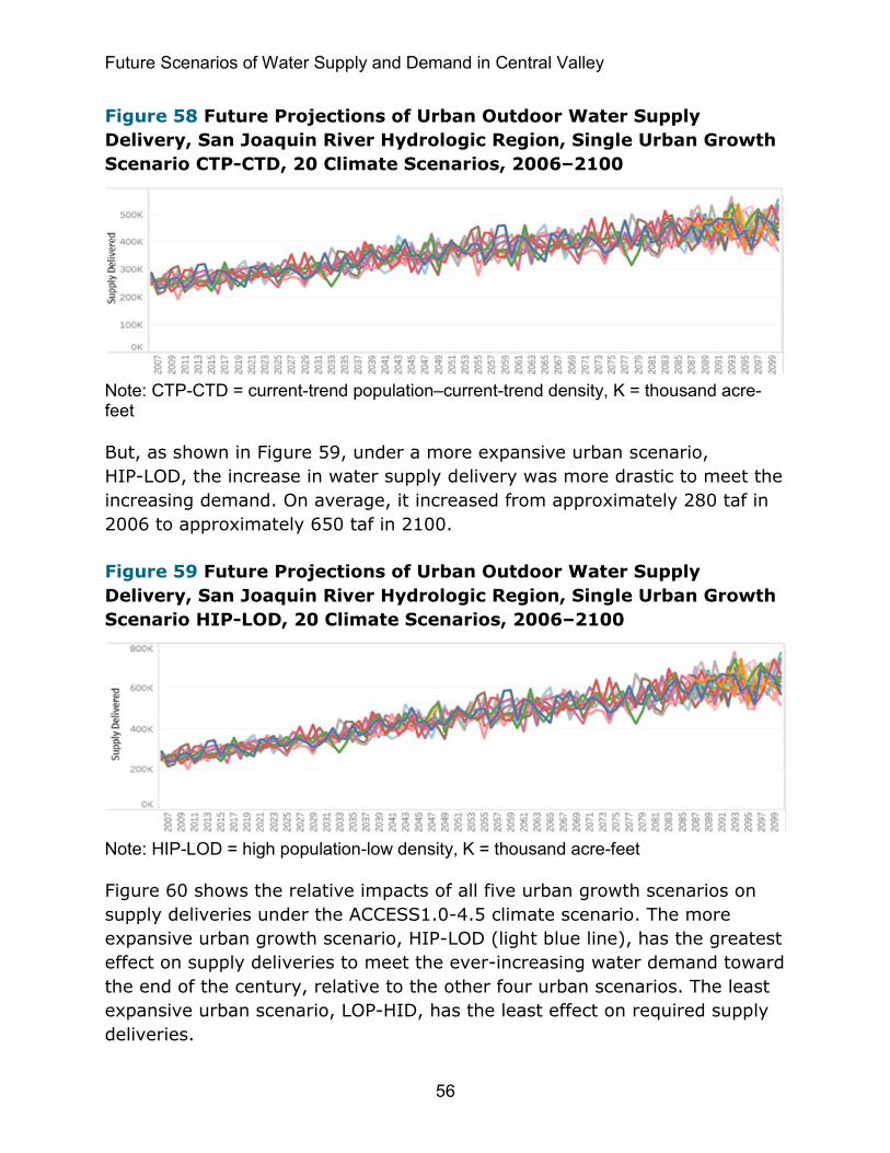
Future Scenarios of Water Supply and Demand in Central Valley
56
Figure 58 Future Projections of Urban Outdoor Water Supply Delivery, San Joaquin River Hydrologic Region, Single Urban Growth Scenario CTP-CTD, 20 Climate Scenarios, 2006–2100
Note: CTP-CTD = current-trend population–current-trend density, K = thousand acre-feet
But, as shown in Figure 59, under a more expansive urban scenario, HIP-LOD, the increase in water supply delivery was more drastic to meet the increasing demand. On average, it increased from approximately 280 taf in 2006 to approximately 650 taf in 2100.
Figure 59 Future Projections of Urban Outdoor Water Supply Delivery, San Joaquin River Hydrologic Region, Single Urban Growth Scenario HIP-LOD, 20 Climate Scenarios, 2006–2100
Note: HIP-LOD = high population-low density, K = thousand acre-feet
Figure 60 shows the relative impacts of all five urban growth scenarios on supply deliveries under the ACCESS1.0-4.5 climate scenario. The more expansive urban growth scenario, HIP-LOD (light blue line), has the greatest effect on supply deliveries to meet the ever-increasing water demand toward the end of the century, relative to the other four urban scenarios. The least expansive urban scenario, LOP-HID, has the least effect on required supply deliveries.

Future Scenarios of Water Supply and Demand in Central Valley
57
Figure 60 Future Projections of Urban Outdoor Supply Delivery, San Joaquin River Hydrologic Region, Single Climate Scenario ACCESS1.0-4.5, Five Urban Growth Scenarios, 2006–2100
Note: K = thousand acre-feet Scenarios legend: Light Blue = high population-low density (HIP-LOD), Red = current trend population-low density (CTP-LOD), Blue = current trend population-current trend density (CTP-CTD), Orange = current trend population-high density (CTP-HID), Green = low population-high density (LOP-HID)
4.2.3.3 Urban Outdoor Unmet Water Demand (Shortages)
Figure 61 shows the volumes of unmet demand in the urban outdoor sector of the San Joaquin River HR under the moderate urban growth scenario CTP-CTD for all 20 climate scenarios from 2006 to 2100. It shows zero unmet demand under all climates, indicating sufficient water supply deliveries to meet all outdoor demand. This is because urban demand sites have the highest priority in meeting their water demand, as set in the current WEAP-CVPA model application. A more rigorous analysis of likelihoods and vulnerabilities to water shortages in different demand sectors are provided in Section 4.2.4.3, “Urban Outdoor Water Shortages.”
As shown in Figure 62, even under a more expansive HIP-LOD urban scenario, all the demand in urban outdoor sectors in the San Joaquin HR are met.

Future Scenarios of Water Supply and Demand in Central Valley
58
Figure 61 Future Projections of Urban Outdoor Unmet Water Demand, San Joaquin River Hydrologic Region, Single Urban Growth Scenario CTP-CTD, 20 Climate Scenarios, 2006–2100
Note: CTP–CTD = current trend population-current trend density
Figure 62 Future Projections of Urban Outdoor Unmet Water Demand, San Joaquin River Hydrologic Region, Single Urban Growth Scenario HIP-LOD, 20 Climate Scenarios, 2006–2100
Note: HIP-LOD = high population-low density
4.2.4 Future Water Shortages: Vulnerability Analysis- Vulnerabilities and Likelihoods Water shortage (unmet demand) is the difference between the requested demand and the supplies delivered to a demand sector in a region. When supplies are not sufficient to meet the total requested demand over an extended period of time, where only a portion of the demand is met, then the region may be deemed vulnerable and prone to extended water shortages. But some regions may reduce their demand as part of their mandatory best management practices and water management strategies, or as a voluntary measure to accept some level of water shortages. This reduced level of demand is termed “demand threshold.” For example,

Future Scenarios of Water Supply and Demand in Central Valley
59
reducing the demand threshold can result in lowering the likelihood of water shortages because available supplies can more frequently meet the reduced demands characterized by the demand threshold.
Through vulnerability analysis, future water shortages and their likelihoods over an extended period of time can be quantified and regions prone to long term water shortages can be identified. This can help guide the planning and allocation of future investments to reduce vulnerabilities and risks to water shortages.
Vulnerability maps were developed to show long-term likelihoods of water shortages at regional HR levels as well as at PA levels. It should be noted, regional-level vulnerabilities may mask vulnerabilities at smaller PA scales. As a result, quantifying and assessing vulnerabilities at PA level will help identify the PAs exhibiting more severe vulnerabilities. Vulnerability analyses described in the following section are provided as examples under selected urban growth and climate scenarios. More detailed information on vulnerability analyses under other future scenarios is available from the companion Tableau Dashboard.

Future Scenarios of Water Supply and Demand in Central Valley
60
4.2.4.1 Agricultural Water Shortages
Figure 63 (a and b) shows long-term future vulnerability of agricultural sectors at regional level in the San Joaquin River HR. It shows the likelihood of water shortages under the CTP-CTD urban growth and the ACCESS1.0_4.5 climate scenarios for 100 percent demand threshold (no demand reduction) (Figure 63a) and 95 percent demand threshold (5 percent demand reduction) (Figure 63b). The figures show when no demand reduction is adopted, the likelihood of water shortages will be approximately 100 percent. This implies there is 100 percent chance that agricultural sectors in the San Joaquin River HR at regional level, as a whole, will not be meeting all their requested demand in every year over the next 100 years. But when a demand reduction plan is adopted (demand threshold of 95 percent), as shown in Figure 63b, the region’s vulnerability to water shortages is reduced to 32.6 percent, meaning there is an approximately 32.6 percent chance that the agricultural sectors in the San Joaquin River HR may face 5 percent (or greater) water shortages over the next 100 years.
Figure 63 Vulnerability Map, Agricultural Water Shortages at 100 Percent and 95 Percent Demand Threshold, San Joaquin (SJ) River Hydrologic Region

Future Scenarios of Water Supply and Demand in Central Valley
61
Figure 64 (a and b) shows a more a detailed vulnerability map at the PA level for the agricultural sector in the San Joaquin River HR. More highly vulnerable PAs are shown in deeper shades of red. Figure 64a shows PA vulnerabilities with no demand reduction. Figure 34b shows vulnerabilities when 5 percent demand reduction is adopted.
Comparison of the vulnerability maps at both HR level and the more refined PA level indicates a wider range of vulnerabilities in the PAs. Some PAs may exhibit much lower vulnerability to water shortages, depending on their demand volumes and available local supplies, relative to other PAs. This important piece of information on PA-level vulnerability may be masked at the HR level. For example, PAs 601, 605, and 607 show no vulnerability (0 percent) and PA 610 shows highest vulnerability (100 percent) even when no demand reduction plan is adopted (Figure 64a). This was masked when considering only regional level vulnerability. But, when 5 percent demand reduction is adopted (Figure 64b), PA 605 also becomes not vulnerable to water shortages of 5 percent (or more). PA 610 remains the most vulnerable (100 percent), indicating an area possibly prone to long-term water shortages.
Figure 64 Vulnerability Map, Planning Area (PA) Level, Agricultural Water Shortages at 100 percent and 95 percent Demand Threshold, San Joaquin River Hydrologic Region

Future Scenarios of Water Supply and Demand in Central Valley
62
4.2.4.2 Urban Indoor Water Shortages
Figure 65 (a and b) shows the likelihood of water shortages in the urban indoor sector of the San Joaquin River HR at 100 percent demand threshold (Figure 65a) and at 95 percent demand threshold (Figure 65b) under the CTP-CTD urban growth and ACCESS1.0_4.5 climate scenarios. Figure 65a shows that when no demand reduction is adopted, the region faces water shortages of approximately 6.3 percent of time over the next 100 years. But, at 5 percent demand reduction (95 percent demand threshold), the likelihood to have shortages of 5 percent (or more) will diminish to almost zero (Figure 65b).
As expected, the urban sector shows a much lower likelihood of facing water shortages (less vulnerable), relative to agricultural sector because urban sector was given a higher demand priority in the current application of the WEAP Central Valley model.
Figure 65 Vulnerability Map, Urban Indoor Water Shortages at 100 Percent and 95 Percent Demand Threshold, San Joaquin (SJ) River Hydrologic Region

Future Scenarios of Water Supply and Demand in Central Valley
63
Figure 66 (a and b) shows the same vulnerability map but at a more detailed PA level. As shown in Figure 66a, most of the region, except PA 610, exhibit very little vulnerability to water shortages, similar to the vulnerability in its agricultural sector as discussed above. PA 610 may face a 6.3 percent chance of water shortages when no demand reduction is adopted. But, when a 5 percent demand reduction (95 percent demand threshold) is adopted, its chances of having water shortages of 5 percent (or greater) is reduced to about 3.2 percent.
A vulnerability map at the PA level can identify the specific PAs prone to future water shortages, while some of those identities could be been masked by considering only HR level vulnerabilities. It appears
PA 610 may face a higher chance of water shortages in the agricultural sector, as well as in urban indoor sector, when compared with other PAs over the next 100 years.
Figure 66 Vulnerability Map, Planning Area (PA) Level, Urban Indoor Water Shortages at 100 Percent and 95 Percent Demand Threshold, San Joaquin River Hydrologic Region

Future Scenarios of Water Supply and Demand in Central Valley
64
4.2.4.3 Urban Outdoor Water Shortages
Figures 67 (a and b) shows the vulnerability of the urban outdoor sector to water shortages in the San Joaquin River region at the HR level over the next 100 years for the CTP-CTD urban growth and ACCESS1.0_4.5 climate scenarios.
Figure 67a shows there is no likelihood (0 percent) of water shortages at a regional level even with no demand reduction plan. This implies the San Joaquin River HR, as a whole, will meet 100 percent of its urban outdoor demand over the next 100 years. The very low likelihoods are because urban sectors in current Central Valley WEAP model have highest demand priorities. Also, when 5 percent demand reduction plan is adopted (95 percent demand threshold), the vulnerability to water shortages remains at 0 percent.
Figure 67 Vulnerability Map, Urban Outdoor Water Shortages at 100 Percent and 95 Percent Demand Threshold, San Joaquin River (SJ) Hydrologic Region

Future Scenarios of Water Supply and Demand in Central Valley
65
Figure 68 (a and b) shows the same urban outdoor vulnerability map, but at more refined PA level. As shown in Figure 68a, none of the PAs show any vulnerability to water shortages in the outdoor sector even when its total demand is requested (i.e., no demand reduction). This implies there are sufficient supplies that are prioritized to meet the urban outdoor demand. Also, when 5 percent demand reduction is adopted (Figure 68b), the vulnerability remains at 0 percent. This was expected, because if there are enough supplies to meet the total requested demand, there will be more than enough to meet the demands at the 5 percent reduced level.
It should be noted, even though the results show no need for demand reduction in urban outdoor sector in the San Joaquin HR to achieve 100 percent reliability, it was under a specific combination of urban growth and climate scenario. This cannot be generalized to other urban growth and climate scenarios because these scenario factors affect the demand side as well as the supply side of the regional water conditions. This may result in a totally different vulnerability outlook for the region. For more detailed analysis under other combinations of urban and climate scenarios, refer to the Tableau Dashboard.
Figure 68 Vulnerability Map, Planning Area (PA) Level, Urban Outdoor Water Shortages at 100 Percent and 95 Percent Demand Threshold, San Joaquin River Hydrologic Region

Future Scenarios of Water Supply and Demand in Central Valley
66
4.3 Tulare Lake Hydrologic Region
4.3.1 Agriculture
4.3.1.1 Agricultural Water Demand
Agricultural water demand calculations in the WEAP Central Valley model are based on two major sets of input parameters and driving factors, (1) irrigated agricultural acreages, and (2) climate factors affecting evapotranspiration and crop consumptive use such as temperature, precipitation, relative humidity, and wind speed. A description of future trend of irrigated agricultural acreages in the Tulare Lake HR, as well as future projection of climate factors including temperature and precipitation at a sample location, are provided in this section.
Agricultural Acreage: Figure 69 shows three projections of future agricultural acreages in the Tulare Lake HR under three future urban growth scenarios. Results are based on UPLAN model studies of future urbanization and loss of irrigated lands described in Update 2013. As shown in Figure 69, irrigated acreages decline because of urbanization and urban encroachment into agricultural lands. As expected, agricultural land reduction is more pronounced under the HIP-LOD urban scenario (red line), decreasing from 3.1 million acres in 2006 to 2.6 million acres in 2100.
Figure 69 Future Projections of Agricultural Acreage, Tulare Lake Hydrologic Region, 2006–2100
Note: CTP-CTD = current trend population-current trend density, HIP-LOD = high population-low density scenario, LOP-HID = low population-high density scenario

Future Scenarios of Water Supply and Demand in Central Valley
67
Climatic Conditions: Agricultural water demand is also affected by climate factors. Figures 70 and 71 show the future projections of monthly temperature and precipitation, respectively, under the 20 climate scenarios at a sample location in the Tulare Lake HR from 2006 to 2100. As shown in Figure 70, the general trend in temperature shows a gradual rise from approximately 15 °C in 2006 to approximately 19.5 °C by the end of the century (2100). The total precipitation (Figure 71) does not show a trend, neither increasing nor decreasing, over the same period.
Figure 70 Future Projections of Temperature, Tulare Lake Hydrologic Region, 2006–2100
Note: GCM = global climate model
Figure 71 Future Projections of Precipitation, Tulare Lake Hydrologic Region, 2006–2100
Note: GCM = global climate model

Future Scenarios of Water Supply and Demand in Central Valley
68
Future Agricultural Water Demand: Figure 72 shows the results of the WEAP-CVPA model projections of future annual agricultural demand in million acre-feet (maf) in the Tulare Lake HR under the collective 20 climate scenarios for the CTP-CTD urban growth scenario from 2006 to 2100. Fluctuations in annual agricultural water demand, as shown in the figure, are the result of inter-annual variability of climatic conditions. Future agricultural water demand has an overall declining trend under the CTP-CTD urban growth scenario. For more detailed results at PA level and for the other four urban growth scenarios, refer to the Tableau Dashboard.
Agricultural water demand, on average, under this moderate CTP-CTD urban growth scenario and under the 20 climate scenarios, declined from approximately 10 maf in 2006 to approximately 9.5 maf in 2100.
Figure 72 Future Projections of Agricultural Water Demand, Tulare Lake Hydrologic Region, Single Urban Growth Scenario CTP-CTD, 20 Climate Scenarios, 2006–2100
Note: CTP-CTD = current-trend population–current-trend density, M = million acre-feet
The decline was slightly more pronounced under the HIP-LOD scenario. As shown in Figure 73, agricultural water demand, on average, declined from 10 maf in 2006 to approximately 9.3 maf in 2100.
Figure 74 illustrates relative effects of the five urban growth scenarios on future agricultural demand in the Sacramento River HR under a single climate scenario, ACCESS1.0_4.5. All five urban growth scenarios have similar effects on agricultural demand at the beginning. But as time progresses toward the end of the century, the effects of urbanization and encroachments into agricultural lands become more pronounced. As
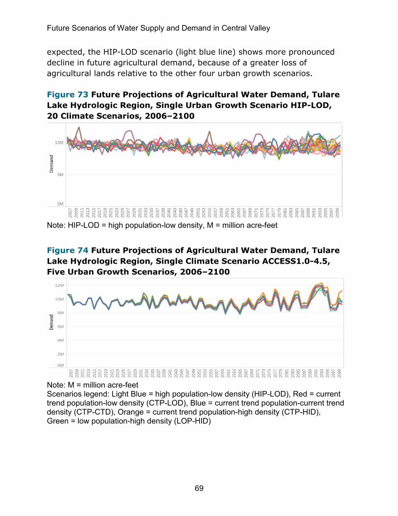
Future Scenarios of Water Supply and Demand in Central Valley
69
expected, the HIP-LOD scenario (light blue line) shows more pronounced decline in future agricultural demand, because of a greater loss of agricultural lands relative to the other four urban growth scenarios.
Figure 73 Future Projections of Agricultural Water Demand, Tulare Lake Hydrologic Region, Single Urban Growth Scenario HIP-LOD, 20 Climate Scenarios, 2006–2100
Note: HIP-LOD = high population-low density, M = million acre-feet
Figure 74 Future Projections of Agricultural Water Demand, Tulare Lake Hydrologic Region, Single Climate Scenario ACCESS1.0-4.5, Five Urban Growth Scenarios, 2006–2100
Note: M = million acre-feet Scenarios legend: Light Blue = high population-low density (HIP-LOD), Red = current trend population-low density (CTP-LOD), Blue = current trend population-current trend density (CTP-CTD), Orange = current trend population-high density (CTP-HID), Green = low population-high density (LOP-HID)

Future Scenarios of Water Supply and Demand in Central Valley
70
4.3.1.2 Agricultural Water Supply Delivery
In WEAP, the amount of water supply deliveries from supply sources (e.g., surface water, groundwater aquifers, and return flows) to demand sites are based on requested demand volumes and supply preferences imposed by water users on their supply options and on their system conveyance capacity or other physical or institutional constraints. Future projections of volumes of water supply deliveries to demand sites are computed at each PA level but are aggregated up to hydrologic region scale for presenting a more summarized information. More detailed analysis and visualization of future trends under each individual climate and individual urban growth scenarios at each PA is available from the companion Tableau Dashboard.
Figure 75 shows future projection of water supply delivery in million acre-feet to all agricultural demand sites within the Tulare Lake HR under the 20 climate scenarios from 2006 to 2100 for the selected CTP-CTD urban growth scenario. The general trends are relatively consistent among the 20 climate scenarios. It also shows an overall declining trend in supply deliveries consistent with the general decline in future agricultural water demand resulting from the loss of agricultural lands. On average, it decreases from approximately 9.7 maf in 2006 to approximately 7.5 maf in 2100. The figure also shows that the annual water supply deliveries vary from year to year because of inter-annual climate variations.
Figure 75 Future Projections of Agricultural Water Supply Delivery, Tulare Lake Hydrologic Region, Single Urban Growth Scenario CTP-CTD, 20 Climate Scenarios, 2006–2100
Note: CTP-CTD = current-trend population–current-trend density, M = million acre-feet
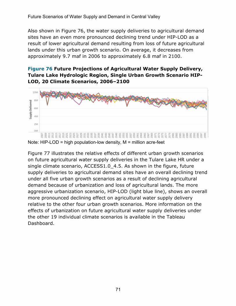
Future Scenarios of Water Supply and Demand in Central Valley
71
Also shown in Figure 76, the water supply deliveries to agricultural demand sites have an even more pronounced declining trend under HIP-LOD as a result of lower agricultural demand resulting from loss of future agricultural lands under this urban growth scenario. On average, it decreases from approximately 9.7 maf in 2006 to approximately 6.8 maf in 2100.
Figure 76 Future Projections of Agricultural Water Supply Delivery, Tulare Lake Hydrologic Region, Single Urban Growth Scenario HIP-LOD, 20 Climate Scenarios, 2006–2100
Note: HIP-LOD = high population-low density, M = million acre-feet
Figure 77 illustrates the relative effects of different urban growth scenarios on future agricultural water supply deliveries in the Tulare Lake HR under a single climate scenario, ACCESS1.0_4.5. As shown in the figure, future supply deliveries to agricultural demand sites have an overall declining trend under all five urban growth scenarios as a result of declining agricultural demand because of urbanization and loss of agricultural lands. The more aggressive urbanization scenario, HIP-LOD (light blue line), shows an overall more pronounced declining effect on agricultural water supply delivery relative to the other four urban growth scenarios. More information on the effects of urbanization on future agricultural water supply deliveries under the other 19 individual climate scenarios is available in the Tableau Dashboard.

Future Scenarios of Water Supply and Demand in Central Valley
72
Figure 77 Future Projections of Agricultural Water Supply Delivery, Tulare Lake Hydrologic Region, Single Climate Scenario ACCESS1.0-4.5, Five Urban Growth Scenarios, 2006–2100
Note: M = million acre-feet Scenarios legend: Light Blue = high population-low density (HIP-LOD), Red = current trend population-low density (CTP-LOD), Blue = current trend population-current trend density (CTP-CTD), Orange = current trend population-high density (CTP-HID), Green = low population-high density (LOP-HID)
4.3.1.3 Agricultural Unmet Water Demand (Shortages)
Generally, the unmet water demand calculation in the WEAP model is based on the difference between the requested demand for water and the amount of supplies delivered. Depending on supply availability, as well as physical, contractual, and legal constraints on water delivery system, the demand sector may not receive all the requested water (i.e., may not meet 100 percent of its demand resulting in an unmet demand [shortage] situation).
Figure 78 shows the projected annual unmet demand in million acre-feet in the Tulare Lake HR agricultural sector from 2006 to 2100 under the 20 climate scenarios for the CTP-CTD urban growth scenario. As shown in the figure, the number and frequency of the shortages increases as time progresses toward the end of the century.
More detailed information at PA level and for the other four urban scenarios is available from the Tableau Dashboard. Also, a more rigorous vulnerability analysis to identify areas in agricultural sector within the Tulare Lake HR prone to long-term water shortages are provided in Section 4.3.4.1, “Agricultural Water Shortages.”

Future Scenarios of Water Supply and Demand in Central Valley
73
Figure 78 Future Projections of Agricultural Unmet Water Demand, Tulare Lake Hydrologic Region, Single Urban Growth Scenario CTP-CTD, 20 Climate Scenarios, 2006–2100
Note: CTP-CTD = current-trend population–current-trend density, M = million acre-feet
Figure 79 shows the amounts and occurrences of unmet water demands in the Tulare Lake HR agricultural sector under a more aggressive HIP-LOD housing scenario. As shown in the figure, the magnitudes and occurrences of shortages become more pronounced toward the end of the century under this aggressive urbanization scenario relative to the more moderate CTP-CTD urban scenario. This is because agricultural demand for water declines even more under the aggressive high population scenario that results in a higher loss of agricultural lands; and because urban demand is given a higher priority in the supply allocation order in the current application of the WEAP-CVPA model. With much of available supplies going to the urban sector, the result is higher shortages in the agricultural sector toward the end of the century.
Figure 79 Future Projections of Agricultural Unmet Water Demand, Tulare Lake Hydrologic Region, Single Urban Growth Scenario HIP-LOD, 20 Climate Scenarios, 2006–2100
Note: HIP-LOD = high population-low density. M = million acre-feet

Future Scenarios of Water Supply and Demand in Central Valley
74
Figure 80 illustrates the relative effects of different urban growth scenarios on future unmet agricultural water demands under a single climate scenario, ACCESS1.0_4.5. As shown in the figure, the expansive CTP-LOD urban growth scenario (red line), generally resulted in a lower amount of unmet agricultural water demand relative to the other four urban scenarios. This is because the loss of more agricultural lands under this expansive LOD scenario results in less demand for water in the agriculture sector.
Figure 80 Future Projections of Agricultural Unmet Water Demand, Tulare Lake Hydrologic Region, Single Climate Scenario ACCESS1.0_4.5, Five Urban Growth Scenarios, 2006–2100
Note: M = million acre-feet Scenarios legend: Light Blue = high population-low density (HIP-LOD), Red = current trend population-low density (CTP-LOD), Blue = current trend population-current trend density (CTP-CTD), Orange = current trend population-high density (CTP-HID), Green = low population-high density (LOP-HID)
4.3.2 Urban Indoor
4.3.2.1 Urban Indoor Water Demand
Urban indoor water demand calculations in the WEAP-CVPA model are primarily based on population and housing densities. Indoor water use includes consumptions in single family and multi-family residentials, as well as in commercial and industrial sectors. It is assumed indoor water use is not affected by climate conditions.
Population: Figure 81 shows three projections of future population in the Tulare Lake HR from 2006 to 2100. The blue line represents the current trend projections, which have the population growing from approximately 2.1 million in 2006 to approximately 7.3 million by 2100. The low projection
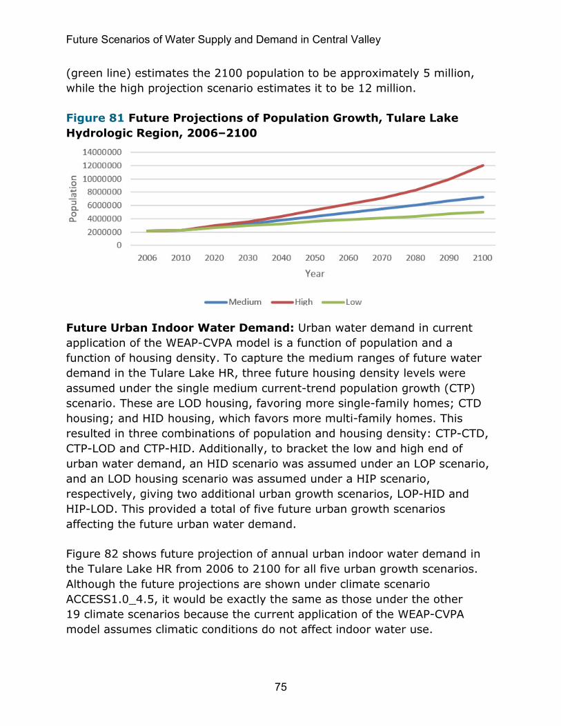
Future Scenarios of Water Supply and Demand in Central Valley
75
(green line) estimates the 2100 population to be approximately 5 million, while the high projection scenario estimates it to be 12 million.
Figure 81 Future Projections of Population Growth, Tulare Lake Hydrologic Region, 2006–2100
Future Urban Indoor Water Demand: Urban water demand in current application of the WEAP-CVPA model is a function of population and a function of housing density. To capture the medium ranges of future water demand in the Tulare Lake HR, three future housing density levels were assumed under the single medium current-trend population growth (CTP) scenario. These are LOD housing, favoring more single-family homes; CTD housing; and HID housing, which favors more multi-family homes. This resulted in three combinations of population and housing density: CTP-CTD, CTP-LOD and CTP-HID. Additionally, to bracket the low and high end of urban water demand, an HID scenario was assumed under an LOP scenario, and an LOD housing scenario was assumed under a HIP scenario, respectively, giving two additional urban growth scenarios, LOP-HID and HIP-LOD. This provided a total of five future urban growth scenarios affecting the future urban water demand.
Figure 82 shows future projection of annual urban indoor water demand in the Tulare Lake HR from 2006 to 2100 for all five urban growth scenarios. Although the future projections are shown under climate scenario ACCESS1.0_4.5, it would be exactly the same as those under the other 19 climate scenarios because the current application of the WEAP-CVPA model assumes climatic conditions do not affect indoor water use.

Future Scenarios of Water Supply and Demand in Central Valley
76
As shown in the Figure 82, the current trend projection CTP-CTD (blue line) represents the mid-level projection and shows an annual projected urban indoor demand starting with approximately 300 taf in 2006 and increasing to approximately 1,700 taf by the end of the century. The red line shows the low-end projection under the LOP-HID scenario which increases to approximately 1,400 taf by 2100. As expected, the high-end urban growth scenario HIP-LOD (orange line) resulted in the highest increase, to approximately 2,500 taf by 2100.
Figure 82 Future Projections of Urban Indoor Water Demand, Tulare Lake Hydrologic Region, Five Urban Growth Scenarios, 2006–2100
Note: K = thousand acre-feet Scenarios legend: Orange = high population-low density (HIP-LOD), Light Blue = current trend population-low density (CTP-LOD), Blue = current trend population-current trend density (CTP-CTD), Green = current trend population-high density (CTP-HID), Red = low population-high density (LOP-HID)
4.3.2.2 Urban Indoor Water Supply Delivery
Figure 83 shows future projections (2006–2100) of volumes of water supplies including surface water, groundwater, and return flows, in thousand acre-feet, delivered to urban indoor demand sites under the ACCESS1.0_8.5 climate scenario for all five urban growth scenarios. Urban indoor water supply deliveries follow a very close trend projection to those of demand volumes requested by urban indoor demand sites, as shown in Figure 82. This is because water supply deliveries to urban indoor demand sites in the current WEAP-CVPA model application is set at a high-priority level. This implies most urban demand sites will receive most of their requested demand volumes except in areas competing with other demand sites and

Future Scenarios of Water Supply and Demand in Central Valley
77
under severe climate conditions as discussed in Section 4.3.2.3, “Urban Indoor Unmet Water Demands (Shortages).”
As shown in Figure 83, the urban scenario LOP-HID (red line) showed low projections of water supply deliveries to urban indoor demand sites which follows its low-end demand trajectory discussed above. As expected, the urban scenario HIP-LOD (orange line) showed a high-end projection because of its high-end water demand.
It should be noted, even though urban indoor demand is assumed not to be a function of climate factors, the amount of available supplies on the supply side are driven by climatic and hydrologic conditions. This is clearly evident in Figure 83 where supply deliveries to indoor demand sites become more erratic toward the end of the century. This is because, as demand for water increases over time, certain climatic and hydrologic conditions may not be able to generate consistent and reliable water supply, resulting in fluctuating supply deliveries toward the end of 2100. The problem becomes even more severe under the high demand HIP-LOD urban growth scenario (orange line). This is in contrast with low-end demand scenario LOP-HID (red line) which provides more consistent supply deliveries with no evidence of erratic behavior throughout the years under the same climate scenario, ACCESS1.0-8. Note: This highlights the model performance in capturing subtle scenario variations under the conditions tested.
Figure 83 Future Projections of Urban Indoor Water Supply Delivery, Tulare Lake Hydrologic Region, Five Urban Growth Scenarios, 2006–2100
Note: K = thousand acre-feet Scenarios legend: Orange = high population-low density (HIP-LOD), Light Blue = current trend population-low density (CTP-LOD), Blue = CTP-CTD, Orange = CTP-HID, Red = LOP-HID

Future Scenarios of Water Supply and Demand in Central Valley
78
4.3.2.3 Urban Indoor Unmet Water Demands (Shortages)
Figure 84 shows future projections of annual unmet demand in the urban indoor sector in thousand acre-feet within the Tulare Lake HR from 2006 to 2100 for the moderate CTP-CTD urban growth scenario for all 20 climate scenarios. Toward the end of the century, the magnitude of unmet demand becomes larger and occurs more frequently depending on severity of hydrologic and climatic conditions. The maximum unmet volume peaks at approximately 320 taf under climate scenario ACCESS1.0_4.5 in 2093.
Figure 84 Future Projections of Urban Indoor Unmet Water Demand, Tulare Lake Hydrologic Region, Single Urban Growth Scenario CTP-CTD, 2006–2100
Note: CTP-CTD = current-trend population–current-trend density, K = thousand acre-feet
But under the more aggressive high-population urban growth scenario, HIP-LOD, the future unmet demand in urban indoor sector becomes even more severe and more frequent toward the end of the century, as shown in Figure 85. It peaks at approximately 480 taf around 2093 under the same ACCESS1.0_4.5 climate scenario. A more rigorous vulnerability analysis to identify Tulare Lake HR urban sector areas prone to long-term water shortages is provided in Section 4.3.4.3, “Urban Outdoor Water Shortages.”

Future Scenarios of Water Supply and Demand in Central Valley
79
Figure 85 Future Projections of Urban Indoor Unmet Water Demand, Tulare Lake Hydrologic Region, Single Urban Growth Scenario HIP-LOD, 2006–2100
Note: HIP-LOD = high population-low density, K = thousand acre-feet
4.3.3 Urban Outdoor
4.3.3.1 Urban Outdoor Water Demand
Unlike urban indoor demand, which was assumed to not be a function of climate in the current WEAP-CVPA model application, the urban outdoor demand in residential, commercial, and large landscapes can vary from year to year as a function of climatic conditions reflected by different climate scenarios. The urban outdoor demand is not only a function of urban expansion, but also a function of climatic conditions which can vary annually and between climate scenarios.
Figure 86 shows future projections of the annual urban outdoor demand in thousand acre-feet in the Tulare Lake HR under the 20 climate scenarios for the moderate CTP-CTD urban scenario from 2006 to 2100. Urban outdoor demand increases over time in response to urban expansion under all 20 climate scenarios. On average, the increase is from approximately 240 taf in 2006 to approximately 410 taf by 2100.

Future Scenarios of Water Supply and Demand in Central Valley
80
Figure 86 Future Projections of Urban Outdoor Water Demand, Tulare Lake Hydrologic Region, Single Urban Growth Scenario CTP-CTD, 20 Climate Scenarios, 2006–2100
Note: CTP-CTD = current-trend population–current-trend density, K = thousand acre-feet
But under a more aggressive urban expansion scenario, HIP-LOD (i.e., more single-family homes), the increase of water demand becomes steeper and more scattered among the 20 climate scenarios toward the end of the century, as shown in Figure 87. On average, it increases from 240 taf in 2006 to approximately 530 taf by 2100.
Figure 87 Future Projections of Urban Outdoor Water Demand, Tulare Lake Hydrologic Region, Single Urban Growth Scenario HIP-LOD, 20 Climate Scenarios, 2006–2100
Note: HIP-LOD = high population-low density, K = thousand acre-feet
Figure 88 shows the relative effects of the five urban growth scenarios on urban outdoor water demand, for climate scenario ACCESS1.0_4.5 from 2006 to 2100. The more aggressive urban expansion

Future Scenarios of Water Supply and Demand in Central Valley
81
HIP-LOD scenario (light blue line) has the greatest impact, especially toward the end of the century. It increased from approximately 270 taf in 2006 to approximately 520 taf around 2100. As expected, the least-expansive scenario, LOP-HID (green line), had the least effect on urban water demand. On average, it increased to a moderate 290 taf toward the end of the century. The annual fluctuation in outdoor water demand under all five urban growth scenarios is the result of inter-annual climate variations affecting outdoor landscape consumptive uses.
Figure 88 Future Projections of Urban Outdoor Water Demand, Tulare Lake Hydrologic Region, Single Climate Scenario ACCESS1.0-4.5, Five Urban Growth Scenarios, 2006–2100
Note: K = thousand acre-feet Scenarios legend: Light Blue = high population-low density (HIP-LOD), Red = current trend population-low density (CTP-LOD), Blue = current trend population-current trend density (CTP-CTD), Orange = current trend population-high density (CTP-HID), Green = low population-high density (LOP-HID)
4.3.3.2 Urban Outdoor Water Supply Delivery
Figure 89 shows water supply deliveries in thousand acre-feet including surface water, groundwater, and return flows, delivered to meet the water demand of outdoor landscape sites within the Tulare Lake HR under all 20 climate scenarios for the moderate urban expansion scenario CTP-CTD from 2006 to 2100. On average, the supply deliveries increased from approximately 240 taf in 2006 to approximately 430 taf by 2100 under this moderate urban expansion scenario.
But under the more expansive urban scenario HIP-LOD, the increase in water supply delivery was more drastic, as shown in Figure 90. On average, it increased from approximately 240 taf in 2006 to approximately 540 taf in 2100.

Future Scenarios of Water Supply and Demand in Central Valley
82
Figure 89 Future Projections of Urban Outdoor Water Supply Delivery, Tulare Lake Hydrologic Region, Single Urban Growth Scenario CTP-CTD, 20 Climate Scenarios, 2006–2100
Note: CTP-CTD = current-trend population–current-trend density, K = thousand acre-feet
Figure 90 Future Projections of Urban Outdoor Water Supply Delivery, Tulare Lake Hydrologic Region, Single Urban Growth Scenario HIP-LOD, 20 Climate Scenarios, 2006–2100
Note: HIP-LOD = high population-low density, K = thousand acre-feet
Figure 91 shows the relative effects of all five urban growth scenarios on supply deliveries to meet the outdoor landscape water demand for the ACCESS1.0-4.5 climate scenario. The more expansive urban growth HIP-LOD scenario (light blue line) has the greatest effect on supply deliveries to meet the ever-increasing water demand toward the end of the century relative to the other four urban scenarios. The least expansive urban scenario, LOP-HID, has the least effect on required supply deliveries (green line).

Future Scenarios of Water Supply and Demand in Central Valley
83
Figure 91 Future Projections of Urban Outdoor Supply Delivery, Tulare Lake Hydrologic Region, Single Climate Scenario ACCESS1.0-4.5, Five Urban Growth Scenarios, 2006–2100
Note: K = thousand acre-feet Scenarios legend: Light Blue = high population-low density (HIP-LOD), Red = current trend population-low density (CTP-LOD), Blue = current trend population-current trend density (CTP-CTD), Orange = current trend population-high density (CTP-HID), Green = low population-high density (LOP-HID)
4.3.3.3 Urban Outdoor Unmet Water Demand (Shortages)
Figure 92 shows the volumes of unmet demand in thousand acre-feet for the moderate urban growth scenario CTP-CTD under 20 climate scenarios for all outdoor landscape sites in the Tulare Lake HR from 2006 to 2100. As mentioned previously, because urban demand sites have the highest priority in meeting their water demand, as set in the current WEAP-CVPA model application, there are only few instances when future outdoor landscape demands are not met; especially more toward the end of the century, as shown in Figure 92. On average, the unmet outdoor demand peaks at approximately 150 taf around 2093 (blue line) under the ACCESS1.0_4.5 climate scenario. A more rigorous analysis of likelihoods and vulnerabilities to water shortages in the urban outdoor sector is provided in Section 4.3.4.3, “Urban Outdoor Water Shortages.”
More detailed information on climate scenarios that result in more frequent occurrences of large quantities of unmet demands is available in the companion Tableau Dashboard.
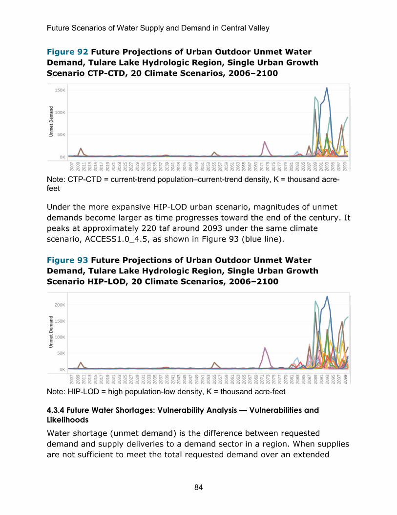
Future Scenarios of Water Supply and Demand in Central Valley
84
Figure 92 Future Projections of Urban Outdoor Unmet Water Demand, Tulare Lake Hydrologic Region, Single Urban Growth Scenario CTP-CTD, 20 Climate Scenarios, 2006–2100
Note: CTP-CTD = current-trend population–current-trend density, K = thousand acre-feet
Under the more expansive HIP-LOD urban scenario, magnitudes of unmet demands become larger as time progresses toward the end of the century. It peaks at approximately 220 taf around 2093 under the same climate scenario, ACCESS1.0_4.5, as shown in Figure 93 (blue line).
Figure 93 Future Projections of Urban Outdoor Unmet Water Demand, Tulare Lake Hydrologic Region, Single Urban Growth Scenario HIP-LOD, 20 Climate Scenarios, 2006–2100
Note: HIP-LOD = high population-low density, K = thousand acre-feet
4.3.4 Future Water Shortages: Vulnerability Analysis — Vulnerabilities and Likelihoods Water shortage (unmet demand) is the difference between requested demand and supply deliveries to a demand sector in a region. When supplies are not sufficient to meet the total requested demand over an extended

Future Scenarios of Water Supply and Demand in Central Valley
85
period of time, or where only a portion of demand is met, then the region may be deemed vulnerable and prone to extended water shortages. But some regions may reduce their demand as part of their mandatory best management practices and water management strategies, or as a voluntary measure, to accept some level of water shortages. This reduced level of demand is termed “demand threshold.” By changing demand thresholds, the likelihood of water shortages can change too. For example, reducing the demand threshold can result in lowering the likelihood of water shortages because available supplies can more frequently meet the reduced level of demands characterized by the demand threshold.
Through vulnerability analysis, future water shortages and their likelihoods over an extended period of time can be quantified and regions prone to long-term water shortages can be identified. This can help guide planning and allocation of future investments and resources to reduce vulnerabilities and risks to water shortages in a region.
Vulnerability maps can show long-term likelihoods of water shortages at the regional HR level and at the PA level. Regional level vulnerabilities may mask risks at smaller scales. As a result, quantifying and assessing PA level vulnerabilities will help identify PAs exhibiting more severe vulnerabilities. Vulnerability analyses described in the following section are provided as examples under selected urban growth and climate scenarios. More detailed information on vulnerability analyses under other future scenarios, is available in companion Tableau Dashboard.

Future Scenarios of Water Supply and Demand in Central Valley
86
4.3.4.1 Agricultural Water Shortages
Figure 94 (a and b) shows the long-term future vulnerability of agricultural sectors at regional level in the Tulare Lake HR. It shows likelihoods of water shortages under the CTP-CTD urban growth and ACCESS1.0_4.5 climate scenarios for 100 percent demand threshold (no demand reduction) (a) and
95 percent demand threshold (5 percent demand reduction) (b). Figure 94a shows, when no demand reduction is adopted, the likelihood of water shortages will be approximately 72.6 percent. This implies agricultural sectors in the Tulare Lake region at HR level, as a whole, will not receive their total requested demand approximately 72.6 percent of time over the next 100 years. But when a 5 percent demand reduction plan is adopted (demand threshold of 95 percent), as shown in Figure 94b, the region vulnerability to water shortages is reduced to 49.5 percent. This implies there will be a lower risk of about 49.5 percent that agricultural sectors may face water shortages of approximately 5 percent (or greater) over the next 100 years.
Figure 94 Vulnerability Map, Agricultural Water Shortages at 100 Percent and 95 Percent Demand Threshold, Tulare Lake (TL) Hydrologic Region
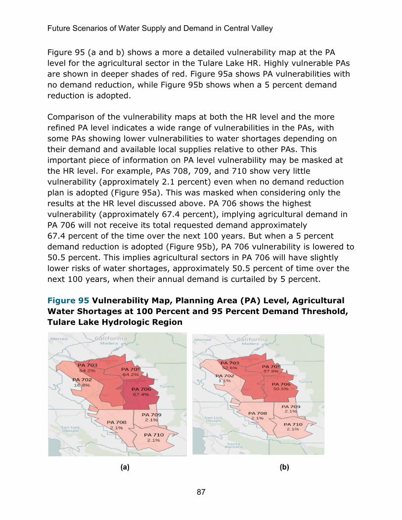
Future Scenarios of Water Supply and Demand in Central Valley
87
Figure 95 (a and b) shows a more a detailed vulnerability map at the PA level for the agricultural sector in the Tulare Lake HR. Highly vulnerable PAs are shown in deeper shades of red. Figure 95a shows PA vulnerabilities with no demand reduction, while Figure 95b shows when a 5 percent demand reduction is adopted.
Comparison of the vulnerability maps at both the HR level and the more refined PA level indicates a wide range of vulnerabilities in the PAs, with some PAs showing lower vulnerabilities to water shortages depending on their demand and available local supplies relative to other PAs. This important piece of information on PA level vulnerability may be masked at the HR level. For example, PAs 708, 709, and 710 show very little vulnerability (approximately 2.1 percent) even when no demand reduction plan is adopted (Figure 95a). This was masked when considering only the results at the HR level discussed above. PA 706 shows the highest vulnerability (approximately 67.4 percent), implying agricultural demand in PA 706 will not receive its total requested demand approximately 67.4 percent of the time over the next 100 years. But when a 5 percent demand reduction is adopted (Figure 95b), PA 706 vulnerability is lowered to 50.5 percent. This implies agricultural sectors in PA 706 will have slightly lower risks of water shortages, approximately 50.5 percent of time over the next 100 years, when their annual demand is curtailed by 5 percent.
Figure 95 Vulnerability Map, Planning Area (PA) Level, Agricultural Water Shortages at 100 Percent and 95 Percent Demand Threshold, Tulare Lake Hydrologic Region
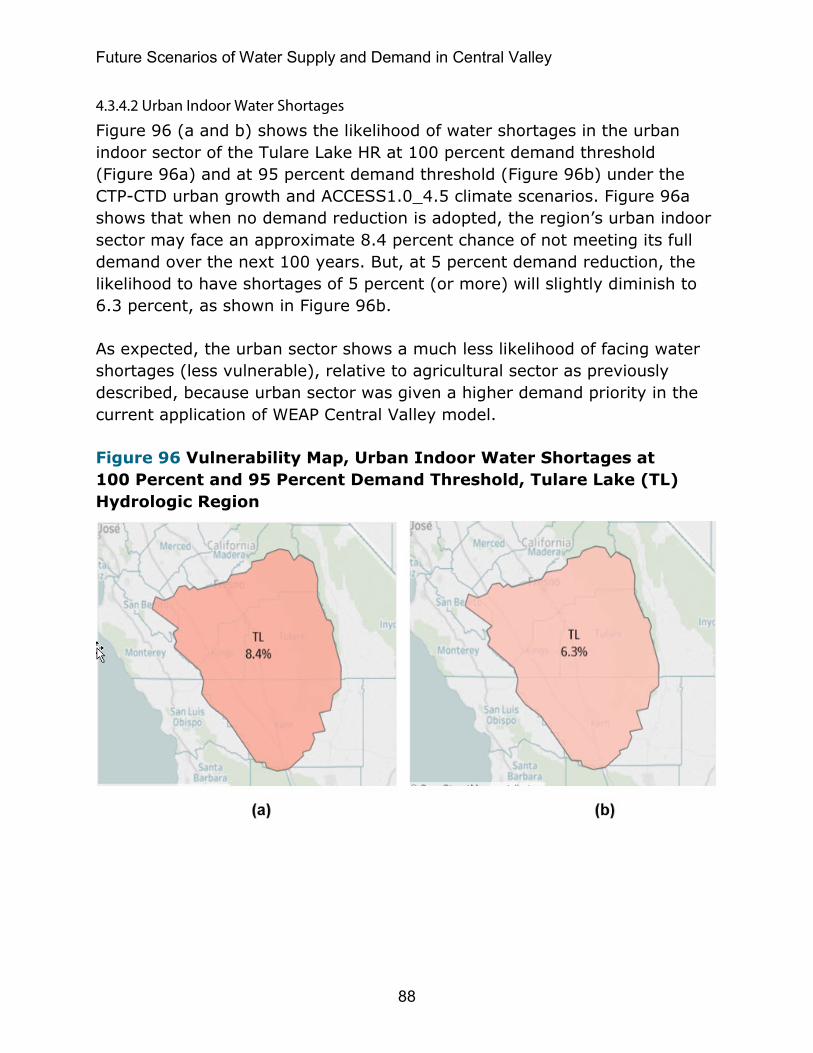
Future Scenarios of Water Supply and Demand in Central Valley
88
4.3.4.2 Urban Indoor Water Shortages
Figure 96 (a and b) shows the likelihood of water shortages in the urban indoor sector of the Tulare Lake HR at 100 percent demand threshold (Figure 96a) and at 95 percent demand threshold (Figure 96b) under the CTP-CTD urban growth and ACCESS1.0_4.5 climate scenarios. Figure 96a shows that when no demand reduction is adopted, the region’s urban indoor sector may face an approximate 8.4 percent chance of not meeting its full demand over the next 100 years. But, at 5 percent demand reduction, the likelihood to have shortages of 5 percent (or more) will slightly diminish to 6.3 percent, as shown in Figure 96b.
As expected, the urban sector shows a much less likelihood of facing water shortages (less vulnerable), relative to agricultural sector as previously described, because urban sector was given a higher demand priority in the current application of WEAP Central Valley model.
Figure 96 Vulnerability Map, Urban Indoor Water Shortages at 100 Percent and 95 Percent Demand Threshold, Tulare Lake (TL) Hydrologic Region

Future Scenarios of Water Supply and Demand in Central Valley
89
Figure 97 (a and b) shows the same urban indoor vulnerability map, but at a more detailed PA level. As shown in Figure 97a, most parts of the region exhibit no vulnerability (0 percent) to water shortages. The exceptions are PA 705 and PA 706 which show vulnerabilities of 7.4 percent and 8.4 percent, respectively. This is similar to the agricultural sectors where these two PAs showed the highest vulnerabilities. This may indicate an underlying water supply issue in these two PAs. But, when a
5 percent demand reduction (95 percent demand threshold) is adopted, PA 706 shows some signs of improvements; its vulnerability slightly drops to approximately 6.3 percent. But, no improvements were seen in PA 705; its vulnerability remains at 7.4 percent. This indicates PA 705 has more serious water supply issues than PA 706 and may be more prone to long-term water shortages.
Vulnerability maps at the PA level can identify specific PAs prone to future water shortages that could have been masked when considering vulnerabilities only at the regional level. For example, PA 705 in the Tulare Lake HR has been identified as one of the problem areas with long-term water supply issues. It may have higher chances of water shortages both in agricultural and urban indoor sectors over the next 100 years when compared with other PAs.
Figure 97 Vulnerability Map, Planning Area (PA) Level, Urban Indoor Water Shortages at 100 Percent and 95 Percent Demand Threshold, Tulare Lake Hydrologic Region

Future Scenarios of Water Supply and Demand in Central Valley
90
4.3.4.3 Urban Outdoor Water Shortages
Figure 98 (a and b) shows vulnerabilities of the urban outdoor sector to water shortages in the Tulare Lake region at HR level over the next 100 years for the CTP-CTD urban growth and ACCESS1.0_4.5 climate scenarios.
Figure 98a shows that likelihood of water shortages at HR level, when no demand reduction is adopted, is very high at 100 percent. This implies Tulare Lake’s regional urban outdoor demand will not be met in any single year over the next 100 years when 100 percent demand is requested. But, when a 5 percent demand reduction is adopted (95 percent demand threshold), the vulnerability to water shortages drops to 6.3 percent, as shown in Figure 98b.
Figure 98 Vulnerability Map, Urban Outdoor Water Shortages at 100 Percent and 95 Percent Demand Threshold, Tulare Lake (TL) Hydrologic Region
Figure 99 (a and b) shows urban outdoor vulnerabilities to water shortages, but at more detailed PA level within the Tulare Lake HR. As Figure 99a shows, when no demand reduction was adopted,
PA 702 was the only PA which showed the highest vulnerability of approximately 100 percent. This implies urban outdoor sectors in PA 702 will not receive their total requested demand in any single year within the next 100 years. Other PAs showed very little or no vulnerabilities. But, when a 5 percent demand reduction is adopted (Figure 99b), PA 702 showed a

Future Scenarios of Water Supply and Demand in Central Valley
91
drastic drop in its vulnerability. It dropped from 100 percent to approximately 5.3 percent. This indicates, annual water supplies in PA 702 are sufficient enough to meet the annual demand at reduced level (5 percent) in most of the years over the next 100 years.
This also implies the 100 percent vulnerability exhibited at regional level discussed above was because of a water shortage problem in a single PA (PA 702) which could have been masked if only considering vulnerabilities at HR level. This is another example of analyzing vulnerabilities at the regional level can lead to wrong conclusions in identifying water shortage issues at local levels. The analysis should be performed at smaller scale, for example, at PA level, to provide more accurate information.
It should also be noted that because the above findings should not be generalized to other urban growth and climate scenarios, the results under other scenario conditions are available in the Tableau Dashboard.
Figure 99 Vulnerability Map, Planning Area (PA) Level, Urban Outdoor Water Shortages at 100 Percent and 95 Percent Demand Threshold, Tulare Lake Hydrologic Region

Future Scenarios of Water Supply and Demand in Central Valley
92
4.4 Future Water Storage Conditions WEAP computes storages of surface reservoirs and groundwater aquifers based on physical capacity, initial capacity, inflows and outflows, operational rules, and conservation of mass during each time step of its computation process. Physical capacity of surface storage is based on known design capacity. Because accurate physical capacity of a groundwater aquifer is not known, an estimate of its physical capacity is used. To remove errors associated with using estimates of aquifer physical capacity, “change in computed storage” for an aquifer is evaluated over time, rather than the absolute storage values.
Climate change and urban growth both affect surface and groundwater storages through changes in inflows and outflows. Urban growth affects only the demand side of the water balance equation, which applies only to outflows. Climate change affects both the demand and the supply. It affects inflow hydrology on supply side, through rainfall and snowmelt runoff. It also affects the outflow releases on the demand side by affecting downstream evapotranspiration requirements of urban outdoor landscape and agricultural crops. Because there are 100 combinations of urban and climate scenarios affecting surface and groundwater storages, the results are discussed only for a limited number of scenarios. For more detailed and interactive analysis of other scenarios, refer to the companion Tableau Dashboard.
4.4.1 Surface Storage Future projections and general trend of monthly storages in major reservoirs in the Central Valley are presented in million acre-feet (maf) under all 20 climate scenarios through 2100 for the urban growth scenario CTP-CTD. To visualize the results under other all five urban growth scenarios, refer to the companion Tableau Dashboard.
Shasta Reservoir: Figure 100 shows that the storage level in Shasta Reservoir remains at less than 2 maf more frequently toward the end of the century. Climate scenario CCSM4_8.5 (green line) results in lowest storage of 1.28 maf around 2097.

Future Scenarios of Water Supply and Demand in Central Valley
93
Figure 100 Future Projections of Monthly Storages in Shasta Reservoir, Single Urban Growth Scenario CTP-CTD, 20 Climate Scenarios, 2006–2100
Note: CTP-CTD = current-trend population–current-trend density, M = million acre-feet
Oroville Reservoir: Figure 101 shows no distinct declining trend in Oroville Reservoir storage over time, except a very low point at 0.9 maf around 2010 under climate scenario CMCC_CMS_4.5.
Figure 101 Future Projections of Monthly Storages in Oroville Reservoir, Single Urban Growth Scenario CTP-CTD, 20 Climate Scenarios, 2006–2100
Note: CTP-CTD = current-trend population–current-trend density, M = million acre-feet
Folsom Reservoir: Figure 102 also shows no distinct declining trend in Folsom Reservoir storage over time, except a very low point of 0.3 maf around 2010 under climate scenario CMCC_CMS_4.5.

Future Scenarios of Water Supply and Demand in Central Valley
94
Figure 102 Future Projections of Monthly Storages in Folsom Reservoir, Single Urban Growth Scenario CTP-CTD, 20 Climate Scenarios, 2006–2100
Note: CTP-CTD = current-trend population–current-trend density, K = thousand acre-feet
San Luis Reservoir: Figure 103 shows future projections of storage in San Luis Reservoir with no distinct declining trend over time, except a low point of approximately 0.1 maf in multiple years under climate scenario CMCC_CMS_4.5 (green line).
Figure 103 Future Projections of Monthly Storages in San Luis Reservoir, Single Urban Growth Scenario CTP-CTD, 20 Climate Scenarios, 2006–2100
Note: CTP-CTD = current-trend population–current-trend density, M = million acre-feet
Don Pedro Reservoir: Figure 104 shows future projections of storage in Don Pedro Reservoir with levels declining around 2090 under all 20 climate scenarios, with low points of approximately 0.6 maf. In addition, storage declined to two distinct very low points, 0.15 maf in 2010 and 0.28 maf in 2055, under the climate scenario CMCC_CMS_4.5 (green line).

Future Scenarios of Water Supply and Demand in Central Valley
95
Figure 104 Future Projections of Monthly Storages in Don Pedro Reservoir, Single Urban Growth Scenario CTP-CTD, 20 Climate Scenarios, 2006–2100
Note: CTP-CTD = current-trend population–current-trend density, M = million acre-feet
New Melones Reservoir: Figure 105 shows future projections of storage in New Melones Reservoir with levels declining around 2090 under all 20 climate scenarios, with a low point of approximately 0.75 maf. In addition, storage declined to two distinct very low points, 0.20 maf in 2010 and 0.27 maf in 2055, under the climate scenario CMCC_CMS_4.5 (green line).
Figure 105 Future Projections of Monthly Storages in New Melones Reservoir, Single Urban Growth Scenario CTP-CTD, 20 Climate Scenarios, 2006–2100
Note: CTP-CTD = current-trend population–current-trend density, M = million acre-feet
New Hogan Reservoir: Figure 106 shows future projections of storage in thousand acre-feet (taf) in New Hogan Reservoir with levels declining around and after 2080 under all 20 climate scenarios, with a low point of approximately 15 taf in 2095.

Future Scenarios of Water Supply and Demand in Central Valley
96
Figure 106 Future Projections of Monthly Storages in New Hogan Reservoir, Single Urban Growth Scenario CTP-CTD, 20 Climate Scenarios, 2006–2100
Note: CTP-CTD = current-trend population–current-trend density, K = thousand acre-feet
New Bullards Bar Reservoir: Figure 107 shows no distinct declining trend in New Bullards Bar Reservoir storages over time, except a very low point of 0.3 maf around 2010 and again in 2055 under the climate scenario CMCC_CMS_4.5. There are also a few instances of low points after 2080.
Figure 107 Future Projections of Monthly Storages in New Bullards Reservoir, Single Urban Growth Scenario CTP-CTD, 20 Climate Scenarios, 2006–2100
Note: CTP-CTD = current-trend population–current-trend density, K = thousand acre-feet
Millerton Reservoir: Figure 108 shows no declining trend in Millerton Reservoir storages over time under any of the 20 climate scenarios.
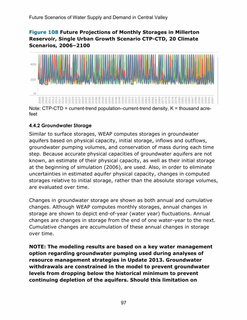
Future Scenarios of Water Supply and Demand in Central Valley
97
Figure 108 Future Projections of Monthly Storages in Millerton Reservoir, Single Urban Growth Scenario CTP-CTD, 20 Climate Scenarios, 2006–2100
Note: CTP-CTD = current-trend population–current-trend density, K = thousand acre-feet
4.4.2 Groundwater Storage Similar to surface storages, WEAP computes storages in groundwater aquifers based on physical capacity, initial storage, inflows and outflows, groundwater pumping volumes, and conservation of mass during each time step. Because accurate physical capacities of groundwater aquifers are not known, an estimate of their physical capacity, as well as their initial storage at the beginning of simulation (2006), are used. Also, in order to eliminate uncertainties in estimated aquifer physical capacity, changes in computed storages relative to initial storage, rather than the absolute storage volumes, are evaluated over time.
Changes in groundwater storage are shown as both annual and cumulative changes. Although WEAP computes monthly storages, annual changes in storage are shown to depict end-of-year (water year) fluctuations. Annual changes are changes in storage from the end of one water-year to the next. Cumulative changes are accumulation of these annual changes in storage over time.
NOTE: The modeling results are based on a key water management option regarding groundwater pumping used during analyses of resource management strategies in Update 2013. Groundwater withdrawals are constrained in the model to prevent groundwater levels from dropping below the historical minimum to prevent continuing depletion of the aquifers. Should this limitation on

Future Scenarios of Water Supply and Demand in Central Valley
98
groundwater pumping be removed, the results are expected to be different.
The following set of figures depict future projections of changes in groundwater storage for climate scenario ACCESS1.0-4.5 and urban growth scenario CTP-CTD. Annual changes are shown as a solid bar and cumulative changes by a solid line. While annual changes show annual gains or losses in groundwater storage, the cumulative storage keeps track of cumulative changes of groundwater storage over time. To visualize the results under all five urban growth scenarios, refer to Tableau Dashboard.
Sacramento River Hydrologic Region: Figure 109 shows end-of-year projections of annual and cumulative changes in groundwater storage in Sacramento River HR in million acre-feet relative to initial storage from 2006 to 2100.
Figure 109 Future Projections of Annual (end of year) Groundwater Storages in Sacramento River Hydrologic Region, Single Urban Growth Scenario CTP-CTD, Climate Scenario ACCESS 1.0-4.5, 2006–2100
Note: CTP-CTD = current-trend population–current-trend density, M = million acre-feet
San Joaquin River Hydrologic Region: Figure 110 shows end-of-year projections of annual and cumulative changes in groundwater storage in San Joaquin River HR in million acre-feet relative to initial storage from 2006 through 2100.

Future Scenarios of Water Supply and Demand in Central Valley
99
Figure 110 Future Projections of Annual (end-of-year) Groundwater Storages in San Joaquin River Hydrologic Region, Single Urban Growth Scenario CTP-CTD, Climate Scenario ACCESS 1.0-4.5, 2006–2100
Note: CTP-CTD = current-trend population–current-trend density, M = million acre-feet
Tulare Lake Hydrologic Region: Figure 111 shows end of year projections of annual and cumulative changes in groundwater storage in Tulare Lake HR in million acre-feet relative to initial storage from start year 2006 through year 2100.
Figure 111 Future Projections of Annual (end-of-year) Groundwater Storages in Tulare Lake River Hydrologic Region, Single Urban Growth Scenario CTP-CTD, Climate Scenario ACCESS 1.0-4.5, 2006–2100
Note: CTP-CTD = current-trend population–current-trend density, M = million acre-feet

Future Scenarios of Water Supply and Demand in Central Valley
100

5. Conclusions and Recommendations
101
5. Conclusions and Recommendations A fully integrated water supply and demand model based on the WEAP analytical tool was used to project future water conditions in California’s Central Valley in support of Update 2018. Future projections are based on a combination of five urban growth scenarios and 20 climate scenarios recommended by DWR’s CCTAG. This resulted in 100 scenarios of alternative futures, accounting for uncertainties of urban growth, land use pattern, and climate factors. The projections provide annual variations of water demand, supply deliveries, and the gap between the demand and the delivered supplies (supply shortfalls) starting from the base year, 2006, through the end of the century, 2100.
Generally, the results indicate future urban indoor and outdoor demands will increase over time in all three hydrologic regions of the Central Valley as a result of population and urban growth scenarios considered in current study. Urban outdoor demand was further influenced by climate factors including precipitation and temperature affecting outdoor landscape consumptive demands resulting in inter-annual variations of outdoor demand over the projection period. From the five urban growth scenarios studied, the HIP-LOD scenario resulted in higher future urban demand projections compared to the other four urban growth scenarios. As expected, the LOP-HID scenario resulted in low-end demand projections.
The results also show that the future agricultural water demand will generally have a downward trend. This is because of loss of agricultural acreages resulting from urbanization and encroachment into farmlands. No future economic factors, federal farming bills, or international food trades were considered in this study. In addition, the results showed that the future agricultural water demands are also greatly influenced by climate factors, such as temperature and precipitation, affecting crop consumptive demand resulting in inter-annual variations over the projection period. Among the five urbanization scenarios studied, the aggressive HIP-LOD scenario (which resulted in a high-end urban demand) shows a low-end water demand in agricultural sector because of a greater loss of agricultural lands to urbanization when compared with four other less-aggressive urban scenarios.

Future Scenarios of Water Supply and Demand in Central Valley
102
The water supply deliveries to meet the required future demand also generally followed the demand trend in urban and agricultural sectors. The results showed the sufficiency of available supplies in the near term. But as time progressed toward the end of the century there were widespread instances of unmet demands (supply shortfalls) because of increasing demand and decreasing supplies as a result of the combined effects of urban growth and climate factors. This was more prevalent in agricultural sectors because urban sectors were assigned a higher demand priority in receiving available supplies in current WEAP demand-priority assignments.
To identify and evaluate vulnerable areas prone to long-term water shortages, a statistical analysis was performed on frequencies and magnitude of future unmet demand (water shortages) both at regional (hydrologic region) and planning area levels. Vulnerability maps for each region were developed in Tableau Dashboard. The results show that the agricultural sector, in general, is more vulnerable to
long-term water shortages relative to urban sectors in the three regions of the Central Valley under the scenarios studied. But the results vary depending on the type of urban growth and climate scenario chosen. To visualize the detailed results, refer to the Tableau Dashboard.
Future projections of surface and groundwater storages in the Central Valley were also evaluated for the next 100 years under the scenarios considered. Some reservoirs are likely to have more incidences of low storage toward the end of the century. Shasta Reservoir shows extended periods of low storage of less than 2 maf around 2090 and beyond, while Oroville and Folsom reservoirs show more consistent trend. Don Pedro and New Melones reservoirs showed similar low storage beyond 2090. New Hogan Reservoir exhibited a continuous downward trend in storage over time toward 2100. Groundwater storage showed more resilience to incidences of low storages. This was partly because higher preference was given to surface storage, rather than to groundwater storage, as a supply option in the current WEAP application. In addition, constraints were imposed on groundwater withdrawals in order to maintain the historical minimum. This assumption was made based on resource management strategies evaluated in Update 2013 to protect the future levels of groundwater aquifers. By adopting different strategies and/or changing these assumptions, the results would be different.

Future Scenarios of Water Supply and Demand in Central Valley
103
The results shown in this report are based on a set of modeling assumptions, limitations, and conditions embedded in the future scenarios evaluated. The results should be considered relative changes that capture the range of possible future water conditions. Also, because the current study covers only the Central Valley, the analyses may need to be extended to the other hydrologic regions of the state at the planning area level to obtain a more complete statewide picture of the future supply and demand conditions. Such analyses would likely help identify remote areas which may be vulnerable to long-term supply shortages or areas which may have potential for future water supply development.
Finally, to improve modeling assumptions and to provide better estimates and more accurate information on future water conditions in California, the following next steps are recommended:
• Improve State Water Project and Central Valley Project reservoir operations and water-supply allocation logic.
• Improve Sacramento-San Joaquin Delta operation and outflow requirements for salinity control based on an artificial neural network.
• Incorporate the effects of climate-driven sea level rise on water supply and demand conditions.
• Improve environmental flow requirements by including the latest biological opinions.
• Expand the existing Central Valley modeling coverage to the other hydrologic regions to provide a more complete statewide picture of future water conditions in California.
• Assess water reliability and the associated economic effects of resource management strategies including supply augmentation and demand reduction options.

Future Scenarios of Water Supply and Demand in Central Valley
104

6. References
105
6. References California Department of Water Resources. 2019a. California Water Plan
Update 2005. Sacramento (CA): California Department of Water Resources. California Natural Resources Agency. Viewed online: http://www.waterplan.water.ca.gov/cwpu2005
California Department of Water Resources. 2019b. California Water Plan Update 2009. Sacramento (CA): California Department of Water Resources. California Natural Resources Agency. Viewed online: http://www.waterplan.water.ca.gov/cwpu2009
California Department of Water Resources. 2019c. California Water Plan Update 2013. Sacramento (CA): California Department of Water Resources. California Natural Resources Agency. Viewed online: http://www.waterplan.water.ca.gov/cwpu2013
California Department of Water Resources. 2019d. Future Scenario Dashboard. California Department of Water Resources. California Natural Resources Agency. Viewed online: https://tableau.cnra.ca.gov/t/DWR_Planning/views/WEAP_Scenarios/DemandSupplyMultiClimate?iframeSizedToWindow=true&:embed=y&:showAppBanner=false&:display_count=no&:showVizHome=no
Jonson H. Demographer, Public Policy Institute of California, Sacramento (CA), April 30, 2012 – email contact with Kibrya S, demographer, Division of Planning, California Department of Water Resources, Sacramento (CA).

Future Scenarios of Water Supply and Demand in Central Valley
106

Appendix A: Validation of the CVPA and WEAP Model
107
Appendix A. Validation of the Central Valley Planning Area and Water Evaluation and Planning Model
Stockholm Environment Institute
U.S. Job No. 10508987 — Task Order T10508987-04612-OM
Vishal K. Mehta and Charles Young
June 26, 2018

Future Scenarios of Water Supply and Demand in Central Valley
108

Future Scenarios of Water Supply and Demand in Central Valley
109
1. Scope of Work The scope of work for this project involved the validation of the Central Valley model runs under selected climate projections, until Water Year (WY) 2099. This scope of work was split into four distinct tasks.
1. Selection of climate projections.
2. Model runs for those projections.
3. Analysis of the model runs to evaluate consistency with the projections (i.e., the validation).
4. Report write-up (this document).
2. Selection of Climate Projections for Validation of Important System Variables Out of 20 climate projections, five were selected based on an analysis of the projections, as well as the recent Sustainable Groundwater Management Act (SGMA)-related climate change dataset guidance available here (downloaded May 16, 2018): https://www.water.ca.gov/Programs/Groundwater-Management/SGMA-Groundwater-Management/Best-Management-Practices-and-Guidance-Documents.
• There were 20 climate projections in the model titled “Central Valley —12 Jan 2017” shared by Mohammad Rayej, senior water resources engineer with the California Department of Water Resources. The projections included monthly climate data for each catchment, up to WY 2099.
• Average annual temperature and annual precipitation were calculated for each projection.
• Anomalies were created for both variables and each projection against overall mean variables and then plotted (Figure A-1).
Based on this analysis (Figure A-1), the following five climate projections were selected:
1. canesm2_85: representing warm-wet climate.
2. cnrm_cm5_45: representing cool-wet climate (also selected by SGMA climate guidance).
3. miroc5_45: representing cool-dry climate.

Future Scenarios of Water Supply and Demand in Central Valley
110
4. hadgem2_es_85: warm-dry climate (also selected by SGMA climate guidance).
5. ccsm4_85: representing a projection close to the ensemble’s central tendency.
These projections are labelled in red in Figure A-1.
Figure A-1 Climate Projections Compared
Note: This figure shows the anomalies of precipitation and temperature against an ensemble mean precipitation and temperature.
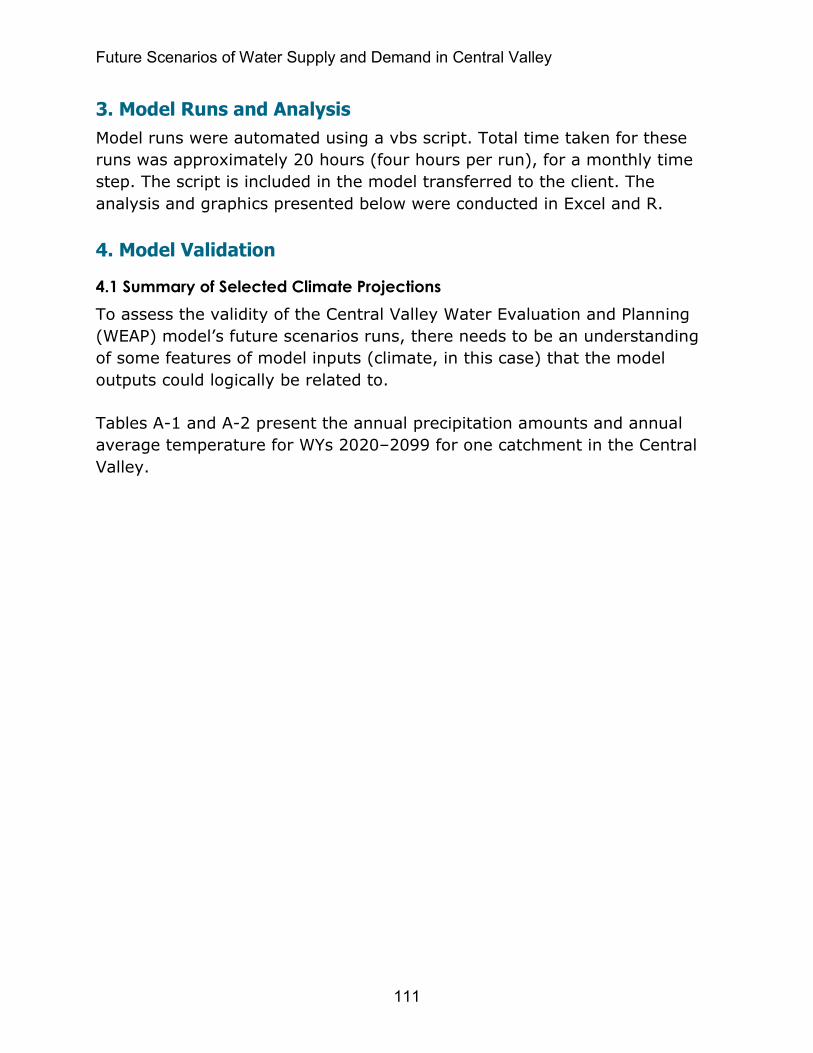
Future Scenarios of Water Supply and Demand in Central Valley
111
3. Model Runs and Analysis Model runs were automated using a vbs script. Total time taken for these runs was approximately 20 hours (four hours per run), for a monthly time step. The script is included in the model transferred to the client. The analysis and graphics presented below were conducted in Excel and R.
4. Model Validation
4.1 Summary of Selected Climate Projections To assess the validity of the Central Valley Water Evaluation and Planning (WEAP) model’s future scenarios runs, there needs to be an understanding of some features of model inputs (climate, in this case) that the model outputs could logically be related to.
Tables A-1 and A-2 present the annual precipitation amounts and annual average temperature for WYs 2020–2099 for one catchment in the Central Valley.

Appendix A: Validation of the CVPA and WEAP Model
112
Table A-1 Summary Statistics of Chosen Climate Projections, Annual Precipitation by Global Climate Model, Water Years 2020–2099 (in millimeters) Statistical Parameter canesm2_85 cnrm_cm5_45 ccsm4_85 hadgem2_es_85 miroc5_45
Minimum 192 264 227 172 170 Median 631 632 553 505 476 Mean 656 668 561 532 502 Maximum 1,472 1,676 1,087 1,135 960 SD 293 230 185 177 186 CV (percent) 45 34 33 33 37
Note: CV = coefficient of variation, SD = standard deviation
Table A-2 Summary Statistics of Chosen Climate Projections, Annual Average Temperature by Global Climate Model, Water Years 2020–2099 (in °C) Statistical Parameter canesm2_85 cnrm_cm5_45 ccsm4_85 hadgem2_es_85 miroc5_45
Minimum 18.1 17.1 16.9 17.3 16.9 First Quarter 19.3 18.3 18.8 19.0 18.3 Median 20.4 18.7 19.5 20.3 18.7 Mean 20.6 18.8 19.4 20.3 18.7 Third Quarter 21.9 19.2 20.3 21.6 19.2 Maximum 23.6 20.1 21.2 23.1 20.0
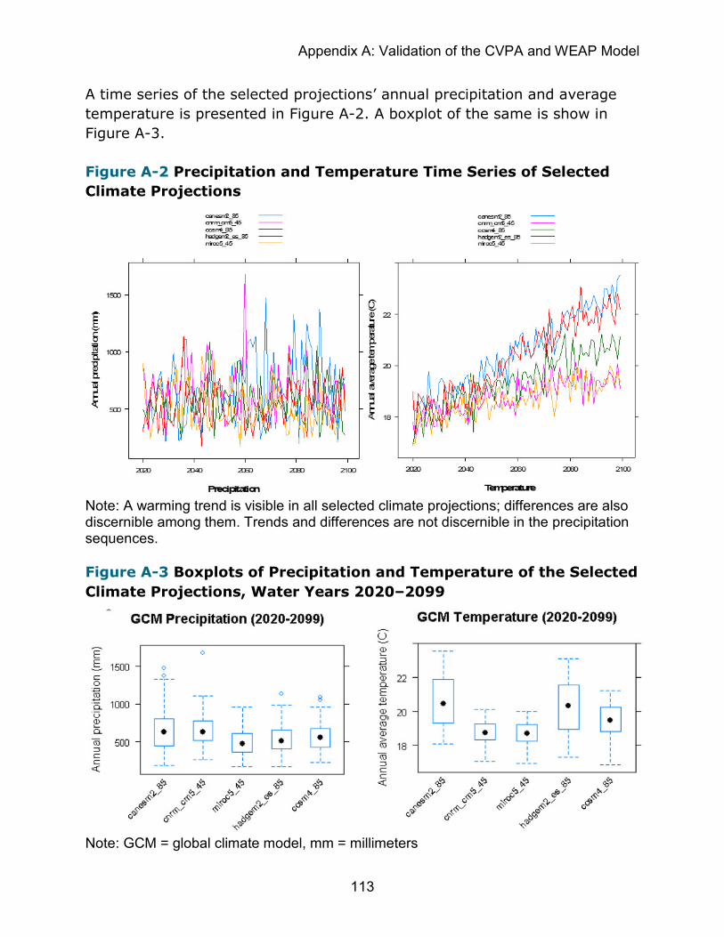
Appendix A: Validation of the CVPA and WEAP Model
113
A time series of the selected projections’ annual precipitation and average temperature is presented in Figure A-2. A boxplot of the same is show in Figure A-3.
Figure A-2 Precipitation and Temperature Time Series of Selected Climate Projections
Note: A warming trend is visible in all selected climate projections; differences are also discernible among them. Trends and differences are not discernible in the precipitation sequences.
Figure A-3 Boxplots of Precipitation and Temperature of the Selected Climate Projections, Water Years 2020–2099
Note: GCM = global climate model, mm = millimeters

Future Scenarios of Water Supply and Demand in Central Valley
114
The key messages that emerge from these tables and figures are:
1. While the qualitative description of the selected projections — based on 2020-2099 averages — is useful, the precipitation sequences and boxplots show high variability and overlap. As a result, several model outputs that are sensitive to precipitation (such as runoff) are expected to show high variability and overlap.
2. The temperature sequences do show a consistent warming trend. In keeping with the respective representative concentration pathway (RCP) forcings, end-of-century temperatures are higher for the RCP8.5 projections (canesm2_85 and hadgem2_es), than for RCP4.5 projections (cnrmcm5_45 and miroc5_45). The projections of ccsm4_85 are between the others. This also explains why the boxplots for the two RCP4.5 sequences show less variability than the others — because they have lower warming trends, they have less overall variation.
3. Because the temperature projections diverge more in the later part of the century, most analysis in the rest of this document is focused on model outputs for the late-century (WYs 2070–2099) period.
Tables A-3 through A-6 present the selected global climate model (GCM) climate summaries for early- and late-century periods.
Table A-3 Precipitation Projections Summary, Water Years 2020–2069 (in millimeters) Global Climate Model Mean Standard Deviation Coefficient of Variation canesm2_85 554 201 36% cnrm_cm5_45 700 222 32% ccsm4_85 547 164 30% hadgem2_es_85 552 201 36% miroc5_45 553 222 40%

Future Scenarios of Water Supply and Demand in Central Valley
115
Table A-4 Precipitation Projections Summary, Water Years 2070–2099 (in millimeters) Global Climate Model Mean Standard Deviation Coefficient of Variation canesm2_85 712 327 46% cnrm_cm5_45 676 176 26% ccsm4_85 584 206 35% hadgem2_es_85 566 165 29% miroc5_45 469 161 34%
Table A-5 Temperature Projections Summary, Water Years 2020–2069 (in °C) Global Climate Model Mean Standard Deviation Coefficient of Variation canesm2_85 19.10 0.58 3% cnrm_cm5_45 18.19 0.46 3% ccsm4_85 18.46 0.77 3% hadgem2_es_85 18.71 0.60 3% miroc5_45 18.11 0.57 3%
Table A-6 Temperature Projections Summary, Water Years 2070–2099 (in °C) Global Climate Model Mean Standard Deviation Coefficient of Variation canesm2_85 22.08 0.78 4% cnrm_cm5_45 19.39 0.47 2% ccsm4_85 20.44 0.58 3% hadgem2_es_85 21.80 0.65 3% miroc5_45 19.29 0.47 2%
4.2 Model Outputs: Hydrology and Water Availability Three results capture important seasonal dynamics of valley rim hydrology and overall water availability.
Rim Inflows
Streamflows from the valley rim in the summer (April through September) are a good indicator of snowmelt contributions because there is little precipitation during this period.

Future Scenarios of Water Supply and Demand in Central Valley
116
The model favorite titled “A-Rim Inflows” collects model-simulated reservoir inflows from April through September from major rivers into the following reservoirs: Folsom, Shasta, Oroville, Camp Far West, Clear Lake, New Bullards Bar, Camanche, New Hogan, Millerton, New Melones, Don Pedro, Lake McClure, Black Butte, Berryessa, Pine Flats, Lake Kaweah, Lake Success, and Isabella Lake. In addition, this model output collects the streamflows on valley rim from Battle and Cow creeks, and Cottonwood and Cosumnes rivers.
It can be hypothesized that rim inflows should be lower when the climate is warmer and drier. Temperature could moderate the effect of precipitation differences between climate projections, with warmer climate sequences producing an earlier hydrograph peak, and cooler temperatures causing a later peak.
April 1 Reservoir Storage
April 1 reservoir storage is a good indicator of winter precipitation response. Here it can be hypothesized that precipitation differences among the climate projections will dominate. The favorite called “A-Reservoir Storage” collects the April storage for Don Pedro, Folsom, Millerton, New Bullards Bar, New Hogan, New Melones, Oroville, San Luis and Shasta reservoirs.
Available Water
The total of the summer rim inflows and April 1 reservoir storage is the amount of available water for the irrigation season. Table A-7 summarizes the average values of these results for WYs 2070–2099.
Summer rim flows for wetter climate projections are indeed more than that for drier projections. But, cooler climates within the same precipitation class show higher summer rimflows, suggesting that the snow lasts longer and melts later into the season. Figure A-4 appears to confirm this. Figure A-4 shows the average monthly rimflows hydrograph for the selected projections. These support the hypotheses of later peaks for cooler climates, but the amplitudes of the peaks reflect the substantial influence of precipitation differences among the selected GCMs.
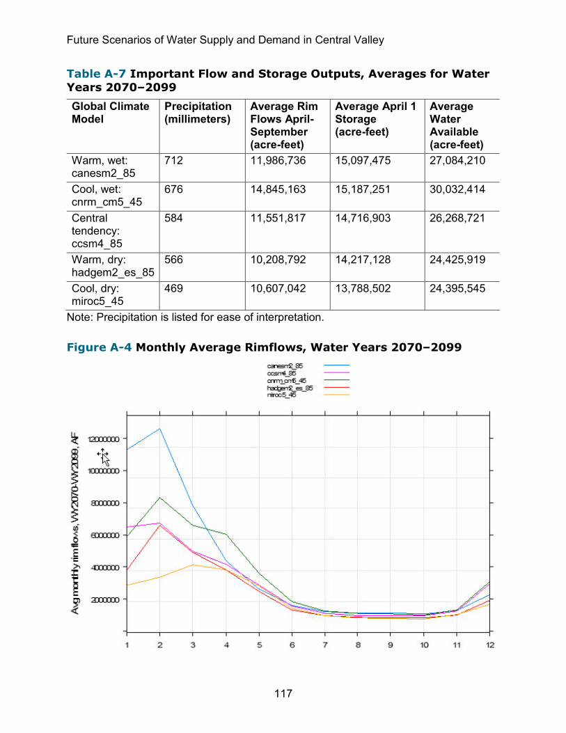
Future Scenarios of Water Supply and Demand in Central Valley
117
Table A-7 Important Flow and Storage Outputs, Averages for Water Years 2070–2099 Global Climate Model
Precipitation (millimeters)
Average Rim Flows April-September (acre-feet)
Average April 1 Storage (acre-feet)
Average Water Available (acre-feet)
Warm, wet: canesm2_85
712 11,986,736 15,097,475 27,084,210
Cool, wet: cnrm_cm5_45
676 14,845,163 15,187,251 30,032,414
Central tendency: ccsm4_85
584 11,551,817 14,716,903 26,268,721
Warm, dry: hadgem2_es_85
566 10,208,792 14,217,128 24,425,919
Cool, dry: miroc5_45
469 10,607,042 13,788,502 24,395,545
Note: Precipitation is listed for ease of interpretation.
Figure A-4 Monthly Average Rimflows, Water Years 2070–2099

Future Scenarios of Water Supply and Demand in Central Valley
118
Table A-7 also shows that the April 1 reservoir storage is correlated to precipitation in an ordinal sense — the greater the precipitation amount, the greater the April 1 storage.
These results, so far, validate the model’s simulated hydrology at the rim, reservoir storages at a crucial time of the water year, and the total water availability in response to the climate projections.
4.3 Water Deliveries
Surface Water Deliveries
Surface water deliveries simulated for each of the selected climate projections are listed in Table A-8. These show that surface deliveries follow the ordinal ranking of the climate projections by precipitation. On average, surface water deliveries are larger in wetter climate projections, which should be expected. The effect of temperature is not pronounced at the annual timescale.
Groundwater Deliveries
Groundwater deliveries simulated for each of the selected climate projections are also listed in Table A-8. These show that groundwater deliveries also follow the ordinal ranking of the climate projections by precipitation. This is because the model run for this project is consistent with previous model versions in that the groundwater deliveries are constrained so that the aquifers do not empty out. Table A-9 shows these withdrawal constraints for a few aquifers; the constraint is set up such that in dry years there are limits imposed on pumping. As a result, in dry climate projections, groundwater pumping is more limited in the model. In essence, these constraints are following the spirit of SGMA, although they were set up in the model years before the passing of SGMA.
On average, ground water deliveries are also larger in wetter climate projections. The effect of temperature is not pronounced at the annual timescale.
Figure A-5 shows the time series of surface water and groundwater deliveries for WYs 2070–2099.
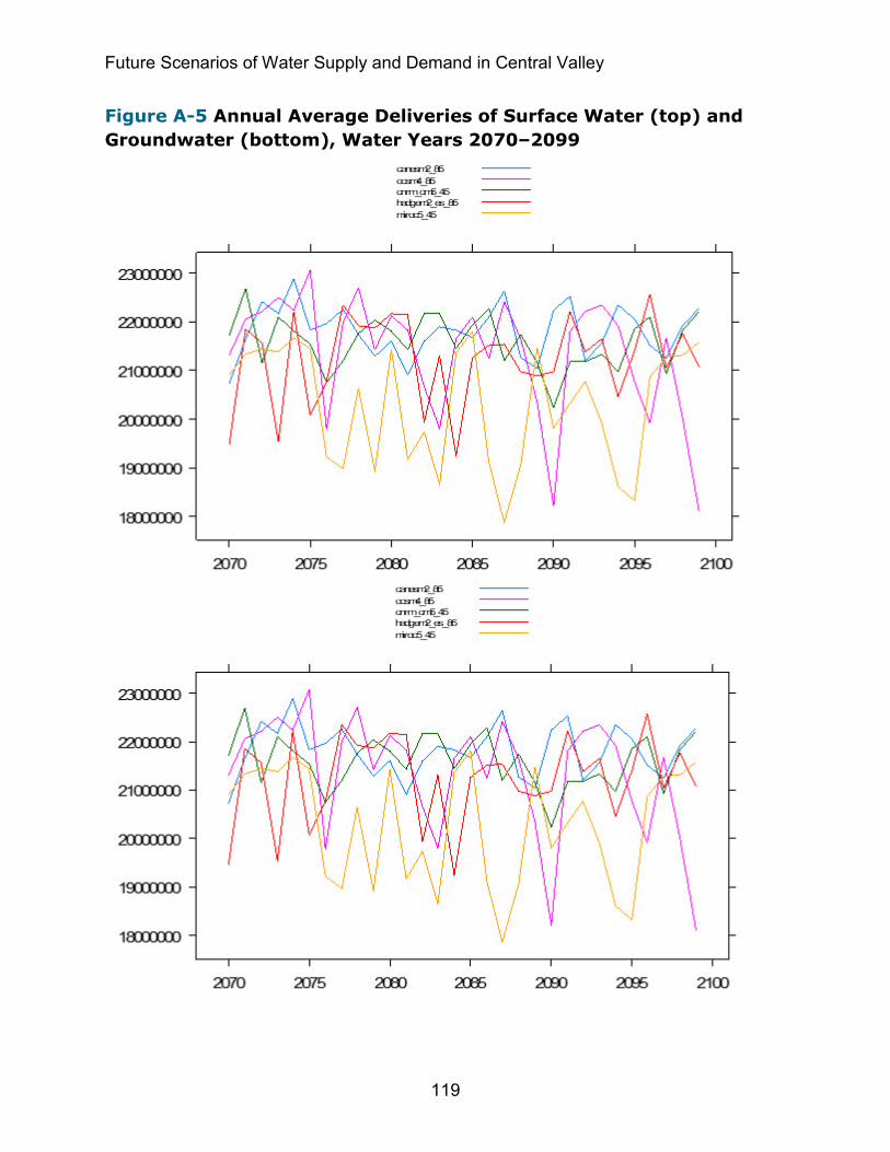
Future Scenarios of Water Supply and Demand in Central Valley
119
Figure A-5 Annual Average Deliveries of Surface Water (top) and Groundwater (bottom), Water Years 2070–2099

Future Scenarios of Water Supply and Demand in Central Valley
120
Table A-8 Surface Water and Groundwater Deliveries, Annual Averages Water Years 2070–2099 Global Climate Model
Precipitation (millimeters)
Surface Water Deliveries (acre-feet)
Groundwater Deliveries (acre-feet)
Warm, wet: canesm2_85
712 21,813,837 9,730,659
Cool, wet: cnrm_cm5_45
676 21,597,940 9,094,998
Central tendency: ccsm4_85
584 21,338,458 8,724,830
Warm, dry: hadgem2_es_85
566 21,242,074 8,117,718
Cool, dry: miroc5_45
469 20,284,024 7,750,591
Table A-9 Annual Average of Maximum Groundwater Withdrawals, Water Years 2070–2099 (for select aquifers) Global Climate Model Maximum Withdrawal
(acre-feet) Warm, wet: canesm2_85
20,399,387
Cool, wet: cnrm_cm5_45
20,258,957
Central tendency: ccsm4_85
17,039,848
Warm, dry: hadgem2_es_85
14,390,868
Cool, dry: miroc5_45
13,244,232
4.4 Delta Flows The final set of results for this validation exercise covers the Sacramento-San Joaquin Delta (Delta) inflows, outflows, and exports.
Delta inflows and outflows should follow patterns of overall water availability (Section 4.2). Table A-10 shows these model results to be consistent with

Future Scenarios of Water Supply and Demand in Central Valley
121
patterns of precipitation, which are correlated with overall water availability (Section 4.2, “San Joaquin River Hydrologic Region”).
Note particularly that there is a large range in annual Delta inflows and outflows among climate projections. Delta inflows and outflows for the driest (miroc5_45) climate is less than half that for the wettest climate (canesm2_85).
Table A-10 Delta Inflows, Outflows and Exports, Annual Average, Water Years 2070–2099 Global Climate Model
Precipitation (millimeters)
Delta Inflows (acre-feet)
Delta Outflows (acre-feet)
Delta Exports (acre-feet)
Warm, wet: canesm2_85
712 49,014,490 43,020,173 5,948,290
Cool, wet: cnrm_cm5_45
676 42,474,123 36,393,528 6,035,147
Central tendency: ccsm4_85
584 34,663,440 28,605,804 6,010,909
Warm: dryhadgem2_es_85
566 27,264,190 21,186,153 6,030,660
Cool, dry: miroc5_45
469 22,149,143 16,110,498 5,991,409
Delta exports are also listed in Table A-10. Delta exports are fairly constant across the five climate projections. The range of Delta exports in Table A-10 is 3 percent of the average, compared to 76 percent in the case of Delta inflows. A closer look by separating exports from the California Aqueduct and the Delta-Mendota Canal shows there are no major reductions in either the aqueduct or canal flows (Table A-11).

Future Scenarios of Water Supply and Demand in Central Valley
122
Table A-11 Delta Exports from California Aqueduct and Delta-Mendota Canal, Water Years 2070–2099 Global Climate Model
California Aqueduct (acre-feet)
Delta-Mendota Canal (acre-feet)
Total (acre-feet)
Warm, wet: canesm2_85
3,656,940 2,291,350 5,948,290
Cool, wet cnrm_cm5_45
3,769,263 2,265,884 6,035,147
Central tendency: ccsm4_85
3,712,998 2,297,911 6,010,909
Warm, dry: hadgem2_es_85
3,711,366 2,319,294 6,030,660
Cool, dry: miroc5_45
3,674,724 2,316,685 5,991,409
A couple of related factors explain this result. One is that the magnitude of exports is an order of magnitude less than the Delta inflows and outflows and it appears that enough water is available in the system to support Delta exports. The other factor is that the climate projections are generally wet when compared to historical climate. To illustrate this, the annual precipitation of WYs 1982–2001 had a mean of 532 millimeters (mm) (coefficient of variation = 35 percent), with a low of 296 mm and a high of 954 mm. The historical climate for this period was the driest when compared to the climate projections in the WY 2020–2069 period (Table A-3), and the second-driest when compared to the climate projections of WYs 2070–2099.
5. Conclusions Out of 20 climate projections, five were selected to test the consistency of key model outputs on the Central Valley WEAP model.
It was concluded that the Central Valley model (the version tested here) is validated based on consistency of:
• Hydrology and water availability with key features of the selected climate projections.
• Water deliveries with key features of the selected climate projections, combined with specific model constraints on groundwater deliveries.
• Modeled Delta inflows and outflows with climate features.
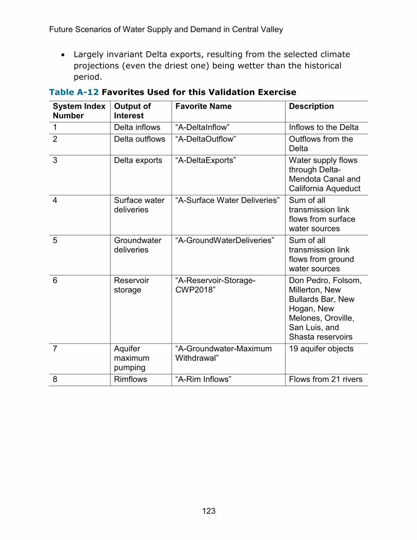
Future Scenarios of Water Supply and Demand in Central Valley
123
• Largely invariant Delta exports, resulting from the selected climate projections (even the driest one) being wetter than the historical period.
Table A-12 Favorites Used for this Validation Exercise System Index Number
Output of Interest
Favorite Name Description
1 Delta inflows “A-DeltaInflow” Inflows to the Delta 2 Delta outflows “A-DeltaOutflow” Outflows from the
Delta 3 Delta exports “A-DeltaExports” Water supply flows
through Delta-Mendota Canal and California Aqueduct
4 Surface water deliveries
“A-Surface Water Deliveries” Sum of all transmission link flows from surface water sources
5 Groundwater deliveries
“A-GroundWaterDeliveries” Sum of all transmission link flows from ground water sources
6 Reservoir storage
“A-Reservoir-Storage-CWP2018”
Don Pedro, Folsom, Millerton, New Bullards Bar, New Hogan, New Melones, Oroville, San Luis, and Shasta reservoirs
7 Aquifer maximum pumping
“A-Groundwater-Maximum Withdrawal”
19 aquifer objects
8 Rimflows “A-Rim Inflows” Flows from 21 rivers