Computers and Structures 202 (2018) 15–24

Contents lists available at ScienceDirect

Computers and Structures

journal homepage: www.elsevier .com/locate /compstruc

Further insights into an implicit time integration scheme for structuraldynamics

https://doi.org/10.1016/j.compstruc.2018.02.0070045-7949/� 2018 Elsevier Ltd. All rights reserved.

⇑ Corresponding author.E-mail address: kjb@mit.edu (K.J. Bathe).

Gunwoo Noh a, Klaus-Jürgen Bathe b,⇑aKyungpook National University, Daegu 41566, Republic of KoreabMassachusetts Institute of Technology, Cambridge, MA 02139, USA

a r t i c l e i n f o a b s t r a c t

Article history:Received 31 October 2017Accepted 12 February 2018

Keywords:DynamicsFinite element solutionsDirect time integrationsImplicit and explicit schemesStability and accuracyBathe method

The objective in this paper is to present some new insights into an implicit direct time integrationscheme, the Bathe method, for the solution of the finite element equations of structural dynamics. Theinsights pertain to the use of the parameters in the method, and in particular the value of the time stepsplitting ratio. We show that with appropriate values of this ratio large amplitude decays can be obtainedas may be desirable in some solutions. We give the theoretical analysis of the method for the parametersused, including for very large time steps, and illustrate numerically the new insights gained.

� 2018 Elsevier Ltd. All rights reserved.

1. Introduction

The finite element method is now quite widely used for thesolution of structural vibrations and wave propagations. For suchsolutions, methods of direct time integration of the governingfinite element equations are frequently used. When so done, forwave propagation analyses, mostly explicit schemes are employed,while for structural vibration solutions mostly implicit schemesare used [1]. While such use is still mostly the case, lately implicitschemes are also increasingly being employed to solve wave prop-agation problems.

An important characteristic of an implicit direct time integra-tion scheme is that it can be unconditionally stable, which meansthat the time step Dt can be selected solely based on accuracy con-siderations. For the solution of the finite element structuraldynamics equations, a frequently used scheme is the trapezoidalrule, a special case of the Newmark method [1,2]. Some other tech-niques are, for example, the Wilson method [1,3,4], the methodsdiscussed by Zhou and Tamma [5], and the three parametermethod [6–8]. More recently, the Bathe method has been proposedand has attracted significant attention and use [9–11].

The Bathe method is a composite scheme using two sub-stepsper time step Dt, but the method is used like a single-step methodwith some intermediate calculations. These, however, make the

method about twice as expensive as the trapezoidal rule per timestep Dt. Since there seems to be a considerable extra cost com-pared to using other methods, an analyst may question why touse this method. The advantages are much better accuracy charac-teristics allowing larger time steps in the integration and, overall,the more effective solution of linear and nonlinear problems. Themethod is now widely used for structural analyses and fluid-structure interactions, see e.g., Refs. [12,13].

The objective in this paper is to focus on some considerationsregarding the method, observations and insights that are relatedto what we have learned since the first publication of the method.The new insights are based on our latest experiences and thoughtsspurred by other publications [13–21]. Hence, this paper might beviewed as a continuation of Ref. [11].

In the next section, we briefly summarize the basic equations ofthe Bathe method. As originally published, there are three param-eters (a; d; c) that can be set. Although it is in practical analyses fre-quently best to simply use the defaults of these parameters, asemphasized in Refs. [10,11], it is important to realize that, ifdesired, the three parameters can of course be changed by the ana-lyst. Of particular interest are the properties when c is changed. Wetherefore discuss, in Sections 3 and 4, the stability and accuracy ofthe method when changing c, where we include the use of c largerthan 1.0 and large time step to period ratios. Finally, in Section 5,we present our concluding remarks.

16 G. Noh, K.J. Bathe / Computers and Structures 202 (2018) 15–24

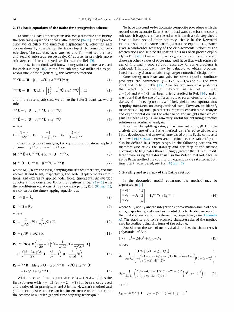
2. The basic equations of the Bathe time integration scheme

To provide a basis for our discussion, we summarize here brieflythe governing equations of the Bathe method [9–11]. In the proce-dure, we calculate the unknown displacements, velocities, andaccelerations by considering the time step Dt to consist of twosub-steps. The sub-step sizes are cDt and ð1� cÞDt for the firstand second sub-steps, respectively. Of course, in principle moresub-steps could be employed, see for example Ref. [9].

In the Bathe method, well-known integration schemes are usedfor each sub-step [10]. In the first sub-step, we utilize the trape-zoidal rule, or more generally, the Newmark method

tþcDt _U ¼ t _Uþ ½ð1� dÞt €Uþ d tþcDt €U�cDt ð1Þ

tþcDtU ¼ tUþ t _UcDt þ 12� a

� �t €Uþ a tþcDt €U

� �c2Dt2 ð2Þ

and in the second sub-step, we utilize the Euler 3-point backwardrule

tþDt _U ¼ c1tUþ c2tþcDtUþ c3tþDtU ð3Þ

tþDt €U ¼ c1t _Uþ c2tþcDt _Uþ c3tþDt _U ð4Þwhere

c1 ¼ 1� ccDt

; c2 ¼ �1ð1� cÞcDt ; c3 ¼ 2� c

ð1� cÞDt ð5Þ

Considering linear analysis, the equilibrium equations appliedat time t þ cDt and time t þ Dt are

M tþcDt €Uþ C tþcDt _Uþ K tþcDtU ¼ tþcDtR ð6Þ

M tþDt €Uþ C tþDt _Uþ K tþDtU ¼ tþDtR ð7ÞwhereM, C, K are the mass, damping and stiffness matrices, and thevectors U and R list, respectively, the nodal displacements (rota-tions) and externally applied nodal forces (moments). An overdotdenotes a time derivative. Using the relations in Eqs. (1)–(5) withthe equilibrium equations at the two time points, Eqs. (6) and (7),we construct the time-stepping equations as

K1tþcDtU ¼ R1 ð8Þ

K2tþDtU ¼ R2 ð9Þ

where

K1 ¼ 1ac2Dt2

Mþ dacDt

Cþ K ð10Þ

K2 ¼ c32Mþ c3Cþ K ð11Þ

R1¼tþcDtR þM12a

� 1� �

t €Uþ 1acDt

t _Uþ 1ac2Dt2

tU� �

þ Cðd� 2aÞcDt

2at €Uþ d

a� 1

� �t _Uþ d

acDttU

� �ð12Þ

R2 ¼ tþDtR �Mðc1c3tUþ c2c3tþcDtUþ c1t _Uþ c2tþcDt _UÞ� Cðc1tUþ c2tþcDtUÞ ð13Þ

While the case of the trapezoidal rule (a ¼ 1=4; d ¼ 1=2) as thefirst sub-step with c ¼ 1=2 (or c ¼ 2�

ffiffiffi2

p) has been mostly used

and analyzed, in principle, a and d in the Newmark method andc in the composite scheme can be chosen. Hence we can interpretthe scheme as a ‘‘quite general time stepping technique.”

To have a second-order accurate composite procedure with thesecond-order accurate Euler 3-point backward rule for the secondsub-step, it is apparent that the scheme in the first sub-step shouldhave at least second-order accuracy. Hence in the Newmarkmethod used in the Bathe scheme, d must be equal to 1/2, whichgives second-order accuracy of the displacements, velocities andaccelerations and also no dissipation. This has been proven explic-itly in Ref. [20]. However, not seeking second-order accuracy andchoosing other values of d, we may well have that with some val-ues of d, a and c good solution accuracy for some problems isachieved. This approach may be valuable to obtain problem-fitted accuracy characteristics (e.g. larger numerical dissipation).

Considering nonlinear analysis, for some specific nonlinearproblems, the parameters c ¼ 0:73, a ¼ 1=4 and d ¼ 1=2 wereidentified to be suitable [17]. Also, for two nonlinear problems,the effect of choosing different values of c witha ¼ 1=4 and d ¼ 1=2 has been briefly studied in Ref. [16], and itwas found that the use of different sets of parameters for differentclasses of nonlinear problems will likely yield a near-optimal timestepping measured on computational cost. However, to identifythese sets of optimal parameters requires considerable analysisand experimentation. On the other hand, the insights that we cangain in linear analysis are also very useful for obtaining effectivesolutions in nonlinear analysis.

Note that the splitting ratio, c, has been set to c 2 ð0;1Þ in theanalysis and use of the Bathe method, as referred to above, andin the development of a new scheme based on the Bathe compositestrategy [14,18,19,21]. However, in principle, the value of c canalso be defined in a larger range. In the following sections, wetherefore also study the stability and accuracy of the methodallowing c to be greater than 1. Using c greater than 1 is quite dif-ferent from using h greater than 1 in the Wilson method, becausein the Bathe method the equilibrium equations are satisfied at bothtime points considered, see Eqs. (6) and (7).

3. Stability and accuracy of the Bathe method

In the decoupled modal equations, the method may beexpressed as [1]

tþDt€xtþDt _xtþDtx

264

375 ¼ A

t€xt _xtx

264

375þ La

tþcDtr þ LbtþDtr ð14Þ

where A, La and Lb are the integration approximation and load oper-ators, respectively, and x and an overdot denote the displacement inthe modal space and a time derivative, respectively (see AppendixA). The stability and some accuracy characteristics of the methodmay be studied using this form of the scheme.

Focusing on the case of no physical damping, the characteristicpolynomial of A is

pðkÞ ¼ k3 � 2A1k2 þ A2k� A3 ð15Þ

where

A1¼ 1b01b02

ð1=4Þc2ð2a�dÞðc�1ÞX40

þ �1þc4a�4c3aþð1=4Þð16aþ2dþ1Þc2þð1=4Þð�4dþ2Þc

!X2

0þðc�2Þ2

0BB@

1CCA;

A2¼ 1b01b02

c4a�4c3aþð1=2Þð8aþ2dþ1Þc2þð1=2Þð�4d�2Þcþ1

!X2

0þðc�2Þ2 !

; ð16Þ

A3 ¼ 0;

b01 ¼ X20ac

2 þ 1; b02 ¼ ðc� 1Þ2X20 þ ðc� 2Þ2

G. Noh, K.J. Bathe / Computers and Structures 202 (2018) 15–24 17

where x0 is the modal natural frequency and X0 ¼ x0Dt.To represent oscillatory solutions, the eigenvalues of A should

remain in the complex plane. Since A3 = 0, we have a zero eigen-value and two non-zero eigenvalues.

The condition for the eigenvalues to be complex conjugate forall positive X0 gives

d ¼ 2a; a > 0 ð17Þwith the additional condition –

(a) Spectral radii of approximation opfor various values of (0,1γ ∈

(b) Percentage period elongations and amplfor various values of (0,1)γ ∈ with 1/ 4α =

Fig. 1. The Bathe method for various va

either

b2 > 0; b22 � 4b1b3 6 0 ð18Þ

orb2 6 0 ð19Þwhere

b1 ¼ �c2ðc2 � 2cþ 2Þ c2a� 2acþ 12

� �aðc� 1Þ2; ð20Þ

erator of the Bathe method when 0ξ =) with 1/ 4α = and 1/ 2δ = .

itude decays of the Bathe method when 0ξ = and 1/ 2δ = .

lues of c with a ¼ 1=4 and d ¼ 1=2.

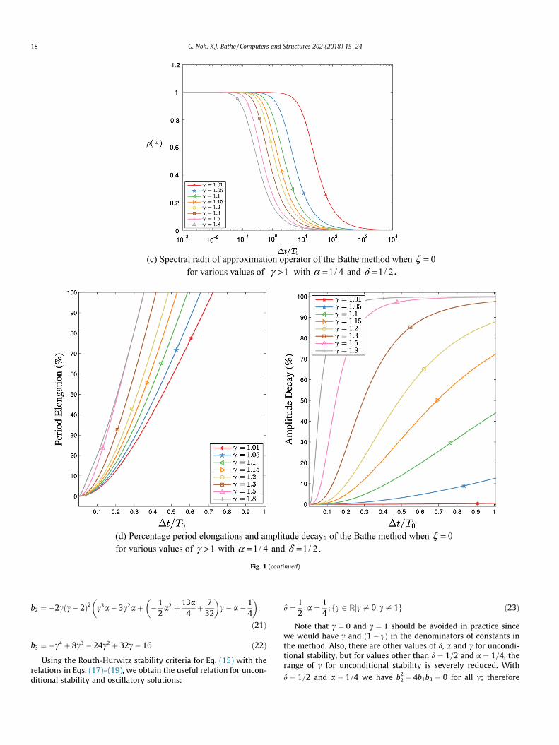
(d) Percentage period elongations and amplitude decays of the Bathe method when 0ξ =for various values of 1γ > with 1/ 4α = and 1/ 2δ = .

(c) Spectral radii of approximation operator of the Bathe method when 0ξ =for various values of 1γ > with 1/ 4α = and 1/ 2δ = .

Fig. 1 (continued)

18 G. Noh, K.J. Bathe / Computers and Structures 202 (2018) 15–24

b2 ¼ �2cðc� 2Þ2 c3a� 3c2aþ �12a2 þ 13a

4þ 732

� �c� a� 1

4

� �;

ð21Þ

b3 ¼ �c4 þ 8c3 � 24c2 þ 32c� 16 ð22ÞUsing the Routh-Hurwitz stability criteria for Eq. (15) with the

relations in Eqs. (17)–(19), we obtain the useful relation for uncon-ditional stability and oscillatory solutions:

d ¼ 12;a ¼ 1

4; fc 2 Rjc – 0; c – 1g ð23Þ

Note that c ¼ 0 and c ¼ 1 should be avoided in practice sincewe would have c and ð1� cÞ in the denominators of constants inthe method. Also, there are other values of d, a and c for uncondi-tional stability, but for values other than d ¼ 1=2 and a ¼ 1=4, therange of c for unconditional stability is severely reduced. With

d ¼ 1=2 and a ¼ 1=4 we have b22 � 4b1b3 ¼ 0 for all c; therefore

G. Noh, K.J. Bathe / Computers and Structures 202 (2018) 15–24 19

the values in Eq. (23) render the method unconditionally stableand the principal roots of the integration approximation operator,A, to be complex conjugate.

Since the principal roots remain in the complex plane for allpositive X0, the spectral radius, qðAÞ, becomes

qðAÞ ¼ffiffiffiffiffiffiA2

pð24Þ

Fig. 1 shows the spectral radii and the period elongations andamplitude decays for various values of c with a ¼ 1=4 andd ¼ 1=2, including when c is greater than 1.0. The spectral radiusexpressed in Eq. (24) with a ¼ 1=4 and d ¼ 1=2 has a local mini-mum at c ¼ 2�

ffiffiffi2

p(within the range 0 < c < 1) and this splitting

ratio provides maximum amplitude decay with minimum periodelongation when c 2 ð0;1Þ, which was already reported[11,17,19,20,22,23]. These curves are quite close to those usingc ¼ 0:5.

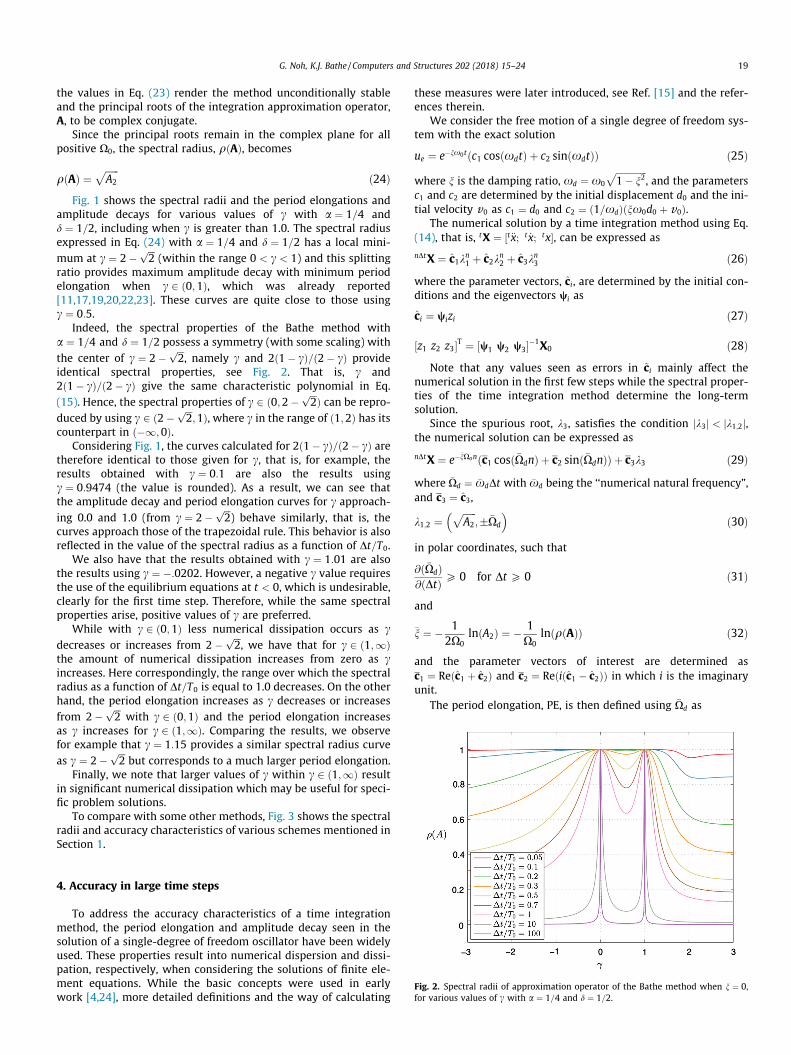
Indeed, the spectral properties of the Bathe method witha ¼ 1=4 and d ¼ 1=2 possess a symmetry (with some scaling) withthe center of c ¼ 2�

ffiffiffi2

p, namely c and 2ð1� cÞ=ð2� cÞ provide

identical spectral properties, see Fig. 2. That is, c and2ð1� cÞ=ð2� cÞ give the same characteristic polynomial in Eq.(15). Hence, the spectral properties of c 2 ð0;2�

ffiffiffi2

pÞ can be repro-

duced by using c 2 ð2�ffiffiffi2

p;1Þ, where c in the range of ð1;2Þ has its

counterpart in ð�1;0Þ.Considering Fig. 1, the curves calculated for 2ð1� cÞ=ð2� cÞ are

therefore identical to those given for c, that is, for example, theresults obtained with c ¼ 0:1 are also the results usingc ¼ 0:9474 (the value is rounded). As a result, we can see thatthe amplitude decay and period elongation curves for c approach-ing 0.0 and 1.0 (from c ¼ 2�

ffiffiffi2

p) behave similarly, that is, the

curves approach those of the trapezoidal rule. This behavior is alsoreflected in the value of the spectral radius as a function of Dt=T0.

We also have that the results obtained with c ¼ 1:01 are alsothe results using c ¼ �:0202. However, a negative c value requiresthe use of the equilibrium equations at t < 0, which is undesirable,clearly for the first time step. Therefore, while the same spectralproperties arise, positive values of c are preferred.

While with c 2 ð0;1Þ less numerical dissipation occurs as cdecreases or increases from 2�

ffiffiffi2

p, we have that for c 2 ð1;1Þ

the amount of numerical dissipation increases from zero as cincreases. Here correspondingly, the range over which the spectralradius as a function of Dt=T0 is equal to 1.0 decreases. On the otherhand, the period elongation increases as c decreases or increasesfrom 2�

ffiffiffi2

pwith c 2 ð0;1Þ and the period elongation increases

as c increases for c 2 ð1;1Þ. Comparing the results, we observefor example that c ¼ 1:15 provides a similar spectral radius curveas c ¼ 2�

ffiffiffi2

pbut corresponds to a much larger period elongation.

Finally, we note that larger values of c within c 2 ð1;1Þ resultin significant numerical dissipation which may be useful for speci-fic problem solutions.

To compare with some other methods, Fig. 3 shows the spectralradii and accuracy characteristics of various schemes mentioned inSection 1.

Fig. 2. Spectral radii of approximation operator of the Bathe method when n ¼ 0,for various values of c with a ¼ 1=4 and d ¼ 1=2.

4. Accuracy in large time steps

To address the accuracy characteristics of a time integrationmethod, the period elongation and amplitude decay seen in thesolution of a single-degree of freedom oscillator have been widelyused. These properties result into numerical dispersion and dissi-pation, respectively, when considering the solutions of finite ele-ment equations. While the basic concepts were used in earlywork [4,24], more detailed definitions and the way of calculating

these measures were later introduced, see Ref. [15] and the refer-ences therein.

We consider the free motion of a single degree of freedom sys-tem with the exact solution

ue ¼ e�nx0tðc1 cosðxdtÞ þ c2 sinðxdtÞÞ ð25Þ

where n is the damping ratio, xd ¼ x0

ffiffiffiffiffiffiffiffiffiffiffiffiffiffi1� n2

p, and the parameters

c1 and c2 are determined by the initial displacement d0 and the ini-tial velocity v0 as c1 ¼ d0 and c2 ¼ ð1=xdÞðnx0d0 þ v0Þ.

The numerical solution by a time integration method using Eq.(14), that is, tX ¼ ½t€x; t _x; tx�, can be expressed as

nDtX ¼ c1kn1 þ c2kn2 þ c3kn3 ð26Þwhere the parameter vectors, ci, are determined by the initial con-ditions and the eigenvectors wi as

ci ¼ wizi ð27Þ

½z1 z2 z3�T ¼ ½w1 w2 w3��1X0 ð28ÞNote that any values seen as errors in ci mainly affect the

numerical solution in the first few steps while the spectral proper-ties of the time integration method determine the long-termsolution.

Since the spurious root, k3, satisfies the condition jk3j < jk1;2j,the numerical solution can be expressed as

nDtX ¼ e��nXonðc1 cosð�XdnÞ þ c2 sinð�XdnÞÞ þ c3k3 ð29Þwhere �Xd ¼ �xdDt with �xd being the ‘‘numerical natural frequency”,and c3 ¼ c3,

k1;2 ¼ffiffiffiffiffiffiA2

p;��Xd

� �ð30Þ

in polar coordinates, such that

@ð�XdÞ@ðDtÞ P 0 for Dt P 0 ð31Þ

and

�n ¼ � 12X0

lnðA2Þ ¼ � 1X0

lnðqðAÞÞ ð32Þ

and the parameter vectors of interest are determined asc1 ¼ Reðc1 þ c2Þ and c2 ¼ Reðiðc1 � c2ÞÞ in which i is the imaginaryunit.

The period elongation, PE, is then defined using �Xd as

20 G. Noh, K.J. Bathe / Computers and Structures 202 (2018) 15–24

PE ¼�Td � T0

T0¼ X0

�Xd� 1 ð33Þ

Using Eq. (29) with the solution at time �Td, the ‘‘numerical nat-ural period”, we obtain the expression for the amplitude decay, AD,as

AD ¼ 1� exp �2p�nX0

�Xd

� �ð34Þ

(a) Spectral radii of approxim

(b) Percentage period elongation

Fig. 3. Spectral radii, period elongations and amplitude decays of various methods. For th[5] and the 3-Par. method is described in Refs. [6–8].

Of course, the frequently used approximate expressionADapprox ¼ 2p�n, is recovered by taking the Taylor expansion on Eq.(34) for small �n. The two expressions provide similar results for asmall AD, while the difference might not be negligible for casesof larger time steps used.

With the expressions in Eqs. (30)–(34), we are able to calculatethe period elongation and the amplitude decay only with A1 and A2,

ation operator when 0ξ =

s and amplitude decays when 0ξ =

e Bathe method a ¼ 1=4 and d ¼ 1=2 are used. The U0V0 method is described in Ref.

Fig. 4. Bathe method with a ¼ 1=4; d ¼ 1=2, c ¼ 1=2. (a) Period elongations calculated using 2 quadrant inverse tangent h ¼ tan�1ffiffiffiffiffiffiffiffiffiffiffiffiffiffiffiffiffiA2 � A2

1

q=A1

� �� �and 4 quadrant inverse

tangent (Eq. (36)). (b) Amplitude decays calculated using 2 quad. inverse tangent, 4 quad. tangent and approximate expression (2p�n). (c) Eigenvalues used in the calculation of4 quad. inverse tangent.

Fig. 5. Numerical results of the single degree of freedom system described by Eq.(37) using the Bathe method with a ¼ 1=4; d ¼ 1=2, c ¼ 1=2 for various time stepsizes; Dt�=T0 ’ 0:854.

Fig. 6. Model problem of three degrees of freedom spring system,k1 ¼ 107; k2 ¼ 1;m1 ¼ 0;m2 ¼ 1;m3 ¼ 1;xp ¼ 1:2.

Fig. 7. Displacement of node 2 for various methods The U0V0 method is describedin Ref. [5] and the 3-Par. method is described in Refs. [6–8].

G. Noh, K.J. Bathe / Computers and Structures 202 (2018) 15–24 21

which are given in Eq. (16) for the Bathe method; we do not needany numerical fitting which was frequently used in earlier works.

Let us now consider �Xd in Eq. (30) for the calculation of PE andAD with larger time steps. Since the two nonzero eigenvalues of Eq.(15) are complex conjugates, we may define the first eigenvalue asthe one rotating counter-clockwise and the second eigenvalue asthe one rotating clockwise as in Eqs. (30) and (31); thus we heredefine �Xd as a ‘‘four” quadrant inverse tangent of the eigenvalue

of the integration approximation operator of the time integrationmethod.

As the time step size increases, the sign of the real part of eachof the eigenvalues, Reðk1;2Þ, first changes from positive to negativewhile the sign of the imaginary part is unchanged. At the point ofthe sign change of Reðk1;2Þ, the first eigenvalue, which rotatescounter-clockwise, rotates from the first quadrant to the secondquadrant of the complex domain. We then may calculate PE andAD accurately until a certain limit using for �Xd > p=2 (as in Ref.[20])

�Xd ¼ tan�1ffiffiffiffiffiffiffiffiffiffiffiffiffiffiffiffiA2 � A2

1

q=A1

� �ð35Þ

where �Xd ¼ p=2 when the real part of the eigenvalues, A1, is zero.However, as the time step size increases further, it reaches the

size Dt� which makes the imaginary part of the eigenvalue become

Fig. 8. Displacement of node 3 for various methods.

Fig. 9. Velocity of node 2 for various methods (the static correction gives thenonzero velocity at time = 0.0).

Fig. 10. Velocity of node 3 for various methods.

Fig. 11. Acceleration of node 2 for various methods.

Fig. 12. Acceleration of node 2 for various methods; ‘‘Bathe c ¼ 0:5ð�Þ” usesa ¼ 1 and d ¼ 3=4 only for the first step, and a ¼ 1=4 and d ¼ 1=2 otherwise.

Fig. 13. Acceleration of node 3 for various methods.

22 G. Noh, K.J. Bathe / Computers and Structures 202 (2018) 15–24

Fig. 14. Reaction force at node 1 for various methods.

Fig. 15. Reaction force at node 1 for various methods; ‘‘Bathe c ¼ 0:5ð�Þ” usesa ¼ 1 and d ¼ 3=4 only for the first step, a ¼ 1=4 and d ¼ 1=2 otherwise.

G. Noh, K.J. Bathe / Computers and Structures 202 (2018) 15–24 23

zero, or A21 ¼ A2. For the Bathe method with

a ¼ 1=4; b ¼ 1=2 and c ¼ 1=2, Dt�=T0 ’ 0:854, see Fig. 4c.Then for the time step size Dt > Dt� (since the angle given by Eq.

(31) further increases as the time step size increases), if Eq. (35) isused for the PE and AD we obtain an unnatural ‘‘kink” in the curvesat the time step size Dt� as shown in Fig. 4a and b. Instead we needto use

�Xd ¼tan�1

ffiffiffiffiffiffiffiffiffiffiffiffiffiffiffiffiA2 � A2

1

q=A1

� �for Dt 6 Dt�

tan�1 �ffiffiffiffiffiffiffiffiffiffiffiffiffiffiffiffiA2 � A2

1

q=A1

� �for Dt > Dt�

ð36Þ

where ðA21 � A2ÞjDt¼Dt� ¼ 0.

To illustrate that we need to use Eq. (36) in our studies of theamplitude decay and period elongation, we solved the singledegree of freedom problem

€uþ 100 u ¼ 0 ð37Þ

with the initial conditions u0 ¼ 1 and _u0 ¼ 0. Fig. 5 shows thenumerical solutions using a ¼ 1=4; d ¼ 1=2; c ¼ 1=2 and various

time steps. We see that there is no sudden change in the trend ofthe numerical solutions around Dt� as predicted using Eq. (36).

5. Illustrative numerical results

The model problem shown in Fig. 6 was already solved in Ref.[11] to illustrate the behavior of some time integration schemes.We solve the problem here again and include the use of the Bathemethod for different values of c. We refer to Refs. [11,1] for thedetails of this model problem and comments on its importance.

Figs. 7–15 show the results obtained using the Bathe method,the U0V0optimal scheme which is a method discussed by Zhou andTamma as a U0-V0 scheme [5], and the 3 parameter method [6–8]. In all solutions we use Dt ¼ 0:2618 (as in Ref. [11]). For theBathe method, we use a ¼ 1=4, d ¼ 1=2 and c ¼ 0:1;0:5;1:3 whilewe use various q1 values for the U0V0optimal scheme and the 3parameter method. The results show that the Bathe method per-forms well with all considered c values, while the other schemes,for the values of q1 considered, do not perform satisfactorily.

Note that there is a bifurcation in the principal roots of the char-acteristic polynomial of the U0V0optimal scheme at a certain timestep size (at the inverted peaks of the curves in Fig. 3(a)). Afterthe bifurcation, the one principal root provides qðAÞjDt¼1 ’ 1 forall values of q1 which is the magnitude of the other principal root.Therefore, the U0V0optimal method does not give the amplitudedecay important in the solution of this problem.

The 3 parameter method provides results similar to those of theNewmark method with values for the parameters to give dissipa-tion (see Ref. [11]).

However using the Bathe method, there is an overshoot in theacceleration at node 2 and for the reaction for the first time step.The overshoot is negative for c 2 ð0;1Þ while it is positive forc > 1. An analytical study of this behavior shows that this over-shoot only occurs in the first step for the given initial conditions,and the overshoot can be eliminated by using a ¼ 1 and d ¼ 3=4only for the first step.

If we use a ¼ 1 and d ¼ 3=4 only for the first step and a ¼ 1=4and d ¼ 1=2 thereafter, we have practically the same solutions asfor the case of a ¼ 1=4 and d ¼ 1=2 for all solution variables, butwithout the overshoot. However, we do not recommend to use thisset of parameter values for all solution times. With these valuesonly first order accuracy is obtained with large period elongationsand amplitude decays, and the algorithm is not unconditionallystable.

6. Concluding remarks

The objective of this paper was to provide some new insightinto an implicit time integration method, the Bathe method, forstructural dynamics. While the method has already been analyzedin earlier papers, additional insight is given in this paper.

The method was introduced about a decade ago for the solutionof structural dynamics problems. In the use of the method and themathematical analyses, it was assumed that the parameterc 2 ð0;1Þ. The analysis we give in this paper shows that usinga ¼ 1=4 and d ¼ 1=2 with any real value of c provides second orderaccuracy, unconditional stability and good behavior in the princi-pal roots of the approximation operator for all time step sizes.The analysis also shows that the use of c > 1 may provide largeramplitude decays, which may be useful in the solution of someproblems. The concept of using an enlarged range of the splittingratio c might also be valuable in the development of new implicittime integration methods based on a composite strategy.

When analyzing time integration methods, like the Bathemethod, for the use of large time steps, it is important to employ

24 G. Noh, K.J. Bathe / Computers and Structures 202 (2018) 15–24

correct measures for period elongations and amplitude decays. Wediscussed this aspect and used appropriate measures.

In the paper, we focused on the solution of structural dynamicsproblems. However, the Bathe method shows also valuable accu-racy characteristics in the solution of wave propagations, wherethe technique suppresses waves that can spatially not be resolvedand can give increasingly more accurate solutions as the time stepsize decreases [22,23,25,26]. An analysis of the method for suchproblem solutions focusing on different values of the parametersd;a and c would be very valuable, in particular when used withoverlapping finite elements [26]. Finally, the observations givenin this paper show that for the design of new composite explicittime integration schemes [27], an enlarged range of the splittingratio might also be considered.

Acknowledgement

This work was partly supported by the Basic Science ResearchProgram (Grant No. 2017R1C1B5077183) through the NationalResearch Foundation of Korea (NRF) funded by the Ministry ofScience and ICT.

Appendix A. The integration operator A and the load operatorsLa and Lb

We give here the expressions for the integration operator A andload operators La and Lb:

A ¼ 1b1b2

a11 a12 a13a21 a22 a23a31 a32 a33

264

375

La ¼ 1b1b2

12 ð2c2a� 4ða� ðd=2ÞÞc� 2dÞX2

0 þ 2dðc� 2ÞnX0

�cð1� cÞaX20Dt � dðc� 2ÞDt

2cð1� cÞanX0Dt2 þ 12 ð�2c2aþ ð4a� 2dÞcþ 2dÞDt2

264

375

Lb ¼ 1b1b2

ðac2X20 þ 2dcX0nþ 1Þðc� 2Þ2

Dtðc� 1Þðc� 2Þðac2X20 þ 2dcX0nþ 1Þ

Dt2ðc� 1Þ2ðac2X20 þ 2dcX0nþ 1Þ

2664

3775

where

b1¼ac2X20þ2dcX0nþ1

b1¼ðc�1Þ2X20þ2nðc�1Þðc�2ÞX0þðc�2Þ2

a11 ¼�2ðX0ncða�d=2Þþa=2�1=4Þðc�2ÞcX20

a12 ¼�4ðc�2ÞX0

Dtð1=4Þac2ðc�1ÞX3

0þð1=2Þðc2aþð�2aþdÞcþa�2dÞncX20

þðc�2Þðn2dcþ1=4ÞX0þð1=2Þnðc�2Þ

!

a13 ¼� 1Dt2

ðc�2ÞX20ðX2

0ac3�2ac2X2

0þ2X0dc2nþX20ac�4dcX0nþc�2Þ

a21 ¼�2DtðX0ncða�ðd=2ÞÞþða=2Þ�ð1=4ÞÞcðc�1ÞX20

a22 ¼X2

0ac4þð�4X20aþ2dX0nÞc3þð1�2X3

0nða�dÞþ4X20a�8dX0nÞc2

þð�4þ2X30nða�dÞþX2

0þ8dX0nÞc�X20þ4

!

a23 ¼� 1Dt

X20ðc�1ÞðX2

0ac3�2ac2X2

0þ2X0dc2nþX20ac�4dcX0nþc�2Þ

a31 ¼4Dt2ðX0ncða�ðd=2ÞÞþða=2Þ�ð1=4ÞÞcðnðc�1ÞX0þðc=2Þ�1Þ

a32 ¼4Dtðð1=4Þc2a�ð1=2Þacþða�dÞn2ÞcX2

0ðc�1Þþð1=2ÞX0ðdc3þ1þða�4dÞc2þð�2aþ4d�1ÞcÞnþð1=4Þðc�2Þ2

!

a33 ¼ð2X0nðc�1Þþc�2ÞðX20ac

3�2ac2X20þ2X0dc2nþX2

0ac�4dcX0nþc�2Þ

Appendix B. Supplementary material

Supplementary data associated with this article can be found, inthe online version, at https://doi.org/10.1016/j.compstruc.2018.02.007.

References

[1] Bathe KJ. Finite element procedures, 2nd ed. Watertown, MA: K.J. Bathe; 2016.<http://meche.mit.edu/people/faculty/kjb@mit.edu> [also published by HigherEducation Press China 2016].

[2] Newmark NM. A method of computation for structural dynamics. J Eng MechDiv (ASCE) 1959;85:67–94.

[3] Wilson EL, Farhoomand I, Bathe KJ. Nonlinear dynamic analysis of complexstructures. Int J Earthquake Eng Struct Dyn 1973;1:241–52.

[4] Bathe KJ, Wilson EL. Stability and accuracy analysis of direct integrationmethods. Int J Earthquake Eng Struct Dyn 1973;1:283–91.

[5] Zhou X, Tamma KK. Design, analysis, and synthesis of generalized single stepsingle solve and optimal algorithms for structural dynamics. Int J Numer MethEng 2004;59:597–668.

[6] Shao HP, Cai CW. A three parameters algorithm for numerical integration ofstructural dynamic equations. Chin J Appl Mech 1988;5(4):76–81 [in Chinese].

[7] Shao HP, Cai CW. The direct integration three-parameters optimal schemes forstructural dynamics. In: Proceedings of the international conference: machinedynamics and engineering applications. Xi’an Jiaotong University Press; 1988.p. C16–20.

[8] Chung J, Hulbert GM. A time integration algorithm for structural dynamicswith improved numerical dissipation: the generalized-alpha method. J ApplMech (ASME) 1993;60:371–5.

[9] Bathe KJ, Baig MMI. On a composite implicit time integration procedure fornonlinear dynamics. Comput Struct 2005;83:2513–24.

[10] Bathe KJ. Conserving energy and momentum in nonlinear dynamics: a simpleimplicit time integration scheme. Comput Struct 2007;85:437–45.

[11] Bathe KJ, Noh G. Insight into an implicit time integration scheme for structuraldynamics. Comput Struct 2012;98–99:1–6.

[12] Bathe KJ, Zhang H. Finite element developments for general fluid flows withstructural interactions. Int J Numer Meth Eng 2004;60:213–32.

[13] Kroyer R, Nilsson K, Bathe KJ. Advances in direct time integration schemes fordynamic analysis. Automotive CAE Companion 2016/2017; 2016. p. 32–5.

[14] Dong S. BDF-like methods for nonlinear dynamic analysis. J Comput Phys2010;229:3019–45.

[15] Benítez JM, Montáns FJ. The value of numerical amplification matrices in timeintegration methods. Comput Struct 2013;128:243–50.

[16] Bathe KJ. Frontiers in finite element procedures & applications. In: ToppingBHV, Iványi P, editors. Computational methods for engineeringtechnology. Stirlingshire, Scotland: Saxe-Coburg Publications; 2014 [chapter1].

[17] Klarmann S, Wagner W. Enhanced studies on a composite time integrationscheme in linear and non-linear dynamics. Comput Mech 2015;55:455–68.

[18] Chandra Y, Zhou Y, Stanciulescu I, Eason T, Spottswood S. A robust compositetime integration scheme for snap-through problems. Comput Mech2015;55:1041–56.

[19] Wen WB, Wei K, Lei HS, Duan SY, Fang DN. A novel sub-step compositeimplicit time integration scheme for structural dynamics. Comput Struct2017;182:176–86.

[20] Zhang J, Liu Y, Liu D. Accuracy of a composite implicit time integration schemefor structural dynamics. Int J Numer Meth Eng 2017;109:368–406.

[21] Kwon S-B, Lee J-M. A non-oscillatory time integration method for numericalsimulation of stress wave propagations. Comput Struct 2017;192:248–68.

[22] Noh G, Ham S, Bathe KJ. Performance of an implicit time integration scheme inthe analysis of wave propagations. Comput Struct 2013;123:93–105.

[23] Ham S, Lai B, Bathe KJ. The method of finite spheres for wave propagationproblems. Comput Struct 2014;142:1–14.

[24] Belytschko T, Hughes TJR, editors. Computational methods for transientanalysis. New York: North-Holland; 1983.

[25] Kim KT, Bathe KJ. Transient implicit wave propagation dynamics with themethod of finite spheres. Comput Struct 2016;173:50–60.

[26] Kim KT, Zhang L, Bathe KJ. Transient implicit wave propagation dynamics withoverlapping finite elements. Comput Struct 2018;199:18–33.

[27] Noh G, Bathe KJ. An explicit time integration scheme for the analysis of wavepropagations. Comput Struct 2013;129:178–93.