fur Mathematik¨ in den Naturwissenschaften Leipzig
53
f ¨ ur Mathematik in den Naturwissenschaften Leipzig From 1970 until present: the Keller-Segel model in chemotaxis and its consequences by Dirk Horstmann Preprint no.: 3 2003
Transcript of fur Mathematik¨ in den Naturwissenschaften Leipzig

fur Mathematikin den Naturwissenschaften
Leipzig
From 1970 until present: the
Keller-Segel model in chemotaxis and
its consequences
by
Dirk Horstmann
Preprint no.: 3 2003


SUBMITTED FOR JOURNAL PUBLICATION.
FROM 1970 UNTIL PRESENT: THE KELLER-SEGEL MODEL IN CHEMOTAXIS AND ITSCONSEQUENCES
DIRK HORSTMANN∗
Abstract. This article summarizes various aspects and results for some general formulations of the classical chemotaxis models alsoknown as Keller-Segel models. It is intended as a survey of results for the most common formulation of this classical model for positivechemotactical movement and offers possible generalizations of these results to more universal models. Furthermore it collects open questionsand outlines mathematical progress in the study of the Keller-Segel model since the first presentation of the equations in 1970.
Key words. Chemotaxis equations, steady state analysis, global existence, finite time blow-up, invariant sets, self-similar solutions,traveling waves
AMS subject classifications. 35B30, 35J20, 35J25, 35J65, 35K50, 35K57, 92C17
1. Introduction. Mathematical analysis of biological phenomena has become more and more important in un-derstanding these complex processes. Thus, the number of mathematicians studying biological and medical phenomenaand problems is continuously increasing in recent years. One such biological topic is the movement of population den-sities or the movement of single particles. Changes in the environment of mobile species can influence its movement.For example, humans sense their environment and given a particular situation or the state of the environment, theymake their decisions as to where to move. For example we might be attracted by a tantalizing smell and move towardsit, since we expect a delicious food, or we move away from a place if there is a repellent odor. Animals and humansalso use this effects (for example) to attract mating partners with special colorful feathers or with enticing perfumesetc. In [85] one can find the silk moth Bombyx mori as an example of a species that uses a special odor to attracta mating partner. During mating season the female moth secretes a scent caused by a pheromone bombykol whichattracts the male to move in direction of the increasing concentration of this scent. This helps the male moths to findthe female. Before presenting another example where changes in the environment affect the movement of a mobilespecies let me cite the following anecdote from the German news magazine “DER SPIEGEL” 36/1998 [45] that is saidto have happened in the late 1950s at the University of Princeton:
“The genius was stunned. In the late 1950s Albert Einstein watched disbelievingly a film of the youngscientist John Tyler Bonner at Princeton University. The star of the movie was an unimpressive tinycreature: an amoeba called Dictyostelium.(...) As soon as “Dicty”,(...), starts to become hungry itundergoes a miraculous metamorphosis.(...) The Dictys become one.(...) Einstein’s question is stillunsolved: Why does Dicty undergo a deadly intermezzo as a complex multicellular organism to livethen alone and autistically?” (Quoted from [45] translated by the author.)
The cellular slime mold Dictyostelium discoideum was discovered by K. B. Raper in 1935 and in the subsequentyears aroused the interest of many scientists. Nowadays Dictyostelium discoideum is a model organism for biomedicalresearch of the National Institutes of Health (NIH). One reason for the growing interest in this cellular slime moldwas caused by the fact that “development in Dictyostelium discoideum results only in two terminal cell types, butprocesses of morphogenesis and pattern formation occur as in many higher organisms” (see [103, page 354]). Thisraised the hope of biologists that studying this cellular slime mold might aid in the understanding of the secret of celldifferentiation. But what initiates the change from a single cell organism to a complex multicellular organism? Andhow does this process take place?
During its life cycle a myxamoebae population of the Dictyostelium grows by cell division as long as there is sufficientnourishment. When the food resources are exhausted the myxamoebae spread over the entire domain available tothem. After a while one cell starts to exude cyclic Adenosine Monophosphate (cAMP) which attracts the othermyxamoebae. The myxamoebae begin to move towards the so-called founder cell and are also stimulated to emitcAMP. The myxamoebae aggregate and start to differentiate. At the end of the aggregation the myxamoebae form apseudoplasmoid, in which every myxamoebae maintains its individual integrity. This pseudoplasmoid moves towardslight sources. After a time a fruiting body is formed and spores are spread. Thus the life cycle begins again. For moredetails on the life cycle of the Dictyostelium we refer to [15], for example.
∗Mathematisches Institut der Universitat zu Koln, Weyertal 86-90, D-50931 Koln, Germany, email: [email protected]
1

2 Submitted for Journal publication: The Keller-Segel model in chemotaxis and its consequences
A reaction to an external stimulus is generally called taxis and is then specified by describing the reason forthe reaction. Therefore, there are many different tactical responses such as chemotaxis, galvanotaxis and phototaxis.In this article I will focus on chemotactical movement of mobile species which can lead to various different patternformations.
Chemotaxis is the influence of chemical substances in the environment on the movement of mobile species. Thiscan lead to strictly oriented movement or to partially oriented and partially tumbling movement. The movementtowards a higher concentration of the chemical substance is termed positive chemotaxis and the movement towardsregions of lower chemical concentration is called negative chemotactical movement. Thus, the Bombyx mori andthe Dictyostelium discoideum are two species that move in a chemotactically positive manner towards the higherconcentration of the bombykol resp. the cAMP. The substances that lead to positive chemotaxis are chemoattractantsand those leading to negative chemotaxis are so-called repellents.
Chemotaxis is an important means for cellular communication. Communication by chemical signals determineshow cells arrange and organize themselves, like for instance in development or in living tissues. A large number ofexamples for mobile species behaving in a chemotactical manner are known. In addition to the above mentioned twoexamples, I would also like to draw attention to a third species, the bacterial strain Rhizobia meliloti. As described in[37], this bacterial strain responds chemotactically to root exudates isolated from the soil of leguminous plants. Thebacterial strain in the surrounding soil of the plants are guided to nodules in the roots of nitrogen-fixing plants by achemical gradient. Therefore, they play an important role in agricultural ecology.
One aspect during positive oriented chemotactical movement is the formation of cells (amoebae, bacteria, etc)amounts during the responds of the species population to the change of the chemical concentrations in the environment.Such aggregation patterns often require a certain threshold number of individuals. Therefore, depending on the case inquestion, that is the species being observed, such threshold phenomena should be reflected in the model. For exampleaggregation in Dictyostelium is only possible if the total number of myxamoebae in the population is larger than athreshold number of myxamoebae. In [26] the threshold value of 5·104 myxamoebae per cm2 is given for Dictyosteliumdiscoideum. This chemotactical effect has been observed in experiments to demonstrate chemotaxis of bacteria (seefor example [116]). Positive and negative chemotaxis can be studied in petri dish cultures. If the bacteria are placedin the center of the dish of agar that contains an attractant, the bacteria will exhaust the local supply and thenmove outward following the attractant gradient they have created. This results in an expanding ring of bacteria. Todemonstrate negative chemotaxis one can place a disk of repellent in a petri dish of semisolid agar and bacteria. Thebacteria will then move away from the repellent. This movement away from the repellent will lead to the creation ofa clear zone around the disk.
Alternatively, one can demonstrate chemotaxis by observing bacteria in the chemical gradient produced when a thincapillary tube is filled with an attractant and lowered into a bacterial suspension. While the attractant diffuses, thebacteria collect and move up the tube. The observed positive chemotactical effect in this experiment is the formationof bacteria (myxamoebae, cells, etc.) bands. Such and similar experiments have been carried out for example by Adler[1]. Adler’s observations correspond to the formation of traveling waves and pulses that spread through the populationdensity. Thus an interesting question is whether or not the mathematical models describing chemotactical movementhave traveling wave solutions.
These phenomena have motivated a large number of scientists to study chemotaxis and to use the mathematicallanguage to describe the observed phenomena. The intention of the present survey is to collect the results for a classicalmodel describing chemotactical movement, to expose the lines of research.
The outline of the present article is as follows:
In the second section two different approaches for modeling chemotaxis will be inculded. This section will also introducethe “classical” chemotaxis model by Keller and Segel, the center of our considerations for the remainder of the paper.The third section is devoted to steady-state analysis for this classical model by Keller and Segel done so far. It willbe shown that all the effects demonstrated in the analysis depend on the functional forms of the three main processesduring chemotactical movement. They are:
a) The sensing of the chemoattactant which has an effect on the oriented movement of the species.b) The production of the chemoattractant by a mobile species or an external source.c) The degradation of the chemoattractant by a mobile species or an external effect.

Submitted for Journal publication: The Keller-Segel model in chemotaxis and its consequences 3
Within the context of steady-state analysis the focus will be on a linear chemotactic sensitivity function but will alsocollect the results for different versions of the Keller-Segel model. When appropriate I will summarize results forother sensitivity functions in a table at the end a section. Section 4 will deal with the possibility of an explosion ofthe solution in finite time in the case of a linear sensitivity function. Here I point out the different lines of researchin chronological order. This can be accomplished without without losing clarity in the results. Section 5 addressesquestions asked in [67] on the possibility of explosion of the solution in finite time in the case of a linear sensitivityfunction. This section is then followed by generalizations of these results for other more general versions of theclassical model in Section 6. In the seventh section of the present article I will present some comparison results forsome general versions of the Keller-Segel model proved by Wolfgang Alt in his Habilitation [3]. This section, however,will be somewhat technical. I will then turn to self-similar solutions and to results on traveling wave solutions forKeller-Segel type systems in Section 8. At some places in the text questions will be formulated that arise from theresults stated in the article. These questions are partially answered in subsequent sections, but some are still openproblems and might be worth further study. Finally I will close this summary of results for the Keller-Segel model inSection 9 with some brief comments on other approaches and models for chemotaxis.
2. Different perspectives to model chemotactical movement and the formulation of the classicalchemotaxis equations. Modeling chemotactical movement of mobile species can be done from two different per-spectives: either from the microscopic or from the macroscopic perspective. Both approaches have been used overthe years and the derivation of the macroscopic equations from the microscopic, or to be precise the validation of thepassage to the limiting equations is still a topic that is studied by a large number of scientists and depending on themodel is still an open problem.
2.1. The macroscopic perspective. The first approach that should be presented here is the macroscopicperspective where one considers the whole population respectively the density of the population at one place andone time directly. This approach leads to a continuous reaction-diffusion model where the diffusion of the populationdensity is modeled with Fourier’s and Fick’s laws and in which the reactions are viewed as functions of the populationdensity and possibly some external signal or control substance.
In the year 1970 Evelyn Fox Keller and Lee A. Segel used this perspective to present a system of four stronglycoupled parabolic partial differential equations, which describes the aggregation of cellular slime molds like the Dic-tyostelium discoideum. Let u(t, x) denote the myxamoebae density of the cellular slime molds and v(t, x) denote achemoattractant concentration at time t in point x. To model the aggregation of a cellular slime population theyassume in [69] the following basic processes that take place during the aggregation phase:
(a) The chemoattractant is produced per amoeba at a rate f(v).(b) There exist an extracellular enzyme that degrades the chemoattractant. The concentration of the is enzyme
at time t in point x is denoted by p(t, x). This enzyme is produced by the myxamoebae at a rate g(c, p) peramoeba.
(c) The chemoattractant and the enzyme react to form a complex E of concentration η which dissociates into afree enzyme plus the degraded product.
v + pr1→←r−1
E r2→ p+ degraded product
(d) The chemoattractant, the enzyme and the complex diffuse according to Fick’s law.
The balance of the myxamoebae density u(t, x) in any control volume D (which holds for example in the special caseof Dictyostelium discoideum aggregation) implies the equation
d
dt
∫D
u(t, x) dx = −∫∂D
(J (u)(t, x) · n(x))dS. (2.1)
Here J (u)(t, x) denotes the flow of the myxamoebae density. This flow contains according to Fick’s law a part that isproportional to the density gradient and according to Fourier’s law for the heat flow a part that is proportional to thechemoattractant gradient. Thus we see that: J (u)(t, x) = k2∇v− k1∇u. As a chemical substance the chemoattractantdiffuses and we get
d
dt
∫D
v(t, x) dx = Q(v)(t,D) −∫∂D
(J (v)(t, x) · n(x))dS, (2.2)

4 Submitted for Journal publication: The Keller-Segel model in chemotaxis and its consequences
where Q(v)(t,D) denotes the produced chemoattractant v(t, x) per domain and time volume. The flow J (v)(t, x) isgiven by: J (v)(t, x) = −kc∇v. Assuming the analogous equations for the enzyme and the complex, and taking thebasic processes into account we derive at the following system:
ut = ∇(k1(u, v)∇u− k2(u, v)∇v), x ∈ Ω, t > 0vt = kc∆v − r1vp+ r−1η + uf(v), x ∈ Ω, t > 0pt = kp∆p− r1vp+ (r−1 + r2)η + ug(v, p), x ∈ Ω, t > 0ηt = kη∆η + r1vp− (r−1 + r2)η, x ∈ Ω, t > 0
∂u/∂n = ∂v/∂n = ∂p/∂n = ∂η/∂n = 0, x ∈ ∂Ω, t > 0u(0, x) = u0(x), v(0, x) = v0(x), x ∈ Ω,p(0, x) = p0(x), η(0, x) = η0(x), x ∈ Ω,
⎫⎪⎪⎪⎪⎪⎪⎪⎪⎬⎪⎪⎪⎪⎪⎪⎪⎪⎭
(2.3)
where r−1, r1 and r2 are constants representing the reaction rates mentioned in assumption (c). Here Ω denotes abounded domain in R
N with boundary ∂Ω.
Simplifying the chemical processes in the life cycle via assuming that the complex is in a steady state with regardto the chemical reaction and that the total concentration of the free and the bounded enzyme is a constant one getsa simplified formulation of this original Keller-Segel model that has already been proposed by E. F. Keller and L. A.Segel themselves to reduce their original system of four strongly coupled parabolic equations to a model that is assimple as possible. Thus their motto that “it is useful for the sake of clarity to employ the simplest reasonable model ”(see [69, page 403]) leads them to the following system of “only two” strongly coupled nonlinear parabolic equations:
ut = ∇(k1(u, v)∇u− k2(u, v)∇v), x ∈ Ω, t > 0vt = kc∆v − k3(v)v + uf(v), x ∈ Ω, t > 0
∂u/∂n = ∂v/∂n = 0, x ∈ ∂Ω, t > 0u(0, x) = u0(x), v(0, x) = v0(x), x ∈ Ω.
⎫⎪⎪⎬⎪⎪⎭ (2.4)
However, it might be necessary to remember the original system if one tries to describe certain pattern formationsduring the aggregation of some particular species. It is possible that the reduction to two equations that was done in[69] was too restrictive to cover all observable generated patterns during the aggregation of mobile species.
2.2. The microscopic approach. From the microscopic perspective one interprets the movement of speciespopulations as a consequence of microscopic irregular movement of single members of the considered population thatresults in a macroscopic regular behaviour of the whole population. This then leads in a parabolic limit to reaction-diffusion processes, however, in this case the passage to the continuum limit of the microscopic problem and thusstudying the resulting, continuous partial differential equations has to be valid and justified. Usually it is assumedthat in a particles population each single particle moves around in a random walk. Leaving the justification of thelimiting process open, this approach gives us at least a formal way to derive reaction-diffusion processes from themicroscopic point of view.
For example in [112] H. G. Othmer and A. Stevens used the microscopic perspective and started with a continuous-time, discrete-space random walk for a single particle in one space dimension. Restricting themselves to one step jumpsand assuming that the conditional probability pi(t) that a walker is at i ∈ Z at time t – conditioned on the fact thatit begins at i = 0 at t = 0 – evolves according to the continuous time master equation
∂pi∂t
= T +i−1(W ) pi−1 + T −i+1(W ) pi+1 − (T +
i (W ) + T −i (W )) pi. (2.5)
Here T ±i (·) are the transition probabilities per unit time for a one-step jump to i ± 1, and (T +i (W ) + T −i (W ))−1
is the mean waiting time at the ith site. It is assumed that these are nonnegative and suitably smooth functions oftheir arguments. The vector W is given by W = (· · · , w−i−1/2, w−i, w−i+1/2, · · · , wo, w1/2, · · · ). For generality andin context with a self-attracting reinforced random walk analyzed by Davis [28] the density of the control species wis defined on the embedded lattice of half the step size. As (2.5) is written, the jump probabilities may depend onthe entire state and on the entire distribution of the control species. Since there is no explicit dependence on theprevious state the process may appear to be Markovian, but if the evolution of wi depends on pi then there is animplicit history dependence, and thus the jump process by itself is not Markovian. However, the composite processfor the evolution (p, w) is a Markov process. There are three distinct types of models that are considered in [112],which differ in the dependence of the transition rates on w,: (i) strictly local models in which for example T ±i areequal, (ii) barrier models in which for example T ±i (W ) = Ti(wi±1/2), and (iii) gradient models for example with

Submitted for Journal publication: The Keller-Segel model in chemotaxis and its consequences 5
T +i−1(W ) = α+ β(τ(wi) − τ(wi−1)) and T −i+1(W ) = α+ β(τ(wi) − τ(wi+1)) for α ≥ 0 and a function τ of the control
substance.
Considering a grid of mesh size h and setting x = ih the formal expansion of the righthand side of equation (2.5)as a function of x to second order in h leads
1. in case (i) to ∂p∂t = h2 ∂2
∂x2 (T (w)p) + O(h4) and so with an assumed scaling limh→0,λ→0
λh2 = D, where λ has
dimension t−1, to the limiting problem ∂p∂t = D ∂2
∂x2 (T (w)p) ,
2. in case (ii) with the same scaling to ∂p∂t = D ∂
∂x
(T (w) ∂p∂x
),
3. and in case (iii) once again with the same scaling as before to ∂p∂t = D ∂
∂x
[p(αp∂p∂x − 2βτ ′(w)∂w∂x
)].
Assuming various possible evolution equations of the control substance w this leads formally from a random walkof a single particle to a limiting diffusion equation for the probability of one particle to be located at x in time t.Of course one can also study these equations as an ad hoc approach for particle densities, but their derivations arethen only formal approaches and by far not rigorous. The key problem to derive the limiting equations from themulti particle random walk is the interaction of the particles via the control species. A rigorous derivation of limitingequations in these cases is not done yet. Simulations of these are presented in [112] and [137].
The first rigorous derivation of chemotaxis equations from a microscopic model, namely an interacting stochasticmany-particle system, has been done in [135] and [139]. In [139] Stevens proved that for large enough particlenumbers the dynamics of the below given interacting particle systems are well described by the solution of chemotaxissystems which for this case describe population densities. Explicit error estimates are also given. For the derivationit was assumed that every particle interacts mainly with those of the other particles which are located in a certainneighbourhood of itself. The neighbourhood is macroscopically small and microscopically large. As a consequencethe interaction range between the particles is shrinking as the number of particles goes to ∞, while the number ofparticles in the shrinking neighbourhoods is also growing to ∞.
So let the subscript u mark the terms related to bacteria and the subscript v mark the terms related to thechemical substance slime particles. Let S(M, t) = Su(M, t) + Sv(M, t) denote the set of all particles in a M -particlesystem. the particles are numbered consecutively by taking a new number for each new-born particle. P kM (t) ∈ R
d,k ∈ S(M, t) describes the position of the kth particle at time t ≥ 0. Furthermore let δx denote the Dirac measure atx ∈ R
d, d ∈ N. Stevens considered the following measure valued empirical processes:
t → SMu(t) =1M
∑k∈Su(M,t)
δPkM (t), t → SMv (t) =
1M
∑k∈Sv(M,t)
δPkM (t) and SM (t) = SMu(t) + SMv (t).
The dynamics of the particles depend on the following smoothed versions of SMu , SMv :
sMu =(SMu ∗WM ∗ WM
)(x), sMv =
(SMv ∗WM ∗ WM
)(x)
where WM and WM are moderately scaled functions of a fixed symmetric function W1 (e.g. a Gaussian): WM =MαW1(Mα/dx) and WM = M αW1(M α/dx), where α and α are constants that for technical reasons have to fulfillcertain smallness conditions (see [139, page 4]). Setting up the corresponding Fokker-Planck equations for each particleand taking the particle interaction into account she ends up with the following equation
dP kM (t) = χM(t, P kM (t)
)∇sMv
(t, P kM (t)
)dt+
√2µdW k(t), (2.6)
where W k(·) are independent Rd-valued standard Brownian motions, µ > 0 is a constant and χM (t, x) is given by the
equation χM (t, x) = χ(sMu(t, x), sMv (t, x)) with a smooth function χ : R+ × R
+ → R+.
Under some technical assumptions she ends up with the weak formulation of the classical chemotaxis system
ut = ∇(µ∇u − χ(u, v)u∇v)vt = η∆v − γ(u, v)v + β(u, v)u
where SMu → u, SMv → v as M → ∞ in probability, η > 0 is a constant and γ(·, ·) and β(·, ·) are smooth, positivefunctions on R
+ × R+. The derivation of the limit dynamics is done by extensions of techniques used by Oelschlager
[108]. For further results on these aspects we refer the interested reader to [112, 138, 135, 136] and [139].
6 Submitted for Journal publication: The Keller-Segel model in chemotaxis and its consequences
Another paper that should be mentioned in the context of the derivation of the Keller-Segel equations as a modelfor population densities from the kinetic equations is [4]. Denoting the density of individuals moving at (t, x) indirection θ and having started their run at time τ by a smooth function σ(t, x, θ, τ) W. Alt started in [4] with thedifferential-integral system
∂
∂tσ(t, x, θ, τ) +
∂
∂τσ(t, x, θ, τ) + θ∇x(c(t, x)σ(t, x, θ, τ)) = −β(t, x, θ, τ)σ(t, x, θ, τ) (2.7)
for τ > 0, θ ∈ Sn−1(= the unit sphere in n-dimensional space), and speed c(t, x) of an individuum from the beginningof the run that stops at time t and point x, with a given probability β(t, x, θ, τ) per unit time. Here we have that
σ(t, x, η, 0) =
∞∫0
∫SN−1
β(t, x, θ, τ)σ(t, x, θ, τ)k(t, x, θ, η) dθ dτ
for each η ∈ SN−1, where k(t, x, θ, η) denotes the given probability of a new chosen direction η after an individuumhas stopped a run with direction θ at (t, x). W. Alt shows that under some additional boundedness assumptions andhypotheses relating the size of some appearing parameters the density
u(t, x) :=∫
SN−1
σ(t, x, θ) dθ =∫
SN−1
⎛⎝ ∞∫
0
σ(t, x, θ, τ) dτ
⎞⎠ dθ
satisfies the first equation of the Keller-Segel model.
Last but not least I should mention the results from C. S. Patlak [114] in this section. In his paper from 1953C. S. Patlak derives the partial differential equation of the random walk problem with persistence of direction andexternal bias. Here persistence of direction or internal bias meants that the probability a particle travels in a givendirection is not necessarily the same for all directions, but depends only on the particle’s previous direction of motion.External bias means that the probability a particle travels in a given direction is dependent upon an external forceon the particle. However, instead of speaking of the probability that a particle is at a point, Patlak speaks of a largenumber of particles moving around and therefore of the density of the particles about a point as a measure of therequired probability. Thus in his picture of a random walk he speaks of a particle traveling in a straight line for acertain length of time τ with an average speed c before turning, where the turning means a change in direction of theparticle’s motion. To make the idea of a random walk completely explicit - as opposed to diffusion - Patlak assumesthat the particles have negligible interactions with each other and thus collision between the particles can be ignored.So let me list up the assumptions that Patlak uses throughout his paper:
1. The particles have negligible interaction with each other.2. Each time the particle turns it start off afresh, with no “memory” of its previous c and τ .3. The amount of time spent in turning is negligible compared to the time the particle spends traveling between
turns.4. During a unit length of time the number of particles in each small reagion, as well as the distributions of c
and τ , remain approximately the same.
For the net displacement of a particle Patlak assumes that the probability of travel in any direction after turningand the distance of travel in a given direction are not necessarily the same for all directions. Now using the assumptionsabove he derives a modified Fokker-Planck equation. From this the partial differential equation for the random walkwith persistence and external bias is obtained, which is more or less the first equation of the Keller-Segel model. Eventhough these results are older than the paper by Keller and Segel system (2.4) is known as “the classical chemotaxismodel” resp. as ”the Keller-Segel model in chemotaxis”.
Since it is not the goal of the present paper to go into the precise details of the derivations and approaches of[4, 112, 114, 138] and [135] we now leave this topic of the different possibilities to model chemotaxis and move to themain goal of the present paper, namely a review of the achieved results for system (2.4) which - as we have seen - canbe derived from the macroscopic and microscopic perspective on chemotactical movement.

Submitted for Journal publication: The Keller-Segel model in chemotaxis and its consequences 7
3. Linear stability analysis for the uniform distribution and nonconstant steady state solutions.Studying the steady state problem of the model (2.4) is already a challenging mathematical problem, showing a largevariety of interesting aspects and uses a lot of astute mathematical techniques. Some tools used for the steady stateanalysis for the Keller-Segel model performed until now were techniques from the calculus of variations to show theexistence of nonconstant stationary solutions and the existence of spike solutions. One tool used in this context is forexample the mountain pass theorem by Ambrosetti and Rabinowitz [142, Theorem 6.1., page 109]. But let us proceedstep by step to illustrate the way of progress on this topic.
In their paper from 1970 E. F. Keller and L. A. Segel studied in the case of two spatial dimensions the stabilityof a uniform state (u0, v0) for the species and the chemical attractant. Studying the effect of small (time dependent)perturbations of these uniform distributions they found by Taylor expansions in u and v of the right hand sides of theequations in (2.4) around the uniform state the following instability condition. The uniform distribution is unstable if
k2(u0, v0)f(v0)k1(u0, v0) (k3(v0) + v0k′3(v0))
+u0f
′(v0)k3(v0) + v0k′3(v0)
> 1, or equivalent ifk2(u0, v0)v0k1(u0, v0)u0
+u0f
′(v0)k3(v0) + v0k′3(v0)
> 1, (3.1)
since a uniform state (u0, v0) satisfies the equality u0f(v0) = v0k3(v0). Here Keller and Segel call the uniform solutionstable if the time dependent perturbations of the uniform distribution decrease with time. On the other hand theycall the uniform distribution unstable, if these perturbations lead to solutions of (2.4) that increase in time.
Even though Keller’s and Segel’s stability analysis of the uniform state in [69] and the presented instability criterionis valid for a very general formulation of the system, the next “landmark” in the studies of the Keller-Segel model wasthe paper by V. Nanjundiah [102]. In that paper Nanjundiah performs a non-linear stability analysis for some versionsof the Keller-Segel model in space dimension N = 2. In a linear stability analysis he first re-derives the instabilitycriterion of the uniform distribution of myxamoebae and cAMP. Then his non-linear stability analysis for the systemgiven by the equations
ut = ∇(∇u − u∇Φ(v)), x ∈ Ω, t > 0vt = kc∆v − γv + αu, x ∈ Ω, t > 0
∂u/∂n = ∂v/∂n = 0, x ∈ ∂Ω, t > 0u(0, x) = u0(x), v(0, x) = v0(x), x ∈ Ω,
⎫⎪⎪⎬⎪⎪⎭
where kc, γ, α are positive constants strictly larger than zero and Φ(v) denoting a chemotactical sensitivity function,leads him to one key statement that is mentioned in [102, page 102] for the case of a linear or a logarithmic chemotacticalsensitivity function Φ(v) is the following:
“The end-point (in time) of the aggregation is such that the cells are distributed in the form of δ-function concentrations.”
We want to sketch Nanjundiah’s arguments leading to the above expectation for the case of a linear sensitivityfunction. So V. Nanjundiah considered in this case the following steady state system:
0 = ∇(∇u − u∇v), x ∈ Ω,0 = ∆v − v + u, x ∈ Ω,0 = ∂u/∂n = ∂v/∂n, x ∈ ∂Ω.
⎫⎬⎭ (3.2)
For a general solution (u, v) of this system we see that the mean values over Ω of u and v are equal to the same constant.The first equation of (3.2) motivates us to define a new function ψ(x) by u(x) = ψ(x)ev(x). In general ψ is strictlypositive and only at those points equal to zero, where u is equal to zero. We now conclude from the first equationthat 0 = ∇ (∇ψev) and therefore ψ satisfies the equation ∆ψ + ∇ψ∇v = 0 in Ω ⊂ R
2 with Neumann boundary dataat ∂Ω. If we restrict ourselves to functions (u, v) that are both finite everywhere we see that ψ = ue−v. Howeverthe equation for ψ implies that this function cannot attain a critical point in Ω, since at such a point the gradientvanishes and ∆ψ would be either strictly positive or strictly negative. According to the boundary conditions Hopf’smaximum principle [31, Hopf’s Lemma, page 330] implies that ψ is equal to a constant. Thus u(x) = const · ev(x).This however implies that u and v attain their extrema at the same point in Ω, since u is a monotonic function of vand as a consequence from the first equation of (3.2) we see that ∇u− u∇v = 0, i.e. the population current vanisheseverywhere in Ω. A result, independent from the reaction terms of the second equation.
However this result contains the assumption that the functions u and v are finite everywhere in Ω and therefore ψis finite in Ω. So if the time dependent equations describe aggregation, such an assumption then has to break down in
8 Submitted for Journal publication: The Keller-Segel model in chemotaxis and its consequences
the points where the aggregation takes place, i.e. in the aggregation centers. From the fact that for the time dependentproblem the L1-norm of the solutions is uniformly bounded by the L1-norm of the initial data we see that the set ofpoints where aggregation takes place has to be a set of measure zero.
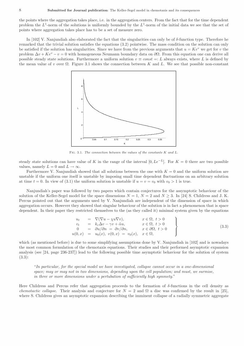
In [102] V. Nanjundiah also elaborated the fact that the singularities can only be of δ-function type. Therefore heremarked that the trivial solution satisfies the equations (3.2) pointwise. The mass condition on the solution can onlybe satisfied if the solution has singularities. Since we have from the previous arguments that u = Kev we get for v theproblem ∆v+Kev − v = 0 with homogeneous Neumann boundary data on ∂Ω. From this equation one can derive allpossible steady state solutions. Furthermore a uniform solution v ≡ const =: L always exists, where L is defined bythe mean value of v over Ω. Figure 3.1 shows the connection between K and L. We see that possible non-constant
0
2
4
6
8
L
0.05 0.1 0.15 0.2 0.25 0.3 0.35
K
Fig. 3.1. The connection between the values of the constants K and L.
steady state solutions can have value of K in the range of the interval [0, Le−L]. For K = 0 there are two possiblevalues, namely L = 0 and L→ ∞.
Furthermore V. Nanjundiah showed that all solutions between the one with K = 0 and the uniform solution areunstable if the uniform one itself is unstable by imposing small time dependent fluctuations on an arbitrary solutionat time t = 0. In view of (3.1) the uniform solution is unstable if u = v = v0 with v0 > 1 is true.
Nanjundiah’s paper was followed by two papers which contain conjectures for the assymptotic behaviour of thesolution of the Keller-Segel model for the space dimensions N = 1, N = 2 and N ≥ 3. In [24] S. Childress and J. K.Percus pointed out that the arguments used by V. Nanjundiah are independent of the dimension of space in whichaggregation occurs. However they showed that singular behaviour of the solution is in fact a phenomenon that is spacedependent. In their paper they restricted themselves to the (as they called it) minimal system given by the equations
ut = ∇(∇u − χu∇v), x ∈ Ω, t > 0vt = kc∆v − γv + αu, x ∈ Ω, t > 00 = ∂u/∂n = ∂v/∂n, x ∈ ∂Ω, t > 0
u(0, x) = u0(x), v(0, x) = v0(x), x ∈ Ω,
⎫⎪⎪⎬⎪⎪⎭ (3.3)
which (as mentioned before) is due to some simplifying assumptions done by V. Nanjundiah in [102] and is nowadaysthe most common formulation of the chemotaxis equations. Their studies and their performed asymptotic expansionanalysis (see [24, page 236-237]) lead to the following possible time asymptotic behaviour for the solution of system(3.3):
“In particular, for the special model we have investigated, collapse cannot occur in a one-dimensionalspace; may or may not in two dimensions, depending upon the cell population; and must, we surmise,in three or more dimensions under a pertubation of sufficiently high symmety.”
Here Childress and Percus refer that aggregation proceeds to the formation of δ-functions in the cell density aschemotactic collapse. Their analysis and conjecture for N = 2 and Ω a disc was confirmed by the result in [25],where S. Childress gives an asymptotic expansion describing the imminent collapse of a radially symmetric aggregate

Submitted for Journal publication: The Keller-Segel model in chemotaxis and its consequences 9
of chemotactic cells. However the studies of the stationary problem continued independently from this conjecture andthe report on the time independent problem should be closed first until the time asymptotic behaviour of the solutionof (3.3) becomes the main subject of the present considerations in the upcoming sections.
The papers by Childress and Percus were followed by the studies of stationary solutions done by R. Schaaf. In[124] she analyzed solutions of the system
0 = ∇(k1(u, v)∇u− k2(u, v)∇v), x ∈ Ω, t > 00 = kc∆v + g(u, v), x ∈ Ω, t > 0
∂u/∂n = ∂v/∂n = 0, x ∈ ∂Ω, t > 0u(0, x) = u0(x), v(0, x) = v0(x), x ∈ Ω.
⎫⎪⎪⎬⎪⎪⎭ (3.4)
with general nonlinearities satisfying the conditions1. Ω ⊂ R
N is a bounded open region with smooth boundary.2. k1, k2 : R
+ × R+ → R
+ are twice continuously differentiable and the ODE
d
dsr(s) = k2(r, s)/k1(r, s)
has a unique solution r : R+ → R
+ for any initial condition r(s0) = r0, s0, r0 ∈ R+.
3. g : R+ × R
+ → R is twice continuously differentiable and g−1(0) = ∅.via bifurcation techniques. Furthermore a criterion for bifurcation of stable nonhomogeneous aggregation patterns isgiven. In [124] R. Schaaf focused on the properties of stationary solutions of the Keller-Segel model with homogeneousNeumann boundary data in a very general setting. She shows that the stationary problem of the Keller-Segel model ina more general setting than the cases studied by V. Nanjundiah can also be reduced to a parameter-dependent singlescalar equation. More precisely she shows the following theorem:
Theorem 3.1 (Schaaf). (u, v) ∈ w ∈ X | w(Ω) ⊂ R+ × w ∈ X | w(Ω) ⊂ R
+ is a solution of (3.4) iff, forλ ∈ R
+,
u(x) = ϕ(v(x), λ) for all x ∈ Ω and kc∆v + g(ϕ(v(x), λ), v) = 0. (3.5)
Here the space X is defined as w ∈ Z | ∂w/∂n = 0 where Z is the space C2,β(Ω,R) with 0 < β < 1 for n > 1and C2(Ω,R) for N = 1. The function ϕ(s, λ) is given by r(s) with
d
dsr(s) = k2(r, s)/k1(r, s), r(1) = λ.
Then bifurcation methods are used in [124] to find natural bifurcation points. Furthermore R. Schaaf gives a stabilityanalysis for the constant stationary solutions of the Keller-Segel model.
For k1(u, v) = 1, k2(u, v) = χu and g(u, v) = −γv + αu the stationary solutions of the Keller-Segel model solvethe equation
kc∆v − γv + αλ exp(χv) = 0 in Ω (3.6)
with homogeneous Neumann boundary data. Of course the question of positive, nontrivial solutions for this equationarises. The existence of nontrivial radially symmetric solutions for this equation has been shown in [11, Proposition1] under the assumption that γ > 0, but Biler did not consider the nonsymmetric case (The Neumann boundary dataimplies that there are no solutions provided γ = 0.).
Using variational techniques introduced by M. Struwe and G. Tarantello in [143] J. Wei and G. Wang [149], T.Senba and T. Suzuki [129, 130] and in [62] myself proved for Ω ⊂ R
2 independently the existence of nontrivial solutionsof (3.6) without symmetry assumptions for γ ≥ 1 and 4π < αχλ/kc. The existence of nontrivial solutions of (3.6) inthe case that αχλ/kc < 4π follows from arguments that will be mentioned later in the present paper.
The idea of the existence proof for γ ≥ 1 and 4π < αχλ/kc is based on the studies of the functional
Fαχλ/kc(v) :=
12
∫Ω
|∇v|2 + γv2dx− αχλ
kclog
⎛⎝ 1|Ω|
∫Ω
ev dx
⎞⎠ ,
10 Submitted for Journal publication: The Keller-Segel model in chemotaxis and its consequences
where v ∈ D := v ∈ H1(Ω) |v has mean value equal to zero over Ω. One easily notices that v ≡ 0 is a strictlocal minimum for Fαχλ/kc
in the case that γ > αχλ|Ω|kc
− µ1, where µ1 is the first eigenvalue of the Laplacian withhomogeneous Neumann boundary data. Then one recognizes that for a smooth domain Ω and αχλ > 4kcπ there is asequence vεε≥0 ⊂ D with
vε(x) = log(
ε2
(ε2 + π|x− x0|2)2
)− 1
|Ω|
∫Ω
log(
ε2
(ε2 + π|x− x0|2)2
)dx,
where x0 is an arbitrary point on ∂Ω, such that Fαχλ/kc(vε) → −∞ and ||∇vε||L2(Ω) → ∞ as ε→ 0. As a consequence
there exists a v0 ∈ D Such that Fαχλ/kc(v0) < 0 and ||v0||H1(Ω) ≥ 1. One now defines
P ≡ p : [0, 1] → D | p is continuous and p(0) = 0, p(1) = v0 and sets kαχλ/kc≡ inf
p∈Pmaxt∈[0,1]
Fαχλ/kc(p(t))
for all αχλ/kc ≥ 4π. Using the fact that the mapping αχλ/kc → kckαχλ/kc
αχλ is monotone decreasing for all αχλ/kc ≥ 4πwe see that it is differentiable for almost every αχλ/kc ≥ 4π. The rest of the proof then consists of the constructionof a Palais-Smale sequence for Fαχλ/kc
that contains a subsequence that converges strongly in H1(Ω) to a criticalpoint of Fαχλ/kc
. The construction of the Palais-Smale sequence can be done exactly as in the paper by M. Struweand G. Tarantello [143]. The existence of the nontrivial critical point of the Functional Fαχλ/kc
over the set D allowsus to conclude the existence of a nontrivial solution of equation (3.6). This is easy to be seen. If one introduces thenew function w := χv − (χ
∫Ω v dx)/|Ω| we get from (3.6) the Euler-Lagrange equation of the minimizing problem
inf Fαχλ/kc(v) over the set D. Thus the existence of a nontrivial critical point of the functional gives us also the
existence of a nontrivial steady state solution of the Keller-Segel model with a linear sensitivity function.
With different methods than those just mentioned Y. Kabeya and W.-M. Ni proved in [68] also the existence ofpositive nontrivial stationary solutions of (3.6). Furthermore they showed the following results:
Theorem 3.2 (Kabeya & Ni). Let Ω ⊂ R2. Suppose that t = λeχt has two positive solutions. Then there exists
a non constant solution vε of (3.6) provided ε :=√kc/γ is sufficiently small. Moreover, there exist constants C1 > 0,
C2 > 0, δ > 0, K > 0 and ε > 0 such that:
supΩvε ≤ C1, inf
Ωvε ≤ C2e
− δε and
∫Ω
(ε2|∇vε|2 + γv2ε)dx ≥ Kε2
for any 0 < ε < ε0. Furthermore for sufficiently small ε > 0 the solution vε has exactly one local maximum point inΩ, which must lie on the boundary ∂Ω.
This theorem is similar to results that have been established for the stationary Keller-Segel model with a logarith-mic chemotactical sensitivity. In this case the transformation introduced by R.Schaaf in [124] leads to the problem
d∆w − w + wp = 0, in Ω with ∂w/∂n = 0, on ∂Ω. (3.7)
In [79, 104] and [105] the authors prove the existence of stationary solutions of this equation for Ω ⊂ RN with N ≥ 2
and 1 < p < (N + 2)/(N − 2) if N ≥ 3 and 1 < p <∞ if N = 2. Their results for this problem can be summarized asfollows:
Theorem 3.3 (Ni & Takagi). Let wd be a least energy solution of (3.7), i.e. a critical point of
Jd(v) :=∫Ω
12(d|∇v|2 + v2) − 1
p+ 1vp+1+ dx
such that Jd(wd) = cd where cd := infh∈Γ
max0≤t≤1
Jd(h(t)), in which Γ := h ∈ C([0, 1];W 1,2(Ω)) | h(0) = 0, h(1) = e
and e ≡ 0 is a nonnegative function in W 1,2(Ω) with Jd(e) = 0. The wd has at most one local maximum in Ω and thisis attained in exactly one point which must lie on the boundary, provided that d is sufficiently small. If Pd ∈ ∂Ω is theunique point at which maxwd is achieved. Then lim
d→0H(Pd) = max
P∈∂ΩH(P ) where H(p) denotes the mean curvature of
∂Ω at P .

Submitted for Journal publication: The Keller-Segel model in chemotaxis and its consequences 11
Of course many generalizations of this result have been published in the recent years (see for example the papersby [46] and [119]), but it is not the goal of the present paper to mention all these results. Therefore I leave this to theinterested reader and turn now to the time dependent problem. However it is recommended to recall the presentedresults when looking at the time asymptotic behaviour of the solution in the upcoming section. Recalling the resultsof the present section will help to understand the results for the time asymptotics of the solution and will help tounderstand which behaviour one might expect for the solution. Before we now definitively turn to the time dependentproblem let us explain some terms used in the present section. We have seen that there are different effects that onecan expect. In some cases we spoke of aggregation and in other cases of a special form of aggregation namely theformation of δ-singularities. This was sometimes called chemotactical collapse. Before we turn to the time dependentmodel we therefore now introduce three important effects in the mathematical language.
Definition 3.4. Let (u(t, x), v(t, x)) be a solution of (2.4) for the corresponding initial data (u0(x), v0(x)). Wesay that the model describes aggregation, if lim inf
t→∞ ||u(t, x)||L∞(Ω) > ||u0(x)||L∞(Ω) and ||u(t, x)||L∞(Ω) < konst for
all t. The solution blows up resp. is a blow-up solution if ||u(t, x)||L∞(Ω) or ||v(t, x)||L∞(Ω) becomes unbounded ineither finite or infinite time, i.e. there exists a time Tmax with 0 < Tmax ≤ ∞ such that
lim supt→Tmax
||u(t, x)||L∞(Ω) = ∞ or lim supt→Tmax
||v(t, x)||L∞(Ω) = ∞.
We will speak of chemotactical collapse if lim supt→∞
||u(t, x)||L∞(Ω) < ||u0(x)||L∞(Ω).
Remark that this definition is almost identical to that given in [112] beside the difference in the allowed blow-uptime for a blow-up solution. Furthermore remark that the three cases do not exclude themselves, i.e. more thanone case can happen for the same solution. At the end of this section let us summarize the mentioned results in thefollowing table:
Table 3.1Collection of results for the stationary Keller-Segel models.
Observation References
For model (2.4) the uniform distribution (u0, v0) becomes unstable if [69]k2(u0,v0)v0)k1(u0,v0)u0
+ u0f′(v0)
k3(v0)+v0k′3(v0) > 1.
All solutions between the one with K = 0 (as defined in this section) [102]and the uniform solution are unstable if the uniform one itself is unstable.
The stationary problem of the Keller-Segel model can be reduced to the [102, 124]parameter-dependent single scalar equation (3.5).
There exist non-constant stationary solutions of the Keller-Segel model; [11, 62, 68, 79, 104, 105, 129]for example for a linear and for a logarithmic chemotactical sensitivity [130] and [149]function.
4. The time dependent problem: The case of a linear chemotactical sensitivity. The conjectures andobservations by V. Nanjundiah, S. Childress and J. K. Percus have been the initiating motivations for a large numberof researchers to study the time asymptotic behaviour of the solution of the system (3.3). There is still an avalancheof publications running and I am pretty sure that by the date of publication of the present paper the number will havealready increased once again. Parallel to the results of this section various papers were published in which versions ofthe Keller-Segel model with a different chemotactic sensitivity function were studied. I will mention these results inan upcoming section. Thus we will only focus on results for (3.3) in this section resp. the upcoming subsections.
4.1. Early results on the time asymptotics and conjectures. The first step in the analysis of the conjecturesof Childress and Percus was done by W. Jager and S. Luckhaus in 1992. In [67] they introduced the transformation
U(t, x) :=|Ω|u(t, x)∫
Ω
u(t, x)dxand V (t, x) := v(t, x) − 1
|Ω|
∫Ω
v(t, x)dx

12 Submitted for Journal publication: The Keller-Segel model in chemotaxis and its consequences
which leads to the system:
Ut = ∇(∇U − χU∇V ), x ∈ Ω, t > 01kc
(Vt + γV ) = ∆V + αkc
(U − 1), x ∈ Ω, t > 0∂U/∂n = ∂V /∂n = 0, x ∈ ∂Ω, t > 0U(0, x) = U0(x), V (0, x) = V0(x). x ∈ Ω,
⎫⎪⎪⎬⎪⎪⎭ (4.1)
Jager and Luckhaus then assume that α = kcα, the constants χ, kc, α are of the order 1ε with ε and γ and α are of
order 1. Thus they get for small ε resp. for ε→ 0 the system
Ut = ∇(∇U − χU∇V ), x ∈ Ω, t > 00 = ∆V + α
kc(U − 1), x ∈ Ω, t > 0
∂U/∂n = ∂V /∂n = 0, x ∈ ∂Ω, t > 0U(0, x) = U0(x) x ∈ Ω.
⎫⎪⎪⎬⎪⎪⎭ (4.2)
Their result in space dimension N = 2 for system (4.2) is summarized as follows:
Theorem 4.1 (Jager & Luckhaus). Let Ω be a bounded open set in R2, ∂Ω is a C1-boundary, U0(x) is C1 and
satisfies the boundary condition.1. There exists a critical number c(Ω) such that αχU0(x) < c(Ω) implies that there exists a unique, smooth
positive solution to (4.2) for all time.2. Let Ω be a disk. There exists a positive number c∗ with the following property: If αχU0(x) > c∗ then radially
symmetric positive initial values can be constructed such that explosion of U(t, x) happens in the center of thedisc in finite time.
Here the notation U0(x) is used for the mean value of U0(x) over the domain Ω. More precisely Jager and Luckhausshow the following Proposition which implies 1. of the previous Theorem 4.1.
Proposition 4.2 (Jager & Luckhaus). Let Ω be a domain satisfying the smoothness assumptions from theTheorem above. Let U(t, x) be a smooth positive solution to (4.2) and t∗ the maximal time of existence, 0 < t∗ ≤ ∞.There exists a positive number c1(Ω) such that t∗ <∞ implies
limk→∞
limt→t∗χαU0(x)
∫Ω
(U(t, x) − k)+dx ≥ c1(Ω).
Proposition 4.2 is shown by multiplying the first equation of (4.2) with ϕ = (U − k)m−1+ where k ≥ 0 and m > 1.
Then the second equation of (4.2) allows to estimate the term
−∫Ω
U∇V∇(U − k)m−1+ dx = −
∫Ω
∇V∇(m− 1m
(U − k)m+ + k(U − k)m−1+
)dx from above by c(k,m)
∫Ω
(U − k)m+dx.
If the statement of Proposition 4.2 did not hold this estimate would allow us to find the following inequality
d
dt
∫Ω
(U − k)m+dx ≤ c2(Ω, k) + c3(k)∫Ω
(U − k)m+ dx for all t ≥ t1
which would give us a bound for the Lm-norms of U(t, x) and the global existence would follow by standard regularityarguments for solutions of elliptic and parabolic equations.
For the proof of the blow-up statement 2. of Theorem 4.1, W. Jager and S. Luckhaus studied the function
M(t, ρ) :=
√ρ∫
0
(U(t, r) − 1)r dr for r = |x|, 0 ≤ ρ ≤ R.
Using the equations of (4.2) they found that M(t, ρ) has to solve the following initial boundary value problem:
∂
∂tM = 4ρ
∂2
∂ρ2M + αχU0(x)
∂
∂ρM + αχU0(x)M, with M(0, ρ) =
√ρ∫
0
(U0(r) − 1)r dr and M(t, 0) = M(t, R) = 0.

Submitted for Journal publication: The Keller-Segel model in chemotaxis and its consequences 13
Constructing a subsolution W (t, ρ) for this problem such that W (t, ρ) ≤M(t, ρ) for all t, ρ and
limt→Tfinite
supρ<ε
W (t, ρ) ≥ ω > 0
for each ε > 0 they proved that the solution has to blow up at time Tfinite in the center of the disk. FurthermoreJager and Luckhaus asked for more information about the blow-up behaviour of the solution of (4.2). In a remark [67,page 820] they formulated the following questions:
“It would be interesting to know more about the set of explosion points at t∗. The solution may globallyexist as weak solutions. The development of singularities after a finite time t∗ is another importanttopic to be studied.”
Even though it was not the next paper in the chronology I now mention the results from M. A. Herrero and J. J.L. Velazquez [49] from 1996 and M. A. Herrero, E. Medina and J. J. L. Velazquez [52, 53] from 1997 and 1998 sincethey studied system (4.2) in those papers. In [49, 54] they focused on the possible formation of δ-function singularitiesin finite time in space dimension N = 2. Using asymptotic expansion methods in [49] their result was the following:
Theorem 4.3 (Herrero & Velazquez). Let R > 0, and let ΩR = x ∈ R2 : |x| < R. Then there exist radial
solutions of (4.2) defined in an interval (0, T ) with T > 0, and such that:
u(t, r) → 8πkcχα
δ(0) + ψ(r) as t→ T, (4.3)
in the sense of measures, where δ(0) is the Dirac measure centered at r = 0, and:
ψ(r) =C
r2e−2| log(r)|1/2
(2| log(r)|)1
2√
2| log(r)|1/2 − 12 (1 + o(1)) (4.4)
as r → 0, where C is a positive constant depending on χ. At t = T , the profile near r = 0 is given by:
u(t, r) =8πkcχα
δ(0) + ψ(r); ψ(r) as in (4.4). (4.5)
Moreover, if we set S(t) = (T − t)(supΩu(t, r)) ≡ (T − t)u(0, t), one has that lim
t→TS(t) = ∞. More precisely, there holds:
S(t) = C1(T − t)−1| log(T − t)|1−1√
| log(T−t)| as t→ T, for some C1 > 0.
So they found solutions that form in finite time a δ-singularity in the center of the disk in R2. Furthermore
they investigated a result for the whole space in the three dimensional case in [52, 53] and [54]. There they studiedself-similar solutions and could formulate the following statements.
Theorem 4.4 (Herrero, Medina & Velazquez).1. Consider (4.2) in space dimension N = 3 with Ω = R
3. Then, for any T > 0 and any constant C > 0, thereexists a radial solution (u(t, r), v(t, r)) of (4.2) that is smooth for all times 0 < t < T , blows up at r = 0 andt = T , and is such that: ∫
|x|≤r
u(T, s) ds→ C.
2. Consider (4.2) in space dimension N = 3 with Ω = R3. For any T > 0 there exists a sequence δnn∈N with
limn→∞ δn = 0, and a sequence of radial solutions (un(t, r), vn(t, r)), that blows up at r = 0 and t = T , andare such that un(t, r) is self-similar, and
un(t, r) ∼(
8πkcχα
+ δn
)(4πr2)−1 as r → 0.
For this solution
N(t, r) :=∫|x|≤r
u(T, s) ds→ 0 as r → 0

14 Submitted for Journal publication: The Keller-Segel model in chemotaxis and its consequences
3. No radial, self-similar solution of (4.2) exists such that N(t, r) < ∞ as r → 0 when N = 2, resp. whenΩ = R
2.
Thus one slowly got more and more insights for the Keller-Segel model but at this point several questions stillremained open. To name a few beside the questions raised in [67] we list the following.
1. What happens if one drops the assumption of radial symmetry of the solution and how does in the case ofblow-up the blow-up profile of the solutions look like?
2. Is it possible to prove blow up results also for the full system (3.3)?3. Can one give the precise value for the threshold value which decides whether the solution might blow up or
not?As in the section before I summarize the results of this section in a table, too.
Table 4.1Possible time asymptotical behaviour of the solutions of the simplified model 4.2.
Dimension Observation References
N=2 There exists a critical value c(Ω) such that a unique, smooth positive solution [67]to (4.2) exists globally in time if αχU0(x) < c(Ω).
Let Ω be a disk. Then there exists a positive number c∗ such that there existsradially symmetric positive initial data with the following property: If αχU0(x) > c∗
then radially symmetric positive initial values can be constructed such that explosionof U(t, x) happens in the center of the disc in finite time.
There exists radially initial data such that the solution of (4.2) forms in the center [49, 54]of a disk Ω a δ-function singularity described in Theorem 4.3 in finite time.
When Ω = R2, then no radial, self-similar solutions of (4.2) exist such that [52, 54]∫
|x|≤ru(T, s) ds <∞ as r → 0.
N=3 Let Ω = R3. Then there exists, for any T > 0 and any constant C > 0, a radial [52, 53, 54]
solution (u(t, r), v(t, r)) of (4.2) that is smooth for all times 0 < t < T ,blows up at r = 0 and t = T , and is such that:
∫|x|≤r
u(T, s) ds→ C.
For any T > 0 there exists a sequence δnn∈N with limn→∞ δn = 0, and asequence of radial solutions (un(t, r), vn(t, r)), that blows up at r = 0 and t = T ,and are such that un(t, r) is self-similar, and un(t, r) ∼
(8πkc
χα + δn
)(4πr2)−1
as r → 0. For this solution∫|x|≤r
u(T, s) ds→ 0 as r → 0.
4.2. Progress and further questions. After W. Jager’s and S. Luckhaus’ paper in 1992 the next step wasperformed by T. Nagai in [87]. In his 1995 article “Blow-up of radially symmetric solutions to a chemotaxis system”[87] he proved the following result for the simplified system
ut = ∇(∇u − χu∇v), x ∈ Ω, t > 00 = kc∆v − γv + αu, x ∈ Ω, t > 0
∂u/∂n = ∂v/∂n = 0, x ∈ ∂Ω, t > 0u(0, x) = u0(x), x ∈ Ω.
⎫⎪⎪⎬⎪⎪⎭ (4.6)
Theorem 4.5 (Nagai).1. Suppose that N = 1, or N = 2 and αχ
∫B(0,R)
u0(x)dx < 4ωN with radially symmetric u0(x). Then Tmax = ∞
and supt≥0
||u(t, ·)||L∞(B(0,R)) + ||v(t, ·)||L∞(B(0,R))
<∞.

Submitted for Journal publication: The Keller-Segel model in chemotaxis and its consequences 15
2. Let N ≥ 2 and u0 be radially symmetric. If
0 > 2N(N − 1)
⎛⎝ 1ωN
∫Ω
u0(x)dx
⎞⎠
2/N⎛⎜⎝ 1ωN
∫B(0,R)
u0(x)|x|Ndx
⎞⎟⎠
(N−2)/N
− N
2αχ
⎛⎝ 1ωn
∫Ω
u0(x)dx
⎞⎠
2
+αχNR−N
⎛⎝ 1ωn
∫Ω
u0(x)dx
⎞⎠⎛⎜⎝ 1ωN
∫B(0,R)
u0(x)|x|Ndx
⎞⎟⎠
+αχγ
⎧⎪⎪⎪⎪⎪⎨⎪⎪⎪⎪⎪⎩
1e
(1ωN
∫Ω
u0(x)dx)3/2
(1ωN
∫B(0,R)
u0(x)|x|Ndx)1/2
, if N = 2
N2(N−2)
(1ωN
∫Ω
u0(x)dx)(2N−2)/N
(1ωN
∫B(0,R)
u0(x)|x|Ndx)2/N
, if N ≥ 3
where ωN denotes the area of the unit sphere SN−1 in RN , then Tmax <∞ and
lim supt→Tmax
||u(t, ·)||L∞(B(0,R)) = ∞.
Furthermore the radially symmetric solution (u(t, r), v(t, r)) of (4.6) satisfies u(t, r) + v(t, r) ≤ K(n) for1n ≤ r ≤ R and 0 ≤ t < Tmax where K(n) denotes a generic positive constant depending on n ∈ N such thatK(n) → ∞ as n→ ∞. Thus the blow-up can only occur at the point r = 0.
While the first statement is easy to check the second is based on some subtle estimates of the expression
MN (t) :=1ωN
∫B(0,R)
u(t, x)|x|Ndx.
The global existence proof of solutions of (4.6) in one space dimension performed in [87] illustrates in a nice wayhow one tries to show the existence of the solution global in time in higher space dimensions. Therefore we firstdemonstrate this proof here. If we integrate for N = 1 the second equation of (4.6) on (−R, x) we get
vx(t, x) = γ
x∫−R
v(t, y)dy − α
x∫−R
u(t, y)dy.
Thus we see that
|vx(t, x)| ≤ α
R∫−R
u0(x)dx on Ω × (0, Tmax).
For x ∈ Ω = (−R,R) we now obtain
2Rv(t, x) =
R∫−R
v(t, y)dy +
R∫−R
x∫y
vx(t, z)dz dy and therefore 0 ≤ v(t, x) ≤ α
2R
(1γ
+ 4R2
)∫Ω
u0(x)dx.
Thus ||v(t, ·)||L∞(Ω) ≤ const and ||vx(t, ·)||L∞(Ω) ≤ const for all 0 < t < Tmax. Multiplying now the first equation of(4.6) with up for p ≥ 1 and integrating the equation over Ω yields
1p+ 1
d
dt
∫Ω
up+1dx =−2pp+ 1
∫Ω
|∇u(p+1)/2|2dx +p(p+ 1)
2· const ·
∫Ω
up+1dx.
Now the bound of the L∞-norm of the solution can be obtained by application of N. D. Alikakos’ version of the Moseriteration introduced in [2]. One therefore sees that the question whether the solution exists globally in time or notdepends crucially on a uniform bound for the L∞-norm of the gradient of v. This simplified version of the Keller-Segel

16 Submitted for Journal publication: The Keller-Segel model in chemotaxis and its consequences
model has been extensively studied by Nagai and his coauthors. Once again we cannot follow the chronology since thedifferent versions of the Keller-Segel model have been studied parallel. Thus I concentrate on the results on system(4.6) in this subsection and turn to the results for the full Keller-Segel model (3.3) resp. (4.1) later on. The simplifiedversions allow to decouple the system. Therefore techniques are available in these cases which are not at hand forthe full parabolic version. For the simplified version (4.6) recent results from Nagai, Senba, Suzuki et al. give moreinformation about the blow-up profile of the solution and the non symmetric blow up. However their proofs are verytechnical and desire fine estimates that are difficult to demonstrate in a simple way. Thus I restrict myself to presenttheir results in Table 4.2 and 4.3.
Table 4.2Possible time asymptotical behaviour of the solutions of the simplified model 4.6 with γ > 0.
Dimension Observation References
N = 1 The solution of the Keller-Segel model exists [87]globally in time and is uniformly bounded for all t ≥ 0.
N = 2 If αχ∫Ω
u0(x)dx < 4π then the classical solution of the Keller-Segel model [87, 89, 90, 91]
exists globally in time and is uniformly bounded for all t ≥ 0. [94, 97] and [126]If Ω is a circle and u0 is radially symmetric or satisfies u(x) = u(−x) in Ω,then this statement holds if αχ
∫Ω
u0(x)dx < 8π.
Let x0 ∈ Ω. If αχ∫Ω
u0(x)dx > 8π and if∫Ω
u0(x)|x − x0|2dx is [98]
sufficiently small, then the corresponding solution of (4.6) and (4.2)blows up in finite time.
Assume that ∂Ω has a line segment L0, and that Ω lies on one side [98]of a line L containing L0. If furthermore αχ
∫Ω
u0(x)dx > 4π and if∫Ω
u0(x)|x − x0|2dx is sufficiently small for a point x0 ∈ L0 that is not an
end-point of L0, then the corresponding solution of (4.6) and (4.2)blows up in finite time.
If Ω is a circle, u0 is radially symmetric and if αχ∫Ω
u0(x)dx > 4ω2, [87]
then there exists a constant C1 depending on 1ω2
∫Ω
u0(x)dx such that
if 0 < 1ω2
∫Ω
u0(x)|x|2dx < C1 then u blows up in finite time.
If αχ∫Ω
u0(x)dx < 8π and Tmax <∞ then there exists a point in x0 ∈ ∂Ω [92, 93]
such that lim supt→Tmax
∫Ω∩B(x0,ε)
u(t, x)dx ≥ 2π/a∗α for any ε > 0, where a∗ is
a root of a∗ − χ/2 − ||u0||L1(Ω)αa∗/16π = 0 such that a∗ < χ.
Suppose Tmax <∞. Then there exist for any isolated blow-up point x0 [92, 93, 127]two positive constants δ, m ≥ m∗ and a non-negative function and [132]f ∈ L1(B(x0, δ) ∩ Ω) ∩C(B(x0, δ) ∩ Ω \ x0) such that u(t, ·) convergesweakly in the Banach space of all Radon measures on B(x0, δ) ∩ Ω tomδx0 + f as t→ Tmax, where m∗ is equal to 4π/αχ if x0 ∈ ∂Ω and equal to8π/αχ if x0 ∈ Ω.
Suppose Ω = R2 and let x0 ∈ R
2. If αχ∫
R2
u0(x)dx > 8π and [95]
if∫
R2
u0(x)|x − x0|2dx is sufficiently small, then the corresponding
solution of (4.6) blows up in finite time.

Submitted for Journal publication: The Keller-Segel model in chemotaxis and its consequences 17
Table 4.3Possible time asymptotical behaviour of the solutions of the simplified model 4.6 with γ > 0.
Dimension Observation References
N ≥ 3 If Ω is a sphere and u0 is radially symmetric, then there exists a constant C1 [87]depending on 1
ωN
∫Ω
u0(x)dx such that if 0 < 1ωN
∫Ω
u0(x)|x|Ndx < C1 then u
blows up in finite time.
Suppose Ω = RN and let x0 ∈ R
N . If∫
RN
u0(x)|x − x0|Ndx is sufficiently small, [95]
then the corresponding solution of (4.6) blows up in finite time.
Of course one can now draw conclusions on the possible number of blow-up points. However I will mention theseconclusions a little bit later. Thus at this point let us turn again to a different line of research.
4.3. Analysis of the system (4.1). Similar to their result for the simplified system (3.3) M. A. Herrero andJ. J. L. Velazquez achieved a very important contribution on the blow-up profile of the solution of the full parabolicsystems (3.3) and the system (4.1) with γ = 0 in their papers [50] and [51]. Using once again asymptotic expansiontheory they were able to describe the blow-up profile of the system (3.3) and proved therefore the possibility of aδ-function formation in finite time for radially symmetric solutions as it was conjectured by Nanjundiah [102] andChildress and Percus [24]. Their main result for system (3.3) is summarized as follows:
Theorem 4.6 (Herrero & Velazquez). Let R > 0, and let ΩR = x ∈ R2 : |x| < R. Then there exist radial
solutions of (3.3) defined in an interval (0, T ) with T > 0, and such that:
u(t, r) → 8πkcχα
δ(0) + ψ(r) as t→ T, (4.7)
in the sense of measures, where δ(0) is the Dirac measure centered at r = 0, and:
ψ(r) =C
r2e−2| log(r)|1/2
(1 + o(1)) (4.8)
as r → 0, where C is a positive constant depending on χ. At t = T , the profile near r = 0 is given by:
u(t, r) =8πkcχα
δ(0) + ψ(r); ψ(r) as in (4.8). (4.9)
Moreover, if we set S(t) = (T − t)(supΩu(t, r)) ≡ (T − t)u(0, t), one has that lim
t→TS(t) = ∞. More precisely, there holds:
S(t) = C1(T − t)−1e√
2| log(T−t)| as t→ T, for some C1 > 0. (4.10)
The studies of the asymptotic behaviour of the solution in the non-symmetric case began with the results of[11, 43, 90] and [153]. In [11, 43, 90] the authors introduce independently from each other a Lyapunov functional forthe system (3.3) resp. (4.1) which became an important tool in the then following studies of the time asymptoticbehaviour of the solution of the systems (3.3) resp.(4.1). This Lyapunov function is given by
F (u(t), v(t)) :=1
2αχ
∫Ω
kc|∇v(t)|2 + γv2(t) + u(t) log(u(t)) − u(t)v(t)dx. (4.11)
Using a Moser-Trudinger type inequality originally formulated by Chang and Yang in [23] the analysis of this functionalshows the following:
1. The functional F (u, v) is bounded from below, if αχ∫Ω
u0(x)dx ≤ 4π.
2. The functional F (u, v) is no longer bounded from below, if αχ∫Ω
u0(x)dx > 4π.
18 Submitted for Journal publication: The Keller-Segel model in chemotaxis and its consequences
3. For radially symmetric functions the functional F (u, v) is bounded from below, if αχ∫Ω
u0(x)dx ≤ 8π. and is
no longer bounded from below, if αχ∫Ω
u0(x)dx > 8π.
Now two different lines of research became recognizable. One considered system (3.3) and used more PDE basedmethods to prove global existence and finite time blow-up results for this system and the other was concerned withsystem (4.1) and used methods more related to the calculus of variations. Once again one has to follow these two linesseparately to get a clear picture of the achieved results. Let us first have a closer look at the results for (3.3)
4.3.1. Results for system (3.3). Since the question of the well-posedness of a negative cross-diffusion systemis not trivial I first turn to the results on the local existence of a solution and possible regularity results. Here oneshould basically mention A. Yagi [153] and T. Nagai, T. Senba and K. Yoshida [90] whose results can be summarizedas follows:
Theorem 4.7. Let Ω be a bounded, smooth domain in R2. Assume u0, v0 ∈ H1+ε0(Ω) for some 0 < ε0 ≤ 1 and
u0(x) ≥<, v0(x) ≥ 0 on Ω. Let Tmax be the maximal existence time of (u(t), v(t)).1. (Yagi) System (3.3) has a non-negative solution (u, v) satisfying
u, v ∈ C([0, Tmax) : H1+ε1(Ω)) ∩C1((0, Tmax) : L2(Ω)) ∩C((0, Tmax) : H2(Ω))
for any 0 < ε1 < minε0, 1/2. Moreover (u, v) has further regularity properties:
u ∈ C1((0, Tmax) : H1(Ω)), v ∈ C14 ((0, Tmax) : H3(Ω)) ∩ C 5
4 ((0, Tmax) : H1(Ω)).
2. (Yagi) If Tmax <∞, then
limt→Tmax
(||u(t, ·)||H1+ε0 (Ω) + ||v(t, ·)||H1+ε0 (Ω)) = ∞,
lim supt→Tmax
||u(t, ·)||Lp(Ω) = ∞ for any 1 < p ≤ ∞,
lim supt→Tmax
||v(t, ·)||H1+ε(Ω) = ∞ for any 0 < ε ≤ ε0.
3. (Nagai, Senba & Yoshida) If ∫Ω
u0(x)dx <4Θkcαχ
,
where Θ = 8π for Ω = x ∈ R2 : |x|2 < R and (u0, v0) is radial in x and Θ = 4π otherwise, then the solution
(u, v) of (3.3) exists globally in time and supt≥0
||u(t, ·)||L∞(Ω) + ||v(t, ·)||L∞(Ω) <∞.
The local existence and regularity results summarized in Theorem 4.7 above have been achieved by using semi-group theory. A. Yagi also proved similar local existence results for more general forms of the system (2.4) in [153] andI will turn to these results later. The bound of the L∞-norm of the solution can once more be achieved by applicationof N. D. Alikakos’ version of the Moser iteration introduced in [2]. Once again the basic and most important step isto find a uniform L∞-norm estimate of ∇v(t, x) for all t ≥ 0. Nagai, Senba and Yoshida succeeded in finding such abound in the case where the functional F (u, v) is bounded from below. A. Yagi studied in [153] which norms of thesolution have to blow-up if the solution exists only for a finite maximal time of existence Tfinite. However beside theresults of Herrero and Velazquez in [50, 51] there are no results, that show the existence of initial data such that thecorresponding solution of (3.3) has to blow up in finite time. However there are results under the assumption thatthere is a solution which blows-up in finite time. Let us therefore now turn to those results, that studies the blow-upprofile and behaviour of such a solution.
Under the main assumption that there is a solution of the Keller-Segel model that blows up in finite time Tfinitesuch that
inf0≤t<Tfinite
F (u(t), v(t)) > 0 or (4.12)
limt→Tfinite
F (u(t), v(t)) = −∞

Submitted for Journal publication: The Keller-Segel model in chemotaxis and its consequences 19
Nagai, Senba and Suzuki proved in [96, 98] the following results.
Theorem 4.8 (Nagai, Senba & Suzuki). Let Ω ⊂ R2 be a bounded domain with smooth boundary ∂Ω. Furthermore
let B denote the set of all those points x0 in Ω such that there is a sequence xkk∈N ⊂ Ω and a sequence tkk∈N ⊂[0, Tfinite) with u(tk, xk) → ∞, tk → Tfinite and xk → x0 as k → ∞. BI ⊂ B denotes the set of all isolated blow-uppoints, i.e x0 ∈ BI, iff there exists a R > 0 such that
sup0≤t<Tfinite
||u(t, ·)||L∞((B(x0,R)\B(x0,r))∩Ω) <∞
for any r ∈ (0, R) with B(x0, R) := x ∈ R2 | |x0 − x| < R. Then the following statements hold:
1. Given x0 ∈ BI , we have 0 < R << 1, m ≥ m∗, and
f ∈ L1(B(x0, P ) ∩ Ω) ∩ C(B(x0, R) ∩ Ω \ x0)
satisfying f ≥ 0 and u(t, ·)dx converges weakly to mδx0(dx)+f dx as t→ Tfinite in the set of Radon measureson B(x0, R) ∩ Ω, where
m∗ :=
8π, x0 ∈ Ω4π, x0 ∈ ∂Ω.
2. If (4.12) occurs, then B = BI .3. If (3.3) is radially symmetric and Tmax <∞ then B = 0.
These results imply that in the case of a finite time blow-up of the solution the set of isolated blow-up points hasfinite cardinality and that
1 < 2 × (BI ∩ Ω) + (BI ∩ ∂Ω) ≤||u0||L1(Ω)
4π.
However a better lower bound of the quantity is of interest in the non radially symmetric case with ||u0||L1(Ω) > 8π.Where does the blow-up occur? Is there only one blow-up point in the interior of Ω or are there two blow-up pointsat the boundary ∂Ω in this case?
Beside the previous results Senba and Suzuki established in [131] the following results using rearrangement andsymmetrization arguments. These results are similar to those achieved independently and by other methods in [62]and [63] for the system (4.1).
Theorem 4.9 (Senba & Suzuki). Let Ω ⊂ R2 be a bounded domain with smooth boundary ∂Ω.
1. If Ω is the unit disk, αχ||u0||L1(Ω) < 8πkc and u0(x) = u0(−x), v0(x) = v0(−x) hold, then the solution of(3.3) exists globally in time and satisfies the equations in the classical sense, i.e. the solution is sufficientlysmooth.
2. If Tmax <∞ then
limt→Tmax
||u(t) log u(t)||L1(Ω) = limt→Tmax
||u(t)v(t)||L1(Ω) = limt→Tmax
||∇v(t)||2L2(Ω) = limt→Tmax
∫Ω
eav(t)dx = ∞,
where a > 1.3. If Ω is simply connected , αχ||u0||L1(Ω) < 8πkc, and Tmax <∞ then
limt→Tmax
∫∂Ω
ev(t)/2dx = ∞.
The last statement in particular implies together with the previous statements on the number of isolated blow-uppoints in Theorem 4.8 that if there is a solution that blows up in finite time for 4πkc < αχ||u0||L1(Ω) < 8πkc thenthe blow-up has to happen at the boundary of the domain. However, at this stage it has to be pointed out that theseresults do not give the existence of a solution that blows-up in either finite or infinite time. These results always usethe existence of a solution that blows up in finite time as an assumption, but do not prove that those solutions in factreally exist.

20 Submitted for Journal publication: The Keller-Segel model in chemotaxis and its consequences
Beside the analysis of the Keller-Segel system (3.3) on a bounded domain T. Nagai also studied the problem onthe whole space R
2. In this situation he could prove that for αχ∫R2
u0(x)dx < 4πkc the solution exists globally in time,
once again via analyzing the functional F (u, v) for Ω = R2 this time. Furthermore he found several decay properties
of the solution but for those results we refer the reader to [95].
Throughout this subsection we focused the two dimensional case and left out the other space dimensions. So what isknown for the cases N = 1 and N ≥ 3? For the case N = 1 the paper by K. Osaki and A. Yagi [109] fills the gapof the missing global existence proof for (3.3). Furthermore they show there that in this case the solution convergesto a stationary solution as t → ∞. For the case of higher space dimensions N ≥ 3 and a bounded domain Ω ⊂ R
N
I am aware of any result on the time asymptotic behaviour of the solution. The local existence of a solution can beestablished in such cases using the results of H. Amann [6, 7] for example. This has been mentioned for example in[61] and [115].
4.3.2. Results for system (4.1). Independent from the previous research line and parallel to those results therewere the results for the system (4.1). Under different regularity assumptions on the domain and the solution thanthose assumed in [90] and [153] H. Gajewski and K. Zacharias proved in [43] the local existence of a weak solution of(4.1) where they defined a weak solution of (4.1) in the following way.
Definition 4.10 (Gajewski & Zacharias). A pair of functions (U(t, x), V (t, x)) with
U ∈ L∞(0, T ;L∞+ (Ω)) ∩ L2(0, T ;H1(Ω)), Ut ∈ L2(0, T ; (H1(Ω))∗),V ∈ L∞(0, T ;L∞(Ω)) ∩C(0, T ;H1(Ω)), Vt ∈ L2(0, T ;L2(Ω))
is called a weak solution of (4.1) if for all h ∈ L2(0, T ;H1(Ω)) the following identities hold:
0 =
T∫0
〈Ut, h〉 dt+
T∫0
∫Ω
(∇U − U∇V ) · ∇h dx dt,
0 =
T∫0
∫Ω
Vth dx dt+
T∫0
∫Ω
(kc∇V · ∇h+ (γV − αχ(U − 1)) · h) dx dt.
Their existence result is:
Theorem 4.11 (Gajewski & Zacharias). Let Ω ⊂ R2 be a bounded domain and its boundary is piecewise from the
class C2. For U0 ∈ L∞+ (Ω) and V0 ∈ W 1,p(Ω), p > 2, and appropriate T > 0 there is a unique weak solution of (4.1)with U(0) = U0, V (0) = V0. Moreover, for 0 ≤ t < T it holds t → U(t) ∈ L∞+ and the function t → ||∇V (t)||2L2(Ω) isabsolutely continuous on [0, T ].
For (4.1) the Lyapunov function F takes the following form:
F (U(t), V (t)) :=1
2αχ
∫Ω
kc|∇V (t)|2 + γV 2(t) dx+∫Ω
U(t)(log(U(t)) − 1) − 1 − U(t)V (t)dx.
In fact Gajewski and Zacharias showed that one can bound F by a functional only depending on V , namely
F (U(t), V (t)) ≥ F(V (t)) =1
2αχ
∫Ω
kc|∇V (t)|2 + γV (t)2 dx− |Ω| log
⎛⎝ 1|Ω|
∫Ω
eV (t)dx
⎞⎠ .
Using the Moser-Trudinger type inequality by Chang and Yang in [23] it is possible to show that F(V ) is lowersemicontinuous and coercive on the set D := V ∈ H1(Ω) | V has mean value zero over the domain Ω if αχ|Ω| < 4Θkc,where Θ denotes the smallest interior angle of the piecewise smooth domain Ω. Therefore the calculus of variationsguarantees the existence of a minimizer of F over the set D. As a conclusion we get the boundedness of the functionalF from below in this case. The boundedness of the Lyapunov functional and the fact that for
U(x) =|Ω|V (x)(∫
Ω
eV (t)dx
)

Submitted for Journal publication: The Keller-Segel model in chemotaxis and its consequences 21
the equality F (U, V ) = F(V ) holds lead Gajewski and Zacharias to:
Theorem 4.12 (Gajewski & Zacharias). Let αχ|Ω| < 4Θkc. Then there exist a sequence tk → ∞ and functionsU∗, V ∗ such that U(tk) → U∗ in L2(Ω), V (tk) V ∗ in H1(Ω), F (U(tk), V (tk)) → F (U∗, V ∗). Moreover the identity
U∗ =|Ω|eV ∗(∫
Ω
eV ∗dx
)
holds, and V ∗ is the solution of the boundary value problem
−kc∆V ∗ + γV ∗ = αχ(U∗ − 1) in Ω,∂V ∗
∂n= 0 on ∂Ω.
As one can see the previous result does not only hold for subsequences as it has been shown in [62, Theorem 3,page 408]. Furthermore the steady state might also be nontrivial in the case where αχ|Ω| < 4Θkc. Gajewski andZacharias presented in [43, Proposition 5.3, page 109] an example in which Ω := (x, y) : 0 < x < a, 0 < y < bdenotes a rectangle where
ab <2πkcαχ
and a2 >π2kc
αχ(log(4) − 1) − γ> 0
and the initial data (U0(x), V0(x)) is given by U0(x) = 1+cos(πxa
)and V0(x) = cos
(πxa
). We then see that F (U0, V0) <
0 = F (1, 0) and thus there has to be a nontrivial stationary solution of system (4.1) also in this case and not only inthe cases mentioned in Section 3.
The boundedness of the Lyapunov functional F (U, V ) by the functional F(V ) has several consequences thatare demonstrated in [62]. However using the same sequence as in the proof of the existence of a nontrivial steadystate solution in section 3 one can show for αχ|Ω| > 4kcπ there is a sequence of functions (Uε, Vε)ε≥0 such thatF (Uε, Vε) → −∞ as ε → 0. Furthermore, if Ω ⊂ R
2 is simply connected and if αχ|Ω| < 8π, p ∈ (1, 8πkc/αχ|Ω|) isarbitrary but fixed and q > 1 is such that 1 = 1/p+1/q then one can bound the functional F(V ) in the following way:
F(V ) ≥∫Ω
(kc
2αχ− p|Ω|
16π
)|∇V |2 +
γ
2αχV 2 dx− 2|Ω|
qlog
⎛⎝∫∂Ω
eqV/2 dS
⎞⎠+K(p, q, α, χ, kc, |Ω|),
where K(p, q, α, χ, kc, |Ω|) denotes a constant depending on p, q, α, χ, kc and |Ω|. However this has the consequencethat we have the following blow-up result which summarizes the results from [60, 62, 63, 64].
Theorem 4.13 (Horstmann & Wang). Let Ω ⊂ R2 be a smooth, simply connected domain and γ > 0. Furthermore
assume that 4kcπ < αχ|Ω| and that αχ|Ω|/kc = 4πm for m ∈ N, then there exist a constant −∞ < K ≤ 0 and initialdata (U0, V0), such that K > F (U0, V0) and the corresponding solution of (4.1) blows up in finite or infinite time. Forthese blow-up solutions the following statements hold:
1.
limt→Tmax
||U(t, x)||L2(Ω) = limt→Tmax
||U(t, x)||L∞(Ω) = ∞
2.
limt→Tmax
||U(t) logU(t)||L1(Ω) = limt→Tmax
∫Ω
U(t, x)V (t, x) dx = ∞
3.
limt→Tmax
||∇V (t, x)||L2(Ω) = limt→Tmax
∫Ω
eV (t,x) dx = limt→Tmax
||V (t, x)||L∞(Ω) = ∞

22 Submitted for Journal publication: The Keller-Segel model in chemotaxis and its consequences
4. If 4πkc < αχ|Ω| < 8πkc and Ω is a simply connected domain, then
limt→Tmax
∫∂Ω
eqV (t,x)/2dS = ∞
for every q ∈ (8πkc/(8πkc − αχ|Ω|),∞).
There are technical reasons why one has to exclude the multiples of 4π in the theorem. From the biological pointof view this makes no sense and there is a hint in [68] that in the second theorem the statements are in fact true ifone only assumes 4kcπ < αχ|Ω|. For γ = 0 there is a similar result for radially symmetric initial data in [64]. Sincethis proof is easy to illustrate I give this theorem and the sketch of the proof, too. So we can formulate our blow-upresult.
Theorem 4.14 (Horstmann). Let Ω = B(0, R) ⊂ R2. Further assume that γ = 0, 8kcπ < αχ|Ω| and αχ|Ω|/kc =
8πq, q ∈ N, then there exist radially symmetric initial data (U0, V0) and let a constant K, such that K > F (U0, V0)and the corresponding solution of (4.1) blows up in finite or infinite time.
The proof of Theorem 4.14 is easily demonstrated. First one shows the existence of the constant K via contra-diction. Thus one assumes that there is no such constant. Therefore there exists for Ω = B(0, R) ⊂ R
2 a sequence(vm)m∈N ∈ D of solutions of the equation
−kc∆vm = αχ
(|Ω|evm
/∫Ω
evmdx − 1), in Ω
∂vm/∂n = 0, on ∂Ω,
⎫⎬⎭
with∫Ω
|∇vm|2 dx <∞ ∀m ∈ N, limm→∞
∫Ω
|∇vm|2dx = ∞ and limm→∞ log
⎛⎝ 1|Ω|
∫Ω
evmdx
⎞⎠ = ∞.
These sequences can therefore be identified as a sequence of stationary solutions of the system (4.1) in the radiallysymmetric setting and with γ = 0. Using the transformation
wm = vm − log
⎛⎝ 1|Ω|
∫Ω
evm
⎞⎠− αχ
4kc|x|2
the function wm solves the problem
−∆wm = αχkcewm+(αχ/4kc)|x|2 , in Ω
∂wm/∂n = − αχ2kc
(x · n(x)), on ∂Ω,
with∫Ω
|∇wm|2 dx <∞ ∀m ∈ N, limm→∞
∫Ω
|∇wm|2dx = ∞ and1|Ω|
∫Ω
ewm+ αχ4kc|x|2dx = 1 ∀m ∈ N.
Using the results from [75] and the Sobolev imbedding theorems we see that vm is in fact C2,β(Ω) provided ∂Ωis Lipschitz and thus wm also belongs to C2,β(Ω). According to a result from Brezis and Merle [20] there exists asubsequence (wmi )mi∈N for these (wm)m∈N such that one of the following three alternatives holds:
1. The sequence (wmi)mi∈N is uniformly bounded in L∞loc(Ω).2. For each compact subset K ⊂ Ω we have:
supKwmi → −∞ uniformly, as mi → ∞.
3. There exists a blow-up set BS = p1, ..., pm ⊂ Ω and sequences (xjmi)j∈1,...,m ⊂ Ω such that for mi → ∞,
xjmi→ pj , wmi(xjmi
) → ∞ for j = 1...m. Furthermore, on each compact subset K ⊂ Ω \ BS we have
supKwmi → −∞, as mi → ∞

Submitted for Journal publication: The Keller-Segel model in chemotaxis and its consequences 23
and
αχ
kcewmi
+(αχ/4kc)|x|2 →m∑j=1
8πqjδx=pj
in the sense of measure, where qj ∈ N.(See [78] for the statement about the qj .)
However as it has been done in [64] one can show that none of these alternatives is possible for such a sequence ofstationary solutions. Therefore such a sequence cannot exist and one can conclude that there exists a constant K ∈ R
(K ≤ 0), such that for all radially symmetric stationary solutions (U, V ) of system (4.1) F (U, V ) ≥ K > −∞ holds.Now let us choose a ε0 arbitrary but fixed, such that K > F(Vε0(x)) where
Vε0 (x) = log(
ε20(ε20 + π|x|2)2
)− 1
|Ω|
∫Ω
log(
ε20(ε20 + π|x|2)2
)dx.
We see that Vε0 (x) ∈W 1,∞(Ω). Now let us set
Uε0(x) =|Ω|eVε0 (x)∫
Ω
eVε0 (x)dx.
We see that Uε0 ∈ L∞+ (Ω) and that F (Uε0(x), Vε0 (x)) = F(Vε0(x)) < K. Choosing U0(x) = Uε0(x) and V0(x) = Vε0(x)the corresponding solution of the Keller-Segel model (4.1) has to blow up in finite or infinite time.
Of course there are questions directly connected with the above results. The two most important are:
1. Is the blow-up time for the blow-up solution from Theorem 4.13 and Theorem 4.14 finite?2. Suppose Tmax <∞, does either inf
0≤t<Tmax
F (U(t), V (t)) > −∞ or limt→Tmax
F (U(t), V (t)) = −∞ hold?
H. Gajewski and K. Zacharias gave in [43, p. 94 & 95] an example for initial data for system (4.1) such that thesolution blows up in the corner of a rhombic domain. They considered the domain
Ω =
(x, y) | |x|
a+
|y|b< 1, a =
√tan(Θ/2)
2, b =
1√2 tan(Θ/2)
with an acute opening angle Θ ≤ π/2. For α = χ = kc = 1 they used the initial data u0(x) = U0(x)/U0(x), where
U0(x) =8(1 + σ)
σexp(−|x|σ
)
with 0 < σ < 1 and as V0(x) the solution of the boundary value problem
∆V0 + U0 (u0 − 1) = 0 in Ω,∂V0
∂n= 0 on ∂Ω.
The corresponding solution (U(t), V (t)) of the equations (4.1) blows up in finite time in a corner of the domain.Furthermore their numerical calculations showed that for this solution the Lyapunov functional F (U(t), V (t)) → −∞in finite time. There is also another numerical example given in [42] where the initial data is such that the functionu(x, 0) already has its maximum in the corner with the smallest interior angle of the rhombic domain. The solutionthen blows up in this corner in finite time.
In Table 4.4 some known results with their references are summarized once again.
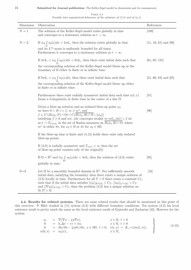
24 Submitted for Journal publication: The Keller-Segel model in chemotaxis and its consequences
Table 4.4Possible time asymptotical behaviour of the solutions of (3.3) and of (4.1).
Dimension Observation References
N = 1 The solution of the Keller-Segel model exists globally in time [109]and converges to a stationary solution as t→ ∞.
N = 2 If αχ∫Ω
u0(x)dx < 4πkc, then the solution exists globally in time [11, 43, 61] and [90]
and its L∞-norm is uniformly bounded for all times.Furthermore it converges to a stationary solution as t→ ∞.
If 4πkc < αχ∫Ω
u0(x)dx < 8πkc, then there exist initial data such that [61, 65, 131]
the corresponding solution of the Keller-Segel model blows up at theboundary of Ω either in finite or in infinite time.
If 8πkc < αχ∫Ω
u0(x)dx, then there exist initial data such that [51, 60, 64] and [65]
the corresponding solution of the Keller-Segel model blows up eitherin finite or in infinite time.
Furthermore there exist radially symmetric initial data such that u(t, x) [51]forms a δ-singularity in finite time in the center of a disc Ω.
Given a blow-up solution and an isolated blow-up point x0,we have 0 < R << 1, m ≥ m∗, and [96]f ∈ L1(B(x0, P ) ∩ Ω) ∩ C(B(x0, R) ∩ Ω \ x0)satisfying f ≥ 0 and u(t, ·)dx converges weakly to mδx0(dx) + f dx
as t→ Tfinite in the set of Radon measures on B(x0, R) ∩ Ω, wherem∗ is either 8π, for x0 ∈ Ω or 4π for x0 ∈ ∂Ω.
If the blow-up time is finite and (4.12) holds there exist only isolatedblow-up points.
If (3.3) is radially symmetric and Tmax <∞ then the setof blow-up point consists only of the origin0.
If Ω = R2 and αχ
∫R2
u0(x)dx < 4πkc then the solution of (3.3) exists [95]
globally in time.
N=3 Let Ω be a smoothly bounded domain in R3. For sufficiently smooth [16]
initial data, satisfying the boundary data there exists a unique solution of(3.3) locally in time. Furthermore for all T > 0 there exists a constant CT ,such that if the initial data satisfies ||v0||H2(Ω) < CT , ||u0||L∞(Ω) < CTand ||∇u0||L2(Ω) < CT , then the problem (3.3) has a unique solution on[0, T ]× Ω.
4.4. Results for related systems. There are some related results that should be mentioned at this point ofthis overview. P. Biler studied in [11] system (3.3) with different boundary conditions. For system (3.3) his localexistence result is pretty much the same as the local existence result of Gajewski and Zacharias [43]. However for thesystem
ut = ∇(∇u− χu∇v), x ∈ Ω, t > 00 = kc∆v − γv + αu, x ∈ Ω, t > 00 = ∂u/∂n− χu∂v/∂n, x ∈ ∂Ω, t > 0, v(t, x) = Kγ ∗ (αu(t, x)),
u(0, x) = u0(x), x ∈ Ω,
⎫⎪⎪⎬⎪⎪⎭ (4.13)

Submitted for Journal publication: The Keller-Segel model in chemotaxis and its consequences 25
where Kγ denotes the Bessel potential, Biler proves the following finite time blow up result:
Theorem 4.15 (Biler). If Ω ⊂ RN , N ≥ 2, is a bounded star-shaped domain ( with respect to the origin ), then
for U0(x) with sufficiently large ||u0(x)||L1(Ω) = M , there is no global in time solution of (4.13).
Results similar to those results in [63, 64] have been proven by G. Wolansky in [151] for the system
0 = ∇(∇u− χu∇v), x ∈ Ω, t > 0vt = kc∆v + αu, x ∈ Ω, t > 00 = ∂u/∂n− χu∂v/∂n, v(t, x) = 0, x ∈ ∂Ω, t > 0
u(0, x) = u0(x), v(0, x) = v0(x) x ∈ Ω.
⎫⎪⎪⎬⎪⎪⎭ (4.14)
This system contains an elliptic equation for the myxamoebae density and a parabolic equation for the cAMP-concentration similar to the second equation in (3.3). Even though he also has a Lyapunov function the techniques heused to prove his blow up result can only be applied to a system with Dirichlet boundary conditions for the secondequation. They fail in the case of Neumann boundary conditions as treated in [63, 64]. In [151] G. Wolansky is ledto an equation for the stationary solutions of his model which is similar to problem (3.6). However in his case theequation is equipped with Dirichlet boundary data, which allows him to use different arguments (more precisely themoving plane method see [31, pp. 521-522]) to exclude the first alternative of the Brezis and Merle [20] result. In thecase that is mentioned in the previous section and [63, 64] one has to use different techniques to get rid of the possiblealternatives stated by Brezis and Merle in [20].
5. Comparison of the questions asked by Jager and Luckhaus with the results so far. Let us nowtake some time and let us see which questions of those asked in [67] have been answered up to now and which remainopen. W. Jager and S. Luckhaus asked about more information on the set of blow-up points. We have seen in theprevious sections that there exists the possibility of blow-up point in the interior and at the boundary of a domainΩ ⊂ R
2. Also the upper bound of the possible number of blow-up points is sharp and known, however a better lowerbound is still needed. Also the location of the boundary blow-up points should be studied more carefully. For smoothdomains the boundary blow-up point should be the point of the greatest curvature which would correspond with thenumerical calculations of H. Gajewski and K. Zacharias in [43] for piecewise smooth domains and with the results andhints from the steady state analysis resp. the shape of the least energy solutions.
The question whether the solution exists globally in time as a weak solution can be negated. However it mightbe possible to study the problem for a different formulation of a solution like L1-solutions. But as far as I know therehas not been any attempt to do so up to now. For the third question we turn to an own subsection.
5.1. What happens after blow-up?. In connection with the question “What happens after the blow up ofthe solution? ” that was already asked in [67], we have seen the solution does not exist globally in time as a weakH1−solution, but is there a notation of a measure valued solution or L1-solution for the Keller-Segel model? Withsuch a notation, which would be natural since the solution belongs to L1(Ω) for all times, it would make sense tostudy the possible movement of the aggregation centers in the considered domain.
Using a different ansatz than that just mentioned, J.J.L. Velazquez made the first step to give an answer to thequestion what will happen after blow-up in [147, 148] using a different approach than the idea of introducing a newnotation of a solution.
In [146] J. J. L. Velazquez studied the question wether aggregation at the interior of the boundary of the domainΩ ⊂ R
2 takes place in a stable manner, or, if on the contrary, solutions exhibit a tendency to move towards theboundary. His result is that after small pertubations of the solution found in [51], the new solution will blow up in amanner entirely similar but in a slightly shifted point of Ω at a slightly different time. Thus his computations indicatethat the possibility of aggregates with high density of u moving quickly towards the boundary does not exist.
He then studies in [147, 148] the system
ut = ∇(∇u −Gε(u)∇v), x ∈ R2, t > 0
0 = ∆v + u, x ∈ R2, t > 0,
(5.1)
where Gε(u) = 1εQ(εu) for a small parameter ε > 0 and an increasing function Q(ξ) satisfying Q(s) = s + O(s2) as
s → 0 and Q(s) ∼ L as s → ∞, where L > 0 is a given number. For Q(s) = s1+s and ε = 0 the system becomes
formally the system (4.2). Using this system Velazquez studies the motion of regions with high densities of u in [147]and derives a system of equation that describes the dynamics of these regions of high densities of u. The well-posednessof the derived system for the dynamics of the high density regions is established in [148]. According to the formal limitas ε→ 0 his results can therefore somehow be interpreted as a formal explanation of the behaviour of the solution of(4.2) after blow up.

26 Submitted for Journal publication: The Keller-Segel model in chemotaxis and its consequences
6. More general formulations of the chemotaxis equations. The original formulation of the Keller-Segelmodel allowed more general functional forms than we assumed in the last section. Even though the question whetherthe given functional form represents the situation in Dictyostelium aggregation in an appropriate way should bediscussed, the system is adequate to describe chemotactical movement of mobile species. A number of possibleplausible functional forms has been proposed by E.F. Keller in [74]. There she proposed several functional forms thatwill also be discussed in the upcoming subsections. Furthermore she discussed the possible existence of traveling wavesolutions, a topic which will be in the center of our observations later during this paper. Since there is a large numberof different examples for species that move positive chemotactically and also a large variety of different models for thechemotactical sensing of the particular species (see for example [80] for a model of the cAMP production and sensingmechanism in Dictyostelium discoideum) it is useful to try to find a more general theory that contains a larger classof possible models. Let us see what results are available in this cases. So let us now turn to more general formulationsof the system without having a particular example in mind. So we focus on the following system of two nonlinearparabolic partial differential equations, which is given by
ut = ∇(k(u, v)∇u − h(u, v)∇v), x ∈ Ω, t > 0vt = kc∆v − f(v)v + g(u, v), x ∈ Ω, t > 0
(6.1)
for Ω ⊂ RN completed with either
∂u
∂n=
∂v
∂n= 0 on ∂Ω × t > 0, (6.2)
or u = 0, v = 0 on ∂Ω × t > 0, (6.3)
or k(u, v)∂u
∂n− h(u, v)
∂v
∂n= 0, v = 0 on ∂Ω × t > 0 (6.4)
as boundary conditions and initial data u(0, x) = u0(x) and v(0, x) = v0(x) x ∈ Ω. Here kc once again is a positiveconstant. For the functions appearing in the model the following conditions have been considered to be reasonable:k(r, s) > 0 for all (r, s) ∈ R × R, the function f satisfies f(s) ≥ const for all s ∈ R and ∂
∂rg(r, s) = 0 holds for all(r, s) ∈ R × R.
The question whether a solution to such problems exist locally in time has been studied in [61] using results byH. Amann [6, 7] and in [153] using other techniques. As it was mentioned in the previous section a Lyapunov functionis a helpful tool for analyzing the time asymptotic behaviour of the solution. So one wonders under which conditionsthe present system has a Lyapunov function. Therefore we turn to this question next.
6.1. Lyapunov functions. For the rest of the present paper we will use the following notations:
F (v) :=
v∫0
f(s)s ds and G(u, v) := −v∫
0
g(u, s) ds.
At some places of the present paper we will assume that∫Ω
F (v) dx ≥ k1
∫Ω
v2 dx (6.5)
is true, where k1 is a nonnegative constant (If we have homogeneous Neumann boundary data we assume k1 > 0!).
Theorem 6.1 (Horstmann). If there exists a function R(u) such that
h(u, v)k(u, v)
[∂2
∂u2G(u, v) +
d2
du2R(u)
]+
∂2
∂u∂vG(u, v) = 0,
then there exists a Lyapunov function for system (6.1), provided ∂2
∂u2G(u, v) + d2
du2R(u) ≥ 0 holds true for the solutionof (6.1). In the case of boundary condition (6.3) we have to assume additionally that ∂
∂uG(0, 0) = 0 = dRdu (0). The
Lyapunov function for system (6.1) is then given by
H(u(t), v(t)) :=∫Ω
kc2|∇v(t)|2 + F (v(t)) + R(u(t)) +G(u(t), v(t))dx.
A large number of examples is given in [61]. Let us here only give two examples for which a Lyapunov functionH(u, v) exists.

Submitted for Journal publication: The Keller-Segel model in chemotaxis and its consequences 27
1. Let consider (6.1) with h(u, v) = u, g(u, v) = 12u
2e−v, k(u, v) = 1, f(v) arbitrary. Then we have theLyapunov function
H(u(t), v(t)) :=∫Ω
kc2|∇v(t)|2 + F (v(t)) +
12u2(t)e−v(t)dx, i.e. R(u) = u2/2.
2. One can also find a whole class of other examples where a Lyapunov function exists. Let us suppose that we
study system (6.1) together with (6.2). Let h(u, v) = h2(u)φ(v) and g(u, v) = φ(v)u∫0
h1(s) ds,
k(u, v) = k(u) +h2(u)h1(u)
d
duh1(u)
v∫0
φ(s)ds
and f(v) be arbitrary. We see that there is a function R(u) such that
d2
du2R(u) =
k(u, v)h1(u)h2(u)
+d
duh1(u)
v∫0
φ(s) ds.
Of course we see in this example that the right hand side has to be independent of v. If this is the case, thenthere exists a Lyapunov function H(u, v) of the type given above, which is possibly unbounded from below.This example includes the systems studied in [43] and [115]. In [115] we have h(u, v) = uφ(v) (with φ(v) > 0),g(u, v) = uφ(v), k(u, v) = 1 and f(v) = const > 0. Finally we get in this case R(u) = u log(u). For furtherresults concerning some special cases of this type of systems see [115].
In fact this result allows to make statements for a larger class of nonlinearities in g(u, v) than those studied before forsystem (6.1) (as far as the author knows). Under certain additional assumptions one can now formulate results forthe time asymptotic behaviour of the solution. Therefore we now make the following main assumption for the rest ofthis section.
Main assumption:∫Ω
G(u, v) +R(u) ≥ k2
∫Ω
|∇v|2 dx+ const withkc2
+ k2 > 0. (6.6)
In some special cases of (6.1) one can show that the solution of (6.1) converges to a possibly nontrivial steadystate as t → ∞ (see [43, 61] and [115]). The results of W. Alt [3], R. Schaaf [124] and K. Post [115] concerning theKeller-Segel model in chemotaxis seem to indicate that such behaviour can also be expected in a more general setting.The following theorem summarizes our results on this aspect.
Theorem 6.2 (Horstmann). Suppose that (u(t), v(t)) is a weak solution of (6.1) and that (6.5) as well as ourmain assumption (6.6) is satisfied. Furthermore let either
1.[∂2
∂u2G(u, v) + d2
du2R(u)]/k(u, v) ≤ k3 and ∂
∂uG(u, v) + dduR(u) > k4 or
2. 0 <[∂2
∂u2G(u, v) + d2
du2R(u)]exp(∂∂uG(u, v) + d
duR(u))≤ k5k(u, v) and
√k(u(t), v(t))
∂2
∂u2G(u, v) + d2
du2R(u(t))∈ L2(Ω)
for all t ≥ 0be true for the solution (u(t), v(t)) of (6.1). Let additionally f be Holder continuous with Holder exponent β ≤ 1 suchthat 0 < β ≤ 1 if N ≤ 3 or β < 2/N if N > 3. Finally assume that |f(v)| ≤ Kf for all v ∈ R. Then there exist asequence (tk)k∈N and two functions v∗ and g∗ such that v(tk) v∗ in H1(Ω) resp. in H1
0 (Ω)), f(v(tk))v(tk) → f(v∗)v∗
in L2(Ω) and g(u(tk), v(tk)) g∗ in L2(Ω). Furthermore∫Ω
kc∇v∗∇ϕ+ f(v∗)v∗ϕ dx =∫Ω
g∗ϕ dx

28 Submitted for Journal publication: The Keller-Segel model in chemotaxis and its consequences
for all ϕ ∈ H1(Ω) (resp. ϕ ∈ H10 (Ω)). Finally we see that
exp
(−[∂∂uG(u(tk), v(tk)) + d
duR(u(tk))]
2
)→ const
in L2(Ω) if 1. holds and, respectively,
exp
([∂∂uG(u(tk), v(tk)) + d
duR(u(tk))]
2
)→ const
in L2(Ω) if 2. holds.
The previous given first example satisfies assumption 1. of Theorem 6.2 while the systems studied in [43] and[115] satisfy assumption 2. of Theorem 6.2. The proof of this theorem goes along the line of the proof of Theorem 5.2in [43, page 107] and can be found in detail in [61].
Furthermore one can also formulate certain conditions under which some Lp−estimates for the solution are possible.This has also been done in [61].
More general forms of the Keller-Segel model (2.4) have also been studied by A. Yagi in [153] for the case of twospace dimensions and in the case of one spatial dimension by K. Osaki and A. Yagi in [109]. In [109] the authors studythe Keller-Segel model (2.4) with k1(u, v) = const, g(u, v) = αu − γv and k2(u, v) = uχ(v) where χ(s) is a smoothfunction of s ∈ (0,∞) satisfying
|χ(i)(s) < | ≤ const ·(s+
1s
)r,
for 0 < s <∞, i = 0, 1, 2 with some positive constant and exponent r. In [109] they show that there exists a compactset of finite fractal dimension which attracts the solutions exponentially.
A. Yagi studied in [153] the two dimensional case of the Keller-Segel model under the assumptions that k1(u, v) =c0 + c1u+ c2v with a positive constant c0 > 0 and non-negative constants c1, c2, and assuming that k2(u, v) = uχ(v)with 0 ≤ χ(s) ≤ b0
(1 + 1
s
), and that χ(s), k3(s), f(s) are smooth functions of s ∈ R
+ satisfying 0 ≤ f(s) ≤ b1,b2 ≤ k3(s) ≤ b3 (sp0 + 1), where b0, b1, b2, b3 are positive constants strictly larger than zero and the exponent p0 > 0.For the initial data he assumed that u0(x) > 0 on Ω, v0(x) ≥ µ0 > 0 on Ω belong to H1+ε0(Ω) with some exponent0 < ε0 ≤ 1 and a positive constant µ0. Using semigroup theory Yagi established the local in time existence of anunique, positive, classical solution in the same space as it has already been mentioned in the case of a linear sensitivityfunction in a previous section. Furthermore he determines blow-up norms of the maximal solution.
6.1.1. Results on finite time blow-up. As it has been already mentioned in the section on the steady statesolutions of the Keller-Segel model Nanjundiah’s conjecture also contained a statement on the time asymptoticalbehaviour of the solution of the Keller-Segel model with a logarithmic chemotactical sensitivity function. Thereforewe will first look at the results for this conjecture and related results. In this subsection we consider (2.4) withk1(u, v) = 1, g(u, v) = 1
ε (u − v), kc = 1ε and k2(u, v) either χuv or χpuvp−1 for p > 0. For ε = 0 it is easy to show
in the same way as it has been done in the case of a linear chemotactical sensitivity function that the solution existsglobally in time and that the L∞-norm of the solution is uniformly bounded for all times. Thus the interesting casesare once more the higher dimensional ones. So let us summarize these cases:
1. Let k2(u, v) = χpuvp−1 for p > 0.(a) Let N = 2 and ε = 0. If 0 < p < 1, then the solution of the Keller-Segel model exists globally in time
and is uniformly bounded. If Ω is a disk, u0 is radially symmetric,∫Ω
u0(x)|x|2dx is sufficiently small and
p > 1, then the corresponding solution of (2.4) blows up in finite time.(See [88, 89, 126].)(b) Let N ≥ 3 and ε = 0. If Ω is a disk, u0 is radially symmetric,
∫Ω
u0(x)|x|(N−2)p+2dx is sufficiently
small and p > 0, then Tmax < ∞ and the corresponding solution of (2.4) blows up in finite time.(See[88, 89, 126].)
2. Let k2(u, v) = χuv .

Submitted for Journal publication: The Keller-Segel model in chemotaxis and its consequences 29
(a) Let N = 2 and ε = 0. If Ω is a disk, u0 is radially symmetric, then the solution is globally bounded intime. (See [88, 89, 126].)
(b) Let N ≥ 3 and ε = 0. If Ω is a disk, u0 is radially symmetric and χ < 2/(N − 2), then the solution isglobally bounded in time. (See [88, 89, 126].)
(c) Let N = 2 and ε = 1. If χ < 1, then the solution of (2.4) exists globally in time and for T > 0 thereexists a constant CT <∞ such that
sup0≤t≤T
(||u(t, ·)||L∞(Ω) + ||v(t, ·)||L∞(Ω)
)< CT .
(See [91].)(d) Let N = 2 and ε = 1. If Ω is a disk, the initial data (u0(x), v0(x)) is radially symmetric and χ < 5/2,
then the solution exists globally in time. (See [91].)(e) Let N ≥ 3 and ε = 0. If Ω is a disk, u0 is radially symmetric,
∫Ω
u0(x)|x|2dx is sufficiently small and
χ > 2N/(N − 2), then the solution of (2.4) blows up in finite time. (See [88, 89, 126].)
Similar results have been obtained by K. Post studying (2.4) with k1(u, v) = 1, k2(u, v) = uφ′(v) g(u, v) = uφ′(v) − vand kc = 1. For the precise details I refer the reader to [115].
Rascle and Ziti analyzed in [118] the system
ut = ∇(µ∇u − χuv−β∇v), x ∈ Ω, t > 0vt = −kuvm, x ∈ Ω,
where the constants χ,k > 0. They constructed self-similar solutions for this system assuming that m < β = 1. Forµ = 0 and one space dimension they observed that the bacterial density concentrated in finite time at the origin. Fortwo space dimensions and initial data for the bacterial density which is zero at the origin they derived chemotacticrings concentrated around the origin after finite time. In higher space dimensions they achieved blow-up of the solutionby an initial singularity of the chemoattractant in the origin.
For µ > 0 Rascle and Ziti observed in one space dimension that there are smooth initial data leading to finitetime blow-up of the solution, while they were unable to construct self-similar solutions in space dimension larger orequal to two for reasonable initial conditions.
6.1.2. Prevention of overcrowding. There are different points of view whether blow-up in chemotaxis isrelevant or not. In fact for the chemotaxis system introduced and derived in the Davis’ case by Othmer and Stevensfor a single particle in [112] blow-up in finite time seems to correspond with the fact that the particle is trappedrespectively localizes in finite time at one particular place (see also [135] for more comments on that aspect). Thusblow-up really makes sense for their model. Furthermore, blowing up of the solution only describes the concentrationof the particle populations in some aggregation centers. Since the Keller-Segel model only wants to describe theaggregation phase of chemotactical movement and not the formation of a fruiting body the blow-up question is surelyworth studying. As J. J. L. Velazquez wrote in [147, pp. 1-2]:
“Blow-up usually takes place in physical or biological models if they are approximations of more real-istic models, usually containing small parameter (say ε > 0), that cannot exhibit singular behavioursunless this parameter is set to zero. Suppose that for ε = 0 the limit problem can develop singularitiesin finite time. The behaviour of the complete model for ε > 0 usually is similar to that of the limitmodel away from the singularities. However, the features of the problem with ε > 0 but small areusually very different from that of the limit problem near the singularities. The presence of blow-upjust indicates that the approximations that lead to the simpler model where blow-up takes place arenot valid anymore near the singularity and that the whole dynamics of the complete model needs to betaken into account here. ”
However there are also other models of Keller-Segel type which exclude the possibility of blow-up solutions directlyby introducing some mechanisms, that provide to strong aggregations or where the chemical production and decaydirectly is such that blow-up is impossible. For example in the case of the linear chemotactical sensitivity functiong(u(t, x), v(t, x)) ∈ L4(Ω) for all t ≥ 0 with an uniform bound for all t ≥ 0 guarantees the global existence of thesolution of system (6.1) ( see for example [61]). One model containing such prevention of an overcrowding of thechemotactical species has been proposed by T. Hillen and K. J. Painter in [56]. They considered the system (6.1) on
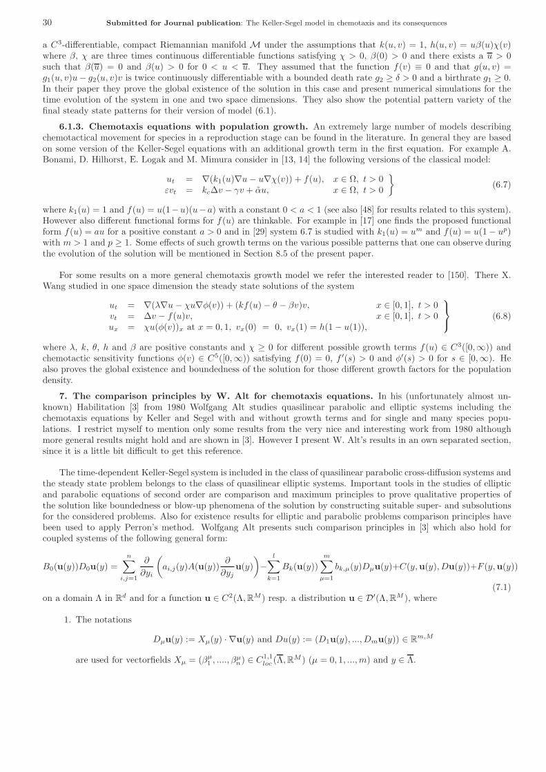
30 Submitted for Journal publication: The Keller-Segel model in chemotaxis and its consequences
a C3-differentiable, compact Riemannian manifold M under the assumptions that k(u, v) = 1, h(u, v) = uβ(u)χ(v)where β, χ are three times continuous differentiable functions satisfying χ > 0, β(0) > 0 and there exists a u > 0such that β(u) = 0 and β(u) > 0 for 0 < u < u. They assumed that the function f(v) ≡ 0 and that g(u, v) =g1(u, v)u− g2(u, v)v is twice continuously differentiable with a bounded death rate g2 ≥ δ > 0 and a birthrate g1 ≥ 0.In their paper they prove the global existence of the solution in this case and present numerical simulations for thetime evolution of the system in one and two space dimensions. They also show the potential pattern variety of thefinal steady state patterns for their version of model (6.1).
6.1.3. Chemotaxis equations with population growth. An extremely large number of models describingchemotactical movement for species in a reproduction stage can be found in the literature. In general they are basedon some version of the Keller-Segel equations with an additional growth term in the first equation. For example A.Bonami, D. Hilhorst, E. Logak and M. Mimura consider in [13, 14] the following versions of the classical model:
ut = ∇(k1(u)∇u− u∇χ(v)) + f(u), x ∈ Ω, t > 0εvt = kc∆v − γv + αu, x ∈ Ω, t > 0
(6.7)
where k1(u) = 1 and f(u) = u(1−u)(u−a) with a constant 0 < a < 1 (see also [48] for results related to this system).However also different functional forms for f(u) are thinkable. For example in [17] one finds the proposed functionalform f(u) = au for a positive constant a > 0 and in [29] system 6.7 is studied with k1(u) = um and f(u) = u(1 − up)with m > 1 and p ≥ 1. Some effects of such growth terms on the various possible patterns that one can observe duringthe evolution of the solution will be mentioned in Section 8.5 of the present paper.
For some results on a more general chemotaxis growth model we refer the interested reader to [150]. There X.Wang studied in one space dimension the steady state solutions of the system
ut = ∇(λ∇u − χu∇φ(v)) + (kf(u) − θ − βv)v, x ∈ [0, 1], t > 0vt = ∆v − f(u)v, x ∈ [0, 1], t > 0ux = χu(φ(v))x at x = 0, 1, vx(0) = 0, vx(1) = h(1 − u(1)),
⎫⎬⎭ (6.8)
where λ, k, θ, h and β are positive constants and χ ≥ 0 for different possible growth terms f(u) ∈ C3([0,∞)) andchemotactic sensitivity functions φ(v) ∈ C5([0,∞)) satisfying f(0) = 0, f ′(s) > 0 and φ′(s) > 0 for s ∈ [0,∞). Healso proves the global existence and boundedness of the solution for those different growth factors for the populationdensity.
7. The comparison principles by W. Alt for chemotaxis equations. In his (unfortunately almost un-known) Habilitation [3] from 1980 Wolfgang Alt studies quasilinear parabolic and elliptic systems including thechemotaxis equations by Keller and Segel with and without growth terms and for single and many species popu-lations. I restrict myself to mention only some results from the very nice and interesting work from 1980 althoughmore general results might hold and are shown in [3]. However I present W. Alt’s results in an own separated section,since it is a little bit difficult to get this reference.
The time-dependent Keller-Segel system is included in the class of quasilinear parabolic cross-diffusion systems andthe steady state problem belongs to the class of quasilinear elliptic systems. Important tools in the studies of ellipticand parabolic equations of second order are comparison and maximum principles to prove qualitative properties ofthe solution like boundedness or blow-up phenomena of the solution by constructing suitable super- and subsolutionsfor the considered problems. Also for existence results for elliptic and parabolic problems comparison principles havebeen used to apply Perron’s method. Wolfgang Alt presents such comparison principles in [3] which also hold forcoupled systems of the following general form:
B0(u(y))D0u(y) =n∑
i,j=1
∂
∂yi
(ai,j(y)A(u(y))
∂
∂yju(y))−
l∑k=1
Bk(u(y))m∑µ=1
bk,µ(y)Dµu(y)+C(y,u(y), Du(y))+F (y,u(y))
(7.1)on a domain Λ in R
d and for a function u ∈ C2(Λ,RM ) resp. a distribution u ∈ D′(Λ,RM ), where
1. The notations
Dµu(y) := Xµ(y) · ∇u(y) and Du(y) := (D1u(y), ..., Dmu(y)) ∈ Rm,M
are used for vectorfields Xµ = (βµ1 , ...., βµn) ∈ C1,1
loc (Λ,RM ) (µ = 0, 1, ...,m) and y ∈ Λ.

Submitted for Journal publication: The Keller-Segel model in chemotaxis and its consequences 31
2. The ai,j are defined as ai,j(y) =m∑
ν,µ=1aν,µ(y)β
µi (y)βµj (y) with continuous functions aµ,ν = anu,µ and (aµ,ν) ≥ 0
on Λ, and satisfy for all y ∈ Λ and all ξ ∈ Rm the inequality
m∑ν,µ=1
ξνξµaν,µ(y) ≥ ζ(y)|ξ|2
with a on Λ lower semicontinuous positive function ζ.3. The functions bi,µ are continuous on Λ.4. The matrix-functions A,Bi : R
M → RM×M are continuous and det(A) ≥ 0 and B0 ≥ 0 on R
M .5. F : Λ × R
M → RM and C : Λ × R
M × Rm,M → R
M are measurable in y ∈ Λ, continuous in z ∈ RM and
w ∈ Rm,M , and uniformly bounded on Λ ×K, with a compact set K ⊂ R
M . For example the function C canbe given by R
M -valued bilinear forms Cµ,ν like:
C(y, z, w) =m∑
µ,ν=1
Cµ,ν [wµ, wν ]
with w = (w1, ..., wm) ∈ RM,m.
Although W. Alt’s results hold for systems in this general setting I restrict myself to systems appropriate to modelchemotaxis and present his results if possible in versions for those problems. From the applicational point of view onewould like to know whether the considered model remains bounded for all times or not. Thus the existence of invariantsets for the system is an interesting topic worth studying. Alt presents such results in his Habilitation. Therefore thefirst result presented here is the following invariance theorem for parabolic systems (see [3, Satz 1.25, page 31 & 32]):
Theorem 7.1 (Alt). Let p ≥ 0 be in C1,1loc (R
M ) and let M be defined as the set M := z ∈ RM | p(z) = 0 = ∅.
Furthermore let us assume that u is a weak solution of the parabolic problem
ut =N∑j=1
∂∂xj
(A(u) ∂
∂xiu)
+ F (u), in Ω × (0, τ) (Ω ⊂ RN
A(u)∂u∂n = ψ(u), on ∂ΩN × [0, τ ]u(x, 0) = u0(x), on ∂ΩD × [0, τ ],
where ∂ΩN and ∂ΩD denote disjunct subsets of ∂Ω. For the boundary conditions we assume that there exists acontinuous family of symmetric M × M -matrices A∗(z) ≥ 0, z ∈ R
M and that there exist vector functions θj :∂ΩN × R
M → R such that
ψj(x, z) = A∗(z)θj(x, z) and θTj (x, z) ·A∗(z) · θj(x, z) ≤ constK
for all z in a compact subset K of RM and x ∈ ∂ΩN , where ψ0 = ψ and ψj = ∂
∂zjψ, for j = 1, ...,M . Furthermore we
suppose that there exists a neighbourhood U of M such that
∇p · ψ ≤ 0, ∇p · F ≤ 0 as well as ∇2p ·A ≥ 0 holds on U \M, if ∇2p exists.
Then u(·, 0) ⊂ M implies u(·, t) ⊂ M for all t ∈ [0, τ ].
But not only the question whether the solution remains in a certain set for all times if the initial data belongs tothis set is an interesting question. One would like to know more about the behaviour of the solution as t → ∞. Asdemonstrated in the previous section the existence of Lyapunov functionals is a helpful tool in the studies of the timeasymptotic as t→ ∞. In [3] W. Alt presents results for the existence of Lyapunov functionals which is different fromthe results of Theorem 6.1 of this paper. To be precise W. Alt proved the following Corollary:
Corollary 7.2 (Alt). Assume that the assumptions of Theorem 7.1 are fulfilled. The Dini-derivative of thefunctional
E(t) :=∫Ω
p(u(t, x))dx, t ∈ [0, τ ]

32 Submitted for Journal publication: The Keller-Segel model in chemotaxis and its consequences
satisfies for all weak solution of problem (7.1) which have values in U the inequality
d
dtE(t) ≤ −
∫Ω
N∑j=1
(∂
∂xju)∇2p(u)A(u)
(∂
∂xju)dx+
∫Ω
∇p(u) · F (u)dx +∫∂Ω
∇p(u) · ψ(u)dS
almost everywhere in [0, τ ]. If for all z ∈ U \M either ∇p ·ψ < 0 or ∇p ·F < 0 holds, then E is a Lyapunov functionalfor M, i.e. d
dtE(t) < 0 as long as E(t) > 0. If for all z ∈ U \M either ∇p ·ψ < 0 or ∇p ·F < 0 or ∇2p ·A < 0 holds,then E is a Lyapunov functional for M∪N0, where N0 contains all constants z0 ∈ R
M , that are zero of ∇p · ψ and∇p · F .
Now, let me demonstrate this results by applying Theorem 7.1 to an example (see [3, Beispiel 1.41, page 38]):
Consider the weak solution of the taxis-system
ut = ∇(k1(u)(∇u − k2(u, v)∇v)) + f(u, v), in Ω × t ≥ 0vt = kc∆v + g(u, v), in Ω × t ≥ 00 = k1(u) ∂u∂n − h(u, v) on ∂Ω × t ≥ 00 = ∂v
∂n , on ∂Ω × t ≥ 0,
(7.2)
where all coefficient functions are continuous and k1(u), kc ≥ 0, k1(u) = 0 for u ≥ u. Furthermore letf(u, v), h(u, v) ≤ 0 for u ≥ u and all v ∈ R and on every compact subset of R
2 the inequalities
|h(u, ·)|2, | ∂∂uh(u, ·)|2, | ∂
∂vh(u, ·)|2 ≤ k1(u)
hold and assume that the initial data (u0, v0) satisfy u0 ≤ u.
We see that this system satisfies the conditions of Theorem 7.1 with
M = (u, v) ∈ R2 | u ≤ u, p(u, v) =
12
(max0, u− u)2 and A(u, v) =(k1(u) −k1(u)k2(u, v)
0 kc
).
Now we have to check the conditions for the boundary data ψ = (h, 0)T . We set
A∗ =(k1 00 1
2 (kc + k1k22)
).
Thus we have ψ = A∗θ with θ = (h/k1, 0)T . We see that θTA∗θ can be bounded uniformly and that the analoguousstaements also hold for the partial derivatives ∂
∂uψ and ∂∂vψ. Thus we conclude with Theorem 7.1 the following:
If the initial data (u0, v0) satisfy u0 ≤ u, then the solution of system (7.2) satisfies u(·, t) ≤ u for allt ≥ 0.
In contrast to this result for weak solutions the next Theorem [3, Satz 2.40] is a strong (local) comparison prin-ciple for classical solutions of system (7.1). Before citing this result we have to introduce “sets of comparison” and“comparison surfaces”.
Definition 7.3. For i = 1, .., I and a domain V ⊂ RM let the functions i belong to the class C1,1
loc (V ,RM ),where i is piecewise of class C2,1
loc (V ,RM ) and the functions ςi belong to the class C1,1loc (V ,R). Then we define for
each y ∈ V the sets of comparison My := z ∈ V | i(z) ≤ ςi(z), i = 1, ..., I and for i = 1, ..., I the i-boundary∂iMy := z ∈ ∂My ⊂ V | i(z) = ςi(z).
Definition 7.4. Let (Vy)y∈Λ denote a continuous family of sets Vy ⊂ V ⊂ RM , with V as in the previous
definition. Furthermore let there be given functions ∈ C1,1loc (V) and ς ∈ C1,1
loc (Λ) such that for each compact set

Submitted for Journal publication: The Keller-Segel model in chemotaxis and its consequences 33
K ⊂ RM and for each relatively compact set Λ∗ ⊂ Λ there exist positive constants c and δ and a continuous family of
projections
πy : Mδy := Vy ∩K ∩ ς(y) − δ ≤ ≤ ς(y) → Vy ∩ = ς(y)
with
|πy(z) − z| ≤ c|(z) − ς(y)| and ∇(z) = 0
for all y ∈ Λ∗ and z ∈ Mδy. Furthermore let there be a finite number of sets Vκ with V =
k0⋃κ=1
Vκ such that |Vκ ∈
C2,1loc (Vκ) and
πy(Vκ ∩ Vy) ⊂ Vκ
for all κ = 1, .., k0 and y ∈ Λ∗ is satisfied. Then we will call the surfaces Vy ∩ = ς(y) surfaces of comparison.
Now let us turn to the strong comparison result for the equation
B0(u(y))D0u(y) = A(u(y))m∑
ν,µ=1
aν,µ(y)DνDµu(y) −l∑i=1
Bi(u(y))m∑
i,µ=1
bi,µ(y)Dµu(y)
+m∑
ν,µ=1
Cν,µ(y,u(y))(Dµu(y) ·Dνu(y)) + F (y,u(y)) (7.3)
where we additionally assume that A, Bi, F and Cν,µ are locally Lipschitz continuous in u and uniformly continuousin y ∈ Λ, and that the functions bi,µ are bounded on Λ:
Theorem 7.5 (Alt). Let us assume that (My)y∈Λ is a family of sets of comparison. Additionally we assume thatfor each z ∈ V, for which y ∈ Λ and i ∈ 1, ..., I exist such that z ∈ ∂iMy, the following properties are satisfied:
∇i(z) = 0, ∇i(z) ∈∑
s=i,z∈∂sMy
R · ∇ϕs(z)
and the points of discontinuity of ∇2i lie on a finite system of smooth surfaces in V, which intersect the surfacez ∈ V | i(z) = ςi(z) in each such z ∈ ∂iMy transversally. Let us suppose that for each pair (i, ςi) and the familiesof sets (V iy)y∈Λ with
V iy := z ∈ V | l(z) ≤ ςl(z), l ∈ 1, ..., I \ i
there exist continuous functions ζi and ιi on Λ × V such that the following three properties are satisfied on ∂iMy,y ∈ Λ:
1. There are continuous functions λi, λi0, ..., λis on V such that for all z ∈ Vy with i(z) = ςi(y) and y ∈ Λ suchthat
∇i(z) · A(z) = λi(z)∇i(z), λi(z) > 0 (7.4)∇i(z) · B0(z) = λi0(z)∇i(z), λi0(z) > 0 (7.5)∇i(z) · Bl(z) = λil(z)∇i(z) + pl(z), λil(z) ∈ R (7.6)
(7.7)
and pl(z) ∈ [∇i(z)]⊥ ⊂ RM , l = 1, ..., s.
2. Let C(y, z) ⊂ Rm,M , (z ∈ V) denote for every y ∈ Λ a (uniform in y ∈ Λ∗) locally Lipschitz continuous, given
family of sets. The matrix W (y) ∈ Rm,m denotes the positive definite root of the symmetric matrix (aν,µ(y))
and ℘i denotes for each i ∈ 1, .., I a continuous vector field on V such that ℘i(z) · ∇i(z) = 1 for all z ∈ V.Furthermore let us assume that for all y ∈ Λ, z ∈ Vy with i(z) = ςi(y) and
w ∈ Pz(W (y) · C(x, z)) := ((W (y) · C(x, z)) − ((W (y) · C(x, z)) · ∇i(z))℘i(z))
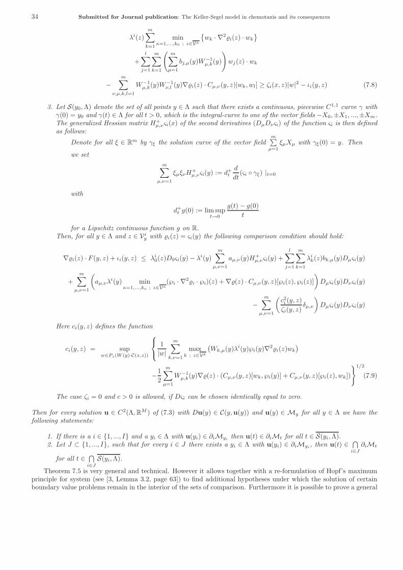
34 Submitted for Journal publication: The Keller-Segel model in chemotaxis and its consequences
λi(z)m∑k=1
minκ=1,...,k0 ; z∈Vκ
wk · ∇2i(z) · wk
+l∑
j=1
m∑k=1
(m∑µ=1
bj,µ(y)W−1µ,k(y)
)wj(z) · wk
−m∑
ν,µ,k,l=1
W−1µ,k(y)W
−1ν,l (y)∇i(z) · Cµ,ν(y, z)|wk, wl] ≥ ζi(x, z)|w|2 − ιi(y, z) (7.8)
3. Let S(y0,Λ) denote the set of all points y ∈ Λ such that there exists a continuous, piecewise C1,1 curve γ withγ(0) = y0 and γ(t) ∈ Λ for all t > 0, which is the integral-curve to one of the vector fields −X0,±X1, ...,±Xm.The generalized Hessian matrix H+
µ,νςi(x) of the second derivatives (DµDνςi) of the function ςi is then definedas follows:
Denote for all ξ ∈ Rm by γξ the solution curve of the vector field
m∑µ=1
ξµXµ with γξ(0) = y. Then
we setm∑
µ,ν=1
ξµξνH+µ,νςi(y) := d+
t
d
dt(ςi γξ) |t=0
with
d+t g(0) := lim sup
t→0
g(t) − g(0)t
for a Lipschitz continuous function g on R.Then, for all y ∈ Λ and z ∈ V iy with i(z) = ςi(y) the following comparison condition should hold:
∇i(z) · F (y, z) + ιi(y, z) ≤ λi0(z)D0ςi(y) − λi(y)m∑
µ,ν=1
aµ,ν(y)H+µ,νςi(y) +
l∑j=1
m∑k=1
λik(z)bk,µ(y)Dµςi(y)
+m∑
µ,ν=1
(aµ,νλ
i(y) minκ=1,...,ko ; z∈Vκ
(℘i · ∇2i · ℘i)(z) + ∇(z) · Cµ,ν(y, z)[℘i(z), ℘i(z)])Dµςi(y)Dνςi(y)
−m∑
µ,ν=1
(c2i (y, z)ζi(y, z)
δµ,ν
)Dµςi(y)Dνςi(y)
Here ci(y, z) defines the function
ci(y, z) = supw∈Pz(W (y)·C(x,z))
⎧⎨⎩ 1
|w|
m∑k,ν=1
maxk ; z∈Vk
(Wk,µ(y)λi(y)℘i(y)∇2i(z)wk
)
−12
m∑µ=1
W−1µ,k(y)∇(z) · (Cµ,ν(y, z)[wk, ℘i(y)] + Cµ,ν(y, z)[℘i(z), wk])
1/2
.(7.9)
The case ζi = 0 and c > 0 is allowed, if Dςi can be chosen identically equal to zero.
Then for every solution u ∈ C2(Λ,RM ) of (7.3) with Du(y) ∈ C(y,u(y)) and u(y) ∈ My for all y ∈ Λ we have thefollowing statements:
1. If there is a i ∈ 1, ..., I and a yi ∈ Λ with u(yi) ∈ ∂iMyi then u(t) ∈ ∂iMt for all t ∈ S(yi,Λ).2. Let J ⊂ 1, ..., I, such that for every i ∈ J there exists a yi ∈ Λ with u(yi) ∈ ∂iMyi, then u(t) ∈
⋂i∈J
∂iMt
for all t ∈⋂i∈J
S(yi,Λ).
Theorem 7.5 is very general and technical. However it allows together with a re-formulation of Hopf’s maximumprinciple for system (see [3, Lemma 3.2, page 63]) to find additional hypotheses under which the solution of certainboundary value problems remain in the interior of the sets of comparison. Furthermore it is possible to prove a general

Submitted for Journal publication: The Keller-Segel model in chemotaxis and its consequences 35
invariance theorem for parabolic systems. Here we only mention an application of these theorems to autonomousparabolic Neumann boundary value problems. Therefore let us once again consider the following problem:
ut =N∑j=1
∂∂xj
(A(u) ∂
∂xiu)
+ F (u), in Ω × (0, τ) (Ω ⊂ RN
A(u)∂u∂n = ψ(u), on ∂ΩN × [0, τ ]
where we assume that F , ψ ∈ C0,1loc (V ,RM ) and A ∈ C1,1
loc (V ,RM,M ) with det(A) ≥ 0.
Theorem 7.6 (Alt). Let i ∈ C1,1loc (V ,R), V ⊂ R
M (i = 1, ..., I) denote given functions and let Q ⊂ RI be also
given. For q ∈ Q the set Mq is defined as
Mq := z ∈ V | i(z) ≤ qi, i = 1, ..., I.
Let q0 ∈ Q be given, such that the initial condition u(0, x) ∈ Mq0 is satisfied for all x ∈ Ω× t = 0. Furthermore weassume that there exists a solution ω ∈ C1([0, τ0],RI) of the system of differential inequalities
d
dtωi(t) ≥ sup
z∈∂iMq
∇i(z) · F (z) , i = 1, .., I, 0 ≤ t ≤ τ0
such that ωi(0) ≥ q0i , i = 1, ..., I and a positive, continuous function ζ0 on [0, τ0], such that the following conditionsare satisfied for
Q := q ∈ RI | ∃t ∈ [0, τ0] with ωi(t) ≤ qi ≤ ωi(t) + ζ0(t) for all i = 1, ..., I :
∇i(z) = 0 holds for all z ∈ RM with a q ∈ Q and z ∈ ∂iMq. Furthermore ∇i(z) ∈
∑s=i,z∈∂sMq
R · ∇ϕs(z) holds on
the “edges” of ∂Mq and is piecewise C2,1. For all z ∈ ∂iMq with q ∈ Q and i ∈ 1, .., I we have:1. ∇i(z)A(z) = λi(z)∇i(z), λi(z) > 02. ∇2i(z)A(z) ≥ 0 on [∇(z)]⊥, for all κ = 1, ..., k0 with z ∈ Vκ.3. ∇i(z) · ψ(z) ≤ 0.
Then u(t, x) ∈ Mω(t) for all (t, x) ∈ Ω × [0, τ0].
This Theorem allows us to make statements on the time asymptotic behaviour of some special cases of the solution ofKeller-Segel type models. For example (see also [3, Beispiel 5.18, pages 109 - 111]) let us consider the system
ut = ∇(k1
1+u (∇u − χu)∇v))
+ (β − αu), in Ω × t ≥ 0vt = ∆v − δv + γu, in Ω × t ≥ 0∂u∂n = 0 = ∂v
∂n , on ∂Ω × t ≥ 0,
⎫⎪⎬⎪⎭ (7.10)
where k1 > 1 and χ, β, α, δ, γ are positive constants. We define m0 = k1 − 1 > βα and
(u, v) = v − m0
k1χlog(u
m0
)+
1k1χ
(u−m0).
Then
∇(u, v) =( 1
k1χ
(1 − m0
u
)1
)and ∇(u, v) · F (u, v) =
1k1χ
(β − αu)(1 − m0
u) + γu− δv.
We now set
1(u, v) = −v, 2(u, v) = (u, v), 3(u, v) = v +1k1χ
(u−m0 −m0 log
(u
m0
))
and
q ∈ R3 with q1 = −a−, q2 = a+ − 1
k1χ
(m0 log
(β
αm0
)− β
α+m0
)and q3 = a+

36 Submitted for Journal publication: The Keller-Segel model in chemotaxis and its consequences
for some 0 ≤ a− < a+. The set of comparison Mq is then convex. Now let us additionally assume that
0 < γ <α− δ
k1χ
(1 − m0
βα
)
holds. Let (u, v) denote the solution of the system (7.10) and let a+0 ≥ γm0/δ be minimal and a−0 > 0 be maximal
such that with q0 defined analogously as above u(0, x) ∈ Mq0 is satisfied for all x ∈ Ω. If we set
a+(t) = a+0 e−δt +
γm0
δ
(1 − e−δt
), t ≥ 0
and choose a− as the solution of the ODE
d
dta−(t) = γu(t) − δa−(t), a−(0) = a−0
where u(t) < β/α is the uniquely defined by the equation
m0 log(αu(t)β
)+β
α− u(t) = −k1χa
+(t)
then we see for the analogously defined q(t) that u(t, x) ∈ Mq(t) for all (t, x) ∈ Ω × [0,∞). The function a+(t)converges as t → ∞ monotone decreasing to a+∞ = γm0/δ, and the function a−(t) converges as t → ∞ monotoneincreasing to a a−∞ ≤ γβ
δα < a+∞ which is the unique solution of the equation
m0 log(δαa−(t)γβ
)−(δ
α− k1χ
)a−(t) +
β
α+k1χm0γ
δ= 0.
Thus we see that the set Mq∞ with the corresponding q∞ is a global attracting set for all positive solutions of (7.10).
Wolfgang Alt’s Habilitation from 1980 contains many results more. However a complete presentation of his niceresults would expand the present work too much. Thus this short presentation of some of his results should be enough.I refer the interested reader to [3] for more results an more applications and examples of the invariance principlesderived by W. Alt.
8. Self-similar solutions and traveling waves. Not only the question whether the solution of (3.3) blows upin finite time or exists globally in time, or the shape of the blow-up profile are mathematically interesting questions.The mathematical fascination of the Keller-Segel model, may also be caused by the fact that one can apply severalmathematical tools resp. theories to show different aspects of the qualitative behaviour of the solution or to prove theexistence of different types of solutions of the various possible forms of the model.
8.1. Self-similar solutions. Beside the results on self-similar solutions for the Keller-Segel model by Herrero,Medina and Velazquez [52, 53] that have been already mentioned in a previous section and the results on self-similarblow-up in [18, 19] in which the case of spatial dimension N > 2 is studied, there is another paper on that particulartopic that should be summarized at this point. In 1999 Y. Mizutani, N. Muramoto and K. Yoshida studied in [82] thequestion whether positive self-similar radial solutions
u(t, x) =1tϕ
(|x|√t
), v(t, x) = ψ
(|x|√t
)
of the problem
ut = ∇(∇u − χu∇v), x ∈ R2, t > 0
εvt = ∆v + αu, x ∈ R2, t > 0
exist or not. Substitution of the previous expressions gives the system
0 = (ϕ′ − χϕψ′)′ + 1r (ϕ′ − ψϕψ′) + r
2ϕ′ + ϕ
0 = ψ′′ + 1rψ′ + εr
2 ψ′ + αϕ
0 = ϕ′(0) = ψ′(0)
⎫⎬⎭ (8.1)

Submitted for Journal publication: The Keller-Segel model in chemotaxis and its consequences 37
for the functions (ϕ, ψ). For r > 0 the first equation thus results in[2r (ϕ′ − χϕψ′) + r2ϕ
]′ = 0 and therefore inϕ = λe−r
2/4eχψ, where λ = ϕ(0)e−χψ(0) > 0. Now substituting this into the second equation we see that ψ solves
0 = ψ′′ +(
1r
+εr
2
)ψ′ + αλe−r
2/4eχψ under the constraint
∞∫0
rψ(r) dr <∞.
Mizutani’s, Muramoto’s and Yoshida’s and T. Nagai’s [81] results are the following:
Theorem 8.1. Let 0 < αχλ log(
εε−1
)< 1/e.
1. (Mizutani & Nagai) Then there exists an 0 < a∗ < 1 such that (8.1) with ψ(0) = a∗ admits a positive solutionsatisfying the mass constraint. Furthermore there exists a µ∗ such that if αχλ > µ∗, there are no positivesolutions of (8.1).
2. (Mizutani, Muramoto & Yoshida) Then there exists an 1 < a∗ such that (8.1) with ψ(0) = a∗ admits apositive solution satisfying the mass constraint. Furthermore ψ(0) tends to infinity as αχλ log
(εε−1
)→ 0.
Using variational techniques like the famous mountain pass theorem (see for instance [142]) Mizutani, Muramotound Yoshida showed both the statements in [82].
Without directly assuming that the self-similar solutions are radially symmetric Naito et al. showed in [99] thatthe ansatz u(x, t) = 1
tϕ(x√t
)and v(x, t) = ψ
(x√t
)leads to the system:
0 = ∇(∇ϕ− ϕ∇ψ) + x2∇ϕ+ ϕ, x ∈ R
2
0 = ∆ψ + εx2 ∇ψ + ϕ, x ∈ R
2
0 ≤ ϕ, ψ in R2 and ϕ(x), ψ(x) → 0 as |x| → ∞.
⎫⎬⎭ (8.2)
The existence of a solution of this system has been proven in [83, Theorem 1.1 and Theorem 1.2, page 429]. In [99]they showed that any classical solution of (8.2) is radially about the origin and satisfies ϕ, ψ ∈ L1(R2). Furthermorethey showed that the solution set of (8.2) can be expressed as a one-parameter family
S = (ϕ(s), ψ(s)) : s ∈ R.
If λ(s) := ||ϕ(s)||L1(R2), then the solution (ϕ(s), ψ(s)) and λ(s) satisfy the following properties:1. s → (ϕ(s), ψ(s)) ∈ C2(R2) × C2(R2) and s → λ(s) ∈ R are continuous.2. (ϕ(s), ψ(s)) → (0, 0) in C2(R2) × C2(R2) and λ(s) → 0 as s→ −∞.3. ||ψ(s)||L∞(R2) → ∞, λ(s) → 8π, and ϕ(s)dx 8πδ0(dx) in the sense of measure as s → ∞, where δ0(dx)
denotes Dirac’s δ−function with support in the origin.4. 0 < λ(s) < 8π for s ∈ R, if 0 < ε ≤ 1/2, and 0 < λ(s) ≤ max4π3/3, 4π3ε2/3 for s ∈ R, if ε > 1/2.
These properties result in the consequence that there exists a critical value 8π ≤ λ∗ ≤ max4π3/3, 4π3ε2/3 suchthat for λ ∈ (0, λ∗) there exists a solution in S such that ||ϕ||L1(R) = λ and for λ > λ∗, there exists no solution in Ssatisfying ||ϕ||L1(R) = λ.
Beside these and the previous results by Herrero, Medina and Velazquez and those by M. P. Brenner, P. Constantin,L. P. Kadanoff, A. Schenkel and S. C. Venkataramani [18, 19] I am not aware of any other results on self-similar radialsolutions for Keller-Segel type models.
8.2. One dimensional traveling wave and pulse solutions. The existence of traveling wave solutions forthe Keller-Segel model has been started by Keller and Segel [71] and was followed by [30, 32, 65, 73, 86] and [106].
The initiation of these studies have been experimental observations by J. Adler and his group starting in 1966.One of the typical experiments with Escherichia coli bacteria done by J. Adler in 1966 has been quoted in [125] andI want to give a quotation of this part from [125], to give the reader an illustration of the experimental setting:
“About a million motile cells of E. coli are placed at one end of a capillary tube filled with a solutioncontaining 2.5 × 10⁻⁴ molar galactose as the energy source, and the ends of the tube are closed withplugs of agar and clay.... The galactose is present in excess over the oxygen, since the concentrationof oxygen in water saturated with air at 37oC is about 2.0× 10⁻⁴ mole/l and it takes six molecules ofoxygen to fully oxidize a molecule of galactose.... Soon afterward, two sharp, easily visible bands ofbacteria have moved out from the origin, and some bacteria remain at the origin.”

38 Submitted for Journal publication: The Keller-Segel model in chemotaxis and its consequences
As a conclusion of these observations Adler stated that
“...the bacteria create a gradient of oxygen or of an energy source, and then they move preferentiallyin the direction of the higher concentration of the chemical. As a consequence, bands of bacteria ...form and move out.”
In [71] E. F. Keller and L. A. Segel used this observation by Adler and showed that a simplified version (proposedin [70]) of their original model (2.4) can describe this phenomenon. They studied in [71] the following system:
ut = µuxx − (δuv−1vx)xvt = −ku
(8.3)
with homogeneous Neumann boundary data. The traveling wave ansatz yields
u(z) = const · (v(z))δ/µe−cz/µ and v(z) =(const · kc−2(δ − µ)e−cz/µ + v1−(δ/µ)
∞)−1/((δ/µ)−1)
,
where −∞ < v∞ := v(∞) <∞. If one assumes v1−(δ/µ)∞ = const · kc−2(δ − µ) then
v(z)v∞
=(1 + e−cz/µ
)−δ/(δ−µ)
andu(z)
c2v∞(µk)−1=
1(δ/µ) − 1
e−cz/µ(1 + e−cz/µ
)−δ/(δ/µ−1)
. (8.4)
Since we are looking for bounded solutions we suppose δ > µ, which implies limcz/µ→−∞
v = 0, limcz/µ→−∞
u = 0.
However the condition δ > µ is not necessary to guarantee the existence of a traveling wave solution. In [73] E.F. Keller and G. M. Odell generalized this result also for the range 0 < δ < µ. In this case the traveling wave ansatzgives a solution for which u(z) and v(z) reach zero at a finite z0. Since it is possible to locate the coordinate originanywhere one pleases by choosing the arbitrary constant generated by integrating the first equation of the Keller-Segelmodel in the traveling wave ansatz once, places the origin at that point. Full solutions of the system are then obtainedby joining the solution of the system with the trivial solution from the point z0. This idea leads to the definition of a“generalized traveling wave solution” for the Keller-Segel model.
Definition 8.2 (see also Keller & Odell and Ebihara, Furusho & Nagai). We denote the set of all real valuedfunctions (u, v) ∈ C(R) × C1(R) such that u ∈ C1(P (v)), where P (v) := z ∈ R | v(z) > 0, as W(R). For(u, v) ∈ W(R) we set
J (z) :=k1(u, v)u′ − k2(u, v)v′ + cu, for z ∈ P (v)
0, for z ∈ P (v)
The set of all generalized traveling wave solutions of the Keller-Segel equations is defined as the set of all (u, v) ∈ W(R)such that there exists a z0 > −∞ with J ∈ C1(R) satisfying J ′ = 0 in R and v ∈ C2(R) solving kcv′′+cv′+g(u, v) = 0in R for some c ∈ R and with v(z) ≡ 0 for all z < z0 . If z0 = −∞ we call the solution traveling wave solution of theKeller-Segel system.
Remark 1. Other authors talk of traveling wave, normalized traveling wave and singular traveling wave solutionsin this context.
In [86], T. Nagai and T. Ikeda studied the existence and stability of traveling wave solutions of the system
ut = µuxx − (δuv−1vx)xvt = εvxx − ku
(8.5)
with homogeneous Neumann boundary data and δ > 1. They considered both cases, ε = 0 and ε > 0. It was provedthat traveling wave solutions (uε, vε) for (8.5) with ε ≥ 0 satisfy
||vε − v0||L∞(R) = O(ε) and ||uε − u0||L∞(R) = O(√ε) as ε→ 0. (8.6)
Here uε(z) is given by e−czvδε . Furthermore it was shown that traveling wave solutions are linearly unstable forperturbations in the sets
X := (u, v) | u, v ∈ L1(R),
∞∫−∞
u(z) dz = 0 and Xw := (u, v) ∈ X | wu,wv ∈ L1(R)

Submitted for Journal publication: The Keller-Segel model in chemotaxis and its consequences 39
where the weight function w(z) equals e−z for z < 1 and eωz for z > 1. Here ω ≥ c, which is the wave speed, and ≥ c/(δ − 1).
In [30] Ebihara et al. proved the existence of a traveling wave solution of (8.5) for δ ≤ 1. In the case of δ < 1 theyproved that the traveling wave solution is a generalized traveling wave solution with z0 > −∞ and v(z) ≡ 0 for allz < z0. Other results on simplified versions of the Keller-Segel equations can also be found in [8, 9, 10, 74, 77, 107].
Let us now try to look a bit closer at the problem of the existence of traveling wave solutions for more generalversions of the Keller-Segel model. Thus let us consider system (6.1) in R × t ≥ 0 with k(u, v) = k(u) andh(u, v) = uφ(v). With the traveling wave ansatz u(t, x) = u(x − ct) = u(z), v(t, x) = v(x − ct) = v(z) and no-fluxboundary conditions for the first equation we obtain
−cu = k(u)uz − uΦ(v)z + const, where Φ(v) =
v∫0
φ(s) ds. (8.7)
Caused by the conservation of mass we can only expect traveling pulse solutions for u. This results in the conditionthat u(z) → 0, z → ±∞. Together with Neumann boundary condition this implies that the constant in (8.7) equalszero. Dividing by u we obtain
−c =k(u)u
uz − Φ(v)z .
If k(u)u is integrable with respect to u and K(u) is invertible with K ′(u) = k(u)
u then u(z) = K−1 (Φ(v(z)) − cz). Ifk(u) = 1, respectively k(u)/u = 1/u, then K(u) = log u + c1 and K−1(y) = ey−c1 . Without loss of generality wecan assume that the constant c1 is equal to zero. If the chemotactical sensitivity function Φ(v(z)) = log(v(z)) thenv(z) = u(z)ecz. Therefore the traveling wave ansatz allows us to solve the first equation of the Keller-Segel modelexplicitly.
8.3. Some short comments on the chemotactic sensitivity function in connection with travelingwave solutions and on necessary and sufficient conditions for chemotactic bands. One major mathematicalconcern in connection with the existence of traveling wave solutions for the Keller-Segel model is the necessity of asingularity in the chemotactic sensitivity function as v approaches small values resp. zero. This has already beenmentioned in [71]. This problem has also been discussed in [125] and some relaxations of the first statements of Kellerand Segel in [70] on the necessity of the singular term had been discussed in that paper. But one fact still remains(see [125, page 198]):
“Although our results perhaps weaken the theoretical reasons for taking φ(v) = δ/v, experimentalresults have shown, that φ(v) = δ/v is in fact the appropriate form (as we have already mentioned)so it does not appear worthwhile to explore these results further.”
In [102] the specific chemotactic sensitivity φ(v) = δ/v is also discussed. There it is also mentioned, that thischoice seems to fit well to experiments, unless the concentrations are very large or very small, for obvious reasons.
Beside numerical simulations of traveling waves solution for some simplified versions of the Keller-Segel model onecan also find the discussion of plausible functional forms of the other terms in the model in [125]. Therefore I referthe interested reader to that paper and for other proposed functional forms to [74] and [102].
E. F. Keller and G. M. Odell gave in [72] necessary and sufficient conditions for the existence of traveling wavesolutions for the system
ut = ∇(k1(v)∇u − u∇(Φ(v)))vt = −g(v)u
. (8.8)
They summarized their results in the following theorem:
Theorem 8.3 (Keller & Odell). Let k1(v), Φ′(v) and g(v) be functions which are1. positive and continuous for v > 0;2. bounded and uniformly bounded away from zero for v ≥ ε, where ε is a positive number;3. allowed to tend to zero, or become unbounded as v → 0+.
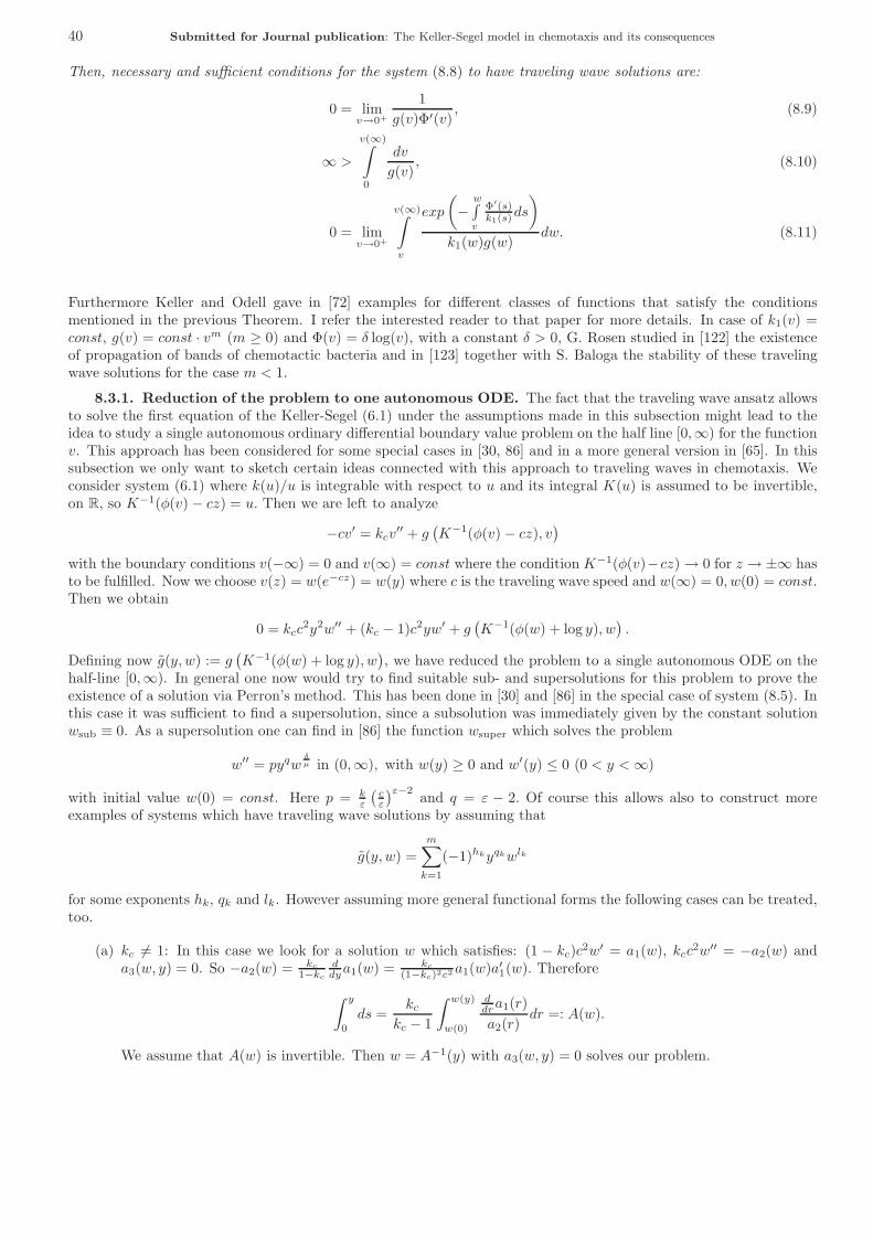
40 Submitted for Journal publication: The Keller-Segel model in chemotaxis and its consequences
Then, necessary and sufficient conditions for the system (8.8) to have traveling wave solutions are:
0 = limv→0+
1g(v)Φ′(v)
, (8.9)
∞ >
v(∞)∫0
dv
g(v), (8.10)
0 = limv→0+
v(∞)∫v
exp
(−
w∫v
Φ′(s)k1(s)
ds
)k1(w)g(w)
dw. (8.11)
Furthermore Keller and Odell gave in [72] examples for different classes of functions that satisfy the conditionsmentioned in the previous Theorem. I refer the interested reader to that paper for more details. In case of k1(v) =const, g(v) = const · vm (m ≥ 0) and Φ(v) = δ log(v), with a constant δ > 0, G. Rosen studied in [122] the existenceof propagation of bands of chemotactic bacteria and in [123] together with S. Baloga the stability of these travelingwave solutions for the case m < 1.
8.3.1. Reduction of the problem to one autonomous ODE. The fact that the traveling wave ansatz allowsto solve the first equation of the Keller-Segel (6.1) under the assumptions made in this subsection might lead to theidea to study a single autonomous ordinary differential boundary value problem on the half line [0,∞) for the functionv. This approach has been considered for some special cases in [30, 86] and in a more general version in [65]. In thissubsection we only want to sketch certain ideas connected with this approach to traveling waves in chemotaxis. Weconsider system (6.1) where k(u)/u is integrable with respect to u and its integral K(u) is assumed to be invertible,on R, so K−1(φ(v) − cz) = u. Then we are left to analyze
−cv′ = kcv′′ + g
(K−1(φ(v) − cz), v
)with the boundary conditions v(−∞) = 0 and v(∞) = const where the condition K−1(φ(v)−cz) → 0 for z → ±∞ hasto be fulfilled. Now we choose v(z) = w(e−cz) = w(y) where c is the traveling wave speed and w(∞) = 0, w(0) = const.Then we obtain
0 = kcc2y2w′′ + (kc − 1)c2yw′ + g
(K−1(φ(w) + log y), w
).
Defining now g(y, w) := g(K−1(φ(w) + log y), w
), we have reduced the problem to a single autonomous ODE on the
half-line [0,∞). In general one now would try to find suitable sub- and supersolutions for this problem to prove theexistence of a solution via Perron’s method. This has been done in [30] and [86] in the special case of system (8.5). Inthis case it was sufficient to find a supersolution, since a subsolution was immediately given by the constant solutionwsub ≡ 0. As a supersolution one can find in [86] the function wsuper which solves the problem
w′′ = pyqwδµ in (0,∞), with w(y) ≥ 0 and w′(y) ≤ 0 (0 < y <∞)
with initial value w(0) = const. Here p = kε
(cε
)ε−2 and q = ε − 2. Of course this allows also to construct moreexamples of systems which have traveling wave solutions by assuming that
g(y, w) =m∑k=1
(−1)hkyqkwlk
for some exponents hk, qk and lk. However assuming more general functional forms the following cases can be treated,too.
(a) kc = 1: In this case we look for a solution w which satisfies: (1 − kc)c2w′ = a1(w), kcc2w′′ = −a2(w) anda3(w, y) = 0. So −a2(w) = kc
1−kc
ddya1(w) = kc
(1−kc)2c2a1(w)a′1(w). Therefore
∫ y
0
ds =kc
kc − 1
∫ w(y)
w(0)
ddra1(r)a2(r)
dr =: A(w).
We assume that A(w) is invertible. Then w = A−1(y) with a3(w, y) = 0 solves our problem.
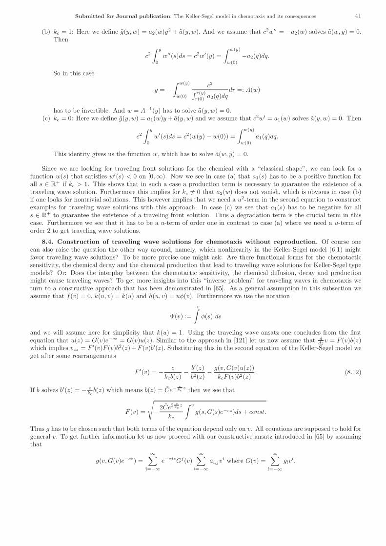
Submitted for Journal publication: The Keller-Segel model in chemotaxis and its consequences 41
(b) kc = 1: Here we define g(y, w) = a2(w)y2 + a(y, w). And we assume that c2w′′ = −a2(w) solves a(w, y) = 0.Then
c2∫ y
0
w′′(s)ds = c2w′(y) =∫ w(y)
w(0)
−a2(q)dq.
So in this case
y = −∫ w(y)
w(0)
c2∫ r(y)r(0) a2(q)dq
dr =: A(w)
has to be invertible. And w = A−1(y) has to solve a(y, w) = 0.(c) kc = 0: Here we define g(y, w) = a1(w)y+ a(y, w) and we assume that c2w′ = a1(w) solves a(y, w) = 0. Then
c2∫ y
0
w′(s)ds = c2(w(y) − w(0)) =∫ w(y)
w(0)
a1(q)dq.
This identity gives us the function w, which has to solve a(w, y) = 0.
Since we are looking for traveling front solutions for the chemical with a “classical shape”, we can look for afunction w(s) that satisfies w′(s) < 0 on [0,∞). Now we see in case (a) that a1(s) has to be a positive function forall s ∈ R
+ if kc > 1. This shows that in such a case a production term is necessary to guarantee the existence of atraveling wave solution. Furthermore this implies for kc = 0 that a2(w) does not vanish, which is obvious in case (b)if one looks for nontrivial solutions. This however implies that we need a u2-term in the second equation to constructexamples for traveling wave solutions with this approach. In case (c) we see that a1(s) has to be negative for alls ∈ R
+ to guarantee the existence of a traveling front solution. Thus a degradation term is the crucial term in thiscase. Furthermore we see that it has to be a u-term of order one in contrast to case (a) where we need a u-term oforder 2 to get traveling wave solutions.
8.4. Construction of traveling wave solutions for chemotaxis without reproduction. Of course onecan also raise the question the other way around, namely, which nonlinearity in the Keller-Segel model (6.1) mightfavor traveling wave solutions? To be more precise one might ask: Are there functional forms for the chemotacticsensitivity, the chemical decay and the chemical production that lead to traveling wave solutions for Keller-Segel typemodels? Or: Does the interplay between the chemotactic sensitivity, the chemical diffusion, decay and productionmight cause traveling waves? To get more insights into this “inverse problem” for traveling waves in chemotaxis weturn to a constructive approach that has been demonstrated in [65]. As a general assumption in this subsection weassume that f(v) = 0, k(u, v) = k(u) and h(u, v) = uφ(v). Furthermore we use the notation
Φ(v) :=
v∫φ(s) ds
and we will assume here for simplicity that k(u) = 1. Using the traveling wave ansatz one concludes from the firstequation that u(z) = G(v)e−cz = G(v)u(z). Similar to the approach in [121] let us now assume that d
dz v = F (v)b(z)which implies vzz = F ′(v)F (v)b2(z)+F (v)b′(z). Substituting this in the second equation of the Keller-Segel model weget after some rearrangements
F ′(v) = − c
kcb(z)− b′(z)b2(z)
− g(v,G(v)u(z))kcF (v)b2(z)
. (8.12)
If b solves b′(z) = − ckcb(z) which means b(z) = Ce−
ckcz then we see that
F (v) =
√−2Ce2
ckcz
kc
∫ v
g(s,G(s)e−cz)ds+ const.
Thus g has to be chosen such that both terms of the equation depend only on v. All equations are supposed to hold forgeneral v. To get further information let us now proceed with our constructive ansatz introduced in [65] by assumingthat
g(v,G(v)e−cz) =∞∑
j=−∞e−cjzGj(v)
∞∑i=−∞
ai,jvi where G(v) =
∞∑l=−∞
glvl.

42 Submitted for Journal publication: The Keller-Segel model in chemotaxis and its consequences
Furthermore let
b(z) =∞∑j=0
bje−cjz and F (v) =
∞∑i=−∞
fivi.
Then, after substituting these expressions in (8.12) we have to compare the coefficients for the vme−cnz. This resultsin
kc
∞∑i=−∞
ififm−i+1
∞∑l=0
blbn−l = −cfmbn + ckcnfmbn −Am,
where Am is the overall coefficient of vm in∑∞i=−∞ ainv
iGn. Now it is possible to treat different cases as it has beendone in detail in [65]. Here we only illustrate the method for an explicit example. First we consider the followingu-equation
ut = uxx − χ (u (log v)x)x
with Neumann boundary conditions and χ ∈ R. After applying the traveling wave ansatz we get u = vχe−cz resp.G(v) = vχ in our notation. Now we want to construct suitable equations for v to get a traveling pulse for u and atraveling wave for v. Let us assume F (v) = f1v. Since b0 = 0 in this case we get:
−kcf1b1c = −cf1b1 − k1 or k1 = vχ∞∑
i=−∞ai1v
i−1 = (kc − 1)b1cf1.
For simplicity we assume that b(z) = e−cz, so b1 = 1 and bj = 0 for j = 1. With this we have
k2 = v2χ∞∑
i=−∞ai2v
i−1 = −kcf21 .
So a1−χ,1 = (kc − 1)cf1 and a1−2χ,2 = −kcf21 . Therefore the second equation has the form
vt = kcvxx + (kc − 1)cf1v1−χu− kcf21 v
1−2χu2. (8.13)
The general system has the traveling pulse and wave solution
u(x, t) = e−χf1
c e−c(x−ct)e−c(x−ct), v(x, t) = e−
f1c e
−c(x−ct), (8.14)
where c is the wave speed.
–20–10
010
20x
–10
–5
0
5
10
t
0.2
0.4
0.6
0.8
1
1.2
1.4
–20–10
010
20x
–10
–5
0
5
10
t
0.2
0.4
0.6
0.8
1
Fig. 8.1. u and v given by (8.14) for f1 = 1 and χ = 0.25.
To avoid singularities in the production and degradation terms it is of special interest to look for 0 < χ < 12 which
means 12 < 1− χ, 1, respectively 0 < 1 − 2χ, 1 for the powers of v in the v-equation. However, qualitatively the shape

Submitted for Journal publication: The Keller-Segel model in chemotaxis and its consequences 43
of the solutions remains the same, independent from the choice of χ ∈ R+. For kc = 0 respectively kc = 1 one obtainspure degradation for v.
It is also possible to construct examples where multiple peak traveling pulse solutions exist by making appropriatechoices for the sensitivity functional. This follows immediately from the following statement from [65]:
Assume there exists a traveling wave solution for the system
ut = (ux − u(log(v))x)xvt = kcvxx + g(u, v)
(8.15)
with homogeneous Neumann boundary data. Then there exists a traveling wave solution for
ut = (ux − u(log(Φ(v))x)xvt = kcvxx + g
(vu
Φ(v) , v),
(8.16)
since in (8.15) we have u(z) = ve−cz and in (8.16) one obtains u(z) = Φ(v)e−cz.Let us consider now a concrete example for multiple peaks traveling waves. As one can easily check the system
ut = (ux − u(log(4v2 − 4v3/2 + v))x)xvt = vxx − 6α2 v2u2
4v2−4v3/2+v.
has the traveling wave solution
u(x− αt) =(1 − e−α(x−αt))2
(1 + e−α(x−αt))4e−α(x−αt) and v(x − αt) = (1 + e−α(x−αt))−2.
The second traveling peak in the population is caused by the sensitivity function. Substituting the solution into the
–10–5
05
10Space x
–4
–2
0
2
4
Time t
0
0.01
0.02
0.03
0.04
0.05
0.06
–10–5
05
10Space x
–4
–2
0
2
4
Time t
0
0.2
0.4
0.6
0.8
1
Fig. 8.2. The function u(x − αt) and v(x − αt) given by the formula above for α = 1.
functional form of the sensitivity function it becomes a perturbation of the traveling front for the chemical distribution.It is also possible to construct more than two traveling peaks by appropriate choices of the sensitivity function.
I want to mention that the constructive approach sketched here also allows different assumptions on k(u) and thatthere are also Keller-Segel type systems with k(u) ≡ 1 that also have traveling wave solutions. For more details seeonce more [65].
Under certain additional assumptions the presented results allow to conclude that there are also traveling wavesolutions on multi-dimensional cylindrical domains. For instance the system
ut = ∇(∇u− u∇(log(v)))
vt = 2∆v + 2v + α2u− 2α2u2
v,
on Ω = R × [0, π] with no-flux boundary conditions for the first equation and where v satisfies homogeneous Dirichletboundary data on ∂Γ has the explicit solution
u(x, y, t) = sin(y)e−α(x−αt)e−e−α(x−αt)
, v(x, y, t) = sin(y)e−e−α(x−αt)
. (8.17)
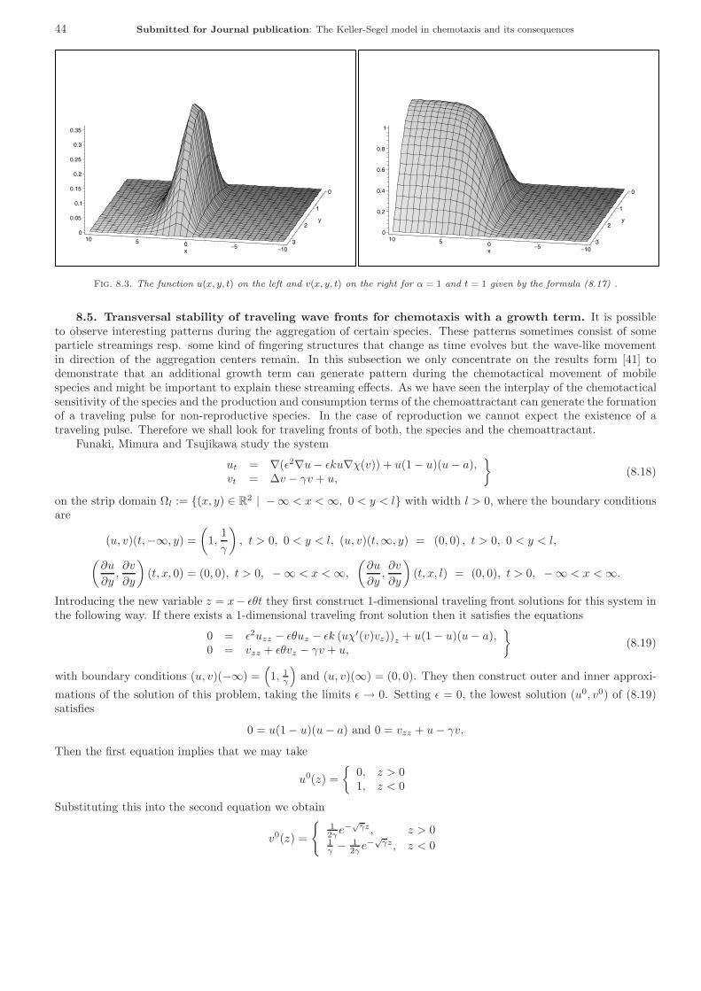
44 Submitted for Journal publication: The Keller-Segel model in chemotaxis and its consequences
–10–50510
x
0
1
2
3
y
0
0.05
0.1
0.15
0.2
0.25
0.3
0.35
–10–50510
x
0
1
2
3
y
0
0.2
0.4
0.6
0.8
1
Fig. 8.3. The function u(x, y, t) on the left and v(x, y, t) on the right for α = 1 and t = 1 given by the formula (8.17) .
8.5. Transversal stability of traveling wave fronts for chemotaxis with a growth term. It is possibleto observe interesting patterns during the aggregation of certain species. These patterns sometimes consist of someparticle streamings resp. some kind of fingering structures that change as time evolves but the wave-like movementin direction of the aggregation centers remain. In this subsection we only concentrate on the results form [41] todemonstrate that an additional growth term can generate pattern during the chemotactical movement of mobilespecies and might be important to explain these streaming effects. As we have seen the interplay of the chemotacticalsensitivity of the species and the production and consumption terms of the chemoattractant can generate the formationof a traveling pulse for non-reproductive species. In the case of reproduction we cannot expect the existence of atraveling pulse. Therefore we shall look for traveling fronts of both, the species and the chemoattractant.
Funaki, Mimura and Tsujikawa study the system
ut = ∇(ε2∇u− εku∇χ(v)) + u(1 − u)(u− a),vt = ∆v − γv + u,
(8.18)
on the strip domain Ωl := (x, y) ∈ R2 | −∞ < x <∞, 0 < y < l with width l > 0, where the boundary conditions
are
(u, v)(t,−∞, y) =(
1,1γ
), t > 0, 0 < y < l, (u, v)(t,∞, y) = (0, 0) , t > 0, 0 < y < l,(
∂u
∂y,∂v
∂y
)(t, x, 0) = (0, 0), t > 0, −∞ < x <∞,
(∂u
∂y,∂v
∂y
)(t, x, l) = (0, 0), t > 0, −∞ < x <∞.
Introducing the new variable z = x− εθt they first construct 1-dimensional traveling front solutions for this system inthe following way. If there exists a 1-dimensional traveling front solution then it satisfies the equations
0 = ε2uzz − εθuz − εk (uχ′(v)vz))z + u(1 − u)(u− a),0 = vzz + εθvz − γv + u,
(8.19)
with boundary conditions (u, v)(−∞) =(1, 1
γ
)and (u, v)(∞) = (0, 0). They then construct outer and inner approxi-
mations of the solution of this problem, taking the limits ε → 0. Setting ε = 0, the lowest solution (u0, v0) of (8.19)satisfies
0 = u(1 − u)(u− a) and 0 = vzz + u− γv.
Then the first equation implies that we may take
u0(z) =
0, z > 01, z < 0
Substituting this into the second equation we obtain
v0(z) =
12γ e−√γz, z > 0
1γ − 1
2γ e−√γz, z < 0

Submitted for Journal publication: The Keller-Segel model in chemotaxis and its consequences 45
which belongs to C1(R). This solution is called an outer solution in R.However as a discontinuous function u0(z) is not a good approximation of the solution in a neighbourhood of
z = 0. In order to construct an approximate solution in a neighbourhood of z = 0, Funaki et al. introduce thestretched variable ξ = z/ε and rewrite the problem as
0 = uξξ + (θ − kχ′(v)vz)uξ − εk(χ′(v)vz)z + u(1 − u)(u− a),0 = vξξ + ε2(θvξ − γv + u),
(8.20)
where (u, v)(ξ) = (u, v)(εξ). Setting now ε = 0 and noting that v0(0) = 12γ we see
0 = uξξ + (θ − kχ′(v)vz)uξ + u(1 − u)(u− a),0 = vξξ,
(8.21)
with boundary conditions u(−∞) = 1, u(∞) = 0, v(±∞) = 12γ . Thus we get v(ξ) ≡ 1
2γ which implies
0 = uξξ +(θ +
k
2√γχ′(
12γ
))uξ + u(1 − u)(u− a).
The existence of an inner solution (u, v)(z/ε) in a neighbourhood of z = 0 is now a consequence from the results in[33]. Matching the outer and inner solution a traveling front solution of the problem can be constructed in one spatialdimension. This is summarized in the following Theorem:
Theorem 8.4 (M. Funaki, M. Mimura & T. Tsujikawa). Fix k > 0 arbitrary. There is ε0 > 0 such that for anyε ∈ (0, ε0) the system (8.19) has a solution (U ε, V ε)(z) for θ = (θ(ε; k) satisfying
limε→0
U ε(z) = u0(z) uniformly in (−∞,−δ) ∪ (δ,∞), limε→0
V ε(z) = v0(z) uniformly in R
with any small constant δ > 0 and
limε→0
θ(ε; k) = θ∗(k) = c− k
2√γχ′(
12γ
).
Moreover limε→0
U ε(εξ) = u(ξ), limε→0
V ε(εξ) = 12γ uniformly on any compact subset of R with respect to C2(R).
Studying in two spatial dimensions the distribution of the eigenvalues of the eigenvalue problem of the linearized systemaround the front solutions with velocity εθ(ε; k) in the strip domain Ωl Funaki et al. find out that the transversalstability of the front shows the following behaviour:
Theorem 8.5 (M. Funaki, M. Mimura & T. Tsujikawa).
1. When χ′′(
12γ
)≤ 0, for any fixed l > 0 and k > 0, there is ε0 > 0 such that all eigenvalues are in the left half
of the complex plane if 0 < ε < ε0. Thus the traveling front solution ids transversally stable.2. When χ′′
(12γ
)> 0, for any fixed l > 0 and k > 0, there is ε0(l, k) > 0 such that the traveling front solution
is unstable for any 0 < ε < ε0(l, k).
Thus the tranversal stability of the wave front depends of the chemotactical sensitivity, where transversally stableis defined in [41] in the following way:
Definition 8.6. A traveling front solution of (8.18) is transversally stable except for translational invariance inx, if and only if zero is a simple eigenvalue of the eigenvalue problem associated with the linearized system of (8.18)around the traveling front solution and the remaining spectrum is contained in a closed sector lying in the left half ofthe complex plane. The traveling front is unstable if it is not stable.
Further results related to this system can also be found in [13] and [14].

46 Submitted for Journal publication: The Keller-Segel model in chemotaxis and its consequences
9. Conclusions and personal comments. There are of course still many open problems in connection withthe various approaches that have been studied for the Keller-Segel model.
This paper dealt solely with the parabolic model proposed by Keller and Segel for the aggregation phase of mobilespecies caused by chemotaxis. However there are also different approaches to chemotaxis and hencealso numerousdifferent models describing chemotaxis. First of all, one must always keep in mind that the model one uses is basedeither on a microscopic or a macroscopic approach and always depends on the species studied. Thus transportand hyperbolic models for chemotaxis have also been proposed. For example transport and hyperbolic models forchemotactical movement have been studied in [4, 5, 34, 37, 38, 55, 57, 59] and [110]. The connection betweenchemotaxis equations as the parabolic limit of velocity jump processes or transport models for chemotaxis has beenstudied in [4, 5, 22, 58, 113] and [114]. I refer to [37] for surveyes on different models for chemotactical movement andto [59] for a survey on the hyperbolic approach to chemotaxis.
Of course there are many publications presenting experimental data on chemotactic effects and the influences ofchanges in the motility or the chemotactic sensitivity of the given species (see for example [35, 36]). Models whichtake the chemotactical movement of n populations according to k sensitivity agents into account have been proposedin [3, Beispiel 2.47, page 58] and in [152] by G. Wolansky. Wolansky has studied a generalization of the Keller-Segelmodel for n populations in the absence of conflicts. Also the effect of multiple attractant gradients on chemotacticalmovement has been studied [140] and numerical solutions for the corresponding models have been calculated [39, 40].Numerical analysis for the Keller-Segel model has been performed, for example, by Gajewski and Zacharias using achemotaxis version of the well-established TOSCA code for solving semiconductor problems and by Nakaguchi andYagi studying the full discrete approximation of the Keller-Segel model by Galerkin Runge-Kutta methods [100, 101].The transport chemotaxis model is dealt with in [21] and [40], for example.
The results available for systems related to the Keller-Segel equations such as the Othmer-Stevens model are sonumerous that I mention only a few [77, 112, 141] and [154]. The well-posedness of the Othmer-Stevens model followsdirectly from the results by Rascle [117].
Of course, the functional forms appearing in the original Keller-Segel model can vary from species to species andsome explicit models for the cAMP oscillation have been proposed (see [80] for the so called Martiel and Goldbetermodel, [111] for a survey on the oscillatory cAMP signaling in Dictyostelium discoideum and [120] for the descriptionof the role of cAMP in the development of Dictyostelium discoideum). The Keller-Segel model has also been usedto describe different problems. For example, in [84] the Keller-Segel equations have been proposed for strip patternformation in alligator embryos. Angiogenesis has also been proposed as another application of Keller-Segel type models(see for example [27] including references). The large number of applications and of possible functional forms resultsdirectly in a large number of models depending on the considered problem. In some particular papers this has alsoresulted in the addition of a third equation to the Keller-Segel model (2.4) or the rediscovery of a more complicatedversion of the Keller-Segel model. This results from attempts to describe more complicated pattern formations duringthe aggregation phase of mobile species such as the attempt to describe spiral waves during the aggregation (see, forexample, [134, 144] and [145] for such extended models).
At the conclusion of this survey I would ask the reader to allow me a personal comment. The references given inthis text are far from complete. I have tried to give the interested reader a brief summary of the latest developmentsin the Keller-Segel model. Thus, this article is intended as continuation of Evelyn Fox Keller’s article “Assessing theKeller-Segel model: How has it fared” of 1980 [74]. It is left to the reader to decide whether I have succeeded.
Acknowledgement: I thank Prof. Dr. Wolfgang Alt for allowing me to include the results from his Habilitation inthis summary of the Keller-Segel system.
REFERENCES
[1] J. Adler, Chemotaxis in bacteria. Ann. Rev. Biochem. 44 (1975), pp. 341–356.[2] N. D. Alikakos, Lp bounds of solutions of reaction-diffusion equations Comm. In Partial Differential Equations, 4 (1979), pp. 827–868.[3] W. Alt, Vergleichsatze fur quasilineare elliptisch-parabolische Systems partieller Differentialgleichungen, Habilitation, Ruprecht-Karl-
Universitat Heidelberg, 1980.[4] W. Alt, Biased Random Walk models for chemotaxis and related diffusion approximations, J. Math Biol. 9 (1980), pp. 147–177.[5] W. Alt, Singular perturbation of differential integral equations describing biased random walks. J. Reine Angew. Math. 322 (1981),
pp. 15 – 41.[6] H. Amann, Dynamic theory of quasilinear parabolic equations II. Reaction-Diffusion Systems, Differential and Integral Eqns. 3
(1990), pp. 13–75.[7] H. Amann, Nonhomogeneous linear and quasilinear elliptic and parabolic boundary value problems, Function Spaces, Differential
Operators and Nonlinear Analysis (Eds. Schmeisser, Triebel), Teubner Texte zur Mathematik 133 (1993), pp. 9–126.

Submitted for Journal publication: The Keller-Segel model in chemotaxis and its consequences 47
[8] F. Berezovskaya and G. Karev, Bifurcation of travelling waves in population taxis models. Physics-Uspekhi, 42 (1999) 917–929.[9] F. Berezovskaya and G. Karev, Parametric portraits of travelling waves of population models with polynomial growth and
autotaxis rates. Spatial heterogeneity in ecological models (Alcalß de Henares, 1998). Nonlinear Anal. Real World Appl. 1(2000) 123–136.
[10] F. Berezovskaya and G. Karev, Polynomial models of populations with autotaxis: ”traveling wave” solutions. (Russian). Mat.Model. 12 (2000) 78–93.
[11] P. Biler, Local and global solvability of some parabolic system modelling chemotaxis, Adv. Math. Sci. Appl. 8 (1998), pp. 715–743.[12] P. Biler, Global solutions to some parabolic-elliptic systems of chemotaxis, Adv. Math. Sci. Appl. 9 (1999), pp. 347–359.[13] A. Bonami, D. Hilhorst, E. Logak, and M. Mimura, A free boundary problem arising in a chemotaxis model, Free boundary problems,
theory and applications (Zakopane, 1995), Pitman Res. Notes Math. Ser. 363, Longman, Harlow (1996), pp. 368–373.[14] A. Bonami, D. Hilhorst, E. Logak, and M. Mimura, Singular limit of a chemotaxis-growth model, Adv. Differential Equations 6
(2001), pp. 1173–1218.[15] J. T. Bonner, The cellular slime molds, Princeton University Press, Princeton, New Jersey, second edition, 1967.[16] A. Boy, Analysis for a system of coupled reaction-diffusion parabolic equations arising in biology. Computers Math. Applic 32 (1996),
pp. 15–21.[17] M. P. Brenner, L. S. Levitov and E. O. Budrene, Physical mechanisms for chemotactic pattern formation by bacteria. Biophys. J. 74
(1998), pp. 1677–1693.[18] M. P. Brenner, P. Constantin, L. P. Kadanoff, A. Schenkel and S. C. Venkataramani, Attraction, Diffusion and Collapse, Nonlinearity
12 (1999), pp. 1071 – 1098.[19] M. P. Brenner, P. Constantin, L. P. Kadanoff, A. Schenkel and S. C. Venkataramani, Blowup in the Chemotaxis equation, Technical
Report University of Chicago.[20] H. Brezis and F. Merle, Uniform estimates and blow-up behaviour for solutions of −∆u = V (x)eu in two dimensions, Comm. P.D.E.
16 (1991), pp. 1223 – 1253.[21] B. J. Brosilow, R. M. Ford, S. Sarman and P. T. Cummings, Numerical solution of transport equations for bacterial chemotaxis:
Effect of discretization of directional motion, SIAM J. Appl. Math. 56 (1996), pp.1639–1663.[22] F. A. C. C. Chalub, P. Markowich, B. Perthame and C. Schmeiser, Kinetic models for chemotaxis and their drift diffusion limit.
Preprint 2002.[23] S.-Y.A. Chang and P. Yang, Conformal deformation of metrics on S2, J. Differential Geometry, 27 (1988), pp. 259–296[24] S. Childress and J.K. Percus, Nonlinear aspects of chemotaxis, Math. Biosc. 56 (1981), pp. 217 – 237.[25] S. Childress, Chemotactic collapse in two dimensions, Lecture Notes in Biomathematics, Springer-Verlag, volume 55, 1984, pp. 61 –
66.[26] M. H. Cohen and A. Robertson, Wave propagation in the early stages of aggregation of cellular slime molds. J. theor. Biol. 31 (1971),
101–118.[27] L. Corrias, B. Perthame and H. Zaag, A model motivated by angiogenesis, Preprint 2002.[28] B. Davis, Reinforced random walks, Probab. theory Related Fields 84 (1990), pp. 203 – 229.[29] F. Dkhil, On the analysis of reaction-diffusion-advection systems arising in chemical and biomathematical models, PhD-thesis,
University of Cergy-Pontoise, France, 2002.[30] Y. Ebihara, Y. Furusho and T. Nagai, Singular solutions of traveling waves in a chemotactic model., Bull. Kyushu Inst. Tech.
Math. Natur. Sci. 39 (1992) 29–38.[31] Evans, L. C. 1998 Partial Differential Equations, American Mathematical Society, Graduate Studies in Mathematics 19, Providence,
Rhode Island.[32] D. L. Feltham and M. A. J. Chaplain, Travelling waves in a model of species migration, Appl. Math. Lett. 13 (2000), pp. 67–73.[33] P. C. Fife and J. B. McLeod, The approach of solutions of nonlinear diffusion equations to traveling front solutions, Arch. Rat. Mech.
Analysis 65 (1977), pp. 335–362.[34] R. M. Ford and D. A. Lauffenburger, Analysis of chemotactic bacterial distributions in population migration assays using mathemat-
ical model applicable to steep or shallow attractant gradients, Bull. Math. Biol. 53 (1991), pp. 721–749.[35] R. M. Ford, B. R. Phillips, J. A. Quinn and D. A. Lauffenburger, Measurement of bacterial random motility and chemotaxis
coefficients: I. Stopped-flow diffusion chamber assay, Biotech. and Bioengin. 37 (1991), pp. 647–660.[36] R. M. Ford and D. A. Lauffenburger, Measurement of bacterial random motility and chemotaxis coefficients: II. Application of
Single-cell-based mathematical model, Biotech. and Bioengin. 37 (1991), pp. 661–672.[37] R. M. Ford, Mathematical modeling and quantitative characterization of bacterial motility and chemotaxis., Modelin the Metabolic
and Physiology Activities of Microorganisms: Chapter 7, John Wiley & sons, Inc. 1992.[38] R. M. Ford and P. T. Cummings, On the relationship between cell balance equations for chemotactic cell populations, SIAM J. Appl.
Math. 52 (1992), pp. 1426–1441.[39] P. D. Frymier, R. M. Ford and P. T. Cummings, Cellular dynamics simulations of bacterial chemotaxis, Chem. Engin. Sci. 48 (1993),
pp. 687–699.[40] P. D. Frymier, R. M. Ford and P. T. Cummings, Analysis of bacterial migration: I. Numerical solution of balance equation, AIChE
J. 40 (1994), pp. 704–715.[41] M. Funaki, M. Mimura and T. Tsujikawa, Traveling front solutions arising in a chemotaxis-growth model, RIMS Kokyuroku 1135
(2000), pp. 52–76.[42] H. Gajewski, W. Jager and A. Koshelev, About loss of regularity and “blow up” of solutions for quasilinear parabolic systems, Preprint
No. 70, Weierstraß-Institut fur Angewandte Analysis und Stochastik, Berlin (1993).[43] H. Gajewski and K. Zacharias, Global behavior of a reaction-diffusion system modelling chemotaxis, Math. Nachr. 195 (1998), pp.
77 – 114.[44] H. Gajewski and K. Zacharias, On a reaction-diffusion system modelling chemotaxis, Proceedings of the Equadiff 99, (eds. B. Fiedler,
K. Groger, J. Sprekels), World Scientific Publishing Co, Singapore, 2000, pp. 1098–1103.[45] J. Grolle (verantwortlicher Redakteur fur Biologie), Wabernder Klecks, DER SPIEGEL 36 (1998), p. 212.[46] C. Gui, J. Wei and M. Winter, Multiple boundary peak solutions for some singulary perturbed Neumann problems, Ann. Inst. H.
Poincare Anal. Non Lineaire 17 (2000), pp. 47–82.[47] G. Harada, T. Nagai, T. Senba and T. Suzuki, Concentration lemma, Brezis-Merle type inequality, and a parabolic system of
chemotaxis, Adv. Differential Equations 6 (2001), pp. 1255–1280.

48 Submitted for Journal publication: The Keller-Segel model in chemotaxis and its consequences
[48] M. Henry, D. Hilhorst and R. Schatzle, Convergence to a viscosity solution for an advection-reaction-diffusion equation arising froma chemotaxis-growth model. Hiroshima Math. J. 29 (1999), pp. 591–630.
[49] M. A. Herrero and J. J. L. Velazquez, Singularity patterns in a chemotaxis model, Math. Ann. 36 (1996), pp. 583 – 623.[50] M. A. Herrero and J. J. L. Velazquez, Chemotactic collapse for the Keller-Segel model, J. Math. Biol. 35 (1996), pp. 583 – 623.[51] M. A. Herrero and J. J. L. Velazquez, A blow-up mechanism for a chemotaxis model, Ann. Scuola Normale Superiore 24 (1997), pp.
633 – 683.[52] M. A. Herrero, E. Medina and J. J. L. Velazquez, Finite-time aggregation into a single point in a reaction diffusion system, Nonlin-
earity 10 (1997), pp. 1739–1754.[53] M. A. Herrero, E. Medina and J. J. L. Velazquez, Self-similar blow-up for a reaction diffusion system, Journal of Computational and
Applied Mathematics 97 (1998), pp. 99 – 119.[54] M. A. Herrero, Asymptotic properties of reaction-diffusion systems modelling chemotaxis, Applied and industrial mathematics,
Venice–2, 1998, Kluwer Acad. Publ., Dordrecht 2000, pp. 89 – 108.[55] T. Hillen and A. Stevens, Hyperbolic models for chemotaxis in 1-D, Nonlinear Anal., Real World Appl. 1 (2000), pp. 409 – 433.[56] T. Hillen and K.J. Painter, Global Existence far a Parabolic Chemotaxis Model with Prevention of Overcrowding, Adv. in Appl.
Math. 26 (2001), pp. 280 – 301.[57] T. Hillen, C. Rohde and F. Lutscher Existence of weak solutions for a hyperbolic model of chemosensitive movement, J. Math. Anal.
Appl. 260 (2001), pp. 173 – 199.[58] T. Hillen and H. G. Othmer, The diffusion limit of transport equations derived from velocity-jump processes, SIAM J. Appl. Math.
61 (2000), pp. 751 – 775.[59] T. Hillen, Hyperbolic models for chemosensitive movement, Math. Models Methods Appl. Sci. 12 (2002), pp. 1 – 28.[60] D. Horstmann, Some blowup results for the Keller-Segel model, Proceedings of the Equadiff 99, (eds. B. Fiedler, K. Groger, J.
Sprekels), World Scientific Publishing Co, Singapore 2000, pp. 1104 – 1106.[61] D. Horstmann, Lyapunov functions and Lp-estimates for a class of reaction-diffusion systems, Colloquium Mathematicum 87 (2001),
pp. 113 – 127.[62] D. Horstmann, The nonsymmetric case of the Keller-Segel model in chemotaxis: some recent results, Nonlinear Differential Equations
and Applications (NoDEA) 8 (2001), pp. 399 – 423.[63] D. Horstmann and G. Wang, Blow-up in a chemotaxis model without symmetry assumptions, European Journal of Applied Mathe-
matics 12 (2001), pp. 159 – 177.[64] D. Horstmann, On the existence of radially symmetric blow-up solutions for the Keller-Segel model, Journal of Mathematical Biology
44 (2002), pp. 463 – 478.[65] D. Horstmann and A. Stevens, A constructive approach to traveling waves in chemotaxis, Preprint no.78: 2001 Max-Planck-Institute
for Mathematics in the Sciences, Leipzig, submitted.[66] D. Horstmann, On some effects of positive chemotactical movement, Preprint submitted.[67] W. Jager and S. Luckhaus, On explosions of solutions to a system of partial differential equations modelling chemotaxis, Trans. Am.
Math. Soc. 329 (1992), pp. 817 – 824.[68] Y. Kabeya and W.-M. Ni, Stationary Keller-Segel model with the linear sensitivity, RIMS Kokyuroku 1025 (1998), pp. 44 – 65.[69] E. F. Keller and L. A. Segel, Initiation of slime mold aggregation viewed as an instability, J. Theor. Biol. 26 (1970), pp. 399 – 415.[70] E. F. Keller and L. A. Segel, Model for chemotaxis, J. Theor. Biol. 30 (1971), pp. 225 – 234.[71] E. F. Keller and L. A. Segel, Traveling bands of chemotactic bacteria: A Theoretical Analysis, J. theor. Biol. 30 (1971), pp. 235 –
248.[72] E. F. Keller and G. M. Odell, Necessary and sufficient conditions for chemotactic bands Math. Biosci. 27 (1975), pp. 309 – 317.[73] E. F. Keller and G. M. Odell, Traveling bands of chemotactic bacteria revisited, J. Theor. Biol. 56 (1976), pp. 243 – 247.[74] E. F. Keller, Assessing the Keller-Segel modell: How has it fared?, Editors W. Jager, H. Rost und P. Tautu, Lecture Notes in
Biomathematics 38, Springer-Verlag, Berlin, Heidelberg, New York 1980, pp. 379 – 387.[75] O. A. Ladyzenskaya and N. N. Ural’ceva, Linear and quasilinear elliptic equations, Academic Press, New York and London, 1968.[76] D. Lauffenburger, C. R. Kennedy and R. Aris Traveling bands of chemotactic bacteria in the context of population growth, Bull. of
Math. Biol. 46 (1984), pp. 19 – 40.[77] H. Levine and B. Sleeman A system of reaction diffusion equations arising in the theory of reinforced random walks, SIAM J. Appl.
Math 57 (1997), pp. 683 – 730.[78] Y. Li and I. Shafrir, Blow-up analysis for solutions of −∆u = V eu in dimension two, Ind. Univ. Math. J. 43 (1994), pp. 1255 – 1270.[79] C.-S. Lin, W.-M. Ni and I. Takagi, Large amplitude stationary solutions to a chemotaxis system, J. Differ. Equations, 72 (1988),
pp. 1 – 27.[80] J.-L. Martiel and A. Goldbeter, A model based on receptor desensitization for cyclic AMP signaling in Dictyostelium cells, Biophys.
J. 52 (1987), pp. 807 – 828.[81] Y. Mizutani and T. Nagai, Self-similar radial solutions to a system of partial differential equations modelling chemotaxis. Bull.
Kyushu Inst. Tech. Math. Natur. Sci. 42 (1995), pp. 19 – 28.[82] Y. Mizutani, N. Muramoto and K. Yoshida, Self-similar radial solutions to a parabolic system modelling chemotaxis via variational
method, Hiroshima Math. J. 29 (1999), pp. 145 – 160.[83] N. Muramoto, Y. Naito and K. Yoshida, Existence of self-similar solutions to a parabolic system modeling chemotaxis, Jpn. J. Ind.
Appl. Math. 17 (2000), pp. 427 – 451.[84] J. D. Murray, Modelling the pattern generating mechanism in the formation of stripes on alligators, Mathematical physics, 9th Int.
Congr. Swansea/UK 1988 (1989), pp. 208 – 213.[85] J. D. Murray, Mathematical Biology, 2nd Ed., Biomathematics Texts 19, Springer Verlag, Heidelberg, New York, 1993.[86] T. Nagai and T. Ikeda, Traveling waves in a chemotactic model, J. Math. Biol. 30 (1991), pp. 169 – 184.[87] T. Nagai, Blow-up of radially symmetric solutions to a chemotaxis system, Adv. Math. Sci. Appl. 5 (1995), pp. 581 – 601.[88] T. Nagai and T. Senba, Global existence and blow-up of radial solutions to a parabolic-elliptic system of chemotaxis, Preprint 1996.[89] T. Nagai and T. Senba, Behavior of radially symmetric solutions of a system related to chemotaxis, Nonlinear Anal., Theory Methods
Appl. 30 (1997), pp. 3837 – 3842.[90] T. Nagai, T. Senba and K. Yoshida, Application of the Moser-Trudinger inequality to a parabolic system of chemotaxis, Funkc.
Ekvacioj, Ser.Int. 40 (1997), pp. 411 – 433.[91] T. Nagai, T. Senba and K. Yoshida, Global existence of solutions to the parabolic systems of chemotaxis, RIMS Kokyuroku 1009

Submitted for Journal publication: The Keller-Segel model in chemotaxis and its consequences 49
(1997), pp. 22 – 28.[92] T. Nagai, T. Senba and T. Suzuki, Concentration behavior of blow-up solutions for a simplified system of chemotaxis, Preprint 1998.[93] T. Nagai, T. Senba and T. Suzuki, Keller-Segel system and the concentration lemma, RIMS Kokyuroku 1025 (1998), pp. 75 – 80.[94] T. Nagai and T. Senba, Global existence and blow-up of radial solutions to a parabolic-elliptic system of chemotaxis, Adv. Math. Sci.
Appl. 8 (1998), pp. 145 – 156.[95] T. Nagai, Behavior of solutions to a parabolic-elliptic system modelling chemotaxis, J. Korean Math. Soc. 37 (2000), pp. 721 – 733.[96] T. Nagai, T. Senba and T. Suzuki, Chemotaxis collapse in a parabolic system of mathematical biology, Hiroshima Math. J. 30 (2000),
pp. 463 – 497.[97] T. Nagai, Global existence and Blowup of solutions to a chemotaxis system, Nonlinear Analysis 47 (2001), pp. 777 – 787.[98] T. Nagai, Blowup of nonradial solutions to parabolic-elliptic systems modeling chemotaxis in two-dimensional domains, J. Inequal.
Appl. 6 (2001), pp. 37 – 55.[99] Y. Naito, T. Suzuki and K. Yoshida, Self-similar solutions to a parabolic system modeling chemotaxis, J. Differential Equations 184
(2002), pp. 386 – 421.[100] E. Nakaguchi and A. Yagi, Full discrete approximation by Galerkin Runge-Kutta methods for a parabolic system of chemotaxis,
Hokkaido Mathematical Journal 31 (2002), pp. 385 – 429.[101] E. Nakaguchi and A. Yagi, Full discrete approximations by Galerkin method for chemotaxis-growth model, Nonlinear Anal.Theory
Meth. Appl. 47 (2001), pp. 6097 – 6107.[102] V. Nanjundiah, Chemotaxis, signal relaying and aggregation morphology, J. Theor. Biol. 42 (1973), pp. 63 – 105.[103] V. Nanjundiah and S. Shweta, The determination of spatial pattern in Dictyostelium discoideum, J. Biosci. 17 (1992), pp. 353 – 394.[104] W.-M. Ni and I. Takagi, On the shape of least-energy solutions to a semilinear Neumann problem, Comm. Pure Appl. Math. 44
(1991), pp. 819 – 851.[105] W.-M. Ni and I. Takagi, Locating the peaks of least energy solutions to a semilinear Neumann problem, Duke Math. J. 70 (1993),
pp. 247 – 281.[106] A. Novick-Cohen and L. A. Segel, A gradually slowing traveling band of chemotactic bacteria. J. Math. Biol. 19 (1984), pp. 125 –
132.[107] G. M. Odell, Travelling bands of chemotactic microorganisms, Chapter 6 of: Mathematical models in molecular and cellular biology,
ed. L.A. Segel, Cambridge University Press, Cambridge (1980), p. 345.[108] K. Oelschlager, On the derivation of reaction-diffusion equations as limit dynamics of systems of moderately interacting stochastic
many particle processes. Probab. Th. Rel. Fields 82 (1989), pp. 565 – 586.[109] K. Osaki and A. Yagi, Finite dimensional attractors for one-dimensional Keller-Segel equations. Funkcialaj Ekvacioj 44 (2001), pp.
441 – 469.[110] H. G. Othmer, S. R. Dunbar and W. Alt, Models of dispersal in biological systems. J. Math. Biol. 26 (1988), pp. 263 – 298.[111] H. G. Othmer and P. Schaap, Oscillatory cAMP Signaling in the development of Dictyostelium discoideum, Comments on Theoretical
Biology 5 (1998), pp. 175 – 282.[112] H. G. Othmer and A. Stevens, Aggregation, blowup, and collapse: the ABCs of taxis in reinforced random walks. SIAM J. Appl.
Math. 57 (1997), pp. 1044 – 1081.[113] H. G. Othmer and T. Hillen, The diffusion limit of transport equations. II: Chemotaxis equations, SIAM J. Appl. Math. 62 (2002),
pp. 1222 – 1250.[114] C. S. Patlak, Random walk with persistence and external bias. Bull. Math: Biophys. 15 (1953), pp. 311 – 338.[115] K. Post, A non-linear parabolic system modeling chemotaxis with sensitivity functions, Dissertation, Humboldt-Universitat zu Berlin,
Institut fur Mathematik 1999.[116] L. M. Prescott, J. P. Harley and D. A. Klein, Microbiology. Wm. C. Brown Publishers, 3rd edition: Chicago, London, 1996.[117] M. Rascle Sur une equation integro-differentielle non lineaire issue de la biologie J. Diff. Eqns 32 (1979), pp. 420 – 453,.[118] M. Rascle and C. Ziti, Finite time blow-up in some models of chemotaxis, J. Math. Biol. 33 (1995), pp. 388 – 414.[119] X. Ren, Least-energy solutions to a non-autonomous semilinear problem with small diffusion coefficient Electric J. Diff. Eqns 1993
(1993), pp. 1 – 21.[120] C. D. Reymond, P. Schaap, M. Veron and J. G. Williams, Dual role of cAMP during Dictyostelium development, Experientia 368
(1995), pp. 1166–1174.[121] M. Rodrigo and M. Mimura, Exact solutions of a competition-diffusion system, Hiroshima Math. J. 30 (2000), pp. 257 – 270.[122] G. Rosen, On the propagation theory for bands of chemotactic bacteria, Math. Biosci. 20 (1974), pp. 185 – 189.[123] G. Rosen and S. Baloga, On the stability of steady propagating bands of chemotactic bacteria, Math. Biosci. 24 (1975), pp. 273 –
279.[124] R. Schaaf, Stationary solutions of chemotaxis systems, Trans. Am. Math. Soc. 292 (1985), pp. 531 – 556.[125] T. L. Scribner, L. A. Segel and E. H. Rogers, A numerical study of the formation and propagation of traveling bands of chemotactic
bacteria, J. Theor. Biol. 46 (1974), pp. 189–219.[126] T. Senba, Blow-up of radially symmetric solutions to some systems of partial differential equations modelling chemotaxis, Adv.
Math. Sci. Appl. 7 (1997), pp. 79 – 92.[127] T. Senba and T. Suzuki, Chemotaxis Collapse in a parabolic-elliptic system of mathematical biology, Preprint 1999.[128] T. Senba, Behavior of solutions to a system related to chemotaxis, Proceedings of the Equadiff 99, (eds. B. Fiedler, K. Groger, J.
Sprekels), World Scientific Publishing Co, Singapore 2000, pp. 1115–1120.[129] T. Senba and T. Suzuki, Some structures of stationary solutions to Keller-Segel model, N. Kenmochi (ed.), Proceedings of the
international conference on free boundary problems: theory and applications, Chiba, Japan, November 7-13, 1999. I. Tokyo:Gakkotosho. GAKUTO Int. Ser., Math. Sci. Appl. 13 (2000), pp. 282 – 297.
[130] T. Senba and T. Suzuki, Some structures of the solution set for a stationary system of chemotaxis, Adv. Math. Sci. Appl. 10 (2000),pp. 191 – 224.
[131] T. Senba and T. Suzuki, Local and norm behavior of blowup solutions to a parabolic system of chemotaxis, J. Korean Math. Soc. 37(2000), pp. 929 – 941.
[132] T. Senba and T. Suzuki, Behavior of solutions to a system related to chemotaxis, Nonlinear Analysis 47 (2001),pp. 2551–2562.[133] T. Senba and T. Suzuki, Weak solutions to a parabolic-elliptic system of chemotaxis, J. Funct. Anal. 191 (2002), pp. 17–51.[134] J. A. Sherratt, Chemotaxis and chemokinesis in eukaryotic cells: The Keller-Segel model equations as an approximation to a detailed
model, Bulletin Math. Biol. 56 (1994), pp. 129–146.
50 Submitted for Journal publication: The Keller-Segel model in chemotaxis and its consequences
[135] A. Stevens, Trail following and aggregation of myxobacteria., J. Biol. Systems 3 (1995), pp. 1059–1068.[136] A. Stevens, Simulation of chemotaxis-equations in two space dimensions., Nonlinear Physics of complex systems - current status
and future trends, J. Parisi, S. C. Muller and W. Zimmermann (eds), Springer, Berlin 1996.[137] A. Stevens and F. Schweitzer, Aggregartion induced by diffusing and nondiffusing media. in Dynamics of Cell and Tissue Motion,
W. Alt, A. Deutsch and G. Dunn, eds. Birkhauser, Basel, Switzerland, 1997, pp. 183 – 192.[138] A. Stevens, A Stochastic cellular automaton modeling gliding and aggregation of myxobacteria. SIAM J. Appl. Math. (electronic) 61
(2000), pp. 172–182.[139] A. Stevens, The derivation of chemotaxis equations as limit dynamics of moderately interacting stochastic many-particle systems.,
SIAM J. Appl. Math. (electronic) 61 (2000), pp. 183–212.[140] I. Strauss, P. D. Frymier, R. M. Ford and P. T. Cummings, Analysis of bacterial migration: II. Studies with multiple attractant
gradients, AIChE J. 41 (1995), pp. 402–414.[141] B. D. Sleeman and H. A. Levine, Partial differential equations of chemotaxis and angiogenesis, Math. Methods Appl. Sci. 24 (2002),
pp. 405–426.[142] M. Struwe, Variational Methods, Springer Verlag Berlin, Heidelberg, New York, second edition 1996.[143] M. Struwe and G. Tarantello, On multivortex solutions in Chern-Simons gauge theory, Bolletino U. M. I. 8 (1998), pp. 109–121.[144] O. O. Vasieva, B. N. Vasiev, V. A. Karpov and A. N. Zaikin, A model of Dictyostelium discoideum aggregation, J. theor. Biol. 171
(1994), pp. 361–367.[145] B. N. Vasiev, P. Hogeweg and A. V. Panfilov, Simulation of Dictyostelium discoideum aggregation via reaction-diffusion model,
Physical Review Letters 73 (1994), pp. 3173–3176.[146] J. J. L. Velazquez, Stability of some mechanisms of chemotactic aggregation, SIAM J. Appl. Math. 62 (2002), pp. 1581–1633
(electronic).[147] J. J. L. Velazquez, Point dynamics in a singular limit of the Keller-Segel model Preprint of the DEPARTAMENTO DE MATEM-
ATICA APLICADA, Universidad Complutense de Madrid 2002.[148] J. J. L. Velazquez, Well posedness of a model of point dynamics in a limit of the Keller-Segel model Preprint of the DEPARTAMENTO
DE MATEMATICA APLICADA, Universidad Complutense de Madrid 2002.[149] G. Wang and J. Wei, Steady state solutions of a reaction-diffusion system modeling chemotaxis, Math. Nachr. 233/234 (2002), pp.
221–236.[150] X. Wang, Qualitative behavior of solutions of chemotactic diffusion systems: effects of motility and chemotaxis and dynamics, SIAM
J. Math. Anal. (electronic) 31 (2000), pp. 535–560.[151] G. Wolansky, A critical parabolic estimate and application to nonlocal equations arising in chemotaxis, Appl. Anal. 66 (1997), pp.
291 – 321.[152] G. Wolansky, Scent and Sensitivity: Equilibria and stability of chemotactic systems in the absence of conflicts, Preprint 1998.[153] A. Yagi, Norm behavior of solutions to a parabolic system of chemotaxis, Math. Japonica 45 (1997), pp. 241 – 265.[154] Y. Yang, H. Chen and W. Liu, On existence of global solutions and blow-up to a system of reaction-diffusion equations modelling
chemotaxis, SIAM J. Math. Anal. 33 (2001), pp. 763–785.
Appendix A. Notation. Throughout the paper we use the following notations. Let Ω ⊂ RN (N ≥ 1) be an open
set. We use the following notation for spaces of differentiable functions on Ω. Ck(Ω) := u : Ω → R | u is k−times
continuous differentiable, Ck(Ω) : u ∈ Ck(Ω) | Dαu is continuous for all |α| ≤ k, C∞(Ω) :=∞⋂k=0
Ck(Ω), and
C∞(Ω) :=∞⋂k=0
Ck(Ω). For the Holder continuous functions we use the notation
Ck,β(Ω) := u ∈ Ck(Ω) |∑|α|≤k
||Dαu||C(Ω) +∑|α|=k
[Dαu]C0,β(Ω) <∞,
where ||u||C(Ω) ≡ supx∈Ω
|u(x)| and [u]C0,β(Ω) ≡ supx,y∈Ω,x =y
|u(x) − u(y)|
|x− y|β
.
We also use the following function spaces. Lr(Ω) := u : Ω → R | u is measurable and ||u||Lr(Ω) <∞, where
||u||Lr(Ω) :=
⎛⎝∫
Ω
|u|rdx
⎞⎠
1/r
for 1 ≤ r <∞.
L∞(Ω) := u : Ω → R | u is measurable and ||u||L∞(Ω) <∞, where ||u||L∞(Ω) := ess supΩ
|u|.
W k,r(Ω) := u : Ω → R | u ∈ Lr(Ω) and Dαu exists weakly for all multiindices α with |α| ≤ k and belong to Lr(Ω),where the norm in W k,r(Ω) is given by
||u||Wk,r(Ω) :=
⎧⎪⎪⎪⎨⎪⎪⎪⎩
( ∑|α|≤k
∫Ω
|Dαu|rdx)1/r
, 1 ≤ r <∞∑|α|≤k
ess supΩ
|Dαu|, r = ∞.

Submitted for Journal publication: The Keller-Segel model in chemotaxis and its consequences 51
We use the notation H1(Ω) for functions belonging to W 1,2(Ω) and H2(Ω) for functions belonging to W 2,2(Ω). Wedenote the dual space of H1(Ω) by (H1(Ω))∗. Finally, the following notations are used for time dependent Lr-spaces:Lr(X ; (0, T )) := u : [0, T ] → X | u is measurable and ||u||Lr(X ;(0,T )) <∞,
||u||Lr(X ;(0,T )) :=
⎛⎝ T∫
0
||u(t)||rX dt
⎞⎠
1/r
for 1 ≤ r <∞ and, ||u||L∞(X ;(0,T )) := ess sup0≤t≤T
||u||X for r = ∞.
C(X ; [0, T ]) := u : [0, T ] → X | u is continuous and ||u||C(X ;[0,T ]) <∞, where ||u||C(X ;[0,T ]) := max0≤t≤T
||u(t)||X .We write Lr(ΩT ) for the function spaces Lr(Lr(Ω); (0, T )) for all 1 ≤ r ≤ ∞.