Funding Liquidity Risk and Hedge Fund Performance the literature. For example, Sadka (2010)...
53
Funding Liquidity Risk and Hedge Fund Performance Mahmut Ilerisoy * J. Sa-Aadu † Ashish Tiwari ‡ January 21, 2018 § Abstract This paper provides evidence on the interaction between hedge funds’ performance and their market liquidity risk and funding liquidity risk. We demonstrate that funding liquidity risk is an important determinant of hedge fund performance. Hedge funds with high loadings on the funding liquidity factor underperform low-loading funds by about 2.47% (11.67%) annually in the high (low) liquidity regime, during 1994-2012; with liquidity regimes identified using a 2-state Markov regime switching model. We further confirm that market liquidity and funding liquidity interact with each other, potentially leading to negative liquidity spirals. These results provide support for the Brunnermeier-Pedersen model that rationalizes the link between market liquidity and funding liquidity. We also document that hedge fund managers are not entirely successful in timing shifts in market liquidity, and lockup provisions are only effective during high liquidity states. JEL Classification: G11, G12, G23 Keywords: Hedge Funds, Liquidity Risk, Funding Liquidity, Liquidity Regimes * Department of Finance, Tippie College of Business, University of Iowa, 108 PBB, Iowa City, IA 52242-1000. Email: [email protected] † Department of Finance, Tippie College of Business, University of Iowa, 108 PBB, Iowa City, IA 52242-1000. Email: [email protected] ‡ Corresponding author. Department of Finance, Tippie College of Business, University of Iowa, 108 PBB, Iowa City, IA 52242-1000. Email: [email protected] § We thank Guillermo Baquero, Biliana Guner (discussant), Ronnie Sadka, Yuehua Tang (discussant), and seminar participants at the University of Iowa, University of Cologne, ESMT/Humboldt University, FMA 2017 Annual Meeting, University of Ghana, Miami University, Ozyegin University, Istanbul, the 8th NCTU International Finance Conference, Taiwan, the 2017 Australasian Finance and Banking Conference, and the 2017 India Finance Conference for helpful comments and suggestions.
Transcript of Funding Liquidity Risk and Hedge Fund Performance the literature. For example, Sadka (2010)...
Funding Liquidity Risk and Hedge Fund Performance
Mahmut Ilerisoy* J. Sa-Aadu† Ashish Tiwari‡
January 21, 2018§
Abstract
This paper provides evidence on the interaction between hedge funds’ performance and their market
liquidity risk and funding liquidity risk. We demonstrate that funding liquidity risk is an important
determinant of hedge fund performance. Hedge funds with high loadings on the funding liquidity factor
underperform low-loading funds by about 2.47% (11.67%) annually in the high (low) liquidity regime,
during 1994-2012; with liquidity regimes identified using a 2-state Markov regime switching model. We
further confirm that market liquidity and funding liquidity interact with each other, potentially leading to
negative liquidity spirals. These results provide support for the Brunnermeier-Pedersen model that
rationalizes the link between market liquidity and funding liquidity. We also document that hedge fund
managers are not entirely successful in timing shifts in market liquidity, and lockup provisions are only
effective during high liquidity states.
JEL Classification: G11, G12, G23
Keywords: Hedge Funds, Liquidity Risk, Funding Liquidity, Liquidity Regimes
* Department of Finance, Tippie College of Business, University of Iowa, 108 PBB, Iowa City, IA 52242-1000.
Email: [email protected] † Department of Finance, Tippie College of Business, University of Iowa, 108 PBB, Iowa City, IA 52242-1000.
Email: [email protected] ‡ Corresponding author. Department of Finance, Tippie College of Business, University of Iowa, 108 PBB, Iowa
City, IA 52242-1000. Email: [email protected]
§ We thank Guillermo Baquero, Biliana Guner (discussant), Ronnie Sadka, Yuehua Tang (discussant), and seminar
participants at the University of Iowa, University of Cologne, ESMT/Humboldt University, FMA 2017 Annual
Meeting, University of Ghana, Miami University, Ozyegin University, Istanbul, the 8th NCTU International Finance
Conference, Taiwan, the 2017 Australasian Finance and Banking Conference, and the 2017 India Finance
Conference for helpful comments and suggestions.
1
I. Introduction
The financial crisis of 2008 provided a dramatic illustration of the importance of liquidity in
financial markets. In addition to this recent episode, a number of other prior events including the
October 1987 market crash, the 1998 Russian debt crisis, and the 2007 Quant (hedge fund) Crisis
have underscored the role of liquidity, or lack thereof, in market downturns.1 Furthermore, the
potential for negative liquidity spirals and the contagious nature of (il)liquidity across asset classes,
can both magnify and prolong the severity of financial crises. For example, Brunnermeier and
Pedersen (2009) develop a model that rationalizes the link between an asset’s market liquidity
reflecting the ease with which it can be traded, and traders’ funding liquidity which reflects the
ease/cost of obtaining funding.2 An important implication of the model is that negative liquidity
spirals can arise under certain conditions. Specifically, according to the model, adverse funding
shocks can lead to portfolio liquidations that hurt asset values and market liquidity, leading to
tighter funding constraints due to increased margin requirements which could further depress
market liquidity.
Hedge funds represent an increasingly important group of investors that are exposed to both
market liquidity risk stemming from the relatively illiquid nature of their portfolio holdings, and
funding liquidity shocks due in large part to their reliance on leverage. As a result, in the wake of
several high profile hedge fund failures in recent years there is increasing concern among
regulators and market participants about the potential systemic risk posed by hedge funds.3 The
relation between market liquidity risk and hedge fund performance has been well established in
1 Examples of academic studies that discuss some of these episodes include Roll (1988), Brunnermeier (2009),
Khandani and Lo (2007), and Billio, Getmansky, and Pelizzon (2010). 2 Drehmann and Nikolaou (2013) define funding liquidity risk as the possibility that over a particular horizon a
financial intermediary will be unable to “settle obligations with immediacy.” 3 See, for example, GAO report number GAO-08-200 entitled 'Hedge Funds: Regulators and Market Participants
Are Taking Steps to Strengthen Market Discipline, but Continued Attention Is Needed' dated February 25, 2008.
2
the literature. For example, Sadka (2010) documents that hedge funds with high market liquidity
risk loadings outperform low-loading funds by about 6% per year on average during 1994-2008.
Similarly, Khandani and Lo (2011) document an average illiquidity premium of 3.96% for a
sample of hedge funds during 1986-2006. As noted above, funding liquidity conditions also play
a critical role in the success or failure of hedge fund strategies given the typically high degree of
leverage employed by hedge funds. Accordingly, in this study we examine the relation between
the funding liquidity risk exposure of hedge funds and their performance, with a particular focus
on the interaction between the funds’ market liquidity risk and funding liquidity risk.
Our paper contributes to the existing literature in several ways. First, we demonstrate that
funding liquidity risk as measured by the sensitivity of a hedge fund’s return to a measure of
market-wide funding costs, is an important determinant of hedge fund performance. Furthermore,
funding liquidity risk plays a critical role in the variation of hedge fund market illiquidity premia
across liquidity regimes identified using a 2-state Markov regime switching model.
Our second contribution follows from the above finding. Specifically, we document the
combined impact of both market liquidity and funding liquidity on hedge fund performance. We
show that hedge fund returns are the highest (lowest) for the funds with high (low) market liquidity
exposure and low (high) funding liquidity exposure. We further confirm that market liquidity and
funding liquidity interact with each other, potentially leading to liquidity spirals, especially in the
low liquidity regime. These results provide empirical evidence in support of the Brunnermeier and
Pedersen’s (2009) theoretical model.
Third, we extend the findings of Cao, et al. (2013) who provide suggestive evidence that hedge
funds can time market liquidity by adjusting their holdings in response to changes in liquidity
conditions. In this paper, we argue that market liquidity has state dependent implications and

3
provide evidence that hedge fund managers are not entirely successful in timing shifts in market
liquidity.4 We show that hedge funds do lower their market liquidity exposure in the low liquidity
regime; however their performance is significantly lower when liquidity dries up. This finding
suggests that funds are likely to engage in asset fire sales when faced with margin calls, resulting
in poor performance. Finally, this paper extends the findings of Aragon (2007) who shows that
lockup restrictions help hedge funds improve their performance. We extend this result by showing
that while lockup provisions enhance hedge fund returns in the high liquidity state; they fail to
improve hedge fund performance during low liquidity periods.
We begin our analysis by confirming the earlier results in the literature regarding the link
between market liquidity risk and hedge fund performance. We first identify hedge funds’ market
liquidity exposure across different liquidity regimes using a sample of hedge funds from the Lipper
TASS hedge fund database. A number of recent studies have emphasized the systematic nature of
the risk posed by market-wide liquidity fluctuations (see, e.g., Chordia, Roll, and Subrahmanyam
(2000)). Using various measures of market-wide liquidity, Pástor and Stambaugh (2003), Acharya
and Pedersen (2005), and Sadka (2006) provide evidence that systematic liquidity risk is priced in
the cross section of asset returns. Furthermore, Sadka (2010) shows that most hedge fund strategies
exhibit significant exposure to a market-wide liquidity factor. Moreover, as discussed above,
recent market episodes suggest that market liquidity conditions can change dramatically over time
with adverse implications for asset values during periods of low liquidity. Accordingly, we use a
market-wide liquidity measure and a 2-state Markov regime switching model to identify periods
with high and low liquidity. We identify market liquidity regimes using the Sadka (2006)
permanent (variable) price impact liquidity measure. Consistent with previous findings in the
4 Sadka (2010) and Khandani and Lo (2011) provide evidence of time variation in market (il)liquidity premia.
4
literature, we show that while most hedge funds exhibit positive loadings on the market liquidity
factor in the high liquidity regime, they appear to decrease their liquidity exposure in the low
liquidity regime.
One explanation for the variation in the market liquidity betas of hedge funds across the high
and low liquidity regimes is that they are able to successfully time market-wide liquidity changes
(see, for example, Cao, et al. (2013)). Another possibility is that binding funding constraints during
periods of low liquidity lead to forced liquidations of assets, thereby lowering the funds’ liquidity
betas during such periods. Based on the extended Fung-Hsieh 8-factor model, we find that funds
with high market liquidity risk loadings outperform low-loading funds by about 5.80% annually
during the high liquidity regime. However, the performance difference between the high- and low-
liquidity loading funds is -11.50% during the low liquidity regime. These results suggest that hedge
funds may not be entirely successful in timing liquidity changes – particularly during periods of
low liquidity.
Further analysis of the performance of the market liquidity sorted portfolios shows that their
alphas display an upward trend across the liquidity beta-sorted deciles in the high liquidity regime.
By contrast, in the low liquidity regime, the performance of hedge funds exhibits a downward
trend as the funds’ exposure to market liquidity increases. The latter result hints at the potential
role played by funding liquidity during the low liquidity regime. In particular, it suggests that
liquidity spirals originating via shocks to funding liquidity could potentially lead to a negative
relation between hedge fund returns and market liquidity during crisis periods.
To investigate this issue we next explore the relation between hedge fund performance and
funding liquidity risk. We employ the TED spread, i.e., the spread between the three-month

5
LIBOR rate and the three-month U.S. Treasury bill rate, as a proxy measure of funding liquidity.5
Since the TED spread in its original form is an illiquidity measure, we employ the negative of the
TED spread as a measure of funding liquidity. Therefore, a positive shock to this measure reflects
an improvement in funding liquidity conditions. Henceforth, for the sake of brevity we refer to
the measure as simply the ‘TED spread.’ We measure a hedge fund’s funding liquidity risk as the
sensitivity of the fund’s returns to the innovations in the TED spread measure using a regression
specification that incorporates the market index return in addition to the TED spread. Our results
show that the hypothetical high-minus-low funding liquidity risk portfolio strategy earns an
annualized performance of -2.47% in the high market liquidity regime during the period 1994-
2012. Interestingly, the strategy’s performance is negative even in the high market liquidity state,
compared to a performance of 5.50% for a similar strategy based on market liquidity sorted
portfolios as mentioned earlier. Furthermore, the strategy has an annualized performance of
-11.67% in the low liquidity regime. These results show that a high funding liquidity risk exposure
is detrimental to hedge fund returns, especially during the low market liquidity state. This result
is also consistent with the dynamic margin-based asset pricing model proposed by Gârleanu and
Pedersen (2011). According to their model, during periods of adverse funding conditions there is
an increase in liquidity-driven risk premia and subsequent decline in asset prices, especially for
assets subject to higher margin requirements.
We further examine the role of the interaction between funding liquidity and market liquidity
in determining the performance of hedge funds. We double-sort funds into quintiles based on their
market liquidity and their funding liquidity exposures and examine the performance of the
resulting 25 (5x5) fund portfolios. Our results show that market liquidity exposure is the driver of
5 The TED spread is a commonly used measure of funding liquidity in the literature (e.g., Boyson, Stahel, and Stulz
(2010), and Teo (2011)).
6
the favorable performance in the high liquidity regime. On the other hand, both market liquidity
and funding liquidity exposures are detrimental to hedge fund performance during the low liquidity
regime, hinting at the existence of negative liquidity spirals.
Finally, we examine whether share restrictions in the form of lockup periods allow hedge funds
to manage the investor flow-related funding liquidity risk. Our results suggest that longer lockup
periods are effective only in the high liquidity states in terms of their ability to mitigate the flow-
induced funding liquidity risk. On the other hand, lockup period restrictions do not help improve
fund performance in the low liquidity state, pointing once again to the dominant effect of negative
liquidity spirals.
We further confirm the robustness of our results to several variations in our primary test design.
These include the use of a TED spread-based funding liquidity measure that is orthogonal to the
market liquidity factor, to assess the funding liquidity betas of hedge funds. Our findings are also
robust to the use of an alternative measure of funding liquidity based on the REPO rate, as well as
a traded funding liquidity measure proposed by Chen and Lu (2017) that is based on return spreads
for “betting-against-beta” (BAB) portfolios of stocks with high- and low-margin requirements.
The results are also robust to an alternative definition of liquidity regimes based on the realized
hedge fund returns. Collectively, our results confirm the role of funding liquidity risk in explaining
the performance of hedge funds.
This study is related to a number of recent studies in the literature. Our results regarding the
interaction between market and funding liquidity are broadly consistent with the findings of
Aragon and Strahan (2012) who document that stocks held by Lehman Brothers’ hedge fund
clients experienced unexpectedly large declines in market liquidity after Lehman’s bankruptcy in
2008. Our findings also complement those of Boyson, Stahel, and Stulz (2010) who find that

7
shocks to asset liquidity and funding liquidity increase the probability of contagion across hedge
fund styles. Their study focuses on return co-movements in the left tails of the return distributions
for various hedge fund styles. Reca, Sias, and Turtle (2014) also focus on the tails of the hedge
fund return distributions and document that liquidity shock-induced contagion is not the primary
factor driving the correlation across hedge fund styles. This suggests that hedge fund returns at
the extreme tails may be driven by other factors, in addition to liquidity shocks.6 By contrast, rather
than focusing on the tails of hedge fund return distributions, in this study our objective is to analyze
the impact of market and funding liquidity risk on hedge fund performance in different liquidity
regimes that are endogenously determined. This framework allows us to explicitly focus on the
dynamics of hedge fund illiquidity premia, and in particular on the interaction between market and
funding liquidity.
The rest of the paper is organized as follows. Section II describes the data. Section III outlines
the Markov regime switching model employed in the analyses. Section IV analyzes the
performance of market liquidity risk-sorted portfolios in the high and low liquidity regimes.
Section V provides evidence on the impact of funding liquidity risk on hedge fund performance.
Section VI analyzes the impact of share restrictions on the performance of funding liquidity risk-
sorted fund portfolios in the two liquidity regimes. Section VII describes a number of robustness
tests, while Section VIII concludes.
II. Data
This section describes the sample of hedge funds, the Fung and Hsieh factors, and the liquidity
factors employed in the empirical analysis.
6 Reca, Sias, and Turtle (2014) conclude that the prior evidence of liquidity shock induced contagion (e.g., Boyson,
Stahel, and Stulz (2010), and Dudley and Nimalendran (2011)) is largely explained by model misspecification and
time-varying market volatility.

8
A. Hedge Fund Sample
Our sample of hedge funds is obtained from the Lipper TASS database. The original sample
extends from January 1994 to May 2012. The Lipper TASS database includes hedge fund data
from the following vendors: Cogendi, FinLab, FactSet (SPAR), PerTrac, and Zephyr.
It is well known that hedge fund data suffer from a number of biases. In order to address the
backfilling bias we delete the first 24 observations of a fund. Another common bias in hedge fund
data is the survivorship bias. To guard against this issue we restrict our sample to the post–1994
period during which “graveyard” funds are retained in the Lipper TASS database. We restrict our
sample to funds with at least 24 months of consecutive return observations. Only funds that report
their returns on a monthly basis and net of all fees are included and a currency code requirement
of "USD" is imposed. All returns are expressed in excess of the risk-free rate. In addition, we
unsmooth hedge fund returns following the procedure recommended by Getmansky, Lo, and
Makarov (2004). We include hedge funds in the following investment styles: convertible arbitrage,
dedicated short bias, emerging markets, equity market neutral, event driven, fixed income
arbitrage, fund of funds, global macro, long/short equity hedge, managed futures, and multi
strategy. The final sample includes 5,599 funds.
Table I reports summary statistics for the sample described above. Panel A reports statistics
(number of funds, average monthly return, standard deviation, skewness, and excess kurtosis) for
all hedge funds. The figures within a category are equally weighted averages of the statistics across
the funds. The cross-sectional average monthly excess return and the average standard deviation
are 29 basis points and 43 basis points, respectively. As may be seen, the sample funds have
negatively skewed returns and thick tails in the return distributions.

9
Panel B reports the statistics by investment style. The Dedicated short bias category exhibits
the lowest performance among all strategies, at -25 basis points. The average monthly performance
of the Fund of Funds category is 10 basis points, which is low compared to other investment styles.
Most of the investment styles display negative skewness. The fixed income arbitrage strategy
exhibits the highest kurtosis, which is largely influenced by the Russian debt crisis in 1998 – an
episode that famously led to the collapse of the fund, Long Term Capital Management (LTCM).
B. Fung and Hsieh Factors
The Fung and Hsieh (2004) seven-factor model is widely used in the literature on hedge fund
performance. The domestic equity factors used in the model are the excess return on the CRSP
value-weighted index and the Fama-French size factor. The fixed-income factors include the
change in the term spread (the difference between the 10-year Treasury constant maturity yield
and Treasury bill yield) and the change in the credit spread (Moody's Baa yield minus 10-year
Treasury constant maturity yield). The model also includes three factors designed to mimic trend
following strategies employed by certain hedge funds that trade in bond (PTFSBD), commodity
(PTFSCOM), and currency (PTFSFX) markets. Recently, Fung and Hsieh have added an eighth
factor to the model, namely, the emerging market factor (MSCI emerging market index). We
compute fund alphas based on the 8-factor model with the above factors.
Table II (Panels A to D) displays the summary statistics for the Fung and Hsieh factors. Most
notably, the trend-following factors have the highest standard deviations with negative average
returns, which confirms the riskiness of these strategies. The credit spread factor has the highest
kurtosis which reflects the widening in credit spreads during crisis periods.
10
C. Liquidity Factors
Liquidity is an important factor affecting asset prices. However, there are several dimensions
to liquidity and it is not easily captured by a single measure. There has been several liquidity
proxies proposed in the literature. In this study we employ two primary liquidity measures: the
Sadka (2006) permanent-variable liquidity measure7, and the 3-month TED spread. The two
measures capture different aspects of liquidity. The Sadka (2006) liquidity factor is a measure of
market liquidity which is typically defined as the ability to trade large quantities quickly, at low
cost, and with minimal price impact. Specifically, Sadka’s (2006) measure is related to permanent
price movements induced by the information content of a trade. On the other hand, the TED spread
is a measure of funding liquidity which essentially reflects the ability to borrow against a security.
The TED spread is calculated as 3-month US LIBOR minus 3-month Treasury yield. Since this is
a measure of illiquidity, to be consistent with the other measure, we add a negative sign to make it
a liquidity measure for which a positive shock represents an enhancement to (funding) liquidity.
Panel E of Table II reports the summary statistics for the liquidity measures. The measures
display negative skewness and high excess kurtosis, which is more pronounced for the TED
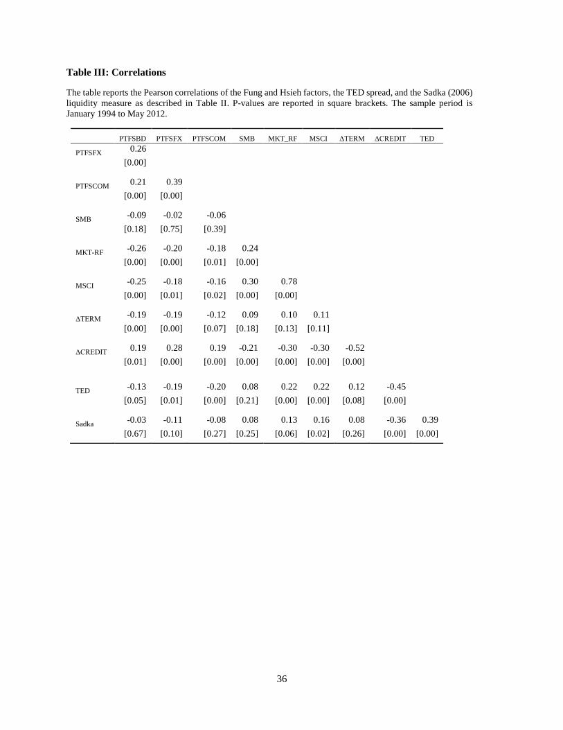
spread. It is of interest to examine the interactions among the factors discussed above. In Table III,
we display the pairwise correlations among the factors used in this study. The correlations among
the liquidity factors are low in general. The only notable correlation is between the liquidity factors
and the credit spread: -0.45, and -0.36 for the TED Spread, and the Sadka (2006) measure,
respectively. This shows that credit conditions worsen during periods of low liquidity.
7 For examples of other market liquidity measures employed in the literature, see Hu, Pan, and Wang (2013), Pástor
and Stambaugh (2003), Amihud (2002), Acharya and Pedersen (2005), and Getmansky, Lo, and Makarov (2004).
Kruttli, Patton, and Ramadorai (2013) construct a measure based on the illiquidity of hedge fund portfolios and show
that it has predictive ability for asset returns.

11
III. Methodology
The purpose of this paper is to study the relationship between the liquidity exposure of hedge
funds and their performance. Hedge funds often employ dynamic strategies which they adjust
depending on the state of the economy and trade a variety of financial securities with non-linear
payoffs, including equity and fixed income derivatives. On the other hand, based on prior research
there is some evidence that the impact of market liquidity on the performance of hedge funds is
state-dependent. For example, Sadka (2010) shows that hedge funds that significantly load on
market liquidity risk outperform low-loading funds by 6% per year, on average. Focusing on nine
months during the recent financial crises (September-November 1998, August-October 2007, and
September-November 2008), he also shows that the performance of this strategy is negative
during the crisis period.
Accordingly, in this study, we employ a 2-state Markov regime switching model8 to
endogenously identify the different liquidity regimes. The regimes are identified based on the
liquidity factors. Our simple regime switching model for the liquidity factor can be expressed as:
tSt tL (1)
2,0~tSt ,
where Lt is the liquidity factor, and St represents a 2-state Markov chain with transition matrix,
Πs:
2221
1211
pp
pps ,
and pij denotes probability of transitioning from state i to state j. Note that the model has two key
regime-specific parameters - the mean of the liquidity factor, tS , and its variance,
2
tS . Therefore,
8 Markov regime switching models are widely used in the literature, e.g., Hamilton (1989, 1990), Ang and Bekaert
(2002), Bekaert and Harvey (1995), Guidolin and Timmermann (2008), and Gray (1996).
12
Markov regime switching model is superior to a methodology which determines the liquidity
regimes by simply segregating the data above and below the median of the liquidity measure.
We determine the high and low liquidity regimes based on a particular liquidity factor by
estimating the above model using maximum likelihood. The model provides us with a time series
of filtered probabilities. For each month in the sample period, the estimated filtered probabilities
for the two states add up to one. The state with the highest filtered probability is identified as the
state of the economy for that month. Accordingly, based on the 2-state model, the state with
filtered probability higher than 50% in a given month is identified as the state of the economy for
that particular month.
Table IV displays the estimation results of the 2-state Markov regime switching model based
on the Sadka (2006) liquidity measure9 during the period April 1983 to December 2012.10 Panel
A reports the estimated means of the liquidity factor for the high and low liquidity regimes. Panel
B displays the expected duration for the high and low liquidity regimes. Panel C reports the
transition matrix. Note that the high liquidity regime is more persistent and has a longer duration
compared to the low liquidity regime. We also note that the low liquidity regime identified by the
model based on the Sadka (2006) liquidity measure includes the three recent liquidity
crises/episodes considered in Sadka (2010).
Figure 1 depicts the filtered probabilities from the Markov regime switching model for the
low liquidity regime. Note that high values of filtered probabilities displayed in Figure 1 indicate
the low liquidity episodes in U.S. financial markets which includes the Russian debt crisis
9 Even though Sadka (2006) measure is an equity based liquidity factor, it measures market-wide liquidity.
Therefore, this measure is suitable in identifying liquidity regimes as it is a systematic risk factor which is priced
across various asset classes. 10 Note that our hedge fund sample covers the period from January 1994 to May 2012. However, in order to
correctly determine the liquidity states we employ the available time series for the Sadka (2006) liquidity measure.
13
(September 1998), the 2001 recession, the recent financial crisis (August 2007 to October 2009)
which includes the period of turmoil related to the Quant (hedge fund) crisis and the bankruptcy
of Lehman Brothers, and the Greek crisis (2011). In all, 34 months are identified as belonging to
the low liquidity regime while the remaining 187 months belong to the high liquidity regime,
during the period January 1994 to May 2012.
IV. Compensation for Market Liquidity Risk and Liquidity Timing
While funding liquidity is the primary focus of this study, we first confirm the results regarding
market liquidity and hedge fund performance documented in the literature (e.g., Sadka (2010)) in
our Markov regime switching framework. The subsequent sections document the main findings of
this study regarding the impact of funding liquidity risk on hedge fund performance.
We begin by first estimating the market liquidity loading of each hedge fund by regressing the
fund returns on the market excess return and the liquidity factor during the prior 24-month period:
i
tt
i
L
m
t
i
m
i
ttf
i
t LRrR , , (2)
where i
tR is a fund’s return in month t, tfr , is the risk free rate, m
tR is the market excess return, and
Lt is Sadka’s (2006) liquidity factor for month t. The first set of estimates is obtained using the
data for the two-year period prior to January 1996. We only include funds with at least 18 months
of non-missing observations. We then sort hedge funds into 10 portfolios based on their estimated
market liquidity exposures, i
L , with equal number of funds in each decile. We implement this
process on a rolling basis each month from January 1996 to May 2012. Funds are kept in the decile
portfolios for one month. Following this procedure we obtain a time series of portfolio returns for
each of the ten market liquidity deciles.
The purpose of this exercise is to compare the performance of the high market liquidity loading
portfolio to the low market liquidity loading portfolio for different states of the economy, namely
14
for the high and low liquidity regimes. To do this we follow a strategy that takes a long position
in the high market liquidity decile portfolio and a short position in the low market liquidity decile
portfolio. The performance of the strategy is evaluated using the Fung-Hsieh 8–factor model
described below:
D
tk
k
DD
stf
D
t tskFrR
,
8
1
, ,, LHs , , (3)
where D
tR is the liquidity decile portfolio return and tfr , is the risk free rate during month t. The
subscript s denotes the high and low liquidity regimes. In the above specification, we incorporate
the 8 Fung-Hsieh factors described previously in Section II.B. However, two of the Fung and Hsieh
factors, namely, the change in the term spread and the change in the credit spread, are non-traded
factors. We replace these two factors by the returns to tradable portfolios so that the intercept or
the alpha of the model represented by Equation (3) can be interpreted as an excess return. As a
proxy for the term spread we use the difference between Barclay’s 7-10 year Treasury index return
and the one-month Treasury bill rate. Similarly, we employ the return difference between
Barclay’s 7-10 year Corporate Baa index return and Barclay’s 7-10 year Treasury Index as a proxy
for the credit spread.
Sadka (2010) documents that, on average, the high liquidity-loading funds outperform low
liquidity-loading funds by about 6% annually.11 However, as noted earlier, hedge funds’
performance might suffer during the low liquidity states. In this section we analyze the
performance of the high-minus-low liquidity strategy in different states of the economy. As
previously noted, we identify liquidity regimes using the 2-state Markov regime switching model
11 In unreported results, we find that the Hu, Pan, and Wang (2013) market (il)liquidity measure (Noise) is priced
across hedge fund returns and provides a 6.12% premium annually in our dataset. However, we also find that the
Pástor and Stambaugh (2003) market liquidity measure is not priced across hedge fund returns. These results are
consistent with Hu, Pan, and Wang (2013).

15
estimated based on the Sadka (2006) liquidity measure. Table V presents the results. Panel A of
the table reports the Fung-Hsieh eight factor alpha12 of the decile portfolios and the performance
of the high-minus-low liquidity beta strategy for the entire sample during the period January 1994
to May 2012. The high-minus-low liquidity beta strategy earns an annualized alpha of 3.76%.13
Panel B of Table V presents the results for the high liquidity regime in which the performance
for the high-minus-low portfolio is 5.80%. However, as shown in panel C of the table, in the low
liquidity regime the high-minus-low portfolio’s performance is much lower: -11.50%.
Furthermore, comparing the alphas for the decile portfolios reported in Panels B and C, we can
see that with the exception of the lowest liquidity beta decile portfolio, the estimated alphas are
consistently lower in the low liquidity state.14
The evidence presented in Table V confirms that the performance of liquidity beta-sorted
hedge fund portfolios is significantly lower during the low liquidity state. This is consistent with
the view that the profitability of many hedge fund strategies seeking to exploit mispricing of
securities is sensitive to market liquidity conditions. In periods of low liquidity, asset prices may
fail to converge to fundamental values leading to the poor performance of many
convergence/arbitrage trading strategies.
Figure 2 displays the average market liquidity betas and annualized 8-factor Fung and Hsieh
alphas for ten decile portfolios presented in Table V. Note that while hedge funds with positive
exposure to market liquidity risk lower their liquidity betas in the low liquidity state, their
corresponding performance is significantly lower in the low liquidity regime. This suggests that
12 In unreported results, we show that our findings are qualitatively similar when based on average monthly excess
returns, in addition to fund alphas, throughout the paper. 13 The 6% Premium reported by Sadka (2010) is calculated for the period 1994 to 2008 using the Fung and Hsieh
(2004) 7-factor model. In our analyses that cover the period 1994 to 2012 we employ the Fung and Hsieh 8-factor
model that includes the emerging market factor in addition to the original Fung and Hsieh (2004) 7 factors. 14 The lowest liquidity beta decile portfolio (Portfolio 1) has negative liquidity exposures in both the high liquidity
state (liquidity beta = -4.06), and the low liquidity state (liquidity beta = -2.40).

16
the reduction in hedge funds’ market liquidity exposure during periods of liquidity crises is not
due to successful liquidity timing, but potentially due to involuntary liquidation of assets, possibly
in order to meet funding requirements. Such forced liquidations could potentially explain the
significantly lower performance in the low liquidity states. Collectively, these results help extend
the earlier findings of Cao, et al. (2013) and provide a more nuanced view of the liquidity timing
ability of hedge funds. In particular, our results suggest that hedge funds are not entirely successful
in timing liquidity changes – particularly during periods of low liquidity.
Furthermore, our results also strongly hint at the potential role played by funding liquidity
during the low liquidity regime. In particular, they suggest that liquidity spirals originating via
shocks to funding liquidity could potentially lead to a negative relation between hedge fund returns
and market liquidity during crisis periods. We investigate the role of funding liquidity in more
detail in the next section.
V. Funding Liquidity Risk
In this section we analyze the performance of the high-minus-low liquidity beta strategy in the
context of the funds’ funding liquidity exposure. As mentioned earlier, we employ the TED
spread15 as a proxy for funding liquidity. Note also that instead of using the TED spread levels, we
employ the innovations in the TED spread to calculate liquidity betas. The innovations are
calculated as the residuals from an AR(1) model for the TED spread. We estimate the funding
liquidity exposures in a framework in which hedge fund returns are regressed on the market excess
return and the funding liquidity measure, i.e., the innovations in the TED spread. Subsequently,
we form the funding liquidity decile portfolios following the same procedure employed in Section
IV for constructing market liquidity decile portfolios.
15 Recall that since the TED spread is an illiquidity measure, we employ the negative of the TED spread as a
measure of funding liquidity.

17
Table VI reports the eight factor Fung and Hsieh alphas for the funding liquidity deciles, as
well as for the performance of the high-minus-low funding liquidity beta strategy. Panel A presents
the results for the whole sample. Panels B and C of the table report results for the high and low
liquidity regimes, respectively. For the entire sample, over the period January 1994 to May 2012,
the high-minus-low liquidity beta strategy earns an annualized performance of -3.40%. Note that
in contrast to the results reported in Table V for market liquidity beta sorted portfolios, the
performance of the high-minus-low strategy based on funding liquidity beta sorted portfolios is
negative. It is evident that the funds with high exposure to funding liquidity underperform funds
with low funding liquidity exposure. This result highlights the importance of funding liquidity risk
exposure in determining the performance of hedge funds.
In panels B and C of Table VI we report the results separately for the two liquidity regimes. In
the high liquidity state, the high-minus-low strategy’s annualized alpha is -2.47%. In the low
liquidity state the results are dramatic, as the strategy’s annualized alpha is -11.67%. These results
show that while funding liquidity exposure hurts hedge fund performance in general; its impact is
severe in the low liquidity regime. One of the reasons for this poor performance is the fact that
hedge funds typically employ high leverage which magnified the impact of the recent crises on
their performance. When combined with high exposure to funding liquidity, highly levered hedge
funds suffered when they faced margin calls in periods of low liquidity. Note that unlike the results
related to market liquidity beta sorted strategy presented in Table V, the performance of the high-
minus-low funding liquidity strategy is negative in both liquidity regimes.
Next, we graphically display the results reported in Table VI. Figure 3 depicts the Fung and
Hsieh 8-factor alphas across the funding liquidity deciles. Panels A and B of the figure show that
hedge funds’ performance declines as their funding liquidity exposure increases, not only in the

18
entire sample but also in the high liquidity regime. Moreover, as seen in Panel C, the impact of
funding liquidity exposure is more pronounced in the low liquidity regime; hedge funds with high
funding liquidity exposure significantly underperform the funds that have low exposure to funding
liquidity risk.
A. Liquidity Spirals
In the model considered by Brunnermeier and Pedersen (2009), under certain conditions
market liquidity and funding liquidity are mutually reinforcing which creates liquidity spirals. In
the model, an adverse shock to speculators’ funding liquidity forces them to lower their leverage
and reduce the liquidity they provide to the market, which in turn leads to diminished overall
market liquidity. When funding liquidity shocks are severe, the decrease in market liquidity makes
funding conditions even more restrictive, which leads to a liquidity spiral. We investigate the
implications of their model in this section.
In Tables V and VI, we reported the fund alphas for each liquidity decile portfolio based on
market liquidity and funding liquidity exposure, respectively. We now jointly consider the two
liquidity scenarios and sequentially sort funds, first by their market liquidity betas, followed by
the funding liquidity betas. The fund alphas are displayed in the form of a two-way matrix in
Table VII. The table shows the annualized fund alphas for a total of 25 (5x5) portfolios. Note that
we divide the sample of hedge funds into quintiles (rather than deciles) based on both the market
and funding liquidity betas, in order to obtain sufficient number of hedge funds in each portfolio.
Panel A (B) displays the results for the high (low) liquidity regime. Along with the performance
of each of the 25 portfolios, the performance of the high-minus-low liquidity beta strategy is also
reported.

19
It is clear from Panel A that, in the high liquidity regime, the fund alphas are the highest for
funds with a high market liquidity exposure (quintiles 4 & 5). On the other hand, the lowest
annualized alpha (-3.77%) is recorded by funds with low market liquidity exposure and high
funding liquidity exposure.16 Also note that the performance of the high-minus-low market
liquidity strategy is positive for four of the five funding liquidity quintiles, with annualized alphas
ranging from -1.22% to 11.81% per year. However, the performance of the high-minus-low
funding liquidity strategy is negative in four of the five market liquidity quintiles, with annualized
performances ranging from -7.20% to 3.37% per year. This shows that while having high exposure
to market liquidity helps hedge funds in the high liquidity regime, exposure to funding liquidity
hurts hedge fund performance.
Panel B of Table VII displays the results for the low liquidity regime. First, note that most of
the annualized alphas of the 25 portfolios are negative (16 out of 25) and generally lower compared
to their corresponding alphas in the high liquidity regime. The performance of the high-minus-low
funding liquidity strategy is strikingly lower in the low liquidity regime with the annualized
performance ranging from -16.30% to -6.41% per year. Further, in contrast to Panel A, the market
liquidity strategies also perform poorly in the low liquidity regime. The performance of the high-
minus-low market liquidity strategy is negative in all funding liquidity quintiles, ranging from -
11.97% to -0.92% per year. These results show that while funding liquidity risk seems more
dominant in the low liquidity regime; both market liquidity and funding liquidity risk exposure
result in negative hedge fund performance in the low liquidity state. This result is consistent with
the negative liquidity spirals hypothesized by Brunnermeier and Pedersen (2009).
16 In unreported results we confirm that a similar pattern holds for monthly excess returns of hedge fund portfolios.
20
Next, we graphically display the annualized fund alphas for the high and low liquidity regimes
in Figures 4 and 5, respectively. The figures shows that in general funds with high exposure to
market liquidity risk in the high liquidity regime (Figure 4) have higher alphas compared to the
low liquidity regime alphas depicted in Figure 5. Moreover, funds with high exposure to funding
liquidity and low exposure to the market liquidity perform poorly in the high liquidity regime. On
the other hand, Figure 5 shows that, in the low liquidity regime, funds with low exposure to funding
liquidity perform better regardless of the level of market liquidity exposure. Similarly, the funds
with high exposure to funding liquidity perform poorly regardless of the level of market liquidity
exposure.
Figures 4 and 5 demonstrate that hedge fund performance varies significantly across different
quintiles of market and funding liquidity. It is clear from the figures that the impact of market
liquidity and funding liquidity on hedge fund performance varies across different liquidity regimes.
Under certain market conditions, reflected in the low liquidity regime, the two liquidity
characteristics mutually reinforce each other. Note that in the high liquidity state (Figure 4), the
best performance is obtained when exposure to funding liquidity and market liquidity is the
highest, hinting at a positive liquidity spiral. In addition, in the low liquidity state (Figure 5), the
worst performance is obtained when exposure to funding liquidity and market liquidity is the
highest which indicates a negative liquidity spiral. These results provide support for a key
prediction of the Brunnermeier and Pedersen (2009) model.
Boyson, Stahel, and Stulz (2010) document that large adverse shocks to market and funding
liquidity increase the probability of worst return contagion across hedge fund styles. The results
presented in Panel B of Table VII and Figure 5 support the findings of Boyson, Stahel, and Shulz

21
(2010), as we document that during poor market liquidity conditions hedge fund returns suffer
severely from exposures to both market and funding liquidity.
B. Discussion
Our results regarding the significance of funding liquidity risk exposure, and the mutually
reinforcing impact of funding liquidity risk and market liquidity risk in the low liquidity regime,
have important implications for understanding the dynamics of hedge fund performance. In
contrast to mutual funds, most hedge fund strategies invest in relatively illiquid assets and employ
significant leverage. This makes them particularly vulnerable to adverse shocks to funding
liquidity conditions as evidenced by the above results that highlight the key role played by funding
liquidity risk exposure. These results also have broader implications in the context of the evolving
market environment. During the past decade, non-traditional intermediaries like hedge funds and
proprietary trading desks of banks have come to play an increasingly prominent role – as liquidity
suppliers and counterparties in transactions in several markets. In recent years hedge funds have
also become important participants in several less developed financial markets. In contrast to
traditional market makers or banking intermediaries that face mandatory capital requirements,
hedge funds are largely unregulated. Further, as highlighted by the events of August 2007 when a
number of hedge funds employing quantitative strategies suffered substantial losses, return
correlations across hedge funds have increased markedly in recent years.17 Our results suggest that
a better understanding of the funding liquidity risk exposure of hedge funds is particularly relevant
for a broader assessment of the robustness of the evolving market ecosystem.
17 See Khandani and Lo (2007) for a fuller discussion of these issues.

22
VI. Impact of Share Restrictions on Fund Performance Across Liquidity Regimes
In order to cope with funding problems related to investor fund flows, many hedge funds adopt
share restrictions. These restrictions may be in the form of a lockup provision specifying a
minimum lockup period during which no redemptions are allowed, or a redemption notice period
specifying a minimum notice that the investor is required to provide before redeeming shares, or
a redemption frequency which sets the time intervals at which investors are allowed to withdraw
their holdings. Funds with share restrictions are likely less funding restricted than otherwise similar
funds. A number of recent studies suggest that such share restrictions have a significant impact on
the ability of hedge funds to manage their funding liquidity risk. For example, Aragon (2007)
shows that funds with lockup restrictions outperform funds without such restrictions by
4-7% annually suggesting that share restrictions enable funds to efficiently manage illiquid assets.
On the other hand, Aiken, Clifford, and Ellis (2015) show that hedge funds with discretionary
liquidity restrictions are unable to avoid sale of illiquid assets and underperform the funds without
discretionary liquidity restrictions. Teo (2011) examines the performance of liquid hedge funds
that grant favorable redemption terms (i.e., redemptions at monthly, or more frequent intervals) to
investors and finds that high net inflow funds outperform low net inflow funds by 4.79% per year.
Furthermore, he documents that within the group of liquid hedge funds the performance impact of
fund flows is stronger when market liquidity is low and when funding liquidity is tight.
Given the aforementioned unconditional results in the literature, it is of interest to examine
how the presence or absence of share restrictions affects the funding liquidity risk and performance
of hedge funds in the high as well as the low liquidity regimes.18 Accordingly, in this section we
analyze the impact of lockup restrictions on the performance of funding liquidity sorted decile
18 Recall that liquidity regimes are determined using the Sadka (2006) market liquidity measure.

23
portfolios in the two regimes. Following Aragon (2007), we define liquid hedge funds as funds
with no lockup restrictions.19 Similarly, we define illiquid hedge funds as funds with lockup
periods. Tables VIII and IX report the performance of the funding liquidity sorted decile portfolios
for the liquid and illiquid hedge funds, respectively. Portfolio excess returns are reported in the
form of 8-factor Fung-Hsieh alphas.
First consider the performance of the respective fund decile portfolios in the high liquidity state
reported in Panel B of Tables VIII and IX. It can be seen that in the high liquidity state the
performance of the decile portfolios of liquid hedge funds (Panel B, Table VIII) is lower compared
to the illiquid hedge funds’ decile portfolios (Panel B of Table IX) in all ten deciles. Furthermore,
in the case of illiquid funds the high-minus-low funding liquidity risk portfolio strategy has a
performance equal to -0.39% per year in the high liquidity regime. By contrast, in the case of
liquid funds the high-minus-low funding liquidity risk portfolio strategy has an annualized
performance of -2.66%. These results suggest that having protection against investor flow-related
funding liquidity risk in the form of lockup restrictions helps hedge funds improve their
performance in the high liquidity state.
On the other hand, as seen in Panel C of Tables VIII and IX, in the low liquidity state the
pairwise comparison between decile portfolios of liquid and illiquid hedge funds is ambiguous.
Furthermore, the performance of the high-minus-low funding liquidity risk portfolio strategy is
actually lower for illiquid funds, with an annualized performance of -16.97% vs. -9.82% for liquid
funds.20 This shows that imposing lockup periods does not improve fund performance in the low
liquidity state. This finding extends the results presented in Aragon (2007) by documenting that
19 Liquid funds are identified using the ‘lockup period’ variable in the Lipper TASS database with values equal to 0.
This results in 75.5% of the funds in our sample being classified as ‘liquid’ funds. 20 The results presented in this section are robust to identifying liquid and illiquid hedge funds using redemption
frequency and redemption notice periods, in addition to lockup periods.

24
funds with lockup restrictions outperform funds without such restrictions only in the high liquidity
state. Evidently, the negative impact of funding liquidity risk on performance in the low liquidity
state (and the impact of negative liquidity spirals) far outweighs any benefits offered by having
lockup restrictions in place. This result also reflects the possibility that funds with lockup
restrictions endogenously choose to invest in relatively less liquid assets which contributes to their
poor performance in the low liquidity state. Furthermore, this finding confirms that the
underperformance of illiquid hedge funds documented by Aiken, Clifford, and Ellis (2015) stems
from the poor performance in the low liquidity state, possibly due to forced asset fire sales. These
findings also contribute to the recent literature by documenting the effectiveness of share
restrictions in different liquidity states. In particular, our results suggest that lockup periods are
effective only in the high liquidity states in terms of their ability to mitigate the flow-induced
funding liquidity risk.
VII. Robustness Tests
In this section we provide additional tests to support the robustness of our results. We begin
by adjusting the funding liquidity measure to account for the potential correlation between
measures of market liquidity and funding liquidity.
A. Correlation between Market and Funding Liquidity Measures
Since funding liquidity conditions and market liquidity measures are positively correlated, it
would be useful to isolate the impact of funding liquidity risk that is orthogonal to market
liquidity.21 To this end, we project the innovations in the TED spread on the market liquidity
measure (i.e., the Sadka (2006) liquidity factor) and use the orthogonal component to compute the
funding liquidity betas and form liquidity beta sorted portfolios. We display the performance of
21 The Pearson correlation coefficient between the Sadka (2006) liquidity factor and the TED spread is 0.39.
25
the new liquidity decile portfolios in Table A.1 in the Appendix. Note that the performance of the
high-minus-low liquidity strategy is negative across the board and the results are consistent with
the results displayed in Table VI. Therefore, our results are robust to the use of the orthogonal
component of the TED spread as a measure of funding liquidity.
B. Alternative Funding Liquidity Measures
One of the main contributions of this paper is to provide evidence on the interaction between
hedge funds’ performance and their funding liquidity risk. The primary funding liquidity measure
employed in this study is the (innovations in) TED spread. In this section we assess the robustness
of our results to alternative funding liquidity measures, namely, the REPO rate22 , a traded funding
liquidity measure proposed by Chen and Lu (2017), and a funding liquidity measure proposed by
Fontaine and Garcia (2012).
REPO Rate
The REPO rate (i.e., the difference between overnight repurchase rate and the 3-month treasury
rate) reflects the actual funding cost experienced by banks and investors, and is available through
DataStream starting in November 1996. Since our hedge fund data starts in January 1994, we use
the FED Funds Rate as a proxy during the period from January 1994 to October 1996.23 Note that
the REPO rate is an illiquidity measure. To be consistent with the methodology employed for the
TED spread, we first add a negative sign to the REPO rate. Secondly, we employ the innovations
in the REPO rates, instead of the levels, when calculating the liquidity betas of hedge funds. The
innovations in the REPO rates are estimated as the residuals from an AR(1) model fitted to the
modified REPO data.
22 The REPO rate is employed as a funding liquidity measure in several studies, including Kambhu (2006), Adrian
and Fleming (2005), and Boyson et al. (2010). 23 Nath (2003) shows that the overnight repurchase rate is of the same order of magnitude as the FED Funds rate.
26
We repeat the analysis performed in Table VI using the REPO data. Table A-2 in the Appendix
presents the results. Note that the performance of the high-minus-low liquidity strategy is negative
in both liquidity states. Specifically, the strategy’s estimated performance is -0.83% and -10.78%
in the high and low liquidity states, respectively. These results confirm that having exposure to
funding liquidity significantly hurts the funds’ performance in the low liquidity state.
Traded Funding Liquidity Measure
Next we repeat the above analysis using a theoretically motivated traded funding liquidity
measure recently proposed by Chen and Lu (2017). The measure is based on return spreads for
“betting-against-beta” (BAB) portfolios of stocks with high- and low-margin requirements.24 We
note that this measure is a funding liquidity factor; therefore we do not add a negative sign as we
did for the TED spread and the REPO rate which are both measures of funding illiquidity. We
repeat the analysis related to funding liquidity exposure of hedge funds by employing the
aforementioned traded funding liquidity measure. Table A-3 presents the results. We note that the
funds which the highest exposure to the traded funding liquidity factor (decile 10) underperform
funds with the lowest exposure in both the high and the low liquidity states. The annualized 10-1
decile portfolio performance is -5.55% and -8.50% in the high and low liquidity states,
respectively. As seen in Panel A of the table, the corresponding unconditional performance (-
5.84% per year) is negative as well.25 These results are consistent with our primary funding
liquidity results presented in Table VI.
24 The trading liquidity factor is the first principal component of five BAB spread portfolios, which are constructed
using five different margin proxies. 25 Chen and Lu (2017) attribute the superior performance of low-sensitivity hedge funds to fund managers' funding
liquidity timing skills which allows them to capitalize on positive funding liquidity shocks and avoid negative shocks.

27
Fontaine and Garcia Measure
Fontaine and Garcia (2012) estimate a funding liquidity factor based on fitting a term structure
model to a panel of pairs of U.S. treasury securities. The estimation relies on the assumption that
price differences between pairs of treasury securities that are similar in their cash flows but differ
in their maturities, can be attributed to a latent liquidity factor. We now repeat the analysis
performed in Table VI using the Fontaine and Garcia (2012) liquidity factor to estimate the
funding liquidity exposure of hedge funds.
Table A-4 presents the results of this analysis. Note that since the Fontaine and Garcia (2012)
factor is an illiquidity measure, we add a negative sign, as we did for the TED spread and the
REPO rate, in order to obtain the relevant liquidity measure. We then calculate hedge fund betas
with respect to this liquidity measure. Panel A of Table A-4 shows that, unconditionally, the
annualized performance of the high-minus-low liquidity strategy is negative, -1.32%, in the overall
sample. This result is qualitatively similar to our unconditional results in Panel A of Table VI
which are based on the use of the TED spread as a funding liquidity measure.
However, as seen in Panel B of Table A-4, in the high liquidity regime the performance of the
high-minus-low funding liquidity strategy is actually positive at 2.31%. This result contrasts
with the corresponding result in Panel B of Table VI which showed a negative performance for
the high-minus-low funding liquidity strategy. A potential reason for the positive performance
of the high-minus-low funding liquidity strategy noted in Panel B of Table A-4 may be the
manner of construction of the Fontaine and Garcia (2012) measure. To see this, note that Hu,
Pan, and Wang (2013) propose a similar illiquidity measure which is also derived from the
deviations of observed treasury prices from their no-arbitrage model-implied prices. Hu, Pan,
and Wang (2013) interpret their measure as a market illiquidity measure and find that the measure
is a priced risk factor for a broad set of assets. Hence, we conjecture that the Fontaine and Garcia
28
(2012) measure might share some elements of market liquidity which may help explain the
positive performance of the high-minus-low funding liquidity strategy in the high liquidity state.
Panel C of Table A-4 presents results for the low liquidity state. The high-minus-low funding
liquidity strategy has an annualized alpha of -16.60 percent which is qualitatively consistent with
our main result presented in Table VI.
C. Liquidity Regimes Determined by Hedge Fund Returns
In this study we identify the high and low liquidity states based on a market liquidity factor,
i.e., the Sadka (2006) market liquidity measure. Alternatively, the regimes can be identified by the
hedge fund returns under the assumption that low hedge fund returns coincide with low liquidity
periods. To this purpose we calculate the average hedge fund returns for each month in the sample
period, and assign the bottom 20% of the returns as belonging to the low liquidity regime. This
procedure results in 55 months of the sample being classified in the low liquidity regime, compared
with the 34 months allocated to the low liquidity regime previously.
Table A.5 exhibits the results obtained by the new liquidity regimes suggested in this section.
First, note that the performance of the decile portfolios is now more pronounced. While the
aforementioned performance is consistently positive in the high liquidity state, it is highly negative
in the low liquidity state, compared to the original results reported in Table VI. Moreover, the
annualized performance of the high-minus-low liquidity strategy is -30.66% in the low liquidity
state, compared to the performance of -11.67% reported in Table VI. Therefore, the results
displayed in Table A.5 are sharper compared to our original results. However, note that identifying
the liquidity regimes using the hedge fund returns mechanically allocates the high and low
performing hedge funds in the high and low liquidity regimes, respectively. Hence, the sharper
results obtained by this methodology are not surprising. On the other hand, the regimes identified
29
based on liquidity factors correctly deliver high and low liquidity periods, and they do not
necessarily perfectly coincide with high and low hedge fund returns. Therefore, the Markov regime
switching methodology employed in this paper is more conservative and successfully isolates the
effects of liquidity exposure in different regimes.
In summary, the results of this section confirm that our primary results are robust to the use of
alternative funding liquidity measures as well to an alternative definition of liquidity regimes.
VIII. Concluding Remarks
This paper provides evidence on the relation between the funding liquidity risk exposure of
hedge funds and their performance. The analysis focuses in particular on the interaction between
the funds’ market liquidity risk and their funding liquidity risk. A key result of the paper is that
funding liquidity risk as measured by the sensitivity of a hedge fund’s return to a measure of
market-wide funding costs, is an important determinant of fund performance. Furthermore,
funding liquidity risk is a critical determinant of the variation in hedge fund illiquidity premia
across liquidity regimes.
Our results contribute to the literature in several ways. First, we demonstrate that funding
liquidity risk as measured by the sensitivity of a hedge fund’s return to a measure of market-wide
funding costs, is an important determinant of hedge fund performance. Second, we examine the
combined impact of both market liquidity risk and funding liquidity risk on hedge fund
performance. We show that hedge fund returns are the highest (lowest) for the funds with high
(low) market liquidity exposure and low (high) funding liquidity exposure. We also show that
market liquidity and funding liquidity interact with each other, potentially leading to liquidity
spirals, especially in the low liquidity regime. These results provide empirical evidence in support
30
of the Brunnermeier and Pedersen’s (2009) theoretical model which rationalizes the link between
market liquidity and funding liquidity.
Third, this paper contributes to the liquidity timing literature. Cao, et al. (2013) document that
hedge funds can time market liquidity by adjusting their holdings as liquidity conditions change.
In this paper, we argue that liquidity has state dependent implications and provide evidence that
hedge fund managers are not entirely successful in timing liquidity changes. We show that hedge
funds do lower their market liquidity exposure in the low liquidity regime; however their
performance is significantly lower when liquidity dries up. This finding suggests that funds are
likely to engage in asset fire sales when faced with margin calls, resulting in poor performance.
Finally, this paper extends the findings by Aragon (2007) who shows that lockup provisions help
hedge funds improve their performance. We extend this result by showing that while lockup
provisions enhance hedge fund returns in the high liquidity state; they fail to improve hedge fund
performance during low liquidity periods.
Given the critical importance of funding liquidity for hedge funds demonstrated in this paper,
investors clearly need to pay attention to the funding liquidity risk exposure of funds. In order to
identify the funding liquidity risk exposure an investor would need to track a hedge fund’s leverage
and the quality of assets held in its portfolio. However, this is not an easy task given the absence
of reporting requirements for hedge funds. The framework adopted in this paper provides a
convenient way to analyze a fund’s funding liquidity exposure from an investment management
perspective.
31
References
Acharya, Viral, and Lasse Heje Pedersen, 2005. Asset Pricing with Liquidity Risk, Journal of
Financial Economics 77, 375–410.
Aiken, Adam L., Christopher P. Clifford, and Jesse A. Ellis, 2015. Hedge Funds and Discretionary
Liquidity Restrictions, Journal of Financial Economics 116, 197-218.
Amihud, Yakov, 2002. Illiquidity and Stock Returns: Cross-Section and Time-Series Effects,
Journal of Financial Markets 5, 31–56.
Adrian, Tobias, and Michael J. Fleming, 2005, What financing data reveal about dealer leverage?
Current Issues in Economics and Finance 11, 1–7.
Ang, Andrew, and Geert Bekaert, 2002. International Asset Allocation With Regime Shifts,
Review of Financial Studies 15, 1137–1187.
Aragon, George O., 2007. Share Restrictions and Asset Pricing: Evidence from the Hedge Fund
Industry. Journal of Financial Economics 83, 33–58.
Aragon, George, and Philip Strahan, 2012. Hedge funds as liquidity providers: Evidence from
the Lehman Bankruptcy, Journal of Financial Economics 103, 570-587.
Bekaert, Geert, and Campbell R. Harvey, 1995. Time-Varying World Market Integration, Journal
of Finance 50, 403–444.
Billio, Monica, Mila Getmansky, and Loriana Pelizzon, 2010. Crises and Hedge Fund Risk,
Working Paper, University of Massachusetts.
Boyson, Nicole, Christof W. Stahel, and Ren´e M. Stulz, 2010. Hedge Fund Contagion and
Liquidity Shocks, Journal of Finance 65, 1789–1816.
Brunnermeier, Markus, and Lasse Heje Pedersen, 2009. Market Liquidity and Funding Liquidity,
Review of Financial Studies 22, 2201–2238.
Brunnermeier, Markus, 2009. Deciphering the Liquidity and Credit Crunch 2007-2008, Journal of
Economic Perspectives 23, 77–100.
Cao, Charles, Yong Chen, Bing Liang, and Andrew W. Lo, 2013. Can Hedge Funds Time Market
Liquidity?, Journal of Financial Economics 109, 493–516.
Chen, Zhuo, and Andrea Lu, 2017. A market-based funding liquidity measure, Working Paper.
Chordia, Tarun, Richard Roll, and Avanidhar Subrahmanyam, 2000. Commonality in liquidity,
Journal of Financial Economics 56, 3–28.

32
Drehmann, Mathias, and Kleopatra Nikolaou, 2013. Funding liquidity risk: Definition and
measurement, Journal of Banking and Finance 37, 2173-2182.
Dudley, Evan, and Mahendrarajah Nimalendran, 2011. Margins and Hedge Fund Contagion,
Journal of Financial and Quantitative Analysis 46, 1227-1257.
Fontaine, Jean-Sébastien, and René Garcia, 2012. Bond Liquidity Premia, Review of Financial
Studies 25(4), 1207–54.
Fung, William, and David A. Hsieh, 2004. Hedge Fund Benchmarks: A Risk Based Approach,
Financial Analysts Journal 60, 65-80.
Gârleanu, Nicolae and Lasse Heje Pedersen, Margin-Based Asset Pricing and Deviations from the
Law of One Price, Review of Financial Studies 24(6), 1980–2022.
Getmansky, Mila, Andrew W. Lo, and Igor Makarov, 2004. An Econometric Analysis of Serial
Correlation and Illiquidity in Hedge-Fund Returns, Journal of Financial Economics 74, 529–610.
Gray, Stephen F., 1996. Modeling the conditional distribution of interest rates as a regime-
switching process, Journal of Financial Economics 42, 27–62.
Guidolin, Massimo, and Allan Timmermann, 2008. International Asset Allocation under Regime
Switching, Skew and Kurtosis Preferences, Review of Financial Studies 21, 889–935.
Hamilton, James D., 1989. A New Approach to the Economic Analysis of Nonstationary Time
Series and the Business Cycle, Econometrica 57, 357–384.
Hamilton, James D., 1990. Analysis of time series subject to changes in regime, Journal of
Econometrics, 45, 39–70.
Hu, Grace X., Jun Pan, J., and Jiang Wang, 2013, Noise as information for illiquidity, Journal of
Finance, 68, 2341–2382.
Kambhu, John, 2006, Trading risk, market liquidity, and convergence trading in the interest rate
swap spread, FRBNY Economic Policy Review 12, 1–13.
Khandani, Amir, and Andrew W. Lo, 2007. What Happened To The Quants in August 2007?,
Journal of Investment Management 5, 5-54.
Khandani, Amir, and Andrew W. Lo, 2011. Illiquidity Premia in Asset Returns: An Empirical
Analysis of Hedge Funds, Mutual Funds, and US Equity Portfolios, Quarterly Journal of Finance,
1 (2), 205-264.
Kruttli, Mathias, Andrew J. Patton, and Tarun Ramadorai, 2013. The Impact of Hedge Funds on
Asset Markets, Review of Asset Pricing Studies 5, 185-226.
Nath, Purnendu, 2003. High Frequency Pairs Trading with US Treasury Securities: Risks and
Rewards for Hedge Funds. Working Paper, London Business School.

33
Pástor, Lubos, and Robert Stambaugh, 2003. Liquidity Risk and Expected Stock Returns, Journal
of Political Economy 111, 642–685.
Reca, Blerina, Richard Sias, and H.J. Turtle, 2014. Hedge Fund Return Dependence and Liquidity
Spirals, Working paper, University of Arizona.
Roll, Richard, 1988. The International Crash of October 1987, Financial Analysts Journal 44, 19-
35.
Sadka, Ronnie, 2006. Momentum and Post-Earnings-Announcement Drift Anomalies: The Role
of Liquidity Risk, Journal of Financial Economics 80, 309–349.
Sadka, Ronnie, 2010. Liquidity risk and the cross-section of hedge-fund returns, Journal of
Financial Economics 98, 54-71.
Teo, Melvyn, 2011. The liquidity risk of liquid hedge funds, Journal of Financial Economics 100,
24-44.

34
Table I: Summary Statistics for Monthly Excess Hedge Fund Returns
Panel A reports statistics (average monthly percentage return, monthly standard deviation in percent,
skewness, and excess kurtosis) for the full sample of hedge funds, and Panel B reports statistics by category.
The figures within a category are equally weighted averages of the statistics across the funds in the category.
The sample includes funds in the Lipper TASS database with at least 24 months of consecutive return data.
Only funds that report their returns on a monthly basis and net of all fees are included and a currency code
of "USD" is imposed. The sample period is January 1994 to May 2012.
Category Funds Mean St. Dev. Skewness Kurtosis
Panel A: Full Sample
All Funds 5599 0.29 4.26 -0.36 3.51
Panel B: By Hedge Fund Category
Directional Funds
Dedicated Short Bias 34 -0.25 6.11 0.28 3.08
Emerging Markets 444 0.42 7.00 -0.36 3.67
Global Macro 223 0.33 4.03 0.10 2.50
Managed Futures 412 0.43 5.19 0.20 2.23
Non-Directional Funds
Convertible Arbitrage 136 0.23 3.50 -0.68 7.05
Equity Market Neutral 202 0.26 2.55 -0.15 3.05
Fixed Income Arbitrage 151 0.24 3.01 -1.02 9.97
Semi-Directional Funds
Event Driven 421 0.37 3.56 -0.49 4.55
Long/Short Equity Hedge 1529 0.43 5.21 -0.09 2.35
Multi Strategy 320 0.36 4.02 -0.44 4.56
Fund of Funds
Fund of Funds 1727 0.10 3.06 -0.70 3.70

35
Table II: Summary Statistics for Factors
The table lists the Fung and Hsieh hedge fund factors and the liquidity factors employed in this paper and reports average monthly percentage returns,
monthly standard deviation in percent, skewness, and excess kurtosis of the factors. The factors are described in the text. The sample period for all
factors is January 1994 to May 2012.
Factor Description Mean St. Dev. Skewness Kurtosis
Panel A: Domestic Equity Factors
MKTXS Excess return of CRSP value-weighted index 0.49 4.64 -0.68 0.93
SMB Fama-French size factor 0.20 3.56 0.87 7.98
Panel B: Fixed Income Factors
D10YR Change in the 10YR Treasury yield -0.02 0.24 -0.17 1.56
DSPRD Change in Moody's Baa yield minus 10YR Treasury yield 0.01 0.20 1.22 15.23
Panel C: Trend Following Factors
PTFSBD Primitive trend follower strategy bond -1.15 15.55 1.39 2.53
PTFSFX Primitive trend follower strategy currency -0.20 19.68 1.34 2.53
PTFSCOM Primitive trend follower strategy commodity -0.53 13.69 1.16 2.28
Panel D: Global Factors
EM MSCI emerging markets 0.70 7.28 -0.49 1.57
Panel E: Liquidity Factors
Sadka Sadka (2006) permanent-variable liquidity measure 0.04 0.59 -0.92 6.23
TED Spread -(3 month US LIBOR - 3 month Treasury yield) -0.48 0.40 -3.03 13.03
36
Table III: Correlations
The table reports the Pearson correlations of the Fung and Hsieh factors, the TED spread, and the Sadka (2006)
liquidity measure as described in Table II. P-values are reported in square brackets. The sample period is
January 1994 to May 2012.
PTFSBD PTFSFX PTFSCOM SMB MKT_RF MSCI ΔTERM ΔCREDIT TED
PTFSFX 0.26
[0.00]
PTFSCOM 0.21 0.39
[0.00] [0.00]
SMB -0.09 -0.02 -0.06
[0.18] [0.75] [0.39]
MKT-RF -0.26 -0.20 -0.18 0.24
[0.00] [0.00] [0.01] [0.00]
MSCI -0.25 -0.18 -0.16 0.30 0.78
[0.00] [0.01] [0.02] [0.00] [0.00]
ΔTERM -0.19 -0.19 -0.12 0.09 0.10 0.11
[0.00] [0.00] [0.07] [0.18] [0.13] [0.11]
ΔCREDIT 0.19 0.28 0.19 -0.21 -0.30 -0.30 -0.52
[0.01] [0.00] [0.00] [0.00] [0.00] [0.00] [0.00]
TED -0.13 -0.19 -0.20 0.08 0.22 0.22 0.12 -0.45
[0.05] [0.01] [0.00] [0.21] [0.00] [0.00] [0.08] [0.00]
Sadka -0.03 -0.11 -0.08 0.08 0.13 0.16 0.08 -0.36 0.39
[0.67] [0.10] [0.27] [0.25] [0.06] [0.02] [0.26] [0.00] [0.00]

37
Table IV: Estimation Results from the 2-State Markov Regime Switching Model
The table exhibits the estimation results from the 2-state Markov regime switching model. Regimes are identified
using the Sadka (2006) liquidity measure. Panel A reports the estimated means of the liquidity measure in the high
and the low liquidity states. The associated p-values are reported in square brackets. Panel B reports the expected
duration of each state in months. Panel C reports the estimated transition probabilities.
Panel A: Mean
High Liquidity State 0.0005
[0.01]
Low Liquidity State -0.0016
[0.19]
Panel B: Expected Duration (months)
High Liquidity State 27.14
Low Liquidity State 8.01
Panel C: Transition Probabilities
High LS Low LS
High Liquidity State 0.96 0.04
Low Liquidity State 0.12 0.88

38
Table V: Performance of Market Liquidity Beta Sorted Portfolios
Hedge funds are sorted into 10 equally weighted portfolios each month according to their historical market liquidity betas. The market liquidity beta is calculated
by a regression of monthly hedge fund returns on the market portfolio and a market liquidity factor (Sadka (2006)), using the 24 months prior to portfolio formation.
Portfolio formation starts January 1996 and only funds with at least 18 months of returns over the two year period are included. The table reports the annualized
fund alphas (in percent) of the decile portfolios and the performance of the high-minus-low portfolio. Fund alphas are calculated using the eight Fung & Hsieh
factors, where credit and term factors are replaced by tradable portfolios. Newey-West t-statistics are reported in square brackets. The portfolio returns cover the
period January 1996 to May 2012. Panel A displays the unconditional results in the whole sample. Panel B and C report the results for the high and low liquidity
regimes, respectively. Liquidity regimes are identified by the Sadka (2006) liquidity measure.
Panel A: All Observations
Market Liquidity Beta Deciles
1 2 3 4 5 6 7 8 9 10 10-1
Alpha 0.21 0.80 1.47 1.96 2.06 2.67 2.02 3.40 3.01 3.97 3.76
[0.39] [2.38] [4.54] [6.97] [7.39] [10.15] [7.59] [9.63] [9.79] [6.55] [4.67]
Panel B: High Liquidity State
Market Liquidity Beta Deciles
1 2 3 4 5 6 7 8 9 10 10-1
Alpha 0.04 1.18 1.67 2.64 2.85 3.40 3.01 5.07 3.99 5.83 5.80
[0.06] [3.21] [5.02] [9.65] [11.15] [14.30] [12.21] [13.31] [13.18] [8.54] [6.36]
Panel C: Low Liquidity State
Market Liquidity Beta Deciles
1 2 3 4 5 6 7 8 9 10 10-1
Alpha 3.80 -0.09 0.40 -1.86 -1.68 -1.00 -2.89 -4.81 -1.38 -7.70 -11.50
[2.91] [-0.10] [0.52] [-3.19] [-2.68] [-1.53] [-4.35] [-5.58] [-1.81] [-5.35] [-5.92]
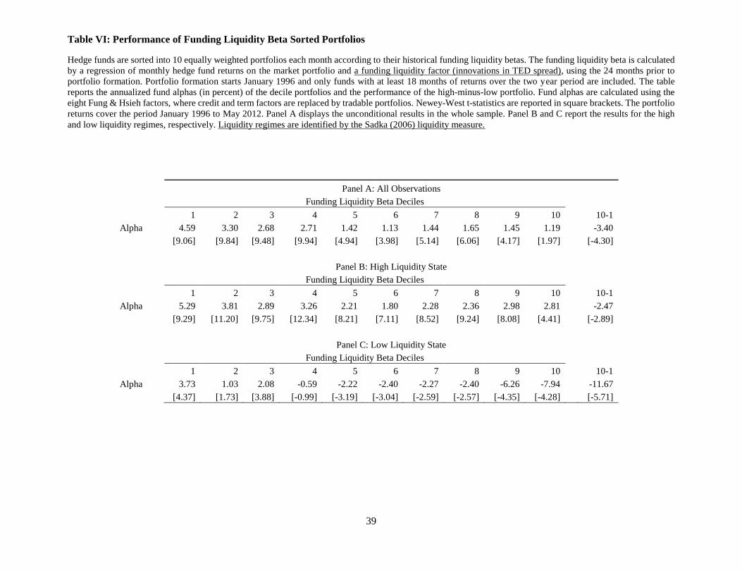
39
Table VI: Performance of Funding Liquidity Beta Sorted Portfolios
Hedge funds are sorted into 10 equally weighted portfolios each month according to their historical funding liquidity betas. The funding liquidity beta is calculated
by a regression of monthly hedge fund returns on the market portfolio and a funding liquidity factor (innovations in TED spread), using the 24 months prior to
portfolio formation. Portfolio formation starts January 1996 and only funds with at least 18 months of returns over the two year period are included. The table
reports the annualized fund alphas (in percent) of the decile portfolios and the performance of the high-minus-low portfolio. Fund alphas are calculated using the
eight Fung & Hsieh factors, where credit and term factors are replaced by tradable portfolios. Newey-West t-statistics are reported in square brackets. The portfolio
returns cover the period January 1996 to May 2012. Panel A displays the unconditional results in the whole sample. Panel B and C report the results for the high
and low liquidity regimes, respectively. Liquidity regimes are identified by the Sadka (2006) liquidity measure.
Panel A: All Observations
Funding Liquidity Beta Deciles
1 2 3 4 5 6 7 8 9 10 10-1
Alpha 4.59 3.30 2.68 2.71 1.42 1.13 1.44 1.65 1.45 1.19 -3.40
[9.06] [9.84] [9.48] [9.94] [4.94] [3.98] [5.14] [6.06] [4.17] [1.97] [-4.30]
Panel B: High Liquidity State
Funding Liquidity Beta Deciles
1 2 3 4 5 6 7 8 9 10 10-1
Alpha 5.29 3.81 2.89 3.26 2.21 1.80 2.28 2.36 2.98 2.81 -2.47
[9.29] [11.20] [9.75] [12.34] [8.21] [7.11] [8.52] [9.24] [8.08] [4.41] [-2.89]
Panel C: Low Liquidity State
Funding Liquidity Beta Deciles
1 2 3 4 5 6 7 8 9 10 10-1
Alpha 3.73 1.03 2.08 -0.59 -2.22 -2.40 -2.27 -2.40 -6.26 -7.94 -11.67
[4.37] [1.73] [3.88] [-0.99] [-3.19] [-3.04] [-2.59] [-2.57] [-4.35] [-4.28] [-5.71]
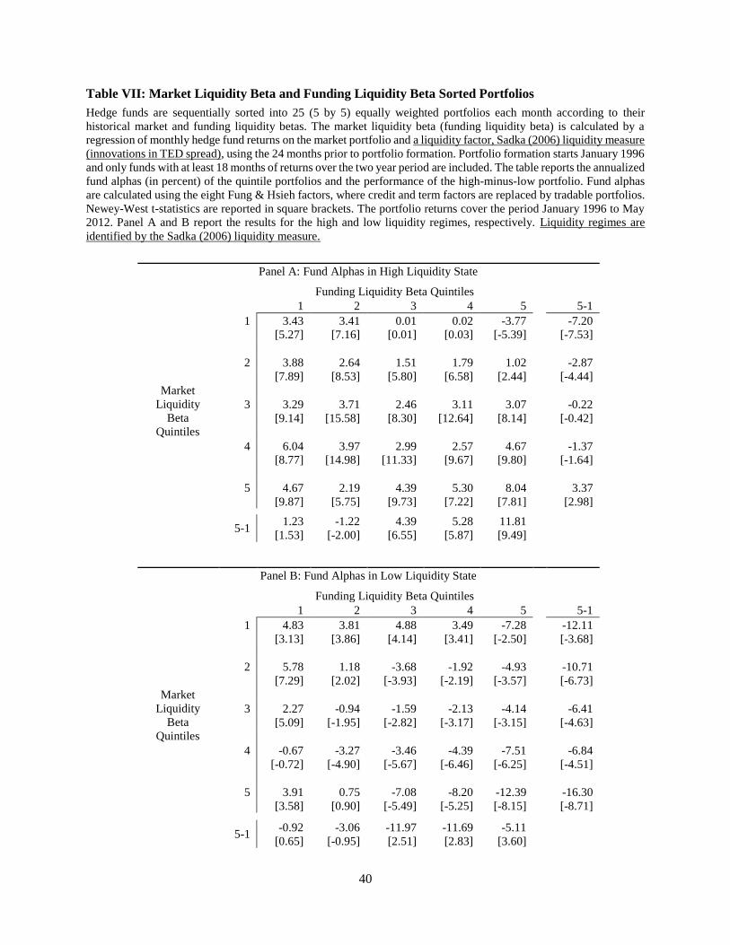
40
Table VII: Market Liquidity Beta and Funding Liquidity Beta Sorted Portfolios
Hedge funds are sequentially sorted into 25 (5 by 5) equally weighted portfolios each month according to their
historical market and funding liquidity betas. The market liquidity beta (funding liquidity beta) is calculated by a
regression of monthly hedge fund returns on the market portfolio and a liquidity factor, Sadka (2006) liquidity measure
(innovations in TED spread), using the 24 months prior to portfolio formation. Portfolio formation starts January 1996
and only funds with at least 18 months of returns over the two year period are included. The table reports the annualized
fund alphas (in percent) of the quintile portfolios and the performance of the high-minus-low portfolio. Fund alphas
are calculated using the eight Fung & Hsieh factors, where credit and term factors are replaced by tradable portfolios.
Newey-West t-statistics are reported in square brackets. The portfolio returns cover the period January 1996 to May
2012. Panel A and B report the results for the high and low liquidity regimes, respectively. Liquidity regimes are
identified by the Sadka (2006) liquidity measure.
Panel A: Fund Alphas in High Liquidity State
Funding Liquidity Beta Quintiles
1 2 3 4 5 5-1
Market
Liquidity
Beta
Quintiles
1 3.43 3.41 0.01 0.02 -3.77 -7.20
[5.27] [7.16] [0.01] [0.03] [-5.39] [-7.53]
2 3.88 2.64 1.51 1.79 1.02 -2.87
[7.89] [8.53] [5.80] [6.58] [2.44] [-4.44]
3 3.29 3.71 2.46 3.11 3.07 -0.22
[9.14] [15.58] [8.30] [12.64] [8.14] [-0.42]
4 6.04 3.97 2.99 2.57 4.67 -1.37
[8.77] [14.98] [11.33] [9.67] [9.80] [-1.64]
5 4.67 2.19 4.39 5.30 8.04 3.37
[9.87] [5.75] [9.73] [7.22] [7.81] [2.98]
5-1 1.23 -1.22 4.39 5.28 11.81
[1.53] [-2.00] [6.55] [5.87] [9.49]
Panel B: Fund Alphas in Low Liquidity State
Funding Liquidity Beta Quintiles
1 2 3 4 5 5-1
Market
Liquidity
Beta
Quintiles
1 4.83 3.81 4.88 3.49 -7.28 -12.11
[3.13] [3.86] [4.14] [3.41] [-2.50] [-3.68]
2 5.78 1.18 -3.68 -1.92 -4.93 -10.71
[7.29] [2.02] [-3.93] [-2.19] [-3.57] [-6.73]
3 2.27 -0.94 -1.59 -2.13 -4.14 -6.41
[5.09] [-1.95] [-2.82] [-3.17] [-3.15] [-4.63]
4 -0.67 -3.27 -3.46 -4.39 -7.51 -6.84
[-0.72] [-4.90] [-5.67] [-6.46] [-6.25] [-4.51]
5 3.91 0.75 -7.08 -8.20 -12.39 -16.30
[3.58] [0.90] [-5.49] [-5.25] [-8.15] [-8.71]
5-1 -0.92 -3.06 -11.97 -11.69 -5.11
[0.65] [-0.95] [2.51] [2.83] [3.60]

41
Table VIII: Performance of Funding Liquidity Beta Sorted Portfolios of Liquid Hedge Funds
Hedge funds with no lockup restrictions (liquid hedge funds) are sorted into 10 equally weighted portfolios each month according to their historical funding liquidity
betas. The funding liquidity beta is calculated by a regression of monthly hedge fund returns on the market portfolio and a funding liquidity factor (innovations in
TED spread), using the 24 months prior to portfolio formation. Portfolio formation starts January 1996 and only funds with at least 18 months of returns over the
two year period are included. The table reports the annualized fund alphas (in percent) of the decile portfolios and the performance of the high-minus-low portfolio.
Fund alphas are calculated using the eight Fung & Hsieh factors, where credit and term factors are replaced by tradable portfolios. T-statistics are reported in square
brackets. The portfolio returns cover the period January 1996 to May 2012. Panel A displays the results for the whole sample. Panel B and C report the results for
the high and low liquidity regimes, respectively. Liquidity regimes are identified by the Sadka (2006) liquidity measure.
Panel A: All Observations
Funding Liquidity Beta Deciles
1 2 3 4 5 6 7 8 9 10 10-1
Alpha 4.03 2.89 2.65 2.23 1.48 1.01 0.63 1.51 1.29 0.86 -3.18
[7.36] [8.35] [8.90] [7.71] [5.50] [3.56] [2.13] [5.56] [3.25] [1.44] [-3.93]
Panel B: High Liquidity State
Funding Liquidity Beta Deciles
1 2 3 4 5 6 7 8 9 10 10-1
Alpha 4.91 3.23 2.81 2.87 2.31 1.69 1.27 2.38 2.97 2.25 -2.66
[7.94] [9.29] [8.99] [10.11] [9.52] [6.47] [4.47] [9.18] [6.68] [3.53] [-2.99]
Panel C: Low Liquidity State
Funding Liquidity Beta Deciles
1 2 3 4 5 6 7 8 9 10 10-1
Alpha 3.63 1.38 2.57 -1.03 -2.26 -1.86 -2.34 -3.22 -6.39 -6.19 -9.82
[3.82] [2.06] [4.81] [-1.46] [-2.97] [-2.60] [-2.43] [-3.09] [-4.63] [-3.51] [-4.90]
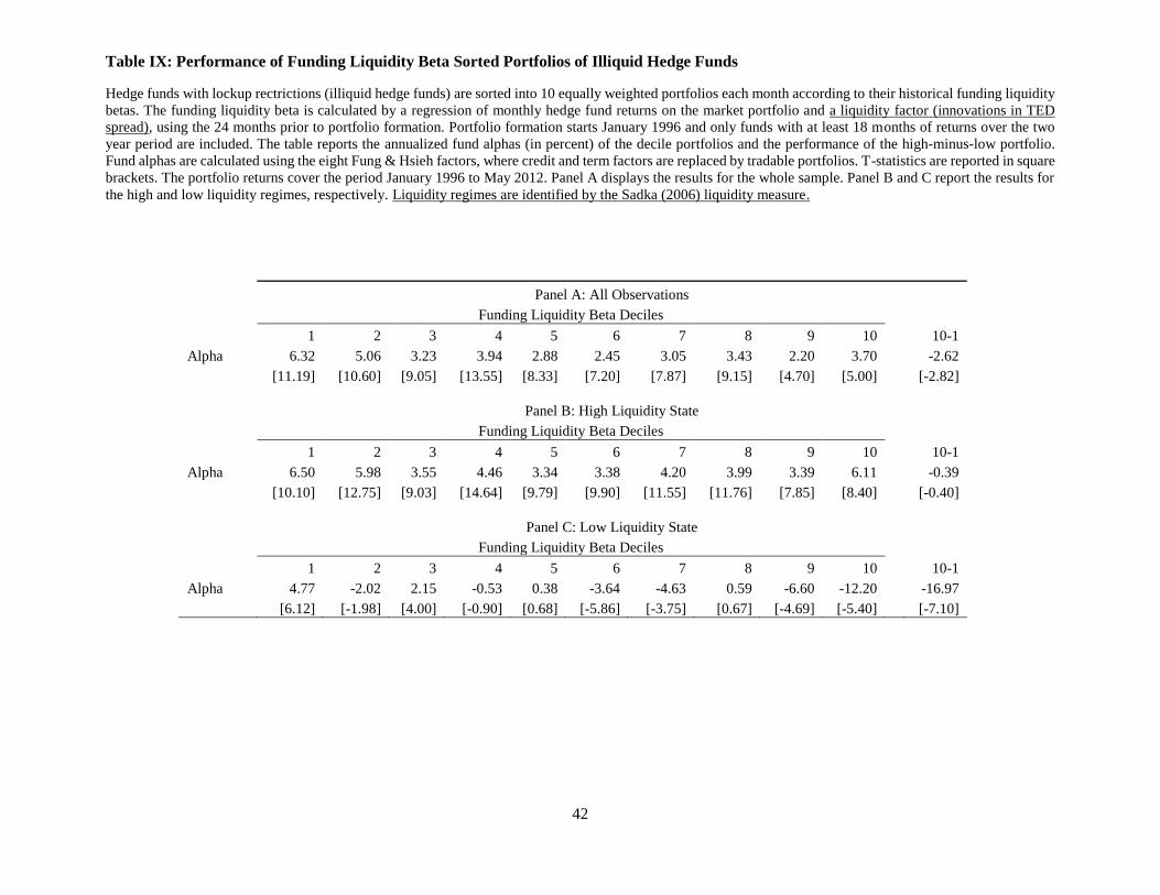
42
Table IX: Performance of Funding Liquidity Beta Sorted Portfolios of Illiquid Hedge Funds
Hedge funds with lockup rectrictions (illiquid hedge funds) are sorted into 10 equally weighted portfolios each month according to their historical funding liquidity
betas. The funding liquidity beta is calculated by a regression of monthly hedge fund returns on the market portfolio and a liquidity factor (innovations in TED
spread), using the 24 months prior to portfolio formation. Portfolio formation starts January 1996 and only funds with at least 18 months of returns over the two
year period are included. The table reports the annualized fund alphas (in percent) of the decile portfolios and the performance of the high-minus-low portfolio.
Fund alphas are calculated using the eight Fung & Hsieh factors, where credit and term factors are replaced by tradable portfolios. T-statistics are reported in square
brackets. The portfolio returns cover the period January 1996 to May 2012. Panel A displays the results for the whole sample. Panel B and C report the results for
the high and low liquidity regimes, respectively. Liquidity regimes are identified by the Sadka (2006) liquidity measure.
Panel A: All Observations
Funding Liquidity Beta Deciles
1 2 3 4 5 6 7 8 9 10 10-1
Alpha 6.32 5.06 3.23 3.94 2.88 2.45 3.05 3.43 2.20 3.70 -2.62
[11.19] [10.60] [9.05] [13.55] [8.33] [7.20] [7.87] [9.15] [4.70] [5.00] [-2.82]
Panel B: High Liquidity State
Funding Liquidity Beta Deciles
1 2 3 4 5 6 7 8 9 10 10-1
Alpha 6.50 5.98 3.55 4.46 3.34 3.38 4.20 3.99 3.39 6.11 -0.39
[10.10] [12.75] [9.03] [14.64] [9.79] [9.90] [11.55] [11.76] [7.85] [8.40] [-0.40]
Panel C: Low Liquidity State
Funding Liquidity Beta Deciles
1 2 3 4 5 6 7 8 9 10 10-1
Alpha 4.77 -2.02 2.15 -0.53 0.38 -3.64 -4.63 0.59 -6.60 -12.20 -16.97
[6.12] [-1.98] [4.00] [-0.90] [0.68] [-5.86] [-3.75] [0.67] [-4.69] [-5.40] [-7.10]
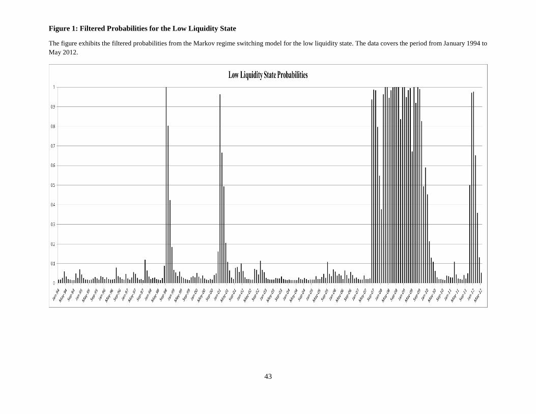
43
Figure 1: Filtered Probabilities for the Low Liquidity State
The figure exhibits the filtered probabilities from the Markov regime switching model for the low liquidity state. The data covers the period from January 1994 to
May 2012.

44
Figure 2: Liquidity Timing Ability of Hedge Funds
The figure exhibits the average market liquidity betas and annualized 8-factor Fung and Hsieh alphas (in percent) for
ten decile portfolios sorted by market liquidity exposure presented in Table V.
Panel A:
Panel B:
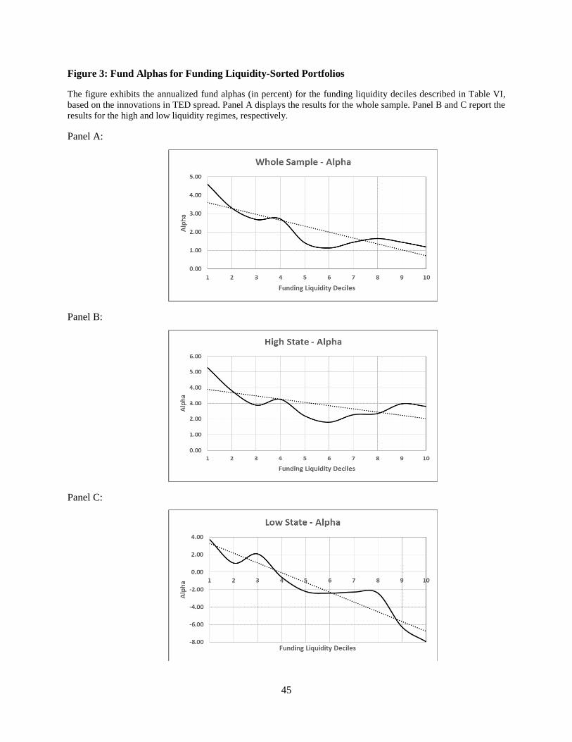
45
Figure 3: Fund Alphas for Funding Liquidity-Sorted Portfolios
The figure exhibits the annualized fund alphas (in percent) for the funding liquidity deciles described in Table VI,
based on the innovations in TED spread. Panel A displays the results for the whole sample. Panel B and C report the
results for the high and low liquidity regimes, respectively.
Panel A:
Panel B:
Panel C:

46
Figure 4: Fund Alphas for Market and Funding Liquidity-Sorted Portfolios (High Liquidity
Regime)
The figure exhibits the annualized fund alphas (in percent) for the market and funding liquidity sorted quintile
portfolios for the high liquidity regime.
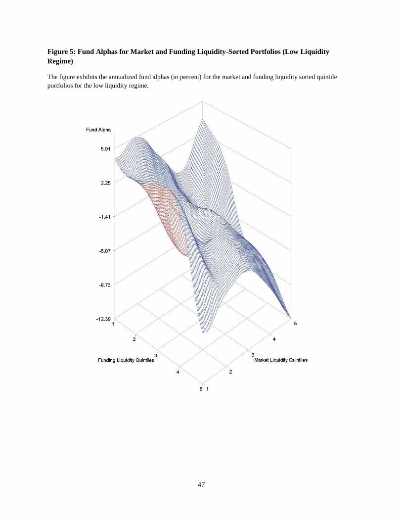
47
Figure 5: Fund Alphas for Market and Funding Liquidity-Sorted Portfolios (Low Liquidity
Regime)
The figure exhibits the annualized fund alphas (in percent) for the market and funding liquidity sorted quintile
portfolios for the low liquidity regime.

48
Table A.1: Performance of Funding Liquidity Beta Sorted Portfolios Identified Using the Orthogonal component of the TED spread
Hedge funds are sorted into 10 equally weighted portfolios each month according to historical funding liquidity betas. The funding liquidity betas are calculated
based on 24-month rolling regressions of monthly hedge fund returns on the market portfolio and the orthogonal component of the innovations in TED spread
when projected onto the Sadka measure. Portfolio formation starts January 1996 and only funds with at least 18 months of returns over the two year period are
included. The table reports the annualized fund alphas (in percent) of the decile portfolios and the performance of the high-minus-low portfolio. Fund alphas are
calculated using the eight Fung & Hsieh factors, where credit and term factors are replaced by tradable portfolios. T-statistics are reported in square brackets. The
portfolio returns cover the period January 1996 to May 2012. Panel A displays the results for the whole sample. Panel B and C report the results for the high and
low liquidity regimes, respectively. Liquidity regimes are identified by the Sadka (2006) liquidity measure.
Panel A: All Observations
Funding Liquidity Beta Deciles
1 2 3 4 5 6 7 8 9 10 10-1
Alpha 4.61 3.12 2.86 3.20 1.43 1.99 1.44 1.23 1.40 0.31 -4.29
[9.07] [9.17] [10.43] [10.88] [5.19] [7.58] [5.41] [4.27] [3.89] [0.54] [-5.53]
Panel B: High Liquidity State
Funding Liquidity Beta Deciles
1 2 3 4 5 6 7 8 9 10 10-1
Alpha 5.37 3.42 3.39 4.11 2.19 2.76 2.45 2.10 2.47 1.46 -3.91
[9.76] [10.37] [13.00] [14.79] [8.88] [11.76] [10.05] [8.04] [6.23] [2.54] [-4.92]
Panel C: Low Liquidity State
Funding Liquidity Beta Deciles
1 2 3 4 5 6 7 8 9 10 10-1
Alpha 2.88 1.88 0.21 -1.30 -2.28 -2.05 -3.34 -3.56 -2.76 -6.81 -9.69
[3.48] [2.83] [0.31] [-2.39] [-3.77] [-2.38] [-3.24] [-3.46] [-2.50] [-3.59] [-4.69]
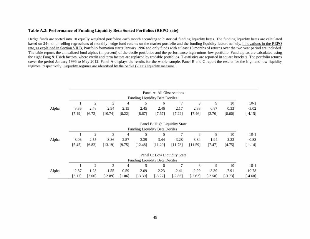
49
Table A.2: Performance of Funding Liquidity Beta Sorted Portfolios (REPO rate)
Hedge funds are sorted into 10 equally weighted portfolios each month according to historical funding liquidity betas. The funding liquidity betas are calculated
based on 24-month rolling regressions of monthly hedge fund returns on the market portfolio and the funding liquidity factor, namely, innovations in the REPO
rate, as explained in Section VII.B, Portfolio formation starts January 1996 and only funds with at least 18 months of returns over the two year period are included.
The table reports the annualized fund alphas (in percent) of the decile portfolios and the performance high-minus-low portfolio. Fund alphas are calculated using
the eight Fung & Hsieh factors, where credit and term factors are replaced by tradable portfolios. T-statistics are reported in square brackets. The portfolio returns
cover the period January 1996 to May 2012. Panel A displays the results for the whole sample. Panel B and C report the results for the high and low liquidity
regimes, respectively. Liquidity regimes are identified by the Sadka (2006) liquidity measure.
Panel A: All Observations
Funding Liquidity Beta Deciles
1 2 3 4 5 6 7 8 9 10 10-1
Alpha 3.36 2.48 2.94 2.15 2.45 2.46 2.17 2.33 0.87 0.33 -3.02
[7.19] [6.72] [10.74] [8.22] [8.67] [7.67] [7.22] [7.46] [2.70] [0.60] [-4.15]
Panel B: High Liquidity State
Funding Liquidity Beta Deciles
1 2 3 4 5 6 7 8 9 10 10-1
Alpha 3.06 2.55 3.86 2.57 3.39 3.44 3.28 3.34 1.94 2.22 -0.83
[5.45] [6.82] [13.19] [9.75] [12.48] [11.29] [11.78] [11.59] [7.47] [4.75] [-1.14]
Panel C: Low Liquidity State
Funding Liquidity Beta Deciles
1 2 3 4 5 6 7 8 9 10 10-1
Alpha 2.87 1.28 -1.55 0.59 -2.09 -2.23 -2.41 -2.29 -3.39 -7.91 -10.78
[3.17] [2.06] [-2.89] [1.06] [-3.39] [-3.27] [-2.86] [-2.62] [-2.58] [-3.73] [-4.68]

50
Table A.3: Performance of Funding Liquidity Beta Sorted Portfolios (Traded Funding Liquidity Measure)
Hedge funds are sorted into 10 equally weighted portfolios each month according to historical funding liquidity betas. The funding liquidity betas are calculated
based on 24-month rolling regressions of monthly hedge fund returns on the market portfolio and the traded liquidity factor proposed by Chen and Lu (2017).
Portfolio formation starts January 1996 and only funds with at least 18 months of returns over the two year period are included. The table reports the annualized
fund alphas (in percent) of the decile portfolios and performance of the high-minus-low portfolio. Fund alphas are calculated using the eight Fung & Hsieh
factors, where credit and term factors are replaced by tradable portfolios. T-statistics are reported in square brackets. The portfolio returns cover the period
January 1996 to May 2012. Panel A displays the results for the whole sample. Panel B and C report the results for the high and low liquidity regimes,
respectively. Liquidity regimes are identified by the Sadka (2006) liquidity measure.
Panel A: All Observations
Funding Liquidity Beta Deciles
1 2 3 4 5 6 7 8 9 10 10-1
Alpha 4.24 3.42 2.32 2.76 2.51 2.43 2.19 1.66 1.63 -1.60 -5.84
[8.93] [9.87] [7.99] [8.59] [8.63] [9.08] [8.32] [5.38] [4.97] [-2.66] [-7.62]
Panel B: High Liquidity State
Funding Liquidity Beta Deciles
1 2 3 4 5 6 7 8 9 10 10-1
Alpha 5.03 4.29 3.34 3.66 3.27 3.23 2.97 2.19 2.19 -0.52 -5.55
[9.23] [10.75] [10.40] [11.44] [12.19] [13.10] [13.41] [7.90] [8.90] [-0.96] [-7.23]
Panel C: Low Liquidity State
Funding Liquidity Beta Deciles
1 2 3 4 5 6 7 8 9 10 10-1
Alpha 0.61 0.04 -2.02 -1.27 -0.96 -1.05 -2.09 -0.78 -1.87 -7.89 -8.50
[0.91] [0.08] [-3.31] [-2.54] [-1.67] [-1.43] [-2.25] [-0.80] [-1.41] [-3.47] [-3.58]

51
Table A.4: Performance of Funding Liquidity Beta Sorted Portfolios (Fontaine and Garcia (2012) Measure)
Hedge funds are sorted into 10 equally weighted portfolios each month according to historical funding liquidity betas. The funding liquidity betas are calculated
based on 24-month rolling regressions of monthly hedge fund returns on the market portfolio and the funding liquidity factor proposed by Fontaine and Garcia
(2012). Portfolio formation starts January 1996 and only funds with at least 18 months of returns over the two year period are included. The table reports the
annualized fund alphas (in percent) of the decile portfolios and performance of the high-minus-low portfolio. Fund alphas are calculated using the eight Fung &
Hsieh factors, where credit and term factors are replaced by tradable portfolios. T-statistics are reported in square brackets. The portfolio returns cover the period
January 1996 to May 2012. Panel A displays the results for the whole sample. Panel B and C report the results for the high and low liquidity regimes,
respectively. Liquidity regimes are identified by the Sadka (2006) liquidity measure.
Panel A: All Observations
Funding Liquidity Beta Deciles
1 2 3 4 5 6 7 8 9 10 10-1
Alpha 3.05 3.33 2.62 1.89 1.20 1.60 1.36 1.66 3.08 1.74 -1.32
[5.60] [10.17] [11.67] [7.17] [3.93] [5.25] [3.87] [5.57] [7.49] [2.67] [-1.55]
Panel B: High Liquidity State
Funding Liquidity Beta Deciles
1 2 3 4 5 6 7 8 9 10 10-1
Alpha 1.94 3.32 2.96 2.79 1.96 2.50 2.55 2.89 4.50 4.25 2.31
[3.61] [9.26] [12.53] [10.91] [6.50] [9.23] [7.83] [11.55] [11.23] [7.31] [2.91]
Panel C: Low Liquidity State
Funding Liquidity Beta Deciles
1 2 3 4 5 6 7 8 9 10 10-1
Alpha 6.65 2.36 1.22 -2.72 -1.86 -2.76 -3.90 -3.63 -2.63 -9.95 -16.60
[2.83] [1.68] [1.39] [-4.11] [-3.16] [-4.99] [-5.62] [-4.74] [-2.71] [-6.38] [-5.89]

52
Table A.5: Performance of Funding Liquidity Beta Sorted Portfolios (Regimes determined by hedge fund returns)
Hedge funds are sorted into 10 equally weighted portfolios each month according to historical funding liquidity betas. The funding liquidity beta is calculated by
a regression of monthly hedge fund returns on the market portfolio and the liquidity factor (innovations in TED spread), using the 24 months prior to portfolio
formation. Portfolio formation starts January 1996 and only funds with at least 18 months of returns over the two year period are included. The table reports the
annualized fund alphas (in percent) of the decile portfolios and the performance of high-minus-low portfolio. Fund alphas are calculated using the eight Fung &
Hsieh factors, where credit and term factors are replaced by tradable portfolios. T-statistics are reported in square brackets. The portfolio returns cover the period
January 1996 to May 2012. Panel A displays the results for the whole sample. Panel B and C report the results for the high and low liquidity regimes, respectively.
Liquidity regimes are identified by the hedge fund returns.
Panel A: All Observations
Funding Liquidity Beta Deciles
1 2 3 4 5 6 7 8 9 10 10-1
Alpha 4.59 3.30 2.68 2.71 1.42 1.13 1.44 1.65 1.45 1.19 -3.40
[9.06] [9.84] [9.48] [9.94] [4.94] [3.98] [5.14] [6.06] [4.17] [1.97] [-4.30]
Panel B: High Liquidity State
Funding Liquidity Beta Deciles
1 2 3 4 5 6 7 8 9 10 10-1
Alpha 8.31 7.08 5.77 5.50 5.86 5.46 5.91 5.88 5.69 5.53 -2.78
[13.60] [19.48] [18.44] [19.50] [23.10] [19.44] [19.84] [17.72] [14.25] [6.53] [-2.67]
Panel C: Low Liquidity State
Funding Liquidity Beta Deciles
1 2 3 4 5 6 7 8 9 10 10-1
Alpha -9.48 -7.31 -8.77 -10.31 -9.98 -11.16 -14.03 -18.20 -27.22 -40.14 -30.66
[-4.50] [-4.91] [-6.40] [-8.82] [-8.25] [-7.67] [-11.48] [-22.57] [-23.20] [-25.98] [-11.74]