Solutions Manual

Fundamentals of Corporate Finance 9th edition Ross, Westerfield, and Jordan

Updated 12-20-2008

CHAPTER 1 INTRODUCTION TO CORPORATE FINANCE Answers to Concepts Review and Critical Thinking Questions 1. Capital budgeting (deciding whether to expand a manufacturing plant), capital structure (deciding

whether to issue new equity and use the proceeds to retire outstanding debt), and working capital management (modifying the firm’s credit collection policy with its customers).

2. Disadvantages: unlimited liability, limited life, difficulty in transferring ownership, hard to raise

capital funds. Some advantages: simpler, less regulation, the owners are also the managers, sometimes personal tax rates are better than corporate tax rates.

3. The primary disadvantage of the corporate form is the double taxation to shareholders of distributed

earnings and dividends. Some advantages include: limited liability, ease of transferability, ability to raise capital, and unlimited life.

4. In response to Sarbanes-Oxley, small firms have elected to go dark because of the costs of

compliance. The costs to comply with Sarbox can be several million dollars, which can be a large percentage of a small firms profits. A major cost of going dark is less access to capital. Since the firm is no longer publicly traded, it can no longer raise money in the public market. Although the company will still have access to bank loans and the private equity market, the costs associated with raising funds in these markets are usually higher than the costs of raising funds in the public market.

5. The treasurer’s office and the controller’s office are the two primary organizational groups that

report directly to the chief financial officer. The controller’s office handles cost and financial accounting, tax management, and management information systems, while the treasurer’s office is responsible for cash and credit management, capital budgeting, and financial planning. Therefore, the study of corporate finance is concentrated within the treasury group’s functions.

6. To maximize the current market value (share price) of the equity of the firm (whether it’s publicly-

traded or not). 7. In the corporate form of ownership, the shareholders are the owners of the firm. The shareholders

elect the directors of the corporation, who in turn appoint the firm’s management. This separation of ownership from control in the corporate form of organization is what causes agency problems to exist. Management may act in its own or someone else’s best interests, rather than those of the shareholders. If such events occur, they may contradict the goal of maximizing the share price of the equity of the firm.

8. A primary market transaction.

B-2 SOLUTIONS

9. In auction markets like the NYSE, brokers and agents meet at a physical location (the exchange) to match buyers and sellers of assets. Dealer markets like NASDAQ consist of dealers operating at dispersed locales who buy and sell assets themselves, communicating with other dealers either electronically or literally over-the-counter.

10. Such organizations frequently pursue social or political missions, so many different goals are

conceivable. One goal that is often cited is revenue minimization; i.e., provide whatever goods and services are offered at the lowest possible cost to society. A better approach might be to observe that even a not-for-profit business has equity. Thus, one answer is that the appropriate goal is to maximize the value of the equity.

11. Presumably, the current stock value reflects the risk, timing, and magnitude of all future cash flows,

both short-term and long-term. If this is correct, then the statement is false. 12. An argument can be made either way. At the one extreme, we could argue that in a market economy,

all of these things are priced. There is thus an optimal level of, for example, ethical and/or illegal behavior, and the framework of stock valuation explicitly includes these. At the other extreme, we could argue that these are non-economic phenomena and are best handled through the political process. A classic (and highly relevant) thought question that illustrates this debate goes something like this: “A firm has estimated that the cost of improving the safety of one of its products is $30 million. However, the firm believes that improving the safety of the product will only save $20 million in product liability claims. What should the firm do?”

13. The goal will be the same, but the best course of action toward that goal may be different because of

differing social, political, and economic institutions. 14. The goal of management should be to maximize the share price for the current shareholders. If

management believes that it can improve the profitability of the firm so that the share price will exceed $35, then they should fight the offer from the outside company. If management believes that this bidder or other unidentified bidders will actually pay more than $35 per share to acquire the company, then they should still fight the offer. However, if the current management cannot increase the value of the firm beyond the bid price, and no other higher bids come in, then management is not acting in the interests of the shareholders by fighting the offer. Since current managers often lose their jobs when the corporation is acquired, poorly monitored managers have an incentive to fight corporate takeovers in situations such as this.

15. We would expect agency problems to be less severe in countries with a relatively small percentage

of individual ownership. Fewer individual owners should reduce the number of diverse opinions concerning corporate goals. The high percentage of institutional ownership might lead to a higher degree of agreement between owners and managers on decisions concerning risky projects. In addition, institutions may be better able to implement effective monitoring mechanisms on managers than can individual owners, based on the institutions’ deeper resources and experiences with their own management. The increase in institutional ownership of stock in the United States and the growing activism of these large shareholder groups may lead to a reduction in agency problems for U.S. corporations and a more efficient market for corporate control.

CHAPTER 1 B-3

16. How much is too much? Who is worth more, Ray Irani or Tiger Woods? The simplest answer is that there is a market for executives just as there is for all types of labor. Executive compensation is the price that clears the market. The same is true for athletes and performers. Having said that, one aspect of executive compensation deserves comment. A primary reason executive compensation has grown so dramatically is that companies have increasingly moved to stock-based compensation. Such movement is obviously consistent with the attempt to better align stockholder and management interests. In recent years, stock prices have soared, so management has cleaned up. It is sometimes argued that much of this reward is simply due to rising stock prices in general, not managerial performance. Perhaps in the future, executive compensation will be designed to reward only differential performance, i.e., stock price increases in excess of general market increases.

CHAPTER 2 FINANCIAL STATEMENTS, TAXES AND CASH FLOW Answers to Concepts Review and Critical Thinking Questions 1. Liquidity measures how quickly and easily an asset can be converted to cash without significant loss

in value. It’s desirable for firms to have high liquidity so that they have a large factor of safety in meeting short-term creditor demands. However, since liquidity also has an opportunity cost associated with it—namely that higher returns can generally be found by investing the cash into productive assets—low liquidity levels are also desirable to the firm. It’s up to the firm’s financial management staff to find a reasonable compromise between these opposing needs.

2. The recognition and matching principles in financial accounting call for revenues, and the costs

associated with producing those revenues, to be “booked” when the revenue process is essentially complete, not necessarily when the cash is collected or bills are paid. Note that this way is not necessarily correct; it’s the way accountants have chosen to do it.

3. Historical costs can be objectively and precisely measured whereas market values can be difficult to

estimate, and different analysts would come up with different numbers. Thus, there is a tradeoff between relevance (market values) and objectivity (book values).

4. Depreciation is a non-cash deduction that reflects adjustments made in asset book values in

accordance with the matching principle in financial accounting. Interest expense is a cash outlay, but it’s a financing cost, not an operating cost.

5. Market values can never be negative. Imagine a share of stock selling for –$20. This would mean

that if you placed an order for 100 shares, you would get the stock along with a check for $2,000. How many shares do you want to buy? More generally, because of corporate and individual bankruptcy laws, net worth for a person or a corporation cannot be negative, implying that liabilities cannot exceed assets in market value.

6. For a successful company that is rapidly expanding, for example, capital outlays will be large,

possibly leading to negative cash flow from assets. In general, what matters is whether the money is spent wisely, not whether cash flow from assets is positive or negative.

7. It’s probably not a good sign for an established company, but it would be fairly ordinary for a start-

up, so it depends. 8. For example, if a company were to become more efficient in inventory management, the amount of

inventory needed would decline. The same might be true if it becomes better at collecting its receivables. In general, anything that leads to a decline in ending NWC relative to beginning would have this effect. Negative net capital spending would mean more long-lived assets were liquidated than purchased.

CHAPTER 2 B-5

9. If a company raises more money from selling stock than it pays in dividends in a particular period, its cash flow to stockholders will be negative. If a company borrows more than it pays in interest, its cash flow to creditors will be negative.

10. The adjustments discussed were purely accounting changes; they had no cash flow or market value

consequences unless the new accounting information caused stockholders to revalue the derivatives.

11. Enterprise value is the theoretical takeover price. In the event of a takeover, an acquirer would have to take on the company's debt, but would pocket its cash. Enterprise value differs significantly from simple market capitalization in several ways, and it may be a more accurate representation of a firm's value. In a takeover, the value of a firm's debt would need to be paid by the buyer when taking over a company. This enterprise value provides a much more accurate takeover valuation because it includes debt in its value calculation.

12. In general, it appears that investors prefer companies that have a steady earnings stream. If true, this

encourages companies to manage earnings. Under GAAP, there are numerous choices for the way a company reports its financial statements. Although not the reason for the choices under GAAP, one outcome is the ability of a company to manage earnings, which is not an ethical decision. Even though earnings and cash flow are often related, earnings management should have little effect on cash flow (except for tax implications). If the market is “fooled” and prefers steady earnings, shareholder wealth can be increased, at least temporarily. However, given the questionable ethics of this practice, the company (and shareholders) will lose value if the practice is discovered.

Solutions to Questions and Problems NOTE: All end of chapter problems were solved using a spreadsheet. Many problems require multiple steps. Due to space and readability constraints, when these intermediate steps are included in this solutions manual, rounding may appear to have occurred. However, the final answer for each problem is found without rounding during any step in the problem. Basic 1. To find owner’s equity, we must construct a balance sheet as follows: Balance Sheet CA $5,100 CL $4,300 NFA 23,800 LTD 7,400 OE ?? TA $28,900 TL & OE $28,900

We know that total liabilities and owner’s equity (TL & OE) must equal total assets of $28,900. We also know that TL & OE is equal to current liabilities plus long-term debt plus owner’s equity, so owner’s equity is:

OE = $28,900 – 7,400 – 4,300 = $17,200 NWC = CA – CL = $5,100 – 4,300 = $800

B-6 SOLUTIONS

2. The income statement for the company is: Income Statement Sales $586,000 Costs 247,000 Depreciation 43,000 EBIT $296,000 Interest 32,000 EBT $264,000 Taxes(35%) 92,400 Net income $171,600 3. One equation for net income is:

Net income = Dividends + Addition to retained earnings Rearranging, we get: Addition to retained earnings = Net income – Dividends = $171,600 – 73,000 = $98,600

4. EPS = Net income / Shares = $171,600 / 85,000 = $2.02 per share DPS = Dividends / Shares = $73,000 / 85,000 = $0.86 per share 5. To find the book value of current assets, we use: NWC = CA – CL. Rearranging to solve for

current assets, we get: CA = NWC + CL = $380,000 + 1,400,000 = $1,480,000

The market value of current assets and fixed assets is given, so: Book value CA = $1,480,000 Market value CA = $1,600,000 Book value NFA = $3,700,000 Market value NFA = $4,900,000 Book value assets = $5,180,000 Market value assets = $6,500,000 6. Taxes = 0.15($50K) + 0.25($25K) + 0.34($25K) + 0.39($236K – 100K) = $75,290 7. The average tax rate is the total tax paid divided by net income, so:

Average tax rate = $75,290 / $236,000 = 31.90% The marginal tax rate is the tax rate on the next $1 of earnings, so the marginal tax rate = 39%.

CHAPTER 2 B-7

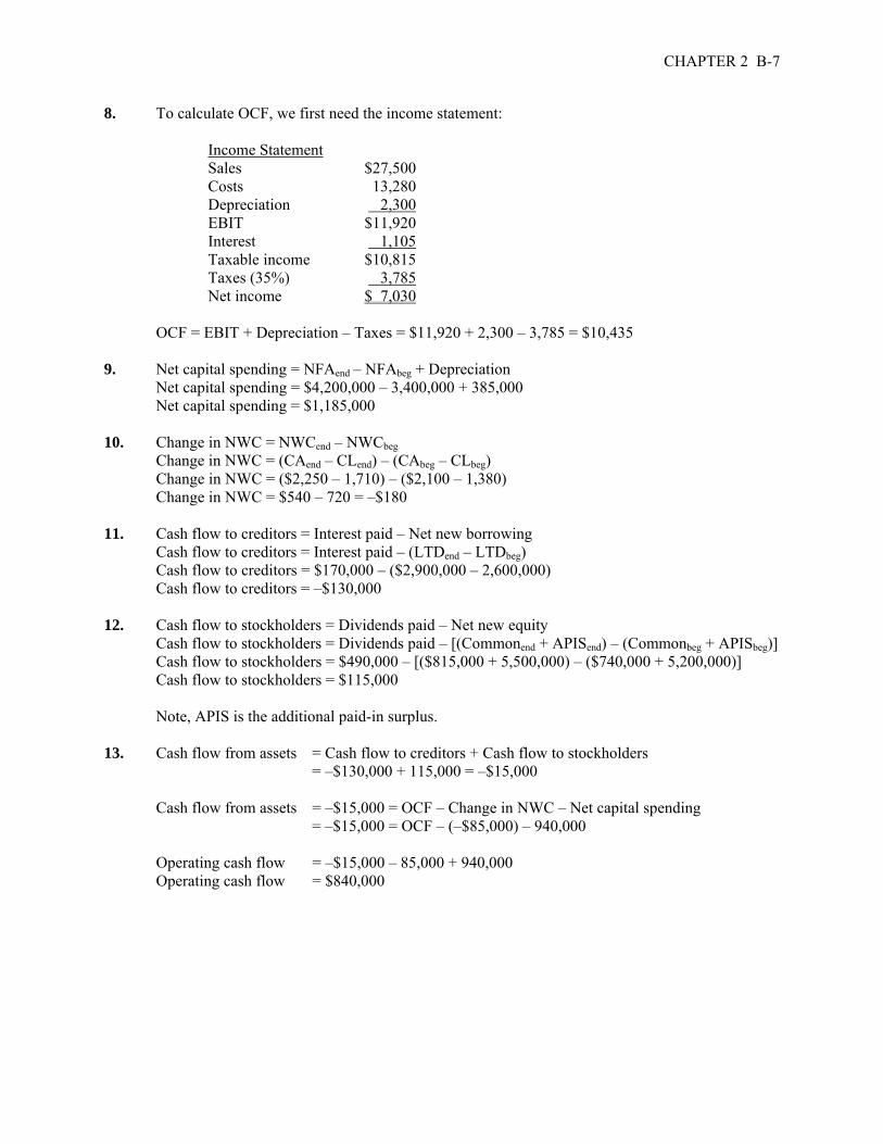
8. To calculate OCF, we first need the income statement:

Income Statement Sales $27,500 Costs 13,280 Depreciation 2,300 EBIT $11,920 Interest 1,105 Taxable income $10,815 Taxes (35%) 3,785 Net income $ 7,030 OCF = EBIT + Depreciation – Taxes = $11,920 + 2,300 – 3,785 = $10,435 9. Net capital spending = NFAend – NFAbeg + Depreciation

Net capital spending = $4,200,000 – 3,400,000 + 385,000 Net capital spending = $1,185,000

10. Change in NWC = NWCend – NWCbeg Change in NWC = (CAend – CLend) – (CAbeg – CLbeg) Change in NWC = ($2,250 – 1,710) – ($2,100 – 1,380) Change in NWC = $540 – 720 = –$180 11. Cash flow to creditors = Interest paid – Net new borrowing Cash flow to creditors = Interest paid – (LTDend – LTDbeg) Cash flow to creditors = $170,000 – ($2,900,000 – 2,600,000) Cash flow to creditors = –$130,000 12. Cash flow to stockholders = Dividends paid – Net new equity Cash flow to stockholders = Dividends paid – [(Commonend + APISend) – (Commonbeg + APISbeg)] Cash flow to stockholders = $490,000 – [($815,000 + 5,500,000) – ($740,000 + 5,200,000)] Cash flow to stockholders = $115,000 Note, APIS is the additional paid-in surplus. 13. Cash flow from assets = Cash flow to creditors + Cash flow to stockholders = –$130,000 + 115,000 = –$15,000 Cash flow from assets = –$15,000 = OCF – Change in NWC – Net capital spending = –$15,000 = OCF – (–$85,000) – 940,000

Operating cash flow = –$15,000 – 85,000 + 940,000 Operating cash flow = $840,000

B-8 SOLUTIONS

Intermediate 14. To find the OCF, we first calculate net income. Income Statement Sales $196,000 Costs 104,000 Other expenses 6,800 Depreciation 9,100 EBIT $76,100 Interest 14,800 Taxable income $61,300 Taxes 21,455 Net income $39,845 Dividends $10,400 Additions to RE $29,445 a. OCF = EBIT + Depreciation – Taxes = $76,100 + 9,100 – 21,455 = $63,745 b. CFC = Interest – Net new LTD = $14,800 – (–7,300) = $22,100

Note that the net new long-term debt is negative because the company repaid part of its long- term debt.

c. CFS = Dividends – Net new equity = $10,400 – 5,700 = $4,700

d. We know that CFA = CFC + CFS, so:

CFA = $22,100 + 4,700 = $26,800

CFA is also equal to OCF – Net capital spending – Change in NWC. We already know OCF. Net capital spending is equal to:

Net capital spending = Increase in NFA + Depreciation = $27,000 + 9,100 = $36,100 Now we can use: CFA = OCF – Net capital spending – Change in NWC $26,800 = $63,745 – 36,100 – Change in NWC

Solving for the change in NWC gives $845, meaning the company increased its NWC by

$845.

15. The solution to this question works the income statement backwards. Starting at the bottom:

Net income = Dividends + Addition to ret. earnings = $1,500 + 5,100 = $6,600

CHAPTER 2 B-9

Now, looking at the income statement: EBT – EBT × Tax rate = Net income Recognize that EBT × Tax rate is simply the calculation for taxes. Solving this for EBT yields: EBT = NI / (1– tax rate) = $6,600 / (1 – 0.35) = $10,154 Now you can calculate: EBIT = EBT + Interest = $10,154 + 4,500 = $14,654 The last step is to use: EBIT = Sales – Costs – Depreciation $14,654 = $41,000 – 19,500 – Depreciation Solving for depreciation, we find that depreciation = $6,846

16. The balance sheet for the company looks like this: Balance Sheet Cash $195,000 Accounts payable $405,000 Accounts receivable 137,000 Notes payable 160,000 Inventory 264,000 Current liabilities $565,000 Current assets $596,000 Long-term debt 1,195,300 Total liabilities $1,760,300 Tangible net fixed assets 2,800,000 Intangible net fixed assets 780,000 Common stock ?? Accumulated ret. earnings 1,934,000 Total assets $4,176,000 Total liab. & owners’ equity $4,176,000 Total liabilities and owners’ equity is: TL & OE = CL + LTD + Common stock + Retained earnings Solving for this equation for equity gives us: Common stock = $4,176,000 – 1,934,000 – 1,760,300 = $481,700 17. The market value of shareholders’ equity cannot be negative. A negative market value in this case

would imply that the company would pay you to own the stock. The market value of shareholders’ equity can be stated as: Shareholders’ equity = Max [(TA – TL), 0]. So, if TA is $8,400, equity is equal to $1,100, and if TA is $6,700, equity is equal to $0. We should note here that the book value of shareholders’ equity can be negative.

B-10 SOLUTIONS

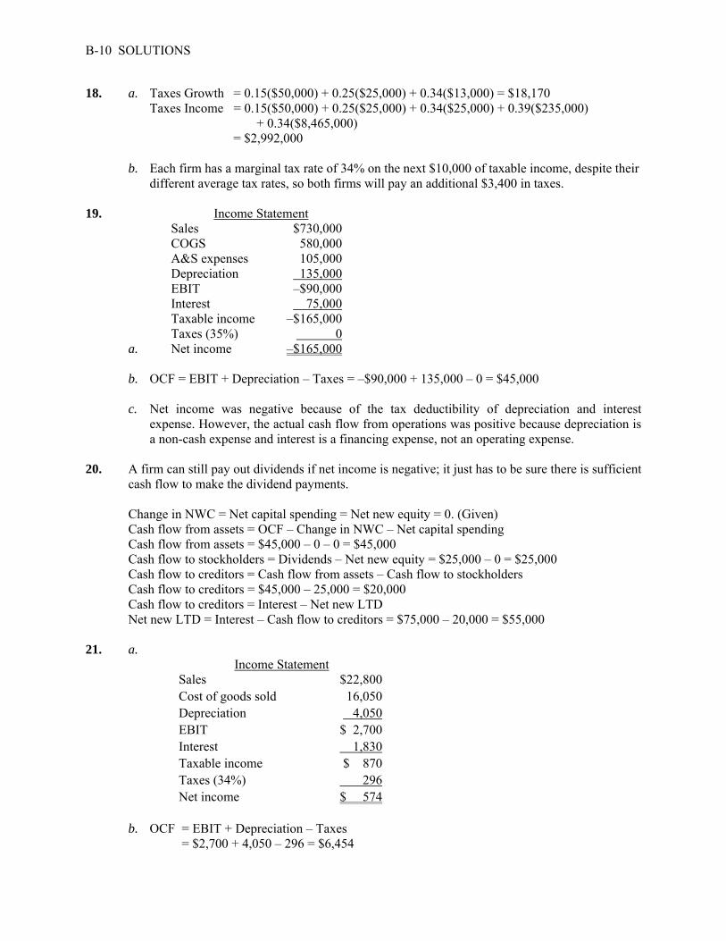
18. a. Taxes Growth = 0.15($50,000) + 0.25($25,000) + 0.34($13,000) = $18,170 Taxes Income = 0.15($50,000) + 0.25($25,000) + 0.34($25,000) + 0.39($235,000) + 0.34($8,465,000) = $2,992,000

b. Each firm has a marginal tax rate of 34% on the next $10,000 of taxable income, despite their different average tax rates, so both firms will pay an additional $3,400 in taxes.

19. Income Statement Sales $730,000 COGS 580,000 A&S expenses 105,000 Depreciation 135,000 EBIT –$90,000 Interest 75,000 Taxable income –$165,000 Taxes (35%) 0 a. Net income –$165,000 b. OCF = EBIT + Depreciation – Taxes = –$90,000 + 135,000 – 0 = $45,000 c. Net income was negative because of the tax deductibility of depreciation and interest

expense. However, the actual cash flow from operations was positive because depreciation is a non-cash expense and interest is a financing expense, not an operating expense.

20. A firm can still pay out dividends if net income is negative; it just has to be sure there is sufficient

cash flow to make the dividend payments. Change in NWC = Net capital spending = Net new equity = 0. (Given) Cash flow from assets = OCF – Change in NWC – Net capital spending Cash flow from assets = $45,000 – 0 – 0 = $45,000 Cash flow to stockholders = Dividends – Net new equity = $25,000 – 0 = $25,000 Cash flow to creditors = Cash flow from assets – Cash flow to stockholders Cash flow to creditors = $45,000 – 25,000 = $20,000 Cash flow to creditors = Interest – Net new LTD Net new LTD = Interest – Cash flow to creditors = $75,000 – 20,000 = $55,000 21. a. Income Statement Sales $22,800 Cost of goods sold 16,050 Depreciation 4,050 EBIT $ 2,700 Interest 1,830 Taxable income $ 870 Taxes (34%) 296 Net income $ 574

b. OCF = EBIT + Depreciation – Taxes = $2,700 + 4,050 – 296 = $6,454

CHAPTER 2 B-11

c. Change in NWC = NWCend – NWCbeg = (CAend – CLend) – (CAbeg – CLbeg) = ($5,930 – 3,150) – ($4,800 – 2,700) = $2,780 – 2,100 = $680 Net capital spending = NFAend – NFAbeg + Depreciation = $16,800 – 13,650 + 4,050 = $7,200 CFA = OCF – Change in NWC – Net capital spending = $6,454 – 680 – 7,200 = –$1,426

The cash flow from assets can be positive or negative, since it represents whether the firm raised funds or distributed funds on a net basis. In this problem, even though net income and OCF are positive, the firm invested heavily in both fixed assets and net working capital; it had to raise a net $1,426 in funds from its stockholders and creditors to make these investments.

d. Cash flow to creditors = Interest – Net new LTD = $1,830 – 0 = $1,830

Cash flow to stockholders = Cash flow from assets – Cash flow to creditors = –$1,426 – 1,830 = –$3,256 We can also calculate the cash flow to stockholders as: Cash flow to stockholders = Dividends – Net new equity Solving for net new equity, we get: Net new equity = $1,300 – (–3,256) = $4,556

The firm had positive earnings in an accounting sense (NI > 0) and had positive cash flow from operations. The firm invested $680 in new net working capital and $7,200 in new fixed assets. The firm had to raise $1,426 from its stakeholders to support this new investment. It accomplished this by raising $4,556 in the form of new equity. After paying out $1,300 of this in the form of dividends to shareholders and $1,830 in the form of interest to creditors, $1,426 was left to meet the firm’s cash flow needs for investment.

22. a. Total assets 2008 = $653 + 2,691 = $3,344 Total liabilities 2008 = $261 + 1,422 = $1,683 Owners’ equity 2008 = $3,344 – 1,683 = $1,661 Total assets 2009 = $707 + 3,240 = $3,947 Total liabilities 2009 = $293 + 1,512 = $1,805 Owners’ equity 2009 = $3,947 – 1,805 = $2,142 b. NWC 2008 = CA08 – CL08 = $653 – 261 = $392 NWC 2009 = CA09 – CL09 = $707 – 293 = $414 Change in NWC = NWC09 – NWC08 = $414 – 392 = $22

B-12 SOLUTIONS

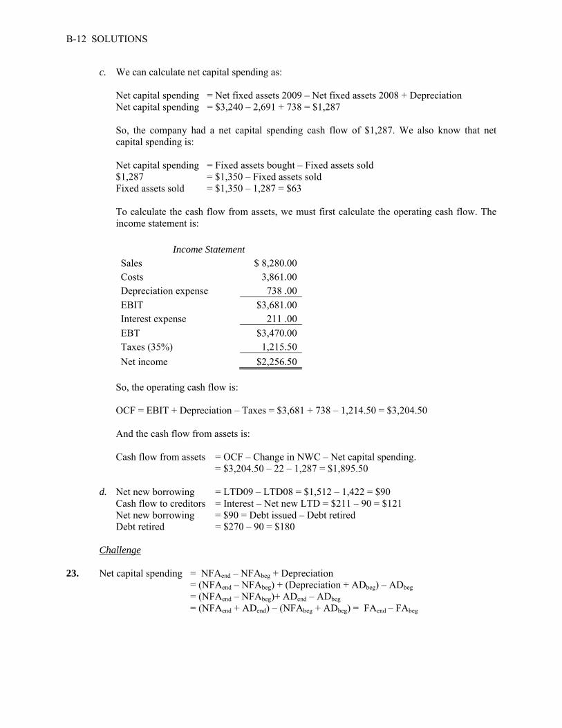
c. We can calculate net capital spending as: Net capital spending = Net fixed assets 2009 – Net fixed assets 2008 + Depreciation Net capital spending = $3,240 – 2,691 + 738 = $1,287

So, the company had a net capital spending cash flow of $1,287. We also know that net capital spending is:

Net capital spending = Fixed assets bought – Fixed assets sold $1,287 = $1,350 – Fixed assets sold Fixed assets sold = $1,350 – 1,287 = $63

To calculate the cash flow from assets, we must first calculate the operating cash flow. The income statement is:

Income Statement Sales $ 8,280.00 Costs 3,861.00 Depreciation expense 738 .00

EBIT $3,681.00 Interest expense 211 .00

EBT $3,470.00 Taxes (35%) 1,215.50

Net income $2,256.50

So, the operating cash flow is:

OCF = EBIT + Depreciation – Taxes = $3,681 + 738 – 1,214.50 = $3,204.50 And the cash flow from assets is: Cash flow from assets = OCF – Change in NWC – Net capital spending. = $3,204.50 – 22 – 1,287 = $1,895.50 d. Net new borrowing = LTD09 – LTD08 = $1,512 – 1,422 = $90 Cash flow to creditors = Interest – Net new LTD = $211 – 90 = $121 Net new borrowing = $90 = Debt issued – Debt retired Debt retired = $270 – 90 = $180 Challenge 23. Net capital spending = NFAend – NFAbeg + Depreciation = (NFAend – NFAbeg) + (Depreciation + ADbeg) – ADbeg = (NFAend – NFAbeg)+ ADend – ADbeg = (NFAend + ADend) – (NFAbeg + ADbeg) = FAend – FAbeg

CHAPTER 2 B-13

24. a. The tax bubble causes average tax rates to catch up to marginal tax rates, thus eliminating the tax advantage of low marginal rates for high income corporations.

b. Taxes = 0.15($50,000) + 0.25($25,000) + 0.34($25,000) + 0.39($235,000) = $113,900 Average tax rate = $113,900 / $335,000 = 34% The marginal tax rate on the next dollar of income is 34 percent. For corporate taxable income levels of $335,000 to $10 million, average tax rates are equal to

marginal tax rates. Taxes = 0.34($10,000,000) + 0.35($5,000,000) + 0.38($3,333,333)= $6,416,667 Average tax rate = $6,416,667 / $18,333,334 = 35% The marginal tax rate on the next dollar of income is 35 percent. For corporate taxable

income levels over $18,333,334, average tax rates are again equal to marginal tax rates. c. Taxes = 0.34($200,000) = $68,000 $68,000 = 0.15($50,000) + 0.25($25,000) + 0.34($25,000) + X($100,000); X($100,000) = $68,000 – 22,250 X = $45,750 / $100,000 X = 45.75% 25.

Balance sheet as of Dec. 31, 2008

Cash $3,792 Accounts payable $3,984 Accounts receivable 5,021 Notes payable 732

Inventory 8,927 Current liabilities $4,716

Current assets $17,740 Long-term debt $12,700 Net fixed assets $31,805 Owners' equity 32,129

Total assets $49,545 Total liab. & equity $49,545

Balance sheet as of Dec. 31, 2009

Cash $4,041 Accounts payable $4,025 Accounts receivable 5,892 Notes payable 717

Inventory 9,555 Current liabilities $4,742

Current assets $19,488 Long-term debt $15,435 Net fixed assets $33,921 Owners' equity 33,232

Total assets $53,409 Total liab. & equity $53,409

B-14 SOLUTIONS

2008 Income Statement 2009 Income Statement Sales $7,233.00 Sales $8,085.00 COGS 2,487.00 COGS 2,942.00 Other expenses 591.00 Other expenses 515.00 Depreciation 1,038.00 Depreciation 1,085.00 EBIT $3,117.00 EBIT $3,543.00 Interest 485.00 Interest 579.00 EBT $2,632.00 EBT $2,964.00 Taxes (34%) 894.88 Taxes (34%) 1,007.76 Net income $1,737.12 Net income $1,956.24 Dividends $882.00 Dividends $1,011.00 Additions to RE 855.12 Additions to RE 945.24 26. OCF = EBIT + Depreciation – Taxes = $3,543 + 1,085 – 1,007.76 = $3,620.24 Change in NWC = NWCend – NWCbeg = (CA – CL) end – (CA – CL) beg = ($19,488 – 4,742) – ($17,740 – 4,716) = $1,722 Net capital spending = NFAend – NFAbeg + Depreciation = $33,921 – 31,805 + 1,085 = $3,201 Cash flow from assets = OCF – Change in NWC – Net capital spending = $3,620.24 – 1,722 – 3,201 = –$1,302.76 Cash flow to creditors = Interest – Net new LTD Net new LTD = LTDend – LTDbeg Cash flow to creditors = $579 – ($15,435 – 12,700) = –$2,156 Net new equity = Common stockend – Common stockbeg Common stock + Retained earnings = Total owners’ equity Net new equity = (OE – RE) end – (OE – RE) beg = OEend – OEbeg + REbeg – REend REend = REbeg + Additions to RE08

Net new equity = OEend – OEbeg + REbeg – (REbeg + Additions to RE08) = OEend – OEbeg – Additions to RE Net new equity = $33,232 – 32,129 – 945.24 = $157.76

CFS = Dividends – Net new equity CFS = $1,011 – 157.76 = $853.24 As a check, cash flow from assets is –$1,302.76. CFA = Cash flow from creditors + Cash flow to stockholders CFA = –$2,156 + 853.24 = –$1,302.76

CHAPTER 3 WORKING WITH FINANCIAL STATEMENTS Answers to Concepts Review and Critical Thinking Questions 1. a. If inventory is purchased with cash, then there is no change in the current ratio. If inventory is

purchased on credit, then there is a decrease in the current ratio if it was initially greater than 1.0. b. Reducing accounts payable with cash increases the current ratio if it was initially greater than 1.0. c. Reducing short-term debt with cash increases the current ratio if it was initially greater than 1.0. d. As long-term debt approaches maturity, the principal repayment and the remaining interest

expense become current liabilities. Thus, if debt is paid off with cash, the current ratio increases if it was initially greater than 1.0. If the debt has not yet become a current liability, then paying it off will reduce the current ratio since current liabilities are not affected.

e. Reduction of accounts receivables and an increase in cash leaves the current ratio unchanged. f. Inventory sold at cost reduces inventory and raises cash, so the current ratio is unchanged. g. Inventory sold for a profit raises cash in excess of the inventory recorded at cost, so the current

ratio increases. 2. The firm has increased inventory relative to other current assets; therefore, assuming current liability

levels remain unchanged, liquidity has potentially decreased. 3. A current ratio of 0.50 means that the firm has twice as much in current liabilities as it does in

current assets; the firm potentially has poor liquidity. If pressed by its short-term creditors and suppliers for immediate payment, the firm might have a difficult time meeting its obligations. A current ratio of 1.50 means the firm has 50% more current assets than it does current liabilities. This probably represents an improvement in liquidity; short-term obligations can generally be met com-pletely with a safety factor built in. A current ratio of 15.0, however, might be excessive. Any excess funds sitting in current assets generally earn little or no return. These excess funds might be put to better use by investing in productive long-term assets or distributing the funds to shareholders.

4. a. Quick ratio provides a measure of the short-term liquidity of the firm, after removing the effects

of inventory, generally the least liquid of the firm’s current assets. b. Cash ratio represents the ability of the firm to completely pay off its current liabilities with its

most liquid asset (cash). c. Total asset turnover measures how much in sales is generated by each dollar of firm assets. d. Equity multiplier represents the degree of leverage for an equity investor of the firm; it measures

the dollar worth of firm assets each equity dollar has a claim to. e. Long-term debt ratio measures the percentage of total firm capitalization funded by long-term

debt.

B-16 SOLUTIONS

f. Times interest earned ratio provides a relative measure of how well the firm’s operating earnings can cover current interest obligations.

g. Profit margin is the accounting measure of bottom-line profit per dollar of sales. h. Return on assets is a measure of bottom-line profit per dollar of total assets. i. Return on equity is a measure of bottom-line profit per dollar of equity. j. Price-earnings ratio reflects how much value per share the market places on a dollar of

accounting earnings for a firm. 5. Common size financial statements express all balance sheet accounts as a percentage of total assets

and all income statement accounts as a percentage of total sales. Using these percentage values rather than nominal dollar values facilitates comparisons between firms of different size or business type. Common-base year financial statements express each account as a ratio between their current year nominal dollar value and some reference year nominal dollar value. Using these ratios allows the total growth trend in the accounts to be measured.

6. Peer group analysis involves comparing the financial ratios and operating performance of a

particular firm to a set of peer group firms in the same industry or line of business. Comparing a firm to its peers allows the financial manager to evaluate whether some aspects of the firm’s operations, finances, or investment activities are out of line with the norm, thereby providing some guidance on appropriate actions to take to adjust these ratios if appropriate. An aspirant group would be a set of firms whose performance the company in question would like to emulate. The financial manager often uses the financial ratios of aspirant groups as the target ratios for his or her firm; some managers are evaluated by how well they match the performance of an identified aspirant group.

7. Return on equity is probably the most important accounting ratio that measures the bottom-line

performance of the firm with respect to the equity shareholders. The Du Pont identity emphasizes the role of a firm’s profitability, asset utilization efficiency, and financial leverage in achieving an ROE figure. For example, a firm with ROE of 20% would seem to be doing well, but this figure may be misleading if it were marginally profitable (low profit margin) and highly levered (high equity multiplier). If the firm’s margins were to erode slightly, the ROE would be heavily impacted.

8. The book-to-bill ratio is intended to measure whether demand is growing or falling. It is closely

followed because it is a barometer for the entire high-tech industry where levels of revenues and earnings have been relatively volatile.

9. If a company is growing by opening new stores, then presumably total revenues would be rising.

Comparing total sales at two different points in time might be misleading. Same-store sales control for this by only looking at revenues of stores open within a specific period.

10. a. For an electric utility such as Con Ed, expressing costs on a per kilowatt hour basis would be a

way to compare costs with other utilities of different sizes. b. For a retailer such as Sears, expressing sales on a per square foot basis would be useful in

comparing revenue production against other retailers. c. For an airline such as Southwest, expressing costs on a per passenger mile basis allows for

comparisons with other airlines by examining how much it costs to fly one passenger one mile.

CHAPTER 3 B-17

d. For an on-line service provider such as AOL, using a per call basis for costs would allow for comparisons with smaller services. A per subscriber basis would also make sense.

e. For a hospital such as Holy Cross, revenues and costs expressed on a per bed basis would be useful.

f. For a college textbook publisher such as McGraw-Hill/Irwin, the leading publisher of finance textbooks for the college market, the obvious standardization would be per book sold.

11. Reporting the sale of Treasury securities as cash flow from operations is an accounting “trick”, and as such, should constitute a possible red flag about the companies accounting practices. For most companies, the gain from a sale of securities should be placed in the financing section. Including the sale of securities in the cash flow from operations would be acceptable for a financial company, such as an investment or commercial bank.

12. Increasing the payables period increases the cash flow from operations. This could be beneficial for

the company as it may be a cheap form of financing, but it is basically a one time change. The payables period cannot be increased indefinitely as it will negatively affect the company’s credit rating if the payables period becomes too long.

Solutions to Questions and Problems NOTE: All end of chapter problems were solved using a spreadsheet. Many problems require multiple steps. Due to space and readability constraints, when these intermediate steps are included in this solutions manual, rounding may appear to have occurred. However, the final answer for each problem is found without rounding during any step in the problem. Basic 1. Using the formula for NWC, we get: NWC = CA – CL CA = CL + NWC = $3,720 + 1,370 = $5,090 So, the current ratio is: Current ratio = CA / CL = $5,090/$3,720 = 1.37 times And the quick ratio is: Quick ratio = (CA – Inventory) / CL = ($5,090 – 1,950) / $3,720 = 0.84 times 2. We need to find net income first. So: Profit margin = Net income / Sales Net income = Sales(Profit margin) Net income = ($29,000,000)(0.08) = $2,320,000 ROA = Net income / TA = $2,320,000 / $17,500,000 = .1326 or 13.26%

B-18 SOLUTIONS

To find ROE, we need to find total equity. TL & OE = TD + TE TE = TL & OE – TD TE = $17,500,000 – 6,300,000 = $11,200,000

ROE = Net income / TE = 2,320,000 / $11,200,000 = .2071 or 20.71% 3. Receivables turnover = Sales / Receivables Receivables turnover = $3,943,709 / $431,287 = 9.14 times Days’ sales in receivables = 365 days / Receivables turnover = 365 / 9.14 = 39.92 days The average collection period for an outstanding accounts receivable balance was 39.92 days. 4. Inventory turnover = COGS / Inventory Inventory turnover = $4,105,612 / $407,534 = 10.07 times Days’ sales in inventory = 365 days / Inventory turnover = 365 / 10.07 = 36.23 days On average, a unit of inventory sat on the shelf 36.23 days before it was sold. 5. Total debt ratio = 0.63 = TD / TA Substituting total debt plus total equity for total assets, we get: 0.63 = TD / (TD + TE) Solving this equation yields: 0.63(TE) = 0.37(TD) Debt/equity ratio = TD / TE = 0.63 / 0.37 = 1.70 Equity multiplier = 1 + D/E = 2.70 6. Net income = Addition to RE + Dividends = $430,000 + 175,000 = $605,000 Earnings per share = NI / Shares = $605,000 / 210,000 = $2.88 per share Dividends per share = Dividends / Shares = $175,000 / 210,000 = $0.83 per share Book value per share = TE / Shares = $5,300,000 / 210,000 = $25.24 per share Market-to-book ratio = Share price / BVPS = $63 / $25.24 = 2.50 times P/E ratio = Share price / EPS = $63 / $2.88 = 21.87 times Sales per share = Sales / Shares = $4,500,000 / 210,000 = $21.43 P/S ratio = Share price / Sales per share = $63 / $21.43 = 2.94 times

CHAPTER 3 B-19

7. ROE = (PM)(TAT)(EM) ROE = (.055)(1.15)(2.80) = .1771 or 17.71% 8. This question gives all of the necessary ratios for the DuPont Identity except the equity multiplier, so,

using the DuPont Identity: ROE = (PM)(TAT)(EM) ROE = .1827 = (.068)(1.95)(EM) EM = .1827 / (.068)(1.95) = 1.38 D/E = EM – 1 = 1.38 – 1 = 0.38 9. Decrease in inventory is a source of cash Decrease in accounts payable is a use of cash Increase in notes payable is a source of cash Increase in accounts receivable is a use of cash Changes in cash = sources – uses = $375 – 190 + 210 – 105 = $290 Cash increased by $290 10. Payables turnover = COGS / Accounts payable Payables turnover = $28,384 / $6,105 = 4.65 times Days’ sales in payables = 365 days / Payables turnover Days’ sales in payables = 365 / 4.65 = 78.51 days The company left its bills to suppliers outstanding for 78.51 days on average. A large value for this

ratio could imply that either (1) the company is having liquidity problems, making it difficult to pay off its short-term obligations, or (2) that the company has successfully negotiated lenient credit terms from its suppliers.

11. New investment in fixed assets is found by: Net investment in FA = (NFAend – NFAbeg) + Depreciation Net investment in FA = $835 + 148 = $983 The company bought $983 in new fixed assets; this is a use of cash. 12. The equity multiplier is: EM = 1 + D/E EM = 1 + 0.65 = 1.65 One formula to calculate return on equity is: ROE = (ROA)(EM) ROE = .085(1.65) = .1403 or 14.03%

B-20 SOLUTIONS

ROE can also be calculated as: ROE = NI / TE So, net income is: NI = ROE(TE) NI = (.1403)($540,000) = $75,735 13. through 15: 2008 #13 2009 #13 #14 #15

Assets Current assets Cash $8,436 2.86% $10,157 3.13% 1.2040 1.0961 Accounts receivable 21,530 7.29% 23,406 7.21% 1.0871 0.9897 Inventory 38,760 13.12% 42,650 13.14% 1.1004 1.0017

Total $68,726 23.26% $76,213 23.48% 1.1089 1.0095

Fixed assets Net plant and equipment 226,706 76.74% 248,306 76.52% 1.0953 0.9971

Total assets $295,432 100% $324,519 100% 1.0985 1.0000

Liabilities and Owners’ Equity

Current liabilities

Accounts payable $43,050 14.57% $46,821 14.43% 1.0876 0.9901

Notes payable 18,384 6.22% 17,382 5.36% 0.9455 0.8608

Total $61,434 20.79% $64,203 19.78% 1.0451 0.9514

Long-term debt 25,000 8.46% 32,000 9.86% 1.2800 1.1653

Owners' equity Common stock and paid-in surplus $40,000 13.54% $40,000 12.33% 1.0000 0.9104

Accumulated retained earnings 168,998 57.20% 188,316 58.03% 1.1143 1.0144

Total $208,998 70.74% $228,316 70.36% 1.0924 0.9945

Total liabilities and owners' equity $295,432 100% $324,519 100% 1.0985 1.0000

The common-size balance sheet answers are found by dividing each category by total assets. For example, the cash percentage for 2008 is:

$8,436 / $295,432 = .0286 or 2.86% This means that cash is 2.86% of total assets.

CHAPTER 3 B-21

The common-base year answers for Question 14 are found by dividing each category value for 2009 by the same category value for 2008. For example, the cash common-base year number is found by:

$10,157 / $8,436 = 1.2040 This means the cash balance in 2009 is 1.2040 times as large as the cash balance in 2008.

The common-size, common-base year answers for Question 15 are found by dividing the common-size percentage for 2009 by the common-size percentage for 2008. For example, the cash calculation is found by:

3.13% / 2.86% = 1.0961 This tells us that cash, as a percentage of assets, increased by 9.61%.

16. 2008

Sources/Uses 2008

Assets Current assets Cash $8,436 $1,721 U $10,157 Accounts receivable 21,530 1,876 U 23,406 Inventory 38,760 3,890 U 42,650

Total $68,726 $7,487 U $76,213

Fixed assets Net plant and equipment $226,706 $21,600 U $248,306

Total assets $295,432 $29,087 U $324,519

Liabilities and Owners’ Equity

Current liabilities

Accounts payable $43,050 3,771 S $46,821

Notes payable 18,384 –1,002 U 17,382

Total $61,434 2,769 S $64,203

Long-term debt 25,000 $7,000 S 32,000

Owners' equity

Common stock and paid-in surplus $40,000 $0 $40,000

Accumulated retained earnings 168,998 19,318 S 188,316

Total $208,998 $19,318 S $228,316

Total liabilities and owners' equity $295,432 $29,087 S $324,519

The firm used $29,087 in cash to acquire new assets. It raised this amount of cash by increasing liabilities and owners’ equity by $29,087. In particular, the needed funds were raised by internal financing (on a net basis), out of the additions to retained earnings, an increase in current liabilities, and by an issue of long-term debt.

B-22 SOLUTIONS

17. a. Current ratio = Current assets / Current liabilities Current ratio 2008 = $68,726 / $61,434 = 1.12 times Current ratio 2009 = $76,213 / $64,203 = 1.19 times b. Quick ratio = (Current assets – Inventory) / Current liabilities Quick ratio 2008 = ($67,726 – 38,760) / $61,434 = 0.49 times Quick ratio 2009 = ($76,213 – 42,650) / $64,203 = 0.52 times c. Cash ratio = Cash / Current liabilities Cash ratio 2008 = $8,436 / $61,434 = 0.14 times Cash ratio 2009 = $10,157 / $64,203 = 0.16 times d. NWC ratio = NWC / Total assets NWC ratio 2008 = ($68,726 – 61,434) / $295,432 = 2.47% NWC ratio 2009 = ($76,213 – 64,203) / $324,519 = 3.70% e. Debt-equity ratio = Total debt / Total equity Debt-equity ratio 2008 = ($61,434 + 25,000) / $208,998 = 0.41 times Debt-equity ratio 2009 = ($64,206 + 32,000) / $228,316 = 0.42 times Equity multiplier = 1 + D/E Equity multiplier 2008 = 1 + 0.41 = 1.41 Equity multiplier 2009 = 1 + 0.42 = 1.42 f. Total debt ratio = (Total assets – Total equity) / Total assets Total debt ratio 2008 = ($295,432 – 208,998) / $295,432 = 0.29 Total debt ratio 2009 = ($324,519 – 228,316) / $324,519 = 0.30 Long-term debt ratio = Long-term debt / (Long-term debt + Total equity) Long-term debt ratio 2008 = $25,000 / ($25,000 + 208,998) = 0.11 Long-term debt ratio 2009 = $32,000 / ($32,000 + 228,316) = 0.12 Intermediate 18. This is a multi-step problem involving several ratios. The ratios given are all part of the DuPont

Identity. The only DuPont Identity ratio not given is the profit margin. If we know the profit margin, we can find the net income since sales are given. So, we begin with the DuPont Identity:

ROE = 0.15 = (PM)(TAT)(EM) = (PM)(S / TA)(1 + D/E) Solving the DuPont Identity for profit margin, we get: PM = [(ROE)(TA)] / [(1 + D/E)(S)] PM = [(0.15)($3,105)] / [(1 + 1.4)( $5,726)] = .0339

Now that we have the profit margin, we can use this number and the given sales figure to solve for net income:

PM = .0339 = NI / S NI = .0339($5,726) = $194.06

CHAPTER 3 B-23

19. This is a multi-step problem involving several ratios. It is often easier to look backward to determine where to start. We need receivables turnover to find days’ sales in receivables. To calculate receivables turnover, we need credit sales, and to find credit sales, we need total sales. Since we are given the profit margin and net income, we can use these to calculate total sales as:

PM = 0.087 = NI / Sales = $218,000 / Sales; Sales = $2,505,747 Credit sales are 70 percent of total sales, so: Credit sales = $2,515,747(0.70) = $1,754,023 Now we can find receivables turnover by: Receivables turnover = Credit sales / Accounts receivable = $1,754,023 / $132,850 = 13.20 times Days’ sales in receivables = 365 days / Receivables turnover = 365 / 13.20 = 27.65 days 20. The solution to this problem requires a number of steps. First, remember that CA + NFA = TA. So, if

we find the CA and the TA, we can solve for NFA. Using the numbers given for the current ratio and the current liabilities, we solve for CA:

CR = CA / CL CA = CR(CL) = 1.25($875) = $1,093.75

To find the total assets, we must first find the total debt and equity from the information given. So, we find the sales using the profit margin:

PM = NI / Sales NI = PM(Sales) = .095($5,870) = $549.10 We now use the net income figure as an input into ROE to find the total equity: ROE = NI / TE TE = NI / ROE = $549.10 / .185 = $2,968.11 Next, we need to find the long-term debt. The long-term debt ratio is: Long-term debt ratio = 0.45 = LTD / (LTD + TE) Inverting both sides gives: 1 / 0.45 = (LTD + TE) / LTD = 1 + (TE / LTD) Substituting the total equity into the equation and solving for long-term debt gives the following: 2.222 = 1 + ($2,968.11 / LTD) LTD = $2,968.11 / 1.222 = $2,428.45

B-24 SOLUTIONS

Now, we can find the total debt of the company: TD = CL + LTD = $875 + 2,428.45 = $3,303.45 And, with the total debt, we can find the TD&E, which is equal to TA: TA = TD + TE = $3,303.45 + 2,968.11 = $6,271.56 And finally, we are ready to solve the balance sheet identity as: NFA = TA – CA = $6,271.56 – 1,093.75 = $5,177.81 21. Child: Profit margin = NI / S = $3.00 / $50 = .06 or 6% Store: Profit margin = NI / S = $22,500,000 / $750,000,000 = .03 or 3% The advertisement is referring to the store’s profit margin, but a more appropriate earnings measure

for the firm’s owners is the return on equity. ROE = NI / TE = NI / (TA – TD) ROE = $22,500,000 / ($420,000,000 – 280,000,000) = .1607 or 16.07% 22. The solution requires substituting two ratios into a third ratio. Rearranging D/TA: Firm A Firm B D / TA = .35 D / TA = .30 (TA – E) / TA = .35 (TA – E) / TA = .30 (TA / TA) – (E / TA) = .35 (TA / TA) – (E / TA) = .30 1 – (E / TA) = .35 1 – (E / TA) = .30 E / TA = .65 E / TA = .30 E = .65(TA) E = .70 (TA) Rearranging ROA, we find: NI / TA = .12 NI / TA = .11 NI = .12(TA) NI = .11(TA) Since ROE = NI / E, we can substitute the above equations into the ROE formula, which yields: ROE = .12(TA) / .65(TA) = .12 / .65 = 18.46% ROE = .11(TA) / .70 (TA) = .11 / .70 = 15.71% 23. This problem requires you to work backward through the income statement. First, recognize that Net income = (1 – t)EBT. Plugging in the numbers given and solving for EBT, we get: EBT = $13,168 / (1 – 0.34) = $19,951.52 Now, we can add interest to EBT to get EBIT as follows: EBIT = EBT + Interest paid = $19,951.52 + 3,605 = $23,556.52

CHAPTER 3 B-25

To get EBITD (earnings before interest, taxes, and depreciation), the numerator in the cash coverage ratio, add depreciation to EBIT: EBITD = EBIT + Depreciation = $23,556.52 + 2,382 = $25,938.52 Now, simply plug the numbers into the cash coverage ratio and calculate: Cash coverage ratio = EBITD / Interest = $25,938.52 / $3,605 = 7.20 times 24. The only ratio given which includes cost of goods sold is the inventory turnover ratio, so it is the last

ratio used. Since current liabilities is given, we start with the current ratio: Current ratio = 1.40 = CA / CL = CA / $365,000 CA = $511,000 Using the quick ratio, we solve for inventory: Quick ratio = 0.85 = (CA – Inventory) / CL = ($511,000 – Inventory) / $365,000 Inventory = CA – (Quick ratio × CL) Inventory = $511,000 – (0.85 × $365,000) Inventory = $200,750 Inventory turnover = 5.82 = COGS / Inventory = COGS / $200,750 COGS = $1,164,350 25. PM = NI / S = –£13,482,000 / £138,793 = –0.0971 or –9.71% As long as both net income and sales are measured in the same currency, there is no problem; in fact,

except for some market value ratios like EPS and BVPS, none of the financial ratios discussed in the text are measured in terms of currency. This is one reason why financial ratio analysis is widely used in international finance to compare the business operations of firms and/or divisions across national economic borders. The net income in dollars is:

NI = PM × Sales NI = –0.0971($274,213,000) = –$26,636,355 26. Short-term solvency ratios: Current ratio = Current assets / Current liabilities Current ratio 2008 = $56,260 / $38,963 = 1.44 times Current ratio 2009 = $60,550 / $43,235 = 1.40 times Quick ratio = (Current assets – Inventory) / Current liabilities Quick ratio 2008 = ($56,260 – 23,084) / $38,963 = 0.85 times Quick ratio 2009 = ($60,550 – 24,650) / $43,235 = 0.83 times Cash ratio = Cash / Current liabilities Cash ratio 2008 = $21,860 / $38,963 = 0.56 times Cash ratio 2009 = $22,050 / $43,235 = 0.51 times

B-26 SOLUTIONS

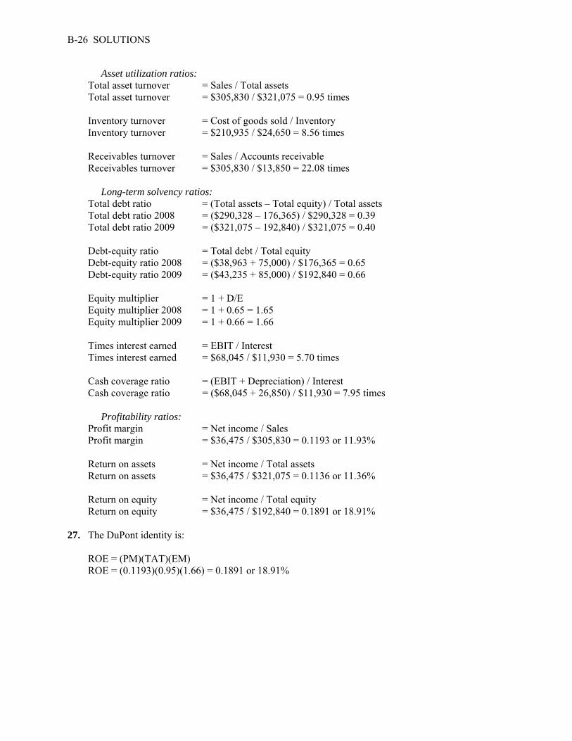
Asset utilization ratios: Total asset turnover = Sales / Total assets Total asset turnover = $305,830 / $321,075 = 0.95 times Inventory turnover = Cost of goods sold / Inventory Inventory turnover = $210,935 / $24,650 = 8.56 times Receivables turnover = Sales / Accounts receivable Receivables turnover = $305,830 / $13,850 = 22.08 times Long-term solvency ratios: Total debt ratio = (Total assets – Total equity) / Total assets Total debt ratio 2008 = ($290,328 – 176,365) / $290,328 = 0.39 Total debt ratio 2009 = ($321,075 – 192,840) / $321,075 = 0.40 Debt-equity ratio = Total debt / Total equity Debt-equity ratio 2008 = ($38,963 + 75,000) / $176,365 = 0.65 Debt-equity ratio 2009 = ($43,235 + 85,000) / $192,840 = 0.66 Equity multiplier = 1 + D/E Equity multiplier 2008 = 1 + 0.65 = 1.65 Equity multiplier 2009 = 1 + 0.66 = 1.66 Times interest earned = EBIT / Interest Times interest earned = $68,045 / $11,930 = 5.70 times Cash coverage ratio = (EBIT + Depreciation) / Interest Cash coverage ratio = ($68,045 + 26,850) / $11,930 = 7.95 times Profitability ratios: Profit margin = Net income / Sales Profit margin = $36,475 / $305,830 = 0.1193 or 11.93% Return on assets = Net income / Total assets Return on assets = $36,475 / $321,075 = 0.1136 or 11.36% Return on equity = Net income / Total equity Return on equity = $36,475 / $192,840 = 0.1891 or 18.91% 27. The DuPont identity is: ROE = (PM)(TAT)(EM) ROE = (0.1193)(0.95)(1.66) = 0.1891 or 18.91%

CHAPTER 3 B-27

28. SMOLIRA GOLF CORP. Statement of Cash Flows

For 2009

Cash, beginning of the year $ 21,860 Operating activities Net income $ 36,475 Plus: Depreciation $ 26,850 Increase in accounts payable 3,530 Increase in other current liabilities 1,742 Less: Increase in accounts receivable $ (2,534) Increase in inventory (1,566)

Net cash from operating activities $ 64,497

Investment activities Fixed asset acquisition $(53,307)

Net cash from investment activities $(53,307)

Financing activities Increase in notes payable $ (1,000) Dividends paid (20,000) Increase in long-term debt 10,000

Net cash from financing activities $(11,000)

Net increase in cash $ 190

Cash, end of year $ 22,050 29. Earnings per share = Net income / Shares Earnings per share = $36,475 / 25,000 = $1.46 per share P/E ratio = Shares price / Earnings per share P/E ratio = $43 / $1.46 = 29.47 times Dividends per share = Dividends / Shares Dividends per share = $20,000 / 25,000 = $0.80 per share Book value per share = Total equity / Shares Book value per share = $192,840 / 25,000 shares = $7.71 per share

B-28 SOLUTIONS

Market-to-book ratio = Share price / Book value per share Market-to-book ratio = $43 / $7.71 = 5.57 times PEG ratio = P/E ratio / Growth rate PEG ratio = 29.47 / 9 = 3.27 times 30. First, we will find the market value of the company’s equity, which is: Market value of equity = Shares × Share price Market value of equity = 25,000($43) = $1,075,000 The total book value of the company’s debt is: Total debt = Current liabilities + Long-term debt Total debt = $43,235 + 85,000 = $128,235 Now we can calculate Tobin’s Q, which is: Tobin’s Q = (Market value of equity + Book value of debt) / Book value of assets Tobin’s Q = ($1,075,000 + 128,235) / $321,075 Tobin’s Q = 3.75 Using the book value of debt implicitly assumes that the book value of debt is equal to the market

value of debt. This will be discussed in more detail in later chapters, but this assumption is generally true. Using the book value of assets assumes that the assets can be replaced at the current value on the balance sheet. There are several reasons this assumption could be flawed. First, inflation during the life of the assets can cause the book value of the assets to understate the market value of the assets. Since assets are recorded at cost when purchased, inflation means that it is more expensive to replace the assets. Second, improvements in technology could mean that the assets could be replaced with more productive, and possibly cheaper, assets. If this is true, the book value can overstate the market value of the assets. Finally, the book value of assets may not accurately represent the market value of the assets because of depreciation. Depreciation is done according to some schedule, generally straight-line or MACRS. Thus, the book value and market value can often diverge.

CHAPTER 4 LONG-TERM FINANCIAL PLANNING AND GROWTH Answers to Concepts Review and Critical Thinking Questions 1. The reason is that, ultimately, sales are the driving force behind a business. A firm’s assets,

employees, and, in fact, just about every aspect of its operations and financing exist to directly or indirectly support sales. Put differently, a firm’s future need for things like capital assets, employees, inventory, and financing are determined by its future sales level.

2. Two assumptions of the sustainable growth formula are that the company does not want to sell new

equity, and that financial policy is fixed. If the company raises outside equity, or increases its debt-equity ratio it can grow at a higher rate than the sustainable growth rate. Of course the company could also grow faster than its profit margin increases, if it changes its dividend policy by increasing the retention ratio, or its total asset turnover increases.

3. The internal growth rate is greater than 15%, because at a 15% growth rate the negative EFN

indicates that there is excess internal financing. If the internal growth rate is greater than 15%, then the sustainable growth rate is certainly greater than 15%, because there is additional debt financing used in that case (assuming the firm is not 100% equity-financed). As the retention ratio is increased, the firm has more internal sources of funding, so the EFN will decline. Conversely, as the retention ratio is decreased, the EFN will rise. If the firm pays out all its earnings in the form of dividends, then the firm has no internal sources of funding (ignoring the effects of accounts payable); the internal growth rate is zero in this case and the EFN will rise to the change in total assets.

4. The sustainable growth rate is greater than 20%, because at a 20% growth rate the negative EFN

indicates that there is excess financing still available. If the firm is 100% equity financed, then the sustainable and internal growth rates are equal and the internal growth rate would be greater than 20%. However, when the firm has some debt, the internal growth rate is always less than the sustainable growth rate, so it is ambiguous whether the internal growth rate would be greater than or less than 20%. If the retention ratio is increased, the firm will have more internal funding sources available, and it will have to take on more debt to keep the debt/equity ratio constant, so the EFN will decline. Conversely, if the retention ratio is decreased, the EFN will rise. If the retention rate is zero, both the internal and sustainable growth rates are zero, and the EFN will rise to the change in total assets.

5. Presumably not, but, of course, if the product had been much less popular, then a similar fate would

have awaited due to lack of sales. 6. Since customers did not pay until shipment, receivables rose. The firm’s NWC, but not its cash,

increased. At the same time, costs were rising faster than cash revenues, so operating cash flow declined. The firm’s capital spending was also rising. Thus, all three components of cash flow from assets were negatively impacted.

B-30 SOLUTIONS

7. Apparently not! In hindsight, the firm may have underestimated costs and also underestimated the

extra demand from the lower price. 8. Financing possibly could have been arranged if the company had taken quick enough action.

Sometimes it becomes apparent that help is needed only when it is too late, again emphasizing the need for planning.

9. All three were important, but the lack of cash or, more generally, financial resources ultimately

spelled doom. An inadequate cash resource is usually cited as the most common cause of small business failure.

10. Demanding cash up front, increasing prices, subcontracting production, and improving financial

resources via new owners or new sources of credit are some of the options. When orders exceed capacity, price increases may be especially beneficial.

Solutions to Questions and Problems  NOTE: All end of chapter problems were solved using a spreadsheet. Many problems require multiple steps. Due to space and readability constraints, when these intermediate steps are included in this solutions manual, rounding may appear to have occurred. However, the final answer for each problem is found without rounding during any step in the problem. Basic 1. It is important to remember that equity will not increase by the same percentage as the other assets.

If every other item on the income statement and balance sheet increases by 15 percent, the pro forma income statement and balance sheet will look like this:

Pro forma income statement Pro forma balance sheet

Sales $ 26,450 Assets $ 18,170 Debt $ 5,980 Costs 19,205 Equity 12,190 Net income $ 7,245 Total $ 18,170 Total $ 18,170 In order for the balance sheet to balance, equity must be: Equity = Total liabilities and equity – Debt Equity = $18,170 – 5,980 Equity = $12,190 Equity increased by: Equity increase = $12,190 – 10,600 Equity increase = $1,590

CHAPTER 4 B-31

Net income is $7,245 but equity only increased by $1,590; therefore, a dividend of: Dividend = $7,245 – 1,590 Dividend = $5,655 must have been paid. Dividends paid is the plug variable. 2. Here we are given the dividend amount, so dividends paid is not a plug variable. If the company pays

out one-half of its net income as dividends, the pro forma income statement and balance sheet will look like this:

Pro forma income statement Pro forma balance sheet Sales $26,450.00 Assets $18,170.00 Debt $ 5,980.00Costs 19,205.00 Equity 14,222.50Net income $ 7,245.00 Total $18,170.00 Total $19,422.50

Dividends $3,622.50 Add. to RE $3,622.50 Note that the balance sheet does not balance. This is due to EFN. The EFN for this company is: EFN = Total assets – Total liabilities and equity EFN = $18,170 – 19,422.50 EFN = –$1,252.50 3. An increase of sales to $7,424 is an increase of: Sales increase = ($7,424 – 6,300) / $6,300 Sales increase = .18 or 18% Assuming costs and assets increase proportionally, the pro forma financial statements will look like

this: Pro forma income statement Pro forma balance sheet

Sales $ 7,434 Assets $ 21,594 Debt $ 12,400 Costs 4,590 Equity 8,744 Net income $ 2,844 Total $ 21,594 Total $ 21,144 If no dividends are paid, the equity account will increase by the net income, so: Equity = $5,900 + 2,844 Equity = $8,744 So the EFN is: EFN = Total assets – Total liabilities and equity EFN = $21,594 – 21,144 = $450

B-32 SOLUTIONS

4. An increase of sales to $21,840 is an increase of: Sales increase = ($21,840 – 19,500) / $19,500 Sales increase = .12 or 12% Assuming costs and assets increase proportionally, the pro forma financial statements will look like

this: Pro forma income statement Pro forma balance sheet

Sales $ 21,840 Assets $109,760 Debt $52,500 Costs 16,800 Equity 79,208 EBIT 5,040 Total $109,760 Total $99,456 Taxes (40%) 2,016 Net income $ 3,024 The payout ratio is constant, so the dividends paid this year is the payout ratio from last year times

net income, or: Dividends = ($1,400 / $2,700)($3,024) Dividends = $1,568 The addition to retained earnings is: Addition to retained earnings = $3,024 – 1,568 Addition to retained earnings = $1,456 And the new equity balance is: Equity = $45,500 + 1,456 Equity = $46,956 So the EFN is: EFN = Total assets – Total liabilities and equity EFN = $109,760 – 99,456 EFN = $10,304 5. Assuming costs and assets increase proportionally, the pro forma financial statements will look like

this: Pro forma income statement Pro forma balance sheet

Sales $4,830.00 CA $4,140.00 CL $2,145.00Costs 3,795.00 FA 9,085.00 LTD 3,650.00Taxable income $1,035.00 Equity 6,159.86Taxes (34%) 351.90 TA $13,225.00 Total D&E $12,224.86Net income $ 683.10

CHAPTER 4 B-33

The payout ratio is 40 percent, so dividends will be: Dividends = 0.40($683.10) Dividends = $273.24 The addition to retained earnings is: Addition to retained earnings = $683.10 – 273.24 Addition to retained earnings = $409.86 So the EFN is: EFN = Total assets – Total liabilities and equity EFN = $13,225 – 12,224.86 EFN = $1,000.14 6. To calculate the internal growth rate, we first need to calculate the ROA, which is: ROA = NI / TA ROA = $2,262 / $39,150 ROA = .0578 or 5.78% The plowback ratio, b, is one minus the payout ratio, so: b = 1 – .30 b = .70 Now we can use the internal growth rate equation to get: Internal growth rate = (ROA × b) / [1 – (ROA × b)] Internal growth rate = [0.0578(.70)] / [1 – 0.0578(.70)] Internal growth rate = .0421 or 4.21% 7. To calculate the sustainable growth rate, we first need to calculate the ROE, which is: ROE = NI / TE ROE = $2,262 / $21,650 ROE = .1045 or 10.45% The plowback ratio, b, is one minus the payout ratio, so: b = 1 – .30 b = .70 Now we can use the sustainable growth rate equation to get: Sustainable growth rate = (ROE × b) / [1 – (ROE × b)] Sustainable growth rate = [0.1045(.70)] / [1 – 0.1045(.70)] Sustainable growth rate = .0789 or 7.89%

B-34 SOLUTIONS

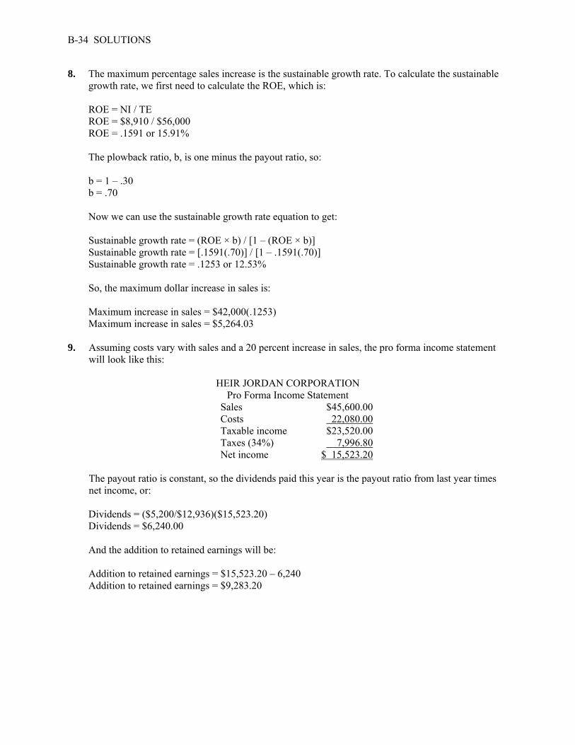
8. The maximum percentage sales increase is the sustainable growth rate. To calculate the sustainable growth rate, we first need to calculate the ROE, which is:

ROE = NI / TE ROE = $8,910 / $56,000 ROE = .1591 or 15.91% The plowback ratio, b, is one minus the payout ratio, so: b = 1 – .30 b = .70 Now we can use the sustainable growth rate equation to get: Sustainable growth rate = (ROE × b) / [1 – (ROE × b)] Sustainable growth rate = [.1591(.70)] / [1 – .1591(.70)] Sustainable growth rate = .1253 or 12.53% So, the maximum dollar increase in sales is: Maximum increase in sales = $42,000(.1253) Maximum increase in sales = $5,264.03 9. Assuming costs vary with sales and a 20 percent increase in sales, the pro forma income statement

will look like this: HEIR JORDAN CORPORATION

Pro Forma Income Statement Sales $45,600.00 Costs 22,080.00 Taxable income $23,520.00 Taxes (34%) 7,996.80 Net income $ 15,523.20

The payout ratio is constant, so the dividends paid this year is the payout ratio from last year times

net income, or: Dividends = ($5,200/$12,936)($15,523.20) Dividends = $6,240.00 And the addition to retained earnings will be: Addition to retained earnings = $15,523.20 – 6,240 Addition to retained earnings = $9,283.20

CHAPTER 4 B-35

10. Below is the balance sheet with the percentage of sales for each account on the balance sheet. Notes payable, total current liabilities, long-term debt, and all equity accounts do not vary directly with sales.

HEIR JORDAN CORPORATION

Balance Sheet ($) (%) ($) (%)

Assets Liabilities and Owners’ Equity Current assets Current liabilities Cash $ 3,050 8.03 Accounts payable $ 1,300 3.42 Accounts receivable 6,900 18.16 Notes payable 6,800 n/a Inventory 7,600 20.00 Total $ 8,100 n/a Total $ 17,550 46.18 Long-term debt 25,000 n/a Fixed assets Owners’ equity Net plant and Common stock and equipment 34,500 90.79 paid-in surplus $ 15,000 n/a Retained earnings 3,950 n/a Total $ 18,950 n/a Total liabilities and owners’ Total assets $ 52,050 136.97 equity $ 52,050 n/a 11. Assuming costs vary with sales and a 15 percent increase in sales, the pro forma income statement

will look like this: HEIR JORDAN CORPORATION

Pro Forma Income Statement Sales $43,700.00 Costs 21,160.00 Taxable income $22,540.00 Taxes (34%) 7,663.60 Net income $ 14,876.40

The payout ratio is constant, so the dividends paid this year is the payout ratio from last year times

net income, or: Dividends = ($5,200/$12,936)($14,876.40) Dividends = $5,980.00 And the addition to retained earnings will be: Addition to retained earnings = $14,876.40 – 5,980 Addition to retained earnings = $8,896.40 The new accumulated retained earnings on the pro forma balance sheet will be: New accumulated retained earnings = $3,950 + 8,896.40 New accumulated retained earnings = $12,846.40

B-36 SOLUTIONS

The pro forma balance sheet will look like this: HEIR JORDAN CORPORATION

Pro Forma Balance Sheet

Assets Liabilities and Owners’ Equity Current assets Current liabilities Cash $ 3,507.50 Accounts payable $ 1,495.00 Accounts receivable 7,935.00 Notes payable 6,800.00 Inventory 8,740.00 Total $ 8,295.00 Total $20,182.50 Long-term debt 25,000.00 Fixed assets Net plant and Owners’ equity equipment 39.675.00 Common stock and paid-in surplus $ 15,000.00 Retained earnings 12,846.40 Total $ 27,846.40 Total liabilities and owners’ Total assets $ 59,857.50 equity $ 61,141.40 So the EFN is: EFN = Total assets – Total liabilities and equity EFN = $59,857.50 – 61,141.40 EFN = –$1,283.90 12. We need to calculate the retention ratio to calculate the internal growth rate. The retention ratio is: b = 1 – .20 b = .80 Now we can use the internal growth rate equation to get: Internal growth rate = (ROA × b) / [1 – (ROA × b)] Internal growth rate = [.08(.80)] / [1 – .08(.80)] Internal growth rate = .0684 or 6.84% 13. We need to calculate the retention ratio to calculate the sustainable growth rate. The retention ratio

is: b = 1 – .25 b = .75 Now we can use the sustainable growth rate equation to get: Sustainable growth rate = (ROE × b) / [1 – (ROE × b)] Sustainable growth rate = [.15(.75)] / [1 – .15(.75)] Sustainable growth rate = .1268 or 12.68%

CHAPTER 4 B-37

14. We first must calculate the ROE to calculate the sustainable growth rate. To do this we must realize two other relationships. The total asset turnover is the inverse of the capital intensity ratio, and the equity multiplier is 1 + D/E. Using these relationships, we get:

ROE = (PM)(TAT)(EM) ROE = (.082)(1/.75)(1 + .40) ROE = .1531 or 15.31% The plowback ratio is one minus the dividend payout ratio, so: b = 1 – ($12,000 / $43,000) b = .7209 Now we can use the sustainable growth rate equation to get: Sustainable growth rate = (ROE × b) / [1 – (ROE × b)] Sustainable growth rate = [.1531(.7209)] / [1 – .1531(.7209)] Sustainable growth rate = .1240 or 12.40% 15. We must first calculate the ROE using the DuPont ratio to calculate the sustainable growth rate. The

ROE is: ROE = (PM)(TAT)(EM) ROE = (.078)(2.50)(1.80) ROE = .3510 or 35.10% The plowback ratio is one minus the dividend payout ratio, so: b = 1 – .60 b = .40 Now we can use the sustainable growth rate equation to get: Sustainable growth rate = (ROE × b) / [1 – (ROE × b)] Sustainable growth rate = [.3510(.40)] / [1 – .3510(.40)] Sustainable growth rate = .1633 or 16.33% Intermediate 16. To determine full capacity sales, we divide the current sales by the capacity the company is currently using, so: Full capacity sales = $550,000 / .95 Full capacity sales = $578,947 The maximum sales growth is the full capacity sales divided by the current sales, so: Maximum sales growth = ($578,947 / $550,000) – 1 Maximum sales growth = .0526 or 5.26%

B-38 SOLUTIONS

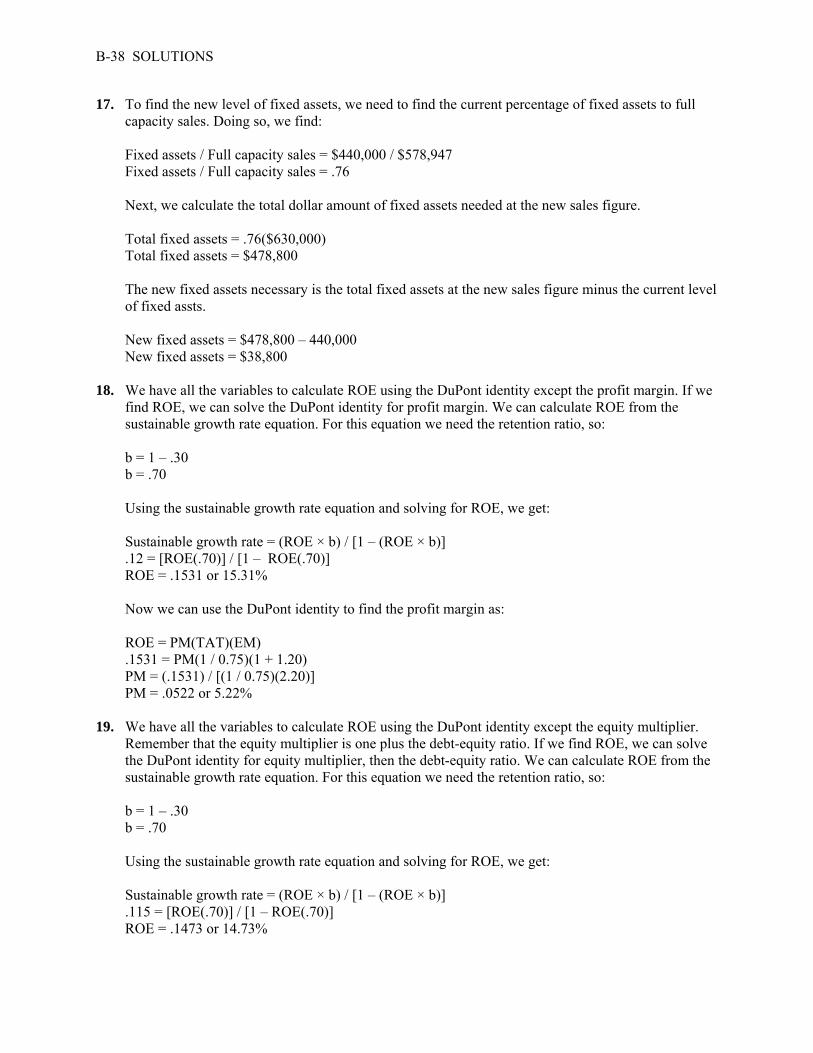
17. To find the new level of fixed assets, we need to find the current percentage of fixed assets to full capacity sales. Doing so, we find:

Fixed assets / Full capacity sales = $440,000 / $578,947 Fixed assets / Full capacity sales = .76 Next, we calculate the total dollar amount of fixed assets needed at the new sales figure. Total fixed assets = .76($630,000) Total fixed assets = $478,800 The new fixed assets necessary is the total fixed assets at the new sales figure minus the current level

of fixed assts. New fixed assets = $478,800 – 440,000 New fixed assets = $38,800 18. We have all the variables to calculate ROE using the DuPont identity except the profit margin. If we

find ROE, we can solve the DuPont identity for profit margin. We can calculate ROE from the sustainable growth rate equation. For this equation we need the retention ratio, so:

b = 1 – .30 b = .70 Using the sustainable growth rate equation and solving for ROE, we get: Sustainable growth rate = (ROE × b) / [1 – (ROE × b)] .12 = [ROE(.70)] / [1 – ROE(.70)] ROE = .1531 or 15.31% Now we can use the DuPont identity to find the profit margin as: ROE = PM(TAT)(EM) .1531 = PM(1 / 0.75)(1 + 1.20) PM = (.1531) / [(1 / 0.75)(2.20)] PM = .0522 or 5.22% 19. We have all the variables to calculate ROE using the DuPont identity except the equity multiplier.

Remember that the equity multiplier is one plus the debt-equity ratio. If we find ROE, we can solve the DuPont identity for equity multiplier, then the debt-equity ratio. We can calculate ROE from the sustainable growth rate equation. For this equation we need the retention ratio, so:

b = 1 – .30 b = .70 Using the sustainable growth rate equation and solving for ROE, we get: Sustainable growth rate = (ROE × b) / [1 – (ROE × b)] .115 = [ROE(.70)] / [1 – ROE(.70)] ROE = .1473 or 14.73%

CHAPTER 4 B-39

Now we can use the DuPont identity to find the equity multiplier as: ROE = PM(TAT)(EM) .1473 = (.062)(1 / .60)EM EM = (.1473)(.60) / .062 EM = 1.43 So, the D/E ratio is: D/E = EM – 1 D/E = 1.43 – 1 D/E = 0.43 20. We are given the profit margin. Remember that: ROA = PM(TAT) We can calculate the ROA from the internal growth rate formula, and then use the ROA in this

equation to find the total asset turnover. The retention ratio is: b = 1 – .25 b = .75 Using the internal growth rate equation to find the ROA, we get: Internal growth rate = (ROA × b) / [1 – (ROA × b)] .07 = [ROA(.75)] / [1 – ROA(.75)] ROA = .0872 or 8.72% Plugging ROA and PM into the equation we began with and solving for TAT, we get: ROA = (PM)(TAT) .0872 = .05(PM) TAT = .0872 / .05 TAT = 1.74 times 21. We should begin by calculating the D/E ratio. We calculate the D/E ratio as follows: Total debt ratio = .65 = TD / TA Inverting both sides we get: 1 / .65 = TA / TD Next, we need to recognize that TA / TD = 1 + TE / TD Substituting this into the previous equation, we get: 1 / .65 = 1 + TE /TD

B-40 SOLUTIONS

Subtract 1 (one) from both sides and inverting again, we get: D/E = 1 / [(1 / .65) – 1] D/E = 1.86 With the D/E ratio, we can calculate the EM and solve for ROE using the DuPont identity: ROE = (PM)(TAT)(EM) ROE = (.048)(1.25)(1 + 1.86) ROE = .1714 or 17.14% Now we can calculate the retention ratio as: b = 1 – .30 b = .70 Finally, putting all the numbers we have calculated into the sustainable growth rate equation, we get: Sustainable growth rate = (ROE × b) / [1 – (ROE × b)] Sustainable growth rate = [.1714(.70)] / [1 – .1714(.70)] Sustainable growth rate = .1364 or 13.64% 22. To calculate the sustainable growth rate, we first must calculate the retention ratio and ROE. The

retention ratio is: b = 1 – $9,300 / $17,500 b = .4686 And the ROE is: ROE = $17,500 / $58,000 ROE = .3017 or 30.17% So, the sustainable growth rate is: Sustainable growth rate = (ROE × b) / [1 – (ROE × b)] Sustainable growth rate = [.3017(.4686)] / [1 – .3017(.4686)] Sustainable growth rate = .1647 or 16.47% If the company grows at the sustainable growth rate, the new level of total assets is: New TA = 1.1647($86,000 + 58,000) = $167,710.84 To find the new level of debt in the company’s balance sheet, we take the percentage of debt in the

capital structure times the new level of total assets. The additional borrowing will be the new level of debt minus the current level of debt. So:

New TD = [D / (D + E)](TA) New TD = [$86,000 / ($86,000 + 58,000)]($167,710.84) New TD = $100,160.64

CHAPTER 4 B-41

And the additional borrowing will be: Additional borrowing = $100,160.04 – 86,000 Additional borrowing = $14,160.64 The growth rate that can be supported with no outside financing is the internal growth rate. To

calculate the internal growth rate, we first need the ROA, which is: ROA = $17,500 / ($86,000 + 58,000) ROA = .1215 or 12.15% This means the internal growth rate is: Internal growth rate = (ROA × b) / [1 – (ROA × b)] Internal growth rate = [.1215(.4686)] / [1 – .1215(.4686)] Internal growth rate = .0604 or 6.04% 23. Since the company issued no new equity, shareholders’ equity increased by retained earnings.

Retained earnings for the year were: Retained earnings = NI – Dividends Retained earnings = $19,000 – 2,500 Retained earnings = $16,500 So, the equity at the end of the year was: Ending equity = $135,000 + 16,500 Ending equity = $151,500 The ROE based on the end of period equity is: ROE = $19,000 / $151,500 ROE = .1254 or 12.54% The plowback ratio is: Plowback ratio = Addition to retained earnings/NI Plowback ratio = $16,500 / $19,000 Plowback ratio = .8684 or 86.84% Using the equation presented in the text for the sustainable growth rate, we get: Sustainable growth rate = (ROE × b) / [1 – (ROE × b)] Sustainable growth rate = [.1254(.8684)] / [1 – .1254(.8684)] Sustainable growth rate = .1222 or 12.22% The ROE based on the beginning of period equity is ROE = $16,500 / $135,000 ROE = .1407 or 14.07%

B-42 SOLUTIONS

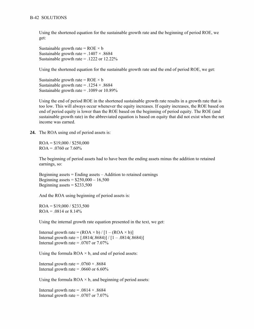
Using the shortened equation for the sustainable growth rate and the beginning of period ROE, we get:

Sustainable growth rate = ROE × b Sustainable growth rate = .1407 × .8684 Sustainable growth rate = .1222 or 12.22% Using the shortened equation for the sustainable growth rate and the end of period ROE, we get: Sustainable growth rate = ROE × b Sustainable growth rate = .1254 × .8684 Sustainable growth rate = .1089 or 10.89% Using the end of period ROE in the shortened sustainable growth rate results in a growth rate that is

too low. This will always occur whenever the equity increases. If equity increases, the ROE based on end of period equity is lower than the ROE based on the beginning of period equity. The ROE (and sustainable growth rate) in the abbreviated equation is based on equity that did not exist when the net income was earned.

24. The ROA using end of period assets is: ROA = $19,000 / $250,000 ROA = .0760 or 7.60% The beginning of period assets had to have been the ending assets minus the addition to retained

earnings, so: Beginning assets = Ending assets – Addition to retained earnings Beginning assets = $250,000 – 16,500 Beginning assets = $233,500 And the ROA using beginning of period assets is: ROA = $19,000 / $233,500 ROA = .0814 or 8.14% Using the internal growth rate equation presented in the text, we get: Internal growth rate = (ROA × b) / [1 – (ROA × b)] Internal growth rate = [.0814(.8684)] / [1 – .0814(.8684)] Internal growth rate = .0707 or 7.07% Using the formula ROA × b, and end of period assets: Internal growth rate = .0760 × .8684 Internal growth rate = .0660 or 6.60% Using the formula ROA × b, and beginning of period assets: Internal growth rate = .0814 × .8684 Internal growth rate = .0707 or 7.07%

CHAPTER 4 B-43

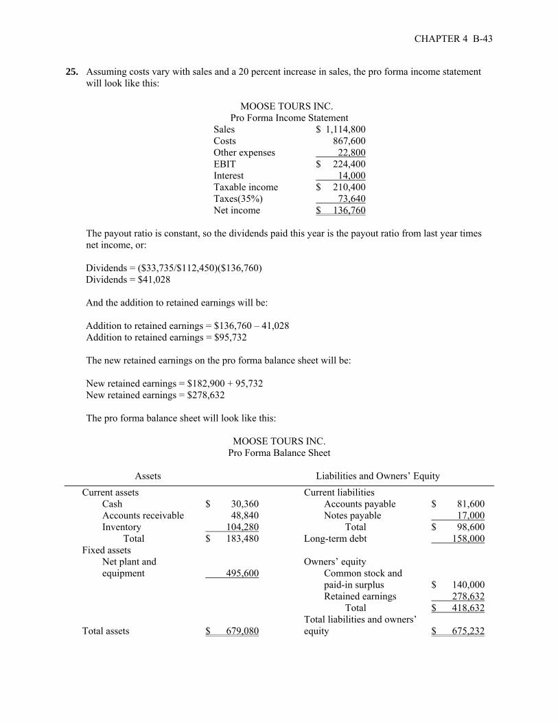
25. Assuming costs vary with sales and a 20 percent increase in sales, the pro forma income statement will look like this:

MOOSE TOURS INC. Pro Forma Income Statement Sales $ 1,114,800 Costs 867,600 Other expenses 22,800 EBIT $ 224,400 Interest 14,000 Taxable income $ 210,400 Taxes(35%) 73,640 Net income $ 136,760 The payout ratio is constant, so the dividends paid this year is the payout ratio from last year times

net income, or: Dividends = ($33,735/$112,450)($136,760) Dividends = $41,028 And the addition to retained earnings will be: Addition to retained earnings = $136,760 – 41,028 Addition to retained earnings = $95,732 The new retained earnings on the pro forma balance sheet will be: New retained earnings = $182,900 + 95,732 New retained earnings = $278,632 The pro forma balance sheet will look like this:

MOOSE TOURS INC.

Pro Forma Balance Sheet Assets Liabilities and Owners’ Equity

Current assets Current liabilities Cash $ 30,360 Accounts payable $ 81,600 Accounts receivable 48,840 Notes payable 17,000 Inventory 104,280 Total $ 98,600 Total $ 183,480 Long-term debt 158,000 Fixed assets Net plant and Owners’ equity equipment 495,600 Common stock and paid-in surplus $ 140,000 Retained earnings 278,632 Total $ 418,632 Total liabilities and owners’ Total assets $ 679,080 equity $ 675,232

B-44 SOLUTIONS

So the EFN is: EFN = Total assets – Total liabilities and equity EFN = $679,080 – 675,232 EFN = $3,848 26. First, we need to calculate full capacity sales, which is: Full capacity sales = $929,000 / .80 Full capacity sales = $1,161,250 The capital intensity ratio at full capacity sales is: Capital intensity ratio = Fixed assets / Full capacity sales Capital intensity ratio = $413,000 / $1,161,250 Capital intensity ratio = .35565 The fixed assets required at full capacity sales is the capital intensity ratio times the projected sales

level: Total fixed assets = .35565($1,161,250) = $396,480 So, EFN is: EFN = ($183,480 + 396,480) – $613,806 = –$95,272 Note that this solution assumes that fixed assets are decreased (sold) so the company has a 100

percent fixed asset utilization. If we assume fixed assets are not sold, the answer becomes: EFN = ($183,480 + 413,000) – $613,806 = –$166,154 27. The D/E ratio of the company is: D/E = ($85,000 + 158,000) / $322,900 D/E = .7526 So the new total debt amount will be: New total debt = .7526($418,632) New total debt = $315,044 This is the new total debt for the company. Given that our calculation for EFN is the amount that

must be raised externally and does not increase spontaneously with sales, we need to subtract the spontaneous increase in accounts payable. The new level of accounts payable will be, which is the current accounts payable times the sales growth, or:

Spontaneous increase in accounts payable = $68,000(.20) Spontaneous increase in accounts payable = $13,600

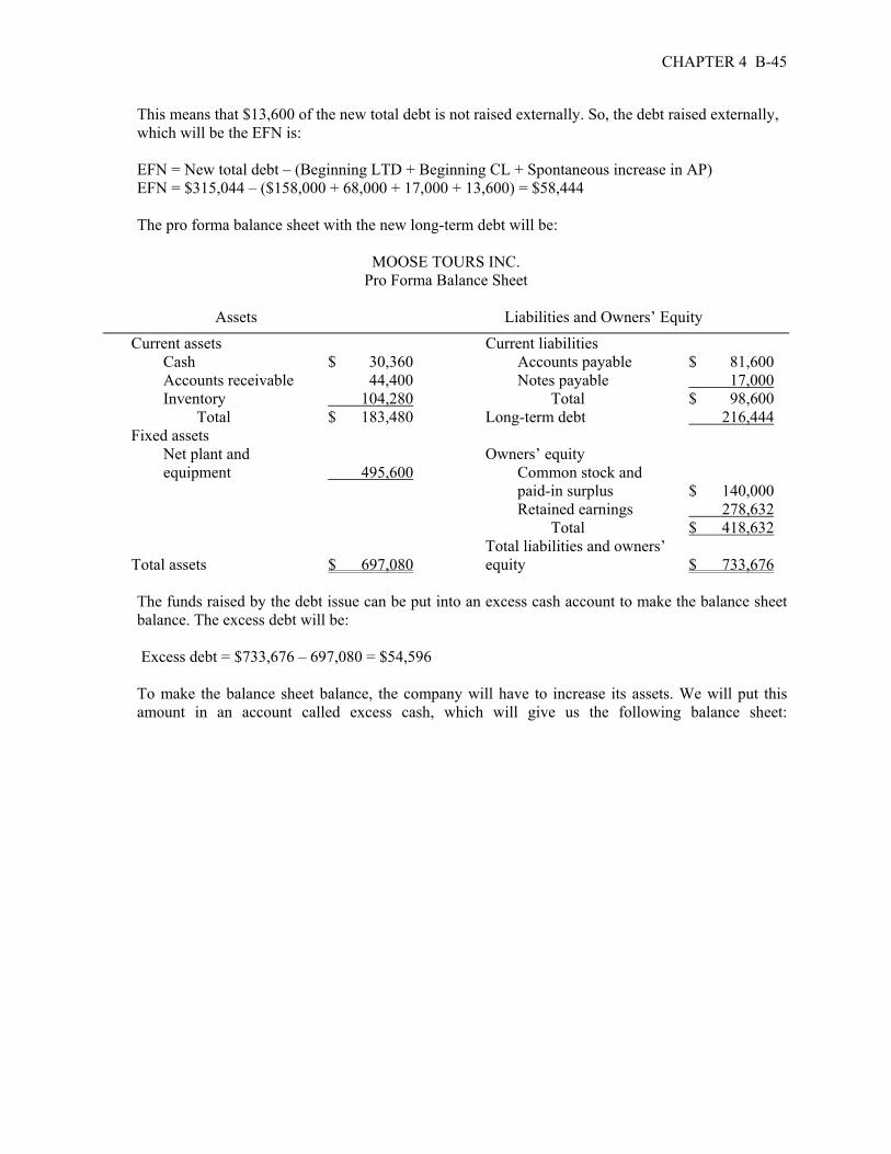
CHAPTER 4 B-45

This means that $13,600 of the new total debt is not raised externally. So, the debt raised externally, which will be the EFN is:

EFN = New total debt – (Beginning LTD + Beginning CL + Spontaneous increase in AP) EFN = $315,044 – ($158,000 + 68,000 + 17,000 + 13,600) = $58,444 The pro forma balance sheet with the new long-term debt will be:

MOOSE TOURS INC. Pro Forma Balance Sheet

Assets Liabilities and Owners’ Equity

Current assets Current liabilities Cash $ 30,360 Accounts payable $ 81,600 Accounts receivable 44,400 Notes payable 17,000 Inventory 104,280 Total $ 98,600 Total $ 183,480 Long-term debt 216,444 Fixed assets Net plant and Owners’ equity equipment 495,600 Common stock and paid-in surplus $ 140,000 Retained earnings 278,632 Total $ 418,632 Total liabilities and owners’ Total assets $ 697,080 equity $ 733,676 The funds raised by the debt issue can be put into an excess cash account to make the balance sheet

balance. The excess debt will be: Excess debt = $733,676 – 697,080 = $54,596 To make the balance sheet balance, the company will have to increase its assets. We will put this

amount in an account called excess cash, which will give us the following balance sheet:

B-46 SOLUTIONS

MOOSE TOURS INC. Pro Forma Balance Sheet

Assets Liabilities and Owners’ Equity Current assets Current liabilities Cash $ 30,360 Accounts payable $ 81,600 Excess cash 54,596 Accounts receivable 44,400 Notes payable 17,000 Inventory 104,280 Total $ 98,600 Total $ 238,076 Long-term debt 216,444 Fixed assets Net plant and Owners’ equity equipment 495,600 Common stock and paid-in surplus $ 140,000 Retained earnings 278,632 Total $ 418,632 Total liabilities and owners’ Total assets $ 733,676 equity $ 733,676 The excess cash has an opportunity cost that we discussed earlier. Increasing fixed assets would also

not be a good idea since the company already has enough fixed assets. A likely scenario would be the repurchase of debt and equity in its current capital structure weights. The company’s debt-assets and equity assets are:

Debt-assets = .7526 / (1 + .7526) = .43 Equity-assets = 1 / (1 + .7526) = .57 So, the amount of debt and equity needed will be: Total debt needed = .43($697,080) = $291,600 Equity needed = .57($697,080) = $387,480 So, the repurchases of debt and equity will be: Debt repurchase = ($98,600 + 216,444) – 291,600 = $23,444 Equity repurchase = $418,632 – 387,480 = $31,152

Assuming all of the debt repurchase is from long-term debt, and the equity repurchase is entirely from the retained earnings, the final pro forma balance sheet will be:

CHAPTER 4 B-47

MOOSE TOURS INC.

Pro Forma Balance Sheet Assets Liabilities and Owners’ Equity

Current assets Current liabilities Cash $ 30,360 Accounts payable $ 81,600 Accounts receivable 44,400 Notes payable 17,000 Inventory 104,280 Total $ 98,600 Total $ 183,480 Long-term debt 193,000 Fixed assets Net plant and Owners’ equity equipment 495,600 Common stock and paid-in surplus $ 140,000 Retained earnings 247,480 Total $ 387,480 Total liabilities and owners’ Total assets $ 697,080 equity $ 697,080 Challenge 28. The pro forma income statements for all three growth rates will be: MOOSE TOURS INC. Pro Forma Income Statement 15 % Sales

Growth20% Sales

Growth25% Sales

Growth Sales $1,068,350 $1,114,800 $1,161,250 Costs 831,450 867,600 903,750 Other expenses 21,850 22,800 23,750 EBIT $215,050 $224,400 $233,750 Interest 14,000 14,000 14,000 Taxable income $201,050 $210,400 $219,750 Taxes (35%) 70,368 73,640 76,913 Net income $130,683 $136,760 $142,838

Dividends $39,205 $41,028 $42,851 Add to RE 91,478 95,732 99,986 We will calculate the EFN for the 15 percent growth rate first. Assuming the payout ratio is constant,

the dividends paid will be: Dividends = ($33,735/$112,450)($130,683) Dividends = $39,205 And the addition to retained earnings will be: Addition to retained earnings = $130,683 – 39,205

B-48 SOLUTIONS

Addition to retained earnings = $91,478 The new retained earnings on the pro forma balance sheet will be: New retained earnings = $182,900 + 91,478 New retained earnings = $274,378 The pro forma balance sheet will look like this: 15% Sales Growth: MOOSE TOURS INC.

Pro Forma Balance Sheet Assets Liabilities and Owners’ Equity

Current assets Current liabilities Cash $ 29,095 Accounts payable $ 78,200 Accounts receivable 46,805 Notes payable 17,000 Inventory 99,935 Total $ 95,200 Total $ 175,835 Long-term debt $ 158,000 Fixed assets Net plant and Owners’ equity equipment 474,950 Common stock and paid-in surplus $ 140,000 Retained earnings 274,378 Total $ 414,378 Total liabilities and owners’ Total assets $ 650,785 equity $ 667,578 So the EFN is: EFN = Total assets – Total liabilities and equity EFN = $650,785 – 667,578 EFN = –$16,793 At a 20 percent growth rate, and assuming the payout ratio is constant, the dividends paid will be: Dividends = ($33,735/$112,450)($136,760) Dividends = $41,028 And the addition to retained earnings will be: Addition to retained earnings = $136,760 – 41,028 Addition to retained earnings = $95,732 The new retained earnings on the pro forma balance sheet will be: New retained earnings = $182,900 + 95,732 New retained earnings = $278,632

CHAPTER 4 B-49

The pro forma balance sheet will look like this: 20% Sales Growth:

MOOSE TOURS INC. Pro Forma Balance Sheet

Assets Liabilities and Owners’ Equity

Current assets Current liabilities Cash $ 30,360 Accounts payable $ 81,600 Accounts receivable 48,840 Notes payable 17,000 Inventory 104,280 Total $ 98,600 Total $ 183,480 Long-term debt $ 158,000 Fixed assets Net plant and Owners’ equity equipment 495,600 Common stock and paid-in surplus $ 140,000 Retained earnings 278,632 Total $ 418,632 Total liabilities and owners’ Total assets $ 679,080 equity $ 675,232 So the EFN is: EFN = Total assets – Total liabilities and equity EFN = $679,080 – 675,232 EFN = $3,848

At a 25 percent growth rate, and assuming the payout ratio is constant, the dividends paid will be: Dividends = ($33,735/$112,450)($142,838) Dividends = $42,851 And the addition to retained earnings will be: Addition to retained earnings = $142,838 – 42,851 Addition to retained earnings = $99,986 The new retained earnings on the pro forma balance sheet will be: New retained earnings = $182,900 + 99,986 New retained earnings = $282,886 The pro forma balance sheet will look like this:

B-50 SOLUTIONS

25% Sales Growth: MOOSE TOURS INC.

Pro Forma Balance Sheet Assets Liabilities and Owners’ Equity

Current assets Current liabilities Cash $ 31,625 Accounts payable $ 85,000 Accounts receivable 50,875 Notes payable 17,000 Inventory 108,625 Total $ 102,000 Total $ 191,125 Long-term debt $ 158,000 Fixed assets Net plant and Owners’ equity equipment 516,250 Common stock and paid-in surplus $ 140,000 Retained earnings 282,886 Total $ 422,886 Total liabilities and owners’ Total assets $ 707,375 equity $ 682,886 So the EFN is: EFN = Total assets – Total liabilities and equity EFN = $707,375 – 682,886 EFN = $24,889 29. The pro forma income statements for all three growth rates will be: MOOSE TOURS INC. Pro Forma Income Statement 20% Sales

Growth30% Sales

Growth35% Sales

Growth Sales $1,114,800 $1,207,700 $1,254,150 Costs 867,600 939,900 976,050 Other expenses 22,800 24,700 25,650 EBIT $224,400 $243,100 $252,450 Interest 14,000 14,000 14,000 Taxable income $210,400 $229,100 $238,450 Taxes (35%) 73,640 80,185 83,458 Net income $136,760 $148,915 $154,993 Dividends $41,028 $44,675 $46,498 Add to RE 95,732 104,241 108,495 At a 30 percent growth rate, and assuming the payout ratio is constant, the dividends paid will be: Dividends = ($30,810/$102,700)($135,948) Dividends = $40,784 And the addition to retained earnings will be:

CHAPTER 4 B-51

Addition to retained earnings = $135,948 – 40,784 Addition to retained earnings = $104,241 The new addition to retained earnings on the pro forma balance sheet will be: New addition to retained earnings = $182,900 + 104,241 New addition to retained earnings = $287,141 The new total debt will be: New total debt = .7556($427,141) New total debt = $321,447 So, the new long-term debt will be the new total debt minus the new short-term debt, or: New long-term debt = $321,447 – 105,400 New long-term debt = $58,047 The pro forma balance sheet will look like this: Sales growth rate = 30% and debt/equity ratio = .7526: MOOSE TOURS INC.

Pro Forma Balance Sheet Assets Liabilities and Owners’ Equity

Current assets Current liabilities Cash $ 32,890 Accounts payable $ 88,400 Accounts receivable 52,910 Notes payable 17,000 Inventory 112,970 Total $ 105,400 Total $ 198,770 Long-term debt 216,047 Fixed assets Net plant and Owners’ equity equipment 536,900 Common stock and paid-in surplus $ 140,000 Retained earnings 287,141 Total $ 427,141 Total liabilities and owners’ Total assets $ 735,670 equity $ 748,587 So the excess debt raised is: Excess debt = $748,587 – 735,670 Excess debt = $12,917 At a 35 percent growth rate, and assuming the payout ratio is constant, the dividends paid will be: Dividends = ($30,810/$102,700)($154,993) Dividends = $46,498

B-52 SOLUTIONS

And the addition to retained earnings will be: Addition to retained earnings = $154,993 – 46,498 Addition to retained earnings = $108,495 The new retained earnings on the pro forma balance sheet will be: New retained earnings = $182,900 + 108,495 New retained earnings = $291,395 The new total debt will be: New total debt = .75255($431,395) New total debt = $324,648 So, the new long-term debt will be the new total debt minus the new short-term debt, or: New long-term debt = $324,648 – 108,800 New long-term debt = $215,848

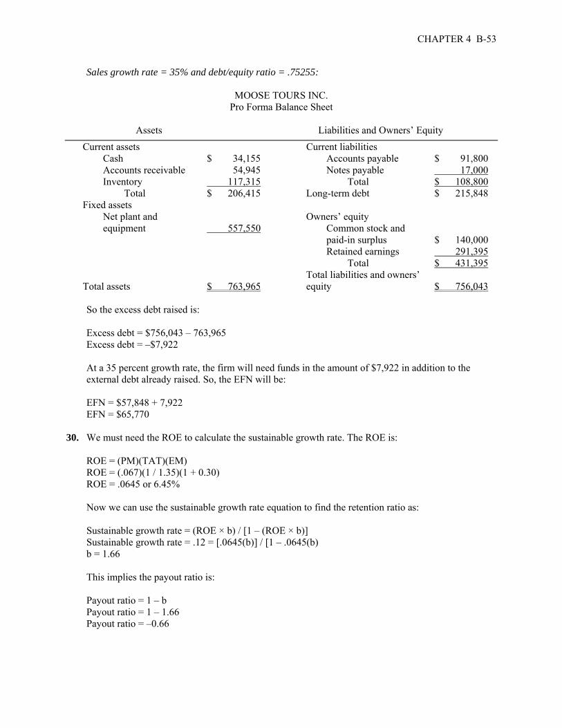
CHAPTER 4 B-53

Sales growth rate = 35% and debt/equity ratio = .75255:

MOOSE TOURS INC. Pro Forma Balance Sheet

Assets Liabilities and Owners’ Equity

Current assets Current liabilities Cash $ 34,155 Accounts payable $ 91,800 Accounts receivable 54,945 Notes payable 17,000 Inventory 117,315 Total $ 108,800 Total $ 206,415 Long-term debt $ 215,848 Fixed assets Net plant and Owners’ equity equipment 557,550 Common stock and paid-in surplus $ 140,000 Retained earnings 291,395 Total $ 431,395 Total liabilities and owners’ Total assets $ 763,965 equity $ 756,043 So the excess debt raised is: Excess debt = $756,043 – 763,965 Excess debt = –$7,922 At a 35 percent growth rate, the firm will need funds in the amount of $7,922 in addition to the

external debt already raised. So, the EFN will be: EFN = $57,848 + 7,922 EFN = $65,770 30. We must need the ROE to calculate the sustainable growth rate. The ROE is: ROE = (PM)(TAT)(EM) ROE = (.067)(1 / 1.35)(1 + 0.30) ROE = .0645 or 6.45% Now we can use the sustainable growth rate equation to find the retention ratio as: Sustainable growth rate = (ROE × b) / [1 – (ROE × b)] Sustainable growth rate = .12 = [.0645(b)] / [1 – .0645(b) b = 1.66 This implies the payout ratio is: Payout ratio = 1 – b Payout ratio = 1 – 1.66 Payout ratio = –0.66

B-54 SOLUTIONS

This is a negative dividend payout ratio of 66 percent, which is impossible. The growth rate is not consistent with the other constraints. The lowest possible payout rate is 0, which corresponds to retention ratio of 1, or total earnings retention.

The maximum sustainable growth rate for this company is: Maximum sustainable growth rate = (ROE × b) / [1 – (ROE × b)] Maximum sustainable growth rate = [.0645(1)] / [1 – .0645(1)] Maximum sustainable growth rate = .0690 or 6.90% 31. We know that EFN is: EFN = Increase in assets – Addition to retained earnings The increase in assets is the beginning assets times the growth rate, so: Increase in assets = A g The addition to retained earnings next year is the current net income times the retention ratio, times

one plus the growth rate, so: Addition to retained earnings = (NI b)(1 + g) And rearranging the profit margin to solve for net income, we get: NI = PM(S) Substituting the last three equations into the EFN equation we started with and rearranging, we get: EFN = A(g) – PM(S)b(1 + g) EFN = A(g) – PM(S)b – [PM(S)b]g EFN = – PM(S)b + [A – PM(S)b]g 32. We start with the EFN equation we derived in Problem 31 and set it equal to zero: EFN = 0 = – PM(S)b + [A – PM(S)b]g Substituting the rearranged profit margin equation into the internal growth rate equation, we have: Internal growth rate = [PM(S)b ] / [A – PM(S)b] Since: ROA = NI / A ROA = PM(S) / A We can substitute this into the internal growth rate equation and divide both the numerator and

denominator by A. This gives: Internal growth rate = {[PM(S)b] / A} / {[A – PM(S)b] / A} Internal growth rate = b(ROA) / [1 – b(ROA)]

CHAPTER 4 B-55

To derive the sustainable growth rate, we must realize that to maintain a constant D/E ratio with no external equity financing, EFN must equal the addition to retained earnings times the D/E ratio:

EFN = (D/E)[PM(S)b(1 + g)] EFN = A(g) – PM(S)b(1 + g) Solving for g and then dividing numerator and denominator by A: Sustainable growth rate = PM(S)b(1 + D/E) / [A – PM(S)b(1 + D/E )] Sustainable growth rate = [ROA(1 + D/E )b] / [1 – ROA(1 + D/E )b] Sustainable growth rate = b(ROE) / [1 – b(ROE)] 33. In the following derivations, the subscript “E” refers to end of period numbers, and the subscript “B”

refers to beginning of period numbers. TE is total equity and TA is total assets. For the sustainable growth rate: Sustainable growth rate = (ROEE × b) / (1 – ROEE × b) Sustainable growth rate = (NI/TEE × b) / (1 – NI/TEE × b) We multiply this equation by: (TEE / TEE) Sustainable growth rate = (NI / TEE × b) / (1 – NI / TEE × b) × (TEE / TEE) Sustainable growth rate = (NI × b) / (TEE – NI × b) Recognize that the numerator is equal to beginning of period equity, that is: (TEE – NI × b) = TEB Substituting this into the previous equation, we get: Sustainable rate = (NI × b) / TEB Which is equivalent to: Sustainable rate = (NI / TEB) × b Since ROEB = NI / TEB

The sustainable growth rate equation is: Sustainable growth rate = ROEB × b For the internal growth rate: Internal growth rate = (ROAE × b) / (1 – ROAE × b) Internal growth rate = (NI / TAE × b) / (1 – NI / TAE × b)

B-56 SOLUTIONS

We multiply this equation by: (TAE / TAE) Internal growth rate = (NI / TAE × b) / (1 – NI / TAE × b) × (TAE / TAE) Internal growth rate = (NI × b) / (TAE – NI × b) Recognize that the numerator is equal to beginning of period assets, that is: (TAE – NI × b) = TAB Substituting this into the previous equation, we get: Internal growth rate = (NI × b) / TAB Which is equivalent to: Internal growth rate = (NI / TAB) × b Since ROAB = NI / TAB

The internal growth rate equation is: Internal growth rate = ROAB × b

CHAPTER 5 INTRODUCTION TO VALUATION: THE TIME VALUE OF MONEY Answers to Concepts Review and Critical Thinking Questions 1. The four parts are the present value (PV), the future value (FV), the discount rate (r), and the life of

the investment (t). 2. Compounding refers to the growth of a dollar amount through time via reinvestment of interest

earned. It is also the process of determining the future value of an investment. Discounting is the process of determining the value today of an amount to be received in the future.

3. Future values grow (assuming a positive rate of return); present values shrink. 4. The future value rises (assuming it’s positive); the present value falls. 5. It would appear to be both deceptive and unethical to run such an ad without a disclaimer or

explanation. 6. It’s a reflection of the time value of money. TMCC gets to use the $24,099. If TMCC uses it wisely,

it will be worth more than $100,000 in thirty years. 7. This will probably make the security less desirable. TMCC will only repurchase the security prior to

maturity if it is to its advantage, i.e. interest rates decline. Given the drop in interest rates needed to make this viable for TMCC, it is unlikely the company will repurchase the security. This is an example of a “call” feature. Such features are discussed at length in a later chapter.

8. The key considerations would be: (1) Is the rate of return implicit in the offer attractive relative to

other, similar risk investments? and (2) How risky is the investment; i.e., how certain are we that we will actually get the $100,000? Thus, our answer does depend on who is making the promise to repay.

9. The Treasury security would have a somewhat higher price because the Treasury is the strongest of

all borrowers. 10. The price would be higher because, as time passes, the price of the security will tend to rise toward

$100,000. This rise is just a reflection of the time value of money. As time passes, the time until receipt of the $100,000 grows shorter, and the present value rises. In 2019, the price will probably be higher for the same reason. We cannot be sure, however, because interest rates could be much higher, or TMCC’s financial position could deteriorate. Either event would tend to depress the security’s price.

B-58 SOLUTIONS

Solutions to Questions and Problems NOTE: All end of chapter problems were solved using a spreadsheet. Many problems require multiple steps. Due to space and readability constraints, when these intermediate steps are included in this solutions manual, rounding may appear to have occurred. However, the final answer for each problem is found without rounding during any step in the problem. Basic 1. The simple interest per year is: $5,000 × .08 = $400 So after 10 years you will have: $400 × 10 = $4,000 in interest. The total balance will be $5,000 + 4,000 = $9,000 With compound interest we use the future value formula: FV = PV(1 +r)t FV = $5,000(1.08)10 = $10,794.62 The difference is: $10,794.62 – 9,000 = $1,794.62 2. To find the FV of a lump sum, we use: FV = PV(1 + r)t FV = $2,250(1.10)11 = $ 6,419.51 FV = $8,752(1.08)7 = $ 14,999.39 FV = $76,355(1.17)14 = $687,764.17 FV = $183,796(1.07)8 = $315,795.75 3. To find the PV of a lump sum, we use: PV = FV / (1 + r)t

PV = $15,451 / (1.07)6 = $ 10,295.65 PV = $51,557 / (1.13)7 = $ 21,914.85 PV = $886,073 / (1.14)23 = $ 43,516.90 PV = $550,164 / (1.09)18 = $116,631.32

CHAPTER 5 B-59

4. To answer this question, we can use either the FV or the PV formula. Both will give the same answer since they are the inverse of each other. We will use the FV formula, that is:

FV = PV(1 + r)t Solving for r, we get: r = (FV / PV)1 / t – 1 FV = $297 = $240(1 + r)2; r = ($297 / $240)1/2 – 1 = 11.24% FV = $1,080 = $360(1 + r)10; r = ($1,080 / $360)1/10 – 1 = 11.61% FV = $185,382 = $39,000(1 + r)15; r = ($185,382 / $39,000)1/15 – 1 = 10.95% FV = $531,618 = $38,261(1 + r)30; r = ($531,618 / $38,261)1/30 – 1 = 9.17% 5. To answer this question, we can use either the FV or the PV formula. Both will give the same answer

since they are the inverse of each other. We will use the FV formula, that is: FV = PV(1 + r)t Solving for t, we get: t = ln(FV / PV) / ln(1 + r) FV = $1,284 = $560(1.09)t; t = ln($1,284/ $560) / ln 1.09 = 9.63 years FV = $4,341 = $810(1.10)t; t = ln($4,341/ $810) / ln 1.10 = 17.61 years FV = $364,518 = $18,400(1.17)t; t = ln($364,518 / $18,400) / ln 1.17 = 19.02 years FV = $173,439 = $21,500(1.15)t; t = ln($173,439 / $21,500) / ln 1.15 = 14.94 years 6. To answer this question, we can use either the FV or the PV formula. Both will give the same answer

since they are the inverse of each other. We will use the FV formula, that is: FV = PV(1 + r)t Solving for r, we get: r = (FV / PV)1 / t – 1 r = ($290,000 / $55,000)1/18 – 1 = .0968 or 9.68%

B-60 SOLUTIONS

7. To find the length of time for money to double, triple, etc., the present value and future value are irrelevant as long as the future value is twice the present value for doubling, three times as large for tripling, etc. To answer this question, we can use either the FV or the PV formula. Both will give the same answer since they are the inverse of each other. We will use the FV formula, that is:

FV = PV(1 + r)t Solving for t, we get: t = ln(FV / PV) / ln(1 + r) The length of time to double your money is: FV = $2 = $1(1.07)t

t = ln 2 / ln 1.07 = 10.24 years The length of time to quadruple your money is: FV = $4 = $1(1.07)t t = ln 4 / ln 1.07 = 20.49 years Notice that the length of time to quadruple your money is twice as long as the time needed to double

your money (the difference in these answers is due to rounding). This is an important concept of time value of money.

8. To answer this question, we can use either the FV or the PV formula. Both will give the same answer

since they are the inverse of each other. We will use the FV formula, that is: FV = PV(1 + r)t Solving for r, we get: r = (FV / PV)1 / t – 1 r = ($314,600 / $200,300)1/7 – 1 = .0666 or 6.66% 9. To answer this question, we can use either the FV or the PV formula. Both will give the same answer

since they are the inverse of each other. We will use the FV formula, that is: FV = PV(1 + r)t Solving for t, we get: t = ln(FV / PV) / ln(1 + r) t = ln ($170,000 / $40,000) / ln 1.053 = 28.02 years 10. To find the PV of a lump sum, we use: PV = FV / (1 + r)t

PV = $650,000,000 / (1.074)20 = $155,893,400.13

CHAPTER 5 B-61

11. To find the PV of a lump sum, we use: PV = FV / (1 + r)t

PV = $1,000,000 / (1.10)80 = $488.19 12. To find the FV of a lump sum, we use: FV = PV(1 + r)t FV = $50(1.045)105 = $5,083.71 13. To answer this question, we can use either the FV or the PV formula. Both will give the same answer

since they are the inverse of each other. We will use the FV formula, that is: FV = PV(1 + r)t Solving for r, we get: r = (FV / PV)1 / t – 1 r = ($1,260,000 / $150)1/112 – 1 = .0840 or 8.40%

To find the FV of the first prize, we use: FV = PV(1 + r)t FV = $1,260,000(1.0840)33 = $18,056,409.94 14. To answer this question, we can use either the FV or the PV formula. Both will give the same answer

since they are the inverse of each other. We will use the FV formula, that is: FV = PV(1 + r)t Solving for r, we get: r = (FV / PV)1 / t – 1 r = ($43,125 / $1)1/113 – 1 = .0990 or 9.90% 15. To answer this question, we can use either the FV or the PV formula. Both will give the same answer

since they are the inverse of each other. We will use the FV formula, that is: FV = PV(1 + r)t Solving for r, we get: r = (FV / PV)1 / t – 1 r = ($10,311,500 / $12,377,500)1/4 – 1 = – 4.46% Notice that the interest rate is negative. This occurs when the FV is less than the PV.

B-62 SOLUTIONS

Intermediate 16. To answer this question, we can use either the FV or the PV formula. Both will give the same answer

since they are the inverse of each other. We will use the FV formula, that is: FV = PV(1 + r)t Solving for r, we get: r = (FV / PV)1 / t – 1 a. PV = $100,000 / (1 + r)30 = $24,099 r = ($100,000 / $24,099)1/30 – 1 = .0486 or 4.86% b. PV = $38,260 / (1 + r)12 = $24,099 r = ($38,260 / $24,099)1/12 – 1 = .0393 or 3.93% c. PV = $100,000 / (1 + r)18 = $38,260 r = ($100,000 / $38,260)1/18 – 1 = .0548 or 5.48% 17. To find the PV of a lump sum, we use: PV = FV / (1 + r)t

PV = $170,000 / (1.12)9 = $61,303.70 18. To find the FV of a lump sum, we use: FV = PV(1 + r)t FV = $4,000(1.11)45 = $438,120.97 FV = $4,000(1.11)35 = $154,299.40 Better start early! 19. We need to find the FV of a lump sum. However, the money will only be invested for six years, so

the number of periods is six. FV = PV(1 + r)t FV = $20,000(1.084)6 = $32,449.33

CHAPTER 5 B-63

20. To answer this question, we can use either the FV or the PV formula. Both will give the same answer since they are the inverse of each other. We will use the FV formula, that is:

FV = PV(1 + r)t Solving for t, we get: t = ln(FV / PV) / ln(1 + r) t = ln($75,000 / $10,000) / ln(1.11) = 19.31 So, the money must be invested for 19.31 years. However, you will not receive the money for

another two years. From now, you’ll wait: 2 years + 19.31 years = 21.31 years Calculator Solutions 1. Enter 10 8% $5,000 N I/Y PV PMT FV Solve for $10,794.62 $10,794.62 – 9,000 = $1,794.62 2. Enter 11 10% $2,250 N I/Y PV PMT FV Solve for $6,419.51 Enter 7 8% $8,752 N I/Y PV PMT FV Solve for $14,999.39 Enter 14 17% $76,355 N I/Y PV PMT FV Solve for $687,764.17 Enter 8 7% $183,796 N I/Y PV PMT FV Solve for $315,795.75 3. Enter 6 7% $15,451 N I/Y PV PMT FV Solve for $10,295.65

B-64 SOLUTIONS

Enter 7 13% $51,557 N I/Y PV PMT FV Solve for $21,914.85 Enter 23 14% $886,073 N I/Y PV PMT FV Solve for $43,516.90 Enter 18 9% $550,164 N I/Y PV PMT FV Solve for $116,631.32 4. Enter 2 $240 $297 N I/Y PV PMT FV Solve for 11.24% Enter 10 $360 $1,080 N I/Y PV PMT FV Solve for 11.61% Enter 15 $39,000 $185,382 N I/Y PV PMT FV Solve for 10.95% Enter 30 $38,261 $531,618 N I/Y PV PMT FV Solve for 9.17% 5. Enter 9% $560 $1,284 N I/Y PV PMT FV Solve for 9.63 Enter 10% $810 $4,341 N I/Y PV PMT FV Solve for 17.61 Enter 17% $18,400 $364,518 N I/Y PV PMT FV Solve for 19.02

CHAPTER 5 B-65

Enter 15% $21,500 $173,439 N I/Y PV PMT FV Solve for 14.94 6. Enter 18 $55,000 $290,000 N I/Y PV PMT FV Solve for 9.68% 7. Enter 7% $1 $2 N I/Y PV PMT FV Solve for 10.24 Enter 7% $1 $4 N I/Y PV PMT FV Solve for 20.49 8. Enter 7 $200,300 $314,600 N I/Y PV PMT FV Solve for 6.66% 9. Enter 5.30% $40,000 $170,000 N I/Y PV PMT FV Solve for 28.02 10. Enter 20 7.4% $650,000,000 N I/Y PV PMT FV Solve for $155,893,400.13 11. Enter 80 10% $1,000,000 N I/Y PV PMT FV Solve for $488.19 12. Enter 105 4.50% $50 N I/Y PV PMT FV Solve for $5,083.71

B-66 SOLUTIONS

13. Enter 112 $150 $1,260,000 N I/Y PV PMT FV Solve for 8.40% Enter 33 8.40% $1,260,000 N I/Y PV PMT FV Solve for $18,056,404.94 14. Enter 113 $1 ±$43,125 N I/Y PV PMT FV Solve for 9.90% 15. Enter 4 $12,377,500 $10,311,500 N I/Y PV PMT FV Solve for –4.46% 16. a. Enter 30 $24,099 $100,000 N I/Y PV PMT FV Solve for 4.86% 16. b. Enter 12 $24,099 $38,260 N I/Y PV PMT FV Solve for 3.93% 16. c. Enter 18 $38,260 $100,000 N I/Y PV PMT FV Solve for 5.48% 17. Enter 9 12% $170,000 N I/Y PV PMT FV Solve for $61,303.70 18. Enter 45 11% $4,000 N I/Y PV PMT FV Solve for $438,120.97 Enter 35 11% $4,000 N I/Y PV PMT FV Solve for $154,299.40

CHAPTER 5 B-67

19. Enter 6 8.40% $20,000 N I/Y PV PMT FV Solve for $32,449.33 20. Enter 11% $10,000 $75,000 N I/Y PV PMT FV Solve for 19.31 From now, you’ll wait 2 + 19.31 = 21.31 years

CHAPTER 6 DISCOUNTED CASH FLOW VALUATION Answers to Concepts Review and Critical Thinking Questions 1. The four pieces are the present value (PV), the periodic cash flow (C), the discount rate (r), and the number

of payments, or the life of the annuity, t. 2. Assuming positive cash flows, both the present and the future values will rise. 3. Assuming positive cash flows, the present value will fall and the future value will rise. 4. It’s deceptive, but very common. The basic concept of time value of money is that a dollar today is not

worth the same as a dollar tomorrow. The deception is particularly irritating given that such lotteries are usually government sponsored!

5. If the total money is fixed, you want as much as possible as soon as possible. The team (or, more

accurately, the team owner) wants just the opposite. 6. The better deal is the one with equal installments. 7. Yes, they should. APRs generally don’t provide the relevant rate. The only advantage is that they are easier

to compute, but, with modern computing equipment, that advantage is not very important. 8. A freshman does. The reason is that the freshman gets to use the money for much longer before interest

starts to accrue. The subsidy is the present value (on the day the loan is made) of the interest that would have accrued up until the time it actually begins to accrue.

9. The problem is that the subsidy makes it easier to repay the loan, not obtain it. However, ability to repay

the loan depends on future employment, not current need. For example, consider a student who is currently needy, but is preparing for a career in a high-paying area (such as corporate finance!). Should this student receive the subsidy? How about a student who is currently not needy, but is preparing for a relatively low-paying job (such as becoming a college professor)?

CHAPTER 6 B-69

10. In general, viatical settlements are ethical. In the case of a viatical settlement, it is simply an exchange of cash today for payment in the future, although the payment depends on the death of the seller. The purchaser of the life insurance policy is bearing the risk that the insured individual will live longer than expected. Although viatical settlements are ethical, they may not be the best choice for an individual. In a Business Week article (October 31, 2005), options were examined for a 72 year old male with a life expectancy of 8 years and a $1 million dollar life insurance policy with an annual premium of $37,000. The four options were: 1) Cash the policy today for $100,000. 2) Sell the policy in a viatical settlement for $275,000. 3) Reduce the death benefit to $375,000, which would keep the policy in force for 12 years without premium payments. 4) Stop paying premiums and don’t reduce the death benefit. This will run the cash value of the policy to zero in 5 years, but the viatical settlement would be worth $475,000 at that time. If he died within 5 years, the beneficiaries would receive $1 million. Ultimately, the decision rests on the individual on what they perceive as best for themselves. The values that will affect the value of the viatical settlement are the discount rate, the face value of the policy, and the health of the individual selling the policy.

Solutions to Questions and Problems NOTE: All end of chapter problems were solved using a spreadsheet. Many problems require multiple steps. Due to space and readability constraints, when these intermediate steps are included in this solutions manual, rounding may appear to have occurred. However, the final answer for each problem is found without rounding during any step in the problem. Basic 1. To solve this problem, we must find the PV of each cash flow and add them. To find the PV of a lump sum,

we use: PV = FV / (1 + r)t

PV@10% = $950 / 1.10 + $1,040 / 1.102 + $1,130 / 1.103 + $1,075 / 1.104 = $3,306.37 PV@18% = $950 / 1.18 + $1,040 / 1.182 + $1,130 / 1.183 + $1,075 / 1.184 = $2,794.22 PV@24% = $950 / 1.24 + $1,040 / 1.242 + $1,130 / 1.243 + $1,075 / 1.244 = $2,489.88 2. To find the PVA, we use the equation: PVA = C({1 – [1/(1 + r)]t } / r ) At a 5 percent interest rate: X@5%: PVA = $6,000{[1 – (1/1.05)9 ] / .05 } = $42,646.93 Y@5%: PVA = $8,000{[1 – (1/1.05)6 ] / .05 } = $40,605.54

B-70 SOLUTIONS

And at a 15 percent interest rate: X@15%: PVA = $6,000{[1 – (1/1.15)9 ] / .15 } = $28,629.50 Y@15%: PVA = $8,000{[1 – (1/1.15)6 ] / .15 } = $30,275.86

Notice that the PV of cash flow X has a greater PV at a 5 percent interest rate, but a lower PV at a 15 percent interest rate. The reason is that X has greater total cash flows. At a lower interest rate, the total cash flow is more important since the cost of waiting (the interest rate) is not as great. At a higher interest rate, Y is more valuable since it has larger cash flows. At the higher interest rate, these bigger cash flows early are more important since the cost of waiting (the interest rate) is so much greater.

3. To solve this problem, we must find the FV of each cash flow and add them. To find the FV of a lump sum,

we use: FV = PV(1 + r)t

FV@8% = $940(1.08)3 + $1,090(1.08)2 + $1,340(1.08) + $1,405 = $5,307.71 FV@11% = $940(1.11)3 + $1,090(1.11)2 + $1,340(1.11) + $1,405 = $5,520.96 FV@24% = $940(1.24)3 + $1,090(1.24)2 + $1,340(1.24) + $1,405 = $6,534.81

Notice we are finding the value at Year 4, the cash flow at Year 4 is simply added to the FV of the other cash flows. In other words, we do not need to compound this cash flow.

4. To find the PVA, we use the equation: PVA = C({1 – [1/(1 + r)]t } / r ) PVA@15 yrs: PVA = $5,300{[1 – (1/1.07)15 ] / .07} = $48,271.94 PVA@40 yrs: PVA = $5,300{[1 – (1/1.07)40 ] / .07} = $70,658.06 PVA@75 yrs: PVA = $5,300{[1 – (1/1.07)75 ] / .07} = $75,240.70 To find the PV of a perpetuity, we use the equation: PV = C / r PV = $5,300 / .07 = $75,714.29

Notice that as the length of the annuity payments increases, the present value of the annuity approaches the present value of the perpetuity. The present value of the 75 year annuity and the present value of the perpetuity imply that the value today of all perpetuity payments beyond 75 years is only $473.59.

CHAPTER 6 B-71

5. Here we have the PVA, the length of the annuity, and the interest rate. We want to calculate the annuity payment. Using the PVA equation:

PVA = C({1 – [1/(1 + r)]t } / r ) PVA = $34,000 = $C{[1 – (1/1.0765)15 ] / .0765} We can now solve this equation for the annuity payment. Doing so, we get: C = $34,000 / 8.74548 = $3,887.72 6. To find the PVA, we use the equation: PVA = C({1 – [1/(1 + r)]t } / r ) PVA = $73,000{[1 – (1/1.085)8 ] / .085} = $411,660.36 7. Here we need to find the FVA. The equation to find the FVA is: FVA = C{[(1 + r)t – 1] / r} FVA for 20 years = $4,000[(1.11220 – 1) / .112] = $262,781.16 FVA for 40 years = $4,000[(1.11240 – 1) / .112] = $2,459,072.63 Notice that because of exponential growth, doubling the number of periods does not merely double the

FVA. 8. Here we have the FVA, the length of the annuity, and the interest rate. We want to calculate the annuity

payment. Using the FVA equation: FVA = C{[(1 + r)t – 1] / r} $90,000 = $C[(1.06810 – 1) / .068] We can now solve this equation for the annuity payment. Doing so, we get: C = $90,000 / 13.68662 = $6,575.77 9. Here we have the PVA, the length of the annuity, and the interest rate. We want to calculate the annuity

payment. Using the PVA equation: PVA = C({1 – [1/(1 + r)]t } / r) $50,000 = C{[1 – (1/1.075)7 ] / .075} We can now solve this equation for the annuity payment. Doing so, we get: C = $50,000 / 5.29660 = $9,440.02 10. This cash flow is a perpetuity. To find the PV of a perpetuity, we use the equation: PV = C / r PV = $25,000 / .072 = $347,222.22

B-72 SOLUTIONS

11. Here we need to find the interest rate that equates the perpetuity cash flows with the PV of the cash flows. Using the PV of a perpetuity equation:

PV = C / r $375,000 = $25,000 / r We can now solve for the interest rate as follows: r = $25,000 / $375,000 = .0667 or 6.67% 12. For discrete compounding, to find the EAR, we use the equation: EAR = [1 + (APR / m)]m – 1 EAR = [1 + (.08 / 4)]4 – 1 = .0824 or 8.24% EAR = [1 + (.16 / 12)]12 – 1 = .1723 or 17.23% EAR = [1 + (.12 / 365)]365 – 1 = .1275 or 12.75% To find the EAR with continuous compounding, we use the equation: EAR = eq – 1 EAR = e.15 – 1 = .1618 or 16.18% 13. Here we are given the EAR and need to find the APR. Using the equation for discrete compounding: EAR = [1 + (APR / m)]m – 1 We can now solve for the APR. Doing so, we get: APR = m[(1 + EAR)1/m – 1] EAR = .0860 = [1 + (APR / 2)]2 – 1 APR = 2[(1.0860)1/2 – 1] = .0842 or 8.42% EAR = .1980 = [1 + (APR / 12)]12 – 1 APR = 12[(1.1980)1/12 – 1] = .1820 or 18.20% EAR = .0940 = [1 + (APR / 52)]52 – 1 APR = 52[(1.0940)1/52 – 1] = .0899 or 8.99% Solving the continuous compounding EAR equation: EAR = eq – 1 We get: APR = ln(1 + EAR) APR = ln(1 + .1650) APR = .1527 or 15.27%

CHAPTER 6 B-73

14. For discrete compounding, to find the EAR, we use the equation: EAR = [1 + (APR / m)]m – 1 So, for each bank, the EAR is: First National: EAR = [1 + (.1420 / 12)]12 – 1 = .1516 or 15.16% First United: EAR = [1 + (.1450 / 2)]2 – 1 = .1503 or 15.03% Notice that the higher APR does not necessarily mean the higher EAR. The number of compounding

periods within a year will also affect the EAR. 15. The reported rate is the APR, so we need to convert the EAR to an APR as follows: EAR = [1 + (APR / m)]m – 1 APR = m[(1 + EAR)1/m – 1] APR = 365[(1.16)1/365 – 1] = .1485 or 14.85% This is deceptive because the borrower is actually paying annualized interest of 16% per year, not the

14.85% reported on the loan contract. 16. For this problem, we simply need to find the FV of a lump sum using the equation: FV = PV(1 + r)t

It is important to note that compounding occurs semiannually. To account for this, we will divide the

interest rate by two (the number of compounding periods in a year), and multiply the number of periods by two. Doing so, we get:

FV = $2,100[1 + (.084/2)]34 = $8,505.93 17. For this problem, we simply need to find the FV of a lump sum using the equation: FV = PV(1 + r)t

It is important to note that compounding occurs daily. To account for this, we will divide the interest rate

by 365 (the number of days in a year, ignoring leap year), and multiply the number of periods by 365. Doing so, we get:

FV in 5 years = $4,500[1 + (.093/365)]5(365) = $7,163.64 FV in 10 years = $4,500[1 + (.093/365)]10(365) = $11,403.94 FV in 20 years = $4,500[1 + (.093/365)]20(365) = $28,899.97

B-74 SOLUTIONS

18. For this problem, we simply need to find the PV of a lump sum using the equation: PV = FV / (1 + r)t

It is important to note that compounding occurs daily. To account for this, we will divide the interest rate

by 365 (the number of days in a year, ignoring leap year), and multiply the number of periods by 365. Doing so, we get:

PV = $58,000 / [(1 + .10/365)7(365)] = $28,804.71 19. The APR is simply the interest rate per period times the number of periods in a year. In this case, the

interest rate is 30 percent per month, and there are 12 months in a year, so we get: APR = 12(30%) = 360% To find the EAR, we use the EAR formula: EAR = [1 + (APR / m)]m – 1 EAR = (1 + .30)12 – 1 = 2,229.81% Notice that we didn’t need to divide the APR by the number of compounding periods per year. We do this

division to get the interest rate per period, but in this problem we are already given the interest rate per period.

20. We first need to find the annuity payment. We have the PVA, the length of the annuity, and the interest

rate. Using the PVA equation: PVA = C({1 – [1/(1 + r)]t } / r) $68,500 = $C[1 – {1 / [1 + (.069/12)]60} / (.069/12)] Solving for the payment, we get: C = $68,500 / 50.622252 = $1,353.15 To find the EAR, we use the EAR equation: EAR = [1 + (APR / m)]m – 1 EAR = [1 + (.069 / 12)]12 – 1 = .0712 or 7.12% 21. Here we need to find the length of an annuity. We know the interest rate, the PV, and the payments. Using

the PVA equation: PVA = C({1 – [1/(1 + r)]t } / r) $18,000 = $500{[1 – (1/1.013)t ] / .013}

CHAPTER 6 B-75

Now we solve for t: 1/1.013t = 1 – {[($18,000)/($500)](.013)} 1/1.013t = 0.532 1.013t = 1/(0.532) = 1.8797 t = ln 1.8797 / ln 1.013 = 48.86 months 22. Here we are trying to find the interest rate when we know the PV and FV. Using the FV equation: FV = PV(1 + r) $4 = $3(1 + r) r = 4/3 – 1 = 33.33% per week The interest rate is 33.33% per week. To find the APR, we multiply this rate by the number of weeks in a

year, so: APR = (52)33.33% = 1,733.33% And using the equation to find the EAR: EAR = [1 + (APR / m)]m – 1 EAR = [1 + .3333]52 – 1 = 313,916,515.69% 23. Here we need to find the interest rate that equates the perpetuity cash flows with the PV of the cash flows.

Using the PV of a perpetuity equation: PV = C / r $95,000 = $1,800 / r We can now solve for the interest rate as follows: r = $1,800 / $95,000 = .0189 or 1.89% per month The interest rate is 1.89% per month. To find the APR, we multiply this rate by the number of months in a

year, so: APR = (12)1.89% = 22.74% And using the equation to find an EAR: EAR = [1 + (APR / m)]m – 1 EAR = [1 + .0189]12 – 1 = 25.26% 24. This problem requires us to find the FVA. The equation to find the FVA is: FVA = C{[(1 + r)t – 1] / r} FVA = $300[{[1 + (.10/12) ]360 – 1} / (.10/12)] = $678,146.38

B-76 SOLUTIONS

25. In the previous problem, the cash flows are monthly and the compounding period is monthly. This assumption still holds. Since the cash flows are annual, we need to use the EAR to calculate the future value of annual cash flows. It is important to remember that you have to make sure the compounding periods of the interest rate is the same as the timing of the cash flows. In this case, we have annual cash flows, so we need the EAR since it is the true annual interest rate you will earn. So, finding the EAR:

EAR = [1 + (APR / m)]m – 1 EAR = [1 + (.10/12)]12 – 1 = .1047 or 10.47% Using the FVA equation, we get: FVA = C{[(1 + r)t – 1] / r} FVA = $3,600[(1.104730 – 1) / .1047] = $647,623.45 26. The cash flows are simply an annuity with four payments per year for four years, or 16 payments. We can

use the PVA equation: PVA = C({1 – [1/(1 + r)]t } / r) PVA = $2,300{[1 – (1/1.0065)16] / .0065} = $34,843.71 27. The cash flows are annual and the compounding period is quarterly, so we need to calculate the EAR to

make the interest rate comparable with the timing of the cash flows. Using the equation for the EAR, we get:

EAR = [1 + (APR / m)]m – 1 EAR = [1 + (.11/4)]4 – 1 = .1146 or 11.46% And now we use the EAR to find the PV of each cash flow as a lump sum and add them together: PV = $725 / 1.1146 + $980 / 1.11462 + $1,360 / 1.11464 = $2,320.36 28. Here the cash flows are annual and the given interest rate is annual, so we can use the interest rate given.

We simply find the PV of each cash flow and add them together. PV = $1,650 / 1.0845 + $4,200 / 1.08453 + $2,430 / 1.08454 = $6,570.86 Intermediate 29. The total interest paid by First Simple Bank is the interest rate per period times the number of periods. In

other words, the interest by First Simple Bank paid over 10 years will be: .07(10) = .7 First Complex Bank pays compound interest, so the interest paid by this bank will be the FV factor of $1,

or: (1 + r)10

CHAPTER 6 B-77

Setting the two equal, we get: (.07)(10) = (1 + r)10 – 1 r = 1.71/10 – 1 = .0545 or 5.45% 30. Here we need to convert an EAR into interest rates for different compounding periods. Using the equation

for the EAR, we get: EAR = [1 + (APR / m)]m – 1 EAR = .17 = (1 + r)2 – 1; r = (1.17)1/2 – 1 = .0817 or 8.17% per six months EAR = .17 = (1 + r)4 – 1; r = (1.17)1/4 – 1 = .0400 or 4.00% per quarter EAR = .17 = (1 + r)12 – 1; r = (1.17)1/12 – 1 = .0132 or 1.32% per month

Notice that the effective six month rate is not twice the effective quarterly rate because of the effect of compounding.

31. Here we need to find the FV of a lump sum, with a changing interest rate. We must do this problem in two

parts. After the first six months, the balance will be: FV = $5,000 [1 + (.015/12)]6 = $5,037.62 This is the balance in six months. The FV in another six months will be: FV = $5,037.62[1 + (.18/12)]6 = $5,508.35 The problem asks for the interest accrued, so, to find the interest, we subtract the beginning balance from the FV. The interest accrued is: Interest = $5,508.35 – 5,000.00 = $508.35 32. We need to find the annuity payment in retirement. Our retirement savings ends and the retirement

withdrawals begin, so the PV of the retirement withdrawals will be the FV of the retirement savings. So, we find the FV of the stock account and the FV of the bond account and add the two FVs.

Stock account: FVA = $700[{[1 + (.11/12) ]360 – 1} / (.11/12)] = $1,963,163.82 Bond account: FVA = $300[{[1 + (.06/12) ]360 – 1} / (.06/12)] = $301,354.51 So, the total amount saved at retirement is: $1,963,163.82 + 301,354.51 = $2,264,518.33 Solving for the withdrawal amount in retirement using the PVA equation gives us: PVA = $2,264,518.33 = $C[1 – {1 / [1 + (.09/12)]300} / (.09/12)] C = $2,264,518.33 / 119.1616 = $19,003.763 withdrawal per month

B-78 SOLUTIONS

33. We need to find the FV of a lump sum in one year and two years. It is important that we use the number of months in compounding since interest is compounded monthly in this case. So: FV in one year = $1(1.0117)12 = $1.15 FV in two years = $1(1.0117)24 = $1.32 There is also another common alternative solution. We could find the EAR, and use the number of years as

our compounding periods. So we will find the EAR first: EAR = (1 + .0117)12 – 1 = .1498 or 14.98% Using the EAR and the number of years to find the FV, we get: FV in one year = $1(1.1498)1 = $1.15 FV in two years = $1(1.1498)2 = $1.32

Either method is correct and acceptable. We have simply made sure that the interest compounding period is the same as the number of periods we use to calculate the FV.

34. Here we are finding the annuity payment necessary to achieve the same FV. The interest rate given is a 12

percent APR, with monthly deposits. We must make sure to use the number of months in the equation. So, using the FVA equation:

Starting today: FVA = C[{[1 + (.12/12) ]480 – 1} / (.12/12)] C = $1,000,000 / 11,764.77 = $85.00 Starting in 10 years: FVA = C[{[1 + (.12/12) ]360 – 1} / (.12/12)] C = $1,000,000 / 3,494.96 = $286.13 Starting in 20 years: FVA = C[{[1 + (.12/12) ]240 – 1} / (.12/12)] C = $1,000,000 / 989.255 = $1,010.86

Notice that a deposit for half the length of time, i.e. 20 years versus 40 years, does not mean that the annuity payment is doubled. In this example, by reducing the savings period by one-half, the deposit necessary to achieve the same ending value is about twelve times as large.

35. Since we are looking to quadruple our money, the PV and FV are irrelevant as long as the FV is three times

as large as the PV. The number of periods is four, the number of quarters per year. So: FV = $3 = $1(1 + r)(12/3) r = .3161 or 31.61%

CHAPTER 6 B-79

36. Since we have an APR compounded monthly and an annual payment, we must first convert the interest rate to an EAR so that the compounding period is the same as the cash flows.

EAR = [1 + (.10 / 12)]12 – 1 = .104713 or 10.4713% PVA1 = $95,000 {[1 – (1 / 1.104713)2] / .104713} = $163,839.09 PVA2 = $45,000 + $70,000{[1 – (1/1.104713)2] / .104713} = $165,723.54 You would choose the second option since it has a higher PV. 37. We can use the present value of a growing perpetuity equation to find the value of your deposits today.

Doing so, we find: PV = C {[1/(r – g)] – [1/(r – g)] × [(1 + g)/(1 + r)]t} PV = $1,000,000{[1/(.08 – .05)] – [1/(.08 – .05)] × [(1 + .05)/(1 + .08)]30} PV = $19,016,563.18 38. Since your salary grows at 4 percent per year, your salary next year will be: Next year’s salary = $50,000 (1 + .04) Next year’s salary = $52,000 This means your deposit next year will be: Next year’s deposit = $52,000(.05) Next year’s deposit = $2,600 Since your salary grows at 4 percent, you deposit will also grow at 4 percent. We can use the present value

of a growing perpetuity equation to find the value of your deposits today. Doing so, we find: PV = C {[1/(r – g)] – [1/(r – g)] × [(1 + g)/(1 + r)]t} PV = $2,600{[1/(.11 – .04)] – [1/(.11 – .04)] × [(1 + .04)/(1 + .11)]40} PV = $34,399.45 Now, we can find the future value of this lump sum in 40 years. We find: FV = PV(1 + r)t FV = $34,366.45(1 + .11)40 FV = $2,235,994.31 This is the value of your savings in 40 years.

B-80 SOLUTIONS

39. The relationship between the PVA and the interest rate is: PVA falls as r increases, and PVA rises as r decreases FVA rises as r increases, and FVA falls as r decreases The present values of $9,000 per year for 10 years at the various interest rates given are: PVA@10% = $9,000{[1 – (1/1.10)15] / .10} = $68,454.72 PVA@5% = $9,000{[1 – (1/1.05)15] / .05} = $93,416.92 PVA@15% = $9,000{[1 – (1/1.15)15] / .15} = $52,626.33 40. Here we are given the FVA, the interest rate, and the amount of the annuity. We need to solve for the

number of payments. Using the FVA equation: FVA = $20,000 = $340[{[1 + (.06/12)]t – 1 } / (.06/12)] Solving for t, we get: 1.005t = 1 + [($20,000)/($340)](.06/12) t = ln 1.294118 / ln 1.005 = 51.69 payments 41. Here we are given the PVA, number of periods, and the amount of the annuity. We need to solve for the

interest rate. Using the PVA equation: PVA = $73,000 = $1,450[{1 – [1 / (1 + r)]60}/ r] To find the interest rate, we need to solve this equation on a financial calculator, using a spreadsheet, or by

trial and error. If you use trial and error, remember that increasing the interest rate lowers the PVA, and decreasing the interest rate increases the PVA. Using a spreadsheet, we find:

r = 0.594% The APR is the periodic interest rate times the number of periods in the year, so: APR = 12(0.594%) = 7.13%

CHAPTER 6 B-81

42. The amount of principal paid on the loan is the PV of the monthly payments you make. So, the present value of the $1,150 monthly payments is:

PVA = $1,150[(1 – {1 / [1 + (.0635/12)]}360) / (.0635/12)] = $184,817.42 The monthly payments of $1,150 will amount to a principal payment of $184,817.42. The amount of

principal you will still owe is: $240,000 – 184,817.42 = $55,182.58 This remaining principal amount will increase at the interest rate on the loan until the end of the loan

period. So the balloon payment in 30 years, which is the FV of the remaining principal will be: Balloon payment = $55,182.58[1 + (.0635/12)]360 = $368,936.54 43. We are given the total PV of all four cash flows. If we find the PV of the three cash flows we know, and subtract them from the total PV, the amount left over must be the PV of the missing cash flow. So, the PV of

the cash flows we know are: PV of Year 1 CF: $1,700 / 1.10 = $1,545.45 PV of Year 3 CF: $2,100 / 1.103 = $1,577.76 PV of Year 4 CF: $2,800 / 1.104 = $1,912.44 So, the PV of the missing CF is: $6,550 – 1,545.45 – 1,577.76 – 1,912.44 = $1,514.35 The question asks for the value of the cash flow in Year 2, so we must find the future value of this amount.

The value of the missing CF is: $1,514.35(1.10)2 = $1,832.36 44. To solve this problem, we simply need to find the PV of each lump sum and add them together. It is

important to note that the first cash flow of $1 million occurs today, so we do not need to discount that cash flow. The PV of the lottery winnings is:

PV = $1,000,000 + $1,500,000/1.09 + $2,000,000/1.092 + $2,500,000/1.093 + $3,000,000/1.094 + $3,500,000/1.095 + $4,000,000/1.096 + $4,500,000/1.097 + $5,000,000/1.098 + $5,500,000/1.099 + $6,000,000/1.0910 PV = $22,812,873.40 45. Here we are finding interest rate for an annuity cash flow. We are given the PVA, number of periods, and

the amount of the annuity. We should also note that the PV of the annuity is not the amount borrowed since we are making a down payment on the warehouse. The amount borrowed is:

Amount borrowed = 0.80($2,900,000) = $2,320,000

B-82 SOLUTIONS

Using the PVA equation: PVA = $2,320,000 = $15,000[{1 – [1 / (1 + r)]360}/ r] Unfortunately this equation cannot be solved to find the interest rate using algebra. To find the interest rate,

we need to solve this equation on a financial calculator, using a spreadsheet, or by trial and error. If you use trial and error, remember that increasing the interest rate lowers the PVA, and decreasing the interest rate increases the PVA. Using a spreadsheet, we find:

r = 0.560% The APR is the monthly interest rate times the number of months in the year, so: APR = 12(0.560%) = 6.72% And the EAR is: EAR = (1 + .00560)12 – 1 = .0693 or 6.93% 46. The profit the firm earns is just the PV of the sales price minus the cost to produce the asset. We find the

PV of the sales price as the PV of a lump sum: PV = $165,000 / 1.134 = $101,197.59 And the firm’s profit is: Profit = $101,197.59 – 94,000.00 = $7,197.59 To find the interest rate at which the firm will break even, we need to find the interest rate using the PV (or

FV) of a lump sum. Using the PV equation for a lump sum, we get: $94,000 = $165,000 / ( 1 + r)4 r = ($165,000 / $94,000)1/4 – 1 = .1510 or 15.10% 47. We want to find the value of the cash flows today, so we will find the PV of the annuity, and then bring the

lump sum PV back to today. The annuity has 18 payments, so the PV of the annuity is: PVA = $4,000{[1 – (1/1.10)18] / .10} = $32,805.65

Since this is an ordinary annuity equation, this is the PV one period before the first payment, so it is the PV at t = 7. To find the value today, we find the PV of this lump sum. The value today is:

PV = $32,805.65 / 1.107 = $16,834.48 48. This question is asking for the present value of an annuity, but the interest rate changes during the life of

the annuity. We need to find the present value of the cash flows for the last eight years first. The PV of these cash flows is:

PVA2 = $1,500 [{1 – 1 / [1 + (.07/12)]96} / (.07/12)] = $110,021.35

CHAPTER 6 B-83

Note that this is the PV of this annuity exactly seven years from today. Now we can discount this lump sum to today. The value of this cash flow today is:

PV = $110,021.35 / [1 + (.11/12)]84 = $51,120.33

Now we need to find the PV of the annuity for the first seven years. The value of these cash flows today is: PVA1 = $1,500 [{1 – 1 / [1 + (.11/12)]84} / (.11/12)] = $87,604.36 The value of the cash flows today is the sum of these two cash flows, so: PV = $51,120.33 + 87,604.36 = $138,724.68 49. Here we are trying to find the dollar amount invested today that will equal the FVA with a known interest

rate, and payments. First we need to determine how much we would have in the annuity account. Finding the FV of the annuity, we get:

FVA = $1,200 [{[ 1 + (.085/12)]180 – 1} / (.085/12)] = $434,143.62 Now we need to find the PV of a lump sum that will give us the same FV. So, using the FV of a lump sum

with continuous compounding, we get: FV = $434,143.62 = PVe.08(15) PV = $434,143.62e–1.20 = $130,761.55 50. To find the value of the perpetuity at t = 7, we first need to use the PV of a perpetuity equation. Using this

equation we find: PV = $3,500 / .062 = $56,451.61 Remember that the PV of a perpetuity (and annuity) equations give the PV one period before the first

payment, so, this is the value of the perpetuity at t = 14. To find the value at t = 7, we find the PV of this lump sum as:

PV = $56,451.61 / 1.0627 = $37,051.41 51. To find the APR and EAR, we need to use the actual cash flows of the loan. In other words, the interest rate

quoted in the problem is only relevant to determine the total interest under the terms given. The interest rate for the cash flows of the loan is:

PVA = $25,000 = $2,416.67{(1 – [1 / (1 + r)]12 ) / r } Again, we cannot solve this equation for r, so we need to solve this equation on a financial calculator, using

a spreadsheet, or by trial and error. Using a spreadsheet, we find: r = 2.361% per month

B-84 SOLUTIONS

So the APR is: APR = 12(2.361%) = 28.33% And the EAR is: EAR = (1.02361)12 – 1 = .3231 or 32.31% 52. The cash flows in this problem are semiannual, so we need the effective semiannual rate. The interest rate given is the APR, so the monthly interest rate is: Monthly rate = .10 / 12 = .00833

To get the semiannual interest rate, we can use the EAR equation, but instead of using 12 months as the exponent, we will use 6 months. The effective semiannual rate is:

Semiannual rate = (1.00833)6 – 1 = .0511 or 5.11%

We can now use this rate to find the PV of the annuity. The PV of the annuity is: PVA @ year 8: $7,000{[1 – (1 / 1.0511)10] / .0511} = $53,776.72 Note, this is the value one period (six months) before the first payment, so it is the value at year 8. So, the value at the various times the questions asked for uses this value 8 years from now.

PV @ year 5: $53,776.72 / 1.05116 = $39,888.33

Note, you can also calculate this present value (as well as the remaining present values) using the number of years. To do this, you need the EAR. The EAR is:

EAR = (1 + .0083)12 – 1 = .1047 or 10.47% So, we can find the PV at year 5 using the following method as well: PV @ year 5: $53,776.72 / 1.10473 = $39,888.33

The value of the annuity at the other times in the problem is:

PV @ year 3: $53,776.72 / 1.051110 = $32,684.88 PV @ year 3: $53,776.72 / 1.10475 = $32,684.88 PV @ year 0: $53,776.72 / 1.051116 = $24,243.67 PV @ year 0: $53,776.72 / 1.10478 = $24,243.67 53. a. If the payments are in the form of an ordinary annuity, the present value will be: PVA = C({1 – [1/(1 + r)t]} / r )) PVA = $10,000[{1 – [1 / (1 + .11)]5}/ .11] PVA = $36,958.97

CHAPTER 6 B-85

If the payments are an annuity due, the present value will be: PVAdue = (1 + r) PVA PVAdue = (1 + .11)$36,958.97 PVAdue = $41,024.46 b. We can find the future value of the ordinary annuity as: FVA = C{[(1 + r)t – 1] / r} FVA = $10,000{[(1 + .11)5 – 1] / .11} FVA = $62,278.01 If the payments are an annuity due, the future value will be: FVAdue = (1 + r) FVA FVAdue = (1 + .11)$62,278.01 FVAdue = $69,128.60 c. Assuming a positive interest rate, the present value of an annuity due will always be larger than the

present value of an ordinary annuity. Each cash flow in an annuity due is received one period earlier, which means there is one period less to discount each cash flow. Assuming a positive interest rate, the future value of an ordinary due will always higher than the future value of an ordinary annuity. Since each cash flow is made one period sooner, each cash flow receives one extra period of compounding.

54. We need to use the PVA due equation, that is: PVAdue = (1 + r) PVA Using this equation: PVAdue = $68,000 = [1 + (.0785/12)] × C[{1 – 1 / [1 + (.0785/12)]60} / (.0785/12) $67,558.06 = $C{1 – [1 / (1 + .0785/12)60]} / (.0785/12) C = $1,364.99 Notice, when we find the payment for the PVA due, we simply discount the PV of the annuity due back

one period. We then use this value as the PV of an ordinary annuity. 55. The payment for a loan repaid with equal payments is the annuity payment with the loan value as the PV of

the annuity. So, the loan payment will be: PVA = $42,000 = C {[1 – 1 / (1 + .08)5] / .08} C = $10,519.17

The interest payment is the beginning balance times the interest rate for the period, and the principal payment is the total payment minus the interest payment. The ending balance is the beginning balance minus the principal payment. The ending balance for a period is the beginning balance for the next period. The amortization table for an equal payment is:

B-86 SOLUTIONS

Year Beginning

Balance Total

PaymentInterest

PaymentPrincipalPayment

Ending Balance

1 $42,000.00 $10,519.17 $3,360.00 $7,159.17 $34,840.83 2 34,840.83 10,519.17 2,787.27 7,731.90 27,108.92 3 27,108.92 10,519.17 2,168.71 8,350.46 18,758.47 4 18,758.47 10,519.17 1,500.68 9,018.49 9,739.97 5 9,739.97 10,519.17 779.20 9,739.97 0.00 In the third year, $2,168.71 of interest is paid. Total interest over life of the loan = $3,360 + 2,787.27 + 2,168.71 + 1,500.68 + 779.20 Total interest over life of the loan = $10,595.86 56. This amortization table calls for equal principal payments of $8,400 per year. The interest payment is the

beginning balance times the interest rate for the period, and the total payment is the principal payment plus the interest payment. The ending balance for a period is the beginning balance for the next period. The amortization table for an equal principal reduction is:

Year Beginning

Balance Total

PaymentInterest

PaymentPrincipalPayment

Ending Balance

1 $42,000.00 $11,760.00 $3,360.00 $8,400.00 $33,600.00 2 33,600.00 11,088.00 2,688.00 8,400.00 25,200.00 3 25,200.00 10,416.00 2,016.00 8,400.00 16,800.00 4 16,800.00 9,744.00 1,344.00 8,400.00 8,400.00 5 8,400.00 9,072.00 672.00 8,400.00 0.00 In the third year, $2,016 of interest is paid. Total interest over life of the loan = $3,360 + 2,688 + 2,016 + 1,344 + 672 = $10,080

Notice that the total payments for the equal principal reduction loan are lower. This is because more principal is repaid early in the loan, which reduces the total interest expense over the life of the loan.

Challenge 57. The cash flows for this problem occur monthly, and the interest rate given is the EAR. Since the cash flows

occur monthly, we must get the effective monthly rate. One way to do this is to find the APR based on monthly compounding, and then divide by 12. So, the pre-retirement APR is:

EAR = .10 = [1 + (APR / 12)]12 – 1; APR = 12[(1.10)1/12 – 1] = .0957 or 9.57% And the post-retirement APR is: EAR = .07 = [1 + (APR / 12)]12 – 1; APR = 12[(1.07)1/12 – 1] = .0678 or 6.78%

CHAPTER 6 B-87

First, we will calculate how much he needs at retirement. The amount needed at retirement is the PV of the monthly spending plus the PV of the inheritance. The PV of these two cash flows is:

PVA = $20,000{1 – [1 / (1 + .0678/12)12(25)]} / (.0678/12) = $2,885,496.45 PV = $900,000 / [1 + (.0678/12)]300 = $165,824.26 So, at retirement, he needs: $2,885,496.45 + 165,824.26 = $3,051,320.71

He will be saving $2,500 per month for the next 10 years until he purchases the cabin. The value of his savings after 10 years will be:

FVA = $2,500[{[ 1 + (.0957/12)]12(10) – 1} / (.0957/12)] = $499,659.64 After he purchases the cabin, the amount he will have left is: $499,659.64 – 380,000 = $119,659.64 He still has 20 years until retirement. When he is ready to retire, this amount will have grown to: FV = $119,659.64[1 + (.0957/12)]12(20) = $805,010.23 So, when he is ready to retire, based on his current savings, he will be short: $3,051,320.71 – 805,010.23 = $2,246,310.48

This amount is the FV of the monthly savings he must make between years 10 and 30. So, finding the annuity payment using the FVA equation, we find his monthly savings will need to be:

FVA = $2,246,310.48 = C[{[ 1 + (.1048/12)]12(20) – 1} / (.1048/12)] C = $3,127.44 58. To answer this question, we should find the PV of both options, and compare them. Since we are

purchasing the car, the lowest PV is the best option. The PV of the leasing is simply the PV of the lease payments, plus the $99. The interest rate we would use for the leasing option is the same as the interest rate of the loan. The PV of leasing is:

PV = $99 + $450{1 – [1 / (1 + .07/12)12(3)]} / (.07/12) = $14,672.91

The PV of purchasing the car is the current price of the car minus the PV of the resale price. The PV of the resale price is:

PV = $23,000 / [1 + (.07/12)]12(3) = $18,654.82 The PV of the decision to purchase is: $32,000 – 18,654.82 = $13,345.18

B-88 SOLUTIONS

In this case, it is cheaper to buy the car than leasing it since the PV of the purchase cash flows is lower. To find the breakeven resale price, we need to find the resale price that makes the PV of the two options the same. In other words, the PV of the decision to buy should be: $32,000 – PV of resale price = $14,672.91 PV of resale price = $17,327.09 The resale price that would make the PV of the lease versus buy decision is the FV of this value, so: Breakeven resale price = $17,327.09[1 + (.07/12)]12(3) = $21,363.01

59. To find the quarterly salary for the player, we first need to find the PV of the current contract. The cash

flows for the contract are annual, and we are given a daily interest rate. We need to find the EAR so the interest compounding is the same as the timing of the cash flows. The EAR is:

EAR = [1 + (.055/365)]365 – 1 = 5.65% The PV of the current contract offer is the sum of the PV of the cash flows. So, the PV is:

PV = $7,000,000 + $4,500,000/1.0565 + $5,000,000/1.05652 + $6,000,000/1.05653 + $6,800,000/1.05654 + $7,900,000/1.05655 + $8,800,000/1.05656

PV = $38,610,482.57

The player wants the contract increased in value by $1,400,000, so the PV of the new contract will be: PV = $38,610,482.57 + 1,400,000 = $40,010,482.57

The player has also requested a signing bonus payable today in the amount of $9 million. We can simply subtract this amount from the PV of the new contract. The remaining amount will be the PV of the future quarterly paychecks.

$40,010,482.57 – 9,000,000 = $31,010,482.57

To find the quarterly payments, first realize that the interest rate we need is the effective quarterly rate. Using the daily interest rate, we can find the quarterly interest rate using the EAR equation, with the number of days being 91.25, the number of days in a quarter (365 / 4). The effective quarterly rate is:

Effective quarterly rate = [1 + (.055/365)]91.25 – 1 = .01384 or 1.384%

Now we have the interest rate, the length of the annuity, and the PV. Using the PVA equation and solving for the payment, we get:

PVA = $31,010,482.57 = C{[1 – (1/1.01384)24] / .01384} C = $1,527,463.76

CHAPTER 6 B-89

60. To find the APR and EAR, we need to use the actual cash flows of the loan. In other words, the interest rate quoted in the problem is only relevant to determine the total interest under the terms given. The cash flows of the loan are the $25,000 you must repay in one year, and the $21,250 you borrow today. The interest rate of the loan is:

$25,000 = $21,250(1 + r) r = ($25,000 / 21,250) – 1 = .1765 or 17.65% Because of the discount, you only get the use of $21,250, and the interest you pay on that amount is

17.65%, not 15%. 61. Here we have cash flows that would have occurred in the past and cash flows that would occur in the

future. We need to bring both cash flows to today. Before we calculate the value of the cash flows today, we must adjust the interest rate so we have the effective monthly interest rate. Finding the APR with monthly compounding and dividing by 12 will give us the effective monthly rate. The APR with monthly compounding is:

APR = 12[(1.08)1/12 – 1] = .0772 or 7.72% To find the value today of the back pay from two years ago, we will find the FV of the annuity, and then

find the FV of the lump sum. Doing so gives us: FVA = ($47,000/12) [{[ 1 + (.0772/12)]12 – 1} / (.0772/12)] = $48,699.39 FV = $48,699.39(1.08) = $52,595.34 Notice we found the FV of the annuity with the effective monthly rate, and then found the FV of the lump

sum with the EAR. Alternatively, we could have found the FV of the lump sum with the effective monthly rate as long as we used 12 periods. The answer would be the same either way.

Now, we need to find the value today of last year’s back pay: FVA = ($50,000/12) [{[ 1 + (.0772/12)]12 – 1} / (.0772/12)] = $51,807.86 Next, we find the value today of the five year’s future salary: PVA = ($55,000/12){[{1 – {1 / [1 + (.0772/12)]12(5)}] / (.0772/12)}= $227,539.14 The value today of the jury award is the sum of salaries, plus the compensation for pain and suffering, and

court costs. The award should be for the amount of: Award = $52,595.34 + 51,807.86 + 227,539.14 + 100,000 + 20,000 = $451,942.34 As the plaintiff, you would prefer a lower interest rate. In this problem, we are calculating both the PV and

FV of annuities. A lower interest rate will decrease the FVA, but increase the PVA. So, by a lower interest rate, we are lowering the value of the back pay. But, we are also increasing the PV of the future salary. Since the future salary is larger and has a longer time, this is the more important cash flow to the plaintiff.

B-90 SOLUTIONS

62. Again, to find the interest rate of a loan, we need to look at the cash flows of the loan. Since this loan is in the form of a lump sum, the amount you will repay is the FV of the principal amount, which will be:

Loan repayment amount = $10,000(1.08) = $10,800 The amount you will receive today is the principal amount of the loan times one minus the points. Amount received = $10,000(1 – .03) = $9,700 Now, we simply find the interest rate for this PV and FV. $10,800 = $9,700(1 + r) r = ($10,800 / $9,700) – 1 = .1134 or 11.34% 63. This is the same question as before, with different values. So: Loan repayment amount = $10,000(1.11) = $11,100 Amount received = $10,000(1 – .02) = $9,800 $11,100 = $9,800(1 + r) r = ($11,100 / $9,800) – 1 = .1327 or 13.27% The effective rate is not affected by the loan amount since it drops out when solving for r. 64. First we will find the APR and EAR for the loan with the refundable fee. Remember, we need to use the

actual cash flows of the loan to find the interest rate. With the $2,300 application fee, you will need to borrow $242,300 to have $240,000 after deducting the fee. Solving for the payment under these circumstances, we get:

PVA = $242,300 = C {[1 – 1/(1.005667)360]/.005667} where .005667 = .068/12 C = $1,579.61

We can now use this amount in the PVA equation with the original amount we wished to borrow, $240,000. Solving for r, we find:

PVA = $240,000 = $1,579.61[{1 – [1 / (1 + r)]360}/ r] Solving for r with a spreadsheet, on a financial calculator, or by trial and error, gives: r = 0.5745% per month APR = 12(0.5745%) = 6.89% EAR = (1 + .005745)12 – 1 = 7.12%

CHAPTER 6 B-91

With the nonrefundable fee, the APR of the loan is simply the quoted APR since the fee is not considered part of the loan. So: APR = 6.80% EAR = [1 + (.068/12)]12 – 1 = 7.02% 65. Be careful of interest rate quotations. The actual interest rate of a loan is determined by the cash flows.

Here, we are told that the PV of the loan is $1,000, and the payments are $41.15 per month for three years, so the interest rate on the loan is:

PVA = $1,000 = $41.15[{1 – [1 / (1 + r)]36 } / r ] Solving for r with a spreadsheet, on a financial calculator, or by trial and error, gives: r = 2.30% per month APR = 12(2.30%) = 27.61% EAR = (1 + .0230)12 – 1 = 31.39% It’s called add-on interest because the interest amount of the loan is added to the principal amount of the

loan before the loan payments are calculated. 66. Here we are solving a two-step time value of money problem. Each question asks for a different possible

cash flow to fund the same retirement plan. Each savings possibility has the same FV, that is, the PV of the retirement spending when your friend is ready to retire. The amount needed when your friend is ready to retire is:

PVA = $105,000{[1 – (1/1.07)20] / .07} = $1,112,371.50 This amount is the same for all three parts of this question. a. If your friend makes equal annual deposits into the account, this is an annuity with the FVA equal to the

amount needed in retirement. The required savings each year will be: FVA = $1,112,371.50 = C[(1.0730 – 1) / .07] C = $11,776.01 b. Here we need to find a lump sum savings amount. Using the FV for a lump sum equation, we get: FV = $1,112,371.50 = PV(1.07)30 PV = $146,129.04

B-92 SOLUTIONS

c. In this problem, we have a lump sum savings in addition to an annual deposit. Since we already know the value needed at retirement, we can subtract the value of the lump sum savings at retirement to find out how much your friend is short. Doing so gives us:

FV of trust fund deposit = $150,000(1.07)10 = $295,072.70 So, the amount your friend still needs at retirement is: FV = $1,112,371.50 – 295,072.70 = $817,298.80 Using the FVA equation, and solving for the payment, we get: $817,298.80 = C[(1.07 30 – 1) / .07] C = $8,652.25

This is the total annual contribution, but your friend’s employer will contribute $1,500 per year, so your friend must contribute:

Friend's contribution = $8,652.25 – 1,500 = $7,152.25 67. We will calculate the number of periods necessary to repay the balance with no fee first. We simply need to

use the PVA equation and solve for the number of payments. Without fee and annual rate = 19.80%: PVA = $10,000 = $200{[1 – (1/1.0165)t ] / .0165 } where .0165 = .198/12 Solving for t, we get: 1/1.0165t = 1 – ($10,000/$200)(.0165) 1/1.0165t = .175 t = ln (1/.175) / ln 1.0165 t = 106.50 months Without fee and annual rate = 6.20%: PVA = $10,000 = $200{[1 – (1/1.005167)t ] / .005167 } where .005167 = .062/12 Solving for t, we get: 1/1.005167t = 1 – ($10,000/$200)(.005167) 1/1.005167t = .7417 t = ln (1/.7417) / ln 1.005167 t = 57.99 months

Note that we do not need to calculate the time necessary to repay your current credit card with a fee since no fee will be incurred. The time to repay the new card with a transfer fee is:

CHAPTER 6 B-93

With fee and annual rate = 6.20%: PVA = $10,200 = $200{ [1 – (1/1.005167)t ] / .005167 } where .005167 = .082/12 Solving for t, we get: 1/1.005167t = 1 – ($10,200/$200)(.005167) 1/1.005167t = .7365 t = ln (1/.7365) / ln 1.005167 t = 59.35 months 68. We need to find the FV of the premiums to compare with the cash payment promised at age 65. We have to

find the value of the premiums at year 6 first since the interest rate changes at that time. So: FV1 = $900(1.12)5 = $1,586.11 FV2 = $900(1.12)4 = $1,416.17 FV3 = $1,000(1.12)3 = $1,404.93 FV4 = $1,000(1.12)2 = $1,254.40 FV5 = $1,100(1.12)1 = $1,232.00

Value at year six = $1,586.11 + 1,416.17 + 1,404.93 + 1,254.40 + 1,232.00 + 1,100 Value at year six = $7,993.60

Finding the FV of this lump sum at the child’s 65th birthday: FV = $7,993.60(1.08)59 = $749,452.56

The policy is not worth buying; the future value of the deposits is $749,452.56, but the policy contract will pay off $500,000. The premiums are worth $249,452.56 more than the policy payoff. Note, we could also compare the PV of the two cash flows. The PV of the premiums is: PV = $900/1.12 + $900/1.122 + $1,000/1.123 + $1,000/1.124 + $1,100/1.125 + $1,100/1.126 PV = $4,049.81 And the value today of the $500,000 at age 65 is: PV = $500,000/1.0859 = $5,332.96 PV = $5,332.96/1.126 = $2,701.84 The premiums still have the higher cash flow. At time zero, the difference is $1,347.97. Whenever you are comparing two or more cash flow streams, the cash flow with the highest value at one time will have the highest value at any other time. Here is a question for you: Suppose you invest $1,347.97, the difference in the cash flows at time zero, for six years at a 12 percent interest rate, and then for 59 years at an 8 percent interest rate. How much will it

B-94 SOLUTIONS

be worth? Without doing calculations, you know it will be worth $249,452.56, the difference in the cash flows at time 65!

69. The monthly payments with a balloon payment loan are calculated assuming a longer amortization schedule, in this case, 30 years. The payments based on a 30-year repayment schedule would be:

PVA = $750,000 = C({1 – [1 / (1 + .081/12)]360} / (.081/12)) C = $5,555.61

Now, at time = 8, we need to find the PV of the payments which have not been made. The balloon payment will be:

PVA = $5,555.61({1 – [1 / (1 + .081/12)]12(22)} / (.081/12)) PVA = $683,700.32 70. Here we need to find the interest rate that makes the PVA, the college costs, equal to the FVA, the savings.

The PV of the college costs are: PVA = $20,000[{1 – [1 / (1 + r)4]} / r ] And the FV of the savings is: FVA = $9,000{[(1 + r)6 – 1 ] / r } Setting these two equations equal to each other, we get: $20,000[{1 – [1 / (1 + r)]4 } / r ] = $9,000{[ (1 + r)6 – 1 ] / r } Reducing the equation gives us: (1 + r)6 – 11,000(1 + r)4 + 29,000 = 0 Now we need to find the roots of this equation. We can solve using trial and error, a root-solving calculator

routine, or a spreadsheet. Using a spreadsheet, we find: r = 8.07% 71. Here we need to find the interest rate that makes us indifferent between an annuity and a perpetuity. To

solve this problem, we need to find the PV of the two options and set them equal to each other. The PV of the perpetuity is:

PV = $20,000 / r And the PV of the annuity is: PVA = $28,000[{1 – [1 / (1 + r)]20 } / r ]

CHAPTER 6 B-95

Setting them equal and solving for r, we get: $20,000 / r = $28,000[ {1 – [1 / (1 + r)]20 } / r ] $20,000 / $28,000 = 1 – [1 / (1 + r)]20 .71431/20 = 1 / (1 + r) r = .0646 or 6.46% 72. The cash flows in this problem occur every two years, so we need to find the effective two year rate. One

way to find the effective two year rate is to use an equation similar to the EAR, except use the number of days in two years as the exponent. (We use the number of days in two years since it is daily compounding; if monthly compounding was assumed, we would use the number of months in two years.) So, the effective two-year interest rate is:

Effective 2-year rate = [1 + (.10/365)]365(2) – 1 = .2214 or 22.14% We can use this interest rate to find the PV of the perpetuity. Doing so, we find: PV = $15,000 /.2214 = $67,760.07

This is an important point: Remember that the PV equation for a perpetuity (and an ordinary annuity) tells you the PV one period before the first cash flow. In this problem, since the cash flows are two years apart, we have found the value of the perpetuity one period (two years) before the first payment, which is one year ago. We need to compound this value for one year to find the value today. The value of the cash flows today is:

PV = $67,760.07(1 + .10/365)365 = $74,885.44

The second part of the question assumes the perpetuity cash flows begin in four years. In this case, when we use the PV of a perpetuity equation, we find the value of the perpetuity two years from today. So, the value of these cash flows today is:

PV = $67,760.07 / (1 + .2214) = $55,478.78 73. To solve for the PVA due:

PVA = ) (1

.... ) (1

) (1 2 tr

C

r

C

r

C

PVAdue = ) (1

.... ) (1

1 - tr

C

r

CC

PVAdue = ) (1

.... ) (1

) (1

) (12

tr

C

r

C

r

Cr

PVAdue = (1 + r) PVA And the FVA due is: FVA = C + C(1 + r) + C(1 + r)2 + …. + C(1 + r)t – 1

FVAdue = C(1 + r) + C(1 + r)2 + …. + C(1 + r)t FVAdue = (1 + r)[C + C(1 + r) + …. + C(1 + r)t – 1] FVAdue = (1 + r)FVA

B-96 SOLUTIONS

74. We need to find the lump sum payment into the retirement account. The present value of the desired amount at retirement is:

PV = FV/(1 + r)t

PV = $2,000,000/(1 + .11)40 PV = $30,768.82 This is the value today. Since the savings are in the form of a growing annuity, we can use the growing

annuity equation and solve for the payment. Doing so, we get: PV = C {[1 – ((1 + g)/(1 + r))t ] / (r – g)} $30,768.82 = C{[1 – ((1 + .03)/(1 + .11))40 ] / (.11 – .03)} C = $2,591.56 This is the amount you need to save next year. So, the percentage of your salary is: Percentage of salary = $2,591.56/$40,000 Percentage of salary = .0648 or 6.48% Note that this is the percentage of your salary you must save each year. Since your salary is increasing at 3

percent, and the savings are increasing at 3 percent, the percentage of salary will remain constant. 75. a. The APR is the interest rate per week times 52 weeks in a year, so: APR = 52(7%) = 364% EAR = (1 + .07)52 – 1 = 32.7253 or 3,273.53% b. In a discount loan, the amount you receive is lowered by the discount, and you repay the full principal.

With a 7 percent discount, you would receive $9.30 for every $10 in principal, so the weekly interest rate would be:

$10 = $9.30(1 + r) r = ($10 / $9.30) – 1 = .0753 or 7.53%

Note the dollar amount we use is irrelevant. In other words, we could use $0.93 and $1, $93 and $100, or any other combination and we would get the same interest rate. Now we can find the APR and the EAR:

APR = 52(7.53%) = 391.40% EAR = (1 + .0753)52 – 1 = 42.5398 or 4,253.98%

CHAPTER 6 B-97

c. Using the cash flows from the loan, we have the PVA and the annuity payments and need to find the interest rate, so:

PVA = $68.92 = $25[{1 – [1 / (1 + r)]4}/ r ] Using a spreadsheet, trial and error, or a financial calculator, we find: r = 16.75% per week APR = 52(16.75%) = 870.99% EAR = 1.167552 – 1 = 3141.7472 or 314,174.72% 76. To answer this, we need to diagram the perpetuity cash flows, which are: (Note, the subscripts are only to

differentiate when the cash flows begin. The cash flows are all the same amount.) ….. C3

C2 C2

C1 C1 C1

Thus, each of the increased cash flows is a perpetuity in itself. So, we can write the cash flows stream as:

C1/R C2/R C3/R C4/R ….

So, we can write the cash flows as the present value of a perpetuity, and a perpetuity of: C2/R C3/R C4/R ….

The present value of this perpetuity is: PV = (C/R) / R = C/R2

So, the present value equation of a perpetuity that increases by C each period is: PV = C/R + C/R2

B-98 SOLUTIONS

77. We are only concerned with the time it takes money to double, so the dollar amounts are irrelevant. So, we can write the future value of a lump sum as:

FV = PV(1 + R)t

$2 = $1(1 + R)t Solving for t, we find: ln(2) = t[ln(1 + R)] t = ln(2) / ln(1 + R) Since R is expressed as a percentage in this case, we can write the expression as: t = ln(2) / ln(1 + R/100) To simplify the equation, we can make use of a Taylor Series expansion: ln(1 + R) = R – R2/2 + R3/3 – ... Since R is small, we can truncate the series after the first term: ln(1 + R) = R

Combine this with the solution for the doubling expression:

t = ln(2) / (R/100) t = 100ln(2) / R t = 69.3147 / R This is the exact (approximate) expression, Since 69.3147 is not easily divisible, and we are only concerned

with an approximation, 72 is substituted. 78. We are only concerned with the time it takes money to double, so the dollar amounts are irrelevant. So, we

can write the future value of a lump sum with continuously compounded interest as: $2 = $1eRt

2 = eRt Rt = ln(2) Rt = .693147 t = .693147 / R Since we are using interest rates while the equation uses decimal form, to make the equation correct with

percentages, we can multiply by 100: t = 69.3147 / R

CHAPTER 6 B-99

Calculator Solutions 1. CFo $0 CFo $0 CFo $0 C01 $950 C01 $950 C01 $950 F01 1 F01 1 F01 1 C02 $1,040 C02 $1,040 C02 $1,040 F02 1 F02 1 F02 1 C03 $1,130 C03 $1,130 C03 $1,130 F03 1 F03 1 F03 1 C04 $1,075 C04 $1,075 C04 $1,075 F04 1 F04 1 F04 1 I = 10 I = 18 I = 24 NPV CPT NPV CPT NPV CPT $3,306.37 $2,794.22 $2,489.88 2. Enter 9 5% $6,000 N I/Y PV PMT FV Solve for $42,646.93 Enter 6 5% $8,000 N I/Y PV PMT FV Solve for $40,605.54 Enter 9 15% $6,000 N I/Y PV PMT FV Solve for $28,629.50 Enter 5 15% $8,000 N I/Y PV PMT FV Solve for $30,275.86 3. Enter 3 8% $940 N I/Y PV PMT FV Solve for $1,184.13 Enter 2 8% $1,090 N I/Y PV PMT FV Solve for $1,271.38 Enter 1 8% $1,340 N I/Y PV PMT FV Solve for $1,447.20 FV = $1,184.13 + 1,271.38 + 1,447.20 + 1,405 = $5,307.71

B-100 SOLUTIONS

Enter 3 11% $940 N I/Y PV PMT FV Solve for $1,285.57 Enter 2 11% $1,090 N I/Y PV PMT FV Solve for $1,342.99 Enter 1 11% $1,340 N I/Y PV PMT FV Solve for $1,487.40 FV = $1,285.57 + 1,342.99 + 1,487.40 + 1,405 = $5,520.96 Enter 3 24% $940 N I/Y PV PMT FV Solve for $1,792.23 Enter 2 24% $1,090 N I/Y PV PMT FV Solve for $1,675.98 Enter 1 24% $1,340 N I/Y PV PMT FV Solve for $1,661.60 FV = $1,792.23 + 1,675.98 + 1,661.60 + 1,405 = $6,534.81 4. Enter 15 7% $5,300 N I/Y PV PMT FV Solve for $48,271.94 Enter 40 7% $5,300 N I/Y PV PMT FV Solve for $70,658.06 Enter 75 7% $5,300 N I/Y PV PMT FV Solve for $75,240.70

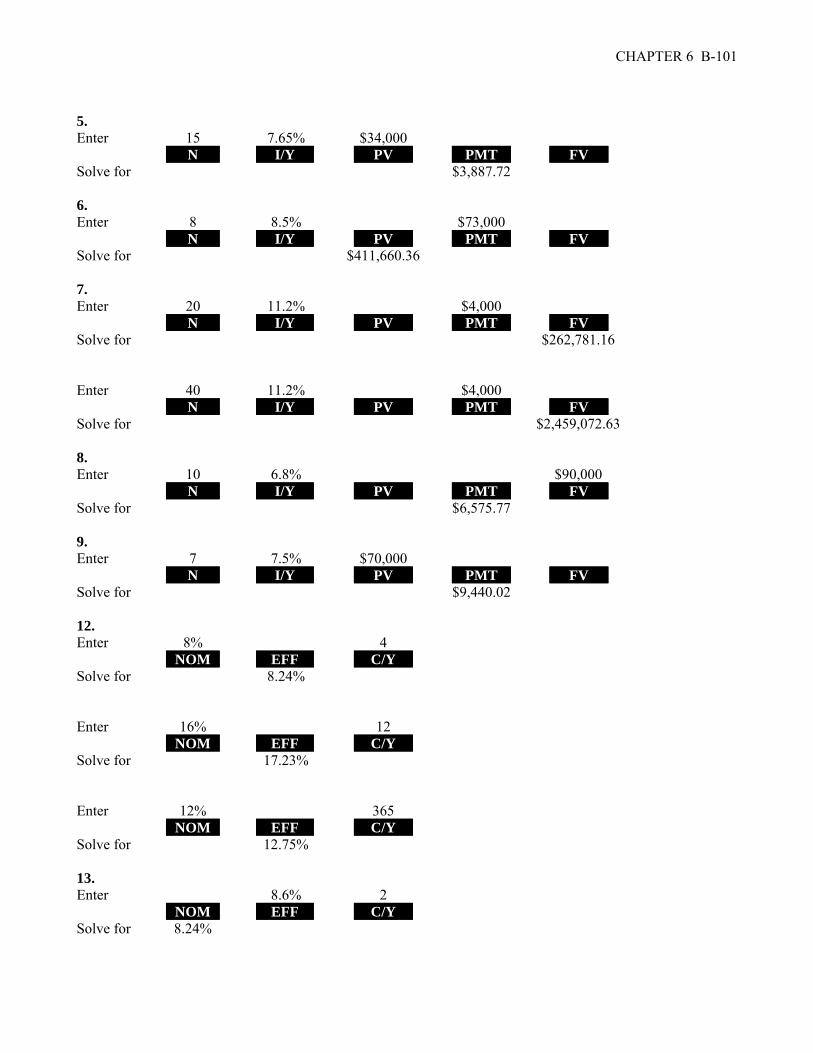
CHAPTER 6 B-101

5. Enter 15 7.65% $34,000 N I/Y PV PMT FV Solve for $3,887.72 6. Enter 8 8.5% $73,000 N I/Y PV PMT FV Solve for $411,660.36 7. Enter 20 11.2% $4,000 N I/Y PV PMT FV Solve for $262,781.16 Enter 40 11.2% $4,000 N I/Y PV PMT FV Solve for $2,459,072.63 8. Enter 10 6.8% $90,000 N I/Y PV PMT FV Solve for $6,575.77 9. Enter 7 7.5% $70,000 N I/Y PV PMT FV Solve for $9,440.02 12. Enter 8% 4 NOM EFF C/Y Solve for 8.24% Enter 16% 12 NOM EFF C/Y Solve for 17.23% Enter 12% 365 NOM EFF C/Y Solve for 12.75% 13. Enter 8.6% 2 NOM EFF C/Y Solve for 8.24%

B-102 SOLUTIONS

Enter 19.8% 12 NOM EFF C/Y Solve for 18.20% Enter 9.40% 52 NOM EFF C/Y Solve for 8.99% 14. Enter 14.2% 12 NOM EFF C/Y Solve for 15.16% Enter 14.5% 2 NOM EFF C/Y Solve for 15.03% 15. Enter 16% 365 NOM EFF C/Y Solve for 14.85% 16. Enter 17 × 2 8.4%/2 $2,100 N I/Y PV PMT FV Solve for $8,505.93 17. Enter 5 365 9.3% / 365 $4,500 N I/Y PV PMT FV Solve for $7,163.64 Enter 10 365 9.3% / 365 $4,500 N I/Y PV PMT FV Solve for $11,403.94 Enter 20 365 9.3% / 365 $4,500 N I/Y PV PMT FV Solve for $28,899.97 18. Enter 7 365 10% / 365 $58,000 N I/Y PV PMT FV Solve for $28,804.71

CHAPTER 6 B-103

19. Enter 360% 12 NOM EFF C/Y Solve for 2,229.81% 20. Enter 60 6.9% / 12 $68,500 N I/Y PV PMT FV Solve for $1,353.15 Enter 6.9% 12 NOM EFF C/Y Solve for 7.12% 21. Enter 1.3% $18,000 $500 N I/Y PV PMT FV Solve for 48.86 22. Enter 1,733.33% 52 NOM EFF C/Y Solve for 313,916,515.69% 23. Enter 22.74% 12 NOM EFF C/Y Solve for 25.26% 24. Enter 30 12 10% / 12 $300 N I/Y PV PMT FV Solve for $678,146.38 25. Enter 10.00% 12 NOM EFF C/Y Solve for 10.47% Enter 30 10.47% $3,600 N I/Y PV PMT FV Solve for $647,623.45 26. Enter 4 4 0.65% $2,300 N I/Y PV PMT FV Solve for $34,843.71

B-104 SOLUTIONS

27. Enter 11.00% 4 NOM EFF C/Y Solve for 11.46% CFo $0 C01 $725 F01 1 C02 $980 F02 1 C03 $0 F03 1 C04 $1,360 F04 1 I = 11.46% NPV CPT $2,320.36 28. CFo $0 C01 $1,650 F01 1 C02 $0 F02 1 C03 $4,200 F03 1 C04 $2,430 F04 1 I = 8.45% NPV CPT $6,570.86 30. Enter 17% 2 NOM EFF C/Y Solve for 16.33% 16.33% / 2 = 8.17% Enter 17% 4 NOM EFF C/Y Solve for 16.01% 16.01% / 4 = 4.00% Enter 17% 12 NOM EFF C/Y Solve for 15.80% 15.80% / 12 = 1.32%

CHAPTER 6 B-105

31. Enter 6 1.50% / 12 $5,000 N I/Y PV PMT FV Solve for $5,037.62 Enter 6 18% / 12 $5,037.62 N I/Y PV PMT FV Solve for $5,508.35 $5,508.35 – 5,000 = $508.35 32. Stock account: Enter 360 11% / 12 $700 N I/Y PV PMT FV Solve for $1,963,163.82 Bond account: Enter 360 6% / 12 $300 N I/Y PV PMT FV Solve for $301,354.51 Savings at retirement = $1,963,163.82 + 301,354.51 = $2,264,518.33 Enter 300 9% / 12 $2,264,518.33 N I/Y PV PMT FV Solve for $19,003.76 33. Enter 12 1.17% $1 N I/Y PV PMT FV Solve for $1.15 Enter 24 1.17% $1 N I/Y PV PMT FV Solve for $1.32 34. Enter 480 12% / 12 $1,000,000 N I/Y PV PMT FV Solve for $85.00 Enter 360 12% / 12 $1,000,000 N I/Y PV PMT FV Solve for $286.13

B-106 SOLUTIONS

Enter 240 12% / 12 $1,000,000 N I/Y PV PMT FV Solve for $1,010.86 35. Enter 12 / 3 $1 $3 N I/Y PV PMT FV Solve for 31.61% 36. Enter 10.00% 12 NOM EFF C/Y Solve for 10.47% Enter 2 10.47% $95,000 N I/Y PV PMT FV Solve for $163,839.09 CFo $45,000 C01 $75,000 F01 2 I = 10.47% NPV CPT $165,723.94 39. Enter 15 10% $9,000 N I/Y PV PMT FV Solve for $68,454.72 Enter 15 5% $9,000 N I/Y PV PMT FV Solve for $93,426.92 Enter 15 15% $9,000 N I/Y PV PMT FV Solve for $52,626.33 40. Enter 6% / 12 $340 $20,000 N I/Y PV PMT FV Solve for 51.69

CHAPTER 6 B-107

41. Enter 60 $73,000 $1,450 N I/Y PV PMT FV Solve for 0.594% 0.594% 12 = 7.13% 42. Enter 360 6.35% / 12 $1,150 N I/Y PV PMT FV Solve for $184,817.42 $240,000 – 184,817.42 = $55,182.58 Enter 360 6.35% / 12 $55,182.58 N I/Y PV PMT FV Solve for $368,936.54 43. CFo $0 C01 $1,700 F01 1 C02 $0 F02 1 C03 $2,100 F03 1 C04 $2,800 F04 1 I = 10% NPV CPT $5,035.65 PV of missing CF = $6,550 – 5,035.65 = $1,514.35 Value of missing CF: Enter 2 10% $1,514.35 N I/Y PV PMT FV Solve for $1,832.36

B-108 SOLUTIONS

44. CFo $1,000,000 C01 $1,500,000 F01 1 C02 $2,500,000 F02 1 C03 $2,800,000 F03 1 C04 $3,000,000 F04 1 C05 $3,500,000 F05 1 C06 $4,000,000 F06 1 C07 $4,500,000 F07 1 C08 $5,000,000 F08 1 C09 $5,500,000 F09 1 C010 $6,000,000 I = 9% NPV CPT $22,812,873 45. Enter 360 .80($2,900,000) $15,000 N I/Y PV PMT FV Solve for 0.560% APR = 0.560% 12 = 6.72% Enter 6.72% 12 NOM EFF C/Y Solve for 6.93% 46. Enter 4 13% $165,000 N I/Y PV PMT FV Solve for $101,197.59

Profit = $101,197.59 – 94,000 = $7,197.59 Enter 4 $94,000 $165,000 N I/Y PV PMT FV Solve for 15.10%

CHAPTER 6 B-109

47. Enter 18 10% $4,000 N I/Y PV PMT FV Solve for $32,805.65 Enter 7 10% $32,805.65 N I/Y PV PMT FV Solve for $16,834.48 48. Enter 84 7% / 12 $1,500 N I/Y PV PMT FV Solve for $87,604.36 Enter 96 11% / 12 $1,500 N I/Y PV PMT FV Solve for $110,021.35 Enter 84 7% / 12 $110,021.35 N I/Y PV PMT FV Solve for $51,120.33 $87,604.36 + 51,120.33 = $138,724.68 49. Enter 15 × 12 8.5%/12 $1,200 N I/Y PV PMT FV Solve for $434,143.62 FV = $434,143.62 = PV e.08(15); PV = $434,143.62e–1.20 = $130,761.55 50. PV@ t = 14: $3,500 / 0.062 = $56,451.61 Enter 7 6.2% $56,451.61 N I/Y PV PMT FV Solve for $37,051.41 51. Enter 12 $25,000 $2,416.67 N I/Y PV PMT FV Solve for 2.361%

APR = 2.361% 12 = 28.33%

Enter 28.33% 12 NOM EFF C/Y Solve for 32.31%

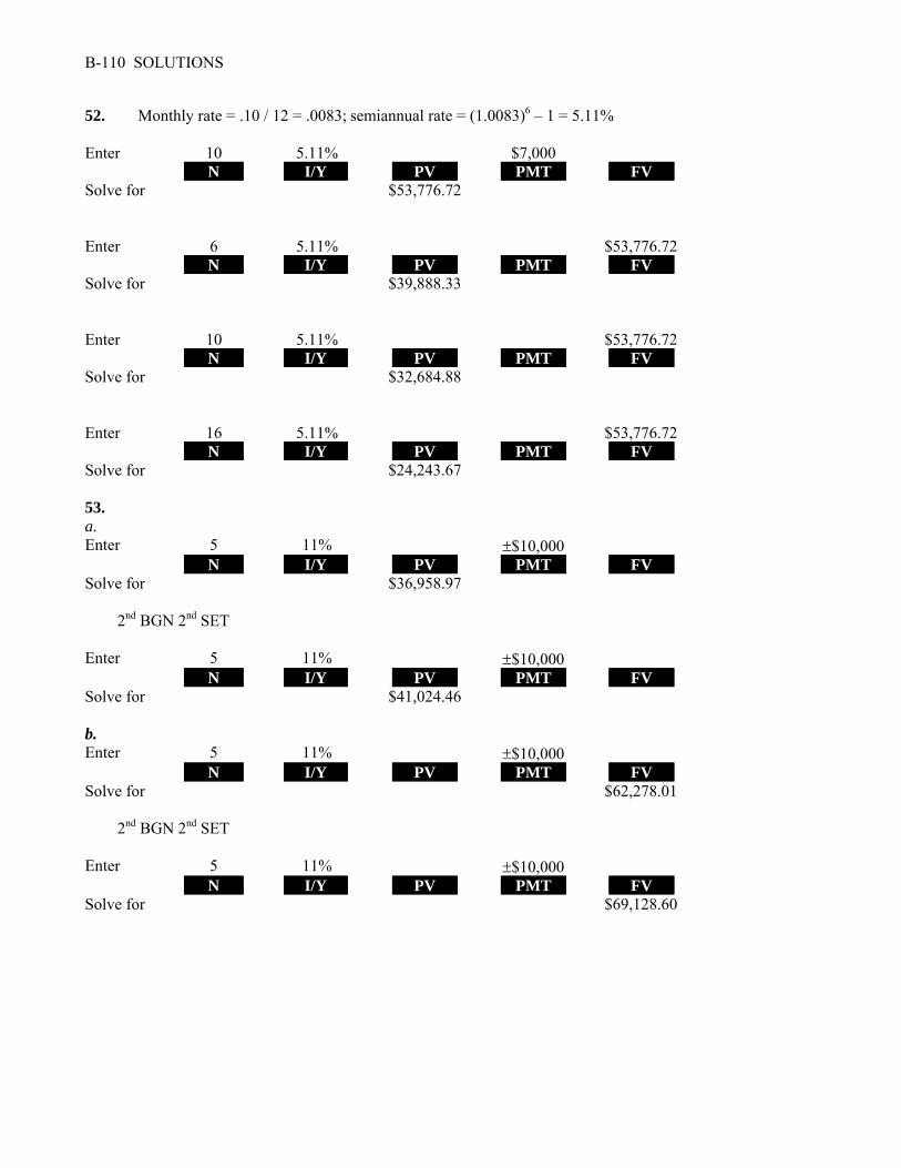
B-110 SOLUTIONS

52. Monthly rate = .10 / 12 = .0083; semiannual rate = (1.0083)6 – 1 = 5.11% Enter 10 5.11% $7,000 N I/Y PV PMT FV Solve for $53,776.72 Enter 6 5.11% $53,776.72 N I/Y PV PMT FV Solve for $39,888.33 Enter 10 5.11% $53,776.72 N I/Y PV PMT FV Solve for $32,684.88 Enter 16 5.11% $53,776.72 N I/Y PV PMT FV Solve for $24,243.67 53. a. Enter 5 11% $10,000 N I/Y PV PMT FV Solve for $36,958.97 2nd BGN 2nd SET Enter 5 11% $10,000 N I/Y PV PMT FV Solve for $41,024.46 b. Enter 5 11% $10,000 N I/Y PV PMT FV Solve for $62,278.01 2nd BGN 2nd SET Enter 5 11% $10,000 N I/Y PV PMT FV Solve for $69,128.60

CHAPTER 6 B-111

54. 2nd BGN 2nd SET Enter 60 7.85% / 12 $68,000 N I/Y PV PMT FV Solve for $1,364.99 57. Pre-retirement APR: Enter 10% 12 NOM EFF C/Y Solve for 9.57%

Post-retirement APR: Enter 7% 12 NOM EFF C/Y Solve for 6.78% At retirement, he needs: Enter 300 6.78% / 12 $20,000 $900,000 N I/Y PV PMT FV Solve for $3,051,320.71 In 10 years, his savings will be worth: Enter 120 7.72% / 12 $2,500 N I/Y PV PMT FV Solve for $499,659.64 After purchasing the cabin, he will have: $499,659.64 – 380,000 = $119,659.64 Each month between years 10 and 30, he needs to save: Enter 240 9.57% / 12 $119,659.64 $3,051,320.71± N I/Y PV PMT FV Solve for $3,127.44 58. PV of purchase: Enter 36 7% / 12 $23,000 N I/Y PV PMT FV Solve for $18,654.82

$32,000 – 18,654.82 = $13,345.18

B-112 SOLUTIONS

PV of lease: Enter 36 7% / 12 $450 N I/Y PV PMT FV Solve for $14,573.99

$14,573.91 + 99 = $14,672.91 Buy the car.

You would be indifferent when the PV of the two cash flows are equal. The present value of the purchase decision must be $14,672.91. Since the difference in the two cash flows is $32,000 – 14,672.91 = $17,327.09, this must be the present value of the future resale price of the car. The break-even resale price of the car is:

Enter 36 7% / 12 $17,327.09 N I/Y PV PMT FV Solve for $21,363.01 59. Enter 5.50% 365 NOM EFF C/Y Solve for 5.65% CFo $7,000,000 C01 $4,500,000 F01 1 C02 $5,000,000 F02 1 C03 $6,000,000 F03 1 C04 $6,800,000 F04 1 C05 $7,900,000 F05 1 C06 $8,800,000 F06 1 I = 5.65% NPV CPT $38,610,482.57 New contract value = $38,610,482.57 + 1,400,000 = $40,010,482.57 PV of payments = $40,010,482.57 – 9,000,000 = $31,010,482.57 Effective quarterly rate = [1 + (.055/365)]91.25 – 1 = .01384 or 1.384% Enter 24 1.384% $31,010,482.57 N I/Y PV PMT FV Solve for $1,527,463.76

CHAPTER 6 B-113

60. Enter 1 $21,250 $25,000 N I/Y PV PMT FV Solve for 17.65% 61. Enter 8% 12 NOM EFF C/Y Solve for 7.72% Enter 12 7.72% / 12 $47,000 / 12 N I/Y PV PMT FV Solve for $48,699.39 Enter 1 8% $48,699.39 N I/Y PV PMT FV Solve for $52,595.34 Enter 12 7.72% / 12 $50,000 / 12 N I/Y PV PMT FV Solve for $51,807.86 Enter 60 7.72% / 12 $55,000 / 12 N I/Y PV PMT FV Solve for $227,539.14 Award = $52,595.34 + 51,807.86 + 227,539.14 + 100,000 + 20,000 = $451,942.34 62. Enter 1 $9,700 $10,800 N I/Y PV PMT FV Solve for 11.34% 63. Enter 1 $9,800 $11,200 N I/Y PV PMT FV Solve for 14.29% 64. Refundable fee: With the $2,300 application fee, you will need to borrow $242,300 to have $240,000 after deducting the fee. Solve for the payment under these circumstances. Enter 30 12 6.80% / 12 $242,300 N I/Y PV PMT FV Solve for $1,579.61

B-114 SOLUTIONS

Enter 30 12 $240,000 $1,579.61 N I/Y PV PMT FV Solve for 0.5745% APR = 0.5745% 12 = 6.89% Enter 6.89% 12 NOM EFF C/Y Solve for 7.12% Without refundable fee: APR = 6.80% Enter 6.80% 12 NOM EFF C/Y Solve for 7.02% 65. Enter 36 $1,000 $41.15 N I/Y PV PMT FV Solve for 2.30% APR = 2.30% 12 = 27.61% Enter 27.61% 12 NOM EFF C/Y Solve for 31.39% 66. What she needs at age 65: Enter 20 7% $105,000 N I/Y PV PMT FV Solve for $1,112,371.50 a. Enter 30 7% $1,112,371.50 N I/Y PV PMT FV Solve for $11,776.01 b. Enter 30 7% $1,112,371.50 N I/Y PV PMT FV Solve for $146,129.04 c. Enter 10 7% $150,000 N I/Y PV PMT FV Solve for $295,072.70

CHAPTER 6 B-115

At 65, she is short: $1,112,371.50 – 295,072.50 = $817,298.80 Enter 30 7% ±$817,298.80 N I/Y PV PMT FV Solve for $8,652.25 Her employer will contribute $1,500 per year, so she must contribute: $8,652.25 – 1,500 = $7,152.25 per year 67. Without fee: Enter 19.8% / 12 $10,000 $200 N I/Y PV PMT FV Solve for 106.50 Enter 6.8% / 12 $10,000 $200 N I/Y PV PMT FV Solve for 57.99 With fee: Enter 6.8% / 12 $10,200 $200 N I/Y PV PMT FV Solve for 59.35 68. Value at Year 6: Enter 5 12% $900 N I/Y PV PMT FV Solve for $1,586.11 Enter 4 12% $900 N I/Y PV PMT FV Solve for $1,416.17 Enter 3 12% $1,000 N I/Y PV PMT FV Solve for $1,404.93 Enter 2 12% $1,000 N I/Y PV PMT FV Solve for $1,254.40

B-116 SOLUTIONS

Enter 1 12% $1,100 N I/Y PV PMT FV Solve for $1,232

So, at Year 5, the value is: $1,586.11 + 1,416.17 + 1,404.93 + 1,254.40 + 1,232

+ 1,100 = $7,993.60 At Year 65, the value is: Enter 59 8% $7,993.60 N I/Y PV PMT FV Solve for $749,452.56 The policy is not worth buying; the future value of the deposits is $749,452.56 but the policy contract will pay off $500,000. 69. Enter 30 12 8.1% / 12 $750,000 N I/Y PV PMT FV Solve for $5,555.61 Enter 22 12 8.1% / 12 $5,555.61 N I/Y PV PMT FV Solve for $683,700.32 70. CFo $9,000 C01 $9,000 F01 5 C02 $20,000 F02 4 IRR CPT 8.07% 75. a. APR = 7% 52 = 364% Enter 364% 52 NOM EFF C/Y Solve for 3,272.53% b. Enter 1 $9.30 $10.00 N I/Y PV PMT FV Solve for 7.53%

CHAPTER 6 B-117

APR = 7.53% 52 = 391.40% Enter 391.40% 52 NOM EFF C/Y Solve for 4,253.98% c. Enter 4 $68.92 $25 N I/Y PV PMT FV Solve for 16.75% APR = 16.75% 52 = 870.99% Enter 870.99% 52 NOM EFF C/Y Solve for 314,174.72%

CHAPTER 7 INTEREST RATES AND BOND VALUATION Answers to Concepts Review and Critical Thinking Questions 1. No. As interest rates fluctuate, the value of a Treasury security will fluctuate. Long-term Treasury

securities have substantial interest rate risk. 2. All else the same, the Treasury security will have lower coupons because of its lower default risk, so

it will have greater interest rate risk. 3. No. If the bid price were higher than the ask price, the implication would be that a dealer was willing

to sell a bond and immediately buy it back at a higher price. How many such transactions would you like to do?

4. Prices and yields move in opposite directions. Since the bid price must be lower, the bid yield must

be higher. 5. There are two benefits. First, the company can take advantage of interest rate declines by calling in

an issue and replacing it with a lower coupon issue. Second, a company might wish to eliminate a covenant for some reason. Calling the issue does this. The cost to the company is a higher coupon. A put provision is desirable from an investor’s standpoint, so it helps the company by reducing the coupon rate on the bond. The cost to the company is that it may have to buy back the bond at an unattractive price.

6. Bond issuers look at outstanding bonds of similar maturity and risk. The yields on such bonds are

used to establish the coupon rate necessary for a particular issue to initially sell for par value. Bond issuers also simply ask potential purchasers what coupon rate would be necessary to attract them. The coupon rate is fixed and simply determines what the bond’s coupon payments will be. The required return is what investors actually demand on the issue, and it will fluctuate through time. The coupon rate and required return are equal only if the bond sells for exactly at par.

7. Yes. Some investors have obligations that are denominated in dollars; i.e., they are nominal. Their

primary concern is that an investment provide the needed nominal dollar amounts. Pension funds, for example, often must plan for pension payments many years in the future. If those payments are fixed in dollar terms, then it is the nominal return on an investment that is important.

8. Companies pay to have their bonds rated simply because unrated bonds can be difficult to sell; many

large investors are prohibited from investing in unrated issues. 9. Treasury bonds have no credit risk since it is backed by the U.S. government, so a rating is not

necessary. Junk bonds often are not rated because there would be no point in an issuer paying a rating agency to assign its bonds a low rating (it’s like paying someone to kick you!).

CHAPTER 7 B-119

10. The term structure is based on pure discount bonds. The yield curve is based on coupon-bearing issues.

11. Bond ratings have a subjective factor to them. Split ratings reflect a difference of opinion among

credit agencies. 12. As a general constitutional principle, the federal government cannot tax the states without their

consent if doing so would interfere with state government functions. At one time, this principle was thought to provide for the tax-exempt status of municipal interest payments. However, modern court rulings make it clear that Congress can revoke the municipal exemption, so the only basis now appears to be historical precedent. The fact that the states and the federal government do not tax each other’s securities is referred to as “reciprocal immunity.”

13. Lack of transparency means that a buyer or seller can’t see recent transactions, so it is much harder

to determine what the best bid and ask prices are at any point in time. 14. Companies charge that bond rating agencies are pressuring them to pay for bond ratings. When a

company pays for a rating, it has the opportunity to make its case for a particular rating. With an unsolicited rating, the company has no input.

15. A 100-year bond looks like a share of preferred stock. In particular, it is a loan with a life that almost

certainly exceeds the life of the lender, assuming that the lender is an individual. With a junk bond, the credit risk can be so high that the borrower is almost certain to default, meaning that the creditors are very likely to end up as part owners of the business. In both cases, the “equity in disguise” has a significant tax advantage.

Solutions to Questions and Problems NOTE: All end of chapter problems were solved using a spreadsheet. Many problems require multiple steps. Due to space and readability constraints, when these intermediate steps are included in this solutions manual, rounding may appear to have occurred. However, the final answer for each problem is found without rounding during any step in the problem. Basic 1. The yield to maturity is the required rate of return on a bond expressed as a nominal annual interest

rate. For noncallable bonds, the yield to maturity and required rate of return are interchangeable terms. Unlike YTM and required return, the coupon rate is not a return used as the interest rate in bond cash flow valuation, but is a fixed percentage of par over the life of the bond used to set the coupon payment amount. For the example given, the coupon rate on the bond is still 10 percent, and the YTM is 8 percent.

2. Price and yield move in opposite directions; if interest rates rise, the price of the bond will fall. This

is because the fixed coupon payments determined by the fixed coupon rate are not as valuable when interest rates rise—hence, the price of the bond decreases.

B-120 SOLUTIONS

NOTE: Most problems do not explicitly list a par value for bonds. Even though a bond can have any par value, in general, corporate bonds in the United States will have a par value of $1,000. We will use this par value in all problems unless a different par value is explicitly stated. 3. The price of any bond is the PV of the interest payment, plus the PV of the par value. Notice this

problem assumes an annual coupon. The price of the bond will be: P = $75({1 – [1/(1 + .0875)]10 } / .0875) + $1,000[1 / (1 + .0875)10] = $918.89 We would like to introduce shorthand notation here. Rather than write (or type, as the case may be)

the entire equation for the PV of a lump sum, or the PVA equation, it is common to abbreviate the equations as:

PVIFR,t = 1 / (1 + r)t which stands for Present Value Interest Factor PVIFAR,t = ({1 – [1/(1 + r)]t } / r ) which stands for Present Value Interest Factor of an Annuity These abbreviations are short hand notation for the equations in which the interest rate and the

number of periods are substituted into the equation and solved. We will use this shorthand notation in remainder of the solutions key.

4. Here we need to find the YTM of a bond. The equation for the bond price is: P = $934 = $90(PVIFAR%,9) + $1,000(PVIFR%,9) Notice the equation cannot be solved directly for R. Using a spreadsheet, a financial calculator, or

trial and error, we find: R = YTM = 10.15% If you are using trial and error to find the YTM of the bond, you might be wondering how to pick an

interest rate to start the process. First, we know the YTM has to be higher than the coupon rate since the bond is a discount bond. That still leaves a lot of interest rates to check. One way to get a starting point is to use the following equation, which will give you an approximation of the YTM:

Approximate YTM = [Annual interest payment + (Price difference from par / Years to maturity)] / [(Price + Par value) / 2] Solving for this problem, we get: Approximate YTM = [$90 + ($64 / 9] / [($934 + 1,000) / 2] = 10.04% This is not the exact YTM, but it is close, and it will give you a place to start.

CHAPTER 7 B-121

5. Here we need to find the coupon rate of the bond. All we need to do is to set up the bond pricing equation and solve for the coupon payment as follows:

P = $1,045 = C(PVIFA7.5%,13) + $1,000(PVIF7.5%,36) Solving for the coupon payment, we get: C = $80.54 The coupon payment is the coupon rate times par value. Using this relationship, we get: Coupon rate = $80.54 / $1,000 = .0805 or 8.05% 6. To find the price of this bond, we need to realize that the maturity of the bond is 10 years. The bond

was issued one year ago, with 11 years to maturity, so there are 10 years left on the bond. Also, the coupons are semiannual, so we need to use the semiannual interest rate and the number of semiannual periods. The price of the bond is:

P = $34.50(PVIFA3.7%,20) + $1,000(PVIF3.7%,20) = $965.10 7. Here we are finding the YTM of a semiannual coupon bond. The bond price equation is: P = $1,050 = $42(PVIFAR%,20) + $1,000(PVIFR%,20) Since we cannot solve the equation directly for R, using a spreadsheet, a financial calculator, or trial

and error, we find: R = 3.837% Since the coupon payments are semiannual, this is the semiannual interest rate. The YTM is the APR

of the bond, so: YTM = 2 3.837% = 7.67% 8. Here we need to find the coupon rate of the bond. All we need to do is to set up the bond pricing

equation and solve for the coupon payment as follows: P = $924 = C(PVIFA3.4%,29) + $1,000(PVIF3.4%,29) Solving for the coupon payment, we get: C = $29.84 Since this is the semiannual payment, the annual coupon payment is: 2 × $29.84 = $59.68 And the coupon rate is the annual coupon payment divided by par value, so: Coupon rate = $59.68 / $1,000 Coupon rate = .0597 or 5.97%

B-122 SOLUTIONS

9. The approximate relationship between nominal interest rates (R), real interest rates (r), and inflation (h) is:

R = r + h Approximate r = .07 – .038 =.032 or 3.20% The Fisher equation, which shows the exact relationship between nominal interest rates, real interest

rates, and inflation is: (1 + R) = (1 + r)(1 + h) (1 + .07) = (1 + r)(1 + .038) Exact r = [(1 + .07) / (1 + .038)] – 1 = .0308 or 3.08% 10. The Fisher equation, which shows the exact relationship between nominal interest rates, real interest

rates, and inflation is: (1 + R) = (1 + r)(1 + h) R = (1 + .047)(1 + .03) – 1 = .0784 or 7.84% 11. The Fisher equation, which shows the exact relationship between nominal interest rates, real interest

rates, and inflation is: (1 + R) = (1 + r)(1 + h) h = [(1 + .14) / (1 + .09)] – 1 = .0459 or 4.59% 12. The Fisher equation, which shows the exact relationship between nominal interest rates, real interest

rates, and inflation is: (1 + R) = (1 + r)(1 + h) r = [(1 + .114) / (1.048)] – 1 = .0630 or 6.30% 13. This is a bond since the maturity is greater than 10 years. The coupon rate, located in the first

column of the quote is 6.125%. The bid price is: Bid price = 120:07 = 120 7/32 = 120.21875% $1,000 = $1,202.1875 The previous day’s ask price is found by: Previous day’s asked price = Today’s asked price – Change = 120 8/32 – (5/32) = 120 3/32 The previous day’s price in dollars was: Previous day’s dollar price = 120.406% $1,000 = $1,204.06

CHAPTER 7 B-123

14. This is a premium bond because it sells for more than 100% of face value. The current yield is: Current yield = Annual coupon payment / Price = $75/$1,351.5625 = 5.978% The YTM is located under the “Asked Yield” column, so the YTM is 4.47%. The bid-ask spread is the difference between the bid price and the ask price, so: Bid-Ask spread = 135:06 – 135:05 = 1/32 Intermediate 15. Here we are finding the YTM of semiannual coupon bonds for various maturity lengths. The bond

price equation is: P = C(PVIFAR%,t) + $1,000(PVIFR%,t) X: P0 = $80(PVIFA6%,13) + $1,000(PVIF6%,13) = $1,177.05 P1 = $80(PVIFA6%,12) + $1,000(PVIF6%,12) = $1,167.68 P3 = $80(PVIFA6%,10) + $1,000(PVIF6%,10) = $1,147.20 P8 = $80(PVIFA6%,5) + $1,000(PVIF6%,5) = $1,084.25 P12 = $80(PVIFA6%,1) + $1,000(PVIF6%,1) = $1,018.87 P13 = $1,000 Y: P0 = $60(PVIFA8%,13) + $1,000(PVIF8%,13) = $841.92 P1 = $60(PVIFA8%,12) + $1,000(PVIF8%,12) = $849.28 P3 = $60(PVIFA8%,10) + $1,000(PVIF8%,10) = $865.80 P8 = $60(PVIFA8%,5) + $1,000(PVIF8%,5) = $920.15 P12 = $60(PVIFA8%,1) + $1,000(PVIF8%,1) = $981.48 P13 = $1,000 All else held equal, the premium over par value for a premium bond declines as maturity approaches,

and the discount from par value for a discount bond declines as maturity approaches. This is called “pull to par.” In both cases, the largest percentage price changes occur at the shortest maturity lengths.

Also, notice that the price of each bond when no time is left to maturity is the par value, even though

the purchaser would receive the par value plus the coupon payment immediately. This is because we calculate the clean price of the bond.

B-124 SOLUTIONS

16. Any bond that sells at par has a YTM equal to the coupon rate. Both bonds sell at par, so the initial YTM on both bonds is the coupon rate, 9 percent. If the YTM suddenly rises to 11 percent:

PSam = $45(PVIFA5.5%,6) + $1,000(PVIF5.5%,6) = $950.04 PDave = $45(PVIFA5.5%,40) + $1,000(PVIF5.5%,40) = $839.54 The percentage change in price is calculated as: Percentage change in price = (New price – Original price) / Original price PSam% = ($950.04 – 1,000) / $1,000 = – 5.00% PDave% = ($839.54 – 1,000) / $1,000 = – 16.05% If the YTM suddenly falls to 7 percent: PSam = $45(PVIFA3.5%,6) + $1,000(PVIF3.5%,6) = $1,053.29 PDave = $45(PVIFA3.5%,40) + $1,000(PVIF3.5%,40) = $1,213.55

PSam% = ($1,053.29 – 1,000) / $1,000 = + 5.33% PDave% = ($1,213.55 – 1,000) / $1,000 = + 21.36% All else the same, the longer the maturity of a bond, the greater is its price sensitivity to changes in

interest rates. 17. Initially, at a YTM of 8 percent, the prices of the two bonds are: PJ = $20(PVIFA4%,18) + $1,000(PVIF4%,18) = $746.81 PK = $60(PVIFA4%,18) + $1,000(PVIF4%,18) = $1,253.19 If the YTM rises from 8 percent to 10 percent: PJ = $20(PVIFA5%,18) + $1,000(PVIF5%,18) = $649.31 PK = $60(PVIFA5%,18) + $1,000(PVIF5%,18) = $1,116.90 The percentage change in price is calculated as: Percentage change in price = (New price – Original price) / Original price PJ% = ($649.31 – 746.81) / $746.81 = – 13.06% PK% = ($1,116.90 – 1,253.19) / $1,253.19 = – 10.88%

CHAPTER 7 B-125

If the YTM declines from 8 percent to 6 percent: PJ = $20(PVIFA3%,18) + $1,000(PVIF3%,18) = $862.46 PK = $60(PVIFA3%,18) + $1,000(PVIF3%,18) = $1,412.61 PJ% = ($862.46 – 746.81) / $746.81 = + 15.49% PK% = ($1,412.61 – 1,253.19) / $1,253.19 = + 12.72% All else the same, the lower the coupon rate on a bond, the greater is its price sensitivity to changes

in interest rates. 18. The bond price equation for this bond is: P0 = $1,068 = $46(PVIFAR%,18) + $1,000(PVIFR%,18) Using a spreadsheet, financial calculator, or trial and error we find: R = 4.06% This is the semiannual interest rate, so the YTM is: YTM = 2 4.06% = 8.12% The current yield is: Current yield = Annual coupon payment / Price = $92 / $1,068 = .0861 or 8.61% The effective annual yield is the same as the EAR, so using the EAR equation from the previous

chapter: Effective annual yield = (1 + 0.0406)2 – 1 = .0829 or 8.29% 19. The company should set the coupon rate on its new bonds equal to the required return. The required

return can be observed in the market by finding the YTM on outstanding bonds of the company. So, the YTM on the bonds currently sold in the market is:

P = $930 = $40(PVIFAR%,40) + $1,000(PVIFR%,40) Using a spreadsheet, financial calculator, or trial and error we find: R = 4.373% This is the semiannual interest rate, so the YTM is: YTM = 2 4.373% = 8.75%

B-126 SOLUTIONS

20. Accrued interest is the coupon payment for the period times the fraction of the period that has passed since the last coupon payment. Since we have a semiannual coupon bond, the coupon payment per six months is one-half of the annual coupon payment. There are four months until the next coupon payment, so two months have passed since the last coupon payment. The accrued interest for the bond is:

Accrued interest = $74/2 × 2/6 = $12.33 And we calculate the clean price as: Clean price = Dirty price – Accrued interest = $968 – 12.33 = $955.67 21. Accrued interest is the coupon payment for the period times the fraction of the period that has passed

since the last coupon payment. Since we have a semiannual coupon bond, the coupon payment per six months is one-half of the annual coupon payment. There are two months until the next coupon payment, so four months have passed since the last coupon payment. The accrued interest for the bond is:

Accrued interest = $68/2 × 4/6 = $22.67 And we calculate the dirty price as: Dirty price = Clean price + Accrued interest = $1,073 + 22.67 = $1,095.67 22. To find the number of years to maturity for the bond, we need to find the price of the bond. Since we

already have the coupon rate, we can use the bond price equation, and solve for the number of years to maturity. We are given the current yield of the bond, so we can calculate the price as:

Current yield = .0755 = $80/P0 P0 = $80/.0755 = $1,059.60 Now that we have the price of the bond, the bond price equation is: P = $1,059.60 = $80[(1 – (1/1.072)t ) / .072 ] + $1,000/1.072t

We can solve this equation for t as follows: $1,059.60(1.072)t = $1,111.11(1.072)t – 1,111.11 + 1,000 111.11 = 51.51(1.072)t 2.1570 = 1.072t t = log 2.1570 / log 1.072 = 11.06 11 years The bond has 11 years to maturity.

CHAPTER 7 B-127

23. The bond has 14 years to maturity, so the bond price equation is: P = $1,089.60 = $36(PVIFAR%,28) + $1,000(PVIFR%,28) Using a spreadsheet, financial calculator, or trial and error we find: R = 3.116% This is the semiannual interest rate, so the YTM is: YTM = 2 3.116% = 6.23% The current yield is the annual coupon payment divided by the bond price, so: Current yield = $72 / $1,089.60 = .0661 or 6.61% 24. a. The bond price is the present value of the cash flows from a bond. The YTM is the interest rate

used in valuing the cash flows from a bond. b. If the coupon rate is higher than the required return on a bond, the bond will sell at a premium,

since it provides periodic income in the form of coupon payments in excess of that required by investors on other similar bonds. If the coupon rate is lower than the required return on a bond, the bond will sell at a discount since it provides insufficient coupon payments compared to that required by investors on other similar bonds. For premium bonds, the coupon rate exceeds the YTM; for discount bonds, the YTM exceeds the coupon rate, and for bonds selling at par, the YTM is equal to the coupon rate.

c. Current yield is defined as the annual coupon payment divided by the current bond price. For

premium bonds, the current yield exceeds the YTM, for discount bonds the current yield is less than the YTM, and for bonds selling at par value, the current yield is equal to the YTM. In all cases, the current yield plus the expected one-period capital gains yield of the bond must be equal to the required return.

25. The price of a zero coupon bond is the PV of the par, so: a. P0 = $1,000/1.04550 = $110.71 b. In one year, the bond will have 24 years to maturity, so the price will be: P1 = $1,000/1.04548 = $120.90

B-128 SOLUTIONS

The interest deduction is the price of the bond at the end of the year, minus the price at the beginning of the year, so:

Year 1 interest deduction = $120.90 – 110.71 = $10.19 The price of the bond when it has one year left to maturity will be: P24 = $1,000/1.0452 = $915.73 Year 24 interest deduction = $1,000 – 915.73 = $84.27 c. Previous IRS regulations required a straight-line calculation of interest. The total interest

received by the bondholder is: Total interest = $1,000 – 110.71 = $889.29 The annual interest deduction is simply the total interest divided by the maturity of the bond, so

the straight-line deduction is: Annual interest deduction = $889.29 / 25 = $35.57 d. The company will prefer straight-line methods when allowed because the valuable interest

deductions occur earlier in the life of the bond. 26. a. The coupon bonds have an 8% coupon which matches the 8% required return, so they will sell

at par. The number of bonds that must be sold is the amount needed divided by the bond price, so:

Number of coupon bonds to sell = $30,000,000 / $1,000 = 30,000 The number of zero coupon bonds to sell would be: Price of zero coupon bonds = $1,000/1.0460 = $95.06 Number of zero coupon bonds to sell = $30,000,000 / $95.06 = 315,589 b. The repayment of the coupon bond will be the par value plus the last coupon payment times the

number of bonds issued. So: Coupon bonds repayment = 30,000($1,040) = $32,400,000 The repayment of the zero coupon bond will be the par value times the number of bonds issued,

so: Zeroes: repayment = 315,589($1,000) = $315,588,822

CHAPTER 7 B-129

c. The total coupon payment for the coupon bonds will be the number bonds times the coupon payment. For the cash flow of the coupon bonds, we need to account for the tax deductibility of the interest payments. To do this, we will multiply the total coupon payment times one minus the tax rate. So:

Coupon bonds: (30,000)($80)(1–.35) = $1,560,000 cash outflow Note that this is cash outflow since the company is making the interest payment. For the zero coupon bonds, the first year interest payment is the difference in the price of the

zero at the end of the year and the beginning of the year. The price of the zeroes in one year will be:

P1 = $1,000/1.0458 = $102.82 The year 1 interest deduction per bond will be this price minus the price at the beginning of the

year, which we found in part b, so: Year 1 interest deduction per bond = $102.82 – 95.06 = $7.76 The total cash flow for the zeroes will be the interest deduction for the year times the number of

zeroes sold, times the tax rate. The cash flow for the zeroes in year 1 will be: Cash flows for zeroes in Year 1 = (315,589)($7.76)(.35) = $856,800.00 Notice the cash flow for the zeroes is a cash inflow. This is because of the tax deductibility of

the imputed interest expense. That is, the company gets to write off the interest expense for the year even though the company did not have a cash flow for the interest expense. This reduces the company’s tax liability, which is a cash inflow.

During the life of the bond, the zero generates cash inflows to the firm in the form of the

interest tax shield of debt. We should note an important point here: If you find the PV of the cash flows from the coupon bond and the zero coupon bond, they will be the same. This is because of the much larger repayment amount for the zeroes.

27. We found the maturity of a bond in Problem 22. However, in this case, the maturity is indeterminate.

A bond selling at par can have any length of maturity. In other words, when we solve the bond pricing equation as we did in Problem 22, the number of periods can be any positive number.

28. We first need to find the real interest rate on the savings. Using the Fisher equation, the real interest

rate is: (1 + R) = (1 + r)(1 + h) 1 + .11 = (1 + r)(1 + .038) r = .0694 or 6.94%

B-130 SOLUTIONS

Now we can use the future value of an annuity equation to find the annual deposit. Doing so, we find:

FVA = C{[(1 + r)t – 1] / r} $1,500,000 = $C[(1.069440 – 1) / .0694] C = $7,637.76 Challenge 29. To find the capital gains yield and the current yield, we need to find the price of the bond. The

current price of Bond P and the price of Bond P in one year is: P: P0 = $120(PVIFA7%,5) + $1,000(PVIF7%,5) = $1,116.69 P1 = $120(PVIFA7%,4) + $1,000(PVIF7%,4) = $1,097.19 Current yield = $120 / $1,116.69 = .1075 or 10.75% The capital gains yield is: Capital gains yield = (New price – Original price) / Original price Capital gains yield = ($1,097.19 – 1,111.69) / $1,116.69 = –.0175 or –1.75% The current price of Bond D and the price of Bond D in one year is: D: P0 = $60(PVIFA7%,5) + $1,000(PVIF7%,5) = $883.31 P1 = $60(PVIFA7%,4) + $1,000(PVIF7%,4) = $902.81 Current yield = $60 / $883.81 = .0679 or 6.79% Capital gains yield = ($902.81 – 883.31) / $883.31 = +.0221 or +2.21% All else held constant, premium bonds pay high current income while having price depreciation as

maturity nears; discount bonds do not pay high current income but have price appreciation as maturity nears. For either bond, the total return is still 9%, but this return is distributed differently between current income and capital gains.

30. a. The rate of return you expect to earn if you purchase a bond and hold it until maturity is the

YTM. The bond price equation for this bond is: P0 = $1,060 = $70(PVIFAR%,10) + $1,000(PVIF R%,10) Using a spreadsheet, financial calculator, or trial and error we find: R = YTM = 6.18%

CHAPTER 7 B-131

b. To find our HPY, we need to find the price of the bond in two years. The price of the bond in two years, at the new interest rate, will be:

P2 = $70(PVIFA5.18%,8) + $1,000(PVIF5.18%,8) = $1,116.92 To calculate the HPY, we need to find the interest rate that equates the price we paid for the

bond with the cash flows we received. The cash flows we received were $70 each year for two years, and the price of the bond when we sold it. The equation to find our HPY is:

P0 = $1,060 = $70(PVIFAR%,2) + $1,116.92(PVIFR%,2) Solving for R, we get: R = HPY = 9.17% The realized HPY is greater than the expected YTM when the bond was bought because interest

rates dropped by 1 percent; bond prices rise when yields fall. 31. The price of any bond (or financial instrument) is the PV of the future cash flows. Even though Bond

M makes different coupons payments, to find the price of the bond, we just find the PV of the cash flows. The PV of the cash flows for Bond M is:

PM = $1,100(PVIFA3.5%,16)(PVIF3.5%,12) + $1,400(PVIFA3.5%,12)(PVIF3.5%,28) + $20,000(PVIF3.5%,40) PM = $19,018.78 Notice that for the coupon payments of $1,400, we found the PVA for the coupon payments, and

then discounted the lump sum back to today. Bond N is a zero coupon bond with a $20,000 par value, therefore, the price of the bond is the PV of

the par, or: PN = $20,000(PVIF3.5%,40) = $5,051.45 32. To calculate this, we need to set up an equation with the callable bond equal to a weighted average of

the noncallable bonds. We will invest X percent of our money in the first noncallable bond, which means our investment in Bond 3 (the other noncallable bond) will be (1 – X). The equation is:

C2 = C1 X + C3(1 – X) 8.25 = 6.50 X + 12(1 – X) 8.25 = 6.50 X + 12 – 12 X X = 0.68181

So, we invest about 68 percent of our money in Bond 1, and about 32 percent in Bond 3. This combination of bonds should have the same value as the callable bond, excluding the value of the call. So:

P2 = 0.68181P1 + 0.31819P3 P2 = 0.68181(106.375) + 0.31819(134.96875) P2 = 115.4730

B-132 SOLUTIONS

The call value is the difference between this implied bond value and the actual bond price. So, the call value is:

Call value = 115.4730 – 103.50 = 11.9730 Assuming $1,000 par value, the call value is $119.73.

33. In general, this is not likely to happen, although it can (and did). The reason this bond has a negative

YTM is that it is a callable U.S. Treasury bond. Market participants know this. Given the high coupon rate of the bond, it is extremely likely to be called, which means the bondholder will not receive all the cash flows promised. A better measure of the return on a callable bond is the yield to call (YTC). The YTC calculation is the basically the same as the YTM calculation, but the number of periods is the number of periods until the call date. If the YTC were calculated on this bond, it would be positive.

34. To find the present value, we need to find the real weekly interest rate. To find the real return, we

need to use the effective annual rates in the Fisher equation. So, we find the real EAR is: (1 + R) = (1 + r)(1 + h) 1 + .084 = (1 + r)(1 + .037) r = .0453 or 4.53% Now, to find the weekly interest rate, we need to find the APR. Using the equation for discrete

compounding: EAR = [1 + (APR / m)]m – 1 We can solve for the APR. Doing so, we get: APR = m[(1 + EAR)1/m – 1] APR = 52[(1 + .0453)1/52 – 1] APR = .0443 or 4.43% So, the weekly interest rate is: Weekly rate = APR / 52 Weekly rate = .0443 / 52 Weekly rate = .0009 or 0.09% Now we can find the present value of the cost of the roses. The real cash flows are an ordinary

annuity, discounted at the real interest rate. So, the present value of the cost of the roses is: PVA = C({1 – [1/(1 + r)]t } / r) PVA = $5({1 – [1/(1 + .0009)]30(52)} / .0009) PVA = $4,312.13

CHAPTER 7 B-133

35. To answer this question, we need to find the monthly interest rate, which is the APR divided by 12. We also must be careful to use the real interest rate. The Fisher equation uses the effective annual rate, so, the real effective annual interest rates, and the monthly interest rates for each account are:

Stock account: (1 + R) = (1 + r)(1 + h) 1 + .11 = (1 + r)(1 + .04) r = .0673 or 6.73% APR = m[(1 + EAR)1/m – 1] APR = 12[(1 + .0673)1/12 – 1] APR = .0653 or 6.53% Monthly rate = APR / 12 Monthly rate = .0653 / 12 Monthly rate = .0054 or 0.54% Bond account: (1 + R) = (1 + r)(1 + h) 1 + .07 = (1 + r)(1 + .04) r = .0288 or 2.88% APR = m[(1 + EAR)1/m – 1] APR = 12[(1 + .0288)1/12 – 1] APR = .0285 or 2.85% Monthly rate = APR / 12 Monthly rate = .0285 / 12 Monthly rate = .0024 or 0.24% Now we can find the future value of the retirement account in real terms. The future value of each

account will be: Stock account: FVA = C {(1 + r )t – 1] / r} FVA = $900{[(1 + .0054)360 – 1] / .0054]} FVA = $1,001,704.05 Bond account: FVA = C {(1 + r )t – 1] / r} FVA = $450{[(1 + .0024)360 – 1] / .0024]} FVA = $255,475.17 The total future value of the retirement account will be the sum of the two accounts, or: Account value = $1,001,704.05 + 255,475.17 Account value = $1,257,179.22

B-134 SOLUTIONS

Now we need to find the monthly interest rate in retirement. We can use the same procedure that we used to find the monthly interest rates for the stock and bond accounts, so:

(1 + R) = (1 + r)(1 + h) 1 + .09 = (1 + r)(1 + .04) r = .0481 or 4.81% APR = m[(1 + EAR)1/m – 1] APR = 12[(1 + .0481)1/12 – 1] APR = .0470 or 4.70% Monthly rate = APR / 12 Monthly rate = .0470 / 12 Monthly rate = .0039 or 0.39% Now we can find the real monthly withdrawal in retirement. Using the present value of an annuity

equation and solving for the payment, we find: PVA = C({1 – [1/(1 + r)]t } / r ) $1,257,179.22 = C({1 – [1/(1 + .0039)]300 } / .0039) C = $7,134.82 This is the real dollar amount of the monthly withdrawals. The nominal monthly withdrawals will

increase by the inflation rate each month. To find the nominal dollar amount of the last withdrawal, we can increase the real dollar withdrawal by the inflation rate. We can increase the real withdrawal by the effective annual inflation rate since we are only interested in the nominal amount of the last withdrawal. So, the last withdrawal in nominal terms will be:

FV = PV(1 + r)t FV = $7,134.82(1 + .04)(30 + 25) FV = $61,690.29 Calculator Solutions 3. Enter 10 8.75% $75 $1,000 N I/Y PV PMT FV Solve for $918.89 4. Enter 9 ±$934 $90 $1,000 N I/Y PV PMT FV Solve for 10.15% 5. Enter 13 7.5% ±$1,045 $1,000 N I/Y PV PMT FV Solve for $80.54 Coupon rate = $80.54 / $1,000 = 8.05%

CHAPTER 7 B-135

6. Enter 20 3.70% $34.50 $1,000 N I/Y PV PMT FV Solve for $965.10 7. Enter 20 ±$1,050 $42 $1,000 N I/Y PV PMT FV Solve for 3.837% 3.837% 2 = 7.67% 8. Enter 29 3.40% ±$924 $1,000 N I/Y PV PMT FV Solve for $29.84 ($29.84 / $1,000)(2) = 5.97% 15. Bond X P0 Enter 13 6% $80 $1,000 N I/Y PV PMT FV Solve for $1,177.05 P1 Enter 12 6% $80 $1,000 N I/Y PV PMT FV Solve for $1,167.68 P3 Enter 10 6% $80 $1,000 N I/Y PV PMT FV Solve for $1,147.20 P8 Enter 5 6% $80 $1,000 N I/Y PV PMT FV Solve for $1,084.25 P12 Enter 1 6% $80 $1,000 N I/Y PV PMT FV Solve for $1,018.87

B-136 SOLUTIONS

Bond Y P0 Enter 13 8% $60 $1,000 N I/Y PV PMT FV Solve for $841.92 P1 Enter 12 8% $60 $1,000 N I/Y PV PMT FV Solve for $849.28 P3 Enter 10 8% $60 $1,000 N I/Y PV PMT FV Solve for $865.80 P8 Enter 5 8% $60 $1,000 N I/Y PV PMT FV Solve for $920.15 P12 Enter 1 8% $60 $1,000 N I/Y PV PMT FV Solve for $981.48 16. If both bonds sell at par, the initial YTM on both bonds is the coupon rate, 9 percent. If the YTM

suddenly rises to 11 percent: PSam Enter 6 5.5% $45 $1,000 N I/Y PV PMT FV Solve for $950.04 PSam% = ($950.04 – 1,000) / $1,000 = – 5.00% PDave Enter 40 5.5% $45 $1,000 N I/Y PV PMT FV Solve for $839.54 PDave% = ($839.54 – 1,000) / $1,000 = – 16.05%

If the YTM suddenly falls to 7 percent:

PSam Enter 6 3.5% $45 $1,000 N I/Y PV PMT FV Solve for $1,053.29 PSam% = ($1,053.29 – 1,000) / $1,000 = + 5.33%

CHAPTER 7 B-137

PDave Enter 40 3.5% $45 $1,000 N I/Y PV PMT FV Solve for $1,1213.55 PDave% = ($1,213.55 – 1,000) / $1,000 = + 21.36% All else the same, the longer the maturity of a bond, the greater is its price sensitivity to changes in interest rates. 17. Initially, at a YTM of 8 percent, the prices of the two bonds are: PJ Enter 18 4% $20 $1,000 N I/Y PV PMT FV Solve for $746.81 PK Enter 18 4% $60 $1,000 N I/Y PV PMT FV Solve for $1,253.19 If the YTM rises from 8 percent to 10 percent: PJ Enter 18 5% $20 $1,000 N I/Y PV PMT FV Solve for $649.31 PJ% = ($649.31 – 746.81) / $746.81 = – 13.06% PK Enter 18 5% $60 $1,000 N I/Y PV PMT FV Solve for $1,116.90 PK% = ($1,116.90 – 1,253.19) / $1,253.19 = – 10.88% If the YTM declines from 8 percent to 6 percent: PJ Enter 18 3% $20 $1,000 N I/Y PV PMT FV Solve for $862.46 PJ% = ($862.46 – 746.81) / $746.81 = + 15.49% PK Enter 18 3% $60 $1,000 N I/Y PV PMT FV Solve for $1,412.61 PK% = ($1,412.61 – 1,253.19) / $1,253.19 = + 12.72%

All else the same, the lower the coupon rate on a bond, the greater is its price sensitivity to changes in interest rates.

B-138 SOLUTIONS

18. Enter 18 ±$1,068 $46 $1,000 N I/Y PV PMT FV Solve for 4.06%

4.06% 2 = 8.12% Enter 8.12 % 2 NOM EFF C/Y Solve for 8.29% 19. The company should set the coupon rate on its new bonds equal to the required return; the required

return can be observed in the market by finding the YTM on outstanding bonds of the company. Enter 40 ±$930 $35 $1,000 N I/Y PV PMT FV Solve for 4.373% 4.373% 2 = 8.75% 22. Current yield = .0755 = $90/P0 ; P0 = $90/.0755 = $1,059.60 Enter 7.2% ±$1,059.60 $80 $1,000 N I/Y PV PMT FV Solve for 11.06 11.06 or 11 years 23. Enter 28 ±$1,089.60 $36 $1,000 N I/Y PV PMT FV Solve for 3.116% 3.116% × 2 = 6.23% 25. a. Po Enter 50 4.5% $1,000 N I/Y PV PMT FV Solve for $110.71 b. P1 Enter 48 4.5% $1,000 N I/Y PV PMT FV Solve for $120.90 year 1 interest deduction = $120.90 – 110.71 = $10.19 P19 Enter 1 4.5% $1,000 N I/Y PV PMT FV Solve for $915.73 year 25 interest deduction = $1,000 – 915.73 = $84.27

CHAPTER 7 B-139

c. Total interest = $1,000 – 110.71 = $889.29 Annual interest deduction = $889.29 / 25 = $35.57 d. The company will prefer straight-line method when allowed because the valuable interest

deductions occur earlier in the life of the bond. 26. a. The coupon bonds have an 8% coupon rate, which matches the 8% required return, so they will

sell at par; # of bonds = $30,000,000/$1,000 = 30,000. For the zeroes: Enter 60 4% $1,000 N I/Y PV PMT FV Solve for $95.06 $30,000,000/$95.06 = 315,589 will be issued. b. Coupon bonds: repayment = 30,000($1,080) = $32,400,000 Zeroes: repayment = 315,589($1,000) = $315,588,822 c. Coupon bonds: (30,000)($80)(1 –.35) = $1,560,000 cash outflow Zeroes: Enter 58 4% $1,000 N I/Y PV PMT FV Solve for $102.82 year 1 interest deduction = $102.82 – 95.06 = $7.76 (315,589)($7.76)(.35) = $856,800.00 cash inflow During the life of the bond, the zero generates cash inflows to the firm in the form of the

interest tax shield of debt. 29. Bond P P0 Enter 5 7% $120 $1,000 N I/Y PV PMT FV Solve for $1,116.69 P1 Enter 4 7% $120 $1,000 N I/Y PV PMT FV Solve for $1,097.19 Current yield = $120 / $1,116.69 = 10.75% Capital gains yield = ($1,097.19 – 1,116.69) / $1,116.69 = –1.75% Bond D P0 Enter 5 7% $60 $1,000 N I/Y PV PMT FV Solve for $883.31

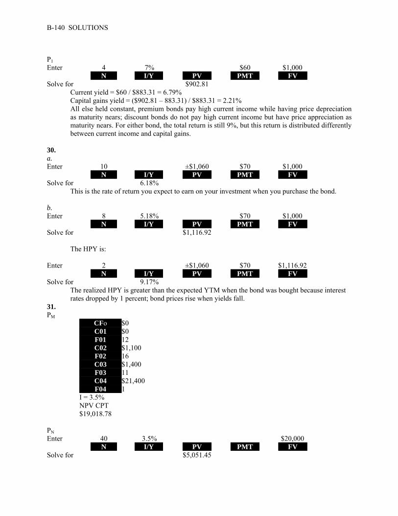
B-140 SOLUTIONS

P1 Enter 4 7% $60 $1,000 N I/Y PV PMT FV Solve for $902.81 Current yield = $60 / $883.31 = 6.79% Capital gains yield = ($902.81 – 883.31) / $883.31 = 2.21% All else held constant, premium bonds pay high current income while having price depreciation

as maturity nears; discount bonds do not pay high current income but have price appreciation as maturity nears. For either bond, the total return is still 9%, but this return is distributed differently between current income and capital gains.

30. a. Enter 10 ±$1,060 $70 $1,000 N I/Y PV PMT FV Solve for 6.18% This is the rate of return you expect to earn on your investment when you purchase the bond. b. Enter 8 5.18% $70 $1,000 N I/Y PV PMT FV Solve for $1,116.92 The HPY is: Enter 2 ±$1,060 $70 $1,116.92 N I/Y PV PMT FV Solve for 9.17%

The realized HPY is greater than the expected YTM when the bond was bought because interest rates dropped by 1 percent; bond prices rise when yields fall.

31. PM CFo $0 C01 $0 F01 12 C02 $1,100 F02 16 C03 $1,400 F03 11 C04 $21,400 F04 1 I = 3.5% NPV CPT $19,018.78 PN Enter 40 3.5% $20,000 N I/Y PV PMT FV Solve for $5,051.45

CHAPTER 8 STOCK VALUATION Answers to Concepts Review and Critical Thinking Questions 1. The value of any investment depends on the present value of its cash flows; i.e., what investors will

actually receive. The cash flows from a share of stock are the dividends. 2. Investors believe the company will eventually start paying dividends (or be sold to another company). 3. In general, companies that need the cash will often forgo dividends since dividends are a cash expense.

Young, growing companies with profitable investment opportunities are one example; another example is a company in financial distress. This question is examined in depth in a later chapter.

4. The general method for valuing a share of stock is to find the present value of all expected future dividends.

The dividend growth model presented in the text is only valid (i) if dividends are expected to occur forever, that is, the stock provides dividends in perpetuity, and (ii) if a constant growth rate of dividends occurs forever. A violation of the first assumption might be a company that is expected to cease operations and dissolve itself some finite number of years from now. The stock of such a company would be valued by applying the general method of valuation explained in this chapter. A violation of the second assumption might be a start-up firm that isn’t currently paying any dividends, but is expected to eventually start making dividend payments some number of years from now. This stock would also be valued by the general dividend valuation method explained in this chapter.

5. The common stock probably has a higher price because the dividend can grow, whereas it is fixed on the

preferred. However, the preferred is less risky because of the dividend and liquidation preference, so it is possible the preferred could be worth more, depending on the circumstances.

6. The two components are the dividend yield and the capital gains yield. For most companies, the capital

gains yield is larger. This is easy to see for companies that pay no dividends. For companies that do pay dividends, the dividend yields are rarely over five percent and are often much less.

7. Yes. If the dividend grows at a steady rate, so does the stock price. In other words, the dividend growth rate

and the capital gains yield are the same. 8. In a corporate election, you can buy votes (by buying shares), so money can be used to influence or even

determine the outcome. Many would argue the same is true in political elections, but, in principle at least, no one has more than one vote.

9. It wouldn’t seem to be. Investors who don’t like the voting features of a particular class of stock are under

no obligation to buy it. 10. Investors buy such stock because they want it, recognizing that the shares have no voting power.

Presumably, investors pay a little less for such shares than they would otherwise.

B-142 SOLUTIONS

11. Presumably, the current stock value reflects the risk, timing and magnitude of all future cash flows, both short-term and long-term. If this is correct, then the statement is false.

12. If this assumption is violated, the two-stage dividend growth model is not valid. In other words, the price

calculated will not be correct. Depending on the stock, it may be more reasonable to assume that the dividends fall from the high growth rate to the low perpetual growth rate over a period of years, rather than in one year.

Solutions to Questions and Problems NOTE: All end of chapter problems were solved using a spreadsheet. Many problems require multiple steps. Due to space and readability constraints, when these intermediate steps are included in this solutions manual, rounding may appear to have occurred. However, the final answer for each problem is found without rounding during any step in the problem. Basic 1. The constant dividend growth model is: Pt = Dt × (1 + g) / (R – g) So the price of the stock today is: P0 = D0 (1 + g) / (R – g) = $1.95 (1.06) / (.11 – .06) = $41.34 The dividend at year 4 is the dividend today times the FVIF for the growth rate in dividends and four years,

so: P3 = D3 (1 + g) / (R – g) = D0 (1 + g)4 / (R – g) = $1.95 (1.06)4 / (.11 – .06) = $49.24 We can do the same thing to find the dividend in Year 16, which gives us the price in Year 15, so: P15 = D15 (1 + g) / (R – g) = D0 (1 + g)16 / (R – g) = $1.95 (1.06)16 / (.11 – .06) = $99.07 There is another feature of the constant dividend growth model: The stock price grows at the dividend

growth rate. So, if we know the stock price today, we can find the future value for any time in the future we want to calculate the stock price. In this problem, we want to know the stock price in three years, and we have already calculated the stock price today. The stock price in three years will be:

P3 = P0(1 + g)3 = $41.34(1 + .06)3 = $49.24 And the stock price in 15 years will be: P15 = P0(1 + g)15 = $41.34(1 + .06)15 = $99.07 2. We need to find the required return of the stock. Using the constant growth model, we can solve the

equation for R. Doing so, we find: R = (D1 / P0) + g = ($2.10 / $48.00) + .05 = .0938 or 9.38%

CHAPTER 8 B-143

3. The dividend yield is the dividend next year divided by the current price, so the dividend yield is: Dividend yield = D1 / P0 = $2.10 / $48.00 = .0438 or 4.38% The capital gains yield, or percentage increase in the stock price, is the same as the dividend growth rate,

so: Capital gains yield = 5% 4. Using the constant growth model, we find the price of the stock today is: P0 = D1 / (R – g) = $3.04 / (.11 – .038) = $42.22 5. The required return of a stock is made up of two parts: The dividend yield and the capital gains yield. So,

the required return of this stock is: R = Dividend yield + Capital gains yield = .063 + .052 = .1150 or 11.50% 6. We know the stock has a required return of 11 percent, and the dividend and capital gains yield are equal,

so: Dividend yield = 1/2(.11) = .055 = Capital gains yield Now we know both the dividend yield and capital gains yield. The dividend is simply the stock price times

the dividend yield, so: D1 = .055($47) = $2.59 This is the dividend next year. The question asks for the dividend this year. Using the relationship between

the dividend this year and the dividend next year: D1 = D0(1 + g) We can solve for the dividend that was just paid: $2.59 = D0(1 + .055) D0 = $2.59 / 1.055 = $2.45 7. The price of any financial instrument is the PV of the future cash flows. The future dividends of this stock

are an annuity for 11 years, so the price of the stock is the PVA, which will be: P0 = $9.75(PVIFA10%,11) = $63.33 8. The price a share of preferred stock is the dividend divided by the required return. This is the same

equation as the constant growth model, with a dividend growth rate of zero percent. Remember, most preferred stock pays a fixed dividend, so the growth rate is zero. Using this equation, we find the price per share of the preferred stock is:

R = D/P0 = $5.50/$108 = .0509 or 5.09%

B-144 SOLUTIONS

9. We can use the constant dividend growth model, which is: Pt = Dt × (1 + g) / (R – g) So the price of each company’s stock today is: Red stock price = $2.35 / (.08 – .05) = $78.33 Yellow stock price = $2.35 / (.11 – .05) = $39.17 Blue stock price = $2.35 / (.14 – .05) = $26.11 As the required return increases, the stock price decreases. This is a function of the time value of money: A

higher discount rate decreases the present value of cash flows. It is also important to note that relatively small changes in the required return can have a dramatic impact on the stock price.

Intermediate 10. This stock has a constant growth rate of dividends, but the required return changes twice. To find the value

of the stock today, we will begin by finding the price of the stock at Year 6, when both the dividend growth rate and the required return are stable forever. The price of the stock in Year 6 will be the dividend in Year 7, divided by the required return minus the growth rate in dividends. So:

P6 = D6 (1 + g) / (R – g) = D0 (1 + g)7 / (R – g) = $3.50 (1.05)7 / (.10 – .05) = $98.50 Now we can find the price of the stock in Year 3. We need to find the price here since the required return

changes at that time. The price of the stock in Year 3 is the PV of the dividends in Years 4, 5, and 6, plus the PV of the stock price in Year 6. The price of the stock in Year 3 is:

P3 = $3.50(1.05)4 / 1.12 + $3.50(1.05)5 / 1.122 + $3.50(1.05)6 / 1.123 + $98.50 / 1.123 P3 = $80.81 Finally, we can find the price of the stock today. The price today will be the PV of the dividends in Years

1, 2, and 3, plus the PV of the stock in Year 3. The price of the stock today is: P0 = $3.50(1.05) / 1.14 + $3.50(1.05)2 / (1.14)2 + $3.50(1.05)3 / (1.14)3 + $80.81 / (1.14)3 P0 = $63.47 11. Here we have a stock that pays no dividends for 10 years. Once the stock begins paying dividends, it will

have a constant growth rate of dividends. We can use the constant growth model at that point. It is important to remember that general constant dividend growth formula is:

Pt = [Dt × (1 + g)] / (R – g) This means that since we will use the dividend in Year 10, we will be finding the stock price in Year 9. The

dividend growth model is similar to the PVA and the PV of a perpetuity: The equation gives you the PV one period before the first payment. So, the price of the stock in Year 9 will be:

P9 = D10 / (R – g) = $10.00 / (.14 – .05) = $111.11

CHAPTER 8 B-145

The price of the stock today is simply the PV of the stock price in the future. We simply discount the future stock price at the required return. The price of the stock today will be:

P0 = $111.11 / 1.149 = $34.17 12. The price of a stock is the PV of the future dividends. This stock is paying four dividends, so the price of

the stock is the PV of these dividends using the required return. The price of the stock is: P0 = $10 / 1.11 + $14 / 1.112 + $18 / 1.113 + $22 / 1.114 + $26 / 1.115 = $63.45 13. With supernormal dividends, we find the price of the stock when the dividends level off at a constant

growth rate, and then find the PV of the future stock price, plus the PV of all dividends during the supernormal growth period. The stock begins constant growth in Year 4, so we can find the price of the stock in Year 4, at the beginning of the constant dividend growth, as:

P4 = D4 (1 + g) / (R – g) = $2.00(1.05) / (.12 – .05) = $30.00 The price of the stock today is the PV of the first four dividends, plus the PV of the Year 3 stock price. So,

the price of the stock today will be: P0 = $11.00 / 1.11 + $8.00 / 1.112 + $5.00 / 1.113 + $2.00 / 1.114 + $30.00 / 1.114 = $40.09 14. With supernormal dividends, we find the price of the stock when the dividends level off at a constant

growth rate, and then find the PV of the futures stock price, plus the PV of all dividends during the supernormal growth period. The stock begins constant growth in Year 4, so we can find the price of the stock in Year 3, one year before the constant dividend growth begins as:

P3 = D3 (1 + g) / (R – g) = D0 (1 + g1)

3 (1 + g2) / (R – g) P3 = $1.80(1.30)3(1.06) / (.13 – .06) P3 = $59.88 The price of the stock today is the PV of the first three dividends, plus the PV of the Year 3 stock price.

The price of the stock today will be: P0 = $1.80(1.30) / 1.13 + $1.80(1.30)2 / 1.132 + $1.80(1.30)3 / 1.133 + $59.88 / 1.133 P0 = $48.70 We could also use the two-stage dividend growth model for this problem, which is: P0 = [D0(1 + g1)/(R – g1)]{1 – [(1 + g1)/(1 + R)]T}+ [(1 + g1)/(1 + R)]T[D0(1 + g1)/(R – g1)] P0 = [$1.80(1.30)/(.13 – .30)][1 – (1.30/1.13)3] + [(1 + .30)/(1 + .13)]3[$1.80(1.06)/(.13 – .06)] P0 = $48.70 15. Here we need to find the dividend next year for a stock experiencing supernormal growth. We know the

stock price, the dividend growth rates, and the required return, but not the dividend. First, we need to realize that the dividend in Year 3 is the current dividend times the FVIF. The dividend in Year 3 will be:

D3 = D0 (1.25)3

B-146 SOLUTIONS

And the dividend in Year 4 will be the dividend in Year 3 times one plus the growth rate, or: D4 = D0 (1.25)3 (1.15) The stock begins constant growth in Year 4, so we can find the price of the stock in Year 4 as the dividend

in Year 5, divided by the required return minus the growth rate. The equation for the price of the stock in Year 4 is:

P4 = D4 (1 + g) / (R – g) Now we can substitute the previous dividend in Year 4 into this equation as follows: P4 = D0 (1 + g1)

3 (1 + g2) (1 + g3) / (R – g) P4 = D0 (1.25)3 (1.15) (1.08) / (.13 – .08) = 48.52D0 When we solve this equation, we find that the stock price in Year 4 is 48.52 times as large as the dividend

today. Now we need to find the equation for the stock price today. The stock price today is the PV of the dividends in Years 1, 2, 3, and 4, plus the PV of the Year 4 price. So:

P0 = D0(1.25)/1.13 + D0(1.25)2/1.132 + D0(1.25)3/1.133+ D0(1.25)3(1.15)/1.134 + 48.52D0/1.134

We can factor out D0 in the equation, and combine the last two terms. Doing so, we get: P0 = $76 = D0{1.25/1.13 + 1.252/1.132 + 1.253/1.133 + [(1.25)3(1.15) + 48.52] / 1.134} Reducing the equation even further by solving all of the terms in the braces, we get: $76 = $34.79D0

D0 = $76 / $34.79 D0 = $2.18 This is the dividend today, so the projected dividend for the next year will be: D1 = $2.18(1.25) D1 = $2.73 16. The constant growth model can be applied even if the dividends are declining by a constant percentage, just

make sure to recognize the negative growth. So, the price of the stock today will be: P0 = D0 (1 + g) / (R – g) P0 = $10.46(1 – .04) / [(.115 – (–.04)] P0 = $64.78 17. We are given the stock price, the dividend growth rate, and the required return, and are asked to find the

dividend. Using the constant dividend growth model, we get: P0 = $64 = D0 (1 + g) / (R – g)

CHAPTER 8 B-147

Solving this equation for the dividend gives us: D0 = $64(.10 – .045) / (1.045) D0 = $3.37 18. The price of a share of preferred stock is the dividend payment divided by the required return. We know the

dividend payment in Year 20, so we can find the price of the stock in Year 19, one year before the first dividend payment. Doing so, we get:

P19 = $20.00 / .064 P19 = $312.50 The price of the stock today is the PV of the stock price in the future, so the price today will be: P0 = $312.50 / (1.064)19 P0 = $96.15 19. The annual dividend paid to stockholders is $1.48, and the dividend yield is 2.1 percent. Using the equation

for the dividend yield: Dividend yield = Dividend / Stock price We can plug the numbers in and solve for the stock price: .021 = $1.48 / P0 P0 = $1.48/.021 = $70.48 The “Net Chg” of the stock shows the stock decreased by $0.23 on this day, so the closing stock price

yesterday was: Yesterday’s closing price = $70.48 + 0.23 = $70.71 To find the net income, we need to find the EPS. The stock quote tells us the P/E ratio for the stock is 19.

Since we know the stock price as well, we can use the P/E ratio to solve for EPS as follows: P/E = 19 = Stock price / EPS = $70.48 / EPS EPS = $70.48 / 19 = $3.71 We know that EPS is just the total net income divided by the number of shares outstanding, so: EPS = NI / Shares = $3.71 = NI / 25,000,000 NI = $3.71(25,000,000) = $92,731,830 20. We can use the two-stage dividend growth model for this problem, which is: P0 = [D0(1 + g1)/(R – g1)]{1 – [(1 + g1)/(1 + R)]T}+ [(1 + g1)/(1 + R)]T[D0(1 + g2)/(R – g2)] P0 = [$1.25(1.28)/(.13 – .28)][1 – (1.28/1.13)8] + [(1.28)/(1.13)]8[$1.25(1.06)/(.13 – .06)] P0 = $69.55

B-148 SOLUTIONS

21. We can use the two-stage dividend growth model for this problem, which is: P0 = [D0(1 + g1)/(R – g1)]{1 – [(1 + g1)/(1 + R)]T}+ [(1 + g1)/(1 + R)]T[D0(1 + g2)/(R – g2)] P0 = [$1.74(1.25)/(.12 – .25)][1 – (1.25/1.12)11] + [(1.25)/(1.12)]11[$1.74(1.06)/(.12 – .06)] P0 = $142.14 Challenge 22. We are asked to find the dividend yield and capital gains yield for each of the stocks. All of the stocks have

a 15 percent required return, which is the sum of the dividend yield and the capital gains yield. To find the components of the total return, we need to find the stock price for each stock. Using this stock price and the dividend, we can calculate the dividend yield. The capital gains yield for the stock will be the total return (required return) minus the dividend yield.

W: P0 = D0(1 + g) / (R – g) = $4.50(1.10)/(.19 – .10) = $55.00 Dividend yield = D1/P0 = $4.50(1.10)/$55.00 = .09 or 9% Capital gains yield = .19 – .09 = .10 or 10% X: P0 = D0(1 + g) / (R – g) = $4.50/(.19 – 0) = $23.68 Dividend yield = D1/P0 = $4.50/$23.68 = .19 or 19% Capital gains yield = .19 – .19 = 0% Y: P0 = D0(1 + g) / (R – g) = $4.50(1 – .05)/(.19 + .05) = $17.81 Dividend yield = D1/P0 = $4.50(0.95)/$17.81 = .24 or 24% Capital gains yield = .19 – .24 = –.05 or –5% Z: P2 = D2(1 + g) / (R – g) = D0(1 + g1)

2(1 + g2)/(R – g2) = $4.50(1.20)2(1.12)/(.19 – .12) = $103.68 P0 = $4.50 (1.20) / (1.19) + $4.50 (1.20)2 / (1.19)2 + $103.68 / (1.19)2 = $82.33 Dividend yield = D1/P0 = $4.50(1.20)/$96.10 = .066 or 6.6% Capital gains yield = .19 – .066 = .124 or 12.4% In all cases, the required return is 19%, but the return is distributed differently between current income and

capital gains. High growth stocks have an appreciable capital gains component but a relatively small current income yield; conversely, mature, negative-growth stocks provide a high current income but also price depreciation over time.

23. a. Using the constant growth model, the price of the stock paying annual dividends will be: P0 = D0(1 + g) / (R – g) = $3.20(1.06)/(.12 – .06) = $56.53

CHAPTER 8 B-149

b. If the company pays quarterly dividends instead of annual dividends, the quarterly dividend will be one-fourth of annual dividend, or:

Quarterly dividend: $3.20(1.06)/4 = $0.848

To find the equivalent annual dividend, we must assume that the quarterly dividends are reinvested at the required return. We can then use this interest rate to find the equivalent annual dividend. In other words, when we receive the quarterly dividend, we reinvest it at the required return on the stock. So, the effective quarterly rate is:

Effective quarterly rate: 1.12.25 – 1 = .0287 The effective annual dividend will be the FVA of the quarterly dividend payments at the effective quarterly required return. In this case, the effective annual dividend will be:

Effective D1 = $0.848(FVIFA2.87%,4) = $3.54 Now, we can use the constant growth model to find the current stock price as: P0 = $3.54/(.12 – .06) = $59.02 Note that we cannot simply find the quarterly effective required return and growth rate to find the

value of the stock. This would assume the dividends increased each quarter, not each year. 24. Here we have a stock with supernormal growth, but the dividend growth changes every year for the first

four years. We can find the price of the stock in Year 3 since the dividend growth rate is constant after the third dividend. The price of the stock in Year 3 will be the dividend in Year 4, divided by the required return minus the constant dividend growth rate. So, the price in Year 3 will be:

P3 = $2.45(1.20)(1.15)(1.10)(1.05) / (.11 – .05) = $65.08 The price of the stock today will be the PV of the first three dividends, plus the PV of the stock price in

Year 3, so: P0 = $2.45(1.20)/(1.11) + $2.45(1.20)(1.15)/1.112 + $2.45(1.20)(1.15)(1.10)/1.113 + $65.08/1.113 P0 = $55.70 25. Here we want to find the required return that makes the PV of the dividends equal to the current stock

price. The equation for the stock price is: P = $2.45(1.20)/(1 + R) + $2.45(1.20)(1.15)/(1 + R)2 + $2.45(1.20)(1.15)(1.10)/(1 + R)3

+ [$2.45(1.20)(1.15)(1.10)(1.05)/(R – .05)]/(1 + R)3 = $63.82

We need to find the roots of this equation. Using spreadsheet, trial and error, or a calculator with a root solving function, we find that: R = 10.24%

B-150 SOLUTIONS

26. Even though the question concerns a stock with a constant growth rate, we need to begin with the equation for two-stage growth given in the chapter, which is:

P0 = 1

10 1

R - g

) g (D

t

R

g

1

1 - 1 1 +

tt

R) (

P

1

We can expand the equation (see Problem 27 for more detail) to the following:

P0 = 1

10 1

R - g

) g (D

t

R

g

1

1 - 1 1 +

t

R

g

1

1 1 2

21

R - g

) g D(

Since the growth rate is constant, g1 = g2 , so:

P0 = R - g

g) (D 10

t

R

g -

1

11 +

t

R

g

1

1

R - g

g) D( 1

Since we want the first t dividends to constitute one-half of the stock price, we can set the two terms on the

right hand side of the equation equal to each other, which gives us:

g - R

g) (1D0

t

R

g -

1

1 1 =

t

R

g

1

1

R - g

g) D( 1

Since g - R

g) (1D0 appears on both sides of the equation, we can eliminate this, which leaves:

1 – t

R 1

g 1 =

t

R

g

1

1

Solving this equation, we get:

1 = t

R 1

g 1 +

t

R

g

1

1

1 = 2t

R 1

g 1

1/2 = t

R

g

1

1

CHAPTER 8 B-151

t ln

R 1

g 1 = ln(0.5)

t =

R

g

1

1ln

ln(0.5)

This expression will tell you the number of dividends that constitute one-half of the current stock price. 27. To find the value of the stock with two-stage dividend growth, consider that the present value of the first t

dividends is the present value of a growing annuity. Additionally, to find the price of the stock, we need to add the present value of the stock price at time t. So, the stock price today is:

P0 = PV of t dividends + PV(Pt) Using g1 to represent the first growth rate and substituting the equation for the present value of a growing

annuity, we get:

P0 = D1

1

1

1

11

R - g

R

g -

t

+ PV(Pt)

Since the dividend in one year will increase at g1, we can re-write the expression as:

P0 = D0(1 + g1)

1

1

1

11

R - g

R

g -

t

+ PV(Pt)

Now we can re-write the equation again as:

P0 = 1

10 1

R - g

) g (D

t

1

R 1

g 1 - 1 + PV(Pt)

To find the price of the stock at time t, we can use the constant dividend growth model, or:

Pt = 2

1 t

g - R

D

The dividend at t + 1 will have grown at g1 for t periods, and at g2 for one period, so: Dt + 1 = D0(1 + g1)

t(1 + g2)

B-152 SOLUTIONS

So, we can re-write the equation as:

Pt = 2

21 11

R - g

) g () g D( t

Next, we can find value today of the future stock price as:

PV(Pt) = 2

21 11

R - g

) g () g D( t ×

t R) ( 1

1

which can be written as:

PV(Pt) = t

R

g

1

1 1 × 2

21

R - g

) g D(

Substituting this into the stock price equation, we get:

P0 = 1

10 1

R - g

) g (D

t

R

g -

1

11 1 +

t

R

g

1

1 1 × 2

21

R - g

) g D(

In this equation, the first term on the right hand side is the present value of the first t dividends, and the

second term is the present value of the stock price when constant dividend growth forever begins. 28. To find the expression when the growth rate for the first stage is exactly equal to the required return,

consider we can find the present value of the dividends in the first stage as:

PV = 1

110

)1(

) (1

R

gD

+

2

210

)1(

) (1

R

gD

+

3

310

)1(

) (1

R

gD

+ …

Since g1 is equal to R, each of the terns reduces to: PV = D0 + D0 + D0 + …. PV = t × D0

So, the expression for the price of a stock when the first growth rate is exactly equal to the required return

is:

Pt = t × D0 +

2

210 11

gR

ggD t

CHAPTER 9 NET PRESENT VALUE AND OTHER INVESTMENT CRITERIA Answers to Concepts Review and Critical Thinking Questions 1. A payback period less than the project’s life means that the NPV is positive for a zero discount rate, but

nothing more definitive can be said. For discount rates greater than zero, the payback period will still be less than the project’s life, but the NPV may be positive, zero, or negative, depending on whether the discount rate is less than, equal to, or greater than the IRR. The discounted payback includes the effect of the relevant discount rate. If a project’s discounted payback period is less than the project’s life, it must be the case that NPV is positive.

2. If a project has a positive NPV for a certain discount rate, then it will also have a positive NPV for a

zero discount rate; thus, the payback period must be less than the project life. Since discounted payback is calculated at the same discount rate as is NPV, if NPV is positive, the discounted payback period must be less than the project’s life. If NPV is positive, then the present value of future cash inflows is greater than the initial investment cost; thus PI must be greater than 1. If NPV is positive for a certain discount rate R, then it will be zero for some larger discount rate R*; thus the IRR must be greater than the required return.

3. a. Payback period is simply the accounting break-even point of a series of cash flows. To actually

compute the payback period, it is assumed that any cash flow occurring during a given period is realized continuously throughout the period, and not at a single point in time. The payback is then the point in time for the series of cash flows when the initial cash outlays are fully recovered. Given some predetermined cutoff for the payback period, the decision rule is to accept projects that payback before this cutoff, and reject projects that take longer to payback.

b. The worst problem associated with payback period is that it ignores the time value of money. In addition, the selection of a hurdle point for payback period is an arbitrary exercise that lacks any steadfast rule or method. The payback period is biased towards short-term projects; it fully ignores any cash flows that occur after the cutoff point.

c. Despite its shortcomings, payback is often used because (1) the analysis is straightforward and simple and (2) accounting numbers and estimates are readily available. Materiality considerations often warrant a payback analysis as sufficient; maintenance projects are another example where the detailed analysis of other methods is often not needed. Since payback is biased towards liquidity, it may be a useful and appropriate analysis method for short-term projects where cash management is most important.

4. a. The discounted payback is calculated the same as is regular payback, with the exception that each

cash flow in the series is first converted to its present value. Thus discounted payback provides a measure of financial/economic break-even because of this discounting, just as regular payback provides a measure of accounting break-even because it does not discount the cash flows. Given some predetermined cutoff for the discounted payback period, the decision rule is to accept projects whose discounted cash flows payback before this cutoff period, and to reject all other projects.

B-154 SOLUTIONS

b. The primary disadvantage to using the discounted payback method is that it ignores all cash flows that occur after the cutoff date, thus biasing this criterion towards short-term projects. As a result, the method may reject projects that in fact have positive NPVs, or it may accept projects with large future cash outlays resulting in negative NPVs. In addition, the selection of a cutoff point is again an arbitrary exercise.

c. Discounted payback is an improvement on regular payback because it takes into account the time value of money. For conventional cash flows and strictly positive discount rates, the discounted payback will always be greater than the regular payback period.

5. a. The average accounting return is interpreted as an average measure of the accounting performance

of a project over time, computed as some average profit measure attributable to the project divided by some average balance sheet value for the project. This text computes AAR as average net income with respect to average (total) book value. Given some predetermined cutoff for AAR, the decision rule is to accept projects with an AAR in excess of the target measure, and reject all other projects.

b. AAR is not a measure of cash flows and market value, but a measure of financial statement accounts that often bear little resemblance to the relevant value of a project. In addition, the selection of a cutoff is arbitrary, and the time value of money is ignored. For a financial manager, both the reliance on accounting numbers rather than relevant market data and the exclusion of time value of money considerations are troubling. Despite these problems, AAR continues to be used in practice because (1) the accounting information is usually available, (2) analysts often use accounting ratios to analyze firm performance, and (3) managerial compensation is often tied to the attainment of certain target accounting ratio goals.

6. a. NPV is simply the present value of a project’s cash flows. NPV specifically measures, after

considering the time value of money, the net increase or decrease in firm wealth due to the project. The decision rule is to accept projects that have a positive NPV, and reject projects with a negative NPV.

b. NPV is superior to the other methods of analysis presented in the text because it has no serious flaws. The method unambiguously ranks mutually exclusive projects, and can differentiate between projects of different scale and time horizon. The only drawback to NPV is that it relies on cash flow and discount rate values that are often estimates and not certain, but this is a problem shared by the other performance criteria as well. A project with NPV = $2,500 implies that the total shareholder wealth of the firm will increase by $2,500 if the project is accepted.

7. a. The IRR is the discount rate that causes the NPV of a series of cash flows to be exactly zero. IRR

can thus be interpreted as a financial break-even rate of return; at the IRR, the net value of the project is zero. The IRR decision rule is to accept projects with IRRs greater than the discount rate, and to reject projects with IRRs less than the discount rate.

b. IRR is the interest rate that causes NPV for a series of cash flows to be zero. NPV is preferred in all situations to IRR; IRR can lead to ambiguous results if there are non-conventional cash flows, and it also ambiguously ranks some mutually exclusive projects. However, for stand-alone projects with conventional cash flows, IRR and NPV are interchangeable techniques.

c. IRR is frequently used because it is easier for many financial managers and analysts to rate performance in relative terms, such as “12%”, than in absolute terms, such as “$46,000.” IRR may be a preferred method to NPV in situations where an appropriate discount rate is unknown are uncertain; in this situation, IRR would provide more information about the project than would NPV.

CHAPTER 9 B-155

8. a. The profitability index is the present value of cash inflows relative to the project cost. As such, it is a benefit/cost ratio, providing a measure of the relative profitability of a project. The profitability index decision rule is to accept projects with a PI greater than one, and to reject projects with a PI less than one.

b. PI = (NPV + cost)/cost = 1 + (NPV/cost). If a firm has a basket of positive NPV projects and is subject to capital rationing, PI may provide a good ranking measure of the projects, indicating the “bang for the buck” of each particular project.

9. For a project with future cash flows that are an annuity: Payback = I / C And the IRR is: 0 = – I + C / IRR Solving the IRR equation for IRR, we get: IRR = C / I Notice this is just the reciprocal of the payback. So: IRR = 1 / PB For long-lived projects with relatively constant cash flows, the sooner the project pays back, the greater

is the IRR. 10. There are a number of reasons. Two of the most important have to do with transportation costs and

exchange rates. Manufacturing in the U.S. places the finished product much closer to the point of sale, resulting in significant savings in transportation costs. It also reduces inventories because goods spend less time in transit. Higher labor costs tend to offset these savings to some degree, at least compared to other possible manufacturing locations. Of great importance is the fact that manufacturing in the U.S. means that a much higher proportion of the costs are paid in dollars. Since sales are in dollars, the net effect is to immunize profits to a large extent against fluctuations in exchange rates. This issue is discussed in greater detail in the chapter on international finance.

11. The single biggest difficulty, by far, is coming up with reliable cash flow estimates. Determining an

appropriate discount rate is also not a simple task. These issues are discussed in greater depth in the next several chapters. The payback approach is probably the simplest, followed by the AAR, but even these require revenue and cost projections. The discounted cash flow measures (discounted payback, NPV, IRR, and profitability index) are really only slightly more difficult in practice.

12. Yes, they are. Such entities generally need to allocate available capital efficiently, just as for-profits do.

However, it is frequently the case that the “revenues” from not-for-profit ventures are not tangible. For example, charitable giving has real opportunity costs, but the benefits are generally hard to measure. To the extent that benefits are measurable, the question of an appropriate required return remains. Payback rules are commonly used in such cases. Finally, realistic cost/benefit analysis along the lines indicated should definitely be used by the U.S. government and would go a long way toward balancing the budget!

B-156 SOLUTIONS

13. The MIRR is calculated by finding the present value of all cash outflows, the future value of all cash inflows to the end of the project, and then calculating the IRR of the two cash flows. As a result, the cash flows have been discounted or compounded by one interest rate (the required return), and then the interest rate between the two remaining cash flows is calculated. As such, the MIRR is not a true interest rate. In contrast, consider the IRR. If you take the initial investment, and calculate the future value at the IRR, you can replicate the future cash flows of the project exactly.

14. The statement is incorrect. It is true that if you calculate the future value of all intermediate cash flows

to the end of the project at the required return, then calculate the NPV of this future value and the initial investment, you will get the same NPV. However, NPV says nothing about reinvestment of intermediate cash flows. The NPV is the present value of the project cash flows. What is actually done with those cash flows once they are generated is not relevant. Put differently, the value of a project depends on the cash flows generated by the project, not on the future value of those cash flows. The fact that the reinvestment “works” only if you use the required return as the reinvestment rate is also irrelevant simply because reinvestment is not relevant in the first place to the value of the project.

One caveat: Our discussion here assumes that the cash flows are truly available once they are generated, meaning that it is up to firm management to decide what to do with the cash flows. In certain cases, there may be a requirement that the cash flows be reinvested. For example, in international investing, a company may be required to reinvest the cash flows in the country in which they are generated and not “repatriate” the money. Such funds are said to be “blocked” and reinvestment becomes relevant because the cash flows are not truly available.

15. The statement is incorrect. It is true that if you calculate the future value of all intermediate cash flows

to the end of the project at the IRR, then calculate the IRR of this future value and the initial investment, you will get the same IRR. However, as in the previous question, what is done with the cash flows once they are generated does not affect the IRR. Consider the following example:

C0 C1 C2 IRR Project A –$100 $10 $110 10%

Suppose this $100 is a deposit into a bank account. The IRR of the cash flows is 10 percent. Does the

IRR change if the Year 1 cash flow is reinvested in the account, or if it is withdrawn and spent on pizza? No. Finally, consider the yield to maturity calculation on a bond. If you think about it, the YTM is the IRR on the bond, but no mention of a reinvestment assumption for the bond coupons is suggested. The reason is that reinvestment is irrelevant to the YTM calculation; in the same way, reinvestment is irrelevant in the IRR calculation. Our caveat about blocked funds applies here as well.

CHAPTER 9 B-157

Solutions to Questions and Problems NOTE: All end of chapter problems were solved using a spreadsheet. Many problems require multiple steps. Due to space and readability constraints, when these intermediate steps are included in this solutions manual, rounding may appear to have occurred. However, the final answer for each problem is found without rounding during any step in the problem. Basic 1. To calculate the payback period, we need to find the time that the project has recovered its initial

investment. After three years, the project has created: $1,600 + 1,900 + 2,300 = $5,800 in cash flows. The project still needs to create another: $6,400 – 5,800 = $600 in cash flows. During the fourth year, the cash flows from the project will be $1,400. So, the payback

period will be 3 years, plus what we still need to make divided by what we will make during the fourth year. The payback period is:

Payback = 3 + ($600 / $1,400) = 3.43 years 2. To calculate the payback period, we need to find the time that the project has recovered its initial

investment. The cash flows in this problem are an annuity, so the calculation is simpler. If the initial cost is $2,400, the payback period is:

Payback = 3 + ($105 / $765) = 3.14 years There is a shortcut to calculate the future cash flows are an annuity. Just divide the initial cost by the

annual cash flow. For the $2,400 cost, the payback period is: Payback = $2,400 / $765 = 3.14 years For an initial cost of $3,600, the payback period is: Payback = $3,600 / $765 = 4.71 years The payback period for an initial cost of $6,500 is a little trickier. Notice that the total cash inflows after

eight years will be: Total cash inflows = 8($765) = $6,120 If the initial cost is $6,500, the project never pays back. Notice that if you use the shortcut for annuity

cash flows, you get: Payback = $6,500 / $765 = 8.50 years This answer does not make sense since the cash flows stop after eight years, so again, we must conclude

the payback period is never.

B-158 SOLUTIONS

3. Project A has cash flows of $19,000 in Year 1, so the cash flows are short by $21,000 of recapturing the initial investment, so the payback for Project A is:

Payback = 1 + ($21,000 / $25,000) = 1.84 years Project B has cash flows of: Cash flows = $14,000 + 17,000 + 24,000 = $55,000 during this first three years. The cash flows are still short by $5,000 of recapturing the initial

investment, so the payback for Project B is: B: Payback = 3 + ($5,000 / $270,000) = 3.019 years Using the payback criterion and a cutoff of 3 years, accept project A and reject project B. 4. When we use discounted payback, we need to find the value of all cash flows today. The value today of

the project cash flows for the first four years is: Value today of Year 1 cash flow = $4,200/1.14 = $3,684.21 Value today of Year 2 cash flow = $5,300/1.142 = $4,078.18 Value today of Year 3 cash flow = $6,100/1.143 = $4,117.33 Value today of Year 4 cash flow = $7,400/1.144 = $4,381.39 To find the discounted payback, we use these values to find the payback period. The discounted first

year cash flow is $3,684.21, so the discounted payback for a $7,000 initial cost is: Discounted payback = 1 + ($7,000 – 3,684.21)/$4,078.18 = 1.81 years For an initial cost of $10,000, the discounted payback is: Discounted payback = 2 + ($10,000 – 3,684.21 – 4,078.18)/$4,117.33 = 2.54 years Notice the calculation of discounted payback. We know the payback period is between two and three

years, so we subtract the discounted values of the Year 1 and Year 2 cash flows from the initial cost. This is the numerator, which is the discounted amount we still need to make to recover our initial investment. We divide this amount by the discounted amount we will earn in Year 3 to get the fractional portion of the discounted payback.

If the initial cost is $13,000, the discounted payback is: Discounted payback = 3 + ($13,000 – 3,684.21 – 4,078.18 – 4,117.33) / $4,381.39 = 3.26 years 5. R = 0%: 3 + ($2,100 / $4,300) = 3.49 years discounted payback = regular payback = 3.49 years R = 5%: $4,300/1.05 + $4,300/1.052 + $4,300/1.053 = $11,709.97 $4,300/1.054 = $3,537.62 discounted payback = 3 + ($15,000 – 11,709.97) / $3,537.62 = 3.93 years

CHAPTER 9 B-159

R = 19%: $4,300(PVIFA19%,6) = $14,662.04 The project never pays back. 6. Our definition of AAR is the average net income divided by the average book value. The average net

income for this project is: Average net income = ($1,938,200 + 2,201,600 + 1,876,000 + 1,329,500) / 4 = $1,836,325 And the average book value is: Average book value = ($15,000,000 + 0) / 2 = $7,500,000 So, the AAR for this project is: AAR = Average net income / Average book value = $1,836,325 / $7,500,000 = .2448 or 24.48% 7. The IRR is the interest rate that makes the NPV of the project equal to zero. So, the equation that defines the

IRR for this project is: 0 = – $34,000 + $16,000/(1+IRR) + $18,000/(1+IRR)2 + $15,000/(1+IRR)3 Using a spreadsheet, financial calculator, or trial and error to find the root of the equation, we find that: IRR = 20.97% Since the IRR is greater than the required return we would accept the project. 8. The NPV of a project is the PV of the outflows minus the PV of the inflows. The equation for the NPV

of this project at an 11 percent required return is: NPV = – $34,000 + $16,000/1.11 + $18,000/1.112 + $15,000/1.113 = $5,991.49 At an 11 percent required return, the NPV is positive, so we would accept the project. The equation for the NPV of the project at a 30 percent required return is: NPV = – $34,000 + $16,000/1.30 + $18,000/1.302 + $15,000/1.303 = –$4,213.93 At a 30 percent required return, the NPV is negative, so we would reject the project. 9. The NPV of a project is the PV of the outflows minus the PV of the inflows. Since the cash inflows are

an annuity, the equation for the NPV of this project at an 8 percent required return is: NPV = –$138,000 + $28,500(PVIFA8%, 9) = $40,036.31 At an 8 percent required return, the NPV is positive, so we would accept the project.

B-160 SOLUTIONS

The equation for the NPV of the project at a 20 percent required return is: NPV = –$138,000 + $28,500(PVIFA20%, 9) = –$23,117.45 At a 20 percent required return, the NPV is negative, so we would reject the project. We would be indifferent to the project if the required return was equal to the IRR of the project, since at

that required return the NPV is zero. The IRR of the project is: 0 = –$138,000 + $28,500(PVIFAIRR, 9) IRR = 14.59% 10. The IRR is the interest rate that makes the NPV of the project equal to zero. So, the equation that defines the

IRR for this project is: 0 = –$19,500 + $9,800/(1+IRR) + $10,300/(1+IRR)2 + $8,600/(1+IRR)3 Using a spreadsheet, financial calculator, or trial and error to find the root of the equation, we find that: IRR = 22.64% 11. The NPV of a project is the PV of the outflows minus the PV of the inflows. At a zero discount rate

(and only at a zero discount rate), the cash flows can be added together across time. So, the NPV of the project at a zero percent required return is:

NPV = –$19,500 + 9,800 + 10,300 + 8,600 = $9,200 The NPV at a 10 percent required return is: NPV = –$19,500 + $9,800/1.1 + $10,300/1.12 + $8,600/1.13 = $4,382.79 The NPV at a 20 percent required return is: NPV = –$19,500 + $9,800/1.2 + $10,300/1.22 + $8,600/1.23 = $796.30 And the NPV at a 30 percent required return is: NPV = –$19,500 + $9,800/1.3 + $10,300/1.32 + $8,600/1.33 = –$1,952.44 Notice that as the required return increases, the NPV of the project decreases. This will always be true

for projects with conventional cash flows. Conventional cash flows are negative at the beginning of the project and positive throughout the rest of the project.

CHAPTER 9 B-161

12. a. The IRR is the interest rate that makes the NPV of the project equal to zero. The equation for the IRR of Project A is:

0 = –$43,000 + $23,000/(1+IRR) + $17,900/(1+IRR)2 + $12,400/(1+IRR)3 + $9,400/(1+IRR)4 Using a spreadsheet, financial calculator, or trial and error to find the root of the equation, we find that: IRR = 20.44% The equation for the IRR of Project B is: 0 = –$43,000 + $7,000/(1+IRR) + $13,800/(1+IRR)2 + $24,000/(1+IRR)3 + $26,000/(1+IRR)4 Using a spreadsheet, financial calculator, or trial and error to find the root of the equation, we find that: IRR = 18.84% Examining the IRRs of the projects, we see that the IRRA is greater than the IRRB, so IRR decision

rule implies accepting project A. This may not be a correct decision; however, because the IRR criterion has a ranking problem for mutually exclusive projects. To see if the IRR decision rule is correct or not, we need to evaluate the project NPVs.

b. The NPV of Project A is: NPVA = –$43,000 + $23,000/1.11+ $17,900/1.112 + $12,400/1.113 + $9,400/1.114 NPVA = $7,507.61 And the NPV of Project B is: NPVB = –$43,000 + $7,000/1.11 + $13,800/1.112 + $24,000/1.113 + $26,000/1.114 NPVB = $9,182.29 The NPVB is greater than the NPVA, so we should accept Project B. c. To find the crossover rate, we subtract the cash flows from one project from the cash flows of the

other project. Here, we will subtract the cash flows for Project B from the cash flows of Project A. Once we find these differential cash flows, we find the IRR. The equation for the crossover rate is:

Crossover rate: 0 = $16,000/(1+R) + $4,100/(1+R)2 – $11,600/(1+R)3 – $16,600/(1+R)4 Using a spreadsheet, financial calculator, or trial and error to find the root of the equation, we find that: R = 15.30% At discount rates above 15.30% choose project A; for discount rates below 15.30% choose project

B; indifferent between A and B at a discount rate of 15.30%.

B-162 SOLUTIONS

13. The IRR is the interest rate that makes the NPV of the project equal to zero. The equation to calculate the IRR of Project X is:

0 = –$15,000 + $8,150/(1+IRR) + $5,050/(1+IRR)2 + $6,800/(1+IRR)3 Using a spreadsheet, financial calculator, or trial and error to find the root of the equation, we find that: IRR = 16.57% For Project Y, the equation to find the IRR is: 0 = –$15,000 + $7,700/(1+IRR) + $5,150/(1+IRR)2 + $7,250/(1+IRR)3 Using a spreadsheet, financial calculator, or trial and error to find the root of the equation, we find that: IRR = 16.45% To find the crossover rate, we subtract the cash flows from one project from the cash flows of the other

project, and find the IRR of the differential cash flows. We will subtract the cash flows from Project Y from the cash flows from Project X. It is irrelevant which cash flows we subtract from the other. Subtracting the cash flows, the equation to calculate the IRR for these differential cash flows is:

Crossover rate: 0 = $450/(1+R) – $100/(1+R)2 – $450/(1+R)3 Using a spreadsheet, financial calculator, or trial and error to find the root of the equation, we find that: R = 11.73% The table below shows the NPV of each project for different required returns. Notice that Project Y

always has a higher NPV for discount rates below 11.73 percent, and always has a lower NPV for discount rates above 11.73 percent.

R $NPVX $NPVY

0% $5,000.00 $5,100.00

5% $3,216.50 $3,267.36

10% $1,691.59 $1,703.23

15% $376.59 $356.78

20% –$766.20 –$811.34

25% –$1,766.40 –$1,832.00 14. a. The equation for the NPV of the project is: NPV = –$45,000,000 + $78,000,000/1.1 – $14,000,000/1.12 = $13,482,142.86 The NPV is greater than 0, so we would accept the project.

CHAPTER 9 B-163

b. The equation for the IRR of the project is: 0 = –$45,000,000 + $78,000,000/(1+IRR) – $14,000,000/(1+IRR)2 From Descartes rule of signs, we know there are potentially two IRRs since the cash flows change

signs twice. From trial and error, the two IRRs are: IRR = 53.00%, –79.67% When there are multiple IRRs, the IRR decision rule is ambiguous. Both IRRs are correct, that is,

both interest rates make the NPV of the project equal to zero. If we are evaluating whether or not to accept this project, we would not want to use the IRR to make our decision.

15. The profitability index is defined as the PV of the cash inflows divided by the PV of the cash outflows.

The equation for the profitability index at a required return of 10 percent is: PI = [$7,300/1.1 + $6,900/1.12 + $5,700/1.13] / $14,000 = 1.187 The equation for the profitability index at a required return of 15 percent is: PI = [$7,300/1.15 + $6,900/1.152 + $5,700/1.153] / $14,000 = 1.094 The equation for the profitability index at a required return of 22 percent is: PI = [$7,300/1.22 + $6,900/1.222 + $5,700/1.223] / $14,000 = 0.983 We would accept the project if the required return were 10 percent or 15 percent since the PI is greater

than one. We would reject the project if the required return were 22 percent since the PI is less than one. 16. a. The profitability index is the PV of the future cash flows divided by the initial investment. The cash

flows for both projects are an annuity, so: PII = $27,000(PVIFA10%,3 ) / $53,000 = 1.267 PIII = $9,100(PVIFA10%,3) / $16,000 = 1.414 The profitability index decision rule implies that we accept project II, since PIII is greater than the

PII. b. The NPV of each project is: NPVI = –$53,000 + $27,000(PVIFA10%,3) = $14,145.00 NPVII = –$16,000 + $9,100(PVIFA10%,3) = $6,630.35 The NPV decision rule implies accepting Project I, since the NPVI is greater than the NPVII.

B-164 SOLUTIONS

c. Using the profitability index to compare mutually exclusive projects can be ambiguous when the magnitude of the cash flows for the two projects are of different scale. In this problem, project I is roughly 3 times as large as project II and produces a larger NPV, yet the profitability index criterion implies that project II is more acceptable.

17. a. The payback period for each project is: A: 3 + ($180,000/$390,000) = 3.46 years B: 2 + ($9,000/$18,000) = 2.50 years The payback criterion implies accepting project B, because it pays back sooner than project A. b. The discounted payback for each project is: A: $20,000/1.15 + $50,000/1.152 + $50,000/1.153 = $88,074.30 $390,000/1.154 = $222,983.77 Discounted payback = 3 + ($390,000 – 88,074.30)/$222,983.77 = 3.95 years B: $19,000/1.15 + $12,000/1.152 + $18,000/1.153 = $37,430.76 $10,500/1.154 = $6,003.41 Discounted payback = 3 + ($40,000 – 37,430.76)/$6,003.41 = 3.43 years The discounted payback criterion implies accepting project B because it pays back sooner than A. c. The NPV for each project is: A: NPV = –$300,000 + $20,000/1.15 + $50,000/1.152 + $50,000/1.153 + $390,000/1.154 NPV = $11,058.07 B: NPV = –$40,000 + $19,000/1.15 + $12,000/1.152 + $18,000/1.153 + $10,500/1.154 NPV = $3,434.16 NPV criterion implies we accept project A because project A has a higher NPV than project B. d. The IRR for each project is: A: $300,000 = $20,000/(1+IRR) + $50,000/(1+IRR)2 + $50,000/(1+IRR)3 + $390,000/(1+IRR)4

Using a spreadsheet, financial calculator, or trial and error to find the root of the equation, we find that:

IRR = 16.20%

CHAPTER 9 B-165

B: $40,000 = $19,000/(1+IRR) + $12,000/(1+IRR)2 + $18,000/(1+IRR)3 + $10,500/(1+IRR)4

Using a spreadsheet, financial calculator, or trial and error to find the root of the equation, we find that:

IRR = 19.50% IRR decision rule implies we accept project B because IRR for B is greater than IRR for A. e. The profitability index for each project is: A: PI = ($20,000/1.15 + $50,000/1.152 + $50,000/1.153 + $390,000/1.154) / $300,000 = 1.037 B: PI = ($19,000/1.15 + $12,000/1.152 + $18,000/1.153 + $10,500/1.154) / $40,000 = 1.086 Profitability index criterion implies accept project B because its PI is greater than project A’s. f. In this instance, the NPV criteria implies that you should accept project A, while profitability index,

payback period, discounted payback, and IRR imply that you should accept project B. The final decision should be based on the NPV since it does not have the ranking problem associated with the other capital budgeting techniques. Therefore, you should accept project A.

18. At a zero discount rate (and only at a zero discount rate), the cash flows can be added together across

time. So, the NPV of the project at a zero percent required return is: NPV = –$684,680 + 263,279 + 294,060 + 227,604 + 174,356 = $274,619 If the required return is infinite, future cash flows have no value. Even if the cash flow in one year is $1

trillion, at an infinite rate of interest, the value of this cash flow today is zero. So, if the future cash flows have no value today, the NPV of the project is simply the cash flow today, so at an infinite interest rate:

NPV = –$684,680 The interest rate that makes the NPV of a project equal to zero is the IRR. The equation for the IRR of

this project is: 0 = –$684,680 + $263,279/(1+IRR) + $294,060/(1+IRR)2 + $227,604/(1+IRR)3 + 174,356/(1+IRR)4 Using a spreadsheet, financial calculator, or trial and error to find the root of the equation, we find that: IRR = 16.23%

B-166 SOLUTIONS

19. The MIRR for the project with all three approaches is: Discounting approach: In the discounting approach, we find the value of all cash outflows to time 0, while any cash inflows

remain at the time at which they occur. So, the discounting the cash outflows to time 0, we find: Time 0 cash flow = –$16,000 – $5,100 / 1.105 Time 0 cash flow = –$19,166.70 So, the MIRR using the discounting approach is: 0 = –$19,166.70 + $6,100/(1+MIRR) + $7,800/(1+MIRR)2 + $8,400/(1+MIRR)3 + 6,500/(1+MIRR)4 Using a spreadsheet, financial calculator, or trial and error to find the root of the equation, we find that: MIRR = 18.18% Reinvestment approach: In the reinvestment approach, we find the future value of all cash except the initial cash flow at the end

of the project. So, reinvesting the cash flows to time 5, we find: Time 5 cash flow = $6,100(1.104) + $7,800(1.103) + $8,400(1.102) + $6,500(1.10) – $5,100 Time 5 cash flow = $31,526.81 So, the MIRR using the discounting approach is: 0 = –$16,000 + $31,526.81/(1+MIRR)5 $31,526.81 / $16,000 = (1+MIRR)5 MIRR = ($31,526.81 / $16,000)1/5 – 1 MIRR = .1453 or 14.53% Combination approach: In the combination approach, we find the value of all cash outflows at time 0, and the value of all cash

inflows at the end of the project. So, the value of the cash flows is: Time 0 cash flow = –$16,000 – $5,100 / 1.105 Time 0 cash flow = –$19,166.70 Time 5 cash flow = $6,100(1.104) + $7,800(1.103) + $8,400(1.102) + $6,500(1.10) Time 5 cash flow = $36,626.81 So, the MIRR using the discounting approach is: 0 = –$19,166.70 + $36,626.81/(1+MIRR)5 $36,626.81 / $19,166.70 = (1+MIRR)5 MIRR = ($36,626.81 / $19,166.70)1/5 – 1 MIRR = .1383 or 13.83%

CHAPTER 9 B-167

Intermediate 20. With different discounting and reinvestment rates, we need to make sure to use the appropriate interest

rate. The MIRR for the project with all three approaches is: Discounting approach: In the discounting approach, we find the value of all cash outflows to time 0 at the discount rate, while

any cash inflows remain at the time at which they occur. So, the discounting the cash outflows to time 0, we find:

Time 0 cash flow = –$16,000 – $5,100 / 1.115 Time 0 cash flow = –$19,026.60 So, the MIRR using the discounting approach is: 0 = –$19,026.60 + $6,100/(1+MIRR) + $7,800/(1+MIRR)2 + $8,400/(1+MIRR)3 + 6,500/(1+MIRR)4 Using a spreadsheet, financial calculator, or trial and error to find the root of the equation, we find that: MIRR = 18.55% Reinvestment approach: In the reinvestment approach, we find the future value of all cash except the initial cash flow at the end

of the project using the reinvestment rate. So, the reinvesting the cash flows to time 5, we find: Time 5 cash flow = $6,100(1.084) + $7,800(1.083) + $8,400(1.082) + $6,500(1.08) – $5,100 Time 5 cash flow = $29,842.50 So, the MIRR using the discounting approach is: 0 = –$16,000 + $29,842.50/(1+MIRR)5 $29,842.50 / $16,000 = (1+MIRR)5 MIRR = ($29,842.50 / $16,000)1/5 – 1 MIRR = .1328 or 13.28% Combination approach: In the combination approach, we find the value of all cash outflows at time 0 using the discount rate,

and the value of all cash inflows at the end of the project using the reinvestment rate. So, the value of the cash flows is:

Time 0 cash flow = –$16,000 – $5,100 / 1.115 Time 0 cash flow = –$19,026.60 Time 5 cash flow = $6,100(1.084) + $7,800(1.083) + $8,400(1.082) + $6,500(1.08) Time 5 cash flow = $34,942.50

B-168 SOLUTIONS

So, the MIRR using the discounting approach is: 0 = –$19,026.60 + $34,942.50/(1+MIRR)5 $34,942.50 / $19,026.60 = (1+MIRR)5 MIRR = ($34,942.50 / $19,026.60)1/5 – 1 MIRR = .1293 or 12.93% 21. Since the NPV index has the cost subtracted in the numerator, NPV index = PI – 1. 22. a. To have a payback equal to the project’s life, given C is a constant cash flow for N years: C = I/N b. To have a positive NPV, I < C (PVIFAR%, N). Thus, C > I / (PVIFAR%, N). c. Benefits = C (PVIFAR%, N) = 2 × costs = 2I C = 2I / (PVIFAR%, N) Challenge 23. Given the seven year payback, the worst case is that the payback occurs at the end of the seventh year.

Thus, the worst-case: NPV = –$724,000 + $724,000/1.127 = –$396,499.17 The best case has infinite cash flows beyond the payback point. Thus, the best-case NPV is infinite. 24. The equation for the IRR of the project is: 0 = –$1,512 + $8,586/(1 + IRR) – $18,210/(1 + IRR)2 + $17,100/(1 + IRR)3 – $6,000/(1 + IRR)4 Using Descartes rule of signs, from looking at the cash flows we know there are four IRRs for this

project. Even with most computer spreadsheets, we have to do some trial and error. From trial and error, IRRs of 25%, 33.33%, 42.86%, and 66.67% are found.

We would accept the project when the NPV is greater than zero. See for yourself if that NPV is greater

than zero for required returns between 25% and 33.33% or between 42.86% and 66.67%. 25. a. Here the cash inflows of the project go on forever, which is a perpetuity. Unlike ordinary

perpetuity cash flows, the cash flows here grow at a constant rate forever, which is a growing perpetuity. If you remember back to the chapter on stock valuation, we presented a formula for valuing a stock with constant growth in dividends. This formula is actually the formula for a growing perpetuity, so we can use it here. The PV of the future cash flows from the project is:

PV of cash inflows = C1/(R – g) PV of cash inflows = $85,000/(.13 – .06) = $1,214,285.71

CHAPTER 9 B-169

NPV is the PV of the outflows minus the PV of the inflows, so the NPV is: NPV of the project = –$1,400,000 + 1,214,285.71 = –$185,714.29 The NPV is negative, so we would reject the project. b. Here we want to know the minimum growth rate in cash flows necessary to accept the project. The

minimum growth rate is the growth rate at which we would have a zero NPV. The equation for a zero NPV, using the equation for the PV of a growing perpetuity is:

0 = –$1,400,000 + $85,000/(.13 – g) Solving for g, we get: g = .0693 or 6.93% 26. The IRR of the project is: $58,000 = $34,000/(1+IRR) + $45,000/(1+IRR)2 Using a spreadsheet, financial calculator, or trial and error to find the root of the equation, we find that: IRR = 22.14% At an interest rate of 12 percent, the NPV is: NPV = $58,000 – $34,000/1.12 – $45,000/1.122 NPV = –$8,230.87 At an interest rate of zero percent, we can add cash flows, so the NPV is: NPV = $58,000 – $34,000 – $45,000 NPV = –$21,000.00 And at an interest rate of 24 percent, the NPV is: NPV = $58,000 – $34,000/1.24 – $45,000/1.242 NPV = +$1,314.26 The cash flows for the project are unconventional. Since the initial cash flow is positive and the

remaining cash flows are negative, the decision rule for IRR in invalid in this case. The NPV profile is upward sloping, indicating that the project is more valuable when the interest rate increases.

B-170 SOLUTIONS

27. The IRR is the interest rate that makes the NPV of the project equal to zero. So, the IRR of the project is:

0 = $20,000 – $26,000 / (1 + IRR) + $13,000 / (1 + IRR)2 Even though it appears there are two IRRs, a spreadsheet, financial calculator, or trial and error will not

give an answer. The reason is that there is no real IRR for this set of cash flows. If you examine the IRR equation, what we are really doing is solving for the roots of the equation. Going back to high school algebra, in this problem we are solving a quadratic equation. In case you don’t remember, the quadratic equation is:

x = a

acbb

2

42

In this case, the equation is:

x = )00026(2

)00013)(00020(4)00026()00026( 2

,

,,,,

The square root term works out to be: 676,000,000 – 1,040,000,000 = –364,000,000 The square root of a negative number is a complex number, so there is no real number solution,

meaning the project has no real IRR. 28. First, we need to find the future value of the cash flows for the one year in which they are blocked by

the government. So, reinvesting each cash inflow for one year, we find: Year 2 cash flow = $205,000(1.04) = $213,200 Year 3 cash flow = $265,000(1.04) = $275,600 Year 4 cash flow = $346,000(1.04) = $359,840 Year 5 cash flow = $220,000(1.04) = $228,800 So, the NPV of the project is: NPV = –$450,000 + $213,200/1.112 + $275,600/1.113 + $359,840/1.114 + $228,800/1.115 NPV = –$2,626.33 And the IRR of the project is: 0 = –$450,000 + $213,200/(1 + IRR)2 + $275,600/(1 + IRR)3 + $359,840/(1 + IRR)4 + $228,800/(1 + IRR)5 Using a spreadsheet, financial calculator, or trial and error to find the root of the equation, we find that: IRR = 10.89%

CHAPTER 9 B-171

While this may look like a MIRR calculation, it is not an MIRR, rather it is a standard IRR calculation. Since the cash inflows are blocked by the government, they are not available to the company for a period of one year. Thus, all we are doing is calculating the IRR based on when the cash flows actually occur for the company.

Calculator Solutions 7. CFo –$34,000 C01 $16,000 F01 1 C02 $18,000 F02 1 C03 $15,000 F03 1 IRR CPT 20.97% 8. CFo –$34,000 CFo –$34,000 C01 $16,000 C01 $16,000 F01 1 F01 1 C02 $18,000 C02 $18,000 F02 1 F02 1 C03 $15,000 C03 $15,000 F03 1 F03 1 I = 11% I = 30% NPV CPT NPV CPT $5,991.49 –$4,213.93 9. CFo –$138,000 CFo –$138,000 CFo –$138,000 C01 $28,500 C01 $28,500 C01 $28,500 F01 9 F01 9 F01 9 I = 8% I = 20% IRR CPT NPV CPT NPV CPT 14.59% $40,036.31 –$23,117.45

B-172 SOLUTIONS

10. CFo –$19,500 C01 $9,800 F01 1 C02 $10,300 F02 1 C03 $8,600 F03 1 IRR CPT 22.64% 11. CFo –$19,500 CFo –$19,500 C01 $9,800 C01 $9,800 F01 1 F01 1 C02 $10,300 C02 $10,300 F02 1 F02 1 C03 $8,600 C03 $8,600 F03 1 F03 1 I = 0% I = 10% NPV CPT NPV CPT $9,200 $4.382.79 CFo –$19,500 CFo –$19,500 C01 $9,800 C01 $9,800 F01 1 F01 1 C02 $10,300 C02 $10,300 F02 1 F02 1 C03 $8,600 C03 $8,600 F03 1 F03 1 I = 20% I = 30% NPV CPT NPV CPT $796.30 –$1,952.44 12. Project A CFo –$43,000 CFo –$43,000 C01 $23,000 C01 $23,000 F01 1 F01 1 C02 $17,900 C02 $17,900 F02 1 F02 1 C03 $12,400 C03 $12,400 F03 1 F03 1 C04 $9,400 C04 $9,400 F04 1 F04 1 IRR CPT I = 11% 20.44% NPV CPT $7,507.61

CHAPTER 9 B-173

Project B CFo –$43,000 CFo –$43,000 C01 $7,000 C01 $7,000 F01 1 F01 1 C02 $13,800 C02 $13,800 F02 1 F02 1 C03 $24,000 C03 $24,000 F03 1 F03 1 C04 $26,000 C04 $26,000 F04 1 F04 1 IRR CPT I = 11% 18.84% NPV CPT $9,182.29

Crossover rate

CFo $0 C01 $16,000 F01 1 C02 $4,100 F02 1 C03 –$11,600 F03 1 C04 –$16,600 F04 1 IRR CPT 15.30% 13. Project X CFo –$15,000 CFo –$15,000 CFo –$15,000 C01 $8,150 C01 $8,150 C01 $8,150 F01 1 F01 1 F01 1 C02 $5,050 C02 $5,050 C02 $5,050 F02 1 F02 1 F02 1 C03 $6,800 C03 $6,800 C03 $6,800 F03 1 F03 1 F03 1 I = 0% I = 15% I = 25% NPV CPT NPV CPT NPV CPT $5,000.00 $376.59 –$1,766.40

B-174 SOLUTIONS

Project Y CFo –$15,000 CFo –$15,000 CFo –$15,000 C01 $7,700 C01 $7,700 C01 $7,700 F01 1 F01 1 F01 1 C02 $5,150 C02 $5,150 C02 $5,150 F02 1 F02 1 F02 1 C03 $7,250 C03 $7,250 C03 $7,250 F03 1 F03 1 F03 1 I = 0% I = 15% I = 25% NPV CPT NPV CPT NPV CPT $5,100.00 $356.78 –$1,832.00

Crossover rate

CFo $0 C01 $450 F01 1 C02 –$100 F02 1 C03 –$450 F03 1 IRR CPT 11.73% 14. CFo –$45,000,000 CFo –$45,000,000 C01 $78,000,000 C01 $78,000,000 F01 1 F01 1 C02 –$14,000,000 C02 –$14,000,000 F02 1 F02 1 I = 10% IRR CPT NPV CPT 53.00% $13,482,142.86

Financial calculators will only give you one IRR, even if there are multiple IRRs. Using trial and error, or a root solving calculator, the other IRR is –79.67%.

CHAPTER 9 B-175

15. CFo $0 CFo $0 CFo $0 C01 $7,300 C01 $7,300 C01 $7,300 F01 1 F01 1 F01 1 C02 $6,900 C02 $6,900 C02 $6,900 F02 1 F02 1 F02 1 C03 $5,700 C03 $5,700 C03 $5,700 F03 1 F03 1 F03 1 I = 10% I = 15% I = 22% NPV CPT NPV CPT NPV CPT $16,621.34 $15,313.06 $13,758.49 @10%: PI = $16,621.34 / $14,000 = 1.187 @15%: PI = $15,313.06 / $14,000 = 1.094 @22%: PI = $13,758.49 / $14,000 = 0.983 16. Project I CFo $0 CFo –$53,000 C01 $27,000 C01 $27,000 F01 3 F01 3 I = 10% I = 10% NPV CPT NPV CPT $67,145.00 $14,145.00

PI = $67,145.00 / $53,000 = 1.267

Project II CFo $0 CFo –$16,000 C01 $9,100 C01 $9,100 F01 3 F01 3 I = 10% I = 10% NPV CPT NPV CPT $22,630.35 $6,630.35 PI = $22,630.35 / $16,000 = 1.414 17. CF(A) c. d. e. Cfo –$300,000 CFo –$300,000 CFo $0 C01 $20,000 C01 $20,000 C01 $20,000 F01 1 F01 1 F01 1 C02 $50,000 C02 $50,000 C02 $50,000 F02 2 F02 2 F02 2 C03 $390,000 C03 $390,000 C03 $390,000 F03 1 F03 1 F03 1 I = 15% IRR CPT I = 15% NPV CPT 16.20% NPV CPT $11,058.07 $311,058.07

PI = $311,058.07 / $300,000 = 1.037

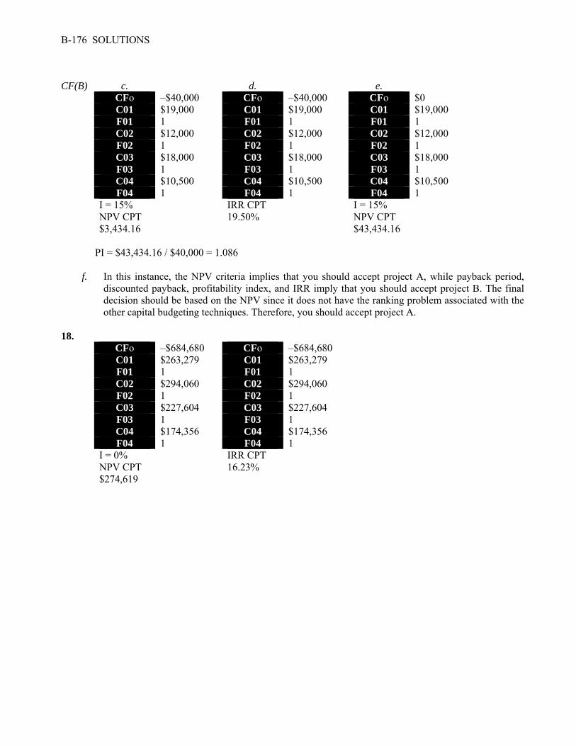
B-176 SOLUTIONS

CF(B) c. d. e. CFo –$40,000 CFo –$40,000 CFo $0 C01 $19,000 C01 $19,000 C01 $19,000 F01 1 F01 1 F01 1 C02 $12,000 C02 $12,000 C02 $12,000 F02 1 F02 1 F02 1 C03 $18,000 C03 $18,000 C03 $18,000 F03 1 F03 1 F03 1 C04 $10,500 C04 $10,500 C04 $10,500 F04 1 F04 1 F04 1 I = 15% IRR CPT I = 15% NPV CPT 19.50% NPV CPT $3,434.16 $43,434.16 PI = $43,434.16 / $40,000 = 1.086 f. In this instance, the NPV criteria implies that you should accept project A, while payback period,

discounted payback, profitability index, and IRR imply that you should accept project B. The final decision should be based on the NPV since it does not have the ranking problem associated with the other capital budgeting techniques. Therefore, you should accept project A.

18. CFo –$684,680 CFo –$684,680 C01 $263,279 C01 $263,279 F01 1 F01 1 C02 $294,060 C02 $294,060 F02 1 F02 1 C03 $227,604 C03 $227,604 F03 1 F03 1 C04 $174,356 C04 $174,356 F04 1 F04 1 I = 0% IRR CPT NPV CPT 16.23% $274,619

CHAPTER 10 MAKING CAPITAL INVESTMENT DECISIONS Answers to Concepts Review and Critical Thinking Questions 1. In this context, an opportunity cost refers to the value of an asset or other input that will be used in a

project. The relevant cost is what the asset or input is actually worth today, not, for example, what it cost to acquire.

2. For tax purposes, a firm would choose MACRS because it provides for larger depreciation deductions

earlier. These larger deductions reduce taxes, but have no other cash consequences. Notice that the choice between MACRS and straight-line is purely a time value issue; the total depreciation is the same, only the timing differs.

3. It’s probably only a mild over-simplification. Current liabilities will all be paid, presumably. The cash

portion of current assets will be retrieved. Some receivables won’t be collected, and some inventory will not be sold, of course. Counterbalancing these losses is the fact that inventory sold above cost (and not replaced at the end of the project’s life) acts to increase working capital. These effects tend to offset one another.

4. Management’s discretion to set the firm’s capital structure is applicable at the firm level. Since any one

particular project could be financed entirely with equity, another project could be financed with debt, and the firm’s overall capital structure remains unchanged, financing costs are not relevant in the analysis of a project’s incremental cash flows according to the stand-alone principle.

5. The EAC approach is appropriate when comparing mutually exclusive projects with different lives that

will be replaced when they wear out. This type of analysis is necessary so that the projects have a common life span over which they can be compared; in effect, each project is assumed to exist over an infinite horizon of N-year repeating projects. Assuming that this type of analysis is valid implies that the project cash flows remain the same forever, thus ignoring the possible effects of, among other things: (1) inflation, (2) changing economic conditions, (3) the increasing unreliability of cash flow estimates that occur far into the future, and (4) the possible effects of future technology improvement that could alter the project cash flows.

6. Depreciation is a non-cash expense, but it is tax-deductible on the income statement. Thus depreciation

causes taxes paid, an actual cash outflow, to be reduced by an amount equal to the depreciation tax shield tcD. A reduction in taxes that would otherwise be paid is the same thing as a cash inflow, so the effects of the depreciation tax shield must be added in to get the total incremental aftertax cash flows.

7. There are two particularly important considerations. The first is erosion. Will the essentialized book

simply displace copies of the existing book that would have otherwise been sold? This is of special concern given the lower price. The second consideration is competition. Will other publishers step in and produce such a product? If so, then any erosion is much less relevant. A particular concern to book publishers (and producers of a variety of other product types) is that the publisher only makes money

B-178 SOLUTIONS

from the sale of new books. Thus, it is important to examine whether the new book would displace sales of used books (good from the publisher’s perspective) or new books (not good). The concern arises any time there is an active market for used product.

8. Definitely. The damage to Porsche’s reputation is definitely a factor the company needed to consider. If

the reputation was damaged, the company would have lost sales of its existing car lines. 9. One company may be able to produce at lower incremental cost or market better. Also, of course, one of

the two may have made a mistake! 10. Porsche would recognize that the outsized profits would dwindle as more product comes to market and

competition becomes more intense.

Solutions to Questions and Problems NOTE: All end of chapter problems were solved using a spreadsheet. Many problems require multiple steps. Due to space and readability constraints, when these intermediate steps are included in this solutions manual, rounding may appear to have occurred. However, the final answer for each problem is found without rounding during any step in the problem. Basic 1. The $6 million acquisition cost of the land six years ago is a sunk cost. The $6.4 million current aftertax

value of the land is an opportunity cost if the land is used rather than sold off. The $14.2 million cash outlay and $890,000 grading expenses are the initial fixed asset investments needed to get the project going. Therefore, the proper year zero cash flow to use in evaluating this project is

$6,400,000 + 14,200,000 + 890,000 = $21,490,000 2. Sales due solely to the new product line are: 19,000($13,000) = $247,000,000 Increased sales of the motor home line occur because of the new product line introduction; thus: 4,500($53,000) = $238,500,000 in new sales is relevant. Erosion of luxury motor coach sales is also due to the new mid-size campers;

thus: 900($91,000) = $81,900,000 loss in sales is relevant. The net sales figure to use in evaluating the new line is thus: $247,000,000 + 238,500,000 – 81,900,000 = $403,600,000

CHAPTER 10 B-179

3. We need to construct a basic income statement. The income statement is: Sales $ 830,000 Variable costs 498,000 Fixed costs 181,000 Depreciation 77,000 EBT $ 74,000 Taxes@35% 25,900 Net income $ 48,100 4. To find the OCF, we need to complete the income statement as follows: Sales $ 824,500 Costs 538,900 Depreciation 126,500 EBT $ 159,100 Taxes@34% 54,094 Net income $ 105,006

The OCF for the company is: OCF = EBIT + Depreciation – Taxes OCF = $159,100 + 126,500 – 54,094 OCF = $231,506 The depreciation tax shield is the depreciation times the tax rate, so: Depreciation tax shield = tcDepreciation Depreciation tax shield = .34($126,500) Depreciation tax shield = $43,010 The depreciation tax shield shows us the increase in OCF by being able to expense depreciation.

5. To calculate the OCF, we first need to calculate net income. The income statement is: Sales $ 108,000 Variable costs 51,000 Depreciation 6,800 EBT $ 50,200 Taxes@35% 17,570 Net income $ 32,630 Using the most common financial calculation for OCF, we get: OCF = EBIT + Depreciation – Taxes OCF = $50,200 + 6,800 – 17,570 OCF = $39,430

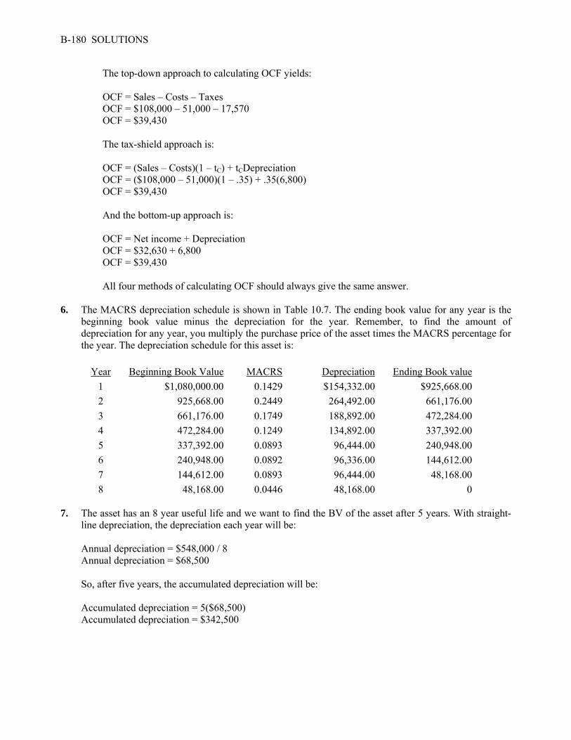
B-180 SOLUTIONS

The top-down approach to calculating OCF yields: OCF = Sales – Costs – Taxes OCF = $108,000 – 51,000 – 17,570 OCF = $39,430 The tax-shield approach is: OCF = (Sales – Costs)(1 – tC) + tCDepreciation OCF = ($108,000 – 51,000)(1 – .35) + .35(6,800) OCF = $39,430 And the bottom-up approach is: OCF = Net income + Depreciation OCF = $32,630 + 6,800 OCF = $39,430 All four methods of calculating OCF should always give the same answer. 6. The MACRS depreciation schedule is shown in Table 10.7. The ending book value for any year is the

beginning book value minus the depreciation for the year. Remember, to find the amount of depreciation for any year, you multiply the purchase price of the asset times the MACRS percentage for the year. The depreciation schedule for this asset is:

Year Beginning Book Value MACRS Depreciation Ending Book value

1 $1,080,000.00 0.1429 $154,332.00 $925,668.00

2 925,668.00 0.2449 264,492.00 661,176.00

3 661,176.00 0.1749 188,892.00 472,284.00

4 472,284.00 0.1249 134,892.00 337,392.00

5 337,392.00 0.0893 96,444.00 240,948.00

6 240,948.00 0.0892 96,336.00 144,612.00

7 144,612.00 0.0893 96,444.00 48,168.00

8 48,168.00 0.0446 48,168.00 0 7. The asset has an 8 year useful life and we want to find the BV of the asset after 5 years. With straight-

line depreciation, the depreciation each year will be: Annual depreciation = $548,000 / 8 Annual depreciation = $68,500 So, after five years, the accumulated depreciation will be: Accumulated depreciation = 5($68,500) Accumulated depreciation = $342,500

CHAPTER 10 B-181

The book value at the end of year five is thus: BV5 = $548,000 – 342,500 BV5 = $205,500 The asset is sold at a loss to book value, so the depreciation tax shield of the loss is recaptured. Aftertax salvage value = $105,000 + ($205,500 – 105,000)(0.35) Aftertax salvage value = $140,175 To find the taxes on salvage value, remember to use the equation: Taxes on salvage value = (BV – MV)tc This equation will always give the correct sign for a tax inflow (refund) or outflow (payment). 8. To find the BV at the end of four years, we need to find the accumulated depreciation for the first four

years. We could calculate a table as in Problem 6, but an easier way is to add the MACRS depreciation amounts for each of the first four years and multiply this percentage times the cost of the asset. We can then subtract this from the asset cost. Doing so, we get:

BV4 = $7,900,000 – 7,900,000(0.2000 + 0.3200 + 0.1920 + 0.1152) BV4 = $1,365,120 The asset is sold at a gain to book value, so this gain is taxable. Aftertax salvage value = $1,400,000 + ($1,365,120 – 1,400,000)(.35) Aftertax salvage value = $1,387,792 9. Using the tax shield approach to calculating OCF (Remember the approach is irrelevant; the final

answer will be the same no matter which of the four methods you use.), we get: OCF = (Sales – Costs)(1 – tC) + tCDepreciation OCF = ($2,650,000 – 840,000)(1 – 0.35) + 0.35($3,900,000/3) OCF = $1,631,500 10. Since we have the OCF, we can find the NPV as the initial cash outlay plus the PV of the OCFs, which

are an annuity, so the NPV is: NPV = –$3,900,000 + $1,631,500(PVIFA12%,3) NPV = $18,587.71

B-182 SOLUTIONS

11. The cash outflow at the beginning of the project will increase because of the spending on NWC. At the end of the project, the company will recover the NWC, so it will be a cash inflow. The sale of the equipment will result in a cash inflow, but we also must account for the taxes which will be paid on this sale. So, the cash flows for each year of the project will be:

Year Cash Flow 0 –$4,200,000 = –$3,900,000 – 300,000 1 1,631,500 2 1,631,500 3 2,068,000 = $1,631,500 + 300,000 + 210,000 + (0 – 210,000)(.35) And the NPV of the project is: NPV = –$4,200,000 + $1,631,500(PVIFA12%,2) + ($2,068,000 / 1.123) NPV = $29,279.79 12. First we will calculate the annual depreciation for the equipment necessary for the project. The

depreciation amount each year will be: Year 1 depreciation = $3,900,000(0.3333) = $1,299,870 Year 2 depreciation = $3,900,000(0.4445) = $1,733,550 Year 3 depreciation = $3,900,000(0.1481) = $577,590 So, the book value of the equipment at the end of three years, which will be the initial investment minus

the accumulated depreciation, is: Book value in 3 years = $3,900,000 – ($1,299,870 + 1,733,550 + 577,590) Book value in 3 years = $288,990 The asset is sold at a loss to book value, so this loss is taxable deductible. Aftertax salvage value = $210,000 + ($288,990 – 210,000)(0.35) Aftertax salvage value = $237,647 To calculate the OCF, we will use the tax shield approach, so the cash flow each year is: OCF = (Sales – Costs)(1 – tC) + tCDepreciation Year Cash Flow 0 –$4,200,000 = –$3,900,000 – 300,000 1 1,631,454.50 = ($1,810,000)(.65) + 0.35($1,299,870) 2 1,783,242.50 = ($1,810,000)(.65) + 0.35($1,733,550) 3 1,916,303.00 = ($1,810,000)(.65) + 0.35($577,590) + $237,647 + 300,000 Remember to include the NWC cost in Year 0, and the recovery of the NWC at the end of the project.

The NPV of the project with these assumptions is: NPV = –$4,200,000 + ($1,631,454.50/1.12) + ($1,783,242.50/1.122) + ($1,916,303.00/1.123) NPV = $42,232.43

CHAPTER 10 B-183

13. First we will calculate the annual depreciation of the new equipment. It will be: Annual depreciation = $560,000/5 Annual depreciation = $112,000 Now, we calculate the aftertax salvage value. The aftertax salvage value is the market price minus (or

plus) the taxes on the sale of the equipment, so: Aftertax salvage value = MV + (BV – MV)tc Very often the book value of the equipment is zero as it is in this case. If the book value is zero, the

equation for the aftertax salvage value becomes: Aftertax salvage value = MV + (0 – MV)tc Aftertax salvage value = MV(1 – tc) We will use this equation to find the aftertax salvage value since we know the book value is zero. So,

the aftertax salvage value is: Aftertax salvage value = $85,000(1 – 0.34) Aftertax salvage value = $56,100 Using the tax shield approach, we find the OCF for the project is: OCF = $165,000(1 – 0.34) + 0.34($112,000) OCF = $146,980 Now we can find the project NPV. Notice we include the NWC in the initial cash outlay. The recovery

of the NWC occurs in Year 5, along with the aftertax salvage value. NPV = –$560,000 – 29,000 + $146,980(PVIFA10%,5) + [($56,100 + 29,000) / 1.105] NPV = $21,010.24 14. First we will calculate the annual depreciation of the new equipment. It will be: Annual depreciation charge = $720,000/5 Annual depreciation charge = $144,000 The aftertax salvage value of the equipment is: Aftertax salvage value = $75,000(1 – 0.35) Aftertax salvage value = $48,750 Using the tax shield approach, the OCF is: OCF = $260,000(1 – 0.35) + 0.35($144,000) OCF = $219,400

B-184 SOLUTIONS

Now we can find the project IRR. There is an unusual feature that is a part of this project. Accepting this project means that we will reduce NWC. This reduction in NWC is a cash inflow at Year 0. This reduction in NWC implies that when the project ends, we will have to increase NWC. So, at the end of the project, we will have a cash outflow to restore the NWC to its level before the project. We also must include the aftertax salvage value at the end of the project. The IRR of the project is:

NPV = 0 = –$720,000 + 110,000 + $219,400(PVIFAIRR%,5) + [($48,750 – 110,000) / (1+IRR)5] IRR = 21.65% 15. To evaluate the project with a $300,000 cost savings, we need the OCF to compute the NPV. Using the

tax shield approach, the OCF is: OCF = $300,000(1 – 0.35) + 0.35($144,000) = $245,400 NPV = –$720,000 + 110,000 + $245,400(PVIFA20%,5) + [($48,750 – 110,000) / (1.20)5] NPV = $99,281.22 The NPV with a $240,000 cost savings is: OCF = $240,000(1 – 0.35) + 0.35($144,000) OCF = $206,400 NPV = –$720,000 + 110,000 + $206,400(PVIFA20%,5) + [($48,750 – 110,000) / (1.20)5] NPV = –$17,352.66 We would accept the project if cost savings were $300,000, and reject the project if the cost savings

were $240,000. The required pretax cost savings that would make us indifferent about the project is the cost savings that results in a zero NPV. The NPV of the project is:

NPV = 0 = –$720,000 + $110,000 + OCF(PVIFA20%,5) + [($48,750 – 110,000) / (1.20)5] Solving for the OCF, we find the necessary OCF for zero NPV is: OCF = $212,202.38 Using the tax shield approach to calculating OCF, we get: OCF = $212,202.38 = (S – C)(1 – 0.35) + 0.35($144,000) (S – C) = $248,926.73 The cost savings that will make us indifferent is $248,926.73.

CHAPTER 10 B-185

16. To calculate the EAC of the project, we first need the NPV of the project. Notice that we include the NWC expenditure at the beginning of the project, and recover the NWC at the end of the project. The NPV of the project is:

NPV = –$270,000 – 25,000 – $42,000(PVIFA11%,5) + $25,000/1.115 = –$435,391.39 Now we can find the EAC of the project. The EAC is: EAC = –$435,391.39 / (PVIFA11%,5) = –$117,803.98 17. We will need the aftertax salvage value of the equipment to compute the EAC. Even though the

equipment for each product has a different initial cost, both have the same salvage value. The aftertax salvage value for both is:

Both cases: aftertax salvage value = $40,000(1 – 0.35) = $26,000 To calculate the EAC, we first need the OCF and NPV of each option. The OCF and NPV for Techron I

is: OCF = –$67,000(1 – 0.35) + 0.35($290,000/3) = –9,716.67 NPV = –$290,000 – $9,716.67(PVIFA10%,3) + ($26,000/1.103) = –$294,629.73 EAC = –$294,629.73 / (PVIFA10%,3) = –$118,474.97 And the OCF and NPV for Techron II is: OCF = –$35,000(1 – 0.35) + 0.35($510,000/5) = $12,950 NPV = –$510,000 + $12,950(PVIFA10%,5) + ($26,000/1.105) = –$444,765.36 EAC = –$444,765.36 / (PVIFA10%,5) = –$117,327.98 The two milling machines have unequal lives, so they can only be compared by expressing both on an

equivalent annual basis, which is what the EAC method does. Thus, you prefer the Techron II because it has the lower (less negative) annual cost.

18. To find the bid price, we need to calculate all other cash flows for the project, and then solve for the bid

price. The aftertax salvage value of the equipment is: Aftertax salvage value = $70,000(1 – 0.35) = $45,500 Now we can solve for the necessary OCF that will give the project a zero NPV. The equation for the

NPV of the project is: NPV = 0 = –$940,000 – 75,000 + OCF(PVIFA12%,5) + [($75,000 + 45,500) / 1.125]

B-186 SOLUTIONS

Solving for the OCF, we find the OCF that makes the project NPV equal to zero is: OCF = $946,625.06 / PVIFA12%,5 = $262,603.01 The easiest way to calculate the bid price is the tax shield approach, so: OCF = $262,603.01 = [(P – v)Q – FC ](1 – tc) + tcD $262,603.01 = [(P – $9.25)(185,000) – $305,000 ](1 – 0.35) + 0.35($940,000/5) P = $12.54 Intermediate 19. First, we will calculate the depreciation each year, which will be: D1 = $560,000(0.2000) = $112,000 D2 = $560,000(0.3200) = $179,200 D3 = $560,000(0.1920) = $107,520 D4 = $560,000(0.1152) = $64,512 The book value of the equipment at the end of the project is: BV4 = $560,000 – ($112,000 + 179,200 + 107,520 + 64,512) = $96,768 The asset is sold at a loss to book value, so this creates a tax refund. After-tax salvage value = $80,000 + ($96,768 – 80,000)(0.35) = $85,868.80 So, the OCF for each year will be: OCF1 = $210,000(1 – 0.35) + 0.35($112,000) = $172,700 OCF2 = $210,000(1 – 0.35) + 0.35($179,200) = $196,220 OCF3 = $210,000(1 – 0.35) + 0.35($107,520) = $171,132 OCF4 = $210,000(1 – 0.35) + 0.35($64,512) = $159,079.20 Now we have all the necessary information to calculate the project NPV. We need to be careful with the

NWC in this project. Notice the project requires $20,000 of NWC at the beginning, and $3,000 more in NWC each successive year. We will subtract the $20,000 from the initial cash flow, and subtract $3,000 each year from the OCF to account for this spending. In Year 4, we will add back the total spent on NWC, which is $29,000. The $3,000 spent on NWC capital during Year 4 is irrelevant. Why? Well, during this year the project required an additional $3,000, but we would get the money back immediately. So, the net cash flow for additional NWC would be zero. With all this, the equation for the NPV of the project is:

NPV = – $560,000 – 20,000 + ($172,700 – 3,000)/1.09 + ($196,220 – 3,000)/1.092

+ ($171,132 – 3,000)/1.093 + ($159,079.20 + 29,000 + 85,868.80)/1.094 NPV = $69,811.79

CHAPTER 10 B-187

20. If we are trying to decide between two projects that will not be replaced when they wear out, the proper capital budgeting method to use is NPV. Both projects only have costs associated with them, not sales, so we will use these to calculate the NPV of each project. Using the tax shield approach to calculate the OCF, the NPV of System A is:

OCFA = –$110,000(1 – 0.34) + 0.34($430,000/4) OCFA = –$36,050 NPVA = –$430,000 – $36,050(PVIFA11%,4) NPVA = –$541,843.17 And the NPV of System B is: OCFB = –$98,000(1 – 0.34) + 0.34($570,000/6) OCFB = –$32,380 NPVB = –$570,000 – $32,380(PVIFA11%,6) NPVB = –$706,984.82 If the system will not be replaced when it wears out, then System A should be chosen, because it has the

more positive NPV. 21. If the equipment will be replaced at the end of its useful life, the correct capital budgeting technique is

EAC. Using the NPVs we calculated in the previous problem, the EAC for each system is: EACA = –$541,843.17 / (PVIFA11%,4) EACA = –$174,650.33 EACB = – $706,984.82 / (PVIFA11%,6) EACB = –$167,114.64 If the conveyor belt system will be continually replaced, we should choose System B since it has the

more positive EAC. 22. To find the bid price, we need to calculate all other cash flows for the project, and then solve for the bid

price. The aftertax salvage value of the equipment is: After-tax salvage value = $540,000(1 – 0.34) After-tax salvage value = $356,400 Now we can solve for the necessary OCF that will give the project a zero NPV. The current aftertax

value of the land is an opportunity cost, but we also need to include the aftertax value of the land in five years since we can sell the land at that time. The equation for the NPV of the project is:

NPV = 0 = –$4,100,000 – 2,700,000 – 600,000 + OCF(PVIFA12%,5) – $50,000(PVIFA12%,4) + {($356,400 + 600,000 + 4(50,000) + 3,200,000] / 1.125}

B-188 SOLUTIONS

Solving for the OCF, we find the OCF that makes the project NPV equal to zero is: OCF = $5,079,929.11 / PVIFA12%,5 OCF = $1,409,221.77 The easiest way to calculate the bid price is the tax shield approach, so: OCF = $1,409,221.77 = [(P – v)Q – FC ](1 – tC) + tcD $1,409,221.77 = [(P – $0.005)(100,000,000) – $950,000](1 – 0.34) + 0.34($4,100,000/5) P = $0.03163 23. At a given price, taking accelerated depreciation compared to straight-line depreciation causes the NPV

to be higher; similarly, at a given price, lower net working capital investment requirements will cause the NPV to be higher. Thus, NPV would be zero at a lower price in this situation. In the case of a bid price, you could submit a lower price and still break-even, or submit the higher price and make a positive NPV.

24. Since we need to calculate the EAC for each machine, sales are irrelevant. EAC only uses the costs of

operating the equipment, not the sales. Using the bottom up approach, or net income plus depreciation, method to calculate OCF, we get:

Machine A Machine B

Variable costs –$3,500,000 –$3,000,000

Fixed costs –170,000 –130,000

Depreciation –483,333 –566,667

EBT –$4,153,333 –$3,696,667

Tax 1,453,667 1,293,833

Net income –$2,699,667 –$2,402,833

+ Depreciation 483,333 566,667

OCF –$2,216,333 –$1,836,167 The NPV and EAC for Machine A is: NPVA = –$2,900,000 – $2,216,333(PVIFA10%,6) NPVA = –$12,552,709.46 EACA = – $12,552.709.46 / (PVIFA10%,6) EACA = –$2,882,194.74 And the NPV and EAC for Machine B is: NPVB = –$5,100,000 – 1,836,167(PVIFA10%,9) NPVB = –$15,674,527.56 EACB = – $15,674,527.56 / (PVIFA10%,9) EACB = –$2,721,733.42 You should choose Machine B since it has a more positive EAC.

CHAPTER 10 B-189

25. A kilowatt hour is 1,000 watts for 1 hour. A 60-watt bulb burning for 500 hours per year uses 30,000 watt hours, or 30 kilowatt hours. Since the cost of a kilowatt hour is $0.101, the cost per year is: Cost per year = 30($0.101) Cost per year = $3.03

The 60-watt bulb will last for 1,000 hours, which is 2 years of use at 500 hours per year. So, the NPV of the 60-watt bulb is:

NPV = –$0.50 – $3.03(PVIFA10%,2) NPV = –$5.76 And the EAC is: EAC = –$5.83 / (PVIFA10%,2) EAC = –$3.32

Now we can find the EAC for the 15-watt CFL. A 15-watt bulb burning for 500 hours per year uses 7,500 watts, or 7.5 kilowatts. And, since the cost of a kilowatt hour is $0.101, the cost per year is:

Cost per year = 7.5($0.101) Cost per year = $0.7575

The 15-watt CFL will last for 12,000 hours, which is 24 years of use at 500 hours per year. So, the NPV of the CFL is:

NPV = –$3.50 – $0.7575(PVIFA10%,24) NPV = –$10.31 And the EAC is: EAC = –$10.85 / (PVIFA10%,24) EAC = –$1.15 Thus, the CFL is much cheaper. But see our next two questions. 26. To solve the EAC algebraically for each bulb, we can set up the variables as follows: W = light bulb wattage C = cost per kilowatt hour H = hours burned per year P = price the light bulb The number of watts use by the bulb per hour is: WPH = W / 1,000 And the kilowatt hours used per year is: KPY = WPH × H

B-190 SOLUTIONS

The electricity cost per year is therefore: ECY = KPY × C The NPV of the decision to but the light bulb is: NPV = – P – ECY(PVIFAR%,t) And the EAC is: EAC = NPV / (PVIFAR%,t) Substituting, we get: EAC = [–P – (W / 1,000 × H × C)PVIFAR%,t] / PFIVAR%,t

We need to set the EAC of the two light bulbs equal to each other and solve for C, the cost per kilowatt hour. Doing so, we find:

[–$0.50 – (60 / 1,000 × 500 × C)PVIFA10%,2] / PVIFA10%,2 = [–$3.50 – (15 / 1,000 × 500 × C)PVIFA10%,24] / PVIFA10%,24 C = $0.004509

So, unless the cost per kilowatt hour is extremely low, it makes sense to use the CFL. But when should you replace the incandescent bulb? See the next question.

27. We are again solving for the breakeven kilowatt hour cost, but now the incandescent bulb has only 500

hours of useful life. In this case, the incandescent bulb has only one year of life left. The breakeven electricity cost under these circumstances is:

[–$0.50 – (60 / 1,000 × 500 × C)PVIFA10%,1] / PVIFA10%,1 = [–$3.50 – (15 / 1,000 × 500 × C)PVIFA10%,24] / PVIFA10%,24 C = –$0.007131

Unless the electricity cost is negative (Not very likely!), it does not make financial sense to replace the incandescent bulb until it burns out.

28. The debate between incandescent bulbs and CFLs is not just a financial debate, but an environmental one

as well. The numbers below correspond to the numbered items in the question:

1. The extra heat generated by an incandescent bulb is waste, but not necessarily in a heated structure, especially in northern climates.

2. Since CFLs last so long, from a financial viewpoint, it might make sense to wait if prices are

declining.

3. Because of the nontrivial health and disposal issues, CFLs are not as attractive as our previous analysis suggests.

CHAPTER 10 B-191

4. From a company’s perspective, the cost of replacing working incandescent bulbs may outweigh the financial benefit. However, since CFLs last longer, the cost of replacing the bulbs will be lower in the long run.

5. Because incandescent bulbs use more power, more coal has to be burned, which generates more

mercury in the environment, potentially offsetting the mercury concern with CFLs.

6. As in the previous question, if CO2 production is an environmental concern, the the lower power consumption from CFLs is a benefit.

7. CFLs require more energy to make, potentially offsetting (at least partially) the energy savings

from their use. Worker safety and site contamination are also negatives for CFLs.

8. This fact favors the incandescent bulb because the purchasers will only receive part of the benefit from the CFL.

9. This fact favors waiting for new technology.

10. This fact also favors waiting for new technology.

While there is always a “best” answer, this question shows that the analysis of the “best” answer is not always easy and may not be possible because of incomplete data. As for how to better legislate the use of CFLs, our analysis suggests that requiring them in new construction might make sense. Rental properties in general should probably be required to use CFLs (why rentals?).

Another piece of legislation that makes sense is requiring the producers of CFLs to supply a disposal kit and proper disposal instructions with each one sold. Finally, we need much better research on the hazards associated with broken bulbs in the home and workplace and proper procedures for dealing with broken bulbs.

29. Surprise! You should definitely upgrade the truck. Here’s why. At 10 mpg, the truck burns 12,000 / 10

= 1,200 gallons of gas per year. The new truck will burn 12,000 / 12.5 = 960 gallons of gas per year, a savings of 240 gallons per year. The car burns 12,000 / 25 = 480 gallons of gas per year, while the new car will burn 12,000 / 40 = 300 gallons of gas per year, a savings of 180 gallons per year, so it’s not even close.

This answer may strike you as counterintuitive, so let’s consider an extreme case. Suppose the car gets

6,000 mpg, and you could upgrade to 12,000 mpg. Should you upgrade? Probably not since you would only save one gallon of gas per year. So, the reason you should upgrade the truck is that it uses so much more gas in the first place.

Notice that the answer doesn’t depend on the cost of gasoline, meaning that if you upgrade, you should

always upgrade the truck. In fact, it doesn’t depend on the miles driven, as long as the miles driven are the same.

B-192 SOLUTIONS

30. Surprise! You should definitely upgrade the truck. Here’s why. At 10 mpg, the truck burns 12,000 / 10 = 1,200

Challenge 31. We will begin by calculating the aftertax salvage value of the equipment at the end of the project’s life.

The aftertax salvage value is the market value of the equipment minus any taxes paid (or refunded), so the aftertax salvage value in four years will be:

Taxes on salvage value = (BV – MV)tC Taxes on salvage value = ($0 – 400,000)(.38) Taxes on salvage value = –$152,000

Market price $400,000

Tax on sale –152,000

Aftertax salvage value $248,000 Now we need to calculate the operating cash flow each year. Using the bottom up approach to

calculating operating cash flow, we find:

Year 0 Year 1 Year 2 Year 3 Year 4

Revenues $2,496,000 $3,354,000 $3,042,000 $2,184,000

Fixed costs 425,000 425,000 425,000 425,000

Variable costs 374,400 503,100 456,300 327,600

Depreciation 1,399,860 1,866,900 622,020 311,220

EBT $296,740 $559,000 $1,538,680 $1,120,180

Taxes 112,761 212,420 584,698 425,668

Net income $183,979 $346,580 $953,982 $694,512

OCF $1,583,839 $2,213,480 $1,576,002 $1,005,732

Capital spending –$4,200,000 $248,000

Land –1,500,000 1,600,000

NWC –125,000 125,000

Total cash flow –$5,825,000 $1,583,839 $2,213,480 $1,576,002 $2,978,732

Notice the calculation of the cash flow at time 0. The capital spending on equipment and investment in

net working capital are cash outflows are both cash outflows. The aftertax selling price of the land is also a cash outflow. Even though no cash is actually spent on the land because the company already owns it, the aftertax cash flow from selling the land is an opportunity cost, so we need to include it in the analysis. The company can sell the land at the end of the project, so we need to include that value as well. With all the project cash flows, we can calculate the NPV, which is:

NPV = –$5,825,000 + $1,583,839 / 1.13 + $2,213,480 / 1.132 + $1,576,002 / 1.133 + $2,978,732 / 1.134

NPV = $229,266.82

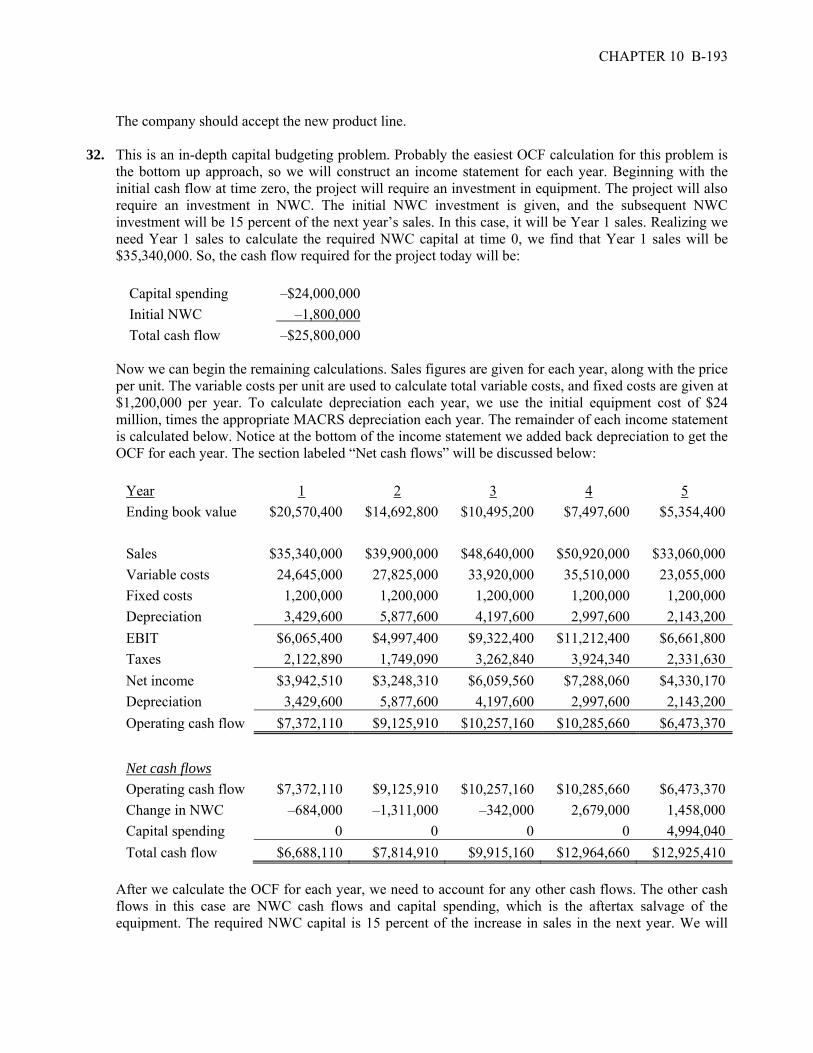
CHAPTER 10 B-193

The company should accept the new product line. 32. This is an in-depth capital budgeting problem. Probably the easiest OCF calculation for this problem is

the bottom up approach, so we will construct an income statement for each year. Beginning with the initial cash flow at time zero, the project will require an investment in equipment. The project will also require an investment in NWC. The initial NWC investment is given, and the subsequent NWC investment will be 15 percent of the next year’s sales. In this case, it will be Year 1 sales. Realizing we need Year 1 sales to calculate the required NWC capital at time 0, we find that Year 1 sales will be $35,340,000. So, the cash flow required for the project today will be:

Capital spending –$24,000,000

Initial NWC –1,800,000

Total cash flow –$25,800,000 Now we can begin the remaining calculations. Sales figures are given for each year, along with the price

per unit. The variable costs per unit are used to calculate total variable costs, and fixed costs are given at $1,200,000 per year. To calculate depreciation each year, we use the initial equipment cost of $24 million, times the appropriate MACRS depreciation each year. The remainder of each income statement is calculated below. Notice at the bottom of the income statement we added back depreciation to get the OCF for each year. The section labeled “Net cash flows” will be discussed below:

Year 1 2 3 4 5

Ending book value $20,570,400 $14,692,800 $10,495,200 $7,497,600 $5,354,400

Sales $35,340,000 $39,900,000 $48,640,000 $50,920,000 $33,060,000

Variable costs 24,645,000 27,825,000 33,920,000 35,510,000 23,055,000

Fixed costs 1,200,000 1,200,000 1,200,000 1,200,000 1,200,000

Depreciation 3,429,600 5,877,600 4,197,600 2,997,600 2,143,200

EBIT $6,065,400 $4,997,400 $9,322,400 $11,212,400 $6,661,800

Taxes 2,122,890 1,749,090 3,262,840 3,924,340 2,331,630

Net income $3,942,510 $3,248,310 $6,059,560 $7,288,060 $4,330,170

Depreciation 3,429,600 5,877,600 4,197,600 2,997,600 2,143,200

Operating cash flow $7,372,110 $9,125,910 $10,257,160 $10,285,660 $6,473,370

Net cash flows

Operating cash flow $7,372,110 $9,125,910 $10,257,160 $10,285,660 $6,473,370

Change in NWC –684,000 –1,311,000 –342,000 2,679,000 1,458,000

Capital spending 0 0 0 0 4,994,040

Total cash flow $6,688,110 $7,814,910 $9,915,160 $12,964,660 $12,925,410 After we calculate the OCF for each year, we need to account for any other cash flows. The other cash

flows in this case are NWC cash flows and capital spending, which is the aftertax salvage of the equipment. The required NWC capital is 15 percent of the increase in sales in the next year. We will

B-194 SOLUTIONS

work through the NWC cash flow for Year 1. The total NWC in Year 1 will be 15 percent of sales increase from Year 1 to Year 2, or:

Increase in NWC for Year 1 = .15($39,900,000 – 35,340,000) Increase in NWC for Year 1 = $684,000 Notice that the NWC cash flow is negative. Since the sales are increasing, we will have to spend more

money to increase NWC. In Year 4, the NWC cash flow is positive since sales are declining. And, in Year 5, the NWC cash flow is the recovery of all NWC the company still has in the project.

To calculate the aftertax salvage value, we first need the book value of the equipment. The book value

at the end of the five years will be the purchase price, minus the total depreciation. So, the ending book value is:

Ending book value = $24,000,000 – ($3,429,600 + 5,877,600 + 4,197,600 + 2,997,600 + 2,143,200) Ending book value = $5,354,400 The market value of the used equipment is 20 percent of the purchase price, or $4.8 million, so the

aftertax salvage value will be: Aftertax salvage value = $4,800,000 + ($5,354,400 – 4,800,000)(.35) Aftertax salvage value = $4,994,040 The aftertax salvage value is included in the total cash flows are capital spending. Now we have all of

the cash flows for the project. The NPV of the project is: NPV = –$25,800,000 + $6,688,110/1.18 + $7,814,910/1.182 + $9,915,160/1.183 + $12,964,660/1.184 + $12,925,410/1.185 NPV = $3,851,952.23 And the IRR is: NPV = 0 = –$25,800,000 + $6,688,110/(1 + IRR) + $7,814,910/(1 + IRR)2 + $9,915,160/(1 + IRR)3 + $12,964,660/(1 + IRR)4 + $12,925,410/(1 + IRR)5 IRR = 23.62% We should accept the project. 33. To find the initial pretax cost savings necessary to buy the new machine, we should use the tax shield

approach to find the OCF. We begin by calculating the depreciation each year using the MACRS depreciation schedule. The depreciation each year is:

D1 = $610,000(0.3333) = $203,313 D2 = $610,000(0.4444) = $271,145 D3 = $610,000(0.1482) = $90,341 D4 = $610,000(0.0741) = $45,201 Using the tax shield approach, the OCF each year is: OCF1 = (S – C)(1 – 0.35) + 0.35($203,313)

CHAPTER 10 B-195

OCF2 = (S – C)(1 – 0.35) + 0.35($271,145) OCF3 = (S – C)(1 – 0.35) + 0.35($90,341) OCF4 = (S – C)(1 – 0.35) + 0.35($45,201) OCF5 = (S – C)(1 – 0.35) Now we need the aftertax salvage value of the equipment. The aftertax salvage value is: After-tax salvage value = $40,000(1 – 0.35) = $26,000 To find the necessary cost reduction, we must realize that we can split the cash flows each year. The

OCF in any given year is the cost reduction (S – C) times one minus the tax rate, which is an annuity for the project life, and the depreciation tax shield. To calculate the necessary cost reduction, we would require a zero NPV. The equation for the NPV of the project is:

NPV = 0 = –$610,000 – 55,000 + (S – C)(0.65)(PVIFA12%,5) + 0.35($203,313/1.12 + $271,145/1.122 + $90,341/1.123 + $45,201/1.124) + ($55,000 + 26,000)/1.125 Solving this equation for the sales minus costs, we get: (S – C)(0.65)(PVIFA12%,5) = $447,288.67 (S – C) = $190,895.74 34. a. This problem is basically the same as Problem 18, except we are given a sales price. The cash flow at Time 0 for all three parts of this question will be:

Capital spending –$940,000

Change in NWC –75,000

Total cash flow –$1,015,000 We will use the initial cash flow and the salvage value we already found in that problem. Using the

bottom up approach to calculating the OCF, we get: Assume price per unit = $13 and units/year = 185,000 Year 1 2 3 4 5 Sales $2,405,000 $2,405,000 $2,405,000 $2,405,000 $2,405,000 Variable costs 1,711,250 1,711,250 1,711,250 1,711,250 1,711,250 Fixed costs 305,000 305,000 305,000 305,000 305,000 Depreciation 188,000 188,000 188,000 188,000 188,000 EBIT 200,750 200,750 200,750 200,750 200,750 Taxes (35%) 70,263 70,263 70,263 70,263 70,263 Net Income 130,488 130,488 130,488 130,488 130,488 Depreciation 188,000 188,000 188,000 188,000 188,000 Operating CF $318,488 $318,488 $318,488 $318,488 $318,488

Year 1 2 3 4 5 Operating CF $318,488 $318,488 $318,488 $318,488 $318,488 Change in NWC 0 0 0 0 75,000 Capital spending 0 0 0 0 45,500 Total CF $318,488 $318,488 $318,488 $318,488 $438,988

B-196 SOLUTIONS

With these cash flows, the NPV of the project is: NPV = –$940,000 – 75,000 + $318,488(PVIFA12%,5) + [($75,000 + 45,500) / 1.125] NPV = $201,451.10 If the actual price is above the bid price that results in a zero NPV, the project will have a positive NPV.

As for the cartons sold, if the number of cartons sold increases, the NPV will increase, and if the costs increase, the NPV will decrease.

b. To find the minimum number of cartons sold to still breakeven, we need to use the tax shield approach

to calculating OCF, and solve the problem similar to finding a bid price. Using the initial cash flow and salvage value we already calculated, the equation for a zero NPV of the project is:

NPV = 0 = –$940,000 – 75,000 + OCF(PVIFA12%,5) + [($75,000 + 45,500) / 1.125] So, the necessary OCF for a zero NPV is:

OCF = $946,625.06 / PVIFA12%,5 = $262,603.01 Now we can use the tax shield approach to solve for the minimum quantity as follows: OCF = $262,603.01 = [(P – v)Q – FC ](1 – tc) + tcD

$262,603.01 = [($13.00 – 9.25)Q – 305,000 ](1 – 0.35) + 0.35($940,000/5) Q = 162,073

As a check, we can calculate the NPV of the project with this quantity. The calculations are: Year 1 2 3 4 5 Sales $2,106,949 $2,106,949 $2,106,949 $2,106,949 $2,106,949 Variable costs 1,499,176 1,499,176 1,499,176 1,499,176 1,499,176 Fixed costs 305,000 305,000 305,000 305,000 305,000 Depreciation 188,000 188,000 188,000 188,000 188,000 EBIT 114,774 114,774 114,774 114,774 114,774 Taxes (35%) 40,171 40,171 40,171 40,171 40,171 Net Income 74,603 74,603 74,603 74,603 74,603 Depreciation 188,000 188,000 188,000 188,000 188,000 Operating CF $262,603 $262,603 $262,603 $262,603 $262,603 Year 1 2 3 4 5 Operating CF $262,603 $262,603 $262,603 $262,603 $262,603 Change in NWC 0 0 0 0 75,000 Capital spending 0 0 0 0 45,500 Total CF $262,603 $262,603 $262,603 $262,603 $383,103

NPV = –$940,000 – 75,000 + $262,603(PVIFA12%,5) + [($75,000 + 45,500) / 1.125] $0 Note, the NPV is not exactly equal to zero because we had to round the number of cartons sold; you

cannot sell one-half of a carton.

CHAPTER 10 B-197

c. To find the highest level of fixed costs and still breakeven, we need to use the tax shield approach to calculating OCF, and solve the problem similar to finding a bid price. Using the initial cash flow and salvage value we already calculated, the equation for a zero NPV of the project is:

NPV = 0 = –$940,000 – 75,000 + OCF(PVIFA12%,5) + [($75,000 + 45,500) / 1.125] OCF = $946,625.06 / PVIFA12%,5 = $262,603.01

Notice this is the same OCF we calculated in part b. Now we can use the tax shield approach to solve for the maximum level of fixed costs as follows:

OCF = $262,603.01 = [(P–v)Q – FC ](1 – tC) + tCD $262,603.01 = [($13.00 – 9.25)(185,000) – FC](1 – 0.35) + 0.35($940,000/5)

FC = $390,976.15 As a check, we can calculate the NPV of the project with this level of fixed costs. The calculations are: Year 1 2 3 4 5 Sales $2,405,000 $2,405,000 $2,405,000 $2,405,000 $2,405,000 Variable costs 1,711,250 1,711,250 1,711,250 1,711,250 1,711,250 Fixed costs 390,976 390,976 390,976 390,976 390,976 Depreciation 188,000 188,000 188,000 188,000 188,000 EBIT 114,774 114,774 114,774 114,774 114,774 Taxes (35%) 40,171 40,171 40,171 40,171 40,171 Net Income 74,603 74,603 74,603 74,603 74,603 Depreciation 188,000 188,000 188,000 188,000 188,000 Operating CF $262,603 $262,603 $262,603 $262,603 $262,603 Year 1 2 3 4 5 Operating CF $262,603 $262,603 $262,603 $262,603 $262,603 Change in NWC 0 0 0 0 75,000 Capital spending 0 0 0 0 45,500 Total CF $262,603 $262,603 $262,603 $262,603 $383,103

NPV = –$940,000 – 75,000 + $262,603(PVIFA12%,5) + [($75,000 + 45,500) / 1.125] $0 35. We need to find the bid price for a project, but the project has extra cash flows. Since we don’t already

produce the keyboard, the sales of the keyboard outside the contract are relevant cash flows. Since we know the extra sales number and price, we can calculate the cash flows generated by these sales. The cash flow generated from the sale of the keyboard outside the contract is:

1 2 3 4

Sales $855,000 $1,710,000 $2,280,000 $1,425,000 Variable costs 525,000 1,050,000 1,400,000 875,000 EBT $330,000 $660,000 $880,000 $550,000 Tax 132,000 264,000 352,000 220,000 Net income (and OCF) $198,000 $396,000 $528,000 $330,000

B-198 SOLUTIONS

So, the addition to NPV of these market sales is: NPV of market sales = $198,000/1.13 + $396,000/1.132 + $528,000/1.133 + $330,000/1.134 NPV of market sales = $1,053,672.99 You may have noticed that we did not include the initial cash outlay, depreciation or fixed costs in the

calculation of cash flows from the market sales. The reason is that it is irrelevant whether or not we include these here. Remember, we are not only trying to determine the bid price, but we are also determining whether or not the project is feasible. In other words, we are trying to calculate the NPV of the project, not just the NPV of the bid price. We will include these cash flows in the bid price calculation. The reason we stated earlier that whether we included these costs in this initial calculation was irrelevant is that you will come up with the same bid price if you include these costs in this calculation, or if you include them in the bid price calculation.

Next, we need to calculate the aftertax salvage value, which is: Aftertax salvage value = $275,000(1 – .40) = $165,000 Instead of solving for a zero NPV as is usual in setting a bid price, the company president requires an

NPV of $100,000, so we will solve for a NPV of that amount. The NPV equation for this project is (remember to include the NWC cash flow at the beginning of the project, and the NWC recovery at the end):

NPV = $100,000 = –$3,400,000 – 95,000 + 1,053,672.99 + OCF (PVIFA13%,4) + [($165,000 + 95,000) / 1.134]

Solving for the OCF, we get: OCF = $2,381,864.14 / PVIFA13%,4 = $800,768.90 Now we can solve for the bid price as follows: OCF = $800,768.90 = [(P – v)Q – FC ](1 – tC) + tCD $800,768.90 = [(P – $175)(17,500) – $600,000](1 – 0.40) + 0.40($3,400,000/4) P = $253.17 36. a. Since the two computers have unequal lives, the correct method to analyze the decision is the

EAC. We will begin with the EAC of the new computer. Using the depreciation tax shield approach, the OCF for the new computer system is:

OCF = ($145,000)(1 – .38) + ($780,000 / 5)(.38) = $149,180 Notice that the costs are positive, which represents a cash inflow. The costs are positive in this

case since the new computer will generate a cost savings. The only initial cash flow for the new computer is cost of $780,000. We next need to calculate the aftertax salvage value, which is:

Aftertax salvage value = $150,000(1 – .38) = $93,000 Now we can calculate the NPV of the new computer as: NPV = –$780,000 + $149,180(PVIFA12%,5) + $93,000 / 1.125

CHAPTER 10 B-199

NPV = –$189,468.79 And the EAC of the new computer is: EAC = –$189,468.79 / (PVIFA12%,5) = –$52,560.49 Analyzing the old computer, the only OCF is the depreciation tax shield, so: OCF = $130,000(.38) = $49,400 The initial cost of the old computer is a little trickier. You might assume that since we already own

the old computer there is no initial cost, but we can sell the old computer, so there is an opportunity cost. We need to account for this opportunity cost. To do so, we will calculate the aftertax salvage value of the old computer today. We need the book value of the old computer to do so. The book value is not given directly, but we are told that the old computer has depreciation of $130,000 per year for the next three years, so we can assume the book value is the total amount of depreciation over the remaining life of the system, or $390,000. So, the aftertax salvage value of the old computer is:

Aftertax salvage value = $210,000 + ($390,000 – 210,000)(.38) = $377,200 This is the initial cost of the old computer system today because we are forgoing the opportunity to

sell it today. We next need to calculate the aftertax salvage value of the computer system in two years since we are “buying” it today. The aftertax salvage value in two years is:

Aftertax salvage value = $60,000 + ($130,000 – 60,000)(.38) = $86,600 Now we can calculate the NPV of the old computer as: NPV = –$377,200 + $49,400(PVIFA11%,2) + 136,000 / 1.122 NPV = –$224,647.49 And the EAC of the old computer is: EAC = –$224,674.49 / (PVIFA12%,2) = –$132,939.47 Even if we are going to replace the system in two years no matter what our decision today, we

should replace it today since the EAC is more positive.

B-200 SOLUTIONS

b. If we are only concerned with whether or not to replace the machine now, and are not worrying about what will happen in two years, the correct analysis is NPV. To calculate the NPV of the decision on the computer system now, we need the difference in the total cash flows of the old computer system and the new computer system. From our previous calculations, we can say the cash flows for each computer system are:

t New computer Old computer Difference 0 –$780,000 –$377,200 –$402,800 1 149,180 49,400 99,780 2 149,180 136,000 13,180 3 149,180 0 149,180 4 149,180 0 149,180 5 242,180 0 242,180

Since we are only concerned with marginal cash flows, the cash flows of the decision to replace

the old computer system with the new computer system are the differential cash flows. The NPV of the decision to replace, ignoring what will happen in two years is:

NPV = –$402,800 + $99,780/1.12 + $13,180/1.122 + $149,180/1.143 + $149,180/1.144 + $242,180/1.145 NPV = $35,205.70 If we are not concerned with what will happen in two years, we should replace the old computer

system.

CHAPTER 11 PROJECT ANALYSIS AND EVALUATION Answers to Concepts Review and Critical Thinking Questions 1. Forecasting risk is the risk that a poor decision is made because of errors in projected cash flows. The

danger is greatest with a new product because the cash flows are probably harder to predict. 2. With a sensitivity analysis, one variable is examined over a broad range of values. With a scenario

analysis, all variables are examined for a limited range of values. 3. It is true that if average revenue is less than average cost, the firm is losing money. This much of the

statement is therefore correct. At the margin, however, accepting a project with marginal revenue in excess of its marginal cost clearly acts to increase operating cash flow.

4. It makes wages and salaries a fixed cost, driving up operating leverage. 5. Fixed costs are relatively high because airlines are relatively capital intensive (and airplanes are

expensive). Skilled employees such as pilots and mechanics mean relatively high wages which, because of union agreements, are relatively fixed. Maintenance expenses are significant and relatively fixed as well.

6. From the shareholder perspective, the financial break-even point is the most important. A project can

exceed the accounting and cash break-even points but still be below the financial break-even point. This causes a reduction in shareholder (your) wealth.

7. The project will reach the cash break-even first, the accounting break-even next and finally the financial

break-even. For a project with an initial investment and sales after, this ordering will always apply. The cash break-even is achieved first since it excludes depreciation. The accounting break-even is next since it includes depreciation. Finally, the financial break-even, which includes the time value of money, is achieved.

8. Soft capital rationing implies that the firm as a whole isn’t short of capital, but the division or project

does not have the necessary capital. The implication is that the firm is passing up positive NPV projects. With hard capital rationing the firm is unable to raise capital for a project under any circumstances. Probably the most common reason for hard capital rationing is financial distress, meaning bankruptcy is a possibility.

9. The implication is that they will face hard capital rationing.

B-202 SOLUTIONS

Solutions to Questions and Problems NOTE: All end of chapter problems were solved using a spreadsheet. Many problems require multiple steps. Due to space and readability constraints, when these intermediate steps are included in this solutions manual, rounding may appear to have occurred. However, the final answer for each problem is found without rounding during any step in the problem. Basic 1. a. The total variable cost per unit is the sum of the two variable costs, so: Total variable costs per unit = $5.43 + 3.13 Total variable costs per unit = $8.56 b. The total costs include all variable costs and fixed costs. We need to make sure we are including

all variable costs for the number of units produced, so: Total costs = Variable costs + Fixed costs Total costs = $8.56(280,000) + $720,000 Total costs = $3,116,800

c. The cash breakeven, that is the point where cash flow is zero, is: QC = $720,000 / ($19.99 – 8.56) QC = 62,992.13 units

And the accounting breakeven is: QA = ($720,000 + 220,000) / ($19.99 – 8.56) QA = 82,239.72 units 2. The total costs include all variable costs and fixed costs. We need to make sure we are including all

variable costs for the number of units produced, so: Total costs = ($24.86 + 14.08)(120,000) + $1,550,000 Total costs = $6,222,800 The marginal cost, or cost of producing one more unit, is the total variable cost per unit, so: Marginal cost = $24.86 + 14.08 Marginal cost = $38.94

CHAPTER 11 B-203

The average cost per unit is the total cost of production, divided by the quantity produced, so: Average cost = Total cost / Total quantity Average cost = $6,222,800/120,000 Average cost = $51.86 Minimum acceptable total revenue = 5,000($38.94) Minimum acceptable total revenue = $194,700 Additional units should be produced only if the cost of producing those units can be recovered. 3. The base-case, best-case, and worst-case values are shown below. Remember that in the best-case, sales

and price increase, while costs decrease. In the worst-case, sales and price decrease, and costs increase. Unit Scenario Unit Sales Unit Price Variable Cost Fixed Costs Base 95,000 $1,900.00 $240.00 $4,800,000 Best 109,250 $2,185.00 $204.00 $4,080,000 Worst 80,750 $1,615.00 $276.00 $5,520,000 4. An estimate for the impact of changes in price on the profitability of the project can be found from the

sensitivity of NPV with respect to price: NPV/P. This measure can be calculated by finding the NPV at any two different price levels and forming the ratio of the changes in these parameters. Whenever a sensitivity analysis is performed, all other variables are held constant at their base-case values.

5. a. To calculate the accounting breakeven, we first need to find the depreciation for each year. The

depreciation is: Depreciation = $724,000/8 Depreciation = $90,500 per year And the accounting breakeven is: QA = ($780,000 + 90,500)/($43 – 29) QA = 62,179 units To calculate the accounting breakeven, we must realize at this point (and only this point), the OCF

is equal to depreciation. So, the DOL at the accounting breakeven is: DOL = 1 + FC/OCF = 1 + FC/D DOL = 1 + [$780,000/$90,500] DOL = 9.919 b. We will use the tax shield approach to calculate the OCF. The OCF is: OCFbase = [(P – v)Q – FC](1 – tc) + tcD

OCFbase = [($43 – 29)(90,000) – $780,000](0.65) + 0.35($90,500) OCFbase = $343,675

B-204 SOLUTIONS

Now we can calculate the NPV using our base-case projections. There is no salvage value or NWC, so the NPV is:

NPVbase = –$724,000 + $343,675(PVIFA15%,8) NPVbase = $818,180.22 To calculate the sensitivity of the NPV to changes in the quantity sold, we will calculate the NPV

at a different quantity. We will use sales of 95,000 units. The NPV at this sales level is: OCFnew = [($43 – 29)(95,000) – $780,000](0.65) + 0.35($90,500) OCFnew = $389,175 And the NPV is: NPVnew = –$724,000 + $389,175(PVIFA15%,8) NPVnew = $1,022,353.35 So, the change in NPV for every unit change in sales is: NPV/S = ($1,022,353.35 – 818,180.22)/(95,000 – 90,000) NPV/S = +$40.835 If sales were to drop by 500 units, then NPV would drop by: NPV drop = $40.835(500) = $20,417.31 You may wonder why we chose 95,000 units. Because it doesn’t matter! Whatever sales number

we use, when we calculate the change in NPV per unit sold, the ratio will be the same. c. To find out how sensitive OCF is to a change in variable costs, we will compute the OCF at a

variable cost of $30. Again, the number we choose to use here is irrelevant: We will get the same ratio of OCF to a one dollar change in variable cost no matter what variable cost we use. So, using the tax shield approach, the OCF at a variable cost of $30 is:

OCFnew = [($43 – 30)(90,000) – 780,000](0.65) + 0.35($90,500) OCFnew = $285,175 So, the change in OCF for a $1 change in variable costs is: OCF/v = ($285,175,450 – 343,675)/($30 – 29) OCF/v = –$58,500 If variable costs decrease by $1 then, OCF would increase by $58,500

CHAPTER 11 B-205

6. We will use the tax shield approach to calculate the OCF for the best- and worst-case scenarios. For the best-case scenario, the price and quantity increase by 10 percent, so we will multiply the base case numbers by 1.1, a 10 percent increase. The variable and fixed costs both decrease by 10 percent, so we will multiply the base case numbers by .9, a 10 percent decrease. Doing so, we get:

OCFbest = {[($43)(1.1) – ($29)(0.9)](90,000)(1.1) – $780,000(0.9)}(0.65) + 0.35($90,500) OCFbest = $939,595 The best-case NPV is: NPVbest = –$724,000 + $939,595(PVIFA15%,8) NPVbest = $3,492,264.85 For the worst-case scenario, the price and quantity decrease by 10 percent, so we will multiply the base

case numbers by .9, a 10 percent decrease. The variable and fixed costs both increase by 10 percent, so we will multiply the base case numbers by 1.1, a 10 percent increase. Doing so, we get:

OCFworst = {[($43)(0.9) – ($29)(1.1)](90,000)(0.9) – $780,000(1.1)}(0.65) + 0.35($90,500) OCFworst = –$168,005 The worst-case NPV is: NPVworst = –$724,000 – $168,005(PVIFA15%,8) NPVworst = –$1,477,892.45 7. The cash breakeven equation is: QC = FC/(P – v) And the accounting breakeven equation is: QA = (FC + D)/(P – v) Using these equations, we find the following cash and accounting breakeven points: (1): QC = $14M/($3,020 – 2,275) QA = ($14M + 6.5M)/($3,020 – 2,275) QC = 18,792 QA = 27,517 (2): QC = $73,000/($38 – 27) QA = ($73,000 + 150,000)/($38 – 27) QC = 6,636 QA = 20,273 (3): QC = $1,200/($11 – 4) QA = ($1,200 + 840)/($11 – 4) QC = 171 QA = 291

B-206 SOLUTIONS

8. We can use the accounting breakeven equation: QA = (FC + D)/(P – v) to solve for the unknown variable in each case. Doing so, we find: (1): QA = 112,800 = ($820,000 + D)/($41 – 30) D = $420,800 (2): QA = 165,000 = ($3.2M + 1.15M)/(P – $43) P = $69.36 (3): QA = 4,385 = ($160,000 + 105,000)/($98 – v) v = $37.57 9. The accounting breakeven for the project is: QA = [$6,000 + ($18,000/4)]/($57 – 32) QA = 540 And the cash breakeven is: QC = $9,000/($57 – 32) QC = 360 At the financial breakeven, the project will have a zero NPV. Since this is true, the initial cost of the

project must be equal to the PV of the cash flows of the project. Using this relationship, we can find the OCF of the project must be:

NPV = 0 implies $18,000 = OCF(PVIFA12%,4) OCF = $5,926.22 Using this OCF, we can find the financial breakeven is: QF = ($9,000 + $5,926.22)/($57 – 32) = 597 And the DOL of the project is: DOL = 1 + ($9,000/$5,926.22) = 2.519 10. In order to calculate the financial breakeven, we need the OCF of the project. We can use the cash and

accounting breakeven points to find this. First, we will use the cash breakeven to find the price of the product as follows:

QC = FC/(P – v) 13,200 = $140,000/(P – $24) P = $34.61

CHAPTER 11 B-207

Now that we know the product price, we can use the accounting breakeven equation to find the depreciation. Doing so, we find the annual depreciation must be:

QA = (FC + D)/(P – v) 15,500 = ($140,000 + D)/($34.61 – 24) Depreciation = $24,394 We now know the annual depreciation amount. Assuming straight-line depreciation is used, the initial

investment in equipment must be five times the annual depreciation, or: Initial investment = 5($24,394) = $121,970 The PV of the OCF must be equal to this value at the financial breakeven since the NPV is zero, so: $121,970 = OCF(PVIFA16%,5) OCF = $37,250.69 We can now use this OCF in the financial breakeven equation to find the financial breakeven sales

quantity is: QF = ($140,000 + 37,250.69)/($34.61 – 24) QF = 16,712 11. We know that the DOL is the percentage change in OCF divided by the percentage change in quantity

sold. Since we have the original and new quantity sold, we can use the DOL equation to find the percentage change in OCF. Doing so, we find:

DOL = %OCF / %Q Solving for the percentage change in OCF, we get: %OCF = (DOL)(%Q) %OCF = 3.40[(70,000 – 65,000)/65,000] %OCF = .2615 or 26.15% The new level of operating leverage is lower since FC/OCF is smaller. 12. Using the DOL equation, we find: DOL = 1 + FC / OCF 3.40 = 1 + $130,000/OCF OCF = $54,167 The percentage change in quantity sold at 58,000 units is: %ΔQ = (58,000 – 65,000) / 65,000 %ΔQ = –.1077 or –10.77%

B-208 SOLUTIONS

So, using the same equation as in the previous problem, we find: %ΔOCF = 3.40(–10.77%) %ΔQ = –36.62% So, the new OCF level will be: New OCF = (1 – .3662)($54,167) New OCF = $34,333 And the new DOL will be: New DOL = 1 + ($130,000/$34,333) New DOL = 4.786 13. The DOL of the project is: DOL = 1 + ($73,000/$87,500) DOL = 1.8343 If the quantity sold changes to 8,500 units, the percentage change in quantity sold is: %Q = (8,500 – 8,000)/8,000 %ΔQ = .0625 or 6.25% So, the OCF at 8,500 units sold is: %OCF = DOL(%Q) %ΔOCF = 1.8343(.0625) %ΔOCF = .1146 or 11.46% This makes the new OCF: New OCF = $87,500(1.1146) New OCF = $97,531 And the DOL at 8,500 units is: DOL = 1 + ($73,000/$97,531) DOL = 1.7485 14. We can use the equation for DOL to calculate fixed costs. The fixed cost must be: DOL = 2.35 = 1 + FC/OCF FC = (2.35 – 1)$41,000 FC = $58,080 If the output rises to 11,000 units, the percentage change in quantity sold is: %Q = (11,000 – 10,000)/10,000 %ΔQ = .10 or 10.00%

CHAPTER 11 B-209

The percentage change in OCF is: %OCF = 2.35(.10) %ΔOCF = .2350 or 23.50% So, the operating cash flow at this level of sales will be: OCF = $43,000(1.235) OCF = $53,105 If the output falls to 9,000 units, the percentage change in quantity sold is: %Q = (9,000 – 10,000)/10,000 %ΔQ = –.10 or –10.00% The percentage change in OCF is: %OCF = 2.35(–.10) %ΔOCF = –.2350 or –23.50% So, the operating cash flow at this level of sales will be: OCF = $43,000(1 – .235) OCF = $32,897 15. Using the equation for DOL, we get: DOL = 1 + FC/OCF At 11,000 units DOL = 1 + $58,050/$53,105 DOL = 2.0931 At 9,000 units DOL = 1 + $58,050/$32,895 DOL = 2.7647 Intermediate 16. a. At the accounting breakeven, the IRR is zero percent since the project recovers the initial

investment. The payback period is N years, the length of the project since the initial investment is exactly recovered over the project life. The NPV at the accounting breakeven is:

NPV = I [(1/N)(PVIFAR%,N) – 1] b. At the cash breakeven level, the IRR is –100 percent, the payback period is negative, and the NPV

is negative and equal to the initial cash outlay.

B-210 SOLUTIONS

c. The definition of the financial breakeven is where the NPV of the project is zero. If this is true, then the IRR of the project is equal to the required return. It is impossible to state the payback period, except to say that the payback period must be less than the length of the project. Since the discounted cash flows are equal to the initial investment, the undiscounted cash flows are greater than the initial investment, so the payback must be less than the project life.

17. Using the tax shield approach, the OCF at 110,000 units will be: OCF = [(P – v)Q – FC](1 – tC) + tC(D) OCF = [($32 – 19)(110,000) – 210,000](0.66) + 0.34($490,000/4) OCF = $846,850 We will calculate the OCF at 111,000 units. The choice of the second level of quantity sold is arbitrary

and irrelevant. No matter what level of units sold we choose, we will still get the same sensitivity. So, the OCF at this level of sales is:

OCF = [($32 – 19)(111,000) – 210,000](0.66) + 0.34($490,000/4) OCF = $855,430 The sensitivity of the OCF to changes in the quantity sold is: Sensitivity = OCF/Q = ($846,850 – 855,430)/(110,000 – 111,000) OCF/Q = +$8.58 OCF will increase by $5.28 for every additional unit sold. 18. At 110,000 units, the DOL is: DOL = 1 + FC/OCF DOL = 1 + ($210,000/$846,850) DOL = 1.2480 The accounting breakeven is: QA = (FC + D)/(P – v) QA = [$210,000 + ($490,000/4)]/($32 – 19) QA = 25,576 And, at the accounting breakeven level, the DOL is: DOL = 1 + [$210,000/($490,000/4)] DOL = 2.7143

CHAPTER 11 B-211

19. a. The base-case, best-case, and worst-case values are shown below. Remember that in the best-case, sales and price increase, while costs decrease. In the worst-case, sales and price decrease, and costs increase.

Scenario Unit sales Variable cost Fixed costs Base 190 $11,200 $410,000 Best 209 $10,080 $369,000 Worst 171 $12,320 $451,000 Using the tax shield approach, the OCF and NPV for the base case estimate is: OCFbase = [($18,000 – 11,200)(190) – $410,000](0.65) + 0.35($1,700,000/4) OCFbase = $722,050 NPVbase = –$1,700,000 + $722,050(PVIFA12%,4) NPVbase = $493,118.10 The OCF and NPV for the worst case estimate are: OCFworst = [($18,000 – 12,320)(171) – $451,000](0.65) + 0.35($1,700,000/4) OCFworst = $486,932 NPVworst = –$1,700,000 + $486,932(PVIFA12%,4) NPVworst = –$221,017.41 And the OCF and NPV for the best case estimate are: OCFbest = [($18,000 – 10,080)(209) – $369,000](0.65) + 0.35($1,700,000/4) OCFbest = $984,832 NPVbest = –$1,700,000 + $984,832(PVIFA12%,4) NPVbest = $1,291,278.83 b. To calculate the sensitivity of the NPV to changes in fixed costs we choose another level of fixed

costs. We will use fixed costs of $420,000. The OCF using this level of fixed costs and the other base case values with the tax shield approach, we get:

OCF = [($18,000 – 11,200)(190) – $410,000](0.65) + 0.35($1,700,000/4) OCF = $715,550 And the NPV is: NPV = –$1,700,000 + $715,550(PVIFA12%,4) NPV = $473,375.32 The sensitivity of NPV to changes in fixed costs is: NPV/FC = ($493,118.10 – 473,375.32)/($410,000 – 420,000) NPV/FC = –$1.974 For every dollar FC increase, NPV falls by $1.974.

B-212 SOLUTIONS

c. The cash breakeven is: QC = FC/(P – v) QC = $410,000/($18,000 – 11,200) QC = 60 d. The accounting breakeven is: QA = (FC + D)/(P – v) QA = [$410,000 + ($1,700,000/4)]/($18,000 – 11,200) QA = 123 At the accounting breakeven, the DOL is: DOL = 1 + FC/OCF DOL = 1 + ($410,000/$425,000) = 1.9647 For each 1% increase in unit sales, OCF will increase by 1.9647%. 20. The marketing study and the research and development are both sunk costs and should be ignored. We

will calculate the sales and variable costs first. Since we will lose sales of the expensive clubs and gain sales of the cheap clubs, these must be accounted for as erosion. The total sales for the new project will be:

Sales New clubs $750 51,000 = $38,250,000 Exp. clubs $1,200 (–11,000) = –13,200,000 Cheap clubs $420 9,500 = 3,990,000 $29,040,000 For the variable costs, we must include the units gained or lost from the existing clubs. Note that the

variable costs of the expensive clubs are an inflow. If we are not producing the sets anymore, we will save these variable costs, which is an inflow. So:

Var. costs New clubs –$330 51,000 = –$16,830,000 Exp. clubs –$650 (–11,000) = 7,150,000 Cheap clubs –$190 9,500 = –1,805,000 –$11,485,000 The pro forma income statement will be: Sales $29,040,000 Variable costs 11,485,000 Costs 8,100,000 Depreciation 3,200,000 EBT $6,255,000 Taxes 2,502,000 Net income $3,753,000

CHAPTER 11 B-213

Using the bottom up OCF calculation, we get: OCF = NI + Depreciation = $3,753,000 + 3,200,000 OCF = $6,953,000 So, the payback period is: Payback period = 3 + $2,791,000/$6,953,000 Payback period = 3.401 years The NPV is: NPV = –$22,400,000 – 1,250,000 + $6,953,000(PVIFA10%,7) + $1,250,000/1.107 NPV = $10,841,563.69 And the IRR is: IRR = –$22,400,000 – 1,250,000 + $6,953,000(PVIFAIRR%,7) + $1,250,000/IRR7 IRR = 22.64% 21. The best case and worst cases for the variables are: Base Case Best Case Worst Case Unit sales (new) 51,000 56,100 45,900 Price (new) $750 $825 $675 VC (new) $330 $297 $363 Fixed costs $8,100,000 $7,290,000 $8,910,000 Sales lost (expensive) 11,000 9,900 12,100 Sales gained (cheap) 9,500 10,450 8,550 Best-case We will calculate the sales and variable costs first. Since we will lose sales of the expensive clubs and

gain sales of the cheap clubs, these must be accounted for as erosion. The total sales for the new project will be:

Sales New clubs $750 56,100 = $46,282,500 Exp. clubs $1,200 (–9,900) = – 11,880,000 Cheap clubs $420 10,450 = 4,389,000 $38,791,500 For the variable costs, we must include the units gained or lost from the existing clubs. Note that the

variable costs of the expensive clubs are an inflow. If we are not producing the sets anymore, we will save these variable costs, which is an inflow. So:

Var. costs New clubs –$297 56,100 = –$16,661,700 Exp. clubs –$650 (–9,900) = 6,435,000 Cheap clubs –$190 10,450 = – 1,985,500 –$12,212,200

B-214 SOLUTIONS

The pro forma income statement will be: Sales $38,791,500 Variable costs 12,212,200 Costs 7,290,000 Depreciation 3,200,000 EBT 16,089,300 Taxes 6,435,720 Net income $9,653,580 Using the bottom up OCF calculation, we get: OCF = Net income + Depreciation = $9,653,580 + 3,200,000 OCF = $12,853,580 And the best-case NPV is: NPV = –$22,400,000 – 1,250,000 + $12,853,580(PVIFA10%,7) + 1,250,000/1.107 NPV = $39,568,058.39 Worst-case We will calculate the sales and variable costs first. Since we will lose sales of the expensive clubs and

gain sales of the cheap clubs, these must be accounted for as erosion. The total sales for the new project will be:

Sales New clubs $675 45,900 = $30,982,500 Exp. clubs $1,200 (– 12,100) = – 14,520,000 Cheap clubs $420 8,550 = 3,591,000 $20,053,500 For the variable costs, we must include the units gained or lost from the existing clubs. Note that the

variable costs of the expensive clubs are an inflow. If we are not producing the sets anymore, we will save these variable costs, which is an inflow. So:

Var. costs New clubs –$363 45,900 = –$16,661,700 Exp. clubs –$650 (– 12,100) = 7,865,000 Cheap clubs –$190 8,550 = – 1,624,500 –$10,421,200 The pro forma income statement will be: Sales $20,053,500 Variable costs 10,421,200 Costs 8,910,000 Depreciation 3,200,000 EBT – 2,477,700 Taxes 991,080 *assumes a tax credit Net income –$1,486,620

CHAPTER 11 B-215

Using the bottom up OCF calculation, we get: OCF = NI + Depreciation = –$1,486,620 + 3,200,000 OCF = $1,713,380 And the worst-case NPV is: NPV = –$22,400,000 – 1,250,000 + $1,713,380(PVIFA10%,7) + 1,250,000/1.107 NPV = –$14,667,100.92 22. To calculate the sensitivity of the NPV to changes in the price of the new club, we simply need to

change the price of the new club. We will choose $800, but the choice is irrelevant as the sensitivity will be the same no matter what price we choose.

We will calculate the sales and variable costs first. Since we will lose sales of the expensive clubs and

gain sales of the cheap clubs, these must be accounted for as erosion. The total sales for the new project will be:

Sales New clubs $800 51,000 = $40,800,000 Exp. clubs $1,200 (–11,000) = –13,200,000 Cheap clubs $420 9,500 = 3,990,000 $31,590,000 For the variable costs, we must include the units gained or lost from the existing clubs. Note that the

variable costs of the expensive clubs are an inflow. If we are not producing the sets anymore, we will save these variable costs, which is an inflow. So:

Var. costs New clubs –$330 51,000 = –$16,830,000 Exp. clubs –$650 (–11,000) = 7,150,000 Cheap clubs –$190 9,500 = –1,805,000 –$11,485,000 The pro forma income statement will be: Sales $31,590,000 Variable costs 11,485,000 Costs 8,100,000 Depreciation 3,200,000 EBT 8,805,000 Taxes 3,522,000 Net income $ 5,283,000 Using the bottom up OCF calculation, we get: OCF = NI + Depreciation = $5,283,000 + 3,200,000 OCF = $8,483,000

B-216 SOLUTIONS

And the NPV is: NPV = –$22,400,000 – 1,250,000 + $8,483,000(PVIFA10%,7) + 1,250,000/1.107 NPV = $18,290,244.48 So, the sensitivity of the NPV to changes in the price of the new club is: NPV/P = ($10,841,563.69 – 18,290,244.48)/($750 – 800) NPV/P = $148,973.62 For every dollar increase (decrease) in the price of the clubs, the NPV increases (decreases) by

$148,973.62. To calculate the sensitivity of the NPV to changes in the quantity sold of the new club, we simply need

to change the quantity sold. We will choose 52,000 units, but the choice is irrelevant as the sensitivity will be the same no matter what quantity we choose.

We will calculate the sales and variable costs first. Since we will lose sales of the expensive clubs and

gain sales of the cheap clubs, these must be accounted for as erosion. The total sales for the new project will be:

Sales New clubs $750 52,000 = $39,000,000 Exp. clubs $1,200 (–11,000) = –13,200,000 Cheap clubs $420 9,500 = 3,990,000 $29,790,000 For the variable costs, we must include the units gained or lost from the existing clubs. Note that the

variable costs of the expensive clubs are an inflow. If we are not producing the sets anymore, we will save these variable costs, which is an inflow. So:

Var. costs New clubs –$330 52,000 = –$17,160,000 Exp. clubs –$650 (–11,000) = 7,150,000 Cheap clubs –$190 9,500 = –1,805,000 –$11,815,000 The pro forma income statement will be: Sales $29,790,000 Variable costs 11,815,000 Costs 8,100,000 Depreciation 3,200,000 EBT 6,675,000 Taxes 2,670,000 Net income $ 4,005,000

CHAPTER 11 B-217

Using the bottom up OCF calculation, we get: OCF = NI + Depreciation = $4,005,000 + 3,200,000 OCF = $7,205,000 The NPV at this quantity is: NPV = –$22,400,000 – $1,250,000 + $7,205,000(PVIFA10%,7) + $1,250,000/1.107 NPV = $12,068,405.23 So, the sensitivity of the NPV to changes in the quantity sold is: NPV/Q = ($10,841,563.69 – 12,068,405.23)/(51,000 – 52,000) NPV/Q = $1,226.84 For an increase (decrease) of one set of clubs sold per year, the NPV increases (decreases) by $1,226.84. 23. a. First we need to determine the total additional cost of the hybrid. The hybrid costs more to

purchase and more each year, so the total additional cost is: Total additional cost = $5,450 + 6($400) Total additional cost = $7,850 Next, we need to determine the cost per mile for each vehicle. The cost per mile is the cost per

gallon of gasoline divided by the miles per gallon, or: Cost per mile for traditional = $3.60/23 Cost per mile for traditional = $0.156522 Cost per mile for hybrid = $3.60/25 Cost per mile for hybrid = $0.144000 So, the savings per mile driven for the hybrid will be: Savings per mile = $0.156522 – 0.144000 Savings per mile = $0.012522 We can now determine the breakeven point by dividing the total additional cost by the savings per

mile, which is: Total breakeven miles = $7,850 / $0.012522 Total breakeven miles = 626,910 So, the miles you would need to drive per year is the total breakeven miles divided by the number

of years of ownership, or: Miles per year = 626,910 miles / 6 years Miles per year = 104,485 miles/year

B-218 SOLUTIONS

b. First, we need to determine the total miles driven over the life of either vehicle, which will be: Total miles driven = 6(15,000) Total miles driven = 90,000 Since we know the total additional cost of the hybrid from part a, we can determine the necessary

savings per mile to make the hybrid financially attractive. The necessary cost savings per mile will be:

Cost savings needed per mile = $7,850 / 90,000 Cost savings needed per mile = $0.08722 Now we can find the price per gallon for the miles driven. If we let P be the price per gallon, the

necessary price per gallon will be: P/23 – P/25 = $0.08722 P(1/23 – 1/25) = $0.08722 P = $25.08 c. To find the number of miles it is necessary to drive, we need the present value of the costs and

savings to be equal to zero. If we let MDPY equal the miles driven per year, the breakeven equation for the hybrid car as:

Cost = 0 = –$5,450 – $400(PVIFA10%,6) + $0.012522(MDPY)(PVIFA10%,6) The savings per mile driven, $0.012522, is the same as we calculated in part a. Solving this

equation for the number of miles driven per year, we find: $0.012522(MDPY)(PVIFA10%,6) = $7,192.10 MDPY(PVIFA10%,6) = 574,369.44 Miles driven per year = 131,879 To find the cost per gallon of gasoline necessary to make the hybrid break even in a financial

sense, if we let CSPG equal the cost savings per gallon of gas, the cost equation is: Cost = 0 = –$5,450 – $400(PVIFA10%,6) + CSPG(15,000)(PVIFA10%,6) Solving this equation for the cost savings per gallon of gas necessary for the hybrid to breakeven

from a financial sense, we find: CSPG(15,000)(PVIFA10%,6) = $7,192.10 CSPG(PVIFA10%,6) = $0.47947 Cost savings per gallon of gas = $0.110091 Now we can find the price per gallon for the miles driven. If we let P be the price per gallon, the

necessary price per gallon will be: P/23 – P/25 = $0.110091 P(1/23 – 1/25) = $0.110091 P = $31.65

CHAPTER 11 B-219

d. The implicit assumption in the previous analysis is that each car depreciates by the same dollar amount.

24. a. The cash flow per plane is the initial cost divided by the breakeven number of planes, or: Cash flow per plane = $13,000,000,000 / 249 Cash flow per plane = $52,208,835 b. In this case the cash flows are a perpetuity. Since we know the cash flow per plane, we need to

determine the annual cash flow necessary to deliver a 20 percent return. Using the perpetuity equation, we find:

PV = C /R $13,000,000,000 = C / .20 C = $2,600,000,000 This is the total cash flow, so the number of planes that must be sold is the total cash flow divided

by the cash flow per plane, or: Number of planes = $2,600,000,000 / $52,208,835 Number of planes = 49.80 or about 50 planes per year c. In this case the cash flows are an annuity. Since we know the cash flow per plane, we need to

determine the annual cash flow necessary to deliver a 20 percent return. Using the present value of an annuity equation, we find:

PV = C(PVIFA20%,10) $13,000,000,000 = C(PVIFA20%,10) C = $3,100,795,839 This is the total cash flow, so the number of planes that must be sold is the total cash flow divided

by the cash flow per plane, or: Number of planes = $3,100,795,839 / $52,208,835 Number of planes = 59.39 or about 60 planes per year Challenge 25. a. The tax shield definition of OCF is: OCF = [(P – v)Q – FC ](1 – tC) + tCD Rearranging and solving for Q, we find: (OCF – tCD)/(1 – tC) = (P – v)Q – FC Q = {FC + [(OCF – tCD)/(1 – tC)]}/(P – v)

B-220 SOLUTIONS

b. The cash breakeven is: QC = $500,000/($40,000 – 20,000) QC = 25 And the accounting breakeven is: QA = {$500,000 + [($700,000 – $700,000(0.38))/0.62]}/($40,000 – 20,000) QA = 60 The financial breakeven is the point at which the NPV is zero, so: OCFF = $3,500,000/PVIFA20%,5 OCFF = $1,170,328.96 So: QF = [FC + (OCF – tC × D)/(1 – tC)]/(P – v) QF = {$500,000 + [$1,170,328.96 – .38($700,000)]/(1 – .38)}/($40,000 – 20,000) QF = 97.93 98 c. At the accounting break-even point, the net income is zero. This using the bottom up definition of

OCF: OCF = NI + D We can see that OCF must be equal to depreciation. So, the accounting breakeven is: QA = {FC + [(D – tCD)/(1 – t)]}/(P – v) QA = (FC + D)/(P – v) QA = (FC + OCF)/(P – v) The tax rate has cancelled out in this case. 26. The DOL is expressed as: DOL = %OCF / %Q DOL = {[(OCF1 – OCF0)/OCF0] / [(Q1 – Q0)/Q0]} The OCF for the initial period and the first period is: OCF1 = [(P – v)Q1 – FC](1 – tC) + tCD OCF0 = [(P – v)Q0 – FC](1 – tC) + tCD The difference between these two cash flows is: OCF1 – OCF0 = (P – v)(1 – tC)(Q1 – Q0)

CHAPTER 11 B-221

Dividing both sides by the initial OCF we get: (OCF1 – OCF0)/OCF0 = (P – v)( 1– tC)(Q1 – Q0) / OCF0 Rearranging we get: [(OCF1 – OCF0)/OCF0][(Q1 – Q0)/Q0] = [(P – v)(1 – tC)Q0]/OCF0 = [OCF0 – tCD + FC(1 – t)]/OCF0 DOL = 1 + [FC(1 – t) – tCD]/OCF0 27. a. Using the tax shield approach, the OCF is: OCF = [($230 – 185)(35,000) – $450,000](0.62) + 0.38($3,200,000/5) OCF = $940,700 And the NPV is: NPV = –$3,200,000 – 360,000 + $940,700(PVIFA13%,5) + [$360,000 + $500,000(1 – .38)]/1.135 NPV = $112,308.60 b. In the worst-case, the OCF is: OCFworst = {[($230)(0.9) – 185](35,000) – $450,000}(0.62) + 0.38($3,680,000/5)

OCFworst = $478,080 And the worst-case NPV is:

NPVworst = –$3,680,000 – $360,000(1.05) + $478,080(PVIFA13%,5) + [$360,000(1.05) + $500,000(0.85)(1 – .38)]/1.135 NPVworst = –$2,028,301.58 The best-case OCF is: OCFbest = {[$230(1.1) – 185](35,000) – $450,000}(0.62) + 0.38($2,720,000/5) OCFbest = $1,403,320 And the best-case NPV is: NPVbest = – $2,720,000 – $360,000(0.95) + $1,403,320(PVIFA13%,5) + [$360,000(0.95) + $500,000(1.15)(1 – .38)]/1.135 NPVbest = $2,252,918.79 28. To calculate the sensitivity to changes in quantity sold, we will choose a quantity of 36,000. The OCF at

this level of sale is: OCF = [($230 – 185)(36,000) – $450,000](0.62) + 0.38($3,200,000/5) OCF = $968,600

B-222 SOLUTIONS

The sensitivity of changes in the OCF to quantity sold is: OCF/Q = ($968,600 – 940,700)/(36,000 – 35,000) OCF/Q = +$27.90 The NPV at this level of sales is: NPV = –$3,200,000 – $360,000 + $968,600(PVIFA13%,5) + [$360,000 + $500,000(1 – .38)]/1.135 NPV = $210,439.36 And the sensitivity of NPV to changes in the quantity sold is: NPV/Q = ($210,439.36 – 112,308.60))/(36,000 – 35,000) NPV/Q = +$98.13 You wouldn’t want the quantity to fall below the point where the NPV is zero. We know the NPV

changes $98.13 for every unit sale, so we can divide the NPV for 35,000 units by the sensitivity to get a change in quantity. Doing so, we get:

$112,308.60 = $98.13(Q) Q = 1,144 For a zero NPV, we need to decrease sales by 1,144 units, so the minimum quantity is: QMin = 35,000 – 1,144 QMin = 33,856 29. At the cash breakeven, the OCF is zero. Setting the tax shield equation equal to zero and solving for the

quantity, we get: OCF = 0 = [($230 – 185)QC – $450,000](0.62) + 0.38($3,200,000/5) QC = 1,283 The accounting breakeven is: QA = [$450,000 + ($3,200,000/5)]/($230 – 185) QA = 24,222 From Problem 28, we know the financial breakeven is 33,856 units.

CHAPTER 11 B-223

30. Using the tax shield approach to calculate the OCF, the DOL is: DOL = 1 + [$450,000(1 – 0.38) – 0.38($3,200,000/5)]/ $940,700 DOL = 1.03806 Thus a 1% rise leads to a 1.03806% rise in OCF. If Q rises to 36,000, then The percentage change in quantity is: Q = (36,000 – 35,000)/35,000 = .02857 or 2.857% So, the percentage change in OCF is: %OCF = 2.857%(1.03806) %OCF = 2.9659% From Problem 26: OCF/OCF = ($968,600 – 940,700)/$940,700 OCF/OCF = 0.029659 In general, if Q rises by 1,000 units, OCF rises by 2.9659%.

CHAPTER 12 SOME LESSONS FROM CAPITAL MARKET HISTORY Answers to Concepts Review and Critical Thinking Questions 1. They all wish they had! Since they didn’t, it must have been the case that the stellar performance was

not foreseeable, at least not by most. 2. As in the previous question, it’s easy to see after the fact that the investment was terrible, but it probably

wasn’t so easy ahead of time. 3. No, stocks are riskier. Some investors are highly risk averse, and the extra possible return doesn’t attract

them relative to the extra risk. 4. On average, the only return that is earned is the required return—investors buy assets with returns in

excess of the required return (positive NPV), bidding up the price and thus causing the return to fall to the required return (zero NPV); investors sell assets with returns less than the required return (negative NPV), driving the price lower and thus causing the return to rise to the required return (zero NPV).

5. The market is not weak form efficient. 6. Yes, historical information is also public information; weak form efficiency is a subset of semi-strong

form efficiency. 7. Ignoring trading costs, on average, such investors merely earn what the market offers; stock investments

all have a zero NPV. If trading costs exist, then these investors lose by the amount of the costs. 8. Unlike gambling, the stock market is a positive sum game; everybody can win. Also, speculators

provide liquidity to markets and thus help to promote efficiency. 9. The EMH only says, within the bounds of increasingly strong assumptions about the information

processing of investors, that assets are fairly priced. An implication of this is that, on average, the typical market participant cannot earn excessive profits from a particular trading strategy. However, that does not mean that a few particular investors cannot outperform the market over a particular investment horizon. Certain investors who do well for a period of time get a lot of attention from the financial press, but the scores of investors who do not do well over the same period of time generally get considerably less attention from the financial press.

10. a. If the market is not weak form efficient, then this information could be acted on and a profit earned

from following the price trend. Under (2), (3), and (4), this information is fully impounded in the current price and no abnormal profit opportunity exists.

CHAPTER 12 B-225

b. Under (2), if the market is not semi-strong form efficient, then this information could be used to buy the stock “cheap” before the rest of the market discovers the financial statement anomaly. Since (2) is stronger than (1), both imply that a profit opportunity exists; under (3) and (4), this information is fully impounded in the current price and no profit opportunity exists.

c. Under (3), if the market is not strong form efficient, then this information could be used as a profitable trading strategy, by noting the buying activity of the insiders as a signal that the stock is underpriced or that good news is imminent. Since (1) and (2) are weaker than (3), all three imply that a profit opportunity exists. Note that this assumes the individual who sees the insider trading is the only one who sees the trading. If the information about the trades made by company management is public information, it will be discounted in the stock price and no profit opportunity exists. Under (4), this information does not signal any profit opportunity for traders; any pertinent information the manager-insiders may have is fully reflected in the current share price.

Solutions to Questions and Problems NOTE: All end of chapter problems were solved using a spreadsheet. Many problems require multiple steps. Due to space and readability constraints, when these intermediate steps are included in this solutions manual, rounding may appear to have occurred. However, the final answer for each problem is found without rounding during any step in the problem. Basic 1. The return of any asset is the increase in price, plus any dividends or cash flows, all divided by the

initial price. The return of this stock is: R = [($102 – 91) + 2.40] / $91 = .1473 or 14.73% 2. The dividend yield is the dividend divided by price at the beginning of the period price, so: Dividend yield = $2.40 / $91 = .0264 or 2.64% And the capital gains yield is the increase in price divided by the initial price, so: Capital gains yield = ($102 – 91) / $91 = .1209 or 12.09% 3. Using the equation for total return, we find: R = [($83 – 91) + 2.40] / $91 = –.0615 or –6.15% And the dividend yield and capital gains yield are: Dividend yield = $2.40 / $91 = .0264 or 2.64% Capital gains yield = ($83 – 91) / $91 = –.0879 or –8.79% Here’s a question for you: Can the dividend yield ever be negative? No, that would mean you were

paying the company for the privilege of owning the stock. It has happened on bonds.

B-226 SOLUTIONS

4. The total dollar return is the increase in price plus the coupon payment, so: Total dollar return = $1,070 – 1,040 + 70 = $100 The total percentage return of the bond is: R = [($1,070 – 1,040) + 70] / $1,040 = .0962 or 9.62%

Notice here that we could have simply used the total dollar return of $100 in the numerator of this equation.

Using the Fisher equation, the real return was: (1 + R) = (1 + r)(1 + h) r = (1.0962 / 1.04) – 1 = .0540 or 5.40% 5. The nominal return is the stated return, which is 12.30 percent. Using the Fisher equation, the real return

was: (1 + R) = (1 + r)(1 + h) r = (1.123)/(1.031) – 1 = .0892 or 8.92% 6. Using the Fisher equation, the real returns for long-term government and corporate bonds were: (1 + R) = (1 + r)(1 + h) rG = 1.058/1.031 – 1 = .0262 or 2.62% rC = 1.062/1.031 – 1 = .0301 or 3.01% 7. The average return is the sum of the returns, divided by the number of returns. The average return for each

stock was:

%7.80or .0780 5

09.16.17.21.08.

1

NxXN

ii

CHAPTER 12 B-227

%60.14or .1460 5

26.21.14.38.16.

1

NyYN

ii

Remembering back to “sadistics,” we calculate the variance of each stock as:

048680.146.26.146.21.146.14.146.38.146.16.

15

1

020670.078.09.078.16.078.17.078.21.078.08.15

1

1

222222

222222

1

22

Y

X

N

iiX Nxx

The standard deviation is the square root of the variance, so the standard deviation of each stock is: X = (.020670)1/2 = .1438 or 14.38% Y = (.048680)1/2 = .2206 or 22.06% 8. We will calculate the sum of the returns for each asset and the observed risk premium first. Doing so,

we get: Year Large co. stock return T-bill return Risk premium 1970 3.94% 6.50% 2.56% 1971 14.30 4.36 9.94 1972 18.99 4.23 14.76 1973 –14.69 7.29 –21.98 1974 –26.47 7.99 –34.46 1975 37.23 5.87 31.36 33.30 36.24 –2.94 a. The average return for large company stocks over this period was: Large company stocks average return = 33.30% / 6 = 5.55% And the average return for T-bills over this period was: T-bills average return = 36.24% / 6 = 6.04%

B-228 SOLUTIONS

b. Using the equation for variance, we find the variance for large company stocks over this period was:

Variance = 1/5[(.0394 – .0555)2 + (.1430 – .0555)2 + (.1899 – .0555)2 + (–.1469 – .0555)2 + (–.2647 – .0555)2 + (.3723 – .0555)2] Variance = 0.053967 And the standard deviation for large company stocks over this period was:

Standard deviation = (0.053967)1/2 = 0.2323 or 23.23% Using the equation for variance, we find the variance for T-bills over this period was: Variance = 1/5[(.0650 – .0604)2 + (.0436 – .0604)2 + (.0423 – .0604)2 + (.0729 – .0604)2 + (.0799 – .0604)2 + (.0587 – .0604)2] Variance = 0.000234

And the standard deviation for T-bills over this period was:

Standard deviation = (0.000234)1/2 = 0.0153 or 1.53% c. The average observed risk premium over this period was: Average observed risk premium = –2.94% / 6 = –0.49% The variance of the observed risk premium was: Variance = 1/5[(–.0256 – (–.0049))2 + (.0994 – (–.0049))2 + (.1476 – (–.0049)))2 + (–.2198 – (–.0049))2 + (–.3446 – (–.0049))2 + (.3136 – (–.0049))2] Variance = 0.059517 And the standard deviation of the observed risk premium was: Standard deviation = (0.059517)1/2 = 0.2440 or 24.40% d. Before the fact, for most assets the risk premium will be positive; investors demand compensation

over and above the risk-free return to invest their money in the risky asset. After the fact, the observed risk premium can be negative if the asset’s nominal return is unexpectedly low, the risk-free return is unexpectedly high, or if some combination of these two events occurs.

9. a. To find the average return, we sum all the returns and divide by the number of returns, so: Average return = (.07 –.12 +.11 +.38 +.14)/5 = .1160 or 11.60%

CHAPTER 12 B-229

b. Using the equation to calculate variance, we find: Variance = 1/4[(.07 – .116)2 + (–.12 – .116)2 + (.11 – .116)2 + (.38 – .116)2 + (.14 – .116)2] Variance = 0.032030 So, the standard deviation is: Standard deviation = (0.03230)1/2 = 0.1790 or 17.90% 10. a. To calculate the average real return, we can use the average return of the asset, and the average

inflation in the Fisher equation. Doing so, we find: (1 + R) = (1 + r)(1 + h) r = (1.160/1.035) – 1 = .0783 or 7.83% b. The average risk premium is simply the average return of the asset, minus the average risk-free

rate, so, the average risk premium for this asset would be:

R RP – fR = .1160 – .042 = .0740 or 7.40% 11. We can find the average real risk-free rate using the Fisher equation. The average real risk-free rate was: (1 + R) = (1 + r)(1 + h)

fr = (1.042/1.035) – 1 = .0068 or 0.68% And to calculate the average real risk premium, we can subtract the average risk-free rate from the

average real return. So, the average real risk premium was:

r rp – fr = 7.83% – 0.68% = 7.15% 12. T-bill rates were highest in the early eighties. This was during a period of high inflation and is

consistent with the Fisher effect.

B-230 SOLUTIONS

Intermediate 13. To find the real return, we first need to find the nominal return, which means we need the current price

of the bond. Going back to the chapter on pricing bonds, we find the current price is: P1 = $80(PVIFA7%,6) + $1,000(PVIF7%,6) = $1,047.67 So the nominal return is: R = [($1,047.67 – 1,030) + 80]/$1,030 = .0948 or 9.48% And, using the Fisher equation, we find the real return is: 1 + R = (1 + r)(1 + h) r = (1.0948/1.042) – 1 = .0507 or 5.07% 14. Here we know the average stock return, and four of the five returns used to compute the average return.

We can work the average return equation backward to find the missing return. The average return is calculated as:

.525 = .07 – .12 + .18 + .19 + R R = .205 or 20.5% The missing return has to be 20.5 percent. Now we can use the equation for the variance to find:

Variance = 1/4[(.07 – .105)2 + (–.12 – .105)2 + (.18 – .105)2 + (.19 – .105)2 + (.205 – .105)2] Variance = 0.018675 And the standard deviation is:

Standard deviation = (0.018675)1/2 = 0.1367 or 13.67% 15. The arithmetic average return is the sum of the known returns divided by the number of returns, so: Arithmetic average return = (.03 + .38 + .21 – .15 + .29 – .13) / 6 Arithmetic average return = .1050 or 10.50% Using the equation for the geometric return, we find: Geometric average return = [(1 + R1) × (1 + R2) × … × (1 + RT)]1/T – 1 Geometric average return = [(1 + .03)(1 + .38)(1 + .21)(1 – .15)(1 + .29)(1 – .13)](1/6) – 1 Geometric average return = .0860 or 8.60% Remember, the geometric average return will always be less than the arithmetic average return if the

returns have any variation.

CHAPTER 12 B-231

16. To calculate the arithmetic and geometric average returns, we must first calculate the return for each year. The return for each year is:

R1 = ($73.66 – 60.18 + 0.60) / $60.18 = .2340 or 23.40% R2 = ($94.18 – 73.66 + 0.64) / $73.66 = .2873 or 28.73% R3 = ($89.35 – 94.18 + 0.72) / $94.18 = –.0436 or –4.36% R4 = ($78.49 – 89.35 + 0.80)/ $89.35 = –.1126 or 11.26% R5 = ($95.05 – 78.49 + 1.20) / $78.49 = .2263 or 12.63% The arithmetic average return was: RA = (0.2340 + 0.2873 – 0.0436 – 0.1126 + 0.2263)/5 = 0.1183 or 11.83% And the geometric average return was: RG = [(1 + .2340)(1 + .2873)(1 – .0436)(1 –.1126)(1 + .2263)]1/5 – 1 = 0.1058 or 10.58% 17. Looking at the long-term corporate bond return history in Figure 12.10, we see that the mean return was

6.2 percent, with a standard deviation of 8.4 percent. In the normal probability distribution, approximately 2/3 of the observations are within one standard deviation of the mean. This means that 1/3 of the observations are outside one standard deviation away from the mean. Or:

Pr(R< –2.2 or R>14.6) 1/3 But we are only interested in one tail here, that is, returns less than –2.2 percent, so: Pr(R< –2.2) 1/6 You can use the z-statistic and the cumulative normal distribution table to find the answer as well.

Doing so, we find: z = (X – µ)/ z = (–2.2% – 6.2)/8.4% = –1.00 Looking at the z-table, this gives a probability of 15.87%, or: Pr(R< –2.2) .1587 or 15.87% The range of returns you would expect to see 95 percent of the time is the mean plus or minus 2

standard deviations, or: 95% level: R ± 2 = 6.2% ± 2(8.4%) = –10.60% to 23.00%

B-232 SOLUTIONS

The range of returns you would expect to see 99 percent of the time is the mean plus or minus 3 standard deviations, or:

99% level: R ± 3 = 6.2% ± 3(8.4%) = –19.00% to 31.40% 18. The mean return for small company stocks was 17.1 percent, with a standard deviation of 32.6 percent.

Doubling your money is a 100% return, so if the return distribution is normal, we can use the z-statistic. So:

z = (X – µ)/ z = (100% – 17.1)/32.6% = 2.543 standard deviations above the mean This corresponds to a probability of 0.55%, or once every 200 years. Tripling your money would be: z = (200% – 17.1)/32.6% = 5.610 standard deviations above the mean. This corresponds to a probability of about .000001%, or about once every 1 million years. 19. It is impossible to lose more than 100 percent of your investment. Therefore, return distributions are

truncated on the lower tail at –100 percent. 20. To find the best forecast, we apply Blume’s formula as follows:

R(5) = 39

1 - 5 × 11.9% +

39

5 - 40 × 15.3% = 14.95%

R(10) = 39

1 - 10 × 11.9% +

39

10 - 40 × 15.3% = 14.52%

R(20) = 39

1 - 20 × 11.9% +

39

20 - 40 × 15.3% = 13.64%

21. The best forecast for a one year return is the arithmetic average, which is 12.3 percent. The geometric

average, found in Table 12.4 is 10.4 percent. To find the best forecast for other periods, we apply Blume’s formula as follows:

R(5) = 1 - 82

1 - 5 × 10.4% +

1 - 82

5 - 82 × 12.3% = 12.21%

R(20) = 1 - 82

1 - 20 × 10.4% +

1 - 82

20 - 82 × 12.3% = 11.85%

R(30) = 1 -82

1 - 30 × 10.4% +

1 - 82

30 - 82 × 12.3% = 11.62%

CHAPTER 12 B-233

22. To find the real return we need to use the Fisher equation. Re-writing the Fisher equation to solve for the real return, we get:

r = [(1 + R)/(1 + h)] – 1 So, the real return each year was:

Year T-bill return Inflation Real return 1973 0.0729 0.0871 –0.0131 1974 0.0799 0.1234 –0.0387 1975 0.0587 0.0694 –0.0100 1976 0.0507 0.0486 0.0020 1977 0.0545 0.0670 –0.0117 1978 0.0764 0.0902 –0.0127 1979 0.1056 0.1329 –0.0241 1980 0.1210 0.1252 –0.0037 0.6197 0.7438 –0.1120

a. The average return for T-bills over this period was: Average return = 0.619 / 8 Average return = .0775 or 7.75% And the average inflation rate was: Average inflation = 0.7438 / 8

Average inflation = .0930 or 9.30%

b. Using the equation for variance, we find the variance for T-bills over this period was: Variance = 1/7[(.0729 – .0775)2 + (.0799 – .0775)2 + (.0587 – .0775)2 + (.0507 – .0775)2 + (.0545 – .0775)2 + (.0764 – .0775)2 + (.1056 – .0775)2 + (.1210 .0775)2] Variance = 0.000616 And the standard deviation for T-bills was: Standard deviation = (0.000616)1/2 Standard deviation = 0.0248 or 2.48% The variance of inflation over this period was:

Variance = 1/7[(.0871 – .0930)2 + (.1234 – .0930)2 + (.0694 – .0930)2 + (.0486 – .0930)2 + (.0670 – .0930)2 + (.0902 – .0930)2 + (.1329 – .0930)2 + (.1252 .0930)2] Variance = 0.000971 And the standard deviation of inflation was: Standard deviation = (0.000971)1/2 Standard deviation = 0.0312 or 3.12%

B-234 SOLUTIONS

c. The average observed real return over this period was: Average observed real return = –.1122 / 8 Average observed real return = –.0140 or –1.40% d. The statement that T-bills have no risk refers to the fact that there is only an extremely small

chance of the government defaulting, so there is little default risk. Since T-bills are short term, there is also very limited interest rate risk. However, as this example shows, there is inflation risk, i.e. the purchasing power of the investment can actually decline over time even if the investor is earning a positive return.

Challenge 23. Using the z-statistic, we find: z = (X – µ)/ z = (0% – 12.3)/20.0% = –0.615 Pr(R≤0) 26.93% 24. For each of the questions asked here, we need to use the z-statistic, which is: z = (X – µ)/ a. z1 = (10% – 6.2)/8.4% = 0.4524 This z-statistic gives us the probability that the return is less than 10 percent, but we are looking

for the probability the return is greater than 10 percent. Given that the total probability is 100 percent (or 1), the probability of a return greater than 10 percent is 1 minus the probability of a return less than 10 percent. Using the cumulative normal distribution table, we get:

Pr(R≥10%) = 1 – Pr(R≤10%) = 1 – .6745 32.55% For a return greater than 0 percent: z2 = (0% – 6.2)/8.4% = –0.7381 Pr(R≥10%) = 1 – Pr(R≤10%) = 1 – .7698 23.02% b. The probability that T-bill returns will be greater than 10 percent is: z3 = (10% – 3.8)/3.1% = 2 Pr(R≥10%) = 1 – Pr(R≤10%) = 1 – .9772 2.28%

CHAPTER 12 B-235

And the probability that T-bill returns will be less than 0 percent is: z4 = (0% – 3.8)/3.1% = –1.2258 Pr(R≤0) 11.01% c. The probability that the return on long-term corporate bonds will be less than –4.18 percent is: z5 = (–4.18% – 6.2)/8.4% = –1.2357 Pr(R≤–4.18%) 10.83% And the probability that T-bill returns will be greater than 10.56 percent is: z6 = (10.56% – 3.8)/3.1% = 2.1806 Pr(R≥10.56%) = 1 – Pr(R≤10.56%) = 1 – .9823 1.46%

CHAPTER 13 RISK, RETURN, AND THE SECURITY MARKET LINE Answers to Concepts Review and Critical Thinking Questions 1. Some of the risk in holding any asset is unique to the asset in question. By investing in a variety of

assets, this unique portion of the total risk can be eliminated at little cost. On the other hand, there are some risks that affect all investments. This portion of the total risk of an asset cannot be costlessly eliminated. In other words, systematic risk can be controlled, but only by a costly reduction in expected returns.

2. If the market expected the growth rate in the coming year to be 2 percent, then there would be no

change in security prices if this expectation had been fully anticipated and priced. However, if the market had been expecting a growth rate other than 2 percent and the expectation was incorporated into security prices, then the government’s announcement would most likely cause security prices in general to change; prices would drop if the anticipated growth rate had been more than 2 percent, and prices would rise if the anticipated growth rate had been less than 2 percent.

3. a. systematic b. unsystematic c. both; probably mostly systematic d. unsystematic e. unsystematic f. systematic 4. a. a change in systematic risk has occurred; market prices in general will most likely decline. b. no change in unsystematic risk; company price will most likely stay constant. c. no change in systematic risk; market prices in general will most likely stay constant. d. a change in unsystematic risk has occurred; company price will most likely decline. e. no change in systematic risk; market prices in general will most likely stay constant. 5. No to both questions. The portfolio expected return is a weighted average of the asset returns, so it must

be less than the largest asset return and greater than the smallest asset return. 6. False. The variance of the individual assets is a measure of the total risk. The variance on a well-

diversified portfolio is a function of systematic risk only. 7. Yes, the standard deviation can be less than that of every asset in the portfolio. However, p cannot be

less than the smallest beta because p is a weighted average of the individual asset betas. 8. Yes. It is possible, in theory, to construct a zero beta portfolio of risky assets whose return would be

equal to the risk-free rate. It is also possible to have a negative beta; the return would be less than the risk-free rate. A negative beta asset would carry a negative risk premium because of its value as a diversification instrument.

CHAPTER 13 B-237

9. Such layoffs generally occur in the context of corporate restructurings. To the extent that the market views a restructuring as value-creating, stock prices will rise. So, it’s not layoffs per se that are being cheered on. Nonetheless, Wall Street does encourage corporations to takes actions to create value, even if such actions involve layoffs.

10. Earnings contain information about recent sales and costs. This information is useful for projecting

future growth rates and cash flows. Thus, unexpectedly low earnings often lead market participants to reduce estimates of future growth rates and cash flows; price drops are the result. The reverse is often true for unexpectedly high earnings.

Solutions to Questions and Problems NOTE: All end of chapter problems were solved using a spreadsheet. Many problems require multiple steps. Due to space and readability constraints, when these intermediate steps are included in this solutions manual, rounding may appear to have occurred. However, the final answer for each problem is found without rounding during any step in the problem. Basic 1. The portfolio weight of an asset is total investment in that asset divided by the total portfolio value.

First, we will find the portfolio value, which is: Total value = 180($45) + 140($27) = $11,880 The portfolio weight for each stock is: WeightA = 180($45)/$11,880 = .6818 WeightB = 140($27)/$11,880 = .3182 2. The expected return of a portfolio is the sum of the weight of each asset times the expected return of

each asset. The total value of the portfolio is: Total value = $2,950 + 3,700 = $6,650 So, the expected return of this portfolio is: E(Rp) = ($2,950/$6,650)(0.11) + ($3,700/$6,650)(0.15) = .1323 or 13.23% 3. The expected return of a portfolio is the sum of the weight of each asset times the expected return of

each asset. So, the expected return of the portfolio is: E(Rp) = .60(.09) + .25(.17) + .15(.13) = .1160 or 11.60%

B-238 SOLUTIONS

4. Here we are given the expected return of the portfolio and the expected return of each asset in the portfolio, and are asked to find the weight of each asset. We can use the equation for the expected return of a portfolio to solve this problem. Since the total weight of a portfolio must equal 1 (100%), the weight of Stock Y must be one minus the weight of Stock X. Mathematically speaking, this means:

E(Rp) = .124 = .14wX + .105(1 – wX) We can now solve this equation for the weight of Stock X as: .124 = .14wX + .105 – .105wX .019 = .035wX wX = 0.542857 So, the dollar amount invested in Stock X is the weight of Stock X times the total portfolio value, or: Investment in X = 0.542857($10,000) = $5,428.57 And the dollar amount invested in Stock Y is: Investment in Y = (1 – 0.542857)($10,000) = $4,574.43 5. The expected return of an asset is the sum of the probability of each return occurring times the

probability of that return occurring. So, the expected return of the asset is: E(R) = .25(–.08) + .75(.21) = .1375 or 13.75% 6. The expected return of an asset is the sum of the probability of each return occurring times the

probability of that return occurring. So, the expected return of the asset is: E(R) = .20(–.05) + .50(.12) + .30(.25) = .1250 or 12.50% 7. The expected return of an asset is the sum of the probability of each return occurring times the

probability of that return occurring. So, the expected return of each stock asset is: E(RA) = .15(.05) + .65(.08) + .20(.13) = .0855 or 8.55% E(RB) = .15(–.17) + .65(.12) + .20(.29) = .1105 or 11.05% To calculate the standard deviation, we first need to calculate the variance. To find the variance, we find

the squared deviations from the expected return. We then multiply each possible squared deviation by its probability, then add all of these up. The result is the variance. So, the variance and standard deviation of each stock is:

A

2 =.15(.05 – .0855)2 + .65(.08 – .0855)2 + .20(.13 – .0855)2 = .00060 A = (.00060)1/2 = .0246 or 2.46%

CHAPTER 13 B-239

B2 =.15(–.17 – .1105)2 + .65(.12 – .1105)2 + .20(.29 – .1105)2 = .01830

B = (.01830)1/2 = .1353 or 13.53% 8. The expected return of a portfolio is the sum of the weight of each asset times the expected return of

each asset. So, the expected return of the portfolio is: E(Rp) = .25(.08) + .55(.15) + .20(.24) = .1505 or 15.05% If we own this portfolio, we would expect to get a return of 15.05 percent. 9. a. To find the expected return of the portfolio, we need to find the return of the portfolio in each state

of the economy. This portfolio is a special case since all three assets have the same weight. To find the expected return in an equally weighted portfolio, we can sum the returns of each asset and divide by the number of assets, so the expected return of the portfolio in each state of the economy is:

Boom: E(Rp) = (.07 + .15 + .33)/3 = .1833 or 18.33% Bust: E(Rp) = (.13 + .03 .06)/3 = .0333 or 3.33% To find the expected return of the portfolio, we multiply the return in each state of the economy by

the probability of that state occurring, and then sum. Doing this, we find: E(Rp) = .35(.1833) + .65(.0333) = .0858 or 8.58% b. This portfolio does not have an equal weight in each asset. We still need to find the return of the

portfolio in each state of the economy. To do this, we will multiply the return of each asset by its portfolio weight and then sum the products to get the portfolio return in each state of the economy. Doing so, we get:

Boom: E(Rp) = .20(.07) +.20(.15) + .60(.33) =.2420 or 24.20% Bust: E(Rp) = .20(.13) +.20(.03) + .60(.06) = –.0040 or –0.40% And the expected return of the portfolio is: E(Rp) = .35(.2420) + .65(.004) = .0821 or 8.21% To find the variance, we find the squared deviations from the expected return. We then multiply

each possible squared deviation by its probability, than add all of these up. The result is the variance. So, the variance and standard deviation of the portfolio is:

p

2 = .35(.2420 – .0821)2 + .65(.0040 – .0821)2 = .013767

B-240 SOLUTIONS

10. a. This portfolio does not have an equal weight in each asset. We first need to find the return of the portfolio in each state of the economy. To do this, we will multiply the return of each asset by its portfolio weight and then sum the products to get the portfolio return in each state of the economy. Doing so, we get:

Boom: E(Rp) = .30(.3) + .40(.45) + .30(.33) = .3690 or 36.90% Good: E(Rp) = .30(.12) + .40(.10) + .30(.15) = .1210 or 12.10% Poor: E(Rp) = .30(.01) + .40(–.15) + .30(–.05) = –.0720 or –7.20% Bust: E(Rp) = .30(–.06) + .40(–.30) + .30(–.09) = –.1650 or –16.50% And the expected return of the portfolio is: E(Rp) = .15(.3690) + .45(.1210) + .35(–.0720) + .05(–.1650) = .0764 or 7.64% b. To calculate the standard deviation, we first need to calculate the variance. To find the variance,

we find the squared deviations from the expected return. We then multiply each possible squared deviation by its probability, than add all of these up. The result is the variance. So, the variance and standard deviation of the portfolio is:

p

2 = .15(.3690 – .0764)2 + .45(.1210 – .0764)2 + .35(–.0720 – .0764)2 + .05(–.1650 – .0764)2 p

2 = .02436 p = (.02436)1/2 = .1561 or 15.61% 11. The beta of a portfolio is the sum of the weight of each asset times the beta of each asset. So, the beta of

the portfolio is: p = .25(.84) + .20(1.17) + .15(1.11) + .40(1.36) = 1.15 12. The beta of a portfolio is the sum of the weight of each asset times the beta of each asset. If the portfolio

is as risky as the market it must have the same beta as the market. Since the beta of the market is one, we know the beta of our portfolio is one. We also need to remember that the beta of the risk-free asset is zero. It has to be zero since the asset has no risk. Setting up the equation for the beta of our portfolio, we get:

p = 1.0 = 1/3(0) + 1/3(1.38) + 1/3(X) Solving for the beta of Stock X, we get: X = 1.62

CHAPTER 13 B-241

13. CAPM states the relationship between the risk of an asset and its expected return. CAPM is: E(Ri) = Rf + [E(RM) – Rf] × i

Substituting the values we are given, we find: E(Ri) = .052 + (.11 – .052)(1.05) = .1129 or 11.29% 14. We are given the values for the CAPM except for the of the stock. We need to substitute these values

into the CAPM, and solve for the of the stock. One important thing we need to realize is that we are given the market risk premium. The market risk premium is the expected return of the market minus the risk-free rate. We must be careful not to use this value as the expected return of the market. Using the CAPM, we find:

E(Ri) = .102 = .045+ .085i i = 0.67 15. Here we need to find the expected return of the market using the CAPM. Substituting the values given,

and solving for the expected return of the market, we find: E(Ri) = .135 = .055 + [E(RM) – .055](1.17) E(RM) = .1234 or 12.34% 16. Here we need to find the risk-free rate using the CAPM. Substituting the values given, and solving for

the risk-free rate, we find: E(Ri) = .14 = Rf + (.115 – Rf)(1.45) .14 = Rf + .16675 – 1.45Rf Rf = .0594 or 5.94% 17. a. Again we have a special case where the portfolio is equally weighted, so we can sum the returns of

each asset and divide by the number of assets. The expected return of the portfolio is: E(Rp) = (.16 + .048)/2 = .1040 or 10.40%

B-242 SOLUTIONS

b. We need to find the portfolio weights that result in a portfolio with a of 0.95. We know the of the risk-free asset is zero. We also know the weight of the risk-free asset is one minus the weight of the stock since the portfolio weights must sum to one, or 100 percent. So:

p = 0.95 = wS(1.35) + (1 – wS)(0) 0.95 = 1.35wS + 0 – 0wS

wS = 0.95/1.35 wS = .7037 And, the weight of the risk-free asset is: wRf = 1 – .7037 = .2963 c. We need to find the portfolio weights that result in a portfolio with an expected return of 8 percent.

We also know the weight of the risk-free asset is one minus the weight of the stock since the portfolio weights must sum to one, or 100 percent. So:

E(Rp) = .08 = .16wS + .048(1 – wS) .08 = .16wS + .048 – .048wS .032 = .112wS

wS = .2857 So, the of the portfolio will be: p = .2857(1.35) + (1 – .2857)(0) = 0.386 d. Solving for the of the portfolio as we did in part a, we find: p = 2.70 = wS(1.35) + (1 – wS)(0) wS = 2.70/1.35 = 2 wRf = 1 – 2 = –1 The portfolio is invested 200% in the stock and –100% in the risk-free asset. This represents

borrowing at the risk-free rate to buy more of the stock. 18. First, we need to find the of the portfolio. The of the risk-free asset is zero, and the weight of the

risk-free asset is one minus the weight of the stock, the of the portfolio is: ßp = wW(1.25) + (1 – wW)(0) = 1.25wW

So, to find the of the portfolio for any weight of the stock, we simply multiply the weight of the stock times its .

CHAPTER 13 B-243

Even though we are solving for the and expected return of a portfolio of one stock and the risk-free asset for different portfolio weights, we are really solving for the SML. Any combination of this stock, and the risk-free asset will fall on the SML. For that matter, a portfolio of any stock and the risk-free asset, or any portfolio of stocks, will fall on the SML. We know the slope of the SML line is the market risk premium, so using the CAPM and the information concerning this stock, the market risk premium is:

E(RW) = .152 = .053 + MRP(1.25) MRP = .099/1.25 = .0792 or 7.92%

So, now we know the CAPM equation for any stock is:

E(Rp) = .053 + .0793p

The slope of the SML is equal to the market risk premium, which is 0.0792. Using these equations to fill in the table, we get the following results:

wW E(Rp) ßp

0.00% 5.30% 0.000

25.00% 7.78% 0.313

50.00% 10.25% 0.625

75.00% 12.73% 0.938

100.00% 15.20% 1.250

125.00% 17.68% 1.563

150.00% 20.15% 1.875 19. There are two ways to correctly answer this question. We will work through both. First, we can use the

CAPM. Substituting in the value we are given for each stock, we find: E(RY) = .08 + .075(1.30) = .1775 or 17.75% It is given in the problem that the expected return of Stock Y is 18.5 percent, but according to the

CAPM, the return of the stock based on its level of risk, the expected return should be 17.75 percent. This means the stock return is too high, given its level of risk. Stock Y plots above the SML and is undervalued. In other words, its price must increase to reduce the expected return to 17.75 percent. For Stock Z, we find:

E(RZ) = .08 + .075(0.70) = .1325 or 13.25% The return given for Stock Z is 12.1 percent, but according to the CAPM the expected return of the

stock should be 13.25 percent based on its level of risk. Stock Z plots below the SML and is overvalued. In other words, its price must decrease to increase the expected return to 13.25 percent.

B-244 SOLUTIONS

We can also answer this question using the reward-to-risk ratio. All assets must have the same reward-to-risk ratio. The reward-to-risk ratio is the risk premium of the asset divided by its . We are given the market risk premium, and we know the of the market is one, so the reward-to-risk ratio for the market is 0.075, or 7.5 percent. Calculating the reward-to-risk ratio for Stock Y, we find:

Reward-to-risk ratio Y = (.185 – .08) / 1.30 = .0808 The reward-to-risk ratio for Stock Y is too high, which means the stock plots above the SML, and the

stock is undervalued. Its price must increase until its reward-to-risk ratio is equal to the market reward-to-risk ratio. For Stock Z, we find:

Reward-to-risk ratio Z = (.121 – .08) / .70 = .0586 The reward-to-risk ratio for Stock Z is too low, which means the stock plots below the SML, and the

stock is overvalued. Its price must decrease until its reward-to-risk ratio is equal to the market reward-to-risk ratio.

20. We need to set the reward-to-risk ratios of the two assets equal to each other, which is: (.185 – Rf)/1.30 = (.121 – Rf)/0.70 We can cross multiply to get: 0.70(.185 – Rf) = 1.30(.121 – Rf) Solving for the risk-free rate, we find: 0.1295 – 0.70Rf = 0.1573 – 1.30Rf Rf = .0463 or 4.63% Intermediate 21. For a portfolio that is equally invested in large-company stocks and long-term bonds: Return = (12.30% + 5.80%)/2 = 9.05% For a portfolio that is equally invested in small stocks and Treasury bills: Return = (17.10% + 3.80%)/2 = 10.45%

CHAPTER 13 B-245

22. We know that the reward-to-risk ratios for all assets must be equal. This can be expressed as: [E(RA) – Rf]/A = [E(RB) – Rf]/ßB

The numerator of each equation is the risk premium of the asset, so: RPA/A = RPB/B We can rearrange this equation to get: B/A = RPB/RPA

If the reward-to-risk ratios are the same, the ratio of the betas of the assets is equal to the ratio of the risk

premiums of the assets. 23. a. We need to find the return of the portfolio in each state of the economy. To do this, we will

multiply the return of each asset by its portfolio weight and then sum the products to get the portfolio return in each state of the economy. Doing so, we get:

Boom: E(Rp) = .4(.24) + .4(.36) + .2(.55) = .3500 or 35.00% Normal: E(Rp) = .4(.17) + .4(.13) + .2(.09) = .1380 or 13.80% Bust: E(Rp) = .4(.00) + .4(–.28) + .2(–.45) = –.2020 or –20.20% And the expected return of the portfolio is: E(Rp) = .35(.35) + .50(.138) + .15(–.202) = .1612 or 16.12% To calculate the standard deviation, we first need to calculate the variance. To find the variance,

we find the squared deviations from the expected return. We then multiply each possible squared deviation by its probability, than add all of these up. The result is the variance. So, the variance and standard deviation of the portfolio is:

2

p = .35(.35 – .1612)2 + .50(.138 – .1612)2 + .15(–.202 – .1612)2 2

p = .03253 p = (.03253)1/2 = .1804 or 18.04% b. The risk premium is the return of a risky asset, minus the risk-free rate. T-bills are often used as

the risk-free rate, so: RPi = E(Rp) – Rf = .1612 – .0380 = .1232 or 12.32%

B-246 SOLUTIONS

c. The approximate expected real return is the expected nominal return minus the inflation rate, so: Approximate expected real return = .1612 – .035 = .1262 or 12.62% To find the exact real return, we will use the Fisher equation. Doing so, we get: 1 + E(Ri) = (1 + h)[1 + e(ri)] 1.1612 = (1.0350)[1 + e(ri)] e(ri) = (1.1612/1.035) – 1 = .1219 or 12.19% The approximate real risk premium is the expected return minus the risk-free rate, so: Approximate expected real risk premium = .1612 – .038 = .1232 or 12.32% The exact expected real risk premium is the approximate expected real risk premium, divided by

one plus the inflation rate, so: Exact expected real risk premium = .1168/1.035 = .1190 or 11.90% 24. Since the portfolio is as risky as the market, the of the portfolio must be equal to one. We also know the

of the risk-free asset is zero. We can use the equation for the of a portfolio to find the weight of the third stock. Doing so, we find:

p = 1.0 = wA(.85) + wB(1.20) + wC(1.35) + wRf(0) Solving for the weight of Stock C, we find: wC = .324074 So, the dollar investment in Stock C must be: Invest in Stock C = .324074($1,000,000) = $324,074.07 We know the total portfolio value and the investment of two stocks in the portfolio, so we can find the

weight of these two stocks. The weights of Stock A and Stock B are: wA = $210,000 / $1,000,000 = .210 wB = $320,000/$1,000,000 = .320

CHAPTER 13 B-247

We also know the total portfolio weight must be one, so the weight of the risk-free asset must be one minus the asset weight we know, or:

1 = wA + wB + wC + wRf = 1 – .210 – .320 – .324074 – wRf wRf = .145926 So, the dollar investment in the risk-free asset must be: Invest in risk-free asset = .145926($1,000,000) = $145,925.93 Challenge 25. We are given the expected return of the assets in the portfolio. We also know the sum of the weights of

each asset must be equal to one. Using this relationship, we can express the expected return of the portfolio as:

E(Rp) = .185 = wX(.172) + wY(.136) .185 = wX(.172) + (1 – wX)(.136) .185 = .172wX + .136 – .136wX .049 = .036wX wX = 1.36111 And the weight of Stock Y is: wY = 1 – 1.36111 wY = –.36111 The amount to invest in Stock Y is: Investment in Stock Y = –.36111($100,000) Investment in Stock Y = –$36,111.11 A negative portfolio weight means that you short sell the stock. If you are not familiar with short

selling, it means you borrow a stock today and sell it. You must then purchase the stock at a later date to repay the borrowed stock. If you short sell a stock, you make a profit if the stock decreases in value.

To find the beta of the portfolio, we can multiply the portfolio weight of each asset times its beta and

sum. So, the beta of the portfolio is: P = 1.36111(1.40) + (–.36111)(0.95) P = 1.56 .

B-248 SOLUTIONS

26. The amount of systematic risk is measured by the of an asset. Since we know the market risk premium and the risk-free rate, if we know the expected return of the asset we can use the CAPM to solve for the of the asset. The expected return of Stock I is:

E(RI) = .25(.11) + .50(.29) + .25(.13) = .2050 or 20.50% Using the CAPM to find the of Stock I, we find: .2050 = .04 + .08I I = 2.06 The total risk of the asset is measured by its standard deviation, so we need to calculate the standard

deviation of Stock I. Beginning with the calculation of the stock’s variance, we find: I

2 = .25(.11 – .2050)2 + .50(.29 – .2050)2 + .25(.13 – .2050)2 I

2 = .00728 I = (.00728)1/2 = .0853 or 8.53% Using the same procedure for Stock II, we find the expected return to be: E(RII) = .25(–.40) + .50(.10) + .25(.56) = .0900 Using the CAPM to find the of Stock II, we find: .0900 = .04 + .08II II = 0.63 And the standard deviation of Stock II is: II

2 = .25(–.40 – .0900)2 + .50(.10 – .0900)2 + .25(.56 – .0900)2 II

2 = .11530 II = (.11530)1/2 = .3396 or 33.96% Although Stock II has more total risk than I, it has much less systematic risk, since its beta is much

smaller than I’s. Thus, I has more systematic risk, and II has more unsystematic and more total risk. Since unsystematic risk can be diversified away, I is actually the “riskier” stock despite the lack of volatility in its returns. Stock I will have a higher risk premium and a greater expected return.

CHAPTER 13 B-249

27. Here we have the expected return and beta for two assets. We can express the returns of the two assets using CAPM. If the CAPM is true, then the security market line holds as well, which means all assets have the same risk premium. Setting the risk premiums of the assets equal to each other and solving for the risk-free rate, we find:

(.132 – Rf)/1.35 = (.101 – Rf)/.80 .80(.132 – Rf) = 1.35(.101 – Rf) .1056 – .8Rf = .13635 – 1.35Rf

.55Rf = .03075 Rf = .0559 or 5.59% Now using CAPM to find the expected return on the market with both stocks, we find: .132 = .0559 + 1.35(RM – .0559) .101 = .0559 + .80(RM – .0559) RM = .1123 or 11.23% RM = .1123 or 11.23% 28. a. The expected return of an asset is the sum of the probability of each return occurring times the

probability of that return occurring. So, the expected return of each stock is: E(RA) = .15(–.08) + .70(.13) + .15(.48) = .1510 or 15.10% E(RB) = .15(–.05) + .70(.14) + .15(.29) = .1340 or 13.40% b. We can use the expected returns we calculated to find the slope of the Security Market Line. We

know that the beta of Stock A is .25 greater than the beta of Stock B. Therefore, as beta increases by .25, the expected return on a security increases by .017 (= .1510 – .1340). The slope of the security market line (SML) equals:

SlopeSML = Rise / Run SlopeSML = Increase in expected return / Increase in beta SlopeSML = (.1510 – .1340) / .25 SlopeSML = .0680 or 6.80%

B-250 SOLUTIONS

Since the market’s beta is 1 and the risk-free rate has a beta of zero, the slope of the Security Market Line equals the expected market risk premium. So, the expected market risk premium must be 6.8 percent.

We could also solve this problem using CAPM. The equations for the expected returns of the two

stocks are: E(RA) = .151 = Rf + (B + .25)(MRP) E(RB) = .134 = Rf + B(MRP) We can rewrite the CAPM equation for Stock A as: .151 = Rf + B(MRP) + .25(MRP) Subtracting the CAPM equation for Stock B from this equation yields: .017 = .25MRP MRP = .068 or 6.8% which is the same answer as our previous result.

CHAPTER 14 COST OF CAPITAL

Answers to Concepts Review and Critical Thinking Questions 1. It is the minimum rate of return the firm must earn overall on its existing assets. If it earns more than

this, value is created. 2. Book values for debt are likely to be much closer to market values than are equity book values. 3. No. The cost of capital depends on the risk of the project, not the source of the money. 4. Interest expense is tax-deductible. There is no difference between pretax and aftertax equity costs. 5. The primary advantage of the DCF model is its simplicity. The method is disadvantaged in that (1) the

model is applicable only to firms that actually pay dividends; many do not; (2) even if a firm does pay dividends, the DCF model requires a constant dividend growth rate forever; (3) the estimated cost of equity from this method is very sensitive to changes in g, which is a very uncertain parameter; and (4) the model does not explicitly consider risk, although risk is implicitly considered to the extent that the market has impounded the relevant risk of the stock into its market price. While the share price and most recent dividend can be observed in the market, the dividend growth rate must be estimated. Two common methods of estimating g are to use analysts’ earnings and payout forecasts or to determine some appropriate average historical g from the firm’s available data.

6. Two primary advantages of the SML approach are that the model explicitly incorporates the relevant

risk of the stock and the method is more widely applicable than is the dividend discount model model, since the SML doesn’t make any assumptions about the firm’s dividends. The primary disadvantages of the SML method are (1) three parameters (the risk-free rate, the expected return on the market, and beta) must be estimated, and (2) the method essentially uses historical information to estimate these parameters. The risk-free rate is usually estimated to be the yield on very short maturity T-bills and is, hence, observable; the market risk premium is usually estimated from historical risk premiums and, hence, is not observable. The stock beta, which is unobservable, is usually estimated either by determining some average historical beta from the firm and the market’s return data, or by using beta estimates provided by analysts and investment firms.

7. The appropriate aftertax cost of debt to the company is the interest rate it would have to pay if it were to

issue new debt today. Hence, if the YTM on outstanding bonds of the company is observed, the company has an accurate estimate of its cost of debt. If the debt is privately-placed, the firm could still estimate its cost of debt by (1) looking at the cost of debt for similar firms in similar risk classes, (2) looking at the average debt cost for firms with the same credit rating (assuming the firm’s private debt is rated), or (3) consulting analysts and investment bankers. Even if the debt is publicly traded, an additional complication is when the firm has more than one issue outstanding; these issues rarely have the same yield because no two issues are ever completely homogeneous.

B-252 SOLUTIONS

8. a. This only considers the dividend yield component of the required return on equity. b. This is the current yield only, not the promised yield to maturity. In addition, it is based on the

book value of the liability, and it ignores taxes. c. Equity is inherently more risky than debt (except, perhaps, in the unusual case where a firm’s

assets have a negative beta). For this reason, the cost of equity exceeds the cost of debt. If taxes are considered in this case, it can be seen that at reasonable tax rates, the cost of equity does exceed the cost of debt.

9. R

Sup = .12 + .75(.08) = .1800 or 18.00%

Both should proceed. The appropriate discount rate does not depend on which company is investing; it depends on the risk of the project. Since Superior is in the business, it is closer to a pure play. Therefore, its cost of capital should be used. With an 18% cost of capital, the project has an NPV of $1 million regardless of who takes it.

10. If the different operating divisions were in much different risk classes, then separate cost of capital

figures should be used for the different divisions; the use of a single, overall cost of capital would be inappropriate. If the single hurdle rate were used, riskier divisions would tend to receive more funds for investment projects, since their return would exceed the hurdle rate despite the fact that they may actually plot below the SML and, hence, be unprofitable projects on a risk-adjusted basis. The typical problem encountered in estimating the cost of capital for a division is that it rarely has its own securities traded on the market, so it is difficult to observe the market’s valuation of the risk of the division. Two typical ways around this are to use a pure play proxy for the division, or to use subjective adjustments of the overall firm hurdle rate based on the perceived risk of the division.

Solutions to Questions and Problems NOTE: All end of chapter problems were solved using a spreadsheet. Many problems require multiple steps. Due to space and readability constraints, when these intermediate steps are included in this solutions manual, rounding may appear to have occurred. However, the final answer for each problem is found without rounding during any step in the problem. Basic 1. With the information given, we can find the cost of equity using the dividend growth model. Using this

model, the cost of equity is: RE = [$2.40(1.055)/$52] + .055 = .1037 or 10.37% 2. Here we have information to calculate the cost of equity using the CAPM. The cost of equity is: RE = .053 + 1.05(.12 – .053) = .1234 or 12.34% 3. We have the information available to calculate the cost of equity using the CAPM and the dividend

growth model. Using the CAPM, we find: RE = .05 + 0.85(.08) = .1180 or 11.80%

CHAPTER 14 B-253

And using the dividend growth model, the cost of equity is RE = [$1.60(1.06)/$37] + .06 = .1058 or 10.58% Both estimates of the cost of equity seem reasonable. If we remember the historical return on large

capitalization stocks, the estimate from the CAPM model is about two percent higher than average, and the estimate from the dividend growth model is about one percent higher than the historical average, so we cannot definitively say one of the estimates is incorrect. Given this, we will use the average of the two, so:

RE = (.1180 + .1058)/2 = .1119 or 11.19% 4. To use the dividend growth model, we first need to find the growth rate in dividends. So, the increase in

dividends each year was: g1 = ($1.12 – 1.05)/$1.05 = .0667 or 6.67% g2 = ($1.19 – 1.12)/$1.12 = .0625 or 6.25% g3 = ($1.30 – 1.19)/$1.19 = .0924 or 9.24% g4 = ($1.43 – 1.30)/$1.30 = .1000 or 10.00% So, the average arithmetic growth rate in dividends was: g = (.0667 + .0625 + .0924 + .1000)/4 = .0804 or 8.04% Using this growth rate in the dividend growth model, we find the cost of equity is: RE = [$1.43(1.0804)/$45.00] + .0804 = .1147 or 11.47% Calculating the geometric growth rate in dividends, we find: $1.43 = $1.05(1 + g)4 g = .0803 or 8.03% The cost of equity using the geometric dividend growth rate is: RE = [$1.43(1.0803)/$45.00] + .0803 = .1146 or 11.46% 5. The cost of preferred stock is the dividend payment divided by the price, so: RP = $6/$96 = .0625 or 6.25% 6. The pretax cost of debt is the YTM of the company’s bonds, so: P0 = $1,070 = $35(PVIFAR%,30) + $1,000(PVIFR%,30) R = 3.137% YTM = 2 × 3.137% = 6.27% And the aftertax cost of debt is: RD = .0627(1 – .35) = .0408 or 4.08%

B-254 SOLUTIONS

7. a. The pretax cost of debt is the YTM of the company’s bonds, so: P0 = $950 = $40(PVIFAR%,46) + $1,000(PVIFR%,46) R = 4.249% YTM = 2 × 4.249% = 8.50% b. The aftertax cost of debt is: RD = .0850(1 – .35) = .0552 or 5.52% c. The after-tax rate is more relevant because that is the actual cost to the company. 8. The book value of debt is the total par value of all outstanding debt, so: BVD = $80,000,000 + 35,000,000 = $115,000,000 To find the market value of debt, we find the price of the bonds and multiply by the number of bonds.

Alternatively, we can multiply the price quote of the bond times the par value of the bonds. Doing so, we find:

MVD = .95($80,000,000) + .61($35,000,000) MVD = $76,000,000 + 21,350,000 MVD = $97,350,000 The YTM of the zero coupon bonds is: PZ = $610 = $1,000(PVIFR%,14) R = 3.594% YTM = 2 × 3.594% = 7.19% So, the aftertax cost of the zero coupon bonds is: RZ = .0719(1 – .35) = .0467 or 4.67% The aftertax cost of debt for the company is the weighted average of the aftertax cost of debt for all

outstanding bond issues. We need to use the market value weights of the bonds. The total aftertax cost of debt for the company is:

RD = .0552($76/$97.35) + .0467($21.35/$97.35) = .0534 or 5.34% 9. a. Using the equation to calculate the WACC, we find: WACC = .60(.14) + .05(.06) + .35(.08)(1 – .35) = .1052 or 10.52% b. Since interest is tax deductible and dividends are not, we must look at the after-tax cost of debt,

which is: .08(1 – .35) = .0520 or 5.20% Hence, on an after-tax basis, debt is cheaper than the preferred stock.

CHAPTER 14 B-255

10. Here we need to use the debt-equity ratio to calculate the WACC. Doing so, we find: WACC = .15(1/1.65) + .09(.65/1.65)(1 – .35) = .1140 or 11.40% 11. Here we have the WACC and need to find the debt-equity ratio of the company. Setting up the WACC

equation, we find: WACC = .0890 = .12(E/V) + .079(D/V)(1 – .35) Rearranging the equation, we find: .0890(V/E) = .12 + .079(.65)(D/E) Now we must realize that the V/E is just the equity multiplier, which is equal to: V/E = 1 + D/E .0890(D/E + 1) = .12 + .05135(D/E) Now we can solve for D/E as: .06765(D/E) = .031 D/E = .8234 12. a. The book value of equity is the book value per share times the number of shares, and the book

value of debt is the face value of the company’s debt, so: BVE = 11,000,000($6) = $66,000,000 BVD = $70,000,000 + 55,000,000 = $125,000,000 So, the total value of the company is: V = $66,000,000 + 125,000,000 = $191,000,000 And the book value weights of equity and debt are: E/V = $66,000,000/$191,000,000 = .3455 D/V = 1 – E/V = .6545 b. The market value of equity is the share price times the number of shares, so: MVE = 11,000,000($68) = $748,000,000 Using the relationship that the total market value of debt is the price quote times the par value of

the bond, we find the market value of debt is: MVD = .93($70,000,000) + 1.04($55,000,000) = $122,300,000

B-256 SOLUTIONS

This makes the total market value of the company: V = $748,000,000 + 122,300,000 = $870,300,000

And the market value weights of equity and debt are:

E/V = $748,000,000/$870,300,000 = .8595 D/V = 1 – E/V = .1405 c. The market value weights are more relevant. 13. First, we will find the cost of equity for the company. The information provided allows us to solve for

the cost of equity using the dividend growth model, so: RE = [$4.10(1.06)/$68] + .06 = .1239 or 12.39% Next, we need to find the YTM on both bond issues. Doing so, we find: P1 = $930 = $35(PVIFAR%,42) + $1,000(PVIFR%,42) R = 3.838% YTM = 3.838% × 2 = 7.68% P2 = $1,040 = $40(PVIFAR%,12) + $1,000(PVIFR%,12) R = 3.584% YTM = 3.584% × 2 = 7.17% To find the weighted average aftertax cost of debt, we need the weight of each bond as a percentage of

the total debt. We find: wD1 = .93($70,000,000)/$122,300,000 = .5323 wD2 = 1.04($55,000,000)/$122,300,000 = .4677 Now we can multiply the weighted average cost of debt times one minus the tax rate to find the

weighted average aftertax cost of debt. This gives us: RD = (1 – .35)[(.5323)(.0768) + (.4677)(.0717)] = .0484 or 4.84% Using these costs we have found and the weight of debt we calculated earlier, the WACC is: WACC = .8595(.1239) + .1405(.0484) = .1133 or 11.33% 14. a. Using the equation to calculate WACC, we find: WACC = .094 = (1/2.05)(.14) + (1.05/2.05)(1 – .35)RD RD = .0772 or 7.72%

CHAPTER 14 B-257

b. Using the equation to calculate WACC, we find: WACC = .094 = (1/2.05)RE + (1.05/2.05)(.068) RE = .1213 or 12.13% 15. We will begin by finding the market value of each type of financing. We find: MVD = 8,000($1,000)(0.92) = $7,360,000 MVE = 250,000($57) = $14,250,000

MVP = 15,000($93) = $1,395,000 And the total market value of the firm is: V = $7,360,000 + 14,250,000 + 1,395,000 = $23,005,000

Now, we can find the cost of equity using the CAPM. The cost of equity is: RE = .045 + 1.05(.08) = .1290 or 12.90% The cost of debt is the YTM of the bonds, so: P0 = $920 = $32.50(PVIFAR%,40) + $1,000(PVIFR%,40) R = 3.632% YTM = 3.632% × 2 = 7.26% And the aftertax cost of debt is: RD = (1 – .35)(.0726) = .0472 or 4.72% The cost of preferred stock is: RP = $5/$93 = .0538 or 5.38% Now we have all of the components to calculate the WACC. The WACC is: WACC = .0472(7.36/23.005) + .1290(14.25/23.005) + .0538(1.395/23.005) = .0983 or 9.83% Notice that we didn’t include the (1 – tC) term in the WACC equation. We used the aftertax cost of debt

in the equation, so the term is not needed here. 16. a. We will begin by finding the market value of each type of financing. We find: MVD = 105,000($1,000)(0.93) = $97,650,000 MVE = 9,000,000($34) = $306,000,000 MVP = 250,000($91) = $22,750,000 And the total market value of the firm is: V = $97,650,000 + 306,000,000 + 22,750,000 = $426,400,000

B-258 SOLUTIONS

So, the market value weights of the company’s financing is: D/V = $97,650,000/$426,400,000 = .2290 P/V = $22,750,000/$426,400,000 = .0534 E/V = $306,000,000/$426,400,000 = .7176 b. For projects equally as risky as the firm itself, the WACC should be used as the discount rate. First we can find the cost of equity using the CAPM. The cost of equity is: RE = .05 + 1.25(.085) = .1563 or 15.63% The cost of debt is the YTM of the bonds, so: P0 = $930 = $37.5(PVIFAR%,30) + $1,000(PVIFR%,30) R = 4.163% YTM = 4.163% × 2 = 8.33% And the aftertax cost of debt is: RD = (1 – .35)(.0833) = .0541 or 5.41% The cost of preferred stock is: RP = $6/$91 = .0659 or 6.59% Now we can calculate the WACC as: WACC = .0541(.2290) + .1563(.7176) + .0659(.0534) = .1280 or 12.80% 17. a. Projects X, Y and Z. b. Using the CAPM to consider the projects, we need to calculate the expected return of the project

given its level of risk. This expected return should then be compared to the expected return of the project. If the return calculated using the CAPM is lower than the project expected return, we should accept the project, if not, we reject the project. After considering risk via the CAPM:

E[W] = .05 + .80(.11 – .05) = .0980 < .10, so accept W E[X] = .05 + .90(.11 – .05) = .1040 < .12, so accept X E[Y] = .05 + 1.45(.11 – .05) = .1370 > .13, so reject Y E[Z] = .05 + 1.60(.11 – .05) = .1460 < .15, so accept Z

c. Project W would be incorrectly rejected; Project Y would be incorrectly accepted.

18. a. He should look at the weighted average flotation cost, not just the debt cost.

CHAPTER 14 B-259

b. The weighted average floatation cost is the weighted average of the floatation costs for debt and equity, so:

fT = .05(.75/1.75) + .08(1/1.75) = .0671 or 6.71% c. The total cost of the equipment including floatation costs is: Amount raised(1 – .0671) = $20,000,000 Amount raised = $20,000,000/(1 – .0671) = $21,439,510 Even if the specific funds are actually being raised completely from debt, the flotation costs, and

hence true investment cost, should be valued as if the firm’s target capital structure is used. 19. We first need to find the weighted average floatation cost. Doing so, we find: fT = .65(.09) + .05(.06) + .30(.03) = .071 or 7.1% And the total cost of the equipment including floatation costs is: Amount raised(1 – .071) = $45,000,000 Amount raised = $45,000,000/(1 – .071) = $48,413,125 Intermediate 20. Using the debt-equity ratio to calculate the WACC, we find: WACC = (.90/1.90)(.048) + (1/1.90)(.13) = .0912 or 9.12% Since the project is riskier than the company, we need to adjust the project discount rate for the

additional risk. Using the subjective risk factor given, we find: Project discount rate = 9.12% + 2.00% = 11.12% We would accept the project if the NPV is positive. The NPV is the PV of the cash outflows plus the PV

of the cash inflows. Since we have the costs, we just need to find the PV of inflows. The cash inflows are a growing perpetuity. If you remember, the equation for the PV of a growing perpetuity is the same as the dividend growth equation, so:

PV of future CF = $2,700,000/(.1112 – .04) = $37,943,787 The project should only be undertaken if its cost is less than $37,943,787 since costs less than this

amount will result in a positive NPV. 21. The total cost of the equipment including floatation costs was: Total costs = $15,000,000 + 850,000 = $15,850,000

B-260 SOLUTIONS

Using the equation to calculate the total cost including floatation costs, we get: Amount raised(1 – fT) = Amount needed after floatation costs $15,850,000(1 – fT) = $15,000,000 fT = .0536 or 5.36% Now, we know the weighted average floatation cost. The equation to calculate the percentage floatation

costs is: fT = .0536 = .07(E/V) + .03(D/V) We can solve this equation to find the debt-equity ratio as follows: .0536(V/E) = .07 + .03(D/E) We must recognize that the V/E term is the equity multiplier, which is (1 + D/E), so: .0536(D/E + 1) = .08 + .03(D/E) D/E = 0.6929 22. To find the aftertax cost of debt for the company, we need to find the weighted average of the four debt

issues. We will begin by calculating the market value of each debt issue, which is: MV1 = 1.03($40,000,000) MV1 = $41,200,000 MV2 = 1.08($35,000,000) MV2 = $37,800,000 MV3 = 0.97($55,000,000) MV3 = $53,500,000 MV4 = 1.11($40,000,000) MV4 = $55,500,000 So, the total market value of the company’s debt is: MVD = $41,200,000 + 37,800,000 + 53,350,000 + 55,500,000 MVD = $187,850,000 The weight of each debt issue is: w1 = $41,200,000/$187,850,000 w1 = .2193 or 21.93% w2 = $37,800,000/$187,850,000 w2 = .2012 or 20.12% w3 = $53,500,000/$187,850,000 w3 = .2840 or 28.40%

CHAPTER 14 B-261

w4 = $55,500,000/$187,850,000 w4 = .2954 or 29.54% Next, we need to find the YTM for each bond issue. The YTM for each issue is: P1 = $1,030 = $35(PVIFAR%,10) + $1,000(PVIFR%,10) R1 = 2.768% YTM1 = 3.146% × 2 YTM1 = 6.29% P2 = $1,080 = $42.50(PVIFAR%,16) + $1,000(PVIFR%,16) R2 = 3.584% YTM2 = 3.584% × 2 YTM2 = 7.17% P3 = $970 = $41(PVIFAR%,31) + $1,000(PVIFR%,31) R3 = 3.654% YTM3 = 4.276% × 2 YTM3 = 8.54% P4 = $1,110 = $49(PVIFAR%,50) + $1,000(PVIFR%,50) R4 = 4.356% YTM4 = 4.356% × 2 YTM4 = 8.71% The weighted average YTM of the company’s debt is thus: YTM = .2193(.0629) + .2012 (.0717) + .2840(.0854) + .2954(.0871) YTM = .0782 or 7.82% And the aftertax cost of debt is: RD = .0782(1 – .034) RD = .0516 or 5.16% 23. a. Using the dividend discount model, the cost of equity is: RE = [(0.80)(1.05)/$61] + .05 RE = .0638 or 6.38% b. Using the CAPM, the cost of equity is: RE = .055 + 1.50(.1200 – .0550) RE = .1525 or 15.25% c. When using the dividend growth model or the CAPM, you must remember that both are estimates

for the cost of equity. Additionally, and perhaps more importantly, each method of estimating the cost of equity depends upon different assumptions.

B-262 SOLUTIONS

Challenge 24. We can use the debt-equity ratio to calculate the weights of equity and debt. The debt of the company

has a weight for long-term debt and a weight for accounts payable. We can use the weight given for accounts payable to calculate the weight of accounts payable and the weight of long-term debt. The weight of each will be:

Accounts payable weight = .20/1.20 = .17 Long-term debt weight = 1/1.20 = .83 Since the accounts payable has the same cost as the overall WACC, we can write the equation for the

WACC as: WACC = (1/1.7)(.14) + (0.7/1.7)[(.20/1.2)WACC + (1/1.2)(.08)(1 – .35)] Solving for WACC, we find: WACC = .0824 + .4118[(.20/1.2)WACC + .0433] WACC = .0824 + (.0686)WACC + .0178 (.9314)WACC = .1002 WACC = .1076 or 10.76% We will use basically the same equation to calculate the weighted average floatation cost, except we

will use the floatation cost for each form of financing. Doing so, we get: Flotation costs = (1/1.7)(.08) + (0.7/1.7)[(.20/1.2)(0) + (1/1.2)(.04)] = .0608 or 6.08% The total amount we need to raise to fund the new equipment will be: Amount raised cost = $45,000,000/(1 – .0608) Amount raised = $47,912,317 Since the cash flows go to perpetuity, we can calculate the present value using the equation for the PV

of a perpetuity. The NPV is: NPV = –$47,912,317 + ($6,200,000/.1076) NPV = $9,719,777 25. We can use the debt-equity ratio to calculate the weights of equity and debt. The weight of debt in the

capital structure is: wD = 1.20 / 2.20 = .5455 or 54.55% And the weight of equity is: wE = 1 – .5455 = .4545 or 45.45%

CHAPTER 14 B-263

Now we can calculate the weighted average floatation costs for the various percentages of internally raised equity. To find the portion of equity floatation costs, we can multiply the equity costs by the percentage of equity raised externally, which is one minus the percentage raised internally. So, if the company raises all equity externally, the floatation costs are:

fT = (0.5455)(.08)(1 – 0) + (0.4545)(.035) fT = .0555 or 5.55% The initial cash outflow for the project needs to be adjusted for the floatation costs. To account for the

floatation costs: Amount raised(1 – .0555) = $145,000,000 Amount raised = $145,000,000/(1 – .0555) Amount raised = $153,512,993 If the company uses 60 percent internally generated equity, the floatation cost is: fT = (0.5455)(.08)(1 – 0.60) + (0.4545)(.035) fT = .0336 or 3.36% And the initial cash flow will be: Amount raised(1 – .0336) = $145,000,000 Amount raised = $145,000,000/(1 – .0336) Amount raised = $150,047,037 If the company uses 100 percent internally generated equity, the floatation cost is: fT = (0.5455)(.08)(1 – 1) + (0.4545)(.035) fT = .0191 or 1.91% And the initial cash flow will be: Amount raised(1 – .0191) = $145,000,000 Amount raised = $145,000,000/(1 – .0191) Amount raised = $147,822,057 26. The $4 million cost of the land 3 years ago is a sunk cost and irrelevant; the $5.1 million appraised

value of the land is an opportunity cost and is relevant. The $6 million land value in 5 years is a relevant cash flow as well. The fact that the company is keeping the land rather than selling it is unimportant. The land is an opportunity cost in 5 years and is a relevant cash flow for this project. The market value capitalization weights are:

MVD = 240,000($1,000)(0.94) = $225,600,000 MVE = 9,000,000($71) = $639,000,000 MVP = 400,000($81) = $32,400,000 The total market value of the company is: V = $225,600,000 + 639,000,000 + 32,400,000 = $897,000,000

B-264 SOLUTIONS

Next we need to find the cost of funds. We have the information available to calculate the cost of equity using the CAPM, so:

RE = .05 + 1.20(.08) = .1460 or 14.60% The cost of debt is the YTM of the company’s outstanding bonds, so: P0 = $940 = $37.50(PVIFAR%,40) + $1,000(PVIFR%,40) R = 4.056% YTM = 4.056% × 2 = 8.11% And the aftertax cost of debt is: RD = (1 – .35)(.0811) = .0527 or 5.27% The cost of preferred stock is: RP = $5.50/$81 = .0679 or 6.79% a. The weighted average floatation cost is the sum of the weight of each source of funds in the capital

structure of the company times the floatation costs, so: fT = ($639/$897)(.08) + ($32.4/$897)(.06) + ($225.6/$897)(.04) = .0692 or 6.92% The initial cash outflow for the project needs to be adjusted for the floatation costs. To account for

the floatation costs: Amount raised(1 – .0692) = $35,000,000 Amount raised = $35,000,000/(1 – .0692) = $37,602,765 So the cash flow at time zero will be: CF0 = –$5,100,000 – 37,602,765 – 1,3000,000 = –$44,002,765 There is an important caveat to this solution. This solution assumes that the increase in net working

capital does not require the company to raise outside funds; therefore the floatation costs are not included. However, this is an assumption and the company could need to raise outside funds for the NWC. If this is true, the initial cash outlay includes these floatation costs, so:

Total cost of NWC including floatation costs: $1,300,000/(1 – .0692) = $1,396,674 This would make the total initial cash flow: CF0 = –$5,100,000 – 37,602,765 – 1,396,674 = –$44,099,439

CHAPTER 14 B-265

b. To find the required return on this project, we first need to calculate the WACC for the company. The company’s WACC is:

WACC = [($639/$897)(.1460) + ($32.4/$897)(.0679) + ($225.6/$897)(.0527)] = .1197 The company wants to use the subjective approach to this project because it is located overseas.

The adjustment factor is 2 percent, so the required return on this project is: Project required return = .1197 + .02 = .1397 c. The annual depreciation for the equipment will be: $35,000,000/8 = $4,375,000 So, the book value of the equipment at the end of five years will be: BV5 = $35,000,000 – 5($4,375,000) = $13,125,000 So, the aftertax salvage value will be: Aftertax salvage value = $6,000,000 + .35($13,125,000 – 6,000,000) = $8,493,750 d. Using the tax shield approach, the OCF for this project is: OCF = [(P – v)Q – FC](1 – t) + tCD OCF = [($10,900 – 9,400)(18,000) – 7,000,000](1 – .35) + .35($35,000,000/8) = $14,531,250

e. The accounting breakeven sales figure for this project is: QA = (FC + D)/(P – v) = ($7,000,000 + 4,375,000)/($10,900 – 9,400) = 7,583 units

f. We have calculated all cash flows of the project. We just need to make sure that in Year 5 we add back the aftertax salvage value and the recovery of the initial NWC. The cash flows for the project are:

Year Flow Cash 0 –$44,002,765 1 14,531,250 2 14,531,250 3 14,531,250 4 14,531,250 5 30,325,000 Using the required return of 13.97 percent, the NPV of the project is: NPV = –$44,002,765 + $14,531,250(PVIFA13.97%,4) + $30,325,000/1.13975 NPV = $14,130,713.81

B-266 SOLUTIONS

And the IRR is: NPV = 0 = –$44,002,765 + $14,531,250(PVIFAIRR%,4) + $30,325,000/(1 + IRR)5 IRR = 25.25% If the initial NWC is assumed to be financed from outside sources, the cash flows are: Year Flow Cash 0 –$44,099,439 1 14,531,250 2 14,531,250 3 14,531,250 4 14,531,250 5 30,325,000 With this assumption, and the required return of 13.97 percent, the NPV of the project is: NPV = –$44,099,439 + $14,531,250(PVIFA13.97%,4) + $30,325,000/1.13975 NPV = $14,034,039.67 And the IRR is: NPV = 0 = –$44,099,439 + $14,531,250(PVIFAIRR%,4) + $30,325,000/(1 + IRR)5 IRR = 25.15%