FUNDAMENTALS OF MULTIPATH ULTRASONIC FLOW METERS FOR GAS MEASUREMENT

Eric Thompson

Regional Sales Manager �������������� �

15415 International Plaza Drive, Suite 100 Houston, Texas 77032

Summary

This paper outlines the operating principles and application of ultrasonic gas flow metering for custody transfer. Basic principles and underlying equations are discussed, as are considerations for applying ultrasonic flow meter technology to station design, installation, and operation. These applications are illustrated based on operating experience with the SICK ultrasonic flow meter, however many of these issues can be generalized to other meter manufacturers.

Introduction

The use of ultrasonic meters for custody (fiscal) applications has grown substantially over the past several years. This is due in part to the release of AGA Report No. 9, Measurement of Gas by Multipath Ultrasonic Meters [Ref 1], Measurement ��������� ��-G-E-06 Provisional Ultrasonic Specification [Ref 2], and the confidence users have gained in the performance and reliability of ultrasonic meters as primary measurement devices. Just like any metering technology, there are design and operational considerations that need to be addressed in order to achieve optimum performance. The best technology will not provide the expected results if it is not installed correctly, or maintained properly. This paper addresses several issues that the engineer should consider when designing ultrasonic meter installations.

Why Use Ultrasonic Meters?

Before discussing installation issues associated with ultrasonic meters (USMs), it might be good to review what the benefits of using USMs are. Since the mid-1990s the installed base of USMs has grown steadily each year. It is estimated that more than $65 million was spent worldwide on purchasing USMs in 2006. There are many reasons why ultrasonic metering is enjoying such healthy sales. Some of the many benefits of this technology include the following:

� Accuracy: Can be calibrated to <0.1%. � Large Turndown: Typically >50:1. � Naturally Bi-directional: Measures volumes in

both directions with comparable performance. � Tolerant of Wet Gas: Important for production

applications. � Non-Intrusive: Minimal pressure drop. � Low Maintenance: No moving parts means

reduced maintenance. � Fault Tolerance: Meters remain relatively

accurate even if sensor(s) should fail. � Integral Diagnostics: Data for determining a

������������������������������������

It is clear that there are many important benefits to using USMs. The most significant, however, is the �������� ��� ��������� ���� �������� �������� � !��� �����question users want to know is whether the meter is still accurate after having been in service for some period of time in the field.

Other primary measurement devices such as orifice and turbine meters offer little insight into whether they are still operating accurately after some period of time. Issues such as contamination from pipeline oil and mill scale can impact the accuracy of any meter. Visual inspection is often required to validate proper operation for traditional primary measurement devices. Ultrasonic meters, on the other hand, offer electronic diagnostics that can help validate proper operation, and thus reduce the internal inspection requirements often required of other devices. These internal diagnostics can also be used to help identify whether the other components at the measurement station, such as temperature measurement and gas composition, are also operating correctly. For these reasons many designers are now specifying the use of ultrasonic meters more today than ever before.

Ultrasonic Meter Basics

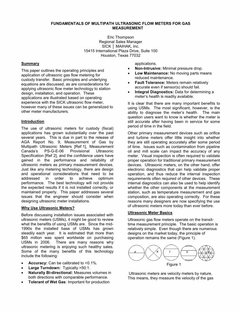
Ultrasonic gas flow meters operate on the transit-time measurement principle. The basic operation is relatively simple. Even though there are numerous designs on the market today, the principle of operation remains the same (Figure 1).

Figure 1

Ultrasonic meters are velocity meters by nature. This means, they measure the velocity of the gas

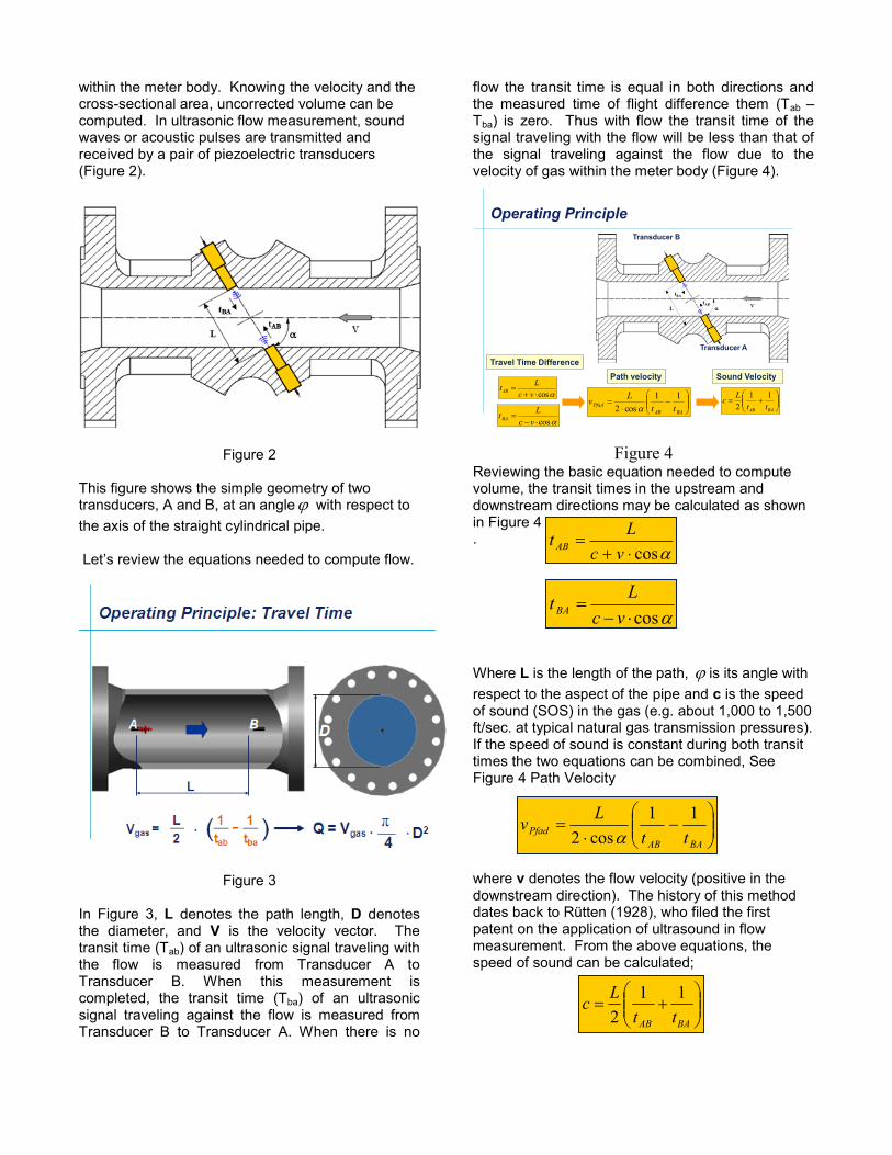
within the meter body. Knowing the velocity and the cross-sectional area, uncorrected volume can be computed. In ultrasonic flow measurement, sound waves or acoustic pulses are transmitted and received by a pair of piezoelectric transducers (Figure 2).

Figure 2

This figure shows the simple geometry of two transducers, A and B, at an angle� with respect to the axis of the straight cylindrical pipe.

"����������#������&'����������������� ��*'���+��#�

Figure 3

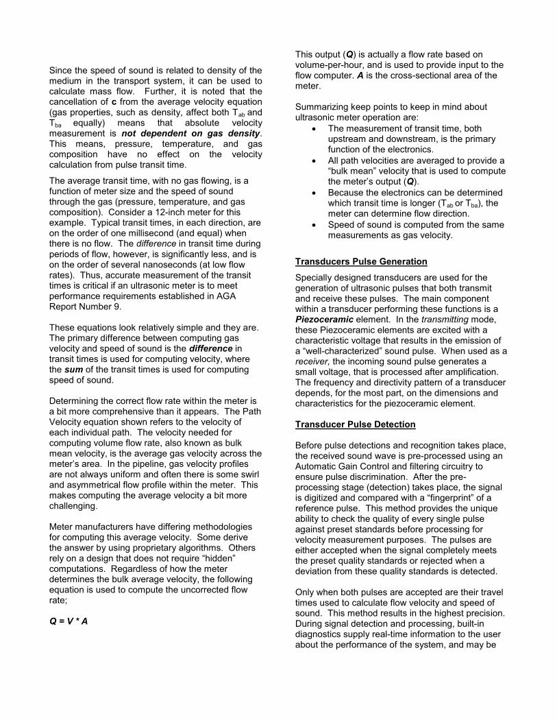
In Figure 3, L denotes the path length, D denotes the diameter, and V is the velocity vector. The transit time (Tab) of an ultrasonic signal traveling with the flow is measured from Transducer A to Transducer B. When this measurement is completed, the transit time (Tba) of an ultrasonic signal traveling against the flow is measured from Transducer B to Transducer A. When there is no

flow the transit time is equal in both directions and the measured time of flight difference them (Tab / Tba) is zero. Thus with flow the transit time of the signal traveling with the flow will be less than that of the signal traveling against the flow due to the velocity of gas within the meter body (Figure 4).

�tAB

tBA

L V

�cos���

vcLtAB

�cos���

vcLtBA

���

��

��

BAABPfad tt

Lv 11cos2 �

Travel Time DifferencePath velocity

Transducer A

Transducer B

Operating Principle

���

���

BAAB ttLc 112

Sound Velocity

Figure 4

Reviewing the basic equation needed to compute volume, the transit times in the upstream and downstream directions may be calculated as shown in Figure 4 . Where L is the length of the path, � is its angle with respect to the aspect of the pipe and c is the speed of sound (SOS) in the gas (e.g. about 1,000 to 1,500 ft/sec. at typical natural gas transmission pressures). If the speed of sound is constant during both transit times the two equations can be combined, See Figure 4 Path Velocity where v denotes the flow velocity (positive in the downstream direction). The history of this method dates back to Rütten (1928), who filed the first patent on the application of ultrasound in flow measurement. From the above equations, the speed of sound can be calculated;

�cos���

vcLt AB

�cos���

vcLtBA

���

��

��

BAABPfad tt

Lv 11cos2 �

���

���

BAAB ttLc 112

Since the speed of sound is related to density of the medium in the transport system, it can be used to calculate mass flow. Further, it is noted that the cancellation of c from the average velocity equation (gas properties, such as density, affect both Tab and Tba equally) means that absolute velocity measurement is not dependent on gas density. This means, pressure, temperature, and gas composition have no effect on the velocity calculation from pulse transit time.

The average transit time, with no gas flowing, is a function of meter size and the speed of sound through the gas (pressure, temperature, and gas composition). Consider a 12-inch meter for this example. Typical transit times, in each direction, are on the order of one millisecond (and equal) when there is no flow. The difference in transit time during periods of flow, however, is significantly less, and is on the order of several nanoseconds (at low flow rates). Thus, accurate measurement of the transit times is critical if an ultrasonic meter is to meet performance requirements established in AGA Report Number 9. These equations look relatively simple and they are. The primary difference between computing gas velocity and speed of sound is the difference in transit times is used for computing velocity, where the sum of the transit times is used for computing speed of sound. Determining the correct flow rate within the meter is a bit more comprehensive than it appears. The Path Velocity equation shown refers to the velocity of each individual path. The velocity needed for computing volume flow rate, also known as bulk mean velocity, is the average gas velocity across the ����������������������*�*��������������� ����*��+�����are not always uniform and often there is some swirl and asymmetrical flow profile within the meter. This makes computing the average velocity a bit more challenging. Meter manufacturers have differing methodologies for computing this average velocity. Some derive the answer by using proprietary algorithms. Others ���������������������������������&'����?������@�computations. Regardless of how the meter determines the bulk average velocity, the following equation is used to compute the uncorrected flow rate; Q = V * A

This output (Q) is actually a flow rate based on volume-per-hour, and is used to provide input to the flow computer. A is the cross-sectional area of the meter. Summarizing keep points to keep in mind about ultrasonic meter operation are:

� The measurement of transit time, both upstream and downstream, is the primary function of the electronics.

� All path velocities are averaged to provide a ?�'�L�����@����� ������������'������ compute �������������'�*'��QQ).

� Because the electronics can be determined which transit time is longer (Tab or Tba), the meter can determine flow direction.

� Speed of sound is computed from the same measurements as gas velocity.

Transducers Pulse Generation

Specially designed transducers are used for the generation of ultrasonic pulses that both transmit and receive these pulses. The main component within a transducer performing these functions is a Piezoceramic element. In the transmitting mode, these Piezoceramic elements are excited with a characteristic voltage that results in the emission of ��?#���- ���� ����X��@���'���*'������Y����'���������receiver, the incoming sound pulse generates a small voltage, that is processed after amplification. The frequency and directivity pattern of a transducer depends, for the most part, on the dimensions and characteristics for the piezoceramic element. Transducer Pulse Detection Before pulse detections and recognition takes place, the received sound wave is pre-processed using an Automatic Gain Control and filtering circuitry to ensure pulse discrimination. After the pre-processing stage (detection) takes place, the signal ���������X������� ��*�����#������?+�����*����@��+���reference pulse. This method provides the unique ability to check the quality of every single pulse against preset standards before processing for velocity measurement purposes. The pulses are either accepted when the signal completely meets the preset quality standards or rejected when a deviation from these quality standards is detected. Only when both pulses are accepted are their travel times used to calculate flow velocity and speed of sound. This method results in the highest precision. During signal detection and processing, built-in diagnostics supply real-time information to the user about the performance of the system, and may be

used to set alarm limits on meter performance. These parameters will be discussed in more detail later. Timing Characteristics The accuracy required in the travel time measurement can be found from the equations. For example, when a velocity of 3 ft/s is measured with 0.5% accuracy along a 3 ft. path length in a gas with sound velocity of 1,300 ft/s, both travel times are of order of 2.5 milli-seconds, and their difference is about 6 micro-seconds, which must be measured with an error no greater than 30 NANO-seconds! This minute travel time difference requires high-speed, high-accuracy digital electronics. The travel times of only a few milli-seconds enable individual ultrasonic flow velocity measurements at high repetition rates. Typical rates are 20 to 50 Hz, depending on pipe diameter. The need for high repetition rates is evident in cases such as surge control applications, where the flow may drop from its set point to its minimum in less than 0.05 seconds. BASIC DIAGNOSTIC INDICATORS One of the principal attributes of modern ultrasonic meters is the ability to monitor their own health, and to diagnose any problems that may occur. Multipath meters are unique in this regard, as they can compare certain measurements between different paths, as well as checking each path individually. ����'��������� ������'�������������������?������ �� L���@� ������ �����������������������������external diagnostics. Internal diagnostics are those indicators derived only from internal measurements of the meter. External diagnostics are those methods in which measurements from the meter are combined with parameters derived from independent sources to detect and identify fault conditions. An example of this would be to compute the gas SOS, based upon composition, and compare to the ������������'�����\�� Gain \����+��������*��������� �������+�������������������� the presence of strong signals on all *������!������ multipath USMs have automatic gain control on all receiver channels. Transducers typically generate the same level of ultrasonic signal time after time. The increase in gain on any path indicates a weaker signal at the receiving transducer. This can be caused by a variety of problems such as transducer deterioration, fouling of the transducer ports, or liquids in the line. However, other factors that affect signal strength include metering pressure and flow

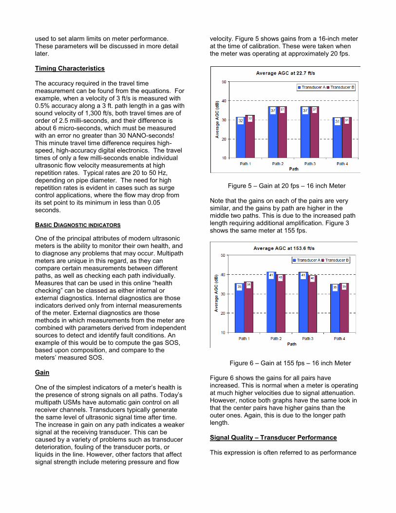
velocity. Figure 5 shows gains from a 16-inch meter at the time of calibration. These were taken when the meter was operating at approximately 20 fps.

Figure 5 / Gain at 20 fps / 16 inch Meter Note that the gains on each of the pairs are very similar, and the gains by path are higher in the middle two paths. This is due to the increased path length requiring additional amplification. Figure 3 shows the same meter at 155 fps.

Figure 6 / Gain at 155 fps / 16 inch Meter Figure 6 shows the gains for all pairs have increased. This is normal when a meter is operating at much higher velocities due to signal attenuation. However, notice both graphs have the same look in that the center pairs have higher gains than the outer ones. Again, this is due to the longer path length. Signal Quality � Transducer Performance This expression is often referred to as performance

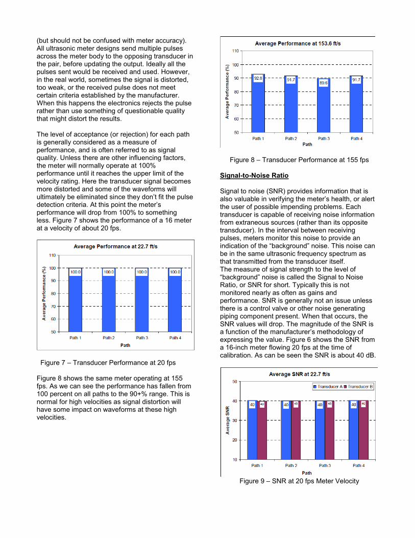
(but should not be confused with meter accuracy). All ultrasonic meter designs send multiple pulses across the meter body to the opposing transducer in the pair, before updating the output. Ideally all the pulses sent would be received and used. However, in the real world, sometimes the signal is distorted, too weak, or the received pulse does not meet certain criteria established by the manufacturer. When this happens the electronics rejects the pulse rather than use something of questionable quality that might distort the results. The level of acceptance (or rejection) for each path is generally considered as a measure of performance, and is often referred to as signal quality. Unless there are other influencing factors, the meter will normally operate at 100% performance until it reaches the upper limit of the velocity rating. Here the transducer signal becomes more distorted and some of the waveforms will '��������������������������� �������������+�������*'�������� ����� ����������������*�����������������performance will drop from 100% to something less. Figure 7 shows the performance of a 16 meter at a velocity of about 20 fps.

Figure 7 / Transducer Performance at 20 fps Figure 8 shows the same meter operating at 155 fps. As we can see the performance has fallen from 100 percent on all paths to the 90+% range. This is normal for high velocities as signal distortion will have some impact on waveforms at these high velocities.

Figure 8 / Transducer Performance at 155 fps

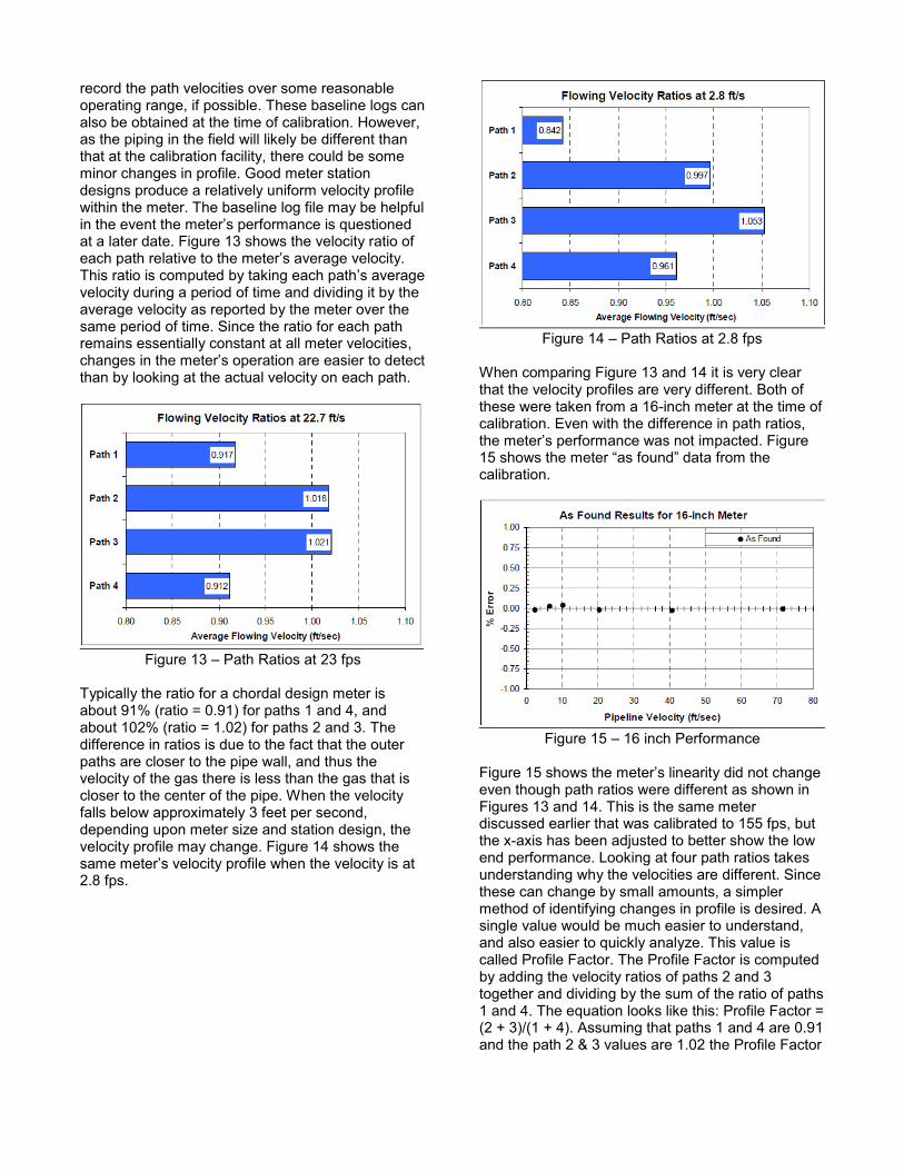
Signal-to-Noise Ratio Signal to noise (SNR) provides information that is ��������'������������+����������������������������������the user of possible impending problems. Each transducer is capable of receiving noise information from extraneous sources (rather than its opposite transducer). In the interval between receiving pulses, meters monitor this noise to provide an ���� �������+�����?�� L���'��@��������This noise can be in the same ultrasonic frequency spectrum as that transmitted from the transducer itself. The measure of signal strength to the level of ?�� L���'��@���������� ��������������������_�����Ratio, or SNR for short. Typically this is not monitored nearly as often as gains and performance. SNR is generally not an issue unless there is a control valve or other noise generating piping component present. When that occurs, the SNR values will drop. The magnitude of the SNR is a function of the manuf� �'�������������������+�expressing the value. Figure 6 shows the SNR from a 16-inch meter flowing 20 fps at the time of calibration. As can be seen the SNR is about 40 dB.

Figure 9 / SNR at 20 fps Meter Velocity

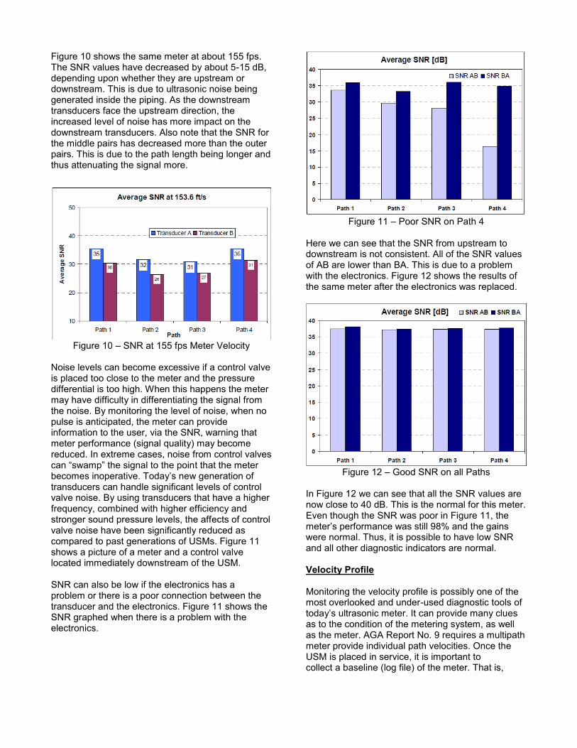
Figure 10 shows the same meter at about 155 fps. The SNR values have decreased by about 5-15 dB, depending upon whether they are upstream or downstream. This is due to ultrasonic noise being generated inside the piping. As the downstream transducers face the upstream direction, the increased level of noise has more impact on the downstream transducers. Also note that the SNR for the middle pairs has decreased more than the outer pairs. This is due to the path length being longer and thus attenuating the signal more.

Figure 10 / SNR at 155 fps Meter Velocity

Noise levels can become excessive if a control valve is placed too close to the meter and the pressure differential is too high. When this happens the meter may have difficulty in differentiating the signal from the noise. By monitoring the level of noise, when no pulse is anticipated, the meter can provide information to the user, via the SNR, warning that meter performance (signal quality) may become reduced. In extreme cases, noise from control valves ���?�#��*@�������������������*���t that the meter �� ��������*���������!���������#�������������+�transducers can handle significant levels of control valve noise. By using transducers that have a higher frequency, combined with higher efficiency and stronger sound pressure levels, the affects of control valve noise have been significantly reduced as compared to past generations of USMs. Figure 11 shows a picture of a meter and a control valve located immediately downstream of the USM. SNR can also be low if the electronics has a problem or there is a poor connection between the transducer and the electronics. Figure 11 shows the SNR graphed when there is a problem with the electronics.

Figure 11 / Poor SNR on Path 4

Here we can see that the SNR from upstream to downstream is not consistent. All of the SNR values of AB are lower than BA. This is due to a problem with the electronics. Figure 12 shows the results of the same meter after the electronics was replaced.

Figure 12 / Good SNR on all Paths

In Figure 12 we can see that all the SNR values are now close to 40 dB. This is the normal for this meter. Even though the SNR was poor in Figure 11, the ��������*��+����� ��#���������`{|���������������were normal. Thus, it is possible to have low SNR and all other diagnostic indicators are normal. Velocity Profile Monitoring the velocity profile is possibly one of the most overlooked and under-used diagnostic tools of ��������'�������� ����������� ���*������������ �'���as to the condition of the metering system, as well as the meter. AGA Report No. 9 requires a multipath meter provide individual path velocities. Once the USM is placed in service, it is important to collect a baseline (log file) of the meter. That is,

record the path velocities over some reasonable operating range, if possible. These baseline logs can also be obtained at the time of calibration. However, as the piping in the field will likely be different than that at the calibration facility, there could be some minor changes in profile. Good meter station designs produce a relatively uniform velocity profile within the meter. The baseline log file may be helpful �������������������������*��+����� �����&'���������at a later date. Figure 13 shows the velocity ratio of �� ��*���������������������������������������� �����This ra������� ��*'���������L������ ��*��������������velocity during a period of time and dividing it by the average velocity as reported by the meter over the same period of time. Since the ratio for each path remains essentially constant at all meter velocities, �����������������������*�������������������������� ��than by looking at the actual velocity on each path.

Figure 13 / Path Ratios at 23 fps

Typically the ratio for a chordal design meter is about 91% (ratio = 0.91) for paths 1 and 4, and about 102% (ratio = 1.02) for paths 2 and 3. The difference in ratios is due to the fact that the outer paths are closer to the pipe wall, and thus the velocity of the gas there is less than the gas that is closer to the center of the pipe. When the velocity falls below approximately 3 feet per second, depending upon meter size and station design, the velocity profile may change. Figure 14 shows the ����������������� ����*��+����#������������ ����������2.8 fps.

Figure 14 / Path Ratios at 2.8 fps

When comparing Figure 13 and 14 it is very clear that the velocity profiles are very different. Both of these were taken from a 16-inch meter at the time of calibration. Even with the difference in path ratios, ������������*��+����� ��#���������*� �����~��'���15 shows th��������?���+�'��@������+��������calibration.

Figure 15 / 16 inch Performance

~��'���������#�������������������������������� ����� even though path ratios were different as shown in Figures 13 and 14. This is the same meter discussed earlier that was calibrated to 155 fps, but the x-axis has been adjusted to better show the low end performance. Looking at four path ratios takes understanding why the velocities are different. Since these can change by small amounts, a simpler method of identifying changes in profile is desired. A single value would be much easier to understand, and also easier to quickly analyze. This value is called Profile Factor. The Profile Factor is computed by adding the velocity ratios of paths 2 and 3 together and dividing by the sum of the ratio of paths 1 and 4. The equation looks like this: Profile Factor = (2 + 3)/(1 + 4). Assuming that paths 1 and 4 are 0.91 and the path 2 & 3 values are 1.02 the Profile Factor

is about 1.12. This value does vary a little from meter to meter due to piping installation effects and to some degree the type of flow conditioner and its distance from the meter. Another method used to analyze path velocities is to compare the sum of paths 1 & 2 to the sum of paths 3 & 4. This provides a look at the symmetry of the profile from top to ��������_��������������������*�������� ������#�������very symmetrical resulting in a value close to 1.000. Figures 13 and 14 show both the Profile and the Symmetry In Figure 16, when the meter was flowing at 20 fps, the Profile Factor was 1.115. As the velocity dropped to 2.8 fps (Figure 17) the Profile Factor changed to 1.137. This is about a 2% change in profile when comparing the middle paths to the outer paths.

Figure 16 / Profile Factor and Symmetry at 20 fps

The other diagnostic worth reviewing is the Symmetry value. Figure 14 shows a significant change (on the order of 10%) in the Symmetry at the lower velocities, but again there was no significant impact on meter performance. This just indicates there was a chan������������������*��+����

Figure 17 / Profile Factor and Symmetry at 3 fps

The Profile Factor can be a valuable indicator of abnormal flow conditions. The previous discussion

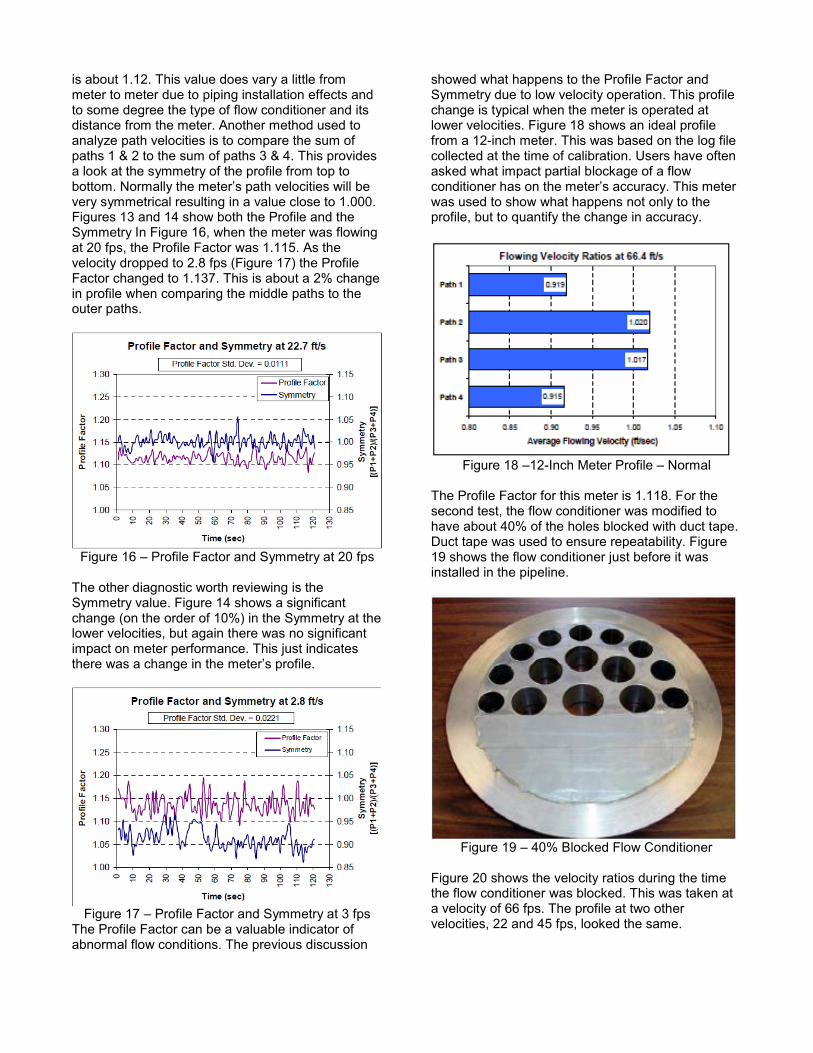
showed what happens to the Profile Factor and Symmetry due to low velocity operation. This profile change is typical when the meter is operated at lower velocities. Figure 18 shows an ideal profile from a 12-inch meter. This was based on the log file collected at the time of calibration. Users have often asked what impact partial blockage of a flow ������������������������������� '�� ���!����������was used to show what happens not only to the profile, but to quantify the change in accuracy.

Figure 18 /12-Inch Meter Profile / Normal

The Profile Factor for this meter is 1.118. For the second test, the flow conditioner was modified to have about 40% of the holes blocked with duct tape. Duct tape was used to ensure repeatability. Figure 19 shows the flow conditioner just before it was installed in the pipeline.

Figure 19 / 40% Blocked Flow Conditioner

Figure 20 shows the velocity ratios during the time the flow conditioner was blocked. This was taken at a velocity of 66 fps. The profile at two other velocities, 22 and 45 fps, looked the same.

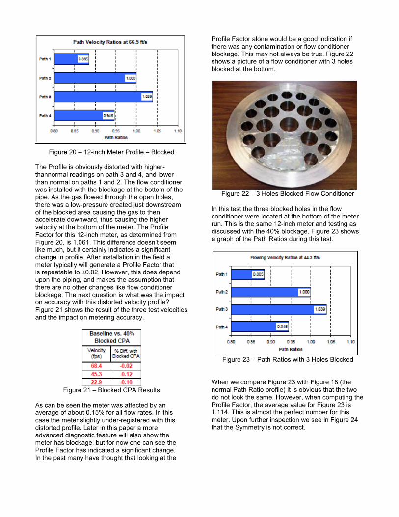
Figure 20 / 12-inch Meter Profile / Blocked

The Profile is obviously distorted with higher-thannormal readings on path 3 and 4, and lower than normal on paths 1 and 2. The flow conditioner was installed with the blockage at the bottom of the pipe. As the gas flowed through the open holes, there was a low-pressure created just downstream of the blocked area causing the gas to then accelerate downward, thus causing the higher velocity at the bottom of the meter. The Profile Factor for this 12-inch meter, as determined from Figure 20, is 1.0����!������++���� ���������������like much, but it certainly indicates a significant change in profile. After installation in the field a meter typically will generate a Profile Factor that is repeatable to ±0.02. However, this does depend upon the piping, and makes the assumption that there are no other changes like flow conditioner blockage. The next question is what was the impact on accuracy with this distorted velocity profile? Figure 21 shows the result of the three test velocities and the impact on metering accuracy.

Figure 21 / Blocked CPA Results

As can be seen the meter was affected by an average of about 0.15% for all flow rates. In this case the meter slightly under-registered with this distorted profile. Later in this paper a more advanced diagnostic feature will also show the meter has blockage, but for now one can see the Profile Factor has indicated a significant change. In the past many have thought that looking at the

Profile Factor alone would be a good indication if there was any contamination or flow conditioner blockage. This may not always be true. Figure 22 shows a picture of a flow conditioner with 3 holes blocked at the bottom.

Figure 22 / 3 Holes Blocked Flow Conditioner

In this test the three blocked holes in the flow conditioner were located at the bottom of the meter run. This is the same 12-inch meter and testing as discussed with the 40% blockage. Figure 23 shows a graph of the Path Ratios during this test.

Figure 23 / Path Ratios with 3 Holes Blocked

When we compare Figure 23 with Figure 18 (the normal Path Ratio profile) it is obvious that the two do not look the same. However, when computing the Profile Factor, the average value for Figure 23 is 1.114. This is almost the perfect number for this meter. Upon further inspection we see in Figure 24 that the Symmetry is not correct.

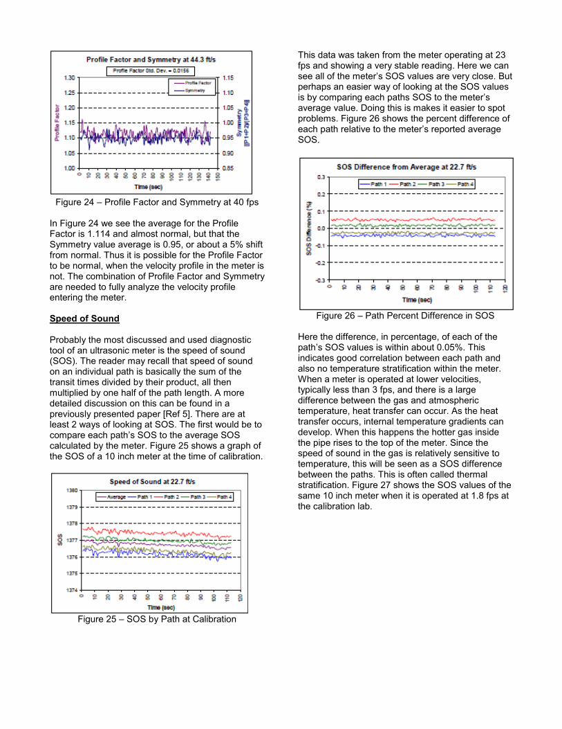
Figure 24 / Profile Factor and Symmetry at 40 fps

In Figure 24 we see the average for the Profile Factor is 1.114 and almost normal, but that the Symmetry value average is 0.95, or about a 5% shift from normal. Thus it is possible for the Profile Factor to be normal, when the velocity profile in the meter is not. The combination of Profile Factor and Symmetry are needed to fully analyze the velocity profile entering the meter. Speed of Sound Probably the most discussed and used diagnostic tool of an ultrasonic meter is the speed of sound (SOS). The reader may recall that speed of sound on an individual path is basically the sum of the transit times divided by their product, all then multiplied by one half of the path length. A more detailed discussion on this can be found in a previously presented paper [Ref 5]. There are at least 2 ways of looking at SOS. The first would be to ��*������ ��*�������\������������������\��calculated by the meter. Figure 25 shows a graph of the SOS of a 10 inch meter at the time of calibration.

Figure 25 / SOS by Path at Calibration

This data was taken from the meter operating at 23 fps and showing a very stable reading. Here we can see all of the me�������\�����'������������ �������'� perhaps an easier way of looking at the SOS values ������ ��*�������� ��*������\�����������������average value. Doing this is makes it easier to spot problems. Figure 26 shows the percent difference of each path ��������������������������*��������������SOS.

Figure 26 / Path Percent Difference in SOS

Here the difference, in percentage, of each of the *�������\�����'������#���������'������|��!��� indicates good correlation between each path and also no temperature stratification within the meter. When a meter is operated at lower velocities, typically less than 3 fps, and there is a large difference between the gas and atmospheric temperature, heat transfer can occur. As the heat transfer occurs, internal temperature gradients can develop. When this happens the hotter gas inside the pipe rises to the top of the meter. Since the speed of sound in the gas is relatively sensitive to temperature, this will be seen as a SOS difference between the paths. This is often called thermal stratification. Figure 27 shows the SOS values of the same 10 inch meter when it is operated at 1.8 fps at the calibration lab.

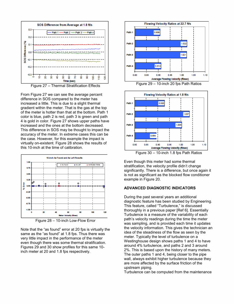
Figure 27 / Thermal Stratification Effects

From Figure 27 we can see the average percent difference in SOS compared to the meter has increased a little. This is due to a slight thermal gradient within the meter. That is the gas at the top of the meter is hotter than that at the bottom. Path 1 color is blue, path 2 is red, path 3 is green and path 4 is gold in color. Figure 27 shows upper paths have increased and the ones at the bottom decreased. This difference in SOS may be thought to impact the accuracy of the meter. In extreme cases this can be the case. However, for this example the impact is virtually on-existent. Figure 28 shows the results of this 10-inch at the time of calibration.

Figure 28 / 10-inch Low-Flow Error

_�������������?���+�'��@�������������+*���������'�������� ������������?���+�'��@������{�+*���!�'��������#�� very little impact in the performance of the meter even though there was some thermal stratification. Figures 29 and 30 show profiles for this same 10-inch meter at 20 and 1.8 fps respectively.

Figure 29 / 10-inch 20 fps Path Ratios

Figure 30 / 10-inch 1.8 fps Path Ratios

Even though this meter had some thermal ������+� ��������������� ����*��+����������� ����� significantly. There is a difference, but once again it is not as significant as the blocked flow conditioner example in Figure 20. ADVANCED DIAGNOSTIC INDICATORS During the past several years an additional diagnostic feature has been studied by Engineering. !����+���'���� ������?!'��'��� ��@������� '�����thoroughly in a previous paper [Ref 6]. Essentially Turbulence is a measure of the variability of each *����������city readings during the time the meter was sampling, and is provided each time it updates the velocity information. This gives the technician an idea of the steadiness of the flow as seen by the meter. Typically the level of turbulence on a Westinghouse design shows paths 1 and 4 to have around 4% turbulence, and paths 2 and 3 around 2%. This is based upon the history of many meters. The outer paths 1 and 4, being closer to the pipe wall, always exhibit higher turbulence because they are more affected by the surface friction of the upstream piping. Turbulence can be computed from the maintenance

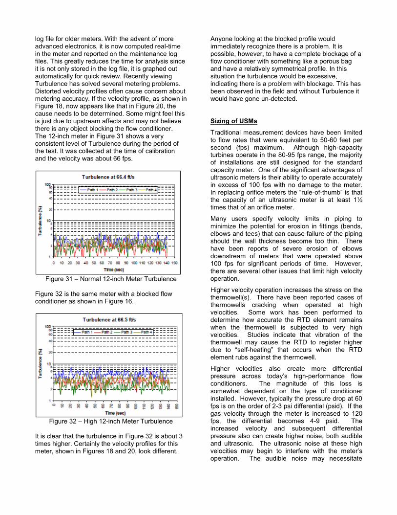
log file for older meters. With the advent of more advanced electronics, it is now computed real-time in the meter and reported on the maintenance log files. This greatly reduces the time for analysis since it is not only stored in the log file, it is graphed out automatically for quick review. Recently viewing Turbulence has solved several metering problems. Distorted velocity profiles often cause concern about metering accuracy. If the velocity profile, as shown in Figure 18, now appears like that in Figure 20, the cause needs to be determined. Some might feel this is just due to upstream affects and may not believe there is any object blocking the flow conditioner. The 12-inch meter in Figure 31 shows a very consistent level of Turbulence during the period of the test. It was collected at the time of calibration and the velocity was about 66 fps.

Figure 31 / Normal 12-inch Meter Turbulence

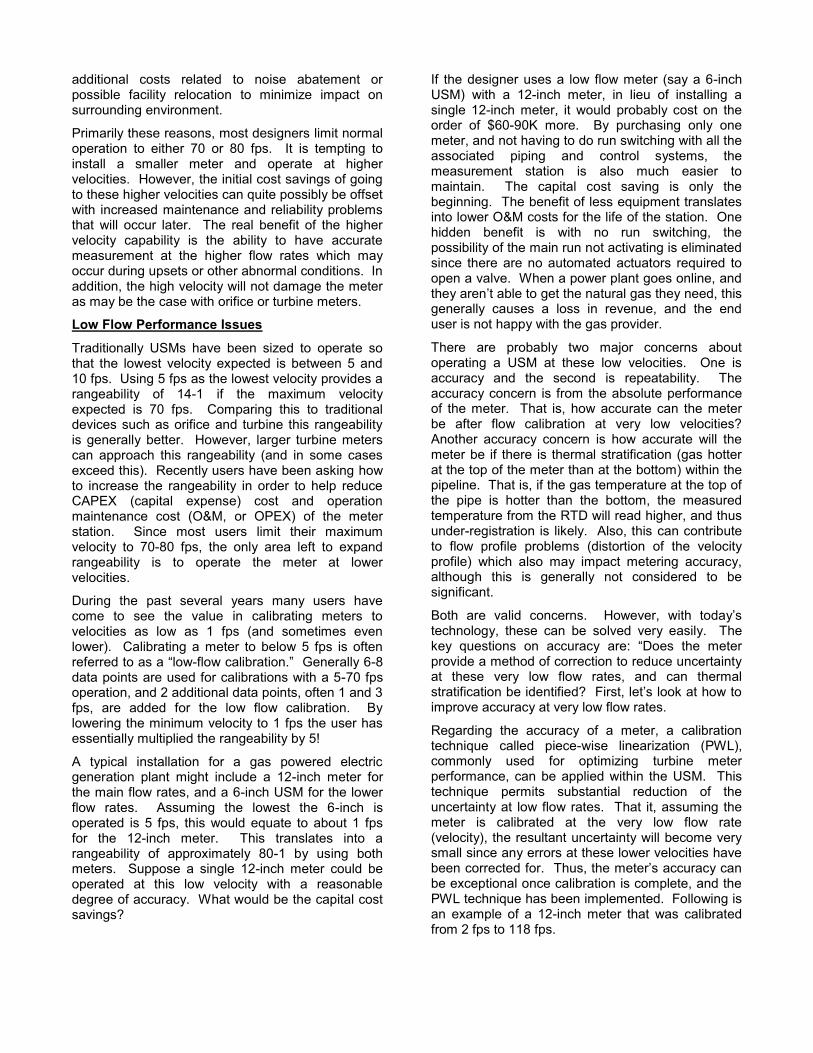
Figure 32 is the same meter with a blocked flow conditioner as shown in Figure 16.

Figure 32 / High 12-inch Meter Turbulence

It is clear that the turbulence in Figure 32 is about 3 times higher. Certainly the velocity profiles for this meter, shown in Figures 18 and 20, look different.

Anyone looking at the blocked profile would immediately recognize there is a problem. It is possible, however, to have a complete blockage of a flow conditioner with something like a porous bag and have a relatively symmetrical profile. In this situation the turbulence would be excessive, indicating there is a problem with blockage. This has been observed in the field and without Turbulence it would have gone un-detected. Sizing of USMs

Traditional measurement devices have been limited to flow rates that were equivalent to 50-60 feet per second (fps) maximum. Although high-capacity turbines operate in the 80-95 fps range, the majority of installations are still designed for the standard capacity meter. One of the significant advantages of ultrasonic meters is their ability to operate accurately in excess of 100 fps with no damage to the meter. �����*�� �������+� �������������?�'��-of-��'��@���������the capacity of an ultrasonic meter is at least 1½ times that of an orifice meter.

Many users specify velocity limits in piping to minimize the potential for erosion in fittings (bends, elbows and tees) that can cause failure of the piping should the wall thickness become too thin. There have been reports of severe erosion of elbows downstream of meters that were operated above 100 fps for significant periods of time. However, there are several other issues that limit high velocity operation.

Higher velocity operation increases the stress on the thermowell(s). There have been reported cases of thermowells cracking when operated at high velocities. Some work has been performed to determine how accurate the RTD element remains when the thermowell is subjected to very high velocities. Studies indicate that vibration of the thermowell may cause the RTD to register higher �'�� ��� ?���+-�������@� ����� � '��� #���� ���� �!��element rubs against the thermowell.

Higher velocities also create more differential *����'��� � ����� �������� ����-performance flow conditioners. The magnitude of this loss is somewhat dependent on the type of conditioner installed. However, typically the pressure drop at 60 fps is on the order of 2-3 psi differential (psid). If the gas velocity through the meter is increased to 120 fps, the differential becomes 4-9 psid. The increased velocity and subsequent differential pressure also can create higher noise, both audible and ultrasonic. The ultrasonic noise at these high ���� ������ ���� ������ ��� �����+���� #���� ���� ��������operation. The audible noise may necessitate

additional costs related to noise abatement or possible facility relocation to minimize impact on surrounding environment.

Primarily these reasons, most designers limit normal operation to either 70 or 80 fps. It is tempting to install a smaller meter and operate at higher velocities. However, the initial cost savings of going to these higher velocities can quite possibly be offset with increased maintenance and reliability problems that will occur later. The real benefit of the higher velocity capability is the ability to have accurate measurement at the higher flow rates which may occur during upsets or other abnormal conditions. In addition, the high velocity will not damage the meter as may be the case with orifice or turbine meters.

Low Flow Performance Issues

Traditionally USMs have been sized to operate so that the lowest velocity expected is between 5 and 10 fps. Using 5 fps as the lowest velocity provides a rangeability of 14-1 if the maximum velocity expected is 70 fps. Comparing this to traditional devices such as orifice and turbine this rangeability is generally better. However, larger turbine meters can approach this rangeability (and in some cases exceed this). Recently users have been asking how to increase the rangeability in order to help reduce CAPEX (capital expense) cost and operation maintenance cost (O&M, or OPEX) of the meter station. Since most users limit their maximum velocity to 70-80 fps, the only area left to expand rangeability is to operate the meter at lower velocities.

During the past several years many users have come to see the value in calibrating meters to velocities as low as 1 fps (and sometimes even lower). Calibrating a meter to below 5 fps is often referred to as a ?��#-+��#� �����������@�������������-8 data points are used for calibrations with a 5-70 fps operation, and 2 additional data points, often 1 and 3 fps, are added for the low flow calibration. By lowering the minimum velocity to 1 fps the user has essentially multiplied the rangeability by 5!

A typical installation for a gas powered electric generation plant might include a 12-inch meter for the main flow rates, and a 6-inch USM for the lower flow rates. Assuming the lowest the 6-inch is operated is 5 fps, this would equate to about 1 fps for the 12-inch meter. This translates into a rangeability of approximately 80-1 by using both meters. Suppose a single 12-inch meter could be operated at this low velocity with a reasonable degree of accuracy. What would be the capital cost savings?

If the designer uses a low flow meter (say a 6-inch USM) with a 12-inch meter, in lieu of installing a single 12-inch meter, it would probably cost on the order of $60-90K more. By purchasing only one meter, and not having to do run switching with all the associated piping and control systems, the measurement station is also much easier to maintain. The capital cost saving is only the beginning. The benefit of less equipment translates into lower O&M costs for the life of the station. One hidden benefit is with no run switching, the possibility of the main run not activating is eliminated since there are no automated actuators required to open a valve. When a power plant goes online, and ������������������������������tural gas they need, this generally causes a loss in revenue, and the end user is not happy with the gas provider.

There are probably two major concerns about operating a USM at these low velocities. One is accuracy and the second is repeatability. The accuracy concern is from the absolute performance of the meter. That is, how accurate can the meter be after flow calibration at very low velocities? Another accuracy concern is how accurate will the meter be if there is thermal stratification (gas hotter at the top of the meter than at the bottom) within the pipeline. That is, if the gas temperature at the top of the pipe is hotter than the bottom, the measured temperature from the RTD will read higher, and thus under-registration is likely. Also, this can contribute to flow profile problems (distortion of the velocity profile) which also may impact metering accuracy, although this is generally not considered to be significant.

����� ���� ������ �� ������ � �#������ #���� ��������technology, these can be solved very easily. The L��� &'�������� ��� � '�� �� ����� ?����� ���� ������provide a method of correction to reduce uncertainty at these very low flow rates, and can thermal ������+� ���������������+������~���������������L������#����improve accuracy at very low flow rates.

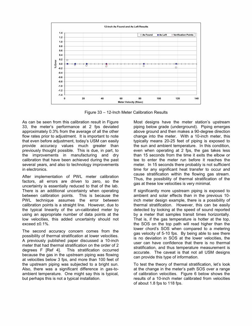
Regarding the accuracy of a meter, a calibration technique called piece-wise linearization (PWL), commonly used for optimizing turbine meter performance, can be applied within the USM. This technique permits substantial reduction of the uncertainty at low flow rates. That it, assuming the meter is calibrated at the very low flow rate (velocity), the resultant uncertainty will become very small since any errors at these lower velocities have ����� ���� ����+�����!�'���������������� '�� �� ���be exceptional once calibration is complete, and the PWL technique has been implemented. Following is an example of a 12-inch meter that was calibrated from 2 fps to 118 fps.

12-inch As Found and As Left Results

-1.4

-1.2

-1.0

-0.8

-0.6

-0.4

-0.2

0.0

0.2

0.4

0.6

0.8

1.0

1.2

1.4

0 20 40 60 80 100 120 140Meter Velocity (ft/sec)

% E

rror

As Found As Left Verification Points

Figure 33 / 12-Inch Meter Calibration Results

As can be seen from this calibration result in Figure ���� ���� �������� *��+����� �� ��� �� +*�� ���������approximately 0.3% from the average of all the other flow rates prior to adjustment. It is important to note ������������+�������'�������������������� ���easily provide accuracy values much greater than previously thought possible. This is due, in part, to the improvements in manufacturing and dry calibration that have been achieved during the past several years, and also to technology improvements in electronics.

After implementation of PWL meter calibration factors, all errors are driven to zero, so the uncertainty is essentially reduced to that of the lab. There is an additional uncertainty when operating between calibration points. This is because the PWL technique assumes the error between calibration points is a straight line. However, due to the typical linearity of the un-calibrated meter by using an appropriate number of data points at the low velocities, this added uncertainty should not exceed ±0.1%.

The second accuracy concern comes from the possibility of thermal stratification at lower velocities. A previously published paper discussed a 10-inch meter that had thermal stratification on the order of 2 degrees F [Ref 4]. This stratification occurred because the gas in the upstream piping was flowing at velocities below 3 fps, and more than 100 feet of the upstream piping was subjected to a bright sun. Also, there was a significant difference in gas-to-ambient temperature. One might say this is typical, but perhaps this is not a typical installation.

����� �������� ����� ���� ������ ���������� '*�������piping below grade (underground). Piping emerges above ground and then makes a 90-degree direction change into the meter. With a 10-inch meter, this typically means 20-25 feet of piping is exposed to the sun and ambient temperature. In this condition, even when operating at 2 fps, the gas takes less than 15 seconds from the time it exits the elbow or tee to enter the meter run before it reaches the meter. In 15 seconds there probably is not sufficient time for any significant heat transfer to occur and cause stratification within the flowing gas stream. Thus, the possibility of thermal stratification of the gas at these low velocities is very minimal.

If significantly more upstream piping is exposed to ambient and solar effects than in the previous 10-inch meter design example, there is a possibility of thermal stratification. However, this can be easily detected by looking at the speed of sound reported by a meter that samples transit times horizontally. That is, if the gas temperature is hotter at the top, the SOS on the top path will read higher than the ��#��� ������� �\�� #���� ��*����� ��� �� ���������gas velocity of 5-10 fps. By being able to see there is no deviation in SOS at the lower velocities, the user can have confidence that there is no thermal stratification, and thus temperature measurement is accurate. The caveat is that not all USM designs can provide this type of information.

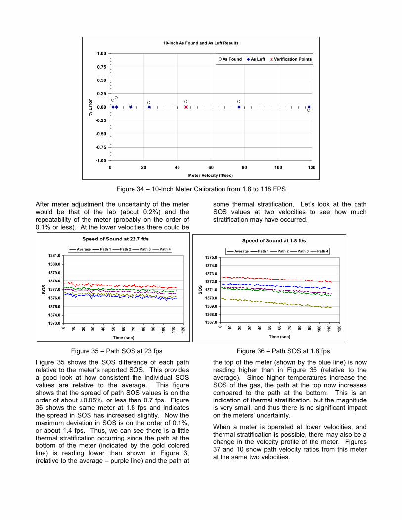
T�� ����� ���� ��������+� ��������������+� ������� ������ ���L�������� ���������������������*�����\���������������of calibration velocities. Figure 6 below shows the results of a 10-inch meter calibrated from velocities of about 1.8 fps to 118 fps.

10-inch As Found and As Left Results

-1.00

-0.75

-0.50

-0.25

0.00

0.25

0.50

0.75

1.00

0 20 40 60 80 100 120Meter Velocity (ft/sec)

% E

rror

As Found As Left Verification Points

Figure 34 / 10-Inch Meter Calibration from 1.8 to 118 FPS

After meter adjustment the uncertainty of the meter would be that of the lab (about 0.2%) and the repeatability of the meter (probably on the order of 0.1% or less). At the lower velocities there could be

����� �������� ������+� ������� � "����� ���L� ��� ���� *����SOS values at two velocities to see how much stratification may have occurred.

Speed of Sound at 22.7 ft/s

1373.0

1374.0

1375.0

1376.0

1377.0

1378.0

1379.0

1380.0

1381.0

0 10 20 30 40 50 60 70 80 90 100

110

120

Time (sec)

SO

S

Average Path 1 Path 2 Path 3 Path 4

Speed of Sound at 1.8 ft/s

1367.0

1368.0

1369.0

1370.0

1371.0

1372.0

1373.0

1374.0

1375.0

0 10 20 30 40 50 60 70 80 90 100

110

120

Time (sec)

SOS

Average Path 1 Path 2 Path 3 Path 4

Figure 35 / Path SOS at 23 fps Figure 36 / Path SOS at 1.8 fps

Figure 35 shows the SOS difference of each path ��������������������������*�������\����!����*��������a good look at how consistent the individual SOS values are relative to the average. This figure shows that the spread of path SOS values is on the order of about ±0.05%, or less than 0.7 fps. Figure 36 shows the same meter at 1.8 fps and indicates the spread in SOS has increased slightly. Now the maximum deviation in SOS is on the order of 0.1%, or about 1.4 fps. Thus, we can see there is a little thermal stratification occurring since the path at the bottom of the meter (indicated by the gold colored line) is reading lower than shown in Figure 3, (relative to the average / purple line) and the path at

the top of the meter (shown by the blue line) is now reading higher than in Figure 35 (relative to the average). Since higher temperatures increase the SOS of the gas, the path at the top now increases compared to the path at the bottom. This is an indication of thermal stratification, but the magnitude is very small, and thus there is no significant impact ���������������'� �����������

When a meter is operated at lower velocities, and thermal stratification is possible, there may also be a change in the velocity profile of the meter. Figures 37 and 10 show path velocity ratios from this meter at the same two velocities.

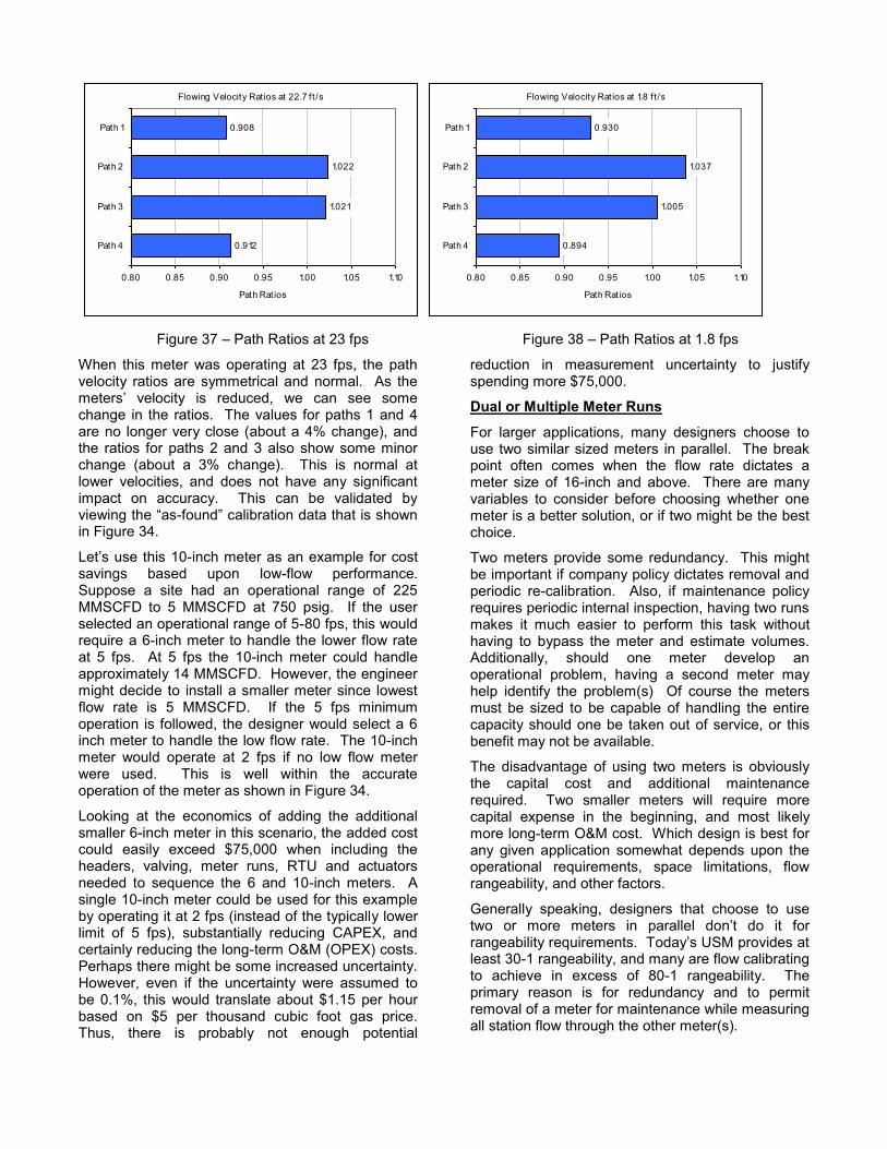
Flowing Velocity Ratios at 22.7 f t /s

0.908

1.022

1.021

0.912

0.80 0.85 0.90 0.95 1.00 1.05 1.10

Path 1

Path 2

Path 3

Path 4

Path Ratios

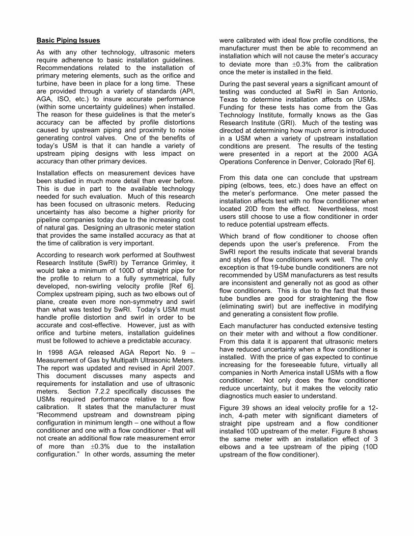
Flowing Velocity Ratios at 1.8 f t /s

0.930

1.037

1.005

0.894

0.80 0.85 0.90 0.95 1.00 1.05 1.10

Path 1

Path 2

Path 3

Path 4

Path Ratios

Figure 37 / Path Ratios at 23 fps Figure 38 / Path Ratios at 1.8 fps

When this meter was operating at 23 fps, the path velocity ratios are symmetrical and normal. As the �������� ���� ���� ��� ���' ���� #�� ��� ���� �����change in the ratios. The values for paths 1 and 4 are no longer very close (about a 4% change), and the ratios for paths 2 and 3 also show some minor change (about a 3% change). This is normal at lower velocities, and does not have any significant impact on accuracy. This can be validated by ���#��������?��-+�'��@� ���������������������������#��in Figure 34.

"�����'����������-inch meter as an example for cost savings based upon low-flow performance. Suppose a site had an operational range of 225 MMSCFD to 5 MMSCFD at 750 psig. If the user selected an operational range of 5-80 fps, this would require a 6-inch meter to handle the lower flow rate at 5 fps. At 5 fps the 10-inch meter could handle approximately 14 MMSCFD. However, the engineer might decide to install a smaller meter since lowest flow rate is 5 MMSCFD. If the 5 fps minimum operation is followed, the designer would select a 6 inch meter to handle the low flow rate. The 10-inch meter would operate at 2 fps if no low flow meter were used. This is well within the accurate operation of the meter as shown in Figure 34.

Looking at the economics of adding the additional smaller 6-inch meter in this scenario, the added cost could easily exceed $75,000 when including the headers, valving, meter runs, RTU and actuators needed to sequence the 6 and 10-inch meters. A single 10-inch meter could be used for this example by operating it at 2 fps (instead of the typically lower limit of 5 fps), substantially reducing CAPEX, and certainly reducing the long-term O&M (OPEX) costs. Perhaps there might be some increased uncertainty. However, even if the uncertainty were assumed to be 0.1%, this would translate about $1.15 per hour based on $5 per thousand cubic foot gas price. Thus, there is probably not enough potential

reduction in measurement uncertainty to justify spending more $75,000.

Dual or Multiple Meter Runs

For larger applications, many designers choose to use two similar sized meters in parallel. The break point often comes when the flow rate dictates a meter size of 16-inch and above. There are many variables to consider before choosing whether one meter is a better solution, or if two might be the best choice.

Two meters provide some redundancy. This might be important if company policy dictates removal and periodic re-calibration. Also, if maintenance policy requires periodic internal inspection, having two runs makes it much easier to perform this task without having to bypass the meter and estimate volumes. Additionally, should one meter develop an operational problem, having a second meter may help identify the problem(s) Of course the meters must be sized to be capable of handling the entire capacity should one be taken out of service, or this benefit may not be available.

The disadvantage of using two meters is obviously the capital cost and additional maintenance required. Two smaller meters will require more capital expense in the beginning, and most likely more long-term O&M cost. Which design is best for any given application somewhat depends upon the operational requirements, space limitations, flow rangeability, and other factors.

Generally speaking, designers that choose to use two or more mete��� ��� *�������� ������ ��� ��� +������������������&'�����������!�����������*�����������least 30-1 rangeability, and many are flow calibrating to achieve in excess of 80-1 rangeability. The primary reason is for redundancy and to permit removal of a meter for maintenance while measuring all station flow through the other meter(s).

Basic Piping Issues

As with any other technology, ultrasonic meters require adherence to basic installation guidelines. Recommendations related to the installation of primary metering elements, such as the orifice and turbine, have been in place for a long time. These are provided through a variety of standards (API, AGA, ISO, etc.) to insure accurate performance (within some uncertainty guidelines) when installed. The reason for th���� �'��������� ��� ����� ���� ��������accuracy can be affected by profile distortions caused by upstream piping and proximity to noise generating control valves. One of the benefits of �������� ���� ��� ����� ��� ��� ������� �� �������� �+�upstream piping designs with less impact on accuracy than other primary devices.

Installation effects on measurement devices have been studied in much more detail than ever before. This is due in part to the available technology needed for such evaluation. Much of this research has been focused on ultrasonic meters. Reducing uncertainty has also become a higher priority for pipeline companies today due to the increasing cost of natural gas. Designing an ultrasonic meter station that provides the same installed accuracy as that at the time of calibration is very important.

According to research work performed at Southwest Research Institute (SwRI) by Terrance Grimley, it would take a minimum of 100D of straight pipe for the profile to return to a fully symmetrical, fully developed, non-swirling velocity profile [Ref 6]. Complex upstream piping, such as two elbows out of plane, create even more non-symmetry and swirl �����#����#��������������#�����!������������'���handle profile distortion and swirl in order to be accurate and cost-effective. However, just as with orifice and turbine meters, installation guidelines must be followed to achieve a predictable accuracy.

In 1998 AGA released AGA Report No. 9 / Measurement of Gas by Multipath Ultrasonic Meters. The report was updated and revised in April 2007. This document discusses many aspects and requirements for installation and use of ultrasonic meters. Section 7.2.2 specifically discusses the USMs required performance relative to a flow calibration. It states that the manufacturer must ?�� ������� '*������� ���� ��#�������� *�*����configuration in minimum length / one without a flow conditioner and one with a flow conditioner - that will not create an additional flow rate measurement error of more than �0.3% due to the installation ��+��'�������@� � ���������#���������'����� ����������

were calibrated with ideal flow profile conditions, the manufacturer must then be able to recommend an �������������#�� ��#�������� �'���������������� '�� ��to deviate more than �0.3% from the calibration once the meter is installed in the field.

During the past several years a significant amount of testing was conducted at SwRI in San Antonio, Texas to determine installation affects on USMs. Funding for these tests has come from the Gas Technology Institute, formally knows as the Gas Research Institute (GRI). Much of the testing was directed at determining how much error is introduced in a USM when a variety of upstream installation conditions are present. The results of the testing were presented in a report at the 2000 AGA Operations Conference in Denver, Colorado [Ref 6].

From this data one can conclude that upstream piping (elbows, tees, etc.) does have an effect on ���� �������� *��+����� ��� � \��� ������ *������ ����installation affects test with no flow conditioner when located 20D from the effect. Nevertheless, most users still choose to use a flow conditioner in order to reduce potential upstream effects.

Which brand of flow conditioner to choose often ��*����� '*��� ���� '������ *��+���� ��� � ~���� ��e SwRI report the results indicate that several brands and styles of flow conditioners work well. The only exception is that 19-tube bundle conditioners are not recommended by USM manufacturers as test results are inconsistent and generally not as good as other flow conditioners. This is due to the fact that these tube bundles are good for straightening the flow (eliminating swirl) but are ineffective in modifying and generating a consistent flow profile.

Each manufacturer has conducted extensive testing on their meter with and without a flow conditioner. From this data it is apparent that ultrasonic meters have reduced uncertainty when a flow conditioner is installed. With the price of gas expected to continue increasing for the foreseeable future, virtually all companies in North America install USMs with a flow conditioner. Not only does the flow conditioner reduce uncertainty, but it makes the velocity ratio diagnostics much easier to understand.

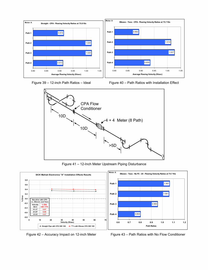
Figure 39 shows an ideal velocity profile for a 12-inch, 4-path meter with significant diameters of straight pipe upstream and a flow conditioner installed 10D upstream of the meter. Figure 8 shows the same meter with an installation effect of 3 elbows and a tee upstream of the piping (10D upstream of the flow conditioner).

Straight - CPA - Flowing Velocity Ratios at 75.8 ft/s

0.915

1.020

1.020

0.913

0.80 0.85 0.90 0.95 1.00 1.05

Path 1

Path 2

Path 3

Path 4

Average Flowing Velocity (ft/sec)

Meter A Elbows - Tees - CPA - Flowing Velocity Ratios at 75.7 ft/s

0.892

1.014

1.027

0.935

0.80 0.85 0.90 0.95 1.00 1.05

Path 1

Path 2

Path 3

Path 4

Average Flowing Velocity (ft/sec)

Meter A

Figure 39 / 12-inch Path Ratios / Ideal Figure 40 / Path Ratios with Installation Effect

10D

10D

>5D

4 + 4 Meter (8 Path)

CPA Flow Conditioner

Figure 41 / 12-Inch Meter Upstream Piping Disturbance

SICK Maihak Electronics "A" Installation Effects Results

-0.8

-0.6

-0.4

-0.2

0.0

0.2

0.4

0.6

0.8

0 10 20 30 40 50 60 70Velocity (ft/sec)

% E

rror

Straight Pipe with CPA 50E 10D "T"s with Elbows CPA 50E 10D

Elbows - Tees - No FC - 20 - Flowing Velocity Ratios at 75.7 ft/s

1.067

1.061

0.960

0.804

0.6 0.7 0.8 0.9 1.0 1.1 1.2

Path 1

Path 2

Path 3

Path 4

Path Ratios

Meter A

Figure 42 / Accuracy Impact on 12-inch Meter Figure 43 / Path Ratios with No Flow Conditioner

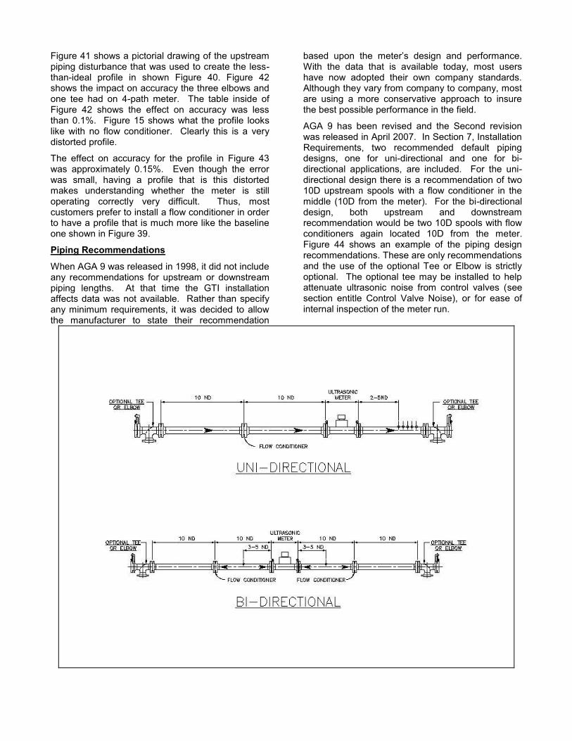
Figure 41 shows a pictorial drawing of the upstream piping disturbance that was used to create the less-than-ideal profile in shown Figure 40. Figure 42 shows the impact on accuracy the three elbows and one tee had on 4-path meter. The table inside of Figure 42 shows the effect on accuracy was less than 0.1%. Figure 15 shows what the profile looks like with no flow conditioner. Clearly this is a very distorted profile.

The effect on accuracy for the profile in Figure 43 was approximately 0.15%. Even though the error was small, having a profile that is this distorted makes understanding whether the meter is still operating correctly very difficult. Thus, most customers prefer to install a flow conditioner in order to have a profile that is much more like the baseline one shown in Figure 39.

Piping Recommendations

When AGA 9 was released in 1998, it did not include any recommendations for upstream or downstream piping lengths. At that time the GTI installation affects data was not available. Rather than specify any minimum requirements, it was decided to allow the manufacturer to state their recommendation

������ '*��� ���� �������� ������� ���� *��+����� ����With the data that is available today, most users have now adopted their own company standards. Although they vary from company to company, most are using a more conservative approach to insure the best possible performance in the field.

AGA 9 has been revised and the Second revision was released in April 2007. In Section 7, Installation Requirements, two recommended default piping designs, one for uni-directional and one for bi-directional applications, are included. For the uni-directional design there is a recommendation of two 10D upstream spools with a flow conditioner in the middle (10D from the meter). For the bi-directional design, both upstream and downstream recommendation would be two 10D spools with flow conditioners again located 10D from the meter. Figure 44 shows an example of the piping design recommendations. These are only recommendations and the use of the optional Tee or Elbow is strictly optional. The optional tee may be installed to help attenuate ultrasonic noise from control valves (see section entitle Control Valve Noise), or for ease of internal inspection of the meter run.

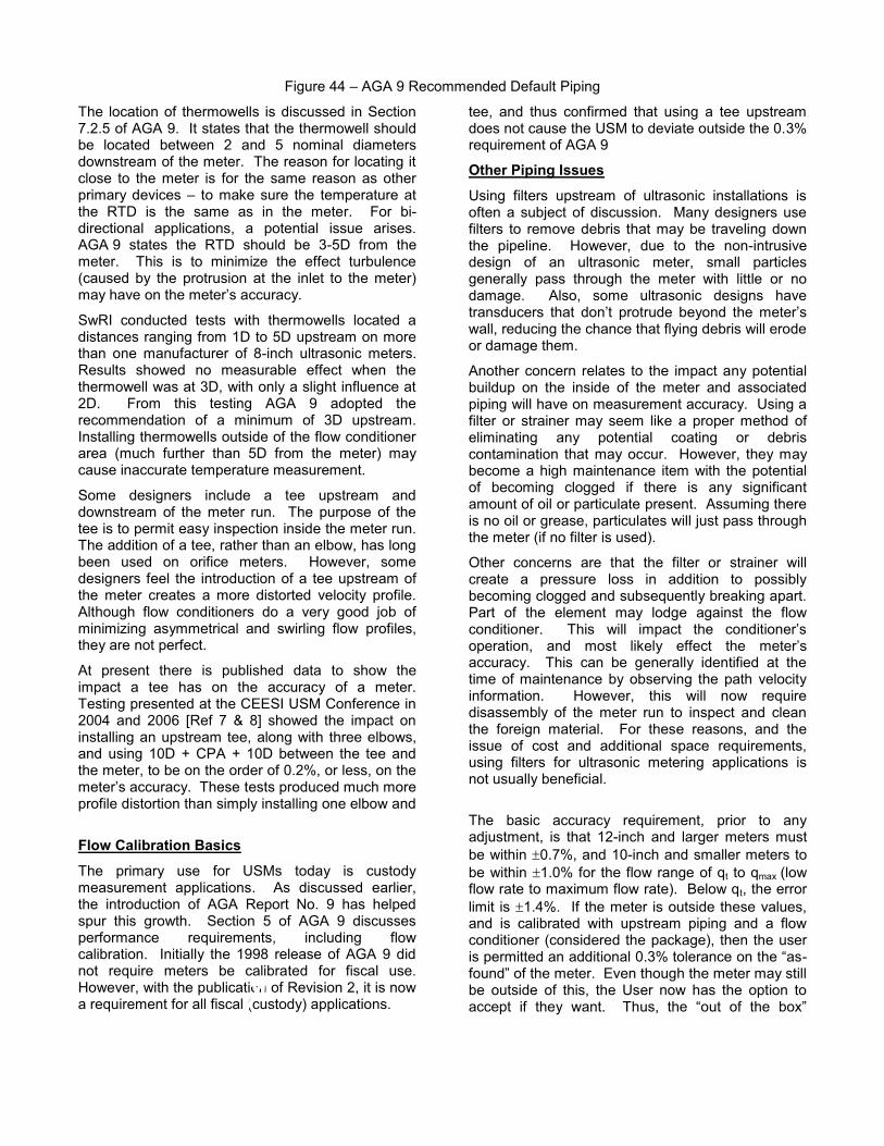
Figure 44 / AGA 9 Recommended Default Piping

The location of thermowells is discussed in Section 7.2.5 of AGA 9. It states that the thermowell should be located between 2 and 5 nominal diameters downstream of the meter. The reason for locating it close to the meter is for the same reason as other primary devices / to make sure the temperature at the RTD is the same as in the meter. For bi-directional applications, a potential issue arises. AGA 9 states the RTD should be 3-5D from the meter. This is to minimize the effect turbulence (caused by the protrusion at the inlet to the meter) ������������������������� '�� ���

SwRI conducted tests with thermowells located a distances ranging from 1D to 5D upstream on more than one manufacturer of 8-inch ultrasonic meters. Results showed no measurable effect when the thermowell was at 3D, with only a slight influence at 2D. From this testing AGA 9 adopted the recommendation of a minimum of 3D upstream. Installing thermowells outside of the flow conditioner area (much further than 5D from the meter) may cause inaccurate temperature measurement.

Some designers include a tee upstream and downstream of the meter run. The purpose of the tee is to permit easy inspection inside the meter run. The addition of a tee, rather than an elbow, has long been used on orifice meters. However, some designers feel the introduction of a tee upstream of the meter creates a more distorted velocity profile. Although flow conditioners do a very good job of minimizing asymmetrical and swirling flow profiles, they are not perfect.

At present there is published data to show the impact a tee has on the accuracy of a meter. Testing presented at the CEESI USM Conference in 2004 and 2006 [Ref 7 & 8] showed the impact on installing an upstream tee, along with three elbows, and using 10D + CPA + 10D between the tee and the meter, to be on the order of 0.2%, or less, on the ��������� '�� ����!�����������*���' ����' �������profile distortion than simply installing one elbow and

tee, and thus confirmed that using a tee upstream does not cause the USM to deviate outside the 0.3% requirement of AGA 9

Other Piping Issues

Using filters upstream of ultrasonic installations is often a subject of discussion. Many designers use filters to remove debris that may be traveling down the pipeline. However, due to the non-intrusive design of an ultrasonic meter, small particles generally pass through the meter with little or no damage. Also, some ultrasonic designs have ������' ���� ����� ������ *����'��� ������� ���� ��������wall, reducing the chance that flying debris will erode or damage them.

Another concern relates to the impact any potential buildup on the inside of the meter and associated piping will have on measurement accuracy. Using a filter or strainer may seem like a proper method of eliminating any potential coating or debris contamination that may occur. However, they may become a high maintenance item with the potential of becoming clogged if there is any significant amount of oil or particulate present. Assuming there is no oil or grease, particulates will just pass through the meter (if no filter is used).

Other concerns are that the filter or strainer will create a pressure loss in addition to possibly becoming clogged and subsequently breaking apart. Part of the element may lodge against the flow ������������ � !���� #���� ��*� �� ���� �������������operation, and mos�� ��L���� �++� �� ���� ��������accuracy. This can be generally identified at the time of maintenance by observing the path velocity information. However, this will now require disassembly of the meter run to inspect and clean the foreign material. For these reasons, and the issue of cost and additional space requirements, using filters for ultrasonic metering applications is not usually beneficial.

Flow Calibration Basics

The primary use for USMs today is custody measurement applications. As discussed earlier, the introduction of AGA Report No. 9 has helped spur this growth. Section 5 of AGA 9 discusses performance requirements, including flow calibration. Initially the 1998 release of AGA 9 did not require meters be calibrated for fiscal use. However, with the publication of Revision 2, it is now a requirement for all fiscal (custody) applications.

The basic accuracy requirement, prior to any adjustment, is that 12-inch and larger meters must be within �0.7%, and 10-inch and smaller meters to be within �1.0% for the flow range of qt to qmax (low flow rate to maximum flow rate). Below qt, the error limit is �1.4%. If the meter is outside these values, and is calibrated with upstream piping and a flow conditioner (considered the package), then the user ���*��������������������������|�������� ���������?��-+�'��@��+���������������������'�����������������������be outside of this, the User now has the option to � �*�� �+� ����� #����� � !�'��� ���� ?�'�� �+� ���� ���@�

performance has less meaning today than in the previous AGA 9 version.

Initially USMs were installed without a flow conditioner. However, customers are using flow conditioners in the majority of applications today. ����� +���� ����� '����� �� ?����� *��+����� �@� +��#�conditioner (not a 19-tube bundle) provides more consistent performance (reduced uncertainty). Even though data exists to support the supposition that some USMs perform quite well without flow conditioners, the added pressure drop and cost is often justified by the reduction in uncertainty. One thing that most everyone does agree upon is that if a flow conditioner is used with a meter, the entire system should be calibrated together.

It should be noted that one of the benefits of the ultrasonic meter is that it does not create significant pressure loss. The pressure drop resulting from the flow conditioner is offset by the lack of pressure drop across the meter (when compared to orifice or turbine meters). As such, total pressure loss across the metering facility as a result of using flow conditioner is probably no greater than with other primary devices for the same given flow rate.

Most companies have standard designs for their meters that typically specify piping upstream and downstream of the flow conditioner(s) and meter. Usually these USMs are calibrated as a unit with the customers upstream and downstream piping spools. Calibrating as a unit helps insure that the accuracy of the meter, once installed in the field, is as close as possible to the results provided by the lab.

In the past most customers felt their applications deserved, and required, less uncertainty than the minimum requirements of the original AGA 9 (where flow calibration was not required). To ensure these higher standards were met, virtually all users began flow calibrating their USM meters used in custody �����+��� �**�� ������� ��� �� ���� ����� �``����� � �� ����2002 AGA Operations Conference a paper was presented that discussed the benefits of flow calibrating ultrasonic meters [Ref 12]. Summarizing from that paper, there are three main reasons users are calibrating meters:

� Reduce uncertainty � Verify performance � Improve rangeability

Calibration Labs

There are several flow labs in North America that provide calibration services. Each will calibrate to any number of points the designer feels are necessary. Typically most designers are requesting �� ��� {� ����� *������� � \� �� ���� ���� ?��-+�'��@� �����points have been determined, an adjustment factor

(or factors) is (are) computed. Facility personnel enter the value(s) into the meter. Usually one or two verification points are used to validate the predicted ?��-��+�@�*��+����� ����!����������������#�������� ������or two flow rates and verify the meter error is zero (or very close to zero). Generally the USM will repeat within �0.1% of the predicted value, with more recent results showing verifications typically on the order of �0.05%.

�'���������������``�����#�������-capacity calibration facilities were commissioned in North America. These two laboratories permit users to cost-effectively calibrate larger USMs (greater than 10-inch) to full capacity, thus reducing the uncertainty related to measurement error when installed in the field. In 1998 when AGA 9 was first published these two facilities were not in operation. Since there was no large capacity calibration facility in North America in 1998, AGA 9 did not require flow calibration. However, the new release of AGA 9 requires flow calibration for fiscal (custody) measurement applications.

Even though there is a substantial amount of data showing USMs to be linear to better than �0.2%, many want to reduce this error further. Because of this, some users have implemented multi-point linearization (PWL), within their flow computers, to further reduce the uncertainty of their USM calibration results. This is not a new technique, and has often been used for turbine meters in the past.

When using this multi-point linearization technique, external to the USM, at least two issues always surface. First, the output signals from the USM (serial, frequency and analog) would then be adjusted in the flow computer to correct all errors. If the output signal (serial or frequency) from the meter is sent to two separate flow computers, care must be taken to ensure both computers are utilizing the same algorithm, or their results will differ. Second, since the linearization is not taking place in the meter, there is no audit trail within the meter to verify �����'�*'��������������'��������� ���������+���� Q?���left@� ������ ��� ��������� *��*������'��������� �!����#���discussed in more detail in an AGA 2002 paper titled ?����+�����+�~��#���������������������� �������� ���+�12].

To overcome the above problem, some USM manufacturers have provided the user with the ability t�� ��*��������Y"� ��� ��������������� ����� ����This allows the linearization to be tested and verified at a test facility, and the meter output does not require external correction which has its inherent problems.

Re-Calibration

AGA 9 does not require an ultrasonic meters to be re-calibrated, and will not require this in the upcoming revision. As USMs have no moving parts, and provide a wide range of diagnostic information, many feel the performance of the meter can be field verified. That is, if the meter is operating correctly, its accuracy should not change, and if it does change, it can be detected. This, however, remains to be proven with a significant number of meters.

The use of USMs for custody transfer applications began increasing rapidly in 1998. Now, with more than 9 years of installed base, there is significant information to conclude USMs may not require re-calibration. Many companies are not certain as to whether or not they will retest their meters in the future. They are waiting for additional data to support their decision. Manufacturers are also trying to show the technology may not require re-calibration.

During the past several years, many meters have been re-calibrated in Canada. Their governmental agency, Measurement Canada, requires USMs to be re-tested every 6 years. The data obtained from these meter re-calibrations, from random re-testing by customers, and long-term data from meters at calibration labs typically shows the meter to be within ±0.3% of the original calibration assuming the meter is clean and operating correctly.

Several users in the US have removed meters in the past year and returned them to the calibration facility for a quick verification. If the meter is clean, the performance on these has typically been within ±0.1-0.3%. Unfortunately, there is very limited published

information to date. Over the next several years, the ���'�������L��#�����������#���� ���*� �� ��� ���� ����-term accuracy of the ultrasonic meter will continue to grow.

Some designers have chosen to incorporate a ��*������ ?��+���� �@� ������ ��� ������ ������� ���������[Ref 13]. The purpose of this meter is to provide an in-situ verification against all the other fiscal meters at that location. The idea is to route all the gas from a given operational meter periodically through the ?��+���� �@� ������ ���� ��L�� ���� ���'������� ������upon the difference. In many ways this is exactly what the calibration facility is doing. However, this technique has several issues that must be addressed.

First, if there are any installation effects on the reference meter, a bias could be introduced in the results. The installation effect could come from the upstream piping or pipeline contamination. Second, the addition of a reference meter adds significantly to the cost of the station. Not only is the designer paying for the additional reference meter, there is an additional cost for each meter run as a separate ball valve must be included to permit diverting the gas through the reference meter. Additionally, the extra reference run requires more space on the skid that adds to the cost. Also, using a reference meter on location somewhat limits the ability to verify performance over the entire range of operation. Finally, removing a meter and having its performance verified at a calibration facility provides �������*�����������������+�������������*��+����� ����This would most likely be required in the event of a dispute by the purchaser of the gas.

CONCLUSIONS During the past several years the industry has learned a lot about USM operational issues. The traditional 5 diagnostic features, gain, signal-to-noise, performance, path velocities and SOS have helped the industry monitor the USM. These 5 features provide a lot of information about the ���������������������������������������������������meter at the time of installation, and monitoring these features on a routine basis can generally identify metering problems in advance of failure. More advanced diagnostic indicators, such as

Turbulence, are paving the way to allow the meter to become virtually maintenance-free. In the future it is likely that a meter will have enough power and intelligence to quickly identify potential measurement problems on a real-time basis. As the industry learns more about not only the USM, and the operation of their own measurement system, the true value of the ultrasonic meter will be recognized. The USM industry is still relatively young and technology will continue to provide more tools to he�*���������������measurement problems.

References:

1. AGA Report No. 9, Measurement of Gas by Multipath Ultrasonic Meters, June 1998.

2. Provisional Specification for the Approval, Verification and Installation and use of

Ultrasonic Gas Meters, Measurement Canada PS-G-E-06, 1998-03-05 (Rev 1, 9-26-2002).

3. John Lansing, Basics of Ultrasonic Flow Meters, AGMSC 2003, Coraopolis, PA.

4. John Lansing, Smart Monitoring and Diagnostics for Ultrasonic Meters, NSFMW 2000, Gleneagles, Scotland.

5. John Lansing, ���� ������ � �� ������������Solve Metering Problems, NSFMW 2005, Tonsberg, Norway

6. T. A. Grimley, Ultrasonic Meter Installation Configuration Testing, AGA Operations Conference, 2000, Denver, CO.

7. Larry Garner & Joel Clancy, Ultrasonic Meter Performance / Flow Calibration Results / CEESI Iowa / Inspection Tees vs. Elbows, CEESI Ultrasonic Conference, June 2004, Estes Park, CO

8. John Lansing, Features and Benefits of the SICK Maihak USM, CEESI Ultrasonic Conference, June 2006, Estes Park, CO

9. John Lansing, Advanced Ultrasonic Meter Diagnostics, Western Gas Measurement Short Course, 2007, Seattle, WA

10. John Lansing, Ultrasonic Meter Station Design Considerations, Western Gas Measurement Short Course, 2003, Victoria, BC, Canada

11. Klaus Zanker, Diagnostic Ability of the Daniel Four-Path Ultrasonic Flow Meter, Southeast Asia Flow Measurement Workshop, 2003, Kuala Lumpur, Malaysia

12. John Lansing, Benefits of Flow Calibrating Ultrasonic Meters, AGA Operations Conference, 2002, Chicago, IL

13. James N. Witte, Ultrasonic Gas Meters from Flow Lab to Field: A Case Study, AGA Operations Conference, 2002, Chicago, IL.

14. T. A. Grimley, Performance Testing of Ultrasonic Flow Meters, AGA Operations Conference, 1997, Nashville, TN

15. Dr. Jim Hall, William Freund, Klaus Zanker & Dale Goodson, Operation of Ultrasonic Flow Meters at Conditions Different Than Their Calibration, NSFMW 2002, St. Andrews, Scotland.

16. John Lansing, Dirty vs. Clean Ultrasonic Flow Meter Performance, AGA Operations Conference, 2002, Chicago, IL.

17. John Stuart, Rick Wilsack, Re-Calibration of a 3-Year Old, Dirty, Ultrasonic Meter, AGA Operations Conference, 2001, Dallas, TX

18. John Lansing, Using Software to Simplify USM Maintenance, AGA Operations Conference, 2003, Kissimmee, FL

19. Jim Micklos, Ultrasonic Gas Flow Meters for Custody Transfer Measurement, ASGMT 2008, Houston, TX

20. Bird R.B., Stewart W.E., and Lightfoot E.N., Transport Phenomena, 1960, Wiley, New York

21. Rütten, O., Deutsches Patent No 520484, 1928

22. Schlichting, H., Boundary Layer Theory, 6th edition, 1968, McGraw-Hill, New York

23. Steenbergen, W., Turbulent Pipe Flow with Swirl, Ph.D Thesis, Eindhoven University, Eindhoven, The Netherlands