Fundamentals of Machine Learning Bootcamp - 24 Nov London 2014

Aykut Erdem // Hacettepe University // Fall 2019
Lecture 23:Dimensionality Reduction
BBM406Fundamentals of
Machine Learning
Image credit: Matthew Turk and Alex Pentland

AdministrativeProject Presentations January 8,10, 2020
• Each project group will have ~8 mins to present their work in class. The suggested outline for the presentations are as follows:- High-level overview of the paper (main contributions)- Problem statement and motivation (clear definition of the problem, why it
is interesting and important)- Key technical ideas (overview of the approach)- Experimental set-up (datasets, evaluation metrics, applications)- Strengths and weaknesses (discussion of the results obtained)
• In addition to classroom presentations, each group should also prepare an engaging video presentation of their work using online tools such as PowToon, moovly or GoAnimate (due January 12, 2020).
2

Final Reports (Due January 15, 2019)• The report should be prepared using LaTeX and 6-8 pages. A typical
organization of a report might follow:- Title, Author(s).- Abstract. This section introduces the problem that you investigated by
providing a general motivation and briefly discusses the approach(es) that you explored.
- Introduction.- Related Work. This section discusses relevant literature for your project
topic.- The Approach. This section gives the technical details about your project
work. You should describe the representation(s) and the algorithm(s) that you employed or proposed as detailed and specific as possible.
- Experimental Results. This section presents some experiments in which you analyze the performance of the approach(es) you proposed or explored. You should provide a qualitative and/or quantitative analysis, and comment on your findings. You may also demonstrate the limitations of the approach(es).
- Conclusions. This section summarizes all your project work, focusing on the key results you obtained. You may also suggest possible directions for future work.
- References. This section gives a list of all related work you reviewed or used3

Last time… Graph-Theoretic ClusteringGoal: Given data points X1, ..., Xn and similarities W(Xi ,Xj), partition the data into groups so that points in a group are similar and points in different groups are dissimilar.
4
Similarity Graph: G(V,E,W) V – Vertices (Data points) E – Edge if similarity > 0 W - Edge weights (similarities)
Partition the graph so that edges within a group have large weights and edges across groups have small weights.
Graph)Clustering)Goal: Given data points X1, …, Xn and similarities W(Xi,Xj), partition the data into groups so that points in a group are similar and points in different groups are dissimilar. Similarity Graph: G(V,E,W) V – Vertices (Data points)
E – Edge if similarity > 0 W - Edge weights (similarities)
Similarity graph
Partition the graph so that edges within a group have large weights and edges across groups have small weights.
slide by Aarti Singh

Last time… K-Means vs. Spectral Clustering• Applying k-means
to Laplacian eigenvectors allows us to find cluster with non-convex boundaries.
5
k=means)vs)Spectral)clustering)Applying k-means to laplacian eigenvectors allows us to find cluster with non-convex boundaries.
Spectral clustering output k-means output
k=means)vs)Spectral)clustering)Applying k-means to laplacian eigenvectors allows us to find cluster with non-convex boundaries.
Spectral clustering output k-means output
slide by Aarti Singh
Examples)Ng et al 2001

6
Bottom-Up (agglomerative):Start with each item in its own cluster, find the best pair to merge into a new cluster. Repeat until all clusters are fused together.
slide by Andrew M
oore
Last time…

Today• Dimensionality Reduction• Principle Component Analysis (PCA)• PCA Applications• PCA Shortcomings• Autoencoders• Independent Component Analysis
7

Dimensionality Reduction
8
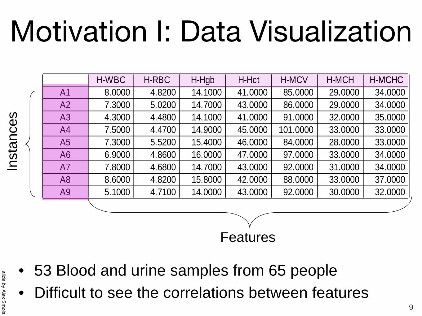
Motivation I: Data Visualization
9
Inst
ance
s
Features
H-WBC H-RBC H-Hgb H-Hct H-MCV H-MCH H-MCHCH-MCHCA1 8.0000 4.8200 14.1000 41.0000 85.0000 29.0000 34.0000 A2 7.3000 5.0200 14.7000 43.0000 86.0000 29.0000 34.0000 A3 4.3000 4.4800 14.1000 41.0000 91.0000 32.0000 35.0000 A4 7.5000 4.4700 14.9000 45.0000 101.0000 33.0000 33.0000 A5 7.3000 5.5200 15.4000 46.0000 84.0000 28.0000 33.0000 A6 6.9000 4.8600 16.0000 47.0000 97.0000 33.0000 34.0000 A7 7.8000 4.6800 14.7000 43.0000 92.0000 31.0000 34.0000 A8 8.6000 4.8200 15.8000 42.0000 88.0000 33.0000 37.0000 A9 5.1000 4.7100 14.0000 43.0000 92.0000 30.0000 32.0000
• 53 Blood and urine samples from 65 people• Difficult to see the correlations between features
slide by Alex Smola

Motivation I: Data Visualization
• Spectral format (65 curves, one for each person• Difficult to compare different patients
10
7
• Spectral format (65 curves, one for each person)
0 10 20 30 40 50 600100200300400500600700800900
1000
measurement
Val
ue
MeasurementDifficult to compare the different patients...
Data Visualization
slide by Alex Smola

Motivation I: Data Visualization• Spectral format (53 pictures, one for each feature)
118
0 10 20 30 40 50 60 700
0.20.40.60.811.21.41.61.8
Person
H-Ba
nds
• Spectral format (53 pictures, one for each feature)
Difficult to see the correlations between the features...
Data Visualization
• Difficult to see the correlations between features
slide by Alex Smola
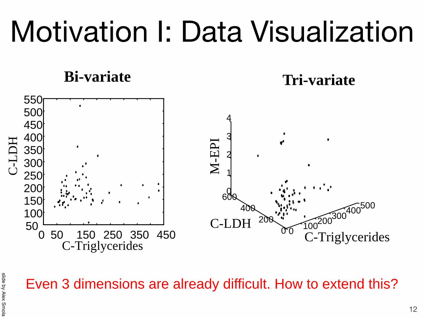
Motivation I: Data Visualization
129
0 50 150 250 350 45050100150200250300350400450500550
C-Triglycerides
C-L
DH
0 100200300400500
0200
4006000
1
2
3
4
C-TriglyceridesC-LDH
M-E
PI
Bi-variate Tri-variate
How can we visualize the other variables???
diffic l o ee in 4 o highe dimen ional pace ...
Data Visualization
slide by Alex Smola
Even 3 dimensions are already difficult. How to extend this?

Motivation I: Data Visualization• Is there a representation better than the
coordinate axes?
• Is it really necessary to show all the 53 dimensions?- ... what if there are strong correlations between
the features?
• How could we find the smallest subspace of the 53-D space that keeps the most information about the original data?
13
slide by Barnabás Póczos and Aarti Singh
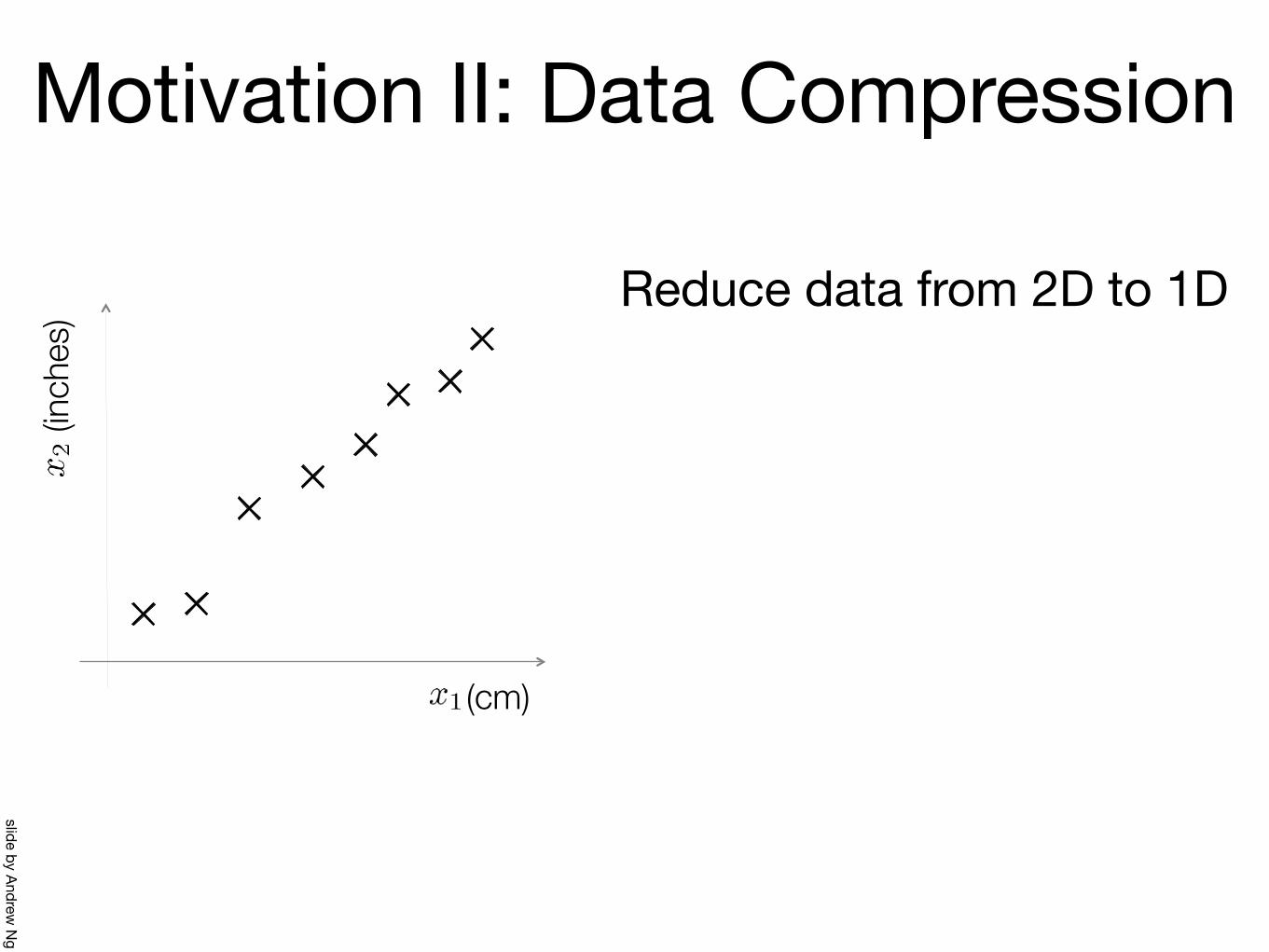
Reduce data from 2D to 1D
Motivation II: Data Compression
slide by Andrew N
g
(inch
es)
(cm)

(inch
es)
(cm)
Motivation II: Data Compression
slide by Andrew N
g
Reduce data from 2D to 1D

Motivation II: Data Compression
slide by Andrew N
g
Reduce data from 3D to 2D

Dimensionality Reduction• Clustering
- One way to summarize a complex real-valued data point with a single categorical variable
• Dimensionality reduction- Another way to simplify complex high-dimensional
data- Summarize data with a lower dimensional real valued
vector
17
slide by Fereshteh Sadeghi
•Given data points in d dimensions•Convert them to data points in r<d dims•With minimal loss of information

Principal Component Analysis
18
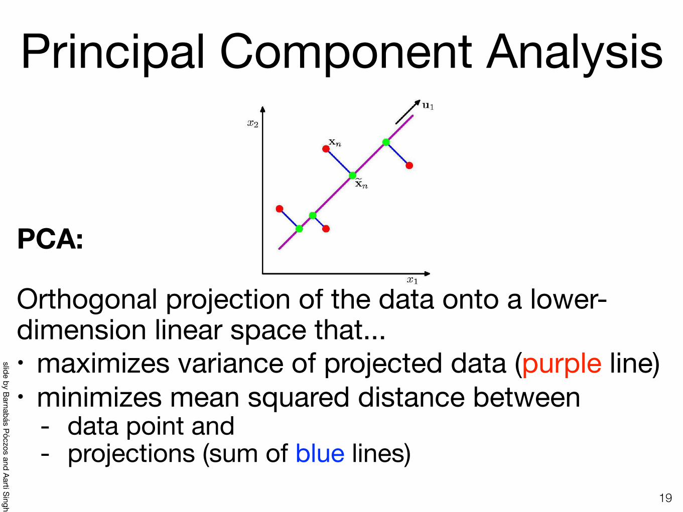
Principal Component Analysis
PCA:
Orthogonal projection of the data onto a lower-dimension linear space that...• maximizes variance of projected data (purple line)• minimizes mean squared distance between
- data point and- projections (sum of blue lines)
19
12
Orthogonal projection of the data onto a lower-dimension linear space that... �maximizes variance of projected data (purple line)
�minimizes mean squared distance between
• data point and • projections (sum of blue lines)
PCA:
Principal Component Analysis
slide by Barnabás Póczos and Aarti Singh

Principal Component Analysis• PCA Vectors originate from the center of
mass.
• Principal component #1: points in the direction of the largest variance.
• Each subsequent principal component- is orthogonal to the previous ones, and- points in the directions of the largest
variance of the residual subspace
20
slide by Barnabás Póczos and Aarti Singh

2D Gaussian dataset
2115
2D Gaussian dataset
slide by Barnabás Póczos and Aarti Singh

1st PCA axis
2216
1st PCA axis
slide by Barnabás Póczos and Aarti Singh

2nd PCA axis
2317
2nd PCA axis
slide by Barnabás Póczos and Aarti Singh
24
slide by Barnabás Póczos and Aarti Singh
19
¦ ¦
�
� m
i
k
ji
Tjji
Tk m 1
21
11
})]({[1
maxarg xwwxwww
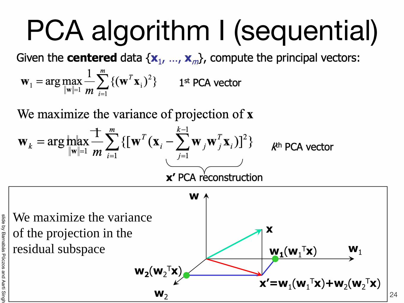
We maximize the variance of the projection in the residual subspace
Maximize the variance of projection of x
x PCA reconstruction
Given w1, , wk-1, we calculate wk principal vector as before:
kth PCA vector
w1(w1Tx)
w2(w2Tx)
x
w1
w2 x =w1(w1
Tx)+w2(w2Tx)
w
PCA algorithm I (sequential) PCA algorithm I (sequential)

2521
• Given data {x1, …, xm}, compute covariance matrix 6
• PCA basis vectors = the eigenvectors of 6�
• Larger eigenvalue � more important eigenvectors
¦
�� 6m
i
Tim 1
))((1
xxxx ¦
m
iim 1
1xxwhere
PCA algorithm II (sample covariance matrix)
PCA algorithm II (sample covariance matrix)
slide by Barnabás Póczos and Aarti Singh
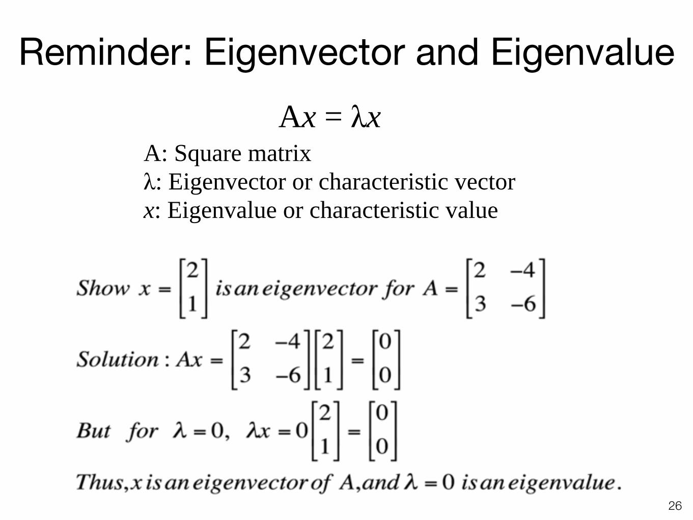
Reminder: Eigenvector and Eigenvalue
26
Ax = λx A: Square matrix λ: Eigenvector or characteristic vector x: Eigenvalue or characteristic value

Reminder: Eigenvector and Eigenvalue
27
Ax - λx = 0(A – λI)x = 0
B = A – λIBx = 0
x = B-10 = 0
If we define a new matrix B:
If B has an inverse: BUT! an eigenvector cannot be zero!!
x will be an eigenvector of A if and only if B does not have an inverse, or equivalently det(B)=0 :
det(A – λI) = 0
Ax = λx

Reminder: Eigenvector and Eigenvalue
28
Example 1: Find the eigenvalues of
two eigenvalues: -1, - 2 Note: The roots of the characteristic equation can be repeated. That is, λ1 = λ2 =…= λk.
If that happens, the eigenvalue is said to be of multiplicity k.Example 2: Find the eigenvalues of
λ = 2 is an eigenvector of multiplicity 3.
úû
ùêë
é--
=51122
A
)2)(1(23
12)5)(2(51
122
2 ++=++=
++-=+-
-=-
llll
lll
ll AI
úúú
û
ù
êêê
ë
é=
200020012
A
0)2(200020012
3 =-=-
---
=- ll
ll
l AI

PCA algorithm II (sample covariance matrix)
29

PCA algorithm III (SVD of the data matrix)
3023
Singular Value Decomposition of the centered data matrix X.
Xfeatures u samples = USVT
X VT S U =
samples
significant
noise
nois
e noise
sign
ific
ant
sig.
PCA algorithm III (SVD of the data matrix)
slide by Barnabás Póczos and Aarti Singh

PCA algorithm III
3124
• Columns of U • the principal vectors, { u(1), …, u(k) } • orthogonal and has unit norm so UTU = I • Can reconstruct the data using linear combinations
of { u(1), …, u(k) }
• Matrix S • Diagonal • Shows importance of each eigenvector
• Columns of VT
• The coefficients for reconstructing the samples
PCA algorithm III
slide by Barnabás Póczos and Aarti Singh

Applications
32

Face Recognition
33

Face Recognition• Want to identify specific person, based on facial image• Robust to glasses, lighting, …
- Can’t just use the given 256 x 256 pixels
34
�Want to identify specific person, based on facial image � R b gla e , ligh ing, � Can j e he gi en 256 256 i el
Face Recognition
26
slide by Barnabás Póczos and Aarti Singh

Applying PCA: Eigenfaces
35
� Example data set: Images of faces Famous Eigenface approach [Turk & Pentland], [Sirovich & Kirby]
� Each face x
256 u 256 values (luminance at location) x in �256u256 (view as 64K dim vector)
� Form X = [ x1 , , xm ] centered data mtx
� Compute 6�= XXT
� Problem: 6 is 64K u 64 H GE!!! 256 x 256 real values
m faces
X =
x1, , xm
Method A: Build a PCA subspace for each person and check which subspace can reconstruct the test image the best
Method B: Build one PCA database for the whole dataset and then classify based on the weights.
Applying PCA: Eigenfaces
27
slide by Barnabás Póczos and Aarti Singh

A Clever Workaround
36
• Note that m<<64K • Use L=XTX instead of 6=XXT
• If v is eigenvector of L then Xv is eigenvector of 6� Proof: L v = J v XTX v = J v X (XTX v) = X(J v) = J Xv (XXT)X v = J (Xv) �����������6��Xv) = J (Xv)
256 x 256 real values
m faces
X =
x1, , xm
29
A Clever Workaround
slide by Barnabás Póczos and Aarti Singh
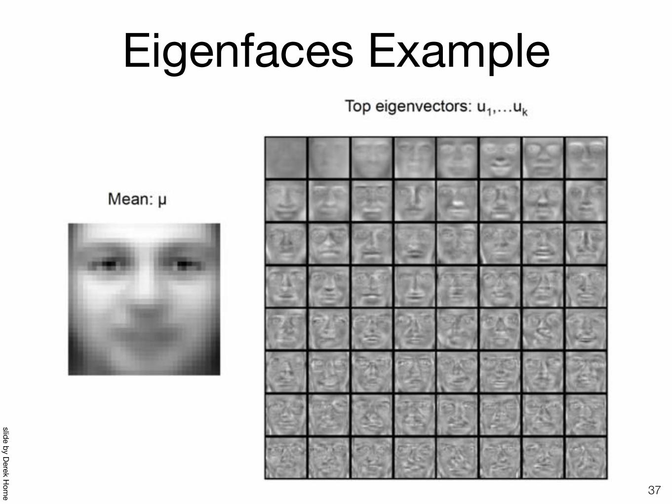
Eigenfaces Example
37
slide by Derek Hom
e

Representation and Reconstruction
38
slide by Derek Hom
e

Principle Components (Method B)
3930
Principle Components (Method B)
slide by Barnabás Póczos and Aarti Singh

Principle Components (Method B)
• … faster if train with …- only people w/out glasses- same lighting conditions
40
� fa e if ain i h only people w/out glasses same lighting conditions
31
Recon c ing (Me hod B)
slide by Barnabás Póczos and Aarti Singh

When projecting strange data• Original images• Reconstruction doesn’t look like the original
41
slide by Alex Smola
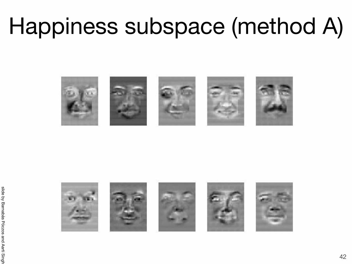
Happiness subspace (method A)
42
33
Happiness subspace (method A)
slide by Barnabás Póczos and Aarti Singh
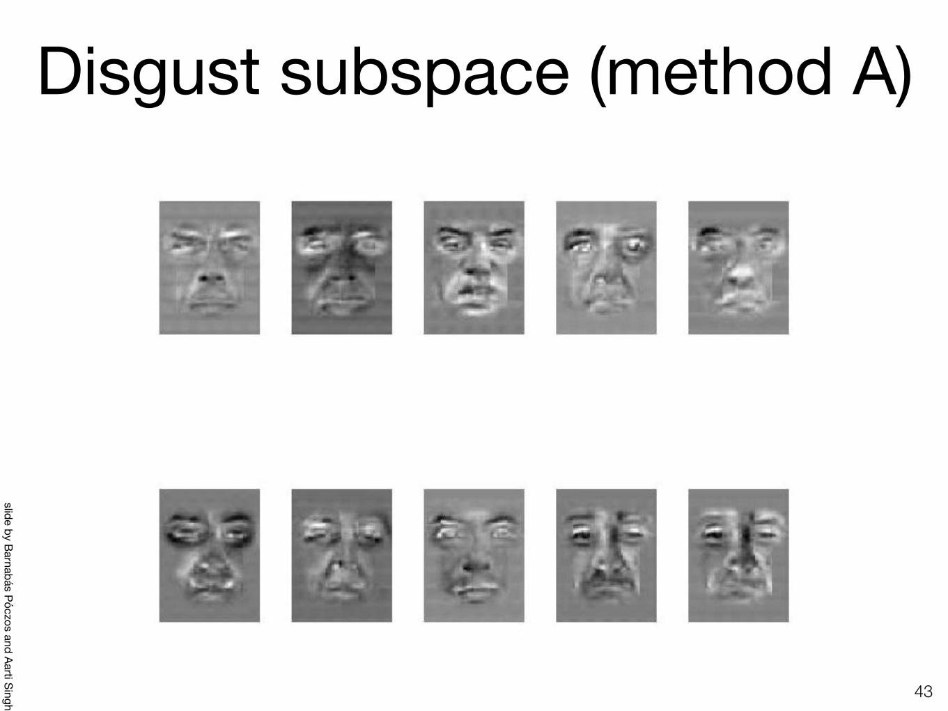
Disgust subspace (method A)
43
34
Disgust subspace (method A)
slide by Barnabás Póczos and Aarti Singh
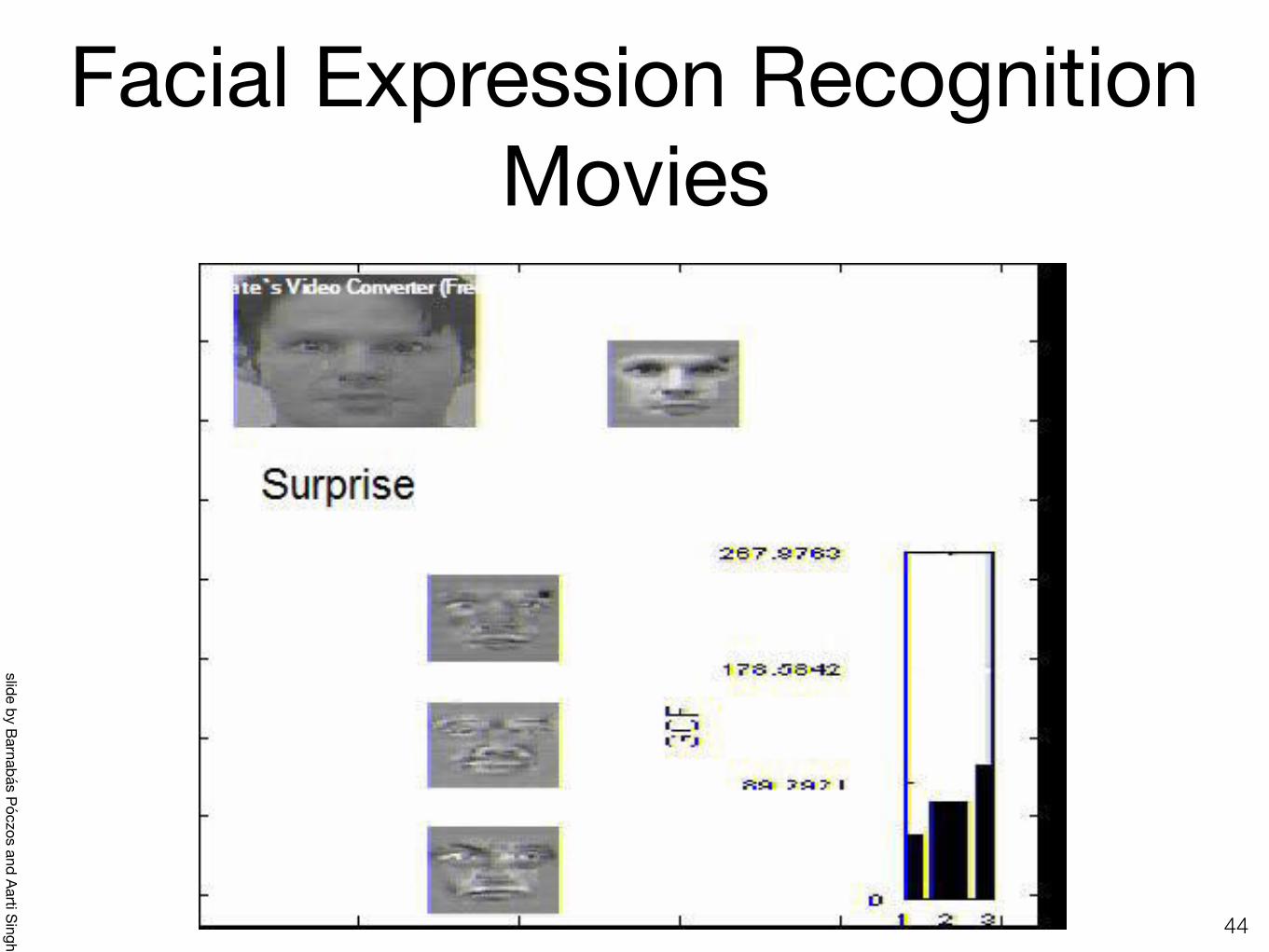
Facial Expression Recognition Movies
4435
Facial Expression Recognition Movies
slide by Barnabás Póczos and Aarti Singh

Facial Expression Recognition Movies
4536
Facial Expression Recognition Movies
slide by Barnabás Póczos and Aarti Singh

Facial Expression Recognition Movies
4637
Facial Expression Recognition Movies
slide by Barnabás Póczos and Aarti Singh

Shortcomings• Requires carefully controlled data:
- All faces centered in frame- Same size- Some sensitivity to angle
• Method is completely knowledge free- (sometimes this is good!)- Doesn’t know that faces are wrapped around
3D objects (heads)- Makes no effort to preserve class distinctions
47
slide by Barnabás Póczos and Aarti Singh

Image Compression
48

Original Image
• Divide the original 372x492 image into patches:- Each patch is an instance
• View each as a 144-D vector 4939
• Divide the original 372x492 image into patches:
• Each patch is an instance that contains 12x12 pixels on a grid
• View each as a 144-D vector
Original Image
slide by Barnabás Póczos and Aarti Singh

L2 error and PCA dim
5040
L2 error and PCA dim
slide by Barnabás Póczos and Aarti Singh
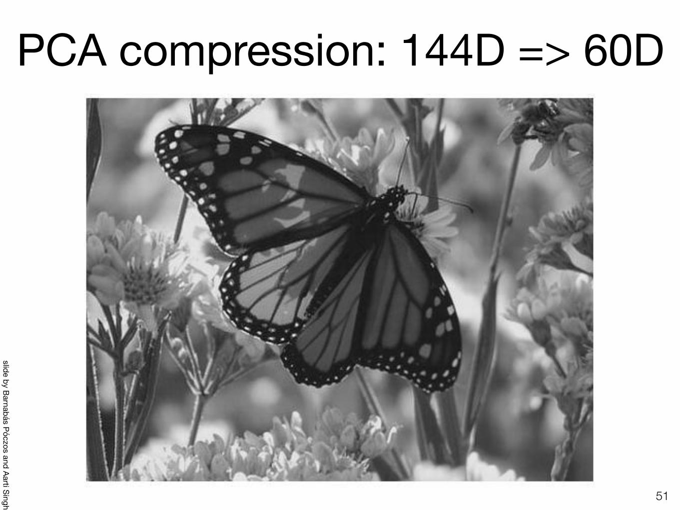
PCA compression: 144D => 60D
5141
PCA compression: 144D ) 60D
slide by Barnabás Póczos and Aarti Singh
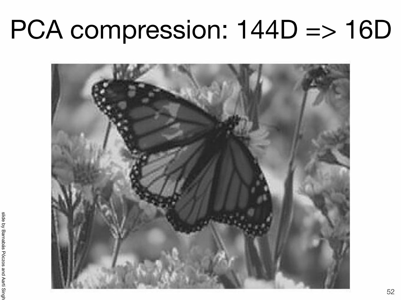
PCA compression: 144D => 16D
5242
PCA compression: 144D ) 16D
slide by Barnabás Póczos and Aarti Singh
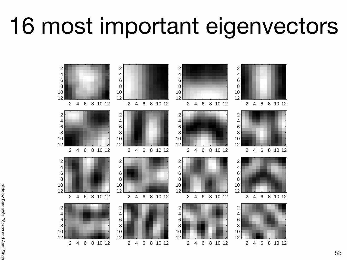
16 most important eigenvectors
5343
2 4 6 8 10 12
2468
1012
2 4 6 8 10 12
2468
1012
2 4 6 8 10 12
2468
1012
2 4 6 8 10 12
2468
1012
2 4 6 8 10 12
2468
1012
2 4 6 8 10 12
2468
1012
2 4 6 8 10 12
2468
1012
2 4 6 8 10 12
2468
1012
2 4 6 8 10 12
2468
1012
2 4 6 8 10 12
2468
1012
2 4 6 8 10 12
2468
1012
2 4 6 8 10 12
2468
1012
2 4 6 8 10 12
2468
1012
2 4 6 8 10 12
2468
1012
2 4 6 8 10 12
2468
1012
2 4 6 8 10 12
2468
1012
16 most important eigenvectors
slide by Barnabás Póczos and Aarti Singh

PCA compression: 144D => 6D
5444
PCA compression: 144D ) 6D
slide by Barnabás Póczos and Aarti Singh

6 most important eigenvectors
5545
2 4 6 8 10 12
2
4
6
8
10
122 4 6 8 10 12
2
4
6
8
10
122 4 6 8 10 12
2
4
6
8
10
12
2 4 6 8 10 12
2
4
6
8
10
122 4 6 8 10 12
2
4
6
8
10
122 4 6 8 10 12
2
4
6
8
10
12
6 most important eigenvectors
slide by Barnabás Póczos and Aarti Singh

PCA compression: 144D => 3D
5646
PCA compression: 144D ) 3D
slide by Barnabás Póczos and Aarti Singh
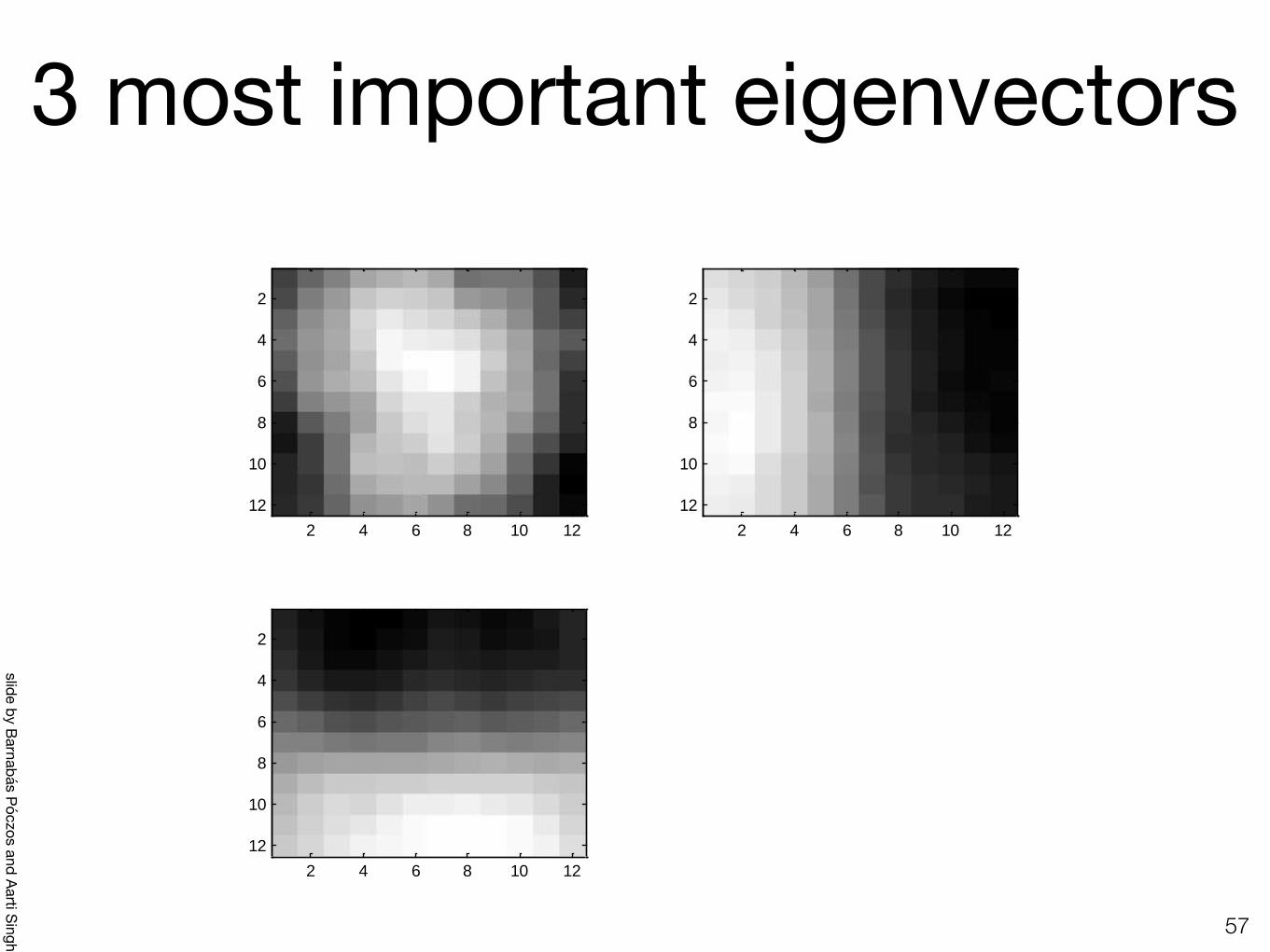
3 most important eigenvectors
5747
2 4 6 8 10 12
2
4
6
8
10
12
2 4 6 8 10 12
2
4
6
8
10
12
2 4 6 8 10 12
2
4
6
8
10
12
3 most important eigenvectors
slide by Barnabás Póczos and Aarti Singh

PCA compression: 144D => 1D
5848
PCA compression: 144D ) 1D
slide by Barnabás Póczos and Aarti Singh

60 most important eigenvectors
• Looks like the discrete cosine bases of JPG!…59
49
Looks like the discrete cosine bases of JPG!...
60 most important eigenvectors
slide by Barnabás Póczos and Aarti Singh

2D Discrete Cosine Basis
6050 http://en.wikipedia.org/wiki/Discrete_cosine_transform
2D Discrete Cosine Basis
slide by Barnabás Póczos and Aarti Singh

Noise Filtering
61

Noise Filtering
6252
x x’
U x
Noise Filtering
slide by Barnabás Póczos and Aarti Singh

Noisy image
63
53
Noisy image
slide by Barnabás Póczos and Aarti Singh

Denoised image using 15 PCA components
6454
Denoised image using 15 PCA components
slide by Barnabás Póczos and Aarti Singh

PCA Shortcomings
65

Problematic Data Set for PCA• PCA doesn’t know labels!
66
56 PCA doesn t know labels!
Problematic Data Set for PCA
slide by Barnabás Póczos and Aarti Singh

PCA vs. Fisher Linear Discriminant
67
PCA for pattern recognition
20
• higher variance• bad for discriminability
• smaller variance• good discriminability
Principal Component Analysis
Fisher Linear DiscriminantLinear Discriminant Analysis
Principal Component Analysis
• higher variance• bad for discriminability
Fisher Linear Discriminant • smaller variance• good discriminability
PCA for pattern recognition
20
• higher variance• bad for discriminability
• smaller variance• good discriminability
Principal Component Analysis
Fisher Linear DiscriminantLinear Discriminant Analysis
PCA for pattern recognition
20
• higher variance• bad for discriminability
• smaller variance• good discriminability
Principal Component Analysis
Fisher Linear DiscriminantLinear Discriminant Analysis
slide by Javier Hernandez Rivera
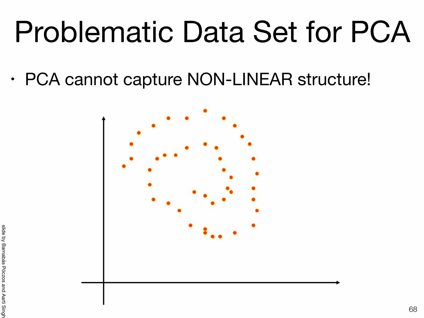
Problematic Data Set for PCA• PCA cannot capture NON-LINEAR structure!
68
58 PCA cannot capture NON-LINEAR structure!
Problematic Data Set for PCA
slide by Barnabás Póczos and Aarti Singh

PCA Conclusions• PCA
- Finds orthonormal basis for data- Sorts dimensions in order of “importance”- Discard low significance dimensions
• Uses:- Get compact description- Ignore noise- Improve classification (hopefully)
• Not magic:- Doesn’t know class labels- Can only capture linear variations
• One of many tricks to reduce dimensionality! 69
slide by Barnabás Póczos and Aarti Singh

Autoencoders
70

Relation to Neural Networks• PCA is closely related to a particular form of neural
network• An autoencoder is a neural network whose outputs
are its own inputs
• The goal is to minimize reconstruction error 71
slide by Sanja Fidler
Relation to Neural Networks
PCA is closely related to a particular form of neural network
An autoencoder is a neural network whose outputs are its own inputs
The goal is to minimize reconstruction error
Urtasun, Zemel, Fidler (UofT) CSC 411: 14-PCA & Autoencoders March 14, 2016 15 / 18

Autoencoders
Definez = f (W x); x = g(V z)
Goal:
minW,V
1
2N
NX
n=1
||x(n) � x(n)||2
If g and f are linear
minW,V
1
2N
NX
n=1
||x(n) � VW x(n)||2
In other words, the optimal solution is PCA.
Urtasun, Zemel, Fidler (UofT) CSC 411: 14-PCA & Autoencoders March 14, 2016 16 / 18
Auto encoders• Define
72
slide by Sanja Fidler

Autoencoders
Definez = f (W x); x = g(V z)
Goal:
minW,V
1
2N
NX
n=1
||x(n) � x(n)||2
If g and f are linear
minW,V
1
2N
NX
n=1
||x(n) � VW x(n)||2
In other words, the optimal solution is PCA.
Urtasun, Zemel, Fidler (UofT) CSC 411: 14-PCA & Autoencoders March 14, 2016 16 / 18
Auto encoders• Define
• Goal:
73
slide by Sanja Fidler

Autoencoders
Definez = f (W x); x = g(V z)
Goal:
minW,V
1
2N
NX
n=1
||x(n) � x(n)||2
If g and f are linear
minW,V
1
2N
NX
n=1
||x(n) � VW x(n)||2
In other words, the optimal solution is PCA.
Urtasun, Zemel, Fidler (UofT) CSC 411: 14-PCA & Autoencoders March 14, 2016 16 / 18
Auto encoders• Define
• Goal:
• If g and f are linear
74
slide by Sanja Fidler

Autoencoders
Definez = f (W x); x = g(V z)
Goal:
minW,V
1
2N
NX
n=1
||x(n) � x(n)||2
If g and f are linear
minW,V
1
2N
NX
n=1
||x(n) � VW x(n)||2
In other words, the optimal solution is PCA.
Urtasun, Zemel, Fidler (UofT) CSC 411: 14-PCA & Autoencoders March 14, 2016 16 / 18
Auto encoders• Define
• Goal:
• If g and f are linear
• In other words, the optimal solution is PCA75
slide by Sanja Fidler

Auto encoders: Nonlinear PCA• What if g( ) is not linear?• Then we are basically doing nonlinear PCA• Some subtleties but in general this is an
accurate description
76
slide by Sanja Fidler
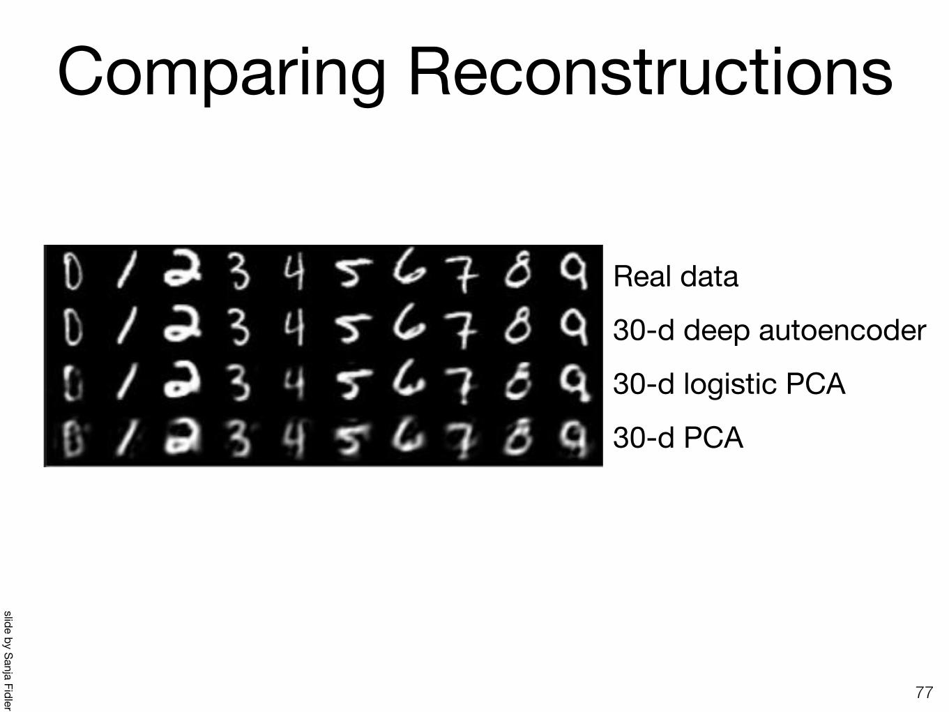
Comparing Reconstructions
77
Comparing Reconstructions
Urtasun, Zemel, Fidler (UofT) CSC 411: 14-PCA & Autoencoders March 14, 2016 18 / 18
Real data
30-d deep autoencoder
30-d logistic PCA
30-d PCA
slide by Sanja Fidler

Independent ComponentAnalysis (ICA)
78
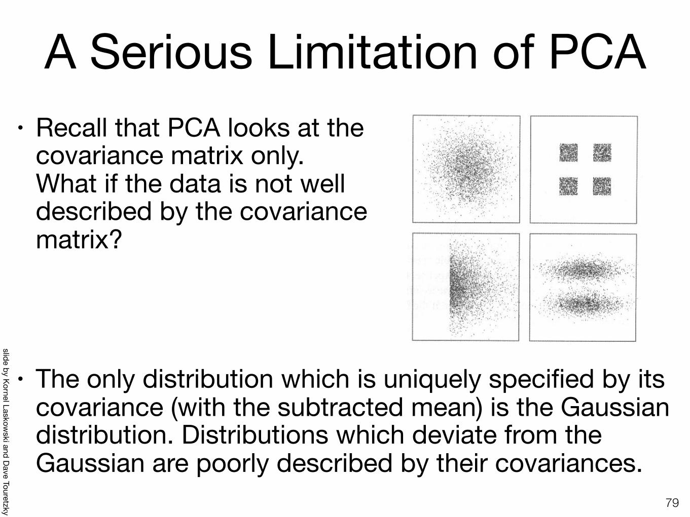
A Serious Limitation of PCA• Recall that PCA looks at the
covariance matrix only. What if the data is not well described by the covariance matrix?
• The only distribution which is uniquely specified by its covariance (with the subtracted mean) is the Gaussian distribution. Distributions which deviate from the Gaussian are poorly described by their covariances.
79
slide by Kornel Laskowski and Dave Touretzky
A More Serious Limitation
Recall that PCA looks at the covariance matrix only. What if thedata is not well described by the covariance matrix?
The only distribution which is uniquely specified by its covariance(with the subtracted mean) is the Gaussian distribution. Distribu-tions which deviate from the Gaussian are poorly described by theircovariances.
41
Faithful vs Meaningful Representations
Even with non-Gaussian data, variance maximization leads to themost faithful representation in a reconstruction error sense (recallthat we trained our autoencoder network using a mean-square errorin an input reconstruction layer).
The mean-square error measure implicitly assumes Gaussianity, sinceit penalizes datapoints close to the mean less that those that arefar away.
But it does not in general lead to the most meaningful representa-tion.
We need to perform gradient descent in some function other thanthe reconstruction error.
42
A Criterion Stronger than Decorrelation
The way to circumvent these problems is to look for componentswhich are statistically independent, rather than just uncorrelated.
For statistical independence, we require that
p(ξ1, ξ2, · · · , ξN) =N∏
i=1p(ξi) (26)
For uncorrelatedness, all we required was that
〈ξiξj 〉 − 〈ξi 〉〈ξj 〉 = 0 , i $= j (27)
Independence is a stronger requirement; under independence,
〈g1(ξi)g2(ξj) 〉 − 〈g1(ξi) 〉〈g2(ξj) 〉 = 0 , i $= j (28)
for any functions g1 and g2.
43
Independent Component Analysis (ICA)
Like Principal Component Analysis, except that we’re looking for atransformation subject to the stronger requirement of independence,rather than uncorrelatedness.
In general, no analytic solution (like eigenvalue decomposition forPCA) exists, so ICA is implemented using neural network models.
To do this, we need an architecture and an objective function todescend/climb in.
Leads to N independent (or as independent as possible) componentsin N-dimensional space; they need not be orthogonal.
When are independent components identical to uncorrelated (prin-cipal) components? When the generative distribution is uniquelydetermined by its first and second moments. This is true of onlythe Gaussian distribution.
44

Faithful vs Meaningful Representations
• Even with non-Gaussian data, variance maximization leads to the most faithful representation in a reconstruction error sense (recall that we trained our autoencoder network using a mean-square error in an input reconstruction layer).
• The mean-square error measure implicitly assumes Gaussianity, since it penalizes datapoints close to the mean less that those that are far away.
• But it does not in general lead to the most meaningful representation.
• We need to perform gradient descent in some function other than the reconstruction error.
80
slide by Kornel Laskowski and Dave Touretzky

A Criterion Stronger than Decorrelation • The way to circumvent these problems is to look for
components which are statistically independent, rather than just uncorrelated.
• For statistical independence, we require that
• For uncorrelatedness, all we required was that
• Independence is a stronger requirement; under independence, for any functions g1 and g2.
81
slide by Kornel Laskowski and Dave Touretzky
A More Serious Limitation
Recall that PCA looks at the covariance matrix only. What if thedata is not well described by the covariance matrix?
The only distribution which is uniquely specified by its covariance(with the subtracted mean) is the Gaussian distribution. Distribu-tions which deviate from the Gaussian are poorly described by theircovariances.
41
Faithful vs Meaningful Representations
Even with non-Gaussian data, variance maximization leads to themost faithful representation in a reconstruction error sense (recallthat we trained our autoencoder network using a mean-square errorin an input reconstruction layer).
The mean-square error measure implicitly assumes Gaussianity, sinceit penalizes datapoints close to the mean less that those that arefar away.
But it does not in general lead to the most meaningful representa-tion.
We need to perform gradient descent in some function other thanthe reconstruction error.
42
A Criterion Stronger than Decorrelation
The way to circumvent these problems is to look for componentswhich are statistically independent, rather than just uncorrelated.
For statistical independence, we require that
p(ξ1, ξ2, · · · , ξN) =N∏
i=1p(ξi) (26)
For uncorrelatedness, all we required was that
〈ξiξj 〉 − 〈ξi 〉〈ξj 〉 = 0 , i $= j (27)
Independence is a stronger requirement; under independence,
〈g1(ξi)g2(ξj) 〉 − 〈g1(ξi) 〉〈g2(ξj) 〉 = 0 , i $= j (28)
for any functions g1 and g2.
43
Independent Component Analysis (ICA)
Like Principal Component Analysis, except that we’re looking for atransformation subject to the stronger requirement of independence,rather than uncorrelatedness.
In general, no analytic solution (like eigenvalue decomposition forPCA) exists, so ICA is implemented using neural network models.
To do this, we need an architecture and an objective function todescend/climb in.
Leads to N independent (or as independent as possible) componentsin N-dimensional space; they need not be orthogonal.
When are independent components identical to uncorrelated (prin-cipal) components? When the generative distribution is uniquelydetermined by its first and second moments. This is true of onlythe Gaussian distribution.
44

Independent Component Analysis (ICA) • Like PCA, except that we’re looking for a transformation subject to the
stronger requirement of independence, rather than uncorrelatedness.
• In general, no analytic solution (like eigenvalue decomposition for PCA) exists, so ICA is implemented using neural network models.
• To do this, we need an architecture and an objective function to descend/climb in.
• Leads to N independent (or as independent as possible) components in N-dimensional space; they need not be orthogonal.
• When are independent components identical to uncorrelated (principal) components? When the generative distribution is uniquely determined by its first and second moments. This is true of only the Gaussian distribution.
82
slide by Kornel Laskowski and Dave Touretzky

Neural Network for ICA• Single layer network:
• Patterns {ξ} are fed into the input layer.
• Inputs multiplied by weights in matrix W.
• Output logistic (vector notation here):
83
slide by Kornel Laskowski and Dave Touretzky
Neural Network for ICA
Single layer network:
Patterns {ξ} are fed into the input layer.
Inputs multiplied by weights in matrix W.
Output logistic (vector notation here):
y =1
1 + eWT ξ(29)
45
Objective Function for ICA
Want to ensure that the outputs yi are maximally independent.
This is identical to requiring that the mutual information be small.Or alternately that the joint entropy be large.
H(p) = entropy of distribution p of firstneuron’s output
H(p|q) = conditional entropy
I(p; q) = H(p) − H(q|p)= H(q) − H(p|q)= mutual information
Gradient ascent in this objective function is called infomax (we’retrying to maximize the enclosed area representing information quan-tities).
46
Blind Source Separation (BSS)
The most famous application of ICA.
Have K sources {sk[t]}, and K signals {xk[t]}. Both {sk[t]} and{xk[t]} are time series (t is a discrete time index).
Each signal is a linear mixture of the sources
xk[t] = Ask[t] + nk[t] (30)
where nk[t] is the noise contribution in the kth signal xk[t], and A isa mixture matrix.
The problem: given xk[n], determine A and sk[n].
47
The Cocktail Party
Want to separate individual voices from a cocktail party. Here’s a2-speaker equivalent:
)#$ ' '#$ $ $#$ & &#$ 5
<*!"'
!!
"
!
=><?@A+*!
)#$ ' '#$ $ $#$ & &#$ 5
<*!"'
!!
"
!
=><?@A+*(
)#$ ' '#$ $ $#$ & &#$ 5
<*!"'
!!
"
!
0-@A.+*B
)#$ ' '#$ $ $#$ & &#$ 5
<*!"'
!!
"
!
0-@A.+*C
48

Objective Function for ICA • Want to ensure that the outputs yi are maximally independent.• This is identical to requiring that the mutual information be
small. Or alternately that the joint entropy be large.
• Gradient ascent in this objective function is called infomax (we’re trying to maximize the enclosed area representing information quantities).
84
slide by Kornel Laskowski and Dave Touretzky
Neural Network for ICA
Single layer network:
Patterns {ξ} are fed into the input layer.
Inputs multiplied by weights in matrix W.
Output logistic (vector notation here):
y =1
1 + eWT ξ(29)
45
Objective Function for ICA
Want to ensure that the outputs yi are maximally independent.
This is identical to requiring that the mutual information be small.Or alternately that the joint entropy be large.
H(p) = entropy of distribution p of firstneuron’s output
H(p|q) = conditional entropy
I(p; q) = H(p) − H(q|p)= H(q) − H(p|q)= mutual information
Gradient ascent in this objective function is called infomax (we’retrying to maximize the enclosed area representing information quan-tities).
46
Blind Source Separation (BSS)
The most famous application of ICA.
Have K sources {sk[t]}, and K signals {xk[t]}. Both {sk[t]} and{xk[t]} are time series (t is a discrete time index).
Each signal is a linear mixture of the sources
xk[t] = Ask[t] + nk[t] (30)
where nk[t] is the noise contribution in the kth signal xk[t], and A isa mixture matrix.
The problem: given xk[n], determine A and sk[n].
47
The Cocktail Party
Want to separate individual voices from a cocktail party. Here’s a2-speaker equivalent:
)#$ ' '#$ $ $#$ & &#$ 5
<*!"'
!!
"
!
=><?@A+*!
)#$ ' '#$ $ $#$ & &#$ 5
<*!"'
!!
"
!
=><?@A+*(
)#$ ' '#$ $ $#$ & &#$ 5
<*!"'
!!
"
!
0-@A.+*B
)#$ ' '#$ $ $#$ & &#$ 5
<*!"'
!!
"
!
0-@A.+*C
48
entropy of distribution p of first neuron’s output
conditional entropy
H(p) − H(q|p) H(q) − H(p|q) mutual information

Blind Source Separation (BSS) • The most famous application of ICA.
• Have K sources {sk[t]}, and K signals {xk[t]}. Both {sk[t]} and {xk[t]} are time series (t is a discrete time index).
• Each signal is a linear mixture of the sourceswhere nk[t] is the noise contribution in the kth signal xk[t], and A is a mixture matrix.
• The problem: given xk[n], determine A and sk[n].
85
slide by Kornel Laskowski and Dave Touretzky
Neural Network for ICA
Single layer network:
Patterns {ξ} are fed into the input layer.
Inputs multiplied by weights in matrix W.
Output logistic (vector notation here):
y =1
1 + eWT ξ(29)
45
Objective Function for ICA
Want to ensure that the outputs yi are maximally independent.
This is identical to requiring that the mutual information be small.Or alternately that the joint entropy be large.
H(p) = entropy of distribution p of firstneuron’s output
H(p|q) = conditional entropy
I(p; q) = H(p) − H(q|p)= H(q) − H(p|q)= mutual information
Gradient ascent in this objective function is called infomax (we’retrying to maximize the enclosed area representing information quan-tities).
46
Blind Source Separation (BSS)
The most famous application of ICA.
Have K sources {sk[t]}, and K signals {xk[t]}. Both {sk[t]} and{xk[t]} are time series (t is a discrete time index).
Each signal is a linear mixture of the sources
xk[t] = Ask[t] + nk[t] (30)
where nk[t] is the noise contribution in the kth signal xk[t], and A isa mixture matrix.
The problem: given xk[n], determine A and sk[n].
47
The Cocktail Party
Want to separate individual voices from a cocktail party. Here’s a2-speaker equivalent:
)#$ ' '#$ $ $#$ & &#$ 5
<*!"'
!!
"
!
=><?@A+*!
)#$ ' '#$ $ $#$ & &#$ 5
<*!"'
!!
"
!
=><?@A+*(
)#$ ' '#$ $ $#$ & &#$ 5
<*!"'
!!
"
!
0-@A.+*B
)#$ ' '#$ $ $#$ & &#$ 5
<*!"'
!!
"
!
0-@A.+*C
48

The Cocktail Party
86
slide by Barnabás Póczos and Aarti Singh
6
ICA Estimation Sources Observation
x(t) = As(t) s(t)
Mixing
y(t)=Wx(t)
The Cocktail Party Problem SOLVING WITH ICA

Demo: The Cocktail Party• Frequency domain ICA (1995)
87Paris Smaragdis
Input mix:
Extracted speech:
http://paris.cs.illinois.edu/demos/index.html