Fundamentals of Ion-surface Interaction
77
1 Prof. Dr. Wolfhard Möller Fundamentals of Ion-Surface Interaction Short Resume of a lecture held at the Technical University of Dresden Issue: Winter 2003/2004 Prof. Dr. Wolfhard Möller Tel. 0351-260-22 45 Forschungszentrum Rossendorf [email protected] Postfach 510119 http://www.fz-rossendorf.de/FWI 01314 Dresden
Transcript of Fundamentals of Ion-surface Interaction
7/31/2019 Fundamentals of Ion-surface Interaction
http://slidepdf.com/reader/full/fundamentals-of-ion-surface-interaction 1/77
1
Prof. Dr. Wolfhard Möller
Fundamentals of Ion-Surface Interaction
Short Resume
of a lecture held at the Technical University of Dresden
Issue: Winter 2003/2004
Prof. Dr. Wolfhard Möller Tel. 0351-260-2245
Forschungszentrum Rossendorf [email protected]
Postfach 510119 http://www.fz-rossendorf.de/FWI
01314 Dresden

7/31/2019 Fundamentals of Ion-surface Interaction
http://slidepdf.com/reader/full/fundamentals-of-ion-surface-interaction 2/77
2
Intention
It is the purpose of these notes to present a short display of the physical issues and the main results
presented in the lecture "Fundamentals of Ion-Surface Interaction". It is not meant to replace a
textbook. For details, extended discussions and mathematical derivations, the reader is referred to the
literature.
Literature
1. N.Bohr: The Penetration of Atomic Particles Through Matter (Kgl.Dan.Vid.Selsk.Mat. Fys.Medd.18,8(1948))
2. Gombas: Statistische Behandlung des Atoms in: Handbuch der Physik Bd. XXXVI (Springer,Berlin 1959)
3. J.Lindhard et al.: Notes on Atomic Collisions I-III (Kgl.Dan.Vid.Selsk.Mat.Fys.Medd.36,10(1968), 33,14(1963), 33,10(1963))
4. U.Fano: Penetration of Protons, Alpha Particles, and Mesons (Ann.Rev.Nucl.Sci. 13(1963)1)5. G.Leibfried: Bestrahlungeffekte in Festkörpern (Teubner, Stuttgart 1965)6. G.Carter, J.S.Colligon: The Ion Bombardment of Solids (Heinemann, London 1968)7. I.M.Torrens: Interatomic Potentials (Academic Press, New York 1972)8. P.Sigmund, Rev.Roum.Phys. 17(1972)823&969&10799. P.Sigmund in: Physics of Ionized Gases 1972, Hrsg. M.Kurepa (Inst. of Physics, Belgrade 1972)10. P.Sigmund, K.B.Winterbon, Nucl.Instrum.Meth. 119(1974)54111. H.Ryssel, I.Ruge: Ionenimplantation (Teubner, Stuttgart 1978)12. Y.H.Ohtsuki: Charged Beam Interaction with Solids (Taylor&Francis, London 1983)13. J.F.Ziegler (Hrsg.): The Stopping and Range of Ions in Solids (Pergamon Press, New York):
Vol.1: J.F.Ziegler, J.P.Biersack, U.Littmark: The Stopping and Range of Ions in Solids (1985)Vol.2: H.H.Andersen: Bibliography and Index of Experimental Range and Stopping Power Data (1977)Vol.3: H.H.Andersen, J.F.Ziegler: Hydrogen, Stopping Power and Ranges in All Elements(1977)Vol.4: J.F.Ziegler: Helium, Stopping Power and Ranges in All Elements (1977)Vol.5: J.F.Ziegler: Stopping Cross-Sections for Energetic Ions in All Elements (1980)Vol.6: U.Littmark, J.F.Ziegler: Range Distributions for Energetic Ions in All Elements (1980)
14. R.Behrisch (Hrsg.): Sputtering by Particle Bombardment, (Springer, Heidelberg):Vol.1: Physical Sputtering of Single-Element Solids (1981)Vol.2: Sputtering of Multicomponent Solids and Chemical Effects (1983)Vol.3: Characteristics of Sputtered Particles, Technical Applications (1991)
15. R.Kelly, M.F.da Silva (Hrsg.): Materials Modification by High-Fluence Ion Beams (Kluwer,Dordrecht 1989)
16. W.Eckstein: Computer Simulation of Ion-Solid Interactions (Springer, Berlin 1991)17. W.Möller in: Vakuumbeschichtung 1, Hrsg. H.Frey (VDI-Verlag, Düsseldorf 1995)18. M.Nastasi, J.K.Hirvonen, J.W.Mayer: Ion-Solid Interactions: Fundamentals and Applications
(Cambridge University Press 1996)19. J.F.Ziegler, The Stopping and Ranges of Ions in Matter ("SRIM-2000"), Computer software
package. Can be downloaded via internet http://www.SRIM.org
20. H.E.Schiøtt, Kgl.Dan.Vid.Selsk.Mat.Fys.Medd. 35,9(1966)
21. K.Weissmann, P.Sigmund, Radiat.Effects 19(1973)7
22. P.Sigmund and A.Gras-Marti, Nucl.Instrum.Meth. 182/183(1981)25
Individual References
Individual references are incomplete and will be added to a future issue.
7/31/2019 Fundamentals of Ion-surface Interaction
http://slidepdf.com/reader/full/fundamentals-of-ion-surface-interaction 3/77
3
Contents
Literature........................................................................................................................................ 2
1. Binary Elastic Collisions in a Spherically Symmetric Potential................................................. 4
1.1 Kinematics.................................................................................................................. 6
1.2 Cross Section............................................................................................................... 6
1.3 Example: Rutherford Scattering.................................................................................. 61.4 Momentum Approximation........................................................................................ 7
2. Atomic Potentials....................................................................................................................... 8
2.1 Thomas-Fermi Statistical Model................................................................................... 8
2.2 Exchange and Correlation............................................................................................ 9
2.3 Other Screening Functions........................................................................................... 9
3. Interatomic Potentials................................................................................................................. 10
3.1 Linear Superposition of Atomic Electron Densities.................................................... 10
3.2 Universal Approximation by Lindhard, Nielsen and Scharff (LNS).......................... 11
3.3 Individual Scattering Cross Sections.......................................................................... 13
4. Classical and Quantum-Mechanical Scattering.......................................................................... 14
4.1 The Bohr Criterion....................................................................................................... 14
4.2 Quantum-Mechanical Scattering Cross Section........................................................... 16
5. Stopping of Ions........................................................................................................................... 17
5.1 Effective Charge............................................................................................................17
5.2 Electronic Stopping – High Velocity............................................................................ 18
5.3 Electronic Stopping – Low Velocity............................................................................. 22
5.4 Electronic Stopping – Empirical Concepts................................................................... 25
5.5 Nuclear Stopping........................................................................................................... 25
5.6 Stopping in Compound Materials..................................................................................27
6. Energy Loss Fluctuations............................................................................................................ 28
6.1 Thickness Fluctuation....................................................................................................28
6.2 Charge State Fluctuation............................................................................................... 28
6.3 Energy Transfer Fluctuation......................................................................................... 297. Multiple Scattering.......................................................................................................................31
8. Ion Ranges................................................................................................................................... 34
9. The Collision Cascade................................................................................................................. 36
10. Transport Equations Governing the Deposition of Particles and Energy................................. 38
10.1 Primary Distributions.................................................................................................. 38
10.2 Distributions of Energy Deposition Including Collision Cascades............................ 43
10.3 Cascade Energy Distribution...................................................................................... 44
10.4 Spatial Cascade Energy Distribution.......................................................................... 46
11. Binary Collision Approximation Computer Simulation of Ion and Energy Deposition........... 47
12. Radiation Damage..................................................................................................................... 53
12.1 Analytical Treatment.................................................................................................. 53
12.2 TRIM Computer Simulation....................................................................................... 5613. Sputtering.................................................................................................................................. 57
13.1 Analytical Treatment................................................................................................... 57
13.2 TRIM Computer Simulation....................................................................................... 62
14. Thermal Spikes.......................................................................................................................... 63
15. High-Fluence Phenomena.......................................................................................................... 66
15.1 Dynamic Binary Collision Approximation Computer Simulation.............................. 66
15.2 Local Saturation.......................................................................................................... 67
15.3 Sputter-Controlled Implantation Profiles.................................................................... 69
15.4 Preferential Sputtering.................................................................................................71
15.5 Ion Mixing...................................................................................................................74
7/31/2019 Fundamentals of Ion-surface Interaction
http://slidepdf.com/reader/full/fundamentals-of-ion-surface-interaction 4/77
4
1. Binary Elastic Collisions in a Spherically Symmetric Potential
1.1 Kinematics
Both ion-atom and ion-electron collisions are treated as binary collisions. This sets a lower energy
limit for the treatment of ion-atom collisions of 10...30 eV. Otherwise, many-body interactions would
have to be taken onto account [16].
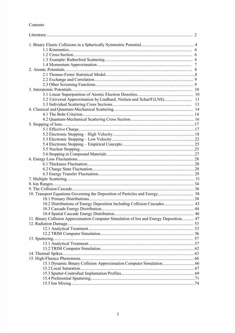
1 – projectile, 2 – target atom (at rest in laboratory frame)
Fig. 1.1
Laboratory System (LS) Center-of-mass System (CMS)
Transformation into CMS yields single-particle scattering kinematics
for a spherically symmetric interaction potential V and with the reduced mass
The energy in the CMS system, being available for the collision, is given by
with E – projectile energy in LS.
Momentum and energy conservation yield the transformations of the asymptotic scattering angles
between CMS and LS for an elastic collision
and the reverse transformation
The energy transferred to the target atom ("recoil") (in LS) is given by
Θ
Φ1
2
ϑ
1
2
212
2
R R R , RV dt
Rd rrrrrr
21
21
mm
mm
E mm
m E
21
2
c
(1.1)
(1.2)
(1.3)
2cos
m
m
sintan
2
1
(1.4)
(1.5)sin
m
marcsin
2
1
2sin E T 2
(1.6)
7/31/2019 Fundamentals of Ion-surface Interaction
http://slidepdf.com/reader/full/fundamentals-of-ion-surface-interaction 5/77
5
with the energy transfer factor
From this, the LS projectile energy after the collision becomes
or after transformation according to (1.4)
Both (1.5) and (1.9) indicate the existence of a maximum scattering angle in LS
For this case, both signs are valid in (1.9), so that two different energies correspond to any LS
scattering angle below the maximum one.
Trivially, the recoil energy is
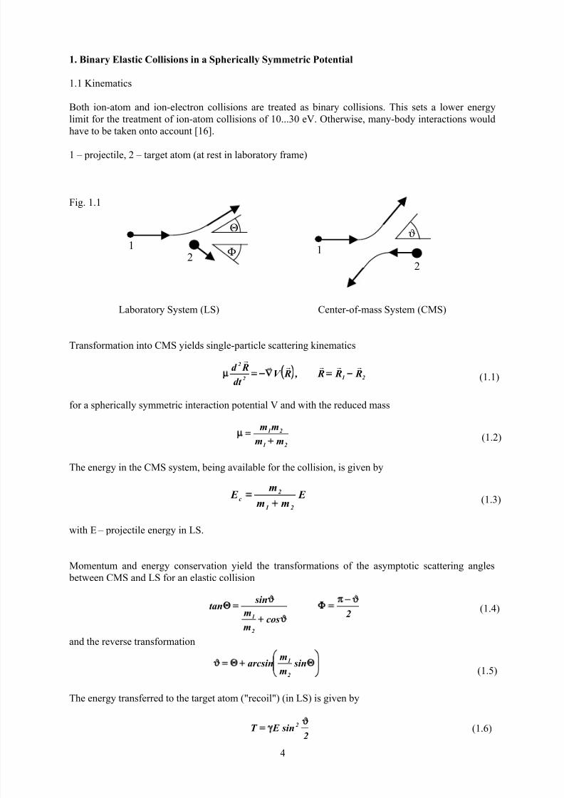
Kinematical curves from (1.9) and (1.11) are shown in Fig. 1.2 for different ions, indicating a
maximum LS scattering angle of 900
for the equal-mass case, and below for heavier projectiles.
2
21
21
mm
mm4
2sin
mm
mm41 E T E E 2
2
21
21
(1.7)
(1.8)
2
2
2
1
2
2
21
1 sinm
mcos
mm
m E E (1.9)
21
1
2max mmif
m
marcsin (1.10)
E E T E 2(1.11)
2
X+ SiE’
E
0.5
1
Scattered
4He
12C
28Si 84Kr
2
X+ BE2’
E
0
0
0.5Recoil Atom
4He
12C28Si
84
Kr
1
Fig. 1.2:
Kinematics of elastic scattering
for the scattered projectile
(different ions incident on
silicon – top) and the recoil
atom (different ions incident on boron – bottom)

7/31/2019 Fundamentals of Ion-surface Interaction
http://slidepdf.com/reader/full/fundamentals-of-ion-surface-interaction 6/77
6
1.2 Cross Section
In cylindrical coordinates, the CMS trajectory is described by the distance R and the angle α (see Fig.
1.3). Energy and angular momentum conservation, and integration yield for the asymptotic scattering
angle at a given impact parameter p the so-called "classical trajectory integral"
with the minimum distance of approach given by
The differential cross section is given by the differential area at p and the scattering into the
differential solid angle around the scattering angle
and can now be calculated from (1.12).
From (1.4), the transformation into the laboratory system is accomplished according to
1.3 Example: Rutherford Scattering
For a Coulomb potential between two interacting charges Q1 and Q2
Fig. 1.3:
Scattering trajectory. Incidence
within a differential ring at a
given impact parameter resultsin a scattering into a
differential solid angle
p R iR
Ec
d d
1
2
1min R
0
2
2
c R
p
E
RV 1
R
1d
p2 (1.12)
0 R
p
E
RV 1
2
min
2
c
(1.13)
d
dp
sin
p
d sin2
pdp2
d
d (1.14)
R4
eQQ RV
0
2
21 (1.16)
cosm
m1
sincosm
m
d
d
d
d
d
d
d
d
2
1
23
2
2
2
1
(1.15)

7/31/2019 Fundamentals of Ion-surface Interaction
http://slidepdf.com/reader/full/fundamentals-of-ion-surface-interaction 7/77
7
(1.12) yields
with the "collision diameter", i.e. the distance of minimum approach for ion-ion scattering at 1800
From this, the Rutherford cross section becomes
1.4 Momentum Approximation
Due to the cylindrical symmetry of the scattering problem, large impact parameters and
correspondingly small deflection angles occur largely preferentially. Therefore, it is often convenient
to describe the scattering in a small-angle approximation.
In the limit of forward scattering, the projectile trajectory is approximated by a straight line (see Fig.
1.4). A force integral leads to a small transverse momentum ∆ py and thereby a small deflection angle
(1.4) reads in small-angle approximation
yielding directly (see (1.3)) the LS deflection which is independent on the mass of the target
R
p2
b
2tan (1.17)
c0
221
E 4
eQQb (1.18)
24
2
E
1
2sin
1
16
b
d
d (1.19)
p
z
y
Fig. 1.4:
Momentum approximation for
small-angle scattering
dz p z V p E
2
E 2
p22
cc
y(1.20)
21
2
mmm (1.21)
dz p z V p E
2 22(1.22)
7/31/2019 Fundamentals of Ion-surface Interaction
http://slidepdf.com/reader/full/fundamentals-of-ion-surface-interaction 8/77
8
2. Atomic Potentials
For the ion – target atom interaction with a sufficiently large minimum distance R min, the interatomic
potential V(R) is influenced by the presence of the electrons, so that a screened Coulomb potential has
to be employed. Naturally, the development of proper interatomic potentials V(R) is closely related to
the choice of the atomic potentials of the collision partners.
The treatment of atomic potentials here will not cover quantum-mechanical calculations of theHartree-Fock-Slater type, but be restricted to statistical models and analytical approximations for
practical uses.
2.1 Thomas-Fermi Statistical Model
From simple quantum statistics in the free electron gas of density ne, the mean kinetic energy density
(i.e. the mean kinetic energy per unit volume) results as
with a0 = 0.053 nm denoting the radius of the first Bohr orbit.
Treating the atom with atomic number Z as the nucleus and an assembly of local free electron gases,
its electrostatic potential given by
A calculus of variation of the total energy
with respect to the electron density yields
with an additive constant φ0. Self-consistency is provided by the Poisson equation
Combining (2.4) and (2.5) in spherical coordinates and writing the potential as a screened Coulomb
potential according to
the substitution r = ax yields for the screening distance
35
ek
35
e0
0
2
32
2
k n:n
4
ae3
10
3 (2.1)
r d r r
r n
4
e
r 4
Zer 3e
00
rrr
r
(2.2)
r d r d r r
r nr n
8
er d
r
r n
4
Zer d E 33ee
0
23e
0
23
k tot
rrrr
rrr
rr
(2.3)
0 0
3 2
k r r r n
3
5e (2.4)
r ne
r e
0
0
ε∆ (2.5)
a
r
r πε 4
Ze(r)
0
(2.6)
31
0
31
03
2
Z
a8853 .0
Z
a
4
3
2
1a (2.7)
7/31/2019 Fundamentals of Ion-surface Interaction
http://slidepdf.com/reader/full/fundamentals-of-ion-surface-interaction 9/77
9
and the Thomas-Fermi equation
Eq. (2.8) is solved numerically with the boundary conditions
as the Coulomb potential holds at small distance to the nucleus, and due to the neutrality of the whole
atom.
The screening function is often approximated by a series of exponentials. The “Moliere”
approximation to the TF function is valid for about x < 5:
2.2 Exchange and Correlation
Quantum-mechanical exchange and correlation have also been described within the framework of the
statistical model, resulting in the following energy densities as function of the electron density:
2.3 Other Screening Functions
The variation problem mentioned above has been solved by Lenz and Jensen using a proper ansatz for
the electron density with appropriate boundary conditions. The resulting screening function is
The most simple screening function is a pure exponential according to Bohr:
Lindhard has given an approximative, so-called “standard” potential
Finally, power-law approximations are used for different regions of x, of the form
corresponding to φ(r)~r –s
.
21
23
TF
2
TF
2
x dx
d (2.8)
010 (2.9)
x 6 x 2 .0 x 3 .0
i
x c
i M e1 .0e55 .0e35 .0eC x i (2.10)
x 67 .9 y;e y002647 .0 y0485 .0 y3344 .0 y1 x y432
LJ (2.13)
y
B e x (2.14)
3 x
x 1 x
2 LS (2.15)
1s
s PL
x
1
s
K x (2.16)
34
eex 3
4
e
0
234
ex n:n16
e3
(2.11)
35
ecorr 3
5
e
0
2
corr n:n4
e46 .0 (2.12)

7/31/2019 Fundamentals of Ion-surface Interaction
http://slidepdf.com/reader/full/fundamentals-of-ion-surface-interaction 10/77
10
Although the following “Universal” screening functions has been formulated for the interatomic
potential (see 3.), it is included here for completeness:
in this case with the screening distance
3. Interatomic Potentials
The interaction potential of two fast atoms, each of which is individually represented by a screened
Coulomb potential, can now be treated in an approximate way.
3.1 Linear Superposition of Atomic Electron Densities
A simple approach is the linear superposition of the individual electron densities to obtain the total
electron density n(r), i.e. neglecting any atomic rearrangements during the collision
0 10 20 30
1
10-2
10-4
(x)
x
Lindhard
Thomas-Fermi
MolièreLenz-Bohr
“Universal”
Fig. 2.1
Different atomic screening
functions
12
r
R
r 1 r 2
Fig. 3.1
Interatomic Coordinates
)r ( n )r ( n )r ( n 2e1ee rrr (3.1)
x 202 .0 x 403 .0 x 942 .0-3.2x
U e0282 .0e28 .0e51 .00.182e(x) (2.17)
23 .0
0
U Z
a8853 .0a (2.18)
7/31/2019 Fundamentals of Ion-surface Interaction
http://slidepdf.com/reader/full/fundamentals-of-ion-surface-interaction 11/77
11
Expressing the total energy (including Coulomb, kinetic, exchange and correlation terms according to
sect. 2) as function of the distance R, and subtracting the total energies of the individual atoms yields
the interaction potential
Eq. (3.2) has to be solved numerically for all R, from which the scattering cross section can be
obtained according to eqs. (2.12-2.14). This is clearly a lengthy procedure and has to be repeated for
each pair of atoms.
3.2 Universal Approximation by Lindhard, Nielsen and Scharff (LNS)
With the aim to obtain a simple and universal description of the interatomic potential and the
scattering cross section of two fast atoms, LNS start from the atomic screened Coulomb potential (see
sect. 2). In the limiting cases of Z1<<Z2 or Z1>>Z2, the interatomic potential would be correctly
described by the screened Coulomb potential of one atom (eq. (2.6)), since the problem can beapproximated by a point charge in the potential of the heavier atom, so that
with a properly chosen screening distance a. For the Thomas-Fermi screening function, the following
choice represents the limits correctly:
For the "Universal" potential (see sect. 2), the screening distance reads correspondingly
The other extreme is obviously the case of Z1=Z2. For this situation, LNS evaluated (3.2) for a number
of atoms and found a reasonable agreement with eqs. (3.3+3.4). Therefore, they assumed (3.3+3.4) to
represent a good approximation of a universal interatomic interaction potential.
r d r n
r
Z r n
r
Z
4
e
R4
e Z Z ) R( V 3
11e
2
2
22e
1
1
0
2
0
2
21
r d r d r r
r nr nr nr n
8
e 3322e11e22e11e
0
2
vv
r d r nr nr nr n33
4
22e3
4
11e3
4
22e11eex
r d r nr nr nr n 335
22e3
5
11e3
5
22e11ecorr
(3.2)
a
R
R4
e Z Z ) R( V
0
2
21(3.3)
2
1
32
232
1
0TF
Z Z
a8853 .0a (3.4)
23 .0
2
23 .0
1
0U
Z Z
a8853 .0a (3.5)
7/31/2019 Fundamentals of Ion-surface Interaction
http://slidepdf.com/reader/full/fundamentals-of-ion-surface-interaction 12/77
12
For the derivation of a universal scattering cross section, LNS consider the limit of small scattering
angles given by the momentum approximation (1.19), which is evaluated for a screened Coulomb
potential yielding
with b from eq. (1.17) and
Further, a reduced energy is introduced according to
so that
represents the universal classical scattering integral in the small-angle approximation. In order to
extrapolate this to wide angles, LNS substitute
and introduce a reduced scattering angle by
Therefore,
becomes a universal scattering integral being valid for all angles. The inverse function of (3.11),
p(t1/2), yields the differential cross section according to dσ = d(π p2), which, according to LNS, is
written as
with f to be calculated numerically from g. f(t1/2
) is defined in such a way that it becomes constant for
a power law potential (see eq. (2.16)) with s = 2. Fig. 3.2 shows the scattering function f for different
screening functions.
a
p g
p
b
(3.6)
d coscoscos
cos g
2
0
c2
21
0 E e Z Z
a4
b
a(3.7)
a
p g
p
a (3.8)
2sin2
2sint 2
1
(3.9)
(3.10)
a
p g
p
at 2 2
1
(3.11)
23
21
2
t 2
t f
adt
d (3.12)
7/31/2019 Fundamentals of Ion-surface Interaction
http://slidepdf.com/reader/full/fundamentals-of-ion-surface-interaction 13/77
13
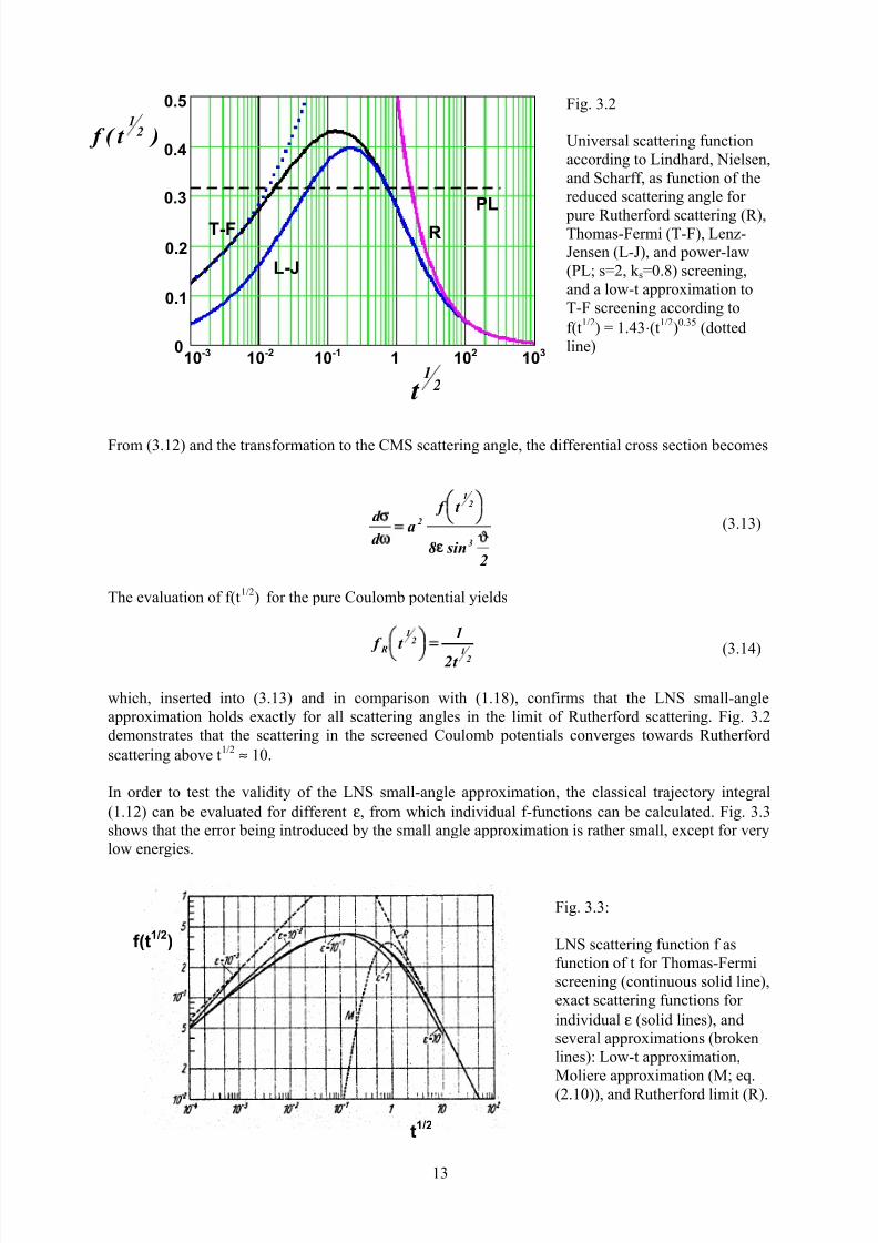
From (3.12) and the transformation to the CMS scattering angle, the differential cross section becomes
The evaluation of f(t1/2
) for the pure Coulomb potential yields
which, inserted into (3.13) and in comparison with (1.18), confirms that the LNS small-angle
approximation holds exactly for all scattering angles in the limit of Rutherford scattering. Fig. 3.2
demonstrates that the scattering in the screened Coulomb potentials converges towards Rutherford
scattering above t1/2
≈ 10.
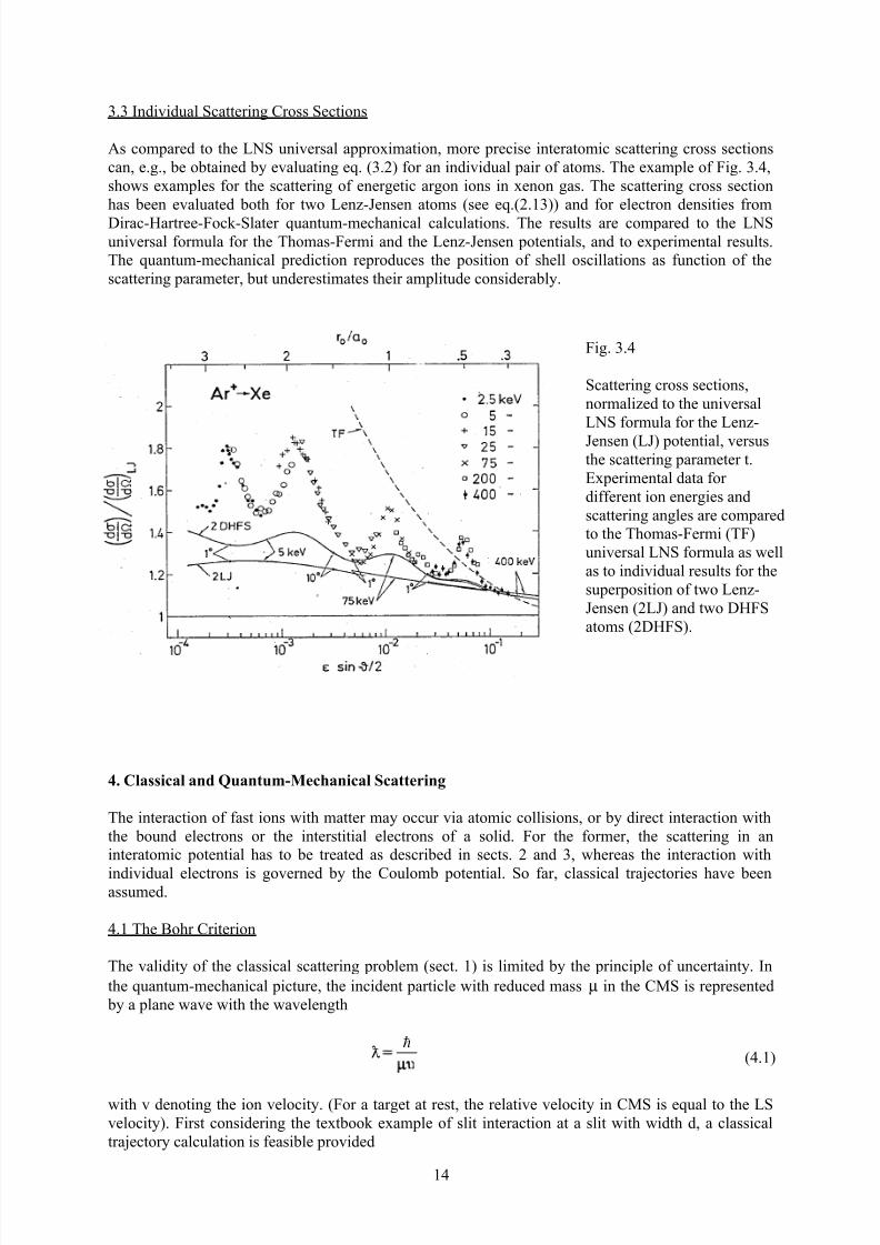
In order to test the validity of the LNS small-angle approximation, the classical trajectory integral
(1.12) can be evaluated for different ε, from which individual f-functions can be calculated. Fig. 3.3
shows that the error being introduced by the small angle approximation is rather small, except for very
low energies.
2sin8
t f
ad
d
3
21
2 (3.13)
21
21
R t 2
1t f
(3.14)
Fig. 3.3:
LNS scattering function f as
function of t for Thomas-Fermi
screening (continuous solid line),
exact scattering functions for
individual ε (solid lines), and
several approximations (broken
lines): Low-t approximation,
Moliere approximation (M; eq.
(2.10)), and Rutherford limit (R).
0
0.2
0.3
0.4
0.5
)t ( f 21
PL
T-F R
L-J
0.1
10-3 10-2 10-1 1 102 103
21
t
Fig. 3.2
Universal scattering function
according to Lindhard, Nielsen,
and Scharff, as function of the
reduced scattering angle for
pure Rutherford scattering (R),Thomas-Fermi (T-F), Lenz-
Jensen (L-J), and power-law
(PL; s=2, k s=0.8) screening,
and a low-t approximation to
T-F screening according to
f(t1/2
) = 1.43⋅(t1/2)
0.35(dotted
line)
t1/2
f(t1/2
)
7/31/2019 Fundamentals of Ion-surface Interaction
http://slidepdf.com/reader/full/fundamentals-of-ion-surface-interaction 14/77
14
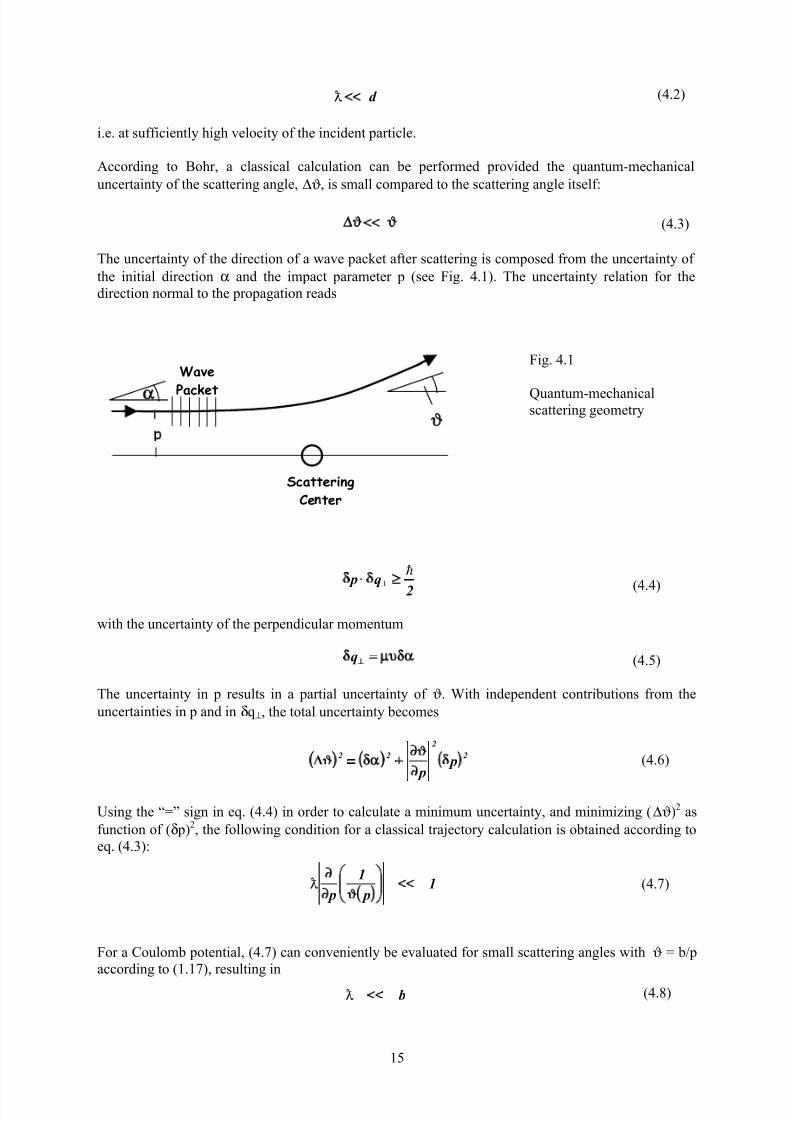
3.3 Individual Scattering Cross Sections
As compared to the LNS universal approximation, more precise interatomic scattering cross sections
can, e.g., be obtained by evaluating eq. (3.2) for an individual pair of atoms. The example of Fig. 3.4,
shows examples for the scattering of energetic argon ions in xenon gas. The scattering cross section
has been evaluated both for two Lenz-Jensen atoms (see eq.(2.13)) and for electron densities from
Dirac-Hartree-Fock-Slater quantum-mechanical calculations. The results are compared to the LNSuniversal formula for the Thomas-Fermi and the Lenz-Jensen potentials, and to experimental results.
The quantum-mechanical prediction reproduces the position of shell oscillations as function of the
scattering parameter, but underestimates their amplitude considerably.
4. Classical and Quantum-Mechanical Scattering
The interaction of fast ions with matter may occur via atomic collisions, or by direct interaction with
the bound electrons or the interstitial electrons of a solid. For the former, the scattering in an
interatomic potential has to be treated as described in sects. 2 and 3, whereas the interaction with
individual electrons is governed by the Coulomb potential. So far, classical trajectories have beenassumed.
4.1 The Bohr Criterion
The validity of the classical scattering problem (sect. 1) is limited by the principle of uncertainty. In
the quantum-mechanical picture, the incident particle with reduced mass µ in the CMS is represented
by a plane wave with the wavelength
with v denoting the ion velocity. (For a target at rest, the relative velocity in CMS is equal to the LS
velocity). First considering the textbook example of slit interaction at a slit with width d, a classical
trajectory calculation is feasible provided
Fig. 3.4
Scattering cross sections,
normalized to the universal
LNS formula for the Lenz-
Jensen (LJ) potential, versusthe scattering parameter t.
Experimental data for
different ion energies and
scattering angles are compared
to the Thomas-Fermi (TF)
universal LNS formula as well
as to individual results for the
superposition of two Lenz-
Jensen (2LJ) and two DHFS
atoms (2DHFS).
hD (4.1)
7/31/2019 Fundamentals of Ion-surface Interaction
http://slidepdf.com/reader/full/fundamentals-of-ion-surface-interaction 15/77
15
i.e. at sufficiently high velocity of the incident particle.
According to Bohr, a classical calculation can be performed provided the quantum-mechanical
uncertainty of the scattering angle, ∆ϑ, is small compared to the scattering angle itself:
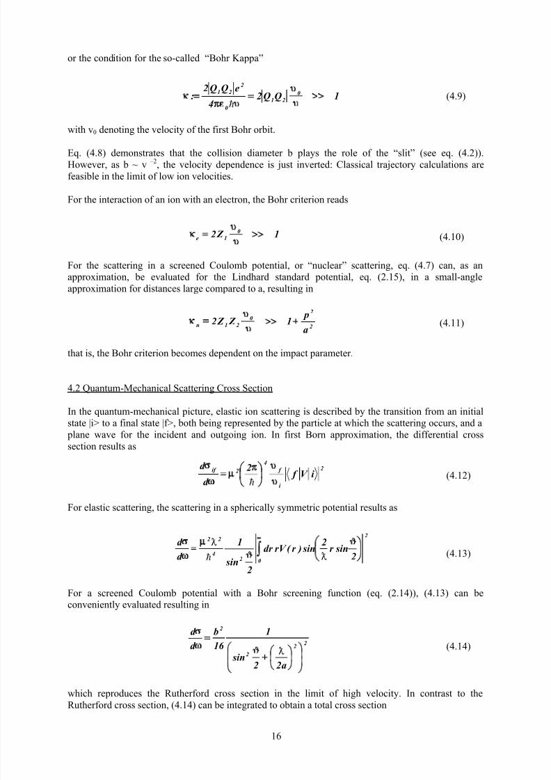
The uncertainty of the direction of a wave packet after scattering is composed from the uncertainty of
the initial direction α and the impact parameter p (see Fig. 4.1). The uncertainty relation for the
direction normal to the propagation reads
with the uncertainty of the perpendicular momentum
The uncertainty in p results in a partial uncertainty of ϑ. With independent contributions from the
uncertainties in p and in δq⊥, the total uncertainty becomes
Using the “=” sign in eq. (4.4) in order to calculate a minimum uncertainty, and minimizing (∆ϑ)2
as
function of (δ p)2, the following condition for a classical trajectory calculation is obtained according to
eq. (4.3):
For a Coulomb potential, (4.7) can conveniently be evaluated for small scattering angles with ϑ = b/p
according to (1.17), resulting in
d D
(4.3)
Scattering
Ce ter
Wave
Packet
Fig. 4.1
Quantum-mechanicalscattering geometry
(4.4)2q p
h
q (4.5)
2
2
22 p
p(4.6)
1 p
1
pD (4.7)
bD
(4.2)
(4.8)
7/31/2019 Fundamentals of Ion-surface Interaction
http://slidepdf.com/reader/full/fundamentals-of-ion-surface-interaction 16/77
16
or the condition for the so-called “Bohr Kappa”
with v0 denoting the velocity of the first Bohr orbit.
Eq. (4.8) demonstrates that the collision diameter b plays the role of the “slit” (see eq. (4.2)).
However, as b ~ v–2
, the velocity dependence is just inverted: Classical trajectory calculations are
feasible in the limit of low ion velocities.
For the interaction of an ion with an electron, the Bohr criterion reads
For the scattering in a screened Coulomb potential, or “nuclear” scattering, eq. (4.7) can, as an
approximation, be evaluated for the Lindhard standard potential, eq. (2.15), in a small-angleapproximation for distances large compared to a, resulting in
that is, the Bohr criterion becomes dependent on the impact parameter.
4.2 Quantum-Mechanical Scattering Cross Section
In the quantum-mechanical picture, elastic ion scattering is described by the transition from an initialstate |i> to a final state |f>, both being represented by the particle at which the scattering occurs, and a
plane wave for the incident and outgoing ion. In first Born approximation, the differential cross
section results as
For elastic scattering, the scattering in a spherically symmetric potential results as
For a screened Coulomb potential with a Bohr screening function (eq. (2.14)), (4.13) can be
conveniently evaluated resulting in
which reproduces the Rutherford cross section in the limit of high velocity. In contrast to the
Rutherford cross section, (4.14) can be integrated to obtain a total cross section
1QQ24
eQQ2: 0
21
0
2
21
h(4.9)
1 Z 2 0
1e (4.10)
2
20
21na
p1 Z Z 2 (4.11)
2
i
f
4
2if i V f
2
d
d
h(4.12)
2
024
22
2sinr 2sin )r ( rV dr
2sin
1d d
Dh
D
(4.13)
22
2
2
a22sin
1
16
b
d
d
D(4.14)
7/31/2019 Fundamentals of Ion-surface Interaction
http://slidepdf.com/reader/full/fundamentals-of-ion-surface-interaction 17/77
17
as the second term in the denominator is negligible except for very low energies (around 1eV and
less).
The validity of the first Born approximation requires a total cross section which is small compared to
the characteristic atomic dimension, i.e. ~ πa2. Therefore, according to (4.15), the first Born
approximation would become questionable for low velocities with κ >> 1. Therefore, the quantum-
mechanical calculations are not feasible in this regime, and classical trajectory calculations are
necessary. The Bohr criterion (4.9) delivers a unique limit between quantum-mechanical and classical
calculations.
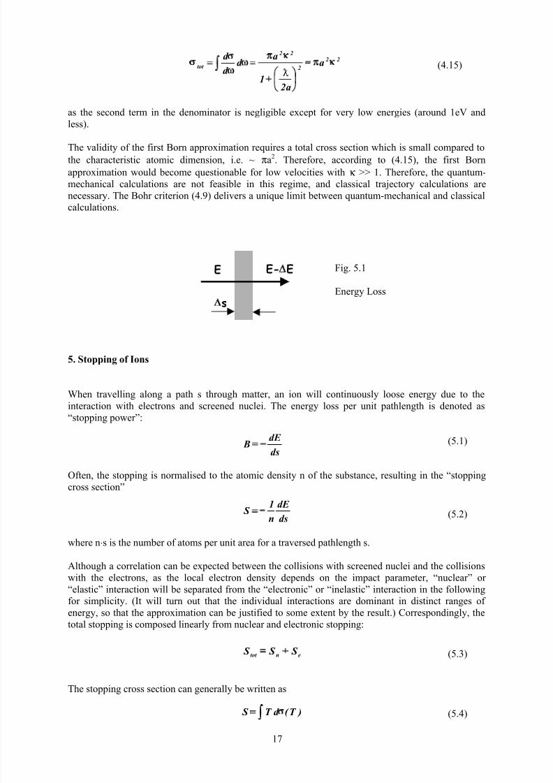
5. Stopping of Ions
When travelling along a path s through matter, an ion will continuously loose energy due to the
interaction with electrons and screened nuclei. The energy loss per unit pathlength is denoted as
“stopping power”:
Often, the stopping is normalised to the atomic density n of the substance, resulting in the “stopping
cross section”
where n⋅s is the number of atoms per unit area for a traversed pathlength s.
Although a correlation can be expected between the collisions with screened nuclei and the collisions
with the electrons, as the local electron density depends on the impact parameter, “nuclear” or
“elastic” interaction will be separated from the “electronic” or “inelastic” interaction in the following
for simplicity. (It will turn out that the individual interactions are dominant in distinct ranges of
energy, so that the approximation can be justified to some extent by the result.) Correspondingly, the
total stopping is composed linearly from nuclear and electronic stopping:
The stopping cross section can generally be written as
22
2
22
tot a
a21
ad
d
d
D(4.15)
Fig. 5.1
Energy LossE E- E
s
ds
dE B (5.1)
ds
dE
n
1 S (5.2)
entot S S S (5.3)
)T ( d T S (5.4)

7/31/2019 Fundamentals of Ion-surface Interaction
http://slidepdf.com/reader/full/fundamentals-of-ion-surface-interaction 18/77
18
for an interaction with the differential cross section dσ and the energy transfer T.
5.1 Effective Charge
In addition to stopping, the electronic interaction of an ion passing through matter results in charge-
changing collisions, so that the actual charge state of a fast ion in matter is continuously fluctuating
and determined by a balance between electron loss and electron attachment. The average charge of the
ion, which depends on its velocity, is denoted as “effective” charge, Z1eff , and is quickly established
(typically within some nm) when an ion of arbitrary charge state impinges onto a solid surface. In the
limit of very low energy, the ion becomes neutral with a vanishing effective charge, so that atomic
electrons interact with the electrons of the solid. Towards high velocities, electron loss dominates, so
that the ions becomes a naked nucleus with Z1eff
= Z1 at sufficiently high energy.
More quantitatively, electron attachment is effective if the ion velocity is lower than the characteristic
orbital velocity of its atomic electrons. Under this conditions, electrons from the electron gas of the
solid have sufficient time to accommodate adiabatically with the moving ion. Taking the average
velocity of electrons in a free electron gas with Z1 electrons
as the characteristic velocity, Bohr has estimated the effective charge of the ion by
with a high-velocity extrapolation that ascertains that Z1eff
cannot exceed Z1.
5.2 Electronic Stopping – High Velocity
For v >> v0Z12/3
, corresponding to E >> 25 keV⋅A1Z14/3
where A1 denotes the atomic mass of the
projectile, the ion is deprived of all its electrons. Then, the evaluation of (4.10) yields for the
interaction with electrons (|Q2|=1):
which does in general not fulfil the Bohr condition for classical trajectory calculations. Therefore,
quantum-mechanical calculations have to be applied in general. For very heavy ions, however, an
approximation by classical mechanics might become more feasible.
Both therefore and in order to discuss some physical concepts which will enter the classical
calculation, we will start here with the latter, though being aware of the fact that it is not justified in
principle.
The evaluation of (5.4) for Rutherford scattering of the ion free electrons yields
with me denoting the electron mass and be the electronic collision diameter (eq. (1.18)). A difficulty in
evaluating the stopping cross section arises from the fact that dσ ~ T-2 according to eqs. (1.6) and(1.19), so that the integral diverges with a lower limit T→ 0. Therefore, a lower limit Tmin has to be
introduced corresponding to a maximum impact parameter pmax, which appears in (5.8).
3 / 2
101 ,e Z (5.5)
32
1
0
1
3 / 1
1
01 ,e
1
eff
1 Z exp1 Z Z Z Z (5.6)
3 / 1
1e Z 2 (5.7)
e
max
2
e
2
2
1
2
0
4
eb
p2log
m
Z Z
4
e4 S (5.8)
7/31/2019 Fundamentals of Ion-surface Interaction
http://slidepdf.com/reader/full/fundamentals-of-ion-surface-interaction 19/77
19
An estimation of pmax is obtained by the so-called “adiabatic cutoff “. Assuming a characteristic time
interval τ of the interaction, the electrons of a target atom contribute to energy loss only if their mean
orbital frequency ω is small compared to the inverse of the characteristic collision time. Otherwise, at
large orbital frequencies, the electron would attach adiabatically to the moving ion.
Using the momentum approximation (eq. (1.21)), the characteristic collision time can be estimated
from the transverse momentum transfer and its associated force integral to be
so that the integration is limited to a maximum impact parameter
Then, the result becomes (the classical “Bohr” formula)
In the classical picture, the energy dependence of the electronic stopping reads as ~E-1
log(CE3/2
), C
being a constant.
Now we will turn to the quantum-mechanical derivation of high-energy electronic stopping, which is
imposed by the Bohr criterion.
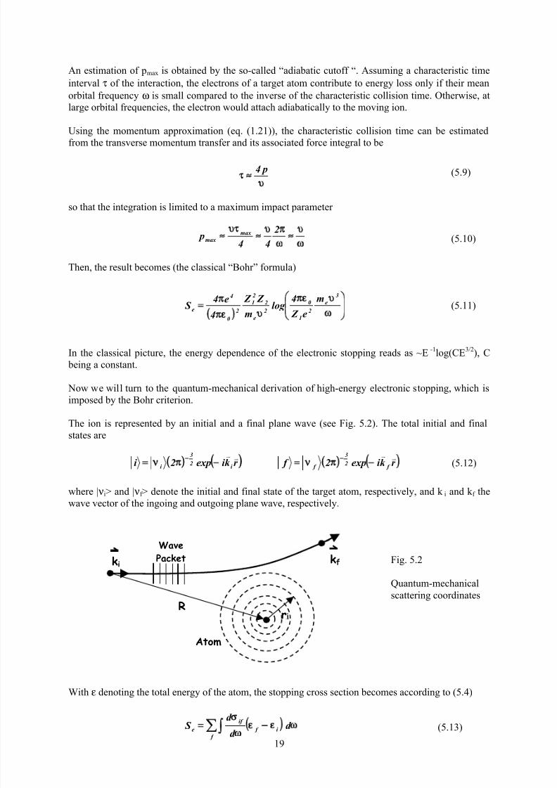
The ion is represented by an initial and a final plane wave (see Fig. 5.2). The total initial and final
states are
where | νi> and | νf > denote the initial and final state of the target atom, respectively, and k i and k f the
wave vector of the ingoing and outgoing plane wave, respectively.
With ε denoting the total energy of the atom, the stopping cross section becomes according to (5.4)
p4 (5.9)
2
44 p max
max (5.10)
3
e
2
1
0
2
e
2
2
1
2
0
4
e
m
e Z
4log
m
Z Z
4
e4 S (5.11)
r k i exp2i i 2
3
i
vv(5.12)r k i exp2 f f
2
3
f
vv
Atom
Wave
Packet
Rr
kfki Fig. 5.2
Quantum-mechanical
scattering coordinates
d d
d S i f
f
if
e (5.13)
7/31/2019 Fundamentals of Ion-surface Interaction
http://slidepdf.com/reader/full/fundamentals-of-ion-surface-interaction 20/77
20
Into (5.13), eq. (4.12) has to be inserted with µ = me and the interaction potential
With the momentum transfer
the intermediate result is
From energy conservation, maximum and minimum momentum transfer for a given final state are
for a maximum energy transfer large compared to the binding energy of the electron.
For simplicity, Hartree wave functions
with the individual orbital wave functions ϕi shall be employed intermediately. (However, the
following finding also hold for more realistic total wave functions.) Then, the matrix element of (5.17)
becomes
Due to the orthonormality of the ϕi , (5.19) is only different from zero if exactly one electronic state
(e.g., numbered j) is altered during the collision: Within the first Born approximation, multiple
electronic excitation or ionisation is excluded. The matrix element is reduced to
to be integrated over the atomic volume. For a characteristic radius a of the atom, the evaluation of
(5.20) can be discriminated. If the momentum transfer is large compared to the inverse of the atomic
radius, the exponential term oscillates quickly, and the matrix element only vanishes if
i.e., the final state of the electron j is a plane wave. This situation stands for the ionisation of the atom,
with
2
2
Z
1i
2
i 0
2
1
Z 1 R
Z
r R
1
4
e Z )r ,...r , R( V vv
vvv
(5.14)
f i k k qvvv
(5.15)
2
f
q
q
i
i
i f i f 32
2
1
2
0
4
e
max
min
r qi expq
dq Z
4
e8 S
vv
h(5.16)
i f
minqh
e
max
m2q (5.17)
2 Z
1i
i i r v (5.18)
i Z
*
f Z Z
3
i ii
*
if i
3
i
i 1
*
f 11
3
i
i
i f 222r d ...r qi expr d ...r d r qi expvvvvvvv
(5.19)
j ji
*
jf j
3
i
i
i f r qi expr d r qi expvvvvv
(5.20)
j j jf r qi exp~r vvv
a
1q for (5.21)
7/31/2019 Fundamentals of Ion-surface Interaction
http://slidepdf.com/reader/full/fundamentals-of-ion-surface-interaction 21/77
21
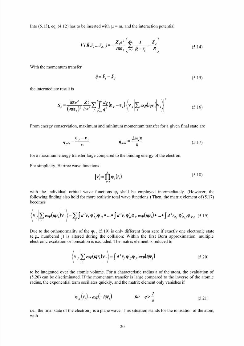
The contributions to the summation over εf and the integration over q in eq. (5.16) are indicated
schematically in the two-dimensional plot of Fig. 5.3. For q < 1/a, the individual energy levels of the
atoms are involved in electronic excitation. (5.16) can now be evaluated individually for the different
regimes of q. For q > 1/a, the integrand can be converted into generalised oscillator strengths, which
drop out due to their normalisation. For q < 1/a, the exponential of (5.20) is expanded to first order,
which leads to dipole oscillator strengths f fi. Adding the expressions for both regimes, the final result
is the Bethe formula
with the “mean ionisation potential” given by
Due to the summation over all possible final states of the excited atom, I cannot readily be calculated.
A reasonable approximation is according to Bloch
It should be noted that the quantum-mechanical result (5.23) differs from the classical one (5.11) only
in the logarithmic terms which varies slowly with energy, anyway.
Two examples are given in Figs. 5.4a and 5.4b. In the limit of very high energy, both the classical and
the quantum-mechanical formula are in good agreement with the experimental data. In the light-ion
case, the Bethe formula works well for κ >> 1. However, also the classical result is a rather good
approximation even for the unsuitable energy regime. For heavy ions, quantum-mechanical
calculations are only feasible for extremely high energy, and the classical picture holds well at
sufficiently high energy.
e
22
i f m2
qh
(5.22)
e
22
m2
qh
i f
minq
h
emax
m2q
i f
q
a
10
Ionisation
Excitation
Fig. 5.3
Contributions to
the stopping power
integral
I
m2log
m
Z Z
4
e4 S
2
e
2
e
2
2
1
2
0
4
e (5.23)
i f
f
fi log f I log h (5.24)
2 Z eV 10 I
(5.25)

7/31/2019 Fundamentals of Ion-surface Interaction
http://slidepdf.com/reader/full/fundamentals-of-ion-surface-interaction 22/77
22
For completeness, it should briefly be mentioned the high-velocity electronic energy loss can also be
derived from the dynamic polarisation of a free electron gas, and the corresponding retarding drag on
the ion (Lindhard and Winter). Again a result similar to (5.23) is obtained. The comparison yields in
this case
Thus, the mean ionisation potential can be calculated more easily from realistic local radial electron
densities ne and the corresponding plasma frequencies ω0.
5.3 Electronic Stopping – Low Velocity
At low velocity with v < v0Z1
2/3
, the combination with the effective charge (eq. (5.6)) yields
1 Z 2 3 / 1
1e (5.27)
StoppingCrossSection
(10
-14
eVcm2)
H Ni
Bohr (class.)
Bethe-Bloch
(qumech.)
Exptl.
Data
0
1
3
2
4
102 103 104 105
Energy (keV)
Fig. 5.4a
High-energy
electronic stopping of
a proton in Ni from
(5.23) and (5.25)
(Bethe-Bloch) and
(5.11) (Bohr) with amean orbital energy
according to (5.25).
The predictions are
compared to semi-
empirical data from
the SRIM-2000
package. The energy
of the Bohr criterion is
indicated at the lower
left.
Ge Si
Bethe-Bloch(qumech.)
Bohr
(class.)
Exptl.Data
10 102 103 1040
1
2
3
4
5
Energy (MeV)
StoppingCrossSection
(10-12
eVcm2)
Fig. 5.4b
As 5.4a, but for
germanium ions in
silicon. Note the
different scales. The
low-velocity limit is
also indicated.
=1
=1v=v0Z12/3
)r ( 2log r ndr r 4 Z
1 I 0e
2
2
h (5.26)

7/31/2019 Fundamentals of Ion-surface Interaction
http://slidepdf.com/reader/full/fundamentals-of-ion-surface-interaction 23/77
23
so that classical trajectory calculations are feasible. In the following, we consider the interaction of the
ion with the target electrons modelled as a free electron gas. By the scattering events with its electrons,
momentum is transferred to the ion. The stopping cross section can be written in terms of the change
of the longitudinal momentum, p=, per time unit:
For low ion velocities being small compared to the Fermi velocity of the electron gas, which is given
by
for a free electron gas, the Fermi sphere of the target electrons is slightly shifted in the frame of the ion
(see Fig. 5.4). According to the Pauli principle, electrons can only transfer momentum to the ion when
their final state lies in a previously unoccupied position beyond the original Fermi sphere. This is
possible for electrons being positioned outside of a sphere with radius vf – v, as indicated by the
shaded area in Fig. 5.4. Its volume is about 4πvf 2v. The velocity of the contributing electrons can be
approximated by vf , and the momentum transfer per scattering event is in the order of m evf . A simple
estimation then shows according to (5.28)
with the ion-electron scattering cross section σ. As an important result, the stopping cross section is
proportional to the ion velocity, due to the Pauli principle.
A more rigorous treatment of the scattering geometry yields, still in the limit v << v f
where σtr denotes the so-called transport cross section given by
dt
dp
n
1
dt
pd
nm2
1 S
2
1
e (5.28)
v v Fig. 5.4
Fermi sphere of the target free
electron gas with Fermi velocity
vf , in the frame of an ion
moving with small velocity v.
The dashed trajectory indicatesan electronic scattering event
which is not forbidden by the
Pauli principle.
31
e
2
e f
n3m
h
(5.29)
f f 2ee Z m S (5.30)
f tr f 2ee Z m S
d d d )cos1(
0
tr
(5.31)
(5.32)

7/31/2019 Fundamentals of Ion-surface Interaction
http://slidepdf.com/reader/full/fundamentals-of-ion-surface-interaction 24/77
24
The evaluation of the differential cross section is rather complex and has to be performed for realistic
local electron densities ne(r,Z1,Z2). Lindhard and Scharff arrive at
where k e is a constant defined by eq. (5.33). The result implicitly assumes that the electronic stopping
acts nonlocally, i.e. independent of the actual position of the ion trajectory with respect to the position
of the atoms which are passed by. Therefore, the result is independent of the actual impact parameter
for a specific collision.
A different approach has been described by Firsov. During the interaction of two atoms, the electronclouds penetrate each other. Electrons transverse the intersecting plane between the two atoms, and, as
v << vf , accommodate their original directed kinetic energy (for both atoms moving in the CM
system) to the dynamic electronic configuration of the interatomic system. For a free electron gas and
a Thomas-Fermi interaction potential Firsov obtains for the electronic energy transfer per atomic
collision
which offers the possibility to compute the energy loss as function of the impact parameter, with a
very steep decrease as function of p for p >> a0. The integration over p yields in good approximation
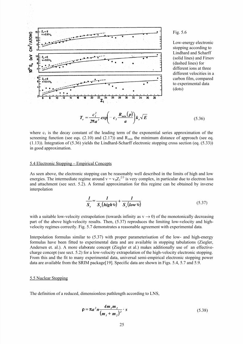
Fig. 5.6 gives an example of low-energy electronic cross sections according to (5.33) and (5.35), in
comparison to experimental values. The average agreement is good, however there are clear shell
oscillations which cause significant deviations from the free-electron gas pictures.
For practical purposes in particular in connection with computer simulation, Oen and Robinson proposed an alternative expression for the local energy transfer (see eq. (5.34)):
E k : Z Z
Z Z
4
ae8 S e
02332
2
32
1
2
6 7
1
0
0
2
e (5.33)
e-
e- R
2
1
Fig. 5.5
Electronic energy loss in
the Firsov picture
5
0
31
21
35
21
0
e
a
p Z Z 16 .01
Z Z
a
35 .0T
h
(5.34)
2
0
21
15
e cmeV Z Z 1015 .5 S (5.35)
7/31/2019 Fundamentals of Ion-surface Interaction
http://slidepdf.com/reader/full/fundamentals-of-ion-surface-interaction 25/77
25
where c1 is the decay constant of the leading term of the exponential series approximation of the
screening function (see eqs. (2.10) and (2.17)) and R min the minimum distance of approach (see eq.
(1.13)). Integration of (5.36) yields the Lindhard-Scharff electronic stopping cross section (eq. (5.33))
in good approximation.
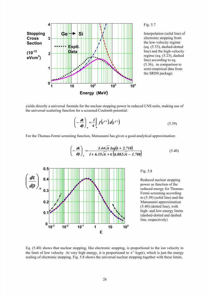
5.4 Electronic Stopping – Empirical Concepts
As seen above, the electronic stopping can be reasonably well described in the limits of high and low
energies. The intermediate regime around v = v0Z1
2/3
is very complex, in particular due to electron lossand attachment (see sect. 5.2). A formal approximation for this regime can be obtained by inverse
interpolation
with a suitable low-velocity extrapolation (towards infinity as v → 0) of the monotonically decreasing
part of the above high-velocity results. Then, (5.37) reproduces the limiting low-velocity and high-
velocity regimes correctly. Fig. 5.7 demonstrates a reasonable agreement with experimental data.
Interpolation formulas similar to (5.37) with proper parameterisation of the low- and high-energy
formulas have been fitted to experimental data and are available in stopping tabulations (Ziegler,Andersen et. al.). A more elaborate concept (Ziegler et al.) makes additionally use of an effective-
charge concept (see sect. 5.2) for a low-velocity extrapolation of the high-velocity electronic stopping.
From this and the fit to many experimental data, universal semi-empirical electronic stopping power
data are available from the SRIM package[19]. Specific data are shown in Figs. 5.4, 5.7 and 5.9.
5.5 Nuclear Stopping
The definition of a reduced, dimensionless pathlength according to LNS,
(5.37)
Fig. 5.6
Low-energy electronic
stopping according to
Lindhard and Scharff
(solid lines) and Firsov(dashed lines) for
different ions at three
different velocities in a
carbon film, compared
to experimental data
(dots)
low S
1
high S
1
S
1
eee
E k a
p Rcexp
a2
cT
e
min
12
2
1
e (5.36)
smm
mm4na
2
21
212(5.38)
7/31/2019 Fundamentals of Ion-surface Interaction
http://slidepdf.com/reader/full/fundamentals-of-ion-surface-interaction 26/77
26
yields directly a universal formula for the nuclear stopping power in reduced LNS units, making use of
the universal scattering function for a screened Coulomb potential:
For the Thomas-Fermi screening function, Matsunami has given a good analytical approximation:
Eq. (5.40) shows that nuclear stopping, like electronic stopping, is proportional to the ion velocity in
the limit of low velocity. At very high energy, it is proportional to ε-1⋅log(ε), which is just the energy
scaling of electronic stopping. Fig. 5.8 shows the universal nuclear stopping together with these limits.
Ge Si
Exptl.
Data
1 10 102 103 104
Energy (MeV)
StoppingCrossSection
(10-12
eVcm2)
0
1
2
3
4 Fig. 5.7
Interpolation (solid line) o
electronic stopping from
the low-velocity regime
(eq. (5.33), dashed-dotted
line) and the high-velocityregime (eq. (5.23), dashed
line) according to eq.
(5.36), in comparison to
semi-empirical data from
the SRIM package.
21
0
21
n
t d t f 1
d
d (5.39)
708 .1882 .6 35 .6 1
718 .2log 44 .3
d
d
n
(5.40)
Fig. 5.8
Reduced nuclear stopping
power as function of the
reduced energy for Thomas-
Fermi screening according
to (5.39) (solid line) and the
Matsunami approximation
(5.40) (dotted line), withhigh- and low-energy limits
(dashed-dotted and dashed
line, respectively)
10-3 10-2 10-1 1 10 102
0.2
0.3
0.4
0.5
0.1
0
nd
d

7/31/2019 Fundamentals of Ion-surface Interaction
http://slidepdf.com/reader/full/fundamentals-of-ion-surface-interaction 27/77
27
Figs. 5.9a+b show the nuclear stopping cross section Se, which is transformed from (5.40) to non-
reduced energy and pathlength, in comparison to the electronic cross section. For heavier ions,
nuclear stopping dominates at low energy and becomes negligible in the limit of high energy. This is a
further justification of the independent treatment of electronic and nuclear interaction. For very light
ions, nuclear stopping can be neglected in a broad range of energies.
5.6 Stopping in Compound Materials
The simplest approximation to the stopping in compound materials is the summation of the pure
element stopping cross sections. Thus, for a two-component material AnBm with the elemental
stopping cross section SA and SB, the stopping cross section is according to “Bragg’s Rule”
By the simple linear superposition, chemical interaction of the elements are neglected. Nevertheless,
Bragg’s rule normally holds rather well. With increasing amount of covalent bonding in thecompound, deviation of up to about 40% are observed, as, e.g., for oxides and hydrocarbons. For a
number of compounds, stopping data are available in the SRIM package[19].
Fig. 5.9b
As Fig. 5.9a, but for
hydrogen in nickel. The
Lindhard-Scharff
electronic stopping has
been corrected by a fitting
factor of 1.3. Note the
different scales.
B A B A mS nS S mn
(5.41)
Ge Si
0
0.5
2
1
1.5
Energy (keV)
StoppingCrossSection(10
-12
eVcm2)
1 102 104 106
10-2 1 102
Energy (keV)
10-16
10-15
10-14
10-13
StoppingCrossSection(eVcm2)
H Ni
Fig. 5.9a
Nuclear (eq.(5.40),
dotted line), electronic
(SRIM package, solid
line, and eq.(5.33),
corrected by fitting factor of 1.2, dashed line) and
total stopping (thin solid
line) cross section versus
ion energy, for
germanium in silicon.

7/31/2019 Fundamentals of Ion-surface Interaction
http://slidepdf.com/reader/full/fundamentals-of-ion-surface-interaction 28/77
28
6. Energy Loss Fluctuations
In addition to the mean energy loss which is described by the stopping power, the energy distribution
of an ion beam is broadened after traversing a sheet of thickness ∆x (see Fig. 5.1)). This is shown
schematically in Fig. 6.1. There are various reasons for energy loss fluctuations, which are partly
“immanent”, i.e. connected to the statistical nature of the collisions which result in energy loss.
However, in an experiment, additional contributions are observed and may obscure the immanent
mechanisms, such as thickness variations of a foil or the influence of target crystallinity and/or texture.
Here, we will remain in the frame of a random substance, and address the most important mechanisms.
6.1 Thickness Fluctuation
When a thin film of thickness x with a mean square variation δx is traversed, the resulting variance of
the ion energy distribution is
that is, the width of the resulting energy distribution is proportional to the stopping power.
6.2 Charge State Fluctuation
As discussed in sect. 5.1, ions with intermediate energies undergo charge change collisions, so that
they exhibit different charge states during their transport through matter. In the energy range of interest, the cross sections of charge-changing collisions are smaller than those of the atomic collision
which determine the energy loss. Thus, as shown in Fig. 6.2 for the simplified case of only two
different charge states, a fraction α of the total pathlength would be spent with one of the charge
states, and the remaining fraction with the other charge state.
2
2
2
th x dx
dE (6.1)
Fig. 6.1
Schematic showing the
broadening of the energy
distribution of an ion beamafter passing through a thin
sheet of matter
Pathlength
ChargeState
1
2
s
E E- E
0 2.5 51.5
2
2.5
f2( )x
x
4 0 40
0.2
0.4
f1( )x
xE E- E E
fE
2
fE
Fig. 6.2
Charge state
fluctuation of anindvidual ion

7/31/2019 Fundamentals of Ion-surface Interaction
http://slidepdf.com/reader/full/fundamentals-of-ion-surface-interaction 29/77
29
The resulting energy loss is
where S1 and S2 denote the stopping cross sections associated to the respective charge states. From
this, the variance of the energy loss distribution becomes
α can be expressed by the charge exchange cross sections σ12 (from 1 to 2) and σ21 (vice versa)
yielding
The resulting width of the energy distribution is proportional to the pathlength and the difference of
the stopping powers.
6.3 Energy Transfer Fluctuation
The conventional treatment of energy straggling covers the statistical nature of the atomic collisions.
With κ i denoting the number of collisions with energy transfer Ti, the energy loss becomes for a
specific trajectory
The variance of the energy loss, assuming Poisson statistics of the collision numbers, i.e. <(κ i-<κ
i>)
2>
= <κ i>, results in
In continuous notation with κ i => n∆s⋅dσ, this becomes
so that the width of the energy distribution scales with the square root of the thickness.
Eq. (6) can easily be evaluated for Rutherford scattering, as first shown by Bohr. (In contrast to
stopping – see sect. 5.3 – the integral converges for a zero minimum energy transfer.) For sufficiently
many independent collisions, i.e. when neglecting energy loss, a Gaussian energy distribution results
with a variance
Energy straggling is thus independent of the ion energy in the limit of high energy. Evaluating (6.8)
for scattering at free electrons (Q22=1, m2=me, me<<m1, ne=nZ2) yields the Bohr formula
i
i i T E
i
2
i i
22 T E E
d T sn 22(6.7)
(6.9)
sn S 1sn S E 21
222
21
222
ce S S sn E E
(6.4)3
2112
21122
21
22
ce
2 S S sn
(6.3)
(6.5)
2
21
2
12
2
2
12
0
42
mm
mQQ
4
e4sn (6.8)
(6.6)
2
0
2
2
1
42
e
4
Z Z e4
sn
(6.2)

7/31/2019 Fundamentals of Ion-surface Interaction
http://slidepdf.com/reader/full/fundamentals-of-ion-surface-interaction 30/77
30
For lower ion energy, Lindhard and Scharff calculated the electronic straggling in a local free electron
gas approximation with the result
with an analytical function and its variable
Nuclear straggling can again easily be written in reduced LNS units
which reproduces (6.8) for the scattering of totally stripped nuclei in the limit of high energy.
2
B
2
3if
2
L
3if 1
2
02
2321
Z
1016 .036 .1 L (6.11)
2121
02
2
n
t d t f t (6.12)
(6.10)
1 103 106
Energy (keV)
10-11
10-9
10-7
EnergyStraggling(eV2cm2)
Ge Si
Electronic
Nuclear Fig. 6.3a
Energy straggling Ω2/n∆s
for germanium ions in
silicon, according to eqs.
(6.9) (dashed-dotted line),(6.10) (solid line) and
(6.12) (dashed line)
10-2 10 104
Energy (keV)
10-14
10-12
10-10
EnergyStraggling(eV
2cm
2)
H Ni
Electronic
Nuclear
Fig. 6.3b
As Fig. 6.3a, but for
hydrogen in nickel
7/31/2019 Fundamentals of Ion-surface Interaction
http://slidepdf.com/reader/full/fundamentals-of-ion-surface-interaction 31/77
31
Figs. 6.3a+b show the energy straggling as function of the ion energy for two different ion-target
combinations. For very light ions, the nuclear straggling can roughly be neglected, whereas it is
dominant for heavy ions (note that the total straggling results from the linear addition of the nuclear
and electronic variances which are shown in the figures.)
It should, however, be noted that only simplified results have been presented, assuming sufficiently
thick layers and neglecting energy loss, which is a contradiction in general. Very thin films, in
particular at high ion energy, may yield strongly asymmetric energy distributions, whereas for thick films the energy loss has to be taken into account.
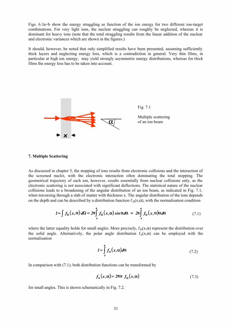
7. Multiple Scattering
As discussed in chapter 5, the stopping of ions results from electronic collisions and the interaction of the screened nuclei, with the electronic interaction often dominating the total stopping. The
geometrical trajectory of each ion, however, results essentially from nuclear collisions only, as the
electronic scattering is not associated with significant deflections. The statistical nature of the nuclear
collisions leads to a broadening of the angular distribution of an ion beam, as indicated in Fig. 7.1,
when traversing through a slab of matter with thickness x. The angular distribution of the ions depends
on the depth and can be described by a distribution function f Ω(x,α), with the normalisation condition
where the latter equality holds for small angles. More precisely, f Ω(x,α) represent the distribution over the solid angle. Alternatively, the polar angle distribution f α(x,α) can be employed with the
normalisation
In comparison with (7.1), both distribution functions can be transformed by
for small angles. This is shown schematically in Fig. 7.2.
x
Fig. 7.1
Multiple scattering
of an ion beam
00
d , x f 2d sin , x f 2d , x f 1 (7.1)
0
d , x f 1 (7.2)
, x f 2 , x f (7.3)

7/31/2019 Fundamentals of Ion-surface Interaction
http://slidepdf.com/reader/full/fundamentals-of-ion-surface-interaction 32/77
32
In order to study the evolution of the distribution function at increasing penetration depth, a thin
incremental slab δx is considered as shown in Fig. 7.3, which describes an example of so-called
"forward" transport. Within this slab, each ion can either change its direction due to a nuclear
collision, or it may just penetrate without any nuclear collision (any energy losses are neglected). In
the former case, for an ensemble of ions described by the angular distribution function, the new
distribution function, f Ω(x+δx,α), results from scattering events which transform fractions of the
original function, f Ω(x,α’), into the direction α. The probability is given by the scattering cross
sections for all directional changes α’→ α. In the latter case, the distribution function is reproducedwith a probability of one minus the total cross section. Therefore:
Although the resulting angle distribution is axially symmetric, the flight direction of individual ions
has both a polar and an azimuthal component. Therefore, in the detailed treatment, two-dimensional
angles and angular distribution have to be considered, which is not explicitly indicated here for
simplicity. The Taylor expansion of the left-hand side results in the Boltzmann type transport equation
By suitable mathematical techniques, the integro-differential equation can be solved for an initially
sharp angular distribution, f(0,α)=δ(α), resulting in the Bothe equation
x
Fig. 7.3
"Forward" transport by
nuclear collisions
f2( )x
x
f3( )x
x
f (x, )
0 0
f (x, )
Fig. 7.2
Angular distribution in solid
angle (left) and polar angle
(right) representation. The
polar angle distribution
vanishes at α=0.
, x f d x n1 , x f d x n , x x f nn
(7.4)
, x f , x f d n x
, x f n
(7.5)
k nexpk J kdk 2
1 , x f 0
0
0
00
n
0
k J 1d d
d k with
(7.6)

7/31/2019 Fundamentals of Ion-surface Interaction
http://slidepdf.com/reader/full/fundamentals-of-ion-surface-interaction 33/77
33
where J0 denotes the zero-order Bessel function. Following Sigmund, the Bothe equation will now be
turned into reduced units. The (small) laboratory scattering angle Θ can be transformed into the
reduced scattering angle, eq. (3.10), by
Correspondingly, the directional angle is transformed into a reduced angle
Further, a reduced thickness is introduced for the purpose of multiple scattering
Then, (7.6) can be rewritten as
Multiple scattering distributions are tabulated for a large range of reduced angles and thickness in ref.
[10]. An example is given in Fig. 7.4.
Fig. 7.4 Multiple scattering distributions for boron in silicon. Note the different presentations: (left)
solid angle distribution, logarithmic; (right) polar angle distribution, linear.
2
21
021
e Z Z 2
aE 4t (7.7)
2
21
0
e Z Z 2
aE 4~(7.8)
nx a2
(7.9)
z exp~ z J zdz 2
1~ , f 0
0~
0
02
~ z J 1~
~ f ~d z with
(7.10)
0 5 101
10
100
1000
0
20
40
(degree)
f (x, ) f (x, )
0 5 10
B+ 100 nm Si
100 keV
500 keV
1 MeV

7/31/2019 Fundamentals of Ion-surface Interaction
http://slidepdf.com/reader/full/fundamentals-of-ion-surface-interaction 34/77
34
8. Ion Ranges
As a consequence of stopping and scattering, each individual incident ion forms a random trajectory as
shown in Fig. 8.1. Stopping alone defines the total pathlength R t. From the endpoint of the trajectory
projected ranges can be defined (longitudinal, R p=, and lateral, R p
⊥). For practical purposes, the
(normal) projected range R p is mostly of interest, since it characterises the implantation depth with
respect to the surface. Obviously, R p is equal to R p=
for normal incidence. As in most implantation
processes the extension of the implanted area is very large compared to the ion range, R p is mostly also
the only range quantity which is accessible to measurement.
For many incident ions, the range distribution is smeared out parallel to the surface (see Fig. 8.2), with
a mean projected range R p. If the range distribution peaks sufficiently far from the surface, the mean
projected range at an angle of incidence α is related to the mean projected range at normal incidence
by
at given energy of incidence.
The mean total pathlength is easily calculated from the total stopping cross section by integration
along the path s, according to
Simple analytical solutions can be obtained for certain energy regimes for a given ion-target
combination. When electronic stopping is proportional to the ion velocity (eq. (5.33)) and nuclear
stopping can be neglected (see Fig. 5.9), the result is
Rt
Rp
Rp Rp =
E Fig. 8.1
Schematic of an ion track for
an ion of incident energy E
and angle of incidence α,
with ran e definitions
E Rp
Fig. 8.2
Schematic of range
distribution at normal
incidence
_
cos )0( R )cos( )( R )( R p p p (8.1)
E
0 tot
R
0
t ) E ( S
E d
n
1ds ) E ( R
t
(8.2)
7/31/2019 Fundamentals of Ion-surface Interaction
http://slidepdf.com/reader/full/fundamentals-of-ion-surface-interaction 35/77
35
that is, stopping and range are proportional to the ion velocity. When nuclear stopping dominates, only
approximate analytical solutions are feasible. Using the power-law approximation (2.16) for the
interatomic screening function, the universal result is in reduced units
with a constant λs to be determined from k s. For the approximation s ≈ 2 (see Fig. 3.2) the mean total
pathlength becomes proportional to the ion energy according to
which is frequently used as an approximation to "nuclear" ranges.
For certain regimes of parameters, analytical transformations are available to calculate the mean
projected range from the mean total pathlength (in view of (8.1), we restrict ourselves to normalincidence). Generally, for m1 >> m2 it can be anticipated that angular scattering is small, so that the
total pathlength is a good approximation also for the projected range.
For the nuclear stopping regime, Lindhard et al. found from transport theory, again in power-law
approximation
where the latter approximation holds again for s = 2.
For the opposite case of high ion energy, where electronic stopping dominates, Schiøtt obtained
which is applicable only in a narrow regime of parameters, in particular for light ions.
For more precise data of projected ranges, transport theory calculations have to be performed (see sect.10). Alternatively, computer simulations of the binary collision approximation (BCA) type can be
employed (see sect. 11). Both are available in the SRIM computer package [19]. Fig. 8.3 shows the
range of nitrogen ions in iron for a broad energy range. The nuclear stopping approximation (8.5)
yields a rough approximation to the mean total pathlength at sufficiently low energy. The ratio of the
mean projected range to the mean total pathlength is about 50% at the lowest energies and 75% at the
highest energies for the present case. For this ratio, eq. (8.6) gives a good result in the nuclear stopping
regime, whereas the light-ion approximation (8.7) fails. The predictions from transport theory and
computer simulation being available in the SRIM package [19] are in excellent agreement.
Further, as a "rule-of-thumb", it is seen that the mean projected ion range, measured in nm, is
approximately equal to the incident energy, measured in keV, which can be used as a first guess for
many ion-target combinations.
32
10en
e
t Z and S S if E nk
2 ) E ( R (8.3)
nes2
s
t S S if 1s )( (8.4)
06 .3 )2s ,( t (8.5)
ne
1
1
2
t
12
1
2
t p S S if m3
m1 ) E ( R
1s24
s
m
m1 ) E ( R ) E ( R (8.6)
21 ) E ( R ) E ( R t p
E S
E S
m
mwith
n
e1
2
5 .0and S S if en
(8.7)

7/31/2019 Fundamentals of Ion-surface Interaction
http://slidepdf.com/reader/full/fundamentals-of-ion-surface-interaction 36/77
36
9. The Collision Cascade
Nuclear collision do not only contribute to the energy loss of fast ions and determine their angular
distributions, but also transfer energy to the atoms of the material, thus creating "primary" recoil
atoms. If the transferred energy is sufficiently large, these primary recoils will move along a trajectory
similar to that of the incident ion, and may again undergo nuclear collisions, thus creating further
generations of recoils and a "collision cascade". Each individual recoil, according to its initial energy,
may come to rest at some distance from its original site. This is shown schematically in Fig. 9.1
In Fig. 9.1, the "final" positions of the ion and the cascade atoms are indicated. Strictly speaking, bothcome to "rest" after their kinetic energy has fallen down to the thermal energy of the target substance.
However, the residual ranges already at eV energies become extremely small and comparable to the
10-1 1 10 102 103 104
Energy (keV)
1
10
10-1
10-2
10-3
10-4
Range
( m)
Rt
Rp
Fig. 8.3
Mean total pathlength of
nitrogen ions in iron, from
eq. (8.2) with stopping
power from SRIM (dotted
line) and from eq. (8.5) (thindashed line), and mean
projected range from SRIM
transport calculation (solid
line), from eq. (8.6) (dashed
line), from eq. (8.7)
(dashed-dotted line), and
from SRIM BCA computer
simulation (dots).
N Fe
• •
• •
•
•
Fig. 9.1
Schematic of an ion
trajectory and the
associated recoil atomswith their individual
trajectories.

7/31/2019 Fundamentals of Ion-surface Interaction
http://slidepdf.com/reader/full/fundamentals-of-ion-surface-interaction 37/77
37
lattice spacing in a solid (see Fig. 8.3). Therefore, if details like the final position in a lattice cell are
not of interest, it is reasonable to define a cutoff energy in the order of a few eV to determine the final
position of an ion or a recoil atom.
In this "collisional" picture, recoil atoms with an initial energy of less than a few eV (which is also in
the order of the binding energy of a lattice atom) are meaningless. Therefore, the generation of cascade
atoms is limited. In physical reality, however, the cascade will continue to dissipate its energy and
finally thermalise with the surrounding medium.
Depending on the amount of deposited energy per unit volume, the collision cascade may be more or
less dense. For low primary energy transfers and an ion range which is large compared to the
extension of individual subcascades (see Fig. 9.2), i.e. typically in the case of light ions at high energy,
the complete cascade is split into many subcascades, whereas in the opposite case the extension of the
subscascades may be in the order of the ion range. Nevertheless, for many incident ions the collision
cascades will also fill the complete space around the ion trajectory also in the former case, so that in
average the two situations of Fig. 9.2 are not entirely different.
The density of deposited energy does not only influence the spatial development of the cascade, but
also its internal dynamics. Conventionally, three regimes are defined (see Fig. 9.3). In the single-
collision regime (Fig. 9.3a), which is typical for light ions at low energy, a cascade does not really
develop and the atomic motion is stopped after a few collision events.
(a) (b) (c)
T
T Fig. 9.2
Schematic of the cascade formation
for an individual ion trajectory,
depending on the average primary
initial energy transfer T: Small
subscascades for light ions at high
energy (top), and one large cascade
for heavy ions at sufficiently low
energy (bottom).
Fig. 9.3
Cascade regimes (schematically): (a) Single collision regime; (b) Linear cascade; (c) Thermal spike

7/31/2019 Fundamentals of Ion-surface Interaction
http://slidepdf.com/reader/full/fundamentals-of-ion-surface-interaction 38/77
38
The "Linear Cascade" regime (Fig. 9.3b) is defined by the requirement that collisions take place
essentially only between fast particles and atoms being at rest (in the collisional sense as discussed
above, i.e. neglecting thermal motion). This regime is the standard regime in the range of ion energies
which are covered by the present lecture, and will be the subject of most of the discussions below. As
the single collision regime, it allows to treat the cascade as a sequence of two-body collisions, which
have been described in chapters 1-4.
In contrast, in the "Thermal Spike" regime (Fig. 9.3c) the cascade becomes so dense that collisions between fast particles play an essential role. In the limit, all lattice atoms within the cascade become a
thermal ensemble with a high temperature, which may exceed the melting temperature of the solid and
even its evaporation temperature on a short time scale.
Finally, it is worth wile to address the charactistic time scales of a collision cascade. The slowing-
down time of a fast atom in a target substance is according to the definition of the stopping cross
section (see eq. (5.2)) with ds = vdt
where m and E denote the mass and the initial energy of the atom, respectively, and E co the cutoff
energy. With the stopping being proportional to the velocity, which holds for the electronic stopping
except for very high energy and for the nuclear stopping at very low energy (see ch. 5), that is for most
ions and the low-energy cascade atoms, (9.1) becomes with the stopping constant k
For the ion-target combination of Fig. 8.3, a slowing-down time of about 5⋅10-13
s is obtained, which is
in the order of the lattice vibration period. The slowing-down time depends only weakly on the initial
energy and on the ion and target species. Thus, the lifetime of a collisional cascade is in the order of
10-13
to 10-12
s.
The lateral extension of a cascade depends both on the characteristic primary energy transfer and the
trajectory of the ion. In the present range of energies, some nm are a good estimate. From this, a
typical area of a cascade, projected onto the surface plane, is in the order of 10-12
to 10-13
cm2. For an
ion flux of 1016
cm-2
s-1
, which is typical for conventional high-current ion implantation, this area is hit
by 103
to 104
ions per second. In comparison with the cascade lifetime as given above, this indicates
an extremely small possibility of overlap of collision cascades initiated by subsequently implanted
ions in the order of 10-9
. Thus, cascade overlap by different ions can be excluded.
10. Transport Equations Governing the Deposition of Particles and Energy
10.1 Primary Distributions
Eq. (7.4) represents a special form of a so-called "forward" transport equation, which delivers a
distribution function of a beam property (deflection angle, particle energy), with the depth x as
parameter. In turn, distributions of particle or energy deposition are defined as functions of the depth
x, with the properties of the incident beam (incident energy E and incident angle, represented by its
directional cosine η) as parameters.
E
E co E S
E d
E 2
m
n
1t (9.1)
co
E
E E
E log
2
m
nk
1
E
E d
2
m
nk
1t
co
(9.2)

7/31/2019 Fundamentals of Ion-surface Interaction
http://slidepdf.com/reader/full/fundamentals-of-ion-surface-interaction 39/77
39
An incident ion can interact with the substance in a differential element of depth δx at the surface,
which, according to the scattering probabilities, results in a modified energy and/or direction at δx.
These new initial conditions contribute to the deposition function f at x+δx, each with their
corresponding distribution functions as function of x due to the translational invariance of the medium,
which is assumed to be homogeneous. In δx, the ion may undergo a nuclear collision ((3) in Fig. 10.1),
changing the direction η to η' and the energy E to E', an electronic collision ((2)), changing the energyE to E-∆E but not the direction, or no collision. Correspondingly, the following ansatz results, which is
given in 1-dimensional form for simplicity:
Here, v denotes the incident velocity and vδt the traversed pathlength through δx, such that
Taylor expansion on the left-hand side yields
Further expanding
yields the Boltzmann type transport equation
x
0 x+ xx
1
2
3E,
Fig. 10.1
Schematic of the "backward"
transport formalism to calculate
deposition distribution functions
, E , x f , E , E d t n , E , x x f n
, E E , x f , E E , E d t nZ e
2
, E , x f d t nZ d t n1e
2n
(10.1)
t x (10.2)
, E , x f , E , x f , E , E d n , E , x x
f
n
, E , x f , E E , x f , E E , E d ne
(10.3)
E d , E , x E
f n , E , x f , E E , x f d n e
e
, E , x E
f E nS e
(10.4)

7/31/2019 Fundamentals of Ion-surface Interaction
http://slidepdf.com/reader/full/fundamentals-of-ion-surface-interaction 40/77
40
For the distribution f R of ion ranges, the normalisation conditions reads
so that f R (x,E,η)dx denotes the probability to find an implanted ion deposited in the depth interval dx
at the depth x.
As already indicated by the integration limits in eq. (10.6), the transport equation is normally solved in
an infinite medium, so that a fraction of f may extend to x < 0. The identification of this fraction with
the ion reflection coefficient R, according to
holds only approximately, since the transport formalism allows a multiple crossing of an ion trajectory
through the "surface" at x = 0, whereas in reality the ion is lost at the first transmission through the
surface.
Different mathematical procedures to solve eq. (10.5) analytically for ion ranges can be found in the
literature, such as in refs. [3,20,21]. In ref. [21], the angular dependence is separated by means of a
Legendre expansion
so that the transport equation can be written down in an recursive form of the Legendre components
f Rl. For these, the ν-th moments are defined according to
The transformation of the transport equation then allows a stepwise calculation of the moments with a proper screened-Coulomb scattering cross section and for a properly chosen electronic stopping cross
section. With the moments of any distribution function, f ν
(x), given, the distribution function itself can
be reconstructed, e.g., by using the Edgeworth expansion
where C is a normalisation constant and
with the moments
, E , x E
f E nS , E , x
x
f e
(10.5)
1dx , E , x f R (10.6)
Rdx , E , x f
0
R
E , x f P 1l 2 , E , x f Rl
ol
l R
(10.7)
(10.8)
dx E , x f x E f Rl Rl (10.9)
....72246 x
C x f 6
1
4
2
3
1
02
nn
x x x
(10.10)
(10.11)
, E , x f , E , x f , E , E d nn
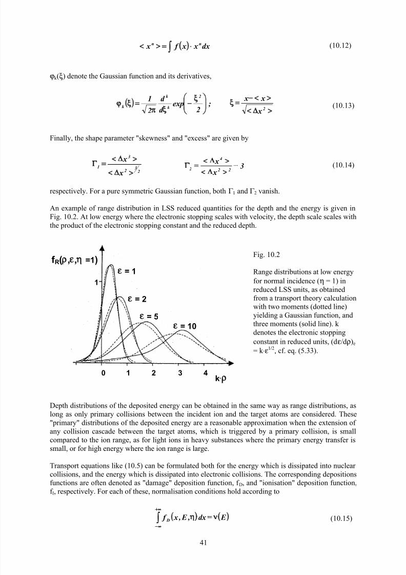
7/31/2019 Fundamentals of Ion-surface Interaction
http://slidepdf.com/reader/full/fundamentals-of-ion-surface-interaction 41/77
41
ϕk (ξ) denote the Gaussian function and its derivatives,
Finally, the shape parameter "skewness" and "excess" are given by
respectively. For a pure symmetric Gaussian function, both Γ 1 and Γ 2 vanish.
An example of range distribution in LSS reduced quantities for the depth and the energy is given in
Fig. 10.2. At low energy where the electronic stopping scales with velocity, the depth scale scales with
the product of the electronic stopping constant and the reduced depth.
Depth distributions of the deposited energy can be obtained in the same way as range distributions, aslong as only primary collisions between the incident ion and the target atoms are considered. These
"primary" distributions of the deposited energy are a reasonable approximation when the extension of
any collision cascade between the target atoms, which is triggered by a primary collision, is small
compared to the ion range, as for light ions in heavy substances where the primary energy transfer is
small, or for high energy where the ion range is large.
Transport equations like (10.5) can be formulated both for the energy which is dissipated into nuclear
collisions, and the energy which is dissipated into electronic collisions. The corresponding depositions
functions are often denoted as "damage" deposition function, f D, and "ionisation" deposition function,
f I, respectively. For each of these, normalisation conditions hold according to
;2
expd d
21
2
k
k
k
dx x x f x nn
2 x x x
23
2
3
1
x
x 3
x
x 22
4
2
Fig. 10.2
Range distributions at low energy
for normal incidence (η = 1) in
reduced LSS units, as obtained
from a transport theory calculation
with two moments (dotted line)
yielding a Gaussian function, and
three moments (solid line). k
denotes the electronic stopping
constant in reduced units, (dε/dρ)e
= k ⋅ε1/2, cf. eq. (5.33).
(10.12)
(10.13)
(10.14)
(10.15) E dx , E , x f D
0 1 2 3 4
1
f R( , , =1)
= 1
= 2 = 5
= 10
k
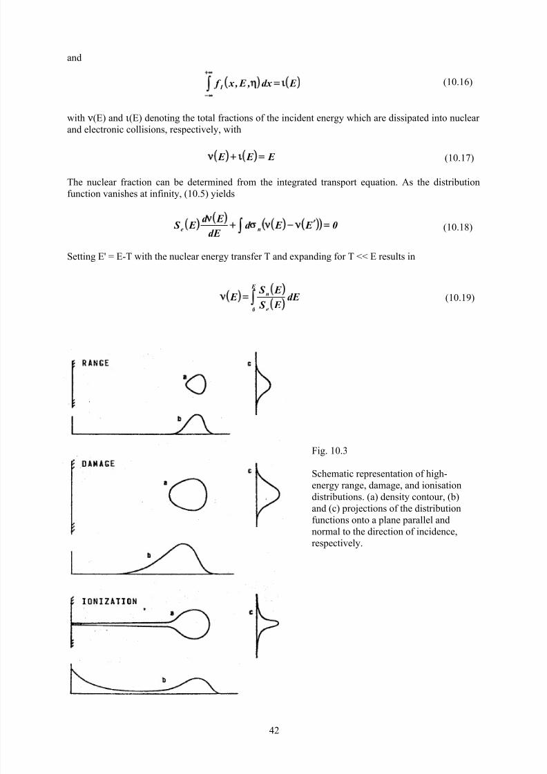
7/31/2019 Fundamentals of Ion-surface Interaction
http://slidepdf.com/reader/full/fundamentals-of-ion-surface-interaction 42/77
42
and
with ν(E) and ι(E) denoting the total fractions of the incident energy which are dissipated into nuclear
and electronic collisions, respectively, with
The nuclear fraction can be determined from the integrated transport equation. As the distribution
function vanishes at infinity, (10.5) yields
Setting E' = E-T with the nuclear energy transfer T and expanding for T << E results in
E dx , E , x f I (10.16)
E E E (10.17)
0 E E d dE
E d E S ne (10.18)
dE E S
E S E
E
0 e
n(10.19)
Fig. 10.3
Schematic representation of high-
energy range, damage, and ionisation
distributions. (a) density contour, (b)
and (c) projections of the distribution
functions onto a plane parallel and
normal to the direction of incidence,
respectively.

7/31/2019 Fundamentals of Ion-surface Interaction
http://slidepdf.com/reader/full/fundamentals-of-ion-surface-interaction 43/77
43
Corresponding evaluations and tabulations can be found in the literature. Fig. 10.3 shows a schematic
representation of high-energy range, damage and ionisation distributions in three dimensions. At small
depth, the nuclear energy deposition is small due to the low scattering cross section at high energy.
Towards the end of the ion trajectories, the ion energy and thereby the nuclear energy dissipation
becomes low, so that the damage distribution normally peaks at slightly lower depth than the range
distribution. However, it has to be taken into account that multiple large angle deflections, which
occur with increasing probability towards the end of the range, may result in multiple energy
deposition events at the same depth for only one incident ion. This also explains the peak of theionisation distribution function at large depth. Otherwise, it reflects the dependence of electron
stopping on energy.
10.2 Distributions of Energy Deposition Including Collision Cascades
In the general case, secondary collision cascades of the target atoms have to be taken into account for
the calculation of the energy deposition. This is mandatory for ion-target combinations with about
equal masses, and for sufficiently low energies.
The validity of the linear cascade regime is assumed. The secondary recoil atoms have to be taken intoaccount which are generated in nuclear collisions (see Fig. 10.4, case (3)). For the treatment of nuclear
energy deposition, the three-dimensional "damage" distribution function is defined in such a way that
the differential amount of energy
is dissipated into the volume element d3r around r, at given incident energy E and direction η. Adding
to the nuclear collision term of eq. (10.1) a term for the recoil atom, with an initial energy equal to the
nuclear energy transfer T and an initial direction η'', results in
Similarly as above and with
the transport equation results as
x
0 x+ xx
E,
1
2
3
Fig. 10.4
Schematic of the transport
mechanism when including
secondary recoil atoms
r d r , , E F dE 3
Dn
vvv(10.20)
r , ,T F r , ,T E F T E E d r nr r , , E F D Dn D
vvvvvvvv
r , , E E F E E E d r nZ Del 2
vvv
r , , E F d r nZ d r n1 Del 2n
vvvv
(10.21)
r
r v
vv (10.22)
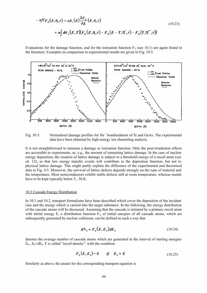
7/31/2019 Fundamentals of Ion-surface Interaction
http://slidepdf.com/reader/full/fundamentals-of-ion-surface-interaction 44/77
44
Evaluations for the damage function, and for the ionisation function FI (see 10.1) are again found in
the literature. Examples in comparison to experimental results are given in Fig. 10.5.
Fig. 10.5: Normalised damage profiles for He+ bombardment of Si and GaAs. The experimental
data have been obtained by high-energy ion channeling analysis.
It is not straightforward to measure a damage or ionisation function. Only the post-irradiation effects
are accessible to experiments, as, e.g., the amount of remaining lattice damage. In the case of nuclear energy deposition, the creation of lattice damage is subject to a threshold energy of a recoil atom (see
ch. 12), so that low energy transfer events will contribute to the deposition function, but not to
physical lattice damage. This might partly explain the difference of the experimental and theoretical
data in Fig. 9.5. Moreover, the survival of lattice defects depends strongly on the type of material and
the temperature. Most semiconductors exhibit stable defects still at room temperature, whereas metals
have to be kept typically below 5...30 K.
10.3 Cascade Energy Distribution
In 10.1 and 10.2, transport formalisms have been described which cover the deposition of the incident
ions and the energy which is carried into the target substance. In the following, the energy distributionof the cascade atoms will be discussed. Assuming that the cascade is initiated by a primary recoil atom
with initial energy E, a distribution function FE of initial energies of all cascade atoms, which are
subsequently generated by nuclear collisions, can be defined in such a way that
denotes the average number of cascade atoms which are generated in the interval of starting energies
E0...E0+dE0. F is called "recoil density", with the condition
Similarly as above, the ansatz for the corresponding transport equation is
r , , E E
F E nS r , , E F D
e D
vvvvvv
r , ,T F r , ,T E F r , , E F T , E d n D D Dn
vvvvvv
(10.23)
00 E 0 dE E , E F dN (10.24)
E E if 0 E , E F 00 E (10.25)

7/31/2019 Fundamentals of Ion-surface Interaction
http://slidepdf.com/reader/full/fundamentals-of-ion-surface-interaction 45/77
45
Formally compared to eq. (10.21), an additional nuclear collision term has to be taken which describes
the direct conversion of the primary atom to an atom with energy E0. This is not contained in the
second term as a starting energy of E0 will not contribute by further collision according to (10.25). The
Taylor expansions, as formerly, yield
If electronic stopping is neglected in view of the rather low energy of most of the cascade atoms, and
the nuclear scattering cross section is evaluated for the power-law screening function (2.16), (10.27)
can be solved analytically by using Laplace transforms and the convolution theorem, yielding
where m = s-1
denotes the inverse of the power index of the screening function (see (2.16)) and
with Γ (y) denoting the Gamma function, and
According to (10.28), the number of cascade atoms scales with the inverse square of their starting
energy (so-called "Coulomb" spectrum), so that (10.28) describes the vast amount of all cascadeatoms. The cascade density diverges with E0→0, which is a contradiction with the assumption of a
linear cascade. However, the lattice atoms are bound to their original sites which has been neglected so
far. With a binding energy U, an approximate solution is, replacing (10.28)
Taking electronic stopping rigorously into account would be rather complicated. Therefore, the total
available energy E is simply replaced by the fraction which is dissipated in nuclear rather than
electronic collisions, resulting in (if the binding is neglected again)
0n00 E E E xd ndE E , E F
00 E 0 E n dE E ,T F E ,T E F T E E d x n
00 E el 2 dE E , E E F E E E d x nZ
00 E el 2n dE E , E F d x nZ d x n1
0 E 0 E 0 E n E , E F E ,T F E ,T E F T E E d
0
0
n
0 E el E E dE
d E , E F
E E S
(10.26)
(10.27)
E E if E
E
m11
m E , E F 02
0
0 E (10.28)
ylog dy
d y (10.29)
E E if 1 E
E
E
1
m11
m E , E F 0
m
00
0 E ~ (10.30)
E U E if E U E
E
m11
m E , E F 0m1
0
m1
0
0 E (10.31)~
2
0
0 E E
E
m11
m E , E F (10.32)
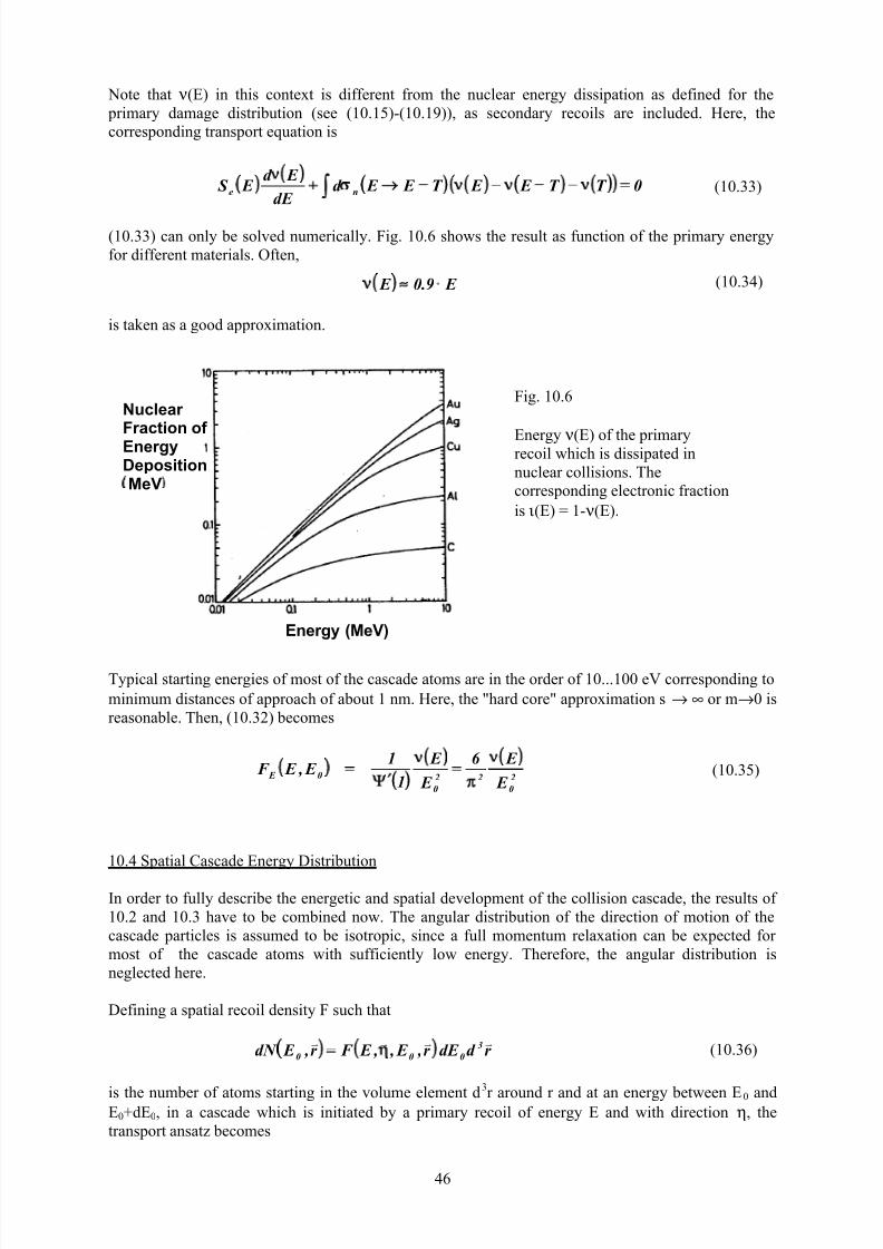
7/31/2019 Fundamentals of Ion-surface Interaction
http://slidepdf.com/reader/full/fundamentals-of-ion-surface-interaction 46/77
46
Note that ν(E) in this context is different from the nuclear energy dissipation as defined for the
primary damage distribution (see (10.15)-(10.19)), as secondary recoils are included. Here, the
corresponding transport equation is
(10.33) can only be solved numerically. Fig. 10.6 shows the result as function of the primary energy
for different materials. Often,
is taken as a good approximation.
Typical starting energies of most of the cascade atoms are in the order of 10...100 eV corresponding to
minimum distances of approach of about 1 nm. Here, the "hard core" approximation s → ∞ or m→0 is
reasonable. Then, (10.32) becomes
10.4 Spatial Cascade Energy Distribution
In order to fully describe the energetic and spatial development of the collision cascade, the results of
10.2 and 10.3 have to be combined now. The angular distribution of the direction of motion of the
cascade particles is assumed to be isotropic, since a full momentum relaxation can be expected for
most of the cascade atoms with sufficiently low energy. Therefore, the angular distribution is
neglected here.
Defining a spatial recoil density F such that
is the number of atoms starting in the volume element d3
r around r and at an energy between E0 andE0+dE0, in a cascade which is initiated by a primary recoil of energy E and with direction η, the
transport ansatz becomes
2
0
22
0
0 E E
E 6
E
E
1
1 E , E F
(10.33)0T T E E T E E d dE
E d E S ne
E 9 .0 E (10.34)
Fig. 10.6
Energy ν(E) of the primaryrecoil which is dissipated in
nuclear collisions. The
corresponding electronic fraction
is ι(E) = 1- ν(E).
(10.35)
r d dE r , E , , E F r , E dN 3
000
vvvv(10.36)
Energy (MeV)
Nuclear Fraction of EnergyDepositionMeV

7/31/2019 Fundamentals of Ion-surface Interaction
http://slidepdf.com/reader/full/fundamentals-of-ion-surface-interaction 47/77
47
with the resulting transport equation
with the conditions
and
The solution of eq. (10.38) proceeds via moment equations (for comparison, see eq. (10.9)). For the
higher moments, the cutoff condition, eq. (10.39), is neglected, as the few additional high-energyatoms, which are artificially included, will little influence the main fraction of the cascade atoms.
Then, the solution is straightforward. With the correct normalisation, the result is
which is plausible as it simply combines the damage function (see eq. (10.20)) with the recoil density
(eq. (10.35)).
11. Binary Collision Approximation Computer Simulation of Ion and Energy Deposition
As demonstrated in the preceding chapter, transport theory calculations of ion slowing down and the
associated recoils atoms, in the linear cascade regime, can provide valuable analytical expressions
which describe the important physical mechanisms and dependencies. However, the solutions are
often complicated and require simplifying assumptions. A major obstacle, e.g., is the treatment of the
surface, as the transport equations can, without considerable additional effort, be solved only in an
infinite medium, thus describing the physical situation of an internally starting beam. The treatment of
an infinite medium in the transport calculations allows for multiple crossing of a given recoil
trajectory through an arbitrary plane in the substance, whereas in reality the particle is lost when firstcrossing the surface. Therefore, also the formation of collision cascades near the surface is
overestimated in infinite medium calculations. This problem arises in particular for low energies
and/or heavy ions with a significant fraction of the total energy being deposited very close to the
r E E d r nr r , E , , E F 0n0
vvvvv
r , E , , E E F E E E d r nZ 0el 2
vvv
r , E , , E F d r nZ d r n1 0 Del 2n
vvvv
r , E , ,T F r , E , ,T E F T E E d r n 00n
vvvvv
(10.37)
r , E , , E E
F E nS r
dE
E E d nr , E , , E F 0e
0
0
0
vvvvvvv
r , E , ,T F r , E , ,T E F r , E , , E F d n 0 D00n
vvvvvv
(10.38)
E E if 0r , E , , E F 00
vv
0 E
3
0 E , E F r d r , E , , E F vvv
(10.39)
(10.40)
2
0
D
20 E
r , , E F 6 r , E , , E F
vvvv
(10.41)
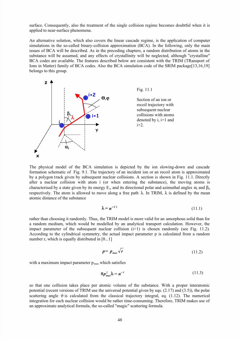
7/31/2019 Fundamentals of Ion-surface Interaction
http://slidepdf.com/reader/full/fundamentals-of-ion-surface-interaction 48/77
48
surface. Consequently, also the treatment of the single collision regime becomes doubtful when it is
applied to near-surface phenomena.
An alternative solution, which also covers the linear cascade regime, is the application of computer
simulations in the so-called binary-collision approximation (BCA). In the following, only the main
issues of BCA will be described. As in the preceding chapters, a random distribution of atoms in the
substance will be assumed, and any effects of crystallinity will be neglected, although "crystalline"
BCA codes are available. The features described below are consistent with the TRIM (TRansport of Ions in Matter) family of BCA codes. Also the BCA simulation code of the SRIM package[13,16,19]
belongs to this group.
The physical model of the BCA simulation is depicted by the ion slowing-down and cascade
formation schematic of Fig. 9.1. The trajectory of an incident ion or an recoil atom is approximated
by a polygon track given by subsequent nuclear collisions. A section is shown in Fig. 11.1. Directlyafter a nuclear collision with atom i (or when entering the substance), the moving atoms is
characterised by a state given by its energy E i, and its directional polar and azimuthal angles αi and βi,
respectively. The atom is allowed to move along a free path λ. In TRIM, λ is defined by the mean
atomic distance of the substance
rather than choosing it randomly. Thus, the TRIM model is more valid for an amorphous solid than for
a random medium, which would be modelled by an analytical transport calculation. However, the
impact parameter of the subsequent nuclear collision (i+1) is chosen randomly (see Fig. 11.2).
According to the cylindrical symmetry, the actual impact parameter p is calculated from a random
number r, which is equally distributed in [0...1]
with a maximum impact parameter pmax which satisfies
so that one collision takes place per atomic volume of the substance. With a proper interatomic
potential (recent versions of TRIM use the universal potential given by eqs. (2.17) and (3.5)), the polar
scattering angle ϑ is calculated from the classical trajectory integral, eq. (1.12). The numericalintegration for each nuclear collision would be rather time-consuming. Therefore, TRIM makes use of
an approximate analytical formula, the so-called "magic" scattering formula.
Fig. 11.1
Section of an ion or
recoil trajectory with
subsequent nuclear
collisions with atoms
denoted by i, i+1 andi+2.
31n (11.1)
r p p max (11.2)
x
z
i
i
i i+1
i+2
12
max n p (11.3)
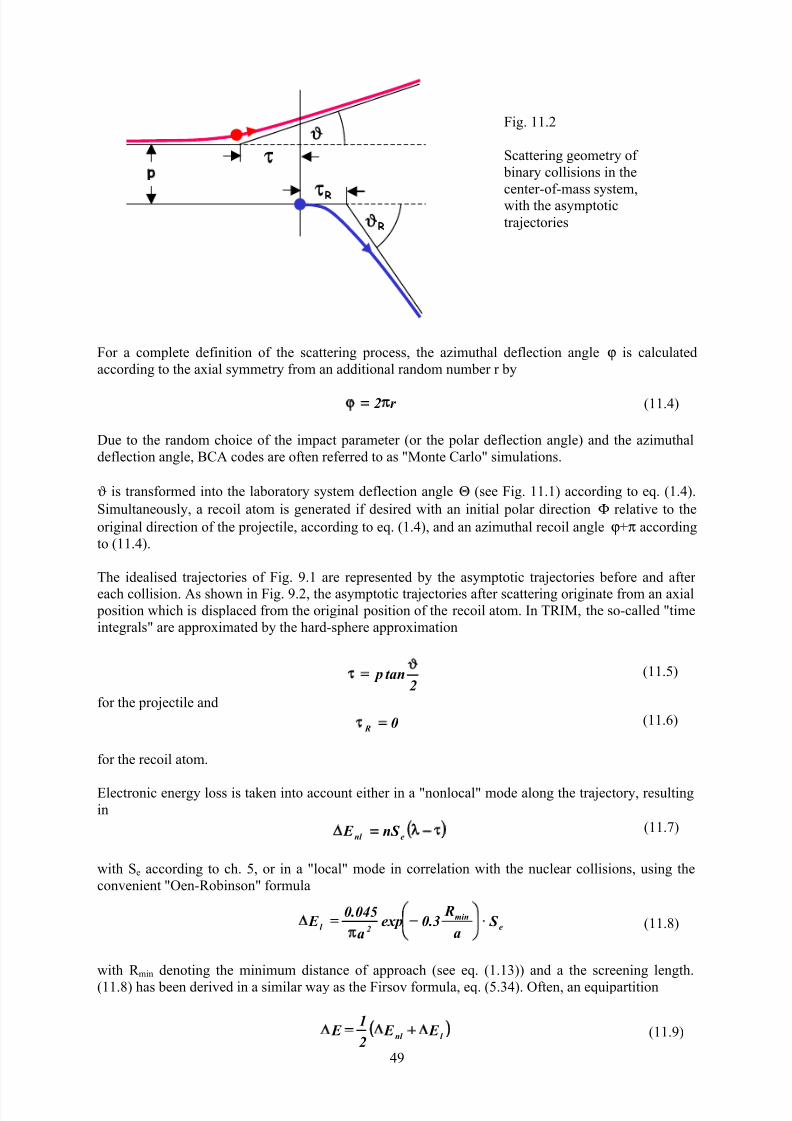
7/31/2019 Fundamentals of Ion-surface Interaction
http://slidepdf.com/reader/full/fundamentals-of-ion-surface-interaction 49/77
49
For a complete definition of the scattering process, the azimuthal deflection angle ϕ is calculated
according to the axial symmetry from an additional random number r by
Due to the random choice of the impact parameter (or the polar deflection angle) and the azimuthal
deflection angle, BCA codes are often referred to as "Monte Carlo" simulations.
ϑ is transformed into the laboratory system deflection angle Θ (see Fig. 11.1) according to eq. (1.4).
Simultaneously, a recoil atom is generated if desired with an initial polar direction Φ relative to the
original direction of the projectile, according to eq. (1.4), and an azimuthal recoil angle ϕ+π according
to (11.4).
The idealised trajectories of Fig. 9.1 are represented by the asymptotic trajectories before and after
each collision. As shown in Fig. 9.2, the asymptotic trajectories after scattering originate from an axial position which is displaced from the original position of the recoil atom. In TRIM, the so-called "time
integrals" are approximated by the hard-sphere approximation
for the projectile and
for the recoil atom.
Electronic energy loss is taken into account either in a "nonlocal" mode along the trajectory, resulting
in
with Se according to ch. 5, or in a "local" mode in correlation with the nuclear collisions, using the
convenient "Oen-Robinson" formula
with R min denoting the minimum distance of approach (see eq. (1.13)) and a the screening length.
(11.8) has been derived in a similar way as the Firsov formula, eq. (5.34). Often, an equipartition
Fig. 11.2
Scattering geometry of
binary collisions in the
center-of-mass system,with the asymptotic
trajectories
r 2 (11.4)
R
R
2tan p (11.5)
0 R(11.6)
enl nS E (11.7)
e
min
2l S a
R3 .0exp
a
045 .0 E (11.8)
l nl E E 2
1 E (11.9)

7/31/2019 Fundamentals of Ion-surface Interaction
http://slidepdf.com/reader/full/fundamentals-of-ion-surface-interaction 50/77
50
is chosen rather arbitrarily.
Including the nuclear energy transfer T (eq. (1.6)), the transformation of the state of the projectile is
now given by
and
where TR denotes the geometrical transformation to the new directional angles. When recoils are
included, the initial state of the generated recoil is given by
and
In (11.12), U b denotes the bulk binding energy of the lattice atoms (a few eV, often it is set to zero due
to the lack of better knowledge).
The trajectories of each incident ion, and, if included in the simulation, all associated recoil atoms are
traced in this way until the kinetic energy has fallen below the cutoff energy E co, which again is chosento several eV (see remark at the beginning of ch. 9).
E T E E i 1i (11.10)
i
i
1i
1i ,TR (11.11)
b1 U T E (11.12)
i
i
1
1
,TR (11.13)
0 20 40 0 20 40 60
0
0
-20
-20
20
20
(a) (b)
(c) (d)
20 keV N Fe
Depth (nm)
LateralSpread(nm)
Fig. 11.3
Ion only (a,c) and ion
plus recoil (b,d)trajectories for 20 keV
nitrogen ions incident on
iron, for 5 (a,b) and 100
(c,d) incident ions, as
obtained from a TRIM
computer simulation.
The three-dimensional
trajectories are projected
onto a plane. Note that
the pairs (a,b) and (c,d)
each represent different
runs with different iontrajectories.
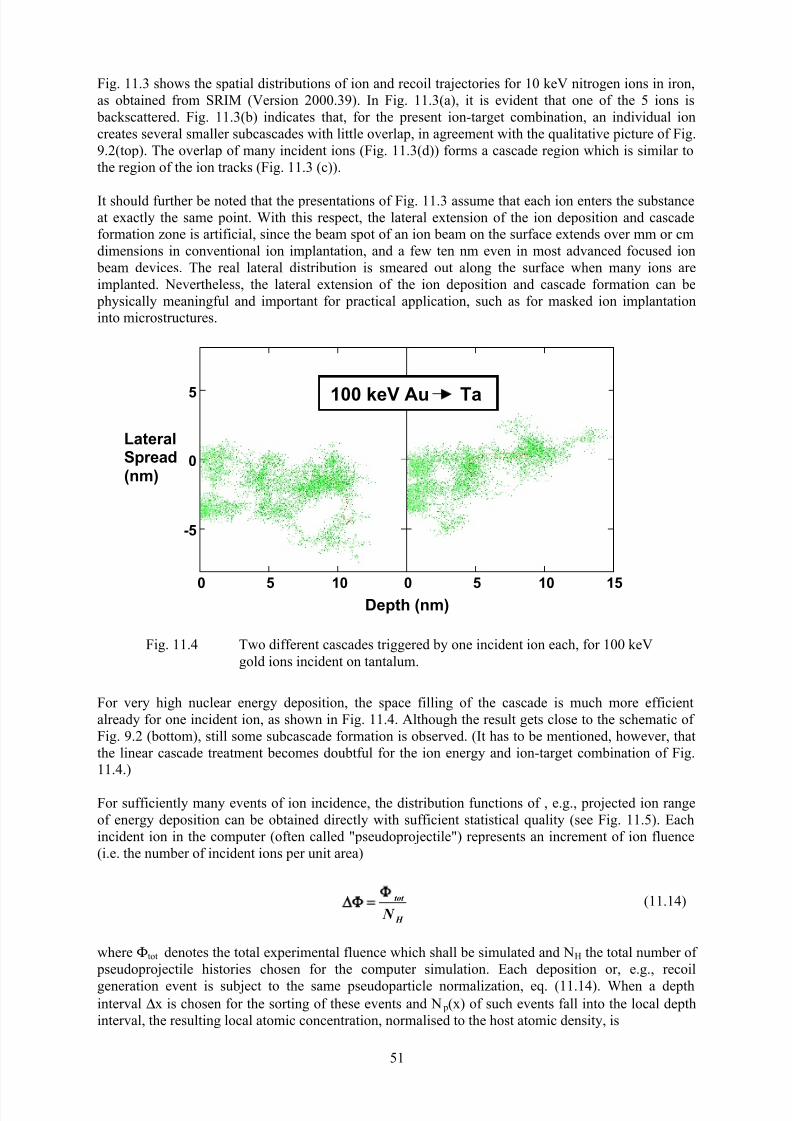
7/31/2019 Fundamentals of Ion-surface Interaction
http://slidepdf.com/reader/full/fundamentals-of-ion-surface-interaction 51/77
51
Fig. 11.3 shows the spatial distributions of ion and recoil trajectories for 10 keV nitrogen ions in iron,
as obtained from SRIM (Version 2000.39). In Fig. 11.3(a), it is evident that one of the 5 ions is
backscattered. Fig. 11.3(b) indicates that, for the present ion-target combination, an individual ion
creates several smaller subcascades with little overlap, in agreement with the qualitative picture of Fig.
9.2(top). The overlap of many incident ions (Fig. 11.3(d)) forms a cascade region which is similar to
the region of the ion tracks (Fig. 11.3 (c)).
It should further be noted that the presentations of Fig. 11.3 assume that each ion enters the substanceat exactly the same point. With this respect, the lateral extension of the ion deposition and cascade
formation zone is artificial, since the beam spot of an ion beam on the surface extends over mm or cm
dimensions in conventional ion implantation, and a few ten nm even in most advanced focused ion
beam devices. The real lateral distribution is smeared out along the surface when many ions are
implanted. Nevertheless, the lateral extension of the ion deposition and cascade formation can be
physically meaningful and important for practical application, such as for masked ion implantation
into microstructures.
For very high nuclear energy deposition, the space filling of the cascade is much more efficient
already for one incident ion, as shown in Fig. 11.4. Although the result gets close to the schematic of
Fig. 9.2 (bottom), still some subcascade formation is observed. (It has to be mentioned, however, that
the linear cascade treatment becomes doubtful for the ion energy and ion-target combination of Fig.
11.4.)
For sufficiently many events of ion incidence, the distribution functions of , e.g., projected ion range
of energy deposition can be obtained directly with sufficient statistical quality (see Fig. 11.5). Each
incident ion in the computer (often called "pseudoprojectile") represents an increment of ion fluence
(i.e. the number of incident ions per unit area)
where Φtot denotes the total experimental fluence which shall be simulated and NH the total number of
pseudoprojectile histories chosen for the computer simulation. Each deposition or, e.g., recoil
generation event is subject to the same pseudoparticle normalization, eq. (11.14). When a depthinterval ∆x is chosen for the sorting of these events and N p(x) of such events fall into the local depth
interval, the resulting local atomic concentration, normalised to the host atomic density, is
0 5 10 0 5 10 15
0
-5
5
LateralSpread(nm)
Depth (nm)
100 keV Au Ta
Fig. 11.4 Two different cascades triggered by one incident ion each, for 100 keV
gold ions incident on tantalum.
H
tot
N (11.14)

7/31/2019 Fundamentals of Ion-surface Interaction
http://slidepdf.com/reader/full/fundamentals-of-ion-surface-interaction 52/77
52
In this way, the ordinate of Fig. 11.5 is defined by c(x)/Φtot. Nevertheless, it should be pointed out that
standard TRIM computer simulations are only valid for the low-fluence limit, so that the results cannot
readily be extrapolated to high fluences with, e.g., resulting implant concentrations close to
stoichiometry or even above, which would be meaningless. In the BCA simulations discussed here,
each incident projectile finds the same, unmodified substance that any effects of, e.g., ion deposition
or surface erosion (see ch. 13) are neglected.
In a similar way, distribution functions of deposited energy can be obtained (Fig. 11.6). The electronic
energy dissipation is sometimes called "ionisation" (such as in SRIM-2000), although the latter
contributes only a fraction (see ch. 5). Also in SRIM-2000, the nuclear energy dissipation is called
"energy to recoils". Note that the definition of nuclear energy dissipation is only meaningful for
primary collisions of the incident ions with target atoms. For the complete cascade, the nuclear energy
deposition vanishes as the nuclear collisions are elastic (or results from the lattice binding only). For
the present ion-target combination, the total fractions of the ion energy which are dissipated into
electronic and nuclear collisions are about equal, in agreement with the fact that electronic and nuclear
stopping in the present energy range are about equal. The mean depth of electronic energy dissipation
is somewhat lower than that of the nuclear counterpart, as electronic stopping decreases more rapidly
with decreasing energy. Although the number of recoils exceeds the number of incident ions by orders
of magnitude, the electronic contribution of the recoils to the energy distribution is small, due to their
small average energy.
Finally a general comment related to BCA computer simulation shall be given. Obviously, the results
depend critically on the choice of certain input parameters, such as the cutoff energy, but they depend
also to a certain extent on "hidden" parameters such as the choice of the interatomic potential or the
choice of the electronic stopping (see eqs. (11.7-9)). By varying these "hidden" inputs within
reasonable limits, variations of the results for, e.g. ranges or energy deposition function, up to several
10% can be obtained. This depends, however, very much on the given problem and the energy range.
Ion ranges obtained from TRIM are normally reliable within 10%.
0 20 40 60
Depth (nm)
Concentration
0
1
2
3Ion Fluence
105
atoms / cm3
ions / cm2 ( )
Fig. 11.5
Projected range distribution
of 20 keV nitrogen ions
implanted into iron, from a
TRIM simulation with 20000
pseudoprojectiles (see Fig.
11.3). The mean projected
range is R p = 24.5 nm, the
standard deviation σ = 12 nm,
the skewness Γ 1 = 0.19, and
the kurtosis Γ 2 = 2.4.
H
tot p
N x n
x N x c (11.15)
20 keV N Fe

7/31/2019 Fundamentals of Ion-surface Interaction
http://slidepdf.com/reader/full/fundamentals-of-ion-surface-interaction 53/77
53
12. Radiation Damage
12.1 Analytical Treatment
The term "radiation damage of materials" covers a wide area of effects which can be observed after
irradiation of a solid with energetic particles. In the present "collisional" picture in the linear-cascade
regime (see beginning of ch. 9) only the initial stage of damage is considered, which is caused by the
permanent displacement of lattice atoms from their original sites by the energy transfer received in
nuclear collisions. It should be mentioned that, in particular in certain oxides but also in other
materials at extremely high energy density which is deposited into electronic collisions, electronicenergy dissipation can be converted into atomic displacement. Further, the restriction to the initial
stage of damage applies only to selected physical situations. It represents a low-fluence approximation
since any interaction of the resulting defects is neglected. It is also a low-temperature approximation
since any thermal migration or recombination of the defects is neglected. However, the definition of
low temperature in this context depends critically on the choice of the material. In metals, simple point
defects may become mobile already at a few K, whereas they are stable around room temperature in
common semiconductors.
Fig. 12.1 depicts the elementary event of radiation damage schematically. In order to produce a
"stable" Frenkel pair consisting of a vacancy at the original site of the recoil and an interstitial atom at
its final position, the distance between the interstitial-vacancy has to be sufficiently large so that an
immediate recombination due to elastic forces in the lattice and/or due to directed atomic bonds is prevented. Therefore, the initial energy transfer to the recoil has to be sufficiently large. This critical
energy transfer depends on the crystalline direction into which the recoil is set into motion. Therefore,
0 20 40 60
Depth (nm)
0
100
200
300
100
200
300
0
400
DepositedEnergy(eV / nm)
20 keV N Fe
Electronic
Nuclear
by Ions
by Recoils
Fig. 11.6
Distribution of deposited
energy into electronic (top)and nuclear (bottom)
collisions for one 20 keV
nitrogen ion implanted into
iron, from a full-cascade
TRIM simulation with 2000
pseudoprojectiles (see Fig.
11.3). The electronic fraction
is split into the energy loss by
the incident ions and by all
recoil atoms in the collision
cascade. The nuclear energy
deposition results only from
primary collisions (see text).

7/31/2019 Fundamentals of Ion-surface Interaction
http://slidepdf.com/reader/full/fundamentals-of-ion-surface-interaction 54/77
54
the "displacement threshold" energy Ud must be understood as an average over different directions.
Thus, for any recoil starting with an initial energy transfer T below the threshold energy, the number
of generated Frenkel pairs is close to zero, even if secondary recoils in a subsequent collision cascade
are taken into account.
.
After terminating the collision cascade, a stable Frenkel pair is characterised by its formation energy
Uf , i.e. the gain of potential energy with respect to the undisturbed lattice, with a contribution from the
vacancy and the interstitial atom:
Apparently, the bulk binding energy U b is smaller than the Frenkel pair formation energy. On the other
hand, the displacement threshold energy must be larger than the Frenkel pair formation energy since
kinetic energy is dissipated during the slowing down of the recoil. Thus
Typical bulk binding energies are a few eV, compared to Frenkel pair formation energies of 5 to 10 eV
and displacement threshold energies of 20 to 80 eV.
There are other mechanisms than the simple transfer of a recoil depicted in Fig. 12.1. For low recoil
energies, so-called "replacement" collision sequences become increasingly important (Fig. 12.2),
which travel in particular in low-indexed directions of a crystal being "focussed" by the potential
resulting from the surrounding atoms, but contribute significantly even in amorphous materials. In
head-on sequences, the nuclear energy loss is effectively switched off in homonuclear materials, so
that the range can become rather large (up to a few hundred atomic distances).
With these considerations, a displacement probability can be defined for each recoil starting with an
energy E0, according to
Fig. 12.1
Elementary radiation damage event in
a collision cascade. A recoil atom
generated by a nuclear collision is
moved from its original site into an
interstitial position, thus forming a
vacancy- interstitial or "Frenkel" pair.
if vf f U U U (12.1)
d f b U U U (12.2)
Fig. 12.2
Schematic of a replacement
collision sequence.
0d E P
d 0 U E if 0
d 0d
d
d 0 U 2 E U if U
U E
d 0 U 2 E if 1(12.3)

7/31/2019 Fundamentals of Ion-surface Interaction
http://slidepdf.com/reader/full/fundamentals-of-ion-surface-interaction 55/77
55
which is depicted in Fig. 12.3. The middle expression of eq. (12.3) shall, in a rather handwaving way,
take into account the reduction of Frenkel pair production per recoil atom due to replacement
collisions at low energy transfers, as many correlated over-threshold recoils generate only one Frenkel
pair.
The total number of Frenkel pairs for one recoil atom starting with energy T, including the complete
associated cascade, is then given by
with FE denoting the recoil density (see sect. 10.3). Inserting eqs. (10.35) and (12.3) results in
This is the so-called "modified Kinchin-Pease" formula. It has to be noted that the bulk binding energy
is implicitly neglected (see sect. 10.3). Originally, Kinchin and Pease had treated the problem using
hard spheres rather than a screened Coulomb potential, and consequently neglecting inelastic energy
loss, resulting in
which, compared to (12.4), makes hardly a difference in view of the theoretical approximations and
the experimental uncertainties in determining NF. Formally, eq. (12.4) allows for subthreshold
damage, too. Therefore, a corrected formula is often employed, where eq. (10.34) for the nuclear deposited energy has already been used:
.
The energy range of the middle contribution guarantees a continuous transition to the modified
Kinchin-Pease formula.
The total number of Frenkel pairs generated by an incident ion of energy E is obtained by integrating
NF(T) according to the cross section of nuclear collisions and along the ion path:
Eo / Ud 0 1 2
Pd(Eo)
0
1
Fig. 12.3
Displacement probability
model employed for the
modified Kinchin-Pease
model.
d d
2F U
T 42 .0
U
T 2log 6 T N (12.5)
d U T if 0
d d U 63 .2T U if 1T N F
elseU
T 38 .0
d
(12.7)
00 E 0
T
U
d F dE E ,T F E P T N
d
(12.4)
d
F U 2
T T N (12.6)

7/31/2019 Fundamentals of Ion-surface Interaction
http://slidepdf.com/reader/full/fundamentals-of-ion-surface-interaction 56/77
56
where γ denotes the energy transfer factor (eq. (1.7)). Inserting the simple Kinchin-Pease result, eq.
(12.6), for simplicity, and assuming an average energy transfer γ E' which is large compared to thedisplacement threshold, the inner integral in (12.8) can, in reasonable approximation, be replaced by
the nuclear stopping cross section Sn. For such a "dense cascade", which occurs for large nuclear
energy deposition, electronic stopping is small, so that Stot ≈ Sn. Thus, in the dense cascade
approximation, the total damage is given by the simple Kinchin-Pease expression with the incident
energy:
All above results for the Frenkel pair generation represent an upper limit since a certain amount of
"dynamic annealing" will take place already in the collisional phase, given by the probability of
recombination of interstitial atoms with vacancies. This probability of dynamic recombinationincreases with increasing cascade density. In this sense, a "cascade efficiency" ξ(T) is defined so that
the effective number of Frenkel pairs is given by
The cascade efficiency is between 1 in the low-density limit (e.g., light ions) and about 0.3 for very
dense cascades for heavy ions with large nuclear stopping.
12.2 TRIM Computer Simulation
There are two different possibilities to treat damage in TRIM computer simulations. In the so-called
"quick" calculation of damage just the ion trajectory is traced rather than the complete collision
cascade. For each primary collision with energy transfer T to the primary recoil, eq. (12.6) is applied
for the generation of Frenkel pair at each primary nuclear collision. In addition to the approximations
implied in the Kinchin-Pease formula, this simplified simulation neglects the spatial extension of the
individual subcascades. If the latter is small compared to the ion range, such as for light ions or at
sufficiently high energy, the error with respect to the depth distribution remains small.
0 20 40 60
Depth (nm)
0
5
10
Frenkel Pair Distribution(nm-1)
Fig. 12.4
Depth distribution of Frenkel
pairs generated by one 20 keV
nitrogen ion incident on iron, as
obtained from a full cascade
TRIM computer simulation with
2000 pseudoprojectiles, with a
displacement threshold energy of
25 eV. The average total number
of Frenkel pairs per ion is 240.
dT dT
T , E d T N
E S
E d E N n
E
U
F
E
0 tot
tot
F
d
(12.8)
d
tot
F U 2
E E N (12.9)
T N T T N F
eff
F (12.10)
20 keV N Fe
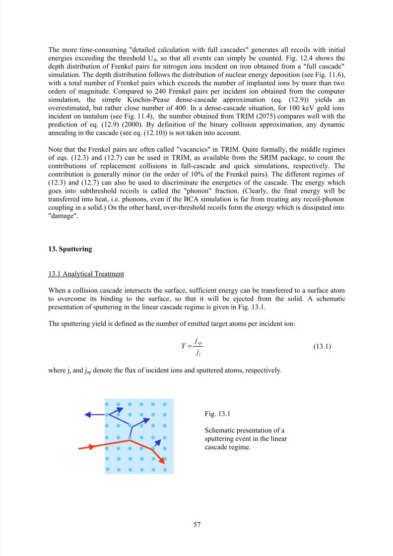
7/31/2019 Fundamentals of Ion-surface Interaction
http://slidepdf.com/reader/full/fundamentals-of-ion-surface-interaction 57/77
57
The more time-consuming "detailed calculation with full cascades" generates all recoils with initial
energies exceeding the threshold Ud, so that all events can simply be counted. Fig. 12.4 shows the
depth distribution of Frenkel pairs for nitrogen ions incident on iron obtained from a "full cascade"
simulation. The depth distribution follows the distribution of nuclear energy deposition (see Fig. 11.6),
with a total number of Frenkel pairs which exceeds the number of implanted ions by more than two
orders of magnitude. Compared to 240 Frenkel pairs per incident ion obtained from the computer
simulation, the simple Kinchin-Pease dense-cascade approximation (eq. (12.9)) yields anoverestimated, but rather close number of 400. In a dense-cascade situation, for 100 keV gold ions
incident on tantalum (see Fig. 11.4), the number obtained from TRIM (2075) compares well with the
prediction of eq. (12.9) (2000). By definition of the binary collision approximation, any dynamic
annealing in the cascade (see eq. (12.10)) is not taken into account.
Note that the Frenkel pairs are often called "vacancies" in TRIM. Quite formally, the middle regimes
of eqs. (12.3) and (12.7) can be used in TRIM, as available from the SRIM package, to count the
contributions of replacement collisions in full-cascade and quick simulations, respectively. The
contribution is generally minor (in the order of 10% of the Frenkel pairs). The different regimes of
(12.3) and (12.7) can also be used to discriminate the energetics of the cascade. The energy which
goes into subthreshold recoils is called the "phonon" fraction. (Clearly, the final energy will be
transferred into heat, i.e. phonons, even if the BCA simulation is far from treating any recoil-phonon
coupling in a solid.) On the other hand, over-threshold recoils form the energy which is dissipated into
"damage".
13. Sputtering
13.1 Analytical Treatment
When a collision cascade intersects the surface, sufficient energy can be transferred to a surface atomto overcome its binding to the surface, so that it will be ejected from the solid. A schematic
presentation of sputtering in the linear cascade regime is given in Fig. 13.1.
The sputtering yield is defined as the number of emitted target atoms per incident ion:
where ji and jsp denote the flux of incident ions and sputtered atoms, respectively.
Fig. 13.1
Schematic presentation of a
sputtering event in the linear
cascade regime.
i
sp
j
jY = (13.1)

7/31/2019 Fundamentals of Ion-surface Interaction
http://slidepdf.com/reader/full/fundamentals-of-ion-surface-interaction 58/77
58
Applying cascade transport theory, now - in contrast to the treatment of radiation damage - the spatial
development of the cascade has to be taken into account in addition to the energetics, as the surface
introduces a local character. Further, the ejection of a surface atom may - according to the surface
binding model which will described below - depend on its ejection angle with respect to the surface
normal, i.e. on its starting direction within the cascade. Therefore, an isotropic angular distribution of
cascade atoms is added to the spatial cascade energy function, eq. (10.41),
The number of cascade atoms per energy interval starting into the direction η0 is then obtained by
integrating over the volume (geometry is indicated in Fig. 13.2):
where df denotes the surface element. ∆x is a shallow depth element from which recoil atoms
contribute to sputtering, and P denotes the probability that a recoil at energy E 0 and angle θ0 is
transmitted through the surface. The surface integral yields the one-dimensional damage function
which is assumed to be constant over ∆x with its value at the very surface, resulting in
∆x, which may depend on E0, can be estimated in the following way: At maximum those recoils can
contribute to sputtering which loose all their energy within ∆x. Then, with E0 /∆x ≈ |dE0/dx|, where
the latter denotes the stopping power of the recoils
It should be noted that eq. (13.5) can also be obtained from a more rigorous treatment of the recoil
fluxes for a stationary incident beam, without the simple assumption on ∆x. The sputtering yieldresults as
2
0
D
300 E
r , , E F
4
6 r , , E , , E F
vvvvv
(13.2)
x
z
E0
0
E
Fig. 13.2
Geometry of a near-surfacecollision cascade (idealized
by a cylindrical volume)
formed by an ion of energy
E and angle of incidence θ,
with a subsurface cascade
atom of energy E0 and at an
angle θ0 with respect to the
surface normal.
000
x
0
D2
0
300
2
, E P r , , E F f d dx E
1
4
6
d dE
Y d vvvv (13.3)
0002
0
D
300
2
, E P cos x E
0 , , E F
4
6
d dE
Y d v
(13.4)
000
00
D
3
00
2
, E P cosdx dE E
0 , , E F
4
6
d dE
Y d v
(13.5)

7/31/2019 Fundamentals of Ion-surface Interaction
http://slidepdf.com/reader/full/fundamentals-of-ion-surface-interaction 59/77
59
For the surface penetration probability, a planar surface model is employed with a threshold being
equal to the surface binding energy Us, which has to be overcome by the normal fraction of the recoil
energy:
The stopping of the recoils is represented by their nuclear stopping in an approximation using the
power law potential, eq. (2.16), yielding for m→0
where λ0 denotes a power law constant and a the screening distance. Then, integration of (13.6) results
in
The damage function is approximated by the nuclear energy deposition of the incident ion. However,
it has to be recalled that the transport theory is valid for the cascade evolution in an infinite medium
with an internally starting ion, with an artificial surface plane to calculate the sputtering yield, so that
the sputtering yield will be overestimated the more as a significant fraction of the cascade forms beyond the "surface" in the infinite medium. This will mainly depend on the masses of the incident ion
and the target material: For large incident ion mass, the real cascade will mainly develop in forward
direction, so that the error remains small, whereas for light ions the probability of momentum reversal
increases. Therefore, a correction factor α is applied. The theoretical calculation of α is complicated
and only successful for high ion-to-target mass ratios. Therefore, a numerical fit obtained from
comparisons of experimental results to eq. (13.10) is employed, which is shown in Fig. 13.3.
The sputtering yield then results according to
0 , , E F , E P coscosd dx dE E
dE
2
6 Y D0000
00
0
2
v(13.6)
00 , E P s0
2
0 U cos E if 1
else0(13.7)
0
2
00n E a
2
E S (13.8)
s
D
2
0
2 U
0 , , E F
na
2
4
3 , E Y
v
(13.9)
cos1m ,m
a E S
U 1
23 , E Y 212
0
n
s
3(13.10)
0.1 1 100
0.2
0.4
0.6
0.8
ζ( )z
ξ( )z
0.1 1 100
0.4
0.8
m2 / m1
(m1,m2)Fig. 13.3
Dependence of the correctionfactor α, eq. (13.10), on the
target-to-ion mass ratio.
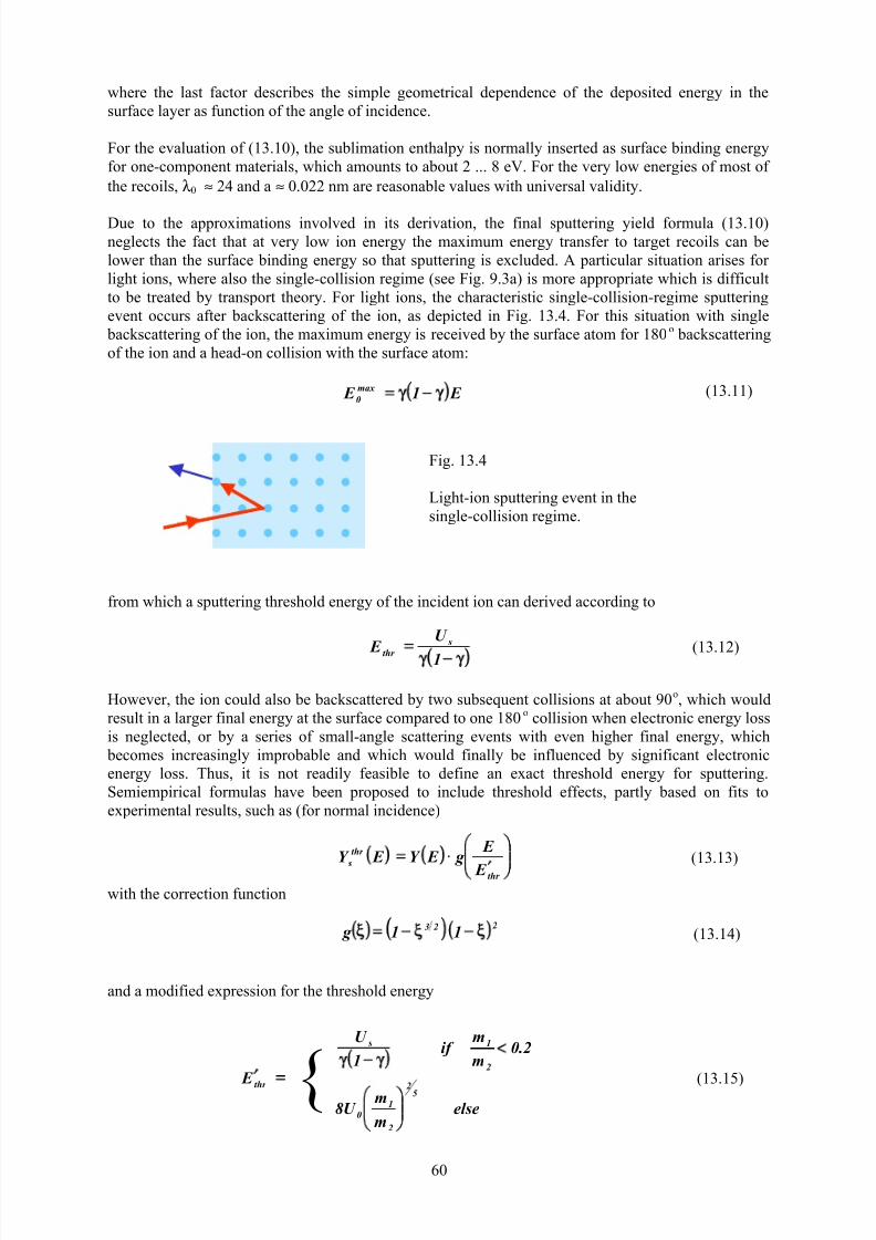
7/31/2019 Fundamentals of Ion-surface Interaction
http://slidepdf.com/reader/full/fundamentals-of-ion-surface-interaction 60/77
60
where the last factor describes the simple geometrical dependence of the deposited energy in the
surface layer as function of the angle of incidence.
For the evaluation of (13.10), the sublimation enthalpy is normally inserted as surface binding energy
for one-component materials, which amounts to about 2 ... 8 eV. For the very low energies of most of
the recoils, λ0 ≈ 24 and a ≈ 0.022 nm are reasonable values with universal validity.
Due to the approximations involved in its derivation, the final sputtering yield formula (13.10)
neglects the fact that at very low ion energy the maximum energy transfer to target recoils can be
lower than the surface binding energy so that sputtering is excluded. A particular situation arises for
light ions, where also the single-collision regime (see Fig. 9.3a) is more appropriate which is difficult
to be treated by transport theory. For light ions, the characteristic single-collision-regime sputtering
event occurs after backscattering of the ion, as depicted in Fig. 13.4. For this situation with single
backscattering of the ion, the maximum energy is received by the surface atom for 180o
backscattering
of the ion and a head-on collision with the surface atom:
from which a sputtering threshold energy of the incident ion can derived according to
However, the ion could also be backscattered by two subsequent collisions at about 90o, which would
result in a larger final energy at the surface compared to one 180o
collision when electronic energy loss
is neglected, or by a series of small-angle scattering events with even higher final energy, which
becomes increasingly improbable and which would finally be influenced by significant electronic
energy loss. Thus, it is not readily feasible to define an exact threshold energy for sputtering.
Semiempirical formulas have been proposed to include threshold effects, partly based on fits to
experimental results, such as (for normal incidence)
with the correction function
and a modified expression for the threshold energy
E 1 E max
0(13.11)
1
U
E s
thr (13.12)
Fig. 13.4
Light-ion sputtering event in the
single-collision regime.
thr
thr
s
E
E g E Y E Y (13.13)
22311 g (13.14)
thr E
2 .0m
mif
1
U
2
1s
elsem
mU 8
52
2
10
(13.15)

7/31/2019 Fundamentals of Ion-surface Interaction
http://slidepdf.com/reader/full/fundamentals-of-ion-surface-interaction 61/77
61
The sputtering yield for nitrogen ions incident on iron, according to eqs. (13.10) and (13.15), is shown
in Fig. 13.5. The threshold correction reduces the sputtering yield at low energies significantly. As
linear cascade sputtering scales with the nuclear stopping, the maximum sputtering yields are between
about 0.01 for light ions and 50 for the heaviest ions, corresponding to energies between about 100 eV
and 100 keV.
An early comparison to experimental data is shown in Fig.13.6 for different rare gases incident on
copper. There is a very good agreement between experiment and the prediction of eq. (13.10), except
for the highest energy densities around the nuclear stopping power maximum for the heaviest
projectile, xenon. This inconsistency is attributed to a significant influence of thermal spikes on
sputtering.
Fig. 13.6
Fig. 13.5
Sputtering yield versus ion energy for
nitrogen ion at iron at normal incidence,
from the Sigmund formula (solid line, eq.
(13.10)), the Bohdansky formula (dashed
line, eqs. (13.13-15)) and different TRIM
simulations, from SRIM vs. 2000.39
(dots), and TRIDYN vs. 4.0 (see ch. 15)
(circles).
Fig. 13.6 Experimental data and theoretical predictions of sputtering yields vs. ion energy, for
the bombardment of copper with different rare gases at normal incidence. Differentsymbols correspond to different data sets. Solid lines are from eq. (13.10), dashed
lines from a low-ener a roximation to nuclear sto in .
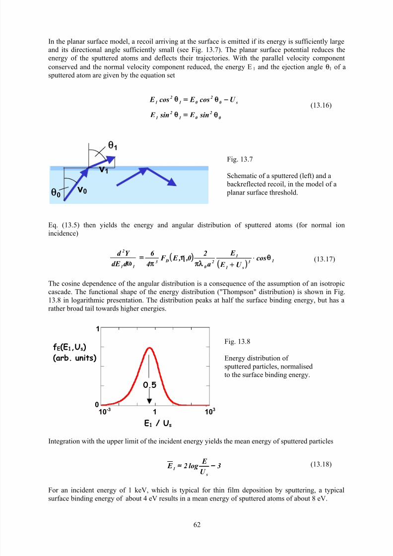
7/31/2019 Fundamentals of Ion-surface Interaction
http://slidepdf.com/reader/full/fundamentals-of-ion-surface-interaction 62/77
62
In the planar surface model, a recoil arriving at the surface is emitted if its energy is sufficiently large
and its directional angle sufficiently small (see Fig. 13.7). The planar surface potential reduces the
energy of the sputtered atoms and deflects their trajectories. With the parallel velocity component
conserved and the normal velocity component reduced, the energy E1 and the ejection angle θ1 of a
sputtered atom are given by the equation set
Eq. (13.5) then yields the energy and angular distribution of sputtered atoms (for normal ion
incidence)
The cosine dependence of the angular distribution is a consequence of the assumption of an isotropic
cascade. The functional shape of the energy distribution ("Thompson" distribution) is shown in Fig.13.8 in logarithmic presentation. The distribution peaks at half the surface binding energy, but has a
rather broad tail towards higher energies.
Integration with the upper limit of the incident energy yields the mean energy of sputtered particles
For an incident energy of 1 keV, which is typical for thin film deposition by sputtering, a typical
surface binding energy of about 4 eV results in a mean energy of sputtered atoms of about 8 eV.
(13.16)
1
0 v
0
v1
0
2
01
2
1 sin E sin E
s02
012
1 U cos E cos E
Fig. 13.7
Schematic of a sputtered (left) and a
backreflected recoil, in the model of a
planar surface threshold.
13
s1
1
2
0
D311
2
cosU E
E
a
20 , , E F
4
6
d dE
Y d v(13.17)
10-3 1 103
1
0
E1 / Us
fE(E1,Us)(arb. units)
0.5
Fig. 13.8
Energy distribution of
sputtered particles, normalised
to the surface binding energy.
3U
E log 2 E
s
1(13.18)
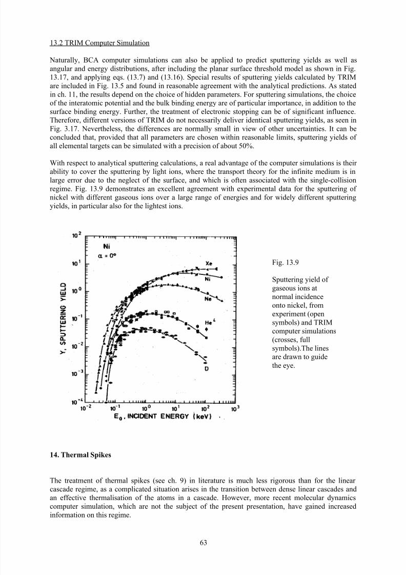
7/31/2019 Fundamentals of Ion-surface Interaction
http://slidepdf.com/reader/full/fundamentals-of-ion-surface-interaction 63/77
63
13.2 TRIM Computer Simulation
Naturally, BCA computer simulations can also be applied to predict sputtering yields as well as
angular and energy distributions, after including the planar surface threshold model as shown in Fig.
13.17, and applying eqs. (13.7) and (13.16). Special results of sputtering yields calculated by TRIM
are included in Fig. 13.5 and found in reasonable agreement with the analytical predictions. As stated
in ch. 11, the results depend on the choice of hidden parameters. For sputtering simulations, the choice
of the interatomic potential and the bulk binding energy are of particular importance, in addition to thesurface binding energy. Further, the treatment of electronic stopping can be of significant influence.
Therefore, different versions of TRIM do not necessarily deliver identical sputtering yields, as seen in
Fig. 3.17. Nevertheless, the differences are normally small in view of other uncertainties. It can be
concluded that, provided that all parameters are chosen within reasonable limits, sputtering yields of
all elemental targets can be simulated with a precision of about 50%.
With respect to analytical sputtering calculations, a real advantage of the computer simulations is their
ability to cover the sputtering by light ions, where the transport theory for the infinite medium is in
large error due to the neglect of the surface, and which is often associated with the single-collision
regime. Fig. 13.9 demonstrates an excellent agreement with experimental data for the sputtering of
nickel with different gaseous ions over a large range of energies and for widely different sputtering
yields, in particular also for the lightest ions.
14. Thermal Spikes
The treatment of thermal spikes (see ch. 9) in literature is much less rigorous than for the linear
cascade regime, as a complicated situation arises in the transition between dense linear cascades and
an effective thermalisation of the atoms in a cascade. However, more recent molecular dynamics
computer simulation, which are not the subject of the present presentation, have gained increasedinformation on this regime.
Fig. 13.9
Sputtering yield of
gaseous ions at
normal incidence
onto nickel, from
experiment (open
symbols) and TRIM
computer simulations
(crosses, full
symbols).The lines
are drawn to guide
the eye.

7/31/2019 Fundamentals of Ion-surface Interaction
http://slidepdf.com/reader/full/fundamentals-of-ion-surface-interaction 64/77
64
It should be noted that here we still cover "collisional" spikes, i.e. at energies above about 1 eV which
are of interest for the formation of defects and for sputtering. Thermal spikes in a more general sense
will result from any cascade which finally will thermalise towards the temperature of the surrounding
material. Atomic rearrangements with low activation energies may still occur at such low energies, but
will not be the matter of the present discussion.
For a simple picture of a thermal spike (Fig. 14.1), the evolution of a cylindrical cascade around a
linear ion track is assumed, which is justified at large ion masses and high energy. Neglecting energy
loss, the system is translationally invariant in the direction of the depth x. For simplicity, a zero
temperature of the material is assumed as initial condition. At t = 0, the time of the ion incidence,
energy is deposited within a negligible time interval along the ion track, with the energy deposition
function being idealised by a planar δ function in circular symmetry, leading to an initial temperature
in the track according to
with the normalisation
In eq. (14.1), ρ and c denote the mass density and the specific heat of the material, respectively.
Around the track, a thermal wave develops in radial direction according to the law of thermal diffusion
with the thermal conductivity λ. The solution yields the temperature at radial distance r as function of
time t:
which fulfills eq. (14.1) as
Fig.14.2 shows a solution for a special case. Close to the ion track, temperatures of a few 104
K
(corresponding to a few eV) are predicted, so that the material will be liquidified and probably be
evaporated. The thermal pulse dissipates quickly at larger distance from the track. The characteristic
time scale, however, demonstrates an inherent contradiction, as it is in the order of one latticevibration period only, so that the above continuum picture is hardly valid.
r v
x
Fig. 14.1
Simplified picture of a cylindrical
thermal spike
1dr r r 2
v
(14.1)0t ,r T cr dx
dE v
(14.2)
r
T r
r r
1
cT
ct
T (14.3)
t 4
cr exp
t 4
1
dx
dE t ,r T
2
(14.4)
r e1
0
r 2
v(14.5)

7/31/2019 Fundamentals of Ion-surface Interaction
http://slidepdf.com/reader/full/fundamentals-of-ion-surface-interaction 65/77
65
It makes little sense to apply the thermal spike picture to the formation of radiation damage, since
radiation damage in a liquid is meaningless, and since excessive dynamic annealing will occur at the
very high temperature after solidification or at radii where the substance remains in the solid phase.
However, one may attempt to calculate sputtering in the thermal spike picture.
Sputtering is modelled by the evaporation from the thermal spike at the surface. For a Maxwellian
energy distribution of atoms with mass m, the energy of which exceeds the surface binding energy, the
outward flux is given by
Thereby, the sputtering yield results according to
With the approximation ρ⋅c ≈ 3nk for the specific heat, the integration yields
which shows the nonlinear dependence on the stopping power in the thermal spike regime.
For the example of xenon in copper the maximum nuclear stopping power is chosen, which is about
6.5 MeV/µm at an energy of about 250 keV. (At this energy, electronic stopping contributes only
about 10% to the total stopping.) With the room temperature value of the thermal conductivity, the
evaluation of eq. (14.8) yields a sputtering yield of Y ≈ 1. However, the thermal conductivity in the
liquid might be smaller by a factor of 2 or 3. Nevertheless, the result is still significantly below the
difference of experimental data and linear cascade prediction in Fig. 13.6, indicating that the above
formalism might be insufficient to treat the sputtering from a thermal spike.
500 keV Xe -> Ni
0 1 2 3 4 5
4
2
0
Time (10-13 s)
Temperature
(104 K)
r = 1 nm
r = 3 nm r = 6 nm
Fig. 14.2
Thermal pulse at different
radial locations for 500
keV xenon ions incident
onto nickel
t ,r kT
U exp
m2
t ,r kT nt ,r j s
(14.6)
t ,r j dt rdr 2Y 0 0
(14.7)
2
23
s23 dx
dE
U
1
m
k
224
23Y (14.8)

7/31/2019 Fundamentals of Ion-surface Interaction
http://slidepdf.com/reader/full/fundamentals-of-ion-surface-interaction 66/77
66
15. High-Fluence Phenomena
The preceding chapters did only cover low-fluence phenomena, i.e. the dynamic alteration of the
target substance due to ion implantation or the formation of defects has been neglected so far.
Sputtering yields can be extrapolated to large fluences as long as the material remains unchanged
during sputtering. This dose not hold for the sputtering of multicomponent substances, where the
collision cascades or preferential sputtering may change the surface composition even in ahomogeneous material, and/or modify the local composition of a layered substance.
15.1 Dynamic Binary Collision Approximation Computer Simulation
The BCA computer simulation of ion bombardment and collision cascade formation can be modified
in a straightforward manner to treat dynamic compositional changes of the substance. Here, the
TRIDYN code will be described which is based on TRIM.
A multicomponent material with atomic components denoted by j (j = 1,...,M) is modelled, where one
or more of these components may be attributed to species of the incident beam. An arbitrary local
stoichiometry can be chosen, represented by discrete depth intervals ∆xi (i = 1,...,N). Each depth
interval is characterised by the fractional compositions qij with
and a total atomic density ni given by
1q M
1 j
ij (15.1)
1 i i+1
x1 xi xi+1
(a)
(b)
(c)
SurfaceUnaffected
Depth
N
xN
Fig. 15.1
Scheme of the dynamic computer
simulation in binary collisionapproximation (TRIDYN).
(a) A pseudoprojectile is implanted and
generates sputtering and recoil atoms.
(b) "Vacancies" and "interstitial atoms"
are left behind.
(c) The individual slabs relaxe.
M
1 j 0 j
ij
i n
q
n
1(15.2)
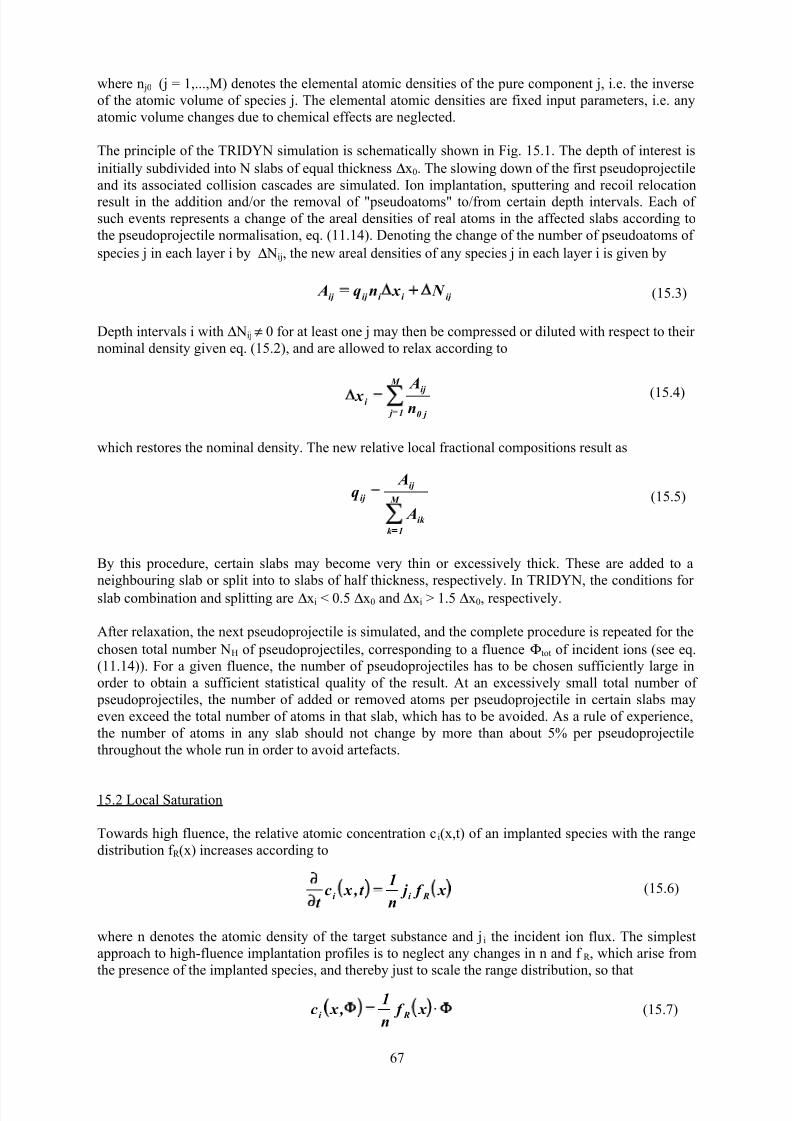
7/31/2019 Fundamentals of Ion-surface Interaction
http://slidepdf.com/reader/full/fundamentals-of-ion-surface-interaction 67/77
67
where n j0 (j = 1,...,M) denotes the elemental atomic densities of the pure component j, i.e. the inverse
of the atomic volume of species j. The elemental atomic densities are fixed input parameters, i.e. any
atomic volume changes due to chemical effects are neglected.
The principle of the TRIDYN simulation is schematically shown in Fig. 15.1. The depth of interest is
initially subdivided into N slabs of equal thickness ∆x0. The slowing down of the first pseudoprojectile
and its associated collision cascades are simulated. Ion implantation, sputtering and recoil relocation
result in the addition and/or the removal of "pseudoatoms" to/from certain depth intervals. Each of
such events represents a change of the areal densities of real atoms in the affected slabs according to
the pseudoprojectile normalisation, eq. (11.14). Denoting the change of the number of pseudoatoms of
species j in each layer i by ∆ Nij, the new areal densities of any species j in each layer i is given by
Depth intervals i with ∆ Nij≠ 0 for at least one j may then be compressed or diluted with respect to their
nominal density given eq. (15.2), and are allowed to relax according to
which restores the nominal density. The new relative local fractional compositions result as
By this procedure, certain slabs may become very thin or excessively thick. These are added to a
neighbouring slab or split into to slabs of half thickness, respectively. In TRIDYN, the conditions for
slab combination and splitting are ∆xi < 0.5 ∆x0 and ∆xi > 1.5 ∆x0, respectively.
After relaxation, the next pseudoprojectile is simulated, and the complete procedure is repeated for the
chosen total number NH of pseudoprojectiles, corresponding to a fluence Φtot of incident ions (see eq.
(11.14)). For a given fluence, the number of pseudoprojectiles has to be chosen sufficiently large in
order to obtain a sufficient statistical quality of the result. At an excessively small total number of
pseudoprojectiles, the number of added or removed atoms per pseudoprojectile in certain slabs may
even exceed the total number of atoms in that slab, which has to be avoided. As a rule of experience,
the number of atoms in any slab should not change by more than about 5% per pseudoprojectile
throughout the whole run in order to avoid artefacts.
15.2 Local Saturation
Towards high fluence, the relative atomic concentration ci(x,t) of an implanted species with the range
distribution f R (x) increases according to
where n denotes the atomic density of the target substance and ji the incident ion flux. The simplest
approach to high-fluence implantation profiles is to neglect any changes in n and f R , which arise from
the presence of the implanted species, and thereby just to scale the range distribution, so that
ij i i ij ij N x nq A (15.3)
M
1 j j 0
ij i
n
A x (15.4)
M
1k
ik
ij
ij
A
Aq (15.5)
x f j n
1t , x c
t Ri i
(15.6)
x f n
1 , x c Ri (15.7)
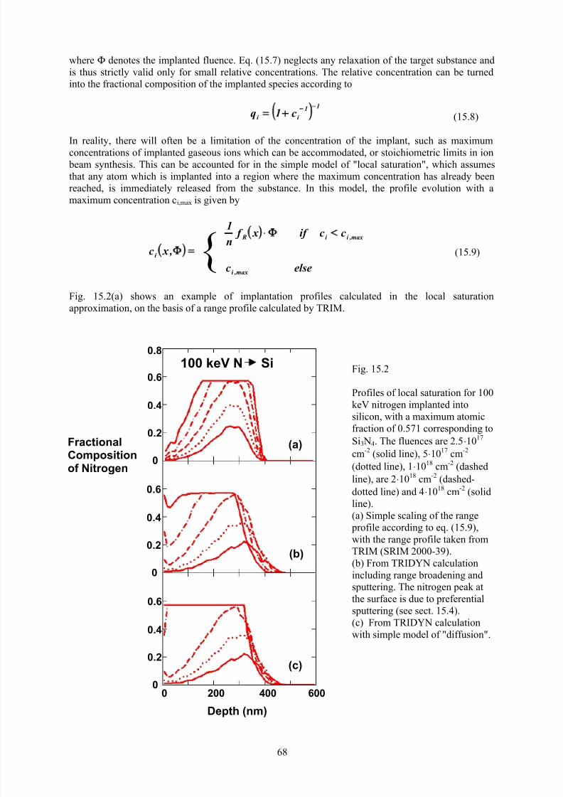
7/31/2019 Fundamentals of Ion-surface Interaction
http://slidepdf.com/reader/full/fundamentals-of-ion-surface-interaction 68/77
68
where Φ denotes the implanted fluence. Eq. (15.7) neglects any relaxation of the target substance and
is thus strictly valid only for small relative concentrations. The relative concentration can be turned
into the fractional composition of the implanted species according to
In reality, there will often be a limitation of the concentration of the implant, such as maximumconcentrations of implanted gaseous ions which can be accommodated, or stoichiometric limits in ion
beam synthesis. This can be accounted for in the simple model of "local saturation", which assumes
that any atom which is implanted into a region where the maximum concentration has already been
reached, is immediately released from the substance. In this model, the profile evolution with a
maximum concentration ci,max is given by
Fig. 15.2(a) shows an example of implantation profiles calculated in the local saturation
approximation, on the basis of a range profile calculated by TRIM.
11
i i c1q (15.8)
, x c i
,max i i R ccif x f n
1
elsec ,max i
(15.9)
0 200 400 600
0
0.2
0.4
0.6
0
0.2
0.4
0.6
0
0.2
0.4
0.6
0.8
Depth (nm)
FractionalCompositionof Nitrogen
100 keV N Si
(a)
(b)
(c)
Fig. 15.2
Profiles of local saturation for 100
keV nitrogen implanted into
silicon, with a maximum atomicfraction of 0.571 corresponding to
Si3 N4. The fluences are 2.5⋅1017
cm-2
(solid line), 5⋅1017
cm-2
(dotted line), 1⋅1018
cm-2
(dashed
line), are 2⋅1018
cm-2
(dashed-
dotted line) and 4⋅1018
cm-2
(solid
line).
(a) Simple scaling of the range
profile according to eq. (15.9),
with the range profile taken from
TRIM (SRIM 2000-39).
(b) From TRIDYN calculation
including range broadening and
sputtering. The nitrogen peak at
the surface is due to preferential
sputtering (see sect. 15.4).
(c) From TRIDYN calculation
with simple model of "diffusion".

7/31/2019 Fundamentals of Ion-surface Interaction
http://slidepdf.com/reader/full/fundamentals-of-ion-surface-interaction 69/77
69
In reality, high-fluence implantation profiles are influenced by a number of effects which cannot easily
be covered by a simple model. The presence of the implanted species influences the stopping and
scattering of the incident ions so that the range profiles may be changed during the implantation. This
may lead to a distortion of the implantation profiles in addition to the distortion which is caused by the
relaxation of the host matrix ("swelling" due to the implanted atoms). Both are covered by dynamic
BCA computer simulations. The model of local saturation can easily be incorporated into the
simulation, by limiting the maximum concentration of the implanted species. The result from a
TRIDYN calculation is shown in Fig. 15.2(b). In comparison with the simple analytical approach,already the profile corresponding to the lowest fluence displayed is broadened due to swelling.
Towards the highest fluences, the profiles are further broadened and shifted towards the surface, due
to sputtering.
In TRIDYN, it is also possible to employ a simplistic model of "diffusion", in which excess atoms are
deposited in the non-saturated regions at the edges of the profiles rather than being discarded.
(Actually, an atom coming to rest in a saturated region is moved to the closest depth interval which is
not saturated.) The result is shown in Fig. 15.2(c), with considerable additional broadening towards the
surface for the highest fluences. It depends critically on the system under investigation which of the
above models can be applied.
15.3 Sputter-Controlled Implantation Profiles
In the example of Fig.15.2, the ion energy has been chosen sufficiently large so that the surface layer
which is removed by sputtering is small compared to the mean projected ion range, and that the local
saturation is not significantly influenced by sputtering. In contrast, at sufficiently small projected
range and/or sufficiently high sputter yield, the high-fluence implantation profiles can be controlled
entirely by ion deposition and sputtering. A qualitative picture is shown in Fig. 15.3.
Fig. 15.3
Schematic representation of
the formation of sputter-
controlled implantation
profiles. Range distribution
and low-fluence profiles (top)
with the surface moving with
a velocity vs due to
sputtering, transient profile(middle) when the sputtered
depth becomes comparable to
the mean projected range,
and stationary final profile
(bottom).
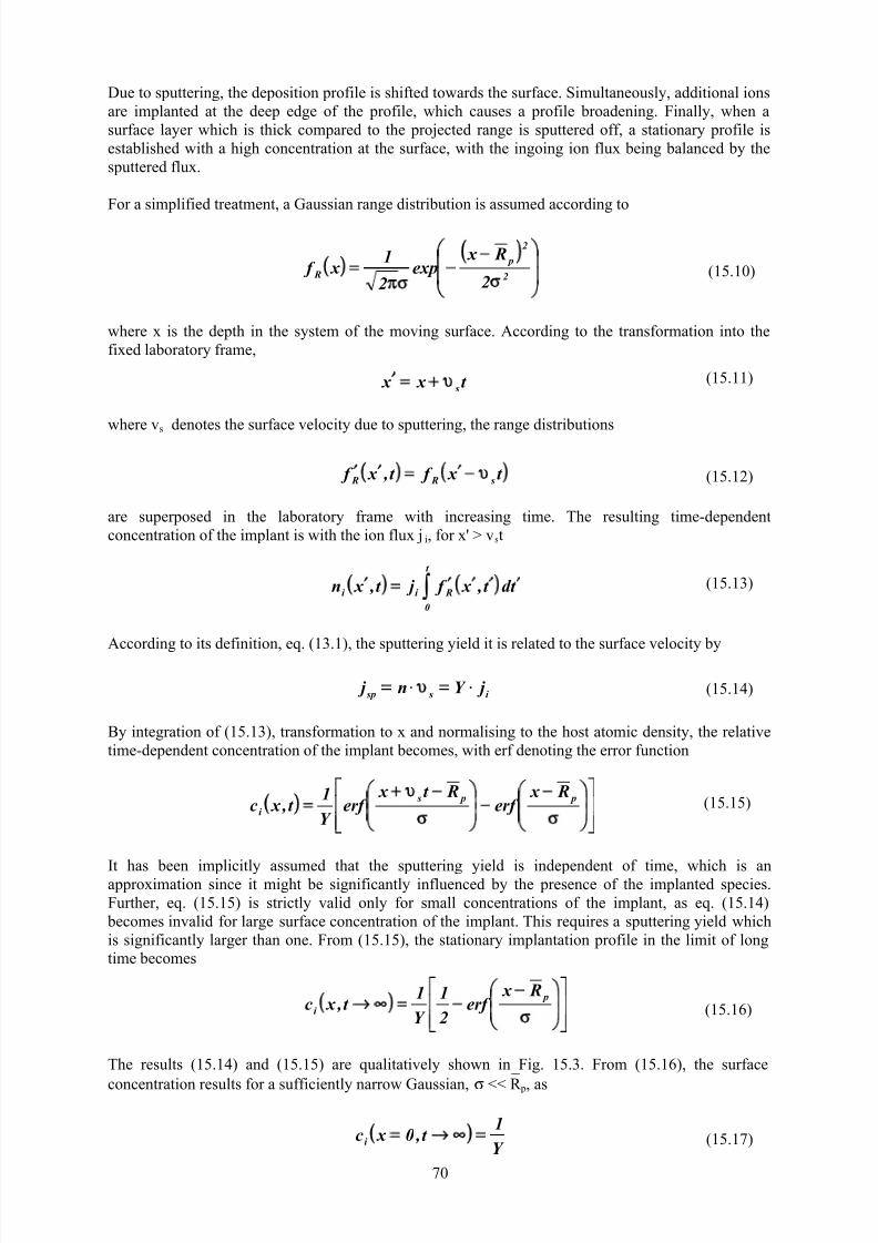
7/31/2019 Fundamentals of Ion-surface Interaction
http://slidepdf.com/reader/full/fundamentals-of-ion-surface-interaction 70/77
70
Due to sputtering, the deposition profile is shifted towards the surface. Simultaneously, additional ions
are implanted at the deep edge of the profile, which causes a profile broadening. Finally, when a
surface layer which is thick compared to the projected range is sputtered off, a stationary profile is
established with a high concentration at the surface, with the ingoing ion flux being balanced by the
sputtered flux.
For a simplified treatment, a Gaussian range distribution is assumed according to
where x is the depth in the system of the moving surface. According to the transformation into the
fixed laboratory frame,
where vs denotes the surface velocity due to sputtering, the range distributions
are superposed in the laboratory frame with increasing time. The resulting time-dependent
concentration of the implant is with the ion flux j i, for x' > vst
According to its definition, eq. (13.1), the sputtering yield it is related to the surface velocity by
By integration of (15.13), transformation to x and normalising to the host atomic density, the relative
time-dependent concentration of the implant becomes, with erf denoting the error function
It has been implicitly assumed that the sputtering yield is independent of time, which is anapproximation since it might be significantly influenced by the presence of the implanted species.
Further, eq. (15.15) is strictly valid only for small concentrations of the implant, as eq. (15.14)
becomes invalid for large surface concentration of the implant. This requires a sputtering yield which
is significantly larger than one. From (15.15), the stationary implantation profile in the limit of long
time becomes
The results (15.14) and (15.15) are qualitatively shown in Fig. 15.3. From (15.16), the surface
concentration results for a sufficiently narrow Gaussian, σ << R p, as
2
2
p
R2
R x exp
2
1 x f (15.10)
t x x s(15.11)
t x f t , x f s R R (15.12)
t d t , x f j t , x n
t
0
Ri i (15.13)
i ssp j Y n j (15.14)
p ps
i
R x erf
Rt x erf
Y
1t , x c (15.15)
p
i
R x erf
2
1
Y
1t , x c (15.16)
_
Y
1t ,0 x c i (15.17)

7/31/2019 Fundamentals of Ion-surface Interaction
http://slidepdf.com/reader/full/fundamentals-of-ion-surface-interaction 71/77
71
i.e., the relative surface concentration is given by the inverse of the sputtering yield.
More exact sputter-controlled implantation profiles can be obtained from dynamic BCA simulations.
Fig. 15.4 shows the retained amount and a sequence of implantation profiles for sulfur ions incident on
molybdenum. The depth profile at the lowest fluence, which reflects the range profile, becomes
significantly distorted at the higher fluences. Stationarity is obtained at a fluence around 1.5 ⋅1017
cm-2
,
after about 20 nm, which is approximately 2.5 times the mean projected range, have been sputtered
off. Compared to the simple error-functional shape predicted by eq. (15.16), there is a concentration
drop at the surface due to preferential sputtering (see sect. 15.4). Nevertheless, the stationary profiles
exhibit a nearly flat top with an atomic fraction of about 0.4, corresponding to a relative concentration
(see eq. (15.8)) of 0.67. The sputtering yield for 10 keV sulfur ions incident on molybdenum is 2
according to the Sigmund formula, eq. (13.10). Thereby, the simple analytical result of eq. (15.17) is
about 30% smaller.
The result demonstrates the impossibility to reach the concentration of the stoichiometric compound,
MoS2, under the present conditions.
15.4 Preferential Sputtering
According to eq. (13.10), the sputter yield is inversely proportional to the surface binding energy. It
also increases with the energy transfer from the incident ion to the target atoms. Both may be different
for the different atomic species in a multicomponent target material. In the limit of low fluence, the
total sputtering yield can, in a first approximation, be superposed from the different components i
according to their surface concentration. For this purpose, so-called "component" sputtering yields Yic
are defined such that the partial sputtering yields Y i are given by
0 5 10 15 20 250
1
2
3
4
5100 %
10 keV S Mo
Sulfur Ion Fluence (1016 cm-2)
RetainedSulfur (10
16cm
-2)
0 10 20 30
Depth (nm)
Sulfur AtomicFraction
0
0.2
0.4
0.6
Fig. 15.4
Sputter-controlled implantation
profile for 10 keV sulfur in
molybdenum from a TRIDYN
(vs. 4.0) computer simulation.
Retained amount vs. ion fluence
(top) and corresponding
implantation profiles (bottom), at
fluences of 1.5⋅1016
cm-2
(solid
line), 3⋅1016
cm-2
(dotted line),
6⋅1016 cm-2 (dashed line), 1.2⋅1017
cm-2
(dashed-dotted line) and
2.4⋅1017 cm-2 (solid line). At the
final fluence, a surface layer of
27.5 nm has been sputtered off.

7/31/2019 Fundamentals of Ion-surface Interaction
http://slidepdf.com/reader/full/fundamentals-of-ion-surface-interaction 72/77
72
with qis
denoting the surface atomic fractions. The total sputtering yield is then
The linear dependence of the partial yields of the surface concentrations neglects any composition-
dependent effects on the sputtering such as due to chemical compound or phase formation. For solid
components, the component sputtering yields can be identified with the sputtering yields of the pure
material of that component (qis=1 in eq. (15.18)).
For different component sputtering yields, the equation
holds for at least one pair of components (i,j). In this case, one or more components are sputtered
preferentially.
Consequently, the surface concentrations are altered at increasing fluence even in a homogeneous
material. For simplicity, we assume a two-component material with the components A and B, with A
being sputtered preferentially. The surface concentration of A, and thereby the partial sputtering yield
of A, will then decrease with increasing fluence towards a stationary state, which is given by
where Yi∞ denote the stationary partial sputtering yields and qi the bulk atomic fractions. Eq. (15.20)
simply states mass conservation, as in the stationary state the altered composition profiles remain
constant but are moved into the bulk due to sputter erosion, so that atoms sputtered at the surface must
be balanced by atoms fed from the bulk into the altered layer (see Fig. (15.5)).
By relating eq. (15.18) for both components and combining with eq. (15.21), the following expression
is obtained for of the stationary surface composition with the atomic fractions (q is)∞
c
i
s
i i Y qY (15.18)
i
i Y Y
s
j
s
i
j
i
q
q
Y
Y
(15.19)
(15.20)
B
A
B
A
q
q
Y
Y (15.21)
Depth
Atomic
Fractions
A
B
Fig. 15.5
Stationary composition profiles in an
initially homogeneous two-component
material due to preferential sputteringof the component B (schematic). The
altered layer is moved into the bulk
due to sputter erosion.
Altered Layer
0
A
0
B
2
B
A
s
B
s
A
Y
Y
q
q
q
q(15.22)
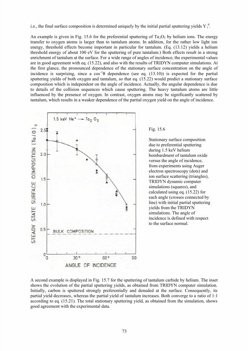
7/31/2019 Fundamentals of Ion-surface Interaction
http://slidepdf.com/reader/full/fundamentals-of-ion-surface-interaction 73/77
73
i.e., the final surface composition is determined uniquely by the initial partial sputtering yields Y i0.
An example is given in Fig. 15.6 for the preferential sputtering of Ta2O5 by helium ions. The energy
transfer to oxygen atoms is larger than to tantalum atoms. In addition, for the rather low light ion
energy, threshold effects become important in particular for tantalum. (Eq. (13.12) yields a helium
threshold energy of about 100 eV for the sputtering of pure tantalum.) Both effects result in a strong
enrichment of tantalum at the surface. For a wide range of angles of incidence, the experimental values
are in good agreement with eq. (15.22), and also with the results of TRIDYN computer simulations. Atthe first glance, the pronounced dependence of the stationary surface concentration on the angle of
incidence is surprising, since a cos-1θ dependence (see eq. (13.10)) is expected for the partial
sputtering yields of both oxygen and tantalum, so that eq. (15.22) would predict a stationary surface
composition which is independent on the angle of incidence. Actually, the angular dependence is due
to details of the collision sequences which cause sputtering. The heavy tantalum atoms are little
influenced by the presence of oxygen. In contrast, oxygen atoms may be significantly scattered by
tantalum, which results in a weaker dependence of the partial oxygen yield on the angle of incidence.
A second example is displayed in Fig. 15.7 for the sputtering of tantalum carbide by helium. The inset
shows the evolution of the partial sputtering yields, as obtained from TRIDYN computer simulation.
Initially, carbon is sputtered strongly preferentially and denuded at the surface. Consequently, its
partial yield decreases, whereas the partial yield of tantalum increases. Both converge to a ratio of 1:1
according to eq. (15.21). The total stationary sputtering yield, as obtained from the simulation, shows
good agreement with the experimental data.
Fig. 15.6
Stationary surface composition
due to preferential sputtering
during 1.5 keV helium
bombardment of tantalum oxide
versus the angle of incidence,
from experiments using Auger
electron spectroscopy (dots) and
ion surface scattering (triangles),
TRIDYN dynamic computer
simulations (squares), and
calculated using eq. (15.22) for
each angle (crosses connected by
line) with initial partial sputtering
yields from the TRIDYN
simulations. The angle of
incidence is defined with respect
to the surface normal.

7/31/2019 Fundamentals of Ion-surface Interaction
http://slidepdf.com/reader/full/fundamentals-of-ion-surface-interaction 74/77
74
15.5 Ion Mixing
In an inhomogeneous multicomponent substance, the relocation of atoms due to ion knockon and in
collision cascades results in "mixing" of the atoms. Prototypes of inhomogeneous materials are a thin
marker of atoms A in an otherwise homogeneous material B, and an A/B bilayer as a simple example
of a multilayer medium (Fig. 15.8).
There are three main mechanism of ion mixing, as indicated in Fig. 15.9. Matrix atoms can be
relocated by primary collisions into or beyond the marker; this leads to marker broadening and to a
shift towards the surface. Marker atoms, which are relocated by primary collisions towards larger
depth, result in a tail of the marker profile, and thereby in a broadening and a shift towards the bulk.
Finally, collision cascades initiated by sufficiently large primary energy transfers are more or less
isotropic and cause mainly a broadening of the marker. These events interact in a complicated way. A
simple analytical prediction can only be obtained for the isotropic cascade mixing [22].
For a marker system, the relocation of the marker atoms is described by relocation cross sectiondσ(x,z), which describes the displacement of a marker atom due to ion bombardment, with an energy
transfer T at a starting angle Θ from an original depth x by a depth increment z (see Fig. 15.10).
Fig. 15.7
Total stationary sputtering
yield of tantalum carbide
during helium bombardment,
as function of the ion energy,
from TRIDYN computer simulation (full points) and
experiments (open triangles).
The line is from an empirical
fit function. The inset shows
the dependence of the partial
sputtering yields on the ion
fluence, at an energy of 1 keV.
Fig. 15.8
Schematic of ion mixing
in a marker system (thin
marker M in a matrix A,
top) and in a bilayer
system (layer A on top of
a layer or bulk B, bottom).
Due to ion bombardment,
the marker and the
interface become diffuse,
respectively.
MA
A B

7/31/2019 Fundamentals of Ion-surface Interaction
http://slidepdf.com/reader/full/fundamentals-of-ion-surface-interaction 75/77
75
Fig. 15.9
For many incident ions, multiple displacements are obtained. The mean displacement of a marker
atom for a given ion fluence Φ is
and the variance (to be shown in analogy to the variance of electronic energy loss - see sect. 6.3)
Collision cascades are mainly developed by matrix atoms, as the number of marker atoms is small.
Matrix atoms of the cascades may collide with marker atoms thus causing them to be relocated. The
relocation cross section is then given by
The first line of eq. (15.24), in the notation of chs. 10 and 13, denotes the flux of matrix cascade atoms
through the marker plane at x. The second line contains the probability of collisions dσm with marker
atoms, which receive an energy transfer T at a direction η'. The cosine term reflects the increased
collision probability at an inclined direction of the matrix atom. f R denotes the range distribution of the
marker recoil atom. Similar to the treatment of sputtering (see eq. (13.5)), the area integral of the
cascade function F can be written as
with FD now denoting the one-dimensional damage function and Sm the stopping cross section of the
matrix atoms in the matrix.
Mechanisms of ion mixing in a marker system: Matrix relocation (left),
marker relocation (middle) and cascade mixing of the marker (right).
Rp(T)
x x+z
Fig. 15.10
Relocation of a marker atom
starting at an angle Θ with anenergy transfer T. R p denotes its
projected range.
z , x d z x (15.22)
z , x d z x x 222
m (15.23)
0000 r , E , , E F 4
1 f d d dE
dz
z , x d vvvv
z , ,T f ,T , , E d cos R00m
1
0
vvv(15.24)
0m0
0 D
300 E nS E cos x , , E F
46 r , E , , E F
41 f d vvvv (15.25)
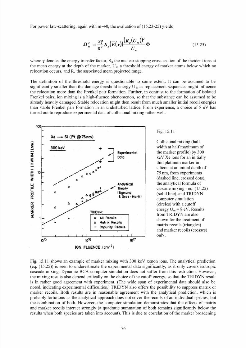
7/31/2019 Fundamentals of Ion-surface Interaction
http://slidepdf.com/reader/full/fundamentals-of-ion-surface-interaction 76/77
76
For power law-scattering, again with m→0, the evaluation of (15.23-25) yields
where γ denotes the energy transfer factor, Sn the nuclear stopping cross section of the incident ions atthe mean energy at the depth of the marker, Um a threshold energy of marker atoms below which no
relocation occurs, and R c the associated mean projected range.
The definition of the threshold energy is questionable to some extent. It can be assumed to be
significantly smaller than the damage threshold energy Ud, as replacement sequences might influence
the relocation more than the Frenkel pair formation. Further, in contrast to the formation of isolated
Frenkel pairs, ion mixing is a high-fluence phenomenon, so that the substance can be assumed to be
already heavily damaged. Stable relocation might then result from much smaller initial recoil energies
than stable Frenkel pair formation in an undisturbed lattice. From experience, a choice of 8 eV has
turned out to reproduce experimental data of collisional mixing rather well.
Fig. 15.11 shows an example of marker mixing with 300 keV xenon ions. The analytical prediction
(eq. (15.25)) is seen to underestimate the experimental data significantly, as it only covers isotropic
cascade mixing. Dynamic BCA computer simulation does not suffer from this restriction. However,
the mixing results also depend critically on the choice of the cutoff energy, so that the TRIDYN result
is in rather good agreement with experiment. (The wide span of experimental data should also be
noted, indicating experimental difficulties.) TRIDYN also offers the possibility to suppress matrix or
marker recoils. Both results are in reasonable agreement with the analytical prediction, which is
probably fortuitous as the analytical approach does not cover the recoils of an individual species, but
the combination of both. However, the computer simulation demonstrates that the effects of matrixand marker recoils interact strongly (a quadratic summation of both remains significantly below the
results when both species are taken into account). This is due to correlation of the marker broadening
m
2
m p
n2
2
mU
U R x E S
2 (15.25)
Fig. 15.11
Collisional mixing (half
width at half maximum of
the marker profile) by 300
keV Xe ions for an initially
thin platinum marker in
silicon at an initial depth of
75 nm, from experiments
(dashed line, crossed dots),
the analytical formula of cascade mixing - eq. (15.25)
(solid line), and TRIDYN
computer simulation
(circles) with a cutoff
energy Um = 8 eV. Results
from TRIDYN are also
shown for the treatment of
matrix recoils (triangles)
and marker recoils (crosses)
onl .
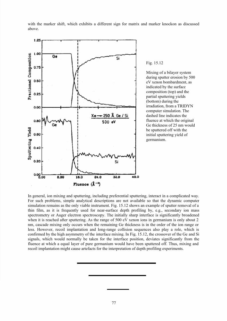
7/31/2019 Fundamentals of Ion-surface Interaction
http://slidepdf.com/reader/full/fundamentals-of-ion-surface-interaction 77/77
with the marker shift, which exhibits a different sign for matrix and marker knockon as discussed
above.
In general, ion mixing and sputtering, including preferential sputtering, interact in a complicated way.
For such problems, simple analytical descriptions are not available so that the dynamic computer
simulation remains as the only viable instrument. Fig. 15.12 shows an example of sputter removal of a
thin film, as it is frequently used for near-surface depth profiling by, e.g., secondary ion mass
spectrometry or Auger electron spectroscopy. The initially sharp interface is significantly broadened
when it is reached after sputtering. As the range of 500 eV xenon ions in germanium is only about 2
nm, cascade mixing only occurs when the remaining Ge thickness is in the order of the ion range or less. However, recoil implantation and long-range collision sequences also play a role, which is
confirmed by the high asymmetry of the interface mixing. In Fig. 15.12, the crossover of the Ge and Si
signals, which would normally be taken for the interface position, deviates significantly from the
fluence at which a equal layer of pure germanium would have been sputtered off Thus mixing and
Fig. 15.12
Mixing of a bilayer system
during sputter erosion by 500
eV xenon bombardment, as
indicated by the surface
composition (top) and the
partial sputtering yields
(bottom) during the
irradiation, from a TRIDYN
computer simulation. Thedashed line indicates the
fluence at which the original
Ge thickness of 25 nm would
be sputtered off with the
initial sputtering yield of
germanium.


![Light-Matter Interaction [Vol 1 - Fundamentals and Applns]](https://static.fdocuments.in/doc/165x107/613c5f71f237e1331c51306c/light-matter-interaction-vol-1-fundamentals-and-applns.jpg)