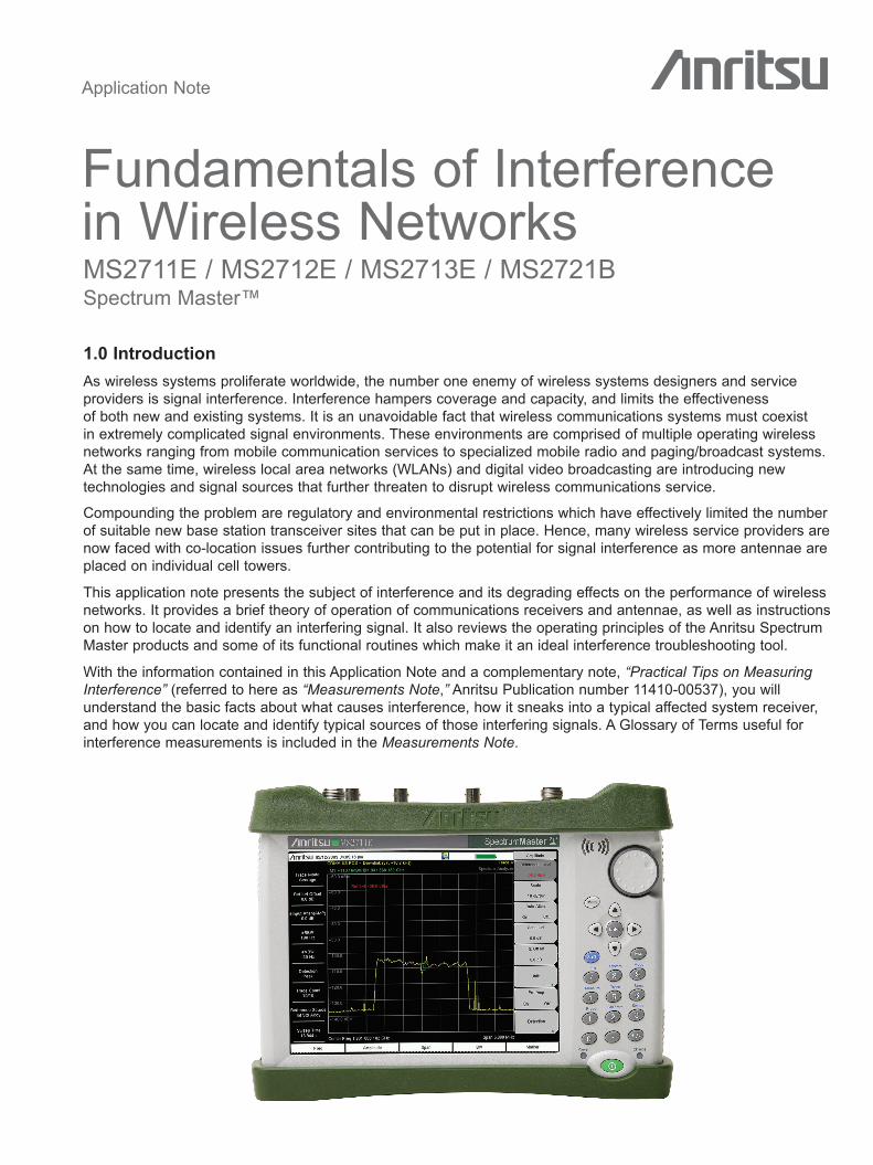
Application Note

Fundamentals of Interference in Wireless NetworksMS2711E / MS2712E / MS2713E / MS2721BSpectrum Master™

1.0 IntroductionAs wireless systems proliferate worldwide, the number one enemy of wireless systems designers and service providers is signal interference. Interference hampers coverage and capacity, and limits the effectiveness of both new and existing systems. It is an unavoidable fact that wireless communications systems must coexist in extremely complicated signal environments. These environments are comprised of multiple operating wireless networks ranging from mobile communication services to specialized mobile radio and paging/broadcast systems. At the same time, wireless local area networks (WLANs) and digital video broadcasting are introducing new technologies and signal sources that further threaten to disrupt wireless communications service.

Compounding the problem are regulatory and environmental restrictions which have effectively limited the number of suitable new base station transceiver sites that can be put in place. Hence, many wireless service providers are now faced with co-location issues further contributing to the potential for signal interference as more antennae are placed on individual cell towers.

This application note presents the subject of interference and its degrading effects on the performance of wireless networks. It provides a brief theory of operation of communications receivers and antennae, as well as instructions on how to locate and identify an interfering signal. It also reviews the operating principles of the Anritsu Spectrum Master products and some of its functional routines which make it an ideal interference troubleshooting tool.

With the information contained in this Application Note and a complementary note, “Practical Tips on Measuring Interference” (referred to here as “Measurements Note,” Anritsu Publication number 11410-00537), you will understand the basic facts about what causes interference, how it sneaks into a typical affected system receiver, and how you can locate and identify typical sources of those interfering signals. A Glossary of Terms useful for interference measurements is included in the Measurements Note.

2

2.0 What is Interference?It’s pretty easy to comprehend the theory of signal interference and to see its effect on an installed system. As a mobile wireless customer, you may have experienced loss of service due to the effects of interference. You may not have thought anything of it as you suffered the inconvenience of having to dial back in to the wireless network.

As a service provider, your system monitors might report a high rate of service impairments in one of your wireless network coverage areas. Based on locale, you may send an engineer or technician to the suspect base station only to find out that the equipment is functioning properly. If something is still corrupting your service, suspecting signal interference as the culprit is your logical conclusion.

2.1 Basic RF Signal TheoryA properly-operating communication system depends on a radio frequency (RF) carrier signal whose frequency has been assigned by the U.S. Federal Communications Commission (FCC). The FCC receives its authority from an adjunct organization of the United Nations, the International Telecommunications Union (ITU).

By modulating voice and data signals onto the RF carrier signal, powerful communications links serve people, businesses and governments around the world. Most modern systems have been migrating to digital modulation formats which are very efficient in the use of the frequency spectrum and highly compatible with the digital microcircuit revolution. These systems conveniently handle both voice and data.

At the R&D phase, every system design aims at transmitting and receiving data or voice with some specified bit-error-rate at optimum signal conditions, usually for a specified carrier-to-interference (C/I) ratio. But the design must also allow for marginal signal conditions and allow for signal fading, reflections, atmospheric effects, rain attenuation, multi-path fades, and interfering signals.

2.2 Licensed vs. UnlicensedIn most worldwide applications of the electromagnetic spectrum, channel frequencies are assigned under a legal license. This licensing process stringently controls the installation practices and the system performance specifications. Transmit powers have maximum limits, and the pointing of the system antennas is carefully regulated. These procedures ensure that most of the world’s licensed systems have a reasonable chance of operating independently and securely, without having to worry about other legal signals interfering.

In recent years, unlicensed communications system designs have been allocated to certain narrow frequency spectrum bands previously reserved for a variety of industrial, scientific and medical (ISM) applications. ISM bands are authorized under FCC Rules, and can be used for unlicensed communications applications. FCC Part 15.247 covers the 2.4 – 2.5 GHz band. For the bands at 5.7 – 5.8 GHz, operating under FCC Part 15.401, higher powers are permitted using directional antennae which increase the chances of unlicensed communication systems interfering with other systems.

Unlicensed systems do not require FCC approval for their purchase and installation. Instead, the system equipment manufacturer must certify that the operating equipment meets “Type” approval, which insures that proper use is made of the frequency spectrum and the emitted power envelope.

3

3.0 What are the Causes and Sources of Interference?

Figure 1. Virtually any real-life system (“Affected System” in this picture) is subject to a variety of continuous or intermittent interfering signals.

Interference results from a variety of sources, usually other transmitters in the area, both licensed and unlicensed.

Whether licensed or unlicensed, sources of interference cause the same results—impaired system performance. The only difference is that there are more potential uncontrolled sources of interference in the unlicensed bands. Figure 1 diagrams a variety of possible interferers. The “Affected System,” a microwave link for an Ethernet data bridge in the 2.4 – 2.5 GHz ISM band, is shown in the center.

When signals from other systems (shown as Figures 1 [a], [b], [c], [d], [e] and [f]) reduce the affected system’s carrier/interference ratio (C/I) below its specification margins, the radio’s data processing fails. [a] is a high-power broadcast signal. [b] is a leaking microwave oven in the ISM band. [c] is a similar system whose transmitter signal overflies its own receiver. [d], [e], and [f] have signals that enter by reflection, sidelobes or backlobes. Each of these interferer modes will be explained individually in Section 3.2.

UHF TVBroadcastStation 50,000W[a]

EntersBack lobes [f]

EntersSide lobes [e]

MicrowaveOven inCoffee Room [b]

Interferer

System Overfly [c]

Building

InterfererReflection [d]

Affected System

4

3.1 Receiver Designs Contain VulnerabilitiesThe ideal receiver design and the modulation schemes it employs minimize its susceptibility to sources of interference. Practically, however, all real-life receivers are susceptible to a certain degree to the interfering mechanisms described in Section 3.2 “Sources of Interference” below. Figure 2 helps explain how receivers fall affected to interfering signals.

Super-heterodyne Receivers – Virtually all communications receivers use the super-heterodyne principle shown in the block diagram in Figure 2. It is relatively inexpensive, highly sensitive to weak signals, and uses well-understood circuit theory from the 1930’s.

Figure 2(a) shows how system signals from the receiving antenna are first filtered with an RF pre-selector (bandpass filter), then mixed with a local oscillator (LO) frequency to yield an intermediate frequency (IF). The frequency chart of Figure 2(b) shows that the LO and mixer function accepts two different reception channels spaced on either side of the LO frequency by the amount of the IF frequency. One is the system design channel (usually the one below the LO frequency) and the other is called the “image.” The pre-selector filter rejects signals in the unwanted image response.

Modulation – Most modern data systems use some form of digital phase modulation for transporting the data on the RF or microwave carrier. The simplest, binary-phase-shift-keying (BPSK), switches the phase of the transmitted carrier between 0 degree phase and 180 degrees to signify a bit “zero” or bit “one.” Other typical digital formats include QPSK (quadra-, or 4-phase, -shift-keying), 16 QAM (quadrature-amplitude-modulation, with 16 phase states), or even 256 QAM. Many other popular modulation formats may be employed, such as QPR (quadrature-partial response), OFDM (orthogonal frequency division multiplex), etc.

Spread Spectrum – For the ISM bands, manufacturers have relied on spread-spectrum modulation techniques to make their systems less susceptible to interference from other in-band ISM signals. There are two basic techniques for spreading a transmit spectrum, frequency hopped spread spectrum (FHSS) and direct-sequence-spread-spectrum (DSSS). Both achieve considerable insensitivity to in-channel noise and single source interferers, e.g., microwave ovens in the 2.4 GHz ISM band.

The wireless, cellular, and PCS communications sector has also introduced its own version of DSSS which is called code-division-multiple-access (CDMA). This alternate system modulation strategy offers the advantage of supporting multiple channels in the same band allocations.

Antennas – In general, antennas fall into two categories: 1) omnidirectional, used in an office wireless-LAN where even coverage is needed, and 2) directional, used in point-to-point applications where you want all transmitted power aimed at a single receiver station.

Antenna

LocalOscillator

Pre-selector

RF Filter MixerIF

AmplifiersData

DemodProcessing Data

(a)

(b)

FrequencyData Passband Image

RF FilterPassband L.O.

Frequency

IFFrequency

IFFrequency

Figure 2(a). A simplified block diagram of a super-heterodyne data receiver. Figure 2(b). A pre-selector bandpass filter rejects signals in the “image” pass-band and other bands.

5

The most basic theoretical antenna, called an “isotropic” emitter, is shown in Figure 3(a). It transmits equal power in every direction of a spherical space around it, much like a light bulb at a distance. The term omni-directional is similar to isotropic. It emits in all directions equally, but usually is taken to mean in azimuth (horizontal, 360˚ directions). In most communications systems, the owner doesn’t wish to pay for power that heads toward the sky, so the pattern is flattened as shown in Figure 3(b). This not only forces the transmit signal direction down to ground level but also produces a 5 – 6 dB antenna gain improvement in the process.

For fixed point-to-point applications, the directional antenna is ideal because transmit power is focused toward the receive antenna and the directional performance helps eliminate interferers. Figure 3(c) shows two typical signal patterns of directional antennas plotted on a polar scale to indicate their directional performance. Plot (P) is an antenna product which is specified to have a beam-width (B/W) of 7° in the frequency band of 2.4-2.5 GHz. It provides an antenna gain of approximately 26 dB and requires a 4-foot diameter parabolic reflector. Plot (F) is a product which is specified to have a B/W of 24°, also in the 2.4-2.5 GHz band, with a gain of 16 dB, but which requires only a 1-foot sized flat panel antenna. It is pretty easy to see that the greater the dish size, the sharper the antenna beam focus.

In polar patterns, the direction of the main lobe is called the boresight direction. The radius of the plot is usually calibrated in dB from the center. Upon closer examination of the plots of Figure 3(c), it can be seen that an interferer system which is positioned at a considerable angle off boresight of the directional beam still can enter the affected receiver, with only 10 or 15 dB of angle rejection. Usually the main lobe is specified as shown by the -3 dB power curve, meaning that the power at those points is only down 50% from the boresight level. Sidelobes and backlobes vary from 15-30 dB below the main lobe and can allow interfering signals to enter from the side or back directions.

Figure 3(d) shows a polar plot pattern of an actual wireless LAN system antenna. These are commonly mounted on the ceilings of office configurations where uniform signal coverage is needed around the office to interconnect mobile laptop computers.

Signal polarization is an antenna characteristic which can furnish added signal rejection capability. Electro-magnetic (EM) signals can be horizontally or vertically polarized, and sometimes, circularly polarized. Two similar systems operating, one vertically- and one horizontally-polarized, can exhibit considerable isolation from each other, typically 20 dB.

Emitter Ground Plane

(a)

Emitter Ground Plane

(c) (d)

(b)

MainLobe

-3 dB

Plot PPlot F Side

Lobe

BackLobe

4 Ft. ParabolicFlat Panel

30

60

90

120

150

180

210

240

270

300

330

0

Figure 3(a). An elevation view of an isotropic emitter. Figure 3(b). Adjusting the emitting elements can flatten the sky-bound pattern of (a). Figure 3(c). Adding a parabolic reflector produces an antenna pattern with a highly-directive “main-lobe” of desired power.Figure 3(d). A polar (azimuth) plot of a wireless-LAN antenna.

6

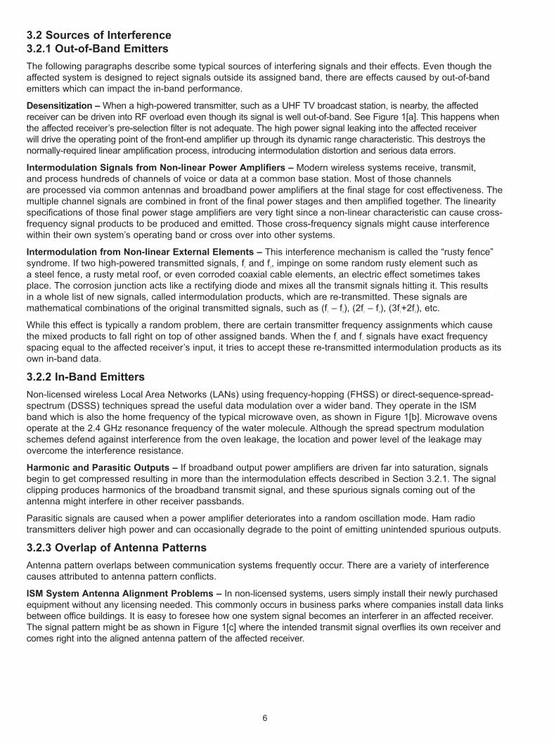
3.2 Sources of Interference3.2.1 Out-of-Band EmittersThe following paragraphs describe some typical sources of interfering signals and their effects. Even though the affected system is designed to reject signals outside its assigned band, there are effects caused by out-of-band emitters which can impact the in-band performance.

Desensitization – When a high-powered transmitter, such as a UHF TV broadcast station, is nearby, the affected receiver can be driven into RF overload even though its signal is well out-of-band. See Figure 1[a]. This happens when the affected receiver’s pre-selection filter is not adequate. The high power signal leaking into the affected receiver will drive the operating point of the front-end amplifier up through its dynamic range characteristic. This destroys the normally-required linear amplification process, introducing intermodulation distortion and serious data errors.

Intermodulation Signals from Non-linear Power Amplifiers – Modern wireless systems receive, transmit, and process hundreds of channels of voice or data at a common base station. Most of those channels are processed via common antennas and broadband power amplifiers at the final stage for cost effectiveness. The multiple channel signals are combined in front of the final power stages and then amplified together. The linearity specifications of those final power stage amplifiers are very tight since a non-linear characteristic can cause cross-frequency signal products to be produced and emitted. Those cross-frequency signals might cause interference within their own system’s operating band or cross over into other systems.

Intermodulation from Non-linear External Elements – This interference mechanism is called the “rusty fence” syndrome. If two high-powered transmitted signals, f1 and f2, impinge on some random rusty element such as a steel fence, a rusty metal roof, or even corroded coaxial cable elements, an electric effect sometimes takes place. The corrosion junction acts like a rectifying diode and mixes all the transmit signals hitting it. This results in a whole list of new signals, called intermodulation products, which are re-transmitted. These signals are mathematical combinations of the original transmitted signals, such as (f1 – f2), (2f1 – f2), (3f1+2f2), etc.

While this effect is typically a random problem, there are certain transmitter frequency assignments which cause the mixed products to fall right on top of other assigned bands. When the f1 and f2 signals have exact frequency spacing equal to the affected receiver’s input, it tries to accept these re-transmitted intermodulation products as its own in-band data.

3.2.2 In-Band Emitters Non-licensed wireless Local Area Networks (LANs) using frequency-hopping (FHSS) or direct-sequence-spread-spectrum (DSSS) techniques spread the useful data modulation over a wider band. They operate in the ISM band which is also the home frequency of the typical microwave oven, as shown in Figure 1[b]. Microwave ovens operate at the 2.4 GHz resonance frequency of the water molecule. Although the spread spectrum modulation schemes defend against interference from the oven leakage, the location and power level of the leakage may overcome the interference resistance.

Harmonic and Parasitic Outputs – If broadband output power amplifiers are driven far into saturation, signals begin to get compressed resulting in more than the intermodulation effects described in Section 3.2.1. The signal clipping produces harmonics of the broadband transmit signal, and these spurious signals coming out of the antenna might interfere in other receiver passbands.

Parasitic signals are caused when a power amplifier deteriorates into a random oscillation mode. Ham radio transmitters deliver high power and can occasionally degrade to the point of emitting unintended spurious outputs.

3.2.3 Overlap of Antenna PatternsAntenna pattern overlaps between communication systems frequently occur. There are a variety of interference causes attributed to antenna pattern conflicts.

ISM System Antenna Alignment Problems – In non-licensed systems, users simply install their newly purchased equipment without any licensing needed. This commonly occurs in business parks where companies install data links between office buildings. It is easy to foresee how one system signal becomes an interferer in an affected receiver. The signal pattern might be as shown in Figure 1[c] where the intended transmit signal overflies its own receiver and comes right into the aligned antenna pattern of the affected receiver.

7

While modulation designs are supposed to offer some rejection of interference due to different frequency-hopping parameters or different DSSS code patterns, it is possible that the interfering signal levels at the affected receiver might still overwhelm the rejection tolerance of the modulation scheme.

It should be noted that even if the antenna pattern lobes of the affected system are relatively narrow (high gain), there is still considerable sensitivity to signals that are as much as 20 to 30 degrees off boresight.

Backlobes and Sidelobes – As shown in Figure 3(c), there are sidelobe and backlobe characteristics in every antenna. This means that interfering signals might cause problems if they enter one of the sidelobes or the backlobe of the affected system as in Figure 1 [e] and [f]. Typical sidelobe and backlobe sensitivity is only 15 – 30 dB down from the main lobe.

Reflections and Fading – The affected system often operates in signal environments which affect its system signals. Heavy rainfall attenuates microwave frequencies. Buildings, hills, and other natural obstructions bend or cause multiple paths to form between transmitter and receiver. These multiple paths, or multipaths, lead to destructive signal cancellations and cause random fades in signal strength.

Other buildings, Figure 1 [D], might reflect interference into the side of the affected antenna’s main lobe. Low flying airplanes can cause a moving reflection which might degrade data randomly.

Cellular Antenna Overlap – Cellular systems, with their theoretical hexagonal base station cell pattern spacing, take advantage of frequency band re-use by assigning the same frequencies to cells that are spaced just one cell distance away. As such, any given cell antenna that happens to be misadjusted for tilt can easily overfly the adjacent cell and impinge on an affected receiver two cells over where the signal frequency assignments are the same.

4.0 How to Determine if Interference is Corrupting your SystemA down-system complaint might be the result of equipment performance degradation leading to marginal data. But just as likely, an interfering signal could be causing poor data or voice reception.

4.1 Recognizing the Interference

Section 3.0 reviewed the generic causes and sources of interfering effects. The frequency of an interfering signal is the most common parameter leading to the identification of the interfering source. Thus, an interference problem can often be categorized by its frequency characteristics.

It should be noted that whether the interfering signal is in-band or out-of-band, the signal is almost certainly coming through the antenna, down the cable, and into the affected receiver. Therefore, a spectrum analyzer connected to the operating system antenna will serve as a substitute measuring receiver which will display and help identify unwanted signals. Remember that the system’s band pre-selection filters are inside its receiver, so many out-of-band signals are naturally present at its antenna input connector.

Interference generally only affects receiver performance. Although it is possible that a source of interference can be physically close to a transmitter, the characteristics of the transmitted signal will not be affected. Thus, the first step in recognizing if interference has corrupted a receiver is to learn the characteristics of the signal that the affected system is intended to receive.

Reviewing the system’s operations manual will indicate what modulated signal should be received. By analyzing the frequency domain using a spectrum analyzer (as opposed to the time domain using an oscilloscope) the signal frequency, power, harmonic content, modulation quality, distortion and noise or interference can easily be measured. If interference is overlapping the intended receiver signal, it will be relatively obvious on the spectrum analyzer display.

A displayed interference “fingerprint” contains important identification characteristics. A modulated signal will have unique characteristics depending on the type of modulation used. Section 5.0 reviews many typical signal characteristics.

8

Selecting the Appropriate Test Equipment

The most useful and accurate tool for qualitative and quantitative analysis of RF and microwave interference in the field is the broadband, hand held spectrum analyzer. The Anritsu Spectrum Master MS2711E is such a tool that features powerful user-convenience parameters (soft keys), calibration-correction routines, and data manipulation and storage capabilities.

Section 4.2.1 presents some key operating principles and discusses parameters relating to interference considerations. Following that, Section 4.2.2 describes some more versatile measuring functions that are important and convenient for a typical interference measurement procedure.

4.2.1 Spectrum Analyzer ParametersWhat do we need to know about a spectrum analyzer to make sure that we can measure the signal environment adequately? Very basically, we need to know the frequency range, sensitivity, dynamic range, frequency resolution and accuracy.

Frequency Range – Frequency range should be the easiest criteria, since you have a good idea of your system’s frequency band and hence the spectrum span you want to observe. Just be sure to give yourself plenty of display width to work with, by setting the frequency span wide enough to include both your affected receiver signals and adjacent interfering signals.

Sensitivity – Sensitivity, although fairly straightforward, can be somewhat confusing. The key is to understand your system specifications and the level of sensitivity required to make your measurements of expected receiver inputs. For example, if your system’s receiver signal strength specification is expected to be on the order of –60 dBm, then you will typically only need an additional 20 to 30 dB of measurement range. Thus, a spectrum analyzer that exhibits a sensitivity of –80 to –90 dBm should do the job nicely.

Frequency Resolution, Dynamic Range, and Sweep Time – Frequency resolution, dynamic range, and sweep time are inter-related. Think of resolution as the shape of a scanning “window” which sweeps across an unknown band of signals. The shape of that sweeping window is similar to that shown in Figure 4. Spectrum analyzers provide for selectable resolutions, and call it resolution bandwidth (RBW). RBW represents the –3 dB width of the passband of the analyzer’s intermediate frequency (IF) amplifier chain. Resolution becomes important when you are trying to measure signals that occur close together in frequency, and you need to be able to distinguish one from the other.

Example: If two perfectly pure signal frequencies are 10 kHz apart, the spectrum analyzer display would show two renditions of the Figure 4 shapes spaced at 10 kHz. Thus, a 10 kHz RBW setting would show that there were two signals present. If the RBW was set to 30 kHz, the two signals 10 kHz apart will tend to display as one. In general, two equal-amplitude signals can be adequately identified if the selected RBW is less than or equal to the separation of the two signals.

Selecting the smallest possible RBW will increase the ability to resolve signals that are close together, but the trade-off is that it will take longer to sweep across a given frequency band of interest. Also, dynamic range decreases as RBW is increased as more noise is integrated as part of the measurement with the wider RBW. So, the optimum RBW setting depends on the spacing of the signals that are to be resolved, the dynamic range required, and the maximum acceptable sweep time.

Selectivity – In some interference applications, there will be signals that have amplitudes that are quite unequal. In this case, “selectivity” becomes an important criteria. It is very possible for the smaller of the two signals to become buried under the filter skirt of the larger signal. See Figure 4.

IF Center Frequency

10 kHz

-50

-60

Freq

Unequal signal60 dB down

-40

-30

-20

-10

-0-3

dB

110 kHz

Figure 4. A spectrum analyzer’s shape factor is defined as the ratio of its IF bandwidths at –60 and –3 dB, in this case 11:1.

9

Shape Factor – A spectrum analyzer’s shape factor defines the ratio of the –60 dB bandwidth to the –3 dB bandwidth of the IF amplifiers. In the Figure 4 example, the 10 kHz RBW filter has a typical shape factor of 11:1, with a resultant –60 dB bandwidth of 110 kHz and a half-bandwidth value of approximately 60 kHz. If two signals are separated by 60 kHz, but one of them is –60 dB lower in amplitude, it will be almost buried in the selectivity skirt of the main signal.

Accuracy – The measurement accuracy of any spectrum analyzer results from the addition of many different accuracy components. Measurement accuracy is important when comparing measured values on unknown signals to published specifications of a system under test. Luckily, when making typical interference measurements, the user is looking for ratios, such as C/I, which determines the operating margin of the desired carrier over the interfering signal in the same operating bandwidth. Thus, absolute accuracy is less critical than relative accuracy.

4.2.2 Spectrum Analyzer Functional Controls and RoutinesThe Anritsu analyzers have the traditional control and input keys of most advanced spectrum analyzers. But it also features more sophisticated “one-button” measurement routines which provide powerful computational assistance when making interference measurements.

Center Frequency and Span – All modern spectrum analyzers have flexible control of their tuning parameters with center frequency and display sweep width (span) being most popular. Span is simply the width of the swept frequency band between the start frequency and the stop frequency. It can be entered with the Center Frequency and the Span soft keys. The GHz, MHz, kHz or Hz soft keys set the units value. Alternatively, the sweep width can be entered by keying in the Start and Stop frequencies.

Resolution Bandwidth (RBW) – With a given RBW, a sweep speed that is too fast will pass by the unknown signal before the detection system has a chance to respond to the signal. But sweeping too slow will just waste the operator’s time.

Thus, for each span width, and each sweep time, there will be an optimum resolution bandwidth (RBW) for best accuracy. Fortunately, the operator can rely on the “automatic” setting feature to provide optimum combinations of span, sweep speed and bandwidth settings which enhance accurate measurement results.

Save-Recall Menus – The Save and Recall menu functions allow you to store the instrument’s many control settings for up to 10 different conditions. Use the Save Setup and Recall Setup modes to achieve quick changes from one commonly-used set of measurement settings to another. Setup location 0 is the factory-preset settings state. The Save/Recall function essentially pre-sets all the instrument controls to user-defined settings, which is quite useful when the job is routine and repetitive. If done before driving to the field, this means minimum keyboard setup times for parameters like carrier level in frequency-allocated channel assignments.

Marker Peak Search and Centering – In a normal search routine, the operator will often set the display span for a spectrum that is wider than the affected receiver channel assignment. This allows a panoramic view of all signals on the air for that span. If a large amplitude possible-interferer signal shows up, the operator can choose a convenient key function called Marker to Peak. This arithmetically looks across the display and picks out the highest signal. It then tunes the selected marker, say M1, to that highest peak and annotates the screen with the M1 frequency. Such information might give immediate clues to the interfering culprit.

Another handy key function, after capturing the M1 marker frequency, is the Marker Freq to Center softkey. This immediately re-centers the display so that the M1 frequency is right at the center. The operator can then narrow the sweep span to get some idea of the signal characteristics of the interferer, e.g., determine whether it is randomly occurring, noisy, or perhaps exhibiting some other revealing characteristic.

10

Display Capture – A very important feature is the ability to capture spectrum displays that are encountered during a long day in the field. The Save Display function permits the operator to take many measurements, name them for the measured situation, and bring the instrument back to the office where they can be downloaded or printed out. Figure 5 in Section 5.3 (page 13) is an example of a field-captured display, with all its annotated data.

The Recall Display key brings an index list to the screen for selecting and calling back saved waveforms. Up to 180 screen displays may be stored for later use.

Preamplifier and Input Attenuator – For most field interference applications, signals will be relatively weak. The preamplifier feature offers a selectable, full-spectrum amplification of 20 dB. The preamplifier has a very low noise figure, meaning that it does not add appreciable noise to the signal it amplifies. The preamplifier can handle 20 mW (+13 dBm) without damage, and if it goes into saturation, an annotated SAT indicator shows on the display.

The input attenuator is a standard feature of all spectrum analyzers that protects the relatively delicate front end mixer and preamplifier stage. The standard input of the analyzer can handle 200 mW (+23 dBm) without damage, so good practice dictates that you first set the input attenuator to 40 or 50 dB if you expect unknown signals with high amplitude. Then adjust the attenuator setting for less attenuation after the signals appear on screen.

Max Hold – In a number of measurements, the randomness of an interfering signal will make the display jump and difficult to visualize. It is helpful in such situations to use the Max Hold function. This feature digitally processes the display trace such that it always remembers and displays the highest signal level at every point on the display.

Demodulator – For additional power in identifying interferer signals, sometimes an audio demodulation of the waveform can assist. There is an AM function plus two FM demodulator functions, narrowband and wideband. The audio output can be heard on accessory earphones or through the built-in speaker on the front panel.

Occupied Bandwidth and Channel Power – The Spectrum Master MS2711E / MS2712E / MS2713E / MS2721B features two computational modes which are very powerful for measurements on wideband data channels such as ISM data links. Occupied Bandwidth (OBW) allows the operator to define the band edges of an occupied band, such as the –20 dBc power points. After the measurement, the M1 and M2 markers show as annotated frequencies on the display and define the band edge frequencies where the signal is –20 dB relative to the carrier.

Channel Power–Channel Power arithmetically computes the integrated power contained in a wideband spectrum after its defined bandwidth is set into the analyzer. This mode is particularly useful in measuring system power in an ISM spread spectrum communications signal, and is described further in the “Practical Tips on Measuring Interference” Anritsu Publication number 11410-00537.

Antenna Accessories – Many field interference measurements will be made with an independent antenna, i.e., not the communication system’s operating antenna. The most versatile kind of independent antenna is the so-called “whip” design. A whip antenna is a linear conductor connected to the Spectrum Master coaxial input connector. Whip antennas are sized for 1/4 wavelength at the specified center frequency. Whip designs are omnidirectional, and insensitive to directional effects.

For additional diagnostic power on certain interference measurements, the operator will sometimes need to use a directional antenna. Microwave data systems are an example where the system antenna directional performance is highly critical. In those cases, a directional antenna attached to the spectrum analyzer can determine the direction of the interfering signal. Directional antenna kits are commercially available for common application bands.

11

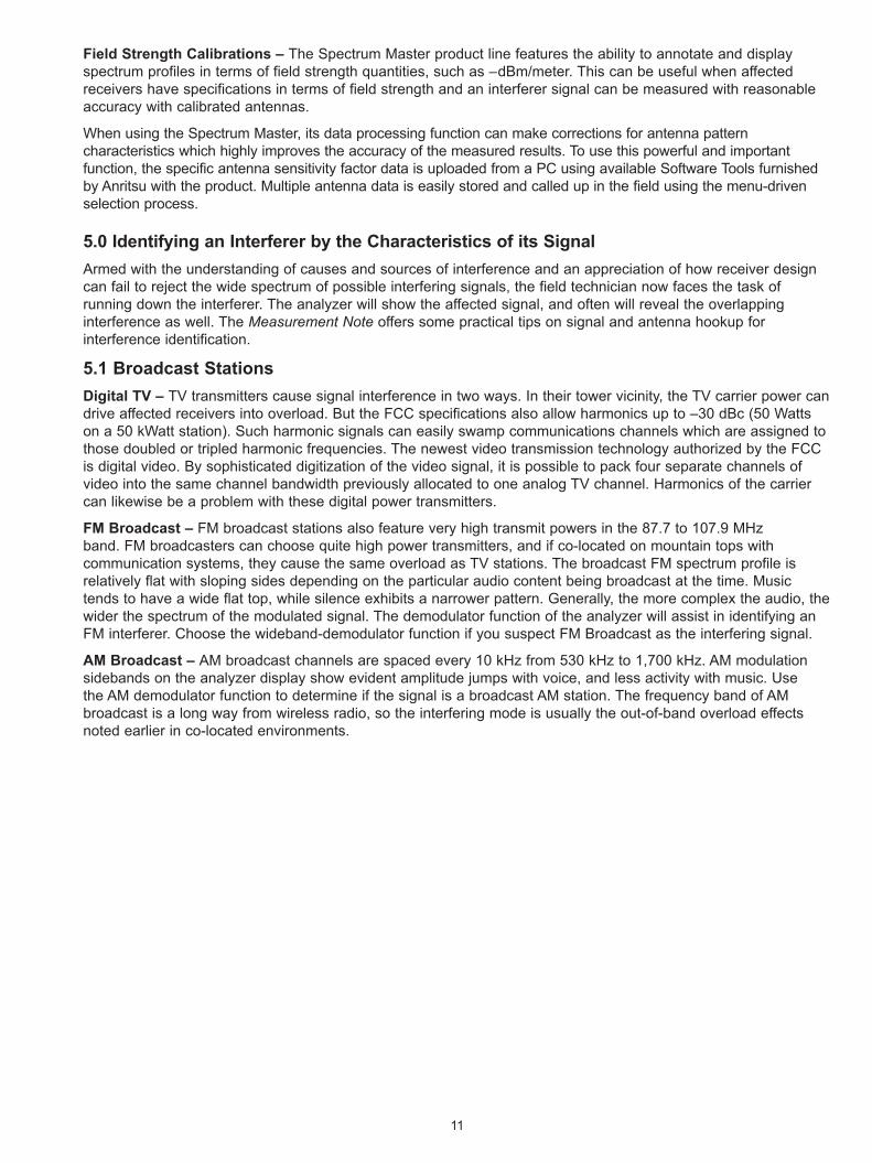
Field Strength Calibrations – The Spectrum Master product line features the ability to annotate and display spectrum profiles in terms of field strength quantities, such as –dBm/meter. This can be useful when affected receivers have specifications in terms of field strength and an interferer signal can be measured with reasonable accuracy with calibrated antennas.

When using the Spectrum Master, its data processing function can make corrections for antenna pattern characteristics which highly improves the accuracy of the measured results. To use this powerful and important function, the specific antenna sensitivity factor data is uploaded from a PC using available Software Tools furnished by Anritsu with the product. Multiple antenna data is easily stored and called up in the field using the menu-driven selection process.

5.0 Identifying an Interferer by the Characteristics of its SignalArmed with the understanding of causes and sources of interference and an appreciation of how receiver design can fail to reject the wide spectrum of possible interfering signals, the field technician now faces the task of running down the interferer. The analyzer will show the affected signal, and often will reveal the overlapping interference as well. The Measurement Note offers some practical tips on signal and antenna hookup for interference identification.

5.1 Broadcast StationsDigital TV – TV transmitters cause signal interference in two ways. In their tower vicinity, the TV carrier power can drive affected receivers into overload. But the FCC specifications also allow harmonics up to –30 dBc (50 Watts on a 50 kWatt station). Such harmonic signals can easily swamp communications channels which are assigned to those doubled or tripled harmonic frequencies. The newest video transmission technology authorized by the FCC is digital video. By sophisticated digitization of the video signal, it is possible to pack four separate channels of video into the same channel bandwidth previously allocated to one analog TV channel. Harmonics of the carrier can likewise be a problem with these digital power transmitters.

FM Broadcast – FM broadcast stations also feature very high transmit powers in the 87.7 to 107.9 MHz band. FM broadcasters can choose quite high power transmitters, and if co-located on mountain tops with communication systems, they cause the same overload as TV stations. The broadcast FM spectrum profile is relatively flat with sloping sides depending on the particular audio content being broadcast at the time. Music tends to have a wide flat top, while silence exhibits a narrower pattern. Generally, the more complex the audio, the wider the spectrum of the modulated signal. The demodulator function of the analyzer will assist in identifying an FM interferer. Choose the wideband-demodulator function if you suspect FM Broadcast as the interfering signal.

AM Broadcast – AM broadcast channels are spaced every 10 kHz from 530 kHz to 1,700 kHz. AM modulation sidebands on the analyzer display show evident amplitude jumps with voice, and less activity with music. Use the AM demodulator function to determine if the signal is a broadcast AM station. The frequency band of AM broadcast is a long way from wireless radio, so the interfering mode is usually the out-of-band overload effects noted earlier in co-located environments.

12

5.2 Traditional Communications SystemsFM Mobile – Before the emergence of the personal mobile wireless (cellular) phones in the 1990’s, public safety applications, such as police, fire and forest service, used narrowband FM technology. These applications still exist in the 50, 150 and 450 MHz FM bands. Typical mobile FM transmitters emit 5 to 150 Watts while their permanent base stations often transmit at 150 Watts with an omni-directional footprint. The spectrum profile of narrowband FM spans about 5 kHz. For help in identifying, use the analyzer narrowband FM demodulator function.

AM Aircraft Communications – Using the VHF frequencies in the 118-136 MHz region, authorities allocated 25 kHz-wide channels for a higher voice quality AM for aircraft communications. Being exceedingly mobile, aircraft interferers are also difficult to pin down since any one aircraft is only in the area for tens of seconds. But again, their ground transmitters can be a constant source of relatively high signal powers. The spectrum profile again reflects the voice nature of this application. The AM demodulator function could be useful here in identifying these types of signals as potential interferers.

Paging Systems – Simple paging systems typically use a frequency-shift-keyed (FSK) modulation format which exhibits a spectrum profile with two separated peaks, each representing one of the two frequencies which shift according to the digital “one” or “zero” being transmitted. As more complex data, such as an alphanumeric message, is transmitted, the space between the two peaks fills in.

Amateur Radio (Ham Radio) – Scattered throughout the frequency spectrum are a number of allocated frequency bands dedicated to “Ham” radio operators. While their transmitters use AM, FM, SSB, FSK, slowscan and fastscan TV modulation, they are also authorized to run experimental transmissions in other formats. Their emitted powers can be quite high since they intend to transmit to others around the earth.

Hams often use large, steerable directional arrays of HF antennas to increase their directional power, so their interfering power can be quite high. Further, these transmitters are mostly found in residential areas where wireless base stations are located. If the affected receiver is not well filtered at its input and is in the boresight direction of the Ham transmitter, there is a possibility of interference. Ham transmitters can contain harmonics which extend into wireless bands. The AM, FM and SSB demodulator functions will assist in identifying these types of interfering signals.

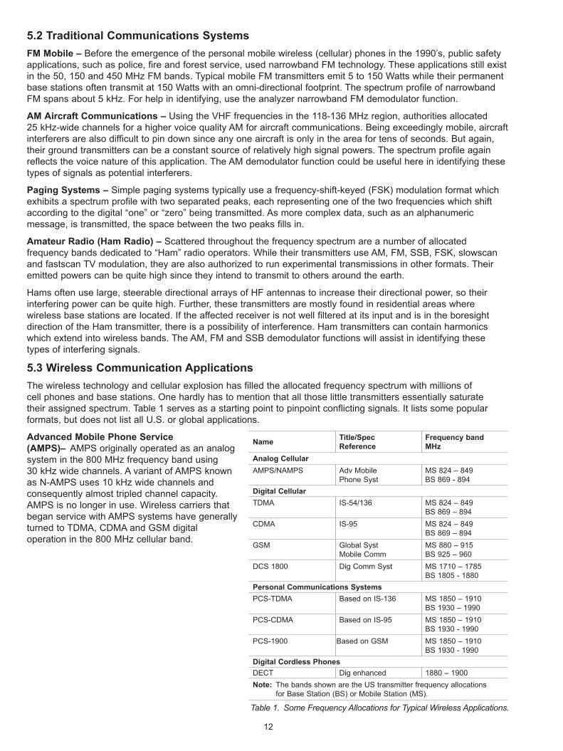
5.3 Wireless Communication Applications The wireless technology and cellular explosion has filled the allocated frequency spectrum with millions of cell phones and base stations. One hardly has to mention that all those little transmitters essentially saturate their assigned spectrum. Table 1 serves as a starting point to pinpoint conflicting signals. It lists some popular formats, but does not list all U.S. or global applications.

Advanced Mobile Phone Service (AMPS)– AMPS originally operated as an analog system in the 800 MHz frequency band using 30 kHz wide channels. A variant of AMPS known as N-AMPS uses 10 kHz wide channels and consequently almost tripled channel capacity. AMPS is no longer in use. Wireless carriers that began service with AMPS systems have generally turned to TDMA, CDMA and GSM digital operation in the 800 MHz cellular band.

Name Title/Spec Reference

Frequency band MHz

Analog CellularAMPS/NAMPS Adv Mobile

Phone SystMS 824 – 849 BS 869 - 894

Digital CellularTDMA IS-54/136 MS 824 – 849

BS 869 – 894CDMA IS-95 MS 824 – 849

BS 869 – 894GSM Global Syst

Mobile CommMS 880 – 915 BS 925 – 960

DCS 1800 Dig Comm Syst MS 1710 – 1785 BS 1805 - 1880

Personal Communications SystemsPCS-TDMA Based on IS-136 MS 1850 – 1910

BS 1930 – 1990PCS-CDMA Based on IS-95 MS 1850 – 1910

BS 1930 - 1990PCS-1900 Based on GSM MS 1850 – 1910

BS 1930 - 1990Digital Cordless PhonesDECT Dig enhanced 1880 – 1900Note: The bands shown are the US transmitter frequency allocations

for Base Station (BS) or Mobile Station (MS).

Table 1. Some Frequency Allocations for Typical Wireless Applications.

13

North American Digital Cellular (NADC, now IS-136) – This is one of the original rollouts of the new cellular technology. It was designed to utilize the existing 30 kHz channel of the Advanced Mobile Phone Service (AMPS) cellular technology. Its spectrum profile fills the 30 kHz channel with a relatively flat top spectrum characteristic.

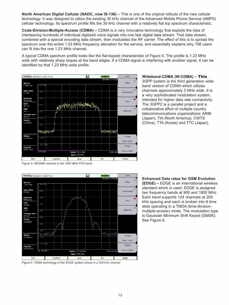
Code-Division-Multiple-Access (CDMA) – CDMA is a very innovative technology that exploits the idea of interleaving hundreds of individual digitized voice signals into one fast digital data stream. That data stream, combined with a special encoding data stream, then modulates the RF carrier. The effect of this is to spread the spectrum over the entire 1.23 MHz frequency allocation for the service, and essentially explains why 798 users can fit into the one 1.23 MHz channel.

A typical CDMA spectrum profile looks like the flat-topped characteristic of Figure 5. The profile is 1.23 MHz wide with relatively sharp slopes at the band edges. If a CDMA signal is interfering with another signal, it can be identified by that 1.23 MHz wide profile.

Wideband-CDMA (W-CDMA) – This 3GPP system is the third generation wide-band version of CDMA which utilizes channels approximately 5 MHz wide. It is a very sophisticated modulation system, intended for higher data rate connectivity. The 3GPP2 is a parallel project and a collaborative effort of multiple country telecommunications organizations; ARIB (Japan), TIA (North America), CWTS (China), TTA (Korea) and TTC (Japan).

Enhanced Data rates for GSM Evolution (EDGE) – EDGE is an international wireless standard which is used. EDGE is assigned two frequency bands at 900 and 1800 MHz. Each band supports 124 channels at 200 kHz spacing and each is broken into 8 time slots operating in a TMDA (time-division-multiple-access) mode. The modulation type is Gaussian Minimum Shift Keyed (GMSK). See Figure 6.

Figure 5. WCDMA channel in the 1900 MHz PCS band.

Figure 6. TDMA technology of the EDGE system shows in a 200 kHz channel.

14

Personal Communications Systems (PCS) – The Personal Communications System (PCS) is a name given to wireless communications systems in the 1800 – 1900 MHz frequency band. PCS was supposed to be a more comprehensive specification than the earlier cellular specification at 800 MHz. However, the only technologies that were implemented were upbanded cellular standards. Thus, the change was simply one of expanding the available spectrum by using the same signal formats at the higher 1800 MHz band. Now consumers rarely know whether their cellular phone is operating in the cellular or PCS band.

• PCS1900 - Upbanded GSM cellular

• TIA/EIA-136 – Upbanded TDMA digital cellular (ANSI-136)

• TIA/EIA-95 or IS-2000 – Upbanded CDMA digital cellular (ANSI-95, cdmaOne or cdma2000)

All PCS systems are digital. The PCS frequency allocation in the US is three 30 MHz allocations and two 10 MHz allocations in the 1850 - 1990 MHz frequency band.

5.4 Unlicensed ISM Data Systems

Table 2. Some Frequency Allocations for Typical Unlicensed ISM Applications.

Table 2 shows some popular ISM-allocated bands. In addition to a myriad of unlicensed applications like microwave ovens and atomic particle accelerators, they now support thousands of unlicensed data communications systems. Customers often prefer these systems because of their inexpensive nature and the ability to install them without a tedious licensing process. They are popular for point-to-point and point-to-multipoint data link applications such as Ethernet bridging for intracompany data bridges. Recent Bluetooth technology promises to further fill the spectrum with close-range personal data applications.

Wireless LANs – Wireless LAN technology in the ISM band was conceived for short-range connectivity systems. Its uses include laptop computers and data management within buildings. Both WLAN technologies, frequency–hopping (FHSS) and direct-sequence (DSSS), depend on spread spectrum technology for data modulation. These schemes trade wider bandwidth for transmission reliability. To a narrow band system, spread spectrum signals just look like random noise.

The typical FHSS system utilizes a 1 MHz power spectrum which is frequency-hopped three times per second across a 75 MHz channel. A typical DSSS system utilizes a constant 25 MHz wide spectrum, from a 1 Watt (+30 dBm) transmitter, which translates to +16 dBm per MHz.

When ISM interference from another similar system brings down a affected receiver, it is highly likely that the interferer is completely legal. It is then up to the affected to determine how to arrange other elements like antennas or perhaps modulation alternatives to solve the problem. There is no appeal to official regulators since these are unlicensed bands.

Name Title/Spec Reference

Frequency Band MHz

Wireless DataBluetooth ISM band 2400 – 2497Wireless LAN IEEE 802.11b and g 2400 – 2484Wireless LAN IEEE 802.11a 5025 – 5710

ISM ApplicationsISM 902 – 928FCC Part 15.247 5725 – 5850

FCC Part 15.407UNII-1 5150 – 5250UNII-2 5250 – 5350UNII-3 5725 – 5825

15

ISM Microwave Data Links – ISM-band systems provide fast installation for applications such as Ethernet-bridges which connect backbone data systems with new wireless base stations without the need for digging underground cables. ISM data links at 5725 – 5850 MHz have considerable advantage over UNII (Unlicensed National Information Infrastructure) systems because they are allowed higher output powers and very high gain antennas. These often give them a 48 dB interference advantage.

Here are the FCC bands:Part 15.247 Technical requirements for intentional radiators 5725 – 5850 MHz Emission B/W –20 dB pointsPart 15.407 Technical requirements for UNII 5150 – 5250 MHz UNII-1 Emission B/W –26 dB points 5250 – 5350 MHz UNII-2 same 5725 – 5825 MHz UNII-3 same

(The word “Part” refers to the FCC regulations indexing format.)

6.0 ConclusionOne of the industry trade association’s web sites shows statistics which estimate that worldwide ownership of wireless devices exceeded 800 million in 2002 and by 2009 has exceeded one billion.[1] Does anyone wonder that competing wireless systems will continue to interfere with each other in regions of high density installations?

Understanding the characteristics of your affected receiver’s modulated signal and the effect that noise or interference has on that signal is the first step in detecting interference within your communications system. Selecting the appropriate test equipment, such as the Anritsu Spectrum Master MS2711E / MS2712E / MS2713E / MS2721B, and employing proper measurement techniques can enhance the likelihood of locating and identifying sources of interference within your system.A companion application note from Anritsu Company, “Practical Tips on Measuring Interference, pn: 11410-00537” offers actual measurement examples and practical routines used by field technicians who search for interference as a life’s work. It also explains the advantages of Anritsu’s Spectrum Master products that are designed to simplify your search for interfering signals.

For those with deeper interest or questions about antennas, there are plenty of Internet resources for further study. The footnote lists the National Spectrum Management Association (NSMA) website “www.nsma.org.” A typical antenna manufacturer website “www.gabrielnet.com” is also listed.

_______Footnote:[1] Cellular Networking Perspectives Ltd. See their very useful, impartial and informative web-site: www.cnp-wireless.com.

It contains a super-comprehensive acronym list of wireless terminology.

Application Note No. 11410-00536, Rev. B Printed in United States 2011-07©2011 Anritsu Company. All Rights Reserved.

® Anritsu All trademarks are registered trademarks of their respective companies. Data subject to change without notice. For the most recent specifications visit: www.anritsu.com

Anritsu Corporation5-1-1 Onna, Atsugi-shi, Kanagawa, 243-8555 Japan Phone: +81-46-223-1111 Fax: +81-46-296-1238

• U.S.A. Anritsu Company1155 East Collins Boulevard, Suite 100, Richardson, TX, 75081 U.S.A. Toll Free: 1-800-ANRITSU (267-4878) Phone: +1-972-644-1777 Fax: +1-972-671-1877• Canada Anritsu Electronics Ltd.700 Silver Seven Road, Suite 120, Kanata, Ontario K2V 1C3, Canada Phone: +1-613-591-2003 Fax: +1-613-591-1006

• Brazil Anritsu Electrônica Ltda.Praça Amadeu Amaral, 27 - 1 Andar 01327-010 - Bela Vista - São Paulo - SP - Brasil Phone: +55-11-3283-2511 Fax: +55-11-3288-6940

• Mexico Anritsu Company, S.A. de C.V.Av. Ejército Nacional No. 579 Piso 9, Col. Granada 11520 México, D.F., México Phone: +52-55-1101-2370 Fax: +52-55-5254-3147

• U.K. Anritsu EMEA Ltd.200 Capability Green, Luton, Bedfordshire LU1 3LU, U.K. Phone: +44-1582-433280 Fax: +44-1582-731303

• France Anritsu S.A.12 Avenue du Québec, Bâtiment Iris 1-Silic 638, 91140 VILLEBON SUR YVETTE, France Phone: +33-1-60-92-15-50 Fax: +33-1-64-46-10-65

• Germany Anritsu GmbHNemetschek Haus, Konrad-Zuse-Platz 1 81829 München, Germany Phone: +49 (0) 89 442308-0 Fax: +49 (0) 89 442308-55

• Italy Anritsu S.p.A.Via Elio Vittorini, 129, 00144 Roma, Italy Phone: +39-06-509-9711 Fax: +39-06-502-2425

• Sweden Anritsu ABBorgafjordsgatan 13, 164 40 KISTA, Sweden Phone: +46-8-534-707-00 Fax: +46-8-534-707-30

• Finland Anritsu ABTeknobulevardi 3-5, FI-01530 VANTAA, Finland Phone: +358-20-741-8100 Fax: +358-20-741-8111

• Denmark Anritsu A/S (for Service Assurance) Anritsu AB (for Test & Measurement)Kirkebjerg Allé 90 DK-2605 Brøndby, Denmark Phone: +45-7211-2200 Fax: +45-7211-2210

• RussiaAnritsu EMEA Ltd. Representation Office in RussiaTverskaya str. 16/2, bld. 1, 7th floor. Russia, 125009, Moscow Phone: +7-495-363-1694 Fax: +7-495-935-8962

• United Arab Emirates Anritsu EMEA Ltd. Dubai Liaison OfficeP O Box 500413 - Dubai Internet City Al Thuraya Building, Tower 1, Suite 701, 7th Floor Dubai, United Arab Emirates Phone: +971-4-3670352 Fax: +971-4-3688460

• Singapore Anritsu Pte. Ltd.60 Alexandra Terrace, #02-08, The Comtech (Lobby A) Singapore 118502 Phone: +65-6282-2400 Fax: +65-6282-2533

• India Anritsu Pte. Ltd. India Branch Office3rd Floor, Shri Lakshminarayan Niwas, #2726, 80 ft Road, HAL 3rd Stage, Bangalore - 560 075, India Phone: +91-80-4058-1300 Fax: +91-80-4058-1301

• P. R. China (Hong Kong) Anritsu Company Ltd.Units 4 & 5, 28th Floor, Greenfield Tower, Concordia Plaza, No. 1 Science Museum Road, Tsim Sha Tsui East, Kowloon, Hong Kong, P.R. China Phone: +852-2301-4980 Fax: +852-2301-3545

• P. R. China (Beijing) Anritsu Company Ltd. Beijing Representative OfficeRoom 2008, Beijing Fortune Building, No. 5 , Dong-San-Huan Bei Road, Chao-Yang District, Beijing 100004, P.R. China Phone: +86-10-6590-9230Fax: +86-10-6590-9235

• Korea Anritsu Corporation, Ltd.8F Hyunjuk Bldg. 832-41, Yeoksam-Dong, Kangnam-ku, Seoul, 135-080, Korea Phone: +82-2-553-6603 Fax: +82-2-553-6604

• Australia Anritsu Pty Ltd.Unit 21/270 Ferntree Gully Road, Notting Hill Victoria, 3168, Australia Phone: +61-3-9558-8177 Fax: +61-3-9558-8255

• Taiwan Anritsu Company Inc.7F, No. 316, Sec. 1, Neihu Rd., Taipei 114, Taiwan Phone: +886-2-8751-1816 Fax: +886-2-8751-1817