FUNDAMENTALS OF CONVECTION S - EECL … · FUNDAMENTALS OF CONVECTION S ... Convection heat...
34
FUNDAMENTALS OF CONVECTION S o far, we have considered conduction, which is the mechanism of heat transfer through a solid or a quiescent fluid. We now consider convec- tion, which is the mechanism of heat transfer through a fluid in the presence of bulk fluid motion. Convection is classified as natural (or free) and forced convection, depend- ing on how the fluid motion is initiated. In forced convection, the fluid is forced to flow over a surface or in a pipe by external means such as a pump or a fan. In natural convection, any fluid motion is caused by natural means such as the buoyancy effect, which manifests itself as the rise of warmer fluid and the fall of the cooler fluid. Convection is also classified as external and inter- nal, depending on whether the fluid is forced to flow over a surface or in a channel. We start this chapter with a general physical description of the convection mechanism. We then discuss the velocity and thermal boundary layers, and laminar and turbulent flows. We continue with the discussion of the dimen- sionless Reynolds, Prandtl, and Nusselt numbers, and their physical signifi- cance. Next we derive the convection equations of on the basis of mass, momentum, and energy conservation, and obtain solutions for flow over a flat plate. We then nondimensionalize the convection equations, and obtain func- tional forms of friction and convection coefficients. Finally, we present analo- gies between momentum and heat transfer. 333 CHAPTER 6 CONTENTS 6–1 Physical Mechanism on Convection 334 6–2 Classification of Fluid Flows 337 6–3 Velocity Boundary Layer 339 6–4 Thermal Boundary Layer 341 6–5 Laminar and Turbulent Flows 342 6–6 Heat and Momentum Transfer in Turbulent Flow 343 6–7 Derivation of Differential Convection Equations 345 6–8 Solutions of Convection Equations for a Flat Plate 352 6–9 Nondimensionalized Convection Equations and Similarity 356 6–10 Functional Forms of Friction and Convection Coefficients 357 6–11 Analogies between Momentum and Heat Transfer 358 cen58933_ch06.qxd 9/4/2002 12:05 PM Page 333
Transcript of FUNDAMENTALS OF CONVECTION S - EECL … · FUNDAMENTALS OF CONVECTION S ... Convection heat...

F U N D A M E N TA L S O FC O N V E C T I O N
So far, we have considered conduction, which is the mechanism of heattransfer through a solid or a quiescent fluid. We now consider convec-tion, which is the mechanism of heat transfer through a fluid in the
presence of bulk fluid motion.Convection is classified as natural (or free) and forced convection, depend-
ing on how the fluid motion is initiated. In forced convection, the fluid isforced to flow over a surface or in a pipe by external means such as a pump ora fan. In natural convection, any fluid motion is caused by natural means suchas the buoyancy effect, which manifests itself as the rise of warmer fluid andthe fall of the cooler fluid. Convection is also classified as external and inter-nal, depending on whether the fluid is forced to flow over a surface or in achannel.
We start this chapter with a general physical description of the convectionmechanism. We then discuss the velocity and thermal boundary layers, andlaminar and turbulent flows. We continue with the discussion of the dimen-sionless Reynolds, Prandtl, and Nusselt numbers, and their physical signifi-cance. Next we derive the convection equations of on the basis of mass,momentum, and energy conservation, and obtain solutions for flow over a flatplate. We then nondimensionalize the convection equations, and obtain func-tional forms of friction and convection coefficients. Finally, we present analo-gies between momentum and heat transfer.
333
CHAPTER
6CONTENTS
6–1 Physical Mechanism onConvection 334
6–2 Classification of Fluid Flows 337
6–3 Velocity Boundary Layer 339
6–4 Thermal Boundary Layer 341
6–5 Laminar and Turbulent Flows 342
6–6 Heat and Momentum Transfer inTurbulent Flow 343
6–7 Derivation of DifferentialConvection Equations 345
6–8 Solutions of ConvectionEquations for a Flat Plate 352
6–9 Nondimensionalized Convection Equations andSimilarity 356
6–10 Functional Forms of Friction and ConvectionCoefficients 357
6–11 Analogies between Momentumand Heat Transfer 358
cen58933_ch06.qxd 9/4/2002 12:05 PM Page 333

6–1 PHYSICAL MECHANISM OF CONVECTIONWe mentioned earlier that there are three basic mechanisms of heat transfer:conduction, convection, and radiation. Conduction and convection are similarin that both mechanisms require the presence of a material medium. But theyare different in that convection requires the presence of fluid motion.
Heat transfer through a solid is always by conduction, since the moleculesof a solid remain at relatively fixed positions. Heat transfer through a liquid orgas, however, can be by conduction or convection, depending on the presenceof any bulk fluid motion. Heat transfer through a fluid is by convection in thepresence of bulk fluid motion and by conduction in the absence of it. There-fore, conduction in a fluid can be viewed as the limiting case of convection,corresponding to the case of quiescent fluid (Fig. 6–1).
Convection heat transfer is complicated by the fact that it involves fluid mo-tion as well as heat conduction. The fluid motion enhances heat transfer, sinceit brings hotter and cooler chunks of fluid into contact, initiating higher ratesof conduction at a greater number of sites in a fluid. Therefore, the rate of heattransfer through a fluid is much higher by convection than it is by conduction.In fact, the higher the fluid velocity, the higher the rate of heat transfer.
To clarify this point further, consider steady heat transfer through a fluidcontained between two parallel plates maintained at different temperatures, asshown in Figure 6–2. The temperatures of the fluid and the plate will be thesame at the points of contact because of the continuity of temperature. As-suming no fluid motion, the energy of the hotter fluid molecules near the hotplate will be transferred to the adjacent cooler fluid molecules. This energywill then be transferred to the next layer of the cooler fluid molecules. Thisenergy will then be transferred to the next layer of the cooler fluid, and so on,until it is finally transferred to the other plate. This is what happens duringconduction through a fluid. Now let us use a syringe to draw some fluid nearthe hot plate and inject it near the cold plate repeatedly. You can imagine thatthis will speed up the heat transfer process considerably, since some energy iscarried to the other side as a result of fluid motion.
Consider the cooling of a hot iron block with a fan blowing air over its topsurface, as shown in Figure 6–3. We know that heat will be transferred fromthe hot block to the surrounding cooler air, and the block will eventuallycool. We also know that the block will cool faster if the fan is switched to ahigher speed. Replacing air by water will enhance the convection heat trans-fer even more.
Experience shows that convection heat transfer strongly depends on thefluid properties dynamic viscosity �, thermal conductivity k, density �, andspecific heat Cp, as well as the fluid velocity �. It also depends on the geome-try and the roughness of the solid surface, in addition to the type of fluid flow(such as being streamlined or turbulent). Thus, we expect the convection heattransfer relations to be rather complex because of the dependence of convec-tion on so many variables. This is not surprising, since convection is the mostcomplex mechanism of heat transfer.
Despite the complexity of convection, the rate of convection heat transfer isobserved to be proportional to the temperature difference and is convenientlyexpressed by Newton’s law of cooling as
�
334HEAT TRANSFER
20°C5 m/s
AIR
AIR
AIR
50°C
(a) Forced convection
(b) Free convection
(c) Conduction
No convectioncurrents
Warmer airrising
Q·
Q·
Q·
FIGURE 6–1Heat transfer from a hot surface to thesurrounding fluid by convection andconduction.
Hot plate, 110°C
Cold plate, 30°C
Fluid
Heat transferthrough thefluidQ
·
FIGURE 6–2Heat transfer through a fluidsandwiched between two parallelplates.
cen58933_ch06.qxd 9/4/2002 12:05 PM Page 334

q·conv � h(Ts � T�) (W/m2) (6-1)
or
Q·
conv � hAs(Ts � T�) (W) (6-2)
where
h � convection heat transfer coefficient, W/m2 � ˚C
As � heat transfer surface area, m2
Ts � temperature of the surface, ˚C
T� � temperature of the fluid sufficiently far from the surface, ˚C
Judging from its units, the convection heat transfer coefficient h can be de-fined as the rate of heat transfer between a solid surface and a fluid per unitsurface area per unit temperature difference.
You should not be deceived by the simple appearance of this relation, be-cause the convection heat transfer coefficient h depends on the several of thementioned variables, and thus is difficult to determine.
When a fluid is forced to flow over a solid surface that is nonporous (i.e.,impermeable to the fluid), it is observed that the fluid in motion comes to acomplete stop at the surface and assumes a zero velocity relative to the sur-face. That is, the fluid layer in direct contact with a solid surface “sticks” tothe surface and there is no slip. In fluid flow, this phenomenon is known as theno-slip condition, and it is due to the viscosity of the fluid (Fig. 6–4).
The no-slip condition is responsible for the development of the velocity pro-file for flow. Because of the friction between the fluid layers, the layer thatsticks to the wall slows the adjacent fluid layer, which slows the next layer,and so on. A consequence of the no-slip condition is that all velocity profilesmust have zero values at the points of contact between a fluid and a solid. Theonly exception to the no-slip condition occurs in extremely rarified gases.
A similar phenomenon occurs for the temperature. When two bodies at dif-ferent temperatures are brought into contact, heat transfer occurs until bothbodies assume the same temperature at the point of contact. Therefore, a fluidand a solid surface will have the same temperature at the point of contact. Thisis known as no-temperature-jump condition.
An implication of the no-slip and the no-temperature jump conditions is thatheat transfer from the solid surface to the fluid layer adjacent to the surface isby pure conduction, since the fluid layer is motionless, and can be expressed as
q·conv � q·cond � �kfluid (W/m2) (6-3)
where T represents the temperature distribution in the fluid and (�T/�y)y�0 isthe temperature gradient at the surface. This heat is then convected away fromthe surface as a result of fluid motion. Note that convection heat transfer froma solid surface to a fluid is merely the conduction heat transfer from the solidsurface to the fluid layer adjacent to the surface. Therefore, we can equateEqs. 6-1 and 6-3 for the heat flux to obtain
�T�y ` y�0
CHAPTER 6335
T� = 15°C Velocityprofile
Hot iron block400°C
Qconv·
Qcond·
� = 3 m/s
FIGURE 6–3The cooling of a hot block by forced
convection.
Relativevelocitiesof fluid layers
Uniformapproachvelocity, �
Zerovelocityat thesurface
Solid block
FIGURE 6–4A fluid flowing over a stationary
surface comes to a complete stop atthe surface because of the no-slip
condition.
cen58933_ch06.qxd 9/4/2002 12:05 PM Page 335

(W/m2 � ˚C) (6-4)
for the determination of the convection heat transfer coefficient when the tem-perature distribution within the fluid is known.
The convection heat transfer coefficient, in general, varies along the flow(or x-) direction. The average or mean convection heat transfer coefficient fora surface in such cases is determined by properly averaging the local convec-tion heat transfer coefficients over the entire surface.
Nusselt NumberIn convection studies, it is common practice to nondimensionalize the gov-erning equations and combine the variables, which group together into di-mensionless numbers in order to reduce the number of total variables. It is alsocommon practice to nondimensionalize the heat transfer coefficient h with theNusselt number, defined as
(6-5)
where k is the thermal conductivity of the fluid and Lc is the characteristiclength. The Nusselt number is named after Wilhelm Nusselt, who made sig-nificant contributions to convective heat transfer in the first half of the twen-tieth century, and it is viewed as the dimensionless convection heat transfercoefficient.
To understand the physical significance of the Nusselt number, consider afluid layer of thickness L and temperature difference T � T2 � T1, as shownin Fig. 6–5. Heat transfer through the fluid layer will be by convection whenthe fluid involves some motion and by conduction when the fluid layer is mo-tionless. Heat flux (the rate of heat transfer per unit time per unit surface area)in either case will be
q·conv � hT (6-6)
and
q·cond � k (6-7)
Taking their ratio gives
(6-8)
which is the Nusselt number. Therefore, the Nusselt number represents the en-hancement of heat transfer through a fluid layer as a result of convection rel-ative to conduction across the same fluid layer. The larger the Nusselt number,the more effective the convection. A Nusselt number of Nu � 1 for a fluidlayer represents heat transfer across the layer by pure conduction.
We use forced convection in daily life more often than you might think(Fig. 6–6). We resort to forced convection whenever we want to increase the
qconv
qcond�
hTkT/L
�hLk
� Nu
TL
Nu �hLc
k
h ��kfluid(�T/�y)y�0
Ts � T�
336HEAT TRANSFER
Blowing on food
FIGURE 6–6We resort to forced convectionwhenever we need to increase therate of heat transfer.
L
T2
T1
∆T = T2 – T1
Fluidlayer
Q·
FIGURE 6–5Heat transfer through a fluid layerof thickness L and temperaturedifference T.
cen58933_ch06.qxd 9/4/2002 12:05 PM Page 336

rate of heat transfer from a hot object. For example, we turn on the fan on hotsummer days to help our body cool more effectively. The higher the fan speed,the better we feel. We stir our soup and blow on a hot slice of pizza to makethem cool faster. The air on windy winter days feels much colder than it actu-ally is. The simplest solution to heating problems in electronics packaging isto use a large enough fan.
6–2 CLASSIFICATION OF FLUID FLOWSConvection heat transfer is closely tied with fluid mechanics, which is the sci-ence that deals with the behavior of fluids at rest or in motion, and the inter-action of fluids with solids or other fluids at the boundaries. There are a widevariety of fluid flow problems encountered in practice, and it is usually con-venient to classify them on the basis of some common characteristics to makeit feasible to study them in groups. There are many ways to classify the fluidflow problems, and below we present some general categories.
Viscous versus Inviscid FlowWhen two fluid layers move relative to each other, a friction force developsbetween them and the slower layer tries to slow down the faster layer. This in-ternal resistance to flow is called the viscosity, which is a measure of internalstickiness of the fluid. Viscosity is caused by cohesive forces between themolecules in liquids, and by the molecular collisions in gases. There is nofluid with zero viscosity, and thus all fluid flows involve viscous effects tosome degree. Flows in which the effects of viscosity are significant are calledviscous flows. The effects of viscosity are very small in some flows, and ne-glecting those effects greatly simplifies the analysis without much loss in ac-curacy. Such idealized flows of zero-viscosity fluids are called frictionless orinviscid flows.
Internal versus External FlowA fluid flow is classified as being internal and external, depending on whetherthe fluid is forced to flow in a confined channel or over a surface. The flow ofan unbounded fluid over a surface such as a plate, a wire, or a pipe is exter-nal flow. The flow in a pipe or duct is internal flow if the fluid is completelybounded by solid surfaces. Water flow in a pipe, for example, is internal flow,and air flow over an exposed pipe during a windy day is external flow(Fig. 6–7). The flow of liquids in a pipe is called open-channel flow if thepipe is partially filled with the liquid and there is a free surface. The flow ofwater in rivers and irrigation ditches are examples of such flows.
Compressible versus Incompressible FlowA fluid flow is classified as being compressible or incompressible, dependingon the density variation of the fluid during flow. The densities of liquids areessentially constant, and thus the flow of liquids is typically incompressible.Therefore, liquids are usually classified as incompressible substances. A pres-sure of 210 atm, for example, will cause the density of liquid water at 1 atm tochange by just 1 percent. Gases, on the other hand, are highly compressible. A
�
CHAPTER 6337
Externalflow
Internalflow
Air
Water
FIGURE 6–7Internal flow of water in a pipe
and the external flow of air overthe same pipe.
cen58933_ch06.qxd 9/4/2002 12:05 PM Page 337

pressure change of just 0.01 atm, for example, will cause a change of 1 per-cent in the density of atmospheric air. However, gas flows can be treated asincompressible if the density changes are under about 5 percent, which is usu-ally the case when the flow velocity is less than 30 percent of the velocity ofsound in that gas (i.e., the Mach number of flow is less than 0.3). The veloc-ity of sound in air at room temperature is 346 m/s. Therefore, the compress-ibility effects of air can be neglected at speeds under 100 m/s. Note that theflow of a gas is not necessarily a compressible flow.
Laminar versus Turbulent FlowSome flows are smooth and orderly while others are rather chaotic. The highlyordered fluid motion characterized by smooth streamlines is called laminar.The flow of high-viscosity fluids such as oils at low velocities is typicallylaminar. The highly disordered fluid motion that typically occurs at high ve-locities characterized by velocity fluctuations is called turbulent. The flow oflow-viscosity fluids such as air at high velocities is typically turbulent. Theflow regime greatly influences the heat transfer rates and the required powerfor pumping.
Natural (or Unforced) versus Forced FlowA fluid flow is said to be natural or forced, depending on how the fluid motionis initiated. In forced flow, a fluid is forced to flow over a surface or in a pipeby external means such as a pump or a fan. In natural flows, any fluid motionis due to a natural means such as the buoyancy effect, which manifests itselfas the rise of the warmer (and thus lighter) fluid and the fall of cooler (andthus denser) fluid. This thermosiphoning effect is commonly used to replacepumps in solar water heating systems by placing the water tank sufficientlyabove the solar collectors (Fig. 6–8).
Steady versus Unsteady (Transient) FlowThe terms steady and uniform are used frequently in engineering, and thus itis important to have a clear understanding of their meanings. The termsteady implies no change with time. The opposite of steady is unsteady, ortransient. The term uniform, however, implies no change with location overa specified region.
Many devices such as turbines, compressors, boilers, condensers, and heatexchangers operate for long periods of time under the same conditions, andthey are classified as steady-flow devices. During steady flow, the fluid prop-erties can change from point to point within a device, but at any fixed pointthey remain constant.
One-, Two-, and Three-Dimensional FlowsA flow field is best characterized by the velocity distribution, and thus a flowis said to be one-, two-, or three-dimensional if the flow velocity � varies inone, two, or three primary dimensions, respectively. A typical fluid flow in-volves a three-dimensional geometry and the velocity may vary in all three di-mensions rendering the flow three-dimensional [�(x, y, z) in rectangularor �(r, , z) in cylindrical coordinates]. However, the variation of velocity in
338HEAT TRANSFER
HotwaterLight hot
water rising
Hot waterstorage tank(above the top of collectors)
Dense coldwater sinking
Coldwater
Hotwater
Coldwater
Sola
r rad
iatio
nSo
lar c
olle
ctor
s
FIGURE 6–8Natural circulation of water in a solarwater heater by thermosiphoning.
cen58933_ch06.qxd 9/4/2002 12:05 PM Page 338

certain direction can be small relative to the variation in other directions, andcan be ignored with negligible error. In such cases, the flow can be modeledconveniently as being one- or two-dimensional, which is easier to analyze.
When the entrance effects are disregarded, fluid flow in a circular pipe isone-dimensional since the velocity varies in the radial r direction but not inthe angular - or axial z-directions (Fig. 6–9). That is, the velocity profile isthe same at any axial z-location, and it is symmetric about the axis of the pipe.Note that even in this simplest flow, the velocity cannot be uniform across thecross section of the pipe because of the no-slip condition. However, for con-venience in calculations, the velocity can be assumed to be constant and thusuniform at a cross section. Fluid flow in a pipe usually approximated as one-dimensional uniform flow.
6–3 VELOCITY BOUNDARY LAYERConsider the parallel flow of a fluid over a flat plate, as shown in Fig. 6–10.Surfaces that are slightly contoured such as turbine blades can also be ap-proximated as flat plates with reasonable accuracy. The x-coordinate is mea-sured along the plate surface from the leading edge of the plate in thedirection of the flow, and y is measured from the surface in the normal direc-tion. The fluid approaches the plate in the x-direction with a uniform upstreamvelocity of �, which is practically identical to the free-stream velocity u� overthe plate away from the surface (this would not be the case for cross flow overblunt bodies such as a cylinder).
For the sake of discussion, we can consider the fluid to consist of adjacentlayers piled on top of each other. The velocity of the particles in the first fluidlayer adjacent to the plate becomes zero because of the no-slip condition. Thismotionless layer slows down the particles of the neighboring fluid layer as aresult of friction between the particles of these two adjoining fluid layers atdifferent velocities. This fluid layer then slows down the molecules of the nextlayer, and so on. Thus, the presence of the plate is felt up to some normal dis-tance � from the plate beyond which the free-stream velocity u� remains es-sentially unchanged. As a result, the x-component of the fluid velocity, u, willvary from 0 at y � 0 to nearly u� at y � � (Fig. 6–11).
�
CHAPTER 6339
r z(r)
velocity profile(remains unchanged)
�
FIGURE 6–9One-dimensional flow in a
circular pipe.
FIGURE 6–10The development of the boundary layer for flow over a flat plate, and the different flow regimes.
Laminar boundarylayer
Transitionregion
Turbulent boundarylayer
y
x0
xcrBoundary-layer thickness, δ
Turbulentlayer
Buffer layerLaminar sublayer
�
u�
u�
cen58933_ch06.qxd 9/4/2002 12:05 PM Page 339

The region of the flow above the plate bounded by � in which the effectsof the viscous shearing forces caused by fluid viscosity are felt is called thevelocity boundary layer. The boundary layer thickness, �, is typically de-fined as the distance y from the surface at which u � 0.99u�.
The hypothetical line of u � 0.99u� divides the flow over a plate into tworegions: the boundary layer region, in which the viscous effects and the ve-locity changes are significant, and the inviscid flow region, in which the fric-tional effects are negligible and the velocity remains essentially constant.
Surface Shear StressConsider the flow of a fluid over the surface of a plate. The fluid layer in con-tact with the surface will try to drag the plate along via friction, exerting a fric-tion force on it. Likewise, a faster fluid layer will try to drag the adjacentslower layer and exert a friction force because of the friction between the twolayers. Friction force per unit area is called shear stress, and is denoted by �.Experimental studies indicate that the shear stress for most fluids is propor-tional to the velocity gradient, and the shear stress at the wall surface is as
(N/m2) (6-9)
where the constant of proportionality � is called the dynamic viscosity ofthe fluid, whose unit is kg/m � s (or equivalently, N � s/m2, or Pa � s, or poise� 0.1 Pa � s).
The fluids that that obey the linear relationship above are called Newtonianfluids, after Sir Isaac Newton who expressed it first in 1687. Most commonfluids such as water, air, gasoline, and oils are Newtonian fluids. Blood andliquid plastics are examples of non-Newtonian fluids. In this text we will con-sider Newtonian fluids only.
In fluid flow and heat transfer studies, the ratio of dynamic viscosity to den-sity appears frequently. For convenience, this ratio is given the name kine-matic viscosity and is expressed as � �/�. Two common units ofkinematic viscosity are m2/s and stoke (1 stoke � 1 cm2/s � 0.0001 m2/s).
The viscosity of a fluid is a measure of its resistance to flow, and it is astrong function of temperature. The viscosities of liquids decrease with tem-perature, whereas the viscosities of gases increase with temperature (Fig.6–12). The viscosities of some fluids at 20˚C are listed in Table 6–1. Note thatthe viscosities of different fluids differ by several orders of magnitude.
The determination of the surface shear stress �s from Eq. 6-9 is not practicalsince it requires a knowledge of the flow velocity profile. A more practical ap-proach in external flow is to relate �s to the upstream velocity � as
(6-10)
where Cf is the dimensionless friction coefficient, whose value in most casesis determined experimentally, and � is the density of the fluid. Note that thefriction coefficient, in general, will vary with location along the surface. Oncethe average friction coefficient over a given surface is available, the frictionforce over the entire surface is determined from
�s � Cf �� 2
2 (N/m2)
�s � � �u�y ` y�0
340HEAT TRANSFER
�
Relativevelocitiesof fluid layers
u� �
0.99�
δ
Zerovelocityat thesurface
FIGURE 6–11The development of a boundary layeron a surface is due to the no-slipcondition.
Liquids
Gases
Temperature
Viscosity
FIGURE 6–12The viscosity of liquids decreases andthe viscosity of gases increases withtemperature.
cen58933_ch06.qxd 9/4/2002 12:05 PM Page 340

(6-11)
where As is the surface area.The friction coefficient is an important parameter in heat transfer studies
since it is directly related to the heat transfer coefficient and the power re-quirements of the pump or fan.
6–4 THERMAL BOUNDARY LAYERWe have seen that a velocity boundary layer develops when a fluid flows overa surface as a result of the fluid layer adjacent to the surface assuming the sur-face velocity (i.e., zero velocity relative to the surface). Also, we defined thevelocity boundary layer as the region in which the fluid velocity varies fromzero to 0.99u�. Likewise, a thermal boundary layer develops when a fluid ata specified temperature flows over a surface that is at a different temperature,as shown in Fig. 6–13.
Consider the flow of a fluid at a uniform temperature of T� over an isother-mal flat plate at temperature Ts. The fluid particles in the layer adjacent to thesurface will reach thermal equilibrium with the plate and assume the surfacetemperature Ts. These fluid particles will then exchange energy with the par-ticles in the adjoining-fluid layer, and so on. As a result, a temperature profilewill develop in the flow field that ranges from Ts at the surface to T� suffi-ciently far from the surface. The flow region over the surface in which thetemperature variation in the direction normal to the surface is significant is thethermal boundary layer. The thickness of the thermal boundary layer �t atany location along the surface is defined as the distance from the surface atwhich the temperature difference T � Ts equals 0.99(T� � Ts). Note that forthe special case of Ts � 0, we have T � 0.99T� at the outer edge of the ther-mal boundary layer, which is analogous to u � 0.99u� for the velocity bound-ary layer.
The thickness of the thermal boundary layer increases in the flow direction,since the effects of heat transfer are felt at greater distances from the surfacefurther down stream.
The convection heat transfer rate anywhere along the surface is directly re-lated to the temperature gradient at that location. Therefore, the shape of thetemperature profile in the thermal boundary layer dictates the convection heattransfer between a solid surface and the fluid flowing over it. In flow over aheated (or cooled) surface, both velocity and thermal boundary layers will de-velop simultaneously. Noting that the fluid velocity will have a strong influ-ence on the temperature profile, the development of the velocity boundarylayer relative to the thermal boundary layer will have a strong effect on theconvection heat transfer.
Prandtl NumberThe relative thickness of the velocity and the thermal boundary layers is bestdescribed by the dimensionless parameter Prandtl number, defined as
(6-12)Pr �Molecular diffusivity of momentum
Molecular diffusivity of heat�
� �
�Cp
k
�
Ff � Cf As ��2
2 (N)
CHAPTER 6341
TABLE 6–1
Dynamic viscosities of some fluidsat 1 atm and 20˚C (unless otherwisestated)
Dynamic viscosity Fluid �, kg/m � s
Glycerin:�20˚C 134.0
0˚C 12.120˚C 1.4940˚C 0.27
Engine oil:SAE 10W 0.10SAE 10W30 0.17SAE 30 0.29SAE 50 0.86
Mercury 0.0015Ethyl alcohol 0.0012Water:
0˚C 0.001820˚C 0.0010
100˚C (liquid) 0.0003100˚C (vapor) 0.000013
Blood, 37˚C 0.0004Gasoline 0.00029Ammonia 0.00022Air 0.000018Hydrogen, 0˚C 0.000009
T�T�
T�
Ts
Ts + 0.99(T� – Ts)
δt
Free-stream
Thermalboundarylayer
x
FIGURE 6–13Thermal boundary layer on a flat plate
(the fluid is hotter than the platesurface).
cen58933_ch06.qxd 9/4/2002 12:05 PM Page 341

It is named after Ludwig Prandtl, who introduced the concept of boundarylayer in 1904 and made significant contributions to boundary layer theory.The Prandtl numbers of fluids range from less than 0.01 for liquid metals tomore than 100,000 for heavy oils (Table 6–2). Note that the Prandtl number isin the order of 10 for water.
The Prandtl numbers of gases are about 1, which indicates that both momen-tum and heat dissipate through the fluid at about the same rate. Heat diffusesvery quickly in liquid metals (Pr � 1) and very slowly in oils (Pr � 1) relativeto momentum. Consequently the thermal boundary layer is much thicker forliquid metals and much thinner for oils relative to the velocity boundary layer.
6–5 LAMINAR AND TURBULENT FLOWSIf you have been around smokers, you probably noticed that the cigarettesmoke rises in a smooth plume for the first few centimeters and then startsfluctuating randomly in all directions as it continues its journey toward thelungs of others (Fig. 6–14). Likewise, a careful inspection of flow in a pipe re-veals that the fluid flow is streamlined at low velocities but turns chaotic asthe velocity is increased above a critical value, as shown in Figure 6–15. Theflow regime in the first case is said to be laminar, characterized by smoothstreamlines and highly-ordered motion, and turbulent in the second case,where it is characterized by velocity fluctuations and highly-disordered mo-tion. The transition from laminar to turbulent flow does not occur suddenly;rather, it occurs over some region in which the flow fluctuates between lami-nar and turbulent flows before it becomes fully turbulent.
We can verify the existence of these laminar, transition, and turbulent flowregimes by injecting some dye streak into the flow in a glass tube, as theBritish scientist Osborn Reynolds (1842–1912) did over a century ago. Wewill observe that the dye streak will form a straight and smooth line at low ve-locities when the flow is laminar (we may see some blurring because of mol-ecular diffusion), will have bursts of fluctuations in the transition regime, andwill zigzag rapidly and randomly when the flow becomes fully turbulent.These zigzags and the dispersion of the dye are indicative of the fluctuationsin the main flow and the rapid mixing of fluid particles from adjacent layers.
Typical velocity profiles in laminar and turbulent flow are also given in Fig-ure 6–10. Note that the velocity profile is approximately parabolic in laminarflow and becomes flatter in turbulent flow, with a sharp drop near the surface.The turbulent boundary layer can be considered to consist of three layers. Thevery thin layer next to the wall where the viscous effects are dominant isthe laminar sublayer. The velocity profile in this layer is nearly linear, andthe flow is streamlined. Next to the laminar sublayer is the buffer layer, inwhich the turbulent effects are significant but not dominant of the diffusioneffects, and next to it is the turbulent layer, in which the turbulent effectsdominate.
The intense mixing of the fluid in turbulent flow as a result of rapid fluctu-ations enhances heat and momentum transfer between fluid particles, whichincreases the friction force on the surface and the convection heat transferrate. It also causes the boundary layer to enlarge. Both the friction and heattransfer coefficients reach maximum values when the flow becomes fully tur-bulent. So it will come as no surprise that a special effort is made in the design
�
342HEAT TRANSFER
TABLE 6–2
Typical ranges of Prandtl numbersfor common fluids
Fluid Pr
Liquid metals 0.004–0.030Gases 0.7–1.0Water 1.7–13.7Light organic fluids 5–50Oils 50–100,000Glycerin 2000–100,000
Smoke
Turbulentflow
Laminarflow
FIGURE 6–14Laminar and turbulent flow regimes ofcigarette smoke.
(a) Laminar flow Die trace
(b) Turbulent flow
FIGURE 6–15The behavior of colored fluid injectedinto the flow in laminar and turbulentflows in a tube.
cen58933_ch06.qxd 9/4/2002 12:05 PM Page 342

of heat transfer coefficients associated with turbulent flow. The enhancementin heat transfer in turbulent flow does not come for free, however. It may benecessary to use a larger pump to overcome the larger friction forces accom-panying the higher heat transfer rate.
Reynolds NumberThe transition from laminar to turbulent flow depends on the surface geome-try, surface roughness, free-stream velocity, surface temperature, and type offluid, among other things. After exhaustive experiments in the 1880s, OsbornReynolds discovered that the flow regime depends mainly on the ratio of theinertia forces to viscous forces in the fluid. This ratio is called the Reynoldsnumber, which is a dimensionless quantity, and is expressed for external flowas (Fig. 6–16)
(6-13)
where � is the upstream velocity (equivalent to the free-stream velocity u� fora flat plate), Lc is the characteristic length of the geometry, and � �/� is thekinematic viscosity of the fluid. For a flat plate, the characteristic length is thedistance x from the leading edge. Note that kinematic viscosity has the unitm2/s, which is identical to the unit of thermal diffusivity, and can be viewed asviscous diffusivity or diffusivity for momentum.
At large Reynolds numbers, the inertia forces, which are proportional to thedensity and the velocity of the fluid, are large relative to the viscous forces,and thus the viscous forces cannot prevent the random and rapid fluctuationsof the fluid. At small Reynolds numbers, however, the viscous forces are largeenough to overcome the inertia forces and to keep the fluid “in line.” Thus theflow is turbulent in the first case and laminar in the second.
The Reynolds number at which the flow becomes turbulent is called thecritical Reynolds number. The value of the critical Reynolds number is dif-ferent for different geometries. For flow over a flat plate, the generally ac-cepted value of the critical Reynolds number is Recr � �xcr/ � u�xcr/ �5 � 105, where xcr is the distance from the leading edge of the plate at whichtransition from laminar to turbulent flow occurs. The value of Recr maychange substantially, however, depending on the level of turbulence in the freestream.
6–6 HEAT AND MOMENTUM TRANSFER INTURBULENT FLOW
Most flows encountered in engineering practice are turbulent, and thus it isimportant to understand how turbulence affects wall shear stress and heattransfer. Turbulent flow is characterized by random and rapid fluctuations ofgroups of fluid particles, called eddies, throughout the boundary layer. Thesefluctuations provide an additional mechanism for momentum and heat trans-fer. In laminar flow, fluid particles flow in an orderly manner along stream-lines, and both momentum and heat are transferred across streamlines bymolecular diffusion. In turbulent flow, the transverse motion of eddies trans-port momentum and heat to other regions of flow before they mix with the restof the fluid and lose their identity, greatly enhancing momentum and heat
�
Re �Inertia forces
Viscous�
�Lc
���Lc
�
CHAPTER 6343
Inertia forces––––––––––––Viscous forces
Re =
=ρ 2/L––––––µ /L2
ρ ––––µ L–––ν
=
=�
�L
�
�
L�
FIGURE 6–16The Reynolds number can be viewed
as the ratio of the inertia forces toviscous forces acting on a fluid
volume element.
cen58933_ch06.qxd 9/4/2002 12:05 PM Page 343

transfer. As a result, turbulent flow is associated with much higher values offriction and heat transfer coefficients (Fig. 6–17).
Even when the mean flow is steady, the eddying motion in turbulent flowcauses significant fluctuations in the values of velocity, temperature, pressure,and even density (in compressible flow). Figure 6–18 shows the variation ofthe instantaneous velocity component u with time at a specified location, ascan be measured with a hot-wire anemometer probe or other sensitive device.We observe that the instantaneous values of the velocity fluctuate about amean value, which suggests that the velocity can be expressed as the sum of amean value and a fluctuating component u�,
u � � u� (6-14)
This is also the case for other properties such as the velocity component v inthe y direction, and thus v � � v�, P � � P�, and T � � T�. The meanvalue of a property at some location is determined by averaging it over a timeinterval that is sufficiently large so that the net effect of fluctuations is zero.Therefore, the time average of fluctuating components is zero, e.g., � � 0.The magnitude of u� is usually just a few percent of , but the high frequen-cies of eddies (in the order of a thousand per second) makes them very effec-tive for the transport of momentum and thermal energy. In steady turbulentflow, the mean values of properties (indicated by an overbar) are independentof time.
Consider the upward eddy motion of a fluid during flow over a surface. Themass flow rate of fluid per unit area normal to flow is �v�. Noting that h � CpTrepresents the energy of the fluid and T� is the eddy temperature relative to themean value, the rate of thermal energy transport by turbulent eddies isq·t � �Cpv�T�. By a similar argument on momentum transfer, the turbulent shearstress can be shown to be �t � �� . Note that � 0 even though � 0and � 0, and experimental results show that is a negative quantity.Terms such as �� are called Reynolds stresses.
The random eddy motion of groups of particles resembles the random mo-tion of molecules in a gas—colliding with each other after traveling a certaindistance and exchanging momentum and heat in the process. Therefore, mo-mentum and heat transport by eddies in turbulent boundary layers is analo-gous to the molecular momentum and heat diffusion. Then turbulent wallshear stress and turbulent heat transfer can be expressed in an analogousmanner as
(6-15)
where �t is called the turbulent viscosity, which accounts for momentumtransport by turbulent eddies, and kt is called the turbulent thermal conduc-tivity, which accounts for thermal energy transport by turbulent eddies. Thenthe total shear stress and total heat flux can be expressed conveniently as
(6-16)
and
(6-17)qtotal � �(k � kt) �T�y � ��Cp(� � �H)
�T�y
�total � (� � �t) �u
_
�y � �( � �M) �u
_
�y
�t � ��u�v� � �t �u
_
�y and qt � �Cp v�T� � �kt �T�y
u�v�u�v�v�
u�u�v�u�v�
u_ u
_
T_
P_
v_
u_
u_
344HEAT TRANSFER
(a) Before turbulence
2 2 2 2 255
712
712
712
712
712
5 5 5
(b) After turbulence
12 2 5 7 5122
72
75
122
127
512
5 7 2
FIGURE 6–17The intense mixing in turbulent flowbrings fluid particles at differenttemperatures into close contact, andthus enhances heat transfer.
u
u'u–
Time, t
FIGURE 6–18Fluctuations of the velocitycomponent u with time at a specifiedlocation in turbulent flow.
cen58933_ch06.qxd 9/4/2002 12:05 PM Page 344

where �M � �t/� is the eddy diffusivity of momentum and �H � kt/�Cp is theeddy diffusivity of heat.
Eddy motion and thus eddy diffusivities are much larger than their molecu-lar counterparts in the core region of a turbulent boundary layer. The eddy mo-tion loses its intensity close to the wall, and diminishes at the wall because ofthe no-slip condition. Therefore, the velocity and temperature profiles arenearly uniform in the core region of a turbulent boundary layer, but very steepin the thin layer adjacent to the wall, resulting in large velocity and tempera-ture gradients at the wall surface. So it is no surprise that the wall shear stressand wall heat flux are much larger in turbulent flow than they are in laminarflow (Fig. 6–19).
Note that molecular diffusivities and � (as well as � and k) are fluid prop-erties, and their values can be found listed in fluid handbooks. Eddy diffusiv-ities �M and �H (as well as �t and kt), however are not fluid properties and theirvalues depend on flow conditions. Eddy diffusivities �M and �H decrease to-wards the wall, becoming zero at the wall.
6–7 DERIVATION OF DIFFERENTIALCONVECTION EQUATIONS*
In this section we derive the governing equations of fluid flow in the bound-ary layers. To keep the analysis at a manageable level, we assume the flow tobe steady and two-dimensional, and the fluid to be Newtonian with constantproperties (density, viscosity, thermal conductivity, etc.).
Consider the parallel flow of a fluid over a surface. We take the flow direc-tion along the surface to be x and the direction normal to the surface to be y,and we choose a differential volume element of length dx, height dy, and unitdepth in the z-direction (normal to the paper) for analysis (Fig. 6–20). Thefluid flows over the surface with a uniform free-stream velocity u�, but the ve-locity within boundary layer is two-dimensional: the x-component of the ve-locity is u, and the y-component is v. Note that u � u(x, y) and v � v(x, y) insteady two-dimensional flow.
Next we apply three fundamental laws to this fluid element: Conservation ofmass, conservation of momentum, and conservation of energy to obtain the con-tinuity, momentum, and energy equations for laminar flow in boundary layers.
Conservation of Mass EquationThe conservation of mass principle is simply a statement that mass cannot becreated or destroyed, and all the mass must be accounted for during an analy-sis. In steady flow, the amount of mass within the control volume remainsconstant, and thus the conservation of mass can be expressed as
(6-18)� Rate of mass flowinto the control volume� � � Rate of mass flow
out of the control volume�
�
CHAPTER 6345
T� or u�
or
Laminar
∂u
∂y y�0
∂T
∂y y�0
T� or u�
or
Turbulent
∂u–
∂y y�0
∂T
∂y y�0
FIGURE 6–19The velocity and temperature gradients
at the wall, and thus the wall shear stressand heat transfer rate, are much larger
for turbulent flow than they are forlaminar flow (T is shown relative to Ts).
*This and the upcoming sections of this chapter deal with theoretical aspects of convection,and can be skipped and be used as a reference if desired without a loss in continuity.
T�u�
∂u
∂x
y
u
u dx
v
x, y dx
dy
dyx dx
Velocityboundary
layer
�
∂v
∂yv dy�
FIGURE 6–20Differential control volume used in thederivation of mass balance in velocity
boundary layer in two-dimensionalflow over a surface.
cen58933_ch06.qxd 9/4/2002 12:05 PM Page 345

Noting that mass flow rate is equal to the product of density, mean velocity,and cross-sectional area normal to flow, the rate at which fluid enters the con-trol volume from the left surface is �u(dy � 1). The rate at which the fluidleaves the control volume from the right surface can be expressed as
(6-19)
Repeating this for the y direction and substituting the results into Eq. 6-18, weobtain
(6-20)
Simplifying and dividing by dx � dy � 1 gives
(6-21)
This is the conservation of mass relation, also known as the continuity equa-tion, or mass balance for steady two-dimensional flow of a fluid with con-stant density.
Conservation of Momentum EquationsThe differential forms of the equations of motion in the velocity boundarylayer are obtained by applying Newton’s second law of motion to a differen-tial control volume element in the boundary layer. Newton’s second law is anexpression for the conservation of momentum, and can be stated as the netforce acting on the control volume is equal to the mass times the accelerationof the fluid element within the control volume, which is also equal to the netrate of momentum outflow from the control volume.
The forces acting on the control volume consist of body forces that actthroughout the entire body of the control volume (such as gravity, electric, andmagnetic forces) and are proportional to the volume of the body, and surfaceforces that act on the control surface (such as the pressure forces due to hy-drostatic pressure and shear stresses due to viscous effects) and are propor-tional to the surface area. The surface forces appear as the control volume isisolated from its surroundings for analysis, and the effect of the detached bodyis replaced by a force at that location. Note that pressure represents the com-pressive force applied on the fluid element by the surrounding fluid, and is al-ways directed to the surface.
We express Newton’s second law of motion for the control volume as
(6-22)
or
�m � ax � Fsurface, x � Fbody, x (6-23)
where the mass of the fluid element within the control volume is
�m � �(dx � dy � 1) (6-24)
(Mass)� Accelerationin a specified direction� � �Net force (body and surface)
acting in that direction �
�u�x �
�v�y � 0
�u(dy � 1) � �v(dx � 1) � ��u ��u�x dx�(dy � 1) � �� �
�v�y dy�(dx � 1)
��u ��u�x dx� (dy � 1)
346HEAT TRANSFER
cen58933_ch06.qxd 9/4/2002 12:05 PM Page 346
Noting that flow is steady and two-dimensional and thus u � u(x, y), the totaldifferential of u is
(6-25)
Then the acceleration of the fluid element in the x direction becomes
(6-26)
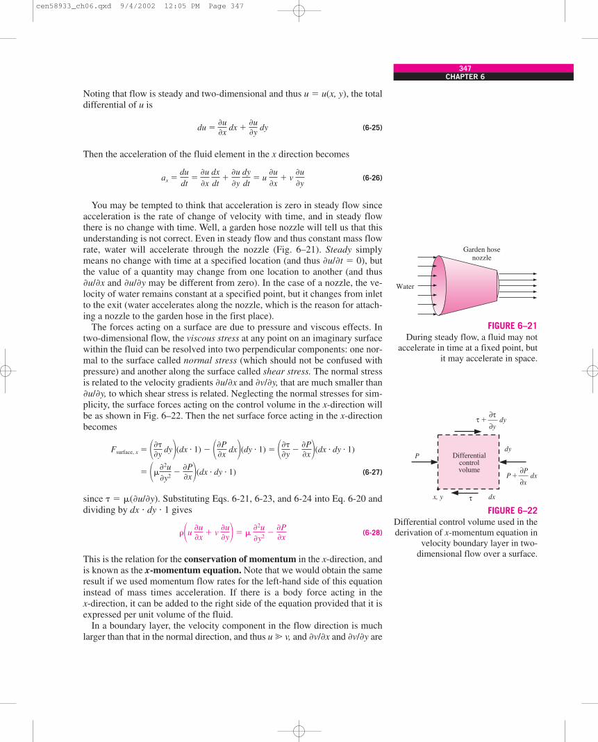
You may be tempted to think that acceleration is zero in steady flow sinceacceleration is the rate of change of velocity with time, and in steady flowthere is no change with time. Well, a garden hose nozzle will tell us that thisunderstanding is not correct. Even in steady flow and thus constant mass flowrate, water will accelerate through the nozzle (Fig. 6–21). Steady simplymeans no change with time at a specified location (and thus �u/�t � 0), butthe value of a quantity may change from one location to another (and thus�u/�x and �u/�y may be different from zero). In the case of a nozzle, the ve-locity of water remains constant at a specified point, but it changes from inletto the exit (water accelerates along the nozzle, which is the reason for attach-ing a nozzle to the garden hose in the first place).
The forces acting on a surface are due to pressure and viscous effects. Intwo-dimensional flow, the viscous stress at any point on an imaginary surfacewithin the fluid can be resolved into two perpendicular components: one nor-mal to the surface called normal stress (which should not be confused withpressure) and another along the surface called shear stress. The normal stressis related to the velocity gradients �u/�x and �v/�y, that are much smaller than�u/�y, to which shear stress is related. Neglecting the normal stresses for sim-plicity, the surface forces acting on the control volume in the x-direction willbe as shown in Fig. 6–22. Then the net surface force acting in the x-directionbecomes
(6-27)
since � � �(�u/�y). Substituting Eqs. 6-21, 6-23, and 6-24 into Eq. 6-20 anddividing by dx � dy � 1 gives
(6-28)
This is the relation for the conservation of momentum in the x-direction, andis known as the x-momentum equation. Note that we would obtain the sameresult if we used momentum flow rates for the left-hand side of this equationinstead of mass times acceleration. If there is a body force acting in thex-direction, it can be added to the right side of the equation provided that it isexpressed per unit volume of the fluid.
In a boundary layer, the velocity component in the flow direction is muchlarger than that in the normal direction, and thus u � v, and �v/�x and �v/�y are
��u �u�x � v
�u�y� � �
�2u�y2 �
�P�x
� ���2u�y2 �
�P�x�(dx � dy � 1)
Fsurface, x � ����y dy�(dx � 1) � ��P
�x dx�(dy � 1) � ����y �
�P�x�(dx � dy � 1)
ax �dudt
��u�x
dxdt
��u�y
dydt
� u �u�x
� v �u�y
du ��u�x dx �
�u�y dy
CHAPTER 6347
Water
Garden hosenozzle
FIGURE 6–21During steady flow, a fluid may not
accelerate in time at a fixed point, butit may accelerate in space.
∂P
∂x
P
P dx
τx, y dx
dy
�
∂τ∂y
dyτ �
Differentialcontrolvolume
FIGURE 6–22Differential control volume used in thederivation of x-momentum equation in
velocity boundary layer in two-dimensional flow over a surface.
cen58933_ch06.qxd 9/4/2002 12:05 PM Page 347

negligible. Also, u varies greatly with y in the normal direction from zero at thewall surface to nearly the free-stream value across the relatively thin boundarylayer, while the variation of u with x along the flow is typically small. There-fore, �u/�y � �u/�x. Similarly, if the fluid and the wall are at different temper-atures and the fluid is heated or cooled during flow, heat conduction will occurprimarily in the direction normal to the surface, and thus �T/�y � �T/�x. Thatis, the velocity and temperature gradients normal to the surface are muchgreater than those along the surface. These simplifications are known as theboundary layer approximations. These approximations greatly simplify theanalysis usually with little loss in accuracy, and make it possible to obtain ana-lytical solutions for certain types of flow problems (Fig. 6–23).
When gravity effects and other body forces are negligible and the boundarylayer approximations are valid, applying Newton’s second law of motion onthe volume element in the y-direction gives the y-momentum equation to be
(6-29)
That is, the variation of pressure in the direction normal to the surface is neg-ligible, and thus P � P(x) and �P/�x � dP/dx. Then it follows that for a givenx, the pressure in the boundary layer is equal to the pressure in the free stream,and the pressure determined by a separate analysis of fluid flow in the freestream (which is typically easier because of the absence of viscous effects)can readily be used in the boundary layer analysis.
The velocity components in the free stream region of a flat plate are u � u�
� constant and v � 0. Substituting these into the x-momentum equations(Eq. 6-28) gives �P/�x � 0. Therefore, for flow over a flat plate, the pres-sure remains constant over the entire plate (both inside and outside the bound-ary layer).
Conservation of Energy EquationThe energy balance for any system undergoing any process is expressed asEin � Eout � Esystem, which states that the change in the energy content of asystem during a process is equal to the difference between the energy inputand the energy output. During a steady-flow process, the total energy contentof a control volume remains constant (and thus Esystem � 0), and the amountof energy entering a control volume in all forms must be equal to the amountof energy leaving it. Then the rate form of the general energy equation reducesfor a steady-flow process to E
·in � E
·out � 0.
Noting that energy can be transferred by heat, work, and mass only, the en-ergy balance for a steady-flow control volume can be written explicitly as
(E·in � E
·out)by heat � (E
·in � E
·out)by work � (E
·in � E
·out)by mass � 0 (6-30)
The total energy of a flowing fluid stream per unit mass is estream � h � ke �pe where h is the enthalpy (which is the sum of internal energy and flow en-ergy), pe � gz is the potential energy, and ke � �2/2 � (u2 � v2)/2 is thekinetic energy of the fluid per unit mass. The kinetic and potential energies areusually very small relative to enthalpy, and therefore it is common practice toneglect them (besides, it can be shown that if kinetic energy is included in theanalysis below, all the terms due to this inclusion cancel each other). We
�P�y � 0
348HEAT TRANSFER
T�u�
y
vx u
FIGURE 6–23Boundary layer approximations.
1) Velocity components:v � u
2) Velocity grandients:
3) Temperature gradients:
�T�x
� �T�y
�u�x
� �u�y
�v�x
� 0, �v�y
� 0
cen58933_ch06.qxd 9/4/2002 12:05 PM Page 348

assume the density �, specific heat Cp, viscosity �, and the thermal conductiv-ity k of the fluid to be constant. Then the energy of the fluid per unit mass canbe expressed as estream � h � CpT.
Energy is a scalar quantity, and thus energy interactions in all directions canbe combined in one equation. Noting that mass flow rate of the fluid enteringthe control volume from the left is �u(dy � 1), the rate of energy transfer to thecontrol volume by mass in the x-direction is, from Fig. 6–24,
(6-31)
Repeating this for the y-direction and adding the results, the net rate of energytransfer to the control volume by mass is determined to be
(6-32)
since �u/�x � �v/�y � 0 from the continuity equation.The net rate of heat conduction to the volume element in the x-direction is
(6-33)
Repeating this for the y-direction and adding the results, the net rate of energytransfer to the control volume by heat conduction becomes
(6-34)
Another mechanism of energy transfer to and from the fluid in the controlvolume is the work done by the body and surface forces. The work done by abody force is determined by multiplying this force by the velocity in the di-rection of the force and the volume of the fluid element, and this work needsto be considered only in the presence of significant gravitational, electric, ormagnetic effects. The surface forces consist of the forces due to fluid pressureand the viscous shear stresses. The work done by pressure (the flow work) isalready accounted for in the analysis above by using enthalpy for the micro-scopic energy of the fluid instead of internal energy. The shear stresses that re-sult from viscous effects are usually very small, and can be neglected in manycases. This is especially the case for applications that involve low or moderatevelocities.
Then the energy equation for the steady two-dimensional flow of a fluidwith constant properties and negligible shear stresses is obtained by substitut-ing Eqs. 6-32 and 6-34 into 6-30 to be
(6-35)�Cp�u �T�x � v
�T�y � � k��2T
�x2 ��2T�y2 �
(Ein � Eout ) by heat � k �2T�x2 dxdy � k
�2T�y2 dxdy � k��2T
�x2 ��2T�y2 �dxdy
� ���x ��k(dy � 1)
�T�x � dx � k
�2T�x2
dx dy
(Ein � Eout)by heat, x � Qx � �Qx ��Qx
�x dx�
� ��Cp�u �T�x � v
�T�y�dxdy
(Ein � Eout)by mass � ��Cp�u �T�x � T
�u�x�dxdy � �Cp�v
�T�y � T
�v�y�dxdy
� ��[�u(dy � 1)CpT ]
�x dx � ��Cp�u �T�x � T
�u�x�dxdy
(Ein �Eout)by mass, x � ( mestream)x � �( mestream)x ��(mestream)x
�x dx�
CHAPTER 6349
dx
dv
Eheat. out. y
Eheat out, x
Emass. out. y
Emass out, y
Eheat in, x
Eheat in, y Emass in, y
Emass in, x
FIGURE 6–24The energy transfers by heat and mass
flow associated with a differentialcontrol volume in the thermalboundary layer in steady two-
dimensional flow.
cen58933_ch06.qxd 9/4/2002 12:05 PM Page 349

which states that the net energy convected by the fluid out of the control vol-ume is equal to the net energy transferred into the control volume by heatconduction.
When the viscous shear stresses are not negligible, their effect is accountedfor by expressing the energy equation as
(6-36)
where the viscous dissipation function � is obtained after a lengthy analysis(see an advanced book such as the one by Schlichting (Ref. 9) for details) to be
(6-37)
Viscous dissipation may play a dominant role in high-speed flows, especiallywhen the viscosity of the fluid is high (like the flow of oil in journal bearings).This manifests itself as a significant rise in fluid temperature due to the con-version of the kinetic energy of the fluid to thermal energy. Viscous dissipa-tion is also significant for high-speed flights of aircraft.
For the special case of a stationary fluid, u � v � 0 and the energy equationreduces, as expected, to the steady two-dimensional heat conduction equation,
(6-38)�2T�x2 �
�2T�y2 � 0
� � 2���u�x�
2� ��v
�y�2� � ��u
�y ��v�x�
2
�Cp�u �T�x � v
�T�y � � k��2T
�x2 ��2T�y2 � � ��
350HEAT TRANSFER
y
0
L
x
� = 12 m/s
Movingplate
Stationaryplate
u(y)
FIGURE 6–25Schematic for Example 6–1.
EXAMPLE 6–1 Temperature Rise of Oil in a Journal Bearing
The flow of oil in a journal bearing can be approximated as parallel flow be-tween two large plates with one plate moving and the other stationary. Suchflows are known as Couette flow.
Consider two large isothermal plates separated by 2-mm-thick oil film. Theupper plates moves at a constant velocity of 12 m/s, while the lower plate is sta-tionary. Both plates are maintained at 20˚C. (a) Obtain relations for the velocityand temperature distributions in the oil. (b) Determine the maximum tempera-ture in the oil and the heat flux from the oil to each plate (Fig. 6–25).
SOLUTION Parallel flow of oil between two plates is considered. The velocityand temperature distributions, the maximum temperature, and the total heattransfer rate are to be determined.Assumptions 1 Steady operating conditions exist. 2 Oil is an incompressiblesubstance with constant properties. 3 Body forces such as gravity are negligible.4 The plates are large so that there is no variation in the z direction.Properties The properties of oil at 20˚C are (Table A-10):
k � 0.145 W/m � K and � � 0.800 kg/m � s � 0.800 N � s/m2
Analysis (a) We take the x-axis to be the flow direction, and y to be the normaldirection. This is parallel flow between two plates, and thus v � 0. Then thecontinuity equation (Eq. 6-21) reduces to
Continuity:�u�x �
�v�y � 0 →
�u�x � 0 → u � u(y)
cen58933_ch06.qxd 9/4/2002 12:05 PM Page 350

CHAPTER 6351
Therefore, the x-component of velocity does not change in the flow direction(i.e., the velocity profile remains unchanged). Noting that u � u(y), v � 0, and�P/�x � 0 (flow is maintained by the motion of the upper plate rather than thepressure gradient), the x-momentum equation (Eq. 6-28) reduces to
x-momentum:
This is a second-order ordinary differential equation, and integrating it twice gives
u(y) � C1y � C2
The fluid velocities at the plate surfaces must be equal to the velocities of theplates because of the no-slip condition. Therefore, the boundary conditions areu(0) � 0 and u(L) � �, and applying them gives the velocity distribution to be
Frictional heating due to viscous dissipation in this case is significant be-cause of the high viscosity of oil and the large plate velocity. The plates areisothermal and there is no change in the flow direction, and thus the tempera-ture depends on y only, T � T(y). Also, u � u(y) and v � 0. Then the energyequation with dissipation (Eqs. 6-36 and 6-37) reduce to
Energy:
since �u/�y � �/L. Dividing both sides by k and integrating twice give
Applying the boundary conditions T (0) � T0 and T(L) � T0 gives the tempera-ture distribution to be
(b) The temperature gradient is determined by differentiating T (y ) with re-spect to y,
The location of maximum temperature is determined by setting dT/dy � 0 andsolving for y,
Therefore, maximum temperature will occur at mid plane, which is not surpris-ing since both plates are maintained at the same temperature. The maximumtemperature is the value of temperature at y � L /2,
� 20 �(0.8 N � s/m2)(12m/s)2
8(0.145 W/m � °C) � 1W
1 N � m/s� � 119°C
Tmax � T �L2� � T0 �
��2
2k �L /2L
�(L /2) 2
L2 � � T0 ���2
8k
dTdy
���2
2kL �1 � 2
yL� � 0 → y �
L2
dTdy
���2
2kL �1 � 2
yL�
T(y) � T0 ��� 2
2k � y
L�
y2
L2�
T(y) � ��
2k � y
L ��2
� C3 y � C4
0 � k �2T�y2 � ���u
�y�2 → k
d 2Tdy2 � ����
L �2
u(y) �yL
�
��u �u�x � v
�u�y� � �
�2u�y2 �
�P�x → d 2u
dy2 � 0
cen58933_ch06.qxd 9/4/2002 12:05 PM Page 351

6–8 SOLUTIONS OF CONVECTION EQUATIONS FORA FLAT PLATE
Consider laminar flow of a fluid over a flat plate, as shown in Fig. 6–19. Sur-faces that are slightly contoured such as turbine blades can also be approxi-mated as flat plates with reasonable accuracy. The x-coordinate is measuredalong the plate surface from the leading edge of the plate in the direction ofthe flow, and y is measured from the surface in the normal direction. The fluidapproaches the plate in the x-direction with a uniform upstream velocity,which is equivalent to the free stream velocity u�.
When viscous dissipation is negligible, the continuity, momentum, and en-ergy equations (Eqs. 6-21, 6-28, and 6-35) reduce for steady, incompressible,laminar flow of a fluid with constant properties over a flat plate to
Continuity: (6-39)
Momentum: (6-40)
Energy: (6-41)
with the boundary conditions (Fig. 6–26)
At x � 0: u(0, y) � u�, T(0, y) � T�
At y � 0: u(x, 0) � 0, v(x, 0) � 0, T(x, 0) � Ts (6-42)
As y → �: u(x, �) � u�, T(x, �) � T�
When fluid properties are assumed to be constant and thus independent of tem-perature, the first two equations can be solved separately for the velocity com-ponents u and v. Once the velocity distribution is available, we can determine
u �T�x � v
�T�y � �
�2T�y2
u �u�x � v
�u�y � v
�2u�y2
�u�x �
�v�y � 0
�
352HEAT TRANSFER
Heat flux at the plates is determined from the definition of heat flux,
Therefore, heat fluxes at the two plates are equal in magnitude but oppositein sign.Discussion A temperature rise of 99˚C confirms our suspicion that viscous dis-sipation is very significant. Also, the heat flux is equivalent to the rate of me-chanical energy dissipation. Therefore, mechanical energy is being converted tothermal energy at a rate of 57.2 kW/m2 of plate area to overcome friction in theoil. Finally, calculations are done using oil properties at 20˚C, but the oil tem-perature turned out to be much higher. Therefore, knowing the strong depen-dence of viscosity on temperature, calculations should be repeated usingproperties at the average temperature of 70˚C to improve accuracy.
qL � �k dTdy`y�L
� �k ��2
2kL (1 � 2) �
��2
2L� �q0 � 28,800 W/m2
� �(0.8 N � s/m2)(12 m/s)2
2(0.002 m) � 1W
1N � m/s� � �28,800 W/m2
q0 � �k dTdy`y�0
� �k ��2
2kL (1 � 0) � �
��2
2L
T�u�
T�u�
u (x, 0) � 0v (x, 0) � 0T (x, 0) � Ts
y
x
FIGURE 6–26Boundary conditions for flowover a flat plate.
cen58933_ch06.qxd 9/4/2002 12:05 PM Page 352

the friction coefficient and the boundary layer thickness using their definitions.Also, knowing u and v, the temperature becomes the only unknown in the lastequation, and it can be solved for temperature distribution.
The continuity and momentum equations were first solved in 1908 by theGerman engineer H. Blasius, a student of L. Prandtl. This was done by trans-forming the two partial differential equations into a single ordinary differen-tial equation by introducing a new independent variable, called the similarityvariable. The finding of such a variable, assuming it exists, is more of an artthan science, and it requires to have a good insight of the problem.
Noticing that the general shape of the velocity profile remains the samealong the plate, Blasius reasoned that the nondimensional velocity profile u/u�
should remain unchanged when plotted against the nondimensional distancey/�, where � is the thickness of the local velocity boundary layer at a given x.That is, although both � and u at a given y vary with x, the velocity u at a fixedy/� remains constant. Blasius was also aware from the work of Stokes that �is proportional to , and thus he defined a dimensionless similarityvariable as
(6-43)
and thus u/u� � function(�). He then introduced a stream function �(x, y) as
(6-44)
so that the continuity equation (Eq. 6-39) is automatically satisfied and thuseliminated (this can be verified easily by direct substitution). He then defineda function f(�) as the dependent variable as
(6-45)
Then the velocity components become
(6-46)
(6-47)
By differentiating these u and v relations, the derivatives of the velocity com-ponents can be shown to be
(6-48)
Substituting these relations into the momentum equation and simplifying, weobtain
(6-49)
which is a third-order nonlinear differential equation. Therefore, the systemof two partial differential equations is transformed into a single ordinary
2 d 3f
d�3 � f d 2f
d�2 � 0
�u�x
� �u�
2x �
d 2fd�2, �u
�y� u��u�
vx d 2fd�2 , �2u
�y2 �u2
�
vx d 3fd�3
� ���
�x� �u� �vx
u�
�f�x
�u�
2 � vu� x
f �12 �u�v
x ��
dfd�
� f�
u ���
�y�
��
�� ��
�y� u� �vx
u�
dfd�
�u�
vx� u�
dfd�
f(�) ��
u��vx/u�
u ���
�y and v � ���
�x
� � y�u�
vx
�vx/u�
CHAPTER 6353
cen58933_ch06.qxd 9/4/2002 12:05 PM Page 353

differential equation by the use of a similarity variable. Using the definitionsof f and �, the boundary conditions in terms of the similarity variables can beexpressed as
(6-50)
The transformed equation with its associated boundary conditions cannot besolved analytically, and thus an alternative solution method is necessary. Theproblem was first solved by Blasius in 1908 using a power series expansion ap-proach, and this original solution is known as the Blasius solution. The prob-lem is later solved more accurately using different numerical approaches, andresults from such a solution are given in Table 6–3. The nondimensional ve-locity profile can be obtained by plotting u/u� against �. The results obtainedby this simplified analysis are in excellent agreement with experimental results.
Recall that we defined the boundary layer thickness as the distance from thesurface for which u/u� � 0.99. We observe from Table 6–3 that the value of �corresponding to u/u� � 0.992 is � � 5.0. Substituting � � 5.0 and y � � intothe definition of the similarity variable (Eq. 6-43) gives 5.0 � � . Thenthe velocity boundary layer thickness becomes
(6-51)
since Rex � u�x/ , where x is the distance from the leading edge of the plate.Note that the boundary layer thickness increases with increasing kinematicviscosity and with increasing distance from the leading edge x, but it de-creases with increasing free-stream velocity u�. Therefore, a large free-streamvelocity will suppress the boundary layer and cause it to be thinner.
The shear stress on the wall can be determined from its definition and the�u/�y relation in Eq. 6-48:
(6-52)
Substituting the value of the second derivative of f at � � 0 from Table 6–3gives
(6-53)
Then the local skin friction coefficient becomes
(6-54)
Note that unlike the boundary layer thickness, wall shear stress and the skinfriction coefficient decrease along the plate as x�1/2.
The Energy EquationKnowing the velocity profile, we are now ready to solve the energy equationfor temperature distribution for the case of constant wall temperature Ts. Firstwe introduce the dimensionless temperature as
Cf, x ��w
��2/2�
�w
�u2� /2
� 0.664 Re �1/2x
�w � 0.332u� ���u�
x�
0.332�u 2�
�Rex
�w � � �u�y ` y�0
� �u��u�
vx d 2f
d�2 ` ��0
� �5.0
�u� /vx�
5.0x
�Rex
�u� /vx
f(0) � 0, dfd�`��0
� 0, and dfd�`���
� 1
354HEAT TRANSFER
TABLE 6–3
Similarity function f and itsderivatives for laminar boundarylayer along a flat plate.
� f
0 0 0 0.3320.5 0.042 0.166 0.3311.0 0.166 0.330 0.3231.5 0.370 0.487 0.3032.0 0.650 0.630 0.2672.5 0.996 0.751 0.2173.0 1.397 0.846 0.1613.5 1.838 0.913 0.1084.0 2.306 0.956 0.0644.5 2.790 0.980 0.0345.0 3.283 0.992 0.0165.5 3.781 0.997 0.0076.0 4.280 0.999 0.002� � 1 0
d2fd � 2
dfd �
�uu�
cen58933_ch06.qxd 9/4/2002 12:05 PM Page 354

(6-55)
Noting that both Ts and T� are constant, substitution into the energy equationgives
(6-56)
Temperature profiles for flow over an isothermal flat plate are similar, just likethe velocity profiles, and thus we expect a similarity solution for temperatureto exist. Further, the thickness of the thermal boundary layer is proportional to
just like the thickness of the velocity boundary layer, and thus thesimilarity variable is also �, and � (�). Using the chain rule and substitut-ing the u and v expressions into the energy equation gives
(6-57)
Simplifying and noting that Pr � /� give
(6-58)
with the boundary conditions (0) � 0 and (�) � 1. Obtaining an equation for as a function of � alone confirms that the temperature profiles are similar,and thus a similarity solution exists. Again a closed-form solution cannot beobtained for this boundary value problem, and it must be solved numerically.
It is interesting to note that for Pr � 1, this equation reduces to Eq. 6-49 when is replaced by df/d�, which is equivalent to u/u� (see Eq. 6-46). The bound-ary conditions for and df/d� are also identical. Thus we conclude that the ve-locity and thermal boundary layers coincide, and the nondimensional velocityand temperature profiles (u/u� and ) are identical for steady, incompressible,laminar flow of a fluid with constant properties and Pr � 1 over an isothermalflat plate (Fig. 6–27). The value of the temperature gradient at the surface(y � 0 or � � 0) in this case is, from Table 6–3, d/d� � d 2f/d�2 � 0.332.
Equation 6-58 is solved for numerous values of Prandtl numbers. ForPr � 0.6, the nondimensional temperature gradient at the surface is found tobe proportional to Pr1/3, and is expressed as
(6-59)
The temperature gradient at the surface is
(6-60)
Then the local convection coefficient and Nusselt number become
(6-61)hx �qs
Ts � T�
��k(�T/�y)y�0
Ts � T�
� 0.332 Pr1/3k �u�
vx
� 0.332 Pr1/3(T� � Ts) �u�
vx
�T�y ` y�0
� (T� � Ts) ��y ` y�0
� (T� � Ts) dd�`��0
��
�y ` y�0
dd�`��0
� 0.332 Pr1/3
2 d 2
d�2 � Pr f dd�
� 0
u� dfd�
d
d� ��
�x�
12 �u�v
x ��
dfd�
� f� d
d� ��
�y� �
d 2
d�2 ���
�y�2
�vx/u� ,
u ��x � v
��y � �
�2
�y2
(x, y) �T(x, y) � Ts
T� � Ts
CHAPTER 6355
T�u�
u/u�
y
x
Pr � 1or �
Velocity or thermalboundary layer
FIGURE 6–27When Pr � 1, the velocity and thermal
boundary layers coincide, and thenondimensional velocity and
temperature profiles are identical forsteady, incompressible, laminar flow
over a flat plate.
cen58933_ch06.qxd 9/4/2002 12:05 PM Page 355

and
(6-62)
The Nux values obtained from this relation agree well with measured values.Solving Eq. 6-58 numerically for the temperature profile for different
Prandtl numbers, and using the definition of the thermal boundary layer, itis determined that �/�t Pr 1/3. Then the thermal boundary layer thicknessbecomes
(6-63)
Note that these relations are valid only for laminar flow over an isothermal flatplate. Also, the effect of variable properties can be accounted for by evaluat-ing all such properties at the film temperature defined as Tf � (Ts � T�)/2.
The Blasius solution gives important insights, but its value is largely histor-ical because of the limitations it involves. Nowadays both laminar and turbu-lent flows over surfaces are routinely analyzed using numerical methods.
6–9 NONDIMENSIONALIZED CONVECTIONEQUATIONS AND SIMILARITY
When viscous dissipation is negligible, the continuity, momentum, and energyequations for steady, incompressible, laminar flow of a fluid with constantproperties are given by Eqs. 6-21, 6-28, and 6-35.
These equations and the boundary conditions can be nondimensionalized bydividing all dependent and independent variables by relevant and meaningfulconstant quantities: all lengths by a characteristic length L (which is the lengthfor a plate), all velocities by a reference velocity � (which is the free streamvelocity for a plate), pressure by �� 2 (which is twice the free stream dynamicpressure for a plate), and temperature by a suitable temperature difference(which is T� � Ts for a plate). We get
where the asterisks are used to denote nondimensional variables. Introducingthese variables into Eqs. 6-21, 6-28, and 6-35 and simplifying give
Continuity: (6-64)
Momentum: (6-65)
Energy: (6-66)
with the boundary conditions
u*(0, y*) � 1, u*(x*, 0) � 0, u*(x*, �) � 1, v*(x*, 0) � 0, (6-67)
T*(0, y*) � 1, T*(x*, 0) � 0, T*(x*, �) � 1
u*�T*
�x*� v*�T*
�y*�
1ReL Pr
�2T*
�y*2
u*�u*
�x*� v*�u*
�y*�
1ReL
�2u*
�y*2 �dP*
dx*
�u*
�x*�
�v*
�y*� 0
x* �xL
, y* �yL
, u* �u�
, v* �v�
, P* �P
��2, and T* �T � Ts
T� � Ts
�
�t ��
Pr1/3 �5.0x
Pr1/3�Rex
Nux �hxxk
� 0.332 Pr1/3Re1/2x Pr � 0.6
356HEAT TRANSFER
cen58933_ch06.qxd 9/4/2002 12:06 PM Page 356
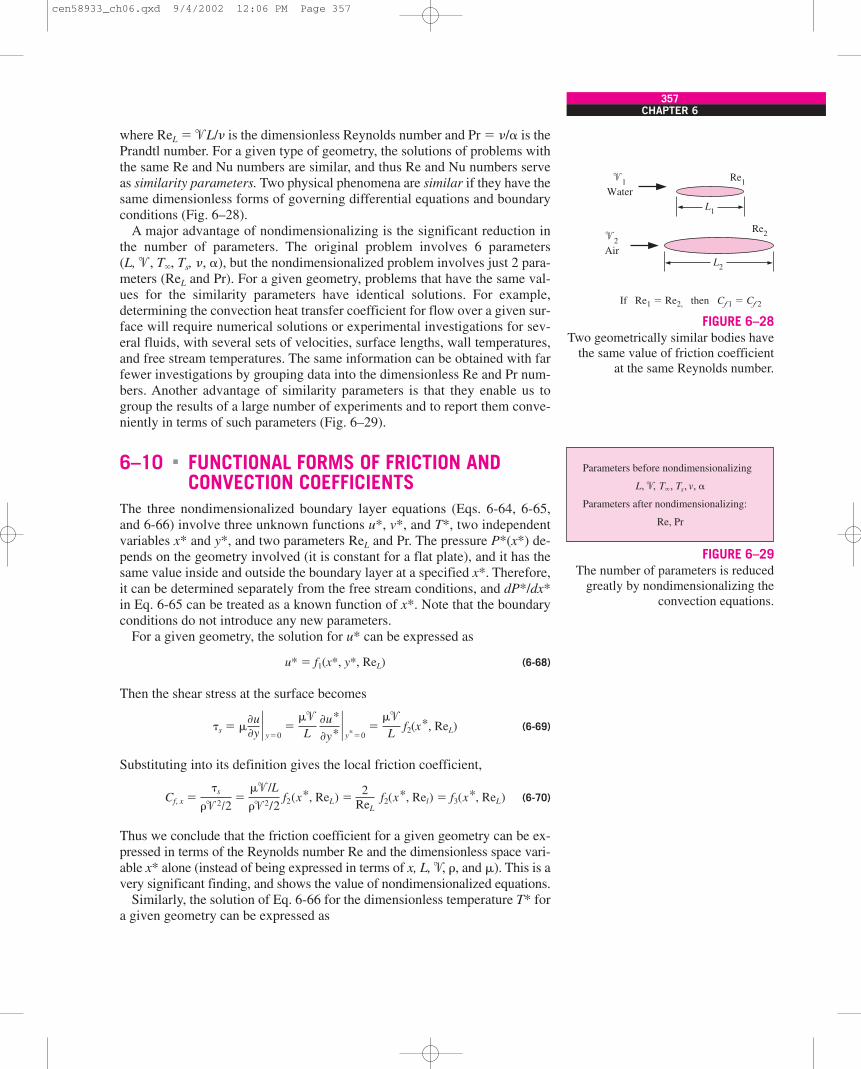
where ReL � �L/ is the dimensionless Reynolds number and Pr � /� is thePrandtl number. For a given type of geometry, the solutions of problems withthe same Re and Nu numbers are similar, and thus Re and Nu numbers serveas similarity parameters. Two physical phenomena are similar if they have thesame dimensionless forms of governing differential equations and boundaryconditions (Fig. 6–28).
A major advantage of nondimensionalizing is the significant reduction inthe number of parameters. The original problem involves 6 parameters(L, �, T�, Ts, , �), but the nondimensionalized problem involves just 2 para-meters (ReL and Pr). For a given geometry, problems that have the same val-ues for the similarity parameters have identical solutions. For example,determining the convection heat transfer coefficient for flow over a given sur-face will require numerical solutions or experimental investigations for sev-eral fluids, with several sets of velocities, surface lengths, wall temperatures,and free stream temperatures. The same information can be obtained with farfewer investigations by grouping data into the dimensionless Re and Pr num-bers. Another advantage of similarity parameters is that they enable us togroup the results of a large number of experiments and to report them conve-niently in terms of such parameters (Fig. 6–29).
6–10 FUNCTIONAL FORMS OF FRICTION ANDCONVECTION COEFFICIENTS
The three nondimensionalized boundary layer equations (Eqs. 6-64, 6-65,and 6-66) involve three unknown functions u*, v*, and T*, two independentvariables x* and y*, and two parameters ReL and Pr. The pressure P*(x*) de-pends on the geometry involved (it is constant for a flat plate), and it has thesame value inside and outside the boundary layer at a specified x*. Therefore,it can be determined separately from the free stream conditions, and dP*/dx*in Eq. 6-65 can be treated as a known function of x*. Note that the boundaryconditions do not introduce any new parameters.
For a given geometry, the solution for u* can be expressed as
u* � f1(x*, y*, ReL) (6-68)
Then the shear stress at the surface becomes
(6-69)
Substituting into its definition gives the local friction coefficient,
(6-70)
Thus we conclude that the friction coefficient for a given geometry can be ex-pressed in terms of the Reynolds number Re and the dimensionless space vari-able x* alone (instead of being expressed in terms of x, L, �, �, and �). This is avery significant finding, and shows the value of nondimensionalized equations.
Similarly, the solution of Eq. 6-66 for the dimensionless temperature T* fora given geometry can be expressed as
Cf, x ��s
��2/2�
��/L
��2/2 f2(x*, ReL) �
2ReL
f2(x*, Rel) � f3(x*, ReL)
�s � ��u�y ` y�0
���
L �u*
�y*`y*�0
���
L f2(x*, ReL)
�
CHAPTER 6357
L1
�1Water
If Re1 � Re2, then C 1 � C 2ƒ ƒ
�2Air
L2
Re2
Re1
FIGURE 6–28Two geometrically similar bodies have
the same value of friction coefficientat the same Reynolds number.
Parameters before nondimensionalizing
Parameters after nondimensionalizing:
Re, Pr
L, �, T�, Ts, v, �
FIGURE 6–29The number of parameters is reduced
greatly by nondimensionalizing theconvection equations.
cen58933_ch06.qxd 9/4/2002 12:06 PM Page 357

T* � g1(x*, y*, ReL, Pr) (6-71)
Using the definition of T*, the convection heat transfer coefficient becomes
(6-72)
Substituting this into the Nusselt number relation gives [or alternately, we canrearrange the relation above in dimensionless form as hL/k � (�T*/�y*)|y*�0
and define the dimensionless group hL/k as the Nusselt number]
(6-73)
Note that the Nusselt number is equivalent to the dimensionless temperaturegradient at the surface, and thus it is properly referred to as the dimensionlessheat transfer coefficient (Fig. 6–30). Also, the Nusselt number for a givengeometry can be expressed in terms of the Reynolds number Re, the Prandtlnumber Pr, and the space variable x*, and such a relation can be used for dif-ferent fluids flowing at different velocities over similar geometries of differ-ent lengths.
The average friction and heat transfer coefficients are determined by inte-grating Cf,x and Nux over the surface of the given body with respect to x* from0 to 1. Integration will remove the dependence on x*, and the average frictioncoefficient and Nusselt number can be expressed as
Cf � f4(ReL) and Nu � g3(ReL , Pr) (6-74)
These relations are extremely valuable as they state that for a given geometry,the friction coefficient can be expressed as a function of Reynolds numberalone, and the Nusselt number as a function of Reynolds and Prandtl numbersalone (Fig. 6–31). Therefore, experimentalists can study a problem with aminimum number of experiments, and report their friction and heat transfercoefficient measurements conveniently in terms of Reynolds and Prandtlnumbers. For example, a friction coefficient relation obtained with air for agiven surface can also be used for water at the same Reynolds number. But itshould be kept in mind that the validity of these relations is limited by the lim-itations on the boundary layer equations used in the analysis.
The experimental data for heat transfer is often represented with reasonableaccuracy by a simple power-law relation of the form
Nu � C (6-75)
where m and n are constant exponents (usually between 0 and 1), and thevalue of the constant C depends on geometry. Sometimes more complex rela-tions are used for better accuracy.
6–11 ANALOGIES BETWEEN MOMENTUM ANDHEAT TRANSFER
In forced convection analysis, we are primarily interested in the determinationof the quantities Cf (to calculate shear stress at the wall) and Nu (to calculateheat transfer rates). Therefore, it is very desirable to have a relation between
�
ReLm Pr n
Nux �hLk
��T*
�y*`y*�0
� g2(x*, ReL, Pr)
h ��k(�T/�y)y�0
Ts � T�
��k(T� � Ts)L(Ts � T�)
�T*
�y* ` y*�0�
k
L �T*
�y* ` y*�0
358HEAT TRANSFER
T*
Laminar
∂T*
∂y*y*�0
� Nuy*
x*
FIGURE 6–30The Nusselt number is equivalent tothe dimensionless temperaturegradient at the surface.
Local Nusselt number:
Nux � function (x*, ReL, Pr)
Average Nusselt number:
Nu � function (ReL, Pr)
A common form of Nusselt number:
Nu = C RemL Pr n
FIGURE 6–31For a given geometry, the averageNusselt number is a function ofReynolds and Prandtl numbers.
cen58933_ch06.qxd 9/4/2002 12:06 PM Page 358

Cf and Nu so that we can calculate one when the other is available. Such rela-tions are developed on the basis of the similarity between momentum and heattransfers in boundary layers, and are known as Reynolds analogy andChilton–Colburn analogy.
Reconsider the nondimensionalized momentum and energy equations forsteady, incompressible, laminar flow of a fluid with constant properties andnegligible viscous dissipation (Eqs. 6-65 and 6-66). When Pr � 1 (which isapproximately the case for gases) and �P*/�x* � 0 (which is the case when,u � u� � � � constant in the free stream, as in flow over a flat plate), theseequations simplify to
Momentum: (6-76)
Energy: (6-77)
which are exactly of the same form for the dimensionless velocity u* and tem-perature T*. The boundary conditions for u* and T* are also identical. There-fore, the functions u* and T* must be identical, and thus the first derivativesof u* and T* at the surface must be equal to each other,
(6-78)
Then from Eqs. 6-69, 6-70, and 6-73 we have
(6-79)
which is known as the Reynolds analogy (Fig. 6–32). This is an importantanalogy since it allows us to determine the heat transfer coefficient for fluidswith Pr � 1 from a knowledge of friction coefficient which is easier to mea-sure. Reynolds analogy is also expressed alternately as
(6-80)
where
(6-81)
is the Stanton number, which is also a dimensionless heat transfer coefficient.Reynolds analogy is of limited use because of the restrictions Pr � 1 and
�P*/�x* � 0 on it, and it is desirable to have an analogy that is applicable overa wide range of Pr. This is done by adding a Prandtl number correction. Thefriction coefficient and Nusselt number for a flat plate are determined in Sec-tion 6-8 to be
Cf, x � 0.664 Rex�1/2 and Nux � 0.332 Pr1/3 Re x
1/2 (6-82)
Taking their ratio and rearranging give the desired relation, known as themodified Reynolds analogy or Chilton–Colburn analogy,
St �h
�Cp��
NuReLPr
Cf, x
2� Stx (Pr � 1)
Cf, x ReL
2� Nux (Pr � 1)
�u*
�y*`y*�0
��T*
�y*`y*�0
u*�T*
�x* � v*�T*
�y* �1
ReL �2T*
�y*2
u*�u*
�x* � v*�u*
�y* �1
ReL �2u*
�y*2
CHAPTER 6359
Profiles: u* � T
Gradients:
Analogy: Cf, x ReL
2� Nux
�u*
�y*`y*�0
��T*
�y*`y*�0
FIGURE 6–32When Pr � 1 and �P*/�x* � 0,
the nondimensional velocity andtemperature profiles become
identical, and Nu is related to Cf
by Reynolds analogy.
cen58933_ch06.qxd 9/4/2002 12:06 PM Page 359

(6-83)
for 0.6 � Pr � 60. Here jH is called the Colburn j-factor. Although this rela-tion is developed using relations for laminar flow over a flat plate (for which�P*/�x* � 0), experimental studies show that it is also applicable approxi-mately for turbulent flow over a surface, even in the presence of pressure gra-dients. For laminar flow, however, the analogy is not applicable unless�P*/�x* � 0. Therefore, it does not apply to laminar flow in a pipe. Analogiesbetween Cf and Nu that are more accurate are also developed, but they aremore complex and beyond the scope of this book. The analogies given abovecan be used for both local and average quantities.
Cf, x
ReL
2� Nux Pr�1/3 or
Cf, x
2�
hx
�Cp� Pr2/3 � jH
360HEAT TRANSFER
EXAMPLE 6–2 Finding Convection Coefficient from Drag Measurement
A 2-m � 3-m flat plate is suspended in a room, and is subjected to air flow par-allel to its surfaces along its 3-m-long side. The free stream temperature andvelocity of air are 20˚C and 7 m/s. The total drag force acting on the plate ismeasured to be 0.86 N. Determine the average convection heat transfer coeffi-cient for the plate (Fig. 6–33).
SOLUTION A flat plate is subjected to air flow, and the drag force acting on itis measured. The average convection coefficient is to be determined.Assumptions 1 Steady operating conditions exist. 2 The edge effects are negli-gible. 3 The local atmospheric pressure is 1 atm.Properties The properties of air at 20˚C and 1 atm are (Table A-15):
� � 1.204 kg/m3, Cp � 1.007 kJ/kg � K, Pr � 0.7309
Analysis The flow is along the 3-m side of the plate, and thus the characteris-tic length is L � 3 m. Both sides of the plate are exposed to air flow, and thusthe total surface area is
As � 2WL � 2(2 m)(3 m) � 12 m2
For flat plates, the drag force is equivalent to friction force. The average frictioncoefficient Cf can be determined from Eq. 6-11,
Solving for Cf and substituting,
Then the average heat transfer coefficient can be determined from the modifiedReynolds analogy (Eq. 6-83) to be
� 12.7 W/m2 · °C
Discussion This example shows the great utility of momentum-heat transferanalogies in that the convection heat transfer coefficient can be determinedfrom a knowledge of friction coefficient, which is easier to determine.
h �Cf
2 ��Cp
Pr2/3�
0.00243
2 (1.204 kg/m3)(7 m/s)(1007 J/kg � °C)
0.73092/3
Cf �Ff
�As�2/2
�0.86 N
(1.204 kg/m3)(12 m2)(7 m/s)2/2 �1kg � m/s2
1 N � � 0.00243
Ff � Cf As ��2
2
L = 3 m
Air20°C, 7 m/s
FIGURE 6–33Schematic for Example 6–2.
cen58933_ch06.qxd 9/4/2002 12:06 PM Page 360

CHAPTER 6361
SUMMARY
Convection heat transfer is expressed by Newton’s law of cool-ing as
Q·
conv � hAs(Ts � T�)
where h is the convection heat transfer coefficient, Ts is the sur-face temperature, and T� is the free-stream temperature. Theconvection coefficient is also expressed as
The Nusselt number, which is the dimensionless heat transfercoefficient, is defined as
where k is the thermal conductivity of the fluid and Lc is thecharacteristic length.
The highly ordered fluid motion characterized by smoothstreamlines is called laminar. The highly disordered fluid mo-tion that typically occurs at high velocities is characterized byvelocity fluctuations is called turbulent. The random and rapidfluctuations of groups of fluid particles, called eddies, providean additional mechanism for momentum and heat transfer.
The region of the flow above the plate bounded by � inwhich the effects of the viscous shearing forces caused by fluidviscosity are felt is called the velocity boundary layer. Theboundary layer thickness, �, is defined as the distance from thesurface at which u � 0.99u�. The hypothetical line ofu � 0.99u� divides the flow over a plate into the boundarylayer region in which the viscous effects and the velocitychanges are significant, and the inviscid flow region, in whichthe frictional effects are negligible.
The friction force per unit area is called shear stress, and theshear stress at the wall surface is expressed as
where � is the dynamic viscosity, � is the upstream velocity,and Cf is the dimensionless friction coefficient. The property � �/� is the kinematic viscosity. The friction force over theentire surface is determined from
The flow region over the surface in which the temperaturevariation in the direction normal to the surface is significant isthe thermal boundary layer. The thickness of the thermalboundary layer �t at any location along the surface is the dis-
tance from the surface at which the temperature differenceT � Ts equals 0.99(T� � Ts). The relative thickness of the ve-locity and the thermal boundary layers is best described by thedimensionless Prandtl number, defined as
For external flow, the dimensionless Reynolds number is ex-pressed as
For a flat plate, the characteristic length is the distance x fromthe leading edge. The Reynolds number at which the flow be-comes turbulent is called the critical Reynolds number. For flowover a flat plate, its value is taken to be Recr � �xcr/v � 5 � 105.
The continuity, momentum, and energy equations for steadytwo-dimensional incompressible flow with constant propertiesare determined from mass, momentum, and energy balancesto be
Continuity:
x-momentum:
Energy: �
where the viscous dissipation function � is
Using the boundary layer approximations and a similarity vari-able, these equations can be solved for parallel steady incom-pressible flow over a flat plate, with the following results:
Velocity boundary layer thickness:
Local friction coefficient:
Local Nusselt number:
Thermal boundary layer thickness:
The average friction coefficient and Nusselt number are ex-pressed in functional form as
�t ��
Pr1/3 �5.0x
Pr1/3 �Rex
Nux �hx xk
� 0.332 Pr1/3 Re 1/2x
Cf, x ��w
��2/2� 0.664 Re�1/2
x
� �5.0
��/vx�
5.0x
�Rex
� � 2���u�x�
2� ��v
�y�2� � ��u
�y�
�v�x�
2
Cp�u �T�x � v
�T�y� � k��2T
�x2 ��2T�y2� � ��
��u �u�x � v
�u�y� � �
�2u�y2 �
�P�x
�u�x
��v�y
� 0
Re �Inertia forces
Viscous forces�
�Lc
v ���Lc
�
Pr �Molecular diffusivity of momentum
Molecular diffusivity of heat�
v� �
�Cp
k
Ff � Cf As ��2
2
�s � � �u�y ` y�0
or �s � Cf ��2
2
Nu �hLc
k
h ��kfluid(�T/�y)y�0
Ts � T�
cen58933_ch06.qxd 9/4/2002 12:06 PM Page 361

362HEAT TRANSFER
Cf � f4(ReL) and Nu � g3(ReL, Pr)
The Nusselt number can be expressed by a simple power-lawrelation of the form
Nu � C ReLm Pr n
where m and n are constant exponents, and the value of theconstant C depends on geometry. The Reynolds analogy relatesthe convection coefficient to the friction coefficient for fluidswith Pr � 1, and is expressed as
where
is the Stanton number. The analogy is extended to other Prandtlnumbers by the modified Reynolds analogy or Chilton–Colburn analogy, expressed as
or
These analogies are also applicable approximately for turbu-lent flow over a surface, even in the presence of pressuregradients.
Cf, x
2�
hx
�Cp� Pr2/3 � jH (0.6 � Pr � 60)
Cf, x ReL
2� NuxPr�1/3
St �h
�Cp��
NuReL Pr
Cf, x ReL
2� Nux or
Cf, x
2� Stx
REFERENCES AND SUGGESTED READING
1. H. Blasius. “The Boundary Layers in Fluids with LittleFriction (in German).” Z. Math. Phys., 56, 1 (1908); pp.1–37; English translation in National AdvisoryCommittee for Aeronautics Technical Memo No. 1256,February 1950.
2. R. W. Fox and A. T. McDonald. Introduction to FluidMechanics. 5th. ed. New York, Wiley, 1999.
3. J. P. Holman. Heat Transfer. 9th ed. New York: McGraw-Hill, 2002.
4. F. P. Incropera and D. P. DeWitt. Introduction to HeatTransfer. 4th ed. New York: John Wiley & Sons, 2002.
5. W. M. Kays and M. E. Crawford. Convective Heat andMass Transfer. 3rd ed. New York: McGraw-Hill, 1993.
6. F. Kreith and M. S. Bohn. Principles of Heat Transfer. 6thed. Pacific Grove, CA: Brooks/Cole, 2001.
7. M. N. Özisik. Heat Transfer—A Basic Approach. NewYork: McGraw-Hill, 1985.
8. O. Reynolds. “On the Experimental Investigation of theCircumstances Which Determine Whether the Motion ofWater Shall Be Direct or Sinuous, and the Law ofResistance in Parallel Channels.” PhilosophicalTransactions of the Royal Society of London 174 (1883),pp. 935–82.
9. H. Schlichting. Boundary Layer Theory. 7th ed. NewYork: McGraw-Hill, 1979.
10. G. G. Stokes. “On the Effect of the Internal Friction ofFluids on the Motion of Pendulums.” CambridgePhilosophical Transactions, IX, 8, 1851.
11. N. V. Suryanarayana. Engineering Heat Transfer. St. Paul,MN: West, 1995.
12. F. M. White. Heat and Mass Transfer. Reading, MA:Addison-Wesley, 1988.
PROBLEMS*
Mechanism and Types of Convection
6–1C What is forced convection? How does it differ from nat-ural convection? Is convection caused by winds forced or nat-ural convection?
6–2C What is external forced convection? How does it differfrom internal forced convection? Can a heat transfer system in-volve both internal and external convection at the same time?Give an example.
*Problems designated by a “C” are concept questions, andstudents are encouraged to answer them all. Problems designatedby an “E” are in English units, and the SI users can ignore them.Problems with an EES-CD icon are solved using EES, andcomplete solutions together with parametric studies are includedon the enclosed CD. Problems with a computer-EES icon arecomprehensive in nature, and are intended to be solved with acomputer, preferably using the EES software that accompaniesthis text.
cen58933_ch06.qxd 9/4/2002 12:06 PM Page 362

CHAPTER 6363
6–3C In which mode of heat transfer is the convection heattransfer coefficient usually higher, natural convection or forcedconvection? Why?
6–4C Consider a hot baked potato. Will the potato cool fasteror slower when we blow the warm air coming from our lungson it instead of letting it cool naturally in the cooler air in theroom? Explain.
6–5C What is the physical significance of the Nusselt number?How is it defined?
6–6C When is heat transfer through a fluid conduction andwhen is it convection? For what case is the rate of heat transferhigher? How does the convection heat transfer coefficient dif-fer from the thermal conductivity of a fluid?
6–7C Define incompressible flow and incompressible fluid.Must the flow of a compressible fluid necessarily be treated ascompressible?
6–8 During air cooling of potatoes, the heat transfer coeffi-cient for combined convection, radiation, and evaporation isdetermined experimentally to be as shown:
Heat Transfer Coefficient, Air Velocity, m/s W/m2 � ˚C
0.66 14.01.00 19.11.36 20.21.73 24.4
Consider a 10-cm-diameter potato initially at 20˚C with a ther-mal conductivity of 0.49 W/m � ˚C. Potatoes are cooled by re-frigerated air at 5˚C at a velocity of 1 m/s. Determine the initialrate of heat transfer from a potato, and the initial value of thetemperature gradient in the potato at the surface.
Answers: 9.0 W, �585°C/m
6–9 An average man has a body surface area of 1.8 m2 and askin temperature of 33˚C. The convection heat transfer coeffi-cient for a clothed person walking in still air is expressed ash � 8.6�0.53 for 0.5 � � � 2 m/s, where � is the walking ve-locity in m/s. Assuming the average surface temperature of theclothed person to be 30˚C, determine the rate of heat loss froman average man walking in still air at 10˚C by convection ata walking velocity of (a) 0.5 m/s, (b) 1.0 m/s, (c) 1.5 m/s, and(d) 2.0 m/s.
6–10 The convection heat transfer coefficient for a clothedperson standing in moving air is expressed as h � 14.8�0.69 for0.15 � � � 1.5 m/s, where � is the air velocity. For a personwith a body surface area of 1.7 m2 and an average surfacetemperature of 29˚C, determine the rate of heat loss from theperson in windy air at 10˚C by convection for air velocities of(a) 0.5 m/s, (b) 1.0 m/s, and (c) 1.5 m/s.
6–11 During air cooling of oranges, grapefruit, and tangelos,the heat transfer coefficient for combined convection, radia-tion, and evaporation for air velocities of 0.11 � � � 0.33 m/s
is determined experimentally and is expressed as h � 5.05kairRe1/3/D, where the diameter D is the characteristic length.Oranges are cooled by refrigerated air at 5˚C and 1 atm at a ve-locity of 0.5 m/s. Determine (a) the initial rate of heat transferfrom a 7-cm-diameter orange initially at 15˚C with a thermalconductivity of 0.50 W/m � ˚C, (b) the value of the initial tem-perature gradient inside the orange at the surface, and (c) thevalue of the Nusselt number.
Velocity and Thermal Boundary Layers
6–12C What is viscosity? What causes viscosity in liquidsand in gases? Is dynamic viscosity typically higher for a liquidor for a gas?
6–13C What is Newtonian fluid? Is water a Newtonianfluid?
6–14C What is the no-slip condition? What causes it?
6–15C Consider two identical small glass balls dropped intotwo identical containers, one filled with water and the otherwith oil. Which ball will reach the bottom of the containerfirst? Why?
6–16C How does the dynamic viscosity of (a) liquids and(b) gases vary with temperature?
6–17C What fluid property is responsible for the develop-ment of the velocity boundary layer? For what kind of fluidswill there be no velocity boundary layer on a flat plate?
6–18C What is the physical significance of the Prandtl num-ber? Does the value of the Prandtl number depend on the typeof flow or the flow geometry? Does the Prandtl number of airchange with pressure? Does it change with temperature?
6–19C Will a thermal boundary layer develop in flow over asurface even if both the fluid and the surface are at the sametemperature?
Laminar and Turbulent Flows
6–20C How does turbulent flow differ from laminar flow?For which flow is the heat transfer coefficient higher?
6–21C What is the physical significance of the Reynoldsnumber? How is it defined for external flow over a plate oflength L?
6–22C What does the friction coefficient represent in flowover a flat plate? How is it related to the drag force acting onthe plate?
Air5°C
1 atm Orange
FIGURE P6–11
cen58933_ch06.qxd 9/4/2002 12:06 PM Page 363

364HEAT TRANSFER
6–23C What is the physical mechanism that causes the fric-tion factor to be higher in turbulent flow?
6–24C What is turbulent viscosity? What is it caused by?
6–25C What is turbulent thermal conductivity? What is itcaused by?
Convection Equations and Similarity Solutions
6–26C Under what conditions can a curved surface betreated as a flat plate in fluid flow and convection analysis?
6–27C Express continuity equation for steady two-dimensional flow with constant properties, and explain whateach term represents.
6–28C Is the acceleration of a fluid particle necessarily zeroin steady flow? Explain.
6–29C For steady two-dimensional flow, what are theboundary layer approximations?
6–30C For what types of fluids and flows is the viscous dis-sipation term in the energy equation likely to be significant?
6–31C For steady two-dimensional flow over an isothermalflat plate in the x-direction, express the boundary conditions forthe velocity components u and v, and the temperature T at theplate surface and at the edge of the boundary layer.
6–32C What is a similarity variable, and what is it used for?For what kinds of functions can we expect a similarity solutionfor a set of partial differential equations to exist?
6–33C Consider steady, laminar, two-dimensional flow overan isothermal plate. Does the thickness of the velocity bound-ary layer increase or decrease with (a) distance from the lead-ing edge, (b) free-stream velocity, and (c) kinematic viscosity?
6–34C Consider steady, laminar, two-dimensional flow overan isothermal plate. Does the wall shear stress increase, de-crease, or remain constant with distance from the leading edge?
6–35C What are the advantages of nondimensionalizing theconvection equations?
6–36C Consider steady, laminar, two-dimensional, incom-pressible flow with constant properties and a Prandtl number ofunity. For a given geometry, is it correct to say that both the av-erage friction and heat transfer coefficients depend on theReynolds number only?
6–37 Oil flow in a journal bearing can be treated as parallelflow between two large isothermal plates with one plate mov-ing at a constant velocity of 12 m/s and the other stationary.Consider such a flow with a uniform spacing of 0.7 mm be-tween the plates. The temperatures of the upper and lowerplates are 40˚C and 15˚C, respectively. By simplifying andsolving the continuity, momentum, and energy equations, de-termine (a) the velocity and temperature distributions in the oil,(b) the maximum temperature and where it occurs, and (c) theheat flux from the oil to each plate.
6–38 Repeat Problem 6–37 for a spacing of 0.4 mm.
6–39 A 6-cm-diameter shaft rotates at 3000 rpm in a 20-cm-long bearing with a uniform clearance of 0.2 mm. At steady op-erating conditions, both the bearing and the shaft in the vicinityof the oil gap are at 50˚C, and the viscosity and thermal con-ductivity of lubricating oil are 0.05 N � s/m2 and 0.17 W/m � K.By simplifying and solving the continuity, momentum, andenergy equations, determine (a) the maximum temperature ofoil, (b) the rates of heat transfer to the bearing and the shaft,and (c) the mechanical power wasted by the viscous dissipationin the oil. Answers: (a) 53.3°C, (b) 419 W, (c) 838 W
6–40 Repeat Problem 6–39 by assuming the shaft to havereached peak temperature and thus heat transfer to the shaft tobe negligible, and the bearing surface still to be maintainedat 50˚C.
6–41 Reconsider Problem 6–39. Using EES (or other) soft-ware, investigate the effect of shaft velocity on the mechanicalpower wasted by viscous dissipation. Let the shaft rotationvary from 0 rpm to 5000 rpm. Plot the power wasted versus theshaft rpm, and discuss the results.
6–42 Consider a 5-cm-diameter shaft rotating at 2500 rpm ina 10-cm-long bearing with a clearance of 0.5 mm. Determinethe power required to rotate the shaft if the fluid in the gap is(a) air, (b) water, and (c) oil at 40˚C and 1 atm.
6–43 Consider the flow of fluid between two large parallelisothermal plates separated by a distance L. The upper plate ismoving at a constant velocity of � and maintained at tempera-ture T0 while the lower plate is stationary and insulated. Bysimplifying and solving the continuity, momentum, and energyequations, obtain relations for the maximum temperature offluid, the location where it occurs, and heat flux at the upperplate.
6–44 Reconsider Problem 6–43. Using the results of this prob-lem, obtain a relation for the volumetric heat generation rate g·,in W/m3. Then express the convection problem as an equivalent
u(y)
12 m/s
FIGURE P6–37
3000 rpm
20 cm
6 cm
FIGURE P6-39
cen58933_ch06.qxd 9/4/2002 12:06 PM Page 364

CHAPTER 6365
conduction problem in the oil layer. Verify your model by solv-ing the conduction problem and obtaining a relation for themaximum temperature, which should be identical to the oneobtained in the convection analysis.
6–45 A 5-cm-diameter shaft rotates at 4500 rpm in a 15-cm-long, 8-cm-outer-diameter cast iron bearing (k � 70 W/m � K)with a uniform clearance of 0.6 mm filled with lubricating oil(� � 0.03 N � s/m2 and k � 0.14 W/m � K). The bearing iscooled externally by a liquid, and its outer surface is main-tained at 40˚C. Disregarding heat conduction through the shaftand assuming one-dimensional heat transfer, determine (a) therate of heat transfer to the coolant, (b) the surface temperatureof the shaft, and (c) the mechanical power wasted by the vis-cous dissipation in oil.
6–46 Repeat Problem 6–45 for a clearance of 1 mm.
Momentum and Heat Transfer Analogies
6–47C How is Reynolds analogy expressed? What is thevalue of it? What are its limitations?
6–48C How is the modified Reynolds analogy expressed?What is the value of it? What are its limitations?
6–49 A 4-m � 4-m flat plate maintained at a constanttemperature of 80˚C is subjected to parallel flow
of air at 1 atm, 20˚C, and 10 m/s. The total drag force actingon the upper surface of the plate is measured to be 2.4 N.Using momentum-heat transfer analogy, determine the aver-age convection heat transfer coefficient, and the rate of heattransfer between the upper surface of the plate and the air.
6–50 A metallic airfoil of elliptical cross section has a mass of50 kg, surface area of 12 m2, and a specific heat of 0.50 kJ/kg �˚C). The airfoil is subjected to air flow at 1 atm, 25˚C, and 8m/s along its 3-m-long side. The average temperature of theairfoil is observed to drop from 160˚C to 150˚C within 2 min ofcooling. Assuming the surface temperature of the airfoil to beequal to its average temperature and using momentum-heattransfer analogy, determine the average friction coefficient ofthe airfoil surface. Answer: 0.000227
6–51 Repeat Problem 6–50 for an air-flow velocity of 12 m/s.
6–52 The electrically heated 0.6-m-high and 1.8-m-longwindshield of a car is subjected to parallel winds at 1 atm, 0˚C,and 80 km/h. The electric power consumption is observed to be50 W when the exposed surface temperature of the windshieldis 4˚C. Disregarding radiation and heat transfer from the innersurface and using the momentum-heat transfer analogy, deter-mine drag force the wind exerts on the windshield.
6–53 Consider an airplane cruising at an altitude of 10 kmwhere standard atmospheric conditions are �50˚C and 26.5kPa at a speed of 800 km/h. Each wing of the airplane can bemodeled as a 25-m � 3-m flat plate, and the friction coefficientof the wings is 0.0016. Using the momentum-heat transferanalogy, determine the heat transfer coefficient for the wings atcruising conditions. Answer: 89.6 W/m2 · °C
Design and Essay Problems
6–54 Design an experiment to measure the viscosity of liquidsusing a vertical funnel with a cylindrical reservoir of height hand a narrow flow section of diameter D and length L. Makingappropriate assumptions, obtain a relation for viscosity interms of easily measurable quantities such as density and vol-ume flow rate.
6–55 A facility is equipped with a wind tunnel, and can mea-sure the friction coefficient for flat surfaces and airfoils. De-sign an experiment to determine the mean heat transfercoefficient for a surface using friction coefficient data.
4500 rpm
15 cm
8 cm5 cm
FIGURE P6–45
cen58933_ch06.qxd 9/4/2002 12:06 PM Page 365

cen58933_ch06.qxd 9/4/2002 12:06 PM Page 366