Fundamentals of Chemometrics and...
65
Fundamentals of Chemometrics and Modeling Dr. Tom Dearing CPAC, University of Washington
Transcript of Fundamentals of Chemometrics and...

Fundamentals of Chemometrics and Modeling
Dr. Tom Dearing
CPAC, University of Washington
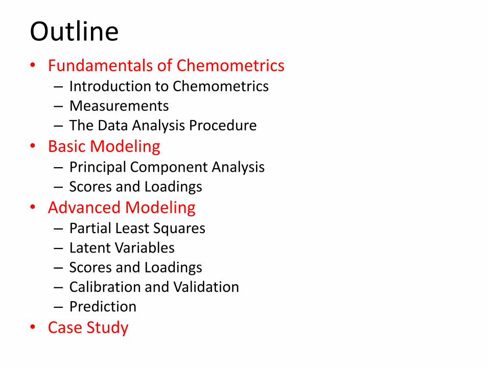
Outline• Fundamentals of Chemometrics
– Introduction to Chemometrics– Measurements– The Data Analysis Procedure
• Basic Modeling– Principal Component Analysis– Scores and Loadings
• Advanced Modeling– Partial Least Squares– Latent Variables– Scores and Loadings– Calibration and Validation– Prediction
• Case Study

Section 1
Through the looking glass…..
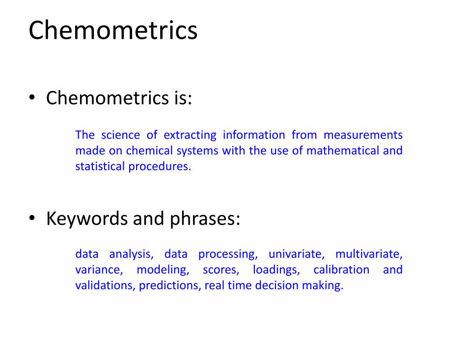
Chemometrics
• Chemometrics is:
• Keywords and phrases:
The science of extracting information from measurementsmade on chemical systems with the use of mathematical andstatistical procedures.
data analysis, data processing, univariate, multivariate,variance, modeling, scores, loadings, calibration andvalidations, predictions, real time decision making.
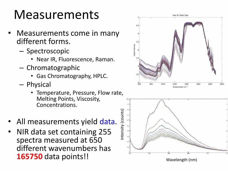
Measurements• Measurements come in many
different forms.– Spectroscopic
• Near IR, Fluorescence, Raman.
– Chromatographic• Gas Chromatography, HPLC.
– Physical• Temperature, Pressure, Flow rate,
Melting Points, Viscosity, Concentrations.
• All measurements yield data.• NIR data set containing 255
spectra measured at 650 different wavenumbers has 165750 data points!!
600 800 1000 1200 1400 1600 1800 20003
3.5
4
4.5
5
5.5
6
6.5
7Near IR Tablet Data
Wavenumber cm-1
Sig
nal In
tensity
Inte
nsi
ty (
cou
nts
)
Wavelength (nm)
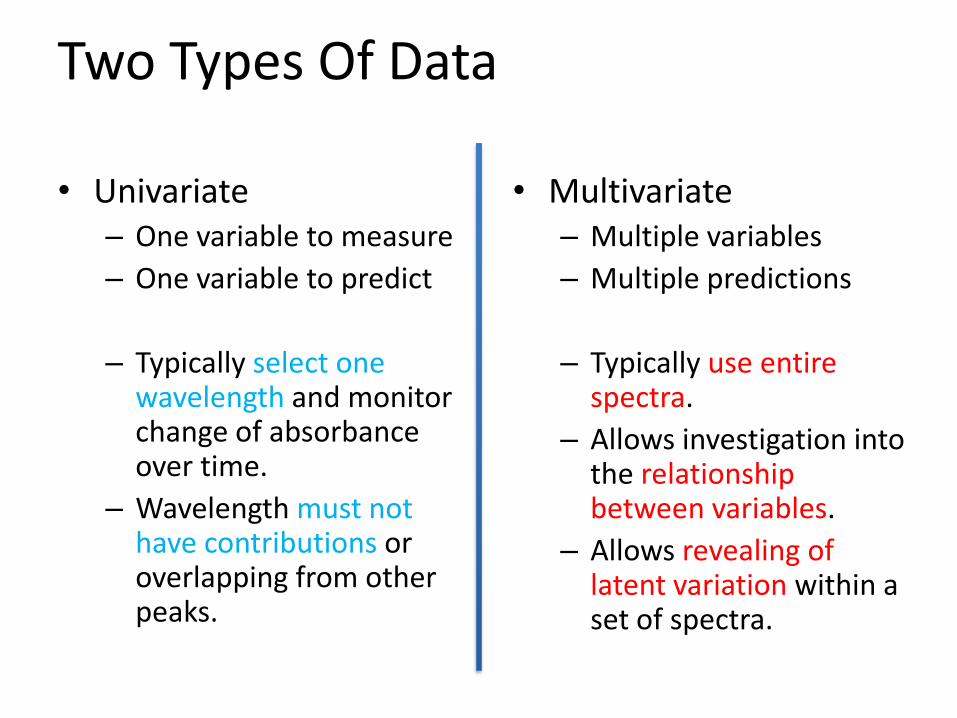
Two Types Of Data
• Univariate– One variable to measure
– One variable to predict
– Typically select one wavelength and monitor change of absorbance over time.
– Wavelength must not have contributions or overlapping from other peaks.
• Multivariate– Multiple variables
– Multiple predictions
– Typically use entire spectra.
– Allows investigation into the relationship between variables.
– Allows revealing of latent variation within a set of spectra.
Multivariate Analysis
• Analysis performed on multiple sets of measurements, wavelengths, samples and data sets.
• Analysis of variance and dependence between variables in crucial to multivariate analysis.
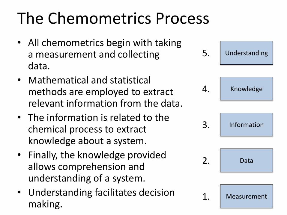
The Chemometrics Process
• All chemometrics begin with taking a measurement and collecting data.
• Mathematical and statistical methods are employed to extract relevant information from the data.
• The information is related to the chemical process to extract knowledge about a system.
• Finally, the knowledge provided allows comprehension and understanding of a system.
• Understanding facilitates decision making.
1. Measurement
2. Data
3. Information
4. Knowledge
5. Understanding
Converting Data to Information
• Advances in measurement science means rate of data collection is extremely fast.
• Large amounts of data produced.
• Data rich, information poor.
• Chemometrics used to remove redundant data, reduce variation not relating to the analytical signal and build models.
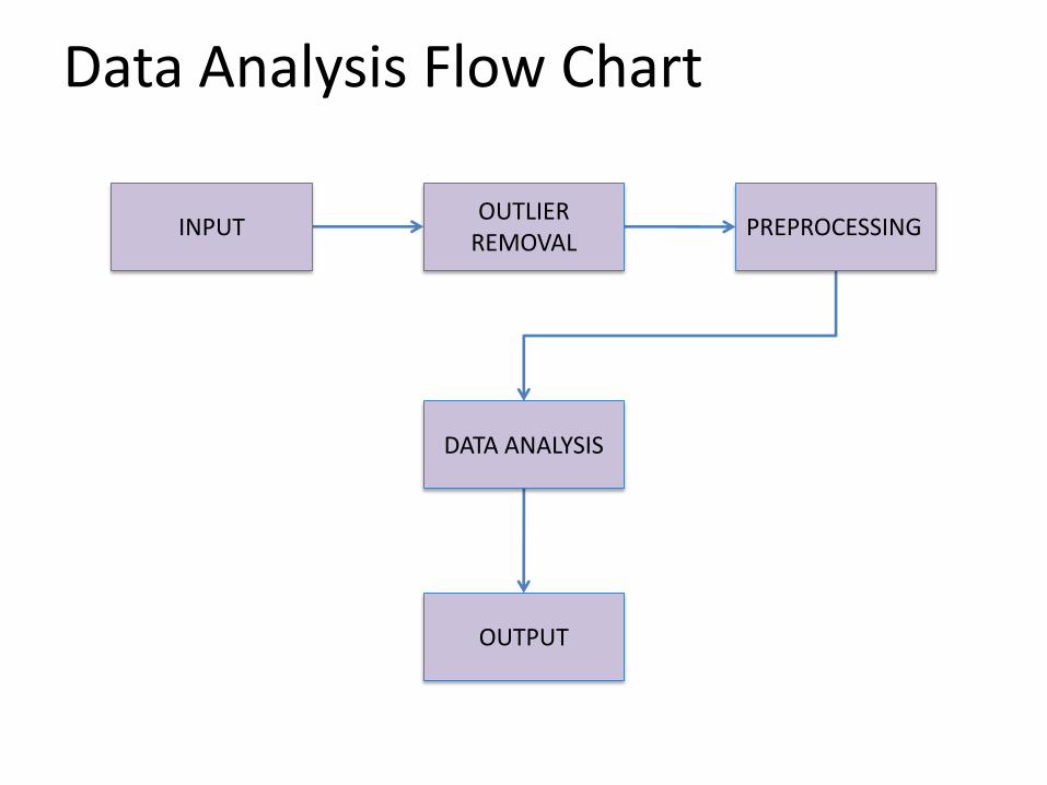
Data Analysis Flow Chart
INPUTOUTLIER
REMOVALPREPROCESSING
DATA ANALYSIS
OUTPUT
Input
• Most overlooked stage of data analysis.
• Most critical stage of all.
• Data must be converted or transferred into the analysis software.
• Proprietary collection software make this task difficult.
• However, some analysis software have excellent data importing functionality
Outliers – Problems and Removal
• Removing outliers is a delicate procedure.
• Grubbs test used to detect outliers.
• Frequently requires knowledge about the process being examined.
• False outliers, samples at extremes of the system that appear infrequently within the data.– These are NOT REMOVED
• True outliers, samples or variable that is statistically different from the other samples.– These ARE REMOVED
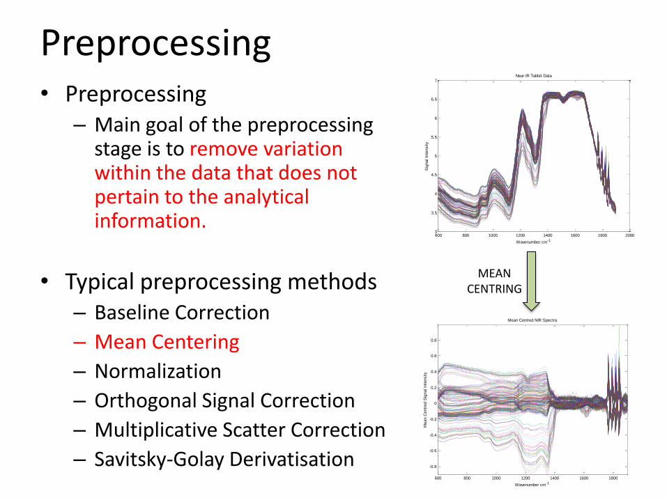
Preprocessing• Preprocessing
– Main goal of the preprocessing stage is to remove variation within the data that does not pertain to the analytical information.
• Typical preprocessing methods– Baseline Correction
– Mean Centering
– Normalization
– Orthogonal Signal Correction
– Multiplicative Scatter Correction
– Savitsky-Golay Derivatisation600 800 1000 1200 1400 1600 1800
-0.8
-0.6
-0.4
-0.2
0
0.2
0.4
0.6
0.8
Mean Centred NIR Spectra
Wavenumber cm-1
Mean C
entr
ed S
ignal In
tensity
600 800 1000 1200 1400 1600 1800 20003
3.5
4
4.5
5
5.5
6
6.5
7Near IR Tablet Data
Wavenumber cm-1
Sig
nal In
tensity
MEAN CENTRING
Data Analysis
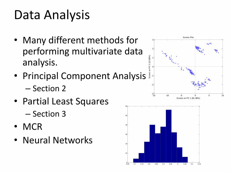
• Many different methods for performing multivariate data analysis.
• Principal Component Analysis– Section 2
• Partial Least Squares– Section 3
• MCR
• Neural Networks
-15 -10 -5 0 5 10-3
-2
-1
0
1
2
3
Scores on PC 1 (81.38%)
Score
s o
n P
C 2
(12.8
8%
)
Scores Plot
4.65 4.7 4.75 4.8 4.85 4.9 4.95 5 5.05 5.1 5.150
10
20
30
40
50
60
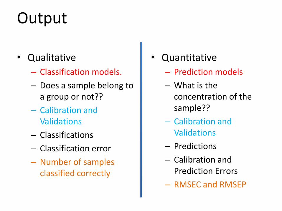
Output
• Qualitative
– Classification models.
– Does a sample belong to a group or not??
– Calibration and Validations
– Classifications
– Classification error
– Number of samples classified correctly
• Quantitative
– Prediction models
– What is the concentration of the sample??
– Calibration and Validations
– Predictions
– Calibration and Prediction Errors
– RMSEC and RMSEP
Error• Many different methods of calculating errors.
• Method used is critical as model quality determined by the error.
• Procedure used can heavily influence model errors. (Discussed later in PCA section).
• The choice of error metric depends on many different factors
• Top Three– What are you showing?
– What is the range of data?
– How many samples do you have?
Summary
• Chemometrics is a method of extracting relevant information from complex chemical data.
• Multivariate data allows analysis robust investigation of overlapping signals.
• Multivariate analysis allows investigation of the relationship between variables.
• The chemometrics process yields understanding and comprehension of the process under investigation.
Summary
• Data analysis is a multistep procedure involving many algorithms and many different paths to go down.
• The end results of data analysis are commonly a model that could provide qualitative or quantitative information.
• MatLab and PLS_Toolbox are software packages used to perform chemometrics analysis.
Section 2
Principal Component Analysis
P.C.A.
PCA
• Method of reducing a set of data into three new sets of variables– Principal Components (PC’s)
– Scores
– Loadings
• Using these three new variables latent variation can be developed and examined.
• Incredibly important for investigating the relationships between samples and variables
PCA
600 800 1000 1200 1400 1600 1800 20003
3.5
4
4.5
5
5.5
6
6.5
7Near IR Tablet Data
Sig
nal In
tensity
Wavenumber cm-1118 120 122 124 126 128 130 132 134 136
-8
-6
-4
-2
0
2
4
6
8
Scores on PC 1 (99.93%)
Score
s o
n P
C 2
(0.0
5%
)Samples/Scores Plot
100 200 300 400 500 6000.025
0.03
0.035
0.04
0.045
0.05
0.055
Variable
Loadin
gs o
n P
C 1
(99.9
3%
)
Variables/Loadings Plot
PCA
SPECTRAL DATA SCORES LOADINGS
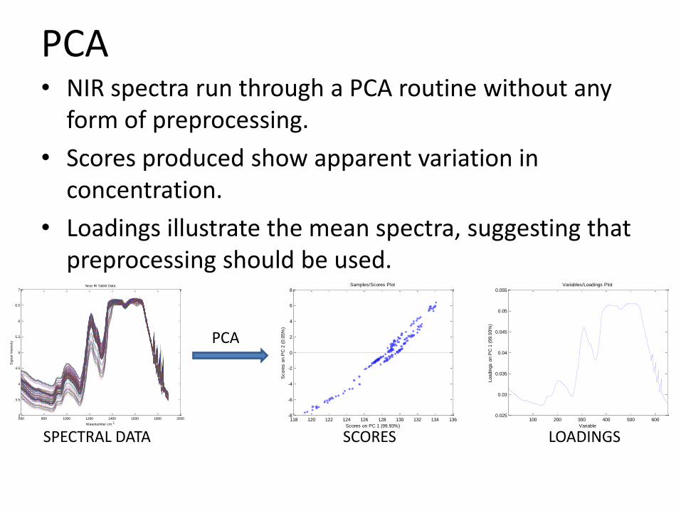
• NIR spectra run through a PCA routine without any form of preprocessing.
• Scores produced show apparent variation in concentration.
• Loadings illustrate the mean spectra, suggesting that preprocessing should be used.
Principal Components
• Each principal component calculated captures as much of the variation within the data as possible.
• This variation is removed and a new principal component is determined.
• The first PC describes the greatest source of variation within the data
Scores
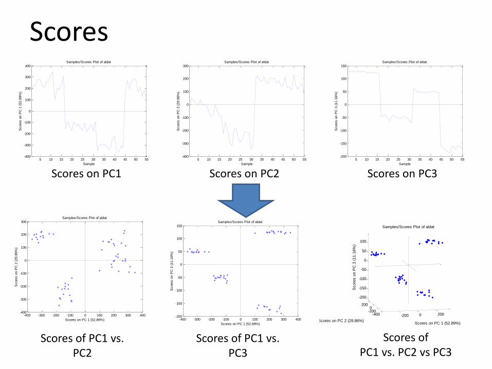
• The scores are organized in a column fashion.
• The first column denotes the scores relating to the variation captured on PC1.
• Intra-sample relationships can be observed by plotting the scores from PC1 against PC2.
• This can be expanded to the scores of the first three PC’s.
Scores
5 10 15 20 25 30 35 40 45 50 55-400
-300
-200
-100
0
100
200
300
400
Sample
Score
s o
n P
C 1
(52.8
9%
)
Samples/Scores Plot of aldat
5 10 15 20 25 30 35 40 45 50 55-400
-300
-200
-100
0
100
200
300
Sample
Score
s o
n P
C 2
(29.8
6%
)
Samples/Scores Plot of aldat
5 10 15 20 25 30 35 40 45 50 55-200
-150
-100
-50
0
50
100
150
Sample
Score
s o
n P
C 3
(11.1
6%
)
Samples/Scores Plot of aldat
Scores on PC1 Scores on PC2 Scores on PC3
-400 -300 -200 -100 0 100 200 300 400-400
-300
-200
-100
0
100
200
300
Scores on PC 1 (52.89%)
Score
s o
n P
C 2
(29.8
6%
)
Samples/Scores Plot of aldat
-400 -300 -200 -100 0 100 200 300 400-200
-150
-100
-50
0
50
100
150
Scores on PC 1 (52.89%)
Score
s o
n P
C 3
(11.1
6%
)
Samples/Scores Plot of aldat
-200 0 200-400-2000
200
-200
-150
-100
-50
0
50
100
Scores on PC 1 (52.89%)
Samples/Scores Plot of aldat
Scores on PC 2 (29.86%)
Score
s o
n P
C 3
(11.1
6%
)
Scores of PC1 vs. PC2
Scores of PC1 vs. PC3
Scores of PC1 vs. PC2 vs PC3
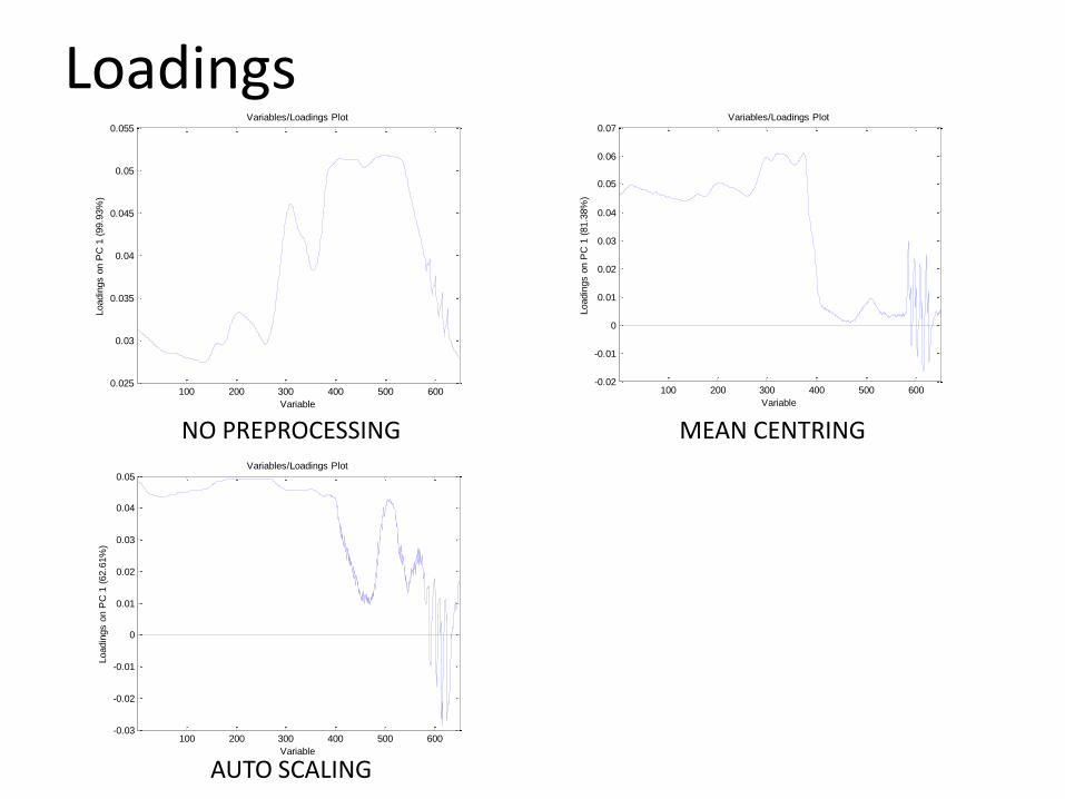
Loadings
• Illustrate the weight or importance of each variable within the original data.
• From loadings it is possible to see the most significant variables.
• Loadings can be used to track the process of a reaction e.g. monitor reactant consumption.
• Deduce variables responsible for the clustering in the scores.
Loadings
100 200 300 400 500 6000.025
0.03
0.035
0.04
0.045
0.05
0.055
Variable
Loadin
gs o
n P
C 1
(99.9
3%
)
Variables/Loadings Plot
100 200 300 400 500 600-0.02
-0.01
0
0.01
0.02
0.03
0.04
0.05
0.06
0.07
Variable
Loadin
gs o
n P
C 1
(81.3
8%
)
Variables/Loadings Plot
100 200 300 400 500 600-0.03
-0.02
-0.01
0
0.01
0.02
0.03
0.04
0.05
Variable
Loadin
gs o
n P
C 1
(62.6
1%
)
Variables/Loadings Plot
NO PREPROCESSING MEAN CENTRING
AUTO SCALING
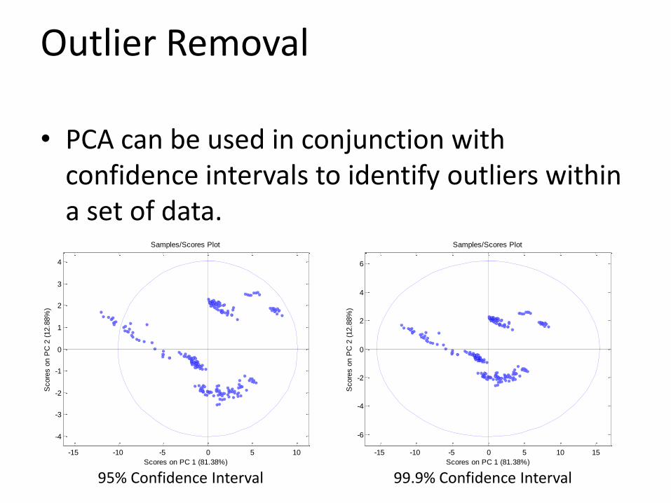
Outlier Removal
• PCA can be used in conjunction with confidence intervals to identify outliers within a set of data.
-15 -10 -5 0 5 10
-4
-3
-2
-1
0
1
2
3
4
Scores on PC 1 (81.38%)
Score
s o
n P
C 2
(12.8
8%
)
Samples/Scores Plot
-15 -10 -5 0 5 10 15
-6
-4
-2
0
2
4
6
Scores on PC 1 (81.38%)
Score
s o
n P
C 2
(12.8
8%
)
Samples/Scores Plot
95% Confidence Interval 99.9% Confidence Interval
Summary
• PCA used to decompose the data into scores and loadings
• Scores reveal information about between sample variation.
• Loadings tell us which variables from within the original data contribute most to the scores.
• PCA can also be used to analyze and investigate data to perform tasks such as outlier removal.
• PCA facilitates process understanding.
Section 3
Partial Least Squares
Inverse Calibration
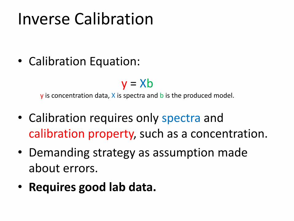
• Calibration Equation:
• Calibration requires only spectra and calibration property, such as a concentration.
• Demanding strategy as assumption made about errors.
• Requires good lab data.
y = Xby is concentration data, X is spectra and b is the produced model.
PLS
• Partial Least Squares (PLS) is an extension of the PCA method.
• PCA extracts PC’s describing the sources of variation within the data.
• PLS takes the PC’s and correlates them with Y-Blockinformation to calculate Latent Variables (LV’s).
• Y-Block information is typically sample concentrations, physical properties.
• PLS is a quantitative procedure and can be used to model and predict y-block information for future samples
The X- and Y-Block
• PLS uses X-Block and Y-Block information.
• X-Block tends to refer to spectra.
• Y-Block relates to the information you want to predict, such as concentration or some physical property.
• Y-Block data is normally collected offline in a lab.
• Y-Block is often referred to as the reference method.
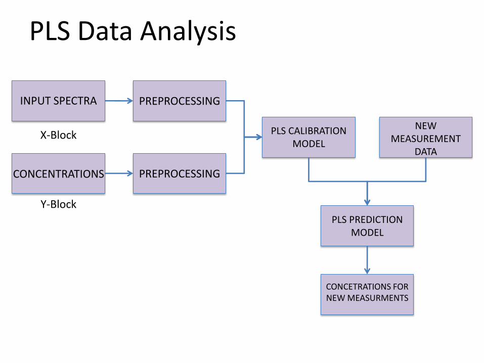
PLS Data Analysis
INPUT SPECTRA PREPROCESSING
CONCENTRATIONS PREPROCESSING
PLS CALIBRATION MODEL
NEW MEASUREMENT
DATA
PLS PREDICTION MODEL
CONCETRATIONS FOR NEW MEASURMENTS
X-Block
Y-Block
Difference between PLS and PCA
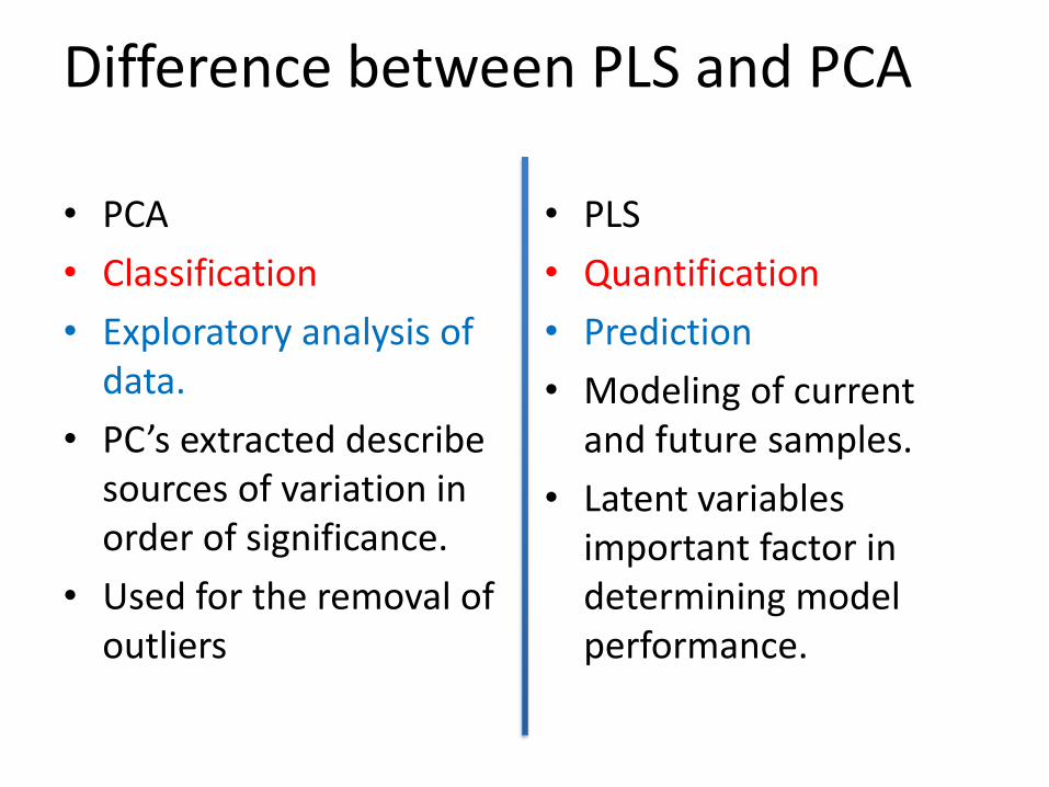
• PCA
• Classification
• Exploratory analysis of data.
• PC’s extracted describe sources of variation in order of significance.
• Used for the removal of outliers
• PLS
• Quantification
• Prediction
• Modeling of current and future samples.
• Latent variables important factor in determining model performance.
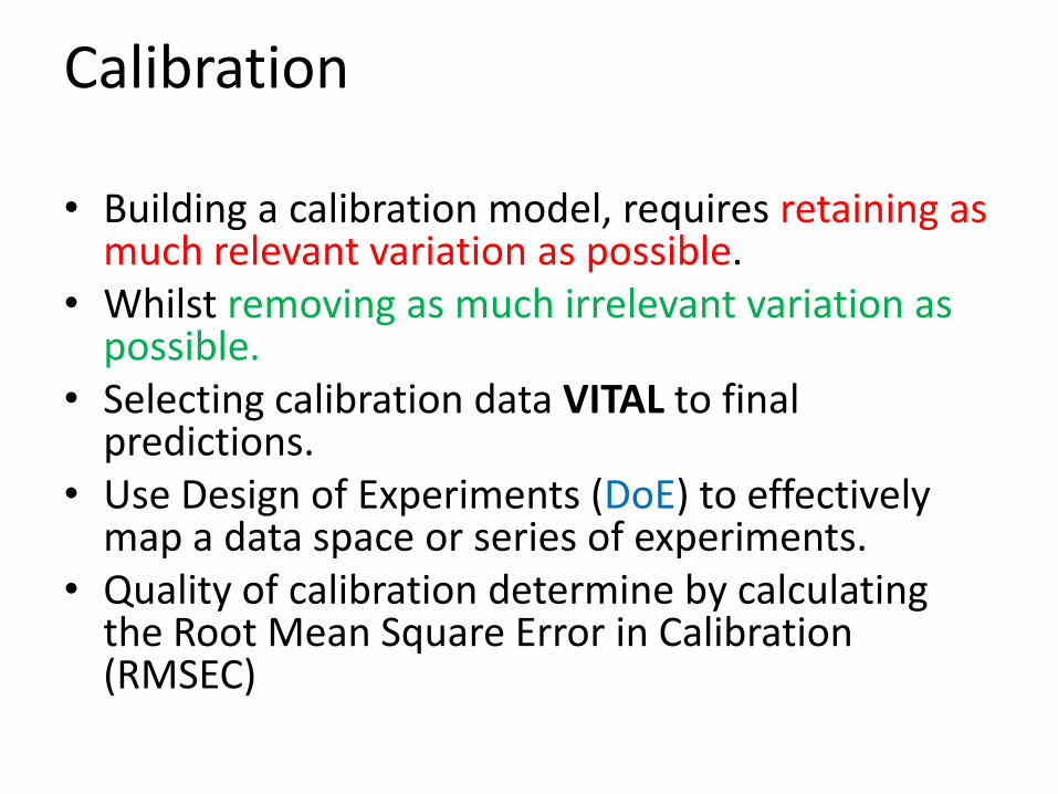
Calibration
• Building a calibration model, requires retaining as much relevant variation as possible.
• Whilst removing as much irrelevant variation as possible.
• Selecting calibration data VITAL to final predictions.
• Use Design of Experiments (DoE) to effectively map a data space or series of experiments.
• Quality of calibration determine by calculating the Root Mean Square Error in Calibration (RMSEC)
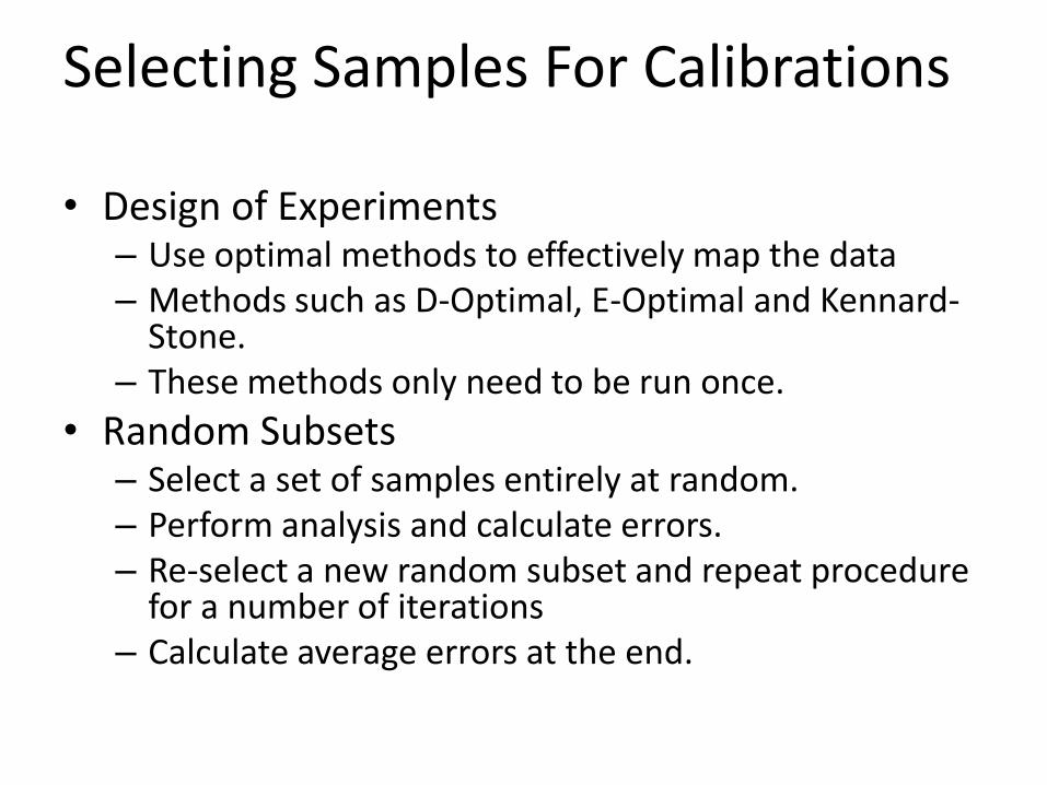
Selecting Samples For Calibrations
• Design of Experiments– Use optimal methods to effectively map the data– Methods such as D-Optimal, E-Optimal and Kennard-
Stone.– These methods only need to be run once.
• Random Subsets– Select a set of samples entirely at random.– Perform analysis and calculate errors.– Re-select a new random subset and repeat procedure
for a number of iterations– Calculate average errors at the end.
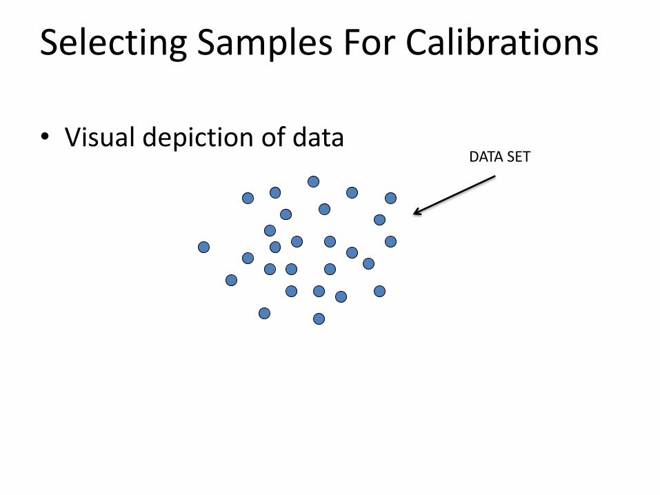
Selecting Samples For Calibrations
• Visual depiction of dataDATA SET
Selecting Samples For Calibrations
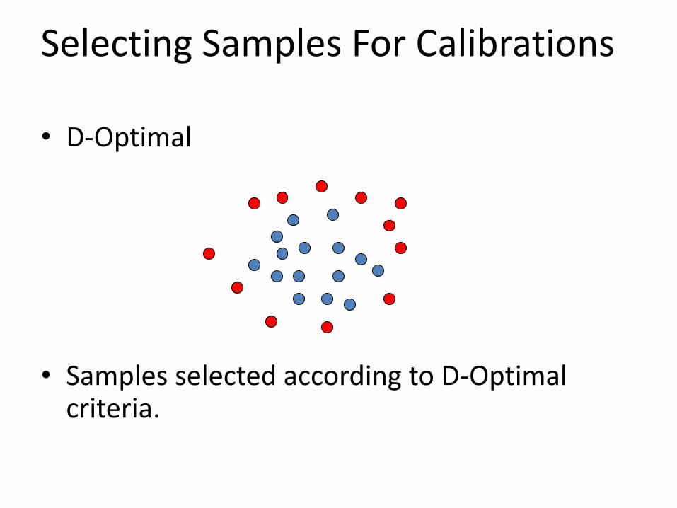
• D-Optimal
• Samples selected according to D-Optimal criteria.
Selecting Samples For Calibrations
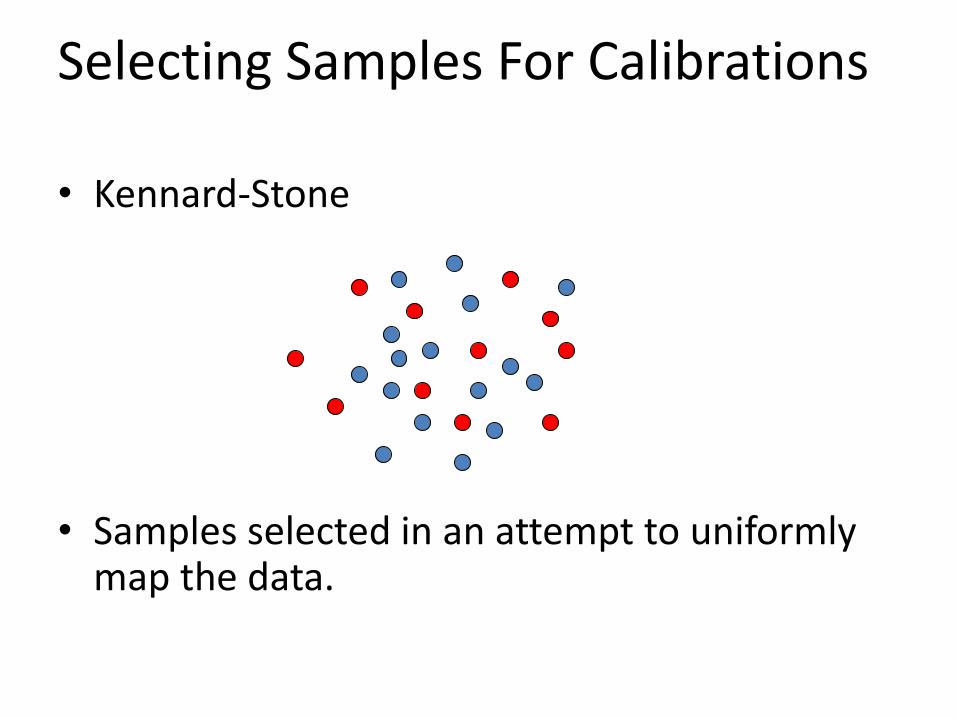
• Kennard-Stone
• Samples selected in an attempt to uniformly map the data.
Validation
• Validation data is used to check the predictive performance of the model.
• Validation can be performed using subsets of the calibration data (Cross Validation).
• Separate validation sets of data can be collected (True Validation).
• Cross validation leads to overly positive results.• Quality of validation calculated using the Root
Mean Square Error in Prediction (RMSEP).• Quality of predictions determines quality of
model.
Modeling
• The quality of calibrations and validations can vary significantly with the number of LV’s included in the model.
• Too few and the model will make poor predictions as there is insufficient information in the calibration
• Too many and the model has become overly focused and contains too much variationmaking it not robust to small amounts of variation.
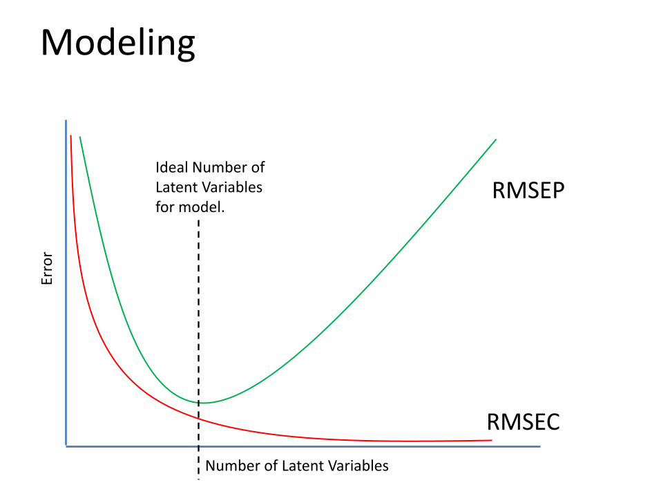
ModelingEr
ror
Number of Latent Variables
RMSEC
RMSEPIdeal Number of Latent Variables for model.
Model Maintenance
• We’ve built the model: So what next?
• Collect lab data weekly to re-validate the model.– Are model results within significant error?– If not what do we do?
• Re-evaluate calibration samples– Is the calibration model still relevant?
• Perform DoE to re-select more data.• Check LV model to make sure appropriate LV’s being used.
• Continual improvement.
MODEL MAINTENANCE
Summary
• PLS implements inverse calibration to incorporate concentration information into a model.
• Makes quantitative predictions of unseen samples
• Requires calibration and validation
• Latent variables have significant effect on model.
• Quality of model determined by prediction and the RMSEP
Case Study
Model Building From Beginning to End
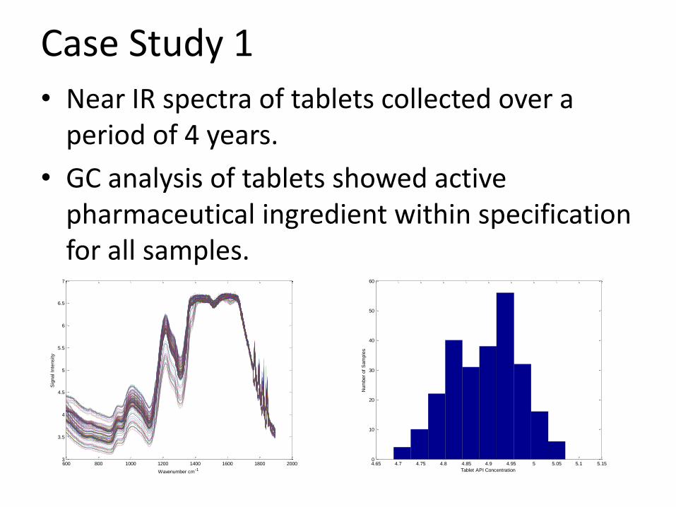
Case Study 1
• Near IR spectra of tablets collected over a period of 4 years.
• GC analysis of tablets showed active pharmaceutical ingredient within specification for all samples.
4.65 4.7 4.75 4.8 4.85 4.9 4.95 5 5.05 5.1 5.150
10
20
30
40
50
60
Tablet API Concentration
Num
ber
of
Sam
ple
s
600 800 1000 1200 1400 1600 1800 20003
3.5
4
4.5
5
5.5
6
6.5
7
Wavenumber cm-1
Sig
nal In
tensity
The Problem
• The NIR calibration model produced has determined 32% samples are out of specification.
• The Plan: Use PCA to investigate and examine the spectra to improve the NIR calibration.
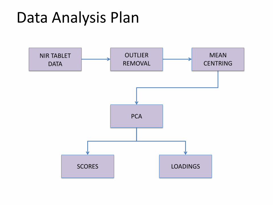
Data Analysis Plan
NIR TABLET DATA
OUTLIER REMOVAL
MEAN CENTRING
PCA
SCORES LOADINGS
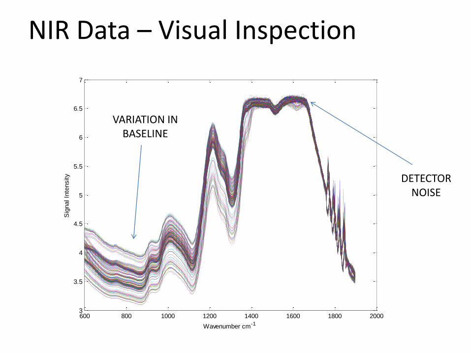
NIR Data – Visual Inspection
600 800 1000 1200 1400 1600 1800 20003
3.5
4
4.5
5
5.5
6
6.5
7
Wavenumber cm-1
Sig
nal In
tensity DETECTOR
NOISE
VARIATION IN BASELINE
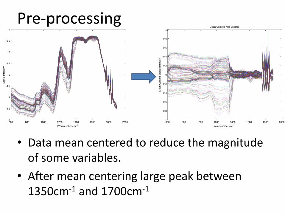
Pre-processing
• Data mean centered to reduce the magnitude of some variables.
• After mean centering large peak between 1350cm-1 and 1700cm-1
600 800 1000 1200 1400 1600 1800 2000-1
-0.8
-0.6
-0.4
-0.2
0
0.2
0.4
0.6
0.8
1
Wavenumber cm-1
Mean C
entr
ed S
ignal In
tensity
Mean Centred NIR Spectra
600 800 1000 1200 1400 1600 1800 20003
3.5
4
4.5
5
5.5
6
6.5
7
Wavenumber cm-1
Sig
nal In
tensity
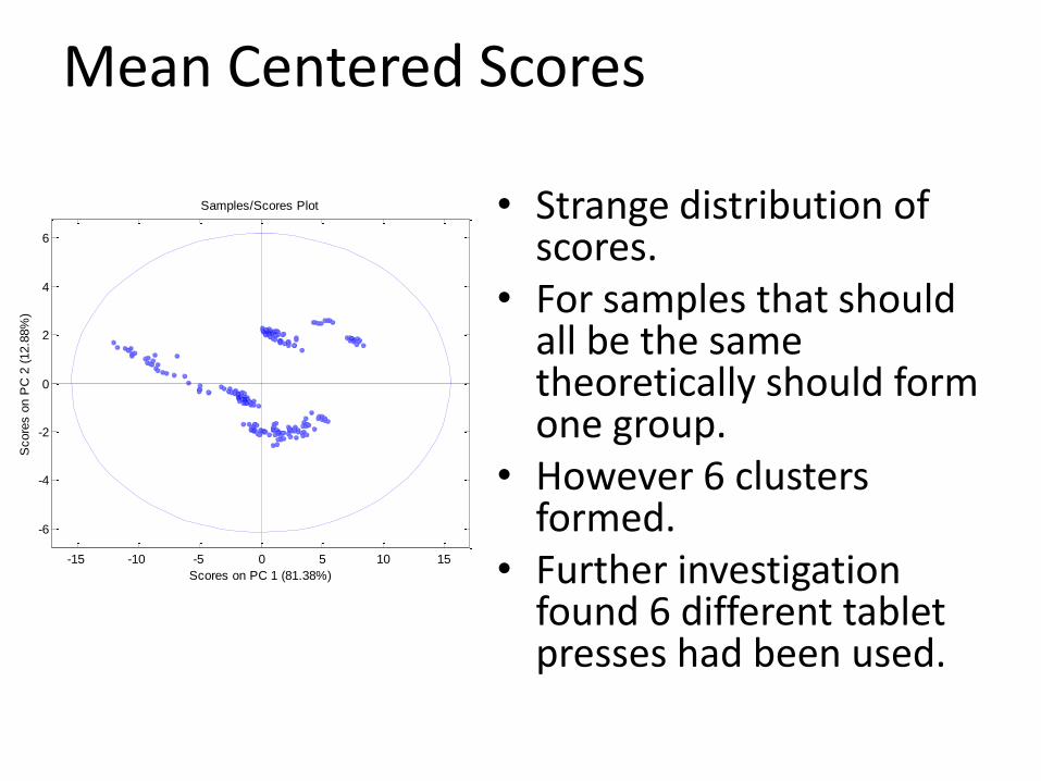
Mean Centered Scores
• Strange distribution of scores.
• For samples that should all be the same theoretically should form one group.
• However 6 clusters formed.
• Further investigation found 6 different tablet presses had been used.
-15 -10 -5 0 5 10 15
-6
-4
-2
0
2
4
6
Scores on PC 1 (81.38%)
Score
s o
n P
C 2
(12.8
8%
)
Samples/Scores Plot
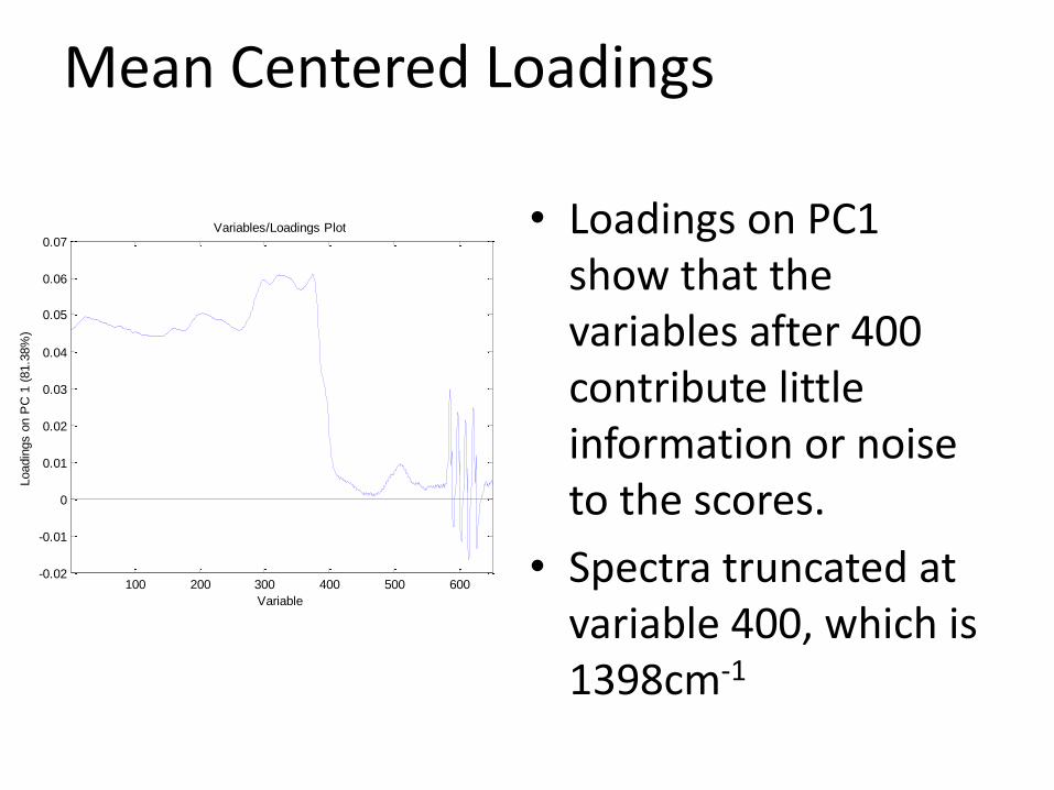
Mean Centered Loadings
• Loadings on PC1 show that the variables after 400 contribute little information or noise to the scores.
• Spectra truncated at variable 400, which is 1398cm-1
100 200 300 400 500 600-0.02
-0.01
0
0.01
0.02
0.03
0.04
0.05
0.06
0.07
Variable
Loadin
gs o
n P
C 1
(81.3
8%
)
Variables/Loadings Plot
Scatter Correction
• Investigation into the manufacturing procedure reveal tablets made using different presses.
• This cause minor variations in the tablet depth.
• This altered the pathlength and scattering of the NIR radiation.
• Preprocessing must be applied to minimize the variation in the data due to the change in tablet depth.
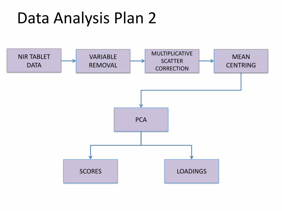
Data Analysis Plan 2
NIR TABLET DATA
VARIABLE REMOVAL
MEAN CENTRING
PCA
SCORES LOADINGS
MULTIPLICATIVE SCATTER
CORRECTION
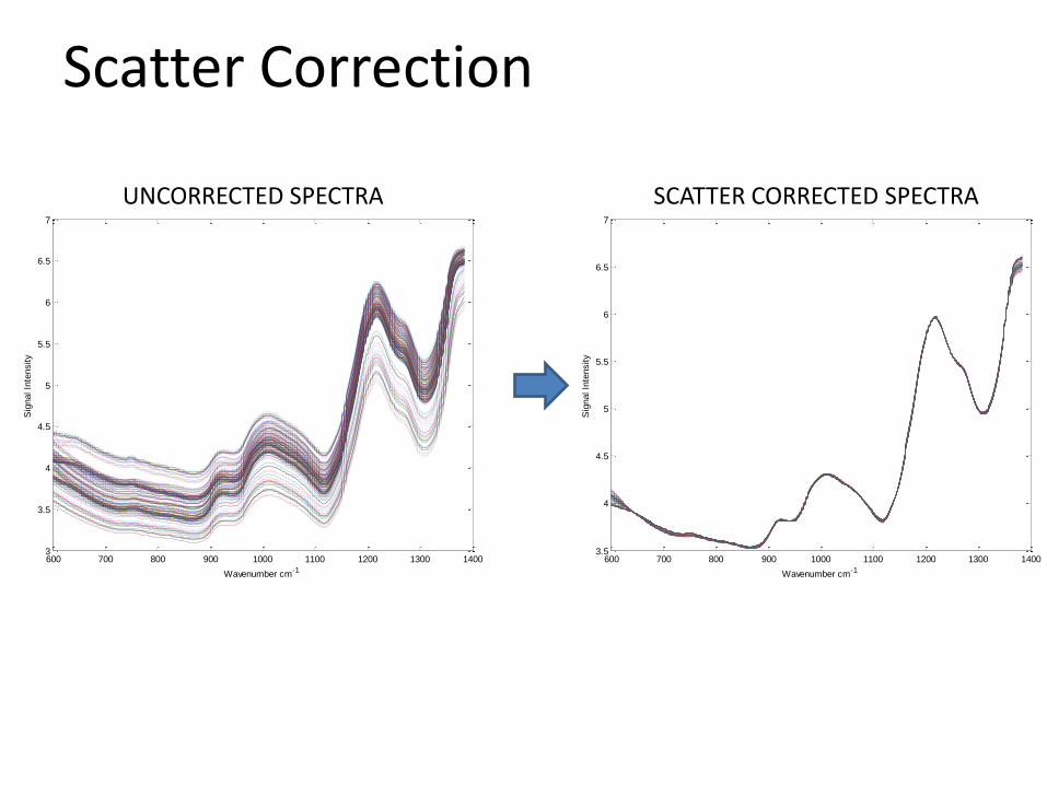
Scatter Correction
600 700 800 900 1000 1100 1200 1300 14003
3.5
4
4.5
5
5.5
6
6.5
7
Wavenumber cm-1
Sig
nal In
tensity
600 700 800 900 1000 1100 1200 1300 14003.5
4
4.5
5
5.5
6
6.5
7
Wavenumber cm-1
Sig
nal In
tensity
UNCORRECTED SPECTRA SCATTER CORRECTED SPECTRA
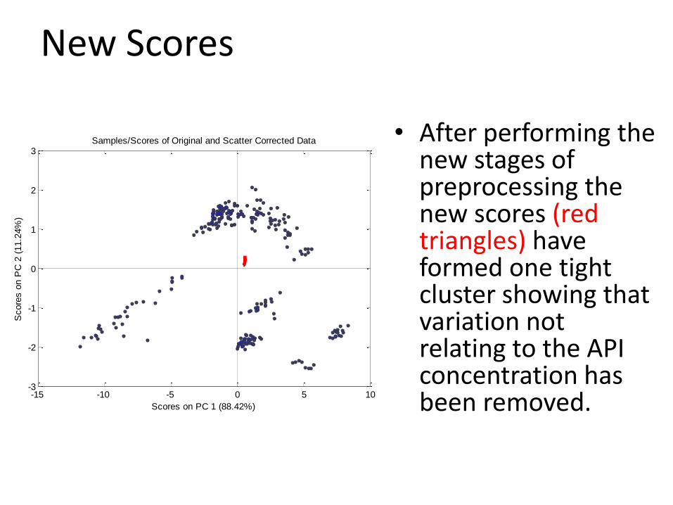
New Scores
• After performing the new stages of preprocessing the new scores (red triangles) have formed one tight cluster showing that variation not relating to the API concentration has been removed.-15 -10 -5 0 5 10
-3
-2
-1
0
1
2
3
Scores on PC 1 (88.42%)
Score
s o
n P
C 2
(11.2
4%
)
Samples/Scores of Original and Scatter Corrected Data
What Next?
Partial Least Squares
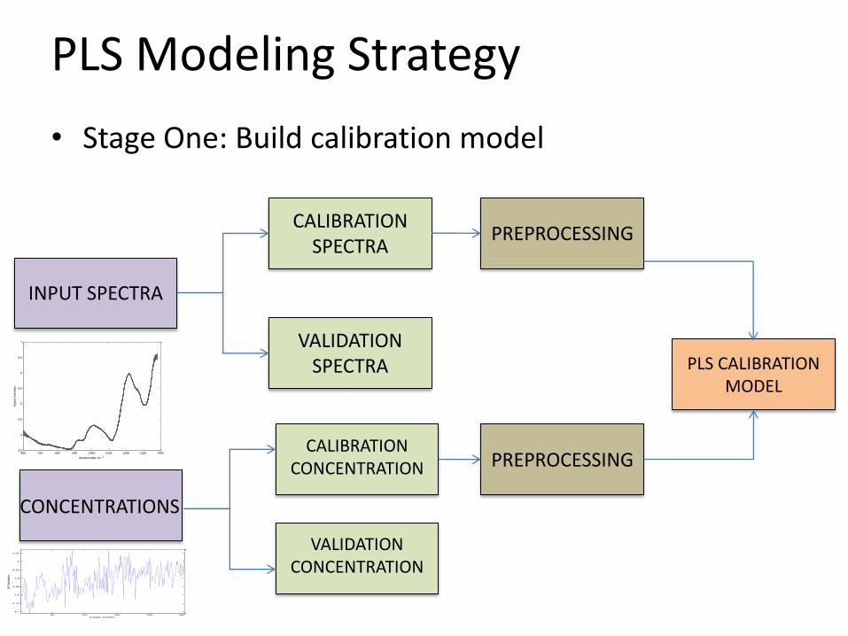
PLS Modeling Strategy
• Stage One: Build calibration model
PLS CALIBRATION MODEL
INPUT SPECTRA
PREPROCESSING
CONCENTRATIONS
PREPROCESSING
VALIDATION SPECTRA
CALIBRATION SPECTRA
VALIDATION CONCENTRATION
CALIBRATION CONCENTRATION
600 700 800 900 1000 1100 1200 1300 14003.5
4
4.5
5
5.5
6
6.5
7
Wavenumber cm-1
Sig
nal In
tensity
50 100 150 200 250
4.7
4.75
4.8
4.85
4.9
4.95
5
5.05
Sample Number
API C
once
ntrati
on
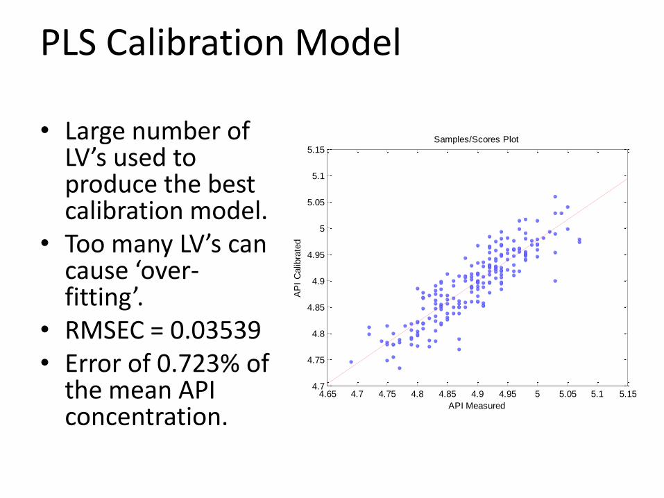
PLS Calibration Model
• Large number of LV’s used to produce the best calibration model.
• Too many LV’s can cause ‘over-fitting’.
• RMSEC = 0.03539• Error of 0.723% of
the mean API concentration.
4.65 4.7 4.75 4.8 4.85 4.9 4.95 5 5.05 5.1 5.154.7
4.75
4.8
4.85
4.9
4.95
5
5.05
5.1
5.15
API Measured
AP
I C
alib
rate
d
Samples/Scores Plot
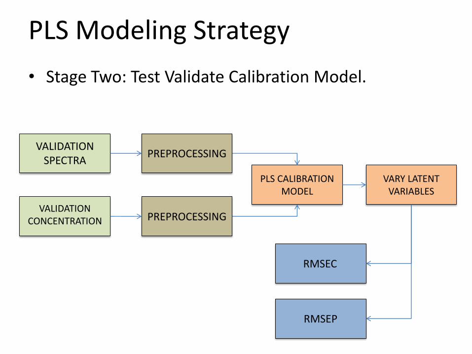
PLS Modeling Strategy
• Stage Two: Test Validate Calibration Model.
PLS CALIBRATION MODEL
PREPROCESSING
PREPROCESSING
VALIDATION SPECTRA
VALIDATION CONCENTRATION
VARY LATENT VARIABLES
RMSEP
RMSEC
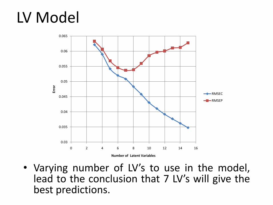
LV Model
• Varying number of LV’s to use in the model,lead to the conclusion that 7 LV’s will give thebest predictions.
0.03
0.035
0.04
0.045
0.05
0.055
0.06
0.065
0 2 4 6 8 10 12 14 16
Erro
r
Number of Latent Variables
RMSEC
RMSEP
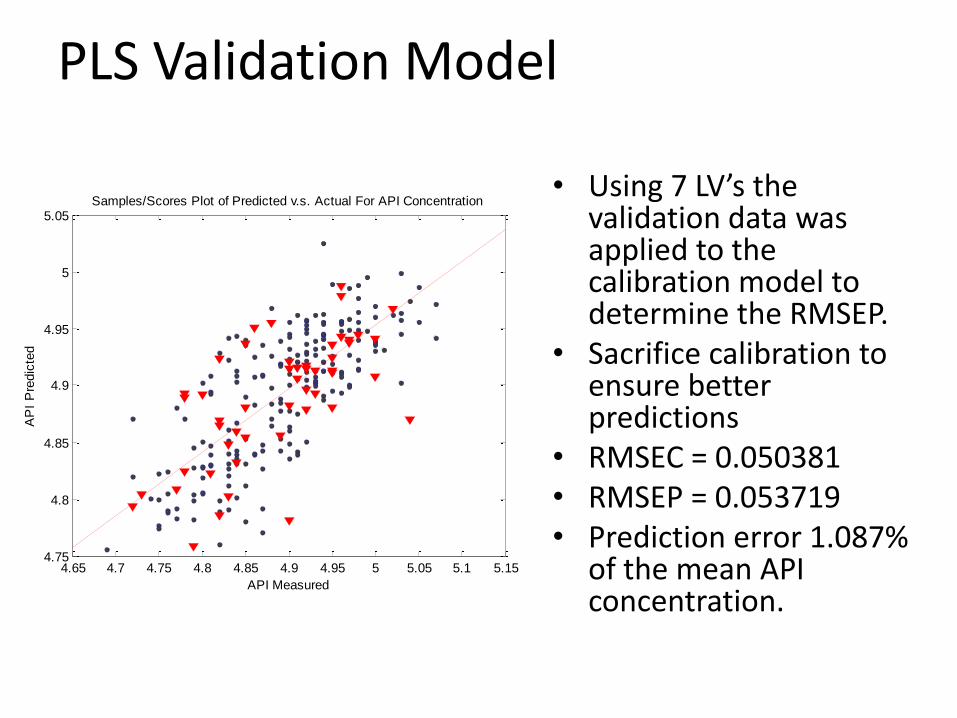
PLS Validation Model
• Using 7 LV’s the validation data was applied to the calibration model to determine the RMSEP.
• Sacrifice calibration to ensure better predictions
• RMSEC = 0.050381• RMSEP = 0.053719• Prediction error 1.087%
of the mean API concentration.
4.65 4.7 4.75 4.8 4.85 4.9 4.95 5 5.05 5.1 5.154.75
4.8
4.85
4.9
4.95
5
5.05
API Measured
AP
I P
redic
ted
Samples/Scores Plot of Predicted v.s. Actual For API Concentration
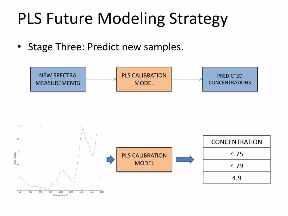
PLS Future Modeling Strategy
• Stage Three: Predict new samples.
PLS CALIBRATION MODEL
NEW SPECTRA MEASUREMENTS
PREDICTED CONCENTRATIONS
PLS CALIBRATION MODEL
CONCENTRATION
4.75
4.79
4.9
600 700 800 900 1000 1100 1200 1300 14003.5
4
4.5
5
5.5
6
Wavenumber cm-1
Sig
nal In
tensity
Case Study Summary
• PCA used to explore variation within the spectra
• Samples and variables selected for calibration.
• Scatter correction and mean centering used to preprocess data.
• PLS model built and validated using calibration and validation data.
• RMSEC and RMSEP calculated.
• Concentrations determined for new sample measurements.
Acknowledgements