Fundamentals of beam physics

Fundamentals of beam physics James B. Rosenzweig

Fundamentals of beam

physics Rosenzw

eig

2

2

This book presents beam physics using a unified approach,emphasizing basic concepts and analysis methods. Whilemany existing resources in beams and accelerators arespecialized to aid the professional practitioner, this textanticipates the needs of physics students. The central concepts underpinning the physics of accelerators, chargedparticle, and photon beams are built up from familiar,intertwining components, such as electromagnetism, relativity, and Hamiltonian dynamics. These componentsare woven into an illustrative set of examples that allowinvestigation of a variety of physical scenarios. With thesetools, single particle dynamics in linear accelerators arediscussed, with general methods that are naturallyextended to circular accelerators. Beyond single particledynamics, the proliferation of commonly used beamdescriptions are surveyed and compared. These methodsprovide a powerful connection between the classicalcharged particle beams, and beams based on coherentwaves – laser beams. Aspects of experimental techniquesare introduced. Numerous exercises, and examples drawnfrom devices such as synchrotrons and free-electron lasers,are included to illustrate relevant physical principles.

James B. Rosenzweig is Professor of Physics at theUniversity of California, Los Angeles, where he is alsoDirector of the Particle Beam Physics Laboratory.

Also published by Oxford University Press

The physics of particle accelerators: an introductionKlaus Wille

An introduction to particle acceleratorsEdmund Wilson

1www.oup.com

9 780198 525547

ISBN 0-19-852554-0

“fm” — 2003/6/28 — page i — #1

FUNDAMENTALS OF BEAM PHYSICS

James Rosenzweig

This is a selection from the beginning of the text. The full text is available through the publisher, Oxford University press.

“fm” — 2003/6/28 — page ii — #2

“fm” — 2003/6/28 — page iii — #3

Fundamentals ofBeam Physics

J.B. ROSENZWEIGDepartment of Physics and AstronomyUniversity of California, Los Angeles

1

“fm” — 2003/6/28 — page iv — #4

3Great Clarendon Street, Oxford OX2 6DP

Oxford University Press is a department of the University of Oxford.It furthers the University’s objective of excellence in research, scholarship,and education by publishing worldwide in

Oxford New York

Auckland Bangkok Buenos Aires Cape Town ChennaiDar es Salaam Delhi Hong Kong Istanbul Karachi KolkataKuala Lumpur Madrid Melbourne Mexico City Mumbai NairobiSão Paulo Shanghai Taipei Tokyo Toronto

Oxford is a registered trade mark of Oxford University Pressin the UK and in certain other countries

Published in the United Statesby Oxford University Press Inc., New York

© Oxford University Press, 2003

The moral rights of the author have been asserted

Database right Oxford University Press (maker)

First published 2003

All rights reserved. No part of this publication may be reproduced,stored in a retrieval system, or transmitted, in any form or by any means,without the prior permission in writing of Oxford University Press,or as expressly permitted by law, or under terms agreed with the appropriatereprographics rights organization. Enquiries concerning reproductionoutside the scope of the above should be sent to the Rights Department,Oxford University Press, at the address above

You must not circulate this book in any other binding or coverand you must impose this same condition on any acquirer

A catalogue record for this title is available from the British Library

Library of Congress Cataloging in Publication Data(Data available)

ISBN 0 19 852554 0

10 9 8 7 6 5 4 3 2 1

Typeset by Newgen Imaging Systems (P) Ltd., Chennai, IndiaPrinted in Great Britainon acid-free paper by The Bath Press, Avon

“fm” — 2003/6/28 — page v — #5

Preface

This book was developed as part of my efforts to build and enhance the accel-erator and beam physics program in the UCLA Department of Physics andAstronomy. This program includes an active research program in advancedaccelerators (particle accelerators based on lasers and/or plasmas) and free-electron lasers (conversely, lasers based on accelerators and particle beams) andis essentially a student-oriented enterprise. Its focus is primarily on graduateeducation and training, but the laboratory activities of the group also include astrong showing of undergraduate students. The desire to introduce both incom-ing graduate students and interested undergraduates to the physics of beamsled me to develop a course, Physics 150, to formally provide the backgroundneeded to enter the field.

In teaching this senior-level course the first few times, I found that I was rely-ing on a combination of excerpts from a variety of accelerator and laser physicstexts and my own notes. Because the hybrid nature of the UCLA research pro-gram in beams is reflected in the course, it was simply not possible to use asingle text for the course’s source material. As one might imagine, in the mix-ing of written references, the notation, level, and assumed background variedwidely from reading to reading. In addition, many existing texts and referencesin this area are geared towards a practitioner of accelerator physics working ata major accelerator facility. Thus this type of text has an emphasis that is heavyon the physics, engineering methods, and technical jargon specific to largeaccelerators at the high-energy frontier. The needs of this professional readerare inherently a bit different than the senior level university student, however.As such, previous texts typically have given less orientation to basic physicsconcepts than the university student needs in order to be properly introduced tothe subject. My desire to clarify the written introduction of beam physics as itis practiced at UCLA to undergraduate students led directly to the productionof this book.

The contents of this book were also flavored by my desire to create the com-pact introduction to beam physics that I wish I could have had—hopefully thereader will benefit from the resulting weight put on the points I have foundto be least clear or intuitive in my journeys in the field. The present book istherefore written with the student constantly in mind, and has been structuredto give a unified discussion of a variety of subjects that may seem to be, onthe surface, disparate. The intent of the book is to provide a coherent introduc-tion to the ideas and concepts behind the physics of particle beams. As such,the book begins, after some introductory historical and conceptual comments,with a review of relativity and mechanics. This discussion is intended to buildup our sets of physics tools, by placing a few standard approaches to moderndynamics, such as Hamiltonian and phase space-based analyses, in the context

“fm” — 2003/6/28 — page vi — #6

vi Preface

of relativistic motion. We then give a presentation of charged particle dynamicsin various combinations of simple magnetostatic and electrostatic field con-figurations, providing another unifying set of basic tools for understandingmore complex scenarios in beam physics. Also, at a higher conceptual level,we examine the physics of circular accelerators using simple extensions of theprinciples developed first in the context linear accelerators, and then use similarapproaches to analyzing both transverse optics and acceleration (longitudinal)dynamics. The adopted emphasis on fundamental, unified tools is motivated bythe challenges of modern accelerators and their applications as encountered inthe laboratory. In present, state-of-the-art beam physics labs, the experimentalsystems display an increasing wealth of physical phenomena, that require aphysicist’s insight to understand.

One of the more unique aspects of this text is that its unified approach isextended to include a discussion of the connection between the methods ofcharged particle beam optics and descriptions of the physics of paraxial lightbeams such as lasers. This unification of concepts, between wave-based lightbeams and classical charged particle beams, is also motivated by experimentalchallenges arising from two complementary sources. The first is that lasers areincreasingly used as critical components in accelerators—for example, they areused to produce intense, picosecond electron pulses in devices termed photoin-jectors, two of which are found at UCLA. The second was already mentionedabove. In advanced accelerators and free-electron lasers, the concepts of accel-erators, particle beams, and lasers are, in fact, merged. These cutting edgesubjects in beam physics are what provide the intellectual impetus behind myresearch program at UCLA. It should not be surprising that such subjects findtheir way into this introductory text in a number of different ways.

This book is also structured so that an abbreviated course consisting of thefirst four chapters may give an introduction to single particle dynamics in accel-erators. Additionally, Chapter 5 introduces the physics of beam distributions(collections of many particles), a subject that is quite necessary if one wishes toapply this text in practice. Further, the notions developed in Chapters 1–5 canthen be used to give the basis for the material on photon beams in Chapter 8.Chapters 6 and 7, which discuss the technical subjects of magnets as well aswaveguides and accelerator cavities, can stand virtually by themselves. Theydo, however, complete the set of basic material offered here, and it is hopedthat they prove useful in practice as an introductory guide to the design and useof accelerator laboratory components.

To aid in streamlining the approach to learning from this text, sections thatcontain general “review” material are marked with the � symbol next to theirtitle. For an advanced student, these sections (the reviews of relativity andmechanics fall into this category) might be omitted on first reading. Othersections are marked by an asterix (*), and contain material which can be con-sidered in some way tangential to the main exposition of topics in beam physics.Such sections, while forming important components of the book as a whole,and may be referenced elsewhere in the text, may contain material that is toolengthy or deep for a fast initial reading. In an alternative approach, muchof the material in both these special sections would be included in appen-dices. Here they are included in the main body of text, both to improve thelogical flow of the book, and to allow illustrative exercises for the student to beincluded.

“fm” — 2003/6/28 — page vii — #7

Preface vii

The exercises in this book, included at the end of each chapter, are meant to bean integral part of the exposition, as some important topics are actually coveredin the exercises. In order to provide a guide to approaching the exercises, andto help emphasize their importance, worked solutions to roughly one-third ofthe problems are included in Appendix A.

The subjects introduced in this book are related in both obvious and subtleways. To aid in tying threads of the text together for the reader, a short summaryis included at each chapter end.

Numerous acknowledgments are in order. One must first find your interestsparked by a field of inquiry; my present colleague David Cline provided thespark for me when I was yet a student. My initial training in accelerator theorywas most heavily influenced by Fred Mills (then at Fermilab), and his stylecan be seen in many of the approaches taken to analyzing beam dynamics inthis text. Other friends, mentors and collaborators of particular note, who havegiven me stimulus to go deeper into the subjects presented here are: Pisin Chen,Richard Cooper, Luca Serafini, and Jim Simpson. A special debt of gratitude isdue to my close colleague, Claudio Pellegrini, who has, with our students andpost-docs, built the UCLA beam physics program with me.

Perhaps the highest level of thanks must go, however to those studentsat UCLA who have provided components of the background, motivation,and critical feedback to finish this text. A no-doubt incomplete listing ofthe graduate students (many of whom are now professional colleagues) fol-lows: Ron Agusstson, Scott Anderson, Gerard Andonian, Kip Bishofberger,Salime Boucher, Nick Barov, Eric Colby, Xiadong Ding, Joel England, SpencerHartman, Mark Hogan, Pietro Musumeci, Sven Reiche, Soren Telfer, AndreiTerebilo, Matt Thompson, Gil Travish and Aaron Tremaine. Special thanks aredue to the undergraduate students who have aided in the editing of this text,Pauline Lay and Maria Perrelli.

As a university professor with a large, active research program, my textbookwriting has generally been performed after the “day job” is done. Therefore,I must also thank my family (my wife, Judy, and children, Max, Julia andIan) for their patience, and occasional cheers—mainly for attempts at artisticgraphics—as this project began to unfold at home.

James RosenzweigLos Angeles, 2002

“fm” — 2003/6/28 — page viii — #8

Contents

1 Introduction to beam physics 11.1 History and uses of particle accelerators 21.2 System of units, and the Maxwell equations� 51.3 Variational methods and phase space� 61.4 Dynamics with special relativity and

electromagnetism� 121.5 Hierarchy of beam descriptions 191.6 The design trajectory, paraxial rays, and change of

independent variable 221.7 Summary and suggested reading 25Exercises 27

2 Charged particle motion in static fields 302.1 Charged particle motion in a uniform

magnetic field 302.2 Circular accelerator 322.3 Focusing in solenoids 352.4 Motion in a uniform electric field 372.5 Motion in quadrupole electric and magnetic fields 402.6 Motion in parallel, uniform electric and

magnetic fields 422.7 Motion in crossed uniform electric and

magnetic fields* 442.8 Motion in a periodic magnetic field* 452.9 Summary and suggested reading 47Exercises 48

3 Linear transverse motion 523.1 Weak focusing in circular accelerators 523.2 Matrix analysis of periodic focusing systems 543.3 Visualization of motion in periodic

focusing systems 603.4 Second-order (ponderomotive) focusing 633.5 Matrix description of motion in bending systems 673.6 Evolution of the momentum dispersion function 703.7 Longitudinal motion and momentum compaction 733.8 Linear transformations in six-dimensional

phase space* 75

“fm” — 2003/6/28 — page ix — #9

Contents ix

3.9 Summary and suggested reading 76Exercises 77

4 Acceleration and longitudinal motion 814.1 Acceleration in periodic

electromagnetic structures 814.2 Linear acceleration in traveling waves 834.3 Violently accelerating systems 864.4 Gentle accelerating systems 874.5 Adiabatic capture 904.6 The moving bucket 934.7 Acceleration in circular machines: the synchrotron 954.8 First-order transverse effects of

accelerating fields* 994.9 Second-order transverse focusing in electromagnetic

accelerating fields* 1024.10 Summary and suggested reading 106Exercises 107

5 Collective descriptions of beam distributions 1105.1 Equilibrium distributions 1115.2 Moments of the distribution function 1145.3 Linear transformations of the distribution function 1155.4 Linear transformations of the second moments 1205.5 The rms envelope equation 1245.6 Differential equation description of

Twiss parameter evolution 1265.7 Oscillations about equilibrium 1285.8 Collective description of longitudinal

beam distributions 1305.9 The Twiss parameters in periodic transverse

focusing systems 1375.10 Summary and suggested reading 145Exercises 146

6 Accelerator technology I: magnetostatic devices 1506.1 Magnets based on current distributions 1506.2 Magnets based on ferromagnetic material 1536.3 Saturation and power loss in ferromagnets 1566.4 Devices using permanent magnet material 1596.5 Summary and suggested reading 164Exercises 165

7 Accelerator technology II: waveguides and cavities 1677.1 Electromagnetic waves in free space� 1677.2 Electromagnetic waves in conducting media� 1687.3 Electromagnetic waves in waveguides� 1717.4 Resonant cavities 1777.5 Equivalent circuits for waveguides and cavities 1837.6 Cavity coupling to the waveguide and the beam 191

“fm” — 2003/6/28 — page x — #10

x Contents

7.7 Intra-cavity (cell-to-cell) coupling 1937.8 Traveling wave versus standing wave cavity

structures 1977.9 Electromagnetic computational design tools* 1997.10 Summary and suggested reading 202Exercises 203

8 Photon beams 2078.1 Photons 2088.2 Ray optics 2108.3 Optical resonators 2138.4 Gaussian light beams 2158.5 Hermite–Gaussian beams 2208.6 Production of coherent radiation: lasers 2238.7 Electromagnetic radiation from relativistic

charged particles 2278.8 Damping due to synchrotron radiation* 2298.9 Undulator radiation and the free-electron laser* 2308.10 Summary and suggested reading 235Exercises 237

Appendix A: Selected problem solutions 241

Appendix B: Advanced topics addressed in volume II 289

Index 291

“chap01” — 2003/6/28 — page 1 — #1

Introduction to beamphysics 1

1.1 History and uses of particleaccelerators 2

1.2 System of units, and theMaxwell equations� 5

1.3 Variational methods andphase space� 6

1.4 Dynamics with specialrelativity andelectromagnetism� 12

1.5 Hierarchy of beamdescriptions 19

1.6 The design trajectory,paraxial rays, and change ofindependent variable 22

1.7 Summary and suggestedreading 25

Exercises 27

This textbook, the first of a planned two-set volume on the physics of accel-erators and beams, is intended to provide a comprehensive introduction to thephysical principles underlying the theory and application of particle beam,accelerator, and photon beam physics, within the context of a one semester(or two quarter) undergraduate course. Its emphasis lies in providing the basicconceptual and analytical tools underpinning further study in the field. Thecourse of study is presented from a unified viewpoint, with connections drawnbetween what may at first seem to be disparate topics made wherever possible.

The book begins, in this chapter, with an overview of the basic con-cepts needed to start the discussion of particle beams—collections of chargedparticles all traveling in nearly the same direction with the nearly the same (pos-sibly relativistic) speed—and accelerators. These concepts include Lagrangianand Hamiltonian approaches to mechanics, and how these methods are appliednaturally in the context of relativistic charged particle motion. After this formalre-introduction to some powerful analysis tools, we then proceed to examinethe motion of charged particles in static electric and magnetic fields, with thepurpose of acquiring a basic understanding of the relevant categories of motion.From these building blocks, we then take up a series of topics in particle beamphysics: linear transverse oscillations, acceleration and longitudinal motion inlinear and circular devices, and envelope descriptions of beams. In this initialvolume, these topics are discussed from the viewpoint of collections of nearlynon-interacting particles, where the forces generated by the particles’ collectiveelectromagnetic fields are too small to be of interest. On the other hand, muchof modern accelerator physics is concerned with intense beams that have verystrong self-forces, and display characteristics of plasmas (ionized gases); thephysics of such systems is beyond the scope of this text, but will be addressedin the following volume. A description of the topics covered in this secondvolume is given in Appendix B.

After the introductory survey of particle and beam dynamics in the firstfive chapters of this volume, we subsequently examine some aspects of relev-ant technologies. In particular, we concentrate on the features of physics andengineering methods used in accelerator magnet and electromagnetic acceler-ating systems most directly related to the material presented on charged particlemotion. Our investigation is then extended to include the comparisons betweensingle particle and collective descriptions of charged particle beam optics on theone hand, and ray and wave optics in coherent electromagnetic (light) beams,such as lasers, on the other. With the introduction of electromagnetic radiationin the text, the discussion progresses to encompass aspects of charged particleradiation processes and their effect on charged particle motion.

“chap01” — 2003/6/28 — page 2 — #2

2 Introduction to beam physics

1.1 History and uses of particle accelerators

The history of particle accelerators is one of physics and technology at thecutting edge, as the desire to use increasingly higher-energy particles for basicresearch in physics has led to vigorous innovation and experimentation. Theseefforts have caused explosive growth in the field of particle accelerators, whichat the dawn of the new millennium has established itself as a fundamentalarea of research in its own right, with its own research journals and societies.It is, however, a cross-disciplinary field, having many connections to othersub-disciplines within the world of physics. Areas of inquiry in which particlebeam physicists have made a significant impact, or have borrowed techniquesfrom, over the years include high-energy physics, nuclear physics, nonlineardynamics, medical physics, plasma physics, and coherent radiation and X-raysources. Particle beams are now an indispensable tool in these endeavors, withthousands of practitioners worldwide using them, and billions of dollars peryear being spent by governments and industry to develop and improve them.

It was not always such! Let us review the history of particle accelerators inorder to provide a context for our discussion and to introduce some conceptsand terminology. This is not meant to be a self-contained discussion—someconcepts are mentioned and can only be defined later—we only wish to sketcha description of the successive generations of accelerators so that, when wediscuss them further in the text, the reader has an idea of the conceptual andchronological roles of these devices.

The history of the particle accelerator begins in the mid-nineteenth centurywith the development of the cathode ray tube, in which electrons are acceleratedacross a vacuum gap with an applied electrostatic potential. The need to createcathode ray tubes spurred the advance of many aspects of modern experimentalphysics, such as voltage sources and vacuum techniques. The cathode raysthemselves were the subject of intense scrutiny, which led to the actual discoveryof the electron and its properties. Notable experiments in this regard includethe determination of the electron’s charge-to-mass ratio by J.J. Thomson, andthe discovery of the photoelectric effect by Lenard and Millikan.

The cathode ray tube evolved1 over time and technological development to1The cathode ray tube evolved most import-antly from the general viewpoint into the tele-vision display and computer monitor. Much ofthis text was being written on a lap-top com-puter with a liquid crystal display, however, sothis ancient accelerator technology may, aftera century of use, be losing its dominance inthis application.

the electrostatic accelerator, which, instead of kV potentials, gave rise to MVpotentials and the creation of electron beams with relativistic velocity. Thetechnological innovations associated with electrostatic accelerators includedseveral inventions such as the belt-charged Van der Graaf accelerator and thecascaded-voltage Cockcroft–Walton generator. These devices could be usedto accelerate both electrons and heavier, ionized particles—allowing the birthof nuclear physics, and playing a key role in the quantum revolution of the1920s and 1930s. During this time, radio-frequency linear accelerators werealso studied, but did not become prominent tools in physics research until later.

The advancement of particle accelerators definitively hit its stride with theinvention of the initial circular accelerators: the ion accelerator known as thecyclotron, and an electron accelerator termed the betatron. The betatron wasproposed as early as 1924 by Wideroe and was made into experimental realityby Kerst and Serber in 1940. This device introduced acceleration based on elec-tromagnetic induction and provided a demonstration of the principle of weakfocusing (giving rise to simple transverse betatron oscillations, discussed inSections 2.2 and 3.1). This transverse focusing effect was also developed in

“chap01” — 2003/6/28 — page 3 — #3

1.1 History and uses of particle accelerators 3

the cyclotron, a machine with an expanding circular geometry (see Fig. 2.14associated with Ex. 2.3). The cyclotron was also notably the first device to showacceleration based on resonance of particle motion with time-varying electro-magnetic fields. Additionally, the cyclotron lends its name to the frequency ofoscillation upon which this resonance is based, the well-known cyclotron fre-quency. This frequency is not constant (see Section 2.1) but turns out to varynoticeably when the particle becomes relativistic. For heavy particles, goingabove a few 100 MeV of kinetic energy required the invention of the synchro-cyclotron, in which the frequency of the applied fields is varied in time. Thecyclotron concept is still employed in many nuclear and medical accelerators,but for higher energies, such devices could not be used. This is due to iron-based magnets that must be used throughout the machine to bend the particlesin circular or spiral orbits. At a certain point one cannot keep building largermagnets, due to the complication and expense involved.

After the Second World War (in which the cyclotron played a part indevelopment of the atomic bomb2), radar technology pushed the invention 2The principles of cyclotron motion were

employed in radioactive isotope separation.of the radio-frequency linear accelerator, by allowing microwave powers highenough to directly accelerate particles in electromagnetic cavities. The Alvarezdrift-tube linear accelerator (linac), a standing wave structure (see Figs 1.1and 4.13), was the first of this category of accelerator, followed by the period-ically loaded traveling wave (e.g. Fig. 4.1) structures typical of modern linacs.The traveling wave linac has allowed the construction of a 50-GeV electronaccelerator at Stanford in which the quark structure of matter was first observed.Higher-energy linacs are now on the horizon, and may be the next frontier toolfor discoveries in particle physics.

Fig. 1.1 The interior of an Alvarez drift-tubelinear accelerator cavity, showing the drifttubes and their supports.

The circular accelerator also underwent a “revolution” in the post-warperiod due to the invention of the synchrotron. The synchrotron, in which theconcept of phase focusing, or phase stability (characterized by longitudinal—in the direction of nominal beam motion—synchrotron oscillations), was fullydeveloped, is a merging of the linac, in that it employs radio-frequency accel-eration, with the circular accelerator and its associated bend magnets. In thesynchrotron, unlike the cyclotron, particles always stay on approximately thesame radius orbit. This is also true of the betatron, but, since (see Ex. 2.2) theacceleration in the betatron arises from electromagnetic induction, the entireinterior area bounded by the particle orbit must have a time-varying magneticfield. The synchrotron, however, is free of the constraints on magnetic field ofboth the betatron and the cyclotron, so the bend magnets need only be placednear that orbit, not the entire device. This innovation, along with the imple-mentation of alternating gradient focusing (also termed strong focusing, asopposed to the weak focusing of the betatron), has allowed very large energysynchrotrons to be built. One such device is the 0.9-TeV (1 TeV = 1012 eV)Tevatron at Fermi National Accelerator laboratory outside of Chicago with aradius of 1 km. One of course could not imagine the cost associated with usingiron in the entire interior of this device! In fact the modern electromagnetsemployed in the Tevatron, which are shown in Fig. 1.2, are superconductingand as such do not rely on iron to achieve high fields.

Fig. 1.2 Bend magnets associated withthe Tevatron collider, presently the world’slargest highest-energy synchroton.

The Tevatron is an example of a synchrotron that is operated as a collider,in which counter-propagating beams of equal energy particles and antiparticlesare squeezed into sub-mm-sized collision regions located inside of the huge,sophisticated particle detectors used to analyze the debris produced in hard

“chap01” — 2003/6/28 — page 4 — #4


collisions. At the Tevatron, the top quark was recently discovered in such aproton–antiproton (pp) collider experiment; at the European laboratory CERN,which built the first pp collider, the W and Z intermediate vector bosons werediscovered some 15 years previously in a similar manner. An aerial view of theentire Tevatron complex at Fermilab is shown in Fig. 1.3. The Tevatron injectionsystem includes a charged particle source, linear accelerator, and two smaller-energy synchrotrons, as well as the collider ring itself. It also has beamlinesthrough which high-energy protons extracted from the rings can be directedonto fixed targets, allowing experiments based on creation of secondary beamsthat consist of more exotic particles, such as muons and neutrinos.

Fig. 1.3 Aerial view of the Tevatron collidercomplex at Fermilab.

The synchrotron also lends its name to the radiation produced by chargedparticles as they bend in magnetic fields—synchrotron radiation. This radia-tion is both a curse and a blessing. As an energy loss mechanism that has astrong dependence on the ratio of the particle energy to its rest energy (seeSection 8.7), it practically limits the energy of electron synchrotrons to thatcurrently achieved, around 100 GeV. On the other hand, synchrotron radiationderived from multi-GeV electron synchrotrons is the preferred source of hardx-rays for research purposes today, with over a dozen such major facilities(synchrotron light sources) world-wide. Synchrotron radiation also forms thephysical basis of the free-electron laser; it can produce coherent radiation inboth long- and short-wavelength regimes that are inaccessible to present lasersources based on quantum systems. Both the need to create collisions in high-energy colliders, and the desire to make a high-intensity free-electron laserimply that the beams involved must be not only energetic, but of very highquality. A measure of this quality is the phase space density of the beam, whichis introduced in Section 1.5.

Today, particle accelerators, while a mature field, present considerable chal-lenges to the physicist who must use and improve these tools. These challengesarise from the need in elementary particle experiments to move to ever increas-ing energies, a trend that is placed in doubt by the cost of future machines.As the present high-energy frontier machines cost well in excess of $109,accelerator physicists are in the process of exploring much more compact andpowerful accelerators based on new physical principles. These new accelerationtechniques may include use of lasers, plasmas, or ultra-high-intensity chargedparticle beams themselves. Accelerators also promise to play a critical futurerole in short-wavelength radiation production, inertial fusion, advanced fissionschemes, medical diagnosis, surgery and therapy, food sterilization, and trans-mutation of nuclear waste. These goals present new challenges worthy of theshort, yet accomplished, history of the field.

Even with the present level of sophistication, the subject of accelerators canbe initially approached in a straightforward way. The fundamental aspects ofparticle motion in accelerators can be appreciated from examination of simpleconfigurations magnetostatic (or, less commonly, electrostatic) fields, whichmay be used to focus and guide the particles, and confined electromagneticfields that allow acceleration. Moreover, analysis of charged particle dynamicsin these physical systems has certain general characteristics, which are dis-cussed in the remainder of the chapter. We begin this discussion by writingthe basic equations governing the electromagnetic field, and then proceed toreview aspects of methods in mechanics—Lagrangians and Hamiltonians, aswell as special relativity. Based upon this discussion, we then introduce the

“chap01” — 2003/6/28 — page 5 — #5

1.2 System of units, and the Maxwell equations� 5

description of beams as distributions in phase space. We finish the presentchapter by examining the notion of the design trajectory and analysis of nearby“paraxial” trajectories.

We note that the following three sections are indicated (by the � symbol)as review, and therefore optional for a first reading of the text. In fact, mostreaders should benefit from the material presented, either as a review for thosewho are familiar with the methods discussed, or as a focused introduction tothe uninitiated. In any case, the results contained in Sections 1.2–1.4 will bereferenced often in the remainder of the text, and will thus need to be seriouslyexamined sooner or later.

1.2 System of units, and the Maxwell equations�

In order to construct our analyses, we must begin by choosing a system ofunits. While classical electromagnetism in general, and particle beam physicsin particular, are a bit more compactly written in cgs units, we use mks or SIunits in this text. This is for two main reasons: (a) ease of translation of theresults into laboratory situations, and (b) familiarity of undergraduate physicsstudents, as well as engineers, with the mks system.

Several basic equations need to be introduced in units-specific context. Theseinclude the Maxwell equations:

�∇ · �B = 0, (1.1)

�∇ · �D = ρe, (1.2)

�∇ × �H = ∂ �D∂t

+ �Je, (1.3)

and

�∇ × �E = −∂ �B∂t

, (1.4)

where ρe and �Je are the free electric charge density and current density,respectively, that are related by the equation of continuity

�∇ · �Je + ∂ρe

∂t= 0. (1.5)

We will also make use of the following relations between the electromagneticfields, the scalar potential φe and the vector potential �A,

�E = −�∇φe − ∂ �A∂t

, (1.6)

�B = �∇ × �A. (1.7)

For completeness, we must also include the constitutive equations,

�D = ε( �D)�E and �B = µ( �H) �H, (1.8)

where ε( �D) andµ( �H) are the electric permittivity and the magnetic permeabilityof a material, respectively. We will not encounter the first of Eq. (1.8) again in

“chap01” — 2003/6/28 — page 6 — #6


the text (except in the context of vacuum electrodynamics, where ε( �D) = ε0,the permittivity of free space) until we discuss propagation of light in Chapter 8.The latter of Eq. (1.8) will be revisited when we discuss the design principlesof electromagnets based on ferric materials. We note here that the constantsε0 = 8.85×10−12C2/N m2 andµ0 = 4π×10−7N/A2 are related to the speedof light c by

c = (ε0µ0)−1/2 = 2.998 × 108m/s. (1.9)

In particle beam physics, one often wishes to use MeV (106 eV=1.6×10−13 J)as the unit of energy. In this case it is useful, when making calculations of appliedacceleration due to an electric field, to quote the electric force (accelerationgradient) qE in terms of eV/m by simply absorbing the charge q, an integermultiple of e, into the units. This same position may be adopted in the contextof applied magnetic forces if one notes that the force qvB also has units of eV/mwhen one absorbs the charge q and multiplies the magnetic field B in tesla (T)by the velocity v in m/s. Note that this implies that the commonly encounteredlevel of 1 T static magnetic field is equivalent to a 299.8 MV/m static electricfield in force for a relativistic (v ≈ c) charged particle. This electric fieldexceeds typical breakdown limits on metallic surfaces by nearly two orders ofmagnitude, giving partial explanation to the predominance of magnetostaticdevices over electrostatic devices for manipulation of charged particle beams.

When considering the self-forces of a collection of charged particles, thecombination of constants e2/4πε0 often arises. This quantity may be convertedto our desired units by writing

e2

4πε0= rcm0c2, (1.10)

where rc is defined as the classical radius of the (assumed |q| = e) and m0 is therest mass of the particle. In the case of the electron, we have a rest energy m0c2 inuseful “high-energy physics” units of mec2 = 0.511 MeV and a classical radiusof re = 2.82×10−15 m. Thus, we may write e2/4πε0 = 1.44×10−15 MeV m.

1.3 Variational methods and phase space�

The study of beam physics is based on the understanding of relativistic motionof charged particles under the influence of electromagnetic fields. Such fieldsare constrained by the relations shown in Eqs (1.1)–(1.7). Given the �E and �Bfields, the analysis of charged particle dynamics can be performed, perhapsmost naturally, using only differential equations derived from the Lorentz forceequation,

d�pdt

= q(�E + �v × �B). (1.11)

While we will base many of our discussions of charged particle motion in thisbook on the Lorentz force equation, more powerful methods are also availablethat use variational principles, that is, Lagrangian and Hamiltonian analyses.These methods, which have traditionally been introduced at the graduate level,are now increasingly taught in undergraduate-level mechanics courses. Thepower of variational methods is found in their rigor, and in the clarity ofthe results obtained when such approaches are applied to problems naturally

“chap01” — 2003/6/28 — page 7 — #7

1.3 Variational methods and phase space� 7

formulated in difficult coordinate systems, such as curvilinear or acceleratingsystems. Even in difficult cases, variational methods give a straightforwardformalism that reliably yields the correct equations of motion.

We now give a short review of these methods, which will also prepare us, ina quite natural way, to discuss the roles of electromagnetic fields and specialrelativity in classical mechanics. This review is meant to clarify these subjectsto the reader who is already conversant in variational methods and relativity.For one who has not studied these subjects before, the following discussion (theremainder of this chapter) may serve as an introduction, albeit a steep one, whichmay be supplemented by material recommended in the bibliography. It may beremarked that beam physics provides some of the most elegant and illustrativeuses of advanced methods in dynamics, as well as the role of relativity inthese dynamics, that are encountered in modern physics. Thus, even if this textserves as a first introduction to these subjects, it will be a physically relevantand, hopefully, rewarding discussion.

The discussion of variational methods nearly always is initiated by introduc-tion of the Lagrangian, which in non-relativistic mechanics is given by

L(�x, �x) = T − V . (1.12)

Most commonly, the potential energy V is a function of the position (coordin-ates) �x and the kinetic energy T is a function of the velocity �x. Note thatwe use the notation �x to indicate the set of M generalized coordinates3 xi 3A generalized coordinate is often a simple

Cartesian distance (x, y, or z), but may also bean angle, as naturally found in cylindrical orspherical polar coordinate systems.

(i = 1, . . . , M), and the associated velocities are, thus, defined as �x ≡ d�x/dt(the compact notation (.) ≡ d/dt will be used in this text to indicate a total timederivative). The application of Lagrangian formalism, and the Hamiltonianformalism that is based upon it, to forces not derivable from a scalar potentialV (such as magnetic forces) is discussed in the next section.

The equations of motion are derived from the Lagrangian by Hamilton’sprinciple, or the principle of extreme action,

δ

∫ t2

t1

L dt = 0. (1.13)

The variation of coordinate and velocity components in the integral in Eq. (1.13),when at an extremum, yields a recipe that gives the Lagrange–Euler equationsof motion,

d

dt

(∂L

∂ xi

)− ∂L

∂xi= 0. (1.14)

The power of these equations is first and foremost in that they rigorously gen-erate forces of constraint and “fictitious forces” such as those arising fromcentripetal acceleration. This is a significant accomplishment, but one that iseventually overshadowed by the use of the Lagrangian to form the basis ofconstructing a Hamiltonian function,

H(�x, �p) ≡ �p · �x − L, (1.15)

where the canonical momenta are defined through the Lagrangian by

pi ≡ ∂L

∂ xi. (1.16)

“chap01” — 2003/6/28 — page 8 — #8


These momenta (momentum components) are new dependent variables in theformalism, replacing the role of the velocity components in the Lagrangian ana-lysis. In the most familiar example, that of non-relativistic motion in Cartesiancoordinates, the kinetic energy is T = 1

2 m0�x2 = �p2/2m0, and the momenta arepi = m0xi, as expected.

In the Hamiltonian formalism, Hamilton’s principle gives twice the numberof equations of motion,

xi = ∂H

∂pi, pi = −∂H

∂xi, (1.17)

as the Lagrange–Euler equations. The first of Eq. (1.17) defines the velocitycomponents in terms of the canonical momentum components; the second,governing the time evolution of the momentum, is a generalization of Eq. (1.11).The canonical momentum components and corresponding coordinates have anearly symmetrical relationship with each other, and pairs of such variablesare termed canonically conjugate. The space (�x, �p) of all such pairs is termedphase space. It should be noted that the canonical momentum is not necessarilyidentical to the more familiar mechanical momentum employed in Eq. (1.11).This point is returned to in Section 1.4.

The Hamiltonian formalism allows constants of the motion to be derivedwith little difficulty. From Eq. (1.17), it is apparent that if the Hamiltonianis independent of the coordinate, then the conjugate momentum componentis a constant of the motion. Likewise, if the Hamiltonian is independent ofthe momentum component, then the conjugate coordinate is a constant of themotion. Further, the Hamiltonian obeys the relation

H = ∂H

∂t, (1.18)

and therefore H is a constant of the motion if it is not explicitly dependent onthe time t.

–2

–1.5

–1

–0.5

0

0.5

1

1.5

2

–4 –3 –2 –1 0 1 2 3 4

px

x

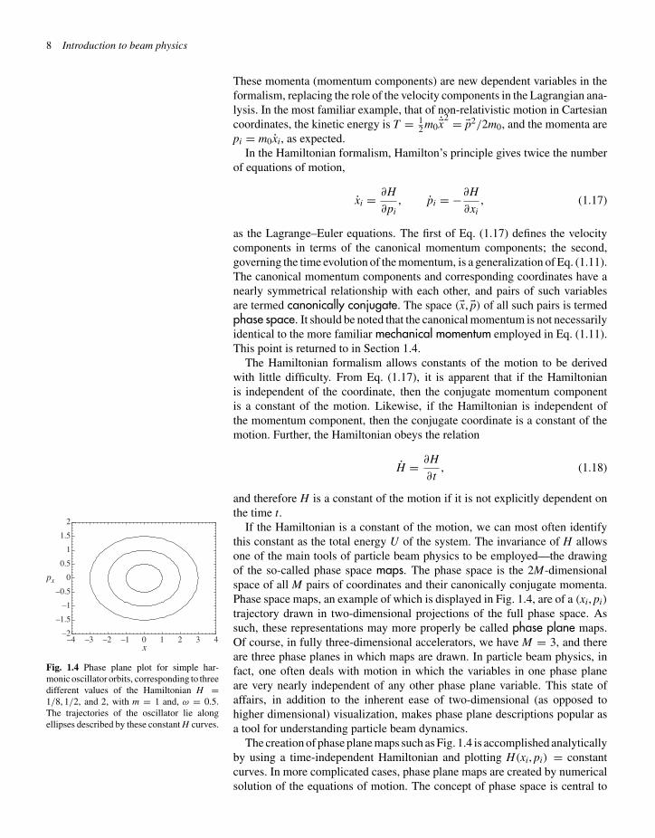
Fig. 1.4 Phase plane plot for simple har-monic oscillator orbits, corresponding to threedifferent values of the Hamiltonian H =1/8, 1/2, and 2, with m = 1 and, ω = 0.5.The trajectories of the oscillator lie alongellipses described by these constant H curves.

If the Hamiltonian is a constant of the motion, we can most often identifythis constant as the total energy U of the system. The invariance of H allowsone of the main tools of particle beam physics to be employed—the drawingof the so-called phase space maps. The phase space is the 2M-dimensionalspace of all M pairs of coordinates and their canonically conjugate momenta.Phase space maps, an example of which is displayed in Fig. 1.4, are of a (xi, pi)

trajectory drawn in two-dimensional projections of the full phase space. Assuch, these representations may more properly be called phase plane maps.Of course, in fully three-dimensional accelerators, we have M = 3, and thereare three phase planes in which maps are drawn. In particle beam physics, infact, one often deals with motion in which the variables in one phase planeare very nearly independent of any other phase plane variable. This state ofaffairs, in addition to the inherent ease of two-dimensional (as opposed tohigher dimensional) visualization, makes phase plane descriptions popular asa tool for understanding particle beam dynamics.

The creation of phase plane maps such as Fig. 1.4 is accomplished analyticallyby using a time-independent Hamiltonian and plotting H(xi, pi) = constantcurves. In more complicated cases, phase plane maps are created by numericalsolution of the equations of motion. The concept of phase space is central to

“chap01” — 2003/6/28 — page 9 — #9


the field of particle beam physics and certain results, such as the invariance ofphase space density (see discussion Section 1.4) can only be clearly discussedin the context of Hamiltonian formalism.

Perhaps the most familiar example of this mapping technique is the one-dimensional non-relativistic simple harmonic oscillator. In this case (forsimplicity indicating the coordinate x1 ⇒ x) the one-dimensional Hamiltonianis of the form

H = 1

2m[p2

x + m2ω2x2], (1.19)

where ω2 = K/m, and K is the oscillator strength or spatial gradient of therestoring force, K = −Fx/x. The phase plane maps associated with simpleharmonic motion are thus ellipses in the two-dimensional (x, px) phase plane,as shown by the examples in Fig. 1.4. Note that the Hamiltonian alone does notindicate the direction in which the system traces out the ellipse, but examinationof the force and velocity direction does—the direction of motion is clearlyclockwise in phase space for this system.

The area of the phase plane ellipse is proportional to the value of theHamiltonian associated with each trajectory, and is therefore also a constantof the motion. This area is given by∮

px dx =∮

pxx dt =∮(H + L) dt = Uτ . (1.20)

where τ is the period of the oscillation. We shall see in Chapter 5 that the areaassociated with a closed trajectory in phase space forms a central place in thetheory particle beam dynamics.

The phase plane map is of great use in visualizing the motion of chargedparticles beyond simple harmonic orbits (see Ex. 1.3) and is profitably employedeven in cases when the Hamiltonian is not a constant of the motion. In the caseof a time-varying Hamiltonian, one may not trivially generate plots like Fig. 1.4,but must often solve the equations of motion (Eq.(1.17)) first. Furthermore, ifone solves these equations in such a case, it may not be illuminating, but ratherconfusing (e.g. Fig. 3.6), to use continuous lines in phase space to illustratethe motion as it advances continuously in time. For systems typical of circularaccelerators, the Hamiltonian varies periodically in time t, however. A valuablestrategy for phase plane plotting in this case is taking periodic “snap-shots” andplotting the instantaneous position in the phase plane once per Hamiltonian (notoscillation) period. This type of map is termed a Poincare plot (e.g. Fig. 3.7)and is discussed further in Chapter 3.

There are also manipulations of the phase space or phase plane variables thatcan be undertaken to create a description where the Hamiltonian is a constantof the motion in the new variables, where it was not constant in the old vari-ables. To see the utility of this approach, consider an explicitly time-dependentHamiltonian, in which the potential arises from a traveling wave so that theHamiltonian can be written

H = 1

2m[p2

x + G(x − vϕ t)], (1.21)

where vϕ is the phase velocity of the wave in the x direction and G is anarbitrary function. The simplest way to make the Hamiltonian into a con-stant of the motion is to perform a mathematical transformation of the system

“chap01” — 2003/6/28 — page 10 — #10


description. Let us examine such a transformation of the coordinates, theGalilean transformation, where

x = x − vϕ t. (1.22)

Now we must transform the Hamiltonian so that the coordinate’s equation ofmotion remains correct. With the new canonical momentum set equal to theold, px = px,

˙x = − ∂H

∂ px= px

m− vϕ = v − vϕ , (1.23)

as expected for a Galilean transformation. To generate Eq. (1.23) as a correctcanonical equation of motion (i.e. one derivable from Eq. (1.17)), the newHamiltonian H must transform from the old Hamiltonian H as

H(x, px) = H(x, px)− vφ px = 1

2m[p2

x + G(x)] − vφ px. (1.24)

Now the new Hamiltonian H(x, px) is explicitly independent of t and is thusa constant of the motion. The trajectory of the charged particle in this wavepotential can, therefore, be visualized, as before, with a phase plane map createdby the simple algebraic relationship between x, px, and H. For example, wemay use Eq. (1.24) with a moving simple harmonic oscillator potential, G(x) =12 Kx2. This leads to

H(x, px) = 1

2m

[p2

x + m2ω2x2 − 2pϕ px

]

= 1

2m

[(px − pϕ)

2 + m2ω2x2]

− Tϕ , (1.25)

where we have defined pϕ and Tϕ as the (non-relativistic) momentum and kineticenergy associated with a particle of mass m traveling at the phase velocity vϕ .In this case, the constant H curves associated with the motion shift upward inpx by pϕ , when compared those shown in Fig. 1.4, to as shown in Fig. 1.5.

Note that the phase plane plots for the moving simple harmonic oscillatorpotential can be made to look identical to the stationary potential plot by use of

Fig. 1.5 Phase plane plot for moving simpleharmonic oscillator orbits corresponding tosame limits in x as those in x found in Fig. 1.4.Here pϕ = 2, with m = 1 and ω = 0.5. Thecurves corresponding to the moving potentialare represented by solid lines, and their coun-terparts from Fig. 1.4 are shown in dashedlines.

–2

–1

0

1

2

3

4

–4 –3 –2 –1 0 1 2 3 4x~

px~

“chap01” — 2003/6/28 — page 11 — #11


our Galilean transformation from x to x and, further, by plotting δp ≡ px − pϕ .Each of the curves in the x frame is associated with values (total energies) ofthe new Hamiltonian H = H − Tϕ . The constant −Tϕ contains no informationabout the system’s dynamics (cf. Eq. (1.17)), however, and may be ignored. Atthis point, we need to clarify that the transformation given by Eqs (1.22)–(1.24)is a purely mathematical change of variables, not a change of physical frame.We will make use of this type of mathematical transformation while discuss-ing acceleration in traveling electromagnetic waves (Chapter 4). The physicalchange of frame is described, of course, not by a Galilean transformation butby a Lorentz transformation, as discussed in Section 1.4.

The type of variable transformation illustrated by Eqs (1.22)–(1.24) is termeda canonical transformation because it preserves the canonically conjugate rela-tionship between the coordinate and the momentum. In general, one does not usesuch an ad hoc way of deriving the transformation but a more rigorous methodbased on generating functions, which are discussed in advanced mechanicstextbooks. These functions come in a variety of types, depending on the vari-ables to be transformed. The generating function always is dependent on a pairof variables per phase plane, some combination of the old and new canonicallyconjugate variables.

As an example, consider use of a generating function to transform theone-dimensional simple harmonic oscillator Hamiltonian, Eq. (1.19) to a par-ticularly interesting new form. The well-known solutions for the motion in sucha system are given by

x(t) = xm cos(ωt + θ0), and px(t) = mωxm sin(ωt + θ0). (1.26)

We would like to transform the Hamiltonian to one that reflects the constantrate of advance in argument of the cosine function in Eq. (1.26), so we proposethat the new coordinate be chosen as θ = ωt + θ0. In this case, we can usea generating function of the form F(x, θ) to transform the simple harmonicoscillator problem into a more useful form. According to Hamilton’s principle,Eq. (1.27) must yield the following formal properties:

px = ∂

∂xF(x, θ), J = ∂

∂θF(x, θ), H ′ = H + ∂

∂tF(x, θ), (1.27)

where J is the new momentum and H ′ is the new Hamiltonian. We candeduce from Eq. (1.27) that a proper generating function is given by F(x, θ) =12 mωx2 cot(θ). Using F(x, θ) to obtain the new momentum and Hamiltonian,we have

H ′ = Jω, (1.28)

which is a constant of the motion. Since ω is a constant, the momentum J ,known as the action, is also a constant. The new canonically conjugate pair aretermed action-angle variables. The action-angle description is important foranalyzing perturbations to simple harmonic systems, a commonly encounteredproblem in particle beam physics. The action is, comparing Eqs (1.18) and(1.25), simply related to the area enclosed by the phase space trajectory,

J = 1

2π

∮px dx. (1.29)

The action is also generally known to be an adiabatic invariant, in that whenthe parameters of an oscillatory system are changed slowly, the action remains a

“chap01” — 2003/6/28 — page 12 — #12


constant. This can be illustrated by writing the differential equation for a slowlyvarying oscillator (with the mass factor set to m = 1) as

x + K(t)x = 0, (1.30)

and substituting an assumed form of the solution

x(t) = C√

a(t) cos(ψ(t)). (1.31)

After some manipulations, we obtain the relations

ψ = 1

aand a − a2 + 4

2a+ 2Ka = 0. (1.32)

The substitution given in Eq. (1.31) is commonly found in the theory of time-dependent oscillators, which is quite important in particle beam physics—it isexplicitly used in an analysis in Chapter 5. The solution of the first equation in(1.32) is formally

ψ =∫

dt

a(t), (1.33)

while the second of these equations’ solution can be examined approximately.Assuming the first and second time derivatives of a are small (a/a � K and(a/a)2 � K)4, one has simply4These conditions give a quantitave definition

of the term “adiabatic”.

a(t) ∼= (K(t))−1/2 or x(t) = C(K(t))−1/4 cos(ψ(t)). (1.34)

The momentum corresponding to this approximate solution is

px(t) = x ∼= C(K(t))1/4 sin(ψ(t)). (1.35)

The area of the phase space ellipse, whose semimajor and semiminor axes arethe maximum excursion in x and px, respectively, is again the value of the actionat that time,

J = 12 px,maxxmax = 1

2 C2. (1.36)

The action is independent of time and dependent only on the initial conditions(taken at t = 0) through the constant C

2. Thus, we have shown the adiabatic

invariance of the action J for oscillators whose strength is slowly varying, aresult pertinent to discussions in future chapters.

We emphasize at this juncture the primary role of the momenta in Hamilto-nian methods, as opposed to the velocity components found in the Lagrangianformalism. This is inherent in both the structure of Hamiltonian and relativisticanalyses, as is reviewed in Section 1.4.

1.4 Dynamics with special relativity andelectromagnetism�

The Hamiltonian formulation of dynamics is naturally suited to analyzingrelativistic systems. We shall see that this is because in the canonical approachto dynamics the roles of the coordinates, momenta, time, and energy havea rigorously defined relationship with each other. The relationships between

“chap01” — 2003/6/28 — page 13 — #13

1.4 Dynamics with special relativity and electromagnetism� 13

these dynamical variables actually become clearer after one studies relativ-istic dynamics, where the ways in which all such variables transform from oneinertial frame to another are emphasized.

The point of departure for the present discussion is precisely this trans-formation, which should be familiar to any reader of this text, the Lorentztransformation. This relation, which governs the transformation of coordinatesand time from one inertial reference frame to another moving at constant speedvf = βf c with respect to the first frame (along what we choose to be the z-axis),is written as

x′ = x, y′ = y, z′ = γf(z − βf ct), ct′ = γf(ct − βf z), (1.37)

where the Lorentz factor γf = (1 − β2f )

−1/2. This Lorentz transformation actsupon the space-time four-vector �X ≡ (x, y, z, ct), and preserves the length, ornorm, of the four-vector. This norm, termed a Lorentz invariant because it isframe independent, is specified by the quantity

| �X|2 = x2 + y2 + z2 − (ct)2. (1.38)

The invariance of the norm of the space-time four-vector is often the startingpoint of the derivation of the Lorentz transformation, as it indicates that thephase velocity c of spherical light waves in vacuum is independent of inertialreference frame.

The invariance property of the norm of �X is therefore entirely equivalent tothe property that the four-vector transforms between frames under the rules of aLorentz transformation. Thus, a four-vector can be defined equivalently eitheras an object that obeys Lorentz transformations or one in which its norm, asdefined by Eq. (1.38), is conserved during such a transformation. The invarianceof four-vector norm is a key tool in performing analyses of relativistic dynamics.

The absolute value of | �X|2, which refers to the “distance” in space-timebetween two events (or implicitly, one event and the origin), can be positive,negative, or zero. If it is positive, it is termed “space-like”, as one may alwaystransform to a frame where the events occur at the same time, but at a separateddistance. If it is negative, it is termed “time-like”, as one may always transformto a frame in which the events occur at the same point in space, but at separatetimes. Space-like pairs of events cannot be causally connected, because they aretoo far separated in space-time for light to propagate between them. If the normof �X is zero, the two events are exactly connected by a signal traveling at thespeed of light. In this case, the events are said to be on each other’s light cone.

Using Lorentz transformations of space and time, it can be trivially shown thatproperties of waves—the wave numbers (spatial frequencies) ki and (temporal)frequency ω—form a four-vector. This is intuitively so, since the wave numbersimply measures spatial intervals while the frequency measures intervals intime. As an illustration of this derivation, consider a plane electromagneticwave moving in the positive z-direction, with functional form cos[kzz −ωt]. Ifone begins in a frame moving with velocity βf c in the z-direction, the inversetransformation

cos

[kzγf(z

′ + βf ct′)− ωγf

(t′ + βf

z′

c

)]

= cos

[γf

(kz − βf

ω

c

)z′ − γf(ω − βf kzc)t

′]

“chap01” — 2003/7/2 — page 14 — #14


can be deduced from Eq. (1.37). We can thus see that kz and ω (Lorentz)transform as z and t, respectively. Further, we know, therefore, that the normof the four-vector (�kc, ω) = (kxc, kxc, kxc, ω) is

∑

i

k2i c2 − ω2 = const. (1.39)

In the case where the constant on the right-hand side of Eq. (1.39) is zero, thiscan be recognized as the dispersion relation for vacuum electromagnetic waves.From a quantum-mechanical viewpoint, such waves correspond to masslessphotons (cf. Section 7.1). When the constant in Eq. (1.39) is not zero, a quantum-mechanical interpretation indicates that we are examining an object of non-vanishing rest mass, or rest energy.

The quantum mechanical indentifications of free particle momenta andenergy in terms of wave properties, pi = hki and U = hω, lead us to the conclu-sion that momentum and energy must also form a four-vector, �P ≡ (�pc, U) =h(�kc, ω), with the invariant

�P2 ≡ �p2c2 − U2 =∑

i

p2i c2 − U2 = const. (1.40)

We must allow for the possibility of Lorentz transformation into the rest frameof the particle, in which case �p = 0 and the invariant can be identified as therest energy of the particle. Thus,

�p2c2 − U2 = −(m0c2)2, (1.41)

where m0 is the rest mass of the particle. Note the norm of the momentum–energy four-vector is always negative (or “energy-like”), because the square ofthe rest energy is positive definite.

As an example of the utility of Lorentz transformations of the (�kc, ω) four-vector, we consider the process known as relativistic Thomson backscatteringwhere a relativistic electron collides head-on with a photon (quantum of light,see Section 8.1), yielding a reversal of photon direction and an increase in thephoton energy and momentum. This process is illustrated in Fig. 1.6, through adiagram of the initial and final momentum vectors of the electron and photon.The term Thomson is somewhat imprecisely5 applied to this scattering process5It is more precise to term this process

“inverse Compton scattering”, as in the endwe see that the photon energy, as observedin the laboratory frame, increases. This is theopposite of what happens in Compton scatter-ing of photons off of electrons that are initiallyat rest. See Exercise 1.6 for further discussionof this point.

whenever the change in the electron momentum during collision is negligible. Inthe frame traveling with the electron, βf = v/c (v is the velocity of the electron),an oncoming photon of laboratory frequency ω has an observed frequency givenby Lorentz transformation, ω′ = ωγf(1 + βf). If we assume that this photonsuffers a reversal of its momentum vector direction but no change in amplitudeduring collision, a second Lorentz transformation of the (�kc, ω) four-vectoryields ωs = ω′γf(1 + βf) = ωγ 2

f (1 + βf)2. Thus, for a highly relativistic

(βf ≈ 1) electron, the frequency (energy) of backscattered light is increased,ωs ∼= 4γ 2

f ω. This scattering process is explored further in Exercise 1.6.

Fig. 1.6 Diagram of electron and photonmomenta in initial and final states of theThomson backscattering process. The viola-tion of momentum conservation is exagger-ated in this picture.

Initial electron state Initial photon state

Final electron state Final photon state

“chap01” — 2003/6/28 — page 15 — #15


While we have now established the four-vector relationship between theenergy and momentum of a physical system, we have not described whatthese quantities are in the familiar terms of mass and velocity. In doing so,we must obtain the well-known expressions of the non-relativistic limit, wherethe momentum �p = m�v and energy U = �p2/2m + const. We must also preservethe most general relationship between the momentum and energy,

dU = �v · d�p, or less specifically,dU

dp= v, (1.42)

where p = |�p| and v = |�v|. This result is derived by noting that the energychange on a particle is equal to the work performed on it, dU = �F · d�l, wherethe force is assumed to still obey Newton’s third law, �F = d�p/dt, and thedifferential length is d�l = �v · dt. Differentiating Eq. (1.40) and combining withEq. (1.42), we also obtain

�v = �pc2

U. (1.43)

Then, solving for the energy as a function of the velocity, we may write((v

c

)2 − 1

)U2 = −(m0c2)4 or U = γm0c2, (1.44)

where we have now defined the Lorentz factor associated with the particlemotion as γ ≡ (1 − (�v2/c2))−1/2. The Lorentz factor of a particle is, therefore,its total (mechanical) energy normalized to its rest energy, and the conditionγ � 1 implies a particle that travels at nearly the speed of light. For electrons,having rest energy mec2 = 0.511 MeV, it is very easy to obtain a particle thattravels nearly at the speed of light—megavolt-class electrostatic acceleratorscan accomplish this feat. However, for the other most commonly acceleratedparticle, the proton (with rest energy mpc2 = 938 MeV), it is relatively difficultto impart enough energy (several GeV) to make the particle relativistic.

Using Eqs (1.43) and (1.44), we also now have an expression for themomentum vector,

�p = γm0�v ≡ �βγm0c, (1.45)

which allows Eq. (1.40) to be written, after removing the common factor ofm0c2 in all quantities, as

γ 2 = �β2γ 2 + 1. (1.46)

Equation (1.40) is valid not only for single particle systems, but also for generalsystems of many (j = 1, . . . , N) objects, in which case we have

∑

j

�pj

2

c2 −∑

j

Uj

2

= constant. (1.47)

For such systems it is still true that, if any of the objects have non-zero restmass, one may transform to a coordinate system in which the total momentumof the system vanishes,

∑j pj = 0.

In this frame, the total energy of the system is obviously minimized. This factallows straightforward calculation of the available energy for particle creation

“chap01” — 2003/6/28 — page 16 — #16


in high-energy physics experiments. Such a calculation serves as an illustrativeexample of the use of a Lorentz invariant norm.

In colliders, where charged particles and their antiparticles counter-circulatein rings (or collide after accelerating in opposing linacs), the colliding species,in general, have equal and opposite momentum. Therefore, the first term inEq. (1.47) vanishes and all of the particle energy (2U) is available for creationof new particles. Thus, the Z0 particle (with a rest energy of 91.8 GeV, 1 GeV =109 eV) has been studied in detail using the LEP collider at CERN, by usingelectron and positron beams accelerated to 45.9 GeV and then collided. Beforethe era of the colliding beam machines, however, the frontier energies forexploring creation of new particles took place in fixed-target experiments wherethe beam particles struck stationary target particles. In the fixed target collision,one may calculate the Lorentz invariant on the right-hand side of Eq. (1.47) byevaluating the left-hand side in the lab frame,

p2bc2 − (Ub + mtc

2)2 = −m2t c4 − m2

t c4 − 2γbmbmtc4 = constant, (1.48)

where the subscripts b and t indicate beam and target particles, respectively.In the center of momentum frame, however, the total momentum vanishes andthe constant in Eq. (1.48) is seen to set a maximum on the total rest energy ofparticles created in the collision,

∑i

mp,ic2 ≤

√2γbmbmtc2. (1.49)

The maximum energy for particle creation in Eq. (1.49) occurs when the beamand target particles annihilate and the newly created particles are at rest in thecenter of momentum frame. Equation (1.49) clearly indicates why collidingbeam machines are so important in exploring the energy frontier. At Ferm-ilab, proton–antiproton collisions occur between counter-propagating beamsof 900 GeV with up to 1.8 TeV available for creation of new particles.6 If one,6Because protons and antiprotons are had-

rons, composed of substituent particles(quarks and gluons), the effective (likely toobserve) energy available for particle creationis considerably smaller than the full beamparticle energy, and the “physics reach” of a1.8-TeV hadron collider may be only in theseveral hundreds of GeV.

instead, substitutes a stationary proton as the target particle with a 900 GeVincident particle, the available energy for particle creation is only 41 GeV!

Equations (1.44) and (1.45) have introduced the relativistically correctmomentum and energy. If one substitutes the relativistically correct form ofthe momenta into Eq. (1.9), it should be emphasized that this Lorentz forcerelation remains valid by construction. It is of interest to examine this vec-tor equation of motion for the momentum in the case (discussed in detail inSection 2.1) where only a magnetic field is present. In such a scenario theenergy of the particle is constant, and we may write

γm0d�vdt

= q(�v × �B). (1.50)

Equation (1.45) displays, upon comparison with the non-relativistic version ofEq. (1.9), an effect known as the transverse relativistic mass increase, wherethe inertial mass under transverse (normal to the velocity) acceleration effect-ively behaves as though m0 → γm0 . Note that this is also true for electric forcesthat are instantaneously transverse. For cases involving energy-changing accel-eration (in which the acceleration is parallel to the velocity vector), the situationis different, as illustrated in Section 2.4.

“chap01” — 2003/6/28 — page 17 — #17


With the results in this section thus far, obtained by emphasizing the invari-ance of the norms of a variety of four-vectors under Lorentz transformation, it isstraightforward to find other relations more typically derived directly by use ofLorentz transformations. For example, let us examine the addition of velocities.Using the notation vf = βf c to designate the relative velocity of a new frame,the velocity in the new frame of a particle whose velocity is v (parallel to vf ) inthe original frame is

v′ = p′c2

U ′ = γf c(pc − βf U)

γf(U − βf pc)= γfγm0c3(β − βf)

γfγm0c2(1 − βfβ)= β − βf

1 − βfβc. (1.51)

This derivation is, perhaps, more transparent than the more standard versionbased on Lorentz transformation of the components of �X, because it beginswith more powerful concepts. It also points to an important facet of the theoryof special relativity—velocities do not play a central role as useful descriptionsof the motion since they do not form a part of a four-vector.

The momenta and energy, on the other hand, do form a four-vector. This isan interesting state of affairs within the context of particle dynamics, becausethese same quantities play a primary role in the Hamiltonian formulation ofmechanics. We now discuss how the two concepts, Hamiltonian and four-vectordynamics, relate to each other in the context of charged particle dynamics inelectromagnetic fields.

We begin by noting that the Lorentz force (Eq. (1.9)) acting on a chargedparticle is written, in terms of potentials, as

�FL = d�pdt

= q(�E + �v × �B)

= q

[−�∇φe − ∂ �A

∂t+ �v × ( �∇ × �A)

]

= q

[−�∇φe − ∂ �A

∂t− (�v · �∇)�A

]= q

[−�∇φe − d�A

dt

]. (1.52)

In the last line of this expression, we have used the definition of the total (partialplus convective) time derivative.

The forces in electromagnetic fields are most generally derived not only froma scalar (electrostatic) potential φ, but from an electromagnetic vector potential�A as well; thus, we must generalize our approach to Hamiltonian analysis. Inparticular, we note that Eq. (1.52) indicates that the equations of motion forthe momenta are not simply derivable from a conservative potential energyfunction. If we define the canonical momenta to be pc,i = pi + qAi, however,the Hamilton equation of motion for this canonical momentum is correctlyobtained by the prescription

dpc,i

dt= −∂H

∂xi= −q

∂φe

∂xi, (1.53)

where the Hamiltonian contains only a conservative (electrostatic) potentialenergy. At this point, what we have considered (á la Newton) to be themomentum in the problem can now be seen to be a mechanical as opposed

“chap01” — 2003/6/28 — page 18 — #18


to canonical momentum. The symmetry between the total “canonical” energy(value of the Hamiltonian) and the canonical momentum is clear—the totalenergy H = U + V = U + qφe (the numerical value of the Hamiltonian func-tion) also has a portion arising from a potential (in this case, qφe). Note thatthe remainder of the total energy (the “mechanical” component) also includesa rest energy component, U = γm0c2 = T + m0c2, that is, the sum of rest andkinetic energies.

From this discussion, it should also be clear that the scalar and vector poten-tials, since they comprise components of the momentum–energy four-vector,also form a four-vector, (�Ac,φ). Further, they are paired with the mechanicalmomenta and energy through the definitions of canonical momenta and energy,pc,i = pi + qAi and H = U + qφ. To complete our survey of electrodynamicfour-vector quantities, we note that the equations governing the potentials canbe written as [

�∇2 − 1

c2

∂2

∂t2

] { �Aφe

}= −

{µ0�Jeρe

ε0

}. (1.54)

Since the potentials form a four-vector, the sources (�Je, ρec) form one as well.This result could also have been alternatively derived directly from chargeconservation, and Lorentz transformation of lengths (and thus charge density)and velocities.

As we have just discussed sources and potentials associated with electro-magnetic fields, it is appropriate at this point to examine the transformationbetween inertial frames of these fields. Since the potentials form a four-vector(�Ac,φe), an obvious starting point of the discussion is to discuss the Lorentztransformation of this four-vector. This relation, governing the transformationof potentials from one frame to another that moves at speed βf c along what weagain choose to be the z-axis is written as

cA′x = cAx, cA′

y = cAy, cA′z = γf(cAz − βfφe), φ′

e = γf(φe − βf cAz).(1.55)

The quantities Ax, Ay, Az, and φ are all, in principle, functions of x, y, z, and t.In the new (primed) frame, the spatio-temporal dependence of these quantitiesmust be expressed in terms of the primed variables, found by substitutionsobtained from the inverse Lorentz transformation

x = x′, y = y′, z = γf(z′ + βf ct′), t = γf(ct′ + βf z′). (1.56)

The fields are obtained from this expression using the following relations:

�E′ = −�∇′φ′e − ∂ �A′

∂t′, �B′ = �∇′ × �A′. (1.57)

The transformation of the electromagnetic fields described by Eqs(1.55)–(1.57)are often written as

�E′⊥ = γf(�E⊥ + �vf × �B⊥), �E′|| = �E||,

�B′⊥ = γf

(�B⊥ − 1

c2�vf × �E⊥

), �B′|| = �B||,

(1.58)

“chap01” — 2003/6/28 — page 19 — #19

1.5 Hierarchy of beam descriptions 19

where the symbols || and ⊥ indicate the components of the field parallel toand perpendicular to the direction of Lorentz transformation of the frame �vf ,respectively.

Now we can return to the derivation of relativistic Lagrangian andHamiltonian mechanics with electromagnetic fields. With our definition ofcanonical momenta, we can proceed to construct the Lagrangian by integratingthe expression that defines these momenta,

pc,i = ∂L

∂ xi= γm0xi + eAi, (1.59)

with respect to the spatial coordinates. We thus obtain

L(�x, �x) = −m0c2

γ+ q�A · �v − qφe(�x), (1.60)

where we have allowed the presence in the Lagrangian of a conservative poten-tial dependent only on �x, and identified it as the negative of the electrostaticpotential energy −qφe(�x).

The relativistically correct Hamiltonian is obtained from Eq. (1.60) by useof the definition

H = �pc · �x − L = �pc · (�pc − q�A)γm0

− L

= (�pc − q�A)2γm0

+ m0c2

γ+ qφe(�x). (1.61)

By multiplying this expression by γm0c2 and using H − qφ = γm0c2, wearrive at

(H − qφe)2 = (�pc − q�A)2c2 + (m0c2)2, (1.62)

or

H =√(�pc − q�A)2c2 + (m0c2)2 + qφe. (1.63)

We note that Eq. (1.62) could have been obtained by direct substitution ofcanonical definitions into Eq. (1.41) governing the norm of the mechanicalmomentum–energy four-vector, that is,

(�pc − q�A)2c2 − (H − qφe)2 = −(m0c2)2. (1.64)

1.5 Hierarchy of beam descriptions

The methods for analyzing single particle dynamics given in Section 1.4 repres-ent the first step in understanding the physics of charged particle beams. A realbeam is made up not of a single particle, however, but a collection of many (N)particles. The second step towards describing the dynamics of an actual beam,therefore, is to consider a collection of N points in phase space, as illustratedin the phase plane plot shown in Fig. 1.7. It is not obvious how to proceed withthe description of such a system, where the phase space has 2NM variables.It is therefore now necessary to discuss a hierarchy of descriptions that beginwith single particle dynamics.

“chap01” — 2003/6/28 — page 20 — #20


Fig. 1.7 Distribution of particles in (x, px)

phase plane.

–3

–2

–1

0

1

2

3

–3 –2 –1 0 1 2 3

p x

x

For many particle beams, the density of particles in phase space is smallenough that the particles are essentially a non-interacting ensemble, with bothmacroscopic and microscopic electromagnetic fields created by the particlesthemselves contributing insignificantly to the motion. In this case, one onlyneeds to solve the single particle equations of motion in the presence ofapplied forces, and then proceed to produce a collective description of thebeam ensembles’ evolution based on the known single-particle orbits. Thisbook assumes the validity of this type of description, which straightfor-wardly leads to analyses based the beam’s distribution. In real charged particlebeams, as well as in the modeling of such beams in multi-particle compu-tations, this distribution is discrete, as illustrated in Fig. 1.7. On the otherhand, for analytical approaches, the distribution is viewed as a smooth prob-ability function7 in a 2M-dimensional phase space f (�x, �p, t), that is, the7With a smooth phase space distribution,

the charge and current distributions asso-ciated with such a distribution are alsocontinuous and smooth. The fields derivedfrom the smooth charge/current densities maybe termed macroscopic. Deviations fromthese approximate fields (near an individualparticle) may be termed microscopic.

number of particles found in a differential phase space volume dV = d3�x d3�pin the neighborhood of a phase space location �x, �p at a time t is simplygiven by f (�x, �p, t) dV . While the computational approach to multi-particledynamics is beyond the scope of this book, analytical approaches basedon the distribution function f (�x, �p, t) will be introduced in Chapter 5. Oneresult concerning phase space distributions deserves prominent discussion atthis point, however, the conservation of phase space density, or Liouville’stheorem.

To begin, we write the total time derivative of the phase space distributionfunction,

df

dt= ∂f

∂t+ �x · �∇�xf + �p · �∇�pf , (1.65)

where the second and third terms on the right-hand side of Eq. (1.62) are theconvective derivatives in phase space, derived simply by the chain rule. (Note:the subscript on the gradient operators indicates differentiation with respect toeither coordinate or momentum components.) If the forces are derivable from

“chap01” — 2003/6/28 — page 21 — #21

1.5 Hierarchy of beam descriptions 21

a Hamiltonian, then

df

dt= ∂f

∂t+

∑i

(dxi

dt

∂f

∂xi+ dpi

dt

∂f

∂pi

)

= ∂f

∂t+

∑i

(∂H

∂pi

∂f

∂xi− ∂H

∂xi

∂f

∂pi

)

= ∂f

∂t+

∑i

(∂H

∂pi

∂H

∂xi

df

dH− ∂H

∂xi

∂H

∂pi

df

dH

)= ∂f

∂t. (1.66)

Because we have assumed that the forces are derived from a Hamiltonian, itcan be seen that the summation in Eq. (1.66) vanishes, and df /dt = ∂f /∂t. InEq. (1.65), it should be understood that the total derivative is taken by movingabout phase space according to the particle’s equations of motion at a givenphase space point (�x, �p). If neither creation nor destruction of the particles areallowed, we also have, by drawing a small constant differential volume dVaround a given particle, f (�x, �p, t) = dV−1 in the neighborhood of this point.Then we have the result that ∂f /∂t = 0 and

df

dt= 0. (1.67)

This result is termed Liouville’s theorem, and it states that the phase spacedensity encountered as one travels with a particle in a Hamiltonian system isconserved. The derivation of Eq. (1.67) may seem to be tautological, sincewe stated that ∂f /∂t = 0 without referring to any property of Hamiltonian.Equation (1.67) is more illustrative than it seems, however, because the proper-ties of the Hamilton equations guarantee that the density of any volume of phasespace whose boundary follows these equations is constant. An alternative pointof view, suggested by Eq. (1.65), is that phase space itself is incompressible.Perhaps the most common statement derived from interpretation of Eq. (1.67)is that the volume occupied by particles in phase space is conserved. For sys-tems in which the motion of all phase planes is uncorrelated, the motion in theseparate phase planes is independent. Then one can state that the emittance orarea occupied by particles in a phase plane is conserved. The conservation ofemittance, which is discussed further in Chapter 5, plays a very important rolein the theory and design of particle accelerators.

Here, we concentrate on cases where Liouville’s theorem holds, since we willalmost exclusively consider motion due to applied forces that are derivable froma Hamiltonian. Deviations from this physical scenario form much of the follow-ing volume on advanced subjects in beam physics so we restrict comment onsuch topics to a few general statements. When multi-particle interaction effectsbecome important, there are two distinct regimes to consider. The first can bedescribed as one in which the collective macroscopic fields arising from thebulk beam charge and current density is the dominant self-interaction mechan-ism of the beam. These self-fields are most often termed space-charge whenthey arise from the near-field of the beam’s charge distribution and wake-fieldswhen they arise from the beam’s collectively radiated fields. The evolution ofthe beam distribution can be dominated by space-charge fields, in which caseone can use a description that is based on the notions of cold fluid motion

“chap01” — 2003/6/28 — page 22 — #22


developed in the field of plasma physics. In this scenario, simple collective(plasma) oscillations are encountered. When only macroscopic beam fields areimportant, these fields may, in principle, be included into the Hamiltonian,Eq. (1.67) is unchanged, and the implications of Liouville’s theorem still hold.

On the other hand, microscopic binary collisions may strongly affect thebeam distribution evolution, and diffusion (heating) may occur in phase space.There are a number of methods for dealing with this complication, but most arebeyond the scope of the present discussion. However, one method is relativelyeasy to appreciate in the context of this section. An explicit non-Hamiltonianterm may be introduced on the right-hand side of Eq. (1.67), which accountsfor the time derivative of the distribution due to collisions (the effects of micro-scopic fields), so that df /dt = ∂f /∂t|coll. In this generalized form, the revisedversion of Eq. (1.67) is termed theBoltzmann equation. Thus, Eq. (1.67), whichis commonly known (when the full derivative is written as in Eq. (1.65)) as theVlasov equation, is also referred to as the collisionless Boltzmann equation.The non-macroscopic-Hamiltonian physics arising from emission of radiationby particle beams gives rise to dissipation and damping of phase space tra-jectories. The description of the effect of such phenomena on the distributionfunction may be treated with a full Boltzmann equation approach, or though ananalysis based on the Fokker–Planck equation.

1.6 The design trajectory, paraxial rays, andchange of independent variable

While a rigorous analysis of classical motion can be performed, as discussedabove, using canonical momenta and coordinates within the confines of theHamiltonian formalism, one often finds it useful in practice to use a morephysically transparent description. This is obtained by use of paraxial rays,vector representations of the local trajectory which, by definition, have an anglewith respect to a design trajectory that is much smaller than unity. Trajectoriesof interest in beam physics are always paraxial—one must confine the beaminside of small, near-axis regions, such as the drift tubes shown in Fig. 1.1.

Both the paraxial ray and the design trajectory are illustrated in Fig. 1.8. Inthis figure, an example of a design trajectory, defined as the ideally preferredtrajectory—a locally straight or curved line— through the system, is displayed.As we shall see, one defines the coordinate system for analyzing beam physicsproblems locally by use of the design trajectory. As a result, the coordinatesystems we encounter in this text may naturally be locally Cartesian, or locallycurvilinear (i.e. inside of bend magnets). Curvilinear coordinate systems areobviously found in circular accelerators where the design trajectory is closedupon itself and is often referred to as the design orbit.

Fig. 1.8 Design trajectory and examples ofsmall angle paraxial rays.

�

Design trajectory

Paraxial rays

“chap01” — 2003/6/28 — page 23 — #23

1.6 The design trajectory, paraxial rays, and change of independent variable 23

Figure 1.8 also displays examples of paraxial rays. The ray is a useful visual-ization tool and can be described mathematically by a coordinate offset, and anangle θ . In a locally Cartesian coordinate system,8 we take the distance along 8When the design orbit is derived from recti-

linear motion, we will choose z as the distancealong the design orbit, in part to easily con-nect to field descriptions written in cylindricalcoordinates. When the design orbit is bent, wewill emphasize the curvilinear nature of thecoordinate system by using the variable s asthe distance along the design orbit.

the design trajectory to be z. In this system, a horizontal offset is designated byx and the horizontal projection of the angle is θx. This angle is given in termsof the momenta as

tan θx = px

pz= vx

vz. (1.68)

Analogous definitions hold for the other transverse offset and angle, whichwe term vertical and indicated by the variable y. We are ultimately interestedin a description of particle dynamics that uses the distance along the designtrajectory as the independent variable. The reason for this is straightforward; inan optics system (for charged particles or photons) the forces encountered arealways specified in space and not in time. Thus, a spatial description is moreefficient and natural.

In order to use z as the independent variable, we must be able to writeequations of motion in terms of z. This is accomplished by writing total timederivatives (written in compact notation as (.) ≡ d/dt) in terms of total spatialderivative in z,

( )′ ≡ d

dz= 1

vz

d

dt. (1.69)

The derivative of a horizontal offset with respect to z is given by

x′ = dx

dz= tan(θx). (1.70)

When analyzing beams, which are by definition are collections of rays localizedin offset and angle near the design orbit, it can be seen from Eq. (1.70) thatthe transverse momentum (normal to the design orbit) is much smaller than thelongitudinal momentum, px,y � pz ∼= |�p|. As a consequence, we may in mostcases use the small angle, or paraxial, approximation, which allows us towrite a series of useful approximate expressions,

x′ = tan(θx) ∼= θx ∼= sin(θx) � 1. (1.71)

It is not immediately apparent how this assumption restricts the offset from thedesign orbit. As we shall see, all particle beam optics systems that focus andcontrol the rays fundamentally resemble simple harmonic oscillators, wherethe transverse force is linear in offset, Fx = −Kx. Using this analogy, we canwrite a model equation for the transverse offset

x + ω2x = 0, (1.72)

whereω2 = K/γm0. Further, Eq. (1.72) can be cast in terms of a ray description,using Eq. (1.70), to obtain

x′′ + k2x = 0. (1.73)

Here, k ≡ ω/vz is the characteristic oscillation wavenumber of the opticssystem. The solutions of Eq. (1.73) are of the form x = xm cos(kz+φ), yieldingan approximate angle of kxm sin(kz + φ), and so the paraxial approximation isobeyed for offsets xm � k−1. Another restriction on the validity of a paraxialdescription is relevant in the case of a curvilinear design orbit. In this case, we

“chap01” — 2003/6/28 — page 24 — #24


must require that xm � R (where R is the local radius of curvature of the designtrajectory) for the paraxial approximation to hold.

When one uses paraxial equations of the physically transparent form shownin Eqs (1.72) and (1.73), the analysis strays somewhat from a rigorous phasespace description. In fact, one often uses this paraxial formalism instead of acanonically correct approach, even to the point of replacing a momentum (e.g.px) with the angle (x′) in phase plane plots. In this case, when we make a plot ofthe trajectory in, for example, the (x, x′) plane, which is an example of a tracespace, we construct what is termed a trace space plot. This does not introducecomplications in understanding the motion at constant values of pz, because wecan always recover the transverse momentum by using px = pzx′ ∼= βγm0cx′.If longitudinal acceleration occurs, however, the angle is diminished and anapparent damping (so-called adiabatic damping, see Section 2.6) of the motionis observed.

With a change of independent variable evidently of high interest to particlebeam physics, we must revisit the question of Hamiltonian analysis in thiscontext. In order to proceed with transformation of the Hamiltonian into onewith a new independent variable, we first note that the symmetry of Eqs (1.62)and (1.64) (in which the energy and momenta are on equal footing) is suggestiveof a notion—the choice of the energy function as the Hamiltonian is a bitarbitrary as well. We could just as naturally have chosen one of the momentaas the Hamiltonian from which we derive equations of motion, and the formof Eq. (1.62) would remain the same, except for a minus sign. The processof changing the Hamiltonian from an energy-based function to a momentum-based function also requires that the independent variable be changed from tto the coordinate canonical to the new Hamiltonian. This can be illustrated byreferring to the stationary property of the action integral (Eq. (1.11)) whichgives rise to the equations of motion,

δ

∫ t2

t1

L dt = δ

∫ t2

t1

(�pc · �x − H) dt = 0. (1.74)

We can accomplish the change of independent variable, from t to z, by rewritingEq. (1.74) as follows:

δ

∫ z(t2)

z(t1)

(pc,xx′ + pc,yy′ − Ht′ + pc,z) dz = 0, (1.75)

where again the prime indicates differentiation with respect to the new inde-pendent variable, ( )′ ≡ d/dz. In Eq. (1.64), the role of the new Hamiltonian isobviously played by −pc,z ≡ G,

G = −pc,z =√(H − qφe)2 − (pc,y − qAy)2c2 − (pc,x − qAx)2c2 − (m0c2)2,

(1.76)the role of the third coordinate is taken by−t, and the role of the third momentumby H. Note that this statement implies that H and −t are canonically conjugate.

This type of independent variable transformation is a canonical transforma-tion by design, and is used in applications, such as particle beam dynamics,where the applied forces are described more naturally by functions of a spatialcoordinate than by functions of time. Because the transformation is canonical,

“chap01” — 2003/6/28 — page 25 — #25

1.7 Summary and suggested reading 25

the Hamilton’s equations of motion are obtained in the usual fashion,

p′c,x = −∂G

∂x= ∂pc,z

∂x, p′

c,y = −∂G

∂y= ∂pc,z

∂y, H ′ = ∂G

∂t= −∂pc,z

∂t,

x′ = ∂G

∂pc,x= − ∂pc,z

∂pc,x, y′ = ∂G

∂pc,y= −∂pc,z

∂pc,y, t′ = − ∂G

∂H= ∂pc,z

∂H.

(1.77)

For problems in which one of the spatial coordinates (z in particle beam physics)is taken to be the independent variable, it is assumed that the motion can befollowed monotonically in this coordinate. Note that this is always the case fortime as an independent variable (as far as we know!). If the trajectory describingthe motion is not a monotonic function of the independent variable, then it isnot uniquely described by this variable. Fortunately, in particle beams thisassumption is also always correct.

1.7 Summary and suggested reading

In this chapter, we have motivated much of the contents of this book by intro-ducing particle accelerators in their scientific and historical context. In order tobuild up the tools needed to analyze the dynamics of charged particle beams,we have reviewed methods in Lagrangian and Hamiltonian dynamics as wellas special relativity, in a unified way. These general subjects gave way to con-cepts more specific to describing the motion charged particles in beams. Wehave examined the notion of phase space, and the conservation of its densityin Hamiltonian systems—the Liouville theorem. We introduced the conceptof the design trajectory, an ideal trajectory through an accelerator or transportsystem, which allows nearby trajectories (paraxial rays) to be defined. Thedesign trajectory also gives one the freedom to analyze the motion using dis-tance along such a trajectory as the independent variable, instead of time. Thisway of approaching description of trajectories is natural in beam optics andother problems in beam physics.

The subject of classical mechanics can be reviewed in a recommendednumber of texts:

1. K.R. Symon, Mechanics (Addison-Wesley, 1971). A classic and readableundergraduate text that introduces variational methods.

2. J.B. Marion and S.T. Thornton, Classical Dynamics of Particles andSystems (Harcourt Brace & Company, 1995). A more expansive treatmentof mechanics for advanced undergraduate readers.

3. H. Goldstein, C. Poole, and J. Safko, Classical Mechanics (Addison-Wesley, 2002). One of the best graduate treatments of variationalprinciples in mechanics.

4. L. Michelotti, Intermediate Classical Mechanics with Applications toBeam Physics (Wiley, 1995). A fairly complete introduction to modernmethods in nonlinear dynamics, with an excellent array of problems and,as a bonus, has detailed examples in beam physics. Written at the graduatelevel.

“chap01” — 2003/6/28 — page 26 — #26


Electromagnetic theory is central to this book, and provides the naturalcontext for introducing special relativity. A selection of useful texts includes:

5. R. Wangsness, Electromagnetic Fields (Wiley, 1986). A complete, juniorlevel introductory text.

6. R. Resnick, Introduction to Special Relativity (Wiley, 1968). A niceprimer on special relativity.

7. M.A. Heald and J.B. Marion, Classical Electromagnetic Radiation(Harcourt Brace & Company, 1995). An advanced undergraduatecourse book.

8. J.D. Jackson, Classical Electrodynamics (Wiley 1975). The standard ingraduate texts.

9. L.D. Landau and E.M. Lifschitz, The Classical Theory of Fields(Addison-Wesley, 1971). A dense, deep investigation for graduatestudents.

10. J. Schwinger, L.L. Deraad, and K. Milton, Classical Electrodynamics(Perseus, 1998). This text is a fine alternative to Jackson’s, and a bitmore modern.

This chapter has introduced some of the more basic notions of particle accel-erators, including phase space descriptions and the design trajectory. Otherrecommended introductory texts, which will also serve as references to thefollowing chapters, may include:

11. M.S. Livingston, Particle Accelerators, Advances in Electronics I,pp. 269–331 (Academic Press, 1948). This monograph gives an over-view of the history of particle accelerators until 1948, and has an excellentreference list pointing to the primary articles in early accelerator scient.It anticipates the rise in importance of the proton synchrotron.

12. D. Edwards and M. Syphers, An Introduction to the Physics of HighEnergy Accelerators (Wiley, 1993). A fine primer on high-energydevices, and good reference book, especially on circular accelerators.Written at senior undergraduate level.

13. H. Wiedemann, Particle Accelerator Physics I: Basic Principles andLinear Beam Dynamics (Springer-Verlag, 1993). Very comprehensiveand rigorous book, concentrating on circular accelerators. Written at thegraduate level.

14. S.Y. Lee, Accelerator Physics (World Scientific, 1996). A compre-hensive and sweeping introduction, especially in the areas of circularaccelerators. Written at the graduate level.

15. M. Reiser, Theory and Design of Charged Particle Beams (Wiley, 1994).An in-depth treatment of beam optics and transverse collective effects,with emphasis on rigorous analytical methods. Written at the graduatelevel.

16. S. Humphries, Jr., Principles of Charged Particle Acceleration (Wiley,1986). This is a strongly pedagogical text with good physics underpin-ning.

17. M. Sands, The Physics of Electron Storage Rings: an Introduction(Stanford, 1970). A ground-breaking book, with clear explanations ofbasic storage ring physics and radiation damping effects. Written at thegraduate level.

“chap01” — 2003/6/28 — page 27 — #27

Exercises 27

There are a number of books one may examine to get a flavor for collectiveeffects in charged particle beams, subjects that have been deemed to lie outsideof this text’s scope:

18. J.P. Lawson, The Physics of Charged Particle Beams (Clarendon Press,1977). Very physics oriented, with excellent melding of plasma physicsnotions into the text. Written at the graduate level.

19. S. Humphries, Jr., Charged Particle Beams (Wiley, 1990). A unifiedpresentation of the physics of high power and high brightness beams.Written at the graduate level, it is a companion to Ref. 16, by the sameauthor.

20. R. B. Miller, Intense Charged Particle Beams (Plenum, 1982). A goodfirst look at very high current beams, with collective forces emphasized.Written at the graduate level.

21. A. Chao, Physics of Collective Beam Instabilities in High Energy Accel-erators (Wiley, 1993). A classic treatment of instabilities, very broad inscope and rigorous in approach. Written at the graduate level.

The are some general references that will aid a student or practitioner in thefield:

22. A. Chao and M. Tigner, editors, Handbook of Accelerator Physics andEngineering (World Scientific, 1999). Not a text, but a vade mecumfor the accelerator field, with summaries of basic principles, and usefulformulae covering almost every conceivable aspect of accelerators. Forprofessional use.

23. The Particle Data Book, an annually-updated updated reference for high-energy physics, available from Lawrence Berkeley National Laboratoryat http://pdg.lbl.gov/.

Exercises

(1.1) Consider the three-dimensional simple harmonic oscil-lator where T = 1

2 m�x2 and V = 12 K�x2.

(a) Construct the Lagrangian of this system in Cartesiancoordinates, �x = (x, y, z).

(b) Derive the canonical momenta and construct theHamiltonian for this system. Show that the totalenergy of the system is conserved, along withthe energy associated with motion in each phaseplane.

(c) Construct the Lagrangian of this system in cyl-indrical coordinates (r, z,φ), noting that �x = ρρ +zz + ρφφ and that �x2 = ρ2.

(d) Construct the Hamilton for this system in cylindricalcoordinates. From inspection of the Hamiltonian,deduce any constants of the motion associated withthe angular momentum.

(e) Construct the Lagrangian of this system in spher-ical polar coordinates (r, θ ,φ), noting that �x =rr + rθ θ + r sin θφφ and that �x2 = r2.

(f) Construct the Hamilton for this system in sphericalpolar coordinates. From inspection of the Hamilto-nian, deduce any constants of the motion associatedwith angular momenta.

(1.2) In order for the motion to be stable in the simple harmonicoscillator case illustrated in Fig. 1.4, the force must berestoring or K > 0. Assuming an unstable system, how-ever, we have K < 0. Plot the curves corresponding toH = − 1

8 , − 12 , and − 2 in (x, px) phase space. Note that

the curves are not closed, indicating unbounded motion.

(1.3) While the forces most commonly associated with chargedparticle motion in accelerators are of the form of a simple

“chap01” — 2003/6/28 — page 28 — #28


harmonic oscillator, meaning they are linearly propor-tional to distance from an equilibrium point (i.e. Fx =−Kx), other types of forces may be present. For instance,in a sextupole magnet, the force is of the form, Fx = −ax2,where a is a constant.

(a) What is the Hamiltonian associated with one-dimensional motion under this applied field?

(b) Draw some representative constant H curves in(x, px) phase space for this Hamiltonian. Commenton whether the motion is bounded or unbounded (seeExample 1.2).

(c) In an octupole-like field, the force is of the formFx = −ax3. Construct the Hamiltonian and plotsome constant H curves. Consider the effect of chan-ging the sign of the constant a and discuss whetherthe motion is bounded or unbounded.

(1.4) Consider an undamped oscillator consisting of a weighthanging from a spring. This spring is set in motion and hasa certain action J and frequencyω. If a window to the cooloutside air is opened in the room containing this oscillator,the spring becomes colder and more rigid, causing ω toslowly rise. As J is an adiabatic invariant, the total energyin the oscillator grows as the thermal energy is removedfrom the spring! Explain. (Hint: consider the microscopicinternal degrees of freedom of the spring.)

(1.5) Show, by Taylor expansion of the particle mechanicalenergy, U = γm0c2 in terms of the velocity when v � c,that this total energy is approximately the sum of theparticle rest energy and the non-relativistic expression forthe kinetic energy.

(1.6) The Thomson backscattering analysis of photons by elec-trons given above is only approximate and applies whenthe incident photon energy is very small compared to therest energy of the electron, m0c2 = 0.511 MeV. This ana-lysis, referred as Compton scattering, should be familiarto the reader. One can thus recognize that Thomson scat-tering, where the scattered photon has the same frequencyas the incident photon in the electron rest frame, is only anapproximate description—a limit of the general Comptonscattering phenomenon for low-energy photons.

(a) The usual Compton scattering analysis is per-formed in the electron rest frame. From theLorentz transformation above, find an expressionof electron energy γmec2 and incident (counter-propagating) photon energy hω such that thephoton energy in the electron rest frame is lessthan 10 per cent of the electron rest energy, hω′ <mec2/10.

(b) By first performing (in the electron rest frame)the usual Compton scattering analysis of scatteredwavelength λ′ as a function of angle θ ′, and thenperforming a Lorentz transformation on the results

back to the lab frame, find the scattered wavelengthas a function of laboratory angle.

(c) Now consider the photon to be incident in the labframe at some arbitrary angle θi, where θi = 0is defined as the counter-propagating case. Findthe angle and energy of the incident photon in theelectron rest frame by Lorentz transformation. Findthe energy of the backscattered light (copropagat-ing with the electron velocity) as a function of θi,using a full Compton analysis.

(d) With the Thomson assumption that (in the elec-tron rest frame) the frequency does not changeduring the scattering event, perform the sameanalysis as in part (c). For an energy in the elec-tron rest frame of hω′ = mec2/10, compare thebackscattered energies given by the Thomson andCompton analyses.

(1.7) Using the Lorentz transformation of the �P four-vector,generalize the addition of velocities expression given byEq. (1.51) to account for any arbitrary angle (set to zeroin Eq. (1.51)) between the particle and frame velocities.

(1.8) Consider a stationary uniform cylinder of charge that hascharge density ρe up to a radius a, and then vanishesoutside of this radius.

(a) From Gauss’ law, find the radial electric fieldassociated with this charge distribution.

(b) Now assume that this distribution is in motion alongits symmetry axis with speed v and with respect tothe lab frame. From Lorentz transformation-derivedrules for determining the fields (Eq. (1.58)), findthe electric and magnetic fields in the lab frameassociated with the moving charge distribution.

(c) From Lorentz transformation of the charge–currentfour-vector, find the density ρ ′

e and current densityJ ′

e,z associated with the moving charge distribution.(d) Using Gauss’ and Ampere’s law directly, calculate

the radial electric field, and the azimuthal magneticfield associated with the moving charge distribution.Compare with your answer in part (b).

(e) What is the net radial force on a particle inside ofthe beam (that has velocity v)?

(1.9) For a beam particle acted upon by the forces given inExercise 1.8:

(a) Determine the scalar and vector potentials. (Hint:find the scalar potential in the rest frame of the beamfirst.)

(b) Construct the Lagrangian for this system.(c) Derive the Hamiltonian for the system in

Exercise 1.8(c).

“chap01” — 2003/6/28 — page 29 — #29

Exercises 29

(d) Derive the radial equations of motion for thisparticle.

(e) If you change the sign of the particle but not itsvelocity, the radial motion of the particle is approx-imately simple harmonic for motion for ρ < a.Under what conditions on ρe, v, and a is this approx-imation valid? Assuming these conditions, plot thephase space using constant H curves both inside andoutside of the beam.

(1.10) Non-equilibrium solutions to the Vlasov equation are gen-erally quite difficult, but it is possible to make a verypowerful statement about solutions for cases in equilib-rium, where ∂f /∂t = 0. As an example of the analysis ofa Vlasov equilibrium, show that for a time-independentHamiltonian, H(�x, �p),

f (�x, �p) = g[H(�x, �p)],is an equilibrium solution to the Vlasov equation, whereg is any differentiable function of the Hamiltonian. Thisresult will be important to the discussion of equilibriumdistributions in Chapter 5 (cf. Ex. 5.2).

(1.11) A practical check on the paraxial approximation is tosee that the error made in assuming that the longitudinalvelocity is approximately the total velocity, vz

∼= v, issmall.

(a) Assuming px,y � pz, write v as a function of px ,py, and pz. Taylor expand this expression to secondorder in px/pz and px/pz (x′ and y′).

(b) For what ratio of√

p2x + p2

y/pz is the error in the

expression vz∼= v kept to 0.1 per cent?

(1.12) For the Hamiltonian derived in Exercise 1.9 for theunlike-sign particle case:

(a) Perform a canonical transformation to use z as theindependent variable.

(b) Derive the equations of motion for the radial andangular coordinates and momenta with z as theindependent variable.

(c) Assuming the angular momentum of the particle iszero, construct (r, r′) trace space plots for motionboth inside and outside of the beam.

(d) What is the equation of motion for H? What about t?

“chap02” — 2003/6/28 — page 30 — #1

2 Charged particlemotion in static fields

2.1 Charged particle motion in auniform magnetic field 30

2.2 Circular accelerator 32

2.3 Focusing in solenoids 35

2.4 Motion in a uniformelectric field 37

2.5 Motion in quadrupoleelectric andmagnetic fields 40

2.6 Motion in parallel, uniformelectric and magneticfields 42

2.7 Motion in crossed uniformelectric and magneticfields* 44

2.8 Motion in a periodicmagnetic field* 45


Exercises 48

Many of the physical scenarios that unfold in the sometimes complex-lookingworld of particle beams and accelerators can be understood by first referring to asimplified situation, from which the essential physics can be extracted. The pur-pose of this chapter is to survey the most illustrative of these situations, whereonly static fields play a role. We thus examine the motion of charged particlesin: uniform (dipole) magnetic and electric fields, both separately and in com-bination; magnetic dipole fields that have periodic longitudinal variation of thedipole orientation (undulators); and magnetic and electric quadrupole fields.These analyses will serve to both introduce physical concepts, and to developmathematical techniques which are needed for the discussions in followingchapters.

2.1 Charged particle motion ina uniform magnetic field

In a uniform (dipole) magnetostatic field, with field direction chosen alongthe z-axis, �B = B0z, the Lorentz force equation governing the time evolutionof the momentum can be written in two components, one parallel and oneperpendicular to the field,

dpz

dt= 0,

d�p⊥dt

= q(�v⊥ × �B) = qB0

γm0(�p⊥ × z). (2.1)

One immediately sees from Eq. (2.1) that pz is a constant of the motion and, fur-ther, since the magnetic force does no work on the particle, the total momentum

p =√

p2z + p2⊥ (and therefore the total energy γm0c2) is also constant. Thus

the transverse momentum must also be constant in amplitude, but changingin direction. It is well known that this implies circular motion in the planeperpendicular to the magnetic field. In general, therefore, the motion is thesuperposition of a circular orbit and a uniform drift normal to the circle—inother words, it is helical. Although the circular orbit traced by the particle in theplane perpendicular to the field is familiar from non-relativistic mechanics, wenow examine this motion in more detail in the context of relativistic particles.

One approach is to write the differential equations governing the transversevelocities,

dvx

dt= qB0

γm0vy,

dvy

dt= − qB0

γm0vx. (2.2)

“chap02” — 2003/6/28 — page 31 — #2

2.1 Charged particle motion in a uniform magnetic field 31

Taking the time derivative of Eq. (2.2) and combining the results with theoriginal expressions yields simple harmonic oscillator equations,

d2vx

dt2+ ω2

c vx = 0,d2vy

dt2+ ω2

c vy = 0, (2.3)

where we have substituted in the relativistic cyclotron frequency,

ωc ≡ qE0

γm0. (2.4)

The relativistically correct transverse velocities are, from Eq. (2.3), obviouslyharmonic functions of time, having angular frequency ωc. This definition of thecyclotron frequency differs from its non-relativistic analogue by the presenceof the factor of γ in the denominator. This factor of γ is due to the relativisticchange to the inertial mass (cf. Eq. 1.50)—the particle appears to be heavier, andthe “fictitious force” associated with centripetal acceleration becomes larger,mv2/R → γmv2/R. This point is explored further in the exercises.

Equations (2.2) and (2.3) taken together indicate harmonic oscillations ofequal amplitude in x and y, which are 90◦ apart, having the general solution

vx = −vm sin(ωct + φ), vy = vm cos(ωct + φ). (2.5)

Equation (2.5) can be integrated to find the transverse motion in its mostgeneral form:

x = R cos(ωct + φ)+ x0, y = R sin(ωct + φ)+ y0. (2.6)

One can easily deduce from Eq. (2.6) that the particle orbit is a circle of radiusR = vm/ωc centered at (x0, y0).

We have not yet established the dependence of R on other physical parametersof the system. To do this, we note that balancing of radial force and centripetalacceleration implies

γmv2⊥R

= qv⊥B0, or p⊥ = qB0R. (2.7)

This relationship between the transverse momentum component and themagnetic field is often written in a form which is useful for easy calculations,

p⊥(MeV/c) = 299.8 · B0(T)R(m). (2.8)

Equation (2.8) recasts the second of Eq. (2.7) in the “engineering” units ofhigh-energy accelerators.

In this discussion we have described the relativistically correct helical motionof a charged particle in a uniform magnetic field, which is the spring-board forexamining two situations of present interest: the circular accelerator, and thefocusing solenoid.

“chap02” — 2003/6/28 — page 32 — #3

32 Charged particle motion in static fields

Fig. 2.1 Helical orbit with small pitch angle(0.1) in uniform magnetic field.

10

5

0

–5

10–5 0 5 10

1

x

z

y

2.2 Circular accelerator

The results of the previous section can be applied to discussion of the circularaccelerator if the pitch angle (θp = tan−1(pz/p⊥)) associated with the motionis small, as is shown in Fig. 2.1. In fact, for simplicity of analysis, we mustbegin the discussion by assuming that the pitch angle vanishes, thus allowingus to initially ignore the out of bend plane motion. To see why this is so, wereintroduce in this context the notion of the circular design orbit, the trajectoryin the accelerator that the ideal particle—the one tracing the exact trajectory thatthe designer desires—follows. Because this orbit must be closed in the circularaccelerator, we are clearly restricted to in-plane motion, with pz = 0. In theexample of Fig. 2.1, we may think of the design orbit as being in the z = 0plane (the bend plane), with radius R = 5 centered on the point x = 0, y = 0.

The motion of charged particle trajectories near the design orbit may be stable(tending to remain near the design orbit) or unstable (tending to diverge fromthe design orbit). In some circular accelerators, it is necessary that the chargedparticles be stored in the accelerator near the design orbit for more than 1010

revolutions, or turns, so it is obviously of paramount importance that motionnear the design orbit be stable.

–2.0

0.0

2.0

4.0

6.0

8.0

10.0

12.0

–2.0 0.0 2.0 4.0 6.0 8.0 10.0 12.0

y

x

Fig. 2.2 Design (solid line) and transverselyperturbed (dashed line) orbits in uniformmagnetic field.

It is obvious from Fig. 2.1 that the vertical motion (along the z-axis, out ofthe bend plane) is not at all stable—the motion in this system is unbounded inthe z-dimension. We shall return to this point in Section 3.1 when we discussmotion in a nonuniform magnetic field, and resolve the problem of unboundedmotion in the dimension normal to the plane containing the design orbit.

Concentrating now on the motion in the bend plane, there are two possibleways in which this motion can be perturbed from the design orbit—first, by anerror in center of curvature of the orbit, and second, by an error in the value ofthe radius of curvature, which is, of course, equivalent to a deviation in particlemomentum from that of the ideal (design) particle. The first type of perturbationis illustrated in Fig. 2.2, which shows two orbits, with the second (perturbed)orbit having the same radius, but with center offset from the design orbit centerby a small amount in y. It can be clearly seen that this perturbed orbit displaysstability, as it passes through the design orbit twice per turn around the circle.Two different classes of perturbations, both leading to an error in the centerof curvature, are displayed in Fig. 2.2: pure angle errors at x = 0, 10 andy = 5; pure offset errors at x = 5 and y = 0, 10. The errors at all other points

“chap02” — 2003/6/28 — page 33 — #4

2.2 Circular accelerator 33

R

x

s

y Fig. 2.3 Locally defined right-handedcoordinate system used with bending design.Here s is the distance along the design orbit,x is the distance from this orbit along theradius of curvature, and y is the distance fromthe design orbit out of the bend plane.

along the trajectory are a superposition of angle and offset perturbations. Fromthese observations, we may strongly suspect that the perturbed trajectory isa harmonic oscillation, but we must first develop the proper analysis tools toverify this suspicion.

As stated in Chapter 1, as we will typically take the distance along the designorbit to be the independent variable (in this case indicated by s), we implicitlywish to analyze the charged particle dynamics near the design orbit. In thepresent case, this orbit is specified by a certain radius of curvature R (andthus a certain momentum p0 = qB0R), and center of curvature, (x0, y0). Withthis choice of analysis geometry, we can locally define a new right-handedcoordinate system (x, y, s), as shown in Fig. 2.3. In this coordinate system,x is the distance of the orbit under consideration from the design orbit, in thedirection measured along the radius and normal to s. The distance y (formerlyindicated by the coordinate z in Section 2.1) is measured from the design orbitto the particle orbit under consideration, in the direction out of the bend plane.1 1This convention, in which the symbol y is

defined to be the distance out of the bend planeis typical of the American literature. Europeanbeam physicists more often use the symbol zinstead, but we do not follow this conven-tion even though it connects more naturallyto our previous discussion. This is becauseour adopted convention makes subsequentderivations somewhat easier to understand,and also because it allows the connectionbetween linear accelerator and circular accel-erator coordinate systems to become moreobvious.

The choice of a right-handed system in this case is a function of the directionof the bend, and in simple circular accelerators, one is free to construct thecurvilinear coordinates once and for all. On the other hand, when we encounterbends in the opposing direction, as in chicane systems (see Chapter 3), wewill choose to consistently define the coordinate x, so that it is positive alongthe direction away from the origin of the bend. As we will also choose to leavethe vertical direction unchanged in this transformation, a left-handed coordinatesystem will result when the bend direction is changed.

The coordinate system shown in Fig. 2.3 is quite similar to a cylindricalcoordinate system, with x related to the radial variable ρ by the definitionx ≡ ρ− R, s replacing the azimuthal angle φ (ds = R dφ), and y, as previouslynoted, replacing z. Thus we can write the equations of motion for orbits in thissystem by using the Lagrange–Euler formulation (see Problem 2.1), as

dpρdt

= γm0v2φ

ρ− qvφB0, (2.9)

where vφ = ρφ is the azimuthal velocity.Equation (2.9) can be cast as a familiar differential equation by using x as

a small variable (x R, which is also equivalent, as will be seen below, tothe paraxial ray approximation) to linearize the relation. This is accomplishedthrough use of a lowest order Taylor series expansion of the motion about thedesign orbit equilibrium (px = pρ = 0) at ρ = R,

dpx

dt∼= −γ0m0v2

0

R2x. (2.10)

“chap02” — 2003/6/28 — page 34 — #5


Using Eq. (2.7), we write the design radius as R = γ0m0v0/qB0, to obtain

d2x

dt2+ ω2

c x = 0, (2.11)

where p0 = γ0m0v0 is the design momentum. Equation (2.11) indicates simpleharmonic motion with the same frequency as that of the cyclotron motiondescribing the design orbit.

Equation (2.11) is written in more standard form by using s as the inde-pendent variable, with shorthand designation of differentiation ( )′ ≡ d/ds =(1/v0) d/dt, as

x′′ +(

1

R

)2

x = 0. (2.12)

The simple harmonic oscillations about the design orbit described by Eq. (2.12),associated with the perturbed orbits of particles having the same momentumas the design particle, are termed betatron oscillations, because they were firstdescribed in the context of the betatron.

These oscillations may seem to be a bit of a mystery at this point, eventhough the mathematical derivation leading to Eqs (2.11) and (2.12) is straight-forward. The question may be asked: if the force and effective mass of thecharged particles on and off of the design orbit are the same, how does the“restoring force” arise? This question can be answered most easily by lookingat the description of the motion using s as the independent variable, and usingthe picture shown in Fig. 2.4.

The total momentum transfer of the particle on an arbitrary offset orbit, asshown in Fig. 2.4, is calculated as follows:

px = −q∫ t2

t1

v0B0 dt = −q∫ s2

s1

B0

(1 + x

R

)ds. (2.13)

The momentum transfer for offset orbits is different in this case because theintegration path length is different—integration of the force equation with sas the independent variable is equivalent to using the angle along the designorbit, as parameterized by ds = R dθ . Integration of the force over the offsetpath length for a given angular increment covers a larger differential lengthdsx = (R + x)dθ . For this reason, the focusing effect described by Eqs (2.11)and (2.12) is sometimes termed path length focusing. This type of focusing

Fig. 2.4 Path length difference betweendesign orbit and offset betatron orbit.

x

design orbitpath lengths

R x

Path length s(1+(x/R))

Design orbit path length s

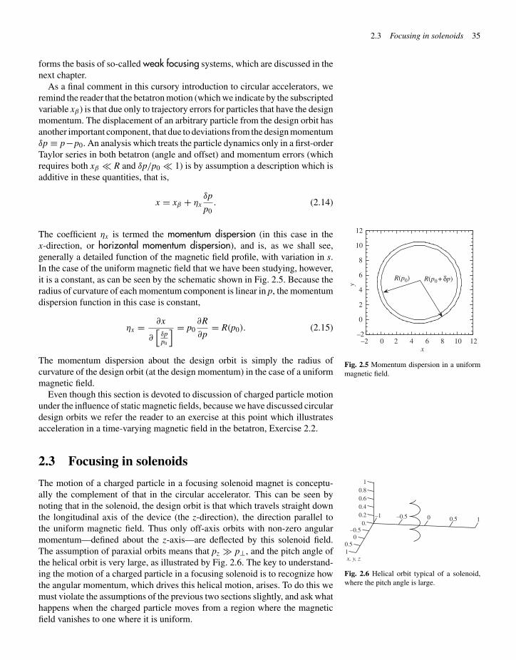
“chap02” — 2003/6/28 — page 35 — #6

2.3 Focusing in solenoids 35

forms the basis of so-called weak focusing systems, which are discussed in thenext chapter.

As a final comment in this cursory introduction to circular accelerators, weremind the reader that the betatron motion (which we indicate by the subscriptedvariable xβ ) is that due only to trajectory errors for particles that have the designmomentum. The displacement of an arbitrary particle from the design orbit hasanother important component, that due to deviations from the design momentumδp ≡ p−p0. An analysis which treats the particle dynamics only in a first-orderTaylor series in both betatron (angle and offset) and momentum errors (whichrequires both xβ R and δp/p0 1) is by assumption a description which isadditive in these quantities, that is,

x = xβ + ηxδp

p0. (2.14)

–2

0

2

4

6

8

10

12

x

R(p0)

y

R(p0 + δp)

–2 0 2 4 6 8 10 12

Fig. 2.5 Momentum dispersion in a uniformmagnetic field.

The coefficient ηx is termed the momentum dispersion (in this case in thex-direction, or horizontal momentum dispersion), and is, as we shall see,generally a detailed function of the magnetic field profile, with variation in s.In the case of the uniform magnetic field that we have been studying, however,it is a constant, as can be seen by the schematic shown in Fig. 2.5. Because theradius of curvature of each momentum component is linear in p, the momentumdispersion function in this case is constant,

ηx = ∂x

∂[δpp0

] = p0∂R

∂p= R(p0). (2.15)

The momentum dispersion about the design orbit is simply the radius ofcurvature of the design orbit (at the design momentum) in the case of a uniformmagnetic field.

Even though this section is devoted to discussion of charged particle motionunder the influence of static magnetic fields, because we have discussed circulardesign orbits we refer the reader to an exercise at this point which illustratesacceleration in a time-varying magnetic field in the betatron, Exercise 2.2.

2.3 Focusing in solenoids1

0.80.60.40.20.

–0.5

–0.5–1

0.5

0.5

1

1

0

0

x, y, z

Fig. 2.6 Helical orbit typical of a solenoid,where the pitch angle is large.

The motion of a charged particle in a focusing solenoid magnet is conceptu-ally the complement of that in the circular accelerator. This can be seen bynoting that in the solenoid, the design orbit is that which travels straight downthe longitudinal axis of the device (the z-direction), the direction parallel tothe uniform magnetic field. Thus only off-axis orbits with non-zero angularmomentum—defined about the z-axis—are deflected by this solenoid field.The assumption of paraxial orbits means that pz � p⊥, and the pitch angle ofthe helical orbit is very large, as illustrated by Fig. 2.6. The key to understand-ing the motion of a charged particle in a focusing solenoid is to recognize howthe angular momentum, which drives this helical motion, arises. To do this wemust violate the assumptions of the previous two sections slightly, and ask whathappens when the charged particle moves from a region where the magneticfield vanishes to one where it is uniform.

“chap02” — 2003/6/28 — page 36 — #7


Fig. 2.7 Fringe field region of solenoid, withinitially offset particle trajectory encounteringradial component of magnetic field.

Symmetryaxis

Coils

Magnetic fieldlines

Charged particletest trajectory

Iron for magneticflux return

In this transitional region, the magnetic field must “fringe” to satisfy thedivergence-free criterion, �∇ · �B = 0. Assuming a cylindrically symmetricgeometry, this criterion becomes

1

ρ

∂

∂ρρBρ = −∂Bz

∂z. (2.16)

Thus, as the charged particle enters the region where the solenoid field Bz

rises and ∂Bz/∂z is non-vanishing, a radial component of the magnetic field isencountered. This is illustrated in Fig. 2.7, in which the fringe-field region of asolenoid is schematically shown.

Particletrajectory

Initial position

x�L �c

Later position

y

yL

xL

Fig. 2.8 Transverse trajectory of chargedparticle with no initial transverse momentum(before magnet) in a solenoid. The rotat-ing Larmor frame is defined by the xL-axispassing through the charged particle thatbegins its motion on the x-axis.

In order to integrate Eq. (2.16), we assume the lowest order approximationon the form of the longitudinal field, that it is independent of radius. Because ofsymmetry, this approximation is good to second order in ρ, that is Bz(ρ, z) ∼=B(0, z)[1+αρ2 +· · · ], where α is a constant. Assuming in the region of interestthat |αρ2| 1, we may write

Bρ ∼= −ρ2

∂Bz

∂z

∣∣∣∣ρ=0

. (2.17)

Further, using the paraxial approximation, we may obtain an excellent estimateof the total angular momentum imparted to a charged particle as it passes throughthe fringe field region of a solenoid by evaluating the force integral assuming aconstant radial offset ρ0,

pφ ∼= q∫ t2

t1

vzBρ dt = q∫ z2

z1

Bρ dz = −qρ0

2

∫ z2

z1

∂Bz

∂z

∣∣∣∣ρ=0

dz

= −qρ0

2

∫ z2

z1

dBz

dz

∣∣∣∣ρ=0

dz = −qρ0

2[Bz(z2)− Bz(z1)] = −q

ρ0

2B0.

(2.18)

Here we have explicitly assumed that the particle velocity does not changesignificantly in direction or magnitude while passing through the magnetostaticfringe field region enclosed in the interval (z1, z2). Equation (2.18) is sometimesknown as Busch’s theorem.

It is important to note that the total transverse momentum2 “kick” imparted2Note that here we are examining the trans-verse momentum “kick” in the angular dir-ection. This should not be confused withthe angular momentum, which has a spe-cific meaning in the context of Hamiltoniandynamics—it is the momentum which iscanonical with the azimuthal coordinate φ(see Ex. 2.4), and of course has units ofmomentum times length.

to a particle entering the solenoid, pφ ∼= qρ0B0/2, gives rise to subsequenttransverse motion with radius of curvature R = pφ/qB0 ∼= ρ0/2. Therefore,a charged particle with no initial transverse motion displays helical motioninside of the solenoid, with radius of curvature such that the particle orbitpasses through the axis (ρ = 0). This somewhat surprising result is illustrated inFig. 2.8, where both the particle trajectory in this case, and the proper coordinatesystem for further analysis of the problem, are shown.

“chap02” — 2003/6/28 — page 37 — #8

2.4 Motion in a uniform electric field 37

If the particle begins its trajectory offset in x (x = x0), but not in y, and withno transverse momentum before the magnetic field region, the angle that thisparticle’s trajectory makes with respect to the x-axis is the Larmor angle θL. Ascan be seen from Fig. 2.8, the Larmor angle is simply related to the cyclotronangle of the motion (centered on x = x0/2) by 2θL − θc = 0, or θL = θc/2.Since the cyclotron angle grows linearly in time, so does the Larmor angle, andthus we can define the Larmor frequency,

ωL ≡ dθL

dt= ωc

2= qB0

2γm0. (2.19)

The Larmor frame can now be introduced—it is simply the frame that rotatesabout the z-axis with the Larmor frequency, as illustrated in Fig. 2.8.

In the Larmor frame, the motion in xL is simple harmonic with the Larmorfrequency,

xL = x0 cos(θL) = x0 cos(ωLt). (2.20)

The central advantage of introducing the Larmor frame is that the motion issimple harmonic for both of the transverse dimensions in this frame. To seethis, we note that the coordinates in the Larmor frame can be written in compactform as (

xL

yL

)=(

cos(ωLt) sin(ωLt)− sin(ωLt) cos(ωLt)

)(x

y

). (2.21)

Thus, we have, using Eqs (2.2) and (2.21),

xL + ω2LxL = 0 and yL + ω2

LyL = 0. (2.22)

These equations describe simple harmonic oscillations in both xL and yL asobserved in the Larmor frame. Thus, the motion in a solenoid can be describedas a rotation about the origin that proceeds at the Larmor frequency, with simpleharmonic (betatron) oscillations occurring in the rotating frame, also proceedingwith angular frequency ωL.

The last point to be made in discussing solenoid focusing concerns cast-ing of the problem in standard accelerator physics form, with the distance zdown the axis of the solenoid used as the independent variable. In the paraxialapproximation, we take vz ∼= v, and thus

x′′L + k2

LxL = 0, (2.23)

y′′L + k2

LyL = 0, with kL = ωL

vz= qB0

2pz

∼= qB0

2p. (2.24)

The inverse of the wave number associated with the betatron harmonic motionin the Larmor frame is approximately twice the radius of curvature R = p/qB0

of a charged particle of the same momentum traveling normal to the solenoidfield.

2.4 Motion in a uniform electric field

The substitution of a uniform electric field �E = E0z for the uniform magneticfield changes our point of view quite dramatically, as the energy of the particle is

“chap02” — 2003/6/28 — page 38 — #9


no longer constant, but increases due to longitudinal acceleration. The equationsof motion in this case, with �B = 0, read

dpz

dt= qE0,

d�p⊥dt

= 0. (2.25)

Since the momentum transverse to the electric field is conserved we may, forthe moment, ignore its effects and concentrate on the one-dimensional problemof the motion in z.

The most straightforward way to accomplish this is to note that the electro-static field �E = E0z may be derived from a potential, and thus the potentialenergy is

qφe = −qE0z. (2.26)

The Hamiltonian, which in this case is the total energy (see Section 1.4), is

H = γm0c2 + qφe = γm0c2 − qE0z. (2.27)

Because the Hamiltonian is independent of t, it is a constant of the motion, andit can be evaluated at given initial conditions, H|z=0. The particle’s mechanical(rest plus kinetic) energy is therefore given by

γm0c2 = H|z=0 + qE0z, (2.28)

or in normalized form,

γ (z) = H|z=0

m0c2+ γ ′z, (2.29)

where γ ′ ≡ qE0/m0c2, and the initial conditions-derived constant H|z=0 =γ |z=0m0c2. Note that the energy increases linearly in z, as dU = �v · d�p, or forone-dimensional motion

dU

dz= dp

dt= qE0. (2.30)

This simple relation helps clarify some jargon encountered in the particle beamphysics field, that the amplitude of the accelerating force (change in momentumper unit time) is referred to as an acceleration gradient, or spatial energygradient, commonly quoted in units of MeV/m. The normalized accelerationgradient γ ′ defines a scale length for acceleration Lacc = γ ′−1, over which theparticle gains one unit of rest energy.

In this simple scenario, other relevant dynamical quantities can be derivedfrom knowledge of γ (z),

p(z) = βγm0c =√γ 2(z)− 1m0c, (2.31)

and

v(z) = βc = p(z)c2

U(z)= c

√1 − 1

γ 2(z). (2.32)

The deduction of the velocity fromγ is of prime importance because it allows thetransformation of independent variable from t, which enters naturally into theequations of motion, to z.

“chap02” — 2003/6/28 — page 39 — #10

2.4 Motion in a uniform electric field 39

In the analysis given in this section, we have effectively adopted z as theindependent variable. It is also interesting to explore acceleration from thepoint of view of explicit time dependence. In this case, we can write the first ofEq. (2.25) as

dpz

dt= m0c

d(βzγ )

dt= m0c[γ + β2

z γ3]dβz

dt∼= γ 3m0c

dβz

dt= qE0, (2.33)

or

dvz

dt= qE0

γ 3m0, (2.34)

where we have assumed in Eq. (2.33) that βz ∼= β, the motion is predominantlyalong the z direction. Equation (2.34) seems to indicate that the effective mass ofa relativistic particle in accelerating parallel to its velocity vector is γ 3m0. Thislongitudinal mass effect will be revisited when we discuss charged particles’longitudinal oscillations in accelerators.

–6

–4

–2

0

2

4

6

–2 0 2 4 6 8γ �z

p z/m

0c

Fig. 2.9 Longitudinal phase plane(γ ′z, pz/m0c) trajectories for uniformacceleration.

Let us now examine a phase plane plot of uniform acceleration, as illustratedin Fig. 2.9. The curves of constant H are hyperbolae, which look locally para-bolic near pz = 0, the region of the non-relativistic limit. Asymptotically inlarge pz/m0c, the ultra-relativistic region, the curves approach straight lines.

In Section 2.3, we found that edge effects—the effects of moving from a field-free region to one with field present—were very important in understanding thetransverse motion of a charged particle in a longitudinal magnetic field. Thisis also true for the case of entry into a uniform electric field. The analysisproceeds just as in Eqs (2.16)–(2.18), and begins with an expansion near theaxis of Eq. (1.17),

1

ρ

∂

∂ρρEρ = −∂Ez

∂z. (2.35)

Integration of Eq. (2.35) outward from the axis yields

Eρ ∼= −ρ2

∂Ez

∂z

∣∣∣∣ρ=0

, (2.36)

which can be further used to find the radial momentum kick imparted to theparticle as in passes through the fringing field region where Eρ is non-zero,

pρ = q∫ t2

t1

Eρ dt = q

v

∫ z2

z1

Eρ dz = −ρq

2v

∫ z2

z1

∂Ez

∂z

∣∣∣∣ρ=0

dz

= −ρq

2v

∫ z2

z1

dEz

dz

∣∣∣∣ρ=0

dz = −ρq

2v[Ez(z2)− Ez(z1)] = −ρq

2vE0. (2.37)

We have assumed in Eq. (2.37) that the particle moves from a field-free regionto one with uniform longitudinal electric field E0. For an accelerating field(qE0 > 0), this effect is obviously focusing, with the momentum kick tend-ing to push the particle towards the axis. When a particle leaves the uniformaccelerating field region, however, the lines of force fringe outward instead ofinward and correct evaluation of Eq. (2.37) in this case yields a defocusingmomentum kick.

“chap02” — 2003/6/28 — page 40 — #11


2.5 Motion in quadrupole electric andmagnetic fields

In our discussion of beam optics thus far we have seen that one can use solenoidalmagnetic fields for focusing particles during linear transport, and path lengthfocusing in circular accelerators. These forms of focusing have introduced somebasic concepts, such as harmonic betatron oscillations about the design orbit,but do not include the most widely used magnetic focusing scheme, that whichemploys transverse quadrupole fields.

Since we are using a coordinate system with one preferred longitudinalaxis (z), we use cylindrical coordinates (ρ,φ, z) to evaluate the form of the scalarpotentials from which either static transverse electric or magnetic3 fields can3If there is no current density �J = 0 in

the region of interest, the magnetic field canbe derived from a scalar potential. The casewhere the current density is non-vanishing istreated in Chapter 6.

be derived. Let ψ be such a potential, which, in the limit of a device long com-pared to its transverse dimensions, approximately obeys the two-dimensionalLaplace equation

�∇2⊥ψ = 0. (2.38)

The solutions to this equation are of a form that is well behaved on axis (ρ = 0)

ψ =∞∑

n=1

anρn cos(nφ)+ bnρ

n sin(nφ), (2.39)

Let us discuss the first few of the n multipole forms of the solution. For n = 1,we have

ψ1 = a1ρ cos(φ)+ b1ρ sin(φ) = a1x + b1y (2.40)

and the fields are of the dipole form. Let us now assume we are talking aboutmagnetic fields, so �B = −�∇ψ , and

�B1 = −�∇ψ1 = −a1x − b1y. (2.41)

The form given in Eq. (2.41) is referred to as a dipole field because it canbe formed with a magnet possessing only two poles. Such magnets will bediscussed further in Chapter 6. They are the devices that yield the uniformfields that we have analyzed in Sections 2.1–2.3.

For n = 2, we have

ψ2 = a2ρ2 cos(2φ)+ b2ρ

2 sin(2φ) = a2(x2 − y2)+ 2b2xy (2.42)

and the associated magnetic field is

�B2 = 2a2(−xx + yy)− 2b2(yx + xy), (2.43)

If the potential coefficient a2 is non-vanishing, there is a force on a chargedparticle traveling in the z direction, directed in the x dimension and which isproportional to y, and vice versa. This type of force is called skew quadrupole,and gives rise to generally undesirable coupling between the x and y phaseplanes. The coefficient b2 indicates the presence of normal quadrupole fields,from which one obtains a force in the x dimension proportional to x, and a forcein y that is proportional to y,

�F⊥ = qvz�z × �B2 = 2qvzb2(yy − xx). (2.44)

Assuming qb2 is positive, this force is focusing in the x dimension and defo-cusing in y. Obviously if qb2 is negative, these focusing/defocusing roles are

“chap02” — 2003/6/28 — page 41 — #12

2.5 Motion in quadrupole electric andmagnetic fields 41

reversed. Since the coefficient b2 measures the gradient in magnetic fieldaway from the axis, one often gives its strength in terms of this gradientb2 = −∂xBx/∂y ≡ B′/2. The term “quadrupole” can be understood by lookingat Fig. 2.10, which shows a design for a quadrupole built at UCLA, with itsfour poles excited by current-carrying coils in alternating polarity. The designprinciples of this magnet are discussed in Chapter 6. Let us content ourselvesat the present to point out that the iron poles, whose surfaces form magneticequipotentials, are hyperbolae, as suggested by Eq. (2.42).

Fig. 2.10 Quadrupole magnet showing ironpole tips and yoke (hatching), current wind-ings (gray), and orientation of magnetic fieldlines.

If we assume paraxial motion near the z-axis, we may write the transverseequations of motion for a particle of charge q and momentum p0 as

x′′ = Fx

γm0v20

= −qB′

p0x, (2.45)

and

y′ = Fy

γm0v20

= qB′

p0y. (2.46)

These equations are written in standard oscillator form as

x′′ + κ20 x = 0 (2.47)

andy′′ − κ2

0 y = 0. (2.48)

The square wave number κ20 ≡ qB′/p0 is sometimes known as the focus-

ing strength K . It can be simply calculated by using the handy shortcutqB′/p0 = B′/BR where BR(Tm) = p0(MeV/c)/299.8 (cf. Eq. 2.8) is knownas the magnetic rigidity of the particle.

Assuming κ20 > 0, one has simple harmonic oscillations in x,

x = x0 cos[κ0(z − z0)] + x′0

κ0sin[κ0(z − z0)], (2.49)

and the motion in y is hyperbolic,

y = y0 cosh[κ0(z − z0)] + x′0

κ0sinh[κ0(z − z0)]. (2.50)

If κ20 < 0, the motion is simple harmonic (oscillatory) in y, and hyperbolic

(unbounded) in x. Focusing with quadrupoles alone can only be accomplishedin one transverse direction at a time. Ways of circumventing this apparent limita-tion in achieving transverse stability, by use of alternating gradient focusing,are discussed in the Chapter 3.

As noted in Chapter 1, it is much easier to build transverse field magnets thantransverse electric field-supporting electrode arrays that impart equal force uponcharged particles traveling nearly the speed of light. Therefore, the transverseelectric field quadrupole is found mainly in very low energy applications suchas the electron microscope. Note that an electric quadrupole that producesdecoupled forces in analogy with the magnetic forces of Eq. (2.41) has anelectrode array with hyperbolic surfaces rotated by 45◦ from that shown inFig. 2.10. In this case we may say that from the viewpoint of electric forces, if

“chap02” — 2003/6/28 — page 42 — #13


the same form of the solution for the electrostatic potential φe is used as wastaken for ψ (Eq. 2.3), then a2 is the coefficient of normal electric quadrupole,and b2 is the coefficient of the skewed electric quadrupole.

The paraxial ray equations in the case of an electric quadrupole are identicalto those given in Eqs (2.47) and (2.48), with κ2

0 ≡ qE′/p0v0. When the motionis focusing in x it is defocusing in y, as before. The differences between the twocases lie in the deviations from the assumptions of the paraxial approximation.In the case of magnetic forces, the energy and total momentum are constant,but the longitudinal momentum pz, and thus the longitudinal velocity vz maychange, which in turn forces a small modification of Eqs (2.47) and (2.48). Withelectric forces the situation is slightly different—the energy is not constant, aswork may be performed on a particle with transverse motion, but the longit-udinal momentum pz is now constant. In this case the longitudinal velocity vz

may also change non-negligibly when the paraxial approximation is not valid.

2.6 Motion in parallel, uniform electric andmagnetic fields

In the case of a uniform electric field, �E = E0z, and a parallel uniform mag-netic field, �B = B0z, the electric field provides uniform acceleration whilethe magnetic field provides solenoidal focusing. This example scenario showsthe combination of acceleration and focusing well, nicely illustrating the phe-nomenon of adiabatic damping of transverse oscillations. The equations ofmotion in this field configuration are

dpz

dt= qE0

d�p⊥dt

= q(�v⊥ × �B) = qB0

γm0(�p⊥ × z). (2.51)

Equation (2.51) are coupled by the presence of γ in the second equation, andso the method of solution offered previously for the transverse motion must bere-examined.

On the other hand, as the amplitude of �p⊥ is invariant, the energy may stillbe trivially found as a function of z,

U(z) = γ (z)mc2 =√(p2⊥ + p2

z |z=0)c2 + (m0c2)2 + qE0z. (2.52)

In the paraxial limit, one may ignore the transverse momentum contribution tothe energy, and Eq. (2.52) gives

U(z) = γ (z)mc2 =√

p2z |z=0c2 + (m0c2)2 + qE0z. (2.53)

After the energy and the longitudinal momentum are determined by Eqs (2.53)and (2.31), one can begin to write the transverse equations of motion in theLarmor frame (rotating with local frequency ωL(z) = qB0/2γ (z)m0) throughthe definition

x′L ≡ pxL

pz, (2.54)

with an analogous expression in yL. Since pxL is a Cartesian projection ofthe constant amplitude �p⊥, we expect the maximum angle in xL (and yL) to be

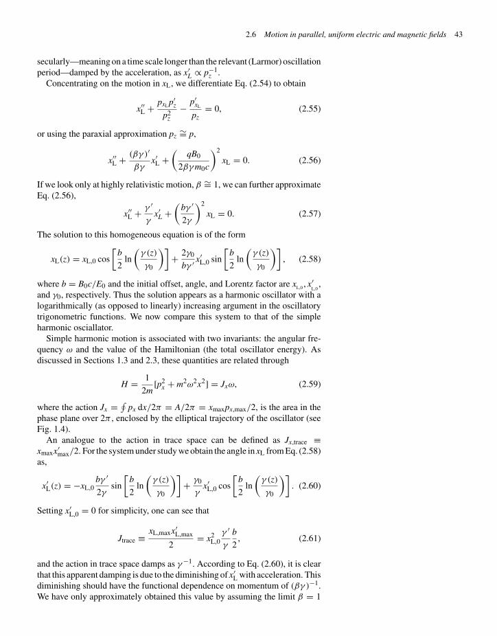
“chap02” — 2003/6/28 — page 43 — #14

2.6 Motion in parallel, uniform electric and magnetic fields 43

secularly—meaning on a time scale longer than the relevant (Larmor) oscillationperiod—damped by the acceleration, as x′

L ∝ p−1z .

Concentrating on the motion in xL, we differentiate Eq. (2.54) to obtain

x′′L + pxL p′

z

p2z

− p′xL

pz= 0, (2.55)

or using the paraxial approximation pz ∼= p,

x′′L + (βγ )′

βγx′

L +(

qB0

2βγm0c

)2

xL = 0. (2.56)

If we look only at highly relativistic motion, β ∼= 1, we can further approximateEq. (2.56),

x′′L + γ ′

γx′

L +(

bγ ′

2γ

)2

xL = 0. (2.57)

The solution to this homogeneous equation is of the form

xL(z) = xL,0 cos

[b

2ln

(γ (z)

γ0

)]+ 2γ0

bγ ′ x′L,0 sin

[b

2ln

(γ (z)

γ0

)], (2.58)

where b = B0c/E0 and the initial offset, angle, and Lorentz factor are xL,0 , x′L,0

,and γ0, respectively. Thus the solution appears as a harmonic oscillator with alogarithmically (as opposed to linearly) increasing argument in the oscillatorytrigonometric functions. We now compare this system to that of the simpleharmonic osciallator.

Simple harmonic motion is associated with two invariants: the angular fre-quency ω and the value of the Hamiltonian (the total oscillator energy). Asdiscussed in Sections 1.3 and 2.3, these quantities are related through

H = 1

2m[p2

x + m2ω2x2] = Jxω, (2.59)

where the action Jx = ∮px dx/2π = A/2π = xmaxpx,max/2, is the area in the

phase plane over 2π , enclosed by the elliptical trajectory of the oscillator (seeFig. 1.4).

An analogue to the action in trace space can be defined as Jx,trace ≡xmaxx′

max/2. For the system under study we obtain the angle in xL from Eq. (2.58)as,

x′L(z) = −xL,0

bγ ′

2γsin

[b

2ln

(γ (z)

γ0

)]+ γ0

γx′

L,0 cos

[b

2ln

(γ (z)

γ0

)]. (2.60)

Setting x′L,0 = 0 for simplicity, one can see that

Jtrace ≡ xL,maxx′L,max

2= x2

L,0γ ′

γ

b

2, (2.61)

and the action in trace space damps as γ−1. According to Eq. (2.60), it is clearthat this apparent damping is due to the diminishing of x′

L with acceleration. Thisdiminishing should have the functional dependence on momentum of (βγ )−1.We have only approximately obtained this value by assuming the limit β = 1

“chap02” — 2003/6/28 — page 44 — #15


for the purposes of solving the paraxial equation of motion, Eq. (2.56), exactly.It should be equally clear that the true phase plane action variable is constantin this case.

As mentioned in Section 1.6, the role of the action in the general theory ofoscillators is that they are adiabatic invariants. This means that if the oscillatorparameters are changed on a time scale that is slow compared to the oscillationperiod, then the action is conserved. The true phase plane action is an adiabaticinvariant and is conserved, not damped, under slow acceleration. On the otherhand, the apparent action in trace space is damped. Because of the guaranteedadiabatic invariance of the phase plane action under slow acceleration and con-comitant changing of the oscillation frequency, the damping of the trace spaceaction is termed adiabatic.

Use of the term adiabatic damping to describe this phenomenon is thus actu-ally a bit of a misnomer. It is especially so in the context of the system describedin this section, where the transverse motion under acceleration is not requiredto be an adiabatic process at all. It was only required to be one in which thetransverse momentum is constant and the longitudinal momentum grows.

2.7 Motion in crossed uniform electric andmagnetic fields*

Let us now consider the case where there are crossed uniform electric andmagnetic fields, which we choose as �E = E0y, and �B = B0z. In this case, thereis a particular solution to Eq. (1.11) obtained when the Lorentz force vanishes,given by

�E + �v × �B = 0. (2.62)

The velocity that is consistent with Eq. (2.62) is termed the drift velocity, andis found by taking the cross-product of Eq. (2.62) with �B, to give

�vd = �E × �B�B2

= E0

B0x. (2.63)

The drift velocity is normal to both the magnetic and electric field directions.

–2.0

0.0

2.0

4.0

6.0

8.0

10.0

12.0

0.0 2.0 4.0 6.0 8.0 10.0 12.0 14.0

y

x

Fig. 2.11 Cycloid motion in crossed electricand magnetic fields: �E = E0 y, �B = B0 z.

The general motion in this case can be deduced by transforming the Lorentzframe traveling with the drift velocity using Eq. (1.58) to obtain

�E′⊥ = γd(�E⊥ + �vd × �B⊥) = 0

�B′ = γd(�B⊥ − 1

c2�vd × �E⊥) = γdB0

(1 − �v2

d

c2

)z = B0

γdz.

(2.64)

The field is purely magnetic and uniform in the new frame. This means thatany motion in this frame is simply that of the helical cyclotron form discussedin Section 2.1. Looking down the axis (z) of the magnetic field, a direction inwhich there is no net force, the motion appears cycloidal, in other words cyclicmotion with a secular velocity (the drift velocity) superimposed, as shown inFigure 2.11.

The drift velocity and associated cycloid motion is not as important of aneffect in accelerators as those encountered in previous sections. Such behavior

“chap02” — 2003/6/28 — page 45 — #16

2.8 Motion in a periodic magnetic field* 45

is notably found in an analysis of intense beam rotation in solenoids due to thelongitudinal magnetic field and the radial self-electric field of the beam (see Ex.2.14). The drift velocity is, however, quite important in plasma physics, and inseparation devices—a particle with the correct velocity passes through a crossedelectric and magnetic field region, regardless of charge. This is an importanttechnique in experimental physics, and can be used for velocity identification ofa particle. The cross-field configuration, in tandem with traversal of a region ofuniform magnetic field, in which the momentum of the particle is determined,allows the mass and energy of the particle to also be determined.

2.8 Motion in a periodic magnetic field*

As a final scenario for this chapter, let us consider the case of a spatially periodic(in the z-direction) static magnetic field. There are two possible configurationsof this undulator magnetic field, a planar or helical polarization, names thatrefer to analogous electromagnetic wave polarizations. In this section we willdiscuss the planar undulator, leaving analysis of the helical configuration forthe exercises. Also, we will emphasize here the bending-plane motion of theparticle, of the undulator, with the out-of-plane motion examined further inChapter 3.

N

S N S N S

S N S N S

N

S

N

y

z

�u

Fig. 2.12 Schematic representation of themagnetic field lines in a planar undulatorconfiguration.

The periodic, vertically polarized magnetic field of interest here can bedescribed mathematically by

�B = B0 sin(kuz)y (2.65)

where ku = 2π/λu is the wave number associated with the undulatorwavelength λu of the field. This expression is valid only in the symmetry planeof the field, which we take to be y = 0. For the planar configuration, there mustbe an additional longitudinal field component, as illustrated in Fig. 2.12, andanalyzed in the Exercise 2.15.

As can be seen by the results of Exercise 2.15, Eq. (2.65) is approximatelycorrect if the vertical offset from the symmetry plane is much smaller thanan undulator wavelength, kuy 1. Let us now examine the electron beamdynamics in the undulator field under this additional constraint, which can beconsidered an extension of the paraxial approximation. We will formulate theproblem in Hamiltonian style. To begin, we write the canonical momenta

pc,x = βxγm0c + qAx = βxγm0c − qB0

kucos(kuz) cosh(kuy),

pc,y = βyγm0c,

pc,z = βzγm0c,

(2.66)

from which we can derive the relativistically correct Hamiltonian,

H =√(

pc,x + qB0

kucos(kuz) cosh(kuy)

)2

c2 + p2c,yc2 + p2

c,yc2 + (m0c2)2,

(2.67)

“chap02” — 2003/6/28 — page 46 — #17


where the electrostatic potential φe vanishes. Viewing z as the independentvariable, we write the new form of the Hamiltonian function as

G = −pz,c =√

H2 − (pc,y − qAy)2c2 − (pc,x − qAx)2c2 − (m0c2)2

=√

U2 −(pc,y − qAy)2c2 −(

pc,x + qB0

kucos(kuz) cosh(kuy)

)2

c2 − (m0c2)2,

(2.68)

where we have substituted the numerical energy U for the old Hamiltonianfunctional energy H. This new Hamiltonian is independent of x and t, andthus the canonical x component of the momentum pc,x is a constant of themotion, as is the total mechanical energy U (or equivalently, the total mechanicalmomentum p0), which is always the case in magnetostatic systems.

The first integrals of the Hamiltonian system (the momenta) are thus asfollows:

pc,x = constant = px0 ⇒ βx γm0c = −qAx + px0 = qB0

kucos(kuz)+ px0,

(2.69)

pc,y = βy γm0c = 0 (by assumption, taking y = 0), (2.70)

and

pc,z =√

p20 −

(q

B0

kucos(kuz)+ px0

)2

. (2.71)

This analysis has been done formally, with the aid of the Hamiltonian, in order tomake more advanced analysis of the motion in undulators possible in followingchapters.

The most important step remaining in the analysis is to find the second integralin x, which is obtained by integrating the paraxial equation

x′ = − ∂G

∂px,c

∼= qB0

p0kucos(kuz)+ px0

p0= qB0

p0kucos(kuz)+ x′

0, (2.72)

to give, with initial (evaluated before entry into the undulator field) horizontaloffset and angle (x0, x′

0),

x ∼= x0 + x′0z + qB0

p0k2u

sin(kuz). (2.73)

It can be seen from Eq. (2.73) that the amplitude of the undulating portionof the transverse motion is qB0/p0k2

u , and from Eq. (2.72) that the maximumangle associated with the undulating part of the motion is qB0/p0ku. This angleis typically much smaller than unity (the bends are paraxial) for magnets ref-ered as undulators. Furthermore, we note that Eq. (2.73) shows that there isno restoring, or focusing force in the x-direction associated with this config-uration of magnetic field—an initial error x′

0 �= 0 is not corrected, and leadseventually to a trajectory with large horizontal offset x.

“chap02” — 2003/6/28 — page 47 — #18

2.9 Summary and suggested reading 47

The conservation of total momentum combined with Eq. (2.69) givesEq. (2.71), which indicates that the longitudinal momentum, and thereforethe longitudinal velocity, must diminish in the undulator, approximately as

pz =√

p20 −

(q

B0

kucos(kuz)

)2 ∼= p0

[1 − 1

2

(qB0

kup0cos(kuz)

)2]

, (2.74)

for paraxial bends. Averaging Eq. (2.74) over a period of the motion, we havesimply

〈pz〉 ∼= p0

[1 −

(qB0

2kup0

)2]

. (2.75)

This “slowing” of the particle in its z-motion is an important effect in free-electron lasers, which are discussed in Chapter 8.


This chapter has been concerned with introducing a number of model prob-lems, based on the relativistic motion of charged particles in static electric andmagnetic field configurations. These configurations have included:

1. Uniform (dipole) magnetic fields, in which we deduce many aspects ofthe motion in both circular accelerators and focusing solenoids from thegeneral case of helical motion. In both scenarios, we found variants ofsimple-harmonic betatron oscillations.

2. Uniform electric fields, in which acceleration of charged particles torelativistic energies are introduced.

3. Quadrupole magnetic and electric fields, where the motion is simpleharmonic in one transverse dimension, and divergent in the other.

4. Superpositions of uniform electric and magnetic fields, which producedamped oscillations when the fields are parallel, and drift motion whenthe fields are crossed.

5. The periodic magnetic dipole field, or magnetic undulator. This device isshown to produce transverse undulating motion, which forms the basis ofthe free-electron laser.

These model problems also allowed us to introduce some rudimentaryexamples of analyses that are based on both relativistic and Hamiltonian form-alisms. These analyses will help form the basis of more complex investigationsof charged particle motion in the coming chapters.

Many texts in electromagnetism also introduce aspects of charged particlemotion in electric and magnetic fields. Readers wishing to review the theory ofelectrostatic and magnetostatic fields may also wish to review such texts. Thefollowing texts may be recommended as a supplement to this chapter:

1. R. Wangsness, Electromagnetic Fields (Wiley, 1986). There are manyexamples of dynamics calculations in this book, including usefulappendices.

2. J.R. Reitz, F.J. Milford, and R.W. Christy, Foundations of Electro-magnetic Theory (Addison-Wesley, 1993). Another fine undergraduateelectromagnetism text with examples.

“chap02” — 2003/6/28 — page 48 — #19


3. J.D. Jackson, Classical Electrodynamics (Wiley, 1975). A wealth ofassigned problems are relevant to our discussions here.

4. L.D. Landau and E.M. Lifschitz, The Classical Theory of Fields(Addison-Wesley, 1971).

5. S. Humphries, Jr., Principles of Charged Particle Acceleration (Wiley,1986). This text also examines many model problems as a path tounderstanding accelerator behavior.

6. J.D. Lawson, The Physics of Charged Particle Reams (Clarendon Press,1977). There are many clear explanations of basic problems in chargedparticle motion.

7. F.F. Chen, Introduction to Plasma Physics and Controlled Fusion:Plasma Physics (Plenum, 1984). The field of plasma physics has a widevariety of physical effects it addresses, and some differing dynamicsproblems are addressed in this excellent introduction.

8. J.B. Marion and S.T. Thornton, Classical Dynamics of Particles andSystems (Harcourt Brace & Company, 1995).

9. H. Goldstein, C. Poole and J. Safko, Classical Mechanics (Addison-Wesley, 2002). Dynamics in electromagnetic fields using modern mech-anics at a sophisticated level.

Exercises

(2.1) The mass increase implied by Eq. (2.4) can beobtained by using the relativistically correct Lagrangian(Eq. 1.60) to write the problem in cylindricalcoordinates,

L(�x, �x) = −m0c2

γ+ q�A · �x.

(a) Show that the cylindrically symmetric vectorpotential for a uniform magnetic field is �A =(B0ρ/2)φ.

(b) Write the Lagrangian in cylindrical coordinates(ρ,φ, z).

(c) Derive the Lagrange–Euler equations to show thatthe transverse motion (centered at the z-axis) iscircular, with appropriate angular frequency andradius of curvature.

(2.2) In the betatron, the design orbit of the electrons is circu-lar, with constant radius R, but the vertical magnetic fieldat the design orbit increases in time. This is described bythe relation

p0(t) = eB0(t)R (i)

which indicates that the design momentum must beincreased in proportion to the strength of the guidingfield. The acceleration for electrons traveling in a strictly

circular orbit is given by

dp0

dt= −eEφ , (ii)

where Eφ is the azimuthal electric field, tangential to theelectron path.

The betatron condition occurs when these require-ments are consistent with each other. In order for this to betrue, the field normal to the bend plane (Bz in cylindricalcoordinates) must not be constant, but it should be a func-tion of ρ, as shown in a representative way in Fig. 2.13.To derive the betatron condition, employ the followingsteps:

(a) Differentiate the expression (i) with respect totime, and

0

0.2

0.4

0.6

0.8

1

1.2

0 0.5 1 1.5 2

�/R

B/B

(0)

Fig. 2.13 Example of magnetic field profile as a function ofradius in a betatron.

“chap02” — 2003/6/28 — page 49 — #20

Exercises 49

(b) Calculate the induced electric field from Stokes theoremapplied to

�∇ × �E = −∂ �B∂t

.

The betatron condition is often given as B0(t) = B(t)/2,where B ≡ (

∫ �B · d �A)/(πR2) is the average normal mag-netic field over the disk whose boundary is the designorbit. Is this the most general form of the betatron con-dition? Note that the betatron condition implies that thefield is as shown in Fig. 2.13, having larger amplitude forρ < R. This point is returned to in the next chapter.

(2.3) The cyclotron spoken of in Chapter 1 is schematic-ally shown in Fig. 2.14. It consists of two opposingD-shaped iron magnet pole pairs (so-called Ds), givingrise to a roughly constant magnetic field B0 normalto the diagram inside of the Ds. This field bends theparticles inside of the D-regions in semi-circular tra-jectories. The Ds also are excited by a time-dependentvoltage source of constant angular frequencyωrf such thatV(t) = V0 sin(ωrf t), where rf stands for radio-frequency.Thus, when the particles cross the gap between the Dsthey can be accelerated by the electric field betweenthe two different potential regions, so that their energyis maximally incremented by U = qV0 per crossing.This occurs only when the motion is synchronous withvoltage wave-form, requiring ωc ∼= ωrf . Note that theparticles have larger radius of curvature as they gainenergy and are eventually ejected from the machine.

~

V

Iron “D”s

Particlesource

Fig. 2.14 Schematic diagram of magnetic field regions, voltageapplication, and design trajectory in a cyclotron. The particlesare embedded in an approximately uniform magnetic field insideof the Ds, and accelerated by an electric field between the Ds.

(a) Assuming the particles are non-relativistic protons(γ ∼= 1) and the magnetic field B0 = 1.5 T, whatis the rf frequency needed for the voltage supply?You may ignore the gap distance in this calculation.

(b) Assume the initial proton kinetic energy fromthe source is 150 keV, V0 = 150 kV, and theradius of curvature of the outside of the Ds is0.75 m. Approximately how many passes through

the system does a proton circulate for before it isejected?

(c) What is the value of γ of the proton at the machineexit? Can you estimate the total phase slippage ofa proton with respect to the applied voltage dur-ing acceleration due to relativistic changes in thecyclotron frequency?

(2.4) The Tevatron at Fermi National Accelerator Laboratory isa circular proton (colliding with counter-propagating anti-protons) accelerator that uses high field superconductingdipole magnets. It is approximately 1 km in radius, andaccelerates protons to 900 GeV in total energy.

(a) What is the average magnetic field needed to keep900 GeV protons on the design orbit?

(b) What is the circulation (cyclotron) frequency inthis accelerator? The protons are injected into theTevatron at 150 GeV. What is the circulation fre-quency at this energy? What is the circulationfrequency at 900 GeV?

(c) If electrons were to be stored in the Tevatron forcollision with the 900 GeV protons instead of anti-protons, what would their energy be? Be carefulwith round-off errors due to calculators in thisproblem.

(2.5) Busch’s theorem can also be derived by use of theHamiltonian formalism.

(a) Using the results of Exercise 2.1, write theHamiltonian inside of a solenoid in terms of cyl-indrical coordinates. Hint: Be careful in handlingthe vector potential component of the angularmomentum.

(b) Show that the canonical angular momentum isconserved in this case.

(c) Assuming the canonical angular momentum iszero (why?), what is the value of the mechan-ical momentum at radial offset ρ? Compare thisto Eq. (2.18).

(2.6) If the transverse momentum is not small compared to thetotal momentum, we may not assume p ∼= pz and thebetatron wave number in the solenoid is not as given byEq. (2.24).

(a) Derive a general expression for the wave numberas a function of initial offset radius at the entranceto the solenoid. Hint: Normalizing the initial off-set radius to p/qB0 may make the answer morephysically meaningful.

(b) At a certain radius, the particle cannot penetratethe interior of the solenoid. This is because all ofits longitudinal momentum is given up to angular

“chap02” — 2003/6/28 — page 50 — #21


motion in the fringe field and the particle is reflec-ted. For an electron with 100 keV kinetic energy,and B0 = 1 T, what is this radius?

(2.7) By differentiation of Eq. (2.21) twice, derive Eq. (2.22).

(2.8) The high-energy linear collider at Stanford contains a lin-ear accelerator of length L = 3 km, which uses electricfields in radio-frequency cavities to accelerate electrons(and positrons) to 50 GeV. The average longitudinalelectric force performing work on the electrons in theaccelerator is 16.7 MeV/m. The proper time τ , as observedin the frame of the accelerating electron, is related to thetime measured in the laboratory t by dt = γ · dτ .

(a) Show that the time for the electrons to go from restto final energy is

t = L

c

[√γf + 1

γf − 1

]≈ L

c

(b) Show that the proper time for the electrons to gofrom rest to final energy is

τ = L

c(γf − 1)cosh−1(γf ).

(c) What is the effective length of the linear acceler-ator as seen by the electrons at final energy? Howlong would it take to traverse this length at the finalvelocity of the electrons?

(2.9) Instead of writing the motion in terms of the variable vz,consider the motion as a function of γ .

(a) Show that

dγ

dt=√γ 2 − 1

γ

qE0

mc.

(b) Integrate this equation and compare to the resultsof directly integrating the first of Eq (2.25).

(2.10) For magnetic focusing channels that use quadrupoles, themotion is the same for particles of like charge but differ-ent mass if the momentum of each species is the same.This can be seen by examination of Eqs (2.42) and (2.43).Now consider the motion of particles with equal charge butunequal mass in electric quadrupoles. What is the condi-tion on dynamical quantities of the different species so thatthey can be focused identically in the electric quadrupolechannel? Show, in the relevant non-relativistic limit, thatthis condition reduces to the equality of kinetic energiesin the two species.

(2.11) For magnetic focusing channels, show that a particle trav-eling in a certain direction in z has the same equation ofmotion as its antiparticle of the same momentum travel-ing in the opposite direction in z. This is the basic opticsprinciple behind particle/antiparticle colliding beam rings.

How do the paraxial optics change for these species ifelectric quadrupoles are used?

(2.12) In deriving Eq. (2.58) as a solution to Eq. (2.57), it ishelpful to initially transform the independent variable tou = ln(γ (z)), with inverse transformation γ = exp(u).This is known as a Cauchy transformation.

(a) Show that this transformation allows Eq. 2.58 to bewritten as

d2xL

du2+(

b

2

)2

xL = 0.

(b) Using the equation derived in part (a), constructEq. (2.58).

(2.13) Can you solve the paraxial equation of motion (analogousto Eq. 2.55) for the case when the electric field is con-stant, but the magnetic field is zero? You may start withx′ ≡ px/pz and px = constant, then integrate.

(2.14) For cylindrically symmetric, intense beams propagatingin equilibrium in solenoids there is an electric self-field inthe radial direction that produces both an outward radialforce and an azimuthal rotation of frequency ωr . This fre-quency may or may not be equal to the Larmor frequency,and the related rotation may be viewed as an example ofthe �E × �B drift discussed previously.

(a) Show, for a uniform density (nb) beam that thisradial space-charge electric force on a particle ofcharge q and rest mass m0 is

Fe = qEρ = q2nb

2ε0ρ ≡ m0

ω2p0

2ρ,

where we have introduced the non-relativisticplasma frequency ωp0 = √

q2nb/ε0m0. Find thenet (beam-induced) force, including the magneticforce, on the particle, and write it in terms of theelectric force and the particle’s axial velocity v0.

(b) When the beam rotates, there are two radial forcesthat are introduced. One is due to centripetal accel-eration, and the other is the radial component ofthe solenoidal force. Equilibrium (net radial forceequal to zero) can be established only when thebeam rotates in a certain direction because boththe centripetal forces and the space-charge forcesare outward. Show that the condition on ω whichproduces equilibrium can be written as

ω2r + ω2

p

2= ωrωc,

where the relativistically correct plasma frequencyis given by ω2

p = ω2p0/γ

3.

“chap02” — 2003/7/2 — page 51 — #22

Exercises 51

(c) Illustrate this equilibrium condition by plottingωp/ωc as a function of ωr/ωc. What rotation fre-quency ωr maximizes the equilibrium density ofthe beam?

(2.15) The magnetic field given in Eq. (2.65) can be derived froma vector potential,

�A = −(B0/ku) cos(kuz)x,

in the y = 0 plane. Unfortunately, this vector potentialdoes not satisfy the Laplace equation in the current-freeregion, ∇2 �A = 0, as required by the Maxwell relations,and so it cannot be valid.

(a) Show that the following appropriate potential (uni-form in x, symmetric in y)

�A = −(B0/ku) cos(kuz) cosh(kuy)x

obeys the Laplace equation.(b) Find the field components associated with this

vector potential.

(2.16) A helically polarized magnetic undulator has an on-axisfield profile given by

�B(z) = B0√2[sin(kuz)x + cos(kuz)y].

It is typically constructed as shown schematically in theFig. 2.15, with two main counter-rotating helical windings(bifilar helical undulator).

(a) The vector potential which gives rise to this fieldcan be written in cylindrical coordinates as

Aφ = B0

ku[I0(kuρ) + I2(kuρ)] cos(φ − kuz)

and

Aρ = −B0

ku[I0(kuρ) − I2(kuρ)] sin(φ − kuz).

Here I0 and I2 are modified Bessel functions.Show that these components satisfy the Laplace

equation, ∇2 �A = 0.

z

I

Fig. 2.15 Schematic of a bifilar helical undulator.

(b) Find the field components for this vector potentialand verify that they give the correct field profileon axis.

(c) Write the Hamiltonian and equations of motion,using z as the independent variable, for the hel-ical undulator. Show that in the limit kuρ 1,there exists an orbit that is a perfect helix, in whichthe mechanical angular momentum is a constant.Note this is not true for the helix in the solen-oid, where the canonical angular momentumis constant (the Hamiltonian is independent ofazimuth).

“chap03” — 2003/6/28 — page 52 — #1

3 Linear transversemotion

3.1 Weak focusing in circularaccelerators 52

3.2 Matrix analysis of periodicfocusing systems 54

3.3 Visualization of motion inperiodicfocusing systems 60

3.4 Second-order(ponderomotive)focusing 63

3.5 Matrix description ofmotion inbending systems 67

3.6 Evolution of the momentumdispersion function 70

3.7 Longitudinal motion andmomentumcompaction 73

3.8 Linear transformations insix-dimensional phasespace* 75


Exercises 77

The phenomenon of stable transverse motion of charged particles near adesign trajectory has been introduced in Chapter 2. Simple harmonic betatronoscillations were encountered in the examples of the focusing solenoid, thequadrupole, and in the circular accelerator. The general physical and mathem-atical tools for describing betatron oscillations are developed in this chapter.The discussion begins, appropriately enough, within the historical context ofthe betatron, where the ideas of path length focusing and quadrupole focusingare used to provide simultaneous stability in both transverse dimensions. Afterintroduction of this type of first-order (in the field strength), or weak, focusingwe will move to the discussion of second-order, or strong, focusing. We end thischapter with a discussion of the first-order effects in transverse motion due to thedispersion of particles having total momenta deviating from the design value.

3.1 Weak focusing in circular accelerators

The motion of a charged particle in a uniform magnetic field has been shownto exhibit effective focusing in the bend (horizontal, x) plane. In a descrip-tion based on examination of trajectories along the circular design orbit, thiseffective focusing is ascribed to differential path lengths taken by particles ondiffering betatron orbits. Such path length focusing is effective in stabilizingthe horizontal motion, but not the vertical motion, which is completely uncon-strained in a uniform magnetic field. On the other hand, in our initial discussionof acceleration in the betatron (see Ex. 2.2), we have seen that the vertical com-ponent of the magnetic field is not uniform, but diminishes with distance awayfrom the axis.

At the design orbit, which defines a curvilinear coordinate system, it is mostnatural to adopt the lowest order (in x ≡ ρ − R) approximation of the variationin the vertical component of the field as,

By(x) = B0 + B′x + · · · . (3.1)

The field gradient is negative, B′ < 0, in the case of the betatron. Equation (3.1)implies, along with Ampere’s law, that a horizontal component of the fieldexists,

Bx(x) =∫ y

0

∂By

∂xdy ∼= B′y. (3.2)

In this coordinate system, it is apparent that, near the design orbit, the mag-netic field appears as a superposition of vertically oriented dipole and verticallyfocusing (horizontally defocusing) quadrupole fields. Since the field is not

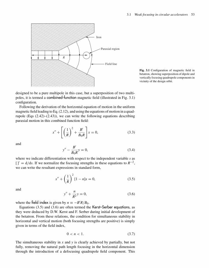
“chap03” — 2003/6/28 — page 53 — #2

3.1 Weak focusing in circular accelerators 53

Iron

R

Paraxial region

Field line

Fig. 3.1 Configuration of magnetic field inbetatron, showing superposition of dipole andvertically focusing quadrupole components invicinity of the design orbit.

designed to be a pure multipole in this case, but a superposition of two multi-poles, it is termed a combined-function magnetic field (illustrated in Fig. 3.1)configuration.

Following the derivation of the horizontal equation of motion in the uniformmagnetic field leading to Eq. (2.12), and using the equations of motion in a quad-rupole (Eqs (2.42)–(2.43)), we can write the following equations describingparaxial motion in this combined function field:

x′′ +[(

1

R

)2

+ B′

B0R

]x = 0, (3.3)

and

y′′ − B′

B0Ry = 0, (3.4)

where we indicate differentiation with respect to the independent variable s as[ ]′ = d/ds. If we normalize the focusing strengths in these equations to R−2,we can write the resultant expressions in standard form,

x′′ +(

1

R

)2

[1 − n]x = 0, (3.5)

andy′′ + n

R2y = 0, (3.6)

where the field index is given by n ≡ −B′R/B0.Equations (3.5) and (3.6) are often termed the Kerst–Serber equations, as

they were deduced by D.W. Kerst and F. Serber during initial development ofthe betatron. From these relations, the condition for simultaneous stability inhorizontal and vertical motion (both focusing strengths are positive) is simplygiven in terms of the field index,

0 < n < 1. (3.7)

The simultaneous stability in x and y is clearly achieved by partially, but notfully, removing the natural path length focusing in the horizontal dimensionthrough the introduction of a defocusing quadrupole field component. This

“chap03” — 2003/6/28 — page 54 — #3

54 Linear transverse motion

component yields a force that is focusing in the vertical dimension, as can beseen in Fig. 3.2.

The Kerst–Serber equations are often written, especially in the context ofsimple magnetic optics systems, with the azimuthal angle θ = s/R around thedesign orbit as the independent variable,

d2x

dθ2+ [1 − n]x = 0 or

d2x

dθ2+ ν2

x x = 0, (3.8)

andd2y

dθ2+ ny = 0 or

d2y

dθ2+ ν2

y x = 0. (3.9)

The forms of the Kerst–Serber equations displayed in Eqs (3.8) and (3.9) areillustrative, because they give a direct normalization of the betatron oscillationfrequency in terms of the circulation frequency. The tunes (normalized frequen-cies), νx = √

1 − n and νy = √n, are the number of betatron oscillations per

revolution in the horizontal and vertical dimensions, respectively. Assumingstability in both dimensions, the tunes are restricted to be smaller than unity.This restriction on the oscillation frequency is the source of the term “weakfocusing.” The weakness of the focusing becomes apparent when one attemptsto scale the circular accelerator to larger design momenta and concomitant lar-ger radii of curvature. For a given angular error of beam particle x′ launchedfrom the design orbit, the maximum offset found in the device is xm = Rx′/νx.Thus, the size of the beam that is contained in the machine scales with theradius of curvature. This scaling has serious implications in the design of themagnets and vacuum systems of the device. If the beam size, and thus the largeclear aperture between magnetic poles becomes too large, the magnet becomesdifficult, if not impossible, to build. Given a way to introduce stable oscilla-tions with much higher tunes νx,y � 1, the size of the beam could be greatlyreduced. The discovery of such a method based on quadrupole magnets, termedstrong focusing, has, therefore, allowed the development of very large radiusof curvature circular accelerators. We will next introduce the tools needed toanalyze strong focusing.

Fy

Fx

Fy

Fx

Design orbit

Fig. 3.2 Close-up view of paraxial regionshown in Fig. 3.1, illustrating the verticallyfocusing components of the magnetic field atvertically offset positions.

3.2 Matrix analysis of periodic focusing systems

The betatron oscillations of a particle in a weak focusing system can be intuit-ively understood, as they are merely examples of simple harmonic motion. Thismotion is characterized by having an oscillator (focusing) strength, κ2

0 , whichis of second-order in field strength and/or the field gradient (parameterized byn in Section 3.1). Specifically, in a weak focusing circular accelerator, the pathlength focusing, when combined with a quadrupole gradient, allows simultan-eous stability in x and y, yielding a focusing strength that is of second-orderin the magnetic field amplitude B0, κ2

0 ∝ B20. In a simple quadrupole, how-

ever, the motion is not simultaneously stable in both transverse dimensions.Even though quadrupoles have a focusing strength that is of first-order in fieldgradient, strong focusing systems—based on arrays of quadrupoles and notdependent on combination with path length focusing—are also second-orderfocusing systems. We also note that systems based on solenoids have a focusing

“chap03” — 2003/6/28 — page 55 — #4

3.2 Matrix analysis of periodic focusing systems 55

strength that is also of second-order in the field amplitude. We may infer fromthese examples that most focusing systems that are simultaneously stable inboth transverse directions are of second order in field gradient or amplitude. Infact, this is characteristic of all focusing schemes that have no charge or currentpresent within the beam channel.1 1An electric focusing system based on a uni-

form column of charged particles (oppositein sign to the beam particles) lying along thebeam axis produces a lens with cylindric-ally symmetric electric focusing fields (seeEx. 2.14), and is, therefore, stable in bothtransverse directions. This type of focusing(ion focusing) has a strength that is of first-order in the resultant electric field. A similardevice based on magnetic fields can be createdby using a current carrying plasma column(plasma lens).

The purpose of this section, as well as in Section 3.3, is to introduce someanalysis methods associated with strong focusing, in cases where the restoringforce is periodic. We indicate this periodicity in the equation of motion bywriting

x′′ + κ2x (z)x = 0 with κ2

x (z + Lp) = κ2x (z). (3.10)

The assumed period length, Lp, must be, in the context of a circular accelerator,no larger than the circumference C of the accelerator. Most large acceleratorsare made up of several (Mp) identical modules and, therefore, have a peri-odicity of Lp = C/Mp. Also, in linear accelerators and transport lines, thisperiodic focusing (often termed alternating gradient focusing) is used by typ-ically employing a very simple array of quadrupole magnets with differing signfield gradients. In fact, because the act of bending the design orbit introducesan asymmetry between the focusing in the bend (x) direction and non-bend( y) direction (as seen in Section 3.1), focusing in rectilinear—as opposed tocurvilinear—transport is inherently simpler. For this reason, and to make thediscussion as general as possible, we adopt z as the independent variable forthe description of the motion in this section as well as in Sections 3.3 and 3.4.

There are two cases of interest that can be readily analyzed: (a) the focusingis piece-wise constant, as in magnetic quadrupoles, and (b) the focusing isa sinusoidally varying function in z. The first case is quite straightforward,as for a piece-wise constant value of the focusing strength, κ2

x (z) = κ20 in

Eq. (3.10), the problem is reduced to that of the simple harmonic oscillator.The only generalization involved is that the focusing changes its oscillatorcharacteristics in discrete steps at a finite number of points in z. Thus, thesolution to the entire problem will involve “stitching together” a number ofsimple harmonic oscillator solutions. This is a straightforward process basedon a matrix description of the dynamics.

The second case requires a perturbative analytical approach, which cannotbe used for all conceivable physical parameters, so it is by nature a bit moreproblematic. In this section, we only discuss the first case and leave the secondcase for Section 3.4. The problem of the sinusoidally varying oscillator strengthis encountered in more esoteric situations in charged particle dynamics (e.g.focusing of particles due to radio-frequency waves, ponderomotive forces inlaser fields), but is of high conceptual value, since it illuminates the physicalbasis of the matrix results.

We now consider a piece-wise constant, periodic focusing described by afocusing strength (κ2

0 ) that may be positive, negative, or vanishing. Physically,these cases may correspond, for example, to a focusing quadrupole, a defocus-ing quadrupole, and a force-free drift, respectively. For κ2

0 > 0, Eq. (3.10) isa differential equation that describes a simple harmonic oscillator, where thesolution can be written, with the constants of integration determined in termsof an initial state vector (a vector defined in trace space),

�x(z0) ≡(

x

x′

)z=z0

=(

xi

x′i

),

“chap03” — 2003/6/28 — page 56 — #5


as

x(z) = xi cos(κ0(z − z0)) + x′i

κ0sin(κ0(z − z0)). (3.11)

By differentiating Eq. (3.11), we also obtain the angle

x′(z) = −κ0xi sin(κ0(z − z0)) + x′i cos(κ0(z − z0)). (3.12)

Equations (3.11) and (3.12) can be conveniently represented by a matrixexpression, illustrating the relationship between the initial state vector �x(z0)

and final state vector �x(z) as

�x(z) = MF · �x(z0) with MF =[

cos(κ0(z − z0))1κ0

sin(κ0(z − z0))

−κ0 sin(κ0(z − z0)) cos(κ0(z − z0))

].

(3.13)

For the transformation of the vector �x through a focusing section (lens) oflength l, the matrix describing the transformation is simply

MF =[

cos(κ0l) 1κ0

sin(κ0l)−κ0 sin(κ0l) cos(κ0l)

]. (3.14)

In the case of a defocusing lens, we have κ20 < 0 in Eq. (3.10), and the

solution to this equation takes the form,

x(z) = xi cosh(|κ0|(z − z0)) + x′i

|κ0| sinh(|κ0|(z − z0)), (3.15)

with

x′(z) = |κ0|xi sinh(|κ0|(z − z0)) + x′i cosh(|κ0|(z − z0)). (3.16)

Thus, the transformation matrix describing the propagation of the vector �xthrough a defocusing lens of length l is written, in analogy with Eq. (3.14), as

MD =[

cosh(|κ0|l) 1|κ0| sinh(|κ0|l)

|κ0| sinh(|κ0|l) cosh(|κ0|l)]

. (3.17)

Two interesting cases can be obtained by taking the limits of Eqs (3.14) and(3.17). The first is the force-free drift, in which case it is obvious that we aretaking the limit that the force disappears, κ0 → 0. As a result, both Eqs (3.14)and (3.17) yield the same limit,

MO =[

1 Ld

0 1

], (3.18)

where Ld is the length of the drift space. In a drift, the position x changes whilethe angle x′ does not.

The other case of interest is the so-called thin-lens limit, where κ20 l is kept

finite and constant, while l → 0 in Eqs (3.14) and (3.17). As a result, we have

MF(D) =[

1 0− 1

f 1

], (3.19)

where the lens focal length is defined as f ≡ (κ20 l)−1, and is positive for focusing

lenses and negative for defocusing lenses. In the thin-lens limit, the change inposition x is negligible and only the angle x′ is transformed.

“chap03” — 2003/6/28 — page 57 — #6


Two properties of the formalism developed so far should be noted. First,all of the transformation matrices—the focusing, defocusing, drift, and thin-lens matrices—have determinant equal to 1. This is a general property oflinear transformations, which are precisely those that can be written as matrixtransformations (see Ex. 3.8). The property of unit determinant transformationmatrix is also a manifestation of Liouville’s theorem, as is discussed later inthis section.

The second notable property of the matrix formalism is that the full solutionof the motion through a number of focusing elements (regions of constant κ2

0 )can be written in terms of the component element matrices’ product. To clarifythis, consider the example of a periodic system composed of a thin focusinglens, followed by a drift, a thin defocusing lens, and a final drift. In this case,the full transformation through one period of the system is written as

�x(Lp+z0) = �x(2Ld+2l+z0) = MO·MD·MO·MF · �x(0) ≡ MT · �x(z0). (3.20)

The total transformation matrix MT, being the product of matrices all of unitdeterminant, also has the property det(MT) = 1. Note that the matrix productgiven in Eq. (3.20) is written in reverse order from that in which the componentmatrices are physically encountered in the beam line. Confusion on the orderingof matrices is the most common mistake made in the matrix analysis of beamdynamics!

For the example of Eq. (3.20), the total transformation matrix can be explicitywritten as

MT =[

∂x∂xi

∂x∂x′

i∂x′∂xi

∂x′∂x′

i

]=

1 − Ld

f −(

Ldf

)22Ld + L2

df

−Ld

f 2Ldf + 1

. (3.21)

Note that in the first display of the matrix elements in Eq. (3.21), we indicatetheir general meaning as the first partial derivatives of the final conditions withrespect to the initial conditions. The partial derivative form of the matrix showsexplicitly that it can also be interpreted as a generalized linear transformationof coordinates in trace space. The determinant of this matrix is known, in thecontext of coordinate transformations, as the Jacobian of the transformation;it is the ratio of differential area elements of the final and original coordinates,det MT = dx dx′/dxi dx′

i . The fact that this determinant is unity in all linear tracespace transformations indicates that they are area preserving, as anticipatedby application of Liouville’s theorem to trace space.

A few salient aspects of the transformation can be deduced by inspection ofEq. (3.21). The matrix element MT11 is the spatial magnification (∂x/∂xi), andit can be seen in this case to be strictly less than one in our example. Further, ifthis matrix element is zero, this indicates a parallel-to-point transformation ofthe trajectory. The “focusing” matrix element MT21 (∂x′/∂xi) can be comparedto that found in Eq. (3.19), to deduce an equivalent thin-lens fthin = f 2/Ld thatis always positive (focusing). The focusing indicated by MT21 is of second-order in the lens strength f because the two first-order contributions, due tothe focusing and defocusing lenses, respectively, cancel. The second-orderfocusing naturally disappears when Ld → 0, as it must when two thin-lensesof equal and opposite strength are directly joined. If the two lenses were ofunequal strength, a first-order effect would appear, but it would be focusing

“chap03” — 2003/6/28 — page 58 — #7


in x and defocusing in y, or vice versa. Thus, in order that there be equal netfocusing in both transverse dimensions x and y, the focusing and defocusinglens strengths in a two-lens system should be equal. When the matrix elementMT12 vanishes, this indicates the point-to-point imaging condition, where thefinal offset is independent of the initial angle. Finally, MT22 is the magnificationin x′; when it vanishes, this indicates a point-to-parallel transformation.

Thus far, we have not explicitly required that the matrix transformationsdiscussed correspond to periodic systems. In many scenarios in charged particleoptics (e.g. circular accelerators and storage rings) and in light optics (e.g.laser resonators, cf. Section 8.3), the particles are stored in a periodic focusingsystem like that described by Eq. (3.20) for many traversals of the system. Ina large colliding beam storage ring, this may mean billions of turns aroundthe machine. It is, therefore, of primary interest to find out what the effectof negotiating this system many times is on the particle motion—in particular,whether or not the motion is linearly stable. Assurance of the stability of particlemotion under forces that are linear in displacement from the design orbit (asin Eq. (3.10)) is a necessary, but not sufficient, condition for absolutely stablemotion. Nonlinear forces may also cause unstable orbits to appear at largeamplitude in an otherwise linearly stable system.

In order to begin this analysis, we first note that the transformationcorresponding to n passes through the system can be written as

�x(NLp + z0) = MnT · �x(z0). (3.22)

This expression is simplified if we note that the transformation of the vector canbe written in terms of eigenvectors (akin to the familiar normal mode vectorsof coupled oscillator systems) as

�x(Lp + z0) = MT · �x(z0) = a1λ1�d1 + a2λ2�d2. (3.23)

In Eq. (3.23), the eigenvectors �dj have the defining property that the matrixtransformation only changes them by a constant factor, MT · �dj = λj�dj. Thecoefficients defined in Eq. (3.23) are the projections aj = �x(z0) · �dj of the initialconditions. Using the eigenvectors, we can recast Eq. (3.22) as

�x(NLp + z0) = MnT · �x(z0) = a1λ

n1�d1 + a2λ

n2�d2. (3.24)

We will see below the physical meaning of these eigenvectors. Before dis-cussing them, we first note, from Eq. (3.24), that the eigenvalues of thetransformation must be complex numbers of unit magnitude, or the motion willbe exponential—meaning either unbounded (positive exponent), or decaying(negative exponent). In either of these cases, the motion is termed unstable.

To find the eigenvalues, we write the transformation of an eigenvector throughone period as

(MT − λjI) · �dj = 0, (3.25)

where I is the identity matrix. Requiring the determinant of the matrix operatingon the eigenvector vanish, we have

λ2j − (MT11 + MT22)λj + (MT11MT22 − MT12MT21) = 0, (3.26)

“chap03” — 2003/6/28 — page 59 — #8


or, using the fact that det(MT) = 1,

λ2j − (MT11 + MT22)λj + 1 = 0. (3.27)

Recognizing that the eigenvalue is of unit magnitude, |λj| = 1, when the motionis stable, we now choose to write it as λj = exp(±iµ). Here µ, when it is real,is referred to as the phase advance per period. With this choice, the solutionto Eq. (3.27) becomes

exp(±iµ) = cos(µ) ± i sin(µ) = Tr(MT)

2± i

√1 −

(Tr(MT)

2

)2

, (3.28)

and we have employed in Eq. (3.28) the definition of the trace of the trans-formation matrix, Tr(MT) ≡ MT11 + MT22. It is clear that the absolute value| exp(±iµ)| = 1 if |Tr(MT)| ≤ 2, and, furthermore, the value of µ is real underthe same condition. Thus, the condition for stable motion, in short, is

|Tr(MT)| = |λ1 + λ2| ≤ 2. (3.29)

For the case of the focus-drift–defocus-drift, or FODO, array (in the contextof periodic systems, the term FODO lattice is applied) discussed above, thisstability criterion becomes

Ld

f≤ 2, (3.30)

which provides an upper limit on the defined phase advance. This limit is givenin the FODO system by

cos(µ) = Tr(MT)

2= 1 − 1

2

(Ld

f

)2

. (3.31)

Note that the maximum stable phase advance per period is µ = π . Also, itmay be remarked that since the eigenvalues of stable motion are complex, theeigenvectors are generally complex.

The meaning of the phase advance per period and the associated eigenvectorscan be illustrated with a few examples of ray tracing, as in Figs 3.3 and 3.4.In these ray plots, the conventional representation of focusing and defocusinglenses as thin convex and concave forms, respectively, is used. The first example,shown in Fig. 3.3, is the case µ = π/2 (λj = ±i), where (the real component of )an eigenvector trajectory (1) with pure offset initial conditions (midway through

z(1)(2)

Fig. 3.3 The real components of the eigen-vector rays for the case µ = π/2 (L/f = √

2)

in a FODO periodic array. Ray (1) is thecosine-like trajectory and ray (2) is the sine-like trajectory (beginning propagation in thecenter of the first lens).

Fig. 3.4 The real component of the eigen-vector ray for the case µ = π (L/f = 2) in aFODO periodic array, showing limits of sta-bility. The eigenvalues are degenerate (bothequal to −1) in this case.

“chap03” — 2003/6/28 — page 60 — #9


the first focusing lens), (x, x′) = (xi, 0), is converted to a trajectory with pureangle and no offset in final (conditions midway through the final focusing lens,(x, x′) = (0, x′

f)). This behavior is reminiscent of the cosine function over thefirst 90◦ of phase advance. Note that trajectory (2) is the converse of trajectory(1) since it begins with only an angular deviation (x, x′) = (0, x′

i), and endswith only an offset (x, x′) = (xf , 0), just as a sine function does over its initial90◦. This example illustrates why the initial conditions of type (1) are said togenerate the cosine-like solution to the motion and the initial conditions of type(2) give rise to the sine-like solution.

This point of view suggests yet another alternative notation for thetransformation matrix, indicating the matrix elements as the coefficients ofthe cosine- and sine-like orbits (C and S), and their derivatives (C′ and S′),

MT =[

C SC′ S′

]. (3.32)

The cosine-like component begins in Fig. 3.3 midway through the first focusinglens with a parallel, unit-offset ray, and the sine-like component begins at thispoint with an on-axis ray having unit angle(!). These are just mathematicaldefinitions; one need not be concerned with a unit angle being a violation of theparaxial ray approximation, as, in practice, the coefficient (initial angle) that ismultiplied by S will always be small compared to unity.

The case of µ = π , where Tr(MT) = −2 and is therefore directly at the limitof stability, is shown in Fig. 3.4. It is revealed that there is only one non-trivialeigenvector corresponding to the degenerate eigenvalue λ = −1. With only oneeigenvector, there can only be one type of stable trajectory, that which entersand exits the focusing lens with equal and opposite angles, and passes throughthe axis at the defocusing lens position. One can see that, as this situation isapproached, µ → π , and the particles tend to undergo very large excursions atthe focusing lens position, while having very small offsets near the defocusinglens. In a beam composed of many particles, this implies that the beam will bemuch larger near the focusing lens than it is near the defocusing lens.

It should be noted that the trace of the matrix describing a period of themotion is independent of the choice of initial position z0—the proof of thisassertion is left for Exercise 3.5. Thus, the eigenvalues and phase advance µ

are independent of this choice. The eigenvectors, in contrast, are dependent onchoice of z0.

3.3 Visualization of motion in periodicfocusing systems

In a periodic focusing system such as the FODO lattice introduced in the previ-ous section, the motion in x, when plotted continuously at every point in z (seeFig. 3.5) shows a simple harmonic oscillator-like behavior, with some notablelocal “errors” in the trajectory. In fact, these errors can be seen to be due to afast, yet small-amplitude, oscillation about a slower, secular simple harmonicmotion. The period of the fast oscillatory motion is clearly identical to that ofthe FODO lattice, due to the alternating sign of the focusing and defocusingforces in a FODO period, while the secular oscillation period is much longer.

“chap03” — 2003/6/28 — page 61 — #10

3.3 Visualization of motion in periodicfocusing systems 61

–3

–2

–1

0

1

2

3

0 5 10 15 20 25 30

x

Lens number

Fig. 3.5 Motion of a particle in a FODO chan-nel with µ = 33◦. Lenses are at positionsmarked with diamond symbols. Note the devi-ation from simple harmonic motion occurringwith the FODO period.

–0.8

–0.6

–0.4

–0.2

0

0.2

0.4

0.6

0.8

–3 –2 –1 0 1 2 3

x�

x

Fig. 3.6 Motion of a particle in a FODOchannel of µ = 33◦, plotted in trace space.The fast deviations from simple harmonicmotion occurring with the FODO period havea large angular spread.

As we shall see below, the fast motion is due to first-order (in the applied fieldamplitude) forces, while the slower motion may be ascribed to second- (orhigher-order) forces that become apparent when averaging over a period of thefast oscillation. The fast motion, despite its small spatial amplitude, will alsobe seen to have relatively large angles associated with it.

The continuous plotting of the motion in a periodic focusing system is espe-cially troublesome if one follows the motion in trace space, as shown in Fig. 3.6.In this plot, the fast errors in the trajectory have large angular oscillations, andthe trace space plot fills in a distorted annular region, yielding unclear informa-tion about the nature of the trajectory. On the other hand, if one only plots thetrace space point of a trajectory once per FODO period, a method of graphicalrepresentation known as a Poincaré plot, then the motion is regular. It is infact an ellipse in trace space, as illustrated by Fig. 3.7, and is thus reassuringlyreminiscent of a simple harmonic oscillator. This “stroboscopic” method ofplotting allows the secular motion to be displayed without the interference ofthe fast oscillations so dramatically illustrated in Fig. 3.6.

“chap03” — 2003/6/28 — page 62 — #11


By examining the eigenvalues and eigenvectors of the matrices for a period ofthe system, it is clear why the secular motion of a particle in a periodically focus-ing system is very nearly simple harmonic. The eigenvalues are λj = exp(±iµ),and so both indicate motion with a single spatial frequency ksec = µ/Lp, whereLp is the length of one period. This motion is therefore simple harmonic aboutthe real components of the eigenvector directions, which are the major andminor axes of the ellipse shown in Fig. 3.7. Since the real components of theeigenvectors are not in general parallel to the (x, x′) axes, the simple harmonicmotion does not necessarily yield an ellipse aligned to these axes, but one thatis aligned to the eigenvector axes.

–0.8

–0.6

–0.4

–0.2

0

0.2

0.4

0.6

0.8

–3 –2 –1 0 1 2 3

x�

x

Fig. 3.7 Poincaré plot of the motion of aparticle in a FODO channel of µ = 33◦,shown previously in Fig. 3.6, but here plottedonly at the end of every FODO array.

This discussion brings up the question of which quantities are independentof where in the period one chooses to interrogate the motion while performinga matrix analysis, or generating a Poincaré plot. As discussed above, and inExercise 3.5, the trace of a matrix is independent of where in the period z0 onechooses to begin the transport description. Thus the eigenvalues of the motionand the phase advance per period are independent of the choice of z0. This isintuitively obvious from Fig. 3.5—the average, secular motion frequency cannotdepend on which point in the fast periodic motion one begins the analysis. On theother hand, the eigenvectors depend on the choice of z0, and so the orientationof the ellipse typified by that shown in Fig. 3.7 is also dependent on choice ofz0. The area inside of the ellipse, being related to the action, and therefore theenergy of the slow, secular oscillation (see Chapter 1), is independent of z0.This area and its physical meaning will be discussed further in this chapter, aswell as in Chapter 5.

If one is concerned primarily with the approximate secular focusing effectsof a periodic lattice, they can be taken into account by use of the smoothapproximation, in which only the average focusing effect is used in the equationof motion,

x′′ + k2secx = 0. (3.33)

This approximation will be used in several upcoming analyses of oscillatoryforces in beam physics phenomena. A direct analytical method for deriving thesmooth (secular), focusing strength k2

sec will be presented in Section 3.4. Fornow, we restate that the average focusing strength employed in Eq. (3.33) can besimply deduced from ksec = µ/L. In the case of an alternating, focus–defocus(no drift) lattice (see Ex. 3.6), the phase advance is given exactly by

cos(µ) = cos

(κ0Lp

2

)cosh

(κ0Lp

2

). (3.34)

For small phase advance per period, µ � 1, Eq. (3.34) can be approximated as

1 − µ2

2∼=

(1 −

(κ0Lp

2

)2)(

1 +(

κ0Lp

2

)2)

or µ ∼= 1

4√

2(κ0Lp)

2,

(3.35)and the average focusing strength is given by

k2sec

∼= 1

32k4

0L2p . (3.36)

Assuming magnetic quadrupole focusing, Eq. (3.36) indicates that the focusingstrength is proportional to the applied field squared, k2

sec ∝ B′2. This is similar to

“chap03” — 2003/6/28 — page 63 — #12

3.4 Second-order (ponderomotive) focusing 63

the situation we have found in solenoid focusing, and it again points to a generalresult mentioned above—all linear focusing that is equal in both transversedimensions, and occurs in a macroscopic charge and current-free region, has anaverage strength that is second-order in the applied field strength. The reasonsfor this result in the context of quadrupole focusing will be more apparent afterthe discussion in Section 3.4.

3.4 Second-order (ponderomotive) focusing

As we noted at the beginning of Section 3.3, periodic focusing lattices canbe analyzed in a number of ways. In many situations encountered in chargedparticle optics the forces are piece-wise constant, and the matrix methods ofSection 3.3 provide an exact and powerful description of the motion. On theother hand, there are situations where the periodic focusing is not piece-wiseconstant, and another method is appropriate, one based on a Fourier decom-position of the periodic forcing function κ2(z). The basis of this analysis isan examination of purely harmonic, or sinusoidally varying, focusing. To bespecific, we consider an equation of motion of the form

x′′ + κ20 sin(kpz)x = 0, (3.37)

where we have chosen the phase of the focusing function for ease of furtheranalysis,2 and defined the wave number associated with the focusing strength 2This form indicates that we will always be

choosing the phase of the focusing function sothat it is odd with respect to the origin. Sincewe are interested only in finding the averagedsecond-order focusing in this analysis, no lossof generality in the discussion is suffered dueto this assumption.

period, kp = 2π/Lp.Equation (3.37) is classified in mathematics texts as a form of Hill’s equation

(an oscillator with periodic “focusing” coefficient), and also more specifically aform of the Mathieu equation (an oscillator with a component of sinusoidallyperiodic focusing). The exact solutions to the Mathieu equation have beenstudied in detail, but these solutions are not terribly useful or illuminating. Forour purposes, therefore, we would like to use approximateperturbativemethodsfrom which we can learn some lessons about the physics of this system. This typeof equation of motion is often found in electrodynamics, most commonly in thecase of a charged particle oscillating in a spatially non-uniform electromagneticwave, e.g. a free-electron near the focus of a powerful laser. We will return tothis example later.

The discussion of Section 3.3, where we saw that the secular simple harmonicmotion in a periodic lattice has a small, fast “error” trajectory overlaid upon it,motivates our choice of analysis method. The approximation we will employhere assumes that the motion can be broken down into two components, onewhich contains the small amplitude fast oscillatory motion (the perturbed partof the motion), and the other that contains the slowly varying or secular, largeamplitude variations in the trajectory. This is written explicitly in one transversedirection as

x = xosc + xsec. (3.38)

By this assumption, we expect the case described by Eq. (3.37), to displaymotion that looks qualitatively similar like the example given in Fig. 3.8.

“chap03” — 2003/6/28 — page 64 — #13


Fig. 3.8 An example of fast, small amplitudeoscillatory motion superimposed upon slow,large amplitude, secular oscillation.

–1.50

–1.00

–0.50

0.00

0.50

1.00

1.50

0.0 1.0 2.0 3.0 4.0 5.0 6.0

xksecz

The oscillatory component is analyzed by making the approximation that theoffset x = xsec ∼= constant (x′′

sec � x′′osc) over an oscillation in the second term

on the right hand side of Eq. (3.37),

x′′osc + κ2

0 sin(kpz)xsec = 0, (3.39)

where we have used the assumed |xosc| � |xsec|.Since we will eventually add the secular solution xsec to the perturbed com-

ponent xosc, we do not have to examine the full solution to Eq. (3.39) at thispoint, only the inhomogeneous solution. We can add the homogeneous com-ponents along with xsec later, when we apply the initial conditions to the fullsolution.

The inhomogeneous component of the solution to Eq. (3.39) is

xosc = sin(kpz)κ2

0

k2p

xsec. (3.40)

This solution for the oscillatory portion of the motion is accurate if theassumptions leading to it are valid, requiring that

|xosc||xsec| � 1 or

κ20

k2p

� 1. (3.41)

In short, if the fast oscillation amplitude is small compared to the secular ampli-tude, then we expect the approximate solution to Eq. (3.39) to be accurate. Thiswill be true if κ2

0 /k2p � 1, implying that the focusing is weak, in the sense

that no significant part of a secular oscillation can occur during the focusingstrength period 2π/kp. This condition, of course, also implies that the secularphase advance per period is small, µ � 1.

With Eq. (3.40) in hand, it is now possible to substitute it into Eq. (3.39) toobtain

x′′ = −κ20 sin(kpz)x ∼= −κ2

0 sin(kpz)

[1 + sin(kpz)

κ20

k2p

]xsec. (3.42)

“chap03” — 2003/6/28 — page 65 — #14

3.4 Second-order (ponderomotive) focusing 65

The next step in the analysis is to convert Eq. (3.42) into an averaged expressionthat will give us the behavior of the secular component of the motion, xsec ≡ 〈x〉,where the indicated average is over a period Lp. We now obtain, by averagingEq. (3.42) over one period of the fast oscillation,

x′′sec ≡ 〈x′′〉 = −〈κ2〉xsec ∼= −κ2

0

2

κ20

k2p

xsec (3.43)

or, in standard simple harmonic oscillator form,

x′′sec + κ4

0

2k2p

xsec = 0. (3.44)

Equation (3.44) predicts simple oscillations having a spatial frequency (wavenumber) ksec = √〈κ2〉 = κ2

0 /√

2kp. The derivation of these oscillations canbe viewed as an algorithm for extracting the smooth approximation pictureequivalent to Eq. (3.37). Note that one of the assumptions used in generatingEq. (3.39) was that x′′

sec � x′′osc, which we now see implies κ4

0 /2k2p � k2

p—essentially the same criterion as given by Eq. (3.41). Equation (3.44) is derivedthrough an averaging technique that is reminiscent of the stroboscopic visual-ization analysis given in the Section 3.3; the slow oscillations in an alternatingperiodic focusing system become easily apparent if one examines the systemonly once per period, á la Poincaré.

The full solution to Eq. (3.37) is, assuming that our analysis is valid for theparameters of interest,

x =[

1 + sin(kpz)κ2

0

k2p

][A cos

(κ2

0√2kp

z

)+ B sin

(κ2

0√2kp

z

)], (3.45)

where A and B are constants of integration. These constants, as mentionedabove, can be used to ensure that the initial conditions are properly taken intoaccount.

Note that, unlike our discussion in Section 3.3, we have no predictions con-cerning the values of the focusing amplitude that will produce instability, asEq. (3.44) always indicates stable, simple harmonic motion. This is becauseEq. (3.44) loses validity in precisely the parameter range where the systemwould be found unstable, κ2

0 ≈ k2p . In this range, one observes that the oscilla-

tions behave as in the thin/thick lens alternating focusing system (see Ex. 3.6) inan unstable regime—x may change wildly in amplitude during a single focusingperiod.

For cases where our approximations are valid, one can trivially predict thephase advance per period µ. This quantity can be seen to be merely the argumentof the sinusoidal functions in the secular component of x,

µ ∼= κ20 Lp/

√2kp = √

2π(κ20 /k2

p) = κ20 L2

p/√

8π , (3.46)

which is nearly the same as that given by Eq. (3.36). It should be noted againthat this approximation is useful only for small values of µ since the validityof the analysis implies κ2

0 � k2p . In fact, if we examine the treatment of the

thin-lens FODO system discussed in Section 3.3, we see that the stability limitis reached when µ = π . Thus, the estimate given in Eq. (3.46) is valid when weare far below the stability limit. If one is near the stability limit, then the actual

“chap03” — 2003/6/28 — page 66 — #15


value of µ can be obtained by integrating Eq. (3.37) numerically over a period.One algorithm to follow involves starting from a maximum or minimum in thefocusing (kpz0 = 0, π), which gives the correct symmetry in focusing with theinitial conditions (x, x′)|z=z0 = (1, 0) to yield the cosine-like orbit. The phaseadvance is then found numerically, through µ = cos−1(x(z0 + Lp)).

Once one has developed this approximate analysis of a sinusoidal focusingfunction, a much more general result follows immediately—the secular oscillat-ory behavior of an arbitrary periodic focusing function κ2(z) can be predicted.Using of a Fourier series representation, one can write (for odd symmetryfunctions κ2(z))

κ2x (z) = κ2

0

∞∑n=0

an sin(nkpz), (3.47)

where the Fourier coefficients

an = 2

Lpκ20

∫ LP

0κ2

x (z) sin(nkpz) dz. (3.48)

Employing the same derivation methods as those given in Eqs (3.38)–(3.43)yields an averaged expression similar to Eq. (3.44),

x′′sec + κ4

0

2k2p

[ ∞∑n=1

a2n

n2

]xsec = 0. (3.49)

This expression can be used to more accurately compare to the results of thematrix analysis introduced in Section 3.3. For the case of a thick-lens focusingdescribed in Exercise 3.6, we have

κ2(z) ={

κ20 , 0 ≤ z < Lp/2,

−κ20 , Lp/2 ≤ z < Lp,

(3.50)

and the Fourier coefficients are

an ={

4/(πn), n odd,

0, n even.(3.51)

The secular focusing in this case is simply described by

x′′sec + 8κ4

0

π2k2p

∞∑

n=1,n odd

1

n4

xsec = 0. (3.52)

The sum in Eq. (3.52) is very close to unity,∑∞

n=1,n odd n−4 = 1.015. Therefore,the focusing is almost exclusively due to the fundamental harmonic n = 1,which gives an average focusing strength 〈κ2〉 = 8κ4

0 /π2k2p . The predicted

“chap03” — 2003/6/28 — page 67 — #16

3.5 Matrix description of motion in bending systems 67

approximate phase advance per period, including all harmonics, is

µ ∼=√

〈κ2〉Lp = 4√

2.03κ20 /k2

p = 5.70 · κ20 /k2

p . (3.53)

The exact phase advance per period can be found by matrix techniques(Eq. (3.34)) and is

µ = cos−1(cos(κ0π/kp) cosh(κ0π/kp)) ∼= π2κ20 /

√3k2

p∼= 5.70 · κ2

0 /k2p ,

(3.54)

which is in complete agreement with Eq. (3.53). We have a curious ancil-lary result from this exercise, a fundamental mathematical artifact obtainedby comparing Eqs (3.53) and (3.54): the series summation

∑∞n=1,n odd n−4 =

π4/96.This type of system, with a sinusoidally time-dependent focusing force, or

more generally, a sinusoidally time-dependent force having a linear gradientin the direction of the force, is found in many situations in physics. A simpleexample is that of a spatially localized electromagnetic wave (e.g. a laser beam).In this case, a charged particle oscillates under the influence of the light wave,but the force is slightly smaller during the half-cycle that the particle spendsin the weaker field region. By this mechanism, the particle is pushed secularlytowards regions of smaller wave intensity or energy density. This effect isknown as a ponderomotive force, and is always characterized by having asecular force (the focusing strength in this case) that is second-order in theapplied field amplitude.

We will also see that the results of this section are directly applicable toanalyzing the focusing experienced by charged particles accelerating in radio-frequency linear accelerators. In this case, the transverse electromagnetic forcesare oscillatory and quickly varying and give rise to a second-order secular, orponderomotive, focusing effect. It is also interesting to note that a similarsecond-order ponderomotive effect occurs in the longitudinal dynamics of theelectrons in a free-electron laser.

3.5 Matrix description of motion inbending systems

The discussions in Sections 3.3 and 3.4, in which the focusing optics areassumed to be periodic functions of the independent variable, have clearly beenmotivated by desire to understand circular accelerators, where the periodicityis enforced every turn around the device. Most of the tools needed to under-stand the motion in circular systems, which of necessity contain magnets thatbend the particle trajectories, have been introduced by now, but a few remain.Here we discuss two of these tools: the method of analyzing entrance and exiteffects in magnets, and a more detailed discussion of the dispersion functionintroduced in Chapter 2. Note that we change our notation convention slightlyin this section, with the independent variable indicated by s and not z, as wehave already done once before for our weak focusing analysis.

We must first examine the coordinate conventions that we are to use beforewe develop the description of the motion in bends. When one encounters a bend

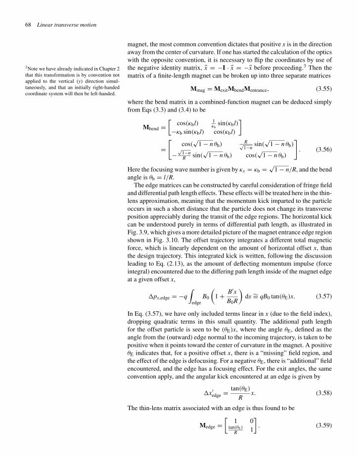
“chap03” — 2003/6/28 — page 68 — #17


magnet, the most common convention dictates that positive x is in the directionaway from the center of curvature. If one has started the calculation of the opticswith the opposite convention, it is necessary to flip the coordinates by use ofthe negative identity matrix, �x = −I · �x = −�x before proceeding.3 Then the3Note we have already indicated in Chapter 2

that this transformation is by convention notapplied to the vertical (y) direction simul-taneously, and that an initially right-handedcoordinate system will then be left-handed.

matrix of a finite-length magnet can be broken up into three separate matrices

Mmag = MexitMbendMentrance, (3.55)

where the bend matrix in a combined-function magnet can be deduced simplyfrom Eqs (3.3) and (3.4) to be

Mbend =[

cos(κbl) 1κb

sin(κbl)−κb sin(κbl) cos(κbl)

]

=[

cos(√

1 − n θb)R√1−n

sin(√

1 − n θb)

−√

1−nR sin(

√1 − n θb) cos(

√1 − n θb)

]. (3.56)

Here the focusing wave number is given by κx = κb = √1 − n/R, and the bend

angle is θb = l/R.The edge matrices can be constructed by careful consideration of fringe field

and differential path length effects. These effects will be treated here in the thin-lens approximation, meaning that the momentum kick imparted to the particleoccurs in such a short distance that the particle does not change its transverseposition appreciably during the transit of the edge regions. The horizontal kickcan be understood purely in terms of differential path length, as illustrated inFig. 3.9, which gives a more detailed picture of the magnet entrance edge regionshown in Fig. 3.10. The offset trajectory integrates a different total magneticforce, which is linearly dependent on the amount of horizontal offset x, thanthe design trajectory. This integrated kick is written, following the discussionleading to Eq. (2.13), as the amount of deflecting momentum impulse (forceintegral) encountered due to the differing path length inside of the magnet edgeat a given offset x,

�px,edge = −q∫

edgeB0

(1 + B′x

B0R

)ds ∼= qB0 tan(θE)x. (3.57)

In Eq. (3.57), we have only included terms linear in x (due to the field index),dropping quadratic terms in this small quantity. The additional path lengthfor the offset particle is seen to be (θE)x, where the angle θE, defined as theangle from the (outward) edge normal to the incoming trajectory, is taken to bepositive when it points toward the center of curvature in the magnet. A positiveθE indicates that, for a positive offset x, there is a “missing” field region, andthe effect of the edge is defocusing. For a negative θE, there is “additional” fieldencountered, and the edge has a focusing effect. For the exit angles, the sameconvention apply, and the angular kick encountered at an edge is given by

�x′edge = tan(θE)

Rx. (3.58)

The thin-lens matrix associated with an edge is thus found to be

Medge =[

1 0tan(θE)

R 1

]. (3.59)

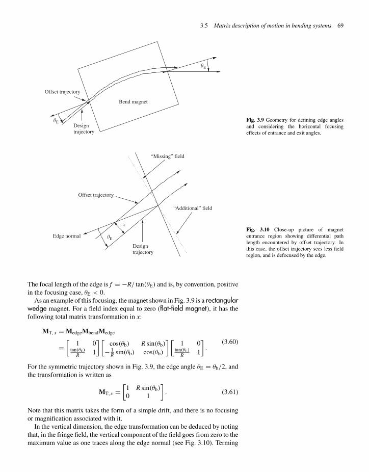
“chap03” — 2003/6/28 — page 69 — #18

3.5 Matrix description of motion in bending systems 69

Bend magnet

Designtrajectory

Offset trajectory

�E

�E Fig. 3.9 Geometry for defining edge anglesand considering the horizontal focusingeffects of entrance and exit angles.

�E

Designtrajectory

Offset trajectory

x

Edge normal

“Missing” field

“Additional” field

Fig. 3.10 Close-up picture of magnetentrance region showing differential pathlength encountered by offset trajectory. Inthis case, the offset trajectory sees less fieldregion, and is defocused by the edge.

The focal length of the edge is f = −R/ tan(θE) and is, by convention, positivein the focusing case, θE < 0.

As an example of this focusing, the magnet shown in Fig. 3.9 is a rectangularwedge magnet. For a field index equal to zero (flat-field magnet), it has thefollowing total matrix transformation in x:

MT, x = MedgeMbendMedge

=[

1 0tan(θE)

R 1

] [cos(θb) R sin(θb)

− 1R sin(θb) cos(θb)

] [1 0

tan(θE)R 1

].

(3.60)

For the symmetric trajectory shown in Fig. 3.9, the edge angle θE = θb/2, andthe transformation is written as

MT, x =[

1 R sin(θb)

0 1

]. (3.61)

Note that this matrix takes the form of a simple drift, and there is no focusingor magnification associated with it.

In the vertical dimension, the edge transformation can be deduced by notingthat, in the fringe field, the vertical component of the field goes from zero to themaximum value as one traces along the edge normal (see Fig. 3.10). Terming

“chap03” — 2003/6/28 — page 70 — #19


this coordinate ξ , we have ∂By/∂ξ = ∂Bξ /∂y �= 0 in the fringe region, and thusthe field lines have a component in the normal direction, Bξ = ∫ y

0 (∂Bξ /∂y) dy ∼=(∂By/∂ξ)y=0 y. If the particle enters the fringe field at a non-zero edge angle,θE, there is a component of Bξ normal to the trajectory, and we have a verticalforce, Fy = qv0 sin(θE)Bξ . This force is gives rise to an integrated angular kick,

�y′edge = − q

p0

∫edge

[Bξ sin(θE)] ds = − q

p0

∫edge

(∂By

∂ξ

)y=0

ysin(θE)

cos(θE)dz

= −qB0

p0tan(θE)y ∼= − tan(θE)

Ry. (3.62)

The vertical kick is equal in magnitude and opposite in sign to the horizontaledge kick.

For the rectangular, flat-field wedge magnet, the focusing lies entirely in thevertical dimension. The total vertical transformation matrix is written as

MT,y =[

1 0− tan(θE)

R 1

] [1 Rθb

0 1

] [1 0

− tan(θE)R 1

]

= 1 − θb tan

(θb2

)Rθb

− tan(

θb2

)R

[2 − θb tan

(θb2

)]1 − θb tan

(θb2

) . (3.63)

This magnet is focusing and has an effective focal length given by

1

fy= tan

(θb2

)R

[2 − θb tan

(θb

2

)]. (3.64)

The rectangular wedge magnet displays the opposite characteristics of the zero-edge angle case, which is termed a sector magnet. In this case, the edge matricesare ignorable, and MT, x = Mbend. The effective horizontal focal length is fx =R/ sin(θb), which for small angle θb � 1 gives the same value as Eq. (3.64).The vertical focusing is a small, but perhaps non-negligible effect in this case.It arises when the charged particle deflects noticeably in the fringe-field regionof the magnet (i.e. when the magnet gap is large). The calculation of this effectis left as an exercise to the reader.

3.6 Evolution of the momentum dispersionfunction

Now that we have essentially concluded our introductory discussion of betatronmotion, where we have been concerned with trajectories of particles possessingthe design momentum, but having offset and angular errors, we can pro-ceed to the discussion of the effects of momentum errors. To do this, wemust re-examine the momentum dispersion function, which was introduced inSection 2.2 and defined by the differential relation ηx = ∂x/∂[δp/p0]. Thisfunction allows us to write the horizontal (transverse, in bend-plane) first-order (in betatron and momentum error amplitude) offset as (see Eq. (2.14))x = xβ + ηx(δp/p0), with the betatron offset xβ being governed by the ana-lyses of Sections 3.1–3.5. If one needs to analyze a beam optics system withbends that do not lie all in one plane, it is also necessary to introduce a verticalmomentum dispersion function, so that y = yβ + ηy(δp/p0).

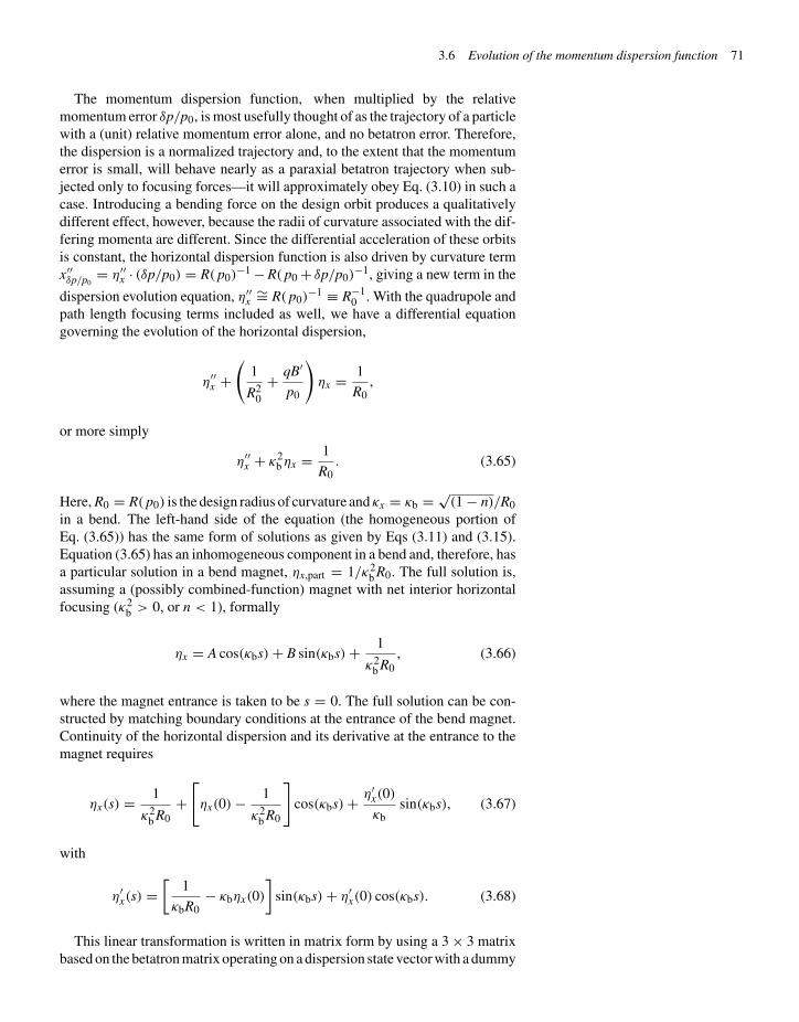
“chap03” — 2003/6/28 — page 71 — #20

3.6 Evolution of the momentum dispersion function 71

The momentum dispersion function, when multiplied by the relativemomentum error δp/p0, is most usefully thought of as the trajectory of a particlewith a (unit) relative momentum error alone, and no betatron error. Therefore,the dispersion is a normalized trajectory and, to the extent that the momentumerror is small, will behave nearly as a paraxial betatron trajectory when sub-jected only to focusing forces—it will approximately obey Eq. (3.10) in such acase. Introducing a bending force on the design orbit produces a qualitativelydifferent effect, however, because the radii of curvature associated with the dif-fering momenta are different. Since the differential acceleration of these orbitsis constant, the horizontal dispersion function is also driven by curvature termx′′δp/p0

= η′′x · (δp/p0) = R( p0)

−1 − R( p0 + δp/p0)−1, giving a new term in the

dispersion evolution equation, η′′x

∼= R( p0)−1 ≡ R−1

0 . With the quadrupole andpath length focusing terms included as well, we have a differential equationgoverning the evolution of the horizontal dispersion,

η′′x +

(1

R20

+ qB′

p0

)ηx = 1

R0,

or more simply

η′′x + κ2

b ηx = 1

R0. (3.65)

Here, R0 = R( p0) is the design radius of curvature and κx = κb = √(1 − n)/R0

in a bend. The left-hand side of the equation (the homogeneous portion ofEq. (3.65)) has the same form of solutions as given by Eqs (3.11) and (3.15).Equation (3.65) has an inhomogeneous component in a bend and, therefore, hasa particular solution in a bend magnet, ηx,part = 1/κ2

b R0. The full solution is,assuming a (possibly combined-function) magnet with net interior horizontalfocusing (κ2

b > 0, or n < 1), formally

ηx = A cos(κbs) + B sin(κbs) + 1

κ2b R0

, (3.66)

where the magnet entrance is taken to be s = 0. The full solution can be con-structed by matching boundary conditions at the entrance of the bend magnet.Continuity of the horizontal dispersion and its derivative at the entrance to themagnet requires

ηx(s) = 1

κ2b R0

+[ηx(0) − 1

κ2b R0

]cos(κbs) + η′

x(0)

κbsin(κbs), (3.67)

with

η′x(s) =

[1

κbR0− κbηx(0)

]sin(κbs) + η′

x(0) cos(κbs). (3.68)

This linear transformation is written in matrix form by using a 3 × 3 matrixbased on the betatron matrix operating on a dispersion state vector with a dummy

“chap03” — 2003/6/28 — page 72 — #21


third entry, that is,ηx(s)

η′x(s)1

=

cos(κbs) 1κb

sin(κbs) 1−cos(κbs)κ2

b R0

−κb sin(κbs) cos(κbs) sin(κbs)κbR0

0 0 1

×ηx(0)

η′x(0)

1

. (3.69)

For defocusing systems with κ2b < 0, it is straightforward to show that

ηx(s)

η′x(s)1

=

cosh(|κb|s) 1κb

sinh(|κb|s) − (1−cosh(|κb|s)|κ2

b |R0

sinh(|κb|sl) cosh(|κb|s) sinh(|κb|s)|κb|R0

0 0 1

×ηx(0)

η′x(0)

1

. (3.70)

The upper left hand 2 × 2 block in the transformation matrices of Eqs (3.69)and (3.70) are simply the betatron transformation matrices, M.

When the beam is in a straight section, R0 → ∞, and the upper two elementsof the third column vanish of the matrix—the third column and third row donot affect the horizontal dispersion or its derivative, as expected. It should benoted in this regard that, since edge matrices are of negligible length, there isno bending of the design orbit and the dispersion transformation matrices areconstructed just as in a straight section. That is, the upper left hand 2 × 2 blockin the transformation matrix is the thin-lens matrix, and the final column is(0,0,1).

As with betatron motion, convention dictates that positive ηx be defined in thedirection away from the center of curvature. If one has started the calculationof the optics with the opposite convention (for instance, when the direction of abend changes from one magnet to the next), it is again necessary to flip the signof ηx and η′

x before proceeding with the matrix calculation of the dispersionand its derivative. In matrix form, this procedure is written

ηx

η′x

1

new

=−1 0 0

0 −1 00 0 1

ηx

η′x

1

old

. (3.71)

For cases where the bending field changes continuously in space, it is notpossible to utilize the matrix-based approach to the solution of the dispersionevolution, and one must solve Eq. (3.65) in another manner. As an example ofthis type of scenario, we recall the case of the magnetic undulator introduced inSection 2.8. In this device, the undulating component of the motion was seento be

x = qB0

p0k2u

sin(kuz), (3.72)

from which we have the relation

∂x

∂p0= − qB0

p20k2

u

sin(kuz), (3.73)

“chap03” — 2003/6/28 — page 73 — #22

3.7 Longitudinal motion and momentum compaction 73

and

ηx = p0∂x

∂p0= − qB0

p20k2

u

sin(kuz) ≡ − au

β0γ0kusin(kuz). (3.74)

Here, we introduce the undulator parameter au ≡ qB0/kum0c, which we willsee (in Chapter 8) plays a central role in the operation of the free-electron laser.

3.7 Longitudinal motion and momentumcompaction

While this chapter is nominally only concerned with first-order transversemotion, in this section we open the door to considering the effects of momentumerrors on longitudinal motion by further discussing the effects of momentumdispersion. As we shall see below, momentum dispersion plays a critical rolein the first-order theory of longitudinal motion and, thus, in the interest of com-pleteness, we include a discussion of this dispersion-based effect. In particletransport systems, longitudinal motion in accelerators can be analyzed approx-imately using a Taylor series expansion of the motion in the relative longitudinalmomentum error. The point of the present analysis is to generate a longitud-inal equation analogous to the paraxial betatron equations of motion found inour treatment of transverse motion, for example, Eqs (3.5) and (3.6). In non-bending systems, this analogy is particularly close, because the paraxial betatronequations are also based on first-order expansion of the motion in transversemomentum errors. With bending systems, because of dispersion, the equationsof motion are slightly more complicated.

Since the independent variable has been taken to be distance along the designtrajectory (s or z), the canonical dependent coordinate in the longitudinal dir-ection is time t, which we then measure in Hamiltonian analyses relative tothe time of arrival of the design particle, τ = t − t0. The variable that playsthe role of the “momentum,” which is canonical to time “coordinate,” is theparticle’s mechanical energy. However, since we will begin our discussion oflongitudinal motion without employing Hamiltonians, and have invested mucheffort in the previous analyses based on momentum differences, we will con-tinue in this somewhat less rigorous way. To make the present analysis connectmore easily to Hamiltonian approaches, we will find it useful to introduce aparameterization of the time through a spatial variable, ζ = −v0τ . This is thedistance that must be traveled at the design velocity by the design particle, toreach the position of the temporally advanced (or delayed) particle.

The time of flight of an off-momentum particle to a point along the designorbit is given by

τ( p) = L( p)

v( p), (3.75)

where L(p) is the distance traveled by the particle as a function of its momentum.The first-order logarithmic expansion of this expression is, assuming theparaxial approximation,

δτ

t0= δL

L0− δvz

v0

∼=[αc − 1

γ 20

]δp

p0. (3.76)

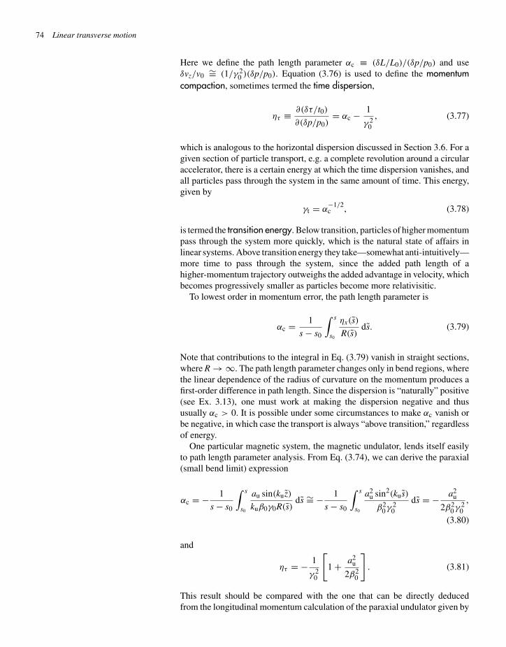
“chap03” — 2003/6/28 — page 74 — #23


Here we define the path length parameter αc ≡ (δL/L0)/(δp/p0) and useδvz/v0 ∼= (1/γ 2

0 )(δp/p0). Equation (3.76) is used to define the momentumcompaction, sometimes termed the time dispersion,

ητ ≡ ∂(δτ/t0)

∂(δp/p0)= αc − 1

γ 20

, (3.77)

which is analogous to the horizontal dispersion discussed in Section 3.6. For agiven section of particle transport, e.g. a complete revolution around a circularaccelerator, there is a certain energy at which the time dispersion vanishes, andall particles pass through the system in the same amount of time. This energy,given by

γt = α−1/2c , (3.78)

is termed the transition energy. Below transition, particles of higher momentumpass through the system more quickly, which is the natural state of affairs inlinear systems. Above transition energy they take—somewhat anti-intuitively—more time to pass through the system, since the added path length of ahigher-momentum trajectory outweighs the added advantage in velocity, whichbecomes progressively smaller as particles become more relativisitic.

To lowest order in momentum error, the path length parameter is

αc = 1

s − s0

∫ s

s0

ηx(s)

R(s)ds. (3.79)

Note that contributions to the integral in Eq. (3.79) vanish in straight sections,where R → ∞. The path length parameter changes only in bend regions, wherethe linear dependence of the radius of curvature on the momentum produces afirst-order difference in path length. Since the dispersion is “naturally” positive(see Ex. 3.13), one must work at making the dispersion negative and thususually αc > 0. It is possible under some circumstances to make αc vanish orbe negative, in which case the transport is always “above transition,” regardlessof energy.

One particular magnetic system, the magnetic undulator, lends itself easilyto path length parameter analysis. From Eq. (3.74), we can derive the paraxial(small bend limit) expression

αc = − 1

s − s0

∫ s

s0

au sin(kuz)

kuβ0γ0R(s)ds ∼= − 1

s − s0

∫ s

s0

a2u sin2(kus)

β20γ 2

0

ds = − a2u

2β20γ 2

0

,

(3.80)

and

ητ = − 1

γ 20

[1 + a2

u

2β20

]. (3.81)

This result should be compared with the one that can be directly deducedfrom the longitudinal momentum calculation of the paraxial undulator given by

“chap03” — 2003/6/28 — page 75 — #24

3.8 Linear transformations in six-dimensional phase space* 75

Eq. (2.75). In this limit we can write, with vz = pzc2/

√p2

0c2 + (m0c2)2,

ητ = − ∂vz

∂pz

p0

v0= −

[1

mγ 30

+(

qB0

2kup0

)2(

1 + β20

β20 (γ0mc)3

)]mγ0

∼= − 1

γ 20

[1 + a2

u

2

], (3.82)

in good agreement with Eq. (3.81).

3.8 Linear transformations in six-dimensionalphase space*

Previously in this chapter, we have introduced analyses of the motion basedon linear dependences of the dynamics on errors in the momenta in one phaseplane (actually, one trace space) at a time. In practice, as one needs to keep trackof the motion in the entire six-dimensional phase space at once when designingan actual accelerator, the 2 × 2 matrices that allow transformation of one two-entry trace space vector at a time is replaced by a 6 × 6 matrix that containsall three ((x, x′)( y, y′), (ζ , ζ ′)) trace space planes, plus additional information,the possible coupling between trace spaces. This generalized transport matrixtransforms the six-entry phase space vector �� ≡ (x, x′, y, y′, ζ , ζ ′), where forsymmetry we have changed our notation somewhat in writing the normalizedlongitudinal momentum error, ζ ′ = δpz/p0 ∼= δp0/p0. The standard form ofthis transformation is

��(s) ≡ R(s, s0) · ��(s0), (3.83)

where the 6 × 6 R(s, s0) matrix is specified to transform the ��-vector from oneposition in the beamline s0 to another s. The matrix R(s, s0) is formally written

R(s, s0) =

∂xf∂xi

∂xf∂x′

i

∂xf∂yi

∂xf∂y′

i

∂xf∂ζi

∂xf∂ζ ′

i∂x′

f∂xi

∂x′f

∂x′i

∂x′f

∂yi

∂x′f

∂y′i

∂x′f

∂ζi

∂x′f

∂ζ ′i

∂yf

∂xi

∂yf

∂x′i

∂yf

∂yi

∂yf

∂y′i

∂yf

∂ζi

∂yf

∂ζ ′i0

∂y′f

∂xi

∂y′f

∂x′i

∂y′f

∂yi

∂y′f

∂y′i

∂y′f

∂ζi

∂y′f

∂ζ ′i

∂ζf

∂xi

∂ζf

∂x′i

∂ζf

∂yi

∂ζf

∂y′i

∂ζf

∂ζi

∂ζf

∂ζ ′i

∂ζ ′f

∂xi

∂ζ ′f

∂x′i

∂ζ ′f

∂yi

∂ζ ′f

∂y′i

∂ζ ′f

∂ζi

∂ζ ′f

∂ζ ′i

,

(3.84)

where the subscript i indicates the initial value of the vector element at s0, andthe subscript f indicates its final value at s. Equations (3.83) and (3.84) explicitlygive the final state phase space vector components in terms of their first-orderdependences on the initial phase space vector components, e.g.

xf = ∂xf

∂xixi + ∂xf

∂x′ix′

i + ∂xf

∂yiyi + ∂xf

∂y′iy′

i + ∂xf

∂ζiζi + ∂xf

∂ζ ′iζ ′

i . (3.85)

With this form in mind, it is possible to identify the components of R(s, s0)

in terms of familiar quantities. The upper left diagonal 2 × 2 block in R(s, s0)

“chap03” — 2003/6/28 — page 76 — #25


is the horizontal betatron transformation matrix; the middle diagonal 2 × 2block is the vertical betatron transformation matrix; the lower right diagonal2 × 2 block is the longitudinal linear transformation matrix (which will bemore familiar when we study acceleration in Chapter 4). Other matrix elementsoutside of these blocks have also been previously discussed—for example R16

and R26 are ηx and η′x, respectively, and R56 is −ητ�s. Matrix elements linking

the initial and final x and y phase planes would be non-zero if the planes arecoupled, as happens in the solenoid, where the Larmor rotation completelymixes the upper left 4 × 4 diagonal block (cf. Ex. 3.20).

The 6 × 6 transport matrix R(s, s0) has much in common with its2 × 2 diagonal blocks. For instance, in the absence of acceleration, it has unitdeterminant, which is a manifestation of Liouville’s theorem concerning phasespace density. The 6 × 6 transport matrix transformation of the ��-vector isused in most of the computer codes employed for accelerator beam dynamicscalculations.


This chapter began with a discussion that deepened the introductory remarksmade on betatron oscillations in Chapter 2, introducing the notion of weakfocusing in circular accelerators. In such a scheme, one can have simultaneousstability in both vertical and horizontal transverse dimensions.

In order to circumvent the natural scaling of weak focusing, strong focus-ing based on periodic arrays of focusing and defocusing (alternating gradient)quadrupoles has been introduced. The piece-wise periodic focusing arising fromthese arrays is analyzed by powerful matrix methods. These methods, along withthe stroboscopic Poincaré trace space-mapping visualization tool, have beenexplored in detail in this chapter. An alternative approach to understanding peri-odic focusing, which employs a perturbative analytical technique, has allowedus to identify alternating gradient focusing as a type of ponderomotive focusing.

Periodic focusing naturally arises in the context of circular machines, sowe, of necessity, examined strong focusing effects, using matrix techniques, inbending systems. The bending of the design trajectory also introduces a newclass of paraxial trajectory error—momentum dispersion. This phenomenonwas also treated in this chapter by use of matrix methods.

Momentum dispersion couples the longitudinal phase plane with the trans-verse phase plane, by causing trajectory errors in the bend plane. Likewise,these trajectory errors can also affect the longitudinal motion of a particle, bychanging its path length through a section of beamline. We have analyzed thecompetition between this effect and the change in the velocity of the particleon the time-of-flight through the system. The results we have obtained will beneeded in Chapters 4 and 5 when we discuss longitudinal motion in circularaccelerators.

Trace (or phase) planes are, in general, coupled by effects like dispersionand rotation (e.g. in solenoids). Thus, we ended this chapter by introducing thegeneral six-dimensional square matrix description of the six-dimensional phasespace dynamics of a charged particle.

The material in this chapter contains the core concepts of charged particletransverse optics. As such, many other texts in accelerator physics also treat

“chap03” — 2003/6/28 — page 77 — #26

Exercises 77

the subjects we have introduced here. There is a wide variety of approaches todiscussing linear transverse motion and many levels at which the discussion isgiven in other books. The following texts may be recommended as a supplementto this chapter:

1. P. Dahl, Introduction to Electron and Ion Optics (Academic Press, 1973).A primer on optics.

2. D.C. Carey, The Optics of Charged Particle Beams (Harwood AcademicPublishers, 1987). A complete treatment of transverse charged particlemotion, including an excellent treatment of higher-order (nonlinear)forces.

3. D. Edwards and M. Syphers, An Introduction to the Physics of High EnergyAccelerators (Wiley, 1993).

4. H. Wiedemann, Particle Accelerator Physics I: Basic Principles and Lin-ear Beam Dynamics (Springer-Verlag, 1993). The rigor of the presentationin this text should be helpful in clarifying issues arising from our lessformal presentation.

5. S.Y. Lee, Accelerator Physics (World Scientific, 1996).

A number of texts may be used as an introduction to advanced topics intransverse beam dynamics:

6. M. Reiser, Theory and Design of Charged Particle Beams. This is anencyclopedic reference on transverse motion in beams, with and withoutcollective effects.

7. M. Berz, Modern Map Methods in Particle Beam Physics. Rigorous treat-ment of modern analytical methods for study of linear and nonlinear beamdynamics. Written at the graduate-to-professional level.

8. H. Wiedemann, Particle Accelerator Physics II: Nonlinear and Higher-order Beam Dynamics (Springer-Verlag, 1999). Advanced topics innonlinear dynamics, using the first volume in the series as a basis. Writtenat the graduate-to-professional level.

Exercises

(3.1) As will be discussed in detail in a following chapter, thesurfaces of the iron in a ferromagnet are roughly mag-netic equipotentials. Given this fact, what mathematicalform should a combined-function magnet surface like thatshown in Fig. 3.1 have to support a combination of dipoleand quadrupole fields?

(3.2) Assuming a mechanism for equipartion of energy, andthus temperature equilibrium, between phase planes, sothat the root-mean-square (rms) angle x′

rms = √〈x′2〉 =√kT/m0c2/βγ = y′

rms, what field index n should one useto guarantee that the beam sizes in a betatron obey xrms =2yrms? You can use xrms = Rx′

rms/νx , yrms = Ry′rms/νy.

(3.3) Explain, in terms of the transverse velocity componentsof the motion, why the oscillator strength associated withbetatron oscillations in solenoids is of second-order, eventhough the force on the particle is first order in the fieldamplitude.

(3.4) Consider a thin-lens system in which there is a repetitiveapplication of a focusing lens with focal length f , eachseparated by a drift of length L.

(a) What is the total transformation matrix correspond-ing to one period of the system in this case?

(b) What is the relationship between f and L thatguarantees linear stability of the transformation?

“chap03” — 2003/6/28 — page 78 — #27


(3.5) To prove that the trace of a matrix M1 is the same as thatof another matrix M2, it is sufficient to show that the twomatrices are related by a similarity transformation,

M1 = A−1M2A,

where A is a matrix of unit determinant. Show that any twomatrices representing a periodic focusing system M1 andM2, corresponding to two different choices of z0(z0,1 andz0,2), are related by such a transformation. Hint: examinematrix A, which is the transformation matrix (M) fromz0,1 to z0,2.

(3.6) Consider a charged particle transport system, createdby two thick lenses of length l, with opposite focusingstrengths κ2

0 and −κ20 , so that the matrix mapping for the

focusing and defocusing lenses are

MF =[

cos(κ0l) (1/κ0) sin(κ0l)−κ sin(κ0l) cos(κ0l)

]

and

MD =[

cosh(κ0l) (1/κ0) sinh(κ0l)κ0 sinh(κ0l) cosh(κ0l)

],

respectively. These two lenses are applied repetitively sothat the transformation of the coordinate vector at the nthstep �x = ( x

x′)

is �xn+1 = MF · MD · �xn.

(a) What is the phase advance per period of theoscillation as a function of κ0l?

(b) Like the case of a thin-lens-based system, whenκ2

0 becomes large enough the transformation isunstable. Unlike the thin-lens case, other regionsof stability are encountered when κ2

0 is raised even.Plot a trajectory from the second stability region(the one encountered after the first unstable region).Hint: It is easy to construct this plot from thepiece-wise solutions to the motion if you start withconditions �x = (xi

0

)at the middle of one of the

lenses. Can you tell from this trajectory why thesecond stability region exists for the alternatingthick lens, but not the alternating thin-lens system?

(3.7) Consider a thin-lens system in which there is a repetitiveapplication of a focusing lens with focal length f1 and defo-cusing lens with focal length −f2, each separated by a driftof length L. Let us examine what happens if f1 �= f2:

(a) What is the total transformation matrix correspond-ing to one period of the system?

(b) Sketch out the region of stability in the parametersf1 and f2. This is best accomplished by drawingthe borders of stability on a two-dimensional plotwhere the axes are f1/L and f2/L.

(3.8) The Wronskian determinant (or simply, the Wronskian)of a linear second-order differential equation

x′′ + v(z)x′ + w(z)x = 0

can be formed as the product of the two linearly inde-pendent solutions of the equation x1 and x2, and their firstderivatives,

W(z) ≡ x1(z)x′2(z) − x′

1(z)x2(z).

(a) Derive the differential equation governing theWronskian,

W ′(z) + v(z)W(z) = 0.

For v(z) = 0, this clearly implies that theWronskian is constant. This constant is determinedin the (simple harmonic oscillator) example ofconstant w(z), in which case one has W = 1.

(b) Show that the solution to the Wronskian differentialequation is

W(z) = W(0) exp

[−

∫ z

0v(z) dz

].

For the damped oscillator equation describingbetatron oscillations during acceleration in a solen-oid (Eq. (2.56)), show that the Wronskian dampsalong with the trace space area, that is, W(z) =βγ (0)/βγ (z).

(3.9) Construct a Poincaré plot of a FODO lattice with a phaseadvance per period equal to 50◦. Verify that the plot pro-duces an ellipse aligned to the (x, x′) axes if one beginsthe matrix construction in the middle of either the focus-ing or defocusing lenses. This requires that the thin-lensmatrix of one of the lenses be split into two equal thin-lensmatrices with twice the focal length.

(3.10) Consider the smooth approximation applied to a FODOlattice. Find the value of k2

sec in the limit that µ � 1. Howdoes this result compare to that of Eq. (3.36)?

(3.11) Consider a charged particle transport system created bytwo repetitively applied thin lenses with opposite focallengths f and −f , separated by a distance Ld.

(a) Using matrix analysis, obtain the phase advanceper period µ. In order to compare this result topart (b), expand Eq. (3.31) for small µ.

(b) Now using the harmonic analysis of Section 3.4,find the value of µ predicted for this system. Inorder to do this, you should take the periodicfocusing to be given by

κ2(z) = −1

fδ

(z − Lp

4

)+ 1

fδ

(z − 3Lp

4

),

where Lp = 2Ld is the period of the system.Compare to the result of part (a).

“chap03” — 2003/6/28 — page 79 — #28

Exercises 79

(3.12) Consider a so-called FOFO particle focusing systemcreated by periodic application of a thick lens of length lwith focusing strength κ2

0 , followed by a drift of length l.

(a) Using matrix methods, find the phase advance perperiod µ as a function of κ0 and l.

(b) If κ0l � 1, find from the matrix result an approx-imate expression for the smooth approximationfocusing strength k2

sec in this case. Hint: the approx-imate extraction of µ2 ∼= 4k2

secl2 from the matrixcalculation must include all terms up to fourth orderin κ0 and second-order in µ2.

(c) Now consider the analysis of this system as thesuperposition of harmonic (sine) components infocusing strength. Write the Fourier decompositionof the focusing strength.

(d) What is the average secular focusing strength ofthis system? Hint: this system is a superposition ofa uniform focusing system of strength κ2

0 /2, andthe FD system analyzed at the end of Section 3.4,also with half-strength ±κ2

0 /2.(e) Compare the results of parts (b) and (d). (You

should obtain near agreement by using the expan-sion of 〈κ2〉 found in Eq. (3.49) up to fourth orderin κ0 and exact agreement if you sum the entireseries in Eq. (3.49).)

(3.13) An ultra-relativistic charged particle accelerates uni-formly under the influence of a longitudinal electric field�E = E0 z. It is also confined by a sinusoidally varyinggradient focusing quadrupole channel, mathematicallystated as B′(z) = B′

0 sin(kpz).

(a) Using the approximation β ∼= 1 and assuming thatthe energy γ m0c2 does not appreciably change overa period of the focusing, find an expression for thesecular focusing strength.

(b) Write the transverse equation of motion á laEq. (2.57) and solve.

(3.14) A common type of spectrometer magnet is shown inFig. 3.11. The particles emitted from the point sourceare dispersed in momentum by the differences in radiusof curvature. The momenta are well determined at thehorizontal focus after the final drift B.

(a) What is the final edge angle as a function of thebend angle θb? Hint: refer to Fig. 2.6 to see therelation between θb and the pole edge orientation.

(b) Write the horizontal matrix transformation includ-ing the drifts A and B.

(c) Determine the length B that yields a point-to-pointhorizontal focus as a function of R, θb, and A. Asone changes R, what curve do these focal pointsdescribe?

MagnetpoleDesign

orbit

Angular error orbits

R

A

B

�b

Fig. 3.11 Flat field spectrometer magnet, showing outline ofpole, and focal properties.

(3.15) In the smooth approximation, one may assign the focus-ing in an entire strong focusing circular accelerator to beproportional to the tune, ksec, x = νx/R0. In this case,the dispersion may also have an average value—deducedfrom the particular solution to Eq. (3.65). Find this valuefor the Tevatron at Fermilab, in which νx = 19.4, and theaverage radius of curvature is R0 = 1 km.

(3.16) The flat-field spectrometer magnet discussed in Exer-cise 3.14 has interesting dispersive properties that aredisplayed schematically in Fig. 3.12.

(a) Show that, in the region after the magnet, themomentum dispersion is constant, η′

x = 0.(b) Find the value of ηx in this region as function of θb

and R0.

Magnetpole Design

orbit

R0

B

�b

A

Off-momentumtrajectory

Fig. 3.12 Flat field spectrometer magnet of Fig. 3.11, showingdispersive properties.

(3.17) Evaluate αc for the spectrometer magnet in Exercise 3.14.

(3.18) A transport line that translates the beam to the side whileallowing the dispersion and its derivative to vanish at thesecond bend exit can be constructed by the deploymentof magnets shown in Fig. 3.13. In this case it can be seenthat the dispersion vanishes at the mid-point between thebend magnets.

“chap03” — 2003/6/28 — page 80 — #29


Sector magnets

Focusing lenses

Off-momentum trajectory

a

s = R�

s = R�a

2b

Fig. 3.13 Schematic of side-translating beamline with no resid-ual dispersion at exit.

(a) Derive the focal length associated with the focus-ing lenses that gives this behavior of the dispersionas a function of a, b, R, and θ . Hint: it is best tonormalize all lengths in the problem to the radiusof curvature in the dipoles, R.

(b) Evaluate αc for this transport system. Rememberthat even though the dispersion function changessign in between the bend magnets, the conventionof the sign of the dispersion in the second bend,with opposing sign radius of curvature, must alsochange. If you do not take this into account, αc willvanish, which is clearly not true, as indicated by theabove picture.

(3.19) A common magnet configuration used to rearrangeparticles longitudinally is the so-called chicane, as shownbelow in Fig. 3.14. It has flat-field dipoles of magnetic fieldinto and out of the viewed plane, as indicated. Note that itis similar to one period of an undulator magnet, but witha large bend angle (not small compared to unity).

The chicane consists of four bend magnets of equalstrength and size so that, for the design energy, R and θ

are the same in each. The first bends out an angle θ , thesecond and third bend in by −θ , and the fourth bends outagain by θ .

+ – – +

R Chicane magnet array�

Fig. 3.14 Chicane magnet array, with design trajectory.

(a) Find the total matrix transformation in x and y. Thisexercise should illustrate that this array of magnetsis equivalent to a drift in x and is focusing in y.

(b) Find the dispersion everywhere inside of the mag-nets. The quantities ηx and η′

x should disappear atthe end of the fourth magnet.

(c) Find the momentum compaction αc = 1/s − s0×∫ ss0

ηx(s)/R(s) ds in this device.(d) For an electron initially trailing the 20 MeV design

electron by 1 psec, chicane magnets with R =0.5 m and θ = 30◦, what must its momentum off-set δp be for it to catch up to the design particle atthe chicane exit?

(3.20) Write the R(s, s0) matrix describing full passage of aparaxial particle through a solenoid magnet. Hint: writethe matrix as the product of three matrices—an entrancematrix that projects the initial conditions into the Larmorframe, a simple harmonic Larmor oscillation matrix(decoupled in xL and yL phase planes), and an exit matrixthat projects the final Larmor (rotated by the Larmor anglein the x–y plane) conditions back into the x and y phaseplanes.

“chap04” — 2003/6/28 — page 81 — #1

Acceleration andlongitudinal motion 4

4.1 Acceleration in periodicelectromagneticstructures 81

4.2 Linear acceleration intraveling waves 83

4.3 Violently acceleratingsystems 86

4.4 Gentle acceleratingsystems 87

4.5 Adiabatic capture 90

4.6 The moving bucket 93

4.7 Acceleration incircular machines:the synchrotron 95

4.8 First-order transverseeffects ofaccelerating fields* 99

4.9 Second-order transversefocusing in electromagneticaccelerating fields* 102


Exercises 107

Now that we have surveyed the basic concepts of linear transverse motion incharged particle optics systems, it is time to turn our attention to the problemof acceleration. This chapter begins with an introduction to acceleration due toconfined electromagnetic waves, as a way of introducing the physics of radio-frequency linear accelerators (rf linacs). Within this context, it is possible tostudy both the strong acceleration typical of electron linear accelerators, and thecomparatively gentle acceleration found in ion linacs. Once the fundamentalways of analyzing linear acceleration and related longitudinal (along the dir-ection of beam propagation) dynamics processes are discussed, these methodsare extended to allow an understanding of longitudinal motion in the circularaccelerator based on rf acceleration, the synchrotron. We end this chapter on acomplementary note to the last sections of Chapter 3—we examine the possibleeffects of the acceleration process on transverse motion.

4.1 Acceleration in periodicelectromagnetic structures

As will be discussed further in Chapter 7, in free space, the solutions to theelectromagnetic wave equation are transversely polarized waves (the electricfield is transverse to the propagation vector) that have phase velocity c, thespeed of light. These properties are problematic from the viewpoint of chargedparticle acceleration, because in order for a charged particle to absorb energyfrom an applied electric force, the motion of the charged particle must havea component parallel to the electric field. This statement is quantified by theexpression that gives the time-rate-of-change of the particle energy,

dU

dt= q(�v · �E). (4.1)

In all of the cases we consider in this chapter, the motion of the particle in anaccelerating wave will be rectilinear in the z-direction, and thus the electric fieldmust be rotated to have a longitudinal component in order for acceleration tooccur. This can be accomplished by using a smooth-walled waveguide, in whichcase we note the existence of the familiar transverse magnetic (TM) modes.1 1If TEM modes are not familiar, please see

the discussion of electromagnetic modes inwaveguides given in Section 7.3.

These modes have a longitudinal electric field, but have phase velocity largerthan c, and thus cannot remain phase synchronous with a charged particle whosevelocity must always be less than c. This means that in order to allow a travelingwave to stay in a nearly constant phase relationship with an accelerating particle,

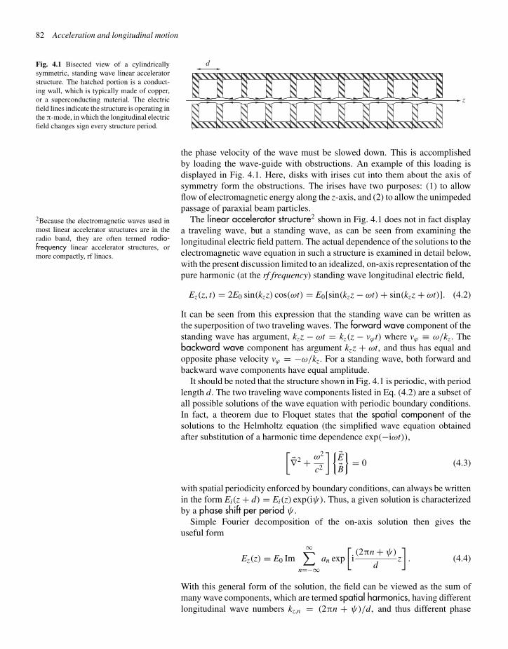
“chap04” — 2003/7/2 — page 82 — #2

82 Acceleration and longitudinal motion

Fig. 4.1 Bisected view of a cylindricallysymmetric, standing wave linear acceleratorstructure. The hatched portion is a conduct-ing wall, which is typically made of copper,or a superconducting material. The electricfield lines indicate the structure is operating inthe π-mode, in which the longitudinal electricfield changes sign every structure period.

z

d

the phase velocity of the wave must be slowed down. This is accomplishedby loading the wave-guide with obstructions. An example of this loading isdisplayed in Fig. 4.1. Here, disks with irises cut into them about the axis ofsymmetry form the obstructions. The irises have two purposes: (1) to allowflow of electromagnetic energy along the z-axis, and (2) to allow the unimpededpassage of paraxial beam particles.

The linear accelerator structure2 shown in Fig. 4.1 does not in fact display2Because the electromagnetic waves used inmost linear accelerator structures are in theradio band, they are often termed radio-frequency linear accelerator structures, ormore compactly, rf linacs.

a traveling wave, but a standing wave, as can be seen from examining thelongitudinal electric field pattern. The actual dependence of the solutions to theelectromagnetic wave equation in such a structure is examined in detail below,with the present discussion limited to an idealized, on-axis representation of thepure harmonic (at the rf frequency) standing wave longitudinal electric field,

Ez(z, t) = 2E0 sin(kzz) cos(ωt) = E0[sin(kzz − ωt)+ sin(kzz + ωt)]. (4.2)

It can be seen from this expression that the standing wave can be written asthe superposition of two traveling waves. The forward wave component of thestanding wave has argument, kzz − ωt = kz(z − vϕ t) where vϕ ≡ ω/kz. Thebackward wave component has argument kzz + ωt, and thus has equal andopposite phase velocity vϕ = −ω/kz. For a standing wave, both forward andbackward wave components have equal amplitude.

It should be noted that the structure shown in Fig. 4.1 is periodic, with periodlength d. The two traveling wave components listed in Eq. (4.2) are a subset ofall possible solutions of the wave equation with periodic boundary conditions.In fact, a theorem due to Floquet states that the spatial component of thesolutions to the Helmholtz equation (the simplified wave equation obtainedafter substitution of a harmonic time dependence exp(−iωt)),

[�∇2 + ω2

c2

] {�E�B}

= 0 (4.3)

with spatial periodicity enforced by boundary conditions, can always be writtenin the form Ei(z + d) = Ei(z) exp(iψ). Thus, a given solution is characterizedby a phase shift per period ψ .

Simple Fourier decomposition of the on-axis solution then gives theuseful form

Ez(z) = E0 Im∞∑

n=−∞an exp

[i(2πn + ψ)

dz

]. (4.4)

With this general form of the solution, the field can be viewed as the sum ofmany wave components, which are termed spatial harmonics, having differentlongitudinal wave numbers kz,n = (2πn + ψ)/d, and thus different phase

“chap04” — 2003/6/28 — page 83 — #3

4.2 Linear acceleration in traveling waves 83

velocities vϕ,n = ω/kz,n. A pure traveling wave solution has only one non-vanishing amplitude coefficient an, whereas a pure standing wave solution hastwo non-vanishing an. In general, in order to have the full solution obey theconducting boundary conditions, all of the components of the Floquet expansionin Eq. (4.4) must be considered. To settle on a normalization convention, willtake a0 = 1 in this text, so that the average accelerating field at the optimalphase in the wave will always be E0.

The structure shown in Fig. 4.1 illustrates the concept of the phase shiftper period well, as it clearly shows a field reversal every period, indicatingψ = π. This is the so π-called-mode, which is a common field configurationfor standing wave accelerators. For a pure harmonic standing wave field, wehave a−1 = −1 and a0 = 1, with all other components vanishing.

If we now consider a charged particle traveling on-axis through an acceleratorstructure at approximately constant velocity vz ∼= vϕ,0 = ω/kz,0, and integrateEq. (4.1) through an integer number of periods M, we obtain an energy gaindue to each spatial harmonic of the field,

�U ={

qE0Md sin(ϕ), n = 0

0, n �= 0.(4.5)

In Eq. (4.5) we have introduced ϕ, the phase of the particle with respect tothe n = 0 wave crest. The n = 0 component is termed the fundamentalspatial harmonic. Because it travels in this case at approximately the samevelocity as the particle (we have ignored the fact that the velocity may changeslightly during the acceleration over the integration interval), it is also termed thesynchronous wave. All other non-synchronous components do not contributein this constant-velocity approximation to the secular (averaged over a period)acceleration occurring over lengths greater than a period of the structure.

What this discussion illustrates is that, for cases where the velocity doesnot change appreciably during a period of the structure, in calculating energygain, all components of the electric field may be neglected except the syn-chronous wave. In fact, even in cases where the particle changes velocitydramatically during passage through a structure, one finds that consideration ofa dominant synchronous component is enough to describe the long-term secu-lar acceleration of the particle. Any notable effects that are due to backward orother non-synchronous components are therefore typically localized to a regionsmaller than a structure period.

4.2 Linear acceleration in traveling waves

We begin our analysis of acceleration in traveling wave structures by adopt-ing a Hamiltonian approach. To construct the Hamiltonian, we note that thelongitudinal electric field associated with a single traveling wave in an acceler-ating structure can be derived from a vector potential with only a longitudinalcomponent,3

3We have at this point decided on a phase con-vention in our description of the sinusoidaltraveling wave. There are of course other pos-sible conventions which are followed in otheranalyses (we could have used, e.g. a cosine),but since we need to discuss such a wide arrayof physical scenarios, and since stable motionwill occur at different phases depending onwhich scenario is discussed, we will stay withthis convention throughout our analysis.

Az(z − vφ t) = − E0

kzvφcos[kz(z − vφ t)], (4.6)

as

Ez(z − vφ t) = −∂Az

∂t= E0 sin[kz(z − vφ t)]. (4.7)

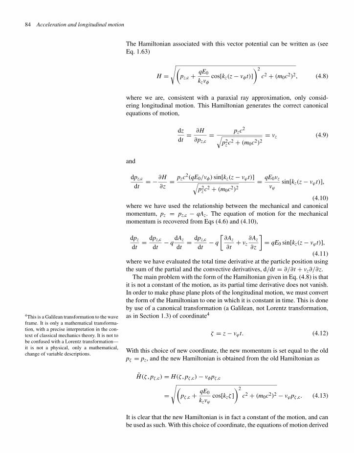
“chap04” — 2003/6/28 — page 84 — #4


The Hamiltonian associated with this vector potential can be written as (seeEq. 1.63)

H =√(

pz,c + qE0

kzvφcos[kz(z − vφ t)]

)2

c2 + (m0c2)2, (4.8)

where we are, consistent with a paraxial ray approximation, only consid-ering longitudinal motion. This Hamiltonian generates the correct canonicalequations of motion,

dz

dt= ∂H

∂pz,c= pzc2√

p2z c2 + (m0c2)2

= vz (4.9)

and

dpz,c

dt= −∂H

∂z= pzc2(qE0/vφ) sin[kz(z − vϕ t)]√

p2z c2 + (m0c2)2

= qE0vz

vϕsin[kz(z − vϕ t)],

(4.10)where we have used the relationship between the mechanical and canonicalmomentum, pz = pz,c − qAz. The equation of motion for the mechanicalmomentum is recovered from Eqs (4.6) and (4.10),

dpz

dt= dpz,c

dt− q

dAz

dt= dpz,c

dt− q

[∂Az

∂t+ vz

∂Az

∂z

]= qE0 sin[kz(z − vϕ t)],

(4.11)where we have evaluated the total time derivative at the particle position usingthe sum of the partial and the convective derivatives, d/dt = ∂/∂t + vz∂/∂z.

The main problem with the form of the Hamiltonian given in Eq. (4.8) is thatit is not a constant of the motion, as its partial time derivative does not vanish.In order to make phase plane plots of the longitudinal motion, we must convertthe form of the Hamiltonian to one in which it is constant in time. This is doneby use of a canonical transformation (a Galilean, not Lorentz transformation,as in Section 1.3) of coordinate44This is a Galilean transformation to the wave

frame. It is only a mathematical transforma-tion, with a precise interpretation in the con-text of classical mechanics theory. It is not tobe confused with a Lorentz transformation—it is not a physical, only a mathematical,change of variable descriptions.

ζ = z − vϕ t. (4.12)

With this choice of new coordinate, the new momentum is set equal to the oldpζ = pz, and the new Hamiltonian is obtained from the old Hamiltonian as

H(ζ , pζ ,c) = H(ζ , pζ ,c)− vφpζ ,c

=√(

pζ ,c + qE0

kzvϕcos[kzζ ]

)2

c2 + (m0c2)2 − vϕpζ ,c. (4.13)

It is clear that the new Hamiltonian is in fact a constant of the motion, and canbe used as such. With this choice of coordinate, the equations of motion derived

“chap04” — 2003/6/28 — page 85 — #5

4.2 Linear acceleration in traveling waves 85

from the new Hamiltonian are thus

dζ

dt= ∂H

∂pζ ,c= pζ ,c + (qE0/kzvϕ)cos[kzζ ]

γm0− vϕ = pζ

γm0− vϕ = vz − vϕ ,

(4.14)and

dpζ ,c

dt= −∂H

∂ζ= qE0vz

vϕsin[kz(ζ )], (4.15)

or, writing Eq. (4.15) in terms of the mechanical momentum,

dpζdt

= qE0 sin[kzζ ]. (4.16)

As can be seen from this short discussion, use of canonical variables is abit trickier in this case than use of familiar mechanical variables. Because wehave concluded the formal discussion of the Hamiltonian, however, we cannow revert to the mechanical description, to write the constant of the motionfunctionally as

H(ζ , pζ ) =√

p2ζ c2 + (m0c2)2 − vϕpζ + qE0

kzcos[kzζ ]. (4.17)

This form of the Hamiltonian could even be used (with less than perfect rigor!)to generate equations of motion, even though it is nominally not written interms of the canonical momentum. In fact, the mechanical momentum in thistime-independent case can effectively be treated as if it were canonical, sincethe form of Eq. (4.17) is identical to that which would be derived from anelectrostatic potential giving the same acceleration as Eq. (4.16).

Since we have already derived the correct equations of motion in Eqs (4.13)–(4.16), the more important use of Eq. (4.17) is that it can be used to visualizethe motion of charged particles in the longitudinal phase plane (ζ , pζ ). Beforewe move into discussion of specific examples of such motion, let us note thatEq. (4.17) can be written in normalized form as

H

m0c2=√(βzγ )2 + 1 − βφβzγ + αrf cos[kzζ ]. (4.18)

In Eq. (4.18), the quantity

αrf ≡ qE0

kzm0c2= γ ′

max

kz(4.19)

is defined as the ratio of the maximum spatial rate of change of the normalizedparticle energy (Lorentz factor γ ), to the maximum rate spatial rate of changeof the particle’s phase in the wave.

It will be seen below that the type of behavior one observes in particle accel-eration by a traveling wave can be divided into two distinct regimes. The firstoccurs when αrf � 1, and is typically encountered in heavy particle (proton orion) linacs, in which the acceleration is very gentle. The second regime occurswhen αrf is of order unity, or above. This is the regime of violent acceleration,which occurs in electron linacs. The physics of violent acceleration is discussedin the next section.

“chap04” — 2003/6/28 — page 86 — #6


4.3 Violently accelerating systems

The case of αrf ≥ 1 corresponds to an accelerating wave in which the particlecan gain more than one unit of rest energy by remaining in synchronism withthe wave for a radian or less of spatial propagation, kz�z ≤ 1. This is a violentacceleration scenario, in the sense that a particle can be picked up from restand accelerated to relativistic velocities in less than one wave cycle, thus beingcaptured by the wave. As illustrated by the examples given in Exercise 4.2,this type of acceleration in practice can only be achieved by use of the lightestcharged particle, the electron (or its antiparticle, the positron). In analyzingthis system, we make use of the approximation that the phase velocity of thewave reaches its ultra-relativistic limit, vϕ → c. We adopt this approximationprecisely because the acceleration in this case is violent, and thus the chargedparticles are expected to asymptotically (actually, within a few rf wavelengths)attain ultra-relativistic velocities. If the vϕ is chosen to be noticeably less thanc, the particles can accelerate past this phase velocity, and eventually outrunthe wave to the point where they may enter a decelerating phase.

In the approximation vϕ = c, we may write the mechanical version of theHamiltonian relation, Eq. (4.17), simply as

H(ζ , pζ ) = m0c2[γ −βzγ +αrf cos[kzζ ]] = m0c2

[√1 − βz

1 + βz+ αrf cos[kzζ ]

].

(4.20)This form of the Hamiltonian allows us to both perform rudimentary analysis,and also to draw modified phase plane plots to illustrate the dynamics of theacceleration process. An example of such a plot is shown in Fig. (4.2), in whichthe momentum axis is parameterized by

χ = m0c2

U − pzc=√

1 + βz

1 − βz, (4.21)

in order to have a positive quantity displayable in a semi-log plot. The verticalaxis chosen to be logarithmic in order to show the large changes in momentumas the particle becomes relativistic.

Figure 4.2, which illustrates a number of curves of constant H, shows sev-eral interesting aspects of the longitudinal motion. The first is that for the

Fig. 4.2 Modified longitudinal phase planeplot, with αrf = 1.

10–1

100

101

102

103

104

–0.4 –0.2 0.0 0.2 0.4

kz�/2�

�

“chap04” — 2003/6/28 — page 87 — #7

4.4 Gentle accelerating systems 87

case shown (αrf = 1), particles initially at rest (χ = 1) can, for certaininitial phases in the wave ϕ0 = kzζ0, be accelerated to very high energy(χ � 1). In addition, at high energy the phase the particle occupies in thewave is approximately stationary,

H = m0c2[χ−1 + αrf cos[kzζ ]] ⇒ αrf m0c2 cos[kzζ ] = αrf m0c2 cos(ϕf).(4.22)

Since the Hamiltonian is a constant of the motion, as χ−1 ⇒ 0 the phase of theparticle in the wave asymptotically approaches ϕf . There is no notable furtherslippage of the particle in the wave as it becomes ultra-relativistic, (that is asits velocity approaches the wave phase velocity, v ⇒ c = vϕ), thus giving thestationary final value of ϕ indicated by Eq. (4.22).

Note that in Fig. 4.2 all motion inϕ is towards the left following the constant Hcurves, as the particles are always traveling slower than the wave. At timesthis velocity difference is significant, and at other times it is imperceptible, inwhich case the direction of the curve is near vertical. Since the motion in ϕ isunidirectional, for positive ϕ the motion is seen to be accelerating, while fornegative ϕ it is decelerating, as could have easily been deduced from Eq. (4.16).

One may ask what the minimum field amplitude is that allows the phe-nomenon of capture, where a particle starts from rest and is subsequentlyaccelerated to very high energy. This field value is termed the trappingthreshold, and gives an idea, for example, of when electrons that are field-emitted from the linac structure walls (so-called dark current) can actually beaccelerated to high energy. An electron that is barely trapped by the acceler-ating wave will approach the fixed point at (ϕf ,χ) = (0, ∞) (here both theaccelerating field and the particle’s velocity relative to the wave vanish), so thefinal value of the Hamiltonian is

H = αrf m0c2 cos(ϕf) ⇒ αrf m0c2. (4.23)

The initial state is given by

H = m0c2[1 + αrf cos(ϕ0)]. (4.24)

We can examine the minimal conditions for trapping by assuming initial phaseϕ0 = π, at the other vanishing phase of the field. Equating the right-hand sidesof Eqs (4.23) and (4.24) (with ϕ0 = π) gives a value for the field correspondingto αrf = 0.5. The barely trapped particle is launched at ϕ0 = π and slips backto at final state at ϕf = 0 for this value of αrf .

4.4 Gentle accelerating systems

The longitudinal motion of a heavy charged particle (a proton, or heavier ion)in an accelerating wave is not similar to that discussed in the last section for anyreasonable values of the electric field amplitude and wavelength (see Ex. 4.2(b)).For heavy particles, one always finds that αrf � 1, and the resulting gentleaccelerating motion is qualitatively different. This situation requires a differentapproach to the analysis than employed in the previous section. For gentleacceleration systems, the energy gain over a wavelength of the accelerator is

“chap04” — 2003/6/28 — page 88 — #8


much less than the rest mass, and so we are not led to assume that the motion isultra-relativistic, nor that the phase asymptotically approaches a constant value.In fact we will see that the motion in these systems is characterized by simpleharmonic motion near the stable fixed point of the system. At this fixed point,the accelerating field vanishes, and the particle has the same velocity as thatof the wave. In Sections 4.2 and 4.3, we have assumed that this phase velocityis constant. While we will begin the discussion of gentle acceleration underthis assumption, we will see that it is necessary to allow this phase velocityto increase in order for significant, long-range gentle acceleration of particlesto occur. This generalization will also cause our view of the phase plane fixedpoint to change somewhat.

We begin by rewriting the Hamiltonian of Eq. (4.17) by expanding it forsmall amplitude motion about the design momentum

p0 = γϕmvϕ = mvϕ√1 − (vϕ/c)2

= mv0√1 − (vo/c)2

= γ0mv0. (4.25)

which is resonant with the phase velocity of the wave. Keeping terms up tosecond order in δp = pζ − p0, we have the expression

H(ζ , δpζ ) ∼= γ0m0c2 + v0δp + δp2

2γ 30 m0

− v0(p0 + δp)+ qE0

kzcos(kzζ )

= m0c2

χ0+ δp2

2γ 30 m0

+ qE0

kzcos(kzζ ). (4.26)

The addition and subtraction of constants in the Hamiltonian have no effect onthe form of the phase plane curves, or on the derived equations of motion. Wetherefore are free to reformulate Eq. (4.26) in more suggestive form,

H(ζ , δpζ ) = (m0c2)

[β2

0

2γ0p20

(δp2)+ αrf [cos(kzζ )+ 1]]

. (4.27)

As a check on the derivation of Eq. (4.27), it is instructive to extract the equationsof motion from it by differentiation

ζ = ∂H

∂(δp)= m0(β0c)2

γ0p20

δp = δp

γ 30 m0

, (4.28)

δp = −∂H

∂ζ= αrf kzm0c2 sin(kzζ ) = qE0 sin(kzζ ). (4.29)

The effective longitudinal mass γ 30 m0 first encountered in Eq. (2.34) is again

displayed in Eq. (4.26).It can be seen from Eq. (4.27) that the maximum fractional momentum change

that can be imparted to a particle in this potential is of the order

δpmax

p0

∼=√

2αrfγ0

β0.

This quantity is much smaller than one by design, however, as we are assumingthat the particles are only moderately relativistic (γ0 is not many orders of

“chap04” — 2003/6/28 — page 89 — #9

4.4 Gentle accelerating systems 89

–0.03

–0.02

–0.01

0.00

0.01

0.02

0.03

0.0 0.2 0.4 0.6 0.8 1.0

kz�/2�

δp/p

0

Fig. 4.3 Phase plane trajectories showingthe stable region (“bucket”) of vibrationalmotion, bounded by a separatrix, withunbounded phase motion (librational motion)outside. This case is for β2

0/γ0 = 0.5, andαrf = 10−4.

magnitude larger than unity), and also that αrf � 1. Also, it can be seen thatthe Hamiltonian in Eq. (4.27) is of the form corresponding to a pendulum,where the stable phase—the minimum “potential energy”—of the pendulum ischosen as ϕmin = π (as above, the particle phase is defined as ϕ = kzζ ).

The phase plane plot of the pendulum-like trajectories (rigorously, it is a tracespace, as we are normalizing the momentum error to the design momentum) isdisplayed in Fig. 4.3 for a physically realistic case, with β2

0/γ0 = 0.5 andαrf = 10−4. The phase plane, which should look familiar to any studentof Hamiltonian mechanics, is divided into two regions: one having stable,bounded orbits (vibrational motion) and one displaying unbounded traject-ories (librational motion). The boundary between the two regions referred toas the separatrix. Note that the existence of an unstable (unbounded) region inphase space is due to the nonlinearity of the applied force, as anticipated by thediscussion of Section 3.2.

In the stable region, or bucket, the small amplitude motion in the neighbor-hood of the fixed point at (ϕ, δp) = (π, 0) is nearly simple harmonic, as isdiscussed further below. The motion inside of the bucket at larger amplitudesis nonlinear—the oscillations slow down as the potential becomes less wellapproximated by a parabola, and the longitudinal focusing becomes effectivelyweaker. As the amplitude approaches that of the separatrix, the period of themotion becomes infinite, since on the separatrix the particles are unable to tra-verse the unstable fixed points at (φ, δp) = (0, 0), and (φ, δp) = (2π, 0). Notethat the motion along the constant H curves in this case is towards positive ζfor δp > 0, and negative ζ for δp < 0. This is needed for the vibrational orbitsto exist, of course, and also points to the fact that the librational orbits alwaysproceed in one direction in ζ above the separatrix, and another direction in theregion below.

The equation for the separatrix can be obtained by evaluating the value ofthe Hamiltonian at an unstable fixed point, for example,

H(0, 0) = 2αrf m0c2. (4.30)

Use of Eqs (4.27) and (4.30) together yields

δpsep

p0= ± 1

β0

√2αrfγ0[1 − cos(kzζ )] = ±

√4αrfγ0

β20

sin

(kzζ

2

). (4.31)

“chap04” — 2003/6/28 — page 90 — #10


Thus the peak momentum offset encountered in the bucket (at kzζ = π) issimply

δpmax

p0= ±

√4αrfγ0

β20

. (4.32)

The area of the stable phase plane (ζ , δp) region or bucket area, Ab, can befound by integrating the area between the curves of the functions given byEq. (4.31),

Ab = 4p0

√αrfγ0

β20

∫ 2π/kz

0sin

(kzζ

2

)dζ = 16p0

kz

√αrfγ0

β20

. (4.33)

These phase plane dynamics are quite unlike those of the transverse motion,which are stable to all amplitudes under linear transformations of the typediscussed in Chapter 3. Because the longitudinal motion is mediated by a sinus-oidal force (instead of one linearly proportional to the offset from a stable fixedpoint), it is inherently nonlinear. In fact, since the force is periodic, we observeunstable fixed points one half of a wavelength away from the stable fixed points.The existence of both types of fixed points implies that only a finite region ofthe phase plane about the stable fixed point has vibrational orbits.

Even though this large amplitude motion (with its nonlinear characteristics)is unfamiliar, the small amplitude motion about the stable fixed point is quitefamiliar. If we expand the Hamiltonian near this point, we have

H(ζ , δp) ∼= (m0c2)

[β2

0

2γ0p20

(δp2)+ αrf(kzδζ )2

2

], (4.34)

where δζ = ζ −π/kz. This small amplitude Hamiltonian can be used to obtainthe equations of motion for δζ and δp, which can be combined to give a singlesimple harmonic oscillator equation, that is,

δζ + αrf(kzc)2

γ 30

δζ = 0. (4.35)

Equation 4.35 gives solutions, termed synchrotron oscillations, that areharmonic with the synchrotron frequency

ωs = kzc

√αrf

γ 30

=√αrf

γ 30

ω

β0. (4.36)

As the ratio inside of the square-root sign on the right-hand side of Eq. (4.36) ismuch smaller than one, the synchrotron frequency is much smaller than the fre-quency of the wave ω. Note that we have used time as the independent variablein writing Eq. (4.35), as opposed to the distance along the design trajectory toallow simple comparison between the rf and synchrotron frequencies.

4.5 Adiabatic capture

The phase plane plot displayed in Fig. 4.3 only tells part of the story, as itmaps the trajectories of particles in the phase plane given a constant value of H.

Fundamentals of beam physics

Documents

Transcript of Fundamentals of beam physics