Louisiana State UniversityLSU Digital Commons

LSU Historical Dissertations and Theses Graduate School

1994

Fundamental Studies of Capillary Electroosmosisand Electrokinetic Removal of Phenol FromKaolinite.Heyi LiLouisiana State University and Agricultural & Mechanical College

Follow this and additional works at: https://digitalcommons.lsu.edu/gradschool_disstheses

This Dissertation is brought to you for free and open access by the Graduate School at LSU Digital Commons. It has been accepted for inclusion inLSU Historical Dissertations and Theses by an authorized administrator of LSU Digital Commons. For more information, please contactgradetd@lsu.edu.

Recommended CitationLi, Heyi, "Fundamental Studies of Capillary Electroosmosis and Electrokinetic Removal of Phenol From Kaolinite." (1994). LSUHistorical Dissertations and Theses. 5815.https://digitalcommons.lsu.edu/gradschool_disstheses/5815

INFORMATION TO USERS

This manuscript has been reproduced from the microfilm master. UMI films the text directly from the original or copy submitted. Thus, some thesis and dissertation copies are in typewriter face, while others may be from any type of computer printer.

The quality of this reproduction is dependent upon the quality of the copy submitted. Broken or indistinct print, colored or poor quality illustrations and photographs, print bleedthrough, substandard margins, and improper alignment can adversely affect reproduction.

In the unlikely event that the author did not send UMI a complete manuscript and there are missing pages, these will be noted. Also, if unauthorized copyright material had to be removed, a note will indicate the deletion.

Oversize materials (e.g., maps, drawings, charts) are reproduced by sectioning the original, beginning at the upper left-hand corner and continuing from left to right in equal sections with small overlaps. Each original is also photographed in one exposure and is included in reduced form at the back of the book.

Photographs included in the original manuscript have been reproduced xerographically in this copy. Higher quality 6" x 9" black and white photographic prints are available for any photographs or illustrations appearing in this copy for an additional charge. Contact UMI directly to order.

U niversity M icrofilm s International A Bell & H ow ell Information C o m p a n y

3 0 0 North Z e e b R o a d . Ann Arbor. Ml 4 8 1 0 6 -1 3 4 6 U SA 3 1 3 /7 6 1 -4 7 0 0 8 0 0 /5 2 1 -0 6 0 0

Order N u m b er 9508588

Fundam ental studies o f capillary electroosm osis and electrokinetic rem oval o f phenol from kaolinite

Li, Heyi, Ph.D.

The Louisiana State University and Agricultural and Mechanical Col., 1994

U M I300 N. ZeebRd.Ann Arbor, MI 48106

FUNDAMENTAL STUDIES OF CAPILLARY ELECTROOSMOSIS AND ELECTROKINETIC REMOVAL OF PHENOL FROM KAOLINITE

A Dissertation

Submitted to the Graduate Faculty of the Louisiana State University and

Agricultural and Mechanical College in partial fulfillment of the

requirements for the degree of Doctor of Philosophy

in

The Department of Chemistry

by Heyi Li

B.S., University of Science and Technology of China, 1986August 1994

ACKNOWLEDGMENTS

Firstly, I wish to thank my wife, Xiaobing Xu, for her constant love, support,

and understanding. I also would like to acknowledge my family in China for their

encouragement and patience.

I would like to express my deep appreciation to my major advisor, Dr. Robert

J. Gale, for his supervision during my studies at Louisiana State University and for

his time, advice, suggestions, and discussions during these years.

Also, I wish to thank Drs. Randall W.- Hall, George G. Stanley, Steven A.

Soper, Robin L. McCarley, and John W. Lynn for serving on my committee, reading

my thesis, and their guidance and suggestions. Many thanks are extended to Dr.

Yalcin B. Acar for his advice and partial guidance of the phenol electrokinetics

research. Appreciation also goes to Dr. John B. Hopkins for his friendship during my

stay in Baton Rouge. Dr. James W. Robinson also should be mentioned, with whom

I enjoyed teaching an analytical chemistry laboratory course at LSU.

My special appreciation goes to many friends here, especially to the graduate

students in Dr. Gale’s group, Mr. D. Alberto Ugaz, Ms. Tran, Mr. Jianzhong Liu,

and Mr. Yide Chang, particularly their friendship, help, and day-to-day discussions.

Finally, I acknowledge the Department of Chemistry, LSU, for providing me

with the financial support of a graduate assistantship.

TABLE OF CONTENTS

ACKNOWLEDGMENTS ........................................................................................ ii

LIST OF TABLES ...................................................................................................... v

LIST OF FIGU RES.................................................................................................... vi

LIST OF SYMBOLS AND ABBREVIATIONS................................................... ix

ABSTRACT ............................................................................................................ xiv

CHAPTER 1. GENERAL INTRODUCTION AND THEORETICALBACKGROUND .............................................................................................. 11.1 Introduction................................................................................................. 11.2 Electroosmosis and Electrokinetic Soil Processing ............................. 2

1.2.1 Helmholtz-Smoluchowski T h e o ry ........................................... 51.2.2 Velocity Profile in Capillary Electroosmosis ....................... 71.2.3 Dependence of f on the Electrolyte Concentration 11

1.3 Capillary Zone E lectrophoresis............................................................ 131.4 Micellar Electrokinetic Capillary Chromatography .......................... 151.5 Thesis O verview .................... : .............................................................. 201.6 References ............................................................................ 21

CHAPTER 2. CAPILLARY SURFACE CONDUCTANCE AND STUDIESOF CAPILLARY ELECTROOSMOSIS................................................... 232.1 Introduction.............................................................................................. 232.2 Experim ental........................................................................................... 242.3 Results and D iscussion .......................................................................... 28

2.3.1 Surface Conductance Measurement using an ImpedanceB ridge...................................................................................... 28

2.3.2 Surface Conductance Measurement using a Lock-InA m plifier................................................................................ 30

2.3.3 Capillary Electroosmosis of KC1 using Phenol as anIndicator ................................................................................ 34

2.4 Conclusions.............................................................................................. 402.5 References .............................................................................................. 41

CHAPTER 3. FUNDAMENTAL STUDIES OF HYDRAULIC ANDELECTROOSMOTIC FLOW THROUGH SILICA CAPILLARIES . . 423.1 Introduction.............................................................................................. 423.2 Theoretical Background ....................................................................... 433.3 Experimental S e c tio n ............................................................................. 473.4 Results and D iscussion .......................................................................... 50

iii

3.4.1 Hydraulic Flow A n a ly sis ...................................................... 503.4.2 Energy Analysis of Hydraulic Flow .................................... 553.4.3 Electroosmotic Flow A n aly sis .............................................. 563.4.4 Energy Analysis of Electroosmotic Flow ........................... 613.4.5 Comparison of kh and ke ...................................................... 63

3.5 Conclusions.............................................................................................. 633.6 References .............................................................................................. 6 6

CHAPTER 4. CAPILLARY ELECTROOSMOSIS ANDELECTROPHORESIS STUDIES WITH DIFFERENT CATIONSAND SURFACTANTS ................................................................................ 6 8

4.1 Introduction.............................................................................................. 6 8

4.2 Experimental S e c tio n ............................................................................. 704.3 Results and D iscussion.......................................................................... 71

4.3.1 Electroosmosis Velocity vs. Applied Electric Voltage . . . 714.3.2 Electroosmosis in Different Size Capillaries .................... 774.3.3 Energy Analysis of Electroosmosis in Different Size

Capillaries ............................................................................. 794.3.4 Electroosmosis as a Function of Cation T y p e .................... 804.3.5 Electroosmosis of SDS at Different Concentrations . . . . 834.3.6 Electroosmosis of CTAC at Different Concentrations . . . 90

4.4 Conclusions.............................................................................................. 944.5 References .............................................................................................. 97

CHAPTER 5. PHENOL REMOVAL FROM KAOLINITE CLAY BYELECTROOSMOSIS ................................................................................... 995.1 Introduction.............................................................................................. 995.2 Testing P ro g ram ................................................................................... 1025.3 Analysis of Results ............................................................................. 109

5.3.1 Phenol Adsorption Isotherm .............................................. 1095.3.2 Electrical Potential Gradients and F l o w .......................... 1105.3.3 Conductivity.......................................................................... 1155.3.4 Effluent pH .......................................................................... 1205.3.5 pH Profiles .......................................................................... 1205.3.6 Efficiency of Phenol R em oval........................................... 1245.3.7 Energy Expenditure ............................................................ 129

5.4 Implications........................................................................................... 1315.5 Conclusions........................................................................................... 1325.6 References ........................................................................................... 134

VITA ........................................................................................................................ 136

iv

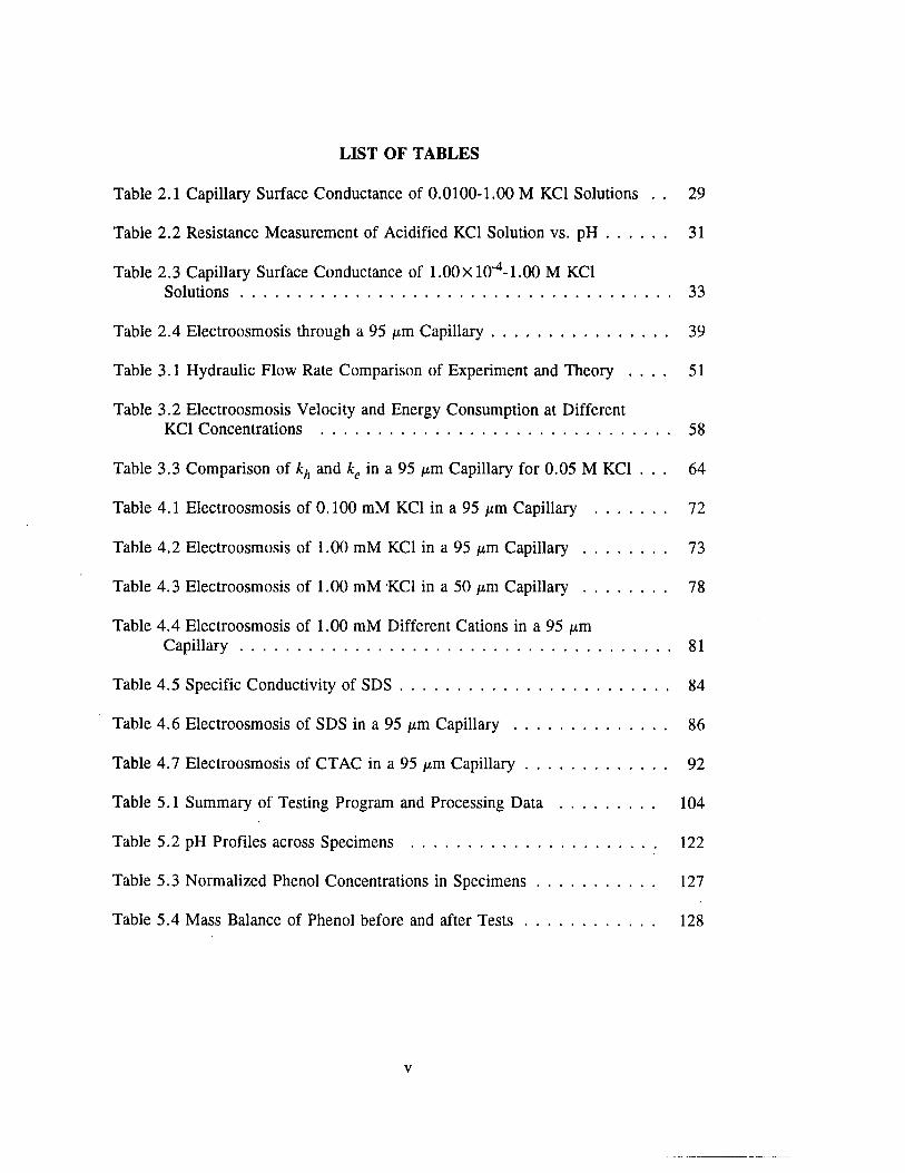
LIST OF TABLES

Table 2.1 Capillary Surface Conductance of 0.0100-1.00 M KC1 Solutions . . 29

Table 2.2 Resistance Measurement of Acidified KC1 Solution vs. p H .............. 31

Table 2.3 Capillary Surface Conductance of 1.00X 10"4 -1.00 M KC1Solu tions......................................................................................................... 33

Table 2.4 Electroosmosis through a 95 fim Capillary........................................... 39

Table 3.1 Hydraulic Flow Rate Comparison of Experiment and Theory . . . . 51

Table 3.2 Electroosmosis Velocity and Energy Consumption at DifferentKC1 Concentrations ..................................................................................... 58

Table 3.3 Comparison of kh and ke in a 95 jxm Capillary for 0.05 M KC1 . . . 64

Table 4.1 Electroosmosis of 0.100 mM KC1 in a 95 /xm Capillary ............... 72

Table 4.2 Electroosmosis of 1.00 mM KC1 in a 95 /xm C a p illa ry .................. 73

Table 4.3 Electroosmosis of 1.00 mM KC1 in a 50 /xm C a p illa ry .................. 78

Table 4.4 Electroosmosis of 1.00 mM Different Cations in a 95 /xmC ap illa ry ......................................................................................................... 81

Table 4.5 Specific Conductivity of S D S ................................................................. 84

Table 4.6 Electroosmosis of SDS in a 95 /xm Capillary ................................... 8 6

Table 4.7 Electroosmosis of CTAC in a 95 /xm C apillary ................................ 92

Table 5.1 Summary of Testing Program and Processing Data ....................... 104

Table 5.2 pH Profiles across Specimens ............................................................ 122

Table 5.3 Normalized Phenol Concentrations in Specim ens............................. 127

Table 5.4 Mass Balance of Phenol before and after T e s ts ............................... 128

v

LIST OF FIGURES

Figure 1.1 Four major electrokinetic phenomena in soils (adapted fromMitchell, [1.8]).................................................................................................... 3

Figure 1.2 Schematic of electrolysis, adsorption/desorption, andelectroosmotic flow............................................................................................. 4

Figure 1.3 Helmholtz-Smoluchowski model for electroosmosis (adaptedfrom Mitchell, [1.8]). ..................................................................................... 8

Figure 1.4 Examples of three different types of surfactants used in MECC:SDS (anionic), CTAC (cationic), and Brij 35 (nonionic) (adaptedfrom Little, [1.28]).......................................................................................... 17

Figure 1.5 Schematic diagrams of (a) the separation principle of MECC, (b) the zone separation in MECC, and (c) chromatogram (adapted from Terabe, [1.27,1.29])........................................................................................ 18

Figure 2.1 The diagram of the apparatus for capillary surface conductance measurement; (a) Using a type 1608-A impedance bridge, (b) Using a PAR™ model 124 lock-in amplifier, (c) The teflon holder for circuit (b).......................................................................................................... 26

Figure 2.2 Total resistance of KC1 (0.100 M) + HC1 (pH) solutions................. 32

Figure 2.3 UV spectra of phenol at different concentrations................................. 35

Figure 2.4 The concentration calibration curves at 209 and 268 nmwavelengths of phenol..................................................................................... 36

Figure 2.5 Typical UV spectra of a catholyte solution after anelectroosmosis test (test 3).............................................................................. 38

Figure 3.1 Velocity profiles obtained from (a) hydraulic (Poiseuille), and(b) electroosmotic (Helmholtz-Smoluchowski) flow................................... 45

Figure 3.2 A schematic diagram of the current measurement fordetermining the electroosmotic flow rate.................................................... 49

Figure 3.3 Hydraulic flow of water and 0.05 M KC1 through a capillary (95/^m diameter, 1 2 . 8 cm length): total height = 1 2 2 cm, half height =62 cm................................................................................................................. 52

Figure 3.4 Hydraulic flow of water through a capillary (95 /xm diameter): total height of water 122 cm; total length = 12.8 cm, half length =6.1 cm.............................................................................................................. 53

Figure 3.5 Hydraulic flow of water through a capillary (52 jxm diameter): total* height = 122 cm; total length = 12.9 cm, half length = 6 . 6

cm....................................................................................................................... 54

Figure 3.6 Electroosmosis velocity at different concentrations of KC1 electrolyte (E = 1500 V; capillary: 95 ^m diameter, 19.3 cm length)................................................................................................................ 59

Figure 4.1 Electroosmosis velocity in a 95 /xm capillary at different electricgradients for 0.100 mM KC1 solution......................................................... 74

Figure 4.2 Electroosmosis velocity in 95 and 50 jxm capillaries at differentelectric gradients for 1.00 mM KC1 Solution.............................................. 75

Figure 4.3 Electroosmosis velocity in a 95 /xm capillary at electric gradient of 208 V/cm for 1.00 mM KC1, LiCl, BPC (butylpyridinium chloride), and THAC (tetrahexylammonium chloride) solutions.............. 82

Figure 4.4 Specific conductivity of SDS (sodium dodecyl sulfate) atdifferent concentrations................................................................................... 85

Figure 4.5 Electroosmosis velocity in a 95 /xm capillary at electric gradient of 209 V/cm for different concentrations of SDS (sodium dodecyl sulfate)...............•............................................................................................... 8 8

Figure 4.6 Specific conductivity of CTAC (cetyltrimethylammoniumchloride) at different concentrations.............................................................. 91

Figure 4.7 Electroosmosis velocity in a 95 /xm capillary at electric gradient of 201 V/cm for different concentrations of CTAC(cetyltrimethylammonium chloride)............................................................... 93

Figure 5.1 Phenol adsorption isotherm on Georgia Kaolinite........................... 106

Figure 5.2 Electroosmotic test setup....................................................................... 107

Figure 5.3 Langmuir isotherm fit of phenol adsorption on kaolinite................ I l l

Figure 5.4 Freundlich isotherm of phenol adsorption on kaolinite.................. 112

Figure 5.5 Total electroosmotic flow with time................................................... 113

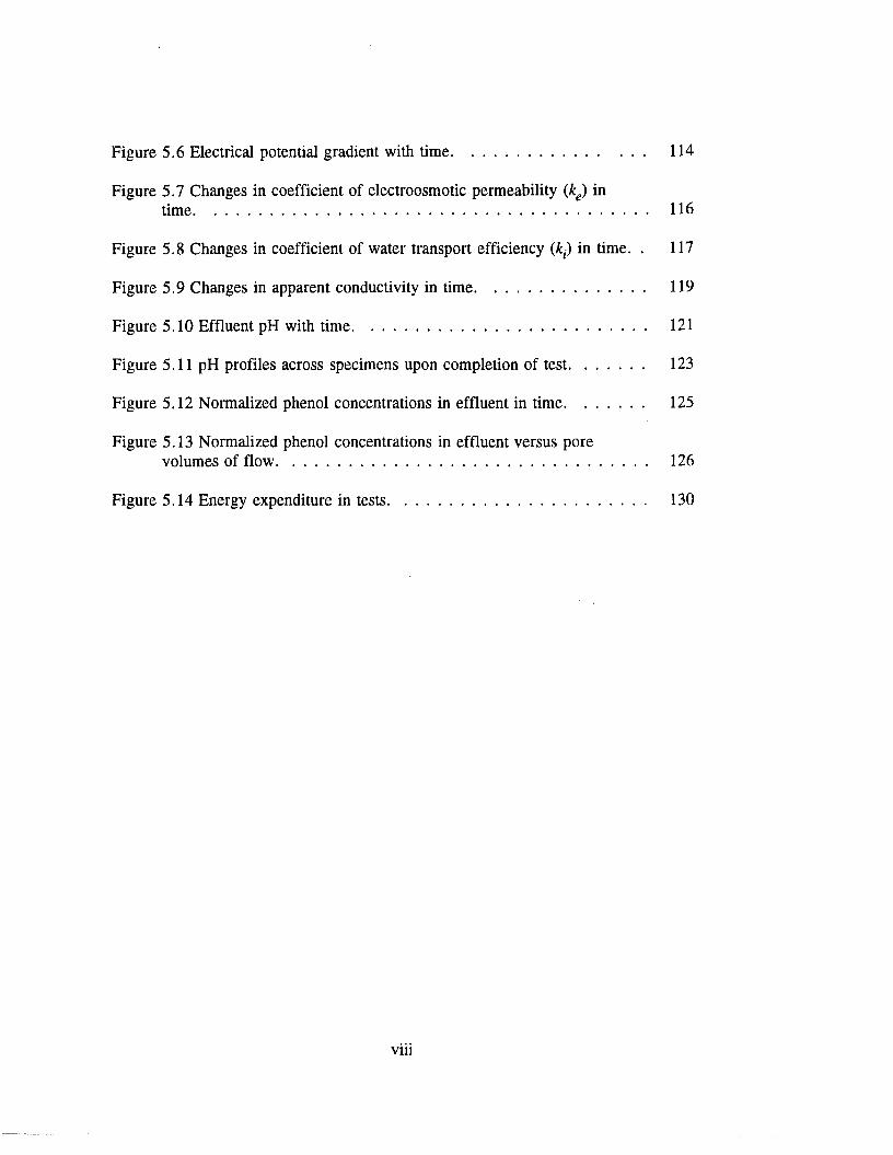
Figure 5.6 Electrical potential gradient with time................................................ 114

Figure 5.7 Changes in coefficient of electroosmotic permeability (ke) intime................................................................................................................. 116

Figure 5.8 Changes in coefficient of water transport efficiency (&,•) in time. . 117

Figure 5.9 Changes in apparent conductivity in time.......................................... 119

Figure 5.10 Effluent pH with time......................................................................... 121

Figure 5.11 pH profiles across specimens upon completion of test.................. 123

Figure 5.12 Normalized phenol concentrations in effluent in time.................... 125

Figure 5.13 Normalized phenol concentrations in effluent versus porevolumes of flow............................................................................................ 126

Figure 5.14 Energy expenditure in tests................................................................ 130

viii

A

AC

aj

A

BPC

Brij 35

BTEX

c, C

cj

CE

CMC

CTAB

CTAC

CZE

d

DC

5

AEe

LIST OF SYMBOLS AND ABBREVIATIONS

capillary radius or molecule radius

cross sectional area

alternating current

radius of the jth ion in the solution

angstrom

butylpyridinium chloride, CH3 (CH2 )3 NC5 H5 C1

polyoxyethylene(23)dodecanol, 1 0 (CH 2 CH 2 0 )2 3 H,nonionic surfactant

benzene, toluene, ethylene, and xylene

concentration

number of moles per unit volume of the jth ion in the solution

capillary electrophoresis

critical micelle concentration

cetyltrimethylammonium bromide, CH3 (CH2 ) 1 5 N(CH3 )3 Br, cationic surfactant

cetyltrimethylammonium chloride, CH3 (CH2 )1 5 N(CH3 )3 C1, cationic surfactant

capillary zone electrophoresis

capillary diameter

direct current

position of the inner Helmholtz layer

energy consumption per flow volume in capillary electroosmosis

energy consumption per flow volume in capillary hydraulic flow

energy based on the excess surface conductivity

hydraulic pressure head

electronic charge

electric voltage

electroosmosis

electric voltage at time of t

energy expenditure per unit volume of soil processed

electric potential gradient, EIL

dielectric constant

permittivity of free space, 8.854 X 10" 1 2 C ^ m ' 1

viscosity

Faraday constant

electrostatic force

frictional force

function related to micellar size and shape

gravitational constant

gigaohm

electrical to mechanical efficiency factor for excess cation species, i

height of hydraulic pressure head

hour

high voltage

current

modified Bessel function of the first kind

l h

! t

L

k

K„

kHz

h

k V

kWh/m3

m

mA

MECC

mM

mS

Mfi

k-

nA

fim

electrical gradient

hydraulic gradient

current at time of t

length of capillary or cell

Boltzmann constant

apparent conductivity

coefficient of electroosmotic permeability

hydraulic conductivity

kilohertz

electroosmotic water transport efficiency

kilovolt

kilo-watt-hour per cubic meter

Debye reciprocal length

mass

milliampere

micellar electrokinetic capillary chromatography

millimolar concentration

millisiemen

megaohm

electrophoretic mobility

microampere

microliter

micron

XI

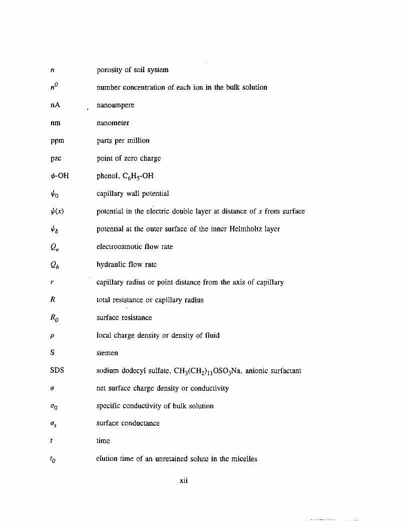
porosity of soil system

number concentration of each ion in the bulk solution

nanoampere

nanometer

parts per million

point of zero charge

phenol, C6 H5-OH

capillary wall potential

potential in the electric double layer at distance of x from surface

potential at the outer surface of the inner Helmholtz layer

electroosmotic flow rate

hydraulic flow rate

capillary radius or point distance from the axis of capillary

total resistance or capillary radius

surface resistance

local charge density or density of fluid

siemen

sodium dodecyl sulfate, CH3 (CH2 ) i i0 S 0 3 Na, anionic surfactant

net surface charge density or conductivity

specific conductivity of bulk solution

surface conductance

time

elution time of an unretained solute in the micelles

tmc retention time of a solute permanently retained in the micelles

tR solute retention time

T absolute temperature

THAC tetrahexylammonium chloride, [C lty C F ^ ^ N C l

6 degree of coverage on the surface

UV ultraviolet

v flow velocity

veo electroosmotic velocity

vep electrophoretic migration velocity

vmax maximum hydraulic flow velocity at the center of capillary

vnet net velocity of species

Vs volume of soil mass processed

vz fluid velocity in the axial direction, z

w/o without

xA thickness of diffuse layer

z ionic charge

Zj charge number of jth ion in the solution

f electrokinetic zeta potential

T zeta potential of the micellar surface

ABSTRACT

Capillary electroosmosis is an important factor in capillary zone electrophoresis

(CZE) and micellar electrokinetic capillary chromatography (MECC). A new

application of electrokinetic phenomena in environmental science is electrokinetic soil

processing, which is an emerging technique with the capability to decontaminate

polluted soils.

Chapter 1 discusses the fundamental theory behind electroosmosis, CZE,

MECC, and electrokinetic soil processing. In chapter 2, the surface conductances of

different concentrations of KC1 solutions in 50 and 100 /xm capillaries were measured

using an AC method, to attempt to characterize capillary double layers. With increase

of KC1 concentration, the surface conductance increases. Chapter 3 involves

fundamental studies of hydraulic and electroosmotic flows through 50 and 100 /xm

capillaries. The results show that hydraulic flow follows the Poiseuille relation. The

energy consumptions for these two flows are compared and hydraulic flow is much

more energy efficient than electroosmotic flow because of bulk IR losses in the latter.

In chapter 4, more detailed studies of capillary electroosmosis indicate that the

electroosmotic velocities for KC1, LiCl, and butylpyridinium chloride (BPC) in a 95

fim capillary are similar, whereas for tetrahexylammonium chloride (THAC) no flow

was detected. Due to the electrophoretic effect, the bulk flow of sodium dodecyl

sulfate (SDS) solutions with concentrations above its CMC (critical micelle

concentration, 8.4 mM) were reversed (cathode toward anode); however, with

concentrations of SDS below its CMC, anodic to cathodic electroosmotic flows were

xiv

observed. Due to the adsorptive effect of cetyltrimethylammonium ion on the

capillary surface, reverse electroosmotic flows of cetyltrimethylammonium chloride

(CTAC) solutions were observed with its concentration above its CMC (0.03 mM).

Finally, Chapter 5 contains the results of electroosmotic flow behavior and

electrochemistry (voltage, current, resistance, pH gradients and conductivity

variations) for phenol removal from kaolinite clay by electroosmosis. The adsorbed

phenol (at concentration of 500 ppm) was removed 85% to 95% by the process and

the energy expenditure was 18-39 kWh/m3 of soil processed.

xv

CHAPTER 1.

GENERAL INTRODUCTION AND THEORETICAL BACKGROUND

1.1 Introduction

Electrokinetic phenomena are finding new applications in separation science,

e.g. capillary electrophoresis (CE) and micellar electrokinetic capillary

chromatography (MECC), and for environmental site restoration (electrokinetic soil

processing). Since the invention of CE in the 1970s [1.1], CE or capillary zone

electrophoresis (CZE) has attracted wide attention. Capillary zone electrophoresis is

a modem separation technique through which charged compounds can be separated

by differences in their electrophoretic mobilities in an electric field applied to a

capillary tube filled with an electrolyte. CZE has become particularly useful in the

biological sciences, because only very small amounts of sample are needed for

analysis and characterization. Micellar electrokinetic capillary chromatography

(MECC), which was first introduced in 1984 [1.2], is a subtechnique of CE. In this

technique, by adding a surfactant at a concentration above its critical micellar

concentration (CMC) to the electrolyte buffer solution, the analytes (neutral or

charged) can be separated through differential partitioning into the micelle. The CMC

of a surfactant is the concentration at or above which micelles of the surfactant form.

Applications of both methods are rapidly growing due to their high efficiency

separation of biochemical and pharmaceutical (charged or neutral) compounds. A

fundamental phenomenon in CE or MECC is electroosmosis, the flow of electrolyte

in an applied electric potential field due to surface forces. Electrokinetic soil

1

processing is an emerging remediation technique with the capability to decontaminate

soils or slurries polluted with heavy metals, radionuclides, or certain organic

compounds'[1.3-1.5].

1.2 Electroosmosis and Electrokinetic Soil Processing

Electroosmosis is a phenomenon in which electrolytes (in most cases, aqueous)

move through a porous medium with a surface charge, due to the application of an

electric field. Electroosmosis, which is one of the four major electrokinetic

phenomena, has been of primary interest in geotechnical engineering because it is used

in practice to dewater soils and to stabilize saturated fine-grained deposits [ 1 .6 ].

These electrokinetic phenomena, which result from the coupling between electrical and

hydraulic flows and gradients in suspensions and porous (soil) media, include

electroosmosis, streaming potential, electrophoresis, and migration or sedimentation

potentials [1.7,1.8]. Electroosmosis and electrophoresis are the movement of pore

water and charged particles, respectively, due to the application of an electrical field.

Streaming potential and sedimentation potential are the generation of an electrical field

due to the movement of an electrolyte under hydraulic potential and the motion of

charged particles in a gravitational field, respectively (Figure 1.1).

As shown in Figure 1.2 [1.6], when an electric potential is applied across a

wet soil mass by immersion or placement of two electrodes, electroosmotic flow

occurs from anode to cathode if the clay or glass surface is negatively charged.

Cations move to cathode and anions move to anode and, since there is generally an

excess of positively charged cations, M+ , in the system to neutralize the net negative

3

Eapplied

Water-

/■ Saturated Clay ' + _________

ELECTROOSMOSIS

Eapplied

+

Particles

Clay suspension

ELECTROPHORESIS

Eapplied

Water

Saturated Clay

Emeas STREAMING POTENTIAL MIGRATION POTENTIAL

Figure 1.1 Four major electrokinetic phenomena in soils (adapted from Mitchell, [1.8]).

4

+M +

+ H +

+ PORE FLUIDH ++

H ++ M + M +

M+ M++ANODE

NEGATIVE CLAY OR GLASS SURFACECATHODE

Figure 1.2 Schematic of electrolysis, adsorption/desorption, and electroosmotic flow.

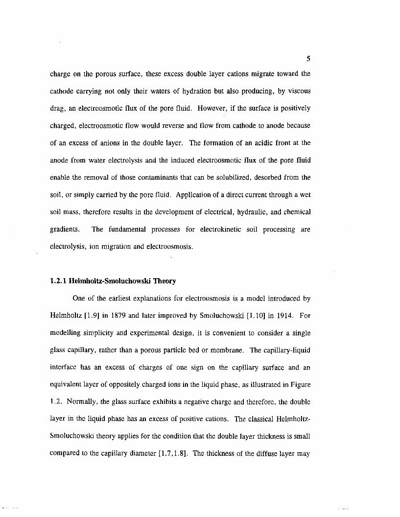
charge on the porous surface, these excess double layer cations migrate toward the

cathode carrying not only their waters of hydration but also producing, by viscous

drag, an electroosmotic flux of the pore fluid. However, if the surface is positively

charged, electroosmotic flow would reverse and flow from cathode to anode because

of an excess of anions in the double layer. The formation of an acidic front at the

anode from water electrolysis and the induced electroosmotic flux of the pore fluid

enable the removal of those contaminants that can be solubilized, desorbed from the

soil, or simply carried by the pore fluid. Application of a direct current through a wet

soil mass, therefore results in the development of electrical, hydraulic, and chemical

gradients. The fundamental processes for electrokinetic soil processing are

electrolysis, ion migration and electroosmosis.

1.2.1 Helmholtz-Smoluchowski Theory

One of the earliest explanations for electroosmosis is a model introduced by

Helmholtz [1.9] in 1879 and later improved by Smoluchowski [1.10] in 1914. For

modelling simplicity and experimental design, it is convenient to consider a single

glass capillary, rather than a porous particle bed or membrane. The capillary-liquid

interface has an excess of charges of one sign on the capillary surface and an

equivalent layer of oppositely charged ions in the liquid phase, as illustrated in Figure

1.2. Normally, the glass surface exhibits a negative charge and therefore, the double

layer in the liquid phase has an excess of positive cations. The classical Helmholtz-

Smoluchowski theory applies for the condition that the double layer thickness is small

compared to the capillary diameter [1.7,1.8], The thickness of the diffuse layer may

6

be approximated to the Debye length, 1 I k , which is of the order of 10 A for 10' 1 M

and 100 A for 1 O' 3 M 1 : 1 electrolyte in water at 25°C, respectively [1.11].

The electroosmotic flow velocity v (m/s) is controlled by the balance between

the electrical force (oEIL) causing movement and friction (drag force, r)v/xA) between

the liquid and the wall, where a (C/m2) is the net surface charge density, EIL (V/m)

is the electrical potential gradient, rj (poise, or dyn • s/cm2) is the viscosity, and xA (m)

is the thickness of diffuse layer [1.8]. Note that the excess charge of ions in the

liquid double layer is equal and opposite to the net surface charge. This theory makes

no assumptions as to how the frictional forces are distributed in the double layer. At

equilibrium

From electrostatic double layer theory, the surface zeta potential, f (V), is given by

where the negative sign means that the zeta potential has a negative value and e

(dimensionless) is the dielectric constant of the medium, e0 is the permittivity of free

space (e0 = 8.854 x 10' 1 2 C ^ 'W 1). Therefore, the electroosmosis velocity, v, is

given by

( 1. 1)

v - eeo^ ET) L

(1.3)

7

Equation 1.3 is called the Helmholtz-Smoluchowski equation. It can be assumed that

a quiescent layer of liquid exists at the surface and a hydrodynamic shear plane exists

within the double layer. The boundary now is that where the liquid may move and

the shear plane has a potential known as the electrokinetic zeta potential, f [1.7]. The

potential f is defined only by the boundary condition and is therefore the potential in

the shear plane in the liquid close to the surface. Figure 1.3 [1.8] illustrates the

Helmhlotz-Smoluchowski model for electroosmosis. This basic theory does not

provide a method to predict the velocity profile in a capillary. Neither does it explain

how the remaining column of liquid outside the double layer may move. This theory

assumes that the velocity of the excess ions is completely transferred to the

surrounding liquid and it does not differentiate solid/liquid and liquid/liquid frictional

forces.

1.2.2 Velocity Profile in Capillary Electroosmosis

One of the most heavily cited, early references offering a theoretical study of

electroosmosis in narrow cylindrical capillaries was published by Rice and Whitehead

in 1965 [1.12], The solution of the Poisson-Boltzmann equation for the local charge

density, p(r) (C/m3), of a double layer at the internal wall of a cylindrical capillary

is given by

p(r) - -eeoK2 - ^ ^ (1.4)

8

+•' |fc " |** " | ^ j | * *| * | ...In.. | ii

^ Velocity Profile

^ I

“KH—I—I—I—1“ H—I—h

Force

Force

Figure 1.3 Helmholtz-Smoluchowski model for electroosmosis (adapted from Mitchell, [1.8]).

where k is the reciprocal Debye length, I0( ) functions are modified Bessel functions

of the first kind, a is the capillary radius with point distance from the axis, r, and \pQ

(V) is the capillary wall potential. This theory postulates that the liquid velocity at

the wall is zero and increases in the radial direction toward the central axis. It also

assumes that the ions can transfer their velocities to the surrounding solvent water

molecules, i.e., it is a continuum model. With the above boundary conditions,

solution of the differential equations leads to the prediction of a maximum, flat flow

profile in most regions of the capillary, except for the double layer region very close

to the wall where the liquid has a small velocity (Figure 1.3). In the absence of any

external pressure, the total force is the electrical force in the axial direction, z, in a

capillary, which is given by the product of the electrical field gradient, EIL, and the

local charge density due to excess ionic charge, p(r). The motion equation can be

written as

1 d ,r ^ r\ . . PM E (1_5)r dr dr 11 L

where vz is the fluid velocity in the axial direction z and 17 is the viscosity. The

solution for this basic motion equation is

viW - (1.6)11 L

This solution was obtained with boundary conditions which assume that the flow

velocity will be constant in the center of the capillary and zero at the wall. The

boundary condition at the surface of the capillary is referred to as the no slip

condition. The term v is the liquid velocity as a function of the radial direction.

10

However, similar to the earlier Helmholtz-Smoluchowski theory, this theory assumes

that the liquid velocity can be equal to the ion velocity without detailing the exact

mechanism by which the ion motion is transferred to the surrounding water molecules.

If na is large (> 5 0 , in most cases, e.g. a > 1 irn, 1 /k < 1 0 0 A, na > 1 0 0 ), the I0

term becomes insignificant. Equation 1.6 becomes

, W . - ^ (1.7)' H L

This is analogous to the Helmholtz-Smoluchowski equation (Equation 1.3). Equation

1.7 gives relatively flat velocity profile across the capillar)'.

Recently, experimental observations of the flow profiles in electroosmosis in

rectangular capillaries have been obtained by Tsuda, et al. [1.13]. They have found

that the zone front is flat at the center and the zone front at the edges, close to the

wall, are ahead compared with the center part. They also have proposed a flow

profile in a circular capillary with the zone front at the edges ahead of that at the

center. The observed flow profile is very different from the existing classical theory.

Taylor and Yeung [1.14] also have obtained images of electroosmotic flow profiles

in circular capillaries. They found in one case the particles detected at the edges close

to the capillary wall are ahead of those in the center of capillary. The excess charge

responsible for fluid motion resides in the double layer very close to the wall, so the

electric force on this excess charge is also located in the double layer close to the

wall. The ions in the double layer move first under the electric force, then the

moving ions drag the surrounding water with them. This may be a reason for the

zone front at the edges close to the wall being ahead of that at the center. A

11

comprehensive review of the equilibrium double layer and associated electrokinetic

phenomena has been written by Dukhin and Derjaguin [1.15] and rigorous treatments

of the classical theory for electrokinetic flow in narrow cylindrical capillaries have

been presented by Newman [1.16], Hunter [1.17], Koh and Anderson [1.18], and

Tikhomolova [1.19].

1.2.3 Dependence of fo n the Electrolyte Concentration

Electroosmosis arises because of the motion of the diffuse layer of ions in

solution relative to the solid surface. It has been postulated that there is a slipping

surface located in the diffuse part of the ion atmosphere [1.7,1.20]. The potential

at the slipping surface is given the symbol f (zeta) and it is called the electrokinetic

zeta potential. The potential f is a function of many parameters including the surface

properties, the surface charge density, the solid-liquid interface, and the nature and

concentration of the electrolyte. Rieger [1.20] has derived a relationship for the

dependence of f on the concentration of electrolyte. If 5 is the thickness of the

immobilized inner Helmholtz (or Stem) layer from a planar surface, the potential \p(x)

(x is the distance from the surface) in the electric double layer can be written as

[1. 11, 1.20]

i | r ( * ) - V 1_ T ) + , l , « T *fx<b ( L 8 )o 0

\Jf(x) - i|r8 exp[(6 -x )/x j i f x>b (19)

12

where \p0 is the surface potential, \p5 is the potential at the outer surface of the inner

Helmholtz layer, and xA is the thickness of diffuse layer (Debye length). Equations

1.8 and 1.9 indicate that the potential decreases linearly in the region between the

surface and inner Helmholtz layer and exponentially in the diffuse region. In refs.

[1.7,1.11], for a z:z electrolyte solution, xA oc C 1/2,

k - —— ~ ( - - ” ° Z - - ) 1/2 - (3.29x107)zC1/2 (1.10)xA eeJcT

in which n° is the number concentration of each ion in the bulk, z is the magnitude

of the charge on the ions, e is the charge of electron, e is the dielectric constant of the

medium, e0 the permittivity of free space, k is the Boltzmann constant, T is the

absolute temperature, and C (mol/L) is the bulk z:z electrolyte concentration. For the

second half of Equation 1.10, it is assumed that T = 298 K, e = 78.49 (dilute

aqueous solutions), and k is given in cm '1. By solving the relation between surface

potential to surface charge density, we get

o - eeQty6lxA ( 1 -1 1 )

where a is the net surface charge density. Now, we calculate the potential f in a

circular capillary. If we assume that a, the radius of the capillar}', is much larger

than the diffuse layer thickness xA, so the result obtained for a planar surface can be

used, then we have

t ( r ) - Cexp[(r-a)/xA] ( 1 1 2 )

where the coordinate r is measured from the center of the capillary. The potential in

the center of capillary is nearly zero because a/xA is very large. Equation 1.11 tells

us that the potential is proportional to the net surface charge density a and also

proportional to xA and thus proportional to C'm . The slipping plane is assumed to

be in the diffuse layer and located at a distance x from the surface into the diffuse

layer, then f can be written as

C - - ^ e ~ (x-6)IXA (1.13)ee 0

Because xA is proportional to C 1/2, we would expect the magnitude of f to depend on

the concentration of electrolyte according to

C - aoC '1/2exp(-pC1/2) (L14)

where a and /3 are constants. If a is independent of electrolyte concentration, then

f should be a monotonic decreasing function of C. The situation will become more

complicated if a is affected by changes in electrolyte concentration. However, in this

theory, the electroosmosis velocity v is proportional to f and thus should decrease with

increase of C for a constant a.

1.3 Capillary Zone Electrophoresis

Capillary zone electrophoresis (CZE) is a technique in which separations are

achieved by the differences in solute electrophoretic mobilities in an electric field

applied to a capillary tube filled with an electrolyte [1.21-1.24]. In 1979, Mikkers

et al. [1.25] performed CZE in 200 Teflon capillaries with on-column UV

14

detection, and in 1981, Jorgenson and Lukacs were the first to introduce capillary

zone electrophoresis in small inner diameter (75 /um), open-tubular glass capillaries

[1.21]. CZE has achieved remarkably rapid development since its introduction in the

early 1980s. The development of CZE offers several exciting methods for fast, highly

efficient separations of ionic species and macromolecules in the area of analytical

biotechnology.

A capillary with 50-100 ^m inner diameter is filled with operating buffer and

each end is immersed in a separate vial of electrolyte. One platinum electrode is

immersed in each electrolyte solution. Upon the application of a constant electric

field Ez (Ez = EIL where E is the voltage applied and L is the length of capillary),

ionic species undergo an electrostatic force, Fe, which is given by

where z the charge of the particular ion. This force causes the acceleration of ions

toward the oppositely charged electrode. The counteracting frictional force (/y) from

the surrounding solution causes the ion to travel at a limiting constant velocity.

Assuming a spherical molecule of radius a, the frictional force can be expressed by

Stoke’s law as [1.26]

where rj is the solution viscosity and vep is electrophoretic migration velocity of the

species. After steady state is reached (Fe = iy), the velocity can be calculated as

(1.15)

(1.16)

v (1.17)

15

where the electrophoretic mobility, fi, is a characteristic property of a given ion in a

given medium and a given temperature. Thus, the viscous drag of the solvent and the

charge and size of the ion control the migration of a species in an applied electric

field. With the application of an electric field, electroosmotic flow (yeo) also may

occur. So, the net velocity vnet of the species from one electrode to another is

v . v +v _ [_ i M +_ L _ ]£ (1.18)to ep t ^ 6 T t t i f l J z

Assuming a negatively charged capillary wall, f is negative and the electroosmotic

flow is from anode to cathode. For negative ions, vep (from cathode to anode) is

against veo\ for positive ions, vep (from anode to cathode) has the same direction

as veo; and for neutral species, vnet is same as veo. Different species have different

electrophoretic migration mobilities (i, thus they can be separated by capillary

electrophoresis.

1.4 Micellar Electrokinetic Capillary Chromatography

Although CZE has a high power for efficiently separating complex samples,

it is not applicable to separation of electrically neutral compounds (they all have the

same velocity which is the electroosmotic flow velocity veo). To overcome this

difficulty, Terabe et al. in 1984 [1.2] introduced micellar electrokinetic capillary

chromatography (MECC), followed by a more thorough study in 1985 [1.27]. Their

solution involved the addition of a surfactant (sodium dodecyl sulfate, SDS) above its

critical micelle concentration (CMC) to provide a medium through which neutral

compounds could partition differentially and, therefore, be separated.

16

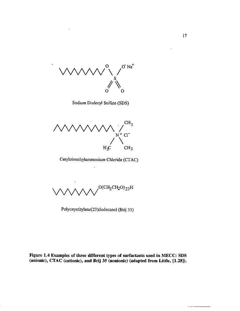
Surfactants are amphophilic molecules bearing both hydrophilic and lipophilic

moieties. Some common surfactants are shown in Figure 1.4 [1.28]. Surfactants

normally are classified by their hydrophilic or "head" groups, being anionic, cationic,

nonionic, or zwitterionic. The lipophilic or "tail" group consists of a straight or

branched chain alkyl group, usually containing more than seven carbons. In dilute

solutions, these molecules generally are observed as discrete monomers. However,

an increase in surfactant concentration will ultimately induce aggregation of the

monomers to form micelles. The concentration at which micellization occurs is

referred to as the critical micelle concentration (CMC). A micelle is a structure

consisting of a hydrophilic surface and lipophilic core. Although micelle formation

occurs above the CMC, the monomer form of the surfactant is still present (Figure

1.5a). Figure 1.5a [1.29] is a schematic diagram of the MECC separation principle.

An ionic surfactant solution of a concentration higher than its CMC is used as an

electrophoretic solution instead of the simple buffer solution used in CE. The micelle

works as the separation carrier, as shown in Figure 1.5a, although the micelle exists

only in a dynamic equilibrium state in the presence of the monomeric surfactant. The

size and shape of the micelle depends on the individual surfactant. The aggregation

number has a distribution, and the average lifetime of the micelle is about 1 second

[1.29]. The net micellar velocity vnet is

vne, = v eo + v ep ■ (L19)

where vep is the micellar electrophoretic velocity. The vep can be positive or negative

depending on whether it follows or opposes electroosmotic flow and is given by

17

O 0 ‘ Na+W W W \ /

s

o o

Sodium Dodecyl Sulfate (SDS)

CH-j

AAAAAAAA /N + cr

/ \H^C c h 3

Cetyltrimethylammonium Chloride (CTAC)

W W W 0™Polyoxyethylene(23)dodecanol (Brij 35)

Figure 1.4 Examples of three different types of surfactants used in MECC: SDS (anionic), CTAC (cationic), and Brij 35 (nonionic) (adapted from Little, [1.28]).

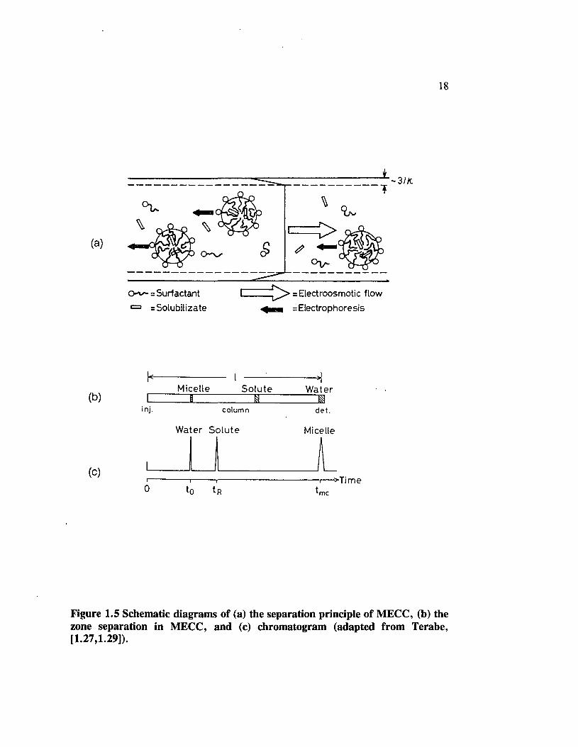
18

(a)

■ = Surfactant ^ =Solubilizate

- 3 I K

= Electroosmotic flow

— = Electrophoresis

H--------------------- i-- :-------------- HMicelle Solute Water

( b ) L. a a ^inj. c o lu m n d e t .

Water Solute Micelle

0 t

Figure 1.5 Schematic diagrams of (a) the separation principle of MECC, (b) the zone separation in MECC, and (c) chromatogram (adapted from Terabe,[1.27,1.29]).

where the function flua) depends on the micellar shape, having a value of 1.5 for a

sphere of ko = oo [1.27], a is the radius of the particle, k is the reciprocal Debye

length of the double layer created at the micelle’s surface, and is the zeta potential

of the micellar surface.

A neutral species injected into the micellar solution will migrate at the

electroosmotic velocity when it is free from the micelle and, at the velocity of the

micelle, when it is incorporated into the micelle. Separation occurs through

differential partitioning of neutral compounds between the micellar and aqueous

phases, i.e. different neutral solutes will partition at slightly different rates as for

stationary phase separation. The analyte will migrate at the velocity between the two

extremes, the electroosmotic velocity, veo, and the velocity of the micelle, vnet, as

shown in Figures 1.5b and 1.5c. Figure 1.5b shows the positions of water, solute,

and micelle in the column at a certain time after the injection; however, at the

injection time, all three are at the same position of injection port. A chemical, Sudan

III [1.27], which was completely solubilized into the micelle of SDS, was used to

present the migration of the micelle. Methanol was used and is regarded as an

insolubilized solute, i.e., as existing only in the aqueous phase ("water" in Figures

1.5b and 1.5c). Appearance of methanol at the detector represents the electroosmotic

velocity alone. Figure 1.5c shows the relative retention times in a chromatogram of

water (methanol), solute, and micelle (Sudan III), with the order t0 < tR < tmc.

Most applications in MECC use anionic micellar systems since the micelles remain

20

in the capillary for a longer time, and this permits solutes to partition more frequently

so that adequate separation can occur.

1.5 Thesis Overview

The following chapters will mainly deal with some fundamental and applied

problems of electroosmosis. In chapter 2, we will measure the surface conductances

of different size capillaries with different concentration of KC1 solutions to attempt to

characterize capillary double layers. Chapter 3 addresses the energy comparison of

hydraulic and electroosmotic flows through silica capillaries. Chapter 4 contains some

studies of electroosmotic flow for different cations (KC1, LiCl, butylpyridinium

chloride (BPC), and tetrahexylammonium chloride (THAC)), together with a selection

of surfactants (negatively charged sodium dodecyl sulfate (SDS) and positively

charged cetyltrimethylammonium chloride (CTAC)). Finally, an example of practical

electrokinetic soil processing is given in chapter 5, whereby phenol is removed from

kaolinite clay.

21

1.6 References

1.1 R. Virtanen, Acta Polytech. Scand. 1974, 123, 1.

1.2 S. Terabe, K. Otsuka, K. Ichikawa, A. Tsuchiya, and T. Ando, A nal Chem. 1984, 56, 113.

1.3 J. Hamed, Y.B. Acar, and R.J. Gale, J. Geotech. Engrg. ASCE, 1991, 112, 241.

1.4 Y.B. Acar, R.J. Gale, D.A. Ugaz, S. Puppala, and C. Leonard, FinalReport- Phase I o f EK-EPA Coop. Agreement CR816828-01-0, Report No. EK-BR- 009-0292, Electrokinetics Inc., Baton Rouge, LA, 1992.

1.5 Y.B. Acar, H. Li, and R.J. Gale, J. Geotech. Engrg. ASCE, 1992, 118, 1837.

1.6 R.J. Gale, H. Li, and Y.B. Acar, "Soil Decontamination using Electrokinetic Processing", Chapter in Environmental Oriented Electrochemistry, Studies in Environmental Science 59, C.A.C. Sequeira (Ed.), Elsevier Science Publishers, 1994, pp. 621-54.

1.7 R. Aveyard and D.A. Haydon, An Introduction to the Principles o f Surface Chemistry, Cambridge University Press, 1973, pp. 40-57.

1.8 J.K. Mitchell, Fundamentals o f Soil Behavior, John Wiley and Sons, Inc., New York, 1976, pp. 353-359.

1.9 H. Helmholtz, Wiedemanns Annalen d. Physik, 1879, Vol. 7, 137.

1.10 M. Smoluchowski, Handbuch der Elektrizitat und Magnetismus, L. Graetz (Ed.), J.A. Barth, Leipzig, 1914, Vol. 2.

1.11 A.J. Bard and L.R. Faulkner, Electrochemical Methods, Fundamentals and Applications, John Wiley & Sons Inc., New York, 1980, pp. 500-510.

1.12 C.L. Rice and R. Whitehead, J. Phys. Chem. 1965, <59, 4017.

1.13 T. Tsuda, M. Ikedo, G. Jones, R. Dadoo, and R.N. Zare, J. Chromatogr. 1993, 632, 201.

1.14 J.A. Taylor and E.S. Yeung, Anal. Chem. 1993, 65, 2928.

22

1.15 S.S. Dukhin and B.V. Derjaguin, Surface and colloid Science, E. Matijevig (Ed.), John Wiley, New York, 1974, Vol. 7, pp. 49-272.

1.16 J.S. Newman, Electrochemical Systems, Prentice-Hall, Inc., NJ, 1973, pp. 190-207.

1.17 R.J. Hunter, Zeta Potential in Colloid Science, Principles and Applications, Academic Press, London, 1981.

1.18 W.H. Koh and J.L. Anderson, AIChE J. 1975, 21, 1176.

1.19 K.P. Tikhomolova, Electro-osmosis, Ellis Horwood Series in Physical Chemistry, New York, 1993.

1.20 P.H. Rieger, Electrochemistry, Prentice-Hall, Inc., Englewood Cliffs, NJ, 1987, pp. 69-95.

1.21 J.W. Jorgenson and K.D. Lukacs, Anal. Chem. 1981, 53, 1298.

1.22 H.H. Lauer and D. McManigill, Anal. Chem. 1986, 58, 166.

1.23 A.S. Cohen, S. Terabe, J.A. Smith, and B.L. Karger, Anal. Chem. 1987, 59,1021.

1.24 S. Terabe and T. Yashima,' Anal. Chem. 1988, 60, 1673.

1.25 F.E.P. Mikkers, .F.M. Everaerts, and T.P.E.M. Verheggen, J. Chromatogr. 1979, 169, 11.

1.26 B.L. Karger and F. Foret, Capillary Electrophoresis Technology. Chromatographic Science Series, Vol. 64, N.A. Guzman (Ed.), Marcel Dekker, Inc., New York, 1993, pp. 3-64.

1.27 S. Terabe, K. Otsuka, and T. Ando, Anal. Chem. 1985, 57, 834.

1.28 E.L. Little, "Comparative Study of Anionic and Nonionic/Anionic SurfactantSystems in Micellar Electrokinetic Capillary Chromatography", Ph.D. dissertation, Louisiana State University, Baton Rouge, LA, May, 1992.

1.29 S. Terabe, Capillary Electrophoresis Technology. Chromatographic Science Series, Vol. 64, N.A. Guzman (Ed.), Marcel Dekker, Inc., New York, 1993, pp. 65-87.

CHAPTER 2.

CAPILLARY SURFACE CONDUCTANCE AND

STUDIES OF CAPILLARY ELECTROOSMOSIS

2.1 Introduction

Electroosmotic flow is an important factor in capillary electrophoresis (CE) and

micellar electrokinetic capillary chromatography (MECC). In recent years,

electroosmosis also has been promoted as a factor for the removal of contaminants

from soil [2.1-2.4]. According to the Helmholtz-Smoluchowski theory [2.5], the

electroosmosis velocity, v, is

r| L

where e is the dielectric constant of the medium, e0 is the permittivity of free space,

rj (poise or dyn • s/cm2) is its viscosity, L is the length of capillary, E is the applied

electric potential, and f is the electrokinetic zeta potential. The potential, f, is a

function of the surface properties of capillary wall, the surface charge density, the

solid-liquid (fused silica glass wall - electrolyte solution) interface, and the nature and

concentration of the electrolyte solution and its pH. The electrokinetic zeta potential

(f) in the electric double layer is a very important parameter for understanding

capillary electroosmotic flow.

Measurement of surface conductances of capillaries are important because they

may provide information to better understand capillary electroosmosis. The surface

conductance is a Gibbs excess quantity and a function of the surface properties of a

23

24

capillary, the surface charge density, and the nature and concentration of the

electrolyte. The surface conductance is due to excess charges in the double layer and

perhaps salt accumulating at the surface. The surface conductance may be used to

help to characterize the static double layer. In this chapter, the surface conductances,

os, of 1.00 x 10‘4 to 1.00 M KC1 solutions in 50 and 100 fim capillaries were

measured using an AC method, which attempts to separate the surface conductances

from the combined bulk values by determining the capillary geometry. With increase

of the concentration of KC1 solution, the surface conductance increases. The as values

are in the range of 10' 5 to 10' 8 siemens for the capillaries studied. Also, a

preliminary test of capillary electroosmosis of 0.100 M KC1 solution in a 95 nm

capillary was made using off-line detection and phenol as an indicator. The

electroosmotic flow rates are 0.17 and 0.10 /al/hr for the electric field gradients (E/L)

of 15 and 7.5 V/cm, respectively. In the next few chapters, capillary electroosmosis

will be studied in more detail using the current-monitoring method [2 .6 ].

2.2 Experimental

Fused silica capillaries for the studies were purchased from Alltech Company

(J & W deactivated fused silica capillary). The diameters of capillaries were

measured under a microscope (Bausch & Lomb) and by magnifying with a video

camera (CCTV camera, Model HV-720u; Philips VCR, Model VR6495AT; Hitachi

video monitor, Model VM-900u). Two standard scales (2 ^m x 50 divisions and 50

jam X 50 divisions) were used for calibration. Two sets of capillaries were purchased

at different times for the experiments. The diameters of these capillaries are slightly

25

different; 52 ± 1 im and 101 ± 1 /xm for the first set; 50 ± 1 /xm and 9 5 + 1 /xm

for the second set. KC1 (reagent grade) was recrystallized first and oven dried, then

1.00 M stotk solution was prepared with deionized distilled water. Dilute KC1

solutions were made from this stock.

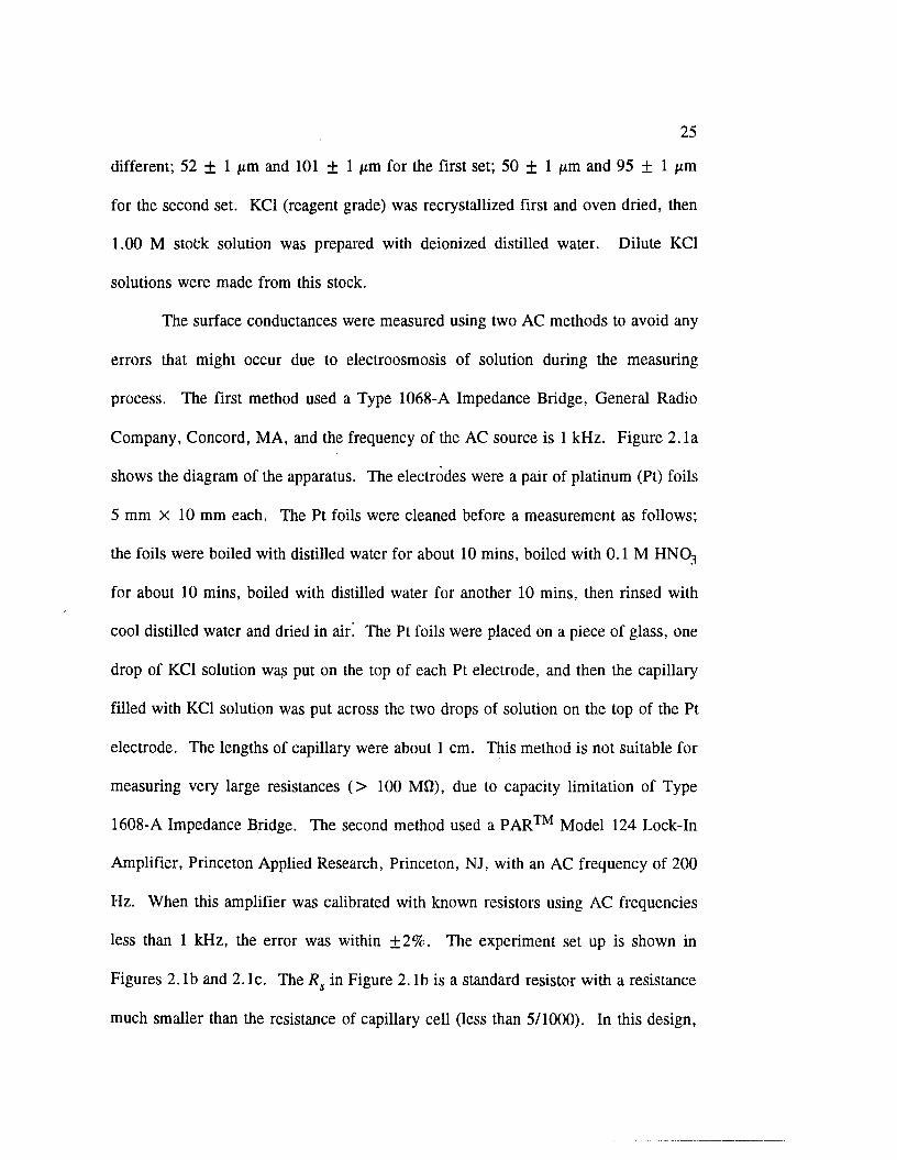
The surface conductances were measured using two AC methods to avoid any

errors that might occur due to electroosmosis of solution during the measuring

process. The first method used a Type 1068-A Impedance Bridge, General Radio

Company, Concord, MA, and the frequency of the AC source is 1 kHz. Figure 2. la

shows the diagram of the apparatus. The electrodes were a pair of platinum (Pt) foils

5 mm X 10 mm each. The Pt foils were cleaned before a measurement as follows;

the foils were boiled with distilled water for about 10 mins, boiled with 0.1 M HN03

for about 1 0 mins, boiled with distilled water for another 1 0 mins, then rinsed with

cool distilled water and dried in air. The Pt foils were placed on a piece of glass, one

drop of KC1 solution was put on the top of each Pt electrode, and then the capillary

filled with KC1 solution was put across the two drops of solution on the top of the Pt

electrode. The lengths of capillary were about 1 cm. This method is not suitable for

measuring very large resistances (> 100 Mfi), due to capacity limitation of Type

1608-A Impedance Bridge. The second method used a PAR™ Model 124 Lock-In

Amplifier, Princeton Applied Research, Princeton, NJ, with an AC frequency of 200

Hz. When this amplifier was calibrated with known resistors using AC frequencies

less than 1 kHz, the error was within ±2% . The experiment set up is shown in

Figures 2. lb and 2. lc. The Rs in Figure 2. lb is a standard resistor with a resistance

much smaller than the resistance of capillary cell (less than 5/1000). In this design,

26

(a)

C ap illary P t F o il E le c tr o d e

I J

■0-

T y p e 1 6 0 8 -A Im p e d a n c e B rid g e

(b)

Rc

A m p lif ie r

C apillary4

A CP A R ™ M o d e l 124 L ock -In A m p lif ie r

d ia m eter 6.5 m m , d e p th 7 m m

P t W ire E le c tr o d e 2 0 m m -*25 m m

TC apillary

13 m m

7 0 m mT e f lo n

Figure 2.1 The diagram of the apparatus for capillary surface conductance measurement; (a) Using a type 1608-A impedance bridge, (b) Using a PAR™ model 124 lock-in amplifier, (c) The teflon holder for circuit (b).

27

the capillary was placed on a Teflon holder, 13 mm x 25 mm x 70 mm (Figure

2. lc). Two large wells (diameter 6.5 mm and depth 7 mm) were made in the top side

in order to create electrolyte reservoirs, and two small holes (about 1.4 mm in

diameter) were drilled from the two sides to reach each hole of the top side. Pt wire

electrodes (diameter 1.5 mm and length 60 mm) were put through the two small holes

from the two sides to connect the electrolyte solution in the two big holes from the

top side. The Pt wire electrodes were cleaned before the measurement using the same

procedure as for the Pt foil electrodes. The capillary lengths were about 2 cm in

these experiments. Using this method, the two connection clips and the electrodes

were far away from each other to reduce errors due to stray capacitances and

electrostatic inductances. Specific conductivity of bulk solution was measured with

a CDM 83 conductivity meter.

A preliminary test of capillary electroosmosis was made for 0.100 M KC1

solution. The electroosmosis test was as follows; one beaker which contains 0.100

M KC1 + 5% phenol was at the anode (+ ) side, and another beaker which contains

0.100 M KC1 was at the cathode (-) side. Two pieces of Pt wire were used as

electrodes. The beakers were connected electrically with a capillary, diameter 95 jum,

length 6.1 cm. A Potentiostat/Galvanostat Model 273, EG&G Princeton Applied

Research, was used to apply a constant current. The experiment was operated under

the constant current mode and voltage was calculated from Ohm’s law. The

resistances of the capillary cell with solution were measured before and after the

electroosmosis test, and the average was used to calculate the voltage. For

comparison purposes, two other beakers were set up with a connecting capillary

28

(without applying DC) to check phenol transfer due to diffusion, migration, and

evaporation. Another beaker containing 0.1 M KC1 solution was placed close to the

cathode area without a capillary to check phenol transfer by evaporation only. The

test time is quite long (4 hours) in order to have enough solution migration from

anode to cathode. After the test, the concentration of phenol in the cathode solution

was measured at 268 nm by the UV-Vis method using a Model 14DS UV-Vis-IR

Spectrophotometer, AVIV, Lakewood, NJ.

2.3.1 Surface Conductance Measurement using an Impedance Bridge

Table 2.1 contains the results of surface conductances of 1.00 x 10‘2, 1.00 X

10'1, and 1.00 M KC1 solutions in 52 /xm (bottom half of table) and 101 /xm (top half

of table) capillaries using a Type 1608-A Impedance Bridge. The specific

conductivities of the bulk solutions were measured first using a CDM 83 conductivity

meter. The surface conductance (<xs) is calculated based on [2.7]

where R is the total resistance (measurement), a0 is the specific conductivity of bulk

solution, r is the radius of capillary, and L is the length of capillary. The as is a so-

called specific surface conductivity. From Equation 2.2

2.3 Results and Discussion

R L + L1 o0nr2 aJZnr (2 .2)

(2 .3)

29

Table 2.1 Capillary Surface Conductance of 0.0100-1.00 M KC1 Solutions

Cone, of KC1 ff0a (mS/cm) Rob (Mfl) Rc (MS2) (S)

0.0100 M 1.43±0.01 8.73 8.5±0.4e 8.0 X10' 8

0.100 M 12.60±0.02 0.990 0.93+0.03 2 .Ox 1 0 ' 6

1.00 M 109.4±0.2 0.114 0.105 ±0.006 2.4X10 ' 5

0.0100 M 1.43+0.01 32.9 26.6±0.5 4 .4x 10' 7

0.100 M 12.60±0.02 3.74 3 .5 ± 0 .1 1.1 X10' 6

l.OOM 109.4+0.2 0.430 0.39±0.01 1.5 x 10' 5

Diameter of capillary: d = 101 ± 1 /xm for the top half of table,d = 52 + 1 /xm for the bottom half of table.

a. Specific conductivity of bulk solution, a0, measured with a CDM 83conductivity meter and values are consistent with the literature values.

b. Resistance of bulk solution, R0 = L/foQirr2), where L = 1 cm (normalized to 1 cm).

c. Resistance, R, measured with a Type 1608-A Impedance Bridge.d. Surface Conductance, as, calculated based on equation:

HR = l/R0 + (os2Trr)/L.e. All errors are the standard deviations (Iff) of 9-12 measurements.

30

After measuring the total resistance, R, as could be calculated by applying Equation

2.3. The surface conductance, as, increases in both capillaries with increase of KC1

concentration. These results are consistent with available literature values, e.g.

[2.8 ,2.9]. The os values are in the range of 10' 5 to 10' 9 siemens for the capillary of

diameter from a few to 100 /xm and concentrations of electrolyte from 0.1 to 10' 6 M.

Table 2.2 lists the results of resistance measurements of 0.100 M KC1 solution

+ different concentrations of HC1 in a 52 /xm capillary. The solutions were made up

by adding a small volume of concentrated HC1 solution to 0.100 M KC1 solutions.

The results are plotted in Figure 2.2; the top line gives the resistances of the bulk

solutions by calculation, assuming no surface conductance is present and the bottom

line indicates the measured resistances. Using HC1 solution to adjust pH value

changes the resistance of the solution automatically because of the addition of H+ and

Cl" ions. All as values are the in the /xS range. The pH at which the surface has zero

charge is called the point of zero charge (pHpzc). Because there is no minimum or

maximum in the resistance curve, Figure 2.2, the pHpzc was not determinable,

however, there appears to be little or no excess surface conductance below about pH

2. Below pH 2, HC1 begins to make a major contribution to the conductance because

of large amount of H+ ion. Because a deactivated capillary is used, the deactivation

may have changed the original properties of the glass surface.

2.3.2 Surface Conductance Measurement using a Lock-In Amplifier

Table 2.3 contains the results of surface conductance measurement of 1.00 x

10'4, 1.00 X 10'3, 1.00 X 10‘2, 0.100, and 1.00 M KC1 solutions in 50 and 95 /xm

31

Table 2.2 Resistance Measurement of Acidified KCI Solution vs. pH

pHa ff0b (mS/cm) Roc (MO) Rd (MO) <rse (nS)

7.0 12.60±0.02f 3.74 3.48±0.11 1 . 2 2

6.5 12.47±0.02 3.78 3.44±0.02 1.60

5.8 12.42±0.02 3.79 3.45±0.03 1.59

4.2 12.55±0.01 3.75 3.42±0.05 1.58

3.1 12.89±0.02 3.65 3.15±0.05 2 . 6 6

2 . 1 16.60±0.08 2.84 2.63±0.02 1.72

1 . 1 52.7±0.1 0.893 0.808±0.014 7.21

Diameter of capillary: d = 52 ± 1 fim.a. Measured by a Coming Model 12 pH meter.b. Specific conductivity of bulk solution (0.1 M KCI with HC1 for different pH),

(r0, measured with a CDM 83 conductivity meter.c. Resistance of bulk solution, R0 = L/(o0irr), where L = 1 cm (normalized to

1 cm).d. Resistance, R, measured with a Type 1608-A Impedance Bridge.e. Surface Conductance, <rs, calculated based on equation:

HR = \IR0 + (os2irr)/L.f. All errors are the standard deviations (ltr) of 6-10 measurements.

Tota

l Re

sista

nce

(MQ

/cm

)

R e s is ta n c e o f KC1 ( 0 . 1 M ) + HC1 (p H )5

4

3

2

1

0

0 1 2 3 4 5 6 7 8

p H

Figure 2.2 Total resistance of KC1 (0.100 M) + HCI (pH) solutions.

Resistance of Bulk Solution

*-□

Measurement

j I I I I I I I i I i I i 1

33

Table 2.3 Capillary Surface Conductance of l.OOx 10'4-1.()0 M KC1 Solutions

Cone, of KC1 ff0a (fiS/cm) Rob («) Rc (Q) <s>l.OOx 10'4 M 17.5±0.2 1.61 X109 (1 .12± 0 .05)X l09e 1.83X 10'8

l.OOx 10'3 M 150±2 1.88x10s (1.62±0.06)X 10s 5.74X 10'8

l.OOx 10'2 M 1390± 10 2.03 X107 (1.94±0.02)X 107 1.53 x 10‘7

0.100 M (12.56±0.01)X 103 2.25 x 106 (2 .1 6 ± 0 .0 3 )x l0 6 1.19X10'6

l.OOM (107.5±0.3)X 103 2.62X105 (2 .48±0 .03)x 105 1.49X10'5

l.OOx 10"4 M 18.8±0.2 5.46 X109 (2 .2 5 ± 0 .0 2 )x l0 9 f ?f

l.OOx 10'3 M 155± 1 6.62X10s (5.73±0.09)X 10s 2.99 X10'8

l.OOX 10’2 M 1330±10 7.72X107 (7.18±0.07)X 107 1.24X 10‘7

0.100 M (12.18±0.01)X 103 8.43X106 (7.86±0.2)X 106 1.09X 10‘6

1.00 M (110.7±0.2)X103 9.28X105 (8.61±0.08)X105 1.07 X10'5

Diameter of capillary: d = 95 ± 1 /im for the top half of table,d = 50 ± 1 fim for the bottom half of table.

a. Specific conductivity of bulk solution, a0, measured with a CDM 83 conductivity meter.

b. Resistance of bulk solution, R0 = L/ioQirr2), where L = 2 cm (normalized to 2 cm).

c. Resistance, R, measured with a PAR™ Model 124 Lock-In Amplifier.d. Surface Conductance, cts, calculated based on equation:

1 /R = 1 / R q + (os2irr)/L.e. All errors are the standard deviations (la) of 4-8 measurements.f. The R value for this concentration has a big error due to its huge resistance

and close to the resistance range of stray capacitances and the electrostatic inductances even without the connecting capillary.

34

capillaries using a PAR™ Model 124 Lock-In Amplifier. These as values increase

with increase of KC1 concentration in both capillaries. The as values at KC1

concentrations of 1.00 M, 0.100 M, and 0.0100 M for the 50 /xm capillary are 1.07

x 10'5, 1.09 x 10‘6, and 1.24 X 10' 7 S, respectively, and for 95 /xm capillary are

1.49 x 10'5, 1.19 x 10'6, and 1.53 x 10' 7 S, respectively. As expected, these

values are reasonably close despite the difference in capillary diameter. The as

values at KC1 concentrations of 1.00 x 10'2, 1.00 x 10'3, and 1.00 x 10' 4 M for 95

/xm capillary in Table 2.3 are 1.53 x 10'7, 5.74 x 10‘8, and 1.83 x 10"8 S,

respectively, and in Ref. [2.9] these values at the same KC1 concentrations for a 100

/xm capillary are 1.21 x 10'6, 4.01 x 10'7, and 2.93 x 10' 8 S, respectively.

Although the literature results show a similar trend with increase of KC1 concentration

the as values are correspondingly larger (~ 10x ). The differences may be ascribed

to the capillary compositions, the surface conditions, small differences in diameters,

the operating temperatures (25°C in Ref. [2.9] and 23°C in our case), and different

experimental methods (DC method in Ref. [2.9] and AC method in our case). The

lower values in our work perhaps indicate a less active glass surface (fewer ionic

sites).

2.3.3 Capillary Electroosmosis of KC1 using Phenol as an Indicator

Figure 2.3 contains UV spectra for phenol at concentrations of 2.5, 5.0, 7.5,

10.0, 12.5 ppm, and Figure 2.4 contains the concentration calibration curves at two

peak wavelengths. Calibration data with the absorption maximum at wavelength 268

nm are used to calculate the concentration of phenol in the electroosmosis tests (at 209

Abs

orba

nce

U V S p ec tra o f P h e n o l fo r C a lib ra tio n1 . 0

0.9

0 . 8

i- \ Phenol Concentrations:0.7 4. \ 12.5 ppm

0 . 6

\1- v \1 M

1 0 . 0 ppm - 7.5 ppm

0.5 \ \ % . 15.0 ppm

t YA-A . i\% M\ % i\• * \\- y A\ ‘A

2.5 ppm0.4

0.3

0 . 2

0 . 1

0 . 0

wuvA* ' %A• \A

-0 . 1 ______ i______ I______i____ 1 . 1 . 1 I

200 220 240 260 280 300

W a v e le n g th (n m )

Figure 2.3 UV spectra of phenol at different concentrations.

36

1.0

0.8

0.6oG03X>)—O

£ 0.4

0.2

0.00 3 6 9 12 15

C o n c e n tr a tio n o f P h e n o l (p p m )

Figure 2.4 The concentration calibration curves at 209 and 268 nm wavelengths of phenol.

at 209 nm

at'268 nm

I

37

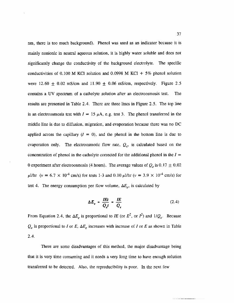
nm, there is too much background). Phenol was used as an indicator because it is

mainly nonionic in neutral aqueous solution, it is highly water soluble and does not

significantly change the conductivity of the background electrolyte. The specific

conductivities of 0.100 M KC1 solution and 0.0998 M KC1 + 5% phenol solution

were 12.60 ± 0.02 mS/cm and 11.90 ± 0.06 mS/cm, respectively. Figure 2.5

contains a UV spectrum of a catholyte solution after an electroosmosis test. The

results are presented in Table 2.4. There are three lines in Figure 2.5. The top line

is an electroosmosis test with / = 15 jaA, e.g. test 3. The phenol transferred in the

middle line is due to diffusion, migration, and evaporation because there was no DC

applied across the capillary (/ = 0 ), and the phenol in the bottom line is due to

evaporation only. The electroosmotic flow rate, Qe, is calculated based on the

concentration of phenol in the catholyte corrected for the additional phenol in the I =

0 experiment after electroosmosis (4 hours). The average values of Qe is 0.17 + 0.02

/xl/hr (v = 6.7 x 10' 4 cm/s) for tests 1-3 and 0.10 /xl/hr (v = 3.9 x 10‘4 cm/s) for

test 4. The energy consumption per flow volume, AEe, is calculated by

A Et - — - — (2.4)' <?/ <?.

From Equation 2.4, the AEe is proportional to IE (or E2, or l 2) and 1 !Qe. Because

Qe is proportional to 1 or E, AEe increases with increase of / or E as shown in Table

2.4.

There are some disadvantages of this method, the major disadvantage being

that it is very time consuming and it needs a very long time to have enough solution

transferred to be detected. Also, the reproducibility is poor. In the next few

Abs

orba

nce

38

0.50

0.45

0.40

0.35I = 15 jiA

0.30

0.25

0.20= 0

0.15

0.10

0.05

0.00 w/o capillary

-0.05280200 260 300220 240

W a v e le n g th (n m )

Figure 2.5 Typical UV spectra of a catholyte solution after an electroosmosis test(test 3).

Table 2.4 Electroosmosis through a 95 /un Capillary

39

Test 1 Test 2 Test 3 Test 4

Current I (^A) 15 15 15 7.5

Voltage Ea (V) 92 92 92 46

Phenol Cone, after Test (ppm) 4.7 4.4 4.5 3.4

Solution Volume (ml) 1 2 . 1 2 12.16 12.13 12.09

W Capillary, 1=0, Phenol conc. (ppm) 2 . 2 1 . 6 1 . 8 1.7

Qe (/ul/hr) 0.15 0.17 0.19 0 . 1 0

AEe (kj/ml) 32 29 26 13

Diameter of capillary: 95 fim, the length of capillary: 6.1 cm.a. The resistance of cell was measured before and after test, R = 6 .1 ± 0.2 Mfl

(n=10), then E = IR.b. Energy consumption per flow volume, AEe = IE!Qe, Qe is the flow rate.

40

chapters, another method will be used to study capillary electroosmosis in more detail.

Nowadays, the most used method for practical chromatographic applications is an on­

line UV or fluorescence detector system using a UV marker or fluorescence marker.

2.4 Conclusions

The AC surface conductivities of 1.00 x 10"4 - 1.00 M KC1 solutions are

measured and found to be in the range of 10"5 to 10‘ 8 siemens for capillaries of 50 ^m

and 100 /*m diameter. Also, the resistances of solutions of 0.100 M KC1 + different

HC1 concentrations increase with increase of pH (decrease of HC1 concentration) but

no minimum or maximum could be found in the curve. The electroosmosis of KC1

solutions containing 5% phenol were also studied in a 95 ^m capillary. The

electroosmotic flow rates are 0.17 and 0.10 ^1/hr for the electric field gradients of 15

and 7.5 V/cm, respectively. However, the method used is very time consuming and

not particularly sensitive. Capillary electroosmosis will be studied in depth in

chapters 3 and 4 using more sensitive the current-monitoring method.

41

2.5 References

2.1 J. Hamed, Y.B. Acar, and R.J. Gale, J. Geotech. Engrg. ASCE, 1991, 112, 241.

2.2 C.J. Bruel, B.A. Segall, and M.T. Walsh, J. Geotech. Engrg. ASCE, 1992, 118, 84.

2.3 A.P. Shapiro and R.F. Probstein, Environ. Sci. Technol. 1993, 27, 283.

2.4 R.F. Probstein and R.E. Hicks, Science 1993, 260, 498.

2.5 J.K. Mitchell, Fundamentals o f Soil Behavior, John Wiley and Sons, Inc.,New York, 1976, pp. 117 and 353-359.

2.6 X. Huang, M.J. Gordon, and R.N. Zare, Anal. Chem. 1988, 60, 1837.

2.7 A.J. Rutgers and M. De Smet, Trans. Faraday Soc. 1947, 43, 102.

2.8 J.A. Schufle and N.T. Yu, J. Colloid Interface Sci. 1968, 26, 395.

2.9 J.A. Schufle, C.T. Yu, and W. Drost-Hansen, J. Colloid Interface Sci. 1976, 54, 184.

CHAPTER 3.

FUNDAMENTAL STUDIES OF HYDRAULIC AND ELECTROOSMOTIC

FLOW THROUGH SILICA CAPILLARIES

3.1 Introduction

Electrokinetic effects are of renewed interest since the emergence of new

separation techniques such as micellar electrokinetic capillary chromatography and the

prospects for a variety of soil decontamination technologies. In recent years,

electrokinetic soil processing has been widely studied as a practical means to remove

contaminants from soils, e.g. [3.1-3.3]. Also, capillary zone electrophoresis (CZE)

and micellar electrokinetic capillary chromatography (MECC) have been growing very

rapidly during this decade because they offer speed and highly efficient separations,

especially for macromolecules in the important area of analytical biotechnology, e.g.

[3.4,3.5]. The four major electrokinetic phenomena in geotechnology are

electroosmosis, streaming potential, electrophoresis, and migration (or sedimentation)

potential [3.6]. Electroosmosis and electrophoresis are the movement of electrolyte

and charged macromolecules, respectively, due to application of an electric field.

Streaming and sedimentation potentials are the generation of currents due to the

movement of electrolyte under hydraulic potential and movement of charged particles

under gravitational forces, respectively. Of the four electrokinetic processing,

electroosmosis has been given the most attention in geotechnical engineering, because

of its practical value for transport of water in fine-grained soils and the ease by which

pumping can be induced electrically in low permeability clays.

42

43

It is, therefore, of considerable practical as well as theoretical interest to study

the energetics and efficiencies of electrokinetic phenomena. To simplify the

experimental design, both hydraulic and electroosmotic flow velocities in cylindrical

silica capillaries were chosen to be determined. In this study, hydraulic and

electroosmotic flow through silica capillaries, 50 and 100 nm diameters, have been

determined experimentally and analyzed theoretically. Hydraulic flow follows the

Poiseuille relation very well, however, with increase of the ionic strength of the fluid,

the rate of electroosmotic flow decreases. Particularly, the energy consumptions are

compared for hydraulic and electroosmotic flow. Results show that, in general,

hydraulic flow is much more energy efficient than electroosmotic flow because of bulk

IR losses in the latter. The classical theory for electrokinetic phenomena possibly

overestimates the transfer of electrical into mechanical energy since both irreversible

thermal as well as ion migration energy losses occur in the conductance of double

layer ions. The physical significance of the electrokinetic zeta potential based on

classical theory, f, needs to be carefully reexamined.

3.2 Theoretical Background

Considering first hydraulic flow through a single capillary, the flow rate, if

laminar flow conditions exist, might be described by the Poiseuille equation, e.g.

[3.7]. The velocity (cm/s) of flow is dependent on the layer distance from the tube

central axis and given by

44

v.maxR2k p 4 t i L

(3.1)

vw - v j i - i R 1

(3.2)

where r (cm) is point distance from the axis, R (cm) is the capillary radius, L (cm)

is the length of the capillary, Ap (dyn/cm2) is the pressure, and 17 (poise or

dyn • s/cm2) is the fluid viscosity. Thus, it is a maximum at the tube axis and assumed

Figure 3.1a [3.7] illustrates the velocity profile of hydraulic flow through a

capillary. The hydraulic force is evenly applied to the whole region of cross section

of the capillary. At the tube inlet, the profile is rectangular. On passage through the

tube, boundary layers develop at the walls and their thickness increases until they

merge at a certain distance, x, from the inlet. The length x is called the entry region.

Also, the velocity profile approaches to a steady-state laminar flow profile, the

velocity in the center of the tube increases to maximum value, vmax; and the velocity

at the walls is zero.

The equation which is used in geotechnical engineering to describe the

hydraulic flow rate Qh in soil systems is [3.6]

in which kh (cm/s) is hydraulic conductivity and zh = (H/L) the hydraulic gradient,

where H (cm) is the hydraulic head pressure and L (cm) is the length of soil section.

to be zero at the wall. The total flow rate <2h (cm3 /s) is given by

Q h ~ k h h f t (3.4)

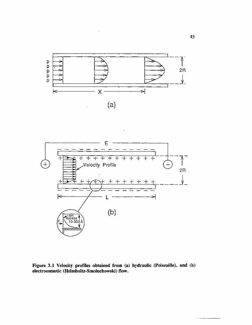
0.0

. CL 0

.0.

2R

(a)

-Velocity Profile2R

ione x c e s s

tsssssssSSs,

Figure 3.1 Velocity profiles obtained from (a) hydraulic (Poiseuille), and (b)electroosmotic (Helmholtz-Smoluchowski) flow.

46

If p is the density of fluid, g is the gravitational constant, and A = irR2', thus kh oc

pgR2/(8ri). Factors to account for the effects of porosity and tortuosity need also to

be included in a practical description of flow through porous media.

There are several theories which attempt to describe the basic velocity profile

of electroosmosis in a capillary [3.5,3.6 ]. One of them most widely used for large

pore capillaries is the Helmholtz-Smoluchowski theory. In this theory, the average

fluid electroosmosis velocity, v, through a capillary is

v - (3.5)r| L

in which e is the dielectric constant of the medium, e0 is the permittivity of free

space, t] is its viscosity, E is the applied electric potential, L is the length of capillary,

and f is called the electrokinetic zeta potential. Figure 3.1b shows the classical

velocity profile of electroosmosis through a capillary. The electric force is applied

very near the surface (to the electric double layer) at the tube wall. The large pore

theory predicts a maximum flat velocity profile through most of the capillary, with

zero velocity at the wall of the capillary. Earlier fundamental studies of capillary

electroosmosis include those of Rutgers et al. [3.8], Rice et al. [3.9], Koh et al.

[3.10], and'Ohshima et al. [3.11,3.12]. An extensive review of the literature prior

to 1974 is available [3.13].

Electroosmosis in a porous medium similarly can be analyzed using a capillary

model. By applying Equation 3.5 to a soil system, an equation for expressing the

flow rate due to electroosmosis is obtained

Qe = kj'A (3.6)

47

in which ie = (E/L) is the electrical gradient and kc ((cm/s)/(V/cm)) is termed the

coefficient of electroosmotic permeability; the parameter kc can be found from the

relation kt cx -(ee0 where n = the porosity of soil system and A = its cross

sectional area. Note that these important expressions depend on the validity of the

classical electrokinetic theory.

The purpose of determining the hydraulic flow through a capillary is to

compare the hydraulic (mechanical) energy with the electric energy which causes

electrolyte flow. The hydraulic flow through silica capillaries has been measured and

analyzed in this paper. Also, the electroosmotic flow through the same kind of

capillary has been studied. Efficiency and energy consumption are compared for the

two flow types.

3.3 Experimental Section

Fused silica capillary (J & W deactivated fused silica capillary, Alltech Co.)

was used in the studies. The diameters of capillaries were measured under a

microscope (Bausch & Lomb) and by magnifying with a video camera (CCTV

camera, Model HV-720u; Philips VCR, Model VR6495AT; Hitachi video monitor,

Model VM-900u). Two standard scales (2 / m x 50 divisions and 50 jam x 50

divisions) were used for calibration. Before each experiment, the capillary was

flushed with deionized water (about 2 ml), or flushed with electrolyte (for the

electroosmosis experiments). KC1 (reagent grade) was recrystallized first and dried,

then 1.00 M stock solution was prepared with high quality deionized distilled water.

Dilute KC1 solutions were made from this stock.

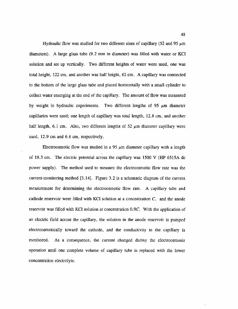
48

Hydraulic flow was studied for two different sizes of capillary (52 and 95 fim

diameters). A large glass tube (9.2 mm in diameter) was filled with water or KC1

solution and set up vertically. Two different heights of water were used, one was

total height, 122 cm, and another was half height, 62 cm. A capillary was connected

to the bottom of the large glass tube and placed horizontally with a small cylinder to

collect water emerging at the end of the capillary. The amount of flow was measured

by weight in hydraulic experiments. Two different lengths of 95 ^m diameter

capillaries were used; one length of capillary was total length, 1 2 . 8 cm, and another

half length, 6.1 cm. Also, two different lengths of 52 fim diameter capillary were

used, 12.9 cm and 6 . 6 cm, respectively.

Electroosmotic flow was studied in a 95 fim diameter capillary with a length

of 19.3 cm. The electric potential across the capillary was 1500 V (HP 6515A dc

power supply). The method used to measure the electroosmotic flow rate was the

current-monitoring method [3.14]. Figure 3.2 is a schematic diagram of the current

measurement for determining the electroosmotic flow rate. A capillary tube and

cathode reservoir were filled with KC1 solution at a concentration C, and the anode

reservoir was filled with KC1 solution at concentration 0.9C. With the application of

an electric field across the capillary, the solution in the anode reservoir is pumped

electroosmotically toward the cathode, and the conductivity in the capillary is

monitored. As a consequence, the current changed during the electroosmosis

operation until one complete volume of capillary tube is replaced with the lower

concentration electrolyte.

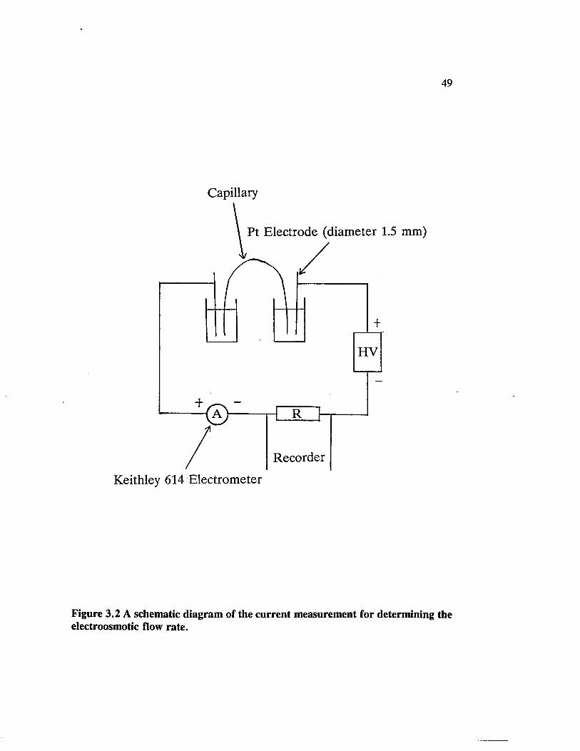
49

C apillary

P t E le c tr o d e (d ia m e te r 1.5 m m )

R e c o r d e r

H V

K e ith le y 6 1 4 E le c tr o m e te r

Figure 3.2 A schematic diagram of the current measurement for determining theelectroosmotic flow rate.

50

All experiments were made at the ambient laboratory temperature, 23±2°C,

approximately. The viscosities of water and 0.067 M KC1 were calculated using data

from the CRC Handbook o f Chemistry and Physics, 69th ed.

3.4 Results and Discussion

3.4.1 Hydraulic Flow Analysis

Hydraulic flow tests have been made to assess the flow rates in capillaries by

applying different pressures to various lengths of capillary. The results are shown in

Figures 3.3-3.5 and are summarized in Table 311. The flow rates after about 2 days

are smaller than those at the beginning of the experiments, probably due to clogging

of the capillary by adventitious dust or biological debris. In accordance to Equation

3.3, the hydraulic flow rate Qh is proportional to R4. For the two different sizes of

capillary used in the experiments, the ratio of the two flow rates should be close to

11.1 [(95/52)4]. Comparing the experimental flow rates for the two different sizes of

capillary, the agreement is reasonable, e.g. 0.61/0.049 = 12. Also, for a same size

capillary, by increasing the height of water, the flow rate increases directly with the

pressure head (Qh oc H). Again, reasonable agreement is observed, e.g. 122/62 =

1.97 (theory), 0.61/0.307 = 1.99 (observed). With an increase of the length of the

capillary, the flow rate decreases with the reciprocal length {Qh oc 1/L). For

example, 6.6/12.9 = 0.512 (theory), 0.0495/0.116 = 0.427 (observed). The last

column of Table 3.1 was calculated based on Equation 3.3, and the theoretical flow

rates are slightly larger in all cases but reasonably close to the experimental flow rates

(20% error margin maximum). The reasons for smaller experimental flow rates

51

Table 3.1 Hydraulic Flow Rate Comparison of Experiment and Theory

Test No. Correlation* Experimental Flow Rate* (ml/hr)

Theoretical Flow Rate (ml/hr)

1 0.9856 0.613±0.023 0.729

2 0.9953 0.605±0.009 0.729

3 0.9978 0.718±0.007 0.731

4 0.9976 0.307 ±0.003 0.371

5 0.9995 1.527 ±0.005 1.53

6 0.9989 0.0495 ±0.0008 0.0650

7 0.9952 0.116±0.003 0.127

* Obtained from least squares line to linear section by a Lotus 123 Program.

Diameter of Capillary: 95 ± 1 fim.

Test 1 & 2: total length of capillary, 12.8 cm; total height of water, 122 cm.Test 3: total length of capillary; total height of 0.05 M KC1 solution, 122 cm.Test 4: total length of capillary; half height of water, 62 cm.Test 5: half length of capillary, 6.1 cm; total height of water.

Diameter of Capillary: 52 ± 1 fim.

Test 6 : total length of capillary, 12.9 cm; total height of water, 122 cm.Test 7: half length of capillary, 6 . 6 cm; total height of water.

Tota

l Vo

lum

e (m

l)

52

60

■I'50Total Height of 0.05 MKC1 .* A'

40

Total Height of Water30

20

Half Height of Water10

00 10 20 30 40 50 60 70 80 90 100 110

T im e (h o u rs)

Figure 3.3 Hydraulic flow of water and 0.05 M KC1 through a capillary (95 jundiameter, 12.8 cm length): total height = 122 cm, half height = 62 cm.

53

150

120

& 90a>sO

> 60 3oH

30

0

0 10 20 30 40 50 60 70 80 90 100 110

T im e (h o u rs)

Half Length*/

V/

/A " 1

Total Length

J k ' x .

/J I I I I i I t 1 I I I I t I

Figure 3.4 Hydraulic flow of water through a capillary (95 pm diameter): totalheight of water 122 cm; total length = 12.8 cm, half length = 6.1 cm.

Tota

l Vo

lum

e (m

l)

54

6

A - A5

4/ Half Length

3Total Length

2

1

0

100 120 1408020 40 600

T im e (h o u rs)

Figure 3.5 Hydraulic flow of water through a capillary (52 pm diameter): totalheight = 122 cm; total length = 12.9 cm, half length = 6.6 cm.

55

might be due to small particles (from dust) slightly clogging the capillary, electrostatic

or frictional drag on the ill-defined surface of the capillary, the errors in the

measurement of capillary diameter, solvent evaporation, and variable capillary

diameter.

It is concluded that the classical Poiseuille model for hydraulic flow reasonably

predicts and accounts for the aqueous flow rates at room temperature through these

silica capillaries as functions of applied pressure and radius and length of capillaries

for the ranges of conditions tested.

3.4.2 Energy Analysis of Hydraulic Flow

For an energy analysis of hydraulic flow, the potential energy, mgH, is used

to cause flow, g is the gravitational constant, H is the height of water, and m is mass.

From the law of conservation of energy

mgH = ]/2 mv2 + (energy consumed) (3.7)

where v is the velocity of fluid exiting the capillary and Vzmv2 is the kinetic energy

of the escaping fluid. So the energy consumption/flow volume, AEh (J/ml), can be

calculated as follows

A£), = (mgH - ‘/2mv2)/Qht = pgH - ‘/zpv2 ~ pgH (3.8)

where p is the density of fluid, thus m = pV = pQ^t. The kinetic energy, Vzpv2 is

very small for this hydraulic flow and can be ignored. For example, in a 95 pm

diameter, 12.8 cm length capillary, if H = 1.22 m (total height), £>h = 0.72 ml/hr

(theoretical flow rate), so v = 2.8 cm/s; thus Vzpv2 = 3.9X10"7 J/ml and pgH =

56

0.012 J/ml. Hence, the hydraulic energy necessary to sustain flow is that required to

overcome the frictional losses and becomes AEh = 0.012 J/ml.

The experiment data (tests 1-4 in Table 3.1) of a 95 ixm diameter and 12.8 cm

length capillary are used to calculate the energy consumption per flow volume versus

the hydraulic flow rates. The hydraulic flow rate has a relationship with AEh as

follow

QhE (ml/hr) = (54 ± 3)AEh (J/ml) (3.9)

The theoretical line predicts a slightly larger value for the hydraulic flow, QhT (ml/h)

= 61A£h (J/ml).

3.4.3 Electroosmotic Flow Analysis

The classical Helmholtz-Smoluchowski theory of electroosmosis is considered

to be applicable to those systems in which the double layer thickness is small

compared to the capillary diameter [3.7,3.13]. Since 99.99% of the potential drop

across a double layer occurs in the distance 9.2I k , where 1 I k is the reciprocal Debye

length, the actual double layer thickness will be no larger than 1 pm for a 10' 5 M 1:1

electrolyte and smaller at larger ionic concentrations [3.15]. For the capillaries and

ionic strength electrolytes used in this study, it shall be assumed that large pore

conditions apply.

In addition to the comprehensive review of electrokinetic phenomena by

Dukhin and Derjaguin [3.13], the theory has also been presented by others, e.g.

[3.9,3.10,3.16]. When, for example, the double layer has an excess of cations in the

solution phase (anions on the solid surface) and an electrical field parallel to the

57

capillary surface is applied, a net, directional force is exerted by the cations on the

liquid causing it to move. At steady state, the electrical force on a cation is assumed

to be equal and opposite to the frictional slip forces within the liquid. If, however,

with the postulation that the electrical force is not transferred completely to

mechanical energy since some of the energy may be lost in heating or eddy current

effects, the equation relating velocity to applied electrical force becomes

- l i A p f r ) (3.10)dr2 r dr r\

in which vz is the fluid velocity in the axial direction z, r is the capillary radial

position, Ez is the electric field strength, p(r) is the excess charge density at point r,

r) is the fluid viscosity, and y i is an electrical to mechanical efficiency factor for

excess cation species, i. Two assumptions implicit in this theory are that the

background ions consist of equal concentrations of negatively and positively charged

ions whose motions result in forces which are equal and cancel and all of the excess

ions are available for momentum energy transfer (i.e. the total ion excess has only

species of one charge). Further, the model is strictly applicable only to dilute

electrolytes since, as pointed out by Koh and Anderson [3.10] the Debye-Hiickel

theory cannot be readily applied to the double layer region since the region is not

electroneutral. Additionally, an electrostatic drag could be created between the

surface charges and the double.layer excess charges [3.2],

Table 3.2 and Figure 3.6 contain a summary of the results of electroosmotic

flow measurements through silica capillaries at different KC1 concentrations. There

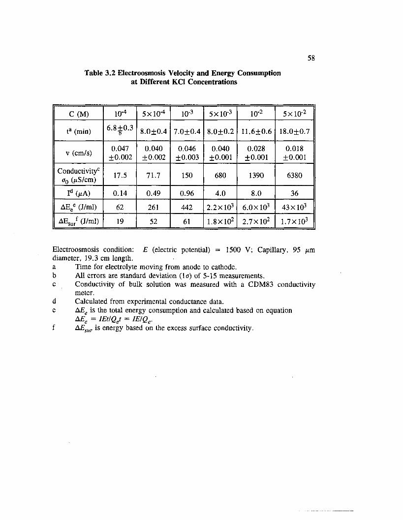
58

Table 3.2 Electroosmosis Velocity and Energy Consumption at Different KC1 Concentrations

c (M) 1 0 " 4 5 x 1 0 ‘4 1 0 ‘ 3 5X 1 0 ‘ 3 1 0 ‘ 2 5 x 1 0 ' 2

ta (min) 6 .8 + 0 .3 8 .0±0.4 7.0±0.4 8 .0 ± 0 . 2 1 1 .6 ± 0 . 6 18.0±0.7

v (cm/s) 0.047± 0 . 0 0 2

0.040± 0 . 0 0 2

0.046±0.003

0.040± 0 . 0 0 1

0.028± 0 . 0 0 1

0.018± 0 . 0 0 1

Conductivity0

a0 (/zS/cm) 17.5 71.7 150 680 1390 6380

Id 0*A) 0.14 0.49 0.96 4.0 8 . 0 36

AEee (J/ml) 62 261 442 2 .2 X 1 0 3 6 .0 x 1 0 3 43X103

AEsurf (J/ml) 19 52 61 1.8 X102 2.7 X102 1.7X103

Electroosmosis condition: E (electric potential) = 1500 V; Capillary, 95 /zmdiameter, 19.3 cm length.a Time for electrolyte moving from anode to cathode,b All errors are standard deviation (la) of 5-15 measurements,c Conductivity of bulk solution was measured with a CDM83 conductivity

meter.d Calculated from experimental conductance data,e AEe is the total energy consumption and calculated based on equation

AEe = IEt/Qet = IEIQe. f &ESur is energy based on the excess surface conductivity.

Ele

ctro

osm

osis

V

eloc

ity

(cm

/s)

59

0.05

0 .04

0.03

0.02

0.01 J I I I I m l I I I I mi l « I I H ml I I I m u

10" 10"* 1 0 '3 10"z

C o n c e n tr a t io n o f K C1 (M )

10-l

Figure 3.6 Electroosmosis velocity at different concentrations of KC1 electrolyte(E = 1500 V; capillary: 95 /tin diameter, 19.3 cm length).

60

was no excess hydraulic pressure applied. Potassium chloride was chosen as the 1:1

background electrolyte since the ionic mobilities of K+ and Cl* are approximately

equal. As the bulk KC1 concentration increased from 1.00 x 10*4 to 5.00 x 10' 2 M,

electroosmotic velocity decreased from 0.047 to 0.018 cm/s. Thus, a 500-fold change

in background concentration resulted in only a 2 .6 -fold decrease in the electroosmotic

flow rate. The zeta-potential at most water solution-glass interfaces can be described

by the equation [3.17]

f = a a C 1/2 exp(-jSC1/2) (3.11)

in which a and /3 are constants, a is net surface charge density, and C is the bulk

concentration of electrolyte. This relation leads to the theoretical prediction that with

increase of C, f decreases and in consequence, the electroosmotic flow rate decreases.

If it is assumed that the excess surface charge density on the silica is constant and

about a 15x reduction of the double layer thickness has occurred [3.18], then the

electroosmotic flow is not a strong factor of bulk ionic strength, nor double layer

thickness. It is possible by calculating the bulk solution conductance in the capillary

to determine the surface conductance due to the ion excess. Some data are

summarized in Table 2.3 (in Chapter 2). With 4 orders of magnitude increase in KC1

concentration, 1.00 x 10*4 - 1.00 M, the surface conductance increases by about 3

orders of magnitude. It is not known, unfortunately, that the excess surface

conductances in high ionic strength solutions are due to only cations or to both cations

and excess salt at the surface. The electroosmotic velocity of KC1 at 10" 2 M = 0.028

cm/s (with electric gradient, E/L = 78 V/cm) compared with that of 10" 2 M Na2 H P0 4

(Pyrex 132-fim capillary) = 0.13 cm/s (with E/L = 100 V/cm), and for 0.05 M KC1

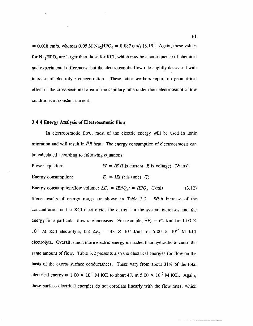
61

= 0.018 cm/s, whereas 0.05 M Na2 HP04 = 0.087 cm/s [3.19]. Again, these values

for Na2 HP0 4 are larger than those for KC1, which may be a consequence of chemical

and experimental differences, but the electroosmotic flow rate slightly decreased with

increase of electrolyte concentration. These latter workers report no geometrical

effect of the cross-sectional area of the capillary tube under their electroosmotic flow

conditions at constant current.

3.4.4 Energy Analysis of Electroosmotic Flow

In electroosmotic flow, most of the electric energy will be used in ionic

migration and will result in I2R heat. The energy consumption of electroosmosis can

be calculated according to following equations

Power equation: W = IE (/ is current, E is voltage) (Watts)

Energy consumption: Ee = IEt (t is time) (J)

Energy consumption/flow volume: AEe = IEt/Qet = IE/Qe (J/ml) (3.12)

Some results of energy usage are shown in Table 3.2. With increase of the

concentration of the KC1 electrolyte, the current in the system increases and the

energy for a particular flow rate increases. For example, AEt = 62 J/ml for 1.00 x

10' 4 M KC1 electrolyte, but AEe = 43 x 103 J/ml for 5.00 x 10' 2 M KC1

electrolyte. Overall, much more electric energy is needed than hydraulic to cause the

same amount of flow. Table 3.2 presents also the electrical energies for flow on the

basis of the excess surface conductances. These vary from about 31% of the total

electrical energy at 1.00 x 10' 4 M KC1 to about 4% at 5.00 x 10' 2 M KC1. Again,

these surface electrical energies do not correlate linearly with the flow rates, which

62

actually decrease despite a higher energy consumption. These energy figures are

based on steady-state values for the conductances and are not adjusted for

electroosmotic transport.

If we make an assumption that similar mechanical energy is required to achieve

equal hydraulic and electroosmotic flow rates, a value for 7i in Equation 3.10 may be

estimated. The efficiency parameter is clearly a function that has not been

theoretically or practically established of the concentration, conductance, and the

radius and charge of excess ion. Considering only the surface conductance as

providing electrical energy to cause electroosmotic flow, at 1.00 x 10' 4 M KC1,

7 i(c, as, rv zj) = 0.012/19 = 0.06% and at 5.00 X 10' 2 M KC1, 7 i(c, as, rv Zi) =

0.012/1.7 x l0 3 = 0.0007%. These figures are extremely small fractions of the

electrical energy associated with the excess surface conductances and this clearly

demonstrates that the classical model for electroosmosis is likely to be incorrect in

assuming that all of the surface electrical energy is available to cause the

electroosmotic flux. The energy equivalency postulate is reasonable given that in

hydraulic flow, the force (pressure) is applied equally over the capillary cross-

sectional area, whereas in electroosmotic flow the force is localized to the double

layer region, seemingly a less efficient process. Further, similar liquid-liquid and

liquid-solid frictional losses should ensue. Since the efficiency parameters are so

small, this brings into question the use of the classical electroosmotic model for

deriving electrokinetic zeta potentials. To fully resolve this question, it should be

stressed that better analytical data of the double layer region are required.

63

3.4.5 Comparison of kh and ke

The hydraulic conductivity, kh, can be calculated theoretically and

experimentally for hydraulic flow through a 95 pm capillary using Equations 3.3 and

3.4. The coefficient of electroosmotic permeability, ke, can be calculated

experimentally for electroosmotic flow through the 95 pm capillary for 0.05 M KC1

solution using Equation 3.6. By using Equations 3.5 and 3.6, the ke value can also

be calculated theoretically with assuming f = -30 mV. It is believed that f has a

value from a few to about -150 mV for different concentration of electrolyte [3.17].

These results are listed in Table 3.3. From Table 3.3, one can see that kh is about

0.29 cm/s and ke is about 2.3 x 10' 4 (cm/s)/(V/cm) for a 95 pm capillary. However,

in real soil systems, the ke values are in the 10' 5 (cm/s)/(V/cm) range and the kh

values are in the range of 10' 4 to 10"9 cm/s depending on the size of particle [3.6].

The diameters of most clays are much smaller (about a few pm or less) [3.6], the kh

values are in the range of 1 0 ' 7 to 1 0 ‘ 9 cm/s which are much smaller than the kh value

for the 95 pm capillary because for soils pore radius is smaller. The ke value for 95

pm capillary is larger than the ke values for soils due to capillary is smooth, probably.

3.5 Conclusions

Hydraulic flow through silica capillaries of diameters 50 and 100 ^m closely

obeyed the Poiseuille equation which assumes laminar flow. The electric energy used

to cause electroosmotic flow is a very small fraction of the total electrical energy,

especially in high ionic strength solutions. With increases of the electrolyte

concentration, the electroosmotic flow rate decreased slightly and the energy

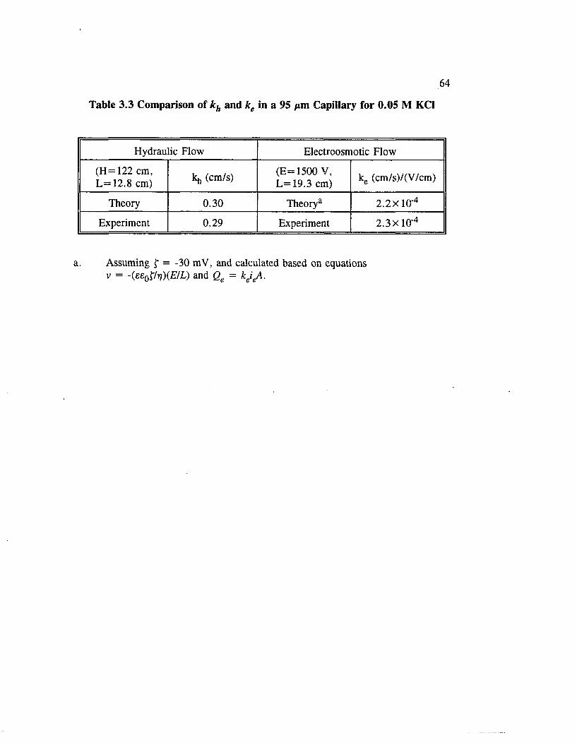
Table 3.3 Comparison of k h and ke in a 95 /*m Capillary for 0.05 M KC1

Hydraulic Flow Electroosmotic Flow

(H = 122 cm, L= 12.8 cm) kh (cm/s) (E= 1500 V,

L —19.3 cm) ke (cm/s)/(V/cm)

Theory 0.30 Theorya 2.2 X10' 4

Experiment 0.29 Experiment 2.3 X 10' 4

a. Assuming f = -30 mV, and calculated based on equations v = -(ee0f/T})(E/L) and Qe = k j / i .

65

consumption per flow volume increased dramatically. Thus, on comparison of

hydraulic flow with electroosmotic flow, hydraulic flow needs much less energy to

cause the same amount of flow. Certainly, hydraulic flow is much more energy

efficient than electroosmotic flow in a 95 ^m diameter capillary because in

electroosmotic flow, most of the applied energy will be lost in ion migration and I2R

heat. The electrical energy consumed in excess surface conductance similarly is far

larger than that needed for hydraulic flow ( 1 0 0 0 -fold or greater) and is an unknown

function of the electrolyte concentration, the surface conductance, the effective ion

radii, surface drag effects, etc. It must not be assumed, however, that the excess

surface conductance is due solely to a single cationic species. Additionally, it is

possible that the surface silica has amphoteric sites and competitive equilibria with

K+ , H + , Cl", and OH' ions and/or ion aggregates occurs. It is postulated that an

electrical to mechanical efficiency factor is required in the classical model for

electroosmosis and data are presented to support this view. Obviously, the

electrokinetic zeta potential will have to be derived based on a better understanding

of the magnitude of y i values and the surface species composition in the solution

phase.

For real soil systems, due to clogging and consolidation of soil, etc., hydraulic

flow may become less practicable; especially when the particle size is fractions of a

micrometer such as for clay [3.6], Thus despite the energy inefficiency of

electroosmosis, since its application provides a convenient pumping mechanism for

fluids through contaminated clay masses, it will continue to be of considerable interest

in environmental engineering as a practical tool for soil decontamination.

66

3.6 References

3.1 Y.B. Acar, A. Alshawabkeh, and R.J. Gale, Proc. Mediterranean Conf. on Environmental Geotechnology, Balkema Publishers Inc., Rotterdam, Netherlands, 1992, p. 321.

3.2 R.J. Gale, H. Li, and Y.B. Acar, "Soil Decontamination using Electrokinetic Processing", Chapter in Environmental Oriented Electrochemistry, Studies in Environmental Science 59, C.A.C. Sequeira (Ed.), Elsevier Science Publishers, 1994, pp. 621-54.

3.3 J. Hamed, Y.B. Acar, and R.J. Gale, J. Geotech. Engrg. ASCE, 1991, 112, 241.

3.4 K. Ghowsi, J.P. Foley, and R.J. Gale, Anal. Chem. 1990, 62 , 2714.

3.5 K. Ghowsi and R.J. Gale, J. Chromatogr. 1991, 559, 95.

3.6 J.K. Mitchell, Fundamentals o f Soil Behavior, John Wiley and Sons, Inc., New York, 1976, pp. 171 and 353-359.

3.7 K. Stulfk and V. Pacakova, Electroanalytical Measurements in Flowing Liquids, John Wiley & Sons, New York, 1987, pp. 36-41.

3.8 A.J. Rutgers and M. De Smet, Trans. Faraday Soc. 1947, 43, 102.

3.9 C.L. Rice and R. Whitehead, J. Phys. Chem. 1965, 69, 4017.

3.10 W-H. Koh and J.L. Anderson, AlChE J. 1975, 21, 1176.

3.11 H. Ohshima and T. Kondo, J Colloid Interface Sci. 1990, 135(2), 443.

3.12 H. Ohshima and T. Kondo, Hydrodyn. 1989, 11, 785.

3.13 S.S. Dukhin and B.V. Derjaguin, Surf. Colloid Sci. 1974, 7, pp 49-272.

3.14 X. Huang, M.J. Gordon, and R.N. Zare, Anal. Chem. 1988, 60, 1837.

3.15 D.M. Mohilner, Electroanalytical Chemistry. A Series o f Advances, A.J. Bard (Ed.), Marcel Dekber, Inc., New York, 1966, Vol. 1, pp. 247 and 318-321.

3.16 J.S. Newman, Electrochemical Systems, Prentice-Hall, Inc., Englewood Cliffs, NJ, 1973, Chapter 9, pp. 190-207.

67

3.17 P.H. Rieger, Electrochemistry, Prentice-Hall, Inc., Englewood Cliffs, NJ, 1987, pp. 86-95.

3.18 A.J. Bard and L.R. Faulkner, Electrochemical Methods, Fundamentals and Applications, John Wiley & Sons Inc., New York, 1980, p. 506.

3.19 T. Tsuda, K. Nomura, and G. Nakagawa, J. Chromatogr. 1982, 248, 241.

CHAPTER 4.

CAPILLARY ELECTROOSMOSIS AND ELECTROPHORESIS STUDIES

WITH DIFFERENT CATIONS AND SURFACTANTS

4.1 Introduction

Capillary zone electrophoresis (CZE or CE) and micellar electrokinetic

capillary chromatography (MECC) are attracting much attention. Many biochemical

and pharmaceutical (charged or neutral) compounds can be separated by MECC. The

resolution of CZE is controlled by several factors which include the electrophoretic

mobilities of sample species, the electroosmotic mobility, the size of the capillary, and

the applied voltage. Electroosmosis and electrophoresis are the two major phenomena

that control CE and MECC.

The electroosmotic flow, a very important factor in CZE and MECC, is

generated by the negative charge on the inner wall of the glass capillary, resulting

from the dissociation of silanol groups. The electroosmosis velocity is dependent on

the following factors; the surface charge and the length of the capillary, the nature and

concentration of background electrolytes and their pH, and the applied voltage.

Electroosmotic flow can be altered by several techniques which include coating the

capillary wall [4.1,4.2], changing the buffer pH [4.3,4.4], and adding organic solvent

[4.5] to the buffer. The separation can also be achieved by adding surfactant or

micelles [4.1,4.2,4.6-4.8 ] to the buffer (MECC), especially for neutral compounds or

charged compounds but with similar electrophoretic mobilities which cannot be

separated by the CE method alone. By the application of an applied radial voltage to

68

69

the capillary wall, which changes the f potential of the capillary wall-solution

interface, electroosmotic flow can also be changed [4.9-4.18].

In Chapter 3, the energy consumptions of hydraulic and electroosmotic flows

through 95 fxm diameter capillaries were compared. It is found that, in general,

hydraulic flow is much more energy efficient than electroosmotic flow because of bulk

IR losses in the electroosmotic flow. However, it is interesting to see how much the

energy consumption of electroosmosis changes with the decrease of capillary diameter.

In this chapter, further studies of electroosmosis in two different sizes of capillaries

have been performed. With decrease of the capillary diameter, the energy consumed

per flow volume decreases slightly in electroosmosis. Capillary electroosmotic flows

of KC1, LiCl, BPC (butylpyridinium chloride), THAC (tetrahexylammonium chloride)

and surfactants, SDS (sodium dodecyl sulfate) and CTAC (cetyltrimethylammonium

chloride) have also been determined by the current-monitoring method. The

electroosmosis velocities for KC1, LiCl, and BPC in a 95 /xm capillary are found to

be similar (close to 0.08 cm/s at electric gradient of 208 V/cm) and for THAC there

is no flow detected. Due to the electrophoretic effect, the overall flow of SDS

solutions with concentration above its CMC (critical micelle concentration, 8.4 mM)

was reversed (cathode toward anode, v = -0.03 cm/s); however, with the

concentration of SDS below its CMC, anodic to cathodic electroosmotic flow (v «

0.05 cm/s) was observed. Due to the adsorptive effect of cetyltrimethylammonium

ion on the capillary surface, the reverse electroosmotic flows (v « -0.09 cm/s) of

CTAC solutions were observed with the concentration of CTAC above its CMC (0.03

mM).

70

4.2 Experimental Section

Fused silica capillary (J & W deactivated fused silica capillary) was used in

the studies.* The deactivation process includes two basic steps: a leaching step to

remove metal oxides at the glass surface and a derivatization step to deactivate surface

silanols [4.19]. The deactivated capillary was used because it has yielded consistent

long-term results [4.16]. Before the electroosmosis process [4.3,4.16], the capillar)'

was rinsed with H2 0 , 0.1 M KOH, H2 0 , and then the operating solution for about

150 pore volumes each. The electroosmotic flow rate was measured using the

current-monitoring method [4.20], which is described in Chapter 3. After each run,

the polarities of cathode and anode reservoirs were reversed to minimize the pH

change during the process of electroosmosis. DC power was supplied by a High

Voltage Regulated DC Power Supply, Model HV-1556 (10-6000 V), Power Designs

Pacific, Inc., Palo Alto, California. A Keithley 614 Electrometer was used to

measure the current and a Linear Instruments Corp. chart recorder was used to record

the current change during the electroosmosis process. Electroosmotic flows were

studied in 95 fim and 50 jam diameter capillaries with lengths of 19 to 21 cm. The

diameters of capillaries were measured under a microscope (Bausch & Lomb) and by

magnifying with a video camera (CCTV camera, Model HV-720u; Philips VCR,

Model VR6495AT; Hitachi video monitor, Model VM-900). Two standard scales

(2 x 50 divisions and 50 pm x 50 divisions) were used for calibration.

KC1 (reagent grade) was recrystallized first and dried, then 1.00 M stock

solution was prepared with deionized distilled water. Dilute KC1 solutions were made

from this stock. All other chemicals were used without further purification. Tetra-

71

hexylammonium chloride (THAC, reagent grade) and cetyltrimethylammonium

chloride (CTAC, 25% solution in water) were obtained from Aldrich Chemical

Company, Milwaukee, WI. LiCl (reagent grade) was obtained from Allied Chemical,

General Chemical Division, Morristown, N.J. Sodium dodecyl sulfate (SDS,

electrophoresis grade) was purchased from Ultra Pure, Life Technologies, Inc.,

Gaithersburg, MD. Jianzhong Liu, a laboratory associate, prepared butylpyridinium

chloride (BPC) by mixing and refluxing pyridine and 1-chlorobutane [4.21].

4.3 Results and Discussion

4.3.1 Electroosmosis Velocity vs. Applied Electric Voltage

Tables 4.1 and 4.2 contain summaries of the results of electroosmotic flow in

a 95 pm capillary of 1.00 x 10' 4 M and 1.00 X 10' 3 M KC1 solution, respectively.

These results are illustrated in Figures 4.1 and 4.2. A linear relationship between the

applied voltage and electroosmosis velocity is shown. From Tables 4.1 and 4.2, the

current is proportional to the applied voltage, so electroosmosis velocity is also

proportional to the current. The results here are different from the results of Terabe

and co-workers [4.7]. From our data, there is no or very small temperature change

or viscosity change during the electroosmosis process. The reason is that the current

is very small in our case and any excess heat dissipated to the surrounding air very

quickly.

According to the Helmholtz-Smoluchowski theory, the average fluid

electroosmosis velocity, v, is proportional to the applied voltage, E, by the following

equation

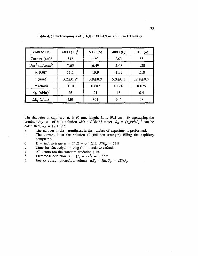
72

Table 4.1 Electroosmosis of 0.100 mM KC1 in a 95 /im Capillary

Voltage (V) 6000 ( l l ) a 5000 (5) 4000 (6 ) 1000 (4)

Current (nA)b 542 460 360 85

I/7rr2 (mA/cm2) 7.65 6.49 5.08 1 . 2 0

R (GQ)C 1 1 . 1 10.9 1 1 . 1 1 1 . 8

t (min)d 3 .2±0 .2e 3.9±0.3 5.3+0.5 12.8±0.5

v (cm/s) 0 . 1 0 0.082 0.060 0.025

Qe (^l/hr)f 26 2 1 15 6.4

AEe (J/ml) 8 450 394 346 48

The diameter of capillary, d, is 95 /*m; length, L, is 19.2 cm. By measuring the conductivity, a0, of bulk solution with a CDM83 meter, R0 = (ag-xi21L)'1 can be calculated, R0 = 17.1 Gft.a The number in the parentheses is the number of experiments performed,b The current is at the solution C (full ion strength) filling the capillary

completely.c R = Ell, average R = 11.2 ± 0.4 Gfl; R/R0 = 65%.d Time for electrolyte moving from anode to cathode,e All errors are the standard deviation (la),f Electroosmotic flow rate, Qe = irr^v = irr2L/t.g Energy consumption/flow volume, AEe = IEt/Qet = IE!Qe.

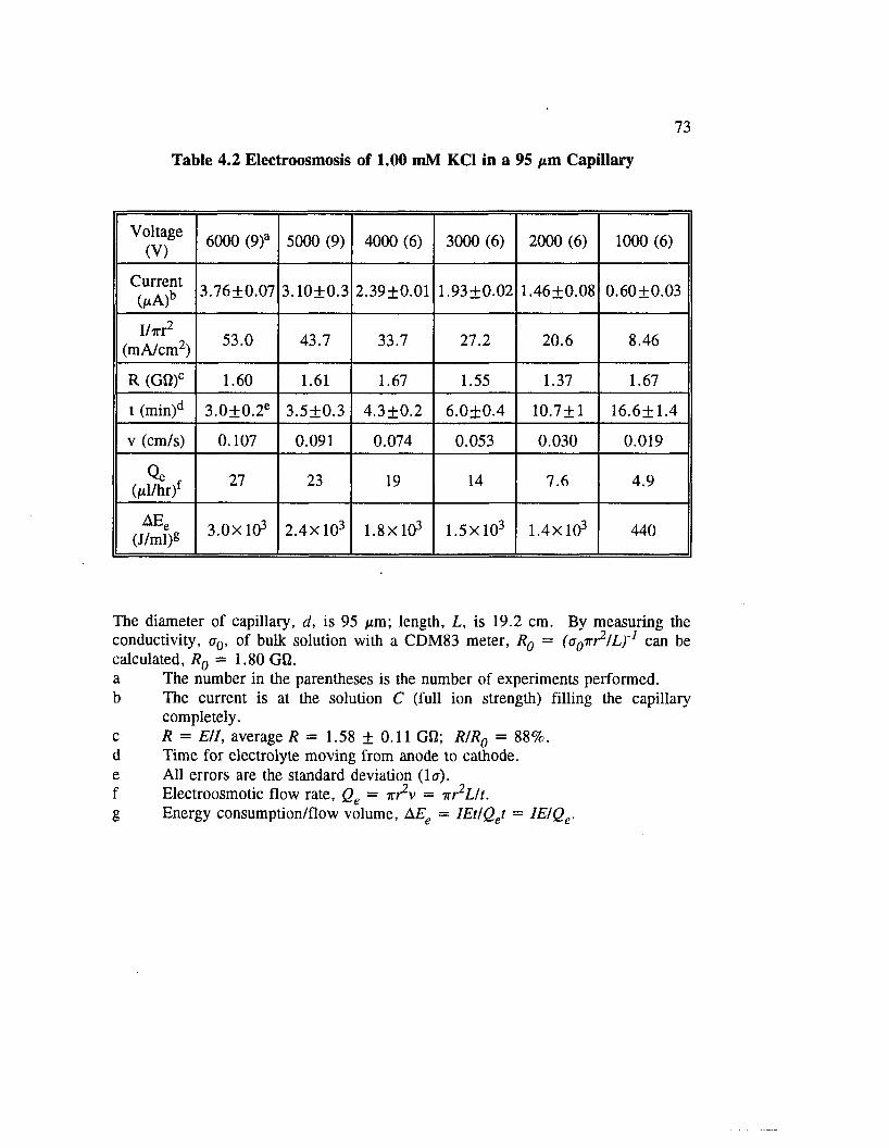
Table 4.2 Electroosmosis of 1.00 mM KC1 in a 95 pm Capillary

73

Voltage(V) 6000 (9)a 5000 (9) 4000 (6 ) 3000 (6 ) 2 0 0 0 (6 ) 1 0 0 0 (6 )

Current(f*A)b 3.76±0.07 3.10±0.3 2.39±0.01 1.93±0.02 1.46±0.08 0.60±0.03

I/irr2

(mA/cm2) 53.0 43.7 33.7 27.2 2 0 . 6 8.46

R (GQ)C 1.60 1.61 1.67 1.55 1.37 1.67

t (min)d 3.0±0.2e 3.5±0.3 4.3±0.2 6 .0 + 0 .4 10.7 + 1 16.6+1.4

v (cm/s) 0.107 0.091 0.074 0.053 0.030 0.019

(pl/hr)f 27 23 19 14 7.6 4.9

AEe(J/ml) 8

3.0 x 103 2.4X103 1.8X103 1.5X103 1.4X103 440

The diameter of capillary, d, is 95 pm; length, L, is 19.2 cm. By measuring the conductivity, a0, of bulk solution with a CDM83 meter, R0 = (oq-k^ IL ) '1 can be calculated, R0 = 1.80 GQ.a The number in the parentheses is the number of experiments performed,b The current is at the solution C (full ion strength) filling the capillary

completely.c R = Ell, average R = 1.58 ± 0.11 GQ; R/R0 = 8 8 %.d Time for electrolyte moving from anode to cathode,e All errors are the standard deviation (Iff),f Electroosmotic flow rate, Qe = irr^v = nr2Lit.g Energy consumption/flow volume, AEe = IEt/Qet = IE/Qe.

Ele

ctro

osm

osis

V

eloc

ity

(cm

/s)

74

0.20

0.16

0.12

0.08

0.04

0.00100 150 200 250 300 3500 50

Electric Gradient (V/cm)

Figure 4.1 Electroosmosis velocity in a 95 /xm capillary at different electric gradients for 0.100 mM KC1 solution.

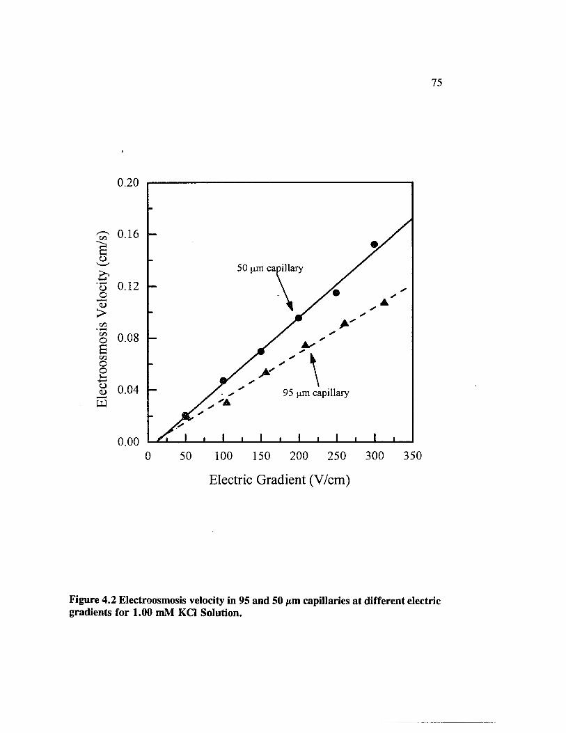
Ele

ctro

osm

osis

V

eloc

ity

(cm

/s)

75

0.20

0.16

50 pm capillary

0.12

0.08

0.04 95 pm capillary

0.00100 150 200 2 50 300 3500 50

Electric Gradient (V/cm)

Figure 4.2 Electroosmosis velocity in 95 and 50 /tin capillaries at different electric gradients for 1.00 mM KC1 Solution.

76

V - -if° i lr\ L

(4.1)

in which e is the dielectric constant of the medium, e0 is the permittivity of free

space, t] (poise or dyn • s/cm2) is its viscosity, L is the length of capillary, and f is the

electrokinetic zeta potential. The negative sign means that when f is negative (in most

cases of fused silica tubing, negative charge on the surface), the liquid flow is toward

the negative electrode (cathode). In an earlier chapter, we have proposed that this

equation should be modified by the inclusion of an efficiency factor. However,

Terabe, et al. [4.7] have claimed that linear relationships were observed between

current and electroosmosis velocities of water, solutions of micelles, and other solutes,

but not between the applied voltages and the velocities. The reason they suggested

was the temperature rise of the solution in the tube which results from Joule heating.

Accordingly, Equation 4.2 was proposed [4.7],

where e is the electronic charge, F is the Faraday constant, aj, Cj, and zj are the

radius, the number of moles per unit volume, and charge number of the y'th ion,

respectively. The authors found that with increase of E or /, 77 decreases due to the

temperature change. One should note however that r/ is not included in Equation 4.2,

so electroosmosis velocity is proportional to current.

v -6 ee0{

/2 (4.2)

77

4.3.2 Electroosmosis in Different Size Capillaries

Based on Equations 4.1 and 4.2, the electroosmosis velocity is proportional to

the electric potential gradient (E/L) or current density (I/irr2), if all other parameters

remain constant. Tsuda, et al. [4.22] have found that electroosmotic flow velocity is

proportional to the current density across the geometrical capillary sectional area,

when different size capillaries were used. Table 4.3 shows our results of

electroosmosis in a 50 fim capillary of 1.00 x 10' 3 M KC1. The electroosmosis

velocity also is found to be proportional to current or voltage gradient in this

capillary, and therefore it is proportional to the current density under this same

capillary. However, when we compare the electroosmosis velocity in the 95 /*m

capillary (shown in Tables 4.2, 4.3, and Figure 4.2) with the electroosmosis velocity

at same electric gradient (E/L) in a 50 pm. capillary, the latter is slightly higher,

especially for the higher electric gradient points. At the same current density for two

different sizes of capillary, the electroosmosis velocity in the 50 ^m capillary is also

higher. For example, for the 50 ^m capillary, at the current density 45.5 mA/cm2,

electroosmosis velocity is 0.152 cm/s, and for the 95 nm capillary at the same current

density, electroosmosis velocities is 0.094 cm/s (value calculated from slope). These

results differ from that predicted by Equation 4.2 and the results of Tsuda and co­

workers [4.22]. Perhaps the surface charges and zeta potentials of the two capillaries

are slightly different although the capillaries are made of same materials by same

manufacture and the charge densities on the glass surfaces could also be slightly

different. The friction may play a different role for different capillaries, i.e. some

Poiseuille character in electroosmotic flow. This is another possible reason of higher

Table 4.3 Electroosmosis of 1.00 mM KC1 in a 50 nm Capillary

78

Voltage(V) 6000 (5)a 5000 (12) 4000 (5) 3000 (5) 2000 (5) 1 0 0 0 (6 )

Current(nA)b 894 ±12 762±11 604±3 456±2 307 ±1 158±1

I/xr2

(mA/cm2) 45.5 38.8 30.8 23.2 15.6 8.05

R (Gfi)c 6.71 6.56 6.62 6.58 6.51 6.34

t (min)d 2 .2±0 .7e 2.9±0.2 3.5+0.2 4.8±0.1 7.1±0.3 16.2 + 1 . 1

v (cm/s) 0.152 0.115 0.095 0.070 0.047 0 . 0 2 1

(jd/hr)f 1 1 8 . 1 6.7 4.9 3.3 1.5

AEe (J/ml) 8 1.8X103 1.7X103 1.3X103 1.0X103 670 380

The diameter of capillary, d, is 50 ^m; length, L, is 20.05 cm. By measuring the conductivity, a0, of bulk solution with a CDM83 meter, R0 = (oqtt IL ) '1 can be calculated, R0 = 7.04 GQ.a The number in the parentheses is the number of experiments performed,b The current is at the solution C (full ion strength) filling the capillary

completely.c R = Ell, average R = 6.55 ± 0.12 Gfi; R/R0 = 93%.d Time for electrolyte moving from anode to cathode,e All errors are the standard deviation (la),f Electroosmotic flow rate, Qe = irr^v = irr2L/t.g Energy consumption/flow volume, AEe = IEt/Qet = IEIQe.

79

electroosmosis velocity in the 50 /xm capillary. It can be concluded that the role of

radius in terms of classical theory is not clear from these data.

4.3.3 Energy Analysis of Electroosmosis in Different Size Capillaries

In Chapter 3, the energy consumptions per flow volume for electroosmosis

(AEe) and hydraulic flow (AEh) in a 95 /xm capillary are compared and it is found that

hydraulic flow is much more energy efficient than electroosmotic flow because of bulk

IR losses in the electroosmosis. With decrease of capillary diameter, both

electroosmotic flow rates and hydraulic flow rates decrease. However, with the

decrease of capillary diameter in electroosmosis, the energy consumption, IE, also

decreases. The energy consumption per flow volume (AEe) could be written as

. „ IEt n r2aE _ 1 oE2 (AAE. - —----------------E------------------ (4.3)Qet L 7i r2v Lv

where r is the capillary radius, v is the electroosmosis velocity, a is the specific

conductivity of the electrolyte, and Qe = irr2v is the electroosmotic flow rate. In

accordance to Equation 4.3, the AEe value increases with the increase of applied

electric field E. The experimental results in Tables 4.2 and 4.3 support this rule

closely. However, the AEe value should not change with the change of capillary

diameter if all other parameters remain constant. Comparing the AEe values of two

different size capillaries in Tables 4.2 and 4.3, the AEe values are slightly different.

For example, for E = 1000, 3000, and 5000 V, AEe = 440, 1500, and 2400 J/ml,

respectively, for electroosmosis in a 95 /xm capillary; and AEe — 380, 1000, and 1700

J/ml, respectively, for electroosmosis in a 50 /xm capillary. The smaller AEe values

80

in the latter cases are because of the higher electroosmosis velocities for the same

conditions.

4.3.4 Electroosmosis as a Function of Cation Type

The electrolytes studied here are potassium chloride (KC1), lithium chloride

(LiCl), butylpyridinium chloride (CH3 (CH2 )3 NC5 H5 C1 , BPC), and tetrahexyl-

ammonium chloride ([CH3 (CH2 )5 ]4 NC1 , THAC) each at the same concentration of

1.00 x 10' 3 M and with the same anion. The four cations were chosen because their

sizes are different with the order of Li+ ’< K+ < CH3 (CH2 )3 NC5 H5+ <

[CH3 (CH2 )5 ]4 N + . Table 4.4 and Figure 4.3 summarize the results of electroosmosis

in a 95 jtm capillary for these four electrolytes. The electroosmosis velocities for KC1,

LiCl, and BPC are about 0.07 cm/s. Between the changes of electrolyte, the capillary

was rinsed with H2 0 , 0.1 M KOH, H2 0 , and then the appropriate electrolyte solution

for about 150 pore volumes each [4.3,4.16]. The electric gradient (E/L = 208 V/cm)

is the same for all cases. Because the concentrations of the solutions are millimolar

for all cases, the dielectric constants (e) and viscosities (r?) of the solutions should be

quite similar. Therefore, it is anticipated that the electrokinetic zeta potentials (f) for

KC1, LiCl, and BPC should be very close. Perhaps highly soluble

CH3 (CH2 )3 NC5 H5+ (considered to be a mid-size cation) did not adsorb appreciably

on the capillary wall during the process, as its electroosmotic flow velocity is

approximately equal to that of K+ or Li+ ions. However, there was no

electroosmotic flow detected for THAC (a large size cation, [CH3 (CH2 )5 ]4 N +). After

the experiments with THAC, the capillary was rinsed several time using the same

81

Table 4.4 Electroosmosis of 1.00 mM Different Cations in a 95 fim Capillary

Cations KCl (8 )a LiCl (7) BPCb (7) THACC (10)

Ro (Gfi)d 1 . 8 6 3.07 2.72 2.73

Current (/*A)e . . . J 1.55+0.08 1.58±0.04 1.56±0.03

R (Gfl) 8 — 2.58 2.53 2.56

R/Ro (%) — 84 93 94

t (min)h 4 .2±0.4 i 4.2±0.2 4.5±0.4 no flow

v (cm/s) 0.076 0.076 0.071 0

Qe (Ml/hrV 19 19 18 0

The diameter of capillary, d, is 95 fim; length, L, is 19.2 cm. a The number in the parentheses is the number of experiments performed,b BPC: Butylpyridinium Chloride, C ltyC iH ^N C sI^C l.c THAC: Tetrahexylammonium Chloride, [CH3 (CH2 )5 ]4 NC1 .d By measuring the conductivity, cr0> °f bulk solution with a CDM83 meter, R0

= (oq-tt /L ) '1 can be calculated, e The current is at the solution C (full ion strength) filling the capillary

completely, f Not measured,g R = Ell, E = 4000 V.h Time for electrolyte moving from anode to cathode,i All errors are the standard deviation (la),j Electroosmotic flow rate, Qe = irr^v = irr2L/t.

Ele

ctro

osm

osis

V

eloc

ity

(cm

/s)

0.20

0.16

0.12

U KC1 L ic l BPC0.08 r - o O A

0.04

THAC

0 .0 0 ' 1 ' 1 ' L0 1 2 3 4 5

Four Different Cations (E/L=208 V/cm)

Figure 4.3 Electroosmosis velocity in a 95 /tm capillary at electric gradient of 208 V/cm for 1.00 mM KC1, LiCl, BPC (butylpyridinium chloride), and THAC (tetra- hexylammonium chloride) solutions.

83

procedure described above and 1.00 x 10' 3 M KC1 was run again and t = 4.7 ± 0.6

min (n=5) or v = 0.068 cm/s, i.e., the flow rate decreased slightly. The reason for

no flow can be explained as the result of adsorption of [CH3 (CH2 )5 ]4 N + on the

capillary wall. However, with the adsorption of cation on the capillary wall, the

electroosmotic flow could reverse toward the anode and this phenomena was not

observed. It is possible that [CH3 (CH2 )5 ]4 N + ion undergoes electrophoresis toward

the cathode under the direct electric voltage and the two effects cancel each other to

cause no flow. The specific conductivities of LiCl, BPC, and THAC are close to 95

/xS/cm, so the currents under a particular electric gradient during the experiments for

three cases are similar.

4.3.5 Electroosmosis of SDS at Different Concentrations

The specific conductivities of sodium dodecyl sulfate (SDS,

CH3 (CH2) n OS03 Na, an anionic surfactant) at different concentrations were measured

first to determine the critical micelle concentration (CMC) of SDS [4.23]. The results

are listed in Table 4.5 and plotted in Figure 4.4. From Figure 4.4, two straight lines

can be drawn. One line (first four points: a0 = 59.3C + 9.86) is at concentrations

below the CMC, and another line (last four points: o0 = 23.1 C + 314) is at

concentrations above the CMC. The intersection of these two lines is the CMC of

SDS, which is 8.4 mM. It is close to literature value of 8.27 mM [4.24],

The results of electroosmosis of SDS at different concentrations in a 95 ftm

capillary are shown in Table 4.6. Before the experiments with SDS solutions, 1.00

x 10' 3 M KC1 was run using the same capillary, and t = 4.0 min or v = 0.080 cm/s.

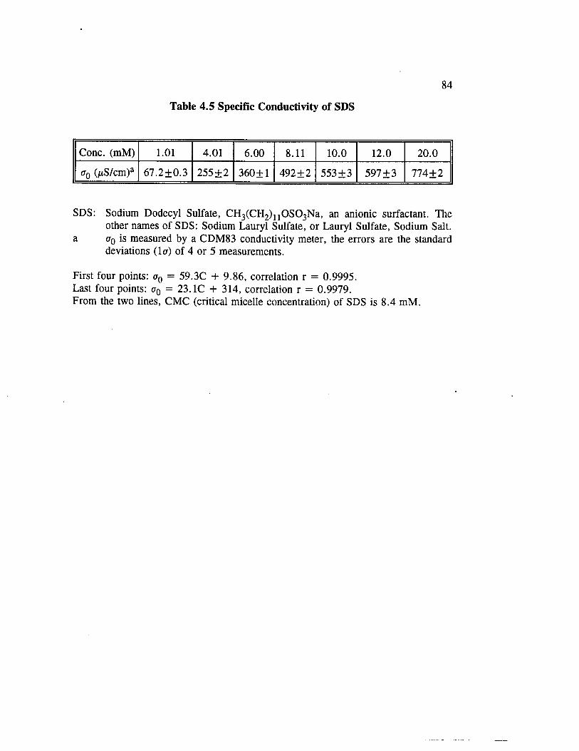
84

Table 4.5 Specific Conductivity of SDS

Cone. (mM) 1 . 0 1 4.01 6 . 0 0 8 . 1 1 1 0 . 0 1 2 . 0 2 0 . 0

(Tq (hS/cm)a 67.2+0.3 255 ±2 360+1 492 ±2 553 ±3 597 ±3 774±2

SDS: Sodium Dodecyl Sulfate, CH3 (CH2 ) 1 1 0 S 0 3 Na, an anionic surfactant. The other names of SDS: Sodium Lauryl Sulfate, or Lauryl Sulfate, Sodium Salt,

a oq is measured by a CDM83 conductivity meter, the errors are the standard deviations (Iff) of 4 or 5 measurements.

First four points: a0 = 59.3C + 9.86, correlation r = 0.9995.Last four points: a0 = 23.1C + 314, correlation r = 0.9979.From the two lines, CMC (critical micelle concentration) of SDS is 8.4 mM.

Spec

ific

Con

duct

ivity

(p

S/cm

)85

800

700

600

500

400 CMC = 8.4 mM

300

200

100

00 4 8 16 20 24

Concentrations o f SDS (mM)

Figure 4.4 Specific conductivity of SDS (sodium dodecyl sulfate) at different concentrations.

86

Table 4.6 Electroosmosis of SDS in a 95 fim Capillary

Cone. (mM) 1.01 (8)a 4.01 (7) 8.11 (7) 12.0 (6) 20.0 (7)

Ro (GQ)b 3.82 1.01 0.520 0.421 0.329

Current (jtA)c 1.14±0.02 4.27±0.05 8.12+0.06 10.43 ±0.03 13.1±0.2

R (Gfl)d 3.51 0.937 0.493 0.384 0.305

R/Ro (%) 92 93 95 91 93

t (min)e 5 .5±0.6f 5.9±0.3 5.7+0.5 9 .0± 1.7 10.1 ±0.8

v (cm/s) 0.058 0.054 0.056 -0.035 -0.032

Qe (/d/hr)8 15 14 14 -9.0 -8.0

Cone. (mM) 4.01 (6)a 8.11 (7) 1.01 (9) 12.0 (6)

Ro (Gfl)b 1.01 0.520 3.82 0.421

Current (f i A f 4.41 ±0.03 8.02+0.04 1.14+0.02 10.11±0.01

R (G«)d 0.907 0.499 3.51 0.396

R/Ro (%) 90 96 92 94

t (min)e 10.7±0.3f 11.3± 1.8 7.8±0.9 9 .6±0 .4

v (cm/s) 0.030 0.028 0.041 -0.033

Qe (/d/hr)8 7.6 7.2 10 -8.5

The diameter of capillary, d, is 95 jam; length, L, is 19.1 cm. SDS: Sodium Dodecyl Sulfate, jOS03Na, an anionic surfactant.a The number in the parentheses is the number of experiments performed,b By measuring the conductivity, <x0, of bulk solution with a CDM83 meter, R0

= (oqTT^/L)’1 can be calculated, c The current is at the solution C (full ion strength) filling the capillary

completely, d R = E/I, E = 4000 V.e Time for electrolyte moving from anode to cathode (or cathode to anode for

negative electroosmotic flow), f All errors are the standard deviation (Iff),g Electroosmotic flow rate, Qe = irr^v = 7rr2L/f.

87

The order of SDS experiments is indicated in Table 4.6 as follows: 1.01, 4.01,

8.11,12.0, 20.0, then repeat 4.01, 8.11, 1.01, and 12.0 mM. Figure 4.5 plots the

results of first five experiments. The first three points in Figure 4.5 show positive

electroosmosis with the electrolyte solution moving from anode (+ ) to cathode (-).

Also, the electroosmosis velocities are close to 0.06 cm/s which is similar to the

electroosmosis velocity for KC1 solution. The Na+ in SDS solution and K+ in KC1

solution play major roles in the electroosmosis and there is no role for R' evident.

However, the last two points in Figure 4.5 show negative electroosmosis, or the

electrolyte solution moving from cathode (-) to anode (+ ). The velocities of negative

flow (close to -0.03 cm/s) are less than that of positive flow (close to 0.06 cm/s),

even though the concentrations of SDS are higher. Because SDS is an anionic

surfactant (CH3(CH2) i10 S 0 3') and originally there is negative charge on the capillary

wall, it is not likely that CH3(CH2)j j0 S 0 3' ions will adsorb appreciably on the

capillary wall. The reason for negative (or reverse) electroosmosis perhaps is due to

an electrophoretic effect of the micelles. Another reason might be the co-adsorption

of Na+ ion on the capillary surface and then R' on Na+ layer; in this case, both

electroosmosis and electrophoresis are in the same direction of cathode to anode. The

net micellar velocity [4.25], vnet, is

v - v +v (4.4)net eo ep

where veo is the electroosmotic velocity and v is the micellar electrophoretic

velocity. The vep can be positive or negative depending on whether it follows or

opposes electroosmotic flow and is given by

Ele

ctro

osm

osis

V

eloc

ity

(cm

/s)

88

0.08

0 .06

0 .04

0.02

0.00

- 0.02

-0 .0410 15 200 255

Cone, o f SDS (mM), (E/L=209 V/cm)

Figure 4.5 Electroosmosis velocity in a 95 /tm capillary at electric gradient of 209 V/cm for different concentrations of SDS (sodium dodecyl sulfate).

89

v - <4-5>3*1

where the function f ( K a ) depends on the micellar shape, having a value of 1.5 for a

sphere of na = oo [4.7], a is the radius of the particle and k is the reciprocal Debye

length. Note that f here is the zeta potential of micellar surface which is different

from that in Equation 4.1. Tsai et al. [4.15] have claimed that in some cases the

absolute electrophoretic velocity of the SDS micelle was greater in magnitude than the

electroosmosis velocity, that is \vep\ > veo. However, in Figure 4.5 of our studies,

for the first three points, the concentrations of SDS are below its CMC, so no micelle

forms; for the last two points, the concentrations of SDS are above its CMC, so

micelle forms. Because there is no micelle in the first three points, the majority of

flow would be the electroosmotic flow from anode toward cathode. For the last two

points, because of the formation of micelle, not only the negative micelle migrates

towards anode, but also the flow created around the micelle competes with

electroosmotic flow (against electroosmotic flow). The result shows the net bulk flow

migrating from cathode to anode. This means that the flow created by the micelles

overcomes the electroosmotic flow. There may be a velocity imposed on the solution

as a consequence of the micelles present and their motion. Here, we call it "negative

electroosmotic flow", but actually, it is probably not an electroosmotic flow nor a

surface effect. This is different from the real electroosmotic flow from cathode to

anode that could be due to an positive charge on the capillary wall and excess anions

in the double layer. The experiments in the bottom half of Table 4.6 were measured

to confirm the above results. Although the absolute flow values of experiments at

90

4.01,8.11, and 1.01 mM SDS are slightly lower, the general trend is the same. That

is, at concentrations below the CMC of SDS the bulk flow occurs from anode to

cathode (regular electroosmotic flow) and at concentrations above the CMC, the bulk

flow results from cathode to anode ("negative electroosmotic flow"). Irreproducibility

may be caused by difficulties in re-establishing the surface charge on the capillary

wall, trace residues, etc.

4.3.6 Electroosmosis of CTAC at Different Concentrations

According to the literature [4.24], the CMC of CTAB (cetyltrimethyl-

ammonium bromide, CH3(CH2)i5 N(CH3)3Br), is 0.026 mM. The CMC of CTAC

(cetyltrimethylammonium chloride, a cationic surfactant) should be close to 0.026

mM, because it contains the same cationic ion (CH3(CH2 )15 N(CH3)3 +). The specific

conductivities of CTAC were measured in the concentrations around 0.03 mM and the

results are plotted in Figure 4.6. However, there is no break point for CTAC (one

straight line in Figure 4.6), so it is very difficult to determine the CMC of CTAC

using this method.

The concentrations of CTAC studied for electroosmosis are all above its CMC

if this is circa 0.03 mM, as shown in Table 4.7. Because the micelle is positively

charged, the electrophoretic direction of the micelle should be towards the cathode (-).

The electroosmosis results are shown in Table 4.7 and plotted in Figure 4.7. The

results show negative electroosmosis for all cases of 0.494, 1.05,5.56, 10.1, and 15.6

mM CTAC. For positive micelles, the v_„ of the micelles is in the direction of anode

to cathode, and the veo is expected to be in the same direction as vep because of the

Spec

ific

Con

duct

ivity

(p

S/cm

)

91

8

7

6

5

4

3

2

00.02 0.03 0 .04 0.05 0.060.00 0.01

Concentrations o f CTAC (mM)

Figure 4.6 Specific conductivity of CTAC (cetyltrimethylammonium chloride) at different concentrations.

92

Table 4.7 Electroosmosis of CTAC in a 95 jim Capillary

Cone. (mM) 0.494 (5)a 1.05 (5) 5.56 (5) 10.1 (5) 15.6 (5)

Ro (Gfl)b 4.95 2.53 0.880 0.552 0.381

Current (/*A)C 0.877±0.009 1.75±0.03 4.75±0.04 7.54±0.15 10.95±0.2

R (GQ)d 4.56 2.28 0.842 0.530 0.365

R/Ro (%) 92 90 96 96 96

t (min)e 3.2±0.1f 3.1 ±0.1 4.8±0.6 4.6±0.2 4.1 ±0.4

v (cm/s) -0.10 -0.11 -0.069 -0.072 -0.081

Qe (jd/hr)8 -26 -27 -18 -18 -21

The diameter of capillary, d, is 95 jxm; length, L, is 19.9 cm. CTAC: Cetyltrimethylammonium Chloride, CH3(CH2)15N(CH3)3C1, a cationic surfactant, a The number in the parentheses is the number of experiments performed,b By measuring the conductivity, a0, of bulk solution with a CDM83 meter, R0

= (oqtti^/L)'1 can be calculated, c The current is at the solution C (full ion strength) filling the capillary

completely, d R = E / I , E = 4000 V.e Time for electrolyte moving from cathode to anode,f All errors are the standard deviation (la),g Electroosmotic flow rate, Qe = tti v = irr2L/t.

Ele

ctro

osm

osis

V

eloc

ity

(cm

/s)

93

-0.15

- 0.12

-0 .09

-0 .06

-0.03

0.0016 20120 84

Cone, o f CTAC (mM), (E/L=201 V/cm)

Figure 4.7 Electroosmosis velocity in a 95 nm capillary at electric gradient of 201 V/cm for different concentrations of CTAC (cetyltrimethylammonium chloride).

94

negative charge of glass capillary wall. However, the bulk flow occurs from cathode

to anode. The reason must be the change of direction of electroosmotic flow and this

flow overcomes the any flow created by the micelles due to an electrophoretic effect.

One explanation might be that so much CH3(CH2)15N(CH3)3+ ion adsorbs on the

surface of capillary wall, it forms a positive layer and electroosmotic flow direction

reverses due to an excess of anions in the double layer. The electrophoretic direction

is still from anode to cathode because the micelles are positive charged. In order to

check the conditions of the capillary and the polarity of surface charge on the capillary

wall, before the experiments with CTAC, 1.00 x 10'3 M KC1 was run using the same

capillary. It was found that t = 3.7 ± 0.3 min (n=6) or v = 0.090 cm/s, which is

close to the other data in Tables 4.2 and 4.4. Before and after the experiment of KC1,

the capillary was rinsed to clean the surface of capillary with H20 , 0.1 M KOH,

H20 , and operating solution for about 150 pore volumes each. After the experiments

of CTAC, the capillary was rinsed again several times using the same procedure, and

then 1.00 x 10"3 M KC1 was run again using the same capillary. It was found that

t = 10.8 ± 2.4 min (n=8) or v = 0.031 cm/s. The electroosmosis velocity

decreased and this may be due to a change of capillary surface resulting from the

strong adsorption of CH3(CH2)15N(CH3)3+ ion which was not completely removed

by the rinsing procedure.

4.4 Conclusions

Our experiments show that the electroosmosis velocity is proportional to the

applied voltage and current which indicates that during these electroosmosis processes

95

temperature changes are not significant. However, the relationship between

electroosmosis velocity and electric current density across the capillary section for two

different sizes of capillaries (50 and 95 nm) is not quite linear and the electroosmosis

velocity is higher for the smaller (50 fim) capillary. The reason might be the slight

differences of the capillary surface properties, or the charge densities on the glass

surfaces. Also, with change of capillary diameters from 95 to 50 pm, the energy

consumptions per flow volume change from 440 to 380 J/ml, 1500 to 1000 J/ml, and

2400 to 1700 J/ml if E — 1000, 3000, and 5000 V, respectively, under the same other

conditions; and, the energy consumption per flow volume increases with the increase

of applied voltage if all other parameters are held constant.

The electroosmosis study as a function of cation radius using 1.00 mM KC1,

LiCl, BPC (butylpyridinium chloride) electrolytes shows that they cause similar

electroosmosis velocities. A solution of 1.00 mM THAC (tetrahexylammonium

chloride) gave no electroosmotic flow. This might be explained by the adsorption of

[CH3(CH2)5 ]4N + ion on the capillary wall or competing effects. The study of SDS

(sodium dodecyl sulfate) shows a very interesting result. At the concentration of SDS

below its CMC of 8.4 mM, normal electroosmotic flow was observed, but at

concentrations of SDS above 8.4 mM, the bulk solution flow reversed and occurred

from cathode (-) to anode (+ ). One reason for reversed bulk flow is that the flow

created by micelles overcomes the electroosmotic flow. The electroosmotic flow of

CTAC (cetyltrimethylammonium chloride) is reversed at all concentrations studied in

the range of 0.5 - 15.6 mM (well above its CMC of 0.03 mM), possibly because

CH3(CH2 )15N(CH3)3+ ion adsorbs on the capillary wall and the surface of the

96

capillary develops a net positive charge. The reason for the reserved flow of CTAC

is completely different from that for SDS, because the micelle (a cationic micelle)

should migrate from anode to cathode. In summary, the use of surfactants greatly

increase the complexity of unravelling the electroosmotic and electrophoretic

processes.

97

4.5 References

4.1 G.J.M. Bruin, J.P. Chang, R.H. Kuhlman, K. Zegers, J.C. Kraak, and H. Poppe, J. Chromatogr. 1989, 471, 429.

4.2 S. Hjerten, J. Chromatogr. 1985, 347, 191.

4.3 H.H. Lauer and D. Mcmanigill, Anal Chem. 1986, 58, 166.

4.4 W.J. Lambert and D.L. Middleton, Anal. Chem. 1990, 62, 1585.

4.5 C. Schwer and E. Kenndler, Anal. Chem. 1991, 63, 1801.

4.6 S. Terabe, K. Otsuka, K. Ichikawa, A. Tsuchiya, and T. Ando, Anal. Chem. 1984, 56, 111.

4.7 S. Terabe, K. Otsuka, and T. Ando, Anal. Chem. 1985, 57, 834.

4.8 A. Cohen, S. Terabe, J.A. Smith, and B.L. Karger, Anal. Chem. 1987, 59, 1021 .

4.9 K. Ghowshi and R.J. Gale, Biosensor Technology, R.P. Buch, W.E. Hatfield, M. Umana, and E.F. Bowden (Eds.), Marcell Dekker, New York, 1990, pp. 55-62.

4.10 K. Ghowshi and R.J. Gale, J. Chromatogr. 1991, 559, 95.

4.11 C.S. Lee, W.C. Blanchard, and C-T. Wu, Anal. Chem. 1990, 62, 1550.

4.12 C.S. Lee, C-T. Wu, T. Lopes, and B. Patel, J. Chromatogr. 1991, 559, 133.

4.13 C.S. Lee, D. McManigill, C-T. Wu, and B. Patel, Anal. Chem. 1991, 63, 1519.

4.14 C-T. Wu, T. Lopes, B. Patel, and C.S. Lee, Anal. Chem. 1992, 64, 886.

4.15 P. Tsai, B. Patel, and C.S. Lee, Anal. Chem. 1993, 65, 1439.

4.16 M.A. Hayes and A.G. Ewing, Anal. Chem. 1992, 64, 512.

4.17 M.A. Hayes, I. Kheterpal, and A.G. Ewing, Anal. Chem. 1993, 65, 27.

4.18 M.A. Hayes, I. Kheterpal, and A.G. Ewing, Anal. Chem. 1993, 65, 2010.

4.19 K. Smith, Separation Times 1993, J&W Scientific, 7(3), 2.

4.20 X. Huang, M.J. Gordon, and R.N. Zare, Anal. Chem. 1988, 60, 1837.

4.21 R.J. Gale and R.A. Osteryoung, Molten Salt Techniques Vol. 1, D.G. Lovering and R.J. Gale (Eds.), Plenum Press, New York, 1983, pp. 66-68.

4.22 T. Tsuda, K. Nomura, and G. Nakagawa, J. Chromatogr. 1982, 248, 241.

4.23 R.J. Williams, J.N. Phillips, and K.J. Mysels, Trans. Faraday Soc. 1955, 51 , 728.

4.24 SIGMA Chemical Catalog, 1992, p. 1538.

4.25 E.L. Little, "Comparative Study of Anionic and Nonionic/Anionic Surfactant Systems in Micellar Electrokinetic Capillary Chromatography", Ph.D. dissertation, Lousisana State University, Baton Rouge, LA, May, 1992.

CHAPTER 5.

P H E N O L R E M O V A L F R O M K A O L L N IT E C L A Y B Y E L E C T R O O S M O S I S

5 .1 I n tr o d u c t io n

Electroosmosis is one of the electrokinetic phenomena in which pore fluid in

a porous medium moves due to application of a low direct current (DC) by electrodes

inserted in the medium. It has been utilized by geotechnical engineers for several

decades as an electrochemical technique for dewatering and stabilizing fine-grained

soil deposits, e.g. Esrig and Gemeinhardt [5.1] and Casagrande [5.2].

Recent studies at Louisiana State University provided a better understanding

of the electrochemistry and demonstrated that the acid front generated by the

electrolysis reaction at the anode advances and eventually flushes across the specimen

by advection, migration and diffusion [5.3-5.5]. Hamed, et al. [5.6], demonstrated

that the movement of this acid front and the migration and advection of the cations

and anions under electrical gradients constitute the mechanisms of removing adsorbed

Pb(II) from kaolinite. The feasibility of removing inorganic contaminants from

kaolinite by using the electrokinetic phenomenon has been demonstrated by Hamed

[5.7]. Shmakin [5.8] notes that the technique has been used in the former Soviet

Union for partial extraction of metals from rocks and soils since the early 1970’s.

The success of the method in removing a variety of other inorganic contaminants has

been demonstrated by laboratory studies and limited pilot-scale field studies, e.g.

Hamnet [5.9], Runnels and Larson [5.10], Lageman et al. [5.11], Banerjee, et al.

[5.12], Hamed, et al. [5.6], Acar, et al. [5.13], and Acar [5.14].

99

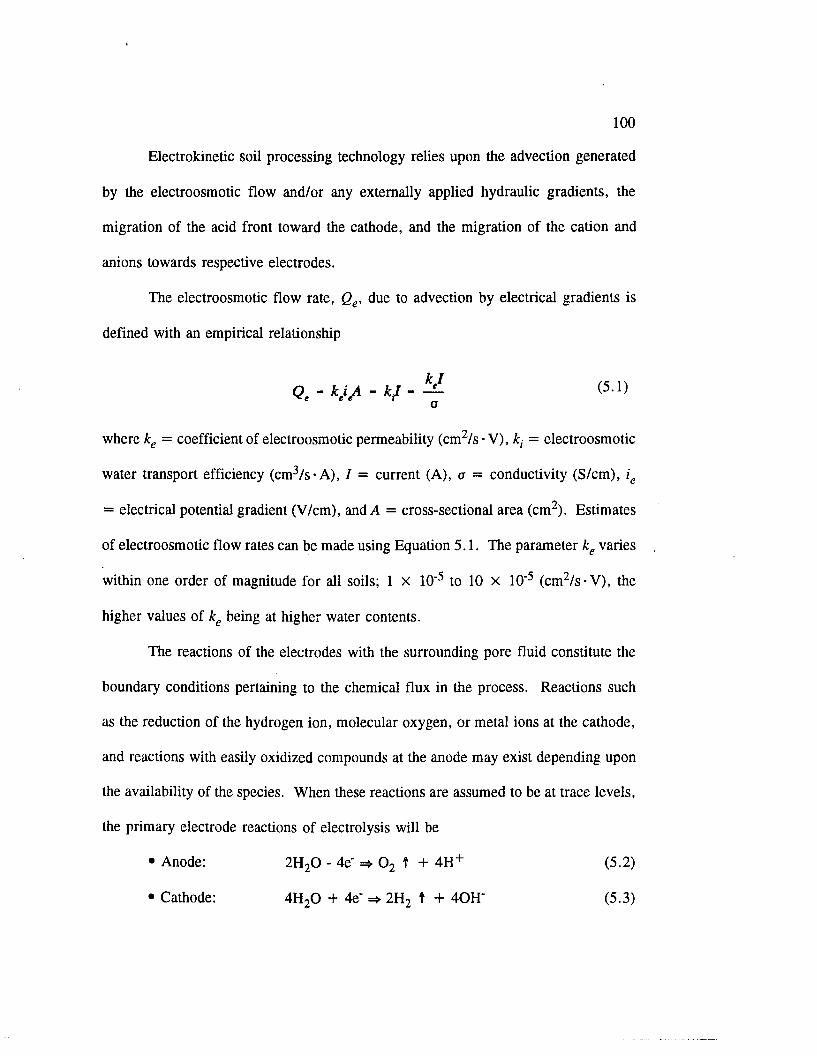
100

Electrokinetic soil processing technology relies upon the advection generated

by the electroosmotic flow and/or any externally applied hydraulic gradients, the

migration of the acid front toward the cathode, and the migration of the cation and

anions towards respective electrodes.

The electroosmotic flow rate, Qe, due to advection by electrical gradients is

defined with an empirical relationship

Q, - - V - “ < 5 1 )

where ke = coefficient of electroosmotic permeability (cm2/s • V), ki = electroosmotic

water transport efficiency (cm3/s-A ), 1 = current (A), a = conductivity (S/cm), ie

= electrical potential gradient (V/cm), and A = cross-sectional area (cm2). Estimates

of electroosmotic flow rates can be made using Equation 5.1. The parameter ke varies

within one order of magnitude for all soils; 1 X 10‘5 to 10 X 10'5 (cm2/s-V ), the

higher values of ke being at higher water contents.

The reactions of the electrodes with the surrounding pore fluid constitute the

boundary conditions pertaining to the chemical flux in the process. Reactions such

as the reduction of the hydrogen ion, molecular oxygen, or metal ions at the cathode,

and reactions with easily oxidized compounds at the anode may exist depending upon

the availability of the species. When these reactions are assumed to be at trace levels,

the primary electrode reactions of electrolysis will be

• Anode: 2H20 - 4e' =* 0 2 t + 4H+ (5.2)

• Cathode: 4H20 + 4e' => 2H2 t + 40H" (5.3)

101

The generation of the acid front at the anode by the reaction described in Equation 5.2

and its advance towards the cathode constitute the second component of the removal

process [5.15]. This acid front sweeps across the specimen in time [5.5].

The migration of anions and cations toward respective electrodes is the third

component of the process. Investigators focused their first studies on inorganic

cations, since removal of these ions would take advantage of the three concurrent

processes. Organic contaminants often have low polarity, and, therefore, the

migration component under electrical currents is not expected to contribute to their

removal. Thus, the feasibility of their removal from soils by electrokinetics is not as

obvious as the ionic species. An observation supporting the potential to remove

organics by application of electrical currents is provided by Segal, et al. [5.16], who

discovered that the organic carbon content substantially increased in the effluent after

electroosmotic consolidation of sludges. Similarly, in a recent study, Bruel et al.

[5.17] demonstrate that benzene, toluene, ethylene, and xylene (BTEX) compounds

in gasoline and trichloroethylene loaded onto kaolinite specimen move toward the

cathode by the electrokinetic phenomena.

This chapter provides an analysis of the results of tests conducted to remove

phenol adsorbed on saturated kaolinite using the electrokinetic soil processing

technique. Assessments of the flow, electrochemistry, and energy requirements also

are presented. Phenol was studied because it is often encountered in groundwater and

soil as an organic contaminant [5.18,5.19]. Its presence may result from the

degradation of pesticides and other chemicals that were used in agriculture, or from

unintentional releases associated with manufacturing processes, production of energy,

102

and water-disposal procedures [5.20]. Since most phenolic compounds are priority

pollutants, their concentrations are subject to scrutiny in water-quality considerations.

The drinking water standard established by the U.S. Environmental Protection Agency

(USEPA) for phenol is 1 ppb or less, due to its potential toxicity [5.21].

Electroosmosis tests are conducted on saturated kaolinite clay specimens loaded with

phenol at a level of 500 y.g per gram of dry kaolinite. This amount was below the

phenol adsorption capacity of this mineral. Electroosmotic flow behavior and the

electrochemistry (voltage, current, resistance, pH gradients and conductivity) in these

experiments are presented. Electroosmotic flow with open electrodes is time-

dependent. An acid front generated at the anode sweeps across the specimen

neutralizing the base at the cathode. The adsorbed phenol was removed 85% to 95%

by the process. The phenol concentration profile in the effluent did not display any

retardation due to desorption. The energy expenditure for removal was of the order

of 18-39 kWh/m3 of soil processed. The study displays that it may be feasible to

remove low-concentration water soluble organic contaminants from cohesive soils by

application of a direct current.

5.2 Testing Program

Three tests were conducted for phenol removal. The conditions were kept

almost identical to those reported in the study presented by Hamed et al. [5.6].

Constant current conditions were used in all tests to keep constant net rates of the

electrolysis reactions at all times and minimize complicated current boundary

conditions. The specimen dimensions, duration of tests, current used, and other

103

parameters in these tests are presented in Table 5.1. Secondary temperature effects

have been reported to decrease the efficiency of electroosmotic flow when the current

density is greater than 5 mA/cm2 [5.22], In order to avoid such effects, the current

density used in all tests was selected about two orders of magnitude lower than 5

mA/cm2.

Air-dry, air-floated Georgia Kaolinite (Thiele Kaolinite Co., Wrens, Georgia)

was used in the study. This mineral was selected due to its low activity and relatively

high electroosmotic water transport efficiency. The physical and engineering

characteristics of this soil were reported by Hamed, at al. [5.6].

Adsorption tests are conducted to determine the phenol adsorption capacity of

the kaolinite. Adsorption isotherms were determined at room temperature. The clay-

phenol combinations were prepared in duplicate, using 3-g solid to 30-ml solution

ratio. The mixture was placed in polyethylene bottles with screw caps. The time

required to achieve equilibrium were reported to be in the range of a few hours to a

few days, e.g. Isaacson and Frink [5.23], Sheriff et al. [5.24], The samples for the

adsorption tests were kept in the shaker for a period of five days of equilibrium.

Subsequent tests investigating the adsorption kinetics demonstrated that phenol

adsorption onto the kaolinite is completed within minutes. Two ml of soil-solution

mixture was sampled, centrifuged, and the clear supernatant was analyzed. The

amounts of phenol adsorbed by the clay were calculated from the differences in the

concentrations of phenol between the original solutions and those of the supernatant

at the end of the experiments. All tests were run in duplicate. The phenol

concentrations used ranged between 10 ppm to 800 ppm.

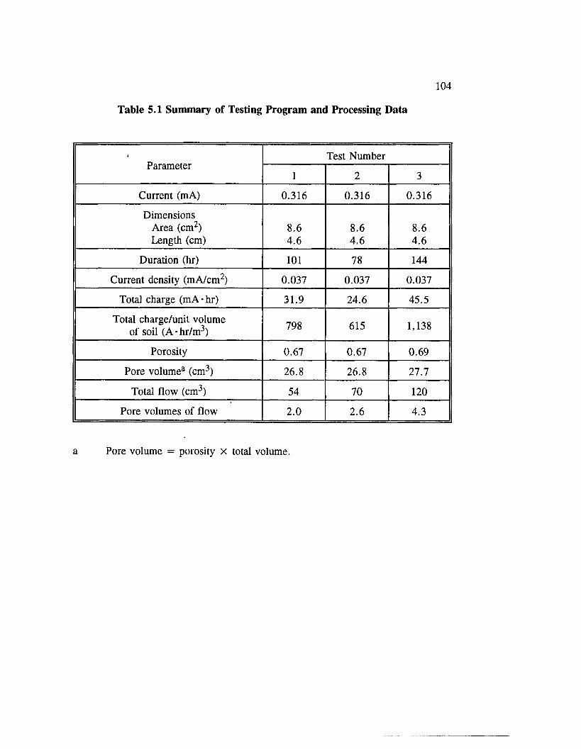
104

Table 5.1 Summary of Testing Program and Processing Data

1Parameter

Test Number

1 2 3

Current (mA) 0.316 0.316 0.316

Dimensions Area (cm2) 8.6 8.6 8.6Length (cm) 4.6 4.6 4.6

Duration (hr) 101 78 144

Current density (mA/cm2) 0.037 0.037 0.037

Total charge (mA • hr) 31.9 24.6 45.5

Total charge/unit volume of soil (A-hr/m3) 798 615 1,138

Porosity 0.67 0.67 0.69

Pore volume3 (cm3) 26.8 26.8 27.7

Total flow (cm3) 54 70 120

Pore volumes of flow 2.0 2.6 4.3

a Pore volume = porosity x total volume.

105

The Pb(II) exchange capacity of the kaolinite was reported to be 1.06

milliequivalent per 100 g of clay, for a pH range of 4.5-5.0 [5.6,5.7]. The phenol

absorptive capacity of kaolinite used in this study is about 1 mg/g of clay (Figure

5.1), close to the cation exchange capacity of this mineral. The phenol-deionized,

distilled water solution had a pH of 6.0-6.5. The pH of the soil-phenol solution

mixture ranged between 4.5-5.0, owing to the exchangeable cations in the kaolinite.

Putnam [5.15] demonstrated that the pH of Georgia kaolinite-deionized, distilled water

mixtures ranged between 4.5-5.5 for solids content (weight of dry solids/weight of

water) of greater than 6-8%. Therefore, the adsorption isotherm provided in Figure

5.1 will be reasonably valid at higher solids content. It was decided to use a phenol

concentration of about 500 ppm (0.5 mg/g of clay), since most phenol at this

concentration will be adsorbed by the kaolinite, and removal will require its

desorption into the pore fluid and advection/migration towards the cathode.

The phenol solution was prepared by adding American Chemical Society

(ACS) reagent-grade phenol crystal into deionized distilled water. Forty grams of dry

clay was mixed with 40 ml of 500 ppm phenol solution, and the slurry was stirred for

30 minutes to allow the phenol distribution to equilibrate between the solid and liquid

phases. The pH of the slurry ranged between 4.5 to 4.8. A total of 53-56 g of clay-

phenol solution slurry was loaded into the test cell. Electroosmosis tests were initiated

within one hour of specimen preparation.

Electroosmosis test specimens were assembled as shown in Figure 5.2.

Specimens were placed in a horizontal configuration. Inert graphite electrodes were

selected to prevent introduction of electrode corrosion products, which might cause

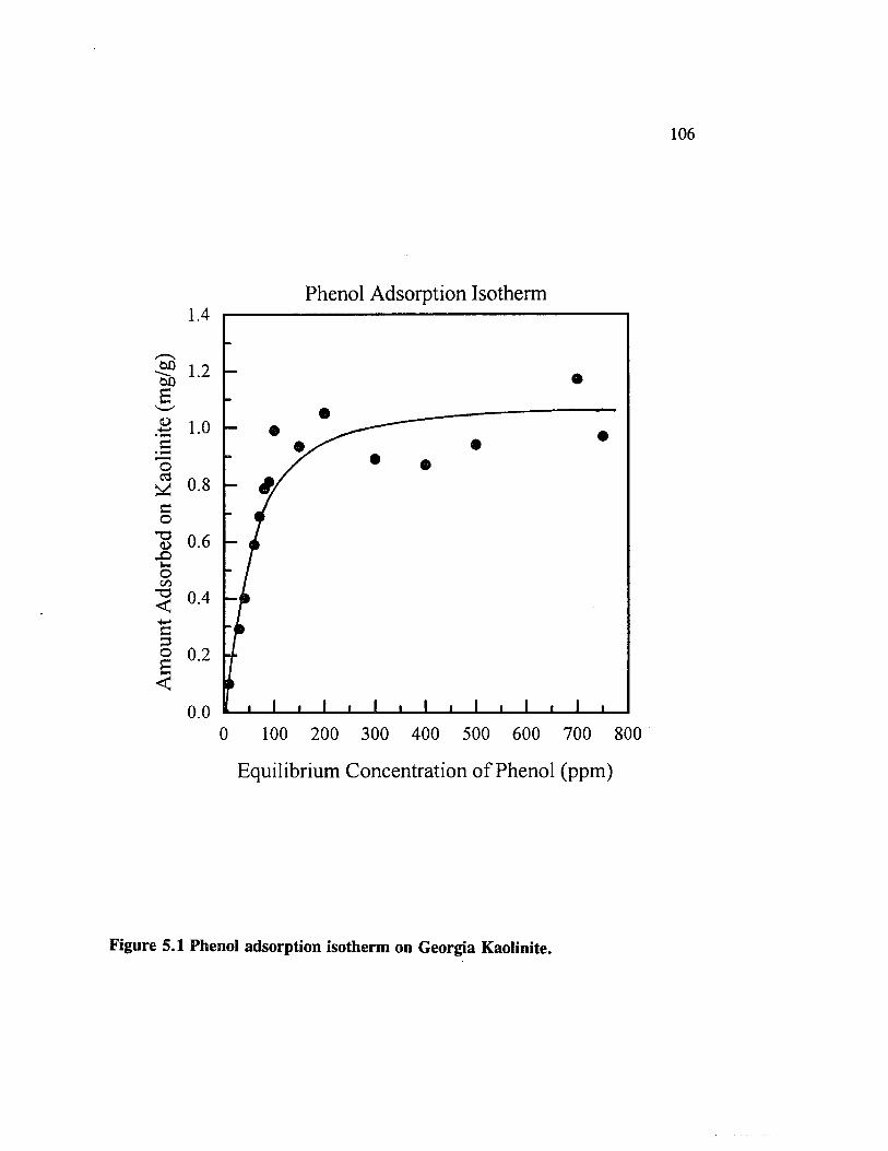
Am

ount

Ads

orbe

d on

Kao

linite

(m

g/g)

106

Phenol Adsorption Isotherm1.4

1.2

1.0

0.8

0.6

0.4

0.2

0.00 100 200 300 400 500 600 700 800

Equilibrium Concentration o f Phenol (ppm)

Figure 5.1 Phenol adsorption isotherm on Georgia Kaolinite.

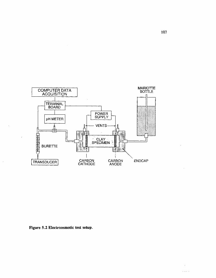
107

MARIOTTEBOTTLECOMPUTER DATA

ACQUISITION

TERMINALBOARD

POWERSUPPLYpH METER

VENTS

• CLAY SPECIMEN

BURETTE

CARBONCATHODE

CARBONANODE

ENDCAPTRANSDUCER

Figure 5.2 Electroosmotic test setup.

108

complicated electrochemistry due to soil interactions. Two pieces of filter papers

were placed at both ends of the specimens. To avoid the development of hydraulic

gradients, a Mariotte bottle was used at the anode side to keep the influent head

constant and at the same elevation as the effluent head. Uniform flow across the

electrodes was ensured by drilling twenty five 1.7-mm (diameter) holes into the

electrodes. Each piece of the electrode was held in place by two screws. The

resistance between the two screws was measured to make sure that the connection

between screw and electrode was good (the resistance < 1.0 ohm). The electric

current was applied to the cell with a constant DC power supply,

Potentiostat/Galvanostat HA-211 A, Hokuto Denko Ltd. The constant current was kept

at 0.316 ± 0.005 mA and the maximum voltage attained in these 4.5 cm length

specimens was 20 volts. The effluent was analyzed for pH and phenol concentration.

After the selected period of current application, the specimen was promptly

removed from the cell and sliced into five sections. Each segment was analyzed for

water content, pH, and phenol content. Phenol was extracted from clay specimens

by adding 20 ml deionized distilled water to each slice of segment (about 5-6 g of

clay) and shaking for one hour; then, the supernatant and the clay were separated by

centrifugation and decantation.

All phenol analysis were made with a Perkin-Elmer 900 Gas Chromatograph

with a column, p/a 20% SP 2100 + 0.1% Carbowax 1500 on Supelcoport 100/200

mesh, and a Flame Ionization Detector. pH was measured by a Coming pH meter

calibrated at two buffer solutions. pH measurements were made either in the effluent

109

or in the soil. In situ pH measurements are made by inserting the combination pH

electrode directly into the soil specimen.

5.3 Analysis of Results

5.3.1 Phenol Adsorption Isotherm

The phenol adsorption isotherm shown in Figure 5.1 indicates that this

kaolinite clay can adsorb about 1 mg of phenol per gram of dry clay within the pH

range of 4.5-5.0. Phenol could be adsorbed by the clay either in the neutral form (</>-

OH) or in the negatively charged form (0-0') [5.18,5.19]. The high rate and capacity

of noncrystalline components for phenolic acids are essentially attributable to the great

reactivity of their positively charged Al-OH2°'5+ and Fe-OH2° 5+ functional groups

toward the negatively charged carboxyl and phenolic hydroxyl groups. Various

researchers reported that phenol are adsorbed to charged surfaces through H-bonding

and/or charge-transfer complexes in addition to the hydrophobic sorption processes

found with neutral compounds [5.20,5.23,5.25,5.26]. Saltzman and Yariv [5.27]

reported that phenol appears to be amphoteric and can act as a H+ acceptor in acid

solutions, and in basic media, as a H + donor. Considering that solution of Georgia

kaolinite with water are acidic (pH range of 4.0-5.0), the writers hypothesized that

phenol would act as H+ acceptor and would be adsorbed primarily by the negatively

charged surfaces of kaolinite.

The Langmuir isotherm [5.28] has a formula

110

(5.4)

where B is a constant, c is the concentration, and 0 is the degree of coverage on the

surface. If the adsorption follows the Langmuir isotherm, c should have a linear

relationship with 0/(l-0). The Freundlich isotherm [5.28] has a formula

so log(c) has a linear relationship with log(6) if the adsorption follows the Freundlich

isotherm. Figures 5.3 and 5.4 are the Langmuir isotherm and Freundlich isotherm

of phenol on kaolinite by applying the data from Figure 5.1 to both Equations 5.4

and 5.6. Figure 5.3 shows a straight line and Figure 5.4 shows a non-linear line,

which indicates that the Langmuir isotherm equation fits best to the adsorption of

phenol on kaolinite. Conversely, Artiola-Fortuny and Fuller [5.29] have claimed that

the Freundlich isotherm equation fits most water-phenol-soil systems well. This

difference to our result may be due to the different surface properties of soils.

5.3.2 Electrical Potential Gradients and Flow

Figures 5.5 and 5.6 show the total electroosmotic flow in time and the

development of the net average electrical potential gradient across the electrodes. The

following observations are made: (1) There was no measurable flow in the first 5-10

hr of current application. Subsequently, the total flow increased rapidly, and then the

flow rate decreased slowly in test 3. Similar trends were reported by Hamed, et al.

Bcn = e (5.5)

where 0 < n < 1. Equation 5.5 can be written as

nlog(fl) + nlog(c) = log(0) (5.6)

111

Langmuir Isotherm o f Phenol on Kaolinite24

20

16

12

8

4

00 100 200 300 400 500 600 700 800

Concentration o f Phenol

Figure 5.3 Langmuir isotherm fit of phenol adsorption on kaolinite.

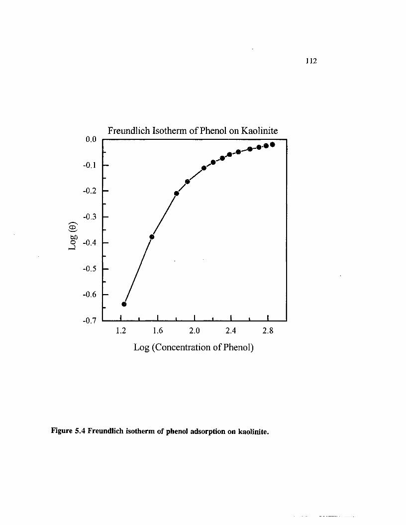
Log

(0)

F r e u n d lich Iso th er m o f P h e n o l o n K a o lin ite0.0

- 0.2

-0.3

-0.4

-0.5

- 0.6

-0.71.2 1.6 2.0 2.4 2.8

L o g (C o n c e n tr a tio n o f P h e n o l)

Figure 5.4 Freundlich isotherm of phenol adsorption on kaolinite.

Flow

Volu

me

(ml)

120

100

80

60

40

20

00 30 60 90 120 150

T im e (h o u r)

- — O — - Test 1

• Test 2

- - A - Jest 3

t? OA * O

AT© _ 0

■ 7 i I i |_____ |_____ |-------- 1_____ |_____ l

Figure 5.5 Total electroosmotic flow with time.

Elec

tric

Pote

ntia

l G

radi

ent,

i e (V

/cm

)114

4.0

3.5

3.0

2.5

2.0

— O—-Test 1 — • — Test 2

- A - Test 30.5

0.0120 15060 900 30

T im e (h o u r)

Figure 5.6 Electrical potential gradient with time.

115

[5.6]. These results further verify that the flow rate in electroosmosis is

time-dependent. (2) Under constant current conditions employed in three tests, the

average cell electrical potential increases rapidly, in test 3 up to a relatively constant

value at about 2.4 V/cm (test 3) from an initial average value of about 0.4 to 0.7

V/cm.

Figures 5.7 and 5.8 show the change in the empirical electroosmotic coefficient

of permeability ke and the electroosmotic water transport efficiency fc, in the tests.

The data indicate that: (1) ke increases to 1.4-2.9 x 10"5 cm2 /s-V at the start of each

test and then decreases by an order of magnitude. (2) kt increases to 0.5 to 1.0

cm3 /sec-A at the start of the test and decreases slowly in test 3 or approaches a

constant in test 2. Time-dependent changes in ke and kt demonstrate that significant

changes occur in the overall resistance and, thus, the chemistry across the cell during

the process. Hamed [5.7] showed that the greatest electrical potential difference

occurs within a narrow zone in the cell in the cathode region. This potential

difference increases gradually in time; possibly due to ion depletion, precipitation, and

H20 formation.

5.3.3 Conductivity

Conductivity is inversely related to the resistance offered to current flow. This

resistance would change due to variations in pore sizes (porosity), tortuosity in the

porous medium, and variations in pore fluid and double layer electrolyte

concentrations. Conductivity is measured in siemens (S) per distance between the

measurement points in a medium. Conductivity rises from a very low value

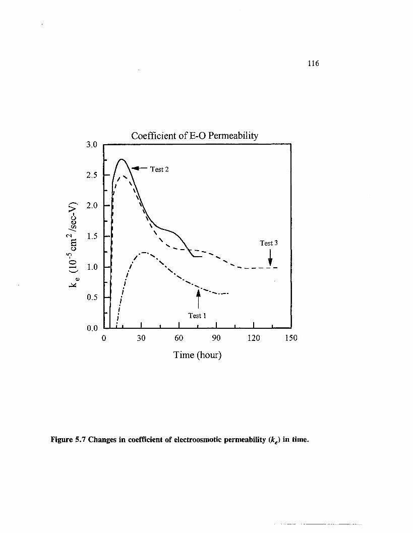
116

C o e f f ic ie n t o f E - 0 P e r m e a b ility3.0

Test 22.5

> 2.0 Io

C /D

^ 1.5Bo

in■O

Test 3

<L>

0.5

Test 1

0.060 90 120 150300

T im e (h o u r)

Figure 5.7 Changes in coefficient of electroosmotic permeability (ke) in time.

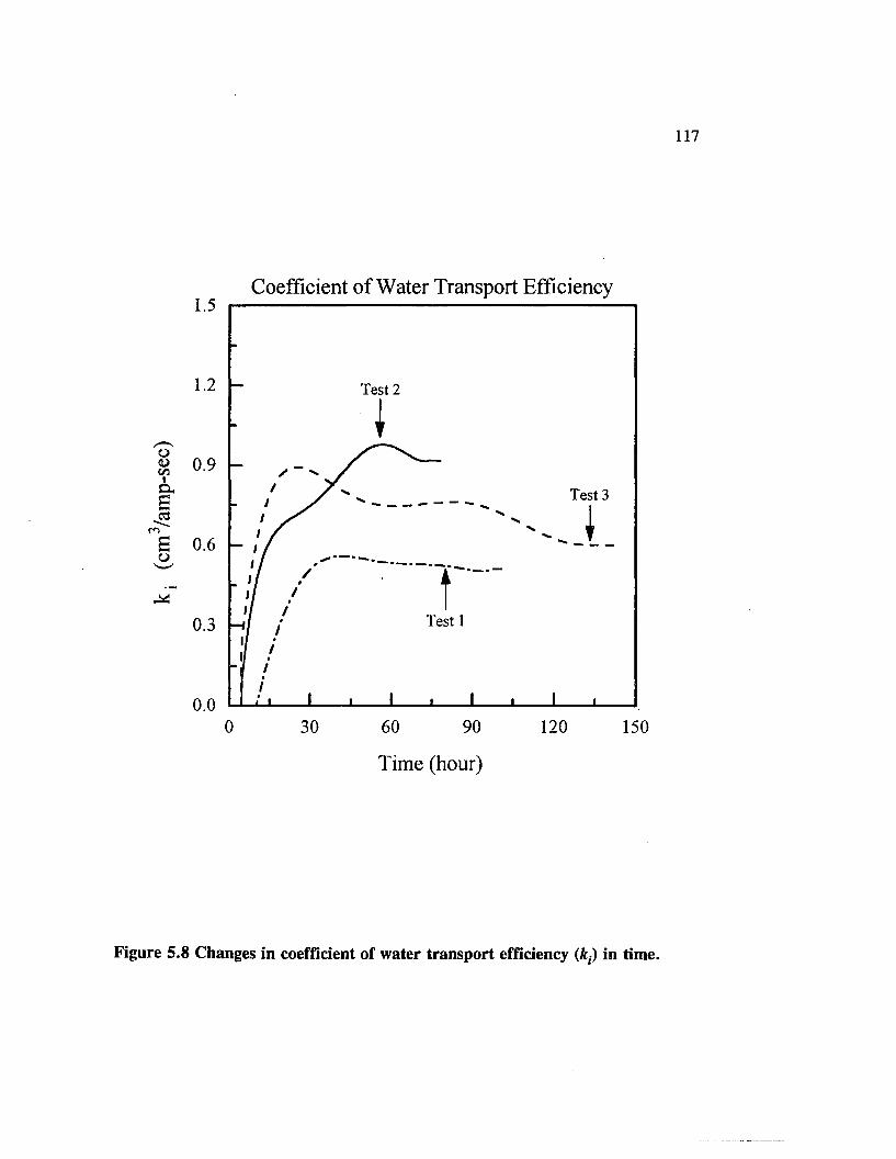
117

0<utfl1cx

.03

o

Coefficient o f Water Transport Efficiency1.5

1.2 Test 2

0.9Test 3

0.6

Test 10.3

0.090 1200 30 60 150

Time (hour)

Figure 5.8 Changes in coefficient of water transport efficiency (kt) in time.

118

(approximately 1 fiS/cm) for deionized, distilled water by orders of magnitude for a

fluid containing electrolytes, depending on their types and concentrations.

In three tests, conductivity can be estimated from the electrical potential drop

across the supplied electrodes and the current across the electrodes (apparent

conductivity). In the relative simple electrolyte system (500 fig phenol per gram of

clay), conductivity values would be sensitive indicators of H + and OH" concentrations

if they exceed other the pore fluid ionic concentrations.

The apparent conductivity, Ka, calculated from the electrical potential drop

across the electrodes, is defined as

It{A)Ucm)Ka{S!cm ) * — ■■■■■, (5.7)

Et(volf)A(cm2)

where I, = the current, Et = the voltage difference between the current-generating

electrodes, L = the specimen length, and A = the cross-sectional area of the

specimen. Apparent conductivities ignore the overpotentials that are necessary to

drive the electrode reactions.

Figure 5.9 shows the change in apparent conductivity with time across the

electrodes in the three tests. Since the tests were performed under constant current

conditions, the decrease in Ka with time reflects an increase in the resistance offered

and an increase in the voltage required to maintain the desired current. In all tests,

the apparent conductivity steadily decreased from 55-80 fiS/cm at the start of the tests

to 15-20 fiS/cm at the end of the tests. Similar phenomena were obtained by Hamed,

et al. [5.6]; this change in the conductivity profile across the specimen implies that

App

aren

t C

ondu

ctiv

ity,

k (p

S/cm

)

1 0 0

O— Test 1

®— Test 2

A - Test 3

I ■ II I

0 30 60 90 120 150

Time (hour)

Figure 5.9 Changes in apparent conductivity in time.

120

the electrical potential gradient increases steadily during the tests. Hamed et al. [5.6]

demonstrated that this was due to the decrease in conductivity in the cathode section

of the cell.

5.3.4 Effluent pH

Figure 5.10 is a plot of the effluent pH with respect to time. When the current

was turned on in test 1 and test 3, the pH values increased to 9.5 and remained the

same for about 40 hours; after which the pH steadily decreased. The trend of pH

values in test 2 is slightly different from other two tests, possibly due to variations in

the procedure or other unknown factors.

5.3.5 pH Profiles

Table 5.2 and Figure 5.11 contain the pH distributions across the specimens

upon completion of the tests. In conformity with the electrolysis reactions, the pH

values of specimen near the anode (about 3.9) are lower than those near the cathode

(about 5.5-6.0). It confirms the reaction given by Equation 5.2 at the anode and the

reaction given by Equation 5.3 at the cathode. The increase in the pH from the anode

to the cathode is a direct consequence of the advance of the acid front by migration,

diffusion, and advection. The acid front generated at the anode flushes across the

cell, neutralizing the base at the cathode, decreasing the effluent pH.

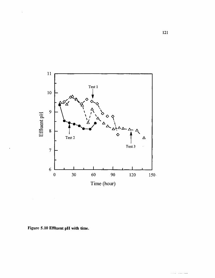
Efflu

ent

pH

11

Test 110 h \

\ \ >>V MA • A \

g L T • - • A- Ao ♦ v

Test 2 T

Test 3

J i I i L30 60 90 120

T im e (h o u r)

A

150

Figure 5.10 Effluent pH with time.

Table 5.2 pH Profiles across Specimens

122

Normalized distance from anode (inlet)

pH

Test 1 Test 2 Test 3

0 .0 -0 . 2 3.9 3.8 3.9

0 .2 -0 .4 4.2 4.3 4.3

0.4-0 . 6 4.5 4.6 5.3

0 .6 -0 . 8 5.0 4.8 5.4

0 .8 - 1 . 0 5.5 4.8 6 . 0

Spec

imen

pH

123

9

8

7

6

5

4

30.0 0.2 0.4 0.6 0.8 1.0

Normalized Distance From Anode

Figure 5.11 pH profiles across specimens upon completion of test.

— O—-Test 1 — — 9 — Test 2

- A - Test 3

Initial pH

Effluent pH

124

5.3.6 Efficiency of Phenol Removal

Figures 5.12 and 5.13 show the change in the effluent phenol concentrations

with time and with the number of pore volumes of flow. The initial phenol

concentration in the kaolinite specimens was 500 ± 25 ppm. It is interesting to note

that the concentration in the effluent was initially in the vicinity of 490 ppm and

decreased steadily to 1 0 to 2 0 ppm with further processing.

Figure 5.13 shows the results with respect to the number of pore volumes of

flow. This figure shows that the phenol concentration at one pore volume of flow was

about 50%, and it reached below 5% within two pore volumes of flow. The

advective-dispersive transport of reactive organic contaminants is discussed by Acar

and Haider [5.30]. These data suggest that the breakthrough of phenol is mainly due

to advective-dispersive transport since there is no indication of any retardation.

However, retardation could be expected due to the desorption process of phenol from

the clay surfaces (Figure 5.1). The observation implies that the desorption process

under electric currents is rather instantaneous with respect to the advective flow. This

is one obvious advantage of the scheme over any other soil flushing technique.

Table 5.3 provides the phenol profile across the specimens at conclusion of the

testing. Table 5.4 provides the mass balance in each test. This table indicates that

85% to 95% of phenol was removed by electrokinetic soil processing. The mass

balances in the three tests lie within 1 0 % of the initial phenol loaded in the specimens.

This error may have arisen due to several reasons: (1) Phenol may have been

volatilized during specimen preparation and extrusion. (2) The test tube and the

electrodes (carbon) may have trapped some of the phenol. They were not checked for

Con

cent

ratio

n Ra

tio

(Eff

luen

t/Ini

tial)

1.0

— O— Test 1

— ®— Test 20.8

0.6

0.4

0.2

A - A - ^ A - A - A - A0.0

0 30 60 90 120 150

Time (hour)

Figure 5.12 Normalized phenol concentrations in effluent in time.

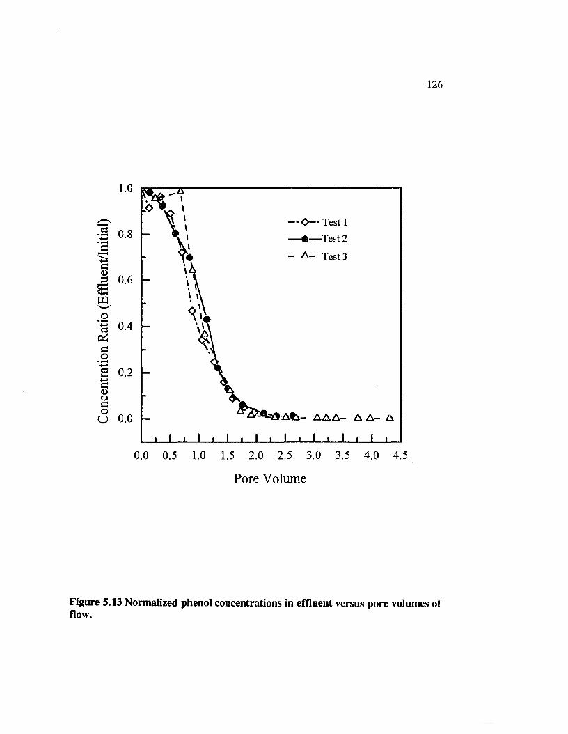
Conc

entr

atio

n Ra

tio

(Effl

uent

/Initi

al)

126

1.0

— O—- Test 1 — • — Test 2

— A— Test 3

0.8

0.6

0.4

0.2

A A A - A A - A0.0

0.0 0.5 1.0 1.5 2.0 2.5 3.0 3.5 4.0 4.5

P o re V o lu m e

Figure 5.13 Normalized phenol concentrations in effluent versus pore volumes of flow.

127

Table 5.3 Normalized Phenol Concentrations in Specimens

Normalized distance from anode (inlet)

Concentration Ratioa (Cf/Cj)

Test 1 Test 2 Test 3

0 .0 -0 . 2 0.03 NDb ND

0 .2 -0 .4 0.05 ND 0 . 0 2

0.4-0 . 6 < 0 . 0 1 0.03 ND

0 .6 -0 . 8 0.06 ND ND

0 .8 - 1 . 0 0 . 0 2 ND ND

a The initial phenol concentration is 500 ± 25 ppm. The accuracy is ± 10%of the datum,

b ND = not detectable (<0 .1 ppm).

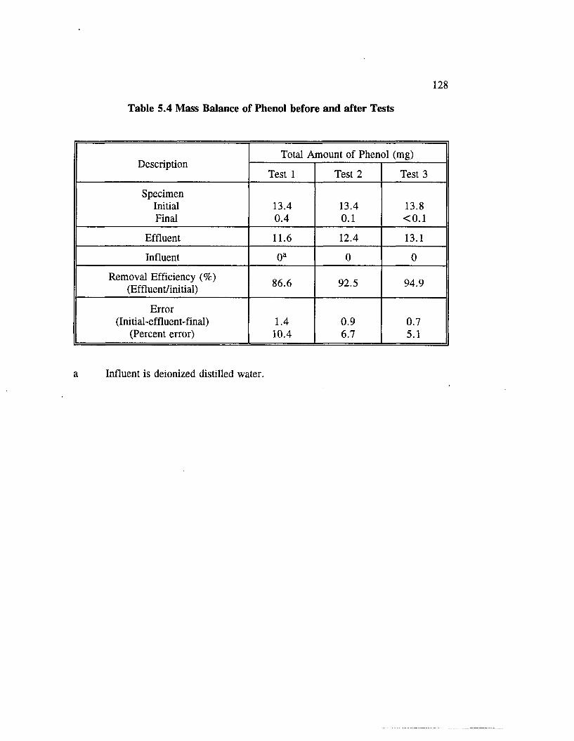
128

Table 5.4 Mass Balance of Phenol before and after Tests

DescriptionTotal Amount of Phenol (mg)

Test 1 Test 2 Test 3

SpecimenInitial 13.4 13.4 13.8Final 0.4 0 . 1 < 0 . 1

Effluent 1 1 . 6 12.4 13.1

Influent 0 a 0 0

Removal Efficiency (%) (Effluent/initial) 8 6 . 6 92.5 94.9

Error(Initial-effluent-final) 1.4 0.9 0.7

(Percent error) 10.4 6.7 5.1

a Influent is deionized distilled water.

129

phenol concentration. (3) The phenol in the specimen, subsequent to the process, is

determined by diluting the mixture with water. All phenol may not have leached out

using this procedure. However, the 10% error is acceptable for the accuracy needed

in this study.

5.3.7 Energy Expenditure

Energy expenditure per unit volume of soil processed, Eu, is given by

E» - j r - y!m - y!,2m < 5 - 8 )S 5 S

where Eu = the energy per unit volume (watt-hr/m3), V5 = the volume of soil mass

processed (m3), R = the resistance (ohm), and t = the time (hr). In tests with

constant current conditions, the energy expended is directly related to the time integral

of the resistance across the cell, or it is inversely related to the time integral of the

apparent conductivity. .

Figure 5.14 shows a plot of the energy expended per unit volume of soil versus

the pore volumes of flow recorded. From the test data presented, it is not possible

to discern the necessary minimum energy needed to flush phenol; however, the results

demonstrate that the energy expenditure upon termination of the tests (phenol removal

by 85%-95%) is in the range of 18 kWh/m3 to 39 kWh/m3. The estimated cost per

cubic yard soil treated for electrokinetic method, incineration, and soil washing and

effluent treatment are about $20 to $30, $50 to $1250, and $100 to $1000,

respectively [5.15]. When it is considered that most phenol was removed at about two

pore volumes (the effluent concentrations are below 5% of the original phenol

Ener

gy

Exp

ende

d, E

u (k

Wh/

m3)

40

35

30

25

20

15

— O— Test 1

— • — Test 2

— A - Test 3

10

5

0

0.0 0.5 1.0 1.5 2.0 2.5 3.0 3.5 4.0 4.5

Pore Volume o f Flow

Figure 5.14 Energy expenditure in tests.

131

concentrations in Figure 5.13), the energy needed in two pore volumes of flow will

be about 12 kWh/m3 to 28 kWh/m3. This low energy expenditure demonstrates the

efficiency of the process in removing phenol.

5.4 Implications

The feasibility of using electrokinetic soil processing in removal of adsorbed

inorganic contaminants from soils has been demonstrated [5.6,5.13,5.14], and the

removal of charged species under electrical gradients is easier to envision. There

were no data regarding the removal of low-polarity organic chemicals by the

technique. This study demonstrates that phenol adsorbed on kaolinite could be

efficiently removed by electrokinetic processing. The study by Bruel et al. [5.17]

shows the transport of BTEX compounds (benzene, toluene, ethylene, and m-xylene)

and trichloroethylene in kaolinite specimens using the technique.

The most interesting aspect of this study is that the phenol breakthrough did

not involve any significant retardation. The adsorption isotherm shown in Figure 5.1

indicates that there would be a retardation associate with desorption of phenol when

the soil pores are flushed with the deionized water supplied at the anode. The fact

that such retardation is not displayed in our tests has the following implications: ( 1 )

The desorption of phenol by hydrogen ion is essentially instantaneous in electrokinetic

soil processing; and (2 ) removal under electroosmosis primarily involves the pore

fluid transport, effects due to migration of protonated phenol may be present in

addition.

132

These test results are very encouraging for the use of electrokinetic soil

processing in remediation of sites contaminated by water-miscible organic

contaminants. The results of the study imply that decontamination can be achieved

in shorter periods of time than the technique of flushing the soil with water.

Furthermore, in fine-grained soils, the application of electrical potentials and the

electroosmotic flow constitute a practical efficient pumping mechanism than the flow

generated by hydraulic potentials. The movement of the acid front from the anode to

the cathode is an added advantage as, in general, it assists in desorption/solubilization

of contaminants. Further studies are needed to investigate removal at higher

concentrations and the influence of natural organic matter on removal rates. Pilot-

scale studies are underway to develop the process for full-scale remediation.

5.5 Conclusions

The following conclusions are obtained from this study, which investigated

phenol removal from the soil using electroosmosis: (1) The acid front generated at the

anode in electroosmosis flushes across the specimen ultimately, decreasing the pH of

the effluent. (2) The coefficient of electroosmotic permeability ke and water transport

efficiency fc- decrease in time as the electrical potential difference increases across the

cell. The chemistry and flow in electrokinetic soil processing are dependent upon the

electrolytes generated at the electrodes and the initial chemistry in the specimen. (3 )

Adsorbed phenol at level of 500 /ng/g of dry kaolinite was efficiently removed by

electrokinetic soil processing. The removed phenol was mostly found in the effluent.

(4) The results suggest that phenol removal is does not display any retardation in

133

effluent concentration profiles. (5) The energy expended in the tests where phenol

was effectively removed varied between 18 kWh/m3 to 39 kWh/m3.

5.6 References

134

5.1 M.I. Esrig and J.P. Gemeinhardt, J. Soil Mech. Found. Engrg. Div. ASCE, 1969, 93, 109.

5.2 L. Casagrande, J. Boston Soc. Civ. Engrg. 1983, 69, 255.

5.3 Y.B. Acar, R.J. Gale, G. Putnam, and J. Hamed, Proc., 2nd Int. Symp. onEnvironmental Geotechnology, 1, Envo Publishing, Bethlehem, PA, 1989, pp. 25-38.

5.4 Y.B. Acar, R.J. Gale, G. Putnam, J. Hamed, and R. Wong, J. Environ. Sci.Health, Part A: Environ. Sci. Engrg. 1990, 25, 687.

5.5 Y.B. Acar, J. Hamed, R.J. Gale, and G- Putnam, Bull. Transp. Res. 1991, Record No. 1288, pp. 23-34.

5.6 J. Hamed, Y.B. Acar, and R.J. Gale, J. Geotech. Engrg. ASCE, 1991, 117, 241.

5.7 J. Hamed, "Decontamination of soil using electroosmosis," Ph.D. dissertation, Louisiana State University, Baton Rouge, LA, 1990.

5.8 B.M. Shmakin, J. Geochem. Explor. 1985, 23, 35.

5.9 R. Hamnet, "A study of the processes involved in the electro-reclamation of contaminated soils," MS thesis, University of Manchester, Manchester, England, 1980.

5.10 D.D. Runnels and J.L. Larson, Ground Water Monitoring Rev. 1986, 81-90.

5.11 R. Lageman, W. Pool, and G. Sebsinge, Chemistry and Industry 1989, 18, 585.

5.12 S. Banerjee, J. Homg, J.F. Ferguson, and P.O. Nelson, "Field scale feasibility of electrokinetic remediation." RREL, CR 811762-01, Unpublished Report Presented to U.S. Environmental Protection Agency Land Pollution Control Division, 1990.

5.13 Y.B. Acar and J. Hamed, Bull. Transp. Res. 1991, Record No. 1312, pp. 153-161.

5.14 Y.B. Acar, Geotech. Special Publication No. 30 ASCE, New York, N.Y., 1992, pp. 1420-1432.

135

5.15 G. Putnam, "Development of pH gradients in electrochemical processing of kaolinite," MS thesis, Louisiana State University, Baton Rouge, LA, 1988.

5.16 B.A. Segal, C.E. O’Bannon, and J.A. Mattias, J. Geotech. Engrg. Div. ASCE, 1980, 106, 1143.

5.17 C.J. Bruel, B.A. Segall, and M.T. Walsh, J. Environ. Engrg. ASCE, 1992, 118, 84.

5.18 P.M. Huang, T.S.C. Wang, M.K. Wang, M.H. Wu, and N.W. Hsu, Soil Sci. 1977, 123, 213.

5.19 D.J. Bishop, J.P. Rnezovich, and F.L. Harrison, Water, Air, and Soil Pollut. 1990, 49, 93.

5.20 S.A. Boyd, Soil Sci. 1982, 134, 337.

5.21 Quality Criteria for Water, U.S. Environmental Protection Agency, Office of Water and Hazardous Materials/Office of Water Planning and Standards, Government Printing Office, Washington, D.C., 1976.

5.22 D.H. Gray, Geotechnique 1970, 20, 81.

5.23 P.J. Isaacson and C.R. Frink, Environ. Sci. Technol. 1984, 18, 43.

5.24 T.S. Sheriff, C.J. Sollars, D. Montgomery and R. Perry, Environ. Technol. Letters 1987, 8, 501.

5.25 J.W. Hamaker and J.M. Thompson, Organic Chemicals in the Soil Environment, C.A.J. Coring and J. Hamaker (Eds.), Vol. 1, Part 2, Marcel Dekker, Inc., New York, N.Y., 1972, pp. 49-143.

5.26 J.R. Campbell, M.J.T. Carrondo, and R.G. Luthy, Environ. Sci. Technol. 1983, 17, 528.

5.27 S. Saltzman and S. Yariv, Soil Sci. Soc. Am. Proc. 1975, 39, 474.

5.28 B.B. Damaskin, O.A. Petrii, and V.V. Batrakov, Adsorption o f Organic Compounds on Electrodes, Plenum Press, New York-London, 1971, pp. 67- 97.

5.29 J. Artiola-Fortuny and W.H. Fuller, Soil Sci. 1982, 133, 18.

5.30 Y.B. Acar and L. Haider, J. Geotech. Engrg. ASCE, 1990, 116, 1031.

VITA

Heyi Li was bom in Huainan, Anhui, P.R. China on March 10, 1964. He

graduated from the Sixth High School of Huainan in 1981. He passed the Chinese

National College Entrance Examination with high scores in 1981 and entered the

University of Science and Technology of China for his undergraduate study, where

he received his Bachelor of Science Degree in Chemistry in July, 1986. In 1986, he

was awarded the 17 Li Da Experimental Scholarship, one of the top two awards in the

university. In August of 1989, he began graduate study at Louisiana State University,

where he worked in the field of Analytical Chemistry under the supervision of Dr.

Robert J. Gale. He is a member of the American Chemical Society and is presently

a candidate for the degree of Doctor of Philosophy at Louisiana State University.

136

DOCTORAL EXAMINATION AND DISSERTATION REPORT

Candidate: Heyi Li

Major Field: Chemistry

Title of Dissertation: Fundamental Studies of CapillaryElectroosmosis and Electrokinetic Removal of Phenol from Kaolinite

Approved:

Major Professor and Chairman

Dean of the Graduate School

EXAMINING COMMITTEE:

Date of Examination:

June 21, 1994