Fundamental Sampling Distributions

EGR 252 - Ch. 8 9th edition 2013 Slide 1

Fundamental Sampling Distributions

Introduction to random sampling and statistical inference

Populations and samples Sampling distribution of means

Central Limit Theorem Other distributions

S2

t-distribution F-distribution


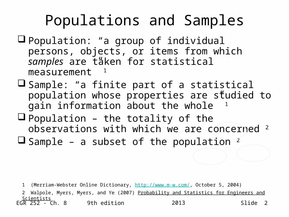
Populations and Samples Population: “a group of individual persons, objects, or

items from which samples are taken for statistical measurement” 1

Sample: “a finite part of a statistical population whose properties are studied to gain information about the whole” 1

Population – the totality of the observations with which we are concerned 2

Sample – a subset of the population 2

1 (Merriam-Webster Online Dictionary, http://www.m-w.com/, October 5, 2004)

2 Walpole, Myers, Myers, and Ye (2007) Probability and Statistics for Engineers and Scientists

http://www.m-w.com/


Examples

Population Sample

Students pursuing undergraduate engineering degrees

1000 engineering students selected at random from all engineering programs in the US

Cars capable of speeds in excess of 160 mph.

50 cars selected at random from among those certified as having achieved 160 mph or more during 2003


More Examples

Population Sample

Potato chips produced at the Frito-Lay plant in Kathleen

10 chips selected at random every 5 minutes as the conveyor passes the inspector

Freshwater lakes and rivers

4 samples taken from randomly selected locations in randomly selected and representative freshwater lakes and rivers


Basic Statistics (review)

Sample Mean:

A class project involved the formation of three 10-person teams (Team Q, Team R and Team S). At the end of the project, team members were asked to give themselves and each other a grade on their contribution to the group. A random sample from two of the teams yielded the following results:

= 87.5

= 85.0

Q R

92 85

95 88

85 75

78 92

n

XX

n

ii

1

QX

RX


Basic Statistics (review) Sample variance equation:

For our example:

Calculate the sample standard deviation (s) for each sample.

SQteam = 7.59386 and SRteam = 7.25718

Q team sample R team sample

92 85

95 88

85 75

78 92

1

)(1

2

2

n

XXS

n

ii


Sampling Distributions

If we conduct the same experiment several times with the same sample size, the probability distribution of the resulting statistic is called a sampling distribution

Sampling distribution of the mean: if n observations are taken from a normal population with mean μ and variance σ2, then:

nn

n

x

x

2

2

22222 ...

...


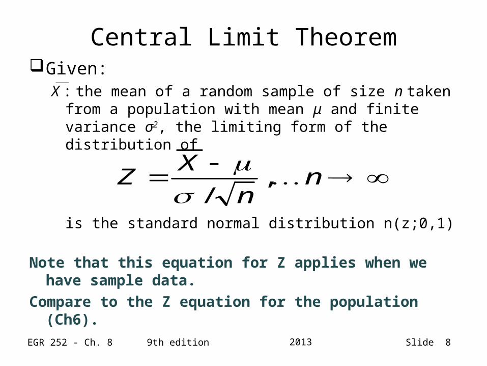
Central Limit TheoremGiven:

X : the mean of a random sample of size n taken from a population with mean μ and finite variance σ2, the limiting form of the distribution of

is the standard normal distribution n(z;0,1)

Note that this equation for Z applies when we have sample data.

Compare to the Z equation for the population (Ch6).

nn

XZ ,

/


Central Limit Theorem-Distribution of X

If the population is known to be normal, the sampling distribution of X will follow a normal distribution.

Even when the distribution of the population is not normal, the sampling distribution of X is normal when n is large.

NOTE: when n is not large, we cannot assume the distribution of X is normal.


Sampling Distribution of the Difference Between Two Averages

Given:Two samples of size n1 and n2 are taken from two

populations with means μ1 and μ2 and variances σ12

and σ22

Then,

2

22

1

21

2121

2

22

1

212

21

)()(

21

21

nn

XXZ

and

nnXX

XX


Sampling Distribution of S2

Given: If S2 is the variance of of a random sample of size n

taken from a population with mean μ and finite variance σ2,

Then,

has a χ 2 distribution with ν = n - 1

n

i

i XXsn

12

2

2

22 )()1(


Chi-squared (χ2) Distribution

χα2 represents the χ2 value above which we find an area

of α, that is, for which P(χ2 > χα2 ) = α.

χ2

α


Example Look at example 8.7, pg. 245: A manufacturer of car batteries

guarantees that his batteries will last, on average, 3 years with a standard deviation of 1 year. A sample of five of the batteries yielded a sample variance of 0.815. Does the manufacturer have reason to suspect the standard deviation is no longer 1 year?μ = 3 σ = 1 n = 5 Degrees of freedom (v) = n-1 s2 = 0.815

If the χ2 value fits within an interval that covers 95% of the χ2 values with 4 degrees of freedom, then the estimate for σ is reasonable.

See Table A.5, (pp. 739-740)χ2

26.31

)815.0)(4()1(2

22

sn

calculated

For alpha = 0.025, Χ2 =11.143 The Χ2 value for alpha = 0.975 is 0.484. 0.484 3.26 11.143


Your turn …

If a sample of size 7 is taken from a normal population (i.e., n = 7), what value of χ2 corresponds to P(χ2 < χα

2) = 0.95? (Hint: first determine α.)

χ2

12.592

95%


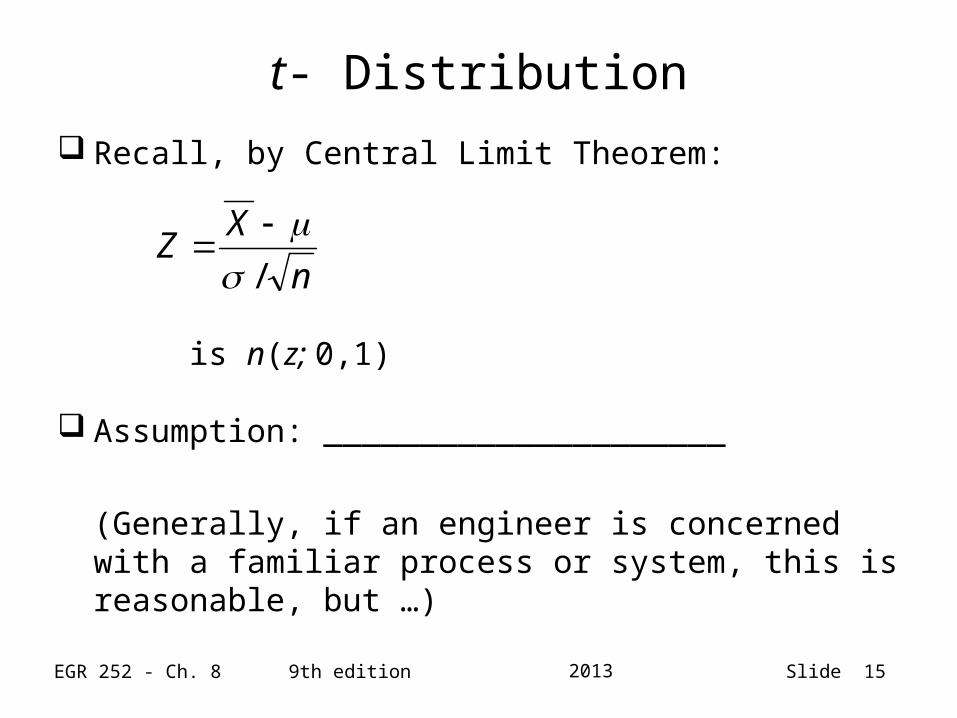
t- Distribution

Recall, by Central Limit Theorem:

is n(z; 0,1)

Assumption: _____________________

(Generally, if an engineer is concerned with a familiar process or system, this is reasonable, but …)

n

XZ

/


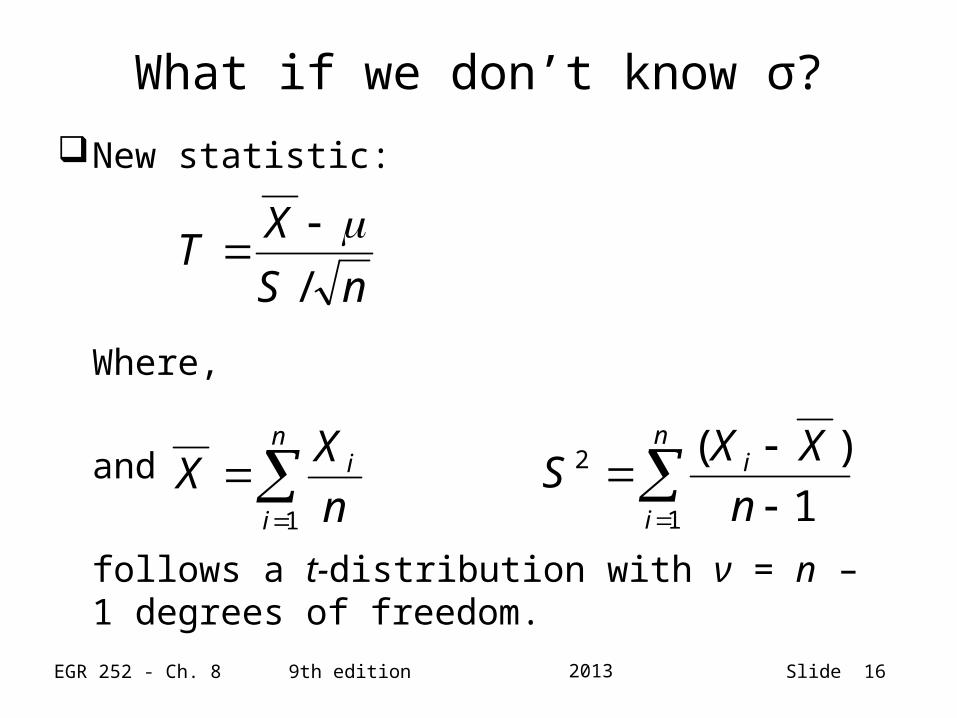
What if we don’t know σ?

New statistic:

Where,

and

follows a t-distribution with ν = n – 1 degrees of freedom.

nS

XT

/

n

i

i

n

XX

1

n

i

i

n

XXS

1

2

1

)(


Characteristics of the t-Distribution

Look at Figure 8.8, pg. 248Note:

Shape: _________________________

Effect of ν: __________________________

See table A.4, pp. 737-738 Note that the table yields the right tail of the distribution.


F-DistributionGiven:

S12 and S2

2, the variances of independent random samples of size n1 and n2 taken from normal populations with variances σ1

2 and σ22, respectively,

Then,

has an F-distribution with ν1 = n1 - 1 and ν2 = n2 – 1 degrees of freedom.

(See table A.6, pp. 741-744)

22

21

21

22

22

22

21

21

/

/

S

S

S

SF

Fundamental Sampling Distributions

Documents

Transcript of Fundamental Sampling Distributions