Fundamental Models for Forecasting Elections

Patrick Hummel (Google) and David Rothschild (Microsoft Research)

����������������

���� ��

This paper develops new fundamental models for forecasting presidential, senatorial, and gubernatorial elections at the state level using fundamental data. Despite the fact that our models can be used to make forecasts of elections earlier than existing models and they do not use data from polls on voting intentions, our models have lower out-of-sample forecasting errors than existing models. Our models also provide early and accurate probabilities of victory. We obtain this accuracy by constructing new methods of incorporating various economic and political indicators into forecasting models. We also obtain new results about the relative importance of approval ratings, economic indicators, and midterm effects in the different types of races, how economic data can be most meaningfully incorporated in forecasting models, the effects of different types of candidate experience on election outcomes, and that second quarter data is as predictive of election outcomes as third quarter data. Keywords: Economic modeling; Elections; Forecasting; Fundamental data; Voting

2

Introduction

Fundamental models for forecasting elections are models that can make forecasts of the

results of elections using only economic and political data that would exist independently of the

election. These models are important for several reasons. First, these models provide accurate

forecasts of the results of elections before polls on voting intentions can accurately forecast

elections and before prediction markets have enough liquidity for meaningful predictions. Second,

fundamental models are also useful in that they give us a better sense of what factors are driving the

outcomes behind elections by indicating which types of economic and political data most

meaningfully correlate with election outcomes.

In this paper we illustrate how fundamental data can be used to make accurate forecasts of

state-level presidential, senatorial, and gubernatorial election outcomes, even restricted to data

available by the end of the second quarter of the election year, before the campaigns begin in

earnest.1 Our results are stronger than previous literature on state-level forecasts of elections for

several reasons. First, for all types of state-level elections where fundamental models already exist

in the literature, we are able to present models that result in lower out-of-sample errors for forecasts

of the binary outcomes of elections as well as the estimated vote shares of the candidates. Second,

we are able to do this even though our models are unique in that they make forecasts of elections at

an earlier date than existing models for state-level forecasts, and our models do not require data on

pre-election polls on voting intentions. Finally, our models provide accurate forecasts of the

probability of victory in senatorial and gubernatorial elections, which is not seen in the literature, as

well as the Electoral College elections, which is rarely seen in the literature. Forecasting

probabilities of victory is most useful for most stakeholders, including researchers and election

observers.

In developing more accurate methods for forecasting elections at the state level, we must

consider several new ways of taking into account how we can use fundamental data to make

forecasts of elections. In this paper we come up with new ways of taking into account a wide range

of fundamental data including information about economic variables, incumbency, state ideology,

previous election results, third party candidates, regional variables, and biographical information

1 The conventions are the traditional start of the election season and occur towards the end of the third quarter in late August or early September.

3

about the candidates. Together, these new ideas enable us to make forecasts that are more accurate

than existing models.

In addition to presenting models that make more accurate forecasts of elections than existing

models, our models also enable us to better understand what types of fundamental data are most

useful for making forecasts of elections. Some of the most meaningful variables in this regard are

economic variables and presidential approval ratings. We note that economic indicators can be most

meaningfully included as trends rather than levels. For instance state-by-state personal income

growth is the most predictive economic variable for the Electoral College and for Senate elections,

whereas absolute levels of economic performance such as state unemployment rates are not

statistically significant when added to such a model. We also find that presidential approval ratings

are significant predictors of election outcomes in all types of elections, but they only have about

one-third to one-fourth as much impact on our forecasted vote shares in senatorial elections and

gubernatorial elections as they do on our forecasted vote shares in presidential elections. Finally, we

note that there is relatively little benefit to including third quarter data; third quarter data on

economic variables and presidential approval ratings is statistically insignificant when added to a

model that already incorporates data through the first two quarters, and replacing second quarter

data on presidential approval ratings with third quarter data does not improve the fit of the model.

By building these models together, we are able to learn about the differences between

presidential, senatorial, and gubernatorial elections. In the context of midterm elections, we find

candidates of the president’s party suffer a penalty during midterms that is as significant in

gubernatorial elections as it is in senatorial elections. We also find evidence that the electoral

fortunes of incumbent gubernatorial parties are not tied to the economic performance in the state,

but are instead tied to the performance of the national economy, and that the results of previous

elections are not meaningful predictors of the results of future gubernatorial elections. Finally, we

study how previous political experience affects the likely fortunes of candidates in senatorial

elections and gubernatorial elections and find some counterintuitive results about how candidates

who have held seemingly less prominent offices may do just as well as candidates who have held

more visible positions.

4

Related L iterature on Forecasting Elections

There is an extensive literature devoted to forecasting the results of elections, much of which

focuses on using pre-election polls or prediction markets to forecast the results of elections; these

papers find that pre-election polls and prediction markets can, after proper adjustments, make

accurate forecasts of the national popular vote in presidential elections a few days before the

election.2 For instance, Arrow et al. (2008) notes that prediction markets resulted in an average

forecasted error of 1.5 percentage points in the national popular vote in recent U.S. presidential

elections, while the final Gallup poll resulted in an average error of 2.1 percentage points, and Berg

et al. (2008a) finds similar results on the average accuracy of prediction markets and polls for

forecasting the national popular vote just before U.S. presidential elections. Holbrook and DeSart

(1999), Kaplan and Barnett (2003), and Soumbatiants et al. (2006) further show that one can use

polls taken just before an election to make fairly accurate forecasts of the state-level results in U.S.

presidential elections, and Rothschild (2009) shows this for both polls and prediction markets.

While polls and prediction markets can both be used to make reasonably accurate forecasts

of election results just before an election, these methods are much less reliable when used months

before an election. Gelman and King (1993) notes that polls for the national popular vote in U.S.

presidential elections tend to oscillate wildly in the months before the election takes place, and as a

result, polls can be highly unreliable indicators of the election outcomes months before the election.

Arrow et al. (2008) further notes that using prediction market data to make forecasts of the national

popular vote five months before a U.S. presidential election would have resulted in an average error

of over 5 percentage points in recent elections, and that using pre-election polls would have resulted

in even less accurate predictions.3 Finally, Rothschild (2009) investigates the errors in both polls

and prediction markets at forecasting probabilities of victory at the state level up to 130 days before

the election, and notes that there is not enough liquidity to even have predictions for some states.

Researchers have investigated many unique methods of forecasting election results months

before the election that may hold more promise than using polls or prediction markets. Several

techniques have been explored for forecasting the results of elections such as using biographical

2 See, for example, Arrow et al. 2008, Berg et al. 2008a; 2008b, Brown and Chappell 1999, Holbrook and DeSart 1999, Kaplan and Barnett 2003, Pickup and Johnston 2008, and Soumbatiants et al. 2006. 3 Erikson and Wlezien (2008a) indicates that the inaccuracy of polls suggests a need to systematically adjust for biases in polls.

5

information (Armstrong and Graefe 2011), using measures of how well candidates would be

expected to handle particular issues (Graefe and Armstrong 2012), surveying experts or voters for

their predictions (Jones et al. 2007; Lewis-Beck and Tien 1999), using indices that reflect a variety

concerns such as whether there has been a major policy change, a major military failure or success,

and social unrest or a scandal (Armstrong and Cuzán 2006; Lichtman 2008), or even using pictures

or silent video clips of candidates (Armstrong et al. 2010; Benjamin and Shapiro 2009). With the

exception of the forecasting methods based on visual depictions of the candidates, so far all of these

approaches have only forecast the national popular vote in U.S. presidential elections.

The most viable and common approach for making forecasts of elections without relying on

polls or prediction markets involves using econometric models. These methods involve predicting

the likely outcome of an election from a variety of economic and political indicators such as

economic growth rates, results of previous elections, incumbency, and a wide variety of other

possible considerations. However, while there is an extensive literature on forecasting elections

using econometric models, so far the vast majority of this literature has focused on forecasting

nationwide results. This holds for forecasting models of presidential elections4, which typically

focus on forecasting the national popular vote, and for forecasting models of congressional

elections5, which typically focus on forecasting the number of seats won by each major party in the

two branches of Congress.

The focus on forecasting nationwide results for these elections is somewhat unsatisfying

because the results of these elections are typically determined at the state or local level. For

instance, the Electoral College elects the U.S. president, where each state has electors that equal its

congressional representation. Further, gubernatorial and senatorial elections are also state-level

elections. Despite this fact, so far only a handful of papers have addressed questions related to

forecasting election outcomes at the state level using econometric methods. Several papers related

to forecasting the results of the U.S. presidential election at the state level are of limited practical

use for forecasting elections because they focus on showing theoretically how one might make

4 See, for example, Abramowitz 2008; 2012 Alesina et al. 1996, Bartels and Zaller 2001, Campbell 2008; 2012, Cuzán 2012; Cuzán and Bundrick 2008, Erikson and Wlezien 2008; 2012, Fair 2009, Haynes and Stone 2004, Hibbs 2008; 2012, Holbrook 2004; 2008; 2012, Lewis-Beck and Tien 2008; 2012, Lockerbie 2008; 2012, Norpoth 2008; 2012, and Sidman et al. 2008. 5 See, for example, Abramowitz 2010, Abramowitz and Segal 1986, Bafumi et al. 2010a, Campbell 2010, Coleman 1997, Cuzán 2010, Fair 2009, Kastellec et al. 2008, Lewis-Beck and Rice 1984; 1985, Lewis-Beck and Tien 2010, and Marra and Ostrom 1989.

6

forecasts of elections if certain data that is only available after elections were available before the

election (Rosenstone 1983; Holbrook 1991; Strumpf and Phillipe 1999).

Campbell (1992), Campbell et al. (2006), and Klarner (2008) have illustrated how one can

combine the results of polls on voting intentions taken two to four months before the election with

other economic and political indicators to make forecasts of the results of U.S. presidential elections

at the state level. Our work differs from these papers in that we do not use polls of voter intentions

in our forecasting model; thus, we provide more identification of our fundamental variables and we

can also use our forecasting model to make predictions further in advance of the election (at least

five months in advance). Despite this, we still find that we obtain lower errors in our out-of-sample

forecasts than the corresponding errors in these papers. For instance, Campbell et al. (2006) reports

that for out-of-sample forecasts, their forecasting model would have correctly predicted how 75% of

the states would have cast their Electoral College votes with average and median errors of 4.8% and

4.2% respectively in their estimated vote shares. By contrast, we find that for out-of-sample

forecasts we would have correctly predicted how over seven additional states would have cast their

Electoral College votes and obtained average and median errors in our estimated vote shares that are

over 1.5 points lower than Campbell’ s errors. Similarly, while Klarner (2008) does not report errors

in out-of-sample forecasts in his paper, we note that the within-sample standard errors in our

forecasting model are roughly 40% lower than those reported in Klarner (2008) and even the

standard errors in our out-of-sample forecasts are lower than the within-sample standard errors

reported for the forecasting model in Klarner (2008).

In work that was published after this paper was first distributed, Berry and Bickers (2012),

Klarner (2012), and Jerôme and Jerôme-Speziari (2012) developed models for forecasting the

Electoral College that did not require pre-election polls on voting intentions. However, the model

for forecasting the Electoral College presented in this paper still contains new ideas not considered

in these papers and also attains out-of-sample errors that are lower than the within-sample errors

reported in these manuscripts. Furthermore, our model made forecasts in 2012 that compared very

favorably to the forecasts in these papers.

We also develop models for forecasting the results of senatorial elections at the state level.

To the best of our knowledge, there are only three other papers that have been written that develop

models for forecasting the results of senatorial elections at the state level. Bardwell and Lewis-Beck

7

(2004) report results of a model that forecasts the results of Senate elections in Maine. Klarner

(2008) develops a model that forecasts the results of Senate elections for all states using information

from pre-election polls on voting intentions, and Klarner (2012) presents a revised model that does

not require pre-election polls on voting intentions. The model we develop shares many features

with the models for forecasting senatorial elections in Klarner (2008, 2012), but we note a few new

ideas that we believe improve the forecasts and we obtain lower errors in our forecasts than those

reported in Klarner (2008, 2012) in spite of the fact that we do not use any data on pre-election polls

on voting intentions in our forecasting model.

Finally, we develop econometric models for forecasting the results of gubernatorial elections

at the state level months before the election. While there have been papers that have investigated

factors that affect vote choice in gubernatorial elections (Adams and Kenney 1989; Atkeson and

Partin 1995; Carsey and Wright 1998; Hansen 1999; Howell and Vanderleeuw 1990; Niemi et al.

1995; Partin 1995; Peltzman 1987; Svoboda 1995), to the best of our knowledge, the only paper that

has developed a fundamental model for forecasting gubernatorial elections at the state level using

data available before the election is Klarner (2012). Our gubernatorial model contains a few new

ideas not considered in Klarner (2012), and again obtains lower errors than those reported in

Klarner (2012).

Estimation Strategy

We construct models to forecast two different types of outcomes: the expected vote share

and probability of victory in each state for presidential, senatorial, and gubernatorial elections. To

construct models to forecast the expected vote share, we run linear regressions of the fraction of the

major party vote received by the Democrats in historical elections on several other economic and

political indicators that are available months before the election. And in constructing models to

forecast the probability each major party will win the election in a state, we run a probit that

regresses the outcome of historical elections on several other economic and political indicators that

are available months before the election.6

6 The forecasts are virtually unaffected by whether we put the variables in terms of the Democratic Party, the Republican Party, or the incumbent party.

8

We determine the significance of a variable by examining both within-sample and out-of-

sample forecasts. Within-sample tests include all elections in the regressions. Out-of-sample tests

predict each year by dropping that year from the sample. Our models do not use variables that are

significant within sample, but fail to improve out-of-sample forecasting errors.

In constructing forecasting models for forecasting presidential elections at the state level, we

focus on the presidential elections that took place from 1972 to the present. We prefer to focus on

races that took place no earlier than 1972 because the 1968 presidential election is one of the rare

presidential election in which a third party candidate did well enough to win Electoral College votes

in several states, and the 1968 election was a watershed for the last major realignment of the major

parties. We also choose to focus on similar time periods in constructing forecasting models for

gubernatorial races and senatorial elections as we do for Electoral College elections. Ultimately for

senatorial and gubernatorial elections we focused on the time period from 1976 to the present.

Our decision to use state-level data is quite rare for forecasting models, but it confers several

advantages. First, we can potentially make more accurate forecasts by considering state-level data

that forecasting models for national variables must ignore. Second, this gives us a better

understanding of the value of certain types of fundamental data since we may have as many as 50

data points in any given year to work with.7 Finally, this enables us to focus on the outcomes that

are most important to stakeholders. In the months leading up to an election, campaigns and parties

are most interested in state-level outcomes so that they can spend their time and money most

efficiently. The national popular vote is not as relevant for most stakeholders.

The full results of the regressions noted in this section are in Table 1 for the Electoral

College, Table 2 for Senate elections, and Table 3 for gubernatorial elections.

Presidential Approval: Naturally, we would expect people to be more likely to vote for candidates

who are of the same party as the incumbent president if they believe that the incumbent president

has been doing a good job. This variable is likely meaningful not only for presidential elections, but

also for senatorial and gubernatorial elections since there is empirical evidence that presidential

coattails are a factor in senatorial elections (Campbell and Summers 1990) and gubernatorial

elections (Holbrook-Provow 1987; Tompkins 1988; Simon 1990). Thus, we use presidential

7 These data points are correlated, so we do not have 50 independent data points in a given year, but we still have more information than if we had only considered the overall national results.

9

approval ratings as a variable in forecasting all three types of elections. In particular, we consider a

variable that is equal to the incumbent president’s approval rating on June 15 minus a constant if a

Democrat is president and the opposite if a Republican is president. For presidential elections we

choose the constant to be equal to the point where an incumbent party would be roughly indifferent

between having the advantage of incumbency and a relatively low approval rating.8 For senatorial

and gubernatorial elections we simply choose the constant to be equal to 50.

Incumbency: The precise manner in which we address incumbency differs slightly depending on

the type of election we wish to forecast. In the case of presidential elections, there is empirical

evidence that voters are less likely to want to reelect members of the incumbent party if the

incumbent party has been in office for multiple terms (Abramowitz 2008). For this reason, we

include a variable that equals 1 (-1) if the Democrats (Republicans) have been in control of the

presidency for at least eight consecutive years and 0 otherwise.

For senatorial and gubernatorial elections, we expect voters to be more likely to elect

incumbents than non-incumbents, as there is empirical evidence that incumbents have an advantage

when it comes to seeking reelection in both of these types of races (Ansolabehere and Snyder 2002;

Highton 2000; Piereson 1977; Tompkins 1984). Thus in forecasting each of these types of races we

include a variable that equals 1 (-1) if an incumbent Democrat (Republican) is running for

reelection and 0 otherwise.

Moreover, since this empirical evidence suggests that the value of this incumbency

advantage has increased over time in gubernatorial elections and Senate elections, we also include

variables that can represent the value of the increase in the size of this incumbency advantage over

time. In particular, we consider dummy variables for incumbency, defined the same as the previous

paragraph, for 1984 and forward, 1992 and forward, and 2000 and forward. Of these variables, we

find that the dummy variable that increases the senatorial incumbency advantage in 1984 and the

variable that increases the gubernatorial advantage in 1992 are the most useful.9

8 For presidential elections this constant is roughly 42. We verify in Table A1 of the supplementary appendix that when this constant is chosen, adding a term representing the advantage of the incumbent party to the regression is not statistically significant within sample. 9 Please see Tables A2 and A4 in the supplementary appendix for details on why these variables are the most helpful ways to account for how the size of incumbency advantage varied over time.

10

There is also empirical evidence that voters vote differently in Senate elections that take

place on a midterm than they do in Senate elections that take place the same year as a presidential

election. Busch (1999), Chappell and Suzuki (1993) and Grofman et al. (1998) all suggest that

voters are less likely to vote for members of the president’s party in Senate elections during a

midterm than they are during a year when there is a presidential election.10 For this reason, in

analyzing Senate elections, we include a variable that is equal to 1 (-1) if a Democrat (Republican)

is president and the election is a midterm and 0 otherwise. We also consider this same variable in

the context of gubernatorial elections.

Past Election Results: One of the best indicators of how states will vote in the future is differences

in how states voted in previous elections. Thus, in forecasting the Electoral College, we consider

variables that represent the difference between the fraction of the major party vote received by the

Democratic candidate in the state and the fraction of the major party vote received by the

Democratic candidate nationwide, in both of the two previous presidential elections.

While these variables are helpful in forecasting the results of future elections, these variables

can also sometimes give a misleading picture of the ideologies of the states. In some previous

presidential elections, there was a major third party candidate who took substantially more votes

from one major party candidate than another. For this reason, we include variables that address how

the vote shares of major third party candidates in previous elections should affect the forecasts we

make for future presidential elections. In particular, we consider the three different third party

candidates who received more than five percent of the national popular vote when they ran for

office. These candidates were Ross Perot (in 1992 and 1996), John Anderson (in 1980), and George

Wallace (in 1968).11 We detail the procedure we use to adjust for third party candidates in the

appendix.

Our senatorial model utilizes the variable representing the results of past presidential

elections along with an analogous variable which gives the Democratic vote share for the Senate

seat in the senatorial election six years ago minus the average Democratic vote share in senatorial

elections six years ago. In addition, in our Senate model we include a dummy variable that equals 1

(-1) if a Democrat (Republican) ran unopposed for the Senate seat in the Senate election that took

10 Bafumi et al. (2010b) and Erikson (1988) also note similar results for Congressional elections. 11 While we are not calibrating on 1968, it is a past election result for years in our sample.

11

place six years ago to correct for circumstances under which the previous senatorial elections would

give a misleading representation of that state’s ideology.

We also take into account regional shifts in preferences that may affect our models. For

instance, Bullock (1988) and Stanley (1988) note that in 1976 there appears to have been a

significant shift toward voters in the South voting more for the Democratic candidate in the

presidential election than they did previously as a result of a Southern Democrat running for

president. To account for this, we include a dummy variable in our regressions that equals 1 if a

state is a Southern state in 1976.

We include a few regional dummies for the gubernatorial elections as well. Since there was

a regional realignment in voting in the South in the late 1970s, we include a dummy variable for the

South in 1980 and earlier. We also find it helpful to include a dummy variable indicating if a state is

in the Midwest, to capture the fact that these states seem to have voted Republican more than the

rest of the country.

Economic Indicators: We expect the performance of the economy to generally affect the prospects

of the incumbent president’s party. Models regularly use national economic variables for

forecasting the national popular vote.12 Furthermore, there is empirical evidence that the general

performance of the national economy affects the electoral fortunes of members of the president’s

party in senatorial elections (Abramowitz and Segal 1986; Carsey and Wright 1998; Lewis-Beck

and Rice 1985) and in gubernatorial elections (Leyden and Borelli 1995; Niemi et al. 1995;

Peltzman 1987).

We explore the metrics of unemployment levels and changes in GDP and income over

various time periods at both the national and state levels. After testing the significance of these

options, we ultimately include two different variables in our forecasting models. The first variable

we utilize is equal to the difference between state personal income growth from January 1 in the

year before the election to March 31 in the year of the election and average state personal income

growth in a typical five-quarter period. The second variable we utilize is equal to the difference

between national annualized second quarter real GDP growth in the year of the election and average

12 See, for example, Abramowitz 2008, Alesina et al. 1996, Campbell 2008, Cuzán and Bundrick 2008, Erikson and Wlezien 2008b, Fair 2009, Haynes and Stone 2004, Hibbs 2008, Holbrook 2008, Lewis-Beck and Tien 2008, and Sidman et al. 2008.

12

annual real GDP growth. We take the negative of both of these variables if there is a Republican

incumbent president.13

State Ideology: In addition to past election results, we also find it helpful to include other measures

of ideology. Since the ideology of a state’s two senators is likely to be correlated with the ideology

of a state, we include a variable that is equal to the sum of the ratings of the incumbent senators in a

state provided by the American Conservative Union in the year before the presidential election

minus the average sum of the ratings of the incumbent senators for a state, as provided by the

American Conservative Union in that year.

We also include a variable that detects changes in state ideology since the last presidential

election. If a state has become more conservative (liberal) since the last presidential election, then

the state is likely to have voted for more conservative (liberal) candidates in the most recent

midterm election than in the last presidential election. We detect this shift by including a variable

that equals the change in the percentage of Democrats in the Lower House of the state legislature as

a result of the midterm elections. In addition, for senatorial and gubernatorial elections, we also

include a variable that is equal to the exact percentage of major party members of the Lower House

of the state legislature that are Democrats.

Senator Ideology: An incumbent senator’s voting record can potentially influence that senator’s

electoral prospects. Canes-Wrone et al. (2002) has noted that an incumbent House member is less

likely to win a general election if that incumbent had a more extreme voting record while in the

House, so we elect to include a variable that represents an incumbent senator’s ideology. In

particular, we include a variable that equals the difference between an incumbent senator’s rating

from the American Conservative Union in the previous year and the average incumbent senator’s

rating from the American Conservative Union if a Republican incumbent senator is running for

reelection and zero otherwise. The fact that this variable equals zero when an incumbent senator is

not running for reelection is important because it is only cases when an incumbent is running for

reelection that we would expect the incumbent’s ideology to affect his party’s reelection prospects;

in this sense our approach is different than the approach taken in Klarner (2008, 2012). While

13 See Table A1 in the supplementary appendix for why levels of unemployment are statistically insignificant in the presidential model.

13

including this variable for an incumbent Republican’s voting record improves our forecasts, we

interestingly found no significance to including a similar variable for a Democrat’s voting record.14

Biographical Information: The last type of information we include in constructing our models for

forecasting elections is biographical information about the candidates. In the context of presidential

elections, there is empirical evidence that presidential candidates tend to gather more votes in their

home states than they would if they were not residents of those states (Garand 1988; Lewis-Beck

and Rice 1983; Rosenstone 1983). Moreover, the size of this home state advantage appears to be

larger for small states than for large states (Garand 1988; Lewis-Beck and Rice 1983). For this

reason, we include a variable that equals 1 (-1) if the state is the Democratic (Republican)

presidential candidate’s home state and the state has less than ten million people, but the state is not

the Republican (Democratic) nominee’s home state, and 0 otherwise. This variable reflects the

boost that a presidential candidate can expect to receive in his home state if the president is from a

small state. We also investigated including an analogous variable for the home state advantage

when the president is from a large state or an additional variable for the home region advantage, but

found that such variables were not statistically significant.15

Furthermore, if a state was one of the candidates’ home states in the previous presidential

election, the results of the previous presidential election are likely to give a misleading picture of

the state’s ideology. We therefore also include a variable that equals 1 (-1) if the state was the

Democratic (Republican) presidential candidate’s home state in the previous election and the state

has less than ten million people but the state is not the Republican (Democratic) nominee’s home

state to correct for these circumstances under which the candidates’ home states in the previous

election would throw off our estimates of the state’s ideology based on prior election results.

In addition to considering biographical information about the presidential candidates, we

also consider biographical information in our forecasts of senatorial and gubernatorial elections.

There is empirical evidence that candidates who have held political office tend to do better than less

experienced candidates both for Senate elections (Abramowitz 1988; Squire 1989; 1992b) and for

gubernatorial elections (Squire 1992a). For this reason, it is desirable to include information about

14 Table A3 in the supplementary appendix notes that such a variable would be statistically insignificant in our Senate model. It should be noted, however, that if we included a single variable that represented the voting records of both Democratic senators and Republican senators seeking reelection that such a variable would still be statistically significant in the model. 15 Please see Table A1 in the supplementary appendix for details.

14

the candidates’ previous job experience as predictors of the outcomes of these elections. We classify

every major party candidate for Senate into one of eleven categories depending on the candidate’s

most recent job experience. In particular, we include separate dummy variables indicating whether a

candidate’s most recent job was as a senator, a governor, a member of the House of

Representatives, a member of a president’s cabinet, a mayor, a lieutenant governor, a state

legislator, some other state-wide office, some other local office, a business executive, or none of the

above.

To the best of our knowledge, this approach of including different dummy variables for the

different types of job experience that a candidate may have had has not been used before in the

literature. The existing models for forecasting Senate elections at the state level that include

biographical information about the candidates instead consider a single variable that may assume

any one of several different arbitrarily chosen values depending on the previous experience of the

candidates (Klarner 2008, 2012). However, we find that our approach leads to more accurate

forecasts than using contrived scales, and our results further suggest that the contrived scales used

in Klarner (2008, 2012) may not accurately represent the value of the various types of political

experience a candidate may have had. Our results similarly suggest that the contrived scale

considered in Squire (1992a) may not accurately represent the value of various types of experience

in gubernatorial elections.

Results – Significance of Var iables

Our results indicate that presidential approval ratings are an important predictor of the

results of presidential, senatorial, and gubernatorial elections. However, the effect of presidential

approval ratings on senatorial and gubernatorial elections is only about one-third to one-fourth of

the size of the Electoral College effect. We also find that there is little benefit to using approval

ratings that are closer to the election. Using third quarter approval ratings instead of second quarter

approval ratings does not improve (and in fact slightly lowers) the fit of our Electoral College

model. And the errors in our gubernatorial model that resulted from using March approval ratings

instead of June approval ratings were barely different (and in fact slightly lower) than the errors we

obtained from using June approval ratings, so we have used March approval ratings for that model.

15

Incumbency is also significant in all three types of elections. Being in power for eight or

more years significantly hurts a president’s party in the Electoral College, as it costs roughly 1.9

percentage points in expectation. We also find that an incumbent senator (governor) who ran for

office before 1984 (1992) would obtain roughly 8.7 (11.1) points more in expectation than a

candidate who has no political experience whatsoever. In addition, our model indicates that the size

of this incumbency advantage has increased by about 4.1 (3.5) points since 1984 (1992), so an

incumbent senator (governor) would now obtain roughly 12.8 (14.6) points more in expectation

than a candidate who has no relevant experience at all.

While these results indicate than an incumbent senator or governor has a significant

advantage over other candidates who do not have relevant experience, an incumbent’s advantage

against an experienced rival is much lower. Our forecasting model includes biographical

information about the opposing candidates, and dropping these terms would result in fairly different

estimates of the coefficients on the incumbency variables. If we dropped all other biographical

information about the candidates, we would estimate that an incumbent senator (governor) obtains

roughly 4.3 (7.1) points more in expectation than a non-incumbent before 1984 (1992) and roughly

8.1 (9.4) points more from 1984 (1992) onwards, indicating that an incumbent’s advantage over a

typically experienced rival is smaller than that suggested by the coefficients in the main regression.

These numbers give a better sense of the size of an incumbent’s advantage over a typically

experienced rival. But in either case, our results suggest that the value of incumbency is at least as

high for governors as it is for senators.

Our results indicate that senatorial (gubernatorial) candidates who are of the same party as

the incumbent president typically obtain about 2.8 (2.6) percentage points less in a midterm election

than they would in an election that takes place at the same time as a presidential election. Thus there

is a significant penalty for the president’s party during midterm elections. While consistent with the

literature on senatorial elections, the conclusion that there is a significant midterm penalty in

gubernatorial elections is actually at odds with the conclusions in the one previous paper we are

aware of that considers midterm effects in gubernatorial elections (Holbrook-Provow 1987).

However, our work considers more recent elections than this paper. This result also suggests that

balancing models that explain why a president’s party suffers during a midterm election from a

voter’s desire to attempt to moderate policies in Washington (e.g. Fiorina 2003) may also be

16

incomplete. Such models cannot explain why a president’s party would also suffer during

gubernatorial elections.

Past election results constitute the most impactful variable category at predicting Electoral

College vote share. Every additional percentage point the Democratic candidate received in the state

in the previous presidential election increases the expected vote share the Democrats will receive in

the current election by 0.72 percentage points. Furthermore, each additional percentage point the

Democrats received two elections ago increases the Democrat’s expected vote share by 0.12

percentage points in the current election. Our results also indicate it is critical to properly adjust for

the third party candidates in using past election results to forecast the Electoral College. For

instance, if we had dropped the term representing Wallace’s vote share in the 1968 presidential

election, then the coefficient on our estimate of the impact of the previous presidential election on

the current presidential election would have decreased from 0.72 to 0.63, roughly a three standard

deviation decrease in the coefficient on this term given the estimated uncertainty in this coefficient.

We would have wrongly concluded that past elections are significantly less predictive of future

elections than they actually are.

Past election results have nearly as much impact in explaining deviations in vote shares as

incumbency in the senatorial model. For every additional percentage point the Democratic

candidate received in the Senate election in the state six years ago, the expected fraction of the vote

that the Democratic candidate will receive in the current election increases by 0.11 percentage

points. Furthermore, each additional percentage point that the Democratic presidential candidate

received in the last presidential election increases the Democratic Senate candidate’s expected vote

share by 0.36 percentage points. However, while the coefficient on the term for results of past

presidential elections is greater than the corresponding coefficient on the term for results of past

senatorial elections, the results of past senatorial elections can contribute nearly as much to shifts in

predicted vote shares amongst the states, as there is more variance in the results of past senatorial

elections than there is in the results of past presidential elections. The standard deviation for the

term representing past Senate elections is 15.0 points, whereas this standard deviation for the term

representing past presidential elections is only 7.4 points.

While past election results are significant and meaningful in the presidential and senatorial

forecasting models, they are not statistically significant in the gubernatorial model. Including a

17

variable for past presidential elections analogous to that considered in the presidential and senatorial

models is not statistically significant in the gubernatorial model, perhaps a reflection of the fact that

gubernatorial elections and presidential elections involve different issues and voting patterns in one

of these types of elections are not especially predictive of voting patterns in the other. In addition,

the results of past gubernatorial elections are also not statistically significant predictors of the

results of future gubernatorial elections.16

The rate of state-wide nominal personal income growth from January 1 in the year before

the election through March 31 in the year of the election is statistically significant and provides a

meaningful description of the state-by-state variation in Electoral College vote share. A one

percentage point change in nominal income growth changes a candidate’s expected vote share by

about 0.21 percentage points. The standard deviation in state-wide income growth is about 4.3

points, so typical differences in the economic performance between the states may alter our

predictions of the Democratic candidates’ vote shares in different states by about a full percentage

point. We also find that this variable has a similar effect on a candidate’s expected vote share in

Senate elections.

We prefer not to use state-wide economic data past the first quarter of the year of the

election because second quarter state-wide income growth is typically not made available until late

September and we wish to develop a model that can be used to make early forecasts. Nonetheless,

it is worth noting that little seems to be lost by restricting attention to first quarter state economic

data. Including second (or third) quarter economic data by replacing the variable considered in the

previous paragraph with state-wide nominal personal income growth from January 1 in the year

before the election through June 30 (September 30) in the year of the election would result in no

further improvement in accuracy.

The changes in income, used in our models, are better predictors of election results than

gauges of the absolute level of performance of the economy such as, for example, absolute levels of

unemployment. For instance, another plausible variable that one might include in a regression is a

measure of unemployment such as the state unemployment rate in June minus average

unemployment over all states in all years times a dummy variable that equals 1 (-1) if a Democrat

(Republican) is president. However, including such a variable would not be statistically significant

16 This is noted in Table A5 in the supplementary appendix.

18

within sample in the regression for the Electoral College.17 Thus changes in income are a better

predictor of election results than absolute levels of unemployment.

Annualized real GDP growth in the second quarter is a statistically significant predictor of

vote shares in gubernatorial elections. A one percent change in annualized real GDP growth

changes each gubernatorial candidate’s expected vote share by just under 0.2 percentage points. The

standard deviation in this variable when restricting attention to elections on even years is 4.4

percentage points, so typical differences in this variable across years may alter the expected vote

shares of Democratic gubernatorial candidates nationwide by about a point.

While we find a small, but statistically significant effect for national economic conditions on

gubernatorial elections, state-wide economic conditions seem to have no additional effect on the

results of gubernatorial elections in the sense that incumbent gubernatorial parties do not benefit

from having superior economic conditions in their state relative to the rest of the country.

Specifically we considered including a variable that equals the difference between state personal

income growth and national personal income growth times a dummy variable that equals 1 (-1) if a

Democrat (Republican) is the incumbent governor and 0 otherwise, but found that such a variable

was not statistically significant within sample.18 This conclusion is consistent with the few studies

of economic effects on gubernatorial elections that have considered gubernatorial election results

for elections over a large time period in all states throughout the country (Adams and Kenney 1989;

Peltzman 1987). Though there have been other studies that have concluded that economic

conditions affect gubernatorial candidates, these studies do not consider the actual outcomes of

elections in their analyses, and also either focus on one or two particular years that may not be

representative of typical elections or focus on a small number of states that may also not be

representative of typical gubernatorial elections.19 Our results thus illustrate that the conclusion

established for elections before the early 1980’s that state-level economic conditions do not have a

significant effect on the results of gubernatorial elections continues hold for more recent elections.

17 See Table A1 in the supplementary appendix for details on using unemployment levels in the Electoral College model. 18 See Table A5 in the supplementary appendix for details. 19 For instance, Atkeson and Partin 1995, Carsey and Wright 1998, Hansen 1999, Howell and Vanderleeuw 1990, Niemi et al. 1995, Partin 1995, and Svoboda 1995 do not consider election outcomes, Atkeson and Partin 1995, Carsey and Wright 1998, Howell and Vanderleeuw 1990, Niemi et al. 1995, Partin 1995, and Svoboda 1995 only consider a few years in their analysis, and Hansen 1999 and Howell and Vanderleeuw 1990 only focus on a small number of states.

19

State ideology, as represented by ideological rankings of the senators and changes in the

composition of the Lower House of the state legislature, are impactful on the Electoral College. For

every one point increase in the sum of ACU ratings of the two senators in a state, the expected vote

share of the Democratic candidate decreases by 0.017 percentage points. Since the standard

deviation of this variable is 58 points, typical differences in this variable can easily change the

predicted vote shares of the states by a full percentage point. Additionally, for every one point

change in the percentage of major party representatives in the Lower House of the state legislature

who are Democrats, the expected vote share of the Democratic candidate increases by 0.076

percentage points. The standard deviation of this variable is 5.9 points, so changes in the

composition of a state legislature as a result of a midterm election will frequently change our

predicted vote shares in the states by a significant fraction of a full percentage point.

Biographical information has little impact on the Electoral College, but it is much more

significant for senatorial and gubernatorial elections. Many of the results we find on the impact of

various types of experience are not surprising. For instance, being a governor (senator) seems to be

the most valuable type of political experience a senatorial (gubernatorial) candidate could have had,

as this increases a candidate’s expected vote share by 10.4 (9.4) percentage points. Having been a

state legislator is the least valuable type of experience one could have had, as this only yields a

candidate about 4 percentage points in expectation. But some other results may be more surprising.

For instance, having held some state-wide office other than a governor or lieutenant governor

increases a candidate’s expected vote share by about as much as having served as a member of the

House of Representatives, and only having served at a local level is also nearly as beneficial as

having served in the House. These results suggest that contrived scales like those used in Klarner

(2008, 2012) and Squire (1992a), which rank experience in state-wide offices and local offices as

significantly less important than experience as a member of the House, may be making assumptions

that the data does not support.

Results – Accuracy of Forecasting Methods

In addition to reporting the within sample errors in our regressions, we also report results to

test how these forecasting methods would perform out of sample. To test this, we calculate the

errors that would result by predicting the election results in a given year when excluding the year

from the sample used to calculate the regression coefficients. This methodology has been used

20

extensively in the literature on elections forecasting to test how well a model will perform out of

sample (for example, this test has been used in Abramowitz 2012, Campbell 1996; 2012, Cuzán and

Bundrick 2008, Erikson and Wlezien 2012, Holbrook 2004, Klarner 2012, Lockerbie 2008; 2012,

and Wlezien and Erikson 2004). For presidential elections we test this for years from 1980-2012

since the treatment of the years 1972 and 1976 in our model makes it infeasible to make out-of-

sample forecasts for these years.20 For senatorial elections and gubernatorial elections, we follow

this procedure for all years in our sample.

On top of this, since these models were constructed prior to the 2012 election, and we used

them to make predictions for that election, we also report how our methodology performed at

making forecasts of the 2012 election. In all cases our results suggest that our models performed at

least as well as expected given the anticipated errors in our forecasting methodology.

Presidential Results

Figure 1 shows the relationship between our forecasted within-sample probabilities of

victory and the actual vote share of the Democratic candidate; the model is able to confidently

predict the binary outcomes of many elections where just a few points separate the candidates. We

also report the within-sample and out-of-sample errors from the probit model we use for forecasting

probabilities of victory. We find that the mean squared error in our predicted probabilities of

winning for within-sample (out-of-sample) forecasts is 0.067 (0.090).21

20 For example, in making out-of-sample forecasts for the year 1976, the dummy variable for the South in 1976 is dropped in the regression that excludes all years except for 1976 since it does not exist outside of 1976. Similarly, the out-of-sample forecasts for the year 1972 are especially inaccurate because we cannot take into account the variable pertaining to Wallace’s 1968 run in making out-of-sample forecasts for that year. 21 Please note that we have dropped Washington DC from our forecasting model for presidential elections; the Democratic candidate has won Washington DC by a landslide in all previous presidential elections.

21

Figure 1 (left), Presidential: Forecasted Probabilities of Victory and Actual Vote Shares

Figure 2 (r ight), Presidential: Forecasted Vote Shares and Actual Vote Shares

Our linear model for forecasting presidential elections does quite well at forecasting both the

expected vote shares of the candidates and at forecasting the binary winners of the elections. Our

regression has a within-sample mean (median) absolute error of 2.86 (2.31) points and predicts the

binary winner in 90.2% of the elections correctly. For out-of-sample forecasts, our model has a

mean (median) absolute error of 3.35 (2.83) points and predicts the binary outcomes in 89.1% of the

elections correctly. The R2 in our regression of the Democratic vote share on the parameters we

consider is 0.846. One can see a plot of how our forecasted vote shares compare to actual vote

shares in Figure 2, where more accurate predictions are closer to the 45-degree line. We detail the

parameters from the main regressions, both OLS and probit, in Table 1.

There are two sources of errors to consider when quantifying the efficacy of the model:

between-year errors (systematic errors in how popular the parties will be nationwide) and within-

year errors (errors in our estimates of the idiosyncratic deviations of the states from the national

trends). A random-effects regression on vote share demonstrates a within-year R2 of 0.810 and a

between-year R2 of 0.925, suggesting that our model is better able to account for the national

variations in vote shares than the idiosyncratic deviations of the states from the national trends. This

fact is not surprising since some of the major variable categories such as presidential approval

ratings and incumbency have no separate identification between the states, whereas some variables

that explain state deviations from national trends (such as economic indicators) also correlate with

national trends.

22

Senatorial Results

Figure 3 shows the relationship between our forecasted within-sample probabilities of

victory and the actual vote share of the Democratic candidate; this model is able to confidently

predict the binary outcomes of many elections with small margins of victory, but the forecasted

probabilities of winning tend to be significantly less certain than in our presidential model. We

derive our forecasting model by running a regression that excludes the few elections where a third

party candidate received more than ten percent of the vote, special elections, elections where a

candidate ran unopposed, and elections in states without a partisan state legislature (and thus

consider a total of 595 elections). We find that the mean squared error in our predicted probabilities

of winning for within-sample (out-of-sample) forecasts is 0.114 (0.133) regardless of whether we

include elections with major third party candidates, indicating that including elections with major

third-party candidates does not hurt our forecasted probabilities of winning.

Figure 3 (left), Senatorial: Forecasted Probabilities of Victory and Actual Vote Shares

Figure 4 (r ight), Senatorial: Forecasted Vote Shares and Actual Vote Shares

Our linear model for forecasting Senate elections does well at forecasting both the expected

vote shares of the candidates and the binary winners of the elections. For these elections, our

forecasting model has a within-sample mean (median) absolute error of 5.16 (4.26) points and

predicts the binary winner in 83.0% of the elections correctly. Following the same procedure as for

the presidential elections to generate out-of-sample forecasts results in a mean (median) absolute

error of 5.42 (4.49) points and predicts the binary winner in 82.7% of the elections correctly. The R2

in our regression of the Democratic vote share on the parameters we consider is 0.718. One can see

23

a plot of how our forecasted vote shares compare to actual vote shares in Figure 4, where more

accurate predictions are closer to the 45-degree line. We detail the parameters from the main

regressions, both OLS and probit, in Table 2.

While we do not anticipate being able to make accurate forecasts in elections with major

third party candidates, here we also report how our forecasting model would perform if we did not

restrict attention to elections where the third party candidate received less than ten percent of the

vote (and thus consider all 613 Senate elections in this time period with a partisan state legislature

that were not special elections). In this case, our forecasting model results in a within-sample mean

(median) absolute error of 5.34 (4.39) points and correctly predicts which candidate wins the

majority of major party votes in 82.9% of elections. For out-of-sample forecasts, our model results

in a mean (median) absolute error of 5.60 (4.59) points and correctly predicts which candidate wins

the majority of major party votes in 82.7% of elections. Thus, including elections with major third

party candidates slightly increases the average errors in our forecasts. While we are not able to

comfortably recreate the forecasts for past special elections and non-partisan legislatures, we are

comfortable using this model to make forecasts for these elections moving forward.

As with our presidential forecasting model, there are two main sources of errors in our

forecasting model for Senate elections. Some of our errors are systematic errors in our estimates of

how popular the parties will be nationwide (between-year errors) and other errors are errors in our

estimates of the idiosyncratic deviations of the states from the national trends (within-year errors). If

we run a random-effects regression on vote share, we obtain a within-year R2 of 0.716 and a

between-year R2 of 0.755, indicating that, unlike our presidential model, our forecasting model for

Senate elections is able to explain national variations in vote shares roughly as well as it explains

idiosyncratic deviations of the states from the national trends. This fact is again not surprising. In

our Senate model, almost all of our variables identify idiosyncratic state deviations from the

national trends, whereas only two variables (presidential approval ratings and the midterm dummy

variable) are the same for all states in a given year. Furthermore, presidential approval ratings are a

less significant predictor of vote shares in Senate elections than they are in presidential elections, so

this variable will not account for national trends as well in Senate elections as it will in presidential

elections.

24

Gubernatorial Results

Figure 5 shows the relationship between our forecasted within-sample probabilities of

victory and the actual vote share of the Democratic candidate. This model is more conservative in

its forecasts of the probabilities of winning in tight races than either our models for the presidency

or for Senate races. We also report the within-sample and out-of-sample errors from our probit

model for forecasting probabilities of victory. We derive our forecasting model for gubernatorial

elections by excluding the few elections where a third party candidate received more than ten

percent of the vote, the few elections that took place on an odd year, and the few elections without a

partisan state legislature (and thus consider a total of 389 elections). We find that the mean squared

error in our predicted probabilities of winning for within-sample (out-of-sample) forecasts is 0.135

(0.154) if we restrict attention to elections on even years where the third party candidate received

less than ten percent of the vote. If we also use our forecasting model to make forecasts of all

elections on even years (including those where a third party candidate received more than ten

percent of the vote), then the mean squared error in our predicted probabilities of winning for

within-sample (out-of-sample) forecasts is 0.140 (0.158).

Figure 5 (left), Gubernatorial: Forecasted Probabilities of Victory and Actual Vote Shares

Figure 6 (r ight), Gubernatorial: Forecasted Vote Shares and Actual Vote Shares

Our linear model for forecasting gubernatorial elections also does well at forecasting both

the expected vote shares of the candidates and the binary winners of the elections. For these

elections, our forecasting model has a within-sample mean (median) absolute error of 5.37 (4.51)

points and predicts the binary winner in 79.1% of the elections correctly. Following the same

25

procedure as for the presidential elections to generate out-of-sample forecasts results in a mean

(median) absolute error of 5.61 (4.53) points and also predicts the binary winner in 78.9% of the

elections correctly. The R2 in our regression of the Democratic vote share on the parameters we

consider is 0.620. One can see a plot of how our forecasted vote shares compare to actual vote

shares in Figure 6, where more accurate predictions are closer to the 45-degree line. We detail the

parameters from the main regressions, both OLS and probit, in Table 3.

While we do not anticipate being able to make accurate forecasts in elections with major

third party candidates, here we also report how our forecasting model would perform if we did not

restrict attention to elections where the third party candidate receives less than ten percent of the

vote (for all 435 elections with a partisan state legislature that took place on an even year). In this

case, our forecasting model results in a within-sample mean (median) absolute error of 5.69 (4.70)

points and correctly predicts which candidate wins the majority of major party votes in 79.1% of

elections. For out-of-sample forecasts, our model results in a mean (median) absolute error of 5.90

(4.76) points and correctly predicts which candidate wins the majority of major party votes in

78.6% of elections. Thus including elections with major third party candidates increases the average

errors in our forecasts by a few tenths of a percentage point.

We now give a sense of how well our model accounts for the systematic errors in our

estimates of how popular the parties will be nationwide (between-year errors) and errors in our

estimates of the idiosyncratic deviations of the states from the national trends (within-year errors).

A random-effects regression on vote share shows a within-year R2 of 0.582 and a between-year R2

of 0.904. These results suggest that, like the presidential model, our gubernatorial model is better

able to account for nationwide trends than idiosyncratic deviations of the states from the national

trends. However, the reason for this is different for our gubernatorial model than it is for our

presidential model. In our presidential model, we included several highly statistically significant

variables that were the same for all states in a given year and thus could only account for national

trends. For gubernatorial elections, the variables that account for national trends are less significant

than they are for presidential elections, but there is little in the way of between-year movements to

identify as the elections are much more independent than the presidential or senatorial elections.

Forecasts for 2012 Elections

26

We developed this methodology prior to the 2012 election, and the 2012 predictions were

publically recorded as part of a major news organization’s coverage of the 2012 elections. We first

unveiled a prediction for the Electoral College in mid-February using a slightly revised version of

this model that made use of February approval ratings and slightly less economic data. This

prediction proved quite accurate, forecasting every state correctly except for Florida with a mean

(median) absolute error of 2.78 (2.14) points in our predicted vote shares. (We have withheld cites

to news articles with the predictions referenced in this section to preserve the double-blind nature of

the review process). We then updated our predictions at the end of the second quarter using a

weighted average of prediction markets, voting intention polls, and predictions from this

fundamental model. Although this forecast continued to predict every state correct except for

Florida, we note here that if we had made a prediction based purely on this fundamental model, our

prediction would have been slightly less accurate than our February forecast, as we would have

instead had a mean (median) absolute error of 2.94 (2.56) points in our predicted vote shares, and

erroneously forecast the outcomes in Florida, Ohio, and New Hampshire. Our February predictions

had given Obama a very small lead in Ohio and New Hampshire and slightly negative new

economic data was enough to barely reverse our February predictions in these states.

At the start of the third quarter we also unveiled a forecast for Senate elections that was

again based on a weighted average of prediction markets, voting intention polls, and predictions

from this fundamental model. But, our fundamental model alone for Senate elections correctly

predicted the outcomes of 30 of the 33 Senate races at the beginning of the third quarter with a

mean (median) absolute error of 3.62 (3.45) points in our predicted vote shares, incorrectly

predicting the outcomes in Indiana, Massachusetts, and North Dakota. Finally, although we did not

publicly make predictions of gubernatorial elections prior to the 2012 election, here we note that our

gubernatorial model would have correctly predicted the outcomes of 9 of the 11 gubernatorial

elections in 2012 with a mean (median) error of 4.89 (2.90) points in our predicted vote shares,

incorrectly predicting the outcomes in Montana and New Hampshire.

All of these results are consistent with the level of accuracy that we expected based on the

average accuracy of the models reported in previous sections. In fact, all of the errors in our 2012

predictions were lower than the corresponding average out-of-sample errors that we reported in

previous sections. Furthermore, these errors compare favorably to those made by the few other

fundamental models that were used to make forecasts of state-level election results a month prior to

27

the 2012 election in the October issue of P.S. Political Science and Politics. While the mean and

median errors in our predicted vote shares in the states for the 2012 presidential election are roughly

the same as those in Klarner (2012), they are between one and two points lower than the errors in

Berry and Bickers (2012) and Jerôme and Jerôme-Speziari (2012). The mean and median errors in

our predicted vote shares from our Senate model in 2012 were also nearly a full point lower than the

errors in the predictions made by Klarner (2012) for the Senate elections, and the median error in

our predicted vote shares for the 2012 gubernatorial elections was nearly two points lower than the

corresponding median error in Klarner (2012).

Calibration of Probabilities

Researchers should judge forecasts on three different metrics: the size of the errors, out-of-

sample robustness, and calibration. We have already shown our models have small errors both in

the probability of victory and expected vote shares. Further, we have demonstrated that they are

robust to out-of-sample years methodically sampled from within our dataset, and for 2012, which

occurred after we generated our models. The third metric, calibration, is unique to probability of

victory; it measures how often an event occurs relative to the forecasted probability. For example, if

a properly calibrated forecast declares 10 events about 30% likely to occur, then three of the events

should occur. This differs from an error in that the goal is to properly discriminate between what we

know and what we do not know; this metric rewards a forecaster for stating 50% on events that are

truly toss-ups, while an error-based accuracy measure punishes having too many 50% forecasts.

The models for Electoral College, senatorial, and gubernatorial elections are all well

calibrated. Figure 7 shows the relationship between our probabilistic forecasts for the Democratic

candidate and the percent of elections won by the Democratic candidate. For every probability our

model created, we round it to the nearest 5% mark. Then, we determine the percent of those

elections that the Democratic candidate won. A well calibrate forecast is close to the 45 degree line

shown in purple; our models stay generally close to the 45 degree line as you move from the lowest

probabilities, which occur with low frequently, to the highest probabilities, which occur with high

frequency.

28

Figure 7, Electoral College, Senatorial, and Gubernatorial: Forecasted Probabilities of

Victory and Percentage of Victories (size weighed by observations)

Discussion

This paper serves two purposes: accurate forecasting and dissecting key categories of

fundamental political information across different types of elections. The models in this paper

represent a significant step forward in early cycle forecasting for presidential, senatorial, and

gubernatorial elections. The detailed results in the previous sections catalog the relationship

between key fundamental categories, a favorite discussion point of academics and pundits, with

more detail and precision than any previous literature.

The presidential model contains several new ideas that enable us to make substantially more

accurate forecasts than existing forecasting models. We have treated information about previous

elections differently than existing models by appropriately adjusting for cases in which third party

candidates would throw off our estimates of the significance of previous elections. We have also

used new measures of state ideology by considering changes in the composition of the Lower House

of the state legislature and American Conservative Union rankings of the senators adjusted for

average rankings in the year. Our forecasting model has also treated information about presidential

approval ratings differently by comparing the president’s approval rating to a constant that reflects

the approval rating at which an incumbent president’s party would be roughly different between

having the advantage of incumbency and having a relatively low approval rating. We have

incorporated economic variables differently by focusing on nominal state income growth. And we

29

have also made other minor changes such as using slightly different treatments of home states and

other regional dummy variables. Combining all these ideas results in a model with out-of-sample

forecasting errors that are substantially lower than any existing models for making forecasts of the

Electoral College before the election even though our method does not require data from pre-

election polls on voting intentions and it can be used to make forecasts as early as June.

Our senatorial model also contains several new ideas that enable us to make more accurate

forecasts than existing forecasting models. We have accounted for economic performance by

including measures of nominal state personal income growth that are statistically significant

predictors of vote shares. Our model also allows the size of an incumbent senator’s incumbency

advantage to vary over time by including a term that explicitly represents the increased value of this

incumbency advantage since 1984. We have treated biographical information about the candidates

more scientifically by precisely determining the average benefits to various types of political

experience that a candidate may have had as well as considering a wider variety of previous

experiences a candidate may have had. And we have treated the ideology of an incumbent senator’s

voting record differently by only considering this as a factor if the incumbent senator is seeking

reelection. As a result we are able to obtain errors in our forecasting model that are lower than those

reported in the existing models for forecasting Senate elections at the state level (Klarner 2008,

2012) in spite of the fact that our model does not make use of pre-election polls on voting

intentions.

Finally, the gubernatorial model presented here represents the only fundamental model we

are aware of besides Klarner (2012) that can be used to make forecasts of gubernatorial elections

with data available before the election. As with our Senate model, we have presented some new

ideas not found in Klarner (2012) by allowing the size of an incumbent governor’s incumbency

advantage to vary over time and treating biographical information about the candidates more

precisely. We have also included regional variables in our forecast that improve the fit of our

model. As a result, we are again able to obtain lower errors in our gubernatorial model than those in

Klarner (2012), and our forecasting model for gubernatorial elections is only slightly less accurate

than our forecasting model for Senate elections.

30

References�

Abramowitz, Alan I. 1988. “Explaining Senate Election Outcomes.” American Political Science

Review 82, 2, 385-403.

Abramowitz, Alan I. 2008. “Forecasting the 2008 Presidential Election with the Time-for-Change

Model.” P.S. Political Science and Politics 41, 4, 691-695.

Abramowitz, Alan I. 2010. “How Large a Wave? Using the Generic Ballot to Forecast the 2010

Midterm Elections.” P.S. Political Science and Politics 43, 4, 631-632.

Abaramowitz, Alan I. 2012. “Forecasting in a Polarized Era: The Time for Change Model and the

2012 Presidential Election.” P.S. Political Science and Politics 45, 4, 618-619.

Abramowitz, Alan I. and Jeffrey A. Segal. 1986. “Determinants of the Outcomes of U.S. Senate

Elections.” Journal of Politics 48, 2, 433-439.

Abrams, Burton A. and James L. Butkiewicz. 1995. “The Influence of State-Level Economic

Conditions on the 1992 U.S. Presidential Election.” Public Choice 85, 1, 1-10.

Adams, James D. and Lawrence W. Kenny. 1989. “The Retention of State Governors.” Public

Choice 62, 1, 1-13.

Alesina, Alberto, John Londregan, and Howard Rosenthal. 1996. “The 1992, 1994, and 1996

Elections: A Comment and a Forecast.” Public Choice 88, 1, 115-125.

Alvarev, Michael R. and Jonathan Nagler. 1995. “Economics, Issues, and the Perot Candidacy:

Voter Choice in the 1992 Presidential Election.” American Journal of Political Science 39, 3, 714-

744.

Ansolabehere, Stephen and James M. Snyder Jr. 2002. “The Incumbency Advantage in U.S.

Elections: An Analysis of State and Federal Offices, 1942-2000.” Election Law Journal 1, 315-339.

31

Armstrong, J. Scott and Alfred G. Cuzán. 2006. “Index Methods for Forecasting: An Application to

the American Presidential Elections.” Foresight: The International Journal of Applied Forecasting

3, 10-13.

Armstrong, J. Scott and Andreas Graefe. 2011. “Predicting Elections from Biographical Information

About Candidates: A Test of the Index Method.” Journal of Business Research 64, 7, 699-706.

Armstrong, J. Scott, Kesten C. Green, Randall J. Jones, and Malcolm Wright. 2010. “Predicting

Elections from Politicians’ Faces.” International Journal of Public Opinion Research 22, 511-522.

Arrow, Kenneth J., Robert Forsythe, Michael Gorham, Robert Hahn, Robin Hanson, John O.

Ledyard, Saul Levmore, Robert Litan, Paul Milgrom, Forrest D. Nelson, George R. Neumann,

Marco Ottaviani, Thomas C. Shelling, Robert J. Shiller, Vernon L. Smith, Erik Snowberg, Cass R.

Sunstein, Paul C. Tetlock, Philip E. Tetlock, Hal R. Varian, Justin Wolfers, and Eric Zitzewitz.

2008. “The Promise of Prediction Markets.” Science 320, 5878, 877-878.

Atkeson, Lonna Rae and Randall W. Partin. 1995. “Economic and Referendum Voting: A

Comparison of Gubernatorial and Senatorial Elections.” American Political Science Review 89, 1,

99-107.

Bafumi, Joseph, Robert S. Erikson, and Christopher Wlezien. 2010a. “Forecasting House Seats

from Generic Congressional Polls: The 2010 Midterm Election.” P.S. Political Science and Politics

43, 4, 633-636.

Bafumi, Joseph, Robert S. Erikson, and Christopher Wlezien. 2010b. “Ideological Balancing,

Generic Polls and Midterm Congressional Elections.” Journal of Politics 72, 3, 705-719.

Bardwell, Kedron and Michael S. Lewis-Beck. 2004. “State-Level Forecasts of U.S. Senate

Elections.” P.S. Political Science and Politics 37, 4, 821-826.

32

Bartels, Larry M. and John Zaller. 2001. “Presidential Vote Models: A Recount” P.S. Political

Science and Politics 34, 1, 9-20.

Benjamin, Daniel J. and Jesse M. Shapiro. 2009. “Thin-Slice Forecasts of Gubernatorial Elections.”

Review of Economics and Statistics 91, 3, 523-536.

Berg, Joyce, Robert Forsythe, Forrest Nelson, and Thomas Rietz. 2008a. “Results from a Dozen

Years of Elections Futures Markets Research.” In Handbook of Experimental Economics Results,

Volume 1, eds. Charles R. Plott and Vernon L. Smith. North-Holland: Amsterdam.

Berg, Joyce A., Forrest D. Nelson, and Thomas E. Reitz. 2008b. “Prediction Market Accuracy in

the Long Run.” International Journal of Forecasting 24, 2, 285-300.

Berry, Michael J. and Kenneth N. Bickers. 2012. “Forecasting the 2012 Presidential Election with

State-Level Economic Indicators.” P.S. Political Science and Politics 45, 4, 669-674.

Brown, Lloyd B. and Henry W. Chappell Jr. 1999. “Forecasting Presidential Elections Using

History and Polls.” International Journal of Forecasting 15, 2, 127-135.

Bullock, Charles S. III. 1988. “Regional Realignment from an Officeholding Perspective.” Journal

of Politics 50, 3, 553-574.

Busch, Andrew E. 1999. Horses in Midstream: U.S. Midterm Elections and Their Consequences,

1894-1998. University of Pittsburgh Press: Pittsburgh.

Campbell, James E. 1992. “Forecasting the Presidential Vote in the States.” American Journal of

Political Science 36, 2, 386-407.

Campbell, James E. 2008. “The Trial-Heat Forecast of the 2008 Presidential Vote: Performance and

Value Considerations in an Open-Seat Election.” P.S. Political Science and Politics 41, 4, 697-701.

33

Campbell, James E. 2010. “The Seats in Trouble Forecast of the 2010 Elections to the U.S. House.”

P.S. Political Science and Politics 43, 4, 627-630.

Campbell, James E. 2012. “Forecasting the Presidential and Congressional Elections of 2012: The

Trial-Heat and Seats-in-Trouble Models.” P.S. Political Science and Politics 45, 4, 630-634.

Campbell, James E., Syed Ali, and Farida Jalalzai. 2006. “Forecasting the Presidential Vote in the

States, 1948-2004: An Update, Revision, and Extension of a State-Level Presidential Forecasting

Model.” Journal of Political Marketing 5, 1, 33-57.

Campbell, James E. and Joe A. Summers. 1990. “Presidential Coattails in Senate Elections.”

American Political Science Review 84, 2, 513-524.

Canes-Wrone, Brandice, David W. Brady, and John F. Cogan. 2002. “Out of Step, Out of Office:

Electoral Accountability and House Members’ Voting.” American Political Science Review 96, 1,

127-140.

Carsey, Thomas M. and Gerald C. Wright. 1998. “State and National Factors in Gubernatorial and

Senatorial Elections.” American Journal of Political Science 42, 3, 994-1002.

Chappell, Henry W. Jr. and Motoshi Suzuki. 1993. “Aggregate Vote Functions for the U.S.

Presidency, Senate and House.” Journal of Politics 55, 1, 207-217.

Coleman, John J. 1997. “The Importance of Being Republican: Forecasting Party Fortunes in House

Midterm Elections.” Journal of Politics 59, 2, 497-519.

Cuzán, Alfred G. 2010. “Will the Republicans Retake the House in 2010?” P.S. Political Science

and Politics 43, 4, 639-641.

Cuzán, Alfred G. 2012. “Forecasting the 2012 Presidential Election with the Fiscal Model.” P.S.

Political Science and Politics 45, 4, 648-650.

34

Cuzán, Alfred G and Charles M. Bundrick. 2008. “Forecasting the 2008 Presidential Election: A

Challenge for the Fiscal Model.” P.S. Political Science and Politics 41, 4, 717-722.

Erikson, Robert S. 1988. “The Puzzle of Midterm Loss.” Journal of Politics 50, 4, 1011-1029.

Erikson, Robert S. and Christopher Wlezien. 2008a. “Are Political Markets Really Superior to Polls

as Election Predictors?” Public Opinion Quarterly 72, 2, 190-215.

Erikson, Robert S. and Christopher Wlezien. 2008b. “Leading Economic Indicators, the Polls, and

the Presidential Vote.” P.S. Political Science and Politics 41, 4, 703-707.

Erikson, Robert S. and Christopher Wlezien. 2012. “The Objective and Subjective Economy and the

Presidential Vote.” P.S. Political Science and Politics 45, 4, 620-624.

Fair, Ray C. 2009. “Presidential and Congressional Vote-Share Equations.” American Journal of

Political Science 53, 1, 55-72.

Fiorina, Morris. 2003. Divided Government. Pearson Longman: New York.

Garand, James C. 1988. “Localism and Regionalism in Presidential Elections.” Western Political

Quarterly 41, 1, 85-103.

Gelman, Andrew and Gary King. 1993. “Why Are American Presidential Election Campaign Polls

So Variable When Votes Are So Predictable?” British Journal of Political Science 23, 4, 409-451.

Graefe, Andreas and J. Scott Armstrong. 2012. “Predicting Elections from the Most Important

Issue: A Test of the Take-the-Best Heuristic.” Journal of Behavioral Decision Making 25, 1, 41-48.

Grofman, Bernard, Thomas L. Burnell, and William Koetzle. 1998. “Why Gain in the Senate but

Midterm Loss in the House? Evidence from a Natural Experiment.” Legislative Studies Quarterly

23, 1, 79-89.

35

Hansen, Susan B. 1999. “ “Life Is Not Fair” : Governors’ Job Performance Ratings and State

Economies.” Political Research Quarterly 52, 1, 167-188.

Haynes, Stephen E. and Joe A. Stone. 2004. “ ‘Guns and Butter’ in U.S. Presidential Elections.”

Economics Bulletin 1, 5.

Hibbs, Douglas A. Jr. 2008. “Implications for the ‘Bread and Peace’ Model for the 2008 US

Presidential Election.” Public Choice 137, 1, 1-10.

Hibbs, Douglas A. Jr. 2012. “Obama’s Reelection Prospects under “Bread and Peace” Voting in the

2012 US Presidential Election.” P.S. Political Science and Politics 45, 4, 635-639.

Highton, Benjamin. 2000. “Senate Elections in the United States, 1920-94.” British Journal of

Political Science 30, 3, 483-506.

Holbrook, Thomas M. 1991. “Presidential Elections in Space and Time.” American Journal of

Political Science 35, 1, 91-109.

Holbrook, Thomas M. 2004. “Good News for Bush? Economic News, Personal Finances, and the

2004 Presidential Election.” P.S. Political Science and Politics 37, 4, 759-761.

Holbrook, Thomas M. 2008. “Incumbency, National Conditions, and the 2008 Presidential

Election.” P.S. Political Science and Politics 41, 4, 709-712.

Holbrook, Thomas M. 2012. “Incumbency, National Conditions, and the 2012 Presidential

Election.” P.S. Political Science and Politics 45, 4, 640-643.

Holbrook, Thomas M. and Jay A. DeSart. 1999. “Using State Polls to Forecast Presidential Election

Outcomes in the American States.” International Journal of Forecasting 15, 2, 137-142.

Holbrook-Provow, Thomas M. 1987. “National Factors in Gubernatorial Elections.” American

Politics Research 15, 4, 471-483.

36

Howell, Susan E. and James M. Vanderleeuw. 1990. “Economic Effects on State Governors.”

American Politics Research 18, 2, 158-168.

Jerôme, Bruno and Véronique Jerôme-Speziari. 2012. “Forecasting the 2012 US Presidential

Election: Lessons from a State-by-State Political Economy Model.” P.S. Political Science and

Politics 45, 4, 663-668.

Jones, Randall J. Jr., J. Scott Armstrong, and Alfred G. Cuzán. 2007. “Forecasting Elections Using

Expert Surveys: An Application Using U.S. Presidential Elections.” Working Paper.

Kaplan, Edward H and Arnold Barnett. 2003. “A New Approach to Estimating the Probability of

Winning the Presidency.” Operations Research 51, 1, 32-40.

Kastellec, Jonathan P., Andrew Gelman, and Jamie P. Chandler. 2008. “The Playing Field Shifts:

Predicting the Seats-Votes Curve in the 2008 U.S. House Elections.” P.S. Political Science and

Politics 41, 4, 729-732.

Kiewiet, D. Roderick. 1979. “Approval Voting: The Case of the 1968 Election.” Polity 12, 1, 170-

181.

Klarner, Carl. 2008. “Forecasting the 2008 U.S. House, Senate, and Presidential Elections at the

District and State Level.” P.S. Political Science and Politics 41, 4, 723-728.

Klarner, Carl. 2012. “State-Level Forecasts of the 2012 Federal and Gubernatorial Elections.” P.S.

Political Science and Politics 45, 4, 655-662.

Lacy, Dean and Barry C. Burden. 1999. “The Vote-Stealing and Turnout Effects of Ross Perot in

the 1992 U.S. Presidential Election.” American Journal of Political Science 43, 1, 233-235.

Lewis-Beck, Michael S. and Tom W. Rice. 1983. “Localism in Presidential Elections: The Home

State Advantage.” American Journal of Political Science 27, 3, 548-556.

37

Lewis-Beck, Michael S. and Tom W. Rice. 1984. “Forecasting U.S. House Elections.” Legislative

Studies Quarterly 9, 3, 475-486.

Lewis-Beck, Michael S. and Tom W. Rice. 1985. “Are Senate Election Outcomes Predictable?”

P.S. Political Science and Politics 18, 4, 745-754.

Lewis-Beck, Michael S. and Charles Tien. 1999. “Voters as Forecasters: A Micromodel of Election

Prediction.” International Journal of Forecasting 15, 2, 175-184.

Lewis-Beck, Michael S. and Charles Tien. 2008. “The Job of a President and the Jobs Model

Forecast: Obama for ’08?” P.S. Political Science and Politics 41, 4, 687-690.

Lewis-Beck, Michael S. and Charles Tien. 2010. “The Referendum Model: A 2010 Congressional

Forecast.” P.S. Political Science and Politics 43, 4, 637-642.

Lewis-Beck, Michael S. and Charles Tien. 2012. “Election Forecasting for Turbulent Times.” P.S.

Political Science and Politics 45, 4, 625-629.

Leyden, Kevin M. and Stephen M. Borrelli. 1995. “The Effect of State Economic Conditions on

Gubernatorial Elections: Does Unified Government Make a Difference?” Political Research

Quarterly 48, 2, 275-290.

Lichtman, Alan J. 2008. “The Keys to the White House: An Index Forecast for 2008.” International

Journal of Forecasting 24, 2, 301-309.

Lockerbie, Brad. 2008. “Election Forecasting: The Future of the Presidency and the House.” P.S.

Political Science and Politics 41, 4, 713-716.

Lockerbie, Brad. 2012. “Economic Expectations and Election Outcomes: The Presidency and the

House in 2012.” P.S. Political Science and Politics 45, 4, 644-647.

38

Marra, Robin F. and Charles M. Ostrom Jr. 1989. “Explaining Seat Change in the U.S. House of

Representatives.” American Journal of Political Science 33, 3, 541-569.

Mayer, Jeremy D. 2002. “Nixon Rides the Backlash to Victory.” The Historian 64, 2, 351-366.

Niemi, Richard G., Harold W. Stanley, and Ronald J. Vogel. 1995. “State Economies and State

Taxes: Do Voters Hold Governors Accountable?” American Journal of Political Science 39, 4, 936-

957.

Norpoth, Helmut. 2008. “On the Razor’s Edge: The Forecast of the Primary Model.” P.S. Political

Science and Politics 41, 4, 683-686.

Norpoth, Helmut and Michael Bednarczuk. 2012. “History and Primary: The Obama Reelection.”

P.S. Political Science and Politics 45, 4, 614-617.

Partin, Ronald W. 1995. “Economic Conditions and Gubernatorial Elections: Is the State Executive

Held Accountable?” American Politics Research 23, 1, 81-95.

Peltzman, Sam. 1987. “Economic Conditions and Gubernatorial Elections.” American Economic

Review Papers and Proceedings 77, 2, 293-297.

Pickup, Mark and Richard Johnston. 2008. “Campaign Trial Heats as Election Forecasts:

Measurement Error and Bias in 2004 Presidential Campaign Polls.” International Journal of

Forecasting 24, 2, 272-284.

Piereson, James E. 1977. “Sources of Candidate Success in Gubernatorial Elections, 1910-1970.”

Journal of Politics 39, 4, 939-958.

Rosenstone, Steven J. 1983. Forecasting Presidential Elections. Yale University Press: New

Haven.

39

Rothschild, David. 2009. “Forecasting Elections: Comparing Prediction Markets, Polls, and their

Biases.” Public Opinion Quarterly 73, 5, 895-916.

Sidman, Andrew H., Maxwell Mak, and Matthew J. Lebo. 2008. “Forecasting Non-Incumbent

Presidential Elections: Lessons Learned from the 2000 Election.” International Journal of

Forecasting 24, 2, 237-258.

Simon, Dennis M. 1989. “Presidents, Governors, and Electoral Accountability.” Journal of Politics

51, 2, 286-304.

Soumbatiants, Souren, Henry W. Chappell Jr., and Eric Johnson. 2006. “Using State Polls to

Forecast U.S. Presidential Election Outcomes.” Public Choice 127, 1, 207-223.

Stanley, Harold W. 1988. “Southern Partisan Changes: Dealignment, Realignment, or Both?”

Journal of Politics 50, 1, 64-88.

Strumpf, Koleman, S. and John R. Phillipe Jr. 1999. “Estimating Presidential Elections: The

Importance of State Fixed Effects and the Role of National Versus Local Information.” Economics

and Politics 11, 1, 33-50.

Squire, Peverill. 1989. “Challengers in U.S. Senate Elections.” Legislative Studies Quarterly 14, 4,

531-547.

Squire, Peverill. 1992a. “Challenger Profile and Gubernatorial Elections.” Western Political

Quarterly 45, 1, 125-142.

Squire, Peverill. 1992b. “Challenger Quality and Voting Behavior in U.S. Senate Elections.”

Legislative Studies Quarterly 17, 2, 247-263.

Svoboda, Craig J. 1995. “Retrospective Voting in Gubernatorial Elections: 1982 and 1986.”

Political Research Quarterly 48, 1, 135-150.

40

Tompkins, Mark E. 1984. “The Electoral Fortunes of Gubernatorial Incumbents: 1947-1981.”

Journal of Politics 46, 2, 520-543.

Tompkins, Mark E. 1988. “Have Gubernatorial Elections Become More Distinctive Contests?”

Journal of Politics 50, 1, 192-205.

Wlezien, Christopher and Robert S. Erikson. 2004. “The Fundamentals, the Polls, and the

Presidential Vote.” P.S. Political Science and Politics 37, 4, 747-750.

41

Table 1: Presidential Forecasting Model: =+8 2 Δ ℎ 764+90�� ℎ 7���6�4��� ℎ������+ ℎ �����+� ℎ��� ℎ 0�� ℎ 6+4 � ℎ 7����� ℎ 70�� ℎ !+" ℎ 764+9#�8+ ℎ 64+9#�8+� ℎ

64+9$+"#�8+ ℎ 7��%�&'( Name Meaning E[vote] Prob[vote]

Dem Percent of Major Party Vote for Dem in State (or dummy variable indicating if Dem won)

Presidential Approval

(President’s Approval Rating in mid June – 42)* Incumbent Party

0.413* (0.015)

0.150* (0.015)

Incumbent Party (8)

1 if Dem President for at least 8 years -1 if Rep President for at least 8 years, 0 otherwise

-1.879* (0.271)

-0.652* (0.155)

State Vote Deviation

State Vote in Presidential Election 4 Years Ago – National Vote

0.724* (0.036)

0.218* (0.028)

State Vote Deviation (2)

State Vote in Presidential Election 8 Years Ago – National Vote

0.117* (0.034)

0.072* (0.020)

Wallace Wallace’s Vote Share in State in 1968

if Southern State and year is 1972 -0.211* (0.032)

Anderson Anderson’s Vote Share in State in 1980 –

National Vote if year is 1984 0.527* (0.152)

0.006 (0.094)

Perot Perot’s Vote Share in State in 1996 –

National Vote if year is 2000 -0.820* (0.238)

-0.033 (0.141)

State Income (9th Qrt to 13th Qrt % Change in Nominal State Income)*

Presidential Incumbent Party 0.212* (0.040)

0.152* (0.031)

ACU Sum of ACU Rankings of Senators –

Average Sum of ACU Rankings of Senators in Year -0.017* (0.004)

-0.004* (0.002)

∆ State Leg Change in %Dems in Lower House of Legislature

after most recent state legislative elections 0.079* (0.027)

0.045* (0.015)

Home State 1 if Dem’s home state, -1 if Rep’s home state,

0 if other or state has pop > 10 mil 4.834* (1.057)

1.712* (0.607)

Previous Home State

1 if Dem’s home state 4 years ago, -1 if Rep’s home state 4 years ago, 0 if other or state pop > 10 mil

-3.036* (1.076)

-1.207 (0.638)

South 76 1 if Southern State and year is 1976 14.021* (1.023)

5.016* (0.682)

Constant Constant 47.366* (0.190)

-0.941* (0.127)

Note: (Standard errors are shown in parentheses) * denotes statistical significance at the 5% level. Observations: 550. R2: 0.846 and Adj R2: 0.842. Those variables dropped from the probit lacked any identification.

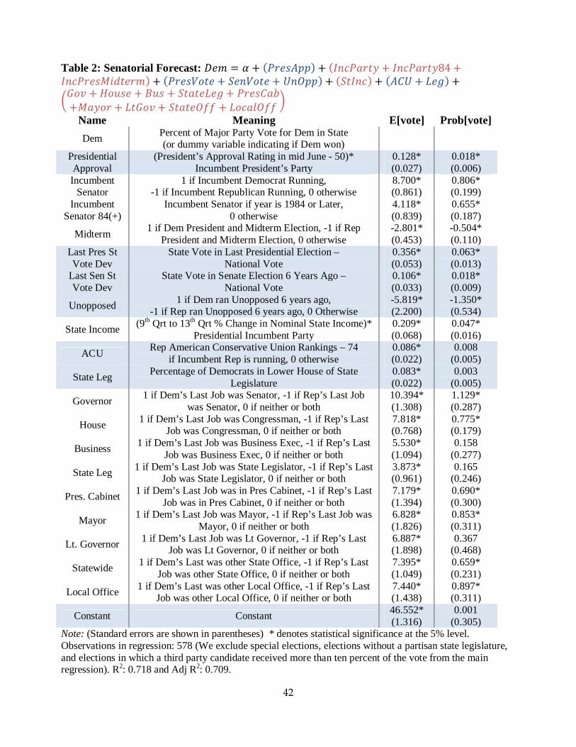
42

Table 2: Senatorial Forecast: =+8 2 Δ ℎ 764+90�� ℎ 7���6�4�� ℎ ���6�4���) ℎ���64+9*+��+48 ℎ 764+9���+ ℎ �+����+ ℎ ��,�� ℎ 7����� ℎ 70�� ℎ !+" ℎ-.�/ ℎ #�%9+ ℎ 0%9 ℎ ����+!+" ℎ 64+9��1ℎ*���4 ℎ !�.�/ ℎ ����+,22 ℎ !����,22 3

Name Meaning E[vote] Prob[vote]

Dem Percent of Major Party Vote for Dem in State (or dummy variable indicating if Dem won)

Presidential Approval

(President’s Approval Rating in mid June - 50)* Incumbent President’s Party

0.128* (0.027)

0.018* (0.006)

Incumbent Senator

1 if Incumbent Democrat Running, -1 if Incumbent Republican Running, 0 otherwise

8.700* (0.861)

0.806* (0.199)

Incumbent Senator 84(+)

Incumbent Senator if year is 1984 or Later, 0 otherwise

4.118* (0.839)

0.655* (0.187)

Midterm 1 if Dem President and Midterm Election, -1 if Rep

President and Midterm Election, 0 otherwise -2.801* (0.453)

-0.504* (0.110)

Last Pres St Vote Dev

State Vote in Last Presidential Election – National Vote

0.356* (0.053)

0.063* (0.013)

Last Sen St Vote Dev

State Vote in Senate Election 6 Years Ago – National Vote

0.106* (0.033)

0.018* (0.009)

Unopposed 1 if Dem ran Unopposed 6 years ago,

-1 if Rep ran Unopposed 6 years ago, 0 Otherwise -5.819* (2.200)

-1.350* (0.534)

State Income (9th Qrt to 13th Qrt % Change in Nominal State Income)*

Presidential Incumbent Party 0.209* (0.068)

0.047* (0.016)

ACU Rep American Conservative Union Rankings – 74

if Incumbent Rep is running, 0 otherwise 0.086* (0.022)

0.008 (0.005)

State Leg Percentage of Democrats in Lower House of State

Legislature 0.083* (0.022)

0.003 (0.005)

Governor 1 if Dem’s Last Job was Senator, -1 if Rep’s Last Job

was Senator, 0 if neither or both 10.394* (1.308)

1.129* (0.287)

House 1 if Dem’s Last Job was Congressman, -1 if Rep’s Last

Job was Congressman, 0 if neither or both 7.818* (0.768)

0.775* (0.179)

Business 1 if Dem’s Last Job was Business Exec, -1 if Rep’s Last

Job was Business Exec, 0 if neither or both 5.530* (1.094)

0.158 (0.277)

State Leg 1 if Dem’s Last Job was State Legislator, -1 if Rep’s Last

Job was State Legislator, 0 if neither or both 3.873* (0.961)

0.165 (0.246)

Pres. Cabinet 1 if Dem’s Last Job was in Pres Cabinet, -1 if Rep’s Last

Job was in Pres Cabinet, 0 if neither or both 7.179* (1.394)

0.690* (0.300)

Mayor 1 if Dem’s Last Job was Mayor, -1 if Rep’s Last Job was

Mayor, 0 if neither or both 6.828* (1.826)

0.853* (0.311)

Lt. Governor 1 if Dem’s Last Job was Lt Governor, -1 if Rep’s Last

Job was Lt Governor, 0 if neither or both 6.887* (1.898)

0.367 (0.468)

Statewide 1 if Dem’s Last was other State Office, -1 if Rep’s Last

Job was other State Office, 0 if neither or both 7.395* (1.049)

0.659* (0.231)

Local Office 1 if Dem’s Last was other Local Office, -1 if Rep’s Last

Job was other Local Office, 0 if neither or both 7.440* (1.438)

0.897* (0.311)

Constant Constant 46.552* (1.316)

0.001 (0.305)

Note: (Standard errors are shown in parentheses) * denotes statistical significance at the 5% level. Observations in regression: 578 (We exclude special elections, elections without a partisan state legislature, and elections in which a third party candidate received more than ten percent of the vote from the main regression). R2: 0.718 and Adj R2: 0.709.

43

Table 3: Gubernatorial Forecasting Model: =+8 2 Δ ℎ 764+90�� ℎ 7���6�4�� ℎ���6�4��4�ℎ ���64+9*+��+48 ℎ 75��+���.=6 ℎ 7!+" ℎ 7*+�6+9� ℎ ��%�&�7 ℎ- �+� ℎ #�%9+ ℎ ����+,22 ℎ 0%9 ℎ ����+!+" ℎ64+9��1 ℎ !����,22 ℎ*���4 ℎ !�.�/ ℎ 5�����.�/3

Name Meaning E[vote] Prob[vote]

Dem Percent of Major Party Vote for Dem in State

(or if Dem won)

Presidential Approval

(President’s Approval Rating in mid March – 50)* Incumbent President’s Party

0.100* (0.031)

0.021* (0.007)

Incumbent Governor

1 if Incumbent Democrat Running, -1 if Incumbent Republican Running, 0 otherwise

11.073* (0.877)

2.251* (0.3544)

Incumbent Gov 92(+)

Incumbent Senator if year is 1992 or Later, 0 otherwise

3.467* (0.959)

0.633* (0.237)

Midterm 1 if Dem President and Midterm Election, -1 if Rep

President and Midterm Election, 0 otherwise -2.601* (0.499)

-0.299* (0.114)

GDP (2nd Quarter % Change in National Real GDP – 3.3)*

Incumbent President’s Party 0.194* (0.085)

0.033 (0.019)

State Leg Percentage of Democrats in Lower House of State

Legislature 0.120* (0.022)

0.012* (0.005)

Midwest 1 if Midwestern State -2.264* (0.863)

-0.481* (0.197)

South 80(-) 1 if Southern State and 1980 or earlier 4.974* (2.337)

-0.363 (0.483)

Senator Experience

1 if Dem’s Last Job was Senator, -1 if Rep’s Last Job was Senator, 0 if neither or both

9.435* (2.777)

2.235* (0.684)

House Experience

1 if Dem’s Last Job was Congressman, -1 if Rep’s Last Job was Congressman, 0 if neither or both

7.177* (1.252)

1.921* (0.381)

Business Experience

1 if Dem’s Last Job was Business Exec, -1 if Rep’s Last Job was Business Exec, 0 if neither or both

6.609* (1.139)

1.811* (0.370)

State Leg Experience

1 if Dem’s Last Job was State Legislator, -1 if Rep’s Last Job was State Legislator, 0 if neither or both

4.616* (1.054)

1.529* (0.364)

Pres Cabinet Experience

1 if Dem’s Last Job was in Pres Cabinet, -1 if Rep’s Last Job was in Pres Cabinet, 0 if neither or both

9.459* (1.779)

2.382* (0.459)

Mayor Experience

1 if Dem’s Last Job was Mayor, -1 if Rep’s Last Job was Mayor, 0 if neither or both

6.651* (1.473)

1.502* (0.416)

Lt Governor Experience

1 if Dem’s Last Job was Lt Governor, -1 if Rep’s Last Job was Lt Governor, 0 if neither or both

4.832* (1.232)

1.283* (0.369)

Governor Experience

1 if Dem’s Last was non-inc Governor, -1 if Rep’s Last Job was non-inc Governor, 0 if neither or both

5.996* (1.860)

1.992* (0.497)

Statewide Experience

1 if Dem’s Last was other State Office, -1 if Rep’s Last Job was other State Office, 0 if neither or both

6.923* (1.052)

1.839* (0.351)

Local Office Experience

1 if Dem’s Last was other Local Office, -1 if Rep’s Last Job was other Local Office, 0 if neither or both

5.204* (1.498)

1.912* (0.423)

Constant Constant 44.139* (1.301)

-0.541 (0.310)

Note: (Standard errors are shown in parentheses) * denotes statistical significance at the 5% level. Observations in regression: 378 (We exclude elections that took place on an odd year, elections without a partisan state legislature, and elections in which a third party candidate received more than ten percent of the vote from the main regression. However, we do also illustrate how this method would have performed at forecasting elections in which the third party candidate received more than ten percent of the vote). R2: 0.620 and Adj R2: 0.601.

44

Appendix 1: Third Par ties

In the 1968 presidential election George Wallace is widely thought to have taken more votes from the Republican candidate Richard Nixon than he did from the Democratic candidate Hubert Humphrey (Kiewiet 1979; Mayer 2002). However, Wallace had a different impact on different states. While the vast majority of Wallace supporters in the South preferred Nixon over Humphrey, roughly equal percentages of Wallace supporters preferred each of the major party candidates in states in other regions (Mayer 2002). Thus, we expect the fraction of the major party vote received by each candidate in the 1968 election to be unrepresentative of the fraction of the major party vote each candidate would receive in the 1972 election in states in the South but not for other states. To take into account how Wallace would impact our forecasting model for the Electoral College, we therefore include a variable that is defined to be the percentage of the vote received by George Wallace in the state in the 1968 presidential election if the state is a Southern state and the year is 1972.

For the other third party presidential candidates we consider, we have no reason to believe that voters who voted for the third party candidate in one state would have preferred one major party candidate over the other with greater frequency than voters who voted for the third party candidate in other states. However, if voters who voted for that third party tended to prefer one major party candidate over the other, then those third party votes will distort the vote share for those years. For this reason, we include a variable for 2000 that is the percentage of the vote received by Ross Perot in the state in the 1996 presidential election minus his national average in 1996. We include the same variable for John Anderson in 1984 for his 1980 challenge.

We also investigated whether including a similar such variable for the fraction of the vote received by Perot in the 1992 presidential election would improve the fit of the model, but found that including such a variable was not statistically significant.22 This may be a reflection of the fact that there is mixed evidence about whether Ross Perot took more votes from the Democratic candidate Bill Clinton or the Republican candidate George H.W. Bush during the 1992 presidential election. Alvarez and Nagler (1995) finds evidence that Perot took more votes from Bush during this election, while Lacy and Burden (1999) finds evidence that Perot took more votes from Clinton than from Bush in the 1992 presidential election, and Abrams and Butkiewicz (1995) and Haynes and Stone (1994) indicate that Perot took votes evenly from Bush and Clinton. This mixed evidence suggests that Perot may not have significantly altered the fraction of the major party vote received by each of the major party candidates, in which case there would be no reason to expect that including a variable representing Perot’s vote share in the 1992 presidential election would improve the fit of our forecasting model.

22 This is noted in Table A1 in the supplementary appendix.