1

The Fundamental Law of Active Management: Time Series Dynamics and Cross-Sectional Properties

Zhuanxin Ding, Ph.D.

Portfolio Manager and Head of Quantitative Strategies

Fuller & Thaler Asset Management

411 Borel Ave, Suite 300

San Mateo, CA 94402

650-931-1507

zding@fullerthaler.com

First Draft October 15, 2009

Revised Feb 24, 2010

ABSTRACT

I derive a generalized version of the fundamental law of active management under

some weak conditions. I show that the original fundamental law of Grinold and

various extensions are all special cases of the generalized fundamental law

presented in this paper. I also show that cross-sectional ICs are usually different

from time series ICs even if the time series ICs are all the same across securities.

The fundamental law derived in this paper is quite robust to forecast model

specification. Our results show that the variation in IC (IC volatility over time)

has a much bigger impact to portfolio IR than the breadth N for a typical

investment universe. I extend the fundamental law to models with multiple factors

and study the impact of missing one or more return or risk factors to portfolio IR.

Our results also show that the transfer coefficient as originally defined by Clarke

et al. (2002) is not able to capture the impact of constraints to portfolio IR in the

presence of IC variation. I redefine the concept of transfer coefficient using the

cross-sectional correlation between the total conditional covariance adjusted

active weights and alphas so that the resulting transfer coefficient has the desired

property.

Since the publication of "The fundamental law of active management" by Grinold (1989)

two decades ago, it has been widely used in the quantitative investment community as a

tool to assess a portfolio manager's ability to add value. According to Grinold (1989), the

fundamental law relates three variables: your skill in forecasting exceptional returns (IC),

the breadth of your strategy (N), and the value added of your investment strategy (IR).

Grinold (1989) claims that "based on assumptions that are not quite true and simplified

with some reasonable approximations" the three variables have the following

relationship:

NICIR = , (1)

where IR is the information ratio, IC is the information coefficient, and N is the breadth.

Even though Grinold (1989) did not give a precise definition of breadth N, portfolio

2

managers or analysts usually use the number of stocks in the investment universe as

breadth. The derivation of the fundamental law is closely related to another Grinold paper

(Grinold (1994)) that shows "Alpha is Volatility Times IC Times Score", i.e.,

1IC −= itrit zi

σα , (2)

whereir

σ is the residual return (will be defined below) volatility and 1−itz is the

standardized forecast signal (score) that is known at the end of time t-1. The theoretical

and empirical development on this line of the fundamental law culminated in the book by

Grinold and Kahn (2000) titled "Active Portfolio Management." Based on the

fundamental law, Grinold and Kahn (2000) conclude that "you (portfolio managers) must

play often and play well to win at the investment management game. It takes only a

modest amount of skill to win as long as that skill is deployed frequently and across a

large number of stocks."

Unfortunately, the theoretically calculated IR number from Grinold's fundamental law

seems to always overestimate the IR a portfolio manager can reach. For example, given a

forecast signal with a monthly average IC of 0.03 and a selection universe of 1000 stocks,

the expected annualized IR from Grinold's formula is 3.29 which is beyond even the most

optimistic portfolio manager's dreams. Portfolio managers are left wondering why

realized information ratios are only a fraction of their predicted value. Clarke et al. (2002,

p50) point out "a common rule of thumb in practice is that the theoretical information

ratio suggested by the fundamental law should be cut in half." However, for the above

mentioned example, the IR estimate will still be too high even if cut by half (IR=1.64).

As noted by Grinold (1989, p32) himself "an observed information ratio above 1.5 is rare

indeed." Of course, it can be the case that the N used in our calculation, which is the

number of stocks available in the investment universe, is not what meant to be the right

measure of breadth by Grinold. Grinold (1989) provides a detailed discussion on this

subject and emphasized the importance of counting only independent bets as breadth.

Grinold (2007) provides some further discussion on this topic. Unfortunately, it is still

not a straightforward exercise to determine what breadth should be used in practice.

Clarke et al. (2002) attribute the reduction in performance to the constraints in the

portfolio construction process and proposed the concept of "the transfer coefficient" to

account for the leaking of IR from Grinold's original formula. They show that constraints

in portfolio construction (constraints such as country or sector exposures, long only, etc.),

leads to suboptimal portfolio weights in terms of alpha generation, thus reducing the

maximum achievable IR. They developed a framework for measuring the deviation of the

optimal constrained weights from optimal non-constrained weights and proposed a

generalized fundamental law as follows:

NICTCIR = , (3)

where TC is the transfer coefficient, defined as the cross-sectional correlation coefficient

between risk-adjusted expected residual returns and risk-adjusted active weights.

According to their simulation study, the typical transfer coefficient is in the range of 0.3

to 0.8. So the original IR calculated from Grinold's formula should be about halved. Even

so, as discussed above, the TC adjusted IR still appears to be too high.

3

In order to understand why that happens, we need to examine the assumptions made by

Grinold in deriving his fundamental law. The original form of the fundamental law by

Grinold is based on the very unrealistic assumption that time series ICs between an

individual stock's residual return and its forecast signal are the same across all securities

and are a constant over time. Grinold (1989, 1994) and Grinold and Kahn (2000) then

used the time series IC and cross-sectional IC interchangeably. In practice, many

quantitative managers run a Fama-Mcbeth type cross-sectional regression to get realized

ICs at different time periods. The ICs calculated this way are far from constant and often

fluctuate around an average IC. As will be shown later in this paper, the cross-sectional

IC can be quite different from the time series IC even if all the securities have a same

time series IC. Qian and Hua (2004) show that a more appropriate IR to use is average IC

divided by the standard deviation of IC

IC

ICIR

σ= , (4)

where ICσ is the standard deviation of IC that Qian and Hua (2004) call "the strategy

risk." In statistics, the quantity 2

IC/1 σ is a measure of how close (precise) the realized

information coefficient at time t, tIC , is to the mean IC. In this sense, the Qian and Hua

formula states that "Information Ratio equals Skill times Precision."

In a more recent paper, Ye (2008) goes one step further to bridge the gap between the

original Grinold (1989) formula and the Qian and Hua (2004) formula. Based on her

assumptions, she establishes that

2

IC/1

ICIR

σ+=

N. (5)

It is obvious that Equation (1) and Equation (4) are special cases of Equation (5) when

0IC =σ (as assumed by Grinold (1989)) or ∞→N .

With all these different versions of fundamental laws, it can be confusing for practitioners

to decide which one to use. It is crucial to have a full grasp of the different underlying

assumptions and the resulting conclusions from these fundamental laws. In this paper, I

try to set up a coherent econometric modeling structure and show that all the different

forms of fundamental laws discussed above can be special cases of an even more general

form of fundamental law based on much weaker assumptions. I will show that time series

ICs are usually different from cross-sectional ICs even if time series ICs are the same

across all individual securities. They will be the same only under some strong conditions.

I will also show that different forms of fundamental laws are a result of either unrealistic

assumptions (Grinold (1989)) or mis-specified residual return covariance matrices for the

expected residual return used (Grinold (1989), Qian and Hua (2004), and Ye(2008)).

When the more relevant conditional residual return covariance matrices are used, we will

arrive at the more general form of the fundamental law presented in this paper.

The form of the generalized fundamental law derived in this paper is quite robust to

model specification. If one uses the risk adjusted residual returns in the analysis instead

of the raw residual returns, one will get the fundamental law in a similar form. Finally I

4

extend the fundamental law to models with more than one factor, and discuss the impact

of missing one or more return or risk factors to the portfolio IR. I also show that the

transfer coefficient as defined by Clarke et al. (2002) will not have the desired property

of measuring the impact of constraints to the portfolio IR in the presence of IC variation.

I redefine the transfer coefficient as the correlation coefficient between total risk adjusted

expected residual returns and total risk adjusted active weights (instead of just the

diagonal portion of the covariance matrix). With this modified definition of the transfer

coefficient, the resulting constrained portfolio IR is always the product of TC and the

unconstrained optimal portfolio IR.

Framework and Notation I will follow the framework and notation in Clarke, de Silva, and Thorley (2002) and Ye

(2008). A variable with subscript i ( N1 ,,L=i ) and t ( T,,1 L=t ) represents the variable

value for security i at the end of time t. A variable in bold represents a vector or matrix.

Given a benchmark portfolio, the total excess return (i.e., return in excess of the risk-free

rate) on any stock i can be decomposed into a systematic portion that is correlated with

the benchmark excess return and a residual return that is not by

,, ittBit

Total

it rRr += β (6)

where

itβ = beta of security i with respect to the benchmark

tBR , = benchmark excess return

itr = realized residual return

The benchmark and the actively managed portfolios are defined by the weights,

itBw , and itPw , , assigned to each of the N stocks in the investable universe respectively. It

is shown in Clarke et al. (2002) that the portfolio active return, which is defined as the

managed portfolio total excess return minus the benchmark total excess return, adjusted

for the managed portfolio's beta with respect to the benchmark, can be written as

,11

,,,,, ∑∑==

∆==−=N

i

itit

N

i

ititPtBtPtPtA rwrwRRR β (7)

where itw∆ is the active weight defined as the difference between the managed portfolio

weight and the benchmark weight at the beginning of time period t. 1 Note that the active

weights, itw∆ , sum to 0 because they are differences in two sets of weights that each sum

to 1. Also note that the stock returns, itr , in (7) are residual, not total, excess returns. As

pointed out in Clarke, et al. (2002), residuals are the relevant component of security

returns when performance is measured against a benchmark on a beta-adjusted basis.

We assume that residual returns follow a conditional normal distribution, and define ex

ante alpha of security i ( N1 ,,L=i ) in period t as the expected residual return

conditional on information available at the end of time period 1I:1 −− tt

)I|( 1−= ttt E rα , (8)

5

and we define risk related to the alpha expectation as the conditional covariance of the

forecast errors

]I|)')([( 1−−−= tttttt E αrαrΩ , (9)

where tα and tr are 1×N vectors with itα and itr as their elements respectively. The

assumption of asset return normality is one of the fundamental assumptions under

Markowitz's mean-variance portfolio choice theory, and the mean and covariance matrix

fully determine a multivariate normal distribution. Under the residual return normality

assumption, the covariance of the forecast errors is the relevant measure of risk. There is

risk because there is uncertainty, and risk is associated to the part of return that we are not

able to predict. If we know the future returns perfectly then there is no uncertainty, hence

no risk. The conditional risk associated with our alpha estimate should be smaller than

the total risk around the unconditional alpha expectation. If this is not the case, then the

forecast provides no additional information and the lagged information set, 1I −t , is

useless. This is the major difference between the risk model used in this paper and the

risk models used in Grinold (1989, 1994), Grinold and Kahn (2000), Clarke et al. (2002),

Qian and Hua (2004), and Ye (2008). Of course, the assumption of stock return normality

may not be valid in practice, and the return and risk models one uses are very likely mis-

specified, which may cause theoretically derived results not to reflect what one gets in

reality. I will give some discussion later on the impact of missing alpha or risk factors in

conditional mean and covariance modeling.

After having specified the conditional mean and covariance matrix, we will then use the

mean-variance analysis tool for portfolio construction based on the theory of utility

maximization. In each period t, the optimal market-neutral portfolio, tP , is selected to

maximize the mean-variance utility function:

0'..

'2

1'

2

1 2

=∆

∆∆−∆=−=∆

1w

wΩwαww

t

tttttPtPtt

ts

UMaxt

λλσα, (10)

where

=Ptα expected active return on the portfolio

=2

Ptσ active risk of the portfolio based on the portfolio holdings

=λ a risk-aversion parameter

=1 1×N vector of 1s

The solution for this optimization problem is

)(1 11

1ΩαΩw−− −=∆ tttt κ

λ, (11)

where 1Ω1

1Ωα

1

1

'

'−

−

=t

ttκ is a scalar.

A certain value of λ corresponds to a certain value of Ptσ since

2' Ptttt σ=∆∆ wΩw . (12)

Substituting (11) into (12) and by some straightforward algebra we have

6

ttttt

Pt

αΩ1αΩα11 ''

1 −− −= κσ

λ . (13)

The optimal portfolio active weight is then

,)('

)(

1

1

1αΩα

1αΩw

κ

κσ

−

−=∆

−

−

ttt

ttPtt (14)

and the expected portfolio return

.)('

'

11αΩα

αw

κσ

α

−=

∆=

−tttPt

ttPt

(15)

If we assume that the target tracking error remains a constant ( PPt σσ = ) at each

rebalance of the portfolio, a typical practice for many quantitative portfolio managers,

then the ex ante expected information ratio of the portfolio is

( ).)('

)('1

1IR

1

1

1

1

1αΩα

1αΩα

κ

κ

σ

α

σ

α

−=

−=

==

−

=

−

=

∑

∑

ttt

T

t

ttt

T

t P

Pt

P

Pt

E

T

T

(16)

This is a very general result that should hold as long as the residual return has a

conditional normal distribution with mean tα and covariance matrix tΩ .

From the above discussion, it is clear that the key is how to forecast the alpha and the

corresponding covariance matrix. As Kahn (1997) points out "active management is

forecasting." Different forecasts will give us different ex ante expected information

ratios. In the literature, two different approaches are used to forecast alpha. One uses time

series models and the other uses a Fama-McBeth type cross-sectional regression

approach. As for covariance matrix, many people use a risk model that does not have a

direct relationship with the alpha estimation, such as the commercial risk models by

BARRA or Northfield. Strictly speaking, a risk model that is detached from the alpha

model will be a mis-specified risk model for the reasons discussed above. This mis-

specification usually results in the underestimation of risk when one runs an actual

portfolio because the very important "strategy risk" is being left out (see Qian and Hua

(2004), Qian, Hua, and Sorensen (2007)).

Time Series Dynamics In the original papers about the fundamental law, Grinold (1989, 1994) concluded that

"alpha is volatility times IC times score" without providing the explicit model

assumptions and technical derivations of his result. In the endnote of his first paper

(1989) he did mention that technical details are available upon request. Detailed

discussions were given instead in Chapters 10 and 11 of the book by Grinold and Kahn

(2000). Unfortunately, even though their Equation (10.1) is assumed to be for a cross

section of N assets, the result in (10.16) is derived through a time series model for each of

the N individual assets. They then use the time series IC and cross-sectional IC

7

interchangeably. The discussion below will show that the result from time series

modeling assumptions cannot be applied to cross-sectional modeling structures without

some further assumptions.

If we assume that the true forecasting relationship between the lagged information set,

1I −t , and the residual returns, itr , is a linear one factor model as follows

ititiit zgr ε+= −1 (17)

for security i over time t = 1, 2, 3, ..., T. In the equation, ig is the time series factor

return ( ig is just a regression coefficient and is different from the usual definition of

factor return from a cross-sectional regression) for security i, 1−itz is the factor exposure

that becomes known at the end of time t-1 that has both time series and cross-sectional

mean 0 and standard deviation 1 (as assumed by Grinold and Kahn (2000), p268),

),(~20

iNit εσε is the idiosyncratic noise that cannot be predicted. We further assume

T1) 01 =− )( ititzE ε for all i and t,

and

T2) 0=)( jtitE εε for ji ≠ .

T1) is a very general assumption for linear regression models stating that the explanatory

variable and the residual are not correlated, and T2) assumes that the forecast errors are

not correlated across stocks so that the idiosyncratic covariance matrix is diagonal. This

is also a common assumption for idiosyncratic noise.

For ease of exposition, we will focus our attention on population quantity and ignore the

sample estimation error of the parameters. Basic regression of Equation (17) gives us,

ii zrits

i

i

ii

ii

iiii

z

r

rz

rz

rzzg

σσ /IC

)Var(

)Var(

)Var()Var(

),Cov(

),Cov()(Var

,

1

=

=

= −

, (18)

where its ,IC is the time series correlation between residual return itr and forecast

signal 1−itz , ir

σ is the standard deviation (volatility) of residual return itr , andizσ is the

standard deviation (volatility) of 1−itz which is 1 by assumption. The time series prediction

for alpha from this model is

11 IC −− == itritstitit zIrEi

σα ,)|( , (19)

and the conditional volatility, or forecast error volatility, is

22

,1

2 )IC1()|Var(ii ritstit Ir σσ ε −== − . (20)

It should be noted here that iir εσσ ≠ when 0IC ≠its , . As we discussed above for

Equation (9), when the forecast signal 1−itz contains useful information for predicting

residual return itr , then the resulting error variance ( 2

iεσ ) should be smaller than the

original unconditional residual return variance ( 2

irσ ). This is the major difference

8

between the risk estimate here and the risk estimate provided by any commercial risk

model which has no connection with alpha estimation.

Substituting the alpha and volatility prediction into Equation (16) we have the ex ante

expected information ratio as

( )

.)IC1(

IC

IC1

IC

)('IR

12

,

1,

12

,

2

1

2

,

1

−−

−=

−=

∑∑=

−

=

−

−

N

i rits

ititsN

i its

itits

ttt

i

zzE

E

σκ

κ1αΩα

(21)

If we assume that the cross-sectional distribution of its ,IC and 1−itz are independent, then as

N becomes large, we have

,IC1

IC

)IC1(

IC

IC1

IC

)IC1(

IC

IC1

ICIR

12

,

2

,

12

,

,2

12

,

2

,

2

,

1,

2

,

2

1

2

,

∑=

−−

−−

−=

−−

−=

−−

−=

N

i its

its

itcs

rits

its

csitcs

its

its

cs

rits

itits

cs

its

itits

cs

zEENzEENE

zEN

zENE

i

i

σκ

σκ

(22)

where csE stands for the cross-sectional expectation operator. In deriving Equation (22)

we used the assumption that the forecast signal, 1−itz , is cross-sectionally normalized to

have mean 0 and standard deviation 1. When all the time series ICs are the same, i.e.

tsits ICIC =, for all i, we have

NN ts

ts

ts ICIC1

ICIR

2≈

−= . (23)

The approximation holds when tsIC is small which is typically the case in empirical work.

Equation (23) proved that the original fundamental law of Grinold (1989) holds

approximately under the time series model assumption when ICs are the same across all

the assets and is small. The reason that the original formula of Grinold (1989) needs to be

adjusted by 2IC1 ts− is that we used the conditional volatility of the residual return

instead of the unconditional one. Some interesting observations can be made from

Equations (22) and (23). When one has the skill to predict some residual returns perfectly

(some 1IC =its , ) then the IR shall go to infinity no matter what the breadth is. This makes

intuitive sense because if one can predict some residual returns perfectly then she/he can

make a sure bet on these stocks against the rest of the universe to achieve the desired

excess return. The IR will be infinity since the optimization is set in such a way that one

can take a leveraged bet. This is not a feature in the original Grinold formula which states

that the IR will increase with the square root of N even if 1IC =ts .

9

If, instead of running a time series regression, we run a "mis-specified" cross-sectional

regression for the model in Equation (17),

itittit zfr ξ+= −1 (24)

for cross-sectional security i = 1, 2 ,..., N at time t. A simple cross-sectional regression

gives us

,)(IC

)(/)(IC

)(

)(

)()(

)(

)(/)(

,

1,

2

1,

2

,

2

1,

2

,

1,

2

1,1,

ttcs

tttcs

ittcs

ittcs

ittcsittcs

itittcs

ittcsitittcst

d

dd

zE

rE

zErE

zrE

zEzrEf

r

zr

=

=

=

=

−

−−

−

−−

(25)

where tcsE , stands for the cross-sectional expectation operator at time t, tcs ,IC is the

cross-sectional correlation between residual return itr and forecast signal 1−itz , )( 1−td z is

the cross-sectional standard deviation (dispersion) 2 of 1−itz , which is 1 by assumption,

and )( td r is the cross-sectional residual return dispersion at time t.

The expected value of tf is

.IC1

1)(

)))(((

))(())(()(

1

,

1

,

11,

1,1,

∑

∑

=

=

−−

−−

=

==

+=

===

N

i

rits

N

i

iitcs

ititititcs

itittcsitittcst

iN

gN

gE

zzgEE

zrEEzrEEfEf

σ

ε

(26)

On the other hand, if we assume tcs ,IC and )( td r are independent over t, then from

Equation (25) we have

,IC

))(()IC(

))(IC(

)(

,

,

δcs

ttcs

ttcs

t

dEE

dE

fEf

=

=

=

=

r

r (27)

where ))(( tdE r=δ is the expected cross-sectional residual return dispersion.

Substituting (26) into (27) we have

∑=

=N

i

ritscs iN 1

, /IC1

IC δσ , (28)

i.e., the expected cross-sectional IC, csIC , is a weighted average of time series ICs and

they are usually not the same. If the time series ICs are the same across all securities,

i.e., tsits ICIC =, for all i then

10

δσδσ /~IC/1

ICIC1

rts

N

i

rtscs iN== ∑

=

, (29)

where ∑=

=N

i

rr iN 1

1σσ~ is the cross-sectional average of the residual return standard

deviation. So as long as δσ ≠r~ , we have the seemly surprising result that the cross-

sectional csIC will be different from the time series tsIC even if the time series ICs are the

same across all securities.

In the extreme case that all residual return standard deviations are the same, i.e. rriσσ =

for all i, we have δσσ == rr~ and tscs ICIC = .

3 So the discussion here shows that the

cross-sectional IC is usually different from the time series IC for an identical set of return

and factor exposures. They will only be the same under the very strong assumption that

the residual return volatilities are the same across all securities.

Given the "mis-specified" cross-sectional model prediction for each individual security,

itrtsitcsit zz σδα ~ICIC == , (30)

we have the forecast error term as

ititrrtsititcsitrtsit zzzii

εσσεδσξ +−=+−= )~(ICICIC , (31)

which is different from itε . The conditional covariance matrix has the following elements:

≠

=−+−=

=

ji

ji

E

ii rtsrrts

jtitij

when0

when)IC1()~(IC

)(

2222 σσσ

ξξω

(32)

Substituting (32) into (16) we have

.)()~(

~~

−+−

−= ∑

=

N

i rtsrrts

itrtsitrts

ii

zzE

12222

222

IC1IC

ICICIR

σσσ

σκσ (33)

If we assume that the cross-sectional distribution ofir

σ and itz are independent, then as N

becomes large, we have

.)~/)(()~/(

∑= −+−

=N

i rrtsrrts

ts

ii1

2222 IC11IC

1ICIR

σσσσ (34)

When all the residual return volatilities are the same we have

NN ts

ts

ts ICIC1

ICIR

2≈

−= , (35)

which is consistent with the result from time series model. When the individual residual

return standard deviation varies across securities, the IR we get from the mis-specified

cross-sectional model will be different from the IR we get from the time series model.

The discussion above shows that the original fundamental law of Grinold (1989, 1994)

only holds under the assumption that the time series ICs are the same across all the

securities and the common IC is small. The cross-sectional IC is only the same as the

11

time series IC if an additional assumption is imposed that all residual return standard

deviations are the same (Ye (2008) made this assumption).

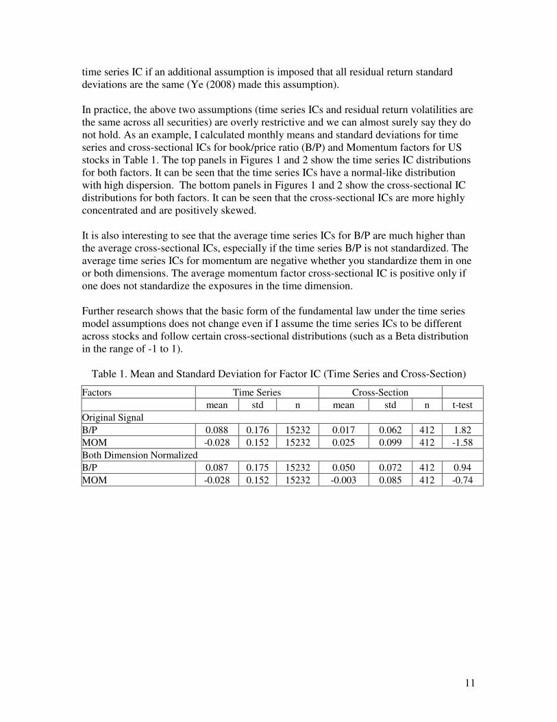
In practice, the above two assumptions (time series ICs and residual return volatilities are

the same across all securities) are overly restrictive and we can almost surely say they do

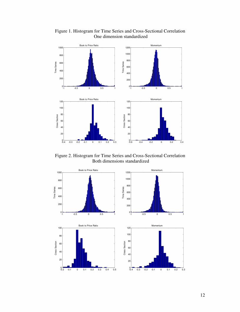
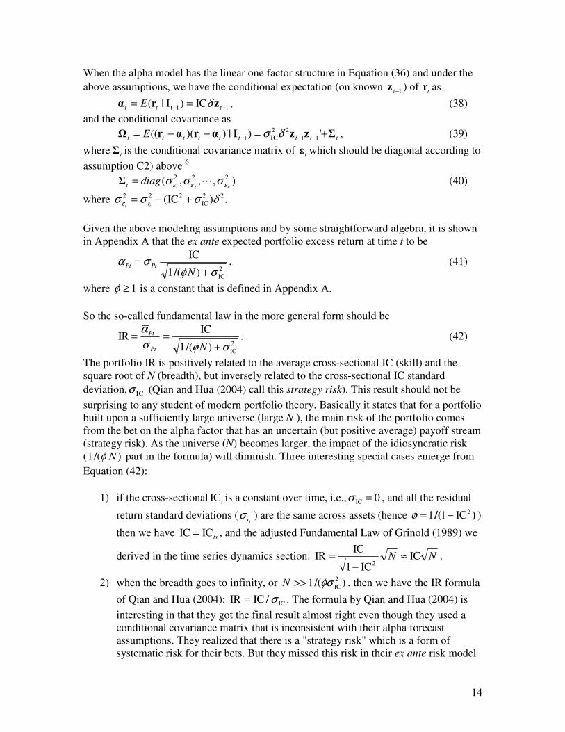
not hold. As an example, I calculated monthly means and standard deviations for time

series and cross-sectional ICs for book/price ratio (B/P) and Momentum factors for US

stocks in Table 1. The top panels in Figures 1 and 2 show the time series IC distributions

for both factors. It can be seen that the time series ICs have a normal-like distribution

with high dispersion. The bottom panels in Figures 1 and 2 show the cross-sectional IC

distributions for both factors. It can be seen that the cross-sectional ICs are more highly

concentrated and are positively skewed.

It is also interesting to see that the average time series ICs for B/P are much higher than

the average cross-sectional ICs, especially if the time series B/P is not standardized. The

average time series ICs for momentum are negative whether you standardize them in one

or both dimensions. The average momentum factor cross-sectional IC is positive only if

one does not standardize the exposures in the time dimension.

Further research shows that the basic form of the fundamental law under the time series

model assumptions does not change even if I assume the time series ICs to be different

across stocks and follow certain cross-sectional distributions (such as a Beta distribution

in the range of -1 to 1).

Table 1. Mean and Standard Deviation for Factor IC (Time Series and Cross-Section)

Factors Time Series Cross-Section

mean std n mean std n t-test

Original Signal

B/P 0.088 0.176 15232 0.017 0.062 412 1.82

MOM -0.028 0.152 15232 0.025 0.099 412 -1.58

Both Dimension Normalized

B/P 0.087 0.175 15232 0.050 0.072 412 0.94

MOM -0.028 0.152 15232 -0.003 0.085 412 -0.74

12

Figure 1. Histogram for Time Series and Cross-Sectional Correlation

One dimension standardized

-1 -0.5 0 0.5 10

200

400

600

800

1000

Tim

e S

eries

Book to Price Ratio

-1 -0.5 0 0.5 10

200

400

600

800

1000

1200

Tim

e S

eries

Momentum

-0.4 -0.3 -0.2 -0.1 0 0.1 0.2 0.30

20

40

60

80

100

120

Cro

ss S

ection

Book to Price Ratio

-0.6 -0.4 -0.2 0 0.2 0.40

20

40

60

80

100

120

Cro

ss S

ection

Momentum

Figure 2. Histogram for Time Series and Cross-Sectional Correlation

Both dimensions standardized

-1 -0.5 0 0.5 10

200

400

600

800

1000Book to Price Ratio

Tim

e S

eries

-1 -0.5 0 0.5 10

200

400

600

800

1000

1200Momentum

Tim

e S

eries

-0.2 -0.1 0 0.1 0.2 0.3 0.4 0.50

20

40

60

80

100Book to Price Ratio

Cro

ss S

ection

-0.4 -0.3 -0.2 -0.1 0 0.1 0.2 0.30

20

40

60

80

100

120Momentum

Cro

ss S

ection

13

Cross-Sectional Properties The above discussion shows the assumption that all time series ICs are the same is not

realistic. I will show below it is also not necessary in deriving the (generalized)

fundamental law. In empirical finance work, many people use a Fama-McBeth type

cross-sectional regression in relating the explanatory variables with asset returns.

Ibragimov and Müller (2009) find that as long as the cross-sectional coefficient

estimators are approximately normal (or scale mixtures of normals) and independent, the

Fama-MacBeth method results in valid inference even for a short panel that is

heterogeneous over time. Due to the small sample conservativeness result, the approach

allows for unknown and unmodelled heterogeneity. Peterson (2009) shows that when the

residuals of a given time period are correlated across firms, the Fama-McBeth method

produces more efficient estimates than OLS and the standard error will be correct.

Another advantage is that the assumptions we have to make to achieve the kind of

fundamental law are much weaker than the assumptions we have to make in the time

series section.

Assume the basic modeling structures are similar to Equation (17), only this time we

have the relationship at time t for i = 1, 2, 3, ..., N assets,

itittit zfr ε+= −1 (36)

where tf is the cross-sectional factor return at time t, 1−itz is the factor exposure that

becomes known at the end of time t-1 that has both time series and cross-sectional mean

0 and standard deviation 1, ),(~20

iNit εσε is the idiosyncratic noise that cannot be

predicted. We will make the same assumptions as in time series model concerning

1−itz and itε :

C1) 0)( 1 =− ititzE ε for all i and t,

and

C2) 0=)( jtitE εε for ji ≠ .

Under the above assumptions, we have,

)(IC ttt df r= , (37)

where )( td r is the cross-sectional residual return dispersion assumed to be a constant (δ )

over time,4 and tIC is the cross-sectional IC (all the ICs discussed in this section will be

cross-sectional IC unless otherwise specified) between the residual returns and the

forecast signals. In empirical work, one needs to get an ex ante estimate for the cross-

sectional correlation tIC before making an estimate for the alpha. The most common and

simple method just uses historical average as an estimate. After the fact we can estimate

the ex post realized tIC using the actual itr and 1−itz . As shown in the bottom panels of

Figures 1 and 2, usually the cross-sectional factor IC spreads around a mean. For ease of

exposition below, we will assume that the cross-sectional factor tIC follows a normal

distribution with mean IC and standard deviation ICσ . 5

14

When the alpha model has the linear one factor structure in Equation (36) and under the

above assumptions, we have the conditional expectation (on known 1−tz ) of tr as

11t IC)I|( −− == ttt E zrα δ , (38)

and the conditional covariance as

ttttttttt E ΣzzIαrαrΩ IC +=−−= −−− ')|)')((( 11

22

1 δσ , (39)

where tΣ is the conditional covariance matrix of tε which should be diagonal according to

assumption C2) above 6

),,,( 222

21 ndiagt εεε σσσ L=Σ (40)

where .)IC( 22

IC

222 δσσσ ε +−=ii r

Given the above modeling assumptions and by some straightforward algebra, it is shown

in Appendix A that the ex ante expected portfolio excess return at time t to be

,)/(1

IC

2

ICσφσα

+=

NPtPt (41)

where 1≥φ is a constant that is defined in Appendix A.

So the so-called fundamental law in the more general form should be

.)/(1

ICIR

2

ICσφσ

α

+==

NPt

Pt (42)

The portfolio IR is positively related to the average cross-sectional IC (skill) and the

square root of N (breadth), but inversely related to the cross-sectional IC standard

deviation, ICσ (Qian and Hua (2004) call this strategy risk). This result should not be

surprising to any student of modern portfolio theory. Basically it states that for a portfolio

built upon a sufficiently large universe (large N ), the main risk of the portfolio comes

from the bet on the alpha factor that has an uncertain (but positive average) payoff stream

(strategy risk). As the universe (N) becomes larger, the impact of the idiosyncratic risk

( )/(1 Nφ part in the formula) will diminish. Three interesting special cases emerge from

Equation (42):

1) if the cross-sectional tIC is a constant over time, i.e., 0IC =σ , and all the residual

return standard deviations (ir

σ ) are the same across assets (hence )/(2IC11 −=φ )

then we have tsICIC = , and the adjusted Fundamental Law of Grinold (1989) we

derived in the time series dynamics section: NN ICIC1

ICIR

2≈

−= .

2) when the breadth goes to infinity, or )/(1 2

ICφσ>>N , then we have the IR formula

of Qian and Hua (2004): IC/ICIR σ= . The formula by Qian and Hua (2004) is

interesting in that they got the final result almost right even though they used a

conditional covariance matrix that is inconsistent with their alpha forecast

assumptions. They realized that there is a "strategy risk" which is a form of

systematic risk for their bets. But they missed this risk in their ex ante risk model

15

because they used a third party risk model that is detached from their alpha

model. This is common to all quantitative strategies that use a third party risk

model. Lee and Stefek (2008) give a very good discussion on this topic. The ex

post realized portfolio risk is mainly from the "strategy risk" that cannot be

diversified away by the optimal portfolio. That is why their ex ante target tracking

error is so different from the ex post tracking error they derived.

3) if all the residual return standard deviations (ir

σ ) are the same at time t but the IC

volatility is not zero (hence )IC1/(1 2

IC

2 σφ −−= ), then we have approximately

the IR formula of Ye (2008) 2

IC

2

IC

2

IC

2 /1

IC

/)IC1(

ICIR

σσσ +≈

+−−=

NN

(empirically factor IC is in the range of 0.02 to 0.05 and IC standard deviation is

around 0.1). The approximation results from Ye (2008) using the unconditional

residual return standard deviation in her risk model instead of the conditional

idiosyncratic error standard deviation that is consistent with the alpha model. In

this formula we will also have the property that IR will go to infinity when IC=1

and 0IC =σ no matter what the breadth (N) is, while Ye's original formula does

not have this feature.

It should be noted that the ex ante and ex post IR calculation should be very close if the

return and risk models are correctly specified (which is a strong assumption!). The

difference between the ex ante and ex post IR should be a result of standard error in

parameter estimation. As the sample size gets bigger, the difference should get smaller. If

this is not the case, then we can be quite sure that the ex ante model specification is

incorrect. Since we ignored the sample estimation error in this paper, we should expect

the ex ante and ex post IR to be the same when the model is correctly specified.

As an example, let us look at the realized portfolio excess returns from the above model

and calculate the ex post IR based on the realized alphas. For ease of exposition, I will

assume )IC1/(1 2

IC

2 σφ −−= t (as will be shown in next section, this is true if we use risk-

adjusted residual returns in analysis). The realized one period portfolio alpha from the

return and risk model is (based on Equation 41)

2

IC

2

IC

2 /)IC1(

IC

σσσα

+−−=

Nt

tPtPt , (43)

where Ptσ is the ex ante portfolio tracking error target set as a constant ( PPt σσ = ). For a

specific time period, tIC can be positive or negative which will result in positive or

negative excess return for the portfolio. The portfolio average excess return over time is

then

16

,IC

largeisn wheIC1

/)IC1(

IC1

1

IC

1 IC

12

IC

2

IC

2

1

σσ

σσ

σσσ

αα

P

T

t

tP

T

tt

tP

T

t

PtPt

NT

NT

T

=

≈

+−−=

=

∑

∑

∑

=

=

=

(44)

and the standard deviation of the portfolio average excess return is

.

large is n whe/)IC(

/)IC1(

IC)(

IC

2

IC

2

IC

2

P

tP

t

tPPt

NStd

NStdStd

σ

σσ

σσσα

=

≈

+−−=

(45)

The ex post realized portfolio IR is then

.IC

)(IR

ICσ

α

α

≈

=Pt

Pt

Std (46)

The approximation holds when N is large. Equation (46) is the same as the ex post IR

formula derived by Qian and Hua (2004).

The interesting extreme case comes when 0IC =σ , i.e., the true tIC is a constant over

time as assumed by Grinold (1989) and Clarke et al (2002). Then the differences among

the ex post estimated tIC are purely a result of sample estimation error. As N gets larger

and larger, one gets a more and more precise estimate for IC and the investment risk

becomes smaller and smaller. The strategy ultimately becomes a money machine when N

is large enough. As discussed in Qian, Hua and Sorensen (2007, p96), the quantity

N/)IC1( 2− is the standard error of the sample correlation coefficient with a sample of

size N. So Equations (44) and (45) become

IC

12

12

ˆ

IC

/)IC1(

IC1

/)IC1(

IC1

σσ

σ

σα

P

T

t

tP

T

tt

tPPt

NT

NT

=

−≈

−=

∑

∑

=

=

(47)

and

17

.

/)IC1(

ˆ

/)IC1(

IC)(

2

IC

2

P

P

t

tPPt

N

NStdStd

σ

σσ

σα

=

−≈

−=

(48)

So the portfolio excess return mean and standard deviation estimates here still give

.ˆ

IC

)(IR

ICσ

α

α

=

≈Pt

Pt

Std (49)

I used IC , ICσ to distinguish the sample mean and standard deviation from the population

values for this special case. The results here show that the ex post portfolio excess return

is proportional to targeted portfolio tracking error, Pσ , i.e., the more risk one takes, the

more return one gets. This is consistent with the fundamentals of financial economics.

The ex post portfolio excess return is also positively related to one’s skill that is

represented by the average IC one can achieve, and inversely related to the volatility of

the skill, ICσ , i.e., the more volatile the skill, the less excess return one can get. The

result also shows that when the risk model, which is represented by the conditional

covariance matrix of the forecasting errors, is correctly specified, then the ex post

realized portfolio tracking error should be very close to the ex ante target tracking error

one sets.

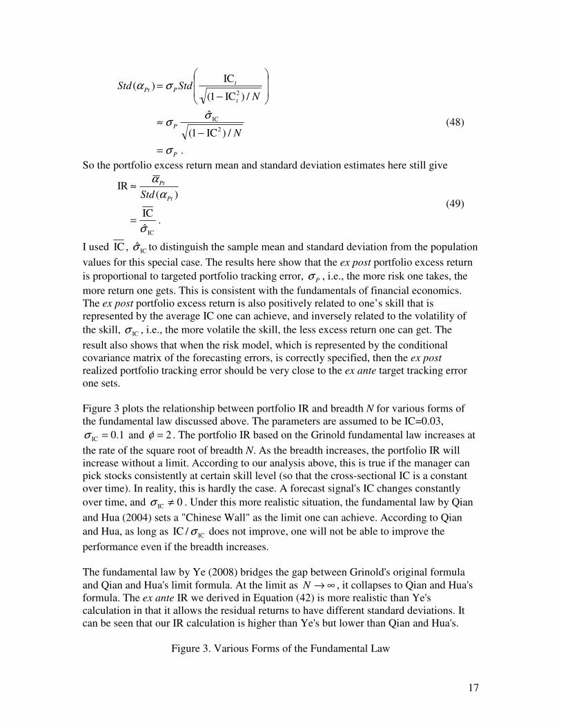
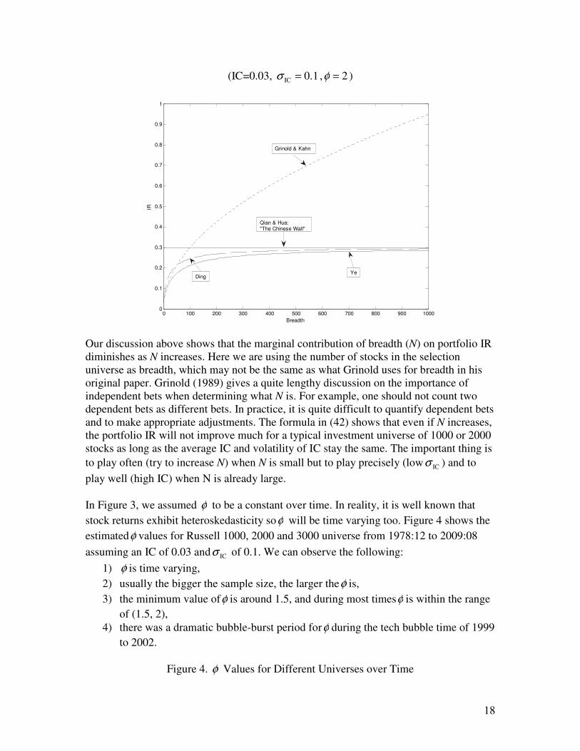
Figure 3 plots the relationship between portfolio IR and breadth N for various forms of

the fundamental law discussed above. The parameters are assumed to be IC=0.03,

1.0IC =σ and 2=φ . The portfolio IR based on the Grinold fundamental law increases at

the rate of the square root of breadth N. As the breadth increases, the portfolio IR will

increase without a limit. According to our analysis above, this is true if the manager can

pick stocks consistently at certain skill level (so that the cross-sectional IC is a constant

over time). In reality, this is hardly the case. A forecast signal's IC changes constantly

over time, and 0IC ≠σ . Under this more realistic situation, the fundamental law by Qian

and Hua (2004) sets a "Chinese Wall" as the limit one can achieve. According to Qian

and Hua, as long as IC/IC σ does not improve, one will not be able to improve the

performance even if the breadth increases.

The fundamental law by Ye (2008) bridges the gap between Grinold's original formula

and Qian and Hua's limit formula. At the limit as ∞→N , it collapses to Qian and Hua's

formula. The ex ante IR we derived in Equation (42) is more realistic than Ye's

calculation in that it allows the residual returns to have different standard deviations. It

can be seen that our IR calculation is higher than Ye's but lower than Qian and Hua's.

Figure 3. Various Forms of the Fundamental Law

18

(IC=0.03, 1.0IC =σ , 2=φ )

0 100 200 300 400 500 600 700 800 900 10000

0.1

0.2

0.3

0.4

0.5

0.6

0.7

0.8

0.9

1

Breadth

IR

Ding

Qian & Hua:"The Chinese Wall"

Grinold & Kahn

Ye

Our discussion above shows that the marginal contribution of breadth (N) on portfolio IR

diminishes as N increases. Here we are using the number of stocks in the selection

universe as breadth, which may not be the same as what Grinold uses for breadth in his

original paper. Grinold (1989) gives a quite lengthy discussion on the importance of

independent bets when determining what N is. For example, one should not count two

dependent bets as different bets. In practice, it is quite difficult to quantify dependent bets

and to make appropriate adjustments. The formula in (42) shows that even if N increases,

the portfolio IR will not improve much for a typical investment universe of 1000 or 2000

stocks as long as the average IC and volatility of IC stay the same. The important thing is

to play often (try to increase N) when N is small but to play precisely (low ICσ ) and to

play well (high IC) when N is already large.

In Figure 3, we assumed φ to be a constant over time. In reality, it is well known that

stock returns exhibit heteroskedasticity soφ will be time varying too. Figure 4 shows the

estimatedφ values for Russell 1000, 2000 and 3000 universe from 1978:12 to 2009:08

assuming an IC of 0.03 and ICσ of 0.1. We can observe the following:

1) φ is time varying,

2) usually the bigger the sample size, the larger theφ is,

3) the minimum value ofφ is around 1.5, and during most timesφ is within the range

of (1.5, 2),

4) there was a dramatic bubble-burst period forφ during the tech bubble time of 1999

to 2002.

Figure 4. φ Values for Different Universes over Time

19

1.2

1.6

2.0

2.4

2.8

3.2

3.6

4.0

1980 1985 1990 1995 2000 2005

R1000R2000R3000

1.5

Table 2 shows the average number of stocks ( N ), average φ (φ ), φN , and φN/1 for

Russell universes of stocks. It will be seen later that for most quantitative factors people

use, φN/1 is much smaller than the factor IC standard deviation, which suggests that

for the most commonly used investment universes the Grinold factor ( N/1 ) has a much

smaller impact than the Qian and Hua factor ( ICσ ). This is also obvious from Figure 3.

Table 2. Average Number of Companies and φ for Russell Indices

(1978:12-2009:8)

Index N φ φN φN/1

Russell 1000 949 1.74 1653 0.025

Russell 1000 Growth 507 1.66 843 0.034

Russell 1000 Value 578 1.57 908 0.033

Russell 2000 1833 2.01 3685 0.016

Russell 2000 Growth 1249 1.88 2347 0.021

Russell 2000 Value 1300 1.90 2465 0.020

Russell 3000 2782 2.12 5903 0.013

Russell 3000 Growth 1756 1.95 3425 0.017

Russell 3000 Value 1878 1.99 3729 0.016

Robustness of the Fundamental Law to Model Specification

In deriving the generalized fundamental law in Equation (42), we assumed the true

relationship to be a linear one factor model between the residual return and the forecast

signal. The residual returns are not risk-adjusted. The cross-sectional heteroskedasticity

20

across residual returns resulted in theφ parameter in Equation (42). In practice, people

may use risk-adjusted residual return as dependent variable to correct for the cross-

sectional heteroskedasticity, i.e.,

itittritit zfrrit

εσ ~~/~

1 +== − , (50)

where itr~ is the risk-adjusted residual return, itrσ is the conditional volatility for residual

return itr as of time t, tf~

is the cross-sectional factor return at time t (which will be

different from the factor return in Equation (36)), 1−itz is the factor exposure that has both

time series and cross-sectional mean 0 and standard deviation 1, )~,(~~ 20i

Nit εσε is the

idiosyncratic noise that cannot be predicted. Under these assumptions, we will have the

cross-sectional IC between risk-adjusted residual return itr~ and 1−itz to be the same as tf~

,

i.e.,

tititt fzr~

),~corr(C~

I 1 == − , (51)

and

2

IC

22 ~C~

I1~ σσ ε −−=i

, (52)

where C~

I and IC~σ are the mean and standard deviation of tC

~I . By using the same

algebra in the previous section, we can get

2

IC

2

IC

2 ~/)~C~

I1(

C~

IR~

Iσσ +−−

=N

. (53)

The formula is identical to Equation (42) when )IC1/(1 2

IC

2 σφ −−= , i.e., when the

residual standard deviations are the same across all the securities. One thing we have to

be aware of is CI~

and 2

IC~σ in Equation (53) will be different from IC and 2

ICσ in Equation

(42).

The above discussion shows that the form of the fundamental law is quite robust to the

forecast model specification. In both cases, the most important impact to portfolio IR is

the IC volatility over time. One insight from Equations (42) and (53) is that a quant

manager should preprocess the residual returns and factor exposures in such a way so that

the resulting cross-sectional IC will have a higher average and lower standard deviation.

One disadvantage with the model specification in Equation (50) is that one has to

estimate the conditional volatility itrσ which can involve estimation errors. A GARCH

type model will be useful for this purpose.

Multifactor Fundamental Law and the Impact of Missing Factors The fundamental law we discussed so far only concerns one factor. In practice, analysts

or portfolio managers rarely use only one factor. Residual return forecast almost always

involves multiple factors. It will be interesting to see the form of fundamental law with

multiple factors and study the consequences of missing one or more factors in modeling.

In deriving the fundamental laws presented in previous sections, we either made the

assumption that the residual return dispersion is a constant over time or used the risk-

21

adjusted residual return in analysis. But this is not necessary if we work on residual

security returns and factor returns directly.

If we assume residual returns follow a linear relationship with factor exposures

tttt εFZr += −1 , (54)

where tr is an 1×N vector of residual returns, 1−tZ is an KN × matrix of factor

exposures, tF is a 1×K vector of factor returns, and tε is an 1×N vector of

idiosyncratic noise. It is shown in Appendix B under some weak regularity conditions

that the ex ante expected portfolio IR has the following relationship with the expected

factor return (F) and factor return covariance ( FΣ )

FΣF

FΣIF

1-

F

1

F

'

))/(1('IR

≈

+= −Nτ

(55)

where )/1( 2

icsE εστ = represents part of the risk related to idiosyncratic noise. As in the

univariate case, this part of the risk will be diversified away as N gets larger, and the

remaining dominant risk is the "strategy risk" represented by the factor return covariance

that cannot be diversified away. When there is only one factor, Equation (55) reduces to

.

/))/1((IR

212

f

fcs

f

NE

f

i

σ

σσ ε

≈

+=

−

(56)

So the expected portfolio IR is just the IR of the factor-mimicking portfolio.

If, instead of using the raw residual return in Equation (54), we use the risk-adjusted

residual returns, then the multi-factor fundamental law in Equation (55) becomes (see

Appendix B)

,'

)/('IR

1-

IC

1

IC

2

ICΣIC

ICΣIIC

≈

+= −Nεσ (57)

where ∑=

+−=K

k

kk

1

22

,IC

2 ))IC(1( σσ ε is the variance for idiosyncratic noise, IC is the cross-

sectional correlation vector between factor exposures and risk-adjusted residual returns,

and ICΣ is the factor IC covariance matrix. Equation (57) reduces to Equation (53) when

there is only one factor.

The above conclusion is based on the assumption that the model is correctly specified

which is almost surely not the case in practice. A natural question to ask is what happens

if the return or risk model is mis-specified. With the fundamental law in multi-factor

format, we can easily study the impact of missing one or more return or risk factors. For

ease of exposition, I will only present the analysis for a 2-factor system here. More

detailed analysis with missing multiple factors can be found in Appendix B. In the

analysis below, I will not purposely distinguish risk factors from alpha factors.

22

Statistically, the only difference should be that the expected IC (or factor return) for risk

factor is zero while that for alpha factor is different from zero.

For a 2-factor system, Equation (B15) reduces to

.IC

ICIC

1

1IC

ICIC2

ICIC

1

1IR

1

1

21

2211

21

212121

IC

1

2

IC

1IC,IC

IC

2

2

IC,IC

2

IC

1

IC,IC

IC

2

IC

1

2

IC

2

2

IC

1

2

IC,IC

σ

σρ

σρσ

ρσσσσρ

≥

−

−+

=

−

+

−≈

(58)

where 21 IC,ICρ is the time series correlation of the two factor ICs.

From Equation (58), it is clear that a mis-specified model, whether it is mis-specified in

the return forecast part or the risk forecast part, will almost always hurt the performance.

For a missing return factor, the adverse impact comes from both the missing return

forecast, 2IC , and the resulting conditional covariance mis-specification, ( 2

IC,IC 211 ρ− ).

For a missing risk factor, the adverse impact only comes from the resulting conditional

covariance mis-specification ( 2

IC,IC 211 ρ− ). This is not surprising indeed! The only

exception is when the missing factor is a risk factor and the risk factor IC is not time-

series correlated with the return factor IC (i.e. when 0IC2 = and 021 IC,IC =ρ ). When the

risk factor is missing, the ex post realized portfolio tracking error will be larger than the

ex ante targeted portfolio tracking error by a factor of 11/1 2

IC,IC 21≥− ρ . So if

21 IC,ICρ is

small, then the impact of missing a risk factor is small.

Fundamental Law with Transfer Coefficient Clarke et al. (2002) proposed the concept of "transfer coefficient" to incorporate the

impact of additional constraints into the fundamental law. They define the transfer

coefficient as the cross-sectional correlation coefficient between the residual return

volatility adjusted active weights and alphas

.

)/()~(

)/,~cov(

)/,~corr(TC

ii

ii

ii

ritrit

ritrit

ritrit

dwd

w

w

σασ

σασ

σασ

∆

∆=

∆=

(59)

This definition has the desired property of measuring the impact of constraints on

portfolio IR when the factor IC is a constant so that 0IC =σ and the residual return

covariance is a diagonal matrix. Under this assumption, the transfer coefficient is the

ratio of the constrained portfolio IR and the unconstrained optimal portfolio IR

23

IRTCR~

I = , (60)

so the transfer coefficient does represent the portion of optimal portfolio IR that can be

transferred into the constrained portfolio.

Ye (2008) extended the transfer coefficient into her version of fundamental law with time

varying IC. Using her approach, she got the following relationship

22 )TC/(1

IC R~

I

ICσ+=

N. (61)

One surprising observation from Equation (61) is that the transfer coefficient as derived

by Ye (2008) will have diminishing impact as breadth N increases. The constrained

portfolio IR will approach the unconstrained optimal portfolio IR as N increases (both

approach IC/IC σ as ∞→N ) no matter what constraints one imposes on the portfolio.

This conclusion is quite counter-intuitive to practitioners as it can lead one to believe that

any portfolio can have the same IR.

So why does this happen? When the cross-sectional IC is time varying as discussed in Ye

(2008) and this paper, the total risk of the residual return is no longer a diagonal

covariance matrix. In fact the majority risk comes from the strategy risk which causes

the off-diagonal elements of the conditional covariance matrix to be non-zero. The

transfer coefficient will not have the desired property if we only use the diagonal portion

of the conditional covariance matrix to adjust the weights and alphas in deriving the

transfer coefficient. Under this more practical situation, the transfer coefficient needs to

be redefined using the total risk adjusted active weights and alphas as follows:

tttttt

tt

αΩαwΩw

αw

1'~'~

'~TC

−∆∆

∆= , (62)

where tw~∆ is the active weights of the constrained portfolio. Using this modified transfer

coefficient definition, we get the constrained portfolio's expected excess return as,

, IR TC

'~'~ ),~Corr(

'~

'~~

12/12/1

2/12/1

Pt

tttttttttt

tttt

ttPt

σ

α

=

∆∆∆=

∆=

∆=

−−

−

αΩαwΩwαΩwΩ

αΩΩw

αw

(63)

where Ptσ is the targeted portfolio tracking error and IR is the information ratio for the

unconstrained optimal portfolio. So the constrained portfolio information ratio ( R~

I ) , the

transfer coefficient (TC) and the optimal unconstrained portfolio information ratio (IR)

have the following relationship

. IR TC

/R~

I

=

= PtPt σα (64)

The impact of the constraints on portfolio IR will be the same as in Clarke et al.'s (2002)

original definition. In this way, a transfer coefficient of 0.5 will reduce the portfolio IR by

50% from the unconstrained optimal level.

24

Empirical Factor IR Comparison In order to compare the differences between the different forms of the fundamental law, I

calculated the IR that can be achieved by various quantitative factors using different

formulas. For each factor, I calculate the ex post realized cross-sectional correlation (IC)

between lagged factor exposures and residual returns, and then calculate the mean and

standard deviation of the time series IC. The results are then substituted into various

formulas to generate Table 3. For all the factors considered here, ICσ is much more

important than φN/1 . I calculated φσ NIC for each factor and they are in the range

of 4 to 10 which means ICσ is 4 to 10 times more important than φN/1 . From the last

four columns of the table, we can see that the expected IR from the Grinold formula is

always much higher than the other three while the other three stay very close to each

other. This is not surprising given the result in Figure 3 and the above discussion.

Table 3. Factor IR Comparison (monthly, data ends 2009:8)

Factor Index φN

1 IC

Mean

IC Stdev

ICσ φ

σ

N

IC

/1 IR

GK

IR

QH

IR

YE

IR

DING

R1000 0.024 0.014 0.139 5.67 0.44 0.10 0.10 0.10

R2000 0.016 0.025 0.113 6.95 1.12 0.22 0.22 0.22 Book to

Price R3000 0.013 0.020 0.114 8.76 1.06 0.17 0.17 0.17

R1000 0.024 0.039 0.119 4.88 1.21 0.33 0.32 0.32

R2000 0.016 0.066 0.122 7.49 2.93 0.54 0.53 0.54 Cash Flow

to Price R3000 0.013 0.058 0.111 8.59 3.17 0.52 0.52 0.52

R1000 0.024 0.031 0.140 5.70 0.95 0.22 0.21 0.22

R2000 0.016 0.067 0.120 7.37 2.96 0.56 0.55 0.55 Earnings to

Price R3000 0.013 0.059 0.121 9.35 3.19 0.48 0.48 0.48

R1000 0.024 0.019 0.129 5.26 0.58 0.15 0.14 0.14

R2000 0.016 0.026 0.104 6.41 1.16 0.25 0.24 0.25 Sales to

Price R3000 0.013 0.023 0.107 8.22 1.25 0.22 0.21 0.21

R1000 0.024 0.029 0.179 7.31 0.91 0.16 0.16 0.16

R2000 0.016 0.055 0.128 7.86 2.46 0.43 0.43 0.43 12-Month

Momentum R3000 0.013 0.049 0.137 10.59 2.68 0.36 0.36 0.36

R1000 0.024 0.015 0.089 3.63 0.46 0.17 0.16 0.16

R2000 0.016 0.026 0.084 5.20 1.16 0.31 0.30 0.30 Share

Repurchase R3000 0.013 0.024 0.083 6.38 1.30 0.29 0.28 0.29

R1000 0.024 0.022 0.118 4.81 0.67 0.18 0.18 0.18

R2000 0.016 0.037 0.105 6.48 1.67 0.36 0.35 0.35 Percent

Short R3000 0.013 0.029 0.101 7.80 1.56 0.28 0.28 0.28

Empirical findings here show that the theoretically calculated IR number from Grinold's

fundamental law needs to be cut by much more than half to be realistic. For a typical

investment universe of 1000 or 2000 stocks, the empirically calculated IR numbers from

formulas derived by Qian and Hua (2004), Ye (2008) and this paper give a more realistic

25

estimate of achievable IR. For investment universes less than 500, an IR using the

formula derived in this paper will give a better estimate. The difference will become

more significant for investment strategies with a much smaller selection universe, such as

a global macro strategy, or a tactical asset allocation strategy. The idiosyncratic risk still

plays a role when N is small. Table 4 shows theoretical examples when the investable

universes have much less choices.

Table 4. Theoretical IR Comparison when N is Small

GK QH YE DING GK QH YE DING

IC ICσ N=10 N=50

0.10 0.32 1.00 0.30 0.41 0.32 1.00 0.58 0.71

0.15 0.32 0.67 0.29 0.37 0.32 0.67 0.49 0.55 0.10

0.20 0.32 0.50 0.27 0.33 0.32 0.50 0.41 0.45

0.10 0.47 1.50 0.45 0.61 0.47 1.50 0.87 1.06

0.15 0.47 1.00 0.43 0.56 0.47 1.00 0.73 0.83 0.15

0.20 0.47 0.75 0.40 0.50 0.47 0.75 0.61 0.67

N=100 N=200

0.10 0.50 0.50 0.35 0.41 0.50 0.50 0.41 0.45

0.15 0.50 0.33 0.28 0.30 0.50 0.33 0.30 0.32 0.05

0.20 0.50 0.25 0.22 0.24 0.50 0.25 0.24 0.24

0.10 1.00 1.00 0.71 0.82 1.41 1.00 0.82 0.89

0.15 1.00 0.67 0.55 0.60 1.41 0.67 0.60 0.63 0.10

0.20 1.00 0.50 0.45 0.47 1.41 0.50 0.47 0.49

Conclusion

I have derived a generalized version of the fundamental law of active management under

some weak assumptions. The original fundamental law of Grinold (1989), the generalized

fundamental laws of Clarke et al. (2002), Qian and Hua (2004), and Ye (2008) are all

special cases of the fundamental law derived in this paper. I show that cross-sectional ICs

are usually different from time series ICs, and they will be the same only under the strong

assumption that either the residual return volatilities are the same across all the securities

or the ICs are calculated using risk-adjusted residual returns with the forecast signal.

I also show that the form of the fundamental law derived in this paper is quite robust to

forecast model specification. According to our generalized fundamental law, the variation

in IC (IC volatility over time) has a much bigger impact to portfolio IR than the breadth

N for a typical investment universe. The fundamental law by Qian and Hua (2004) sets a

"Chinese Wall" as the upper limit for the portfolio IR a portfolio manager can reach when

the cross-sectional IC varies over time. The fundamental law by Grinold (1989) is

derived under some unrealistic assumptions and always overestimates by a large margin

the IR a portfolio manager can actually reach. I extend the fundamental law to models

with multiple factors and study the impact of missing one or more return or risk factors. It

is shown that a mis-specified model, whether it is mis-specified in the return forecast part

or risk forecast part, will almost always hurt performance. The exception occurs when a

26

missing risk factor (IC=0) has a zero time series IC correlation with all the other factors.

For the commonly used quantitative return and risk factors, I found that the impact of a

missing risk factor is usually small.

Our results also show that the transfer coefficient as originally defined by Clarke et al.

(2002) is not able to capture the impact of constraints to portfolio IR in the presence of IC

variation. One will get the wrong conclusion that portfolio constraints do not have much

impact on portfolio IR in the presence of IC variation when N is large. I redefine the

concept of transfer coefficient using the cross-sectional correlation between the total

conditional covariance adjusted weights and alphas. The modified transfer coefficient

captures the impact of portfolio constraints on portfolio IR as desired.

One insight from this paper is that portfolio managers should try to play well (high IC)

and play precisely (low ICσ ). Extra efforts should be made to process the information and

to build models that can increase IC and reduce IC variation.

——————————————————————————————————————————

I thank Xiaohong Chen, Roger Clarke, Russell Fuller, Tom Fuller, John Kling, Doug Stone, Wei Su, Yixiao

Sun, Yining Tung, Jia Ye, and two anonymous referees for helpful discussions and comments. Richard

Grinold provided me with his original technical notes. Yining Tung helped with some empirical

calculations in the paper. ——————————————————————————————————————————

Appendix A

Given the conditional forecasting error covariance matrix in Equation (39) and based on

the Woodbury matrix identity, we have the inverse matrix of tΩ as

1

11

111 ' −−−

−−− −= tttttt ΣzzΣΣΩ ϕ , (A1)

where

1

1

1

22

IC

22

IC

'1 −−

−+=

ttt zΣzδσ

δσϕ . (A2)

Substituting (A1) into Equation (15) we have

.)'1/())IC/(''(IC

)'1))(IC/(''(IC

)'(''''

)'(')'('

))('('

)('

1

1

1

22

IC

1

11

1

1

1

1

1

1

11

1

1

1

11

111

11

11

1

11

111

11

11

1

11

11

1

−−

−−

−−−

−

−−

−−

−−−

−

−−−

−−−−−

−−

−−−

−−−−−

−−

−−−

−−

−

+−=

−−=

−−−=

−−−=

−−=

−=

ttttttttPt

ttttttttPt

tttttttttttttttPt

tttttttttttttPt

tttttttPt

tttPtPt

zΣz1ΣzzΣz

zΣz1ΣzzΣz

1ΣzzΣΣααΣzzΣααΣα

1ΣzzΣΣααΣzzΣΣα

1αΣzzΣΣα

1αΩα

δσδκδσ

ϕδκδσ

ϕκϕσ

ϕκϕσ

κϕσ

κσα

(A3)

27

When iεσ , 1−itz are cross-sectionally independent, then as N becomes large we have

,)/(1

IC

))/1(/(1

IC

))/1(1/()/1(IC

))/1()(1/()/1()(IC

))/(1/()/(IC

))/(1/()/(IC

)/(1/IC

)/(IC

2

IC

2

IC

22

222

IC

22

22

1

22

IC

22

1

2

1

22

IC

2

1

2

1

1

22

IC

2

1

1

1

2

1

1

22

IC

1

2

1

2

1

1

σφσ

σσδσ

σδσσδσ

σδσσδσ

σδσσδσ

σδσσδσ

σδσσδ

κσδσα

ε

εε

εε

εε

εε

εεε

+=

+=

+=

+=

+=

+=

+

−=

−−

−−

=−

=−

−

=−

=−

=−

∑∑

∑∑∑

N

NE

ENEN

EzENEzEN

zENzEN

zz

zzz

Pt

cs

Pt

cscsPt

csitcscsitcsPt

itcsitcsPt

N

i

it

N

i

itPt

N

i

it

N

i

it

N

i

itPtPt

i

ii

ii

ii

ii

iii

(A4)

where

.1

111

)IC(

111

111

12

1

2

122

IC

221

2

12

1

2

≥

≥

+−=

=

∑∑

∑∑

∑∑

==

==

==

N

i r

N

i

r

N

i r

N

i

r

N

i

N

i

r

i

i

i

i

i

i

NN

NN

NN

σσ

δσσσ

σσφ

ε

(A5)

The last line in (A5) is based on Jensen's inequality. In the derivation we used the fact

that 0/1

1

2

1 =∑=

−

N

i

it iz

Nεσ when ∞→N since 1−itz and

iεσ are cross-sectionally independent

by assumption.

Appendix B

Assume residual security returns tr and security factor exposures 1−tZ are related through

a linear factor model as follows

tttt εFZr += −1 , (B1)

where tr is an 1×N vector of residual returns, 1−tZ is an KN × matrix of factor

exposures that become known at the end of time t-1, tF is a 1×K vector of factor

returns, and ),(~I| 1 εΣ0ε Ntt − is an 1×N vector of idiosyncratic noise with mean 0

and covariance ),,,( 222

21 Ndiag εεεε σσσ L=Σ . The factor exposures are normalized to have

28

both time series and cross-sectional mean 0 and standard deviation 1, and are cross-

sectionally orthogonal to each other so that IZZ =−− Ntt /' 11 , Other regularity

assumptions like those in C1) and C2) also apply. We further assume that factor returns

follow a multivariate normal distribution

),(~I| F1 ΣFF Ntt − . (B2)

Based on the above assumptions, we have

,1FZα −= tt (B3)

and

εΣ+= −− '1F1 ttt ZΣZΩ . (B4)

Applying Woodbury matrix identity, we get the inverse of the conditional covariance

matrix as

1

1

1

1

1

1

1

F1

111 ')'( −−

−−

−−

−−

−−− ΣΣ+Σ−Σ= εεεε ttttt ZZZΣZΩ . (B5)

Substituting Equations (B3) and (B5) into the two components of the IR formula in

Equation (16) we get

FΣIF

FΣZΣZF

FΣZΣZF

FZΣZZΣZΣΣF

FΣZΣZΣZΣZF

FZΣZZΣZΣIZΣZF

FZΣZZΣZΣZΣΣZFαΩα

1

F

1

F

1

1

1

1

1

F

1

1

1

1

11

1

1

11

1

1

1

FF

1

F

1

1

1

1

1

F1

1

1

1

1

1

1

1

1

1

1

F1

1

1

1

1

1

1

1

1

1

1

F1

11

1

1

))/(1('

)/)/'(('

))'(('

))')('(('

)'(''

)')'((''

)')'(('''

−

−−−

−−

−−−

−−

−−−

−−−

−−

−

−−−

−−

−−

−−

−−

−−

−−

−−

−−

−

−−

−−

−−

−−

−−−

−−

+=

+=

+=

+=

+=

+−=

+−=

N

NNtt

tt

tttt

tttt

tttttt

ttttttttt

τ

ε

ε

εε

εε

εεε

εεεε

(B6)

and

,

)/('))/(1('

'))'('('

)')'(('''

1

1

1

F

1

1

1

1

1

1

1

F1

1

1

1

1

1

1

1

1

1

F1

11

1

1

0

1ΣZΣIF

1ΣZZΣZΣZΣZIF

1ΣZZΣZΣZΣΣZF1Ωα

=

+=

+−=

+−=

−−

−

−−

−−

−−

−−

−−

−−

−−

−−

−−

−−−

−

NN t

ttttt

ttttttt

ττ ε

εεε

εεεε

(B7)

where we assumed kiz and iεσ to be cross-sectionally independent and used the facts that

for Klk ,,2,1, L= ,

29

( )

≠

====

=

=

=

∑

∑

=

−−

−−

=

−−

−−

−

lk

lkN

E

EzzE

zzE

zz

NN

N

i

cs

csitlitkcs

itlitk

cs

N

i

itlitk

tltk

ii

i

i

i

en wh 0

when )/1(1

)/1(

)/1(

1/'

1

22

2

1,1,

2

1,1,

12

1,1,

1,

1

1,

τσσ

σ

σ

σ

εε

ε

ε

ε

ε ZΣZ

(B8)

and

.0

)/1()(

)/(

)/(1

/'

2

1,

2

1,

1

2

1,

1

1,

=

=

=

=

−

−

=−

−− ∑

i

i

i

csitkcs

itkcs

N

i

itktk

EzE

zE

zN

N

ε

ε

εε

σ

σ

σ1ΣZ

(B9)

So the ex ante expected portfolio IR is

( )( )

.'

))/(1('

'

)('IR

1

F

1

F

1

1

FΣF

FΣIF

αΩα

1αΩα

−

−

−

−

≈

+=

=

−=

N

E

E

ttt

ttt

τ (B10)

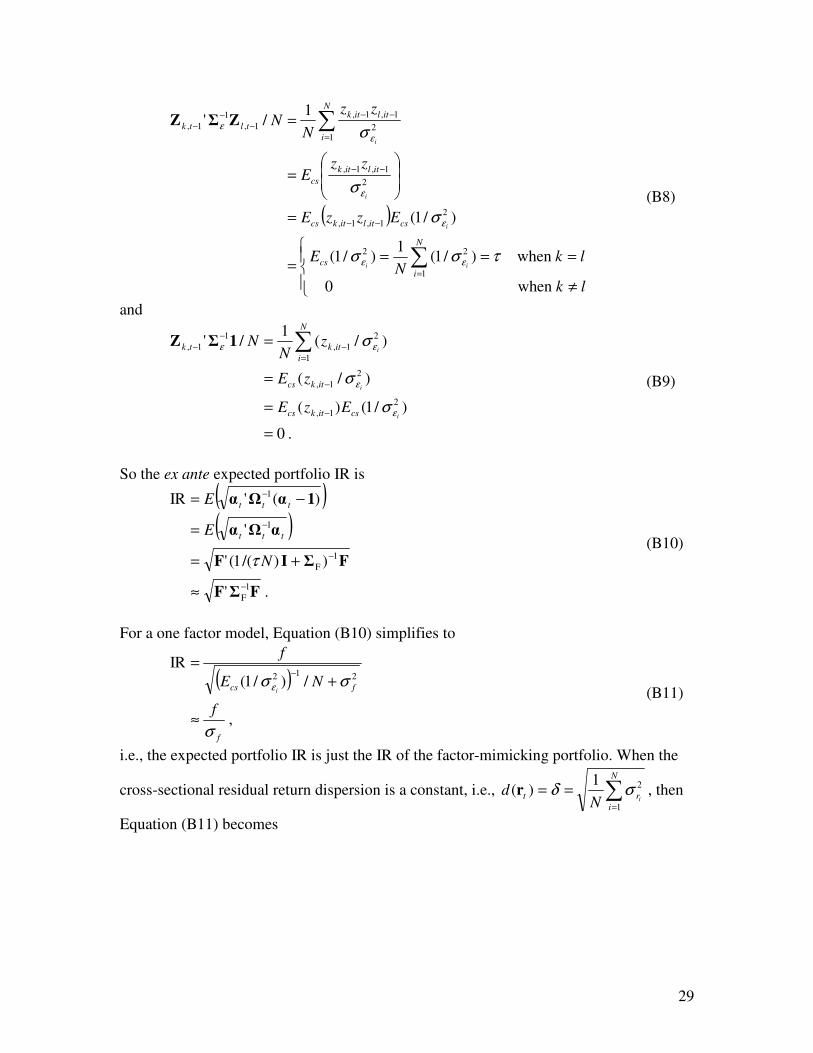
For a one factor model, Equation (B10) simplifies to

( )

,

/)/1(

IR212

f

fcs

f

NE

f

i

σ

σσ ε

≈

+=

−

(B11)

i.e., the expected portfolio IR is just the IR of the factor-mimicking portfolio. When the

cross-sectional residual return dispersion is a constant, i.e., ∑=

==N

i

rt iNd

1

21)( σδr , then

Equation (B11) becomes

30

( )

( )

2

IC

2

IC

122

2

IC

212

)/(1

IC

/)/1(

IC

/)/1(

ICIR

σφ

σσδ

σδσ

δ

ε

ε

+=

+=

+=

−

−

N

NE

NE

i

i

cs

cs

(B12)

where φ is the same as defined in (A5). The formula above is exactly the same as

Equation (42) which is what should be expected.

By applying the same assumptions for deriving Equation (B12) to Equation (B10),

we get the multifactor fundamental law in terms of IC as follows:

( )

ICΣIC

ICΣIIC

FΣIF

1

IC

1

IC

1

F

'

)/(1'

))/(1('IR

−

−

−

≈

+=

+=

N

N

φ

τ

(B13)

where δ/FIC = is the cross-section correlation vector between factor exposures and

residual security returns, and 2

FIC /δΣΣ = is the factor IC covariance matrix. It should

be emphasized that the results in Equations (B12) and (B13) are only valid when the

cross-sectional residual return dispersion is a constant. When this assumption is violated,

then the IR calculated from Equations (B10) and (B11) will usually be smaller than that

from (B12) and (B13).

To avoid the problem of cross-sectional heteroskedasticity in cross-sectional regression,

one can use the risk-adjusted residual security returns as the dependant variable, i.e.,

tttttt εICZrΛr +== −−

1

2/1~

where ),,,( 222

21 Nrrrt diag σσσ L=Λ , and 2

irσ is the residual return variance for security i. By

using the same algebra one can get

( )

ICΣIC

ICΣIIC

1

IC

1

IC

2

'

/'IR

−

−

≈

+= Nεσ (B14)

where ∑=

+−=K

k

kk

1

22

,IC

2 )IC(1 σσ ε . It should be emphasized again that the ICs in Equation

(B14) are the cross-sectional correlation between risk-adjusted residual security returns

and factor exposures, while the ICs in Equation (B13) are the correlation between the raw

residual security returns and factor exposures, hence they will usually be different.

With the fundamental law in multifactor format, we can easily study the impact of

missing one or more return or risk factors. In the analysis below, I will study the impact

of missing factors based on factor ICs, the analysis based on factor returns is almost

identical. I will not purposely distinguish risk factors from alpha factors. Statistically, the

31

only difference should be that the expected IC (or factor return) for risk factor is zero

while that for alpha factor is different from zero. I will separate the factors into two

groups with iIC and iiΣ (i=1,2) as their factor IC and IC covariance respectively. I will

also assume that the inter-group factor IC covariance to be 12Σ . Under these assumptions,

we can write Equation (B13) as follows 7

1

1

111

1

1

11122

1

1

1

111221

1

111

2

1

1

2212

1211

21

1

IC

'

)'()''('

')''(

'IR

ICΣIC

ICΣΣICEICΣΣICICΣIC

IC

IC

ΣΣ

ΣΣICIC

ICΣIC

−

−−−−

−

−

≥

−−+=

=

≈

(B15)

where 12

1

111222 ' ΣΣΣΣE−−= .

So 2IR will be reduced by a amount of

0)'()'()''( 1

1

11122

1

12

1

1112221

1

11122 ≥−−− −−−−ICΣΣICΣΣΣΣICΣΣIC (B16)

when the second group of 2k factors are missing. The impacts come from both alpha

model mis-specification (when 0IC ≠2 ) and risk model mis-specification (when

0IC =2 but 0)')'(' 1

1

1112

1

12

1

11122212

1

111 >− −−−−ICΣΣΣΣΣΣΣΣIC ).

Alternatively the IR can be expressed as

)()'('IR 2

1

22121

1

2

1

221212

1

222 ICΣΣICDICΣΣICICΣIC−−−− −−+≈ (B17)

where '12

1

221211 ΣΣΣΣD−−= . When 0IC =2 , then the missing group is purely risk

factors,

,'

)'('

')'(''IR

1

1

111

1

1

12

1

2212111

1

1

1112

1

12

1

11122212

1

1111

1

111

ICΣIC

ICΣΣΣΣIC

ICΣΣΣΣΣΣΣΣICICΣIC

−

−−

−−−−−

≥

−=

−+=

(B18)

so the reduction in IR comes only from missed risk allocation. When 0Σ =12 , i.e., the

alpha group factor ICs and risk group factor ICs are not correlated, then missing risk

factors will not impact the final portfolio performance.

Notes 1 We used the fact that the benchmark residual return is zero in deriving Equation (7), i.e.,

01

, =∑=

N

i

ititB rw .

This is true because

32

∑∑∑∑====

+=+==N

i

ititBtB

N

i

ititB

N

i

tBititB

N

i

Total

ititBtB rwRrwRwrwR1

,,

1

,

1

,,

1

,, β .

2 We define the realized cross-sectional residual return dispersion at time t as

)()(1

)(1

)( 22

1

22

1

2

titcs

N

i

tit

N

i

titt rrErrN

rrN

d −=−=−= ∑∑==

r ,

where ∑=

=N

i

itt rN

r1

1is the average cross-sectional residual return which we will assume to be

zero in this article. The expected cross-sectional residual return dispersion is then

( ))()(1

))(( 22

1

22

titcs

N

i

titt rrEErrN

EdE −=

−== ∑

=

rδ .

3 We can decompose itr as itrit er σ= where )1,0(~ Neit . So

r

N

i

itr

N

i

itt eN

ErN

EdE σσδ =

=

== ∑∑

== 1

2

1

2 11))(( r

as ∞→N by law of large numbers.

4 When we assume the cross-sectional residual return dispersion is a constant, i.e.,

drN

dN

i

itt == ∑=1

21)(r ,

then

ddE t == ))(( rδ .

On the other hand,

2

1

2

1

22 1)(

1))(( d

NrE

NdE

N

i

r

N

i

itt i∑∑==

=== σr .

So we have

∑=

===N

i

rt iNddE

1

21))(( σδ r .

5 The assumption of normality in the information coefficient is approximate because IC is

bounded by 1± .

6 The unconditional covariance of tr is ΣΣrr ++= zttE

22

IC

2 )IC()'( δσ , where zΣ is the

covariance matrix of 1−tz with 1 in the diagonal.

7 The inverse of a partitioned matrix is repeatedly used in the derivation, see Magnus and

Neudecker (2002, p11) .

References

33

Clarke, Roger, Harindra de Silva, and Steven Thorley. 2002. “Portfolio Constraints and

the Fundamental Law of Active Management.” Financial Analysts Journal, vol. 58, no. 5

(September/October):48–66.

Grinold, Richard C. 1989. “The Fundamental Law of Active Management.” The Journal

of Portfolio Management, vol. 15, no. 3 (Spring): 30–38.

Grinold, Richard C. 1994. “Alpha is Volatility Times IC times Score.” The Journal of

Portfolio Management, vol. 20, no. 4 (Summer): 9–16.

Grinold, Richard C. 2007. “Dynamic Portfolio Analysis.” The Journal of Portfolio

Management, vol. 34, no. 1 (Fall): 12–26.

Grinold, Richard C., and Ronald N. Kahn. 2000. Active Portfolio Management. 2nd ed.

New York: McGraw-Hill.

Ibragimov, R. and Müller, U. (2009). "t-statistic Based Correlation and Heterogeneity

Robust Inference," forthcoming in the Journal of Business & Economic Statistics.

Kahn, Ronald, 1997. "Seven Quantitative Insights into Active Management Part 3: The

Fundamental Law of Active Management," BARRA Newsletter, Winter.

Lee, Jyh-Huei and Dan Stefek. “Do Risk Factors Eat Alphas.” The Journal of Portfolio

Management, vol. 34, no. 4 (Summer 2008), pp. 12-25.

Magnus, Jan R. and Heinz Neudecker. 2002. Matrix Differential Calculus with

Applications in Statistics and Econometrics. Revised Edition. New York: John Wiley &

Sons.

Petersen, M. A. (2009), “Estimating standard errors in finance panel data sets: Comparing

approaches,” The Review of Financial Studies, 22, 435-480.

Qian, Edward, and Ronald Hua. “Active Risk and Information Ratio.” The Journal of

Investment Management, vol 2, no. 3 (2004), pp. 20-34.

Qian, E., Hua, R., and Sorensen, E.H. (2007). Quantitative Equity Portfolio Management:

Modern Techniques and Applications, London: CRC Press.

Sorensen, Eric H., Ronald Hua, Edward Qian, and Robert Schoen. “Multiple Alpha

Sources and Active Management.” The Journal of Portfolio Management, vol. 30, no. 2

(Winter 2004), pp. 39-45.

Sorensen, Eric H., Ronald Hua, and Edward Qian. 2007. “Aspects of Constrained Long–

Short Equity Portfolios.” The Journal of Portfolio Management, vol. 33, no. 2

(Winter):12–22.

Ye, Jia. "How Variation in Signal Quality Affects Performance." Financial Analysts

Journal, vol. 64, no. 4 (2008), 48-61.