Fundamental Fluid Mechanics for Engineers
439
-
Upload
emannuelfernandes -
Category
Documents
-
view
182 -
download
2
description
Livro de base sobre mecânica dos fluidos para Engenharia
Transcript of Fundamental Fluid Mechanics for Engineers

7/21/2019 Fundamental Fluid Mechanics for Engineers
http://slidepdf.com/reader/full/fundamental-fluid-mechanics-for-engineers 1/438
7/21/2019 Fundamental Fluid Mechanics for Engineers
http://slidepdf.com/reader/full/fundamental-fluid-mechanics-for-engineers 2/438
FUNDAMNTAL
FLUID MeCHANlCS
FOR TH€
PRACTICING
€NGlN€€R

7/21/2019 Fundamental Fluid Mechanics for Engineers
http://slidepdf.com/reader/full/fundamental-fluid-mechanics-for-engineers 3/438
MECHANICAL ENGINEERING
A
Series of Textbooks and Reference Books
Editor
L.L.Faulkner
Columbus Division, Battelle Memorial Institute
and Department o Mechanical Engineering
Ihe Ohio State University
Columbus, Ohio
1. Spring Designer s Handbook, Harold Carlson
2. Computer-Aided Graphics and Design,Daniel L. Ryan
3. Lubrication Fundamentals, J. George Wills
4.
Solar Engineering fo r Domestic Buildings, William A. Himmelman
5.
Applied Engineering Mechanics: Statics and Dynamics,
G. Booth-
6.
Centrifugal Pump Clinic,
lgor J. Karassik
7 . Computer-Aided Kinetics for Machine Design, Daniel L. Ryan
g.
Plastics Products Design Handbook, Part: Materials and Compo-
nents; Part B: ProcessesandDesign for Processes, edited by
Edward Miller
9.
Turbomachinery: Basic Theory and Applications, Earl Logan, Jr.
10. Vibrations
o f
Shells and Plates,
Werner Soedel
11. FlatandCorrugatedDiaphragmDesignHandbook, Mario Di
12.
PractjcaI StressAnalysis in Engineering Design,
Alexander Blake
13. An introduction to the Design and Behavior
o f
Bolted Joints, John
14. Optimal Engineering Design: Principles and Applications, James
15. Spring Manufacturing Handbook, Harold Carlson
16.
Industrial Noise Control: Fundamentals and Applications,
edited
17.
GearsandTheir Vibration: ABasic Approach to Understanding
1g.
Chains for Power Transmission and Material Handling: Design and
1g , Corrosion and Corrosion Protection Handbook, dited
b Y
Philip A*
20. Gear Drive Systems: Design and Application, Peter LYnwander
royd and C. Poli
Giovanni
H. Bickford
N.
Siddall
by Lewis H. Bell
Gear Noise,
J.
Derek Smith
Applications Handbook, American Chain Association
Schweitzer

7/21/2019 Fundamental Fluid Mechanics for Engineers
http://slidepdf.com/reader/full/fundamental-fluid-mechanics-for-engineers 4/438
21.
22.
23.
24.
25.
26.
27.
28.
29.
30.
31.
32.
33.
34.
35.
36.
37.
38.
39.
40.
41.
42.
43.
44.
45.
Controlling n-Plant Airborne Contaminants: Systems Design and
Calculations, John D. Constance
CAD/CAM Systems Planning and Implementation,harlesS. Knox
ProbabilisticEngineeringDesign:Principles and Applications,
James
N.
Siddall
Traction Drives: Selection and pplication, FrederickW. Heilich Ill
and Eugene E.Shube
Finite Element Methods: An Introduction, Ronald L. Huston and
Chris E. Passerello
Mechanical Fasteningf Plastics: An Engineering Handbook, ray-
ton Lincoln, Kenneth J. Gomes, and James F. Braden
Lubrication n Practice: Second Edition,edited by W. S. Robertson
Principles
o f
Automated Drafting,
Daniel L. Ryan
Practical Seal Design,edited by LeonardJ. Martini
Engineering Documentationor CAD/CAM Applications, CharlesS.
Knox
DesignDimensioning with ComputerGraphics Applications,
Jerome C. Lange
Mechanism Analysis: Simplified Graphical and Analytical Tech-
niques, Lyndon0. arton
CAD/CAM Systems: Justification, Implementation, Productivity
Measurement,
Edward
J.
Preston, George
W.
Crawford, and Mark
E.
Coticchia
Steam Plant Calculations Manual, V. Ganapathy
Design Assurance
or
Engineers and Managers,
John A.Burgess
Heat Transfer Fluids and Systems for Process and EnergyAppli-
cations,
Jasbir Singh
Potential Flows: Computer Graphic Solutions,Robert H. Kirchhoff
Computer-Aided Graphics and Design: Second Edition, Daniel
L.
Ryan
Electronically Controlled Proportional Valves: Selection andppli-
cation, Michael J. Tonyan, edited by Tobi Goldoftas
Pressure Gauge Handbook,AMETEK, U.S. Gauge Division, edited
by Philip W. Harland
Fabric Filtration for Combustion Sources: Fundamentalsnd Basic
Technology,
R. P. Donovan
Design of Mechanical Joints, Alexander Blake
CAD/CAM Dictionary,
Edward J. Preston, George W. Crawford,
and Mark
E.
Coticchia
Machinery Adhesives
for
Locking, Retaining, and Sealing,
Girard
S.
Haviland
Couplings andJoints: Design, Selection, and Application, Jon R.
Mancuso
46. Shaft Alignment Handbook, John Piotrowski

7/21/2019 Fundamental Fluid Mechanics for Engineers
http://slidepdf.com/reader/full/fundamental-fluid-mechanics-for-engineers 5/438
47.
48.
49.
50.
51.
52.
53.
54.
55.
56.
57.
58.
59.
60.
61.
62.
63.
64.
65.
66.
67.
68.
69.
BASIC Programs or Steam Plant Engineers: Boilers, Combustion,
Fluid Flow, and Heat Transfer,
V.
Ganapathy
Solving Mechanical Design Problems with ComputerGraphics,
Jerome C. Lange
Plastics Gearing: Selection and Application,
Clifford
E.
Adams
Clutches and Brakes: Design and Selection,
William C. Orthwein
Transducers n Mechanical and Electronic Design,arry L. Trietley
Metallurgical Applications of Shock- Wave and High-Strain-Rate
Phenomena,
edited by Lawrence
E.
Murr, Karl P. Staudhammer,
and Marc A. Meyers
Magnesium Products Design,
Robert S. Busk
How to Integrate CAD/CAM Systems: Management and Technol-
ogy,
William D. Engelke
Cam Design and Manufacture: Second Edition; with cam design
software for the IBM PC and compatibles, disk included,
Preben
W. Jensen
Solid-state AC Motor Controls: Selection and pplication, Sylves-
ter Campbell
Fundamentals of Robotics, David D. Ardayfio
Belt Selection and pplication for Engineers, edited by Wallace D.
Erickson
Developing Three-Dimensional CAD oftware with the IBM PC,
C.
Stan Wei
OrganizingData .for CIM Applications,
Charles S. Knox, with
contributions by Thomas C. Boos, Ross S. Culverhouse, and Paul
F. Muchnicki
Computer-Aided Simulation in RailwayDynamics,
by Rao V.
Dukkipati and Joseph R. Amyot
Fiber-Reinforced Composites: Materials, Manufacturing, and De-
sign,
P.
K. Mallick
Photoelectric Sensors and Controls: Selection and Application,
Scott M. Juds
finite Element Analysis with PersonalComputers,
Edward R.
Champion, Jr., and J. Michael Ensminger
Ultrasonics:Fundamentals,Technology, Applications: Second
Edition, Revised and Expanded,
Dale Ensminger
Applied Finite Element Modeling: Practical Problem Solving for
Engineers,
Jeffrey M.
Steele
Measurement and nstrumentation in Engineering: Princales and
Basic Laboratory Experiments, Francis S. Tse and Ivan
E.
Morse
Centrifugal Pump Clinic: Second Edition, Revised and Expanded,
lgor J. Karassik
Practical Stress Analysis in Engineering Design: Second Edition,
Revised and Expanded, Alexander Blake

7/21/2019 Fundamental Fluid Mechanics for Engineers
http://slidepdf.com/reader/full/fundamental-fluid-mechanics-for-engineers 6/438
70.
71.
72.
73.
74.
75.
76.
77.
78.
79.
80.
81.
82.
An Introduction to the Design and Behavior of Bolted Joints:
Second Edition, Revised and Expanded,
ohn H. Bickford
High Vacuum Technology: A Practical Guide,
Marsbed
H.
Habla-
nian
Pressure Sensors: Selection and Application,
Duane Tandeske
Zinc Handbook: Properties, Processing, and Use in Design, Frank
Porter
Thermal Fatigue f Metals, Andrzej Weronski and Tadeuzejwow-
ski
Classical and Modern Mechanisms for Engineers and Inventors,
Preben W. Jensen
Handbook of Electronic Package Design, edited
by
Michael Pecht
Shock- Wave and High-Strain-Rate Phenomenan Materials,
edited
by Marc A. Meyers, Lawrence E.Murr, and Karl
P.
Staudhammer
Industrial Refrigeration: Principles, Design and pplications, P. C.
Koelet
Applied Combustion, Eugene L. Keating
Engine Oils andutomotive Lubrication,edited
by
WilfriedJ. Bartz
MechanismAnalysis: Simplified and Graphical Techniques, Second
Edition, Revised and Expanded,Lyndon0. arton
Fundamental Fluid Mechanics for the Practicing Engineer,
James
W. Murdock
Additional Volumes in Preparation
Fiber-Rein orced Composites: Materials, Manufacturing, and De-
sign, Second Edition, Revised and Expanded,P. K. Mallick
Introduction to Engineering Materials: Behavior, Properties, and
Selection, G. T. Murray
Vibrations of ShellsandPlates:SecondEdition,Revisedand
Expanded,
Werner Soedel
Mechanical Engineering Software
Spring Design with an IBM PC,
AI Dietrich
Mechanical Design Failurenalysis: With Failure Analysis System
Software for the IBM PC, David
G.
Ullman

7/21/2019 Fundamental Fluid Mechanics for Engineers
http://slidepdf.com/reader/full/fundamental-fluid-mechanics-for-engineers 7/438
This Page Intentionally Left Blank
7/21/2019 Fundamental Fluid Mechanics for Engineers
http://slidepdf.com/reader/full/fundamental-fluid-mechanics-for-engineers 8/438
PUNDAMNTAL
F
LUlDMKHANICS
f 0 R
TH€
PRACTICING€NGIN€€R
J A M S
WAURDOCK
D r e x e l Un i v e r s i t y
P h i la d e l p h i a , P e n n s y l v a n i a
MarcelDekker, Inc. NewYork.Basel
HongKong
7/21/2019 Fundamental Fluid Mechanics for Engineers
http://slidepdf.com/reader/full/fundamental-fluid-mechanics-for-engineers 9/438
Library
of
Congress
Cataloging-in-Publication
ata
Murdock, James W.
Fundamental fluid mechanics for the practicing engineer
/
James
W.
Murdock.
p. cm.
--
(Mechanicalengineering
;
82)
Includes bibliographical references and index.
ISBN
0-8247-8808-7
(acid-free paper)
1.
Fluid mechanics.
I
itle.
II.
Series:Mechanical
engineering (Marcel Dekker, Inc.) ;
82.
TA357.M88993
620.1’06-d~20
92-39547
CIP
This book is printed on acid-free paper.
Copyright
@
1993
by
MARCEL DEKKER, INC.
All
Rights
Reserved.
Neither thisbook nor any part may be reproduced or transmitted n any
form
or by any means, electronic or mechanical, including photocopying, micro-
filming,
and recording, or by any information storage and retrieval system,
without permission in writing from the publisher.
MARCEL DEKKER, NC.
270
Madison
Avenue, New York, New York
10016
Current printing (last digit):
l 0 9 8 7 6 5 4 3 2 1
PRINTED INTHE UNITED
STATES OF AMERICA

7/21/2019 Fundamental Fluid Mechanics for Engineers
http://slidepdf.com/reader/full/fundamental-fluid-mechanics-for-engineers 10/438
To my
friend
Dorothy M. Thompson

7/21/2019 Fundamental Fluid Mechanics for Engineers
http://slidepdf.com/reader/full/fundamental-fluid-mechanics-for-engineers 11/438
This Page Intentionally Left Blank
7/21/2019 Fundamental Fluid Mechanics for Engineers
http://slidepdf.com/reader/full/fundamental-fluid-mechanics-for-engineers 12/438
As the title suggests, this book is writtenfor the practicing engineer. Its
purpose is o bridge the gap between he fundamentals presented n mod-
ern mathematically oriented fluid mechanics textbooks and the needs of
practicing engineers.The minimum mathematical level required
or
clarity
of concepts and academic integrity is used. It is essentially a self-study
book to be used by engineers with no to totally recalled knowledge of
this subject. It is also a “thumb-through” book-all required equations
are repeated with the derivation of each concept, eliminating the need to
refer to other sections. This book can be used and understoodby almost
anyone with an elementary knowledgeof calculus and physics.
This book uses a dual system of units, U.S. Customary Units (U. S.)
and Syst&me nternationale d’Unites (SI). In keeping withhe “practical”
emphasis, lbf/in.2 (psi) is used or pressure in place of lbf/ft2 and Ibm/ft3
for density in place of slugs/ft3. The unit of slugs for mass is not used,
but conversion factors are provided. A step-by-stepprocedure is followed
throughout this book to eliminate any guessing games betweenhe author
and the reader. Each new concept
is
followed by at least one example.
An organized method of problem solving is presented. Each example is
solved by an approach statement, development of the needed equations
for the particular application, data sources, and numerical solutions in
U.
S .
and SI units. There are
76
fully solved tutorial examples to serve
as models.
V

7/21/2019 Fundamental Fluid Mechanics for Engineers
http://slidepdf.com/reader/full/fundamental-fluid-mechanics-for-engineers 13/438
vi Preface
The book is organized into six hapters. The first fivechapters, “Basic
Definitions,” “Fluid Statics,” “Fluid Kinematics,“ “Fluid Dynamics and
Energy Relations,” and “Gas Dynamics.” provide the basic theoretical
foundations. In wiifing Chapter
5,
“Gas DynamicTparticular care was
taken to consider the non-mechanical engineer who normally does not
take a course on this subject. Also, since gas dynamics involves some
thermodynamics concepts, these were included o eliminate the necessity
to refer to
a
text on this subject. Last, Chapter
6,
“Dimensionless Pa-
rameters,” was included because this subject is ne of the most powerful
tools of engineering, but is seldom used because it s usually “skipped”
to make way for other material.
A
step-by-step method of using Buck-
ingham’s I1 theorem as well as
a
format for dimensional analysis is pre-
sented.
There are three appendixes. Appendix A contains saturated, critical,
and gasproperties of 49 selected fluids, and viscosity and densityf com-
pressed water and superheated steam. Appendix B is a history of units,
a description of SI and U. S. systems, and conversion factors. Appendix
C contains properties of areas, pipes, and tubing. These appendixeswere
designed to provide hard to find fluid properties and other information of
help to the practicing engineer.
It would be impossible to acknowledge the aid of all persons-pro-
fessors, students at Drexel, and former associates at the Naval Ship-
Systems Engineering Center-who helped make this work possible.I am
indebted to Mr. Simon Yates of Marcel Dekker, Inc., for his encourage-
ment and assistance. I
am
indebted to John Bloomer, a Drexel graduate
student, for checking the original manuscript.
James W . Murdock
7/21/2019 Fundamental Fluid Mechanics for Engineers
http://slidepdf.com/reader/full/fundamental-fluid-mechanics-for-engineers 14/438
Preface
V
Principal Symbols and Abbreviations
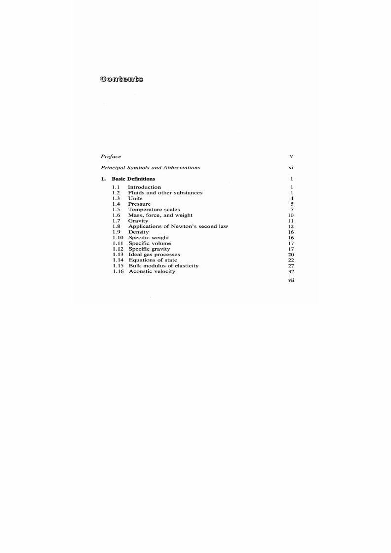
1.
BasicDefinitions
1.1
Introduction
1.2
Fluidsand other substances
1.3
Units
1.4 Pressure
1.5
Temperature scales
1.6
Mass, force, andweight
1.7 Gravity
1.8 Applications of Newton’ssecond law
1.9
Density
1.10 Specificweight
1.11 Specific volume
1.12 Specificgravity
1.13 Idealgas processes
1.14
Equations of state
1.15 Bulk modulus of elasticity
1.16 Acousticvelocity
xi
1
1
1
4
5
7
10
11
12
16
16
17
17
20
22
27
32
vii

7/21/2019 Fundamental Fluid Mechanics for Engineers
http://slidepdf.com/reader/full/fundamental-fluid-mechanics-for-engineers 15/438
viii
1.17
Viscosity
1.18 Surface tension and capillarity
1.19
Vapor pressure
References
2. FluidStatics
2.1
2.2
2.3
2.4
2.5
2.6
2.7
2.8
2.9
2.10
2.11
2.12
Introduction
Fluid statics
Basic equation of fluid statics
Pressure-height relations for incompressible fluids
Pressure-sensing devices
Pressure-height relations for ideal gases
Atmosphere
Liquid force on plane surfaces
Liquid force on curved surfaces
Stress
in
pipes due to internal pressure
Acceleration of fluid masses
Buoyancy and flotation
3. FluidKinematics
3.1 Introduction
3.2
Fluidinematics
3.3
Steady andunsteady low
3.4
Streamlinesand streamtubes
3.5 Velocityrofile
3.6
Correction for kineticenergy
3.7
Continuityquation
4.
Fluid Dynamics and Energy Relations
4.1
4.2
4.3
4.4
4.5
4.6
4.7
4.8
4.9
4.10
4.11
Introduction
Fluid dynamics
Equation of motion
Hydraulic radius
One-dimensional steady-flow equation of motion
Specific energy
Specific potential energy
Specific kinetic energy
Specific internal energy
Specific flow work
Specific enthalpy
Contents
34
38
42
45
46
46
46
47
49
51
62
64
70
77
81
86
97
105
105
105
106
108
109
115
118
124
124
124
125
127
129
133
133
133
134
135
136
7/21/2019 Fundamental Fluid Mechanics for Engineers
http://slidepdf.com/reader/full/fundamental-fluid-mechanics-for-engineers 16/438
Contents
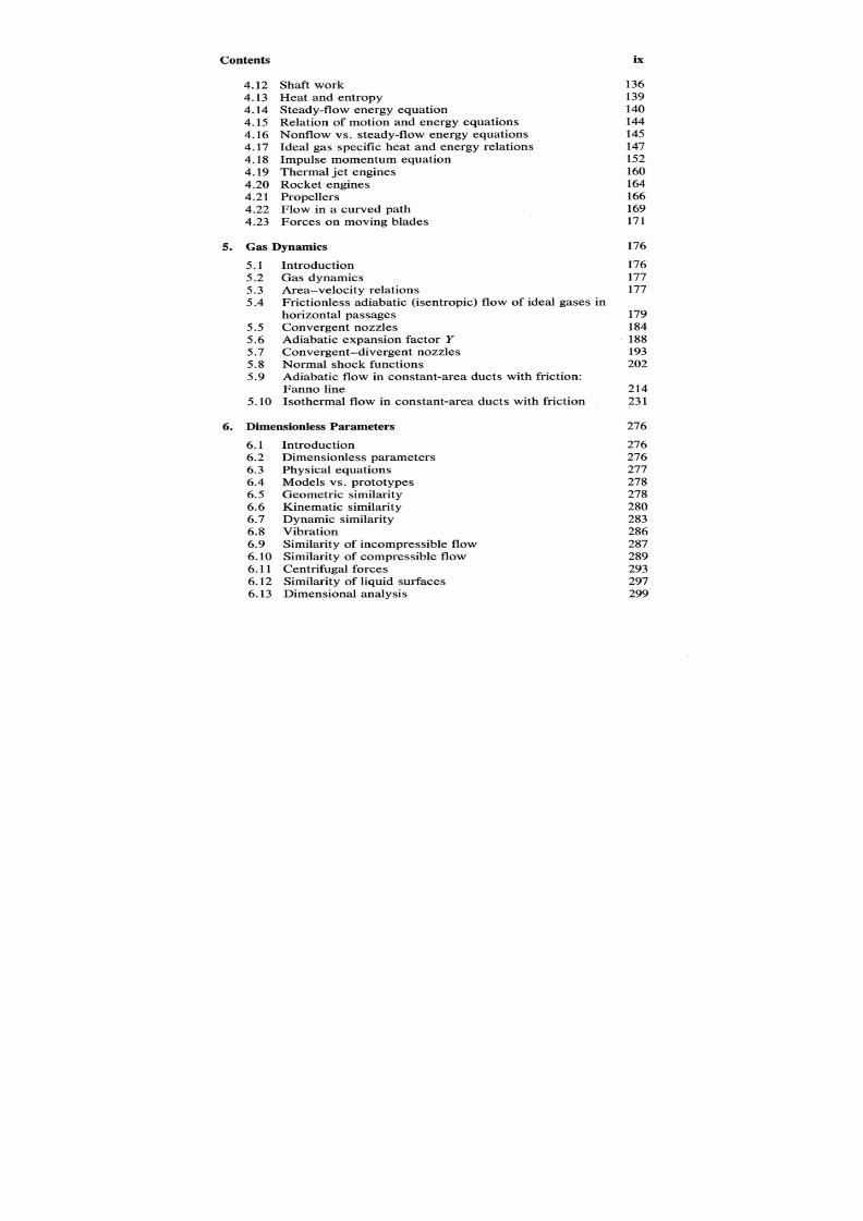
4.12
4.13
4.14
4.15
4.16
4.17
4.18
4.19
4.20
4.21
4.22
4.23
Shaft work
Heat and entropy
Steady-flow energy equation
Relation of motion and energy equations
Nonflow vs. steady-flow energy equations
Ideal gas specific heat and energy relations
Impulse momentum equation
Thermal jet engines
Rocket engines
Propellers
Flow in a curved path
Forces on moving blades
5. Gas
Dynamics
5.1
5.2
5.3
5.4
5.5
5.6
5.7
5.8
5.9
5.10
Introduction
Gas dynamics
Area-velocity relations
Frictionless adiabatic (isentropic) flowof ideal gases in
horizontal passages
Convergent nozzles
Adiabatic expansion factor Y
Convergent-divergent nozzles
Normal shock functions
Adiabatic flow in constant-area ducts with friction:
Fanno line
Isothermal flow in constant-area ducts with friction
6.
DimensionlessParameters
6.1
6.2
6.3
6.4
6.5
6.6
6.7
6.8
6.9
6.10
6.11
6.12
6.13
Introduction
Dimensionless parameters
Physical equations
Models vs. prototypes
Geometric similarity
Kinematic similarity
Dynamic similarity
Vibration
Similarity of incompressible flow
Similarity of compressible flow
Centrifugal forces
Similarity of liquid surfaces
Dimensional analysis
ix
136
139
140
144
145
147
152
160
164
166
169
171
176
176
177
177
179
184
188
193
202
214
23
1
276
276
276
277
278
278
280
283
286
287
289
293
297
299

7/21/2019 Fundamental Fluid Mechanics for Engineers
http://slidepdf.com/reader/full/fundamental-fluid-mechanics-for-engineers 17/438
X Contents
6.14 Lord Rayleigh’smethod
6.15 The Buckingham ll theorem
6.16 Parameters for fluid machinery
AppendixA.FluidProperties
Table A-l Critical and saturated properties of selected fluids
Table A-2 Properties of selected gases
Table A-3 Density and viscosity of steam and compressed water
Appendix B. Dimensions, Unit Systems, and Conversion Factors
B.1 Introduction
B.2ackground
B.3imensions
B.4
SI
Units
B.5 U. S.
Customary Units and relation to
SI
units
Table B-l Conversion factors
Appendix
C.
Properties
of
Areas, Pipes, and Tubing
Table C-l Properties of areas
Table C-2 Values of flow areas A and hydraulic radius
Rh
for
various cross sections
Table C-3 Properties of wrought steel and stainless steel pipe
Table C-4 Properties of 250 psi cast iron pipe
Table C-5 Properties of seamless copper water tube
Table C-6 Allowable stress values for selected piping materials
Index
300
302
306
317
318
340
369
373
373
373
375
376
380
382
389
390
393
394
404
405
408
409
7/21/2019 Fundamental Fluid Mechanics for Engineers
http://slidepdf.com/reader/full/fundamental-fluid-mechanics-for-engineers 18/438
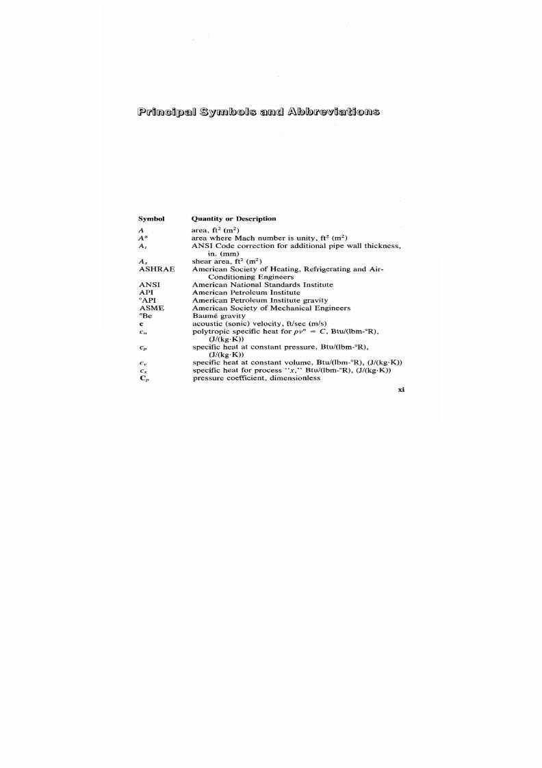
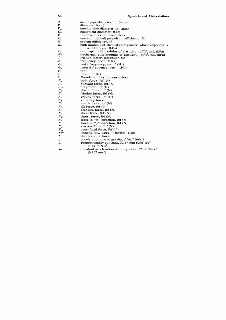
Symbol
A
A*
At
A S
ASHRAE
ANSI
API
"API
ASME
"Be
C
C n
CP
Quantity or Description
area, ft2 (m2)
area where Mach number is unity, ft2 (m2)
ANSI Code correction for additional pipe wall hickness,
in. (mm)
shear area, ft2 (m')
American Society of Heating, Refrigerating and Air-
American National Standards Institute
American Petroleum Institute
American Petroleum Institute gravity
American Society of Mechanical Engineers
Baume gravity
acoustic (sonic) velocity, ft/sec (m/s)
polytropic specific heat for
p v n
= C , Btu/(lbm-"R),
specific heat at constant pressure, Btu/(lbm-"R),
specific heat at constant volume, Btu/(lbm-"R), (J/(kg-K))
specific heat for process x, Btu/(lbm-"R), (J/(kg.K))
pressure coefficient, dimensionless
Conditioning Engineers
(J/(kg-K))
(J/(kg-K))
x i
7/21/2019 Fundamental Fluid Mechanics for Engineers
http://slidepdf.com/reader/full/fundamental-fluid-mechanics-for-engineers 19/438
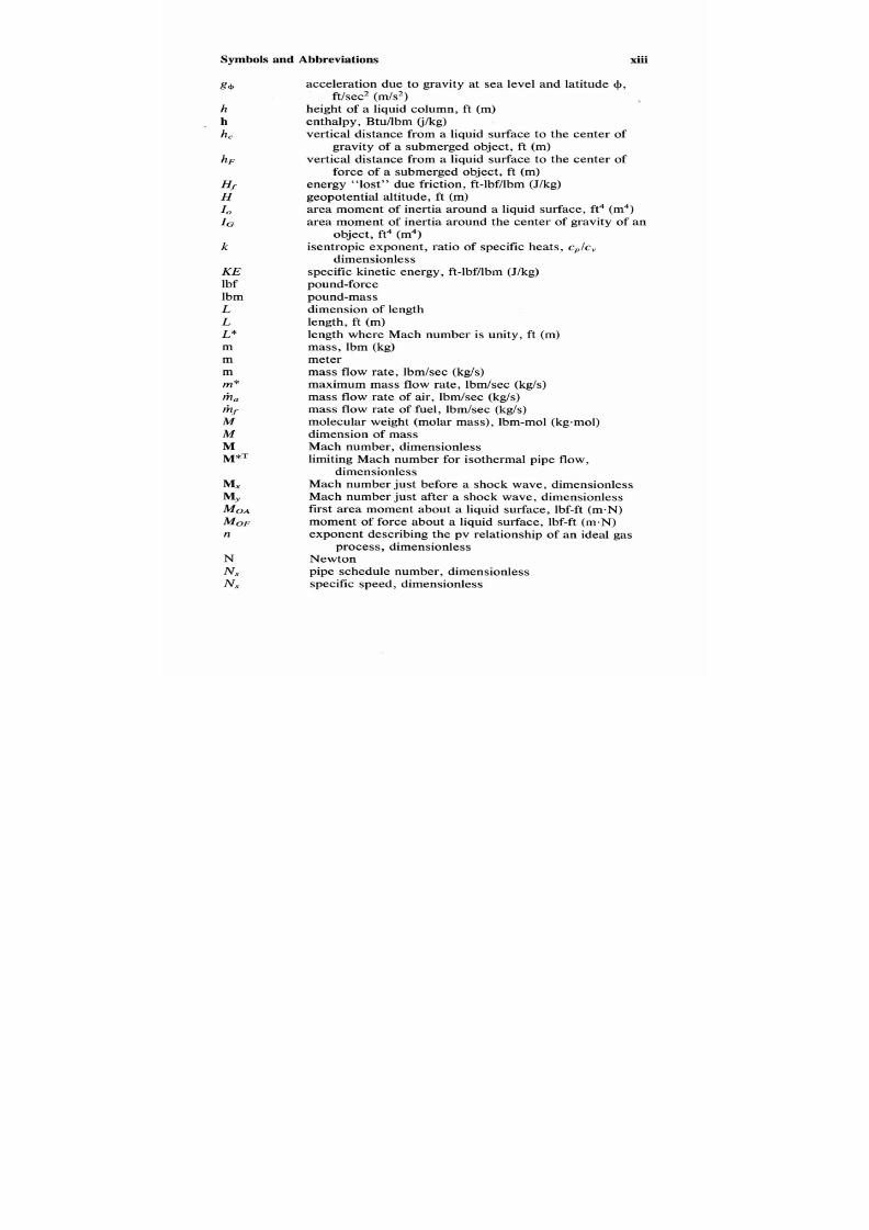
xii
Symbols and Abbreviations
go
inside pipe diameter, in.
(mm)
diameter, ft
(m)
outside pipe diameter, in.
(mm)
equivalent diameter, ft (m)
Euler number, dimensionless
maximum (ideal) propulsion efficiency, %
system efficiency,
%
bulk modulus of elasticity for process whose exponent is
isentropic bulk modulus of elasticity, lbf/ft2,psi, (kPa)
isothermal bulk modulus of elasticity, lbf/ft2,psi, (kPa)
friction factor, dimensionless
frequency, sec” (Hz)
wake frequency, sec” (Hz)
natural frequency, sec” (Hz)
foot
force, lbf (N)
Froude number, dimensionless
body force, lbf (N)
buoyant force, lbf
(N)
drag force, lbf (N)
elastic force, lbf (N)
friction force, lbf (N)
gravity force, lbf (N)
vibratory force
inertia force, lbf (N)
lift force, lbf (N)
pressure force, lbf
(N)
shear force, lbf (N)
thrust force, lbf (N)
force in “x” direction, lbf
(N)
force in “y” direction, lbf (N)
viscous force, lbf (N)
centrifugal force, lbf (N)
specific flow work, ft-lbf/lbm (J/kg)
dimension of force
acceleration due to gravity, ft/sec2
m/s2)
proportionality constant, 32.17 lbm-ft/lbf-sec2
standard acceleration due to gravity, 32.17 ftlsec’
n, bf/ft2, psi, (kPa)
(1
kgdN*s2)
(9.807 m/s2)
7/21/2019 Fundamental Fluid Mechanics for Engineers
http://slidepdf.com/reader/full/fundamental-fluid-mechanics-for-engineers 20/438
Symbols
g4
h
h
hc
hF
Hf
H
10
IC
k
K E
Ibf
Ibm
L
L
L*
m
m
m
m*
m,
m f
M
M
M
M*T
M,
MY
MOF
n
N
NS
Ns
M O A
acceleration due to gravity at sea level and latitude4,
height of a liquid column, ft (m)
enthalpy, Btu/lbm (j/kg)
vertical distance from a liquid surface to the center of
gravity of a submerged object, ft (m)
vertical distance from a liquid surface to the center of
force of
a
submerged object, ft (m)
energy “lost” due friction, ft-lbf/lbm (J/kg)
geopotential altitude, ft (m)
area moment of inertia around a liquid surface, ft4
(m4)
area moment of inertia around the center of gravity of an
isentropic exponent, ratio of specific heats, c&,
specific kinetic energy, ft-lbf/lbm (J/kg)
pound-force
pound-mass
dimension of length
length, ft
(m)
length where Mach number is unity, ft (m)
mass, lbm (kg)
meter
mass flow rate, Ibm/sec (kg/s)
maximum mass flow rate, lbm/sec (kg/s)
mass flow rate of air, lbm/sec (kg/s)
mass flow rate of fuel, lbm/sec (kg/s)
molecular weight (molar mass), Ibm-mol (kg-mol)
dimension of mass
Mach number, dimensionless
limiting Mach number for isothermal pipe flow,
Mach number just before a shock wave, dimensionless
Mach number just after a shock wave, dimensionless
first area moment about a liquid surface, Ibf-ft (m.N)
moment of force about a liquid surface, lbf-ft (m-N)
exponent describing the pv relationship of an ideal gas
Newton
pipe schedule number, dimensionless
specific speed, dimensionless
ft/sec2
m/s2)
object, ft4 (m4)
dimensionless
dimensionless
process, dimensionless

7/21/2019 Fundamental Fluid Mechanics for Engineers
http://slidepdf.com/reader/full/fundamental-fluid-mechanics-for-engineers 21/438
XiV Symbols and Abbreviations
NSPrJS
N S T U S
P
P*
Po
P o
Pr
Pv
Px
PY
PVr
psia
P a
P
-
pump specific speed U. S. units) rpm x g ~ m ’ ~ / f t ~ ’ ~
turbine specific speed (U. S . units) rpm x bh~’” l f t~’~
pressure, lbf/in.2, lbf/ft2 (kPa)
pressure where Mach number is unity, lbf/in.2, lbf/ft2
atmospheric (barometric) pressure, lbf/in.2, lbf/ft2 (kPa)
critical pressure of a substance, lbf/in.2, (kPa)
gage pressure, psig (kPa gage)
measured pressure, lbf/in.2, lbf/ft2 (kPa)
pressure at the inner wall of a curved pipe, lbf/in.2,
stagnation pressure, lbf/in.2, lbf/ft2 (kPa)
pressure at the outer wall of
a
curved pipe, lbf/in.2,
reduced pressure, p/pc. dimensionless
vapor pressure, psia (kPa)
pressure just before a shock wave, psia (kPa)
pressure just after
a
shock wave, psia (kPa)
reduced vapor pressure, p v / p c .dimensionless
absolute pressure, Ibf/in.2
gage pressure, lbf/in.*
difference between internal andexternal pressure,
lbf/in.2 (kPa)
shear perimeter, ft
(m)
power, ft-lbf/sec (W)
ideal power, ft-lbf/sec(W)
useful power, ft-lbf/sec
(W)
power supplied, ft-lbf/sec(W)
Pascal
specific potential energy, ft-lbfflbm (J/kg)
heat-transfer at constant pressure, Btuflbm (J/kg)
heat-transfer at constant volume, Btuflbm (J/kg)
heat-transfer, Btu/lbm (J/kg)
volume rate of flow, ft3/sec
(m3/$
radius, ft
(m)
mean radius of Earth, 20.86 X lo6 ft (6357 km)
inner internal radius of a curved pipe, ft
(m)
internal radius of a pipe, ft
(m)
outer internal radius of a curved pipe, ft (m)
gas constant, Btuflbm-”R, (J/kg.K)
hydraulic radius, ft
(m)
distance along the tube of an inclined manometer, ft (m)
( k W
lbf/ft2 (kPa)
lbf/ft2 (kPa)

7/21/2019 Fundamental Fluid Mechanics for Engineers
http://slidepdf.com/reader/full/fundamental-fluid-mechanics-for-engineers 22/438
Symbols and Abbreviations
xv
universal gas constant, 1545 Btuhbm-mol-"R
Reynolds number, dimensionless
second
entropy, Btuhbm-"R (J/kg.s)
maximum entropy change Eq. (5.81), Btuhbm-"R (J/kg.s)
entropy just before a shock wave, Btuhbm-"R (J/kg.s)
entropy just after a shock wave, Btuhbm-"R (J/kg.s)
second
specific gravity, dimensionless
Strouhal number, dimensionless
Systkme Internationale d'Unites
inclined manometer scale, ft (m)
kinematic viscosity-Saybolt Seconds Furol
kinematic viscosity-Saybolt Seconds Universal
scale reading on a cistern-type manometer, ft (m)
stress, lbf/in.' (kPa)
maximum allowable stress, lbf/in.' (kPa)
circumferential stress, lbf/in.' (kPa)
longitudinal stress, lbf/in.2 (kPa)
time, sec
(S)
measured temperature, "F, ("C)
Celsius scale temperature
Fahrenheit scale temperature
minimum pipe wall thickness, in. (mm)
schedule pipe wall thickness, in.
(mm)
pipe wall thickness,. in. (mm)
absolute temperature, "R
(K)
absolute temperature where Mach number is unity,
critical temperature of a substance, "R (K)
Kelvin scale temperature
reduced temperature,
TIT,
,dimensionless
Rankine scale temperature
stagnation temperature "R (K)
temperature just before a shock wave, "R (K)
temperature just after a shock wave, "R (K)
dimension of time
internal energy, Btuhbm (J/kg)
local velocity, ft/sec2 m/s2)
maximum local velocity, ft/sec2 (m/s2)
United States Customary Units
(8 314
J/kg.mol.K)
"R (K)

7/21/2019 Fundamental Fluid Mechanics for Engineers
http://slidepdf.com/reader/full/fundamental-fluid-mechanics-for-engineers 23/438
XVi
Symbols and Abbreviations
Y
Y
Y
Y C
YF
Y G
velocity, ft/sec (m/s)
acoustic velocity, ft/sec (m/s)
jet velocity, ft/sec (m/s)
vehicle velocity, ft/sec
(m/s)
velocity just before a shock wave, ft/sec (m/s)
velocity just after a shock wave, ft/sec (m/s)
velocity ratio, dimensionless
volume, ft3 (m3)
work ft-lbf (J)
nonflow shaft work, ft-lbfhbm (J/kg)
steady-flow shaft work, ftlbfhbm (J/kg)
Webber number, dimensionless
horizontal distance, ft
(m)
horizontal distance
to
center of gravity of an object as
vertical distance, in., ft
(m)
ANSI Code correction for material and temperature
linear distance from a liquid surface, ft
(m)
linear distance from a liquid surface to the center of
gravity of a plane submerged object, ft
(m)
linear distance from a liquid surface to the center of
force of a plane submerged object, ft (m)
vertical distance to center of gravity of an object as
shown in Table
C-l ,
ft
(m)
(page 390)
adiabatic expansion factor Y , ratio
elevation above a datum, ft (m)
compressibility factor, dimensionless
acceleration, ft/sec2 (m/s2)
kinetic energy correction factor, dimensionless
specific weight, lbf/ft3, N/m2)
angle O, radians
dynamic viscosity, lbf-seclft’ (Pa.$
kinematic viscosity, ft’hec, m’/s
density, lbm/ft3 (kg/m3)
density where Mach number isunity, lbm/ft3
(kg/m3)
stagnation density, Ibm/ft3 (kg/m3)
density just before a shock wave, lbm/ft3 (kg/m3)
density just after a shock wave, lbm/ft3kg/m3)
surface tension, lbf/ft
(N/m)
unit shear stress, lbf/ft’ (kPa)
acentric factor, dimensionless
angular velocity, radians/second
shown in Table
C-l ,
ft (m) (page 390)

7/21/2019 Fundamental Fluid Mechanics for Engineers
http://slidepdf.com/reader/full/fundamental-fluid-mechanics-for-engineers 24/438
1.1 INTRODUCTION
This chapter is concerned with establishing the basic definitions needed
for the study of fluid mechanics and its applications. Included are fluid
properties, units, gravity, Newton’s second law, and thermodynamic pro-
cesses.
The reader who needs only definitions
of
fluid properties sh,ould turn
to Table
1.1
at the end
of
the chapter. If only numerical values of fluid
properties are desired, then thischapter should be skipped and he reader
should go to Appendix A.
This chapter may be used s a text
for
tutorial
or
for refresher purposes.
Each concept is explained and derived mathematically as needed. The
minimum level of mathematics is used for derivations consistent with
academic integrity and clarity f concept. There are 17 examples of fully
solved problems.
1.2
FLUIDS AND OTHER SUBSTANCES
Substances may be classified by their response when at rest to the im-
position
of
a shear force. Consider the two very large lates, one moving,
1

7/21/2019 Fundamental Fluid Mechanics for Engineers
http://slidepdf.com/reader/full/fundamental-fluid-mechanics-for-engineers 25/438
2 Chapter 1
the other stationary, separated by a small distance y as shown in Figure
1.1.
The space between these plates is filled with substance whose sur-
faces adhere in such a manner that the upper surface of.the substance
moves at the same velocity as the upper plate and the bottom surface is
stationary. As
a
result of the imposition of the shear force
F,,
the upper
surface of the substance attains a velocity U.As y approaches d y , U
approaches dU and the rate of deformation of the substance becomes
dUldy . The unit shear stress T
= F,A,,
where
A ,
is the shear area. De-
formation characteristics of various substances are shown in Figure
l
.2.
An ideal or elastic solid will resist the shear force and its rate of de-
formation will be zero regardless of loading and hence is coincident with
the ordinate (vertical axis) of Figure
1.2.
A
plastic
will resist shear until its yield stress is attained, and then the
application of additional loading will cause it to deform continuously or
flow. If the deformation rate
is
directly proportional to the applied shear
stress less that required to start flow, then it is called an ideal plastic.
If the substance is unable to resist even the slightest amount of shear
force without flowing, then its called afluid. An idealfluidhas no internal
friction, and hence its deformation rate coincides with the abscissa (hor-
izontal axis) of Figure
1.2.
All real fluids have internal friction,
so
that
their rate of deformation is a function of the applied shear stress. If the
rate of deformation is proportional to the applied shear stress, then it is
called a Newtonian fluid,and if not, it is a non-Newtonian flu id.
Kinds of
Fluids
For the purposes of the application of fluid mechanics to design it is
convenient to consider two kinds of fluids: compressible and incompres-
U
Figure
1.1 How of a substance between parallel plates.
7/21/2019 Fundamental Fluid Mechanics for Engineers
http://slidepdf.com/reader/full/fundamental-fluid-mechanics-for-engineers 26/438
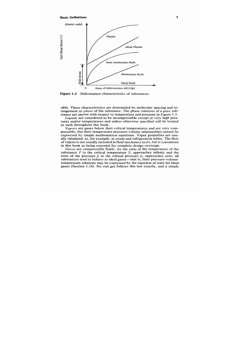
Basic Definitions
3
Elastic
solid
c
0
Rate
of
deformation
(dU/dy)
Figure
1.2
Deformation characteristics of substances.
sible. These characteristics are determined by molecular spacing and ar-
rangement or phase of the substance. The phase relationsof a pure sub-
stance are shown with espect to temperature andpressure in Figure 1.3.
Liquids
are considered to be incompressible exceptat very high pres-
sures and/or temperatures and unless otherwise specifiedwill be treated
as such throughout this book.
Vapors are gases below their critical temperatures and are very com-
pressible, but their temperature-pressure-volume relationships annot be
expressed by simple mathematical equations. Vapor properties are usu-
ally tabulated, as, for example, in steam and refrigeration tables.he flow
of vapors is not usually included in fluid mechanicsexts, but is considered
in this book as being essentiakfor complete design coverage.
Gases
are compressible fluids.
As
the ratio
of
the temperature of the
substance T to the critical temperature Tc approaches infinity and the
ratio of the pressure p to the critical pressure pc approaches zero, all
substances tend to behave as ideal gases-that is, their pressure-volume-
temperature relations may be expressed by the equation of state for ideal
gases (Section 1.14). No real gas follows this law exactly, and a simple

7/21/2019 Fundamental Fluid Mechanics for Engineers
http://slidepdf.com/reader/full/fundamental-fluid-mechanics-for-engineers 27/438
4
Chapter 1
Figure 1.3 Phase diagram of
a
pure substance.
non-ideal gas equation of state is also presented in Section
1.14.
Fluid
mechanics texts do not usually cover non-ideal gases, but non-ideal gases
are included in this book because theyre sometimes neededn the design
of fluid systems.
1.3 UNITS
For the foreseeable future designers in the United States will be faced
with the problems involved in converting fromts customary units
U.S.)
of measure to the Syst6me Internationale d’UnitesSI) units. During this
long period, which will probably span the professional life of those who
use this book, both systems will be employed. This makes it mandatory
that those engaged in design and application be proficient in the use of
both systems.
Both systems of units are used in this volume. Although equal weight
is given to each system, all basic physical constants and standards are
defined by international agreements in SI units. This sometimes results
in the use of precise but inexact values for physical constants and stan-
dards in U.S. units.
Appendix
C
explains the SI system of units in regard to fluid mechanics
and provides conversion factors. The U.S. system is not really system,
since its units are based on customary use. nsofar as practical, the units
used in this book are those traditionally used
in
mechanics, the foot (ft)

7/21/2019 Fundamental Fluid Mechanics for Engineers
http://slidepdf.com/reader/full/fundamental-fluid-mechanics-for-engineers 28/438
Basic
Definitions 5
for length, the second (sec) for time, and the pound-force (Ibf) for force.
Although the slug is the customary unit for mass
in
fluid mechanics, the
pound-mass (lbm) was chosen for the mass unit in because it is used in
general engineering practice.
This book follows the SI practice [l]* of leaving a space after each
group of three digits, counting from he decimal point. This is done with
metric units only, because in many countries a comma is used to signify
a decimal point.Thus
5,720,626 is
written 5
720 626
and
0.43875
is written
as 0.438 75. A four-digit number, for example, 5,280, is written either as
5 280 or 5280.
1.4
PRESSURE
Definition:
Force pernit area
Symbol: P
Dimensions: FL- or ML”T-2
Units: US.: bf/in.2,bf/ft2
SI:
N/m2 or Pa
Fluid for ces
that can act on a substance are
shear, tension,
and
compres-
sion. By definition, fluids in
a
static state cannot resist any shear force
without flowing. Fluids willsupport small tensile orces due to the prop-
erty of surface tension (Section 1.17). Fluids can withstand compression
forces, commonly called pressure.
Atmospheric Pressure
The
actual
atmospheric pressure is the weight per unit area of the air
above a datum and varies with weather conditions. Since thisressure is
usually measured with a barometer, it is commonly called barometric
pressure.
Standard Atmospheric Pressure
By international agreement the standard atmospheric pressure is defined
as
101.325
kN/m2 (kPa). Converting this value into common units, we
have 14.696 lbf/in.2 and29.92 in. of mercury at 32°F. For most practical
purposes 14.70 lbf/in.2 may be used for atmospheric pressure.
*
Num bers in brackets are those
of
references at the end of this chapter.

7/21/2019 Fundamental Fluid Mechanics for Engineers
http://slidepdf.com/reader/full/fundamental-fluid-mechanics-for-engineers 29/438
6
Chapter 1
P
Gdge
Actualtmosphericressure
AbsoluteNegatfve Gauge)
Vacuum
Atmospheric
+
bsolute
v b
Figure 1.4
Pressure relations.
Observed
Pressures
Most pressure-sensing devices (Section2.5) (the barometer is an excep-
tion) indicate the difference between the pressure to be measured and
atmospheric pressure. As shown in Figure
1.4,
if the pressure being sensed
is greater than atmospheric it is called gage pressure, and if lower (neg-
ative gage) it is called a
vacuum.
The algebraic sum of the instrument
reading and the actual atmospheric pressure is the true or absolute pres-
sure. Thus:
where p is the absolute pressure,
P b
the atmospheric (barometric) pres-
sure, and p i the instrument reading (positivefor gage pressure, negative
for vacuum).
All
instrument readings must e con verted to abso lute pres -
sure before they are used in calculations.
Conventional American engineeringpractice is to use the unit lbf/in.*
(psi) for pressure. Gage pressures are indicated by psig and bsolute pres-
sures by psia. Vacuums are almost always reported n inches of mercury
at 32°F. There is no equivalentof gage pressure in the SI system, so.that
all pressures are absolute unless gage is specified.
Example 1.1 During the test of a steam turbine the observed vacuum in
the condenser was 27.56 in. (700 mm) of mercury at 32°F (OOC) and the
actual atmospheric pressure was 14.89 psia (102.7 kPa). What was the
absolute pressure in the condenser?
7/21/2019 Fundamental Fluid Mechanics for Engineers
http://slidepdf.com/reader/full/fundamental-fluid-mechanics-for-engineers 30/438
Basic Definitions 7
Solution
Since the vacuum is given in units of the height of a liquid column and
the atmospheric pressure in units f force per unit area, the vacuum should
be converted to force per unit area units using conversion factors from
Appendix B. Equation (1.1) should then be applied noting hat a vacuum
is a negative gage.
US. nits
pi = (-27.56) x (4.912 x 10") = - 3.54 psig
p
=
14.89
+
( -
13.54)
=
1.35
psia
SI Units
p i =
(-700) X 133.32
=
-93 324
Pa =
-93.3
kPa
p =
102.7
-
93.3
=
9.4
kPa
1.5
TEMPERATURE SCALES
Unlike the other properties discussed in this book, temperature is based
on a thermodynamic concept that is independent
f
the physical properties
of any substance. The thermodynamic temperature can be shown to be
related to the equation of state of an ideal gas (Section 1.14). The ther-
modynamic temperature is called an
absolute temperature
because its
datum is absolute zero. The thermodynamic temperature scale has little
practical value unless numbers can be assigned to the temperatures at
which real substances freeze or boil
so
that temperature sensing devices
may be calibrated. The International Practical Temperature Scale is a
document which defines and assigns numbers to fixed points (freezing,
tiiple, and/or boiling) of selected substances and prescribes methods and
instruments for interpolating between fixed points. Although the Inter-
national Practical Scale is dependent on the physical properties of sub-
stances, it attempts to reproduce the thermodynamic temperature scale
within the knowledge of the state of the art. For a detailed explanation
of the International Practical Scale, reference [2] by R. P. Benedict
is
recommended.
The Fahrenheit temperature scale is used in the United States for or-
dinary temperature measurements. It was invented in
1702
by Daniel Ga-
briel Fahrenheit
(1686-1736),
a German physicist. On this scale water
freezes (ice point) at
32°F
and boils at
212°F
(steam point) and standard
atmospheric pressure.

7/21/2019 Fundamental Fluid Mechanics for Engineers
http://slidepdf.com/reader/full/fundamental-fluid-mechanics-for-engineers 31/438
8
Chapter
1
Figure
1.5 Temperature scales.
The Celsius temperature scale
formerly centigrade) wasirst proposed
in
1742
by Anders Celsius
(1701-1742),
a Swedish astronomer. On the
Celsius scale the ice point is
0°C
and the steam point
100°C.
The Kelvin temperature scale s named in honor f the English scientist
Lord Kelvin (William Thompson,
1826-1907)
and is the absolute Celsius
scale. The kelvin (K with no degree sign) is defined as the SI unit
of
temperature as
1/273.16of
the fraction of the thermodynamic temperature
of
the triple point of water. The International Practical Temperature Scale
assigns
a
value of
0.01"C
to the triple point of water.
The Rankine temperature scale is named in honor of the Scottish en-
gineer William J . Rankine
(1820-1872)
and is the absolute Fahrenheit
scale.
Temperature scale relations are shown in Figure
1.5.
The Celsius scale
has 100 degrees between he ice and steam points andhe Fahrenheit
180.
The relation between the scales may be shown as AtF/Atc =
180/100
=
1.8,
where tF is the Fahrenheit temperature and tc is the Celsius. At the
ice point tF
=
32°F and
tc
= O"C, so that
tFF -
32
A t cc -
0
-
-
1.8
Solving first for tF and then for t c ,
tF =
1.8tc + 32

7/21/2019 Fundamental Fluid Mechanics for Engineers
http://slidepdf.com/reader/full/fundamental-fluid-mechanics-for-engineers 32/438
Basic Definitions
9
and
The triple point of water on the Celsius scale is fixed at O.Ol"C, and
on the Kelvin 273.16 K, so that TK = tc
+
(273.16 - 0.01) or
TK
=
tc + 273.151.4)
where TK is the absolute temperature in kelvins.
Because the Kelvin and Rankine scales are the absolute scales
of
the
Celsius and Fahrenheit scales, respectively, with the same differences
between the steam and ice points, we can write &/At, =
ATRIATK
=
1.8, where TR is the temperature in degrees Rankine. Since both are to
absolute zero,
TR = 1.8TK (1.5)
From the above, the following relations can be derived:
TR =
tF
459.671.6)
and
TR 1.8tc
+
491.67
For most engineering calculations:
TK
= tc + 273
and
TR
= tF +
460
Example 1.2 Convert 45°F to (a) degrees Rankine, (b) degrees Celsius,
and
( c )
kelvins.
Solution
For engineering accuracy apply equations (1.9) o convert to Rankine,
(1.3) o Celsius, and (1.8) o kelvins.
US. nits
TR = 45
+
460 = 505"R
SI Units
tc
= (45
-
32)/1.8= 7.22 C
TK =
7 +
273 = 280 K
7/21/2019 Fundamental Fluid Mechanics for Engineers
http://slidepdf.com/reader/full/fundamental-fluid-mechanics-for-engineers 33/438
10 Chapter 1
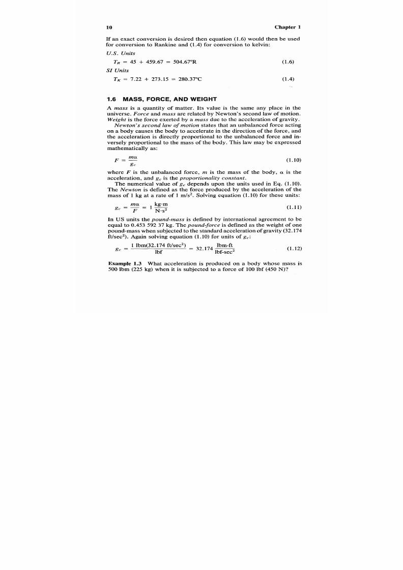
If an exact conversion is desired then equation (1.6) would then be used
for conversion to Rankine and (1.4) for conversion to kelvin:
U.S.
Units
TR = 45
+
459.67 = 504.67”R (1.6)
SI
Units
TK = 7.22 3- 273.15 = 280.37”C (1.4)
1.6
MASS,
FORCE,
AND
WEIGHT
A muss is a quantity of matter. Its value is the same any place in the
universe.
Force
and muss are related by Newton’s second lawf motion.
Weight is the force exerted by a mass due to the acceleration f gravity.
Newton’s second law ofmot ion states that an unbalanced force acting
on a body causes the body to accelerate in the direction of the force, and
the acceleration is directly proportional to the unbalanced force and in-
versely proportional to the mass of the body. This law may be expressed
mathematically as:
ma
gc
F = -
(1.10)
where
F
is the unbalanced force, m is the mass of the body,
c x
is the
acceleration, and
g,
is the proportionality constant.
The numerical value of gc depends upon the units used in Eq. (1.10).
The Newton is defined as the force produced by the acceleration of the
mass of 1 kg at a rate of 1 S’. Solving equation(1.10) for these units:
m a kg-m
g ,= ” =1 -
F
N*s’
(1.11)
In US units the pound-muss is defined by international agreement o be
equal to 0.453 592 37 kg. The pound-force is defined as the weight of one
pound-mass when subjectedo the standard acceleration f gravity (32.174
ft/sec*). Again solving equation
(1.10) for units of g,:
1 lbm(32.174t/sec’)bm-ft
lbf-sec’
,
=
lbf
=
32.174
(1.12)
Example
1.3
What acceleration is produced on a body whose mass is
500
lbm (225 kg) when it is subjected o a force of 100 lbf (450
N)?

7/21/2019 Fundamental Fluid Mechanics for Engineers
http://slidepdf.com/reader/full/fundamental-fluid-mechanics-for-engineers 34/438
Basic
11
Solution
Rearranging equation (1.10) o solve for acceleration results in:
a = F g J m
(1.10)
U . S .
Units
a
= 100 x 32.1741500
=
6.435ft/sec’
S I
Units
=
450 X
11225
= 2 m/s2
1.7
GRAVITY
The standard acceleration due to gravity of the earth is fixed as
g , =
9.806 65
m / s 2
by international agreement. For engineering calculations:
g ,
=
32.17 ft/sec2
=
9.807/s21.13)
Standard gravity occurs at a atitude of
4
= 45’32’33”. For other latitudes
at sea level the acceleration due to gravity, g+ may be calculated from:
g+ g,(l
-
0.0026373
COS
2+ + 5.9
X COS’
24) (1.14)
Variation of gravity at sea level is less than0.30%
so
that unless extreme
accuracy is required he assumption that
g4 = g ,
is good enough or most
engineering purposes. For elevations above sea level, gravity must be
estimated using:
(1.15)
where
re
is the mean radius of Earth, 20.86 x lo6 ft (6 357 km), and z is
the elevation above sea level.
Example 1.4
Estimate the acceleration due to Earth’s gravity on a sat-
ellite orbiting at 100 miles (161
km)
above sea level.
Solution
This example is solved using equation1.15) assuming , = g + , and noting
that
U.S.
units must be converted to feet:

7/21/2019 Fundamental Fluid Mechanics for Engineers
http://slidepdf.com/reader/full/fundamental-fluid-mechanics-for-engineers 35/438
12
US. nits
Chapter
1
32.17
x
(20.86
x
g = (20.86 x lo6 + 100 x 5280)2
=
30.60
ft/sec2
SI
Units
9.807
x
6 3572
g
=
(6 357 + 161)2
(1.15)
= 9.329 m / s 2 (1.15)
1.8
APPLICATIONS
OF
NEWTON’S SECOND LAW
Newton’s second law may
be used to establish the relationship between
(a) force, mass, and acceleration, (b) work and energy, and/or impulse
and momentum. Force, mass, and acceleration relationships wereestab-
lished in Section
1.6
by equation
(1.10).
Work
and Energy
Work
is defined
as
the amount of
energy
required to exert a constant force
on
a
body which moves through a distance in the same direction as the
applied force,
or
work = force
X
distance
Mathematically,
W = L F d x
(1.16)
where W is the work, and F is the applied force through the distance dx.
Substituting equation
(1.10)
for force in equation
(1.16),
(1.17)
Potential Energy
Potential energy
is defined as the energy required to lift a body to .its
present height from some datum. Substituting PE (specific potential en-
ergy) for W l m ,g fora, nd dz (elevation change)or dx in equation (1.17),
(1.18)

7/21/2019 Fundamental Fluid Mechanics for Engineers
http://slidepdf.com/reader/full/fundamental-fluid-mechanics-for-engineers 36/438
Basic Definitions
13
For
a
field of constant gravity equation (1.18) integrates to:
PE
=
-
z
8 c
(1.19)
If the gravity field is not constant, then equation (1.15) is substituted for
g in equation (1.18),
(l 20)
Example 1.5
A Boeing 727 et aircraft has a mass of 145,000 lbm ( 6 4 400
kg) and is flying at an altitude of 33,000 ft (10 km) above sea level. Cal-
culate the potential energy of the aircraft, assuming (a) constant gravity
and (b) variation of gravity with elevation. (c) Compare esults.
Solution
The specific potential energy for part (a) is calculated using equation
(1.19), and equation (1.20) for part (b). The total energy is calculated in
each
case
by multiplying the specific potential energy byhe mass
of
the
aircraft. The difference in results may be calculated from the following:
A% = 100(PEa - PEb)/PE, (x)
U . S . Units
1.
PE
= (32.17/32.17)(33,000)1.19)
= 33,000 ft-lbf/lbm
mPE = 145,000 X 33,000 = 4.785 X lo9 ft-lbf
2. PE = 32.17 x 33,000/(32.17)(1
+
33,000/20.86 x lo6))
= 32,948t-lbf/lbm0)
mPE
=
145,000 X 32,948
=
4.777 X lo9ft-lbf
3.
Difference between
1
and 2
A = 100(33,000 - 32,948)/33,000 = 0.16%
S I
Units
1. PE = (9.807/1)(10 OOO
= 98.07 kJkg
mPE = 6 4 400 X 98.07 = 6 316 MJ
(x)
(1.19)
7/21/2019 Fundamental Fluid Mechanics for Engineers
http://slidepdf.com/reader/full/fundamental-fluid-mechanics-for-engineers 37/438
14
2. PE = 9.807 x 10OOO/l X (1
+
10/6 57)
= 97.92 kJkg
mPE
+
6 4
400 X 9792 = 6 306 MJ
3.
Differencebetween 1 and 2
A = lOO(98.07
-
97.92)/98.07 = 0.15%
Chapter
1
(1.20)
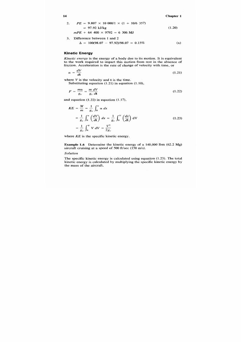
Kinetic Energy
Kinetic energy
is the energy of
a
body due to its motion. It is equivalent
to the work required to impart this motion from rest in the absence of
friction. Acceleration is the rate of change of velocity with time, or
dV
dt
a = -
where V is the velocity and
t
is the time.
Substituting equation (1.21) in equation (l.lO),
and equation
( l 22)
in equation
( l .17),
KE = - - l a d .
1
m
gc
(1.21)
(1.22)
(1.23)
where
KE
is the specific kinetic energy.
Example 1.6 Determine the kinetic energy of a 140,000 lbm (62.2 Mg)
hircraft cruising at a speed of
500
ft/sec
(150
ds).
Solution
The specific kinetic energy is calculated using equation
1.23).
The total
kinetic energy is calculated by multiplying the specific kinetic energy by
the mass of the aircraft.

7/21/2019 Fundamental Fluid Mechanics for Engineers
http://slidepdf.com/reader/full/fundamental-fluid-mechanics-for-engineers 38/438
Basic Definitions
15
U . S .
Units
K E
=
5002/2
x
32.17
=
3886
ft-lbf/lbm
m K E = 140,000 x 3886 =
544.0
x lo6 ft-lbf
SI Units
K E
= 1502/2 X
1 = 1 1
250
Jkg
m K E =
62 600
x
1 1 250
=
704.3
MJ
(1.23)
(1.23)
Impulse and Momentum
Equation (1.22) may be written in the following form:
m dV
F d t =
gc
The impulse of a force is the integral of the left-hand sideof this equation:
Impulse of a force = J]:t (1.24)
For a constant force applied between
tl
and
t 2 ,
Impulse
of
a force = J]:dt = F J]:t = F ( t z
-
t , ) (1.25)
Momentum is the product of mass times velocity and may be obtained
by integrating the right-hand side of equation (1.22):
Momentum change
= - Jvy dV
=
m(V2 - V , )
gcc
Equating equations (1.25) and (1.26),
(1.26)
(1.27)
or
Impulse
of
a force = momentum change
For constant mass and force between t l and t2 equation (1.27) may be
written in the following form:
(1.28)
where ri? is the mass flow rate.

7/21/2019 Fundamental Fluid Mechanics for Engineers
http://slidepdf.com/reader/full/fundamental-fluid-mechanics-for-engineers 39/438
16 Chapter 1
Example
1.7
Compute the thrust (force) produced when 20 lbdsec (9
kg/s) of fluid flows through a jet propulsion system if its inlet velocity is
100
ft/sec
(30
d s )
and its exit velocity is
400
ft/sec
(120
ds).
Solution
This example is solved using equation 1.28).
US.
nits
F = 20(400
-
100)/32;17 = 186.5 lbf
SI Units
F =
9(120
-
30)/1 = 810 N
(1.28)
(1.28)
1.9 DENSITY
Definition:
Mass per unit volume
Symbol:
p rho)
Dimensions: M L - 3 or F p L - 4
Units:
U.S.: lbdft’ SI: kg/m3
Density is mass per unit volume and its numerical value is the same
any place in the universe because (Section 1.6) it represents
a
quantity
of matter.
1.10 SPECIFIC WEIGHT
Definition:
Weight (force) per unit volume
Symbol: Y (gamma)
Dimensions:
F L P 3
or
ML-’T-=
Units:
U.S.:
lbf/ft3 SI: N/m3
Specific weight s the weight or force (F,) exerted by mass of substance
per unit volume (density) due o the local acceleration of gravity. Unlike
density, the numerical value of specific weight varies with local gravity.
Equation (1.10) related force to mass, and since both density and spe-
cific weight have the same volume (V) units:
(1.29)
Example 1.8 A
liquid has a density of 50 bdft’ (800 kg/m3). Compute
its specific weight in a space station where the gravity is 16 ft/sec3 (5
ds’) .
7/21/2019 Fundamental Fluid Mechanics for Engineers
http://slidepdf.com/reader/full/fundamental-fluid-mechanics-for-engineers 40/438
Basic Definitions
17
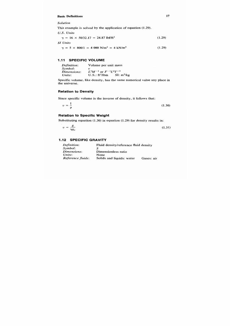
Solution
This example is solved by the application of equation
(1.29).
US.
nits
Y = 16 x 50132.17 = 24.87 Ibf/ft3
SI Units
y
= 5
X
800/1 = 4 O00 N/m3 = 4 kN/m3
(1.29)
(1.29)
1.l
SPECIFIC VOLUME
Definition:
Volume per unit mass
Symbol:
V
Dimensions:
L3M” or
F”L4T-2
Units:
U.S.:
ft3/lbm
SI:
m3/kg
Specific volume, likedensity, has the same numerical value any place n
the universe.
Relation to Density
Since specific volume is he inverse of density, it follows that:
1
P
v = -
(1.30)
Relation to Specific Weight
Substituting equation (1.30) in equation (1.29) for density results
in:
1.12
SPECIFIC
GRAVITY
(1.31)
Definition:
Fluid densitylreference fluid density
Symbol:
S
Dimensions:
Dimensionless ratio
Units:
None
Referencefluids:
Solidsandiquids: water Gases: air

7/21/2019 Fundamental Fluid Mechanics for Engineers
http://slidepdf.com/reader/full/fundamental-fluid-mechanics-for-engineers 41/438
18
Chapter 1
Specific Gravity of Liquids
Since the density of liquids varies withemperature and at high pressures
with pressure, for a precise definition of the specific gravity of a liquid,
the temperatures and pressures of the liquid and water should be stated.
In actual practice two temperatures are stated, for example,
60/60"F
(15.56/15.56"C),where the upper temperature pertains to the fluid and the
lower to water. The density of water at 60°F (15.56"C) is 62.37 lbm/ft3
(999.1 kg/m3). If no temperatures are stated it should be assumed that
reference is made to water at its maximum density. Themaximum density
of water at atmospheric pressure is at 39.16"F (3.98"C)and has a value
of
62.43
lbm/ft3
(1000.0
kg/m3). Based on the above, the specific gravity
of liquids can be computed using:
&*W
= -
f
P w
(1.32)
where pfis the density of the fluid at temperature rfand
pw
is the density
of water at temperature tw.
Specffic Gravity of Gases
For gases it is common American engineering practiceo use the ratio of
molecular weight (molar mass) of the gas to that of air (28.9644), thus
eliminating the necessity of stating the pressures and temperatures for
ideal gases.
Hydrometer Scale Conversions
In certain fields
of
industry hydrometer scalesre used that have rbitrary
graduations. In the petroleum and chemical industries, the Baume ("Be)
and the American Petroleum Institute ("API) are used. Conversions are
as follows
Baume
Scale
Heavier than water:
145
145 -
"Be
60tWF (15.56t15.56'C)
=
Lighter than water:
140
130 + "Be
60/60°F
15.56t15.56'C)
=
(1.33)
(1.34)

7/21/2019 Fundamental Fluid Mechanics for Engineers
http://slidepdf.com/reader/full/fundamental-fluid-mechanics-for-engineers 42/438
Basic Definitions
19
American Petroleum nstitute Scale
141.5
131.5 + "API
aO/WF
(15.5f315.56 C)
=
(1.35)
The BaumC scale for liquids lighter than water is very nearlyhe same
as the American Petroleum Institute Scale, both being 10"for a specific
gravity of unity. The use of the American Petroleum Institute (API) scale
is recommended by the American National Standards Institute (ANSI).
Standardized hydrometers are available
in
various ranges from - 1"API
to 101"API for specificgravityranges of
1.0843
to
0.6068
at
60/60"F
(15.56/15.56"C).
For detailsconcerningstandardizedhydrometers the
ASTM standard [3] should be consulted.
Example 1.9 A liquid has a density of 55 lbm/ft3
(879
kg/m3) at
60°F
(1536°C). Calculate (a) its American PetroleumInstitute gravity, and (b)
its BaumC gravity.
Solution
1.
The specific gravity s calculated using equation
(1.32)
noting that the
density of water at
60°F (1536°C)
is
62.37
lbm/ft3
(999.1
kg/m3).
2.
For Part
(a)
solve equation
(1.35)
for "API:
"API = 141.5/Sr/t
-
131.5 (1.35)
3.
Since by inspection it is obvious that the liquid is lighter than water,
equation (1.34) is solved for "Be:
"Be =
140/Sr/t
-
130 (1.34)
US. nits
(1) S ~ O / ~ * F5Y62.37 = 0.8818 (1.32)
(2)
(a) "API =
141.5/0.8818
-
131.5
=
29.0 (1.34)
(3) (b) "Be
=
140/0.8818
-
130
= 28.8 (1.32)
SI
Units
(1)
S15.5f315.5aoc =
8811999.1 = 0.8818 (1.32)
(2) (a)
"API
=
14130.8818
-
131.5 (1.32)
=
29.0

7/21/2019 Fundamental Fluid Mechanics for Engineers
http://slidepdf.com/reader/full/fundamental-fluid-mechanics-for-engineers 43/438
20
(3) (b) "Be = 140/0.8818 - 130
=
28.8
Chapter 1
(1.34)
1.13 IDEAL GAS PROCESSES
The state of a substance is the condition of its existence and is determined
by any two independent properties. Consider the p-v diagram shown in
Figure 1.6. In this case state point
1
is determined by p1 and v l . f one
or more properties are changed, the fluid is said to have undergone
a
process. If, for example, the pressure in Figure 1.6 is changed from p1
to
p2
the resulting specific volumes
v2.
The manner in which this change
takes place determines the path of the process. If the fluid can be made
to return to its original state by exactly returning ts path then he process
is said to be reversible.
A
reversible process is frictionless and cannot
occur in nature, so that reversible processes serve as ideals.
Polytropic Process
All ideal gas processes are
polytropic
processes, and the processes dis-
cussed below are all special cases of the polytropic. For an ideal gas the
relation between pressure and specific volume is given by:
pv = c (1.36)
P
P1
P2
Figure 1.6 Process diagram.

7/21/2019 Fundamental Fluid Mechanics for Engineers
http://slidepdf.com/reader/full/fundamental-fluid-mechanics-for-engineers 44/438
Basic
If
equation
(1.36)
is written in logarithmic form (log, + n log,
v
= log,
c) and differentiated,
dp ndv
v
dP
- + - = O or
n = - -
P
dv
V
(1.37)
Equation
(1.37)
indicates that n is the slopeof thep-v curve and establishes
the pressure-specific volume relationship or the process. The value
of
n
for a polytropic process ranges from
+ W
to
-W,
depending upon the
nature of the process.
Isentropic Process
If a process takes place without heat transfer and is reversible (friction-
less) then it follows a path of constant entropy ( S ) , and hence it is called
isentropic. This same process is also called a reversible adiabatic and
sometimes (incorrectly) an adiabatic process. The path of this process is
given by:
(S
= c ) pv = pvk = c
(1.38)
where
k
is the isentropic exponent ( k = c,/c,), c, is the specific heat at
constant pressure, and
c,
is the specific heat at constant volume.
Isothermal Process
If a process takes place at constant temperature it is called an isothermal
process. From the equation of state for an ideal gas,p v =
RT
[equation
(1.42),
Section
1.141.
Differentiating equation
(1.42)
for
T
= c , we have
d ( p v ) =
0 or
v dp = - p d v ; substituting this relation in equation
(1.37),
(1.39)
Isobaric Process
If a Process takes place at constant pressure it is called an isobaric pro-
cess. For
a
constant pressure process,
dp
=
0,
and substituting this re-
lation in equation
(1.37),
(1.40)

7/21/2019 Fundamental Fluid Mechanics for Engineers
http://slidepdf.com/reader/full/fundamental-fluid-mechanics-for-engineers 45/438
22
Chapter 1
Isometric Process
If
a
process takes place at constant volume it is called an isometric pro-
cess. The path of this process is given by:
(1.41)
Example
1.10 In an ideal gas reversible process the pressure at initial
state was 50 psia (345 kPa) and the specific volume is 400 ft3/lbm (25
m3/kg). The pressure at the final state was 125 psia
(860
kPa) and he final
specific volume
200
ft3/lbm
(12.5
m3kg). Compute the value of the ex-
ponent
of
the process path pv".
Solution
Equation (1.36)may be written in logarithmic form as follows:
log,(pd
+
n log,(vd = log,(pz) +
n
log,(v2) (x)
Solving equation (x) for n:
U . S .
Units
n = log,(50/125)/log,(200/400) = 1.32
S I Units
n
= log,(345/860)/log,(12.5/25) = 1.32
1.14 EQUATIONS
OF
STATE
An equation of state is one that defines the relationships of pressure-
temperature and volume. Reid et al. [4] resent and evaluate a number
of proposed equations of state and provide an excellent sourceof infor-
mation on this subject.
Equation of State
for
an Ideal Gas
An ideal gas is one that obeys the equation of state (1.42) nd whose
internal energy is a function of temperature. The equation of state for an
ideal gas is
pv = RT (1.42)
7/21/2019 Fundamental Fluid Mechanics for Engineers
http://slidepdf.com/reader/full/fundamental-fluid-mechanics-for-engineers 46/438
Basic
23
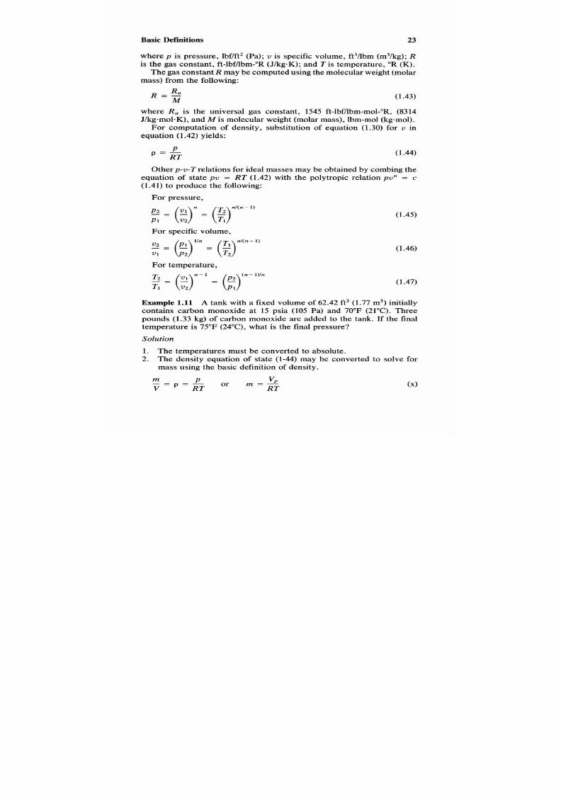
where p is pressure, lbf/ft2 (Pa); v is specific volume, ft3/lbm (m3/kg);
is the gas constant, ft-lbf/lbm-"R (J/kg*K);and Tis temperature, "R (K).
The gas constantR may becomputed using he molecular weight (molar
mass) from the following:
(1.43)
where R , is the universalgas constant, 1545 ft-lbf/lbm-mol-"R, (8314
J/kgmol.K), and M s molecular weight (molarmass), lbm-mol (kg-mol).
For computation of density, substitution of equation
(1.30)
for
v
in
equation
(1.42)
yields:
P
P = @
Otherp-v-T relations for ideal massesmay be obtained by combing he
equation of state p v
=
RT (1.42) with the polytropic relation pv
=
c
(1.41)
to produce the following:
For pressure,
For specific volume,
For temperature,
Tz
n - 1
(n-
I)/n
(1.45)
(1.46)
(1.47)
Example
1.11 A tank with a fixed volume of 62.42 ft3 (1.77 m3) initially
contains carbon monoxide at
15
psia (105 Pa) and
70°F (21°C).
Three
pounds (1.33 kg) of carbon monoxide are added to the tank. If the final
temperature is
75°F (24 C),
what is the final pressure?
Solution
1.
The temperatures must be converted to absolute.
2. The density equation of state (1-44) may be converted to solve for
mass using the basic definition of density.
m
V - p = -
or
m = -
v,
RT

7/21/2019 Fundamental Fluid Mechanics for Engineers
http://slidepdf.com/reader/full/fundamental-fluid-mechanics-for-engineers 47/438
2 4 Chapter 1
3.
Applying the principle of conservation of mass:
Final mass
=
initial mass
+
mass added
US.
nits
From Table
A-l
and equation
(1.43),
R
=
154Y28.010
=
55.16
ft-lbf/lbm-
"R
for
CO:
Ti =
70 + 460
=
530"R
Tf=75
+ 460
=
535"R
p i =
144
X
15
=
2160
Ibf/ft2
(1.9)
p f 535 X (21601530 + 55.16 X 3/62.42)
=
3598
lbf/ft2 =
3598/144
=
24.99
psia
SI Units
From Table A-l and equation
(1.43),
R =
8 314/28.010
=
296.8 J/kg.K
for CO:
Ti
=
21
+
273
=
294 K
Tf
= 24 + 273
=
297 (1.8)
pi =
105
X
1000
=
105 000
Pa
p f =
297(105000/294
+
296.8 X 1.3311.77)
=
172308
Pa
=
172.3
MPa
Equation of State
for
a Real Gas
The equation of state of an ideal gas
(1.42)
may be modified for a real
gas as follows:
p v
=
ZRT or Z =
V
RT
(1.48)
where Z is the compressibility factor.Note that when Z is unity the sub-
stance is in the ideal gas state. Thus the deviation of the compressibility
factor from unity is a measure of non-idealness of the state of the sub-
stance.

7/21/2019 Fundamental Fluid Mechanics for Engineers
http://slidepdf.com/reader/full/fundamental-fluid-mechanics-for-engineers 48/438
Basic Definitions
25
Principle of Corresponding States
The principle of corresponding states assumes that all substances obey
the same equation of state expressed in terms of critical properties. Con-
sider the phase diagram
of
Figure 1.3. If the pressure were divided by
the critical pressure and the temperature by the critical temperature and
the data replotted, then we would have a dimensionless diagram where
the critical point C would be unity. The pressure would then be stated
as:
P
p
= -
p c
(1.49)
and the temperature as:
T
Tc
T,
=
-
( 1 SO )
where P , is the reduced pressure and T, the reduced temperature.
Values of P , and T, for selected fluids are given in Table
A-l
and for
almost all substances in references
[5]
and [6]. The value
of 2
using P ,
and
T,
may be obtained from compressibility harts found in every ther-
modynamics text.
Redlich-Kwong Equation of State
The most successful two-parameter equation of state was formulated in
1949 by Redlich and Kwong [5]. The equation requires only hat the crit-
ical pressure, critical temperature, and molecular weight (molar mass) be
known about the substance. The equation is as follows:
R T
a
p = - -
V - b T'"v(v - b )
where
Q.4275R2Tz"
P c
a =
and
Q.08664RTc
Pc
b =
(1.51)
(1.52)
(1.53)
In this
form
of the Redlich-Kwong equation, only the pressure can be
solved directly usingemperature and specific volume. Solutionor either

7/21/2019 Fundamental Fluid Mechanics for Engineers
http://slidepdf.com/reader/full/fundamental-fluid-mechanics-for-engineers 49/438
26 Chapter
1
temperature or specific volume requires a trial and error process. By
combing the definition of compressibility factor of equation (1.48) with
equation (1.51) and solving for
Z
the following cubic expression can be
obtained:
2 3
- z + ( A
where
A =
0 .4275~~
T;I2
and
B =
0.08664~~
T ,
B2 - B ) Z - A B
=
0
(1.54)
(1
S S )
(1.56)
Example 1.12 A rigid tank whose volume is 100 ft3 (2.83 m3) s filled
with 430 Ibm (190 kg)
of
Refrigerant 12 (CCI2F2) at 400°F (200°C). sti-
mate the pressure exerted by the refrigerant on the tank, using (a) the
ideal gas equation state and (b) the Redlich-Kwong equation of state.
Compare results with published data.
Solution
1. Obtain critical data from Table A-l
.
2.
Compute specific volume from definition
v
=
Vlm
and absolute tem-
3. For part (a) solve equation (1.42) for pressure.
4. For part (b) solve equation (1.52) for constant U , equation (1.53) for
perature.
constant b, and finally equation 1.51 for pressure.
US. nits
1. From Table A-l and equation (1.43), R = 15451120.914 = 12.78 ft-
lbf/lbm-"R, Tc = 233.24 + 460 = 693"R, pc = 598.3 psia, p c
=
598.3
X 144 = 86,155 bf/ft2.
2. v = 100/430 = 0.2326ft3Abm,
T =
400
+
460 = 860"R.
3. For part
(a),
ideal gas pressure,
Pi = 12.78 X 86010.2326 = 47,252 lbf/ft2
(1.42)
=
47,2521144
=
328 psia
4.
For part
(b),
Redlich-Kwong pressure,
0.4275 x 12.7fI2 x 693'"
86,155
U =
= 10,246
(1.52)

7/21/2019 Fundamental Fluid Mechanics for Engineers
http://slidepdf.com/reader/full/fundamental-fluid-mechanics-for-engineers 50/438
Basic 27
b =
0.08664x 12.78x 693 = o.08906
86,155
(1.53)
12.78
x
8600,246
PRK =
-
0.2326- 0.008906 8601”
X
0.2326(0.2326- 0.008906)
=
42,418
bf/ft2
=
42,4181144
=
295
psia
(1.51)
From ASHRAE tables [6] he value of pressure at 400°F and 0.2326
ft3/lbm is
300
psia. The error using the ideal gas equation is
9.33%
and the error using the
Redlich-Kwong equation is
1.7%
SI Units
1.
FromTable A-l ndequation (143), R = 8314/120.914= 68.76
2.
v = 2.831190= 0.01489, = 200
+
273
=
473
K.
3.
For part (a), ideal gas pressure,
Jkg-K., T, = 111.80
+
273
=
385
K, c
= 4.125
X l o
Pa.
pi
= 68.76
x
473/0.01489
=
2 184 250a (1.42)
=
2 184 250/10002 184
kPa
4 For part (b), Redlich-Kwong pressure,
0.4725
x
68.762x 385’”
4.125x l o6
=
= 1425
0.08664
x
68.76x 385
4.125x IO6
b =
= 0.00056
(152)
(1.53)
68.76x 473425
PRK
=
0.01489
-
0.00056 473’”
X
0.01489
X
(0.01489
-
0.00056)
-
=
1
962 534a
=
1
962 534/1000
1
963kPa
Converting ASHRAE tables [6]to SI Units the value of pressure at
200°C
and
0.01489
m3/kg is 1
988
kPa. The error using the ideal gas
equation
is 9.86%
and the error using the Redlich-Kwong equation
is
188%
1.15
BULKMODULUS OF ELASTICITY
Definition:
Stress/volumetric strain
Symbol:
E

7/21/2019 Fundamental Fluid Mechanics for Engineers
http://slidepdf.com/reader/full/fundamental-fluid-mechanics-for-engineers 51/438
7/21/2019 Fundamental Fluid Mechanics for Engineers
http://slidepdf.com/reader/full/fundamental-fluid-mechanics-for-engineers 52/438
Basic
Definitions 29
(1.58)
should be written as:
En
= -v
(3
n
(1.59)
where
En
is the bulk modulus of elasticity for process
n
and ( ~3 p ld v ) ~n-
dicates the pressure-specific volume for that process. Although any num-
ber of process are possible, conventional practice is o use only the iso-
thermal bulk modulus
(ET)
and the isentro pic bulk m odulus
(E,) .
Ideal Gases
If equation (1.37) is written s np =
-
(dp/dv),, nd substituted in equation
(1S9):
E,,
=
-v (3
= np
n
(1.60)
For an ideal gashe bulk modulus f elasticity ishe product of the process
exponent and the pressure.
For an isothermal process,
n
=
1
so
that from equation
(1.60),
ET
=
np
= p (1.61)
For an isentropic process
n
=
k ,
so
that from equation (1.6),
E, = np = kp (1.62)
The relationship of
E ,
and
ET
is establishedby dividing equation1.61)
by
1.62),
resulting in
It has been demonstrated that the relationship expressed by equation
(1.63) can be applied to all fluids, not ust ideal gases.
Liquids
At constant temperature the bulk modulusof most liquidsdecreases with
temperature. Water is one exception and increases to a maximum value
at 120°F
(49°C)
and decreases in value above that temperature at atmos-
pheric pressure. At constant temperature the bulk modulus increases with
pressure for all liquids.No simple relationship similaro pv
= c
for ideal
gases exist for liquids. For liquids equation (1.59) may be approximated
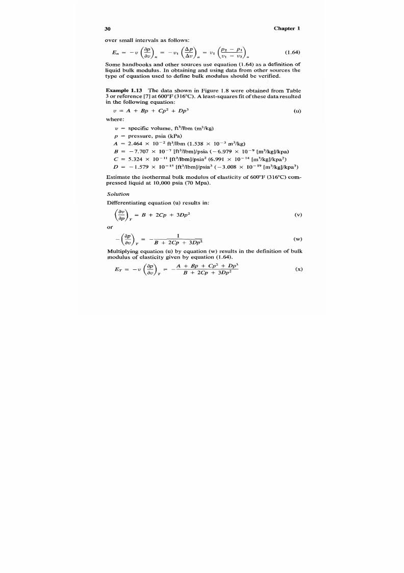
7/21/2019 Fundamental Fluid Mechanics for Engineers
http://slidepdf.com/reader/full/fundamental-fluid-mechanics-for-engineers 53/438
30
Chapter
1
over small intervals as follows:
E ,
=
-v
rg)n
-v1
( g ) n
v1
r?)
V2
n
Some handbooks and other sources use equation(1.64) as a definition of
liquid bulk modulus. In obtaining and using data from other sources the
type of equation used to define bulk modulus should be verified.
Example
1.13 The data shown in Figure 1.8 were obtained from Table
3
or
reference [7 ]at 600°F (316°C).A least-squaresfit of theseata resulted
in the following equation:
v = A
+
Bp
+
Cp2 + Dp3
(U)
where:
v
= specific volume, ft3/lbm (m3/kg)
p = pressure, psia (kPa)
A = 2.464 X ft3/lbm(1.538 X lo-’ m’/kg)
B
=
-7.707
x
10”
[ft3/lbm]/psia
- 6 . 9 7 9
x
[m3/kg]/kpa)
C = 5.324 x
l o - ”
[ft3/lbm]/psia26.991 x [m3/kg]/kpa2)
D =
-
1.579 X [ft3/lbm]/psia3 -3 .008
x
[m3/kg]/kpa3)
Estimate the isothermal bulk modulus of elasticity of 600°F316°C)com-
pressed liquid at 10,000 psia (70 Mpa).
Solution
Differentiating equation
(U)
results in:
g ) T B + 2Cp + 3Dp2
or
1
T B
+
2Cp + 3Dp2 W)
Multiplying equation
(U)
by equation
(W)
results in the definition of bulk
modulus of elasticity given by equation (1.64).
E T = -V($) = -A
+
Bp + Cp2 + Dp3
T B + 2Cp + 3Dp2
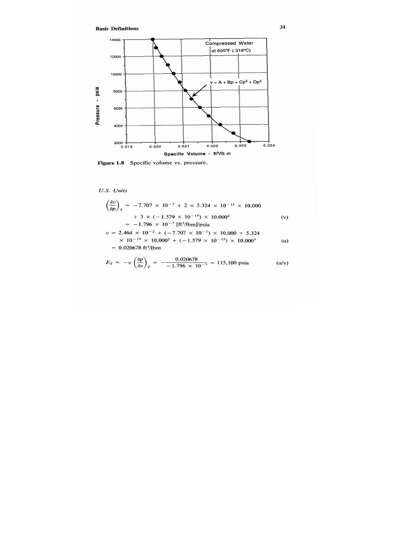
7/21/2019 Fundamental Fluid Mechanics for Engineers
http://slidepdf.com/reader/full/fundamental-fluid-mechanics-for-engineers 54/438
Basic 31
Speci f ic
Volume
- RsAb m
Figure 1.8 Specific volume vs. pressure.
U.S. nits
(g)T
-7.707
x +
2
x
5.324
x IO-''
x
10,OOO
+ 3 X
( -
1.579 X
lo"')
X
10,0002
(v)
= -
1.796
x [ft3/lbm]/psia
ZI
=
2.464
X +
(-7.707
X X 10,000 +
5.324
x 10-11 X 10,0002 + (-1.579
X 10-15)
X 10,0003
(U)
=
0.020678
ft3/lbm
ET = -v($) = -
0.020678
T -1.796 x
=
115,lOopsia

7/21/2019 Fundamental Fluid Mechanics for Engineers
http://slidepdf.com/reader/full/fundamental-fluid-mechanics-for-engineers 55/438
32 Chapter
1
SI
Units
(g)T
-6.979
X
+
2 X 6.991 X
X
70 00
+
3 X (-3.008 X
10-19)
X 700002
(v)
= - 1.613 X [m3/kg]/kpa
v
= 1.538
x
+ (-6.979
X x
70,000 + 6.991
X
10-14
X 70
0002 +
(-3.008
X 10-19)
X 70
0003
(v)
= 0.001289 m3/kg
1.l
ACOUSTIC VELOCITY
Definition: Speed of a small pressure (sound) wave n a fluid
Symbol:
C
Dimensions:
LT
Units: U.S.: ft/sec SI:
m/s
Derivation
of
Basic Equations
Consider an elastic fluid in a rigid pipe fitted with a piston as shown in
Figure 1.9. The pipe hasa uniform cross-sectional rea of A . As the result
of the application of force
dF
the piston is suddenly advanced with a
velocity of Vfor a time dt. The fluid pressure
p
is increased byhe amount
of dp which travels as a wave front with a velocity of c . During the ap-
plication timedt, the piston moves a distance of V dt and the wave front
advances a distance of
c dt.
The result of this piston movement is to
decrease the volume c dt A by the amount of the volume V dt
A .
From Section 1.15, equation (1.57), the bulk modulus of the fluid is
stress dPP c dP
strain
-
VN
( V
dt
A ) / ( c
dt
A )
V
E = - - - - - - -
=
or
V E
c
=
--
dP
(1.65)

7/21/2019 Fundamental Fluid Mechanics for Engineers
http://slidepdf.com/reader/full/fundamental-fluid-mechanics-for-engineers 56/438
Basic
33
1
2
O d t
*
dF
Figure 1.9 Notation for acoustic velocity.
The force
dF
imposed is
(p
+
dp) A
-
PA
=
dp
A . The mass of fluid
accelerated in time
dt
is pc
dt A ,
so that the mass flow rate is
riz
=
m/dt
= (pc
dt A) dt
= p d . The velocity change is from V to
0.
From the
impulse-momentum equation
(1.28),
F
=
riz(V2
-
VJ)/gc:
dF
=
dp
A
=
p c 4 0
-
v)
dP
g c
or
c =
--
gc PV
Multiplying equation ( l .65) by equation (1.66),
or
c =
(1.66)
(1.67)
The numerical value of E depends on the process. It is assumed that a
small pressure (sound) wave will travel through the fluid without either
heat transfer or friction. With these assumptions the process becomes
isentropic and equation (1.67) becomes
c =
p c
P
(1.68)
Equation (1.68) may be used for any fluid whose value of E, and p are
known.

7/21/2019 Fundamental Fluid Mechanics for Engineers
http://slidepdf.com/reader/full/fundamental-fluid-mechanics-for-engineers 57/438
3 4
Chapter
1
Ideal Gases
From equation
(1.62)
E,
=
kp
and from equation
(1.44)
p
=
p / R T .
Sub-
stituting these values in equation
(1.68),
(1.69)
Example 1.14 Estimate the acoustic velocity of air at 68°F (20°C).
Solution
1 .
From Table
A-l ,
M
=
28.96,
Table
A-2,
k
=
1.400,
R
=
R,/M
2. Convert temperature to absolute.
3. Solve equation (1.69) for acoustic velocity
U . S .
Units
1 . R = 154Y28.96 = 53.35 ft-lbfAbm (1.43)
2 . T
=
68 + 460 = 528"R.
3.
c
= (1.400 x 32.17 x 53.35
x
528)O.' = 1126ftlsec. (1.69)
SI
Units
1 .
R = 8314/28.96 = 287.0 J/kg*K, (1.43)
2. T = 20 + 273 = 293 K.
(1.43)
3.
c
= (1.400 x 1
x
287
x
293)O.'
=
343 m/sec. (1.69)
1
l
7
VISCOSITY
Dynamic Viscosity
Definition: Shearing stredrate of shearing strain
Symbol: P mu)
Dimensions: FL-'T or ML T
Units: U.S. : Ibf-sec/ft2 SI: Ndm2 or Pa-s
Viscosity is the resistance of a fluid to motion-its internal friction.
As
discussed in Section 1.2,
a
fluid in a static state is by definition unable
to resist even the slightest amount of shear stress. Application of shear
force results in the continual and permanent distortion known s flow.
In Section
1.2,
consideration of Figure
1 . 1
led to the development of
the unit shear stress 7 = F,/A,, where F, is the shear force and A , is the
shear area. Also developed from considerationf Figure 1 . 1 was the rate
of deformation (shearing strain) as d U / d y , where
U
is the velocity and y
is the distance perpendicular to the shear. The definition of viscosity can
7/21/2019 Fundamental Fluid Mechanics for Engineers
http://slidepdf.com/reader/full/fundamental-fluid-mechanics-for-engineers 58/438
Basic
35
be expressed mathematically as follows:
shearing stress
FJA,
7
dy
= rate of shearing strain
dUldyU
=p=
1.70)
where p s the viscosity. It is customary to write equation (1.70) in the
following form:
.=P($)
(1.70)
In this form various publications call he (a) coefficient of viscosity, (b)
absolute viscosity, or (c) dynamic viscosity (used in this book).
Kinematic Viscosity
DeJinition:
Dynamic viscosityldensity
Symbol:
v
(nu)
Dimensions:
L2 T
Units: U.S.: ft'lsec SI: m2/s
Kinematic viscosity is defineds the ratio of the dynamic viscosity to he
density. Because the dynamic viscosity is in force units and the density
is in mass units in both U.S. and
SI
systems it is necessary to introduce
the proportionality constant (Section 1.6, equations 1.1 ) and (1.12) to
relate dynamic and absolute viscosities, thus:
v = -
gcP
P
US.
nits
v = - =cP (lbm-ft/lbf-sec2)(lbf-seclft2) ft2
= -
P (lbm/ft3) sec
SI Units
(1.71)
Characteristics
In a flowing fluid tangential(shear) stresses arise from two different mo-
lecularphenomena. The first s the cohesive (attractive) forces of the .
molecules, which resist motion. The second is the molecular activity,
which causes resistance to flow due to molecular momentum transfer.

7/21/2019 Fundamental Fluid Mechanics for Engineers
http://slidepdf.com/reader/full/fundamental-fluid-mechanics-for-engineers 59/438
36
Chapter
1
Molecular momentum transfer may bevisualizedbyconsidering two
trains made upof coal cars moving in he same direction on parallelracks
but at different speeds. As these trains pass each other coal is thrown
from one train to the other and viceversa. From considerations f impulse
and momentum, each will tend to resist the motion of the other to some
degree, and the slower train will tend to speed up and the faster train to
slow down.
Liquid Viscosities
In liquids cohesive forces predominate. Since cohesive forces decrease
with increasing temperatures, so do the liquid viscosities.
Gas Viscosities
In ideal gases, cohesive forces are absent. Molecular activity increases
with temperature and so does viscosity.
Other Units of Viscosity
A unit of dynamic viscosity names after Jean Louis Poiseuille (1799-
1869), a French scientist, apoise is definedas one dyne-second perquare
centimeter. In the SI system this is equal to
0.1
N d m 2 or
0.1.
Pass. The
viscosity of water at
20°C
is
1 .002
p,Pa.s or
1.002 x
poises. Because
of the magnitude
of
the poise, the centipoise,
1/00
poise, is used. The
viscosity of water at 20°C is thus approximately one centipoise. Theon-
version factor for
U . S .
unitss
2.089 X
lbf-sec/ft’/centipoise.
A unit of kinematic viscosity namedfter George GabrielStokes
(1819-
1903),
an English scientist, a stoke is defined as one square centimeter
per second. In SI units the stoke is equal to 1 x m%. In U.S . units
the stoke isequal to 1.076
X
ft3/sec. Like the poise, the centistoke
is used because of size.
The standard viscometer for industrial work in the United States is the
Saybolt universal viscometer [8]. It consists essentially of a metal tube
and an orifice built to rigid specifications and calibrated with fluids of
known viscosity. The time required for a gravity flow of 60 cm3 is a
measure of the kinematic viscosity ofhe fluid and is called
SU
(Saybolt
Seconds Universal). Approximate conversionsf SSU to centistokes may
be made using the following equations:
centistokes =
0.226SSU -
ssu
95 32
<
SSU
<
100 (1.72)

7/21/2019 Fundamental Fluid Mechanics for Engineers
http://slidepdf.com/reader/full/fundamental-fluid-mechanics-for-engineers 60/438
Basic
37
centistokes = 0.22OSSU --
ssu
35 ssu > 1001.73)
For very viscous oils a larger orifice is used in the Saybolt viscometer
and the time in seconds is called SSF (Saybolt Seconds Furol). he term
furol is an contraction of fuel and road oils. Approximate conversionsf
SSF to centistokes may be made using the following equations:
centistokes = 2.24SSF -
SSF
184 25 < SSF < 401.74)
centistokes
=
2.16SSF
-
SSF
o
SSF
>
401.75)
For exact conversions reference [8] should be consulted.
Example 1.15 An oil is tested in an industrial laboratory t a temperature
of
60°F
(15.6"C). It took 400 sec for 60 cm3 of this oil to flow through a
standard Saybolt universal viscometer. A standard hydrometer indicated
that the oil had a gravity of 20"API. Compute the dynamic viscosity of
this oil.
Solution
1.
The specific gravity of the oil is calculated from equation (1 5):
S
= 141.5/(131.5 + "API)
S
=
141.5/(131.5
+
20)
=
0.9340
(1.35)
2. The kinematic viscosity is computed using equation (1.73):
centistokes = 0.22OSSU - 135/SSUSSU > 100
v
= 0.220
X
400 - 135/400 = 87.66 centistokes
(1.73)
3. The density of the oil is calculated using equation (1.32):
Po = SPW (1.32)
4. The dynamic viscosity is computed from equation (1.71):
P
=
V P k C
(1.71)
US. nits
3. The density of water at 60°F is 62.37 lbm/ft3 (Section 1.12):
p.
= 0.9340 x 62.37 = 58.25bm/ft31.32)
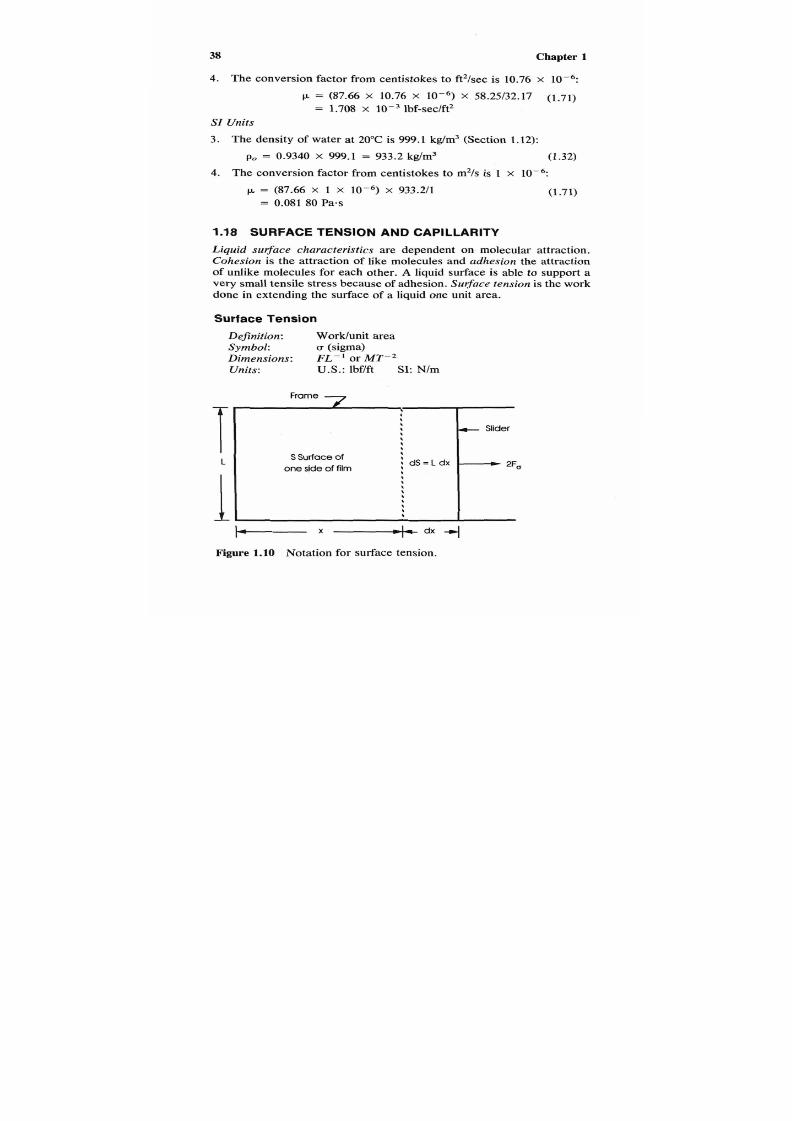
7/21/2019 Fundamental Fluid Mechanics for Engineers
http://slidepdf.com/reader/full/fundamental-fluid-mechanics-for-engineers 61/438
38
Chapter
1
4. The conversion factor from centistokes to ft2/sec is 10.76 x lod6:
p
=
(87.66
x
10.76
x
x
58.2Y32.17 (1.71)
= 1.708 X lbf-sec/ft2
SI Units
3. The density of water at 20°C
is
999.1 kglm3 (Section 1.12):
p = 0.9340 x 999.1 = 933.2 kg/m3 (1.32)
4. The conversion factor from centistokes to m2/s is 1 X
p =
(87.66
X 1
X
X
933.2/1 (1.71)
=
0.081 80 Pass
1.18 SURFACE TENSION
AND
CAPILLARITY
Liquid
su$uce
characteristics
are dependent on molecular attraction.
Cohesion is the attraction of like molecules and adhesion the attraction
of unlike molecules for each other.
A
liquid surface is able to support a
very small tensile stress because of adhesion. Su$uce tension is the work
done in extending the surface of a liquid one unit area.
Surface Tension
Definition:
Workfunit area
Symbol:
U
(sigma)
Dimensions:
FL
or
M T - 2
Units:
U.S.: lbf/ft SI: Nlm
T
l
Frame
I
I
I
I
I
I
I
I
S Surfaceof
one slde
of
film
I
d S = L d x
+
Slider
2F,
* X - d X - l
Figure 1.10 Notation for surface tension.
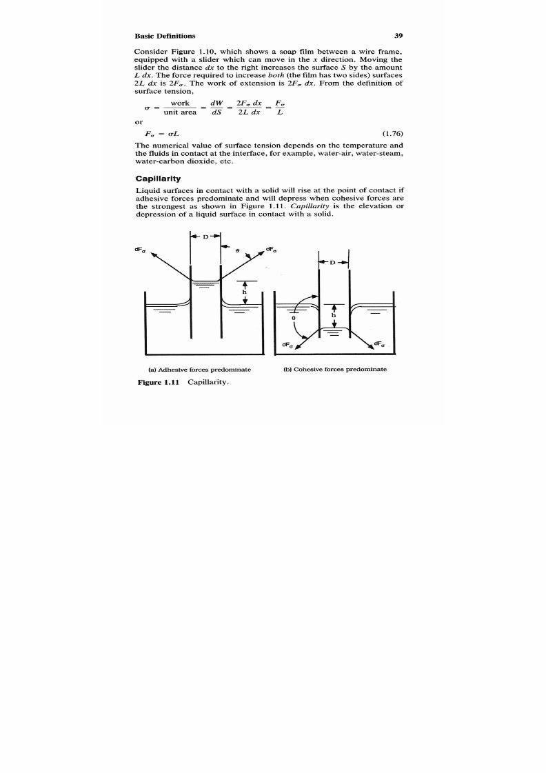
7/21/2019 Fundamental Fluid Mechanics for Engineers
http://slidepdf.com/reader/full/fundamental-fluid-mechanics-for-engineers 62/438
Basic
39
Consider Figure
1.10,
which shows a soap film between a wire frame,
equipped with
a
slider which can move in the x direction. Moving the
slider the distance
dx
to the right increases the surface
S
by the amount
L dx. The force required to increase both (the
film
has two sides) surfaces
2L
dx is
2F,.
The work of extension is
2F,
dx. From the definition of
surface tension,
work
dW 2F, dx F,
unit area
dS
2L
dx
L
=
-
or
F,
=
u L (1.76)
The numerical value of surface tension depends on the temperature and
the fluids in contact at the interface, for example, water-air, water-steam,
water-carbon dioxide, etc.
Capillarity
Liquid surfaces in contact with a solid will rise at the point of contact if
adhesive forces predominate and will depress when cohesive forces are
the strongest as shown in Figure 1
l 1.
Capillarity is the elevation
or
depression of
a
liquid surface in contact with
a
solid.
(a)
Adhesive forces predominate
Figure
1.11
Capillarity.
I
(b)
Cohesive forces predominate
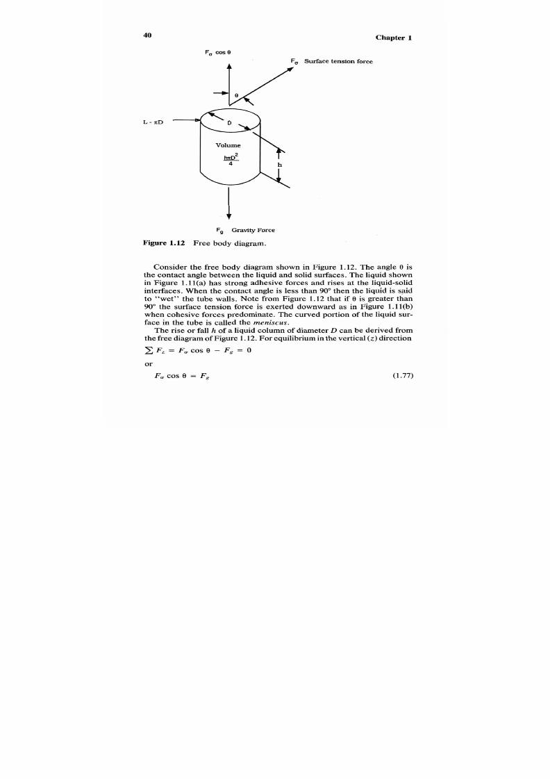
7/21/2019 Fundamental Fluid Mechanics for Engineers
http://slidepdf.com/reader/full/fundamental-fluid-mechanics-for-engineers 63/438
40
Chapter 1
L - Z D
FP Gravity
Force
Figure
1.12
Free body diagram.
Consider the free body diagram shown in Figure 1.12. The angle 8 is
the contact angle between he liquid and solid urfaces. The liquid shown
in Figure
l.ll(a)
has strong adhesive forces and rises at the liquid-solid
interfaces. When the contact angle is less than 90” then the liquid is said
to “wet” the tube walls. Note from Figure 1.12 that if
8
is greater than
90” the surface tension force is exerted downward as in Figure l.l l(b)
when cohesive forces predominate. The curved portion f the liquid sur-
face in the tube is called the meniscus.
The rise or fall
h
of
a
liquid columnof diameter
D
can be derived from
the free diagram of Figure 1.12. For equilibrium inhe vertical
( z )
direction
C
F, =
F , COS
€I-
Fg =
0
or
F , COS e = F*
(1.77)
7/21/2019 Fundamental Fluid Mechanics for Engineers
http://slidepdf.com/reader/full/fundamental-fluid-mechanics-for-engineers 64/438
Basic
Definitions 41
If the small mass of the fluid above the meniscus is neglected, then the
mass of the fluid in the tube above (or below) the surface of the tank is
m
=
ph.rrD2/4.
From equation
(l.lO),
F
=
m d g c
and
Fg
=
m g / g c ,
so
that
the gravity force is Fg = (ph.rrD2/4)g/gc= pgh.rrD2/4gc.The portion of
the surface tension force acting in z direction isF , cos
8.
From equation
(1.76),
F , = uL.
The length
L
is the circumference of the tube, so that
F,
= UL =
UTD. Substituting the above in equation (1.77),
F~ COS e = COS e = F* =
gh.rrD2
4gc
or
(1.78)
From equation
(1.78)
it is evident that as the tube diameter approaches
zero, the elevation (or depression) of the meniscus approaches infinity
and there is no theoretical limit to the rise (or fall) of a liquid tube due
to capillarity. Mercury ishe only manometer fluidhat has a angle 8 other
than zero. For mercury, 8
=
140".
Example 1.16 What is the minimum diameter of
a
glass tube in contact
with water at 68°F (20°C)n air required for an elevation of the meniscus
of
0.1
in.
2.54
mm)?
Solution
1 . The contact angle for water, 8
= 0".
2. Obtain values of p and U from Table A-l .
3.
Calculate the diameter using equation
(1.78):
D = 4(coS B)g,/pgh (1.78)
U . S .
Units
3.
From Table
A - l ,
for water, U =
4.985 X
lbf/ft,p =
62.32
lbm/ft3.
4.
D
= 4 x 4.985 x ~O (COS
0)
x 32.17/[62.32 X 32.17 X (0.1/12)]
= 0.0384 ft = 0.0384 X 12 = 0.46 in. =
$
in. (1.78)
SI
Units
3. From Table A - l , for water,
U
= 72.75
X
N/m, p = 998.3 kg/m3.
4. D = 4 X 72.7510-3(cos 0)
X
1/(998.3
X
9.807
X
2.54
X
=
0.0117 m = 0.0117
x
1000 = 11.7 mm
=
12 mm (1.78)

7/21/2019 Fundamental Fluid Mechanics for Engineers
http://slidepdf.com/reader/full/fundamental-fluid-mechanics-for-engineers 65/438
42 Chapter
1
1.19
VAPORPRESSURE
Definition:
The pressure exerted when a solid
or
liquid is in equi-
Symbol: P v
Dimensions: F L - or M L T - 2
Units: U.S. : lbf/in.2,bf/ft2 SI: N/s2or Pa
librium with its own vapor.
Vapor pressure is a function of the temperature of a given substance. The
temperature-pressure relation is shown as line
ABC
of Figure 1.3.
Cavitation
If at some point in he flow of a liquid the existing fluidpressure is equal
to less than p u , the liquid will vaporize and a cavity or void will form.
Fluctuations of liquidpressures above and below he vapor pressure result
in the formation and collapsef vapor bubbles. The combinationf some-
times violent collapse of these bubbles and related chemical reactions
results not only in poor performance but also at times in severe damage
to equipment. It is necessary in the design of fluid equipment to avoid
this phenomenon.
Cavitation Velocity
The velocity at which cavitation takes place in a steady flow system may
be determined by considering Figure
1.13.
The fluid mass shown has a
length of dx, an area normal to its motion of d A , and the movement of
this mass
is
horizontal. The mass of this fluid element is
p
dA dx. For
frictionless movement the pressure forces opposing each other must be
equal to the fluid mass times ts acceleration, or from equation
(l . lO),
F,
Figure 1.13 Notation for cavitation study.

7/21/2019 Fundamental Fluid Mechanics for Engineers
http://slidepdf.com/reader/full/fundamental-fluid-mechanics-for-engineers 66/438
Basic
43
=
ma,/ ,
and from equation
1.21) a,
=
d V /d t .
Substituting these values
in equation
(1. IO),
(1.79)
Noting that by definition V = dx/d t , and substituting in equation (1.79),
F, = (y)( )& dV =
p
dA V d V
gc
From Figure (1.13) the sum of the pressure forces is
CF,
= p d A -
( p
+
d p ) d A = - d p d A
= F ,
or
F, = - d p d A
Substituting equation (1.81) in equation (1.79),
p d A V d V
g c
F, = - d p d A =
which reduces to
pV dV
d p + - = O
g c
(1.80)
(1.81)
(1.82)
Integrating equation (1.82) for a liquid (pconstant) between the limits of
p s (pressure when at rest) and p , and from
0
to
V , ,
d p +
I
dV = ( p , - p , ) +
P E 02)
€ c
Q
2gc
which reduces to
v,
=p
P, )
P
(1.83)
where V , is the velocity at which a liquid with a pressure of p s at rest
will begin to vaporize.
Example 1.17 Water at
68°F
(20°C) is at rest at standard atmosphere. At
what velocity will vaporization start?
Solution
1.
Obtain p , and p from Table A-l and p , from Section 1.4.
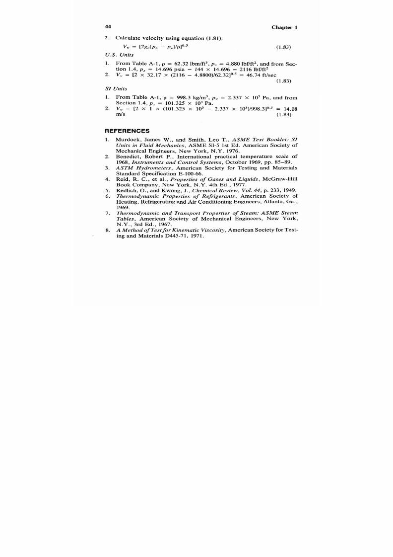
7/21/2019 Fundamental Fluid Mechanics for Engineers
http://slidepdf.com/reader/full/fundamental-fluid-mechanics-for-engineers 67/438
44 Chapter 1
2. Calculate velocity using equation (1.81):
vu
=
[2gc(Ps
-
Pu)/Plo.5
US. nits
(1.83)
1. From Table
A- l , p
= 62.32 lbm/ft3,p , = 4.880 lbf/ft2, and fromSec-
tion 1.4, p s = 14.696 psia = 144
X
14.696 = 2116 lbf/ft2
2. V , = [2 x 32.17 x (2116 - 4.8800)/62.32]0.5= 46.74 ft/sec
(1 33)
SI Units
1. From Table
A-l ,
p
=
998.3kg/m3,
p ,
=
2.337
X
lo3 Pa, and from
2.
V ,
= [2
X
1 x (101.325
X
lo3 - 2.337 x 10³)/998.3]0.5= 14.08
Section 1.4, p s = 101.325 X lo3 Pa.
m/S (1.83)
REFERENCES
1.
2.
3.
4.
5.
6.
7.
8.
Murdock, James
W .,
and Smith, Leo T., ASME Text Booklet: SI
Units in Fluid Mechanics,
ASME SI-5 1s t Ed. American Society of
Mechanical Engineers, New York, N.Y. 1976.
Benedict,Robert P., International practical temperature scale of
1968,Instruments and Control Systems, October 1969, pp. 85-89.
ASTM Hydrometers, American Society for Testing and Materials
Standard Specification E-100-66.
Reid, R. C., et al.,
Properties
of
G ases and Liquids,
McGraw-Hill
Book Company, New York, N.Y. 4th Ed., 1977.
Redlich, O., and Kwong, J., Chemical Review, Vol.44, p. 233,1949.
ThermodynamicProperties of Refr igerants, AmericanSocietyof
Heating, Refrigerating and Air Conditioning Engineers,tlanta, Ga.,
1969.
Thermodynamic and Transport Properties of Steam: ASM E Steam
Tables,
AmericanSociety of MechanicalEngineers,New York,
N.Y., 3rd
Ed.,
1967.
A Method
of
Test fo r Kinematic Visco sity,American Society or Test-
ing and Materials D445-7 1, 1971.

7/21/2019 Fundamental Fluid Mechanics for Engineers
http://slidepdf.com/reader/full/fundamental-fluid-mechanics-for-engineers 68/438
Basic Definitions
45
Table 1.1 Summary of Fluid Mechanics Properties
7/21/2019 Fundamental Fluid Mechanics for Engineers
http://slidepdf.com/reader/full/fundamental-fluid-mechanics-for-engineers 69/438
2.1 INTRODUCTION
This chapter is concerned with establishing the basic relations of fluid
statics. Included are the basic equation of fluid statics, pressure-height
relations for incompressible fluids and for ideal gases, pressure-sensing
devices, liquid forces on plane and curved surfaces, stress in pipes due
to internal pressure, acceleration of fluid masses, and finally buoyancy
and flotation.
The following sections of this chapter may be of special interest to
designers: Section2.5, Pressure-Sensing Devices; Section .7, which de-
scribes the 1976 U.S. Standard Atmosphere; and Section 2.10, which
includes ANSUASME Code equations for pipe stress.
This chapter may be used s
a
text for tutorial or for refresher purposes.
Each concept
is
explained and derived mathematicallyas needed. As in
Chapter 1, the minimum level of mathematics is usedor derivations con-
sistent with academic integrity and clarityf concept. There are
16
tutorial
P typexamples ofullyolvedroblems.
2.2 FLUIDSTATICS
Fluid statics is that branch of fluid mechanics that deals with fluids that
are at rest with respect to the surfaces that bound them. The entire fluid
mass may be in motion, but all fluid particles re at rest with each other.
46

7/21/2019 Fundamental Fluid Mechanics for Engineers
http://slidepdf.com/reader/full/fundamental-fluid-mechanics-for-engineers 70/438
Fluid Statics
7
There are two kinds of forces to be considered: (1) surface for ces ,
forces due to direct contact with other fluid particlesor solid walls (forces
due to pressure and tangential, that is, shear stress), and
(2)
bodyforces ,
forces acting on the fluid particles at a distance (e.g., gravity, magnetic
field, etc.). Since there is no motion of a fluid layer relative to another
fluid layer, the shear stress everywhere in the fluid must be zero and the
only surface force that can act on
a
fluid particle is normalressure force.
Because the entire fluid mass may be accelerated, body forces other than
gravity may act in any direction on a fluid particle.
The great French philosopher and mathematician Blaise Pascal1623-
1662)
is given credit for the first definite statement that the pressure in a
static fluid is the same in all directions.
2.3 BASIC EQUATION OF FLUID STATICS
Body
Forces
The infinitesimal fluid cube shown in Figure 2.1 has a mass of p
dx
dy
dz
This cube is a particle in a large containerof fluid where allhe particles
Y
X
dx
l a
Fu
= P & *
Figure 2.1 Notation for basic equation of fluid statics.

7/21/2019 Fundamental Fluid Mechanics for Engineers
http://slidepdf.com/reader/full/fundamental-fluid-mechanics-for-engineers 71/438
48
Chapter
2
are at rest with respect to each other. The entire fluid mass is subject to
body force accelerations of a,,a,, and a,,opposite the directions of x ,
y ,
and
z
respectively. In addition, the acceleration due to gravity,
g ,
acts
opposite to the direction of z . Although, for clarity, only the z direction
forces are shown in Figure 2.1, forces also act in the x and
y
directions.
From equation (1.lo), F
=
m a / g c , the body forces are Fbx =
(p
d x d y
dz)a,/g,, Ft.,
= (p x
dy dz)a,/g,, Fbz
= (p
x dy d z )az /gc ,nd the gravity
force F g =
(p dx
dy dz)g/g,.
Vertical Forces
By definition of pressure F =
PA,
he upward pressure force is
F,,
= p
d x d y
and the downward pressure force is
Fd = ( p
+
d p ) d x d y
Considering the cube of Figure
2.1
to be a free body and only vertical
components acting:
2 , =
F ,
-
Fd
-
Fbz
-
F g
=
0
d p
=
g ) d z
(x ,
y constant)
gc
Combined
Forces
In a like manner, itmay be shown hat with only y directionforces acting,
and with only x direction forces acting ,
p a x d x
d p
=
-- ( y , z constant)
$?c
Forces may be combined by consideringhe pressure differences between
points 2 and
1
of Figure 2.1. In path
1
”*
a ,
x is vaned and y and z are
held constant so that equation (2.3) applies to the difference between a
and 1. In a like manner, equation (2.2) may be used for path
a
-+
b
and

7/21/2019 Fundamental Fluid Mechanics for Engineers
http://slidepdf.com/reader/full/fundamental-fluid-mechanics-for-engineers 72/438
Fluid Statics 49
equation (2.1) for path b + 2. The total difference is the sum
of
each
component
or
p a dx pay d~ p(az + g ) dz
dp = --
gcc
or
Equation (2.4)
is
the basic equation of fluid statics.
2.4
PRESSURE-HEIGHTRELATIONS FOR
INCOMPRESSIBLE FLUIDS
For a fluid at rest and subject only
t o
gravitational force,
a x ,
y , and a,
are zero, reducing equation (2.4)
o:
Integrating equation 2.5) for an incompressible fluidn
a
field of constant
gravity* and substituting
y
= pg/gc from equation (1.29),
= -Y(ZZ - z l ) = h
which reduces to
(PI
-
P Z )
= AP =
y h
(2.6)
where h = (z2 - z l ) , or the height of a liquid column. The relationships
of equation (2.6) are shown in Figure 2.2.
Example 2.1 The large closed tank shown in Figure 2.3 is partly filled
with benzene at 68°F (20°C).
If
the pressure on the surface is saturation,
what is the absolute pressure of the benzene 10 ft (3 m) below the liquid
surface?
*
If equation (1.15) is solved for
z , z
=
r , [ (g+/g) '
-
11.
For a 0.1% change in
theearth'sgravitationalattraction, z
=
20.9
X
lo6 [(1.001)'
-
l] = 10,OOO ft
3 km. In any practical engineering application involving liquid columns, con-
stant gravity may be assumed.

7/21/2019 Fundamental Fluid Mechanics for Engineers
http://slidepdf.com/reader/full/fundamental-fluid-mechanics-for-engineers 73/438
50
Chapter 2
Figure 2.2 Pressure equivalence.
Figure
2.3
Notation
for
Example
2.1.

7/21/2019 Fundamental Fluid Mechanics for Engineers
http://slidepdf.com/reader/full/fundamental-fluid-mechanics-for-engineers 74/438
Fluid Statics 51
Solution
This example is solvedby noting that the absolute pressure at any depth
below
a
liquid surface is the sum of the surface pressure and pressure
equivalent due to the liquid depth.
1 .
Obtain fluid data from Table A- 1.
2 . Calculatespecificweightusingequation (1.29), assuming standard
3. Calculate pressure due to liquid depth using equation (2.6).
4 . Add vapor pressure to the liquid pressure.
US.
nits
1 . From Table A-l at 68"F,
p u
= 1.453 psia, pf = 54.79 lbm/ft3.
2.
y =
54.79
X
32.17132.17 = 54.79 lbflft3 (1.29)
3. p =
10
x
54.79
=
547.9
lbflft2 =
547.91144
=
3.805
psi.
4.
cp
= 1.453 + 3.805 = 5.26 psia.
SI Units
1 .
From Table
A-l
at
20°C
p u
=
10.04
kPa
pf =
877.7
kg/m3.
gravity.
2.
y
= 877.7
x
9.80711 = 8 608
N/m3
3. p =
3 x 8 608
=
25823
=
25.58 kPa.
4.
cp =
10.04
+
25.58
=
35.62
kPa.
(1.29)
2.5 PRESSURE-SENSING DEVICES
Bourdon
tube gages are used
for
measuring pressure differences. The
essential features are shown in Figure 2.4. The Bourdon tube is made of
metal and has an elliptical cross section. The tube is fixed at
B
and free
to move at C.'
As
the difference between the internal and the external
pressures increases, the elliptical cross section tends to become circular,
and the free end of the tube (point
C )
moves outward, moving the pointer
D through suitable linkage. It should be noted hat when the outside pres-
sure is atmospheric, the Bourdon tube indicates
gage
pressure and when
the internal pressure is less than the atmosphere, then a negative gage
pressure or vacuum is sensed. Refer to Figure 1.4 for these relationships.
Example 2.2
A precision Bourdon gage s used to measure the pressure
of
steam in a horizontal pipe whose centerline is
20
ft
(6
m) above floor
level. The gage is mounted on a panel board with its centerline
4
ft
(1.2

7/21/2019 Fundamental Fluid Mechanics for Engineers
http://slidepdf.com/reader/full/fundamental-fluid-mechanics-for-engineers 75/438
52
40
50 60
I
Chapter 2
I 0
0 -
. 80
7 Section AA
Figure
2.4
Bourdon tube gage.
m) above floor level. The tubing connecting the pipe to the gage runs
horizontally for a short distance from the pipe before descending.to the
gage. The horizontal portion of the tubing is finned and allof the tubing
is uninsulated to insure condensation to protect the gage from the steam
temperature. The average temperature of the water in the tubing is 86°F
(30°C).
The barometric pressure is
30.00
in. Hg at
32°F (101.59
kPa). The
local gravity is 32.10 ft/sec2 (9.805 m/ s 2 ) . The gage indicates 100.22 psi.
(691.00 kPa). What is the absolute pressure of the steam in the pipe?
Solution
This problem is solved by noting that the gage indicates the sum of the
pressure due to the height of the water column above the gage and the
steam pressure less the barometric pressure, or:
Solving (a) for steam pressure:
1. Obtain fluid data from Table A- l .

7/21/2019 Fundamental Fluid Mechanics for Engineers
http://slidepdf.com/reader/full/fundamental-fluid-mechanics-for-engineers 76/438
Fluid
Statics 53
2. Calculate specific weight using equation (1.29).
3. Solveequation (b).
US.
nits
1. From Table A-l for water at 86"F, pf = 62.15 lbm/ft3
2. y = 62.15 X 32.10/32.17 = 62.01 lbf/ft3 (1.29)
3. = 30.00 x .49115 = 14.745 psiaTable 17.1)
ps = 100.22
-
62.01(20 - 4)/144
+
14.73
=
108.04
psiab)
SI
Units
1. From Table A-l for water at 30 C, f = 995.6 kg/m3
2. y = 995.6 x 9.805/1 = 962 N/m3 (1.29)
3. p s = 691.00 - 9762(6 - 1.2)/1000 +
101.59
= 745.73 kPa b)
Credit for the discovery of the barometer is given to Evangelista Tor-
ricelli (1608-1647), an Italian scientist who related barometric height to
weight of the atmosphere. Figure 2.5 shows the essential features of an
elementary barometer.
In
its most primitive
form,
the barometer is made
Figure 2.5 Barometer.
7/21/2019 Fundamental Fluid Mechanics for Engineers
http://slidepdf.com/reader/full/fundamental-fluid-mechanics-for-engineers 77/438
54 Chapter 2
by filling a long glass tube with mercury and inverting it in a pan
of
mercury. If the height of the mercury column is ess than the tube, then
mercury vapor will
form
at the top of the tube. Application
of
equation
(2.6)
yields
pb = y h -t p v (2.7)
The vapor pressure of mercury is very small; from Table-l we find hat
vapor pressure of mercury at 32°F (0°C) is 3.957 x psia (2.728 X
When a barometer type arrangement is filled with a fluid other than
mercury, then the vapor pressure must be taken into account as shown
in Example 2.3.
Pa). For all practical purposes, P b = yh .
Example 2.3 A barometer of the type shown in Figure 2.5 is filled with
carbon tetrachloride at 68°F(20°C).How high willhe carbon tetrachloride
rise in the tube when the barometric pressure is 14.696psia (101.325kPa)?
Solution
This problem is solved by the application
of
equation (2.7):
h =
( P b
- P v ) h (a)
1. Obtain fluid data from Table
A-l .
2. Calculatespecificweightusingequation (1.29) assuming standard
3. Solve equation (a) for height.
US. nits
1 . From Table A-l for carbon tetrachloride at 68"F, p v = 1.76 psia, pf
gravity.
=
99.42 Ibm/ft3.
2. y
=
99.42 x 32.17/32.17 = 99.42
lbf/ft3
3. h = (14.696 - 1.76) X 144/99.42 = 18.74 ft (a)
SI Units
1. From Table A-l for carbon tetrachloride at 20 C, ,, = 12.13 kPa, pf
2.
y
=
1
592.5
x
9.807/1
=
15
618
N/m
3.
h = (101.325 - 12.13) X 1000/1518 = 5.71 m (a)
Manometers are one of the oldest means of measuring pressure. They
were used as early as 1662 by Robert Boyleo make precise measurements
= 1 592.5 kg/m3.
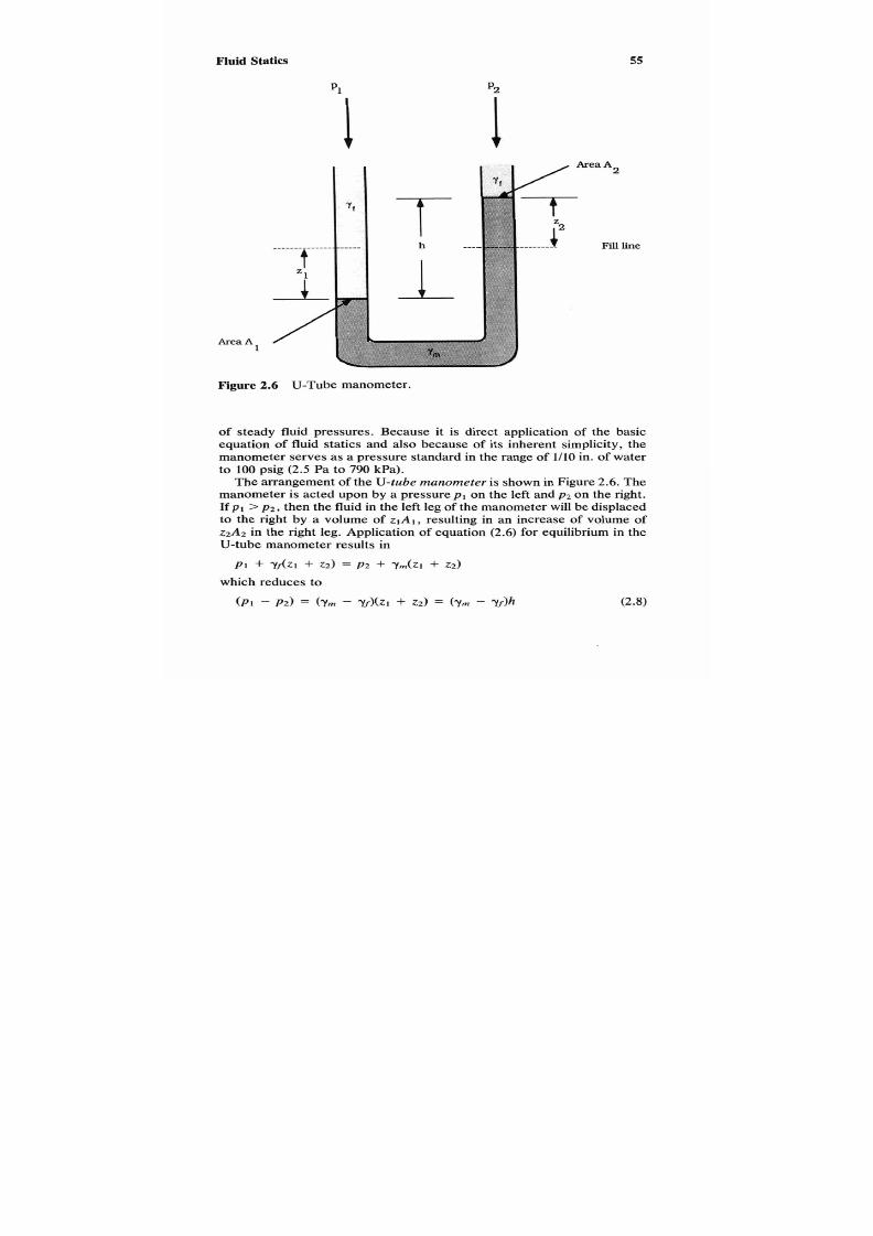
7/21/2019 Fundamental Fluid Mechanics for Engineers
http://slidepdf.com/reader/full/fundamental-fluid-mechanics-for-engineers 78/438
Fluid Statics
P1
p2
Area
A
1
Figure 2.6 U-Tubemanometer.
of steady fluid pressures. Because it is direct application of the basic
equation of fluid statics and also because of its inherent simplicity, the
manometer serves as a pressure standard in the range of
1/10
in. of water
to
100
psig (2.5 Pa to 790kPa).
The arrangement of the U-tube manometer s shown in Figure 2.6. he
manometer is acted upon by a pressure p1on the left and
p 2
on the right.
If
p ,
> p 2 , then the fluid in the left legof the manometer will be displaced
to the right by a volume of
z l A l ,
resulting in an increase of volume of
z2A2 in the right leg. Application of equation (2.6) for equilibrium in the
U-tube manometer results in

7/21/2019 Fundamental Fluid Mechanics for Engineers
http://slidepdf.com/reader/full/fundamental-fluid-mechanics-for-engineers 79/438
56 Chapter 2
p1
Area
A
1
Figure
2.7
Well
or
cistern type manometer.
where - y m is the specific weightof the manometer fluid and yf hat of the
fluid whose differential is being sensed.
One of the disadvantages
of
the U-tube manometer is that unless A I
=
A2
exactly, then both legs must be observed simultaneously.For this
reason, the well or cistern type shown in Figure 2.7 is sometimes used.
In the well
or
cistern type
of
manometer, the areas
A ,
and
A2
are con-
trolled to give a maximum deflection of
z2
and a minimum for
zl.
From
consideration of volumetric displacement f the liquid from ne leg to the
other:
Z I A I= ~ 2 A 2
7/21/2019 Fundamental Fluid Mechanics for Engineers
http://slidepdf.com/reader/full/fundamental-fluid-mechanics-for-engineers 80/438
Fluid
Statics
57
or
ZI
=
z ~ A ~ A I
Substituting in equation (2.8),
P1 - P 2 = (Ym - Yf)
(a,
2 A 2
+
22)
= (Ym
-
Yf) I
+
2)
2
Note that as A I+
W,
A 2 / A 1
+
0. By making the area A I very large, the
designer of a well type of manometer can create a condition where z +
h. The difference in area ratios is usually taken care of by scale gradu-
ations.
Commercial manufacturers of the well type of manometer correct for
the area ratios so that pI p * ) = ( y m - yf)S,,,where S,, is the scale
reading and is equal to z2(1
+
A 2 A I ) . or this reason, scales should not
be interchanged between U-tube or well type, nor between well types
without consulting the manufacturer.
The
inclined manometer,
as shown in Figure 2.8 is a special form of
the well type. It is designed to enhance the readability of small pressure
differentials. From consideration of the geometry of this device, for dis-
placement,
Z I A I R i A 2
or
and for slope
z2
= R i sin
6
Substituting in equation (2.8),
(2.10)
where
R i
is
the distance along the inclined tube. Commercial inclined
manometers also have special scales so that
( P I - ~ 2 )
( ~ m
Yf)Si
where
Si
s the inclinedmanometer scale and sequal to ( A 2 A 1
+
sin €))Ri .

7/21/2019 Fundamental Fluid Mechanics for Engineers
http://slidepdf.com/reader/full/fundamental-fluid-mechanics-for-engineers 81/438
58
Chapter
2
k e a A 7
keaA2
7
7-
ill line
Figure
2.8
Inclinedmanometer.
In actual practice, inclined manometers are used for measurement of
small air pressures. Their scales are usually graduated to read in inches
of water, but they use many other fluids. Care must be taken o “level”
these instruments and to insure that the correct liquid is usedas specified
by the manufacturer. Scales should never be interchanged.
Application
The equations derived above are simple, but actual installationsmay re-
quire more complex ones. Since there is almost an infinite number of
combinations and arrangements hat can be used, it is better to derive an
equation for each actual case, as will be shown inhe examples that follow.

7/21/2019 Fundamental Fluid Mechanics for Engineers
http://slidepdf.com/reader/full/fundamental-fluid-mechanics-for-engineers 82/438
Fluid Statics 59
Example
2.4 The U-tubemanometershown inFigure 2.9 connects
closed tanks
A
and
B .
Tank
A
is partly filled with benzeneo a height
zA
of 3 t (915 mm) above the manometer fill line. The elevation ofhe mer-
cury column ZI s 4 in. (100
mm)
above the
fill
line. Tank
B
is partly filled
with carbon tetrachloride to a height of
zB
of 2.5 ft (760 mm) above the
manometer
fill
line. The depression f the mercury columnz2 is 4 in. (100
mm)
below the fill line. All fluids are at 68°F (20°C). Compute the dif-
ference of air pressures p A
-
p B ;
Solution
This problem is solved by developing an equation for this application
based on static equilibrium.
P A + Y A ( Z A - ZI)+ y A
=
PB +
YB(ZB
+
22)
( 4
Solving for
p A -
p B ,
P A
- P B
= Y B ~ B
22) -
Y A ( Z A
-
ZI)
- Y ~ Z I ~ 2 )
(b)
1. Obtain fluid data from Table A-l
2. Calculatespecificweightsusingequation (1.29) assuming standard
3. Calculate P A - P B using equation (b)
gravity.
I I
Tetrachloride
Carbon
J
Figure 2.9
Notation for Example 2.4.

7/21/2019 Fundamental Fluid Mechanics for Engineers
http://slidepdf.com/reader/full/fundamental-fluid-mechanics-for-engineers 83/438
60
Chapter
2
US. nits
1.
From Table. A-
1
at
68°F;
Benzene
PA = 54.79 lbm/ft3
Carbon tetrachloride
p B =
99.42 lbm/ft3
Mercury
p m = 845.67 lbm/ft3
2.
?A
= 54.79 X 32.17/32.17 = 54.79 lbf/ft3 (1.29)
?B
= 99.42
X
32.17/32.17 = 99.42bf/ft31.29)
= 845.67 X 32.17/32.17 = 845.67 lbf/ft3 (1.29)
3.
PA
-
PB
=
99.42(2.5
+
4/12)
-
54.79(3
-
4/12)
-845.67(4/12 + 4/12) (b)
PA
- P B = -428.2 lbf/ft2
=
-428.2/144 = -2.97psi
P B > P B
S . I .
Units
1. From Table A-l at 20°C:
Benzene
PA
=
877.7 kg/m3
Carbon tetrachloride
p B
=
1592.5kg/m3
Mercury
p m = 13 546.3 kg/m3
2. ?A = 877.7
X
9.807/1
= 8
608/m31.29)
T B = 1592.5 x 9.807/1 =
15
618/m31.29)
y m = 1346.3 X 9.807/1 = 13249/m31.29)
3.
P A
- = 1518(760
X
+ 100
X
-
8 608(915
x
-
100
x
- 132 849(100 x + 100 x
P A - pB = -20.15 kPa
P B > P A
Example
2.5
Tanks 1 and 2 of Figure 2.10 are filled with air. The bar-
ometric pressure is 14.50 psia (100 kPa). Gauge A indicates 30 psi (206.9
kPa) and
he
=
71.50 in.
(1
.816 m). Both manometers contain mercury at
68°F 20°C). Compute the value of h,.
Solution
This example is solved by derivingan equation for this application. The
absolute pressure in tank
1
is given by equation
(1.1).

7/21/2019 Fundamental Fluid Mechanics for Engineers
http://slidepdf.com/reader/full/fundamental-fluid-mechanics-for-engineers 84/438
Fluid
Statics
0 -
A
L
Tank
No.1 I Tank No.2
Figure
2.10 Notation for Example 2.5.
PI = P b + P A
The difference in tank pressures is sensed by manometer
B , so
that from
equation
(2.6):
PI - P2 = yhB (b)
Manometer C senses the difference between the pressure in Tank 2 and
the atmosphere,
so
that from equation (2.6):
P b - P2
=
y h c
(c)
Subtracting equation (a) from equation (c):
P I
-
p2
=
P A
+
?he
Equating equation (d) and equation (c):
y h c
= P A
+ yhe
or hc = he
- PAIT
(e)
1.
Obtain fluid data from Table
A-l.
2. Calculate specific weight using equation (1.29) standard gravity.
3. Solve equation (e) for height.
US. nits
1. From Table
A-l
for mercury at 68 C,
p
= 845.67 lbdft.
2. y = 845.67 x 32.17132.17
=
845.67 lbf/ft3 (1.29)
3.
hc =
71.50112 - 30 X 1441845.67
=
0.8500 ft
=
0.8500 X 12
=
10.20
in.
(6)

7/21/2019 Fundamental Fluid Mechanics for Engineers
http://slidepdf.com/reader/full/fundamental-fluid-mechanics-for-engineers 85/438
62
Chapter 2
SI Units
1.
From Table
A-l
for mercury at
20°C,
p
=
13 546.3
kg/m3.
2.
y
= 1346.3
X
9.80711
=
13249 N/m3 (1.29)
3. hc = 1.816
-
206.9 X 1000/132849 = 0.259 m = 259 mm (e)
2.6
PRESSURE-HEIGHT RELATIONS FOR IDEAL GASES
The equation for a static fluid in a gravitational fieldmay be written as
To integrate the left-hand term of this equation, the functional rela-
tionship between pressure and density must be established for a com-
pressible fluid.The right-hand term equires that the relationship between
the acceleration due to gravity and altitude be established.
We may proceed to establish these by noting from equation (1.30):
1
P = ;
From equation (1.37):
lln
v = VI e)
From the equation of state of an ideal gas:
R
T I
P1
v1 =
(1.30)
(1.37)
(1.42)
Substituting the above when in the left-hand side of equation (2.5):
or
(2.11)
(1.15)
7/21/2019 Fundamental Fluid Mechanics for Engineers
http://slidepdf.com/reader/full/fundamental-fluid-mechanics-for-engineers 86/438
Fluid Statics
Substituting in equation (2.11):
Integrating the right-hand term of equation (2.12):
63
(2.12)
(2.13)
We see from equation (2.13) that mathematically there are only two values
of
l /n that need be considered, one when
n
= 1 and when
n
# 1. Since
the value of
n
for an isothermal process f an ideal gas is (Section 1.13),
we have two equations, one for isothermal processes and another for
nonisothermal processes.
Isothermal Process
Integrating the left-hand term of equation (2.13) for n =
1:
(2.14)
Nonisothermal Processes
For
all other processes, the left-hand term of equation
(2.13)
integrates
as follows:
(2.15)
Temperature relations may be established from equation 1.47):
Substituting equation (1.47) in equation (2.15),
(1.47)

7/21/2019 Fundamental Fluid Mechanics for Engineers
http://slidepdf.com/reader/full/fundamental-fluid-mechanics-for-engineers 87/438
6 4
Chapter 2
(2.16).
2.7 ATMOSPHERE
The atmosphere isa gaseous envelopehat surrounds the Earth, extending
from sea level to an altitude of several hundred miles. The altitude for
near space has been set arbitrarily at 50 miles (80 km).
The earth's atmosphere is divided into five levels based onemperature
variation. The troposphere extends from sea level to 54,000 ft (16.5 km)
at the equator, decreasing to
28,000
ft
(8.5
km) at the poles, and is com-
posed of approximately
79%
nitrogen and
21%
oxygen. With increasing
altitude from sea level, the temperature decreases from 59°F (15°C) to
-69.7"F (-56.5"C). Above the troposphere is the stratosphere, which
extends to approximately
65,000
ft
(19.8
km) and exists at a relatively
constant temperature of
- 9.7"F ( - 59.5"C).
The mesosphere extends
from nearly
5,000
ft
(10.8
km)
to
300,000
ft
(91.4
km), and itsemperature
increases from - 9.7"F(- 65°C) to +28.67"F(- 1.85 F), hen decreases
to
- 34°F (92."C).
The mesosphere is characterized by an ozone layer,
which absorbs the ultraviolet radiation from the sun. Above the meso-
sphere is the thermosphere, also called the ionosphere, which extends
from approximately 300,000 ft (19.4 km) to 1,OOO,OOO ft (305 km). The
temperature in this layer ncreases from
- 34°F (- 2°C)
to nearly
2200°F
(1200°C). The composition is primarily ionized atoms of the lighter gases.
The last level is the exosphere, which extends to the space environment.
U.S. Standard Atmosphere
Because of wide variations in the atmosphere, a standard atmosphere is
used for design purposes. The United States Standard Atmosphere for-
mulated in
1976
extends from sea level to
3,280,840
ft
(1 000
km). For
altitudes abo ve 282,152 j i (86 km) the hydrostatic equilibrium
of
the at-
mosphere gradually breaks down due todiffusion and vertical transport
of
the individual ga s spe cie s.For this reason the pressure-heigh t relations
given in this section arevalid only fo r altitudes below 282 ,152 ft (86 km ).
The standard assumes that gravity is constant at all sea-level ocations
or
g+
= go =
32.1740
ft/sec2
(9.80665
m /s 2 ) .For altitudes from sea level
to
282,152
ft
(86
km) the atmosphere is divided into seven layers based
on geopotential ltitude
H
(the altitude if gravitational accelerations con-

7/21/2019 Fundamental Fluid Mechanics for Engineers
http://slidepdf.com/reader/full/fundamental-fluid-mechanics-for-engineers 88/438
Fluid Statics
65
stant). The relationship between geometric altitude and geopotential al-
titude is given by equation (2.17) as follows:
(2.17)
The temperature at any altitude may be computed using equation (2.18):
where Tz is the temperature at altitude z , "R
(K),
b is the base temper-
ature, from Table 2.l(c) for
z ,
"R (K),
dT/dz
is the temperature gradient,
from Table 2.1(c)or z, "R/ft (Wm), and z b s the base altitude, from Table
2.l(c) for
z,
ft (m). The pressure at any altitude
z
may be computed using
equations (2.19) or (2.20) as applicable:
(2.20)
where pt is the pressure at altitude z , psia (Pa),
P b
is the base pressure,
from Table2.l(c) for z, psia (Pa),n is the process slope, from Table.l(c)
at
z,
ratio,
P b
is the base pressure, from Table2.l(c) for
z ,
psia (Pa), and
n is the process slope, from Table 2.l(c) at z , ratio.
The value of sonic velocity is calculated using equation (1.69) and as-
suming that
k
has a constant value of 1.4. The value of dynamic viscosity
is calculated from the Sutherland equation:
(2.21)
where
pz
s the dynamic viscosity at altitude , lbf-sec/ft2 (Paes),3 is the
3.045 x IO-' lbf-secl(ft2- R' )(1.458 x Pa-s/K'"), T , is the tem-
perature at altitude z , "R (K), and S, is the Sutherland constant, 198.72"R
(110.4 K).
Tables 2.l(a) and (b) contain pertinent data on the
U.S.
Standard At-
mosphere up to 352,272 ft (86
km).
Figure 2.11 shows the temperature-
altitude profile of this altitude range.
Example
2.6
Assuming that the U . S . Standard Atmosphere 1976 is cor-
rect, estimate the error in temperature and pressure made at 16,400 ft
(5
km) by assuming that the atmosphere fromsea level to that altitude is (a)
incompressible, (b) isothermal, and (c) isentropic.
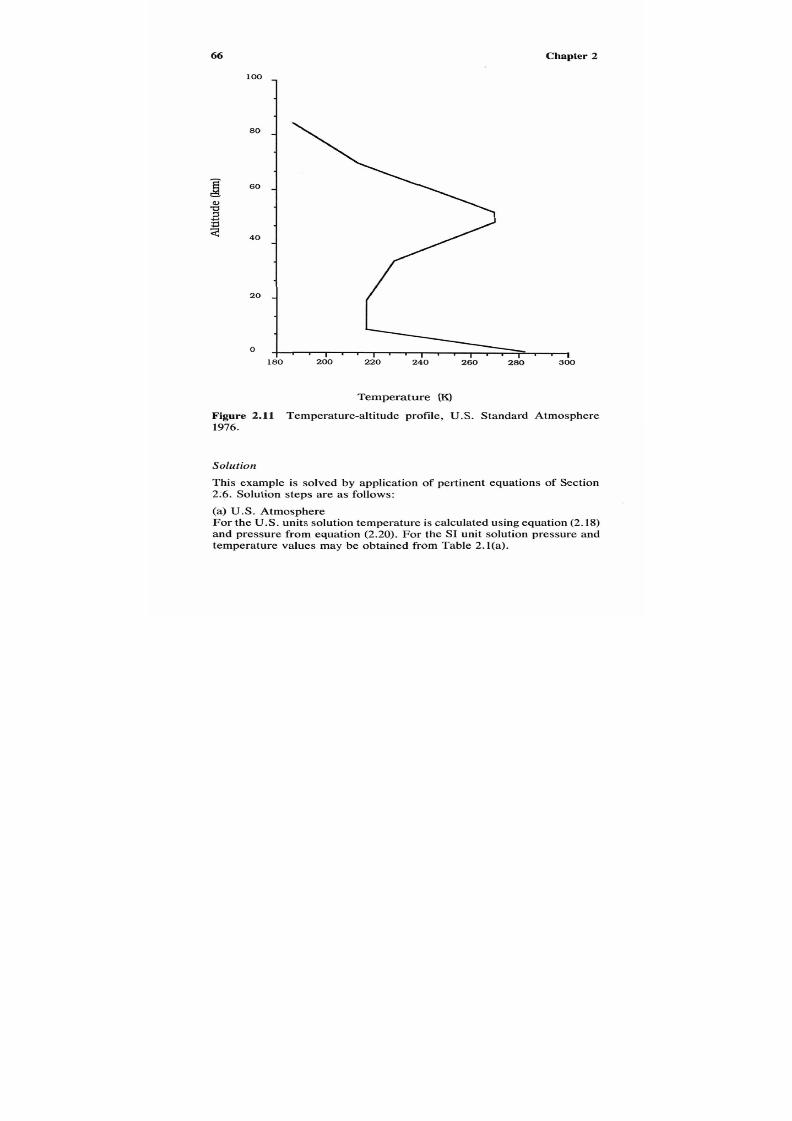
7/21/2019 Fundamental Fluid Mechanics for Engineers
http://slidepdf.com/reader/full/fundamental-fluid-mechanics-for-engineers 89/438
66
Chapter 2
0
180 200 220
240
260
280
300
c
18'0
00
Temperature
(K)
Figure 2.11
Temperature-altitudeprofile, U.S . StandardAtmosphere
1976.
Solution
This example is solved by application of pertinent equations of Section
2.6. Solution steps are as follows:
(a) U.S.Atmosphere
For the U.S. units solution emperature is calculated using equation (2.18)
and pressure from equation 2.20). For the SI unit solution pressure and
temperature values may be obtained from Table 2.l(a).

7/21/2019 Fundamental Fluid Mechanics for Engineers
http://slidepdf.com/reader/full/fundamental-fluid-mechanics-for-engineers 90/438
Fluid Statics 67
(b) Incompressible
1.
Obtain fluid data from Tables
2.1 , 18.1,
and
18.3.
2 . Integrating equation (2.5) for constant density and variable gravity
results in:
or
3.
For a constant-density process for an ideal gas:
(c) Isothermal
4 .
By definition,
Tz
=
To.
(c)
5 .
The term pz is calculated using equation
(2.19)
modified as follows:
(d) Isentropic
6. The term Tz s calculated using equation (2.16) as follows:
Tz
=
To
-
7)
,R(
1 :
re)]
k - l
7.
The term
pz
is calculated using equation
(2.20)
as follows:
Wk-
Pz =
Po
2)
US.
nits
(a)U.S. Atmosphere
Tz = 518.67
+
-0.00356(16,400
- 0)
= 460.29"R
460.29 ~.234%9/(1.234%9-~)
pz = 14.696
518.67) =
7.85-psia

7/21/2019 Fundamental Fluid Mechanics for Engineers
http://slidepdf.com/reader/full/fundamental-fluid-mechanics-for-engineers 91/438
68 Chapter
2
(b) Incompressible
1. FromTable 2.l(b), TO
=
518.67"R, p.
=
14.70 psia,
p
=
0.07647
lbm/ft3. From Table A-l,
M
= 28.97 lbm-mol. From Table 18.2, k =
1.4.
R = 154Y28.97 = 53.33t-lbf/(lbm-"R)1.43)
2. pz = 14.70 -
0.07647
x
32.17
x
16,400
[32.17
X
(1
+
16,400/20,860,000)](&) (a)
= 6.00 psia
Error
=
100
x
(6.00
-
7.85)/7.85
=
-23.57%
3.Tz
=
518.67 X (6.00 h4.70) = 211.93"R
Error
=
100
x
(211.93
-
460.29)/460.29 = -54.10%
(c) Isothermal
4.Tz = To = 518.67"R
Error = 100
X
(518.67 - 460.29)/460.29 = 12.68%
5 . pz= 14.70exp
-32.17
X
16,404
[
2.17
X
53.33
X
518.67
X
(1+ 16,400/20,860,000)
1
= 8.13psia
Error
=
100 x (8.13 - 7.85)/7.85 = 3.57% (dl
(d) Isentropic
6. Tz=518.67-
32.17
x
16,400
[l*;.;
'1
[
2.17
x
53.33
x
(1
+
16,400/20,860,000)
1
= 430.88"R
Error
=
100
x
(430.88 - 460.29)/460.29 = -6.39%e)
= 7.68 psia
Error =
100
x (7.68
-
7.85)/7.85 = -2.17%
SI
Units
(a) U.S. Atmosphere
From Table 2.l(a), Tz = 255.71 K , pz = 54
090
Pa.
(b) Incompressible
1.
FromTable2.1(a),To = 288.15K,po = 101 300Pa,po = 1.225kg/m3.

7/21/2019 Fundamental Fluid Mechanics for Engineers
http://slidepdf.com/reader/full/fundamental-fluid-mechanics-for-engineers 92/438
Fluid
Statics
69
From Table A- l , M = 28.97 kg-mol. From Table 18.2, k = 1.4.
R
=
8314/28.97
=
287.0 J/(kg*K) (1.43)
2. p z = 101300 -
1.225 x 9.807
x
5 000 = 41
279
Pa
1 x (1 + 5 000/6357 000)
(a)
Error = 100
x
(41279 - 54090)/54090 = -23.68%
3. Tz= 288.15 X (4179110100) = 117.42 K (b)
Error = 100 x (117.42 - 255.71)/255.71
=
-54.08%
(c) Isothermal
4.
5.
Tz=
To
= 288.15 K (c)
Error =
100
x (288.15 - 255.71)/255.71 = 12.68%
p z =
101
300 Exp
-9.80 7 X 5
000
[
X 287.0 X 2 88.15 X (1 +
5
000/6 357 000)
= 56 015 Pa (dl
Error = 100 x (56 015 - 54 090)/54
090
= 3.56%
(d) Isentropic
6.807 x 5 000
6.
Tz
= 288.15 -
e4l.; '1
[
X 287.0
X
(1 +
5
00016357 000)1
= 239.37 K
Error = 100
x
(239.37 - 255.71)/255.71 = -6.39%e)
7. p z =
101
300
=
5228 Pa
Error = 100
x
(52 928 - 54 090)/54
090
= -2.18%
Summary
Pressure error
(%)
Process U.S. SI
U.S.
SI
Incompressible
-
4.10
-
4.08
- 3 S 7
- 3.68
Isothermal
- 12.68 - 12.68
3.57
3.56
Isentropic
-
.39
-
6.39
2.17
-2.17
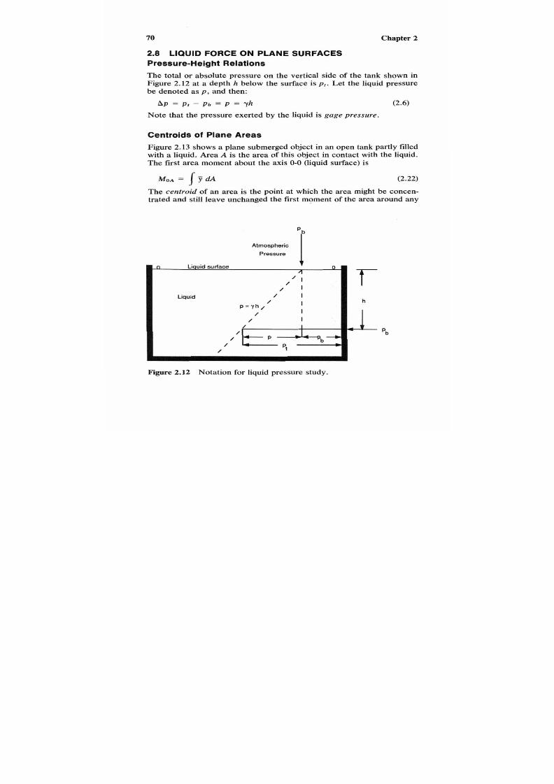
7/21/2019 Fundamental Fluid Mechanics for Engineers
http://slidepdf.com/reader/full/fundamental-fluid-mechanics-for-engineers 93/438
70
Chapter
2
2.8
LIQUID FORCE ON PLANE SURFACES
Pressure-Height Relations
The total or absolute pressure on the vertical side of the tank shown in
Figure 2.12 at a depth
h
below the surface is p t . Let the liquid pressure
be denoted as p , and then:
Centroids
of
Plane Areas
Figure 2.13 shows a plane submerged object in an open tank partly filled
with
a
liquid. Area
A
is the area of this object in contact with the liquid.
The first area moment about the axis 0-0 (liquid surface) is
MOA =
I
A
(2.22)
The centroid of an area is the point at which the area might be concen-
trated and still leave unchanged the first moment of the area around any
Atmospheric ]
ressure
D Liquidurface
0
Liauid / I
/
/ ____
/
Figure
2.12
Notation for liquid pressure study.

7/21/2019 Fundamental Fluid Mechanics for Engineers
http://slidepdf.com/reader/full/fundamental-fluid-mechanics-for-engineers 94/438
Fluid Statics 71
“ 0
Liquid level \
Figure
2.13
Notation for liquid force
on
plane submerged surfaces.
axis. The centroid of an area is also its center
ofgrav i ty ,
thus,
MOA
= dA
= Si,A
2.23)
where
y c
s the distance from the liquid surface
-0
to the center of gravity
of
the area.
Force
Exerted
The force F exerted at a depth h from the liquid surface is
(2.24)
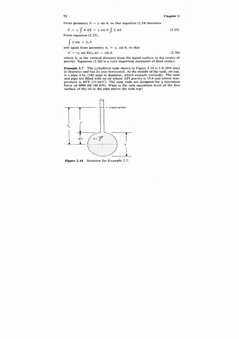
7/21/2019 Fundamental Fluid Mechanics for Engineers
http://slidepdf.com/reader/full/fundamental-fluid-mechanics-for-engineers 95/438
72 Chapter 2
From geometry h
= y
sin 8,
so
that equation (2.24) becomes
F = y I h d A = y s i n e I j j d A
(2.25)
From equation (2.23),
dA
=
jj,A
and again from geometry h, =
y,
sin e,
so
that
F
=
(y sin)(y,A)
=
yh,A
(2.26)
where h, is the vertical distance from the liquid surface to the center of
gravity. Equation (2.26) is a very important statement of fluid statics.
Example
2.7
The cylindrical tank shown in Figure 2.14 is 3 ft
(914
mm)
in diameter and has its axis horizontal. At he middle of the tank, on top,
is a pipe 4 in. (102 mm) in diameter, which extends vertically. The tank
and pipe are filled with an oil whose
API
gravity is 15.6 and whose tem-
perature is
60°F
15.66 C). The tank ends are designed for a maximum
force of
9000
lbf
(40
kN). What is the safe maximum level of the free
surface of the oil in the pipe above the tank top?
Figure
2.14
Notation for Example 2.7.
7/21/2019 Fundamental Fluid Mechanics for Engineers
http://slidepdf.com/reader/full/fundamental-fluid-mechanics-for-engineers 96/438
Fluid
Statics 73
Solution
This example is solved byhe application of equation
(1.35)
to obtain the
specific gravity of the oil and equation (2.26) to calculate the maximum
oil level. The specific gravity at 60°F (15.56"C) is calculated as follows
S = 141.5/(131.5 + 15.6) = 0.9619 (1.35)
The specific weight is calculated using equations (1.29) and (1.32).
PgPwg
v = - = -
From equation (2.23),
gcc
F
h
= -
c
?A
From Figure
2.14,
d
ITd
and
A
=
= h . - -
c 2
4
so that
4 F
d
ymd
2
= -
1.
Obtain density of water from Table
A-l
and compute specific weight
2. Calculate height using equation (c).
using equation (a).
US.
nits
1.
From Table
A-l
at
60°C,
p
= 62.37
lbm/ft3.
y
= 0.9619 X 62.37 X 32.17/32.17 = 59.99 lbf/ft3
2.
z
= 4 X 9OOO/(59.99 X IT X 3')
-
3/2 = 19.72 ft
SI Units
1 .
From Table
A-l
at 15.56"C,
p w
=
999.1
kg/m3.
y
= 0.9619 X 999.1 X 9.807/1 = 9 425 N/m3
(a)
- 914 x 10-3/2
=
6.01 m
(c)
2. = 4 X (40 X 103)/[ 9 425 X IT X (914 X 10-3)21

7/21/2019 Fundamental Fluid Mechanics for Engineers
http://slidepdf.com/reader/full/fundamental-fluid-mechanics-for-engineers 97/438
74
Chapter
2
Location of Liquid Force
If the moment of forces around the axis 0-0 (liquid surfaceof Figure 2.13)
is taken, then
I d M O = J J d F
=
YFF
or
(2.27)
where
Y F
is the distance from the liquid surface to the point where
F
would act if it were concentrated in one location (center of force). From
equation (2.25), dF = ?(sin 8)y dA and from equation (2.26), F = y c A
sin
8.
Substituting in equation (2.27),
Noting that
J y 2
dA
s the second moment
or
moment of inertia
or
Io ,
and
substituting in equation (2.28),
(2.29)
Because equation (2.29) requires that the moment of inertia around the
liquid surface be known, it is not always conveniento apply.
To
transfer
the moment of inertiao the center of gravity of the area, we may proceed
as follows, using the parallel axis theorem:
dl0 = y 2A =
( J J , -
Ay)’ dA (2.30)
Integrating equation (2.30)
(2.31)
By definition of
a
centroid, the first moment around the center of gravity
J
A y d A =
0,
and the second moment or moment of inertia around the
center of gravity
ZG
= J A y 2
dA;
substituting in equation (2.31),
(2.32)

7/21/2019 Fundamental Fluid Mechanics for Engineers
http://slidepdf.com/reader/full/fundamental-fluid-mechanics-for-engineers 98/438

7/21/2019 Fundamental Fluid Mechanics for Engineers
http://slidepdf.com/reader/full/fundamental-fluid-mechanics-for-engineers 99/438
76
Chapter
2
Solution
This example is solved by application of the concepts of this subsection,
geometrical data from Table
C-l ,
and the properties of water from Table
A - l . From Table C-l (rectangle),
A = a b (a)
From Figure
2.16
and equation (c),
h,
=
y ,
=
b - y ~ + ~ = b - b 1 2 + ~ = b 1 2 + ~ ( 4
The force exerted by the water on the gate is computed using equation
(2.26) and substituting values from equations (a) and (d):
Fwater
=
yhJ = y(b12 + c)ab (e)
The location of the force exerted by the water is computed using equation
(2.33)and substituting values from equations and (d).
IC
b b2112
y F = y , + F = - + c + -
y c A 2 b12 + c
b b2112
2 b12 + c
= - - -
Taking moments around the hinge (Figure
2 . 1 3 ,
or
Substituting from equation (i) for Fwater, equation (g) for Z n equation
(h), and simplifying results in:
y a b ( b
+
3 c )
6
Gate
=
1.
Obtain density from TableA - l and calculate he specific weight using
2 .
Solve example using equation (i).
equation
(1.35).

7/21/2019 Fundamental Fluid Mechanics for Engineers
http://slidepdf.com/reader/full/fundamental-fluid-mechanics-for-engineers 100/438

7/21/2019 Fundamental Fluid Mechanics for Engineers
http://slidepdf.com/reader/full/fundamental-fluid-mechanics-for-engineers 101/438

7/21/2019 Fundamental Fluid Mechanics for Engineers
http://slidepdf.com/reader/full/fundamental-fluid-mechanics-for-engineers 102/438
Fluid Statics 79
F, = &Ap (2.39)
where
h ,
is the distance from the liquid surface to the center of gravity
of the projected area AEE'A'. From Figure 2.16, h,
= c
+
b/2 , and the
projected area Ap = b w . Substituting
in
equation (2.39),
F,
= yhcxAp =
y(c +
b/2)bw2.40)
Location of orizontal forc e
may bedetermined by applicationf equa-
tion
(2.33),
noting that for a vertical distance
h,
=
h ,
and Y F =
h,=,,
(2.41)
From Table C - l , ZG/A for a rectangle isb2/12;again from Figure .16, h,
=
c
+ b/2 , and substituting in equation (2 .41) ,
(2.42)
The magnitude of the resultantforce
F
may be determined by noting that
F
is the hypotenuse of the right triangle formed by
F,
and
F,
in Figure
2.16.
From trigonometry,
F = -
(2.43)
This force
F
will act at the intersection of hFxand
xG ,
shown in Figure
2.16
as CF (center of force).
Example 2.9 The curved surface shown
in
Figure 2.16 is immersed in
a
tank filled with a liquid whose specific weight is 50 lbf/ft3(7 850 N/m3).
The edge EE'
is
horizontal and is30 ft (9.14 m) below the liquid surface.
The curved surface is a parabola whose vertex is at
A .
The horizontal
distance a is 20 ft (6.10 m), the vertical distance b is 24 ft (7.32 m), and
the width
W
is 10 ft (3.05 m). Calculate (a) the magnitude and (b) location
of the total liquid force on the surface
AEw.
Solution
This example is solved by application f the concepts of this subsection
and geometrical data from TableC - l .
From Table
C-l
for a half parabola,
2ab
3
3a
=jG = -
8
A = -

7/21/2019 Fundamental Fluid Mechanics for Engineers
http://slidepdf.com/reader/full/fundamental-fluid-mechanics-for-engineers 103/438
80 Chapter
2
1. The total vertical force is calculated by substituting equation (a) in
equation (2.35) and then substituting in equation (2.37):
The total vertical force is computed from equation 2.40):
F, = y b w ( c
+
b)/2 ( 4
The combined force is computed by substituting quations (c) and d)
in equation (2.43):
F = d F m = y w
a2 c + - + b 2 c + -
J
( 236)2
( y
2. The location of the vertical force is computed by substituting equa-
tions (a) and (b) in equation (2.38):
-
ZGA - (3a/8)(2ab/3) (C +
:)
2c a2c
2
ac
+
A
ac
+
(2ab/3)
F
=
-
-
2b
c + -
3
(0
The location of the horizontal force is calculated using equation2.42).
U.S.
nits
1 . The total force is
+
24’ (20
+
T)’
= 599,213 lbf
2. For location of vertical force,
(20/2)(30 + 2412)
30
+
2 x 24/3
F
=
9.13
ft
Location of horizontal force is
hFx
= 30 + 2412 + 242‘12 = 43.14 ft
30 + 24/2

7/21/2019 Fundamental Fluid Mechanics for Engineers
http://slidepdf.com/reader/full/fundamental-fluid-mechanics-for-engineers 104/438
Fluid Statics 81
SI
Units
1.
The total force is
F = 7 850
2
X
7.32)2 ( 72
3
+ 7.32’9.14
+
-
= 3 037 298 N
=
3 037 kN
2.
For
location of vertical force,
(6.1012)(9.14
+
7.3212)
FF =
Location of horizontal force is
9.14 +
2
x 7.3213
= 2.78
m
hFx = 9.14
+
7.3212 +
7.32’112
9.14 + 7.3212
= 13.18 m (2.42)
2.10
STRESS IN PIPES DUE TO INTERNAL PRESSURE
Stress
When a fluid is contained the forces due to fluid pressure produce equal
but opposite resisting forces in the container. These resistingforces pro-
duce stress in the material of the container.
Definition:
-
orce per unit area
Symbol:
S
Dimensions: FL-’
or
ML-‘T- ’
Uni t s : ,
U.S.: lbflin’ SI: kPa
Tensile Stress
When the internal pressure exceeds the external, the size of the container
is increased because of the elasticity of the container material. This in-
crease in size produces tension .in the structure, and hence the material
is subjected to tensile stress.
Thin
Wall
All stress relations developed n this chapter are based on the assumption
that stress in a given cross section is uniform.
For
this to be valid it is

7/21/2019 Fundamental Fluid Mechanics for Engineers
http://slidepdf.com/reader/full/fundamental-fluid-mechanics-for-engineers 105/438
82 Chapter
2
necessary that the thickness of the walls with respect to the size of the
container be small. For the purpose of defining “thin,” pipes whose wall
thickness is less than one-tenth of their internal diameters will be con-
sidered thin-walled.
Pipes
Figure 2.17 shows a cylinder subjected o an internalpressure. The stress
produced may be reduced to longitudinal
(3,)
and circumferential
(S,)
components. Figure 2.17 a) shows the circumferential areas and 2.17(b)
shows the forces. The fluid force
FP
=
FAp,
where
F
is the difference
-
L F
C
(C)
Figure
2.17 Stress in pipes.

7/21/2019 Fundamental Fluid Mechanics for Engineers
http://slidepdf.com/reader/full/fundamental-fluid-mechanics-for-engineers 106/438
Fluid
Statics
83
between the internal and external pressures and
A ,
is the projected area,
and is equal to DL. The resisting force F ,
= S,A,
where
A ,
is the cir-
cumferential stress area and is equalo 2twLwhere
t ,
is the wall thickness.
From the free-body diagram f Fig. 2.17(b) he resisting forces must equal
the fluid forces, or
FP = FAp = F DL = F, = S,A, = S,2twL
which reduces to
(2.44)
For the longitudinal component, Figure 2.17(c) showshe areas and Figure
2.18(d) shows he stresses. The fluid force F =
FA,
where
A
is the cross-
sectional area and equal to nD2/4. The resisting force FL = S A Lwhere
AL
is the area of the annulus and is equal to the difference between the
cross-sectional areas (D + 2tw)2/4 nd nD2/4, which reduces to ntw(D+
t , ) . Since tw s small with respect to D,
A L
= ntwD. From the free-body
diagram of Figure 2.17(d)he resisting forces must equal he fluid forces,
or
F =
FA
= pnD2/4 =
FL
=
S A L =
SLTtw(D
+
t,) = SLntwD
-
which reduces to
(2.45)
Dividing equation (2.44) by equation (2.45),
Fsc 2t,D
or
SL
=
-
S,
FISL 4twD 2
-
- = -
Because the longitudinal stress is only half he circumferential stress, the
circumferential stress is the determining one for thickness calculations.
Equations (2.44) and (2.45) were derived to show only theoretical relations
and should not be used for design.
Design
Equations
The American National Standard ANSIIASME B.31.1 Code or Pressure
Piping recommends an equation which
may
be derived from equation
(2.44) as follows: replace t, by
t , - A , ,
where t , is the minimum wall
thickness and A , is additional wall thickness required to compensate for
material removed in threading, grooving, etc., and to provide for me-

7/21/2019 Fundamental Fluid Mechanics for Engineers
http://slidepdf.com/reader/full/fundamental-fluid-mechanics-for-engineers 107/438
84
Chapter 2
chanical strength, replace D by
Do
- 2y(t,,, - At) where DO s the outer
diameter and
y
is a correction factor for material and temperature; also
replace
3,
by
3,
where
3,
is
the allowable stress. Substituting these values
in equation (2.44),
(2.46)
For service at and below 900°F (482"C),
y
=
0.4
and equation (2.46)
becomes:
(2.47)
Piping
Schedules
Table C-3 shows someproperties of wrought steel and wrought iron pipe
from American National tandard ANSI B36.10-1970. In 1939 the B36.10
committee surveyed the pipe sizes then in use and assigned schedule
numbers to them. These numbers were based on an allowancef 0.1 for
A,, y =
0,
and
r,,,
= 7t,/8, where t , is schedule thickness, and the factor
7/8 to allow for a 124% variation in wall thickness. Substitutingn equation
(2.461,
2(7ts/8
-
0.1)
N s
a Do -
2(0)(7tS/8
-
0.1)
1000
=-
or
(2.48)
where N ,
is
the schedule number.
The relationship
N , =
1000p/~asveryapproximateowing to the
rounding off of values of existing sizes and the variation between equa-
tions (2.47) and (2.48) and should not be used for design. Schedule num-
bers always give conservative values. In using piping schedules, values
of t,,, must be increased by wall thickness tolerance to obtain
t ,
and the
values of t s selected must always e equal to or greater than the calculated
value of
t , .
For design the American National Standards Codes must be
used.
Example
2.10
A carbon steel pipe is required for 1800 psig (12.4 MPa
gage) and 300°F (149°C) service. The pipe must have a minimum flow

7/21/2019 Fundamental Fluid Mechanics for Engineers
http://slidepdf.com/reader/full/fundamental-fluid-mechanics-for-engineers 108/438
Fluid
Statics 85
area of 0.6 ft2
(55
750 mm2). The ANSVASME B31.1-1986 gives a value
of
A, =
0,
y = 0.04, and an allowable stress of 15.0 x
IO3
psi (103.4
MPa). For
a
mill tolerance of
12.5%
for wall thickness, what pipe size
and schedule should be used?
Solution
This example is solved by applicationof the equations given in this sec-
tion.
1.
2.
3.
4.
The approximate pipe size is computed using
The approximate schedule number is computed using
Compute minimum wall thickness by solving equation
(2.47)
for t ,
t , =
+
A,
23, + 2y7i
From Table C-3select the schedule number that satisfies both the
minimum area and thickness requirements.
U.S.
nits
1.
The approximate pipe size is
D = (4 x 0.6
x
144/,rr)0.5 = 1 1 in.
Since there is no 1 1 in. pipe,
12
in. pipe should be selected. From
Table
C-3, Do
=
12.750
in.
2. The approximate schedule number is
N, = IO00
x
1800/15000 = 120 (b)
3.
Compute the minimum wall thickness:
1800
x
12.750
2
x
15,000
+
2
x
0.4 x 1800
, =
+
0
= 0.730 in.
For 12.5% mill tolerance,
t ,
= 8t,/7 = 8
X
.730/7
=
0.834 in.
7/21/2019 Fundamental Fluid Mechanics for Engineers
http://slidepdf.com/reader/full/fundamental-fluid-mechanics-for-engineers 109/438
86
Chapter
2
4.
From Table
C-3
for
12
in. pipe (Schedule
loo),
f,
=
0.844
in.
>
0.834
in.
A =
0.6674
ft2 >
0.6
ft2
Note that Schedule 120 with ts
= 1.00
in. and A = 0.6303 ft2 would
have also met the requirements but would be a very conservative
design.
SI
Units
1 .
The approximate pipe size is
D =
(4
X 55
75O/~r)O.~ 266
mm
From Table
C-3,
Do =
332.9 m.
2.
The approximate schedule number is
N ,
= IO00 x
12.4h03.4
=
120
3.
Computeminimumwall hickness:
12.4
x
323.9
2
x
103.4
+
2
x
0.4
x
12.4
m
=
+
0
= 18.53 mm
For
12.5%
mill tolerance,
f,=
8tJ7
=
8
X
.18.53/7
=
21.18
mm
4. From Table
C-3
for 323.9 mm Do pipe (Schedule loo),
f, =
21.44
mm >
21.18
mm
A =
62 020
mm2> 55
750
mm2
Note that Schedule
120
with f,
=
25.40
mm and
A
=
58
580
mm2
would have also met the requirements but would be a very conserv-
ative design.
2.11 ACCELERATION OF FLUID MASSES
Static Acceleration
Fluid masses may be subject to various types of uniform acceleration
without relative motion occurring between he fluid particles or between
fluid particles and their boundaries.As was discussedn Section
2.2,
shear
stress must be absent, thus permitting the accelerated fluid mass to be
treated as a static fluid. Under these conditions the basic equation for
fluid statics, equation
(2.4),
applies. Integrating equation
(2.4)
for an in-

7/21/2019 Fundamental Fluid Mechanics for Engineers
http://slidepdf.com/reader/full/fundamental-fluid-mechanics-for-engineers 110/438
Fluid Statics 87
compressible fluid
p
constant) in a field of constant gravity
( g
constant),
for uniform acceleration ( a x , y ,and a,constant), results in
D’Alembert’s Principle
Jean Le Rond d’Alembert (1717-1783), a French scientist, noted that
Newton’s second law couldbe written as
f ” - = O
a
gc
(1.10)
where -m d g , is a fictitious force and is sometimes called the reversed
effective force or the inertia force. This principle may be used to reduce
a
problem of dynamics to one of statics. In the derivation of the basic
equation of fluid statics, equation (2.4), the body force accelerations
a x
a,,, nd a,were assumed to act opposite the directions
x ,
y ,
and z , re-
spectively. With the employment of the inertia force concept then the
accelerations may be assumed to act in the directions of x ,
y ,
and z ,
respectively, in equation (2.49).
Translation
Consider the liquid mass shown in Figure.18 being uniformly ccelerated
upward at an angleof
p
and a rate of a.The acceleration in the y direction
a y
s zero. Letting
p2 - pl =
ps
- p
(where
ps
s the surface pressure),
x2 -
x1 =
-L ,
z2 . - z 1 =
h ,
and
ay
=
0.
Equation (2.48) becomes:
which reduces to
Ap
=
p - ps
=
- (a,+ g ) h -
axLI
gc
At the liquid surface
p
=
ps
or
Ap
=
0, h
=
ho,
L = LO
(2.49)

7/21/2019 Fundamental Fluid Mechanics for Engineers
http://slidepdf.com/reader/full/fundamental-fluid-mechanics-for-engineers 111/438
88 Chapter 2
T
i
Figure 2.18 Notation for translation.
which when substituted in equation (2.48) becomes
0
= - (az +
g)ho
-
ad01
gc
which reduces to
h
Lo a,
+
g
- =
t an0
(2.50)
A P = (?)( ) [(az
g)h -
aX, O) l
=
y
1
+
-
h ( L =
0)
( 3
(2.51)

7/21/2019 Fundamental Fluid Mechanics for Engineers
http://slidepdf.com/reader/full/fundamental-fluid-mechanics-for-engineers 112/438
Fluid Statics
89
Comparing equation (2.51) with equation (2.6),
b p =
y h for an unacce-
lerated liquid, it becomes evident that the ratio of the two is
1
+
=,/g.
The
horizontal fo rc e
may be obtained by multiplying equation
(2.39)
by
this ratio, or:
(2.52)
In a like manner the vertical fo rc e is the effective weight of the liquid
above the bottom and may be obtained by multiplying equation2.34) by
the same ratio:
(2.53)
Example2.11
The open tank shown in Figure 2.18 contains200 ft3 (5.66
m3) of water whose specific weights
62.42
lbf/ft3
(9
790N/m3). The tank
is 6 ft (1.83 m) high, 5 ft (1.52 m) wide, and 10 ft (3.05 m) long. The angle
of the incline is 30". Determine (1) the maximum acceleration to which
the tank may be subjected without spilling any water,
(2)
the maximum
end force during the acceleration, and (3) the total force required to ac-
celeiate the fluid mass.
Solution
This example s solved by the application of the equations of this section
and the principles of geometry.
1 . The maximum acceleration without spilling water. Letting V,H , L o ,
and
W
represent the volume, height, length, and width of the tank
respectively, then the height of the water in the tank without accel-
eration becomes:
volume V
H , = - - -
area LOW
-
The maximum rise of water on rear end of the tank is H
-
H , and
the drop on the forward end will be the same, so that
Noting from geometry that
a,
= a cos p and a, = a sin p, and
substituting in equation (2.50), results in:
ho
ax
a cos p
Lo a, + g
a sin
p
+ g
-

7/21/2019 Fundamental Fluid Mechanics for Engineers
http://slidepdf.com/reader/full/fundamental-fluid-mechanics-for-engineers 113/438
90
Chapter 2
2.
3.
Solving equation (c) for a and substituting from equation (b)or ho:
g
-
g
a =
(Lo/ho)
cos
p
- sin
p [(Lo/2(H
-
VLoW)]
cos
p
- sin P
( 4
The maximum end force during the acceleration. The maximum end
force will occur on the end A (maximum height of water) and may
be calculated using equation (2.52) noting that
h,
= H12 and A ,
=
WH.
-
The total force required
to
accelerate the fluid mass: The total force
may be calculated from equation ( 1
. lo )
and noting from equation
(1.29)
that
y = pg/g,:
US. nits
Given: H = 6 ft, W =
5
ft, Lo = 10 ft, V = 200 ft3,
p
= 30".
1.
The
maximum
acceleration without spilling water:
32.17
[10/2(6 - 200/10 x 5)
cos
30" -
sin
30"
=
= 19.32 ft/sec2
a,
=
19.32
cos
30"
=
16.73
ft/sec2
a, =
19.32
sin
30"
=
9.66
ft/sec2
2. The maximum end force during acceleration:
F, =
62.42
1 +-
'66
x 62
- 7305 1bf
(
32.17)
3.
The total force required to accelerate the fluid mass:
F = 62.42 X 200
X
19.32/32.17
=
7496
lbf
(0
SI
Units
Given:
H
= 1.83 m,
W
= 1.52 m, Lo = 3.01 m, V = 5.66
m3,
p = 30".

7/21/2019 Fundamental Fluid Mechanics for Engineers
http://slidepdf.com/reader/full/fundamental-fluid-mechanics-for-engineers 114/438
Fluid Statics
91
1. The maximum acceleration without spilling water:
9.807
[(3.0512(1.83 - 5.6613.05 x 1.52)] cos 30
-
sin 30
=
= 5.88 m/s2
a, = 5.88 cos 30
=
5.09
d s 2
az=
5.88 sin 30 = 2.94 m / s 2
2. The maximum end force during acceleration:
F,
=
9790
1
+
(
9.807) 2
2.94.52
x
1.83*
=
32 386
N
3. The total force required to accelerate the fluid mass:
F
=
9 790
x
5.66
x
5.8819.807
=
3323 N 0
Example 2.12 The U-tube manometer shown n Figure 2.19 with vertical
legs
20
in. (508 mm) apart is partly filled with a liquid to be used as an
accelerometer. I t is installed on an automobile that is accelerated uni-
formly from
15
mph
(6.71
d s )
to
50
mph
(22.35
4 s )
on a level road.
What
is
the difference in level between the two legs during the acceler-
ation?
Solution
This example is solvedy the application of equation (1.21), which defines
acceleration, andequation (2.50).For uniformaccelerationequation
a -
X
Figure 2.19 Notation for horizontal acceleration.

7/21/2019 Fundamental Fluid Mechanics for Engineers
http://slidepdf.com/reader/full/fundamental-fluid-mechanics-for-engineers 115/438
92 Chapter
2
(1.21) may be written as:
.
dV
AV
V2
-
V1
a x =
"
-
dt At t
For a level road,
=
0
so
that equation (2.50) may be modified s follows:
or
US.
nits
a x = 5 Is) (
)
=
3.422
280
ftlmi
3600 seclhr
20
x
3.422
32.17
0 = =
2.13
in.
SI Units
22.35
-
6.71
ax
=
15
508 x 1.043
9.807
= 1.043 m/s2
h0
= = 54.01
mm
ft/sec2
(2.50)
Rotat ion
Consider the fluid mass shown in Figure
2.20
being rotated around the
z
axis at
a
constant angular velocity of
W
radians per second. The accel-
eration of the fluid mass p dy
dx
dz is -w2x (radially inward). The ac-
celeration in the y direction a,, s zero, and gravity is the only force in
the
z
direction,
so
that
a,
is also zero. Using the inertia force concept
discussed in conjunction with ranslation, a x =
-w2x
and equation (2.4)
for rotation becomes
dp = -- (-o*x
dx
+ g dz) (2.54)
g c

7/21/2019 Fundamental Fluid Mechanics for Engineers
http://slidepdf.com/reader/full/fundamental-fluid-mechanics-for-engineers 116/438
Fluid
Statics
93
ccelerated liquid
I
I
I
Line of
constant
pressure 1
I
Figure 2.20
Notation for rotation.
Integrating equation (2.54) and using the relation
y = pg/gc
of equation
(1.29,
I2
YO2
d p =- 2 dx - y i2z
g
(2.55)
Lines of constant pressure occur when 2 = p l , reducing equation (2.55)
to:

7/21/2019 Fundamental Fluid Mechanics for Engineers
http://slidepdf.com/reader/full/fundamental-fluid-mechanics-for-engineers 117/438
94 Chapter
2
The liquid surface is a special case of constant pressure. From Figure
2.23, when x1 =
0,
z1 = A. If we let x2 = r , then z2 - z1 = z - A and
equation (2.56) becomes:
At the wall of the container r = ro and h.
=
zo - A:
(2.58)
From equations
(2.56)
through
(2.58),
it may be seen that
all constant
pressure lines including he surface areparabolic (TableC-l). The volume
of a paraboloid of revolution is one-halfhat of its circumscribed cylinder.
If no liquid is spilled, then
zs = z
0
(2.59)
If
some liquid is spilled then equation (2.59) represents the surface dis-
tance
after
rotation.
Pressure-height relations for the rotating fluid may be established by
letting X I = x2. Then equation (2.55) becomes
( P 2
- P11 = -y(z2 -
Zl)
or
b p = yh (x constant)
Note that this is the same as for unaccelerated fluids.
Example 2.13 The open cylindrical tank shownn Figure 2.21 is 3 ft (914
mm) in diameter and 20 ft (6 096 mm) high. It is filled to the brim with
water whose specific weight is 62.15 lbt/ft3 (9765 N/m3) and rotated
around its vertical center line at 200 rpm. Determine (1) the volume of
water spilled and 2) the gage pressure exerted by the liquid on he bottom
of the tank
1
ft (305 mm) from the center line.
Solution
This example is solved using he principles and equations from this sec-
tion. The rotational speed is calculated as follows:
o = 21~(200/60) = 20.94 rad/sec
1. Volume spilled. Since the tank was full before rotation, the cross-
hatched area in Figure 2.21 is a paraboloid of revolution representing
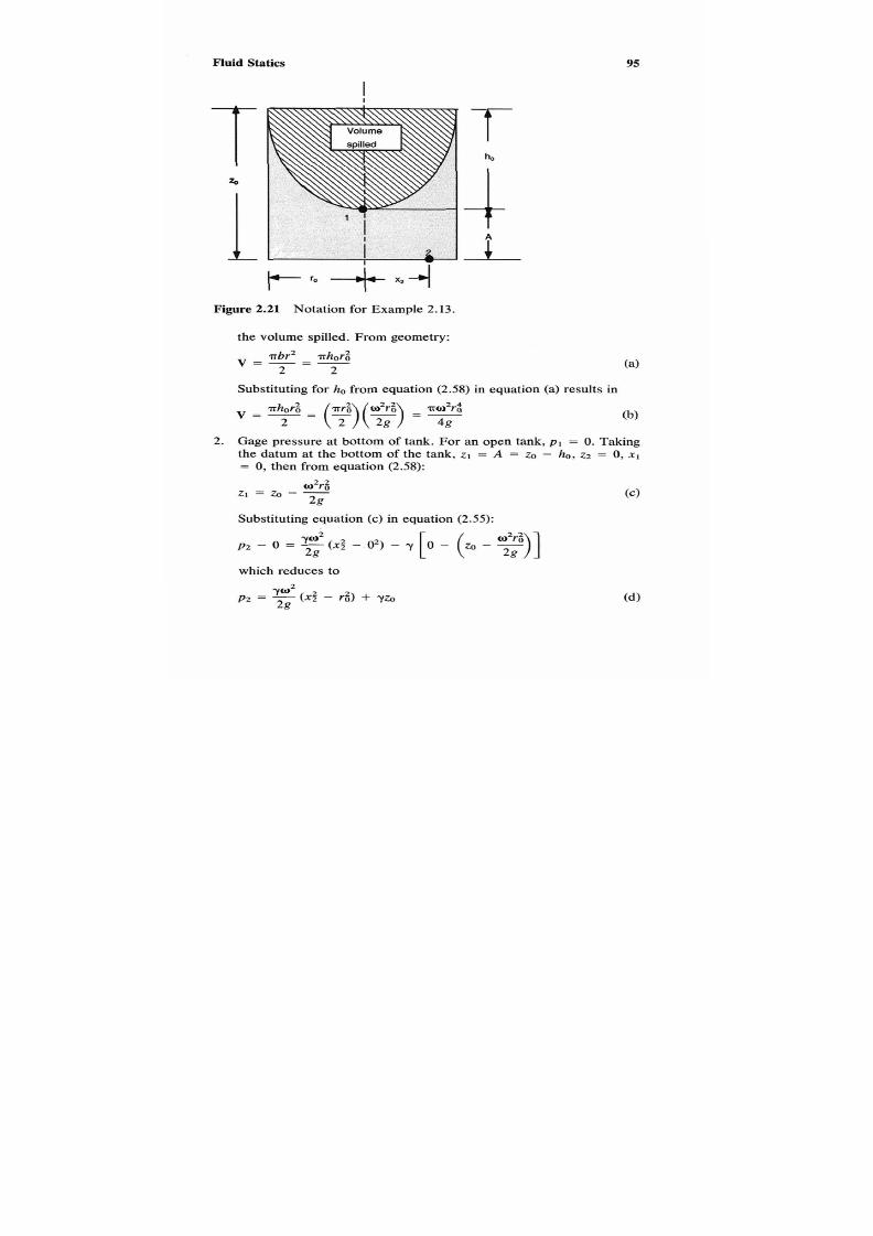
7/21/2019 Fundamental Fluid Mechanics for Engineers
http://slidepdf.com/reader/full/fundamental-fluid-mechanics-for-engineers 118/438
Fluid
Statics 95
Figure 2.21
Notation for Example 2.13.
the volume spilled. From geometry:
v = -
Substituting for h0 from equation (2.58) n equation (a) results in
wbr2hor8
2 2
= -
2. Gage pressure at bottom of tank. For an open tank, p1 = 0. Taking
the datum at the bottom of the tank, z =
A
=
zo
-
ho, z2 = 0 , x1
=
0,
then from equation
2.58):
w2r$
2g
21 = zo
-
-
Substituting equation (c) in equation (2.55):
(c)
which reduces to

7/21/2019 Fundamental Fluid Mechanics for Engineers
http://slidepdf.com/reader/full/fundamental-fluid-mechanics-for-engineers 119/438
96
US. nits
1.Volumepilled:
IT X
20.94’
X
(3/2)4
4 X 32.17
V =
= 54.19 ft3
Gage pressure at bottom of tank:
62.15 x 20.94’
p2 =
2g
[l’
-
(3/2)’] + 62.15
X
20
=
713.55 Ibf/ft’
= 713.55/144 = 4.96 psig
SI
Units
1. Volume pilled:
IT
X
20.94’
X
(914
X
10-3/2)4
V =
4 x 9.807
= 1.53 m3
2. Gage pressure at bottom of tank:
+ 9765 x 6 94 x
=
3423N/m’
= 34.22 kPa (gage)
Chapter 2
(b)
Example 2.14 The closed cylindrical tank shown in Figure 2.22 is 13 ft
(3.96 m) in diameter and 33 ft (10.16 m) high. It is rotated at 25 rad/sec
around
a
vertical axis 10 ft (3.05 m) from the tank center line. The tank
is filled with an oil whose specific weight is 58.81 lbf/ft3 (9 238 N/m3).
Compute the maximum differential pressure in the tank.
Solution
This problem is solved by the application of equation (2.55). Analysis of
this equation indicates thathe minimum pressure will occur at minimum
radius of rotation and maximum elevation (point 1 of Figure 2.22) and
that the maximum pressure will occur at point 2. From Figure 2.22, x1
=
r - ro, x’
=
r
+
ro,
and zz
-
z1 = - o.
Substituting these values in
equation (2.55):

7/21/2019 Fundamental Fluid Mechanics for Engineers
http://slidepdf.com/reader/full/fundamental-fluid-mechanics-for-engineers 120/438
Fluid Statics
97
b - d
Axis
of
rotation
W
- ,
+
l
I
i
20
Figure
2.22
Notation for Example 2.14.
US. nits
2 x 25' x 10 x (1312) 33]
p2
-
p1
=
58.81
[
32.17
= 150,474 lbf/ft'
=
150,174/144
=
1,045psi
SI
Units
p2
-
p1
= 9
238
2 x
25'
x. .05 x
(3.96/2)
,,.,,]
9.807
=
7 204 631 Pa = 7 205 kPa
~
2.12 BUOYANCY AND FLOTATION
Principles
The elementary principlesof buoyancy and flotation were established by
Archimedes (287-212
B.c.).
These principles are usually statedas follows:

7/21/2019 Fundamental Fluid Mechanics for Engineers
http://slidepdf.com/reader/full/fundamental-fluid-mechanics-for-engineers 121/438
98
Chapter
2
(1) a
body immersed n a fluid is buoyed up by force equal to the weight
of fluid displaced by the body, and (2) a floating body displaces its own
weight
of
the fluid in which it floats. These principles are readily proved
by the methods of Section 2.9.
Buoyant Force
Consider the body
ABCD
shown in Figure 2.23. Dashed linesA E and BF
are vertical projections. The force Fzd exerted by the fluid vertically on
the body is the weight of the fluid above ABC. This weight is
Fzd
=
Y ~ E A C B F
(2.60)
In a like manner, the upward vertical force is the weight aboveA B D , or
= YVEADBF (2.61)
The net upward force is the buoyant force FB defined as follows:
FB = FZU- Fzd = Y ~ E A D B F
Y ~ E A C B F
Y ~ A B C D (2.62)
Thus the buoyant force is the weight of the fluid displaced and always
acts upward.
Figure 2.23
Notation for submerged bodies.

7/21/2019 Fundamental Fluid Mechanics for Engineers
http://slidepdf.com/reader/full/fundamental-fluid-mechanics-for-engineers 122/438
Fluid Statics
99
Figure
2.24 Notation for floating bodies.
When an object floats as shown in Figure 2.24, the buoyant force FB
then becomes
FB = ~ V A B D (2.63)
The weight of the body Fg acts downward, so that for vertical equilibrium
C F z = O = F g - F s
or
FB
=
FR
Free
Body Analysis
The equation developed for flotation is a special case where the body is
lighter than the fluid it can displace.
A
more general approach is that of
the free body diagram. If an object immersed in a liquid is heavier than
the fluid it can displace, it will sink to the bottom unless an upward orce
is
applied to prevent it.
A
lighter-than-air ship
or
balloon will continue
o
rise unless a downward force is applied or it reaches an altitude where
its density
is
the same as the atmosphere.
Figure 2.25 is a free-body diagram of an object immersed in a fluid.
For vertical equilibrium,
E F L
= 0 =
FB
-
FB
-
F=
(2.65)

7/21/2019 Fundamental Fluid Mechanics for Engineers
http://slidepdf.com/reader/full/fundamental-fluid-mechanics-for-engineers 123/438
Chapter 2
Figure
2.25 Free body diagram.
where FB is the buoyant force, FR is the weight of body, FL is the force
required to prevent body from rising, and(- F L ) is the force required to
raise the object.
Example 2.15
A
cylindrical drum4 ft (1.22 m) in diameter and9 ft
(2.74
m)
long floats half submerged in seawater whose specific weight is 6 4
lbf/ft3 (IO. kN/m3). It is proposed to anchor this drum submerged with
concrete whose specific weight is 50 lbf/ft3(23.5
kN/m3).
Determine the
minimum volume f concrete required to completely submerge this drum.
Solution
This problem is solved by the application of the principles of buoyancy
and flotation presented in this section. From equation (2.62) the buoyant
force is:
where
yf
is the specific weight of the sea water, V, is the volume of the
drum, and VC s volume of the concrete. The force due to gravity is the
weight of the drum and is equal to the water displaced when floating half

7/21/2019 Fundamental Fluid Mechanics for Engineers
http://slidepdf.com/reader/full/fundamental-fluid-mechanics-for-engineers 124/438
Fluid
Statics
submerged,or:
Fg
=
Yfvd/2
The force required to anchor the drum is
FL =
?,Vc
Using the free body diagram of Figure
2.25
and equation
(2.65):
FL = FB
-
F8 =
YcVc
=
YAVd
+
VC)
-
Yfvd/2
Solving equation (d) for V , , noting that
vd
=
.rrd2L/4:
v, = .rr x 429
= 42.08
ft3
8(150/64 - 1)
SI
Units
IT X 1.222 X 2.74
v, =
8(23.5/10.1
-
1)
=
1.21
m3
Example 2.16 The crude hydrometer shown in Figure
2.26
consists of a
cylinder
4
in.
(13
mm) in diameter and
2
in.
(50 mm)
in height surmounted
by
a
cylinder
4
in. (3 mm) in diameter and
10
in.
(250 mm)
high. Lead
shot is added until the total weight is
0.02
lbf
(90
mN).
To
what depth
(C)
above the larger cylinder will this hydrometer float when immersed
in a liquid whose specific weight is
78
lbf/ft3
(12 250
N/m3)?
SoZution
Solving equation
(a)
for C:
C =
F g l ~ y
-
D2B
d2
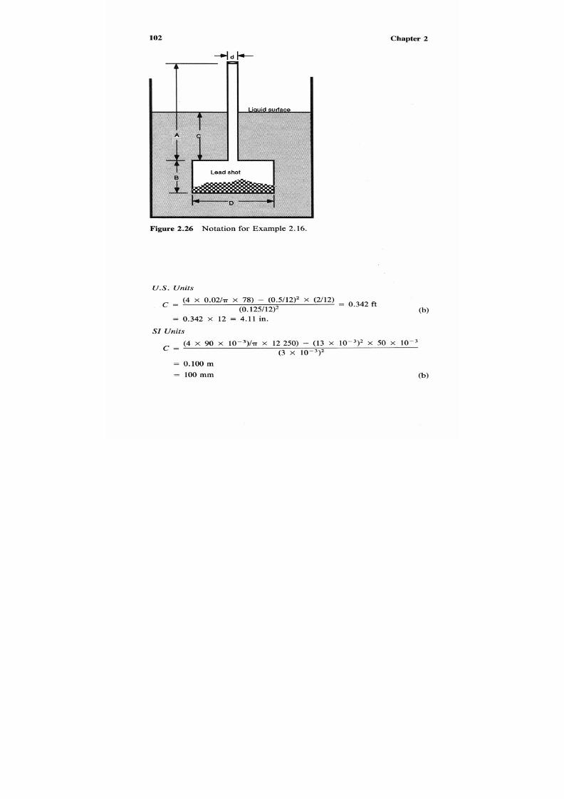
7/21/2019 Fundamental Fluid Mechanics for Engineers
http://slidepdf.com/reader/full/fundamental-fluid-mechanics-for-engineers 125/438
Chapter
2
02
Figure 2.26 Notation for Example 2.16.
US. nits
C =
(4
X
0.02/1~ 78)
-
(0.5/12)2
X
(2112) = o.342
ft
(0.125/12)2
= 0.342
x
12
=
4.11 in.
SI Units
(4
X 90 X
IO-^)^
X
12250)
-
(13
X IO-^)^ X 50
X W
(3 X 10⁻³)2
C =
= 0.100 m
=
100
(b)

7/21/2019 Fundamental Fluid Mechanics for Engineers
http://slidepdf.com/reader/full/fundamental-fluid-mechanics-for-engineers 126/438
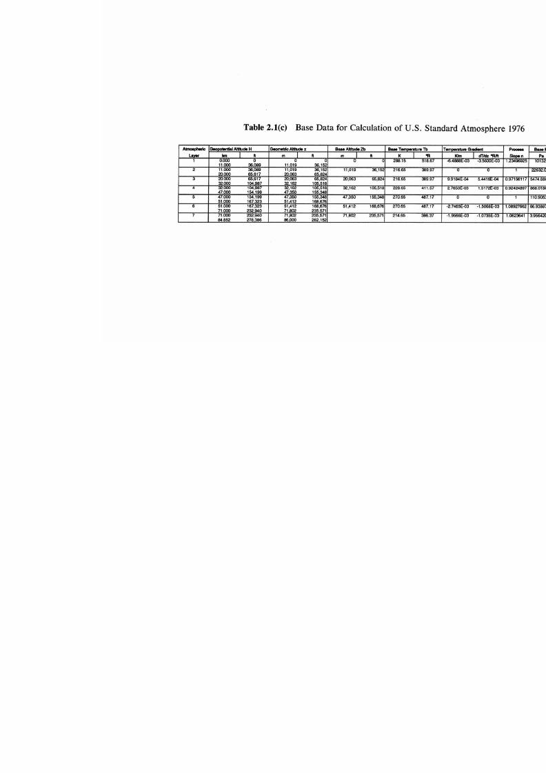
7/21/2019 Fundamental Fluid Mechanics for Engineers
http://slidepdf.com/reader/full/fundamental-fluid-mechanics-for-engineers 127/438

7/21/2019 Fundamental Fluid Mechanics for Engineers
http://slidepdf.com/reader/full/fundamental-fluid-mechanics-for-engineers 128/438
3.1
INTRODUCTION
This chapter is concerned with establishing he basic relationshipsof ve-
locity with rea in flow ystems and with he continuity equation. Methods
of reducing two- and three-dimensional flows o one-dimensional are il-
lustrated.
This chapter may be skipped by readers who are familiar with fluid
kinematics andlor the continuity equation . It is suggested that those who
are interested in boundary layer phenom ena read this chapter f ir s t.
This chapter may be used as a text for tutorial
or
refresher purposes.
Each concept is explained and derived mathematicallys needed. In keep-
ing with the concept of minimum mathematics, the vector approach is
not used.There are seven tutorial type examplesf fully solved problems.
3.2
FLUID KINEMATICS
Fluid kinematics is the branch of fluid mechanics that deals with the
geometry of fluid motion without considerationf forces causing motion.
It will be assumed hat any fluid particle is very large in size withespect
to a molecule and is hence continuous,
so
hat we are concerned with a
continuum.
105

7/21/2019 Fundamental Fluid Mechanics for Engineers
http://slidepdf.com/reader/full/fundamental-fluid-mechanics-for-engineers 129/438
106
Chapter
3
A quantity such as velocity or fluid particle displacement muste mea-
sured relative to some convenientcoordinate system. Two methods have
been devised for representing fluid motion. One describes the behavior
of a single fluidparticle; the other is concerned with several fluid particles
passing by certain points or sections of a fluid.
The description of the behavior of individual fluid particles is called
the Lagrangian method after Joseph Louis Lagrange
(1736-1813).
This
method of analysis involves establishinga coordinate system relative to
a moving fluid particleas it moves through the continuum and measuring
all quantities relative to the moving particle.The behavior of the individual
fluid particle is
of
no practical importance in fluid mechanics, and this
method is seldom used.
The establishment of a fixed coordinate system and he observation
of
the fluid passing through this system is called the Euler method after
Leonhard Euler (1707-1783). The Eulerian method will be used for the
most part throughout this book.
3.3 STEADY AND UNSTEADY FLOW
If
at every point in the continuum the local velocity
U,
nd any other
fluid property, remains unchanged with time,he flow is said to be
steady
f low.
While flow is generally unsteady by nature, many real cases of
unsteady flow may be reduced to the case of steady flow, a case that is
far easier to analyze mathematically. One technique for doing this is to
use a temporal mean or average.
U
t
Figure
3.1
Notation for unsteady flow.

7/21/2019 Fundamental Fluid Mechanics for Engineers
http://slidepdf.com/reader/full/fundamental-fluid-mechanics-for-engineers 130/438
Fluid
107
\\
Figure 3.2 Boat moving through still water.
Consider the velocity U ' at a point in space and time shown n Figure
3.1. The temporal mean average of U' is U as defined by
More generally,
(Temporal fluid property) = -
I
instantaneous fluid property)
d t
t
This technique
may
be used for small cyclic variations of fluid prop-
erties such
as
in turbulent flow or for large but rapidly changing cycles
such as those producedbyhigh-speedreciprocatingmachinery. The
amount of error produced will, of course, vary with the application.
Another technique that may be used that
is
free of error is to change
the space reference. Consider he boat shown n Figure 3.2 moving in still
water with a speed of V,. As the boat passes point
A
located at
xl, y1
the
wave produced will cause the fluid at point A to change from a velocity
of zero to a complicated variation with time until longfter the boat has
passed before t returns to zero again. If the point of reference is switched

7/21/2019 Fundamental Fluid Mechanics for Engineers
http://slidepdf.com/reader/full/fundamental-fluid-mechanics-for-engineers 131/438
108
Chapter3
Figure
3.3
Water flowing around a boat.
to the boat, then point
A
has a velocity of -V, at all times, as shown in
Figure 3.3. This method may be used any timebody is moved t constant
speed in an undisturbed fluid. Note that all that was actually done was
to reverse the direction of the velocity.
3.4
STREAMLINES AND STREAMTUBES
Velocity s a vector and hence has both magnitude and direction.
A
streamline is a line that gives the direction of the velocity of the fluid at
each point.
If
an almost instantaneous photograph were madef a flowing
fluid, the movements of a given particle would appear as a short streak
EL
c *.*
I
B
4''
treak
of a
particle
..-..
Stream line of particles
A t o
E
Figure
3.4
Streamlines.

7/21/2019 Fundamental Fluid Mechanics for Engineers
http://slidepdf.com/reader/full/fundamental-fluid-mechanics-for-engineers 132/438
Fluid 109
on the photograph. The direction of the streak would be tangent to the
flow path at that point and at that instant, and the length of the streak
would be proportional to the instantaneous velocity of that particle. Figure
3.4 shows the construction of the streamline from the particle streaks.
This streamline is also tangent everywhere to the velocity vectors.
When streamlines are drawn through a closed curve in a steady flow,
they form a boundary, which the fluid particles cannot pass. The space
between streamlines becomes a tube or passage and is called a
stream-
tube. The streamtube may be isolated from the rest of the fluid for anal-
ysis. The use of the streamtube concept broadens he application of fluid
flow principles;for example, it allows treatinghe flow inside a pipe and
the flow aroundan object with the same laws.A streamtube of small size
approaches its own axis, a central streamline; thus equations developed
for a streamtube may also be applied to a streamline.
3.5 VELOCITYPROFILE
Volumetric Flow Rate
In
the flow of real fluids, the individual streamlines will have different
velocities past a section. Figure
3.5
shows the steady flow of a fluid in a
circular pipe. The velocity profile is obtained by plotting he velocity
U
of each streamline as it passes section
A- A.
The streamtube that is formed
by the space between the streamlines is an annulus whose area normal
A
A
Figure
3.5
Velocityprofile.

7/21/2019 Fundamental Fluid Mechanics for Engineers
http://slidepdf.com/reader/full/fundamental-fluid-mechanics-for-engineers 133/438
110 Chapter
3
to the flow isd A as shown in Figure 3.5 or the streamtube whose velocity
is
U.
The volume rate of flow
Q
past section
A-A
is given by
Q = l U d A
(3.3)
Average Velocity
In many engineering applications, he velocity profile is nearly a straight
line or can be reduced to one so that the average velocity
V
may be used.
The average velocity
V
is defined as follows:
Methods of Flow Analysis
All flows take place between boundaries hat are three-dimensional. The
terms
one-dimensional, wo-dimensional, and three-dimensional flow
refer to the number of dimensions required o describe the velocity profile
of the streamtubes at a given section.
For one-dimensional flow, a line (L ) s necessary to describe the ve-
locity profile as shown in Figures 3.3 and 3.6(a).
(a) Onedim ensional f low
(b)
Two-dimensionallow
(c)
hree-dimensional f low
Figure 3.6 Types of flow.

7/21/2019 Fundamental Fluid Mechanics for Engineers
http://slidepdf.com/reader/full/fundamental-fluid-mechanics-for-engineers 134/438
Fluid
111
For two-dimensional flow, an area (L2) s necessary to describe the
velocity profile as shown in Figure 3.6(b)-for example, the flow
of
a
fluid between two parallelplates.
For three-dimensional flow, volume (L3)s necessary o describe the
velocity profile as shown in Figures 3.6(c) and 3.8. The usual example is
flow in a pipe, but the conduit or duct need not be circular for a three-
dimensional velocity profile. Three-dimensional flow, of course, is the
general case.
Example 3.1
An artificial canal is 100 ft (30.48 m) wide and is of rec-
tangular cross section. Water flows in this canal to a depth of
25
ft
(7.62
m). Measurements made f the velocity profile at a typical sectionare as
follows:
Measurement station Depthelocity
Numberocation ft (m) ftlsec ( S)
1
surface
0
0)
1.18 (0.360)
2 115depth
5 (1.524)
1.26
(0.384)
3 215depth
103.048)
1.16
(0.354)
4 315 depth
15
(4.572)
0.95
(0.290)
5 415 depth
206.096)
0.55
(0.168)
6 bottom
257.620)
0
0)
Estimate 1) the volumetric flow rate and (2) the average velocity of
the water as it flows past this section.
Solution
In order to solve this example, its necessary to evaluate U dA from test
data without knowing the functional relationship between the local ve-
locity and area. One method for doing this is to plot the data and draw
a smooth curve of the velocity profile and measure the enclosed area
mechanically. Another methods to use curve-fitting techniqueso derive
an equation that best represents the data and integrate this equation. A
third method is to use either the trapezoidal rule or Simpson's rule to
approximate the integral. Because he intent heres to illustrate streamline

7/21/2019 Fundamental Fluid Mechanics for Engineers
http://slidepdf.com/reader/full/fundamental-fluid-mechanics-for-engineers 135/438
112 Chapter 3
and streamtube concepts rather than to obtain maximum numerical ac-
curacy, the trapezoidal rule is used to solve this example.
(a) Apply the trapezoidal rule.
Divide the velocity profile into five evenly spaced depths
Ay
based on
the six measured velocities. The measured velocities may then be con-
sidered streamlines and the spaces between them streamtubes. Assume
that the velocity of a streamtube is the average of its bounding streamline
velocities.
1. Volumetric flow rate. For each streamtube, the volume flow rate is:
Q =
I
d A = UW
2.
For
the average velocity, from equation (3.4):
V = 2 QIA = C QIWyo
US. nits
1 .
Volumetricflow rate:
C Q
= [$(1.18 +
0)
+ 1.26
+
1.16 + 0.95 + 0.551
x
100
x
2515
=
2255
ft3/sec
2. The average velocity:
V
= 2255/(100
x
25) = 0.902 fdsec
SI
Units
1 . Volumetric low ate:
c
Q
=
[$(0.360
+
0)
+
0.384
+
0.354
+
0.290
+
0.1681
(dl
x
30.48 x 7.62015 = 63.92 m3/s
2. The averagevelocity:
V = 63.92/(30.48 X 7.620) = 0.275 S
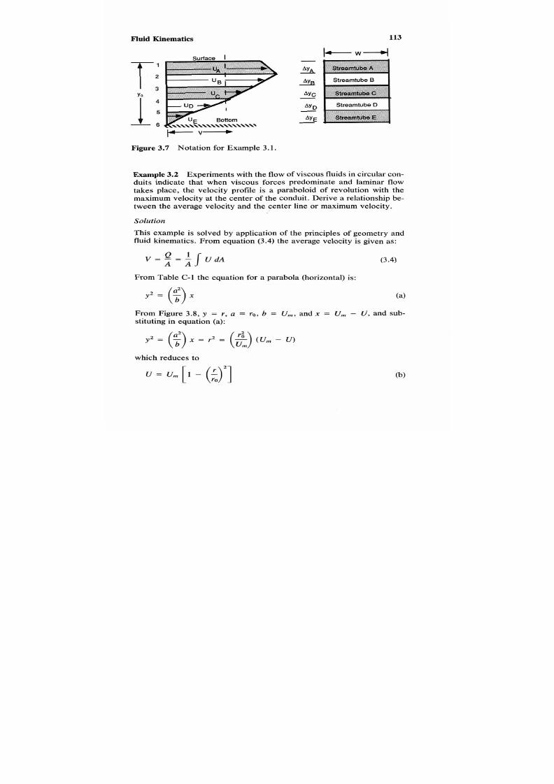
7/21/2019 Fundamental Fluid Mechanics for Engineers
http://slidepdf.com/reader/full/fundamental-fluid-mechanics-for-engineers 136/438
113
Figure 3.7 Notation for Example 3.1.
Example
3.2 Experiments with the flow
of
viscous fluids n circular con-
duits indicate that when viscous forces predominate and laminar flow
takes place, the velocity profile is a paraboloid
of
revolution with the
maximum velocity at the center of the conduit. Derive a relationship be-
tween the average velocity and the center line or maximum velocity.
From Table
C-l
the equation for a parabola (horizontal) is:
y 2 = 6).
From Figure 3.8, y
=
r , a =
ro,
b
= U,,,,
and x =
U,,,
- U , and sub-
stituting in equation (a):
which reduces to
U
=
U,,, [ -
Q 2 ]

7/21/2019 Fundamental Fluid Mechanics for Engineers
http://slidepdf.com/reader/full/fundamental-fluid-mechanics-for-engineers 137/438
114
Chapter
3
dA
=
2nrr
7 -
Figure 3.8 Notation for three-dimensional flow in circular conduits.
From Figure 3.8, d A
=
21rr dr; substituting this relation for d A and also
for U from equation (b) in equation
(3.4),
v = -
rn
2
or U,,, = 2V
Example
3.3 Velocity profile for turbulent flow in smooth circular pipes
may be empirically expressed by:
U
urn
( I
- ) a
where the value of exponent a varies from 2 to depending on the flow
conditions,
f
being used for wide ranges
of
turbulent flow. Derive a re-
lationship between the average velocity and the center line or maximum
velocity and determine the numerical relationship when
a
= f.
Solution
This example is solved by application of the principles of geometry and
fluid kinematics. From equation
(3.4)
the average velocity is given as:

7/21/2019 Fundamental Fluid Mechanics for Engineers
http://slidepdf.com/reader/full/fundamental-fluid-mechanics-for-engineers 138/438
Fluid 115
From Figure 3.8 , d A = 2 n r d r ,substituting this relation for d A and also
for U from equation
(a)
in equation (3.4):
Solving equation (b)for V/Urn:
Integrate by substitution. Let U = ro
-
r , then d u = -dr and r = ro
-
U:
V
- = -
ua(rO
-
U ) ( - d u )
(dl
(ro -
r )a+2 O
-
a + 2 1 o
Finally,
V 2
urn
( a
+
l ) ( a
+
2 )
For a = 4
V 2
Urn
V7
+
l ) (1/7 + 2)
”
= 0.8167
iY
.6 CORRECTION
FOR
KINETIC ENERG
Kinetic Energy
The kinetic energyof a body was shown in Chapter 1 to be
V2
K E =
2gc
(1.23)
For a streamtube, the kinetic energy
K E
flowing pasta section is he sum
of the kinetic energies of all the streamtubes, or
K E = 2 ( Ud A ) = -
U 3
d A
2gc 2gc
(3.5)
For one-dimensional flow
U
= V = constant, so that equation
(3.5)
be-
comes:

7/21/2019 Fundamental Fluid Mechanics for Engineers
http://slidepdf.com/reader/full/fundamental-fluid-mechanics-for-engineers 139/438
116
Chapter
3
Correct ion
Let
a
(alpha) be
a
correction factor to reduce the kinetic energy of two-
and three-dimensional flows o one-dimensional flow, or:
a =
KEone-dimensional
-
V 3 A / 2 g ,
(3.7)
3
a = AI ( dA
Values of
(Y
for three-dimensional flow range from for laminar flow
(Example
3.4)
to nearly unity for turbulent flow (Example 3.5) . As the
fluid velocity increases, the value of alpha approaches unity. The total
kinetic energy s small compared with ther terms except at high-velocity
gas flows where
(Y =
1.Because of this and the fact that the true value
of alpha is not always known, this correction is often neglected.
Example
3.4 Determine the value of (Y for three-dimensional laminar flow
using the information developed in Example 3.2.
Solution
This example s solved by usinghe relation betweenV and U,,,eveloped
in Example 3.2 and using this relationship
in
equation (3 .7) . From Ex-
ample 3.2,
2
U =
rn
[ l -
(-$
and V
=
-rn
2
so
that
=
[
- ( 3 1 = 2
[
1
-
LJ2]
v U m / 2
Substituting equation (a) in equation
(3.7),
=
[
1
- ( 9 2 ] 3 dr
Equation (b) may be integrated by substitutions as follows. Let U = [l
-
(r/rO)*],
hen du = - (2r /r$) dr and
J
du = u4/4 = (1/4)[1
-
( r / r ~ ) ~ ] ~ .
Substitution of the above in Eq. (b) yields:
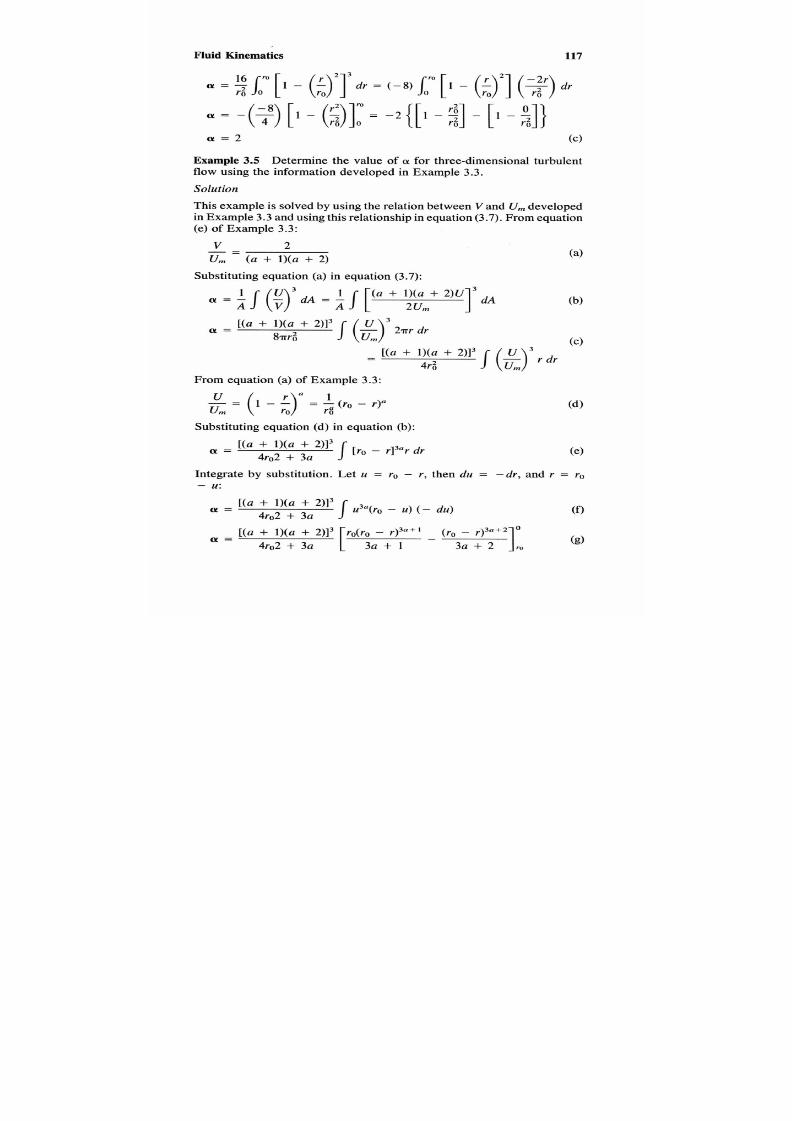
7/21/2019 Fundamental Fluid Mechanics for Engineers
http://slidepdf.com/reader/full/fundamental-fluid-mechanics-for-engineers 140/438
Fluid
Kinematics 117
a
= [
-
( 9 2 ] 3
dr = ( -8) [ l - ro ($) dr
a = - ($)[ l -
( S ) ] ; =- 2 { [ 1 - $ ]
- [
-;l}
Example 3.5 Determine the value of (Y for three-dimensional turbulent
flow using the information developed in Example 3.3.
Solution
This example s solved by using he relation betweenV and U,,,eveloped
in Example 3.3 and usinghis relationship in equation (3.7). From equation
(e) of Example 3.3:
V 2
U, ( a + l)(a + 2)
Substituting equation (a) in equation (3.7):
From equation
(a) of
Example 3.3:
Substituting equation
(d)
in equation (b):
Integrate by substitution. Let u =
ro -
r , then du = -d r , and
r =
ro
-
U:
[ ( a + l ) ( a +
2)i3 ro(ro
- r)3a+' (ro3i
;3;+2];
a =
4r02
+
3a
[
3 a + 1
-
(8)
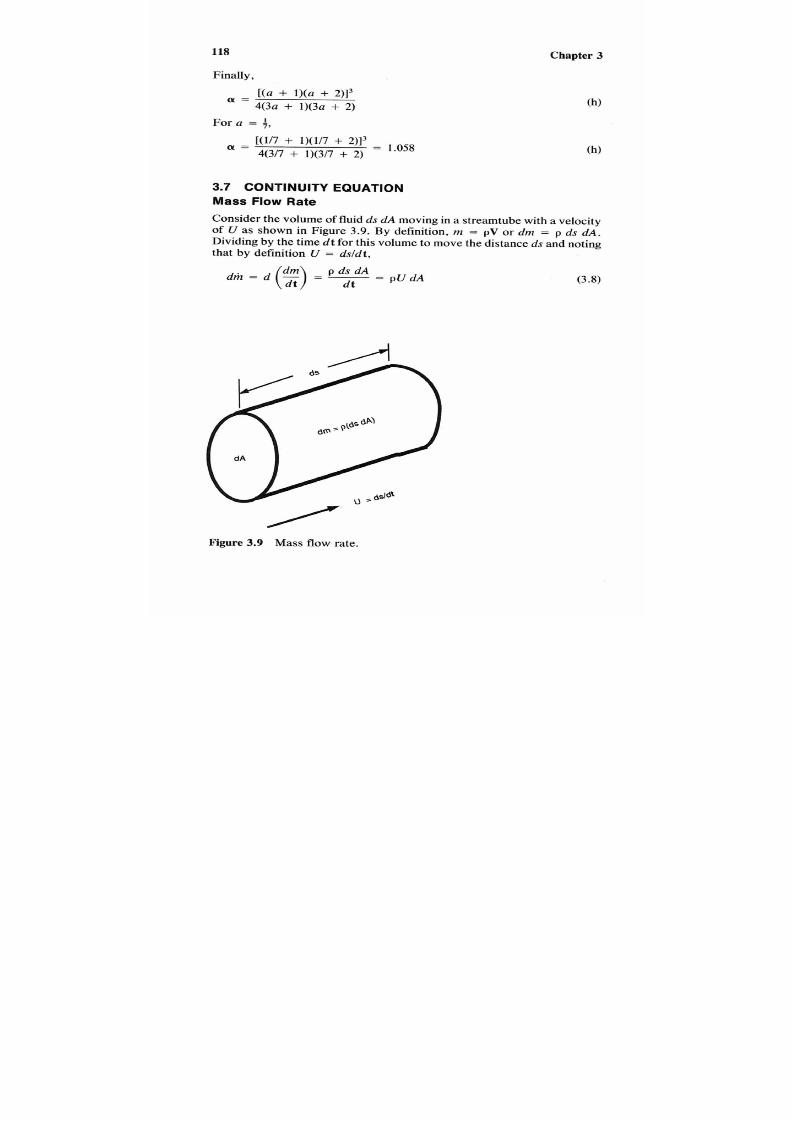
7/21/2019 Fundamental Fluid Mechanics for Engineers
http://slidepdf.com/reader/full/fundamental-fluid-mechanics-for-engineers 141/438
118
Finally,
[ ( a
+ +
211~
a =
4(3a + 1)(3a +
2)
For
a =
f,
[(1/7
+
I)(l/7 + 2)13
a =
4(3/7 + 1)(3/7 + 2)
= 1.058
3.7 CONTINUITY EQUATION
Mass Flow Rate
Consider the volume
of
fluid d s d Amoving
in a
streamtube with
a
velocity
of
U
as
shown in Figure 3.9. By definition, m
=
pV or dm = p ds dA.
Dividing by he time d t for this volume to move the distance s and noting
that by definition U = d s / d t ,
Figure
3.9 Mass flow rate.
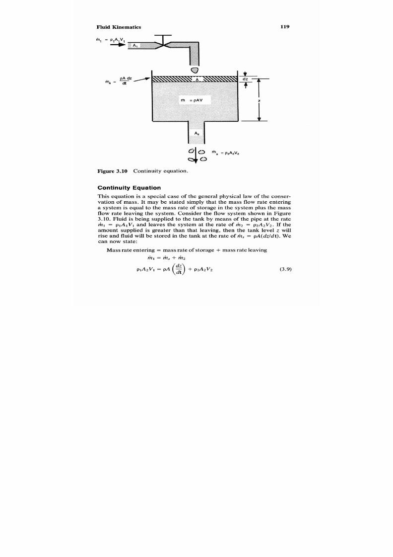
7/21/2019 Fundamental Fluid Mechanics for Engineers
http://slidepdf.com/reader/full/fundamental-fluid-mechanics-for-engineers 142/438
Fluid Kinematics
119
t
l
Figure 3.10 Continuity equation.
Continuity Equation
This equation is a special case of the general physical law of the conser-
vation of mass. It may be stated simply that the mass flow rate entering
a system is equal to the mass rate of storage in the system plus the mass
flow rate leaving the system. Consider the flow system shown in Figure
3.10.
Fluid is being supplied to the tank by means of the pipe at the rate
rizl
=
p l A I V l and leaves the system at the rate of
riz2 =
p2A2V2. If the
amount supplied is greater than that leaving, then the tank level
z
will
rise and fluidwill be stored in the tank at the rate ofriz,
=
pA(dz/dt) . We
can now state:
Mass rate entering = mass rate of storage
+
mass rate leaving
h, riz,+
h*

7/21/2019 Fundamental Fluid Mechanics for Engineers
http://slidepdf.com/reader/full/fundamental-fluid-mechanics-for-engineers 143/438
120 Chapter 3
Steady State
If
the amount supplied is equal
to
the amount removed, then
dz
is zero
or there is no storage. Equation (3.10) becomes:
rit = plAlVl = pzAzV2
=
*
=
pnAnVn = PAV (3.10)
The relationship of density to specific volume p
=
l/v (equation (1.30))
allows the equation of continuity to be written as:
V A
= pAV
=
V
(3.11)
The mass flow rate is constant any place in a steady-state system.
For
compressible fluid, it is sometimes convenient o use a differential form
of
equation (3.11), which may be obtained by writing it in logarithmic
form and differentiating, noting hat rit is a constant:
loge V + log, A
-
loge V = loge rit (3.12)
dV dA dv
v v v
-
0
(3.13)
Using the equation
(1.30)
relationship
v
=
l/p
gain, equation
(3.14)
may
be written as:
(3.14)
Example
3.6
A
12
in. size schedule 40 steel pipe reduces to a 6 in. size
schedule 40 pipe and then expands to an
8
in. size schedule 40 pipe, as
All schedule 40 steel pipe :
Figure
3.11 Notation for Example 3.6.

7/21/2019 Fundamental Fluid Mechanics for Engineers
http://slidepdf.com/reader/full/fundamental-fluid-mechanics-for-engineers 144/438
Fluid Kinematics 121
shown in Figure 3.11. If the average velocity in the 12 in. size pipe is
13.12 ft/sec (4 m/s), compute the average velocity in the 6 in. size and
the
8
in. size pipes, for
any incompressible flu id .
Solution
This example is solved by the application of the continuity equation to
an incompressible fluid. Writing equation3.11) in the notation of Figure
3.11:
h p 1 2 A n V n
=
P&vn
=
PsAsVs
(a)
Noting that for an incompressible fluid
p
is
a constant and that the pipe
area =
rd2/4.
Substituting in equation (a) and simplifying:
dT2V12
=
dgv6
=
d f v s (b)
Solving equation (b)for V s and v8
v6 = V I ~ ( ~ I Z & ) ~ (c)
and
vs
=
V 1 2 ( d n / d s ) ~
( 4
N ote that fo r incompressible fl o w in circular pi pe s, the velocity varies
inversely with the square of the diameter.
From Table C-3, Schedule 40, steel pipe:
Pipe size Internal diameter, ft (mm)
6 in.
8 in.
12
in.
0.5054
0.6651
0.9948
(154.1)
(202.7)
(303.3)
U.S.
Units
v6
= V12(d12 /d6 )~ 13.12(0.9948/0.5054)2 = 50.83 ft/SeC (c)
vs = V 1 2 ( d 1 2 / d s ) ~ 13.12(0.9948/0.6651)2 = 29.35 ft/sec (dl
S I Units
v6
= V12(dlz/ds)’ = 4(303.3/154.1)2 = 15.50 m/S (c)
vs
=
V 1 2 ( d 1 2 / d s ) ~ 4(303.3/202.7)2 = 8.96 m / S ( 4
Example
3.7
Air discharges froma 12in. size standard steel pipe through
a 4 in. (100 mm) inside diameter nozzle into the atmosphere, as shown

7/21/2019 Fundamental Fluid Mechanics for Engineers
http://slidepdf.com/reader/full/fundamental-fluid-mechanics-for-engineers 145/438
122
Chapter 3
12 in.
size
Std
S t e e l
p i p e 7
I
Figure
3.12
Notation for Example
3.7.
in Figure
3.12.
The pressure in the duct is
20
psia
(140
kPa), and atmos-
pheric pressure is
14.7
psia (101 kPa). The temperature of the air in the
pipe just upstream of the nozzle is
140°C
60”C), and the velocity is
18
ft/sec (5.5 m/s). For isentropicflow, compute (1) the mass flow rate and
(2) the velocity in the nozzle jet. (Assume that the isentropic exponent
of air has a constant value of
1.4.)
Solution
This example is solved usinghe continuity equation, ideal gas processes
(Section
1.13),
and the ideal gas equation of state (Section
1.14).
1. The mass rate of flow may be calculated using equation
(3.1 1):
The specific volume
of
the air in the pipe may be calculated from
equation
(1.42), pv
= R T , and Eq.
(1.43),
R = R , / M
RTp RuTp
v,=-=-
P P MPP
Substituting equation (b) in equation (a):
2. Solvingequation(a) for the velocity of the jet, note that for an
isentropic process from equation(1.38) p v k = c and that A = 7rd2/4:
vj =
v,
($p)(;)
= v, ( ) 2
7/21/2019 Fundamental Fluid Mechanics for Engineers
http://slidepdf.com/reader/full/fundamental-fluid-mechanics-for-engineers 146/438
Fluid Kinematics 123
3. Common data. From Table C-3 or
a 12
in. size standard steel pipe,
d,
=
1
ft
(304.8
mm) A
=
0.7854
ft
(72 70
X
m')
From Table A-l for air, M
=
28.97. From Section 1.14, R, = 1545
ft/lbf/(lbm-mol-"R) (8 314 Jkg.mo1.K).
US. nits
T,
=
140 + 460 = 600"R Aj = ~(4/12)~/4 00873 ft2
1. Mass low rate:
0.7854
x
18
x
28.97
x
(20
x
144)
1545 x 600
m =
= 1.272 lbm/sec (c)
2. Jet velocity:
V = 18 = 201.8 ft/sec
SI Units
Tp
=
60
+
273
=
333
K
Aj
=
~ ( 1 0 0 10-3)2/4
=
7 854 x m'
1. Mass low rate:
72 970
x
x 5.5 x 28.97 x 140
x
IO3
8 314
x
333
m =
= 0.588 kg/s
2. Jet velocity:
304.8
111.4
Vj = 5.5
(100)~
E)
= 64.52 m/s
Ideal Gas Relations
Two useful relations for ideal gases were developed in the solution of
Example 3.7. For mass flow rate:
AVMp
AVp
m=-=-
RUTT
(ideal gas only)
and for velocity variation with passagearea:
V2 = VI e)
@
ln (idealgasonly)
(3.15)
(3.16)

7/21/2019 Fundamental Fluid Mechanics for Engineers
http://slidepdf.com/reader/full/fundamental-fluid-mechanics-for-engineers 147/438
4.1
INTRODUCTION
This chapter is concerned with establishing the basic relationships for
energy and force. Equations for these relations are developed for use in
the application chapters to follow.
This chapter may be skipped by readers who are familiar with the
energy equation and the impulse mom entum equation.
This chapter may be used as text for tutorial or refresher purposes.
Each concept is explained and derived mathematicallys needed. In keep-
ing with the concept of minimum level of mathematics, the vector ap-
proach is not used. There are 11 tutorial type examples of fully solved
problems.
4.2
FLUID DYNAMICS
Fluid dynamics is the branch
of
fluid mechanics that deals with energy
and force. This chapter considers the equation of motion, the energy
equation, and the impulse-momentum equation. The continuity equation
was developed inChapter
3
as a special case of the principle of the con-
servation
of
mass. The equation
of
motion is an application f Newton’s
second law o fluid flow n a streamtube. The energy equationis a special
124

7/21/2019 Fundamental Fluid Mechanics for Engineers
http://slidepdf.com/reader/full/fundamental-fluid-mechanics-for-engineers 148/438
Fluidynamicsd 125
case of the principle of the conservation of energy. The mpulse-momen-
tum equationwas developed n Chapter 1 as a special case of the equation
of motion.
The equation ofmotionwas first developedn 1750 by Leonhard Euler
and is sometimes called the Euler equation, although Euler’s equations
were writtenfor a frictionless fluid. Euler’s equation laidhe groundwork
for an analytical approach to the studyf fluid dynamics. The introduction
of viscous effects allowsor a more general interpretationf the equation
and makes it more applicable o the solution of practical problems.
The energy equation for steady flow is simply an accounting of all of
the energy entering
r
leaving a control volume. Althoughan energy equa-
tion may be developedo consider all forms f energy,
in
fluid mechanics,
chemical, electrical, and atomic energies are not normally considered.
The impulse-momentum equation, along with the continuity equation
and energy equation,provides a third basic tool for the solution of fluid
flow problems. Sometimests application leads tohe solution of problems
that cannot be solved by the energy principle alone; more often it is used
in conjunction with the energy principle to obtain more comprehensive
solutions of engineering problems.
4.3 EQUATION
OF
MOTION
Derivation
1.
2.
3.
Consider the fluid element flowing steadily in streamtube shown in Fig-
ure
4.1.
This element has a length of d L , an area normal to the motion
of dA, and a perimeter of d P . The elemental mass isd A d L . he increase
in elevation of this mass is
d z ,
and the motion of the element is upward.
Forces tending to change the velocity
U
of this fluid mass are:
Pressure forces on the ends of the element:
Gravity force due to the component of weight in the direction of mo-
tion:
pg
dA
dLdz
pg
dA dz
dF, = -
gc x) - g c
Friction force on the outer surface of the element:
dFf
=
- 7
dP dL
(4.3)

7/21/2019 Fundamental Fluid Mechanics for Engineers
http://slidepdf.com/reader/full/fundamental-fluid-mechanics-for-engineers 149/438
126
Chapter
4
dP
Q
\
AFQ \
L
/
dz
Figure 4.1
Elements
of
a streamtube.
4. The combined force becomes:
C dF = dFp + dF,
+
dFf
=
- d p dA - dA
dz
-
7
dP dL
gc
= -dA
( d p +
(4.4)
With application of Newton's second law (equation
1.
lo):
p dA U L
(p
A ) ( U U )
. ,
-
g c
(x)
gc
Substituting from equation (4.4) for 2 F, equation (4.5) may be
written as
Simplifying equation (4.6) and setting it equal to zero, results in
g U dUp
7
dL dP
d z
+
gc
gc + - + P ; j ; i ) = o
(4.7)
7/21/2019 Fundamental Fluid Mechanics for Engineers
http://slidepdf.com/reader/full/fundamental-fluid-mechanics-for-engineers 150/438
Fluid Dynamics and Energy Relations
Substituting
v = l /p
from equation
(1.30)
results in
- d z
+ -
8 c g c
U d U
+
v d p
+
m d L
(g)
0
127
(4 .8)
4.4
HYDRAULIC RADIUS
Definition:
Fluid flow aredshear perimeter
Symbol:
Rh
Dimensions:
L
Units:
US.: t SI: m
In the derivation of the equation
of
motion, the shape of the streamtube
cross section was not specified.The ratio of the fluid area (dA)o shear
area dP dL
is a function
of
streamtube flow shape and is a constant
for
a
given geometry. The hydraulic radius Rh may be used to define this
ratio per unit of Iength as follows:
Hydraulic radius =
fluidlow area dA
A
shear perimeter
dP P
= R
-
h = -
(4 .9)
The hydraulic radius is usedo compute flow osses in noncircular flow
passages and circular conduits flowing partly full f liquids. For this rea-
son, it is important to relate the hydraulic radius to the diameter D of a
circular pipe:
The equivalent diameter
D ,
is
D , = 4Rh
(4.10)
(4.11)
Example
4.1 A
iquid flows in the rectangular duct shown
in
Figure 4.2
to a depth of 2 ft (0.61 m). If the duct is 6 ft (1.83 m) wide and
3
ft (0.91
m) deep, compute 1 ) the hydraulic radius Rh and ( 2 ) the equivalent di-
ameter D , .
Solution
This example is solved by notinghat the shear perimeter consists
of
that
portion of the fluid that is in contact with the walls of the duct.
1.
The hydraulic radius. From Figure 4.1 , the fluid flow area is
A
= bh ( 4

7/21/2019 Fundamental Fluid Mechanics for Engineers
http://slidepdf.com/reader/full/fundamental-fluid-mechanics-for-engineers 151/438
128
Chapter
4
Figure 4.2 Notation for Example 4.1.
and the shear perimeter is
P = h + b + h = 2 h + b
From equation (4.9):
A bh
P
2 h + b
R h = - = -
2. Equivalentdiameter:
D , =
4Rh
US.Units
1. The hydraulicradius:
R -
6 x 2
h - 2 x 2 + 6
=
1.2ft
2. Equivalentdiameter:
D ,
= 4 X 1.2 = 4.8 ft
SI
Units
1 . The hydraulicradius:
1.83 x 0.61
2 x 0.61 + 1.83
h = = 0.366 m
( c )
(4.11)
7/21/2019 Fundamental Fluid Mechanics for Engineers
http://slidepdf.com/reader/full/fundamental-fluid-mechanics-for-engineers 152/438
Fluidynamicsd 129
2. Equivalentdiameter:
D ,
=
4
x
0.366
=
1.464
m
(4.11)
Values of the fluid flow areaA and the hydraulic radius
h
and equiv-
alent diameter D , for various cross sections are given in Table C-2.
4.5
ONE-DIMENSIONAL STEADY-FLOW EQUATION OF
MOTION
When the flow is one-dimensional, V =
U.
ubstituting this value of U
and the definition of hydraulic radius of equation (4.9) in equation (4.8),
g
V dV m
” d z
+ -
+ v d p + - d L = O
?c
gc
Rh
(4.12)
Integrating equation
(4.12)
between sections
1
and 2,
g vf - v: + 1 2 v d p +- I 2 d L = 0
- 22 - Z l )
+
2gc R h
I
(4.13)
gc
Let
(4.14)
whereHf s the energy “lost” due to friction. Substituting thisn equation
(4.13) results in
For an incompressiblefluid
(v1
= VZ), equation
(4.15)
becomes
(4.15)
(4.16)
For frictionless flow of an incompressible fluid
(Hf 0),
equation
(4.16)
reduces to
(4.17)
Multiplying equation (4.17) by
gc/g
and noting from equation (1.31) that
v
=
g/ygc esults in

7/21/2019 Fundamental Fluid Mechanics for Engineers
http://slidepdf.com/reader/full/fundamental-fluid-mechanics-for-engineers 153/438
130
or
Chapter 4
(4.18)
This s the equationproposed byDanielBernoulli nhis “Hydrody-
namica” published in
1738.
Example
4.2 The system shown in Figure 4.3 consists of a 12 in. size
Type L seamless copper water tube that reduces to a 6 in. size tube and
then expands to an
8
in. size tube. Water (y = 62.31 lbf/ft3,
9
790 N/m3)
flows steadily and without friction through this system. At section
1
in
the 12in. size, the pipe center line is 10 ft (3.05
m)
above the datum, the
pressure is
20
psia
(138
kPa), and the velocity is
4
ft/sec
(1.22 m/s).
At
section
2
in the
6
in. size, the center line is15ft
(4.57
m) above the datum.
At section 3 in the 8 in. size, the center line is 20 ft
(6.10
m) above the
datum. Find
1)
the volumetric flow rate, (2) the velocity, and (3) the
pressure at sections 2 and 3 of Figure 4.3.
Solution
This example is solvedy the application of Bernoulli’s equationfor fric-
tionless flow and the continuity equation.
1. For frictionless flow, the fluid energy is the same at all sections of
the system, so that equation (4.18) may be written as:
where
H,
is the total fluid energy at each section. The term
H1
may
be calculated from section 1 ata:
2.
The continuity equation
(3.11)
for steady flow of an incompressible
fluid
(p
=
c),
m
=
PAIVI
=
pA2V2
=
pA3V3
(c)
reduces to
mlp
= Q =
AIVI
=
A2V2
=
A3V3
(dl
The volume flow rate is calculated from section 1 data:

7/21/2019 Fundamental Fluid Mechanics for Engineers
http://slidepdf.com/reader/full/fundamental-fluid-mechanics-for-engineers 154/438
Fluid Dynamics and Energy Relations
131
Figure
4.3 Notation for Example
4.2.
3. At section 2,
V2
= QIAZ
4. Atsection 3,
V3
=
QIA3
5. Common data, from Table C-5, Type seamless copper water tubing:
Sectionize ft’
(mm’)
1 12 in.
0.7295 (67 790)
2 in.
0.1863 (17 320)
3 8 in.
0.3255 (30 250)
7/21/2019 Fundamental Fluid Mechanics for Engineers
http://slidepdf.com/reader/full/fundamental-fluid-mechanics-for-engineers 155/438
132
Chapter
4
U.S.
nits
1.
Totalhead:
4'20
x 144
Ht
=
10
+
2
X
32.17 62.31
=
56.47 ft
2. Volumetric flow rate(all sections):
Q
= 0.7295
X
4
=
2.918 ft31sec
3. At section 2:
V2
=
2.918/0.1863
=
15.66fVsec
4. At section 3:
V,
= 2.91810.3255 = 8.96
ftlsec
SI Units
1 . Totalhead:
Hr =
3.05 +
122'38 X 103
2 x 9.807 9 790
= 17.22 m
2. Volumetric
flow
rate(all sections):
Q
=
67790
x
10-6 .x 1.22
=
0.0827
m3/s
3.
At section 2:
V2 =
0.0827117320 X 10 j
=
4.77 m / ~
p2
= 9 79017.22
-
4.57
-
(
4*772 ) X = 112.5 kPa
2
x
9.807
(g)
4.
At section
3:
V3 = 0.0827/(3050
X
= 2.74
m / ~
(h)
2.742 ) X
x 9.807
=
105.1
kPa (i)

7/21/2019 Fundamental Fluid Mechanics for Engineers
http://slidepdf.com/reader/full/fundamental-fluid-mechanics-for-engineers 156/438
Fluid Dynamics and Energy Relations
133
4.6
SPECIFIC ENERGY
Definition:
Energy per unitmass
Dimensions: FLM = (M L T -') L '
=
L 2 P
Units: U.S.: ft-lbf/lbmI: Jkg
Before developing the energy equation,
a
general discussionof energy is
in order. Two sets of energy will be considered. The first is the energy
of the fluid at a section, and the second is the energy added to or taken
from the fluid between sections. The total energy possessed by a fluid at
a section is dependent on the net energy added toor taken from he fluid
between it and prior section, but the individual energies re independent
of their counterparts at the prior section. For this reason, fluid energies
are called point functions. The energies added to or taken from the fluid
between sections depend on the manner or process, and these transitional
energies are called path functions because of their dependence on the
process undergone. The total amount of energy in a system cannot be
measured but must be referenced to some arbitrary datum. In fluid me-
chanics, we are interested in energy
change, and any convenient datum
may be used.
4.7
SPECIFIC POTENTIALENERGY
The potential energy of a fluid mass is the energy possessed by itdue to
its elevation relative to some arbitrary datum, as stated in Section 1.8. It
is equivalent to the work that would be required to lift it from the datum
to its elevation in the absence of friction.
The change in specific potential energy
A P E )
may be computed from
equation (1.18) for
a
field of constant gravity as follows:
(4.18)
Note that equation
(4.18)
is the same as the first term of equation
(4.13).
4.8
SPECIFIC KINETICENERGY
The kinetic energy of a fluid mass is the energy possessed by it due to
its motion, as stated in Section 1.8. It is equivalent to the work required
to impart the motion from rest in the absence of friction.

7/21/2019 Fundamental Fluid Mechanics for Engineers
http://slidepdf.com/reader/full/fundamental-fluid-mechanics-for-engineers 157/438
134
Chapter 4
The change in specific kinetic energy ( A K E ) may be computed from
equation ( l 23) as follows:
(4.19)
Note that equation
(4.19)
is the same as the second term f equation
(4.13).
Equation
(4.19)
may be used only for one-dimensional flow. As was
shown in Section
3.6,
the correction factor C L should be applied for two-
and three-dimensional flows. Application of equation
(3.7)
to equation
(4.19)
results in
AKE =
a2v; - CL1v:
2gc
(4.20)
where a1 and a2 are the kinetic energy correction factors for the velocity
distributions at sections 1 and 2 respectively.
N ot e that equation (4 .20 ) s seldom used in engineering pra ctic e. For
turbulent fl ow in pip es where the velocity is high the kinetic energy cor-
rection fac tor
i s
nearly unity (see Example 3.5) and when the flow is
laminar the velocity is low and the kinetic energy correction factor is 2
(Example 3. 4) the change n specific kinetic energy is usually insignificant.
4.9
SPECIFIC INTERNAL ENERGY
The internal energy of a body is the sum total of the
kinetic
and
potential
energies of its molecules, apart from any kinetic or potential energy of
the body as a whole. The total kinetic internal energy s due primarily to
the translation, rotation, and vibration of its molecules. The potential
internal energy is due to the bonding or attractive forces that hold the
molecules in a phase.
The potential internal energy decreases as a substance changes from
solid to liquid to gaseous phases as the bonding forces decrease. In the
gas phase, the internal energy is mainly kinetic. As the ideal gas state is
approached and molecular activity increases with temperature increase,
the internal energy becomes wholly kinetic, andhus the internal energy
of an ideal gas is a pure temperature function.
The symbol for specific internal energy is
,
nd the change in specific
internal energy is given by
Au
=
l2 u
= u2 - u t
(4.21)

7/21/2019 Fundamental Fluid Mechanics for Engineers
http://slidepdf.com/reader/full/fundamental-fluid-mechanics-for-engineers 158/438
Fluid Dynamics and Energy Relations
135
Units
For the
SI
system, the joule per kilogram or newton meter per kilogram
is used. For the
U.S.
customary units, conventional practice iso use the
British thermal unit per pound mass (Btuhbm). For fluid mechanics, it
will be necessary to convert the Btu to.ft-lbf (778.2 t-lbf = 1Btu).
4.10
SPECIFIC FLOW WORK
Flow work
is the amount of mechanical energy required to “push” or
force
a
flowing fluidacross a section boundary. Considerhe steady-flow
system shown in Figure 4.4. Fluid enters the system at section 1, where
the flow area is A , and the pressure is p l , and leaves at section 2, where
the flow area is A 2 and the pressure p 2 . The force acting to prevent the
System boundaries
Flow
direction
-
Section
boundaries
Figure
4.4
Flow work.

7/21/2019 Fundamental Fluid Mechanics for Engineers
http://slidepdf.com/reader/full/fundamental-fluid-mechanics-for-engineers 159/438
136 Chapter 4
fluid from crossinga section boundary is
F
=
pA
.
(4.22)
where p is the pressure at the section boundary andA is the flow area.
Substituting equation (4.22) in equation (1.16),
F W = - J F d r = J $ &
(4.23)
where
F W
is the specific flow work. Notinghat A
dr
is the volume V of
fluid being “pushed” across a section
mu,
quation
(4.23)
may be written as
A F W
=
1’“-=;“
(:v) 4 p m v )
-
boundary and by definition V =
where A F W is the change in specific flow work.
4.11
SPECIFIC ENTHALPY
It is sometimes desirable to combine certain fluid properties to obtain a
new one. Enthalpy is a defined property combining internalenergy, pres-
sure, and specific volume.
The symbol for specific enthalpy ish, and specific enthalpy is defined
by the following equation:
h = u + p v (4.25)
The change in specific enthalpy becomes
Units
For the SI system, the joule per kilogram or newton meter per kilogram
is used. For the U.S. customary units, conventional practice is to use the
British thermal unit per pound mass (Btdlbm). For fluid mechanics, it
will be necessary to convert the Btu to ftllbf (778.2 ft-lbf =
1Btu).
4.12 SHAFT WORK
Definition
Shaft work is that form of mechanical energy which crosses the bound-
aries of a system by being transmitted through the shaft of a machine.

7/21/2019 Fundamental Fluid Mechanics for Engineers
http://slidepdf.com/reader/full/fundamental-fluid-mechanics-for-engineers 160/438
Fluidynamics
137
The result of this transmission is to increase or decrease the total amount
of energy stored in
a
fluid.
Shaft work is mechanical energy in
ransition
and cannot be stored as
such in
a
fluid. For example, consider a pump pumping water from a
lower level to
a
higher one. While the pump is in operation, shaft work
is transmitted to the water and this increase in energy causes the water
to rise to a higher elevation. After the pump has stopped, the amount of
energy added to the fluid less losses is now stored in the water
in
the
form of increased mechanical potential energy.
Because the first engines built by humans were made o extract work
from the fluid energy, conventional ractice is to call shaft work one by
a fluid
positive work,
and work done n a fluid
negative work.
Shaft work
may also be classed as steady flow or nonfrow according to the type of
machine and process.
Nonflow Shaft Work
Process
Consider the cylinder and piston arrangement shownn Figure
4.5. As
the piston advances from the state point
1
to point 2, the fluid in the
P
Figure 4.5 Nonflow shaft work.
7/21/2019 Fundamental Fluid Mechanics for Engineers
http://slidepdf.com/reader/full/fundamental-fluid-mechanics-for-engineers 161/438
138 Chapter 4
cylinder expands and work is done
by
the fluid . If the piston were made
to retract, then the fluid would be compressed and work would be done
on the flu id.
Equations
The force exerted by the fluid on the piston of Figure 4.5 is given by
F = p A (4.22)
Substituting equation
(4.22)
n equation
(1.16),
noting that the area of the
piston A is a constant so that A dx = dV and that by definition V
=
mu,
results in
(4.27)
where W n f s the specific shaft work.
Function
Equation
(4.27)
s a mathematical statement that the shaft work is the
area “under” the pressure-specific volume curve of Figure
4.5.
There are
an infinite number of ways that the fluid can change from tate
1
to state
2.Shown in Figure.5 are three curves which represent the paths of three
possible processes . Path
1-y-2
as chosen to represent the actual path of
the process or state change. Had path
1-x-2
een chosen, the amount of
work would have been greater;
if
1-2-2,he work would have been less.
For this reason, shaft work is called a path function. Before equation
(4-
27)
can be integrated, the pressure-specific volume relationship must be
known.
Steady-Flow
Shaft Work
Equations
The specific steady-flow shaft work may be expressed as follows:
where
W ,
is the steady-flow shaft work per unit mass. Because the dif-
ferential
of
shaft work is inexact, the Greek symbol
6
is used instead
of
d. Equation
(4.28)may
be then written as follows:
Wsf = J SWSf
(4.29)

7/21/2019 Fundamental Fluid Mechanics for Engineers
http://slidepdf.com/reader/full/fundamental-fluid-mechanics-for-engineers 162/438
Fluid Dynamics and Energy Relations
139
4.13 HEAT AND ENTROPY
Heat
is
that form of thermal energy which crosses the boundaries of a
system without the transfer of mass as a result of a difference in tem-
perature between the system and ts surroundings. The effectf this trans-
fer is to increase
or
decrease the total amount of energy stored in a fluid.
Heat is thermal energy in transition, and like shaft work it cannot be
stored as such in a fluid. Because the first devices made y humans were
to produce shaft work by adding heat, heat added to a substance is pos-
itive, and heat rejected is negative.
ntropy
is that fluid property required
by the second law of thermodynamics to describehe path of a reversible
process. Entropy is defined by the following equation:
q =
J T d s
(4.30)
where
q
is the heat transferred per unit mass and is the entropy per unit
mass.
Process
Heat may also be expressed as
4
=
L* 4 f 2 -
41
(4.31)
where
q is
the heat transferred per unit mass. Note that the symbol
6
is
used in place of
d
to remind us that the differential of heat transfer is
inexact.
Equations (4.30) and (4.31) may be combined as follows:
q
= J 8 q
= J T d s
(4.32)
Equation (4.32) is a mathematical statement; heat is he area “under” the
temperature-entropy curve of Figure 4.6. As with shaft work, there is an
infinite number of ways that the heat can be transferred from point1 o
2, so that heat, like shaft work, is a pa th function. The relation between
temperature and entropy must be established before equation (4.32) can
be integrated.
Units
In the SI system, the joule per kilogram
or
newton meter per kilogram is
used for heat and the joule/kilogram kelvin is used for entropy. In the
U.S .
system, the British thermal unit per pound mass is used for heat,

7/21/2019 Fundamental Fluid Mechanics for Engineers
http://slidepdf.com/reader/full/fundamental-fluid-mechanics-for-engineers 163/438
140
T
Chapter 4
I
1
S
Figure
4.6
Temperature-entropy plane.
and the British thermal unit/pound mass degree Rankine is used for en-
tropy. For fluid mechanics, it will be necessary to convert the Btu to ft-
lbf and the Btu/lbm-"R to ft-lbf/lbm-"F (778.2 ft-lbf = 1 Btu).
4.14 STEADY-FLOW ENERGY EQUATION
The steady-flow energy equation is readily derived y the application of
the principles of conservation of energy to a thermodynamic system. The
following forms of energy are considered.
Stored in Fluid
PotentialenergyAPE = - z2 - ZI)
g c
KineticnergyKE =
v=:
v:
k c
(4.18)
(4.19)

7/21/2019 Fundamental Fluid Mechanics for Engineers
http://slidepdf.com/reader/full/fundamental-fluid-mechanics-for-engineers 164/438
Fluidynamics
141
Internal energy
AU =
~2
- ~1
(4.21)
Flow work AFW
=
~ 2 ~ 2
p lV1
(4.24)
In Transition
Shaft work
I
SW,,
=
W,,
(4.29)
Heatsfer Jsq = 9
(4.32)
The basic requirement for the satisfaction of the principle of conservation
of energy may be stated:
C
Energy entering system - c nergy stored in system
(4.33)
= C
energy leaving system
In a steady-flow system, the energy stored in the system does not change
with time, so that for any given period of time, equation
(4.33)
reduces
to
C
Energyn
= C
energyut
(4.34)
Equation (4.34) may be modified to show the types
of
energy as follows:
Energy stored in enteringfluid + energy in transition added
tosys tem = energy n ransitionremoved fromsystem (4.35)
+
energy stored in fluid leaving
Consider the block diagram of Figure
4.7.
The fluid enters the system
through section
1
transporting with it its stored energy,
and leaves the system at section
2,
removing its stored energy,
g
vt
- 2
+-
U 2 + p2v2
gc
2gc
Since heat
(4)
dded to a system is considered positive, he arrow shows
heat being added between sections
1
and 2. In a like manner, the steady-
flow shaft work (W,,) s shown to be leaving between sections
1
and
2
because work done by the fluid is considered positive.

7/21/2019 Fundamental Fluid Mechanics for Engineers
http://slidepdf.com/reader/full/fundamental-fluid-mechanics-for-engineers 165/438
142
Chapter
4
.-
C
0
a
U, +
PlV,
-
Transitional
wsf
t
I 2
Steady-flow
System
I
q
Path functions
Figure 4.7 Steady-flowenergydiagram.
Application
of
Figure 4.7 to equation (4.35) results in:
0
3
.-
(4.36)

7/21/2019 Fundamental Fluid Mechanics for Engineers
http://slidepdf.com/reader/full/fundamental-fluid-mechanics-for-engineers 166/438
Fluid Dynamics and Energy Relations
143
Equation (4.36) may be written as:
and equation (4.37) may be written as:
q = W s f + APE + A K E + AU + AFW
(4.37)
(4.38)
Example 4.3 Test data froma steady-flow air compressor re as follows:
P I
=
14.79 psia (101.97 Pa)
p2
=
99.76 sia687.8 Pa)
tl =
69.27"F20.71"C) t 2 = 362.0"F183.3"C)
v1
= 13.24 t3/lbm 0.8265m3/kg) v 2 = 3.049 t3/lbm 0.1904m'lkg)
VI = 185.2 ft/sec (56.45 m/s) V, = 42.63 ft/sec12.99 m/s)
U I = 90.96Btu/lbm 210.92kJ/kg) uz = 140.9Btu/lbm 327.7kJ/kg)
If the heat transferred out of the system is 16.73 Btu/lbm (38.91 kJ/kg),
and the outlet is 10 ft (3.05 m) above the inlet, find the steady-flow work
for each pound mass of air.
Solution
This example is solved by writing equation 4.38) as follows:
W s f
= q -
A P E
+
A K E
+
AU
+
AFW]
(a)
US. nits
1. Calculating the individual terms of equation (a):
q =
( -
16.73) X 778.2
(4.32)
= - 13 019 ft-lbfhbm
(out
o f s y s t e m )
APE =
32.17(10
-
0)/32.17 = 10t-lbf/lbm4.18)
A K E
= (42.63' - 185.2')/2
X
32.17 = -505 ft-lbf/lbm 4.19)
Au
= (140.9 - 90.68) x 778.2 = 39 81 ft-lbfhbm4.21)
(4.24)
FW = (99.76 X 3.049 - 14.79 X 13.24)
X
144
= 15 602 ft-lbf/lbm
2. Substituting the above in equation
(a):
W s f = - 13 019 -
[IO +
(-505) + 39081 + 156021
= -67 207 t-lbf/lbm workdoneonair)

7/21/2019 Fundamental Fluid Mechanics for Engineers
http://slidepdf.com/reader/full/fundamental-fluid-mechanics-for-engineers 167/438
144 Chapter 4
SI Units
1. Calculating the individual terms of equation
(a):
4 = -38.91 X lo3 = -38910J/kg ( o u t of
sys tem)
(4.32)
APE
= 9.807 X (3.05 - 0)/1 = 30 J/kg4.18)
AKE = (12.992 - 56.452)/2
X
1 = - 109/kg4.19)
AU = 327.7
X
lo3 - 210.92 x lo3 = 116680 /kg4.21)
(4.24)
F W =
687.8
X lo3 X
0.1904 - 101.97
X
lo3
X
0.8265
=
46679 J/kg
2. Substituting the above in equation (a):
WSf =
-38 910 - [30 + (- 1 509)
+
116 780
+
46 6791
(a)
= - 00 890 J/kg = - 00.9 kJ/kg (work done on air)
4.15
RELATION OF MOTION AND ENERGY EQUATIONS
The equation of motion was derived in Section 4.5 without consideration
of steady-state shaft work. Had shaft work been considered,he resulting
one-dimensional equation of motion (4.15) would have been:
WSf
=
-
22 - 21) +
”
v:
+ i2dp +
Hf
= 0 (4.39)
gc &?c
(4.40)
4 =
WSf
+
(22
- Zl) +
v; - v:
gc
+
u
- U I +
i 2 v d p
+
1 2 p d v
As
the equations are now written, the equation of motion (4.39) con-
tains no thermal energy erms and the energy equation(4.41) contains no
term for friction. If equation (4.39) s subtracted from equation 4.41) and
solved for Hf, the following is obtained:.
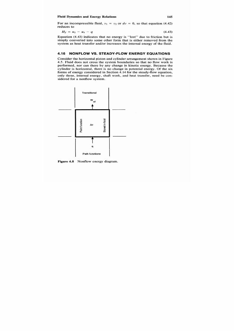
7/21/2019 Fundamental Fluid Mechanics for Engineers
http://slidepdf.com/reader/full/fundamental-fluid-mechanics-for-engineers 168/438
Fluidynamicsd 145
For an incompressible fluid,
v I
= v2 or dv
= 0,
so that equation (4.42)
reduces to
Hf
~2
-
~1
- q (4.43)
Equation (4.43) indicates that no energy is “lost” due to friction but is
simply converted into some other form that is either removed from the
system as heat transfer and/or increases the internal energy of the fluid.
4.16
NONFLOW VS. STEADY-FLOW ENERGY EQUATIONS
Consider the horizontal piston and cylinder arrangement shownn Figure
4.5. Fluid does not cross the system boundaries so that no flow work is
performed, nor can there by any change in kinetic energy. Baause the
cylinder is horizontal, there is no change in potential energy. Of the six
forms of energy considered in Section 4.14 for the steady-flow equation,
only three, internal energy, shaft work, and heat transfer, need be con-
sidered for a nonflow system.
Transitional
q
Path functions
Figure 4.8
Nonflow
energy diagram.

7/21/2019 Fundamental Fluid Mechanics for Engineers
http://slidepdf.com/reader/full/fundamental-fluid-mechanics-for-engineers 169/438
146
Chapter 4
P
Figure 4.9 Steady-flow energy relations.
From Figure 4 .8 , application of the principle of conservation of energy
leads to
q
=
AU
+
W n f (4.44)
Noting from equation (4.21) that
A U
= ~2 - ~1
and from equation (4 .27) that
2
W n f
= L
P
dv
the nonflow equation may be written as
q = u z - u 1 +
L
P dv
If equation (4.45) is subtracted from equation (4.41),
8
v
- v:
0
= W,, + -
z2
- z d
+
+ L 2 V d P
gc ? c
or
(4.45)
(4.46)
Equation (4.46) may also be written in the following form:
L2 dp = W s f + APE + A K E
(4.47)
7/21/2019 Fundamental Fluid Mechanics for Engineers
http://slidepdf.com/reader/full/fundamental-fluid-mechanics-for-engineers 170/438
Fluidynamics
147
From equation(1.37), n = - ( v d p ) / ( p d v ) ,nd from equation 4.27), W n f
= J p dv; using these relations and equation (4.47) results in
r 2
(4.48)
Note that in the absence
of
potential and kinetic energy changeshe pro-
cess path n is the ratio between the steady-flow work and the nonflow
work for a reversible process. If the
-J
v dp from equation
(4.46),
A h
from equation
(4.26),
and
J T d s
from equation
(4.32)
are substituted in
equation (4.37), results are as follows:
= - J 2 v d p + A h = L* ds
(4.49)
Equation
(4.49)
may be written in differential form as follows:
S q
= T d s =
-V
dp + d h (4.50)
Writing equation
4.45)
in differential form and noting from equation
4.32)
that Sq =
T
ds:
Sq = T d s = p d v + du (4.51)
Equation (4.50) was developed from he steady-flow energy equation and
equation
(4.51)
from the nonflow. Noting that by definition
d h
=
du
+
d ( p v ) = U + p dv + v dp , and substituting in equation (4.50):
T d s = - v d p
+
A h
(4.51)
From the above i t is evident that equations4.50) and (4.51) may beused
f o r either steady-flow or nonflow processes.
4.17 IDEAL GAS SPECIFIC HEAT AND ENERGY
RELATIONS
The purpose of this section is to develop ideal gas relations for use in
Chapter 5.

7/21/2019 Fundamental Fluid Mechanics for Engineers
http://slidepdf.com/reader/full/fundamental-fluid-mechanics-for-engineers 171/438
148
Chapter
4
Specific Heats
The specific heat of any substance is defined by the following equation:
c, = (2)
(4.52)
where
c,
is the specific heat for process x.
For the
SI
system, the joule per kilogramper kelvin [J/(kg.K)]or new-
ton meter per kilogram per kelvin is used. For the U.S. customary units,
conventional practice is to use the British thermal unit per pound mass
per degree Rankine [Btu/(lbm-"R)]. For fluid mechanics, it will be nec-
essary to convert the Btu to ft-lbf
(778.2
ft-lbf
=
1
Btu).
Constant-Volume Specific Heat
Note that if equation
(4.51)
is solved for a constant-volume process ( d v
= O),
6qu = p ( 0 ) + du = du
(4.53)
From equation
(4.52),
I
c,
= (Z), = C V = (S)
U
(4.54)
Since the internal energy of an ideal gas s a function of temperature only,
the partial notation may be dropped and equation(4.54) may be then be
written as:
du =
cu
dT
(4.55)
Equation (4.55) may be used
for
any ideal gas process.
Constant-Pressure Specific Heat
Note that if equation (4.51) is solved for a constant-pressure process ( d p
= O),
6qp =
-u(O) +
dh
= dh (4.56)
From equation
(4.52):
c,
= (g), c,
=
(g)
P
(4.57)
Since the enthalpy of an ideal gas is a function of temperature only, the

7/21/2019 Fundamental Fluid Mechanics for Engineers
http://slidepdf.com/reader/full/fundamental-fluid-mechanics-for-engineers 172/438
Fluidynamicsd
149
partial notation may be dropped and equation
4.57)
may be then be writ-
ten as:
d h
= c,
dT
(4.58)
Equation (4.58) may be used for anydeal gas process.
Ratio of Specific Heats
If the relation of equation
(4.58)
is substituted in equation
(4.501,
T d s
= - V
d p + C , dT (4.59)
For an isentropic process ( d s = 0) equation
(4.59)
reduces to:
v d p
=
c, dT (S = constant) (4.60)
If the relation of equation (4.55) is substituted in equation
(4.51),
T d s = p d v + c v d T
(4.61)
For an isentropic process ( d s = 0) equation (4.61) reduces to:
-pv
=
cv
dT
(S
=
constant)
(4.62)
Substituting equation
(4.60)
and equation
(4.62)
in equation
(1.31),
(4.63)
where
k
is the ratio of specific heats and is the exponent of an isentropic
process.
If the definition of enthalpy is written in differential form and from
equation
(1.42)
p v
=
R T ,
from equation
(4.55)
du
=
cv
d T ,
and from
equation
(4.58)
d h = c , dT , then
d h
=
d u
+
d ( p v ) = c, dT
=
cV
dT + R dT
or
(4.64)
C ,
- C,, = R
Dividing equation
(4.64)
by
cv ,
% - 5 = - = k - 1 = - R
CVV
CV
CV
or
(4.65)
R
CV =
k -
1

7/21/2019 Fundamental Fluid Mechanics for Engineers
http://slidepdf.com/reader/full/fundamental-fluid-mechanics-for-engineers 173/438
150
and in a like manner,
k R
c, =
k - l
Chapter 4
(4.66)
Polytropic Specific Heat
Integrating equation
(4.27)
for a polytropic process using un = C [equa-
tion ( l 36)],
(4.67)
Writing equation
(4.68)
in differential form and substituting
c,
-
c,
=
R
from equation (4.64) results in:
R
dT ( C ,
-
C,) dT
p d v = - -
l - n
l - n
-
(4.69)
Substituting cn
d T f o r T d s
and
p d v
from equation4.69) in equation (4.61)
and noting that
c,/c,
= k and solving for c,,:
T d s
=
p d v
+
c,dT
=
c , d T
= (
- dT
+
c,
dTl - n
or (4.70)
cn =
c, - nc,
I - n
Isentropic Energy Relations
The path of frictionless adiabatic flow of an ideal gas is from equation
(1.38),
p v k = a constant. If the friction term
(UT
dLIRh) of the equation
of motion
(4.12) is
dropped, and the equation is integrated between sec-

7/21/2019 Fundamental Fluid Mechanics for Engineers
http://slidepdf.com/reader/full/fundamental-fluid-mechanics-for-engineers 174/438
Fluid Dynamics and Energy Relations
151
tions 1 and 2 then for frictionless flow:
(4.71)
The third term of equation
(4.71)
may be integrated by noting from equa-
tion (1.46) that v
=
v l ( p 1 / p ) ’ l k ,o that:
dP
p’/k = vlpiIk[ L )
- 1 p ( k - ~ ) l k ]
(4.72)
2
i2
dp
=
vlpiIk
( k -
I ) lk
Substituting equation
(4.72)
in equation
(4.71):
- 2 2 - Zl)
+
v’, v:
gc
2gc
(4.73)
( k -
1)lk
+
PI V l ( h)e) - l ] = 0
Substituting from the equation of state (1.42)
plul
=
R T I
and from equa-
tion
(1.47)
T2/TI
=
( p 2 / p l ) ‘ k - 1 ) 1 k
n equation
(4.73)
results in:
(4.74)
Substituting from equation (4.66) c,, = R k / ( k - 1) and from equation
(4.58) d h = c,, dT in equation (4.74) results in
(4.75)
The same result may be arrived at from the energy equation. For an
isentropic process,
q
=
0,
and for no shaft work, W s f =
0,
and by defi-
nition
u2
- ul + p2v2 = p l v l = h2 - h l . Substituting in equation (4.37):
q =
W s f
+ (22 - 21) +
v’, v:
+ U 2
- U1
+
p2u2
-
plvl
gc 2gc
g
v’, v:
0 = 0
+
- 2 2 - Zl) +
+ h2
-
h1
gc
2gc
(4.75)

7/21/2019 Fundamental Fluid Mechanics for Engineers
http://slidepdf.com/reader/full/fundamental-fluid-mechanics-for-engineers 175/438
152
Chapter 4
Finally, the general energy equation4.37) may bewritten in the following
form by substituting for h2 - hr the value
of
[ kR l (k - 1)](T2 -
T1):
(4.76)
4.18
IMPULSEMOMENTUM EQUATION
The impulse momentum equation is used to calculate the forces exerted
on a solid boundary by
a
moving stream. It was derived in Section
1.8
as an application
of
Newton’s second law. This resulted n
m
F = - ( V
gc
2
-
V,)
(1.28)
Substituting
2
(the summation
of
all forces acting)
for
F
and from
equation (3.10)
m
=
pAV
yields
(4.77)
In the application of equation (4.77), it must be remembered that ve-
locity is a vector and as such has both magnitude and direction. The
impulse-momentum equation is often used in conjunction with the con-
tinuity and energy equations to solve engineering problems. Because of
the wide variety of applications possible, some examples are given to
illustrate methods of attack.
In general, the “free body” method is used to compute the forces
involved on the boundaries on a control volume. The symbol
F
is used
for the force exerted by the boundaries on the fluid. There is an equal
but opposite force exerted by the fluid on the boundaries.
Example
4.4
Carbon dioxide flows steadily through a horizontal 6 in.
Schedule 40 wrought iron pipe at a mass rate of flow
of
24 lbmlsec ( 1 1
kg/s). At section1, the pressure is 120 psia (827 kPa) and he temperature
100°F (38°C). At section 2, the pressure is 80 psia (552 kPa) and he tem-
perature is 109°F (43°C). Find he friction force opposing the motion (see
Figure 4.10).

7/21/2019 Fundamental Fluid Mechanics for Engineers
http://slidepdf.com/reader/full/fundamental-fluid-mechanics-for-engineers 176/438
Fluid Dynamics and Energy Relations
153
1
2
PIA, ”m
-e
v 2
Free-body diagram
of
pipe
1
-
4”
P A
- f
Figure
4.10
Notation for Example
4.4.
Solution
This example s solved by the application of the impulse momentum equa-
tion (4.77), the continuity equation
3.11),
and the ideal gas equation of
state
(1.42).
1.
Derive an equation for this application. From the “free body” dia-
gram of Figure
4.10,
Solving equation (a) for F f , noting that for
a
pipe of uniform cross-
section, A 2 =
A I
= A :
From equation (3.11) V
=
m v / A , substituting in equation p),
and from equation
(1.42)
v = R T / p , substituting in equation (c),
=
A(p1
-
P 2 )
- v2 -
v1)
m2
&A
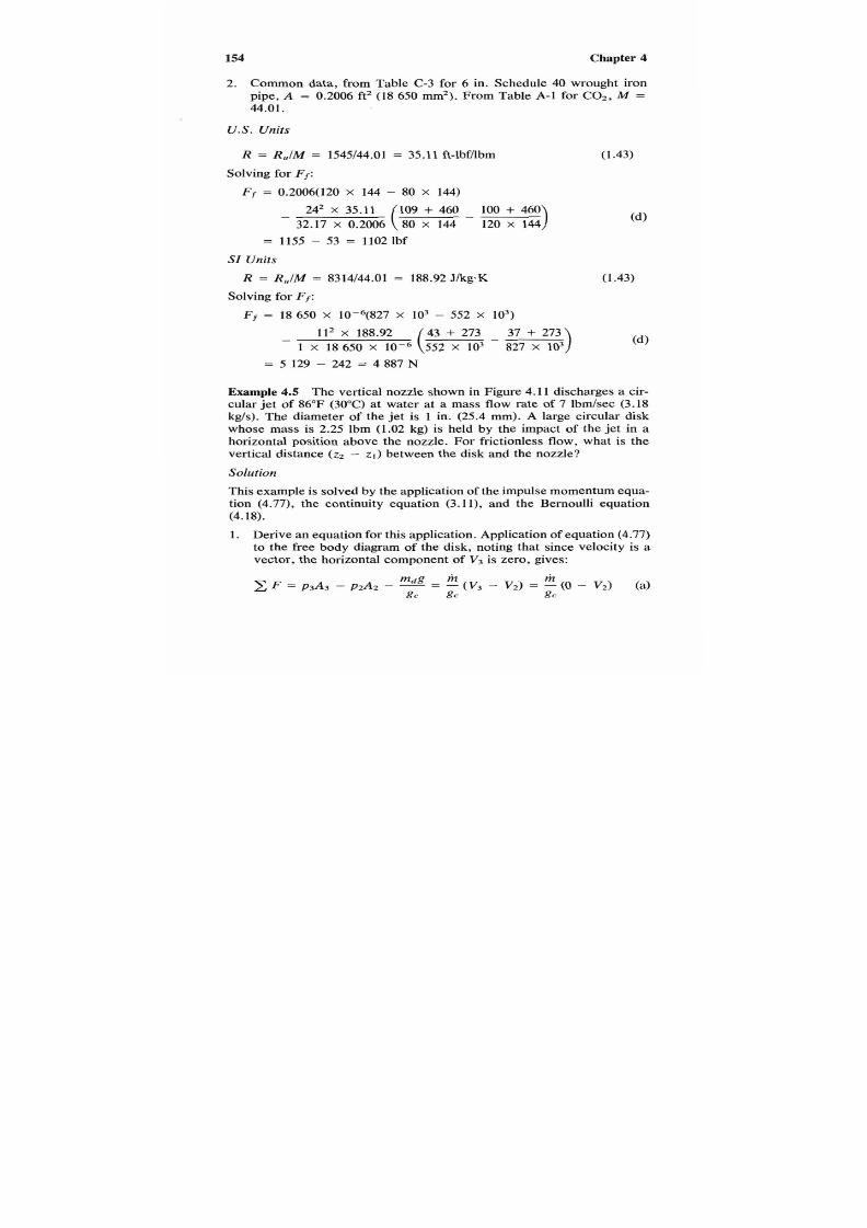
7/21/2019 Fundamental Fluid Mechanics for Engineers
http://slidepdf.com/reader/full/fundamental-fluid-mechanics-for-engineers 177/438
154 Chapter
2.Common data, from Table
C-3
for 6 in. Schedule 40 wrought iron
pipe,
A
= 0.2006 ft2 (18 650 mm2). From Table A-l for C02, M
=
44.01.
US.
nits
R
=
R, /M
=
154Y44.01
=
35.11 ft-lbf/lbm
( I
.43)
Solving for Ff:
Ff
= 0.2006(120
X
144 - 80 X
144)
-
242 x 35.11109
+
460
100
+
460)
32.17
x
0.20060
x
14420
x
144
-
( 4
= 1155 - 53 = 1102 bf
SI
Units
R = R J M =
8314144.01
=
188.92J1kg.K
Solving for Ff:
Ff = 18650
x
10-6(827 X IO3 - 552 X
IO3)
(1.43)
- 1 1 2 x
188.92 (43
+
273
-
37
+
273)
1
x
1850
x
552
x IO3
827
x IO3
( 4
= 5 129 - 242 = 4 887
N
Example 4.5 The vertical nozzle shown in Figure 4.11 discharges a cir-
cular jet of 86°F
(30°C)
at water at a mass flow rate of 7 lbm/sec (3.18
kg/$.
The diameter of the jet is
1
in. (25.4 mm). A large circular disk
whose mass is 2.25 Ibm (1.02 kg) is held by the impact of the jet
in
a
horizontal position above the nozzle. For frictionless flow, what is the
vertical distance (22 -
z l )
between the disk and the nozzle?
Solution
This example s solved by the applicationf the impulse momentum qua-
tion (4.77), the continuity equation (3.11), and the Bernoulli equation
(4.18).
1.
Derive an equation or this application. Applicationof equation (4.77)
to the free body diagram of the disk, noting that since velocity is a
vector, the horizontal component of
V 3
is zero, gives:
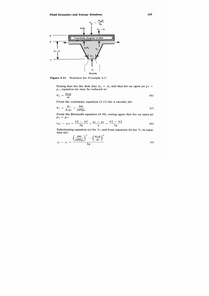
7/21/2019 Fundamental Fluid Mechanics for Engineers
http://slidepdf.com/reader/full/fundamental-fluid-mechanics-for-engineers 178/438
Fluid Dynamicsndnergyations
155
3
2
1
I
:
v1 :
Nozzle
Figure
4.11
Notation for Example
4.5.
Noting that for the disk that A2 = A3 nd that for an open jet p2 =
p3, equation (a)
may
be reduced to:
v 2 =
dg
m
From the continuity equation
3.11)
for a circular jet:
m 4m
vl=-=-
AIPI TDj2pl
From the Bernoulli equation (4.18), noting again that for an open jet
p2 =
p1:
Substituting equation(c) for
V1
and from equation
b)
for
V2
in equa-
tion (d):
z2 - ZI =
2g
(e)

7/21/2019 Fundamental Fluid Mechanics for Engineers
http://slidepdf.com/reader/full/fundamental-fluid-mechanics-for-engineers 179/438

7/21/2019 Fundamental Fluid Mechanics for Engineers
http://slidepdf.com/reader/full/fundamental-fluid-mechanics-for-engineers 180/438
Fluid Dynamics and Energy Relations
157
FY F
v,
P A
(a) ( W
Figure
4.12
Notation for Example 4.6.
1.
Exit pressure. From the Bernoulli equation
4.18)
for frictionless
flow:
noting from equation
(1.29)
that
y = pg/gc,
for a horizontal bend zz
= zl,
and substituting from equations (a) and (b)
for
Vxl and Vy2,
respectively, in equation (c):
2.
The
x
direction force,
from
equation
(4.77):

7/21/2019 Fundamental Fluid Mechanics for Engineers
http://slidepdf.com/reader/full/fundamental-fluid-mechanics-for-engineers 181/438
158 Chapter 4
Solving equation (e) for F,, and substituting for
V,,
from equation
(4 :
(0
3. The y direction force, from equation (4.77):
Solving equation (g) for
Fy
and substituting for
V y 2
from equation
(b):
(h)
4. The magnitude of the resulting force may be calculated from equation
(2.43):
F = -
( 9
5.
Finally, the angle of the resolved force may be computed using
0 = tan" E)
6.
Common data, from Table
A-l
for CCL at
68°F (20°C):
=
99.42
lbm/ft3 (1 592.5 kg/m3).
US. nits
1. Exit pressure p 2 :
p2 = 50
X
144 +
8 x 1252
32.17 X IT^ X 99.42
= 7,200
-
950
=
6,250
lbf/ft2
= 6,2501144 = 43.40 psia
2. Fx:
F,
=
144 X
(50
- 14.70)
+
4 x 1252
32.17
X
X
(6/12)2
X
99.42
=
998
+
25
=
1023
lbf
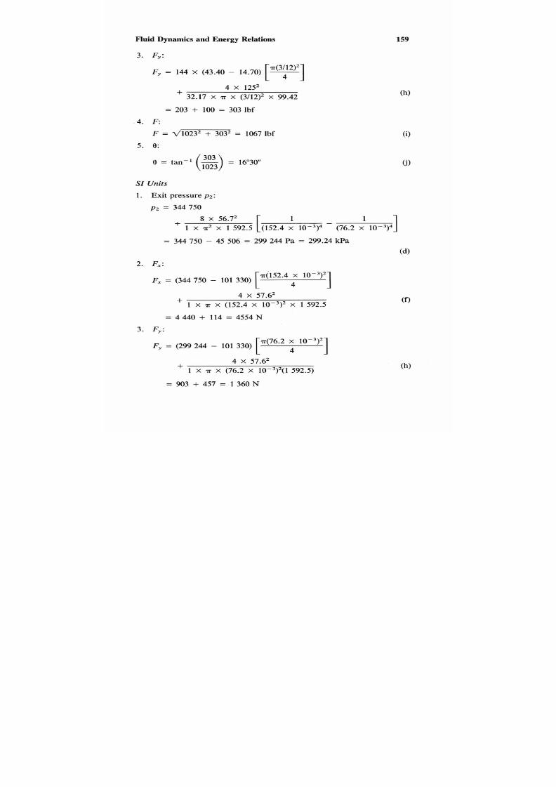
7/21/2019 Fundamental Fluid Mechanics for Engineers
http://slidepdf.com/reader/full/fundamental-fluid-mechanics-for-engineers 182/438
Fluid
Dynamics and Energy Relations
159
3. F y :
Fy =
144
X
(43.40
-
14.70)
~
[=(3:2)21
4 x 1252
' 32.17
X
7 ~
X
(3/12)2
X
99.42
= 203 + 100 = 303
Ibf
.4. F
F
=
d1023'
+
3032
=
1067
lbf
5. e:
0
=
tan" (g)16'30"
SI Units
1. Exit pressure
p z :
p2 =
344 750
+
8 x
56.72
1 X 7~ 1592.5152.4 X 10-3)4 (76.2
X
-
= 344 750 - 45 506 = 299 244 Pa = 299.24 kPa
2. Fx:
F, = (344750
-
101330)
4 x
[71(m.4
4
IO-^)^
1
57.62
+
1
X
T
X
(152.4
x
10-3)2
x
1592.5
= 4 440
+
114
=
4554 N
3. F y :
Fy =
(299 244
-
101 330) ~ ~ ( 7 6 . 210-3)21
4 x 57.62
+
1 X T X (76.2 X 10⁻³)2(1592.5)
= 903 + 457 = 1 360 N
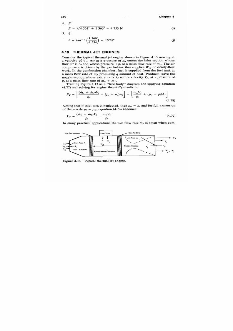
7/21/2019 Fundamental Fluid Mechanics for Engineers
http://slidepdf.com/reader/full/fundamental-fluid-mechanics-for-engineers 183/438
160
4. F
F
=
d 4 5542
+
1 3602
=
4 753
N
5 . e:
4.19 THERMAL JET ENGINES
Consider the typical thermal jet engine shown in Figure
4.13
moving at
a velocity of Vu.Air at a pressure of pa enters the inlet section whose
flow air is Ai
and whose pressure is
pi
t a mass flow rate of m,. The air
compressor is driven by the gas turbine that supplies W s f of steady-flow
work. In the combustion chamber, fuel is supplied from the fuel tank at
a mass flow rate of mf roducing q amount of heat. Products leave the
nozzle section whose exit area is Aiwith a velocity F, t a pressure of
p j
at a mass flow rate of h a + hf.
Treating Figure4.13 as a "free body" diagram and applying equation
(4.77)
and solving for engine thrust
FT
results in:
(4.78)
Noting that if inlet loss is neglected, then p a = pi nd for full expansion
of the nozzle p j = p a , equation
(4.78)
becomes:
(4.79)
In many practical applications the fuel flow rate
m f
s small when com-
Airornpresaor
Fuel
Tank
esTurbine
Nozzle
Section
F T
m
i
Figure
4.13
Typical thermal jet engine.

7/21/2019 Fundamental Fluid Mechanics for Engineers
http://slidepdf.com/reader/full/fundamental-fluid-mechanics-for-engineers 184/438
Fluid
Dynamics andnergyelations
161
pared to the air flow ratem,o that the engine thrust may be approximated
by
m a
gc
FT=-( - V,)
The useful power developed
P,
is
(4.80)
(4.81)
The minimum power needed to change the kinetic energy of the fluid,
assuming that
m f
is small with regard to
m, ,
produces an ideal power
input of
Pi:
(4.82)
The maximum (ideal) propulsion efficiency
Ei
s given by
Note that for 100% ideal efficiency,
&
=
V,
and no power is produced
The system efficiencyE, s defined as the ratio of the useful powerP, to
the power supplied
P,
or
E,
= -
,
PS
(4.84)
Example
4.7
An airplane whose jet engine is shown in Figure 4.13 flies
at a constant altitude where the temperature is -
8°F
(-
50°C)
and at a
speed of
360
mph
(161
d s ) . Heat in the amount of
425
Btu/lbm
(989
kJ/kg)
is added to the air in the propulsion system. The system mass flow rate
is
12.5 lbdsec (5.67
kg/s)
of air. Hot gases leave the gas turbineat 1292°F
(700°C). Assuming that the hot gas has the same properties as air and
neglecting the weight of fuel, determine (a) hrust produced,
(2)
maximum
propulsive efficiency, and
(3)
system efficiency.
Solution
This problem is solved using he equations developed in this section plus
the ideal gas energy equation4.76) developed in Section4.17. First, solve
7/21/2019 Fundamental Fluid Mechanics for Engineers
http://slidepdf.com/reader/full/fundamental-fluid-mechanics-for-engineers 185/438
162 Chapter 4
for jet velocity. Writing equation
4.76)
in the notation of Figure
4.13
and
solving for the jet velocity
vj
results in :
. = J2gc [ - W S f
-
-
(Zj -
ZIJ
-
k F C
- TV)] +
v?
gc
( 4
Noting that for horizontal flight zv =
zj
and that the steady-flow work
W s f
produced by the turbine is required to drive the compressor, the net
W s f
is 0, and equation
(a)
reduces to:
1 .
2.
3.
4;
Thrust. The thrust produced, neglecting the mass of fuel, is calculated
using equation (4.80):
Ideal efficiency. The maximum propulsive efficiency is calculated
using equation (4.83):
2
E .
=
' 1 + VJVV
System efficiency. The system efficiency is calculated usingquations
(4.81) and (4.84):
Common data. From Table
A- l ,
for air
M
=
28.97,
and from Table
A-2, for air at -58°F (-50°C)
k
= 1.402, and at 1292°F (700°C) k =
1.339. Average k = 1.371.
US.
Units
First solve for jet velocity:
R
=
R,/M = 1545/28.97 =
53.33 (ft-lbf)/(lbm-"R)
(1.43)
V, = 360 (mi/hr) X 5280 (ft/mi)/3600 (sec/hr)= 528 ft/sec
q
= 425 (Btdlbm) X 778.2 (ft-lbf/Btu)= 330,735 ft-lbf/lbm
TV=
-
8
+
460 = 402"R T j = 1292 + 460 = 1752"R

7/21/2019 Fundamental Fluid Mechanics for Engineers
http://slidepdf.com/reader/full/fundamental-fluid-mechanics-for-engineers 186/438
Fluidynamics
163
J
X 32.17
[
30,735 -
x
53’33) (152 - 402) + 528’
1.371 - 1
1
= 2 107 ft/sec
1. Thrust:
FT =
-2.6
[2107 - 5281 = 618 lbf
32.17
(c)
2. Ideal fficiency:
2
E . = -
’ 1 + 21071528
3. System fficiency:
-
618 x 528
12.6
x
330,735
, =
0.4008
or
40%
= 0.0783 or 7.8%
SI
Units
First solve
for
jet velocity:
R = R,IM = 814128.97
=
287 Jl(kg*K) (1.43)
TV=
-50 +
273 = 223
K Tj
= 700 + 273 = 973
K
989
x
o3
- x 287
(973
-
223)
+
161’
(
1.371
-
1 )
]
=
643
m/s
1. Thrust:
5.67
1
T =
-
646 - 161) = 2 733 N
2. Ideal fficiency:
2
1 + 6431161
3.System fficiency:
E;
=
= 0.4005 or 40%
E , = 2733
x =
0.0785 or 7.9%
5.67 X 989 X
lo3
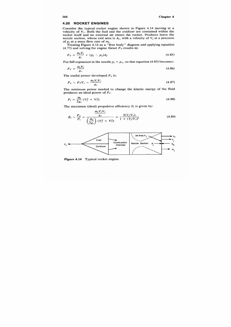
7/21/2019 Fundamental Fluid Mechanics for Engineers
http://slidepdf.com/reader/full/fundamental-fluid-mechanics-for-engineers 187/438
164 Chapter
4.20 ROCKET ENGINES
Consider the typical rocket engine shown in Figure
4.14
moving at a
velocity of V, . Both the fuel and the oxidizer are contained within the
rocket itself and no external air enters the rocket. Products leave the
nozzle section, whose exit area is
Aj,
ith
a
velocity of
vj
at a pressure
of pi at a mass flow rate of mj.
Treating Figure4.14 as a “free body” diagram and applying equation
(4.77)
and solving for engine thrust
FT
results in:
FT = ( p i
-
pa)Aj
mjvj
(4.85)
For full expansion n the nozzlepi = pa, o that equation
(4.85)
becomes:
(4.86)
8,
FT =-
j
j
8 c
The useful power developedP,,s:
P, = FTV, =-
j v j v ,
8 c
(4.87)
The
minimum
power needed to change the kinetic energy of the fluid
produces an ideal power of Pi:
The maximum (ideal) propulsive efficiencyEi s given by:
(4.88)
(4.89)
“r-”
I
.
Combustion Nozzle
Section
p . 4 -
lx idizer
Chamber
Pa
1
-m
” “
,’ --.-
I -.
i
I * c
l
-
Figure 4.14 Typical rocket engine.

7/21/2019 Fundamental Fluid Mechanics for Engineers
http://slidepdf.com/reader/full/fundamental-fluid-mechanics-for-engineers 188/438
Fluid
Dynamicsndnergyations
165
Example
4.8 A solid-fueled rocket of the type shown in Figure4.14 pro-
duced a jet 6 in. (152.4
mm)
in diameter with a velocity of 1,475 ft/sec
(450 d s )
and
a
density of
0.0482
lbm/ft3
0.772
kg/m3). Theocket velocity
in level steady flight is 1,100 ft/sec (335 ds) . Determine
1)
the thrust
produced,
(2)
useful power, and (3) maximum propulsive efficiency.
Solution
This example is solved usinghe continuity equation
3.10)
and the equa-
tions derived in this section. The mass flow rate is from equation
(3.10):
1.
Thrust produced, from equation (4.86):
2. Useful power, from equation (4.87):
P ,
= FTV, (c)
3.
Maximum propulsive efficiency, from equation
(4.89):
US. nits
mj = 0.0482 x
T
x (6/12)2 x 1475/4 = 13.96 lbdsec
(a)
T
13.96
X
1475132.17 =
640
bf
(b)
P ,
=
640
X
11001550 = 1280 hp (c)
2 x (147511100)
E . =
' 1+
(1475/1100)2
= 0.96 or 96%
SI Units
mj = 0.772 X T X (152.4 X X 45014 = 6.337 kg/s (a)
T
6.337
X
45011
=
2 852
N (b)
P , = 2 852
X
335 = 95520 = 955 kW (C)
2
x
(4501335)
1+
(4501335)2
i
=
=
0.96 or 96%
7/21/2019 Fundamental Fluid Mechanics for Engineers
http://slidepdf.com/reader/full/fundamental-fluid-mechanics-for-engineers 189/438
166 Chapter
4
4.21 PROPELLERS
Although propellers for ships and aircraft cannot be designed with the
energy and impulse-momentum relations alone, application of these re-
lations to problems leads to some of the laws that characterize their op-
eration.
Slipstream Analysis
The stream of fluid passing through the propeller of Figure 4.15 is called
the slipstream. Fluid approaches the slipstream with a velocity of V , and
leaves with a velocity
V 2 .
Within the propeller boundary, the velocity is
V , and work in the amount of W , is added between sectionsA and
B
by
the propeller. The inlet and outlet pressures are
p 1
and
p 2 ,
respectively,
and are equal to each other. The pressure at section A is p A and at B is
If the equation of motion written considering shaft work4.39) s mod-
ified for frictionlessflow and integrated or an incompressible fluid, noting
that from equation (1.30)
v
= l/p, he following results:
P B
g
v;
-
v:
p2
-
P1
W,,
+
- z 2
-
Z l ) +
+- -
- 0
gc
2gc P
(4.90)
Writing equation (4 .90)between sections 1and 2 and noting that
if
work
is added to a systemt has a negative sign (Section 4.14 , Figure 4.7) and
that for-
a
horizontal slipstream z2 =
z1
-W, +
vi:
-
v:
p2 -
p1
2gc
P
+-=
0
(4.91)
Between sections
I
and
A
where
W ,
=
0
application of equation
(4.91)
yields:
(4.92)
Between sections B and 2 where
W ,
= 0 application of equation (4.91)
yields:
Adding equations (4 .92)and (4 .93) ,noting that
p 1 =
p 2 :
(4.93)
(4.94)
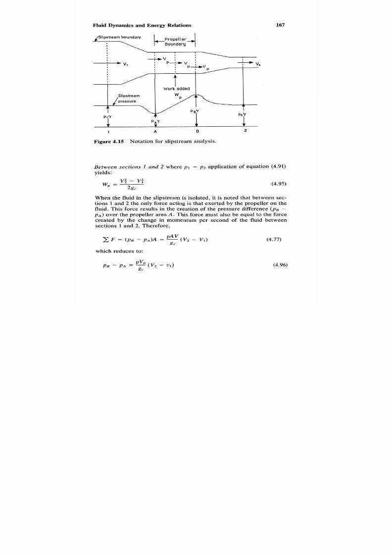
7/21/2019 Fundamental Fluid Mechanics for Engineers
http://slidepdf.com/reader/full/fundamental-fluid-mechanics-for-engineers 190/438
Fluid Dynamics and Energy Relations
is l ip str eam boundary
\ B o u n d a r yro p e l l e r
4
I
I
I
I
I l
l
I
I
+v : I
I
-,
I
I
I
I
I
I
Y .
t
Wo r k added
Slipstream
pressure
Ab
t
P l Y
PI Y
P A Y
l A
B
v
2
167
Figure
4.15 Notation for slipstream analysis.
Between sections I and 2 where P I = p 2 application of equation
(4.91)
yields:
v;
-
v:
2gc
W, =
(4.95)
When the fluid in the slipstream is isolated, it is notedhat between sec-
tions 1 and 2 the only force acting is that exerted by the propeller on the
fluid. This force results in the creation of the pressure difference ( p B
-
p A ) over the propeller area
A .
This force must also be equal to the force
created by the change in momentum per second of the fluid between
sections 1 and 2. Therefore,
which reduces to:
(4.77)
(4.96)

7/21/2019 Fundamental Fluid Mechanics for Engineers
http://slidepdf.com/reader/full/fundamental-fluid-mechanics-for-engineers 191/438
168
Chapter 4
Letting equation
(4.94)
equal equation
(4.96),
which reduces to:
v2 + VI
2
, =
The useful power of the propeller is:
(4.97)
(4.98)
The minimum ideal power is that required to change the kinetic energy
or
(4.99)
The maximum propeller efficiency s obtained by dividing equation4.98)
by equation (4.97) or
Ep
=
O C
pAVp
(%
(4.100)
Substituting equation (4.97) for V , in equation (4.100) yields:
V1
Ei =
VP
(4.101)
Example
4.9 A
propeller
14
in.
(356) mm
in diameter drives a torpedo
through sea water
( p
=
6 4
lbm/ft3
(1 026
kg/m3) at 22 knots. The ideal
propeller efficiency is 75%. Determine
(1)
useful power and (2 ) power
added to the water.
Solution
This problem is solved by using the continuity equation
(3.10)
and the
equations derived in this section.
1.
Useful power, from equations
(4.101)
and
(4.97):
V ,
=
Vl/Ei
V2 = 2Vp - V I = 2V1/Ei - VI = Vl(2/Ei
- 1)
(a)
(b)

7/21/2019 Fundamental Fluid Mechanics for Engineers
http://slidepdf.com/reader/full/fundamental-fluid-mechanics-for-engineers 192/438
Fluidynamicsd
169
Substituting from equation (a) and equation (b) in equation (4.98):
PAVP PI@( VI /E;)
(V2
-
V d V I =
,
=
-
[VI(2/Ei
-
1)
-
Vl]Vl
gc 4gc
which reduces to:
2. Power added to water, from equation (4.101):
P p
=
P d E ;
US. nits
From Table B.l, VI = 22 knots
X
1.6878 = 37.14 ft/sec.
1.
P,
=
6 4
X 7 ~ X (14/12)*
X
37.143
2 x 32.17
x
0.75
= 96,847 ft-lbf/sec (4
96,847
550
= - =
176 hp
2.
Pp = 176/0.75 = 235 hp (dl
SI Units
From Table B.l, VI = 22 knots X 5.1444 X 10” = 11.32 m/s.
1026
X
T
X
(356
X
10-3)2
X
11.323
2
x
1
x
0.75
. P , =
= 131681
J/s
= 132kW
2. Pp = 13210.75 = 176W (dl
4.22 FLOW IN
A
CURVED PATH
In Section 2.11 the effects of rotating a fluid mass were explored. This
type of rotating produces
a
“forced vortex,”
so
called because the fluid
is forced to rotate because energy is supplied from somexternal source.
When a fluid flows through a bend, it is also rotated around some axis,
but the energy required to produce this rotation is supplied from the en-

7/21/2019 Fundamental Fluid Mechanics for Engineers
http://slidepdf.com/reader/full/fundamental-fluid-mechanics-for-engineers 193/438
170
Chapter 4
t
t
-
-
I i
- 5 .
*.
*.,
/
o
I I
X I
I
I
t I
-:
Figure
4.16
Notation for flow in a curved path.
ergy already in the fluid mass. This is called a "free vortex" because
it
is "free" of outside energy.
Consider the fluid mass p(ro
-
T i ) dA of Figure 4.16 being rotated as
it flows through a bend of outer radius r,, inner radiusr i , with a velocity
of V . Application of Newton's second law to this mass results in:
which reduces to:
(4.103)
Example
4.10
.Benzene at
68°F
(20°C)flows at a rate of
8
ft3/sec (0.227
m3/s) in a square horizontal duct. This duct makes a turn of 90 with an
inner radiusof
1
ft (305 mm) and an outer radius of 2 ft (610 mm). Assume

7/21/2019 Fundamental Fluid Mechanics for Engineers
http://slidepdf.com/reader/full/fundamental-fluid-mechanics-for-engineers 194/438
Fluidynamics andnergyelations 171
frictionless flow and alculate the difference in pressure between the inner
and outer wall.
Solution
This example is solved by the application of equation
(4.103)
and the
equation of continuity (3.4). For one-dimensional incompressible flow,
from equation
(3.4),
V =
Q/A
(note that this is the flow area, not the area
shown in Figure
4.16).
Substituting in equation
(4.103)
for V ,
Po
-
pi = 2
(52)
e2
ro
+ ri
g,A’
For a bend of square cross-section A = (ro - ri)’ and equation (a) be-
comes:
which reduces to:
US.
nits
From Table
A-l
for
68°F
benzene (C&), p =
54.79
lbm/ft3.
2 x 54.79 x 82
32.17
x
(2
+ 1 ) x
(2
-
l ) 3
o - Pi
=
= 72.66 lbf/ft’
=
72.661144
= 0.505 psi
SI
Units
From Table A-l for
20°C
benzene (C6H6),
p
= 877.7 kg/m3.
2
x
877.7
x
0.227’
Po - Pi =
1 X
(610
X
10-3 + 305 X 10-3)
X
(610
X
10-3
- 305 X 10-313
=
3 481 Pa
4.23 FORCES
ON MOVING
BLADES
Consider the fluid jet whose area is A issuing from nozzle with velocity
of
V ,
as shown in Figure 4.17. The fluid jet impinges on the blade, which
is moving at a velocity of
U
n the direction of the jet, and turns the jet
through an angle of 0 degrees.

7/21/2019 Fundamental Fluid Mechanics for Engineers
http://slidepdf.com/reader/full/fundamental-fluid-mechanics-for-engineers 195/438
172
Chapter 4
Nozzle
1
vy,
=
0
7
v,,
=
v
-
U
F Y
F
Figure
4.17
Notation for blade study.
Assuming that the flow is without friction, the jet enters and leaves
the blade witha velocity of
( V
- U) ith respect to it. In the x direction,
the velocity V,, is ( V - U) nd VX2 = ( V
-
U) os
8.
In the y direction,
V,, is zero, and V,, = ( V - U) in
8.
Application of Eq. (4.77) in x direction yields:
- pA(V - U)'(COS8 - 1)
-
gc
And in the y direction:
-
pA(V
-
U)' sin 8
-
gc
(4.104)
(4.105)
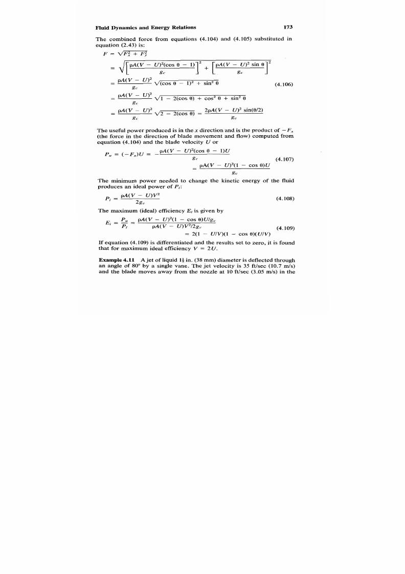
7/21/2019 Fundamental Fluid Mechanics for Engineers
http://slidepdf.com/reader/full/fundamental-fluid-mechanics-for-engineers 196/438
Fluidynamics
173
The combined force from equations
(4.104)
and
(4.105)
substituted in
equation
(2.43)
is:
pA(V -
U)’(COS
8 -
1)
3’ [ A(V - g ~ 2
in
e
gc I’
pA(V - U ) 2
8 c
pA(V -
U ) 2
gc
pA(V -
U)’
2
- COS
e) =
(4.106)
2pA(V - U)’ in(8/2)
gc gc
The useful power produced s in the
x
direction and s the product
of - F ,
(the force in the direction of blade movement and flow) computed from
equation
(4.104)
and the blade velocity U or
P,
=
( - F , ) U
= -
A(V
-
U)’(COS
8
-
l ) U
gc (4.107)
-
PA( V
- U)2( - COS e)u
-
gc
The minimum power needed to change the kinetic energy of the fluid
produces an ideal power of P i :
pA(V - U)V2
2gc
Pi
=
(4.108)
The maximum (ideal) efficiencyEi s given by
P ,
PA(V - U)’ - COS e)U/gc
E . = - =
’
Pi pA(V
- U)V212gc
(4.109)
= 2(1
-
U/V)(I -
COS
e)(u/v)
If
equation
(4.109) is
differentiated and he results set to zero, it is found
that for maximum ideal efficiency V = 2 U .
Example 4.11 A
jet of liquid
14
in.
(38
mm) diameter is deflected through
an angle of
80”
by
a
single vane. The jet velocity is
35
ftlsec
(10.7 &S)
and the blade moves away from the nozzle at
10
ft/sec
(3.05 m/s)
in the

7/21/2019 Fundamental Fluid Mechanics for Engineers
http://slidepdf.com/reader/full/fundamental-fluid-mechanics-for-engineers 197/438
174 Chapter
4
direction of the entering jet. Assume frictionless flow and = 79 lbm/ft3
(1 265 kg/m3) and calculate (1) the total force on the blade, (b) the useful
power, and (c) the ideal blade efficiency.
Solution
The example is solved by the application of the equations developed in
this section. The area is calculated using
A =
mD2/4 (a)
1.
The total force on the blade is calculated using equation (4.106):
F =
2pA(V
-
U)’
in(0/2)
g c
2. The useful power is calculated using equation (4.107):
P ,
=
PA(
V
-
v)’ 1
- COS 0 ) V / g ,
(c)
3. The ideal blade efficiency is calculated using equation (4.109):
Ei
= 2(1 - U/V)(1 - COS 0)( U/V). (dl
US. nits
A = ~(1.5/12)~/4 0.01227 ft2
(a)
1. The total force on the blade:
F = 2
x
79 x 0.01227 x (35
- x
sin(80/2)/32.17= 24.21bf
(b)
2. The usefulpower:
P ,
= 79
X
0.01227(35
-
X
[l - COS(~O)] 10/32.17 (c)
= 155.6 ft-lbf/sec = 155.6/550 = 0.29 hp
3. The ideal blade efficiency:
E;
= 2(1 - 10/35) X [ l - COS(~O)] 10/35
(dl
= 0.337 or 33.7%
SI Units
A
= m(38 X 10-3)2/4 = 1.134
X
m2
(a)
1. The total force on the blade:
F = 2
X
1 265
X
1.134
X X
(10.7 - 3.05)2in(80/2)/1b)
= 107.9 N

7/21/2019 Fundamental Fluid Mechanics for Engineers
http://slidepdf.com/reader/full/fundamental-fluid-mechanics-for-engineers 198/438
Fluidynamics
175
2. The usefulpower:
P,,
=
1
265
X
1.134
X X
(10.7
-
3.05)*
X [l
-
C O S ~ O ) ] X 3.05/1 (c)
= 212 JIs = 0.21 kW
3. The idealbladeefficiency:
Ei
= 2 X (1 - 3.0Y10.7)
X
[ l -
COS(~O) ]
X (3.05110.7)
(d)
= 0.337 or 33.7%

7/21/2019 Fundamental Fluid Mechanics for Engineers
http://slidepdf.com/reader/full/fundamental-fluid-mechanics-for-engineers 199/438
5.1
INTRODUCTION
This chapter is a continuation of the material on ideal gases presented in
Chapter 4. It is concerned with some of the effects of the elasticity of
ideal gases. The scope of this chapter is limited to the development of
those concepts and theoretical equations needed for the understanding of
compressible flow through pipes and flow meters.
This chapter ma y be skipped by readers who are either familiar with
or not interested in comp ress ibleflow .
One of the problems with this subject is the difficulty of seeing the
woods (concepts) because of the trees (complex-looking equations).Four
tables of functions are provided to reduce computational effort. This chap-
ter may be usedas a text for tutoriaLor refresher purposes. Each concept
is explained and derived mathematicallys needed. The mathematics in-
volved is at the minimum level needed for clarity of concept. The ther-
modynamic aspects of gas dynamics are fully explained, making it un-
necessary to consult a text on that subject. There are 11 tutorial type
examples of fully solved problems.
176

7/21/2019 Fundamental Fluid Mechanics for Engineers
http://slidepdf.com/reader/full/fundamental-fluid-mechanics-for-engineers 200/438
GasDynamics 177
5.2
GAS DYNAMICS
Gas dynamics
s the branch of fluid dynamics concerned withhe motion
of gases and consequent effects. Gas dynamics combines the principles
of fluid mechanics and thermodynamics. This subject is based on the
application of four fundamentals:
1. Newton's second laws of motion.
2.
The law of conservation of mass.
3. The first law of thermodynamics.
4.
The second law of thermodynamics.
Because the potential energy changes n ideal gas systems are usually
small compared with other energy changes, all systems in this chapter
are assumed to be horizontal, and thus
z z -
z 1 = 0. It is further assumed
that the flow is one-dimensional and that all fluids are in the ideal gas
stare.
5.3
AREA-VELOCITY RELATIONS
In this section the differences between incompressible and compressible
flow area-velocity relations are developed.
Incompressible Fluids
Repeating the continuity equation in differential form from Section
.7,
dV dA dp
V A P
-
-+ =o
(3.14)
For an incompressible fluid,dp = 0, so that equation
(3.14)
reduces to
dV dA
V
Inspection of equation
(5.1)
indicates the following:
1.
If area increases, velocity decreases.
2. If area decreases, velocity increases.
3.
If area is constant, velocity is constant.
4.
There are no critical values.

7/21/2019 Fundamental Fluid Mechanics for Engineers
http://slidepdf.com/reader/full/fundamental-fluid-mechanics-for-engineers 201/438
178
Chapter 5
Compressible Fluids
The equation of motion
(4.12)
for a
horizontal system
( d z
=
0)
and for
frictionless flow
(7
= 0) becomes
V dV
v d p =
0
gc
Substituting the defining equation (1.30) v = llp in equation (5.2),
V d V d p
- + - = o
gc
P
(5.3)
Substituting equation (1.67) of Section 1.16, p = Egc/c2 ,and equation
(1.58)
of Section
1.15, dp
= - E
dvlv,
in equation (5.3) and dividing by
v2
V d V d p
- + - = -
dV (- E dvlv)
&V2 pv2 g c v V 2 ( E g c / c 2 )
= o
or
(5.4)
In Section 3.7 the continuity equation (3.13) was developed in the fol-
lowing differential form:
dV dA d v
V A v
-
0
(3.13)
Substituting the relationship for dvlv from equation
5.4)
in equation (3.13)
and solving for d A results in
d Av dV
A v V v v
The ratio of actual velocity V to the speed of sound c is known as the
Mach number,
M ,
named in honor ofErnst Mach, an Austrian physicist.
For an ideal gas from equation (1.69), c = (kgCRT) ln o that

7/21/2019 Fundamental Fluid Mechanics for Engineers
http://slidepdf.com/reader/full/fundamental-fluid-mechanics-for-engineers 202/438
Gas
Dynamics
179
Substituting from equation 5.6) in equation (5.5) and rearranging erms,
Analysis of equation (5.7) leads o the following conclusions:
(1)
V < c,
M
C
1
dAIA varies Velo city subsonic
as -dVIV If area increases, velocity de-
creases. Same as for incompres-
sible flow.
(2)
V
= c, M = 1
dAIA Velocityonic
equals Sonicelocity can exist only
zero where the change in area is zero,
i.e., at the end of a convergent
passage.
(3) V >
c ,
M
> 1
dAIA varies Velo city supersonic
as dVIV If area increases, velocityn-
creases-reverse of incompres-
sible flow. Also, supersonic ve-
locityan exist only in the
expanding portion of a passage
after a constriction where sonic
(acoustic) velocity existed.
5.4
FRICTIONLESS ADIABATIC (ISENTROPIC) FLOW OF
General Considerations
IDEAL GASES IN HORIZONTAL PASSAGES
Frictionless adiabatic (isentropic) compressible flowf an ideal gas must
satisfy the following requirements:
1. The ideal gas la w. The equation of state for an ideal gas (1.42) is
p v
=
RT
2.
The process relationsh ip. For an ideal gas undergoing an isentropic
process, from equation (1.38),
pvk = p * v : = p2v:

7/21/2019 Fundamental Fluid Mechanics for Engineers
http://slidepdf.com/reader/full/fundamental-fluid-mechanics-for-engineers 203/438
1ao Chapter 5
3.
Conservation of mass.
The continuity equation
(3.1 1)
may be ex-
pressed as
m=-=--
VlVlz V 2
V
v1 v2
--
4.
Conservation
of
energy.
The sum of all the energy at a section is the
same for all sections. Equation (4.75) for a horizontal passage may
be written as:
Derivation
of
Equations
For an ideal gas, equation (4.74) may be written as:
R k T V' RkTl
V : RkT2 V $
+ - = - + - = - + -
k - l 2g, k
-
l
2g, k - l 2gc
(5.9)
Substituting for Mach number from equation (5.6), M =
V / ( k g c R n l
in
equation
(5.9)
and simplifying results in:
which reduces to:
(5.10)
Stagnation Condition
The stagnation state exists when the velocity is zero and hence he Mach
number is also zero (see Figure
5.1).
Let
To
represent the temperature
when
M = 0
( V
= 0):
To is the tagnation temperature.In equation (5.10)
substituting
TO
or
T l
and
T
for
T2
and M for M 2 results in:
1+
(q
2
T
To 1
+
F)'
- =
= [l
+
(v)
'] (5.11)
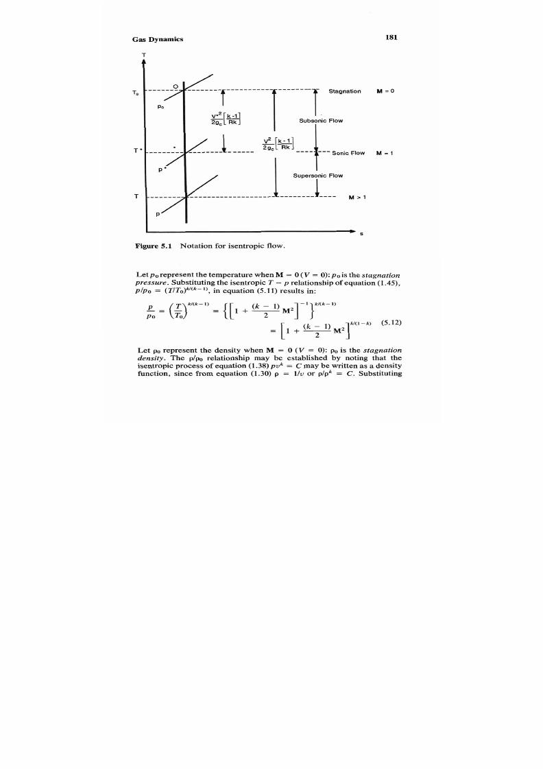
7/21/2019 Fundamental Fluid Mechanics for Engineers
http://slidepdf.com/reader/full/fundamental-fluid-mechanics-for-engineers 204/438
Gas Dynamics
T
181
T '
T
Stagnat ion
Supersonic Flow
l
.
M = O
M
=l
Figure
5.1
Notation for isentropic flow.
Letp . represent the temperature when M =
0 (V
= 0): p0 is the stagnation
pressure. Substituting the isentropic T
-
p relationship of equation (1.45),
plpo
=
( T / T o ) ~ ( ~ - ' ) ,n equation (5.11) results in:
W(k
-
1)
E = ( $ )
= { [ 1 + 7 M 2 ]k
-
1) }
P o
- 1 W ( k - l )
M ( 1 - k ) 5.12)
=
[l
+
Let p represent the density when
M
=
0 ( V
=
0):
p is the stagnation
density. The p/po relationship maybeestablishedbynoting that the
isentropic process of equation (1.38) p v k =
C
may be written as a density
function, since from equation (1.30) p = l/v
or p/pk
= C. Substituting

7/21/2019 Fundamental Fluid Mechanics for Engineers
http://slidepdf.com/reader/full/fundamental-fluid-mechanics-for-engineers 205/438
182
Chapter
5
these values in equation (5.12) results in:
Critical Conditions
Critical conditions xist when the Mach number is unity.et T* represent
the temperature when M = 1, where T* is the critical temperature. Sub-
stituting in equation (5.11) T* for T and M* for M results in:
(5.14)
Let p * represent the pressure whenM
=
1, where p* is the critical
pressure. Substituting in equation (5.12) p* for p and 1 for M results in:
P* 2
[
+ M*)2]
Po
k - l
W(1- k )
2
W ( 1 -
k )
2
W ( k - 1)
(5.15)
= [ + - l
(l)’]
= (-)
+ l
Let
p*
epresent the pressure when M
=
1, where
p*
s the critical den sity.
Substituting in equation (5.13) p* or p and 1 for M results in:
P*
2
Po
k - l
1/(1- k )
-
[
+
-(M*)’]
2
1 4 1 - ) 2 V(k - 1) (5.16)
= [ + - l (l)’] = (-)+ l
Let
V*
represent the velocity when M
=
1 where
V*
is the critical ve-
locity.
From equation (5.6)
V
= M(kgcRT)ln,
so
that:
(5.17)
Substituting from equation (5.11) for T/To and from equation (5.14) for
TOIT*,

7/21/2019 Fundamental Fluid Mechanics for Engineers
http://slidepdf.com/reader/full/fundamental-fluid-mechanics-for-engineers 206/438
Gas
Dynamics
183
I k + l
(5.18)
= M /2(1
+
FM')
- l
The
critical
area A* is obtained by writing the continuity equation 3.
O)
pAV = p*A*V* as follows:
Substituting from equation
(5.16)
for
p * / p o ,
equation
(5.13)
for
equation (5.18) for V * / V results in:
l / ( k - 1) I K k - 1)
$=(&) 1
X
k + l
(5.20)
=I
(-)(l
2 + ?M2)]- l
( k + 1 ) R ( k -
1)
M k + l
Note that A/A* is always greater than one and that equation (5.20) has
two solutions. For every area ratio except unity, there are two Mach
numbers, one subsonic and one supersonic, that will satisfy equation
(5.20).
Writing the continuity equation
(3.15)
for an ideal gas
(riz =
AVp/R7' )
substituting for T* from equation(5.14), for p* from equation(5.15), and
for V* from equation (1.69) results in:
W ( k- )
.
A*V*p*
m*
=
RT*
-
R
(*)
+ 1
(5.21)
where m * s the maximum mass flow rate.

7/21/2019 Fundamental Fluid Mechanics for Engineers
http://slidepdf.com/reader/full/fundamental-fluid-mechanics-for-engineers 207/438
184 Chapter 5
Tabulated Values
of
Isentropic Flow Functions
It has been found useful to compute and tabulate certain standard isen-
tropic functions. These functions are all dimensionlessatios and are func-
tions of Mach number. Table
5.1
contains the following ratios.
Function
Equation
~~
M* = VlV*
AIA*
TIT0
PIP0
PIP0
5.18
5.20
5.11
5.12
5.13
In applying this table it should be noted that all data are based on the
assumption that the gas is ideal, and he molecular weight, specific eats,
and ratios of specific heats are constant. Table
A-2
gives valuesof k for
ideal gases as a function of temperature. When the temperature range is
known before calculations he average value of k should be used. If one
of the temperatures is not known, use the k value for the known tem-
perature and check for variation after the other is computed.
5.5 CONVERGENTNOZZLES
Consider the flow of an ideal gas from large tank through a convergent
nozzle that discharges into the atmosphere
or
to another large tank as
shown in Figure5.2. Stagnation conditions exist in bothanks as well as
the atmosphere. From Section
5.3
only subsonic flow can exist in the
Supply Tank
0
r
I
I
2
l
I .
I
I
I
_
4 Receiving Tank
A,-,-
4
L ,
Figure
5.2
Notation for convergent nozzle study.

7/21/2019 Fundamental Fluid Mechanics for Engineers
http://slidepdf.com/reader/full/fundamental-fluid-mechanics-for-engineers 208/438
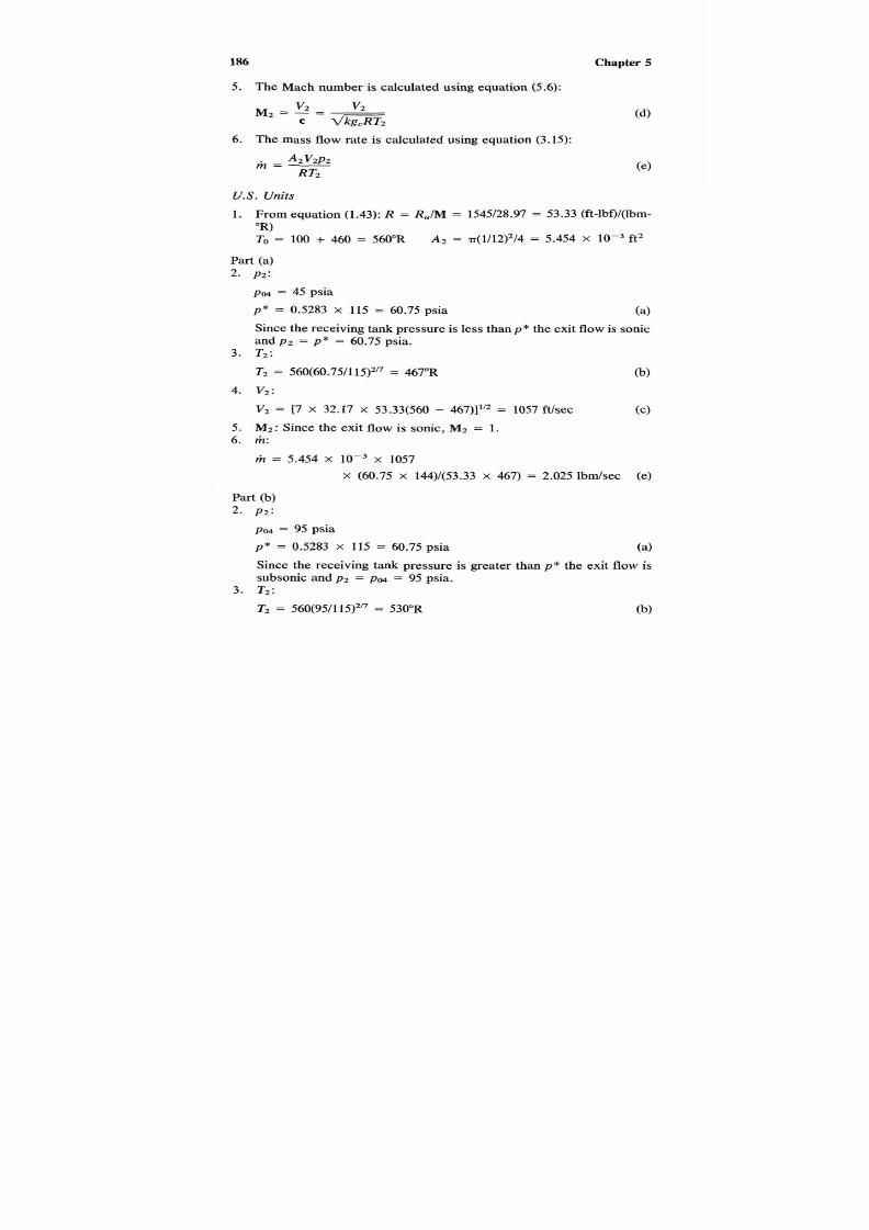
7/21/2019 Fundamental Fluid Mechanics for Engineers
http://slidepdf.com/reader/full/fundamental-fluid-mechanics-for-engineers 209/438
186 Chapter 5
5.
The Mach number is calculated using equation (5.6):
6 .
The mass flow rate is calculated using equation
(3.15):
US.Units
1 .
From equation
(1.43):
R
=
R U N
=
154Y28.97
=
53.33
(ft-lbf)/(lbm-
"R)
To
= 100 + 460 = 560"R A2
=
~(1/12)'/4
=
5.454 X ftz
Part (a)
2.
p2:
p04
= 45 psia
p * = 0.5283
X
115 = 60.75 psia ( 4
Since the receiving tankpressure is less than
p
*
the exit flow is sonic
and
p2
=
p * = 60.75
psia.
3. T2:
Tz
=
560(60.75/115)2"
=
467"R
(b)
4.
v2:
V Z = [7 X 32.17 X 53.33(560 - 467)]"' = 1057 ftlsec (c)
5.
M 2 :
Since the exit
flow
is sonic,
M 2
=
1 .
6. rit:
riz = 5.454 X 10-3 X 1057
x (60.75 x 144)/(53.33 x 467) =
2.025
Ibm/sec (e)
Part (b)
2.
p 2 :
po4
= 95
psia
p * = 0.5283 X 115 = 60.75 psia
Since the receiving tank pressure is greater than p * the exit flow is
subsonic and p 2 = p 0 4 = 95 psia.
3. T2:
T2 = 560(95/115)2" = 530"R (b)

7/21/2019 Fundamental Fluid Mechanics for Engineers
http://slidepdf.com/reader/full/fundamental-fluid-mechanics-for-engineers 210/438
Gas Dynamics 187
4.
v 2 :
V2
=
[7
x
32.17
x
53.33(560
-
530)]'"
=
600
ft/sec (c)
5 .
M 2 :
M2 = 600/[1.4 X 32.17 X 53.33 X 5301'" = 0.532 (dl
6. m:
h
5.454 X X 600
(e)
x (95 x 144)/(53.33 x 530) = 1.584 lbdsec
SI
Units
1. R =
RUM
= 814/28.97 = 287.0 J/(kgl-K) (1.43)
To
=
38 + 273 = 311 K,
A2
= ~(25.4 10-3)2/4
= 5.067
x
m'
Part (a)
2.
p 2 :
p04 = 310 kPa
p *
= 0.5283
X
793 = 418.9kPa
Since the receiving tank pressure is less than
p *
the exit flow s sonic
and p 2 = p * = 418.9 kPa.
3. T2:
T2
= 311(418.9/793)2" = 259 K (b)
4.
v 2 :
V2 = [7 X 1 X 287.0(311 - 259)]'j2 = 323 d s (C)
5. M 2 : Since the exit flow is sonic, M 2
=
1.
6.
m:
h 5.067
X loF4 X
323 X 481.9
X 103/(287.0
X
259) = 1.061kg/s
(e)
Part (b)
2.
p2:
p04 = 655 kPa
p *
= 0.5283 x 793 = 418.9 kPaa)
Since the receiving tank pressure is greater than p * the exit flow is
subsonic and p 2 = po4 = 655 kPa.

7/21/2019 Fundamental Fluid Mechanics for Engineers
http://slidepdf.com/reader/full/fundamental-fluid-mechanics-for-engineers 211/438
188 Chapter 5
3. T z :
Tz
=
31(655/793)2"
=
294
K
(b)
4 .2:
Vz = [7 X 1 X 287.0(311 - 294)]'" = 185
&S
(c)
5.
Mz:
M2 = 185/[1.4
X
1 X 287.0
X
2941'"
=
0.538 (dl
6 . m:
riz = 5.067
X x
185
x
655
(e)
X' 103/(287.0
X
294) = 0.728 kg/s
5.6
ADIABATIC EXPANSION FACTOR Y
The adiabatic expansion factor Y s the ratio of the mass flow rate of a
compressible fluid o that of an incompressible fluid underhe same con-
ditions. This actor is important inhe flow of compressible fluidsn some
metering devices such as the flow nozzle and the Venturi meter.
Consider conditionsat the nozzle inlet Section of Figure 5.2. At this
section both the area A I and the velocity VI are finite. Writing equation
(5.9) for the kinetic energy change between Sections and 2:
(5.22)
In Section 3.7, equation (3.17) was developed for velocity-area-pressure
continuity relations for ideal gas flow inpassage. Writing equation3.16)
for an isentropic process and solving for V1 results in
(5.23)
Substituting for VI from equation 5.23) in equation (5.23) and solvingfor
(5.24)
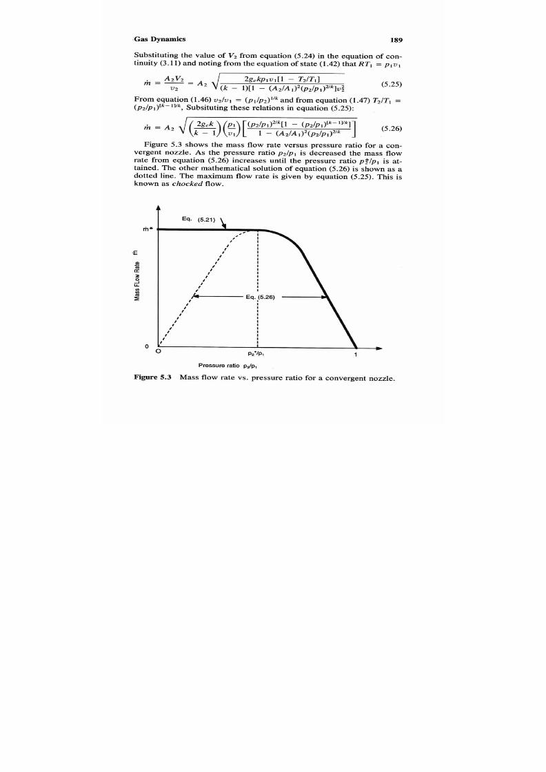
7/21/2019 Fundamental Fluid Mechanics for Engineers
http://slidepdf.com/reader/full/fundamental-fluid-mechanics-for-engineers 212/438
.Gas
Dynamics 189
Substituting the value of V2 from equation (5.24) in the equation of con-
tinuity (3.11) and noting from he equation of state
(1.42)
that RTI
=
p lv l
From equation
(1.46) vz /v l
= ( ~ ~ / p ~ ) ’ / ~nd from equation
(1.47)
T2/T1
=
( ~ ~ / p ~ ) [ ~ - I l ’ ~ ,ubsituting these relations in equation (5.25):
Figure 5.3 shows the mass flow rate versus pressure ratio for a con-
vergent nozzle. As the pressure ratio p 2 / p I is decreased the mass flow
rate from equation (5.26) increases until the pressure ratio pP/p l is at-
tained. The other mathematical solutionof equation (5.26)
is shown as
a
dotted line. The maximum flow rate is given by equation
(5.25).
This is
known as
chocked
flow.
m*
a
c
d
3
m
0
Pressureratio
pJp,
Figure
5.3 Mass flow rate vs. pressure ratio for a convergent nozzle.

7/21/2019 Fundamental Fluid Mechanics for Engineers
http://slidepdf.com/reader/full/fundamental-fluid-mechanics-for-engineers 213/438
190 Chapter 5
Differentiating equation(5.26) with respect to
( p z / p l )
and setting dm/
d(pzIp1)
=
0
we have
k + l
For the special case of Az/A1 =
0,
equation (5.27) reduces to:
(5.27)
(5.15)
This of course is the same result that was obtained from he convergent
nozzle discharging from large tank. When an incompressible fluid flows
without friction through horizontal nozzle he mass flow rate m may be
obtained by writinghe Bernoulli equation
4.17)
for a horizontal passage:
(5.28)
From the continuity equation 3.11) m i = VIA1/vl= VzAZvZ.Noting that
for incompressible flowvz =
V I ,
the incompressible mass flow is
hi =
VlAI/ul
=
VzAZv1.
Substituting in equation
(5.28),
(hivllA2)' - (r izb~l /A1)~
2gc
which reduces to
= Vl(P1
-
P z )
(5.29)
The
adiabatic expansion factor
Y is defined as
riz mass low rate of a compressible luid
hi mass flow rate of an incompressible fluid
y = -
-
(5.30)
Substituting equation(5.26) for riz and equation (5.29) for mi in equation
(5.30) and simplifying results in
y = - - -\ i
k ( p 2 / ~ 1 ) ~ ~ [ 1( P Z / P I ) [ ~ - ~ ' / ~ I [ ~(Az/A)'I
mi k
- 1)[1 - p z / ~ l l [ l- (A$A1)2(~z/~l)ukl
(5.31)
Values of the adiabatic expansionfactor Yare given in Table5.2. In this
table the diameter ratio (p eta) is used where
(5.32)
7/21/2019 Fundamental Fluid Mechanics for Engineers
http://slidepdf.com/reader/full/fundamental-fluid-mechanics-for-engineers 214/438
Gas
191
The use of the expansion factor from Table 5.2 facilitates computation.
An expression for compressible flow may be obtained by substituting
equation (5.29) for m i in equation
(5.30)
and solving for h, oting the
definition of
P
rom equation (5.32)
(5.33)
Example 5.2 Nitrogen flows in
a
4 in. size Schedule 40 steel pipe that
reduces to
a
2
in. size Schedule
40
steel pipe. In the inlet section, the
temperature is 100°F 38°C) and the pressure is 100 psia (690kPa). Assume
adiabatic frictionless flow and ideal gas properties and determine (a) the
minimum pressure that can exist in the 2 in. size pipe, (b) the maximum
mass flow rate, and (c) the mass flow rate if the pressure in the 2 in. size
pipe is 70 psia (483 kPa).
Solution
This example is solved by using Table 5.2.
1. Minimum pressure. The critical pressure ratio p*/pI s obtained from
Table 5.2 at P nd
k:
P * =
P l ( P * / P l )
(a)
2. Maximum mass flow rate. The critical adiabatic expansion factor
Y*
is obtained from Table5.2 at p and k . The maximum mass flow rate
is calculated from equation 5.33):
3. The mass flow rate for
p 2 .
The adiabatic expansion factor
Y
is ob-
tained from Table 5.2 at P,
p z / p l ,
and k . The mass flow rate is cal-
culated from equation(5.33).
4. Common data. From Table A-l for
N Z ,
M = 28.013. From Table A-
2, the value of
k
for
N 2
for 122°F
(50°C)
and below is 1.400. From
Table C-3, Schedule 40 steel pipe:

7/21/2019 Fundamental Fluid Mechanics for Engineers
http://slidepdf.com/reader/full/fundamental-fluid-mechanics-for-engineers 215/438
192 Chapter 5
Internal Diameter
R o w area
Sectionize ftmm)t3mm)*
Pipe
1 4 in. 0.3355
102.3
0.08841 8 219
2
in.
0.1723 52.52
0.02330 2 166
~~
p = D1/D2 = 0.1723/0.3355 = 52.52/102.3 = 0.51355.32)
US. nits
TI = 100 + 460 = 560"R
R
= R,/M = 154Y28.013
=
55.15
(ft-lbf)/lbm-"R)
(1.43)
1. Minimum pressure:
(1.42) V I = RT1/pl = 55.15 x 560/(100 X 144) = 2.145 ft3/lbm
From Table
5.2
at
k
=
1.4,
p
= 0.5135,
p * / p l =
0.5375
(interpolated).
p*
= 100
X
(0.5375) = 53.75 psia (a)
2. Maximum mass flow rate:FromTable 5.2 at k = 1.4, p = 0.5135,
Y* = 0.6962.
m
= 0.6962
X
0.02330
2 X 32.17(100 X 144
-
53.75
X
144)
2.145(1
-
0.51354)
= 7.51
Ibndsec (b)
3.
The mass flow rate for p 2
= 70
psia. From Table
5.2
at k
= 1.4,
p
= 0.5135, p 2 / p 1 = 70/100 = 0.7, and
Y
= 0.8116.
2 X 32.17(100 X 144
-
70 X 144)
=
x 0'02330
J
2.145(1 - 0.51354)
(c)
= 7.07 lbndsec
SI
Units
TI = 38
+
273 = 311 K
R = RUM 8 314/28.013 = 296.8 J/(kg.K) (1.43)
1. Minimum pressure:
v1 = RTl/pl = 296.8
x
311/690
x
lo3 = 0.1338
m3/kg
(1.42)
7/21/2019 Fundamental Fluid Mechanics for Engineers
http://slidepdf.com/reader/full/fundamental-fluid-mechanics-for-engineers 216/438
Gas
Dynamics
193
From Table 5.2 at
k =
1.4,
p
= 0.5135, and p*/pl = 0.5375 (inter-
polated).
p* = 690 x (0.5375) = 370.9 kPa (a)
2. Maximum mass flow rate: From Table 5.2 at k = 1.4, p = 0.5135,
and Y* = 0.6962.
m * = 0.6962 X 2166
2
X 1 X
(690
X
lo3 - 370.9
X
lo3)
x
J
0.1338(1 - 0.51354)
0 )
= 3.41 kg/s
3. The mass flow rate for p2 = 483 kPa. From Table 5.2 at k = 1.4,
p
= 0.5135 pdp1 = 483/690 = 0.7, and Y = 0.8116.
h* 0.8116
X
2166
2
X
I
X
(690
X
103 - 483
X
103)
x
d
0.1338(1 - 0.51354)
= 3.21 kg/s
5.7 CONVERGENT-DIVERGENTNOZZLES
Area-Pressure Relations
The mass flow ate through any sectionf the convergent-divergent nozzle
shown in Figure 5.4 may be determined by modifying equation (5.26)or
stagnation conditions
( A 2
= A , , A 1= A o , A , /Ao , 0, and
p1
= PO,
v 1
=
v o , v2 =
v
m = A , J[ ] p?] p1 [
-
e)(k-l)/k]5.34)
The area-pressure relations may be established by squaring equation
(5.34) and equating for sections 2 and 3:
which reduces to
(5.35)

7/21/2019 Fundamental Fluid Mechanics for Engineers
http://slidepdf.com/reader/full/fundamental-fluid-mechanics-for-engineers 217/438
194 Chapter
5
I
Supply Tank
Throat
I
VC4 + 0
L
Figure 5.4
Notation for convergent-divergent nozzle study.
If the velocity in the throat is sonic, then from equation(5.15):
Substituting equation
(5.15)
in equation (5.39,
(k+
l)/(&-
1
(5.15)
(5.36)
Note that equation (5.36) has
two
solutions, one for isentropic compres-
sion (subsonic flow) and the other for isentropic expansion (supersonic
flow).
Flow Through
a
Convergent-Divergent Nozzle
Consider the arrangement shown n Figure
5.5.
The supply tank ressure
p . is maintained constant and the receiving tank pressure p m may be
lowered from
p .
to zero. As soon as
p m
is below
P O ,
low begins.
Path A represents the flow for any p3 higher than 1338. Since the flow
in the throat for path A is subsonic ( p M
>
p * ) , the flow throughout the
nozzlemust be subsonic. In the divergentsection the process is an
isentropic expansion and n the convergent section it s one of isentropic
compression. Path
A ,
for example, represents compressible flow through
an ideal Venturi meter.
Path
B
represents an isentropic expansion in the divergent portion and
an isentropic compression n the divergent sectionafter sonic flow n the

7/21/2019 Fundamental Fluid Mechanics for Engineers
http://slidepdf.com/reader/full/fundamental-fluid-mechanics-for-engineers 218/438
Gas Dynamics
Shock
195
1 2 X L 3
Figure 5.5 Pressures in
a
convergent-divergent nozzle.

7/21/2019 Fundamental Fluid Mechanics for Engineers
http://slidepdf.com/reader/full/fundamental-fluid-mechanics-for-engineers 219/438
1%
Chapter
5
throat. Except for the throat, the flow in both portions of the nozzle is
subsonic. Pressure p38 is the pressure calculated from the subsonic so-
lution of equation (5.36).
Path C represents an isentropic expansion in the both the convergent
and divergent sections of the nozzle. The flow in the convergent section
is subsonic and in the divergent section it is supersonic. Pressure
p 3 c
is
the pressure calculated from the supersonic solution of equation (5.36).
Note that any receiving tank pressure (PM) ower than p S c will have no
effect on this process.
Path
D
represents any pressure betweenpse and p3c. The gas expands
along an isentropic path to the throat and continues along path
C
until
the distance
x
n the divergent portion of the nozzle is reached. At this
point
a
shock wave is formed and the pressure (and other properties)
essentially jump to point y. From point y to the exit, path
D
is one of
isentropic compression. The flow in the divergent portion is supersonic
to point
x
and subsonic from point
y.
Discussion of this phenomena is
continued in Section 5.9,Compression Shock Wave.
Equation (5.26) or (5.33) may besed to calculate the mass rate of flow
through the nozzle for path
A .
For all other paths equation
5.21)
should
be used.
Isentropic Flow Calculations
Nozzle flow calculations usually falln the following categories:
1.
Design to produce a given flow for specified conditions.
2. Compute the performance of a given design.
Forcategories 1 and 2 there are calculations for (a)expansion (path
C ) ,
to deliver kinetic energy or jet propulsive devicesor for turbine
nozzle-blade stages, and (b) ompression (path
B ) ,
o deliver specified
exit conditions for diffuser devices.
3. For use as metering devices (path
A ) .
Four examples are used to illustrate calculation methods:
Example 5.3-l(a), design of a nozzle for full expansion.
Example 5.4-l(b), design of a diffuser.
Example 5.5-2(a) and (b), performance of a nozzle for both compression
and expansion.

7/21/2019 Fundamental Fluid Mechanics for Engineers
http://slidepdf.com/reader/full/fundamental-fluid-mechanics-for-engineers 220/438
Gas Dynamics 197
Example 5.3
Design an ideal convergent-divergent nozzle that is to de-
liver
4.5 Ibndsec (2 kg/s) of air from a large plenum chamber at 100 psia
(700
kPa) and
240°F
(1
16°C)
to another plenum chamber where he pres-
sure is maintained at
10
psia
(70
kPa). Determine a) area of nozzle throat
and (b) area of nozzle exit.
Solution
This example is solved by the application of the mass flow rate equation
(5.21) and the use of Table 5.1.
Common data
From Table A-l for air,
M
=
28.97.
From Table
A-2,
the value
of
k
for
air at 302°F (150°C) and below ranges from1.395 to 1.402
=
1.4.
p04/p0 = 10 psidl00
psia
=
70 kPd700 kPa
= 0.1
From Table 5.1 at k
=
1.4:
PIP0
0.1
W4 0.09352
0.1 (interpolated)
M
2.10 2.20 2.159
(interpolated)
AIA*
1.8370
2.005
1.938 (interpolated)
(a)
Area of nozzle throat
Since the exit flow is supersonic the flow at throat must be sonic,
so
from
equation (5.21):
(b)
Exit area
A3
=
A*(A/A*)
=
1.938A*
U.S.
Units
To = 240
+
460 = 700"R
R =
R U M =
154Y28.97
=
53.33 (ft-lbf)/(lbm-"R) (1.43)

7/21/2019 Fundamental Fluid Mechanics for Engineers
http://slidepdf.com/reader/full/fundamental-fluid-mechanics-for-engineers 221/438
198 Chapter 5
(a) Throat area
= 0.01554 x 144 = 2.238
(b) Exit area
A3 =
1.938
X
2.238 = 4.337 in.2
SI
Units
To
=
116
+
273
=
389
K
R
= R U M = 8 314/28.97 = 287 J/(kg-K)
(a) Throat area
A* = 1.460 x 2 $87.089
700
X
103
= 1.394
x
m'
= 1.394
x x
1 x IO6 = 1 394 mm2
(b) Exit area
(1.43)
A3 = 1.938
X 1
394 = 2 701m2 (c)
Example 5.4 Design an ideal diffuser (Figure 5.3, convergent section)
that will meet the following specifications:
Fluid: Ideal gas k = 1.4,
M
= 28.
Mass
flow
rate:
riz
=
120 Ibdsec (54.4 kg/s).
Inlet conditions:
p2 = 10 psia (70Pa)
t2 = 0°F
( -
I8OC)
V2
=
700 ft/sec (213 S)
Exit conditions:
V ,
=
300 fdsec (91.5m/s)
Determine
(a)
inlet area A2 and (b) exit area A 3 .
Solution
This example
is
solved by application of basic relations. The inlet Mach
number is computed using equations (5.6) and (1.69). Specific volumes
7/21/2019 Fundamental Fluid Mechanics for Engineers
http://slidepdf.com/reader/full/fundamental-fluid-mechanics-for-engineers 222/438
Gas
Dynamics 199
are computed from he equation of state (1.42), areas from the continuity
equation (3.11), exit temperature from the energy equation 5.9), and exit
pressures from the isentropic process relationship equation (1.45).
1.
Inlet area A2
The inlet Mach number and
s
computed using quations (5.6) and (1.69).
M2 = V21(kgcRT2)1n (a)
The specific volume comes from equation 1.42):
v2 = RT2Ip2 (b)
The inlet area is from the continuity equation (3.11):
A2 = rizv2IV2
( 4
2. Exit area As
The exit temperature is computed from equation 5.9):
The exit pressure is computed from equation (1.45):
p3 = = p2(T3/T2)'.4'[1.4"] = P2(T3/T2)3.5
The exit specific volume is from equation (1.42):
v3 = RT3/p3
Finally, the exit area A3 comes from equation(3.11):
A3
=
rizv3IV3
US.Units
T2 = t2 = 460 = 0 + 460 = 460"R
R = R U M= 1545128 =
55.18
(ft-lbf)l(lbm-"R)
1. Inlet area A2
M2
=
7001(32.17
X
1.4
X
55.18
X
460)1'2
=
0.6544
Inlet
flow
is subsonic.
v2 = 55.17
X
460/(10
X
144) = 17.62 ft3/lbm
A2 = 120
X
17.621700 = 3.021 ft2
(1.43)
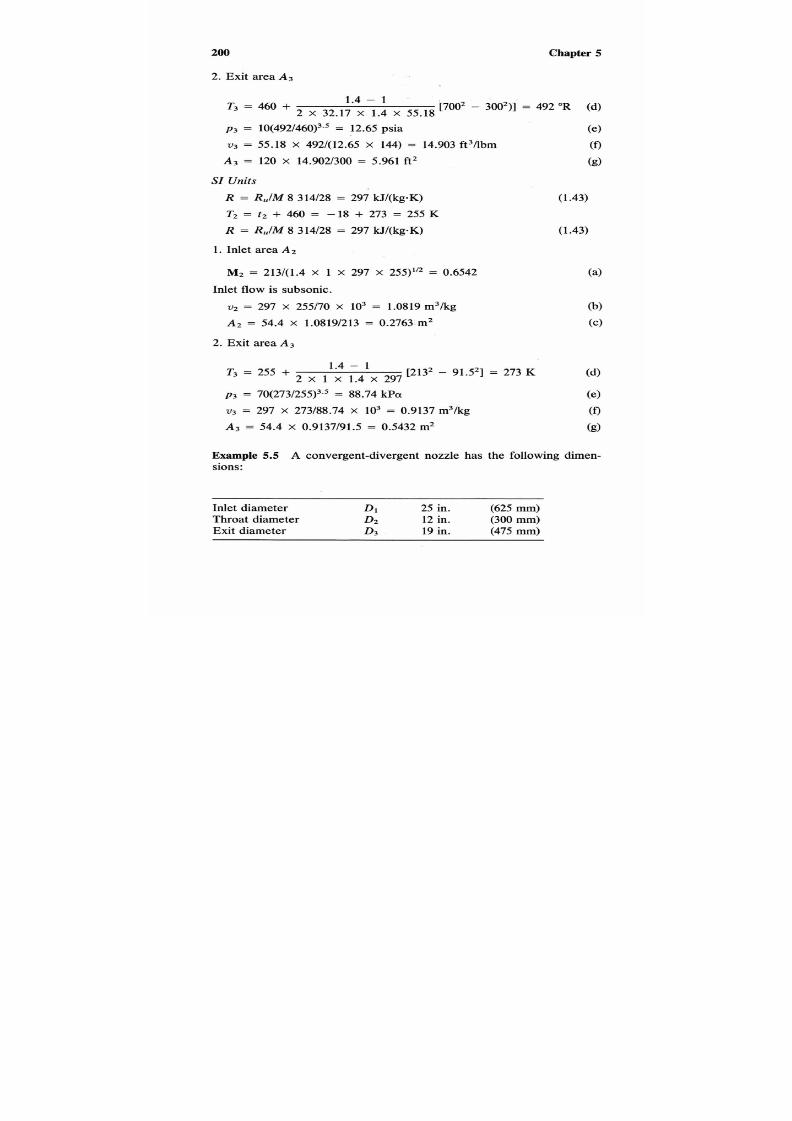
7/21/2019 Fundamental Fluid Mechanics for Engineers
http://slidepdf.com/reader/full/fundamental-fluid-mechanics-for-engineers 223/438
200
2. Exit area A 3
Chapter
5
1.4
-
1
T3 = 460 +
2
x
32.17 x 1.4
x
55.18
[7W2 - 30O2)]'= 492 R (d)
p3 = 10(4921460)3.' = 12.65 psia
v 3 = 55.18 X 4921(12.65 x 144) = 14.903 ft3/lbm
A3
= 120
X
14.9021300 = 5.961 ft2
SI Units
R
=
R,lM
8 314128
=
297 kJ/(kg-K)
T2 = t 2 + 460 = - 18 + 273 = 255 K
R
=
R,IM 8 314128 = 297 kJ/(kg-K)
1. Inlet area A 2
M2
=
2131(1.4
X
1
X
297
X
255)ln
=
0.6542
Inlet
flow
is subsonic.
v2 = 297 x 255170 x
lo3
= 1.0819 m3kg
A 2 = 54.4 x 1.08191213 = 0.2763m'
2. Exit areaA3
1.4 - 1
T3 = 255 +
2 x 1 x 1.4 x 297
[2132 - 91.52] = 273 K
p3 = 70(273/255)3.5
=
88.74
kp~r
v3 = 297 X 273188.74 x
lo3
= 0.9137m31kg
A3
= 54.4
x
0.9137191.5 = 0.5432
m2
Example
5.5 A
convergent-divergent nozzle has the following dimen-
sions:
Inlet diameter D1 25 in.
(625 mm)
Throat diameter
Dz
12 in.
(300 mm)
Exit diameter
D3
19n.
(475 mm)

7/21/2019 Fundamental Fluid Mechanics for Engineers
http://slidepdf.com/reader/full/fundamental-fluid-mechanics-for-engineers 224/438
Gas Dynamics
201
Oxygen at 30 psia (207 kpa) and 68°F(20°C) nters this nozzle. The flow
in the throat is sonic. Determineby calculation (do not use Table 5.1)he
(a) range
of
Mach numbers and (b) pressure range at exit for isentropic
flow.
Solution
This example is solved by use of basic equations as requested in the
problem statement. Most of the information desired is in dimensionless
form, so the numerical unit computations are included in the theoretical
development as appropriate.
Common data
From
Table A-2, k for oxygen at 212°F 100°C) and below ranges from
1.386 to 1.400 = 1.4.
AI/A2 = = (25/12)2 = (625/300)2 = 4.340
A3/A2 = = (19/12)2 = (475/300)2
=
2.507
For
part (a), The Mach number-area relationship s given by equation
(5.20):
(k-
1)
( 4
1.4 - 1
1.4+1/2(1.4-l)
-
rlL)(1
+
-M2)]
.4
+ 1
which reduces to
M = A* 7)+ M2
A
( k = 1.4)
For sonic velocity in the throat, AJA2 = AJA* = 4.340.
Solving equation (b)by trial and error,
1 5 + M : 3
M1 = 4.340
7)
0.135,.09
Since the flow in the divergent section can’t be supersonic,
M1
=
0.135
For exit Mach numbers, A3/A2 = A3/A* = 2.507.
Solving equation (b) by trial and rror,
1 5 + M : 3
M3=-
2,507
[
-
= 0.239, 2.45

7/21/2019 Fundamental Fluid Mechanics for Engineers
http://slidepdf.com/reader/full/fundamental-fluid-mechanics-for-engineers 225/438
202 Chapter 5
The value O M3 can range from 0.238 o 2.45 depending on he exit pres-
sure.
For part
(b),
the stagnation pressure-Mach number relations re given
by equation (5.12):
P
Po
2
- = [ 1 + 1 M 2 ]
k -
1)
= [ l + (1.4
-
1)
M z ~. 4 /( 1 .4 - l )
(c)
=
(1
-
0.2~2135
Relating p3
and p I using equation (c):
For isentropic compression M3 = 0.239,
p3max
from equation (d) is
U S . Units
P3
max =
0.973 X 30
=
29.19 psia
S I
Units
P3 max
=
0.973
X
207 = 201 kPa
For isentropic expansion M3
=
2.45, p3 from equation (d) is
1
+ 0.2
x
0.139
1 +
0.2
x
2.4S
min
=
P1
=
0.064OPl
U . S .
Units
P3
min
= 0.0640
X 30 = 1.92 psia
S I
Units
P3 min = 0.0640 X 207
=
13.2 kPa
5.8 NORMAL SHOCK FUNCTIONS
Compression
Shock
Wave
We continue the discussion of path D (Figure5.5)from Section5.7. When
sonic flow xists in the throat and supersonic flow beginsn the diverging
section of a convergent-divergent nozzle, and he exit pressure p3 is be-
tween that required for isentropic compression (path B ) p3B and that for
isentropic expansion (path B ) p3c, a compression shock wave will be

7/21/2019 Fundamental Fluid Mechanics for Engineers
http://slidepdf.com/reader/full/fundamental-fluid-mechanics-for-engineers 226/438
Gas Dynamics 203
formed. This wave is formed to satisfy the requirements for the conser-
vation of mass and energy. This typef wave is associated with large and
sudden rises in pressure, density, temperature, and entropy. Figure
5.6
shows this phenomena on the T-S plane. The shock wave is so thin that
for computation purposes it may be considered
as
a single line,
as
shown
in Figure
5.4.
Temperature-Mach number-velocity relations for
a
normal shock are
shown in Figure 5.6.
Conservation
of Energy
The formation
of
a
shock wave does not change the total energy of the
system, so that energy relations may be established by writing equation
(5.9) in terms of temperatures before
(TJ
and after
(T, )
the shock wave.
T O
RT,
V :
RT,
Ta+ = - = - + - = To,
k
- 1 2gc
k
-
1
2gc
T
(5.37)
A
Po4
....... H -
o Stagnation
...............................
Pv
i
M sonic Flow
Px
b s
S V
Figure 5.6 Notation for shock wave study.

7/21/2019 Fundamental Fluid Mechanics for Engineers
http://slidepdf.com/reader/full/fundamental-fluid-mechanics-for-engineers 227/438
204 Chapter
5
Substituting the value of acoustic velocity from equation (1.69) and for
Mach number from equation (5.6) as was done in the development of
equation
(5.10)
results in:
m
L
l+”:
L - l
Tx
2
l+”:
k - l
(5.38)
Conservation
of
Mass
The continuity equation (3.15) for an ideal gas rit
=
AVpIRT may be
written in terms of Mach number by noting that the definition of Mach
number from equation5.6) is M = V/(kg,RT)”*.Substituting these values
in equation
(3.15)
for before and after the shock wave, we have
Solving for M y ,
M y =
M x p ”4
P Y
(5.39)
Impulse-Momentum Concept
The impulse-momentum equation
(4.76)
when applied to the shock wave
of Figure 5.5 yields
( P x
-
P Y M =
AVX
[ V y
-
V,] =
YAVY
[ V ,
-
Vxl (4.76)
gc gc
which reduces to
(5.40)
Substituting in the equation above the definition of Mach number of qua-
tion
(5.6),
V
=
M(kg,RT)”*,
and from the equation of state
(1.44)
p
=
p1RT results in:
P Y +
g c
=
P x
+
gc
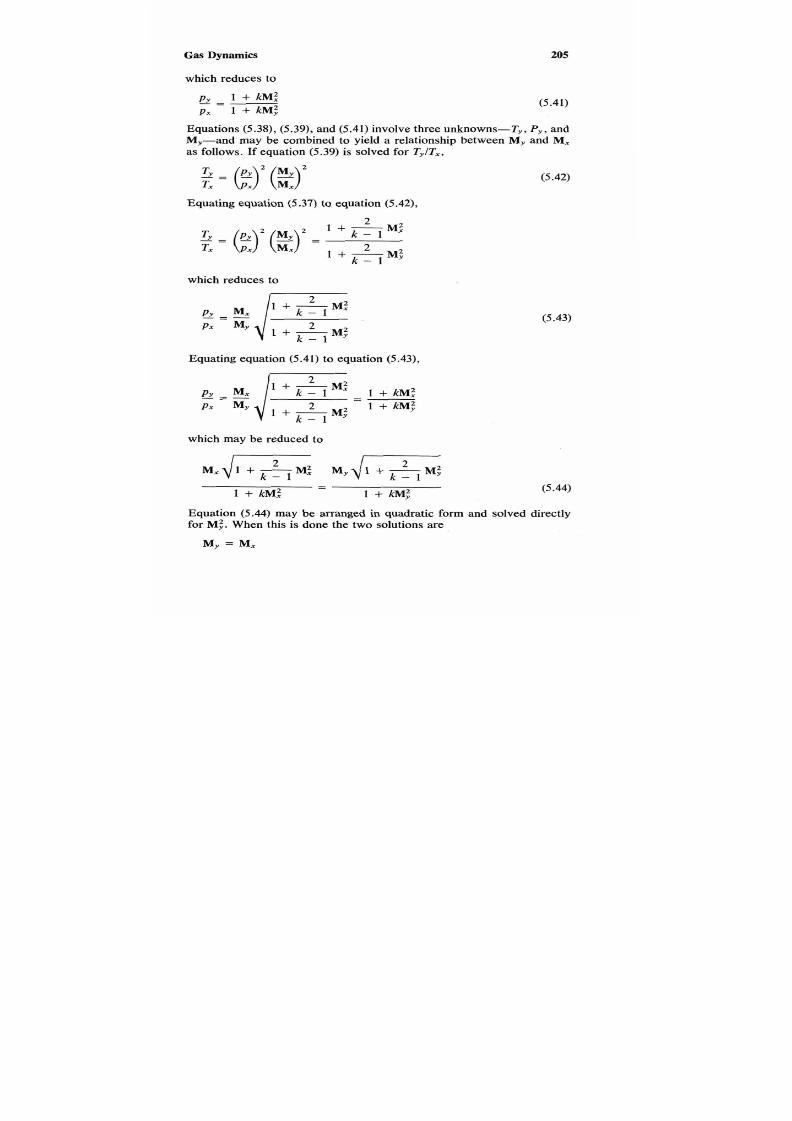
7/21/2019 Fundamental Fluid Mechanics for Engineers
http://slidepdf.com/reader/full/fundamental-fluid-mechanics-for-engineers 228/438
Gas Dynamics 205
which reduces to
& =
+
kM:
p x
1
+ kM;
(5.41)
Equations
(5.38), (5.39),
and
(5.41)
involve three unknowns-T,, P,, and
My-and may be combined to yield
a
relationship between M, and M,
as follows. If equation
(5.39)
is solved for T,/Tx,
Equating equation
(5.37) to
equation
(5.42),
which reduces
to
I e
Equating equation
(5.41)
to equation
(5.43),
I
which may be reduced to
M,
d z
- 1
M,
d z
-
1
-
1
+
kM:
1
+
kM;
(5.42)
(5.43)
Equation (5.44) may be arranged in quadratic form and solved directly
for
M;.
When this is done the two solutions are
M,
=
M,

7/21/2019 Fundamental Fluid Mechanics for Engineers
http://slidepdf.com/reader/full/fundamental-fluid-mechanics-for-engineers 229/438
206 Chapter
5
M:
+
k - l
L
M,'
=
2k
M:
- 1
k -
1
(5.45)
The first solution is trivial because the Mach number mustdecrease after
a shock wave, and therefore equation (5.45) represents the physical so-
lution. Solving equation (5.45) for M y results in:
(k
-
1)M:
+
2
2kM:
-
k
+ 1
(5.46)
Temperature ratios are obtained by substituting M; from equation(5.46)
in equation (5.38):
Y
Tx
-
*
I+
k - l
L
n
l+ ,'
k -
1
L
I+
L
k - l
2 ME
+
2/(k
-
1)
l + -
- 1 1 2k
]
M:
- 1
k -
1
(5.47)
2k
- 1
k - l
-
(k
+ l)*
2(k -
1)
M:
Pressure ratios are obtained by substituting
M;
from equation
(5.46)
in
equation (5.41):
pY= 1
+
kM: -
1 +
kM:k k +
1
p x 1 +
kM,'- k + l
k - l
--
M"
2k
1
: + 2/(k
- 1)
"2-1
k - l
(5.48)
Density ratios may be obtained using the equation of state (1.44):
P Y
(5.49)
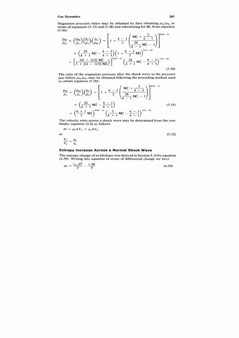
7/21/2019 Fundamental Fluid Mechanics for Engineers
http://slidepdf.com/reader/full/fundamental-fluid-mechanics-for-engineers 230/438
Gas
Dynamics 207
Stagnation pressure ratios may be obtained by first obtaining p~ylpo ,n
terms of equations
(5.12)
and
(5.48)
and substituting or
M
rom equation
(5.46):
M(k- )
[(k
+
1/2
M?
(
2k
. .
=
[ + [(k -
1)/2]
M
k + 1 k +l
M: -
(5.50)
The ratio of the stagnation pressure after the shock wave o the pressure
just before pOy/poxmay be obtained followinghe preceding method used
to obtain equation (5.50):
. 2
W(k-
I )
M
+
PS,= poy p.
P x ( p y ) ( p ) =
[
+ -l(
- l
k M - 1
M
-
k +l
M(k- 1)
= -; M) (&M--
k +l
(5.51)
The velocity ratio across a shock wavemay be determined fromhe con-
tinuity equation (3.9) as follows
m = pxAVx
=
pyAVy
or
(5.52)
Entropy Increase Across a Normal Shock Wave
The entropy change of an ideal gas was derived in Section.16by equation
(4.59).
Writing this equation in terms of differential change we have
c ,
dT
v d p
T T
d s = - - -
(4.59)

7/21/2019 Fundamental Fluid Mechanics for Engineers
http://slidepdf.com/reader/full/fundamental-fluid-mechanics-for-engineers 231/438
208 Chapter
5
Substituting from equation
4.66) c,
=
kR/ (k
- 1 ) and from the equation
of state of an ideal gas
(1.42)
v /T = Rlp in equation
(4.59)
results in:
(5.53)
( k F 1 ) T R -
dTp
P
=
Integrating equation (5.53) for constant specific heat ratios between the
limits of
x
and y results in:
(5.54)
kR
S, -
sx
=
k -
1 log, 2) -
R
log,
k)
Equation
(5.54)
may be put in dimensionless formby dividing both sides
by R and substituting for Ty/Ty rom equation (5.47) and for pylpx from
equation (5.48) with the following result:
S,
-
S, k ( l + y M : ) ( = M :- l 2k
-
1
= -log,[
- l ( k +
1)
2 ( k -
1 )
M'
-
log,
[ k ?
1
M: -
k - l I
(5.55)
Tabulated Values
of
Normal Shock Functions
As in the case of isentropic
flow
functions it has been found useful to
compute and tabulate certain standard normal shock functions. These
functions are all dimensionless atios and are functions of the Mach num-
ber
M,
ust upstream of the shock wave. Table
5.3
contains the following
ratios.
Function
(5.46)
(5.48)
(5.47)
(5.49),
(5.52)
(5.50)
(5.51)
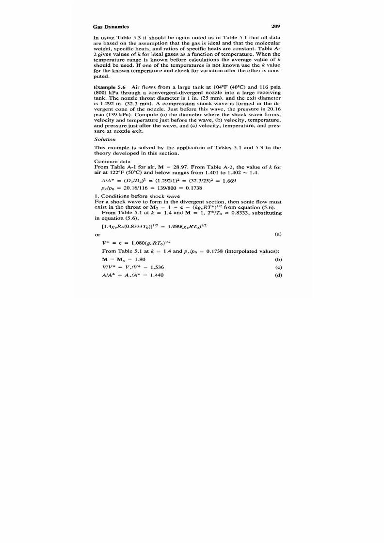
7/21/2019 Fundamental Fluid Mechanics for Engineers
http://slidepdf.com/reader/full/fundamental-fluid-mechanics-for-engineers 232/438
Gas
Dynamics
209
In using Table 5.3 it should be again noted as in Table 5.1 that all data
are based on the assumption that the gas is ideal and that the molecular
weight, specific heats, and ratios of specific heats are constant. Table
A-
2 gives valuesof
k
for ideal gasesas a function of temperature. When the
temperature range is known before calculations the average value of k
should be used. If one of the temperatures is not known use the k value
for the known temperature and check or variation after the other is com-
puted.
Example
5.6
Air flows from a large tank at 104°F (40°C) and 116 psia
(800)
kPa through a convergent-divergent nozzle into a large receiving
tank. The nozzle throat diameter is 1 in. (25 mm), and the exit diameter
is
1.292
in.
(32.3
mm).
A
compression shock wave is formed in the di-
vergent cone of the nozzle. Just before this wave, the pressure is 20.16
psia (139 kPa). Compute (a) the diameter where the shock wave forms,
velocity and temperature just before the wave, (b) velocity,emperature,
and pressure just after the wave, and (c) velocity,emperature, and pres-
sure at nozzle exit.
Solution
This example
is
solved by the application of Tables
5.1
and
5.3
to the
theory developed in this section.
Common data
From Table A-l for air, M = 28.97. From Table A-2, the value of
k
for
air at 122°F (5OOC) and below ranges from 1.401 to 1.402
=
1.4.
AIA* = (&/Oz)’ = (1.29211)’ = (32.3/25)2 = 1.669
pxIpo
=
20.161116
=
139/800
=
0.1738
1. Conditions before shock wave
For
a
shock wave to form in the divergent section, then sonic flow must
exist in the throat or M2 1 = c = (kg,RT*)’” from equation (5.6).
From Table 5.1 at k = 1.4 and M = 1 , T*ITo = 0.8333, substituting
in equation
(5.6),
[ l .4g,R~(O.8333To)]”’ = 1 . O S O ( ~ , R T O ) ~ ~
or
(a)
V* = C = I.OSO(g,RTo)’”
From Table 5.1 at
k
= 1.4 and pxIpo = 0.1738 (interpolated values):
M =
M,
= 1.80
(b)
VlV* = V,IV* = 1.536 (c)
AIA*
+
A,/A* = 1.440
(d)

7/21/2019 Fundamental Fluid Mechanics for Engineers
http://slidepdf.com/reader/full/fundamental-fluid-mechanics-for-engineers 233/438
210
Chapter 5
From equation (d) and from geometry he diameter is
0 = D2(AX/A*)’” = 1.202 (0
Substituting Eq. (a)for V* in Eq. (c),
V,
=
1.536V* = 1 . 5 3 6 ~
(g)
2. Conditions just after the shock wave
From Table 5.3 at
k
= 1.4, M, = 1.80, and from equation (a),
M,
=
0.6165
(h)
pylpx = 3.613 ( 9
T,/T, = 1.532 m
Vx/Vy
=
2.359
(k)
3. Exit conditions
Examination of Figure 5.5 indicates that the path of the air just after the
shock wave is an isentropic compression to the nozzle exit.
The Machnumber just downstreamfrom the shockwave,
M,,
is
0.6165. From Table
5.1
at k = 1.4 and M, = 0.6165,
A/A* = Ay/Ay* = 1.172
(1)
The area ratio just upstream of the shock wave was found to be
AIA* = A,/A* =
1.440
(dl
The differencebetween hesearea atios epresents the adjustment
needed to satisfy the requirements fo r the conservation of energy and
mass.
The term
A,
represents the area at which critical flow wouldake
place at the constant entropy path from just downstream of the shock
wave to exit of the nozzle.
Noting that
A,
=
A,
and dividing equation
(1)
by equation (d),
A*IA,* = (A,/A,*)/(A,/A*)
=
1.172/1.440 = 0.8139 (m)
The area ratio at the nozzle exit is
A3/A2 = A3/A* = (&/02)2 = (1.292/1.)2 = (32.3/25)* = 1.669 (n)
Multiplying equation (m) by equation (n),
A3IA,*
=
(A*/A,)(AJA*) = 0.8139
X
1.669 = 1.358 ( 0 )
From
Table 5.1 at k = 1.4 and A3/A,* = 1.358 (interpolated),
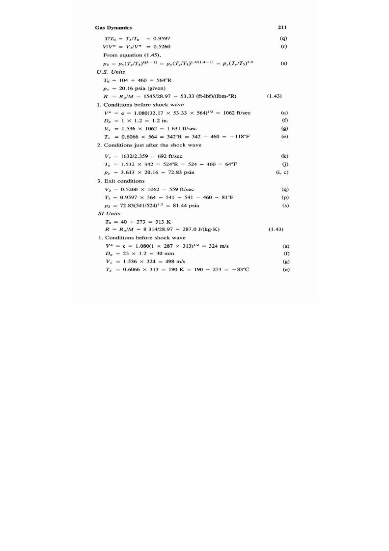
7/21/2019 Fundamental Fluid Mechanics for Engineers
http://slidepdf.com/reader/full/fundamental-fluid-mechanics-for-engineers 234/438
Gas
Dynamics
211
TT0
= TJTo = 0.9597
Vl V*
=
V31V*
=
0.5260
From equation (1. 43,
p3 =
py Tyl T~k[k-l l
py(Ty/T3)1.4/[1.4-'1]~y(Tyl T3)~
US. nits
To
= 104
+ 460 564 R
p, = 20.16
psia (given)
R
=
RJ M
=
1545128.97
=
53. 33
(ft-lbf)I(lbm-"R)
1.
Conditions before shock wave
V* = c
=
l .OgO32.17
x
53. 33 x
564)'
= 1062ft/sec
D , =
1
x 1.2= 1.2
n.
V,
=
1.536 x 1062= 1 631ft/sec
T = 0.6066X 564 = 342 R
=
342- 460 = -118°F
2. Conditions just after the shock w ave
V
=
163212.359
=
692
ft/sec
Ty = 1.532
X
342 = 524 R= 524- 460
=
64°F
p, = 3.613X 20.16= 72.83
psia
3. Exit conditions
V
=
0.5260
x
1062
=
559ft/sec
T3
=
0.9597 X 564
=
541 = 541 - 460
=
81°F
p 3
= 72.83(5411524)3.5= 81.44psia
SI
Units
To
=
40 + 273 =
313
K
R = RIM =
8
314128.97= 287.0Jl(kg-K)
1.
Conditions before shock w ave
V* = C = 1080(1
X
287 x 313' = 324
m/s
D ,
= 25
x
1.2= 30
mm
V = 1.536 X 324 = 498
mls
T = 0.6066
X
313 = 190K = 190- 273 = -83°C
(1.43)
(1.43)
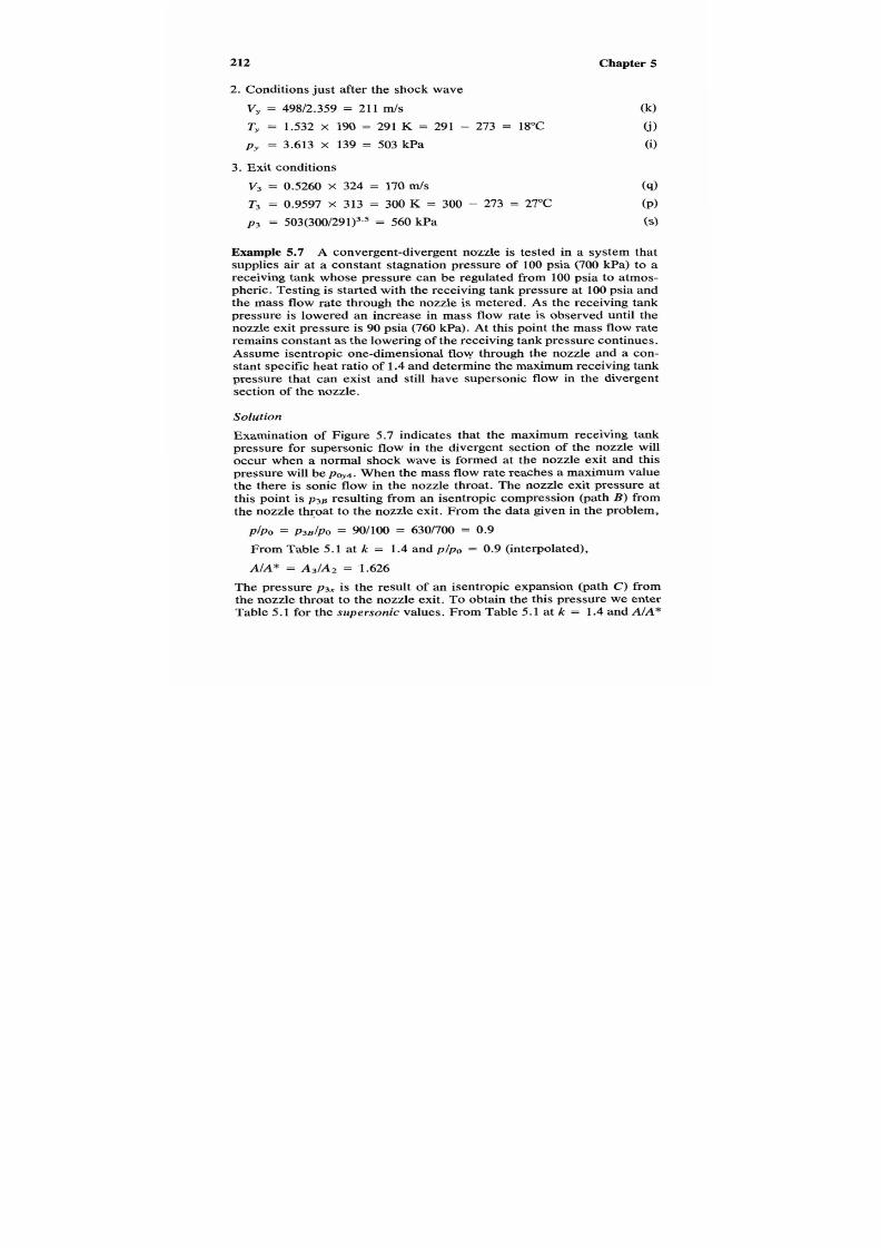
7/21/2019 Fundamental Fluid Mechanics for Engineers
http://slidepdf.com/reader/full/fundamental-fluid-mechanics-for-engineers 235/438
212 Chapter S
2.
Conditions just after the shock wave
V,
=
49812.359
=
211
d s
(k)
Ty = 1.532
X
190 = 291 K
=
291
-
273
=
18°C
0)
p, =
3.613 x 139
=
503
kPa
( 9
3.
Exit conditions
V3
=
0.5260 X 324 = 170
d~
(9)
T3
=
0.9597
X
313 =
300
K =
300
-
27327°C
(P)
p3
=
503(3001291)3.5
=
560
kPa
( 9
Example 5.7 A convergent-divergent nozzle is tested in a system that
supplies air at a constant stagnation pressure of 100 psia
(700
kPa) to
a
receiving tank whose pressure can be regulated from100 psia to atmos-
pheric. Testing is started with the receiving tank pressure at
100
psia and
the mass flow rate through the nozzle is metered. As the receiving tank
pressure is lowered an increase in mass flow rate is observed until the
nozzle exit pressure is
90
psia
(760
kPa). At this point he mass flow rate
remains constant as the lowering of he receiving tankpressure continues.
Assume isentropic one-dimensional flow through the nozzle and
a
con-
stant specific heat atio of 1.4 and determine he maximum receiving ank
pressure that can exist and still have supersonic flow in the divergent
section of the nozzle.
Solution
Examination of Figure
5.7
indicates that the maximum receiving tank
pressure for supersonic flow in the divergent section of the nozzle will
occur when a normal shock wave is formed at the nozzle exit and this
pressure will be
pW4.
When the mass flowrate reaches a maximum value
the there is sonic flow in the nozzle throat. The nozzle exit pressure at
this point is
p3B
resulting from an isentropic compression (path B ) from
the nozzle throat to the nozzle exit. From he data given in the problem,
From Table
5.1
at
k
=
1.4
and plpo
=
0.9
(interpolated),
A/A*
=
A3IA2
=
l . 626
The pressure
p3x
is the result of an isentropic expansion (path
C)
from
the nozzle throat to the nozzle exit. To obtain the this pressure we enter
Table
5.1
for the
supersonic
values. From Table
5.1
at k =
1.4
and
AlA*

7/21/2019 Fundamental Fluid Mechanics for Engineers
http://slidepdf.com/reader/full/fundamental-fluid-mechanics-for-engineers 236/438
Gas Dynamics 213
Shock
Wave,
I
4
Receiving
Tank
X Y
Tank
.
PO4
I
I
8
I
1 2
3
I
I
I
I
I
8
I
I
I
I
I
I
I
I
t
t
t
t
t
I
a
I
I
tank pressure
I
I
1 2 3
Figure 5.7
Notation for normal shock at nozzle exit.
=
1.626
(interpolated),
M
=
1.953
P i P o = px31po = 0.1378

7/21/2019 Fundamental Fluid Mechanics for Engineers
http://slidepdf.com/reader/full/fundamental-fluid-mechanics-for-engineers 237/438
214
Multiplying equation (a) by equation
(b),
PO , . ~ /PO
( P O , . ~ / P ~ ~ ) ( ~ ~ ~ / P O )
0.1378
X
4.351
=
0.5996
or
poy4
= 059%po
U . S .
Units
pw 4 = 0.5996 X 100 = 59.96 psia
SI Units
pW4 = 0.5996 x 700 = 419.7 kPa
5.9
ADIABATIC FLOW IN CONSTANT-AREA DUCTS WITH
FRICTION: FANNO LINE
The flow of fluids in most industrial and power piping applications may
be assumed o be adiabatic.The primary reasons for this assumptionare:
1. The piping lengths are relatively short (and hence heat transfer areas
small) with respect to large mass flow ates so that the heat transfer
is negligible.
2. The pipes are insulated.
In adiabatic flow with friction, the gas may enter the pipe either with
subsonic or supersonic velocity as shown in Figure 5.8.
In case
(a)
the gas enters the pipe witha subsonic velocity.The second
law of thermodynamics requires hat for an adiabatic process the entropy
may not decrease.
The effect of friction is to limit the expansion of the
gas fromp a to
p *
and sonic velocity.For this reason supersonic flow an
not exist in a pipe if the initial flow is subsonic.
In case (b) the gas enters the pipe with a supersonic velocity. Again,
the second law of thermodynamics requires that for an adiabatic process
the entropy maynot decr ease .The effect of friction is to limit the compres-
sion of the gas from b to p* and sonic velocity.For this reason subsonic
flow can not exist in a pipe
if
the initial flow is supersonic.
The limiting velocity in either case is sonic.
General Considerations
Adiabatic compressible flow of an ideal gas with friction in a constant
area duct must satisfy the following requirements:
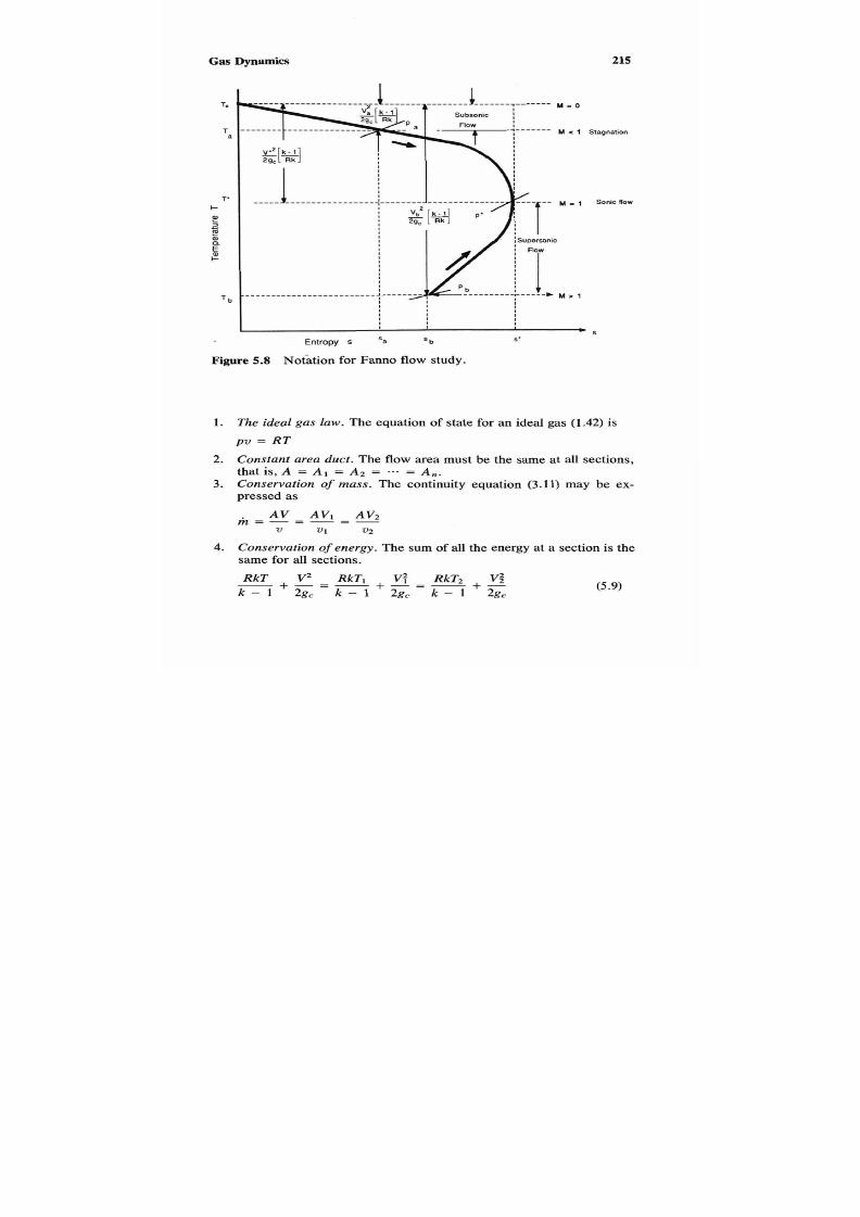
7/21/2019 Fundamental Fluid Mechanics for Engineers
http://slidepdf.com/reader/full/fundamental-fluid-mechanics-for-engineers 238/438
Gas Dynamics
215
[ a:
_ _
M - 0
M c l
I
I
M - 1
l
l
l
M > 1
I I
I
I I
l
I
I I
I l
I
I
I
I
m
Entropy S 'a 'b 5 .
Stagnation
Sonic flow
S
Figure
5.8
Nocation for Fanno
flow
study.
1.
The ideal gas law .
The equation
of
state
for
an ideal gas (1.42)
is
pv = RT
2. Constan t area duct. The
flow
area must be the same at all sections ,
3. Conservation
of
mass .
Thecontinuityequation
(3.11)
maybe ex-
that is, A = A l = A Z = - e - = A , .
pressed as
.
AV AV1V2
m = - = - = -
V
V1
v2
4. Conservation of energy. The sum of all the energy at a section is the
same for all sections.
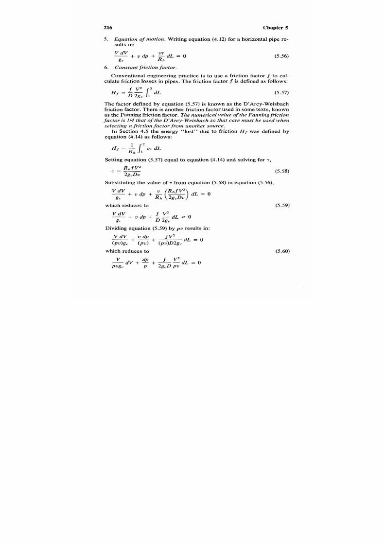
7/21/2019 Fundamental Fluid Mechanics for Engineers
http://slidepdf.com/reader/full/fundamental-fluid-mechanics-for-engineers 239/438
216 Chapter
5
5.
Equation of motion.
Writing equation
(4.12)
for a horizontal pipe re-
sults in:
V dV
- + v d p + - d L = O
7
gc
Rh
(5.56)
6 . Constant friction fa ct or .
Conventional engineering practice is to use
a
friction factor f to cal-
culate friction losses in pipes. The friction factor
f
is defined as follows:
(5.57)
The factor defined by equation
(5.57)
is known as the D'Arcy-Weisbach
friction factor. There is another friction factor used in some exts, known
as the Fanning friction actor.
The numerical value
of
the Fann ing friction
facto r is
1/4
hat of the D'Arcy- Weisbach
o
that care must be
used
when
selecting a friction fa cto r fr om nother source.
In Section
4.5
the energy "lost" due to friction
H f
was defined by
equation
(4.14)
as follows:
Setting equation
(5.57)
equal to equation
(4.14)
and solving for
T,
(5.58)
Substituting the value of 7 from equation (5.58) in equation
(5.56),
-V V
+
v d p
+ (-)
h f v 2
dL
=
0
gc R h
which reduces to
(5.59)
Dividing equation
(5.59)
by
p v
results in:
which reduces to
(5.60)

7/21/2019 Fundamental Fluid Mechanics for Engineers
http://slidepdf.com/reader/full/fundamental-fluid-mechanics-for-engineers 240/438
Gas Dynamics 217
For an ideal gas from the equation of state (1.42) p v = R T . Substituting
for
p v
in equation
(5.60),
(5.61)
Derivation
of
Equations
All of the terms of equation (5.61) can be expressed as functions of Mach
number. If the first term of equation (5.61) is multiplied by V/V and the
relation
V’
=
k g c R TM 2
from equation
(5.6)
is substituted, the following
expression results:
v
V = ’) d V = - - -
V’
d V ( k g c R T M 2 ) d V
RTgc
V
RTgc
-
RTgc V RTgc V (5.62)
The energy equation for an ideal gas
(5.9)
may be written as follows:
RkTo RkT V’
k - l- l 2gc
-
= -
Differentiating equation 5.63),
kR V d V
k - l
gc k - l
d T + - = O = - kgcR dT + V dV =
0
(5.63)
Dividing equation
(5.64)
by
V’
=
kgcRTM2,
or (5.65)
dT
T
- ( k - 1)M’-
V
- =
Writing V’ =
kgcRTM2
in logarithmic form, differentiating, and solving
for dTIT,
2 lo& V = loge(kgcR) + log, T + 2 log, M
dVT d M dTV
d M
2 - =
-
2 -
V T M V M
r
- -
T
- 2 - - 2 -
(5.66)

7/21/2019 Fundamental Fluid Mechanics for Engineers
http://slidepdf.com/reader/full/fundamental-fluid-mechanics-for-engineers 241/438

7/21/2019 Fundamental Fluid Mechanics for Engineers
http://slidepdf.com/reader/full/fundamental-fluid-mechanics-for-engineers 242/438
Gas Dynamics
219
The last term of equation (5.61) may be converted to a Mach number
relation by substitution of V 2 = kg,RTM2:
v2 f (kgcRTM2) f
2 0 RTg,
2 0
RTgc
2 0
L
= -
dL
= M2
dL
(5.71)
Substituting equations (5.68), (5.69), and (5.70) for the first, second, and
third terms of equation (5.61), respectively:
(5.72)
Solving equation(5.72) for f dLID,
f
2(1
-
M')
Z d L =
dM
1 1dM
2 d M k + l
k
M 3
(5.73)
2
D 1 L = j ; i dMS ' l2[ ( k - 1 )
l+"
2
f
-
L 2
-
L 1 ) = -
- -
D
:(A ;I)
+ - l
loge
[
(-)
: (k
-
1)MI
+
2
2k M I (k - 1)M: + 21
(5.74)
The maximum length L* is obtained at the point in the pipe where the
velocity is sonic. Substituting in equation (5.74) L* for L2
-
L
I ,
M for
M1,nd 1 for M2 results in:

7/21/2019 Fundamental Fluid Mechanics for Engineers
http://slidepdf.com/reader/full/fundamental-fluid-mechanics-for-engineers 243/438
220 Chapter 5
( k
- 1)12 +
2
( k
-
1)M 2
+
2
1
( k
+ 1)M 2
= -
k M 2 2k
(5.75)
2
Texts and reference sources that use the Fanning friction factor exp
thef irs t term
of
equation
(5.75) as 4fL*lD.
For adiabatic flow the total energy at each section is constant whether
or not friction s involved,
so
that equation (5.10)may be applied. Writing
this equation for
T I
=
T , T Z
=
T * ,
M I = M , and M 2
= 1
results in:
or (5.76)
Again writing the continuity equation for an ideal gas
(3.15)
noting from
equation
(5.6)
hat V = M ( k g c R T ) l R ,
Solving for p21pI = V I T 2 / V 2 T l ,
Substituting T2/T1 from equation
(5.10)
in equation
(5.77),
(5.77)
(5.78)

7/21/2019 Fundamental Fluid Mechanics for Engineers
http://slidepdf.com/reader/full/fundamental-fluid-mechanics-for-engineers 244/438
Gas Dynamics
221
Substituting in equation (5.78) for
p 1
= p , p 2
= p * , = M,
and
=
1
results in:
or (5.79)
k +
1
2
Ifequation
(5.53)
is written in dimensionless form and integrated etween
limits of
1
and 2,
L L J
(5.80)
Substituting in equation (5 .80)
for
s2
-
s1
= S * , M 1 = M,
and
= 1
results in:

7/21/2019 Fundamental Fluid Mechanics for Engineers
http://slidepdf.com/reader/full/fundamental-fluid-mechanics-for-engineers 245/438
222
Chapter 5
S*
-
log,
R
1
M
-
(5.81)
The stagnation pressure ratio is obtained by multiplying the stagnation
pressure ratioof equation (5.13) by the pressure ratioof equation (5.78):
P02
= [ l
X
which reduces to
(k - 1) M:
( ~ + I V Z ( ~ - I )
l + -
@ = % [02 M1
1
+ - M $
k Z 1 )
]
(5.82)
Substituting p0 for p o l , p$ for p02, M for M I , and 1 for M 2 in equation
(5.83)
L 2
J

7/21/2019 Fundamental Fluid Mechanics for Engineers
http://slidepdf.com/reader/full/fundamental-fluid-mechanics-for-engineers 246/438
Gas Dynamics 223
The density ratio is obtained by writing the equation of state
(1.42) p
=
p/RT and then substituting equation (5.78) for pZlp1 and equation
(5.10)
for T1/Tz as follows:
(5.84)
Substituting in equation
(5.78)
forpl = p,p2 = p*, M , =
M ,
and =
1 results in:
/
k + l
and finally from the continuity equation
(3.10),
m p AV
=
p*AV*
or
v
P*
v*
P
_
-
(5.85)
(5.86)
Tabulated Values
of
Fanno Flow Functions
As in the case of isentropic flow and normal shock unctions, it has been
found useful to compute and tabulate certain standard Fanno flow func-
tions. These functions are all dimensionless ratios and are functions of
the inlet Mach number M . Table
5.4
contains the following ratios:

7/21/2019 Fundamental Fluid Mechanics for Engineers
http://slidepdf.com/reader/full/fundamental-fluid-mechanics-for-engineers 247/438
224
Chapter 5
Function Equation(s)
TIT*
(5.76)
PIP * (5.79)
PO/Pt (5.83)
v/v* =
p*lp (5.85), (5.86)
fL*/D
(5.75)
s*/R
(5.81)
In using Table
5.4
it should be again noted as in Tables 5.1 and
5.3
that
all data are based on the assumption that the gas is ideal andhe molecular
weight, specificheats, and ratios of specific heats are constant. Table A-
2 gives valuesof k for ideal gases as
a
function of temperature. When the
temperature range is known before calculations the average value of
k
should be used. If one of the temperatures is not known, use he k value
for the known temperature and check or variation after the other is com-
puted.
‘Application of Fanno Flow Functions
Figure
5.9
shows a real pipe and two imaginary pipes.he first imaginary
pipe has the length required to pass the gas from a Mach number of M I
(inlet Mach number of the real pipe) to sonic velocity
M*.
The second
imaginary pipe hashe length requiredo pass the gas from Mach number
of
M2
(exit Mach number of the real pipe) to sonic velocity
M*.
The length of the pipe L may be calculated as follows: The maximum
length of an imaginary pipe fLTIDs obtained from Table.4 [or computed
from equation
(5.75)]
for a Mach number of M I . In a like manner the
maximum length fL?/D is obtained for
a
Mach number of M2 for the
second imaginary pipe. The length L of the real pipe is then calculated
from the following:
L = - [ ( y ) - ( ~ ) ] = L t - L $fLT
(5.87)
The pipe shown in Figure 5.10 is supplied by a convergent-divergent
nozzle. This nozzlean deliver gas o the pipe at subsonic, sonicor super-
sonic velocities. The following examples are used to illustrate some of
the more common types of flow:
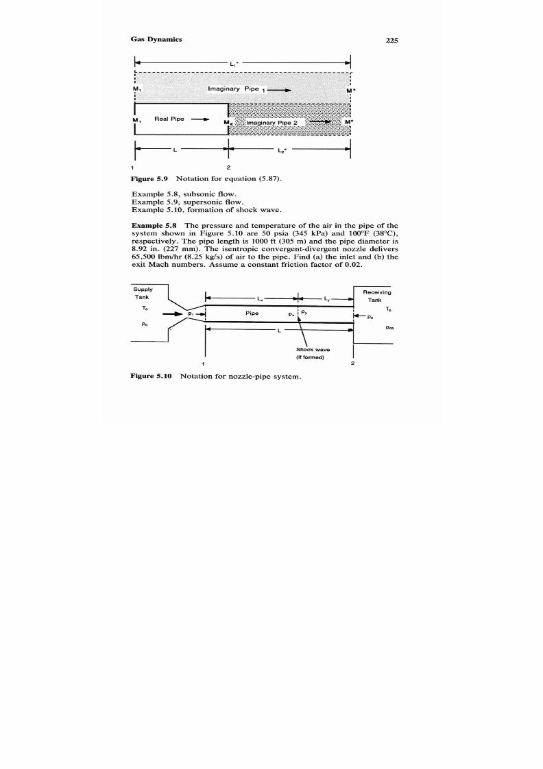
7/21/2019 Fundamental Fluid Mechanics for Engineers
http://slidepdf.com/reader/full/fundamental-fluid-mechanics-for-engineers 248/438
Gas
Dynamics
225
,'
L * . - ~
I
I
I
I
1
2
Figure 5.9
Notation for equation (5.87).
Example 5.8, subsonic flow.
Example 5.9,supersonic flow.
Example
5.10,
formation of shock wave.
Example 5.8 The pressure and temperature of the air in the pipe of the
system shown in Figure 5.10 are
50
psia (345 kPa) and 100°F (38 C),
respectively. The pipe length is
1000
ft 305
m)
and the pipe diameter is
8.92
in.
(227
mm). The isentropic convergent-divergent nozzle delivers
65,500
lbm/hr (8.25
kg/s)
of air to the pipe. Find (a) the inlet and (b) the
exit Mach numbers. Assume a constant friction factor of
0.02.
Supply
Tank
Receiving
Tank
To
-
C+
Pipe p. PY
To
l
IC
P2
Po
PCQ
Shock wave
(If
formed) I
1
2
Figure
5.10 Notation for nozzle-pipe system.
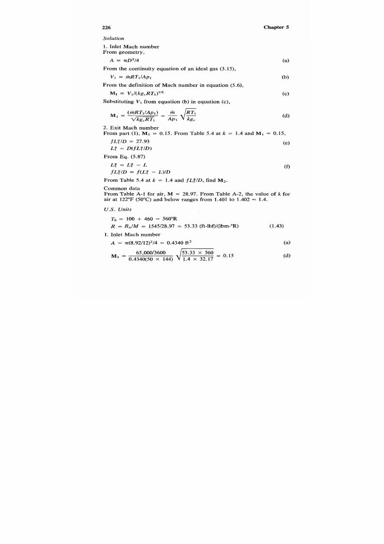
7/21/2019 Fundamental Fluid Mechanics for Engineers
http://slidepdf.com/reader/full/fundamental-fluid-mechanics-for-engineers 249/438
226
Chapter
5
Solution
1.
Inlet Mach number
From geometry,
A
= nD214
From the continuity equation of an ideal gas (3 .13 ,
V1 =
rizRTlIAp1
From the definition of Mach number in equation (5.6),
M1
=
VII (kgcRTl ) ln
Substituting
V I
rom equation (b) in equation (c),
2. Exit Mach number
From part ( l) , M I = 0.15. From Table 5.4 at k = 1.4 and
M I
= 0.15,
f L T l D
=
27.93
LT =
D ( f L T / D )
(e)
From Eq. (5.87)
LP
=
LT - L
f L P / D
= f(LT -
L ) lD
From Table 5.4 at k
=
1.4 and f L P / D , find
M*.
Common data
From Table
A - l
for air, M
=
28.97.
From Table
A-2,
the value of
k
for
air at 122°F (50°C) and below ranges from 1.401 to 1.402
=
1.4.
US.
nits
To
= 100 +
460 =
560"R
R
=
R,/M
=
1545128.97
=
53.33 (ft-lbf)l(lbm-"R)
1.
Inlet Mach number
A =
1r(8.92/12)~14
=
0.4340 ft2
M -
65,000136003.33
x
560
- 0.4340(50
x 144)
1.4 x 32.17
=
0.15
(1.43)
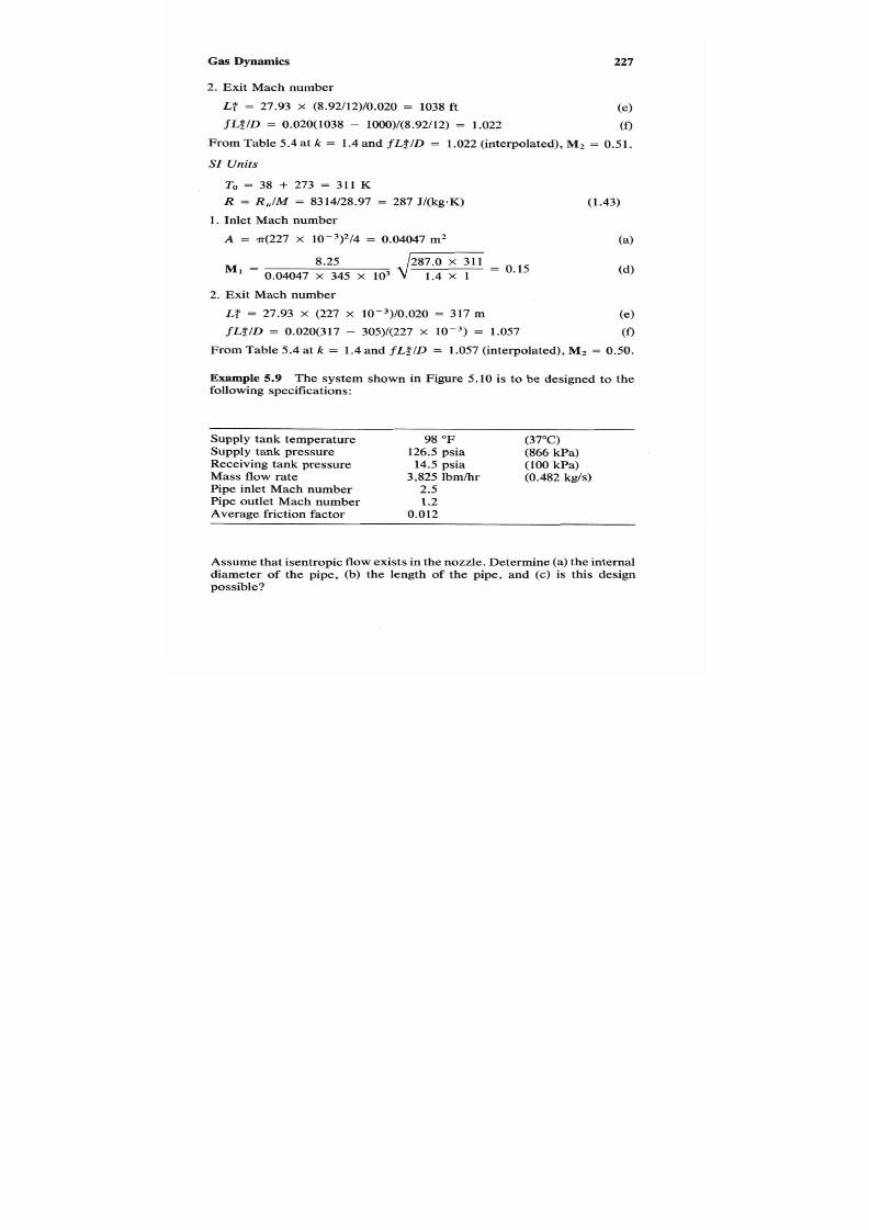
7/21/2019 Fundamental Fluid Mechanics for Engineers
http://slidepdf.com/reader/full/fundamental-fluid-mechanics-for-engineers 250/438
Gas Dynamics 227
2. Exit Mach number
LT
=
27.93
X
(8.92/12)/0.020
=
1038 ft
(e)
f L t / D = 0.020(1038
-
1000)/(8.92/12) = 1.022 0
From Table 5.4 at
k
= 1.4 andf L t / D = 1.022 (interpolated),
M2
= 0.51.
SI Units
To
= 38
+
273
=
311 K
R = R J M =
8314/28.97 = 287 J/(kg.K)
1.
Inlet Mach number
A
= ~ ( 2 2 7 10-3)2/4 = 0.04047 m2
(1.43)
( 4
M1 =
8.2587.0 x 311
0.04047
x
345
x
IO3 1.4 x
1
= 0.15
2. Exit Mach number
LT = 27.93 x (227 x 10-3)/0.020 = 317 (e)
f L q / D = 0.020(317
-
305)/(227 x IOT3 ) = 1.057 (0
From Table 5.4 at k
=
1.4 and
f L P / D =
1.057 (interpolated), M: = 0.50.
Example
5.9
The system shown in Figure 5.10 is to be designed to the
following specifications:
Supply tank temperature
98 "F (37°C)
Supply tank pressure
126.5 psia (866Pa)
Receiving tank pressure
14.5 psia (100 kPa)
Mass flow rate
3,825bm/hr0.482g/s)
Pipe inlet Mach number
2.5
Pipe outlet Mach number
1.2
Average friction factor
0.012
Assume that isentropic flow exists inhe nozzle. Determine (a)he internal
diameter
of
the pipe, (b) the length of the pipe, and (c) is this design
possible?
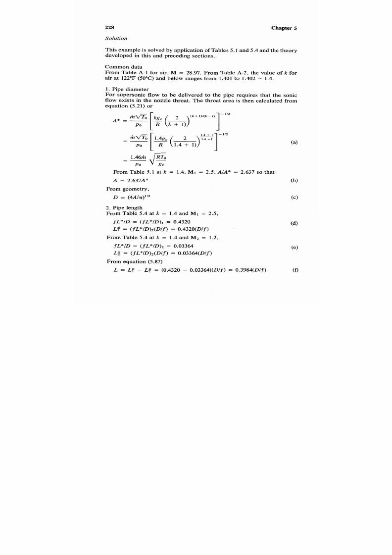
7/21/2019 Fundamental Fluid Mechanics for Engineers
http://slidepdf.com/reader/full/fundamental-fluid-mechanics-for-engineers 251/438
228 Chapter 5
Solution
This example s solved by application of Tables
5 .1
and
5.4
and the theory
developed in this and preceding sections.
Common data
From Table
A-l
for air, M =
28.97.
From Table
A-2,
the value of k for
air at 122°F (5OOC) and below ranges from 1.401 to 1.402 = 1.4.
1.
Pipe diameter
For supersonic flow to be delivered to the pipe requires that the sonic
flow exists in the nozzle throat. The throat area is then calculated from
equation (5.21) or
Po
1.4
+
1)
Po
From Table 5.1 at
k
= 1.4, M1 = 2.5, A/A* = 2.637 so that
A
=
2.637A*
From geometry,
D
=
(4Ah)ln
2.
Pipe length
From Table 5.4 at k = 1.4 and
M 1
= 2.5,
fL*/D = (fL*/D)l = 0.4320
LT
=
(fL*/D)z(D/f)
=
0.4320(D/f)
From Table 5.4 at
k
= 1.4 and
M2
= 1.2,
fL*/D = (fL*/D)2 = 0.03364
L2 = (fL*/D)z(D/f) = O.O3364(D/f)
From equation
(5.87)
L
=
LT
-
L2
=
(0.4320
-
O.O3364)(D/f)
=
0.3984(D/f) 0

7/21/2019 Fundamental Fluid Mechanics for Engineers
http://slidepdf.com/reader/full/fundamental-fluid-mechanics-for-engineers 252/438
Gas
Dynamics
229
3. Is design possible?
This design is possible if the receiving tank stagnation pressure is equal
to or ess than pipe exit stagnation pressure 0rp03
2 pO2.
rom Table 5.4
at
k
= 1.4,
At M1 = 2.5po/pg = pol/p$
=
2.637
At M2 = 1.2po/p$' = p02/p$' + 1.030
p02/po1 = (PO~/P$')/(PO~/P$')1.03012.637 = 0.3906
US.
nits
To = 98
+
460 = 558"R
R
=
R , / M = 154Y28.97 = 53.33it-lbf)/(lbm-"R)1.43)
1. Pipe diameter
A*
=
1.46 x (3825/3600)3.33 x 558
126.5 J 32.17
= 0.373 in 2
A =
2.637
X
0.373 = 0.9836 in.2
D =
(4
X
0.9836/1~)'~ 1.19 in.
2. Pipe length
L = 0.3984(1/0.012) = 33.2 in.
3.
Is
process possible?
Stagnation pressure at pipe exit:
p02
= 126.5
X
0.3906 = 49.4psia
Receiving tank pressure is p03 = 14.5:
P0302 ok
SI Units
To = 37 + 273 = 310 K
R = R J M = 8314/28.97 = 287 J/(kg-K)
1. Pipe diameter
(1.43)
A* =
1.46
x
0.482 $87
x
310
= 2.424
x
m 2
866
X
lo3 1
A = 2.637 x 2.424
x
= 6.392 x m*
(b)
.
D
= (4
x
6.392
x
10-4/7r)1n = 0.02858 m = 25.45mm
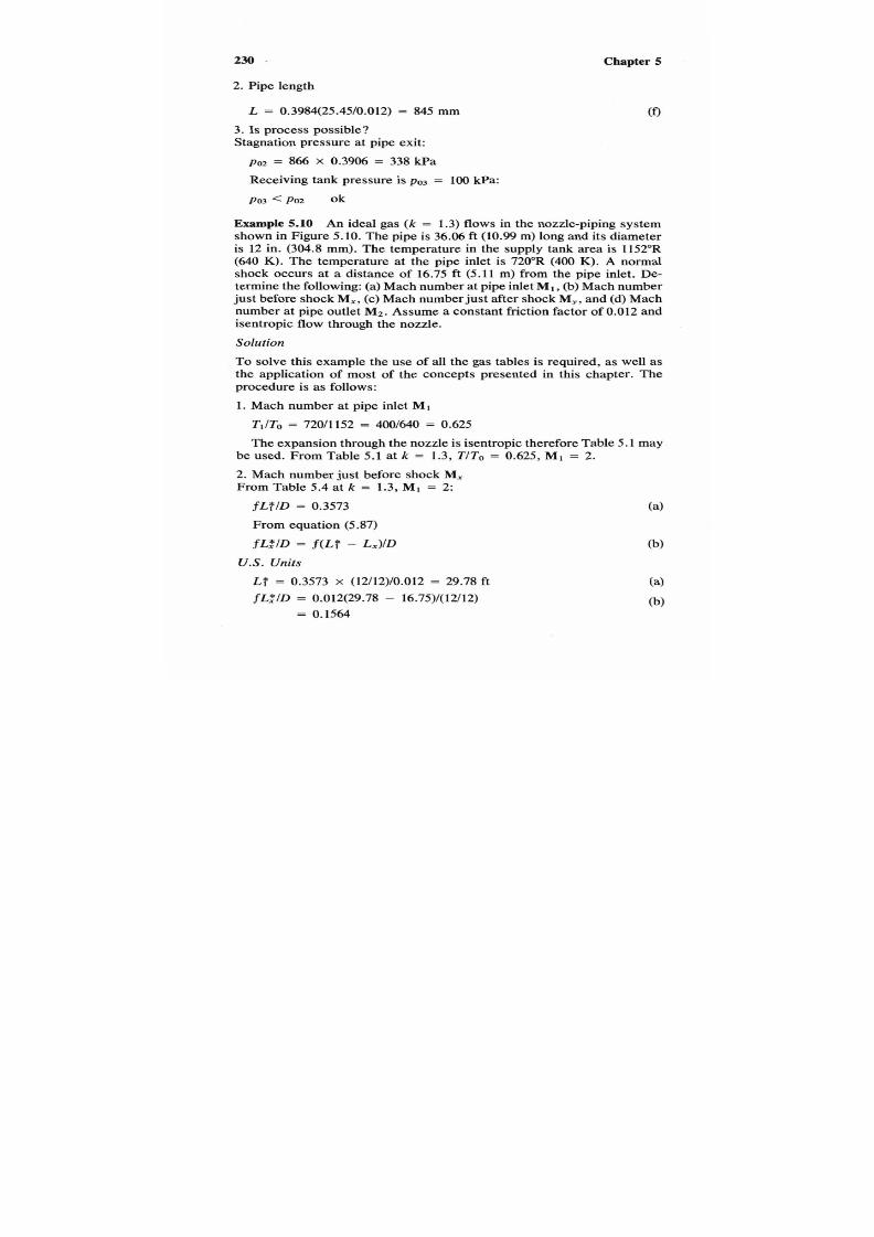
7/21/2019 Fundamental Fluid Mechanics for Engineers
http://slidepdf.com/reader/full/fundamental-fluid-mechanics-for-engineers 253/438
230
-
2. Pipe length
L = 0.3984(25.4510.012) = 845mm
3. Is process possible?
Stagnation pressure at pipe exit:
p02 = 866 X 0.3906 = 338 kPa
Receiving tank pressure is p 3
=
100 kPa:
Chapter
5
0
Example
5.10
An ideal gas ( k = 1.3) flows in the nozzle-piping system
shown in Figure 5.10. The pipe is 36.06 ft (10.99 m) long and its diameter
is 12 in. (304.8 mm). The temperature in the supply tank area is 1152"R
(640
K).The temperature at the pipe inlet is 720"R (400
K).
A normal
shock occurs at a distance of 16.75 ft (5.11 m) from the pipe inlet. De-
termine the following: (a) Mach number t pipe inletM , , (b) Mach number
just before shockM,, (c) Mach number ust after shock M,, and (d) Mach
number at pipe outlet
M2.
Assume a constant friction factor of 0.012 and
isentropic flow through the nozzle.
Solution
To solve this example he use of
all
he gas tables is required,
as
well as
the application of most of the concepts presented in this chapter. The
procedure is as follows:
1. Mach number at pipe inletM
T,/To = 72011152
=
4001640 = 0.625
The expansion throughhe nozzle is isentropic therefore Table
5.1
may
be used. From Table 5.1 at k = 1.3, TITo = 0.625, M , = 2.
2. Mach number just before shock M,
From Table 5.4 at k = 1.3,
M ,
= 2:
fLTlD = 0.3573
From equation (5.87)
fL,*lD = f(LT
-
L,)ID
US. nits
LT = 0.3573
X
(12/12)10.012 = 29.78 ft
fL,*ID = 0.012(29.78 - 16.75)1(12112)
= 0.1564

7/21/2019 Fundamental Fluid Mechanics for Engineers
http://slidepdf.com/reader/full/fundamental-fluid-mechanics-for-engineers 254/438
Gas Dynamics
231
SIUnits
LT
=
0.3573
x
(304.8
x
10-3)/0.012
=
9.075
m
f L , * / D= 0.012(9.075 - 5.105)/(304.8 X
=
0.1563
From Table
5.4
at k =
1.3
and
f L , * / D
=
0.1564,
M , =
1.5
3. Mach number ust after shock
M,,
From Table 5.3 at k = 1.3 and
M,
= 1.5,
M , = 0.6942
4. Mach number at pipe outlet M 2
From Table
5.4
at
k
=
1.3
and M , =
0.6942
(interpolated),
f L , * / D=
0.2479
(c)
From equation
(5.87),
f L T / D = f ( L 9
-
L, ) /D
US.Units
LT
=
0.2479
X
(12/12)/0.012 = 20.66 ft (c)
The length L , = L - L , =
36.06 - 16.75
=
19.31
ft.
f L q / D = 0.012(20.66
-
19.31)/(12/12)
(dl
= 0.0162
From Table 5.4 at k
= 1.3
and f L T / D = 0.0162, M 2 0.9.
SIUnits
LT = 0.2479 X (304.8 X 10-3)/0.012 = 6.30 m
The length L2 = L
-
L , =
10.99
-
5.11
=
5.88
m.
f L q / D = 0.012(6.30 - 5.88)/(304.8 x
= 0.0165
From Table 5.4 at
k
= 1.3 and f L T / D
=
0.0165,
M 2 =
0.9.
As
is demonstrated in this section, the limiting Mach number for iso-
thermal flow is l / f i . For Mach numbers less than this value the pipe

7/21/2019 Fundamental Fluid Mechanics for Engineers
http://slidepdf.com/reader/full/fundamental-fluid-mechanics-for-engineers 255/438
232
Chapter
5
must be heated, and for Mach numbers greater than
I / G
he pipe must
be cooled. Flow in gas transmission piplines is essentially isothermal.
These lines are uninsulated and their flowing temperature is very close
to ambient temperature. Flow in these lines are at low Mach numbers
significantly less than
l/G.
Figure
5.11
shows relations for isothermal
flow.
General Conslderations
Isothermal compressible flow
of
an ideal gas with friction in
a
constant
area duct must satisfy the following requirements:
1.
The ideal
gas
law. The equation of state for an ideal gas
(1.42)
is
p v = RT
2 .
The process relationship.
For an ideal gas undergoing an isothermal
process, from equation
1.39)
and the numerical value of the process
exponent n = 1,
PV =
PV'
= plvl =
~ 2 ~ 2
RT
(5 .88)
3.
Constant-area duct.
The flow area must be the same at
all
sections,
that is, A = A1 = A2 = = A,,.
T
A
1
Heating an d acceleration
deaccelerat ion
T
--
'T
S
Figure
5.11
Notation for isothermal flow.
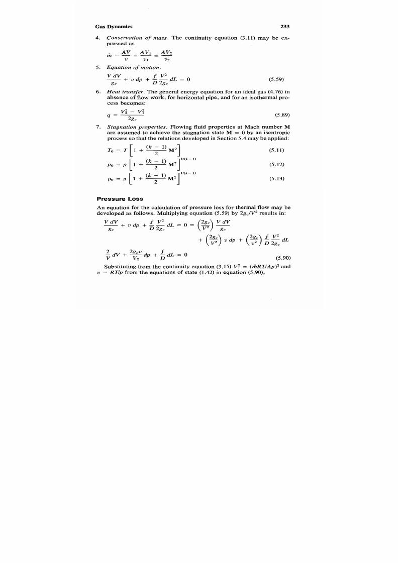
7/21/2019 Fundamental Fluid Mechanics for Engineers
http://slidepdf.com/reader/full/fundamental-fluid-mechanics-for-engineers 256/438
Gas Dynamics 233
4.
5.
6.
7.
Conservation of mass . The continuity equation (3.11) may be ex-
pressed as
Equation
of
motion.
(5.59)
Heat transfer. The general energy equation or an ideal gas
(4.76)
in
absence of flow work, or horizontal pipe, and or an isothermal pro-
cess becqmes:
(5.89)
Stagnation properties. Flowing fluid properties at Mach number
M
are assumed to achieve the stagnation state
M
= 0 by an isentropic
process
so
that the relations developed n Section
5.4
may be applied:
(5.11)
(5.12)
(5.13)
Pressure Loss
An equation for the calculation of pressure loss for thermal flowmay be
developed as follows. Multiplying equation (5.59) by 2gc/Vz results in:
V dV f v2
- + v d p + - - d L = O =
D 2gc
c
v d p
+
2
- d V + - - p + - d L = O
gcv f
V v2
D
(5.90)
Substituting from the continuity equation (3.15)V
=
(r;lRT/Ap)' and
v = RT/p from the equations of state (1.42) in equation (5.90),

7/21/2019 Fundamental Fluid Mechanics for Engineers
http://slidepdf.com/reader/full/fundamental-fluid-mechanics-for-engineers 257/438
234
Chapter
5
Integrating equation (5.91),
Noting again from he continuity equation
3.15)
for isothermal flow with
VZ/VI = (mRT/Ap2) / (mRT/Ap, )= p1/p2 andsubstituting in equation
(5.92) and solving for p ; results in:
2 ( h / A ) 2
P 2
= p?
--
T [2 logek) 1
c
(5.93)
Examination of equation (5.93) indicates that a reiterative solution is nec-
essary to compute
p2.
In most cases the term
2
lo&(p1/p2)
is small com-
pared with f L / D and may be ignored for a first trial solution of p ? .
Limiting
Mach Number
In the derivation of equations for acoustic velocity in section
1.16,
the
velocity of pressure wave was developed as
(1.67)
where the value of E depended on the process. In Section 1.15 it was
.shown in equation (1.61) that for an ideal gas he value of the isothermal
bulk modulus was ET
=
p . Substituting p or
E
and and p = p / R T from
the equation of state (1.44) in equation (1.67) results in
(5.94)
The limiting Mach number M*T is then obtained by dividing equation
(5.94) by the acoustic velocity of an ideal gas = (kgCRT)’”from equation
(1.69)
or
(5.95)

7/21/2019 Fundamental Fluid Mechanics for Engineers
http://slidepdf.com/reader/full/fundamental-fluid-mechanics-for-engineers 258/438
Gas Dynamics
235
Maximum Length
In Section 5.9 the continuity equation
for
an ideal gas
(3.15)
was differ-
entiated for a constant area duct resulting in equation (5.59). Application
of this equation for constant temperature dT =
0
results in:
dpTV iiV
- = " -
= o - -
P T V
V
or
P dV
- - -
P
V
(5.69)
(5.96)
Substituting in the equation of motion (5.90) v = R T / p from the equation
of state (1.42), dplp = - V / V from equation (5.96), noting that d V / V =
d
d M 2 / 2 M 2 ,
and solving for f
dLID
results in
(5.97)
Integrating equation (5.97) between the limits of L =
0
and
L
= L*= and
M
and M*= = l l a ,
LJL*'& =
'I
l v k 1 - kM2
D o k~
M 4
d M 2
(5.98)
f L * =
1
- k M 2
D
kM2
="
-
+
log,(kM2)
Entropy Change
A differential equation or entropy change of an ideal gas was developed
in Section 5.8 as equation (5.53). Writing this equation in dimensionless
form and notingfor an isothermal process
dT =
0 , we have:
(5.99)
From equation (5.%), dVIV = - d p /p =
d ;
substituting in equation
(5.99),
dspV
d M
R
P V M
-
(5.100)

7/21/2019 Fundamental Fluid Mechanics for Engineers
http://slidepdf.com/reader/full/fundamental-fluid-mechanics-for-engineers 259/438
236
Chapter
5
Integrating Eq.
(5.100)
between the limits of 1 and
2,
(5.101)
Substituting
sz
- SI or s * ~nd MI = M and M2 = 1 1 4 n equation
(5.101) results in:
(5.102)
Heat
Transfer
Examination of equation
(5.89)
indicates that the heat transfer needed to
maintain isothermal flow s the change in kinetic energy. Substitution of
V* = kgcRTM2from equation (5.6) in equation (5.89) results in:
(5.103)
Substituting
q**
for
q
and Ml = M and M2 = l / d n equation (5.103),
q*= =
[(h)'
M2] = T (1
-
kM2)
2
(5.104)
Note that if
M is
greater than 1 1 4 he pipe must be cooled to maintain
isothermal flow, and f M is less pipe must be heated.
Example
5.11
Natural gas at 68°F 20°C) and 348 psia (2400 kPa) enters
an 18 in. standard steel pipe with a velocity of 9.84 ftlsec (3
S).
The
pipe
is
a
horizontal straight run
24.85
miles
(40
km)
long. Assume that
natural gas has the same properties as methane (CH& the flow is iso-
thermal and that the average friction factor is 0.0129. Estimate the pres-
sure at the end of the pipe.
Solution
This example is solved by the application of equation (5.93) as follows.
1. Compute the mass flow rate using equation (3.15):
(mlA)
=
VpIRT
(a)
2.
Solve equation
(5.93)
by trial and error:
2 - 2
(mlA)'
Pz-pl" RT [ log, e)
g ]
gc
For first trial, assume 2 log&llpz) is small compared withf L / D .

7/21/2019 Fundamental Fluid Mechanics for Engineers
http://slidepdf.com/reader/full/fundamental-fluid-mechanics-for-engineers 260/438
Gas
Dynamics
237
3. Common data: From Table C-3 for 18 in. standard pipe, D = 1.438
ft (438.1 mm). From Table A-l for CH4,M = 16.043.
US. nits
T =
68 + 460 = 528"R
R = R J M = 1545h6.043 = 96.30ft-lbf)/(lbm-"R)1.43)
1. ( & / A ) = 9.48 x (348 x 144)/(96.30 x 528)
=
9.343 bm/(ft2-sec)
2.
p2:
(348
X
144)'
-
9.3431296*30
-l
32.17
=
v
X 528[ 1og, (348,~:44) 0.0129(24.85 x 5280
1.438 1
= d2.5112 X lo9
-
137,969[2oge(50112/p2) + 11771 (b)
By trial and error,p2 = 48,465 lbf/ft2 = 48,465/144 = 336.6 psia
S I Units
T = 20 + 273 = 293 K
R
=
R , / M
= 8314/16.043 = 518.2 J/(kg.K)
1. ( & / A ) = 3
X
2400 x 103/(518.2
X
293) = 47.42 kg/(m2-s)
2. p2:
(1.43)
438.1 x
=
65.76 X 1OI2
-
3.4142 X 10' [ 10g,
lo3)
+ 11781
By
trial and error,
p2 = 2314 768 = 2 315 kPa
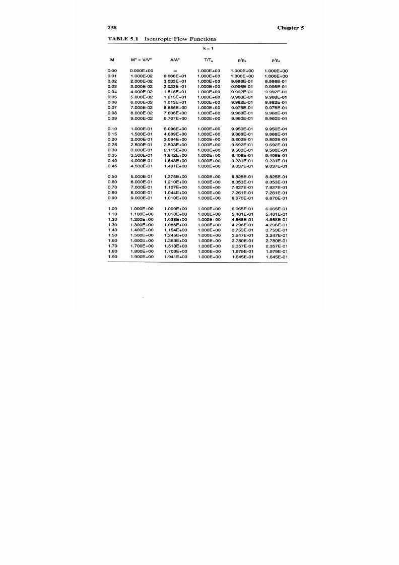
7/21/2019 Fundamental Fluid Mechanics for Engineers
http://slidepdf.com/reader/full/fundamental-fluid-mechanics-for-engineers 261/438
238
TABLE 5.1
Isentropic F l o w Functions
Chapter 5
M
0.00
0.01
0.02
0.03
0.04
0.05
0.06
0.07
0.08
0.09
0.10
0.1 5
0.20
0.25
0.30
0.35
0.40
0.45
0.50
0.60
0.70
0.80
0.90
1
oo
1.10
1.20
1.30
1.40
1.50
1.60
1.70
1.80
1.90
M' =
VN'
0.000E+00
1.000E-02
2.000E-02
3.000E-02
4.000E-02
5.000E-02
6.000E-02
7.000E-02
8.000E-02
9.000E-02
1.000E-01
1.500E-01
2.000E-01
2.500E-01
3.000E-01
3.500E-01
4.000E-01
4.500E-01
5.000E-01
6.000E-01
7.000E-01
8.000E-01
9.000E-01
1.000E+00
1.100E+00
1.200E+00
1.300E+00
1.400E+00
1.500E+00
1.600E+00
1.700E+00
1.800E+00
1.900E+00
AIA
m
6.066E+01
3.033E+01
2.023E+01
1.518E+01
1.215E+01
1.013E+01
8.686E+00
7.606E+00
6.767E+00
6.096E+OO
4.089E+00
3.094E+00
2.503E+00
2.1 15E+00
1.842E+00
1.643E+00
1.491 E+OO
1.375E+00
1.210E+00
1.107E+00
1.044E+00
1.010E+00
1.000E+00
1.010E+00
1.038E+00
1.086E+00
1
.l
4E+00
1.245E+00
1.363E+00
1.513E+00
1.703E+00
1g41 E+OO
PIP0
l
000E+00
1.000E+00
9.998E-01
9.996E-01
9.992E-01
9.988E-01
9.982E-01
9.976E-01
9.968E-01
9.960E-01
9.950E-01
9.888E-01
9.802E-01
9.692E-01
9.560E-01
9.406E-01
9.231 E-01
9.037E-01
8.825E-01
8.353E-01
7.827E-01
7.261 E-01
6.670E-01
6.065E-01
5.461 E-01
4.868E-01
4.296E-01
3.753E-01
3.247E-01
2.780E-01
2.357E-01
1.979E-01
1.645E-01
PIP.
1.000E+00
1.000E+00
9.998E-01
9.996E-01
9.992E-01
9.988E-01
9.982E-01
9.976E-01
9.968E-01
9.960E-01
9.950E-01
9.888E-01
9.802E-01
9.692E-01
9.560E-01
9.406E-01
9.231 E-01
9.037E-01
8.825E-01
8.353E-01
7.827E-01
7.261 E-01
6.670E-01
6.065E-01
5.461 E-01
4.868E-01
4.296E-01
3.753E-01
3.247E-01
2.780E-01
2.357E-01
1.979E-01
1M5E-01

7/21/2019 Fundamental Fluid Mechanics for Engineers
http://slidepdf.com/reader/full/fundamental-fluid-mechanics-for-engineers 262/438

7/21/2019 Fundamental Fluid Mechanics for Engineers
http://slidepdf.com/reader/full/fundamental-fluid-mechanics-for-engineers 263/438
240
Chapter
5
TABLE .1
Isentropic
Flow
Functions
(Continued)
M
0.00
0.01
0.02
0.03
0.04
0.05
0.06
0.07
0.08
0.09
0.1
0
0.1 5
0.20
0.25
0.30
0.35
0.40
0.45
0.50
0.60
0.70
0.80
0.90
1oo
1.10
1.20
1.30
1.40
1.50
1.60
1.70
180
1.90
M' = VN'
0.000E+00
1.025E-02
2.049E-02
3.074E-02
4.099E-02
5.123E-02
6.148E-02
7.172E-02
8.196E-02
9.220E-02
1.024E-01
1.536E-01
2.047E-01
2.558E-01
3.067E-01
3.575E-01
4.082E-01
4.588E-01
5.092E-01
6.094E-01
7.087E-01
8.069E-01
9.041 E-01
1.000E+00
1.095E+00
1.188E+00
1.279E+00
1.369E+00
1.457E+00
1.544E+00
1.628E+00
1.71 1 E+OO
1.792E+00
AIA'
5.991 E+01
2.996E41
1.998E+01
1.499E+01
1.200E+01
l000E+01
8.581 E+OO
7.514E+00
6.685E+00
6.023E+00
4.042E+00
3.059E+00
2.476E+00
2.093E+00
1.825E+00
1.629E+00
1.480E+00
1.365E+00
1.204E+00
1.l4E+00
1.042E+00
1.01 OE+OO
l.OOOE+OO
1.009E+00
1.036E+00
1.080E+00
1.142E+00
1.223E+00
1.326E+00
1.454E+00
1.61 OE+OO
1 .E01 E+OO
k=
.1
TKO
l.OOOE+OO
1.000E+00
1.000E+00
1.000E+00
9.999E-01
9.999E-01
9.998E-01
9.998E-01
9.997E-01
9.996E-01
9.995E-01
9.989E-01
9.980E-01
9.969E-01
9.955E-01
9.939E-01
9.921 E-01
9.900E-01
9.877E-01
9.823E-01
9.761 E-01
9.69OE-01
9.61 1 E-01
9.524E-01
9.430E-01
9.328E-01
9.221 E-01
9.107E-01
8.989E-01
8.865E-01
8.737E-01
8.606E-01
8.471 E-01
PIP,
1.000E+00
9.999E-01
9.998E-01
9.995E-01
9.991 E-01
9.986E-01
9.980E-01
9.973E-01
9.965E-01
9.956E-01
9.945E-01
9.877E-01
9.783E-01
9.663E-01
9.518E-01
9.350E-01
9.161E-01
8.951 E-01
8.723E-01
8.218E-01
7.662E-01
7.072E-01
6.462E-01
5.847E-01
5.241 E-01
4.654E-01
4.097E-01
3.576E-01
3.095E-01
2.658E-01
2.266E-01
1.91 7E-01
1.61 2E-01
pip0
1.000E+00
1.000E+00
9.998E-01
9.996E-01
9.992E-01
9.988E-01
9.982E-01
9.976E-01
9.968E-01
9.960E-01
9.950E-01
9.888E-01
9.802E-01
9.693E-01
9.561 E-01
9.408E-01
9.234E-01
9.042E-01
8.832E-01
8.366E-01
7.850E-01
7.298E-01
6.723E-01
6.139E-01
5.558E-01
4.989E-01
4.443E-01
3.926E-01
3.443E-01
2.999E-01
2.593E-01
2.228E-01
1.903E-01

7/21/2019 Fundamental Fluid Mechanics for Engineers
http://slidepdf.com/reader/full/fundamental-fluid-mechanics-for-engineers 264/438
Gas Dynamics
TABLE 5.1
Isentropic
Row
Functions
(Continued)
241
M
2.00
2.10
2.20
2.30
2.40
2.50
2.60
2.70
2.80
2.90
3.00
3.10
3.20
3.30
3.40
3.50
3.60
3.70
3.80
3.90
4.00
4.50
5.00
5.50
6.00
6.50
7.00
7.50
8.00
9.00
10
20
30
M' = VN'
1.871 E+OO
1.948E+00
2.023E+00
2.096E+00
2.1 67E+00
2.236E+00
2.303E+00
2.368E+00
2.432E+00
2.493E+00
2.553E+00
2.61 1 E+OO
2.667E+00
2.721 E+OO
2.773E+00
2.824E+00
2.874E+00
2.921 E+OO
2.967E+00
3.012E+00
3.055E+00
3.250E+00
3.416E+00
3.556E+00
3.674E+00
3.775E+00
3.862E+00
3.936E+00
4.000E+00
4.1 04E+00
4.1 83E+00
4.472E+00
4.532E+00
NA'
2.032E+00
2.312E+00
2.651 E 4 0
3.061 E+OO
3.560E+00
4.1 65E+00
4.901 E+OO
5.799E+00
6.896E+00
8.237E+00
9.880E+00
1.190E+01
1.438E+01
1.743E+01
2.1 19E+01
2.583E+01
3.157E+01
3.866E+01
4.743E+01
5.829E+01
7.175E+01
2.058E+02
5.977E+02
1.731 E+03
4.949E+03
1.388E+04
3.798E+04
1.01 2E+05
2.621 E+05
1.614E+06
8.874E+06
2.290E+12
5.746E+15
k.:
1.1
Tnb
8.333E-01
8.193E-01
8.052E-01
7.908E-01
7.764E-01
7.619E-01
7.474E-01
7.329E-01
7.184E-01
7.040E-01
6.897E-01
6.754E-01
6.614E-01
6.475E-01
6.337E-01
6.202E-01
6.068E-01
5.936E-01
5.807E-01
5.680E-01
5.556E-01
4.969E-01
4.444E-01
3.980E-01
3.571 E-01
3.213E-01
2.899E-01
2.623E-01
2.381 E-01
1.980E-01
1.667E-01
4.762E-02
2.1 74E-02
P/P,
1.346E-01
1
.l
7E-01
9.21 9E-02
7.566E-02
6.179E-02
5.022E-02
4.064E-02
3.276E-02
2.630E-02
2.1 04E-02
1.679E-02
1.335E-02
1.059E-02
8.382E-03
6.619E-03
5.21 8E-03
4.106E-03
3.227E-03
2.533E-03
1.986E-03
1.556E-03
4.559E-04
l
337E-04
3.970E-05
1.206E-05
3.765E-06
1.21 3E-06
4.043E-07
1.394E-07
1.836E-08
2.756E-09
2.855E-15
5.125E-19
PIP,
1.61 5E-01
1.363E-01
1.145E-01
9.568E-02
7.959E-02
6.592E-02
5.438E-02
4.470E-02
3.661 E-02
2.989E-02
2.434E-02
1.977E-02
1.601 E-02
1.295E-02
1.045E-02
8.41 4E-03
6.767E-03
5.436E-03
4.362E-03
3.497E-03
2.801 E-03
9.176E-04
3.007E-04
9.976E-05
3.376E-05
1.172E-05
4.186E-06
1.541 E-06
5.855E-07
9.270E-08
1.654E-08
5.995E-14
2.357E-17

7/21/2019 Fundamental Fluid Mechanics for Engineers
http://slidepdf.com/reader/full/fundamental-fluid-mechanics-for-engineers 265/438
242 Chapter
S
TABLE 5.1 Isentropic How Functions
(Continued)
M
0.00
0.01
0.02
0.03
0.04
0.05
0.06
0.07
0.08
0.09
0.10
0.1
5
0.20
0.25
0.30
0.35
0.40
0.45
0.50
0.60
0.70
0.80
0.90
1oo
1.10
1.20
1.30
1.40
1.50
1.60
1.70
1B O
1.90
M' = VN'
0.000E+00
1.049E-02
2.098E-02
3.146E-02
4.195E-02
5.243E-02
6.292E-02
7.340E-02
8.388E-02
9.435E-02
1.048E-01
1.571 E-01
2.093E-01
2.614E-01
3.132E-01
3.649E-01
4.162E-01
4.673E-01
5.180E-01
6.183E-01
7.168E-01
8.134E-01
9.079E-01
1.000E+00
1.090E+00
1.177E+00
1.261 E+OO
1.343E+00
1.421 E+OO
1.497E+00
1.570E+00
1.641 E+OO
1.708E+00
NA'
Do
5.921 E+01
2.961 E+01
1.974E+01
1.481 E+01
1
.l
6E+01
9.887E+00
8.480E+00
7.426E+00
6.607E+00
5.953E+00
3.996E+00
3.026E+00
2.451 E+OO
2.073E+00
1.809E+00
1.61 5E+00
1.469E+00
1.356E+00
1
.l
9E+00
1
.l
0E+00
1.041 E+OO
1.010E+00
1.000E+00
1.009E+00
1.034E+00
1.075E+00
1.132E+00
1.205E+00
1.296E+00
1.407E+00
1.540E+00
1.697E+00
ke1.2
T r r ,
1.000E+00
1.000E+00
1.000E+00
9.999E-01
9.998E-01
9.998E-01
9.996E-01
9.995E-01
9.994E-01
9.992E-01
9.990E-01
9.978E-01
9.960E-01
9.938E-01
9.91 1 E-01
9.879E-01
9.843E-01
9.802E-01
9.756E-01
9.653E-01
9.533E-01
9.398E-01
9.251 E-01
9.091 E-01
8.921 E-01
8.741 E-01
8.554E-01
8.361 E-01
8.163E-01
7.962E-01
7.758E-01
7.553E-01
7.348E-01
PIP,
1.000E+00
9.999E-01
9.998E-01
9.995E-01
9.990E-01
9.985E-01
9.978E-01
9.971 E-01
9.962E-01
9.952E-01
9.940E-01
9.866E-01
9.763E-01
9.633E-01
9.477E-01
9.296E-01
9.092E-01
8.867E-01
8.623E-01
8.088E-01
7.505E-01
6.892E-01
6.267E-01
5.645E-01
5.039E-01
4.461 E-01
3.918E-01
3.41 7E-01
2.959E-01
2.547E-01
2.180E-01
1.856E-01
1.573E-01
P~P,
1.000E+00
1.000E+00
9.998E-01
9.996E-01
9.992E-01
9.988E-01
9.982E-01
9.976E-01
9.968E-01
9.960E-01
9.950E-01
9.888E-01
9.802E-01
9.693E-01
9.562E-01
9.409E-01
9.237E-01
9.046E-01
8.839E-01
8.379E-01
7.873E-01
7.333E-01
6.774E-01
6.209E-01
5.649E-01
5.104E-01
4.581 E-01
4.086E-01
3.625E-01
3.199E-01
2.81 OE-01
2.458E-01
2.141E-01

7/21/2019 Fundamental Fluid Mechanics for Engineers
http://slidepdf.com/reader/full/fundamental-fluid-mechanics-for-engineers 266/438
Gas Dynamics
TABLE 5.1 Isentropic How Functions (Continued)
243
M
2.00
2.1
0
2.20
2.30
2.40
2.50
2.60
2.70
2.80
2.90
3.00
3.10
3.20
3.30
3.40
3.50
3.60
3.70
3.80
3.90
4.00
4.50
5.00
5.50
6.00
6.50
7.00
7.50
8.00
9.00
10
20
30
M' =
VN'
1.773E+00
1.835E+00
1.894E+00
1 .g51+OO
2.005E+00
2.057E+00
2.106E+00
2.1 54E+00
2.199E+00
2.242E+00
2.283E+00
2.322E+00
2.359E+00
2.395E+00
2.429E+00
2.461 E+OO
2.492E+00
2.521 E+OO
2.549E+00
2.576E+00
2.602E+00
2.714E+00
2.803E+00
2.875E+00
2.934E+00
2.982E+00
3.023E+00
3.056E+00
3.084E+00
3.1 29E+00
3.162E+00
3.276E+00
3.298E+00
NA'
1.884E+00
2.103E+00
2.359E+00
2.660E+00
3.01
1
E+OO
3.421 E+OO
3.898E+00
4.455E+00
5.103E+00
5.858E+00
6.735E+00
7.755E+00
8.940E+00
1.032E+01
1 l91 E+01
1.376E+01
1.590E+01
1.838E+01
2.1 24E+01
2.454E+01
2.836E+01
5.796E+01
1
.l
3E+02
2.281 E+02
4.359E+02
8.108E+02
1.469E+03
2.593E+03
4.467E+03
1.238E+04
3.1 62E+04
2.196E+07
1.175E+09
k =
1.2
T r r ,
7.143E-01
6.940E-01
6.739E-01
6.54OE-01
6.345E-01
6.154E-01
5.967E-01
5.784E-01
5.605E-01
5.432E-01
5.263E-01
5.099E-01
4.941 E-01
4.787E-01
4.638E-01
4.494E-01
4.355E-01
4.221 E-01
4.092E-01
3.967E-01
3.846E-01
3.306E-01
2.857E-01
2.484E-01
2.174E-01
1.914E-01
1.695E-01
1.509E-01
1.351 E-01
1.099E-01
9.091 E-02
2.439E-02
1.099E-02
PIP0
1.328E-01
1.117E-01
9.363E-02
7.826E-02
6.526E-02
5.431 E-02
4.51 2E-02
3.743E-02
3.102E-02
2.568E-02
2.126E-02
1.758E-02
1.455E-02
1.203E-02
9.957E-03
8.242E-03
6.826E-03
5.657E-03
4.692E-03
3.895E-03
3.237E-03
1.305E-03
5.440E-04
2.352E-04
1.055E-04
4.91 5E-05
2.371 E-05
1.l3E-05
6.090E-06
1.761 E-06
5.645E-07
2.105E-10
1.761 E-l2
PIP0
1.859E-01
1.609E-01
1.389E-01
1.197E-01
1.029E-01
8.825E-02
7.562E-02
6.472E-02
5.534E-02
4.729E-02
4.039E-02
3.448E-02
2.944E-02
2.514E-02
2.147E-02
1.834E-02
1.567E-02
1.340E-02
1.147E-02
9.821 E-03
8.41 7E-03
3.948E-03
1.904E-03
9.466E-04
4.855E-04
2.568E-04
1.399E-04
7.836E-05
4.507E-05
1.602E-05
6.209E-06
8.631 E-09
1.602E-10

7/21/2019 Fundamental Fluid Mechanics for Engineers
http://slidepdf.com/reader/full/fundamental-fluid-mechanics-for-engineers 267/438
244 Chapter 5
TABLE
5.1
Isentropic
Flow
Functions (Continued)
M
0.00
0.01
0.02
0.03
0.04
0.05
0.06
0.07
0.08
0.09
0.10
0.1
5
0.20
0.25
0.30
0.35
0.40
0.45
0.50
0.60
0.70
0.80
0.90
1 oo
1 l0
1.20
1.30
1.40
1.50
1.60
1.70
1.80
1.90
M
=
VN'
0.000E+00
1.072E-02
2.145E-02
3.217E-02
4.289E-02
5.361 E-02
6.433E-02
7.504E-02
8.575E-02
9.646E-02
1.072E-01
1.606E-01
2.138E-01
2.668E-01
3.196E-01
3.719E-01
4.239E-01
4.754E-01
5.264E-01
6.267E-01
7.245E-01
8.195E-01
9.1 14E-01
l
000E+00
1.085E+00
1.l7E+00
1.245E+00
1.320E+00
1.391 E+OO
1.458E+00
1.523E+00
1.583E+00
1.641 E+OO
NA'
e a
5.853E+01
2.927E+01
1.952E+01
1.464E+01
1.172E+01
9.774E+00
8.384E+OO
7.342E+00
6.533E+00
5.886E+00
3.952E+00
2.994E+00
2.426E+00
2.054E+00
1.793E+00
1.602E+00
1.459E+00
1.348E+00
1.193E+00
1.097E+00
1.040E+00
1.009E+00
1.000E+00
1.008E+00
1.032E+00
1.070E+00
1.123E+00
1.189E+00
1.271 E+OO
1.369E+00
1.484E+00
1.61 8E+00
k =
1.3
Trr,
1.000E+00
1.000E+00
9.999E-01
9.999E-01
9.998E-01
9.996E-01
9.995E-01
9.993E-01
9.990E-01
9.988E-01
9.985E-01
9.966E-01
9.940E-01
9.907E-01
9.867E-01
9.820E-01
9.766E-01
9.705E-01
9.639E-01
9.488E-01
9.315E-01
9.124E-01
8.917E-01
8.696E-01
8.464E-01
8.224E-01
7.978E-01
7.728E-01
7.477E-01
7.225E-01
6.976E-01
6.729E-01
6.487E-01
PIP0
1.000E+00
9.999E-01
9.997E-01
9.994E-01
9.99OE-01
9.984E-01
9.977E-01
9.968E-01
9.959E-01
9.948E-01
9.935E-01
9.855E-01
9.744E-01
9.604E-01
9.435E-01
9.241 E-01
9.023E-01
8.784E-01
8.525E-01
7.962E-01
7.354E-01
6.722E-01
6.084E-01
5.457E-01
4.854E-01
4.285E-01
3.757E-01
3.273E-01
2.836E-01
2.446E-01
2.100E-01
1.797E-01
1.533E-01
pip0
1.000E+00
1.000E+00
9.998E-01
9.996E-01
9.992E-01
9.988E-01
9.982E-01
9.976E-01
9.968E-01
9.960E-01
9.950E-01
9.888E-01
9.803E-01
9.694E-01
9.563E-01
9.41 1 E-01
9.240E-01
9.051 E-01
8.845E-01
8.392E-01
7.895E-01
7.367E-01
6.823E-01
6.276E-01
5.735E-01
5.21 1 E-01
4.709E-01
4.235E-01
3.793E-01
3.385E-01
3.01 1 E-01
2.671 E-01
2.363E-01
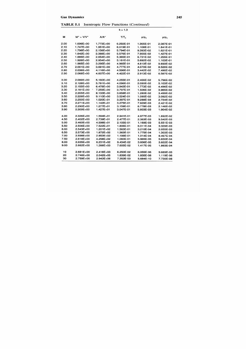
7/21/2019 Fundamental Fluid Mechanics for Engineers
http://slidepdf.com/reader/full/fundamental-fluid-mechanics-for-engineers 268/438
Gas Dynamics
TABLE 5.1 Isentropic
Flow
Functions (Continued)
245
M
2.00
2.1
0
2.20
2.30
2.40
2.50
2.60
2.70
2.80
2.90
3.00
3.10
3.20
3.30
3.40
3.50
3.60
3.70
3.80
3.90
4.00
4.50
5.00
5.50
6.00
6.50
7.00
7.50
8.00
9.00
10
20
30
M' = VN'
1.696E+00
1.747E+00
1.796E+00
1.842E+00
1.885E+00
1.926E+00
1.965E+00
2.001 E+OO
2.036E+00
2.068E+00
2.099E+00
2.128E+00
2.155E+00
A I A
1.773E+00
lg51E+OO
2.1 56E+00
2.388E+00
2.654E+00
2.954E+00
3.295E+00
3.681 E+OO
4.1 16E+00
4.607E+00
5.160E+00
5.781 E+OO
6.478E+00
2.181+OO.259E+00
2.205E+00
2.228E+00
2.250E+00
2.271 E+OO
2.290E+00
2.309E+00
2.326E+00
2.402E+00
2.460E+00
2.506E+00
2.543E+00
2.573E+00
2.598E+00
2.61 8E+00
2.635E+00
2.662E+00
2.681 E+OO
2.746E+00
2.759E+00
8.133E+00
9.1 1OE+OO
1.020E+01
1.142E+01
1.277E+01
1.427E+01
1.594E+01
2.739E+01
4.596E+01
7.522E+01
1.201 E+02
1.872E+02
2.853E+02
4.258E+02
6.231 E+02
1.266E+03
2.416E+03
2.042E+05
2.943E+06
k=
.3
Tlr.
6.250E-01
6.019E-01
5.794E-01
5.576E-01
5.365E-01
5.161E-01
4.965E-01
4.777E-01
4.596E-01
4.422E-01
4.255E-01
4.096E-01
3.943E-01
3.797E-01
3.658E-01
3.524E-01
3.397E-01
3.275E-01
3.1 59E-01
3.047E-01
2.941 E-01
2.477E-01
2.105E-01
1.806E-01
1.563E-01
1.363E-01
1.l8E-01
1.060E-01
9.434E-02
7.605E-02
6.250E-02
1.639E-02
7.353E-03
PJP~
1305E-01
1
.l
8E-01
9.393E-02
7.955E-02
6.731 E-02
5.692E-02
4.813E-02
4.070E-02
3.442E-02
2.913E-02
2.466E-02
2.090E-02
1.773E-02
1.506E-02
1.280E-02
1.090E-02
9.288E-03
7.929E-03
6.778E-03
5.803E-03
4.977~03
2363E-03
1.l9E-03
6.01 1 E-04
3.210E-04
1.775E-04
1.014E-04
5.965E-05
3.606E-05
1.41 7E-05
6.055E-06
1.835E-08
5.684E-10
PIP.
2.087E-01
1.841 E-01
1.621 E-01
1.427E-01
1.255E-01
1.103E-01
9.693E-02
8.520E-02
7.490E-02
6.587E-02
5.796E-02
5.103E-02
4.496E-02
3.965E-02
3.499E-02
3.092E-02
2.734E-02
2.421 E-02
2.146E-02
1.904E-02
1.692E-02
9.542E-03
5.551 E-03
3.329E-03
2.055E-03
1.303E-03
8.467E-04
5.63OE-04
3.822E-04
1.863E-04
9.689E-05
1.119E-06
7.730E-08

7/21/2019 Fundamental Fluid Mechanics for Engineers
http://slidepdf.com/reader/full/fundamental-fluid-mechanics-for-engineers 269/438
246
Chapter
5
TABLE 5.1 Isentropic
Flow
Functions (Continued)
M
0.00
0.01
0.02
0.03
0.04
0.05
0.06
0.07
0.08
0.09
0.10
0.1
5
0.20
0.25
0.30
0.35
0.40
0.45
0.50
0.60
0.70
0.80
0.90
1oo
1.10
1.20
1.30
1.40
1.50
1.60
1.70
1.80
1.90
M' = VN'
0.000E+00
1.095E-02
2.191E-02
3.286E-02
4.381 E-02
5.476E-02
6.570E-02
7.664E-02
8.758E-02
9.851 E-02
1.094E-01
1.639E-01
2.1 82E-01
2.722E-01
3.257E-01
3.788E-01
4.313E-01
4.833E-01
5.345E-01
6.348E-01
7.318E-01
8.251 E-01
9.146E-01
1.000E+00
1.081 E+OO
l
158E+00
1.231 E+OO
1.300E+00
1.365E+00
1.425E+00
1.482E+00
1.536E+00
1.586E+00
NA'
Do
5.787E+01
2.894E+01
1.930E+01
1.448E+01
1.159E+01
9.666E+00
8.292E+00
7.262E+00
6.461 E+OO
5.822E+00
3.910E+00
2.964E+00
2.403E+00
2.035E+00
1.778E+00
1.590E+00
1.449E+00
1.340E+00
1
.l
8E+00
1.094E+00
1.038E+00
1.009E+00
1.000E+00
1.008E+00
1.030E+00
1.066E+00
1
.l
5E+00
1
.l
6E+00
l
250E+00
1.338E+00
1.439E+00
1.555E+00
k=
.4
TKO
l.WOE+OO
1.000E+00
9.999E-01
9.998E-01
9.997E-01
9.995E-01
9.993E-01
9.990E-01
9.987E-01
9.984E-01
9.980E-01
9.955E-01
9.921 E41
9.877E-01
9.823E-01
9.761 E-01
9.690E-01
9.61 1 E-01
9.524E-01
9.328E-01
9.107E-01
8.865E-01
8.606E-01
8.333E-01
8.052E-01
7.764E-01
7.474E-01
7.184E-01
6.897E-01
6.614E-01
6.337E-01
6.068E-01
5.807E-01
PiPo
1.000E+00
9.999E-01
9.997E-01
9.994E-01
9.989E-01
9.983E-01
9.975E-01
9.966E-01
9.955E-01
9.944E-01
9.930E-01
9.844E-01
9.725E-01
9.575E-01
9.395E-01
9.188E-01
8.956E-01
8.703E-01
8.430E-01
7.84OE-01
7.209E-01
6.560E-01
5.913E-01
5.283E-01
4.684E-01
4.124E-01
3.609E-01
3.142E-01
2.724E-01
2.353E-01
2.026E-01
1.740E-01
1.492E-01
PIP,
1.000E+00
l
000E+00
9.998E-01
9.996E-01
9.992E-01
9.988E-01
9.982E-01
9.976E-01
9.968E-01
9.960E-01
9.950E-01
9.888E-01
9.803E-01
9.694E-01
9.564E-01
9.413E-01
9.243E-01
9.055E-01
8.852E-01
8.405E-01
7.916E-01
7.400E-01
6.870E-01
6.339E-01
5.817E-01
5.31 1 E-01
4.829E-01
4.374E-01
3.950E-01
3.557E-01
3.197E-01
2.868E-01
2.570E-01

7/21/2019 Fundamental Fluid Mechanics for Engineers
http://slidepdf.com/reader/full/fundamental-fluid-mechanics-for-engineers 270/438
Gas Dynamics
TABLE 5.1
Isentropic Flow Functions
(Continued)
247
M
2.00
2.10
2.20
2.30
2.40
2.50
2.60
2.70
2.80
2.90
3.00
3.1
0
3.20
3.30
3.40
3.50
3.60
3.70
3.80
3.90
4.00
4.50
5.00
5.50
6.00
6.50
7.00
7.50
8.00
9.00
10
20
30
M' = VN*
1.633E+00
1.677E+00
1.71 8E+00
1.756E+00
1.792E+00
1.826E+00
1.857E+00
1.887E+00
1.91 4E+00
1.940E+00
1.964E+00
1.987E+00
2.008E+00
2.028E+00
2.047E+00
2.064E+OO
2.081 E+OO
2.096E+00
2.1 11E+OO
2.125E+00
2.138E+00
2.1 94E+00
2.236E+00
2.269E+00
2.295E+00
2.31 6E+00
2.333E+00
2.347E+00
2.359E+00
2.377E+00
2.390E+00
2.434E+00
2.443E+00
AIA'
1.688E+00
1.837E+00
2.005E+00
2.193E+OO
2.403E+00
2.637E+OO
2.896E+00
3.1 83E+00
3.500E+00
3.850E+00
4.235E+00
4.657E+00
5.121E+00
5.629E+00
6.1 84E+00
6.790E+00
7.450E+00
8.169E+00
8.951 E+OO
9.799E+00
1.072E+01
1.656E+01
2.500E+01
3.687E+01
5.31 8E+01
7.513E+01
1.041 E+02
1.41 8E+02
1 .g01 E+02
3.272E+02
5.359E+02
1.538E+04
1
.l
4E+05
k =
1.4
Tlr,
5.556E-01
5.313E-01
5.081 E-01
4.859E-01
4.647E-01
4.444E-01
4.252E-01
4.068E-01
3.894E-01
3.729E-01
3.571 E-01
3.422E-01
3.281 E-01
3.147E-01
3.019E-01
2.899E-01
2.784E-01
2.675E-01
2.572E-01
2.474E-01
2.381 E-01
1.980E-01
1.667E-01
1.41 8E-01
l
220E-01
1.058E-01
9.259E-02
8.163E-02
7.246E-02
5.814E-02
4.762E-02
1.235E-02
5.525E-03
PIP0
1.278E-01
1.094E-01
9.352E-02
7.997E-02
6.840E-02
5.853E-02
5.01 2E-02
4.295E-02
3.685E-02
3.165E-02
2.722E-02
2.345E-02
2.023E-02
1.748E-02
1.51 2E-02
1.31 1 E-02
1
.l
8E-02
9.903E-03
8.629E-03
7.532E-03
6.586E-03
3.455E-03
1.890E-03
1.075E-03
6.334E-04
3.855E-04
2.416E-04
1.554E-04
1.024E-04
4.739E-05
2.356E-05
2.091 E-07
l254E-08
PIP0
2.300E-01
2.058E-01
1.841 E-01
1.646E-01
1.472E-01
1.317E-01
1.179E-01
1.056E-01
9.463E-02
8.489E-02
7.623E-02
6.852E-02
6.165E-02
5.554E-02
5.009E-02
4.523E-02
4.089E-02
3.702E-02
3.355E-02
3.044E-02
2.766E-02
1.745E-02
1 .134E-02
7.578E-03
5.1 94E-03
3.643E-03
2.609E-03
1.904E-03
1.414E-03
8.150E-04
4.948E-04
1.694E-05
2.269E-06
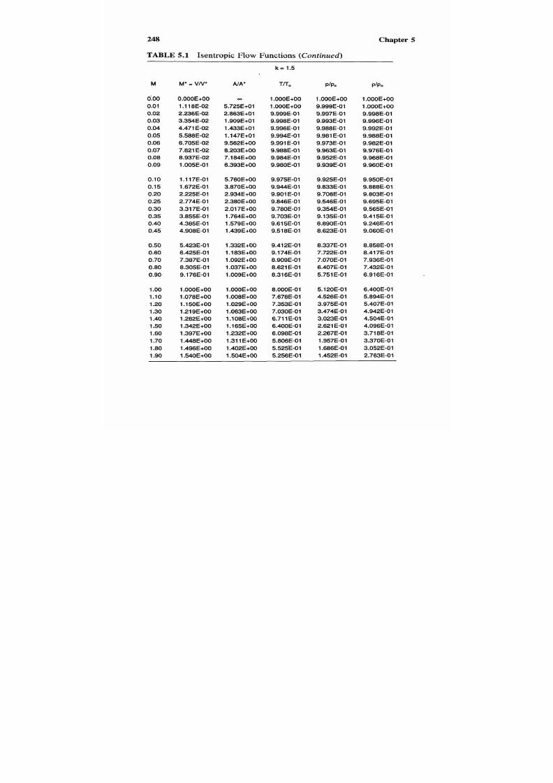
7/21/2019 Fundamental Fluid Mechanics for Engineers
http://slidepdf.com/reader/full/fundamental-fluid-mechanics-for-engineers 271/438
248 Chapter 5
TABLE
5.1
Isentropic
Flow
Functions
(Continued)
M
0.00
0.01
0.02
0.03
0.04
0.05
0.06
0.07
0.08
0.09
0.1
0
0.1 5
0.20
0.25
0.30
0.35
0.40
0.45
0.50
0.60
0.70
0.80
0.90
1oo
1.10
1.20
1.30
1.40
1.50
1.60
1.70
180
1.90
M' = UN'
0.000E+00
1.l
8E-02
2.236E-02
3.354E-02
4.471 E-02
5.588E-02
6.705E-02
7.821 E-02
8.937E-02
1.005E-01
1.117E-01
1.672E-01
2.225E-01
2.774E-01
3.317E-01
3.855E-01
4.385E-01
4.908E-01
5.423E-01
6.425E-01
7.387E-01
8.305E-01
9.1 76E-01
1.000E+00
1.078E+00
1.l
0E+00
1.21 9E+00
1282E+00
1.342E+00
1397E+00
1.448E+00
1.496E+00
1.54OE+00
AIA
m
5.725E+01
2.863E+01
1.909E+01
1.433E+01
1.147E+01
9.562E+00
8.203E+00
7.1 84E+00
6.393E+00
5.760E+00
3.870E+00
2.934E+00
2.380E+00
2.01 7E+00
1.764E+OO
1.579E+00
1.439E+00
1.332E+00
1
.l
3E+00
1.092E+00
1.037E+00
1.009E+00
1.000E+00
1.008E+00
1.029E+00
1.063€+00
1.108E+00
1
.l
5E+00
1.232E+00
1.31 1+OO
1.402E+00
l504E+00
k =
1.5
Tlr,
1.000E+00
1.000E+00
9.999E-01
9.998E-01
9.996E-01
9.994E-01
9.991 E-01
9.988E-01
9.984E-01
9.980E-01
9.975E-01
9.944E-01
9.901 E-01
9.846E-01
9.780E-01
9.703E-01
9.615E-01
9.518E-01
9.412E-01
9.174E-01
8.909E-01
8.621 E41
8.316E-01
8.000E-01
7.678E-01
7.353E-01
7.030E-01
6.71 1 -01
6.400E-01
6.098E-01
5.806E-01
5.525E-01
5.256E-01
PIP.
1.000E+00
9.999E-01
9.997E-01
9.993E-01
9.988E-01
9.981 E-01
9.973E-01
9.963E-01
9.952E-01
9.939E-01
9.925E-01
9.833E-01
9.706E-01
9.546E-01
9.354E-01
9.135E-01
8.890E-01
8.623E-01
8.337E-01
7.722E-01
7.070E-01
6.407E-01
5.751 E-01
5.120E-01
4.526E-01
3.975E-01
3.474E-01
3.023E-01
2.621 E-01
2.267E-01
1.957E-01
1.686E-01
1.452E-01
P/Po
1.000E+00
1.000E+00
9.998E-01
9.996E-01
9.992E-01
9.988E-01
9.982E-01
9.976E-01
9.968E-01
9.960E-01
9.950E-01
9.888E-01
9.803E-01
9.695E-01
9.565E-01
9.415E-01
9.246E-01
9.060E-01
8.858E-01
8.417E-01
7.936E-01
7.432E-01
6.91 6E-01
6.400E-01
5.894E-01
5.407E-01
4.942E-01
4.504E-01
4.096E-01
3.718E-01
3.370E-01
3.052E-01
2.763E-01

7/21/2019 Fundamental Fluid Mechanics for Engineers
http://slidepdf.com/reader/full/fundamental-fluid-mechanics-for-engineers 272/438
Gas
Dynamics
249
TABLE
5.1
Isentropic
Flow
Functions (Continued)
M
2.00
2.10
2.20
2.30
2.40
2.50
2.60
2.70
2.80
2.90
3.00
3.10
3.20
3.30
3.40
3.50
3.60
3.70
3.80
3.90
4.00
4.50
5.00
5.50
6.00
6.50
7.00
7.50
8.00
9.00
10
20
30
M'
= VN'
1.581 E+OO
1 619E+00
1.655E+00
1.687E+00
1.71 8E+00
1.746E+00
l3772E+0O
1.797E+00
1.820E+00
1.841
E+OO
1.861 E+OO
1.879E+00
1.896E+00
1.912E+00
1.927E+00
1 .g41+OO
1.955E+00
1.967E+00
1.979E+00
1.990E+00
2.000E+00
2.043E+OO
2.076E+00
2.1 01 E+OO
2.121 E+OO
2.137E+00
2.150E+00
2.161 E+OO
2.169E+00
2.183E+00
2.193E+00
2.225E+00
2.231 E+OO
A I A
1.61 9E+00
1.747E+00
1.889E+00
2.046E+00
2.21 8E+00
2.407E+00
2.613E+00
2.838E+OO
3.082E+00
3.347E+00
3.633E+00
3.943E+00
4.278E+00
4.638E+00
5.025E+00
5.441 E+OO
5.886E+00
6.363E+00
6.874E+00
7.41 9E+00
8.000E+00
1.151E+01
1.620E+01
2.233E+01
3.017E+01
4.004E+01
5.226E+01
6.721 E+01
8.526E+01
1.324E+02
1.973E+02
2.934E+03
1.465E+04
k=
.5
Tlr,
5.000E-01
4.756E-01
4.525E-01
4.306E-01
4.098E-01
3.902E-01
3.717E-01
3.543E-01
3.378E-01
3.223E-01
3.077E-01
2.939E-01
2.809E-01
2.686E-01
2.571 E-01
2.462E-01
2.358E-01
2.261 E-01
2.169E-01
2.082E-01
2.000E-01
1.649E-01
1.379E-01
1.168E-01
1.000E-01
8.649E-02
7.547E-02
6.639E-02
5.882E-02
4.706E-02
3.846E-02
9.901 E-03
4.425E-03
PIP,
1.250E-01
1.076E-01
9.265E-02
7.982E-02
6.884E-02
5.943E-02
5.137E-02
4.447E-02
3.856E-02
3.349E-02
2.913E-02
2.539E-02
2.21 6E-02
1.939E-02
1.699E-02
1.491 E-02
1.31 2E-02
1 l
56E-02
1.021 E-02
9.028E-03
8.000E-03
4.488E-03
2.624E-03
1.593E-03
1.000E-03
6.469E-04
4.299E-04
2.926E-04
2.035E-04
1.042E-04
5.690E-05
9.706E-07
8.663E-08
PIP.
2.500E-01
2.262E-01
2.047E-01
1.854E-01
1.680E-01
1.523E-01
1.382E-01
1.255E-01
1 l41 E41
1.039E-01
9.467E-02
8.638E-02
7.890E-02
7.21 7E-02
6.608E-02
6.059E-02
5.562E-02
5.1 13E-02
4.705E-02
4.336E-02
4.000E-02
2.721 E-02
1.902E-02
1.364E-02
1.000E-02
7.480E-03
5.696E-03
4.408E-03
3.460E-03
2.21 5E-03
1.479E-03
9.803E-05
1.958E-05
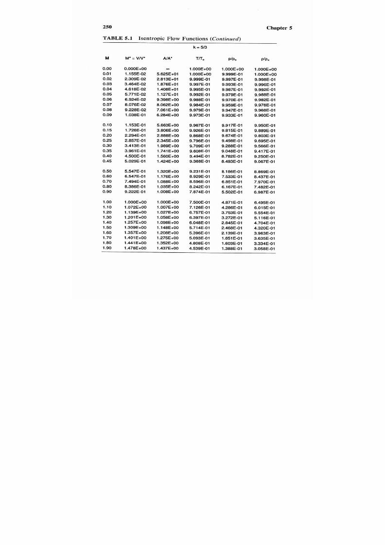
7/21/2019 Fundamental Fluid Mechanics for Engineers
http://slidepdf.com/reader/full/fundamental-fluid-mechanics-for-engineers 273/438
250 Chapter
5
TABLE
5.1 Isentropic Flow Functions (Continued)
M
0.00
0.01
0.02
0.03
0.04
0.05
0.06
0.07
0.08
0.09
0.10
0.15
0.20
0.25
0.30
0.35
0.40
0.45
0.50
0.60
0.70
0.80
0.90
1
oo
1.10
1.20
1.30
1.40
1 so
1.60
1.70
1.80
1.90
M'
= VN'
0.000E+00
1
.l
5E-02
2.309E-02
3.464E-02
4.618E-02
5.771 E-02
6.924E-02
8.076E-02
9.228E-02
1.038E-01
1.153E-01
1.726E-01
2.294E-01
2.857E-01
3.413E-01
3.961 E-01
4.500E-01
5.029E-01
5.547E-01
6.547E-01
7.494E-01
8.386E-01
9.222E-01
1.000E+00
1.072E+00
l
139E+00
1.201 E+OO
1.257E+00
1.309E+00
1.357E+00
1.401 E+OO
1.441 E+OO
1.478E+00
AIA*
0 0
5.625E+01
2.813E+01
1.876E+01
1.408E+01
1.127E+01
9.398E+00
8.062E+00
7.061 E+OO
6.284E+00
5.663E+00
3.806E+00
2.888E+00
2.345E+00
1.989E+00
1.741 E+OO
1.560E+00
1.424E+00
1.320E+00
1.176E+00
1.088E+00
1.035E+00
1.008E+00
1.000E+00
1.007E+00
1.027E+00
1.058E+00
1.098E+00
1.1 48E+00
1.208E+00
1.275E+00
1.352E+00
1.437E+00
k=
/73
TKO
1.000E+00
1.000E+00
9.999E-01
9.997E-01
9.995E-01
9.992E-01
9.988E-01
9.984E-01
9.979E-01
9.973E-01
9.967E-01
9.926E-01
9.868E-01
9.796E-01
9.709E-01
9.608E-01
9.494E-01
9.368E-01
9.231 E-01
8.929E-01
8.596E-01
8.242E-01
7.874E-01
7.500E-01
7.126E-01
6.757E-01
6.397E-01
6.048E-01
5.714E-01
5.396E-01
5.093E-01
4.808E-01
4.539E-01
PIP0
1.000E+00
9.999E-01
9.997E-01
9.993E-01
9.987E-01
9.979E-01
9.970E-01
9.959E-01
9.947E-01
9.933E-01
9.917E-01
9.815E-01
9.674E-01
9.498E-01
9.288E-01
9.048E-01
8.782E-01
8.493E-01
8.186E-01
7.533E-01
6.851 E4 1
6.167E-01
5.502E-01
4.871 E-01
4.286E-01
3.753E-01
3.272E-01
2.845E-01
2.468E-01
2.139E-01
1.851 E-01
1.603E-01
1.388E-01
pip0
1.000E+00
1.000E+00
9.998E-01
9.996E-01
9.992E-01
9.988E-01
9.982E-01
9.976E-01
9.968E-01
9.960E-01
9.950E-01
9.889E-01
9.803E-01
9.695E-01
9.566E-01
9.417E-01
9.250E-01
9.067E-01
8.869E-01
8.437E-01
7.970E-01
7.482E-01
6.987E-01
6.495E-01
6.015E-01
5.554E-01
5.116E-01
4.704E-01
4.320E-01
3.963E-01
3.635E-01
3.334E-01
3.058E-01

7/21/2019 Fundamental Fluid Mechanics for Engineers
http://slidepdf.com/reader/full/fundamental-fluid-mechanics-for-engineers 274/438
Gas Dynamics
TABLE 5.1 Isentropic Flow Functions (Continued)
251
M
2.00
2.10
2.20
2.30
2.40
2.50
2.60
2.70
2.80
2.90
3.00
3.10
3.20
3.30
3.40
3.50
3.60
3.70
3.80
3.90
4.00
4.50
5.00
5.50
6.00
6.50
7.00
7.50
8.00
9.00
10
20
30
M' = VN'
1.512E+00
1.543E+00
1.571 E+OO
1.598E+00
1.622E+00
1.644E+00
1.664E+00
1.683E+00
1.701 E+OO
1.717E+00
1.732E+00
1.746E+00
1.759E+00
1.771 E+OO
1.782E+00
1.793E+00
1.802E+00
1.81 1 +OO
1.820E+00
1.828E+00
1.835E+00
1.867E+00
1.890E+00
1.908E+00
1.922E+00
1.933E+00
1 .g41+OO
1.949E+00
1.955E+00
1.964E+00
1 .g71+OO
1.993E+00
1.997E+00
NA'
1.531 E+OO
1.634E+00
1.746E+00
1.868E+00
1.998E+00
2.139E+00
2.290E+00
2.451 E+OO
2.623E+00
2.806E+00
3.000E+00
3.206E+00
3.424E+00
3.654E+00
3.897E+00
4.1 53E+00
4.422E+00
4.705E+00
5.003E+00
5.314E+00
5.641 E+OO
7.508E+00
9.800E+00
1.256E+01
1.584E+01
1.969E+01
2.414E+01
2.925E+01
3.507E+01
4.900E+01
6.631 E+01
5.075E+02
1.699E+03
k-
5/3
Tr r ,
4.286E-01
4.049E-01
3.827E-01
3.619E-01
3.425E-01
3.243E-01
3.074E-01
2.915E-01
2.768E-01
2.629E-01
2.500E-01
2.379E-01
2.266E-01
2.160E-01
2.060E-01
1.967E-01
1.880E-01
1.797E-01
1.720E-01
1.647E-01
1.579E-01
1.290E-01
1.071 E-01
9.023E-02
7.692E-02
6.630E-02
5.769E-02
5.063E-02
4.478E-02
3.571 E-02
2.913E-02
7.444E-03
3.322E-03
PIP,
1.202E-01
1.043E-01
9.058E-02
7.878E-02
6.863E-02
5.990E-02
5.238E-02
4.589E-02
4.029E-02
3.545E-02
3.125E-02
2.761 E-02
2.444E-02
2.1 68E-02
1.927E-02
1.71 6E-02
1.532E-02
1.370E-02
1.227E-02
1.102E-02
9.906E-03
5.981 E-03
3.758E-03
2.445E-03
1.641 E-03
1.132E-03
7.995E-04
5.769E-04
4.242E-04
2.41 OE-04
1.448E-04
4.781 E-06
6.362E-07
P/P.
2.806E-01
2.576E-01
2.367E-01
2.177E-01
2.004E-01
1.847E-01
1.704E-01
1.574E-01
1.456E-01
1.348E-01
1.250E-01
1.160E-01
1.079E-01
l
004E-01
9.353E-02
8.725E-02
8.150E-02
7.621 E-02
7.134E-02
6.687E-02
6.274E-02
4.635E-02
3.507E-02
2.710E-02
2.133E-02
1.707E-02
1.386E-02
1.139E-02
9.475E-03
6.749E-03
4.971 E-03
6.423E-04
1.915E-04

7/21/2019 Fundamental Fluid Mechanics for Engineers
http://slidepdf.com/reader/full/fundamental-fluid-mechanics-for-engineers 275/438
252 Chapter 5
Table 5.2
Adiabatic
Expansion
Factor
Y
Beta
Heat Ratio
atio
Specific
B
k
1 oo
1.10
1.20
0.00
1.30
1.40
1.50
1.67
1 oo
1.10
1.20
0.1
0
1.30
1.40
1.50
T
1.10
1.20
0.20
1.40
1.30
1.50
1.10
1.40
1.50
1.67
Critical
T
Val
p4Jp1
0.6065
0.5847
0.5645
0.5457
0.5283
0.51 20
0.4871
0.6065
0.5847
0.5645
0.5457
0.5283
0.51 20
0.4872
0.6067
0.5849
0.5647
0.5459
0.5285
0.5122
0.4873
0.6070
0.5851
0.5649
0.5462
0.5288
0.51 25
0.4876
0.6074
0.5856
0.5654
0.5467
0.5293
0.5130
0.4882
IS
Y*
0.6837
0.6895
0.6949
0.7000
0.7050
0.7097
0.7170
0.6837
0.6894
0.6949
0.7000
0.7050
0.7096
0.7170
0.6835
0.6893
0.6947
0.6998
0.7048
0.7095
0.71 68
0.6833
0.6890
0.6944
0.6996
0.7045
0.7092
0.71 65
0.6827
0.6885
0.6939
0.6991
0.7040
0.7087
0.71 61
Ac
PJP,
0.60
0.7021
0.7229
0.7409
0.7568
0.7709
0.791
0
0.7021
0.7228
0.7409
0.7568
0.7709
0.7910
0.701 8
0.7225
0.7406
0.7565
0.7706
0.7907
0.701 3
0.7220
0.7401
0.7560
0.7701
0.7903
0.7004
0.721 2
0.7393
0.7552
0.7693
0.7895
batic
Er
PJP,
0.70
0.7633
0.7821
0.7981
0.81 20
0.8241
0.8347
0.8498
0.7632
0.7820
0.7981
0.81 20
0.8240
0.8347
0.8498
0.7630
0.781 8
0.7978
0.81 17
0.8238
0.8344
0.8496
0.7625
0.7813
0.7974
0.81 13
0.8234
0.8341
0.8492
0.761 7
0.7805
0.7967
0.8106
0.8227
0.8334
0.8486
ansion
F
PJPl
0.80
0.8450
0.8580
0.8689
0.8783
0.8865
0.8936
0.9037
0.8450
0.8580
0.8689
0.8783
0.8865
0.8936
0.9037
0.8448
0.8578
0.8687
0.8781
0.8863
0.8934
0.9035
0.8444
0.8574
0.8684
0.8778
0.8860
0.8932
0.9033
0.8438
0.8568
0.8678
0.8773
0.8855
0.8927
0.9028
%or
Y
i
PJP,
0.90
0.9238
0.9305
0.9361
0.9408
0.9449
0.9485
0.9535
0.9238
0.9305
0.9361
0.9408
0.9449
0.9485
0.9535
0.9237
0.9303
0.9359
0.9407
0.9448
0.9484
0.9534
0.9235
0.9302
0.9358
0.9405
0.9447
0.9482
0.9533
0.9231
0.9298
0.9354
0.9402
0.9444
0.9480
0.9530
PJP,
l
oo
1.om0

7/21/2019 Fundamental Fluid Mechanics for Engineers
http://slidepdf.com/reader/full/fundamental-fluid-mechanics-for-engineers 276/438
Gas
Dynamics 253
Table
5.2
Adiabatic Expansion Factor Y (Continued)
Beta
Ratio
P
0.40
0.50
0.60
0.625
0.70
1.10
1.20
1.30
1.40
1.50
1.67
1
oo
1.10
1.20
1.30
1.40
1.50
0.5877
0.5676
0.5489
0.531 5
0.51 53
0.4905
0.61 37
0.5921
0.5721
0.5536
0.5363
0.5201
I
0.4954
0.6219
1.10
1.20
1.30
1.40
1.50
0.6006
0.5809
0.5625
0.5454
0.5294
:al
es
Y
0.6806
0.6864
0.691 8
0.6970
0.7019
0.7066
0.7140
0.6760
0.681 8
0.6872
0.6924
0.6974
0.7020
0.7094
0.6672
0.6730
0.6785
0.6836
0.6886
0.6933
0.7008
0.6641
0.6699
0.6753
0.6805
0.6854
0.6902
0.6976
l
0.6513
0.6570
0.6625
0.6677
0.6727
0.6774
Adiabatic
D
PdPl
I
PdPl
0.6966
0.7175
0.7357
0.751 7
0.7659
0.7863
0.6884
0.7094
0.7278
0.7441
0.7585
0.7772
0.7935
0.8075
0.81 98
0.8306
0.8460
0.7506
0.7699
0.7865
0.8008
0.8133
0.8244
-
0.7557
0.6939
0.8286 0.7653
0.8121 0.7440
0.8006
.7292
0.7876 0.7126
0.7728
-
0.7505
0.7305
0.6882
0.8244 0.7603
0.8076 0.7387
0.7960 0.7238
0.7828 0.7071
0.7677
-
0.7290
0.7083
0.6651
0.8066
.7393
0.7889
.7170
0.7765 0.701 6
0.7627 0.6844
0.7470
'ansion Factor
Y
PdPl
I
PdPl I PdP1
0.8542
0.8654
0.8750
0.8833
0.8906
0.9283
0.9341
0.9390
0.9432
0.9469
0.8486
0.9444
.8860
0.9405
.8785
0.9362
.8700
0.931 1
.8601
0.9251
0.8374
0.8495
0.8599
0.8690
0.8770
0.8883
0.8189
0.8333
0.8456
0.8562
0.8655
0.8736
0.8851
0.8007
0.8161
0.8292
0.8406
0.8506
0.8593
0.871 9
1 oo
0.91 86
0.9250
0.9305
0.9352
1OOO(
0.9394
0.9452
0.9084
0.91 62
0.9228
0.9284
0.9333
0.9375
0.9435
0.8973
0.9059
0.9131
0.9193
0.9247
0.9294
0.9361

7/21/2019 Fundamental Fluid Mechanics for Engineers
http://slidepdf.com/reader/full/fundamental-fluid-mechanics-for-engineers 277/438
254 Chapter
5
TABLE 5.2 Adiabatic Expansion Factor Y (Continued)
Beta
PdPl
JPl
alues
eat Ratio Ratio
Adiabatic
E x
riticalpecific
P
0.70
.60
4
'lp,
1.00
0.7263
.6502 0.6091
.20
0.7078
.6447 0.6279
.10
0.6865
.6389
.6482
0.75
0.7886
.7185
.6726 0.5359
.67
0.7700
.6955
.6651 0.5596
.50
0.7571 0.6797
.6603
.5750
.40
0.7426
.6622
.6554 0.5915
.30
1.00
0.6971
.6332 0.6258
.20
0.6779
.6277
.6441 1.10
0.6560.6220 0.6638
0.80
0.7627
.6890
.6556
.5544
.67
0.7428
.6653
.6481
.5776
.50
0.7292 0.6491
.6433
.5927
.40
0.7141
.6384 0.6087
.30
1 OO
0.6540
.6090
.6495
.20
0.6341
.6037 0.6670
.10
0.61 17
.5980 0.6857
0.85 0.6717.6142 0.6331.30
1.40
0.7021
.6239 0.6033
.50
0.6877
.6191 0.6177
1.67
0.7234
.6458
.6313 0.5809
1.00
0.5860
.5722 0.6850
.20
-
.5670 0.7012
.10
-
.5614
.7184
0.90
0.6043
.5773
.6699
.30
1.40
-
.5065 0.7463
.20
-
.5015
.7599
.10
-
.4963 0.7743.00
0.6587
.5942 0.621
.67
0.6361
.5868
.6421
.50
0.6209
.5822 0.6556
0.95
-
.51 13 0.7335
.30
1.40
0.5344
.5272 0.6917
.67
-
.5202 0.7097
.50
-
.5158
.7213
ansion Factor
Y
PdPt
0.9081
.8231
0.9022
.81 29
0.8955
.801 3
0.8878
.7882
0.8788
.7732
0.8683.7559
0.9283
.8582
0.921
0
.8447
0.91 58
.8353
0.9098
.8246
0.9030
.81 25
0.8951
.7986
0.8857
.7824
0.90
.80
PdPl
0.7346
0.8632
.7509
0.8528
0.8871 0.7895
0.8801
.7781
0.8722.7653
PdPl
1oo
1
om0

7/21/2019 Fundamental Fluid Mechanics for Engineers
http://slidepdf.com/reader/full/fundamental-fluid-mechanics-for-engineers 278/438
Gas
Dynamics 255
TABLE
5.3 Normal
Shock Functions
1
oo
1.05
1.10
1.15
1.20
l
25
1.30
l35
1.40
1.45
1.50
1.60
1.70
1.80
1.90
2.00
2.1 0
2.20
2.30
2.40
2.50
3.00
3.50
4.00
4.50
5.00
6.00
7.00
8.00
9.00
10.00
20.00
30.00
1 .000E+00
9.524E-01
9.091 E-01
8.696E-01
8.333E-01
8.000E-01
7.692E-01
7.407E-01
7.1 43E-01
6.897E-01
6.667E-01
6.250E-01
5.882E-01
5.556E-01
5.263E-01
5.000E-01
4.762E-01
4.545E-01
4.348E-01
4.1 67E-01
4.000E-01
3.333E-01
2.857E-01
2.500E-01
2.222E-01
2.000E-01
1.667E-01
1.429E-01
1.250E-01
1
.l
1 E-01
1.000E-01
5.000E-02
3.333E-02
lOOOE+OO
1.l3E+OO
1.21 OE+OO
1.323E+00
1.440E+00
l563E+00
1.690E+00
1.823E+00
1.960E+00
2.1 03E+00
2.250E+00
2.560E+00
2.890E+00
3.240E+00
3.61 OE+OO
4.000E+00
4.41 OE+OO
4.840E+00
5.290E+00
5.760E+00
6.250E+00
9.000E+00
1.225E+01
1.600E+01
2.025E+01
2.500E+01
3.6OOE+Ol
4.900E+01
6.400E+01
8.1 00E+01
1 OOOE+02
4.000E+02
9.000E+02~
1.000E+00
1.000E+00
1.000E+00
1.000E+00
1.000E+00
1.000E+00
1.000E+00
l.OOOE+W
1.000E+00
1.000E+00
1.000E+00
1.000E+00
1 OOOE+OO
1.000E+00
1.000E+00
1.000E+00
1.000E+00
1.000E+00
l000E+00
1.000E+00
1.000E+00
1 OOOE+OO
1.000E+00
1.000E+00
1.000E+00
1.000E+00
l.OOOE+OO
1.000E+00
1.000E+00
1.000E+00
1.000E+00
1.000E+00
1.000E+00
1 OOOE+OO
1.103E+00
1.21 OE+OO
l
323E+00
1.440E+00
1.563E+00
l
690E+00
1.823E+00
1.960E+00
2.103E+00
2.250E+O0
2.560E+00
2.890E+00
3.240E+00
3.61 OE+OO
4.000E+00
4.41 OE+OO
4.840E+00
5.290E+00
5.760E+00
6.250E+00
9.000E+00
1.225E+01
1.600E+01
2.025E+01
2.500E+01
3.600E+01
4.900E+01
6.400E+01
8.100E+01
l
000E+02
4.000E+02
9.000E+02
1.000E+00
9.998E-01
9.988E-01
9.964E-01
9.91 9E-01
9.851 E-01
9.759E-01
9.640E-01
9.494E-01
9.321 E-01
9.122E-01
8.653E-01
8.1 00E-01
7.482E-01
6.820E-01
6.1 34E-01
5.446E-01
4.772E-01
4.129E-01
3.527E-01
2.975E-01
2.791 E-02
5.538E-03
1.057E-01
8.31 6E-04
9.505E-05
5.559E-07
1.133E-09
8.169E-13
2.100E-16
1.938E-20
5.543E-85
3.326E-193
1.649E+OO
l735E+OO
1.829E+OO
1.930E+00
2.038E+00
2.152E+00
2.272E+00
2.398E+00
2.530E+00
2.667E+OO
2.81OE+OO
3.1 12E+00
3.436E+00
3.781 E+OO
4.146E+00
4.533E+00
4.939E+00
5.367E+00
5.81 4E+00
6.282E+00
6.771 E+OO
9.514E+OO
1.276E+O1
1.651 E+01
2.076E+O1
2.551 E+O1
3.65OE+Ol
4.95OE+Ol
6.45OE+Ol
8.1 5OE+Ol
l
005E+02
4.005E+02
9.005E+02
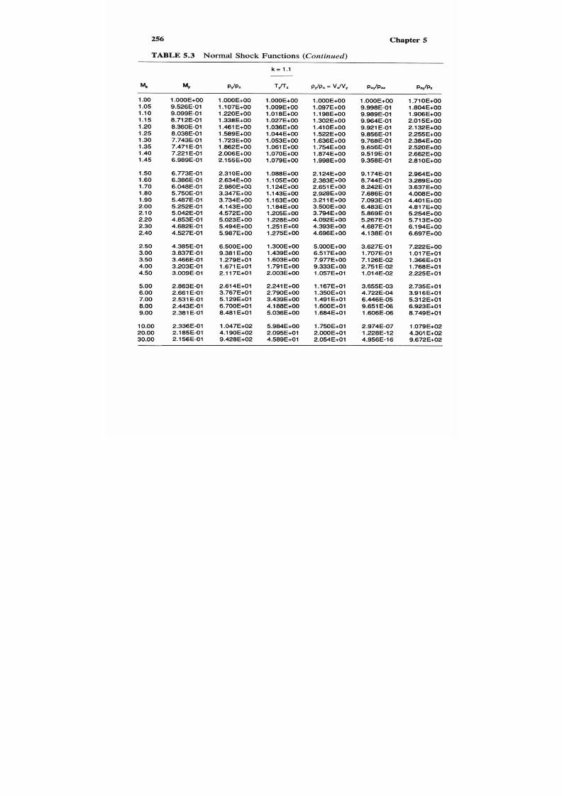
7/21/2019 Fundamental Fluid Mechanics for Engineers
http://slidepdf.com/reader/full/fundamental-fluid-mechanics-for-engineers 279/438
256
Chapter
5
TABLE
5.3 Normal Shock Functions
(Continued)
k = l . l
1oo
1.05
1.10
1.15
1.20
1.25
1.30
1.35
1.40
1.45
1.50
1.60
1.70
1.80
1.90
2.00
2.10
2.20
2.30
2.40
2.50
3.00
3.50
4.00
4.50
5.00
6.00
7.00
8.00
9.00
10.00
20.00
30.00
1OOOE+OO
9.526E-01
9.099E-01
8.712E-01
8.360E-01
8.038E-01
7.743E-01
7.471 E-01
7.221 E-01
6.989E-01
6.773E-01
6.386E-01
6.048E-01
5.750E-01
5.487E-01
5.252E-01
5.042E-01
4.853E-01
4.682E-01
4.527E-01
4.385E-01
3.837E-01
3.466E-01
3.203E-01
3.009E-01
2.863E-01
2.661 E-01
2.531 E-01
2.443E-01
2.381 E-01
2.336E-01
2.1 85E-01
2.156E-01
1.000E+00
1.107E+00
1.220E+00
1.338E+00
1.461 E+OO
1.589E+00
1.723E+00
1.862E+00
2.006E+00
2.1 55E+00
2.31 OE+OO
2.634E+00
2.980E+00
3.347E+00
3.734E+00
4.143E+00
4.572E+00
5.023E+00
5.494E+00
5.987E+00
6.500E+00
9.381 E+OO
1.279E+01
1.671 E+01
2.1 17E+01
2.614E+OI
3.767E+01
5.129E+OI
6.700E+01
8.481 E+01
1.047E+02
4.190E+02
9.428E+02
1.000E+00
1.009E+00
1.018E+00
1.027E+00
1.036E+00
1.044E+00
1.053E+00
1.061 E+OO
1.070E+00
1.079E+00
1.088E+00
l
l
5E+00
1
.l
4E+00
1
l3E+00
1 l3E+00
1
l
4E+00
1.205E+00
1.228E+00
1.251 E+OO
1.275E+00
1.300E+00
1.439E+00
1.603E+00
1.791 E+OO
2.003E+00
2.241 E+OO
2.790E+00
3.439E+00
4.1 88E+00
5.036E+00
5.984E+OO
2.095E+01
4.589E+01
1.000E+00
1.097E+00
1 l
8E+00
1.302E+00
1.41 OE+OO
1.522E+00
1.636E+00
1.754E+00
1.874E+00
l998E+00
2.124E+OO
2.383E+00
2.651 E+OO
2.928E+00
3.21
1
E+OO
3.500E+00
3.794E+00
4.092E+00
4.393E+00
4.696E+00
5.000E+00
6.517E+00
7.977E+00
9.333E+00
1.057E+01
1.167E+01
1.350E+01
1.491 E+01
1.600E+01
1.684E+01
1.750E+01
2.000E+01
2.054E+01
1.000E+00
9.998E-01
9.989E-01
9.964E-01
9.921 E-01
9.856E-01
9.768E-01
9.656E-01
9.51 9E-01
9.358E-01
9.174E-01
8.744E-01
8.242E-01
7.686E-01
7.093E-01
6.483E-01
5.869E-01
5.267E-01
4.687E-01
4.1 38E-01
3.627E-01
1.707E-01
7.1 26E-02
2.751 E-02
1.01 4E-02
3.655E-03
4.722E-04
6.446E-05
9.651 E-06
1.606E-06
2.974E-07
1.228E-12
4.956E-16
1.71OE+OO
1.804E+OO
1.906E+OO
2.015E+OO
2.1 32E+00
2.255E+00
2.384E+00
2.520E+00
2.662E+00
2.810E+00
2.964E+OO
3.289E+OO
3.637E+OO
4.008E+OO
4.401 E+OO
4.81 7E+OO
5.254E+00
5.713E+OO
6.1 94E+00
6.697E+OO
7.222E+OO
1.017E+01
1.366E+01
1.768E+01
2.225E+01
2.735E+01
3.91 6E+01
5.312E+01
6.923E+OI
8.749E+OI
1.079E+02
4.301 E+02
9.672E+02

7/21/2019 Fundamental Fluid Mechanics for Engineers
http://slidepdf.com/reader/full/fundamental-fluid-mechanics-for-engineers 280/438
Gas
Dynamics
257
TABLE
5.3
Normal
Shock Functions
(Continued)
k=
.2
1oo
1.05
1.10
1.15
1.20
1.25
1.30
1.35
1.40
1.45
1.50
1.60
1.70
1.80
1.90
2.00
2.10
2.20
2.30
2.40
2.50
3.00
3.50
4.00
4.50
5.00
6.00
7.00
8.00
9.00
10.00
20.00
30.00
1 OWE+OO
9.528E-01
9.106E-01
8.726E-01
8.383E-01
8.071 E-01
7.787E-01
7.527E-01
7.288E-01
7.067E-01
6.864E-01
6.501 E-01
6.186E-01
5.91 2E-01
5.671 E-01
5.458E-01
5.268E-01
5.099E-01
4.947E-01
4.81 OE-01
4.686E-01
4.21 4E-01
3.904E-01
3.690E-01
3.536E-01
3.421 E-01
3.267E-01
3.1 70E-01
3.106E-01
3.061 E-01
3.029E-01
2.923E-01
2.903E-01
l000E+00
l
l
2E+00
l
229E+00
l
352E+00
1.480E+00
l
614E+00
l
753E+00
1.897E+00
2.047E+00
2.203E+00
2.364E+00
2.702E+00
3.062E+00
3.444E+00
3.847E+00
4.273E+00
4.720E+00
5.189E+00
5.680E+00
6.193E+00
6.727E+00
9.727E+00
1.327E+01
1.736E+01
2.200E+01
2.71 8E+01
3.91 8E+01
5.336E+01
6.973E+01
8.827E+01
1.090E+02
4.363E+02
9.81 7E+02
l.OWE+W
1.01 8E+00
1.035E+00
1.052E+00
1.069E+00
1.086E+00
1
.l
2E+00
.l .l
9E+00
1
.l
6E+00
1
.l
3E+00
1
.l
0E+00
1.205E+00
1.241 E+OO
1.279E+00
1.31 9E+00
1.360E+00
1.402E+00
1.446E+00
1.492E+00
1.540E+00
1.590E+00
1.867E+00
2.192E+00
2.565E+00
2.988E+00
3.460E+W
4.551 E+OO
5.841 E+OO
7.329E+00
9.016E+00
1.090E+01
4.065E+01
9.024E+01
1 OOOE+OO
1.092E+00
l l
7E+00
l
285E+00
1.385E+00
l
486E+00
1.590E+00
1.696E+00
1.803E+00
1.91 1 +OO
2.020E+00
2.242E+00
2.466E+00
2.692E+00
2.918E+00
3.143E+00
3.366E+00
3.588E+00
3.806E+00
4.020E+00
4.231 E+OO
5.21l +OO
6.056E+00
6.769E+00
7.364E+00
7.857E+00
8.609E+00
9.136E+00
9.514E+00
9.791 E+OO
l.OOOE+Ol
1.073E+01
l
088E+01
l.OOOE+W
9.998E-01
9.989E-01
9.965E-01
9.924E-01
9.861 E-01
9.777E-01
9.671 E-01
9.542E-01
9.391 E-01
9.220E-01
8.822E-01
8.362E-01
7.856E-01
7.320E-01
6.767E-01
6.21 3E-01
5.667E-01
5.139E-01
4.636E-01
4.1 62E-01
2.298E-01
1.198E-01
6.096E-02
3.093E-02
1.586E-02
4.408E-03
1.343E-03
4.498E-04
1.644E-04
6.499E-05
9.665E-08
1.81 8E-09
1.772E+OO
l873E+OO
1.982E+OO
2.1OOE+OO
2.224E+OO
2.356E+OO
2.495E+OO
2.641 E+OO
2.793E+00
2.951 E+OO
3.1 16E+OO
3.464E+OO
3.836E+00
4.232E+00
4.652E+00
5.096E+00
5.563E+OO
6.053E+OO
6.567E+00
7.1 04E+OO
7.664E+OO
1.081 E+O1
1.453E+O1
1.883E+O1
2.37OE+Ol
2.91 5E+01
4.176E+O1
5.666E+O1
7.386E+O1
9.335E+01
1
.l
1 E+02
4.591 E+02
1.032E+03

7/21/2019 Fundamental Fluid Mechanics for Engineers
http://slidepdf.com/reader/full/fundamental-fluid-mechanics-for-engineers 281/438
258 Chapter 5
TABLE
5.3 Normal
Shock Functions (Continued)
k=
.3
l
oo
1.05
1.10
1.15
1.20
1.25
1.30
1.35
1.40
1.45
1.50
1.60
1.70
1.80
1.90
2.00
2.1
0
2.20
2.30
2.40
2.50
3.00
3.50
4.00
4.50
5.00
6.00
7.00
8.00
9.00
10.00
20.00
30.00
1 OOOE+OO
9.530E-01
9.1 12E-01
8.739E-01
8.403E-01
8.100E-01
7.825E-01
7.575E-01
7.346E-01
7.136E-01
6.942E-01
6.599E-01
6.304E-01
6.048E-01
5.825E-01
5.629E-01
5.455E-01
5.301 E-01
5.163E-01
5.040E-01
4.929E-01
4.51 1 E-01
4.241 E-01
4.058E-01
3.927E-01
3.832E-01
3.704E-01
3.625501
3.573E-01
3.536E-01
3.51 OE-01
3.426E-01
3.410E-01
1
OOOE+OO
1.l6E+00
1.237E+00
1.365E+00
1.497E+00
1.636E+00
1.78OE+OO
1.930E+00
2.085E+00
2.246E+00
2.413E+00
2.763E+00
3.137E+00
3.532E+OO
3.950E+00
4.391 E+OO
4.855E+00
5.341 E+OO
5.850E+00
6.381 E+OO
6.935E+00
1.004E+01
1.372E+01
1.796E+01
2.276E+01
2.81 3E+01
4.057E+01
5.526E+01
7.222E+01
9.143E+01
1
.l
9E+02
4.520E+02
1.01 7E+03
l.OOOE+OO
1.026E+00
1.051 E+OO
1.075E+00
1
.i
0E+00
1.l4E+00
1.l
8E+OO
1.l2E+00
1.l7E+00
1.222E+00
1.247E+00
1.299E+00
1.353E+OO
1.409E+00
1.467E+00
1.527E+00
1.591 E+OO
1.656E+00
1.725E+00
1.796E+00
1.869€+00
2.280E+00
2.763E+00
3.318E+00
3.946E+00
4.648E+00
6.271 E+OO
8.189€+00
1.040E+01
1.291 E+01
1.571 E+01
5.994E+O1
1.337E+02
1.000E+00
1.088E+00
1.l8E+00
l
269E+00
1.362E+00
1.456E+00
1.55OE+OO
1.646E+00
1.742E+00
1.838E+00
1.935E+00
2.127E+00
2.318E+00
2.507E+00
2.693E+00
2.875E+00
3.052E+00
3.225E+00
3.392E+00
3.554E+00
3.71
O€+OO
4.404E+00
4.965E+00
5.41 2E+00
5.768E+00
6.053E+00
6.469E+00
6.749E+00
6.943E+00
7.084E+00
7.188E+00
7.541 E+OO
7.61 OE+OO
1.000E+00
9.999E-01
9.989E-01
9.966E-01
9.926E-01
9.866E-01
9.786E-01
9.685E-01
9.563E-01
9.421 E-01
9.261 E-01
8.891 E-01
8.466E-01
8.001 E-01
7.51 OE-01
7.006E-01
6.499E-01
6.000E-01
5.515E-01
5.050E-01
4.61 OE-01
2.822E-01
1.677E-01
9.933E-02
5.939E-02
3.61 3E-02
1.422E-02
6.098E-03
2.827E-03
1.404E-03
7.402E-04
8.945E-06
6.232E-07
1.832E+OO
1g41 E+OO
2.058E+00
2.1 83E+OO
2.31 6E+00
2.457E+00
2.605E+OO
2.760E+00
2.922E+00
3.09OE+OO
3.265E+OO
3.635E+OO
4.031 E+OO
4.452E+00
4.899E+00
5.370E+00
5.866E+OO
6.387E+00
6.933€+00
7.503E+00
8.098E+OO
1
.l
4E+01
1.539E+Ol
1.996E+01
2.513E+01
3.092E+01
4.431 E+O1
6.014E+01
7.84OE+Ol
9.910E+01
1.222E+02
4.875E+02
1.096E+03

7/21/2019 Fundamental Fluid Mechanics for Engineers
http://slidepdf.com/reader/full/fundamental-fluid-mechanics-for-engineers 282/438
Gas Dynamics 259
TABLE 5.3 Normal Shock Functions (Continued)
k =
1.4
1 oo
1.05
1.10
1.15
1.20
1.25
1.30
1.35
1.40
1.45
1.50
1.60
1.70
1.80
l90
2.00
2.1
0
2.20
2.30
2.40
2.50
3.00
3.50
4.00
4.50
5.00
6.00
7.00
8.00
9.00
10.00
20.00
30.00
1 OOOE+OO
9.531 E-01
9.1 18E-01
8.750E-01
8.422E-01
8.126E-01
7.860E-01
7.61 8E-01
7.397E-01
7.196E-01
7.01 1 E-01
6.684E-01
6.405E-01
6.1 65E-01
5.956E-01
5.774E-01
5.61 3E-01
5.471 E-01
5.344E-01
5.231 E-01
5.1 30E-01
4.752E-01
4.51 2E-01
4.350E-01
4.236E-01
4.152E-01
4.042E-01
3.974E-01
3.929E-01
3.898E-01
3.876E-01
3.804E-01
3.790E-01
1.000E+00
1.120E+00
1.245E+00
1.376E+00
1.51 3E+00
1.656E+00
1.805E+00
1.960E+00
2.1 20E+00
2.286E+00
2.458E+00
2.820E+00
3.205E+00
3.61 3E+00
4.045E+00
4.500E+00
4.978E+00
5.480E+00
6.005E+00
6.553E+00
7.1 25E+00
1.033E+01
1.41 3E+01
1.850E+01
2.346E+01
2.900E+01
4.1 83E+01
5.700E+01
7.450E+01
9.433E+01
1
.l
5E+02
4.665E+02
1.050E+03
1.000E+00
1.033E+00
1.065E+00
1.097E+00
1
.l
8E+00
1.l9E+00
1
.l
1 E+OO
1.223E+00
1.255E+00
l
287E+00
1.320E+00
1.388E+00
1.458E+00
1.532E+00
1.608E+00
1.688E+00
1.770E+00
1.857E+00
1.947E+00
2.040E+00
2.1 38E+00
2.679E+00
3.315E+00
4.047E+00
4.875E+00
5.800E+00
7.941 E+OO
1.047E+01
1.339E+01
1.669E+01
1.000E+00
l.O84E+OO
1.169E+00
1.255E+OO
1.342E+00
1.429E+00
1.51 6E+00
1.603E+00
1.690E+00
1.776E+00
1.862E+00
2.032E+00
2.198E+00
2.359E+00
2.516E+00
2.667E+00
2.812E+00
2.951 E+OO
3.085E+00
3.212E+00
3.333E+00
3.857E+00
4.261 E+OO
4.571 E+OO
4.812E+00
5.000E+00
5.268E+00
5.444E+00
5.565E+00
5.651 E+OO
1.000E+00
9.999E-01
9.989E-01
9.967E-01
9.928E-01
9.871 E41
9.697E-01
9.794E-01
9.582E-01
9.448E-01
9.298E-01
8.952E-01
8.557E-01
8.1 27E-01
7.674E-01
7.209E-01
6.742E-01
6.281 E-01
5.833E-01
5.401 E-01
4.990E-01
3.283E-01
2.1 29E-01
1.388E-01
9.1 70E-02
6.172E-02
2.965E-02
1.535E-02
8.488E-03
4.964E-03
1.893E+OO
2.008E+OO
2.133E+OO
2.266E+00
2.408E+OO
2.557E+OO
2.71 4E+00
2.878E+OO
3.049E+OO
3.228E+OO
3.413E+OO
3.805E+OO
4.224E+OO
4.67OE+OO
5.142E+OO
5.64OE+OO
6.1 65E+OO
6.71 6E+OO
7.294E+OO
7.897E+00
8.526E+OO
1.206E+01
1.624E+01
2.1 07E+01
2.654E+01
3.265E+O1
4.682E+01
6.355E+Ol
8.287E+01
1.048E+02
l 2.039E+01
5.714E+00
3.045E-03
1.292E+02
l
7.872E+01
5.926E+00
1.078E-04 5.1 55E+02
l
1.759E+02
5.967E+00
1.453E-05 1.l9E+03
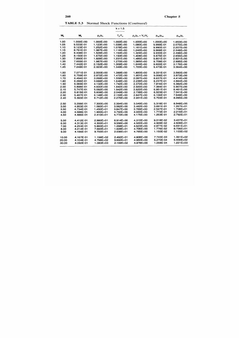
7/21/2019 Fundamental Fluid Mechanics for Engineers
http://slidepdf.com/reader/full/fundamental-fluid-mechanics-for-engineers 283/438
260
Chapter
5
TABLE 5.3 Normal Shock
Functions
(Continued)
1oo
1.05
1.10
1.15
1.20
1.25
1.30
l35
1.40
1A5
1.50
1.60
l
70
1.80
1.90
2.00
2.1
0
2.20
2.30
2.40
2.50
3.00
3.50
4.00
4.50
5.00
6.00
7.00
8.00
9.00
10.00
20.00
30.00
1OOOE+OO
9.533E-01
9.123E-01
8.761 E-01
8.438E-01
8.150E-01
7.890E-01
7.655E-01
7.442E-01
7.248E-01
7.071 E-01
6.759E-01
6.494E-01
6.266E-01
6.069E-01
5.898E-01
5.747E-01
5.61 5E-01
5.497E-01
5.393E-01
5.299E-01
4.953E-01
4.734E-01
4.588E-01
4.486E-01
4.41 2E-01
4.31 3E-01
4.253E-01
4.21 4E-01
4.186E-01
4.1 67E-01
4.104E-01
4.092E-01
1
OOOE+OO
1
.l
3E+00
1.252E+00
1.387E+00
1.528E+00
1.675E+00
1.828E+00
1.987E+00
2.1 52E+00
2.323E+00
2.500E+00
2.872E+00
3.268E+00
3.688E+00
4.1 32E+00
4.600E+00
5.092E+00
5.608E+00
6.148E+00
6.71 2E+OO
7,3OOE+OO
1.060E+01
1.450E+01
1.900E+01
2.41 OE+Ol
2.980E+01
4.300E+01
5.86OE+Ol
7.660E+01
9.700E+01
1.l8E+02
4.798E+02
1.080E+03
1.000E+00
1.039E+00
1.078E+00
1
.l
6E+00
1
l
4E+00
1
l
3E+00
1.231 E+OO
l270E+00
1.309E+00
1.349E+00
1.389E+00
1.472E+00
1.558E+00
1.648E+00
1.742E+00
1.840E+00
1.942E+00
2.049E+00
2.159E+00
2.275E+00
2.394E+00
3.062E+00
3.847E+00
4.750E+00
5.772E+00
6.914E+00
9.556E+00
1.268E+O1
1.628E+01
2.036E+01
2.492E+01
9.692E+01
2.1 69E+02
1.000E+00
1 .O8OE+00
1
l
1 E+OO
1.242E+00
1.324E+00
1.404E+00
1.485E+00
1.565E+00
1.644E+00
1.723E+00
1.800E+00
1 .g51 +OO
2.097E+00
2.238E+OO
2.372E+00
2.500E+00
2.622E+00
2.738E+00
2.847E+00
2.951 E+OO
3.049E+OO
3.462E+00
3.769E+00
4.000E+00
4.175E+00
4.31OE+OO
4.500E+00
4.623E+OO
4.706E+00
4.765E+00
4.808E+00
4.950E+00
4.978E+00
l
000E+00
9.999E-01
9.990E-01
9.968E-01
9.930E-01
9.875E-01
9.801 E-01
9.709E-01
9.600E-01
9.473E-01
9.331 E-01
9.006E-01
8.637E-01
8.237E-01
7.81 6E-01
7.384E-01
6.951 E-01
6.523E-01
6.1 06E-01
5.703E-01
5.31 8E-01
3.691 E-01
2.547E-01
1.773E-01
1.253E-01
9.01 8E-02
2.877E-02
4.928E-02
1.776E-02
1.l0E-02
7.743E-03
5.270E-04
1.058E-04
1.953E+OO
2.075E+00
2.207E+00
2.348E+00
2.498E+OO
2.656E+OO
2.821 E+OO
2.995E+00
3.1 76E+00
3.364E+OO
3.56OE+OO
3.973E+OO
4.414E+OO
4.884E+OO
5.382E+00
5.907E+00
6.461
E+OO
7.041 E+OO
7.649E+00
8.285E+00
8.948E+OO
1.267E+01
1.708E+Ol
2.21 6E+01
2.792E+O1
3.437E+O1
4.928E+O1
6.691E+O1
8.726E+01
1
.l
3E+02
1.361 E+02
5.430E+02
1.221 E+03

7/21/2019 Fundamental Fluid Mechanics for Engineers
http://slidepdf.com/reader/full/fundamental-fluid-mechanics-for-engineers 284/438
Gas
Dynamics
261
TABLE
5.3
Normal
Shock Functions
(Continued)
Y
M,
PJ PZ
k =
5/3
P d P ,
1oo
1.05
1.10
1.15
1.20
1.25
l
30
l
35
1.40
l
45
l
50
l60
1.70
1.80
1.90
2.00
2.1
0
2.20
2.30
2.40
2.50
3.00
3.50
4.00
4.50
5.00
6.00
7.00
8.00
9.00
10.00
20.00
30.00
1OOOE+OO
9.535E-01
9.131 E-01
8.776E-01
8.463E-01
8.1 84E-01
7.935E-01
7.71 1 E-01
7.509E-01
7.325E-01
7.158E-01
6.866E-01
6.620E-01
6.41 OE-01
6.229E-01
6.073E-01
5.936E-01
5.817E-01
5.71 1 E-01
5.61 7E-01
5.534E-01
5.227E-01
5.036E-01
4.91 OE-01
4.822E-01
4.758E-01
4.674E-01
4.623E-01
4.589E-01
4.566E-01
4.550E-01
4.497E-01
4.487E-01
l.OOOE+OO
1.128E+00
1.263E+00
1.403E+00
l550E+00
1.704E+00
1.863E+00
2.029E+00
2.201 E+OO
2.379E+00
2.564E+00
2.951 E+OO
3.364E+00
3.802E+00
4.265E+00
4.753E+00
5.266E+00
5.804E+00
6.367E+00
6.954E+00
7.567E+00
1
.l
1 E+01
1.507E+O1
1.976E+01
2.508E+01
3.1 02E+01
4.478E+01
6.1 04E+Ol
7.981 E+01
1.01 1 E+02
1.248E+02
5.001 E+02
1
.l
6E+03
1OOOE+OO
1.050E+00
1.099E+00
1.l7E+00
1
.l
6E+00
1.244E+00
1.293E+00
l343E+00
1.393E+00
1.445E+00
l
497E+00
1.604E+00
1.71 6E+00
1.833E+00
1.955E+00
2.083E+00
2.216E+00
2.355E+00
2.499E+00
2.650E+00
2.806E+00
3.678E+00
4.704E+00
5.885E+00
7.221 E+OO
8.714E+00
1.21 7E+01
1.625E+01
2.096E+01
2.630E+Ol
3.226E+01
1.264E+02
2.834€+02
1.000E+00
1.075E+00
1.149E+00
1.223E+OO
1.297E+00
1.369E+00
1.441 E+OO
1.51 1 E+OO
l
580E+00
1.647E+00
1.71 3E+00
1.840E+00
1.960E+00
2.074E+00
2.181 E+OO
2.282E+00
2.376E+00
2.465E+00
2.548E+00
2.625E+00
2.697E+00
2.993E+OO
3.204E+OO
3.358E+00
3.473E+00
3.560E+00
3.680E+00
3.756E+00
3.807E+OO
3.843E+00
3.870E+00
3.956E+00
3.972E+00
1.000E+00
9.999E-01
9.990E-01
9.969E-01
9.934E-01
9.882E-01
9.81 3E-01
9.728E-01
9.627E-01
9.51 1 E-01
9.381 E-01
9.087E-01
8.754E-01
8.395E-01
8.01 9E-01
7.634E-01
7.248E-01
6.866E-01
6.493E-01
6.131 E-01
5.782E-01
4.283E-01
3.1 77E-01
2.384E-01
1.81 6E-01
1.406E-01
8.831 E-02
5.854E-02
4.059E-02
2.920E-02
2.167E-02
8.684EL04
2.885E-03
2.055E+00
2.1 89E+00
2.333E+OO
2.487E+OO
2.650E+00
2.822E+00
3.002E+00
3.191 E+OO
3.388E+00
3.592E+00
3.805E+OO
4.254E+OO
4.733E+OO
5.243E+OO
5.784E+00
6.354E+00
6.954E+OO
7.584E+OO
8.244E+00
8.934E+00
9.653E+00
1.369E+O1
l
847E+01
2.398E+01
3.024E+01
3.722E+O1
5.340E+01
7.253E+O1
9.459E+01
1
.l
6E+02
1.476E+02
5.889E+02
1.324€+03
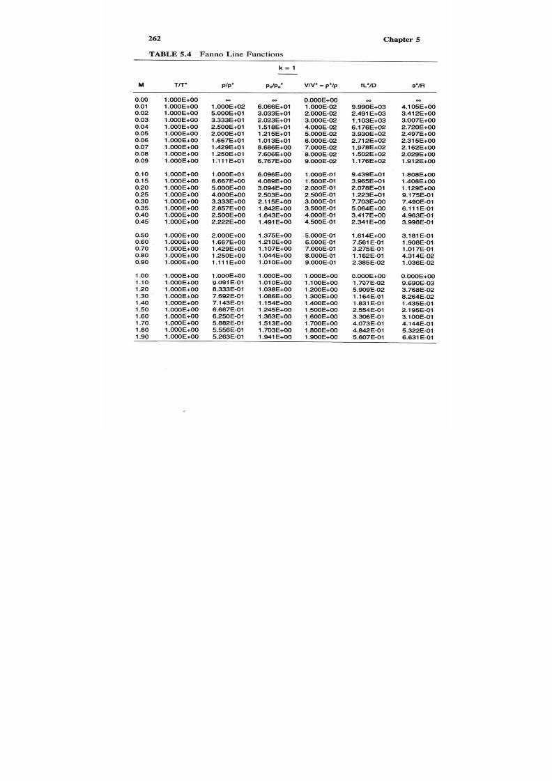
7/21/2019 Fundamental Fluid Mechanics for Engineers
http://slidepdf.com/reader/full/fundamental-fluid-mechanics-for-engineers 285/438
262 Chapter 5
TABLE
5.4
FannoLineFunctions
k = l
M
T T PIP' pJpo* VN' =
p lp
fL*/D
S'/R
0.00
0.01
0.02
0.03
0.04
0.05
0.06
0.07
0.08
0.09
0.10
0.1 5
0.20
0.25
0.30
0.35
0.40
0.45
0.50
0.60
0.70
0.80
0.90
1 oo
1.10
1.20
1.30
1.40
1.50
1.60
1.70
1.80
1.000E+00
1.000E+00
1.000E+00
1.000E+00
1.000E+00
1.000E+00
1.000E+00
1.000E+00
1.000E+00
1.000E+00
1.000E+00
1.000E+00
1.000E+00
1.000E+00
1.000E+00
1.000E+00
1.000E+00
1.000E+00
1.000E+00
1.000E+00
1.000E+00
1.000E+00
l000E+00
1.000E+00
1.000E+00
1.000E+00
1.000E+00
1 OOOE+OO
1.000E+00
1.000E+00
1.000E+00
l000E+00
1.000E+02
5.000E+01
3.333E+01
2.500E+01
2.000E+01
1.667E+01
1.429E+01
1.250E+01
1
.l
1 E+01
1.000E+01
6.667E+00
5.000E+00
4.000E+00
3.333E+00
2.857E+00
2.500E+00
2.222E+00
2.000E+00
1.667E+00
1.429E+00
1.250E+00
1
.l
1 E+OO
1.000E+00
9.091 E-01
8.333E-01
7.692E-01
7.143E-01
6.667E-01
6.25OE-01
5.882E-01
5.556E-01
6.066E+01
3.033E+01
2.023E+01
1.51 8E+01
1.21 5E+01
1.01 3E+01
8.686E+00
7.606E+00
6.767E+00
6.096E+00
4.089E+00
3.094E+00
2.503E+00
2.1 15E+00
1.842E+00
1.643E+00
1.491 E+OO
l375E+00
l21 OE+W
1.107E+00
1.044E+00
1.01 OE+OO
1.000E+00
1.01 OE+OO
1.038E+00
1.086E+OO
l l4E+00
1.245E+00
1.363E+00
1.51 3E+00
1.703E+00
m
0.000E+00
1.000E-02
2.000E-02
3.000E-02
4.OOOE-02
5.000E-02
6.000E-02
7.OOOE-02
8.OOOE-02
9.OOOE-02
1 00OE-01
1.5OOE-01
2.000E-01
2.5OOE-01
3.000E-01
3.5OOE-01
4.000E-01
4.500E-01
5.000E-01
6.000E-01
7.000E-01
8.000E-01
9.000E-01
1 .000E+00
1
.l0E+00
1.200E+00
1.300E+00
1.400E+00
1.500E+00
1.600E+00
1.700E+00
1.800E+00
9.990E+03
2.491 E+03
1.l3E+03
6.176E+02
3.930E+02
2.71 2E+02
1.978E+02
1.502E+02
1
.l
6E+02
9.439E+01
3.965E+01
2.078E+01
1.223E+O1
7.703E+00
5.064E+00
3.41 7E+Ob
2.341 E+OO
1.61 4E+00
7.561 E41
3.275E-01
1.l2E-01
2.385E-02
0.000E+00
1.707E-02
5.909E-02
1.l4E-01
1.831 E-01
2.554E-01
3.306E-01
4.073E-01
4.842E-01
OD
4.105E+OO
3.41 2E+00
3.007E+00
2.720E+00
2.497E+00
2.31 5E+00
2.1 62E+00
2.029E+00
1.91 2E+OO
1.808E+00
1.408E+00
l l
9E+00
m
9.1 75E-01
7.490E-01
6.1 1 1 E-01
4.963E-01
3.998E-01
3.181 E-01
1.908E-01
1.01 7E-01
4.31 4E-02
1.036E-02
0.000E+00
9.690E-03
3.768E-02
8.264E-02
1 M5E-01
2.1 95E-01
3.100E-01
4.144E-01
5.322E-01
6.631 E-01
.90 l000E+00.263E-01 .W1 E+OO 1.900E+00.607E-01
~~~~
~.
F
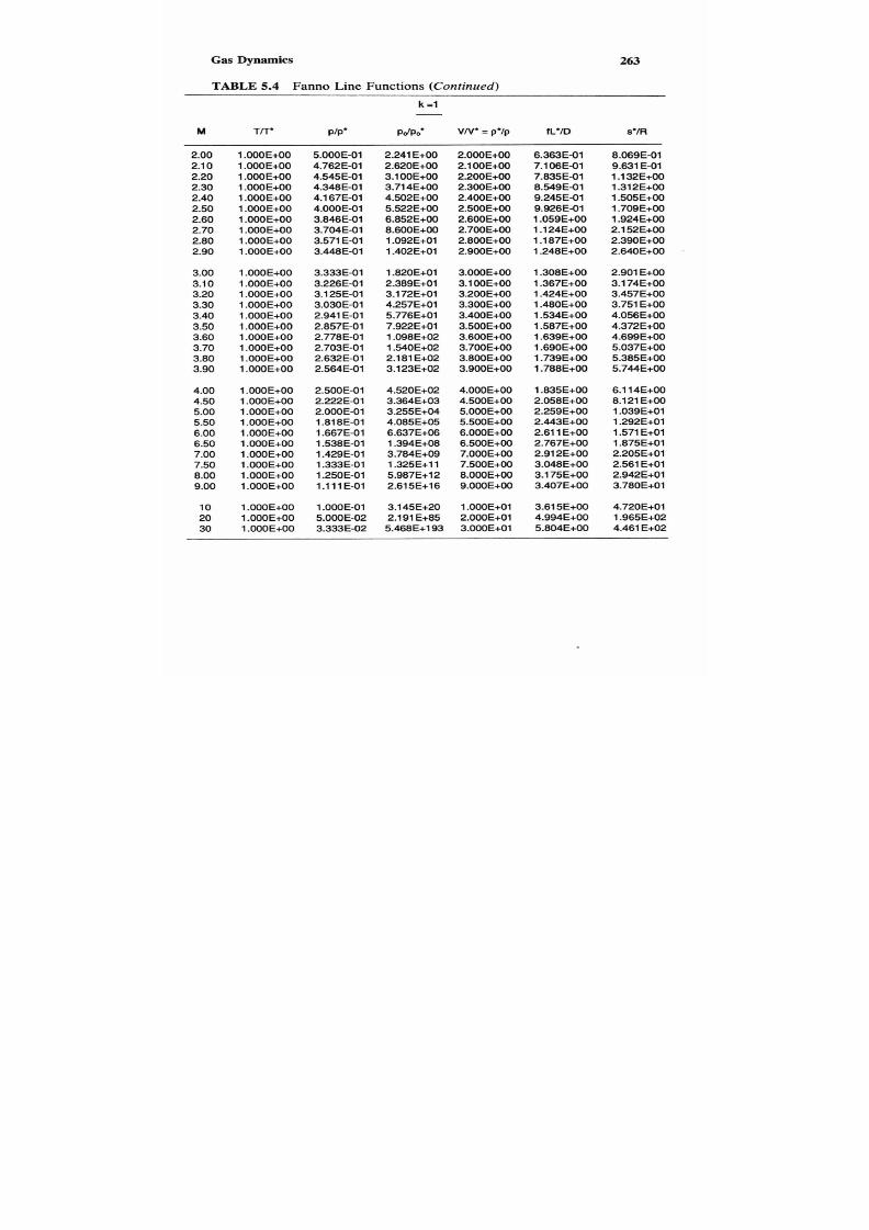
7/21/2019 Fundamental Fluid Mechanics for Engineers
http://slidepdf.com/reader/full/fundamental-fluid-mechanics-for-engineers 286/438
Gas Dynamics 263
TABLE
.4 Fanno
Line Functions (Continued)
2.00
2.1 0
2.20
2.30
2.40
2.50
2.60
2.70
2.80
2.90
3.00
3.1
0
3.20
3.30
3.40
3.50
3.60
3.70
3.80
3.90
4.00
4.50
5.00
5.50
6.00
6.50
7.00
7.50
8.00
9.00
10
20
30
l.OOOE+OO
1.000E+00
1.000E+00
l
000E+00
1.000E+00
1.000E+00
1.000E+00
1.000E+00
1.000E+00
1.000E+00
1.000E+00
1.000E+00
1.000E+00
1.000E+00
l.OOOE+OO
1.000E+00
1.000E+00
1.000E+00
1.000E+00
l
000E+00
1 OOOE+OO
1.000E+00
1.000E+00
1 OOOE+OO
1.000E+00
1.000E+00
1.000E+00
1.000E+00
1.000E+00
1.000E+00
1.000E+00
l000E+00
1.000E+00
5.OOOE-01
4.762E-01
4.545E-01
4.348E-01
4.167E-01
4.OOOE-01
3.846E-01
3.704E-01
3.571 E-01
3.448E-01
3.333E-01
3.226E-01
3.1 25E-01
3.030E-01
2.941 E-01
2.857E-01
2.778E-01
2.703E-01
2.632E-01
2.564E-01
2.5OOE-01
2.222E-01
2.000E-01
1.81 8E-01
1.667E-01
1.538E-01
1.429E-01
1.333E-01
1.250E-01
1.111E-01
1 OOOE-01
5.000E-02
3.333E-02
2.241 E+OO
2.620E+OO
3.100E+OO
3.71 4E+00
4.502E+00
5.522E+00
6.852E+00
8.600E+00
1.092E+01
l402E+01
1.82OE+Ol
2.389E+01
3.1 72E+01
4.257E+01
5.776E+O1
7.922E+01
1.098E+02
1.540E+02
2.181 E+02
3.123E+02
4.520E+02
3.364E+03
3.255E+04
4.085E+05
6.637E+06
1.394E+08
3.784E+09
1.325E+11
5.987E+12
2.61 5E+16
3.145E+20
2.191 E+85
5.468E+193
6.363E-01
7.106E-01
7.835E-01
8.549E-01
9.245E-01
9.926E-01
1.059E+00
1.l4E+OO
1.l7E+00
1.248E+00
1.308E+00
1.367E+00
1.424E+00
1.480E+00
1.534E+00
1.587E+00
l
639E+00
1.690E+00
1.739E+00
1.788E+00
1.835E+00
2.058E+00
2.259E+00
2.443E+00
2.61 1 E+OO
2.767E+OO
2.91 2E+00
3.048E+00
3.175E+00
3.407E+00
3.61 5E+W
4.994E+00
5.804E+00
8.069E-01
9.631 E-01
1.l2E+OO
1.312E+OO
1.505E+00
1.709E+00
1.924E+00
2.1 52E+00
2.390E+00
2.640E+00
2.901 E+OO
3.1 74E+OO
3.457E+00
3.751 E+OO
4.056E+00
4.372E+00
4.699E+00
5.037E+00
5.385E+00
5.744E+OO
6.1 14E+00
8.1 21 E+OO
l039E+01
1.292E+01
1.571 E+01
1.875E+01
2.205E+01
2.561 E+01
2.942E+01
3.780E+01
4.720E+01
1.965E+02
4.461 E+02
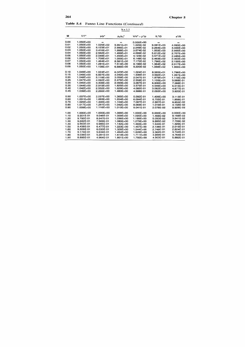
7/21/2019 Fundamental Fluid Mechanics for Engineers
http://slidepdf.com/reader/full/fundamental-fluid-mechanics-for-engineers 287/438
264 Chapter 5
Table
5.4
FannoLineFunctions (Continued)
k =
1.1
0.00
0.01
0.02
0.03
0.04
0.05
0.06
0.07
0.08
0.09
0.1
0
0.1 5
0.20
0.25
0.30
0.35
0.40
0.45
0.50
0.60
0.70
0.80
0.90
1oo
1.10
l20
1.30
1.40
1.50
1.60
1.70
1
O
1.90
1.050E+00
l
050E+00
1.050E+00
1.050E+00
1.050E+00
1.050E+00
1.050E+00
1.050E+00
1.050E+00
1.050E+00
1.049E+00
1.049E+00
1.048E+00
1.047E+00
1.045E+00
1.044E+00
1.042E+00
1.039E+00
1.037E+00
1.031 E+OO
1.025E+00
1.017E+00
1.009E+00
1OOOE+OO
9.901 E-01
9.795E-01
9.682E-01
9.563E-01
9.438E-01
9.309E-01
9.174E-01
9.036E-01
8.895E-01
1.025E+02
5.123E+01
3.41 6E+01
2.562E+01
2.049E+01
1.708E+01
1.464E+01
1.281 E+01
1
.l8E+01
l
024E+Ol
6.827E+00
5.1 18E+00
4.092E+00
3.408E+00
2.91 9E+00
2.552E+00
2.266E+00
2.037E+00
1.693E+00
1.446E+00
1.261 E+OO
1
.l
6E+00
1.000E+00
oa
9.046E-01
8.247E-01
7.569E-01
6.985E-01
6.477E-01
6.030E-01
5.634E-01
5.281 E-01
4.964E-01
5.991 E+O1
2.996E+O1
1.998E+01
1.499E+01
1.200E+01
1.000E+01
8.581 E+W
7.51 4E+00
6.685E+00
6.023E+OO
4.042E+W
3.059E+00
2.476E+00
2.093E+00
1.825E+00
1.629E+00
1.480E+00
1.365E+OO
l204E+00
1.104E+OO
1.042E+00
1.01 OE+OO
l.WOE+W
1.009E+00
1.036E+00
1.080E+00
1.142E+00
1.223E+00
1.326E+00
1.454E+00
1.61 OE+OO
1 .e01+OO
OD
OOOOE+OO
1.025E-02
2.049E-02
3.074E-02
4.099E-02
5.123E-02
6.148E-02
7.1 72E-02
8.196E-02
9.220E-02
1.024E-01
l536E-01
2.047E-01
2.558E-01
3.067E-01
4.082E-01
3.575E-01
4.588E-01
5.092E-01
6.094E-01
7.087E-01
8.069E-01
9.041 E-01
1OWE+OO
1.095E+00
1
l
88E+00
1.279E+00
1.369E+00
1.457E+00
1.544E+00
1.628E+00
1.71 1 E+OO
1.792E+00
9.081 E+03
2.264E+03
1.003E+03
5.61 2E+02
3.571 E+02
2.463E+02
1.796E+02
1.364E+02
1.068E+02
8.565E+01
3.592E+01
1.879E+01
1.103E+Ol
6.936E+W
4.549E+00
3.062E+00
2.093E+00
1.439E+OO
6.705E-01
2.887E-01
1.01 9E-01
2.078E-02
O.WOE+W
1A8E-02
5.050E-02
1.544E-01
2.138E-01
2.749E-01
3.362E-01
3.969E-01
4.563E-01
0 0
9.885E-02
4.093€+00
3.400E+00
2.995E+00
2.707E+00
2.485E+00
2.303E+00
2.1 50E+00
2.01 7E+00
1.900E+00
1.796E+W
1.397E+00
1.l
8E+00
7.388E-01
6.01 6E-01
m
9.068E-01
4.877E-01
3.920E-01
3.1 13E-01
1.858E-01
9.853E-02
4.158E-02
9.928E-03
O.OOOE+W
9.168E-03
3.541 E-02
7.709E-02
1.329E-01
2.01 6E-01
2.824E-01
3.742E-01
4.764E-01
5.882E-01

7/21/2019 Fundamental Fluid Mechanics for Engineers
http://slidepdf.com/reader/full/fundamental-fluid-mechanics-for-engineers 288/438
Gas
Dynamics 265
Table
5.4 Fanno
Line
Functions
(Continued)
k = 1.1
2.00
2.10
2.20
2.30
2.40
2.50
2.60
2.70
2.80
2.90
3.00
3.10
3.20
3.30
3.40
3.50
3.60
3.70
3.80
3.90
4.00
4.50
5.00
5.50
6.00
6.50
7.00
7.50
8.00
9.00
10
20
30
8.75OE-01
8.603E-01
8.454E-01
8.304E-01
8.1 52E-01
8.000E-01
7.848E-01
7.695E-01
7.543E-01
7.392E-01
7.241 E-01
7.092E-01
6.944E-01
6.798E-01
6.654E-01
6.512E-01
6.371 E-01
6.233E-01
6.098E-01
5.964E-01
5.833801
5.217E-01
4.667E-01
4.1 79E-01
3.750E-01
3.373E-01
3.043E-01
2.754E-01
2.500E-01
2.079E-01
1.75OE-01
5.OOOE-02
2.283E-02
4.677E-01
4.417E-01
4.1 79E-01
3.962E-01
3.762E-01
3.578E-01
3.407E-01
3.249E-01
3.1 02E-01
2.965E-01
2.837E-01
2.71 7E-01
2.604E-01
2.499E-01
2.399E-01
2.306E-01
2.217E-01
2.1 34E-01
2.055E-01
1.980E-01
1.909E-01
1.605E-01
1.366E-01
1
.l
5E-01
1.021 E-01
8.936E-02
7.881 E-02
6.997E-02
6.25OE-02
5.066E-02
4.1 83E-02
1.118E-02
5.036E-03
2.032E+00
2.31 2E+00
2.651 E+OO
3.061 E+OO
3.560E+00
4.165E+00
4.901 E+OO
5.799E+00
6.896E+00
8.237E+00
9.880E+00
1.190E+01
1.438E+01
1.743E+01
2.1 19E+01
2.583E+01
3.157E+01
3.866E+01
4.743E+01
5.829E+01
7.175E+01
2.058E+02
5.977E+02
1.731 E+03
4.949E+03
1.388E+04
3.798E+04
1.01 2E+05
2.621 E+05
1.61 4E+06
8.874E+06
2.290E+12
5.746E+15
1B71E+OO
1.948E+00
2.023E+00
2.096E+00
2.1 67E+00
2.236E+00
2.303E+00
2.368E+00
2.432E+00
2.493E+00
2.553E+00
2.611E+OO
2.667E+00
2.721 E+OO
2.773E+00
2.824E+00
2.874E+00
2.921 E+OO
2.967E+00
3.01 2E+00
3.055E+00
3.25OE+OO
3.41 6E+00
3.556E+00
3.674E+00
3.775E+00
3.862E+00
3.936E+00
4.000E+00
4.1 04E+00
4.1 83E+00
4.472E+00
4.532E+00
5.140E-01
5.698E-01
6.237E-01
6.754E-01
7.251 E-01
7.726E-01
8.182E-01
8.61 7Eal
9.034E-01
9.432E-01
9.812E-01
1.017E+00
1.052E+00
1.085E+00
1.l7E+00
1.l7E+00
l
176E+00
1.204E+00
1.230E+00
1.256E+00
1.280E+00
1.386E+00
1.472E+00
1.543E+00
1.601 E+OO
1.649E+00
1.689E+00
1.723E+00
1.752E+00
1.798E+00
l
832E+00
1.953E+00
1.977E+00
7.089E-01
8.380E-01
9.748E-01
1
.l
9E+00
1.270E+00
1.427E+00
1.590E+00
1.758E+00
1g31 E+OO
2.1 09E+00
2.291 E+OO
2.476E+00
2.666E+00
2.858E+00
3.054E+00
3.252E+00
3.452E+00
3.655E+00
3.859E+OO
4.066E+00
4.273E+OO
5.327E+00
6.393E+00
7.456E+00
8.507E+00
9.538E+00
1.054E+01
1
.l
2E+01
1.248E+01
1.429E+01
1.600E+Ol
2.846E+01
3.629E+01

7/21/2019 Fundamental Fluid Mechanics for Engineers
http://slidepdf.com/reader/full/fundamental-fluid-mechanics-for-engineers 289/438
266
Chapter 5
TABLE
5.4
Fanno Line Functions
(Continued)
k -
1.2
M
Til-* PIP' PdPo VN '=
p*/p
fL*tD
s*m
0.00
0.01
0.02
0.03
0.04
0.05
0.06
0.07
0.08
0.09
0.10
0.1 5
0.20
0.25
0.30
0.35
0.40
0.45
0.50
0.60
0.70
0.80
0.90
1oo
1.10
l
20
1.30
1.40
1.50
1.60
1.70
1.80
1.90
l l0E+OO
1
.l
0E+00
1
.l
OE+OO
1.100E+00
1
.l
0E+00
1.100E+00
1.100E+00
1.099E+00
1.099E+00
1.099E+00
1.099E+00
1.098E+00
1.096E+00
1.093E+00
1.090E+00
1.087E+00
l
083E+00
1.078E+00
1.073E+00
1.062E+00
1.049E+00
1.034E+00
1.01 8E+00
1.000E+00
9.813E-01
9.615E-01
9.41OE-01
9.197E-01
8.98OE-01
8.758E-01
8.534E-01
8.308E-01
8.082E-01
1.049E+02
5.244E+01
3.496E+01
2.622E+01
2.097E+01
1.748E+01
1.498E+01
1.31 1 E+01
1.165E+01
1.048E+01
6.984E+00
5.234E+00
4.182E+00
3.480E+00
2.978€+00
2.601 E+OO
2.307E+00
2.072E+00
1.71 7E+00
1.463E+00
1.271 E+OO
1 l21 E+OO
1.000E+00
m
9.005E-01
8.1 72E-01
7.462E-01
6.85OE-01
6.31 7E-01
5.849E-01
5.434E-01
5.064E-01
4.732E-01
5.921 E+01
2.961 E+01
1.974E+01
1.481 E+01
1.186E+01
9.887E+00
8.480E+00
7.426E+00
6.607E+00
5.953E+00
3.996E+00
3.026E+00
2.451 E+OO
2.073E+00
1.809E+00
l615E+00
1.469E+00
1.356E+00
1
.l
9E+00
1.100E+00
1.041 E+OO
1.01 OE+M
1.000E+00
1.009E+00
1.034E+00
1.075E+00
1
.l2E+00
1.205E+00
1.296E+00
1.407E+00
1.540E+00
1.697E+00
m
0.000E+00
1.049E-02
2.098E-02
3.146E-02
4.195E-02
5.243E-02
6.292E-02
7.340E-02
8.388E-02
9.435E-02
1M8E-01
1.571 E-01
2.093E-01
2.614E-01
3.1 32E-01
3.649E-01
4.162E-01
4.673E-01
5.180E-01
6.183E-01
7.168E-01
8.134E-01
9.079E-01
1.000E+00
l.O9OE+00
1
.l
7E+00
1.261 E+OO
1.343E+00
1.421 E+OO
1.497E+00
1.570E+00
1.641 E+OO
1.708E+00
8.324E+03
2.075E+03
9.188E+02
5.142E+02
3.271 E+02
2.256E+02
1.644E+02
1.248E+02
9.772E+01
7.837E+01
3.281 E+01
1.71 3E+01
1.004E+01
6.298E+00
4.121 E+OO
2.768E+00
1.887E+00
1.294E+00
5.999E-01
2.570E-01
9.01 6E-02
1.828E-02
0.000E+00
1.277E-02
4.367E-02
8.500E-02
1.320E-01
181 7E-01
2.323E-01
2.825E-01
3.316E-01
3.791 E41
m
4.081 E+OO
3.388E+00
2.983E+00
2.696E+00
2.473E+00
2.291 E+OO
2.138E+00
2.005E+00
1.888E+00
1.784E+00
1.385E+00
1
.l
7E+00
8.964E-01
7.290E-01
5.926E-01
4.794E-01
3.846E-01
m
3.048E-01
1
81
1
E-01
9.557E-02
4.01 3E-02
9.530E-03
0.000E+W
8.7OOE-03
3.339E-02
7.225E-02
1.237E-01
1.865E-01
2.594E-01
3.41 4E-01
4.31 6E-01
5.291 E41
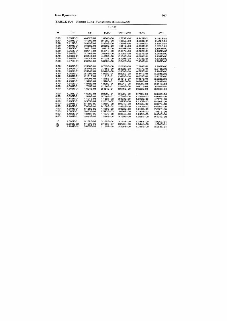
7/21/2019 Fundamental Fluid Mechanics for Engineers
http://slidepdf.com/reader/full/fundamental-fluid-mechanics-for-engineers 290/438
Gas Dynamics
267
TABLE 5.4 Fanno Line Functions
(Continued)
k =
1.2
2.00
2.10
2.20
2.30
2.40
2.50
2.60
2.70
2.80
2.90
3.00
3.1
0
3.20
3.30
3.40
3.50
3.60
3.70
3.80
3.90
4.00
4.50
5.00
5.50
6.00
6.50
7.00
7.50
8.00
9.00
10
20
30
7.857E-01
7.634E-01
7.412E-01
7.194E-01
6.98OE-01
6.769E-01
6.563E-01
6.362E-01
6.1 66E-01
5.975E-01
5.789E-01
5.609E-01
5.435E-01
5.266E-01
5.1 02E-01
4.944E-01
4.791 E-01
4.643E-01
4.501 E-01
4.363E-01
4.231 E41
3.636E-01
3.143E-01
2.733E-01
2.391 E-01
2.1 05E-01
1.864E-01
1.66OE-01
1.486E-01
1.209E-01
1000E-01
2.683E-02
1.209E-02
4.432E-01
4.1 60E-01
3.913E-01
3.688E-01
3.481 E41
3.291 E-01
3.1 16E-01
2.954E-01
2.804E-01
2.665E-01
2.536E-01
2.416E-01
2.304E-01
2.1 99E-01
2.1 01 E-01
2.009E-01
1.923E-01
1.842E-01
1.765E-01
1.694E-01
l
626E-01
1.340E-01
1
.l
1 E-01
9.505E-02
8.1 50E-02
7.059E-02
6.1 68E-02
5.433E-02
4.819E-02
3.863E-02
3.162E-02
8.1 9OE-03
3.665E-03
1.884E+00
2.103E+OO
2.359E+00
2.660E+00
3.01
1
E+OO
3.421 E+OO
3.898E+00
4.455E+00
5.103E+00
5.858E+00
6.735E+00
7.755E+00
8.940E+00
1.032E+01
1 l91 E+01
1.376E+O1
1.590E+Ol
1.838E+01
2.124E+01
2.454E+01
2.836E+01
5.796E+01
1.163E+02
2.281 E+02
4.359E+02
8.108E+02
1.469E+03
2.593E+03
4.467E+03
1.238E+04
3.162E+04
2.196E+07
1.175E+09
1.773E+00'
1.835E+00
1.894E+00
1g51 E+OO
2.005E+00
2.057E+00
2.1 06E+00
2.1 54E+00
2.1 99E+00
2.242E+00
2.283E+00
2.322E+OO
2.359E+00
2.395E+00
2.429E+00
2.461 E+OO
2.492E+00
2.521 E+OO
2.549E+00
2.576E+00
2.602E+00
2.714E+00
2.803E+00
2.875E+00
2.934E+00
2.982E+00
3.023E+00
3.056E+00
3.084E+00
3.1 29E+00
3.1 62E+00
3.276E+00
3.298E+00
4.247E-01
4.683E-01
5.099E-01
5.493E-01
5.868E-01
6.222E-01
6.557E-01
6.874E-01
7.173E-01
7.456E-01
7.724E-01
7.977E-01
8.215E-01
8.441 E-01
8.655E-01
8.857E-01
9.048E-01
9.229E-01
9.401 E-01
9.563E-01
9.718E-01
1.038E+00
1.090E+00
1.l0E+00
1.163E+00
1
.l
0E+00
1.21 2E+00
1.230E+00
1.245E+00
1.268E+00
1.286E+00
l
344E+00
1.356E+00
6.332E-01
7.432E-01
8.584E-01
9.783E-01
1
.l
2E+00
1.230E+00
1.361 E+OO
1.494€+00
1.630E+00
1.768E+00
1.907E+00 ,
2.048E+00
2.191 E+OO
2.334E+00
2.477E+00
2.622E+00
2.766E+00
2.91 1 E+OO
3.056E+00
3.200E+00
3.345E+00
4.060E+00
4.757E+00
5.430E+00
6.077E+00
6.698E+00
7.292E+00
7.861 E+OO
8.404E+00
9.424E+00

7/21/2019 Fundamental Fluid Mechanics for Engineers
http://slidepdf.com/reader/full/fundamental-fluid-mechanics-for-engineers 291/438
Chapter
5
TABLE
5.4 Fanno Line Functions (Continued)
k =
1.3
0.00
0.01
0.02
0.03
0.04
0.05
0.06
0.07
0.08
0.09
0.10
0.15
0.20
0.25
0.30
0.35
0.40
0.45
0.50
0.60
0.70
0.80
0.90
1
oo
1.10
1.20
1.30
1.40
1.50
1.60
1.70
l
eo
l
90
1.15OE+OO
1
.l
0E+00
1.15OE+OO
1.150E+00
l
l
0E+00
1.150E+00
1.149E+00
1.149E+00
1.149E+00
1.149E+00
1.148E+OO
1.146E+00
1.143E+00
1.139E+OO
1.135E+00
1.129E+00
1.123E+00
1.116E+00
1
.l
8E+00
1.091 E+OO
1.071 E+OO
1.049E+00
1.025E+00
1OOOE+OO
9.733E-01
9.457E-01-
9.1 74E-01
8.887E-01
8.598E-01
8.309E-01
8.022E-01
7.739E-01
7.460E-01
1.072E+02
5.362E+01
3.574E+01
2.681 E+01
2.144E+01
1.787E+01
1.531 E+01
1.340E+01
1 l91 E+01
1.072E+01
7.137E+OO
5.346E+00
4.270E+00
3.551 E+OO
3.036E+00
2.649E+00
2.348E+00
2.106E+OO
1.741 E+OO
1.479E+00
1.280E+00
1.125E+00
1.000E+00
m
8.969E-01
8.1 04E-01
7.368E-01
6.734E-01
6.1 82E-01
5.697E-01
5.269E-01
4.887E-01
4.546E-01
5.853E+01
2.927E+01
1.952E+O1
1.464E+Ol
1.l2E+01
9.774E+00
8.384E+00
7.342E+00
6.533E+00
5.886E+00
3.952E+00
2.994E+00
2.426E+00
2.054E+00
1.793E+00
1.602E+00
1.459E+00
1.348E+00
1.l3E+00
1.097E+00
1.040E+00
1.009E+00
1.000E+00
l
008E+00
1.032E+00
1.070E+00
l l3E+00
1.189E+00
1.271 E+OO
1.369E+00
l
484E+00
1.61 8E+00
m
O.OWE+OO
1.072E-02
2.145E-02
3.21 7E-02
4.289E-02
5.361 E-02
6.433E-02
7.504E-02
8.575E-02
9.646E-02
1.072E-01
1.606E-01
2.138E-01
2.668E-01
3.196E-01
3.71 SE-01
4.239E-01
4.754E-01
5.264E-01
6.267E-01
7.245E-01
8.195E-01
9.1 14E-01
1.000E+00
1.085E+00
1
.l
7E+00
1.245E+00
1.320E+00
1.391 E+OO
1.458E+00
1.523E+00
1.583E+00
1.641 E+OO
7.684E+03
1.91 6E+03
8.479E+02
4.744E+02
3.01 7E+02
2.081 E+02
1.51 6E+02
1.l1 E+02
9.006E+01
7.22OE+Ol
3.01 8E+01
1.573E+01
9.201 E+OO
5.759E+00
3.760E+00
2.520E+00
1.71 4E+00
1.l2E+00
5.409E-01
2.305E-01
8.045E-02
1.623E-02
0.000E+00
1.l2E-02
3.816E-02
7.388E-02
1.142E-01
1.564E-01
1.990E-01
2.408E-01
2.81 4E-01
3.203E-01
m
4.069E+00
3.376E+OO
2.971 E+OO
2.684E+00
2.461 E+OO
2.280E+00
2.1 26E+00
1.994E+00
1.877E+00
1.773E+00
1.374E+00
1.097E+00
OD
8.863E-01
7.1 96E-01
5.839E-01
4.714E-01
3.775E-01
2.985E-01
1.767E-01
9.280E-02
3.878E-02
9.164E-03
0.000E+OO
8.278E-03
3.160E-02
6.798E-02
1.l8E-01
1.735E-01
2.400E-01
3.141 E-01
3.948E-01
4.81 3E-01

7/21/2019 Fundamental Fluid Mechanics for Engineers
http://slidepdf.com/reader/full/fundamental-fluid-mechanics-for-engineers 292/438
Gas Dynamics
269
TABLE
5.4
Fanno Line Functions (Continued)
k =
1.3
M Tff
PIP' p&;
VN*=p* Ip fL'D s*m
2.00
2.1
0
2.20
2.30
2.40
2.50
2.60
2.70
2.80
2.90
3.00
3.10
3.20
3.30
3.40
3.50
3.60
3.70
3.80
3.90
4.00
4.50
5.00
5.50
6.00
6.50
7.00
7.50
8.00
9.00
10
20
30
7.188E-01
6.921 E-01
6.663E-01
6.412E-01
6.1 7OE-01
5.935E-01
5.71OE-01
5.493E-01
5.285E-01
5.085E-01
4.894E-01
4.71OE-01
4.535E-01
4.367E-01
4.206E-01
4.053E-01
3.906E-01
3.766E-01
3.632E-01
3.504E-01
3.382E-01
2.848E-01
2.421 E-01
2.077E-01
l797E-01
1.567E-01
1.377E-01
l219E-01
1.085E-01
8.745E-02
7.188E-02
1.885E-02
8.456E-03
4.239E-01
3.962E-01
3.71OE-01
3.482E-01
3.273E-01
3.082E-01
2.906E-01
2.745E-01
2.596E-01
2.459E-01
2.332E-01
2.214E-01
2.104E-01
2.002E-01
1.908E-01
1B19E-01
1.736E-01
1.659E-01
1.586E-01
1.51 8E-01
1.454E-01
1.l6E-01
9.841 E-02
8.286E-02
7.065E-02
6.091 E-02
5.302E-02
4.654602
4.1 17E-02
3.286E-02
2.681 E-02
6.865E-03
3.065E-03
1.773E+00
1g51 E+OO
2.156E+00
2.388E+00
2.654E+00
2.954E+00
3.295E+00
3.681 E+OO
4.1 16E+00
4.607E+00
5.160E+W
5.781 E+W
6.478E+00
7.259E+00
8.1 33E+00
9.1 1 OE+OO
1.020E+01
1.142E+01
1.277E+01
1.427E+01
1.594E+01
2.739E+01
4.596E+01
7.522E+01
1.201 E+02
1.872€+02
2.853E+02
4.258E+02
6.231 E+02
1.266E+03
2.416E+03
2.042E+05
2.943E+06
1.696E+00
1.747E+00
1.796E+00
1.842E+00
1.885E+00
1.926E+00
1.965E+00
2.001 E+OO
2.036E+00
2.068E+00
2.099E+00
2.128E+00
2.1 55E+00
2.1 81 E+OO
2.205E+00
2.228E+00
2.250E+00
2.271 E+OO
2.290E+00
2.309E+00
2.326E+W
2.402E+00
2.460E+00
2.506E+00
2.543E+OO
2.573E+00
2.598E+00
2.618E+00
2.635E+00
2.662E+00
2.681
E+W
2.746E+00
2.759E+00
3.573E-01
3.924E-01
4.255E-01
4.567E-01
4.860E-01
5.135E-01
5.394E-01
5.636E-01
5.864E-01
6.077E-01
6.277E-01
6.465E-01
6.642E-01
6.808E-01
6.964E-01
7.1 10E-01
7.248E-01
7.379E-01
7.501 E-01
7.617E-01
7.726E-01
8.189E-01
8.543E-01
8.81 9E-01
9.037E-01
9.212E-01
9.355E-01
9.472E-01
9.570E-01
9.722E-01
9.832E-01
1.020E+00
1.027E+00
5.728E-01
6.686E-01
7.68OE-01
8.707E-01
9.759E-01
1.083E+00
l l3E+00
1.303E+W
1.41 5E+00
1.528E+OO
1.641 E+W
1.755E+OO
1.868E+00
1.982E+00
2.096E+00
2.209E+00
2.322E+00
2.435E+00
2.547E+00
2.658E+00
2.769E+W
3.31OE+OO
3,828E+00
4.320€+00
4.788E+00
5.232E+00
5.654E+00
6.054E+00
6.435E+00
7.143E+00
7.79OE+OO
1.223E+01
1.489E+01

7/21/2019 Fundamental Fluid Mechanics for Engineers
http://slidepdf.com/reader/full/fundamental-fluid-mechanics-for-engineers 293/438
270 Chapter 5
TABLE 5.4
Fanno Line Functions
(Continued)
k =
1.4
0.00
0.01
0.02
0.03
0.04
0.05
0.06
0.07
0.08
0.09
0.10
0.1 5
0.20
0.25
0.30
0.35
0.40
0.45
0.50
0.60
0.70
0.80
0.90
l
oo
1.10
1.20
1.30
1.40
1.50
1.60
1.70
1 O
1.90
1.200E+00
1.200E+00
1.200E+00
1.200E+00
1.200E+00
1.l9E+00
1.l9E+00
1.199E+00
1.198E+00
1.198E+00
1.l8E+00
1.l5E+00
1.l0E+00
1.185E+00
1.179E+00
1.l1 E+OO
1.163E+00
1.153E+00
1.l3E+00
1
.l
9E+00
1.093E+00
1.064E+00
1.033E+00
1.000E+00
9.662E-01
9.31 7E-01
8.969E-01
8.621 E-01
8.276E-01
7.937E-01
7.605E-01
7.282E-01
6.969E-01
1.095E42
5.477E+01
3.651 E+01
2.738E+01
2.190E+01
1.825E+01
1.564E+Ol
1.368E+01
1.21 6E+01
1.094E+01
7.287E+00
5.455E+00
4.355E+00
3.61 9E+00
3.092E+00
2.696E+00
2.386E+00
2.138E+00
1.763E+00
1.493E+00
1.289E+00
1.129E+00
1OOOE+OO
0 0
8.936E-01
8.044E-01
7.285E-01
6.632E-01
6.065E-01
5.568E-01
5.1 30E-01
4.741 E-01
4.394E-01
5.787E+01
2.894E+01
1.930E+01
1.448E+01
1.l9E+01
9.666E+00
8.292E+00
7.262E+00
6.461 E+OO
5.822E+00
3.91OE+OO
2.964E+00
2.403E+00
2.035E+00
1.778E+00
1.590E+00
1.449E+00
1.340E+00
1
.l
8E+00
1.094E+00
1.038E+00
1.009E+00
1.000E+00
1.008E+00
1.030E+00
1.066E+00
1
.l
5E+00
1.176E+00
1.250E+00
l338E+00
l
439E+00
l555E+00
m
0.000E+00
1B95E-02
2.191 E-02
3.286E-02
4.381 E-02
5.476E-02
6.570E-02
7.664E-02
8.758E-02
9.851 E-02
1.094E-01
1.639E-01
2.182E-01
2.722E-01
3.257E-01
3.788E-01
4.31 3E-01
4.833E-01
5.345E-01
6.348E-01
7.31 8E-01
8.251 E-01
9.146E-01
1.000E+00
1.081 E+OO
1.l8E+00
1.231 E+OO
1.300E+00
1.365E+00
1.425E+00
1.482E+00
1.536E+00
1.586E+00
7.1 34E+03
1.778E+03
7.871 E+02
4.404E+02
2.800E+02
1.930E+02
1.407E+02
1.067E+02
8.350E+01
6.692E+01
2.793E+01
1.453E+01
8.483E+00
5.299E+00
3.452E+00
2.308E+00
1.566E+00
1.069E+00
4.908E-01
2.081 E-01
7.229E-02
1.451 E-02
0.000E+00
9.935E-03
3.364E-02
6.483E-02
9.974E-02
1.361 E41
1.724E-01
2.078E-01
2.41 9E-01
2.743E-01
m
4.058E+00
3.365E+00
2.96OE+OO
2.673E+00
2.450E+00
2.269E+00
2.115E+00
1.983E+00
1.866E+00
1.762E+00
1.364E+00
1.086E+00
m
8.766E-01
7.105E-01
5.755E-01
4.638E-01
3.706E-01
2.926E-01
1.724E-01
9.01 8E-02
3.752E-02
8.824E-03
0.000E+00
7.894E-03
2.999E-02
6.420E-02
1.088E-01
l
623E-01
2.233E-01
2.909E-01
3.639E-01
4.41 6E-01

7/21/2019 Fundamental Fluid Mechanics for Engineers
http://slidepdf.com/reader/full/fundamental-fluid-mechanics-for-engineers 294/438
Gas Dynamics
271
TABLE 5.4
Fanno Line Functions
(Continued)
k =
1.4
2.00
2.1
0
2.20
2.30
2.40
2.50
2.60
2.70
2.80
2.90
3.00
3.1
0
3.20
3.30
3.40
3.50
3.60
3.70
3.80
3.90
4.00
4.50
5.00
5.50
6.00
6.50
7.00
7.50
8.00
9.00
l 0
20
30
6.667E-01
6.376E-01
6.098E-01
5.831 E-01
5.576E-01
5.333E-01
5.1 02E-01
4.882E-01
4.673E-01
4.474E-01
4.286E-01
4.1 07E-01
3.937E-01
3.776E-01
3.623E-01
3.478E-01
3.341 E-01
3.21OE-01
3.086E-01
2.969E-01
2.857E-01
2.376E-01
2.000E-01
1.702E-01
1.463E-01
1.27OE-01
1.111E-01
9.796E-02
8.696E-02
6.9n~-o2
5.71 4E-02
1.481 E-02
6.63OE-03
4.082E-01
3.802E-01
3.549E-01
3.32OE-01
3.1 11 E-01
2.921 E-01
2.747E-01
2.588E-01
2.441 E-01
2.307E-01
2.182E-01
2.067E-01
1 .g61 E-01
l862E-01
1.77OE-01
1.685E-01
1.606E-01
1.531 E-01
1.462E-01
1.397E-01
1.336E-01
1.083E-01
8.944E-02
7.501 E-02
6.376E-02
5.482E-02
4.762E-02
4.1 73E-02
3.686E-02
2.935E-02
2.39OE-02
6.086E-03
2.714E-03
1.688E+00
1.837E+00
2.005E+00
2.1 93E+00
2.403E+00
2.637E+00
2.896E+00
3.1 83E+00
3.500E+00
3.850E+00
4.235E+00
4.657E+M)
5.121 E+OO
5.629E+OO
6.184E+00
6.790E+00
7.450E+00
8.169E+OO
8.951 E+OO
9.799E+00
1.072E+01
1.656E+01
2.500E+01
3.687E+01
5.31 8E+01
7.51 3E+01
1.041 E+02
1.41 8E+02
1 .g01 E+02
3.272E+02
5.359E+02
1.538E+04
1.l4E+05
1.633E+00
1.677E+00
1.71 8E+OO
1.756E+00
1.792E+00
1.826E+00
1.857E+00
1.887E+00
1.91 4E+00
l
940E+00
1.964E+OO
1.987E+00
2.008E+00
2.028E+00
2.047E+00
2.064E+00
2.081 E+OO
2.096E+00
2.1 11 E+OO
2.1 25E+00
2.138E+00
2.1 94E+00
2.236E+00
2.269E+00
2.295E+00
2.316E+00
2.333E+00
2.347E+00
2.359E+00
2.377E+00
2.390E+OO
2.434E+00
2.443E+00
3.050E-01
3.339E-01
3.609E-01
3.862E-01
4.099E-01
4.320E-01
4.526E-01
4.718E-01
4.898E-01
5.065E-01
5.222E-01
5.368E-01
5.504E-01
5.632E-01
5.752E-01
5.864E-01
5.970E-01
6.068E-01
6.161 E41
6.248E-01
6.331 E41
6.676E-01
6.938E-01
7.140E-01
7.299E-01
7.425E-01
7.528E-01
7.612E-01
7.682E-01
7.790E-01
7.868E-01
8.126E-01
8.176E-01
5.232E-01
6.081 E-01
6.956E-01
7.853E-01
8.768E-01
9.695E-01
1.063E+00
1
.l8E+00
1.253E+00
1.348E+00
1.443E+00
1.538E+OO
1.633E+00
1.728E+00
1.822E+00
1.91 5E+00
2.008E+00
2.1 00E+00
2.1 92E+00
2.282E+00
2.372E+OO
2.807E+00
3.219E+00
3.607E+00
3.974E+00
4.31 9E+00
4.646E+00
4.955E+00
5.248E+00
5.791 E+OO
6.284E+W
9.641 E+OO
1.l5E+01
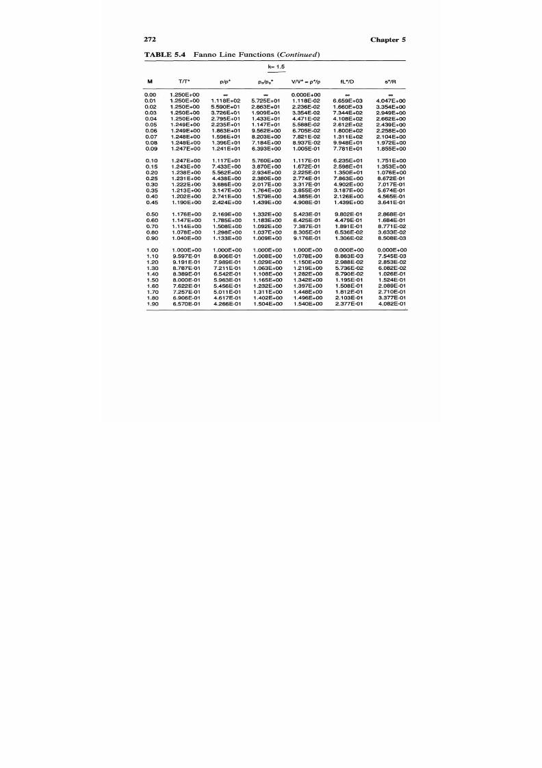
7/21/2019 Fundamental Fluid Mechanics for Engineers
http://slidepdf.com/reader/full/fundamental-fluid-mechanics-for-engineers 295/438
272 Chapter 5
0.00
0.01
0.02
0.03
0.04
0.05
0.06
0.07
0.08
0.09
0.10
0.1 5
0.20
0.25
0.30
0.35
0.40
0.45
0.50
0.60
0.70
0.80
0.90
1
oo
1.10
l
20
1.30
1.40
1.50
1.60
1.70
1.80
1.90
1.250E+00
1.250E+00
l
250E+00
l
250E+OO
1.250E+00
1.249E+00
1.249E+00
1.248E+00
1.248E+00
1.247E+00
1.247E+00
1.243E+00
1.238E+00
1.231 E+OO
1.222E+00
1.213E+00
1.202E+OO
1.190E+00
1.176E+00
1.147E+00
1.l4E+OO
l.O78E+OO
1.040E+00
1.000E+00
9.597E-01
9.1 91 E-01
8.787E-01
8.389E-01
8.000E-01
7.622E-01
7.257E-01
6.906E-01
6.57OE-01
1.l8E+02
5.590E+01
3.726E+O1
2.795E+01
2.235E+01
1.863E+01
l
596E+01
1.396E+01
1.241 E+01
1.l
7E+01
7.433E+00
5.562E+00
4.438E+00
3.686E+00
3.147E+00
2.741 E+OO
2.424E+00
2.169E+00
1.785€+00
1.508€+00
1.298E+00
1.133E+OO
1.000E+00
8.906E-01
0 0
7.989E-01
7.21
1
E-01
6.542E-01
5.963E-01
5.456E-01
5.01 1 E-01
4.61 7E-01
4.266E-01
5.725E+01
2.863E+01
1.909E+01
1.433E+01
1.147E+O1
9.562E+00
8.203E+00
7.1 84E+00
6.393E+00
5.760E+00
3.870E+00
2.934E+00
2.380E+00
2.01 7E+00
1.764E+00
1.579E+OO
1.439E+00
1.332E+00
1.183E+00
1.092E+00
1.037E+00
l009E+OO
1.000E+00
l.O08E+OO
l
029E+00
1.063E+00
1.108E+00
l165E+00
1.232E+00
1.31 1 +OO
1.402E+00
1.504E+00
0 0
0.000E+00
1
.l8E-02
2.236E-02
3.354E-02
4.471 E-02
5.588E-02
6.705E-02
7.821 E-02
8.937E-02
1.005E-01
1
.l
7E-Ol
1.672E-01
2.225E-01
2.774E-01
3.31 7E-01
3.855E-01
4.385E-01
4.908E-01
5.423E-01
6.425E-01
7.387E-01
8.305E-01
9.176E-01
1.000E+00
1.078E+00
1
.l0E+00
1.21 9E+00
1.282E+00
1.342E+00
1.397E+00
1.448E+00
1.496E+00
1.540E+00
6.659E+03
1.660E+03
7.344E+02
4.1 08E+02
2.61 2E+02
1.800E+02
1.31 1 E+02
9.948E+01
7.781 E+01
6.235E+O1
2.598E+01
1.350E+01
7.863E+00
4.902E+00
3.1 87E+00
2.1 26E+00
1.439E+00
9.802E-01
4.479E-01
1.891 E-01
6.536E-02
1.306E-02
0.000E+00
8.863E-03
2.988E-02
5.736E-02
8.790E-02
1.195E-01
1.508E-01
1.812E-01
2.103E-01
2.377E-01
0 0
4.047E+OO
3.354E+00
2.949E+00
2.662E+00
2.439E+OO
2.258E+00
2.1 04E+00
1.972E+00
1.855E+00
1.751 E+00
1.353E+00
l
076E+OO
OD
8.672E-01
7.01 7E-01
5.674E-01
4.565E-01
3.641
E-01
2.868E-01
8.771 E-02
8.508E-03
OOOOE+OO
1.684E-01
3.633E-02
7.545E-03
2.853E-02
6.082E-02
1.026E-01
1.524E-01
2.089E-01
2.71 OE-01
3.377E-01
4.082501

7/21/2019 Fundamental Fluid Mechanics for Engineers
http://slidepdf.com/reader/full/fundamental-fluid-mechanics-for-engineers 296/438
Gas Dynamics
TABLE 5.4
Fanno Line Functions (Continued)
273
k=
1.5
M TTT' PIPdp, v iv*=p*/p fL*/D s*m
2.00
2.10
2.20
2.30
2.40
2.50
2.60
2.70
2.80
2.90
3.00
3.10
3.20
3.30
3.40
3.50
3.60
3.70
3.80
3.90
4.00
4.50
5.00
5.50
6.00
6.50
7.00
7.50
8.00
9.00
10
20
30
6.250E-01
5.945E-01
5.382E-01
5.656E-01
5.123E-01
4.878E-01
4.647E-01
4.429E-01
4.223E-01
4.029E-01
3.846E-01
3.674E-01
3.51 1E-01
3.358E-01
3.21 3E-01
3.077E-01
2.948E-01
2.826E-01
2.71lE-01
2.603E-01
2.5WE-01
2.062E-01
1.724E-01
1.460E-01
1.25OE-01
1081 E-01
9.434E-02
8.299E-02
7.353E-02
5.882E-02
4.808E-02
l
238E-02
5.531 E-03
3.953E-01
3.672E-01
3.419E-01
3.190E-01
2.982E-01
2.794E-01
2.622E-01
2.465E-01
2.321 E-01
2.1 89E-01
2.067E-01
1.955E-01
1.852E-01
l
756E-01
1.667E-01
1.585E-01
1.508E-01
1.437E-01
1.37OE-01
1.308E-01
1.25OE-01
1.009E-01
8.305E-02
6.947E-02
5.893E-02
5.058E-02
4.388E-02
3.841 E-02
3.39OE-02
2.695E-02
2.193E-02
5.562E-03
2.479E-03
1.61 9E+W
1.747E+00
1.889E+00
2.046E+00
2.21 8E+00
2.407E+00
2.61 3E+00
2.838E+OO
3.082E+00
3.347E+00
3.633E+W
3.943E+00
4.278E+00
4.638E+00
5.025E+00
5.441 E+OO
5.886E+00
6.363E+00
6.874E+00
7.41 9E+00
8.000E+W
1.l1 E+01
1.620E+01
2.233E+O1
3.01 7E+Ol
4.004E+01
5.226E+01
6.721 E+01
8.526E+Ol
1.324E+02
1.973E+02
2.934E+03
1.465E+04
1.581
E+W
1.61 9E+00
1.655E+OO
1.687E+00
1.71 8E+00
l746E+00
1.772E+00
1.797E+00
1
820E+00
1.841 E+OO
1.861 E+OO
1.879E+00
l
896E+00
1.91 2E+OO
1.927E+00
1g41 E+OO
1.955E+00
1.967E+00
1.979E+00
1.990E+00
2.0WE+W
2.043E+00
2.076E+OO
2.101 E+OO
2.1 21 E+OO
2.1 37E+00
2.150E+00
2.1 61 E+OO
2.1 69E+00
2.1 83E+00
2.1 93E+W
2.225E+00
2.231 E+OO
2.636E-01
2.877E-01
3.103E-01
3.313E-01
3.508E-01
3.690E-01
3.858E-01
4.01 5E-01
4.160E-01
4.296E-01
4.422E-01
4.539E-01
4.648E-01
4.750E-01
4.846E-01
4.935E-01
5.01 8E-01
5.096E-01
5.169E-01
5.238E-01
5.302E-01
5.572E-01
5.775E-01
5.931 E-01
6.052E-01
6.149E-01
6.227E-01
6.291 E-01
6.344E-01
6.426E-01
6.485E-01
6.679E-01
6.71 6E-01
4.81 9E-01
5.58OE-01
6.362E-01
7.1 58E-01
7.967E-01
8.783E-01
9.605E-01
l043E+W
1.l5E+00
1.208E+00
1.290E+W
1.372E+00
1.453E+00
1.534€+00
1.61 4E+00
1.694E+00
1.773E+00
1.851 E+OO
1.928E+00
2.004E+00
2.079E+W
2.443E+00
2.785E+00
3.1 06E+00
3.407E+00
3.690E+00
3.956E+00
4.208E+00
4.446E+00
4.886E+00
5.285E+OO
7.984E+00
9.592E+00
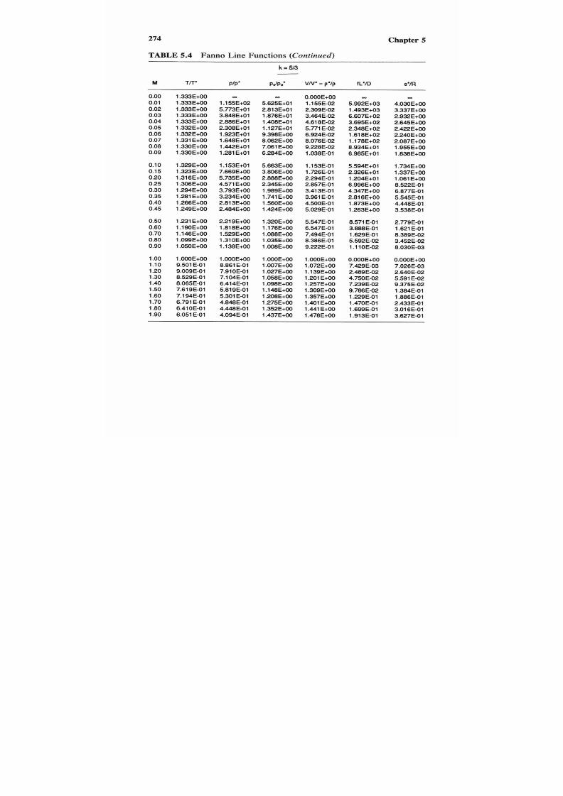
7/21/2019 Fundamental Fluid Mechanics for Engineers
http://slidepdf.com/reader/full/fundamental-fluid-mechanics-for-engineers 297/438
274
Chapter
5
TABLE 5.4
Fanno Line Functions
(Continued)
M
0.00
0.01
0.02
0.03
0.04
0.05
0.06
0.07
0.08
0.09
0.10
0.1
5
0.20
0.25
0.30
0.35
0.40
0.45
0.50
0.60
0.70
0.80
0.90
1oo
1.10
l20
1.30
1.40
1.50
1.60
1.70
1.80
1.90
T P
1.333E+00
1.333E+00
1.333E+00
1.333E+00
1.333E+00
1.332E+00
1.332E+00
1.331 E+OO
1.330E+00
1.330E+00
1.329E+00
1.323E+00
1.316E+00
1.306E+00
l294E+00
1.281 E+OO
1.266E+00
1.249E+00
1.231 E+OO
1.190E+00
1.146E+00
1.099E+00
1.050E+00
1OOOE+OO
9.501 E-01
9.009E-01
8.529E-01
8.065E-01
7.619E-01
7.1 94E-01
6.791 E-01
6.41 OE-01
6.051 E-01
PIP'
k
=
513
PdPo*
1.155E+02
5.773E+01
3.848E+01
2.886E+01
2.308E+01
1.923E+01
1.648E+01
1.442E+01
1.281 E+01
0 0
1.l3E+01
7.669E40
5.735E40
4.571 E+OO
3.793E+00
3.234E+00
2.81 3E+00
2.484E+00
2.219E40
1 81 8E+00
1.529E+00
1.31 OE+OO
1.l8E+00
1.000E+00
8.861 E41
7.910E-01
7.1 04E-01
6.414E-01
5.819E-01
5.301 E-01
4.848E-01
4.448E-01
4.094E-01
5.625E+Ol
2.81 3E+01
1.876E+Ol
1.408E+01
1.127E+01
9.398E+00
8.062E+00
7.061 E+OO
6.284E+00
OD
5.663E+W
3.806E+00
2.888E+00
2.345E+00
1.989E+00
1.741 E+OO
1.560E+00
1.424E+00
1.320E+00
1.l6E+W
1.088E+00
1.035E+00
1.008E+00
1.000E+00
1.007E+00
1.027E+00
1.058E+00
1.098E+00
1.148€+00
1.208E+00
l275E+00
1.352E+00
1.437E+00
VN' = p /p
0.000E+00
1.155E-02
2.309E-02
3.464E-02
4.61 8E-02
5.771 E-02
6.924E-02
8.076E-02
9.228E-02
1.038E-01
1.153E-01
1.726E-01
2.294E-01
2.857E-01
3.41 3E-01
3.961 E-01
4.500E-01
5.029E-01
5.547E-01
6.547E-01
7.494E-01
8.386E-01
9.222E-01
1.000E+00
1.072E+00
1.l9E+00
1.201 E+OO
1.257E+00
1.309E+00
1.357E+00
1.401 E+OO
l441 E+OO
1.478E+00
fL*m
0 0
5.992E+03
1.493E+03
6.607E+02
3.695E+02
2.348E+02
1.61 8E+02
1.178E+02
8.934E+01
6.985E+01
5.594E+Ol
2.326E+01
1.204E+01
6.996E+00
4.347E+00
2.81 6E+00
1.873E+00
1.263E+00
8.571 E41
3.888E-01
1.629E-01
5.592E-02
1.110E-02
0.000€+00
7.429E-03
2.489E-02
4.750E-02
7.239E-02
9.786E-02
1.229E-01
1.470E-01
1.699E-01
1.913E-01
4.030E+00
3.337E+00
2.932E+00
2.645E+00
2.422E+00
2.240E+00
2.087E+00
1.955E+00
1.838E+00
OD
1.734E+00
1.337E+00
1.061 E+OO
6.877E-01
8.522E-01
5.545E-01
4.448E-01
3.538E-01
2.779E-01
1.621 E-01
8.389E-02
3.452E-02
8.030E-03
0.000E+00
7.026E-03
2.640E-02
5.591 E-02
9.375E-02
1.384E-01
1.886E-01
2.433E-01
3.01 6E-01
3.627E-01
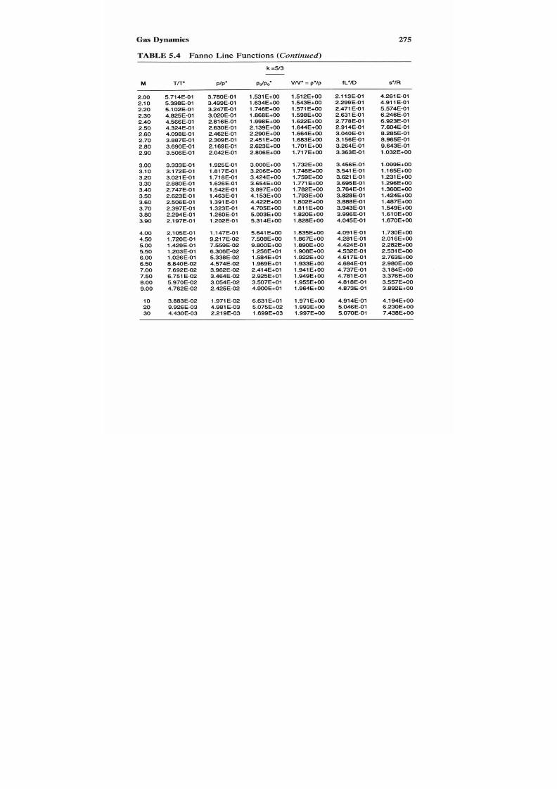
7/21/2019 Fundamental Fluid Mechanics for Engineers
http://slidepdf.com/reader/full/fundamental-fluid-mechanics-for-engineers 298/438
Gas Dynamics 275
TABLE
.4
Fanno
Line
Functions (Continued)
k
=5/3
-
M TIT' PIP' p&< VN ' =
p lp fL'/D s'lR
2.00
2.10
2.20
2.30
2.40
2.50
2.60
2.70
2.80
2.90
3.00
3.10
3.20
3.30
3.40
3.50
3.60
3.70
3.80
3.90
4.00
4.50
5.00
5.50
6.00
6.50
7.00
7.50
8.00
9.00
10
20
30
5.71 4E-01
5.398E-01
5.1 02E-01
4.825E-01
4.566E-01
4.324E-01
4.098E-01
3.887E-01
3.690E-01
3.506E-01
3.333E-01
3.1 72E-01
3.021 E-01
2.88OE-01
2.747E-01
2.623E-01
2.506E-01
2.397E-01
2.294E-01
2.1 97E-01
2.1 05E-01
1.720E-01
1.429E-01
1.203E-01
1.026E-01
8.84OE-02
7.692E-02
6.751 E-02
5.970E-02
4.762E-02
3.883E-02
9.926E-03
4.430E-03
3.78OE-01
3.499E-01
3.247E-01
3.02OE-01
2.816E-01
2.63OE-01
2.462E-01
2.309E-01
2.169E-01
2.042E-01
1.925E-01
1.817E-01
1.71 8E-01
1.626E-01
1.542E-01
1.463E-01
1.391 E-01
1.323E-01
1.260E-01
1.202E-01
1.147E-01
9.217E-02
7.559E-02
6.306E-02
5.338E-02
4.574E-02
3.962E-02
3.464E-02
3.054E-02
2.425E-02
1g71 E-02
4.981 E-03
2.219E-03
1.531 E+OO
l634E+00
1.746E+00
1.868E+00
1.998E+00
2.139E+00
2.290E+00
2.451 E+OO
2.623E+00
2.806E+00
3.000E+00
3.206E+OO
3.424E+00
3.654E+00
3.897E+00
4.1 53E+00
4.422E+00
4.705E+00
5.003E+00
5.31 4E+00
5.641 E+OO
7.508E+00
9.800E+00
1.256E+01
1.584E+01
1.969E+01
2.414E+01
2.925E+01
3.507E+01
4.900E+01
6.631 E+01
5.075E+02
1.699E+03
1.51 2E+W
1.543E+00
1.571 E+OO
1.598E+00
1.622E+OO
1.644E+00
1.664E+00
1.683E+OO
1.701 E+OO
l
717E+00
1.732E+OO
1.746E+00
1.759E+00
1.771 E+OO
1.782E+00
1.793E+OO
1.802E+00
1B1 1 E+OO
1.820E+00
1.828E+00
1.835E+00
1.867E+00
1.89OE+OO
1.908E+00
l922E+00
1.933E+00
1g41 E+OO
1.949E+00
1.955E+00
1.964E+00
l
g71E+OO
1.993E+00
1.997E+00
2.1 13E-01
2.299E-01
2.471 E-01
2.631 E-01
2.778E-01
2.914E-01
3.040E-01
3.156E-01
3.264E-01
3.363E-01
3.456E-01
3.541 E-01
3.621 E41
3.695E-01
3.764E-01
3.828E-01
3.888E-01
3.943E-01
3.996E-01
4.045E-01
4.091 E41
4.281 E-01
4.424E-01
4.532E-01
4.617E-01
4.684E-01
4.737E-01
4.781 E-01
4.81 8E-01
4.873E-01
4.914E-01
5.046E-01
5.070E-01
4.261 E-01
4.911E-01
5.574E-01
6.246E-01
6.923E-01
7.604E-01
8.285E-01
8.965E-01
9.643E-01
1.032E+OO
1.099E+00
1
.l
5E+OO
1.231 E+OO
1.296E+00
1.36OE+OO
1.424E+00
1.487E+00
1.549E+00
1.61 OE+OO
1.670E+00
1.730E+00
2.01 6E+00
2.282E+00
2.531 E+OO
2.763E+00
2.980E+00
3.1 84E+00
3.376E+00
3.557E+00
3.892E+00
4.1 94E+00
6.230E+00
7.438E+00

7/21/2019 Fundamental Fluid Mechanics for Engineers
http://slidepdf.com/reader/full/fundamental-fluid-mechanics-for-engineers 299/438
6.1 INTRODUCTION
Standard dimensionless numbers are developed for use in model testing
by two methods. The first is the force ratio method and the second is
Buckingham’s
II
theorem.
A
very formal procedure and formatfor using
the later method is provided in the event that the reader could use it in
some practical application.
This chapter ma y be sk ipped by rea ders wh o are either familiar with
or have
no
interest in this subject.
This chapter may be used as a text for tutorial or for refresher purposes.
Algebra is highest levelf mathematics needed.There are 14 tutorial-type
examples of fully solved problems.
6.2 DIMENSIONLESS
PARAMETERS
Modem fluid mechanics s based ona combination of theoretical analysis
and experimental ata. Very often, the engineer is faced with he necessity
of obtaining dependable, practical esults
in
situations where for various
reasons the flow phenomenacannot be described mathematically and ex-
perimental data must be considered. The generation and use of dimen-
sionless parameters provide a powerful and useful tool in1) reducing the
number of variables requiredor an experimental program,2) establishing
276

7/21/2019 Fundamental Fluid Mechanics for Engineers
http://slidepdf.com/reader/full/fundamental-fluid-mechanics-for-engineers 300/438
Dimensionless 277
the principles of model design and testing,(3) developing equations, and
(4)
converting data from one system of units to another. Dimensionless
parameters
may
be generated by
(1)
physical equations,
(2) principles of
similarity, and (3) imensional analysis.
All physical equations should be dimensionally correct,
so
that a di-
mensionless parameter may be generated by simply dividing oneside of
the equation by the other, as will be illustrated. The principles of similarity
are used to develop dimensionless parameters for model-prototype re-
lations to insure geometric, kinematic, and dynamic similarity by con-
sideration of dimensions, velocities, andorces involved between he two.
Dimensional analysis
is the mathematics of dimensions and quantities.
Two formal methodsare used, the Lord Rayleigh’s and the Buckingham
IItheorem. Lord Rayleigh
(1842-1919),
who was born ohn William Strut
in Essex, England, popularized the principle of dynamic similarity by
introducing in 1899 a generalization of the principle. Edgar Buckingham
(1867-1940) was
a
physicist at the National Bureau of Standards. In a
series of papers published in
1914
and
1915
he brought o American notice
the uses of dimensional analysis and presented his
Il
theorem.
6.3 PHYSICAL EQUATIONS
Good engineering practice demands that all physical equations be di-
mensionally consistent. All terms in an equation must have the same
dimensions. Dissimilar quantities cannot be added or subtracted when
forming a true physical equation. For example,
coffee + eggs + bacon
+
toast = breakfast
may be true, but this is not the type of relationship being considered.
Dimensionless parameters may be derived by simply dividingone side
of any physical equation by he other. A minimum of two dimensionless
parameters will be formed, one being the inverse of the other.
Example 6.1 What two dimensionless numberswill be formed by divid-
ing the equation for the velocity of sound by itself?
Solution
c =
P
(1.68)
( 4
n
7/21/2019 Fundamental Fluid Mechanics for Engineers
http://slidepdf.com/reader/full/fundamental-fluid-mechanics-for-engineers 301/438
278
N2 =
C
Chapter 6
N1 = NF'
Both N I and
N Z
re velocity ratios.
6.4 MODELS VS. PROTOTYPES
There are many times whenfor economic or other reasons it is desirable
to determine the performance of a structure or machine by testingnother
structure or machine. This type of testing is called model testing. The
structure or machine being tested is called the model and the structure
whose performance is to be predicted is called the prototype. A model
may be smaller than, the same size as, or larger than the prototype.
Model experiments on airplanes, rockets, missiles, pipes, ships, canals,
turbines, pumps, and other structures and machines have resulted in sav-
ings that more than justified the expenditure of funds for the design, con-
struction, and testingof the model. Under some ituations, the model and
prototype may be the same piece of equipment, for example, the cali-
bration of a flow meter with water in a laboratory to predict its perfor-
mance when metering steam. Many manufacturers of fluid machinery
have test equipment that is limited to one or two fluids andare forced to
test with what they have available in rder to predict performanceunder
other conditions.
6.5
GEOMETRIC SIMILARITY
Geometric similarity xists between model and rototype when the ratios
of all corresponding dimensions in the model and prototype are equal.
These ratios may be written:
Figure 6.1 shows a pipe whose length is
,
internal diameter is
D ,
and
absolute surface roughness is E. Standard values of E and EIDare given
in Table C-3for wrought steel and iron pipe, Table C-4 for 250 psi cast
iron pipe, and Table C-5for seamless copper water tube.

7/21/2019 Fundamental Fluid Mechanics for Engineers
http://slidepdf.com/reader/full/fundamental-fluid-mechanics-for-engineers 302/438
Dimensionless 279
f
D
E
is the average absolute
surface roughnessof the
piping material
Figure 6.1 Notation for geometric similarity.
Example
6.2 It is desired to use a smaller pipeas a model for
a
standard
30-in. pipe. Available re sections of 3-in. schedule 40 wrought steel pipe,
10-in. 250 psi cast iron pipe, and l-in. type
K
seamless copper water tube.
For geometric similarity, which section should be used as the model?
What should be the length of the model if the prototype length is 100 ft
(30.48 m)?
Solution
1. Common data
~
Internal diameterRoughness
Pipeizee ft (mm) EID X lo6
30 in. Std. c-3 2.438
(742.9)
61 S 3
3 in. Schedule 40
c-3 0.2557
(77.82)
588.6
10 in. 250 psi
c-4 0.8517
(259.5)
998.0
1 in. Type K
c-5 0.08292
(25.28)
60.30
Source

7/21/2019 Fundamental Fluid Mechanics for Engineers
http://slidepdf.com/reader/full/fundamental-fluid-mechanics-for-engineers 303/438
280
Chapter
6
2. Criteriu fo r selection
There are three length variables to be consider for geometric similarity:
L ,
D ,
and E. These variables may be reduced to two length ratios, with
the common denominator being the internal pipe diameter
D .
The nu-
merical values ofhe first of these ratios
EID
is available from pipingables
as already shown.
Model (do),,, lo6
(EID), X
IO6
(EID)mI(EID)p
3 in. Schedule
40
steel 588.6 61.53 10
10 in. 250 psi cast iron
988.0
61 .S3 16
1
in. Type K copper
60.30
61S3 1
Pipe
Pipe
water tube
The only way that the first two pipes could be used for geometric
similarity would be to machine their internal surfaces to achieve the re-
quired relative smoothness
ID
of
61.53.
The seamless opper water pipe,
on the other hand, has almosthe required relative smoothness and should
be used.
3.
Model length
For
similarity, the
LID
ratio
of
the model must equal he
LID
ratio
of
the
prototype, or:
(LID),
= 100/2.438 = (30.48)/(742.9 X
=
41 (a)
L ,
=
(L/D)pDm
=
4 1 0 ,
(b)
US.
Units
L , =
41 x 0.08292
=
3.40 ft
S I Units
L,,, = 41 x 25.28
x
l o u 3
=
1.04
m
(b)
6.6
KINEMATIC
SIMILARITY
Kinematicsimilarity exists betweenmodeland prototype when their
streamlines are geometrically similar. Comparisonf the velocity profiles
of
Figure
6 .2
(a) with
(b)
and (c) indicates that (a) and
(b)
have kinematic
similarity, but
(a)
and (c) and (b) do not.

7/21/2019 Fundamental Fluid Mechanics for Engineers
http://slidepdf.com/reader/full/fundamental-fluid-mechanics-for-engineers 304/438
Dimensionless Parameters
281
(b) (c)
Figure 6.2 Notation for kinematic similarity.
Some
of
the more common kinematic similarity ratios are:
Acceleration
ar -
m L,T,-~
CL ,
L,T,
- - L , T , - ~ (6.3)
Velocity V, =
, L,T,
= L,T,
, L,T,-'
Volume flow rate Q r =
L?T,
m LLT,
Qp JZT,
Example
6.3 Ethanol at 68°F 20°C) is to flow in a tube with a 12 in. (300
mm) inside diameter and with an average velocity of
0.05
ft/sec
(15
mm/
S). Topredict the performance of the 12 in. (300 mm)ube, a geometrically
similar 4 in. (75 mm) tube is to be tested using 104°F (40°C) benzene. If
the flow in the 12 in. (300 mm tube) is laminar (kinematic viscosity de-
termines the velocity gradient), at what average velocity should he ben-
zene flow in the 3 in.
(75
mm) tube for kinematic similarity?

7/21/2019 Fundamental Fluid Mechanics for Engineers
http://slidepdf.com/reader/full/fundamental-fluid-mechanics-for-engineers 305/438
282
Chapter
6
Solution
When kinematic viscosity determines the velocity gradient, then for ki-
nematic similarity
Substituting equation (a) in equation (6.4),
V ,
=
L,T;'
=
L , ( V , L ; ~ )
= V,L;I = = (?)(?)
V P
From the definition of kinematic viscosity of equation (1.71),
v = g c p h (c)
Subsisting equationc)in equation(b), noting that the characteristic ength
is the diameter, and solving for V,,,:
US.
nits
From TableA- 1:
Ethanol at 68°F p = 49.44 ibm/ft3 pp = 23.87
x
lbf-sec/
ft2
Benzene at 104°F p,,, = 53.55 lbm/ft3 p,,, = 10.36 x lbf-
sec/ft2
(b)
,,,
=
0.05(10.36 X 10⁻⁶/23.87 X 10-6) 49.44/53.55) 12/3)
= 0.08 ft/sec
SI Units
From Table A-l:
Ethanol at
20°C
pp
=
791.9
kg/m3
pp
=
1
143
x
Pa-s
Benzene at 40°C
p,,,
= 857.7
kg/m3
p,,,
= 496 x 10-6 Pa.s
V m = 15(496 X
10-6/1
143 X
10-6)(791.9/857.7)(300/75)
= 24 mmls
(dl

7/21/2019 Fundamental Fluid Mechanics for Engineers
http://slidepdf.com/reader/full/fundamental-fluid-mechanics-for-engineers 306/438
Dimensionless 283
6.7 DYNAMIC SIMILARITY
To
maintain geometric and kinematic similarity, it is necessary to have
dynamic
or
force similarity. Consider the model-prototype relations for
the flow around the object shown in Figure
6.3.
For geometric similarity,
For kinematic similarity,
- = - =
A m U B m
U A p U B p
V r
(6.4)
F1
Figure 6.3
Notation
for
dynamic acceleration.

7/21/2019 Fundamental Fluid Mechanics for Engineers
http://slidepdf.com/reader/full/fundamental-fluid-mechanics-for-engineers 307/438
284 Chapter 6
Consider next the forces acting on pointC of Figure 6.3 without spec-
ifying their nature. From the geometric similarityof their vector polygons
and Newton's law, which f course applies to both model andprototype.
for dynamic similarity,
For dynamic similarity, these force ratios must be maintained on all
corresponding fluid particles throughouthe flow pattern. From the force
polygon of Figure 6.3, noting that forces are vectors (the symbol c de-
notes vector addition), it is evident that
Examination of equation (6.7) s well as the force polygon of Figure
(6.3) eads to the conclusion that if three of the four terms are known,
the other may be determined. This leads to a more general conclusion
that dynamic similaritymay becharacterized by an equality f force ratios
numbering one less than the total number of forces involved. Any force
ratio may be eliminated depending upon he quantities which are desired
in the equations. For total model-prototype force ratio, comparisons of
force polygons yield
Fluid Forces
The fluid forces that are considered here are those acting on a fluid ele-
ment whose mass = pL3, area = L 2 , length = L , and velocity = (LIT) .
Inertia for ce Fi =
(mass)
X
(acceleration)
( p L 3 ) ( L / P )
proportionality constant
-
gc (6.9)
gc
Viscous
force
F , = (viscous shear stress) X (shear area)
(6.10)
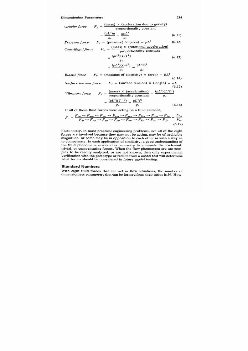
7/21/2019 Fundamental Fluid Mechanics for Engineers
http://slidepdf.com/reader/full/fundamental-fluid-mechanics-for-engineers 308/438
Dimensionless
285
Gravity fo rce g =
(mass) x (accleration due to gravity)
proportionality constant
(6.11)
Pressure fo rc e FP = (pressure)
X
(area) = pL2 6.12)
Centrifugal fo rce F,,, =
(mass) x (rotational acceleration)
proportionality constant
Elastic fo rc e FE = (modulus of elasticity) x (area) = EL2
Surface ension fo rc eF , = (surface ension) X (length) = uL
(6.14)
(6.15)
Vibratory for ce F
-
(mass)
x
(acceleration)
-
( p L 3 ) ( L / P )
-
proportionality constant
-
g c
(6.16)
If all of these fluid forces were acting on a fluid element,
F,
=
Fim * F W * gm * Fpm * Fmm * E m * um * fm - Fim
Fip * Fpp * gp * Fpp * Fop * FE^ * Fop * Ffp Fip
(6.17)
Fortunately, in most practical engineering problems, not allof the eight
forces are involved because they may not be acting, may bef negligible
magnitude, or some may be in opposition o each other in such
a
way as
to compensate. In each application of similarity,a good understanding of
the fluid phenomena involved is necessary to eliminate the irrelevant,
trivial, or compensating forces. When the flow phenomena are too com-
plex to be readily analyzed, or are not known, then only experimental
verification with he prototype or results from
a
model test will determine
what forces should be considered in future model testing.
Standard Numbers
With eight fluid forces that can act in flow situations, the number of
dimensionless parameters that can be formed fromheir ratios is 56. How-

7/21/2019 Fundamental Fluid Mechanics for Engineers
http://slidepdf.com/reader/full/fundamental-fluid-mechanics-for-engineers 309/438
286 Chapter 6
ever, conventional practice is to take the ratio of the inertia force to the
other fluid forces, because the inertia force is the vector sum of all of he
other forces involved in a given flow situation. Results obtained by di-
viding the inertia force by each of the other forces are shown in Table
6.1 compared with the standard numbers that are used in conventional
practice.
Example
6.4
A seaplane is to take off at 80 mph (129 km/h). At what
speed should a 1/60 model be towed to insure similarity of inertia and
gravity forces?
Solution
From Table 6.1 it is evident that
for
similarity of the inertia and gravity
forces the Froude number of the model and the prototype must be the
same or
V
= (G),,, = (G),
V
which reduces to
US.
nits
V,,, = 0.1291
x
80
=
10.33mph
SIUnits
V,,,
=
0.1291
X
129
=
16.65km/h
6.8 VIBRATION
In the flow of fluids aroundobjects and in he motion of bodies immersed
in fluids,
vibration may
occur because of the formation of a wake caused
by alternate shedding of eddies in a periodic fashion or by the vibration
of the objector the body. The Strouhal number S is the ratio of the velocity
of vibration L7 to the velocity of the fluid
V.
Since the vibration may be
fluid induced
or
structure induced, two frequencies mustbe considered,
the wake frequency f,, and the natural frequency of the structure
f,,.
Fluid-induced forces are usually of small magnitude, but as the wake
frequency approaches the natural frequency f the structure, the vibratory
forces increase very rapidly. When f, =
f,,,
the structure will go into

7/21/2019 Fundamental Fluid Mechanics for Engineers
http://slidepdf.com/reader/full/fundamental-fluid-mechanics-for-engineers 310/438
Dimensionless
287
resonance and fail. This imposeson the model designer he requirement
of matching to scale the natural frequency characteristics of the prototype.
All further discussions of model-prototype relations are made under the
assumption either that vibratory forces are absent or that they are taken
care of in the design of the model or in the test program.
6.9
SIMILARITY OF INCOMPRESSIBLE FLOW
This section considers the flow of incompressible fluids around anbject,
the motion of immersed bodies in incompressible fluids, and he flow of
incompressible fluids in conduits. It includes, for example, a submarine
traveling under water but not partly submerged. It also includes aircraft
moving in atmospheres that may be considered incompressible.
In these situations, the gravity force, although acting on all fluid par-
ticles, does not affect the flow pattern. Except for rotating machinery,
which is considered in a later section, centrifugal forces are absent. By
definition of an incompressible fluid,elastic forces are zero. Since there
is no liquid-gas interface, surface tension forces are absent. This leaves
inertia, viscous, and pressure forces acting. With these forces acting, the
flow can be characterized by two dimensionless parameters. Using tan-
dard numbers, these are the Reynolds number and the Euler number.
Reynolds Number
This number was named in honor of Osborne Reynolds
(1842-1912),
an
English engineer who developed it analytically and verified itby exper-
iments. In Section
6.7,
Table
6.1,
the Reynolds number was derived as:
R =
nertia force pLV
viscous force Kgc
(6.18)
Noting from he definition of kinematic viscosity in equation1.71) that
p
= vp/gc , we can now write:
(6.19)
Euler Number
This number was named in honor of Leonhard Euler
(1707-1783).
Con-
ventional practice (Table
6.1)
is to use the pressure coefficient, which is
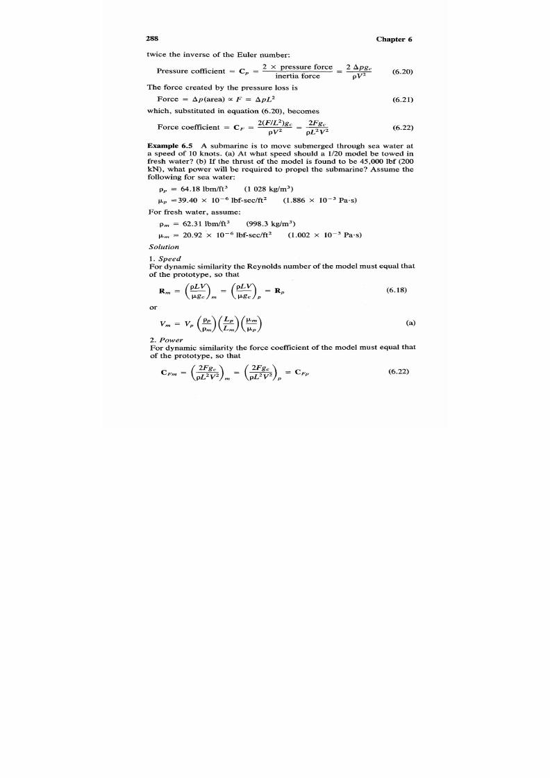
7/21/2019 Fundamental Fluid Mechanics for Engineers
http://slidepdf.com/reader/full/fundamental-fluid-mechanics-for-engineers 311/438
288
Chapter
6
twice the inverse of the Euler number:
Pressure cofficient = C , =
2
X
pressure force
-
2
Apg,
nertia force PV2
(6.20)
The force created by the pressure loss is
Force
=
Ap(area)
a F
= ApL2
(6.21)
which, substituted in equation (6.20), becomes
Force coefficient =
C F
=
2(F/L2)gcFgc
PV2
p L 2V
= -
(6.22)
Example 6.5
A submarine is to move submerged through sea water at
a speed of 10 knots. (a) At what speed should a 1/20 model be towed in
fresh water? (b) If the thrust of the model is found to be 45,000 lbf (200
kN),
what power will be required to propel the submarine? Assume the
following for sea water:
pp = 64.18 lbm/ft3 1028 kg/m3)
p p =39.40
x
1 O j lbf-sedft' (1.886 X Pa.$
For fresh water, assume:
pm = 62.31 lbm/ft3
(998.3
kg/m3)
p m = 20.92 x IOm6 lbf-sec/ft2 (1.002 x Pa-s)
Solution
1.
Speed
For dynamic similarity he Reynolds number f the model must equalhat
of the prototype,
so
that
or
(6.18)
2.
Power
For dynamic similarity he force coefficient of the model must equal hat
of the prototype, so that
(6.22)

7/21/2019 Fundamental Fluid Mechanics for Engineers
http://slidepdf.com/reader/full/fundamental-fluid-mechanics-for-engineers 312/438
Dimensionless 289
or
The power required to propel the submarine is computed using equation
(4.87):
P, = FpV,
(C)
US. nits
From Table
B.l,
V ,
=
10
x
1.6878
=
16.88 ft/sec.
1.Model towing speed
=
( G ) ( T ) (
64.1800.92 x
39.40
x
2. Po wer required to prop el the submarine
F P
= 45,000
( G ) ( T ) * ( G ) =
155,023
64.1806.88
P , = 155,023 x 16.88
=
2 . 6 1 6 ~
o6
ft-lbf/lbm
= 2.617X lO6/55O = 4,757 hp
SI Units
From Table B.l, V,
=
10~0.51444
=
5.144
m/s.
1.Model towing speed
2. Po wer required to prop el the submarine
F, = 200 000 K)028 (i)'0
(E)
.144 = 688 201
P ,
=
687 149 x 5.144 = 3 534 693 W
=
3 534 kW
6.10 SIMILARITY OF COMPRESSIBLE FLOW
This section considers the flow of compressible fluids around anobject,
the motion of immersed bodies in compressible fluids, and the flow of
compressible fluids in conduits. It does not consider the flow of com-
pressible fluids in rotating machinery and aircraft during takeoffor after
landing.

7/21/2019 Fundamental Fluid Mechanics for Engineers
http://slidepdf.com/reader/full/fundamental-fluid-mechanics-for-engineers 313/438
290
Chapter 6
From the discussion given in Section 6.9, it is evident that the only
difference between compressible and incompressible flow is the elastic
force. This means that the ratio of the inertia to elastic forces,
or
Cauchy
number, must now be considered in addition to the Reynolds number.
The Cauchy number was namedo honor Baron Augustin Louisde Cau-
chy (1789-1857), a French engineer turned mathematician who contrib-
uted greatly to the analysis of wave motion.
In Section 5.3 he Mach number for an ideal gas was defined by equa-
tion (5.6) as:
Conventional practice is to use the square root of the Cauchy numberor
Mach number. From Table 6.1 he Mach number may be derived as
M =
inertia force
V
V
elastic force
a
T
(6.23)
Although equations (5.6) and (6.23)are identical in result, equation (6.23)
presents an elementary physical understandingf the Mach number phe-
nomena.
Example 6.6 A Gin. valve installed in a Schedule 80 wrought iron pipe
is designed to receive 12,400 Ibm/hr (1.56 kg/s) of hydrogen at 100 psia
(690 kPa) and 122°F
(50°C).
This value is to be tested with air under
dynamically similar conditions. When air is supplied at 122°F (20"C), he
pressure loss is found to be 5 Ibf/in.2 (34.5 kPa). Determinea) the velocity
of air supplied, (b) the air pressure, and (c) the estimated pressure loss
expected with the designed flow of hydrogen.
Solution
In this examplehe model andprototype are the same pieceof equipment,
the 6-in. valve. It is the prototype when hydrogen is flowing, and the
model when air is flowing.
For
dynamic similarity the model-prototype
relationship must satisfy the following:
Mach number similarity
Reynolds number similarity
Euler number similairty (pressure coefficient)
1. The air velocity for Mach number similarity
The velocity of the prototype may be computed fromhe continuity equa-
tion (3.15) for an ideal gas:
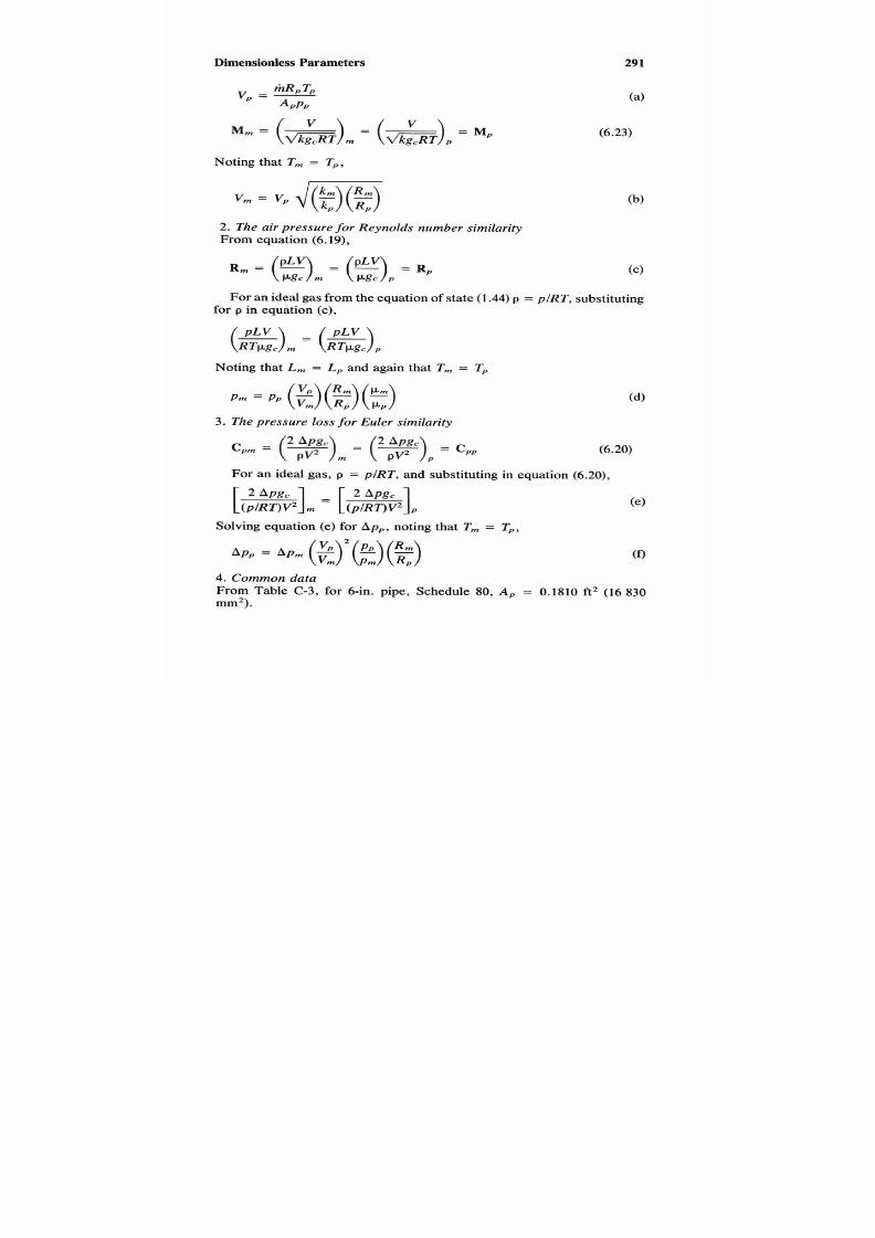
7/21/2019 Fundamental Fluid Mechanics for Engineers
http://slidepdf.com/reader/full/fundamental-fluid-mechanics-for-engineers 314/438
Dimensionless Parameters
*PTP
v, =
PPP
V
M m =
( m T ) m
= (d )p =
Noting that T ,
=
T p ,
2.
The air pressure fo r R eynolds num ber similarity
From equation (6.19),
PLV
291
(a)
(6.23)
For an ideal gas fromhe equation of state (1.44) p = p / R T , substituting
for p in equation (c),
Noting that L , = L P and again that T,,,
=
T,
3. The pressu re
loss
fo r Euler similarity
(6.20)
For an ideal gas, p
= p / R T ,
and substituting in equation (6.20),
Solving equation (e) for
b p p ,
noting that
T ,
=
T p ,
4.
Common data
From Table C-3, for 6-in. pipe, Schedule 80, A , = 0.1810 ft2 (16 830
mm2).

7/21/2019 Fundamental Fluid Mechanics for Engineers
http://slidepdf.com/reader/full/fundamental-fluid-mechanics-for-engineers 315/438
292
Chapter
6
US. nits
T,
=
T,,,
=
122
+
460
=
582"R
From Table A-l, for
H Z
M, = 2.016, and for air M,,, = 28.97.
From Table A-2 for
H z
at 122"F,
k , =
1.399 and
p,,
0.196 x
lbf-seclft2. For air at 122"F, k,,, = 1.401 and
p,,,,
= 0.410 x Ibf-sec/
ft2.
From
equation (1.43),
R = R,IM
R,,,
=
1545128.97
=
53.33ft-lbfI(lbm-'R)
R, = 154512.016 = 766.4 ft-lbf/(lbm-"R)
1. Velocity of the model V,,,
v,
=
(12,400/3600) x 766.4
x
582
=
589.5 ft/sec
0.1810(144
x
100)
Vm = 589.5
J(-)
.402
(-)
3.33 = 155.7 ft/sec
1.39966.4
2.
Model
air pressure
p,,,
P m = loo(E)( )0.196
X
10"j
=
55.11 psia (dl
589.53.33.410
x
3. Prototype pressure loss b p ,
Ap,
=
5
=
9.05 psia
SI
Units
Tp = T m
=
50 + 273
=
323K
From Table A-l, for H ZM, = 2.016, and
for
air M,,, = 28.97. From
Table A-2 for H Zat 50"C, k , = 1.399 and
pp
= 9.4
x
Pass. For air
at 50"C, km = 1.401 and p,,,, = 1.96 x Pavs.
From equation (1.43),
R = R,IM
R,,, =
8314128.97 = 287.0 J/(kg*K)
R, = 831412.016 = 4124 Jl(kg.K)
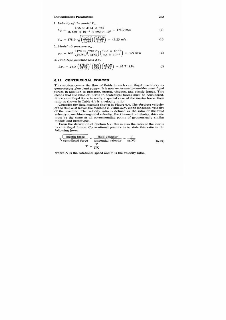
7/21/2019 Fundamental Fluid Mechanics for Engineers
http://slidepdf.com/reader/full/fundamental-fluid-mechanics-for-engineers 316/438
Dimensionless Parameters
293
1. Velocity
of
the model
V,,,
1.56
x
4124
x
323
1630
X X
690
X lo3
v, =
=
178.9
mls
V,,,
=
178.9
J =)r=)
.399 4124
=
47.23
mls
2. Model air pressure p m
3. Prototype pressure
loss
h p ,
Ap, = 34.5
(g)*( )(=)
90 287.0 = 62.71 kPa
6.11
CENTRIFUGAL FORCES
This section covers the flow of fluids in such centrifugal machinery as
compressors, fans, and pumps. t is now necessary o consider centrifugal
forces in addition to pressure, inertia, viscous, and elastic forces. This
means that the ratio of inertia to centrifugal forces must be considered.
Since centrifugal force is really a special case of the inertia force, their
ratio as shown in Table 6.1 is a velocity ratio.
Consider the fluid machine shown in Figure 6.4. Thebsolute velocity
of the fluid as it leaves the machine
is
V and wD/2 ishe tangential velocity
of
the machine. The velocity ratio is defined as the ratio of the fluid
velocity to machine tangential velocity.or kinematic similarity, thisatio
must be the same at all corresponding points of geometrically similar
models and prototypes.
From the derivation of Section 6.7, this s also the ratio of the inertia
to centrifugal forces. Conventional practice is to state this ratio in the
following form:
fluidelocity V
centrifugal force tangentialelocitywD/2
= -
(6.24)
V
v=-
DN
where
N
is the rotational speed and
V
is the velocity ratio.

7/21/2019 Fundamental Fluid Mechanics for Engineers
http://slidepdf.com/reader/full/fundamental-fluid-mechanics-for-engineers 317/438
294
Chapter 6
Absolute fluid
the runner
Tangential velocity
Figure 6.4 Notation for velocity ratio.
Substituting equation6.24) for
V
in equation (6.23), we obtain for Mach
number:
(6.25)
Making the sam e substitution for Reynolds number in equation (6.18),
noting that the characteristic length is
D ,
(6.26)
Example 6.6 A centrifugal com pressor is to com press methane delivered
to
it
at atmospheric pressure and 122°F (5OOC). The com pressor has an

7/21/2019 Fundamental Fluid Mechanics for Engineers
http://slidepdf.com/reader/full/fundamental-fluid-mechanics-for-engineers 318/438
Dimensionless 295
impeller diameter of12 in. (300 mm) and rotates at 100
rps.
It is proposed
to test a geometrically similar 3-in.75 mm) compressor with
air
The air
source is 32°F
(OOC)
and
5
atmospheres. At what speed should he model
be tested for dynamic similarity?
Solution
Thisexample
is
solvedby first determining the rotationalspeed for
Reynolds number similarity and then checkingo see that the air source
pressure is sufficient to obtain Mach number similarity t the calculated
model rotational speed.
1. Determine rotational speed fo r Mach number similarity
or
(6.25)
2. Check air pressure o r Reynolds number similarity
From equation (1.44) for an ideal gas p =
p / R T
and substituting in
equation (b)
,
or
U . S . Units
Tp
=
122 + 460 = 582"R T , = 32 + 460 = 492"R
Table A-l for CH 4, MP = 16.043; for air
M,
=
28.97. From Table A-2
for CH4at 122"F, k p
=
1.293 and p p = 0.248
x
lbf-sec/ft2; or
air

7/21/2019 Fundamental Fluid Mechanics for Engineers
http://slidepdf.com/reader/full/fundamental-fluid-mechanics-for-engineers 319/438
296 Chapter 6
at 32"F, km
=
1.401 and
=
0.360 X lbf-sec/ft2. romquation
(1.43):
R = R, /M
R ,
=
154Y28.97 = 53.33 t-lbf/(lbm-"R)
R , = 1545A6.043 = 96.30ft-lbfl(1bm-"R)
1.
Determine rotational speed for Mach umber similarity
Nm
loo
(Y)
d EiiJ G) 582)
=
285rPs
1.4013.3392
2. Check air pressure for Re yno ldsnum ber similarity
P m =
1
x
100.360
x
53.3392
285.248
X
=
3.8 at mos
Air
can be throttled down from
5
atmospheres.
SI
Units
Tp = 50
+
273
=
323 K
T ,
= 0
+
273 = 273 K
From TableA-l for C H 4 ,M ,
=
16.043; for air M , = 28.97. From Table
A-2, for CH4 at 20"C, k p = 1.293and p = 11.9 x Pass; for air at
O T ,
km
=
1.401 and
p
17.2
x
Pass.Fromequation (1.43):
R
=
R,IM
R ,
=
8314128.97
=
287.0
J/(kg-K)
R P = 8314116.043
=
518.2 J/(kg.K)
1.
Determine rotational speed or M ac hnum ber similarity
N m
= loo
0
(E ic2)(323)
=
285rPs
1.40187.073
2. Check air pressure fo r Reyn olds num ber similarity
Pm
= x
(F)*(%(
1.9
x
10-6)
518.2)323)
007.2
x
287.073
= 3.8 atoms
Air
can be throttled down from
5
atmospheres.

7/21/2019 Fundamental Fluid Mechanics for Engineers
http://slidepdf.com/reader/full/fundamental-fluid-mechanics-for-engineers 320/438
Dimensionless Parameters
297
6.12
SIMILARITY OF LIQUID SURFACES
This sectionconsiders flow at liquid-gas interfaces. It includes ships, sea-
planes during take-off, submarines partly submerged,iers, dams, rivers,
spillways, harbors, etc. Resistance at liquid surfaces is due to surface
tension and wave action. Since wave action is due to gravity, we now
consider the remaining force ratios discussed in Section 6.7.
Surface tension, as was stated in Chapter
1,
enables the fluid to support
a very small tensile force. It is generally a minor property in fluid me-
chanics and exerts a negligible effect on wave formationxcept when the
waves are small, say less than 1 in. (25 mm). Thus, the effects of surface
tension on
a
model might be considerable, but not on the prototype.
To
avoid this type of “scale effect” surface tension should be considered.
The ratio of inertia to surface tension forces is known as the Weber
number, in honor of Moritz Weber 1871-1951), a professor of naval me-
chanics at the Polytechnic Institute of Berlin, who first formulated this
number. From the derivation in Section 6.7,
inertia force
pLV2
surface tension force ug,
=
“
(6.27)
The effect of wave resistance is very important in obtaining similarity
at liquid surfaces. The ratio of the inertia to gravity forces is usually
considered in its square root form. In this form, it is called the Froude
number, in honor of William Froude (1810-1879), an Englishman who
developed many towing-tank techniques, particularly the conversion of
wave and boundary layer resistance from model to prototype scale. It is
one of the ironies of history that Froude’s name s inseparably associated
with a law of similarity andnumber, the first of which he did not originate
and the second of which he never used. His very great contribution to
boundary layer research is relatively unknown outside the field of naval
architecture. From the derivation of Section 6.7,
F =
J
nertia force V
gravity force
“
(6.28)
As
will be seen in the two examples o follow, it is usually impractical
to obtain complete dynamic similarity in model-prototype arrangements
when liquid surfaces are involved.
Example 6.7
An ocean vessel 500ft (152.4 m) long is to travel at
a
speed
of
15
knots. A 1/25 model of this ship is to be tested in
a
towing tank
using
sea
water at design temperature. Determine (a) the model speed

7/21/2019 Fundamental Fluid Mechanics for Engineers
http://slidepdf.com/reader/full/fundamental-fluid-mechanics-for-engineers 321/438
298
Chapter
6
required for wave resistance similarity, (b) viscous or skin friction simi-
larity, (c) surface tension similarity, and (d) the model size required for
complete dynamic similarity.
Solution
The model speed for wave resistance requires equality of Froude num-
bers. The speed for skin friction equires Reynolds number similarity and
for surface tension similarity requires Weber number equality.
1. Wave resistance similarity
V
= ( d m ( )p =
or
V,,, = V ,6
15 &
=
3
knots
2. Skin friction similarity (sam e fluid -sam e tem pera ture )
or
=
R,
=
15(1)(7)(1) =
375 knots
3. Surfac e tension similarity (sam e fluid -sam e tem pera ture)
pLV2
pLV2
=(x),,,
(x)WP
or
4.
Co m plete similarity
For Reynolds and Froude number similarity, setting equation (b) equal
to equation (a),

7/21/2019 Fundamental Fluid Mechanics for Engineers
http://slidepdf.com/reader/full/fundamental-fluid-mechanics-for-engineers 322/438
Dimensionless Parameters
299
which reduces to
For the same fluid, L,/L, =
1, or
model and prototype must be the
same size. No practical way has been found o model for complete simi-
larity. Engineeringpractice is to model for wave resistance and to correct
by calculation for skin friction resistance.
Example 6.8 A U256 model of a reservoir is drained in
5
min by opening
the sluice gate. How long should it take to empty the prototype?
Solution
Since, from priordiscussion, complete dynamic similarity annot be ob-
tained, it is evident in this case that although viscous forces must be
present the dominating forces are inertia and gravity andhe Froude num-
ber should be used for similarity. From equation (6.28),
From equation (6.4),
V ,
=
L,T, or
(g),
(h),
Substituting equation (b) in equation (a),
or
6.13
DIMENSIONAL ANALYSIS
Dimensional analysis s the mathematicsof dimensions and quantities and
provides procedural techniques whereby the variables that are assumed
to be significant in a problem can be formed into dimensionless param-
eters, the number of parameters being less than the number of variables.
This is a great advantage because fewer experimental runs are then re-

7/21/2019 Fundamental Fluid Mechanics for Engineers
http://slidepdf.com/reader/full/fundamental-fluid-mechanics-for-engineers 323/438
300 Chapter 6
quired to establish a relationship between the parameters than between
the variables. While the user is not presumed to have any knowledge of
the fundamental physical equations, the more knowledgeable the user,
the better the results. If any significant variable
or
variables are omitted,
then the relationship obtained from dimensional analysis will not apply
to the physical problem.On the other hand, inclusion of all possible vari-
ables will result in losinghe principal advantageof dimensional analysis,
that is, the reduction of the amount of experimental data required to es-
tablish relationships. Two formal methods of dimensional analysis are
used, the Method of Lord Rayleigh and Buckingham's II theorem.
Dimensions used in mechanicsare mass
M ,
lenth
L,
ime
T ,
and force
F . Corresponding engineeringunits for these dimensions are the pound
(kilogram), the foot (meter), the second (second), and the pound force
(Newton). Any system in mechanics can be defined by hree fundamental
dimensions. Two ystems are used, the force ( F L T )and the mass ( M L T ) .
In the force system mass is a derived quantity, and in the mass system
force is a derived quantity. Force and mass are related by Newton's law:
F =
(M/g, )LT-* and (Mlg , ) = FL
p.
ote that any quantity containing
a mass dimension must also containhe proportionality constantg,. Table
6.2
shows some common variables and their units and dimensions.
6.14 LORD RAYLEIGH'S METHOD
The method developed by Lord Rayleigh uses algebra to determine in-
terrelationships between variables. While this method may be used for
any number of variables, it becomes relatively complex and is not gen-
erally used for more than four. This method is most easily described by
the next two examples.
Example
6.9
In laminar flow, the unit shear stress T is some function of
the fluid dynamic viscosityp, he velocity gradient
dU,
and the distance
between laminae
dy.
Develop a relationship using the Lord Rayleigh
method of dimensional analysis.
Solution
1.
Write a functional relationship of the variables:
2.
Write a dimensional equation in the FLT or MLT system obtaining
data from Table
6.2:
( F L - * ) = f (FL-2T)u(LT- ' )b (L) (b)

7/21/2019 Fundamental Fluid Mechanics for Engineers
http://slidepdf.com/reader/full/fundamental-fluid-mechanics-for-engineers 324/438
Dimensionless Parameters
301
3. Solve the dimensional equation for exponents:
7
L d U dY Solution
Force F
l = a + O + O
a = 1
Length
L
-2 =
- 2 ~ b +
C
b =
- C
Time T O = a - b + O
b = 1
c =
-1
4.
Insert exponents in functional equation (a):
The functional relationshipcannot be obtained from dimensional anal-
ysis. Only physical analysis andlor experiments can determinehis. From
the physical analysis of Section 1.18, equation (1.70),
Example 6.10 The velocity of sound c n a gas depends upon fluid density
p, pressure
p ,
and dynamic viscosity
p.
Develop a relationship usinghe
Lord Rayleigh method'of dimensional analysis.
Solution
1.
2.
3.
Write a functional relationship of the variables
c = f [ ( P ~ g c ) "P b~ "1 ( 4
Write a dimensional equation in the
FLT
or
MLT
system obtaining
data from Table 6.2:
(FL ) = f(ML-3)"(ML"T-Z)b(ML-1T"l)c (b)
Solve the dimensional equationfor exponent:
c
P/&
P
P
Solution
Mass M
O =
a
+
b + c
LengthL
- 1
=
-3a
-
b
-
c
Time T
O = 0
- 2 b
- C
M + L
-1 = -2a
+
0 +
0
a = 112
L - T
-1
= - 3 a
+ b + O
M o = 112 - 112
+
c
c = o
-1 =
-3(112) + b + 0 b
=
- 112

7/21/2019 Fundamental Fluid Mechanics for Engineers
http://slidepdf.com/reader/full/fundamental-fluid-mechanics-for-engineers 325/438
302
Chapter 6
4. Insert exponents in functional equation (a):
Note that this analysis rejected viscosity, showinghat the velocity of
sound is involved in a frictionless process. Again we cannot determine
the functional relationship from dimensional analysis alone. From the
physical analysis of Section 1.16, equation (1.68),
For
an ideal gas from equation1.62), E , = k p , and substitutingn equation
( 4
compared with
f m
from dimensional analysis.
6.15
THE BUCKINGHAM
II
THEOREM
The Buckingham ll theorem serves the same purpose as the method of
Lord Rayleigh for deriving equations expressing one variable in termsf
its dependent variables. The ll theorem is preferred when the number of
variables exceeds four. Applicationof the theorem results in the formation
of
dimensionless parameters called IT ratios. These ratios have no relation
to 3.1416. Application of this theorem is illustrated in the following ex-
ample.
Example
6.11 Experiments are to be conducted with gas bubbles rising
in a still liquid. Consider a gas bubble of diameter D rising in a liquid
whose density is
p,
surface tension U viscosity p, ising with a velocity
of
V
in a gravitational field of
g.
Find a set of parameters for organizing
experimental results.
Solution
This example s solved as an integral partof the remainder of the text of
this section.
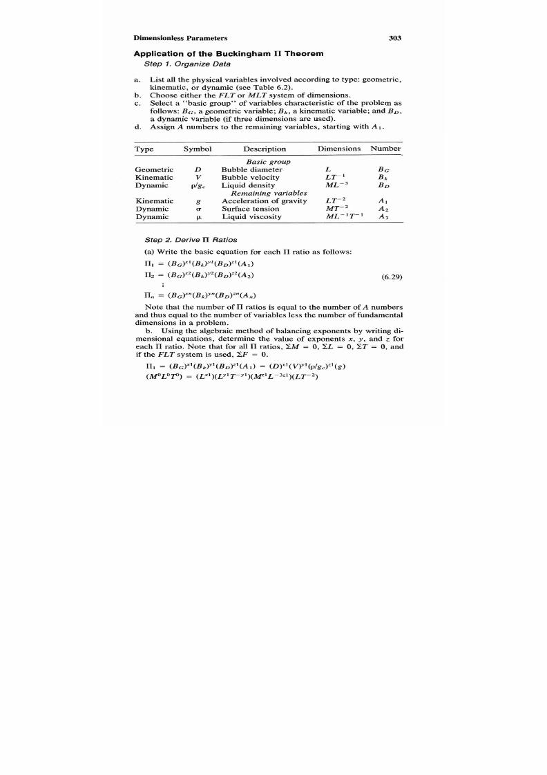
7/21/2019 Fundamental Fluid Mechanics for Engineers
http://slidepdf.com/reader/full/fundamental-fluid-mechanics-for-engineers 326/438
Dimensionless Parameters
303
Application
of
the Buckingham
ll
Theorem
Step
1.
Org anize Data
a.
List all the physical variables involved according o type: geometric,
b. Choose either the
FLT
or
MLT
system of dimensions.
c. Select a "basic group" of variables characteristic of the problem as
follows: B G , a geometric variable;B k , a kinematic variable; andB D ,
a
dynamic variable (if three dimensions are used).
kinematic, or dynamic (see Table 6.2).
d. Assign A numbers to the remaining variables, starting withA 1 .
Type Symbolescriptionimensionsumber
Basic group
Geometric
D
Bubbleiameter
L B G
Kinematic
V Bubbleelocity
L T - Bk
Dynamic p/gc Liquidensity
M L - 3
B D
Kinematic
g
Acceleration of gravity
LT-'
A1
Dynamic
U
Surface tension
M T - ~ A Z
Dynamic p Liquidiscosity
ML T-' A3
Remaining variables
(6.29)
Note that the number of ll ratios is equal o the number
of
A numbers
and thus equal to the number of variables less the number of fundamental
dimensions in a problem.
b. Using the algebraic method of balancing exponents by writing di-
mensional equations, determine the value of exponents
x,
y,
and
z
for
each
ll
ratio. Note that for all ll ratios, Z M
=
0, ZL
=
0 ,
ZT =
0,
and
if the FLT system
is
used, ZF = 0.
n1 = ( B G Y 1 ( B ~ ) Y 1 ( B ~ ) Z 1 ( A 1 )(DY'(v)Y'(p/gc)Z'(g)
( M L o p )
=
( L x 1 ) ( L y ' T - y 1 ) ( W 1 L - 3 2 1 ) ( L T - ' )

7/21/2019 Fundamental Fluid Mechanics for Engineers
http://slidepdf.com/reader/full/fundamental-fluid-mechanics-for-engineers 327/438
304 Chapter
6
n1 D
v
P k C
g Solution
Mass,
M
o = o + o
+
Z ] + O
z1
=
0
Length L 0 = x +
y1
- 321 + 1
Time T
o = o
- y 1 + 0
- 2
L
y ] =
-2
O = x 1 - 2
- 0 + l X] =
1
n1
D
V P k C g
Solution
Mass, M o = o
+ o +
2 2 + l z 2 = - 1
Length L 0
=
x 2 + y 2
-
3z2 +
0
Time T
o = o - y 2 +
0
- 2
L
y 2 = -2
0
=
x 2
-
2
-
3(-1)
+
0
x2=
- 1
n~
D V P k C g
Solution
Mass,
M
o = o + o
+
z3
+ l z 3 = - 1
Length
L
0 =
x3
+ y3
-
3z3
+ o
Time T
o = o
- y 3 +
0
- 1
y3=
- 1
L
0 = x3 - 2 -
3(-1)
+ 0
x3 = - 1
Step 3. Convert ll Rat ios to Convent ion al Pract ice
One statement of the Buckingham ll theorem is that any ratio may
be taken
as
a function of all of the others, or

7/21/2019 Fundamental Fluid Mechanics for Engineers
http://slidepdf.com/reader/full/fundamental-fluid-mechanics-for-engineers 328/438
Dimensionless 305
f(&,
n2 n3 , =
0
(6.30)
Equation (6.30) is mathematical shorthand for a functional statement. It
could be written, for example, as
n2
=
fml ,n3
* * ,
K )
(d)
Equation (d) states that 112 is some function of l l ~ nd l l ~ s hrough ll,,,
but it is not a statement of what function
ll2
is of the other ll ratios. This
can only be determined by physical and/or experimental analysis. Thus
we are free to substitute any function in equation (6.29); for example,
I’I,
may be replaced with 2 l l i
or
ll,, with a l l : .
The procedures set forth in this section are designed to produce ratios
containing the same terms as those resulting from the application of the
principles of similarity
so
that the physical significance may be under-
stood. However, any other combinations might have been used. The only
real requirement for a “basic group” is that it contain the same number
of terms as there are dimensions in a problem and that each of these
dimensions be represented in it.
The maximum number of combinations C
or
ll ratios that can be ob-
tained from
V
independent variablesn
B
fundamental dimensionss given
by
C(V,B + 1) =
V
( b + 1) (V - B - l)
(6.31)
Solution of equation (6.31) for B = 3 fundamental dimensions esults in
the following:
V Variables C Combinations
5 5
6 15
7
35
8
70
9
10 210
This tabulation indicates the importance of selecting the variables that
make up he “basic group.” It is not hat the other solutions are incorrect,
they are just asalid as the conventional ratios, but their relationo force
ratios may not be so easily seen. In the force ratios of Section 6.7, the
inertia force was always used in combination with the other forces. It
would have been just as correct to use any of the other forms.

7/21/2019 Fundamental Fluid Mechanics for Engineers
http://slidepdf.com/reader/full/fundamental-fluid-mechanics-for-engineers 329/438
306
Chapter
6
The
ll
ratios derived for this example may be converted into conven-
tional practice as follows:
D&?
ll,
=
-
V 2
This is recognized from Section
.7,
Table
6.1,
as the inverse of the square
of the Froude number F,and
ll2 =-
C
DV‘p
is the inverse of the Weber number
W ,
and
is the inverse of the Reynolds number
R.
Let
U1 =
m 2 ,
Then
V = K(Dg) ’” 0
where
K
= f (W,R)
(g)
Equation g) tells us that the experimental program must includehe varia-
tion of the three
ll
ratios instead of the six original variables.
To conserve space, the format for dimensional analysis shownn Table
6.3
will be used throught the balance of this book.
6.16
PARAMETERS FOR FLUID MACHINERY
Dimensional Analysis
Consider any fluid machine (turbine, pump, compressor, fan, etc.) han-
dling a fluid at a volume rate of flow of Q, density
p,
viscosity
p,
bulk
modulus of elasticity of E , and with an energy transfer rate (head) per
unit mass of
H .
The power developed
or
supplied is
P,
he characteristic
machine diameter is D , and the machine operates at
a
rotational speed
of
N .
Determine the parameters that define machine characteristics.
Application of the Buckingham
II
theorem is shown in Table 6.4. Let
n1 = m 2 , H,,
r24,
ns)
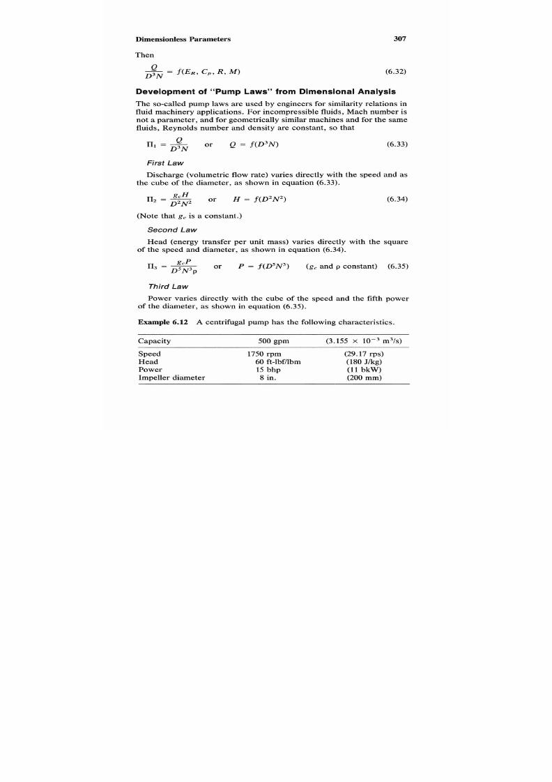
7/21/2019 Fundamental Fluid Mechanics for Engineers
http://slidepdf.com/reader/full/fundamental-fluid-mechanics-for-engineers 330/438
Dimensionless
307
Then
(6.32)
Development of “ Pump Laws” from Dimensional Analysis
The so-called pump lawsare used by engineers for similarity relations in
fluid machinery applications. For incompressible fluids, Mach number is
not a parameter, and for geometrically similar machines andor the same
fluids, Reynolds number and density are constant, so that
Q
n,
=
D 3 N
or
(6.33)
First Law
Discharge (volumetric flow ate) varies directly with he speed and as
the cube of the diameter, as shown in equation (6.33).
n2 =-
D = N *
or H =
f ( D Z N 2 )
(6.34)
(Note that g , is a constant.)
Second Law
Head (energy transfer per unit mass) varies directly with the square
of the speed and diameter, as shown in equation (6.34).
r I 3 =-
D 5 N 3 p
or P
= f ( D S N 3 )
( g , and
p
constant) (6.35)
Third
Law
Power varies directly with the cube of the speed and the fifth power
of the diameter, as shown in equation (6.35).
Example
6.12
A
centrifugal pump has the following characteristics.
Capacity
500
gpm
(3.155
x
m3/s)
Speed 1750 rpm (29.17 rps)
Head 60 ft-lbf/lbm
(180 J/kg)
Power
15
bhp
11
kW)
Impeller diameter
8
in.
(200 mm)

7/21/2019 Fundamental Fluid Mechanics for Engineers
http://slidepdf.com/reader/full/fundamental-fluid-mechanics-for-engineers 331/438
308 Chapter 6
The pump is driven by a constant-speed motor. In a certain application,
the capacity is to be reduced to 21 1 gpm (1.331 X IOe3) by changing the
impeller.
Determine
(a)
the required impeller diameter, (b) the head developed,
and
(c)
power required with the new impeller.
Solution
This example is solved by application
of
the “pump laws.”
(a) First law
Discharge (volumetric flowate) varies directly withhe speed andas the
cube
of
the diameter, using equation (6.33):
(b) Second
law
Head varies directly with the square
of
the speed and diameter, as in
equation (6.34):
(c) Third Zuw
Power varies directly with the cube
of
the speed and the fifth power of
the diameter, as shown in equation (6.35):
US. nits
D2
=
8(211/500)’” = 6 in.
H2 = 60(6/8)2 = 33.75 ft-lbfhbm
Pz = 15(6/8)5
=
3.56 bhp
SI Units
D2
=
200(1.331
x
10-3/3.155
x
10-3)1/3
=
150
mm
H2
= 180(150/200)2 =
101
Jkg
Pz = 11(150/200)5 = 2.61 bkW
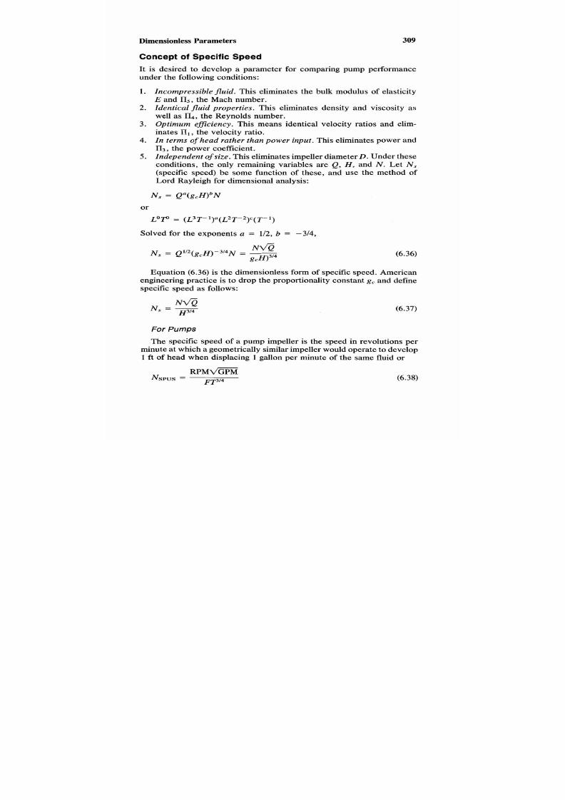
7/21/2019 Fundamental Fluid Mechanics for Engineers
http://slidepdf.com/reader/full/fundamental-fluid-mechanics-for-engineers 332/438
Dimensionless 309
Concept of Specific Speed
It is desired to develop a parameter for comparing pump performance
under the following conditions:
1.
2.
3.
4.
5.
Incompressible fluid.This eliminates the bulk modulus of elasticity
E
and
115,
the Mach number.
Identical fluid prop erties. This eliminates density and viscosity as
well as l&, the Reynolds number.
Optimu m efficiency. This means identical velocity ratios and elim-
inates II,, he velocity ratio.
In
terms
of
head rather thanpower input.
This eliminates power and
I I 3 ,
the power coefficient.
Independent
of
size. This eliminates impeller diameter. Under these
conditions, the only remaining variables are Q, H , and N . Let N ,
(specific speed) be some function of these, and use the method
of
Lord Rayleigh for dimensional analysis:
N s = Q a ( g c H l b N
or
L o p = ( L 3 T - 1 ) a ( L 2 T - 2 ) C ( T - 1 )
Solved for the exponents a = 1/2, b = -3/4,
(6.36)
Equation (6.36) is the dimensionless formof specific speed. American
engineering practice is to drop the proportionality constant
g ,
and define
specific speed as follows:
(6.37)
For
Pumps
.The specific speedof a pump impeller is the speed in revolutions per
minute at which
a
geometrically similar impellerould operate to develop
1 ft
of
head when displacing 1 gallon per minute of the same fluid or
R
NSPUS =
FT3I4
(6.38)

7/21/2019 Fundamental Fluid Mechanics for Engineers
http://slidepdf.com/reader/full/fundamental-fluid-mechanics-for-engineers 333/438
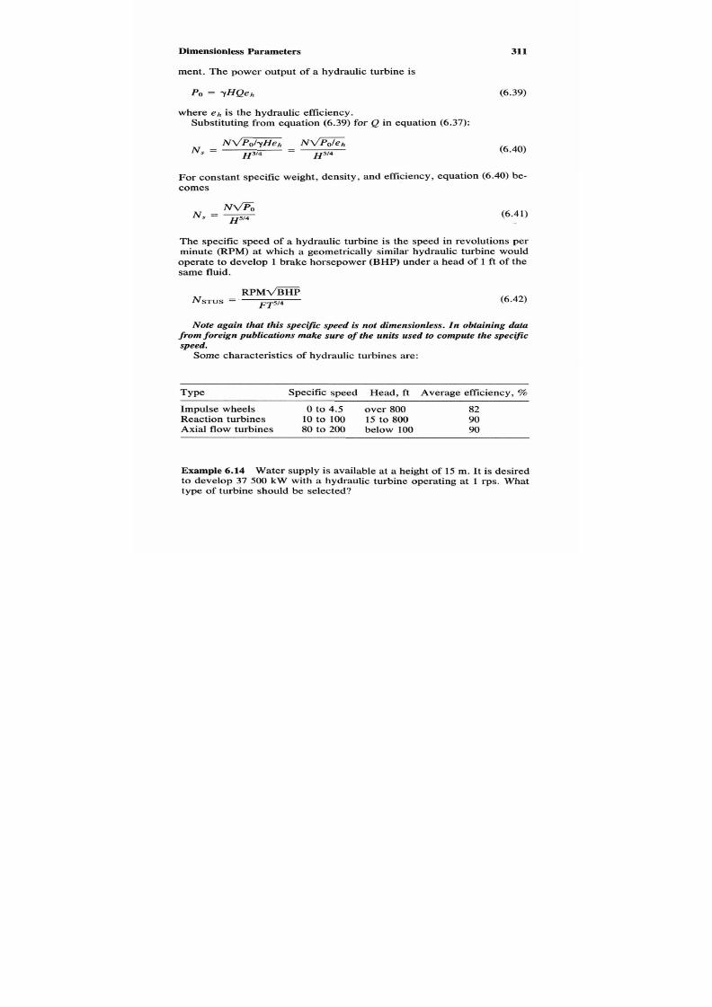
7/21/2019 Fundamental Fluid Mechanics for Engineers
http://slidepdf.com/reader/full/fundamental-fluid-mechanics-for-engineers 334/438
Dimensionless
311
ment. The power output of
a
hydraulic turbine is
where e h is the hydraulic efficiency.
Substituting from equation 6.39) for
Q
in equation (6.37):
N-h N m h
N ,
= ~ 3 1 4
-
~ 5 1 4
(6.40)
For
constant specific weight, density, and efficiency, equation
6.40)
be-
comes
(6.41)
The specific speed of
a
hydraulic turbine is the speed in revolutions per
minute (RPM) at which
a
geometrically similar hydraulic turbine would
operate to develop
1
brake horsepower (BHP) under head of
1
ft of the
same fluid.
(6.42)
Note again that this specific speed is not dimensionless. In obtaining
data
from foreign publications make sure of the units used to compute the specific
speed.
Some characteristics of hydraulic turbines are:
Type Specificpeed Head, ft Averagefficiency, %
Impulse wheels
0
to 4.5 over 800 82
Reaction turbines
10 to 100 15 to 800
90
Axial flow turbines
80 to 200
below 100 90
Example
6.14
Water supply is available at a height of 15 m. It is desired
to develop 37
500
kW with a hydraulic turbine operating at 1
rps.
What
type of turbine should be selected?

7/21/2019 Fundamental Fluid Mechanics for Engineers
http://slidepdf.com/reader/full/fundamental-fluid-mechanics-for-engineers 335/438
312 . Chapter 6
Solution
Since data on specific speeds in
SI
units are not available it
is
necessary
to convert to U.S. units using Table B .1 .
H
=
151.3048
=
49.21 ft
N = I x 6 0 = i j O r p m
Po = 37
500
X 1000/745.70
=
50,288 hp
Calculate the specific speed:
RPM-
60-
NSTUS
-
FTsi4
49.2lSi4
=
103 (6.42)
From the above characteristics
o f
hydraulic turbines with
a
head
of
49 ft
and a specific speed of 103, an axial flow turbine should be selected.

7/21/2019 Fundamental Fluid Mechanics for Engineers
http://slidepdf.com/reader/full/fundamental-fluid-mechanics-for-engineers 336/438
Dimensionless Parameters
Table 6.1
Standard
Numbers
Foroe
R a t i o
E q u a t i o n s
I
=
p L V E
pL'V'/ g
Inertia
5 pL2V2/gc
Vibration
7
=
K
313
R e s u l t
Form
I
Symbol I Name
Convent ional Pract ioe
I
-
2
9
L' r ' V
S
Strouhal
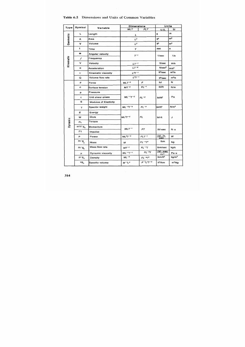
7/21/2019 Fundamental Fluid Mechanics for Engineers
http://slidepdf.com/reader/full/fundamental-fluid-mechanics-for-engineers 337/438
Table 6.2 Dimensions and Units of Comm on Variables
I I
I I
I I
314
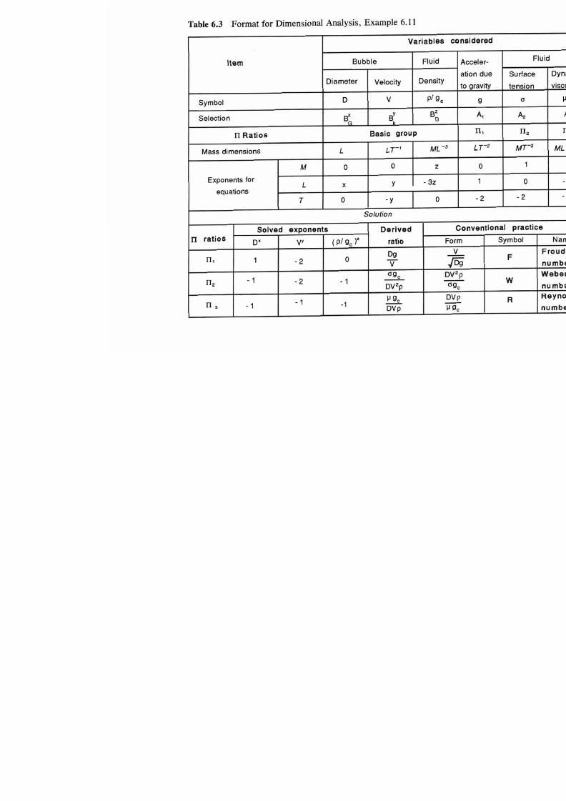
7/21/2019 Fundamental Fluid Mechanics for Engineers
http://slidepdf.com/reader/full/fundamental-fluid-mechanics-for-engineers 338/438
a
c
.-
h
vC
a
n
0
0
Q
.
>
c
t
a
.
E
n
c
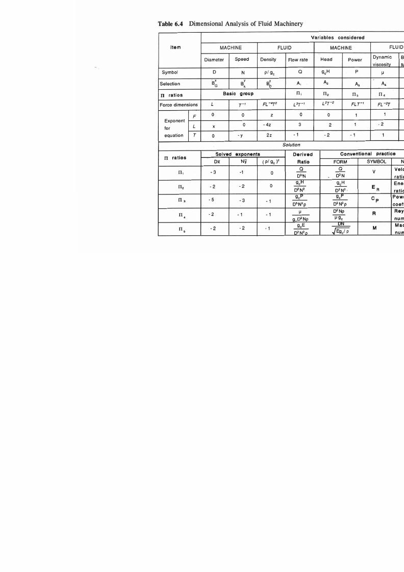
7/21/2019 Fundamental Fluid Mechanics for Engineers
http://slidepdf.com/reader/full/fundamental-fluid-mechanics-for-engineers 339/438
0
(
U
-
0
m
C
N
0
0
2
.
F
C
V
.
C
c
t 5
6
X
0
0
0
C
c
c
c
a
0
c
‘
G
o
m
a
3
a
P

7/21/2019 Fundamental Fluid Mechanics for Engineers
http://slidepdf.com/reader/full/fundamental-fluid-mechanics-for-engineers 340/438
Table A-l Critical and Saturated Properties
of
Selected Fluids
Table
A-2
Properties of Selected Gases
Table
A-3
Density and Viscosity of Steam and Compressed Water
317

7/21/2019 Fundamental Fluid Mechanics for Engineers
http://slidepdf.com/reader/full/fundamental-fluid-mechanics-for-engineers 341/438

7/21/2019 Fundamental Fluid Mechanics for Engineers
http://slidepdf.com/reader/full/fundamental-fluid-mechanics-for-engineers 342/438

7/21/2019 Fundamental Fluid Mechanics for Engineers
http://slidepdf.com/reader/full/fundamental-fluid-mechanics-for-engineers 343/438

7/21/2019 Fundamental Fluid Mechanics for Engineers
http://slidepdf.com/reader/full/fundamental-fluid-mechanics-for-engineers 344/438

7/21/2019 Fundamental Fluid Mechanics for Engineers
http://slidepdf.com/reader/full/fundamental-fluid-mechanics-for-engineers 345/438

7/21/2019 Fundamental Fluid Mechanics for Engineers
http://slidepdf.com/reader/full/fundamental-fluid-mechanics-for-engineers 346/438
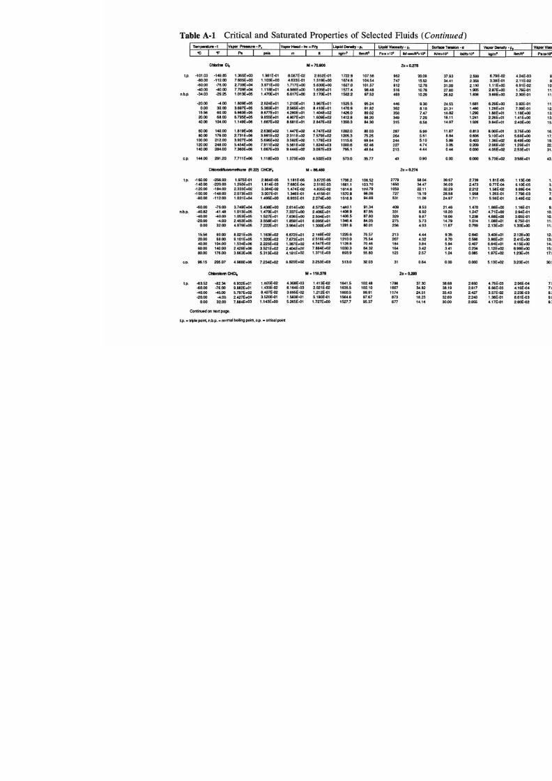
7/21/2019 Fundamental Fluid Mechanics for Engineers
http://slidepdf.com/reader/full/fundamental-fluid-mechanics-for-engineers 347/438
P
d
d
d

7/21/2019 Fundamental Fluid Mechanics for Engineers
http://slidepdf.com/reader/full/fundamental-fluid-mechanics-for-engineers 348/438
L

7/21/2019 Fundamental Fluid Mechanics for Engineers
http://slidepdf.com/reader/full/fundamental-fluid-mechanics-for-engineers 349/438
.

7/21/2019 Fundamental Fluid Mechanics for Engineers
http://slidepdf.com/reader/full/fundamental-fluid-mechanics-for-engineers 350/438
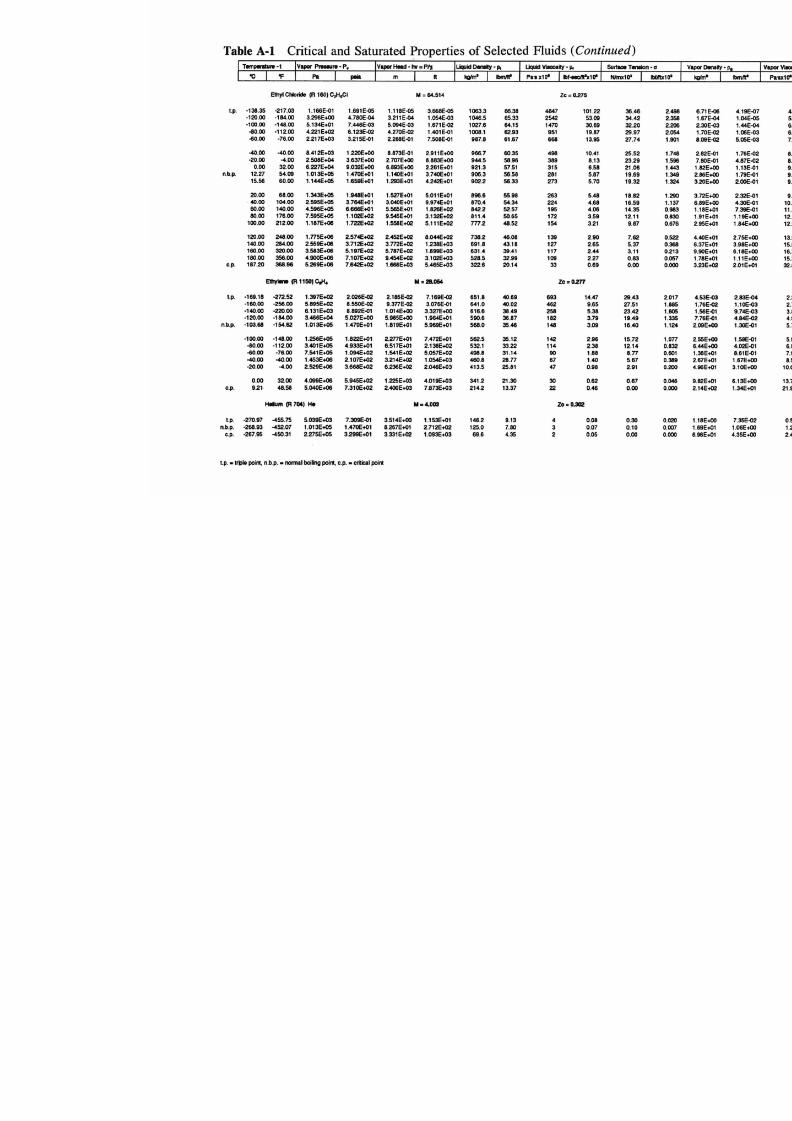
7/21/2019 Fundamental Fluid Mechanics for Engineers
http://slidepdf.com/reader/full/fundamental-fluid-mechanics-for-engineers 351/438
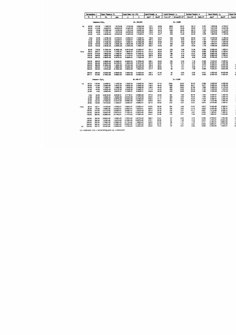
7/21/2019 Fundamental Fluid Mechanics for Engineers
http://slidepdf.com/reader/full/fundamental-fluid-mechanics-for-engineers 352/438

7/21/2019 Fundamental Fluid Mechanics for Engineers
http://slidepdf.com/reader/full/fundamental-fluid-mechanics-for-engineers 353/438
n
.

7/21/2019 Fundamental Fluid Mechanics for Engineers
http://slidepdf.com/reader/full/fundamental-fluid-mechanics-for-engineers 354/438
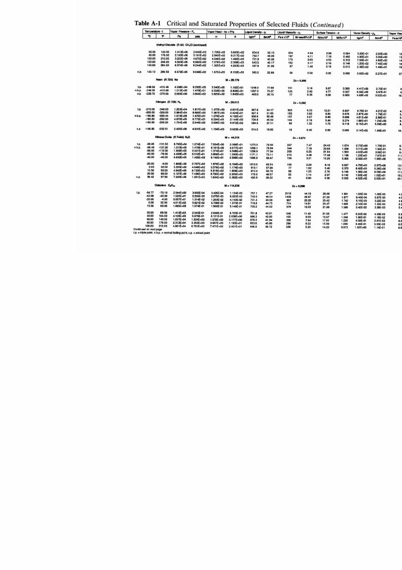
7/21/2019 Fundamental Fluid Mechanics for Engineers
http://slidepdf.com/reader/full/fundamental-fluid-mechanics-for-engineers 355/438

7/21/2019 Fundamental Fluid Mechanics for Engineers
http://slidepdf.com/reader/full/fundamental-fluid-mechanics-for-engineers 356/438

7/21/2019 Fundamental Fluid Mechanics for Engineers
http://slidepdf.com/reader/full/fundamental-fluid-mechanics-for-engineers 357/438

7/21/2019 Fundamental Fluid Mechanics for Engineers
http://slidepdf.com/reader/full/fundamental-fluid-mechanics-for-engineers 358/438

7/21/2019 Fundamental Fluid Mechanics for Engineers
http://slidepdf.com/reader/full/fundamental-fluid-mechanics-for-engineers 359/438
L

7/21/2019 Fundamental Fluid Mechanics for Engineers
http://slidepdf.com/reader/full/fundamental-fluid-mechanics-for-engineers 360/438

7/21/2019 Fundamental Fluid Mechanics for Engineers
http://slidepdf.com/reader/full/fundamental-fluid-mechanics-for-engineers 361/438
r
le
3
E
8
1
f
1
3
9
8W
W
W
f

7/21/2019 Fundamental Fluid Mechanics for Engineers
http://slidepdf.com/reader/full/fundamental-fluid-mechanics-for-engineers 362/438
Appendix Tables A-2 and A-3 fo l low on pages 340-372
339

7/21/2019 Fundamental Fluid Mechanics for Engineers
http://slidepdf.com/reader/full/fundamental-fluid-mechanics-for-engineers 363/438
8
8
8
8
8
+
+
+
+
+
w
w
w
w
w
0
J
V
-
Y
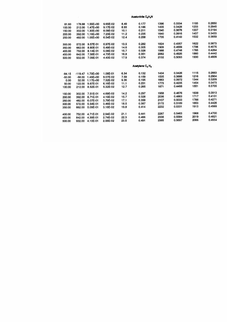
7/21/2019 Fundamental Fluid Mechanics for Engineers
http://slidepdf.com/reader/full/fundamental-fluid-mechanics-for-engineers 364/438
0
0
0
0
0
0
0
0
0
0
0
0
0
0
0
0
0
0
0
0
0
0
0

7/21/2019 Fundamental Fluid Mechanics for Engineers
http://slidepdf.com/reader/full/fundamental-fluid-mechanics-for-engineers 365/438
d
o
o
r
9
9
9
9
9
9
9
9
-
-
U
N
N
N
N
N
N
r
n
.
-
Q
r
n
~
N
C
n
p
w
q
8
8
M
6
R
N
N
N
N
N
w
w
u
l
w
w
9
9
9
9
r
n
r
n
0
r
n
N
u
i
v
v

7/21/2019 Fundamental Fluid Mechanics for Engineers
http://slidepdf.com/reader/full/fundamental-fluid-mechanics-for-engineers 366/438
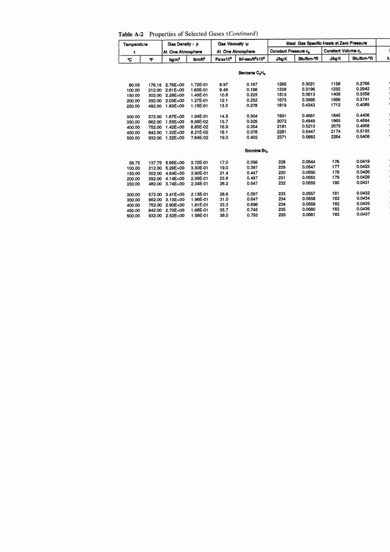
7/21/2019 Fundamental Fluid Mechanics for Engineers
http://slidepdf.com/reader/full/fundamental-fluid-mechanics-for-engineers 367/438

7/21/2019 Fundamental Fluid Mechanics for Engineers
http://slidepdf.com/reader/full/fundamental-fluid-mechanics-for-engineers 368/438
?
?
?
?
Q
Q
Q
9
F
N
N
N
N
N
N
N
w
w
w
w
w
w
w
w
w
w
E
6
8
8
%
%
R
$
%
F
P
?
?
?
?
S
?
S
?
m
m
l
u
-
0
m
m
b
-
N
N
N
N
c
u
c
u
N
N
c
u
c
v
c
u
.
c
m
?
m
2
3
2
g
8

7/21/2019 Fundamental Fluid Mechanics for Engineers
http://slidepdf.com/reader/full/fundamental-fluid-mechanics-for-engineers 369/438
0
0
0
0
0
U
w
w
w
w
w
U
)
U
P
W
(
U
9
9
?
N
O
9
3

7/21/2019 Fundamental Fluid Mechanics for Engineers
http://slidepdf.com/reader/full/fundamental-fluid-mechanics-for-engineers 370/438
B
0
0
0
0
0
0
0
0
0
0
0
0
0
0
0
0
0
0
0
0
0
0
0
0
0
0
0
0
0
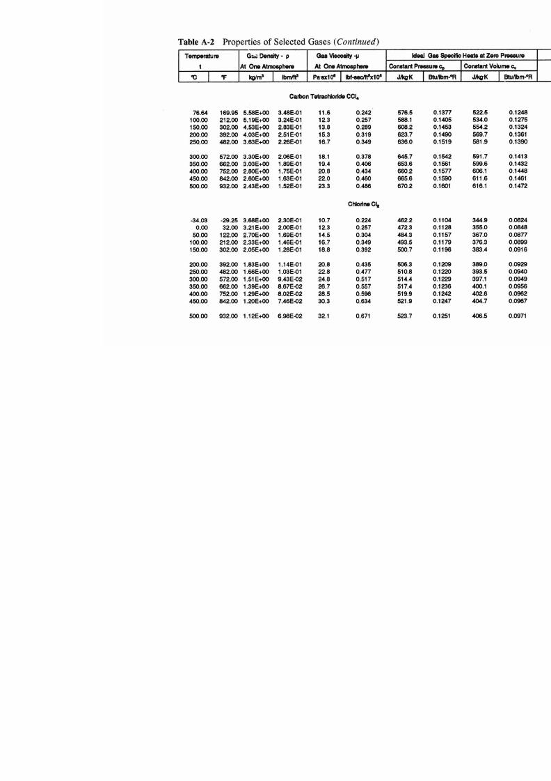
7/21/2019 Fundamental Fluid Mechanics for Engineers
http://slidepdf.com/reader/full/fundamental-fluid-mechanics-for-engineers 371/438
C
0
0
0
0
0
0
0
0
0
0
0
0
0
0
0
0
0
0
0
0
0
b
t
a
6
l
C
0
0
0
0
0
c
j
c
j
e
i
n
i
o
i

7/21/2019 Fundamental Fluid Mechanics for Engineers
http://slidepdf.com/reader/full/fundamental-fluid-mechanics-for-engineers 372/438

7/21/2019 Fundamental Fluid Mechanics for Engineers
http://slidepdf.com/reader/full/fundamental-fluid-mechanics-for-engineers 373/438
r
a
m
0
0
.
O
k
N
P
I
0
0
0
0
0
"
"
"
?
c

7/21/2019 Fundamental Fluid Mechanics for Engineers
http://slidepdf.com/reader/full/fundamental-fluid-mechanics-for-engineers 374/438
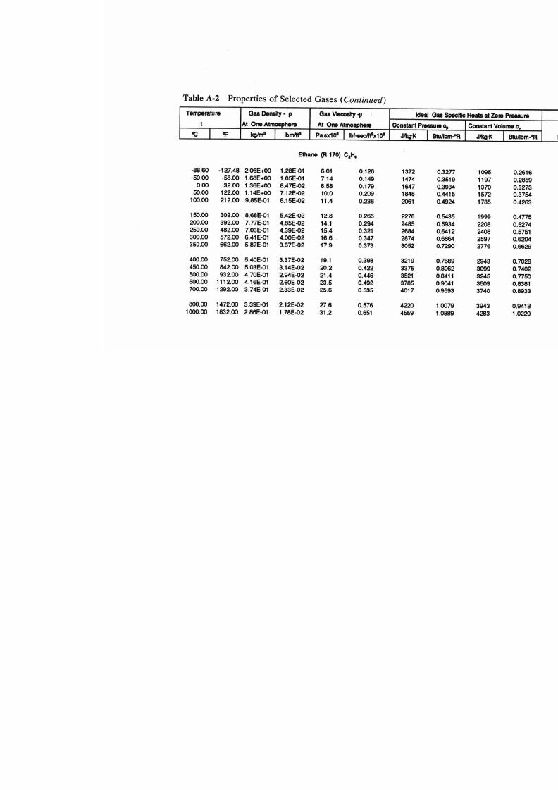
7/21/2019 Fundamental Fluid Mechanics for Engineers
http://slidepdf.com/reader/full/fundamental-fluid-mechanics-for-engineers 375/438
0
0
0
0
0
e
5
s
3
g
C
.
-
S
?
?
?
S
?
r

7/21/2019 Fundamental Fluid Mechanics for Engineers
http://slidepdf.com/reader/full/fundamental-fluid-mechanics-for-engineers 376/438
0
0
0
0
0
c
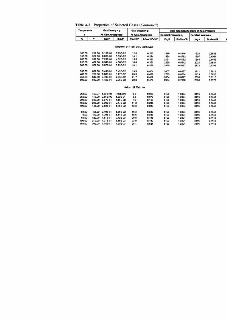
7/21/2019 Fundamental Fluid Mechanics for Engineers
http://slidepdf.com/reader/full/fundamental-fluid-mechanics-for-engineers 377/438
C
.
r
.
0
0
0
0
C
C
0
0
0
0
1
E
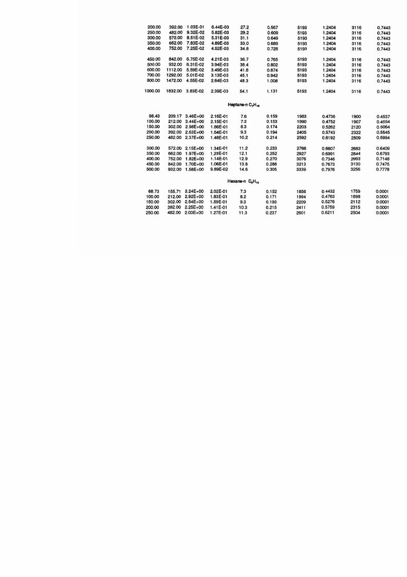
7/21/2019 Fundamental Fluid Mechanics for Engineers
http://slidepdf.com/reader/full/fundamental-fluid-mechanics-for-engineers 378/438
C
.
C
.
C
.
.
.
.
.
.
i
0
I
t
I
0
w
m
m
m
Q
?
I
C
0
0
0
0
0

7/21/2019 Fundamental Fluid Mechanics for Engineers
http://slidepdf.com/reader/full/fundamental-fluid-mechanics-for-engineers 379/438
C
0
I
C
N
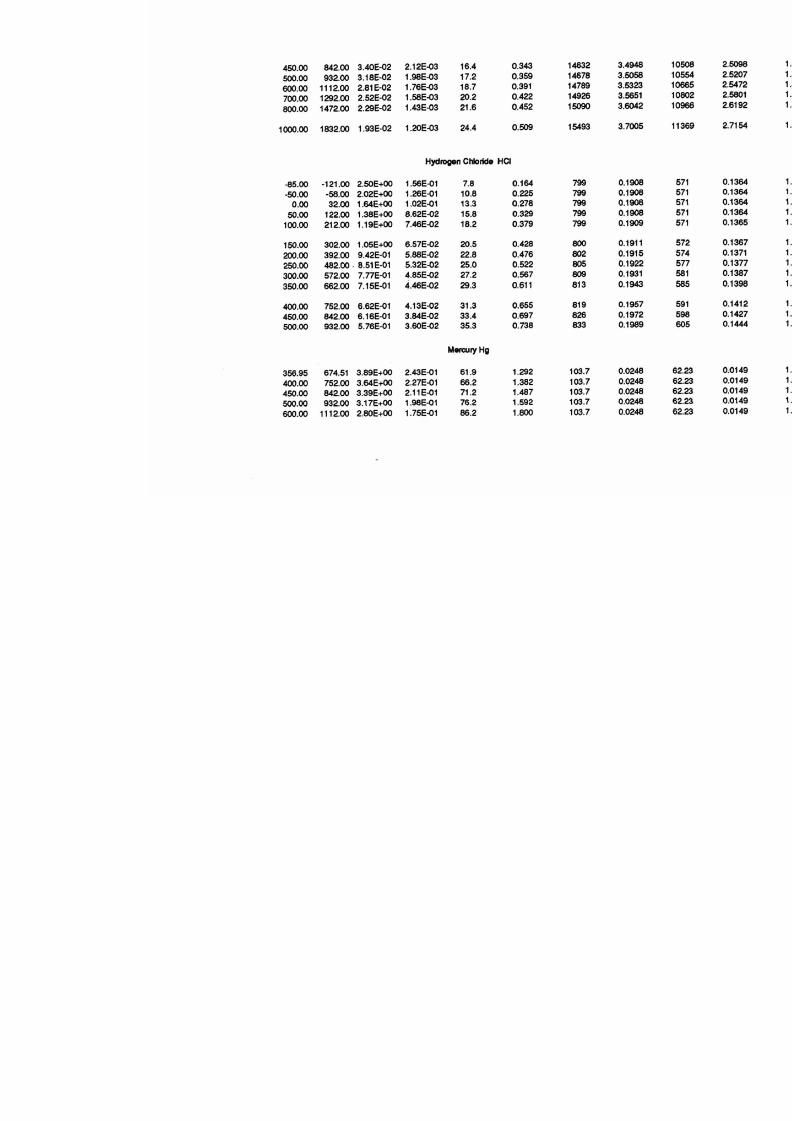
7/21/2019 Fundamental Fluid Mechanics for Engineers
http://slidepdf.com/reader/full/fundamental-fluid-mechanics-for-engineers 380/438
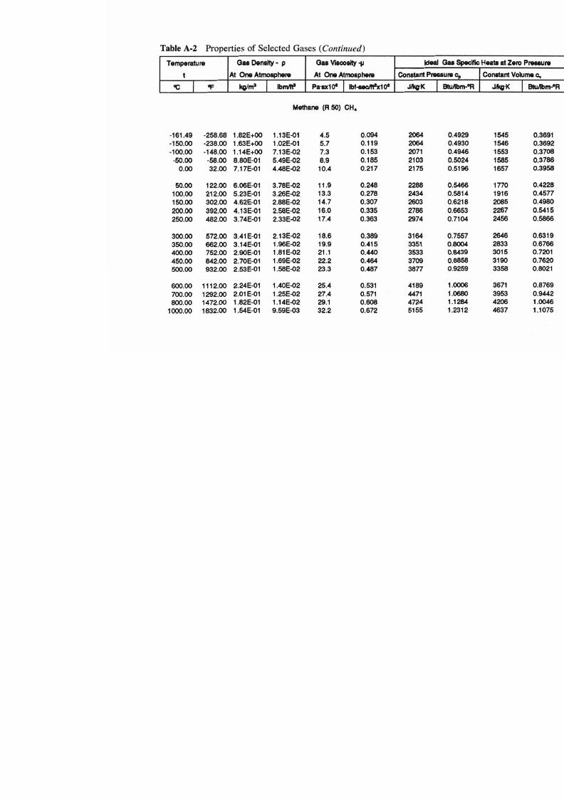
7/21/2019 Fundamental Fluid Mechanics for Engineers
http://slidepdf.com/reader/full/fundamental-fluid-mechanics-for-engineers 381/438

7/21/2019 Fundamental Fluid Mechanics for Engineers
http://slidepdf.com/reader/full/fundamental-fluid-mechanics-for-engineers 382/438
0
0
0
0
4

7/21/2019 Fundamental Fluid Mechanics for Engineers
http://slidepdf.com/reader/full/fundamental-fluid-mechanics-for-engineers 383/438
z
0
V
C
Q
0
0
0
V
r
r
r
r
r
r
r
r
r
r
u
i
d
o
m
m

7/21/2019 Fundamental Fluid Mechanics for Engineers
http://slidepdf.com/reader/full/fundamental-fluid-mechanics-for-engineers 384/438

7/21/2019 Fundamental Fluid Mechanics for Engineers
http://slidepdf.com/reader/full/fundamental-fluid-mechanics-for-engineers 385/438
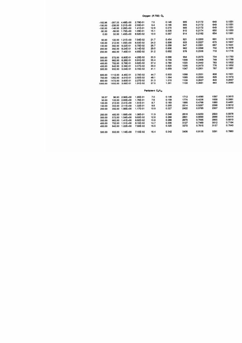
7/21/2019 Fundamental Fluid Mechanics for Engineers
http://slidepdf.com/reader/full/fundamental-fluid-mechanics-for-engineers 386/438

7/21/2019 Fundamental Fluid Mechanics for Engineers
http://slidepdf.com/reader/full/fundamental-fluid-mechanics-for-engineers 387/438

7/21/2019 Fundamental Fluid Mechanics for Engineers
http://slidepdf.com/reader/full/fundamental-fluid-mechanics-for-engineers 388/438

7/21/2019 Fundamental Fluid Mechanics for Engineers
http://slidepdf.com/reader/full/fundamental-fluid-mechanics-for-engineers 389/438
0
0
0
0
0
8
5
8
3
0
8r
C
+
+
+
+
+
U
l
w
w
w
w
0
O
Q
F
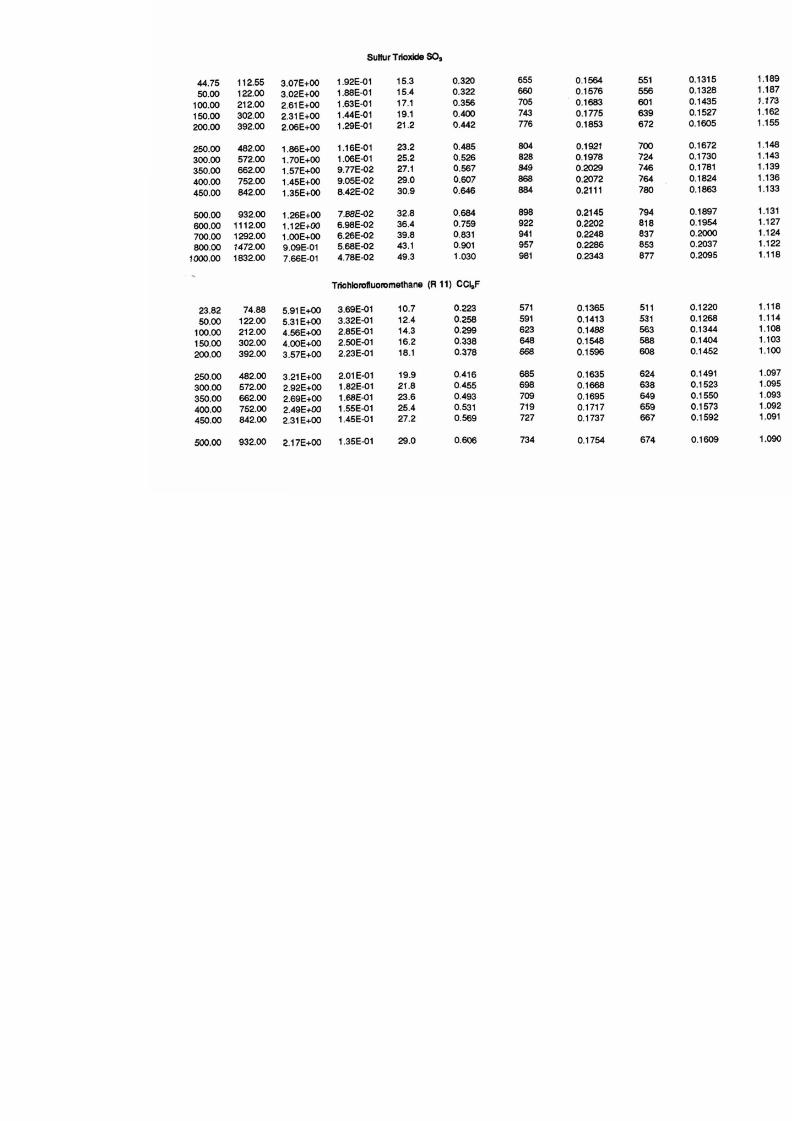
7/21/2019 Fundamental Fluid Mechanics for Engineers
http://slidepdf.com/reader/full/fundamental-fluid-mechanics-for-engineers 390/438
U
,
0
$
@
g
$
8
(
D
0
0
0
0
0
0
0
0
0
0
0
0

7/21/2019 Fundamental Fluid Mechanics for Engineers
http://slidepdf.com/reader/full/fundamental-fluid-mechanics-for-engineers 391/438
$
$
0
0
0
0
0
0
0
0
0
0

7/21/2019 Fundamental Fluid Mechanics for Engineers
http://slidepdf.com/reader/full/fundamental-fluid-mechanics-for-engineers 392/438
Fluid
Properties
369
Table A-3
Density and Viscosity
of
Steam and Compressed Water
l ° F
I
plbrmrt.'
I
Z-pvmT
I
l b f - d l
V f P k c
1.F
I
plbmm)
Z-pvlRT
I
p l b f 4 I
vV/sec
1 psia 10 psia
3 2
1 0 0
62.42
1.926E-05 3.737E-05
.472E-04 62.42
7.510E-06
.432E-05 4.892E-04
1.350 0.385E-06
.423E-06
.841E-05 62.00
3 2
.926E-05
.737E-05 5.472E-05
61 .g61 4.628E-05 1 1.398E-05
0.002998.99601.145E-07
101.74)
101.74)
200.002546
0.9993 2.528E-07
300
0.00221
1 OOOO 2.963E-07
400.001954
1.0001 3.422E-07
600 0.001585
1.0003 4.374E-07
800
0.001333 1.00 04 5.336E-07
1000 0 .00150 1.0004 6.286E-07
1200.00 10 12 1.0004 7.216E-07
1400.00 090 3 1.0005 6.115E-07
14.696
psia
800
1 0 0 0
1 2 0 0
7.26OE-O6 1(193.21)1 60.2614.268E-041 6.604E-061 3.525 E-06
2.302E-031(193.21)1 0.026031 0.988 41.490E-071.078E-04
1.926E-051 32 I 62.42 0.002736 3.736E-05 1.926E-05
7.432E-06 10 0 62.00 .002420 .423E-05 .385E-06
3.396E-06 20 0 60.13 .002117 .337E-06 .391E-06
3.166E-061(26l.O2)l
57.901 0.0019581 4.144E -061 2.303E-06
2.211E-04 (261.02)l
0.11751 0.96531 2.844E-071.791E-05
1 0 0
3 2
2 0 0
300
[327.82)1 56.371 0.0037841 3.437E-061 1.962E-061(381.80)1
54.381 0.0073411 2.8778-061 1.702E-06
[327.62)1 0.22571 0.94501 3.034E-071 4.325E-051(381.60)1
0.43721 0.91311 3.254E-071 2.395E-05
4 0 0
1400
.890E-04
.122E-07 0.9989 0.09042 1400
1200
2.291E-04 7.221E-07 0.9978
.1014
2 0 0
l 0 0 0
.752E-04
.291E-07 0.9959 0,11550 0 0
800
.5078-04
.291E-07 0.9924 0.134400
6 0 0
.724E-05
.362E-07 0.9852 0.16090 0
4 0 0.375E-05
.385E-07 0.9641 0.2026
300
psia
3 2
4 0 0
.636E-06
.730E-06 0.01092 53.680 0
300
.154E-06
.838E-06 0,01157
7.34
00
200
.393E-06
.346E-06 0.01269 60.170 0
1 0 0.360E-06
.423E-05 0.014512.030 0
3 2
.920E-05
.7271-05 0.01641 62.46
(417.35)
52.94 0.01085 2.601E-06
1.581E-06
(444.6(
(417.35)
(444.6(
.687E-05
.399E-07 0.8863 0.6482
6 0 0
1400.619E-05
.136E-07 0.9956
.2721 1400
1200.607E-05
.2338-07 0.9924 0.3059 1200
1000.792E-05
.298E-07 0.9867
.3498 1000
800
.188E-05
.333E-07 0.9763
.4097
00
6 0 0.798E-05
.339E-07 0.9531 0.4969
0.4238
1.143E-04 7.227E-07
8.725E-05 6.295E-07 0
.2321
8.336E-05 5.335E-07 0
.2709
4.280E-05 4.350E-07 0
.3270
2.540E-05 3.346E-07 0
0.181 1 1.444E+03
.129E+00
.9972
400 psia
62.50
1.508E-06 2.424E-06
1.71
1.637E-06 2.733E-06
2.154E-06 3.641 E-06
7.37
3.396E-06 6.350E-06
7.376E-06 1.423E-05
.01934
2.07
1.917E-05 3.724E-05
0.8613 0.8625 3.513E-07 1.312E-05
0.6774 0.9360 4.328E-07 2.056E-05
0.5509
7.209E-05 8.143E-07
5.695E-05 7.240E-07
4.327E-05 6.302E-07
3.1 14E-05
.332E-07 0.9680

7/21/2019 Fundamental Fluid Mechanics for Engineers
http://slidepdf.com/reader/full/fundamental-fluid-mechanics-for-engineers 393/438
370
Appendix
Table A-3
Density and Viscosity
of
Steam and Compressed Water (Continued)
t'F
p R r
I
Z=pWRT
U l b f - d l
v ~ / s a c
taF
I
p l b d
I
Z=pvlRT
I
p I b f d I
v ( r h
500 ps ia
32
100
62.54
7.362E-06
.423E-05
.04826
2.19 100
.376E-06
.423E-05 0.02417
2.07
1.904E-05
.705E-05
.05455 62.62
2
.914E-05 3.721E-05
.02731
1000
ps ia
200
3.3998-06
.372E-06
.04221 60.31
00
.396E-06 6.354E-06
.02114
0.20
300
1.643E-06 2.753
.03624 53.91
00.638E-06
.736E-06
.01618 53.73
00
2.160E-06 3.862
.03842 57.54
00
.155E-06 3.646E-06
.01926
7.41
467.01)l0.631
0.017901 2.294E-06) 1.458E-06)(544.58)1
6.321 0.0361 1 1.912E-061 1.326E-06
:467.01)] 1.078051]
0.84061 3.608E-071 1.077E-051(544.58)1
.2381 0.74741 3.971E-071 5.710E-06
600
0.566512000
1.181E-05
.341E-07 0.9167
.45500.470E-05
.332E-07
.9598 0.694569
00
7.061E-06 4.264
.8142
.94700.609E-05 4.318E-07
.9180
.86326
2.873E-05 8.192
.9845 0,91735 1400
.763E-05 8.151E-07
.9924 0.455021
400
2.255E-05 7.264
.9737
.039
200
.546E-05 7.246E-07
.9870 0.512636
200
1.691E-05.335E-07 0.9544.206000.446E-05 6.307E-07.9776
1500 ps ia
2000
ps ia
32
60.42
00
7.344E-06 1.424E
2.3800.358E-06 1.4248-05
.07229 62.27 100
1.681E-05 3.675
.1087 62.852.692E-05
.690E-05 0.08168
2.74
1.653E-06 2.786
.07205 54.23
00 1.626E-06 2.733E-06 0.05419 54.08
00
2.170E-06 3.697
.07654 57.7700
.165E-06 3.679E-06 0.05754 57.64
00
3.408E-06 6.406
.08417 60.5000
.403E-06 6.390E-06 0.06320
(596.90)
3.571
00
1.244E-05
.507E-05 0.07865
6.99
635.80)
.821E-06 4.284E-07 0.6610 3.608
596.90)
1.271E-06 1.694
2.8800.270E-06 1.663E-06
.05594 42.63
1.431 E-05 6.289E
.9767 1.367
400
1.11lE-05 7.381
.137
200 1.492E-05
.329E-07 0.9604 1.581
200
8.151E-06
.427E-07
.9072 2.537 l000 1.106E-0
.9310 1.654000
5.358E-06 5.421
00.514E-06 5.369E-07 0.6700 2.299
00
2.796E-06 4.615
.5774 5.311
635.80)
.872E-06
.296E-07 0.6657
-
2500 ps ia
3000
ps ia
32
100
62.93
1.660E-05 3.646
.1625 63.05
7.331E-06 1.425
2.46
32.872E-05 3.661E-05 0.1357
200 60.61 0.1050 6.4278-06
.412E-06 200
1.29ZE-06 1,746E00.273E-06 1.719E-06 0.0912
3.44
00
1.664E-06 2.821
.1074 54.5500
.658E-06 2.804E-06
.08984.4100
2.182E-06 3.93300.177E-06 3.9158-06 0.0955 57.8700
3.418E-06 6.446
0.68
1668.10)
9.524E-06 8.407
.840
400 1.144E-05 8.345E-07 0.9616 2.348
7.329E-06
.510E-07 0.9208 3.297
200 6.640E-06 7.442E-07
.9340
.709200
5.259E-06 6.573
3.194E-06 5.642E00.063E-06
.507E-07 0.7643
.36100
1.633E-06 5.968E
695.33)
.131E-06 5.068E-07 0.4866 7.651
668.10)
1.228E-06 1.113
.1496 29.17
(695.33)
.228E-06 1.335E-06 0.1064 34.98
4000
ps ia
5000
ps ia
32
60.9800
7.306E-06 1.426
.2386 62.89
00
.300E-06 1.427E-05 0.1909 62.8900
1.827E-05 3.5942.640E-05 3.619E-05
.2159
3.29
5.741E-06 8.704
400 7.152506 8.545E-07
.9398
.644
400
4.347E-06 7.875
200
2.994E-06 7.092
.708000
1.526E-06 6.02600
.101E-06
.205E-07 0.5613 9.502
00
1.314E-06 1.86500.294E-06 1.803E-06
.1415
4.8200
1.685E-06 2.89400
2.193E-06 4.009
8.82
00 2.194505 3.970E-05
.1519
8.2200
3.443E-06.525E-06 0.2088 60.9800 3.422E-06.485E-06 0.1670
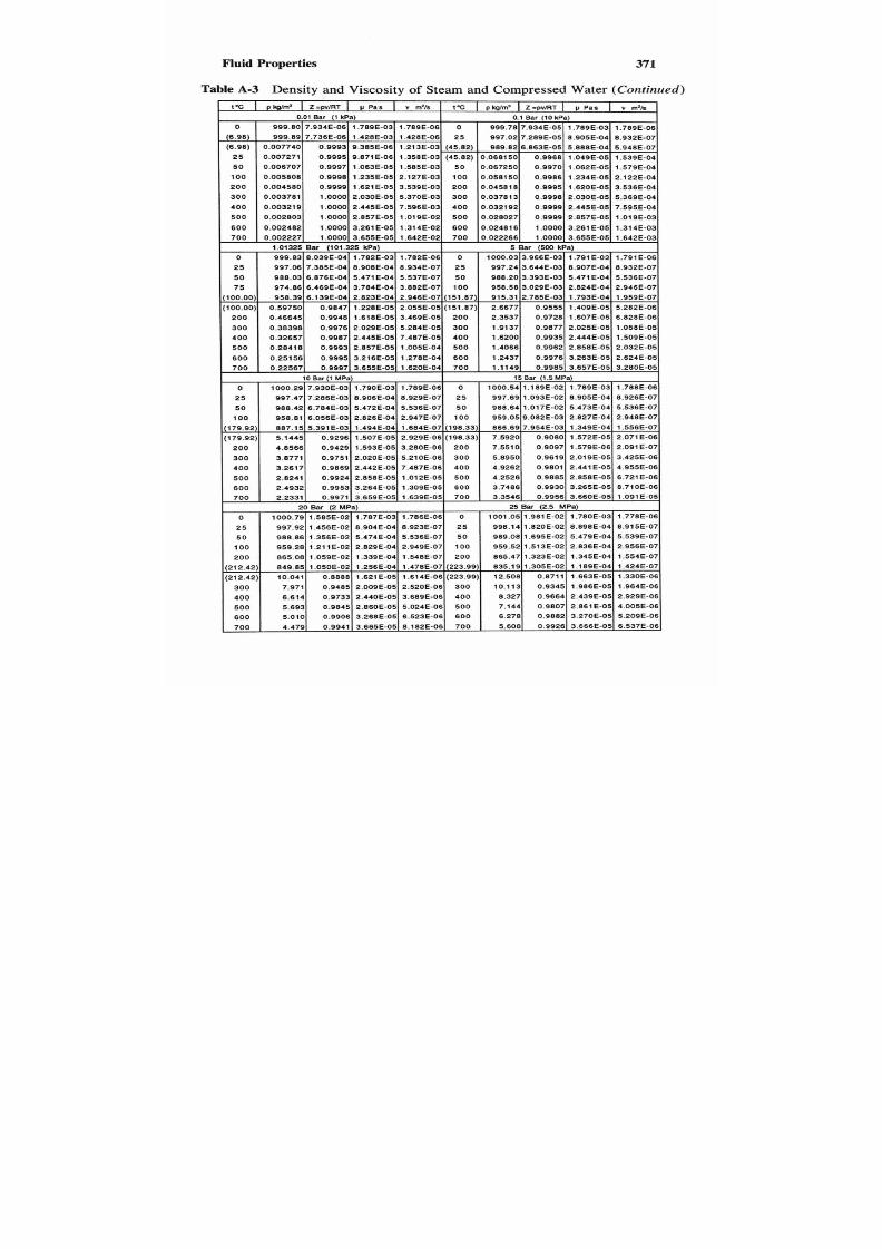
7/21/2019 Fundamental Fluid Mechanics for Engineers
http://slidepdf.com/reader/full/fundamental-fluid-mechanics-for-engineers 394/438
Fluid
371
Table
A-3
Density and Viscosity of Steam and Compressed Water (Continued)
tOC
I
p W m 5
Z-pv/RT
p
Pa%
I
v
m71 s
1%
p W m J
I
2-pvlRT
I
p
Paa
v
m7/s
0.01Bar 1kPa)
0
999.80
5.948E-07
.888E-04 6.863E-05
89.82
45.82)
.213E-03
.385E-06.9993 0.007740
6.98)
8.932E-07
.905E-04 7.289E-05 997.02
5.428E-06
.428E-03 7.736E-06 999.89
8.98)
1.789E-06
.789E-03
.934E-05 999.78
.789E-06 1.789E-03
.934E-06
2 5 0 .007271 0 .9995
9.87lE-06 1.358E-03
1.642E-03 3.655E-05 1
OOOO
.0222660 0.642E-02 3.655E-05 1.0000 0.0022270 0
1.314E-03
.261E-05
.0000 0.0248160 0.314E-02 3.261E-05 1
OOOO
.00248200
1.019E-03 2.857E-05.9999 0.028027 500 1.019E-02 2.8570 0
7.595E-04
.445E-05 0.9999 0.032192 4000 0
5.369E-04 2.030E-05 0.
.03781300.370E-03 2.030E-05 1.0000
.003781
00
3.536E-04
.620E-05 0.9995 0.045818
0 0.539E-03 1.621E-05 0.9999 0.0045800 0
2.122E-04
.234E-05 0.9986 0.058150
00
.127E-03
.235E-05 0.9998 0.0058080 0
1.579E-04 1.062E-05
.9970 0.0672500.585E-03 1.063E-05
.9997 0.0067070
1.539E-04
.049E-05 0.9968 0.068150
45.82)
0.1 Bar (10 kPa)
1.01325
kPa)
ar
(500Pa)ar101,325
0
2.946E-07 2.824E-04 3
.784E-04 6.469E-04 974.865
5.536E-07 5.4718-04 30.5378-07
.471E-04 6.876E-04 988.030
8.932E-07 8.907E-04
.644E-03
97.24
5
.934E-07 8.908E-04
.385E-04
9 7 . 0 6 2 5
1.791E-06
.791E-03 3.966E-03 1000.03.782E-06 1.782E-03 8.039E-0499.83
(100.00)
958.39 6.139E-04 2.823E-04
.946E-07 1.959E-07 1.793E-04 2.785E-03 915.31
151.87)
(100.00)
0 .59750
0.9847 1.228E-05 2.055E-05
151.87)
3.280E-05 3.657E-05 0
.114900.620E-04 3.855E-05
.9997 0.225670 0
2.624E-05 3.263E-05
.243700.278E-04
.2168-05 0.9995
.25156
00
2.032E-05 2.858E-05
.005E-04
.857E-05 0.9993 0.284180 0
1.509E-05 2.444E-05
.9935 1.6200
0 0
.487E-05
.445E-05 0.9987 0.326570 0
1.058E-05 2.025E-05.9877.9137
00
.284E-05.029E-05 0.9976 0.38398
00
6.828E-06
.607E-05
.9728
.3537 200 3.469E-05
.618E-05
.9948
.466450 0
5.282E-06 1.409E-05
10 Bar (1 MPa)
15Bar (1SMPa)
0
2.948E-07
.827E-04 9.0828-03 959.05
0 0.947E-07
.826E-04 6.056E-03 958.810 0
5.536E-07 5.473E-04 1
88.640.536E-07
.472E-04 8.784E-03 988.42
0
8.926E-07
.905E-04 1.093E-02 997.695
.929E-07 8.906E-04
.286E-03 997.475
1.788E-06 1.789E-03 1
.789E-06
.790E-03 7.930E-03
000.29
179.92
(179.92)
7 0 0
5 0
1 0 0
2 0 0
887 .15 5.391E-031 1.494E-04 1 1.684E-071(198.33)1 866.6917.954E-031 1.349E-0411.556E-Of
5.14451 0.92961 1.507E-051 2.929E-061(198.33)1 7.5 920 1.9080l.572E-051.071E-06
4.8566
7 0 0
.639E-05
.659E-05
.9971 2.2331
6 0 0.309E-05
.264E-05
.9953 2.4932
5 0 0
.012E-05.858E-05 0.9924
.8241
4 0 0
.487E-06
.442E-05 0.9869 3.2617
300
.210E-06 2.020E-05
.9751 3.8771
2 0 0.280E-06
.593E-05 0.9429
20 Bar (2 MPa)
1000.791 1.585E-02 1 1.787E-031 1.786E-06
0
7.5510.9097.579E-06.091E-07
5.8950.9619.019E-05.425E-06
4.9262.9801.441-05.955E-06
4.2526.9885.858E-05.721E-06
3.7486.9930.265E-05.710E-06
997.92
1.554E-07 1.345E-04
65.47 200
.548E-07 1.339E-04
.059E-02 865.08
2.956E-07
.836E-04 1.513E-02 959.52
0 0
.949E-07
.829E-04 1.211E-02
59.28
5.539E-07 5.479E-04
.695E-02 989.080
.536E-07
.474E-04 1.3566-02
88.86
8.915E-07 8.898E-04
.820E-02 998.14
5.923E-07
.904E-04
.456E-02
(212.42)
4.005E-06
.861E-05 0.9807
.1440 0
.024E-06 2.860E-05
.9845 5.693
0 0
2.929E-06
.439E-05 0.9664
.327 400
.689E-06 2.440E-05
.9733
.614
0 0
1.964E-06 1.986E-05
.9345 10.113
00
.52OE-06.009E-05 0.9485
.971
00
1.330E-06 1.663E-05
2.508
223.99)
.814E-06 1.621E-05.8888
0.041
212.42)
1.424E-07 1.189E-04
.305E-02 835.19
223.99)
.478E-07
.256E-04 1.050E-02
49.85
800
5.209E-06
.270E-05 0.9882 8.278
0 0
.523E-06.268E-05 0.9906
.010
7 0 0
6.537E-06
.666E-05 0.9926
.6080 0
.182E-06
.665E-05 0.9941
.479
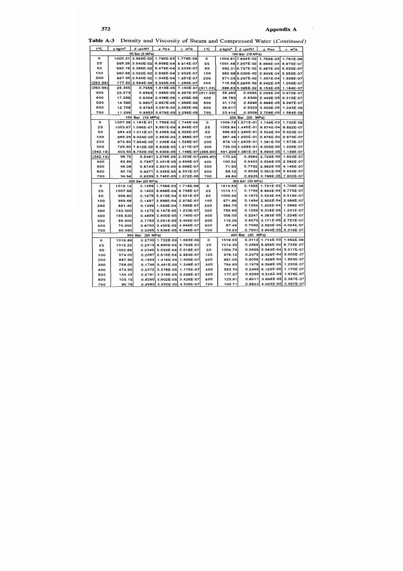
7/21/2019 Fundamental Fluid Mechanics for Engineers
http://slidepdf.com/reader/full/fundamental-fluid-mechanics-for-engineers 395/438
372 A '
00
Bar
(10
MPa)
1004.81 7.894E-02 1.769E-03 1.761E-06
1001.48 7.257E-02 8.889E-04 8.876E-07
992.31 6.757E-02 5.487E-04 5.530E-07
962.98 6.030E-02 2.849E-04 2.959E-07
871.03 5.257E-02 1.357E-04 1.558E-07
715.58 5.2838-02 8.642E-05 1.208E-07
688.63 5.386E-021 8.153E-05 1.184E-07
55.4801 0.6685 2.036E-05 3.670E-07
Table
A-3
Density and Viscosity of Steam and Compressed Water (Continued)
tc
I
P W ~
Z = P V ~ T
v
pa.6
I
v
mz/s
tc
p k g l d
I
ZPpvmT
I
,,
pa*
I
v
mz16
50 Bar (5MPa)
0
200
551 E-07
345E-04.640E-0267.35
00
100
.952E-07
.836E-04
.022E-0260.68
00
50
.533E-07
.479E-04
.386E-02
90.16
0
25
.914E-07
.898E-04
.640E-02 998.26
5
0
.779E-06.780E-03
.965E-02
000.31
(263.98)
777.52
2.594E-02 9.993E-05
1.285E-07
300
(263.98)
(31 1.03)
.997E-07
.986E-05.8563
2.07300
(311.03)
.150E-07
.813E-05
.7955
5.355
400 17.299 0.9304 2.438E-05 1.409E-06 400
500
14.586
0.9607
2.867E-05
700
.256E-06.679E-05
.98531.29900
600
.582E-06
.281E-05.9763
2.70900
500.966E-06
-
150
200 Bar
( 2 0
MPa)
Pa)ar (15
0
1.225E-07.006E-05
.029E-0135.00
00
.217E-07.832E-05.812E-02
25.90
00
1.573E-07
.381 E-04
.043E-0178.10
00
.528E-07
.336E-04.854E-02
74.60
00
2.973E-07.876E-04.200E-0167.4800
.966E-07.863E-04
.024E-0265.25
00
5.523E-07.504E-04.346E-0196.53
0
.526507
.495E-04.011E-0194.43
0
8.822E-07
.874E-04
.445E-01005.84
5
.849E-07.881E-04
.086E-01003.67
5
1.732E-06.749E-03 1.571E-01009.73.746E-06.759E-03
.181E-01007.28
(342.19)
603.50
8.752E-02
6.930E-05
1.148E-07
(365.80)
491.200
5.834E-07.391E-05.8539
8.12
00
.331E-07.345E-05.92710.1500
4.146E-07.982E-05
.7792
1.93
00
.088E-07.9276-05 0.87438.0800
2.582E-07 2.596E-0
00.54
00
.899E-07
.491E-05.75573.8900
1.603E-07.729E-05 0.3984
70.25
365.80)
.353E-07.276E-05.5461
6.72
(342.19)
1.139E-07
.594E-05
.381E-01
700
7.600E-07.788E-05.8935
9.8400
.072E-06.746E-05.955934.94
250
Bar (25 MPa)
MPa)ar (30
00
0
5.519E-07.523E-04.1675
000.660
.521E-07.513E-04.1679 998.600
8.775E-07
.864E-04.1799
010.115
.798E-07.868E-04.1802007.995
1.706E-06.73lE-03
.1955
014.53
.718E-06.739E-03.1959 1012.14
l 0 0
5.316E-07 3.893E-0.7601
3.2300
.388E-07
.838E-05.92650.080
00
4.024E-07
.520E-05
.7092
7.4800
.866E-07.45OE-05.8750
0.900
00
2.751E-07 3.171E-0
15.2600
.405E-07.061E-05
.77939.900
00
1.224E-07
.383E-05 0.2247
58.0500
.740E-07.900E-05
,
0.4829
66.630
00
1.241E-07
.318E-05.1259
50.9000
.233E-07.167E-05.127243.300
00
1.588E-07 1.405E-0.'1294
84.7000
.580E-07 1.393E-04 0.129981.40
00
2.986E-07.902E-04.149471.8600.979E-07.889E-04.149769.68
350
MPa)ar (40
00
MPa)
ar (35
0
2.987E-07.698E-05.8017
23.81
00
.426E-07.602E-05.8260
05.15
00
1.976E-07.516E-05
.6299
77.9700
.298E-07
.319E-05.679144..43
00
1.170E-07.129E-05 0.2459
23.7000
.175E-07.578E-05
.2372
74.90
00
1.25EE-07.598E-05
.1978
84.6000
.248E-07.461E-05.174658.00
00
1.603E-07
.428E-04.2056
91.0000
.595E-07.416E-04.1805 887.90
00
3.000E-07.928E-04
.2379
76.1200
.993E-07
.915E-04.208774.00
00
5.517E-07 5.543E-0004.70
0
.518E-07.533E-04.2340002.690
8.733E-07 8.858E-0
014.305
.7538-07.860E-04.2513
012.225
1.682E-06 1.714E-0
019.23
.693E-06.722E-03.2730
016.89
700
3.997E-07.025E-05
.8843
00.71
00
.558E-07.955E-05.89806.78

7/21/2019 Fundamental Fluid Mechanics for Engineers
http://slidepdf.com/reader/full/fundamental-fluid-mechanics-for-engineers 396/438
7/21/2019 Fundamental Fluid Mechanics for Engineers
http://slidepdf.com/reader/full/fundamental-fluid-mechanics-for-engineers 397/438
374 Appendix B
partly decimal and partly sexagesimal, with0 and 6 used in an alternating
fashion. This survives today in our division of the circle into 360 parts,
and we still use the sexagesimal basis for angular measurement. TheSu-
merians were the first to use the notion of 12 subdivisions by dividing the
day into 30 smaller units to give a total of 360 divisions for one 24-hour
cycle.
Ancient linear units were derived from proportionsf the human body.
The most important of these were the cubit (length of the forearm), the
digit (width of he finger), the foot, and the fathom (the distance between
a man’s outstretched arms). Sixteen Roman digits made a Roman foot,
but the foot was also subdivided into
12
parts called
unciae,
which later
became inches. The Romans retained the cubit but rated it at 24 digits.
In the course of time, this became the English yard, which is really a
double cubit. For longer distances, the Romans used a unit of 5000 ft,
which they called mille passus (1000 paces), or a mile.
The oldest weighing apparatus known is a prehistoric Egyptian balance
with limestone weights dating back to
5000
B.C. For several thousand
years, weighing seems o have beenrestricted to gold and silver andther
items of great value, while or ordinary commercialpurposes, goods were
either counted or measured by volume.We still buy oranges byhe dozen
instead of the pound. The first coins were nothing more than pieces of
previous metal stamped withmark of some kind o indicate their weight
and fineness. The pound is still both a monetary unit and a unit of mass
measure. A treatise written at the beginning of the fourteenth century on
English weights and measures begins:
By consent of the whole realm the King’s measure was made so that
an English penny which is called Sterling, round without clipping, shall
weigh thirty-two grains f dry wheat fromhe middle of the ear; twenty
pence make an ounce and twelve ounces make a pound and eight
pounds makea gallon of wine and eight gallons of wine makebushel
of London.
As technology grew n the nineteenth century, there was a great need
for international standardization. In 1872 an international meeting was
held in France and was attended by representatives of 26 countries, in-
cluding the United States. Out of this meeting came the international
treaty, the Metric Convention, which was signed by17 countries, in-
cluding the United States, in 1875. The treaty (a) set up metric standards
for length and mass, (b) established the International Bureau of Weights
and Measures (abbreviated fromhe French as BIPM: PM for the French
“Poids et Mesures,” meaning weights and measures), (c) established the
General Conference of Weights and Measures (CGPM), which meets

7/21/2019 Fundamental Fluid Mechanics for Engineers
http://slidepdf.com/reader/full/fundamental-fluid-mechanics-for-engineers 398/438
Dimensions,nitystems,onversion
Factors
375
every
6
years, and (d) set up an International Committee of Weights and
Measures (CIPM), which meets very
2
years and which implements he
recommendations of the General Conference anddirects the activities of
the International Bureau.
8 . 3
DIMENSIONS
Dimensions represent physical quantities, and units describe their mag-
nitudes. The inch, foot, cubit, yard, fathom, rod, chain, mile, and meter
all describe different magnitudes f the physical quantity whose dimension
is length. n the study of fluid mechanics, nterest centers on the following
dimensions:
Dimension
Length
Time
Mass
Force
L
T
M
F
Dimensions for other physical quantities may be established by ap-
plication of the above dimensions to the definition of the physical quantity,
as shown by the following examples.
Physical quantity Definitionerivation
Velocity
Lengthhime
LIT
=
LT
Acceleration
Velocityltime
LT IT = L T w 2
Force Mass-acceleration
M s L T - ~ M LT - 2 = F
Mass Forcelacceleration
FILT-2 = FL T2 = M
From this table its evident that force and mass re related by Newton's
second law of motion,
so
that, in any consistent dimensional system, if
one is chosen as a fundamental dimension, the other is a derived dimen-
sion. Two dimensional systems are used in fluid mechanics, the
force
system,
FLT,
and the
mass
system,
MLT.
Again, one may derive di-
mensions for physical quantities by applying them o the definition of the
physical quantity, as shown in the following examples.

7/21/2019 Fundamental Fluid Mechanics for Engineers
http://slidepdf.com/reader/full/fundamental-fluid-mechanics-for-engineers 399/438
376 Appendix B
Physical
quantityefinition Force systemassystem
Pressure Forcelarea
FIL2 = F L - 2
M L T - ~ I L ~
=
Work
Force-length
F.L = FL
M L T - ~ - L
Power
Workltime
FLIT = FLT-
M L 2 T W 2 / T
Density
'
Masslvolume F L P / L 3 =
MIL3 = ML-'
Mass flow
Massltime FL T2/T = MIT
=
MT
M L - ~ T - ~
M L ~-
ML2T - 3
F L - 4 P
FL T
8.4 SI UNITS
The 1960 Eleventh General Conference on Weights and Measures defined
an international system f units, the Syst&me nternationale d'Unites (des-
ignated as SI in all languages). This system, with six base units, was
adopted by the official representatives of the
36
participating nations,
including the United States. The seventh base unit, the mole, was adopted
by the fourteenth CIPM in 1972. Since 1964, it has been he policy of the
U.S.
National Bureau f Standards to use these SI units in its publications,
except where communications might e impaired. At present, the Amer-
ican National Standards Institute, the American Society of Mechanical
Engineers, the American Society for Testing and Materials, and most
other American professional engineering societies are requiring that SI
units-be included in their codes and standards along with the
U.S.
cus-
tomary units as new documents are being prepared
or
old ones revised.
The SI system includes three classes of units: base units, supplemen-
tary units, and derived units. The seven base units are as follows:
~~
Physicaluantityame
of
unitymbol
Length
meter m
Mass kilogramg
Time
second
S
Electric current
ampere A
Temperature
kelvin
K
Luminous intensity
candela cd
Amount of substance
moleol

7/21/2019 Fundamental Fluid Mechanics for Engineers
http://slidepdf.com/reader/full/fundamental-fluid-mechanics-for-engineers 400/438
Dimensions, Unit Systems, Conversion Factors
The base units are defined as follows:
377
1.
2.
3.
4.
5.
6.
7.
Unit of length is the meter, which is the length equal to
1
650 763.73
wavelengths in vacuum of the radiation corresponding to the tran-
sition between levels 2pI0and 5ds of the krypton-86 atom.
Note:
In
conformance withSI practice, one writes the number of wavelengths
in groups of three digits without commas.
Unit of mass is the kilogram, which is equal to the mass of the in-
ternational prototype of the kilogram, located at the BIPM head-
quarters.
Unit of time is the second, which
5s
the duration of 9 192 631 770
periods of the radiation corresponding to the transition between the
two hyperfine levels of the ground state of the cesium-l33 atom.
Unit of electric current is the ampere, which is that constant current
which, if maintained in two straight parallel conductors of infinite
length, of negligible circular cross section, and placed 1 meter apart
in vacuum, would produce between these conductors a force equal
to 2 x newtons per meter of length(newton is a derived unit).
Unit of thermodynamic temperature is the kelvin, which is the frac-
tion U273.16 of the thermodynamic temperature of the triple pointof
water.
Unit of luminous intensity is the candela, which is the luminous in-
tensity, in the perpendicular direction, of a surface of 1/600000 square
meter
of
a blackbody at the temperature of freezing platinum under
a pressure 101 325 newtons per square meter.
Unit of substance is the mole, which is the amount of substance of
a system which contains as many elementary entities as there are
atoms in 0.012 kilogram of carbon-12.
The two supplementary units are:
Physical quantity
Name of unit
Symbol
Plane angle radian rad
Solid angle steradian
sr
There are 15derived units with special names. Thosef interest in the
field of fluid mechanics are
Frequency
hertz
1 HZ
=
1 S - '
Force
newton
1
N = g-m/s2
Pressure and stress pascal 1 pa =
1
N/m2
Work, energy, quantity of
joule 1 J = 1 N.m
Poweratt 1 W = 1 J/s
heat

7/21/2019 Fundamental Fluid Mechanics for Engineers
http://slidepdf.com/reader/full/fundamental-fluid-mechanics-for-engineers 401/438

7/21/2019 Fundamental Fluid Mechanics for Engineers
http://slidepdf.com/reader/full/fundamental-fluid-mechanics-for-engineers 402/438
Dimensions,nitystems,onversionactors
379
Prefixes are to be used only with base units, except in the case of the
SI mass unit, which contains the prefix symbol k. Multiples and sub-
multiples of mass are formed by adding the prefixes to the word gram:
for example, milligram (mg) insteadof microkilogram (pkg).
The symbol of a prefix is considered to be combined with the unit
symbol to which it is directly attached, forming with it a symbol for a
new unit, which can be provided with a positive or negative exponent
and which can be combined with ther unit symbols to form symbols or
compound units. Compound prefixes should not be used; for example,
write nm (namometer) instead f mpm. Consider he following examples:
1 cm3 = (10-~m)~= i o d 6 m 3
1 =
(10-6s)"
=
106s"
1 mm2/s = (io-3m)2/s = 10-6m2/s
Some units not in the
SI
system have such widespread use and play
such an important role hat they must be retained for general use. Those
of interest to the field of fluid mechanics are:
Nameymbollue SI units
Minutein 1 min = 60
S
Hour h l h = 60min = 3600s
Day d I d = 24h = 86400s
Degree
0
1" = (d180) rad
Minute
Second
Liter 1C = 1 dm3 = m 3
Metricon t 1 t
= I O
kg
l
1' = (1/60)6 = ( d l 0 800) rad
1"
=
(1/60)'
=
(d648 000) rad
1
Other units of interest that are to be temporarily accepted for inter-
national use are:
Nautical mile
1 nautical mile = 1 852
m
Knot
1 nautical mile per hour = (1 852/3 600)
m/s
Bar
1 bar
=
0.1 MPa
= lo5
Pa
Standard atmosphere
1 atm = 101325 Pa

7/21/2019 Fundamental Fluid Mechanics for Engineers
http://slidepdf.com/reader/full/fundamental-fluid-mechanics-for-engineers 403/438
380
Appendix
B
CGS units of interest with special names that are not to be used in-
ternationally are:
Erg
1
erg =
10” J
Dyne dYn
1 dyn = N
Poise P
1
P =
1
dyn-s/cm2=
0.1
Pass
Stoke St
1 St = 1 cm2/s = m2/s
Other units of interest that are not to be used internationally are:
Torr
torr
1
torr = (101 325)/(760) Pa
Kilogram-force
kgf 1 kgf = 9.80675
N
Calorie
cal 1 cal = 4.186 8
J
B.5 U S . CUSTOMARY UNITS AND RELATION TO SI UNITS
In the United States the units of weights and lengths commonly employed
are identical for practical purposes with the corresponding Englishunits,
but the capacity units differ from those now in use in the British Com-
monwealth, the U.S. gallon being defined as 231 cubic inches, and the
bushel as 2150.42* cubic inches, whereas the corresponding British Im-
perialunits are, respectively, 277.42 cubic nchesand 2219.36 cubic
inches.
Length
By agreement in 1959 among the national standards laboratories of the
English-speaking nations 1 yard was fixed as 0.9144 meters, whence 1
foot equals 0.9144/3, or 0.3048 meters; and 1 inch equals 0.3048 X
100/
12, or
2.54
centimeters.
*
The standard
U.S.
ushel is the Winchester bushel, which
s
in cylindrical
orm,
18.5 in. in diameter and 8 in. deep. The exact capacity is (~ /4 )( 18 .5 )~ (8 ) 684.5
cubic inches (2150.420 172 in.3).
7/21/2019 Fundamental Fluid Mechanics for Engineers
http://slidepdf.com/reader/full/fundamental-fluid-mechanics-for-engineers 404/438
Dimensions, Unit Systems, Conversion Factors
381
Time
The second used in the United States is identical to the
SI
second.
Mass
The same
1959
agreement that fixed the value of length of the meter also
fixed the value of the pound mass (lbm) as
453.592
37grams. This same
value was lso adopted by the Sixth International Steam Table Conference
in
1967
and is the exact conversion for SI units.

7/21/2019 Fundamental Fluid Mechanics for Engineers
http://slidepdf.com/reader/full/fundamental-fluid-mechanics-for-engineers 405/438
382
Appendix B
Table
B-l ConversionFactors
Acoelerat ion
MULTIPLY U.S. Unit [
SI
Unit
I
feet I meters
I
byppropriateactor to
4 OBTAIN
per second
per second
per second
per second
feet per second per second
kilometers per hour per second
3.048~1-1
9.8067
.21 74x1O1
tandard gravity
4.4704~1
-1
.4667iles per hour per second
1.2808
eters per second per second
2.7778~1-1
.1 134x10-'
Area
OBTAIN
square miles
8.3613~10-~ 9
quare yards
l
1
0-6
.0764~1-5quare millimeters
25900x1OS.7878~17
Density
MULTIPLY
SI
Unit
S. Unit
by appropriate factor to
kilogram per
ound mass per
OBTAIN
cubic meter
ubic foot
grams per cubic centimeter
1
.2428~10-~
ilograms Der cubic meter
1x10³
.2428~10'
pound mass per cubic inch
5.1538~10~
.2174~10'
lugs per cubic foot
1.1983~10~.4805ound mass per U.S. gallon
1.6018~10~ 1
pound mass per cubic foot
2.7680~10~ 1.728~13

7/21/2019 Fundamental Fluid Mechanics for Engineers
http://slidepdf.com/reader/full/fundamental-fluid-mechanics-for-engineers 406/438
Dimensions,nitystems,onversionactors 383
Table
B-l
Conversion Factors
(Cont inued)
Energy
(work,
heat)
MULTIPLY
by
appropriateactorooot-pound
newton-meter)
Britishhermalnit 7.7817~10~ 1.0551103
calorie
3.0880
4.1 868
foot-pound 1.3558
I joulenewton-meter) I 7.3756~10-l I 1 I
Energy,speci f ic
MULTIPLY
SI
Unit
by
appropriate factor to
British thermal unit per pound
7.7817~10~ 2.326~10'
calorie perram
1.4007~1 3
foot-poundorce DerDound 2.9891
I ioule Der kilooram I 3.3455~10
I
l
Energyhassnltemperature
Gas Constant, Specific Entropy and Specific Heat
MULTIPLY
U.S.
Unit
kilogramer pound mass
y appropriate factorto
joule per
oot-pound force
SI Unit
I
perdegree
OBTAIN
-
ankine ke vin
per
barxcubiccentimeter
gram x kelvin
1.8588~10' 1x1
o2
l
British thermal units
wund mass xdearees Rankine
I
7.7817~10' 4.1868~1
3
l
foot-pound orce
pound mass xdegree Rankine
1
5.3803
joule
kilogram x kelvin
1.8588~10
1
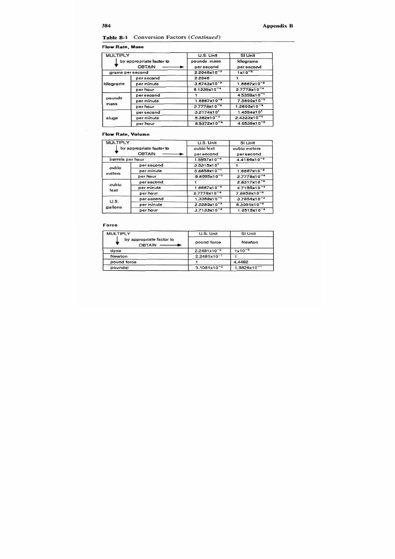
7/21/2019 Fundamental Fluid Mechanics for Engineers
http://slidepdf.com/reader/full/fundamental-fluid-mechanics-for-engineers 407/438
384
Appendix
B
Table
B - l ConversionFactors (Continued)
Flow
Rate,
Mass
MULTIPLY SI Unit U.S. Unit
by
appropriate factor
o
1 2.2046
er second
persecondper econd
OBTAIN-
ki lograms
oundsmass
grams persecond
1x1 0-32046x1 0 - 3
ki lograms
1.6687xlO-*. 6 7 4 3 ~ 1-'
er minute
per hour
2 . 7 7 7 8 ~ 1.1 239x1 0
pounds
mass
slugs
persecond 4 .5359~10-
pe r second 3 .21 74~ 10 '. 4 5 9 4 ~ 1 0 '
Flow Rate, Volume
Force
MULTIPLY SI Unit
.S. Unit
4 by
appropriate actor
to
OBTAIN pound force Newton
dyne
1.3826x10-'. 1 0 8 1 ~ 1 0 - ~
ounda l
4.4482
ound force
1
.2481x10-'
ewton
l~lO ~
. 2 4 8 1 ~ 1 0 - ~

7/21/2019 Fundamental Fluid Mechanics for Engineers
http://slidepdf.com/reader/full/fundamental-fluid-mechanics-for-engineers 408/438
Dimensions,nitystems,onversionactors 385
Table B-l Conversion Factors (Continued)
Length
I 4 by appropriateaclor
b
ORTAIN
meters
-- _.
I
I
centimeters
I
3 2 8 0 8 x 1
0-* I
1x10⁻²
~~
fee t
9.1 44x1"
ards
12352x1
O3
. 0 7 8 1 ~ 13
nauticalilesinternational)
1x1
0-
. 2 8 0 8 ~ 1 0 -
i l l imeters
1 .B093x1
3
. 2 8 0 ~ 1
3
i les
1
.2808eters
1x1
o3
. 2 8 0 8 ~ 1
3
i lometers
2 . 5 4 ~ 1
-
. 3 3 3 3 ~ 1 0
nches
3 . 0 4 8 ~ 1 0
Mass

7/21/2019 Fundamental Fluid Mechanics for Engineers
http://slidepdf.com/reader/full/fundamental-fluid-mechanics-for-engineers 409/438
Appendix
B
Table B - l ConversionPactors (Continued)
by appropr iate acb r to
I MULTIPLY
I
U.S. Uni t I SI Un i t
1
4
by appro pr ia te fac tor
to
poun d fo rce
O B T A I N
-
er squ are nch
a tmospheres , s tandard
1XI 05.4504~10'
ars
1.01325~15
.4696~10'
Pasca ls
inches o f
2.9890~13
.3354~10"
t 39.16
F
3.98 C)eet of
2.4886~10'. 6 0 0 5 ~ 1 0 ~
t 68
F 20
C)
ater
2.4908~10'.6128x1Ot
t 39.16 F 3.98 C)
wate r
at 68
F 20
C]
4.3278~10" 2.9839~1 O3
me r c u r y
3.3884~10'.91 15x1
0n c h e s
t32 F
1 .3332xG3 1.9337~10"en t ime te rs
l 0°C
1.3332~10' 1.9337~1ti l l imeters
I
Pasca ls
I 1.4504~10" I 1
1
p o u n d s f o r c e p e r s q u a r eoot
I 6.9444~10-
I 4.7880~10'
p o u n d s f o r c e p e r s q u a r e i n c h
I 1
I 6.8948~13

7/21/2019 Fundamental Fluid Mechanics for Engineers
http://slidepdf.com/reader/full/fundamental-fluid-mechanics-for-engineers 410/438
Dimensions,nitystems,onversionactors 387
Table'B-l Conversion Factors (Continued)
Specific Volume
MULTIPLY I
US.
Unit
SI
Unit
I
b y appropriate factorb
L
pound mass per kilogram
OBTAIN-
cubic meter
ubic foot per
cubiccentimeter Deraram
1x1
0-
.6018~1 - ~
cubic inch per pound mass
5.7870~10"
3.6127~1
-'
cubicfoot per poundmass
1 6.2428~1 - ~
cubic meter per kilogram
8.3454xlO-'.3368~10-~
.S.
gallon per poundmass
1
.6018~10'
. -
Surface
Tension
MULTIPLY
U.S. Unit I SI Unit
1
y
appropriate factor to
poundorce I Newton per
v
OBTAIN
-
meter
er foot
pounds force per foot
1
.8522~1-2
ewton per meter
1.4594~10'

7/21/2019 Fundamental Fluid Mechanics for Engineers
http://slidepdf.com/reader/full/fundamental-fluid-mechanics-for-engineers 411/438
388 Appendix B
Table
B-l Conversion
Factors (Cont inued)
Vkawity,
Dynamic
by appropriate factoro
Viscosity,
Kinematic
MULTIPLY
~~ ~~~~~
U.S. Unit
SI Unit
4
by
appropriate factor o square meters
quare feet
OBTAIN
___
per second per second
centistokes 1x1
0-
.0764~1
- S
I squareeeterecond I 1 I 9.2903~10-” I
I square meters persecond I 1.0764~10‘
Volume
MULTIPLY SI Unit U.S. Unit
4
by appropriate actor to
OBTAIN ___
cubic feet
cubicmeters
I barrels42 U.S. gallons) I 5.6146 1.5899~10“ I
cubic feet
1.531 5x1
0’
ubic meters
1.6387~1-’
.7870~1O“
ubic inches
2.831 7x10⁻²
Gallons, Imperial
1x10-3.531 5x10⁻²iters
3.7854~1
-3
.3368x10-’
allons, U.S.liquid 231in.3)
4.5461 x10-3.6054~10”

7/21/2019 Fundamental Fluid Mechanics for Engineers
http://slidepdf.com/reader/full/fundamental-fluid-mechanics-for-engineers 412/438
Table C-l Properties of Areas
Table C-2 Values of Flow Areas A and Hydraulic Radius R h for Various
Table C-3 Properties of Wrought Steel and Stainless Steel Pipe
Table C-4 Properties
of
250 psi Cast Iron Pipe
Table C-5 Properties
of
Seam less Copper Water Tube
Table C-6 Allowable Stress Values
for
Selected Piping Materials
Cross Sections
389
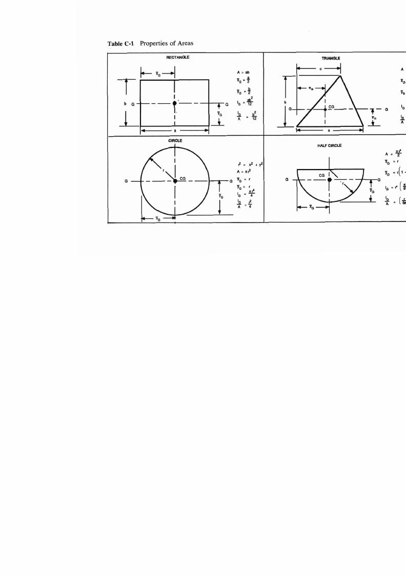
7/21/2019 Fundamental Fluid Mechanics for Engineers
http://slidepdf.com/reader/full/fundamental-fluid-mechanics-for-engineers 413/438
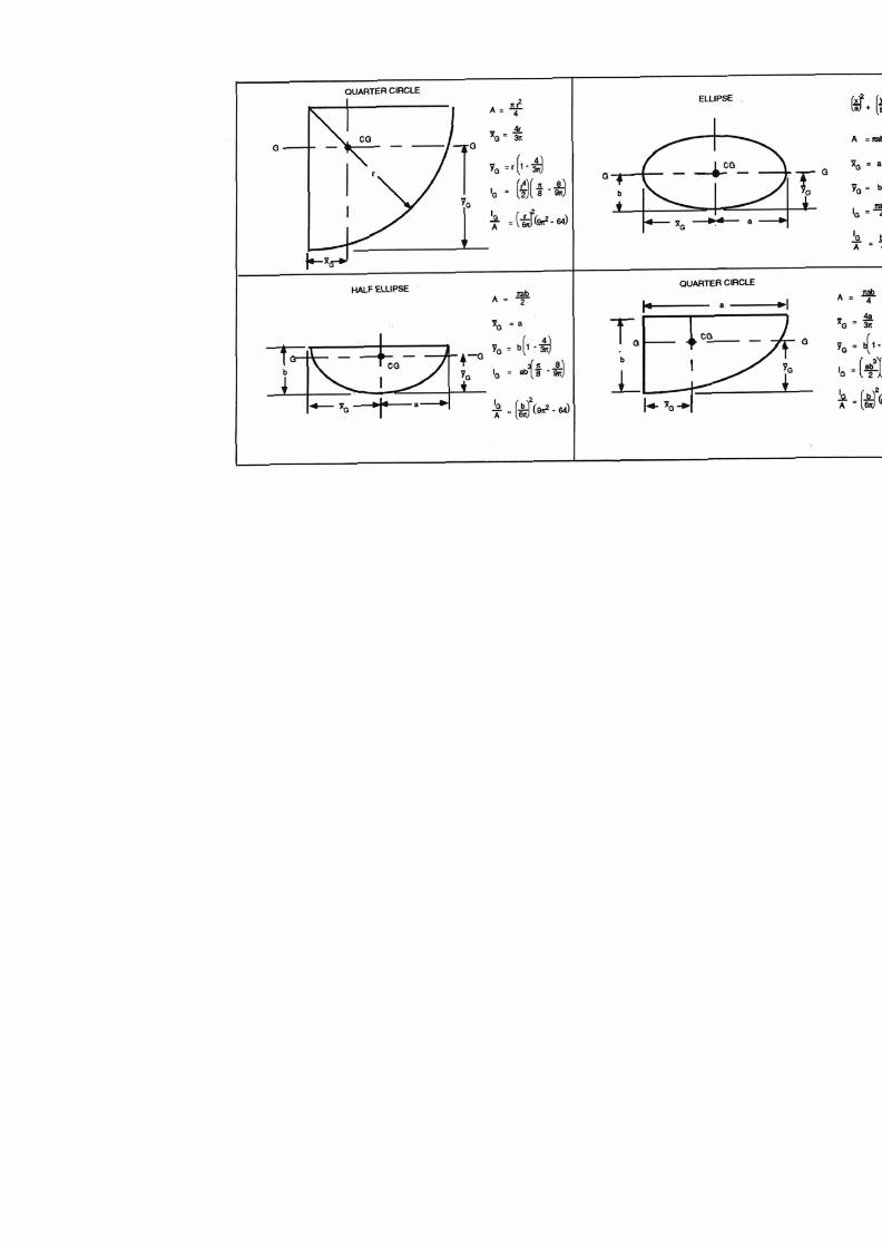
7/21/2019 Fundamental Fluid Mechanics for Engineers
http://slidepdf.com/reader/full/fundamental-fluid-mechanics-for-engineers 414/438
n
+
C
I
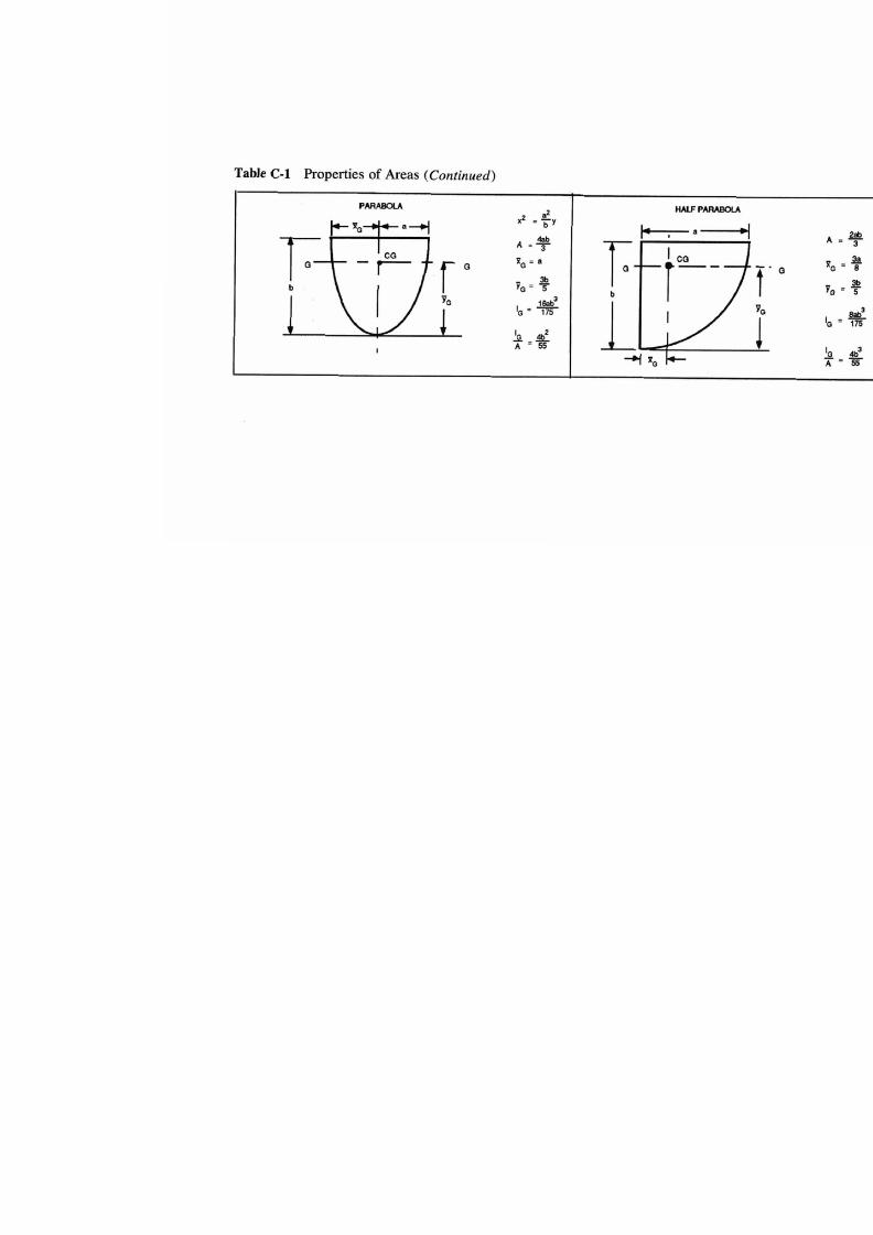
7/21/2019 Fundamental Fluid Mechanics for Engineers
http://slidepdf.com/reader/full/fundamental-fluid-mechanics-for-engineers 415/438

7/21/2019 Fundamental Fluid Mechanics for Engineers
http://slidepdf.com/reader/full/fundamental-fluid-mechanics-for-engineers 416/438
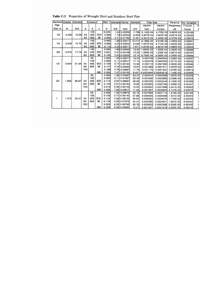
7/21/2019 Fundamental Fluid Mechanics for Engineers
http://slidepdf.com/reader/full/fundamental-fluid-mechanics-for-engineers 417/438

7/21/2019 Fundamental Fluid Mechanics for Engineers
http://slidepdf.com/reader/full/fundamental-fluid-mechanics-for-engineers 418/438

7/21/2019 Fundamental Fluid Mechanics for Engineers
http://slidepdf.com/reader/full/fundamental-fluid-mechanics-for-engineers 419/438

7/21/2019 Fundamental Fluid Mechanics for Engineers
http://slidepdf.com/reader/full/fundamental-fluid-mechanics-for-engineers 420/438

7/21/2019 Fundamental Fluid Mechanics for Engineers
http://slidepdf.com/reader/full/fundamental-fluid-mechanics-for-engineers 421/438
vv
d
Qc
c
.3

7/21/2019 Fundamental Fluid Mechanics for Engineers
http://slidepdf.com/reader/full/fundamental-fluid-mechanics-for-engineers 422/438

7/21/2019 Fundamental Fluid Mechanics for Engineers
http://slidepdf.com/reader/full/fundamental-fluid-mechanics-for-engineers 423/438
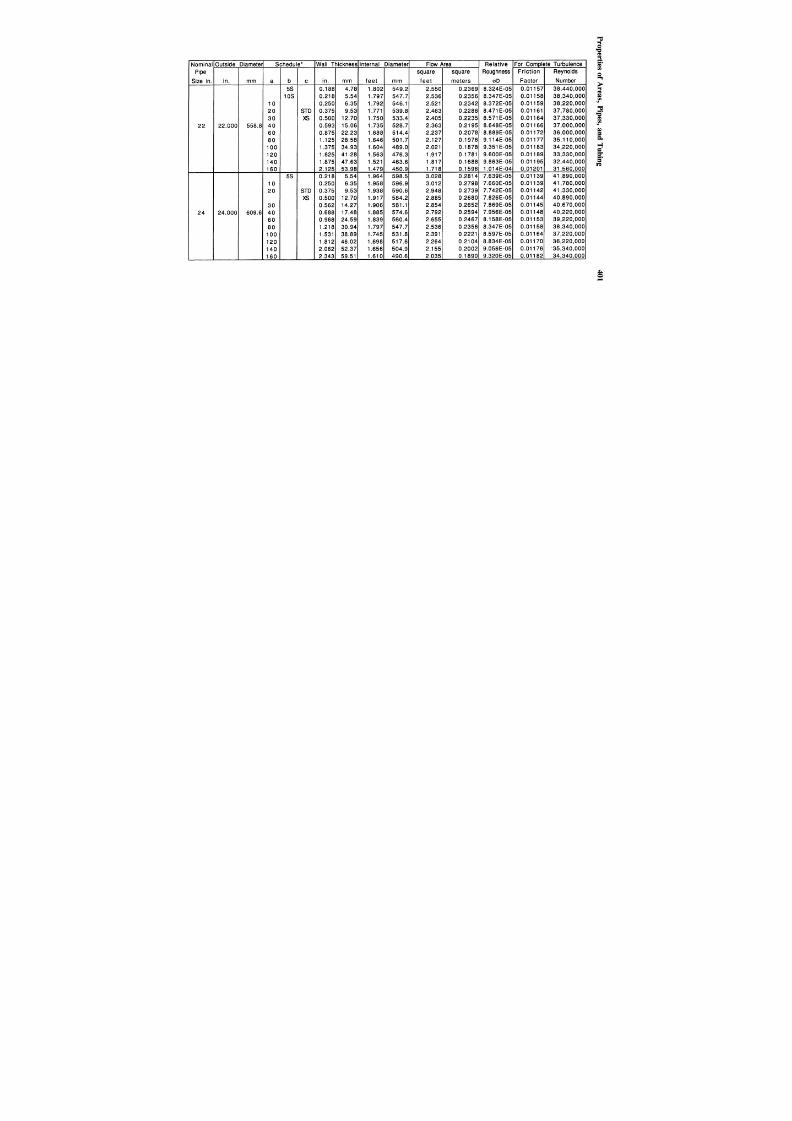
7/21/2019 Fundamental Fluid Mechanics for Engineers
http://slidepdf.com/reader/full/fundamental-fluid-mechanics-for-engineers 424/438
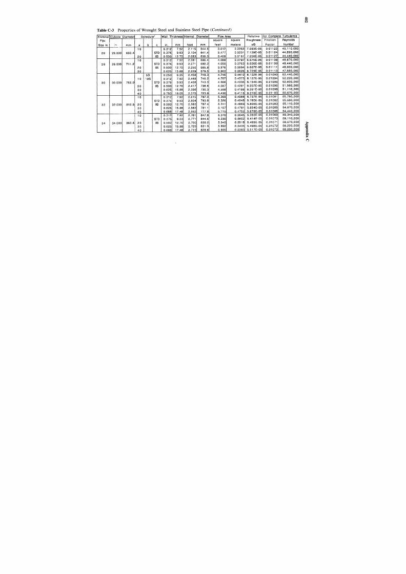
7/21/2019 Fundamental Fluid Mechanics for Engineers
http://slidepdf.com/reader/full/fundamental-fluid-mechanics-for-engineers 425/438

7/21/2019 Fundamental Fluid Mechanics for Engineers
http://slidepdf.com/reader/full/fundamental-fluid-mechanics-for-engineers 426/438
.
c
0
O
D

7/21/2019 Fundamental Fluid Mechanics for Engineers
http://slidepdf.com/reader/full/fundamental-fluid-mechanics-for-engineers 427/438

7/21/2019 Fundamental Fluid Mechanics for Engineers
http://slidepdf.com/reader/full/fundamental-fluid-mechanics-for-engineers 428/438
c
cx
3
c
d
E
m
-
g
.
t

7/21/2019 Fundamental Fluid Mechanics for Engineers
http://slidepdf.com/reader/full/fundamental-fluid-mechanics-for-engineers 429/438

7/21/2019 Fundamental Fluid Mechanics for Engineers
http://slidepdf.com/reader/full/fundamental-fluid-mechanics-for-engineers 430/438
2
m
4
c
c
v
N
c0
m
v
N
m
m
c
v
cm
m
c
r
m
N
c
4
c
r
v
W
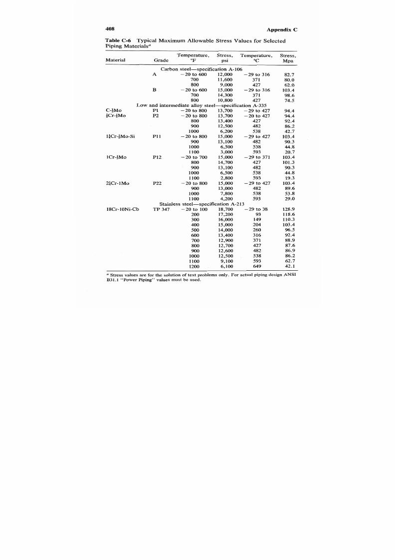
7/21/2019 Fundamental Fluid Mechanics for Engineers
http://slidepdf.com/reader/full/fundamental-fluid-mechanics-for-engineers 431/438
408
Appendix C
Table
C-6 Typical
Maximum
Allowable
Stress Values
for
Selected
Piping Materials"
Temperature, Stress, Temperature,
Material Grade "F psi
"C
Carbon steel-specification A-106
A -20 to 6002,000 -29 to 316
B -20 to 600 15,000 -29 to 316
7001,6007 1
800,00027
7004,30071
8000,80027
Low and intermediate alloy steel-specification A-335
C-~Mo P1 -20 to 8003,700 - 9 to 427
fCr-4Mo P2 -20 to 8003,700 -20 to 427
800
13,40027
900
12,50082
1000
6,20038
900
13,10082
1000
6,50038
1100
3,00093
800
14,70027
900 13,10082
1000 6,50038
1100
2,80093
900
13,00082
1000 7,80038
1100 4,20093
l4Cr-fMo-Si1 -20 to 8005,000 -29 to 427
1Cr-4Mo12 -20 to 7005,000 -29 to 371
P22 -20 to 8005,000 -29 to 427
Stainless steel-specification A-213
18Cr-1ONi-Cb
Tp
347 -20 to 1008,700 -29 to 38
200 17,2003
300 16,00049
400
15,00004
500 14,00060
600
13,40016
700 12,9007 1
800 12,70027
900
12,60082
1000
12,50038
1100
9,10093
1200
.
6,10049
24Cr-1Mo
Stress,
MPa
82.7
80.0
62.0
103.4
98.6
74.5
94.4
94.4
92.4
86.2
42.7
103.4
90.3
44.8
20.7
103.4
101.3
90.3
44.8
19.3
103.4
89.6
53.8
29.0
128.9
118.6
110.3
103.4
96.5
92.4
88.9
87.6
86.9
86.2
62.7
42.1
a Stress values arefor the solution of text problems only.
For
actual
piping design ANSI
B31.1
"Power Piping" values must be used.

7/21/2019 Fundamental Fluid Mechanics for Engineers
http://slidepdf.com/reader/full/fundamental-fluid-mechanics-for-engineers 432/438

7/21/2019 Fundamental Fluid Mechanics for Engineers
http://slidepdf.com/reader/full/fundamental-fluid-mechanics-for-engineers 433/438
410
Index
Bourdon tube gage, 51-53
Buckingham, Edgar, 277
Buckingham ll theorem,
Bulk modulus of elasticity
302-306
definition, 27
ideal gases, 29
liquids, 29-30
Buoyancy,
97-102
Buoyant force, 98-99
Capillarity,
38-41
Cast iron pipe, table, 404
Cauchy, Baron Augustin Louis
de, 290
Cauchy number,
313
Cavitation, 42-44
velocity, 42
Celsius, Anders, 8
Celsius temperature, 8-10
Centrifugal force,
285, 293-296
Centroids of plane areas, 70
Circle, properties of, 390
Coefficient
force, definition, 288
pressure, definition, 288
Compressed water, density and
viscosity of, table,
Compressibility factor of
370-372
compressed water and
steam, table, 370-372
Compressible flow, similarity of,
Compression shock wave,
Compressors, 143-144,160,
Continuity equation,
118-123
Convergent-divergent nozzles,
isentropic flow calculations,
289-293
202-2 14
294-296
ideal gas, 123
192-203, 209-2 14
196-202
Convergent nozzles, 184-188
Conversion factors, table
Copper water tube, table,
Corresponding states, principle
Critical flow, 182-183
Critical properties of selected
382-388
405-406
of, 25
fluids, table, 317-338
d’Alembert, Jean, 87
d’Alembert’s principle, 87
D’Arcy-Weisbach friction
Density
factor, 216
compressed water and steam,
definition, 16
table, 370-372
Design equations for pipes,
Diameter, equivalent,
127-129
Dimensional analysis
Buckingham ll theorem,
fluid machinery, 306, 316
format for, 315
Rayleigh method,
300-302
83-86
302-306
Dimensionless parameters,
Dimensions, 314, 375-376
276-3 16
of common variables, table,
314
Dynamic similarity,283-384
Dynamic viscosity,34-35
Efficiency
blade, 174-175
jet engine, 161
propellers, 168
rocket engine, 164
system, jet engine, 161

7/21/2019 Fundamental Fluid Mechanics for Engineers
http://slidepdf.com/reader/full/fundamental-fluid-mechanics-for-engineers 434/438
Index
411
Elastic force, 285
Elastic solid, 2
Ellipse, properties of,
391
Energy
definition, 12-16
equation, 140-145
internal, 134- 135
isentropic, 150-152
kinetic, 14-15, 133-134
potential, 12-14
specific,
133
rocket, 164
thermal jet, 160-163
Enthalpy, 136
Entropy, 139-140
Equations
Bernoulli, 130
continuity, 118-123
energy,
140-144
Euler’s 125
fluid statics, 47-48
ideal gas, 22-24
impulse and momentum,
motion, 124-126, 129-132
physical, 277-278
real gas,
24-25
Redlich-Kwong, 25-27
Equations of state
ideal gas, 22-24
real gas, 24-25
Redlich-Kwong, 25-27
Engines
15-16, 152-168
Equivalent diameter, 127-129
Euler, Leonhard, 106, 125, 277
Euler’s
equation,
125
number, 287-288
Exosphere, 64
Fahrenheit, Daniel Gabriel,7
Fahrenheit, temperature, 7-9
Fanning friction factor, 216
Fanno line
applications,
214-224
definition, 214-231
equations, 217-223
functions, table, 262-275
Flotation, 97-92
Flow
analysis methods, 115
areas of selected cross
sections, table,
393
curved path, 169-170
incompressible, similarity of,
Newtonian, 2
non-Newtonian, 2
one dimensional,
111
rate, mass, 118-123
rate, volumetric, 109-110
similarity
of
compressible,
similarity of incompressible,
steady, 106-108
three dimensional,
111
two dimensional,
11 1
unsteady, 106-108
work, 135- 136
dynamics, 124-175
forces, 284-285
ideal, 2
kinematics, 105-123
machinery parameters,
Newtonian, 2
properties, table,
317-371
statics, 46-104
Foot, definition, 380
Force@)
buoyant, 98-99
centrifugal, 285, 293-296
287-289
289-293
287-289
Fluid
306-31
1

7/21/2019 Fundamental Fluid Mechanics for Engineers
http://slidepdf.com/reader/full/fundamental-fluid-mechanics-for-engineers 435/438
412
Index
[Force(s)]
coefficient, definition, 288
curved surfaces, liquid,
77-81
elastic, 285
fluid, 284-285
gravity, 285
inertia, 284
moving blades, 171-174
plane areas, liquid,
71-76
pressure, 285
relation to mass, 10
shear,
2
surface tension, 285
vibratory, 285
viscous, 284
Free-body analysis, 99-100
Frequency
structure, 286
wake, 286
Friction factor
D’Arcy-Weisbach, 216
Fanning, 216
number, definition, 297
William, 297
Froude
Gage pressure, 6
Gallon, definition,
380
Gas dynamics,
176-275
Gas turbine, 160
Gasses
definition, 3
properties of selected, table,
Geometric similarity, 278-280
Gravity
339-368
definition, 11-12
force,
285
specific,
17-20,
API,
18-20,
Baum6, 18-20
Half
circle, properties of, 390
[Half]
ellipse, properties of, 391
parabola, properties of,
392
Heat, 139-140
History of units, 373-375
Hydraulic radius
definition, 127
description, 127-129
selected cross sections, table,
393
Hydrometers, 18-20,101-102
Ideal
jet engine, efficiency, 161
plastic, 2
rocket engine, efficiency, 164
Ideal fluid, 2
Ideal gas(es)
bulk modulus of elasticity,
29
continuity equation,
123
equation of state, 22-24
isentropic
energy relations, 150-152
process, 2
process, 21
specific heats, 148-149
process, 22
specific heat, 148
isothermal process, 21
polytropic
flow, 179-184
isobaric
isometric
process, 20-21
specific heart,
150
pressure-height relations,
processes,
20-22
ratio of specific heats,
sonic velocity, 34
specific heat, 148-150
viscosity, 36
62-64
149-150

7/21/2019 Fundamental Fluid Mechanics for Engineers
http://slidepdf.com/reader/full/fundamental-fluid-mechanics-for-engineers 436/438
Index
Impulse and momentum, 15-16,
Inclined manometers,
57-58
Incompressible flow, similarity
Inertia force, 284
Internal energy, 134-135
International Practical
Ionosphere,
6 4
Isentropic
energy relations, 150-152
flow
152-168, 204-297
Of, 287-289
Temperature Scale, 7-8
functions, 184
pipes, limiting flow rate,
pipes, limiting pressure,
table, 238-249
191-193
191-193
,
ideal gases,
179-184
Isobaric process, 21
Isometric process, 22
Isothermal
process, 21
flow with friction, 231-237
process, 21
Jet engine,
160-163
efficiency, ideal,
system efficiency
thrust, 161
161
',161
useful power, 161
Kelvin, Lord, 8
Kelvin temperature,
8-10
Kilogram, 377, 381
Kinematic similarity,280-282
Kinematic viscosity, 35-36
Kinetic energy, 14-15, 133-134
correction, 115-1
18
413
Lagrange, Joseph Louis, 106
Liquid(s)
bulk modulus of elasticity,
force
29-30
curved surfaces, 77-81
location, 74-77
plane areas, 71-76
viscosity, 36
Mach, Emst, 178
Mach number, definition, 178
Manometers
applications, 58-62
general, 54-62
inclined, 57-58
U-tube, 55-56,91-92
well-type, 56-58
Mass flow rate, 118-123
Mass, definition,
10, 377, 381
Mesosphere,
6 4
Meter, definition, 377
Model prototype relations
compressor, 294-296
definition, 278
linear, 297-299
pipes, 279-282
reservoir, 290-293
seaplane,
286
submarine, 288-289
valve, 299
Mole, definition, 377
Momentum and impulse, 15-16,
Motion and energy equations,
152-168
144-145
Newton, definition, 10
Newton's second law
of
motion,
Newtonian fluid,2
Nonflow shaft work, 137-138
10-16

7/21/2019 Fundamental Fluid Mechanics for Engineers
http://slidepdf.com/reader/full/fundamental-fluid-mechanics-for-engineers 437/438
414
Index
Non-Newtonian fluid,
2
Normal shock functions, 202,
214
table, 255-261
Normal shock wave, entropy
Nozzles
increase, 207-208
convergent, 184- 188
convergent-divergent,
192-203, 209-2 14
Observed pressure, 6
One dimensional flow,
11
1
Parabola, properties of, 392
Pascal, Blaise, 47
Phase, 3-4
Physical equations,
277-278
Pipe flow with friction
adiabatic, 214-231
isothermal, 231-237
cast iron, table,‘404
seamless copper water tube,
stainless steel, table, 394-403
wrought steel, table,
394-403
allowable stress values for
Pipe properties
table, 405-406
Piping
selected materials, table,
408
design equations for, 83-86
schedule numbers, 84-86
stress in, 77-81
thin wall, 81-82
Plastic, ideal,
2
Poiseuille, Jean Louis, 36
Polytropic processes, 20-21
Potential energy, 12-14, 133
Power, useful, jet engine, 161
Pressure
atmospheric, 5
barometric,
6
coefficient, definition,288
definition, 5
force, 285
gage,
6
height relations
ideal gases, 62-64
incompressible fluids,49-51
sensing devices, 51-62
standard atmospheric, 5
vapor, 42-44
Propellers, 166-169
Properties
fluid mechanics, table, 45
selected fluids, table, 317-371
selected gases, table, 339-368
Proportionality constant,
10-1
1
Prototypes,
278
Pump laws, 307-308
Quarter circle, properties of, 391
Quarter ellipse, properties of,
39
Radius, hydraulic, 127-129
Rankine temperature, 8-10
Rankine,
William J . ,
8
Rayleigh, Lord,
277
Rayleigh’s method, 300-302
Real gas, equation of state, 24
Rectangle, properties of, 390
Redlich-Kwong equation of
state, 25-27
Reynolds number, 287
Reynolds, Osborne, 287
Rocket engines, 164-165
Saturated properties of selected
Saybolt viscosity, 36-38
fluids, table, 317-338
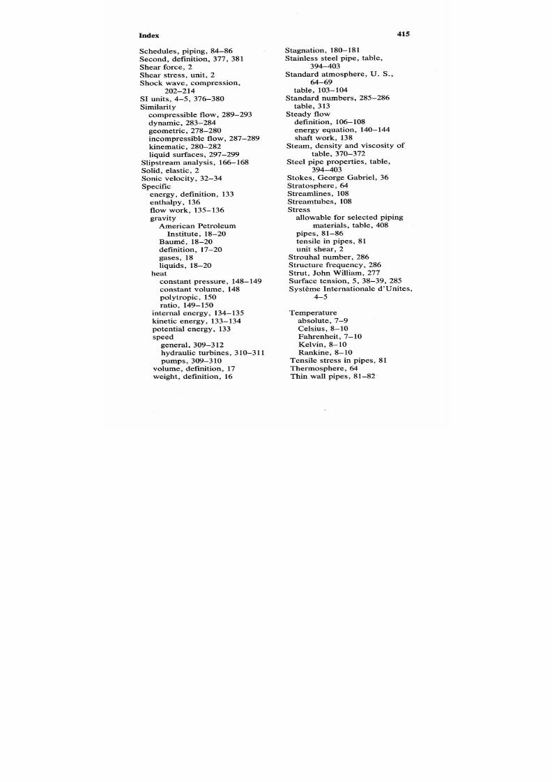
7/21/2019 Fundamental Fluid Mechanics for Engineers
http://slidepdf.com/reader/full/fundamental-fluid-mechanics-for-engineers 438/438
Index
415
Schedules, piping, 84-86
Second, definition, 377, 381
Shear force,
2
Shear stress, unit,
2
Shock wave, compression,
SI units, 4-5, 376-380
Similarity
202-214
compressible flow,289-293
dynamic, 283-284
geometric, 278-280
incompressible flow,
287-289
kinematic, 280-282
liquid surfaces, 297-299
Slipstream analysis, 166-168
Solid, elastic,
2
Sonic velocity, 32-34
Specific
energy, definition, 133
enthalpy,
136
flow work, 135-136
gravity
American Petroleum
Institute, 18-20
BaumC, 18-20
definition, 17-20
gases, 18
liquids, 18-20
Stagnation, 180-181
Stainless steel pipe, table,
Standard atmosphere, U. S. ,
394-403
64-69
table, 103-104
Standard numbers, 285-286
table, 313
Steady flow
definition, 106-108
energy equation, 140-144
shaft work,
138
Steam, density and viscosity of
table, 370-372
Steel pipe properties, table,
Stokes, George Gabriel, 36
Stratosphere, 6 4
Streamlines, 108
Streamtubes,
108
Stress
394-403
allowable for selected piping
materials, table, 408
pipes, 81-86
tensile in pipes,
81
unit shear, 2
Strouhal number, 286
Structure frequency, 286