Fundamental Drivers of the Cost and Price of Operating ... · PDF fileoperating reserve...

NREL is a national laboratory of the U.S. Department of Energy Office of Energy Efficiency & Renewable Energy Operated by the Alliance for Sustainable Energy, LLC This report is available at no cost from the National Renewable Energy Laboratory (NREL) at www.nrel.gov/publications.

Contract No. DE-AC36-08GO28308

Fundamental Drivers of the Cost and Price of Operating Reserves Marissa Hummon, Paul Denholm, Jennie Jorgenson, and David Palchak National Renewable Energy Laboratory

Brendan Kirby Consultant

Ookie Ma U.S. Department of Energy

Technical Report NREL/TP-6A20-58491 July 2013

NREL is a national laboratory of the U.S. Department of Energy Office of Energy Efficiency & Renewable Energy Operated by the Alliance for Sustainable Energy, LLC This report is available at no cost from the National Renewable Energy Laboratory (NREL) at www.nrel.gov/publications.

Contract No. DE-AC36-08GO28308

National Renewable Energy Laboratory 15013 Denver West Parkway Golden, CO 80401 303-275-3000 • www.nrel.gov

Fundamental Drivers of the Cost and Price of Operating Reserves Marissa Hummon, Paul Denholm, Jennie Jorgenson, and David Palchak National Renewable Energy Laboratory

Brendan Kirby Consultant

Ookie Ma U.S. Department of Energy

Prepared under Task No. SA12.0200

Technical Report NREL/TP-6A20-58491 July 2013

NOTICE

This report was prepared as an account of work sponsored by an agency of the United States government. Neither the United States government nor any agency thereof, nor any of their employees, makes any warranty, express or implied, or assumes any legal liability or responsibility for the accuracy, completeness, or usefulness of any information, apparatus, product, or process disclosed, or represents that its use would not infringe privately owned rights. Reference herein to any specific commercial product, process, or service by trade name, trademark, manufacturer, or otherwise does not necessarily constitute or imply its endorsement, recommendation, or favoring by the United States government or any agency thereof. The views and opinions of authors expressed herein do not necessarily state or reflect those of the United States government or any agency thereof.

This report is available at no cost from the National Renewable Energy Laboratory (NREL) at www.nrel.gov/publications.

Available electronically at http://www.osti.gov/bridge

Available for a processing fee to U.S. Department of Energy and its contractors, in paper, from:

U.S. Department of Energy Office of Scientific and Technical Information P.O. Box 62 Oak Ridge, TN 37831-0062 phone: 865.576.8401 fax: 865.576.5728 email: mailto:[email protected]

Available for sale to the public, in paper, from:

U.S. Department of Commerce National Technical Information Service 5285 Port Royal Road Springfield, VA 22161 phone: 800.553.6847 fax: 703.605.6900 email: [email protected] online ordering: http://www.ntis.gov/help/ordermethods.aspx

Cover Photos: (left to right) photo by Pat Corkery, NREL 16416, photo from SunEdison, NREL 17423, photo by Pat Corkery, NREL 16560, photo by Dennis Schroeder, NREL 17613, photo by Dean Armstrong, NREL 17436, photo by Pat Corkery, NREL 17721.

Printed on paper containing at least 50% wastepaper, including 10% post consumer waste.

http://www.osti.gov/bridge

mailto:[email protected]

mailto:[email protected]

http://www.ntis.gov/help/ordermethods.aspx

iii

Foreword This report is one of a series stemming from the U.S. Department of Energy (DOE) Demand Response and Energy Storage Integration Study. This study is a multi-national-laboratory effort to assess the potential value of demand response and energy storage to electricity systems with different penetration levels of variable renewable resources and to improve our understanding of associated markets and institutions. This study was originated, sponsored, and managed jointly by the DOE Office of Energy Efficiency and Renewable Energy and the DOE Office of Electricity Delivery and Energy Reliability.

Grid modernization and technological advances are enabling resources, such as demand response and energy storage, to support a wider array of electric power system operations. Historically, thermal generators and hydropower in combination with transmission and distribution assets have been adequate to serve customer loads reliably and with sufficient power quality, even as variable renewable generation like wind and solar power become a larger part of the national energy supply. While demand response and energy storage can serve as alternatives or complements to traditional power system assets in some applications, their values are not entirely clear. This study seeks to address the extent to which demand response and energy storage can provide cost-effective benefits to the grid and to highlight institutions and market rules that facilitate their use.

The project was initiated and informed by the results of two DOE workshops: one on energy storage and the other on demand response. The workshops were attended by members of the electric power industry, researchers, and policymakers, and the study design and goals reflect their contributions to the collective thinking of the project team. Additional information and the full series of reports can be found at www.eere.energy.gov/analysis/.

The authors would like to thank the following individuals for their valuable input and comments during the analysis and publication process: Nate Blair, Chunlian Jin, Michael Kintner-Meyer, Mark O’Malley, Michael Milligan, Krishnappa Subbarao, Keith Searight, Aaron Townsend, and Aidan Tuohy. Any errors or omissions are solely the responsibility of the authors.


http://www.eere.energy.gov/analysis/

iv

Abstract Operating reserves impose a cost on the electric power system by forcing system operators to keep partially loaded spinning generators available to respond to system contingencies and random variation in demand. In many regions of the United States, thermal and hydropower plants provide a large fraction of the operating reserve requirement. Alternative sources of operating reserves, such as demand response and energy storage, may provide these services at lower cost. However, to estimate the potential value of these services, the cost of reserve services under various grid conditions must first be established.

This analysis used a commercial grid simulation tool to evaluate the cost and price of several operating reserve services, including spinning contingency reserve, upward regulation reserve, and a proposed flexibility/ramping reserve. These reserve products were evaluated in a utility system in the western United States, considering different system characteristics, renewable energy penetration, and several other sensitivities.

Overall, the analysis demonstrates that the price of operating reserves depends greatly on many assumptions regarding the operational flexibility of the generation fleet, including ramp rates and the fraction of the fleet available to provide reserves. In addition, a large fraction of the regulation price in this analysis was derived from the assumed generator bid prices (based on the cost of generators operating at non-steady state while providing regulation reserves). Unlike other generator performance data (such as heat rate), information related to an individual generator’s ability to provide reserves is not publicly available. Therefore, reproducing the cost of reserves in a production cost model involves significant uncertainty.

While variable renewables increase the total reserve requirements, the additional operational cost of these reserves appears modest in the evaluated system. Wind and solar generation tend to free up generation capacity in proportion to its production, largely canceling out the net cost of the additional operating reserves. However, further work is needed to address issues, such as down reserves and implementation of fast-response regulation, which were not included in this study. Finally, this analysis points to the need to consider how the operation of the power system and composition of the conventional generation fleet may evolve if wind and solar power reach high penetration levels.


v

Table of Contents 1 Introduction ........................................................................................................................................... 1 2 Energy and Operating Reserves Costs .............................................................................................. 3 3 Simulation of Operating Reserves Costs ........................................................................................... 5

3.1 Test System Description ................................................................................................................ 5 3.2 Reserve Requirements ................................................................................................................... 6 3.3 Unit Commitment and Dispatch Simulations .............................................................................. 10

4 Cost and Price of Ancillary Services ................................................................................................ 11 4.1 Surplus Ramp Capacity in Energy Dispatch ............................................................................... 11 4.2 Operating Reserve Opportunity Costs ......................................................................................... 14 4.3 Base Case Energy and Reserve Costs ......................................................................................... 19

5 Sensitivity Results .............................................................................................................................. 24 5.1 Availability of Fleet to Provide Regulation and Flexibility Reserves ......................................... 24 5.2 Impact of Renewable Generation Penetration ............................................................................. 28

5.2.1 Reserve requirements as a function of renewable energy penetration ........................... 28 5.2.2 Cost and Price Impacts for Renewable Penetration Scenarios ....................................... 30 5.2.3 Impact of Progressively Increasing Flexible Hydroelectric Generation ........................ 33

5.3 Impact of Increased Reserve Requirement and Natural Gas Price .............................................. 35 6 Conclusions ........................................................................................................................................ 38 References ................................................................................................................................................. 40 Appendix. Supplemental Data ................................................................................................................. 43

A.1 Calculating Surplus Ramp Capacity .............................................................................................. 43 A.2 Reserves and Energy Prices ........................................................................................................... 44

Time Series, Distributions, and Statistics .................................................................................... 44 Price of Reserves: Effect of the availability of surplus ramp capacity ........................................ 44

A.3 Cost to System for Reserves (All Sensitivities) ............................................................................. 46 A.4 Flexibility Reserve Violations ....................................................................................................... 48


vi

List of Figures Figure 1. Simplified example of ideal and reserve-constrained dispatch ........................................4 Figure 2. Regulation reserve requirement for the base scenario with 15% renewable penetration

in April (top) and July (bottom) .................................................................................................8 Figure 3. (a) Energy dispatch and (b, c, and d) ramping capacity available for regulation,

contingency, and flexibility reserves, respectively, for the base case of the test system at the end of July ..........................................................................................................................12

Figure 4. (a) Energy dispatch and (b, c, and d) ramping capacity available for regulation, contingency, and flexibility reserves, respectively, for the base case of the test system in April. ....................................................................................................................................13

Figure 5. Seasonal and daily variation in the fraction of the reserve requirement that can be met with surplus ramp capacity ...............................................................................................14

Figure 6. Change in energy dispatch when system is required to hold reserves capacity: (a) summer (b) spring...............................................................................................................16

Figure 7. Opportunity cost for generators drive the price of reserves (a) summer (b) spring .......18 Figure 8. Average annual load factor (during online hours) for the cases without and with

reserves requirements...............................................................................................................20 Figure 9. System price duration curve for regulation in the base system and three markets

in 2011 .....................................................................................................................................22 Figure 10. Price duration curve for spinning contingency reserves for the base case system

(simulated) and three markets in 2011 .....................................................................................23 Figure 11. Regulation reserve price duration curve for four levels of fleet availability: 40%,

60%, 80%, and 100% ...............................................................................................................26 Figure 12. Average hourly prices for regulation in summer and spring for four levels of fleet

availability: 40%, 60%, 80%, and 100% .................................................................................26 Figure 13. Reserve provision (a) regulation, (b), contingency, (c) flexibility when CTs are

allowed to provide regulation ..................................................................................................27 Figure 14. Example time series for the five renewable penetration scenarios: (a) Generation from

wind and solar for April 15–17 (b) Total and net load for the same time period ....................28 Figure 15. Annual reserve requirement (GW-h) per GWh of renewable generation for regulation

(95th percentile of 5-minute ramps) and flexibility (67th percentile of 20-minute ramps) .....30 Figure 16. Annual (a) energy dispatch and (b-d) reserve provision for additional flexible

hydropower penetration cases ..................................................................................................34 Figure A-1. Example dispatch of a single generator ......................................................................43 Figure A-2. Distribution of energy prices with and without the penalty prices removed .............44 Figure A-3. Reserve marginal price for sensitivities of Fleet Availability as a function of the

percent of reserve requirement covered at no opportunity cost to the system .........................45


vii

List of Tables Table 1. Characteristics of Test System Conventional Generators in 2020 ....................................6 Table 2. Summary of Operating Reserves in Base Case of Test System ........................................9 Table 3. Assumed Additional Operating Cost for Units Providing Regulation Reserves .............10 Table 4. Energy Results for Base Case ..........................................................................................19 Table 5. System Costs for Base Case.............................................................................................20 Table 6. Marginal Reserve and Energy Price for Base Case .........................................................21 Table 7. Fleet Availability Sensitivities .........................................................................................24 Table 8. Increase in Generation Cost with Reduction in Fleet Availability ..................................25 Table 9. Total Ancillary Service Cost to Consumers for Various Availabilities of Fleet

Provision ..................................................................................................................................27 Table 10. Reserve Requirements by Renewable Penetration Scenario .........................................29 Table 11. Reserve Cost and Price for Renewable Penetration Scenarios ......................................31 Table 12. Incremental Benefits and Costs of Renewable Penetration and Reserve

Requirements ...........................................................................................................................32 Table 13. Mean Percent of Incremental Reserve Requirement Covered by the Incremental

Increase in Ramping Capacity Available at No Opportunity Cost to the Generators .............33 Table 14. Reserve Cost and Price for Flexible Hydropower Penetration Scenarios .....................35 Table 15. Reserves Cost and Price for Increased Reserve Requirement Scenarios .......................36 Table 16. Reserve Cost and Price for of Natural Gas Price Scenarios ..........................................37 Table A-1. Cost of Holding Reserves for All Sensitivity Scenarios..............................................46 Table A-2. Flexibility Reserve Violations .....................................................................................48


1

1 Introduction Operating reserves are among a larger class of services often referred to as ancillary services that help ensure grid reliability. Operating reserves include contingency reserves (the ability to respond to a major contingency such as an unscheduled power plant or transmission line outage) and regulation reserves (the ability to respond to small, random fluctuations around normal load) (NERC 2013). Another operating reserve service, referred to as load-following reserve, is part of sub-hourly energy scheduling, but it has not yet been a distinct market product.1 However, a flexibility or ramping reserve product is being proposed to address the increased variability and uncertainty created by renewable energy sources such as wind and solar (Xu and Tretheway 2012; Navid et al. 2011). Operating reserves are provided by a mix of sources including partially loaded thermal and hydroelectric power plants or responsive loads and storage able to change output in a short period.

The provision of operating reserves incurs a cost to system operators and plant owners. Before the introduction of open access transmission and the advent of restructured markets, there was a general awareness of the existence of these costs but little quantification of them.2 These costs were embedded in the total cost incurred by vertically integrated utilities, along with the provision of energy and capacity.3

Electric sector restructuring created markets for several types of operating reserves. Among these were markets for regulation reserve and spinning contingency reserve. These markets initially demonstrated relatively high prices for these services and attracted attention from potential market entrants, including technology suppliers that have historically struggled to gain market acceptance for technologies such as energy storage and demand response. These markets have also created opportunities for non-traditional sources of reserves such as vehicle-to-grid services that could support deployment of electric vehicles or plug-in hybrid electric vehicles (Kempton and Tomic 2005).

Historical market data are useful as an indicator of what a market participant would have received under prevailing conditions but provide limited insight into future opportunities. It is challenging to understand the relationship between operating reserve prices and fuel prices, the impact of new market entrants, and changes in market rules. As a result, potential market entrants face significant risk when relying on historical market data while making investment decisions.

1 The nomenclature used for various ancillary services and operating reserves (especially spinning reserves) varies significantly. While the NERC Glossary of Terms Used in Reliability Standards (NERC 2013) indicates that spinning reserve applies to both contingency and regulation, the term spinning reserve often is used to refer to only contingency reserves. For additional discussion of terms applied to various reserve products, see Ela et al. (2011). 2 This issue has been noted previously—“ancillary services have been produced all along by traditional utilities as part of the bundled electricity product they provide to their customers. Because the utilities sold them as part of a bundled product, even they have only limited knowledge of the actual costs to produce each service” (Hirst and Kirby 1998). 3 An example of a previous estimate of reserve costs in real utilities systems is Kirby and Hirst (1996) who estimated the total operating reserves costs as between 0.5% and 1.2% of the total costs for several U.S. utilities. Their estimates included both the additional capacity costs and operating costs, including: “fuel associated with heat-rate degradation from constant cycling, the costs of out-of-merit-order dispatch, plus additional maintenance to compensate for wear and tear on the units caused by cycling.”


2

Better understanding of reserve prices is even more important when considering the impact of increased deployment of variable renewable energy sources such as wind and solar. These sources increase the variability and uncertainty of the net load and may increase requirements for operating reserves on multiple time scales.4 They also change the operation of the conventional generator fleet, and they can both increase and decrease the availability of generators to provide reserves depending on multiple factors. The impact of renewables on reserve prices cannot easily be extracted from historical data, given the significant interaction between operating reserve prices and energy prices and given the significant changes that will occur to the system as a whole when adding zero fuel cost sources such as wind and solar.

This report describes an evaluation of the underlying cost sensitivities of several classes of operating reserves. Section 2 summarizes the cost origins of operating reserves. Section 3 describes the simulation of a power system with operating reserves. Section 4 provides results of a test system examining the cost of reserves. Section 5 explores the sensitivity of reserve costs to such factors as renewable penetration, fuel price, and individual generator constraints. The overall goal of this study is to explore the fundamental drivers of operating reserve costs and provide insights into the opportunities for new technologies to provide cost-effective reserve services to utilities and system operators.

4 The term “net load” may be used to describe the normal load minus the contribution from variable generation sources such as solar and wind. It describes the load that the system operator must meet with conventional thermal and hydropower resources.


3

2 Energy and Operating Reserves Costs Utilities and system operators optimize the operation of an electric power system by committing and dispatching generators in order of production cost (from lowest to highest) until the sum of the individual generator’s output equals load in each time interval. The dispatch is calculated using software that considers the many additional constraints imposed by individual generators, such as minimum load point, minimum up and downtimes, and ramp rates.

System dispatch is complicated by the need to keep operating reserves which incurs a cost that can be calculated by the dispatch software. Fundamentally, the cost of operating reserves is driven by the need to keep a subset of generators operating at part load, available to increase output if needed. From the perspective of an individual generator, keeping a unit at part load incurs an opportunity cost because it cannot be dispatched to its full output. From the system perspective, the need for reserves can result in higher generation costs because keeping plants at part load increases the number of plants that are online. These additional online units have equal or higher production costs than the generators that were backed down to provide reserves. This ultimately results in higher operational costs (more fuel use and more units started) per unit of energy actually produced. In addition, partial loading can reduce the efficiency of individual power plants, particularly when plants are providing regulation reserve, which requires continuous changes in output over short periods. Non-steady state operation resulting from providing regulation reserves can also increase O&M requirements (Kumar et al. 2012).

Figure 1 provides a simplified illustration of the change in dispatch (and possible cost impacts) needed to provide operating reserves. The figure on the left shows an idealized dispatch of a small electric power system. Two baseload units provide most of the energy, while an intermediate load and two peaking units change output in response to the variation in normal demand. In the “ideal” dispatch, the intermediate load unit might be unable to rapidly increase output to provide operating reserves. Furthermore, during the transition periods when the load-following units are nearing their full output—but before additional units are turned on—capacity left in the load-following units may be insufficient to provide necessary operating capacity for regulation or contingencies. A dispatch that provides the necessary reserves is provided on the right. In this case, lower-cost units reduce output to accommodate the more flexible units providing reserves. This increases the overall cost of operating the entire system.


4

Figure 1. Simplified example of ideal and reserve-constrained dispatch

A least-cost dispatch, whether in a vertically integrated utility or in a market environment, requires co-optimization of both energy and reserves to pick the mix of generators that provides the overall least-cost system operation. While the addition of reserve services greatly increases the complexity of the optimal dispatch problem, system operators use sophisticated software tools to calculate this cost as part of daily market operation (PJM 2012). In contrast to the cost of energy, which can be understood with basic knowledge of fuel prices and power plant performance characteristics, the cost of operating reserves in a real system is inherently a function of the interaction of multiple power plants. The incremental and total cost of reserves in any hour is entirely a function of which generators are online, which generators can provide reserves, and sometimes complicated market rules for procuring and pricing operating reserves. This makes it more difficult to evaluate the cost implications of different fuel prices, generator mixes, or other changes to a power system that occur over time.


5

3 Simulation of Operating Reserves Costs In an attempt to understand the drivers of reserve costs, we simulated the operation of a power system with software that co-optimizes provision of energy and reserves. We used a commercial software tool (PLEXOS)5 to perform the simulations in a test system and evaluate the sensitivity of reserve prices to a variety of operational constraints, fuel prices, and other factors.

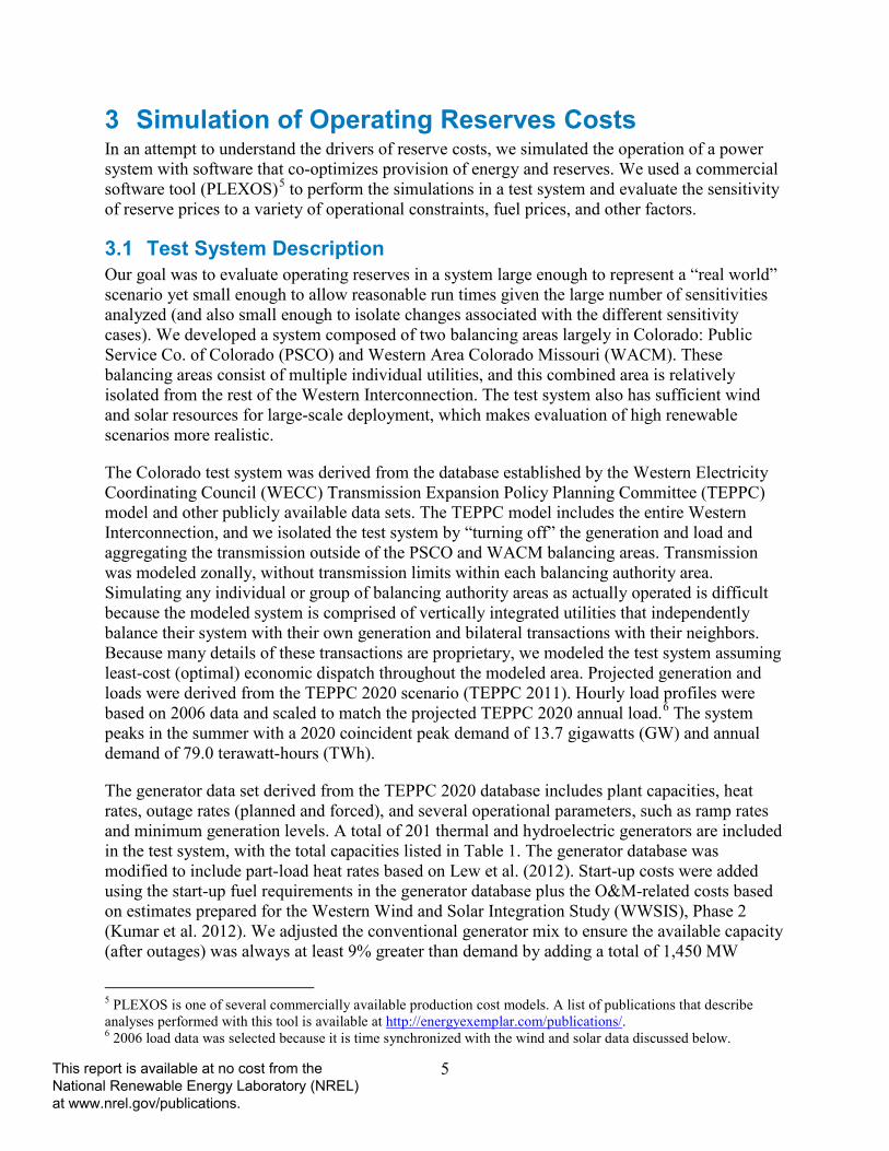
3.1 Test System Description Our goal was to evaluate operating reserves in a system large enough to represent a “real world” scenario yet small enough to allow reasonable run times given the large number of sensitivities analyzed (and also small enough to isolate changes associated with the different sensitivity cases). We developed a system composed of two balancing areas largely in Colorado: Public Service Co. of Colorado (PSCO) and Western Area Colorado Missouri (WACM). These balancing areas consist of multiple individual utilities, and this combined area is relatively isolated from the rest of the Western Interconnection. The test system also has sufficient wind and solar resources for large-scale deployment, which makes evaluation of high renewable scenarios more realistic.

The Colorado test system was derived from the database established by the Western Electricity Coordinating Council (WECC) Transmission Expansion Policy Planning Committee (TEPPC) model and other publicly available data sets. The TEPPC model includes the entire Western Interconnection, and we isolated the test system by “turning off” the generation and load and aggregating the transmission outside of the PSCO and WACM balancing areas. Transmission was modeled zonally, without transmission limits within each balancing authority area. Simulating any individual or group of balancing authority areas as actually operated is difficult because the modeled system is comprised of vertically integrated utilities that independently balance their system with their own generation and bilateral transactions with their neighbors. Because many details of these transactions are proprietary, we modeled the test system assuming least-cost (optimal) economic dispatch throughout the modeled area. Projected generation and loads were derived from the TEPPC 2020 scenario (TEPPC 2011). Hourly load profiles were based on 2006 data and scaled to match the projected TEPPC 2020 annual load.6 The system peaks in the summer with a 2020 coincident peak demand of 13.7 gigawatts (GW) and annual demand of 79.0 terawatt-hours (TWh).

The generator data set derived from the TEPPC 2020 database includes plant capacities, heat rates, outage rates (planned and forced), and several operational parameters, such as ramp rates and minimum generation levels. A total of 201 thermal and hydroelectric generators are included in the test system, with the total capacities listed in Table 1. The generator database was modified to include part-load heat rates based on Lew et al. (2012). Start-up costs were added using the start-up fuel requirements in the generator database plus the O&M-related costs based on estimates prepared for the Western Wind and Solar Integration Study (WWSIS), Phase 2 (Kumar et al. 2012). We adjusted the conventional generator mix to ensure the available capacity (after outages) was always at least 9% greater than demand by adding a total of 1,450 MW

5 PLEXOS is one of several commercially available production cost models. A list of publications that describe analyses performed with this tool is available at http://energyexemplar.com/publications/. 6 2006 load data was selected because it is time synchronized with the wind and solar data discussed below.


http://energyexemplar.com/publications/

6

(690 MW of combustion turbines and 760 MW of combined cycle units). This adjustment was necessary in part because the simulated system does not include contracted capacity from surrounding regions or any capacity contribution from solar and wind resources.

Table 1. Characteristics of Test System Conventional Generators in 2020

Technology System Capacity (MW)

Coal 6,180

Combined Cycle (CC) 4,284

Gas Combustion Turbine (CT) 4,653

Hydropower 777

Pumped Storage Hydropower 560

Othera 242

Total 16,696 a Includes oil- and gas-fired internal combustion and steam generators

The base test system assumes a wind and solar penetration of 16% on an energy basis. A total of 3,347 MW of wind (generating about 10.7 TWh annually) and 878 MW of PV (generating about 1.8 TWh annually) was added to the system. For comparison, Colorado received about 11% of its electricity from wind in 2012.7 Solar photovolatic (PV) profiles were generated using the System Advisor Model (Gilman and Dobos 2012) with meteorology data for 2006. Wind data were derived from the WWSIS data set (GE Energy 2010), also with meteorology data for 2006.8 Discrete wind and solar plants were added from the WWSIS data sets until the installed capacity produced the targeted energy penetration. The sites were chosen based on capacity factor and do not necessarily reflect existing or planned locations for wind and solar plants.

Fuel prices were derived from the TEPPC 2020 database. Coal prices were $1.42 per million British thermal units (MMBtu) for all plants. Natural gas prices varied by plant and for most plants were in the range of $3.90/MMBtu to $4.20/MMBtu, with a generation-weighted average of $4.10/MMBtu. This is slightly lower than the EIA’s 2012 Annual Energy Outlook projection for the delivered price of natural gas to the electric power sector in the Rocky Mountain region of $4.46/MMBtu in 2020 (EIA 2012a). No constraints or costs were applied to carbon or other emissions.

3.2 Reserve Requirements We included three classes of operating reserves that require generators to be synchronized to the grid and be able to rapidly increase output:9 contingency, regulation, and flexibility reserves.10

7 Colorado generated 6,045 gigawatt-hours (GWh) from wind in 2012 compared to total generation of 53,594 GWh (EIA 2012b). 8 All generation profiles were adjusted to be time synchronized with 2020, which is a leap year. 9 This is an oversimplification. Contingency reserves require the ability to rapidly increase in output. While we are only simulating up reserves, regulation up and flexibility reserves require the ability to ramp up and down while following a reserve signal.


7

Contingency reserves were based on the single largest unit (an 810-MW coal plant), and were allocated with 451 MW to PSCO and 359 MW to WACM, with the requirement that 50% was met by spinning units.11 We did not model the non-spinning portion of this reserve requirement.12 This contingency reserve was assumed to be constant for all hours of the year, and it corresponds to an average spinning reserve requirement of about 4.5% of load. Any partially loaded plant, constrained by the 10-minute ramp rate of individual generators, was allowed to provide contingency reserves. Contingency reserves were independent of wind and solar penetration, assuming no single wind or solar plant (including associated transmission) becomes the single largest contingency.

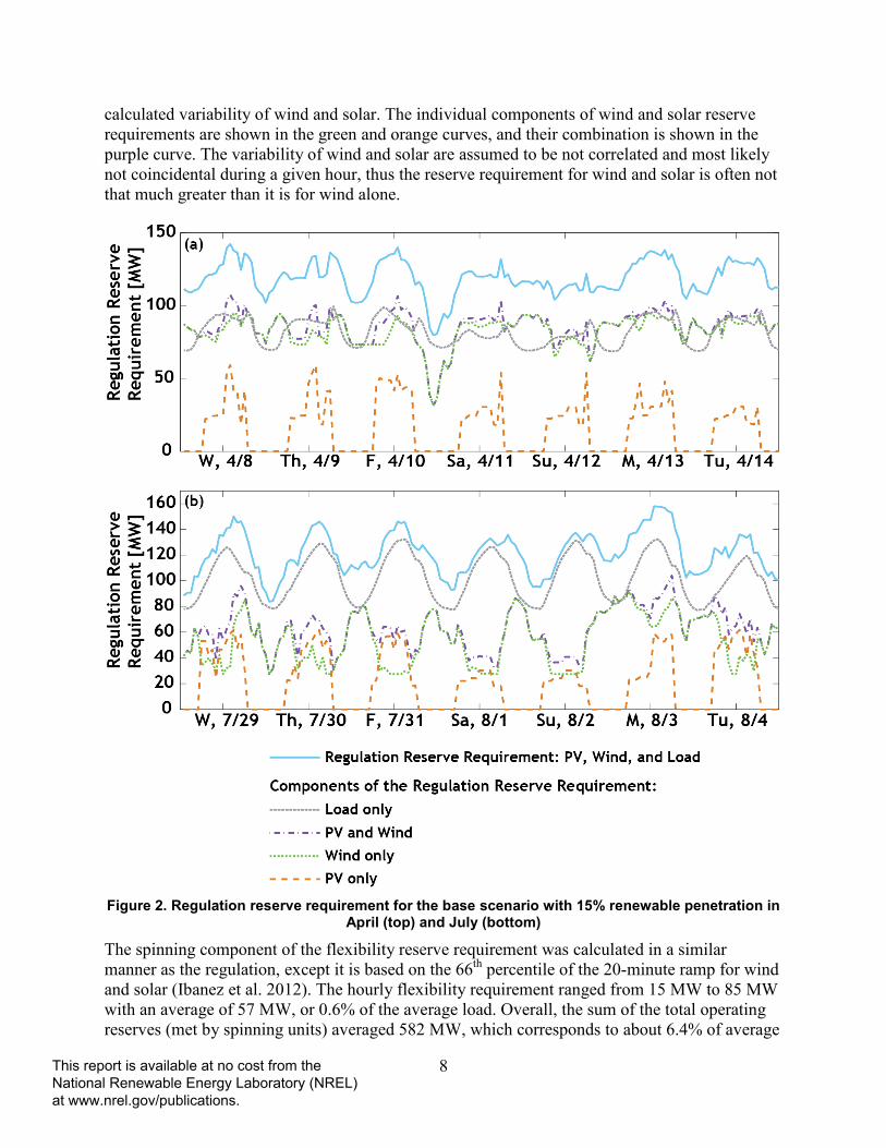
Regulation and flexibility reserve requirements vary over time based on the statistical variability of load, wind, and PV, with the methodology described in detail by Ibanez et al. (2012). For these services, only the “upward” reserve requirements were evaluated. The need for downward reserves becomes more important at high renewable penetration when conventional thermal generators are operated at or near their minimum generation points for more hours of the year.13 The regulation reserve requirement is calculated by geometrically adding the expected variability for wind, solar, and load. Geometric addition is used to calculate the combined variance of uncorrelated random variables.14 The origin of the variability for wind (changes in hub-height wind speed), solar (size and speed of clouds), and load (aggregation of consumer behavior) are assumed to be uncorrelated. The statistical variability for solar was found by calculating the 95th percentile of the 5-minute ramps, normalized by both the installed solar capacity as well as the “predicted” clear sky solar power production based on Ibanez et al. (2012). In other words, the regulation requirement did not increase for sunrise, which is a predictable event. The statistical variability for wind was the 95th percentile of the 5-minute ramps of the wind power, normalized by the installed wind capacity. We assumed regulation due to load variability was 1% of average hourly load.15 The regulation reserve requirement (requiring a 5-minute response) for the system ranged from 73 MW to 166 MW with an average of 120 MW, equal to about 1.3% of the average load.

Figure 2 provides an example of the relative contribution of load, wind, and solar to the upward regulation requirement. It shows each component of the variability over one-week periods in spring (Figure 2a) and summer (Figure 2b). The total regulation requirement (the top blue curve) is the combined requirement due to load (equal to 1% of total load, shown in black) and the

10 For additional discussion of these reserves (especially flexibility reserves, which are not yet a well-defined market product), see Ela et al. (2011). 11 The PSCO and WACM balancing areas are part of the Rocky Mountain Reserve Group, which shares contingency reserves based on these values. 12 This would tend to slightly underestimate total production cost; however, market-clearing prices for non-spinning reserves are typically very low as there is often little opportunity cost for holding non-spinning reserves. 13 The need to keep down reserves can impose an opportunity cost in a manner similar to “upward reserves”. The actual cost of downward reserves was not evaluated in this study. Future work will evaluate the cost and price of separate up and down reserve products in these scenarios. 14 Geometric addition is equal to the square root of the sum of the squares. 15 Regulation requirements vary by region. ERCOT determines regulation requirements based on historical variability of the 5-minute net load and historical regulation deployments. We did not have 5-minute load data for the test system, so used a fixed percentage, similar to PJM which bases regulation requirement on 1% of peak load during peak hours and 1% of valley during off-peak hours. See Ela et al. (2011) for additional details of regional regulation requirements.


8

calculated variability of wind and solar. The individual components of wind and solar reserve requirements are shown in the green and orange curves, and their combination is shown in the purple curve. The variability of wind and solar are assumed to be not correlated and most likely not coincidental during a given hour, thus the reserve requirement for wind and solar is often not that much greater than it is for wind alone.

Figure 2. Regulation reserve requirement for the base scenario with 15% renewable penetration in

April (top) and July (bottom)

The spinning component of the flexibility reserve requirement was calculated in a similar manner as the regulation, except it is based on the 66th percentile of the 20-minute ramp for wind and solar (Ibanez et al. 2012). The hourly flexibility requirement ranged from 15 MW to 85 MW with an average of 57 MW, or 0.6% of the average load. Overall, the sum of the total operating reserves (met by spinning units) averaged 582 MW, which corresponds to about 6.4% of average


9

load. Table 2 summarizes the general characteristics of the three modeled reserve services. Reserves were modeled as “soft constraints,” meaning the system was allowed to not meet requirements if the cost exceeded the high threshold value shown in Table 2. The requirement to meet load was also modeled as a soft constraint, with a penalty price of $10,000/MWh. However, in all scenarios, there was no lost load and no violations of either regulation or contingency reserve requirements. There were a few hours of flexibility reserve violations, due in part to the lower penalty price (see the appendix for details).

Table 2. Summary of Operating Reserves in Base Case of Test System

Operating Reserve Service

System Drivers

Time to Respond (min)

Requirement (% of Load) Mean (Min/Max)

Penalty ($/MW-h)a

Regulation Up PV, wind, load 5 1.33 (1.00/1.71) 9,500

Contingency largest generator 10 4.54 (2.97/5.95) 9,000

Flexibility Up PV, wind 20 0.64 (0.13/1.07) 8,500 a The unit “MW-h” is sometimes applied to capacity-related services such as operating reserves. It represents a unit of capacity (MW) held for one hour. It is distinct from MWh which is a unit of energy. The availability and constraints of individual generators providing reserves is a major driver for the cost of providing reserves. Not all generators are capable of providing regulation reserves based on operational practice or lack of necessary equipment to follow a regulation signal. For assigning which plants can provide regulation, we based our assumptions on the PLEXOS database established for the California Independent System Operator’s “33% Renewable Integration Study” (CAISO 2011). This data set assigns regulation capability to a subset of plants, which is about 60% of total capacity within California (as measured by their ramp rate). Similarly, we allowed only 60% of all dispatchable generators (coal, gas combined cycle [CC]), dispatchable hydro, and pumped storage) to provide regulation. Cases where up to 100% of the conventional fleet is allowed to provide reserves are considered in Section 5.1. Based on feedback from various utilities and system operators, we further restricted combustion turbines (CTs) from providing regulation in the base case. We also considered the impact of allowing CTs to provide regulation in Section 5.1. We allowed all dispatchable plants (including CTs) to provide flexibility and contingency reserves.

An additional cost was assigned to plants providing regulation, associated with additional wear and tear and heat rate degradation associated with non steady-state operation. This is functionally equivalent to a generator regulation “bid cost” in restructured markets, discussed in PJM (2013). The assumed regulation costs by unit type are provided in Table 3.


10

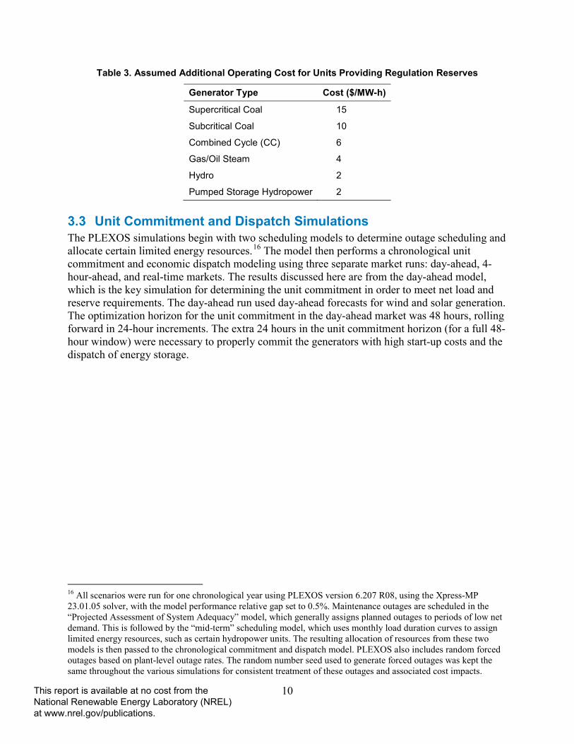
Table 3. Assumed Additional Operating Cost for Units Providing Regulation Reserves

Generator Type Cost ($/MW-h)

Supercritical Coal 15

Subcritical Coal 10

Combined Cycle (CC) 6

Gas/Oil Steam 4

Hydro 2

Pumped Storage Hydropower 2 3.3 Unit Commitment and Dispatch Simulations The PLEXOS simulations begin with two scheduling models to determine outage scheduling and allocate certain limited energy resources.16 The model then performs a chronological unit commitment and economic dispatch modeling using three separate market runs: day-ahead, 4-hour-ahead, and real-time markets. The results discussed here are from the day-ahead model, which is the key simulation for determining the unit commitment in order to meet net load and reserve requirements. The day-ahead run used day-ahead forecasts for wind and solar generation. The optimization horizon for the unit commitment in the day-ahead market was 48 hours, rolling forward in 24-hour increments. The extra 24 hours in the unit commitment horizon (for a full 48-hour window) were necessary to properly commit the generators with high start-up costs and the dispatch of energy storage.

16 All scenarios were run for one chronological year using PLEXOS version 6.207 R08, using the Xpress-MP 23.01.05 solver, with the model performance relative gap set to 0.5%. Maintenance outages are scheduled in the “Projected Assessment of System Adequacy” model, which generally assigns planned outages to periods of low net demand. This is followed by the “mid-term” scheduling model, which uses monthly load duration curves to assign limited energy resources, such as certain hydropower units. The resulting allocation of resources from these two models is then passed to the chronological commitment and dispatch model. PLEXOS also includes random forced outages based on plant-level outage rates. The random number seed used to generate forced outages was kept the same throughout the various simulations for consistent treatment of these outages and associated cost impacts.


11

4 Cost and Price of Ancillary Services The costs of operating reserves can be examined using either total costs or short-run marginal costs of production. The total cost of reserves can be estimated by examining the commitment and dispatch of a system with and without reserve constraints. The difference in production cost between the two cases represents the total costs of holding reserves. The marginal cost of reserves is based on the change in total costs resulting from holding the last unit of reserves (i.e., the marginal unit). This quantity is typically an output of the optimization algorithm used by production cost models; in ISO/RTO markets, it equates to a market-clearing price paid to all providers of reserves. In this report, we use the term “price” to represent this marginal cost, which would correspond to the price of reserves calculated and reported in a market environment.17 In order to understand the cost and price of ancillary services we examine two concepts: first, how does the unit commitment optimization change when the system must provide energy and reserves as opposed to providing only energy; and second, how does this change in unit commitment and dispatch result in the price of reserves. Section 4.1 examines the surplus ramp capacity of units committed to provide only energy. Section 4.2 demonstrates the relationship between the price of reserves and the lost opportunity cost associated with generators holding capacity to provide reserves. Section 4.3 presents the base case results for the cost and price of reserves.

4.1 Surplus Ramp Capacity in Energy Dispatch The scheduling of energy alone often results in some additional ramping capability beyond what is necessary to move from one energy-scheduling interval to the next. This “surplus” ramp capacity is then available to provide reserves without any additional cost to the system.18 The dispatch stack from a week in July for the test system is shown in Figure 3(a). In this scenario, the reserve requirements within the unit commitment model were set to zero, and this dispatch was optimized only for the system energy requirements. Figure 3 (b, c, and d) shows the hourly system requirements for each of the reserve products (solid line) in the corresponding hours, and the sum of all surplus ramp capacity available for each reserve product (shaded area), that can be utilized at no additional cost to the system. Surplus ramp capacity for each generator in each time step is calculated by multiplying the available ramp rate of the generator times the response time of the reserve product (see Table 2), limited by the total undispatched capacity for the time step. The available ramp rate excludes ramping capacity required for energy dispatch, e.g. if the unit needs 2 MW/min to ramp between dispatch points and the maximum ramp rate is 5 MW/min, the available ramp rate is 3 MW/min.

The surplus ramp capacity is due to the operational constraints of the individual generators, including generator minimum load point, maximum ramp rate, and minimum up-time. Because of these restrictions, the system must often commit and dispatch units that operate at part load and are therefore available to be ramped and provide reserves at no additional production cost to the system as a whole. In this example in summer, the peak load in the middle of the day and significant ramping requirements over the early part of the day required a significant number of

17 This assumes that prices in a restructured market result from generators bidding their marginal costs for both energy and regulation reserves. As a result, real bidding strategies and high prices that result from scarcity bids are not captured in these simulations. 18 This ignores the additional costs for regulation reserves.


12

generators to be online during the overnight hours. These units were backed down (output reduced and therefore operating below their maximum) and were therefore able to provide upward reserves. Overall, this results in ramp capacity to provide reserves available overnight but not during the day.

Figure 4 shows the system dispatch (again without any reserve requirements) for a week in April. The lower variation in demand (compared to summer) requires fewer units to be online at part load. As a result, there is lower surplus ramp capacity available for reserves during most hours.

Figure 3. (a) Energy dispatch and (b, c, and d) ramping capacity available for regulation, contingency, and flexibility reserves, respectively, for the base case of the test system at the end

of July


13

Figure 4. (a) Energy dispatch and (b, c, and d) ramping capacity available for regulation,

contingency, and flexibility reserves, respectively, for the base case of the test system in April


14

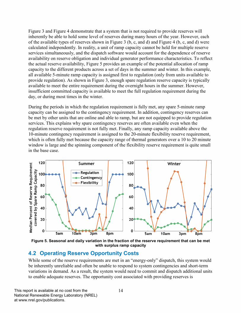
Figure 3 and Figure 4 demonstrate that a system that is not required to provide reserves will inherently be able to hold some level of reserves during many hours of the year. However, each of the available types of reserves shown in Figure 3 (b, c, and d) and Figure 4 (b, c, and d) were calculated independently. In reality, a unit of ramp capacity cannot be held for multiple reserve services simultaneously, and the dispatch software would account for the dependence of reserve availability on reserve obligation and individual generator performance characteristics. To reflect the actual reserve availability, Figure 5 provides an example of the potential allocation of ramp capacity to the different products across a set of days in the summer and winter. In this example, all available 5-minute ramp capacity is assigned first to regulation (only from units available to provide regulation). As shown in Figure 3, enough spare regulation reserve capacity is typically available to meet the entire requirement during the overnight hours in the summer. However, insufficient committed capacity is available to meet the full regulation requirement during the day, or during most times in the winter.

During the periods in which the regulation requirement is fully met, any spare 5-minute ramp capacity can be assigned to the contingency requirement. In addition, contingency reserves can be met by other units that are online and able to ramp, but are not equipped to provide regulation services. This explains why spare contingency reserves are often available even when the regulation reserve requirement is not fully met. Finally, any ramp capacity available above the 10-minute contingency requirement is assigned to the 20-minute flexibility reserve requirement, which is often fully met because the capacity range of thermal generators over a 10 to 20 minute window is large and the spinning component of the flexibility reserve requirement is quite small in the base case.

Figure 5. Seasonal and daily variation in the fraction of the reserve requirement that can be met

with surplus ramp capacity

4.2 Operating Reserve Opportunity Costs While some of the reserve requirements are met in an “energy-only” dispatch, this system would be inherently unreliable and often be unable to respond to system contingencies and short-term variations in demand. As a result, the system would need to commit and dispatch additional units to enable adequate reserves. The opportunity cost associated with providing reserves is


15

calculated by the system operator and forms the basis for the price of reserves in restructured markets. From the perspective of a market participant, lost opportunity cost represents the energy market profit a generator will lose when backed down to provide both energy and reserves (approximately equal to the energy market price minus the generator’s variable production cost times the reserve amount provided by the generator).19 From the perspective of a system operator, lost opportunity cost represents the additional costs associated with supplying energy from higher production cost units due to having to meet the reserve requirement. The PLEXOS model calculates opportunity cost in a similar manner to the market software used by system operators. This includes the effect of reduced generator efficiency when operating at part load to provide reserves.20

Figure 6 illustrates the change in dispatch between the previous case of no reserves and the actual reserve-constrained dispatch (in which the reserve requirements were added to the model). The overall amount of energy provided in each hour is the same (because adding reserves does not change the overall energy requirement), but a shift in the source of generation by generator type occurs because of the additional constraints imposed by requiring operating reserves. In nearly every hour, there is a shift from lower-cost to higher-cost units (from coal to combined-cycle or from combined-cycle to gas combustion turbine generation). This result follows the conceptual illustration of reserve-constrained dispatch (Figure 1), in which higher-cost units are started to create more “headroom” (available dispatchable capacity) in the entire generation fleet.

19 This is a simplified description. System operator market manuals have complete description (where opportunity cost is actually often referred to as “lost opportunity cost”) (PJM 2013). For example the NYISO provides the following definition “ Lost Opportunity Cost - 'LOC' - The foregone profit associated with the provision of Ancillary Services, which is equal to the product of: (1) the difference between (a) the Energy that a Generator could have sold at the specific LBMP and (b) the Energy sold as a result of reducing the Generator's output to provide an Ancillary Service under the direction of the NYISO; and (2) the LBMP existing at the time the Generator was instructed to provide the Ancillary Service, less the Generator's Energy bid for the same MW segment.” http://www.nyiso.com/public/markets_operations/services/customer_support/glossary/index.jsp 20 However this does not include the impact of non steady-state operation that occurs when a generator is continually following a regulation signal. System operators do not include this impact in the opportunity cost calculation. It is part of a separate bid to capture the impacts of reduced efficiency, additional O&M and other costs associated with operation in this manner (PJM 2013).


http://www.nyiso.com/public/markets_operations/services/customer_support/glossary/index.jsp

16

Figure 6. Change in energy dispatch when system is required to hold reserves capacity:

(a) summer (b) spring. Numbers greater than zero demonstrate the generation was added when the system was required to hold reserves.

This shift in generation from lower-cost to higher-cost units increases the overall cost of production, and it is the basis for the price of the reserves services, equal to the opportunity cost incurred for holding the marginal unit of reserves. Figure 7 demonstrates the calculated price for regulation reserves for the same period. In Figure 7a (summer, shown in the top chart), during each overnight period, the system has sufficient capacity to meet the regulation reserve requirement without changing the dispatch (as previously demonstrated in Figure 3). As a result, there is no opportunity cost (at least for upward reserves), and the cost of regulation reserves is only the operational cost of providing regulation with the marginal generator (in this case, a combined-cycle generator with a regulation operational cost of $6/MW-h). 21

When insufficient reserves are available from the “energy-only” dispatch, the system operator must re-dispatch the system to create adequate ramping capacity of the proper type. As demonstrated in Figure 3, during the day the combined-cycle units would typically ramp up to their maximum output and be unable to provide regulation reserves. Because we assume

21 As discussed in Section 3.2, the origin of this cost is the additional wear-and-tear and other impacts associated with the rapid response required by following a regulation signal.


17

combustion turbines are unable to provide regulation reserves in our base case (with a sensitivity scenario in Section 5.1), at least some of the combined-cycle units must be operated at part load to provide these reserves. It follows that additional generation capacity must be started to provide the energy otherwise provided by combined-cycle units. Figure 6 demonstrates that most of this energy is from combustion turbines, with small contributions from oil-gas steam generators and other more expensive generators. This incurs a generator opportunity cost, which is the difference between the cost of providing energy from a combined-cycle unit and the combustion turbine. In a market setting, when a combustion turbine or steam unit is operated in order for combined-cycle units to back down and provide reserves, the combined-cycle unit loses the opportunity to sell energy.

The price of the reserves calculated by the production cost model (equivalent to a market-clearing price in a market setting) was based on the marginal cost difference between the higher-cost generator that had to be turned on and the lower-cost generator held at part load to provide reserves. In the period illustrated in Figure 7(a), the marginal cost of combined-cycle units in the generator fleet was in the range of $27/MWh to $33/MWh, while the cost of most combustion turbines were in the range of $37/MWh to $47/MWh. The price of regulation reserves is the difference in the marginal costs between the combined-cycle and combustion turbine (in the range of $4/MWh to $20/MWh with an average of about $11/MWh) plus the addition operational cost of a combined-cycle when providing regulation (which we assume is $6/MW-h). As a result, the price of regulation during the day ranged from $10/MW-h to $26/MW-h). As before, we use $/MWh to measure the cost of energy, while we use $/MW-h as the cost of reserves capacity held in each hour.


18

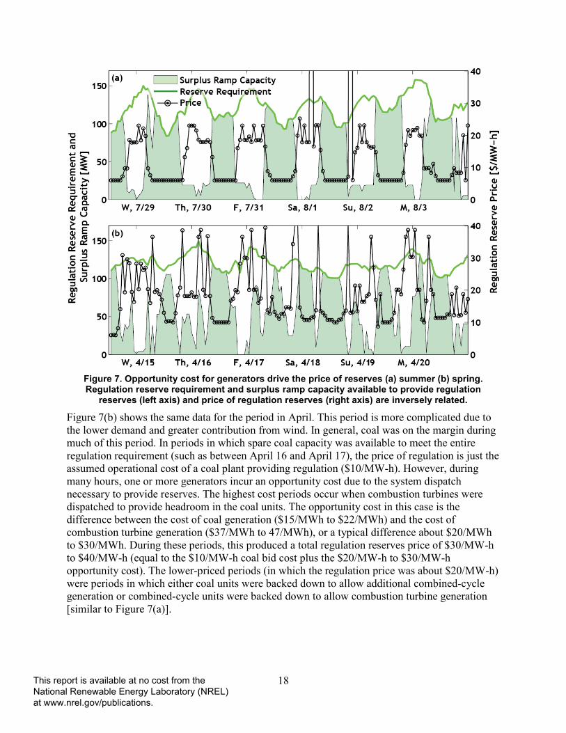
Figure 7. Opportunity cost for generators drive the price of reserves (a) summer (b) spring. Regulation reserve requirement and surplus ramp capacity available to provide regulation

reserves (left axis) and price of regulation reserves (right axis) are inversely related.

Figure 7(b) shows the same data for the period in April. This period is more complicated due to the lower demand and greater contribution from wind. In general, coal was on the margin during much of this period. In periods in which spare coal capacity was available to meet the entire regulation requirement (such as between April 16 and April 17), the price of regulation is just the assumed operational cost of a coal plant providing regulation ($10/MW-h). However, during many hours, one or more generators incur an opportunity cost due to the system dispatch necessary to provide reserves. The highest cost periods occur when combustion turbines were dispatched to provide headroom in the coal units. The opportunity cost in this case is the difference between the cost of coal generation ($15/MWh to $22/MWh) and the cost of combustion turbine generation ($37/MWh to 47/MWh), or a typical difference about $20/MWh to $30/MWh. During these periods, this produced a total regulation reserves price of $30/MW-h to $40/MW-h (equal to the $10/MW-h coal bid cost plus the $20/MW-h to $30/MW-h opportunity cost). The lower-priced periods (in which the regulation price was about $20/MW-h) were periods in which either coal units were backed down to allow additional combined-cycle generation or combined-cycle units were backed down to allow combustion turbine generation [similar to Figure 7(a)].


19

4.3 Base Case Energy and Reserve Costs The qualitative results from Section 4.1 can be translated into the total cost and price of providing various reserve services. Table 4 summarizes the generation and fuel use for the cases with and without reserves, demonstrating the shift in generation illustrated in Figure 6. Specifically, Table 4 demonstrates how in this system holding reserves required coal units to reduce output to accommodate additional gas-fired generation and increased the generation from lower efficiency gas-units. The net effect is that the system holding operating reserves burned about 0.8% less coal but nearly 5% more gas (and about 0.3% more total fuel) compared to a system that did not require operating reserves.

In addition to cost related to fuel use, the system will incur additional costs when providing reserves due to more frequent unit starts. When the system was required to provide capacity for reserves, the CT fleet had a 64% increase in the MW-starts, which are calculated by multiplying the capacity of the unit by the number of starts over the year, summed across all similar units.

Table 4. Energy Results for Base Case

Generation (GWh)a

Without Reserves

With Reserves

Increase (Absolute/%)

Coal 46,478 46,129 -348 / -0.8%

Gas Combined Cycle (CC) 14,652 14,736 84 / 0.6%

Gas Combustion Turbine (CT) 796 1,055 258 / 33.3%

Hydropower 3,795 3,792 -3 / -0.1%

Pumped Hydropower Storage 871 1,055 184 / 21.2%

Wind 10,705 10,705 0 / 0%b

PV 1,834 1,834 0 / 0%b

Otherc 11 101 90 / 788.5%

Total Generation (GWh)d 79,143 79,408 265 / 0.3%

Fuel Use (1,000 MMBTU)

Without Reserves

With Reserves

Increase (Absolute/%)

Coal 491,952 488,099 -3,853 / -0.8%

Gas 120,996 126,871 5,875 / 4.9%

Total Fuel Use 612,948 614,970 2,022 / 0.3% a gigawatt-hours b Neither wind nor PV experienced curtailment in these cases. c Includes oil- and gas-fired internal combustion and steam generators.

d The difference in generation is associated with the additional use of pumped storage including losses.

The change in dispatch required when providing reserves can also be observed in terms of the greater part-load operation, illustrated in Figure 8. In the base case without reserve provision, the annual average load factor of coal, CC, and CT units (when the units are actually online) was


20

about 100%, 80%, and 80%, respectively. When the system holds reserves, CTs are operated at part load more often as they are often turned on just to provide headroom in the CC units. Because they are more expensive to operate, they are held at close to their minimum generation points, resulting in an annual average load factor of about 40% (again as measured only during hours when operating—their annual average capacity factor is much less at about 3%.)

Figure 8. Average annual load factor (during online hours) for the cases without and with reserves

requirements

The overall cost associated with holding all operating reserves is summarized in Table 5. The increased fuel use and unit starts increased the cost of serving load by about $27 million (2%), with the majority of the increased costs (about 69%) due to increased fuel costs.

Table 5. System Costs for Base Case

Cost Without Reserves

With Reserves

Increase (000$/%)

Total Fuel Cost (000$) 1,192,466 1,211,294 18,828 / 1.6%

Total VOM Cost (000$) 152,749 152,089 -660 / -0.4%

Total Start Cost (000$) 54,481 58,960 4,479 / 8.2%

Total Regulation Cost (000$)a - 4,730 4,730 / -

Total Production Cost (000$) 1,399,696 1,427,073 27,377/2.0%

a This is the variable operating costs associated with units providing regulation, as described in Section 3.2.

The overall 2% increase in generation costs can also be expressed as an additional cost of $0.4/MWh above the average “base” (no reserves) cost of generation, which equals $17.8/MWh. This low average energy cost is because well over half of the generation was derived from coal units with a variable production cost of about $20/MWh, and about 20% of the system generation was derived from zero marginal cost wind, solar and hydropower. This total production cost difference can also be expressed in terms of the average cost per unit of reserve services. The total reserve requirements in the base case was 5100 GW-h, and dividing the


21

difference in production cost by this value gives an average cost of $5.8/MW-h for reserves of all types. This average cost of all reserve services, calculated by comparing the two different cases, does not correspond to the marginal costs (prices) that would be calculated for each reserve service in a market setting. These prices were calculated by the model for each hour. Summary statistics of the reserve prices calculated by the model are provided in Table 6.

Table 6. Marginal Reserve and Energy Price for Base Case

Service

Median Price ($/MW-h)

Mean Price ($/MW-h)

33rd Percentile/67th Percentile ($/MW-h)

Number of Hours with a Zero Opportunity Costa

Regulation 13.81 15.48 9.20 / 17.76 1292

Contingency 3.32 6.15 1.37 / 6.47 1268

Flexibility 0 1.63 0 / 0 7196

Energyb 32.39 28.99 27.41 / 32.89 0 a This corresponds to zero overall cost for contingency and flexibility reserves. For regulation reserves, this corresponds to hours where the marginal price was equal to a generator bid cost. b Price of energy has units of $/MWh

The average price ($/MW-h) of regulation reserves in the base system was $15.5/MW-h.22 For comparison, the average market-clearing price for regulation in 2011 was $11.8/MW-h in the New York Independent System Operator (NYISO), $10.8/MW-h in the Midwest Independent System Operator (MISO), and $16.1/MW-h in the California ISO (CAISO). Price duration curves for the base system and these historical market prices are provided in Figure 9. As discussed in Section 5, these prices were strongly correlated to the price of natural gas. For comparison, the average price of natural gas delivered to electric power consumers (per MMBtu) in 2011 was $4.60 in California, $5.43 in New York, and $4.4-$4.8 for several states in MISO.23 It should be noted that changes to regulation markets required by FERC Order 755 may have a substantial impact on regulation prices and create new incentives for fast response regulation services.24 Additional data sets and analysis are needed to determine the additional benefits associated with faster response regulation services, and appropriate methods to model their

22 The mean price was calculated after removing penalty prices associated with reserve shortages. In the base case, there are 29 hours with a flexibility reserve shortage totaling 48.8 MW-h, or about 0.01% of the total flexibility requirement. There were also about 6 hours per year of high reserve prices due to a soft-constraint on hydropower operation. These high prices were also removed. 23 $4.80 in Wisconsin and Illinois, $4.65 in Michigan, and $4.43 in Indiana (EIA at http://www.eia.gov/dnav/ng/ ng_pri_sum_dcu_nus_a.htm) 24 FERC order 755 “requires RTOs and ISOs to compensate frequency regulation resources based on the actual service provided, including …a payment for performance that reflects the quantity of frequency regulation service provided by a resource when the resource is accurately following the dispatch signal” (FERC 2011). Among the impacts of this rule is to potentially increase the payments to units that can follow a regulation signal quickly and accurately. In late 2012 PJM modified their regulation market to include two signals (fast and slow) and generators can choose which signal they follow with corresponding payments for performance (Monitoring Analytics 2013). This new market mechanism may incentivize fast responding storage and demand response.


http://www.eia.gov/dnav/ng/ng_pri_sum_dcu_nus_a.htm

http://www.eia.gov/dnav/ng/ng_pri_sum_dcu_nus_a.htm

22

impact on system costs and reserve prices. It is also expected to reduce the amount of required regulation (Monitoring Analytics 2013).25

Figure 9. System price duration curve for regulation in the base system and three markets in 2011

The corresponding price duration curves for spinning reserves are shown in Figure 10. The average price ($/MW-h) of spinning reserves in the base system across the two balancing areas simulated in the test system was $6.2/MW-h. 26 The values can be compared to 2011 average market clearing prices of $7.4/MW-h in NYISO, $2.8/MW-h in MISO, and $7.2/MW-h in CAISO. Of note is the large number of hours in which the price of spinning reserves is close to zero, which is often observed in the clearing price for spinning reserves in wholesale markets. For example, in 2011, the clearing price for spinning reserves in both MISO and CAISO was less than $1/MW-h for more than 2,000 hours.

25 After PJM implementation of a new ancillary service optimizer and performance based regulation, the regulation requirement has declined from 1.0% of the forecast peak load during peak hours and forecast valley load during off-peak hours to 0.70%. 26 As with regulation reserves, this excludes hours of extremely high prices driven by internal model penalties.


23

Figure 10. Price duration curve for spinning contingency reserves for the base case system

(simulated) and three markets in 2011

As shown in Table 6, the cost of flexibility reserves were very low due to the relatively slow response rate requirement (20 minutes compared to 10 minutes for spinning reserves and 5 minutes for regulation) and small overall requirement. However, the actual use of flexibility reserves in real-time dispatch could be of greater impact. This reserve service has yet to be implemented in a restructured market, and our assumptions regarding requirements and use may be substantially different from those for a flexibility product actually implemented by utilities and system operators. Additional analysis of performance of flexibility reserves using sub-hourly dispatch would be required to fully evaluate the potential benefits of this service.


24

5 Sensitivity Results We investigated four aspects of the power system simulation that may affect the provision, cost, and price of operating reserves: implementing constraints on the thermal fleet to provide regulation and flexibility (Section 5.1); penetration of variable generation sources (Section 5.2); increasing the reserve requirement for regulation and flexibility (Section 5.3); and increasing the price of natural gas (also in Section 5.3). As discussed in Section 4.3, we used two primary metrics to compare the quantitative impact of the sensitivities: total costs and price. Total costs are reported in terms of the total operational cost associated with holding all reserves, the percentage cost increase, and the total cost per unit of reserves, calculated by dividing the operational cost increase by the total quantity (MW-h) of reserves. Price represents the marginal cost of the individual reserves services, which is a proxy for the market-clearing prices of reserves that would occur in a market setting. We report both the mean (average) and median values of each service; the appendix provides additional details of the methods used to calculate reserve prices including the impact of flexibility reserve shortages.

5.1 Availability of Fleet to Provide Regulation and Flexibility Reserves

Our base case assumptions placed several restrictions on the generation fleet to provide operating reserves. For example, we assumed that only 60% of the fleet (as measured by ramp rate) was available to provide regulation reserves, and that CTs could not provide regulation. To explore the sensitivity to these assumptions, we developed a set of scenarios by varying four parameters, producing a total of eight sensitivity scenarios, which are described in Table 7.

Table 7. Fleet Availability Sensitivities

Parameter Base Case Sensitivities on Base Case

Reserve available (% of fleet available to provide flexibility and regulation)

60% 40%, 80%,100%

CTs provide regulation No Yes

Thermal plant ramp rates TEPPC 2022 Base Assumptions x0.75 (1.33 response ratio), x1.5 (0.667 response ratio)

Regulation cost Each unit has a non-zero cost for providing regulation reserve services.

Remove regulation bid price

Table 8 summarizes the results of the sensitivity cases. As expected, increasing the overall flexibility of the generator fleet reduced both the cost and price of holding reserves.


25

Table 8. Increase in Generation Cost with Reduction in Fleet Availability

Price of Reserves ($/MW-h)

Scenario

Cost of Providing Reserves (M$)

Percent Increase in Total Generation Cost Due to Reserves

Increase in Generation Cost per Unit of Total Reserves ($/MW-h)

Regulation Mean/ Median

Contingency Mean/ Median

Flexibility Mean/ Median

40% Fleet available for regulation & flexibility

27.9 2.0% 5.46 17.72 / 16.71 6.25 / 3.44 1.69 / 0

60% fleet available (Base Case) 27.4 2.0% 5.37 15.48 / 13.81 6.15 / 3.32 1.62 / 0

80% fleet available 25.1 1.8% 4.91 13.28 / 10.61 6.01 / 2.98 1.16 / 0

100% fleet available 23.5 1.7% 4.6 10.14 / 8.36 5.49 / 2.72 0.50 / 0

Base Case plus CTs provide regulation 25.9 1.9% 5.08 12.31 / 9.13 5.80 / 2.79 1.63 / 0

Base Case plus no regulation bid 21.9 1.6% 4.29 8.42 / 7.24 5.92 / 2.91 2.37 / 0

Base Case plus reduce ramp rate for coal and CCs by 25%

28.9 2.1% 5.67 18.17 / 17.32 6.76 / 4.5 1.36 / 0

Base Case plus increase ramp rate for coal and CCs by 50%

25.3 1.8% 4.95 13.95 / 10.06 4.84 / 1.7 3.81 / 0

The large variation in reserve prices in Table 8 illustrates the sensitivity of the cost and price of reserves to generator fleet characteristics.27 Figure 11 shows the impact of the fleet availability assumption more directly, illustrating the price duration curves for regulation from four cases of fleet availability. (The plateaus in the price duration curves represent hours of zero opportunity costs in which the price was set by regulation “bid” prices.) The figure shows that a large range of costs can be generated by changing assumptions regarding the fleet availability for providing regulation reserves. One possible solution to the data availability problem is to use historical price data to “calibrate” the model, adjusting generator ramp rates and availability until similar reserve prices are derived. However, this method is only applicable when simulating an area with a restructured market, such as the CAISO system illustrated in the reference curve. In addition, it is not clear that simply matching prices would establish a correlation to the actual origin of reserve costs. For example, similar prices could be derived by adjusting the fleet availability, while the actual driver may be fleet ramp rates.

27 We are not aware of a publically available data set for ramp rate capabilities and the ability of individual generators to provide regulation reserves. This is in contrast to generator capacity, fuel type, and heat rate data which are available directly or can be easily derived from publicly available data sets,


26

Figure 11. Regulation reserve price duration curve for four levels of fleet availability:

40%, 60%, 80%, and 100%

Figure 12 demonstrates that this reduction in price is consistent across seasons, showing average regulation prices in the summer and spring for the various flexibility cases.

Figure 12. Average hourly prices for regulation in summer and spring for four levels of fleet

availability: 40%, 60%, 80%, and 100%

The large range in values for the cost and price of reserves will also have a significant impact when considering the potential market value for reserves and overall benefits associated with increasing the fraction of the generation fleet available to provide reserves.

For example, adding the ability of CTs to provide regulation resulted in a substantial shift in which generators provide regulation and contingency reserves and the associated cost of providing reserves. Figure 13 provides the mix of generators that provided regulation, contingency, and flexibility in the base case and in the case where CTs were allowed to provide regulation. Because CTs are often on the margin (particularly in the summer), they could often provide regulation at low or zero opportunity cost. As a result, when allowed to provide


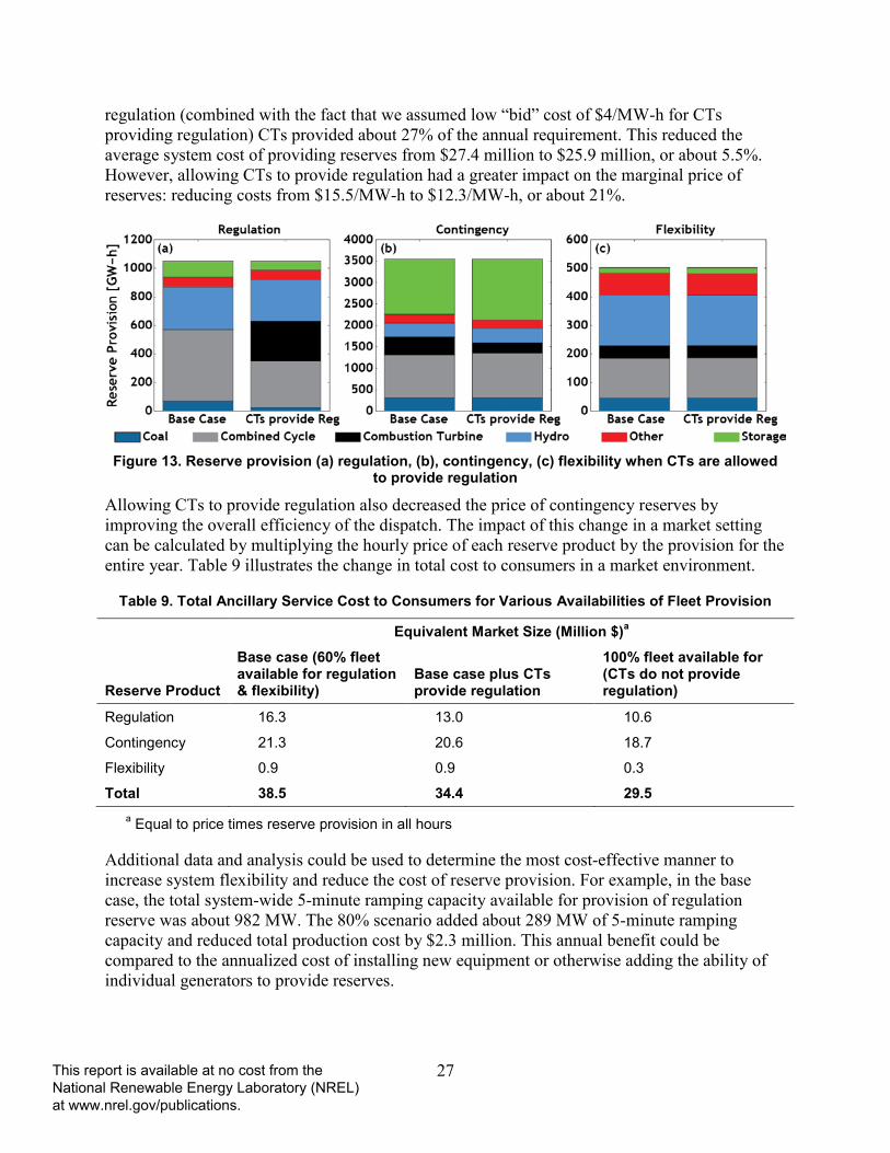
27

regulation (combined with the fact that we assumed low “bid” cost of $4/MW-h for CTs providing regulation) CTs provided about 27% of the annual requirement. This reduced the average system cost of providing reserves from $27.4 million to $25.9 million, or about 5.5%. However, allowing CTs to provide regulation had a greater impact on the marginal price of reserves: reducing costs from $15.5/MW-h to $12.3/MW-h, or about 21%.

Figure 13. Reserve provision (a) regulation, (b), contingency, (c) flexibility when CTs are allowed

to provide regulation

Allowing CTs to provide regulation also decreased the price of contingency reserves by improving the overall efficiency of the dispatch. The impact of this change in a market setting can be calculated by multiplying the hourly price of each reserve product by the provision for the entire year. Table 9 illustrates the change in total cost to consumers in a market environment.

Table 9. Total Ancillary Service Cost to Consumers for Various Availabilities of Fleet Provision

Equivalent Market Size (Million $)a

Reserve Product

Base case (60% fleet available for regulation & flexibility)

Base case plus CTs provide regulation

100% fleet available for (CTs do not provide regulation)

Regulation 16.3 13.0 10.6

Contingency 21.3 20.6 18.7

Flexibility 0.9 0.9 0.3

Total 38.5 34.4 29.5 a Equal to price times reserve provision in all hours

Additional data and analysis could be used to determine the most cost-effective manner to increase system flexibility and reduce the cost of reserve provision. For example, in the base case, the total system-wide 5-minute ramping capacity available for provision of regulation reserve was about 982 MW. The 80% scenario added about 289 MW of 5-minute ramping capacity and reduced total production cost by $2.3 million. This annual benefit could be compared to the annualized cost of installing new equipment or otherwise adding the ability of individual generators to provide reserves.


28

5.2 Impact of Renewable Generation Penetration 5.2.1 Reserve requirements as a function of renewable energy penetration We simulated five progressively increasing penetrations of PV and wind power that ranged from about 16% to 35% generation from solar and wind at a constant ratio for solar to wind of 1:5.5. The actual percentages were not in exactly 5% increments due to the use of discrete plant capacity. Table 10 provides the actual percentages in each scenario. Figure 14 illustrates time series from the five renewable penetration scenarios as well as the net load in each scenario for three days in spring.

Figure 14. Example time series for the five renewable penetration scenarios: (a) Generation from wind and solar for April 15–17 (b) Total and net load for the same time period. Increasing

penetrations of renewable generation introduce higher ramping requirements and lower net load.


29

Table 10. Reserve Requirements by Renewable Penetration Scenario

System Property

RE = 15% (Base case)

RE = 20%

RE = 25%

RE = 30%

RE = 35%

No RE Casea

Total Generation [GWh] 78,761 79,449 79,454 79,426 79,375 79,369

PV Generation [GWh] (% of Demand)

1,834 (2.3%)

2,556 (3.2%)

3,168 (4%)

3,750 (4.7%)

4,260 (5.4%) 0

Wind Generation [GWh] (% of Demand)

10,705 (13.6%)

13,838 (17.4%)

18,097 (22.8%)

21,433 (27%)

23,752 (29.9%) 0

Regulation Requirement [GW-h] 1,050 1,134 1,281 1,364 1,422 782

Regulation Requirement Due to Renewables [GW-h]b 700 822 1,015 1,118 1,187 0

Contingency Requirement [GW-h] 3,548 3,548 3,548 3,548 3,548 3,548

Flexibility Requirement [GW-h] 502 600 769 855 918 0 a No RE Case Regulation requirement is based on 1% of Load

b Regulation requirement based on the 95th percentile of 5-minute variability of wind and solar power and 1% of load. We calculated the regulation requirement due to solar and wind power variability by taking the square root of the total regulation requirement squared minus the 1% load requirement squared.

Solar and wind generation increases the variability of the net load across multiple time scales, increasing the reserve requirements for both regulation and flexibility. Figure 15 shows the calculated reserves requirement as a function of generation from wind and solar plants, using the techniques described in Section 3.2. Each incremental unit of renewables added an incremental amount of additional reserves; however, there is a downward trend in the amount of additional reserves needed as a function of renewable penetration. This was due to the assumptions regarding the deployment of wind and solar in the simulated scenarios. The wind and solar plants were sited using the methods described in WWSIS II (Lew et al. 2013), mainly by resource quality and proximity to load. Scenarios were created by adding discrete wind and solar plants, typically deployed over larger areas. Plants that are further apart in space have less correlation between their high frequency variability.28 For consistency, we did not modify the generator mix in the renewables scenarios. This discounts the ability of PV and wind to provide firm capacity, and avoid new conventional generation or facilitate retirement of older generators. In reality, the addition of large amount of renewables will almost certainly result in a different mix of generators, especially as solar and wind reduce the capacity factors of conventional generators (Mills and Wiser 2012). For example, the increase in renewable penetration from 16% to 35% results in a decrease in capacity factor of coal units from 85% to 74% and of combined-cycle units from 42% to 17%.

28 For comparison, the regulation requirements per unit of renewables in this test case is substantially higher than in the WWSIS II study due the difference in spatial diversity between this footprint in this study and the large area in WWSIS II.


30

Figure 15. Annual reserve requirement (GW-h) per GWh of renewable generation for regulation

(95th percentile of 5-minute ramps) and flexibility (67th percentile of 20-minute ramps)

While the reserve requirements per unit of renewable energy (RE) decreased, the total reserve requirements increased, as summarized in Table 10. Overall, the sum of the total operating reserves (met by spinning units) averaged 582 MW in the base case, which corresponds to about 6.4% of average load, and rose to 672 MW (7.4% of load) when the renewable generation penetration was 35%.

5.2.2 Cost and Price Impacts for Renewable Penetration Scenarios Table 11 summarizes the results of the changes in cost and price of reserves as a function of renewable penetration. These results indicate that several factors interact to drive the cost and price of providing reserves.


31

Table 11. Reserve Cost and Price for Renewable Penetration Scenarios

Scenario

Total Production Cost (M$)


Percent Increase in Total Generation Cost Associated with Reserves

Increase in Generation Cost per Total Reserves ($/MW-h)


Regulation Mean/ Median

Contingency Mean/ Median

Flexibility Mean/ Median

15% PV and Wind Generation (Base Case)

1,427.1

27.4 2.0% 5.4 15.48 / 13.81 6.15 / 3.32 1.62 / 0

20% PV and Wind Generation

1,309.3 29.1 2.3% 5.5 16.31 / 14.61 6.14 / 3.09 2.05 / 0


1,170.3 32.3 2.8% 5.8 16.95 / 14.58 5.88 / 2.81 2.21 / 0


1,071.8 32.1 3.1% 5.6 16.81 / 14.52 5.31 / 2.61 2.3 / 0


1,003.3 31.2 3.2% 5.3 16.53 / 14.52 5.04 / 2.51 2.18 / 0

The first results column in Table 11 lists the total production cost in the each case (with reserves provision), which decline as a function of wind and solar penetration as they displace fuel consumption. The second column lists the total cost of providing reserves, calculated by taking the difference in production cost between cases with and without all reserve products. Increasing wind and solar from 15% to 25% increased the total cost of providing reserves. This was due largely to the increase in the amount of regulation and flexibility reserves required (Table 14). The price of regulation reserves (or cost per unit of reserves) increased from the 15% to 20% case then fell a small amount, while the price of contingency reserves actually fell in all scenarios. Overall, the cost of providing reserves increased by about 18% from the 15% to the 25% scenario.

Beyond 25%, the total cost of reserves decreased. While the amount of reserves required was still increasing, as seen in Figure 15, the rate of increase decreased per unit of renewable generation, while the cost per unit of reserves also fell. In combination, these factors resulted in a cost reduction associated with providing reserves at the higher levels of wind and solar penetration. As a percentage of total production costs, the cost of reserves increased in all scenarios, largely due to the decrease in overall production cost.

The decreasing price of reserves, particularly in the higher RE scenarios were driven by the increased availability of lower-cost generators to provide reserves. The variability of the net load actually increased the availability of partially loaded generators able to provide reserves. However, as mentioned previously, as wind and solar reduce the energy generation from conventional units, this may result in retirements, which would change the overall generation mix. Further analysis is needed to evaluate the price of reserves in scenarios where the


32

conventional generation mix changes as a function of renewable penetration, considering both the capacity value of renewables and the impact of renewables on fleet operation and flexibility requirements.

The increased cost associated with providing reserves can be compared to the reduction in fuel cost in each scenario. Table 12 summarizes the incremental benefit of each of the renewables cases compared to the cost of the increased reserves provision. It should be emphasized that these results are for a single system, without consideration of the evolving grid, which may include new mechanisms to increase flexibility and improve integration of variable generation sources. The first column lists the incremental operational benefit, calculated by comparing the incremental difference in production cost in each case. (In each case, “incremental” represents moving from one penetration to the next—for example from 15% to 20%, or 20% to 25%.) The second column lists the operational benefit per unit of wind and solar. The change as a function of penetration was mostly due to the decreasing displacement of natural gas and increased displacement of lower-cost coal. The third column lists the incremental cost of reserves for each case. This represents a reduction in benefit compared to scenarios where renewables did not add additional reserves. The highest reduction in benefits is associated with moving from 20% to 25%, when about 2% of the potential benefit of renewables was lost due to the increased reserve requirement—or instead of producing savings of $142.1 million, the savings was actually only the $139.0 million seen in the first column. This case translated to an incremental reserves cost per unit of wind and solar equal to about $0.6/MWh (provided in the final column). Of note, a wind integration study conducted for the PSCO (Butler et al. 2011) showed an incremental regulation cost of $0.1/MWh of wind generation at a 20% wind penetration level, rising to $0.2/MWh for 3 GW of installed wind generation. While the results were of a similar order of magnitude, they were not directly comparable as regulation costs in the PSCO study were taken from PSCO’s open access transmission tariff rather than calculated from production cost modeling.

Table 12. Incremental Benefits and Costs of Renewable Penetration and Reserve Requirements

Scenario

Incremental Operational Benefit of RE (M$)

Incremental Operational Benefit per unit of RE ($/MWh)

Incremental Cost of Reserves (M$)

Fraction of Potential Benefit lost due to increase reserves cost

Incremental Reserves Cost per unit of RE ($/MWh)

20% PV and Wind Generation 117.8 30.5 1.74 1.5% 0.5

25% PV and Wind Generation 139.0 28.5 3.14 2.2% 0.6

30% PV and Wind Generation 98.5 25.1 -0.13 -0.1% 0

35% PV and Wind Generation 68.4 24.2 -0.91 -1.3% -0.3

As seen in Table 12, beyond 25%, the incremental cost of reserves was actually negative. As discussed previously, this was because the increased reserve requirements from wind and solar occurs largely during periods of greatest wind and solar output. This results in partially loaded


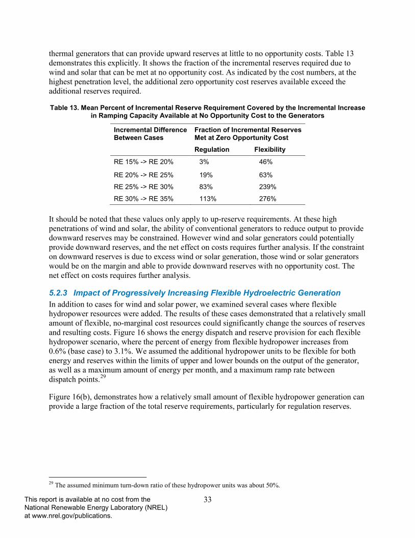
33

thermal generators that can provide upward reserves at little to no opportunity costs. Table 13 demonstrates this explicitly. It shows the fraction of the incremental reserves required due to wind and solar that can be met at no opportunity cost. As indicated by the cost numbers, at the highest penetration level, the additional zero opportunity cost reserves available exceed the additional reserves required.

Table 13. Mean Percent of Incremental Reserve Requirement Covered by the Incremental Increase in Ramping Capacity Available at No Opportunity Cost to the Generators

Incremental Difference Between Cases

Fraction of Incremental Reserves Met at Zero Opportunity Cost

Regulation Flexibility

RE 15% -> RE 20% 3% 46%

RE 20% -> RE 25% 19% 63%

RE 25% -> RE 30% 83% 239%

RE 30% -> RE 35% 113% 276% It should be noted that these values only apply to up-reserve requirements. At these high penetrations of wind and solar, the ability of conventional generators to reduce output to provide downward reserves may be constrained. However wind and solar generators could potentially provide downward reserves, and the net effect on costs requires further analysis. If the constraint on downward reserves is due to excess wind or solar generation, those wind or solar generators would be on the margin and able to provide downward reserves with no opportunity cost. The net effect on costs requires further analysis.

5.2.3 Impact of Progressively Increasing Flexible Hydroelectric Generation In addition to cases for wind and solar power, we examined several cases where flexible hydropower resources were added. The results of these cases demonstrated that a relatively small amount of flexible, no-marginal cost resources could significantly change the sources of reserves and resulting costs. Figure 16 shows the energy dispatch and reserve provision for each flexible hydropower scenario, where the percent of energy from flexible hydropower increases from 0.6% (base case) to 3.1%. We assumed the additional hydropower units to be flexible for both energy and reserves within the limits of upper and lower bounds on the output of the generator, as well as a maximum amount of energy per month, and a maximum ramp rate between dispatch points.29

Figure 16(b), demonstrates how a relatively small amount of flexible hydropower generation can provide a large fraction of the total reserve requirements, particularly for regulation reserves.

29 The assumed minimum turn-down ratio of these hydropower units was about 50%.


34

Figure 16. Annual (a) energy dispatch and (b-d) reserve provision for additional flexible

hydropower penetration cases


35

Table 14 shows the impact of this additional resource on reserve cost and price, demonstrating how a relatively small amount of this resource can collapse the price for regulation reserves. This also demonstrates one of the challenges in incentivizing new market entrances for reserve services, where new resources can provide significant system benefits, but may be unable to capture these benefits in a market environment (Kirby et al. 2011; Denholm et al. 2013).

Table 14. Reserve Cost and Price for Flexible Hydropower Penetration Scenarios


Increase in Total Generation Cost Associated with Reserves (%)



Scenario Regulation Mean/Median

Contingency Mean/Median

Flexibility Mean/Median

Base case (0.6% of energy from flexible hydro)

27.4 2.0% 5.37 15.48 / 13.81 6.15 / 3.32 1.62 / 0

Add 0.5% flexible hydropower (1.1% total)

24.8 1.8% 4.86 14.42 / 10.78 6.4 / 2.58 1.23 / 0


22.9 1.7% 4.48 14.26 / 8.84 7.21 / 2.31 2.68 / 0


21.3 1.6% 4.18 12.71 / 7.58 6.71 / 1.8 1.19 / 0


20.0 1.5% 3.92 10.58 / 6 6.35 / 1.72 1.09 / 0


19.0 1.4% 3.72 8.76 / 2.91 6.2 / 0.99 2.46 / 0

5.3 Impact of Increased Reserve Requirement and Natural Gas Price The final set of sensitivities considered the amount of reserves required and the impact of fuel prices. There is still considerable uncertainty as to the amount of regulation needed as a function of wind and solar penetration, and flexibility reserve products have yet to be defined in detail. As a result, we examined several cases where the reserves were increased by 50% and 100%. Table 15 demonstrates the significant impact both on production cost associated with reserves and on the corresponding price.


36

Table 15. Reserves Cost and Price for Increased Reserve Requirement Scenarios


Increase in Total Generation Cost (%)






Base Case 27.4 2.0% 5.37 15.48 / 13.81 6.15 / 3.32 1.62 / 0

Flexibility requirements increased by 50%

28.0 2.00% 5.23 15.12 / 13.55 5.87 / 3.04 2.52 / 0

Flexibility requirements increased by 100%

29.1 2.1% 5.19 15.07 / 13.54 5.92 / 2.87 3.26 / 0

Regulation requirements increased by 50%

37.9 2.7% 6.74 21.45 / 20.12 6.5 / 3.99 2.45 / 0

Regulation requirements increased by 100%

50.6 3.6% 8.23 25.34 / 22.98 6.73 / 4.12 2.43 / 0

Reg & Flex requirements increased by 50%

38.7 2.8% 6.58 21.21 / 20.07 6.39 / 3.94 2.64 / 0

Reg & Flex requirements increased by 100%

52.6 3.8% 7.9 25.18 / 22.75 6.53 / 3.8 3.36 / 0

Table 16 shows the corresponding change in cost and price for scenarios where the price of natural gas was increased by 50% and 100% (to a generation-weighted averages of about $6.3/MMBtu and $8.4/MMBtu, respectively). Of note in these results is the greater sensitivity in reserve costs compared to overall production cost. In the scenario with a 50% increase in natural gas prices, the total production cost increased from $1.43 billion to $1.68 billion, or about 18%. In contrast, the cost of reserves increased by $11.9 million, or about 44%, because the cost of reserves is strongly correlated with the marginal units, which are often fueled by natural gas.


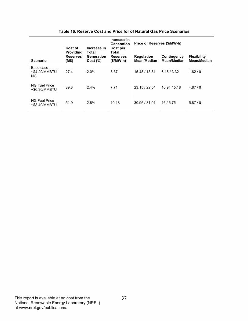
37

Table 16. Reserve Cost and Price for of Natural Gas Price Scenarios


Increase in Total Generation Cost (%)






Base case ~$4.20/MMBTU NG

27.4 2.0% 5.37 15.48 / 13.81 6.15 / 3.32 1.62 / 0

NG Fuel Price ~$6.30/MMBTU 39.3 2.4% 7.71 23.15 / 22.54 10.94 / 5.18 4.87 / 0

NG Fuel Price ~$8.40/MMBTU 51.9 2.8% 10.18 30.96 / 31.01 16 / 6.75 5.87 / 0


38

6 Conclusions The primary goal of this analysis was to explore the origin of the costs of several operating reserve products. Analysis of the energy-only dispatch showed that the system often has spare ramp capacity, at no cost to the system, that could provide some or all of the operation reserve requirements. However, the system often requires a change in dispatch to provide reserves, which requires increase in generation from higher-cost generators and decrease in output from lower-cost generators. This incurs a cost to the system and also creates an opportunity cost for individual generators. The opportunity cost of the marginal generator providing reserves sets the price of reserves. Using a commercial production cost model, we generated regulation and contingency reserve prices in the range of recent historical prices for reserves in restructured markets. The total cost of providing reserves in our simulation added about 2% to the total cost of providing energy.

We found that the reserve price was sensitive to a variety of factors including fleet availability to provide reserves, renewable generation penetration, availability of flexible hydro generation, and the price of natural gas. The hourly price for reserves depended greatly on many assumptions regarding the operational flexibility of the generation fleet, in particular the assumed ramp rates and the fraction of fleet available to provide reserves. In addition, a large fraction of regulation price in these simulations was derived from the generator bid prices, or the assumed cost of generators operating at non-steady state while providing regulation reserves. Because performance data related to an individual generator’s ability to provide reserve are not widely available, reproducing the cost of reserves in a production cost model involves significant uncertainty. In several cases, increasing the overall fleet flexibility—by allowing more generators to provide reserves but not necessarily increasing the performance of individual generators—greatly decreased the cost of reserves provision and drove prices to near zero for many hours of the year. This adds risks for market entrants hoping to take advantage of reserve markets.

We modeled the increase in reserve requirements with the addition of solar and wind generation to the system and compared the cost impacts of increased reserve requirements to the net benefits of avoided fuel and other costs. The greatest increase in reserve costs actually occurred at the lowest penetration of renewables evaluated. From 15% to 20% wind and solar generation, the added renewables offset $31/MWh of production costs, primarily through fuel savings, but these savings are reduced by $0.5/MWh of increased operating reserve costs, leaving a net savings of $30.5/MWh. At higher levels, from 30%–35% wind and solar generation, the incremental operational savings declines to $23.9/MWh. The decline in incremental production cost savings can be attributed to two types of impacts. First, at increasing levels, wind and solar displace increasingly lower-cost generation. Second, by displacing energy from conventional generation, those plants tend to operate more frequently at part load. Consequently, at high levels of wind and solar generation, the increased costs associated with part load operation are actually reduced by the increased availability of ramp capacity at no cost to the system. Thus, the cost of the increased need for operating reserves due to wind and solar variability is actually negative at $-0.3/MWh, and the total incremental savings is $24.2/MWh. Notably, operating reserve prices and costs scale with natural gas prices. While increased gas prices increase the costs of operating reserves, they also increase the value of wind and solar generation by displacing more expense fuel.


39

Additional analysis is needed to understand the impact of renewables on several aspects of reserve cost. The provision of down reserves was not evaluated in this study and might become more important at higher penetrations of variable renewable generation. Greater wind and solar penetration may also increase the actual deployment of regulating and flexibility reserves. Sub-hourly analysis is needed to evaluate the impact of reserve provision, along with new rules for compensating generators for their accuracy in following a regulation signal. Finally, this analysis points to the need to consider how the operation of the power system and composition of the conventional generation fleet evolves if wind and solar power reach high penetration levels.

In summary, reserves costs are driven by the opportunity cost incurred by generators that lose energy revenue in order to provide capacity for reserves. This opportunity cost is highly sensitive to the fleet of generators and their operational characteristics. Future systems will include new market participants including renewable generation, storage systems, or demand response, and these participants will affect the energy dispatch and therefore change the price of reserves. This work demonstrates that production cost models can emulate the price of reserves and can serve as a valuable tool for understanding the economic potential of new technologies.


40

References Butler, J.; Zavadil, R.M.; Mousseau, T. (2011). Public Service Company of Colorado 2 GW and 3 GW Wind Integration Cost Study. Denver, CO: Xcel Energy Inc and Knoxville, TN: EnerNex Corporation. http://www.xcelenergy.com/staticfiles/xe/Regulatory/Regulatory%20PDFs/ PSCo-ERP-2011/Attachment-2.13-1-2G-3G-Wind-Integration-Cost-Study.pdf.

California ISO (CAISO). (April 29, 2011). “Summary of Preliminary Results of 33% Renewable Integration Study –2010. CPUC LTPP Docket No. R.10-05-006.”

Denholm, P.; Jorgenson, J.; Hummon, M.; Jenkin, T.; Palchak, D.; Kirby, B.; Ma, O.; O'Malley, M. (2013). Value of Energy Storage for Grid Applications. NREL/TP-6A20-58465. Golden, CO: National Renewable Energy Laboratory.

U.S. Energy Information Administration (EIA). (2012a). “Electric Power Monthly with Data for June 2012.” EIA. Accessed June 13, 2013. http://www.eia.gov/electricity/monthly/update/.

EIA. (2012b). “Electric Power Monthly with Data for December 2012.” EIA. Accessed June 13, 2013. http://www.eia.gov/electricity/monthly/update/.

Ela, E.; Milligan, M.; Kirby, B. (2011). Operating Reserves and Variable Generation. A Comprehensive Review of Current Strategies, Studies, and Fundamental Research on the Impact That Increased Penetration of Variable Renewable Generation has on Power System Operating Reserves. NREL/TP-5500-51978. Golden, CO: National Renewable Energy Laboratory.

Federal Energy Regulatory Commission (FERC). (2011). Order No 755. (October 20, 2011): 18 CFR Part 35. Accessed July 11, 2013: http://www.ferc.gov/whats-new/comm-meet/2011/ 102011/E-28.pdf.

GE Energy. (2010). Western Wind and Solar Integration Study. NREL/SR-550-47434. Work performed by GE Energy. Golden, CO: National Renewable Energy Laboratory.

Gilman, P.; Dobos, A. (2012). System Advisor Model, SAM 2011.12.2: General Description. TP-6A20-53437. Golden, CO: National Renewable Energy Laboratory.

Hirst, E.; Kirby, B. (1998). Unbundling Generation and Transmission Services for Competitive Electricity Markets: Examining Ancillary Services. NRRI 98-05. Work performed by Oak Ridge National Laboratory: Oak Ridge, Tennessee. Columbus, Ohio: The National Regulatory Research Institute.

Ibanez, E.; Brinkman, G.; Hummon, M.; Lew, D. (2012). A Solar Reserve Methodology for Renewable Energy Integration Studies Based on Sub-Hourly Variability Analysis: Preprint. To be presented at the 2nd Annual International Workshop on Integration of Solar Power into Power Systems Conference in Lisbon, Portugal. November 12–13, 2012. NREL/CP-5500-56169. Golden, CO: National Renewable Energy Laboratory; 8 pp.


http://www.xcelenergy.com/staticfiles/xe/Regulatory/Regulatory%20PDFs/PSCo-ERP-2011/Attachment-2.13-1-2G-3G-Wind-Integration-Cost-Study.pdf

http://www.xcelenergy.com/staticfiles/xe/Regulatory/Regulatory%20PDFs/PSCo-ERP-2011/Attachment-2.13-1-2G-3G-Wind-Integration-Cost-Study.pdf

http://www.eia.gov/electricity/monthly/update/

http://www.eia.gov/electricity/monthly/update/

http://www.ferc.gov/whats-new/comm-meet/2011/102011/E-28.pdf

http://www.ferc.gov/whats-new/comm-meet/2011/102011/E-28.pdf

41

Kirby, B. (2011). “Energy Storage Management for VG Integration.” PR-5500-53295. Golden, CO: National Renewable Energy Laboratory. Accessed April 24, 2013: http://www.nrel.gov/docs/fy12osti/53295.pdf.

Kumar, N.; Besuner, P.M.; Lefton, S.A.; Agan, D.D.; Hilleman, D.D. (April 2012). Power Plant Cycling Costs. EAS 12047831-2-1. Work performed by Intertek APTECH: Sunnyvale, CA and Houston, TX. Golden, CO: National Renewable Energy Laboratory and Salt Lake City, UT: Western Electricity Coordinating Council; 83 pp. Accessed November 5, 2012: http://wind .nrel.gov/public/WWIS/APTECHfinalv2.pdf.

Kempton, W.; Tomic, J. (2005). “Vehicle-to-Grid Power Fundamentals: Calculating Capacity and Net Revenue.” Journal of Power Sources (144:1); pp. 280-294.

Kirby, B. (2011). “Energy Storage Management for VG Integration.” PR-5500-53295. Golden, CO: National Renewable Energy Laboratory. Accessed April 24, 2013: http://www.nrel.gov/docs/fy12osti/53295.pdf.

Kirby, B.; Hirst, E. (1996). Ancillary-Service Costs for 12 U.S. Electric Utilities. ORNL/CON-427. Oak Ridge, TN: Oak Ridge National Laboratory.

Lew, D.; Brinkman, G.; Ibanez, E.; Kumar, N.; Lefton, S.; Jordan, G.; Venkataraman, S.; King, J. (2013). Western Wind and Solar Integration Study Phase 2. NREL/PR-5500-57922. Golden, CO: National Renewable Energy Laboratory.

Lew, D.; Brinkman, G.; Kumar, N.; Besuner, P.; Agan, D.; Lefton, S. (2012). “Impacts of Wind and Solar on Fossil-Fueled Generators: Preprint.” Presented at IEEE Power and Energy Society General Meeting, San Diego, California, July 22–26, 2012. CP-5500-53504. Golden, CO: National Renewable Energy Laboratory.

Mills, A.; Wiser, R. (June 2012). Changes in the Economic Value of Variable Generation at High Penetration Levels: A Pilot Case Study of California. LBNL-5445E. Berkeley, CA: Lawrence Berkeley National Laboratory.

Monitoring Analytics, LLC. (2013). State of the Market Report for PJM 2012. Accessed July 16, 2013: http://www.monitoringanalytics.com/reports/PJM_State_of_the_Market/2012/2012-som-pjm-volume1.pdf

Navid, N.; Rosenwald, G.; Chatterjee, D. (2011). Ramp Capability for Load Following in the MISO Markets. Midwest Independent System Operator.

NERC (2013). “Glossary of Terms Used in Reliability Standards.” (2013). Accessed May 9, 2013: http://www.nerc.com/files/Glossary_of_Terms.pdf.

NERC. (2012). 2012 Summer Reliability Assessment. May 2012. Atlanta, GA: North American Electric Reliability Corporation. Accessed June 13, 2013: http://www.nerc.com/ files/2012SRA.pdf.


http://www.nrel.gov/docs/fy12osti/53295.pdf

http://wind.nrel.gov/public/WWIS/APTECHfinalv2.pdf

http://wind.nrel.gov/public/WWIS/APTECHfinalv2.pdf

http://www.nrel.gov/docs/fy12osti/53295.pdf

http://www.monitoringanalytics.com/reports/PJM_State_of_the_Market/2012/2012-som-pjm-volume1.pdf

http://www.monitoringanalytics.com/reports/PJM_State_of_the_Market/2012/2012-som-pjm-volume1.pdf

http://www.nerc.com/files/Glossary_of_Terms.pdf

http://www.nerc.com/files/2012SRA.pdf

http://www.nerc.com/files/2012SRA.pdf

42

NERC. (March 2011). Special Report: Ancillary Service and Balancing Authority Area Solutions to Integrate Variable Generation. Princeton, NJ: NERC.

PJM (2013). PJM Manual 11: Energy & Ancillary Services Market Operations, Revision: 60, Effective Date: June 1, 2013. Norristown, PA: PJM.

PJM. (2012). PJM Manual 15: Cost Development Guidelines. Revision 20. November 1, 2012. Norristown, PA: PJM.

Transmission Expansion Planning Policy Committee (TEPPC) Western Electricity Coordinating Council (WECC). (September 2011). TEPPC 2010 Study Program 10-Year Regional Transmission Plan. Salt Lake City, UT: WECC.

Xu, L.; Tretheway, D. (2012). Flexible Ramping Products: Draft Final Proposal. California Independent System Operator.


43

Appendix. Supplemental Data A.1 Calculating Surplus Ramp Capacity Zero marginal reserve costs (or zero opportunity costs in the case of regulation) occur when sufficient reserves are available from the unit commitment optimized to solely meet demand. Figure A-1 is an example of a generator with a maximum capacity of 300 MW and a ramp rate of 1.25 MW/min. During hours 2 to 4, the generator is turning on, thus the ramp rate of the unit is entirely occupied by energy production, and no capacity is available for reserves. During hours 5–7, the generator is ramping slowly, and thus can hold all available reserves. During hours 8, 9, and 11, the reserve provision is curtailed by the limited maximum available capacity.

Figure A-1. Example dispatch of a single generator. Spare ramp capacity is calculated for each

generator, for each hour.

We applied this calculation to each generator in the system where the siulation did not hold reserves to calculate the inherent spare capacity in the dispatch. Based on the unit commitment, the surplus ramp capacity available for reserves Rx={reg, cont, flex}, available from a generator g, with maximum ramp rate of rg, maximum capacity of Cmax,g, and a dispatch point of dg,t, at time t are:

Rx=reg,g,t = min{5 × rg, Ag,t} Rx=cont,g,t = min{5 × rg, (Ag,t + Rx=reg,g,t)} Rx=flex,g,t = min{10 × rg, (Ag,t + Rx=reg,g,t + Rx=cont,g,t)}

where, Ag,t = Mg,t – (dt – dt-1) Mg,t = max{60 × rg, Cg,t} Cg,t = Cmax,g – dg,t


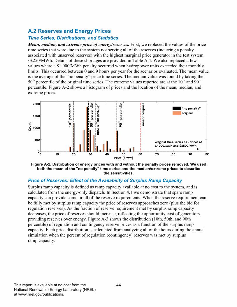
44

A.2 Reserves and Energy Prices Time Series, Distributions, and Statistics Mean, median, and extreme price of energy/reserves. First, we replaced the values of the price time series that were due to the system not serving all of the reserves (incurring a penalty associated with unserved reserves) with the highest marginal price generator in the test system, ~$250/MWh. Details of these shortages are provided in Table A.4. We also replaced a few values where a $1,000/MWh penalty occurred when hydropower units exceeded their monthly limits. This occurred between 0 and 9 hours per year for the scenarios evaluated. The mean value is the average of the “no penalty” price time series. The median value was found by taking the 50th percentile of the original time series. The extreme values reported are at the 10th and 90th percentile. Figure A-2 shows a histogram of prices and the location of the mean, median, and extreme prices.

Figure A-2. Distribution of energy prices with and without the penalty prices removed. We used

both the mean of the "no penalty" time series and the median/extreme prices to describe the sensitivities.

Price of Reserves: Effect of the Availability of Surplus Ramp Capacity Surplus ramp capacity is defined as ramp capacity available at no cost to the system, and is calculated from the energy-only dispatch. In Section 4.1 we demonstrate that spare ramp capacity can provide some or all of the reserve requirements. When the reserve requirement can be fully met by surplus ramp capacity the price of reserves approaches zero (plus the bid for regulation reserves). As the fraction of reserve requirement met by surplus ramp capacity decreases, the price of reserves should increase, reflecting the opportunity cost of generators providing reserves over energy. Figure A-3 shows the distribution (10th, 50th, and 90th percentile) of regulation and contingency reserve prices as a function of the surplus ramp capacity. Each price distribution is calculated from analyzing all of the hours during the annual simulation when the percent of regulation (contingency) reserves was met by surplus ramp capacity.


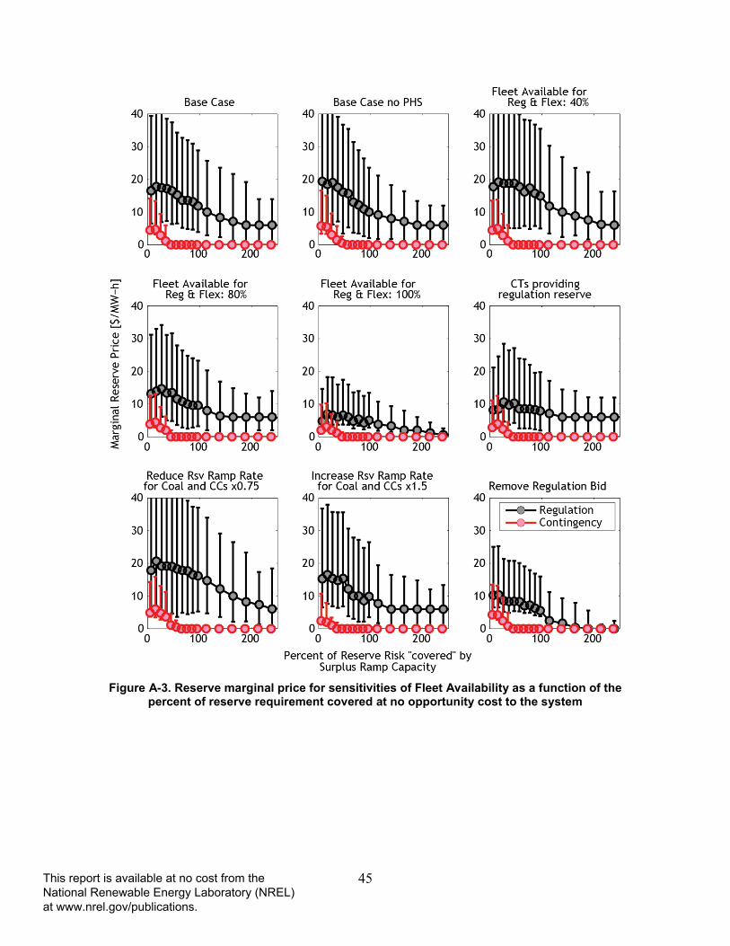
45

Figure A-3. Reserve marginal price for sensitivities of Fleet Availability as a function of the

percent of reserve requirement covered at no opportunity cost to the system


46

A.3 Cost to System for Reserves (All Sensitivities) Table A-1. Cost of Holding Reserves for All Sensitivity Scenarios

Scenario Fuel

Cos

t

Varia

ble

O&

M

Cos

t

Star

tup

Cos

t

Reg

ulat

ion

Bid

Pr

ice

Tota

l Gen

erat

ion

Cos

t

Incr

ease

in T

otal

C

ost

% In

crea

se in

To

tal C

ost

($/MW-h Reserves) (M$)

Base Case 3.69 -0.13 0.88 0.93 5.37 27.38 1.96%

Base Case no PHS 5.41 -0.27 0.61 1.02 6.76 34.49 2.43%

Add 0.5% Flexible Hydropower 3.35 -0.11 0.89 0.73 4.86 24.81 1.79%





40% Fleet Available for Reg & Flex 3.77 -0.14 0.89 0.94 5.46 27.85 1.99%

60% Fleet Available for Reg & Flex (Base case) 3.69 -0.13 0.88 0.93 5.37 27.38 1.96%



60% Fleet Available for Reg & Flex plus CTs providing Reg 3.65 -0.11 0.89 0.44 4.87 24.82 1.77%

60% Fleet Available for Reg & Flex plus No Regulation Bid 3.49 -0.12 0.92 0.00 4.29 21.86 1.56%

60% Fleet Available for Reg & Flex plus Reduce Reserve Ramp Rate for Coal and CCs by 25% 4.11 -0.16 0.76 0.96 5.67 28.93 2.07%

60% Fleet Available for Reg & Flex plus Increase Reserve Ramp Rate for Coal and CCs by 50% 3.31 -0.10 0.84 0.91 4.95 25.27 1.81%

15% PV and Wind Generation (Base case) 3.69 -0.13 0.88 0.93 5.37 27.38 1.96%

20% PV and Wind Generation 3.57 -0.15 1.02 1.06 5.51 29.12 2.28%





47

Scenario Fuel

Cos

t

Varia

ble

O&

M

Cos

t

Star

tup

Cos

t

Reg

ulat

ion

Bid

Pr

ice

Tota

l Gen

erat

ion

Cos

t

Incr

ease

in T

otal

C

ost

% In

crea

se in

To

tal C

ost

($/MW-h Reserves) (M$)

Base Case 3.69 -0.13 0.88 0.93 5.37 27.38 1.96%

Flex Risk Increased by 50% 3.64 -0.12 0.83 0.88 5.23 28.00 2.00%

Flex Risk Increased by 100% 3.63 -0.12 0.85 0.84 5.19 29.10 2.08%

Regulation Risk Increased by 50% 4.56 -0.20 0.83 1.55 6.74 37.88 2.71%

Regulation Risk Increased by 100% 5.62 -0.29 0.72 2.18 8.23 50.60 3.62%

Reg & Flex Risk Increased by 50% 4.45 -0.19 0.84 1.47 6.58 38.67 2.76%

Reg & Flex Risk Increased by 100% 5.37 -0.27 0.78 2.01 7.90 52.56 3.76%

NG Fuel Price Increased by 0% (Base case) 3.69 -0.13 0.88 0.93 5.37 27.38 1.96%

NG Fuel Price increased by 50% 6.41 -0.11 0.45 0.95 7.71 39.32 2.39%

NG Fuel Price increased by 100% 8.97 -0.10 0.35 0.96 10.18 51.93 2.76%


48

A.4 Flexibility Reserve Violations There were no violations of contingency or regulation reserves in any scenario.

Table A-2. Flexibility Reserve Violations

Scenario

Hours of Flex Reserve Shortage

Flex Shortage (MW-h)

% of Flex Shorted

Base Case 29 49 0.0097

Base Case no PHS 18 38 0.0076

Add 0.5% Flexible Hydropower 30 46 0.0092





40% Fleet Available for Reg & Flex 37 65 0.0129

60% Fleet Available for Reg & Flex (Base case) 29 49 0.0097



60% Fleet Available for Reg & Flex plus CTs providing Reg 26 32 0.0063

60% Fleet Available for Reg & Flex plus No Regulation Bid 31 50 0.01

60% Fleet Available for Reg & Flex plus Reduce Reserve Ramp Rate for Coal and CCs by 25% 34 46 0.0091

60% Fleet Available for Reg & Flex plus Increase Reserve Ramp Rate for Coal and CCs by 50% 32 60 0.0119

15% PV and Wind Generation (Base case) 29 49 0.0097

20% PV and Wind Generation 27 33 0.0055




Base Case 29 49 0.0097

Flex Risk Increased by 50% 40 65 0.0086

Flex Risk Increased by 100% 40 71 0.0071

Regulation Risk Increased by 50% 33 48 0.0096

Regulation Risk Increased by 100% 47 86 0.017

Reg & Flex Risk Increased by 50% 46 69 0.0091

Reg & Flex Risk Increased by 100% 61 107 0.0107


49

Scenario

Hours of Flex Reserve Shortage

Flex Shortage (MW-h)

% of Flex Shorted

NG Fuel Price Increased by 0% (Base case) 29 49 0.0097

NG Fuel Price increased by 50% 34 61 0.0121

NG Fuel Price increased by 100% 35 61 0.0121


Fundamental Drivers of the Cost and Price of Operating ... · PDF fileoperating reserve...

Documents

Transcript of Fundamental Drivers of the Cost and Price of Operating ... · PDF fileoperating reserve...