20/05/2010 IHES

Fundamental constants, gravitation and cosmology

Jean-Philippe UZAN

Constants Physical theories involve constants

These parameters cannot be determined by the theory that introduces them.

These arbitrary parameters have to be assumed constant: - experimental validation - no evolution equation

By testing their constancy, we thus test the laws of physics in which they appear.

A physical measurement is always a comparison of two quantities, one can be thought as a unit

- it only gives access to dimensionless numbers - we consider variation of dimensionless combinations of constants

JPU, Rev. Mod. Phys. 75, 403 (2003); Liv. Rev. Relat. (to appear, 2010) JPU, [astro-ph/0409424, arXiv:0907.3081] R. Lehoucq, JPU, Les constantes fondamentales (Belin, 2005) G.F.R. Ellis and JPU, Am. J. Phys. 73 (2005) 240 JPU, B. Leclercq, De l’importance d’être une constante (Dunod, 2005)

translated as “The natural laws of the universe” (Praxis, 2008).

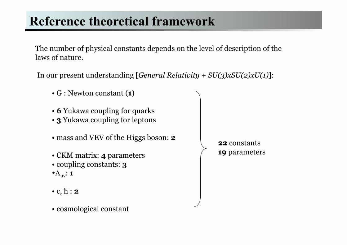
Reference theoretical framework

The number of physical constants depends on the level of description of the laws of nature.

In our present understanding [General Relativity + SU(3)xSU(2)xU(1)]:

•  G : Newton constant (1)

•  6 Yukawa coupling for quarks •  3 Yukawa coupling for leptons

•  mass and VEV of the Higgs boson: 2

•  CKM matrix: 4 parameters •  coupling constants: 3 • Λuv: 1

•  c, ħ : 2

•  cosmological constant

22 constants 19 parameters

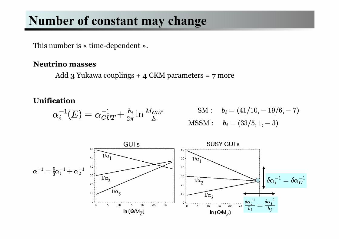
Number of constant may change

This number is « time-dependent ».

Neutrino masses

Unification

Add 3 Yukawa couplings + 4 CKM parameters = 7 more

3 fondamental units

3

Synthetiser, limiting value,... ...

Constants

Dimensions (M, L, T)

Units (kg, m, s)

Why these numbers ?

constant ?

Fondamental parameters

Constants

Are they constant? Test of physcis and GR, Variations are predicted by most extensions of general relativity. Important question from a cosmological point of view

Why do they have the value we measure? Why is the universe just so? Cosmology allows a way to attack this question

I- Links to general relativity and example of theories with varying constants

II- Setting constraints on variation of fundamental constants Phyisical systems – general approach

III- 2 detailed examples: BBN – 3alpha

IV- links to cosmology & conclusions

Part I: constants and gravity

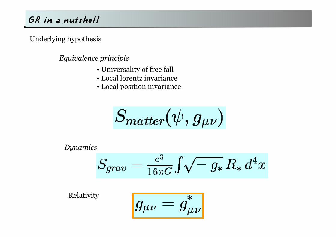
Underlying hypothesis

Equivalence principle

Dynamics

•  Universality of free fall •  Local lorentz invariance •  Local position invariance

Relativity

GR in a nutshell

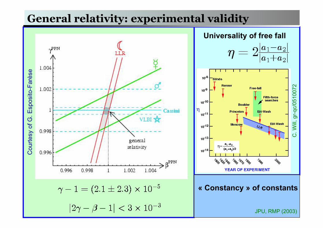
General relativity: experimental validity Universality of free fall

C. W

ill, g

r-qc

/051

0072

Cou

rtesy

of G

. Esp

osito

-Far

èse

« Constancy » of constants

JPU, RMP (2003)

Equivalence principle and constants

Action of a test mass:

with

(geodesic)

(Newtonian limit)

Equivalence principle and constants

Action of a test mass:

with

(NOT a geodesic)

(Newtonian limit)

Dependence on some constants

Anomalous force Composition dependent

The same in purely Newtonian

If some constants vary then the mass of any nuclei becomes spacetime dependent

In Newtonian terms, a free motion implies

If a constant varies then

Universality of free-fall is violated

Field theory

If a constant is varying, this implies that it has to be replaced by a dynamical field

This has 2 consequences: 1- the equations derived with this parameter constant will be modified one cannot just make it vary in the equations

2- the theory will provide an equation of evolution for this new parameter

The field responsible for the time variation of the « constant » is also responsible for a long-range (composition-dependent) interaction

i.e. at the origin of the deviation from General Relativity.

Example: ST theory

Most general theories of gravity that include a scalar field beside the metric Mathematically consistent Motivated by superstring dilaton in the graviton supermultiplet, modulii after dimensional reduction Consistent field theory to satisfy WEP Useful extension of GR (simple but general enough)

spin 2 spin 0

ST theory: déviation from GR and variation

Time variation of G

Cou

rtesy

of E

spos

ito-F

arès

e

Constraints valid for a (almost) massless field.

graviton scalar

Example of varying fine structure constant

It is a priori « easy » to design a theory with varying fundamental constants

But that may have dramatic implications.

Consider

Requires to be close to the minimum

Violation of UFF is quantified by

It is of the order of

Extra-dimensions

Such terms arise when compatifying a higher-dimensional theories

Example:

5D theory

4D effective theory

Com

pactification

Varying fine structure constant

Varying G

String (inspired)

Damour, Polyakov (1994)

Little is known about these functions

For the attracttion mechanism to exist: they must have a minimum at a common value

In Jordan frame

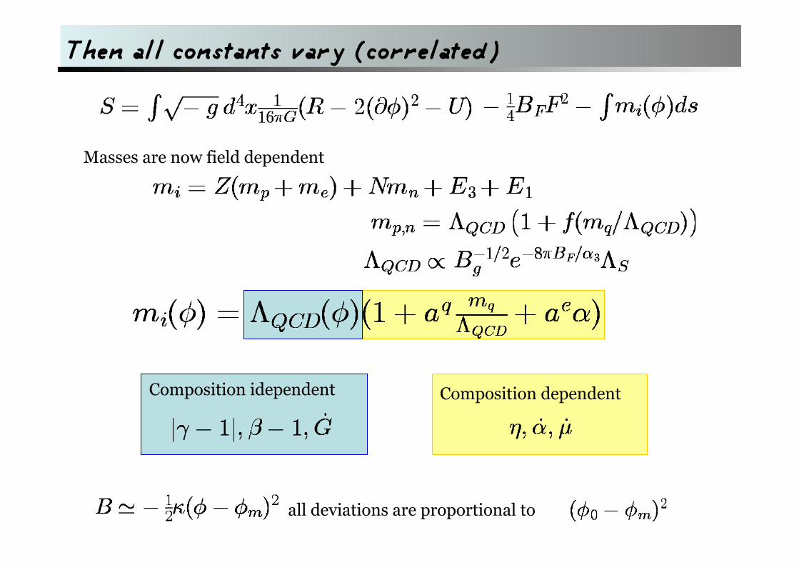
Then all constants vary (correlated)

Masses are now field dependent

Composition idependent Composition dependent

all deviations are proportional to

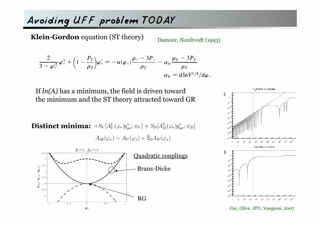
Avoiding UFF problem TODAY

Damour, Nordtvedt (1993)

Coc, Olive, JPU, Vangioni, 2007

Klein-Gordon equation (ST theory)

If ln(A) has a minimum, the field is driven toward the minimum and the ST theory attracted toward GR

Distinct minima:

Quadratic couplings

Brans-Dicke

RG

Summary

The constancy of fundamental constants is a test of the equivalence principle.

The magnitude of the variation of the constants, violation of the universality of free fall and other deviations from GR are of the same order.

« Dynamical constants » are generic in most extenstions of GR (extra-dimensions, string inspired model.

If one constant is varying then many other constants will also be varying (a consequence of unification).

They open a window on these theories or challenge them to explain why the constants vary so little (stabilisation mechanism).

In order to satisfy the constraints from the UFF today, there are 2 possibilities: - Least coupling principle - Chameleon mechanism

In both cases, the variations in the past are expected to be larger than on Solar system scales.

Part II: Testing for constancy

JPU, Rev. Mod. Phys. 75, 403 (2003) JPU, [astro-ph/0409424] R. Lehoucq, JPU, Les constantes fondamentales (Belin, 2005) G.F.R. Ellis and JPU, Am. J. Phys. 73 (2005) 240 JPU, B. Leclercq, De l’importance d’être une constante (Dunod, 2005)

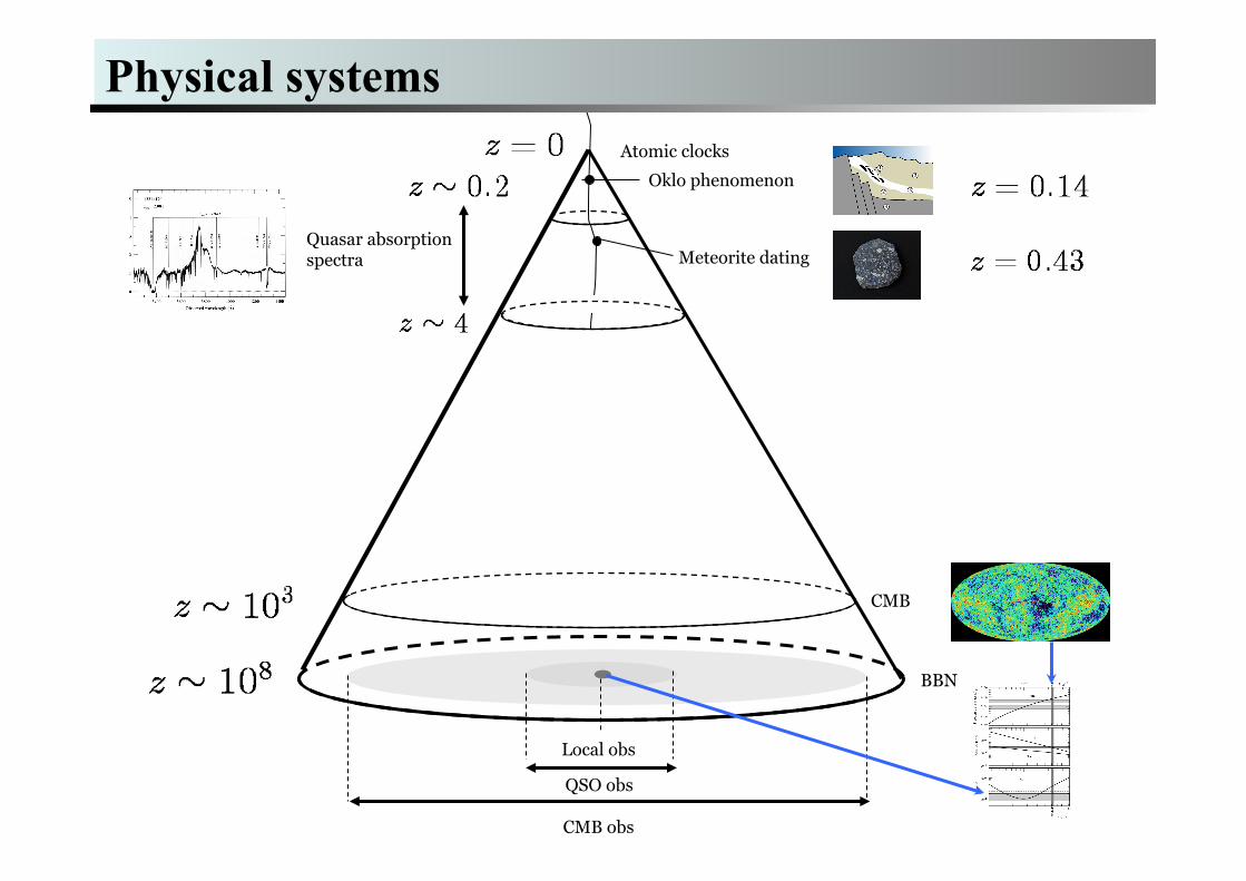
Atomic clocks

Oklo phenomenon

Meteorite dating Quasar absorption spectra

CMB

BBN

Local obs

QSO obs

CMB obs

Physical systems

Observables and primary constraints A given physical system gives us an observable quantity

External parameters: temperature,...:

Primary physical parameters

From a physical model of our system we can deduce the sensitivities to the primary physical parameters

The primary physical parameters are usually not fundamental constants.

Physical systems

System Observable Primary constraint

Other hypothesis

Atomic clocks Clock rates α, µ, gi -

Quasar spectra Atomic spectra α, µ, gp Cloud physical properties

Oklo Isotopic ratio Er Geophysical model

Meteorite dating Isotopic ratio λ

CMB Temperature anisotropies

α, µ Cosmological model

BBN Light element abundances

Q, τn, me, mN, α, Bd

Cosmological model

Atomic clocks

Based the comparison of atomic clocks using different transitions and atoms: e.g. hfs Cs vs fs Mg : gpµ ;

 hfs Cs vs hfs H: (gp/gI)α

Marion (2003) Bize (2003) Fischer (2004) Bize (2005) Fortier (2007)

Peik (2006) Peik (2004)

Blatt (2008) Cingöz (2008)

Blatt (2008)

Oklo- a natural nuclear reactor

It operated 2 billion years ago, during 200 000 years !!

Oklo: why?

4 conditions : 1- Naturally high in

U235,

2- moderator : water,

3- low abundance of neutron absorber,

4- size of the room.

Oklo-constraints

Natural nuclear reactor in Gabon, operating 1.8 Gyr ago (z~0.14)

Abundance of Samarium isotopes

From isotopic abundances of Sm, U and Gd, one can measure the cross section averaged on the thermal neutron flux

From a model of Sm nuclei, one can infer

s~1Mev so that

Shlyakhter, Nature 264 (1976) 340 Damour, Dyson, NPB 480 (1996) 37 Fujii et al., NPB 573 (2000) 377 Lamoreaux, torgerson, nucl-th/0309048 Flambaum, shuryak, PRD67 (2002) 083507

Damour, Dyson, NPB 480 (1996) 37

Fujii et al., NPB 573 (2000) 377 2 branches.

Meteorite dating

Bounds on the variation of couplings can be obtained by Constraints on the lifetime of long-lives nuclei (α and β decayers)

For β decayers,

Rhenium: Peebles, Dicke, PR 128 (1962) 2006

Use of laboratory data +meteorites data

Olive et al., PRD 69 (2004) 027701

Caveats: meteorites datation / averaged value

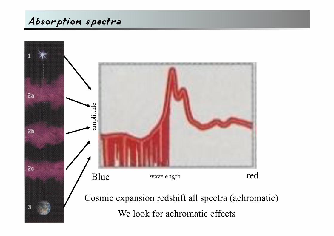
Absorption spectra

wavelength

ampl

itude

Cosmic expansion redshift all spectra (achromatic)

red Blue

We look for achromatic effects

QSO

3 main methods:

Alkali doublet (AD)

Single Ion Differential α Measurement (SIDAM)

Many multiplet (MM)

Fine structure doublet,

Si IV alkali doublet

Single atom Rather weak limit

Savedoff 1956

Webb et al. 1999

Levshakov et al. 1999

VLT/UVES: Si IV in 15 systems, 1.6<z<3

Chand et al. 2004

Compares transitions from multiplet and/or atoms s-p vs d-p transitions in heavy elements Better sensitivity

Analog to MM but with a single atom / FeII

HIRES/Keck: Si IV in 21 systems, 2<z<3

Murphy et al. 2001

QSO: many multiplets

The many-multiplet method is based on the corrrelation of the shifts of different lines of different atoms.

Dzuba et al. 1999-2005

Relativistic N-body with varying α:

HIRES-Keck, 153 systems, 0.2<z<4.2

Murphy et al. 2004 5σ detection !

First implemented on 30 systems with MgII and FeII Webb et al. 1999

QSO: VLT/UVES analysis

Selection of the absorption spectra: - lines with similar ionization potentials most likely to originate from similar regions in the cloud - avoid lines contaminated by atmospheric lines - at least one anchor line is not saturated redshift measurement is robust - reject strongly saturated systems

Only 23 systems lower statistics / better controlles systematics

VLT/UVES

Chand et al. 2004

DOES NOT CONFIRM HIRES/Keck DETECTION

Controversy

VLT/UVES: selection a priori of the systems data publicly available on the WEB

HIRES/Keck: signal comes from only some systems data not public

χ2 not smooth for some systems 2 problematic systems that dominate the analysis

If removed

Srianand et al. 2007

Reanalysis of the VLT/UVES data by Murphy et al. χ2 no smooth for some systems argue

Murphy et al. 2006

CMB

Effect on the position of the Doppler peak on polarization (reionisation)

Degeneracies: cosmological parameters

electron mass origin of primordial fluctuations

Analysis of WMAP data

Martins et al. PLB 585 (2004) 29; G. Rocha et al, N. Astron. Rev. 47 (2003) 863

It changes the recombination history 1- modifies the optical depth

2- induces a change in the hydrogen and helium abundances (xe)

Summary of the constraints on α

Meteorites

Part III: Coupled variation

Example of BBN & 3α

BBN: generality

BBN predicts the primordial abundances of D, He-3, He-4, Li-7

Mainly based on the balance between 1- expansion rate of the universe 2- weak interaction rate which controls n/p at the onset of BBN

Predictions depend on

Example: helium production

freeze-out temperature is roughly given by

Coulomb barrier:

Coc,Nunes,Olive,JPU,Vangioni 2006

BBN: effective BBN parameters Independent variations of the BBN parameters

Abundances are very sensitive to BD.

Equilibrium abundance of D and the reaction rate p(n,γ)D depend exponentially on BD.

These parameters are not independent.

Difficulty: QCD and its role in low energy nuclear reactions.

Coc,Nunes,Olive,JPU,Vangioni 2006

BBN: fundamental parameters (1)

Neutron lifetime:

Neutron-proton mass difference:

BBN: fundamental parameters (2)

D binding energy:

Use a potential model

Flambaum,Shuryak 2003

Most important parameter beside Λ is the strange quark mass. One needs to trace the dependence in ms.

This allows to determine all the primary parameters in terms of (hi, v, Λ,α)

BBN: assuming GUT

The low-energy expression for the QCD scale

The value of R depends on the particular GUT theory and particle content Which control the value of MGUT and of α(MGUT). Typically R=36.

GUT:

We deduce

Assume (for simplicity) hi=h

  Helium burning

  Triple alpha reaction 3α→12C

  Competing with 12C(α,γ)16O

  Hydrogen burning (at Z = 0)

  Slow pp chain

  CNO with C from 3α→12C

  Three steps :

  αα↔8Be (lifetime ~ 10-16 s) leads to an equilibrium

  8Be+α→12C* (288 keV, l=0 resonance, the “Hoyle state”)

  12C*→12C + 2γ

  Resonant reaction unlike e.g. 12C(α,γ)16O

  Sensitive to the position of the “Hoyle state”

  Sensitive to the variation of “constants”

Stellar carbon production

12C production and variation of the strong interaction [Rozental 1988]

C/O in Red Giant stars [Oberhummer et al. 2000; 2001]

1.3, 5 and 20 M stars, Z=Z / Limits on effective N-N interaction

C/O in low, intermediate and high mass stars [Schlattl et al. 2004]

1.3, 5, 15 and 25 M stars, Z=Z / Limits on resonance energy shift

1.  Equillibrium between 4He and the short lived (~10-16 s) 8Be : αα↔8Be

2.  Resonant capture to the (l=0, Jπ=0+) Hoyle state: 8Be+α→12C*(→12C+γ)

Simple formula used in previous studies

1.  Saha equation (thermal equilibrium)

2.  Sharp resonance analytic expression:

€

NA2 〈σv〉ααα = 33/ 26NA

2 2πMαkBT

3

5γ exp −Qααα

kBT

Approximations

1.  Thermal equilibrium

2.  Sharp resonance

3.  8Be decay faster than α capture

with Qααα= ER(8Be) + ER(12C) and γ≈Γγ

Nucleus 8Be 12C

ER (keV) 91.84±0.04 287.6±0.2

Γα (eV) 5.57±0.25 8.3±1.0

Γγ (meV) - 3.7±0.5

ER = resonance energy of 8Be g.s. or 12C Hoyle level (w.r.t. 2α or 8Be+α)

Stellar carbon production Triple α coincidence (Hoyle)

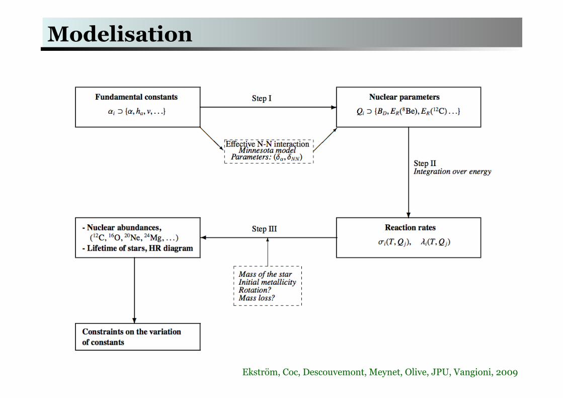
Modelisation

Ekström, Coc, Descouvemont, Meynet, Olive, JPU, Vangioni, 2009

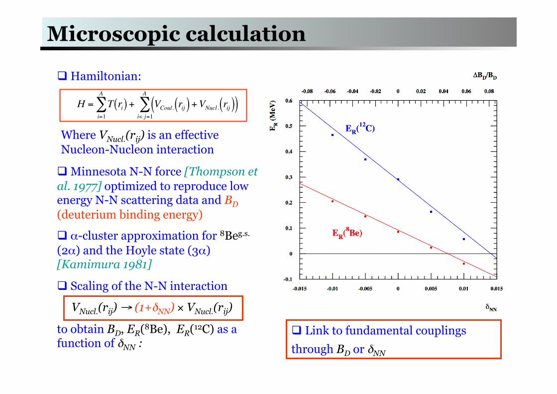
  Minnesota N-N force [Thompson et al. 1977] optimized to reproduce low energy N-N scattering data and BD (deuterium binding energy)

  α-cluster approximation for 8Beg.s. (2α) and the Hoyle state (3α) [Kamimura 1981]

  Scaling of the N-N interaction

VNucl.(rij) → (1+δNN) × VNucl.(rij)

to obtain BD, ER(8Be), ER(12C) as a function of δNN :

  Hamiltonian:

€

H = T ri( )i=1

A

∑ + VCoul. rij( ) +VNucl . rij( )( )i< j=1

A

∑

Where VNucl.(rij) is an effective Nucleon-Nucleon interaction

  Link to fundamental couplings through BD or δNN

Microscopic calculation

Composition at the end ofcore He burning Stellar evolution of massive Pop. III stars

We choose typical masses of 15 and 60 M stars/ Z=0 ⇒Very specific stellar evolution

60 M Z = 0

 The standard region: Both 12C and 16O are produced.

  The 16O region: The 3α is slower than 12C(α,γ)16O resulting in a higher TC and a conversion of most 12C into 16O

  The 24Mg region: With an even weaker 3α, a higher TC is achieved and 12C(α,γ)16O(α,γ)20Ne(α,γ)24Mg transforms 12C into 24Mg

  The 12C region: The 3α is faster than 12C(α,γ)16O and 12C is not transformed into 16O

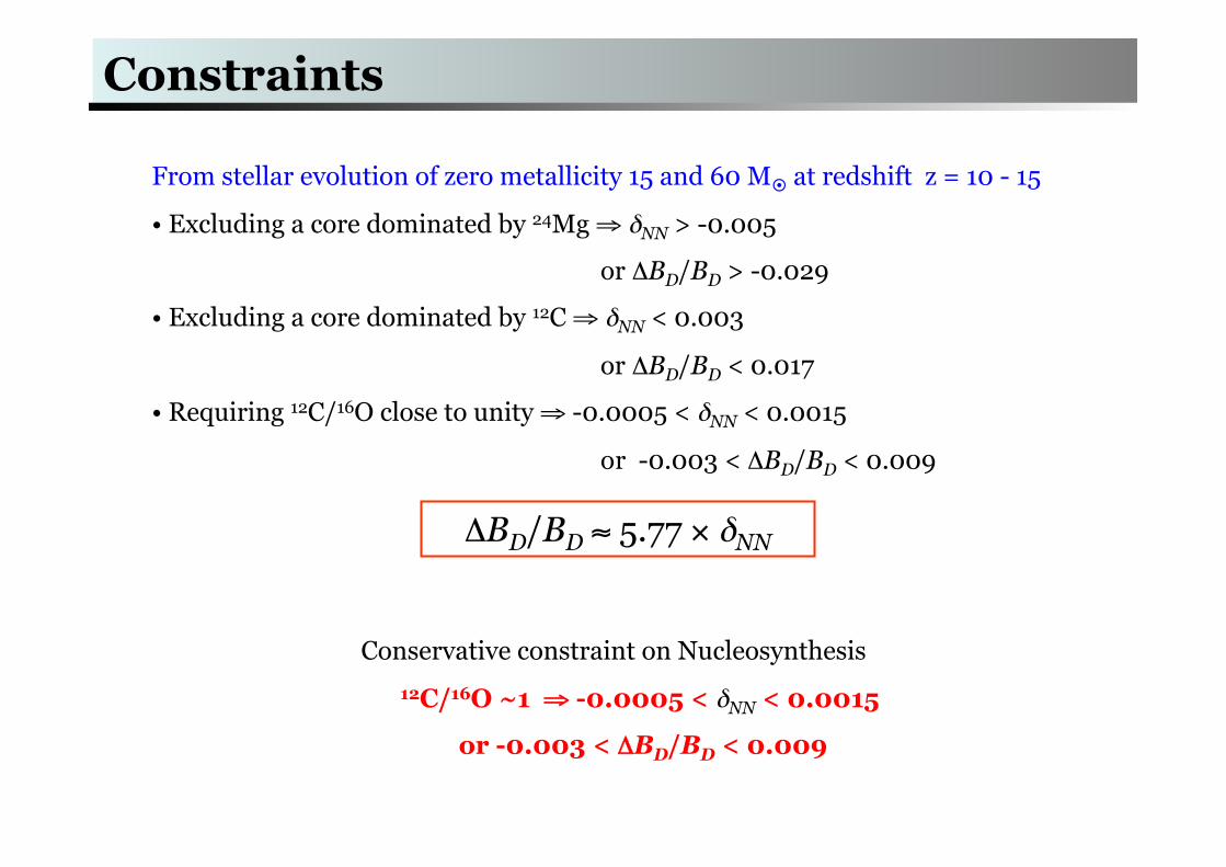
Constraints

From stellar evolution of zero metallicity 15 and 60 M at redshift z = 10 - 15

•  Excluding a core dominated by 24Mg ⇒ δNN > -0.005

or ΔBD/BD > -0.029

•  Excluding a core dominated by 12C ⇒ δNN < 0.003

or ΔBD/BD < 0.017

•  Requiring 12C/16O close to unity ⇒ -0.0005 < δNN < 0.0015

or -0.003 < ΔBD/BD < 0.009

ΔBD/BD ≈ 5.77 × δNN

Conservative constraint on Nucleosynthesis 12C/16O ~1 ⇒ -0.0005 < δNN < 0.0015

or -0.003 < ΔBD/BD < 0.009

Conclusions

Constants are a transversal way to look at the history of physics and at the structure of its theory.

Observational developments allow to set strong constraints on their possible variation

They allow to test general relativity and may open a window on more fundamental theories of gravity

Atomic clocks

Oklo phenomenon

Meteorite dating Quasar absorption spectra

Pop III stars

21 cm

CMB

BBN

Future evolution

Dirac (1937) Numerological argument G ~ 1/t

Kaluza (1919) – Klein (1926) multi-dimensional theories

Jordan (1949) variable constant = new dynamical field.

Fierz (1956) Effects on atomic spectra Scalar-tensor theories

Savedoff (1956) Tests on astrophys. spectra

Lee-Yang (1955) Dicke (1957) Implication on the universality of free fall

Teller (1948)–Gamow (1948) Constraints on Dirac hypothesis New formulation

Scherk-Schwarz (1974) Witten (1987) String theory: all dimensionless constants are dynamical

Oklo (1972), quasars... Experimental constraints